Prediction of Ground Thaw Formations Around an Oil Well

Source: http://simmakers.com/ground-thawing-oil-well/

(Keywords: borehole, oil wells, water well, permafrost soil, permafrost, frost 3d universal, permafrost well

operation, ground thawing around borehole, unfrozen water content distribution, soil thermal field)

Oil well operations in permafrost areas cause the formation of thaw bulbs around wellbores, that may result in

borehole and pipeline buckling failure. Consequently, well design requires the simulation of the permafrost

thermal regime and thaw bulbs around the well cluster.

Today, Frost 3D Universal is the most convenient tool for performing such simulations. In order to create a computer model of the borehole thermal influence on the permafrost, the following information is needed:

1. Meteorological data: air temperature variation, wind speed, change in snow cover thickness.

2. Geological soil structure and thermophysical properties around simulated boreholes: thermal conductivity and volumetric heat capacity in thawed and frozen state, initial temperature of the water-ice phase transition,

density of dry soil, total gravimetric soil moisture (over all types of soil water), dependence of unfrozen water

content on temperature. 3. Temperature and velocity of pumped oil

4. Well structure and thermophysical properties of used material (cement, thermal insulation, etc.)

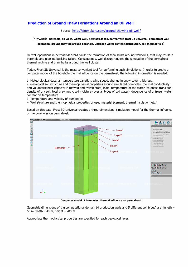
Based on this data, Frost 3D Universal creates a three-dimensional simulation model for the thermal influence of the boreholes on permafrost.

Computer model of boreholes’ thermal influence on permafrost

Geometric dimensions of the computational domain (4 production wells and 5 different soil types) are: length –

60 m, width – 40 m, height – 200 m.

Appropriate thermophysical properties are specified for each geological layer.

Parameters material short text

Layer1 Layer2 Layer3 Layer4 Layer5

Volumetric heat capacity of thawed ground, J/(м3•оС)

2.92×106 3.20×106 2.89×106 2.86×106 2.79×106

Volumetric heat capacity of frozen ground

J/(м3•оС) 1.83×106 2.20×106 2.01×106 1.92×106 2.19×106

Heat conductivity of thawed ground, W/(m•оС) 1.86 1.8 1.78 1.8 1.27

Heat conductivity of frozen ground,W/(m•оС) 2.1 1.88 1.91 1.93 1.85

Total gravimetric soil moisture, % 0,2 0.3 0.25 0.15 0.25

Density of dry soil,Kg/m3 1400 1600 1400 1400 1600

Phase transition temperature, оС 0 -0.2 -0.1 -0.6 -0.2

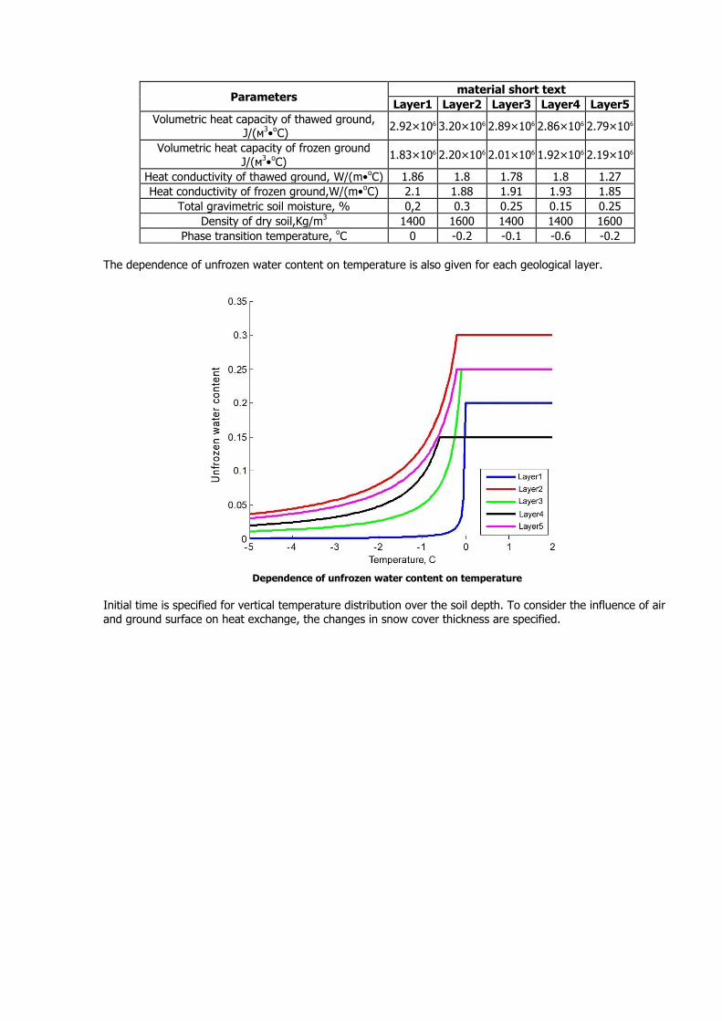
The dependence of unfrozen water content on temperature is also given for each geological layer.

Dependence of unfrozen water content on temperature

Initial time is specified for vertical temperature distribution over the soil depth. To consider the influence of air

and ground surface on heat exchange, the changes in snow cover thickness are specified.

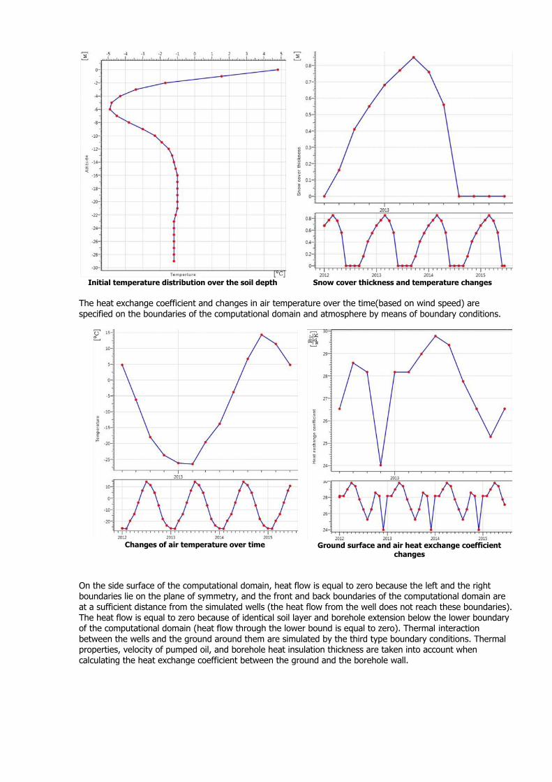
The heat exchange coefficient and changes in air temperature over the time(based on wind speed) are

specified on the boundaries of the computational domain and atmosphere by means of boundary conditions.

On the side surface of the computational domain, heat flow is equal to zero because the left and the right boundaries lie on the plane of symmetry, and the front and back boundaries of the computational domain are

at a sufficient distance from the simulated wells (the heat flow from the well does not reach these boundaries).

The heat flow is equal to zero because of identical soil layer and borehole extension below the lower boundary of the computational domain (heat flow through the lower bound is equal to zero). Thermal interaction

between the wells and the ground around them are simulated by the third type boundary conditions. Thermal properties, velocity of pumped oil, and borehole heat insulation thickness are taken into account when

calculating the heat exchange coefficient between the ground and the borehole wall.

Initial temperature distribution over the soil depth

Snow cover thickness and temperature changes

Changes of air temperature over time

Ground surface and air heat exchange coefficient

changes

Specification of boundary conditions for borehole thermal analysis

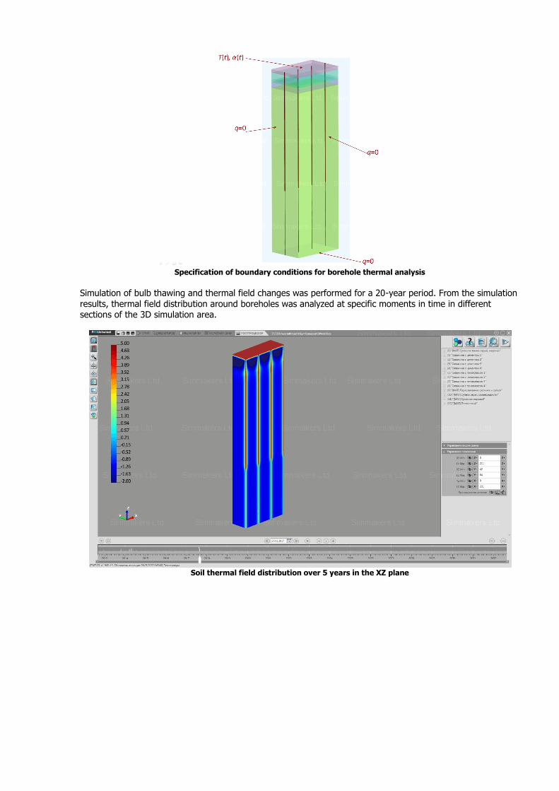
Simulation of bulb thawing and thermal field changes was performed for a 20-year period. From the simulation

results, thermal field distribution around boreholes was analyzed at specific moments in time in different sections of the 3D simulation area.

Soil thermal field distribution over 5 years in the XZ plane

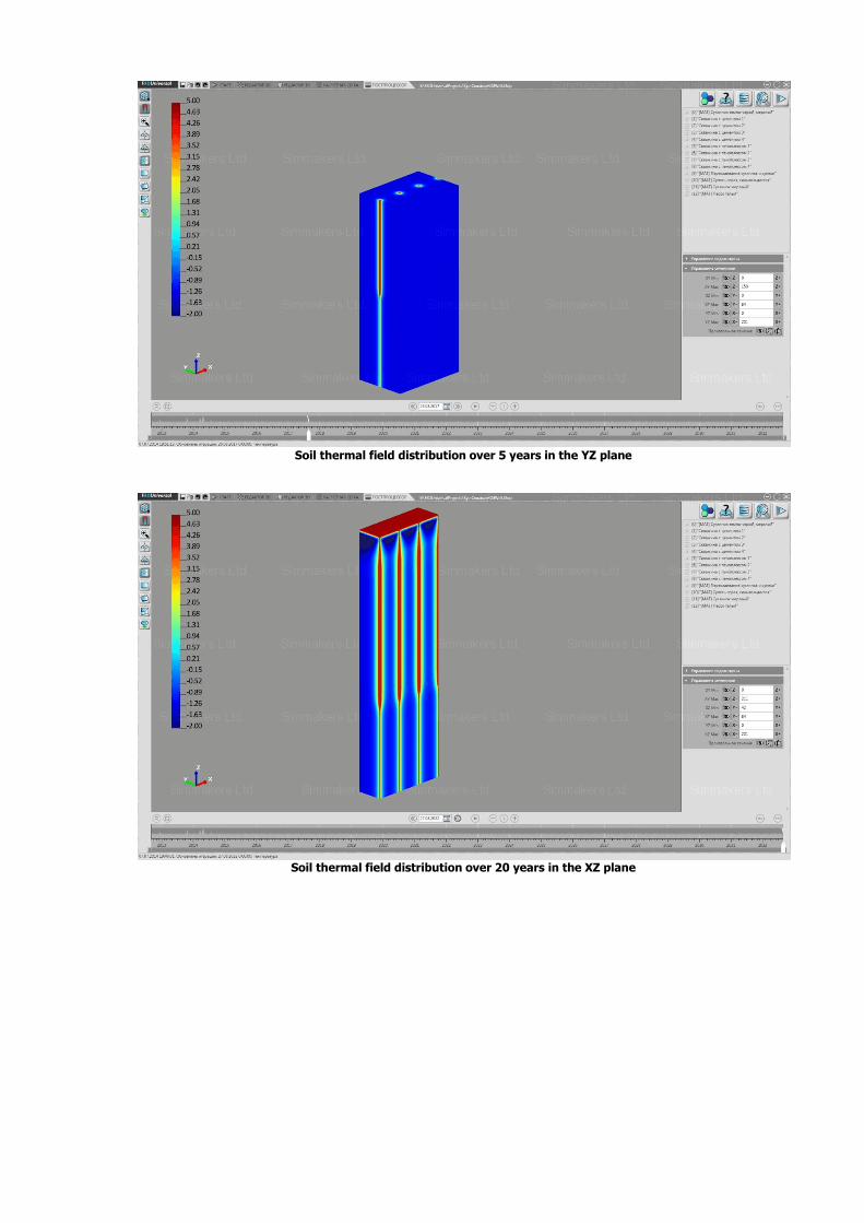
Soil thermal field distribution over 5 years in the YZ plane

Soil thermal field distribution over 20 years in the XZ plane

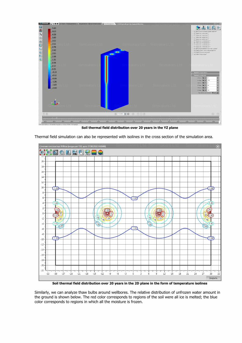
Soil thermal field distribution over 20 years in the YZ plane

Thermal field simulation can also be represented with isolines in the cross section of the simulation area.

Soil thermal field distribution over 20 years in the 2D plane in the form of temperature isolines

Similarly, we can analyze thaw bulbs around wellbores. The relative distribution of unfrozen water amount in the ground is shown below. The red color corresponds to regions of the soil were all ice is melted; the blue

color corresponds to regions in which all the moisture is frozen.

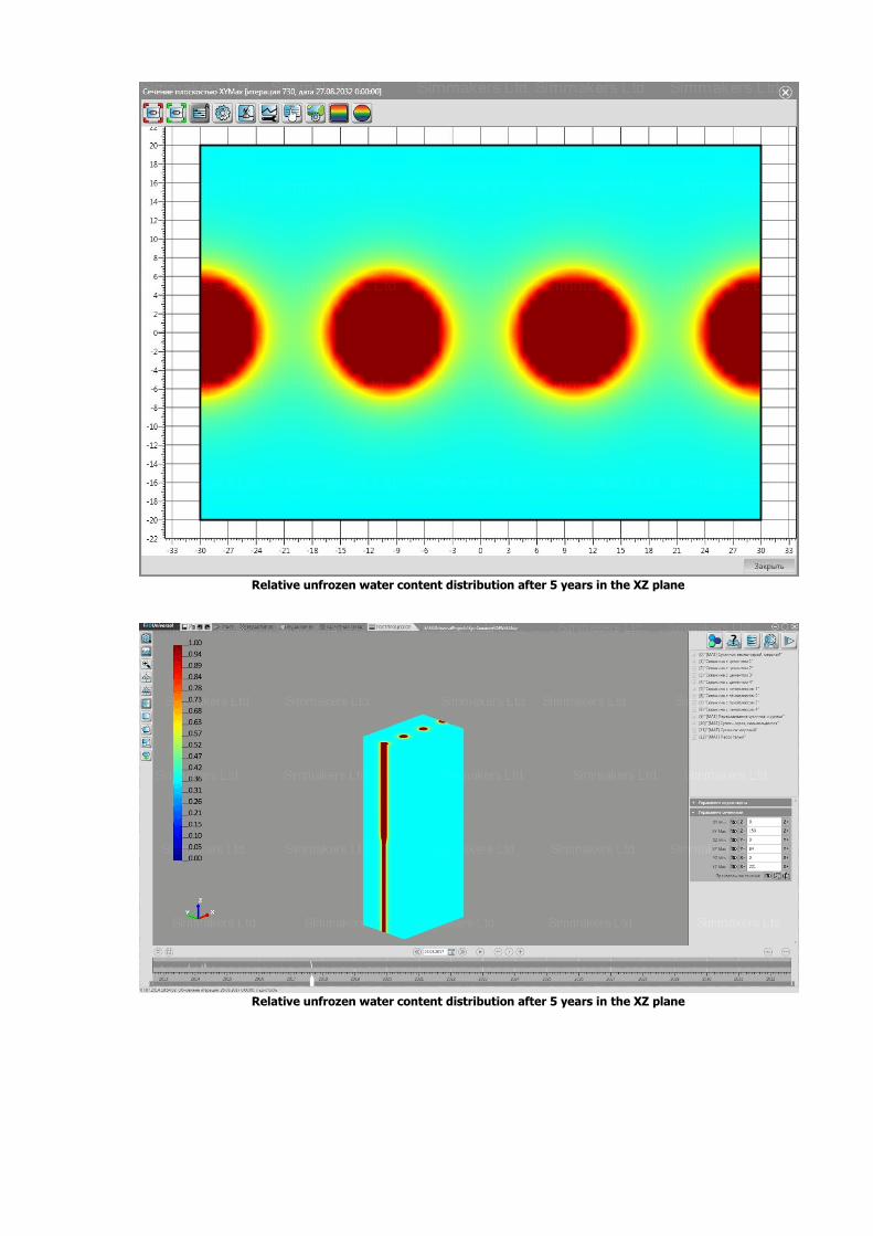
Relative unfrozen water content distribution after 5 years in the XZ plane

Relative unfrozen water content distribution after 5 years in the XZ plane

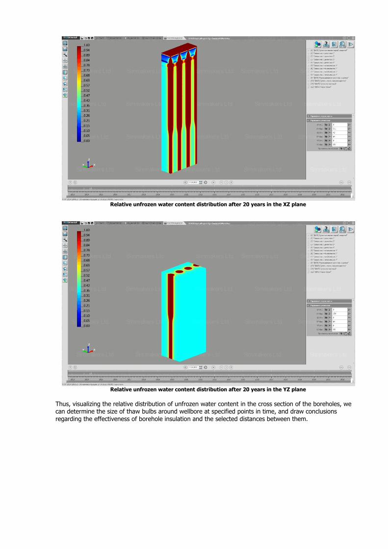
Relative unfrozen water content distribution after 20 years in the XZ plane

Relative unfrozen water content distribution after 20 years in the YZ plane

Thus, visualizing the relative distribution of unfrozen water content in the cross section of the boreholes, we can determine the size of thaw bulbs around wellbore at specified points in time, and draw conclusions

regarding the effectiveness of borehole insulation and the selected distances between them.

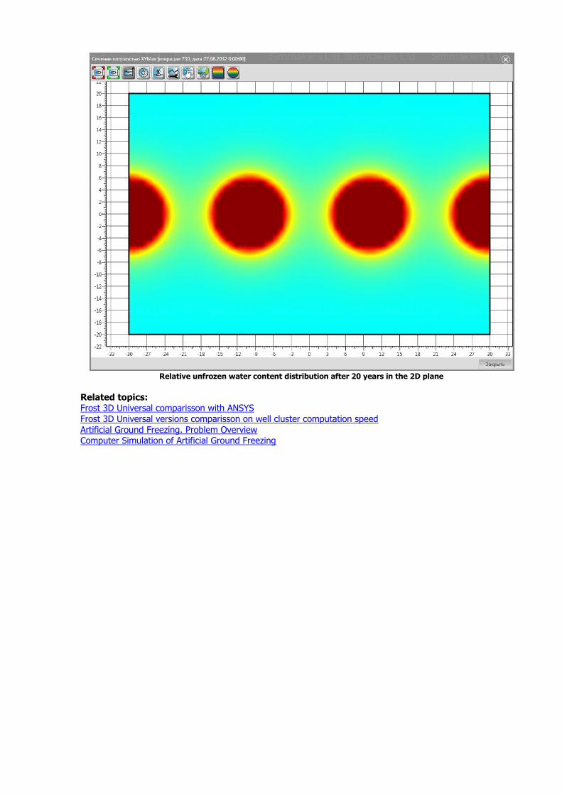
Relative unfrozen water content distribution after 20 years in the 2D plane

Related topics: Frost 3D Universal comparisson with ANSYS

Frost 3D Universal versions comparisson on well cluster computation speed

Artificial Ground Freezing. Problem Overview Computer Simulation of Artificial Ground Freezing