prediction of inverse kinematics solution of a redundant
TRANSCRIPT

Prediction of Inverse Kinematics Solution of a
Redundant Manipulator using
ANFIS
A Thesis Submitted in Fulfilment of
The Requirement for the Award of The Degree
OF
Master of technology
IN
Machine Design and Analysis
BY
LAYATITDEV DAS
(ROLL NO. 210ME1122)
NATIONAL INSTITUTE OF TECHNOLOGY
ROURKELA - 769008, INDIA MAY – 2012

Prediction of Inverse Kinematics Solution of a
Redundant Manipulator using
ANFIS
A Thesis Submitted in Fulfilment of
The Requirement for the Award of The Degree
OF
Master of technology
IN
Machine Design and Analysis
BY
LAYATITDEV DAS
(ROLL NO. 210ME1122)
Under the guidance of
Dr. S.S. Mahapatra
Professor, Department of Mechanical Engineering
NATIONAL INSTITUTE OF TECHNOLOGY ROURKELA - 769008, INDIA
MAY – 2012

CERTIFICATE
This is to certify that the thesis entitled, “ Prediction of Inverse Kinematics
Solution of a Redundant Manipulator using ANFIS” being submitted by
Layatitdev Das for the award of the degree of Master of Technology (Machine
Design and Analysis) of NIT Rourkela, is a record of bonafide research work carried
out by him under my supervision and guidance. Mr. Layatitdev Das has worked for
more than one year on the above problem at the Department of Mechanical
Engineering, National Institute of Technology, Rourkela and this has reached the
standard fulfilling the requirements and the regulation relating to the degree.
The contents of this thesis, in full or part, have not been submitted to any other
university or institution for the award of any degree or diploma.
Dr. Siba Sankar Mahapatra
Professor
Department of Mechanical Engineering
NIT, Rourkela
NATIONAL INSTITUTE OF TECHNOLOGY
ROURKELA – 769008
INDIA

i
ACKNOWLEDGEMENTS
While bringing out this thesis to its final form, I came across a number of
people whose contributions in various ways helped my field of research and they
deserve special thanks. It is a pleasure to convey my gratitude to all of them.
First and foremost, I would like to express my deep sense of gratitude and
indebtedness to my supervisor Prof. S.S. Mahapatra for his invaluable
encouragement, suggestions and support from an early stage of this research and
providing me extraordinary experiences throughout the work. Above all, his priceless
and meticulous supervision at each and every phase of work inspired me in
innumerable ways.
I specially acknowledge him for his advice, supervision, and the vital
contribution as and when required during this research. His involvement with
originality has triggered and nourished my intellectual maturity that will help me for a
long time to come. I am proud to record that I had the opportunity to work with an
exceptionally experienced Professor like him.
I am highly grateful to Prof. S.K. Sarangi, Director, National Institute of
Technology, Rourkela, Prof. R.K. Sahoo, Former Head, Department of Mechanical
Engineering and Prof. K.P. Maity, Head, Department of Mechanical Engineering for
their kind support and permission to use the facilities available in the Institute.
I am obliged to Asst. Prof. Pramod Kumar Parida, Debaprasanna Puhan,
Gouri Shankar Beriha, Chitrasen Samantra, Ankita Singh, Priyanka Jena,
Abhisek Tiwary, Jambeswar Sahu, Chinmay kumar Mohanty,Chabi Ram, Nitin
kumar Sahu, Shailesh Dewangan and Sri P.K. Pal for their support and co-
operation that is difficult to express in words. The time spent with them will remain in
my memory for years to come.
Finally, I am deeply indebted to my mother, Mrs. Malati Das, my father, Mr.
Khageswar Das, my younger brothers, Bhabatitdev Das, and Priyabrata Das and
to my family members for their moral support and continuous encouragement while
carrying out this study. I dedicate this thesis to almighty deity Maa Sarala and Maa
Kali.
Layatitdev Das
ii
ABSTRACT
In this thesis, a method for forward and inverse kinematics analysis of a 5-DOF and a 7-
DOF Redundant manipulator is proposed. Obtaining the trajectory and computing the
required joint angles for a higher DOF robot manipulator is one of the important concerns in
robot kinematics and control. When a robotic system possesses more degree of freedom
(DOF) than those required to execute a given task is called Redundant Manipulator. The
difficulties in solving the inverse kinematics (IK) equations of these redundant robot
manipulator arises due to the presence of uncertain, time varying and non-linear nature of
equations having transcendental functions. In this thesis, the ability of ANFIS (Adaptive
Neuro-Fuzzy Inference System) is used to the generated data for solving inverse kinematics
problem. The proposed hybrid neuro-fuzzy system combines the learning capabilities of
neural networks with fuzzy inference system for nonlinear function approximation. A single-
output Sugeno-type FIS (Fuzzy Inference System) using grid partitioning has been modeled
in this work. The Denavit-Hartenberg (D-H) representation is used to model robot links and
solve the transformation matrices of each joint. The forward kinematics and inverse
kinematics for a 5-DOF and 7-DOF manipulator are analyzed systemically.
ANFIS have been successfully used for prediction of IKs of 5-DOF and 7-DOF
Redundant manipulator in this work. After comparing the output, it is concluded that the
predicting ability of ANFIS is excellent as this approach provides a general frame work for
combination of NN and fuzzy logic. The Efficiency of ANFIS can be concluded by observing
the surface plot, residual plot and normal probability plot. This current study in using
different nonlinear models for the prediction of the IKs of a 5-DOF and 7-DOF Redundant
manipulator will give a valuable source of information for other modellers.
Keywords: 5-DOF and 7-DOF Redundant Robot Manipulator; Inverse kinematics; ANFIS;
Denavit-Harbenterg (D-H) notation.

iii
Contents
Chapter
No.
Titles Page No.
Acknowledgement i
Abstract ii
Contents iii
List of Tables vii
List of Figures viii
Glossary of Terms xii
1 Introduction
1.1. Introduction to Robotics 2
1.2. History of Robotics 2
1.3 Laws of Robotics 5
1.4 Components and Structure of Robots 5
1.5 Redundant Manipulator 6
1.6 Degree of Freedom (DOF) 7
1.7 Motivations 7
1.8 Objectives of the Thesis 8
1.9 Research methods 9
1.10 Structure of the Thesis 10

iv
2 Literature Review 11
3 Forward kinematics and Inverse kinematics 18
3.1 Denavit-Hertenberg Notation (D-H notation) 21
3.2 The forward kinematics of 5-DOF and 7-DOF RM
3.2.1 Coordinate frame of a 5-DOF RM
23
3.2.2 Forward kinematics calculation of the
5-DOF RM
24
3.2.3 Workspace for 5-DOF RM. 26
3.2.4 Coordinate frame for 7-DOF RM 27
3.2.5 Forward kinematics calculation of 7-DOF RM 27
3.2.6 Workspace for 7-DOF RM
3.3 Inverse kinematics of 5-DOF RM
4 ANFIS Architecture 36
4.1 ANFIS Architecture for 5-DOF RM 41
4.2 ANFIS Architecture for 7-DOF RM 43
5 Result and Discussion 46
5.1 3-D Surface viewer Analysis 46
5.1.1 3-D Surface plots obtained for all joint angles
of 5-DOF RM
46

v
5.1.2 3-D Surface plots obtained for all joint angles
of 7-DOF RM
48
5.2 Residual plot Analysis
5.2.1 The Residual plot of Training data for all joint
angles of 5-DOF RM
52
5.2.2 The Residual plot of Testing data for all joint
angles of 5-DOF RM.
54
5.2.3 The Residual plot of Training data for all joint
angles of 7-DOF RM
56
5.2.4 The Residual plot of Testing data for all joint
angles of 7-DOF RM
58
5.3 Normal probability plot Analysis 61
5.3.1 Normal probability plot analysis of Training
data for all joint angles of 5-DOF RM
62
5.3.2 Normal probability plot analysis of Testing data
for all joint angles of 5-DOF RM
64
5.3.3 Normal probability plot analysis of Training
data for all joint angles of 7-DOF RM
65
5.3.4 Normal probability plot analysis of Testing data
for all joint angles of 7-DOF RM
67
5.4 Application of Artificial Neural Network
68

vi
6 Conclusion and future work 73
6.1 Conclusion 73
6.2 Future work 73
7 References 76

vii
List of Tables
Table No. Caption Page No.
1. Angle of rotation of joints 24
2. The D-H parameters of the 5-DOF Redundant manipulator 24
3. The D-H parameters of the 7-DOF Redundant manipulator 27
4. ANFIS information used for solving 7-DOF Redundant
manipulator
43
5 Performance of ANFIS model used 70
6 Performance of ANN model used 70

viii
List of Figures
Figure No. Caption Page
No.
1. The first industrial robot: UNIMATE 2
2. Puma Robotic Arm 3
3. Symbolic representation of robot joints 6
4. Forward and Inverse kinematics scheme 20
5. D-H parameters of a link i.e. iiii ,d,a, 22
6. A Pioneer Arm Redundant manipulator 23
7. Coordinate frame for the 5-DOF Redundant manipulator (RM) 23
8. Workspace for 5-DOF Redundant manipulator 27
9. Coordinate frame for a 7-DOF Redundant manipulator 27
10. Workspace for 7-DOF Redundant manipulator 30
11. Elbow –in and Elbow-out configuration 32
12. The Sugeno fuzzy model for three inputs 37
13. Architecture of three inputs with seven membership functions of the
ANFIS model
41
14. ANFIS model structure used for 5-DOF Redundant manipulator 42
15. ANFIS model structure used for 5-DOF Redundant manipulator 44
16. Surface plot for 1 of 5-DOF Redundant manipulator 47
17. Surface plot for 2 of 5-DOF Redundant manipulator 47
18 Surface plot for 3 of 5-DOF Redundant manipulator 47
ix
19. Surface plot for 4 of 5-DOF Redundant manipulator 48
20. Surface plot for 5 of 5-DOF Redundant manipulator 48
21. Surface plot for 1 of 7-DOF Redundant manipulator 49
22. Surface plot for 2 of 7-DOF Redundant manipulator 49
23. Surface plot for 3 of 7-DOF Redundant manipulator 50
24. Surface plot for 4 of 7-DOF Redundant manipulator 50
25. Surface plot for 5 of 7-DOF Redundant manipulator 50
26. Surface plot for 6 of 7-DOF Redundant manipulator 51
27. Surface plot for 7 of 7-DOF Redundant manipulator (RM) 51
28. Residual plot of training data for 1 of 5-DOF RM 52
29. Residual plot of training data for 2 of 5-DOF RM 53
30. Residual plot of training data for 3 of 5-DOF RM 53
31. Residual plot of training data for 4 of 5-DOF RM 53
32. Residual plot of training data for 5 of 5-DOF RM 54
33. Residual plot of testing data for 1 of 5-DOF RM 54
34. Residual plot of testing data for 2 of 5-DOF RM 55
35. Residual plot of testing data for 3 of 5-DOF RM 55
36. Residual plot of testing data for 4 of 5-DOF RM 55
37. Residual plot of testing data for 5 of 5-DOF RM 56
38. Residual plot of training data for 1 of 7-DOF RM 56

x
39. Residual plot of training data for 2 of 7-DOF RM 57
40. Residual plot of training data for 3 of 7-DOF RM 57
41. Residual plot of training data for 4 of 7-DOF RM 57
42. Residual plot of training data for 5 of 7-DOF RM 58
43. Residual plot of training data for 6 of 7-DOF RM 58
44. Residual plot of training data for 7 of 7-DOF RM 58
45. Residual plot of testing data for 1 of 7-DOF RM 59
46. Residual plot of testing data for 2 of 7-DOF RM 59
47. Residual plot of testing data for 3 of 7-DOF RM 60
48. Residual plot of testing data for 4 of 7-DOF RM 60
49. Residual plot of testing data for 5 of 7-DOF RM 60
50. Residual plot of testing data for 6 of 7-DOF RM 61
51. Residual plot of testing data for 7 of 7-DOF RM 61
52. Normal probability plot for residuals (Training data for 1 of 5- DOF RM) 62
53. Normal probability plot for residuals (Training data for 2 of 5- DOF RM) 62
54. Normal probability plot for residuals (Training data for 3 of 5- DOF RM) 63
55. Normal probability plot for residuals (Training data for 4 of 5- DOF RM) 63
56. Normal probability plot for residuals (Training data for 5 of 5- DOF RM) 63
57. Normal probability plot for residuals (Testing data for 1 of 5- DOF RM) 64
58. Normal probability plot for residuals (Testing data for 2 of 5- DOF RM) 64

xi
59. Normal probability plot for residuals (Testing data for 5 of 5- DOF RM) 64
60. Normal probability plot for residuals (Testing data for 4 of 5- DOF RM) 65
61. Normal probability plot for residuals (Testing data for 5 of 5- DOF RM) 65
62. Normal probability plot for residuals (Training data for 3 of 7- DOF RM) 66
63. Normal probability plot for residuals (Training data for 5 of 7- DOF RM) 66
64. Normal probability plot for residuals (Training data for 7 of 7- DOF RM) 66
65. Normal probability plot for residuals (Testing data for 3 of 7- DOF RM) 67
66. Normal probability plot for residuals (Testing data for 5 of 7- DOF RM) 67
67. Normal probability plot for residuals (Testing data for 7 of 7- DOF RM) 67
68. Schematic representation of Neural network used 68
69. Comparison of Mean Square Error plot for Training data of 7-DOF
RM
71
70. Comparison of Mean Square Error plot for Testing data of 7-DOF RM 71

xii
GLOSSARY of terms
DOF Degree of Freedom
IK Inverse Kinematic
FK Forward Kinematics
FIS Fuzzy Inference System
NF Neuro Fuzzy
NN Neural Network
ANN Artificial Neural Network
ANFIS Adaptive Neuro Fuzzy Inference System
D-H Denavit-Hartenberg
RM Redundant Manipulator

M.Tech. Project Report 2012
Mechanical Engineering Department, N.I.T Rourkela Page 1
CHAPTER 1

M.Tech. Project Report 2012
Mechanical Engineering Department, N.I.T Rourkela Page 2
Chapter 1
1. INTRODUCTION
1.1. Introduction to Robotics
Word robot was coined by a Czech novelist Karel Capek in 1920. The term robot derives
from the Czech word robota, meaning forced work or compulsory service. A robot is
reprogrammable, multifunctional manipulator designed to move material, parts, tools, or
specialized devices through various programmed motions for the performance of a variety of
tasks [1]. A simpler version it can be define as, an automatic device that performs functions
normally ascribed to humans or a machine in the form of a human.
1.2. History of Robotics
The first industrial robot named UNIMATE; it is the first programmable robot designed by
George Devol in1954, who coined the term Universal Automation. The first UNIMATE was
installed at a General Motors plant to work with heated die-casting machines.
Figure 1. The first industrial robot: UNIMATE
In 1978, the Puma (Programmable Universal Machine for Assembly) robot is developed
by Victor Scheinman at pioneering robot company Unimation with a General Motors design
support. These robots are widely used in various organisations such as Nokia corporation,
NASA, Robotics and Welding organization.

M.Tech. Project Report 2012
Mechanical Engineering Department, N.I.T Rourkela Page 3
Figure 2. Puma Robotic Arm
Then the robot industries enters a phase of rapid growth to till date, as various type of
robot are being developed with various new technology, which are being used in various
industries for various work. Few of these milestones in the history of robotics are given
below.
1947 — The first servoed electric powered teleoperator is developed.
1948 — A teleoperator is developed incorporating force feedback.
1949 — Research on numerically controlled milling machine is initiated.
1954 — George Devol designs the first programmable robot.
1956 — Joseph Engelberger, a Columbia University physics student, buys the rights to
Devol’s robot and founds the Unimation Company.
1961 — The first Unimate robot is installed in a Trenton, New Jersey plant of General
Motors to tend an die casting machine.
1961 — The first robot incorporating force feedback is developed.
1963 — The first robot vision system is developed.
1971 — The Stanford Arm is developed at Stanford University.
1973 — The first robot programming language (WAVE) is developed at Stanford.
1974 — Cincinnati Milacron introduced the T3 robot with computer control.
1975 — Unimation Inc. registers its first financial profit.
1976 — The Remote Center Compliance (RCC) device for part insertion in assembly is
developed at Draper Labs in Boston.
1976 — Robot arms are used on the Viking I and II space probes and land on Mars.
1978 — Unimation introduces the PUMA robot, based on designs from a General Motors
study.
1979 — The SCARA robot design is introduced in Japan
M.Tech. Project Report 2012
Mechanical Engineering Department, N.I.T Rourkela Page 4
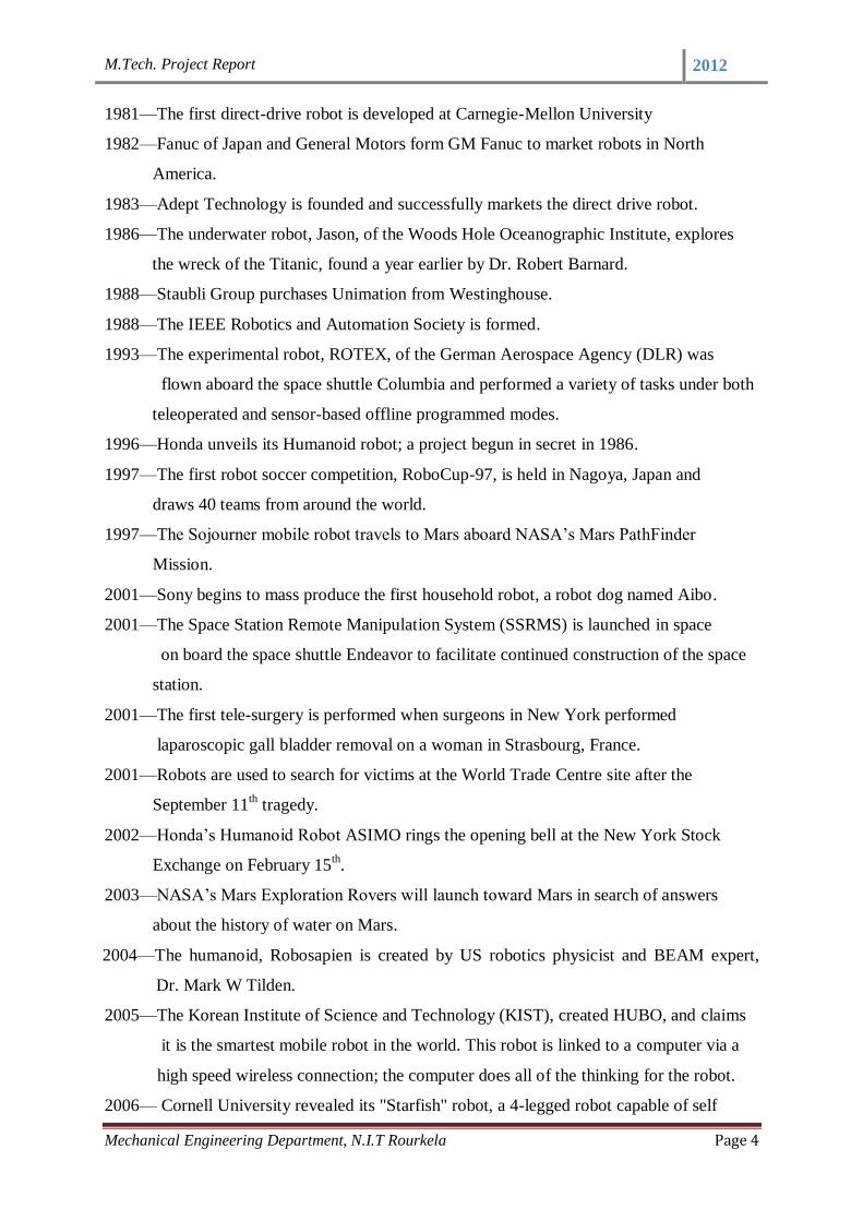
1981—The first direct-drive robot is developed at Carnegie-Mellon University
1982—Fanuc of Japan and General Motors form GM Fanuc to market robots in North
America.
1983—Adept Technology is founded and successfully markets the direct drive robot.
1986—The underwater robot, Jason, of the Woods Hole Oceanographic Institute, explores
the wreck of the Titanic, found a year earlier by Dr. Robert Barnard.
1988—Staubli Group purchases Unimation from Westinghouse.
1988—The IEEE Robotics and Automation Society is formed.
1993—The experimental robot, ROTEX, of the German Aerospace Agency (DLR) was
flown aboard the space shuttle Columbia and performed a variety of tasks under both
teleoperated and sensor-based offline programmed modes.
1996—Honda unveils its Humanoid robot; a project begun in secret in 1986.
1997—The first robot soccer competition, RoboCup-97, is held in Nagoya, Japan and
draws 40 teams from around the world.
1997—The Sojourner mobile robot travels to Mars aboard NASA’s Mars PathFinder
Mission.
2001—Sony begins to mass produce the first household robot, a robot dog named Aibo.
2001—The Space Station Remote Manipulation System (SSRMS) is launched in space
on board the space shuttle Endeavor to facilitate continued construction of the space
station.
2001—The first tele-surgery is performed when surgeons in New York performed
laparoscopic gall bladder removal on a woman in Strasbourg, France.
2001—Robots are used to search for victims at the World Trade Centre site after the
September 11th tragedy.
2002—Honda’s Humanoid Robot ASIMO rings the opening bell at the New York Stock
Exchange on February 15th.
2003—NASA’s Mars Exploration Rovers will launch toward Mars in search of answers
about the history of water on Mars.
2004—The humanoid, Robosapien is created by US robotics physicist and BEAM expert,
Dr. Mark W Tilden.
2005—The Korean Institute of Science and Technology (KIST), created HUBO, and claims
it is the smartest mobile robot in the world. This robot is linked to a computer via a
high speed wireless connection; the computer does all of the thinking for the robot.
2006— Cornell University revealed its "Starfish" robot, a 4-legged robot capable of self

M.Tech. Project Report 2012
Mechanical Engineering Department, N.I.T Rourkela Page 5
modelling and learning to walk after having been damaged.
2007—TOMY (Japanese toy co. Ltd.) launched the entertainment robot, i-robot, which is a
humanoid bipedal robot that can walk like a human beings and performs kicks and
punches and also some entertaining tricks and special actions under "Special Action
Mode".
2010— To present —Robonaut 2, the latest generation of the astronaut helpers, launched to
the space station aboard Space Shuttle Discovery on the STS-133 mission. It is the
first humanoid robot in space, and although its primary job for now is teaching
engineers how dexterous robots behave in space, the hope is that through upgrades
and advancements, it could one day venture outside the station to help spacewalkers
make repairs or additions to the station or perform scientific work.
1.3. Laws of Robotics
Asimov [2] proposed three "Laws of Robotics", and later added a 'Zeroth law'.
Zeroth Law: A robot may not injure humanity, or, through inaction, allow humanity to come
to harm.
First Law: A robot may not injure a human being, or, through inaction, allow a human being
to come to harm, unless this would violate a higher order law.
Second Law: A robot must obey orders given it by human beings, expect where such orders
would conflict with a higher order law.
Third Law: A robot must protect its own existence as long as such protection does not
conflict with a higher order law [3].
1.4. Components and Structure of Robots
The basic components of an industrial robot are:
The manipulator
The End-Effector (Which is a part of the manipulator)
The Power supply
The controller
Robot Manipulators are composed of links connected by joints into a kinematic chain.

M.Tech. Project Report 2012
Mechanical Engineering Department, N.I.T Rourkela Page 6
Joints are typically rotary (revolute) or linear (prismatic). A revolute joint rotates about a
motion axis and a prismatic joint slide along a motion axis. It can also be define as a
prismatic joint is a joint, where the pair of links makes a translational displacement along a
fixed axis. In other words, one link slides on the other along a straight line. Therefore, it is
also called a sliding joint. A revolute joint is a joint, where a pair of links rotates about a
fixed axis. This type of joint is often referred to as a hinge, articulated, or rotational joint.
Figure 3. Symbolic representation of robot joints.
The end-effector which is a gripper tool, a special device, or fixture attached to the robot’s
arm, actually performs the work.
Power supply provides and regulates the energy that is converted to motion by the robot
actuator, and it may be electric, pneumatic, or hydraulic.
The controller initiates, terminates, and coordinates the motion of sequences of a robot. Also
it accepts the necessary inputs to the robot and provides the outputs to interface with the
outside world. In other words the controller processes the sensory information and computes
the control commands for the actuator to carry out specified tasks.
1.5. Redundant Manipulator
A manipulator is required have a minimum of six degree of freedom if it needs to acquire any
random position and orientation in its operational space or work space. Assuming one joint is
Revolute Prismatic
2 D
3 D

M.Tech. Project Report 2012
Mechanical Engineering Department, N.I.T Rourkela Page 7
required for each degree of freedom, such a manipulator needs to be composed of minimum
of six joints. Usually in standard practice three degree of freedom is implemented in the
robotic arm so it can acquire the desired position in its work space. The arm is then fitted
with a wrist composed of three joints to acquire the desired orientation. Such a manipulator is
called non-redundant. Though non-redundant manipulators are kinematically simple to design
and solve, but the non-redundancy leads to two fundamental problems: singularity and
inability to avoid obstacles. The singularities of the robot manipulator are present both in the
arm and the wrist and can occur anywhere inside the workspace of the manipulator. While
passing through these singularities, the manipulator can effectively lose certain degree of
freedom, resulting in uncontrollability along those directions [4]. The obstacle avoidance is
another desirable characteristic to effectively plan the motion trajectories, especially for
manipulators designed to perform demanding tasks in constricted environment [5]. The above
two problems can be solved by adding a additional degree of freedom to the manipulator [6]
These additional degree of freedom can be added to the joints, which effectively become
singular in certain positions like shoulder, elbow, or wrist and hence help to overcome the
singularities or obstacles avoidance. So a redundant manipulator should possess at least one
degree-of-freedom (DOF) more than the number required for the general free positioning.
The Redundant can also be define as, when a manipulator can reach a specified position with
more than one configuration of the linkages , the manipulator is said to be redundant. From a
general point of view, any robotic system in which the way of achieving a given task is not
unique may be called redundant.
A redundant manipulator offer several potential advantages over a non-redundant
manipulator. The extra DOF that require for the free positioning of manipulator can be used
to move around or between obstacles and thereby to manipulate in situations that otherwise
would be inaccessible. Due to the redundancy the manipulators become flexible, compliant,
extremely dextrous and capable of dynamic adaptive, in unstructured environment.
1.6. Degree of Freedom (DOF)
The number of joints determines the degrees-of-freedom (DOF) of the manipulator.
Typically, a manipulator should possess at least six independent DOF: three for positioning
and three for orientation. With fewer than six DOF the arm cannot reach every point in its
work environment with arbitrary orientation. Certain applications such as reaching around or
behind obstacles require more than six DOF. The difficulty of controlling a manipulator

M.Tech. Project Report 2012
Mechanical Engineering Department, N.I.T Rourkela Page 8
increases rapidly with the number of links. A manipulator having more than six links is
referred to as a kinematically redundant manipulator.
1.7. Motivations
The motivation for this thesis is to obtain the inverse kinematic solutions of redundant
manipulator such as 5-DOF Redundant manipulator and 7-DOF Redundant manipulator. As
the inverse kinematic equation of these types of manipulators contain non-linear equations,
time varying equations and transcendental functions. Due to the complexity in solving this
type of equation by geometric, iterative or algebraic method is very difficult and time
consuming. It is very important to solve the inverse kinematics solution for this type of
redundant manipulator to know the exact operational space and to avoid the obstacles. So
various researcher had applied various methods for solving the kinematic equation. L.
Sciavicco et al. [7] used inverse jacobian, pseudo inverse jacobian or jacobian transpose and
solve the IK problem of 7-DOF redundant manipulator iteratively. But the main drawback of
this method are, these are slow and suffer from singularity issue. Shimizu et al. [8] proposed
an IK solution for the PA 10-7C 7-DOF manipulator and considered arm angle as redundancy
parameter. In his study, a detailed analysis of the variation of the joint angle with the arm
angle parameter is considered, which is then utilizes for redundancy resolution. However link
offset were not considered in his work. Some authors also applied ANN, due to its adapting
and learning nature. Although ANN are very efficient in adopting and learning but they have
the negative attribute of ‘black box’. To overcome this drawback, various author adopted
neuro fuzzy method like ANFIS (Adaptive Neuro-fuzzy Inference system). This can be
justify as ANFIS combines the advantage of ANN and fuzzy logic technique without having
any of their disadvantage [9]. The neuro fuzzy system are must widely studied hybrid system
now a days, as due to the advantages of two very important modelling technique i.e. NN [10]
and Fuzzy logic [11]. So the goal of this thesis is to predict the inverse kinematics solution
for the redundant manipulator using ANFIS. As a result suitable posture and the trajectories
for the manipulator can be planned for execution of different work in various fields.
1.8. Objectives of the Thesis
The objective of this thesis is to solve the inverse kinematics equations of the redundant
manipulator. The inverse kinematics equations of this type of manipulator are highly
unpredictable as this equation are highly non-linear and contains transcendental function. The
complexity in solving this equation increases due to increase in higher DOF. So various
authors had used neuro-fuzzy method (ANFIS) to solve the non-linear and complex equations

M.Tech. Project Report 2012
Mechanical Engineering Department, N.I.T Rourkela Page 9
arise in different field. ANFIS was adopted by different researcher in their work, for
mathematical modelling of the data, as it have high range of potential for solving the complex
and nonlinear equations arise in different field like in marketing, manufacturing industries,
civil engineering etc. Li ke et al. [12] applied ANFIS to solve the forecast problem of
microwave effect by adopting microwave parameters and its threshold as variable. Then they
develop an ANFIS model to study its forecasting ability. By comparing the output of ANFIS
with training and testing data, they concluded with good forecasting ability, small error and
low data requirement are found with ANFIS. Srinivasan et al. [13] applied ANFIS based on
PD plus I controller to the dynamic model of 6-DOF robot manipulator (PUMA Robot).
Numerical simulation using the dynamic model of 6-DOF robot arm shows the effectiveness
of the approach in trajectory tracking problems. After the successfully implementation of
ANFIS in various field for solving the non-linear equations, it is concluded that ANFIS is a
best technique can be used for solving the non-linear equation arises in the inverse kinematic
equation in robotics.
The main objectives of this thesis can be summarized as:
– The difficulties in solving the Inverse kinematics (IK) of the redundant manipulator
increases, as the IK equations posses an infinite number of solution due to the presence
of uncertain, time varying and non-linear nature of these equations having
transcendental functions. So in this thesis ANFIS is adopted for estimating the IK
solution of a 7-DOF Redundant manipulator.
– The Denavit-Harbenterg (D-H) representation is used to model robot links and solve
the transformation matrices of each joint.
– The solution of the IK of redundant manipulator predicted by the ANFIS model is
compared with the analytical value. It is found that the predicting ability of ANFIS is
excellent. As it is a combination of neural network (NN) and neuro-fuzzy (NF)
technique.
– The data predicted with ANFIS for 5-DOF and 7-DOF Redundant manipulator, in
this work clearly depicts that the proposed method results in an acceptable error. Hence
ANFIS can be utilized to provide fast and acceptable solutions of the inverse
kinematics, thereby making ANFIS as an alternate approach to map the inverse
kinematic solutions.
1.9. Research methods
The theoretical discussion and results, or the method adopted in this thesis regarding the
prediction of inverse kinematics solution of the redundant manipulator have been kept

M.Tech. Project Report 2012
Mechanical Engineering Department, N.I.T Rourkela Page 10
general without reference to any particular manipulator. The purpose is to keep the findings
useful for other developments and continue the research and discussion process on a wider
scale. In the latter part of the thesis, the ANFIS methodology used for the prediction of IK
solution of the redundant manipulator is carried out and the predicted values are verified with
the analytical values. The D-H notation is used to model the robot link and solve the
transformation matrices of each joint. Then multiplying each transformation matrices gives
the global transformation matrix of the manipulator. The global transformation matrix
consists of the position and orientations of the joint, and gives the forward kinematics
equations. Then, using this forward kinematics equation with the joint limits, the position of
the end-effector are been calculated. The position of the end-effector is taken as the inputs to
trained in ANFIS to calculate the joint angles as output, this leads to the IK. The forward and
inverse kinematics of the redundant manipulator is briefly described in the latter chapter. The
data are trained in ANFIS many times such as to get a appropriate mathematical model. After
the training of the data, the predicted values are compared with the analytical value. The
residual of the analytical and predicted values are found out and the mean square error,
normal probability plot and the regression plots are also carried out. It is concluded that the
mean square error and the residual are accepted, thereby making ANFIS as an alternative
technique for solving the non-linear equation of redundant manipulator.
1.10. Structure of the Thesis
The thesis is divided into 7 chapters covering the literature review, forward and inverse
kinematics, ANFIS architecture, result and discussion, summary and conclusion followed by
references. A brief description of each chapter is provided in the following paragraph.
Chapter 2 provides the literature review relevant to the research work. An effort has been
made to comprehensively cover the work of different researchers in the field robotics for
study of inverse kinematic. Various methods used by different authors for solving the IK is
covered in this part.
In chapter 3 the theoretical back ground for forward and inverse kinematic is described. The
chapter starts with a description of basic principle and assumption used for D-H notation and
leads to the formulation and mathematical representation of forward and inverse kinematics
of the 5-DOF and 7-DOF redundant manipulator.
The description of the ANFIS methodology used in this work is the subject of chapter 4. It
covers the steps to carry out the ANFIS technology such as loading, training and testing of
M.Tech. Project Report 2012
Mechanical Engineering Department, N.I.T Rourkela Page 11
the data. It describe about the membership functions, number of membership functions, and
total number of rules are used with the ANFIS structure diagram.
The result and discussions are carried out in chapter 5. It comprises of 3D surface viewer
plots of all joint angles with input parameters for 5-DOF and 7-DOF redundant manipulator.
The residual plots, normal probability plots and the regression plots are given in this chapter.
The summary and conclusion of the research work are presented in chapter 6. The chapter
also contains brief discussion about the topic which may which may require further study and
investigation.
The thesis is concluded in chapter 7 with references.
*******

M.Tech. Project Report 2012
Mechanical Engineering Department, N.I.T Rourkela Page 12
CHAPTER 2

M.Tech. Project Report 2012
Mechanical Engineering Department, N.I.T Rourkela Page 13
Chapter-2
2. LITERETURE REVIEW
Obtaining the inverse kinematics solution has been one of the main concerns in robot
kinematics research. The complexity of the solutions increases with higher DOF due to robot
geometry, non-linear equations (i.e. trigonometric equations occurring when transforming
between Cartesian and joint spaces) and singularity problems. Obtaining the inverse
kinematics solution requires the solution of nonlinear equations having transcendental
functions. In spite of the difficulties and time consuming in solving the inverse kinematics of
a complex robot, researchers used traditional methods like algebraic [14], geometric [15], and
iterative [16] procedures. But these methods have their own drawbacks as algebraic methods
do not guarantee closed form solutions. In case of geometric methods, closed form solutions
for the first three joints of the manipulator must exist geometrically. The iterative methods
converge to only a single solution depending on the starting point and will not work near
singularities [17]. In other words, for complex manipulators, these methods are time
consuming and produce highly complex mathematical formulation, which cannot be
modelled concisely for a robot to work in the real world. Calderon et al. [18] proposed a
hybrid approach to inverse kinematics and control and a resolve motion rate control method
are experimented to evaluate their performances in terms of accuracy and time response in
trajectory tracking. Xu et al. [19] proposed an analytical solution for a 5-DOF manipulator to
follow a given trajectory while keeping the orientation of one axis in the end-effector frame
by considering the singular position problem. Gan et al. [20] derived a complete analytical
inverse kinematics (IK) model, which is able to control the P2Arm to any given position and
orientation, in its reachable space, so that the P2Arm gripper mounted on a mobile robot can
be controlled to move to any reachable position in an unknown environment. Utilization of
artificial neural networks (ANN) and fuzzy logic for solving the inverse kinematics equation
of various robotic arms is also considered by researchers. Hasan and Assadi [21] adopted an
application of ANN to the solution of the IK problem for serial robot manipulators. In his
study, two networks were trained and compared to examine the effect of the Jacobian matrix
to the efficiency of the inverse kinematics solution.
A Kinematically redundant manipulator is a robotic arm posses extra degree of freedom
(DOF) than those required to establish an arbitrary position and orientation of the end-
effector. A redundant manipulator offer several potential advantages over a non-redundant

M.Tech. Project Report 2012
Mechanical Engineering Department, N.I.T Rourkela Page 14
manipulator. The extra DOF that require for the free positioning of manipulator can be used
to move around or between obstacles and thereby to manipulate in situations that otherwise
would be inaccessible [22],[23],[24]. Due to the redundancy the manipulators become
flexible, compliant, extremely dextrous and capable of dynamic adaptive, in unstructured
environment [25]. . The redundancy of the robot increases with increasing in DOF and there
exist many IK solutions for a given end-effector configuration for this type of robot. So
various researcher have proposed many methods to solve the IK equation of redundant
manipulator. L. Sciavicco et.al. [26] used inverse jacobian, pseudo inverse jacobian or
jacobian transpose and solve the IK problem of 7-DOF redundant manipulator iteratively. But
the main drawback of this method are, these are slow and suffer from singularity issue.
Shimizu et.al. [27] proposed an IK solution for the PA 10-7C 7-DOF manipulator and
considered arm angle as redundancy parameter. In his study, a detailed analysis of the
variation of the joint angle with the arm angle parameter is considered, which is then utilizes
for redundancy resolution. However link offset were not considered in his work. An
analytical solution for IK of a redundant 7-DOF manipulator with link offset was carried out
by G.K Singh and J. Claassens [28]. They have considered a 7-DOF Barrett whole arm
manipulator with link offset and concluded that the possibility of in-elbow and out-elbow
poses of a given end-effector pose arise due to the presence of link offset. They also
presented a geometric method for computing the joint variable for any geometric pose. Dahm
and Jublin [29] used angle parameter as redundancy and derived a closed-form inverse
solution of 7-DOF manipulator. They also analysed the limitation of the parameter caused by
a joint limit based on a geometric construction. The analysis has its own drawback as priority
is being given to one of the wrist joint limit. Based on the closed-form inverse solution and
using angle parameters by Dahm and Joublin in his work, Moradi and Lee [30] minimised
elbow movement by developing a redundancy resolution method.
Due to the presence of non-linearity, complexity, and transcendal function as well as
singularity issue in solving the IK, various researchers used different methods like iteration,
geometrical, closed-form inverse solution, redundancy resolution as discussed in above
theory. But some researchers also adopted methods like algorithms, neural network, neuro
fuzzy in recent year for solving the non-linear equation arises in different area such as in civil
engineering for constitutive modelling [31], for structural analysis and design [32], for
structural dynamics and control [33], for non-destructive testing methods of material [34] and
many disciplines including business, engineering, medicine, and science [35]. Liegeois [36]

M.Tech. Project Report 2012
Mechanical Engineering Department, N.I.T Rourkela Page 15
first introduced a gradient projection algorithm to utilise the redundancy to avoid mechanical
joint limit. In his work, he obtained a homogeneous solution by considering the pseudo
inverse method and projected it on to the null space of jacobian matrix but selection of
appropriate scalar coefficient that determine the magnitude of self motion and oscillation in
the joint trajectory are the main drawback of this algorithm. One of the main drawbacks to
utilize redundant manipulators in an industrial environment is joint drift. The well known
Closed-loop inverse kinematics (CLIK) algorithm was proposed by Siciliano [37], to
overcome the joint drift for open-chain robot manipulators, by including the feedback for the
end-effector’s position and orientation. Wampler [38] proposed a least square method to
generate the feasible output around singularities, by utilising a generalised inverse matrix of
jacobian, known as singularity robust pseudoinverse.
Due to the adapting and learning nature, ANN is an efficient method to solve non-linear
problems. So it has a wide range of application in manufacturing industry, precisely for
Electro discharge machining (EDM) process. Various authors had adopted ANN with
different training algorithms namely Levenberg-Marquardt algorithm, scaled conjugate
gradient algorithm, Orient descent algorithm, Gaussi Netwon algorithm and with different
activation finction like logistic sigmoid, tangent sigmoid, pure lin to model the EDM process.
Mandel et.al. [39] used ANN with back propagation as learning algorithm to model EDM
process. They concluded that by considering different input parameters such as roughness,
material removal rate (MRR), and Tool wear rate (TWR) are found to be efficient for
predicting the response parameters. Panda and Bhoi [40], predicted MRR of D2 grads steel
by developing a artificial feed forward NN model based on Levenberg-Marquardt back
propagation technique and logistic sigmoid activation function. The model performs faster
and provides more accurate result for predicting MRR. Goa et.al. [41] considered different
algorithm like L-M algorithm, resilient algorithm, Gausi-Newton algorithm to established
different model for machining process. After several training of models and comparing the
generalisation performance they conclude that L-M algorithm provides faster and more
accurate result. Despite of the NN approach by different authors as discussed above, some
authors have also adopted neuro fuzzy (NF) method for solving non-linear and complex
equation. Although ANN are very efficient in adopting and learning but they have the
negative attribute of ‘black box’. To overcome this drawback, various author adopted neuro
fuzzy method like ANFIS. This can be justify as ANFIS combines the advantage of ANN and
fuzzy logic technique without having any of their disadvantage [42]. The neuro fuzzy system

M.Tech. Project Report 2012
Mechanical Engineering Department, N.I.T Rourkela Page 16
are must widely studied hybrid system now a days, as due to the advantages of two very
important modelling technique i.e. NN [43] and Fuzzy logic [44]. Malki et.al. [45] adopted
adaptive neuro fuzzy relationships to model the UH-60A Black Hawk pilot floor vertical
vibration. They have considered 200 data of UH-60A helicopter flight envelop for training
and testing purpose. They conducted the study in two parts i.e. the first part involves level
flight conditions and the second part involves the entire (200 points) database including
maneuver condition. They concluded from their study that neuro fuzzy model can
successfully predict the pilot vibration. LI ke et.al. [46] applied ANFIS to solve the forecast
problem of microwave effect by adopting microwave parameters and its threshold as
variable. Then they develop an ANFIS model to study its forecasting ability. By comparing
the output of ANFIS with training and testing data, they concluded with good forecasting
ability, small error and low data requirement are found with ANFIS. Srinivasan et.al. [47]
applied ANFIS based on PD plus I controller to the dynamic model of 6-DOF robot
manipulator (PUMA Robot). Numerical simulation using the dynamic model of 6-DOF robot
arm shows the effectiveness of the approach in trajectory tracking problems. Comparative
evaluation with respect to PID, fuzzy PD+I controls are presented to validate the controller
design. They concluded that a satisfactory tracking precision could be achieved using ANFIS
based PD+I controller combination than fuzzy PD+I only or conventional PID only.
Roohollah Noori et.al [48], predicted daily carbon monoxide (CO) concentration in the
atmosphere of Tehran by means of ANN and ANFIS models. In this study they used Forward
selection (FS) and Gamma test (GT) methods, for selecting input variables for developing
hybrid models with ANN and ANFIS. They concluded that Input selection improves
prediction capability of both ANN and ANFIS models and it not only reduces the output error
but reduces the time of calculation due to less input variable. U. Yüzgeç et.al., [49],
investigates different modelling approaches and compares for drying of baker’s yeast in a
fluidized bed dryer based on ANN and ANFIS. In this work they investigates four modelling
concepts: modelling based on the mass and energy balance, modelling based on diffusion
mechanism in the granule, modelling based on recurrent ANN and modelling based on
ANFIS, to predict the dry matter of product, product temperature and product quality.
Most of the researchers have studied only a limited numbers of nonlinear model using
ANFIS and ANN, as discussed above in the above theory. Despite the widespread application
of these nonlinear mathematical models in various field such as in civil engineering,
manufacturing industry, marketing field, business field, some authors have carried out a
comparison study using different nonlinear models of NN and NF, which gives a valuable

M.Tech. Project Report 2012
Mechanical Engineering Department, N.I.T Rourkela Page 17
information for modellers. Mahmut Bilgehan [50], carried out the buckling analysis of
slender prismatic columns with a single non-propagating open edge crack subjected to axial
loads, using ANFIS and ANN model. The main feature of his work is to study the feasibility
of using ANFIS and NN for predicting the critical buckling load of fixed-free, pinned-pinned,
fixed-pinned and fixed-fixed supported, axially loaded compression rods. After the
comparative study made using NN and NF technique, he concluded that the proposed ANFIS
architecture with Gaussian membership function is found to perform better than the
multilayer feed forward ANN learning by back propagation algorithm. Mahmut Bilgehan
[51], again considered the same model of NN and NF as used for analysis of slender
prismatic columns, and had successfully applied it for the evaluation of relationships between
concrete compressive strength and ultrasonic pulse velocity (UPV) values using experiment
data obtained from many cores taken from different reinforced concrete structure having
different ages and unknown ratio of concrete mixture. He carried out a comparative study of
NN and NF technique on the basis of statistical measure to evaluate the performance of the
model used. Then by comparing the result, he found that the proposed ANFIS architecture
performed better than the multilayer feed-forward ANN model.
In the present study, ANFIS is implemented to analyze the kinematics equation of PArm
5-DOF robot manipulator having 6-DOF end-effector and 7-DOF redundant manipulator.
Jang [52] reported that the ANFIS can be employed to model nonlinear functions, identify
nonlinear components on-line in a control system, and predict a chaotic time series. It is a
hybrid neuro-fuzzy technique that brings learning capabilities of neural networks to fuzzy
inference systems. The learning algorithm tunes the membership functions of a Mamdani or
Sugeno-type Fuzzy Inference System using the training input-output data. According to Jang
[53], ANFIS is divided into two steps. For the first step of consequent parameters training,
the least square (LS) method is used and the output of ANFIS is a linear combination of the
consequent parameters. After the consequent parameters have been adjusted, the premise
parameters are updated by gradient descent principle in the second step. It is concluded that
ANFIS use the hybrid learning algorithm that combines least square method with gradient
descent method to adjust the parameter of membership function. The detail coverage of
ANFIS can be found in (Jang, [52]; Jang, [53]; Sadjadian et al., [54]). Due to its high
interpretability and computational efficiency and built-in optimal and adaptive techniques,
ANFIS is widely used in pattern recognition, robotics, nonlinear regression, nonlinear system
identification and adaptive system processing and also it can be used to predict the inverse

M.Tech. Project Report 2012
Mechanical Engineering Department, N.I.T Rourkela Page 18
kinematics solution. It is to be noted that ANFIS is suitable for solving complex, nonlinear
mathematical equation for control of higher DOF robot manipulators.
*****

M.Tech. Project Report 2012
Mechanical Engineering Department, N.I.T Rourkela Page 19
CHAPTER 3

M.Tech. Project Report 2012
Mechanical Engineering Department, N.I.T Rourkela Page 20
Chapter 3
3. FORWARD KINEMATICS AND INVERSE KINEMATICS
In this section of the thesis the forward kinematics and the inverse kinematics of the 5-
DOF and 7-DOF redundant manipulator is discussed. The Denavit-Hartenberg (D-H)
notation for these two manipulators is discussed with steps used for deriving the forward
kinematics is presented. Then this chapter is concluded with the solution of inverse
kinematics for the 5-DOF redundant manipulator is given.
The forward kinematics is concerned with the relationship between the individual joints
of the robot manipulator and the position (x,y, and z) and orientation ( ) of the end-effector.
Stated more formally, the forward kinematics is to determine the position and orientation
of the end-effector, given the values for the joint variables ( iiii ,d,a, ) of the robot. The
joint variables are the angles between the links in the case of revolute or rotational joints, and
the link extension in the case of prismatic or sliding joints. The forward kinematics is to be
contrasted with the inverse kinematics, which will be studied in the next section of this
chapter, and which is concerned with determining values for the joint variables that achieve a
desired position and orientation for the end-effector of the robot. The above mention theory is
explained diagrammatically in figure 4.
Figure 4. Forward and Inverse kinematics scheme
Inverse
kinematics
Inputs: 2 and 3, output: 1
Joint angles n21 ,......,,
Where n = natural number.
(1)
Forward
kinematics
Position and
Orientation of
End-Effector.
(2)
Link parameters n21 l,....,l,l
(3)
Inputs: 1 and 3, output: 2
M.Tech. Project Report 2012
Mechanical Engineering Department, N.I.T Rourkela Page 21
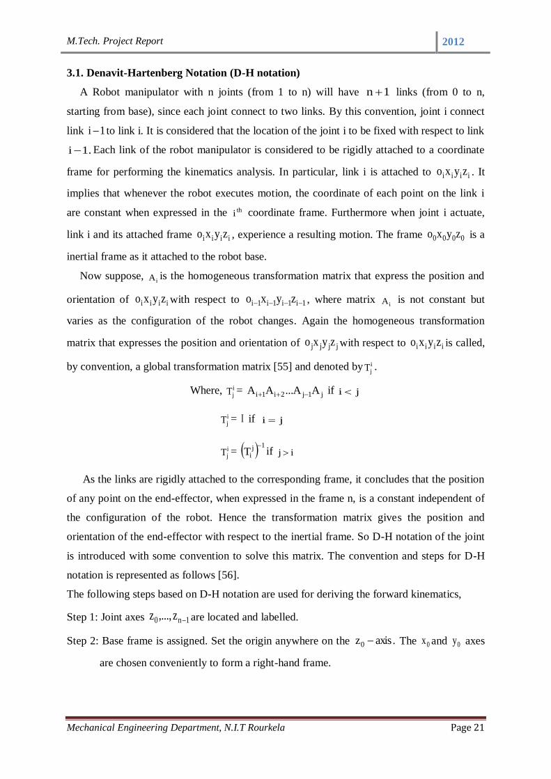
3.1. Denavit-Hartenberg Notation (D-H notation)
A Robot manipulator with n joints (from 1 to n) will have 1n links (from 0 to n,
starting from base), since each joint connect to two links. By this convention, joint i connect
link 1i to link i. It is considered that the location of the joint i to be fixed with respect to link
.1i Each link of the robot manipulator is considered to be rigidly attached to a coordinate
frame for performing the kinematics analysis. In particular, link i is attached to iiii zyxo . It
implies that whenever the robot executes motion, the coordinate of each point on the link i
are constant when expressed in the thi coordinate frame. Furthermore when joint i actuate,
link i and its attached frame iiii zyxo , experience a resulting motion. The frame 0000 zyxo is a
inertial frame as it attached to the robot base.
Now suppose, iA is the homogeneous transformation matrix that express the position and
orientation of iiii zyxo with respect to 1i1i1i1i zyxo , where matrix iA is not constant but
varies as the configuration of the robot changes. Again the homogeneous transformation
matrix that expresses the position and orientation of jjjj zyxo with respect to iiii zyxo is called,
by convention, a global transformation matrix [55] and denoted by ijT .
Where, ijT = j1j2i1i AA...AA if ji
ijT = I if ji
ijT = 1j
iT
if ij
As the links are rigidly attached to the corresponding frame, it concludes that the position
of any point on the end-effector, when expressed in the frame n, is a constant independent of
the configuration of the robot. Hence the transformation matrix gives the position and
orientation of the end-effector with respect to the inertial frame. So D-H notation of the joint
is introduced with some convention to solve this matrix. The convention and steps for D-H
notation is represented as follows [56].
The following steps based on D-H notation are used for deriving the forward kinematics,
Step 1: Joint axes 1n0 z,...,z are located and labelled.
Step 2: Base frame is assigned. Set the origin anywhere on the .axisz0 The 0x and 0y axes
are chosen conveniently to form a right-hand frame.

M.Tech. Project Report 2012
Mechanical Engineering Department, N.I.T Rourkela Page 22
Step 3: The origin io is located, where the common normal to iz and 1iz intersects at iz . If
iz intersects 1iz , ia located at this intersection. If iz and 1iz are parallel, locate io in
any convenient position along iz .
Step 4: ix is considered along the common normal between 1iz and iz through io , or in
thedirection normal to the i1i zz plane if 1iz and iz intersect.
Step 5: iy is established to complete a right-hand frame.
Step 6: The end-effector frame is assigned as nnnn zyxo . Assuming the thn joint is revolute,
set azn along the direction 1nz . The origin on is taken conveniently along nz
direction, preferably at the centre of the gripper or at the tip of any tool that the
manipulator may be carrying.
Step 7: All the link parameters iiii ,d,a, are tabulated.
Figure 5. D-H parameters of a link i.e. iiii ,d,a,
Step 8: The homogeneous transformation matrices iA is determined by substituting the
above parameters as shown in equation (1).
Step 9: Then the global transformation matrix End0T is formed, as shown in equation (2).
This then gives the position and orientation of the tool frame expressed in base coordinates.
In this convention, each homogeneous transformation matrix iA is represented as a
product of four basic transformations:
),x(Rot)a,x(Trans)d,z(Trans),z(RotA iiiii

M.Tech. Project Report 2012
Mechanical Engineering Department, N.I.T Rourkela Page 23
(1)
1000
d)cos(α)sin(α0
)sin(θa)sin(αθcos))cos(αcos(θ)sin(θ
)cos(θa))sin(αsin(θ)cos(α)sin(θθcos
iii
iiiiiii
iiiiiii
Where
four quantities iiii ,d,a, are parameter associate with link i and joint i. The
four parameters iiii ,d,a, in the above equation are generally given name as joint angle,
link length, link offset, and link twist.
3.2. The forward kinematics of a 5-DOF and 7-DOF Redundant manipulator.
3.2.1. Coordinate frame of a 5-DOF Redundant manipulator.
Figure 6. A Pioneer Arm Redundant manipulator
Figure 7. Coordinate frame for the 5-DOF Redundant manipulator

M.Tech. Project Report 2012
Mechanical Engineering Department, N.I.T Rourkela Page 24
Table 1. Angle of rotation of joints
Types of Joint Range of Rotation
Rotating base/ shoulder (1 ) 00 1800
Rotating elbow (2 ) 00 1500
Pivoting elbow (3 )
00 1500
Rotating wrist (4 ) 00 850
Pivoting wrist (5 )
00 4515
3.2.2. Forward kinematics calculation of the 5-DOF Redundant manipulator.
Robot control actions are executed in the joint coordinates while robot motions are
specified in the Cartesian coordinates. Conversion of the position and orientation of a robot
manipulator end-effecter from Cartesian space to joint space is called as inverse kinematics
problem, which is of fundamental importance in calculating desired joint angles for robot
manipulator design and control. The Denavit-Hartenberg (DH) notation and methodology
[56] is used to derive the kinematics of the 5-DOF Redundant manipulator. The coordinates
frame assignment and the DH parameters are depicted in Figure 2 and listed in Table 2
respectively where )z,y,x( 444 represents the local coordinate frames at the five joints
respectively, )z,y,x( 555 represents rotation coordinate frame at the end-effector where θi
represents rotation about the Z-axis and transition on about the X- axis, id transition along the
Z-axis, and ia transition along the X-axis.
Table 2. The D-H parameters of the 5-DOF Redundant manipulator.
Frame i (degree)
id (mm) ia (mm) i (degree)
O0 - O1 1 130d1
1a = 70 -90
O1 – O2 2 0
2a = 160 0
O2 – O3 390 0 0 -90
O3 – O4 4 140d4 0 90
O4 – O5 5 0 0 -90
O5 – O6 0 120d6 0 0

M.Tech. Project Report 2012
Mechanical Engineering Department, N.I.T Rourkela Page 25
The transformation matrix Ai between two neighbouring frames 1io and io is expressed
in equation (1) as,
),x(Rot)a,x(Trans)d,z(Trans),z(RotA iiiii
1000
d)cos(α)sin(α0
)sin(θa)sin(αθcos))cos(αcos(θ)sin(θ
)cos(θa))sin(αsin(θ)cos(α)sin(θθcos
iii
iiiiiii
iiiiiii
(1)
By substituting the D-H parameters in Table 1 into equation (1), it can be obtained the
individual transformation matrices 1A to 6 A and the general transformation matrix from the
first joint to the last joint of the 5-DOF Redundant manipulator can be derived by
multiplying all the individual transformation matrices (0T6).
1000
paon
paon
paon
AAAAAATzzzz
yyyy
xxxx
65432160
(2)
where )p,p,p( zyx are the positions and )a,a,a(),o,o,o(),n,n,n( zyxzyxzyx are the
orientations of the end-effector. The orientation and position of the end-effector can be
calculated in terms of joint angles and the D-H parameters of the manipulator are shown in
following matrix as:
1000
dsa
sdcsdsccdcssccscssccc
sacsacsd
ccsdsscdscssd
ccs
sscscssccss1sscs
cscccss
caccaccd
cccdsssdscscd
ccc
sssscsccssscscc
cssccsc
122
23452365423652354234235235423
112122314
523165416542316
5231
54154231
414235231
54154231
112122314
523165416542316
5231
54154231
4142315231
5414231 5
(3)
where )( sins and )( cosc ),( sins ),( cosc 32233223iiii
By equalizing the matrices in equations (2) and (3), the following equations are derived
112122314523165416542316x caccaccdcccdsssdscscdp (4)
M.Tech. Project Report 2012
Mechanical Engineering Department, N.I.T Rourkela Page 26
112122314523165416542316y sacsacsdccsdsscdscssdp (5)
1222345234523654236z dsasdcsdcsdsccdp (6)
523154154231x scccssccscn (7)
523154154231y scscscccssn (8)
5235423z sscccn (9)
414231x csssco (10)
414231y ccssso (11)
423z sco (12)
523154154231x ccccssscsca (13)
523154154231y ccssscscssa (14)
5235423z csscca (15)
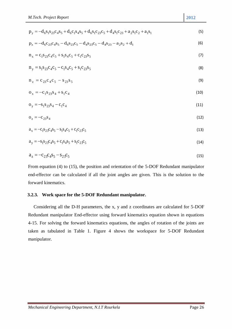
From equation (4) to (15), the position and orientation of the 5-DOF Redundant manipulator
end-effector can be calculated if all the joint angles are given. This is the solution to the
forward kinematics.
3.2.3. Work space for the 5-DOF Redundant manipulator.
Considering all the D-H parameters, the x, y and z coordinates are calculated for 5-DOF
Redundant manipulator End-effector using forward kinematics equation shown in equations
4-15. For solving the forward kinematics equations, the angles of rotation of the joints are
taken as tabulated in Table 1. Figure 4 shows the workspace for 5-DOF Redundant
manipulator.

M.Tech. Project Report 2012
Mechanical Engineering Department, N.I.T Rourkela Page 27
Figure 8. Work space for 5-DOF Redundant manipulator
3.2.4. Coordinate frame of a 7-DOF Redundant manipulator.
Figure 9. Coordinate frame for a 7-DOF Redundant manipulator
3.2.5. Forward kinematics calculation of the 7-DOF Redundant manipulator.
The D-H parameter for the 7-DOF Redundant manipulator is tabulated in Table 2.
Table 3. The D-H parameters of the 7-DOF Redundant manipulator
frame Link i(degree) id (cm) ia (cm) i (degree)
10 oo 1 270 to2701 30d1 0 0

M.Tech. Project Report 2012
Mechanical Engineering Department, N.I.T Rourkela Page 28
By substituting the D-H parameters in Table 2 into equation (1), the individual
transformation matrices A1 to AEnd can be obtained and the global transformation matrix
)T( End0 from the first joint to the last joint of the 7-DOF Redundant manipulator can be
derived by multiplying all the individual transformation matrices. So,
(16)
1000
paon
paon
paon
AAAAAAAATzzzz
yyyy
xxxx
End7654321End0
Where zyx p,p,p
are the positions and )a,a,a( and ),o,o,o(),n,n,n( zyxzyxzyx are the
orientations of the end-effector. The orientation and position of the end-effector can be
calculated in terms of joint angles and the D-H parameters of the manipulator are shown in
following equations:
cssccccsssccs
ccssscscsccsscsssccccsscccn
2121421214376
21213576572121421214357567x
(17)
sscccsccssccs
sccsscscscssccssccsccsscccn
2121421214376
21213576572121421214357567y
(18)
scssccssssccssccsccscsccn 543753743673367356754367z
(19)
ccsssss
csscssscccccscssccccssscco
2121356
2121421214356212142121436x
(20)
21 oo 2 110 to1102 0 0 -90
32 oo 3 180 to1803 35d3 0 90
43 oo 4 110 to1104 0 0 -90
54 oo 5 180 to1805 31d5 0 90
65 oo 6
90 to906 0 0 -90
76 oo 7 270 to2707 0 0 90
Endo7 End _ 42d7 0 0

M.Tech. Project Report 2012
Mechanical Engineering Department, N.I.T Rourkela Page 29
sccssss
ssccssccscccssscccsccsscco
2121356
2121421214356212142121436y
(21)
ccs scs ccsso 6436355436z
(22)
cssccccssscss
ccssscccsscsscsssccccscccsa
2121421214376
21213576572121421214357567x
(23)
sscccsccsscss
sccssccscsssccssccsccscccsa
2121421214367
21213575672121421214357567y
(24)
ccc sscc ssss cscs ccscs a 75353473467356754367z
(25)
csscdcssccccssscdssd
ccssscccssdcsscsssccccscccsdp
21213212142121435677
2121357657721214212143575677x
(26)
sscccsccsscdssd
sccsscccssdssccssccscccsccsdp
212142121435677
2121357657721214212143755677y
(27)
dssdcccdccssdssssdccssdcccssdp 13453577473573467736577456377z
(28)
From equation (17)-(28), are the position and orientation of the 7-DOF Redundant
manipulator end-effector and the exact value of these equations can be calculated if all the
joint angles are given. This is the solution to the forward kinematics.
3.2.6. Work space for the 7-DOF Redundant manipulator.
Considering all the D-H parameters, the x, y and z coordinates (i.e. End-effector
coordinates) are calculated for 7-DOF Redundant manipulator using forward kinematics
equation as shown in equations 17-28. For solving the forward kinematics equations, the
angles of rotation of the joints are taken as tabulated in Table 2. Figure 6 shows the
workspace for this manipulator.

M.Tech. Project Report 2012
Mechanical Engineering Department, N.I.T Rourkela Page 30
Figure 10. Work space for 7-DOF Redundant manipulator
3.3. Inverse kinematics of 5-DOF Redundant manipulator.
The forward kinematics equations (4)-(15) are highly nonlinear and discontinuous. It is
obvious that the inverse kinematics solution is very difficult to derive. This paper uses
various tricky strategies to solve the inverse kinematics of the 5-DOF robot manipulator.
From equations (4) and (13), the following equation is derived:
)acacd(cadp 1222341x6x (29)
Similarly by manipulating in similar way from equations (5) and (14), the following equation
is derived as:
)acacd(sadp 1222341y6y (30)
It can be noted that the values of 2 and 3 in 5-DOF Redundant manipulator only
takes integral values in a limited range. By checking all possible joint angles 2 and 3
that 0)acacd( 122234 holds good, which means that x6x adp and y6y adp will not
equals to zero at same time. Now considering the two possible situations,
If 0)acacd( 122234 , the solution for 1 is,
)adp,adp2tana x6xy6y1 (31)
Otherwise, )pad,pad2tana xx6yy61 (32)

M.Tech. Project Report 2012
Mechanical Engineering Department, N.I.T Rourkela Page 31
In solving the inverse kinematics solution of a higher DOF robot, 1tana function cannot
show the effect of the individual sign for numerator and denominator but represent the angle
in first or fourth quadrant. To overcome this problem and determine the joint in the correct
quadrant, atan2 function is introduced in equations (31) and (32).
Now for deriving solutions for 2 and3 , equations (29) and (30) can be represented as
follows:
11x6x22234 ac/)adp(cacd (33)
11y6y22234 as/)adp(cacd (34)
From equations (6) and (15), the following equation can be derived,
122234z6z dsasdadp (35)
Now considering equations (33) and (35),
let 11x6x ac/)adp(r (36)
and 122234z dsasdr (37)
Now squaring the equations (36) and (37) followed by addition, equation (38) can be derived
as follows:
2z
2223223242
24 rra)sscc(da2d (38)
Solving the terms 232232 sscc in equation (38), we get
) ( cos)( cos) ( cos cos)sscc( 3333232232
Therefore, there are several possible solutions for 3 , which are as follows:
42
24
22
2z
2
3da2
darracos ±= (39)
or
42
2z
224
22
3da2
rrdacosa (40)
Where the positive sign on the right hand side of the equation denotes for the elbow-out
and the negative sign represents elbow-in configuration. The two solutions for the elbow-out
and elbow-in of the 5-DOF Redundant manipulator are shown in the Figure 10.

M.Tech. Project Report 2012
Mechanical Engineering Department, N.I.T Rourkela Page 32
Figure 11. Elbow –in and Elbow-out configuration
Now consider the possible solutions for2 .
For the sake of convenience, equation (35) can be rewritten as equation (41):
221234 saBsd (41)
Where 11zz6 Bdpad
Considering the equations (33) and (34), equation (42) is derived as:
2y6y
2x6x 22 234 )pda()pda( =ca +cd (42)
Let 2y6y
2x6x 2 )pda()pda(=B , so equation (42) can be rewritten as
222234 caBcd (43)
Rearranging equations (41) and (43) and solving for21 B,B . Equations (44) and (45) are
derived as:
23422341 c )s(d + s )a + c(d = B (44)
23422342 s )s(d - c )a + c(d = B (45)
Dividing both sides of (44) and (45), by 22
21 BB , equations (46) and (47) are derived as,
22
21
12 2
BB
B = cos * sin +sin * cos
(46)
22
21
22 2
BB
B = cos * sin -sin * cos
(47)
where 22
21
234
BB
)acd( = cos
and
22
21
34
BB
)sd( = sin
The equations (46) and (47) are rewritten as:
22
21
12
BB
B = ) + sin(
(48)
M.Tech. Project Report 2012
Mechanical Engineering Department, N.I.T Rourkela Page 33
And 22
21
22
BB
B= ) + cos(
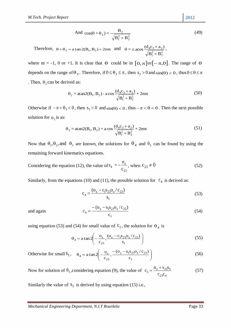
(49)
Therefore, m2)B,B(2tana 212 and
22
21
234
BB
)acd(acos ±=
,
where m = -1, 0 or +1. It is clear that could be in ,0 or 0, . The range of
depends on the range of 3 . Therefore, if 30 , then 0s3 and 0)sin( , thus 0
. Then, 2 can be derived as:
2m +BB
)acd(cosa - )B ,atan2(B =
22
21
234212
(50)
Otherwise if 03 , then 0s3 and 0)sin( , thus 0 . Then the next possible
solution for 2 is as:
2m +BB
)acd(cosa + )B ,atan2(B =
22
21
234212
(51)
Now that 321 and,, are known, the solutions for 4 and 5 can be found by using the
remaining forward kinematics equations.
Considering the equation (12), the value of23
z4
c
o= s , when 0c23 (52)
Similarly, from the equations (10) and (11), the possible solution for 4c is derived as:
1
23z231x4
s
)c/osco(c
(53)
and again 1
23z231y4
c
)c/osso(c
(54)
using equation (53) and (54) for small value of 1c , the solution for 4 is
1
23z231z
23
z4
s
)c/osco(,
c
o2tana (55)
Otherwise for small 1s ,
1
23z231y
23
z4
c
)c/osso(,
c
o2tana (56)
Now for solution of 5 ,considering equation (9), the value of 423
523z5
cc
ssnc
(57)
Similarly the value of 5s is derived by using equation (15) i.e.,

M.Tech. Project Report 2012
Mechanical Engineering Department, N.I.T Rourkela Page 34
423
523z5
cc
csas
(58)
using equation (41) in (40) and vice versa, the term 5c and 5s is rewritten as:
223
24
223
z23423z5
scc
asccnc
and 2
2324
223
z23423z5
scc
)nscca(s
now using this above derivation of 5c and 5s , 5 is derived as follows:
z23423zz23423z5 asccn,nscca2tana (59)
The above derivations with various conditions being taken into account provide a
complete analytical solution to inverse kinematics of 5-DOF Redundant manipulator. It is to
be noted that there exist two possible solutions for 4321 ,,, depicted in (31) or (32), (50)
or (51), (39) or (40), (55) or (56) respectively. So to know which solution holds good to study
the inverse kinematics, all joint angles are obtained and compared using the forward
kinematics solution. This process is being applied for .,,, 4321 To choose the correct
solution, all the four sets of possible solutions (joint angles) calculated, which generate four
possible corresponding positions and orientations using the forward kinematics. By
comparing the errors between these four generated positions and orientations and the given
position and orientation, one set of joint angles, which produces the minimum error, is chosen
as the correct solution. The solutions (32), (50), (39), and (56) holds correct for obtaining the
values of 4321 ,,, respectively.
*****

M.Tech. Project Report 2012
Mechanical Engineering Department, N.I.T Rourkela Page 35
CHAPTER 4

M.Tech. Project Report 2012
Mechanical Engineering Department, N.I.T Rourkela Page 36
Chapter 4
4. ANFIS Architecture
ANFIS stands for adaptive neuro-fuzzy inference system developed by Roger Jang [57]. It
is a feed forward adaptive neural network which implies a fuzzy inference system through its
structure and neurons. He reported that the ANFIS architecture can be employed to model
nonlinear functions, identify nonlinear components on-line in a control system, and predict a
chaotic time series. It is a hybrid neuro-fuzzy technique that brings learning capabilities of
neural networks to fuzzy inference systems. It is a part of the fuzzy logic toolbox in
MATLAB R2008a software of Math Work Inc [58]. The fuzzy inference system (FIS) is a
popular computing frame work based on the concepts of fuzzy set theory, fuzzy if-then rule,
and fuzzy reasoning. It has found successful application in a wide variety of fields, such as
automatic control, data classification, decision analysis, expert system, time series prediction,
robotics, and pattern recognition. The basic structure of a FIS consists of 3 conceptual
components: a rule base, which contains a selection of fuzzy rules: a database, which define
the membership function used in fuzzy rules; a reasoning mechanism, which performs the
inference procedure upon the rules and given facts to derive a reasonable output or
conclusion. The basic FIS can take either fuzzy input or crisp inputs, but outputs it produces
are almost always fuzzy sets. Sometime it is necessary to have a crisp output, especially in a
situation where a FIS is used as a controller. Therefore, method of defuzzification is needed
to extract a crisp value that best represent a fuzzy set.
For solving the IK of 5-DOF and 7-DOF redundant manipulator used in this work Sugeno
fuzzy inference system is used, to obtain the fuzzy model,. The Sugeno FIS was proposed by
Takagi, Sugeno, and Kang [59, 60] in an effort to develop a systematic approach to generate
fuzzy rules from a given input and output data set. The typical fuzzy rule in a Sugeno fuzzy
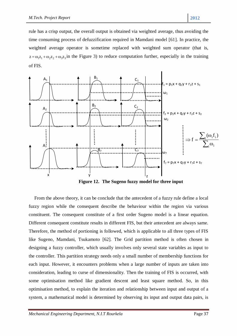
model for three inputs used in this work for both the manipulator has the form:
If x is A, y is B and z is C, then )z,y,x(fz ,
where A, B, C are fuzzy sets in the antecedent, while )z,y,x(fz is a crisp function in
the consequent. Usually,
)z,y,x(f is a polynomial in the input variables x, y, and z but it can
be any function as long as it can appropriately describe the output of the model with the fuzzy
region specified by antecedent of the rule. When )z,y,x(f is a first order polynomial, the
resulting FIS is called first order Sugeno fuzzy model. When the fuzzy rule is generated,
fuzzy reasoning procedure for the fuzzy model is followed as shown in Figure 3. Since each
M.Tech. Project Report 2012
Mechanical Engineering Department, N.I.T Rourkela Page 37
rule has a crisp output, the overall output is obtained via weighted average, thus avoiding the
time consuming process of defuzzification required in Mamdani model [61]. In practice, the
weighted average operator is sometime replaced with weighted sum operator (that is,
332211 zzzz in the Figure 3) to reduce computation further, especially in the training
of FIS.
Figure 12. The Sugeno fuzzy model for three input
From the above theory, it can be conclude that the antecedent of a fuzzy rule define a local
fuzzy region while the consequent describe the behaviour within the region via various
constituent. The consequent constitute of a first order Sugeno model is a linear equation.
Different consequent constitute results in different FIS, but their antecedent are always same.
Therefore, the method of portioning is followed, which is applicable to all three types of FIS
like Sugeno, Mamdani, Tsukamoto [62]. The Grid partition method is often chosen in
designing a fuzzy controller, which usually involves only several state variables as input to
the controller. This partition strategy needs only a small number of membership functions for
each input. However, it encounters problems when a large number of inputs are taken into
consideration, leading to curse of dimensionality. Then the training of FIS is occurred, with
some optimisation method like gradient descent and least square method. So, in this
optimisation method, to explain the iteration and relationship between input and output of a
system, a mathematical model is determined by observing its input and output data pairs, is
A1
A2
A7
B1
B2
B7
C1
C2
C7
f1 = p1x + q1y + r1z + s1
f2 = p2x + q2y + r2z + s2
f7 = p7x + q7y + r7z + s7
ω1
ω2
ω7
i i
i ii )f(f
x y z

M.Tech. Project Report 2012
Mechanical Engineering Department, N.I.T Rourkela Page 38
generally refer to as system identification. The system identification includes the following
steps [63].
Specify and parameterize a class of mathematical model representing the system to
be identified.
Perform parameter identification to choose the parameters that best fit the training
data.
Conduct validation tests to see if the model identified responds correctly to an
unseen data set.
Terminate the procedure once the results of the validation tests are satisfactory.
Otherwise, another class of model is selected and steps 2 through step 4 are
repeated.
From the above discussions, it is concluded that ANFIS is a fuzzy rule-based model using
neural network like structure (i.e. involving nodes and links). It consists of five layers
implementing fuzzy inference systems as schematically shown in Figure 12. The square
nodes are adaptive nodes and the circle nodes are fixed ones. Figure 12 shows a simple
ANFIS model that has been used in this work with three inputs (x, y, and z), seven
membership functions for each input, and 343 rules for three inputs. The first layer of ANFIS
determines the degree to a fuzzy condition involving the given input by using membership
functions (Ai and Bi). The second layer evaluates the truth value (matching degree) of the
premise of each rule in the rule base. The third layer normalizes these truth values. The fourth
layer computes the consequent of each rule. Finally, the fifth layer computes the aggregate
output of all the rules.
The above mentioned layers for a first order Sugeno model can be describe in detail as
follow. Here the Gaussian membership function is used for 7-DOF Redundant manipulator.
Layer 1: (Input layer)
In this layer, each node is equal to a fuzzy set and output of a node in the respective fuzzy set
is equal to the input variable membership grade. The parameters of each node determine the
membership function (Gaussian membership function for this present work) form in the fuzzy
set of that node.
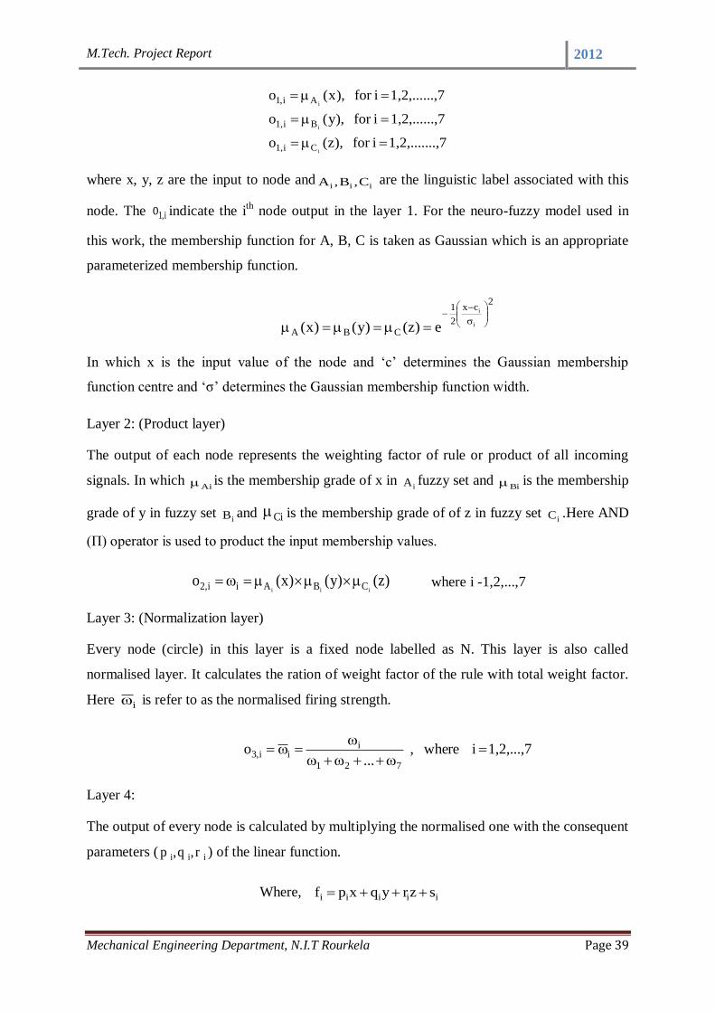
M.Tech. Project Report 2012
Mechanical Engineering Department, N.I.T Rourkela Page 39
.,71,2,...... ifor ),z(o
,71,2,......ifor ),y(o
,71,2,...... ifor ),x(o
i
i
i
Ci1,
Bi1,
Ai,1
where x, y, z are the input to node andiii C,B,A are the linguistic label associated with this
node. The i,1o indicate the ith
node output in the layer 1. For the neuro-fuzzy model used in
this work, the membership function for A, B, C is taken as Gaussian which is an appropriate
parameterized membership function.
2cx
2
1
CBAi
i
e)z()y()x(
In which x is the input value of the node and ‘c’ determines the Gaussian membership
function centre and ‘σ’ determines the Gaussian membership function width.
Layer 2: (Product layer)
The output of each node represents the weighting factor of rule or product of all incoming
signals. In which Ai is the membership grade of x in
iA fuzzy set and Bi is the membership
grade of y in fuzzy set iB and Ci is the membership grade of of z in fuzzy set
iC .Here AND
(Π) operator is used to product the input membership values.
)z()y()x(oiii CBAii,2 where i -1,2,...,7
Layer 3: (Normalization layer)
Every node (circle) in this layer is a fixed node labelled as N. This layer is also called
normalised layer. It calculates the ration of weight factor of the rule with total weight factor.
Here i is refer to as the normalised firing strength.
1,2,...,7 i where, ...
o721
iii,3
Layer 4:
The output of every node is calculated by multiplying the normalised one with the consequent
parameters ( iii r, q, p ) of the linear function.
Where, iiiii szryqxpf
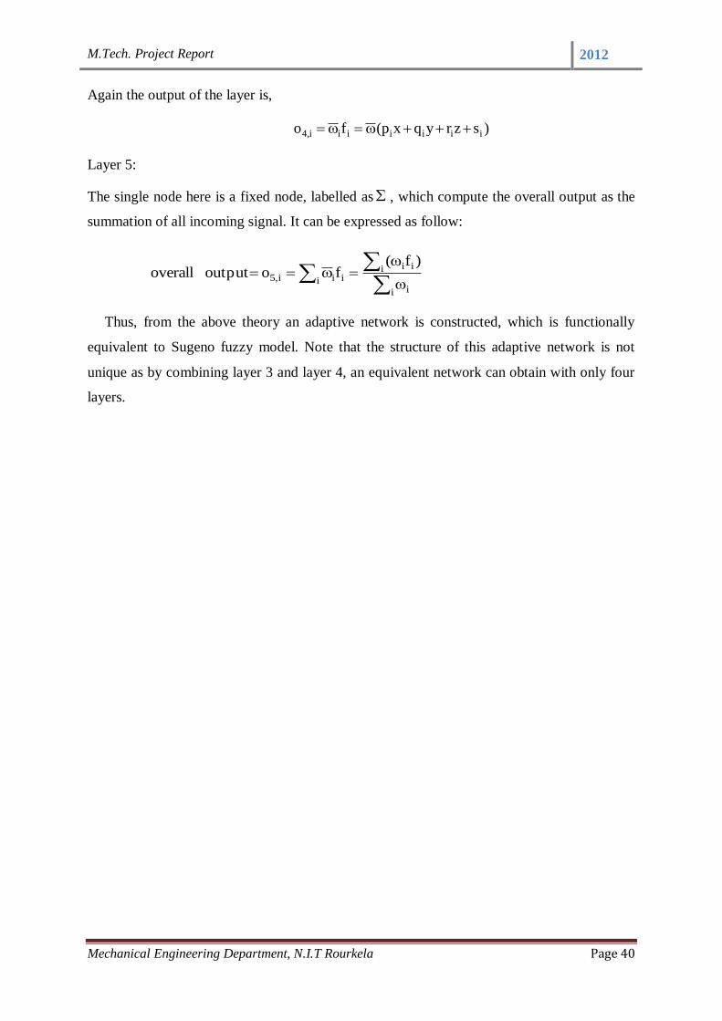
M.Tech. Project Report 2012
Mechanical Engineering Department, N.I.T Rourkela Page 40
Again the output of the layer is,
)szryqxp(fo iiiiiii,4
Layer 5:
The single node here is a fixed node, labelled as , which compute the overall output as the
summation of all incoming signal. It can be expressed as follow:
i i
i ii
i iii5,
)f(fo output overall
Thus, from the above theory an adaptive network is constructed, which is functionally
equivalent to Sugeno fuzzy model. Note that the structure of this adaptive network is not
unique as by combining layer 3 and layer 4, an equivalent network can obtain with only four
layers.

M.Tech. Project Report 2012
Mechanical Engineering Department, N.I.T Rourkela Page 41
Figure 13. Architecture of three inputs with seven membership functions of the ANFIS model
4.1 ANFIS Architecture used for 5-DOF Redundant manipulator.
The coordinates and the angles obtained from forward kinematics solutions are used as
training data to train ANFIS network with the triangular membership function with a hybrid
learning algorithm. For solving the inverse kinematics equation of 5-DOF Redundant
manipulator, in this work, considers the ANFIS structure with first order Sugeno model
containing 343 rules. For the neuro-fuzzy model used in this work, 1024 data points
analytically obtained using forward kinematics, of which 776 are used for training and the
remaining 248 are used for testing (or validating).
f
n
x
y
z
П
П
П
П
П
П
П
N
N
N
N
N
N
N
∑
Inputs
i1 .. i3
Inputs
i1 .. i3
Inputs
i1 .. i3
Inputs
i1 .. i3
Inputs
i1 .. i3
Inputs
i1 .. i3
Inputs
i1 .. i3
Layer 1 Layer 2 Layer 3 Layer 5 Layer 4
ω1
ωn
1
11f
nnf
A4
A3
A7
A2
A1
A5 A6
C1
C2
C3
C4
C5
C7
C6
B1
B2
B3
B4
B5
B6
B7

M.Tech. Project Report 2012
Mechanical Engineering Department, N.I.T Rourkela Page 42
Training of ANFIS is usually performed by using ANFIS editor GUI of MATLAB [64].
The ANFIS Editor GUI window displays the four main sub displays. These are 1. Load data,
2. Generate FIS, 3. Train FIS and 4. Test FIS. Once the FIS is generated, the model structure
can be viewed as shown in Figure 13.
Figure 14. ANFIS model structure used for 5-DOF Redundant manipulator
The branches in Figure 13 are color coded. Color coding of branches characterize the rules
and indicate whether and, or, not are used in the rules. The input is represented by the left-
most node and the output by the right-most node. The node represents a normalization factor
for the rules. Clicking on the nodes indicates information about the structure. To start the
training, GENFIS1 function is used. GENFIS1 uses the grid partitioning and it generates
rules by enumerating all possible combinations of membership functions of all inputs; this
leads to an exponential explosion even when the number of inputs is moderately large. For
instance, for a fuzzy inference system with 3 inputs, each with seven membership functions,
the grid partitioning leads to 343 (=7^3) rules. GENFIS1 use a given training data set to
generate an initial fuzzy inference system (represented by a FIS matrix) that can be fine-tuned
via the ANFIS command. GENFIS1 produces a grid partitioning of the input space and a
fuzzy inference system where each rule has zero coefficients in its output equation.

M.Tech. Project Report 2012
Mechanical Engineering Department, N.I.T Rourkela Page 43
4.2 ANFIS Architecture used for 7-DOF Redundant manipulator.
For solving the inverse kinematics equation of 7-DOF Redundant manipulator, in this
work, the grid partitioning option in the ANFIS toolbox is used. For each input, 7
membership function (Gaussian membership) are used along with 343(=7^3) fuzzy rules are
applied for all three inputs. For the neuro-fuzzy model used, 2187 data points are analytically
obtained from MATLAB, of which 1640 are used for training and the remaining 547 are used
for testing (validating). The model structure for the 7-DOF Redundant manipulator used in
ANFIS can be viewed as similar to the structure obtained for 5-DOF Redundant manipulator
as discussed in the previous section. For obtaining the model for 7-DOF Redundant
manipulator the Gaussian membership function with seven number of membership for each
input is used as shown in following figure 14. The model structure obtained for 7-DOF
manipulator. The Anfis information used for solving the 7-DOF Redundant manipulator for
this work is tabulated in Table. 4.
Table 4. ANFIS information used for solving 7-DOF Redundant manipulator
3 inputs : Cartesian coordinates: x, y, and z
1 output : joint coordinate (θ)
7 member functions each input node : Sugeno types
Number of nodes : 734
Number of linear parameters : 1372
Number of nonlinear parameters : 42
Total number of parameters : 1414
Number of training data pairs : 1638
Number of checking data pairs : 2187
Number of fuzzy rules : 343

M.Tech. Project Report 2012
Mechanical Engineering Department, N.I.T Rourkela Page 44
Figure 15. ANFIS model structure used for 5-DOF Redundant manipulator
*****

M.Tech. Project Report 2012
Mechanical Engineering Department, N.I.T Rourkela Page 45
CHAPTER 5

M.Tech. Project Report 2012
Mechanical Engineering Department, N.I.T Rourkela Page 46
Chapter 5
5. RESULT AND DISCUSSION
In this section of the thesis the surface plots, the residual plots and the normal probability
plots for the 5-DOF and 7-DOF redundant manipulator is carried out. The surface plots
obtained for this type of manipulators explains the efficiency of the ANFIS methodology.
The residual plots obtained by comparing the predicted data from the ANFIS and the
analytical data show that, the data predicted using ANFIS methodology deviate very less
from the analytical data. The last section of this chapter is concluded with obtaining the
normal probability plots. The details of the plots are explains in the following section.
5.1 3-D Surface viewer Analysis
In this section the 3-D surface plots, obtained for the 5-DOF and 7-DOF Redundant
manipulator is discussed. The surface plot dispaly both the connecting lines and faces of the
surface in color. The surf command in MATLAB tool is use to create the 3-D surface plots of
the matrix data. The surface plot explains the relation between the output and two inputs.
5.1.1 3-D Surface plots obtained for all joint angles of 5-DOF Redundant manipulator
Figures 15-19 show surface plot of five ANFIS networks relating inputs with joint angles
of 5-DOF Redundant manipulator. Figure 15 indicates the surface plot between Cartesian
coordinates y and z for 1 . It shows that when the values of y and z moving in a positive
direction, there is a marginal increase followed by a decrease in 1 values. The inputs-output
surface plot of 2 is shown in Figure 16. The Figure depicts that the value of 2 increases
linearly when moving in the positive direction of y coordinate to some values of y and then
there is a sudden increase of 2 values. No significant change in the value of 2 is observed
with change in values of z coordinate. By moving from negative direction to the positive
direction of x and y coordinates, the 3 value decreases first then followed by slightly
increase, can be easily conclude from figure 17. Similarly the surface plot of 5 with input
variables x and z coordinate is depicted in figure 19. It shows that the value of inputs has
significant effect in determining the value of 5 . It concludes from the surface plot that the
contribution of interdependent parameters toward obtaining the output can easily provide
through the ANFIS algorithm and can be hardly obtained otherwise without employing

M.Tech. Project Report 2012
Mechanical Engineering Department, N.I.T Rourkela Page 47
massive computations. All the surface viewer plots show that the total surface is covered by
the rule base.
Figure 16. Surface plot for 1
Figure 17. Surface plot for 2
Figure 18. Surface plot for 3

M.Tech. Project Report 2012
Mechanical Engineering Department, N.I.T Rourkela Page 48
Figure 19. Surface plot for 4
Figure 20. Surface plot for 5
5.1.2 3-D Surface plots obtained for all joint angles of 7-DOF Redundant manipulator
The following Figure 19-25 shows the three dimensional surface plot of ANFIS network
relating to the joint angle of 7-DOF Redundant manipulator. Figure 19 indicates the surface
plot between Cartesian coordinates y and z for 1 . When the value of z decreases, there is a
sudden increase in 1 value followed by decrease at the middle range of z value and there is
no significant change in 1 value for y coordinate. The inputs-output surface plot of 2 is
shown in Figure 20. The Figure depicts that the value of 2 decrease first followed by
increase, for the increase in the value of z. No significant change in the value of 2 is
observed with change in values of y coordinate. When y changes from positive value to
negative value, there is a marginal increase in the value of 3 as well as there is no
significant change with the value of z, as clearly noticed from Figure 21. With the increase in
y value, at its middle range, the value of 5 decrease first then increase, where as there is no
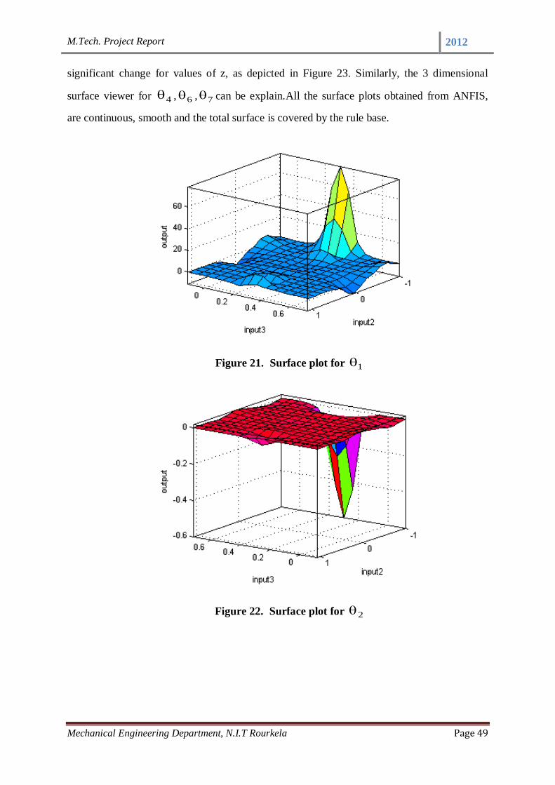
M.Tech. Project Report 2012
Mechanical Engineering Department, N.I.T Rourkela Page 49
significant change for values of z, as depicted in Figure 23. Similarly, the 3 dimensional
surface viewer for 4 , 6 , 7 can be explain.All the surface plots obtained from ANFIS,
are continuous, smooth and the total surface is covered by the rule base.
Figure 21. Surface plot for 1
Figure 22. Surface plot for 2

M.Tech. Project Report 2012
Mechanical Engineering Department, N.I.T Rourkela Page 50
Figure 23. Surface plot for 3
Figure 24. Surface plot for 4
Figure 25. Surface plot for 5
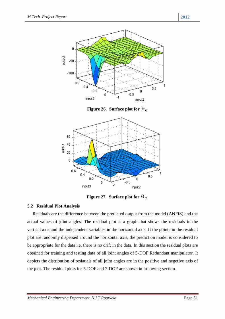
M.Tech. Project Report 2012
Mechanical Engineering Department, N.I.T Rourkela Page 51
Figure 26. Surface plot for 6
Figure 27. Surface plot for 7
5.2 Residual Plot Analysis
Residuals are the difference between the predicted output from the model (ANFIS) and the
actual values of joint angles. The residual plot is a graph that shows the residuals in the
vertical axis and the independent variables in the horizontal axis. If the points in the residual
plot are randomly dispersed around the horizontal axis, the prediction model is considered to
be appropriate for the data i.e. there is no drift in the data. In this section the residual plots are
obtained for training and testing data of all joint angles of 5-DOF Redundant manipulator. It
depicts the distribution of resiauals of all joint angles are in the positive and negetive axis of
the plot. The residual plots for 5-DOF and 7-DOF are shown in following section.

M.Tech. Project Report 2012
Mechanical Engineering Department, N.I.T Rourkela Page 52
5.2.1 The Residual plot of Training data for all joint angle of 5-DOF Redundant
manipulator.
The residual plots of training data for 54321 and ,,, of 5-DOF Redundant robot
manipulator are depicted in Figures 27-31 respectively. The residual plot shows a fairly
random pattern as some of the residuals are in positive and some are lies in the negative side
of the horizontal axis. Figure 27 shows a random pattern indicating a good fit for training
data of 1 . As a very large number of residuals lie close to the horizontal axis shown in
Figure 28, it indicates a reasonably good fit for 2 . The Figures 29-30 indicates a decent fit
to the model of 3 and 4 as most of the residuals lie between -0.01 to 0.01. The Figure 31
explains the residual plot for training data of 5 . It indicates a few of the residuals of 5 lies
beyond the range -0.1 to 0.1 and does not alter the prediction model of the data. The average
absolute error (actual minus and predicted values) for the training data are found to be
0.0700, 0.0011, 0.0330, 0.0850, and 0.0240 for the joint coordinates 54321 and ,,,
respectively. Similarly, the average absolute error of the testing data for the joint coordinates
54321 and ,,, are found to be 0.06, 0.03, 0.09,0.10, and 0.11 respectively.
Figure 28. Residual plot of training data for 1
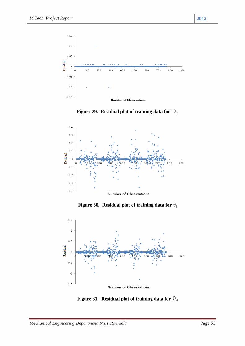
M.Tech. Project Report 2012
Mechanical Engineering Department, N.I.T Rourkela Page 53
Figure 29. Residual plot of training data for 2
Figure 30. Residual plot of training data for 3
Figure 31. Residual plot of training data for 4

M.Tech. Project Report 2012
Mechanical Engineering Department, N.I.T Rourkela Page 54
Figure 32. Residual plot of training data for 5
5.2.2 The Residual plot of Testing data for all joint angle of 5-DOF Redundant
manipulator.
The residual plots of testing data for 54321 and ,,, of 5-DOF Redundant robot
manipulator are studied. The residual plot shows a fairly random pattern as some of the
residuals are in positive axis and some are lies in the negative axis of the of the graph. Figure
32 shows a random pattern indicating a good fit for training data of 1 . As a very large
number of residuals lie close to the horizontal axis shown in Figure 33, it indicates a
reasonably good fit for 2 . The residuals for 3 lie between -0.2 to 0.2 and distributed over
both sides of the mean line. It indicates that the prediction model is well suited for the study
Figure 34. The Figures 35-36 indicates a decent fit to the model of 4 and 5 as most of the
residuals lie between -0.03 to 0.03.
Figure 33. Residual plot of testing data for 1
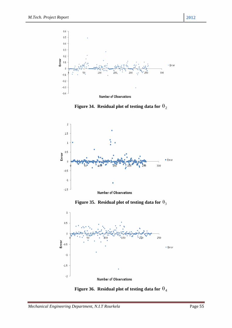
M.Tech. Project Report 2012
Mechanical Engineering Department, N.I.T Rourkela Page 55
Figure 34. Residual plot of testing data for 2
Figure 35. Residual plot of testing data for 3
Figure 36. Residual plot of testing data for 4
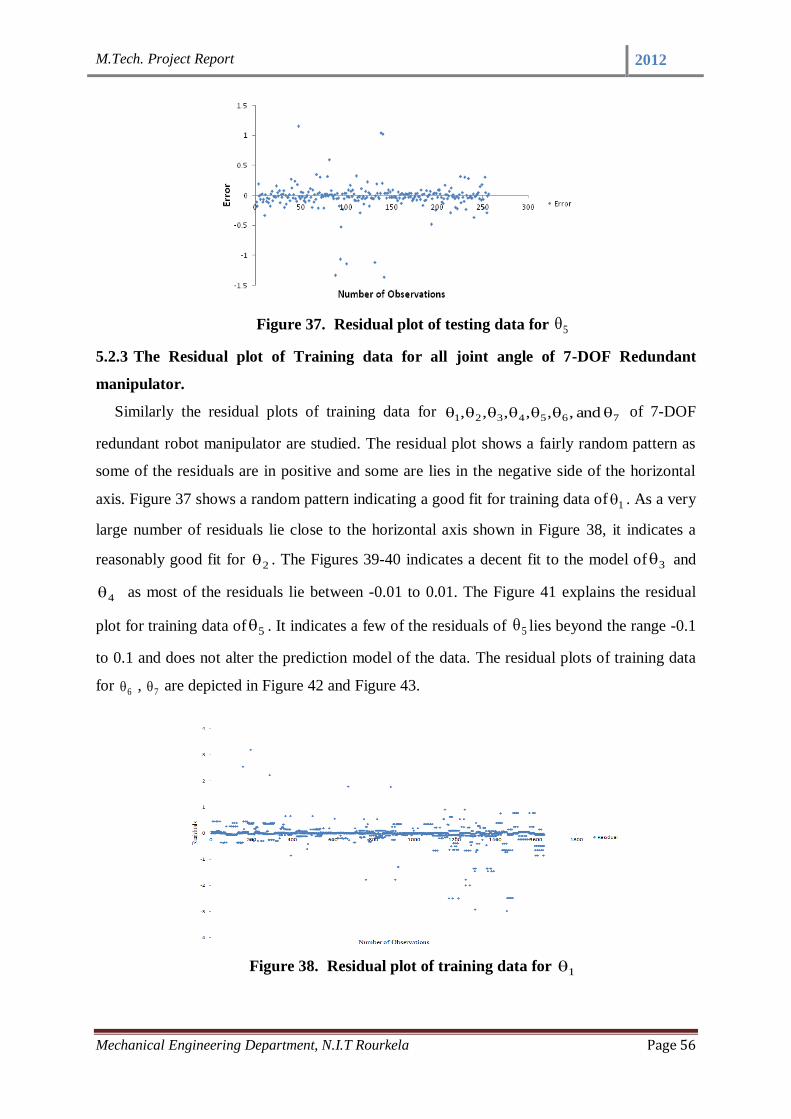
M.Tech. Project Report 2012
Mechanical Engineering Department, N.I.T Rourkela Page 56
Figure 37. Residual plot of testing data for 5
5.2.3 The Residual plot of Training data for all joint angle of 7-DOF Redundant
manipulator.
Similarly the residual plots of training data for 7654321 and ,,,,,, of 7-DOF
redundant robot manipulator are studied. The residual plot shows a fairly random pattern as
some of the residuals are in positive and some are lies in the negative side of the horizontal
axis. Figure 37 shows a random pattern indicating a good fit for training data of 1 . As a very
large number of residuals lie close to the horizontal axis shown in Figure 38, it indicates a
reasonably good fit for 2 . The Figures 39-40 indicates a decent fit to the model of 3 and
4 as most of the residuals lie between -0.01 to 0.01. The Figure 41 explains the residual
plot for training data of 5 . It indicates a few of the residuals of 5 lies beyond the range -0.1
to 0.1 and does not alter the prediction model of the data. The residual plots of training data
for 6 , 7 are depicted in Figure 42 and Figure 43.
Figure 38. Residual plot of training data for 1

M.Tech. Project Report 2012
Mechanical Engineering Department, N.I.T Rourkela Page 57
Figure 39. Residual plot of training data for 2
Figure 40. Residual plot of training data for 3
Figure 41. Residual plot of training data for 4
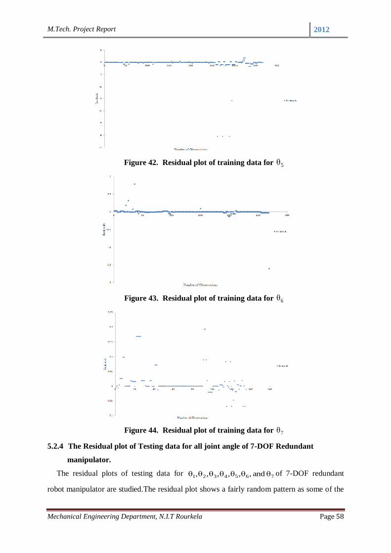
M.Tech. Project Report 2012
Mechanical Engineering Department, N.I.T Rourkela Page 58
Figure 42. Residual plot of training data for 5
Figure 43. Residual plot of training data for 6
Figure 44. Residual plot of training data for 7
5.2.4 The Residual plot of Testing data for all joint angle of 7-DOF Redundant
manipulator.
The residual plots of testing data for 7654321 and ,,,,,, of 7-DOF redundant
robot manipulator are studied.The residual plot shows a fairly random pattern as some of the
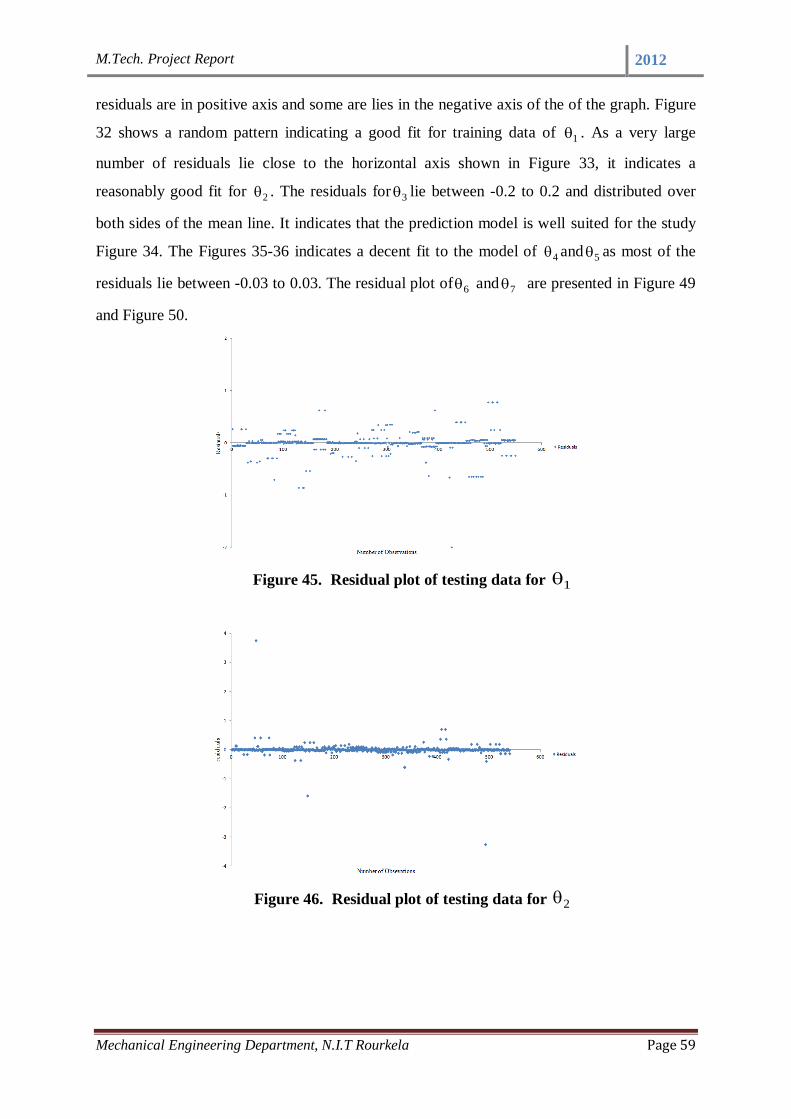
M.Tech. Project Report 2012
Mechanical Engineering Department, N.I.T Rourkela Page 59
residuals are in positive axis and some are lies in the negative axis of the of the graph. Figure
32 shows a random pattern indicating a good fit for training data of 1 . As a very large
number of residuals lie close to the horizontal axis shown in Figure 33, it indicates a
reasonably good fit for 2 . The residuals for 3 lie between -0.2 to 0.2 and distributed over
both sides of the mean line. It indicates that the prediction model is well suited for the study
Figure 34. The Figures 35-36 indicates a decent fit to the model of 4 and 5 as most of the
residuals lie between -0.03 to 0.03. The residual plot of 6 and 7 are presented in Figure 49
and Figure 50.
Figure 45. Residual plot of testing data for 1
Figure 46. Residual plot of testing data for 2
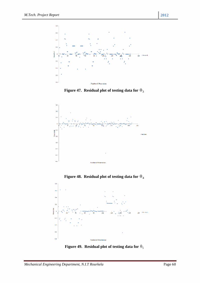
M.Tech. Project Report 2012
Mechanical Engineering Department, N.I.T Rourkela Page 60
Figure 47. Residual plot of testing data for 3
Figure 48. Residual plot of testing data for 4
Figure 49. Residual plot of testing data for 5

M.Tech. Project Report 2012
Mechanical Engineering Department, N.I.T Rourkela Page 61
Figure 50. Residual plot of testing data for 6
Figure 51. Residual plot of testing data for 7
5.3 Normal Probability Plot Analysis
The normal probability plot [65] is a graphical technique for assessing whether or not a
data set is approximately normally distributed, if it is nearly straight, the data satisfy the
nearly normal condition. The data are plotted against a theoretical normal distribution in such
a way that the points should form an approximate straight line. Departures from this straight
line indicate departures from normality. It provides a good assessment of the adequacy of the
normal model for a set of data. It can also be define as, in the normal probability plot, the
normal distribution is represented by a straight line angled at 45 degrees. The actual
distribution is plotted against this line so that any differences are shown as deviations from
the straight line, making identification of differences quite apparent and interpretable. In this
section, the normal probability plot of residuals of training and testing data of all joint angles
for the 5-DOF and 7-DOF Redundant manipulator is depicted in the following Figures. The
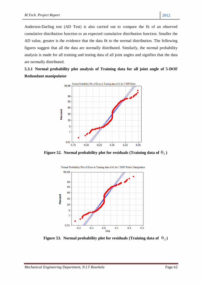
M.Tech. Project Report 2012
Mechanical Engineering Department, N.I.T Rourkela Page 62
Anderson-Darling test (AD Test) is also carried out to compare the fit of an observed
cumulative distribution function to an expected cumulative distribution function. Smaller the
AD value, greater is the evidence that the data fit to the normal distribution. The following
figures suggest that all the data are normally distributed. Similarly, the normal probability
analysis is made for all training and testing data of all joint angles and signifies that the data
are normally distributed.
5.3.1 Normal probability plot analysis of Training data for all joint angle of 5-DOF
Redundant manipulator
Figure 52. Normal probability plot for residuals (Training data of 1 )
Figure 53. Normal probability plot for residuals (Training data of 2 )

M.Tech. Project Report 2012
Mechanical Engineering Department, N.I.T Rourkela Page 63
Figure 54. Normal probability plot for residuals (Training data of 3 )
Figure 55. Normal probability plot for residuals (Training data of 4 )
Figure 56. Normal probability plot for residuals (Training data of 5 )
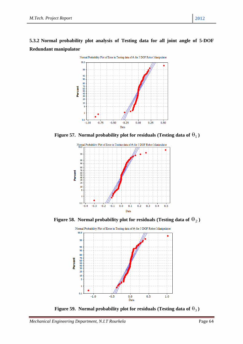
M.Tech. Project Report 2012
Mechanical Engineering Department, N.I.T Rourkela Page 64
5.3.2 Normal probability plot analysis of Testing data for all joint angle of 5-DOF
Redundant manipulator
Figure 57. Normal probability plot for residuals (Testing data of 1 )
Figure 58. Normal probability plot for residuals (Testing data of 2 )
Figure 59. Normal probability plot for residuals (Testing data of 3 )
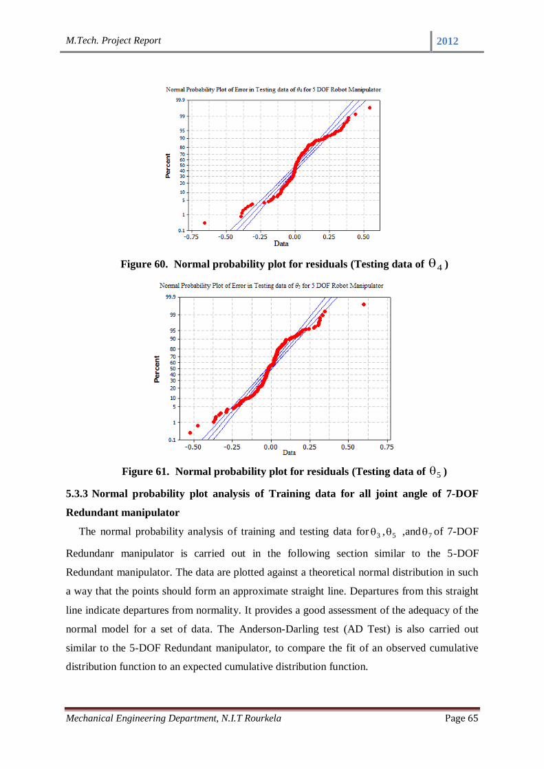
M.Tech. Project Report 2012
Mechanical Engineering Department, N.I.T Rourkela Page 65
Figure 60. Normal probability plot for residuals (Testing data of 4 )
Figure 61. Normal probability plot for residuals (Testing data of 5 )
5.3.3 Normal probability plot analysis of Training data for all joint angle of 7-DOF
Redundant manipulator
The normal probability analysis of training and testing data for 3 , 5 ,and 7 of 7-DOF
Redundanr manipulator is carried out in the following section similar to the 5-DOF
Redundant manipulator. The data are plotted against a theoretical normal distribution in such
a way that the points should form an approximate straight line. Departures from this straight
line indicate departures from normality. It provides a good assessment of the adequacy of the
normal model for a set of data. The Anderson-Darling test (AD Test) is also carried out
similar to the 5-DOF Redundant manipulator, to compare the fit of an observed cumulative
distribution function to an expected cumulative distribution function.

M.Tech. Project Report 2012
Mechanical Engineering Department, N.I.T Rourkela Page 66
Figure 62. Normal probability plot for residuals (Training data of 3 )
Figure 63. Normal probability plot for residuals (Training data of 5 )
Figure 64. Normal probability plot for residuals (Training data of 7 )
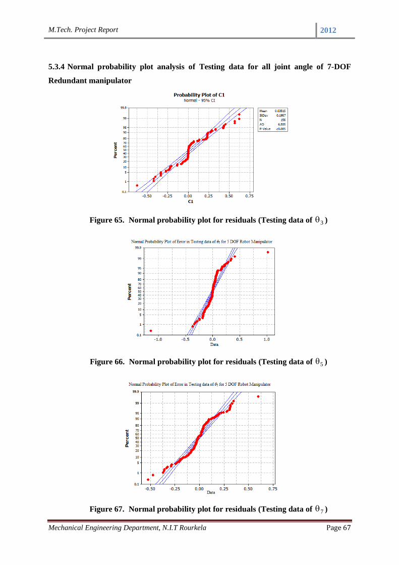
M.Tech. Project Report 2012
Mechanical Engineering Department, N.I.T Rourkela Page 67
5.3.4 Normal probability plot analysis of Testing data for all joint angle of 7-DOF
Redundant manipulator
Figure 65. Normal probability plot for residuals (Testing data of 3 )
Figure 66. Normal probability plot for residuals (Testing data of 5 )
Figure 67. Normal probability plot for residuals (Testing data of 7 )
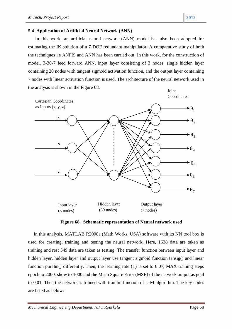
M.Tech. Project Report 2012
Mechanical Engineering Department, N.I.T Rourkela Page 68
5.4 Application of Artificial Neural Network (ANN)
In this work, an artificial neural network (ANN) model has also been adopted for
estimating the IK solution of a 7-DOF redundant manipulator. A comparative study of both
the techniques i.e ANFIS and ANN has been carried out. In this work, for the construction of
model, 3-30-7 feed forward ANN, input layer consisting of 3 nodes, single hidden layer
containing 20 nodes with tangent sigmoid activation function, and the output layer containing
7 nodes with linear activation function is used. The architecture of the neural network used in
the analysis is shown in the Figure 68.
Figure 68. Schematic representation of Neural network used
In this analysis, MATLAB R2008a (Math Works, USA) software with its NN tool box is
used for creating, training and testing the neural network. Here, 1638 data are taken as
training and rest 549 data are taken as testing. The transfer function between input layer and
hidden layer, hidden layer and output layer use tangent sigmoid function tansig() and linear
function purelin() differently. Then, the learning rate (lr) is set to 0.07, MAX training steps
epoch to 2000, show to 1000 and the Mean Square Error (MSE) of the network output as goal
to 0.01. Then the network is trained with trainlm function of L-M algorithm. The key codes
are listed as below:
Input layer
(3 nodes)
Hidden layer
(30 nodes)
Output layer
(7 nodes)
x
y
z
1
Cartesian Coordinates
as Inputs (x, y, z)
Joint
Coordinates
as Outputs
2
3
4
5
6
7

M.Tech. Project Report 2012
Mechanical Engineering Department, N.I.T Rourkela Page 69
net= newff ([-1 1; -1 1; -1 1],[30, 7], {‘tansig’, ‘purelin’, ‘trainlm’)};
net.trainparam.show= 1000;
net.trainparam.lr= 0.07;
net.trainparam.epochs= 2000;
net.trainparam.goal= 1e-3;
net= init(net);
net= train(net, pn, tn);
The performance of ANN and ANFIS model is compared using three statistics such as
mean square error (MSE), mean bias error (MBE), and coefficient of determination (R2).
MSE=
N
APN
1i
2ii
,
MBE=
N
APN
1i
ii
,
N
1i
2
ii
N
1i
2ii
2
A~
A
PA
1R ,
where iii A~
and,A ,P are the predicted, actual and average actual output of the network
respectively, and N is the total number of observation. The comparative analysis of training
data (Tr) and testing data (Ts) of the ANFIS and ANN using three statistical criteria (MSE,
MBE, R2) is being carried out and is tabulated in the following Table 5and Table 6.
According to these tables, for ANN and ANFIS model, the MSE values range between 1.06
to 2.25 and between 0.046 to 0.623 respectively and R2 values range between 0.9150 to
0.9823 and 0.9448 to 0.9998 respectively. These are in narrow ranges. In all the analyses, the
ANFIS model result in the better prediction of the inverse kinematics solution of the 7-DOF
redundant manipulators. The ANFIS model outperformed the ANN model and provides the
best performance i.e., lowest MSE, lowest MBE and highest R2. The results of the study also
indicate that the predictive capability of ANN models used is poor as compared to the ANFIS
model used for solving inverse kinematics equation of 7-DOF redundant manipulator.
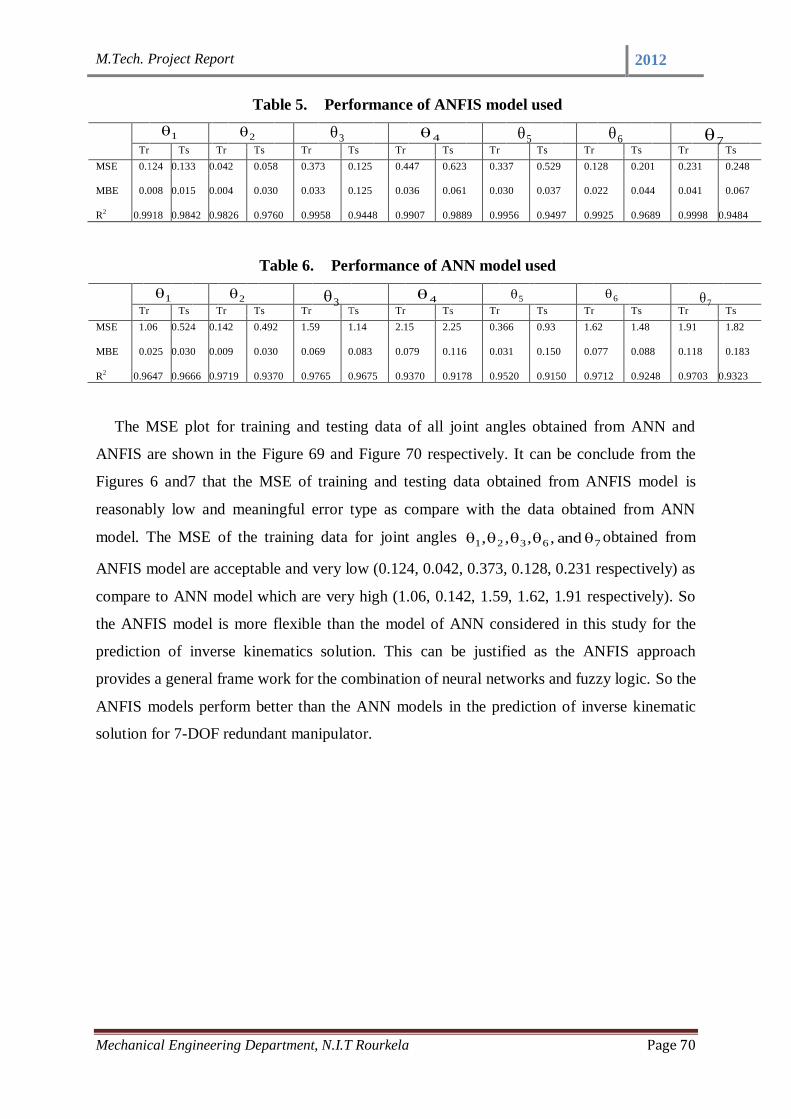
M.Tech. Project Report 2012
Mechanical Engineering Department, N.I.T Rourkela Page 70
Table 5. Performance of ANFIS model used
Tr Ts Tr Ts Tr Ts Tr Ts Tr Ts Tr Ts Tr Ts
MSE
MBE
R2
0.124
0.008
0.9918
0.133
0.015
0.9842
0.042
0.004
0.9826
0.058
0.030
0.9760
0.373
0.033
0.9958
0.125
0.125
0.9448
0.447
0.036
0.9907
0.623
0.061
0.9889
0.337
0.030
0.9956
0.529
0.037
0.9497
0.128
0.022
0.9925
0.201
0.044
0.9689
0.231
0.041
0.9998
0.248
0.067
0.9484
Table 6. Performance of ANN model used
Tr Ts Tr Ts Tr Ts Tr Ts Tr Ts Tr Ts Tr Ts
MSE
MBE
R2
1.06
0.025
0.9647
0.524
0.030
0.9666
0.142
0.009
0.9719
0.492
0.030
0.9370
1.59
0.069
0.9765
1.14
0.083
0.9675
2.15
0.079
0.9370
2.25
0.116
0.9178
0.366
0.031
0.9520
0.93
0.150
0.9150
1.62
0.077
0.9712
1.48
0.088
0.9248
1.91
0.118
0.9703
1.82
0.183
0.9323
The MSE plot for training and testing data of all joint angles obtained from ANN and
ANFIS are shown in the Figure 69 and Figure 70 respectively. It can be conclude from the
Figures 6 and7 that the MSE of training and testing data obtained from ANFIS model is
reasonably low and meaningful error type as compare with the data obtained from ANN
model. The MSE of the training data for joint angles 76321 and ,,,, obtained from
ANFIS model are acceptable and very low (0.124, 0.042, 0.373, 0.128, 0.231 respectively) as
compare to ANN model which are very high (1.06, 0.142, 1.59, 1.62, 1.91 respectively). So
the ANFIS model is more flexible than the model of ANN considered in this study for the
prediction of inverse kinematics solution. This can be justified as the ANFIS approach
provides a general frame work for the combination of neural networks and fuzzy logic. So the
ANFIS models perform better than the ANN models in the prediction of inverse kinematic
solution for 7-DOF redundant manipulator.
1
2
3
4
5
6
7
2 6 3 5 4 1
7

M.Tech. Project Report 2012
Mechanical Engineering Department, N.I.T Rourkela Page 71
Figure 69. Comparison of Mean Square Error plot for Training data
Figure 70. Comparison of Mean Square Error plot for Testing data.
By comparing the output from ANFIS and ANN model on the basis of global statistic i.e.
MSE, MBE, and R2, it can be concludes that the ANFIS model is more flexible than the ANN
model considered in this research, for prediction of IKs. As the ANFIS approach provides a
general frame work for combination of NN and fuzzy logic. The efficiency of ANFIS over
ANN can also be concluded by observing the graphs and tables which shows the comparison
MSE, MBE, R2 for the two models. Based on comparison of the results of these two
techniques, it is found that the proposed ANFIS model with Gaussian membership function is
more efficient than the multilayer feed forward ANN using Levenberg-Marquardt (LM)
algorithm for predicting the IK of the 7-DOF redundant manipulator.
*****
0
0.5
1
1.5
2
2.5
3
0 1 2 3 4 5 6 7 8
Mea
n S
quar
e E
rror
(MS
E)
MSE comparision in Training Data of all joint angles
ANFIS
ANN
0
0.5
1
1.5
2
2.5
0 2 4 6 8
Mea
n S
quare
Err
or
(MS
E)
MSE comparision in Testing data of all joint angles
ANFIS ANN

M.Tech. Project Report 2012
Mechanical Engineering Department, N.I.T Rourkela Page 72
CHAPTER 6

M.Tech. Project Report 2012
Mechanical Engineering Department, N.I.T Rourkela Page 73
Chapter 6
6. CONCLUSION AND FUTURE WORK
6.1 CONCLUSION
In this study, the inverse kinematics solution using ANFIS for a 5-DOF and 7-DOF
Redundant manipulator is presented. The difference in joint angle deduced and predicted with
ANFIS model for a 5-DOF and 7-DOF Redundant manipulator clearly depicts that the
proposed method results with an acceptable error. The modelling efficiency of this technique
was obtained by taking three end-effector coordinates as input parameters and five and seven
joint positions for a 5-DOF and 7-DOF Redundant manipulator respectivly as output
parameters in training and testing data of NF models. Also, the ANFIS model used with a
smaller number of iteration steps with the hybrid learning algorithm. Hence, the trained
ANFIS model can be utilized to solve complex, nonlinear and discontinuous kinematics
equation complex robot manipulator; thereby, making ANFIS an alternative approach to deal
with inverse kinematics. The analytical inverse kinematics model derived always provide
correct joint angles for moving the arm end-effector to any given reachable positions and
orientations.
As the ANFIS approach provides a general frame work for combination of NN and fuzzy
logic. The efficiency of ANFIS for predicting the IK of Redundant manipulator can be
concluded by observing the 3-D surface viewer, residual and normal probability graphs. The
normal probability plots of the model are also plotted. The normal probability plot of
residuals of training and testing data obtained from ANFIS shows that the data set of ANFIS
are approximately normally distributed.
The methods used for deriving the inverse kinematics model for the these manipulators
could be applied to other types of robotic arms, such as the EduBots developed by the
Robotica Ltd, Pioneer 2 robotic arm (P2Arm), 5-DOF Lynx 6 Educational Robot arm. It can
be concluded that the solution developed in this paper will make the PArm more useful in
application with unpredicted trajectory movement in unknown environment.
6.2 FUTURE WORK
In this work a hybrid neuro-fuuzy technology is used for the study of inverse kinematics of
redundant robot manipulator. ANFIS is adopted for solving the IK of higher DOF robot
manipulator. Due to its compactness and adaptive nature this technology is highly efficiency

M.Tech. Project Report 2012
Mechanical Engineering Department, N.I.T Rourkela Page 74
in predicting the IK of higher DOF robot manipulator. So this technology can used in
different robot in different field to know the joint angles, orientations, and the robot working
space to avoid osstacles.
The robotics industry has reached one plateau with the successful introduction of robots
into automotive manufacturing for spot welding and painting, are two areas where robotic
usage is almost universal. There are several other areas where the usage of robotics is in its
infancy and this chapter is dedicated to brief descriptions of some of these fields along with a
quick assessment of their current status.
A 20 meters long and 6-DOF remote robot manipulator is commonly used in space for
repairing satellites and other coordinated activities on self-propelled platform. So ANFIS can
be used to this robot for its free positioning and to determine its path. Apart from this, the
neuro fuzzy technique can be used in various field to determine the positions and
orientations. It can be used for:
Under water manipulator
Nuclear, toxic waste disposal and mining robot
Firefighting, construction and agricultural robot
Medical application
*****

M.Tech. Project Report 2012
Mechanical Engineering Department, N.I.T Rourkela Page 75
CHAPTER 7

M.Tech. Project Report 2012
Mechanical Engineering Department, N.I.T Rourkela Page 76
Chapter 7
7. REFERENCES
[1] Deb S.R. Robotics technology and flexible automation, Tata McGrow-Hill Publishing
Company Limited. New-Delhi, 2008.
[2] Clarke, R. Asimov’s Laws of Robotics: Implications for Information Technology- part II,
Computer, 27(1), September (1994): pp.57–66.
[3] Martin, F.G. Robotic Explorations: A Hands-On Introduction to Engineering, Prentice
Hall, New Jersey, 2001.
[4] Featherstone R. Position and velocity transformations between robot end-effector
coordinates and joint angles. International journal of Robotic Research, SAGE
Publications, 2(2), (1983), pp. 35-45.
[5] Nieminen and Peetu, et al. Water hydraulic manipulator for fail safe and fault tolerant
remote handling operations at ITER, Fusion Engineering and Design, Elsevier, Vol. 84,
(2009), pp. 1420-1424.
[6] Hollerbach J.M. Optimum kinematic design for seven degree of freedom manipulator,
Second International Symposium on Robotics Research. Cambridge: MIT Press, (1985):
pp. 215-222.
[7] Sciavicco L. and Siciliano B. Modelling and Control of Robot Manipulators , Springer
Second edition, (2000), Chapter 3, pp. 96.
[8] Shimizu M., Kakuya H. Yoon W, Kitagaki K., and Kosuge K., Analytical Inverse
Kinematic Computation for 7-DOF Redundant Manipulators with Joint Limits and its
application to Redundancy. Resolution, IEEE Transaction on Robotics, October (2008),
24(5).
[9] Vassilopoulos A.P and Bedi R. Adaptive neuro-fuzzy inference system in modelling
fatigue life of multidirectional composite laminates, Computation and Material Science.43
(2008): pp. 1086-1093.
[10] Haykin S., Neural Networks- A Comprehensive Foundation, McMillan College
Publishing, New York, 1998.
[11] Mendel J.M. Fuzzy logic system for engineering: A tutorial, Proceeding, IEEE. 83(3)
(1995): pp. 345-377.
[12] Ke L., Hong-ge M., Hai-jing Z. Application of Adaptive Neuro-Fuzzy Inference System
to Forecast of Microwave Effect, IEEE Conference Publications, (2009) , pp. 1- 3.

M.Tech. Project Report 2012
Mechanical Engineering Department, N.I.T Rourkela Page 77
[13] Alavandar S. and Nigam M. J. Adaptive Neuro-Fuzzy Inference System based control of
six DOF robot manipulator, Journal of Engineering Science and Technology Review,1
(2008): pp.106- 111.
[14] Craig J.J. Introduction to Robotics: Mechanisms and Controls, Addison-Wesley,
Reading, MA, 1989.
[15] Lee G.C.S. Dynamics and Control, Robot Arm Kinematics, Computer, 15(1982),
Issue.12: pp. 62-79.
[16] Korein J.U and Balder N.I. Techniques for generating the goal-directed motion of
articulated structures’, Institute of Electrical and Electronics Engineers Computer
Graphics Applications, 2(1982), Issue. 9: pp. 71-81.
[17] Srinivasan A and Nigam M.J. ‘Neuro-Fuzzy based Approach for Inverse Kinematics
Solution of Industrial Robot Manipulators’, International Journal of Computers,
Communications and Control, III(2008), No. 3: pp. 224-234.
[18] Calderon C.A.A., Alfaro E.M.R.P, Gan J.Q. and Hu H. Trajectory generation and
tracking of a 5-DOF Robotic Arm. CONTROL, University of Bath, (2004).
[19] De X., Calderon C.A.A., Gan J.Q., H Hu. An Analysis of the Inverse Kinematics for a 5-
DOF Manipulator, International Journal of Automation and Computing,(2) (2005): pp.
114-124.
[20] Gan J.Q., Oyama E., Rosales E.M. and Hu, H. A complete analytical solution to the
inverse kinematics of the Pioneer 2 robotic arm, Robotica, Cambridge University Press.
23(2005): pp. 123–129.
[21] Hasan A.T. and Al-Assadi H.M.A.A. Performance Prediction Network for Serial
Manipulators Inverse Kinematics solution Passing Through Singular Configurations,
International Journal of Advanced Robotic Systems, 7(2010), No. 4: pp. 10-23.
[22] Conkur E. S. and Buckingham R. Clarifying the definition of redundancy as used in
robotics. Robotica, 15 No 5 (1997): pp. 583-586.
[23] Chiaverini S. Singularity-robust task-priority redundancy resolution for real time
kinematic control of robot manipulators. IEEE Transaction on Robotics Automation, 13
No 3 (1997): pp. 398-410.
[24] Yoshikawa T. Foundation of Robotics: Analysis and Control. MIT Press (1988).
[25] Braganza D., Dawson D.M., Walker I.D., and Nath N. Neural Network Grasping
Controller for Continuum Robots. IEEE Conference on Decision Control, (2006):
pp.6445-6449.

M.Tech. Project Report 2012
Mechanical Engineering Department, N.I.T Rourkela Page 78
[26] Sciavicco L. and Siciliano B. Modelling and Control of Robot Manipulators , Springer
Second edition, Chapter 3, (2000), pp. 96.
[27] Shimizu M., Kakuya H., Yoon W., Kitagaki K., and Kosuge K. Analytical Inverse
Kinematic Computation for 7-DOF Redundant Manipulators with Joint Limits and its
application to Redundancy. Resolution, IEEE Transaction on Robotics, 24 No. 5:
October. (2008).
[28] Singh G.K. and Claassens J., An Analytical Solution for the Inverse Kinematics of a
Redundant 7DoF Manipulator with Link Offsets, The 2010 IEEE/RSJ International
Conference on Intelligent Robots and Systems. October (2010) :18-22. Taipei, Taiwan.
[29] Dahm P. and Joublin F. Closed form solution for the inverse kinematics of a redundant
robot arm,” Institute of Neuroinformatics, Ruhr-Univ. Bochum, 44780, Bochum,
Germany, Internal Rep. 97-08, (1997).
[30] Moradi H. and Lee S. Joint limit analysis and elbow movement minimization for
redundant manipulators using closed form method, In Advances in Intelligent
Computing, Berlin/Heidelberg: Springer, Part 2, 3645(2005): pp. 423–432.
[31] Ghaboussi J., Garrett J.H. and Wu X. Knowledge-based modeling of material behaviour
with neural networks, Journal of Engineering Mechanics. 117 (1991): pp.132–153.
[32] Consolazio G.R. Iterative equation solver for bridge analysis using neural networks,
Computer-Aided Civil and Infrastructure Engineering. 15 (2000): pp.107–119.
[33] Chen H.M., Tsai K.H., Qi G.Z., Yang J.C.S., Amini F. Neural networks for structural
control, Journal of Computing in Civil Engineering, 9(1995):pp.168–176.
[34] Bilgehan M., Turgut P. Artificial neural network approach to predict compressive
strength of concrete through ultrasonic pulse velocity, Research in Nondestructive
Evaluation. 21 (1) (2010): pp.1–17.
[35] Inel M. Modeling ultimate deformation capacity of RC columns using artificial neural
networks, Enggineering Structure. 29 (2007): pp.329–335.
[36] Liegeois A. Automatic supervisory control of the configuration and behavior of
multibody mechanisms, IEEE Transaction Systems on Man, and Cybernetics, 7 No. 12:
(1977), pp. 868–871, ISSN 0018-9472.
[37] Sciavicco, L. & Siciliano, B. A solution algorithm to the inverse kinematic problem for
redundant manipulators, IEEE Journal of Robotics and Automation, 4(4) (1988): pp.
303–310, ISSN 0882-4967.
M.Tech. Project Report 2012
Mechanical Engineering Department, N.I.T Rourkela Page 79
[38] Wampler, C.W. Manipulator inverse kinematic solutions based on vector formulations
and damped least-squares methods, IEEE Transaction on Systems, Man, and
Cybernetics,16 No. 1 (1986):pp. 93–101, ISSN 0018-9472.
[39] Mandal D., Pal S.K., Saha P. Modeling of electrical discharge machining process using
back propagation neural network and multi-objective optimization using non-dominating
sorting genetic algorithm-II. J Mater Process Technol 186(2007): pp.154–162.
[40] Panda D.K., and Bhoi R.K. Artificial neural network prediction of material removal rate
in electro-discharge machining. Material Manufaturing Process. 20 (2005): pp.645–672.
[41] Gao Q., Zhang Q., Su S., Zhang J., Ge R. Prediction models and generalization
performance study in electrical discharge machining. Applied Mechanics and Materials
.10 No.12(2008): pp.677–681. Cited by (since 1996).
[42] Vassilopoulos A.P and Bedi R. Adaptive neuro-fuzzy inference system in modelling
fatigue life of multidirectional composite laminates, Computational Materials Science.
(2008), pp. 1086-1093.
[43] Haykin S. Neural Networks-A Comprehensive Foundation, McMillan College
Publishing, New York, (1998).
[44] Mendel J.M. Fuzzy logic system for engineering: A tutorial, Proceeding of IEEE. 83(3)
(1995): pp. 345-377.
[45] Heidar A., Kottapalli S. And Langari R. Adaptive Neuro-fuzzy Modeling of UH-60A
Pilot Vibration, American Institute of Aeronautics and Astronautics. (2003).
[46] Ke L., Hong-ge M. and Hai-jing Z. Application of Adaptive Neuro-Fuzzy Inference
System to Forecast of Microwave Effect, IEEE Conference Publications, ( 2009). pp. 1 –
3.
[47] AlavandarS. and Nigam M. J. Adaptive Neuro-Fuzzy Inference System based control of
six DOF robot manipulator, Journal of Engineering Science and Technology Review 1
(2008) 106- 111.
[48] Roohollah Noori et.al. Uncertainty analysis of developed ANN and ANFIS models in
prediction of carbon monoxide daily concentration, ELSEVIER, International journal
for scientists and researchers in different disciplines interested in air pollution and its
societal impacts, Atmospheric Environment, , 44(2010): pp. 476-482.
[49] Yüzgeç U. Et al. Comparison of Different Modeling Concepts for Drying Process of
Baker’s Yeast. 7th IFAC International Symposium on Advanced Control of Chemical
Processes, Koç University Campus, Turkey. Vol. 7 Part.1,2009.

M.Tech. Project Report 2012
Mechanical Engineering Department, N.I.T Rourkela Page 80
[50] Bilgehan M. Comparison of ANFIS and NN models—With a study in critical buckling
load estimation, Applied Soft Computing, Journal of the World Federation on Soft
Computing (WFSC), ELSEVIER, (2011),pp. 3779–3791.
[51] Bilgehan M. A comparative study for the concrete compressive strength estimation using
neural network and neuro-fuzzy modeling approaches, Non-destructive Testing and
Evaluation, Taylor and Francis, Vol. 26, No.1, March (2011): pp 35-55.
[52] Jang J. S. R., Sun C. T. and Mizutani E. Neuro-Fuzzy and Soft Computing, Prentice Hall,
New York.1997.
[53] Jang J. S. R. ‘ANFIS: Adaptive-Network-based Fuzzy Inference Systems’, Transactions
on Systems, Man, and Cybernetics, 23 No. 3(1993): pp. 665-685.
[54] Sadjadian H., Taghirad H. D. and Fatehi A. Neural Networks Approaches for Computing
the Forward Kinematics of a Redundant Parallel Manipulator, International Journal of
Computational Intelligence, 2, No. 1(2005): pp. 40-47.
[55] Spong M.W., Hutchinson S., and Vidyasagar M. Robot Dynamics and Control Second
Edition, pp-62. January 28, 2004.
[56] Mittal R.K., Nagrath I.J. Robotics and Control. Tata McGraw-Hill publishing company,
Delhi, 2007, pp. 76-79.
[57] Jang J. S. R., Sun C. T. and Mizutani E. Neuro-Fuzzy and Soft Computing, Prentice Hall,
New York,1997.
[58] Zadeh L.A. Fuzzy Logic Toolbox User Guide, The Math Works, Berkeley, CA, Version
2, January 10, 1995-1998.
[59] Sugeno M.and Kang G.T., Structure Identification of Fuzzy model, Fuzzy Sets and
System, 28(1988):pp.15-33.
[60] Takagi T., Sugeno M. Fuzzy Identification of Systems and its Application to Modeling
Control, IEEE Transaction on System, Man and Cybernetics, 15(1985):pp.116-132.
[61] Mamdani E.H., Assilian S. An Experiment in Linguistic Synthesis with a Fuzzy Logic
Controller, International journal of Man-Machine Studies, 7 (1) (1975):pp.1-13.
[62] Tsukamoto Y. An Approach to Fuzzy Reasoning Method. In Madan M. Gupta,
Rammohan K. Ragade, and Ronald R. Yager, editors, Advances in Fuzzy Set Theory and
Applications, North-Holland, Amsterdam, 1979, pp.137-149.
[63] Jang J. S. R., Sun C. T., and Mizutani E. Neuro-Fuzzy and Soft Computing, Prentice
Hall, NewYork, pp.96-97.
[64] Koivo H . ANFIS :Adaptive Neuro-Fuzzy Inference System. European,

M.Tech. Project Report 2012
Mechanical Engineering Department, N.I.T Rourkela Page 81
Symposium on Intelligent Technology, Aachen, Germany, 2000.
[65] Chambers, John, William Cleveland, Beat Kleiner, and Paul Tukey, Graphical Methods
for Data Analysis, Wadsworth,1983.
*****