Prediction of mobility, handling, and tractive efficiency

of wheeled off-road vehicles

Carmine Senatore

Dissertation submitted to the Faculty of theVirginia Polytechnic Institute and State University

in partial fulfillment of the requirements for the degree of

Doctor of Philosophyin

Engineering Mechanics

Dr. Shane Ross, Co-ChairDr. Corina Sandu, Co-Chair

Dr. Mark CramerDr. Norman DowlingDr. Scott Hendricks

May 3, 2010Blacksburg, Virginia

Keywords: energy efficiency, fuel economy, multi passlateral force, torque distribution, tractive efficiency

tire dynamics, off-road, tire soil interaction

Copyright 2010, Carmine Senatore

Prediction of mobility, handling, and tractive efficiency

of wheeled off-road vehicles

Carmine Senatore

ABSTRACT

Our society is heavily and intrinsically dependent on energy transformation and usage.

In a world scenario where resources are being depleted while their demand is increasing, it

is crucial to optimize every process. During the last decade the concept of energy efficiency

has become a leitmotif in several fields and has directly influenced our everyday life: from

light bulbs to airplane turbines, there has been a general shift from pure performance to

better efficiency.

In this vein, we focus on the mobility and tractive efficiency of off-road vehicles. These

vehicles are adopted in military, agriculture, construction, exploration, recreation, and min-

ing applications and are intended to operate on soft, deformable terrain.

The performance of off-road vehicles is deeply influenced by the tire-soil interaction

mechanism. Soft soil can drastically reduce the traction performance of tires up to the

point of making motion impossible. In this study, a tire model able to predict the perfor-

mance of rigid wheels and flexible tires is developed. The model follows a semi-empirical

approach for steady-state conditions and predicts basic features, such as the drawbar pull,

the driving torque and the lateral force, as well as complex behaviors, such as the slip-sinkage

phenomenon and the multi-pass effect. The tractive efficiency of different tire-soil configu-

rations is simulated and discussed. To investigate the handling and the traction efficiency,

the tire model is implemented into a four-wheel vehicle model. Several tire geometries, ve-

hicle configurations (FWD, RWD, AWD), soil types, and terrain profiles are considered to

evaluate the performance under different simulation scenarios. The simulation environment

represents an effective tool to realistically analyze the impact of tire parameters (size, in-

flation pressure) and torque distribution on the energy efficiency. It is verified that larger

tires and decreased inflation pressure generally provide better traction and energy efficiency

(under steady-state working conditions). The torque distribution strategy between the axles

deeply affects the traction and the efficiency: the two variables can’t clearly be maximized

at the same time and a trade-off has to be found.

iii

Acknowledgments

I am heartily thankful to my advisors, Dr. Shane Ross and Dr. Corina Sandu, whose

encouragement, guidance and support helped me achieve my goals. I wish to also thank the

members of my Ph.D. committee for their valuable time and suggestions in improving upon

my research work.

I am grateful to Dr. Brendan Juin-Yih Chan for the work he has done on off-road tire

modeling: his research has been inspirational for my thesis. For all the helpful suggestions

and encouragements, I thank my friends and fellow students of the ESM department, Piyush

Grover, Phanindra Tallapragada, and Amir Ebrahim Bozorg Magham.

I truly appreciate the friendship and encouragements I received from my friends Kaushik

Das, Bob Simonds, Jose Herrera-Alonso, Gabriela Lopez-Velasco, Tom Pardikes, Kevin Bier-

lein, Golnaz Taghvatalab. A special thanks goes to Nancy and Gary Rookers for their con-

stant encouragement and help. During the last five years many Italians crossed my path in

Blacksburg, a dynamic group of lovely and exquisite persons: Matteo Alvaro, Attilio Arcari,

Vincenzo Antignani, Andrea Apolloni, Fabrizio Borghi, Gabriele Enea, Rosario Esposito,

Letizia Imbres, Paolo Finotelli, Davide Locatelli, Andrea Mola, Marta Murreddu, Maurizio

Paschero, Silvia Perotta, Massimiliano Rolandi, Giovanni Sansavini, Davide Spinello.

It has been an honor for me to meet with Edoardo Nicoli, a sincere friend, a wise

counselor, and an extraordinary bicycle mate. I am grateful to Fabrizio Re, for his support

and friendship during my years in Milan. I would like also to thank my old friends Paolo

Avagliano, Antonio Castaldo D’Ursi, and Andrea Salerno: three wonderful persons that

never stopped to inspire, support, and help me.

This thesis would not have been possible without the love and the encouragement of my

family: my father Antonio, my mother Teresa, and my sister Danila have always supported

me and they helped me realizing my dreams.

Finally, I would like to express my gratitude to Anna Laura for her love and patience.

She has always been a source of inspiration and motivation, I am forever indebted to her.

iv

Contents

1 Introduction 1

1.1 Preface . . . . . . . . . . . . . . . . . . . . . . . . . . . . . . . . . . . . . . . 1

1.2 Problem Statement . . . . . . . . . . . . . . . . . . . . . . . . . . . . . . . . 4

1.3 Research Objectives . . . . . . . . . . . . . . . . . . . . . . . . . . . . . . . . 5

1.4 Research Contribution . . . . . . . . . . . . . . . . . . . . . . . . . . . . . . 7

1.5 Dissertation Outline . . . . . . . . . . . . . . . . . . . . . . . . . . . . . . . 7

2 Review of Literature 9

2.1 Tire Mechanics Terminology . . . . . . . . . . . . . . . . . . . . . . . . . . . 9

2.2 Tire History and Evolution . . . . . . . . . . . . . . . . . . . . . . . . . . . . 12

2.3 Terramechanics Approach to Tire-Terrain Modeling . . . . . . . . . . . . . . 13

2.3.1 Empirical Methods . . . . . . . . . . . . . . . . . . . . . . . . . . . . 14

2.3.2 Semi-Empirical Methods . . . . . . . . . . . . . . . . . . . . . . . . . 17

2.3.3 Analytical Methods . . . . . . . . . . . . . . . . . . . . . . . . . . . . 19

2.3.4 Finite Element Methods . . . . . . . . . . . . . . . . . . . . . . . . . 21

2.4 Off-Road Vehicle Dynamics . . . . . . . . . . . . . . . . . . . . . . . . . . . 22

2.5 Tractive Efficiency . . . . . . . . . . . . . . . . . . . . . . . . . . . . . . . . 24

2.6 Review of Literature Summary . . . . . . . . . . . . . . . . . . . . . . . . . 26

3 Tire Model Development 27

3.1 Pressure-Sinkage Equation . . . . . . . . . . . . . . . . . . . . . . . . . . . . 27

v

3.1.1 Discussion on the Use of the Reece Equation for Tire Stress Distribu-

tion Estimation . . . . . . . . . . . . . . . . . . . . . . . . . . . . . . 30

3.2 Shear Stress . . . . . . . . . . . . . . . . . . . . . . . . . . . . . . . . . . . . 30

3.3 Normal and Tangential Stress Distribution . . . . . . . . . . . . . . . . . . . 31

3.4 Rigid Wheel and Flexible Tire . . . . . . . . . . . . . . . . . . . . . . . . . . 35

3.5 Drawbar Pull, Driving Torque, and Lateral Force . . . . . . . . . . . . . . . 37

3.6 Multi-Pass Effect . . . . . . . . . . . . . . . . . . . . . . . . . . . . . . . . . 40

3.7 Results . . . . . . . . . . . . . . . . . . . . . . . . . . . . . . . . . . . . . . . 43

3.7.1 Dry Sand - Rigid Wheel . . . . . . . . . . . . . . . . . . . . . . . . . 44

3.7.2 Moist Yolo Loam - Flexible Tire . . . . . . . . . . . . . . . . . . . . . 47

3.8 Considerations . . . . . . . . . . . . . . . . . . . . . . . . . . . . . . . . . . 49

4 Tractive Efficiency 51

4.1 Power-train Efficiency . . . . . . . . . . . . . . . . . . . . . . . . . . . . . . 52

4.1.1 Internal Combustion Engine . . . . . . . . . . . . . . . . . . . . . . . 52

4.1.2 Electric Motor . . . . . . . . . . . . . . . . . . . . . . . . . . . . . . . 55

4.2 Aerodynamic Efficiency . . . . . . . . . . . . . . . . . . . . . . . . . . . . . . 55

4.3 Tractive Efficiency . . . . . . . . . . . . . . . . . . . . . . . . . . . . . . . . 57

5 Vehicle Model Development 61

5.1 Mathematical Model . . . . . . . . . . . . . . . . . . . . . . . . . . . . . . . 61

5.1.1 Equations of Motion . . . . . . . . . . . . . . . . . . . . . . . . . . . 62

5.1.2 External Forces . . . . . . . . . . . . . . . . . . . . . . . . . . . . . . 66

5.1.3 Internal Forces . . . . . . . . . . . . . . . . . . . . . . . . . . . . . . 70

5.1.4 Tire Forces Generation Process . . . . . . . . . . . . . . . . . . . . . 71

5.1.5 Velocity Controller . . . . . . . . . . . . . . . . . . . . . . . . . . . . 74

5.1.6 Torque Distribution . . . . . . . . . . . . . . . . . . . . . . . . . . . . 74

5.1.7 Vehicle Parameters . . . . . . . . . . . . . . . . . . . . . . . . . . . . 75

vi

5.2 Vehicle Model Validation . . . . . . . . . . . . . . . . . . . . . . . . . . . . . 75

5.2.1 Acceleration and Braking . . . . . . . . . . . . . . . . . . . . . . . . 76

5.2.2 Double Lane Change . . . . . . . . . . . . . . . . . . . . . . . . . . . 78

5.3 Results . . . . . . . . . . . . . . . . . . . . . . . . . . . . . . . . . . . . . . . 81

5.3.1 Dry Sand Longitudinal . . . . . . . . . . . . . . . . . . . . . . . . . . 82

5.3.2 Moist Yolo Loam Longitudinal . . . . . . . . . . . . . . . . . . . . . . 88

5.3.3 Dry Sand Lateral . . . . . . . . . . . . . . . . . . . . . . . . . . . . . 93

5.3.4 Moist Yolo Loam Lateral . . . . . . . . . . . . . . . . . . . . . . . . . 95

6 Conclusions and Future Work 97

6.1 Research Summary and Contribution . . . . . . . . . . . . . . . . . . . . . . 97

6.2 Recommendations for Future Research . . . . . . . . . . . . . . . . . . . . . 98

Bibliography 100

vii

List of Figures

1.1 Renewable energy sources worldwide at the end of 2008 [1]. . . . . . . . . . 2

1.2 Energy flow in a typical mid-size car traveling on flat, hard surface. (Reprinted

from [2] , obtained from Transportation Research Board Special Report 286

under the FOIA.) . . . . . . . . . . . . . . . . . . . . . . . . . . . . . . . . . 4

2.1 Definition of the tire axis system and most relevant quantities according to

SAE J670e [3]. . . . . . . . . . . . . . . . . . . . . . . . . . . . . . . . . . . . 11

2.2 Construction layout of a bias-ply (a) and a radial-ply (b) tire. Adapted from [4] 13

2.3 Descriptive plot of a wheel rolling into soft terrain. . . . . . . . . . . . . . . 21

2.4 Definition of the vehicle axis system according to SAE J670e [3]. . . . . . . . 23

2.5 Torque flow in a four wheel drive vehicle. The torque produced by the engine

is split by the central differential and reaches the axles. At the axles is split

again by the axles differentials delivered to the wheels. Arrows’ length is not

proportional to torque magnitude; the axle differentials always split the torque

equally between the axles. . . . . . . . . . . . . . . . . . . . . . . . . . . . . 26

3.1 A schematic representation of the bevameter test. A load is applied on a

penetrometer while sinkage z and normal pressure σn are recorded. The ex-

perimental data is then fitted with (3.1). . . . . . . . . . . . . . . . . . . . . 29

3.2 (a) An example of a deformed tire driven on a soft surface. The tire is deform-

ing and sinking into the ground. (b) A detail of the contact patch area. The

normal stress σn and the tangential stress τx acting along the contact patch

are shown. . . . . . . . . . . . . . . . . . . . . . . . . . . . . . . . . . . . . . 32

3.3 A schematic representation of the normal stress distribution as adopted by

Harnisch et al. [5] and by Wong at al. [6]. In this study, Wong’s approach is

used. . . . . . . . . . . . . . . . . . . . . . . . . . . . . . . . . . . . . . . . . 33

viii

3.4 (a) Normal stress distribution along the contact patch of a driven (sd = 0.2)

rigid wheel. The stress increases from the entry angle θe, reaches the maximum

at θm, and decreases back to zero at the exit angle θb. (b) Tangential stress

distribution along the contact patch under the same assumptions. . . . . . . 34

3.5 Exaggerated plot of a deformed tire sitting on hard surface (a) and driven on a

soft terrain (b). When stationary the only portion in contact with the terrain

is the flat region between θr and θf which in this particular configuration

correspond to θb and θe. When the tire is rolling, the section of maximum

deflection is rotated on an angle θm =θf

2and the entry and exit angle θe,b

don’t necessarily correspond to θf and θr. . . . . . . . . . . . . . . . . . . . . 36

3.6 A schematic representation of the lateral force generation. The lateral force

is composed of two components: the shear force in the lateral direction Fys

and the bulldozing force Fybd. The first one is due to the lateral slip of the

tire imposed by the steering action. This force acts along the contact patch

beneath the tire. The bulldozing force acts on the side of the tire and is due

to the wheel compacting the terrain in the lateral direction. . . . . . . . . . 39

3.7 Response to repetitive load of a mineral terrain. . . . . . . . . . . . . . . . . 41

3.8 Example of terrain properties variation for multiple passage. The data has

been extrapolated from the Figure 25 of [7] and regards a loam soil with fine

grained sand at 16.5% of moisture content. . . . . . . . . . . . . . . . . . . . 42

3.9 Trend of drawbar pull (a) and driving torque (b) for different vertical loads

and slip ratio. Results obtained for a rigid wheel running on dry sand. . . . . 44

3.10 Experimental data compared with the model prediction. Rigid wheels with

different geometries have been tested on dry sand. . . . . . . . . . . . . . . . 44

3.11 Slip-sinkage behavior of rigid wheels of different geometries. . . . . . . . . . 45

3.12 Lateral force versus slip angle for different slip ratios (a) and vertical loads

(b). Results obtained for a rigid wheel on dry sand. . . . . . . . . . . . . . . 45

3.13 Combined slip envelope for different slip angles (a) and vertical loads (b).

Results obtained for a rigid wheel on dry sand. . . . . . . . . . . . . . . . . . 46

3.14 Multi-pass influence on the performance of rigid wheels on dry sand. In (a)

the longitudinal force is presented while (b) shows the relative sinkage. . . . 47

3.15 Trend of drawbar pull (a) and driving torque (b) for different vertical loads

and slip ratio. Results obtained for flexible tire on moist Yolo loam. . . . . . 47

ix

3.16 Variation of drawbar pull (a) with inflation pressure and trend of the sinkage

(b) with inflation pressure. Results obtained for flexible tire on moist Yolo

loam. . . . . . . . . . . . . . . . . . . . . . . . . . . . . . . . . . . . . . . . . 48

3.17 Lateral force versus slip angle for different slip ratio (a) and vertical load (b).

Results obtained for flexible tire on moist Yolo loam. . . . . . . . . . . . . . 48

3.18 Combined slip envelope for different slip angles (a) and vertical loads (b).

Results obtained for flexible tire on moist Yolo loam. . . . . . . . . . . . . . 49

3.19 Multi-pass influence on the performance of flexible tires on moist Yolo loam.

(a) presents the variation of longitudinal force while (b) the relative sinkage

for multiple passages over the same patch of terrain. . . . . . . . . . . . . . . 49

4.1 Energy requirement for two driving conditions [8]. . . . . . . . . . . . . . . . 52

4.2 Exemplar torque/power curve for an engine. The maximum output power is

120 kW at 3300 RPM, while the maximum torque is 270 Nm at 1450 RPM. 53

4.3 Map of a diesel engine. The power/torque specifications are the same as Figure

4.2. The islands represent lines of constant Brake Specific Fuel Consumption

(BSFC), the grams of fuel burned to produce a kWh of energy. The maximum

occurs close to 1600 RPM at full load (thicker boundary line). On the y-axis

is the brake mean effective pressure (bmep), a measure of an engine’s capacity

to do work directly related to the torque. . . . . . . . . . . . . . . . . . . . . 54

4.4 Typical efficiency map for an electric motor for hybrid vehicles applications. 56

4.5 Tractive efficiency under different operational scenarios for a tire rolling on

dry sand. In (a) different sizes and the multi-pass effect influence is showed.

In (b) different loads are investigated. . . . . . . . . . . . . . . . . . . . . . . 59

4.6 Tractive efficiency under different operational scenarios for a tire rolling on

moist Yolo loam. In (a) different inflation pressures, tire sizes, and the multi-

pass effect influence is showed. In (b) different loads are investigated. . . . . 60

5.1 Schematic representation of the vehicle model. The earth-fixed reference frame

X, Y, Z is showed and can be arbitrarily located. The vehicle motion is de-

scribed in terms of the right-handed reference frame x, y, z attached to the

vehicle center of gravity. The wheels displacement is constrained in the z-

direction of the vehicle-fixed reference frame. To keep the plot clear the

x′, y′, z′ frame is illustrated in more detail in Figure 5.2. . . . . . . . . . . . . 63

x

5.2 Top-view of a vehicle during a right turn. The wheels reference frames x′, y′, z′

are highlighted and the Ackermann steering geometry is presented. . . . . . 66

5.3 A schematic representation of how the driver input is translated into actual

driving forces at the wheels. . . . . . . . . . . . . . . . . . . . . . . . . . . . 72

5.4 Longitudinal velocity of the vehicle during an acceleration and braking ma-

neuver. . . . . . . . . . . . . . . . . . . . . . . . . . . . . . . . . . . . . . . . 76

5.5 Pitch angle of the vehicle during an acceleration and braking maneuver. . . . 77

5.6 Pitch angle of the vehicle during an acceleration and braking maneuver. . . . 77

5.7 Trajectory followed by the vehicle during a double lane change maneuver. . . 78

5.8 Vehicle longitudinal velocity during a double lane change maneuver. . . . . . 79

5.9 Vehicle roll angle during a double lane change maneuver. . . . . . . . . . . . 79

5.10 Vehicle pitch angle during a double lane change maneuver. . . . . . . . . . . 80

5.11 Vehicle yaw angle during a double lane change maneuver. . . . . . . . . . . . 80

5.12 Vertical load distribution during a double lane change maneuver. Solid lines:

Model. Dashed lines: CarSim. The vertical load increases on the outer wheels

and decreases on the inner ones due to dynamic weight transfer phenomenon. 81

5.13 (a) Velocity profile for a vehicle running on a flat dry sand terrain. The

simulation starts from a slightly lower velocity in order to reach smooth steady

state conditions. (b) The torque delivered at the tires during the maneuver. 82

5.14 (a) Sinkage distribution for the three vehicle configurations. The value of

sinkage is relative to each wheel. (b) Vertical load distribution during the

maneuver. When steady state conditions are reached the load transfer phe-

nomena still persist because the tires are still producing longitudinal forces

that influence the pitch angle of the vehicle. . . . . . . . . . . . . . . . . . . 83

5.15 (a) Sinkage distribution for the three vehicle configurations. The value of

sinkage is relative to each wheel. (b) Vertical load distribution during the

maneuver. When steady state conditions are reached the load transfer phe-

nomena still persist because the tires are still producing longitudinal forces to

overcame the resistance forces; this influence the pitch angle of the vehicle. . 84

5.16 (a) Tire angular velocity and (b) instantaneous power requirement to move

at 25 km/h on dry sand. . . . . . . . . . . . . . . . . . . . . . . . . . . . . . 84

xi

5.17 Power vs. torque distribution for a vehicle traveling at 25 km/h on flat dry

sand. 0 % (100 %) on the x-axis means that the torque is fully biased on the

front (rear) axle of the vehicle. On the same plot the slip difference between

the front and rear axle is presented. . . . . . . . . . . . . . . . . . . . . . . . 85

5.18 Power vs torque distribution for a vehicle traveling at 25 km/h on a 10 %

incline. 0 % (100 %) on the x-axis means that the torque is fully biased on

the front (rear) axle of the vehicle. . . . . . . . . . . . . . . . . . . . . . . . 86

5.19 (a) Vehicle with a significant static load distribution unbalance during a

straight run at 50 km/h on dry sand. (b) Power vs torque distribution among

the axles. . . . . . . . . . . . . . . . . . . . . . . . . . . . . . . . . . . . . . 86

5.20 Power requirement for four vehicle configurations. Vehicle speed is 50km/h

and the terrain is flat dry sand. Nominal parameters (concerning the standard

case) are: Radius = 0.4 m, Width = 0.265 m, Torque = 50%F - 50% R. . . . 87

5.21 (a) Velocity profile for a vehicle running on a flat loamy terrain. The simula-

tion starts from a slightly lower velocity in order to reach smooth steady state

conditions. (b) The torque delivered at the tires during the maneuver. . . . . 88

5.22 (a) Sinkage distribution for the three vehicle configurations. The value of

sinkage is relative to each wheel. (b) Vertical load distribution during the

maneuver. When steady state conditions are reached the load transfer phe-

nomena still persist because the tires are still producing longitudinal forces

that influence the pitch angle of the vehicle. . . . . . . . . . . . . . . . . . . 89

5.23 (a) Sinkage distribution for the three vehicle configurations. The value of

sinkage is relative to each wheel. (b) Vertical load distribution during the

maneuver. When steady state conditions are reached the load transfer phe-

nomena still persist because the tires are still producing longitudinal forces

that influence the pitch angle of the vehicle. . . . . . . . . . . . . . . . . . . 89

5.24 (a) Tire angular velocity and (b) instantaneous power requirement to move

at 50 km/h on moist loam. . . . . . . . . . . . . . . . . . . . . . . . . . . . . 90

5.25 Power vs torque distribution for a vehicle traveling at 50 km/h on flat loam.

0 % (100 %) on the x-axis means that the torque is fully biased on the front

(rear) axle of the vehicle. . . . . . . . . . . . . . . . . . . . . . . . . . . . . . 90

xii

5.26 (a)Longitudinal velocity for three vehicles traveling at 50 km/h on a 10%

inclined moist loam terrain. The rear wheel drive configuration does not

allow to reach comfortably the desired target speed. (b) Power requirement

for the same maneuver; the RWD saturates because the imposed slip ratio

limit is achieved during the simulation. The FWD vehicle is able to climb the

hill but it is less efficient than the AWD one. . . . . . . . . . . . . . . . . . . 91

5.27 Torque distribution influence on the performance of an AWD vehicle driving

at 50 km/h on a 10% inclined loam terrain. The best efficiency is reached

when 60% of the total torque is delivered to the rear axle. . . . . . . . . . . 92

5.28 (a) Sinkage of a vehicle with decreased tire pressure traveling at 50 km/h on

moist loam. (b) Slip under the same conditions. . . . . . . . . . . . . . . . . 92

5.29 (a)Longitudinal tire forces for a vehicle with decreased tire pressure traveling

at 50 km/h on moist loam. (b) Power requirement for the same maneuver. . 93

5.30 Torque distribution influence on the performance of an AWD vehicle driving

at 50 km/h on a flat loamy terrain with reduced tire inflation pressure. The

best efficiency is reached when 60% of the total torque is delivered to the rear

axle. . . . . . . . . . . . . . . . . . . . . . . . . . . . . . . . . . . . . . . . . 93

5.31 Steering action during the lateral dynamic test. The steering angles δ comply

with the Ackermann steering geometry introduced in (5.4). For a right turn

the outer wheel is the left one and consequently δ0 = δl and δi = δr. . . . . . 94

5.32 (a)Roll angle of FWD, RWD, and AWD vehicles during a right turn maneuver

on dry sand. (b) The load is transfered to the outer wheels (the left ones). . 94

5.33 (a)Sinkage of FWD, RWD, and AWD vehicle during a right turn maneuver

on dry sand. The outer wheels (left ones), being more loaded, sink more. (b)

The instantaneous power requirement to complete the maneuver. . . . . . . . 95

5.34 (a)Roll angle of FWD, RWD, and AWD vehicles during a right turn maneuver

on moist Yolo loam. (b) The load is transfered to the outer wheels (the left

ones). . . . . . . . . . . . . . . . . . . . . . . . . . . . . . . . . . . . . . . . 95

5.35 (a)Sinkage of FWD, RWD, and AWD vehicle during a right turn maneuver

on moist Yolo loam. The outer wheels (left ones), being more loaded, sink

more. (b) The instantaneous power requirement to complete the maneuver. . 96

xiii

List of Tables

3.1 Undisturbed soil properties adopted in the simulations. 43

3.2 Nominal tire properties adopted in the simulations. 43

5.1 Vehicle specifications. . 75

xiv

Chapter 1

Introduction

1.1 Preface

Energy is a concept that can be elegantly understood through the first law of thermodynam-

ics:

dU = δQ− δW (1.1)

This simple equation states an extremely important concept of classical physics: work

W and heat Q are two aspects of the same concept, the energy. The energy radiating from

the sun makes life on earth possible; it remained the only source of energy until hominids

became capable of controlling the fire. This became an essential tool for human beings and,

in combination with devices able to harvest energy from water flows or wind (i.e. mills and

sailboats), represented the main source of energy until the 18th century (without considering

the muscular work of slaves, draft and pack animals).

The revolution occurred after the invention of the steam-engine: a machine able to

produce mechanical work from the the combustion of coal. In history books it has gained

the appellative of industrial revolution, but it would deserve the name of energetic revo-

lution. The introduction of the steam-engine boosted the development of steam-powered

ships, railways, and later in the 19th century of the internal combustion engine and electri-

1

Figure 1.1: Renewable energy sources worldwide at the end of 2008 [1].

cal power generation systems. Since then the main source of energy fossil fuels. The only

competitive alternative appeared with the introduction of nuclear power generation. This

technology was undermined by some accidents (Three Mile Island, Chernobyl, Tokaimura

the most (in)famous) that understandably turned public opinion against atomic energy. The

higher cost (financial and political) due to higher safety requirements and the problem of

radioactive waste disposal still remain an issue and, together with the scarcity of uranium,

will probably continue to determine the fate of this technology.

Although strenuous efforts to move to alternative/renewable sources have been made,

at the end of 2008 more than 80% of world electric energy was produced from fossil fuels

(see Fig. 1.1). These resources are constantly depleting without regeneration and even if it

is true that the oil shortages are often a result of market’s laws (drilling capacity is decided

by the countries/companies) there is no doubt that one day the oil will end. The first energy

crisis struck in the 70’s and highlighted how much our society is energy-dependent.

Figure 1.1 shows that it would be naive to think that a single technology could be

the panacea for the energy crisis. A very specialized and targeted effort in several fields is

necessary, in order to harvest energy in the most efficient way from many different sources.

2

The problem of energy production and transformation is directly linked to another challenge

that our generation has to face: global warming [9]. Increasing the efficiency is not only a

way to reduce energy consumption but also emissions.

The problem is not limited to energy production but it directly extends to the energy

consumption. Highly efficient devices help to reduce the energy requirement or, from another

perspective, guarantee the same standards to a larger number of persons, while exploiting

the same resources. For this reason during the last decade the concept of energy efficiency

has become a leitmotif in several fields, and it has directly influenced our everyday life.

The introduction of the Toyota Prius [10], the first full hybrid electric mid-size car, has

marked an era and opened new frontiers for more efficient vehicles. It is symptomatic that

in many fields a general shift from pure performance to increased efficiency is occurring. For

example computer components (processors, video cards, hard disks etc) are now marketed

and reviewed not only by performance but also by their consumption. Even the motor-

sport competition world is moving in the same direction: FIM (Federation Internationale de

Motocyclisme) regulations [11] now require reduced fuel tank size for Moto-GP competitions

(in order to push manufacturers to increase fuel economy) while the FIA [12] (Federation

Internationale de l’Automobile) introduced the KERS (Kinetic Energy Recovery Systems)

for the 2009 Formula 1 season. Ferrari (Ferrari 599 HY-Kers [13]) and Porsche (Porsche

Intelligent Performance [14]), two brands historically synonymous with pure performance,

have revealed projects for high performance hybrid cars: a shock for some purists, yet a

courageous commitment by the companies. The aforementioned only represent a handful of

examples among many.

It is clear that in an energy-dependent society, energy efficiency is a critical component

of machinery design and plays a central role when resources are scarce. The results obtained

in this dissertation are not limited to devices operated using fossil fuels: they regard a general

class of vehicles or particular sub-systems that can find applications regardless of the main

source of vehicle power.

3

1.2 Problem Statement

The following discussion will start from on-road vehicles and successively move to off-road

vehicles. The automotive sector started to consciously think about the fuel economy only

in the 70’s, when the first energy crisis occurred. That event encouraged researchers and

companies [15] to spend great effort in order to optimize the energy consumption of vehicles.

Regarding fuel economy, the power-train is the first component that comes to mind, but

there are two other factors that have great impact on the overall energetic performance: the

aerodynamic drag and the rolling resistance.

Figure 1.2: Energy flow in a typical mid-size car traveling on flat, hard surface. (Reprinted from[2] , obtained from Transportation Research Board Special Report 286 under the FOIA.)

After the impulse given by the 1973’s crisis faded, the average miles per gallon (or

MPG) of the American car fleet almost flattened and new interest in the topic arose again

only in 2005, when the oil reached unprecedented price record. The performance of inter-

nal combustion engines remains bounded by the physical limit imposed by the 2nd law of

thermodynamics and modern engines already approach this limit of 20-35% efficiency (in

this case defined as energy stored in the fuel divided by the mechanical energy delivered

by the engine). From this point of view the 4-7% of energy absorbed in rolling resistance

and the 3-11% in aerodynamic drag represent a consistent share of the output available

from the engine (see Fig. 1.2). As a consequence tire dynamics still plays a crucial role in

energy consumption analysis. In response to increasing oil prices, the European market is

witnessing a shift toward smaller engine cars: the idea is to reduce the weight of the vehicle

4

introducing smaller and more efficient engines. This process, commonly called downsizing,

is necessary in order to exploit resources in a better way and it is slowly finding its way also

in the American market. Dr. Lino Guzzella (a professor at the ETH Zrich and an expert of

modeling and control of internal combustion engine systems) during a plenary lecture at the

2008 American Control Conference held in Seattle [16], highlighted that better fuel economy

will be achieved through the following strategies:� decrease car weight through the reduction of passive and active safety devices that will

become less important when cars will share informations between each other (presence

of obstacles ahead, traffic information, threat forecasting),� adoption of smaller and more efficient engines (possible for lighter vehicles).

The energy efficiency of off-road vehicles has not been extensively studied in recent

years. Main contributors to the field are Bekker and Wong which laid the foundation for

the off road mobility studies [17, 18]. In the off-road context the energy flow showed in

Figure 1.2 is still valid but the rolling resistance assumes a predominant role. Mobility is

highly dependent on soil properties, factors like the sinkage and the slippage deeply affect

the capability of a vehicle to move. In military applications, off-road operations are common

and the possibility of saving fuel has a strategic and tactical relevance. Vehicle operation

on unpaved surfaces is common also in agriculture, construction, exploration, recreation,

and mining machinery. These applications would benefit from a better understanding of

parameters that affect the fuel consumption.

1.3 Research Objectives

The scope of this research is to establish a tool for predicting mobility, handling and tractive

efficiency of off-road vehicles. The study of off-road vehicles has originally focused on the

mobility aspect, having as a primary objective the capability to ascertain if a vehicle was able

to move on a certain terrain. The performance of land vehicles are intrinsically influenced by

tire behavior. The present work focuses on the development of a tire model able to describe

not only the mobility but also the salient features encountered in off-road operations (i.e.

5

slip-sinkage, bulldozing, multi-pass, parameter sensitivity). The sinkage represents the main

source of rolling resistance during off-road operations while the repetitive passage over the

same patch of terrain can significantly modify the response of the tires. A tire model able

to predict these aspects allows one to comprehensively study the performance of an off-road

vehicle. For this reason the tire model developed is then implemented into a full-vehicle model

in order to simulate the tractive efficiency of a full vehicle during standard maneuvering.

The objectives can be summarized as follows:

1. Development of a semi-empirical tire model able to predict: longitudinal force, torque,

lateral force, slip-sinkage effect, multi-pass behavior and bulldozing phenomenon. The

tire model is based on empirical expressions and theoretical assumptions in order to

realistically estimates the parameters influence.

2. Investigate the influence of tire parameters on the tractive efficiency. Verify the ca-

pability of the developed tire model to correctly predict the tractive efficiency of tires

during off-road operations.

3. Combine the information obtained above to simulate the performance of a vehicle

transversing unprepared terrain. The tractive efficiency of the vehicle is analyzed and

general directions for torque distribution strategies are provided. Standard maneuvers

are simulated in order to characterize the handling of the vehicle.

These aims will be achieved under the assumptions that:

1. The tire properties remain constant during the simulation. No heating and wearing

phenomenon are considered.

2. The terrain is homogeneous.

3. The full-vehicle model satisfies simplifying assumptions that will be discussed in more

detail in Chapter 5.

6

1.4 Research Contribution

This research describes and implements a detailed semi-empirical tire model for off-road

vehicle simulations. An accurate tire model is necessary for the analysis of mobility, handling

and tractive efficiency during off-road operations. The principal contributions of this study

can be summarized as follows:� Improved existing semi-empirical off-road tire model for faster, but still accurate, vehicle

dynamics simulations. The tire model accounts for complex behaviors such as the multi-

pass effect and the slip-sinkage phenomenon.� Simulation of a full vehicle while adopting a detailed off-road tire model.� Analysis of the torque distribution strategy that can help in minimizing the energy

consumption.

1.5 Dissertation Outline

The dissertation is outlined proceed as follows.

Chapter 2 will present a review of literature introducing the basic concepts of tire

mechanics. A brief overview of tire history will be given and the terramechanics approach to

tire-terrain problems will be illustrated. The chapter is concluded by a discussion of a full

off-road vehicle simulation.

Chapter 3 introduces the tire model. The development of the model is explained and the

method is discussed in detail. Results for longitudinal, lateral, and combined slip operations

are presented.

Chapter 4 discusses the economy of land vehicles. A brief review of internal combustion

engines and electric motor efficiency is given. Thereafter the basic concepts related to the

aerodynamic drag are presented, and finally the tractive efficiency of tires operating in off-

road conditions is discussed.

Chapter 5 introduces the full vehicle model. The model is illustrated and basic back-

7

ground of vehicle dynamics is provided. The chapter shows the simulation results of vehicles

running on flat terrain, sloped terrain, sand, and loam. Different drive configurations are

analyzed (RWD,FWD,AWD) as well as tire parameters (size, width, inflation pressure).

Chapter 6 will present conclusive remarks, highlight the research findings and propose

future work directions.

8

Chapter 2

Review of Literature

The dynamics of a wheeled vehicle are substantially influenced by the behavior of its tires.

The tire is the device that allows the vehicle to convert the energy delivered by the engine

into useful work (motion). Behind a simple description and appearance it is hidden an

extremely complex engineering subsystem: its geometry, design and construction can deeply

affect vehicle performance and efficiency. For this reason a realistic analysis of the dynamics

of a vehicle cannot be achieved without an accurate tire model.

This chapter will present:

1. a brief introduction on tire mechanics terminology,

2. an overview of tire evolution,

3. the main contributions to tire models development for off-road applications,

4. a discussion of full off-road vehicle models for dynamics simulations, and

5. a brief introduction on vehicle efficiency.

2.1 Tire Mechanics Terminology

This section introduces the basic terminology commonly adopted by the vehicle dynamics

community. The SAE standard [3], extensively used in the automotive industry, is adopted.

9

The origin of the tire axis system is located at the bottom of the tire, ideally at the center of

the contact patch in contact with the soil. A Cartesian right-handed axis system is chosen

with the x-axis pointing in the direction of wheel heading, the z-axis perpendicular to the

road plane with a positive direction downward, and the y-axis in the road plane with the its

direction chosen to make the axis system orthogonal, as shown in Figure 2.1. The definition

of the most relevant quantities is given below:� The slip angle α is the angle between the x-axis and the direction of travel of the center

of the contact patch. A positive slip angle corresponds to a clockwise rotation of the

tire when looking from the top.� The inclination angle γ (also camber angle) is the angle between the z-axis and the

wheel plane.� The longitudinal force Fx is the component of the tire force vector in the x-direction.� The lateral force Fy is the component of the tire force vector in the y-direction.� The normal or vertical force Fz is the component of the tire force vector in the z-

direction.� The overturning moment Mx is the component of the tire moment vector tending to

rotate the tire about the x-axis, positive clockwise when looking in the positive direction

of the x-axis.� The rolling resistance moment My is the component of the tire moment vector tending

to rotate the tire about the y-axis, positive clockwise when looking in the positive

direction of the y-axis.� The aligning moment (or torque) Mz is the component of the tire moment vector

tending to rotate the tire about the z-axis, positive clockwise when looking in the

positive direction of the z-axis.� The wheel torque T is the external torque applied to the tire from the vehicle about

the spin axis. Since the inclination angle γ will be taken equal to zero, the wheel torque

will correspond to the resistance moment throughout the dissertation.

10

Figure 2.1: Definition of the tire axis system and most relevant quantities according to SAE J670e[3].� The undeformed tire radius Ru is the radius of the newly unloaded tire inflated to the

normal recommended pressure and mounted on the specified rim.� The angular velocity of the wheel (or spin) ω is the angular velocity of the wheel on

which the tire is mounted.� The longitudinal slip or slip ratio sd is a measure of the difference between the effective

angular velocity ω and the longitudinal velocity of the tire (the speed of the center of

the wheel in the longitudinal direction). Due to a relative slip between the tire and

the road there will be a difference between the theoretical tire velocity (i.e. ωRu for a

rigid wheel) and the actual velocity of the tire in its the travel direction (denoted here

as V ).

sd = 1 − V

ωRu

. (2.1)

Among the quantities that we have just introduced two of them deserve particular

attention: the slip ratio sd and the slip angle α. The ability of a tire to produce longitudinal

(lateral) force is strictly related to its slip ratio (angle). When a vehicle accelerates, brakes or

simply coasts the tires are not simply rolling but there is always a relative motion somewhere

11

in the contact patch (i.e. the slip).

2.2 Tire History and Evolution

Tire history begins after the introduction of the vulcanization process by Charles Goodyear

in 1843. Vulcanized rubber made possible the construction of flexible wheels (the tire), that

later became an essential component of motor vehicles. In the following years a series of

design evolutions occurred and the most relevant can be summarized as follow: pneumatic

removable tires (1890 circa), cord reinforced tires (1900 circa), grooved tires (1908), radial

tires (1946).

The tire, as a vehicle subsystem, has multiple roles:� It has to support the vehicle load.� It has to transfer to the ground the energy delivered by the engine and provide the

vehicle with steering capabilities.� It behaves as a secondary suspension. This guarantees better performance and comfort

(it should be noted here that for the primary suspension system comfort is only a side

effect, handling being the principal reason for its introduction).

The dominant design today is the radial-ply construction. This approach was introduced

originally by Michelin and quickly became the standard as it brought consistent advantages

over the bias-ply design. Examples of the most common tire structures are given in Figure

2.2.

Tires are not simply a rubber structure but are made of several layers of different

materials. In order to guarantee the desired strength, layers of polyester, steel and/or other

textile materials are joint together into a complicated structure. The bias-ply or cross design

was the first design introduced but it has now almost disappeared from the market in favor

of the radial design. The radial design provides a wider footprint on the ground, better

ground pressure distribution, and reduced friction [19]. These results are obtained thanks

to the different orientation of the plies and the introduction of reinforcing steel belts: such

12

(a) (b)

Figure 2.2: Construction layout of a bias-ply (a) and a radial-ply (b) tire. Adapted from [4]

modifications allow the sidewall and tread to deform independently and avoid the heat

generation produced by the friction of the crossed plies. These enhanced properties allow the

radial design to attain better tire life, improved handling and fuel economy. This study will

not consider the differences between bias-ply and radial-ply design because during off-road

operations, the principal resistance force is not tire hysteresis but the terrain compaction.

Under this assumption the tire construction technique does not play a major role.

2.3 Terramechanics Approach to Tire-Terrain Modeling

The reference book for on-road tire modeling is the work by Pacejka [19]. However, the

development of tire models for off-road applications follows distinct methodologies that will

be presented in this section. In some cases, Pacejka’s and similar on-road models have been

modified to account for off-road testing by reducing the coefficient of friction in order to

simulate the lack of traction on rough terrain. This represents a very first approximation

since it disregards effects such the sinkage, the multi-pass, the bulldozing effects etc.

The tire model presented in this dissertation follows the approach proposed by the

terramechanics community. Terramechanics is the engineering field that studies the soil

properties and the interaction between wheeled or tracked vehicles and deformable terrain.

13

The father of this discipline is considered M. G. Bekker, author of Theory of land locomotion

[17], published in 1950 and become a classic in the terramechanics community. After the

Second World War the proliferation of automobiles has pushed the automotive industry to

focus on on-road locomotion problems but the study of vehicles moving on unprepared terrain

remained a subject of interest for the Army, for planetary exploration agencies, agricultural

field, construction, recreation, and mining industries.

Amongst the terramechanics community four primary approaches can be summarized:� empirical methods,� semi-empirical methods,� analytical methods,� finite element methods.

The main features of the aforementioned methodologies will be presented in the following

sections.

2.3.1 Empirical Methods

The first methods introduced to study the mobility of vehicles over unprepared terrain are

mainly empirical. The most common one was introduced by M. G. Bekker [17, 20, 21],

while working for the Land Locomotion Laboratory in the U.S. Army Detroit Arsenal in the

50’s. The key contribution of Dr. Bekker is the introduction of a semi-empirical equation

that relates the sinkage with the normal pressure of a plate pushed down into the soil. The

proposed relation is commonly referred as Bekker equation,

σn =

(

kc

b+ kφ

)

zn, (2.2)

where:

σn = pressure normal acting on the sinkage plate,

kc = cohesion-dependent parameter,

14

kφ = friction angle dependent parameter,

n = sinkage index,

b = plate width,

z = sinkage.

The parameters introduced in (2.2) are obtained from field tests conducted with a

bevameter. The bevameter is a device that records the sinking and the normal pressure

exerted on a plate of width b while it is pressed into the terrain at constant displacement

rate. Bekker proposed also a relation to characterize the shear strength of the soil,

τ =K3

2K1

√

K22 − 1

(

e

“

−K2+√

K2

2−1

”

K1i − e

“

−K2−

√K2

2−1

”

K1i

)

, (2.3)

where K1, K2, and K3 are constants obtained through experiment similar to the one de-

scribed above. It should be mentioned that in the method proposed by Bekker there is no

coupling between the shear displacement and the normal stress. For this reason Janosi and

Hanamoto [22] introduced an alternative formulation that has gained great popularity in the

terramechanics community. They assumed that the shear stress, tangential to the surface

of the sinkage plate, can be predicted through a combination of the Mohr-Coulomb Failure

Criterion and the normal stress distribution,

τ = (c+ σn tan(φ))(

1 − e−jk

)

, (2.4)

where:

c+ σn tan(φ) = is the Mohr-Coulomb failure criterion,

c = soil cohesion,

j = soil-plate interface shear displacement,

k = shear deformation modulus in the direction of motion,

φ = internal angle of friction.

15

However, this formulation is still empirical, it introduces a strong causative physical

connection between the kinematics (the shear displacement) and the stresses (the Mohr-

Coulomb criterion) which is completely absent in the Bekker shear equation (2.3). Several

researches used the approach proposed by Janosi and Hanamoto with good results: especially

on sand, saturated clay, fresh snow and peat [23].

A development of Bekker (2.2) was proposed by Reece, with the intent of giving more

physics insight to the pressure sinkage dependency. Reece suggested an equation that sepa-

rately accounts for the cohesion of the soil and the soil weight,

σn = (ck′c + bγsk′

φ)(z

b

)n

, (2.5)

where:

σn = pressure normal to the sinkage plate,

k′c = cohesion-dependent parameter,

k′φ = friction angle dependent parameter,

n = sinkage index,

b = plate width,

γ = unit weight of the soil,

c = soil cohesion.

15

The Reece equation (2.5) is extremely similar to Bekker’s (2.2) but it has the advantage

to adopt purely dimensionless constants (k′c and k′φ) and normalized sinkage (zb).

The Bekker/Reece equations (2.2),(2.5) and Janosi-Hanamoto equation (2.4) represent

the foundation of empirical and semi-empirical models. They have been extensively used

by several researchers to model locomotion problems, and even with some limitations, they

proved to be valid modeling tools.

16

Researchers at the Waterways Experimentation Station (WES) [24] developed a popular

empirical method for determining the mobility of both wheeled and tracked vehicles. The

method assesses the mobility on a ”go/no go” basis. A cone penetrometer is used to measure

the strength of the soil and obtain a cone index. The cone index is compared with a mobility

index obtained from the vehicle characteristics such as the vehicle weight, the contact area,

the size of grouser, the engine power, and the type of transmission. If the mobility index

exceeds the cone index the motion is possible; otherwise the vehicle is stuck. A similar

approach was proposed by Brixius [25] for agricultural vehicle mobility prediction. These

methods are purely empirical, they solely provide information regarding the mobility of the

vehicle; a detailed analysis of the tire-terrain interaction is not conducted.

2.3.2 Semi-Empirical Methods

The tire model adopted and expanded in this study, follows the semi-empirical model pro-

posed by Chan and Sandu [26, 27, 28, 29]. This section presents an overview: a detailed

description will be provided in Chapter 3 where the tire model will be explained step by

step.

Bekker developed the first semi-empirical method based on (2.2),(2.3). This method

[21] provides estimate for the sinkage, drawbar pull, resistance force, and other significant

variables through empirical formulas related to the properties of the terrain. A significant

step forward was the model proposed by Wong and Reece [6, 30]. In their formulation

the the normal stress and the shear stress along the wheel were calculated starting from

(2.2),(2.4). The stresses were integrated along the contact patch in order to calculate the

forces acting on the wheel. More details regarding this method will be given in Chapter 3.

It should be mentioned that this approach has been implemented by many researchers and

demonstrated to provide reasonable results especially for non cohesive soils, for example,

the dry sand. Wong and Reece did not investigate lateral dynamics. Amongst the best and

most comprehensive studies in this field there is the one by Schwanghart [31]. The author

calculated the lateral force considering two contribution: the lateral shear at the contact

patch (based on (2.4)) and the bulldozing effect (based on the work by Hettiaratchi-Reece

[32] and Terzaghi [33]).

17

Grecenko’s [34, 35] slip and drift model (SDM) was the first model that included both the

longitudinal (slip) and lateral (drift) dynamics. The SDM model follows a completely differ-

ent approach compared to Wong and Schwanghart and will be briefly introduced. Grecenko

defined the deformation gradient as follows,

u =j

x= f

(

Fu

Fz

)

, (2.6)

where:

u = deformation gradient,

j = shear deformation,

x = coordinate along the contact patch,

Fu = total shear force,

Fz = total normal force.

A constraint equation that relates the lateral and longitudinal forces is stipulated,

(1 − sd)Fx tan(α) − Fysd = 0. (2.7)

Grecenco then calculates:� the coefficient of friction as a function of the gradient of deformation µ = f(u)� the maximum shear stress as a function of the shear deformation τmax = f(j)

The longitudinal and lateral forces are finally linked to the total shear force through the

following expression,

Fu =(

F 2x + F 2

y

)1/2= τmb

∫ 1

0

f(ux)dx. (2.8)

None of the aforementioned studies included the multi-pass effect. When a tire rolls

(being either driven, braked, or towed) on a patch of terrain it compacts the soil and creates

18

a rut. Soil properties in the rut region are different from the properties of undeformed terrain.

The repetitive loading of terrain has been studied by Bekker [21] and Wong [23, 18]; both

authors highlighted that during the unloading process the pressure-sinkage relation follows a

constant slope line. This finding was exploited by Harnisch et al. [5] to develop an off-road

tire model capable of simulating the multi-pass effect. The Harnisch et al. model follows an

approach similar to Wong and will be discussed in more detail in Chapter 3.

Holm [7] collected extremely valuable experimental data regarding the multi-pass effect

of tires. The author did not propose a theory to explain the results, but he provided ex-

perimental evidence that supports the approach proposed in this work: the soil density and

cohesion increases after each pass (similar conclusions are presented in Bekker’s work [21]).

Among the most advanced off-road tire models for real-time vehicle simulation is the

System Technologies Inc. (STI) tire model. It was developed in 1997 for on-road applications

and was later extended to account for off-road operations [36]. The model is based on Wong

and Bekker studies and it seems to account only for rigid tire operating mode.

2.3.3 Analytical Methods

Analytical methods follow a different approach from empirical and semi-empirical models.

They are not based on (2.2): the stress state under the contact patch is reconstructed solving

the differential equations that govern the soil state under the wheel. The benchmark study in

the field remains the one performed by Karafiath and Nowatzki [37]. The authors calculated

the stress state at the tire contact patch by computing the forward and backward slip line

fields of the soil. Adopting plasticity theory they characterized the soil under the wheel as

follows,

(1 + sin(φ) cos(2θ))∂σ

∂x+ sin(φ) sin(2θ)

∂σ

∂z− 2σ sin(φ)

(

sin(2θ)∂θ

∂x− cos(2θ)

∂θ

∂z

)

= γ sin(ǫ),

(2.9)

19

sin(φ) sin(2θ)∂σ

∂x+ (1 − sin(φ) cos(2θ))

∂σ

∂z+ 2σ sin(φ)

(

cos(2θ)∂θ

∂x+ sin(2θ)

∂θ

∂z

)

= γ cos(ǫ),

(2.10)

where:

ǫ = angle of inclination of the x-axis from the horizontal,

θ = angle between the horizontal and the direction of the major principal stress,

φ = angle of internal friction.

These equations are valid for the plane strain condition and assume the Mohr-Coulomb

failure criteria to hold. Equations (2.9) and (2.10) elegantly describe the state of stress of

the soil beneath the tire but their solution relies on the definition of the proper boundary

conditions. The position of the slip line fields are defined by three central angles (illustrated

in Figure 2.3.3) :

θe = the entry angle,

θb = the exit angle,

θm = angle of separation (angle at witch the slip lines fields meet).

These angles are not known a priori. Only two conditions can be derived to characterize

them:� Equilibrium of vertical forces requires that the vertical component of the stresses inte-

grated along the contact patch must equal the vertical load acting on the tire.� Continuity requires that the normal and shear stress at the angle of separation θm must

match.

One of the angles introduced above have necessarily to be assumed because only two

conditions are available and three variables need to be calculated. A similar problem also

arises with semi-empirical models where the stress state is solved through (2.2),(2.4) instead

20

Figure 2.3: Descriptive plot of a wheel rolling into soft terrain.

of (2.9),(2.10) but the entry, exit, and separation angles need to be calculated in some way.

More details will be given in the tire development chapter, Chapter 3. The Karafiath and

Nowatzki method has a strong theoretical background but is computationally expensive and

not suitable for vehicle dynamics simulation.

2.3.4 Finite Element Methods

The increase of computing power over the last three decades boosted the introduction of finite

element methods (FEM) for the solution of continuum mechanics problems. The application

of finite element codes to tire mechanics problems allows the researcher to study the behavior

of tires in detail; full three-dimensional analysis including heating and vibrational effects of

the carcass are possible. The vast majority of the literature available regards on-road tire

models but there are also good studies in the area of terramechanics.

Shoop et al. [38, 39] have successfully adopted FEM codes to simulate tires rolling

on deformable terrain and snow (see also [40]). Nakashima et Oida [41] combined finite

element analysis (FEA) and discrete element analysis (DEA) to model the tire-soil behavior.

Adopting a diversified approach, the tire is considered as a continuum (FEA) and the terrain

as an agglomerate of discrete particles (DEA). Similar approaches have been followed by

many researchers [42, 43, 44]: this methodology is attractive because it produces an extremely

21

realistic kinematic simulation of the soil particles (especially for non cohesive soils).

The principal limitation associated with FEM analysis is the long computational time,

and the need to provide accurate boundary conditions. Finite element methods provide

extremely detailed information that would certainly help the tire design, but they are at the

moment not suitable for real-time vehicle simulation.

2.4 Off-Road Vehicle Dynamics

Vehicle dynamics is a well documented subject and extensively analyzed in the literature.

The simulation of an off-road vehicle differs from the on-road counterpart mainly for the tire-

terrain model. Books by Genta [8] and Gillespie [45] represent a good source of information

for understanding the principles of vehicle dynamics and the best approaches to modeling.

To a good, first approximation, the vehicle can me modeled as a rigid body having six degrees

of freedom that can be described by the coordinates illustrated in Figure 2.4:� u = longitudinal velocity. The component of velocity in the x-direction of the vehicle-

fixed reference frame.� v = side or lateral velocity. The component of velocity in the y-direction of the vehicle-

fixed reference frame.� w = normal of vertical velocity. The component of velocity in the z-direction of the

vehicle-fixed reference frame.� p = roll velocity. The component of angular velocity in the x-direction of the vehicle-

fixed reference frame.� q = pitch velocity. The component of angular velocity in the y-direction of the vehicle-

fixed reference frame.� r = yaw velocity. The component of angular velocity in the z-direction of the vehicle-

fixed reference frame.

22

Figure 2.4: Definition of the vehicle axis system according to SAE J670e [3].

This thesis follows a well-established approach to study the dynamics of the vehicle that

will be discussed later in Chapter 5. It should be mentioned that due to the lack of off-road

tire models for real-time vehicle simulations there is not a rich literature in the field.

Letherwood and Gunter [46] modeled a heavy vehicle adopting a simplified tire model

and “after an extensive set of parameter and design studies, it was determined that better

correlation between the simulation results and the field and laboratory test results could not

be achieved partly because of errors introduced into the model results by the use of simplified

tire and steering models”.

Cranfield University at Silsoe started a program dedicated to off-road vehicle testing

but for the moment only direct testing has been performed [47].

Studies have been conducted in the field of unmanned vehicles (DARPA Grand Chal-

lenge, but also other projects sponsored by the same agency) where the University of Stan-

ford has taken the lead [48, 49]. In this case, the tires have been modeled in a simplified

way, starting from an on-road model. It should be mentioned that the off-road sections of

23

the DARPA challenge were not extremely severe, and a simplified tire model still provided

acceptable results.

A vehicle model that incorporates a full scale off-road tire model has been proposed by

Sharaf et al. [50]. The authors adopted Harnisch et al. AS2TM tire model [5] and performed

standard handling maneuvers. The results were not validated against experiments but yield

to realistic prediction of the quantities of interest.

2.5 Tractive Efficiency

The efficiency of land vehicles (on and off-road) depends on three main factors:� Power-train: thermodynamics losses in the engine and frictional losses in the engine

and drive-train.� Aerodynamics: frictional and shape losses due to the the viscous effects of the air

flowing around the vehicle.� Tire rolling resistance: resistance force that develops at the tire-terrain interface. For

on-road applications it is mainly due to the hysteresis of the tire, for off-road to the

terrain compaction (the hysteresis phenomenon is still present but on a reduced scale).

This study sets aside the first two aspects and focuses on the impact of the rolling

resistance (more details will follow in Chapter 4). A well documented parameter to study

the tractive efficiency is the following,

ηt =Fxvx

Tω. (2.11)

The tractive efficiency ηt measures the ratio between driving power Tω applied to the

wheels and the tractive power Fxvx effectively generated. Under ideal assumptions the entire

torque transmitted to the wheels would be transformed into forward velocity (pure rolling

without slipping). In reality, slip phenomena and terrain compaction limit the net traction

and reduce the tractive efficiency. An exhaustive discussion on tractive efficiency is given

24

by Zoz and Grisso [51]. Their analysis focuses on agricultural tires but it can be extended,

without loss of generality, to off-road vehicles in general. Adopting the Brixius approach [25]

they discuss the performance and efficiency of agricultural tractors. The outcomes are:� Peak of tractive efficiency is reached in the 10-20% slip range.� Larger tires provide better efficiency.� Lower inflation pressure increases the tractive efficiency.� Increased axle load has contrasting effects.

A tire model for vehicle simulation has to correctly predict the aforementioned results

in order to provide realistic estimates of the energy consumption. Chapter 4 will show the

results obtained with the proposed tire model and will present a general discussion on the

efficiency of off-road vehicles.

Another parameter that influences the mobility (and the efficiency) is the torque dis-

tribution among the axles. In order to improve traction, off-road vehicles usually adopt all

wheel drive schemes (AWD or 4WD). An excellent review of strategies and the philosophies

behind various traction schemes is given by Mohan [52]. Figure 2.5 presents the typical

torque path into an off-road vehicle. The axle differentials splits the torque evenly between

the left and right wheels while the central differential can be tuned to distribute the torque

unevenly between the axles.

Sharaf et al. [53] simulated a full vehicle adopting the AS2TM tire model developed by

Harnisch et al. [5] and concluded that “in order to achieve the maximum tractive efficiency,

the driving torque should be distributed to match the weight distribution between the front

and rear axles in a manner as to minimize the slip difference between them”.

Yamakawa et al. [54] studied independent wheel drive vehicles and highlighted in their

conclusions that “torque allocation based on the vertical load on the individual wheels is

one possible method for efficiently controlling wheel torque for vehicles with independently

driven wheels”.

25

Figure 2.5: Torque flow in a four wheel drive vehicle. The torque produced by the engine issplit by the central differential and reaches the axles. At the axles is split again by the axlesdifferentials delivered to the wheels. Arrows’ length is not proportional to torque magnitude; theaxle differentials always split the torque equally between the axles.

Chapter 5 will analyze the torque distribution adopting the tire model proposed in this

study and will present an extensive analysis on the tractive efficiency of off-road vehicles.

2.6 Review of Literature Summary

This chapter provided an overview of the previous studies on tire-terrain interaction and

discussed the most advanced methodologies to analyze the tractive efficiency of off-road

vehicles. The research presented in this thesis attempts to overcome some limitations intro-

duced by the Chan and Sandu tire model [26, 27, 28] and implements the model into a full

vehicle in order to predict both the mobility and the efficiency. Most of the previous stud-

ies on tire-soil interaction primarily dealt with mobility and focused on tractive capabilities

rather then tractive efficiency. The studies that analyzed the tractive efficiency adopted pure

empirical models (Zoz and Grisso [51]), simplified models (Yamakawa et al. [54]) or focused

on different aspects (Sharaf et al. studied visco-lock differentials [53]).

Chapters 3, 4, and 5 will present in detail the development of the tire model, the

discussion on the tractive efficiency, and the study of mobility and efficiency of a full-vehicle

during off-road operation.

26

Chapter 3

Tire Model Development

The model presented in this chapter is valid for both rigid wheels and flexible tires. The

rigid wheel implementation is based on the model developed by Wong and Reece [6, 30]

while the flexible tire implementation follows the approach proposed by Chan and Sandu

[26, 27, 28]. The original formulations have been modified in several aspects in order to

improve the model capabilities. These aspects will be clarified in the following sections

where the model peculiarities will be explained. The rigid wheel can be considered a first

approximation of a flexible tire. When the terrain stiffness is significantly lower than the

total tire stiffness (the carcass stiffness plus the inflation pressure), the flexible tire can be

approximated as a rigid wheel, greatly simplifying the analysis. The study of rigid wheels

is relevant as some vehicles are natively equipped with rigid wheels. This is the case of

robots for extraterrestrial exploration [55, 56, 57] where rubber compounds cannot be used

because of the severe environmental conditions (extreme temperature gradients and, possibly,

unfavorable atmospheric chemical composition).

3.1 Pressure-Sinkage Equation

The first step for a semi-empirical method is to estimate the stress distribution along the

contact patch. Normal and shear stresses develop at the interface between a rotating tire

and the soil surface. The normal stress is calculated from the pressure-sinkage equation

27

originally introduced by Bekker [17] and later modified by Reece (3.1),

σn = (ck′c + bγsk′

φ)(z

b

)n

, (3.1)

where:

σn = pressure normal to the sinkage plate,

z = sinkage,

n = sinkage index,

c = soil cohesion,

γ = soil density,

k′c = cohesion dependent soil coefficient,

k′φ = frictional dependent soil coefficient,

b = parameter related to the geometry of the penetrometer (the radius for circular

plates or the smaller linear dimension for rectangular plates).

Equation (3.1) is a modified version of the Bekker sinkage-pressure equation (2.2), also

known as Bekker-Reece equation, where the ratio z/b is introduced for two reasons: make the

parameters k′c and k′φ dimensionless and provide a single equation that accounts for different

plate shapes. The exponent n, is crucial because it defines the trend of the relationship.

Most soils behave almost linearly having n in the range of [0.8-1.2]. The density γ can

be readily obtained while the cohesion c is usually calculated through a series of uni-axial

and tri-axial compression tests [58]. The sinkage index n, and the constants k′c and k′φ are

obtained using a bevameter or a penetrometer. These devices apply a constantly increasing

load on a plate which is pushed perpendicularly down into the terrain. At the same time

the sinkage is measured and the experimental data points are assumed to be represented by

(3.1) with appropriately chosen parameters (a more detailed description of the procedure

can be found in [18], a schematic representation of the test is shown 3.1).

28

Figure 3.1: A schematic representation of the bevameter test. A load is applied on a penetrometerwhile sinkage z and normal pressure σn are recorded. The experimental data is then fitted with(3.1).

Direct terrain testing is not the only way to obtain terrain parameters. In the robotic

field alternative methodologies to estimate terrain properties have been developed (primarily

intended for unmanned vehicles). The novel approaches can be divided into two classes:

1. on-line parameter estimation,

2. computer vision terrain analysis.

The first strategy has been developed by Iagnemma [59, 60, 61] and consists of a parameter

estimation algorithm based on the dynamics of the vehicle. The terrain properties can be

estimated measuring the torque, the vertical load, the sinkage, and the slip ratio of the

wheel: however, this assumes that the response of the wheel is well known (i.e. there is a

need of an accurate tire model). The second strategy follows a computer science approach:

a camera mounted on the vehicle takes a picture of the terrain and compares the picture

with an internal database. Once the soil has been recognized (at least which kind of soil) its

standard properties can be extrapolated [62, 63].

29

3.1.1 Discussion on the Use of the Reece Equation for Tire Stress Distribution

Estimation

In the terramechanics community it is widely accepted to use the Reece-Bekker equation

(3.1) to calculate the normal stress distribution along the contact patch of a tire. In order to

have a better understanding of the limitations and features of this formulation some remarks

are necessary. During the characterization of (3.1) the constants are obtained for a plate

sinking perpendicularly to the terrain surface; the pressure acts along the z direction. For

a sinking wheel, the stress calculated at any sinkage is considered to act along the radial

direction of the wheel and not along the z direction. Another approximation is represented

by the fact that the tire contact patch is thought as the penetrometer plate: the former has a

round shape while the latter has a flat contact surface. The Reece equation is obtained under

tri-axial loading conditions while the rotating tire not only exerts a vertical load but it also

applies a shear during the penetration. It should be mentioned here that this formulation

also assumes the terrain to be homogeneous and isotropic.

These approximations should be kept in mind in order to understand the great variability

of experimental results.

3.2 Shear Stress

The calculation of the shear stress beneath the wheel is based upon an empirical expression

first introduced by Janosi and Hanamoto [22] and widely used,

τx(θ) = τmax

(

1 − e−jxkx

)

, (3.2)

where:

τmax = the limiting shear stress,

jx = the shear displacement of the terrain,

kx = the shear deformation modulus.

30

The shear deformation modulus can be obtained experimentally from shear tests and it has

a strong impact on the prediction of the shear stress.

The limiting shear stress τmax can be related to the normal stress through the Mohr-

Coulomb equation:

τmax = c+ σn(θ) tanφ, (3.3)

where:

c = soil cohesion (as previously stated in (3.1)),

φ = the angle of shear resistance or angle of internal friction.

It should be mentioned that the terrain below a rolling tire is under a complex stress state

which theoretically is not properly represented by the Mohr-Coulomb failure criterion as

expressed by (3.3). The shear displacement jx is calculated integrating the shear velocity of

the terrain in contact with the wheel (assuming that the velocity of terrain particles at the

interface matches the velocity of the tire):

jx(θ) =

∫ θe

θb

Reff (θ)[1 − (1 − sd) cos(θ)] dθ (3.4)

An example of tangential shear distribution is given in Figure 3.4b. Notwithstanding

the discussed approximations, equations (3.2),(3.3), (3.4) have been shown to describe fairly

well the shear distribution over a wide range of terrain [23].

3.3 Normal and Tangential Stress Distribution

The normal stress is calculated from (3.1) where the sinkage z is substituted by the following

expression,

z = Reff(cos(θ) − cos(θe)), (3.5)

where:

31

(a)

−0.04 −0.02 0 0.02 0.04 0.06

−0.42

−0.41

−0.4

−0.39

−0.38

−0.37

−0.36

−0.35

−0.34

−0.33

Radius [m]

Rad

ius

[m]

Undeformed tire profile

τx

σn

Contact patch profile

(b)

Figure 3.2: (a) An example of a deformed tire driven on a soft surface. The tire is deforming andsinking into the ground. (b) A detail of the contact patch area. The normal stress σn and thetangential stress τx acting along the contact patch are shown.

θ = the central angle (i.e. the angle describing the angular position of the tire element

starting counterclockwise from the bottom of the tire).

θe = the entry angle (i.e. the angle at which the terrain enters in contact with the

wheel).

Reff = the effective radius which will be discussed later in section 3.4.

Substituting (3.5) into (3.1) leads to a pressure distribution along the contact patch that

starts from zero at the entry angle and monotonically increases. The maximum is reached

at the point where the highest sinkage occurs; this point, for a rigid wheel, is necessarily

located at the bottom of the wheel. This method has been adopted by Harnisch et al. [5]

but it should be noted that experiments and the theory of plastic equilibrium [37, 18, 64]

show that the maximum of the pressure distribution occurs somewhere half-way between the

entry and exit angles and is a function of the slip ratio; even though the sinkage increases

monotonically from the entry angle to the bottom of the wheel, the stress distribution does

not follow this trend (see Fig. 3.3).

In order to reproduce a stress distribution similar to the one highlighted in the experi-

ments, the normal stress is defined in this study as a piecewise function [6]. From the leading

edge θe to the location of the maximum normal stress, θm, the stress is calculated using (3.6),

32

Figure 3.3: A schematic representation of the normal stress distribution as adopted by Harnisch etal. [5] and by Wong at al. [6]. In this study, Wong’s approach is used.

σnf (θ) = (ck′c + bγsk′

φ)

(

Reff

b

)n

(cos(θ) − cos(θe))n, (3.6)

while the normal stress that goes from the maximum stress point, θm, to the trailing edge,

θb, can be evaluated by (3.7),

σnr(θ) = (ck′c + bγsk′

φ)

(

Reff

b

)n(

cos

(

θe −(

θ − θr

θm − θr

)

(θe − θm)

)

− cos(θe)

)n

. (3.7)

In these equations the quantity b is defined as:

b = min(

l′p, w)

, (3.8)

where l′p is the projected contact patch length and w is the tire width. This distinction is

important because for some tire geometry the smallest dimension of the contact patch is the

contact patch length and not the tire width. An example of normal stress distribution is

given in Figure 3.4.

33

−5 0 5 10 15 200

100

200

300

400

500

600

700

800

θ [deg]

σ n [kP

a]

θm

< θ < θe

θb < θ < θ

m

(a)

0 5 10 150

50

100

150

200

θ [deg]

τ [k

Pa]

(b)

Figure 3.4: (a) Normal stress distribution along the contact patch of a driven (sd = 0.2) rigid wheel.The stress increases from the entry angle θe, reaches the maximum at θm, and decreases back tozero at the exit angle θb. (b) Tangential stress distribution along the contact patch under the sameassumptions.

With this implementation it is crucial to correctly estimate the value of θm. Chan and

Sandu [26] proposed a method based on the Mohr-Coulomb failure criterion and the theory

of plastic equilibrium: this approach is elegant but does not always lead to accurate results

in terms of sinkage prediction [26, 65]. In this study, θm is thought to be a linear function of

the slip ratio and the entry angle. This is an empirical estimation successfully implemented

in other studies [6, 66, 67].

θm = (c0 + c1|sd|)θe, (3.9)

c0 and c1 are two constants. Since θm is usually half-way between the entry angle and exit

angle, c0 can be selected in the range of [0.4, 0.5] and c1 ∈ [0.2, 0.4] (this has been verified in

[6]). Equation (3.9) guarantees that θm increases with the slip resulting in a better prediction

of slip-sinkage behavior. Another method adopted to improve the calculation of slip-sinkage

is to linearly relate the sinkage exponent n to the slip ratio [67].

n = n0 + n1|sd| (3.10)

This is again an empirical approximation but it contains some physical insight. The

exponent n is experimentally obtained for steady soil loading tests performed with a pen-

etrometer. The response of the soil in contact with a rolling/slipping tire is presumably

34

different. Equation (3.10) describes this phenomenon as suggested in [67].

3.4 Rigid Wheel and Flexible Tire

A tire operating on deformable soil can be approximated as a rigid wheel if the pressure

distribution along the contact patch does not exceed the inflated carcass stiffness. When this

is verified the effective radius is a constant, and it equals the undeformed radius, Reff = Ru.

When the inflated carcass pressure is exceeded, the tire deforms and a different approach is

needed. The problem becomes extremely complex because both the tire and the terrain are

deformable. Chan and Sandu proposed to calculate the deflected shape of the tire through

the following equation:

Reff =

Ru − Ru

(

1 − 1− δRu

cos(θ)

)

if θr < θ ≤ θf

Ru − Ru

(

1 − 1− δRu

cos(θf )

)

e−β

“√1+ζ2+ζ

”

(θ−θf )if θf < θ ≤ π

Ru − Ru

(

1 − 1− δRu

cos(2π+θr)

)

eβ

“√1+ζ2

−ζ”

(θ−(2π+θr)if π < θ ≤ 2π + θr

(3.11)

ζ and β are two parameters related to the stiffness, damping, size, inflation pressure, angular

velocity and construction of the tire and are obtained experimentally [26, 68, 69, 70]. An

example of a deformed tire is given in Fig. 3.5. The tire has a flat shape between the angles

θf and θr and a round shape (connected through a logarithm spiral) elsewhere.

The Harnisch et al. model [5] adopts the larger substitute circle to model the behavior

of an elastic tire. The basic principle was suggested by Bekker but never carried out because

of the complexity of the calculation. This approach consists in the substitution of a larger

radius for the calculation of the contact patch: this allows one to have a flatter contact region

that mimics the shape of a deflected tire. This approach led to satisfactory results, but in

this study the method proposed by Chan and Sandu is preferred because:� it provides a more solid theoretical approach,� the shape parameters can be calculated from physical characterization tests,

35

� it directly relates tires properties such as the inflation pressure and the carcass stiffness

to the tire vertical deformation (a parameter easily obtainable from direct testing),� the calculated shape matches the experimental results obtained by Freitag [71].

Freitag [71] showed that a driven tire tends to assume an undeformed rigid wheel shape

for increasing slip ratio. In order to simulate this behavior the inflation pressure is artificially

related to the slip ratio,

pi = p0 + p1|sd|, (3.12)

where p0 is the original inflation pressure and p1 is a constant. Equation (3.12) guarantees

that the tire deflection decreases for high slip operations (this behavior has been measured

also by Holm [7].

(a) (b)

Figure 3.5: Exaggerated plot of a deformed tire sitting on hard surface (a) and driven on a softterrain (b). When stationary the only portion in contact with the terrain is the flat region betweenθr and θf which in this particular configuration correspond to θb and θe. When the tire is rolling,

the section of maximum deflection is rotated on an angle θm =θf

2 and the entry and exit angle θe,b

don’t necessarily correspond to θf and θr.

When the tire is driven on deformable soil, the flat section between θf and θr (first line of

(3.11)) rotates counterclockwise [71, 37]. This phenomenon determines the amount of sinkage

and it is a function of the slip, the vertical load and the inflation pressure. Assuming that the

maximum deflection of the tire corresponds to the point where the maximum stress occurs,

36

the rotation of the flat section can be set equal to the angle θm. For flexible implementation

θm is calculated as follow,

θm = (c0(Fz, pi) + c1(Fz, pi)|sd|)θe. (3.13)

Equation (3.13) is identical to (3.9) but the terms c0 and c1 are now a function of the

vertical load Fz and inflation pressure pi. This ensures that the predicted sinkage increases

with vertical load and decreases with inflation pressure.

3.5 Drawbar Pull, Driving Torque, and Lateral Force

Once the normal and tangential stress distributions are known it is possible to calculate the

drawbar pull and the driving torque. The balance of vertical forces needs to be calculated

first: it ensures that the vertical force produced along the contact patch balances the vertical

load of the vehicle, as given in (3.14),

W = w

∫ θe

θb

Reff (θ) (σn(θ) cos(θeff ) + τx(θ) sin(θeff )) dθ, (3.14)

where W is the weight force of the vehicle and the right hand side term represents the

integrated stress along the contact patch acting in the vertical direction (i.e., the vertical

force exerted by the tire). The tire width is w while θeff is the effective angle that the

deformed tire shape creates with the vertical axis; for the rigid wheel model θeff is equal to

θ. In (3.14) we have two unknowns: the entry angle θe and the exit angle θb. The exit angle

is smaller than the entry one because the wheel (rigid or flexible) is sinking into the ground

and while it is moving forward it compacts the terrain, as seen in Fig. 3.2. Since no other

analytical expressions can be derived, θb is estimated as follows (a distinction between the

rigid wheel and flexible tire operational mode is required):

For rigid wheel implementation, the exit angle is assumed to be constant and small

in magnitude. The wheel necessarily leaves the terrain flat and so the exit angle cannot

physically be large (indeed, it is not equal to zero because of frictional phenomenon that

37

displace the ground under the rotating wheel and because of the elastic response of the

terrain).

For flexible tire implementation we propose to calculate the exit angle based on the

lowest point in contact with the terrain. After calculating the shape of the tire (3.11) and

the counterclockwise rotation (i.e., θm calculated in (3.13)) it is assumed that the lowest

point in the tire deformed configuration is the last point in contact with the terrain and θb

is calculated accordingly; the entry angle θe is still determined by (3.14). The value of the

exit angle plays a important role in the determination of tractive performance. In fact, θb

influences the size and location of the contact patch and can drastically change the model

outcome.

The drawbar pull (which will be labeled as Fx) is calculated from the integration of the

normal and shear stresses decomposed along the longitudinal direction,

Fx = w

∫ θe

θb

Reff (θ) (τx(θ) cos(θeff) − σn(θ) sin(θeff )) dθ. (3.15)

It should be mentioned that this expression already includes the soil compaction resistance,

given by the last term of the integral.

The driving torque is given by the following expression:

T = w

∫ θe

θb

R2eff (θ)τx(θ)dθ. (3.16)

The lateral force Fy is generated by the lateral shear displacement jy and by the bull-

dozing effect (due to the tire sinkage and soil surcharge, see Fig. 3.6). The component Fys

associated with the lateral shear is calculated similarly to (3.2), as given in (3.17),

Fys = w

∫ θe

θb

τy(θ)dθ = w

∫ θe

θb

(c+ σn(θ) tan(φ))(

1 − e−jy

kx

)

dθ. (3.17)

The lateral force Fybd associated with the bulldozing effect is calculated as a function of the

sinkage, z, as presented in (3.18),

38

Figure 3.6: A schematic representation of the lateral force generation. The lateral force is composedof two components: the shear force in the lateral direction Fys and the bulldozing force Fybd. Thefirst one is due to the lateral slip of the tire imposed by the steering action. This force acts alongthe contact patch beneath the tire. The bulldozing force acts on the side of the tire and is due tothe wheel compacting the terrain in the lateral direction.

Fybd = w

∫ θe

θb

(γsz2Nγ + czNc + qzNq) cos(δf )dθ, (3.18)

where

Nγ = soil specific weight coefficient,

Nc = soil cohesion coefficient,

Nq = soil surcharge load coefficient,

q = surcharge load from accumulated bulldozed soil,

δf = angle between the normal to the surface of the wall and the direction of motion.

Equation 3.18 is based on the Hettiaratchi-Reece equation [32] for a wall moving into

a mass of soil and was adopted for the first time by Schwanghart [31], to model the lateral

stress due to sinkage. The total lateral force acting on the tire can be calculated through:

Fy = Fys + Fybd. (3.19)

39

During combined slip operation the lateral and longitudinal shear stresses acting at the

contact patch are limited by a failure envelope. The following criterion is adopted:

(

τxτxmax

)2

+

(

τyτymax

)2

≤ 1. (3.20)

During cornering the soil undergoes complex loading state and the adoption of (3.20)

represents only the first approximation as previously discussed for the definition of τmax.

3.6 Multi-Pass Effect

The multi-pass effect has a strong impact on the evaluation of the traction of off-road vehi-

cles. Repetitive loading of deformable soils showed that during the unloading and reloading

process the pressure-sinkage relation can be approximated with a straight line [18, 21]. An

example of repetitive loading is given in Figure 3.7. A body of undisturbed of soil undergoes

an initial loading from 0 to A. The unloading and successive reloading follows the dashed

line to point B. The same happens with successive reloading. The pressure-sinkage from 0

to A is modeled with Reece equation 3.1 while Wong [23] suggests to model the section AB

as follow:

σ = pu − ku(zu − z) (3.21)

where

pu = pressure when the unloading begins (A or C),

zu = sinkage when the unloading begins (A or C),

ku = terrain stiffness parameter representing the average slope of the unloading-reloading

section (AB or CD).

The terrain stiffness ku is found to be a function of zu, and Wong proposes a linear

approximation to model it:

40

ku = k0 + Auzu (3.22)

where k0 and Au are soil dependent parameters that can be calculated from experimental

data.

0 10 20 30 40 50 60 70 80 900

500

1000

1500

2000

2500

3000

3500

z [mm]

σ [k

Pa]

1st loading history

2nd loading history

3rd loading history

A

B

C

D

Figure 3.7: Response to repetitive load of a mineral terrain.

The modeling of repetitive loading introduced by Wong cannot be directly implemented

into the model because of the way the normal stress along the contact patch have been

obtained (a piecewise function that does not strictly follow the monotonic trend of the

sinkage). The repetitive loading method proposed by Wong was directly implemented by

Harnisch et al. [5]. They estimated the normal stress strictly following the pressure-sinkage

equation (see Fig. 3.3), the stress reach the maximum for the maxim value of sinkage). This

allowed them to straightforwardly calculate the multi-pass effect following the repetitive

loading curve of Figure 3.7.

In this thesis a different approach is taken. The most relevant study concerning the

multiple pass of wheels on the same patch of terrain is the one performed by Holm [7]. The

41

Undisturbed 1 Pass 2 Pass 3 Pass 4 Pass1.5

1.6

1.7

1.8

1.9

2

2.1

2.2

2.3

Soi

l Den

sity

γ [k

g/m

3 ]

Undisturbed

Toweds

d = 0.15

sd = 0.50

Figure 3.8: Example of terrain properties variation for multiple passage. The data has beenextrapolated from the Figure 25 of [7] and regards a loam soil with fine grained sand at 16.5% ofmoisture content.

study shows that the terrain changes its properties after each pass and the variations are a

function of the slip. If the first wheel is towed (zero torque pass) the terrain properties vary

mildly, while the passage of a slipping tire produces a stronger effect on the soil, as shown

in Figure 3.8. Terrain density increases after each pass and, considering the obtained results

and related work from Bekker [21], also the cohesion of the material is considered to have

increased. The greatest variation occurs between the first and second pass: successive runs

have less impact on the behaviour of the terrain. This phenomenon is incorporated into the

model introducing a dependency of soil properties c, γs, and kx upon the number and type

of passes,

c = (c+ csd) + c1sd, (3.23)

γs = (γs + γsd) + γs1sd, (3.24)

42

kx = (kx + ksd) + kx1sd, (3.25)

where the parameters csd, γsd, and ksd are functions of the type of pass. For a pass of a

towed wheel they are equal to zero while they increase for passages performed at higher slip.

Parameters c1, γs1, and kx1 are functions of the number of passes and determine the variation

of soil properties after each pass.

3.7 Results

The results are divided into two subsections: dry sand and moist Yolo loam. Dry sand is a

non-cohesive and loose soil; on such terrain the inflated carcass pressure is never exceeded

and the tire operates as a rigid wheel. The Yolo loam is a firmer soil which exhibits a

steeper pressure-sinkage curve; on this terrain both the soil and the tire deforms. The

aforementioned sections will discuss the longitudinal and lateral traction, the sinkage and

the multi-pass effect. The soil and tire properties adopted in this thesis are taken from [26]

and summarized in Tables 3.1, 3.2.

No direct testing has been performed; the capabilities and features of the model are

compared with literature data. In the case of rigid wheels on dry sand the data collected

under known experimental setup by B. Taylor [65] is explicitly presented and discussed.

Table 3.1: Undisturbed soil properties adopted in the simula-tions.

Soil k′

c k′

phi n c [Pa] φ [deg] kx,ky

[m]γs

[kg/m3]

Dry Sand 2 17,658.75 0.77 130 31.1 0.038 15,696Yolo Loam 3.25 4,600 0.99 22,670 22 0.015 12,341

Table 3.2: Nominal tire properties adopted in the simulations.

Ru [m] w [m] pi [kPa]

0.4 0.265 240

43

3.7.1 Dry Sand - Rigid Wheel

Longitudinal Motion

On dry sand the tire operates as a rigid wheel. Figure 3.9 shows the trend of the drawbar

pull and torque versus the slip ratio at different vertical loads. The longitudinal force is

much higher (in absolute value) for negative slip because of the sinkage phenomenon: the

terrain compaction force always acts against the direction of travel.

−0.8 −0.6 −0.4 −0.2 0 0.2 0.4 0.6 0.8−15

−10

−5

0

5

Slip Ratio sd

Dra

wba

r F

x [kN

]

Fz = 5000 N

Fz = 7000 N

Fz = 9000 N

(a)

−0.8 −0.6 −0.4 −0.2 0 0.2 0.4 0.6 0.8

−3

−2

−1

0

1

2

3

Slip Ratio sd

Tor

que

T [k

Nm

]

Fz = 5000 N

Fz = 7000 N

Fz = 9000 N

(b)

Figure 3.9: Trend of drawbar pull (a) and driving torque (b) for different vertical loads and slipratio. Results obtained for a rigid wheel running on dry sand.

Figure 3.10 presents a comparison between experimental data and the model proposed

in this thesis. The tested wheels are rigid rims without lugs and the following geometric

properties: 20x7, 32x7 and 32x11 (diameter x width in inches).

0 0.1 0.2 0.3 0.4 0.5 0.6

−50

0

50

100

150

Slip Ratio sd

Dra

wba

r F

x [N]

Experiment 20x7R

Experiment 32x7R

Experiment 32x11R

Model 20x7R

Model 32x7R

Model 32x11R

(a)

0 0.1 0.2 0.3 0.4 0.5 0.60

20

40

60

80

Slip Ratio sd

Tor

que

T [N

m]

(b)

Figure 3.10: Experimental data compared with the model prediction. Rigid wheels with differentgeometries have been tested on dry sand.

The nominal vertical load is set to 507N ,but for technical reasons, it does not remain

constant during the test [65]; this partially explains the scatter in the data. For this reason,

44

the results are obtained using the measured vertical load instead of the nominal one (it

should be mentioned that [65] used the nominal vertical load to fit the data). The figures

show that the model is able to predict fairly well the performance of the three wheels for

positive slip: in particular, it shows to be sensitive to the wheel geometry. For negative slip,

the model is in poor agreement with the experiments.

0 0.1 0.2 0.3 0.4 0.5 0.620

30

40

50

60

70

Slip Ratio sd

Sin

kage

[mm

]

20x7R 32x7R32x11R

Figure 3.11: Slip-sinkage behavior of rigid wheels of different geometries.

Figure 3.11 presents the slip sinkage behavior predicted. The trend is qualitatively in

agreement with experimental results presented in [67, 72]: the sinkage continuously increases

with slip and larger wheels sink less.

−40 −30 −20 −10 0 10 20 30 40−6

−4

−2

0

2

4

6

Late

ral F

orce

Fy [k

N]

Slip Angle αc [deg]

sd = 0

sd = 0.1

sd = 0.2

sd = 0.3

sd = 0.4

Fz = 8000 N

(a)

−40 −30 −20 −10 0 10 20 30 40−8

−6

−4

−2

0

2

4

6

8

Late

ral F

orce

Fy [k

N]

Slip Angle αc [deg]

Fz = 6000 N

Fz = 8000 N

Fz = 10000 N

sd = 0.1

(b)

Figure 3.12: Lateral force versus slip angle for different slip ratios (a) and vertical loads (b). Resultsobtained for a rigid wheel on dry sand.

Lateral Motion and Combined Slip

Figure 3.12 shows the trend of lateral force versus slip angle αc for various slip ratios and

vertical loads. While tires rolling on hard surfaces (i.e., on-road) show a flat response for

higher slip angle this does not happen on soft terrain: the lateral force does not exhibit a

maximum. This happens because the lateral force is due not only to the shear displacement

45

at the contact patch but also to the bulldozing effect (3.19). The term Fys saturates for large

slip angles but the term Fybd monotonically increases because of the slip-sinkage phenomenon.

Same results have been obtained by [31].

−6 −5 −4 −3 −2 −1 0 1−4

−3

−2

−1

0

1

2

3

4

Drawbar Fx [kN]

Late

ral F

orce

Fy [k

N]

αc = ± 2 deg

αc = ± 5 deg

αc = ± 10 deg

Fz = 5000 N

(a)

−12 −10 −8 −6 −4 −2 0 2

−6

−4

−2

0

2

4

6

Drawbar Fx [kN]

Late

ral F

orce

Fy [k

N]

Fz = 5000 N

Fz = 7000 N

Fz = 9000 N

αc = ± 5 deg

(b)

Figure 3.13: Combined slip envelope for different slip angles (a) and vertical loads (b). Resultsobtained for a rigid wheel on dry sand.

Figure 3.13 presents the combined slip Fy vs. Fx for various slip angles and vertical

loads. The plot is biased towards negative values of drawbar pull because of the slip-sinkage

behavior. The combined slip envelopes degenerate for larger slip angles: during off-road

maneuvering the forces that the tire is able to exchange with the terrain are limited. For

modest values of vertical loads (compared to the tire geometry) it is possible to obtain

combined slip results for larger slip angles [73]

Multi-pass on Dry Sand

The multi-pass effect can radically change the performance of tires rolling into ruts created

by other tires of the same or other vehicles. Figure 3.14 shows the variations of drawbar

pull and sinkage for multiple passages predicted by the model. As mentioned previously

the way the first pass is performed affects the terrain properties and the performance of the

second pass. This has direct implications for multi-axle vehicles where only some of the axles

are driven. The drawbar pull increases at the successive passages while the relative sinkage

decreases because of terrain compaction.

46

0 0.1 0.2 0.3 0.4 0.5 0.6 0.7 0.8 0.9−1

0

1

2

3

4

Slip Ratio sd

Dra

wba

r F

x [kN

]

1st pass

2nd pass (1st pass towed)

2nd pass (1st pass driven)

(a)

0 0.1 0.2 0.3 0.4 0.5 0.6 0.7 0.8 0.90

50

100

150

200

Slip Ratio sd

Sin

kage

[mm

]

1st pass

2nd pass (1st pass towed)

2nd pass (1st pass driven)

(b)

Figure 3.14: Multi-pass influence on the performance of rigid wheels on dry sand. In (a) thelongitudinal force is presented while (b) shows the relative sinkage.

3.7.2 Moist Yolo Loam - Flexible Tire

Longitudinal Motion

On moist Yolo loam the tire operates in the flexible mode. The loam being a firmer soil, the

sinkage effect is reduced, this leads to improved drawbar pull capabilities. Figure 3.15 shows

the trend of the drawbar pull and torque versus the slip ratio at different vertical loads.

−0.8 −0.6 −0.4 −0.2 0 0.2 0.4 0.6 0.8

−6

−4

−2

0

2

4

Slip Ratio sd

Dra

wba

r F

x [kN

]

Fz = 6000 N

Fz = 8000 N

Fz = 10000 N

(a)

−0.8 −0.6 −0.4 −0.2 0 0.2 0.4 0.6 0.8−2

−1

0

1

2

Slip Ratio sd

Tor

que

T [k

Nm

]

Fz = 6000 N

Fz = 8000 N

Fz = 10000 N

(b)

Figure 3.15: Trend of drawbar pull (a) and driving torque (b) for different vertical loads and slipratio. Results obtained for flexible tire on moist Yolo loam.

Figure 3.16 presents the drawbar pull and the sinkage at various inflation pressure.

Decreasing the inflation pressure provides a larger contact patch that helps improve the

traction and at the same time reduces the sinkage [74].

47

−0.8 −0.6 −0.4 −0.2 0 0.2 0.4 0.6 0.8−6

−4

−2

0

2

4

Slip Ratio sd

Dra

wba

r F

x [kN

]

pi = 240 kPa (nominal)

pi = 180 kPa (−25 %)

pi = 120 kPa (−50 %)

Fz = 8000 N

(a)

−0.8 −0.6 −0.4 −0.2 0 0.2 0.4 0.6 0.80

5

10

15

20

Slip Ratio sd

Sin

kage

[mm

]

pi = 240 kPa (nominal)

pi = 180 kPa (−25 %)

pi = 120 kPa (−50 %)

Fz = 8000 N

(b)

Figure 3.16: Variation of drawbar pull (a) with inflation pressure and trend of the sinkage (b) withinflation pressure. Results obtained for flexible tire on moist Yolo loam.

Lateral Motion and Combined Slip

Figure 3.17 shows the trend of lateral force versus slip angle αc for various slip ratios and

vertical loads. The results are similar to the ones obtained with rigid wheels on dry sand;

the lateral force does not exhibit a maximum or a plateau.

Figure 3.18 presents the combined slip Fy vs. Fx for various slip angles and vertical

loads. Also, in this case, the flexible tires behave similarly to the rigid wheels. However,

larger slip angles can be reached during combined slip maneuver.

−40 −30 −20 −10 0 10 20 30 40−5

−4

−3

−2

−1

0

1

2

3

4

5

Late

ral F

orce

Fy [k

N]

Slip Angle αc [deg]

sd = 0

sd = 0.1

sd = 0.2

sd = 0.3

sd = 0.4

Fz = 8000 N

(a)

−40 −30 −20 −10 0 10 20 30 40−6

−4

−2

0

2

4

6

Late

ral F

orce

Fy [k

N]

Slip Angle αc [deg]

Fz = 6000 N

Fz = 8000 N

Fz = 10000 N

sd = 0.1

(b)

Figure 3.17: Lateral force versus slip angle for different slip ratio (a) and vertical load (b). Resultsobtained for flexible tire on moist Yolo loam.

On dry sand, conspicuous sinkage generated large resistance forces in the longitudinal

direction: this limited the combined slip. When the tire is steered the ability to produce

longitudinal force (in the tire-fixed reference frame) suddenly drops: the phenomenon is more

significant in dry sand because of the larger sinkage.

48

−5 −4 −3 −2 −1 0 1 2−4

−3

−2

−1

0

1

2

3

4

Drawbar Fx [kN]

Late

ral F

orce

Fy [k

N]

αc = ±5 deg

αc = ±10 deg

αc = ±15 deg

Fz = 8000 N

(a)

−8 −7 −6 −5 −4 −3 −2 −1 0 1 2

−4

−3

−2

−1

0

1

2

3

4

Drawbar Fx [kN]

Late

ral F

orce

Fy [k

N]

Fz = 6000 N

Fz = 8000 N

Fz = 10000 N

αc = ±10 deg

(b)

Figure 3.18: Combined slip envelope for different slip angles (a) and vertical loads (b). Resultsobtained for flexible tire on moist Yolo loam.

Multi-pass on Moist Yolo Loam

Also when the tires behaves in a flexible way the multi-pass effect produces similar results.

Successive passes increase the traction capability and decrease the relative sinkage, this is

shown in Figure 3.19.

0 0.1 0.2 0.3 0.4 0.5 0.6 0.7 0.8 0.9

0

0.5

1

1.5

2

2.5

3

3.5

Slip Ratio sd

Dra

wba

r F

x [kN

]

1st pass

2nd pass (1st pass towed)

2nd pass (1st pass driven)

(a)

0 0.1 0.2 0.3 0.4 0.5 0.6 0.7 0.8 0.90

5

10

15

20

Slip Ratio sd

Sin

kage

[mm

]

1st pass

2nd pass (1st pass towed)

2nd pass (1st pass driven)

(b)

Figure 3.19: Multi-pass influence on the performance of flexible tires on moist Yolo loam. (a)presents the variation of longitudinal force while (b) the relative sinkage for multiple passages overthe same patch of terrain.

3.8 Considerations

In this chapter, an enhanced off-road capable tire model has been developed. The semi-

empirical approach, well established in the terramechanics community, has been discussed

and improved in order to combine, into a single model all the salient features that an off-road

tire exhibits. The model is sensitive to tire geometry and consistently predicts the response

49

to variable tire sizes and inflation pressure.

The results show that it is licit to assume the sinkage exponent n is a function of

the slip. This ensures a more accurate estimate of the sinkage without deteriorating the

prediction of the traction and torque. An adequate tuning of the parameters introduced

in the (3.10), (3.9), (3.12), (3.23), (3.24), (3.25) allows one to obtain from a single model

consistent measures of drawbar pull, torque, lateral force, sinkage, multi-pass effect. These

parameters can be identified from terrain and tire testing.

The results obtained in this chapter will be exploited in following chapters to analyze

the efficiency of tires rolling on deformable terrain (Chapter 4) and to simulate a full vehicle

(Chapter 5).

50

Chapter 4

Tractive Efficiency

The efficiency of land vehicles (on and off-road) depends on three main factors:� Power-train: thermodynamic losses in the engine and frictional losses in the engine and

drive-train.� Aerodynamics: frictional and shape losses to the the viscous effects of the air flowing

around the vehicle.� Tire rolling resistance: resistance force that develops at the tire-terrain interface. For

on-road applications this is mainly due to the hysteresis of the tire while in off-road

to the terrain compaction (the hysteresis phenomenon is still present but on a reduced

scale).

This study does not consider the first two aspects, however, a brief description of their

influence will be given in the next sections.

It should be kept in mind that the efficiency is largely influenced by the mass of the

vehicle. Figure 4.1 shows the energy requirement for different driving conditions [8]; during

a standard city cycle, the acceleration contribution (directly related to the vehicle mass) is

predominant. For highway operations, when the traveling velocity stays constant, the mass

has no impact; on the contrary it is interesting to notice that the rolling resistance has a

steady impact.

51

Figure 4.1: Energy requirement for two driving conditions [8].

4.1 Power-train Efficiency

In a motor vehicle, the term power-train refers to the group of components that generate

power and deliver it to the road surface, water, or air. This includes the engine, transmission,

drive-shafts, differentials, and the final drive. Large off-road vehicles usually adopt internal

combustion engines while small robotic vehicles preferably implement electric motors. A

brief description of the efficiency of both solutions will be given.

4.1.1 Internal Combustion Engine

In the internal combustion engine (ICE) the combustion of a fuel (generally fossil fuel) with

an oxidizer (usually air) produces an expansion of high temperature and pressure gases that,

acting on the movable piston(s), generates useful mechanical work. In this section, some

of the relevant features of internal combustion engines will be discussed; for an exhaustive

dissertation on the topic the reader can refer to specialized books [75, 76, 77].

The torque/power vs. RPM (revolution per minute) plot of an engine provides use-

ful information regarding engine performance. Figure 4.2 presents the engine power/torque

curves for a large displacement engine (the plot has been created bearing in mind the specifi-

cation of a large SUV engine). In the automotive practice these plots are obtained at full load

(full throttle overture) and they provide concise information of the vehicle’s performance.

52

0 500 1000 1500 2000 2500 3000 3500 40000

50

100

150

200

250

300

T [N

m]

ω [RPM]

0 500 1000 1500 2000 2500 3000 3500 40000

50

100

150

P [k

W]Torque

Power

Figure 4.2: Exemplar torque/power curve for an engine. The maximum output power is 120 kWat 3300 RPM, while the maximum torque is 270 Nm at 1450 RPM.

However, the power/torque curves do not provide any information regarding the efficiency

of the engine.

A measure of the fuel consumption is given by the brake specific fuel consumption

(BSFC) map presented in Figure 4.3 [8, 78]. The BSFC has a maximum close to the maxi-

mum of the torque at full load (the thicker blue line represents the torque at full load), this

means that the engine reaches its peak of efficiency if operated at full load at 1700 RPM

and 80 kW. A careful analysis reveals that for a given power requirement the engine is more

efficient if operated at lower RPM: on a manual transmission it is always better to drive with

the highest possible gear in order to be more efficient.

The gearbox of a car is designed in such a way that for every driving condition the

engine works as close as possible to the efficiency peak. One of the drawbacks is represented

by the fact that the peak of efficiency occurs at full load: in realistic driving conditions it is

not convenient to drive in the vicinity of the peak because no reserve of power is available.

For example, consider a car traveling at constant velocity. Suppose that 80 kW of power

are needed to overtake all the resistances (road grade resistance, aerodynamic resistance,

rolling resistance). The engine of this car would work somewhere on the curve of constant

80 kW power of Fig. 4.3. The exact location depends on the ratio between the tire angular

velocity and the engine shaft velocity, which is determined by the differential and the gearbox.

53

1000 1500 2000 2500 3000 3500 40000

2

4

6

8

10

10 kW20 kW30 kW40 kW50 kW60 kW70 kW80 kW90 kW100 kW110 kW120 kW

201

208

228

261

308

368

441

Engine Speed [RPM]

bmep

[bar

]A

B

Lines of constant BSFC [g/kWh]

Figure 4.3: Map of a diesel engine. The power/torque specifications are the same as Figure 4.2.The islands represent lines of constant Brake Specific Fuel Consumption (BSFC), the grams of fuelburned to produce a kWh of energy. The maximum occurs close to 1600 RPM at full load (thickerboundary line). On the y-axis is the brake mean effective pressure (bmep), a measure of an engine’scapacity to do work directly related to the torque.

The working condition that maximizes the efficiency is located at A. If the engine is running

in the A position and the driver needs some extra power to overtake another vehicle or

simply because he encounters a steeper terrain, he would necessarily have to shift because

the engine is already close to the full load line (the thicker upper boundary blue line). Even if

it is less efficient the engine is more often operated closer to the B position which guarantees

a better driving experience.

The above example illustrates that it is extremely important to properly design the

gearing of the differentials and of the gearbox: the total gear ratio will determine the engine

working point in Fig. 4.3. The choice of the right gearing can help to increase the efficiency

(work as close as possible to the peak of efficiency at the given power requirement) but the

total consumption is always increased if the power requirement grows (the power grows ten

times while the efficiency almost doubles from the worst to the best case).

The analysis of the the efficiency of the full vehicle will be performed in this perspective;

the objective will be the reduction of power required to drive the wheels. The drive-line

usually has an efficiency between 0.87 and 0.93 while the axle differentials have virtually

54

unitary efficiency if the vehicle is proceeding on a straight line trajectory [8]. The power

that the engine produces is transformed at the desired torque/angular velocity combination

by the drive-line and it reaches the wheels where it is transfered to the ground (the efficiency

of the drive-line is almost constant along the working range). A reduction of the power

required by the wheels directly translates in a reduction of the power required from the

engine, and consequently reduces the consumption.

4.1.2 Electric Motor

The electric motor is a unit that converts electrical energy into mechanical work. Electric

engines are usually preferred on small robots and have recently been employed into hybrid

vehicles where they work in cooperation with the ICE. Small robots often have an electric

motor for every wheel: in this way the inefficiency of the drive-line is removed all together.

This is possible because electric engines have an unique property; they can produce torque

at zero angular velocity. For this reason they can be mounted directly on the wheel hub, no

clutch or gear reduction is strictly necessary.

Figure 4.4 presents the engine map for a large electric motor. The efficiency of electric

units can be fairly high (> 90%) and like in ICE it benefits from working close to the full-load

region. If the motor is attached to a drive-line, the correct choice of gear ratios can guarantee

an improved fuel economy over a wide range of operating conditions (as seen for the ICE).

If the motor is directly attached to the wheels only one vehicle speed will be optimized.

4.2 Aerodynamic Efficiency

The aerodynamic efficiency of a vehicle is a complex engineering problem that requires the

most advanced techniques in the area of fluid dynamics. Genta [8] provides a detailed analysis

of the aerodynamic forces acting on a vehicle, to be briefly summarized in this chapter. The

air surrounding a vehicle moving on earth does not behave as an ideal/inviscid flow. The fluid

viscosity causes the tangential forces which produce frictional drag and modify the pressure

distribution along the body. Frictional drag is usually not very significant for low-viscosity

55

Figure 4.4: Typical efficiency map for an electric motor for hybrid vehicles applications.

fluids such as air, while the modified pressure distribution generates a lift force, a side force

and a longitudinal force. The lift force and the side force will not be included in this study,

while the longitudinal resistance force will be included in the full vehicle model.

The aerodynamic drag force can be decomposed in three terms:

1. friction drag,

2. induced drag,

3. shape drag.

The friction drag is due to tangential forces acting on the body and, as previously stated,

does not have a significant impact when the fluid has low viscosity (almost 10% of the

total aerodynamic drag can be caused by the friction drag). The induced drag is related

to the energy dissipation needed for the generation of the trailing vortexes and it modestly

contributes to the total drag. The shape drag is due to the field of low pressure in the wake:

this represents the predominant component of the aerodynamic drag.

56

The total aerodynamic resistance force is expressed as:

Fdrag =1

2ρV 2SCf , (4.1)

where:

ρ = air density,

V = longitudinal vehicle velocity,

S = vehicle frontal area,

Cf = coefficient of drag.

The coefficient of drag, usually obtained experimentally, includes the components of fric-

tion drag, induced drag, and shape drag. The aerodynamic efficiency improves for decreased

values of Cf . This can be obtained with streamlined body shape, with the introduction of

aerodynamic appendixes, and with the adoption of devices aimed to increase the pressure in

the wake.

4.3 Tractive Efficiency

The motion resistance at the tire-soil interface is predominantly influenced by the terrain

compaction that results from sinkage. A measure of the efficiency can be obtained comparing

the thrust power with the driving power:

ηt =Fxvx

Tω=Fx(1 − sd)Rl

T. (4.2)

This tractive efficiency depends upon the slip sd and the effective rolling radius Rl and it

gives a measure of the capability to convert the power delivered to the wheels into effective

mobility (the effective rolling radius is either the undeformed radius Ru for rigid wheels or

min(Reff) for flexible tires).

Tractive efficiency can be split into two terms: efficiency of motion,

57

ηm =FxRl

T, (4.3)

and efficiency of slip,

ηs = 1 − sd. (4.4)

The efficiency of motion is a direct measure of the ability to convert the applied torque

into useful drawbar pull. The efficiency of slip measures the losses due to slip effect. For

a four wheel drive vehicle, assuming same performance of the two front and rear tires, it is

possible to express the slip efficiency as follows [18]:

ηs = 1 − sdfufFf + sdrurFr

ufFf + urFr. (4.5)

where the indexes f and r refer to the front and rear axle respectively. Introducing the ratio

of theoretical speed,

Kv =uf

ur=

1 − sdr

1 − sdf, (4.6)

and the coefficient of thrust distribution,

Kd =Fr

Ff + Fr, (4.7)

and through some mathematical manipulations it is possible to express the slip efficiency for

a four wheel drive vehicle as follows:

ηs = 1 − sdf (1 − sdr) − (sdf − sdr)Kd

(1 − sdr) − (sdf − sdr)Kd. (4.8)

Setting the first partial derivative of (4.8) with respect to Kd equal to zero it is possible

to find the optimal slip distribution:

∂ηs

∂Kd=

(1 − sdf )(1 − sdr)(sdf − sdr)

[(1 − sdr) − (sdf − sdr)Kd]2 = 0 (4.9)

Equation (4.9) is satisfied when sdf and sdr are both equal to 1 (100% slip) and when

ssd = sdr. Clearly the first possibility corresponds to zero efficiency because if both axles have

58

100% of slip the vehicle cannot move. The slip efficiency is maximized when the slip difference

between the front and the rear axle is minimized. More results regarding a full vehicle will

be presented in Chapter 5. In this section the performance of a single tire is investigated.

Traction efficiency for dry sand is presented in Figure 4.5. These plots regard rigid wheels

since tires behave rigidly on dry sand. Larger and wider tires, decreasing the sinkage, have a

beneficial impact on the efficiency. Also the multi-pass effect enhances the efficiency. This is

expected because firmer soil reduces the sinkage and provides better traction. The increase

of vertical load (due to increased vehicle weight or load transfer phenomena during motion)

has a marginal negative effect: higher values of Fz enhance the tractive performance but at

the same time increase the sinkage and deteriorate the efficiency.

0 0.1 0.2 0.3 0.4 0.5 0.6 0.7 0.8 0.90

0.1

0.2

0.3

0.4

0.5

0.6

0.7

0.8

Slip Ratio sd

Tra

ctiv

e E

ffici

ency

ηt

Nominal (Ru = 0.4 m and b = 0.265 m)

2nd pass (1st pass driven)R

u = 0.45 m and b = 0.265 m

Ru = 0.45 m and b = 0.325 m

(a)

0 0.1 0.2 0.3 0.4 0.5 0.6 0.7 0.8 0.90

0.1

0.2

0.3

0.4

0.5

0.6

0.7

0.8

Slip Ratio sd

Tra

ctiv

e E

ffici

ency

ηt

Fz = 5000 N

Fz = 7000 N

Fz = 9000 N

(b)

Figure 4.5: Tractive efficiency under different operational scenarios for a tire rolling on dry sand.In (a) different sizes and the multi-pass effect influence is showed. In (b) different loads are inves-tigated.

Figure 4.6 presents the tractive efficiency for tires rolling on loam terrain. The efficiency

increases for larger tires, lower inflation pressure and successive pass traveling on firmer soil.

This happens because in these conditions the sinkage decreases leading to a reduced resistance

compaction force. During on-road operations higher inflation pressure guarantees better fuel

economy but this is not the case in off-road. Reduced inflation pressure not only improves

the traction but it also reduces the sinkage, which also improves the efficiency (the hysteresis

losses are negligible if compared with the terrain compaction resistance). The increase in

vertical load has a stronger impact than that showed by dry sand. This is due to the fact

that loam is a firmer soil and the compaction resistance due to sinkage is more significant.

The efficiency, for both soils, has a peak in the range of 10-20% slip. It should be

remembered that it is not possible to force the tires to work at an imposed slip ratio (the

59

0 0.1 0.2 0.3 0.4 0.5 0.6 0.7 0.8 0.90

0.2

0.4

0.6

0.8

1

Slip Ratio sd

Tra

ctiv

e E

ffici

ency

ηt

Nominal

2nd pass (1st pass driven)Larger diameter (R

u = 0.45 m)

Decreased inflation pressure (pi = 120 kPa)

(a)

0 0.1 0.2 0.3 0.4 0.5 0.6 0.7 0.8 0.90

0.2

0.4

0.6

0.8

1

Slip Ratio sd

Tra

ctiv

e E

ffici

ency

ηt

Fz = 5000 N

Fz = 7000 N

Fz = 9000 N

(b)

Figure 4.6: Tractive efficiency under different operational scenarios for a tire rolling on moist Yololoam. In (a) different inflation pressures, tire sizes, and the multi-pass effect influence is showed.In (b) different loads are investigated.

slip is indirectly controlled by the driver through the control of the desired vehicle speed).

What can be done is to properly match the tires, the power-train ratio and the torque

distribution in order to optimize the motion in specific working conditions. This will be

addressed in Chapter 5.

60

Chapter 5

Vehicle Model Development

In this chapter a full vehicle model is developed. In first two sections the mathematical

model will be described and validated. In the results’ section the efficiency of some standard

driving scenarios will be analyzed and discussed.

5.1 Mathematical Model

The model described below is intended to highlight the salient features of vehicle dynamics

in order to realistically simulate vehicle motion on soft terrain.

Before starting with the description of the model some basic terminology needs to be

reviewed. In the automotive field the mass of the vehicle body (including the frame) is

usually referred as the sprung or suspended mass. On the other hand, the mass of the

wheels and moving suspension parts are called unsprung masses.

The vehicle model includes:� the off-road tire model presented in Chapter 3,� the sprung mass inertial properties,� independent suspension,� Ackermann steering geometry,

61

� aerodynamic drag resistance in the longitudinal direction,� drive-train kinematics(engine, transmission, differential).

However, to limit the complexity of the simulation some simplifications are introduced:� vehicle body flexibility is not considered,� the steering mechanism is modeled only in its kinematics,� the inertia properties of the drive-line are not considered,� no camber or toe angle is considered,� suspensions’ kinematics is linear.

Next sections will discuss in details the development of the model, its validation, and

the results of several case studies.

5.1.1 Equations of Motion

The vehicle model is based on the analysis discussed in [8, 79, 80, 50]. Figure 5.1 presents

the vehicle model scheme. Five masses are considered:� the vehicle sprung mass ms, concentrated at the center of gravity of the body,� four unsprung masses mu located at the center of the wheel hubs. These masses account

for the rims, the tires, and suspension assemblies.

Three reference frames are defined following the recommendations of SAE J670e [3]:� the inertial reference frame X, Y, Z: a right-handed earth-fixed coordinate system� the vehicle reference frame x, y, z: a right-handed vehicle-fixed coordinate system at-

tached to the sprung mass. The origin is located at the center of gravity (CG) of the

sprung mass.

62

Figure 5.1: Schematic representation of the vehicle model. The earth-fixed reference frame X,Y,Z

is showed and can be arbitrarily located. The vehicle motion is described in terms of the right-handed reference frame x, y, z attached to the vehicle center of gravity. The wheels displacementis constrained in the z-direction of the vehicle-fixed reference frame. To keep the plot clear thex′, y′, z′ frame is illustrated in more detail in Figure 5.2.� the tire reference frame x′, y′, z′: four right-handed tire-fixed coordinate systems at-

tached to the unsprung masses. The z′-direction is always parallel to the vehicle-fixed

z-direction. Directions x′ and y′ are parallel to x and y only for the rear wheels (which

are not steered). The suffixes fl, fr, rl, rr will be used to refer respectively to: front-

left, front-right, rear-left and rear-right (intended for an observer that is sitting in the

car, facing the positive direction of the x-axis in the vehicle-fixed reference frame).

The sprung mass is modeled as a 6 degree of freedom (DOF) rigid body.

The wheels are connected to the vehicle body via springs and dampers. No relative

motion in the x and y directions between the wheels and the car body is assumed. The tire

displacement is constrained in the z vehicle-fixed direction only. However, the wheels have

an extra degree of freedom represented by the angular velocity.

The non-linear and unsteady sprung mass motion can be described by the Newton-Euler

equations, written with respect to the vehicle-fixed reference frame. This choice guarantees

a straight forward calculation of the external forces acting on the body. The equations of

63

motion can be written as follow [79]:

∑

Fx = ms(u+ wq − vr)∑

Fy = ms(v + ur − wp)∑

Fz = ms(w + vp− uq)∑

Mx = Lx + qLz − rLy

∑

My = Ly + rLx − pLz

∑

Mz = Lz + pLy − qLx, (5.1)

where:

u, v, w = vehicle-fixed components of the sprung mass linear velocity,

p, q, r = vehicle-fixed components of the sprung mass angular velocity,

Fx, Fy, Fz = vehicle-fixed components of external and internal forces,

Mx,My,Mz = vehicle-fixed components of external and internal moments,

Lx, Ly, Lz = vehicle-fixed components of angular momentum.

The unsprung masses are modeled with a quarter car model. As previously stated the

motion of the wheels is constrained to the z-direction in the vehicle-fixed reference frame.

The dynamics of the unsprung masses can be modeled as follow:

muz′

fl = Fsfl + kt(z′

tfl − z′fl)

muz′

fr = Fsfr + kt(z′

tfr − z′fr)

muz′

rl = Fsrl + kt(z′

trl − z′rl)

muz′

rr = Fsrr + kt(z′

trr − z′rr), (5.2)

where:

z′fl, z′

fr, z′

rl, z′

rr = tires vertical displacement,

64

Fsfl, Fsfr, Fsrl, Fsrr = suspension forces which will be discussed in the internal forces

section 5.1.3,

kt = tire stiffness,

z′tfl, z′

tfr, z′

trl, z′

trr = terrain vertical displacement.

The calculation of the roll, pitch, and yaw angles (Euler angles) requires the integration

of the angular velocity components p, q, r through the kinematic differential equation (5.3). It

should be recalled that direct integration of the angular velocity components yields erroneous

results. The correct approach integrates the angular velocity components along the axes of

rotation of the Euler angles. In this study the order of rotations chosen is yaw, pitch, roll:

φ = p+ (q sin φ+ r cosφ) tan θ

θ = q cos φ− r sin φ

ψ = (q sin φ+ r cosφ) sec θ (5.3)

The presence of tan θ and sec θ introduces a singularity when the pitch angle equals π2.

This problem can be avoided with introducing the quaternions or an indexing scheme. How-

ever, no countermeasure is taken because the pitch angle will remain small during motion.

The external forces acting on the vehicle are:� forces and moments generated at the tire-terrain contact patches,� aerodynamic force (only in the x-direction),� gravitational force,

The internal forces are:� forces produced by the springs compression/extension,� forces produced by the dampers compression/extension.

65

5.1.2 External Forces

Tire Forces

The torque generated by the engine flows into the transmission and the differentials and

reaches the tires where it is transfered to the ground via the contact patch-terrain interaction.

The vehicle considered in this study has steering capabilities only at the front axle, as shown

in Figure 5.2.

Figure 5.2: Top-view of a vehicle during a right turn. The wheels reference frames x′, y′, z′ arehighlighted and the Ackermann steering geometry is presented.

When the vehicle is turning the inner and outer wheels follow circles of different radii.

To avoid slip phenomenon the left and right wheels have to be steered by a different angle.

This condition is called Ackermann steering geometry and is expressed by:

cot δo − cot δi =B

L, (5.4)

where:

66

δo = steering angle of the outer wheel,

δi = steering angle of the inner wheel,

B = vehicle track,

L = vehicle wheel base (see Figure 5.2).

The tire forces are calculated in the reference frame attached to the wheels. For the

rear tires the wheel coordinate system is parallel (in all three directions) to the vehicle-fixed

reference frame. The front tire-reference frame is rotated around the z-axis by the angle δ

(see Figure 5.2).

The forces generated by the tires can be summarized as follow:

Fxt = Fx′fl cos(δl) − Fy′fl sin(δl) + Fx′fr cos(δr) − Fy′fr sin(δr) + Fxrl + Fxrr

Fyt = Fx′fl sin(δl) − Fy′fl cos(δl) + Fx′fr sin(δr) − Fy′fr cos(δr) − Fy′rl − Fy′rr, (5.5)

where

Fxt = force in the x direction of the vehicle-fixed reference frame generated by the tires

Fyt = force in the y direction of the vehicle-fixed reference frame generated by the tires

The steering angles δl and δr are defined according to (5.4), depending on whether the

vehicle is turning left or right.

Tire forces also generate moments that can be calculated as follows:

67

Mxt = + (Fx′fl sin(δl) + Fy′fl cos(δl))

(

z − B

2φ− aθ − z′fl

)

+ (Fx′fr sin(δr) + Fy′fr cos(δr))

(

z +B

2φ− aθ − z′fr

)

+Fy′rl

(

z − B

2φ+ bθ − z′rl

)

+Fy′rr

(

z +B

2φ+ bθ − z′rr

)

Myt = + (Fx′fl cos(δl) − Fy′fl sin(δl))

(

z − B

2φ− aθ − z′fl

)

+ (Fx′fr cos(δr) − Fy′fr sin(δr))

(

z +B

2φ− aθ − z′fr

)

+Fx′rl

(

z − B

2φ+ bθ − z′rl

)

+Fx′rr

(

z +B

2φ+ bθ − z′rr

)

Mzt = −Fx′fl sin(δl)a + Fx′fl cos(δl)B

2− Fy′fl cos(δl)a− Fy′fl sin(δl)

B

2

−Fx′fr sin(δr)a− Fx′fr cos(δr)B

2− Fy′fr cos(δr)a+ Fy′fr sin(δr)

B

2

+Fx′rlB

2+ Fy′rlb− Fx′rr

B

2+ Fy′rrb, (5.6)

where:

Mxt = roll moment the x-direction of the vehicle-fixed reference frame generated by

the tires,

Myt = pitch moment the y-direction of the vehicle-fixed reference frame generated by

the tires,

Mzt = yaw moment the z-direction of the vehicle-fixed reference frame generated by

the tires.

Equations (5.5) and (5.6) contribute to the external forces acting on the sprung mass.

68

Aerodynamic Forces

The aerodynamic drag has been discussed in Section 4.2. The effect of air resistance is

included in the model as a force acting in x-direction of the vehicle-fixed reference frame.

Lateral and vertical forces due to aerodynamic effects are not considered. It is assumed that

the aerodynamic drag force is applied at the CG of the vehicle, therefore no moments are

generated. The drag is modeled with the following equation:

Fxd =1

2ρScu

2, (5.7)

where:

ρ = air density,

Sc = drag area (includes the vehicle frontal area and the coefficient of drag Cf),

u = velocity in the x-direction of the vehicle-fixed reference frame.

Gravitational Forces

The gravitational force is included into the model as an external force. A vector normal to

the terrain profile is defined as follows:

~nt =

sin(θt) cos(φt)

− sin(φt)

cos(θt) cos(φt)

(5.8)

where:

φt = terrain profile inclination in the x-direction of the vehicle-fixed reference frame,

θt = terrain profile inclination in the y-direction of the vehicle-fixed reference frame,

Hence, the gravitational forces acting on the vehicle can be written as a function of the

terrain normal vector. ~nt:

69

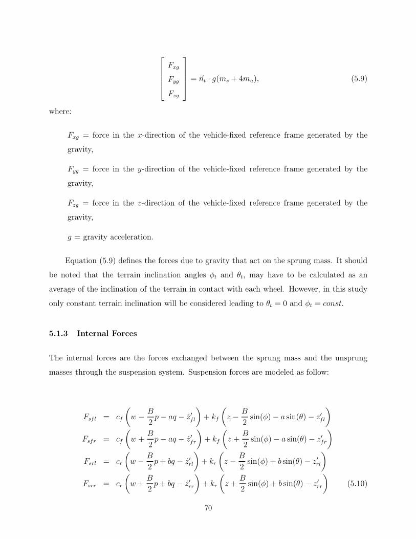
Fxg

Fyg

Fzg

= ~nt · g(ms + 4mu), (5.9)

where:

Fxg = force in the x-direction of the vehicle-fixed reference frame generated by the

gravity,

Fyg = force in the y-direction of the vehicle-fixed reference frame generated by the

gravity,

Fzg = force in the z-direction of the vehicle-fixed reference frame generated by the

gravity,

g = gravity acceleration.

Equation (5.9) defines the forces due to gravity that act on the sprung mass. It should

be noted that the terrain inclination angles φt and θt, may have to be calculated as an

average of the inclination of the terrain in contact with each wheel. However, in this study

only constant terrain inclination will be considered leading to θt = 0 and φt = const.

5.1.3 Internal Forces

The internal forces are the forces exchanged between the sprung mass and the unsprung

masses through the suspension system. Suspension forces are modeled as follow:

Fsfl = cf

(

w − B

2p− aq − z′fl

)

+ kf

(

z − B

2sin(φ) − a sin(θ) − z′fl

)

Fsfr = cf

(

w +B

2p− aq − z′fr

)

+ kf

(

z +B

2sin(φ) − a sin(θ) − z′fr

)

Fsrl = cr

(

w − B

2p+ bq − z′rl

)

+ kr

(

z − B

2sin(φ) + b sin(θ) − z′rl

)

Fsrr = cr

(

w +B

2p+ bq − z′rr

)

+ kr

(

z +B

2sin(φ) + b sin(θ) − z′rr

)

(5.10)

70

where:

Fsfl = is force in the front-left suspension,

Fsfr = is force in the front-right suspension,

Fsrl = is force in the rear-left suspension,

Fsrr = is force in the rear-rear suspension,

cf = is the damping coefficient of the front suspensions,

cr = is the damping coefficient of the rear suspensions,

kf = is the stiffness coefficient of the front suspensions,

kr = is the stiffness coefficient of the rear suspensions.

Since the unsprung masses are constrained to move in the z-direction of the the vehicle-

fixed reference frame, the assumption that all the suspension forces act in the vehicle-fixed

z-direction is made. The suspension forces, being internal forces, act on the unsprung mass

(5.2) and contribute to the term Fz in the equations of motion of the sprung mass (5.1).

5.1.4 Tire Forces Generation Process

The development of the tire model (Chapter 3) showed that three parameters control the

behavior of a given tire (this assumes that the inflation pressure, the tire geometry and the

tire properties are fixed):

Fzw = vertical load acting on the wheel (generically labeled as Fz in Chapter 3),

sd = slip ratio,

αc = slip angle.

From the vehicle dynamics point of view the perspective is slightly different. The lateral

dynamics of the tires is governed by the steering action imposed by the driver and by the

71

dynamics of the vehicle. The longitudinal dynamics of the tires is governed by the torque

applied to the axle (decided again by the driver through the gas pedal). The amount of slip

is not known a priori but depends on the amount of torque imposed by the engine. The

process is described in Figure 5.3.

Figure 5.3: A schematic representation of how the driver input is translated into actual drivingforces at the wheels.

Once the slip ratio is known it is possible to calculate the angular velocity of each wheel

from the definition of the slip (2.1),

ωw =u

Rl(1 − sd), (5.11)

where Rl is the rolling radius and it is equal to Ru (undeformed radius) for rigid wheels and

Ru − Fzw

ktfor flexible tires. The calculation of the angular velocity of the wheels is necessary

to estimate the instantaneous power delivered to the wheels.

The above discussion showed that for the calculation of the lateral and longitudinal

forces it is necessary to calculate the vertical load and the slip angle at each wheel first. The

vertical load can be evaluated from the following equations:

72

Fzwfl = Fzgb

4L+ Fsfl

Fzwfr = Fzgb

4L+ Fsfr

Fzwrl = Fzga

4L+ Fsrl

Fzwrr = Fzga

4L+ Fsrr, (5.12)

This formulation assumes no lateral inclination of the road profile (i.e., θt = 0). Equa-

tions (5.12) are calculated at every time step and fed to the tire model.

The slip angle is defined as follows:

αc = tan−1

(

Vty

Vtx

)

, (5.13)

where:

Vtx′ = velocity in the x′-direction of the tire-fixed reference frame,

Vty′ = velocity in the y′-direction of the tire-fixed reference frame,

Assuming small pitch and roll angles, for the rigid body motion, the slip angles can be

calculated as follows:

αcfl = tan−1

(

v + aψ

u+ B2ψ

)

− δl

αcfr = tan−1

(

v + aψ

u− B2ψ

)

− δr

αcrl = tan−1

(

v − bψ

u+ B2ψ

)

αcrr = tan−1

(

v − bψ

u− B2ψ

)

, (5.14)

73

the front slip angles have to keep into account the steering angles δ, while the rear slip

angles can be directly calculated from the velocities of the corners of the vehicle.

5.1.5 Velocity Controller

A proportional integral (PI) controller is introduced to maintain the imposed cruise speed.

The error function ǫ depends on the difference between the target velocity Vset and the

longitudinal velocity u:

ǫ(t) = Vset − u(t), (5.15)

where the notation explicitly includes the time dependence. The controller acts on the torque

delivered to the wheels through the following equation:

T (t) = Kpǫ(t) +Ki

∫ t

0

ǫ(τ)dτ (5.16)

where:

Kp = proportional gain,

Ki = integral gain.

5.1.6 Torque Distribution

For front (rear) wheel drive vehicles the torque is equally divided on the left and right wheels

of the axle, in this case no torque is delivered to the rear (front) axle. The non driven wheels

will receive zero torque but will produce a negative force because of the terrain compaction

resistance that still acts on them.

In the case of four wheel drive vehicles the torque will be distributed equally among

the left and right wheels (the axle differentials always slip the torque equally). On the

other hand, the torque distribution among the front and rear axles (governed by the central

differential) will be varied.

74

5.1.7 Vehicle Parameters

The vehicle parameters adopted in the simulations which follow represent typical values for

a large SUV and have been summarized in Table 5.1.

Table 5.1: Vehicle specifications.

ms = 2500 kg mu = 44 kgJx = 1165 kgm2 cf = 2700 Ns/mJy = 5348 kgm2 cr = 3300 Ns/mJz = 5721 kgm2 kf = 25 kN/ma = 1.48 m kr = 21 kN/mb = 1.52 m ρ = 1.28 kg/m3

L = 3 m Sc = 2.44 m2

B = 1.7 m kt = 270395 kN/m

5.2 Vehicle Model Validation

The dynamic response of the vehicle model has been validated performing two standard

maneuvers:� Acceleration and braking on a straight-line trajectory,� Double lane change at constant velocity.

The results have been compared with CarSim®, a software for high-fidelity vehicle

dynamics simulation. CarSim has been initialized in order to match closely the assumptions

done in this study:� vehicle properties have been taken from Table 5.1,� simple independent suspensions have been selected,� zero toe and camber angle,� linear springs and dampers,� aerodynamic forces only in the the x vehicle-fixed direction.

75

0 5 10 15 20 25 30−20

0

20

40

60

80

Time [s]

u [k

m/h

]

Model

CarSim

Figure 5.4: Longitudinal velocity of the vehicle during an acceleration and braking maneuver.

For this validation process the on-road tire model, built-in CarSim, has been adopted.

This was the only option since no off-road tire model is implemented in CarSim. The aim

of the validation is to verify that the model predicts correctly the dynamics of the vehicle:

in particular it is important to estimate the weight transfer among the axle because the

vertical load distribution influences the behavior of the tires. In the next sections the model

developed in this thesis will be addressed simply as model while the results obtained from

CarSim will be labeled as CarSim.

5.2.1 Acceleration and Braking

The first test consists in a straight-line acceleration and then braking maneuver. Since the

model does not include a gearbox model (needed during an acceleration from rest up to

80k/h) the longitudinal component of tire forces has been directly fed from CarSim into the

model: the variables labeled Fx L1, Fx R1, Fx L2, Fx R2, extracted from the CarSim

workspace, have been equaled to Fx′fl, Fx′fr, Fx′rl, Fx′rr. Figure 5.4 shows the profile of the

longitudinal velocity during the 30 second test. A perfect agreement is found between the

model and CarSim.

Figure 5.5 presents the trend of the pitch angle θ. The car pitches up during the

acceleration (negative pitch in the body-fixed reference frame) and down during the braking

76

0 5 10 15 20 25 30−2

−1.5

−1

−0.5

0

0.5

1

1.5

2

Time [s]

θ [d

eg]

Model

CarSim

Figure 5.5: Pitch angle of the vehicle during an acceleration and braking maneuver.

section. The peaks in the graph are due to the shifting process during which a short transient

occurs. Excellent agreement holds between the model and CarSim.

The variation of vertical load during the motion is showed in Figure 5.6.

0 5 10 15 20 25 305

5.5

6

6.5

7

7.5

8

8.5

Time [s]

Fz [k

N]

Front axle − Model

Rear axle − Model

Front axle − CarSim

Rear axle − CarSim

Figure 5.6: Pitch angle of the vehicle during an acceleration and braking maneuver.

During the acceleration the load is transfered to the rear axle, while the front axle is

more loaded during the braking. As for the pitch also the load distribution is influenced by

the shifting process. The agreement between the model and CarSim is good: it is noticed that

the CarSim response is more dampened. This might be due to an extra damping coefficient

77

that has not been considered in the model.

5.2.2 Double Lane Change

The double lane change is the typical maneuver that a driver performs while passing another

vehicle on the highway. The trajectory followed, at constant longitudinal velocity, by the

vehicle is showed in Figure 5.7. For this test the CarSim workspace variables Steer L1

and Steer R1 have been passed to the the model as the steering angles δl and δr. The

longitudinal velocity has been kept constant with the controller introduced by (5.16).

0 50 100 150 200−1

0

1

2

3

4

X [m]

Y [m

]

u = 50 km\hu = 50 km\h

u = 50 km\h

u = 50 km\h

Figure 5.7: Trajectory followed by the vehicle during a double lane change maneuver.

Figure 5.8 shows the longitudinal velocity during 15 second. The response is slightly

different because of the intrinsic differences between the model and CarSim. CarSim includes

the compliance of the drive-line while the controller introduced in this thesis acts directly

on the torque. The slight variation of longitudinal velocity occurs because of the coupling

terms seen in (5.1). When the vehicle starts to steer a slip angle develops at the each

corner (not only at the steered wheels) and the lateral force develops. The variation of the

lateral velocity creates an unbalance in the longitudinal velocity that consequently needs to

be adjusted. The trend of u reflects the the trend of the roll angle φ; both variations are

primarily caused by the variation of lateral velocity.

The roll angle φ is presented in Figure 5.9. The vehicle rolls significantly during the

78

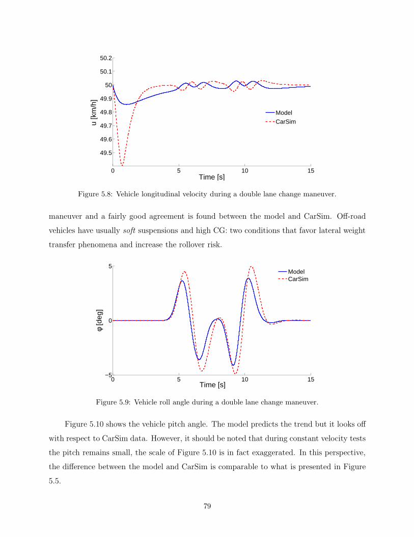
0 5 10 15

49.5

49.6

49.7

49.8

49.9

50

50.1

50.2

Time [s]

u [k

m/h

]

Model

CarSim

Figure 5.8: Vehicle longitudinal velocity during a double lane change maneuver.

maneuver and a fairly good agreement is found between the model and CarSim. Off-road

vehicles have usually soft suspensions and high CG: two conditions that favor lateral weight

transfer phenomena and increase the rollover risk.

0 5 10 15−5

0

5

Time [s]

φ [d

eg]

ModelCarSim

Figure 5.9: Vehicle roll angle during a double lane change maneuver.

Figure 5.10 shows the vehicle pitch angle. The model predicts the trend but it looks off

with respect to CarSim data. However, it should be noted that during constant velocity tests

the pitch remains small, the scale of Figure 5.10 is in fact exaggerated. In this perspective,

the difference between the model and CarSim is comparable to what is presented in Figure

5.5.

79

0 5 10 15−0.3

−0.25

−0.2

−0.15

−0.1

−0.05

0

0.05

Time [s]

θ [d

eg]

ModelCarSim

Figure 5.10: Vehicle pitch angle during a double lane change maneuver.

The vehicle yaw ψ is shown in Figure 5.11. The model estimates accurately the yaw,

the result is reasonably comparable with CarSim.

0 5 10 15

−10

−5

0

5

10

Time [s]

ψ [d

eg]

Model

CarSim

Figure 5.11: Vehicle yaw angle during a double lane change maneuver.

The last Figure 5.12 of this section shows the vertical load distribution acting on the

wheels. During cornering the outer wheels are more loaded that the inner ones. This

phenomenon is correctly estimated by the model: the results are in fairly good agreement

with CarSim as well.

80

0 5 10 154

5

6

7

8

9

Time [s]

Fz [k

N]

Front Left

Front Right

Rear Left

Rear Right

Figure 5.12: Vertical load distribution during a double lane change maneuver. Solid lines: Model.Dashed lines: CarSim. The vertical load increases on the outer wheels and decreases on the innerones due to dynamic weight transfer phenomenon.

5.3 Results

Hitherto, the tire model and the vehicle model have been developed and explained distinctly.

In this section the results for a full-vehicle, and adopting the tire model developed in Chapter

3, are presented. Since the tire model has been developed under steady state assumptions,

the full-vehicle simulation is performed at constant longitudinal speed. The simulations are

started at a velocity slightly lower than the target one, and the PI controller (5.16) is used to

reach smoothly the cruise speed. The efficiency is analyzed when steady state conditions are

reached. The transients have to be regarded as a first approximation of the vehicle dynamics.

The results are divided into four sections:� Longitudinal motion on dry sand.� Longitudinal motion on moist Yolo loam.� Lateral motion on dry sand.� Lateral motion on moist Yolo loam.

The full-vehicle model can be exploited to simulate several different maneuvers. The

81

influence of the vehicle and the tire-terrain parameters (Tables 5.1, 3.1, 3.2) can be investi-

gated. For every run large amount of output data is produced and it is unpractical to present

all the results here. The author decided to investigate a restricted set of parameters: details

will be provided in the following sections.

5.3.1 Dry Sand Longitudinal

In this section the motion and the efficiency of a vehicle traveling on a straight line on dry

sand are analyzed. The sand is a non cohesive soil and the tire will always perform as a rigid

wheel in this section.

Flat Terrain

Figure 5.13 shows the velocity profile and the applied torque, for a vehicle that starts at 20

km/h and has to reach the target speed of 25 km/h. FWD, RWD and AWD configurations

are plotted together: in every configuration the vehicle is able to reach the imposed speed.

The PI controller adjusts the torque correctly in order to reach the target speed.

0 5 10 1520

21

22

23

24

25

26

Time [s]

u [k

m/h

]

FWD

RWD

AWD

(a)

0 5 10 15

0

0.2

0.4

0.6

0.8

1

1.2

Time [s]

Tor

que

[kN

/m]

FWD Front Axle

FWD Rear Axle

RWD Front Axle

RWD Rear Axle

AWD Front Axle

AWD Rear Axle

(b)

Figure 5.13: (a) Velocity profile for a vehicle running on a flat dry sand terrain. The simulationstarts from a slightly lower velocity in order to reach smooth steady state conditions. (b) Thetorque delivered at the tires during the maneuver.

The sinkage is presented if Figure 5.14(a) . The front wheels of a FWD vehicle sink

considerably because they are driven (sd > 0) and they negotiate a virgin patch of terrain

which is less cohesive: two conditions that influences the slip-sinkage behavior. The rear

82

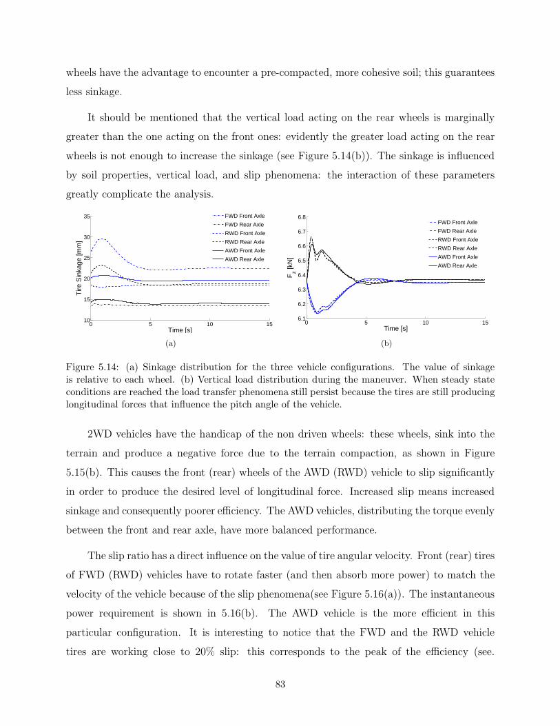
wheels have the advantage to encounter a pre-compacted, more cohesive soil; this guarantees

less sinkage.

It should be mentioned that the vertical load acting on the rear wheels is marginally

greater than the one acting on the front ones: evidently the greater load acting on the rear

wheels is not enough to increase the sinkage (see Figure 5.14(b)). The sinkage is influenced

by soil properties, vertical load, and slip phenomena: the interaction of these parameters

greatly complicate the analysis.

0 5 10 1510

15

20

25

30

35

Time [s]

Tire

Sin

kage

[mm

]

FWD Front Axle

FWD Rear Axle

RWD Front Axle

RWD Rear Axle

AWD Front Axle

AWD Rear Axle

(a)

0 5 10 156.1

6.2

6.3

6.4

6.5

6.6

6.7

6.8

Time [s]

Fz [k

N]

FWD Front Axle

FWD Rear Axle

RWD Front Axle

RWD Rear Axle

AWD Front Axle

AWD Rear Axle

(b)

Figure 5.14: (a) Sinkage distribution for the three vehicle configurations. The value of sinkageis relative to each wheel. (b) Vertical load distribution during the maneuver. When steady stateconditions are reached the load transfer phenomena still persist because the tires are still producinglongitudinal forces that influence the pitch angle of the vehicle.

2WD vehicles have the handicap of the non driven wheels: these wheels, sink into the

terrain and produce a negative force due to the terrain compaction, as shown in Figure

5.15(b). This causes the front (rear) wheels of the AWD (RWD) vehicle to slip significantly

in order to produce the desired level of longitudinal force. Increased slip means increased

sinkage and consequently poorer efficiency. The AWD vehicles, distributing the torque evenly

between the front and rear axle, have more balanced performance.

The slip ratio has a direct influence on the value of tire angular velocity. Front (rear) tires

of FWD (RWD) vehicles have to rotate faster (and then absorb more power) to match the

velocity of the vehicle because of the slip phenomena(see Figure 5.16(a)). The instantaneous

power requirement is shown in 5.16(b). The AWD vehicle is the more efficient in this

particular configuration. It is interesting to notice that the FWD and the RWD vehicle

tires are working close to 20% slip: this corresponds to the peak of the efficiency (see.

83

0 5 10 15−0.1

0

0.1

0.2

0.3

0.4

0.5

0.6

Time [s]

s d

FWD Front Axle

FWD Rear Axle

RWD Front Axle

RWD Rear Axle

AWD Front Axle

AWD Rear Axle

(a)

0 5 10 15−1

−0.5

0

0.5

1

1.5

2

2.5

Time [s]

Fx’ [

kN]

FWD Front Axle

FWD Rear Axle

RWD Front Axle

RWD Rear Axle

AWD Front Axle

AWD Rear Axle

(b)

Figure 5.15: (a) Sinkage distribution for the three vehicle configurations. The value of sinkageis relative to each wheel. (b) Vertical load distribution during the maneuver. When steady stateconditions are reached the load transfer phenomena still persist because the tires are still producinglongitudinal forces to overcame the resistance forces; this influence the pitch angle of the vehicle.

Figure 4.5) for the tires but not for the whole vehicle. This is due to the rolling resistance of

their non-drive wheel. Tests have been conducted also at 50 km/h and 100 km/h obtaining

similar results. At 100 km/h the FWD and RWD vehicles would require the tires to work at

more than 50% slip with power peak of 200kW: this is unpractical and it means that FWD

and RWD could hardly travel at more than 50km/h on dry sand.

The influence of torque distribution on the tractive efficiency has been studied varying

the torque ratio among the front and rear axle. Figure 5.17 presents the power requirement

for a full range of transmission configurations. In this plot 0 % means that all the available

torque is delivered to the front axle (i.e. FWD vehicle,) while 100 % means that the rear

0 5 10 15

14

16

18

20

22

24

26

28

30

Time [s]

Tire

Ang

ula

Vel

ocity

ω [r

ad/s

]

FWD Front Axle

FWD Rear Axle

RWD Front Axle

RWD Rear Axle

AWD Front Axle

AWD Rear Axle

(a)

0 5 10 1510

20

30

40

50

60

Time [s]

Pow

er [k

W]

FWD

RWD

AWD

(b)

Figure 5.16: (a) Tire angular velocity and (b) instantaneous power requirement to move at 25 km/hon dry sand.

84

0 10 20 30 40 50 60 70 80 90 10020

22

24

26

Pow

er [k

W]

Torque delivered to the rear axle [%]

0 10 20 30 40 50 60 70 80 90 1000

0.1

0.2

0.3

∆ s d

Power

Slip difference between axles

Figure 5.17: Power vs. torque distribution for a vehicle traveling at 25 km/h on flat dry sand. 0 %(100 %) on the x-axis means that the torque is fully biased on the front (rear) axle of the vehicle.On the same plot the slip difference between the front and rear axle is presented.

axle receives full torque (i.e. RWD vehicle). For a vehicle traveling at 25 km/h there is

a minimum in the vicinity of 50 %. Similar trend has been observed for higher velocities.

Distributing the torque slightly toward the rear axle can improve the efficiency of the vehicle

without sacrificing the performance. On the same plot the slip difference between the front

and rear axle is presented. The minimization of the slip difference optimizes the slip efficiency

(see (4.8)) but does not necessarily improves the overall performance.

Inclined Terrain

The same analysis has been performed on a vehicle climbing a constant slope of 10 %

inclination. In this scenario pure front wheel drive or rear wheel drive vehicles can’t easily

maintain a speed of 25 km/h. Figure 5.18 present the power vs torque distribution trend

for this scenario. The trend is similar to the results obtained for flat terrain operations: the

best efficiency is obtained when the torque is biased toward the rear axle.

Influence of the Static Load Distribution

The results for the torque distribution presented in Figures 5.17, 5.18 suggest that deliv-

ering more torque to the rear axle can improve tractive performance. It should be noted

85

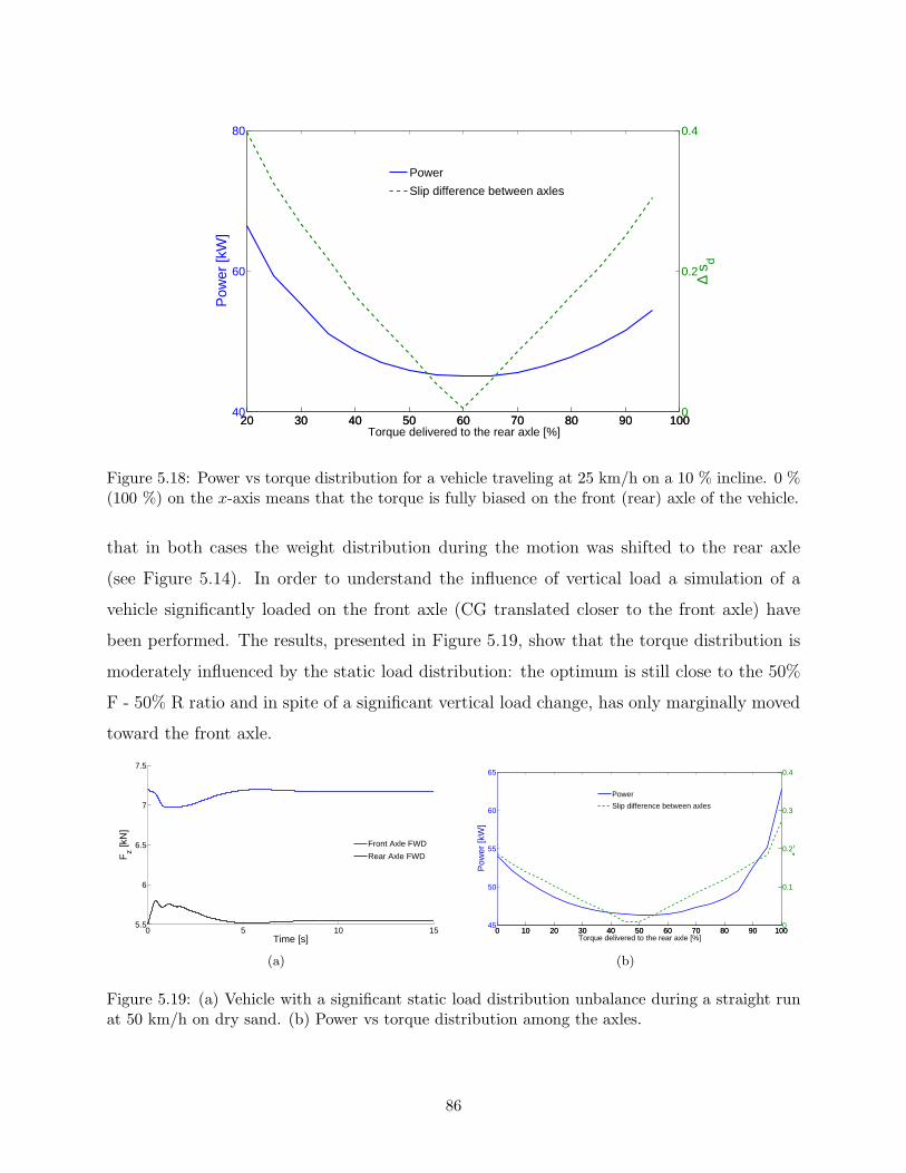
20 30 40 50 60 70 80 90 10040

60

80

Pow

er [k

W]

Torque delivered to the rear axle [%]

20 30 40 50 60 70 80 90 1000

0.2

0.4

∆ s d

Power

Slip difference between axles

Figure 5.18: Power vs torque distribution for a vehicle traveling at 25 km/h on a 10 % incline. 0 %(100 %) on the x-axis means that the torque is fully biased on the front (rear) axle of the vehicle.

that in both cases the weight distribution during the motion was shifted to the rear axle

(see Figure 5.14). In order to understand the influence of vertical load a simulation of a

vehicle significantly loaded on the front axle (CG translated closer to the front axle) have

been performed. The results, presented in Figure 5.19, show that the torque distribution is

moderately influenced by the static load distribution: the optimum is still close to the 50%

F - 50% R ratio and in spite of a significant vertical load change, has only marginally moved

toward the front axle.

0 5 10 155.5

6

6.5

7

7.5

Time [s]

Fz [k

N]

Front Axle FWD

Rear Axle FWD

(a)

0 10 20 30 40 50 60 70 80 90 10045

50

55

60

65

Pow

er [k

W]

Torque delivered to the rear axle [%]

0 10 20 30 40 50 60 70 80 90 1000

0.1

0.2

0.3

0.4

∆ s

Power

Slip difference between axles

(b)

Figure 5.19: (a) Vehicle with a significant static load distribution unbalance during a straight runat 50 km/h on dry sand. (b) Power vs torque distribution among the axles.

86

Tire Size Influence

The efficiency has been evaluated also for tires of different dimensions. The results confirm

that larger and wider tires provide better performance in off-road scenarios. Figure 5.20

presents an aggregated result obtained for an AWD vehicle running on flat dry sand at 50

km/h. The “standard” vehicle had nominal tires (radius = 0.4 m and width = 0.265 m) and

torque evenly distributed among the axle (50% Front -50% Rear). The one labeled “torque

optimized” adopted a torque distribution of 60 % Rear - 40% Front, while the other two

vehicles adopted larger tires (radius = 0.45 m) and wider tires (width = 0.325 m). The

parameter that has the strongest influence is the tire radius because it directly affects the

sinkage.

Standard Torque optimized width = 0.325 m R_u = 0.45 m30

35

40

45

50

Pow

er [k

W]

− 4%

− 16%− 13%

Figure 5.20: Power requirement for four vehicle configurations. Vehicle speed is 50km/h and theterrain is flat dry sand. Nominal parameters (concerning the standard case) are: Radius = 0.4 m,Width = 0.265 m, Torque = 50%F - 50% R.

However, increased tire size would imply a general increase of weight and will penalize

the dynamics performance and then the consumption. Moreover, a change of tire size,

would modify the kinematic ratio between tire revolutions and engine revolutions: this would

require an careful analysis of the drive-line ratio. On the other hand, for vehicles with a

central differential Figure 5.17 has to be considered at the design stage: a modification of

the differential ratio would add no weight to the vehicle and possibly increase the efficiency.

For vehicles with electric motors, mounted directly on wheels hub, the control the driving

87

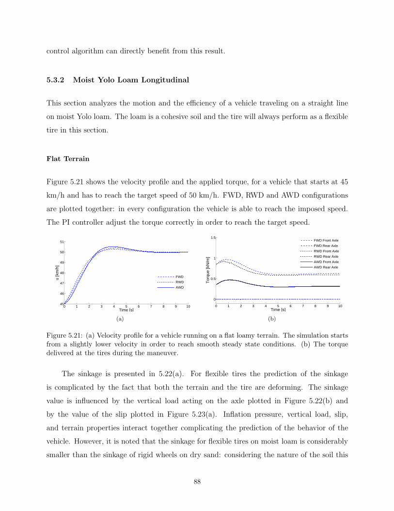
control algorithm can directly benefit from this result.

5.3.2 Moist Yolo Loam Longitudinal

This section analyzes the motion and the efficiency of a vehicle traveling on a straight line

on moist Yolo loam. The loam is a cohesive soil and the tire will always perform as a flexible

tire in this section.

Flat Terrain

Figure 5.21 shows the velocity profile and the applied torque, for a vehicle that starts at 45

km/h and has to reach the target speed of 50 km/h. FWD, RWD and AWD configurations

are plotted together: in every configuration the vehicle is able to reach the imposed speed.

The PI controller adjust the torque correctly in order to reach the target speed.

0 1 2 3 4 5 6 7 8 9 1045

46

47

48

49

50

51

Time [s]

u [k

m/h

]

FWD

RWD

AWD

(a)

0 1 2 3 4 5 6 7 8 9 10

0

0.5

1

1.5

Time [s]

Tor

que

[kN

/m]

FWD Front Axle

FWD Rear Axle

RWD Front Axle

RWD Rear Axle

AWD Front Axle

AWD Rear Axle

(b)

Figure 5.21: (a) Velocity profile for a vehicle running on a flat loamy terrain. The simulation startsfrom a slightly lower velocity in order to reach smooth steady state conditions. (b) The torquedelivered at the tires during the maneuver.

The sinkage is presented in 5.22(a). For flexible tires the prediction of the sinkage

is complicated by the fact that both the terrain and the tire are deforming. The sinkage

value is influenced by the vertical load acting on the axle plotted in Figure 5.22(b) and

by the value of the slip plotted in Figure 5.23(a). Inflation pressure, vertical load, slip,

and terrain properties interact together complicating the prediction of the behavior of the

vehicle. However, it is noted that the sinkage for flexible tires on moist loam is considerably

smaller than the sinkage of rigid wheels on dry sand: considering the nature of the soil this

88

is expected.

0 1 2 3 4 5 6 7 8 9 103

4

5

6

7

8

9

Time [s]

Tire

Sin

kage

[mm

]

FWD Front Axle

FWD Rear Axle

RWD Front Axle

RWD Rear Axle

AWD Front Axle

AWD Rear Axle

(a)

0 1 2 3 4 5 6 7 8 9 106

6.2

6.4

6.6

6.8

7

Time [s]

Fz [k

N]

FWD Front Axle

FWD Rear Axle

RWD Front Axle

RWD Rear Axle

AWD Front Axle

AWD Rear Axle

(b)

Figure 5.22: (a) Sinkage distribution for the three vehicle configurations. The value of sinkageis relative to each wheel. (b) Vertical load distribution during the maneuver. When steady stateconditions are reached the load transfer phenomena still persist because the tires are still producinglongitudinal forces that influence the pitch angle of the vehicle.

The reduced sinkage is compensated by the fact that the loam is a firmer soil that

requires more energy to be compressed. The longitudinal force for the non driven wheels

remains consistent also when traveling on moist loam, as Figure 5.23(b) shows. Also on a

firmer soil the non driven wheels represent an handicap for the 2WD vehicles.

0 1 2 3 4 5 6 7 8 9 10−0.2

−0.1

0

0.1

0.2

0.3

0.4

0.5

0.6

Time [s]

s d

FWD Front Axle

FWD Rear Axle

RWD Front Axle

RWD Rear Axle

AWD Front Axle

AWD Rear Axle

(a)

0 1 2 3 4 5 6 7 8 9 10−1

−0.5

0

0.5

1

1.5

2

2.5

Time [s]

Fx’ [

kN]

FWD Front Axle

FWD Rear Axle

RWD Front Axle

RWD Rear Axle

AWD Front Axle

AWD Rear Axle

(b)

Figure 5.23: (a) Sinkage distribution for the three vehicle configurations. The value of sinkageis relative to each wheel. (b) Vertical load distribution during the maneuver. When steady stateconditions are reached the load transfer phenomena still persist because the tires are still producinglongitudinal forces that influence the pitch angle of the vehicle.

The slip ratio has a direct influence on the value of tire angular velocity. Front (rear)

tires of FWD (RWD) vehicles have to rotate faster (and then absorb more power) to match

the velocity of the vehicle because of the slip effect, as shown in Figure 5.24(a).

The instantaneous power requirement is presented in 5.24(b). The AWD vehicle is

89

0 1 2 3 4 5 6 7 8 9 1030

35

40

45

50

55

60

65

Time [s]

Tire

Ang

ula

Vel

ocity

ω [r

ad/s

]

FWD Front Axle

FWD Rear Axle

RWD Front Axle

RWD Rear Axle

AWD Front Axle

AWD Rear Axle

(a)

0 1 2 3 4 5 6 7 8 9 1040

50

60

70

80

90

100

110

120

Time [s]

Pow

er [k

W]

FWD

RWD

AWD

(b)

Figure 5.24: (a) Tire angular velocity and (b) instantaneous power requirement to move at 50 km/hon moist loam.

the more efficient in this particular configuration but the FWD and RWD vehicles are now

closer. Flexible tires, reducing the compaction resistance of non driven wheels, improve the

performance of 2 wheels drive vehicles on deformable soil. The limiting case is represented by

the on-road case where the rolling resistance of the non driven wheels is extremely reduced

and the 2WD configurations have better efficiency.

0 10 20 30 40 50 60 70 80 90 10046

47

48

49

50

51

52

53

54

55

56

Pow

er [k

W]

Torque delivered to the rear axle [%]

0 10 20 30 40 50 60 70 80 90 1000

0.02

0.04

0.06

0.08

0.1

0.12

0.14

0.16

0.18

0.2

∆ s d

Power

Slip difference between axles

Figure 5.25: Power vs torque distribution for a vehicle traveling at 50 km/h on flat loam. 0 % (100%) on the x-axis means that the torque is fully biased on the front (rear) axle of the vehicle.

The influence of torque distribution on the tractive efficiency has been studied varying

the torque ratio among the front and rear axle. Figure 5.25 presents the power requirement

for a full range of transmission configurations.

90

Inclined Terrain

A series of simulations for vehicles traveling on constantly inclined terrain have been per-

formed. Road grade of 10% has been selected and the vehicle speed has been set to 50 km/h.

Figure 5.26(a) shows that the RWD vehicle does not allow to comfortably reach the target

speed.

0 2 4 6 8 1044

45

46

47

48

49

50

51

Time [s]

u [k

m/h

]

FWD

RWD

AWD

(a)

0 2 4 6 8 100

50

100

150

200

250

Time [s]P

ower

[kW

]

FWD

RWD

AWD

(b)

Figure 5.26: (a)Longitudinal velocity for three vehicles traveling at 50 km/h on a 10% inclinedmoist loam terrain. The rear wheel drive configuration does not allow to reach comfortably thedesired target speed. (b) Power requirement for the same maneuver; the RWD saturates becausethe imposed slip ratio limit is achieved during the simulation. The FWD vehicle is able to climbthe hill but it is less efficient than the AWD one.

The instantaneous power requirement plot, Figure 5.26, demonstrates that even applying

an amount of power beyond 200 kW it is impossible to travel at the desired speed: tires are

not able to provide enough traction. In this operational conditions the AWD vehicle provides

the best performance. Figure 5.27 presents the power vs torque distribution trend for this

scenario. The trend is similar to flat terrain operations: a minimum of power is observed for

the the situation of torque biased toward the rear. It should be noted that on moist Yolo

loam the variation of power is less significant.

Tire Inflation Pressure Influence

The tire pressure has been decreased in order to investigate its influence on the efficiency

of the vehicle. Figure 5.28(a)(b) shows the sinkage and the slip for a tire inflation pressure

25% lower than the nominal one. The decrease in the inflation pressure guarantees larger

contact patch area and consequently less sinkage.

91

25 30 35 40 45 50 55 60 65 70 7580

90

100

110

120

Pow

er [k

W]

Torque delivered to the rear axle [%]

25 30 35 40 45 50 55 60 65 70 750

0.1

0.2

0.3

0.4

∆ s d

Power

Slip difference between axles

Figure 5.27: Torque distribution influence on the performance of an AWD vehicle driving at 50km/h on a 10% inclined loam terrain. The best efficiency is reached when 60% of the total torqueis delivered to the rear axle.

In this operational conditions the resistance force due to terrain compaction decreases

consistently and this improves the performance. Figure 5.29 presents the longitudinal force

and the instantaneous power requirement for FWD, RWD and AWD vehicles running on

under-inflated tires. The AWD vehicle is the one that requires less power to be operated

at 50 km/h on loamy terrain. Figure 5.30 shows the instantaneous power requirement for a

large range of torque distribution. The best efficiency is reached when the torque is biased

to the rear axle. Under-inflated tires provide better efficiency on off road terrain, the power

requirement is about 10% less then normally inflated tires.

0 1 2 3 4 5 6 7 8 9 10

2.4

2.6

2.8

3

3.2

3.4

3.6

Time [s]

Tire

Sin

kage

[mm

]

FWD Front Axle

FWD Rear Axle

RWD Front Axle

RWD Rear Axle

AWD Front Axle

AWD Rear Axle

(a)

0 1 2 3 4 5 6 7 8 9 10−0.2

−0.1

0

0.1

0.2

0.3

0.4

0.5

0.6

Time [s]

s d

FWD Front Axle

FWD Rear Axle

RWD Front Axle

RWD Rear Axle

AWD Front Axle

AWD Rear Axle

(b)

Figure 5.28: (a) Sinkage of a vehicle with decreased tire pressure traveling at 50 km/h on moistloam. (b) Slip under the same conditions.

92

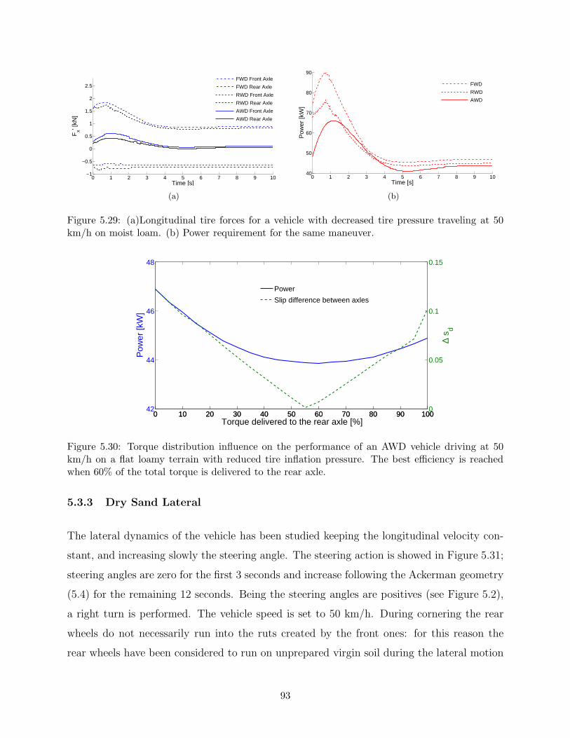
0 1 2 3 4 5 6 7 8 9 10−1

−0.5

0

0.5

1

1.5

2

2.5

Time [s]

Fx’ [

kN]

FWD Front Axle

FWD Rear Axle

RWD Front Axle

RWD Rear Axle

AWD Front Axle

AWD Rear Axle

(a)

0 1 2 3 4 5 6 7 8 9 1040

50

60

70

80

90

Time [s]

Pow

er [k

W]

FWD

RWD

AWD

(b)

Figure 5.29: (a)Longitudinal tire forces for a vehicle with decreased tire pressure traveling at 50km/h on moist loam. (b) Power requirement for the same maneuver.

0 10 20 30 40 50 60 70 80 90 10042

44

46

48

Pow

er [k

W]

Torque delivered to the rear axle [%]

0 10 20 30 40 50 60 70 80 90 1000

0.05

0.1

0.15

∆ s d

Power

Slip difference between axles

Figure 5.30: Torque distribution influence on the performance of an AWD vehicle driving at 50km/h on a flat loamy terrain with reduced tire inflation pressure. The best efficiency is reachedwhen 60% of the total torque is delivered to the rear axle.

5.3.3 Dry Sand Lateral

The lateral dynamics of the vehicle has been studied keeping the longitudinal velocity con-

stant, and increasing slowly the steering angle. The steering action is showed in Figure 5.31;

steering angles are zero for the first 3 seconds and increase following the Ackerman geometry

(5.4) for the remaining 12 seconds. Being the steering angles are positives (see Figure 5.2),

a right turn is performed. The vehicle speed is set to 50 km/h. During cornering the rear

wheels do not necessarily run into the ruts created by the front ones: for this reason the

rear wheels have been considered to run on unprepared virgin soil during the lateral motion

93

simulation.

0 5 10 150

10

20

30

40

50

Time [s]

Ste

erin

g A

ngle

δ [d

eg]

δl = δ

o

δr = δ

i

Figure 5.31: Steering action during the lateral dynamic test. The steering angles δ comply withthe Ackermann steering geometry introduced in (5.4). For a right turn the outer wheel is the leftone and consequently δ0 = δl and δi = δr.

Figure 5.32(a) presents the roll angle of the FWD, RWD, and AWD vehicles. The drive

configuration does not affect significantly the roll angle which reaches large values toward

the end of the test (the steering angle is constantly increased, the vehicle has to follow

a decreasing curvature radius turn). The vertical load distribution is presented in Figure

5.32(b) and shows that the outer wheels (the left ones) are overloaded during the maneuver.

0 5 10 15−6

−5

−4

−3

−2

−1

0

Time [s]

φ [d

eg]

FWD

RWD

AWD

(a)

0 2 4 6 8 10 12 144

5

6

7

8

9

Time [s]

Fz [k

N]

FWD − Front Left

FWD − Front Right

FWD − Rear Left

FWD − Rear Right

RWD − Front Left

RWD − Front Right

RWD − Rear Left

RWD − Rear Right

AWD − Front Left

AWD − Front Right

AWD − Rear Left

AWD − Rear Right

(b)

Figure 5.32: (a)Roll angle of FWD, RWD, and AWD vehicles during a right turn maneuver on drysand. (b) The load is transfered to the outer wheels (the left ones).

Tire sinkage for this maneuver is presented in Figure 5.33(a). The outer (left) tires have

to withstand more vertical load during a right turn, consequently they are sinking more. The

instantaneous power requirement to complete the maneuver is presented in Figure 5.33(b).

It should be noted that in normal driving conditions, most of the time is spent in straight

line motion and the economy of the vehicle is primarily affected by its performance in this

94

working condition. Moreover, steering is an maneuver necessary to follow the road course or

avoid obstacles; generally it cannot be altered arbitrarily. In this perspective Figure 5.33 can

only provide general indications. AWD vehicles remain more efficient than 2WD vehicles

and are less sensitive to increasing steering angle.

0 2 4 6 8 10 12 1410

15

20

25

30

Time [s]

Tire

Sin

kage

[mm

]

FWD − Front Left

FWD − Front Right

FWD − Rear Left

FWD − Rear Right

RWD − Front Left

RWD − Front Right

RWD − Rear Left

RWD − Rear Right

AWD − Front Left

AWD − Front Right

AWD − Rear Left

AWD − Rear Right

(a)

0 5 10 1540

50

60

70

80

90

100

110

120

130

Time [s]

Pow

er [k

W]

FWD

RWD

AWD

(b)

Figure 5.33: (a)Sinkage of FWD, RWD, and AWD vehicle during a right turn maneuver on drysand. The outer wheels (left ones), being more loaded, sink more. (b) The instantaneous powerrequirement to complete the maneuver.

5.3.4 Moist Yolo Loam Lateral

The same maneuver showed in Figure 5.31 has been simulated for a vehicle traveling on moist

Yolo loam. The longitudinal velocity has been kept constant through the PI controller; a

right turn with constantly decreasing radius has been imposed. Figure 5.34(a) presents the

roll angle of the FWD, RWD, and AWD vehicles. The result is similar to what it has been

obtained on dry sand. The vertical load is larger on the outer wheels (the left ones), as

shown in Figure 5.34(b)

0 5 10 15−6

−5

−4

−3

−2

−1

0

Time [s]

φ [d

eg]

FWD

RWD

AWD

(a)

0 2 4 6 8 10 12 144

5

6

7

8

9

Time [s]

Fz [k

N]

FWD − Front Left

FWD − Front Right

FWD − Rear Left

FWD − Rear Right

RWD − Front Left

RWD − Front Right

RWD − Rear Left

RWD − Rear Right

AWD − Front Left

AWD − Front Right

AWD − Rear Left

AWD − Rear Right

(b)

Figure 5.34: (a)Roll angle of FWD, RWD, and AWD vehicles during a right turn maneuver onmoist Yolo loam. (b) The load is transfered to the outer wheels (the left ones).

95

Tire sinkage is reduced on moist Yolo loam (Figure 5.35(a)). The outer (left) tires have

to withstand more vertical load during a right turn, consequently they are sinking more. The

instantaneous power requirement to complete the maneuver is presented in Figure 5.35(b).

On loamy terrain the AWD configuration provides better efficiency during cornering and,

like on sandy terrain, it is less sensitive to increasing steering action.

0 2 4 6 8 10 12 142

4

6

8

10

12

14

Time [s]

Tire

Sin

kage

[mm

]

FWD − Front Left

FWD − Front Right

FWD − Rear Left

FWD − Rear Right

RWD − Front Left

RWD − Front Right

RWD − Rear Left

RWD − Rear Right

AWD − Front Left

AWD − Front Right

AWD − Rear Left

AWD − Rear Right

(a)

0 5 10 1540

60

80

100

120

140

Time [s]

Pow

er [k

W]

FWD

RWD

AWD

(b)

Figure 5.35: (a)Sinkage of FWD, RWD, and AWD vehicle during a right turn maneuver on moistYolo loam. The outer wheels (left ones), being more loaded, sink more. (b) The instantaneouspower requirement to complete the maneuver.

96

Chapter 6

Conclusions and Future Work

This chapter summarizes the contributions of this study and suggests directions for future

research.

6.1 Research Summary and Contribution

This thesis established a tool for predicting mobility, handling and tractive efficiency of off-

road vehicles. A semi-empirical off-road tire model, based on the work of Wong and Reece

[6, 30] and Chan and Sandu [26], has been developed and modified. The model is able to

predict the salient features encountered in off-road operations. The slip-sinkage behavior

and the multi-pass effect have been implemented through the introduction of semi-empirical

equations. The response of the model has been extensively investigated in order to verify

the influence of several parameters. Variations of vertical load, tire geometry, tire inflation

pressure, and soil states (i.e. multi-pass) showed that the model consistently predict tire

tractive performance.

The study then moved on the analysis of a full vehicle. It has been showed that the

proposed tire-model can be successfully adopted to simulate the large motion of an off-

road vehicle. An analysis of the the tractive performance has been conducted. The study

showed that it is possible to improve the efficiency of off-road vehicles acting on the torque

distribution of the vehicle. Shifting the torque toward the rear axle can help to exploit in a

97

better way the tractive resources of the vehicle and obtain an improvement of the efficiency,

without sacrificing the performance. This result has been obtained analyzing the vehicle with

a high level of detail. The study highlighted that the motion of a vehicle can be optimized

acting on torque distribution. It should be remembered that varying parameters such as the

tire sizes, the static weight balance, and the torque distribution can significantly modify the

response of the vehicle. This can have implications on the safety and comfort. The static load

distribution influences traction but does not have a significant impact on tractive efficiency:

the best tractive efficiency, under a large range of operational conditions, is reached when

the torque distribution is biased toward the rear axle. This operational condition helps to

optimize the slip efficiency which dominantly influences the overall tractive efficiency. This

research proves that the modeling of off-road tires can have a strong impact on the design

and control of off-road vehicles. Tires complex behaviors such as the multi-pass, the slip

sinkage, and the parameters sensitivity cannot be ignored when analyzing off-road vehicles.

6.2 Recommendations for Future Research

Transient Maneuvering

The tire model has been developed under steady-state assumptions. In particular, the ter-

rain semi-empirical characterization is valid for quasi-static loading conditions. Thus, there

is a need to evaluate the response during transients. The problem regards both the tire and

the terrain: during transient the contact patch location and shape varies and the terrain

properties may not be properly described by Bekker-Reece and Janosi-Hanamoto formula-

tions. Extending the tire model beyond steady-state assumptions will allow to realistically

simulate complex maneuvers such has the J-turn or the fish-hook maneuver.

Identify the Parameters Introduced in this Thesis

This research introduced several parameters in order to relate the slip with the soil and tire

properties. Experimental tests are needed to identify these parameters and fully validate the

model. Soil cohesion, density, and shear modulus have to be properly characterized in order

98

to obtain realistic results for the multi-pass effect.

Improvement of Flexible Tire Model

The flexible tire model introduced by [26] provides a realistic computation of the tire deflected

shape. However, the stress distribution along the contact patch is not necessarily consistent

with the tire deformation. This happens because the tire deformation is calculated for a

tire sitting on a hard surface, and the assumption that the shape stays constant during

off-road motion is made. In reality, the deformation of the tire and the terrain are not two

disjoint phenomena and should be considered at the same time. The approach proposed

by [26] remains attractive because provides a solid, theoretical, approach but it needs to

be improved in order to calculate a tire deformed shape that is consistent with the stress

distribution.

Variable Tire Pressure

Variable tire pressure mechanisms (VTP) for military vehicles have been developed since

War World II. Future work may exploit the results obtained in this thesis to implement

control strategies for VTP systems. Differential inflation pressure among the axles might

provide beneficial effects on both traction and mobility.

Differentials and in-hub Motors

In this research the differentials were considered as black-box entities. An thorough analysis

of the available solutions and their implementation is suggested. Thanks to the development

of lighter and more powerful electric engines, it is today possible to think about vehicles

with in-hub motors. Such vehicles could directly benefit from the results obtained in this

thesis. However, the vast majority of vehicles is still using mechanical coupling among the

axles (even hybrid vehicles) and the study of the differentials remains a relevant topic.

99

Bibliography

[1] Renewables global status report: 2009 update. Technical report, Renewable Energy

Policy Network for the 21st Century, 2009.

[2] National Research Council. Tires and passenger vehicle fuel economy. Technical report,

Board on Energy and Environmental Systems, 2006. Informing Consumers, Improving

Performance.

[3] Society of Automotive Engineers. Vehicle dynamics terminology. In SAE J670e, War-

rendale, PA, 1978.

[4] Wheelstyres.com. http://wheelstyres.com/ [April 2010].

[5] C. Harnisch, B. Lach, R. Jakobs, M. Troulis, and O. Nehls. A new tyre-soil interac-

tion model for vehicle simulation on deformable ground. Vehicle System Dynamics,

43(Supplement):384–394, 2005.

[6] J. Y. Wong and A. R. Reece. Prediction of rigid wheel performance based on analysis

of soil-wheel stresses, Part I. Performance of driven rigid wheels. Journal of Terrame-

chanics, 4(1):81–98, 1967.

[7] I. C. Holm. Multi-pass behaviour of pneumatic tires. Journal of Terramechanics,

6(3):47–71, 1969.

[8] G. Genta. Motor vehicle dynamics : modeling and simulation. World Scientific, Singa-

pore, 1997.

[9] A. Weaver. Keynote speech: Graduate research symposium. In 26th Annual GSA

Research Symposium, Blacksburg, VA, March - 24 2010.

100

[10] Toyota. Toyota Prius website. www.toyota.com/Prius [April 2010].

[11] Federation Intenationale de Motocyclisme. FIM Road Racing World Championship

Grand Prix Regulations. www.fim-live.com, 1st edition, January 2010.

[12] Federation Internationale de l’Automobile. FIA Formula One Technical Regulations.

www.fia.com, February 2010.

[13] Ferrari. Ferrari 599 HY-Kers website. http://www.ferrari.com [April 2010].

[14] Porsche. Porsche intelligent performance website.

http://www.porsche.com/microsite/intelligent-performance/usa.aspx [April 2010].

[15] M. L. Poulton. Fuel Efficient Car Technology. Computational Mechanics Publications,

Southampton, 1997.

[16] L. Guzzella. Automotive systems - an automatic control bonanza. In American Control

Conference Plenary Lecture, Seattle, WA, June - 11 2008.

[17] M. G. Bekker. Theory of Land Locomotion; the mechanics of vehicle mobility. The

University of Michigan Press, Ann Arbor, 1956.

[18] J. Y. Wong. Theory Of Ground Vehicles. John Wiley & Sons, New York, 3rd edition,

2001.

[19] H. B. Pacejka. Tire and vehicle dynamics. SAE International, Warrendale, PA, 2nd

edition, 2006.

[20] M. G. Bekker. Off-The-Road Locomotion; research and development in terramechanics.

The University of Michigan Press, Ann Arbor, 1960.

[21] M. G. Bekker. Introduction to Terrain-Vehicle Systems. The University of Michigan

Press, Ann Arbor, 1969.

[22] Z. Janosi and B. Hanamoto. Analytical determination of drawbar pull as a function

of slip for tracked vehicles in deformable soils. In Proceedings of the 1st International

Conference on Terrain-Vehicle Systems, Turin, Italy, 1961.

101

[23] J. Y. Wong. Terramechanics and Off-Road Vehicles. Elsevier, Amsterdam, The Nether-

lands, 1989.

[24] G. N. Durham. Powered wheels in the turned mode operating on yielding soils. Technical

report, US Army Waterways Experiment Station, Vicksburg, 1976.

[25] W. Brixius. Traction prediction equations for bias-ply tires. In Transactions of the

ASAE (871622), St. Joseph, MI, 1987.

[26] B. J. Chan. Development of an off-road capable tire model for vehicle dynamics simula-

tions. PhD thesis, Virginia Polytechnic Institute and State University, Blacksburg, VA,

2008.

[27] B. J. Chan and C. Sandu. A semi-analytical approach to off-road tire modeling for

vehicle dynamics simulations. In Proceedings of 16th ISTVS International Conference,

Turin, Italy, 2008.

[28] B. J. Chan and C. Sandu. A novel wheel-soil interaction model for off-road vehicle

dynamics simulation. In Proceedings of ASME IDETC, 9th Int. Conf. on AVTT, Sept.

4-7, 2007, Las Vegas, NV.

[29] B. J. Chan, N. Thompson, C. Sandu, and H. Dankowicz. A novel tire-soil interaction

model for simulation of off-road vehicles. In Proceedings of 14th ISTVS International

Conference, Sept. 25-29, 2005, Hayama, Japan.

[30] J. Y. Wong and A. R. Reece. Prediction of rigid wheel performance based on analysis

of soil-wheel stresses, Part II. Performance of towed rigid wheels. Journal of Terrame-

chanics, 4(2):7–25, 1967.

[31] H. Schwanghart. Lateral forces on steered tyres in loose soil. Journal of Terramechanics,

1(1):9–29, 1968.

[32] R. R. P. Hettiaratchi and A. R. Reece. Symmetrical three-dimensional soil failure.

Journal of Terramechanics, 4(3):45–76, 1967.

[33] K. Terzaghi, R. B. Peck, and G. Mesri. Soil Mechanics in Engineering Practice. John

Wiley & Sons, New York, 3rd edition, 1996.

102

[34] A. Grecenko. Slip and drift of the wheel with tyre on soft ground. In Proceedings of 3rd

ISTVS International Conference, volume II, pages 76–95, Essen, Germany, 1969.

[35] A. Grecenko. The slip and drift model of a wheel with tyre compared to some other

attempts in this field. Journal of Terramechanics, 29(6):599–604, 1992.

[36] C. Liang, R. W. Allen, T. J. Rosenthal, J. Chrstos, and P. Nunez. Tire modeling for

off-road vehicle simulation. In Proceedings of the 2004 SAE Automotive Dynamics,

Stability & Controls Conference, Detroit, MI, 2004.

[37] L. L. Karafiath and E. A. Nowatzki. Soil Mechanics For Off-Road Vehicle Engineering.

Trans Tech Publications, Clausthal, Germany, 1978.

[38] S. Shoop, , I. Darnell, and K. Kestler. Analysis of tire models for rolling on a deformable

substrate. Tire Science and Technology, 30(3):180–197, July 2002.

[39] S. Shoop, K. Kestler, and R. Haehnel. Finite element modeling of tires on snow. Tire

Science and Technology, 34(1):2–37, March 2006.

[40] S. Oida, E. Seta, H. Heguri, and K. Kato. Soil/tire interaction analysis using fem and

fvm. Tire Science and Technology, 2005.

[41] H. Nakashima and A. Oida. Algorithm and implementation of soiltire contact analysis

code based on dynamic fede method. Journal of Terramechanics, 41:127–137, April-July

2004.

[42] J. R. Luchini, M. M. Motil, and W. V. Mars. Tread depth effects on tire rolling resis-

tance. Tire Science and Technology, 29(3):134–154, July 2001.

[43] R. Zhang and J. Li. Simulation on mechanical behavior of cohesive soil by distinct

element method. Journal of Terramechanics, 43(3):303–316, July 2006.

[44] T. Koizumi, N. Tsujiuchi, and S. Mori. Simulation of grouser-soil interaction by us-

ing 3-dimensional dem considering particle roughness. In Proceedings of 16th ISTVS

International Conference, pages 221–227, Turin, Italy, 2008.

[45] T. D. Gillespie. Fundamentals of vehicle dynamics. Society of Automotive Engineers,

Warrendale, PA, 1992.

103

[46] M. D. Letherwood and D. D. Gunter. Ground vehicle modeling and simulation of

military vehicles using high performance computing. Parallel Computing, 27:109–140,

2001.

[47] R. J. Godwin, J. L. Brighton, K. Blackburn, T. E. Richards, D. Ansorge, and P. N.

Wheeler. Off-road dynamics research at cranfield university at silsoe. In ASABE Annual

International Meeting, Portland, OR, July 9-12.

[48] Defense Advanced Research Projects Agency. Darpa urban challenge.

http://www.darpa.mil/grandchallenge/index.asp [April 2010].

[49] G. M. Hoffmann, C. J. Tomlin, M. Montemerlo, and S. Thrun. Autonomous automobile

trajectory tracking for off-road driving: Controller design, experimental validation and

racing. In American Control Conference, New York, NY, July 11-13 2007.

[50] A.M. Sharaf, H. Rahnejat, and P.D. King. Analysis of handling characteristics of all-

wheel-drive off-road vehicles. Int. J. Heavy Vehicle Systems, 15(1):89–106, 2008.

[51] F. M. Zoz and R. D. Grisso. Traction and tractor performance. In Agricultural Equip-

ment Technology Conference, volume Tractor Design, Louisville, KY, February 2003.

[52] S. Mohan. All-wheel drive / four-wheel drive systems and strategies. In FISITA World

Automotive Congress, Seoul, Korea, June 12-15 2000.

[53] A. M. Sharaf, G. Mavros, H. Rahnejat, P. D. King, and S. K. Mohan. Optimisation

of awd off-road vehicle performance using visco-lock devices. Int. J. Heavy Vehicle

Systems, 15(2/3/4):188–207, 2008.

[54] J. Yamakawa, A. Kojima, and K. Watanabe. A method of torque control for independent

wheel drive vehicles on rough terrain. Journal of Terramechanics, 44:371–281, 2007.

[55] A. Vivake, D. Delap, and C. Creager. The development of wheels for the lunar roving

vehicle. Technical report, NASA, Glenn Research Center, Cleveland, OH, December

2009.

[56] R. Bauer, W. Leung, and T. Barfoot. Experimental and simulation results of wheel-soil

interaction for planetary rovers. In International Conference on Intelligent Robots and

Systems, Edmonton, August 2-6 2005.

104

[57] H. Nakashima, H. Fujiib, A. Oidaa, M. Momozuc, Y. Kawasea, H. Kanamorid, S. Aokie,

and T. Yokoyamae. Parametric analysis of lugged wheel performance for a lunar micro-

rover by means of dem. Journal of Terramechanics, 44(2):153–162, April 2007.

[58] N. E. Dowling. Mechanical Behavior of Materials.

[59] K. Iagnemma. Terrain Estimation Methods for Enhanced Autonomous Rover Mobility,

chapter 17. TSI Press, July 2006.

[60] K. Iagnemma, S. Kang, H. Shibly, and S. Dubowsky. On-line terrain parameter estima-

tion for planetary rovers. IEEE Transactions on Robotics and Automation, 20(5):921–

927, October 2004.

[61] K. Iagnemma and S. Dubowsky. Mobile Robots in Rough Terrain: Estimation, Motion

Planning, and Control with application to Planetary Rovers, volume 12 of Springer

Tracts in Advanced Robotics (STAR) Series. Springer, June 2004.

[62] C. Brooks and K. Iagnemma. Visual detection of novel terrain via two-class classifi-

cation. In Proceedings of the 24th Annual ACM Symposium on Applied Computing,

Honolulu, HI, March 2009.

[63] A. Angelova, L. Matthies, D. Helmick, and P. Perona. Fast terrain classification us-

ing variable-length representation for autonomous navigation. In IEEE Conference on

Computer Vision and Pattern Recognition (CVPR), 2007.

[64] J. G . Perumpral, J. B. Liljedahl, and W. H. Perloff. A numerical method for pre-

dicting the stress distribution and soil deformation under a tractor wheel. Journal of

Terramechanics, 8(1):9–22, 1971.

[65] B. P. Taylor. Experimental evaluation and semi-empirical modeling of the tractive

performance of rigid and flexible wheels on lunar soil simulant. Master’s thesis, Virginia

Polytechnic Institute and State University, Blacksburg, VA, 2009.

[66] H. Shibly, K. Iagnemma, and S. Dubowsky. An equivalent soil mechanics formulation

for rigid wheels in deformable terrain, with application to planetary exploration rovers.

Journal of Terramechanics, 42:1–13, 2005.

105

[67] D. Liang, G. Hai-bo, D. Zong, and T. Jian-guo. Wheel slip-sinkage and its prediction

model of lunar rover. J. Cent. South Univ. Technol., 17:129–135, 2010.

[68] M. Loo. A model analysis of tire behavior under vertical loading and straight-line free

rolling. Tire Science and Technology, 13(2):67–90, 1985.

[69] Z. Yu, H. Tan, X. Du, and L. Sun. A simple analysis method for contact deformation

of rolling tire. Vehicle System Dynamics, 36(6):435–443, 2001.

[70] S. Gong. A Study of in-plane Dynamics of Tires. PhD thesis, T.U. Delft, Delft, Nether-

lands, 1993.

[71] D. R. Freitag and M. E. Smith. Center-line deflection of pneumatic tires moving in dry

sand. Journal of Terramechanics, 3(1):31–46, 1966.

[72] M. Laysko. Slip sinkage effect in soil-vehicle mechanics. Journal of Terramechanics,

47:21–31, 2010.

[73] G. Ishigami, A. Miwa, K. Nagatani, and K. Yoshida. Terramechanics-based for steer-

ing maneuver of planetary exploration rovers on loose soil. Journal of Field Robotics,

24(3):233–250, 2007.

[74] Y. Fujimoto. Performance of elastic wheels on yielding cohesive souls. Journal of

Terramechanics, 14(4):191–210, 1977.

[75] J. I. Ramos. Internal combustion engine modeling. Hemisphere Pub. Corp., New York,

1989.

[76] J. B. Heywood. Internal combustion engine fundamentals. McGraw-Hill, New York,

1988.

[77] C. F. Taylor. The internal-combustion engine in theory and practice. M.I.T. Press,

Cambridge, MA, 1985.

[78] B. Georgi, S. Hunkert, J. Liang, and M Willmann. Realizing future trends in diesel

engine development. Society of Automotive Engineers, (972686), August 1997.

[79] B. Etkin. he Dynamics of Flight, Stability and Control. John Wiley & Sons, New York,

NY, 3rd edition, 1995.

106

[80] T. D. Day, S. G. Roberts, and A. R. York. SIMON: A new vehicle simulation model for

vehicle design and safety research. SAE International, (2001-01-0503), 2001.

107