Prediction of self-diffusion coefficient and shear viscosityof water and its binary mixtures with methanol andethanol by molecular simulation

Gabriela Guevara-Carrion,1 Jadran Vrabec,2 and Hans Hasse1a

1 Laboratory for Engineering Thermodynamics, University ofKaiserslautern, 67663 Kaiserslautern, Germany.

2 Thermodynamics and Energy Technology, University of Paderborn, 33098Paderborn, Germany.

(Dated: December 20, 2010)

Density, self-diffusion coefficient and shear viscosity of pure liquid waterare predicted for temperatures between 280 and 373 K by molecular dynamicssimulation and the Green-Kubo method. Four different rigid non-polarizablewater models are assessed: SPC, SPC/E, TIP4P and TIP4P/2005. Thepressure dependence of the self-diffusion coefficient and the shear viscosityfor pure liquid water is also calculated and the anomalous behavior of theseproperties is qualitatively well predicted. Furthermore, transport propertiesas well excess volume and excess enthalpy of aqueous binary mixtures con-taining methanol or ethanol, based on the SPC/E and TIP4P/2005 watermodels, are calculated. Under the tested conditions, the TIP4P/2005 modelgives the best quantitative and qualitative agreement with experiments forthe regarded transport properties. The deviations from experimental dataare of 5 to 15% for pure liquid water and 5 to 20% for the water + alcoholmixtures. Moreover, the center of mass power spectrum of water as well asthe investigated mixtures are analyzed and the hydrogen-bonding structureis discussed for the different states.

Keywords: Green-Kubo, excess enthalpy, excess volume, TIP4P/2005, TIP4P,SPC/E, water structure, spectral density.

a To whom correspondence should be adressed, Email:hans.hasse@mv.uni-kl.de

1

1 Introduction

The importance of water was recognized already by early civilizations suchthat it occupied a prominent place in ancient cosmologies and mythologies [1].Nowadays, it is well known that water plays a key role in biological and chem-ical processes. Hence, water is one of the most thoroughly investigated sub-stances also due to its unique physical and chemical properties. Mixtures ofwater and alcohols are also interesting systems, in part due to their complexdynamics resulting from the presence of hydrophobic groups and hydrogen-bonding. These mixtures are also important because of their extensive useas solvents and are thus in the center of long-standing experimental andtheoretical investigations.

A thorough knowledge of the transport properties of water and its mix-tures with alcohols is particularly significant, since these properties are neededin both natural science and engineering applications. However, they aregenerally difficult to model accurately, especially with phenomenological ap-proaches. In this context, molecular simulation offers a promising route topredict transport properties and to understand the link between molecularstructure and macroscopic behavior.

In the last decades, there has been a quest for a molecular water poten-tial that is capable of reproducing qualitatively and quantitatively all therelevant thermodynamic properties and that is also transferable to aqueoussolutions. As early as 1933, Bernal and Fowler [2] proposed the first molec-ular model of water. Since then, numerous potential models for water havebeen proposed: rigid, flexible, polarizable, etc. [3]. However, despite thelarge number of water models in the literature, only a handful is activelybeing used. The central aim of this work is to reveal the current capabilitiesand limits of available simple rigid, non-polarizable models for predictions ofthermodynamic transport properties of water and its binary mixtures withsmall alcohols in the liquid phase.

The prediction of transport properties is a challenging test for molecularmodels. E.g., this task was proposed for mixtures of the type water + shortalcohol as a benchmark for water models [4]. In the present work, fourcommonly used rigid, non-polarizable molecular models from the literaturewere assessed in this sense: simple point charge (SPC) [5], extended simplepoint charge (SPC/E) [6], four point transferable intermolecular potential(TIP4P) [7] and a modification thereof (TIP4P/2005) [8]. The two modelswith the best performance for pure liquid water (SPC/E and TIP4P/2005)were subsequently employed for the simulation of aqueous alcoholic mixtures.

2

The advantage of all studied molecular models is that they are easy toimplement and computationally inexpensive. Most of them have been exten-sively studied with respect to static and dynamic properties prediction. Vegaet al. [9] have recently made a comparison of different rigid, non-polarizablewater models for a variety of properties including the self-diffusion coef-ficient. In general, they found that the TIP4P/2005 water model yieldsthe best results, however, this model have problems predicting properties ofthe saturated vapor phase [10]. Table 1 shows a comparison of the calcu-lated self-diffusion coefficient of liquid water at around ambient conditionsby different authors, e.g., SPC [11–19], SPC/E [6, 13–20], TIP4P [9, 15–17],TIP4P/2005 [9]. Although the simulation results from the literature exhibitsome scatter, in most cases, the self-diffusion coefficient of water was sig-nificantly overestimated, which will be discussed below in detail. There arealso numerous publications on the shear viscosity using the discussed watermodels, e.g., SPC [12–14,22–24], SPC/E [12–14,23–28], TIP4P [4,28,29] andTIP4P/2005 [28]. However, a direct comparison of the studied models onthe basis of literature data is hardly feasible due to the large scatter of thesimulation results, which is a consequence of the use of different system size,cut-off radius, electrostatic treatment and simulation methods, cf. Table 2.

In this work, self-diffusion coefficient and shear viscosity were predictedusing equilibrium molecular dynamics simulation and the Green-Kubo for-malism. A relatively large system size and cut-off radius were chosen toobtain accurate results. Furthermore, both transport properties were pre-dicted in the liquid phase over a wide temperature range.

The potential models for methanol [30] and ethanol [31] used in this workare also rigid, non-polarizable and of united-atom type. Both models weredeveloped in our group and have recently been successfully tested on theirability to predict transport properties of the pure fluids and their binarymixture [32].

Mixtures of water and alcohols show non-idealities for different thermody-namic properties, e.g. self-diffusion coefficient, shear viscosity, excess volumeand excess enthalpy. This behavior has been subject of many studies onmicroscopic and macroscopic properties [33–40]. E.g., the two self-diffusioncoefficients of methanol and water in their binary mixture have been pre-dicted using rigid [4, 41–43], flexible [44, 45] and polarizable [46] potentialsby molecular simulation. Compared to the aqueous methanol mixture, pub-lications on dynamic properties of aqueous ethanol mixtures by molecularsimulation are rather recent [4, 47–50]. On the other hand, many attemptshave been made to predict excess volume and excess enthalpy of binary aque-ous methanol or ethanol mixtures by molecular simulation [4, 41, 46, 48–54].

3

The shear viscosity of binary mixtures of water with methanol [4, 55] andethanol [4] has also been calculated by molecular simulation. However, toour knowledge, the large excess shear viscosity upon mixing was not cor-rectly predicted neither qualitatively nor quantitatively. Most of the pub-lished simulation work on aqueous alcoholic mixtures is based on the SPC/Eand TIP4P water models and the (UA and AA) OPLS models [56] for thealcohols. In this work, the simulations of aqueous alcoholic mixtures wereperformed based on the SPC/E and TIP4P/2005 models. There are, to ourknowledge, only two previous simulation works on aqueous mixtures wherethese two models were compared, studying solubility [57] and self-diffusionin the mixture water + formamide [58]. In both works, it was found thatthe TIP4P/2005 model yields better results. In a recent work, Dopazo-Pazet al. [59] tested the TIP4P, TIP4P/2005 and TIP4P/ice water models forthe prediction of first- and second-order excess thermodynamic derivativesfor the mixture water + methanol. They found the best agreement with theexperimental data for the simulations based on the TIP4P/2005 model.

This paper is organized as follows: first, the molecular models, simula-tion methodology and technical details are described. Second, the simulationresults for density, self-diffusion coefficient and shear viscosity for pure liq-uid water based on the SPC, SPC/E, TIP4P and TIP4P/2005 models arepresented and compared to experimental data. Subsequently, an analysis ondifferences of the fluid structure due to the water models is made by meansof the power spectrum. Simulative predictions for self-diffusion coefficient,shear viscosity, excess enthalpy and excess volume are given for the two bi-nary mixtures: water + methanol and water + ethanol. Both the SPC/Eand the TIP4P/2005 models were employed for this task. Additionally, thecomposition dependence of the spectral density of water and the alcohols intheir binary mixtures is investigated. Finally, some conclusions are drawn.

2 Molecular models

Throughout this work, rigid, non-polarizable molecular models of united-atom type were used. The models account for the intermolecular interactions,including hydrogen-bonding, by a set of Lennard-Jones (LJ) sites and pointcharges which may or may not coincide with the LJ site positions. Thepotential energy uij between two molecules i and j can be written as

4

uij (rijab) =n∑

a=1

m∑

b=1

4εab

[(σab

rijab

)12

−(

σab

rijab

)6]

+qiaqjb

4πε0rijab

, (1)

where a is the site index of molecule i, b the site index of molecule j, while nand m are the numbers of interaction sites of molecules i and j, respectively.rijab represents the site-site distance between molecules i and j. The LJsize and energy parameters are σab and εab. qia and qjb are the point chargeslocated at the sites a and b of the molecules i and j, and ε0 is the permittivityof vacuum.

For water, models with three site positions (SPC and SPC/E) as well asmodels with four site positions (TIP4P and TIP4P/2005) were used. Themolecular models for both methanol and ethanol were taken from prior work[30,31] as well. The interested reader is referred to the original publicationsfor detailed information about the six molecular pure substance models andtheir parameters.

To define a molecular model for a binary mixture on the basis of pair-wise additive pure substance models, only the unlike interactions have to bespecified. In case of polar interaction sites, i.e. point charges here, this canstraightforwardly be done using the laws of electrostatics. However, for theunlike LJ parameters there is no physically sound approach [60] and combin-ing rules have to be employed for predictions. Here, the interactions betweenunlike LJ sites of two molecules were determined by the Lorentz-Berthelotcombining rule

σab =σaa + σbb

2, (2)

and

εab =√

εaaεbb . (3)

Thus all mixture data presented below are strictly predictive.

3 Methodology

Transport properties

Throughout, equilibrium molecular dynamics simulation and the Green-Kuboformalism [61,62] were used to calculate the self-diffusion coefficient and the

5

shear viscosity. This formalism establishes a direct relationship between atransport coefficient and the time integral of the autocorrelation function ofthe corresponding microscopic flux in a system in equilibrium.

The Green-Kubo expression for the self-diffusion coefficient Di is

Di =1

3Ni

∫ ∞

0

dt⟨vk(t) · vk(0)

⟩, (4)

where vk(t) is the center of mass velocity vector of molecule k at some timet and <...> denotes the ensemble average. Eq. (4) is an average over all Nmolecules of type i in a simulation, since all contribute to the self-diffusioncoefficient.

The shear viscosity η can be related to the time autocorrelation functionof the off-diagonal elements of the stress tensor Jxy

p [63]

η =1

V kBT

∫ ∞

0

dt⟨Jxy

p (t) · Jxyp (0)

⟩, (5)

where V stands for the molar volume, kB is the Boltzmann constant andT denotes the temperature. Averaging over all three independent elementsof the stress tensor, i.e. Jxy

p , Jxzp and Jyz

p , improves the statistics of thesimulation. The component Jxy

p of the microscopic stress tensor Jp is givenby [64]

Jxyp =

N∑i=1

mvxi vy

i −1

2

N∑i=1

N∑

j 6=i

n∑

k=1

n∑

l=1

rxij

∂uij

∂rykl

. (6)

Here, the lower indices l and k count the interaction sites, and the upperindices x and y denote the spatial vector components, e.g. for velocity vx

i orsite-site distance rx

ij. Eqs. (5) and (6) may directly be applied to mixtures.

Excess properties

To determine excess properties, three simulations at a specified pair of tem-perature and pressure were performed, two for the pure substances and onefor the mixture at a specified composition. A binary excess property is thengiven by

yE = y − x1 · y1 − x2 · y2, (7)

6

where yE represents the excess volume vE or the excess enthalpy hE here.Enthalpies or volumes of the two pure substances and their binary mixtureare denoted by y1, y2 and y, respectively.

3.1 Simulation details

Molecular dynamics simulations were performed using the program ms2 [65].These were done in two steps: first, a simulation in the isobaric-isothermal(NpT ) ensemble was performed to calculate the density at the desired tem-perature and pressure. In the second step, a canonic (NV T ) ensemble sim-ulation was performed at this temperature and density, to determine thetransport properties. Newton’s equations of motion were solved using a fifth-order Gear predictor-corrector numerical integrator. The temperature wascontrolled by velocity scaling. Here, the velocities are scaled such that theactual kinetic energy matches the specified temperature. The scaling is ap-plied equally over all molecular degrees of freedom. In all simulations, theintegration time step was 0.98 fs. The simulations were carried out in a cubicbox with periodic boundary conditions.

To avoid size and cut-off effects, the influence of the number of particlesand the cut-off radius on the predicted self-diffusion coefficient of pure liquidwater was studied for two different models, i.e. SPC/E and TIP4P. For smallsystems containing up to 600 molecules, the self-diffusion coefficient increasessignificantly with particle number, which agrees with the findings of otherauthors [15]. For a larger number of particles, the importance of the sizeeffect decreases smoothly as can be seen in Fig. 1. Furthermore, both testedwater models show a decrease of the calculated self-diffusion coefficient withincreasing cut-off radius, cf. Fig. 1. However, for cut-off radii greater than15 A, this dependence is rather weak. Accordingly, given that water showsordering up to of 14 A [66], the simulations discussed below were performedusing 2048 molecules and the cut-off radius was set to rc = 15 A. The LJ longrange interactions were corrected using angle averaging [67]. Electrostaticlong-range corrections were considered by the reaction field technique withconducting boundary conditions (εRF = ∞).

The use of the reaction field for water simulations has recently been chal-lenged by Van der Spoel et al. [16]. They found extreme differences for theself-diffusion coefficient, depending on whether Ewald summation or the re-action field with (εRF = 78.5) was used. However, their results based onthe reaction field method deviate strongly from simulation results by otherauthors and from those of this work as can be seen in Table 1. The present

7

results agree well with those of Van der Spoel et al. [16] based on particlemesh Ewald (PME).

The simulations in the NpT ensemble were equilibrated over 8×104 timesteps, followed by a production run over 3 × 105 time steps. When excessproperties were evaluated, the equilibration and production runs were longer,105 and 5× 105 time steps, respectively.

In the NV T ensemble, the simulations were equilibrated over 105 timesteps, followed by production runs of 1 to 2.5 × 106 time steps. The self-diffusion coefficient and the shear viscosity were calculated by Eqs. (4) to(6) with up to 1.4×103 independent time origins of the autocorrelation func-tions. The sampling length of the autocorrelation functions varied between9 and 14 ps. The separation between the time origins was chosen such thatall autocorrelation functions have decayed at least to 1/e of their normal-ized value to achieve their time independence [68]. The uncertainties of thepredicted values were estimated using a block averaging method [69].

4 Simulation results of pure water

4.1 Density

The calculated liquid water density at ambient pressure is shown for a rangeof 100 K around ambient temperature in Fig. 2 for the four tested modelstogether with a correlation of experimental data [70]. Numerical simulationresults are given in the Table 1 of the supplementary material. In the studiedtemperature range, the best results were obtained with TIP4P/2005. Thisfinding is not surprising, since the TIP4P/2005 model was parameterized toreproduce the water density maximum [8]. Although the SPC/E and TIP4Pmodels perform fairly well at ambient temperature, the predicted water den-sity deviates strongly from experimental values for temperatures above 320K. The performance of the SPC model is not good in the whole regardedtemperature range. Likewise, it has been shown [9] that the TIP4P/2005model performs also better than other commonly used rigid, non-polarizablemodels not considered here, e.g. TIP4P/Ew, TIP3P and TIP5P.

4.2 Self-diffusion coefficient

The self-diffusion coefficient of pure liquid water was predicted at 0.1 MPain the temperature range from 280 to 360 K for all four water models consid-

8

ered here. Present numerical data are given in the supplementary material(Table 1). The obtained values for the self-diffusion coefficient are in goodagreement with the results published by other authors, cf. Table 1. Fig. 3shows experimental and predicted values for the self-diffusion coefficient asa function of temperature. The statistical error of the simulation data isestimated to be in the order of 1%. In the studied temperature range, themobility of the SPC, SPC/E and TIP4P molecular models is higher than thatof real water molecules, hence, the self-diffusion coefficient is overestimated.On the other hand, the predictions on the basis of the TIP4P/2005 modelare in very good agreement with the experimental data. At temperaturesabove 330 K, a tendency to underestimate the self-diffusion coefficient couldbe inferred, however, care should be taken due to the large scatter of theexperimental data.

Since the results at ambient pressure on the basis of the TIP4P/2005model are very satisfactory, additional calculations for pressures up to 300MPa were performed for that model. The simulation results are listed in thesupplementary material (Table 2). As an example, the results for 200 MPaare plotted in Fig. 4 together with experimental data. In general, a very goodagreement between simulation results and experimental data was found forthe studied temperature and pressure range. In contrast to most molecularliquids, the self-diffusion coefficient of water increases with pressure at tem-peratures below 300 K. This anomalous behavior was qualitatively predictedhere, cf. Fig. 5. Pi et al. [80] also observed that behavior for TIP4P/2005 atpressures up to 100 MPa and temperatures below 280 K. However, there is anoverestimation of the increase of the self-diffusion coefficient at 273.15 K, andthe pressure at which it starts to decrease is higher than that observed experi-mentally. These results suggest a less developed structure in the TIP4P/2005fluid close to the triple point, which allows more hydrogen-bond breaking dueto pressure than in case of real water. It should be noted that this anomalywas also predicted by other authors using the SPC/E [81–84] and TIP4P [85]models. However, the reported values [81–84] are only in qualitative agree-ment with experimental data, as the predicted increase of the self-diffusioncoefficient is mostly significantly lower.

4.3 Shear viscosity

The shear viscosity of pure liquid water was predicted at 0.1 MPa in thetemperature range from 275 to 360 K using the four studied water models.Numerical data are given in the supplementary material (Table 1). Withintheir statistical uncertainties (10 to 17%), the present simulation results at

9

298.15 K are in agreement with the shear viscosity values published by otherauthors at similar temperatures using NEMD and EMD methods, cf. Table2.

In Fig. 6, the predicted shear viscosity is shown a function of temperatureand compared to a correlation of experimental data [86]. As found by otherauthors, cf. Table 2, the shear viscosity of water is generally underestimatedby the SPC, SPC/E and TIP4P models. This is consistent with the overes-timation of the self-diffusion coefficient, as indicated by the Stokes-Einsteinrelationship. Accordingly, the shear viscosity obtained with the TIP4P/2005model shows the best agreement with the experimental data.

As for the self-diffusion coefficient, the shear viscosity of pure liquid wa-ter was predicted for pressures up to 300 MPa using the TIP4P/2005 model.The results are given in the supplementary material (Table 2). In general,the present shear viscosity values are in very good agreement with the exper-iment. Exemplarily, Fig. 7 shows the calculated shear viscosity at 200 MPacompared to a correlation of experimental data [86]. The anomalous decreaseof the shear viscosity with pressure at temperatures below 300 K can be in-ferred from the present results, unfortunately, due to the high uncertaintiesof the simulation results, a sound conclusion cannot be made.

4.4 Power spectrum

Autocorrelation functions provide an interesting insight into the liquid state.They decay fast and generally show short memory effects due to the stronginteraction of individual molecules with their nearest neighbors. In this work,the velocity autocorrelation function (VACF) of water was calculated to de-termine the self-diffusion coefficient. The VACF can be analyzed more deeplywhen the Fourier transform of the VACF is regarded. The resulting powerspectrum provide information on the frequency of the bands in the IR spec-trum of the liquid. Thereby, some qualitative characteristics of the IR bandsfor model fluids can be predicted. Power spectra are commonly studied whenflexible models are used, but also provide interesting information for the rigidmodels studied here. The power spectrum S(ω) of a given autocorrelationfunction C(t) is given by [87]

S(ω) =

∫ ∞

0

dt C(t) · cos(ωt). (8)

The center of mass spectral densities at low frequencies obtained thereby arerelated to the translational motions of the molecules. Fig. 8 shows the nor-

10

malized spectral densities at 280 K and 0.1 MPa for the SPC, SPC/E, TIP4Pand TIP4P/2005 models. All spectra show a maximum close to 50 cm−1

(peak I) and a second peak (II) at around 250 cm−1. These peaks have beenassociated with the IR bands near 60 cm−1 and 170 cm−1 observed in Ramanmeasurements [88,89]. Peak I has been attributed to the bending motion ofthe O· · ·O· · ·O angle [88], but also to the backscattering or vibration of wa-ter molecules inside the cage formed by their nearest neighbors [90]. Peak IIis believed to be related to the restricted translation of two hydrogen-bondedmolecules against each other along the O−H· · ·O direction [88]. Martı etal. [90] have shown that this peak of the spectral density is less pronouncedwhen the number of hydrogen-bonds decreases. This suggests that the peakat low frequency characterizes the strength of the hydrogen-bonded struc-ture of the cage of neighbors, while the peak at high frequencies indicatesthe strength of the hydrogen-bond.

The intensity and to a lesser extent the position of the peaks in the powerspectrum varies for the different water models. Peak I is the highest for theTIP4P/2005 model, followed by the SPC/E and TIP4P models. This sug-gests the presence of a more stable structure in TIP4P/2005 water, whichcould explain the lower and more appropriate values of the self-diffusioncoefficient. For the three site water models, peak II is less pronounced andslightly shifted to higher frequencies. TIP4P/2005 water also shows the high-est peak II. Accordingly, it could be inferred that TIP4P/2005 water exhibitsthe strongest hydrogen-bonding network among the studied models.

The intensity of peak II decreases when the temperature increases, cf. Fig.9. This change has been associated with the break down of the hydrogen-bonded network [88]. Fig. 10 shows the change of the power spectrum ofTIP4P/2005 water with pressure at 280 K. The magnitude of peak II de-creases with increasing pressure. This implies a distortion of the hydrogen-bonds with pressure, which is considered to be the main reason of the en-hancement of the self-diffusion coefficient with increasing pressure [79,91,92].At temperatures above around 310 K, the self-diffusion anomaly can not beobserved anymore and peak II is more pronounced and somewhat shifted tohigher frequencies, cf. inset in Fig. 10. These results suggest an increase inthe hydrogen-bonding strength due to compression.

11

5 Simulation results of binary aqueous mix-

tures

5.1 Water + Methanol

Self-diffusion coefficient

Self-diffusion coefficients of water and methanol in their binary mixture werepredicted on the basis of the methanol model developed in prior work of ourgroup [30] as well as the SPC/E and TIP4P/2005 water models at ambientconditions for the entire composition range. Numerical simulation resultsare presented in Table 3 of the supplementary material. The estimated sta-tistical uncertainty of the simulation data is between 1 and 2%. Fig. 11shows the comparison between present simulation results on the basis of theTIP4P/2005 model and the experimental values of the self-diffusion coeffi-cients of water and methanol at 278.15 and 298.15 K. Unfortunately, thereported experimental data are somewhat contradictory, especially for wa-ter. Considering these uncertainties, a good agreement between the predictedself-diffusion coefficients of water and methanol with the experimental datawas found, i.e. the largest deviations are approximately 14% at the minimumof the self-diffusion coefficient. Furthermore, the composition dependence ofthis property is correctly predicted for both components. The self-diffusioncoefficients on the basis of the SPC/E model (not shown graphically) arearound 5 to 25% higher than the values obtained for the TIP4P/2005 modeland hence, further off the experimental data.

In comparison to other rigid water models, the combination of the TIP4P/2005model and the methanol model by Schnabel et al. [30] show the best per-formance for predicting of the self-diffusion coefficients of both componentsin their mixture. For instance, both self-diffusion coefficients were overesti-mated by 30 to 70% using the TIP4P model for water and the AA−OPLSmodel for methanol by Wensink et al. [4]. The predictions of Weerasinghe andSmith [41], using the SPC/E model and a Kirkwood-Buff derived force fieldfor methanol, are significantly too high at low methanol mole fractions andthe self-diffusion coefficient minima for both water and methanol are shiftedto xMeOH = 0.8 mol/mol. Ferrario et al. [42] used the TIP4P water modeltogether with their own methanol model [94] to obtain the self-diffusion coef-ficients. Their pioneering simulation results are in relatively good agreementwith the experiment, but show a large scatter and high statistical uncertain-ties. Zhong et al. [46] used rigid, polarizable force fields and underestimated

12

the self-diffusion coefficient of both components by about 20%. The presentresults are comparable in accuracy to the predictions by Palinkas et al. [44]and Hawlicka et al. [45] based on more complex flexible models.

Shear viscosity

Table 3 of the supplementary material lists the numerical simulation resultsfor the mixture methanol + water at ambient conditions in the entire compo-sition range as obtained in the present work with the SPC/E and TIP4P/2005water models and the methanol model by Schnabel et al. The estimated sim-ulation uncertainty is on average 12%. Fig. 12 shows the predicted shearviscosity at 278.15 and 298.15 K for the TIP4P/2005 model together with ex-perimental data. The non-ideality of the shear viscosity at low methanol molefractions is qualitatively predicted with both tested water models (SPC/Eresults are not shown graphically), however, the predictions based on theTIP4P/2005 model are also quantitatively correct. Simulation results basedon the TIP4P/2005 model deviate from the experiment on average by 4%at 298.15 K and by 12% at 278.15 K. The maximum deviation at 278.15 Kis about −14% and occurs around the shear viscosity maximum, which isenhanced when the temperature is low.

There are only a few works on the shear viscosity of this mixture based onother models. E.g., at ambient conditions, the simulation results of Wheeleret al. [55], using the SPC/E model for water and the methanol model byvan Leeuwen and Smit [98], underpredicted the shear viscosity by 15% onaverage, with deviations of up to−25% from experimental values. The resultsby Wensink et al. [4], using the TIP4P model for water and the AA−OPLSmodel for methanol, deviate between −25 and −50% from the experiment.

Power spectrum

To obtain an insight on the influence of the neighborhood on the averageindividual molecular motion, the center of mass spectral density of bothcomponents in their mixture was analyzed. Fig. 13 shows the normalizedpower spectrum of pure liquid methanol and that of methanol in aqueousliquid mixtures with different compositions. The power spectrum of puremethanol is similar to that of pure water, it exhibits a maximum close to 50cm−1 (peak I) and a shoulder at around 150 cm−1 (peak II). Analogously,peak I can be assigned to the motion of the particles inside the cage formedby their neighbors. However, in contrast to water, this band is not found

13

experimentally [87]. Peak II can be related to the presence and the strength ofhydrogen-bonding. Upon addition of water, peak II of the methanol spectraldensity gradually disappears, suggesting the break down of the hydrogen-bonded methanol chains, which is in agreement with experimental Ramanobservations [99] and other MD studies [39,42,44]. At the same time, peak Igrows and broadens, which could be a consequence of an increasing numberof neighboring water molecules around the methanol molecules. At xMeOH '0.3 mol/mol, only peak I can be observed in the power spectrum and itdecreases in magnitude upon further increase of water concentration. Thissuggests the presence of a very stable structure around methanol molecules,which coincides with the self-diffusion coefficient minimum, cf. Fig. 13. Forhigher water mole fractions, peak I becomes gradually shorter and narrower,reflecting a weakening of the cage structure. Moreover, a shoulder at around250 cm−1 (peak III) appears, which could be related to the presence of strongwater-methanol hydrogen-bonding.

The normalized spectral density of water in the liquid mixture water +methanol is shown in Fig. 14 for selected compositions. As discussed above,the pure water spectrum shows two well defined peaks. When methanolis added up to a mole fraction of xMeOH ' 0.3 mol/mol, both peaks in-crease in magnitude, which suggests the presence of more stable water struc-tures than in pure water. The origin and nature of this enhanced waterstructure has been subject of many experimental and theoretical studies,e.g. [39, 44, 100–102]. Since the shape of peak I remains almost constant, nosignificant changes in composition or in the structure of the cage of neighborsare expected. Hence, the present results are consistent with the presence ofwater clusters with a further stabilization of the tetrahedral cage structure.

When the methanol concentration is increased to the self-diffusion min-imum mole fraction at xMeOH ' 0.4 mol/mol, peak I remains unchanged,while peak II reaches a maximum. Hence, it could be inferred that the waterhydrogen-bonded structure of the cage is strengthened, while the interac-tions with methanol molecules hardly change. This is consistent with thepresence of a hydration structure around the alcohol molecules [40]. Forhigher methanol mole fractions, the main feature of the power spectrum isthe progressive appearance of a shoulder at around 170 cm−1 (peak III),which could be related to the presence of water-methanol hydrogen-bonds.Moreover, peak I has a lower magnitude and is shifted to lower frequencies,suggesting a change in structure and in composition of the cage of neighbors.

14

Excess volume and excess enthalpy

Excess volume and excess enthalpy are basic mixing properties. In caseof water + methanol, the non-ideal mixing effects are very strong. Table4 of the supplementary material contains the present numerical simulationresults from the TIP4P/2005 water model at ambient conditions. They arecompared in Figs. 15 and 16 to experimental data, present results based onthe SPC/E model and those based on other models reported in the literature.

The predicted excess volume from the TIP4P/2005 model, cf. Fig. 15,agrees better with the experiment than that from the SPC/E model. Ingeneral, there is a fair agreement with the experiment, however, the sim-ulation data yield less pronounced (negative) excess volumes at equimolarcomposition, where the influence of mixing is strongest. Here, the excessvolume, predicted on the basis of the TIP4P/2005 model, is off by about20%. The present results are unexpectedly similar to those based on theTIP4P model for water and the UA−OPLS model for methanol by Gonzalez-Salgado and Nezbeda [51], who also employed different mixing rules. Theresults of Freitas [54], using the same models and mixing rules as [51], arein somewhat better agreement with the experimental data for xMeOH < 0.5mol/mol. Similar results with a slight shift of the excess volume minimumtowards higher methanol mole fractions were obtained by Wensink et al. [4]using the TIP4P model for water and the AA−OPLS model for methanol.On the other hand, the excess volume was predicted with a very good accu-racy from a Kirkwood-Buff derived force field for methanol and the SPC/Emodel for water by Weerasinghe and Smith [41].

In Figure 16, present results for the excess enthalpy on the basis of theSPC/E and TIP4P/2005 models are shown together with simulation datafrom the literature and experimental data. The agreement of both presentpredictions is poor for xMeOH < 0.8 mol/mol. The results for the TIP4P/2005model are just slightly better than those found in the literature for the TIP4Pwater model together with the UA−OPLS [51] and the AA−OPLS [41] mod-els for methanol. The results based on the same molecular models (TIP4Pand UA−OPLS) by Koh et al. [52] and Freitas [54] are mostly in betteragreement with the experiment, but their data strongly scatter and havelarge uncertainties. It has been argued that the poor results obtained withnon-polarizable models are because of the presence of significant polarizationeffects [41]. However, the values of the excess enthalpy reported by Zhonget al. [46] and Yu et al. [53], using polarizable molecular models, are notsignificantly better.

After submission of the reviewd version of this paper, we bacame aware of

15

the work of Perera et al. [116] on the prediction of excess enthalpy and volumeof the mixture water + methanol by molecular simulation on the basis of theSPC/E model for water and the OPLS model for methanol. Their resultsare similar to present simulation data using the SPC/E model of water.

5.2 Water + Ethanol

Self-diffusion coefficient

The self-diffusion coefficients of water and ethanol were predicted in theirbinary mixture on the basis of the SPC/E and TIP4P/2005 water modelsand the ethanol model by Schnabel et al. [31] at ambient conditions for theentire composition range. Numerical results with an estimated statisticaluncertainty of 1 to 2% are listed in Table 5 of the supplementary material.Fig. 17 shows the predicted self-diffusion coefficients of water and ethanolin their mixture at 278.15 and 298.15 K on the basis of the TIP4P/2005model compared to experimental values as far as available. The agreementbetween the predicted self-diffusion coefficients and the experimental data isgood for both components. The present data mostly slightly underestimatethe self-diffusion coefficients, especially in the ethanol-rich region, where thedeviations from experimental values are up to 9% for ethanol and up to 13%for water. The composition of the ethanol self-diffusion coefficient minimum,predicted to be xEtOH ' 0.25 mol/mol, is in good agreement with the exper-iment (xEtOH ' 0.2 mol/mol [40]). Similar findings hold for the self-diffusioncoefficient of water, for which the minimum is shifted towards higher ethanolconcentrations. On the other hand, the self-diffusion coefficients obtained onthe basis of the SPC/E model are mostly higher than the experimental values(up to 35%, not shown graphically), especially in the water-rich compositionrange. Moreover, the self-diffusion minima of both ethanol and water arestrongly shifted towards the ethanol-rich composition range.

The predictions obtained in this work on the basis of the TIP4P/2005model are in better agreement with the available experimental data thanthose published for other molecular models. E.g., the self-diffusion coef-ficients of water and ethanol have been significantly overestimated over thewhole composition range using the TIP4P model for water and the AA−OPLSmodel for ethanol [4]. The predictions by Muller-Plathe [49] and those byZhang et al. [47], using the same SPC water model but different rigid, allatom models for ethanol, are up to 50% higher than the experimental valuesand the self-diffusion minima are shifted towards higher ethanol concentra-tions. Even though the compositions of the self-diffusion coefficient minima

16

were correctly predicted using polarizable models in the work of Noskov etal. [48], their absolute values are almost throughout too low with deviationsof up to −40%.

Shear viscosity

The present predicted shear viscosity data for the binary mixture water +ethanol for the SPC/E and TIP4P/2005 models at ambient conditions in theentire composition range are listed in Table 5 of the supplementary material.The estimated statistical uncertainty is on average 13%. Simulation data arecompared to experimental data on the basis of the TIP4P/2005 model in Fig.18. In general, the shear viscosity agrees well with the experiment for bothmodels (SPC/E not shown graphically). Nevertheless, the data obtainedusing the TIP4P/2005 model are more accurate, despite an underestimationof the shear viscosity maximum of about −15%. For lower temperatures,where the non-ideality of the mixture is enhanced, the predictions are stillgood in absolute terms as can be seen in Fig. 18. However, it should benoted that the statistical accuracy of the predictions is somewhat lower.

To our knowledge, there is only one previous prediction of the shear vis-cosity of this mixture by molecular simulation. Wensink et al. [4] used theTIP4P model for water and the AA−OPLS model for ethanol and foundlarger deviations from the experimental data.

Power spectrum

The center of mass power spectra of the mixture water + ethanol were ana-lyzed at ambient conditions for different compositions. The spectral densityof pure ethanol shows a low frequency band centered at around 30 cm−1

(peak I), which similarly to peak I of the power spectrum of pure waterand pure methanol, can be related to the vibration of molecules inside theircage of neighbors, cf. Fig. 19. The weakly pronounced shoulder at frequen-cies between 200 and 250 cm−1 (peak II) was associated with the degreeof hydrogen-bonding by Saiz et al. [110]. In the mixture water + ethanol,the magnitude of peak I in the ethanol spectrum increases, hardly chang-ing its shape, up to a mole fraction of xEtOH ' 0.5 mol/mol, while peak IIslightly shifts to higher frequencies. These results suggest an increase in theself-association strength of ethanol molecules, which is consistent with thedecrease of the self-diffusion coefficient and the presence of the critical perco-lation point of water at xEtOH slightly below 0.5 mol/mol [47]. Upon further

17

increase of the water content, i.e. xEtOH = 0.5 to 0.25 mol/mol, the shapeof peak I changes significantly, it shifts to higher frequencies, broadens andits magnitude increases slowly to reach a maximum. This peak magnitudemaximum corresponds to the self-diffusion coefficient minimum, cf. Fig. 19,and can be related to the formation of a stable cage structure, where watermolecules are gradually included. For xEtOH < 0.25 mol/mol, the right-shiftand the change of the shape of peaks I and II become more apparent. Thisimplies a qualitative change of the ethanol neighbors, associated with a de-crease of the strength of the cage structure.

Fig. 20 shows the normalized spectral density of water in its mixturewith ethanol at different compositions. Similarly to the power spectrum ofwater in its mixture with methanol, the two characteristic water peaks in-crease with increasing ethanol mole fraction, keeping their shape up to amole fraction of xEtOH = 0.4 mol/mol. These results indicate the presence ofwater clusters with a strengthened hydrogen-bond network, as suggested bynuclear magnetic resonance experiments [111] and molecular dynamics stud-ies [47]. By increasing the ethanol content, i.e. xEtOH > 0.5 mol/mol, peakI gradually flattens while peak II increases in magnitude. This suggests thedistortion of the structure of the cage of neighbors, caused by the presence ofethanol molecules, but also a modification in the hydrogen-bonding charac-teristics. Hence, it can be deduced that the slow change of the self-diffusioncoefficient of water in this composition range is a result of a trade-off betweenthe freedom of movement due to the distortion of the cage structure and theformation or the strengthening of hydrogen-bonds. Note that a higher peakII, being shifted to lower frequencies, could be an indication for the formationof strong water-ethanol hydrogen-bonds, being in agreement to chemical shiftstudies [111,112] and the increase in the total number of hydrogen-bonds assupported by excess entropy measurements [113].

Excess volume and excess enthalpy

The volume and enthalpy as well as their excess values for the mixture water+ ethanol are listed in Table 6 of the supplementary material. The simula-tion results based on the TIP4P/2005 and SPC/E models are compared toexperimental data at ambient conditions, cf. Figs. 21 and 22.

The predicted excess volume based on the TIP4P/2005 model, cf. Fig. 21,agrees better with the experiment in all cases than that based on the SPC/Emodel. A qualitative agreement with the experiment was achieved with theTIP4P/2005 model. However, there is a tendency of the simulation data

18

towards a less negative excess volume, especially near equimolar composition,where the deviation is up to 20%. As can be seen in Fig. 21, the presentresults are slightly more accurate than the ones for the TIP4P model forwater in combination with the AA−OPLS model for ethanol as reported byWensink et al. [4].

Fig. 22 shows the predicted excess enthalpy on the basis of the SPC/Eand TIP4P/2005 models in comparison to experimental data and predictionsby other authors. The results based on the TIP4P/2005 model agree wellwith the experiment, despite a small shift in the position of the minimum.Nonetheless, the present results are valuable since rigid, non-polarizable mod-els were used. The predictions of the excess enthalpy found in the literaturefor other molecular models are rather poor [4, 49], with the exception ofthe qualitatively correct predictions of Zhang et al. [50]. They used theTIP4P model for water and a modification of the rigid ethanol model by vanLeeuwen [115], obtaining similar results to those of this work for the SPC/Emodel, which are too low in absolute terms.

6 Conclusion

In this work the current capabilities of molecular modelling and simulationfor the prediction of transport properties of pure liquid water and its mixtureswith methanol and ethanol using classical rigid, non-polarizable models arestudied. Furthermore, some information on the hydrogen-bonding structurein these fluids was obtained through the center of mass power spectra. It wasshown that transport properties can be predicted on the basis of little sophis-ticated molecular models with good accuracy, when the TIP4P/2005 watermodel is used together with the methanol and ethanol models by Schnabel etal. [30,31]. Hence, the use of flexible or polarizable models is not necessarilyrequired. A careful parameterization of the pure substance molecular mod-els and the use of adequate simulation methods are of greater importance.However, the poor prediction of the excess enthalpy of the mixture water +methanol clearly shows that there are still limitations to be overcome.

Although most of the molecular dynamics simulation work in the litera-ture on water or aqueous mixtures is based on the SPC/E model, the presentresults show, in agreement with other recent studies, the superiority of theTIP4P/2005 model for the prediction of transport and excess properties.Furthermore, present analysis suggest that TIP4P/2005 water exhibits thestrongest hydrogen-bonding network among the regarded models. Therefore,the TIP4P/2005 model should be preferred in the liquid state, not only for

19

the present applications, but also for the study of dynamic processes suchas protein folding, where the hydrogen-bonding structure of water plays asignificant role and computationally inexpensive water models are needed.Nevertheless, the TIP4P/2005 model should be used carefully, since it failsto describe the properties of the saturated vapor phase.

Acknowledgments

The simulations were performed on the national super computer NEC SX-8at the High Performance Computing Center Stuttgart (HLRS) and on theHP X6000 super computer at the Steinbuch Center for Computing, Karl-sruhe under the grant LAMO. The presented research was conducted underthe auspices of the Boltzmann-Zuse Society of Computational Molecular En-gineering (BZS).

20

References

[1] P. Kramer and J. Boyer, Water Relations of Plants and Soils (AcademicPress, San Diego, 1995) p.16.

[2] J. D. Bernal and R. H. Fowler, J. Chem. Phys. 1, 515 (1933).

[3] B. Guillot, J. Mol. Liq. 101, 219 (2002).

[4] E. J. W. Wensink, C. Hoffmann, P. J. van Maaren and D. van der Spoel,J. Chem. Phys. 119, 7308 (2003).

[5] H. J. C. Berendsen, J. P. M. Postma, W. F. van Gusteren and J. Her-mans, Intermolecular Forces, edited by B. Pullman (Reidel, Dordrecht,1981) p.331.

[6] H. J. C. Berendsen, J. R. Grigera and T. P. Straatsma, J. Phys. Chem.91, 6269 (1987).

[7] W. L. Jorgensen, J. Chandrasekhar, J. D. Madura, R. W. Impey andM. L. Klein, J. Chem. Phys. 79, 926 (1983).

[8] J. L. F. Abascal and C. Vega, J. Chem. Phys. 123, 234505 (2005).

[9] C. Vega, J. L. F Abascal, M. M. Conde and J. L. Aragones, FaradayDiscuss. 141, 251 (2009).

[10] C. Vega, J. L. F Abascal and I. Nezbeda, J. Chem. Phys. 125, 034503(2006).

[11] M. Prevost, D. van Belle, G. Lippens and S. Wodak, Mol. Phys. 71, 587(1990).

[12] P. E. Smith and W. F. Gunsteren, Chem. Phys. Lett. 215, 315 (1993).

[13] Y. Wu, H. L. Tepper and G. A. Voth, J. Chem. Phys. 124, 024503(2006).

[14] A. Glattli, X. Daura and W. F. van Gunsteren, J. Chem. Phys. 116,9811 (2002).

[15] D. van der Spoel, P. J. van Maaren and J. C. Berendsen, J. Chem. Phys.108, 10220 (1998).

[16] D. van der Spoel and P. J. van Maaren, J. Chem. Theory Comput. 2, 1(2006).

21

[17] K. Watanabe and M. L. Klein, Chem. Phys. 131, 157 (1989).

[18] P. Mark, and L. Nilsson, J. Phys. Chem. A 105, 9954 (2001).

[19] M. W. Mahoney and W. L. Jorgensen, J. Chem. Phys. 114, 363 (2001).

[20] A. Chandra and T. Ichiye, J. Chem. Phys. 111, 2701 (1999).

[21] H. W. Horn, W. C. Swope, J. W. Pitera, J. D. Madura, T. J. Dick, G.L. Hura and T. Head-Gordon, J. Chem. Phys. 120, 9665 (2004).

[22] P. T. Cummings and T. L. Varner, J. Chem. Phys. 89, 6391 (1988).

[23] B. Hess, J. Chem. Phys. 116, 209 (2002).

[24] T. Chen, B. Smit and A.T. Bell, J. Chem. Phys. 131, 246101 (2009).

[25] S. Balasubramanian, C. J. van Mundy and M. L. Klein, J. Chem. Phys.105, 11190 (1996).

[26] J. T. Slusher, Mol. Phys. 98, 287 (2000).

[27] G. J. Guo and Y. G. Zhang, Mol. Phys. 99, 283 (2001).

[28] M. A. Gonzalez and J. L. F. Abascal, J. Chem. Phys. 132, 096101(2010).

[29] D. Bertolini and A. Tani, Phys. Rev. E 52, 1699 (1995).

[30] T. Schnabel, A. Srivastava, J. Vrabec and H. Hasse, J. Phys. Chem. B111, 9871 (2007).

[31] T. Schnabel, J. Vrabec and H. Hasse, Fluid Phase Equil. 233, 134(2005).

[32] G. Guevara-Carrion, C. Nieto-Draghi, J. Vrabec and H. Hasse, J. Phys.Chem. B 112, 16664 (2008).

[33] L. Dougan, R. Hargreaves, S. P. Bates, J. L. Finney, V. Reat, A. K.Soper and J. Crain, J. Chem. Phys. 122, 174514 (2005).

[34] C. Nieto-Draghi, R. Hargreaves and S. P. Bates, J. Phys.: Condens.Matter 17, S3265 (2005).

[35] T. S. van Erp and E. J. Meijer, J. Chem. Phys. 118, 8831 (2003).

[36] T. S. van Erp and E. J. Meijer, Chem. Phys. Lett. 333, 290 (2001).

22

[37] J.T. Slusher, Fluid Phase Equil. 154, 181 (1999).

[38] B. Kvamme, Fluid Phase Equil. 131, 1 (1997).

[39] A. Laaksonen, P. G. Kusalik and I. M. Svishchev, J. Phys. Chem. 101,5910 (1997).

[40] W. S. Price, H. Ide and Y. Arata, J. Phys. Chem. A 107, 4784 (2003).

[41] S. Weerasinghe and P. E. Smith, J. Phys. Chem. B 109, 15080 (2005).

[42] M. Ferrario, M. Haughney, I. R. McDonald and M. L. Klein, J. Chem.Phys. 93, 5156 (1990).

[43] I. M. J. J. van de Ven-Lucassen, T. J. H. Vlugt, A. J. J. van der Zandenand P. J. A. M. Merkhof, Mol. Sim. 23, 79 (1999).

[44] G. Palinkas, I. Bako and K. Heinzinger, Mol. Phys. 73, 897 (1991).

[45] E. Hawlicka and D. Swiatla-Wojcik, Phys. Chem. Chem. Phys. 2, 3175(2000).

[46] Y. Zhong, G. L. Warren and S. Patel, J. Comput. Chem. 29, 1142(2008).

[47] L. Zhang, Q. Wang, and Y. C. Liu, J. Chem. Phys. 125, 104502 (2006).

[48] S. Y. Noskov, G. Lamoureux and B. Roux, J. Phys. Chem. B 109, 6705(2005).

[49] F. Muller-Plathe, Mol. Simul. 18, 133 (1996).

[50] C. Zhang, and X. Yang, Fluid Phase Equil. 231, 1 (2005).

[51] D. Gonzalez-Salgado and I. Nezbeda, Fluid Phase Equil. 240, 161(2006).

[52] C. Koh, H. Tanaka, J. M. Walsh, K. E. Gubbins and J. A. Zollweg,Fluid Phase Equil. 83, 51 (1993).

[53] H. Yu, D. P. Geerke, H. Liu and W. F. van Gunsteren, J. Comput.Chem. 27, 1494 (2006).

[54] L. C. Gomide Freitas, J. Mol. Struct. 282, 151 (1993).

[55] D. R. Wheeler and R. L. Rowley, Mol. Phys. 94, 555 (1998).

23

[56] W. L. Jorgensen, J. Phys. Chem. 90, 1276 (1986).

[57] P. J. Dyer, H. Docherty and P. T. Cummings, J. Chem. Phys. 129,024508 (2008).

[58] M. D. Elola and M. L. Branka, J. Chem. Phys. 125, 184506 (2006).

[59] Y. Dopazo-Paz, P. Gomez-Alvarez and D. Gonzalez-Salgado, Collect.Czech. Chem. Commun. 75, 617 (2010).

[60] A. J. Haslam, A. Galindo and G. Jackson, Fluid Phase Equil. 266, 105(2008).

[61] M. S. Green, J. Chem. Phys. 22, 398 (1954).

[62] R. Kubo, J. Phys. Soc. Jpn. 12, 570 (1957).

[63] K. E. Gubbins, Statistical Mechanics, Vol. 1 (The Chemical SocietyBurlington house, London, 1972).

[64] C. Hoheisel, Phys. Rep. 245, 111 (1994).

[65] S. Deublein, B. Eckl, J. Stoll, S. V. Lishchuk, G. Guevara-Carrion, C.W. Glass, T. Merker, M. Bernreuther, J. Vrabec and H. Hasse, “ms2:A Molecular Simulation Tool for Thermodynamic Properties”, Comput.Phys. Commun. (submitted).

[66] C. Chipot, C. Milot, B. Migret and P. A. Kollman, J. Chem. Phys. 101,7953 (1994).

[67] R. Lustig, Mol. Phys. 65, 175 (1988).

[68] M. Schoen and C. Hoheisel, Mol. Phys. 52, 33 (1984).

[69] M. P. Allen and D. J. Tidesley, Computer Simulation of Liquids, 2nded., (Clarendon, Oxford,1987).

[70] W. Wagner and A. Pruss, J. Phys. Chem. Ref. Data 31, 387 (2002).

[71] F. A. L. Dullien, AIChE J. 18, 62 (1972).

[72] K. T. Gillen, D. C. Douglass and M. J. R. Hoch, J. Chem. Phys. 57,5117 (1972).

[73] R. Mills, J. Phys. Chem. 77, 685 (1973).

24

[74] K. R. Harris and L. A. Woolf, J. Chem. Soc., Faraday Trans. 1 76, 377(1980).

[75] A. J. Easteal, W. E. Price and L. A. Woolf, J. Chem. Soc., FaradayTrans. 1 85, 1091 (1989).

[76] M. Holz, S. R. Heil and A. Sacco, Phys. Chem. Chem. Phys. 2, 4740(2000).

[77] K. Yoshida, C. Wakai, N. Matubayasi and M. Nakahara, J. Chem. Phys.123, 164506 (2005).

[78] K. R. Harris and P. J. Newitt, J. Chem. Eng. Data 42, 346 (1997).

[79] K. Krynicki, C. D. Green and D.W. Sawyer, Faraday Discuss. Chem.Soc. 66, 199 (1978).

[80] H. L. Pi, J. L. Aragones, C. Vega, E. G. Noya, J. L. F. Abascal, M.Gonzalez and C. McBride, Mol. Phys. 107, 365 (2009).

[81] K. Bagchi, S. Balasubramanian and M. L. Klein, J. Chem. Phys. 107,8561 (1997).

[82] F. W. Starr, S. Harrington, F. Sciortino and H. E. Stanley, Phys. Rev.Lett. 82, 3629 (1999).

[83] A. Scala, F. W. Starr, W. La Nave, F. Sciortino and H. E. Stanley,Nature 406, 166 (2000).

[84] P. A. Netz, F. Starr, M. C. Barbosa and H. E. Stanley, J. Mol. Liq. 101,159 (2002).

[85] R. Reddy and M. Berkowitz, J. Chem. Phys. 87, 6682 (1987).

[86] J. Kestin, J. V. Sengers, B. Kamgar-Parsi, and J. M. H. Levelt Sengers,J. Phys. Chem. Ref. Data 13, 175 (1984).

[87] J. Martı, J. A. Padro and E. Guardia, J. Mol. Liq. 64, 1 (1995).

[88] G. E. Walrafen, M. R. Fisher, M. S. Hokmadabi and W. -H. Yang, J.Chem. Phys. 85, 6970 (1986).

[89] P. A. Madden and R. W. Impey, Chem. Phys. Lett. 123, 502 (1986).

[90] J. Martı, J. A. Padro and E. Guardia, J. Chem. Phys. 105, 639 (1996).

25

[91] F. X. Prielmeier, E. W. Lang, R. J. Speedy, J. and H. -D. Ludemann,Phys. Rev. Lett. 59, 1128 (1987).

[92] J. R. Errington and P. G. Debenedetti, Nature 409, 318 (2001).

[93] Z. J. Derlacki, A. J. Easteal, A. V. J. Edge and L. A. Woolf, J. Phys.Chem. 89, 5318 (1985).

[94] M. Haughney, M. Ferrario and I. R. McDonald, Mol. Phys. 58, 849(1986).

[95] S. Z. Mikhail and W. R. Kimel, J. Chem. Eng. Data 6, 533 (1961).

[96] H. Kubota, S. Tsuda, M. Murata, T. Yamamoto, Y. Tanaka, and T.Makita, Rev. Phys. Chem. Jpn. 49, 59 (1979).

[97] J. D. Isdale, A. J. Easteal and L. A. Woolf, Int. J. Thermophys. 6, 439(1985).

[98] M. E. van Leeuwen and B. Smit, J. Phys. Chem. 99, 1831 (1995).

[99] S. Dixit, W. C. K. Poon and J. Crain, J. Phys.: Condens. Matter 12,L323 (2000).

[100] H. S. Frank and M. W. Evans, J. Chem. Phys. 13, 507 (1945).

[101] S. Okazaki, H. Touhara and K. Nakanishi, J. Chem. Phys. 81, 890(1984).

[102] C. Corsaro, J. Spooren, C. Branca, N. Leone, M. Broccio, C. Kim, S.H. Chen, H. E. Stanley and F. Mallamace, J. Phys. Chem. B 112, 10449(2008).

[103] H. A. Zarei, F. Jalili and S. Assadi, J. Chem. Eng. Data 52, 2517(2007).

[104] M. L. McGlashan and A. G. Williamson, J. Chem. Eng. Data 21, 196(1976).

[105] R. F. Lama and B. C. Y. Lu, J. Chem. Eng. Data 10, 216 (1965).

[106] K. R. Harris, P. J. Newitt and Z. J. Derlacki, J. Chem. Soc., FaradayTrans 94, 1963 (1998).

[107] R. L. Kay and T. L. Broadwater, J. Sol. Chem. 5, 57 (1976).

26

[108] Y. Tanaka, T. Yamamoto, Y. Satomi, H. Kubota and T. Makita, Rev.Phys. Chem. Jpn. 47, 12 (1977).

[109] E. C. Bingham and R. F. Jackson, Bull. Bureau Standards 14, 59(1918).

[110] L. Saiz, J. A. Padro and E. Guardia, J. Phys. Chem. B 101, 78 (1997).

[111] K. Mizuno, Y. Miyashita, Y. Shindo and H. Ogawa, J. Phys. Chem.99, 3225 (1995).

[112] K. Mizuno, Y. Kimura, H. Morichika, Y. Nishimura, S. Shimada, S.Maeda, S. Imafuji and T. Ochi, J. Mol. Liq. 85, 139 (2000).

[113] J. A. Larkin, J. Chem. Thermodyn. 7, 137 (1975).

[114] J. A. Boyne and A. G. Williamson, J. Chem. Eng. Data 12, 318 (1967).

[115] M. E. van Leeuwen, Mol. Phys. 87, 101 (1996).

[116] A. Perera, L. Zoranic, F. Sokolic and R. Mazighi, J. Mol. Liquids, doi:10.1016/j.molliq.2010.05.006 (2010).

27

Table 1. Self-diffusion coefficient of pure liquid water from the literature,calculated at around 300 K and 0.1 MPa based on different molecular mod-els. The number of particles is N . Different methods were applied: Meansquare displacement (MSD), Green-Kubo (GK), Ewald summation (ES), par-ticle mesh Ewald (PME), reaction field (RF) and force shifting (FS).

Model Method Electrostatics N T Di Ref.K 10−9m2s−1

SPC GK ES 216 300 4.69 [11]MSD RF 512 300 5.28 [12]MSD PME 216 298.2 4.02 [13]MSD RF 1000 300.7 4.2 [14]MSD RF 820 301 4.5 [15]MSD PME 2201 298.15 4.29 [16]MSD RF 2201 298.15 2.71 [16]GK ES 216 298 3.6 [17]

MSD FS 901 298.6 4.2 [18]MSD na∗ 267 298.15 3.85 [19]GK RF 2048 298.15 4.34 This work

SPC/E na na 216 300 2.5 [6]MSD PME 216 298.2 2.41 [13]MSD RF 1000 301 2.4 [14]MSD RF 820 301 2.8 [15]MSD PME 2201 298.15 2.7 [16]GK ES 216 298 2.4 [17]

MSD FS 901 298.2 2.8 [18]MSD na 267 298.15 2.49 [19]MSD ES 256 298 2.58 [20]GK ES 256 298 2.75 [20]GK RF 2048 298.15 2.72 This work

TIP4P MSD ES 360 298 3.22 [9]MSD RF 820 301 3.9 [15]MSD RF 2201 298.15 3.02 [16]MSD PME 2201 298.15 3.73 [16]GK ES 216 298 3.3 [17]GK RF 2048 298.15 3.69 This work

TIP4P/Ew MSD ES 512 297.4 2.4 [21]TIP4P/2005 MSD ES 360 298 2.07 [9]

GK RF 2048 298.15 2.25 This work

∗ not specified by the authors.

28

Table 2. Shear viscosity of for pure liquid water from the literature, calcu-lated at around 300 K and 0.1 MPa based on different molecular models. Thenumber of particles is N . Different methods were applied: Equilibrium molec-ular dynamics (EMD), non-equilibrium molecular dynamics (NEMD), Ewaldsummation (ES), particle mesh Ewald (PME) and reaction field (RF).

Model Method Electrostatics N T η Ref.K 10−4Pa s

SPC EMD RF 512 300 5.8 [12]NEMD PME 864 300.2 4.0 [13]EMD RF 1000 300.7 4.9 [14]

NEMD PME 3456 300 4.0 [23]NEMD RF 3456 300 4.0 [23]EMD RF 2048 298.15 4.9 This work

SPC/E EMD RF 512 301 9.1 [12]NEMD PME 864 300.2 7.2 [13]EMD RF 1000 300.7 4.9 [14]

NEMD PME 6912 300 6.4 [23]EMD ES 512 303.15 6.6 [25]

NEMD ES 512 303.15 6.2 [25]EMD ES 224 298 6.6 [26]EMD ES 256 303 6.5 [27]EMD PME 500 298 7.3 [28]

NEMD ES 300 298.15 7.5 [55]EMD RF 2048 298.15 8.2 This work

TIP4P NEMD PME 1000 298 4.8 [4]NEMD PME 1000 298 4.6 [4]EMD PME 500 298 4.9 [28]EMD na∗ 343 298 4.7 [29]EMD RF 2048 298.15 5.6 This work

TIP4P/2005 EMD PME 500 298 8.6 [28]EMD RF 2048 298.15 8.9 This work

∗ not specified by the authors.

29

Figure 1. System size (left) and cut-off radius (right) dependence of thepredicted self-diffusion coefficient of pure liquid water at 298.15 K and 0.1MPa. Present simulation results are shown for the SPC/E (•) and TIP4P (N)models. Lines are drawn as a guide to the eye.

30

Figure 2. Temperature dependence of the predicted density of pure liquid wa-ter at 0.1 MPa. Present simulation results are shown for the SPC (N), SPC/E(H), TIP4P (¥) and TIP4P/2005 (•) models in comparison to a correlationof experimental data (−) [70].

31

Figure 3. Temperature dependence of the predicted self-diffusion coefficientof pure liquid water at 0.1 MPa. Present simulation results are shown for theSPC (N), SPC/E (H), TIP4P (¥) and TIP4P/2005 (•) models in comparisonto experimental data (+) [71–77].

32

Figure 4. Temperature dependence of the predicted shear viscosity of pureliquid water at 200 MPa. Present simulation results for the TIP4P/2005 (•)model are shown in comparison to experimental data (+) [74,78,79].

33

Figure 5. Pressure dependence of the predicted self-diffusion coefficient ofpure liquid water at 273.15 K (H), 280 K (N) and 298.15 K (•). Presentsimulation results for the TIP4P/2005 model are shown in comparison to ex-perimental data at 274.15 K (O), 283.15 K (4) and 298.15 K (◦) [74,78].

34

Figure 6. Temperature dependence of the predicted shear viscosity of pureliquid water at 0.1 MPa. Present simulation results for the SPC (N), SPC/E(H), TIP4P (¥) and TIP4P/2005 (•) models are shown in comparison to acorrelation of experimental data (−) [86].

35

Figure 7. Temperature dependence of the predicted shear viscosity of pureliquid water at 200 MPa. Present simulation results for the TIP4P/2005 (•)model are shown in comparison to a correlation of experimental data (+) [86].

36

Figure 8. Normalized power spectrum of pure liquid water at 280 K and 0.1MPa for the SPC (· · · ), SPC/E (−−), TIP4P(− · −) and TIP4P/2005 (−)models.

37

Figure 9. Normalized power spectrum of pure liquid water at 0.1 MPa and280 K (−), 298.15 K (− · −), 333.15 K (−−) and 363.15 K (· · · ) for theTIP4P/2005 model.

38

Figure 10. Normalized power spectrum of pure liquid water at 280 K and333.15 K (inset) and at 0.1 MPa (−) and 300 MPa (−−) for the TIP4P/2005model.

39

Figure 11. Self-diffusion coefficient of methanol (left) and water (right)in their binary mixture at 0.1 MPa and 278.15 K (•) as well as 298.15 K(N). Present simulation results for the TIP4P/2005 model (full symbols) arecompared to experimental data (empty symbols) [45,93].

40

Figure 12. Shear viscosity of the mixture water + methanol at 0.1 MPaand 278.15 K (•) as well as 298.15 K (N). Present simulation results for theTIP4P/2005 model (full symbols) are compared to experimental data (emptysymbols) [95–97].

41

Figure 13. Normalized power spectrum of pure methanol and methanol in itsaqueous mixture at 298.15 K, 0.1 MPa and xMeOH = 0.05 mol/mol (−−), 0.1mol/mol (· · · ), 0.3 mol/mol (−), 0.7 mol/mol (− ·−) and 1 mol/mol (− · ·−).

42

Figure 14. Normalized power spectrum of pure water and water in its mixturewith methanol at 298.15 K, 0.1 MPa and xMeOH = 0 mol/mol (− · ·−), 0.2mol/mol (· · · ), 0.4 mol/mol (−), 0.6 mol/mol (− · −) and 0.9 mol/mol (−−).

43

Figure 15. Excess volume of water + methanol at 298.15 K and 0.1 MPa.Present simulation results for the TIP4P/2005 (•) and SPC/E (N) models arecompared to simulation results from the literature (◦) [41], (♦) [51], (4) [52],(O) [4], (¤) [54] and experimental data (+) [103,104].

44

Figure 16. Excess enthalpy of water + methanol at 298.15 K and 0.1 MPa.Present simulation results for the TIP4P/2005 (•) and SPC/E (N) models arecompared to simulation results from the literature (◦) [41], (♦) [51], (4) [52],(O) [53], (¤) [54] and experimental data (+) [105].

45

Figure 17. Self-diffusion coefficient of ethanol (left) and water (right) in theirbinary mixture at 0.1 MPa and 278.15 K (•) as well as 298.15 K (N). Presentsimulation results for the TIP4P/2005 model (full symbols) are compared toexperimental data (empty symbols) as far as available [40,106].

46

Figure 18. Shear viscosity of the mixture water + ethanol at 0.1 MPa and278.15 K (•) as well as 298.15 K (N). Present simulation results for theTIP4P/2005 model (full symbols) are compared to experimental data (emptysymbols) [103,107–109].

47

Figure 19. Normalized power spectrum of pure ethanol and ethanol in itsaqueous mixture at 298.15 K, 0.1 MPa and xEtOH = 0.1 mol/mol (−), 0.25mol/mol (· · · ), 0.5 mol/mol (−·−), 0.9 mol/mol (−−) and 1 mol/mol (−··−).

48

Figure 20. Normalized power spectrum of pure water and water in its mixturewith ethanol at 298.15 K, 0.1 MPa and xEtOH = 0 mol/mol (−··−), 0.1 mol/mol(· · · ), 0.3 mol/mol (− · −), 0.6 mol/mol (−−) and 0.9 mol/mol (− · −).

49

Figure 21. Excess volume of the mixture water + ethanol at 298.15 Kand 0.1 MPa. Present simulation results for the TIP4P/2005 (•) and SPC/E(N) models are compared to simulation results from the literature (◦) [4] andexperimental data (+) [103].

50

Figure 22. Excess enthalpy of the mixture water + ethanol at 298 K and0.1 MPa. Present simulation results for the TIP4P/2005 (•) and SPC/E (N)models are compared to simulation results from the literature (◦) [49], (4) [4],(O) [50] and experimental data (+) [105,114].

51

Supplemental material to:

Prediction of self-diffusion coefficient and shear viscosity of waterand its binary mixtures with methanol and ethanol by molecular

simulation

by: Gabriela Guevara-Carrion, Jadran Vrabec and Hans Hasse

1

Table 1. Self-diffusion coefficient and shear viscosity of pure liquid waterfrom present NV T simulations based on different molecular models. The den-sities were chosen to yield a pressure of 0.1 MPa. The number in parenthesesindicates the statistical uncertainty in the last digit.

T ρ Di ηK mol l−1 10−9m2s−1 10−4Pa s

SPC

280 54.78 3.11 (2) 6.1 (7)298.15 54.09 4.34 (3) 4.9 (6)328.15 52.76 6.80 (4) 2.8 (4)

SPC/E

280 55.76 1.79 (1) 13 (1)288.15 55.52 2.17 (1) 10 (1)298.15 55.27 2.72 (2) 8.2 (9)313.15 54.82 3.60 (2) 6.0 (7)328.15 54.28 4.66 (3) 5.3 (7)343.15 53.65 5.74 (4) 4.8 (6)363.15 52.72 7.39 (4) 3.8 (5)373.15 52.28 8.21 (4) 2.7 (4)

TIP4P

280 55.54 2.49 (2) 8 (1)288.15 55.34 3.00 (2) 7.2 (8)298.15 55.06 3.69 (2) 5.6 (7)313.15 54.52 4.84 (2) 4.0 (6)333.15 53.67 5.72 (3) 3.0 (5)343.15 53.19 7.56 (4) 2.2 (4)363.15 52.14 9.69 (5) 2.0 (3)

TIP4P/2005

273.15 55.43 1.11 (1) 18 (2)280 55.41 1.38 (1) 14 (2)288.15 55.40 1.75 (1) 11 (1)298.15 55.29 2.26 (2) 8.9 (9)313.15 54.92 3.05 (2) 6.7 (7)333.15 54.41 4.42 (3) 4.5 (6)353.15 53.74 5.94 (3) 3.8 (5)363.15 53.35 6.93 (4) 3.5 (5)

2

Table 2. Self-diffusion coefficient and shear viscosity of pure liquid waterfrom present NV T simulations based on the TIP4P/2005 model at differenttemperatures and pressures. The densities were chosen to yield the givenpressures. The number in parentheses indicates the statistical uncertainty inthe last digit.

T ρ Di ηK mol l−1 10−9m2s−1 10−4Pa s

p = 50 MPa

260 56.68 0.770 (7) −273.15 54.73 1.22 (1) 16 (2)280 56.73 1.47 (1) 16 (2)288.15 56.64 1.77 (1) 14 (1)298.15 56.47 2.30 (2) 9.9 (9)313.15 56.19 3.10 (2) 8.1 (8)333.15 55.62 4.34 (3) 5.2 (7)343.15 55.30 5.04 (3) 4.6 (7)363.15 54.59 6.62 (4) 4.3 (6)380 53.95 3.49 (6) 3.5 (5)

p = 100 MPa

260 57.97 0.837 (7) −273.15 57.96 1.261 (9) 16 (2)280 57.87 1.52 (1) 14 (1)288.15 57.72 1.86 (1) 8.7 (9)298.15 57.60 2.30 (2) 7.9 (9)313.15 57.26 3.09 (2) 7.6 (8)333.15 56.70 4.32 (3) 6.2 (7)343.15 56.42 4.97 (3) 5.4 (6)363.15 55.77 6.49 (4) 4.0 (5)380 55.14 7.77 (4) 3.8 (5)400 54.33 7.77 (4) 2.7 (4)

Continued on next page

3

Table 2 – continued from previous page

T ρ Di ηK mol l−1 10−9m2s−1 10−4Pa s

p = 200 MPa

260 60.22 0.890 (8) −273.15 60.06 1.310 (9) 16 (2)280 59.86 1.55 (1) 14 (1)288.15 59.77 1.88 (1) 12 (1)298.15 59.55 2.27 (1) 8.3 (9)313.15 59.21 3.05 (2) 6.8 (8)333.15 58.65 4.18 (2) 6.0 (8)343.15 58.33 4.78 (3) 5.7 (7)363.15 57.69 6.08 (3) 4.2 (6)380 57.12 7.36 (4) 3.1 (5)400 56.40 8.94 (4) 3.0 (5)

p = 300 MPa

260 62.10 0.897 (9) −273.15 61.80 1.30 (1) 18 (2)280 61.66 1.54 (1) 16 (2)288.15 61.43 1.86 (1) 15 (1)298.15 61.22 2.28 (1) 10 (1)313.15 60.82 2.97 (2) 7.8 (9)333.15 60.26 4.05 (2) 5.5 (7)363.15 59.35 5.86 (3) 4.1 (6)373.15 59.04 6.47 (4) 3.9 (6)400 58.14 8.38 (5) 2.3 (4)

4

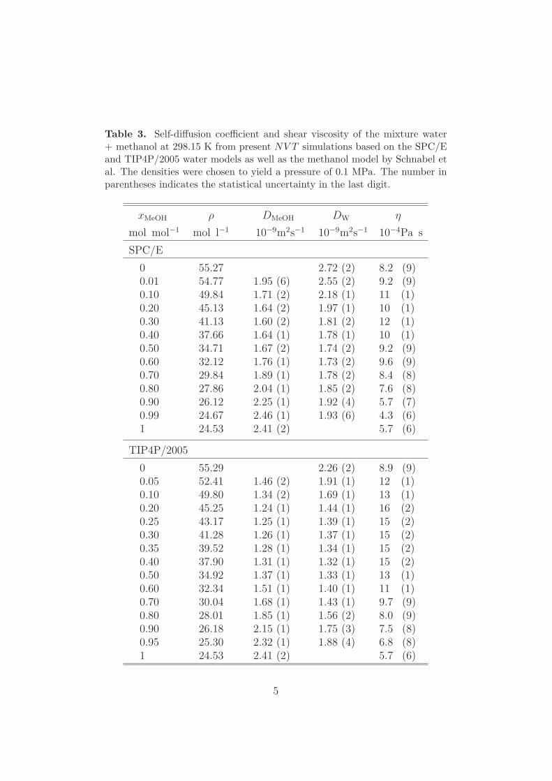
Table 3. Self-diffusion coefficient and shear viscosity of the mixture water+ methanol at 298.15 K from present NV T simulations based on the SPC/Eand TIP4P/2005 water models as well as the methanol model by Schnabel etal. The densities were chosen to yield a pressure of 0.1 MPa. The number inparentheses indicates the statistical uncertainty in the last digit.

xMeOH ρ DMeOH DW η

mol mol−1 mol l−1 10−9m2s−1 10−9m2s−1 10−4Pa s

SPC/E

0 55.27 2.72 (2) 8.2 (9)0.01 54.77 1.95 (6) 2.55 (2) 9.2 (9)0.10 49.84 1.71 (2) 2.18 (1) 11 (1)0.20 45.13 1.64 (2) 1.97 (1) 10 (1)0.30 41.13 1.60 (2) 1.81 (2) 12 (1)0.40 37.66 1.64 (1) 1.78 (1) 10 (1)0.50 34.71 1.67 (2) 1.74 (2) 9.2 (9)0.60 32.12 1.76 (1) 1.73 (2) 9.6 (9)0.70 29.84 1.89 (1) 1.78 (2) 8.4 (8)0.80 27.86 2.04 (1) 1.85 (2) 7.6 (8)0.90 26.12 2.25 (1) 1.92 (4) 5.7 (7)0.99 24.67 2.46 (1) 1.93 (6) 4.3 (6)1 24.53 2.41 (2) 5.7 (6)

TIP4P/2005

0 55.29 2.26 (2) 8.9 (9)0.05 52.41 1.46 (2) 1.91 (1) 12 (1)0.10 49.80 1.34 (2) 1.69 (1) 13 (1)0.20 45.25 1.24 (1) 1.44 (1) 16 (2)0.25 43.17 1.25 (1) 1.39 (1) 15 (2)0.30 41.28 1.26 (1) 1.37 (1) 15 (2)0.35 39.52 1.28 (1) 1.34 (1) 15 (2)0.40 37.90 1.31 (1) 1.32 (1) 15 (2)0.50 34.92 1.37 (1) 1.33 (1) 13 (1)0.60 32.34 1.51 (1) 1.40 (1) 11 (1)0.70 30.04 1.68 (1) 1.43 (1) 9.7 (9)0.80 28.01 1.85 (1) 1.56 (2) 8.0 (9)0.90 26.18 2.15 (1) 1.75 (3) 7.5 (8)0.95 25.30 2.32 (1) 1.88 (4) 6.8 (8)1 24.53 2.41 (2) 5.7 (6)

5

Table 4. Volume, excess volume, enthalpy and excess enthalpy of the mixturewater + methanol at 298.15 K and 0.1 MPa from present NpT simulations onthe basis of the SPC/E and TIP4P/2005 water models as well as the methanolmodel by Schnabel et al. The number in parentheses indicates the statisticaluncertainty in the last digit.

xMeOH v vE h hE

mol mol−1 cm−3 mol−1 cm−3 mol−1 kJ mol−1 J mol−1

SPC/E

0 18.092 (5) −49.223 (4)0.01 18.256 (5) −0.063 (7) −49.154 (7) −24 (8)0.10 20.065 (5) −0.298 (7) −48.392 (7) −99 (9)0.20 22.160 (6) −0.475 (8) −47.467 (6) −104 (8)0.30 24.314 (6) −0.594 (8) −46.517 (6) −84 (7)0.40 26.556 (6) −0.622 (7) −45.551 (8) −49 (8)0.50 28.313 (7) −0.637 (8) −44.630 (7) −57 (9)0.60 31.135 (7) −0.587 (8) −43.696 (7) −54 (8)0.70 33.518 (7) −0.476 (8) −42.802 (7) −90 (8)0.80 35.894 (8) −0.371 (9) −41.896 (8) −114 (9)0.90 38.295 (8) −0.242 (9) −40.951 (7) −99 (8)0.99 40.527 (9) −0.05 (1) −40.013 (6) +2 (8)1 40.753 (7) −39.922 (5)

TIP4P/2005

0 18.087 (6) −50.288 (4)0.01 18.292 (5) −0.022 (8) −50.213 (6) −29 (7)0.10 20.081 (4) −0.273 (7) −49.533 (5) −282 (6)0.20 22.101 (4) −0.520 (6) −48.622 (5) −408 (7)0.25 23.162 (6) −0.592 (8) −48.117 (7) −420 (8)0.30 24.226 (5) −0.661 (7) −47.607 (5) −429 (6)0.35 25.304 (6) −0.716 (8) −47.094 (7) −435 (7)0.40 26.383 (5) −0.771 (6) −46.588 (6) −447 (7)0.50 28.639 (6) −0.781 (7) −45.554 (5) −449 (6)0.60 30.925 (6) −0.761 (8) −44.525 (5) −456 (6)0.70 33.288 (6) −0.665 (8) −43.466 (6) −434 (7)0.80 35.695 (6) −0.525 (8) −42.361 (5) −366 (6)0.90 38.195 (7) −0.291 (9) −41.186 (6) −227 (7)0.99 40.506 (8) −0.02 (1) −40.028 (6) −2 (8)1 40.753 (7) −39.922 (5)

6

Table 5. Self-diffusion coefficient and shear viscosity of the mixture water+ ethanol at 298.15 K from present NV T simulations based on the SPC/Eand TIP4P/2005 water models as well as the ethanol model by Schnabel etal. The densities were chosen to yield a pressure of 0.1 MPa. The number inparentheses indicates the statistical uncertainty in the last digit.

xEtOH ρ DEtOH DW η

mol mol−1 mol l−1 10−9m2s−1 10−9m2s−1 10−4Pa s

SPC/E

0 55.27 2.72 (2) 8.2 (9)0.01 54.23 1.46 (6) 2.55 (2) 7.9 (9)0.10 46.07 0.99 (1) 1.68 (1) 12 (1)0.20 39.15 0.83 (1) 1.33 (1) 19 (2)0.30 33.89 0.794 (9) 1.14 (1) 21 (2)0.40 29.80 0.760 (8) 1.04 (1) 20 (2)0.50 26.62 0.767 (9) 0.98 (1) 18 (2)0.60 23.99 0.777 (8) 0.92 (1) 16 (2)0.70 21.84 0.812 (1) 0.90 (2) 15 (2)0.80 20.02 0.867 (8) 0.89 (1) 14 (1)0.90 18.45 0.899 (9) 0.84 (2) 12 (1)0.99 17.22 1.014 (9) 0.93 (6) 11 (1)1 17.11 1.07 (1) 11 (1)

TIP4P/2005

0 55.29 2.26 (2) 8.9 (9)0.01 54.16 1.08 (4) 2.07 (1) 11 (1)0.10 46.13 0.71 (1) 1.25 (1) 18 (2)0.20 39.33 0.606 (7) 0.931 (8) 21 (2)0.25 36.54 0.579 (6) 0.878 (7) 25 (3)0.30 34.11 0.585 (6) 0.814 (8) 23 (3)0.40 30.05 0.594 (6) 0.760 (8) 20 (2)0.50 26.77 0.635 (6) 0.747 (9) 18 (2)0.60 24.13 0.675 (6) 0.739 (9) 17 (2)0.65 22.99 0.681 (5) 0.735 (9) 16 (2)0.70 21.94 0.718 (6) 0.759 (9) 16 (2)0.80 20.08 0.808 (7) 0.79 (1) 14 (1)0.85 19.25 0.855 (7) 0.81 (2) 15 (2)0.90 18.49 0.909 (6) 0.83 (2) 13 (1)0.99 17.24 1.06 (7) 0.89 (7) 12 (1)1 17.11 1.07 (1) 11 (1)

7

Table 6. Volume, excess volume, enthalpy and excess enthalpy of the mixturewater + ethanol at 298.15 K and 0.1 MPa from present NpT simulations onthe basis of the SPC/E and TIP4P/2005 water models as well as the ethanolmodel by Schnabel et al. The numbers in parentheses indicate the statisticaluncertainty in the last digits.

xEtOH v vE h hE

mol mol−1 cm−3 mol−1 cm−3 mol−1 kJ mol−1 J mol−1

SPC/E

0 18.092 (5) −49.223 (4)0.10 21.707 (6) −0.420 (8) −48.647 (6) −300 (8)0.20 25.544 (7) −0.618 (9) −48.387 (8) −315 (9)0.30 29.503 (7) −0.69 (1) −47.776 (9) −280 (10)0.40 33.537 (8) −0.69 (2) −47.131 (9) −211 (10)0.50 37.570 (9) −0.70 (2) −46.538 (9) −194 (10)0.60 41.683 (9) −0.62 (2) −45.898 (9) −130 (11)0.70 45.796 (9) −0.54 (3) −45.321 (8) −128 (10)0.80 49.96 (1) −0.41 (3) −44.688 (8) −71 (11)0.90 54.20 (1) −0.20 (3) −44.094 (8) −54 (11)1 58.44 (1) −43.465 (8)

TIP4P/2005

0 18.087 (6) −50.288 (4)0.10 21.678 (4) −0.445 (7) −50.159 (6) −554 (7)0.20 25.423 (5) −0.735 (9) −49.600 (7) −677 (8)0.30 29.314 (6) −0.88 (1) −48.890 (7) −649 (8)0.40 33.279 (8) −0.95 (1) −48.147 (7) −589 (8)0.50 37.355 (9) −0.91 (2) −47.378 (9) −502 (10)0.60 41.443 (8) −0.86 (2) −46.617 (7) −423 (9)0.65 43.506 (9) −0.81 (2) −46.239 (9) −386 (10)0.70 45.561 (9) −0.77 (2) −45.854 (8) −342 (10)0.80 49.79 (1) −0.58 (3) −45.073 (7) −243 (9)0.85 51.93 (1) −0.45 (3) −44.671 (8) −182 (11)0.90 54.07 (1) −0.33 (3) −44.292 (7) −145 (10)1 58.44 (1) −43.465 (8)

8