prediction of shear wave velocity from petrophysical data ... · prediction of shear wave velocity...

ngineering 55 (2007) 201–212www.elsevier.com/locate/petrol

Journal of Petroleum Science and E

Prediction of shear wave velocity from petrophysical data utilizingintelligent systems: An example from a sandstone reservoir of

Carnarvon Basin, Australia

M.R. Rezaee 1, A. Kadkhodaie Ilkhchi ⁎, A. Barabadi 2

School of Geology, University College of Science, University of Tehran, Iran

Received 6 June 2005; received in revised form 9 August 2006; accepted 10 August 2006

Abstract

Shear wave velocity (Vs) associated with compressional wave velocity (Vp) can provide accurate data for geophysical study of areservoir. These so called petroacoustic studies have important role in reservoir characterization objectives such as lithologydetermination, identifying pore fluid type, and geophysical interpretation. In this study, fuzzy logic, neuro-fuzzy and artificialneural network approaches were used as intelligent tools to predict Vs from conventional log data.

The log data of two wells were used to construct intelligent models in a sandstone reservoir of the Carnarvon Basin, NW Shelfof Australia. A third well was used to evaluate the reliability of the models.

The results showed that intelligent models were successful for prediction of Vs from conventional well log data. In themeanwhile, similar responses from different other intelligent methods indicated their validity for solving complex problems.© 2006 Elsevier B.V. All rights reserved.

Keywords: Shear wave velocity; Fuzzy logic; Neuro-fuzzy; Artificial neural network; Petrophysical data; Carnarvon Basin; Australia

1. Introduction

Reservoir characterization is a prerequisite study for oiland gas field development. Vs is an important parameter forreservoir characterization studies. Some intervals of reser-voirs may not have Vs data due to high costs of measuring.The absence of recorded shear-wave data in most casesimposes severe limitations in seismic interpretation andprospect evaluation. The accuracy of the shear-wave

⁎ Corresponding author. Tel./fax: +98 21 66491623.E-mail addresses: [email protected],

[email protected] (M.R. Rezaee), [email protected](A. Kadkhodaie Ilkhchi), [email protected] (A. Barabadi).1 Present address: School of Geology and Geophysics, University of

Oklahoma, USA. Fax: +98 21 66491623.2 Tel./fax: +98 21 66491623.

0920-4105/$ - see front matter © 2006 Elsevier B.V. All rights reserved.doi:10.1016/j.petrol.2006.08.008

velocity estimation schemes is especially important whenperforming AVO modeling. Therefore, it will be useful topredict Vs from well log data without direct measuring. Upto now, several studies have been carried out for thispurpose. Pickett (1963), Castagna et al., (1985), Krief et al.(1990), Greenberg and Castagna (1992), Castagna et al.(1993), Bastos et al. (1998), Domenico (1984), Han (1989),Gassmann (1951) andMurphy et al. (1993) have introducedempirical relationships for Vs calculation. In recent years,artificial intelligence has been used formodeling purposes inmany petroleum related sciences. The present study focuseson the following objectives for a sandstone reservoir ofCarnarvon Basin, Australia:

a) To apply intelligent systems including fuzzy logic(FL), neuro-fuzzy (NF) and artificial neural network

mailto:[email protected]




http://dx.doi.org/10.1016/j.petrol.2006.08.008

Fig. 3. Membership functions for porosity cutoff in CL (a) and FL(b) approaches (μ: grade of membership).

Fig. 1. Membership functions for a crisp set C and a fuzzy set F.

202 M.R. Rezaee et al. / Journal of Petroleum Science and Engineering 55 (2007) 201–212

(ANN) for Vs prediction from conventional welllogs,

b) To compare and evaluate the results of the usedintelligent systems,

c) To verify the basic concepts and validity of theintelligent systems.

2. Methods used

2.1. Fuzzy logic

The basic concept of fuzzy logic, or fuzzy set theory,was first introduced by Zadeh in 1965. Unlike crisp

Fig. 2. A comparison of “and”, “or” and “not”

logic (CL), which a value may or may not belong to oneclass, fuzzy sets allow partial membership. Themembership or non-membership of an element X in

operators from FL and CL approaches.

Table 1List of the parameters that control seismic velocities (Wang, 2001)

Environment Fluid Rock

Reservoir pressure Saturation Pore shapeGeometry of layer Gas to oil ratio PorosityProduction history Fluid type FracturingReservoir Hygrophilic IsotropyProcesses Fluid phase Clay ContentTemperature Viscosity Bulk DensityStress history TextureFrequency Cementation

LithificatioinHistoryCompaction

Fig. 4. Schematic structure of a neuro-fuzzy system (from Kamali and Mirshady, 2004).

203M.R. Rezaee et al. / Journal of Petroleum Science and Engineering 55 (2007) 201–212

crisp set C is described by a characteristic function ofμC(x), where:

lCðxÞ ¼ 1 if xaC0 otherwise

�ð1Þ

Fuzzy set theory extends this concept by definingpartial membership which can take values ranging from0 to 1:

lFðxÞ : XY½0; 1� ð2Þ

Where X refers to the universal set defined in specificproblem and F is a fuzzy set (Yagar and Zadeh, 1992).Fig. 1 shows the membership function for a crisp set Cand fuzzy set F.

2.1.1. Fuzzy inference system (FIS)Fuzzy inference is the process of formulating from a

given input to an output using fuzzy logic (Matlabuser's guide, 2001). There are two types of fuzzyinference systems including Mamdani and Assilian(1975) and Takagi and Sugeno (1985). Mamdani'smethod attempts to control a system by synthesizing aset of linguistic control rules obtained from experiencedhuman operators. The Takagi–Sugeno method issimilar to the Mamdani's FIS. The output membershipfunctions (MFs) is the main difference betweenMamdani and Takagi–Sugeno methods. In Takagi–Sugeno-type FIS (Matlab user's guide, 2001), MFs areconstant or linear, and membership functions aredefined by a clustering process. A small cluster radiususually yields many small clusters however; a largecluster radius yields a few large clusters in the data(Chiu, 1994). Each of these clusters refers to amembership function. Each membership function gen-

erates a set of fuzzy if-then rule for formulating inputsto outputs. A simple fuzzy if-then rule is described asbelow:

If Vp is high; then Vs is high

This rule is composed of two parts includingantecedent (if part) and consequent (then part). Whenantecedent has multiple parts, fuzzy logic operators willconnect (interpret) them. The most common fuzzyoperators are “and”, “or” and “not”. For example in thefollowing rule “and” operator has been used:

If ðVp is lowÞ and ðNPHI is highÞ; then ðVs is lowÞ

Fig. 2 compares the operators from FL and CLapproaches. The closer a given input is to the “if ” part ofthe rule; the more the “then” part will be influenced.Finally, fuzzy system adds up all of the “then” parts anduses a defuzzification method to give the final output(Kosko, 1991).

Table 2List of the wells and intervals that have shear velocity (Vs) data in thestudied area

Well Formation TopsMDRT (m)

Lithology Vs

BAY-1 Sealevel 27.84Seabed 57.0Toolonga calcilutite ? Calcareous

claystoneGearle siltstone 827.0 Silty claystoneWindalia radiolarite 982.0 Interbedded

siltstone,claystone

Windalia sand 1554.0Muderong shale 1610.0 Massive

claystoneMardie greensand 1633.0 Glauconitic

siltstone,claystone

Barrow group 1788.0 Interbeddedsandstone,siltstone,claystone

Dupuy formation 1809.0 Claystone, arg.sandstone,siltstone

Bay sandstone 3255.0 Sandstone,argillaceoussandstone

Dingo shale 3537.5 ClaystoneTotal depth 3710.0

Emperor-1 Sealevel 27.70Seabed 45.50Toolonga Calcilutite 474.0Gearle Siltstone 734.0 ClaystoneWindalia Radiolarite 1290.0 ClaystoneWindalia Sand 1352.0 ClaystoneMuderong Shale 1406.0 ClaystoneMardie Greensand 1504.5 Claystone/

glauconiticsiltstoneand sandstone

Barrow Group 1530.5 Sandstone,claystone,argillaceoussandstone

Top Foresets 1748.0 Dominantlyargillaceoussandstone

Primary Objective 2209.0 Sandstone,argillaceoussandstone

Total Depth 2360.0East Spar4AST1

Sealevel 123.0Undifferentiated 123.0 Calcarenite,

sandstone,claystone

Withnell Formation 1318.0 Calcareousclaystoneand siltstone

Table 2 (continued)

Well Formation TopsMDRT (m)

Lithology Vs

East Spar4AST1

Toolonga Calcilutite 1344.0 Calcareousclaystoneand siltstone

Gearle Siltstone 1749.0 ClaystoneWindalia Radiolarite 2226.0 ClaystoneMuderong Shale 2244.0 ClaystoneMardie Greensand 2507.0 Greensand

and siltstoneBarrow Group 2520.1 Sandstone,

siltstoneTotal Depth 2750.0


2.1.2. Why to use fuzzy sets?Generally, definitions in geoscience disciplines are not

clear-cut and most of the time, are associated withuncertainties. Regarding to imprecise nature of fuzzy sets,it is appropriate to use fuzzy reasoning for solvingproblems which accompany vagueness and imperfection.The following simple example can clarify the subject.

The cutoff value of porosity for oil reservoirs isgenerally about 5%. It means if an interval has morethan 5% porosity, it will be considered as net pay. Fig. 3shows the membership functions for porosity cutofffrom CL and FL approaches, respectively. According toCL approach (Fig. 3a); the porosity value of 4% will notbe economic. However, FL proposes that it will beeconomic up to the degree of 0.7 (Fig. 3b). Therefore,fuzzy reasoning is very close to reality and can be asuitable tool for prediction of reservoir properties.

2.2. Neuro-fuzzy

In recent years, considerable attention has beendevoted to the use of hybrid neural network and fuzzylogic techniques. It has been shown that neural networkmodels can be used to construct internal models thatrecognize fuzzy rules. Neuro-fuzzy modeling is atechnique for describing the behavior of a systemusing fuzzy inference rules within a neural networkstructure (Nikravesh and Aminzadeh, 2003).

Fig. 4 shows a NF system using the following fuzzyrules in layer 1 and 2 (Kamali and Mirshady, 2004):

Rule 1: If (x1 is A1) and (x2 is B1), then (class is 1)Rule 2: If (x1 is A2) and (x2 is B2), then (class is 2)Rule 3: If (x1 is A1) and (x2 is B2), then (class is 1)

If several fuzzy rules have the same consequence class,layer 3 combines their firing strengths. Usually, the maxi-mum connective (operator) is used. In layer 4 the fuzzy


values of the classes are available. The values describehowwell the input of the systemmatches to the classes. Inlayer 5, if the crisp classification is needed, the best-matching class for the input is chosen as output(Defuzzification).

2.3. Back-propagation neural network

ANN is a new tool for solving complex problems inpetroleum industry. A back propagation artificial neural

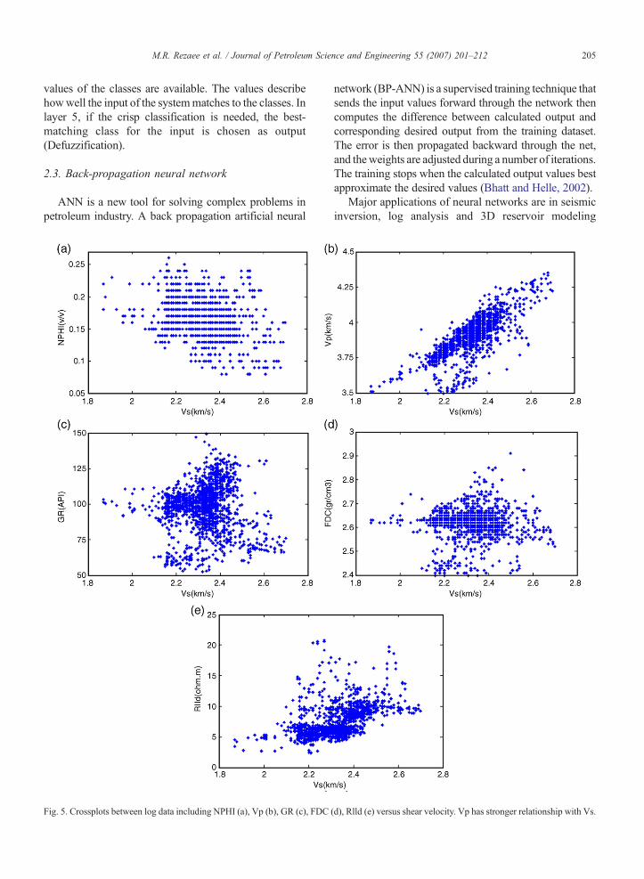
Fig. 5. Crossplots between log data including NPHI (a), Vp (b), GR (c), FDC

network (BP-ANN) is a supervised training technique thatsends the input values forward through the network thencomputes the difference between calculated output andcorresponding desired output from the training dataset.The error is then propagated backward through the net,and theweights are adjusted during a number of iterations.The training stops when the calculated output values bestapproximate the desired values (Bhatt and Helle, 2002).

Major applications of neural networks are in seismicinversion, log analysis and 3D reservoir modeling

(d), Rlld (e) versus shear velocity. Vp has stronger relationship with Vs.

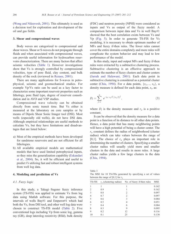
Table 3The MSE for 10 TS-FISs generated by specifying a set of valuesbetween the range of [0,1] for ra

TS-FIS ra (clustering radius) No. of fuzzy if-then rules MSE

1 1 1 0.1622 0.9 1 0.1623 0.8 2 0.0974 0.7 2 0.0975 0.6 3 0.0846 0.5 4 0.0517 0.4 6 0.0848 0.3 9 0.0959 0.2 12 0.11610 0.1 25 0.130


(Wong and Nikravesh, 2001). This ultimately is used asa decision tool for exploration and development of theoil and gas fields.

3. Shear and compressional waves

Body waves are categorized to compressional andshear waves. Shear or S-waves do not propagate throughfluids and when associated with compressional waves,can provide useful information for hydrocarbon reser-voirs characterization. There are many factors that affectseismic velocities (Table 1). However investigationsshow that Vs is strongly controlled by compressionalvelocities, type of pore fluid, clay content, and bulkdensity of the rock (reviewed in Rezaee, 2001).

There are many applications for S-waves in petro-physical, seismic and geomechanical studies. Forexample Vp/Vs ratio can be used as a key factor tocharacterize some important reservoir properties such aslithology, pore fluid type, degree of reservoir consoli-dation and in AVO and VSP studies.

Compressional wave velocity can be obtaineddirectly from sonic transit time. But Vs either ismeasured at the laboratory on core samples or bymeans of Dipole Shear Sonic Imager tool (DSI). Mostwells (especially old wells), do not have DSI data.Although empirical relationships are useful methods tocalculate Vs, but they have limitations and disadvan-tages that are listed below:

a) Most of the empirical methods have been developedfor sandstone reservoirs and are not efficient for alllithologies.

b) All available empirical models are mathematicalmodels that have used limited petrophysical inputs,so they miss the generalization capability (Eskandariet al., 2004). So, it will be efficient and useful topredict Vs utilizing fast and robust intelligent systemsfrom well log data.

4. Modeling and prediction of Vs

4.1. Fuzzy logic

In this study, a Takagi–Sugeno fuzzy inferencesystem (TS-FIS) was applied to estimate Vs from logdata using Matlab software. For this purpose, theintervals of wells Bay#1 and Emperor#1 which hadboth the Vs, from DSI tool, and other well log data werechosen to construct TS-FIS model (Table 2). Fiveconventional logs including Vp from sonic log, gammaray (GR), deep laterolog resistivity (Rlld), bulk density

(FDC) and neutron porosity (NPHI) were considered asinputs and Vs as output of the fuzzy model. Acomparison between input data and Vs in well Bay#1showed that the best correlation exists between Vs andVp (Fig. 5). In order to generate TS-FIS for Vsmodeling, it is necessary to obtain optimum number ofMFs and fuzzy if-then rules. The fewer rules cannotcover the entire domains completely and more rules willcomplicate the system behavior and may lead to lowperformance of the model.

In this study, input and output MFs and fuzzy if-thenrules were extracted by a subtractive clustering process.Subtractive clustering is an effective approach toestimate the number of fuzzy clusters and cluster centers(Jarrah and Halawani, 2001). Each data point insubtractive clustering is considered as a potential clustercenter (Chiu, 1994). For n data points, {x1,…, xn}, adensity measure is defined for each data point, xi, as:

Di ¼Xnj¼i

e−jxi−xjO2=ðra=2Þ2 ; ð3Þ

where Di is the density measure and ra is a positiveconstant.

It can be observed that the density measure for a datapoint is a function of its distance to all other data points.Hence, a data point that has many neighboring pointswill have a high potential of being a cluster center. Thera constant defines the radius of neighborhood (clusterradius) which can take values between the range of[0,1]. The choice of ra plays an important role indetermining the number of clusters. Specifying a smallercluster radius will usually yield more and smallerclusters in the data and results in more rules. A largecluster radius yields a few large clusters in the data(Chiu, 1994).

Fig. 6. Extracted membership functions using subtractive clustering (cluster radius=0.5) for Vp (a), GR (b), Rlld (c), FDC (d), NPHI (e) (μ: grade ofmembership).


Fig. 7. Formulation between well log data (inputs) to Vs (output) usingthe TS-FIS.


The first cluster center is chosen to be the data pointthat has the highest density measure. Then, the densitymeasure for each data point, xi, is reduced according toEq. (4):

Di ¼ Di−Dc1e−Oxi−xc1 j2=ðrb=2Þ2 ; ð4Þ

where xc1 is the point selected as the first cluster centerand Dc1 is its density measure for xc1. The constant rbdefines the radius of neighborhood within which thereduction in density will be measurable. The constant rbis usually greater than ra to avoid having closely spacedcenters and is set to 1.5ra (Chiu, 1994). It is evident thatdata points close to the cluster center will havesignificantly reduced density measure so that they arenot likely to be selected as the next cluster center. Afterthe first cluster, the next cluster center is chosen and thedensity measure is reduced again. This process continuesuntil a sufficient number of clusters are attainted.

In the present study, the optimum number of rulesand MFs were extracted by specifying a set of valuesbetween 0 and 1 for ra, (Table 3) and then performanceof model was measured for the test well at each stage.According to Table 3, choosing the value of 0.5 for thera has yielded the lowest MSE (e.g. 0.051) and this hasgenerated four rules associated with four Gaussian typemembership functions for each of the input data setwhich were captioned by low, moderate, high, andvery high, respectively (Fig. 6). As mentioned before,in TS-FIS the output MFs are linear or constant valuesand will have a set of parameters. In this case study,the output (Vs) has four linear MFs with followingparameters:

Output MF1: [0.4404 0.0011 0.0237 −0.1244 0.19970.6488] (low)

Output MF2: [0.6559 −0.0016 0.0020 −0.4819 0.31311.1310] (moderate)

Output MF3: [0.5010 0.0005 0.0354 0.3417 0.5817−0.8943] (high)

Output MF4: [0.5984 −0.0039 0.0099 0.5631 1.1650−1.3970] (very high)

Followings are generated fuzzy if-then rules byformulating input to output MFs (Fig. 7):

1) If (Vp is very high), and (GR is high), and (Rlld isModerate), and (FDC is high) and (NPHI ismoderate), then (Vs is very high).

2) If (Vp is moderate) and (GR is low) and (Rlld ishigh) and (FDC is low) and (NPHI is low), then(Vs is moderate).

3) If (Vp is high) and (GR is very high) and (Rlld islow) and (FDC is very high) and (NPHI is veryhigh), then (Vs is high).

4) If (Vp is low) and (GR is moderate) and (Rlld isvery high) and (FDC is moderate) and (NPHI ishigh), then (Vs is low).

The accuracy of the fuzzy model was measured bymean squared error (MSE) function which is about0.001. When the MFs and fuzzy if-then rules werederived, following steps were carried out by using TS-FIS for prediction of shear wave velocity which isillustrated in Fig. 8, graphically:

Step 1. Fuzzify inputs: The FIS takes the inputs anddetermines the degree to which the inputsbelong to each membership function.

Step 2. Apply fuzzy operator and truncation method:For the case that the antecedent of a given rulehas more than one part, the fuzzy operator (inthis study “and” operator) is applied to obtainone rule that represents the result of theantecedent for that rule. The most commonoperators are shown below:

and use the minimum of the optionsor use the maximum of the optionsnot use 1− option

Applying the fuzzy operators gives a value to theantecedent of each rule, and then the output member-ship function is truncated by this value.

Fig. 8. A graphical illustration showing formulation of conventional well log inputs to Vs using four fuzzy if-then rules generated by TS-FIS. Eachinput is covered by four Gaussian membership functions (for example, Vp mf1, Vp mf2, Vp mf3, Vp mf4 which are captioned by very high, high,moderate, and low, respectively). By passing a row of the inputs matrix including Vp=3.8 Km/s, GR=89.5 Api, Rlld=12.5Ωm, FDC=2.61 gr/cm3,and NPHI=0.17 from the FIS, its related MFs are affected in each rule. For example, the Vp value of 3.8 will affect the Vp mf1, Vp mf2, Vp mf3, andVp mf4 to the degrees (grade of membership) that are shown by the height of yellow color. This procedure will be done for entire inputs to each rule.Because the antecedent of each rule has more than one part, the fuzzy “and” operator is applied to obtain one rule that represents the result of theantecedent for that rule. Applying the fuzzy operators gives a value to the antecedent of each rule, and then the output membership function istruncated by this value. Then outputs of each rule that fit into a fuzzy set are combined into a single fuzzy set (aggregation). Finally, FIS uses aweighted average method (defuzzify) for the resulting Vs which is a crisp numerical value. This process is repeated for other rows of inputs matrix.(For interpretation of the references to colour in this figure legend, the reader is referred to the web version of this article.)

Fig. 9. Crossplot showing correlation coefficient between measuredand predicted Vs using FL for the test well East Spar#4 AST1.


Step 3. Apply aggregation method: In this step, outputsof each rule that fit into a fuzzy set are combinedinto a single fuzzy set.

Step 4. Defuzzify: The input for defuzzification processis the results of aggregation method. Then FISuses a defuzzification method (in this study, aweighted average) for the resulting output whichis a crisp numerical value.

Using the methodology described above, the inputsmatrix of the well logs data of the test well was passedfrom the TS-FIS and Vs was calculated. Measured errorusing MSE function is 0.051 and correlation coefficientbetween real and FL predicted Vs (637 data points) is0.946 (Fig. 9).

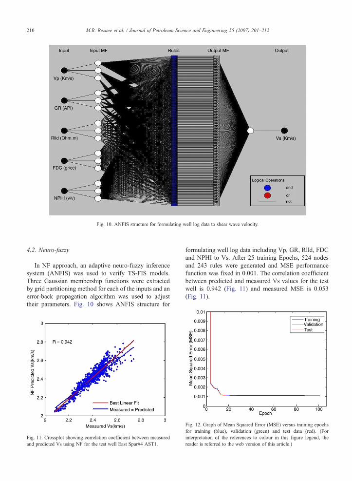
Fig. 10. ANFIS structure for formulating well log data to shear wave velocity.


4.2. Neuro-fuzzy

In NF approach, an adaptive neuro-fuzzy inferencesystem (ANFIS) was used to verify TS-FIS models.Three Gaussian membership functions were extractedby grid partitioning method for each of the inputs and anerror-back propagation algorithm was used to adjusttheir parameters. Fig. 10 shows ANFIS structure for

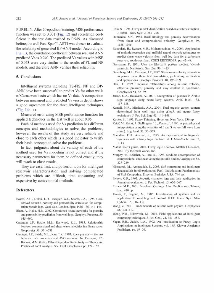
Fig. 11. Crossplot showing correlation coefficient between measuredand predicted Vs using NF for the test well East Spar#4 AST1.

formulating well log data including Vp, GR, Rlld, FDCand NPHI to Vs. After 25 training Epochs, 524 nodesand 243 rules were generated and MSE performancefunction was fixed in 0.001. The correlation coefficientbetween predicted and measured Vs values for the testwell is 0.942 (Fig. 11) and measured MSE is 0.053(Fig. 11).

Fig. 12. Graph of Mean Squared Error (MSE) versus training epochsfor training (blue), validation (green) and test data (red). (Forinterpretation of the references to colour in this figure legend, thereader is referred to the web version of this article.)

Fig. 13. Crossplot showing correlation coefficient between measuredand predicted Vs using ANN for the test well East Spar#4 AST1.

Fig. 14. A comparison between measured and predicted Vs using FL(a), NFshown by solid lines and predicted values by dotted lines.


4.3. Artificial neural network

In this section, we used a three layered BP-ANN toverify fuzzy and neuro-fuzzy results. The network wasgenerated in MATLAB environment and consists of aninput layer, a hidden layer and an output layer. The datasetof two wells were divided into three groups includingtraining (766 data points), validation (276 data points) andtest data (294 data points). Similar to TS-FIS and ANFIS,five inputs including Vp, GR, Rlld, FDC and NPHI datafrom wells Bay#1 and Emperor#1 which had both the Vsand well log data, were considered in the first layer.Number of neurons in the hidden layer were 7, and theoutput layer included one neuron for Vs data. A Leven-berg–Marquardt training function associated with MSEperformance function was used to optimize weights anddefault bias values. Used transfer function from layer oneto layer two is TANSIG and from layer two to layer three is

(b) and ANN(c) for the test well East Spar#4 AST1. Real values were


PURELIN. After 20 epochs of training,MSE performancefunction was set to 0.001 (Fig. 12) and correlation coef-ficient in the test data reached to 0.989. As discussedbefore, the well East-Spar#4AST1was chosen to evaluatethe reliability of generated BP-ANN model. According toFig. 13, the correlation coefficient between real and ANNpredicted Vs is 0.940. The predicted Vs values with MSEof 0.053 were very similar to the results of FL and NFmodels, and therefore ANN verifies their reliability.

5. Conclusions

Intelligent systems including TS-FIS, NF and BP-ANN have been successful to predict Vs for other wellsof Carnarvon basin which has no Vs data. A comparisonbetween measured and predicted Vs versus depth showsa good agreement for the three intelligent techniques(Fig. 14a–c).

Measured error using MSE performance function forapplied techniques in the test well is about 0.05.

Each of methods used for Vs prediction has differentconcepts and methodologies to solve the problems,however, the results of this study are very reliable andclose to each other which is a good indicator to verifytheir basic concepts to solve the problems.

In fact, judgment about the validity of each of themethod used for Vs modeling is not correct and if thenecessary parameters for them be defined exactly, theywill reach to close results.

They are easy, fast, and powerful tools for intelligentreservoir characterization and solving complicatedproblems which are difficult, time consuming andexpensive by conventional methods.

References

Bastos, A.C., Dillon, L.D., Vasquez, G.F., Soares, J.A., 1998. Core-derived acoustic, porosity and permeability correlation for compu-tation pseudo-logs. Geol. Soc. London, Spec. Publ. 136, 141–146.

Bhatt, A., Helle, H.B., 2002. Committee neural networks for porosityand permeability prediction from well logs. Geophys. Prospect. 50,645–660.

Castagna, J.P., Batzle, M.L., Eastwood, R.L., 1985. Relationshipbetween compressional and shear wave velocities in silicate rocks.Geophysics 50, 571–581.

Castagna, J.P., Batzle, M.L., Kan, T.K., 1993. Rock physics — the linkbetween rock properties and AVO response. In: Castagna, J.P.,Backus, M.M. (Eds.), Offset-Dependent Reflectivity— Theory andPractice of AVO Analysis. Soc. Expl. Geophysics, pp. 124–157.

Chiu, S., 1994. Fuzzy model identification based on cluster estimation.J. Intell. Fuzzy Syst. 2, 267–278.

Domenico, S.N., 1984. Rock lithology and porosity determinationfrom shear and compressional velocity. Geophysics 49,1188–1195.

Eskandari, H., Rezaee, M.R., Mohammadnia, M., 2004. Applicationof multiple regression and artificial neural network techniques topredict shear wave velocity from well log data for a carbonatereservoir, south-west Iran. CSEG RECORDER, pp. 42–48.

Gassmann, F., 1951. Uber die Elastizität poröser medien. Viertel-jahrsschr. Nat.forsch. Ges. Zur. 96, 1–23.

Greenberg, M.L., Castagna, J.P., 1992. Shear wave velocity estimationin porous rocks: theoretical formulation, prelimining verificationand applications. Geophys. Prospect. 40, 195–209.

Han, D., 1989. Empirical relationships among seismic velocity,effective pressure, porosity and clay content in sandstone.Geophysics 54, 82–89.

Jarrah, O.A., Halawani, A., 2001. Recognition of gestures in Arabicsign language using neuro-fuzzy systems. Artif. Intell. 133,117–138.

Kamali, M.R., Mirshady, A.A., 2004. Total organic carbon contentdetermined from well logs using ΔlogR and neuro fuzzytechniques. J. Pet. Sci. Eng. 45, 141–148.

Kosko, B., 1991. Fuzzy Thinking. Hyperion, New York. 336 pp.Krief, M., Garat, J., Stellingwerf, J., Venter, J., 1990. A petrophysical

interpretation using the velocities of P and S waves(full wave fromsonic). Log Anal. 31, 35–369.

Mamdani, E.H., Assilian, S., 1975. An experimental in linguisticsynthesis with a fuzzy logic control. Int. J. Man-Mach. Stud. 7,1–13.

Matlab user's guide, 2001. Fuzzy logic Toolbox, Matlab CD-Room,2001. By the math works, Inc.

Murphy, W., Reischer, A., Hsu, K., 1993. Modulus decomposition ofcompressional and shear velocities in sand bodies. Geophysics 58,227–239.

Nikravesh, M., Aminzadeh, F., 2003. Soft computing and intelligentdata analysis in oil exploration. Part1: Introduction: Fundamentalsof Soft Computing. Elsevier, Berkeley, USA. 744 pp.

Pickett, G.R., 1963. Acoustic character logs and their application information evaluation. J. Pet. Technol. 15, 650–667.

Rezaee, M.R., 2001. Petroleum Geology. Alavi Publications, Tehran,Iran. 410 pp.

Takagi, T., Sugeno, M., 1985. Identification of systems and itsapplication to modeling and control. IEEE Trans. Syst. ManCybern. 15, 116–132.

Wang, Z., 2001. Fundamentals of seismic rock physics. Geophysics66, 398–412.

Wong, P.M., Nikravesh, M., 2001. Field applications of intelligentcomputing techniques. J. Pet. Geol. 24, 381–387.

Yagar, R.R., Zadeh, L.A., 1992. An Introduction to Fuzzy LogicApplications in Intelligent Systems, vol. 165. Kluwer AcademicPublishers, pp. 69–70.

prediction of shear wave velocity from petrophysical data ... · prediction of shear wave velocity...

Documents