Fourth International Symposium on Marine Propulsors smp’15, Austin, Texas, USA, June 2015

Prediction of Steady Performance of Contra-Rotating Propellers with Rudder

Yasuhiko Inukai1, Takashi Kanemaru2, Jun Ando2

1 Japan Marine United Inc.,Tokyo, Japan

2 Kyushu University,Fukuoka, Japan

ABSTRACT

To reduce fuel oil costs and emission of greenhouse gases

of ships in operation, application of Contra-Rotating

Propellers (CRP) will be one of the solutions, which have

high propulsive efficiency. The prediction of CRP

performance is more difficult than that of a conventional

single propeller because the aft and forward propeller

interact each other strongly. Moreover, an existence of a

rudder changes the power balance between the aft and

forward propeller. To solve the interaction between two

propellers and a rudder correctly is key to successful design

of CRP. Although many performance prediction methods of

CRP have been developed until now, most of them use a

simplified model regarding to a trailing wake deformation

and geometries of a propeller and a rudder. Recently, the

authors have developed a prediction method of steady

performance of CRP without a rudder, in which we treat

trailing wake deformation rigorously by using a simple

surface panel method “SQCM”. For further improvement as

a design tool for CRP, we include an influence of a rudder,

represented by source distributions on the surface and

discrete vortex distributions arranged on the mean camber

surface according to QCM (Quasi-Continuous vortex lattice

Method), in the method. To verify the present method, we

carried out open water tests for CRP combined with a

rudder and sea trial with varying the horsepower ratio

between aft and forward propeller. The present method

shows good agreements with the experiments and we

confirm its validity.

Keywords

Conta-Rotating Propellers, SQCM, Rudder.

1 INTRODUCTION

Contra-rotating propellers (CRP) is well known and

promising technology as one of the most efficient

propulsion. The high performance has been shown in many

reports (e.g. Inukai. 2011, Nishiyama et al. 1990). The

number of the application is expected to increase in the

circumstance that energy saving technologies draw much

more attention than ever since EEDI entered into force in

2013. In order to apply CRP successfully to various kinds of

vessels, a sophisticated performance prediction method is

necessary.

While a number of researches have been done for predicting

characteristics of CRP, those considering an effect of a

rudder are few. It is well known that a rudder influences

much on the characteristics of CRP (Sasaki. 1990). The

difference of the wake fraction of the rudder between the aft

and forward propeller changes the power balance among

two propellers. And a rudder resistance increases than that

of a conventional single propeller because there is less

rotational flow in the propeller slipstream. Sasaki (1990)

presented a design method for CRP, including an effect of a

rudder based on a simplified theory by representing a

propeller as infinite blade disk and a rudder as a rectangular

plane on which sources and vortices are distributed. He

verified the effectiveness of the method by comparing

calculation to self-propulsion tests. Although his method is

good for understanding an effect of a rudder on CRP, it is

too simple for practical design because accurate geometry

of propeller and rudder cannot be treated.

The authors (2014) have recently developed a steady

performance prediction method of CRP based on a

simplified surface panel method “SQCM” (Ando. 1995)

with fully wake alignment. Subsequently, we undertook a

development of a steady performance prediction method of

CRP with an effect of a rudder. A rudder is represented a

rudder as source distributions on the rudder surface and

discrete vortex distributions arranged on the mean camber

surface as well as a propeller. To verify the accuracy of the

present method, open water tests with rudder were carried

out. Then, in the sea trials of vessels with CRP, we changes

the propeller speed ratios between the aft and forward

propeller and measured how the power balances between

the aft and forward propeller changed.

In this paper, an outline of the present method is described

at first. Then, we compare the calculation with experiments

and discuss the comparison results.

2 CALCULATION METHOD

The“SQCM” (Source and Quasi-Continuous vortex lattice

Method) is a simplified surface panel method developed at

Kyushu University. This method uses source distributions

(Hess et al. 1964) on the blade surface and discrete vortex

distributions arranged on the mean camber surface

according to QCM (Quasi-Continuous vortex lattice

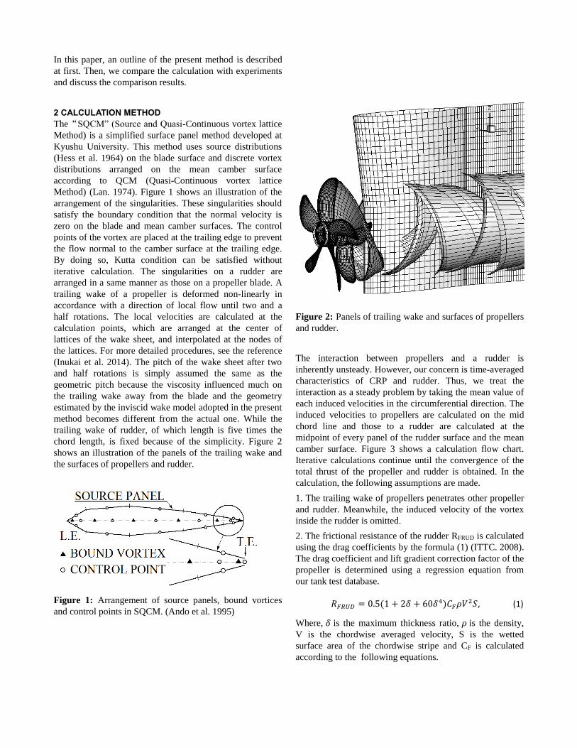
Method) (Lan. 1974). Figure 1 shows an illustration of the

arrangement of the singularities. These singularities should

satisfy the boundary condition that the normal velocity is

zero on the blade and mean camber surfaces. The control

points of the vortex are placed at the trailing edge to prevent

the flow normal to the camber surface at the trailing edge.

By doing so, Kutta condition can be satisfied without

iterative calculation. The singularities on a rudder are

arranged in a same manner as those on a propeller blade. A

trailing wake of a propeller is deformed non-linearly in

accordance with a direction of local flow until two and a

half rotations. The local velocities are calculated at the

calculation points, which are arranged at the center of

lattices of the wake sheet, and interpolated at the nodes of

the lattices. For more detailed procedures, see the reference

(Inukai et al. 2014). The pitch of the wake sheet after two

and half rotations is simply assumed the same as the

geometric pitch because the viscosity influenced much on

the trailing wake away from the blade and the geometry

estimated by the inviscid wake model adopted in the present

method becomes different from the actual one. While the

trailing wake of rudder, of which length is five times the

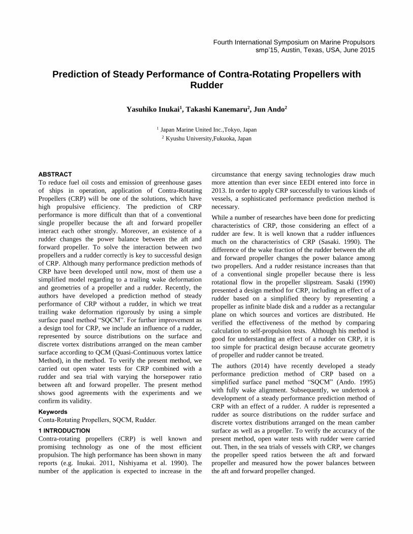
chord length, is fixed because of the simplicity. Figure 2

shows an illustration of the panels of the trailing wake and

the surfaces of propellers and rudder.

Figure 1: Arrangement of source panels, bound vortices

and control points in SQCM. (Ando et al. 1995)

Figure 2: Panels of trailing wake and surfaces of propellers

and rudder.

The interaction between propellers and a rudder is

inherently unsteady. However, our concern is time-averaged

characteristics of CRP and rudder. Thus, we treat the

interaction as a steady problem by taking the mean value of

each induced velocities in the circumferential direction. The

induced velocities to propellers are calculated on the mid

chord line and those to a rudder are calculated at the

midpoint of every panel of the rudder surface and the mean

camber surface. Figure 3 shows a calculation flow chart.

Iterative calculations continue until the convergence of the

total thrust of the propeller and rudder is obtained. In the

calculation, the following assumptions are made.

1. The trailing wake of propellers penetrates other propeller

and rudder. Meanwhile, the induced velocity of the vortex

inside the rudder is omitted.

2. The frictional resistance of the rudder RFRUD is calculated

using the drag coefficients by the formula (1) (ITTC. 2008).

The drag coefficient and lift gradient correction factor of the

propeller is determined using a regression equation from

our tank test database.

𝑅𝐹𝑅𝑈𝐷 = 0.5(1 + 2𝛿 + 60𝛿4)𝐶𝐹𝜌𝑉2𝑆, (1)

Where, 𝛿 is the maximum thickness ratio, 𝜌 is the density,

V is the chordwise averaged velocity, S is the wetted

surface area of the chordwise stripe and CF is calculated

according to the following equations.

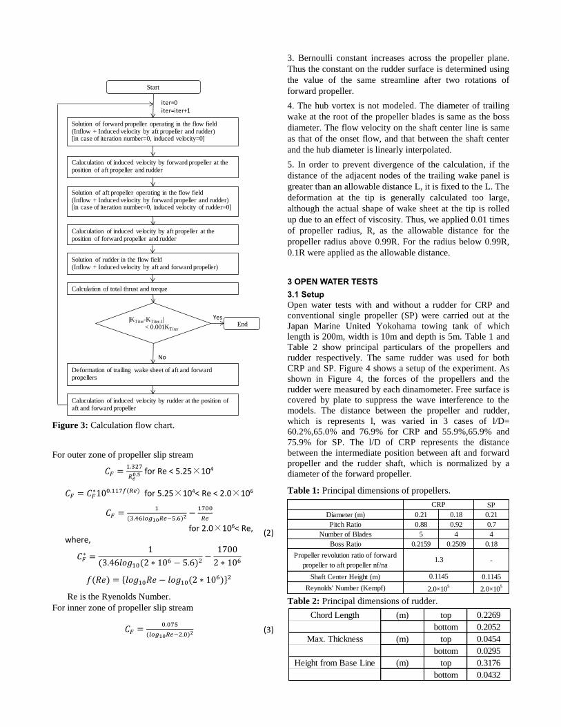
Figure 3: Calculation flow chart.

For outer zone of propeller slip stream

𝐶𝐹 =1.327

𝑅𝑒0.5 for Re < 5.25×104

𝐶𝐹 = 𝐶𝐹∗100.117𝑓(𝑅𝑒) for 5.25×104< Re < 2.0×106

𝐶𝐹 =1

(3.46𝑙𝑜𝑔10𝑅𝑒−5.6)2 −1700

𝑅𝑒

for 2.0×106< Re, where,

𝐶𝐹∗ =

1

(3.46𝑙𝑜𝑔10(2 ∗ 106 − 5.6)2−

1700

2 ∗ 106

𝑓(𝑅𝑒) = {𝑙𝑜𝑔10𝑅𝑒 − 𝑙𝑜𝑔10(2 ∗ 106)}2

Re is the Ryenolds Number.

(2)

For inner zone of propeller slip stream

𝐶𝐹 =

0.075

(𝑙𝑜𝑔10𝑅𝑒−2.0)2 (3)

3. Bernoulli constant increases across the propeller plane.

Thus the constant on the rudder surface is determined using

the value of the same streamline after two rotations of

forward propeller.

4. The hub vortex is not modeled. The diameter of trailing

wake at the root of the propeller blades is same as the boss

diameter. The flow velocity on the shaft center line is same

as that of the onset flow, and that between the shaft center

and the hub diameter is linearly interpolated.

5. In order to prevent divergence of the calculation, if the

distance of the adjacent nodes of the trailing wake panel is

greater than an allowable distance L, it is fixed to the L. The

deformation at the tip is generally calculated too large,

although the actual shape of wake sheet at the tip is rolled

up due to an effect of viscosity. Thus, we applied 0.01 times

of propeller radius, R, as the allowable distance for the

propeller radius above 0.99R. For the radius below 0.99R,

0.1R were applied as the allowable distance.

3 OPEN WATER TESTS

3.1 Setup

Open water tests with and without a rudder for CRP and

conventional single propeller (SP) were carried out at the

Japan Marine United Yokohama towing tank of which

length is 200m, width is 10m and depth is 5m. Table 1 and

Table 2 show principal particulars of the propellers and

rudder respectively. The same rudder was used for both

CRP and SP. Figure 4 shows a setup of the experiment. As

shown in Figure 4, the forces of the propellers and the

rudder were measured by each dinamometer. Free surface is

covered by plate to suppress the wave interference to the

models. The distance between the propeller and rudder,

which is represents l, was varied in 3 cases of l/D=

60.2%,65.0% and 76.9% for CRP and 55.9%,65.9% and

75.9% for SP. The l/D of CRP represents the distance

between the intermediate position between aft and forward

propeller and the rudder shaft, which is normalized by a

diameter of the forward propeller.

Table 1: Principal dimensions of propellers.

Table 2: Principal dimensions of rudder.

Solution of forward propeller operating in the flow field(Inflow + Induced velocity by aft propeller and rudder)[in case of iteration number=0, induced velocity=0]

Caluculation of induced velocity by forward propeller at the position of aft propeller and rudder

Caluculation of induced velocity by rudder at the position of aft and forward propeller

Solution of aft propeller operating in the flow field(Inflow + Induced velocity by forward propeller and rudder)[in case of iteration number=0, induced velocity of rudder=0]

Deformation of trailing wake sheet of aft and forward propellers

Calculation of total thrust and torque

|KTiter-KTiter-1|< 0.001KTiter

Start

End

iter=0iter=iter+1

Yes

No

Solution of rudder in the flow field(Inflow + Induced velocity by aft and forward propeller)

Caluculation of induced velocity by aft propeller at the position of forward propeller and rudder

SP

Diameter (m) 0.21 0.18 0.21

Pitch Ratio 0.88 0.92 0.7

Number of Blades 5 4 4

Boss Ratio 0.2159 0.2509 0.18

Propeller revolution ratio of forward

propeller to aft propeller nf/na-

Shaft Center Height (m) 0.1145

Reynolds' Number (Kempf) 2.0×105

1.3

CRP

2.0×105

0.1145

Chord Length (m) top 0.2269

bottom 0.2052

Max. Thickness (m) top 0.0454

bottom 0.0295

Height from Base Line (m) top 0.3176

bottom 0.0432

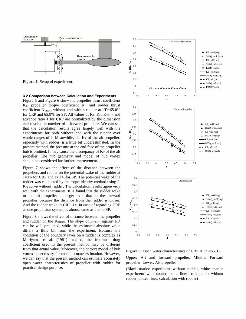
Figure 4: Setup of experiment.

3.2 Comparison between Calculation and Experiments

Figure 5 and Figure 6 show the propeller thrust coefficient

KT, propeller torque coefficient KQ and rudder thrust

coefficient KTRUD without and with a rudder at l/D=65.0%

for CRP and 65.9% for SP. All values of KT, KQ, KTRUD and

advance ratio J for CRP are normalized by the dimension

and revolution number of a forward propeller. We can see

that the calculation results agree largely well with the

experiments for both without and with the rudder over

whole ranges of J. Meanwhile, the KT of the aft propeller,

especially with rudder, is a little bit underestimated. In the

present method, the pressure at the end face of the propeller

hub is omitted. It may cause the discrepancy of KT of the aft

propeller. The hub geometry and model of hub vortex

should be considered for further improvement.

Figure 7 shows the effect of the distance between the

propellers and rudder on the potential wake of the rudder at

J=0.6 for CRP and J=0.45for SP. The potential wake of the

rudder was calculated by the toque identity method using J-

KQ curve without rudder. The calculation results agree very

well with the experiments. It is found that the rudder wake

to the aft propeller is larger than that to the forward

propeller because the distance from the rudder is closer.

And the rudder wake to CRP, i.e. in case of regarding CRP

as one propulsion system, is almost same as that to SP.

Figure 8 shows the effect of distance between the propeller

and rudder on the KTRUD. The slope of KTRUD against l/D

can be well predicted, while the estimated absolute value

differs a little bit from the experiment. Because the

condition of the boundary layer on a rudder is complex as

Moriyama et al. (1981) studied, the frictional drag

coefficient used in the present method may be different

from that actual value. Moreover, the correct model of hub

vortex is necessary for more accurate estimation. However,

we can say that the present method can estimate accurately

open water characteristics of propeller with rudder for

practical design purpose.

Figure 5: Open water characteristics of CRP at l/D=65.0%

Upper: Aft and forward propeller, Middle: Forward

propeller, Lower: Aft propeller

(Black marks: experiment without rudder, white marks:

experiment with rudder, solid lines: calculation without

rudder, dotted lines: calculation with rudder)

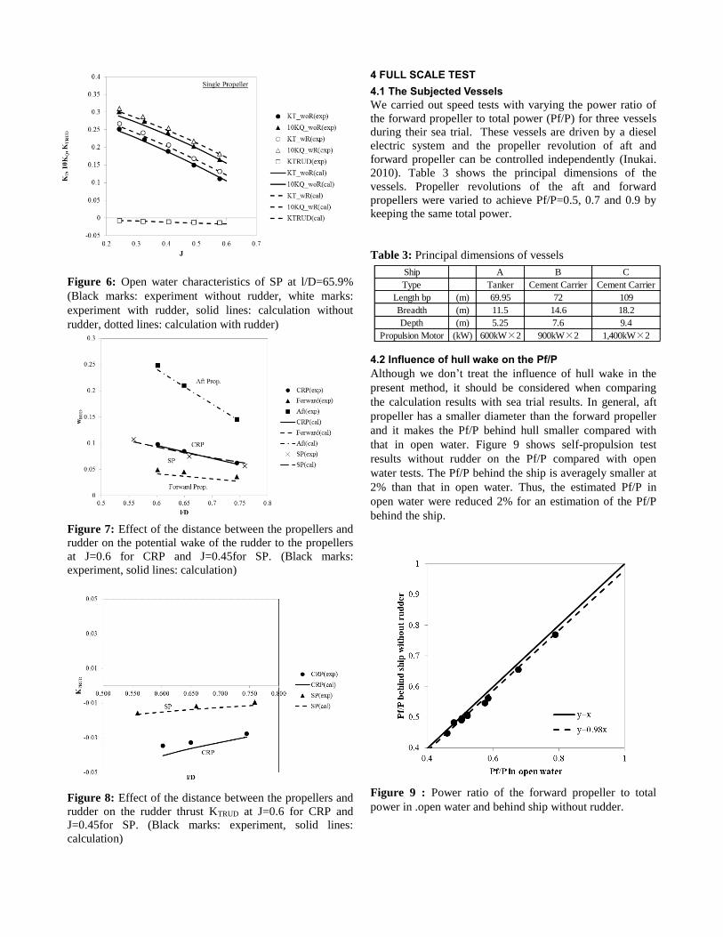
Figure 6: Open water characteristics of SP at l/D=65.9%

(Black marks: experiment without rudder, white marks:

experiment with rudder, solid lines: calculation without

rudder, dotted lines: calculation with rudder)

Figure 7: Effect of the distance between the propellers and

rudder on the potential wake of the rudder to the propellers

at J=0.6 for CRP and J=0.45for SP. (Black marks:

experiment, solid lines: calculation)

Figure 8: Effect of the distance between the propellers and

rudder on the rudder thrust KTRUD at J=0.6 for CRP and

J=0.45for SP. (Black marks: experiment, solid lines:

calculation)

4 FULL SCALE TEST

4.1 The Subjected Vessels

We carried out speed tests with varying the power ratio of

the forward propeller to total power (Pf/P) for three vessels

during their sea trial. These vessels are driven by a diesel

electric system and the propeller revolution of aft and

forward propeller can be controlled independently (Inukai.

2010). Table 3 shows the principal dimensions of the

vessels. Propeller revolutions of the aft and forward

propellers were varied to achieve Pf/P=0.5, 0.7 and 0.9 by

keeping the same total power.

Table 3: Principal dimensions of vessels

4.2 Influence of hull wake on the Pf/P

Although we don’t treat the influence of hull wake in the

present method, it should be considered when comparing

the calculation results with sea trial results. In general, aft

propeller has a smaller diameter than the forward propeller

and it makes the Pf/P behind hull smaller compared with

that in open water. Figure 9 shows self-propulsion test

results without rudder on the Pf/P compared with open

water tests. The Pf/P behind the ship is averagely smaller at

2% than that in open water. Thus, the estimated Pf/P in

open water were reduced 2% for an estimation of the Pf/P

behind the ship.

Figure 9 : Power ratio of the forward propeller to total

power in .open water and behind ship without rudder.

Ship A B C

Type Tanker Cement Carrier Cement Carrier

Length bp (m) 69.95 72 109

Breadth (m) 11.5 14.6 18.2

Depth (m) 5.25 7.6 9.4

Propulsion Motor (kW) 600kW×2 900kW×2 1,400kW×2

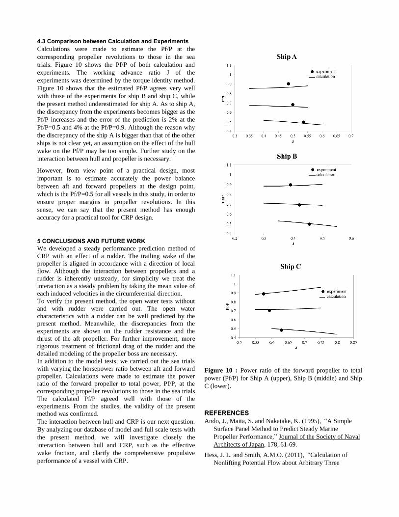
4.3 Comparison between Calculation and Experiments

Calculations were made to estimate the Pf/P at the

corresponding propeller revolutions to those in the sea

trials. Figure 10 shows the Pf/P of both calculation and

experiments. The working advance ratio J of the

experiments was determined by the torque identity method.

Figure 10 shows that the estimated Pf/P agrees very well

with those of the experiments for ship B and ship C, while

the present method underestimated for ship A. As to ship A,

the discrepancy from the experiments becomes bigger as the

Pf/P increases and the error of the prediction is 2% at the

Pf/P=0.5 and 4% at the Pf/P=0.9. Although the reason why

the discrepancy of the ship A is bigger than that of the other

ships is not clear yet, an assumption on the effect of the hull

wake on the Pf/P may be too simple. Further study on the

interaction between hull and propeller is necessary.

However, from view point of a practical design, most

important is to estimate accurately the power balance

between aft and forward propellers at the design point,

which is the Pf/P=0.5 for all vessels in this study, in order to

ensure proper margins in propeller revolutions. In this

sense, we can say that the present method has enough

accuracy for a practical tool for CRP design.

5 CONCLUSIONS AND FUTURE WORK

We developed a steady performance prediction method of

CRP with an effect of a rudder. The trailing wake of the

propeller is aligned in accordance with a direction of local

flow. Although the interaction between propellers and a

rudder is inherently unsteady, for simplicity we treat the

interaction as a steady problem by taking the mean value of

each induced velocities in the circumferential direction.

To verify the present method, the open water tests without

and with rudder were carried out. The open water

characteristics with a rudder can be well predicted by the

present method. Meanwhile, the discrepancies from the

experiments are shown on the rudder resistance and the

thrust of the aft propeller. For further improvement, more

rigorous treatment of frictional drag of the rudder and the

detailed modeling of the propeller boss are necessary.

In addition to the model tests, we carried out the sea trials

with varying the horsepower ratio between aft and forward

propeller. Calculations were made to estimate the power

ratio of the forward propeller to total power, Pf/P, at the

corresponding propeller revolutions to those in the sea trials.

The calculated Pf/P agreed well with those of the

experiments. From the studies, the validity of the present

method was confirmed.

The interaction between hull and CRP is our next question.

By analyzing our database of model and full scale tests with

the present method, we will investigate closely the

interaction between hull and CRP, such as the effective

wake fraction, and clarify the comprehensive propulsive

performance of a vessel with CRP.

Figure 10 : Power ratio of the forward propeller to total

power (Pf/P) for Ship A (upper), Ship B (middle) and Ship

C (lower).

REFERENCES

Ando, J., Maita, S. and Nakatake, K. (1995), “A Simple

Surface Panel Method to Predict Steady Marine

Propeller Performance,” Journal of the Society of Naval

Architects of Japan, 178, 61-69.

Hess, J. L. and Smith, A.M.O. (2011), “Calculation of

Nonlifting Potential Flow about Arbitrary Three

Dimensional Bodies,” Journal of Ship Research, 8(2),

22-44.

Lan, C. E. (1974), “A Quasi-Vortex-attice Method in Thin

Wing Theory,” Journal of Aircraft, 11(9), 518-527.

Inukai, Y. (2011), “Development of Electric Propulsion

Vessels with Contra-Rotating Propeller,” Journal of the

Japan Institution of Marine Engineering, 46(3), 313-319.

Inukai, Y., Kanemaru, T. and Ando, J. (2014), “Prediction

of Steady Performance of Contra-Rotating Propellers

Including Wake Alignment,” Proc. of 11th International

Conference on Hydrodynamics, Singapore.

ITTC. (2008), “The Specialist Committee on Azimuthing

Podded Propulsion, Report and Recommendations to the

25th ITTC,” Proc. of 25th ITTC, Japan.

Moriyama, F and Yamazaki, R. (1981). “On the Forces

Acting on Rudder in Propeller Slip stream,” Transaction

of the West Japan Society of Naval Architects, 62, 23-

40.

Nishiyama, S., Okamoto, Y., Ishida, S., Fujino, R., and

Oshima, M. (1990). “Development of Contra Rotating

Propeller System for JUNO a 37,000DWT Class Bulk-

Carrier,” Transaction of Society of Naval Architects and

Marine Engineers, 98, 27-52.

Sasaki, N. (1990). “Study on Contrarotating Propellers,”

PH.D. Thesis, Kyushu University, Japan

DISCUSSION

Question from Ki-Han Kim

Your open water testing setup is not really open water

due to the upstream strut and dynameter housing. How do

you acocount for the effect of upsteam disturbunce in your

open water performance?

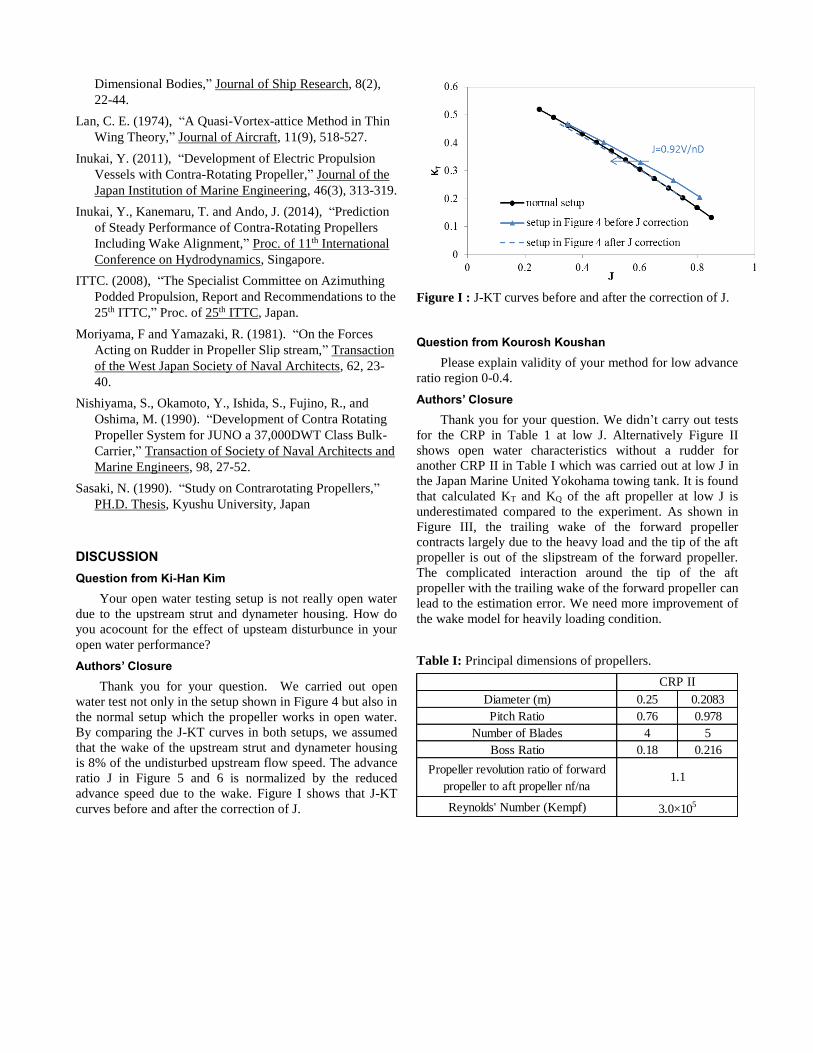
Authors’ Closure

Thank you for your question. We carried out open

water test not only in the setup shown in Figure 4 but also in

the normal setup which the propeller works in open water.

By comparing the J-KT curves in both setups, we assumed

that the wake of the upstream strut and dynameter housing

is 8% of the undisturbed upstream flow speed. The advance

ratio J in Figure 5 and 6 is normalized by the reduced

advance speed due to the wake. Figure I shows that J-KT

curves before and after the correction of J.

Figure I : J-KT curves before and after the correction of J.

Question from Kourosh Koushan

Please explain validity of your method for low advance

ratio region 0-0.4.

Authors’ Closure

Thank you for your question. We didn’t carry out tests

for the CRP in Table 1 at low J. Alternatively Figure II

shows open water characteristics without a rudder for

another CRP II in Table I which was carried out at low J in

the Japan Marine United Yokohama towing tank. It is found

that calculated KT and KQ of the aft propeller at low J is

underestimated compared to the experiment. As shown in

Figure III, the trailing wake of the forward propeller

contracts largely due to the heavy load and the tip of the aft

propeller is out of the slipstream of the forward propeller.

The complicated interaction around the tip of the aft

propeller with the trailing wake of the forward propeller can

lead to the estimation error. We need more improvement of

the wake model for heavily loading condition.

Table I: Principal dimensions of propellers.

Diameter (m) 0.25 0.2083

Pitch Ratio 0.76 0.978

Number of Blades 4 5

Boss Ratio 0.18 0.216

Propeller revolution ratio of forward

propeller to aft propeller nf/na

Reynolds' Number (Kempf)

CRP II

1.1

3.0×105

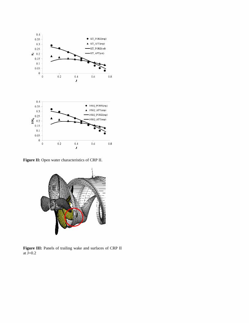
Figure II: Open water characteristics of CRP II.

Figure III: Panels of trailing wake and surfaces of CRP II

at J=0.2