Prediction of the Burning Rates of Charring Polymers March 2010 DOT/FAA/AR-TN09/59 This document is available to the U.S. public through the National Technical Information Services (NTIS), Springfield, Virginia 22161.

U.S. Department of Transportation Federal Aviation Administration

ote

tech

nica

l not

e te

chni

ca

NOTICE

This document is disseminated under the sponsorship of the U.S. Department of Transportation in the interest of information exchange. The United States Government assumes no liability for the contents or use thereof. The United States Government does not endorse products or manufacturers. Trade or manufacturer's names appear herein solely because they are considered essential to the objective of this report. This document does not constitute FAA certification policy. Consult your local FAA aircraft certification office as to its use. This report is available at the Federal Aviation Administration William J. Hughes Technical Center’s Full-Text Technical Reports page: actlibrary.act.faa.gov in Adobe Acrobat portable document format (PDF).

Technical Report Documentation Page 1. Report No.

DOT/FAA/AR-TN09/59

2. Government Accession No. 3. Recipient's Catalog No.

4. Title and Subtitle

PREDICTION OF THE BURNING RATES OF CHARRING POLYMERS

5. Report Date

March 2010

6. Performing Organization Code

7. Author(s)

Stanislav I. Stoliarov*, Sean Crowley, Richard N. Walters, and Richard E. Lyon

8. Performing Organization Report No.

9. Performing Organization Name and Address

*SRA International, Inc. 1201 New Road, Suite 242 Linwood, NJ 08221 Federal Aviation Administration William J. Hughes Technical Center NextGen & Operations Planning Airport and Aircraft Safety Research and Development Division Fire Safety Branch Atlantic City International Airport, NJ 08405

10. Work Unit No. (TRAIS)

11. Contract or Grant No.

12. Sponsoring Agency Name and Address

U.S. Department of Transportation Federal Aviation Administration Air Traffic Organization NextGen & Operations Planning Office of Research and Technology Development Washington, DC 20591

13. Type of Report and Period Covered

Technical Note

14. Sponsoring Agency Code ANM-115

15. Supplementary Notes

16. Abstract

The processes that take place in the condensed phase of a burning polymer play an important role in the overall combustion. Quantitative understanding of these processes is critical for prediction of ignition and growth of fires. During the past decade, a significant effort has been made to develop mathematical models of polymer pyrolysis. In the current study, a model of burning of two widely used charring polymers, bisphenol A polycarbonate and poly(vinyl chloride), was developed and validated. The modeling was performed using a flexible computational framework called ThermaKin, which was developed in the Federal Aviation Administration laboratory. ThermaKin solves time-resolved energy and mass conservation equations describing a one-dimensional material object subjected to external heat. Most of the model parameters were obtained from the results of direct property measurements, which is a key distinguishing aspect of this work. The model was employed to simulate cone calorimetry experiments performed under a broad range of conditions. Possible sources of error in the model parameterization were analyzed. The results of this study demonstrate that a one-dimensional numerical pyrolysis model can be used to predict the outcome of cone calorimetry experiments performed on a charring and intumescing polymer. A simple submodel based on the properties of graphite and a single adjustable heat transfer parameter provides a reasonable approximation to the carbonaceous char description. 17. Key Words

Material flammability, Pyrolysis model, Cone calorimetry, Charring polymer, Intumescence, ThermaKin

18. Distribution Statement

This document is available to the U.S. public through the National Technical Information Service (NTIS), Springfield, Virginia 22161.

19. Security Classif. (of this report) Unclassified

20. Security Classif. (of this page) Unclassified

21. No. of Pages 29

22. Price

Form DOT F 1700.7 (8-72) Reproduction of completed page authorized

TABLE OF CONTENTS

Page EXECUTIVE SUMMARY ix

INTRODUCTION 1

METHODS AND MATERIALS 1

ThermaKin 1 Thermogravimetric Analysis 3 Microscale Combustion Calorimetry 3 Cone Calorimetry 4 Materials 4

RESULTS 4

Model Parametrization 4 Model Setup 9 Comparison of Modeling With Experiments 10 Model Sensitivity to Uncertainties 16

CONCLUSIONS 18

REFERENCES 18

iii

LIST OF FIGURES

Figure Page 1 Results of TGA Experiments and Reaction Modeling 5

2 Results of MCC Experiments 7

3 Photographs of 6-mm-Thick Samples of PC and PVC Burnt in the Cone Calorimeter at EHF0 = 75 kW m-2 10

4 Results of Six Cone Calorimetry Experiments Performed on Each Polymer Under Identical Conditions 11

5 Results of Fitting Experimental Heat Release Rates With PC_char and PVC_char Heat Transfer Parameters 13

6 Comparison of Model Predictions With the Results of Cone Calorimetry Experiments Performed at a Wide Range of Conditions 14

7 Model Sensitivity to Uncertainties in Decomposition Kinetics 17

8 Model Sensitivity to Uncertainties in the Heats of Decomposition 17

iv

LIST OF TABLES

Table Page 1 Decomposition Reaction Parameters 6 2 Physical Properties of Material Components 8 3 Summary of Results of Cone Calorimetry Experiments and Simulations 16

v

vi

LIST OF SYMBOLS AND ACRONYMS

ξ Concentration α Absorption coefficient ρ Density λ Gas transfer coefficient θ Stoichiometric coefficient σ Stefan-Boltzmann constant ν Convection coefficient ζ Critical mass flux A Arrhenius pre-exponential factor β Heating rate c Heat capacity Subscript c Component CEcone Efficiency of cone calorimetry combustion E Arrhenius activation energy Subscript E Ambient Subscript g Gaseous component EHF0 Initial value of EHF EHFt Time-dependent correction of EHF H Convective heat flux h Heat of reaction HRRcone Heat release rate obtained by cone calorimeter HRRMCC Heat release rate obtained by MCC I Radiative heat flux J Mass flux k Thermal conductivity L Distance between plates Subscript M Mixture MLRTGA Mass loss rate obtained by TGA Np Number of plates in layer r Reaction rate Subscript r Reaction or reactant R Gas constant Subscript S Surface boundary t Time T Temperature x Cartesian coordinate μ Yield of nonvolatile product γ Reflectivity ω Radiative heat transfer coefficient τp Areal density of plate τ Areal density of layer

AHRR Average heat release rate CHR Critical heat release rate EHF Incident external radiative heat flux HCC Heat of complete of combustion KB Kaowool blanket MCC Microscale combustion calorimeter PC Polycarbonate PVC Poly(vinyl chloride) TGA Thermogravimetric analyzer TTI Time to ignition

vii/viii

EXECUTIVE SUMMARY

A quantitative understanding of the processes that take place in the condensed phase of a burning material is critical to predict the ignition and growth of fires. In the current study, a burning model of two widely used charring polymers, bisphenol A polycarbonate and poly(vinyl chloride), was developed and validated. This is the second study in a series; the first one focused on noncharring polymers. The modeling was performed using a flexible computational framework called ThermaKin, which was developed in the Federal Aviation Administration laboratory. ThermaKin solves time-resolved energy and mass conservation equations describing a one-dimensional material object subjected to external heat. Most of the model parameters were obtained from the results of direct property measurements, which is a key distinguishing aspect of this work. The model was employed to simulate cone calorimetry experiments performed under a broad range of conditions. Possible sources of error in the model parameterization were analyzed. This study represents an important step toward development of a comprehensive computational methodology for assessment of the impact of ultra-fire-resistant materials and material substitutions on the likelihood of an in-flight fire and the severity of a postcrash fire.

ix/x

INTRODUCTION

The processes that take place in the condensed phase of a burning polymer play an important role in the overall combustion [1]. Quantitative understanding of these processes is critical to predict the ignition and growth of fires. During the past decade, a significant effort has been made to develop mathematical models of polymer pyrolysis. The principal objective of this effort is to provide the means for extrapolating the results of a bench-scale fire test to a large-scale fire scenario. Typically, the model parameters, which describe thermal and chemical properties of a given material, are obtained by fitting the results of cone calorimetry [2] or fire propagation apparatus experiments [3]. The parameterized pyrolysis model is subsequently used in conjunction with a model of gas-phase combustion to predict the development of a large-scale fire. The main drawback of this approach is that the problem of deriving material properties from the results of fire calorimetry tends to be underdefined (i.e., there is more than one set of property values that gives an equally good fit). As a consequence, this approach provides only a limited insight into the physics and chemistry of pyrolysis. In the current study, a one-dimensional numerical model of burning called ThermaKin [4 and 5] was used to simulate cone calorimetry tests performed on widely used charring polymers—bisphenol A polycarbonate (PC) and poly(vinyl chloride) (PVC). Most of the model parameters were obtained from the results of direct property measurements, which is the key distinguishing aspect of this work. This is the second study in a series; the first [6] focused on noncharring polymers (poly(methylmethacrylate), high-impact polystyrene, and high-density polyethylene). The results of both studies indicate that a combination of material properties describing energy transport and thermally induced chemical transformations defines polymer burning behavior in a wide range of conditions. Moreover, most of these properties (perhaps all of them in the future) can be measured in small-scale laboratory tests (such as thermogravimetric analysis or differential scanning calorimetry) or obtained from existing structure-property correlations. Thus, in addition to being more rigorous, the current approach to pyrolysis model parameterization may prove to be more cost-effective because the small-scale tests tend to be easier to perform and require much less sample. This technical note is organized as follows. The Methods and Materials section contains an overview of the numerical and experimental techniques employed in this study and a specification of the polymeric materials that were investigated. The Results section contains a detailed description of the model parameterization and setup and a comparison of the modeling results with the cone calorimetry experiments. This section also includes analyses of two important questions: What is the best way to represent intumescent char within the framework of the model? And how sensitive is the model output to uncertainties in the input parameters? The Conclusions section summarizes the key findings.

METHODS AND MATERIALS

ThermaKin.

ThermaKin is a flexible computational framework that solves energy and mass conservation equations describing a one-dimensional material object subjected to external heat. Only a brief

1

description of the framework is given here; a complete description can be found in earlier publications [4 and 5]. In this framework, the material is represented by a mixture of components, which may interact chemically and physically. The components are assigned individual properties and categorized as solids, liquids, or gases. The governing equations can be summarized as follows:

4

0

σξ 1Tcomp gasesreac

c c M r r g g Mc r g S

T Tc k r h J c dT It x x x I

α⎛ ⎞ ⎛ ⎞∂ ∂ ∂ ∂⎛ ⎞= + − + −⎜ ⎟ ⎜⎜ ⎟∂ ∂ ∂ ∂⎝ ⎠ ⎝ ⎠⎝ ⎠

∑ ∑ ∑ ∫T

⎟ (1)

ξ

θreac

g ggr r

r

Jr

t x∂ ∂

= −∂ ∂∑ (2)

exp ξrr r

Er ART

⎛ ⎞= −⎜ ⎟⎝ ⎠

r (3)

ξ

ρ λρ

gg g M

g

Jx

⎛ ⎞∂= − ⎜⎜∂ ⎝ ⎠

⎟⎟ (4)

Equation 1 is the energy conservation statement; equation 2 is the mass balance for a gaseous component. Equation 3 is an expression of the first-order reaction rate, r (second order reactions between different components can also be defined within the ThermaKin framework). Equation 4 is the definition of a gaseous component mass flux (J). Only gaseous components are assumed to be mobile, which means that, for a liquid or solid component, the last right-hand-side term in the mass balance equation is 0. ξ, c, and ρ are concentration, heat capacity, and density of a component. T is temperature; t is time; and x is the Cartesian coordinate. h is the heat of reaction; θ is a stoichiometric coefficient, which is negative when the corresponding component is a reactant and positive when it is a product. A and E are the Arrhenius parameters, and R is the gas constant. k, λ, and α are thermal conductivity, gas transfer, and radiation absorption coefficients, respectively. IS is the flux of infrared radiation from an external source incident onto the material surface. I is the flux of the radiation inside the material, which is computed using a generalized form of Beer-Lambert law and corrected for the material reflectivity. σ is the Stefan-Boltzmann constant. Subscript or superscript g is used to refer to a gaseous component; subscript c is used for all types of components (including gaseous). Subscript r is used to refer to a reaction and the corresponding reactant. Subscript M indicates a property of mixture (rather than that of an individual component).

2

The boundary conditions are defined separately for the two surfaces of the material object. These definitions include radiative (IS) and convective (HS) heat fluxes. The convective heat flux into the material is expressed as: ( )νS EH T T= − S (5) where ν is convection coefficient; TS is the material surface temperature; and TE is the temperature outside of material. Both IS and TE can be defined as a piecewise linear function of time. The radiative and convective heat fluxes can also be related to gaseous component fluxes out of the material (-JS). These relations are based on the following criterion:

CIζ

ggasesS

g g

J−= ∑ (6)

where ζg are critical mass fluxes specified for gaseous components. When CI reaches 1, a constant value can be added to IS and the values of ν and TE can be reset. These relations are used to simulate the effects of appearance of flame on the material surface. The system of equations described above is solved numerically by subdividing the material object into finite elements and computing changes in the element temperature and composition in small time steps. In the current study, all calculations were performed using a 0.05-mm element size and a 0.005-s time step (the only exception was thermogravimetric analysis modeling, which was performed using a 0.01-mm element size). Increasing or reducing these integration parameters by a factor of 2 did not produce any significant changes in the results of the calculations. THERMOGRAVIMETRIC ANALYSIS.

A Mettler Toledo TGA/SDTA851e thermogravimetric analyzer (TGA) was used to study the kinetics of polymer decomposition. Small polymer samples of (5-8)×10-6 kg were heated from 320 to 1070 K at the heating rate (β) of 0.05, 0.17, or 0.5 K s-1. The sample mass and mass loss rate (MLRTGA) were recorded as functions of time and temperature. The experiments were conducted in a nitrogen atmosphere. The sample compartment was continuously purged with 6×10-7 m3 s-1 of ultra-high-purity nitrogen. MICROSCALE COMBUSTION CALORIMETRY.

A microscale combustion calorimeter (MCC) built according to the standard [7] was used to determine the heats of complete combustion (HCC) of gaseous products of polymer pyrolysis. The pyrolysis was performed in a nitrogen atmosphere by heating a (4-5)×10-6 kg sample of material from 350 to 1100 K at β = 1 K s-1. The pyrolysis gases were purged from the sample chamber by ultra-high-purity nitrogen flowing at 1.3×10-6 m3 s-1, mixed with excess of oxygen, and combusted at 1173 K for 10 s. The heat release rate (HRRMCC) determined from the oxygen consumption was recorded as a function of time and sample temperature.

3

CONE CALORIMETRY.

The heat released by burning polymers was measured using a cone calorimeter built by Fire Testing Technology Limited. The standard setup, calibration, and measurement procedures [2] were followed. Polymer samples were mounted horizontally, using a specimen holder with an edge frame. The bottom of the holder was lined with a 20-mm-thick and 48-kg m-3-dense Kaowool blanket (manufactured by Thermal Ceramics), which rested on top of 13-mm-thick Kaowool M board. The bottom and sides of each sample were wrapped with aluminum foil. The heat release rate (HRRcone) was determined from changes in oxygen, carbon monoxide, and carbon dioxide concentrations in dried exhaust gas. HRRcone and sample mass were recorded as a function of time. The only deviation from the standard was in the distance between the bottom of the cone heater and the initial position of the top surface (face) of a polymer sample. This distance was set at 38 mm (instead of 25 mm specified in the standard). This was done to partially accommodate intumescence of the burning samples. As a consequence of the distance adjustment, the gap between the initial position of the sample face and a spark plug, which was used to ignite the sample, increased to 20 mm (13 mm is specified in the standard). During the heat release measurements, the external heat flux (provided by the cone heater) was set at 50, 75, or 92 kW m-2. These settings were obtained by using a Schmidt-Boelter flux meter positioned at a location equivalent to the initial position of the center of the sample face. Shifting this flux meter within the sample face plain revealed minor (<5%) heat flux fluctuations. However, lifting the flux meter to the level of the cone heater bottom showed a systematic 15% increase in the heat flux. This observation was used to specify how the heat flux incident onto the sample face changes as the sample expands (due to intumescence). MATERIALS.

The polymers used in this study were provided in the form of large (approximately 1×2 m) sheets of two thicknesses: 3 and ≈6 mm. PC was produced by GE Plastics under the trade name Lexan® 9034. PVC was produced by HPG International, Inc. under the trade name Versadur® 150. PC sheets were transparent; PVC sheets were not transparent and had a grey color. Cone calorimetry samples were cut directly from the supplied sheets using a 101×101-mm template. In addition, 9-mm-thick cone samples of PC and PVC were prepared by compression molding. The compression molding was carried out at 450 K following the procedure described in a previous publication [6].

RESULTS

MODEL PARAMETRIZATION.

The results of the TGA experiments, shown in figure 1, were used to parameterize polymer decomposition kinetics. The thermal decomposition of PC was represented by a single first-order reaction.

4

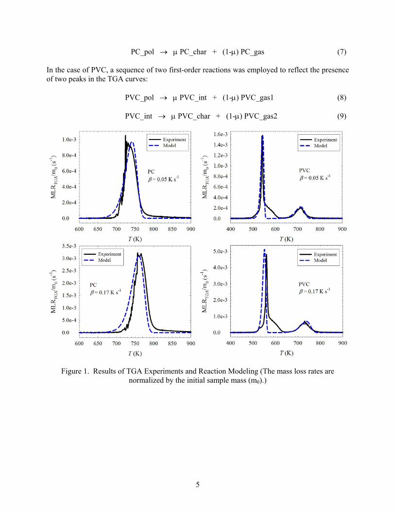
PC_pol → μ PC_char + (1-μ) PC_gas (7) In the case of PVC, a sequence of two first-order reactions was employed to reflect the presence of two peaks in the TGA curves: PVC_pol → μ PVC_int + (1-μ) PVC_gas1 (8) PVC_int → μ PVC_char + (1-μ) PVC_gas2 (9)

Figure 1. Results of TGA Experiments and Reaction Modeling (The mass loss rates are

normalized by the initial sample mass (m0).)

5

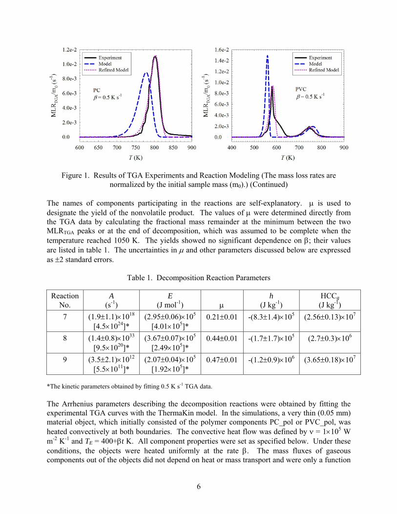
Figure 1. Results of TGA Experiments and Reaction Modeling (The mass loss rates are

normalized by the initial sample mass (m0).) (Continued)

The names of components participating in the reactions are self-explanatory. μ is used to designate the yield of the nonvolatile product. The values of μ were determined directly from the TGA data by calculating the fractional mass remainder at the minimum between the two MLRTGA peaks or at the end of decomposition, which was assumed to be complete when the temperature reached 1050 K. The yields showed no significant dependence on β; their values are listed in table 1. The uncertainties in μ and other parameters discussed below are expressed as ±2 standard errors.

Table 1. Decomposition Reaction Parameters

Reaction No.

A (s-1)

E (J mol-1) μ

h (J kg-1)

HCCg (J kg-1)

7

(1.9±1.1)×1018

[4.5×1024]* (2.95±0.06)×105

[4.01×105]* 0.21±0.01

-(8.3±1.4)×105

(2.56±0.13)×107

8

(1.4±0.8)×1033

[9.5×1020]* (3.67±0.07)×105

[2.49×105]* 0.44±0.01

-(1.7±1.7)×105

(2.7±0.3)×106

9

(3.5±2.1)×1012

[5.5×1011]* (2.07±0.04)×105

[1.92×105]* 0.47±0.01

-(1.2±0.9)×106

(3.65±0.18)×107

*The kinetic parameters obtained by fitting 0.5 K s-1 TGA data. The Arrhenius parameters describing the decomposition reactions were obtained by fitting the experimental TGA curves with the ThermaKin model. In the simulations, a very thin (0.05 mm) material object, which initially consisted of the polymer components PC_pol or PVC_pol, was heated convectively at both boundaries. The convective heat flow was defined by ν = 1×105 W m-2 K-1 and TE = 400+βt K. All component properties were set as specified below. Under these conditions, the objects were heated uniformly at the rate β. The mass fluxes of gaseous components out of the objects did not depend on heat or mass transport and were only a function

6

of the Arrhenius parameters (provided that the μ values were fixed). These parameters were adjusted incrementally until the calculated mass loss rates showed good agreement with the experimental TGA curves. The Arrhenius parameters obtained by fitting 0.05 K s-1 TGA curves are listed in table 1; the calculated mass loss rates are depicted in figure 1. The lowest heating rate experiments were chosen for the parameter determination because they are least likely to be affected by heat or mass transport issues. Modeling of 0.17 K s-1 TGA curves using these parameters produced a fair agreement with the experiments (see figure 1). However, in the case of 0.5-K s-1 heating rate, the agreement was rather poor. The exact source of the disagreement is not clear. To examine potential effects of this disagreement on the cone calorimetry modeling, 0.5 K s-1 TGA data were refitted. The resulting Arrhenius parameters are listed in table 1 in square brackets. The heats of the decomposition reactions were measured in a previous study [8] using differential scanning calorimetry. These heats, which were renormalized for PVC to reflect the stoichiometry of reactions 8 and 9, are listed in table 1. Table 1 also contains HCC values for the gaseous decomposition products. These values were obtained by numerically integrating the HRRMCC peaks shown in figure 2 and renormalizing the integrated values by the mass lost in each decomposition step (determined from the TGA data). It was assumed that the two lowest temperature (overlapping) peaks of the PVC HRRMCC curve corresponded to the lowest temperature peak (described by reaction 8) of the TGA curves. Thus, while reaction 8 is responsible for the majority of mass loss, it contributes relatively little to the heat release.

Figure 2. Results of MCC Experiments (The heat release rates are normalized by the initial

sample mass (m0).)

Physical properties of material components were obtained from measurements and analyses of literature data. The property information is summarized in table 2. The densities of PC_pol and PVC_pol were determined by measuring dimensions of 0.1-0.2 kg rectangular pieces of PC and PVC at room temperature (≈300 K). The density values were assumed to be temperature independent. Temperature-dependent heat capacities of PC_pol and PVC_pol were determined in a previous study [8]. These heat capacities were averaged over the room-decomposition temperature ranges (740 K was used for PC decomposition temperature; 715 K was used for PVC). Preliminary modeling of the cone calorimetry experiments showed that substitution of

7

the temperature-resolved heat capacities by the average values (reported in table 2 and used in all further calculations) has no significant impact on the outcome of the simulations.

Table 2. Physical Properties of Material Components

Component ρ

(kg m-3) c

(J kg-1 K-1) k

(W m-1 K-1) γ α

(m2 kg-1) PC_pol 1180 ±60 1900 ±300 0.22 ±0.03 0.10 ±0.05 1.5 ±0.5 PC_char see text 1720 ±170 see text 0.15 ±0.05 ≈100 PC_gas — ≈1000 — — ≈1.5 PVC_pol 1430 ±70 1550 ±250 0.17 ±0.02 0.10 ±0.05 1.5 ±0.5 PVC_int see text ≈1550 ≈0.17 ≈0.10 see text PVC_char see text 1720 ±170 see text 0.15 ±0.05 ≈100 PVC_gas1 — 840 ±150 — — ≈1.5 PVC_gas2 — ≈1000 — — ≈1.5

The thermal conductivities of PC_pol and PVC_pol were obtained from the literature. The data on thermal conductivity of PC show a large scatter. Van Krevelen [9] reports kPC = 0.193 W m-1 K-1 (at room temperature), while more recent data from Zhang, et al. [10] (obtained for 300-520 K temperature range) indicate that kPC is significantly higher, 0.247 W m-1 K-1. In the case of PVC, Van Krevelen’s value of 0.168 W m-1 K-1 is close to the value of 0.163 W m-1 K-1 reported by Brandrup, et al. [11]. The thermal conductivities assigned to the components (see table 2) are averages of the aforementioned literature values. The reflectivities (γ) of PC_pol and PVC_pol were calculated from the absorptance data obtained by Hallman, et al. [12], for 1000 K blackbody radiation. It was assumed that no radiation was transmitted through the PC and PVC samples used in that study. These reflectivities and the total transmissivities of 0.5-mm-thick polymer films to 873 K blackbody radiation determined by Tsilingiris [13] were used to calculate absorption coefficients for these components. The calculations were performed using the approach described previously [6]. The values of the reflectivities and absorption coefficients (normalized by the component densities) are listed in table 2. For PVC_int, all physical properties with the exception of ρ and α, were assumed to be the same as those of PVC_pol. The values of ρ and α used for this component are discussed below. PC_char and PVC_char are expected to have molecular structures similar to that of graphite [14]. Their heat capacities and reflectivities were assigned the corresponding graphite values [15 and 16] obtained for 700-1100 K temperature range (see table 2). This range was selected to reflect the temperatures at which PC_char and PVC_char were present in the cone calorimetry simulations. These components were assumed to be essentially nontransparent to infrared radiation; their absorption coefficients were set to 100 m2 kg-1. The densities and thermal conductivities of these components were determined from the cone calorimetry experiments, which are discussed later in this section.

8

In most ThermaKin simulations performed in this study, the gaseous components (PC_gas, PVC_gas1, and PVC_gas2) were specified not to contribute to the material’s volume. Therefore, their densities, thermal conductivities, and reflectivities, weighted by the component volumetric fractions, are irrelevant and were not defined. The absorption coefficients of these components were assumed be the same as those of the unreacted polymers. The heat capacity of PVC_gas1 was assigned temperature-averaged (500-1100 K) heat capacity of hydrogen chloride, 840 J kg-1 K-1 [17], because of substantial evidence indicating that HCl represents more than 80 weight percent (% w/w) of the gaseous products released during the first step of PVC degradation [18]. The quantitative compositions of PC_gas and PVC_gas2 are not known; their heat capacities were assumed to be 1000 J kg-1 K-1. MODEL SETUP.

The one-dimensional objects that were used to model the cone calorimetry experiments consisted of two layers. The top layer, which represented a polymer sample, was initially composed of PC_pol or PVC_pol. The initial thickness of this layer was taken to be equal to the initial sample thickness. The bottom layer consisted of component KB that represented the Kaowool blanket used in the experiments. This component was assigned the physical properties of the blanket, ρ = 48 kg m-3, c = 800 J kg-1 K-1, and k = 0.08 W m-1 K-1, which were obtained from the manufacturer. The KB layer was specified to be 15 mm thick; increasing this thickness by a factor of 2 made no significant impact on the results of the simulations. In most simulations, the gas transfer coefficient was set sufficiently high, 2×10-5 m2 s-1 for all components representing polymer samples, to ensure that the fluxes of gaseous components out of a material object were always equal to the rates of their production inside the object. In other words, the mass transfer was made so fast that it had no effect on mass loss or heat release rates. To simulate the presence of aluminum foil between the sample and insulating blanket, the KB layer was specified to be impenetrable to gas flow and external radiation (γ = 1). The initial temperature of the objects was always set at 305 K (a few degrees above room temperature) to take into account a slight heating caused by the flux penetrating the cone heater shutter. Before ignition, the top surface of the objects was subjected to radiative heat and convective cooling. The incident external radiative heat flux (EHF) was specified to be equal to the experimental heat flux set point. The convection was defined by ν = 10 W m-2 K-1 and TE = 300 K. The value of the convection coefficient is the mean of the values calculated (8.2 W m-2 K-1) and measured (11 W m-2 K-1) in previous studies [6 and 19]. After ignition, the convective cooling was turned off. A time-dependent correction (EHFt) was added to the initial value of EHF (EHF0) to account for the sample expansion (details are provided below). An additional 15 kW m-2 of incident radiative heat flux was applied to the surface to simulate the presence of flame. This heat flux is the mean of the values obtained from direct [20] and indirect [6] measurements performed on several polymeric materials. These measurements indicate that, for the horizontal cone calorimetry configuration, the flame heat flux is relatively insensitive to EHF and the chemical nature of the polymer. The top surface was specified to have no resistance to the outward gas flow. The bottom surface was defined to be completely impenetrable to energy and mass. The gaseous component critical mass fluxes, which define ignition (see equation 6), were determined from the cone calorimetry data as described below.

9

COMPARISON OF MODELING WITH EXPERIMENTS.

During the cone calorimetry experiments, both polymers produced intumescent char. At the end of tests, the volumes of PC and PVC samples increased approximately 10 and 7 times, respectively. The end of test was declared 30 s after flame out. In a few cases where the samples were left under the heater after the end of test, they continued to smolder and release heat (at a fairly steady rate) for extended periods of time. The char images are shown in figure 3. While these images are representative, even when the tests were performed under identical conditions, the char shapes and superficial structural features were found to differ significantly from test to test. These shape fluctuations are probably related to a relatively poor repeatability of the tests performed at EHF0 = 75 kW m-2 on 6-mm-thick samples, the results of which are shown in figure 4. During two tests (one of PC and the other of PVC), the char was punctured multiple times using a thin (≈1.5 mm in diameter) stainless steel spear. The punctures had no significant effect on the HRRcone, which indicates the absence of large pockets of pressurized gases inside the pyrolyzing materials. This observation is consistent with the assumption that the mass transport is not the rate-limiting step of the pyrolysis processes.

Figure 3. Photographs of 6-mm-Thick Samples of PC (left) and PVC (right) Burnt in the Cone

Calorimeter at EHF0 = 75 kW m-2 (Both tests were stopped at about 200 s; the samples were removed from under the cone heater and photographed.)

10

Figure 4. Results of Six Cone Calorimetry Experiments Performed on Each Polymer Under Identical Conditions

The test results shown in figure 4 were used to determine the efficiency of the cone calorimetry combustion (CEcone). First, the effective heats of combustion of gaseous pyrolysis products were computed by dividing the total heat released by the total mass lost in each cone test. Subsequently, the effective heat values were divided by the total heats released in the MCC experiments (which were also normalized by the lost mass) to obtain CEcone. For PC, the value of CEcone was found to be 0.84 ±0.03; for PVC, the value was notably lower, 0.75 ±0.03. These values were used to convert the surface mass fluxes calculated by ThermaKin to heat release rate:

(10) ( gS

gases

gg J−= ∑ HCCCEHRR conecone )

They were also used to specify the critical mass fluxes:

gcone

CHRζCE HCCg

= (11)

where CHR is the critical heat release rate. CHR was used to define ignition in the model and calculate the time to ignition (TTI) from experimental HRRcone curves. It was set at 20 kW m-2, which gave the best agreement between the TTI determined from experimental HRRcone and the corresponding times of appearance of sustained flame recorded by an operator. To account for the effects of sample expansion on EHF, the times of char surface reaching half and full distances to the cone heater bottom were recorded. At EHF0 = 75 kW m-2, PC samples reached the cone bottom at about 75 s. At 50 kW m-2 and 92 kW m-2, it took 150 and 50 s, respectively. The expansion occurred after ignition and was very rapid. Therefore, for PC, EHFt was specified to be a step function that increased from 0 to 0.15×EHF0 (in accordance with the heat flux measurements described above) at these times. It should be noted that, after reaching

11

the heater bottom, PC char entered the heater and, in some cases, was in direct contact with parts of the heating element. The heat flux inside the heater was found to be highly nonuniform and difficult to measure. Therefore, no additional corrections were applied to account for this behavior. In the case of PVC, the sample expansion also occurred after ignition; however, it was much more gradual. At EHF0 = 75 kW m-2, it took about 300 s for the samples to reach the heater bottom. At 50 kW m-2 and 92 kW m-2, it took 450 and 250 s, respectively. The thin (3×10-3 m) sample only reached half the distance to the bottom (in half the time). Thus, for PVC, EHFt was specified to increase linearly from 0 to 0.15×EHF0 (to 0.075×EHF0 in the case of thin sample) between TTI and the times indicated above. After that, the EHFt was held steady. To complete the model formulation, a submodel describing the intumescent chars needed to be defined. In this study, two approaches to defining intumescence were examined. In the first approach, material expansion was formulated to be a result of retention of gaseous decomposition products by PC_char and PVC_char. However, it was found that the number of unknown parameters associated with this approach was too large and these parameters were too interdependent to carry physical sense. Therefore, a simpler approach was adopted, in which the chemical reactions (equations 7-9) define the expansion. In this approach, gaseous components did not contribute to the material’s volume. Instead, PC_char and PVC_char were assigned the densities that produce experimentally observed sample expansion. This approach was further simplified by observing that the effect of the char-representing component layers on the heat flow was almost completely defined by the product of their ρ and k (because the densities are inversely proportional to the layer thicknesses). Computationally expensive simulations of the actual expansion were avoided by specifying ρPC char = 248 kg m-3, ρPVC int = 629 kg m-3, and ρPVC

char = 296 kg m-3, which kept the decomposing sample volumes unchanged. To relate the values of kPC char and kPVC char used in these simulations to the thermal conductivities of the actual chars, they were multiplied by the corresponding experimental sample expansion factors (≈10 for PC and ≈7 for PVC). Two heat transfer modes inside PC_char and PVC_char were considered. These components were assumed to transfer heat either through conduction or radiation. The radiative transfer was described using the radiative diffusion approximation [21]: (12) 3ωk T= Representative experimental heat release curves obtained at EHF0 = 75 kW m-2 for 6-mm-thick samples were used to determine k for the conductive chars and ω for the radiative chars. The results of fitting these curves with the heat transfer parameters are shown in figure 5. The conductivities of PC_char and PVC_char were found to be 0.37 and 0.26 W m-1 K-1. The values of the radiative heat transfer coefficient ω were determined to be 4.9×10-10 and 3.5×10-10 W m-1 K-4, respectively. Considering significant uncertainties in the experimental data (see figure 4), the model describes the experiments reasonably well. The conductive and radiative char submodels produced almost identical results. However, when the conductivity values were recalculated to the actual char dimensions, they appeared to be too high to be consistent with the char structures, which contain at least 85% w/w of gas-filled void (based on the assumption that the solid in the char has the density of graphite, 2200 kg m-3 [22]). Therefore, the radiative char

12

submodel was used in all further calculations. It should be noted that, for PVC, the absorption coefficient of PVC_int was also adjusted during the fitting procedure to be 3.9 m2 kg-1. The only feature of the HRRcone curve that was found to be sensitive to this coefficient was the height of the second (from the left) narrow maximum.

Figure 5. Results of Fitting Experimental Heat Release Rates With PC_char and PVC_char Heat Transfer Parameters

One way to interpret the radiative char submodel is to consider the char to be a stack of dense, highly conductive and highly absorptive plates separated by low-density, low-conductivity, and high-transparency (i.e., gaseous) gaps. For such system, the product of ρ and k can be expressed using a detailed formula for the radiative diffusion approximation [21]:

( )3

3τ τ τ16 σ 16 16ρ ω σ τ3 α 3 3

p p pp

Tk T L TL L L

⎛ ⎞ ⎛ ⎞ ⎛ ⎞⎛ ⎞ ⎛ ⎞= = = =⎜ ⎟ ⎜ ⎟ ⎜ ⎟⎜ ⎟ ⎜ ⎟⎝ ⎠⎝ ⎠⎝ ⎠ ⎝ ⎠ ⎝ ⎠

3 3σT (13)

where τp is the areal density of a single plate; L is the distance between the plates; and α is the absorption coefficient, which is approximated by the reciprocal of L. The expression indicates that the char thermal transparency, which is defined by the product of ρ and k (provided that the char heat capacity is constant), depends only on τp. In other words, assuming that the plate material is about the same for all chars, the thermal barrier efficiency of the char layer of a given areal density τ is proportional to the number of plates in this layer, Np = τ /τp, and does not depend on any other factors. This observation leads to a simple criterion for the barrier efficiency:

1 16 σChBEτ τ 3 ρω

p

p

N= = = (14)

For PC_char and PVC_char, the values of this criterion are 2.5 and 2.9 m2 kg-1, respectively. Thus, despite the fact that PVC samples show less expansion, the char produced by this polymer is a better heat shield than the char produced by PC.

13

The predictive power of the fully parameterized models of PC and PVC was examined by simulating a series of cone calorimetry tests, which were performed under conditions considerably different from those used in the parameterization. A comparison of the simulation results with the experiments is shown in figure 6. All HRRcone curves (including those shown in figure 5) were characterized by calculating TTI and the average heat release rate (AHRR). TTI was defined as the time when the heat release rate exceeds the CHR value (20 kW m-2) for the first time. AHRR was determined by calculating the mean heat release rate for the time interval between the initial rise of HRRcone above a significant heat release threshold and final drop below the threshold. The value of the threshold was set at 200 kW m-2 for PC and 100 kW m-2 for PVC. The peak heat release parameter, which is frequently employed in the characterization of HRRcone curves, was not used in the current case because it was not clear which of the multiple peaks present in each curve contributes most to the development of a larger-scale fire.

Figure 6. Comparison of Model Predictions With the Results of Cone Calorimetry Experiments Performed at a Wide Range of Conditions

14

Figure 6. Comparison of Model Predictions With the Results of Cone Calorimetry Experiments

Performed at a Wide Range of Conditions (Continued) The calculated TTI and AHRR are reported in table 3. For most tests, the differences between the experimental and simulated values were less than or comparable to the experimental uncertainties. These uncertainties were estimated from the results obtained at EHF0 = 75 kW m-2 for 6-mm-thick samples (see figure 4) to be ±15% (for both TTI and AHRR). In addition, only the absolute differences in TTI that exceed the HRRcone signal time resolution, which was estimated to be 4 s, were considered to be significant. For one PC test and two PVC tests, the simulated AHRR and/or TTI (which are marked by asterisks in table 3) significantly deviate from the corresponding experimental values. In the case of the PVC test performed at EHF0 = 50 kW m-2, the discrepancies can be explained by the difficulties in maintaining a sustained flame during the experiment. As evident from the data shown in figure 6, the sample self-extinguished multiple times and had to be reignited. The sources of discrepancies observed for 3-mm samples of PC and PVC are less clear. One possible explanation is that a pre-ignition warping of the thin samples observed in the experiments produced nonuniform fluxes of gaseous pyrolysis products, which resulted in delayed ignitions.

15

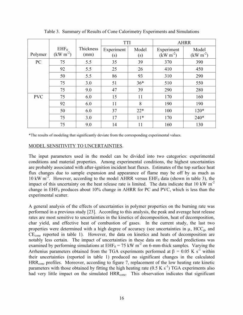
Table 3. Summary of Results of Cone Calorimetry Experiments and Simulations

TTI AHRR

Polymer EHF0

(kW m-2) Thickness

(mm) Experiment

(s) Model

(s) Experiment (kW m-2)

Model (kW m-2)

75 5.5 35 39 370 390 92 5.5 25 26 410 450 50 5.5 86 93 310 290 75 3.0 51 36* 510 550

PC

75 9.0 47 39 290 280 75 6.0 15 11 170 160 92 6.0 11 8 190 190 50 6.0 37 22* 100 120* 75 3.0 17 11* 170 240*

PVC

75 9.0 14 11 160 130 *The results of modeling that significantly deviate from the corresponding experimental values. MODEL SENSITIVITY TO UNCERTAINTIES.

The input parameters used in the model can be divided into two categories: experimental conditions and material properties. Among experimental conditions, the highest uncertainties are probably associated with after-ignition incident heat fluxes. Estimates of the top surface heat flux changes due to sample expansion and appearance of flame may be off by as much as 10 kW m-2. However, according to the model AHRR versus EHF0 data (shown in table 3), the impact of this uncertainty on the heat release rate is limited. The data indicate that 10 kW m-2 change in EHF0 produces about 10% change in AHRR for PC and PVC, which is less than the experimental scatter. A general analysis of the effects of uncertainties in polymer properties on the burning rate was performed in a previous study [23]. According to this analysis, the peak and average heat release rates are most sensitive to uncertainties in the kinetics of decomposition, heat of decomposition, char yield, and effective heat of combustion of gases. In the current study, the last two properties were determined with a high degree of accuracy (see uncertainties in μ, HCCg, and CEcone reported in table 1). However, the data on kinetics and heats of decomposition are notably less certain. The impact of uncertainties in these data on the model predictions was examined by performing simulations at EHF0 = 75 kW m-2 on 6-mm-thick samples. Varying the Arrhenius parameters obtained from the TGA experiments performed at β = 0.05 K s-1 within their uncertainties (reported in table 1) produced no significant changes in the calculated HRRcone profiles. Moreover, according to figure 7, replacement of the low heating rate kinetic parameters with those obtained by fitting the high heating rate (0.5 K s-1) TGA experiments also had very little impact on the simulated HRRcone. This observation indicates that significant

16

differences in the kinetic parameters, which result in considerably different TGA traces (see figure 1), do not always translate into significant differences in the heat release rate profiles.

Figure 7. Model Sensitivity to Uncertainties in Decomposition Kinetics

The effects of uncertainties in the heats of decomposition are demonstrated by the HRRcone histories shown in figure 8. In the case of PVC, where h values of both reactions (8 and 9) were varied simultaneously to their lower and upper limits, the effect is dramatic. The magnitude of the effect indicates that the value of PVC_char radiative heat transfer coefficient (determined by fitting experimental HRRcone with the model) is highly uncertain. Thus, the consistency of the PVC model can clearly benefit from a more accurate decomposition reaction thermochemistry.

Figure 8. Model Sensitivity to Uncertainties in the Heats of Decomposition

17

CONCLUSIONS

The results of this study demonstrate that a one-dimensional numerical pyrolysis model can be used to predict the outcome of cone calorimetry experiments performed on a charring and intumescing polymer. The predictions require the knowledge of the thermal and optical properties of the polymer and a quantitative description of the kinetics and thermodynamics of its decomposition. All this information can be obtained from direct measurements or from existing structure-property correlations. The predictions also require the knowledge of the properties of the decomposition products, in particular, of those products that comprise the intumescent char. Due to fragility and inhomogeneity, a direct characterization of the char (at least of those observed in this work) appears to be very difficult. However, according to these results, a simple submodel based on the properties of graphite and a single adjustable heat transfer parameter, the value of which is determined using the results of one cone calorimetry experiment, provides a reasonable approximation to the carbonaceous char description. The agreement between the model predictions and experiments is not perfect. One possible reason for the discrepancies is a low accuracy of the polymer heats of decomposition, especially of those obtained for poly(vinyl chloride). Experimental methodologies for determination and verification of these heat values need further improvement. It is also possible that the discrepancies arise from the inability of a one-dimensional model to capture three-dimensional processes. Both flame and char structures observed in the cone calorimetry experiments are clearly multidimensional. Availability of a three-dimensional pyrolysis model might help resolve this issue. However, the application of such a model will also increase the number and nature of unknown parameters and may lead to simulation of the aspects of the system behavior that are fundamentally or practically irreproducible (or chaotic).

REFERENCES

1. Kashiwagi, T., “Polymer Combustion and Flammability—Role of the Condensed Phase,” Twenty-Fifth Symposium (International) on Combustion/The Combustion Institute, 1994, pp. 1423-1437.

2. ASTM Standard E 1354-04a, “Standard Test Method for Heat and Visible Smoke

Release Rates for Materials and Products Using an Oxygen Consumption Calorimeter,” ASTM International, West Conshohocken, Pennsylvania, 2007.

3. ASTM Standard E 2058-06, “Standard Test Methods for Measurement of Synthetic Polymer

Material Flammability Using a Fire Propagation Apparatus,” ASTM International, West Conshohocken, Pennsylvania, 2007.

4. Stoliarov, S.I. and Lyon, R.E., “Thermo-Kinetic Model of Burning,” FAA report

DOT/FAA/AR-TN08/17, May 2008. (Available for download at www.fire.tc.faa.gov /reports/reports.asp).

18

5. Stoliarov, S.I. and Lyon, R.E., “Thermo-Kinetic Model of Burning for Pyrolyzing Materials,” Proceedings of the Ninth International Symposium on Fire Safety Science, 2009, pp. 1141-1152.

6. Stoliarov, S.I., Crowley, S., Lyon, R.E., and Linteris, G.T., “Prediction of the Burning

Rates of Non-Charring Polymers,” Combustion and Flame, Vol. 156, 2009, pp. 1068-1083.

7. ASTM Standard D 7309-07, “Test Method for Determining Flammability Characteristics

of Plastics and Other Solid Materials Using Microscale Combustion Calorimetry,” ASTM International, West Conshohocken, Pennsylvania, 2007.

8. Stoliarov, S.I. and Walters, R.N., “Determination of the Heats of Gasification of

Polymers Using Differential Scanning Calorimetry,” Polymer Degradation and Stability, Vol. 93, 2008, pp. 422-427.

9. Van Krevelen, D.W., Properties of Polymers, Third Edition, Elsevier, Amsterdam, 1990. 10. Zhang, X., Hendro, W., Fujii, M., Tomimura, T., and Imaishi, N., “Measurements of the

Thermal Conductivity and Thermal Diffusivity of Polymer Melts With the Short-Hot-Wire Method,” International Journal of Thermophysics, Vol. 23, 2002, pp. 1077-1090.

11. Brandrup, J., Immergut, E.H., Grulke, E.A., Abe, A., and Bloch, D.R., eds., Polymer

Handbook, Fourth Edition, John Wiley & Sons, New York, New York, 1999. 12. Hallman, J.R., Welker, J.R., and Sliepcevich, C.M., “Polymer Surface Reflectance-

Absorptance Characteristics,” Polymer Engineering and Science, Vol. 14, 1974, pp. 717-723.

13. Tsilingiris, P.T., “Comparative Evaluation of the Infrared Transmission of Polymer

Films,” Energy Conversion and Management, Vol. 44, 2003, pp. 2839-2856. 14. Factor, A., “Char Formation in Aromatic Engineering Polymers,” Fire and Polymers:

Hazards Identification and Prevention, Nelson, G.L., ed., ACS Symposium Series 425, American Chemical Society, Washington, DC, 1990, pp. 274-287.

15. Lide, D.R., ed., CRC Handbook of Chemistry and Physics, 73rd Edition, CRC Press, Boca

Raton, Florida, 1992. 16. Matsumoto, T., Ono, A., Noumaru, Y., and Takeda, F., “Measurements of Specific Heat

Capacity and Emissivity of Graphite Samples Using Pulse Current Heating at High Temperatures (III),” Proceedings of the Seventeenth Japan Symposium on Thermophysical Properties, 1996, pp. 183-186.

17. Chase, M.W., Jr., “NIST-JANAF Themochemical Tables, Fourth Edition,” Journal of

Physical Chemical Reference Data, monograph 9, 1998, pp. 1-1951.

19

20

18. Cullis, C.F. and Hirschler, M.M., The Combustion of Organic Polymers, Clarendon

Press, Oxford, 1981. 19. Quintiere, J.G. and Liu, X., “Flammability Properties of Clay-Nylon Nanocomposites,”

FAA report DOT/FAA/AR-07/29, June 2007. 20. Beaulieu, P.A. and Dembsey, N.A., “Effect of Oxygen on Flame Heat Flux in Horizontal

and Vertical Orientations,” Fire Safety Journal, Vol. 43, 2008, pp. 410-428. 21. Siegel, R. and Howell, J., Thermal Radiation Heat Transfer, Fourth Edition, Taylor &

Francis, New York, New York, 2002. 22. Holman, J.P., Heat Transfer, Ninth Edition, McGraw-Hill, Boston, Massachusetts, 2002. 23. Stoliarov, S.I., Safronava, N., and Lyon, R.E., “The Effect of Variation in Polymer

Properties on the Rate of Burning,” Fire and Materials, Vol. 33, 2009, pp. 257-271.