MASTER THESIS

Prediction power of accounting-based bankruptcy prediction models: Evidence from Dutch and Belgian public and large private firms

Anika Bouwmeester (1501712)

Faculty of Behavioural, Management and Social Sciences (BMS)

MSc Business Administration – Track Financial Management

Department of Finance and Accounting

First supervisor: Prof. dr. R. Kabir

Second supervisor: Dr. X. Huang

July 23, 2020

June, 2020

Acknowledgements

This master thesis has been written to finalize my Master of Science in Business Administration with a

specialization in Financial Management at the University of Twente. I would like to thank my two

supervisors, prof. dr. Rezaul Kabir and dr. Xiaohong Huang. Both offered valuable feedback which

helped me to improve my master thesis. Finally, I would like to thank my family, boyfriend, and friends

for their interest, support and encouragement during the writing process of my master thesis.

Anika Bouwmeester

Enschede, July 2020

Abstract

This study examined the prediction power of the accounting-based bankruptcy prediction models of

Altman (1983), Ohlson (1980), and Zmijewski (1984) for Dutch and Belgian public and large private

firms. These bankruptcy prediction models include different financial ratios as independent variables

and are developed using different econometric methods: multiple discriminant analysis, logistic

regression, and probit regression, respectively. It is tested if one of the prediction models outperforms

the others, which econometric method is best for developing the models, if the coefficients of the models

are non-stationary, and what the optimal time horizon for predicting bankruptcy is. The performance of

the three models is assessed using two different estimation samples with firm observations from 2007 –

2010, and 2012 – 2015, and a hold-out sample with firm observations from 2016 – 2019. These different

time periods for the estimation samples are chosen because of the different economic environments.

During the first time period (2007 – 2010), several important events occurred such as the financial crisis

in 2007 and the European debt crisis in 2010. Firms from all industries, except the financial and

insurance industry, were included in the samples. The results show that the models of Altman (1983),

Ohlson (1980), and Zmijewski (1984) predicted respectively 32.39%, 47.89%, and 38.03% of the

bankrupt firms and 99.58%, 99.72%, and 100.00% of the non-bankrupt firms correctly. No statistical

significant difference was found between the three prediction models of Altman (1983), Ohlson (1980),

and Zmijewski (1984), and between the three econometric methods multiple discriminant analysis, logit

regression, and probit regression. Additionally, no evidence was found for the non-stationarity of the

coefficients. Finally, this study concludes that the optimal time horizon for predicting bankruptcy is one

fiscal year before the event.

Keywords: bankruptcy prediction, Altman Z-score, Ohlson O-score, Zmijewski score, multiple

discriminant analysis, logistic regression, probit regression, the Netherlands, Belgium, public firms,

private firms

Table of Contents

1 Introduction .......................................................................................................................................... 1

2 Literature review .................................................................................................................................. 5

2.1 Corporate bankruptcy .................................................................................................................... 5

2.1.1 Financial distress and bankruptcy .......................................................................................... 5

2.1.2 Causes of bankruptcy ............................................................................................................. 6

2.1.3 Bankruptcy procedure in the Netherlands .............................................................................. 7

2.1.4 Bankruptcy procedure in Belgium .......................................................................................... 8

2.2 Bankruptcy prediction ................................................................................................................. 10

2.2.1 Bankruptcy or financial distress prediction? ........................................................................ 10

2.2.2 An overview of bankruptcy prediction models .................................................................... 10

2.3 Accounting-based bankruptcy prediction models ....................................................................... 12

2.3.1 Altman (1968) ...................................................................................................................... 12

2.3.2 Altman (1983) ...................................................................................................................... 13

2.3.3 Ohlson (1980) ....................................................................................................................... 14

2.3.4 Zmijewski (1984) ................................................................................................................. 16

2.4 Market-based bankruptcy prediction models .............................................................................. 17

2.4.1 Shumway (2001) .................................................................................................................. 17

2.4.2 Hillegeist, Keating, Cram, and Lundstedt (2004) ................................................................. 17

2.5 Comparing accounting-based and market-based bankruptcy prediction models ........................ 18

2.6 Assessing bankruptcy prediction models .................................................................................... 20

2.7 Review empirical findings prior research .................................................................................... 22

3 Conceptual Framework ...................................................................................................................... 26

3.1 Hypothesis 1: Model performance .............................................................................................. 26

3.2 Hypothesis 2: Econometric method performance ....................................................................... 28

3.3 Hypothesis 3: Non-stationarity of the coefficients of the models ............................................... 28

3.4 Hypothesis 4: Optimal time horizon ............................................................................................ 30

4 Research methodology ....................................................................................................................... 31

4.1 Hypothesis testing ....................................................................................................................... 31

4.1.1 Hypothesis 1: Model performance ....................................................................................... 31

4.1.2 Hypothesis 2: Econometric method performance ................................................................ 31

4.1.3 Hypothesis 3: Non-stationarity of the coefficients of the models ........................................ 32

4.1.4 Hypothesis 4: Optimal time horizon ..................................................................................... 32

4.2 Variables ...................................................................................................................................... 33

4.2.1 Dependent variables ............................................................................................................. 33

4.2.2 Independent variables ........................................................................................................... 33

4.3 Sample selection .......................................................................................................................... 33

4.4 Testing model assumptions ......................................................................................................... 36

4.4.1 Multivariate normality .......................................................................................................... 36

4.4.2 Equality of variance-covariance ........................................................................................... 37

4.4.3 Multicollinearity ................................................................................................................... 37

5 Empirical results ................................................................................................................................. 38

5.1 Descriptive statistics .................................................................................................................... 38

5.2 Difference between Dutch and Belgian firms ............................................................................. 45

5.3 Hypothesis tests ........................................................................................................................... 47

5.3.1 Hypothesis 1: Model performance ....................................................................................... 47

5.3.2 Hypothesis 2: Econometric method performance ................................................................ 48

5.3.3 Hypothesis 3: Non-stationarity of the coefficients of the models ........................................ 52

5.3.4 Hypothesis 4: Optimal time horizon ..................................................................................... 54

6 Conclusion and discussion ................................................................................................................. 57

6.1 Summary of results ...................................................................................................................... 57

6.2 Limitations................................................................................................................................... 59

6.3 Future research ............................................................................................................................ 60

References ............................................................................................................................................. 62

Appendices ............................................................................................................................................ 68

Appendix A: Financial ratios of the bankruptcy prediction models .................................................. 68

Appendix B: List of bankrupt firms in sample .................................................................................. 69

Appendix C: Testing model assumptions .......................................................................................... 75

C.I Multivariate normality ............................................................................................................. 75

C.II Equality of variance-covariance ............................................................................................. 77

C.III Multicollinearity ................................................................................................................... 78

Appendix D: Goodness of fit measures ............................................................................................. 79

Appendix E: Coefficients of the models ........................................................................................... 80

E.I Estimation sample 2012 – 2015 (t-1) ....................................................................................... 80

E.II Estimation sample 2007 – 2010 (t-1) ..................................................................................... 84

E.III Estimation sample 2012 – 2015 (t-2) .................................................................................... 85

1

1 Introduction

Since the 1960s an increasing number of corporate bankruptcy prediction models have emerged (Adnan

Aziz & Dar, 2006). Corporate bankruptcy prediction is of great interest to various stakeholders including

shareholders, managers, employees, creditors, suppliers, clients, and the government (Dimitras, Zanakis,

& Zopounidis, 1996; Fejér-Király, 2015). Bankruptcy prediction models can be helpful in two different

ways. First, bankruptcy prediction can be used as an early warning system to prevent bankruptcy. If the

model is able to predict a potential bankruptcy a few years in advance, actions like reorganization or

merger of the firm can be undertaken (Dimitras et al, 1996; Pompe & Bilderbeek, 2005; Fejér-Király,

2015). Second, predicting the possibility of bankruptcy can help investors evaluate and select firms to

invest in, in order to prevent the risk of losing their investment (Dimitras et al., 1996; Karamzadeh,

2013). Bankruptcy might have a contagious effect within an industry, where one firm’s bankruptcy leads

to another firm’s bankruptcy if their activities depend on one another (Lang & Stulz, 1992; Fejér-Király,

2015).

Two of the most widely used methods for predicting corporate bankruptcy are analysis of

financial ratios and analysis of market risk (Karamzadeh, 2013), also known as accounting-based

bankruptcy prediction models and market-based bankruptcy prediction models, respectively. This thesis

will focus on accounting-based bankruptcy prediction models, because these models do not rely on

market data. Accounting-based models estimate the possibility of bankruptcy by using a group of

financial ratios (Karamzadeh, 2013). The majority of firms are private firms and for privately held firms

only accounting data and no market data are available. The banking industry is the main provider of

loans in the economy and for private firms, and is therefore especially interested in reducing the amount

of non-performing loans. In order to reduce their own risk of default, banks need to predict the possibility

of default of a potential borrower (Atiya, 2001; Altman, Iwanicz-Drozdowska, Laitinen, & Suvas, 2017).

Therefore, it is important to test the accounting-based bankruptcy prediction models. The key

accounting-based bankruptcy prediction models are the models of Altman (1968), Ohlson (1980) and

Zmijewski (1984) (Wu, Gaunt, & Gray, 2010).

This master thesis will test the accounting-based bankruptcy prediction models on Dutch and

Belgian public and large private firms. The number of bankruptcies in the Netherlands decreased since

2013 until 2017 and since then the trend has been relatively stable (Statistics Netherlands, 2019). The

number of Belgian bankruptcies also decreased since 2013, and the trend has been relatively stable since

2015 (Statbel, 2020). Despite this current trend of bankruptcies in the Netherlands and Belgium, it will

still be important to examine if the bankruptcy prediction models are generalizable to Dutch and Belgian

public and large private firms because bankruptcies will always occur. The main goal of this master

thesis is to examine the prediction power of the accounting-based bankruptcy prediction models of

2

Altman (1968), Ohlson (1980), and Zmijewski (1984) when applied to Dutch and Belgian public and

large private firms. Given the above, this thesis will answer the following research question:

How accurate are the accounting-based bankruptcy prediction models for Dutch and Belgian public

and large private firms?

The literature provides contradictory empirical results concerning the best performing

bankruptcy prediction model (e.g. Begley, Ming, & Watts, 1996; Grice & Ingram, 2001; Grice Jr. &

Dugan, 2003; Wu et al., 2010). This master thesis will therefore test if one of the models of Altman

(1968), Ohlson (1980) or Zmijewski (1984) outperforms the others regarding their prediction power

when applied to Dutch and Belgian public and large private firms. Since the three prediction models are

developed using different econometric methods, it will also be tested if one of these econometric

methods outperforms the others regarding their prediction power. It appears that all three models are

sensitive to time periods and that the relation between financial ratios and financial distress changes

over time. This can lead to a decline of the accuracy rate of the models when applied to time periods

that differ from the time periods used to develop the models (Grice & Dugan, 2001; Grice & Ingram,

2001). In addition to different time periods, different economic environments also affects the accuracy

and structure of bankruptcy prediction models, suggesting that the coefficients of the accounting-based

bankruptcy prediction models are non-stationary (Mensah, 1984). It will be tested if the accounting-

based bankruptcy prediction models retain their accuracy over time, and if re-estimating the coefficients

of the prediction models improves the predictive accuracy. Finally, the optimal time horizon for

predicting bankruptcy will be assessed.

The sample of this master thesis includes Dutch and Belgian public and large private and non-

financial firms across all industries. Studies of bankruptcy prediction mainly focus on publicly listed

companies outside the European Union, mostly in the United States (U.S.) (e.g. Altman, 1968; Ohlson,

1980, Zmijewski, 1984; Grice & Ingram, 2001; Shumway, 2001; Grice Jr. & Dugan, 2003; Chava &

Jarrow, 2004; Hillegeist, Keating, Cram, & Lundstedt, 2004). However, bankruptcy prediction for

private firms is also important since private firms play a critical role in most economies (Filipe,

Grammatikos, & Michala, 2016), but have much higher failure rates on average than public companies

(Jones & Wang, 2019). According to Jones and Wang (2019), the following factors might be the reason

that most studies focus on publicly listed firms instead of private firms. First, the available data for

private firms tend to be less complete and reliable since most private firms are not subject to mandatory

external auditing requirements or compliance with accounting standards. Second, as already mentioned,

bankruptcy prediction for private firms is limited to financial ratios, in contrast to bankruptcy prediction

for public firms, where market data can be included. Last, most private firms have heterogeneous

business and legal structures, which makes it more difficult to predict bankruptcy. Additionally, a Dutch

and Belgian context is chosen because firms in these two countries were affected by the financial crisis

in 2007, the European debt crisis in 2010, and the regulatory response to the financial crisis, Basel III.

This provides an interesting economic environment to test the predictive accuracy of the three models.

3

This master thesis therefore contributes to the existing literature by including private firms in the sample

and by assessing the usability of the three accounting-based bankruptcy prediction models in a Dutch

and Belgian setting, and by providing which model performs best in this setting. Additionally, another

contribution of this master thesis is that it tests the accounting-based bankruptcy prediction models in

two different periods (2007-2010 and 2016-2019) with different economic environments.

Other students from the University of Twente also conducted research on bankruptcy prediction.

Boekhorst (2018) evaluated the predictive ability of the Altman Z-score model (1983) for Dutch private

firms. A critic is that the sample consisted of bankrupt and active firms in the time period 2007 – 2015,

which is a quite large time period and during this time period the economic environment has changed a

lot. This may have biased the results. Additionally, firms from all industries, including the financial and

insurance industry, were included in the sample. Most studies about bankruptcy prediction exclude firms

from the financial and insurance industries because of their different structure of capital compared to

firms in other industries. A strength of the study of Boekhorst (2018) is the use of a large sample size,

which makes the results more reliable. However, the high ratio active firms/bankrupt firms in the sample

is not proportional to the actual bankruptcy rate and this ratio is not constant per sample, which

potentially biased the results. He also did not partition the data into an estimation sample and hold-out

sample to verify the predictive performance of the Z-score model.

Elferink (2018) adjusted existing prediction models to achieve an accuracy higher than 80% in

an exclusively Dutch setting. He only tested and re-estimated the Z-score model of Altman (1968), and

did not include other accounting-based bankruptcy prediction models. However, he did investigated

additional ratios that could increase the performance of the prediction model. Another strength of his

research is that he tested and re-estimated the Z-score model of Altman (1968) using several econometric

methods: multiple discriminant analysis, logistic regression, and neural network. The sample consisted

of 125 matched pairs of bankrupt and non-bankrupt firms. However, the actual amount of non-bankrupt

firms is much higher than the actual amount of bankrupt firms, meaning that, just as the sample of

Boekhorst (2018), the sample is not proportional to the actual bankruptcy rate, leading to potential bias

of the results.

Machielsen (2015) assessed the predictive accuracy and information content of the bankruptcy

prediction models of Altman (1968) and Ohlson (1980) for publicly listed firms in the European Union.

Whereas many studies only focus on predictive accuracy, the study of Machielsen (2015) also measures

the information content of the models. Information content measures whether one model score contains

more information about bankruptcy than another variable (or set of variables). A weakness of the study

of Machielsen (2015) might be that 3 out of 25 countries are overrepresented in the samples, which

could potentially lead to sampling bias. However, the robustness checks he conducted conclude that the

effect of the sampling bias was marginal. A strength of the study is that he includes macroeconomic

variables to absorb the change in macroeconomic environment to ensure that the model remains accurate

and informative under changing macroeconomic circumstances.

4

Despite that several other students already conducted their master thesis on bankruptcy

prediction, this master thesis still contributes to the existing literature because it focuses on three

accounting-based bankruptcy prediction models for Dutch and Belgian public and large private firms,

which has not been done before. This thesis is structured as follows. Chapter two provides a literature

review of corporate bankruptcy, the bankruptcy procedure and the key bankruptcy prediction models.

This chapter also features a review of the key empirical findings of prior research. Chapter three presents

the conceptual framework in which the hypotheses are developed. Chapter four presents the research

methodology. The empirical results of the hypotheses are presented in chapter five. Finally, the

conclusion and discussion follows in chapter six.

5

2 Literature review

This chapter discusses the theoretical framework of this master thesis. The first section addresses

corporate bankruptcy; the definition of financial distress and bankruptcy, the causes of bankruptcy, and

the bankruptcy procedure in the Netherlands and Belgium will be discussed. In the second section, the

focus will be on bankruptcy prediction, and in this section an overview of bankruptcy prediction models

will be provided. The third section will be devoted to the key accounting-based bankruptcy prediction

models of Altman (1968, 1983), Ohlson (1980), and Zmijewski (1984). The fourth section will review

the two key market-based bankruptcy prediction models of Shumway (2001) and Hillegeist et al. (2004).

This is followed by a comparison of the accounting-based and market-based bankruptcy prediction

models in section five. Section six features the assessment of the bankruptcy prediction models. Finally,

a summary table containing the most important contributions and results of key articles in the literature

of bankruptcy prediction will be provided.

2.1 Corporate bankruptcy

2.1.1 Financial distress and bankruptcy

In corporate failure studies, the terms financial distress and bankruptcy are often used as synonyms,

while they do not have the same definition (Karels & Prakash, 1987; Wruck, 1990; Balcaen & Ooghe,

2006). Financial distress is a broad concept that includes several situations in which firms face some

form of financial difficulty (Doumpos & Zopounidis, 1999). There are many definitions of financial

distress (Altman, 2013). According to Li and Li (1999), a firm is financially distressed when the firm’s

cash flows are insufficient to cover current obligations to creditors and/or the expected present value of

the firm is below the outstanding debt level. Bankruptcy is a legal procedure where companies have

already taken a legal action (Fejér-Király, 2015), bankruptcy is therefore described as the legal definition

of financial distress (Doumpos & Zopounidis, 1999; Kahya & Theodossiou, 1999). Financially

distressed firms still have the chance of being reorganized and to continue their activities (Fejér-Király,

2015). Financial distress precedes bankruptcy and persists until the firm or creditor decides to file a legal

action (Karels & Prakash, 1987; Platt & Platt, 2002). Financially distressed firms are more likely to

declare bankruptcy than firms that do not experience financial distress. However, a financially distressed

firm does not inevitably file for bankruptcy (Grice Jr. & Dugan, 2003; Tinoco & Wilson, 2013).

A bankruptcy filing implies that the debtor cannot pay all of their debts to the creditors and the

legal procedure of bankruptcy is aimed at relieving the debtor from all or some of their debts (Jackson,

1982; White, 1989). To keep the market economy healthy, it is necessary that firms that are no longer

competitive disappear from the market so that their resources can be redistributed in favour of healthy

firms. This results in a growing competition in the market economy and allows only the best firms to

survive on the market (Garškiene & Garškaite, 2004; Ooghe & Waeyaert, 2004). The bankruptcy

6

Source: Ooghe and Waeyaert (2004)

procedure must ensure that the liquidation of such firms proceeds in an orderly manner (Ooghe &

Waeyaert, 2004). This theory suggests that only economically inefficient firms whose resources could

be better used by healthier firms should file for bankruptcy. However, in practice firms can also file for

bankruptcy voluntarily, meaning that firms in bankruptcy might not always be economically inefficient

(White, 1989). Managers choose to voluntarily liquidate when financial conditions make it value-

increasing for shareholders and managers (Fleming & Moon, 1995). For shareholders, the expected

value of a voluntarily exit always exceeds the expected value of a court driven exit (Balcaen, Manigart,

Buyze, & Ooghe, 2012).

2.1.2 Causes of bankruptcy

Generally, bankruptcy is not the result of a sudden event, but is caused by multiple factors (Ooghe &

Waeyaert, 2004; Lukason & Hoffman, 2014; Kisman & Krisandi, 2019). Bankruptcy is the result of

multiple failures of the company to run its business operations in the long term in order to achieve its

economic goals (Kisman & Krisandi, 2019). Before a company files for bankruptcy, it experiences a

failure process which varies in length in which the company gradually evolves towards the final stage

of the decline process, bankruptcy (Ooghe & Waeyaert, 2004; Lukason & Hoffman, 2014). Ooghe and

Waeyaert (2004) developed a conceptual failure model that explains the different causes of failure. The

model distinguishes external factors and internal factors. External factors include the (1) general

environment and (2) immediate environment. Internal factors include (1) management, (2) corporate

policy and (3) company’s characteristics (Ooghe & Waeyaert, 2004). Table 1 provides an overview of

the causes of bankruptcy.

Table 1 Causes of bankruptcy

External factors

General environment Economics, technology, foreign countries, politics,

social factors

Immediate environment Customers, suppliers, competitors, banks and credit

institutions, stockholders, government

Internal factors

Management Motivation, qualities, skills, personal characteristics

Corporate policy Strategy and investments, commercial, operational,

personnel, finance and administration, corporate

governance

Company’s characteristics Maturity, size, industry, flexibility

Management has little or no control over external factors (Mellahi & Wilkinson, 2004; Ooghe

& Waeyaert, 2004; Lukason & Hoffman, 2014). However, management should take these

uncontrollable external factors into account in their strategy (Ooghe & Waeyaert, 2004). Inflation, tax

7

systems, law, depression in foreign currencies, economic downturns, competition, changes in

demographics, technology or regulations are external factors that can cause bankruptcy (Lukason &

Hoffman, 2014; Kisman & Krisandi, 2019), and these factors require a response from management

(Lukason & Hoffman, 2014). Internal causes of failure are within management’s control (Mellahi &

Wilkinson, 2004; Ooghe & Waeyaert, 2004; Lukason & Hoffman, 2014). Internal factors are the

management’s decisions/actions and can be operational (short term) or strategic (long term) (Lukason

& Hoffman, 2014). Lack of knowledge and experience from the management in managing assets and

liabilities effectively (Kisman & Krisandi, 2019), poor management skills, insufficient marketing, and

lack of ability to compete with other similar business (Wu, 2010) are internal factors that increases the

probability of bankruptcy. There are also uncontrollable internal factors such as illness or death of key

personnel, or a fire (Lukason & Hoffman, 2014). In extreme cases, external and internal factors can have

a direct effect on bankruptcy. For instance, because of a major environmental disaster, economic crisis,

or management mistake (Mellahi & Wilkinson, 2004). It appears that internal factors are the main causes

of bankruptcy (Ooghe & Waeyaert, 2004), in particular managerial errors and weaknesses in operational

management (Hall, 1992; Ooghe & De Prijcker, 2008).

2.1.3 Bankruptcy procedure in the Netherlands

Financial distress of a firm can lead to reorganization under court supervision (Li & Li, 1999), private

reorganization (Gilson, John, & Lang, 1990), a formal exit procedure, or a private exit (Li & Li, 1999;

Balcaen et al., 2012). A formal exit procedure includes bankruptcy, and a private exit includes voluntary

liquidation and merger and acquisition (Balcaen et al., 2012). Liquidation occurs when a firms sells all

assets, pays off creditors, and distributes the residual funds to shareholders (Ghosh, Owers, & Rogers,

1991). Due to the high transaction costs, bankruptcies are the least preferred exit option (Balcaen et al.,

2012). The Dutch Bankruptcy Code provides two in-court procedures for financially distressed firms in

the Netherlands: suspension of payment or filing for bankruptcy, and one outside-court procedure:

informal reorganization (Boot & Ligterink, 2000; Couwenberg & de Jong, 2008; Couwenberg &

Lubben, 2011); Hummelen, 2015).

Firms in financial distress can request a suspension of payment only if the firm has prospects to

recover in a short time (Couwenberg & de Jong, 2008). The purpose of suspension of payment is to

provide the management of the firm the opportunity to prevent bankruptcy. This request can only be

done by the debtor. If the court does not provide suspension of payment, firms often end up filing for

bankruptcy. During the suspension of payment procedure, the management of the firm retains control

(Boot & Ligterink, 2000). The suspension of payment procedure applies only to ordinary creditors, and

does not apply to secured creditors and creditors holding preferred claims (Boot & Ligterink, 2000;

Couwenberg & de Jong, 2008). The firm offers the ordinary creditors an agreement, and when the

creditors accept the agreement, the procedure of suspension of payment ends. If the firm fails during the

suspension of payment, it is not possible to request another suspension of payment in the bankruptcy

8

procedure (Couwenberg & de Jong, 2008). Many firms use the suspension of payment procedure to

enter bankruptcy, because company directors can start a suspension of payment procedure but cannot

file for bankruptcy. Only shareholders of the firm can directly file for bankruptcy, but it takes too much

time to organize a shareholder meeting (Couwenberg & Lubben, 2011).

The other option for firms in financial distress is filing for bankruptcy. The Dutch bankruptcy

law system is a liquidation-based system, with a rudimentary reorganization provision, in which the

rules facilitate, or even force, the trustee to sell the firm’s assets in bankruptcy (Couwenberg, 2001;

Couwenberg & Lubben, 2011). The bankruptcy starts with the filing of a petition with the court

(Hummelen, 2015). Both the firm, through its shareholders, and the creditors of the firm, once a payment

is missed, may file for bankruptcy (Boot & Ligterink, 2000; Couwenberg & de Jong, 2008). Like a

Chapter 7 procedure in the U.S., the purpose of bankruptcy is to cash out all the assets of the firm and

to distribute the proceeds among the creditors, where the interests of the creditors are paramount (Boot

& Ligterink, 2000; Hummelen, 2015). The assets of the firm can be sold as piecemeal or going concern,

by means of a private sale or a public auction (Couwenberg & de Jong, 2008). At the beginning of the

bankruptcy process, the court appoints an independent trustee which takes over the control of the

management of the firm. The trustee has the option to continue the operations of the firm as a going

concern, if this results in a higher return than liquidation. Since 1992, as well as with the suspension of

payment procedure, firms in financial distress are protected from its creditors by an automatic stay of

assets provision in a cool down period of at most two months (Boot & Ligterink, 2000; Couwenberg &

de Jong, 2008).

Unlike Chapter 11 in the U.S., the Dutch Bankruptcy Code has no separate reorganization

procedure for which a debtor can file. However, firms in financial distress can enter an informal

reorganization procedure in order to renegotiate with the creditors (Boot & Ligterink, 2000;

Couwenberg, 2001; Hummelen, 2015). Only the debtor may propose such a reorganization plan

(Hummelen, 2015). The solution can be asset restructuring, liabilities restructuring, or a combination of

both (Boot & Ligterink, 2000). If the renegotiations fail, firms will in most cases file for bankruptcy

(Couwenberg, 2001). Since the negotiations occur outside the bankruptcy proceedings, it is necessary

that all creditors agree with the intended reorganization. These negotiations become more complex when

more creditors are involved, therefore informal reorganization only succeeds if there is a dominant

creditor. In the Netherlands, most of the time banks are the dominant creditor (Boot & Ligterink, 2000).

2.1.4 Bankruptcy procedure in Belgium

The Belgian Bankruptcy Code provides three restructuring and liquidation proceedings: bankruptcy,

formal reorganization, and voluntary liquidation. The bankruptcy procedure is aimed at liquidation of

the firm, as a going concern or through selling the assets piece by piece, in order to pay the debts of the

firm. Under the Belgian Bankruptcy Code, a firm should file for bankruptcy if the firm has generally

stopped paying its debts, and if the firm has lost the confidence of its creditors. Both the board of

9

directors of the firm and the creditors of the firm may file for bankruptcy. If the bankruptcy is declared

by the court, a curator is appointed who takes over all responsibilities from the board of directors. The

curator assumes control over the assets, accounts, archives and information of the firm. The task of the

curator is to sell the assets of the firm and pay the creditors of the firm, according to their priority rights.

The court also appoints a judge-commissioner to supervise the curator. Generally, at the end of the

bankruptcy procedure the firm will no longer exist and the shareholders lose their stake in the firm.

However, if the proceeds of selling the firm as a going concern are higher than the proceeds of selling

the assets piece by piece, the court may authorize that the firm temporarily continues its activities under

the supervision of the curator (Baker & McKenzie, 2016).

Instead of an informal reorganization procedure, the Belgian Bankruptcy Code provides a

formal reorganization procedure. Belgium, just as many other European countries, reformed their

bankruptcy legislations to stimulate reorganization and firm survival. The liquidation focused

bankruptcy system has transformed into a legislation encompassing both a formal reorganization and

liquidation procedure similar to the U.S.. The formal reorganization procedure is almost similar with the

legal reorganization rules of the U.S. Chapter 11. A firm that files for formal reorganization receives

creditor protection for up to six months, and during this period a reorganization plan is composed which

has to be approved by the majority of creditors and the bankruptcy court. Upon approval of the

reorganization plan, the firm stays under protection of the court for up to three years. During this period,

the management of the firm is assisted and supervised by a court appointed administrator (Dewaelheyns

& Van Hulle, 2008). The board of directors, the public prosecutor and any other third party with a

legitimate interest can file for formal reorganization (Baker & McKenzie, 2016).

In addition to the formal reorganization and liquidation procedure, the Belgian Bankruptcy Code

also allows firms to apply for voluntary liquidation. The board of directors of the firm appoints a

liquidator, which has to be confirmed by the court. During the voluntary liquidation procedure, the

liquidator must sell the assets and pay the creditors of the firm. The shareholders of the firm receive the

residual proceeds. After completing the liquidation procedure, the liquidator must prepare a plan for the

distribution of the assets to the different creditors and submit this plan to the court for approval. After

the plan is approved by the court, the liquidation can be closed and the firm does not longer exist as a

legal entity (Baker & McKenzie, 2016).

In Europe, most of the bankruptcies are initiated by the creditor and thus involuntary. Creditors

may not be aware of the real financial situation, because the debtor wants to continue operating the firm

as long as possible and therefore hides the real financial situation. In that case, filing for bankruptcy by

creditors may come too late and the value of the firm’s assets has already largely disappeared. Timely

starting either liquidation or reorganization procedures is important. The bankruptcy procedure would

be optimal when the maximum value of the firm is realized at the lowest costs (Brouwer, 2006).

10

2.2 Bankruptcy prediction

2.2.1 Bankruptcy or financial distress prediction?

Grice Jr. and Dugan (2003) state that it is not clear whether the corporate failure prediction models are

specifically useful to predict the event of bankruptcy or to predict financial distress. Many studies use

bankruptcy as the definition of failure, other studies define failure as financial distress, and some studies

do not clarify the definition of failure used for the research at all. This makes it difficult to compare the

different prediction models (Bellovary, Giacomino, & Akers, 2007). According to Gilbert, Menon and

Schwartz (1990), the financial dimensions that separate bankrupt from healthy firms are different than

the financial dimensions that separate bankrupt from financially distressed firms. Therefore, bankruptcy

prediction models are not able to distinguish financially distressed firms filing for bankruptcy from

financially distressed firms avoiding bankruptcy. Most corporate failure studies describe prediction

models of bankruptcy, and limited studies attempt to develop prediction models of financial distress.

This can be explained by the lack of a consistent definition of financial distress and the difficulty to

objectively define the onset of financial distress, in contrast to the definition of bankruptcy and the

definitive bankruptcy date (Platt & Platt, 2002; Balcaen & Ooghe, 2006).

The models of Altman (1968), Ohlson (1980) and Zmijewski (1984) are developed to predict

the event of bankruptcy. The bankrupt group in the sample of Altman (1968) included ‘‘manufacturers

that filed a bankruptcy petition under Chapter X of the National Bankruptcy Act’’ (p. 593). The bankrupt

group in the sample of Ohlson (1980) included failed firms that ‘‘must have filed for bankruptcy in the

sense of Chapter X, Chapter XI, or some other notification indicating bankruptcy proceedings’’ (p. 114).

Zmijewski (1984) included financially distressed firms in his sample on the basis of the following

definition: ‘‘financial distress is defined as the act of filing a petition for bankruptcy’’ (p. 63). This

definition of financial distress implies that the Zmijewski (1984) model predicts bankruptcy instead of

financial distress. As in the study of Zmijewski (1984), several studies that intent to predict financial

distress, based on the title of the study, instead predict bankruptcy, based on their definition of financial

distress (Platt & Platt, 2002). Since the models of Altman (1968), Ohlson (1980) and Zmijewski (1984)

predict the event of bankruptcy, this master thesis will also use the legal definition of bankruptcy for the

firms that are included in the samples.

2.2.2 An overview of bankruptcy prediction models

In the 1930’s the first literature appeared about the use of a firm’s financial ratios to predict bankruptcy.

The bankruptcy prediction models differ in the amount of ratios and which ratios are used, and the

method used to develop the model. Till the mid-1960’s, the bankruptcy prediction models were based

on univariate ratio analysis. The most widely recognized univariate study is that of Beaver (1966)

(Bellovary et al., 2007). Beaver (1966) examined the usefulness of accounting data, by comparing

financial ratios one-by-one. Beaver (1966) noticed the possibility to use multivariate ratio analysis that

11

would predict bankruptcy better than the single ratios, and suggested future research to use several

different ratios over time. Altman (1968) elaborated this suggestion and developed the first bankruptcy

prediction model based on multivariate ratio analysis in 1968 (Bellovary et al., 2007; Fejér-Király,

2015). The number and complexity of bankruptcy prediction models have increased enormously since

Altman’s (1968) model, due to the growing availability of data and the development of improved

econometrical techniques (Bellovary et al., 2007; Lee & Choi, 2013). The dependent variable in

bankruptcy prediction models is generally a dichotomous variable, where a company is either bankrupt

or non-bankrupt. The independent variables are often financial ratios, including measures of

profitability, liquidity, and leverage. Some studies include market-driven variables as independent

variables, such as the volatility of stock returns and past excess returns (Wu et al., 2010).

On the basis of the type of technique applied, the bankruptcy prediction models can be

categorized into two groups: statistical and intelligent models (Adnan Aziz & Dar, 2006; Kumar & Ravi,

2007; Demyanyk & Hasan, 2010). Statistical models can again be divided into accounting-based

prediction models, using accounting data, and market-based prediction models, using market data (Singh

& Mishra, 2016). Statistical models can be based on both univariate and multivariate analysis. In the

early stages of bankruptcy prediction, multiple discriminant analysis (MDA) was a frequently used

statistical method, and in the later stages, due to advancement and technology, other statistical methods

such as logit analysis and probit analysis became more popular (Bellovary et al., 2007; Siddiqui, 2012).

Intelligent models depend heavily on computer technology and are mainly multivariate (Adnan Aziz &

Dar, 2006). Intelligent models have similarities with functions of the human brain (Demyanyk & Hasan,

2010). Examples of intelligent models are fuzzy models, neural networks, decision trees, rough sets,

case-based reasoning, support vector machines, data envelopment analysis, and soft computing (Kumar

& Ravi, 2007). The most widely used intelligent model is neural networks (Demyanyk & Hasan, 2010).

Neural networks models mimic the biological neural networks of the human nervous system (Demyanyk

& Hasan, 2010; Kumar & Ravi, 2007). Statistical models have some constraining assumptions, such as

linearity, normality, and independence among variables. The effectiveness and validity of statistical

models is limited when these assumptions are violated (Zhang, Hu, Patuwo, Indro, 1999; Shin, Lee, &

Kim, 2005; Lee & Choi, 2013). In contrast, intelligent models are less vulnerable to these assumptions,

and are therefore more useful as most financial data do not meet the assumptions of statistical models

(Shin et al., 2005; Demyanyk & Hasan, 2010). Statistical and intelligent bankruptcy prediction models

both have limitations. Both prediction models focus on the symptoms instead of the underlying causes

of bankruptcy. Moreover, economic theoretical foundation why companies are expected to go bankrupt

and other companies not is missing (Morris, 1997; Adnan Aziz & Dar, 2006). Because intelligent models

use techniques that lie beyond the field of Business Administration, this master thesis will focus only

on statistical models.

According to Wu et al. (2010), the key statistical bankruptcy prediction models are the MDA

model of Altman (1968), the logit model of Ohlson (1980), the probit model of Zmijewski (1984), the

12

hazard model of Shumway (2001), and the Black-Scholes-Merton option pricing model of Hillegeist et

al. (2004). The models of Altman (1968), Ohlson (1980), and Zmijewski (1984) are based on accounting

data, and the models of Shumway (2001), and Hillegeist et al. (2004) are based on both accounting and

market data. These bankruptcy prediction models will be explained in the next two sections.

2.3 Accounting-based bankruptcy prediction models

2.3.1 Altman (1968)

Altman (1968) had doubts about the outcomes of the traditional univariate ratio analysis regarding

bankruptcy prediction, and extended the traditional univariate ratio analysis by combining several

financial ratios into the first multivariate bankruptcy prediction model. Altman (1968) conducted a study

to find out which financial ratios are most important in predicting bankruptcy, what weight should be

attached to those selected ratios, and how the weight should objectively be established. Altman (1968)

used MDA as statistical technique to construct the prediction model which is now known as the Altman

Z-score. ‘‘MDA is a statistical technique used to classify an observation into one of several a priori

groupings dependent upon the observation's individual characteristics’’ (Altman, 1968, p. 591). The

advantage of MDA relative to traditional univariate ratio analysis is that MDA can consider an entire

set of variables, as well as the interaction of these variables. A univariate analysis can only consider the

measurements used for group assignments one at a time (Altman, 1968). The dependent variable in

MDA is qualitative, and the independent variables are quantitative. The first step in MDA is to determine

group classifications, with a minimum of two groups. In the study of Altman (1968) two groups are

classified: bankrupt firms and non-bankrupt firms. The result of MDA is a linear combination of

independent variables, which provides the best distinction between the group of bankrupt firms and non-

bankrupt firms (Altman, 1968). The function is of the form:

𝑍 = 𝑣1𝑥1 + 𝑣2𝑥2 + ⋯ + 𝑣𝑛𝑥𝑛 (Equation 1)

Where: v = Discriminant coefficients

x = Independent variables

In the original study of Altman (1968), the initial sample consisted of 66 manufacturing firms

with 33 firms which filed for bankruptcy between 1946 and 1965 in group 1, and 33 firms which still

existed in 1966 in group 2. Data for the initial sample are derived from financial statements one reporting

period prior to bankruptcy. From the 22 potentially helpful financial ratios, classified into liquidity,

profitability, leverage, solvency, and activity ratios, only the best predictive five financial ratios where

included in the final model. The final discriminant function is as follows:

𝑍 = 0.012𝑥1 + 0.014𝑥2 + 0.033𝑥3 + 0.006𝑥4 + 0.999𝑥5 (Equation 2)

Where: x1 = Working capital/Total assets

13

x2 = Retained earnings/Total assets

x3 = Earnings before interest and taxes/Total assets

x4 = Market value equity/Book value of total debt

x5 = Sales/Total assets

In MDA, the financial characteristics of a firm are combined into one single multivariate

discriminant score. In the study of Altman (1968), this is called the Z-score. The discriminant score has

a value between -∞ and +∞, and this score indicates the financial health of the firm. Based on the

discriminant score and a certain cut-off point, firms are classified into the bankrupt or non-bankrupt

group. Firms are assigned to the group they most closely resemble. Firms are classified into the bankrupt

group if its Z-score is less than the cut-off point, and firms are classified into the non-bankrupt group if

its Z-score exceeds or equals the cut-off point (Balcaen & Ooghe, 2006).

The use of MDA is based on several assumptions: (1) dependent variable must be dichotomous,

(2) independent variables are multivariate normally distributed, (3) equal variance-covariance matrices

across the bankrupt and non-bankrupt group, (4) prior probability of failure and the misclassification

costs are specified, and (5) data must be absent of multicollinearity (Balcaen & Ooghe, 2006). According

to Collins and Green (1982), two assumptions of the MDA model are mostly violated in bankruptcy

prediction, the assumption about normal distribution of independent variables and the assumption about

equal variance-covariance matrices. The first assumption is mostly violated because financial ratios

generally are non-normal distributed. The second assumptions is mostly violated because the variability

of the financial ratios of future bankrupt firms is generally different than the variability of non-bankrupt

healthy firms.

The model of Altman (1968) is extremely accurate in predicting 95% of the total sample

correctly one fiscal year prior to bankruptcy. The model predicted 94% of the bankrupt firms and 97%

of the non-bankrupt firms correctly one fiscal year prior to bankruptcy. Firms having a Z-score >2.99

are predicted not to go bankrupt, while firms having a Z-score <1.81 are predicted to go bankrupt. Z-

scores between 1.81 and 2.99 are defined as the ‘‘gray area’’ or ‘‘zone of ignorance’’. The Altman Z-

score is also able to predict bankruptcy two years prior to the event, but with a decline in accuracy rate

to 72%.

2.3.2 Altman (1983)

The original model of Altman (1968) is only applicable to publicly traded companies. Altman (1983)

therefore developed a revised Z-score model that can be applied to firms in the private sector. In this

revised model, the book value of equity is substituted for the market value of equity in variable X4. The

original model is completely re-estimated, and all coefficients have changed in the revised Z-score

model. The revised Z-score model with a new X4 variable is as follows:

14

𝑍′ = 0.717𝑥1 + 0.847𝑥2 + 3.107𝑥3 + 0.420𝑥4 + 0.998𝑥5 (Equation 3)

Where: x4 = Book value equity/Book value of total debt

The revised Z-score model of Altman (1983) predicted 90.9% of bankrupt firms and 97% of

non-bankrupt firms correctly, one year prior to bankruptcy. Firms having a Z’-score >2.99 are predicted

not to go bankrupt, while firms having a Z’-score <1.23 are predicted to go bankrupt. Z’-scores between

1.23 and 2.99 are defined as the ‘‘gray area’’ or ‘‘zone of ignorance’’.

2.3.3 Ohlson (1980)

Another accounting-based bankruptcy prediction model is the logit model of Ohlson (1980), known as

the O-score. Ohlson (1980) used logit analysis instead of the MDA methodology Altman (1968) used,

to avoid problems associated with MDA. According to Ohlson (1980), the following problems occur

when using MDA:

− There are certain statistical requirements that must be fulfilled when using MDA, which limits

the scope of the investigation.

− The output of the MDA model is an ordinal ranking score which has little intuitive

interpretation.

− Bankrupt and non-bankrupt firms are matched according to criteria such as size and industry,

and these tend to be somewhat arbitrary. It is by no means obvious what is really gained or lost

by different matching procedures, including no matching at all.

Like in the MDA, the dependent variable in logit regression is qualitative, and the independent

variables are quantitative. The logit regression combines several variables into a multivariate probability

score for each firm, P, which indicates the probability of bankruptcy:

𝑃 =1

1+𝑒−(𝛽0+𝛽1𝑥1+𝛽2𝑥2+⋯+ 𝛽𝑛𝑥𝑛) =1

1+𝑒−(𝐷𝑖) (Equation 4)

Where: β = Coefficients, and β0 = intercept

x = Independent variables

Di = The logit for firm i

The logit score P has a value between 0 and 1 and is increasing in Di. If Di approaches negative

infinity, P will be 0 and if D1 approaches positive infinity, P will be 1. In logit regression, the probability

of bankruptcy, P, follows the logistic distribution. Based on the logit score and a certain cut-off point,

firms are assigned to the bankrupt or the non-bankrupt group. Like in the MDA model, firms will be

assigned to the group they most closely resemble. Firms are classified into the bankrupt group if its logit

score exceeds the cut-off point, and is classified into the non-bankrupt group if its score is lower than or

equals the cut-ff point (Balcaen & Ooghe, 2006). Logit regression does not require the restrictive

15

assumptions of MDA. Logit regression is based on three assumptions: (1) the dependent variable must

be dichotomous, (2) the cost of type I and type II error rates should be considered in the selection of the

optimal cut-off point probability, and (3) the data must be absent of multicollinearity since logit

regression is extremely sensitive to multicollinearity (Balcaen & Ooghe, 2006).

In the study of Ohlson (1980), the sample consisted of 105 bankrupt firms and 2,058 non-bankrupt

firms in the period from 1970 to 1976. The sample excludes small or privately held firms, because the

firms in the sample had to be traded on some stock exchange or over-the-counter-market. The firms also

must be classified as an industrial. Ohlson (1980) obtained three years of data prior to the date of

bankruptcy and developed three logit models. Model 1 predicts bankruptcy within one year, model 2

within two years given that the company did not fail within the subsequent year, and model 3 within one

or two years. Ohlson (1980) identified four factors that were statistically significant in affecting the

probability of bankruptcy. These factors are:

1. The size of the company

2. Financial structure as reflected by a measure of leverage

3. Performance measure or combination of performance measures

4. Some measures of current liquidity.

The final logit model of Ohlson (1980) that predicts bankruptcy within one year consist of nine

financial ratios and is as follows:

𝑂 = −1.32 − 0.407𝑥1 + 6.03𝑥2 − 1.43𝑥3 + 0.0757𝑥4 − 2.37𝑥5 − 1.83𝑥6 + 0.285𝑥7 − 1.72𝑥8 − 0.521𝑥9

(Equation 5)

Where: x1 = log (Total assets/GNP price-level index)

x2 = Total liabilities/Total assets

x3 = Working capital/Total assets

x4 = Current liabilities/Current assets

x5 = 1 if total liabilities > total assets, 0 otherwise

x6 = Net income/Total assets

x7 = Funds provided by operations/Total liabilities

x8 = 1 if net income was negative for the last two years, 0 otherwise

x9 = (NIt – NIt-1) / (|NIt| + |NIt-1|), where NIt is net income for the most recent period

The outcome of the prediction model lies between 0 and 1. The optimal cut-off point which

minimizes the sum of errors is 0.038, meaning that firms with a probability smaller than 0.038 are

16

predicted not to go bankrupt and firms with a probability higher than 0.038 are predicted to go bankrupt.

Using this cut-off point, 82.6% of the non-bankrupt firms and 87.6% of the bankrupt firms were

correctly classified. The overall accuracy rate of the estimation-sample was 96% and for the hold-out

sample 85% (Ohlson, 1980).

2.3.4 Zmijewski (1984)

Zmijewski (1984) used probit regression to develop a bankruptcy prediction model. Zmijewski (1984)

examined two estimation biases, choice-based sample bias and sample selection bias, that are the result

of data collection limitations in bankruptcy prediction studies. The first problem, related to choice-based

sample bias, is the low frequency rate of firms filing for bankruptcy in the population, which will lead

to oversampling bankrupt firms. The second problem, related to sample selection bias, is the

unavailability of data for bankrupt firms, and sample selection bias arises when only observation with

complete data are used to estimate the model and incomplete data observations occur nonrandomly.

Like in the MDA and the logit regression, the dependent variable in probit regression is

qualitative, and the independent variables are quantitative. Probit regression is similar to logit regression,

the main difference between these models is that probit regression models assume a cumulative normal

distribution instead of logistic function (Balcaen & Ooghe, 2006). As in the logit model, the probability

of bankruptcy, P, is bounded between 0 and 1.

𝑃 = ∅(𝛽1𝑥1 + 𝛽2𝑥2 + ⋯ + 𝛽𝑛𝑥𝑛) (Equation 6)

Where: β = Coefficients

x = Independent variables

The sample in the study of Zmijewski (1984) consisted of all firms listed on the American and

New York Stock Exchange during the period 1972 through 1978 which have industry codes of less than

6000. This restriction excludes firms in the financial, service and public administration sector.

According to Zmijewski (1984), a firm is bankrupt if it filed a bankruptcy petition during this period

and non-bankrupt if it did not. Zmijewski (1984) randomly partitioned the total sample into an estimation

sample and a prediction sample. The estimation sample contained 40 bankrupt and 800 non-bankrupt

firms, and the prediction sample contained 41 bankrupt and 800 non-bankrupt firms. The probit model

of Zmijewski (1984) consist of three financial ratios and is as follows:

𝑍𝑚 = −4.336 − 4.513𝑥1 + 5.679𝑥2 − 0.004𝑥3 (Equation 7)

Where: x1 = Net income/Total assets

x2 = Total debt/Total assets

x3 = Current assets/Current liabilities

17

Like the logit model of Ohlson (1980), the outcome of this probit model lies between 0 and 1.

The cut-off point is 0.5, meaning that firms with a probability higher than or equal to 0.5 are classified

as bankrupt, and firms with a probability smaller than 0.5 are classified as non-bankrupt. The accuracy

rate of the model of Zmijewski (1984) for the estimation-sample was 99%, the accuracy rate for the

hold-out sample was not reported.

2.4 Market-based bankruptcy prediction models

2.4.1 Shumway (2001)

Shumway (2001) argues that accounting-based bankruptcy prediction models produce bankruptcy

probabilities that are biased and inconsistent, because these models ignore the fact that characteristics

of firms change through time. In order to be more accurate than the accounting-based prediction,

Shumway (2001) developed a simple hazard model that explicitly accounts for time, including both

accounting ratios and market-driven variables. The dependent variable is the time spent by a firm in the

healthy group. When firms are no longer part of the healthy group for some reason other than

bankruptcy, for instance a merger, these firms are no longer observed. In the accounting-based

prediction models, these firms stay in the healthy group. The hazard model can be seen as a binary logit

model that includes each firm year as a separate observation (Shumway, 2001), and is similar to the

logit model of Ohlson (1980). However, the main difference between the hazard model of Shumway

(2001) and the logit model of Ohlson (1980) is that the hazard model of Shumway (2001) uses all firm-

years for each firm. In contrast to the model of Ohlson (1980), which only uses one firm-year (single

set of variables observed at a single point in time) for each observation (Wu et al., 2010).

The final sample contained 300 bankruptcies between 1962 and 1992. Shumway (2001)

combines three market-driven variables with two financial ratios. The market-driven variables include

market size, past stock returns, and idiosyncratic standard deviation of stock returns. The financial ratios

are the ratio of net income to total assets, and the ratio of total liabilities to total assets.

2.4.2 Hillegeist, Keating, Cram, and Lundstedt (2004)

The Black-Scholes-Merton Probability of Bankruptcy (BSM-Prob) model of Hillegeist et al. (2004) is

another market-based bankruptcy prediction model, and is based on the Black-Scholes-Merton option-

pricing model from Black and Scholes (1973), and Merton (1974). Hillegeist et al. (2004) argue that the

stock market provides information regarding bankruptcy prediction in addition to the financial

statements. The variables that are used in the model to predict bankruptcy are the market value of equity,

the standard deviation of equity returns, and total liabilities. In the model, equity can be seen as a call

option on the value of the firm’s assets. If the value of the firm’s assets is lower than the value of the

firm’s debt at maturity, the call option will not be exercised and the firm will be bankrupt and turned

over to its debtholders. Option-pricing models provide guidance about the theoretical determinants of

18

bankruptcy risk and the structure of the model ensures that bankruptcy-related information can be

extracted from market prices. The final sample included 78.100 firm-year observations and 756 initial

bankruptcies between 1980 and 2000. The probability of bankruptcy is the probability that the market

value of assets, VA, is less than the face value of the liabilities, X, at time T, and this probability is

formulated as follows (Hillegeist et al., 2004):

𝐵𝑆𝑀 − 𝑃𝑟𝑜𝑏 = 𝑁(−𝑙𝑛

𝑉𝐴𝑋

+(𝜇−𝛿−(𝜎2

𝐴2

))(𝑇)

𝜎𝐴√𝑇) (Equation 8)

Where: N = Cumulative density function of a standard normal distribution

VA = Market value of assets

X = Face value of liabilities

µ = Expected return on assets

δ = Dividend rate

σA = Asset volatility

T = Time to maturity of debt (taken as 1)

2.5 Comparing accounting-based and market-based bankruptcy prediction models

Some authors question the validity of accounting-based bankruptcy prediction models (e.g., Hillegeist

et al., 2004; Beaver, McNichols, & Rhie, 2005; Agarwal & Taffler, 2008, among others). As mentioned

in the previous section, accounting-based bankruptcy prediction models use a firm’s financial statement

to calculate the financial ratios that are used to estimate a firm’s probability of bankruptcy. Hillegeist et

al. (2004) argue that financial statements are limited in predicting the probability of bankruptcy since

financial statements are formulated under the going-concern principle, which assumes that the firm will

not go bankrupt. Additionally, financial statements report the past performance of a firm and may

therefore not be informative about predicting a firm’s bankruptcy in the future. Due to the conservatism

principle and historical cost accounting, the book value of an asset in the financial statement may differ

from the market value of that asset (Hillegeist et al., 2004; Agarwal & Taffler, 2008). Agarwal and

Taffler (2008) state that financial statements are subject to manipulation by management and that

accounting-based bankruptcy prediction models might be too sample specific, because the financial

ratios and their weightings used in those models are derived from sample analysis. Another critic about

accounting-based bankruptcy prediction models is that these models do not provide measures of asset

volatility, while, ceteris paribus, the probability of bankruptcy increases with volatility (Hillegeist et al.,

2004; Beaver et al., 2005). Lastly, accounting-based prediction models lack theoretical grounding

(Agarwal & Taffler, 2008). All these aspects limit the performance of accounting-based bankruptcy

prediction models. However, market-based prediction models also have limitations. The BSM-Prob

19

model of Hillegeist et al. (2004) has some simplifying assumptions that are violated in practice and

impacts the performance of the model, leading to errors and biases in the bankruptcy prediction results.

For instance, the model assumes that all of the firm’s liabilities mature in one year, which substantially

underestimates the actual duration of the liabilities and can lead to higher BSM-Prob estimates. Another

assumption of the BSM-Prob model is that the asset returns are normally distributed (Hillegeist et al.,

2004). Additionally, the stock market does not fully reflect all publicly available information in financial

statements (Sloan, 1996). Finally, it is difficult to extract the bankruptcy prediction related information

from market prices (Hillegeist et al., 2004).

The literature has not provided a conclusive answer to which models, accounting- or market-

based, predict bankruptcy more accurate. Shumway (2001) states that hazard models, using both

accounting and market data, predict bankruptcy more accurate than accounting-based prediction models

because of three reasons. First, hazard prediction models control for each firm’s period at risk

automatically, in contrast to accounting-based prediction models that do not adjust for period at risk.

Second, hazard models include independent variables that change with time. Third, hazard models profit

by using much more data, resulting in more efficient bankruptcy prediction. According to Tinoco and

Wilson (2013), market variables act as complement in accounting-based prediction models, because it

adds information that is not contained in financial statements (Tinoco & Wilson, 2013). Agarwal and

Taffler (2008) argue that, whereas accounting-based prediction models lack theoretical grounding,

market-based prediction models do include theoretical grounds for bankruptcy prediction. Another

profit of market-based prediction models is that market variables are not influenced by accounting

policies, in contrast to the financial variables used in accounting-based prediction models. Moreover,

market prices reflect future expected cashflows, hence should be more suitable to predict bankruptcy.

Finally, the output of market-based prediction models is not time or sample dependent (Agarwal &

Taffler, 2008). However, Agarwal and Taffler (2008) also argue that accounting-based prediction

models have significant economic benefit over the market-based prediction models, because of the

following reasons. Corporate failure is generally not a sudden event, instead it lasts several years and is

therefore recorded in the firm’s financial statements. These financial statements are used to calculate the

variables in accounting-based prediction models. A financial measure that combines different

accounting information simultaneously is minimally affected by window dressing, due to the double

entry system of accounting. Finally, the accounting information that loan covenants are based on is more

likely to be represented in accounting-based prediction models.

Several studies compared the performance of accounting-based bankruptcy prediction models

with the performance of market-based bankruptcy prediction models. ‘‘Whether a market-based

probability of bankruptcy measure derived from an option-pricing model or an accounting-based

probability of bankruptcy measure performs better is ultimately an empirical question’’ (Hillegeist et

al., 2004, p. 7). Hillegeist et al. (2004) compared the accuracy of the accounting-based models of Altman

(1968) and Ohlson (1980) with the accuracy of their BSM-Prob model, and conclude that their market-

20

based model outperforms the accounting-based models. Chava and Jarrow (2004) compare the hazard

model of Shumway (2001) to the models of Altman (1968) and Zmijewski (1984), and conclude that

the hazard model of Shumway (2001) predicts bankruptcy more accurate than the accounting-based

models of Altman (1968) and Zmijewski (1984). Similarly, other authors state that hazard models, using

both market and accounting data, outperform bankruptcy prediction models that are based on accounting

data only (Wu et al., 2010; Bauer & Agarwal, 2014). Wu et al. (2010) conclude that a comprehensive

model that includes accounting data, market data, and firm-characteristics provide the most accurate

bankruptcy prediction. In contrast, Reisz and Perlich (2004) find that the accounting-based prediction

model of Altman (1968) outperforms market-based prediction models over a 1 year period, although

market-based prediction models perform better over longer forecast horizons. Consistent with the

findings of Campbell, Hilscher, and Szilagyi (2008), that market-based variables become more

important relative to accounting-based variables when increasing the forecast horizon. Agarwal and

Taffler (2008) and Trujillo-Ponce, Samaniego-Medina, and Cardone-Riportella (2014) conclude that the

predictive accuracy of accounting-based and market-based prediction models shows little difference.

Due to the limited data availability of market data for private firms, this master thesis will focus

only on the accounting-based bankruptcy prediction models of Altman (1983), Ohlson (1980), and

Zmijewski (1984).

2.6 Assessing bankruptcy prediction models

Bankruptcy prediction models are mostly assessed on the basis of type I and type II error rates (Balcaen

& Ooghe, 2006). A type I error means misclassifying a bankrupt firm as a non-bankrupt firm, and a type

II error means misclassifying a non-bankrupt firm as bankrupt (Berg, 2007; Agarwal & Taffler, 2008).

This measure requires the specification of a certain cut-off point (Balcaen & Ooghe, 2006). However,

the models of Altman (1983), Ohlson (1980), and Zmijewski (1984) use different cut-off points that

distinguish the two groups (bankrupt and non-bankrupt firms), which makes it difficult to generalize.

Balcaen and Ooghe (2006) suggested to use the receiver operating characteristic (ROC) curve, because

this measure does not require the specification of a certain cut-off point. The ROC curve is a widely

used method to compare the accuracy of different prediction models (e.g., Chava & Jarrow, 2004;

Agarwal & Taffler, 2008; Giacosa, Halili, Mazzoleni, Teodori, & Veneziani, 2016, among others).

Figure 1 (Engelmann, Hayden, & Tasche, 2003, p. 83), is an example of a ROC curve plotted

in a graph. The horizontal X-axis, false alarm rate, is the probability of misclassifying a non-bankrupt

firm as bankrupt (Type II error). The vertical Y-axis, hit rate, is the probability of correctly classifying

a bankrupt firm as bankrupt (1 – Type I error). The performance of a model is better the steeper the ROC

curve is at the left, and the closer the ROC curve’s position is to the point (0,1), presented as the perfect

model in figure 1. The line of the rating model in figure 1 shows the ROC curve of the model being

evaluated. The diagonal line shows the ROC curve of a random model that randomly classifies bankrupt

and non-bankrupt firms.

21

Note: Reprinted from ‘‘Testing rating accuracy’’, by Engelmann, B., Hayden, E., & Tasche, D., 2003, Risk,

16(1), p. 83.

The area under the ROC curve (AUC) represents the effectiveness of the different models, the

larger the AUC, the better the model can predict bankrupt and non-bankrupt firms (Engelmann et al.,

2003; Giacosa et al., 2016). The AUC has a value between 0 and 1. A value of 0.5 indicates a random

model without discriminative power, a value of 1.0 shows a perfect model (Engelmann et al., 2003;

Chava & Jarrow, 2004; Singh & Mishra, 2016). The accuracy ratio (AR) is a scaled version of the AUC-

statistic, and can be calculated as (Engelmann et al., 2003):

𝐴𝑅 = 2 ∗ (𝐴𝑈𝐶 − 0.50) (Equation 9)

The following test statistic will be used to compare the AUC-statistics for two different models,

provided by Agarwal and Taffler (2007):

𝑧 = 𝐴1−𝐴2

√(𝑆𝐸(𝐴1))2+(𝑆𝐸(𝐴2))2 (Equation 10)

Where: A1 = area under the ROC curve model 1

A2 = area under the ROC curve model 2

SE(A1) = standard error model 1

SE(A2) = standard error model 2

The standard errors of the AUC-statistics will be computed using the following formula (Hanley

& McNeil, 1982):

𝑆𝐸(𝐴) = √𝐴(1−𝐴)+(𝑛𝐵−1)(𝑄1−𝐴2)+(𝑛𝑁𝐵−1)(𝑄2−𝐴2)

𝑛𝐵𝑛𝑁𝐵 (Equation 11)

Where: A = area under the ROC curve

nB = number of bankrupt firms in the sample

Figure 1 Receiver operating characteristic curve

22

nNB = number of non-bankrupt firms in the sample

Q1 = A/(2 – A)

Q2 = 2A2/(1 + A)

The ROC curve does not distinguish between a type I error and a type II error (Agarwal &

Taffler, 2008). However, the costs of a type I error and a type II error are different, type I errors are

more costly than type II errors (Bellovary et al., 2007). A type I error can result in losing a whole loan

amount, while the cost of a type II error is only the opportunity cost of not lending to that firm (Agarwal

& Taffler, 2008). In order to be able to use the ROC curve for comparing the models, this master thesis

does not have a preference for a type I or a type II error.

2.7 Review empirical findings prior research

Table 2 presents a short summary of the key articles in the literature of bankruptcy prediction, including

the contributions and the results of the articles. The articles are sorted by publication date.

Table 2 Overview of key research papers in bankruptcy prediction

Authors Model Contributions Results

Altman (1968) Altman Extended the traditional univariate

ratio analysis, and introduced MDA

for predicting bankruptcy.

Extremely accurate in predicting 95%

of total sample correctly one year

prior to bankruptcy.

Altman (1983) Altman Introduced the revised Z-score model

for predicting bankruptcy that can be

applied to firms in the private sector.

Predicted 90.9% of bankrupt firms

and 97% of non-bankrupt firms

correctly.

Ohlson (1980) Ohlson Used logit analysis for predicting

bankruptcy to avoid problems

associated with MDA.

Overall accuracy rate of the

estimation sample was 96% and of the

hold-out sample 85%.

Zmijewski

(1984)

Zmijewski Used probit regression for predicting

bankruptcy and examined two

estimation biases: choice-based

sample bias and sample selection

bias.

Accuracy rate of the estimation-

sample was 99%.

Begley, Ming,

& Watts (1996)

Altman

Ohlson

Applying Altman’s (1968) and

Ohlson’s (1980) original models to

data from the 1980s and re-estimating

both models using data from the

1980s.

The models of Altman (1968) and

Ohlson (1980) do not perform as well

in more recent periods, even when the

coefficients are re-estimated.

Ohlson’s original model (1980)

displays the strongest overall

performance.

23

Moyer (1977) Altman Testing the predictive power of

Altman’s model (1968) when applied

to a dataset from firms during the

1965 – 1975 time period. Re-

estimating the coefficients of

Altman’s model (1968) based upon

the new sample.

The original model of Altman (1968)

is not generally suitable when applied

to a sample of larger firms outside the

original sample period. Those who

wish to use the Altman model (1968)

are advised to examine carefully its

suitability to the particular data set

being examined.

Mensah (1984) Detailing why different

macroeconomic environments can be

expected to have an impact on the

stationarity of bankruptcy prediction

models.

The accuracy and structure of

predictive models differ across

different economic environments.

The accuracy may improve if the

models are re-estimated over

different time periods.

Grice & Ingram

(2001)

Altman Testing the usefulness of Altman’s

original model (1968) for predicting

bankruptcy in recent periods. Testing

the usefulness for predicting

bankruptcy of non-manufacturing

firms.

Altman’s original model (1968) is not

as useful for predicting bankruptcy in

recent periods as it was for the periods

in which it was developed and tested

by Altman (1968). Altman’s original

model (1968) is not as useful for

predicting bankruptcy of non-

manufacturing firms as it is for

predicting bankruptcy of

manufacturing firms.

Grice & Dugan

(2001)

Ohlson

Zmijewski

Evaluating the generalizability of the

Ohlson (1980) and Zmijewski (1984)

models using time periods, industries,

and financial conditions other than

those used to originally develop the

models.

Both models are sensitive to time

periods. The accuracy of the models

declined when applied to time periods

different from those used to develop

the models. Researchers should use

the bankruptcy prediction models

cautiously.

Grice Jr. and

Dugan (2003)

Ohlson

Zmijewski

Evaluating the sensitivity of the

Ohlson (1980) and Zmijewski (1984)

models using time periods, industries,

and financial conditions other than

those used to originally develop the

models.

The relation between the financial

ratios and financial distress changes

over time, and the relative importance

of the financial ratios is not constant.

Researchers who use the Ohlson

(1980) and Zmijewski (1984) models

using recent data should re-estimate

the models’ coefficients to improve

the predictive accuracy of the models.

Shumway

(2001)

Altman

Ohlson

Zmijewski

Developed a hazard model for

predicting bankruptcy, including both

accounting ratios and market-driven

variables.

Some of the financial ratios used by

Altman (1968), Ohlson (1980), and

Zmijewski (1984) are not statistically

significant, while several market-

driven variables are strongly related

to bankruptcy probability.

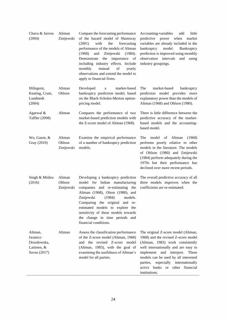
24

Chava & Jarrow

(2004)

Altman

Zmijewski

Compare the forecasting performance

of the hazard model of Shumway

(2001) with the forecasting

performance of the models of Altman

(1968) and Zmijewski (1984).

Demonstrate the importance of

including industry effects. Include

monthly instead of yearly

observations and extend the model to

apply to financial firms.

Accounting-variables add little

predictive power when market

variables are already included in the

bankruptcy model. Bankruptcy

prediction is improved using monthly

observation intervals and using

industry groupings.

Hillegeist,

Keating, Cram,

Lundstedt

(2004)

Altman

Ohlson

Developed a market-based

bankruptcy prediction model, based

on the Black-Scholes-Merton option-

pricing model.

The market-based bankruptcy

prediction model provides more

explanatory power than the models of

Altman (1968) and Ohlson (1980).

Agarwal &

Taffler (2008)

Altman Compares the performance of two

market-based prediction models with

the Z-score model of Altman (1968).

There is little difference between the

predictive accuracy of the market-

based models and the accounting-

based model.

Wu, Gaunt, &

Gray (2010)

Altman

Ohlson

Zmijewski

Examine the empirical performance

of a number of bankruptcy prediction

models.

The model of Altman (1968)

performs poorly relative to other

models in the literature. The models

of Ohlson (1980) and Zmijewski

(1984) perform adequately during the

1970s but their performance has

declined over more recent periods.

Singh & Mishra

(2016)

Altman

Ohlson

Zmijewski

Developing a bankruptcy prediction

model for Indian manufacturing

companies and re-estimating the

Altman (1968), Olson (1980), and

Zmijewski (1984) models.

Comparing the original and re-

estimated models to explore the

sensitivity of these models towards

the change in time periods and

financial conditions.

The overall predictive accuracy of all

three models improves when the

coefficients are re-estimated.

Altman,

Iwanicz-

Drozdowska,

Laitinen, &

Suvas (2017)

Altman Assess the classification performance

of the Z-score model (Altman, 1968)

and the revised Z-score model

(Altman, 1983), with the goal of

examining the usefulness of Altman’s

model for all parties.

The original Z-score model (Altman,

1968) and the revised Z-score model

(Altman, 1983) work consistently

well internationally and are easy to

implement and interpret. These

models can be used by all interested

parties, especially internationally

active banks or other financial

institutions.

25

In summary, the key articles state that the accounting-based bankruptcy prediction models of

Altman (1968, 1983), Ohlson (1980), and Zmijewski (1984) do not perform satisfactory when applied

to a different sample (e.g. more recent sample, different economic environment) than the original

sample. Mensah (1984), Grice Jr. and Dugan (2003), and Singh and Mishra (2016) suggest to re-estimate

the coefficients of the models to improve the prediction accuracy. This suggestion will be followed in

this master thesis; the coefficients will be re-estimated using the more recent data of Dutch and Belgian

public and large private firms. The articles also state that in general market-based bankruptcy prediction

models perform better than the accounting-based models. However, section 2.5 already explained that

due to the limited data availability of market data for private firms, this master thesis only examines the

accounting-based models. Finally, the articles also test whether one of the models outperforms the others

regarding their prediction power. However, the articles do not provide a conclusive answer about this.

The hypotheses, described in chapter 3, will be based on the contributions and the results of these key

research papers.

26

3 Conceptual Framework

In this chapter, several hypotheses will be provided in order to test the predictive accuracy of the

accounting-based bankruptcy prediction models of Altman (1983), Ohlson (1980), and Zmijewski

(1984) when applied to Dutch and Belgian public and large private firms.

3.1 Hypothesis 1: Model performance

This master thesis features the accounting-based bankruptcy prediction models of Altman (1983)1,

Ohlson (1980) and Zmijewski (1984). All three bankruptcy prediction models are constructed using

different statistical techniques and different samples, and include different (amount of) financial ratios.

Altman’s model (1983) includes five financial ratios as independent variables, Ohlson’s model (1980)

nine, and Zmijewski’s model (1984) three. The original studies show that the accuracy rate of the three

models are all high. Considering that the relative importance of the financial ratios used in the

bankruptcy prediction models change over time and when applied to a different environment (Mensah,

1984; Platt & Platt, 1990; Grice Jr & Dugan, 2003), it is interesting to test how these models perform

for Dutch and Belgian public and large private firms at present time. The question that arises is whether

one of these models outperforms the others regarding their prediction power when applied to Dutch and

Belgian public and large private firms.

The five financial ratios of Altman (1968, 1983) can be classified into liquidity, profitability,

leverage, solvency, and activity. Altman (1968) did not select these ratios on a theoretical basis, but on

the basis of their popularity in the literature and his belief about their potential relevancy to bankruptcy

(Grice & Ingram, 2001). The nine financial ratios of Ohlson (1980) can be classified into size, leverage,

liquidity and profitability. Ohlson (1980) selected these ratios because they appeared to be the ones most

frequently mentioned in the literature. The three financial ratios of Zmijewski (1984) can be classified

into profitability, leverage and liquidity. Zmijewski (1984) also did not select these ratios on a theoretical

basis, but on the basis of their performance in prior studies (Grice Jr. & Dugan, 2003). The model of

Ohlson (1980) includes the most financial ratios, but the model of Altman (1983) includes more different

classifications. The model of Zmijewski (1984) includes the least number of financial ratios and

different classifications. The study of Yap, Yong, and Poon (2010) examined the extent to which

financial ratios predict bankruptcy of Malaysian firms. Their results suggest that the financial ratio

categories liquidity and profitability are most significant in predicting the event of bankruptcy. The

results of the study of Liang, Lu, Tsai, and Shih (2016), based on a sample of Taiwan firms, suggest that

the financial ratios that measure solvency and profitability are the most important ratios in bankruptcy

1 Side note: The revised Z-score model of Altman (1983) is based on the original Z-score model of Altman (1968)

and includes the same variables as the original model of Altman (1968), only the market value of equity is replaced

by the book value of equity. The revised model (1983) is therefore almost equal to the original model of Altman

(1968), and because the original model (1968) is more reviewed in the existing literature, this comparison of the

predictive power for the first hypothesis includes reviews of the original model of Altman (1968).

27

prediction. The study of Cultrera and Brédart (2016) developed a bankruptcy prediction model for

Belgian firms and concludes that financial ratios reflecting the profitability and liquidity are the best

predictors of bankruptcy for Belgian firms. According to Son, Hyun, Phan, and Hwang (2019) the ratio

classifications liquidity and solvency appear to be the most important ratios for predicting bankruptcy.

Concluding, according to the literature the financial ratio categories profitability, liquidity and solvency

are the best for predicting bankruptcy. The models of Altman (1983) and Zmijewski (1984) include

these categories, the model of Ohlson (1980) lacks the category solvency. Koh and Killough (1990)

suggest that it is not necessary to include a large number of financial ratios in a model to predict

bankruptcy. All that it needs is a set of dominant ratios derived from a larger set of related ratios. Using

a smaller set of financial ratios, duplication of information resulting from highly correlated financial

ratios or the problem of multicollinearity will be avoided. Therefore, on the basis of the financial ratios

included in the models, it is expected that Zmijewski’s (1984) model outperforms the models of Altman

(1983) and Ohlson (1980). However, Shumway (2001) states that Zmijewski’s model (1984) is

essentially a one-variable model, because only one of three variables is significantly related to

bankruptcy and two variables are strongly correlated.

Existing literature extensively analysed the predictive power of the three bankruptcy prediction

models. For example, the study of Ashraf, Félix, and Serrasqueiro (2019) compared the predictive

accuracy of the three models for firms in Pakistan which are at an early stage and advanced stage of

financial distress. They concluded that Zmijewski’s model (1984) has the highest overall prediction

accuracy, Altman’s model (1968) predicts bankruptcy most accurate for both types of firms (at an early

stage and advanced stage of financial distress), and the model of Ohlson (1980) performed poorly

relative to Altman’s (1968) and Zmijewski’s (1984) model. The study of Begley et al. (1996) re-

estimated the models of Altman (1968) and Ohlson (1980) and compared the performance of Ohlson’s

original model to the re-estimated model and to that of Altman’s original and re-estimated models. They

conclude that Ohlson’s original model displays the strongest overall performance. According to Wu et

al. (2010), the model of Altman (1968) performs poorly relative to other models, among which the

models of Ohlson (1980) and Zmijewski (1984). The models of Ohlson and Zmijewski perform

adequately during the 1970’s, but their performance had deteriorated over more recent periods. Agarwal

and Taffler (2008) argue that neither of the accounting-based prediction models are a sufficient statistic

for predicting bankruptcy. Finally, Grice and Ingram (2001) and Grice Jr. and Dugan (2003) conclude

that the results of all three models to predict bankruptcy should be interpreted cautiously. In the study

of Grice Jr. and Dugan (2003), the models of Ohlson (1980) and Zmijewski (1984) were not sensitive

to industry classifications. In contrast, in the study of Grice and Ingram (2001) Altman’s model (1968)

was sensitive to industry classifications, meaning that the overall accuracy of the model was

significantly higher for manufacturing firms than for the entire sample that included non-manufacturing

firms. All three models were not sensitive to types of financial distress (Grice & Ingram, 2001; Grice Jr.

& Dugan, 2003). It can be concluded that, on the basis of the predictive power of the models, none of

28

the models outperforms the other, according to the existing literature. Therefore, the first hypothesis is

that there is no difference in the predictive power between the three models.

H1: There is no difference in the predictive power between the models of Altman (1983), Ohlson (1980),

and Zmijewski (1984).

3.2 Hypothesis 2: Econometric method performance

Whereas the first hypothesis tests the difference between the three models, this hypothesis tests the

difference between the econometric method used to develop the models. The prediction models of

Altman (1983), Ohlson (1980), and Zmijewski (1984) are developed using different econometric

methods. Altman (1983) used MDA, Ohlson (1980) used logit regression and Zmijewski (1984) used

probit regression. The question is whether one of these econometric methods outperforms the others

regarding their prediction power. Probit regression is similar to logistic regression, only the calculation

of probability differs (Dimitras et al., 1996). According to Balcaen and Ooghe (2006), logit regression

is a much more popular econometric method in bankruptcy prediction studies than probit regression.

MDA is based on certain assumptions which are mentioned in section 2.3.1. However, these assumptions

are often violated in empirical financial ratio analysis (Charitou, Neophytou, & Charalambous, 2004;

Altman et al., 2017). Logit and probit regression overcome the restricting statistical assumptions

inherent in MDA, including the assumptions that the independent variables (the financial ratios) must

be multivariate normally distributed and that the bankrupt and non-bankrupt group have equal variance-

covariance matrices (Ohlson, 1980; Begley et al., 1996; Altman et al., 2017). In addition to the less strict

assumptions, logit and probit regression have the following advantages over MDA models: (1) logit and

probit regression permit an evaluation of the significance of the individual independent variables in the

model (Mensah, 1984), and (2) the output of the MDA model is an ordinal ranking score which has little

intuitive interpretation and the output of the logit and probit models are a probability score, which makes

the results more accurate (Ohlson, 1980). The second hypothesis is that the econometric methods logit

and probit regression are more accurate than the econometric method MDA, regarding bankruptcy

prediction.

H2: All else equal, a bankruptcy prediction model using logit or probit regression is more accurate than

a bankruptcy prediction model using multiple discriminant analysis.

3.3 Hypothesis 3: Non-stationarity of the coefficients of the models

The models of Altman (1983), Ohlson (1980) and Zmijewski (1984) estimate the possibility of

bankruptcy by using a group of financial ratios. A condition to accurate predict bankruptcy is stationarity

of the independent variables (Wood & Piesse, 1987; Platt & Platt, 1990). This means that the relationship

between the independent variables and the dependent variable must be similar in the forecast and

estimation periods (Platt & Platt, 1990). However, the relative importance of the financial ratios used in

the bankruptcy prediction models changes over time (Platt & Platt, 1990; Grice Jr & Dugan, 2003).

29

Several studies (e.g., Begley et al., 1996; Hillegeist et al., 2004; Singh & Mishra, 2016, among others)

conclude that after re-estimating the coefficients of the accounting-based bankruptcy prediction models,

the coefficients of the models changed from the original values. This finding indicates that the

accounting variables are not stable over time, and that utilizing the bankruptcy prediction models using

recent data results in lower predictive ability than utilizing the models using the original data. The study

of Begley et al. (1996) shows that the models of Altman (1968) and Ohlson (1980) do not predict

bankruptcy as well in more recent periods. It appears that the prediction power of bankruptcy prediction

models declines when applied to a different environment than the original environment of the model,

which implies that the accuracy of a bankruptcy prediction model is affected by factors relating to the

environment (Mensah, 1984; Karas & Režňáková, 2014). Platt and Platt (1990) indicate that a different

environment may change the relationships between the dependent variable (bankruptcy) and

independent variables (financial ratios), the average range of the independent variables, and the

relationships among the independent variables. These differences are a result of phases of the business

cycle, changes in competition, changes in corporate strategy, and technological changes. For example,

Begley et al. (1996) argue that during the 1980s the acceptable amount of corporate debt increased and

the bankruptcy law changed, which affected the variables in the bankruptcy prediction models. The

former change affects the predictive ability of the models of Altman (1968), Ohlson (1980), and

Zmijewski (1984) because these models include leverage variables. Therefore, the same amount of debt

indicates a different probability of bankruptcy during the 1980s compared to the probability during the

period before the 1980s. Due to a change in the bankruptcy law, firms could also file for bankruptcy

because of strategic reasons. This strategic use of bankruptcy might be uncorrelated with the variables

in the bankruptcy prediction models, resulting in classification errors. Mensah (1984) states that the

financial condition of firms might be affected by external economic environments, and that these

environments change over time. Due to these external economic environmental changes, non-

stationarity in the independent variables is suspected. Mensah (1984) identifies three external

macroeconomic factors that can change over time: (1) inflation, (2) interest rates and credit availability,

and (3) business cycle (recession/expansion phases). Changes in the inflation rate leads to higher

production costs, but these costs cannot always be passed on to selling prices. However, if these costs

do get passed on, a fall in demand is the result. Higher interest rates and credit unavailability can cause

firms to fail due to the higher borrowing costs in excess of profit margins. Firms that file for bankruptcy

in the recession phase of the business cycle, are firms which cannot succeed if the sales declines

continuously. The effects that can cause failure are inadequate capitalization, insufficient cash flows,

the lack of dependable relationships with creditors, and higher than normal levels of receivables and

inventories. In contrast to an expansionary environment, where failure can occur if interest rate and

inflation dominate. The third hypothesis is divided in two parts. Hypothesis 3a states that due to the non-

stationarity of the financial ratios, the accounting-based bankruptcy prediction models will not retain

their accuracy over time.

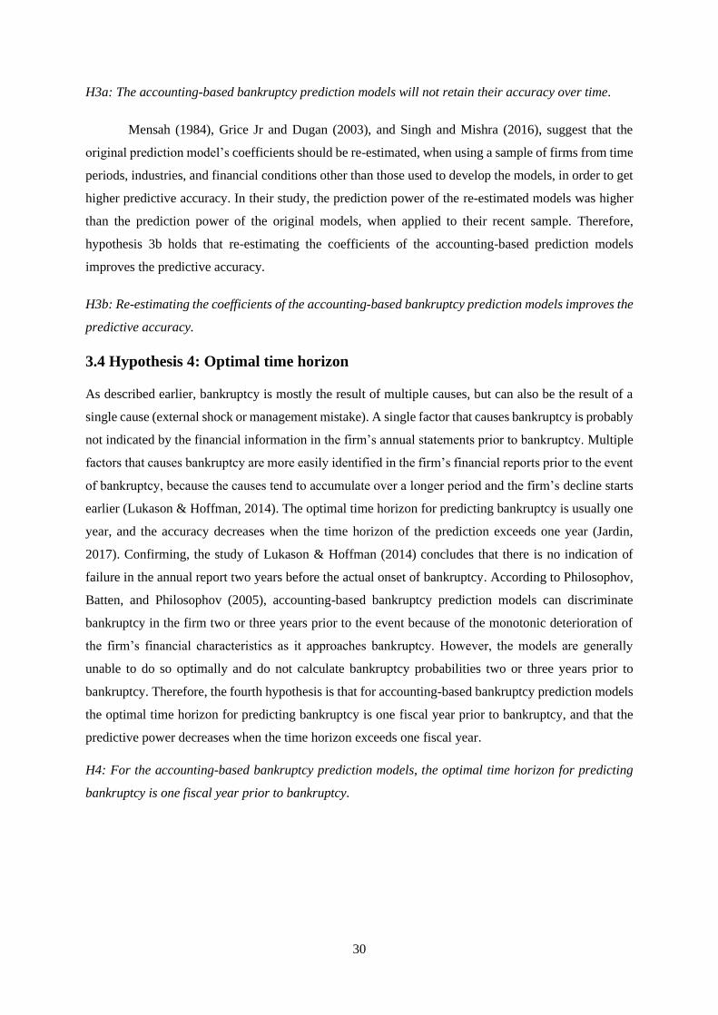
30

H3a: The accounting-based bankruptcy prediction models will not retain their accuracy over time.

Mensah (1984), Grice Jr and Dugan (2003), and Singh and Mishra (2016), suggest that the

original prediction model’s coefficients should be re-estimated, when using a sample of firms from time

periods, industries, and financial conditions other than those used to develop the models, in order to get

higher predictive accuracy. In their study, the prediction power of the re-estimated models was higher

than the prediction power of the original models, when applied to their recent sample. Therefore,

hypothesis 3b holds that re-estimating the coefficients of the accounting-based prediction models

improves the predictive accuracy.

H3b: Re-estimating the coefficients of the accounting-based bankruptcy prediction models improves the

predictive accuracy.

3.4 Hypothesis 4: Optimal time horizon

As described earlier, bankruptcy is mostly the result of multiple causes, but can also be the result of a

single cause (external shock or management mistake). A single factor that causes bankruptcy is probably

not indicated by the financial information in the firm’s annual statements prior to bankruptcy. Multiple

factors that causes bankruptcy are more easily identified in the firm’s financial reports prior to the event

of bankruptcy, because the causes tend to accumulate over a longer period and the firm’s decline starts

earlier (Lukason & Hoffman, 2014). The optimal time horizon for predicting bankruptcy is usually one

year, and the accuracy decreases when the time horizon of the prediction exceeds one year (Jardin,

2017). Confirming, the study of Lukason & Hoffman (2014) concludes that there is no indication of

failure in the annual report two years before the actual onset of bankruptcy. According to Philosophov,

Batten, and Philosophov (2005), accounting-based bankruptcy prediction models can discriminate

bankruptcy in the firm two or three years prior to the event because of the monotonic deterioration of

the firm’s financial characteristics as it approaches bankruptcy. However, the models are generally

unable to do so optimally and do not calculate bankruptcy probabilities two or three years prior to

bankruptcy. Therefore, the fourth hypothesis is that for accounting-based bankruptcy prediction models

the optimal time horizon for predicting bankruptcy is one fiscal year prior to bankruptcy, and that the

predictive power decreases when the time horizon exceeds one fiscal year.

H4: For the accounting-based bankruptcy prediction models, the optimal time horizon for predicting

bankruptcy is one fiscal year prior to bankruptcy.

31

4 Research methodology

In this chapter, the research methodology of this master thesis will be discussed. First, the focus will be

on the research design to test the hypotheses. The second section will present the variables that are used

in this master thesis. The third section, the sample selection, will describe which data and sample source

will be used in this master thesis and includes the criteria for inclusion of a firm in the samples. Finally,

a section will be devoted to testing of the model assumptions.

4.1 Hypothesis testing

4.1.1 Hypothesis 1: Model performance

Hypothesis 1 tests whether there is a statistical significant difference in the prediction power between

the models of Altman (1983), Ohlson (1980), and Zmijewski (1984). The statistical analysis begins with

re-estimating the coefficients of the models using the methodology originally employed to derive the

model. This is also done in the studies of Grice Jr and Dugan (2003), Singh and Mishra (2016) and

Altman et al. (2017). The methodologies used by the original studies of Altman (1983), Ohlson (1980),

and Zmijewski (1984) are: MDA, logit regression, and probit regression, respectively. In order to avoid

possible non-stationarity of the independent variables, the coefficients should be re-estimated as closely

as possible to the prediction period in the hope that no fundamental changes occur in the economic

environment (Mensah, 1984). Therefore, the coefficients of the models will be estimated with

observations from 2012 – 2015 and tested on a hold-out sample with observations from 2016 – 2019.

The predictive accuracy of the re-estimated models is assessed by the AUC-statistic of the hold-out

sample (see section 2.6). The difference in the prediction power between the re-estimated models is

assessed by testing the statistical significance of the difference between the AUC-statistics for the three

models. This comparison will be done using the test statistic provided by Agarwal and Taffler (2007),

formulated as equation 9 in section 2.6.

4.1.2 Hypothesis 2: Econometric method performance

Hypothesis 2 holds that a bankruptcy prediction model based on logit regression or probit regression is

more accurate than a bankruptcy prediction model based on MDA. To test this hypothesis, all three

econometric methods will be applied to all three prediction models. The models of Altman (1983),

Ohlson (1980), and Zmijewski (1984) will be re-estimated using MDA, logit regression, and probit

regression to assess the effect of the econometric estimation method. By using three different sets of

financial ratios, the possibility that a particular set of financial ratios causes a model performing better

than another can be excluded. Again, to avoid possible non-stationarity of the independent variables, the

estimation period should be as close as possible to the prediction period. Therefore, the model

coefficients will be estimated with observations from 2012 – 2015 and tested on a hold-out sample with

32

observations from 2016 – 2019. The predictive accuracy of the re-estimated models is assessed by the

AUC-statistic of the hold-out sample. For the models of Altman (1983), Ohlson (1980) and Zmijewski

(1984), the AUC-statistics of the re-estimated models using logit and probit regression will be compared

to the AUC-statistics of the re-estimated models using MDA. The test statistic of Agarwal and Taffler

(2007) will be used to test if the differences between the AUC-statistics are statistically significant.

4.1.3 Hypothesis 3: Non-stationarity of the coefficients of the models

Hypothesis 3a assumes that the accounting-based bankruptcy prediction models of Altman (1983),

Ohlson (1980), and Zmijewski (1984) will not retain their accuracy over time. Hypothesis 3b assumes

that re-estimating the coefficients of these models improves the predictive accuracy. According to Grice

Jr. and Dugan (2003) the accuracy rate of the hold-out sample is upwardly biased if (1) the time periods

of the estimation and the hold-out sample are not substantially different, (2) the hold-out sample consists

of firms from the same restricted set of industries as those in the estimation sample, and (3) the hold-out

samples are small. The first bias will be addressed by using an estimation sample from a substantially

different period than the hold-out sample. The second bias will be addressed by using a wide variety of

industries in both estimation and hold-out samples. The third bias will be addressed by using a hold-out

sample that is not smaller than the estimation sample. Unlike hypothesis 1 and 2, the coefficients of the

models will be estimated with observations from 2007 – 2010 and tested on a hold-out sample with

observations from 2016 – 2019. These time periods are chosen because of the different economic

environments. Several important events occurred during the period 2007 – 2010, such as the financial

crisis in 2007 and the European debt crisis in 2010 and the regulatory response to the financial crisis,

Basel III. Basel III imposes stricter capital requirements for banks, by increasing more liquid assets and

longer-term sources of funding (Agnese, Rizzo, & Vento, 2018). For all observations in the estimation

sample, from 2007 – 2010, bankruptcy probabilities will be computed according to each model. The

bankruptcy probabilities are also calculated for all observations in the hold-out sample, from 2016-2019.

The predictive accuracy for each model of both the estimation sample and the hold-out sample is

assessed by the AUC-statistic. For hypothesis 3a, the AUC-statistic of each model in the hold-out sample

will be compared to the AUC-statistic of the models in the estimation sample, using the test statistic of

Agarwal and Taffler (2007). For hypothesis 3b, the AUC-statistics of the hold-out sample will be

compared to the AUC-statistics of the hold-out sample of hypothesis 1. The AUC-statistics of the hold-

out sample of hypothesis 1 are estimated with observations from 2012 – 2015 instead of observations

from 2007 – 2010, which makes it possible to test if the predictive accuracy increases when the

coefficients are re-estimated more closely to the hold-out sample.

4.1.4 Hypothesis 4: Optimal time horizon

Hypothesis 4 states that the optimal time horizon for predicting bankruptcy is one fiscal year prior to

bankruptcy for the accounting-based bankruptcy prediction models of Altman (1983), Ohlson (1980),

33

and Zmijewski (1984), and that the predictive power decreases when the time horizon exceeds one fiscal

year. Again, to avoid possible non-stationarity of the independent variables, the estimation period should

be as close as possible to the prediction period. Therefore, the coefficients of the models will be

estimated with observations from 2012 – 2015 and tested on a hold-out sample with observations form

2016 – 2019. The firms in these samples will be analysed one (t-1) and two (t-2) fiscal years prior to the

event of bankruptcy or non-bankruptcy, meaning that for each firm in the sample per year data is

gathered from one and two fiscal years before the event. The predictive accuracy of the models will be

estimated for predicting bankruptcy one fiscal year and two fiscal years before the event. The AUC-

statistics of all three models from predicting bankruptcy one fiscal year before the event will be

compared to the AUC-statistics from predicting bankruptcy two fiscal years before the event, using the

test statistic of Agarwal and Taffler (2007).

4.2 Variables

4.2.1 Dependent variables

The dependent variable in all models is a dichotomous variable, a firm is either bankrupt or non-

bankrupt. For MDA, firms are classified into the bankrupt group if the score is less than the cut-off

point, and firms are classified into the non-bankrupt group if the score exceeds or equals the cut-off

point. For logit and probit regression, firms are classified into the bankrupt group if the probability score

is higher than or equal to 0.5, and firms are classified into the non-bankrupt group if the probability

score is smaller than 0.5.

4.2.2 Independent variables

The independent variables are the different financial ratios used by the three prediction models of

Altman (1983), Ohlson (1980), and Zmijewski (1984). The independent variable market value of equity

/ book value of total debt of the original Z-score model of Altman (1968) cannot be applied to private

firms, because there are no market values available for private firms. The revised Z-score model of

Altman (1983) replaced this independent variable by book value of equity / book value of total debt. The

other variables of the revised Z-score model of Altman (1983) are the same variables as in the original

Z-score model of Altman (1968). The independent variables are summarized in appendix A. For all

hypotheses, the independent variables of all three model will be used.

4.3 Sample selection

The financial ratios used in the prediction models (see appendix A) have to be calculated on the basis of

the financial statements of the Dutch and Belgian public and large private firms. Data will be obtained

from ORBIS, a database of the University of Twente. ORBIS provides data about the financial ratios of

the companies and provides information about whether a company is bankrupt or not. This master thesis

includes two different estimation samples, used to estimate the coefficients of the models, and one hold-

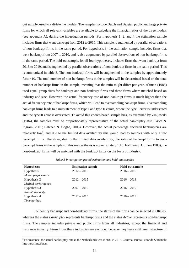
34

out sample, used to validate the models. The samples include Dutch and Belgian public and large private

firms for which all relevant variables are available to calculate the financial ratios of the three models

(see appendix A), during the investigation periods. For hypothesis 1, 2, and 4 the estimation sample

includes firms that went bankrupt from 2012 to 2015. This sample is augmented by parallel observations

of non-bankrupt firms in the same period. For hypothesis 3, the estimation sample includes firms that

went bankrupt from 2007 to 2010, and is also augmented by parallel observations of non-bankrupt firms

in the same period. The hold-out sample, for all four hypotheses, includes firms that went bankrupt from

2016 to 2019, and is augmented by parallel observations of non-bankrupt firms in the same period. This

is summarized in table 3. The non-bankrupt firms will be augmented in the samples by approximately

factor 10. The total number of non-bankrupt firms in the samples will be determined based on the total

number of bankrupt firms in the sample, meaning that the ratio might differ per year. Altman (1983)

used equal group sizes for bankrupt and non-bankrupt firms and these firms where matched based on

industry and size. However, the actual frequency rate of non-bankrupt firms is much higher than the

actual frequency rate of bankrupt firms, which will lead to oversampling bankrupt firms. Oversampling

bankrupt firms leads to a misstatement of type I and type II errors, where the type I error is understated

and the type II error is overstated. To avoid this choice-based sample bias, as examined by Zmijewski

(1984), the samples must be proportionately representative of the actual bankruptcy rate (Grice &

Ingram, 2001; Balcaen & Ooghe, 2006). However, the actual percentage declared bankruptcies are

relatively low2, and due to the limited data availability this would lead to samples with only a few

bankrupt firms. Therefore, due to the limited data availability, the ratio of bankrupt firms to non-

bankrupt firms in the samples of this master thesis is approximately 1:10. Following Altman (1983), the

non-bankrupt firms will be matched with the bankrupt firms on the basis of industry.

Table 3 Investigation period estimation and hold-out samples

Hypotheses Estimation sample Hold-out sample

Hypothesis 1

Model performance

2012 – 2015 2016 – 2019

Hypothesis 2

Method performance

2012 – 2015 2016 – 2019

Hypothesis 3

Non-stationarity

2007 – 2010 2016 – 2019

Hypothesis 4

Time horizon

2012 – 2015 2016 – 2019

To identify bankrupt and non-bankrupt firms, the status of the firms can be selected in ORBIS,

whereas the status Bankruptcy represents bankrupt firms and the status Active represents non-bankrupt

firms. The samples includes private and public firms from all industries, except the financial and

insurance industry. Firms from these industries are excluded because they have a different structure of

2 For instance, the actual bankruptcy rate in the Netherlands was 0.78% in 2018. Centraal Bureau voor de Statistiek:

http://statline.cbs.nl

35

capital than firms in other industries. Therefore, firms with a NACE Rev. 2 classification of Financial

and Insurance activities are excluded from the samples. Small firms are also excluded from the samples,

because financial reports of small firms do not provide sufficient information about the likelihood of

bankruptcy (Balcaen & Ooghe, 2006; Gupta, Gregoriou, & Healy, 2015). ORBIS divides companies on

the criteria size into four categories: Small, Medium, Large, and Very large. Only the categories Large

and Very Large are included in the samples. Meaning that companies are included in the samples when

they have an operating revenue >= €10 million, total assets >= €20 million, and number of employees

>= 150. Table 4 provides an overview of the criteria of the samples that will be used in this master thesis.

Table 4 Criteria of the samples

Criteria Value

Status (bankrupt firms) Bankruptcy

Status (non-bankrupt firms) Active

Country The Netherlands + Belgium

Legal form Private limited company + public limited company

Size Large + very large

Investigation period See table 3

NACE Rev. 2 All except financial and insurance activities

The firms in the samples will be analysed one and two fiscal years prior to the event of

bankruptcy or non-bankruptcy. Therefore, for each private firm in the samples per year, the accounting

data is gathered from financial statements one and two fiscal years before the event. Only Dutch and

Belgian private and public firms for which all relevant financial information is available during the

investigation periods will be included in the samples. After the elimination of missing values and

matching the non-bankrupt firms to bankrupt firms with a ratio of 1:10 based on industry, the final

estimation sample for hypothesis 1, 2, and 4 (period 2012 – 2015) contains 113 bankrupt and 1130 non-

bankrupt firms. The final estimation sample for hypothesis 3 (period 2007 – 2010) contains 43 bankrupt

and 412 non-bankrupt firms. The hold-out sample for all hypotheses (period 2016 – 2019) contains 71

bankrupt and 710 non-bankrupt firms. Table 5 shows the sample composition, where panel A shows the

characteristics of the 2007 – 2010 estimation sample, panel B of the 2012 – 2015 estimation sample and

panel C of the 2016 – 2019 hold-out sample. Appendix B provides a list of all the bankrupt firms in the

samples.

36

Table 5 Sample composition

Panel A: estimation sample 2007 – 2010

Industry name NACE Rev.

2 section

Bankrupt

firms

Non-bankrupt

firms

Total

Administrative and support service

activities

N 2 13 15

Construction F 2 20 22

Information and communication J 3 27 30

Manufacturing C 11 121 132

Professional, scientific and technical

activities

M 5 42 47

Transportation and storage H 4 32 36

Water supply E 1 7 8

Wholesale and retail trade G 14 150 165

Total: 42 412 454

Panel B: estimation sample 2012 – 2015

Accommodation and food service activities I 1 10 11

Administrative and support service

activities

N 7 70 77

Agriculture, forestry and fishing A 1 10 11

Arts, entertainment and recreation R 2 20 22

Construction F 16 160 176

Human health and social work activities Q 2 20 22

Information and communication J 1 10 11

Manufacturing C 35 350 385

Professional, scientific and technical

activities

M 6 60 66

Transportation and storage H 6 60 66

Water supply E 1 10 11

Wholesale and retail trade G 35 350 385

Total: 113 1130 1243

Panel C: hold-out sample 2016 – 2019

Administrative and support service

activities

N 3 30 33

Construction F 13 130 143

Information and communication J 3 30 33

Manufacturing C 11 110 121

Professional, scientific and technical

activities

M 6 60 66

Real estate activities L 2 20 22

Transportation and storage H 2 20 22

Water supply E 1 10 11

Wholesale and retail trade G 30 300 330

Total: 71 710 781

4.4 Testing model assumptions

4.4.1 Multivariate normality

Multivariate normality is an assumption for the MDA method. According to Looney (1995), many

practitioners are reluctant to test this assumption. However, testing the multivariate normality

37

assumption can be done using tests of the univariate normality assumption. Each variable separately will

be tested for univariate normality. One of the most commonly used test for univariate normality is the

Shapiro-Wilks test (Looney, 1995). This test calculates the level of significance for the differences from

a normal distribution (Hair, Black, Babin, & Anderson, 2010). If the variables are not univariate

normally distributed, multivariate normality can also be rejected because all univariate marginal

distributions of a multivariate distribution are themselves univariate normal (Looney, 1995). The null

hypothesis of the Shapiro-Wilks test is that the data are normally distributed. If the null hypothesis is

rejected (p<0.05), there is evidence that the data are not normally distributed, indicating that the

assumption of multivariate normality is violated. Appendix C.I presents the results of testing this

assumption.

4.4.2 Equality of variance-covariance

Equality of variance-covariance is also an assumption only for the MDA method. This assumption that

the dependent variable exhibits equal levels of variance and covariance across the range of independent

variables can be tested using the Box’s M statistic (Hair et al., 2010). The null hypothesis of the Box’

M test assumes that the covariance matrices are equal. If the Box’s M statistic is statistically significant

(p<0.05), it means that the null hypotheses can be rejected and that the assumption of equal variance

and covariance is violated. Appendix C.II presents the results of testing this assumption.

4.4.3 Multicollinearity

Absence of multicollinearity is an assumption for MDA, logit regression and probit regression. The

financial ratios as input for the MDA, logit regression and probit regression must be absent of

multicollinearity. If the data are present of multicollinearity, the independent variables are highly

correlated. The data will be checked for the presence of multicollinearity via the VIF-statistic. Large

VIF-statistics indicate multicollinearity, if any of the VIF-statistics exceeds 10, it can be stated that the

data are not absent of multicollinearity (Paul, 2006). Appendix C.III presents the results of testing this

assumption.

38

5 Empirical results

This chapter will provide the empirical results of this master thesis. First, the descriptive statistics for

every variable used in the different samples will be presented. Second, for each hypothesis separately,

the results of the tests will be reported.

5.1 Descriptive statistics

Table 6 presents the descriptive statistics of the data that are used to test the hypotheses. Panel A shows

the descriptive statistics of the estimation sample used in hypothesis 3, panel B the estimation sample

used in hypotheses 1 and 2, panel C the estimation sample used in hypothesis 4, panel D the hold-out

sample used in hypothesis 1, 2, and 3, and panel E the hold-out sample used in hypothesis 4. Following

Altman et al. (2017), the independent variables are winsorized to prevent the influence of outliers. In

the study of Altman et al. (2017), the independent variables are winsorized at 1 and 99 per cent.

However, Nyitrai and Virág (2019) conducted a study about different approaches for identifying and

handling outliers in bankruptcy prediction models and how these approaches affect the predictive power

of the models. They concluded that in the case of discriminant analysis and logistic regression,

winsorization is more effective when it is applied at higher cut values of the distribution, at the third or

fifth percentiles instead of the first. Therefore, in this master thesis all independent variables are

winsorized at 5 and 95 per cent to minimize outliers.

A t-test is conducted in order to determine whether there is a statistical significant difference

between the two group means. The null hypothesis of the t-test assumes equality of means between the

bankrupt and non-bankrupt group. Rejecting the null hypothesis (p<0.05) indicates that the means of the

two groups are significantly different. Additionally, an independent samples t-test is conducted to test

if the two groups have equal medians. The null hypothesis of the independent samples t-test assumes

that the medians for the bankrupt group and the non-bankrupt group are equal. Rejecting the null

hypothesis (p<0.05) indicates that the medians of the two groups are significantly different. The p-values

as a result of the t-test and median-test are presented in table 6. Panel A, B, and C show similar results,

in these three samples the means and medians of all financial ratios are significantly different between

the bankrupt and non-bankrupt group. The results of the sample presented in panel D show that only the

financial ratio SALES/TA (x5) of the model of Altman (1983) has equal means and medians between

the bankrupt and non-bankrupt group. In the sample of panel E, again the mean and median of Altman’s

(1983) financial ratio SALES/TA (x5) and the mean of Ohlson’s (1980) financial ratio OENEG (x5)

show no significant difference between the bankrupt and non-bankrupt group. The means and medians

of all other financial ratios are significantly different between the two groups.

A comparison of the bankrupt and non-bankrupt means indicates that for the Altman (1983)

variables WC/TA (x1), RE/TA (x2), EBIT/TA (x3), and BVEQ/BVTD (x4) the bankrupt means are lower

than the non-bankrupt means. For the SALES/TA (x5) variable, the bankrupt means are higher than the

39

non-bankrupt means. The data looks comparable to the data used by Grice and Ingram (2001), the mean

differences for x1, x2, x3 and x5 show the same direction. For x4, Grice and Ingram (2001) did not have

a significant mean difference. For the Ohlson (1980) variables SIZE (x1), WC/TA (x3), NI/TA (x6),

FU/TL (x7), and CHNI (x9), the bankrupt means are lower than the non-bankrupt means. For the

variables TL/TA (x2), CL/CA (x4), OENEG (x5), and INTWO (x8), the bankrupt means are higher than

the non-bankrupt means. The data used for the Ohlson (1980) variables is comparable to the data used

by Grice Jr. and Dugan (2003), the mean differences for all variables show the same direction. For the

Zmijewski (1984) variables NI/TA (x1) and CA/CL (x3) the bankrupt means are lower than the non-

bankrupt means. For the variable TD/TA (x2) the bankrupt means are higher than the non-bankrupt

means. The mean differences in this data are also comparable to the mean differences in the data used

by Grice Jr. and Dugan (2003) for all three variables. The general finding of the descriptive statistics is

that the financial ratios are significantly different between the bankrupt and the non-bankrupt group.

40

Table 6 Descriptive statistics

Panel A: Estimation sample 2007 – 2010 one fiscal year before bankruptcy

Altman WC/TA RE/TA EBIT/TA BVEQ/BVTD SALES/TA

Ba NBb B NB B NB B NB B NB

N 42 412 42 412 42 412 42 412 42 412

Mean -0.100 0.219 -0.167 0.289 -0.114 0.082 0.059 1.024 2.686 1.924

Median -0.019 0.205 0.002 0.288 -0.020 0.056 0.065 0.579 2.246 1.678

SD 0.294 0.243 0.411 0.255 0.212 0.117 0.294 1.229 1.877 1.273

Min -0.934 -0.256 -1.405 -0.221 -0.704 -0.108 -0.496 -0.037 0.117 0.169

Max 0.311 0.640 0.288 0.745 0.070 0.355 0.801 4.801 6.915 5.102

p (mean) 0.000*** 0.000*** 0.000*** 0.000*** 0.014**

p (median) 0.000*** 0.000*** 0.000*** 0.000*** 0.034**

Ohlson SIZE TL/TA WC/TA CL/CA OENEG NI/TA FU/TL INTWO CHNI

N 42 412 42 412 42 412 42 412 42 412 42 412 42 412 42 412 42 412

Mean 1.984 2.459 1.028 0.622 -0.100 0.219 1.193 0.742 0.333 0.061 -0.159 0.060 -0.089 0.176 0.381 0.114 -0.409 0.067

Median 1.969 2.438 0.939 0.633 -0.019 0.205 1.039 0.698 0 0 -0.047 0.041 -0.021 0.094 0 0 -0.722 0.045

SD 0.407 0.555 0.337 0.243 0.294 0.243 0.483 0.372 0.477 0.239 0.260 0.101 0.165 0.258 0.492 0.318 0.661 0.633

Min 1.314 1.556 0.559 0.172 -0.934 -0.256 0.584 0.216 0 0 -0.824 -0.131 -0.538 -0.161 0 0 -1 -1

Max 3.038 3.650 1.984 1.039 0.311 0.640 2.392 1.695 1 1 0.088 0.290 0.089 0.855 1 1 1 1

p (mean) 0.000*** 0.000*** 0.000*** 0.000*** 0.001*** 0.000*** 0.000*** 0.001*** 0.000***

p (median) 0.000*** 0.000*** 0.000*** 0.000*** 0.000*** 0.000*** 0.000*** 0.000*** 0.002***

Zmijewski NI/TA TD/TA CA/CL

N 42 412 42 412 42 412

Mean -0.159 0.060 1.028 0.622 0.953 1.766

Median -0.047 0.041 0.939 0.633 0.963 1.433

SD 0.260 0.101 0.337 0.243 0.321 1.024

Min -0.824 -0.131 0.559 0.172 0.418 0.590

Max 0.088 0.290 1.984 1.039 1.718 4.630

p (mean) 0.000*** 0.000*** 0.000***

p (median) 0.000*** 0.000*** 0.000***

41

Panel B: Estimation sample 2012 – 2015 one fiscal year before bankruptcy

Altman WC/TA RE/TA EBIT/TA BVEQ/BVTD SALES/TA

Ba NBb B NB B NB B NB B NB

N 113 1130 113 1130 113 1130 113 1130 113 1130

Mean -0.127 0.230 -0.189 0.291 -0.116 0.071 0.122 1.189 2.840 1.881

Median -0.047 0.231 -0.030 0.280 -0.045 0.051 0.118 0.568 2.117 1.646

SD 0.365 0.260 0.512 0.266 0.200 0.093 0.386 1.561 2.033 1.445

Min -1.034 -0.285 -1.638 -0.237 -0.682 -0.079 -0.529 0.005 0.525 0.053

Max 0.370 0.706 0.497 0.781 0.137 0.297 1.094 6.172 8.533 5.630

p (mean) 0.000*** 0.000*** 0.000*** 0.000*** 0.000***

p (median) 0.000*** 0.000*** 0.000*** 0.000*** 0.000***

Ohlson SIZE TL/TA WC/TA CL/CA OENEG NI/TA FU/TL INTWO CHNI

N 113 1130 113 1130 113 1130 113 1130 113 1130 113 1130 113 1130 113 1130 113 1130

Mean 1.967 2.462 1.011 0.608 -0.127 0.230 1.327 0.756 0.336 0.047 -0.145 0.056 -0.090 0.164 0.496 0.106 -0.225 0.029

Median 1.916 2.383 0.894 0.638 -0.047 0.231 1.057 0.668 0 0 -0.061 0.040 -0.055 0.084 0 0 -0.155 0.020

SD 0.420 0.609 0.396 0.249 0.365 0.260 0.795 0.463 0.475 0.212 0.213 0.083 0.180 0.240 0.502 0.308 0.646 0.542

Min 1.134 1.502 0.479 0.139 -1.034 -0.285 0.466 0.160 0 0 -0.733 -0.094 -0.482 -0.138 0 0 -1 -1

Max 2.757 3.761 2.122 0.995 0.370 0.706 3.764 2.102 1 1 0.128 0.257 0.300 0.830 1 1 1 1

p (mean) 0.000*** 0.000*** 0.000*** 0.000*** 0.000*** 0.000*** 0.000*** 0.000*** 0.000***

p (median) 0.000*** 0.000*** 0.000*** 0.000*** 0.000*** 0.000*** 0.000*** 0.000*** 0.003***

Zmijewski NI/TA TD/TA CA/CL

N 113 1130 113 1130 113 1130

Mean -0.145 0.056 1.011 0.608 0.977 1.941

Median -0.061 0.040 0.894 0.638 0.946 1.497

SD 0.213 0.083 0.396 0.249 0.461 1.406

Min -0.733 -0.094 0.479 0.139 0.266 0.476

Max 0.128 0.257 2.122 0.995 2.150 6.256

p (mean) 0.000*** 0.000*** 0.000***

p (median) 0.000*** 0.000*** 0.000***

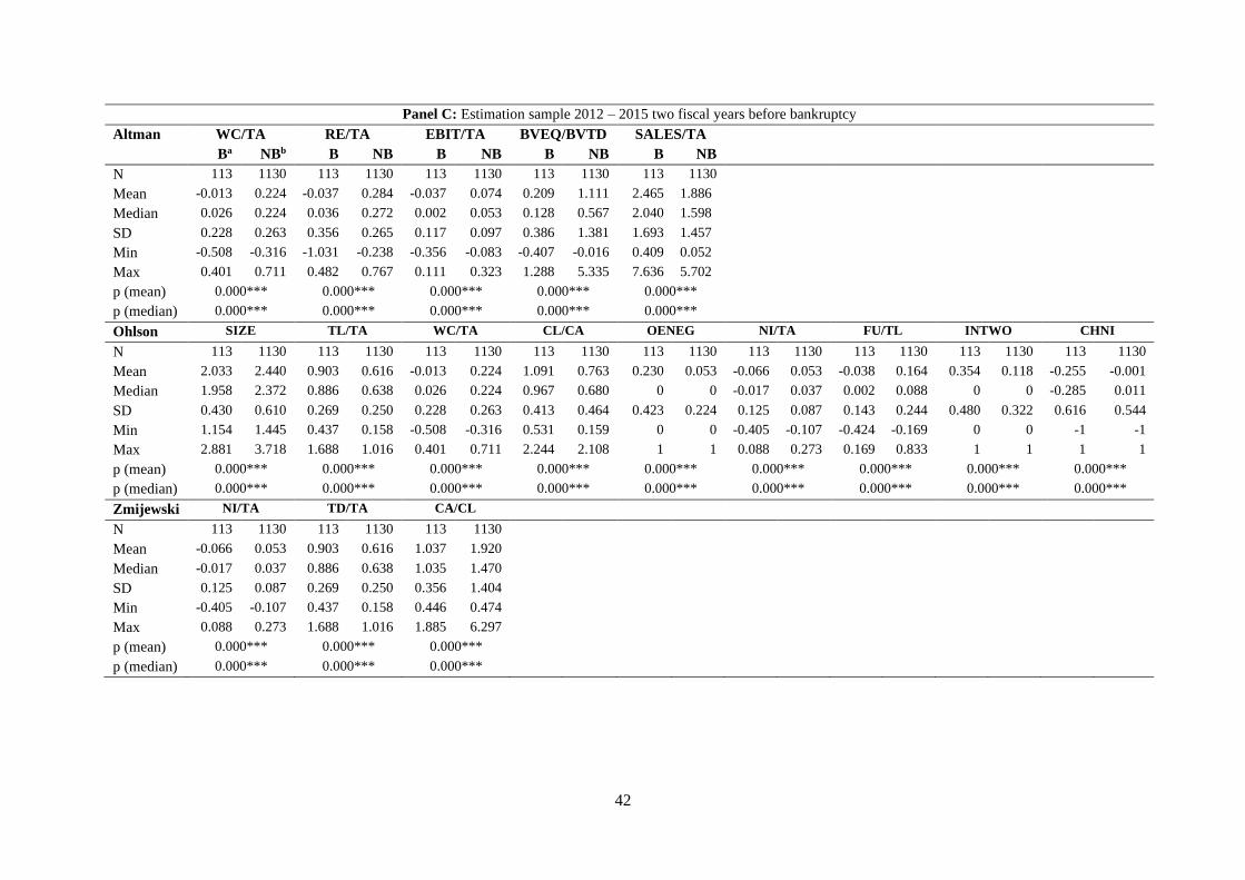
42

Panel C: Estimation sample 2012 – 2015 two fiscal years before bankruptcy

Altman WC/TA RE/TA EBIT/TA BVEQ/BVTD SALES/TA

Ba NBb B NB B NB B NB B NB

N 113 1130 113 1130 113 1130 113 1130 113 1130

Mean -0.013 0.224 -0.037 0.284 -0.037 0.074 0.209 1.111 2.465 1.886

Median 0.026 0.224 0.036 0.272 0.002 0.053 0.128 0.567 2.040 1.598

SD 0.228 0.263 0.356 0.265 0.117 0.097 0.386 1.381 1.693 1.457

Min -0.508 -0.316 -1.031 -0.238 -0.356 -0.083 -0.407 -0.016 0.409 0.052

Max 0.401 0.711 0.482 0.767 0.111 0.323 1.288 5.335 7.636 5.702

p (mean) 0.000*** 0.000*** 0.000*** 0.000*** 0.000***

p (median) 0.000*** 0.000*** 0.000*** 0.000*** 0.000***

Ohlson SIZE TL/TA WC/TA CL/CA OENEG NI/TA FU/TL INTWO CHNI

N 113 1130 113 1130 113 1130 113 1130 113 1130 113 1130 113 1130 113 1130 113 1130

Mean 2.033 2.440 0.903 0.616 -0.013 0.224 1.091 0.763 0.230 0.053 -0.066 0.053 -0.038 0.164 0.354 0.118 -0.255 -0.001

Median 1.958 2.372 0.886 0.638 0.026 0.224 0.967 0.680 0 0 -0.017 0.037 0.002 0.088 0 0 -0.285 0.011

SD 0.430 0.610 0.269 0.250 0.228 0.263 0.413 0.464 0.423 0.224 0.125 0.087 0.143 0.244 0.480 0.322 0.616 0.544

Min 1.154 1.445 0.437 0.158 -0.508 -0.316 0.531 0.159 0 0 -0.405 -0.107 -0.424 -0.169 0 0 -1 -1

Max 2.881 3.718 1.688 1.016 0.401 0.711 2.244 2.108 1 1 0.088 0.273 0.169 0.833 1 1 1 1

p (mean) 0.000*** 0.000*** 0.000*** 0.000*** 0.000*** 0.000*** 0.000*** 0.000*** 0.000***

p (median) 0.000*** 0.000*** 0.000*** 0.000*** 0.000*** 0.000*** 0.000*** 0.000*** 0.000***

Zmijewski NI/TA TD/TA CA/CL

N 113 1130 113 1130 113 1130

Mean -0.066 0.053 0.903 0.616 1.037 1.920

Median -0.017 0.037 0.886 0.638 1.035 1.470

SD 0.125 0.087 0.269 0.250 0.356 1.404

Min -0.405 -0.107 0.437 0.158 0.446 0.474

Max 0.088 0.273 1.688 1.016 1.885 6.297

p (mean) 0.000*** 0.000*** 0.000***

p (median) 0.000*** 0.000*** 0.000***

43

Panel D: Estimation sample 2016 – 2019 one fiscal year before bankruptcy

Altman WC/TA RE/TA EBIT/TA BVEQ/BVTD SALES/TA

Ba NBb B NB B NB B NB B NB

N 71 710 71 710 71 710 71 710 71 710

Mean -0.101 0.209 -0.258 0.297 -0.158 0.067 0.286 0.966 2.045 2.040

Median -0.043 0.190 0.004 0.257 -0.043 0.057 0.090 0.529 1.770 1.764

SD 0.484 0.247 0.839 0.235 0.311 0.076 0.819 1.140 1.395 1.480

Min -1.551 -0.234 -3.529 -0.080 -1.195 -0.075 -0.617 0.017 0.213 0.112

Max 0.692 0.873 0.685 0.771 0.145 0.244 3.005 4.313 5.800 5.682

p (mean) 0.000*** 0.000*** 0.000*** 0.000*** 0.975

p (median) 0.000*** 0.000*** 0.000*** 0.000*** 0.902

Ohlson SIZE TL/TA WC/TA CL/CA OENEG NI/TA FU/TL INTWO CHNI

N 71 710 71 710 71 710 71 710 71 710 71 710 71 710 71 710 71 710

Mean 2.067 2.650 1.015 0.628 -0.101 0.209 1.361 0.778 0.282 0.034 -0.219 0.049 -0.118 0.148 0.437 0.076 -0.243 0.017

Median 2.021 2.513 0.917 0.654 -0.043 0.190 1.045 0.720 0 0 -0.083 0.041 -0.043 0.091 0 0 -0.293 0.042

SD 0.379 0.675 0.534 0.231 0.484 0.246 1.072 0.407 0.453 0.181 0.361 0.072 0.242 0.188 0.499 0.265 0.669 0.527

Min 1.403 1.693 0.250 0.188 -1.551 -0.234 0.232 0.188 0 0 -1.300 -0.097 -0.781 -0.098 0 0 -1 -1

Max 2.891 4.144 2.736 0.983 0.692 0.689 4.935 1.882 1 1 0.091 0.228 0.286 0.659 1 1 1 1

p (mean) 0.000*** 0.000*** 0.000*** 0.000*** 0.000*** 0.000*** 0.000*** 0.000*** 0.002***

p (median) 0.000*** 0.000*** 0.000*** 0.000*** 0.000*** 0.000*** 0.000*** 0.000*** 0.081*

Zmijewski NI/TA TD/TA CA/CL

N 71 710 71 710 71 710

Mean -0.219 0.049 1.015 0.628 1.156 1.751

Median -0.083 0.041 0.917 0.654 0.957 1.388

SD 0.361 0.072 0.534 0.231 0.912 1.156

Min -1.300 -0.097 0.250 0.188 0.204 0.532

Max 0.091 0.228 2.736 0.983 4.383 5.306

p (mean) 0.000*** 0.000*** 0.000***

p (median) 0.000*** 0.000*** 0.000***

44

Panel E: Estimation sample 2016 – 2019 two fiscal years before bankruptcy

Altman WC/TA RE/TA EBIT/TA BVEQ/BVTD SALES/TA

Ba NBb B NB B NB B NB B NB

N 71 710 71 710 71 710 71 710 71 710

Mean 0.073 0.208 0.042 0.293 -0.034 0.067 0.498 0.960 1.854 2.045

Median 0.066 0.184 0.047 0.270 0.000 0.057 0.216 0.510 1.641 1.736

SD 0.271 0.248 0.341 0.230 0.123 0.070 0.952 1.151 1.163 1.462

Min -0.515 -0.255 -0.988 -0.055 -0.388 -0.055 -0.312 0.023 0.134 0.155

Max 0.653 0.691 0.703 0.756 0.123 0.224 3.919 4.424 4.870 5.562

p (mean) 0.000*** 0.000*** 0.000*** 0.000*** 0.200

p (median) 0.006*** 0.000*** 0.000*** 0.000*** 0.804

Ohlson SIZE TL/TA WC/TA CL/CA OENEG NI/TA FU/TL INTWO CHNI

N 71 710 71 710 71 710 71 710 71 710 71 710 71 710 71 710 71 710

Mean 2.136 2.640 0.802 0.630 0.073 0.208 0.994 0.767 0.085 0.030 -0.046 0.050 -0.031 0.142 0.408 0.082 -0.138 0.037

Median 2.116 2.518 0.822 0.662 0.066 0.184 0.903 0.719 0 0 -0.002 0.039 -0.005 0.090 0 0 -0.172 0.038

SD 0.358 0.692 0.259 0.230 0.271 0.248 0.492 0.377 0.280 0.170 0.107 0.064 0.153 0.169 0.495 0.274 0.618 0.496

Min 1.466 1.672 0.204 0.184 -0.515 -0.255 0.213 0.206 0 0 -0.366 -0.075 -0.403 -0.086 0 0 -1 -1

Max 2.939 4.178 1.456 0.977 0.653 0.691 2.358 1.732 1 1 0.071 0.199 0.287 0.593 1 1 1 1

p (mean) 0.000*** 0.000*** 0.000*** 0.000*** 0.109 0.000*** 0.000*** 0.000*** 0.024**

p (median) 0.000*** 0.000*** 0.006*** 0.000*** 0.029** 0.000*** 0.000*** 0.000*** 0.001***

Zmijewski NI/TA TD/TA CA/CL

N 71 710 71 710 71 710

Mean -0.046 0.050 0.802 0.630 1.338 1.725

Median -0.002 0.039 0.822 0.662 1.108 1.391

SD 0.107 0.064 0.259 0.230 0.965 1.070

Min -0.366 -0.075 0.204 0.184 0.432 0.577

Max 0.071 0.199 1.456 0.977 4.699 4.846

p (mean) 0.000*** 0.000*** 0.002***

p (median) 0.000*** 0.000*** 0.000***

Variable definitions are as follows: WC/TA = working capital/total assets, RE/TA = retained earnings/total assets, EBIT/TA = earnings before interest and taxes/total assets, BVEQ/BVTD

= book value equity/book value of total debt, SALES/TA = sales/total assets, SIZE = log(total assets/GNP price-level index), TL/TA = total liabilities/total assets, WC/TA = working

capital/total assets, CL/CA = current liabilities/current assets, OENEG = 1 if total liabilities > total assets, 0 otherwise, NI/TA = net income/total assets, FU/TL = funds provided by

operations/total liabilities, INTWO = 1 if net income was negative for the last two years, 0 otherwise, CHNI = change in net income for the last to previous year, NI/TA = net income/total

assets, TD/TA = total debt/total assets, CA/CL = current assets/current liabilities a B= bankrupt firms b NB = non-bankrupt firms ***<1% **<5% *<10%

45

5.2 Difference between Dutch and Belgian firms

The Netherlands and Belgium have different bankruptcy procedures, which are discussed in section

2.1.3 and 2.1.4. Therefore, before testing the hypotheses, it is tested if the prediction accuracy differs

between these two countries. For this test, the models of Altman (1983), Ohlson (1980), and Zmijewski

(1984) are developed using the estimation sample with firm observations from 2012 – 2015 and tested

on the hold-out sample with firm observations from 2016 – 2019. Each model is developed when applied

only on Dutch firms and when applied only on Belgian firms, and data from one fiscal year before the

event of bankruptcy is used. The test statistic (z) of Agarwal and Taffler (2007) is used to compare the

AUC-statistics of the two countries. The results are shown in table 7, where panel A shows the results

of Dutch firms, panel B the results of Belgian firms, and panel C the test statistics. The table reports

both the in sample and out-of-sample results, however, only the out-of-sample results will be further

analysed since the in sample results only measure classification accuracy, not predictive accuracy.

The model of Altman (1983) has an out-of-sample AUC-score of 0.564 (AR = 12.80%) when

applied to Dutch firms only, and 0.658 (AR = 31.60%) when applied to Belgian firms only. Ohlson’s

model (1980) has an out-of-sample AUC-score of 0.667 (AR = 33.40%) when applied to Dutch firms

only, and 0.737 (47.40%) when applied to Belgian firms only. Zmijewski’s model (1984) has an out-of-

sample AUC-score of 0.667 (AR = 33.40%) when applied to Dutch firms only, and 0.714 (AR = 42.80%)

when applied to Belgian firms only. All three test statistics, as reported in panel C of table 7, are not

statistical significant. This indicates that the prediction accuracy does not differ between the Netherlands

and Belgium.

46

Table 7 Comparing predictive accuracy Dutch and Belgian firms

Panel A: Dutch firms

AUC-statistic Accuracy ratio

In sample Out-of-sample In sample Out-of-sample

N 605 350 605 350

I. Altman (1983)

MDA

0.639**

(0.066)

0.564

(0.078)

27.80% 12.80%

II. Ohlson (1980)

Logit regression

0.690***

(0.065)

0.667**

(0.078)

38.00% 33.40%

III. Zmijewski (1984)

Probit regression

0.619*

(0.066)

0.667**

(0.078)

23.80% 33.40%

Panel B: Belgian firms

N 638 431 638 431

IV. Altman (1983)

MDA

0.687***

(0.032)

0.658***

(0.042)

37.40% 31.60%

V. Ohlson (1980)

Logit regression

0.735***

(0.031)

0.737***

(0.040)

47.00% 47.40%

VI. Zmijewski (1984)

Probit regression

0.722***

(0.032)

0.714***

(0.041)

44.40% 42.80%

Panel C: Test statistic

z (IV – I) 0.654 1.061

z (V – II) 0.625 0.799

z (VI – III) 1.404 0.533

The AUC-statistic measures predictive accuracy and has a value between 0 and 1. A value of 0.5 indicates a

random model and a value of 1.0 shows a perfect model. Standard errors in parentheses. The accuracy ratio (AR)

is a scaled version of the AUC-statistic. The test statistic z is used to compare the AUC-statistics.

***<1%

**<5%

*<10%

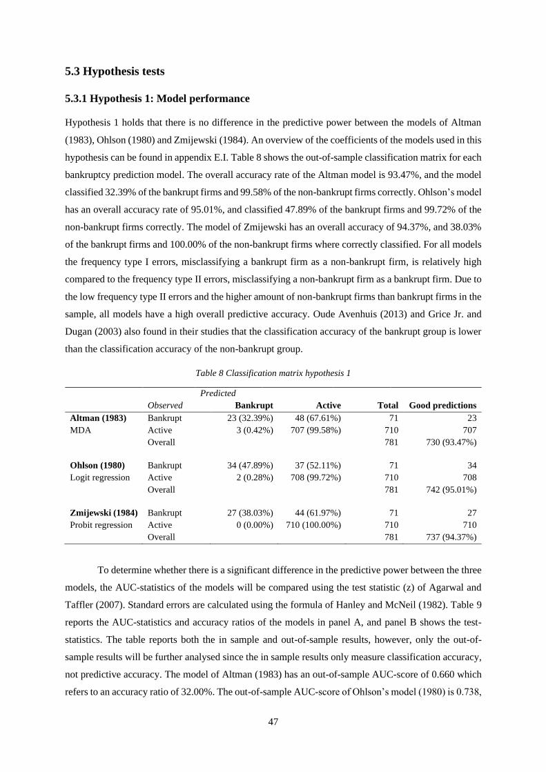
47

5.3 Hypothesis tests

5.3.1 Hypothesis 1: Model performance

Hypothesis 1 holds that there is no difference in the predictive power between the models of Altman

(1983), Ohlson (1980) and Zmijewski (1984). An overview of the coefficients of the models used in this

hypothesis can be found in appendix E.I. Table 8 shows the out-of-sample classification matrix for each

bankruptcy prediction model. The overall accuracy rate of the Altman model is 93.47%, and the model

classified 32.39% of the bankrupt firms and 99.58% of the non-bankrupt firms correctly. Ohlson’s model

has an overall accuracy rate of 95.01%, and classified 47.89% of the bankrupt firms and 99.72% of the

non-bankrupt firms correctly. The model of Zmijewski has an overall accuracy of 94.37%, and 38.03%

of the bankrupt firms and 100.00% of the non-bankrupt firms where correctly classified. For all models

the frequency type I errors, misclassifying a bankrupt firm as a non-bankrupt firm, is relatively high

compared to the frequency type II errors, misclassifying a non-bankrupt firm as a bankrupt firm. Due to

the low frequency type II errors and the higher amount of non-bankrupt firms than bankrupt firms in the

sample, all models have a high overall predictive accuracy. Oude Avenhuis (2013) and Grice Jr. and

Dugan (2003) also found in their studies that the classification accuracy of the bankrupt group is lower

than the classification accuracy of the non-bankrupt group.

Table 8 Classification matrix hypothesis 1

Predicted

Observed Bankrupt Active Total Good predictions

Altman (1983) Bankrupt 23 (32.39%) 48 (67.61%) 71 23

MDA Active 3 (0.42%) 707 (99.58%) 710 707

Overall 781 730 (93.47%)

Ohlson (1980) Bankrupt 34 (47.89%) 37 (52.11%) 71 34

Logit regression Active 2 (0.28%) 708 (99.72%) 710 708

Overall 781 742 (95.01%)

Zmijewski (1984) Bankrupt 27 (38.03%) 44 (61.97%) 71 27

Probit regression Active 0 (0.00%) 710 (100.00%) 710 710

Overall 781 737 (94.37%)

To determine whether there is a significant difference in the predictive power between the three

models, the AUC-statistics of the models will be compared using the test statistic (z) of Agarwal and

Taffler (2007). Standard errors are calculated using the formula of Hanley and McNeil (1982). Table 9

reports the AUC-statistics and accuracy ratios of the models in panel A, and panel B shows the test-

statistics. The table reports both the in sample and out-of-sample results, however, only the out-of-

sample results will be further analysed since the in sample results only measure classification accuracy,

not predictive accuracy. The model of Altman (1983) has an out-of-sample AUC-score of 0.660 which

refers to an accuracy ratio of 32.00%. The out-of-sample AUC-score of Ohlson’s model (1980) is 0.738,

48

and its accuracy ratio 47.60%. Zmijewski’s model (1984) has an out-of-sample AUC-score of 0.690 and

accuracy ratio of 38.00%. It is clear that not one of the models outperforms the other models, since all

three test statistics, as reported in panel B of table 9, are not statistical significant. This indicates that

there is no statistical significant difference between the three prediction models. Therefore, hypothesis

1 is not rejected.

Table 9 Comparing predictive accuracy hypothesis 1

Panel A: AUC-statistic and accuracy ratio

AUC-statistic Accuracy ratio

In sample Out-of-sample In sample Out-of-sample

N 1243 781 1243 781

I. Altman (1983)

MDA

0.683***

(0.029)

0.660***

(0.037)

36.60% 32.00%

II. Ohlson (1980)

Logit regression

0.714***

(0.028)

0.738***

(0.035)

42.80% 47.60%

III. Zmijewski (1984)

Probit regression

0.704***

(0.028)

0.690***

(0.036)

40.80% 38.00%

Panel B: Test statistic

z (II – I) 0.769 1.531

z (III – I) 0.521 0.581

z (III – II) -0.253 -0.956

The AUC-statistic measures predictive accuracy and has a value between 0 and 1. A value of 0.5 indicates a

random model and a value of 1.0 shows a perfect model. Standard errors in parentheses. The accuracy ratio (AR)

is a scaled version of the AUC-statistic. The test statistic z is used to compare the AUC-statistics.

***<1%

**<5%

*<10%

5.3.2 Hypothesis 2: Econometric method performance

Hypothesis 2 holds that a bankruptcy prediction model using logit regression or probit regression is

more accurate than a bankruptcy prediction model using MDA. An overview of the coefficients of the

models used in this hypothesis can be found in appendix E.I. Table 10 shows the out-of-sample

classification matrix of each particular prediction model, where panel A represents the models with the

variables of Altman (1983), panel B the models with the variables of Ohlson (1980), and panel C the

models with the variables of Zmijewski (1984). For each set of variables, the models are estimated by

MDA, logit regression and probit regression. The original econometric method for the models of Altman

(1983), Ohlson (1980), and Zmijewski (1984) are MDA, logit regression, and probit regression,

respectively. The out-of-sample classification results of the prediction models estimated with their

original econometric method are already reported in table 8 from hypothesis 1, but for clarity also

reported in table 10. The models estimated by MDA classified 32.39% (Altman’s variables), 39.44%

(Ohlson’s variables), and 36.62% (Zmijewski’s variables) of the bankrupt firms correctly. The models

estimated by logit regression classified 38.03% (Altman’s variables), 47.89% (Ohlson’s variables), and

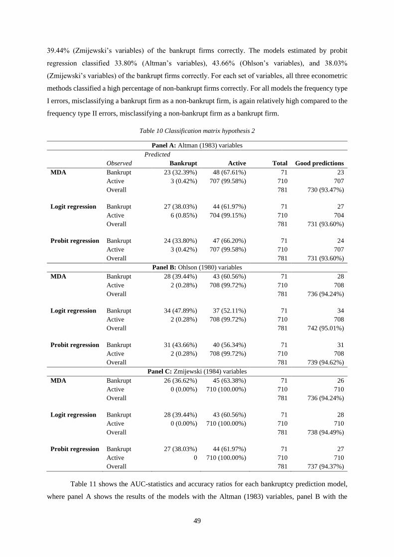
49

39.44% (Zmijewski’s variables) of the bankrupt firms correctly. The models estimated by probit

regression classified 33.80% (Altman’s variables), 43.66% (Ohlson’s variables), and 38.03%

(Zmijewski’s variables) of the bankrupt firms correctly. For each set of variables, all three econometric

methods classified a high percentage of non-bankrupt firms correctly. For all models the frequency type

I errors, misclassifying a bankrupt firm as a non-bankrupt firm, is again relatively high compared to the

frequency type II errors, misclassifying a non-bankrupt firm as a bankrupt firm.

Table 10 Classification matrix hypothesis 2

Panel A: Altman (1983) variables

Predicted

Observed Bankrupt Active Total Good predictions

MDA Bankrupt 23 (32.39%) 48 (67.61%) 71 23

Active 3 (0.42%) 707 (99.58%) 710 707

Overall 781 730 (93.47%)

Logit regression Bankrupt 27 (38.03%) 44 (61.97%) 71 27

Active 6 (0.85%) 704 (99.15%) 710 704

Overall 781 731 (93.60%)

Probit regression Bankrupt 24 (33.80%) 47 (66.20%) 71 24

Active 3 (0.42%) 707 (99.58%) 710 707

Overall 781 731 (93.60%)

Panel B: Ohlson (1980) variables

MDA Bankrupt 28 (39.44%) 43 (60.56%) 71 28

Active 2 (0.28%) 708 (99.72%) 710 708

Overall 781 736 (94.24%)

Logit regression Bankrupt 34 (47.89%) 37 (52.11%) 71 34

Active 2 (0.28%) 708 (99.72%) 710 708

Overall 781 742 (95.01%)

Probit regression Bankrupt 31 (43.66%) 40 (56.34%) 71 31

Active 2 (0.28%) 708 (99.72%) 710 708

Overall 781 739 (94.62%)

Panel C: Zmijewski (1984) variables

MDA Bankrupt 26 (36.62%) 45 (63.38%) 71 26

Active 0 (0.00%) 710 (100.00%) 710 710

Overall 781 736 (94.24%)

Logit regression Bankrupt 28 (39.44%) 43 (60.56%) 71 28

Active 0 (0.00%) 710 (100.00%) 710 710

Overall 781 738 (94.49%)

Probit regression Bankrupt 27 (38.03%) 44 (61.97%) 71 27

Active 0 710 (100.00%) 710 710

Overall 781 737 (94.37%)

Table 11 shows the AUC-statistics and accuracy ratios for each bankruptcy prediction model,

where panel A shows the results of the models with the Altman (1983) variables, panel B with the

50

Ohlson (1980) variables, panel C with the Zmijewski (1984) variables. Each model is estimated by

MDA, logit regression and probit regression. The AUC-statistics and accuracy ratios of the prediction

models estimated with their original econometric method are already reported in table 9 from hypothesis

1, but for clarity also reported in table 11. Again, for the same reason as in hypothesis 1, only the out-

of-sample results will be analysed. The Agarwal and Taffler (2007) test statistic (z) is used to compare

the AUC-statistics. The out-of-sample AUC-score of the model with the Altman (1983) variables is

0.660 (AR = 32.00%) when estimated by MDA, 0.686 (AR = 37.20%) when estimated by logit

regression, and 0.667 (AR = 33.40%) when estimated by probit regression. The test statistics are not

statistically significant, indicating that estimating prediction models with logit regression or probit

regression instead of MDA does not significantly improve the AUC-score with the Altman (1983)

variables. The models with the Ohlson (1980) variables show similar results. The out-of-sample AUC-

score of this model is 0.696 (AR = 39.20%) when estimated by MDA, 0.738 (AR = 47.60%) when

estimated by logit regression, and 0.717 (AR = 43.40%) when estimated by probit regression. The test

statistics are not statistically significant, the AUC-scores are not significantly improved by using logit

regression or probit regression instead of MDA for the Ohlson (1980) variables. The models with the

Zmijewski (1984) variables also show similar results. This model has an out-of-sample AUC-score of

0.683 (AR = 36.60%) when estimated by MDA, 0.697 (AR = 39.40%) when estimated by logit

regression, and 0.690 (AR = 38.00%) when estimated by probit regression. Again, all the test statistics

are not significant. The AUC-score for the Zmijewski (1984) variables is not significantly improved

when estimating the models by logit regression or probit regression instead of MDA. Concluding,

prediction models estimated by logit regression or probit regression are not significantly more accurate

than the bankruptcy prediction models estimated by MDA. Therefore, hypothesis 2 is rejected.

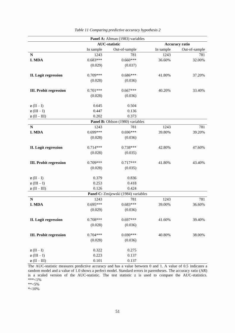
51

Table 11 Comparing predictive accuracy hypothesis 2

Panel A: Altman (1983) variables

AUC-statistic Accuracy ratio

In sample Out-of-sample In sample Out-of-sample

N 1243 781 1243 781

I. MDA

0.683***

(0.029)

0.660***

(0.037)

36.60% 32.00%

II. Logit regression 0.709***

(0.028)

0.686***

(0.036)

41.80% 37.20%

III. Probit regression 0.701***

(0.028)

0.667***

(0.036)

40.20% 33.40%

z (II – I) 0.645 0.504

z (III – I) 0.447 0.136

z (II – III) 0.202 0.373

Panel B: Ohlson (1980) variables

N 1243 781 1243 781

I. MDA

0.699***

(0.028)

0.696***

(0.036)

39.80% 39.20%

II. Logit regression 0.714***

(0.028)

0.738***

(0.035)

42.80% 47.60%

III. Probit regression 0.709***

(0.028)

0.717***

(0.035)

41.80% 43.40%

z (II – I) 0.379 0.836

z (III – I) 0.253 0.418

z (II – III) 0.126 0.424

Panel C: Zmijewski (1984) variables

N 1243 781 1243 781

I. MDA

0.695***

(0.029)

0.683***

(0.036)

39.00% 36.60%

II. Logit regression 0.708***

(0.028)

0.697***

(0.036)

41.60% 39.40%

III. Probit regression 0.704***

(0.028)

0.690***

(0.036)

40.80% 38.00%

z (II – I) 0.322 0.275

z (III – I) 0.223 0.137

z (II – III) 0.101 0.137

The AUC-statistic measures predictive accuracy and has a value between 0 and 1. A value of 0.5 indicates a

random model and a value of 1.0 shows a perfect model. Standard errors in parentheses. The accuracy ratio (AR)

is a scaled version of the AUC-statistic. The test statistic z is used to compare the AUC-statistics.

***<1%

**<5%

*<10%

52

5.3.3 Hypothesis 3: Non-stationarity of the coefficients of the models

Hypothesis 3a holds that the accounting-based bankruptcy prediction models will not retain their

accuracy over time. Hypothesis 3b holds that re-estimating the coefficients of these models will improve

the predictive accuracy. An overview of the coefficients of the models used in this hypothesis can be

found in appendix E.II. Table 12 shows the classification matrix of the models, where panel A shows

the in-sample results of the estimation sample 2007 – 2010, panel B the out-of-sample results of the

estimation sample 2007 – 2010 (tested on the hold-out sample 2016 – 2019), and panel C the out-of-

sample results of the estimation sample 2012 – 2015 from hypothesis 1 (tested on the hold-out sample

2016 – 2019).

To test hypothesis 3a, the out-of-sample results in panel A will be compared to the in sample

results of panel B. If the prediction models do not retain their accuracy over time, the results in panel B

should be lower than the results in panel A. The model of Altman (1983) classified 28.57% of the

bankrupt firms correctly with the estimation sample and 29.58% with the hold-out sample. Ohlson’s

model (1980) classified 42.86% of the bankrupt firms correctly with the estimation sample and 43.66%

with the hold-out sample. Zmijewski’s model (1984) classified 28.57% of the bankrupt firms correctly

with the estimation sample and 36.62% with the hold-out sample.

To test hypothesis 3b, the out-of-sample results in panel B will be compared to the out-of-sample

results in panel C. If re-estimating the coefficients of the models does improve the predictive accuracy,

the results in panel C should be higher than the results in panel B. For Altman’s model (1983) the

classification percentage of bankrupt firms is 29.58% when estimated with observations from 2007 –

2010, and 32.39% when the coefficients are re-estimated with observations from 2012 – 2015. For

Ohlson’s model (1980) the classification percentage of bankrupt firms is 43.66% for the 2007 – 2010

observations and 47.89% for the 2012 – 2015 observations. The model of Zmijewski (1984) classified

36.62% of the bankrupt firms correctly with the estimation sample 2007 – 2010 and 38.03% with the

estimation sample 2012 – 2015.

All models are able to classify (most of) the non-bankrupt firms correctly. Again, for all models

the frequency type I errors, misclassifying a bankrupt firm as a non-bankrupt firm, is relatively high

compared to the type II errors, misclassifying a non-bankrupt firm as a bankrupt firm.

53

Table 12 Classification matrix hypothesis 3

Panel A: In sample

(estimation sample 2007 – 2010)

Predicted

Observed Bankrupt Active Total Good predictions

Altman (1983) Bankrupt 12 (28.57%) 30 (71.43%) 42 12

MDA Active 4 (0.97%) 408 (99.03%) 412 408

Overall 454 420 (92.51%)

Ohlson (1980) Bankrupt 18 (42.86%) 24 (57.14%) 42 18

Logit regression Active 5 (1.21%) 407 (98.77%) 412 407

Overall 454 425 (93.61%)

Zmijewski (1984) Bankrupt 12 (28.57%) 30 (71.43%) 42 12

Probit regression Active 0 (0.00%) 412 (100.00%) 412 412

Overall 454 424 (93.39%)

Panel B: Out-of-sample

(estimation sample 2007 – 2010 tested on hold-out sample 2016 – 2019)

Altman (1983) Bankrupt 21 (29.58%) 50 (70.42%) 71 21

MDA Active 4 (0.56%) 706 (99.44%) 710 706

Overall 781 727 (93.09%)

Ohlson (1980) Bankrupt 31 (43.66%) 40 (56.34%) 71 31

Logit regression Active 4 (0.56%) 706 (99.44%) 710 706

Overall 781 737 (94.37%)

Zmijewski (1984) Bankrupt 26 (36.62%) 45 (63.38%) 71 26

Probit regression Active 0 (0.00%) 710 (100.00%) 710 710

Overall 781 736 (94.24%)

Panel C: Out-of-sample H1

(estimation sample 2012 – 2015 tested on hold-out sample 2016 – 2019)

Altman (1983) Bankrupt 23 (32.39%) 48 (67.61%) 71 23

MDA Active 3 (0.42%) 707 (99.58%) 710 707

Overall 781 730 (93.47%)

Ohlson (1980) Bankrupt 34 (47.89%) 37 (52.11%) 71 34

Logit regression Active 2 (0.28%) 708 (99.72%) 710 708

Overall 781 742 (95.01%)

Zmijewski (1984) Bankrupt 27 (38.03%) 44 (61.97%) 71 27

Probit regression Active 0 710 (100.00%) 710 710

Overall 781 737 (94.37%)

Table 13 shows the AUC-statistics and accuracy ratios to test hypothesis 3a and 3b. The test

statistic (z) of Agarwal and Taffler (2007) is used to test whether the difference between the AUC-

statistics is statistically significant. For hypothesis 3a, the AUC-scores of the columns I and II will be

compared. For Altman’s model (1983) the in sample AUC-score is 0.638 (AR = 27.60%), and the out-

of-sample AUC-score is 0.645 (AR = 29.00%). The model of Ohlson (1980) has an in sample AUC-

score of 0.708 (AR = 41.60%), and an out-of-sample AUC-score of 0.715 (AR = 43.00%). Zmijewski’s

54

model (1984) has an in sample AUC-score of 0.643 (AR = 28.60%), and an out-of-sample AUC-score

of 0.683 (AR = 36.60%). For this hypothesis, the first test statistic z (II – I) compares the AUC-statistics.

For all three models, this test statistic is not statistically significant. This indicates that the bankruptcy

prediction models do retain their accuracy over time. Therefore, hypothesis 3a is rejected.

For hypothesis 3b, the AUC-scores of the columns III and II will be compared. Altman’s model

(1983) has an out-of-sample AUC-score of 0.645 (AR = 29.00%) for the estimation sample 2007 – 2010,

and an out-of-sample AUC-score of 0.660 (AR = 32.00%) for the estimation sample 2012 – 2015. For

the model of Ohlson (1980), the out-of-sample AUC-score for the estimation sample 2007 – 2010 is

0.715 (AR = 43.00%), and the out-of-sample AUC-score for the estimation sample 2012 – 2015 is 0.738

(AR = 47.60%). The model of Zmijewski (1984) has an out-of-sample AUC-score of 0.683 (AR =

36.60%) for the estimation sample 2007 – 2010, and an out-of-sample AUC-score of 0.690 (AR =

38.00%) for the estimation sample 2012 – 2015. For this hypothesis, the second test statistic z (III – II)

is used. For all three models, this test statistic is not statistically significant, indicating that re-estimating

the coefficients of the models does not improve the predictive accuracy. Therefore, hypothesis 3b is also

rejected.

Table 13 Comparing predictive accuracy hypothesis 3

Panel A: AUC-statistics and accuracy ratios

AUC-statistic Accuracy ratio

I. In sample II. Out-of-

sample

III. Out-of-

sample H1

In sample Out-of-

sample

Out-of-

sample H1

N 454 781 781 454 781 781

Altman (1983)

MDA

0.638***

(0.048)

0.645***

(0.037)

0.660**

(0.037)

27.60% 29.00% 32.00%

Ohlson (1980)

Logit regression

0.708***

(0.046)

0.715***

(0.036)

0.738***

(0.035)

41.60%

43.00% 47.60%

Zmijewski (1984)

Probit regression

0.643***

(0.048)

0.683***

(0.036)

0.690***

(0.036)

28.60% 36.60% 38.00%

Panel B: Test statistic

Altman

(1983)

Ohlson

(1980)

Zmijewski

(1984)

z (II – I) 0.116 0.120 0.667

z (III – II) 0.287 0.458 0.137

The AUC-statistic measures predictive accuracy and has a value between 0 and 1. A value of 0.5 indicates a

random model and a value of 1.0 shows a perfect model. Standard errors in parentheses. The accuracy ratio (AR)

is a scaled version of the AUC-statistic. The test statistic z is used to compare the AUC-statistics.

***<1%

**<5%

*<10%

5.3.4 Hypothesis 4: Optimal time horizon

Hypothesis 4 holds that the optimal time horizon for predicting bankruptcy is one fiscal year prior to

bankruptcy. An overview of the coefficients of the models used in this hypothesis can be found in

55

appendix E.III. Table 14 shows the out-of-sample classification matrix of the prediction models, where

panel A shows the results of the prediction one fiscal year before bankruptcy, and panel B the results of

the prediction two fiscal years before bankruptcy. The results in panel A are the same results as reported

in table 8 of hypothesis 1. Altman’s model (1983) classified 32.39% of the bankrupt firms correctly with

a time horizon of one year, and 12.68% with a time horizon of two years. The model of Ohlson (1980)

classified 47.89% bankrupt firms correctly with a time horizon of one year, and 19.72% bankrupt firm

with a time horizon of two years. Zmijewski’s model (1984) classified 38.03% bankrupt firms correctly

with a time horizon of one year, and 11.27% with a time horizon of two years. Models with a time

horizon of two fiscal years before bankruptcy, just as the models with a time horizon of one fiscal year

before bankruptcy, classified almost every non-bankrupt firm correctly. Like in the other hypotheses,

for all models the frequency type I errors, misclassifying a bankrupt firm as a non-bankrupt firm, is

relatively high compared to the frequency type II errors, misclassifying a non-bankrupt firm as a

bankrupt firm.

Table 14 Classification matrix hypothesis 4

Panel A: One fiscal year before bankruptcy

Predicted

Observed Bankrupt Active Total Good predictions

Altman (1983) Bankrupt 23 (32.39%) 48 (67.61%) 71 23

MDA Active 3 (0.42%) 707 (99.58%) 710 707

Overall 781 730 (93.47%)

Ohlson (1980) Bankrupt 34 (47.89%) 37 (52.11%) 71 34

Logit regression Active 2 (0.28%) 708 (99.72%) 710 708

Overall 781 742 (95.01%)

Zmijewski (1984) Bankrupt 27 (38.03%) 44 (61.97%) 71 27

Probit regression Active 0 (0.00%) 710 (100.00%) 710 710

Overall 781 737 (94.37%)

Panel B: Two fiscal years before bankruptcy

Altman (1983) Bankrupt 9 (12.68%) 62 (87.32%) 71 9

MDA Active 0 (0.00%) 710 (100.00%) 710 710

Overall 781 719 (92.06%)

Ohlson (1980) Bankrupt 14 (19.72%) 57 (80.28%) 71 14

Logit regression Active 1 (0.14%) 709 (99.86%) 710 709

Overall 781 723 (92.57%

Zmijewski (1984) Bankrupt 8 (11.27%) 63 (88.73%) 71 8

Probit regression Active 0 (0.00%) 710 (100.00%) 710 710

Overall 781 718 (91.93%)

Table 15 shows the AUC-statistics and accuracy ratios to test hypothesis 4, where panel A

reports the results of the models with data from one year before bankruptcy, panel B the results of the

models with data from two years before bankruptcy, and panel C the test statistic (z) of Agarwal and

Taffler (2007). Panel A shows the same results as in table 9 panel A from hypothesis 1. Again, for the

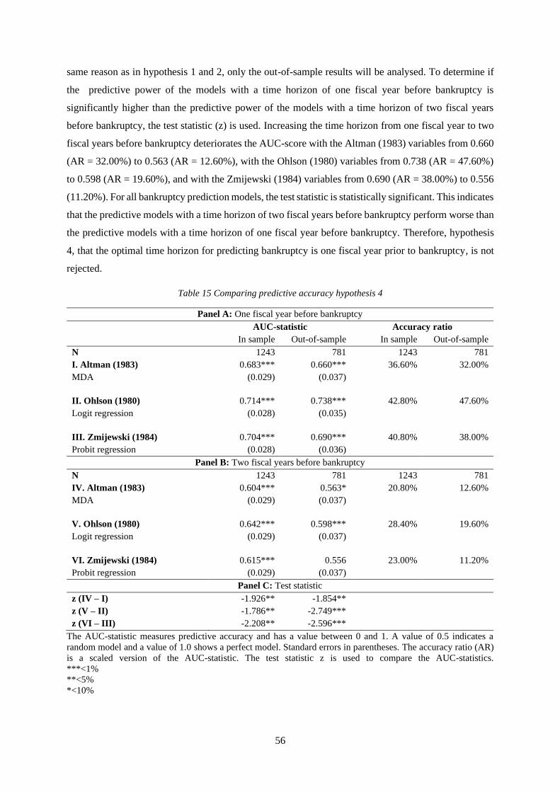
56

same reason as in hypothesis 1 and 2, only the out-of-sample results will be analysed. To determine if

the predictive power of the models with a time horizon of one fiscal year before bankruptcy is

significantly higher than the predictive power of the models with a time horizon of two fiscal years

before bankruptcy, the test statistic (z) is used. Increasing the time horizon from one fiscal year to two

fiscal years before bankruptcy deteriorates the AUC-score with the Altman (1983) variables from 0.660

(AR = 32.00%) to 0.563 (AR = 12.60%), with the Ohlson (1980) variables from 0.738 (AR = 47.60%)

to 0.598 (AR = 19.60%), and with the Zmijewski (1984) variables from 0.690 (AR = 38.00%) to 0.556

(11.20%). For all bankruptcy prediction models, the test statistic is statistically significant. This indicates

that the predictive models with a time horizon of two fiscal years before bankruptcy perform worse than

the predictive models with a time horizon of one fiscal year before bankruptcy. Therefore, hypothesis

4, that the optimal time horizon for predicting bankruptcy is one fiscal year prior to bankruptcy, is not

rejected.

Table 15 Comparing predictive accuracy hypothesis 4

Panel A: One fiscal year before bankruptcy

AUC-statistic Accuracy ratio

In sample Out-of-sample In sample Out-of-sample

N 1243 781 1243 781

I. Altman (1983)

MDA

0.683***

(0.029)

0.660***

(0.037)

36.60% 32.00%

II. Ohlson (1980)

Logit regression

0.714***

(0.028)

0.738***

(0.035)

42.80% 47.60%

III. Zmijewski (1984)

Probit regression

0.704***

(0.028)

0.690***

(0.036)

40.80% 38.00%

Panel B: Two fiscal years before bankruptcy

N 1243 781 1243 781

IV. Altman (1983)

MDA

0.604***

(0.029)

0.563*

(0.037)

20.80% 12.60%

V. Ohlson (1980)

Logit regression

0.642***

(0.029)

0.598***

(0.037)

28.40% 19.60%

VI. Zmijewski (1984)

Probit regression

0.615***

(0.029)

0.556

(0.037)

23.00% 11.20%

Panel C: Test statistic

z (IV – I) -1.926** -1.854**

z (V – II) -1.786** -2.749***

z (VI – III) -2.208** -2.596***

The AUC-statistic measures predictive accuracy and has a value between 0 and 1. A value of 0.5 indicates a

random model and a value of 1.0 shows a perfect model. Standard errors in parentheses. The accuracy ratio (AR)

is a scaled version of the AUC-statistic. The test statistic z is used to compare the AUC-statistics.

***<1%

**<5%

*<10%

57

6 Conclusion and discussion

This chapter includes the conclusion and discussion of this study. First, a summary of the results will be

reported. Second, the limitations of this study will be discussed. Finally, suggestions for future research

will be provided.

6.1 Summary of results

This study examined the prediction power of the accounting-based bankruptcy prediction models of

Altman (1983), Ohlson (1980), and Zmijewski (1984) for Dutch and Belgian public and large private

firms. These bankruptcy prediction models include different financial ratios as independent variables

and are developed using different econometric methods (MDA, logit regression, and probit regression).

This study addressed the following research question:

How accurate are the accounting-based bankruptcy prediction models for Dutch and Belgian public

and large private firms?

Four hypotheses were tested in order to assess the predictive accuracy of these bankruptcy

prediction models. The first hypothesis states that there is no difference in the predictive power between

the models of Altman (1983), Ohlson (1980) and Zmijewski (1984). Several researchers conducted a

similar study on the performance of these accounting-based bankruptcy prediction models, but reported

different results about which model outperformed the other models (e.g. Begley et al., 1996; Grice &

Ingram, 2001; Grice Jr. & Dugan, 2003; Wu et al., 2010; Ashraf et al., 2019). The results of this study

show that there indeed is no difference in predictive power between the models for Dutch and Belgian

public and large private firms. The accuracy ratio, which is the scaled version of the AUC-statistic, for

the models of Altman (1983), Ohlson (1980), and Zmijewski (1984), are respectively 32.00%, 47.60%,

and 38.00%. The difference in predictive power is not statistically significant and therefore hypothesis

1 is not rejected.

With the second hypothesis, this study tries to examine whether a bankruptcy prediction model

using logit regression or probit regression is more accurate than a bankruptcy prediction model using

MDA. Theory does imply that logit and probit regression are better econometric methods for predicting

bankruptcy, due to the restricting statistical assumptions inherent in MDA which are mostly violated in

bankruptcy prediction. However, Altman (2017) conducted a similar test with only logit regression, and

concluded that re-estimation of the coefficients using logit regression only marginally improved the

predictive accuracy. This master thesis shows similar results. First, in line with the conclusion of Collins

and Green (1982), two assumptions of the MDA model are violated, the assumption about multivariate

normality and the assumption about equality of variance-covariance. Violation of these assumptions

limits the effectiveness and validity of MDA (Zhang et al., 1999; Shin et al., 2005; Lee & Choi, 2013).

58

The sets of variables of the models of Altman (1983), Ohlson (1980), and Zmijewski (1984) are used to

estimate bankruptcy prediction models using MDA, logit regression, and probit regression. The results

show that logit regression and probit regression do not outperform MDA. Hypothesis 2 is rejected and

therefore there is no reason to recommend future practitioners of bankruptcy prediction models to use

logit regression or probit regression instead of MDA for estimating the prediction model.

Hypothesis 3a states that the prediction models of Altman (1983), Ohlson (1980), and

Zmijewski (1984) will not retain their accuracy over time. Several researchers found that the accuracy

of a bankruptcy prediction model is affected by factors relating to the environment and that a different

environment may change the relationships between variables (e.g. Mensah, 1984; Platt & Platt, 1990;

Grice Jr & Dugan, 2003; Karas & Režňáková, 2014). To test hypothesis 3a, coefficients of the models

are re-estimated with observations from 2007 – 2010 and evaluated with observations from 2016 – 2019.

These time periods are chosen because of the different economic environments. Several important events

occurred during the period 2007 – 2010, such as the financial crisis in 2007 and the European debt crisis

in 2010 and the regulatory response to the financial crisis, Basel III (stricter capital requirements for

banks). However, the results show that the bankruptcy prediction models do retain their accuracy over

time because the differences in accuracy ratios were not statistically significant. The accuracy ratio of

Altman’s model (1983) is 27.60% in the 2007 – 2010 period and 29.00% in the 2016 – 2019 period.

Ohlson’s model (1980) has an accuracy ratio of 41.60% in the first period and 43.00% in the latter

period. The accuracy ratio of Zmijewski’s model (1984) is 28.60% in the first period and 36.60% in the

latter period. Therefore, hypothesis 3a is rejected.

Hypothesis 3b states that re-estimating the coefficients of the models of Altman (1983), Ohlson

(1980), and Zmijewski (1984) will improve the predictive accuracy. Several researchers suggest that the

coefficients of the models should be re-estimated when for instance using a sample of firms from time

periods other than those used to develop the models (Mensah, 1984; Grice Jr and Dugan, 2003; Singh

and Mishra, 2016). However, the results of this study show that re-estimating the coefficients of the

models with observations from a more recent period does not improve the predictive accuracy. The

accuracy ratio of Altman’s model (1983) is 29.00% when estimated with observations of 2007 – 2010,

and 32.00% when estimated with the more recent observations of 2012 – 2015 (both tested on the hold-

out sample of 2016 – 2019). Ohlson’s model (1980) has an accuracy ratio of 43.00% for the time period

2007 – 2010, and 47.60% for the more recent time period 2012 – 2015. The model of Zmijewski (1984)

has an accuracy ratio of 36.60% for the first time period, and 38.00% for the latter (more recent) time

period. Because these differences in accuracy ratios are not statistically significant, hypothesis 3b is

rejected.

The fourth hypothesis provides a test whether the optimal time horizon for predicting

bankruptcy with the models of Altman (1983), Ohlson (1980), and Zmijewski (1984) is one fiscal year

prior to bankruptcy. Other researchers, such as Philosophov et al. (2005) and Jardin (2017) concluded

that the predictive accuracy decreases when the time horizon exceeds one year. Lukason & Hoffman

59

(2014) state that there is no indication of failure in the financial statements two years before the actual

onset of bankruptcy. This study shows similar results, because the accuracy ratio of all three models

decreased when the time horizon increased from one year to two years. The accuracy ratio of Altman’s

model (1983) decreased from 32.00% to 12.60%, of Ohlson’s model (1980) from 47.60% to 19.60%,

and of Zmijewski’s model (1984) from 38.00% to 11.20%. These differences are statistically significant,

therefore hypothesis 4 is not rejected.

Finally answering the main research question of this master thesis of how accurate the

accounting-based bankruptcy prediction models are for Dutch and Belgian public and large private

firms. Estimated with the econometric methods originally employed to derive the models and with a

time horizon of predicting bankruptcy one fiscal year prior to bankruptcy, the overall accuracy of the

models of Altman (1983), Ohlson (1980), and Zmijewski (1984) are 93.47%, 95.01%, and 94.37%,

respectively. However, the models predicted respectively 32.39%, 47.89%, and 38.03% of the bankrupt

firms correctly, and 99.58%, 99.72%, and 100.00% of the non-bankrupt firms correctly. This means that

all three models have a relatively high frequency type I errors, compared to the frequency type II errors.

The overall accuracy is high because for every bankrupt firm, 10 non-bankrupt firms are included in the

samples and thus 90.91% of the total samples consists of non-bankrupt firms. The low prediction

accuracy of bankrupt firms indicate that neither of the accounting-based bankruptcy prediction models

is a sufficient model for predicting bankruptcy for Dutch and Belgian public and large private firms

(Agarwal and Taffler, 2008 reach the same conclusion with their data). In line with Grice and Ingram

(2001), and Grice Jr. and Dugan (2003), it is recommended that those who want to employ one of these

models for predicting bankruptcy should do so cautiously.

6.2 Limitations

This master thesis is subject to several limitations. The major limitation of this study is the limited data

availability. First, to avoid choice-based sample bias, the samples must be proportionately representative

of the actual bankruptcy rate (Grice & Ingram, 2001; Balcaen & Ooghe, 2006). However, due to the

limited data availability, this would lead to samples with only a few bankrupt firms. Therefore the ratio

of bankrupt firms to non-bankrupt firms is set to 1:10, instead of the actual bankruptcy rate, meaning

that the bankrupt firms are oversampled. Second, the estimation sample with observations from 2007 to

2010 consisted of a limited set of firms for which all financial data was available. This resulted in a

relatively low sample size of 42 bankrupt and 412 non-bankrupt firms compared to the sample size of

the estimation sample with observations from 2012 to 2015 which consisted of 113 bankrupt and 1130

non-bankrupt firms. Third, due to the limited data availability of Dutch bankrupt firms, Belgian bankrupt

firms were overrepresented in the samples which could potentially lead to sampling bias. The last

limitation due to the limited data availability is the time period of the estimation sample used for testing

hypothesis 3a and 3b. To test the hypotheses that the prediction models will not retain their accuracy

over time, and that re-estimating the coefficients improves the predictive accuracy, the estimation

60

sample was supposed to contain observations from 2004 to 2007. This time period would be optimal,

because after this period, the financial crisis in 2007 and the European debt crisis in 2010 happened.

Firms in this pre-crisis estimation sample should therefore have a different economic environment than

firms in the after-crisis hold-out sample. However, due to the limited data availability it was not possible

to include a pre-crisis sample with observations from 2004 to 2007, but eventually the sample consisted

of observations during the crisis, from 2007 to 2010. Therefore, the difference in economic environment

between the estimation and hold-out sample is likely less than the difference if there was enough data

available to include observations from 2004 to 2007 in the estimation sample.

Another limitation of this master thesis is the definition used for bankrupt firms. In this study,

the definition of bankrupt firms that are included in the samples is based on a legal definition of

bankruptcy. However, firms can also file for bankruptcy for other reasons than financial distress. For

example, lawsuits as a result of strategic management decisions could also result in a firm filing for

bankruptcy (Grice & Dugan, 2001), and firms also file for bankruptcy voluntarily when financial

conditions make it value-increasing for shareholders and managers (Fleming & Moon, 1995). Therefore,

firms in bankruptcy might not always be economically inefficient (White, 1989). However, the variables

of the models of Altman (1983), Ohlson (1980), and Zmijewski (1984) do not incorporate proxies for

non-financial events that cause bankruptcy (Grice & Dugan, 2001). Using the legal definition of

bankruptcy and not excluding bankrupt firms that have filed for bankruptcy due to a non-financial event

could lead to biased results.

A limitation of this study is that it analysed only three accounting-based bankruptcy prediction

models and focused only on predicting bankruptcy with data from financial statements. However,

financial statement are limited in predicting the probability of bankruptcy, among other things because

financial statements are formulated under the going-concern principle and because financial statements

report the past performance of a firm and may therefore not be informative about predicting bankruptcy

in the future (Hillegeist et al., 2004). Additionally, accounting-based prediction models lack theoretical

grounding (Agarwal & Taffler, 2008). Future research suggestions that addresses this limitation will be

given in the next section.

The predictive accuracy of the models was assessed using the AUC-statistic, but this statistic

does not distinguish between a type I error and a type II error (Agarwal & Taffler, 2008). Therefore,

using the AUC-statistic for comparing the predictive accuracy indicates that this study does not have a

preference for a type I or a type II error. However, a type I error is more costly than a type II error,

because the former can result in losing a whole loan amount while the latter results in only the

opportunity cost of not lending to that firm (Agarwal & Taffler, 2008).

6.3 Future research

Future research on bankruptcy prediction in a Dutch and Belgian setting should also analyse market-

based bankruptcy prediction models, like the models of Shumway (2001) and Hillegeist et al. (2004), in

61

addition to the accounting-based bankruptcy prediction models in order to compare the performance of

these two types of prediction models. Additionally, this master thesis only analysed the original variables

of the models of Altman (1983), Ohlson (1980), and Zmijewski (1984). Future research should focus on

modifications and extensions of these models to increase the predictive accuracy, such as introducing

new variables: financial, non-financial, and macroeconomic variables.

The results of this study indicate that the optimal time horizon for predicting bankruptcy with

the accounting-based prediction models is one fiscal year before bankruptcy and that the predictive

accuracy decreases drastically when the time horizon increases. A suggestion for future research is

therefore to focus on how to predict bankruptcy several years before the event instead of one year.

Because if a potential bankruptcy can be predicted a few years in advance, actions like reorganization

or merger of the firm can be undertaken (Dimitras et al, 1996; Pompe & Bilderbeek, 2005; Fejér-Király,

2015).

Due to the limited data availability this study focused on both public and private firms and on

both Dutch and Belgian firms. Future research should focus on testing the usefulness of the prediction

models with data from only private firms, since most studies focus on public firms. To ensure sufficient

data availability, more European countries could be included. Additionally, future research should test

its usefulness with data from only the Netherlands or only Belgium.

62

References

Adnan Aziz, M., & Dar, H. A. (2006). Predicting corporate bankruptcy: where we stand? Corporate

Governance: The International Journal of Business in Society, 6(1), 18-33.

Agarwal, V., & Taffler, R. J. (2007). Twenty-five years of the Taffler z-score model: does it really have

predictive ability? Accounting and Business Research, 37(4), 285-300.

Agarwal, V., & Taffler, R. (2008). Comparing the performance of market-based and accounting-based

bankruptcy prediction models. Journal of Banking & Finance, 32(8), 1541-1551.

Agnese, P., Rizzo, M., & Vento, G. A. (2018). SMEs finance and bankruptcies: the role of credit

guarantee schemes in the UK. Journal of Applied Finance and Banking, 8(3), 1-16.

Altman, E. I. (1968). Financial ratios, discriminant analysis and the prediction of corporate bankruptcy.

The Journal of Finance, 23(4), 589-609.

Altman, E. I. (1983). Corporate financial distress: A complete guide to predicting, avoiding, and dealing

with bankruptcy. Wiley Interscience, John Wiley and Sons.

Altman, E. I. (2013). Predicting financial distress of companies: revisiting the Z-score and ZETA®

models. In Handbook of Research Methods and Applications in Empirical Finance. Edward

Elgar Publishing.

Altman, E. I., Iwanicz-Drozdowska, M., Laitinen, E. K., & Suvas, A. (2017). Financial distress

prediction in an international context: A review and empirical analysis of Altman’s Z-score

model. Journal of International Financial Management & Accounting, 28(2), 131-171.

Ashraf, S., GS Félix, E., & Serrasqueiro, Z. (2019). Do traditional financial distress prediction models

predict the early warning signs of financial distress? Journal of Risk and Financial Management,

12(2), 55.

Atiya, A. F. (2001). Bankruptcy prediction for credit risk using neural networks: A survey and new

results. IEEE Transactions on Neural Networks, 12(4), 929-935.

Baker & McKenzie (2016). Global restructuring & insolvency guide 2016. Retrieved from

http://restructuring.bakermckenzie.com/wp-content/uploads/sites/23/2016/12/Global-

Restructuring-Insolvency-Guide-New-Logo-Belgium.pdf

Balcaen, S., & Ooghe, H. (2006). 35 years of studies on business failure: An overview of the classic

statistical methodologies and their related problems. The British Accounting Review, 38(1), 63-

93.

Balcaen, S., Manigart, S., Buyze, J., & Ooghe, H. (2012). Firm exit after distress: differentiating between

bankruptcy, voluntary liquidation and M&A. Small Business Economics, 39(4), 949-975.

Bauer, J., & Agarwal, V. (2014). Are hazard models superior to traditional bankruptcy prediction

approaches? A comprehensive test. Journal of Banking & Finance, 40, 432-442.

Beaver, W. H. (1966). Financial ratios as predictors of failure. Journal of Accounting Research, 71-111.

Beaver, W. H., McNichols, M. F., & Rhie, J. W. (2005). Have financial statements become less

informative? Evidence from the ability of financial ratios to predict bankruptcy. Review of

Accounting studies, 10(1), 93-122.

Begley, J., Ming, J., & Watts, S. (1996). Bankruptcy classification errors in the 1980s: an empirical

analysis of Altman’s and Ohlson’s models. Review of accounting Studies, 1(4), 267-284.

Bellovary, J. L., Giacomino, D. E., & Akers, M. D. (2007). A review of bankruptcy prediction studies:

1930 to present. Journal of Financial education, 1-42.

63

Berg, D. (2007). Bankruptcy prediction by generalized additive models. Applied Stochastic Models in

Business and Industry, 23(2), 129-143.

Black, F., & Scholes, M. (1973). The pricing of options and corporate liabilities. Journal of Political

Economy, 81(3), 637-654.

Boekhorst, P. (2018). Bankruptcy prediction for Dutch private firms using the Altman Z-score model.

(Unpublished master’s thesis). University of Twente, Enschede, Netherlands.

Boot, A. W. A., & Ligterink, J. E. (2000). Faillissementswetgeving in internationaal perspectief. MAB,

74(11), 492-499.

Brouwer, M. (2006). Reorganization in US and European bankruptcy law. European Journal of Law

and Economics, 22(1), 5-20.

Campbell, J. Y., Hilscher, J., & Szilagyi, J. (2008). In search of distress risk. The Journal of Finance,

63(6), 2899-2939.

Charitou, A., Neophytou, E., & Charalambous, C. (2004). Predicting corporate failure: empirical

evidence for the UK. European Accounting Review, 13(3), 465-497.

Chava, S., & Jarrow, R. A. (2004). Bankruptcy prediction with industry effects. Review of Finance, 8(4),

537-569.

Collins, R. A., & Green, R. D. (1982). Statistical methods for bankruptcy forecasting. Journal of

Economics and Business, 34(4), 349-354.

Couwenberg, O. (2001). Survival rates in bankruptcy systems: overlooking the evidence. European

Journal of Law and Economics, 12(3), 253-273.

Couwenberg, O., & De Jong, A. (2008). Costs and recovery rates in the Dutch liquidation-based

bankruptcy system. European Journal of Law and Economics, 26(2), 105-127.

Couwenberg, O., & Lubben, S. J. (2011). The costs of chapter 11 on context: American and Dutch

business bankruptcy. American Bankruptcy Law Journal, 85(1), 63-89.

Cultrera, L., & Brédart, X. (2016). Bankruptcy prediction: the case of Belgian SMEs. Review of

Accounting and Finance, 15(1), 101-119.

Demyanyk, Y., & Hasan, I. (2010). Financial crises and bank failures: A review of prediction methods.

Omega, 38(5), 315-324.

Dewaelheyns, N., & Van Hulle, C. (2008). Legal reform and aggregate small and micro business

bankruptcy rates: evidence from the 1997 Belgian bankruptcy code. Small Business Economics,

31(4), 409.

Dimitras, A. I., Zanakis, S. H., Zopounidis, C. (1996). A survey of business failures with an emphasis

on prediction methods and industrial applications. European Journal of Operational Research,

90(3), 487-513.

Doumpos, M., & Zopounidis, C. (1999). A multicriteria discrimination method for the prediction of

financial distress: The case of Greece. Multinational Finance Journal, 3(2), 71-101.

du Jardin, P. (2017). Dynamics of firm financial evolution and bankruptcy prediction. Expert Systems

with Applications, 75, 25-43.

Elferink, N. (2018). Financial distress prediction in the Netherlands: an application of multiple

discriminant analysis, logistic regression and neural network. (Unpublished master’s thesis).

University of Twente, Enschede, Netherlands.

Engelmann, B., Hayden, E., & Tasche, D. (2003). Testing rating accuracy. Risk, 16(1), 82-86.

64

Fejér-Király, G. (2015). Bankruptcy prediction: A survey on evolution, critiques, and solutions. Acta

Universitatis Sapientiae, Economics and Business, 3(1), 93-108.

Filipe, S. F., Grammatikos, T., & Michala, D. (2016). Forecasting distress in European SME portfolios.

Journal of Banking & Finance, 64, 112-135.

Fleming, M. J., & Moon, J. J. (1995). Preserving firm value through exit: the case of voluntary

liquidations. FRB of New York Staff Report, 8.

Garškiene, A., & Garškaite, K. (2004). Enterprise bankruptcy in Lithuania. Journal of Business

Economics and Management, 5(1), 51-58.

Ghosh, C., Owers, J. E., & Rogers, R. C. (1991). The financial characteristics associated with voluntary

liquidations. Journal of Business Finance & Accounting, 18(6), 773-789.

Giacosa, E., Halili, E., Mazzoleni, A., Teodori, C., & Veneziani, M. (2016). Re-estimation of company

insolvency prediction models: Survey on Italian manufacturing companies. Corporate

Ownership and Control, 14(1), 159-174.

Gilbert, L. R., Menon, K., & Schwartz, K. B. (1990). Predicting bankruptcy for firms in financial

distress. Journal of Business Finance & Accounting, 17(1), 161-171.

Gilson, S. C., John, K., & Lang, L. H. (1990). Troubled debt restructurings: An empirical study of private

reorganization of firms in default. Journal of Financial Economics, 27(2), 315-353.

Grice Jr, J. S., & Dugan, M. T. (2003). Re-estimations of the Zmijewski and Ohlson bankruptcy

prediction models. Advances in Accounting, 20, 77-93.

Grice, J. S., & Dugan, M. T. (2001). The limitations of bankruptcy prediction models: some cautions

for the researcher. Review of Quantitative Finance and Accounting, 17(2), 151-166.

Grice, J. S., & Ingram, R. W. (2001). Tests of the generalizability of Altman’s bankruptcy prediction

model. Journal of Business Research, 54(1), 53-6.

Gupta, J., Gregoriou, A., & Healy, J. (2015). Forecasting bankruptcy for SMEs using hazard function:

To what extend does size matter? Review of Quantitative Finance and Accounting, 45(4), 845-

869.

Hair, J. F., Black, W. C., Babin, B. J., & Anderson, R. E. (2010). Multivariate data analysis (Vol. 7).

Upper Saddle River, NJ: Pearson Prentice Hall.

Hall, G. (1992). Reasons for insolvency amongst small firms – a review and fresh evidence. Small

Business Economics, 4(3), 237-250.

Hanley, J. A., & McNeil, B. J. (1982). The meaning and use of the area under a receiver operating

characteristic (ROC) curve. Radiology, 143(1), 29-36.

Hillegeist, S. A., Keating, E. K., Cram, D. P., & Lundstedt, K. G. (2004). Assessing the probability of

bankruptcy. Review of Accounting Studies, 9(1), 5-34.

Hummelen, J. M. (2015). Shaping bankruptcy law: what form should it take? Norton Journal of

Bankruptcy Law and Practice, 24(1), 52-88.

Jackson, T. H. (1982). Bankruptcy, non-bankruptcy entitlements, and the creditors’ bargain. The Yale

Law Journal, 91(5), 857-907.

Jones, S., & Wang, T. (2019). Predicting private company failure: A multi-class analysis. Journal of

International Financial Markets, Institutions and Money, 61, 161-188.

Kahya, E., & Theodossiou, P. (1999). Predicting corporate financial distress: A time-series CUSUM

methodology. Review of Quantitative Finance and Accounting, 13(4), 323-345.

65

Karamzadeh, M. S. (2013). Application and comparison of Altman and Ohlson models to predict

bankruptcy of companies. Research Journal of Applied Sciences, Engineering and

Technology, 5(6), 2007-2011.

Karas, M., & Režňáková, M. (2014). To what degree is the accuracy of a bankruptcy prediction model

affected by the environment? The case of the Baltic States and the Czech Republic. Procedia-

Social and Behavioral Sciences, 156, 564-568.

Karels, G. V., & Prakash, A. J. (1987). Multivariate normality and forecasting of business bankruptcy.

Journal of Business Finance & Accounting, 14(4), 573-593.

Kisman, Z., & Krisandi, D. (2019). How to predict financial distress in the wholesale sector: lesson from

Indonesion Stock Exchange. Journal of Economics and Business, 2(3), 569-585.

Koh, H. C., & Killough, L. N. (1990). The use of multiple discriminant analysis in the assessment of the

going-concern status of an audit client. Journal of Business Finance & Accounting, 17(2), 179-

192.

Kumar, P. R., & Ravi, V. (2007). Bankruptcy prediction in banks and firms via statistical and intelligent

techniques – A review. European Journal of Operational Research, 180(1), 1-28.

Lang, L. H., & Stulz, R. (1992). Contagion and competitive intra-industry effects of bankruptcy

announcements: An empirical analysis. Journal of Financial Economics, 32(1), 45-60.

Lee, S., & Choi, W. S. (2013). A multi-industry bankruptcy prediction model using back-propagation

neural network and multivariate discriminant analysis. Expert Systems with Applications, 40(8),

2941-2946.

Li, D. D., & Li, S. (1999). An agency theory of the bankruptcy law. International Review of Economics

& Finance, 8(1), 1-24.

Liang, D., Lu, C. C., Tsai, C. F., & Shih, G. A. (2016). Financial ratios and corporate governance

indicators in bankruptcy prediction: a comprehensive study. European Journal of Operational

Research, 252(2), 561-572.

Looney, S. W. (1995). How to use tests for univariate normality to assess multivariate normality. The

American Statistician, 49(1), 64-70.

Lukason, O., & Hoffman, R. C. (2014). Firm bankruptcy probability and causes: an integrated study.

International Journal of Business and Management, 9(11), 80-91.

Machielsen, B. (2015). The accuracy and information content of two traditional statistical methods in

forecasting bankruptcy: evidence from European countries. (Unpublished master’s thesis).

University of Twente, Enschede, Netherlands.

Mellahi, K., & Wilkinson, A. (2004). Organizational failure: a critique of recent research and a proposed

integrative framework. International Journal of Management Reviews, 5(1), 21-41.

Mensah, Y. M. (1984). An examination of the stationarity of multivariate bankruptcy prediction models:

A methodological study. Journal of Accounting Research, 380-395.

Merton, R. C. (1974). On the pricing of corporate debt: The risk structure of interest rates. The Journal

of Finance, 29(2), 449-470.

Mihalovic, M. (2016). Performance comparison of multiple discriminant analysis and logit models in

bankruptcy prediction. Economics & Sociology, 9(4), 101-118.

Morris, R. (1997). Early warning indicators of corporate failure: A critical review of previous research

and further empirical evidence. Brookfield, United States of America: Ashgate Publishing Ltd.

66

Moyer, R. C. (1977). Forecasting financial failure: a re-examination. Financial Management (pre-1986),

6(1), 11-17.

Nyitrai, T., & Virág, M. (2019). The effects of handling outliers on the performance of bankruptcy

prediction models. Socio-Economic Planning Sciences, 67, 34-42.

Ohlson, J. A. (1980). Financial ratios and the probabilistic prediction of bankruptcy. Journal of

Accounting Research, 18(1), 109-131.

Ooghe, H., & Waeyaert, N. (2004). Oorzaken van faling: literatuuroverzicht en conceptueel

verklaringsmodel. Economisch en Sociaal Tijdschrift, 57(4), 367-393.

Ooghe, H., & De Prijcker, S. (2008). Failure processes and causes of company bankruptcy: a typology.

Management Decision, 46(2), 223-242.

Paul, R. K. (2006). Multicollinearity: causes, effects and remedies. IASRI, New Delhi, 58-65.

Philosophov, L. V., Batten, J. A., & Philosophov, V. L. (2005). Assessing the time horizon of bankruptcy

using financial ratios and the maturity schedule of long-term debt. Proceedings of the European

Finance Association 32nd Annual Meeting, 1-39.

Platt, H. D., & Platt, M. B. (1990). Development of a class of stable predictive variables: The case of

bankruptcy prediction. Journal of Business Finance & Accounting, 17(1), 31-51.

Platt, H. D., & Platt, M. B. (2002). Predicting corporate financial distress: Reflections on choice-based

sample bias. Journal of Economics and Finance, 26(2), 184-199.

Pompe, P. P., & Bilderbeek, J. (2005). Bankruptcy prediction: The influence of the year prior to failure

selected for model building and the effects in a period of economic decline. Intelligent Systems

in Accounting, Finance & Management: International Journal, 13(2), 95-112.

Reisz, A. S., & Perlich, C. (2007). A market-based framework for bankruptcy prediction. Journal of

Financial Stability, 3(2), 85-131.

Shin, K. S., Lee, T. S., & Kim, H. J. (2005). An application of support vector machines in bankruptcy

prediction model. Expert Systems with Applications, 28(1), 127-135.

Shumway, T. (2001). Forecasting bankruptcy more accurately: A simple hazard model. The Journal of

Business, 74(1), 101-124.

Siddiqui, S. A. (2012). Business bankruptcy prediction models: A significant study of the Altman’s Z-

score model. Available at SSRN 2128475.

Singh, B. P., & Mishra, A. K. (2016). Re-estimation and comparisons of alternative accounting based

bankruptcy prediction models for Indian companies. Financial Innovation, 2(1), 6.

Sloan, R. G. (1996). Do stock prices fully reflect information in accruals and cash flows about future

earnings? Accounting Review, 289-315.

Son, H., Hyun, C., Phan, D., & Hwang, H. J. (2019). Data analytic approach for bankruptcy prediction.

Expert Systems with Applications, 138, 112816.

Statbel. (2020, April 22). Maart 2020: 869 faillissementen. Retrieved from:

https://statbel.fgov.be/nl/themas/ondernemingen/faillissementen#figures

Statistics Netherlands. (2019, June 12). Fewer bankruptcies in May. Retrieved from:

https://www.cbs.nl/en-gb/news/2019/24/fewer-bankruptcies-in-may

Tinoco, M. H., & Wilson, N. (2013). Financial distress and bankruptcy prediction among listed

companies using accounting, market and macroeconomic variables. International Review of

Financial Analysis, 30, 394-419.

67

Trujillo-Ponce, A., Samaniego-Medina, R., & Cardone-Riportella, C. (2014). Examining what best

explains corporate credit risk: accounting-based versus market-based models. Journal of

Business and Economics and Management, 15(2), 253-276.

White, M. J. (1989). The corporate bankruptcy decision. Journal of Economic Perspectives, 3(2), 129-

151.

Wood, D., & Piesse, J. (1987). The information value of MDA based financial indicators. Journal of

Business Finance & Accounting, 14(1), 27-38.

Wruck, K. H. (1990). Financial distress, reorganization, and organization efficiency. Journal of

Financial Economics, 27(2), 419-444.

Wu, W. W. (2010). Beyond business failure prediction. Expert systems with applications, 37(3), 2371-

2376.

Wu, Y., Gaunt, C., & Gray, S. (2010). A comparison of alternative bankruptcy prediction models.

Journal of Contemporary Accounting & Economics, 6(1), 34-45.

Yap, B. C. F., Yong, D. G. F., & Poon, W. C. (2010). How well do financial ratios and multiple

discriminant analysis predict company failures in Malaysia. International Research Journal of

Finance and Economics, 54(13), 166-175.

Zhang, G., Hu, M. Y., Patuwo, B. E., & Indro, D. C. (1999). Artificial neural networks in bankruptcy

prediction: General framework and cross-validation analysis. European Journal of Operational

Research, 116(1), 16-32.

Zmijewski, M. E. (1984). Methodological issues related to the estimation of financial distress prediction

models. Journal of Accounting Research, 22, 59-82.

68

Appendices

Appendix A: Financial ratios of the bankruptcy prediction models

Table 16 Financial ratios bankruptcy prediction models

Model Financial ratios Variable Ratio classification

Altman (1983) x1 = Working capital/Total assets WC/TA Liquidity

x2 = Retained earnings/Total assets RE/TA Leverage

x3 = Earnings before interest and

taxes/Total assets

EBIT/TA Profitability

x4 = Book value equity/Book value of

total debt

BVEQ/BVTD Solvency

x5 = Sales/Total assets SALES/TA Activity

Ohlson (1980) x1 = log (Total assets/GNP price-level

index)

SIZE Size

x2 = Total liabilities/Total assets TL/TA Leverage

x3 = Working capital/Total assets WC/TA Liquidity

x4 = Current liabilities/Current assets CL/CA Liquidity

x5 = 1 if total liabilities > total assets, 0

otherwise

OENEG Leverage

x6 = Net income/Total assets NI/TA Profitability

x7 = Funds provided by

operations/Total liabilities

FU/TL Liquidity

x8 = 1 if net income was negative for

the last two years, 0 otherwise

INTWO Liquidity

x9 = (NIt – NIt-1) / (|NIt| + |NIt-1|),

where NIt is net income for the most

recent period

CHNI Profitability

Zmijewski (1984) x1 = Net income/Total assets NI/TA Profitability

x2 = Total debt/Total assets TD/TA Solvency/leverage

x3 = Current assets/Current liabilities CA/CL Liquidity

69

Appendix B: List of bankrupt firms in sample

Table 17 Bankrupt firms in samples

Company name Type Industry Country Year

1st Belgium Service Private Administrative and support

service activities Belgium 2012

A.T.M. Public Manufacturing Belgium 2010

Abs Distribution Public Wholesale and retail trade Belgium 2012

Adriana Benelux Private Wholesale and retail trade Belgium 2008

Agro Technics Public Wholesale and retail trade Belgium 2016

Aktiesport B.V. Private Wholesale and retail trade Netherlands 2016

Alfacam Public Art, entertainment and recreation Belgium 2013

Algemene Aannemingen

Merckx Public Construction Belgium 2008

Algemene

Bouwonderneming Frans

Willems

Public Construction Belgium 2019

Algrondbo Private Construction Belgium 2013

Alpha Technologies Public Professional, scientific and

technical activities Belgium 2017

Aluminium Delfzijl B.V. Private Manufacturing Netherlands 2013

Antwerp Ship Repair Public Manufacturing Belgium 2013

Apollo Fruit B.V. Private Wholesale and retail trade Netherlands 2012

Arend-Sosef B.V. Private Wholesale and retail trade Netherlands 2014

Aristophil Public Art, entertainment and recreation Belgium 2014

Arlex International Public Wholesale and retail trade Belgium 2014

Asap Maintenance &

Shipping Private Wholesale and retail trade Belgium 2014

ATMR & E Public Manufacturing Belgium 2015

Autos Public Wholesale and retail trade Belgium 2010

Belgo Metal Public Manufacturing Belgium 2015

Belucon Public Wholesale and retail trade Belgium 2014

Bernard Langeraet Private Wholesale and retail trade Belgium 2016

Best Medical Belgium S.A. Public Manufacturing Belgium 2012

Bfan Public Manufacturing Belgium 2013

Big Fish Private Wholesale and retail trade Belgium 2019

Bmtech Public Manufacturing Belgium 2012

Bois et Materiaux de

Construction Public Wholesale and retail trade Belgium 2015

Bonustijd Private Transportation and storage Belgium 2013

Bosal Benelux Public Manufacturing Belgium 2015

Bouwbedrijf Loix Public Construction Belgium 2018

Bouwcentrale Modern Public Construction Belgium 2016

Buro Immo Private Construction Belgium 2014

Casterman Printing Public Manufacturing Belgium 2016

Casters Algemene

Ondernemingen Public Construction Belgium 2018

Cegeac Public Wholesale and retail trade Belgium 2014

Centratec Public Wholesale and retail trade Belgium 2017

Charles Vogele

(Netherlands) B.V. Private Wholesale and retail trade Netherlands 2017

Chateau – Caravans Public Manufacturing Belgium 2007

70

Cib Incentives Public Administrative and support

service activities Belgium 2007

Cipla Europe Public Wholesale and retail trade Belgium 2018

Construction Tour et

Finition Private Construction Belgium 2015

Cool Cat Nederland B.V. Private Real estate activities Netherlands 2019

Corsan Public Information and communication Belgium 2016

De Boever’s Brandstoffen Public Wholesale and retail trade Belgium 2007

Dejaeghere-Spinning Mills Public Manufacturing Belgium 2007

DH-Group Public Wholesale and retail trade Belgium 2016

Domotech Private Construction Belgium 2016

Domotherm Public Wholesale and retail trade Belgium 2016

Dorleska Diamonds Public Wholesale and retail trade Belgium 2007

Draka Polymer Films B.V. Private Manufacturing Netherlands 2019

Duro Home Public Construction Belgium 2013

Durobor Public Manufacturing Belgium 2012

Durobor Group Public Manufacturing Belgium 2017

Dwbel Private Manufacturing Belgium 2015

Eagle Construct Public Manufacturing Belgium 2015

ECS Technics Public Construction Belgium 2012

EKB Container Logistic

Group Belgium Public Transportation and storage Belgium 2013

Electrawinds Public Professional, scientific and

technical activities Belgium 2019

Elgeka Private Construction Belgium 2017

Erudict Public Information and communication Belgium 2009

Etablissements Lequet et

Herkenne Public Wholesale and retail trade Belgium 2015

Euroferco Public Wholesale and retail trade Belgium 2012

Euro-Med 2005 Private Wholesale and retail trade Belgium 2008

Europem Public Professional, scientific and

technical activities Belgium 2019

Eurotube Industries Public Manufacturing Belgium 2015

Exelco Sourcing Private Wholesale and retail trade Belgium 2018

Facility Services Private Administrative and support

service activities Belgium 2014

Ferryways Public Transportation and storage Belgium 2008

Firestar Diamond Private Wholesale and retail trade Belgium 2018

First Line Telecom Public Information and communication Belgium 2009

Fishco Private Wholesale and retail trade Belgium 2018

FL Sport B.V. Private Wholesale and retail trade Netherlands 2016

Flash Travel Public Administrative and support

service activities Belgium 2012

Fleks

Kinderopvangorganisatie

B.V.

Private Human health and social work

activities Netherlands 2013

Fontijne Grotnes B.V. Private Manufacturing Netherlands 2016

Free Record Shop Belgium Public Wholesale and retail trade Belgium 2013

G & G International Public Manufacturing Belgium 2015

Gacssolutions Public Manufacturing Belgium 2012

Garage Regniers Public Wholesale and retail trade Belgium 2015

Garage Vanderkeilen Private Wholesale and retail trade Belgium 2014

71

Garpet Public Professional, scientific and

technical activities Belgium 2016

Gateway Public Information and communication Belgium 2016

GDB International Public Wholesale and retail trade Belgium 2012

Gebroeders de Waele Public Construction Belgium 2015

Geens Public Wholesale and retail trade Belgium 2007

Geens Benelux Public Wholesale and retail trade Belgium 2007

Gevalo Public Manufacturing Belgium 2013

Gibson Innovations

Netherlands B.V. Private Manufacturing Netherlands 2018

Gilleman Textiles Public Wholesale and retail trade Belgium 2016

Giraud Belgie Public Transportation and storage Belgium 2010

Goemaere Public Wholesale and retail trade Belgium 2015

Goes International

Transport B.V. Private Transportation and storage Netherlands 2014

Grandeco Wallfashion

Group Public Manufacturing Belgium 2013

Grondinvest Public Construction Belgium 2017

Hacherelle Public Wholesale and retail trade Belgium 2018

Harry Verbinnen Private Manufacturing Belgium 2013

Helio Charleroi Public Manufacturing Belgium 2019

Hoebeek Public Wholesale and retail trade Belgium 2017

Ideal-Services Private Human health and social work

activities Belgium 2014

Idem Papers – Idempapers Public Manufacturing Belgium 2017

Inalco Public Manufacturing Belgium 2016

Innoconcepts N.V. Public Administrative and support

service activities Netherlands 2010

Internationaal Transport &

Logistiek Europe Public Transportation and storage Belgium 2012

International Russian

Import and Lease Public Wholesale and retail trade Belgium 2012

Jory Public Professional, scientific and

technical activities Belgium 2013

Jurriens West B.V. Private Construction Netherlands 2016

K. Vijay Private Wholesale and retail trade Belgium 2017

Karlie Flamingo Public Wholesale and retail trade Belgium 2016

Kesar Public Wholesale and retail trade Belgium 2012

Koster Metalen B.V. Private Construction Netherlands 2015

Koxka Belgium Public Manufacturing Belgium 2015

Kroonservice Logistics Public Transportation and storage Belgium 2013

L.C.M.C. Public Manufacturing Belgium 2014

LBG Bakeries Public Professional, scientific and

technical activities Belgium 2015

Liefmans Breweries Public Manufacturing Belgium 2007

Link2biz International

Verkort Link2Biz Public Transportation and storage Belgium 2010

Lintor Public Manufacturing Belgium 2013

Liza Dimon Private Wholesale and retail trade Belgium 2013

Macintosh Retail Group

N.V. Public Wholesale and retail trade Netherlands 2015

Marconi Oranje B.V. Private Construction Netherlands 2016

72

Mare Tours Public Administrative and support

service activities Belgium 2018

Marval Gems Private Wholesale and retail trade Belgium 2010

McGregor Retail Belgium Public Wholesale and retail trade Belgium 2017

Meister Coordination

Center Public Manufacturing Belgium 2014

Memory Corp Public Information and communication Belgium 2007

Metaal Constructies

Couwenberg en Schellens Public Manufacturing Belgium 2019

Mexx Belgium Public Wholesale and retail trade Belgium 2014

Mitra Energy &

Infrastructure Public Manufacturing Belgium 2010

Mitro Public Construction Belgium 2018

Momitube Public Manufacturing Belgium 2015

Montagny B.V. Private Real estate activities Netherlands 2019

Mooy Logistics B.V. Private Transportation and storage Netherlands 2018

Myliti Public Wholesale and retail trade Belgium 2017

Nedfield N.V. Public Manufacturing Netherlands 2009

Nelca Public Manufacturing Belgium 2007

Neochim Public Manufacturing Belgium 2012

Niche Trading Public Wholesale and retail trade Belgium 2019

Nordvries Private Wholesale and retail trade Belgium 2019

O.W. Bunker (Belgium) Public Wholesale and retail trade Belgium 2014

O.W. Bunker (Netherlands)

B.V. Private Wholesale and retail trade Netherlands 2014

Oceanwide Private Wholesale and retail trade Belgium 2018

Ondernemingen Arthur

Moens – Entreprises

Arthur Moens

Public Construction Belgium 2008

OXL Public Transportation and storage Belgium 2015

Packing Creative Systems Public Manufacturing Belgium 2012

Parallel Groep ETB Vos

B.V. Private Construction Netherlands 2015

Paulus Henri en Zonen Public Wholesale and retail trade Belgium 2007

PDC B.V. Private Wholesale and retail trade Netherlands 2016

Phanos Westwijk B.V. Private Construction Netherlands 2012

Photo Hall Multimedia Public Wholesale and retail trade Belgium 2012

Plastruco Technics Public Manufacturing Belgium 2012

Poets & Strijkhuisje Private Administrative and support

service activities Belgium 2017

Polygone International

S.A. Public Manufacturing Belgium 2012

Potato Masters Public Wholesale and retail trade Belgium 2014

Pouw Automotive B.V. Private Wholesale and retail trade Netherlands 2014

Prime Champ Materials

B.V. Private Wholesale and retail trade Netherlands 2013

Prime Champ Packaging

B.V. Private

Administrative and support

service activities Netherlands 2013

Prime Champ Production

B.V. Private Agriculture, forestry and fishing Netherlands 2013

Prime Champ Sales B.V. Private Wholesale and retail trade Netherlands 2013

Primo-Stadion Public Wholesale and retail trade Belgium 2016

73

Print and Display Public Professional, scientific and

technical activities Belgium 2012

Prodac Public Wholesale and retail trade Belgium 2012

Proficos Public Manufacturing Belgium 2015

Provad Public Wholesale and retail trade Belgium 2014

Quintens Bakeries

Morlanwelz Public Manufacturing Belgium 2015

R. en F. Folding Boxes Public Manufacturing Belgium 2008

Raamfabriek Vlieghe Public Manufacturing Belgium 2016

Raben Belgium Private Transportation and storage Belgium 2007

Racking Storage Public Manufacturing Belgium 2008

Reef Hout B.V. Private Manufacturing Netherlands 2012

Refining & Trading

Holland N.V. Public Water supply Netherlands 2015

Reklameadviesbureau

Indus Public

Professional, scientific and

technical activities Belgium 2009

Retrain Public Administrative and support

service activities Belgium 2014

Royal Imtech N.V. Public Construction Netherlands 2015

RSB Transmissions

Belgium Public Manufacturing Belgium 2014

Ruby Belgium Public Professional, scientific and

technical activities Belgium 2016

Safetic Public Administrative and support

service activities Belgium 2012

SC Retail Public Wholesale and retail trade Belgium 2015

Service Innovation Group

Belgium Public

Professional, scientific and

technical activities Belgium 2014

Signature Vermeulen Public Construction Belgium 2014

Sikan Public Wholesale and retail trade Belgium 2009

Sinomet Recycling Public Water supply Belgium 2009

Sisyphus Public Professional, scientific and

technical activities Belgium 2017

SL Services B.V. Private Wholesale and retail trade Netherlands 2016

Slavenburg B.V. Private Construction Netherlands 2013

SLC Public Wholesale and retail trade Belgium 2019

Sleurs Energy Public Manufacturing Belgium 2012

Sobelmar Shipping Public Transportation and storage Belgium 2016

Societe Mediterraneenne

de Participations Public

Professional, scientific and

technical activities Belgium 2010

Solfruit International B.V. Private Wholesale and retail trade Netherlands 2012

Sowaco Public Construction Belgium 2012

Spidiam Private Wholesale and retail trade Belgium 2010

Squatra Private Administrative and support

service activities Belgium 2014

Starman Bruxelles Hotel Private Accommodation and food service

activities Belgium 2014

Star-Oil Private Professional, scientific and

technical activities Belgium 2009

Steverlynck Group Public Manufacturing Belgium 2007

Strongbow Hvac Private Construction Belgium 2017

Sunswitch Public Construction Belgium 2014

74

T. Palm – Elbo Public Construction Belgium 2018

Taylormail Belgique Public Information and communication Belgium 2018

TDS Public Manufacturing Belgium 2015

Tec Servicegroup Public Professional, scientific and

technical activities Belgium 2012

Teidem B.V. Private Wholesale and retail trade Netherlands 2016

Thieme Mediacenter

Rotterdam B.V. Private

Professional, scientific and

technical activities Netherlands 2010

Thieme Rotatie Zwolle

B.V. Private Manufacturing Netherlands 2010

Thomas Cook Belgium Public Administrative and support

service activities Belgium 2019

THR B.V. Private Wholesale and retail trade Netherlands 2019

Tissage de Kalken Public Wholesale and retail trade Belgium 2016

Topcom Europe Public Wholesale and retail trade Belgium 2012

Trading, Maintenance et

Services Public

Professional, scientific and

technical activities Belgium 2010

Trinity Group B.V. Private Wholesale and retail trade Netherlands 2015

Triple S Public Manufacturing Belgium 2019

V & R Electrics Solar

Company Private Construction Belgium 2013

Valdunes Belux Public Manufacturing Belgium 2014

Vanhaverbeke Automotive Private Wholesale and retail trade Belgium 2010

Veehandel R. van Calster Private Wholesale and retail trade Belgium 2010

Verlihold Public Professional, scientific and

technical activities Belgium 2013

Verona Public Construction Belgium 2018

Video Square Private Wholesale and retail trade Belgium 2009

Viva Services Private Wholesale and retail trade Belgium 2015

Waste Oil Services Public Water supply Belgium 2016

Wegenbouw Huijbregts Private Construction Belgium 2013

Westcoast Public Wholesale and retail trade Belgium 2013

Wetenschappelijke

Boekhandel J. Story –

Scientia

Public Information and communication Belgium 2014

Win System Public Manufacturing Belgium 2014

Windeo Green Futur

Benelux Public Manufacturing Belgium 2014

75

Appendix C: Testing model assumptions

C.I Multivariate normality

Multivariate normality is an assumption for the MDA method. This assumption is tested using the

Shapiro-Wilks test, where the null hypothesis is that the data are normally distributed. Table 18 shows

the results of the Shapiro-Wilks test, where panel A presents the results for the Altman (1983) variables,

panel B for the Ohlson (1980) variables, and panel C for the Zmijewski (1984) variables. For Altman’s

model (1983) the results are presented for all three estimation samples, and for Ohlson’s model (1980)

and Zmijewski’s model (1984) only the results for the estimation sample 2012 – 2015 (t-1) are presented.

All p-values are statistically significant at the 1% level, meaning that for all financial ratios for all three

models in all samples the null hypothesis that the data are normally distributed can be rejected and that

this assumption is violated.

Table 18 Shapiro-Wilks test

Panel A: Model of Altman (1983)

Financial ratio

Status Shapiro-Wilk

2007 – 2010 (t-1)

Shapiro-Wilk

2012 – 2015 (t-1)

Shapiro-Wilk

2012 – 2015 (t-2)

WC/TA Bankrupt 0.893***

(0.001)

0.920***

(0.000)

0.966***

(0.005)

Non-bankrupt 0.974***

(0.000)

0.979***

(0.000)

0.979***

(0.000)

RE/TA Bankrupt 0.720***

(0.000)

0.869***

(0.000)

0.855***

(0.000)

Non-bankrupt 0.976***

(0.000)

0.977***

(0.000)

0.976***

(0.000)

EBIT/TA Bankrupt 0.758***

(0.000)

0.862***

(0.000)

0.876***

(0.000)

Non-bankrupt 0.935***

(0.000)

0.935***

(0.000)

0.926***

(0.000)

BVEQ/BVTD Bankrupt 0.948*

(0.056)

0.930***

(0.000)

0.853***

(0.000)

Non-bankrupt 0.740***

(0.000)

0.695***

(0.000)

0.732***

(0.000)

SALES/TA Bankrupt 0.927***

(0.010)

0.819***

(0.000)

0.841***

(0.000)

Non-bankrupt 0.922***

(0.000)

0.904***

(0.000)

0.903***

(0.000)

Note: Statistical significance indicated in parentheses.

***<1%

**<5%

*<10%

76

Panel B: Model of Ohlson (1980)

Shapiro-Wilk

2012 – 2015 (t-1)

SIZE Bankrupt 0.976**

(0.043)

Non-bankrupt 0.960***

(0.000)

TL/TA Bankrupt 0.856***

(0.000)

Non-bankrupt 0.959***

(0.000)

WC/TA Bankrupt 0.920***

(0.000)

Non-bankrupt 0.979***

(0.000)

CL/CA Bankrupt 0.802***

(0.000)

Non-bankrupt 0.864***

(0.000)

OENEG Bankrupt 0.596***

(0.000)

Non-bankrupt 0.215***

(0.000)

NI/TA Bankrupt 0.864***

(0.000)

Non-bankrupt 0.946***

(0.000)

FU/TL Bankrupt 0.941***

(0.000)

Non-bankrupt 0.836***

(0.000)

INTWO Bankrupt 0.636***

(0.000)

Non-bankrupt 0.354***

(0.000)

CHNI Bankrupt 0.904***

(0.000)

Non-bankrupt 0.955***

(0.000)

Note: Statistical significance indicated in parentheses.

***<1%

**<5%

*<10%

77

Panel C: Model of Zmijewski (1984)

Shapiro-Wilk

2012 – 2015 (t-1)

NI/TA Bankrupt 0.864***

(0.000)

Non-bankrupt 0.946***

(0.000)

TD/TA Bankrupt 0.856***

(0.000)

Non-bankrupt 0.959***

(0.000)

CA/CL Bankrupt 0.945***

(0.000)

Non-bankrupt 0.773***

(0.000)

Note: Statistical significance indicated in parentheses.

***<1%

**<5%

*<10%

C.II Equality of variance-covariance

Equality of variance-covariance is an assumption for the MDA method. This assumption is tested using

the Box’s M test, where the null hypothesis assumes that the observed variance-covariance matrices for

the dependent variables are equal across groups. Table 19 presents the results of the Box’s M test for all

three models. Again, as in the multivariate normality test, for Altman’s model (1983) the results are

presented for all three estimation samples, and for Ohlson’s model (1980) and Zmijewski’s model

(1984) only the results for the estimation sample 2012 – 2015 (t-1) are presented. The p-values of the

three models are all statistically significant at the 1% level, meaning that for all three models the null

hypothesis of equal variance-covariance matrices can be rejected and that this assumption is violated.

Table 19 Box’s M test

Box’s M

2007 – 2010 (t-1)

Box’s M

2012 – 2015 (t-1)

Box’s M

2012 – 2015 (t-2)

Altman (1983)

(MDA)

215.404***

(0.000)

725.521***

(0.000)

325.788***

(0.000)

Ohlson (1980)

(MDA)

1185.351***

(0.000)

Zmijewski (1984)

(MDA)

570.007***

(0.000)

Note: Statistical significance indicated in parentheses.

***<1%

**<5%

*<10%

78

C.III Multicollinearity

Absence of multicollinearity is an assumption for the MDA, logit and probit method. This assumption

is tested with the VIF-statistic. VIF-statistics exceeding 10 indicates that the data are not absent of

multicollinearity. Table 20 shows the VIF-statistics of all financial ratios in all three estimation samples,

where panel A presents the model of Altman (1983), panel B the model of Ohlson (1980), and panel C

the model of Zmijewski (1984). All VIF-statistics are below 10, indicating that the data are absent of

multicollinearity and that this assumption is met.

Table 20 VIF-statistic

Panel A: Model of Altman (1983)

Financial ratio VIF

2007 – 2010 (t-1)

VIF

2012 – 2015 (t-1)

VIF

2012 – 2015 (t-2)

WC/TA 1.640 1.674 1.505

RE/TA 2.511 2.514 2.246

EBIT/TA 1.414 1.456 1.330

BVEQ/BVTD 1.897 1.686 1.901

SALES/TA 1.124 1.128 1.161

Panel B: Model of Ohlson (1980)

SIZE 1.122 1.111 1.095

TL/TA 2.477 2.310 1.957

WC/TA 7.036 5.402 5.255

CL/CA 6.634 4.716 4.699

OENEG 1.669 1.593 1.543

NI/TA 3.431 2.865 3.581

FU/TL 2.518 2.307 2.983

INTWO 1.348 1.428 1.510

CHNI 1.205 1.193 1.194

Panel C: Model of Zmijewski (1984)

NI/TA 1.460 1.292 1.223

TD/TA 2.183 1.834 1.726

CA/CL 1.623 1.512 1.484

79

Appendix D: Goodness of fit measures

For the three econometric methods used in this master thesis, MDA, logit regression, and probit

regression, the goodness of fit will be reported in the following appendices below the estimated

coefficients of the models. For MDA the Eigenvalue and Wilks’ lambda statistics will be reported. The

Eigenvalue represents the amount of variance accounted for by a factor, the higher the Eigenvalue the

better the model can differentiate between groups. Wilks’ lambda tests the overall significance between

groups and measures how well the model separates cases into groups. A statistically significant Wilks’

lambda statistic indicates that there is a relationship between the dependent groups and the independent

variables (Hair et al., 2010).

For logit regression, the -2 Log likelihood (-2LL), Cox and Snell R2, and Hosmer-Lemeshow

statistics will be reported. The -2LL statistic shows how well the maximum likelihood estimation

procedure fits. The minimum value for -2LL is 0, which corresponds to a perfect fit. A lower -2LL value

indicates a better fit of the model. The Hosmer and Lemeshow test provides a comprehensive measure

of predictive accuracy that is not based on the likelihood value, but rather on the actual prediction of the

dependent variable. A smaller difference in the observed and predicted classification indicates better

model fit. If the Hosmer and Lemeshow test statistic is statistically significant, it means that there is a

significant difference between the expected values and the data and that the model is not well calibrated.

Cox and Snell R2 is based on the log likelihood for the model compared to the log likelihood for a

baseline model. Higher values of the Cox and Snell R2 statistic indicates greater model fit. This measure

is limited in that it cannot reach the maximum value of 1 (Hair et al., 2010).

For probit regression, the Log likelihood statistic will be reported. The Log likelihood statistic

measures the goodness of fit of the models estimated by probit regression. The value can lie between

negative infinity and positive infinity, and the higher the value, the better is the model.

80

Appendix E: Coefficients of the models

E.I Estimation sample 2012 – 2015 (t-1)

Table 21 shows the coefficients of the models used in hypothesis 1, 2, 3, and 4, obtained from the

estimation sample 2012 – 2015 with data from one fiscal year before bankruptcy. For these hypotheses,

the models are estimated by their original econometric method.

Table 21 Coefficients of the models with sample 2012 – 2015 (t-1)

Altman

MDA

Ohlson

Logit regression

Zmijewski

Probit regression

Intercept -0.283 Intercept -2.180

(0.108)

Intercept -2.279***

(0.000)

WC/TA 0.917 SIZE -1.329***

(0.000)

NI/TA -7.043***

(0.000)

RE/TA 1.197 TL/TA 3.163***

(0.000)

TD/TA 1.551***

(0.000)

EBIT/TA 6.105 WC/TA -3.103**

(0.021)

CA/CL -0.197**

(0.049)

BVEQ/BVTD -0.069 CL/CA -0.812

(0.164)

SALES/TA -0.229 OENEG 1.446***

(0.002)

NI/TA -15.032***

(0.000)

FU/TL -0.506

(0.791)

INTWO 0.031

(0.928)

CHNI 0.212

(0.365)

N 1243 N 1243 N 1243

Eigenvalue 0.398 -2 Log likelihood 409.974 Log likelihood -226.880

Wilks’ lambda 0.715*** Cox and Snell R2 0.244

(0.000) Nagelkerke R2 0.534

Hosmer-Lemeshow 13.484*

(0.096)

Note: Statistical significance indicated in parentheses. For MDA the dependent variable setup is: above the cut-

off point = non-bankrupt and below the cut-off point = bankrupt. For logit and probit regression, the dependent

variable setup is: 1 = bankrupt and 0 = non-bankrupt.

***<1%

**<5%

*<10%

81

Table 22 shows the coefficients of the models used in hypothesis 2, obtained from the estimation

sample 2012 – 2015 with data from one fiscal year before bankruptcy. For this hypothesis, the models

are estimated by MDA, logit regression and probit regression. Panel A reports the coefficients of

Altman’s model (1983), panel B the coefficients of Ohlson’s model (1980), and panel C the coefficients

of Zmijewski’s model (1984).

Table 22 Coefficients of the models with sample 2012 – 2015 (t-1)

Panel A: Altman (1983) variables

MDA Logit regression Probit regression

Intercept -0.283 -2.180***

(0.000)

-1.253***

(0.000)

WC/TA 0.917 -1.755***

(0.005)

-0.936***

(0.004)

RE/TA 1.197 -0.517

(0.460)

-0.342

(0.339)

EBIT/TA 6.105 -13.570***

(0.000)

-6.833***

(0.000)

BVEQ/BVTD -0.069 -1.015**

(0.029)

-0.400**

(0.049)

SALES/TA -0.229 0.255**

(0.001)

0.142***

(0.000)

N 1243 1243 1243

Eigenvalue 0.398

Wilks’ lambda 0.715***

(0.000)

-2 Log likelihood 438.927

Cox and Snell R2 0.226

Nagelkerke R2 0.495

Hosmer-Lemeshow 15.789**

(0.045)

Log likelihood -223.112

Note: Statistical significance indicated in parentheses. For MDA the dependent variable setup is: above the cut-

off point = non-bankrupt and below the cut-off point = bankrupt. For logit and probit regression, the dependent

variable setup is: 1 = bankrupt and 0 = non-bankrupt.

***<1%

**<5%

*<10%

82

Panel B: Ohlson (1980) variables

MDA Logit regression Probit

Intercept -0.932

-2.180

(0.108)

-0.104

(0.867)

SIZE 0.493

-1.329***

(0.000)

-0.777***

(0.000)

TL/TA -1.062

3.163***

(0.000)

1.510***

(0.001)

WC/TA 1.116

-3.103**

(0.021)

-1.730**

(0.012)

CL/CA 0.207

-0.812

(0.164)

-0.465

(0.129)

OENEG -0.109

1.446***

(0.002)

-0.717***

(0.006)

NI/TA 8.124

-15.032***

(0.000)

-8.431***

(0.000)

FU/TL -1.429

-0.506

(0.791)

0.344

(0.698)

INTWO -0.407

0.031

(0.928)

-0.018

(0.924)

CHNI -0.010 0.212

(0.365)

0.116

(0.342)

N 1243 1243 1243

Eigenvalue 0.481

Wilks’ lambda 0.675***

(0.000)

-2 Log likelihood 409.974

Cox and Snell R2 0.244

Nagelkerke R2 0.534

Hosmer-Lemeshow 13.484*

(0.096)

Log likelihood -205.776

Note: Statistical significance indicated in parentheses. For MDA the dependent variable setup is: above the cut-

off point = non-bankrupt and below the cut-off point = bankrupt. For logit and probit regression, the dependent

variable setup is: 1 = bankrupt and 0 = non-bankrupt.

***<1%

**<5%

*<10%

83

Panel C: Zmijewski (1984) variables

MDA Logit regression Probit

Intercept 0.940

-4.295***

(0.000)

-2.279***

(0.000)

NI/TA 7.492

-13.917***

(0.000)

-7.043***

(0.000)

TD/TA -1.765

3.060***

(0.000)

1.551***

(0.000)

CA/CL -0.044 -0.402*

(0.053)

-0.197**

(0.049)

N 1243 1243 1243

Eigenvalue 0.391

Wilks’ lambda 0.719***

(0.000)

-2 Log likelihood 446.900

Cox and Snell R2 0.221

Nagelkerke R2 0.484

Hosmer-Lemeshow 13.301

(0.102)

Log likelihood -226.880

Note: Statistical significance indicated in parentheses. For MDA the dependent variable setup is: above the cut-

off point = non-bankrupt and below the cut-off point = bankrupt. For logit and probit regression, the dependent

variable setup is: 1 = bankrupt and 0 = non-bankrupt.

***<1%

**<5%

*<10%

84

E.II Estimation sample 2007 – 2010 (t-1)

Table 23 shows the coefficients of the models used in hypothesis 3, obtained from the estimation sample

2007 – 2010 with data from one fiscal year before bankruptcy. For this hypothesis, the models are

estimated by their original econometric method.

Table 23 Coefficients of the models with sample 2007 – 2010 (t-1)

Altman

MDA

Ohlson

Logit regression

Zmijewski

Probit regression

Intercept -0.267 Intercept -7.184**

(0.014)

Intercept -2.550***

(0.000)

WC/TA 0.950 SIZE -1.816***

(0.000)

NI/TA -4.393***

(0.001)

RE/TA 2.035 TL/TA 7.296***

(0.000)

TD/TA 2.087***

(0.002)

EBIT/TA 4.148 WC/TA 0.209

(0.940)

CA/CL -0.346

(0.151)

BVEQ/BVTD -0.153 CL/CA 0.606

(0.668)

SALES/TA -0.270 OENEG 2.410***

(0.002)

NI/TA -5.089

(0.273)

FU/TL -5.702*

(0.072)

INTWO 0.240

(0.666)

CHNI -0.453

(0.200)

N 454 N 454 N 454

Eigenvalue 0.374 -2 Log likelihood 149.374 Log likelihood -88.496

Wilks’ lambda 0.728*** Cox and Snell R2 0.250

(0.000) Nagelkerke R2 0.543

Hosmer-Lemeshow 8.425

(0.393)

Note: Statistical significance indicated in parentheses. For MDA the dependent variable setup is: above the cut-

off point = non-bankrupt and below the cut-off point = bankrupt. For logit and probit regression, the dependent

variable setup is: 1 = bankrupt and 0 = non-bankrupt.

***<1%

**<5%

*<10%

85

E.III Estimation sample 2012 – 2015 (t-2)

Table 24 shows the coefficients of the models used in hypothesis 4, obtained from the estimation sample

2012 – 2015 with data from two fiscal years before bankruptcy. For this hypothesis, the models are

estimated by their original econometric method.

Table 24 Coefficients of the models with sample 2012 – 2015( t-2)

Altman

MDA

Ohlson

Logit regression

Zmijewski

Probit regression

Intercept -0.518 Intercept -1.732

(0.183)

Intercept -1.770***

(0.000)

WC/TA 0.950 SIZE -1.232***

(0.000)

NI/TA -5.764***

(0.000)

RE/TA 1.610 TL/TA 3.032***

(0.000)

TD/TA 1.176***

(0.000)

EBIT/TA 6.017 WC/TA -4.503***

(0.001)

CA/CL -0.302***

(0.006)

BVEQ/BVTD -0.047 CL/CA -1.715***

(0.007)

SALES/TA -0.217 OENEG 1.925***

(0.000)

NI/TA -13.242***

(0.000)

FU/TL -0.819

(0.603)

INTWO 0.320

(0.364)

CHNI 0.046

(0.824)

N 1243 N 1243 N 1243

Eigenvalue 0.186 -2 Log likelihood 505.199 Log likelihood -277.086

Wilks’ lambda 0.843*** Cox and Snell R2 0.184

(0.000) Nagelkerke R2 0.402

Hosmer-Lemeshow 4.668

(0.792)

Note: Statistical significance indicated in parentheses. For MDA the dependent variable setup is: above the cut-

off point = non-bankrupt and below the cut-off point = bankrupt. For logit and probit regression, the dependent

variable setup is: 1 = bankrupt and 0 = non-bankrupt.

***<1%

**<5%

*<10%