predictions of thermal buckling strengths of hypersonic ... · predictions of thermal buckling...
TRANSCRIPT

NASA Technical Memorandum 4643
Predictions of Thermal Buckling Strengths of Hypersonic Aircraft Sandwich Panels Using Minimum Potential Energy and Finite Element Methods
William L. Ko
May 1995

National Aeronautics and Space Administration
Office of Management
Scientific and Technical Information Program
1995
NASA Technical Memorandum 4643
Predictions of Thermal Buckling Strengths of Hypersonic Aircraft Sandwich Panels Using Minimum Potential Energy and Finite Element Methods
William L. Ko
Dryden Flight Research CenterEdwards, California

CONTENTS
PAGE
ABSTRACT . . . . . . . . . . . . . . . . . . . . . . . . . . . . . . . . . . . . . . . . . . . . . . . . . . . . . . . . . . . . . . . . . . . . . . . . . . . . . . 1
NOMENCLATURE . . . . . . . . . . . . . . . . . . . . . . . . . . . . . . . . . . . . . . . . . . . . . . . . . . . . . . . . . . . . . . . . . . . . . . . . 1
INTRODUCTION. . . . . . . . . . . . . . . . . . . . . . . . . . . . . . . . . . . . . . . . . . . . . . . . . . . . . . . . . . . . . . . . . . . . . . . . . . 3
DESCRIPTION OF PROBLEM. . . . . . . . . . . . . . . . . . . . . . . . . . . . . . . . . . . . . . . . . . . . . . . . . . . . . . . . . . . . . . . 4
RAYLEIGH–RITZ THERMAL BUCKLING ANALYSIS. . . . . . . . . . . . . . . . . . . . . . . . . . . . . . . . . . . . . . . . . . 4Panel Boundary Conditions . . . . . . . . . . . . . . . . . . . . . . . . . . . . . . . . . . . . . . . . . . . . . . . . . . . . . . . . . . . . . . . 4Deformation Functions . . . . . . . . . . . . . . . . . . . . . . . . . . . . . . . . . . . . . . . . . . . . . . . . . . . . . . . . . . . . . . . . . . . 5Thermal Buckling Equations . . . . . . . . . . . . . . . . . . . . . . . . . . . . . . . . . . . . . . . . . . . . . . . . . . . . . . . . . . . . . . 6
FINITE ELEMENT THERMAL BUCKLING ANALYSIS . . . . . . . . . . . . . . . . . . . . . . . . . . . . . . . . . . . . . . . . . 9Finite Element Modeling . . . . . . . . . . . . . . . . . . . . . . . . . . . . . . . . . . . . . . . . . . . . . . . . . . . . . . . . . . . . . . . . . 9Eigenvalue Extractions . . . . . . . . . . . . . . . . . . . . . . . . . . . . . . . . . . . . . . . . . . . . . . . . . . . . . . . . . . . . . . . . . . 10
NUMERICAL EXAMPLES. . . . . . . . . . . . . . . . . . . . . . . . . . . . . . . . . . . . . . . . . . . . . . . . . . . . . . . . . . . . . . . . . 11
RESULTS . . . . . . . . . . . . . . . . . . . . . . . . . . . . . . . . . . . . . . . . . . . . . . . . . . . . . . . . . . . . . . . . . . . . . . . . . . . . . . . 12Eigenvalue Iterations . . . . . . . . . . . . . . . . . . . . . . . . . . . . . . . . . . . . . . . . . . . . . . . . . . . . . . . . . . . . . . . . . . . 12Buckling Temperatures . . . . . . . . . . . . . . . . . . . . . . . . . . . . . . . . . . . . . . . . . . . . . . . . . . . . . . . . . . . . . . . . . . 13
CONCLUSIONS. . . . . . . . . . . . . . . . . . . . . . . . . . . . . . . . . . . . . . . . . . . . . . . . . . . . . . . . . . . . . . . . . . . . . . . . . . 14
APPENDIX A—COEFFICIENTS OF CHARACTERISTIC EQUATIONS . . . . . . . . . . . . . . . . . . . . . . . . . . . 30
APPENDIX B—BUCKLING EQUATIONS. . . . . . . . . . . . . . . . . . . . . . . . . . . . . . . . . . . . . . . . . . . . . . . . . . . . 39
REFERENCES . . . . . . . . . . . . . . . . . . . . . . . . . . . . . . . . . . . . . . . . . . . . . . . . . . . . . . . . . . . . . . . . . . . . . . . . . . . 48
TABLES
1. Sizes of three finite element models A, B, and C (c.f., fig. 6). . . . . . . . . . . . . . . . . . . . . . . . . . . . . . . . . . . . 10
2. Buckling temperatures of sandwich panels calculated using minimum energyand finite element models . . . . . . . . . . . . . . . . . . . . . . . . . . . . . . . . . . . . . . . . . . . . . . . . . . . . . . . . . . . . . . . 13
FIGURES
1. Rectangular honeycomb-core sandwich panel . . . . . . . . . . . . . . . . . . . . . . . . . . . . . . . . . . . . . . . . . . . . . . . 15
2. Rectangular sandwich panel under thermal loading . . . . . . . . . . . . . . . . . . . . . . . . . . . . . . . . . . . . . . . . . . . 15
3. Four types of edge conditions . . . . . . . . . . . . . . . . . . . . . . . . . . . . . . . . . . . . . . . . . . . . . . . . . . . . . . . . . . . . 16
4. Edge distortions of sandwich panel under different edge conditions;no edge distortions for 4C condition. . . . . . . . . . . . . . . . . . . . . . . . . . . . . . . . . . . . . . . . . . . . . . . . . . . . . . . 17
iii

5. Quarter-panel and half-panel regions for finite element models. . . . . . . . . . . . . . . . . . . . . . . . . . . . . . . . . . 18
6. Three finite element models generated for sandwich panels of different aspect ratios . . . . . . . . . . . . . . . . 19
7. Modeling of sandwich panel. . . . . . . . . . . . . . . . . . . . . . . . . . . . . . . . . . . . . . . . . . . . . . . . . . . . . . . . . . . . . 20
8. Simulation of different edge conditions . . . . . . . . . . . . . . . . . . . . . . . . . . . . . . . . . . . . . . . . . . . . . . . . . . . . 21
9. Convergence curves of eigenvalue iterations; 4C condition; b/a = 1 . . . . . . . . . . . . . . . . . . . . . . . . . . . . . . 22
10. Increase of processor time with number of eigenvalue iterations;ELXSI 6400 computer . . . . . . . . . . . . . . . . . . . . . . . . . . . . . . . . . . . . . . . . . . . . . . . . . . . . . . . . . . . . . . . . . 22
11. Buckled shapes of b/a = 1 sandwich panel under different edge conditions;half panel. . . . . . . . . . . . . . . . . . . . . . . . . . . . . . . . . . . . . . . . . . . . . . . . . . . . . . . . . . . . . . . . . . . . . . . . . . . . 23
12. Buckled shapes of b/a = 2 sandwich panel under different edge conditions;full panel . . . . . . . . . . . . . . . . . . . . . . . . . . . . . . . . . . . . . . . . . . . . . . . . . . . . . . . . . . . . . . . . . . . . . . . . . . . . 25
13. Buckled shapes of b/a = 3 sandwich panel under different edge conditions;half panel. . . . . . . . . . . . . . . . . . . . . . . . . . . . . . . . . . . . . . . . . . . . . . . . . . . . . . . . . . . . . . . . . . . . . . . . . . . . 27
14. Buckling temperature curves for titanium sandwich panels under differentedge conditions; a = constant . . . . . . . . . . . . . . . . . . . . . . . . . . . . . . . . . . . . . . . . . . . . . . . . . . . . . . . . . . . . 29
iv

ABSTRACT
Thermal buckling characteristics of hypersonic aircraft sandwich panels of various aspect ratios were investi-gated. The panel is fastened at its four edges to the substructures under four different edge conditions and is subject-ed to uniform temperature loading. Minimum potential energy theory and finite element methods were used tocalculate the panel buckling temperatures. The two methods gave fairly close buckling temperatures. However, thefinite element method gave slightly lower buckling temperatures than those given by the minimum potential energytheory. The reasons for this slight discrepancy in eigensolutions are discussed in detail. In addition, the effect ofeigenshifting on the eigenvalue convergence rate is discussed.
NOMENCLATURE
Fourier coefficients of trial function for w, in.
extensional stiffnesses of sandwich panel,
lb/in
a length of sandwich panel, in.
coefficients of characteristic equations
b width of sandwich panel, in.
Fourier coefficients of trial function for in/in
c shift factor in eigenvalue extractions
Fourier coefficients of trial function for in/in
bending stiffnesses of sandwich panel,
in–lb
transverse shear stiffnesses in xz-, yz-planes, lb/in
flexural stiffness parameter, in–lb
relative displacements of actual face sheets in x-, y-, and z-directions, in.
relative displacements of finite element face sheets in x-, y-, and z-directions, in.
effective Young’s moduli of honeycomb core, lb/in2
Young’s moduli of face sheets, lb/in2
effective Young’s modulus of finite element sandwich core in z-direction, lb/in2
effective shear moduli of honeycomb core, lb/in2
Amn Akl,
Aij A112tsEx
1 νxyνyx–------------------------- A12,
2tsνyxEx
1 νxyνyx–-------------------------= =
A212tsνxyEy
1 νxy– νyx----------------------- A22,
2tsEy
1 νxyνyx–------------------------- A66, 2tsGxy,= = =
amnklij
Bmn Bkl, γ xz,
Cmn Ckl, γ yz,
Dij D11
2ExIs
1 νxyνyx–------------------------- D12,
2νyxExIs
1 νxyνyx–-------------------------= =
D21
2νxyEyIs
1 νxyνyx–------------------------- D22,
2EyIs
1 νxyνyx–------------------------- D66, 2GxyIs,= = =
DQx DQy, DQx hcGcxz DQy, hcGcyz,= =
D* D11D22,
d1 d2 d3, ,
d'1 d'2 d'3, ,
Ecx Ecy Ecz, ,
Ex Ey,
E'cz
Gcxy Gcxz Gcyz, ,

effective transverse shear moduli of finite element sandwich core, lb/in2
shear modulus of face sheets, lb/in2
h depth of sandwich panel = distance between middle planes of two face sheets, in.
depth of honeycomb core, in.
i index, 1, 2, 3, …
moment of inertia, per unit width, of a face sheet taken with respect to horizontal centroidal
axis of the sandwich panel, in4/in
j index, 1, 2, 3, …
JLOC joint location (used in figures and tables)
K system stiffness matrix
k index, 1, 2, 3, …
system initial stress stiffness matrix corresponding to a particular applied force condition
compressive buckling load factors in x- and y-directions,
shear buckling load factor,
l index, 1, 2, 3, …
m number of buckle half waves in x-direction
bending moment intensities, (in–lb)/in
n number of buckle half waves in y-direction
thermal forces, lb/in
SPAR structural performance and resizing finite element computer program
thickness of sandwich face sheets, in.
displacement components in x-, y-, and z-directions, respectively, in.
X displacement vector
rectangular Cartesian coordinates
global x- and y-coordinates for finite element model
coefficients of thermal expansion, in/in-°F
coefficients of thermal shear distortion, in/in-°F
transverse shear strain in xz- and yz-planes, in/in
temperature rise, °F
assumed buckling temperature, °F
G'cxz G'cyz,
Gxy
hc hc h ts,–=
Is
Is14---tsh
2 112------ts
3,+=
Kg
kx, ky kx
NxT
a2
π2D*
------------- ky,Ny
Ta
2
π2D*
-------------= =
kxy kxy
NxyT
a2
π2D*
---------------=
Mx My,
NxT
NyT
NxyT, ,
ts
u, v, w
x, y, z
xG yG,
αx αy,
αxy
γ xz γ yz,
∆T
∆Ta
2

critical buckling temperature, °F
numerical coefficient of in
numerical factor in buckling equation, which changes with the edge condition
eigenvalue of i-th buckling mode
Poisson ratios of face sheets, also used for those of sandwich panel
Poisson ratios of honeycomb core
numerical coefficient of in
specific weight of titanium honeycomb core, lb/in3
specific weight of titanium material, lb/in3
INTRODUCTION
Hypersonic aircraft structural panels are subjected not only to aerodynamic loading (mechanical loading), butalso to aerodynamic heating (thermal loading). These structural panels are usually called hot structural panels be-cause they operate at elevated temperatures. For certain cases, the thermal load could be the primary load, and there-fore, it could be a key factor in the design of the hot structures. When a monolithic hot structure is subjected touniform temperature field and is allowed to expand freely, no thermal stresses can be generated in the structural pan-el. When the temperature field is nonuniform, thermal stresses can build up in the panel even if it can expand freely.In actual applications, the structural panels are attached to relatively cooler substructures (i.e., spars and ribs, bothof which act as heat sinks); the panels are, therefore, constrained from free expansion. These constraints will causethermal stresses to build up in the panels. The heating over an individual panel surface is usually relatively uniform;however, the panel surface temperatures are seldom uniform over the entire panel surface because the panel edgesare attached to the heat sinks (i.e., relatively cooler substructures). The temperature rise over the panel surface willthen have a plateau in a large central region and will taper down near the cooler edges. That is, the temperature riseprofile over the panel surface will look like a truncated dome shape. High-intensity thermal loading could induce(1) thermal buckling, (2) material degradation, (3) thermal creep, (4) thermal yielding, (5) thermal cracking aftercooling down, etc. Excess thermal deformation caused by thermal buckling could disturb the airflow field, creatinglocalized hot spots that could degrade the panel's structural performance.
When the structural panels are applied as the hypersonic aircraft wing skins, the aerodynamic loading duringhypersonic flight will cause the wing upper panels to be under combined spanwise compression (resulting from wingbending) and shear (resulting from wing torsion). On the other hand, the wing lower skin panels will be subjectedto combined spanwise tension and shear loading. Under thermal loading, both the wing upper and lower skin panelswill be under mainly biaxial compression with certain localized shear. The thermal loading will increase the mechan-ical compressive stresses in the wing upper panels, and tend to reduce the mechanical compressive stresses in thewing lower panels. Thus, the thermomechanical buckling characteristics of the hot structural panels are a criticalconcern in the hypersonic aircraft wing structural panels.
Thermal buckling problems of single plates (continuous or laminated composites) were investigated by severalauthors in recent years (refs. 1–6), and thermomechanical buckling characteristics of the hot structural sandwichpanels were analyzed extensively by Ko and Jackson (refs. 7–12). Using the minimum potential energy method, Koand Jackson developed thermomechanical buckling equations for orthotropic rectangular sandwich panels subjectedto combined mechanical compressive and shear loading, or under thermal loading (refs. 11–12).
∆Tcr
ζ NyT
amnkl11
η
λi
νxy νyz,
νcxy νcyz νcxz, ,
ξ NxT
amnkl11
ρHc
ρTi
3

This report investigates the thermal buckling characteristics of uniformly heated rectangular titanium sandwichpanels of different aspect ratios supported under four different edge conditions. The thermal buckling loads (or buck-ling temperatures) will be calculated using Ko–Jackson thermal buckling equations (refs. 11–12) and the finite ele-ment method for the purpose of validating the Ko-Jackson theory. The thermal buckling solutions obtained from thetwo methods will be compared and their discrepancies discussed.
DESCRIPTION OF PROBLEM
Figure 1 shows the geometry of the hypersonic aircraft rectangular sandwich panel. The sandwich panel haslength a, width b, and depth h. It is fabricated with titanium face sheets of the same thicknesses joined togetherthrough a titanium honeycomb core of depth using the enhanced diffusion bonding process (ref. 13). Figure 2shows the combined thermal forces acting on the middle plane of the sandwich panel.
For the thermal buckling analysis, the panel will be subjected to uniform temperature field under four differentedge conditions shown in figure 3. The edges in the x- and y-directions are defined, respectively, as sides and ends.The minimum potential energy thermal buckling theory developed by Ko and Jackson (refs. 11–12) and the finiteelement method will be used to calculate panel buckling temperatures, and the eigensolutions based on the twomethods will be compared.
RAYLEIGH–RITZ THERMAL BUCKLING ANALYSIS
In the thermal buckling analysis of sandwich panels conducted by Ko and Jackson (refs. 11–12), the extensionaland bending stiffnesses are provided by the two face sheets, and the panel transverse shear stiffness is provided bythe sandwich core only.
Panel Boundary Conditions
The four sets of boundary conditions used in the Ko and Jackson thermal buckling analysis (refs. 11–12) aregiven below.
Case 1: Four edges simply supported (4S condition)
(1)
(2)
Case 2: Four edges clamped (4C condition)
(3)
(4)
Case 3: Two sides clamped, two ends simply supported (2C2S condition)
(5)
(6)
ts,hc
x 0 a: , u v w Mx γ yz 0= = = = = =
y 0 b: , u v w My γ xz 0= = = = = =
x 0 a: , u v w∂w∂x------- γ xz γ yz 0= = = = = = =
y 0 b: , u v w∂w∂y------- γ xz γ yz 0= = = = = = =
x 0 a: , u v w Mx γ yz 0= = = = = =
y 0 b: , u v w∂w∂y------- γ xz γ yz 0= = = = = = =
4

Case 4: Two sides simply supported, two ends clamped (2S2C condition)
(7)
(8)
For anisotropic sandwich panels, cases 3 and 4 will give different thermal buckling solutions.
Deformation Functions
For satisfying the different sets of boundary conditions (1) through (8), the associated deformation functions chosen by Ko and Jackson (refs. 11–12) in the thermal buckling analysis of the sandwich panels have
the following forms:
Case 1: 4S condition
(9)
(10)
(11)
Case 2: 4C condition
(12)
(13)
(14)
x 0 a: , u v w∂w∂x------- γ xz γ yz 0= = = = = = =
y 0 b: , u v w My γ xz 0= = = = = =
w, γ xz, γ yz{ }
w x y,( ) Amnmπx
a----------- nπy
b---------sinsin
n 1=
∞
∑m 1=
∞
∑=
γ xz x y,( ) Bmnmπx
a----------- nπy
b---------sincos
n 1=
∞
∑m 1=
∞
∑=
γ yz x y,( ) Cmnmπx
a----------- nπy
b---------cossin
n 1=
∞
∑m 1=
∞
∑=
w x y,( ) πxa
------ πyb
------ Amnmπx
a----------- nπy
b---------sinsin
n 1=
∞
∑m 1=
∞
∑sinsin=
γ xz x y,( ) πxa
------ πyb
------ Bmnmπx
a----------- nπy
b---------sinsin
n 1=
∞
∑m 1=
∞
∑sincos=
πxa
------ πyb
------ mBmnmπx
a----------- nπy
b---------sincos
n 1=
∞
∑m 1=
∞
∑sinsin+
γ yz x y,( ) πxa
------ πyb
------ Cmnmπx
a----------- nπy
b---------sinsin
n 1=
∞
∑m 1=
∞
∑cossin=
πxa
------ πyb
------ nCmnmπx
a----------- nπy
b---------cossin
n 1=
∞
∑m 1=
∞
∑sinsin+
5

Case 3: 2C2S condition
(15)
(16)
(17)
Case 4: 2S2C condition
(18)
(19)
(20)
The choice of these four sets of deformation functions, each of which satisfies the associated boundary condi-tions (1) through (8), is for the mathematical amenability of the eigenvalue solutions. As shown in figure 4, the zerotransverse shear distortions (i.e., or ) at the panel edges cannot be enforced simultaneously in theactual panel deformations, except for the 4C condition.
Thermal Buckling Equations
The thermal buckling equations developed by Ko and Jackson (refs. 11–12) for uniformly heated and con-strained rectangular orthotropic sandwich panels using the Rayleigh–Ritz method, written in terms of temperaturerise for each set of integral values {m, n} (or mode shape), have the following form
(21)
w x y,( ) πyb
------ Amnmπx
a----------- nπy
b---------sinsin
n 1=
∞
∑m 1=
∞
∑sin=
γ xz x y,( ) πyb
------ Bmnmπx
a----------- nπy
b---------sincos
n 1=
∞
∑m 1=
∞
∑sin=
γ yz x y,( ) πyb
------ Cmnmπx
a----------- nπy
b---------sinsin
n 1=
∞
∑m 1=
∞
∑cos=
πyb
------ nCmnsinmπx
a----------- nπy
b---------cos
n 1=
∞
∑m 1=
∞
∑sin+
w x y,( ) πxa
------ Amnmπx
a----------- nπy
b---------sinsin
n 1=
∞
∑m 1=
∞
∑sin=
γ xz x y,( ) πxa
------ Bmnmπx
a----------- nπy
b---------sinsin
n 1=
∞
∑m 1=
∞
∑cos=
πxa
------ mBmnmπx
a-----------cos nπy
b---------sin
n 1=
∞
∑m 1=
∞
∑sin+
γ yz x y,( ) πxa
------sin Cmnmπx
a----------- nπy
b---------cossin
n 1=
∞
∑m 1=
∞
∑=
γ xz 0= γ yz 0=
∆T
Mmnkl
∆T--------------- Pmnkl δmnkl+ + Akl
l∑
k∑ 0=
6

The bending-stiffness parameter and the extensional stiffness parameter in equation (21) aredefined as
(22)
(23)
The characteristic coefficients (i, j = 1, 2, 3) appearing in equation (22) are defined in appendix A, and
in equation (22) is the first part of containing no thermal loading terms (i.e., terms containing
). The parameters in equation (23) are, respectively, the numerical coefficients of the load factors
contained in The values of change with the indicial and edge conditions (ref. 12).
The numerical parameter appearing in equations (22) and (23), and the special delta function appearing in equation (21), are defined for different edge conditions as (ref. 12)
Case 1: 4S condition
(24)
Case 2: 4C condition
(25)
Case 3: 2C2S condition
(26)
Case 4: 2S2C condition
(27)
Mmnkl Pmnkl
Mmnklab
ηA66αxy
---------------------- amnkl11– amnkl
12amnkl
23amnkl
31amnkl
21amnkl
33–( ) amnkl
13amnkl
21amnkl
32amnkl
22amnkl
31–( )+
amnkl22
amnkl33
amnkl23
amnkl32
–---------------------------------------------------------------------------------------------------------------------------------------------------------------------- +≡
classicalthin plate
theory term transverse shear effect terms
Pmnklab
ηA66αxy
---------------------- ξ m k,( ) A11αx A12αy+( ) ζ n l,( ) A21αx A22αy+( )+[ ]≡
amnklij
amnkl11–
amnkl11
,
kx, ky{ } ξ ζ,{ }
kx, ky{ } amnkl
11. ξ ζ,{ }
η, δmnkl,
η 32=
δmnklmnkl
m2
k2
–( ) n2
l2
–( )-------------------------------------------- m k±; odd n l±, odd= = =
η 16( )3
2-------------=
δmnklmnkl m
2k
22–+[ ] n
2l2
2–+[ ]
m2
k2
–( ) n2
l2
–( ) m k+( )24–[ ] m k–( )2
4–[ ] n l+( )24–[ ] n l–( )2
4–[ ]----------------------------------------------------------------------------------------------------------------------------------------------------------------------------------- m k±; odd, n l± = odd= =
η 83
=
δmnklmnkl 2 n
2l2
+( )–[ ]
m2
k2
–( ) n2
l2
–( ) n l+( )24–[ ] n l–( )2
4–[ ]------------------------------------------------------------------------------------------------------------- m k±; odd, n l± = odd= =
η 83
=
δmnklmnkl 2 m
2k
2+( )–[ ]
m2
k2
–( ) n2
l2
–( ) m k+( )24–[ ] m k–( )2
4–[ ]------------------------------------------------------------------------------------------------------------------ m k±; odd, n l± = odd= =
7

In the thermal buckling equation (21), both and terms contain temperature dependent materialproperties. Thus, in the eigenvalue solution process using equation (21), one has to assume a buckling temperature
and use the material properties corresponding to as inputs to calculate the buckling temperature This material property iteration process must continue until approaches Thus, in the thermal buckling,the eigenvalue solution process is a multi-step process. However, in the mechanical buckling, only one step eigen-value solution process is required.
When the coefficient of thermal shear distortion is zero (i.e., ), the buckling equation (21) takes onthe form
(28)
where and are defined as
(29)
(30)
When equation (28) is reduced to the isotropic case with no transverse shear effects, the buckling temperature will be independent of the material’s modulus of elasticity (ref. 14).
The characteristic equation (21) forms a system of infinite number of simultaneous homogeneous equations,each of which is associated with each indicial combination of {m, n}. Those simultaneous equations, generated fromequation (21), have the following characteristics. The first two terms of equation (21) arenonzero only for the indicial conditions {m = k or m – k = 2} and {n = l or n – l = 2} based on the indicial constraintsfor (appendix A). Thus, if (m ± n) is even, then (k ± l) is also even, and if (m ± n) is odd, then (k ± l) is alsoodd. The special delta function in the third term of equation (21) is nonzero only when (m ± k) is odd and(n ± l) is odd. It follows that (m ± k) ± (n ± l) = (m ± n) ± (k ± l) = even. This implies that if (m ± n) is even, then(k ± l) is also even, and if (m ± n) is odd, so also is (k ± l). Because of these indicial characteristics, there is no cou-pling between the even case (i.e., symmetric buckling) and the odd case (i.e., antisymmetric buckling). Thus, thesimultaneous equations generated from equation (21) may be divided into two groups that are independent of eachother—one group for which (m ± n) is even, and the other group for which (m ± n) is odd (refs. 11–12).
For the deflection coefficients to have nontrivial solutions for given aspect ratio b/a, the determinant of co-efficients of unknown of the simultaneous homogeneous equations written out from equation (21) must vanish.The largest eigenvalue thus obtained will give the lowest buckling temperature The determinants ofthe coefficients of the simultaneous equations written out from equation (21) up to order 12 are given in appendix Bfor the cases m ± n = even (symmetric buckling) and m ± n = odd (antisymmetric buckling) for different edge con-ditions. The determinants of order 12 were found to give sufficiently accurate eigensolutions and, therefore, the de-terminants were truncated at order 12 in the present eigenvalue extractions. In appendix B one notices that for the4S edge condition only, terms form the diagonal terms of the determinants, and the nonzerooff-diagonal terms consist only of numerical values given by However, for the rest of edge conditions,
not only appear in the diagonal terms, but also in the off-diagonal terms (mixed with thenumerical terms associated with ).
Mmnkl Pmnkl
∆Ta ∆Ta ∆Tcr .∆Ta ∆Tcr .
αxy 0=
Mmnkl
∆T--------------- Pmnkl+
l∑
k∑ Akl 0=
Mmnkl Pmnkl
Mmnkl amnkl11
+ amnkl
12 amnkl
23amnkl
31amnkl
21amnkl
33–( ) amnkl
13amnkl
21amnkl
32amnkl
22amnkl
31–( )+
amnkl22
amnkl33
amnkl23
amnkl32
–----------------------------------------------------------------------------------------------------------------------------------------------------------------------≡
Pmnkl ξ m k,( ) A11αx A12αy+( ) ζ n l,( ) A21αx A22αy+( )+[ ]≡
∆Tcr
Mmnkl ∆T Pmnkl+⁄( )
amnklij
δmnkl
AklAkl1/∆T ∆Tcr .
Mmnkl ∆T Pmnkl+⁄( )δmnkl.
Mmnkl ∆T Pmnkl+⁄( )δmnkl
8

FINITE ELEMENT THERMAL BUCKLING ANALYSIS
The structural performance and resizing (SPAR) finite element computer program (ref. 15) was used in the finiteelement thermal buckling analysis of the sandwich panels.
Finite Element Modeling
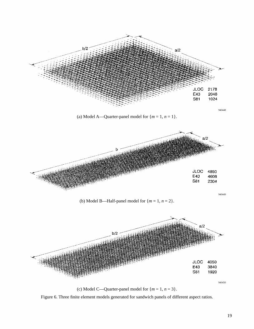
To gather thermal buckling data of sandwich panels having a wide range of aspect ratios b/a, three basic finiteelement models of different b/a were set up so that each model would cover certain limited range of b/a. Changingb/a of each model was accomplished by simply modifying length b and keeping length a constant. Sometimes moreelements had to be added to an overstretched model to maintain proper element aspect ratios. An overstretchedmodel without additional elements could result in local buckling of slender element cells rather than global bucklingof the panels (i.e., local buckling temperature is less than the global buckling temperature). For low b/a (< 1.8) andhigh b/a (> 2.9) aspect ratio panels (figs. 5(a) and 5(c)) for which the lowest buckling mode were symmetric, onlythe quarter panels were modeled. The SPAR constraint commands SYMMETRY PLANE = 1 and SYMMETRYPLANE = 2 (ref. 15) were then used to generate the full panels. For moderate b/a (1.8 ≤ b/a ≤ 2.9) aspect ratio pan-els (fig. 5(b)) for which the lowest buckling mode could be either symmetric or antisymmetric, half panels weremodeled. The SPAR constraints command SYMMETRY PLANE = 1 was then used to generate the full panels. Forpurely antisymmetric buckling, one can model only a quarter panel and use the constraint commands SYMMETRYPLANE = 1 and ANTISYMMETRY PLANE = 2 to generate the whole panel. However, such quarter-panel modelswere not used in gathering the buckling data because they consistently gave somewhat higher buckling temperaturesthan those given by the half-panel models. Figure 6 shows the three basic finite element models set up for the sand-wich panels. Both models A and C are the quarter-panel models, but model B is a half-panel model. From these ba-sic models, several modified models (not model shown) were also set up for handling certain aspect ratios and edgeconditions.
Each face sheet of the sandwich panel was modeled with one layer of E43 elements (quadrilateral combinedmembrane and bending elements) and the sandwich core with one layer of S81 elements (hexahedron (or brick) el-ements), which connect the upper and the lower face-sheet elements E43. Because the joint locations of those facesheet elements E43 are located in the middle planes of the respective face sheets, the finite element core depth willthen be h instead of the actual depth (fig. 7). Thus, to simulate the actual relative displacements (or maintain samestiffness) between the two face sheets in the sandwich thickness direction and the x- and y-directions (i.e., and and fig. 7), the thickness elastic modulus and the transverse shear moduli and
of the S81 elements had to be increased slightly according to the following relationships:
(31)
(32)
(33)
One can also model the sandwich core with one layer of S81 elements having the exact depth and then con-nect the gaps between E43 joints and S81 joints with rigid elements. However, this alternative modeling method re-quires twice as many total joint locations, and therefore, it was not used.
hcd3 d'3=
d1 d'1= d2 d'2,= E'cz, G'cxzG'cyz
E'cz Ecz hhc-----=
G'cxz Gcxz hhc-----=
G'cyz Gcyz hhc-----=
hc,
9

For simply supported edges, free rotation and free transverse shear deformation must be allowed (fig. 8(a)). Tosimulate this type of edge, pin-ended rigid rods were attached to the panel edge for connecting the two face sheets(sandwich core carries no extensional and bending stiffnesses), and then the midpoints of the rigid rods were pin-jointed to fix points lying in the sandwich middle plane (fig. 8(a)). Each pin-ended rigid rod was modeled with twoidentical E22 elements (beam element for which the intrinsic stiffness matrix is given). To simulate the rigidity ofthe rod, extensional and transverse shear stiffnesses of the E22 elements were made very large. The pin-joint condi-tion at the face sheet edges was simulated by assigning zero values to the rotational spring constants in the stiffnessmatrix for the E22 elements. The pin-joint condition at the middle-plane fixed points was simulated by relaxing thethree rotational constraints. Two methods were used to connect the ends of the E22 elements to the middle planefixed points. In the first method (center drawing of fig. 8(a)), the first joint of each E22 element was connected tothe associated joint of E43 element and its end point to the panel middle-plane fixed point. In the second method(right-hand drawing of fig. 8(a)), the ends of the two identical E22 elements, whose first joints were connected tothe upper and the lower face sheets, were connected together to the middle-plane fixed point through E25 element(zero length element used to elastically connect geometrically coincidental joints). The stiffnesses of the E25 weremade so large that the two E22 elements, connected together by the E25 element, will behave like one rigid rod.These two types of simply supported edge simulations were found to give identical thermal buckling solutions. Inmost of the buckling data gathering, the first edge simulation was used because it required less joint locations.
For the clamped edge (fig. 8(b)), the edges of the two face sheets were built into fixed vertical walls to generatethe desired constraints of zero slope, zero in-plane displacements, and zero transverse shear deformations.
Table 1 shows the sizes of the three finite element models set up for the sandwich panels of different b/a.
To make sure that the above finite element models gave accurate eigensolutions, the sandwich cores of model Awas modified to two layers of S81 elements to investigate the eigensolution convergencies. It turned out that boththe basic and the modified models gave practically identical eigensolutions. Because the modified model requiredabout three times longer computational time, it was not used in the actual buckling data gatherings.
Eigenvalue Extractions
The eigenvalue equation for buckling problems is of the form
(34)
where
Table 1. Sizes of three finite element models A, B, and C (c.f., fig. 6).
Feature Model A Model B Model C
JLOC 2178 4850 4050
E43 2048 4608 3840
S81 1024 2304 1920
= system initial stress stiffness matrix (or differential stiffness matrix), corresponding to particular applied force condition (e.g., thermal loading), and in general a function of
K = system stiffness matrix
X = displacement vector
= eigenvalues for various buckling modes
λKgX KX+ 0=
KgX
λi
10

The eigenvalues (i = 1,2,3,…) are the load factors by which the static load (mechanical or thermal) must bemultiplied to produce buckling loads corresponding to various buckling modes. Namely, if the applied temperatureload is then the buckling temperature for the i-th buckling mode is obtained from
(35)
If it is desired to find eigenvalues in the neighborhood of c, then the following shifted eigenvalue equation may beused.
(36)
In the eigenvalue extractions, the SPAR program uses an iterative process consisting of a Stodola matrix iterationprocedure, followed by a Rayleigh–Ritz procedure, and then followed by a second Stodola procedure. This processresults in successively refined approximations of i eigenvectors associated with the i eigenvalues of equation (34)closest to zero. Reference 15 describes the details of this process.
NUMERICAL EXAMPLES
The hot structural sandwich panels analyzed were fabricated with titanium face sheets and titanium sandwichcore having the following geometrical and material properties.
Geometry:
Material properties:
a = 24 in.
b = varying
h = 0.75 in.
=
= 0.06 in.
Face sheets
70 °F 900 °F*
0.31 0.31
0 0
0.16 0.16
*Mach 15 flight temperature.
λi
∆T, ∆Tcr
∆Tcr λi∆T=
λ c–( )KgX K c Kg+( )X+ 0=
hc h ts– 0.69 in.=
ts
Ex Ey lb/in2,= 16 106× 13.1 106×
Gxy lb/in2, 6.2 106× 5.0 106×
νxy νyx=
αx αy in/in-°F,= 4.85 10 6–× 5.35 10 6–×
αxy in/in-°F,
ρTi lb/in3,
11

The main objective of the present report is to study the general trend of thermal buckling characteristics of sand-wich panels under different edge conditions, and to validate Ko-Jackson theory (ref. 12). Because of the lack of ma-terial property data at high temperatures, the material iteration process was not performed, and the face sheetproperties at 900 °F and sandwich core properties at 600 °F were used in the buckling temperature calculations.
RESULTS
Eigenvalue Iterations
In finite element eigenvalue extractions, the maximum number of iterations was set to be 100. For most cases(with or without eigenshifting), however, the eigenvalues converged well below 100 iterations based on the conver-gence criterion (| λi – λi–1 | / λi) < 10–4. Figure 9 compares the convergence curves of eigenvalue iterations with andwithout shifting for the square panel (b/a = 1) under the 4C condition. With shifting, the number of iterations couldbe reduced from 14 to 9 iterations. For certain cases, the number of eigenvalue iterations with shifting turned out tobe very close or even identical to that without shifting. For certain problems, such as the thermocryogenic bucklingof cryogenic tanks (ref. 16), eigenshifting could drastically reduce the number of eigenvalue iterations (i.e., reduc-tion in computer time). For the present sandwich panel buckling problem, however, the reduction in the number ofeigenvalue iterations through the eigenshifting turned out to be relatively small or negligible.
In most of the thermal buckling data gathering, the eigenshifting method was used. The shifting factors usedwere near the values of the buckling temperatures predicted from the energy theory. In figure 10 the ELXSI 6400computer processor times are plotted as functions of the number of eigenvalue iterations for the four edge conditions.The processor time per iteration (i.e., slope of the data fitting line) for the 4S, 4C, 2C2S, and 2S2C conditions are,respectively, 2.45, 1.88, 2.48, and 2.06 minutes.
Honeycomb core (properties at 600 °F)
=
=
=
=
=
=
=
=
=
=
=
=
Ecx 2.7778 104 lb/in2×
Ecy 2.7778 104 lb/in2×
Ecz 2.7778 105 lb/in2×
Gcxy 0.00613 lb/in2
Gcyz 0.81967 105 lb/in2×
Gcxz 1.81 105 lb/in2×
νcxy 0.658 10 2–×
νcyz 0.643 10 6–×
νcxz 0.643 10 6–×
αx αy=5.37 10 6–× in/in-°F
αxy 0 in/in-°F
ρHc 3.674 10 3–× lb/in3
12

Buckling Temperatures
Figures 11, 12, and 13, respectively, show the lowest-mode buckling shapes of sandwich panels of aspect ratiosb/a = 1, 2, and 3 under the four different edge conditions. Notice that at the simply supported edges of the 4S caseand at the clamped edges of the 2C2S and 2S2C cases, the transverse shear deformations cannot be zero (fig. 4). Athigher b/a (figs. 12 and 13), the 4C and 2S2C cases required finer element models for obtaining global buckling. Thesquare panel (b/a = 1, fig. 11), under all the four different edge conditions, buckled symmetrically with {m = 1, n =1} buckling mode. For the b/a = 2 rectangular panel (fig. 12), the 4S, 4C and 2C2S conditions still induced symmet-rical buckling mode of {m = 1, n = 1}. However, under the 2S2C condition, the rectangular panel buckled antisym-metrically under {m = 1, n = 2} buckling mode. For the slender panel of b/a = 3 (fig. 13), both 4S and 2C2Sconditions continued to induce symmetrical buckling mode of {m = 1, n = 1}. However, under the 4C and 2S2Cconditions, the multiple symmetrical buckling mode of {m = 1, n = 3} turned out to be the lowest buckling mode. Infigure 14 the thermal buckling temperatures calculated using the minimum energy method (solid curves) and the fi-nite element method (circular symbols) are plotted as functions of panel aspect ratio b/a for the four cases of edgeconditions. Notice that for the high values of b/a, the thermal buckling solutions for the 2C2S and 2S2C cases ap-proach those of the 4S and 4C cases, respectively, because the constraint effects of the shorter edges of the slenderpanels diminish. The buckling solutions obtained from the two methods compare fairly well. The average solutiondifference between the two methods are 3.87%, 1.62%, 2.04% and 2.71% respectively for the 4S, 4C, 2C2S and2S2C cases. The finite element method tends to give slightly lower buckling temperatures than those given by theminimum-energy method. The reason could be the following: (1) the finite element method allows deformations inthe sandwich thickness direction, which the minimum energy theory ignores, (2) the theoretical edge conditions ofzero and (eqs. (1), (2), (5)–(8)) cannot be enforced properly in the finite element edge constraints for the4S, 2C2S, and 2S2C conditions (fig 4), and (3) the finite element modeling assumptions. For the 4C case only, allthe theoretical edge conditions could be enforced in the finite element edge constraints. For 4S, 4C and 2C2S cases,the discrepancy of the eignsolutions between the two methods is larger at the low values of b/a, and gradually di-minishes at high values of b/a. This solution discrepancy is minimum for the 4C case, and maximum for the 4S case(because both and cannot be zero at the edges of the finite element modes). For the 2S2C case, the solutiondiscrepancy is almost unaffected by the change of b/a. Table 2 lists the buckling temperatures calculated fromthe minimum energy and the finite element methods.
Table 2. Buckling temperatures of sandwich panels calculated using minimum energy and finiteelement models.
°F
4S 4C 2C2S 2S2C
b/aEnergytheory
Finiteelement
Energytheory
Finiteelement
Energytheory
Finiteelement
Energytheory
Finiteelement
0.5 1297 1207 2541 2498 2424 2366 1512 1464
0.6 1051 970 2169 2126 1995 1938 1334 1286
0.7 885 815 1889 1847 1654 1603 1232 1187
0.8 769 710 1683 1645 1387 1343 1175 1132
0.9 682 637 1535 1499 1181 1143 1144 1105
1.0 622 583 1428 1396 1021 988 1128 1093
1.1 575 547 1352 1322 897 866 1122 1090
1.2 538 513 1297 1271 799 774 1121 1092
1.4 486 465 1232 1209 662 640 1126 1102
1.6 451 436 1199 1179 573 560 1136 1116
γ xz γ yz
γ xz γ yz∆Tcr
∆Tcr ,
13

CONCLUSIONS
Thermal buckling characteristics of hypersonic aircraft honeycomb-core sandwich panels subjected to uniformtemperature loading were analyzed using minimum energy theory and finite element methods. The thermal bucklingcurves were generated for titanium sandwich panels of various aspect ratios. The two methods predicted very closebuckling temperatures, and thus, the Ko-Jackson theory was validated. The finite element method tended to giveslightly lower buckling temperatures than those given by the minimum energy theory. The slight discrepancies inthe eigensolutions between the two methods could be attributed to the following:
1. The minimum energy theory does not consider deformations in the panel thickness direction, whereas thefinite element method does.
2. The theoretical zero transverse shear deformations at the panel edges cannot be enforced in the finiteelement models with simply supported edges and cannot be enforced simultaneously in the finite elementsmodels with mixed simply supported and clamped edges.
3. Assumptions made in finite element modeling.
The discrepancy of the eigensolutions between the minimum energy theory and the finite element method is thelargest for the simply supported edge condition, because the zero transverse shear deformations at the panel edgescannot be constrained in the finite element models. This solution discrepancy is larger at low values of b/a and grad-ually decreases as b/a increases. For the sandwich panels the eigenshifting has small effect on the improvement ofthe eigenvalue convergence rate.
The author gratefully acknowledges the contribution of the late Raymond H. Jackson, NASA mathematician, insetting up computer programs for the eigenvalue extractions.
Dryden Flight Research CenterNational Aeronautics and Space AdministrationEdwards, California, June 14, 1994
Table 2. Concluded.
°F
4S 4C 2C2S 2S2C
b/aEnergytheory
Finiteelement
Energytheory
Finiteelement
Energytheory
Finiteelement
Energytheory
Finiteelement
1.8 427 416 1183 1165 514 504 1144 1130
2.0 409 403 1175 1160 473 471 1128 1096
2.2 396 391 1172 1158 444 439 1122 1092
2.4 386 382 1171 1156 423 419 1121 1094
2.6 379 376 1164 1155 407 404 1122 1099
2.8 372 370 1156 1151 395 393 1126 1100
3.0 367 366 1150 1145 386 384 1128 1095
4.0 353 348 1140 1121 360 360 1124 1100
∆Tcr ,
14

940387
Figure 1. Rectangular honeycomb-core sandwich panel.
940455
Figure 2. Rectangular sandwich panel under thermal loading.
15

940463 940464
940465 940466
Figure 3. Four types of edge conditions.
(a) Four edges simply supported (4S condition). (b) Four edges clamped (4C condition).
(c) Two sides clamped, two ends simply supported (2C2S condition).
(d) Two sides simply supported, two ends clamped (2S2C condition).
16

940388
(a) 4S condition.
940389
(b) 4C condition.
940390
(c) 2C2S condition.
940391
(d) 2S2C condition.
Figure 4. Edge distortions of sandwich panel under different edge conditions; no edge distortions for 4C condition.
17

940460
(a) Symmetric buckling (m = 1, n = 1).
940461
(b) Antisymmetric buckling (m = 1, n = 2).
940462
(c) Symmetric buckling (m = 1, n = 3).
Figure 5. Quarter-panel and half-panel regions for finite element models.
18
940448
(a) Model A—Quarter-panel model for {m = 1, n = 1}.
940449
(b) Model B—Half-panel model for {m = 1, n = 2}.
940450
(c) Model C—Quarter-panel model for {m = 1, n = 3}.
Figure 6. Three finite element models generated for sandwich panels of different aspect ratios.
19

940392
Figure 7. Modeling of sandwich panel.
20

940393
(a) Simply supported edge.
940394
(b) Clamped edge.
Figure 8. Simulation of different edge conditions.
21

940397
Figure 9. Convergence curves of eigenvalue iterations; 4C condition; b/a = 1.
940398
Figure 10. Increase of processor time with number of eigenvalue iterations; ELXSI 6400 computer.
22

940451
(a) 4S condition {m = 1, n = 1}.
940452
(b) 4C condition {m = 1, n = 1}.
Figure 11. Buckled shapes of b/a = 1 sandwich panel under different edge conditions; half panel.
23

940453
(c) 2C2S condition {m = 1, n = 1}.
940454
(d) 2S2C condition {m = 1, n = 1}.
Figure 11. Concluded.
24

940456
(a) 4S condition {m = 1, n = 1}.
940457
(b) 4C condition {m = 1, n = 1}.
Figure 12. Buckled shapes of b/a = 2 sandwich panel under different edge conditions; full panel.
25

940458
(c) 2C2S condition {m = 1, n = 1}.
940459
(d) 2S2C condition {m = 1, n = 2}.
Figure 12. Concluded.
26

940403
(a) 4S condition {m = 1, n = 1}.
940404
(b) 4C condition {m = 1, n = 3}.
Figure 13. Buckled shapes of b/a = 3 sandwich panel under different edge conditions; half panel.
27

940405
(c) 2C2S condition {m = 1, n = 1}.
940406
(d) 2S2C condition {m = 1, n = 3}.
Figure 13. Concluded.
28

940474
Figure 14. Buckling temperature curves for titanium sandwich panels under different edge conditions; a = constant.
29

APPENDIX A
COEFFICIENTS OF CHARACTERISTIC EQUATIONS
The characteristic coefficients appearing in equation (22) are defined in the following for different indi-cial and edge conditions (ref. 12).
Case 1: 4S condition
(1) m = k, n = l
(A-1)
(2) m ≠ k, n ≠ l
(A-2)
amnklij
amnmn11
D11mπa
------- 4
2 D12 2D66+( ) mπa
------- 2 nπ
b------
2D22
nπb
------ 4
++=
D* πa---
2kx
mπa
------- 2
kynπb
------ 2
+–
amnmn12
amnmn21
D11mπa
------- 3
D12 2D66+( ) mπa
------- nπ
b------
2+–= =
amnmn13
amnmn31
D22nπb
------ 3
D12 2D66+( ) mπa
------- 2 nπ
b------
+–= =
amnmn22
D11mπa
------- 2
D66nπb
------ 2
DQx++=
amnmn23
amnmn32
D12 D66+( ) mπa
------- nπ
b------
= =
amnmn33
D22nπb
------ 2
D66mπa
------- 2
DQy++=
amnklij
0=
30

Case 2: 4C condition
(1) m = n = k = l = 1
(A-3)
(2) m = k = 1, n = l ≠ 1
(A-4)
a111111
12D11πa---
48 D12 2D66+( ) π
a---
2 πb---
212D22
πb---
4++=
3D* πa---
2kx
πa---
2ky
πb---
2+–
a111112
a111121
12D11πa---
34 D12 2D66+( ) π
a---
πb---
2+–= =
a111113
a111131
12D22πb---
34 D12 2D66+( ) π
a---
2 πb---
+–= =
a111122
12D11πa---
24D66
πb---
23DQx++=
a111123
a111132
4 D12 D66+( ) πa---
πb---
= =
a111133
12D22πb---
24D66
πa---
23DQy++=
a1n1n11
8D11πa---
44 D12 2D66+( ) π
a---
2 πb---
21 n
2+( ) 3
2---D22
πb---
41 n
2+( )
24n
2+[ ]++=
D* πa---
22kx
πa---
2 32---k
yπb---
21 n
2+( )+–
a1n1n12
a1n1n21
8D11πa---
32 D12 2D66+( ) π
a---
πb---
21 n
2+( )+–= =
a1n1n13
a1n1n31
32---D22
πb---
31 n
2+( )
24n
2+[ ] 2 D12 2D66+( ) π
a---
2 πb---
1 n2
+( )+
–= =
a1n1n22
8D11πa---
22D66
πb---
21 n
2+( ) 2DQx+ +=
a1n1n23
a1n1n32
2 D12 D66+( ) πa---
πb---
1 n2
+( )= =
a1n1n33 3
2---D22
πb---
21 n
2+( )
24n
2+[ ] 2D66
πa---
21 n
2+( ) 3
2---DQy 1 n
2+( )+ +=
31
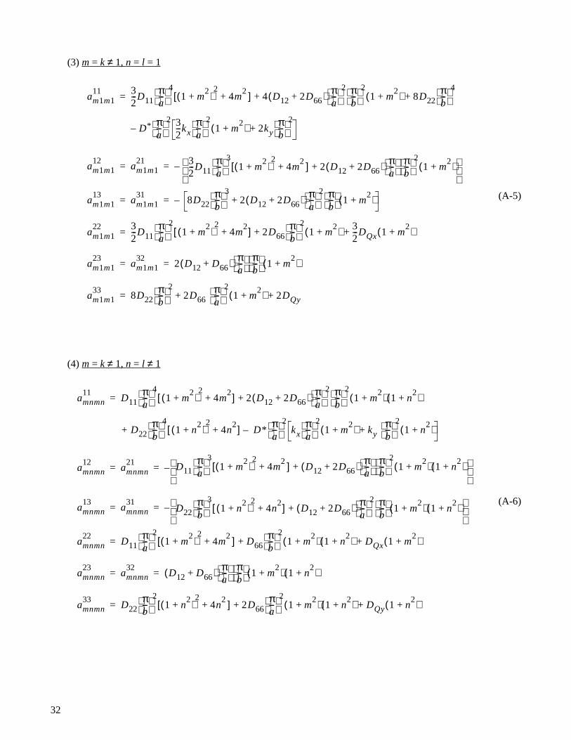
(3) m = k ≠ 1, n = l = 1
(A-5)
(4) m = k ≠ 1, n = l ≠ 1
(A-6)
am1m111 3
2---D11
πa---
41 m
2+( )
24m
2+[ ] 4 D12 2D66+( ) π
a---
2 πb---
21 m
2+( ) 8D22
πb---
4++=
D* πa---
2 32---kx
πa---
21 m
2+( ) 2ky
πb---
2+–
am1m112
am1m121 3
2---D11
πa---
31 m
2+( )
24m
2+[ ] 2 D12 2D66+( ) π
a---
πb---
21 m
2+( )+
–= =
am1m113
am1m131
8D22πb---
32 D12 2D66+( ) π
a---
2 πb---
1 m2
+( )+–= =
am1m122 3
2---D11
πa---
21 m
2+( )
24m
2+[ ] 2D66
πb---
21 m
2+( ) 3
2---DQx 1 m
2+( )++=
am1m123
am1m132
2 D12 D66+( ) πa---
πb---
1 m2
+( )= =
am1m133
8D22πb---
22D66
πa---
21 m
2+( ) 2DQy++=
amnmn11
D11πa---
41 m
2+( )
24m
2+[ ] 2 D12 2D66+( ) π
a---
2 πb---
21 m
2+( ) 1 n
2+( )+=
+ D22πb---
41 n
2+( )
24n
2+[ ] D *
πa---
2kx
πa---
21 m
2+( ) ky
πb---
21 n
2+( )+–
amnmn12
amnmn21 D11
πa---
31 m
2+( )
24m
2+[ ] D12 2D66+( ) π
a---
πb---
21 m
2+( ) 1 n
2+( )+
–= =
amnmn13
amnmn31
D22πb---
31 n
2+( )
24n
2+[ ] D12 2D66+( ) π
a---
2 πb---
1 m2
+( ) 1 n2
+( )+ –= =
amnmn22
D11πa---
21 m
2+( )
24m
2+[ ] D66
πb---
21 m
2+( ) 1 n
2+( ) DQx 1 m
2+( )++=
amnmn23
amnmn32
D12 D66+( ) πa---
πb---
1 m2
+( ) 1 n2
+( )= =
amnmn33
D22πb---
21 n
2+( )
24n
2+[ ] 2D66
πa---
21 m
2+( ) 1 n
2+( ) DQy 1 n
2+( )++=
32

(5) m = k = 1, n – l = 2
(A-7)
(6) m = k ≠ 1, n – l = 2
(A-8)
a1n1l11
4D11πa---
42 D12 2D66+( ) π
a---
2 πb---
21 l+( )2 3
4---D22
πb---
41 l+( )4
++–=
+D* πa---
2kx
πa---
2 34---ky
πb---
21 l+( )2
+
a1n1l12
a1n1l21
4D11πa---
3D12 2D66+( ) π
a---
πb---
21 l+( )2
+= =
a1n1l13
a1n1l31 3
4---D22
πb---
31 l+( )4
D12 2D66+( ) πa---
2 πb---
1 l+( )2+= =
a1n1l22
4D11πa---
2D66
πb---
21 l+( )2 DQx+ +–=
a1n1l23
a1n1l32
D12 D66+( ) πa---
πb---
1 l+( )2–= =
a1n1l33
34---D22
πb---
21 l+( )4
D66πa---
21 l+( )2 3
4---DQy 1 l+( )2
+ +–=
amnml11
12--- D11
π4---
41 m
2+( )
24m
2+[ ] 2 D12 2D66+( ) π
a---
2 πb---
21 m
2+( ) 1 l+( )2
+
–=
+ D22πb---
41 l+( )4
D*
2------- π
a---
2kx
πa---
21 m
2+( ) ky
πb---
21 l+( )2
++
amnml12
amnml21 1
2--- D11
πa---
31 m
2+( )
24m
2+[ ] D12 2D66+( ) π
a---
πb---
21 m
2+( ) 1 l+( )2
+
= =
amnml13
amnml31 1
2--- D22
πb---
31 l+( )4
D12 2D66+( ) πa---
2 πb---
+ 1 m2
+( ) 1 l+( )2
= =
amnml22
12--- D11
πa---
21 m
2+( )
24m
2+[ ] D66
πb---
21 m
2+( ) 1 l+( )2
+ DQx 1 m2
+( )+
–=
amnml23
amnml32
12--- D12 D66+( ) π
a---
πb---
1 m2
+( ) 1 l+( )2–= =
amnml33
12--- D22
πb---
21 l+( )4
D66+ πa---
21 m
2+( ) 1 l+( )2
DQy 1 l+( )2+–=
33

(7) m – k = 2, n = l = 1
(A-9)
(8) m – k = 2, n = l ≠ 1
(A-10)
am1k111
34---D11
πa---
41 k+( )4
2 D12 2D66+( ) πa---
2 πb---
21 k+( )2
4D22πb---
4++–=
+ D* πa---
2 34---kx
πa---
21 k+( )2
kyπb---
2+
am1k112
amlkl21 3
4---D11
πa---
31 k+( )4
D12 2D66+( ) πa---
πb---
21 k+( )2
+= =
am1k113
amlkl31
4D22πb---
3D12 2D66+( ) π
a---
2 πb---
1 k+( )2+= =
am1k122
34---D11
πa---
21 k+( )4
D66πb---
21 k+( )2 3
4---DQx 1 k+( )2
++–=
am1k123
amlkl32
D12 D66+( ) πa---
πb---
1 k+( )2–= =
am1k133
4D22πb---
2D66
πa---
21 k+( )2
DQy++–=
amnkn11
12--- D11
πa---
41 k+( )4
2 D12 2D66+( ) πa---
2 πb---
21 k+( )2
1 n2
+( )+
–=
+ D22πb---
41 n
2+( )
24n
2+[ ]
D*
2------- π
a---
2kx
πa---
21 k+( )2
kyπb---
21 n
2+( )++
amnkn12
amnkn21 1
2--- D11
πa---
31 k+( )4
D12 2D66+( ) πa---
πb---
21 k+( )2
1 n2
+( )+= =
amnkn13
amnkn31 1
2--- D22
πb---
31 n
2+( )
24n
2+[ ] D12 2D66+( ) π
a---
2 πb---
1 k+( )21 n
2+( )+= =
amnkn22
12---– D11
πa---
21 k+( )4
D66πb---
21 k+( )2
1 n2
+( ) DQx 1 k+( )2+ +=
amnkn23
amnkn32
12--- D12 D66+( ) π
a---
πb---
1 k+( )21 n
2+( )–= =
amnkn33
12---– D22
πb---
21 n
2+( )
24n
2+[ ] + D66
πa---
21 k+
2( ) 1 n2
+( ) D+ Qy 1 n2
+( )
=
34

(9) m – k = 2, n – l = 2
(A-11)
Case 3: 2C2S condition
(1) m = k, n = l = 1
(A-12)
amnkl11 1
4--- D11
πa---
41 k+( )4
2 D12 2D66+( ) πa---
2 πb---
21 k+( )2
1 l+( )2+=
+ D22πb---
41 l+( )4
– D*
4------- π
a---
2kx
πa---
21 k+( )2
kyπb---
21 l+( )2
+
amnkl12
amnkl21
– 14--- D11
πa---
31 k+( )4
D12 2D66+( ) πa---
πb---
21 k+( )2
1 l+( )2+= =
amnkl13
amnkl31
– 14--- D22
πb---
31 l+( )4
+ D12 2D66+( ) πa---
2 πb---
1 k+( )21 l+( )2
= =
amnkl22 1
4--- D11
πa---
21 k+( )4
D66πb---
21 k+( )2
1 l+( )2DQx 1 k+( )2
+ +=
amnkl23
amnkl32 1
4--- D12 D66+( ) π
a---
πb---
1 k+( )21 l+( )2
= =
amnkl33 1
4--- D22
πb---
21 l+( )4
D66πa---
21 k+( )2
1 l+( )2DQy 1 l+( )2
+ +=
am1m111
3D11mπa
------- 4
8 D12 2D66+( ) mπa
------- 2 π
b---
216D22
πb---
4++=
D* πa---
23kx
mπa
------- 2
4kyπb---
2+–
am1m112
am1m121
3D11mπa
------- 3
4 D12 2D66+( ) mπa
------- π
b---
2+–= =
am1m113
am1m131
16D22πb---
34 D12 2D66+( ) mπ
a-------
2 πb---
+–= =
am1m122
3D11mπa
------- 2
4D66πb---
23DQx++=
am1m123
am1m132
4 D12 D66+( ) mπa
------- π
b---
= =
am1m133
16D22πb---
24D66
mπa
------- 2
4DQx++=
35

(2) m = k, n = l ≠ 1
(A-13)
(3) m = k, n – l = 2
(A-14)
amnmn11
2D11mπa
------- 4
4 D12 2D66+( ) mπa
------- 2 π
b---
21 n
2+( ) 2D22
πb---
41 n
2+( )
24n
2+[ ]++=
2D* πa---
2kx
mπa
------- 2
kyπb---
21 n
2+( )+–
amnmn12
amnmn21
2D11mπa
------- 3
2 D12 2D66+( ) mπa
------- π
b---
21 n
2+( )+–= =
amnmn13
amnmn31
2D22πb---
31 n
2+( )
24n
2+[ ] 2 D12 2D66+( ) mπ
a-------
2 πb---
1 n2
+( )+
–= =
amnmn22
2D11mπa
------- 2
2D66πb---
21 n
2+( ) 2DQx++=
amnmn23
amnmn32
2 D12 D66+( ) mπa
------- π
b---
1 n2
+( )= =
amnmn33
2D22πb---
21 n
2+( )
24n
2+[ ] 2D66
mπa
------- 2
1 n2
+( ) 2DQy 1 n2
+( )+ +=
amnml11
D11mπa
------- 4
2 D12 2D66+( ) mπa
------- 2 π
b---
21 l+( )2
D22πb---
41 l+( )4
++–=
D* πa---
2kx
mπa
------- 2
kyπb---
21 l+( )2
++
amnml12
amnml21
D11mπa
------- 3
D12 2D66+( ) mπa
------- π
b---
21 l+( )2
+= =
amnml13
amnml31
D22πb---
31 l+( )4
D12 2D66+( ) mπa
------- 2 π
b---
1 l+( )2+= =
amnml22
D11mπa
------- 2
D66πb---
21 l+( )2
DQx+ +–=
amnml23
amnml32
D12 D66+( ) mπa
------- π
b---
1 l+( )2–= =
amnml33
D22πb---
21 l+( )4
D66mπa
------- 2
1 l+( )2DQy+ + 1 l+( )2
–=
36

Case 4: 2S2C condition
(1) m = k = 1, n = 1
(A-15)
(2) m = k ≠ 1, n = l
(A-16)
a1n1n11
16D11πa---
48 D12 2D66+( ) π
a---
2 nπb
------ 2
3D22nπb
------ 4
++=
D* πa---
24kx
πa---
23ky
nπb
------ 2
+–
a1n1n12
a1n1n21
16D11πa---
34 D12 2D66+( ) π
a---
nπb
------ 2
+–= =
a1n1n13
a1n1n31
3D22nπb
------ 3
4 D12 2D66+( ) πa---
2 nπb
------ +–= =
a1n1n22
16D11πa---
24D66
nπb
------ 2
4DQx++=
a1n1n23
a1n1n32
4 D12 D66+( ) πa---
nπb
------ = =
a1n1n33
3D22nπb
------ 2
4D66πa---
23DQx++=
amnmn11
2D11πa---
41 m
2+( )
24m
2+[ ] 4 D12 2D66+( ) π
a---
2 nπb
------ 2
1 m2
+( ) 2D22nπb
------ 4
++=
2D* πa---
2kx
πa---
21 m
2+( ) ky
nπb
------ 2
+–
amnmn12
amnmn21
2D11πa---
31 m
2+( )
24m
2+[ ] 2 D12 2D66+( ) π
a---
nπb
------ 2
1 m2
+( )+ –= =
amnmn13
amnmn31
2D22nπb
------ 3
2 D12 2D66+( ) 1 m2
+( ) πa---
2 nπb
------ +–= =
amnmn22
2D11πa---
21 m
2+( )
24m
2+[ ] 2D66
nπb
------ 2
1 m2
+( ) 2DQy 1 m2
+( )+ +=
amnmn23
amnmn32
2 D12 D66+( ) πa---
nπb
------ 1 m
2+( )= =
amnmn33
2D22nπb
------ 2
2D66πa---
21 m
2+( ) 2DQy++=
37

(3) m – k = 2, n = l
(A-17)
amnkn11
D11πa---
41 k+( )4
2 D12 2D66+( ) πa---
2 nπb
------ 2
1 k+( )2D22
nπb
------ 4
++–=
D* πa---
2kx
πa---
21 k+( )2
kynπb
------ 2
++
amnkn12
amnkn21
D11πa---
31 k+( )4
D12 2D66+( ) πa---
nπb
------ 2
1 k+( )2+= =
amnkn13
amnkn31
D22nπb
------ 3
D12 2D66+( ) πa---
2 nπb
------ 1 k+( )2
+= =
amnkn22
D11πa---
21 k+( )4
D66nπb
------ 2
1 k+( )2DQx 1 k+( )2
++–=
amnkn23
amnkn32
D12 D66+( ) πa---
nπb
------ 1 k+( )2
–= =
amnkn33
D22nπb
------ 2
D66πa---
21 k+( )2
DQy++–=
38

APPENDIX B
BUCKLING EQUATIONS
The buckling equations (eigenvalue solution equations) written out from equation (21) up to order 12 (i.e., 12 ×12 matrices) for the cases m ± n = even (symmetric buckling) and m ± n = odd (antisymmetric buckling) for differentedge conditions are given on the following pages (ref. 12).
39

40
0 0
0 0
0
0 0
0 0
0= 0
0 0
0
0 0
0
(B-1)
A35 A44 A53
16225---------
1635------
47--- 4
7---
1635------
1627------–
83--- 120
147---------–
14449---------
120147---------– 8
3---
11627------–
M3535
∆T-------------- P3535+
8021------–
M4444
∆T-------------- P4444+
8021------–
M5353
∆T-------------- P5353+
Case 1: 4S conditionm ± n = even (symmetric buckling)
m=1, n=1 0 0 0 0 0
m=1, n=3 0 0 0 0
m=2, n=2 0 0
m=3, n=1 0 0 0
m=1, n=5 0 0
m=2, n=4 0
m=3, n=3 0
m=4, n=2Symmetry
m=5, n=1
m=3, n=5
m=4, n=4
m=5, n=3
Akl → A11 A13 A22 A31 A15 A24 A33 A42 A51
M1111
∆T-------------- P1111+
49--- 8
45------ 8
45------
M1313
∆T-------------- P1313+
45---– 8
7--- 8
25------–
M2222
∆T-------------- P2222+
45---– 20
63------– 36
25------ 20
63------–
M3131
∆T-------------- P3131+
825------– 8
7---
M1515
∆T-------------- P1515+
4027------– 8
63------–
M2424
∆T-------------- P2424+
7235------– 8
63------–
M3333
∆T-------------- P3333+
7235------–
M4242
∆T-------------- P4242+
4027------–
M5151
∆T-------------- P515+

41
0
0 0
0
0 0
0
0 0= 0
0
0 0
0
0
(B-2)
A43 A52 A61
825------ 4
35------–
2063------
1635------– 8
175---------–
47---–
7235------ 4
9---–
4027------
845------– 36
1225------------–
100441---------–
414449---------– 8
45------–
M4343
∆T-------------- P4343+
83---–
M5252
∆T-------------- P5252+
2011------–
M6161
∆T-------------- P6161+
m ± n = odd (antisymmetric buckling) (4S)
m=1, n=2 0 0 0 0
m=2, n=1 – 0 0 0
m=1, n=4 – 0 0 0
m=2, n=3 0 0
m=3, n=2 0 0
m=4, n=1 0
m=1, n=6 0
m=2, n=5Symmetry
m=3, n=4
m=4, n=3
m=5, n=2
m=6, n=1
Akl → A12 A21 A14 A23 A32 A41 A16 A25 A34
M1212
∆T-------------- P1212+
49---– 4
5--- 8
45------– 20
63------
M2121
∆T-------------- P2121+
845------ 4
5--- 4
35------– 8
25------
M1414
∆T-------------- P1414+
87--- 16
225---------– 40
27------
M2323
∆T-------------- P2323+
3625------– 4
9---– 72
35------
M3232
∆T-------------- P3232+
87---– 4
7---–
M4141
∆T-------------- P4141+
8175---------– 16
35------–
M1616
∆T-------------- P1616+
2011------–
M2525
∆T-------------- P2525+
83---–
M3434
∆T-------------- P343+

42
0 0
0
0
0
= 0
0
(B-3)
A35 A44 A53
1611025---------------
M1335
∆T-------------- P1335+
36833075---------------–
443675------------–
M2244
∆T-------------- P2244+
443675------------–
1368
33075---------------–
M3153
∆T-------------- P3153+
M1535
∆T-------------- P1535+
20814553---------------
1041323------------
M2444
∆T-------------- P2444+
18411025---------------
1
M3335
∆T-------------- P3335+
846499225---------------
M3353
∆T-------------- P3353+
18411025---------------
M4244
∆T-------------- P4244+
1041323------------
1208
14553---------------
M5153
∆T-------------- P5153+
M3535
∆T-------------- P3535+
478443659---------------–
M3553
∆T-------------- P3553+
M4444
∆T-------------- P4444+
478443659---------------–
M5353
∆T-------------- P5353+
Case 2: 4C conditionm ± n = even (symmetric buckling)
m=1, n=1 0 0
m=1, n=3 0
m=2, n=2
m=3, n=1 0
m=1, n=5 0
m=2, n=4
m=3, n=3
m=4, n=2Symmetry
m=5, n=1
m=3, n=5
m=4, n=4
m=5, n=3
Akl → A11 A13 A22 A31 A15 A24 A33 A42 A51
M1111
∆T-------------- P1111+
M1113
∆T-------------- P1113+
4225---------
M1131
∆T-------------- P1131+
81575------------–
M1133
∆T-------------- P1133+
81575------------–
M1313
∆T-------------- P1313+
441575------------–
M1331
∆T-------------- P1331+
M1315
∆T-------------- P1315+
1844725------------
M1333
∆T-------------- P1333+
8811025---------------
M2222
∆T-------------- P2222+
441575------------– 4
525---------
M2224
∆T-------------- P2224+
48411025---------------
M2242
∆T-------------- P2242+
4525---------
M3131
∆T-------------- P3131+
8811025---------------
M3133
∆T-------------- P3133+
1844725------------
M3151
∆T-------------- P315+
M1515
∆T-------------- P1515+
1042079------------–
M1533
∆T-------------- P1533+
83675------------–
M2424
∆T-------------- P2424+
202433075---------------–
M2442
∆T-------------- P2442+
83675------------–
M3333
∆T-------------- P3333+
202433075---------------–
M3351
∆T-------------- P335+
M4242
∆T-------------- P4242+
1042079------------–
M5151
∆T-------------- P515+

43
0
0
0
0
= 0
0
0
(B-4)
A43 A52 A61
488
11025---------------– 4
4725------------
M2143
∆T-------------- P2143+
4525---------–
4368
33075--------------- 8
33075---------------–
M2343
∆T-------------- P2343+
443675------------
4202433075---------------
M3252
∆T-------------- P3252+
17217325---------------
M4143
∆T-------------- P4143+
1042079------------
M4161
∆T-------------- P4161+
4344
121275------------------– 4
99225---------------–
M2543
∆T-------------- P2543+
41225------------–
4846499225---------------–
M3452
∆T-------------- P3452+
344121275------------------–
M4343
∆T-------------- P4343+
1041323------------–
M4361
∆T-------------- P4361+
M5252
∆T-------------- P5252+
2363861------------–
M6161
∆T-------------- P6161+
m ± n = odd (antisymmetric buckling) (4C)
m=1, n=2 0
m=2, n=1 0
m=1, n=4
m=2, n=3
m=3, n=2 0
m=4, n=1 0
m=1, n=6
m=2, n=5Symmetry
m=3, n=4
m=4, n=3
m=5, n=2
m=6, n=1
Akl → A12 A21 A14 A23 A32 A41 A16 A25 A34
M1212
∆T-------------- P1212+
4225---------–
M1214
∆T-------------- P1214+
441575------------
M1232
∆T-------------- P1232+
81575------------ 4
525---------–
M1234
∆T-------------- P123+
M2121
∆T-------------- P2121+
81575------------
M2123
∆T-------------- P2123+
441575------------
M2141
∆T-------------- P2141+
44725------------ 88
11025---------------–
M1414
∆T-------------- P1414+
1844725------------–
M1432
∆T-------------- P1432+
1611025---------------–
M1416
∆T-------------- P1416+
1042079------------
M1434
∆T-------------- P143+
M2323
∆T-------------- P2323+
48411025---------------–
M2341
∆T-------------- P2341+
17217325---------------
M2325
∆T-------------- P2325+
202433075---------------
M3232
∆T-------------- P3232+
1844725------------– 44
3675------------
M3234
∆T-------------- P323+
M4141
∆T-------------- P4141+
833075---------------– 368
33075---------------
M1616
∆T-------------- P1616+
2363861------------–
M1634
∆T-------------- P163+
M2525
∆T-------------- P2525+
1041323------------–
M3434
∆T-------------- P343+

44
0 0
0 0
0
0 0
0 0
0= 0
0
0
0
(B-5)
A35 A44 A53
161575------------–
3684725------------
12175---------– 44
441---------
16245---------–
2082079------------–
104231--------- 184
1323------------–
M3335
∆T-------------- P3335+
368735---------
24245---------
M4244
∆T-------------- P4244+
88189---------
116189---------
M5153
∆T-------------- P5153+
M3535
∆T-------------- P3535+
10401617------------–
M4444
∆T-------------- P4444+
368567---------–
M5353
∆T-------------- P5353+
Case 3: 2C2S conditionm ± n = even (symmetric buckling)
m=1, n=1 0 0 0 0
m=1, n=3 0 0 0
m=2, n=2 0
m=3, n=1 0 0
m=1, n=5 0 0
m=2, n=4 0
m=3, n=3 0
m=4, n=2Symmetry
–
m=5, n=1
m=3, n=5
m=4, n=4
m=5, n=3
Akl → A11 A13 A22 A31 A15 A24 A33 A42 A51
M1111
∆T-------------- P1111+
M1113
∆T-------------- P1113+
445------ 8
315---------– 8
225---------
M1313
∆T-------------- P1313+
44315---------–
M1315
∆T-------------- P1315+
184945--------- 88
1575------------–
M2222
∆T-------------- P2222+
425------– 4
105---------
M2224
∆T-------------- P2224+
44175--------- 4
63------–
M3131
∆T-------------- P3131+
8175---------
M3133
∆T-------------- P3133+
835------
M1515
∆T-------------- P1515+
5202079------------– 8
525---------
M2424
∆T-------------- P2424+
184525---------– 8
441---------
M3333
∆T-------------- P3333+
88245---------–
M4242
∆T-------------- P4242+
827------
M5151
∆T-------------- P515+

45
0
0 0
0
0 – 0
0
0= 0
0
0 0
0
0
(B-6)
A43 A52 A61
881575------------ 4
175---------–
463------
3684725------------– 8
1225------------
44441---------
488245--------- 4
45------–
M4143
∆T-------------- P4143+
827------
34417325--------------- 4
3675------------
4147---------
4368735---------– 8
315---------
M4343
∆T-------------- P4343+
88189---------–
M5252
∆T-------------- P5252+
411------–
M6161
∆T-------------- P6161+
m ± n = odd (antisymmetric buckling) (2C2S)
m=1, n=2 0 0 0
m=2, n=1 0 0
m=1, n=4 0 0
m=2, n=3 0
m=3, n=2 0
m=4, n=1 0
m=1, n=6 0
m=2, n=5Symmetry
m=3, n=4
m=4, n=3
m=5, n=2
m=6, n=1
Akl → A12 A21 A14 A23 A32 A41 A16 A25 A34
M1212
∆T-------------- P1212+
425------–
M1214
∆T-------------- P1214+
44315--------- 8
225---------– 4
105---------–
M2121
∆T-------------- P2121+
8315---------
M2123
∆T-------------- P2123+
425------ 4
925--------- 8
175---------–
M1414
∆T-------------- P1414+
184945---------– 16
1575------------
M1416
∆T-------------- P1416+
5202079------------
M2323
∆T-------------- P2323+
44175---------– 172
3465------------
M2325
∆T-------------- P2325+
184525---------
M3232
∆T-------------- P3232+
835------– 12
175---------
M3234
∆T-------------- P323+
M4141
∆T-------------- P4141+
84725------------ 16
245---------
M1616
∆T-------------- P1616+
11803861------------–
M2525
∆T-------------- P2525+
104231---------–
M3434
∆T-------------- P343+

46
0 0
0 0
0
0 0
0
= 0
0
0
0 0
0
(B-7)
A35 A44 A53
161575------------–
16245---------–
44441--------- 12
175---------–
13684725------------
M1535
∆T-------------- P1535+
16189---------
88189---------
M2444
∆T-------------- P2444+
24245---------
368735---------
M3353
∆T-------------- P3353+
1841323------------– 104
231---------
12082079------------–
M3535
∆T-------------- P3535+
368567---------–
M4444
∆T-------------- P4444+
10401617------------–
M5353
∆T-------------- P5353+
Case 4: 2S2C conditionm ± n = even (symmetric buckling)
m=1, n=1 0 0 0 0
m=1, n=3 0 0 0
m=2, n=2 0
m=3, n=1 0 0
m=1, n=5 0 0
m=2, n=4 0
m=3, n=3 0
m=4, n=2Symmetry
m=5, n=1
m=3, n=5
m=4, n=4
m=5, n=3
Akl → A11 A13 A22 A31 A15 A24 A33 A42 A51
M1111
∆T-------------- P1111+
445------
M1131
∆T-------------- P1131+
8225--------- 8
315---------–
M1313
∆T-------------- P1313+
425------– 8
35------
M1333
∆T-------------- P1333+
8175---------
M2222
∆T-------------- P2222+
44315---------– 4
63------– 44
175---------
M2242
∆T-------------- P2242+
4105---------
M3131
∆T-------------- P3131+
881575------------– 184
945---------
M3151
∆T-------------- P315+
M1515
∆T-------------- P1515+
827------– 8
441---------
M2424
∆T-------------- P2424+
88245---------– 8
525---------
M3333
∆T-------------- P3333+
184525---------–
M4242
∆T-------------- P4242+
5202079------------–
M5151
∆T-------------- P515+

47
0
0 0
0
0
0= 0
0
0 0
0
0
(B-8)
A43 A52 A61
8175---------– 4
945---------
4105---------–
416245--------- 8
4725------------
M2343
∆T-------------- P2343+
12175---------
184525---------
M3252
∆T-------------- P3252+
1723465------------
5202079------------
M4161
∆T-------------- P4161+
8315--------- 4
3675------------
4147---------
4368735---------– 344
17325---------------
M4343
∆T-------------- P4343+
104231---------–
M5252
∆T-------------- P5252+
11803861------------–
M6161
∆T-------------- P6161+
m ± n = odd (antisymmetric buckling) (2S2C)
m=1, n=2 0 0 0
m=2, n=1 0 0
m=1, n=4 0 0
m=2, n=3 0 0
m=3, n=2 0 0
m=4, n=1 0
m=1, n=6 0
m=2, n=5Symmetry
m=3, n=4
m=4, n=3
m=5, n=2
m=6, n=1
Akl → A12 A21 A14 A23 A32 A41 A16 A25 A34
M1212
∆T-------------- P1212+
445------– 4
25------
M1232
∆T-------------- P1232+
8315--------- 4
63------
M2121
∆T-------------- P2121+
8225---------– 44
315---------
M2141
∆T-------------- P2141+
4175---------– 88
1575------------
M1414
∆T-------------- P1414+
835------– 16
1575------------ 8
27------
M1434
∆T-------------- P143+
M2323
∆T-------------- P2323+
44175---------– 4
45------– 88
245---------
M3232
∆T-------------- P3232+
184945---------– 44
441---------–
M4141
∆T-------------- P4141+
81225------------ 368
4725------------–
M1616
∆T-------------- P1616+
411------–
M2525
∆T-------------- P2525+
88189---------–
M3434
∆T-------------- P343+

REFERENCES
1. Gowda, R. M. Siddaveere and K. A. V. Pandalai, Thermal Buckling of Orthotropic Plates, Studies inStructural Mechanics, Hoff's 65th Anniversary Volume, Indian Institute of Technology, Madras-36,India, 1970, pp. 9–44.
2. Tauchert, T. R. and N. N. Huang, “Thermal Buckling and Postbuckling Behavior of AntisymmetricAngle-Ply Laminates,” Proc. Internat'l Symp. Composite Materials and Structures, Beijing, China,June 1986, pp. 357–362.
3. Tauchert, T. R. and N. N. Huang, “Thermal Buckling of Symmetric Angle-Ply Laminated Plates,”Composite Structures, I. H. Marshall-editor, Elsevier Applied Science, London, 1987, pp. 1424–1435.
4. Thangaratnam, Kari R., Palaninathan, and J. Ramachandran, “Thermal Buckling of Composite Lami-nated Plates,” Computers and Structures, Vol. 32, No. 5, 1989, pp. 1117–1124.
5. Huang, N.N. and T.R. Tauchert, “Postbuckling Response of Antisymmetric Angle-Ply Laminates toUniform Temperature Loading,” Acta Mechanica, Vol. 72, 1988, pp. 173–183.
6. Tauchert, Theodore R., “Thermal Stresses in Plates—Statical Problems,” in Thermal Stresses I, Vol. 1,Elsevier Sciences Publishing Co., New York, 1986, pp. 23–141.
7. Ko, William L. and Raymond H. Jackson, Thermal Behavior of a Titanium Honeycomb-Core Sand-wich Panel, NASA TM-101732, 1991.
8. Ko, William L. and Raymond H. Jackson, “Combined Compressive and Shear Buckling Analysis ofHypersonic Aircraft Structural Sandwich Panels,” AIAA Paper No. 92-2487-CP. Presented at the 33rdAIAA/ASME/ASCE/AHS/ASC Structures, Structural Dynamics and Materials Conference, Dallas,Texas, April 13–15, 1992; also NASA TM-4290, 1991.
9. Ko, William L. and Raymond H. Jackson, Combined-Load Buckling Behavior of Metal-Matrix Com-posite Sandwich Panels Under Different Thermal Environments, NASA TM-4321, 1991.
10. Ko, William L. and Raymond H. Jackson, “Compressive and Shear Buckling Analysis of Metal MatrixComposite Sandwich Panels under Different Thermal Environments,” Composite Structures, Vol. 25,July 1993, pp. 227–239.
11. Ko, William L., “Mechanical and Thermal Buckling Analysis of Sandwich Panels Under DifferentEdge Conditions,” Proc. 1st Pacific International Conference on Aerospace Science and Technology,Tainan, Taiwan, Dec. 6–9, 1993.
12. Ko, William L. and Raymond H. Jackson, Mechanical and Thermal Buckling of Rectangular Sand-wich Panels Under Different Edge Conditions, NASA TM-4535, 1994.
13. Tenney, D. R., W. B. Lisagor, and S. C. Dixon, “Materials and Structures for Hypersonic Vehicles,”J. Aircraft, Vol. 26, no. 11, Nov. 1989, pp. 953–970.
48

14. Thornton, Earl A. “Thermal Buckling of Plates and Shells,” Applied Mechanics Review, Vol. 46,No. 10, October 1993, pp. 485–506.
15. Whetstone, W. D., SPAR Structural Analysis System Reference Manual, System Level 13A, Vol. 1,Program Execution, NASA CR-158970-1, Dec. 1978.
16. Ko, William L. “Thermocryogenic Buckling and Stress Analyses of 9 Partially Filled Cryogenic TankSubjected to Cylindrical Strip Heating,” Proceedings of 2nd Thermal Structures Conference,Charlottesville, Virginia, Oct. 18–20, 1994. Also, NASA TM-4579, Oct. 1994.
49

REPORT DOCUMENTATION PAGE Form ApprovedOMB No. 0704-0188
Public reporting burden for this collection of information is estimated to average 1 hour per response, including the time for reviewing instructions, searching existing data sources, gathering andmaintaining the data needed, and completing and reviewing the collection of information. Send comments regarding this burden estimate or any other aspect of this collection of information,including suggestions for reducing this burden, to Washington Headquarters Services, Directorate for Information Operations and Reports, 1215 Jefferson Davis Highway, Suite 1204, Arlington,VA 22202-4302, and to the Office of Management and Budget, Paperwork Reduction Project (0704-0188), Washington, DC 20503.
1. AGENCY USE ONLY (Leave blank) 2. REPORT DATE 3. REPORT TYPE AND DATES COVERED
4. TITLE AND SUBTITLE 5. FUNDING NUMBERS
6. AUTHOR(S)
8. PERFORMING ORGANIZATION REPORT NUMBER
7. PERFORMING ORGANIZATION NAME(S) AND ADDRESS(ES)
9. SPONSORING/MONITORING AGENCY NAME(S) AND ADDRESS(ES) 10. SPONSORING/MONITORING AGENCY REPORT NUMBER
11. SUPPLEMENTARY NOTES
12a. DISTRIBUTION/AVAILABILITY STATEMENT 12b. DISTRIBUTION CODE
13. ABSTRACT (Maximum 200 words)
14. SUBJECT TERMS 15. NUMBER OF PAGES
16. PRICE CODE
17. SECURITY CLASSIFICATION OF REPORT
18. SECURITY CLASSIFICATION OF THIS PAGE
19. SECURITY CLASSIFICATION OF ABSTRACT
20. LIMITATION OF ABSTRACT
NSN 7540-01-280-5500 Standard Form 298 (Rev. 2-89)Prescribed by ANSI Std. Z39-18298-102
Predictions of Thermal Buckling Strengths of Hypersonic Aircraft SandwichPanels Using Minimum Potential Energy and Finite Element Methods
WU 505-70-63
William L. Ko
NASA Dryden Flight Research CenterP.O. Box 273Edwards, California 93523-0273
H-2009
National Aeronautics and Space AdministrationWashington, DC 20546-0001 NASA TM-4643
Thermal buckling characteristics of hypersonic aircraft sandwich panels of various aspect ratios were investigated. Thepanel is fastened at its four edges to the substructures under four different edge conditions and is subjected to uniformtemperature loading. Minimum potential energy theory and finite element methods were used to calculate the panelbuckling temperatures. The two methods gave fairly close buckling temperatures. However, the finite element methodgave slightly lower buckling temperatures than those given by the minimum potential energy theory. The reasons for thisslight discrepancy in eigensolutions are discussed in detail. In addition, the effect of eigenshifting on the eigenvalueconvergence rate is discussed.
Different edge conditions, Finite element method, Minimum potential energy theory,Sandwich panels, Thermal bucklings
A04
54
Unclassified Unclassified Unclassified Unlimited
May 1995 Technical Memorandum
Available from the NASA Center for AeroSpace Information, 800 Elkridge Landing Road, Linthicum Heights, MD 21090; (301)621-0390
Unclassified—UnlimitedSubject Category 39