Journal of Neuroscience, 30(9):3531-43, 2010.

Predictive coding as a model of response properties in cortical area V1

M. W. SpratlingDivision of Engineering, King’s College London, London. WC2R 2LS. UK.andCentre for Brain and Cognitive Development, Birkbeck, University of London, London. WC1E 7JL. UK.

Abstract

A simple model is shown to account for a large range of V1 classical, and non-classical, receptive field proper-ties including orientation-tuning, spatial and temporal frequency tuning, cross-orientation suppression, surroundsuppression, and facilitation and inhibition by flankers and textured surrounds. The model is an implementa-tion of the predictive coding theory of cortical function and thus provides a single computational explanationfor a diverse range of neurophysiological findings. Furthermore, since predictive coding can be related to thebiased competition theory and is a specific example of more general theories of hierarchical perceptual inferencethe current results relate V1 response properties to a wider, more unified, framework for understanding corticalfunction.

1 IntroductionPredictive coding (PC) provides an elegant theory of how bottom-up evidence is combined with top-down priorsin order to compute the most likely interpretation of sensory data. Specifically, PC proposes that an internalrepresentation of the world generates predictions which are compared with stimulus-driven activity in order tocalculate the residual error between the prediction and the sensory evidence. A number of previous proposals forhow PC could be implemented in cortical circuitry have all suggested that cortical feedback connections carrypredictions and that these act on regions at preceding stages along an information processing pathway in order tocalculate the residual error which is then propagated via cortical feedforward connections (Barlow, 1994; Friston,2005, 2009; Jehee et al., 2006; Kilner et al., 2007; Mumford, 1992; Murray et al., 2004; Rao and Ballard, 1999).

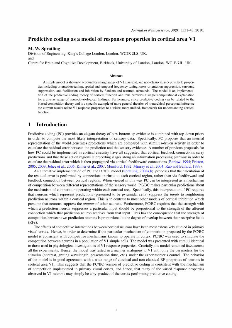
An alternative implementation of PC, the PC/BC model (Spratling, 2008a,b), proposes that the calculation ofthe residual error is performed by connections intrinsic to each cortical region, rather than via feedforward andfeedback connection between cortical regions. When viewed in this way PC can be interpreted as a mechanismof competition between different representations of the sensory world. PC/BC makes particular predictions aboutthe mechanism of competition operating within each cortical area. Specifically, this interpretation of PC requiresthat neurons which represent predictions (presumed to be pyramidal cells) suppress the inputs to neighboringprediction neurons within a cortical region. This is in contrast to most other models of cortical inhibition whichpresume that neurons suppress the outputs of other neurons. Furthermore, PC/BC requires that the strength withwhich a prediction neuron suppresses a particular input should be proportional to the strength of the afferentconnection which that prediction neuron receives from that input. This has the consequence that the strength ofcompetition between two prediction neurons is proportional to the degree of overlap between their receptive fields(RFs).

The effects of competitive interactions between cortical neurons have been most extensively studied in primaryvisual cortex. Hence, in order to determine if the particular mechanism of competition proposed by the PC/BCmodel is consistent with competitive mechanisms known to operate in cortex, PC/BC was used to simulate thecompetition between neurons in a population of V1 simple cells. The model was presented with stimuli identicalto those used in physiological investigations of V1 response properties. Crucially, the model remained fixed acrossall the experiments. Hence, the model was tested in a manner analogous to V1 with only the parameters for thestimulus (contrast, grating wavelength, presentation time, etc.) under the experimenter’s control. The behaviorof the model is in good agreement with a wide range of classical and non-classical RF properties of neurons incortical area V1. This suggests that the PC/BC version of predictive coding is consistent with the mechanismof competition implemented in primary visual cortex, and hence, that many of the varied response propertiesobserved in V1 neurons may simply be a by-product of the cortex performing predictive coding.

1

(W )S2

T

xW W

S1 T(W )

S2S1

S1 S2

S2S1 S1 S2e y e y

Figure 1: The PC/BC model: a reformulation of predictive coding (Rao and Ballard, 1999) that can beinterpreted as a form of biased competition model. Rectangles represent populations of neurons, with ylabeling populations of prediction neurons and e labeling populations of error-detecting neurons. Openarrows signify excitatory connections, filled arrows indicate inhibitory connections, crossed connectionssignify a many-to-many connectivity pattern between the neurons in two populations, parallel connec-tions indicate a one-to-one mapping of connections between the neurons in two populations, and largeshaded boxes with rounded corners indicate different cortical areas or processing stages.

2 Methods

2.1 The PC/BC ModelSpratling (2008a) introduced a nonlinear model of predictive coding (nonlinear PC/BC), illustrated in Figure 1,that is implemented using the following equations:

eSi = ySi−1 �(ε2 +

(WSi

)TySi)

(1)

ySi ←(ε1 + ySi

)⊗WSieSi (2)

ySi ← ySi ⊗(

1 + η(WSi+1

)TySi+1

)(3)

Where superscripts of the form Si indicate processing stage i of a hierarchical neural network; eSi is a (m by1) vector of error-detecting neuron activations; ySi is a (n by 1) vector of prediction neuron activations; WSi

is a (n by m) matrix of synaptic weight values normalized such that the sum of each row is equal to ψ; WSi

is a matrix representing the same synaptic weight values as W but such that the rows are normalized to have amaximum value of ψ; ε1, ε2, and η are parameters; and� and⊗ indicate element-wise division and multiplicationrespectively. These equations are evaluated in the order 1, 2, 3 and the values of ySi given by equation 3 are thensubstituted back into equations 1 and 2 to recursively calculate the changing neural activations at each time-step.

A value of ψ equal to one has been used in previous work (De Meyer and Spratling, 2009; Spratling, 2008a;Spratling et al., 2009). Changing the value of this particular parameter has no effect on the behavior of the model,except to scale the activation values of the error-detecting neurons by 1

ψ . In these experiments a value of ψ equalto 5000 was used to produce error neuron activations of the same order of magnitude as the prediction neuronactivations (see Fig. S6).

Equation 1 describes the calculation of the neural activity for each population of error-detecting neurons. Thesevalues are a function of the activity of the prediction neurons in the preceding cortical area divisively modulatedby a weighted sum of the outputs of the prediction neurons in the current area (Spratling et al., 2009). Theactivation of the error-detecting neurons can be interpreted in two ways. Firstly, e can be considered to representthe residual error between the input to the current processing stage (ySi−1) and the reconstruction of the input((

WSi)T

ySi)

generated by the prediction neurons at the current processing stage. The values of e indicate

the degree of mismatch between the top-down reconstruction of the input and the actual input (assuming ε2 issufficiently small to be negligible). When a value within e is greater than 1

ψ it indicates that a particular elementof the input is under-represented in the reconstruction, a value of less than 1

ψ indicates that a particular elementof the input is over-represented in the reconstruction, and a value of 1

ψ indicates that the top-down reconstructionperfectly predicts the bottom-up stimulation. A second interpretation is that e represents the inhibited inputsto a population of competing prediction neurons. Each prediction neuron modulates its own inputs, which helpsstabilize the response of the prediction neurons, since a strongly (or weakly) active prediction neuron will suppress

2

TW

x WV1

ye

Figure 2: The model of V1 implemented using PC/BC. The prediction neurons (labeled y) are assumedto correspond to V1 simple cells and the response of one of these neurons is recorded. The RFs of theseprediction neurons are determined by the definition of the weight matrix W. Prediction neurons competeto represent the input stimulus x via divisive feedback which acts on the error-detecting neurons (labelede) and is carried by connections from the prediction neurons to the error-detecting neurons which havestrength proportional to the corresponding reciprocal weights from the error-detecting neurons to theprediction neurons.

(magnify) its inputs, and hence, reduce (enhance) its own response. Prediction neurons that share inputs (i.e., thathave overlapping RFs) will also modulate each other’s inputs. This generates a form of competition between theprediction neurons, such that each neuron effectively tries to block other prediction neurons from responding tothe inputs which it represents.

Equation 2 describes the updating of the prediction neuron activations. The response of each prediction neuronis a function of its activation at the previous iteration and a weighted sum of afferent inputs from the error-detectingneurons. Equation 3 describes the effects on the prediction neuron activations of top-down inputs from predictionneurons at the next stage in the neural hierarchy. These top-down inputs are a weighted sum of the activity of theprediction neurons at the subsequent processing stage and have a purely modulatory effect on the current process-ing stage. This feedback allows predictions generated by neurons higher up a processing hierarchy (which havelarger receptive fields) to influence the strength of each prediction made at the current processing stage. Equiv-alently, feedback can be interpreted as influencing the outcome of the competition occurring between predictionneurons at the current processing stage. Hence, the PC/BC model can also be interpreted as an implementation ofthe biased competition model of cortical function (Spratling, 2008a,b).

2.2 The V1 ModelThis article is concerned with modeling a single cortical region, V1, in isolation. Hence, only a single processingstage will be modeled (Fig. 2). Furthermore, all top-down, modulatory, inputs to this area are ignored (i.e.,yV 1+1 = 0), and hence, equation 3 can also be ignored. Since there is only one processing stage in the model, thesuperscripts will be dropped, and the input to V1 will be described by a vector, x = yV 1−1, of inputs coming froma model of the lateral geniculate nucleus (LGN), see below. The model can thus be simplified to the following twoequations.

e = x�(ε2 + WTy

)(4)

y← (ε1 + y)⊗We (5)

There equations describe the competition occurring within one processing stage (cortical area) of the PC/BCmodel. This mechanism of competition is called Divisive Input Modulation (DIM), and has been shown to haveexcellent pattern recognition abilities on an artificial task (Spratling et al., 2009).

Despite the simplicity of the model, simulating a large population of neurons receiving input from a reasonablylarge image is computationally demanding using the matrix multiplication method described by equations 4 and5. Furthermore, individually specifying the synaptic weight values for a large population of neurons can beinconvenient. For an application, like a model of V1, where neurons have RFs restricted to a small fraction of theinput image, and where the same patterns of weights are repeated at different spatial locations, it is possible toimplement DIM in a more tractable manner using linear filtering and convolution, as follows:

E = X�

(ε2 +

p∑k=1

(wk ∗Yk)

)(6)

Yk ← (ε1 + Yk)⊗ (wk ?E) (7)

3

(a)

⇒ON OFF

−0.0100.01

(b)

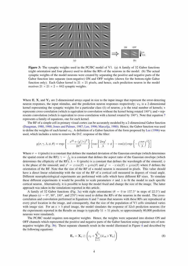
Figure 3: The synaptic weights used in the PC/BC model of V1. (a) A family of 32 Gabor functions(eight orientation and four phases) used to define the RFs of the neurons in the model. (b) The actualsynaptic weights of the model neurons were created by separating the positive and negative parts of theGabor function into separate (non-negative) ON and OFF weights (shown for the bottom-right Gaborfunction only). Each Gabor kernel is 21 × 21 pixels, and hence, each prediction neuron in the modelreceives 21× 21× 2 = 882 synaptic weights.

Where E, X, and Yk are 2-dimensional arrays equal in size to the input image that represent the error-detectingneuron responses, the input stimulus, and the prediction neuron responses respectively; wk is a 2-dimensionalkernel representing the synaptic weights for a particular class (k) of neuron; p is the total number of kernels; ?represents cross-correlation (which is equivalent to convolution without the kernel being rotated 180o); and ∗ rep-resents convolution (which is equivalent to cross-correlation with a kernel rotated by 180o). Note that equation 7represents a family of equations, one for each kernel.

The RF of a simple cell in primary visual cortex can be accurately modeled by a 2-dimensional Gabor function(Daugman, 1980, 1988; Jones and Palmer, 1987; Lee, 1996; Marcelja, 1980). Hence, the Gabor function was usedto define the weights of each kernel wk. A definition of a Gabor function of the form proposed by Lee (1996) wasused, which includes a term to remove the D.C. response of the filter:

g(σ, γ, λ, φ, θ) = exp

{−x′2 + (y′/γ)2

2σ2

}[cos{

2πy′

λ+ φ

}− cos(φ) exp

{−(πσλ

)2}]

Where σ = 4 (pixels) is a constant that defines the standard deviation of the Gaussian envelope (which determinesthe spatial extent of the RF); γ = 1√

2is a constant that defines the aspect ratio of the Gaussian envelope (which

determines the ellipticity of the RF); λ = 6 (pixels) is a constant that defines the wavelength of the sinusoid; φis the phase of the sinusoid; and x′ = x cos(θ) + y sin(θ) and y′ = −x sin(θ) + y cos(θ) where θ defines theorientation of the RF. Note that the size of the RF of a model neuron is measured in pixels. This value shouldhave a direct linear relationship with the size of the RF of a cortical cell measured in degrees of visual angle.Different neurophysiological experiments are performed with cells which have different RF sizes. To simulatethese different experiments it would be possible to scale parameters σ and λ to fit the model to each specificcortical neuron. Alternatively, it is possible to keep the model fixed and change the size of the image. The latterapproach was taken in the simulations reported in this article.

A family of 32 Gabor functions (Fig. 3a) with eight orientations (θ = 0 to 157.5o in steps of 22.5o) andfour phases (φ = 0o, 90o, 180o, and 270o) were used to define the RFs of the neurons in the model. The cross-correlation and convolution performed in Equations 6 and 7 mean that neurons with these RFs are reproduced atevery pixel location in the image, and consequently, that the size of the population of V1 cells simulated varieswith image size. For an a × b pixel image, the model simulates the response of 32ab prediction neurons (forthe experiments reported in the Results an image is typically 51 × 51 pixels, so approximately 80,000 predictionneurons were simulated).

The PC/BC model requires non-negative weights. Hence, the weights were separated into distinct ON andOFF channels which represented the positive and negative parts of the Gabor function using separate sets of non-negative weights (Fig. 3b). These separate channels result in the model illustrated in Figure 4 and described bythe following equations:

Eo = Xo �

(ε2 +

p∑k=1

(wok ∗Yk)

)(8)

4

*

* *

*

I

XOFF OFF

ON ONX

V1

E

E

Y

Figure 4: The PC/BC model of V1 implemented using convolution and with separate ON and OFFchannels. The input image I is preprocessed by convolution with a circular-symmetric on-center/off-surround kernel (to generate the input to the ON channel of the V1 model), and a circular-symmetricoff-center/on-surround kernel (to generate the input to the OFF channel of the V1 model). The predic-tion neurons (labeled Y), which represent V1 simple cells, generate the responses which were recordedduring the experiments. These responses were generated by convolving the outputs of the (ON and OFFchannels of the) error-detecting neurons (labeled E) with (the ON and OFF channels of) a number of ker-nels representing V1 RFs. This convolution process effectively reproduces the same RFs at every pixellocation in the image. The responses of the error-detecting neurons are influenced by divisive feedbackfrom the prediction neurons, which is also calculated by convolving the prediction neuron outputs withthe weight kernels.

Yk ← (ε1 + Yk)⊗∑o

(wok ?Eo) (9)

Where o ∈ [ON,OFF ]. The kernels wON,k and wOFF,k were normalized so that sum of all the weights in boththe ON and OFF channel was equal to ψ, and wON,k and wOFF,k were normalized so that the maximum valueacross both the ON and OFF channel was equal to ψ.

For each new input image, the prediction neuron responses (Y) were initialized to zero, and then the aboveequations were iterated to record the response of Y for a number of iterations (t). This recording time, t, was theonly parameter (apart from the input image) that was varied during the experiments reported in the Results. Theresponse of the prediction neurons on the first iteration is given by:

Yk =ε1ε2

(∑o

wok ?Xo

)(10)

The bracketed term on the right-hand side of equation 10 represents the output produced by a set of linear filterswhen applied to the image. This initial, linear, response is scaled by the ratio ε1

ε2. To ensure that this initial transient

did not dominate the recorded responses, values of ε1 = 0.0001 and ε2 = 50 were used. Given the large value ofψ used here, these values are similar to those used previously to simulate the interactions between attention andlong-range lateral connections in V1 (De Meyer and Spratling, 2009).

Results from neurophysiological studies are generally presented by showing how the mean evoked firing rate ofthe recorded neuron changes as a particular parameter of the input stimulus is varied. Results from the model weregenerated in the same way by recording the activity of a single prediction neuron, in response to each input image,for a number of iterations (t) of the PC/BC algorithm. The average response was then calculated by simply takingthe mean activity of the recorded prediction neuron over the t iterations that the stimulus was presented. As fortypical physiological experiments, the stimulus parameters other than the one being varied during the experiment,were matched to the preferred parameters of the neuron under test (e.g., the stimulus was centered over the RF, atthe recorded neuron’s preferred orientation, spatial frequency, temporal frequency, etc.). Furthermore, the range ofgray-scale values in the input image I were set equal to the fractional Michelson contrast used for the presentationof stimuli in the corresponding physiological experiment, if this value was reported.

2.3 The LGN Model (Image Pre-processing)The input to the model of V1, described above, was an input image (I) pre-processed by convolution with aLaplacian-of-Gaussian (LoG) filter (l) with standard deviation equal to one. This is virtually identical to the

5

Difference-of-Gaussians (DoG) filter that has traditionally been used to model circular RFs in LGN. The outputfrom this filter was subject to a saturating non-linearity, such that:

X = tanh {2π(I ∗ l)}

The positive and rectified negative responses were separated into two images XON and XOFF simulating theoutputs of cells in retina and LGN with circular-symmetric on-center/off-surround and off-center/on-surroundRFs. This pre-processing is illustrated in Figure 4. Consistent with neurophysiological data (Reid and Alonso,1995), the ON-center LGN neurons provided input to the ON sub-field of the model V1 simple cells, while theOFF-center LGN neurons provided input to the OFF sub-field of the model V1 neurons.

In most experiments static stimuli were used. Hence, I and the values of XON and XOFF remained constantthroughout each experiment. However, in some experiments it was necessary to simulate moving stimuli. Todo this the input image was changed, and new XON and XOFF values were calculated, for each iteration ofthe PC/BC algorithm. The amount the input image changed between consecutive iterations reflected the speedof the temporally changing stimulus. For example, to simulate an object moving at 10 pixels per iteration theobject would be displaced by 10 pixels in one image compared to the previous one. Since moving stimuli in theexperiments reported here were sinusoidal gratings speed was measured in cycles per iteration, where the numberof cycles refers to the phase shift between sinusoids in consecutive images.

2.4 CodeSoftware, written in MATLAB, which implements the PC/BC model described above is available at http://www.corinet.org/mike/code.html.

3 ResultsThe following sections present simulations of a number of experiments performed to assess the response prop-erties of cells in V1. These experiments cover basic tuning preferences (orientation tuning, size tuning, spatialfrequency tuning, and temporal frequency tuning), suppression due to additional stimuli appearing within the clas-sical receptive field (cross-orientation suppression) and outside the classical receptive field (surround suppression,and suppression due to textured surrounds), and facilitation due to flankers.

3.1 Basic Tuning PropertiesSimple cells in V1 are selective for a number of stimulus properties such as color, orientation, direction of motion,spatial frequency, temporal frequency, eye of origin, binocular disparity and stimulus size and location. The modelpresented here is restricted to gray-scale pixel values coming from a single image, and has no mechanism fordistinguishing direction of motion. However, it generates behavior that closely matches typical tuning propertiesof V1 cells for those properties that it does model, namely: orientation, spatial frequency, temporal frequency, andsize.

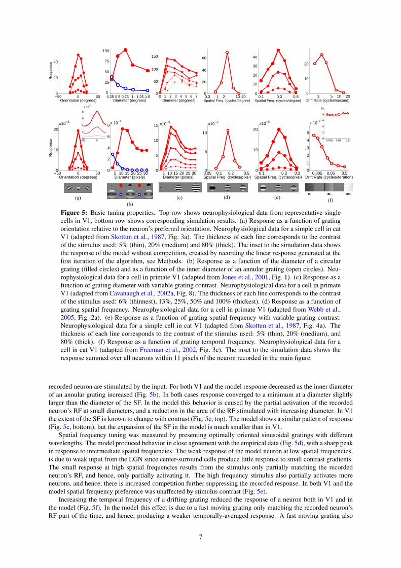
Orientation tuning was measured by presenting, at various orientations, a sinusoidal grating centered overthe recorded neuron’s RF (Fig. 5a). Both the V1 neuron and the model neuron showed selectivity for a particularstimulus orientation, with the response falling quickly as the orientation of the stimulus diverged from the preferredorientation. This selectivity was unaltered by stimulus contrast, with a stimulus far from the preferred orientationproducing a weak response even when presented at high contrast. Orientation tuning in the model was partiallydue to the alignment of the strongest afferent weights along a specific orientation. However, tuning was sharpenedby the competition occurring between neurons in the model. This can be seen by observing the orientation tuningproduced when competition was removed from the model (inset to Fig. 5a). Without competition, the neuron hadthe same orientation preference, but was much more broadly tuned producing a strong response (> 42% of themaximum) at all orientations, even at 90 degrees from the preferred orientation (data not shown).

Both V1 and the model show the same pattern of results when tested with circular sinusoidal gratings ofvarious diameters (Fig. 5b). At small stimulus diameters the response increased with increasing stimulus size.However, it reached a peak at a certain diameter, defining the summation field (SF) (Angelucci et al., 2002), afterwhich the response became increasingly suppressed before reaching a plateau at large stimulus diameters. In themodel, the initial increase in response with stimulus size is due to more of the RF of the recorded neuron beingstimulated. However, as the stimulus becomes larger, more neurons neighboring the recorded neuron also becomestimulated. These neurons engage in a competition to represent the input, and this ongoing competition reducesthe recorded response. The plateau is reached when all the neighboring neurons that have RFs that overlap with the

6

Res

pons

e 40

20

Orientation (degrees)500−50

0 0

100

75

50

25

0.25 0.5 0.75 1 1.25 1.5Diameter (degrees)

Res

pons

eDiameter (degrees)

00

1 2 3 4 5 6 7

50

100

150

Spatial Freq. (cycles/degree)0.3 1 2 100

20

40

60

Res

pons

e

20

40

30

20

10

0

Spatial Freq. (cycles/degree)0.1 0.80.3

Res

pons

e 20

10

0

Res

pons

e

Drift Rate (cycles/second)5 102 20

−50 0 500

10

20

Orientation (degrees)

Res

pons

e

x10−3

−50 0 500

2

4

6

8

x 10−3

Orientation (degrees)

Res

pons

e

5 10 15 20 25 300

2

4

6

8x 10

−3

Diameter (pixels)

Res

pons

e

5 10 15 20 25 300

5

10

15

Diameter (pixels)

Res

pons

e

x10−3

0.05 0.1 0.2 0.50

5

10

Spatial Freq. (cycles/pixel)

Res

pons

e

x10−3

0.1 0.2 0.30

10

20

Spatial Freq. (cycles/pixel)

Res

pons

e

x10−3

0.005 0.05 0.50

1

2

3

4

5

x 10−3

Drift Rate (cycles/iteration)

Res

pons

e 0.005 0.05 0.50

2

4

6

8

10

Drift Rate (cycles/iteration)

Res

pons

e

(a)(b)

(c) (d) (e) (f)

Figure 5: Basic tuning properties. Top row shows neurophysiological data from representative singlecells in V1, bottom row shows corresponding simulation results. (a) Response as a function of gratingorientation relative to the neuron’s preferred orientation. Neurophysiological data for a simple cell in catV1 (adapted from Skottun et al., 1987, Fig. 3a). The thickness of each line corresponds to the contrastof the stimulus used: 5% (thin), 20% (medium) and 80% (thick). The inset to the simulation data showsthe response of the model without competition, created by recording the linear response generated at thefirst iteration of the algorithm, see Methods. (b) Response as a function of the diameter of a circulargrating (filled circles) and as a function of the inner diameter of an annular grating (open circles). Neu-rophysiological data for a cell in primate V1 (adapted from Jones et al., 2001, Fig. 1). (c) Response as afunction of grating diameter with variable grating contrast. Neurophysiological data for a cell in primateV1 (adapted from Cavanaugh et al., 2002a, Fig. 8). The thickness of each line corresponds to the contrastof the stimulus used: 6% (thinnest), 13%, 25%, 50% and 100% (thickest). (d) Response as a function ofgrating spatial frequency. Neurophysiological data for a cell in primate V1 (adapted from Webb et al.,2005, Fig. 2a). (e) Response as a function of grating spatial frequency with variable grating contrast.Neurophysiological data for a simple cell in cat V1 (adapted from Skottun et al., 1987, Fig. 4a). Thethickness of each line corresponds to the contrast of the stimulus used: 5% (thin), 20% (medium), and80% (thick). (f) Response as a function of grating temporal frequency. Neurophysiological data for acell in cat V1 (adapted from Freeman et al., 2002, Fig. 3c). The inset to the simulation data shows theresponse summed over all neurons within 11 pixels of the neuron recorded in the main figure.

recorded neuron are stimulated by the input. For both V1 and the model response decreased as the inner diameterof an annular grating increased (Fig. 5b). In both cases response converged to a minimum at a diameter slightlylarger than the diameter of the SF. In the model this behavior is caused by the partial activation of the recordedneuron’s RF at small diameters, and a reduction in the area of the RF stimulated with increasing diameter. In V1the extent of the SF is known to change with contrast (Fig. 5c, top). The model shows a similar pattern of response(Fig. 5c, bottom), but the expansion of the SF in the model is much smaller than in V1.

Spatial frequency tuning was measured by presenting optimally oriented sinusoidal gratings with differentwavelengths. The model produced behavior in close agreement with the empirical data (Fig. 5d), with a sharp peakin response to intermediate spatial frequencies. The weak response of the model neuron at low spatial frequencies,is due to weak input from the LGN since center-surround cells produce little response to small contrast gradients.The small response at high spatial frequencies results from the stimulus only partially matching the recordedneuron’s RF, and hence, only partially activating it. The high frequency stimulus also partially activates moreneurons, and hence, there is increased competition further suppressing the recorded response. In both V1 and themodel spatial frequency preference was unaffected by stimulus contrast (Fig. 5e).

Increasing the temporal frequency of a drifting grating reduced the response of a neuron both in V1 and inthe model (Fig. 5f). In the model this effect is due to a fast moving grating only matching the recorded neuron’sRF part of the time, and hence, producing a weaker temporally-averaged response. A fast moving grating also

7

Orientation (degrees)0−100 100

Res

pons

e

1

0 0

Test Contrast0.1 0.5 1

20

40

60

Res

pons

e

00

Mask Contrast10.50.1

20

0

40

60

Res

pons

e

0.1 1 30

10

20

30

Res

pons

e

Spatial Freq. (cycles/degree)

0

Drift Rate (cycles/second)

1

Sup

pres

sion

Inde

x

205 102

−100 0 1000

2

4

6

8

10

Orientation (degrees)

Res

pons

e

x10−3

0.1 0.5 10

2

4

6

8

10

Test Contrast

Res

pons

e

x10−3

0.1 0.5 10

2

4

6

8

10

Mask Contrast

Res

pons

e

x10−3

0.05 0.2 0.50

1

2

3

x 10−3

Spatial Freq. (cycles/pixel)

Res

pons

e

0.005 0.05 0.50

2

4

6

8x 10

−3

Drift Rate (cycles/iteration)

Res

pons

e

(a)(b) (c) (d)

(e)

Figure 6: Cross-orientation suppression. Top row shows neurophysiological data from representativesingle cells in V1, bottom row shows corresponding simulation results. (a) Response as a function of theorientation of a single grating (squares) and as a function of the orientation of a mask grating additivelysuperimposed on an optimally orientated grating (circles). Neurophysiological data for a cell in cat V1(data from Bonds, 1989, figure adapted from Schwartz and Simoncelli, 2001, Fig. 5). (b) Responseas a function of the contrast of the optimally orientated grating for several different orthogonal maskcontrasts. The thickness of each line corresponds to the contrast of the mask grating: 0% (thinnest), 6%,12%, 25%, and 50% (thickest). Neurophysiological data for a cell in cat V1 (adapted from Freemanet al., 2002, Fig. 2). (c) The data in (b) replotted to show response as a function of the contrast ofthe orthogonal mask grating for several different optimally oriented grating contrasts. The thickness ofeach line corresponds to the contrast of the optimally oriented grating: 0% (thinnest), 6%, 12%, 25%,and 50% (thickest). (d) Response as a function of the spatial frequency of an orthogonal mask grating.Neurophysiological data for a simple cell in cat V1 (adapted from DeAngelis et al., 1992, Fig. 3b). Thehorizontal lines show the response to the optimally oriented grating presented in isolation. (e) Responseas a function of the temporal frequency of an orthogonal mask grating. Neurophysiological data for acell in cat V1 (adapted from Freeman et al., 2002, Fig. 3e). Note that the physiological data is presentedin the form of a suppression index: a value of 0 corresponds to no suppression and values greater thanzero correspond to stronger suppression. For the model data the horizontal line shows the response tothe optimally orientated gating in the absence of the mask, hence the mask generates strong suppressionacross a range of temporal frequencies, consistent with the neurophysiological data.

activates many other neurons (since the stimulus matches different neuron’s RFs at different times), and hence,there is increased competition further suppressing the recorded neuron’s response. In effect the response to thestimulus becomes distributed across many neurons and the sum of the responses of all neurons in the modelremains almost constant with changing drift rate (inset to Fig. 5f).

3.2 Cross-Orientation SuppressionThe previous section considered behavior when a single grating was present in the RF of the recorded neuron.When a second grating (the mask) is superimposed on the stimulus this leads to partial suppression of the response(Fig. 6a). For both V1 and the model, suppression was weakest for mask orientations close to the preferredorientation of the neuron, and strongest for masks presented at orientations that did not evoke a response whensuch a grating was presented in isolation. In the model, neurons representing different orientations at the samespatial location have overlapping RFs, and hence, compete to respond to stimuli appearing within this overlappingregion. When the stimulus consists of two gratings with significantly different orientations the two sets of neuronsrepresenting these orientations are both active, but the ongoing competition to respond to the inputs they sharereduces the response of neurons in both sets. When the stimulus consists of two gratings at similar orientationscompetition is even stronger as the neurons representing similar orientation at the same location have RFs thatoverlap more. However, the effective contrast of the stimulus also increases, and hence, the recorded neuron

8

Res

pons

e

20

90 135450

10

0180

Orientation (degrees)

Res

pons

e

20

10

090 135 180450

Orientation (degrees)

Res

pons

e

20

10

00 90 135 180

Orientation (degrees)45

Res

pons

e

0

10

20

90 135 180450Orientation (degrees)

0 45 90 135 1800

0.01

Orientation (degrees)

Res

pons

e

0 45 90 135 1800

0.01

Orientation (degrees)

Res

pons

e

0 45 90 135 1800

0.01

Orientation (degrees)

Res

pons

e

0 45 90 135 1800

0.01

Orientation (degrees)

Res

pons

e

Figure 7: Cross-orientation suppression with varying orientation. Response as a function of gratingorientation for two gratings presented in isolation (dashed lines) and for both gratings presented simul-taneously (solid lines). The top row shows responses from a single cell in tree shrew V1 (adapted fromMacEvoy et al., 2009, Fig. 4), the bottom row shows responses from the model. The angle between thetwo gratings increases from left to right: 22.5o (left column), 45o, 67.5o and 90o (right column).

receives a stronger afferent input which increases its response despite the competition.Figure 6b and c shows the effects of changing the contrasts of two superimposed orthogonal gratings. In

both V1 and the model, increasing the contrast of the optimally orientated grating increases the response, and theresponse rises more quickly for lower mask contrasts. Equivalently, increasing the contrast of the mask reducesthe response. In the model, the former effect is due to increasing the afferent input to the recorded neuron as thecontrast of the grating at the preferred orientation increases. The latter effect is due to increased competition fromother neurons which receive increased afferent input as the contrast of the mask increases.

Changing the spatial frequency of an orthogonal mask also affects the strength of the suppression generated(Fig. 6d). In the model, neurons show spatial frequency tuning (Fig. 5d). Hence, neurons selective to the mask’sorientation were only stimulated, and hence only generated suppression, when the mask’s spatial frequency wasclose to the preferred spatial frequency of those neurons.

Stimuli presented at high temporal frequencies also generate weak responses in the model and in V1 (Fig. 5f).It might therefore be expected that a mask presented at a high temporal frequency would be ineffective (Carandiniet al., 2002). However, this is not the case (Fig. 6e). Even when the temporal frequency of the mask grating washigh the response to the plaid stimulus was much weaker than the response to the optimal grating, and hence, therewas strong cross-orientation suppression. This occurred even at temporal frequencies where the mask, presentedalone, produced very little response in a neuron tuned to the orientation of the mask (Fig. 5f). However, the totalactivity across all neurons remains approximately constant with temporal frequency (inset to Fig. 5f), hence, thetotal inhibition received also remains approximately constant. The current model thus suggests that it is only thedistribution of the source of suppression, rather than its total strength, that changes with temporal frequency andthis argues against suggestions that cortex is not a source of the suppression generated by high temporal frequencystimuli (Carandini et al., 2002; Li et al., 2006; Priebe and Ferster, 2006).

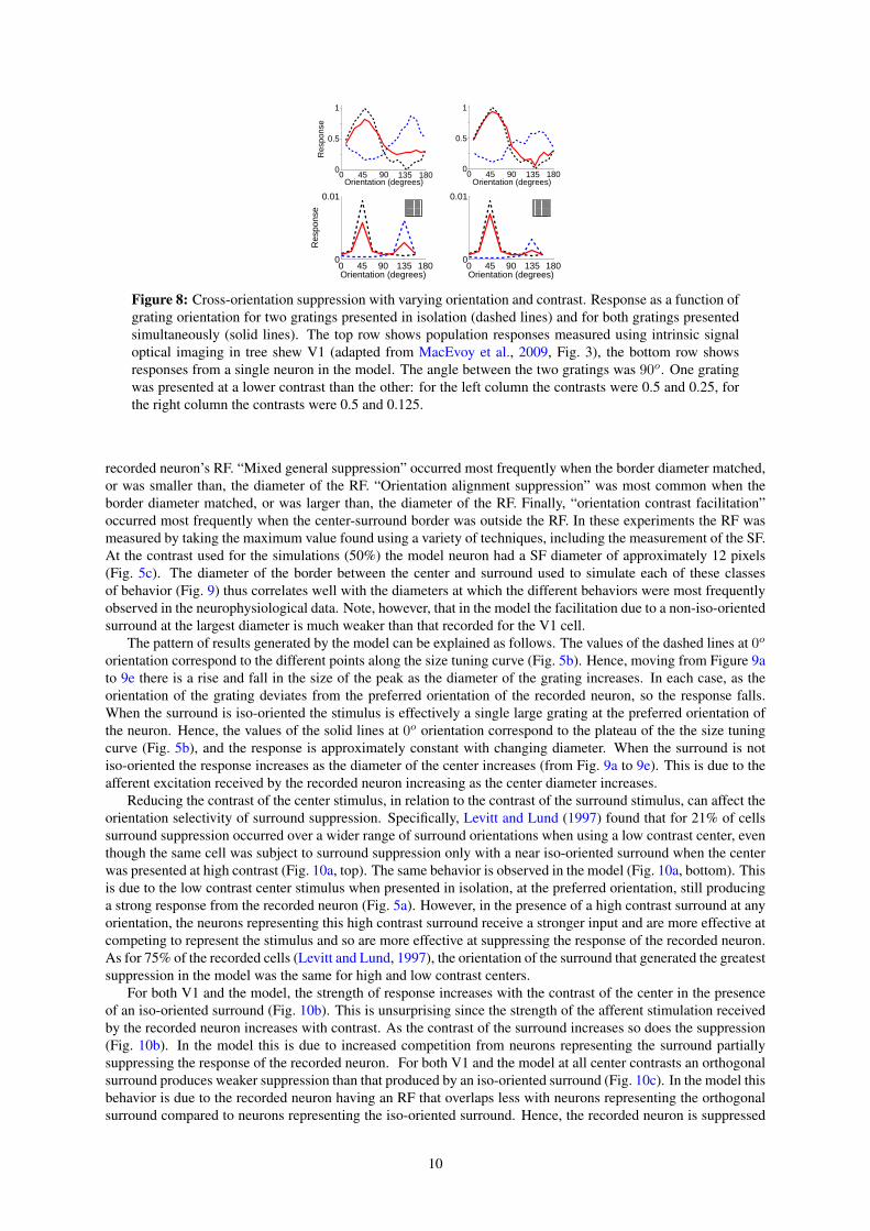
The experiments described above consider the effects of a non-optimally-oriented grating on the response toa grating at the recorded neuron’s preferred orientation. Figure 7 shows the effects of a mask on the response toa grating at a range of orientations, not just the preferred orientation. For both V1 and the model the response tothe plaid is approximately the average of the responses generated by each grating when presented in isolation. Inthe model this effect is due to the competition that occurs between neurons tuned to different orientations at thesame spatial location. These neurons are both activated by the plaid stimulus but they compete to respond to thatpart of the input that they both represent. This competition reduces the response of both neurons in comparisonto their responses when only as single grating is presented. When the contrasts of the two gratings are unequal,the response to the plaid is biased towards that generated when the higher contrast grating is presented in isolation(Fig. 8). In the model, this effect is due to the neurons representing the higher contrast grating receiving thestronger input and being able to more effectively compete to represent the stimulus.

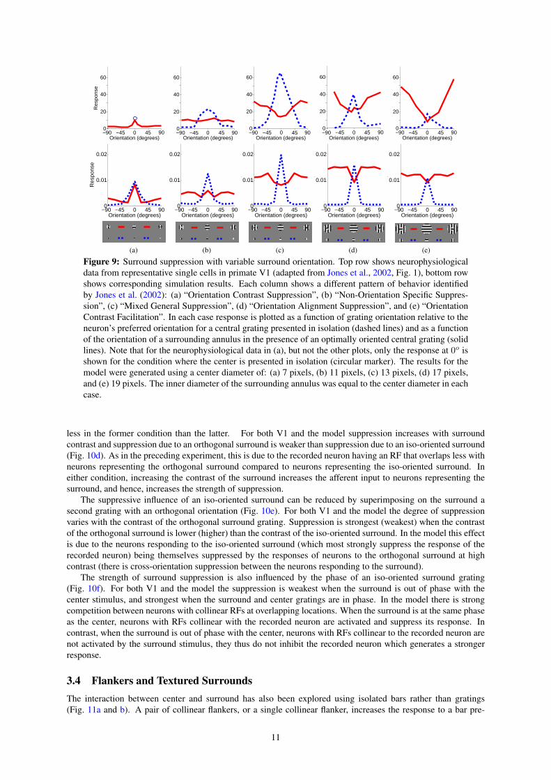
3.3 Surround SuppressionAnother form of suppression that has been widely studied in V1 is that due to one grating surrounding (ratherthan being superimposed upon) another. The effects of such surrounds can be either suppressive or facilitatory.Jones et al. (2002) observed five distinct patterns of behavior (Fig. 9). “Orientation contrast suppression” and“non-orientation specific suppression” occurred most frequently when the center-surround border was within the

9

0

0.5

1

90450 135 180

Res

pons

e

Orientation (degrees)

0.5

1

Res

pons

e

0

Orientation (degrees)90 135 180450

0 45 90 135 1800

0.01

Orientation (degrees)

Res

pons

e

0 45 90 135 1800

0.01

Orientation (degrees)

Res

pons

e

Figure 8: Cross-orientation suppression with varying orientation and contrast. Response as a function ofgrating orientation for two gratings presented in isolation (dashed lines) and for both gratings presentedsimultaneously (solid lines). The top row shows population responses measured using intrinsic signaloptical imaging in tree shew V1 (adapted from MacEvoy et al., 2009, Fig. 3), the bottom row showsresponses from a single neuron in the model. The angle between the two gratings was 90o. One gratingwas presented at a lower contrast than the other: for the left column the contrasts were 0.5 and 0.25, forthe right column the contrasts were 0.5 and 0.125.

recorded neuron’s RF. “Mixed general suppression” occurred most frequently when the border diameter matched,or was smaller than, the diameter of the RF. “Orientation alignment suppression” was most common when theborder diameter matched, or was larger than, the diameter of the RF. Finally, “orientation contrast facilitation”occurred most frequently when the center-surround border was outside the RF. In these experiments the RF wasmeasured by taking the maximum value found using a variety of techniques, including the measurement of the SF.At the contrast used for the simulations (50%) the model neuron had a SF diameter of approximately 12 pixels(Fig. 5c). The diameter of the border between the center and surround used to simulate each of these classesof behavior (Fig. 9) thus correlates well with the diameters at which the different behaviors were most frequentlyobserved in the neurophysiological data. Note, however, that in the model the facilitation due to a non-iso-orientedsurround at the largest diameter is much weaker than that recorded for the V1 cell.

The pattern of results generated by the model can be explained as follows. The values of the dashed lines at 0o

orientation correspond to the different points along the size tuning curve (Fig. 5b). Hence, moving from Figure 9ato 9e there is a rise and fall in the size of the peak as the diameter of the grating increases. In each case, as theorientation of the grating deviates from the preferred orientation of the recorded neuron, so the response falls.When the surround is iso-oriented the stimulus is effectively a single large grating at the preferred orientation ofthe neuron. Hence, the values of the solid lines at 0o orientation correspond to the plateau of the the size tuningcurve (Fig. 5b), and the response is approximately constant with changing diameter. When the surround is notiso-oriented the response increases as the diameter of the center increases (from Fig. 9a to 9e). This is due to theafferent excitation received by the recorded neuron increasing as the center diameter increases.

Reducing the contrast of the center stimulus, in relation to the contrast of the surround stimulus, can affect theorientation selectivity of surround suppression. Specifically, Levitt and Lund (1997) found that for 21% of cellssurround suppression occurred over a wider range of surround orientations when using a low contrast center, eventhough the same cell was subject to surround suppression only with a near iso-oriented surround when the centerwas presented at high contrast (Fig. 10a, top). The same behavior is observed in the model (Fig. 10a, bottom). Thisis due to the low contrast center stimulus when presented in isolation, at the preferred orientation, still producinga strong response from the recorded neuron (Fig. 5a). However, in the presence of a high contrast surround at anyorientation, the neurons representing this high contrast surround receive a stronger input and are more effective atcompeting to represent the stimulus and so are more effective at suppressing the response of the recorded neuron.As for 75% of the recorded cells (Levitt and Lund, 1997), the orientation of the surround that generated the greatestsuppression in the model was the same for high and low contrast centers.

For both V1 and the model, the strength of response increases with the contrast of the center in the presenceof an iso-oriented surround (Fig. 10b). This is unsurprising since the strength of the afferent stimulation receivedby the recorded neuron increases with contrast. As the contrast of the surround increases so does the suppression(Fig. 10b). In the model this is due to increased competition from neurons representing the surround partiallysuppressing the response of the recorded neuron. For both V1 and the model at all center contrasts an orthogonalsurround produces weaker suppression than that produced by an iso-oriented surround (Fig. 10c). In the model thisbehavior is due to the recorded neuron having an RF that overlaps less with neurons representing the orthogonalsurround compared to neurons representing the iso-oriented surround. Hence, the recorded neuron is suppressed

10

Orientation (degrees)0 45 90−45−90

0

20

40

60

Res

pons

e

Orientation (degrees)0−45−90

045 90

20

40

60

Res

pons

e

Orientation (degrees)0 45 90−45−90

20

40

60

0

Res

pons

e

Orientation (degrees)0 45 90−45−90

0

60

40

20

Res

pons

e

Orientation (degrees)0 45 90−45−90

0

20

40

60

Res

pons

e

−90 −45 0 45 900

0.01

0.02

Orientation (degrees)

Res

pons

e

−90 −45 0 45 900

0.01

0.02

Orientation (degrees)

Res

pons

e

−90 −45 0 45 900

0.01

0.02

Orientation (degrees)

Res

pons

e

−90 −45 0 45 900

0.01

0.02

Orientation (degrees)

Res

pons

e

−90 −45 0 45 900

0.01

0.02

Orientation (degrees)

Res

pons

e

(a) (b) (c) (d) (e)

Figure 9: Surround suppression with variable surround orientation. Top row shows neurophysiologicaldata from representative single cells in primate V1 (adapted from Jones et al., 2002, Fig. 1), bottom rowshows corresponding simulation results. Each column shows a different pattern of behavior identifiedby Jones et al. (2002): (a) “Orientation Contrast Suppression”, (b) “Non-Orientation Specific Suppres-sion”, (c) “Mixed General Suppression”, (d) “Orientation Alignment Suppression”, and (e) “OrientationContrast Facilitation”. In each case response is plotted as a function of grating orientation relative to theneuron’s preferred orientation for a central grating presented in isolation (dashed lines) and as a functionof the orientation of a surrounding annulus in the presence of an optimally oriented central grating (solidlines). Note that for the neurophysiological data in (a), but not the other plots, only the response at 0o isshown for the condition where the center is presented in isolation (circular marker). The results for themodel were generated using a center diameter of: (a) 7 pixels, (b) 11 pixels, (c) 13 pixels, (d) 17 pixels,and (e) 19 pixels. The inner diameter of the surrounding annulus was equal to the center diameter in eachcase.

less in the former condition than the latter. For both V1 and the model suppression increases with surroundcontrast and suppression due to an orthogonal surround is weaker than suppression due to an iso-oriented surround(Fig. 10d). As in the preceding experiment, this is due to the recorded neuron having an RF that overlaps less withneurons representing the orthogonal surround compared to neurons representing the iso-oriented surround. Ineither condition, increasing the contrast of the surround increases the afferent input to neurons representing thesurround, and hence, increases the strength of suppression.

The suppressive influence of an iso-oriented surround can be reduced by superimposing on the surround asecond grating with an orthogonal orientation (Fig. 10e). For both V1 and the model the degree of suppressionvaries with the contrast of the orthogonal surround grating. Suppression is strongest (weakest) when the contrastof the orthogonal surround is lower (higher) than the contrast of the iso-oriented surround. In the model this effectis due to the neurons responding to the iso-oriented surround (which most strongly suppress the response of therecorded neuron) being themselves suppressed by the responses of neurons to the orthogonal surround at highcontrast (there is cross-orientation suppression between the neurons responding to the surround).

The strength of surround suppression is also influenced by the phase of an iso-oriented surround grating(Fig. 10f). For both V1 and the model the suppression is weakest when the surround is out of phase with thecenter stimulus, and strongest when the surround and center gratings are in phase. In the model there is strongcompetition between neurons with collinear RFs at overlapping locations. When the surround is at the same phaseas the center, neurons with RFs collinear with the recorded neuron are activated and suppress its response. Incontrast, when the surround is out of phase with the center, neurons with RFs collinear to the recorded neuron arenot activated by the surround stimulus, they thus do not inhibit the recorded neuron which generates a strongerresponse.

3.4 Flankers and Textured SurroundsThe interaction between center and surround has also been explored using isolated bars rather than gratings(Fig. 11a and b). A pair of collinear flankers, or a single collinear flanker, increases the response to a bar pre-

11

60

Orientation (degrees)0 90−90 −45 45

Res

pons

e

0

120

Centre Contrast0.13 0.50 0.03

0

30

60

90

Res

pons

e

Res

pons

e

Centre Contrast10.10.01

0

40

80

Surround Contrast0.1 10.01

0

20

40

60

Res

pons

e

Contrast0 0.01 0.1 1

0

10

20

Res

pons

e

Phase (degrees)180 27090

0

40

60

20Res

pons

e

0 360

−90 −45 0 45 900

0.01

0.02

0.03

Orientation (degrees)

Res

pons

e

0 0.03 0.13 0.50

0.01

0.02

Centre Contrast

Res

pons

e

0.01 0.1 10

0.01

0.02

0.03

Centre Contrast

Res

pons

e

0.01 0.1 10

0.01

0.02

0.03

Surround Contrast

Res

pons

e

0 0.01 0.1 10

0.01

0.02

0.03

Contrast

Res

pons

e

0 90 180 270 3600

0.02

0.04

0.06

Phase (degrees)

Res

pons

e

(a)

(b) (c) (d) (e) (f)

Figure 10: Surround suppression with variable contrast and variable surround phase. Top row showsneurophysiological data from representative single cells in V1, bottom row shows corresponding simu-lation results. (a) Response plotted as a function of grating orientation relative to the neuron’s preferredorientation for a central grating presented in isolation (dashed line), as a function of the orientation ofa surrounding annulus in the presence of an optimally oriented central grating (solid line), and as afunction of surround orientation for a center contrast much smaller than the surround contrast (dash-dotline). The horizontal lines show the response to the low contrast center stimulus presented alone at thepreferred orientation. Neurophysiological data for a cell in primate V1 (adapted from Levitt and Lund,1997, Fig. 1d). (b) Response as a function of the contrast of the central grating in the presence of aniso-oriented surround. Neurophysiological data for a cell in primate V1 (adapted from Cavanaugh et al.,2002a, Fig. 5b). The thickness of each line corresponds to the contrast of the grating in the annularsurround: 0% (thinnest), 3%, 6%, 12%, 25%, and 50% (thickest). (c) Response as a function of thecontrast of the central grating with no surround (filled circles), an iso-oriented surround (open circles),and an orthogonal surround (squares), in the latter two cases the surround contrast was fixed at 50%.Neurophysiological data for a simple cell in primate V1 (adapted from Cavanaugh et al., 2002b, Fig. 5a).(d) Response as a function of the contrast of the surround grating with an iso-oriented surround (circles),and an orthogonal surround (squares), in both cases the center contrast was fixed at 40%. Neurophysio-logical data for a cell in primate V1 (adapted from Webb et al., 2005, Fig. 6). (e) Response as a functionof the contrast of an orthogonal surround grating superimposed upon an iso-oriented surround grating inthe presence of an optimally oriented center. Neurophysiological data for a cell in cat V1 (adapted fromWalker et al., 2002, Fig. 2b). The contrast of the center and the iso-oriented surround were fixed at 30%.The horizontal lines indicate the response to the central grating in isolation. (f) Response as a function ofthe phase of the grating in the surround. Neurophysiological data for a cell in primate V1 (adapted fromXu et al., 2005, Fig. 2a). The horizontal lines indicate the response to the central grating in isolation.

sented at the center of the RF, even though these flanking stimuli produce little response when presented alone.Furthermore, the enhancement due to a collinear flanker can be blocked by a perpendicular bar separating thecentral bar from the flanker. In contrast to collinear flankers, parallel flankers suppress the response to the centralbar. The model produces behavior that is mostly consistent with the physiological data (Fig. 11f). The resultsof the model can be explained as follows. The collinear flankers partially activate the RF of the recorded neu-ron, and hence, its response is enhanced due to increased afferent input. Hence, the model suggests that somenon-classical RF effects may result from the inadvertent stimulation of the classical RF. The collinear flankerswhen presented in isolation are much better represented by other neurons, and hence, the recorded neuron’s re-sponse is suppressed. When a collinear flanker is presented together with an orthogonal flanker, the recordedneuron receives greater afferent input but there is also stronger competition to represent that input (from neuronsselective for the orthogonal bar) so this configuration has little overall effect on the response. Finally, the parallelflankers activate neighboring neurons which compete with the recorded neuron, suppressing its response. In the

12

0

10

20

30

Res

pons

e

(a)

0

10

20

30

40

50

Res

pons

e

(b)

0

10

20

30

Res

pons

e

(c)

0

10

20

30

Res

pons

e

(d)

0

0.5

1

Nor

mal

ized

Res

pons

e

(e)

0

1

2

3

4

5x 10

−3

Res

pons

e

(f)

0

0.5

1

1.5

x 10−3

Res

pons

e(g)

0

1

2

x 10−3

Res

pons

e

0

0.5

1

1.5

x 10−3

Res

pons

e

(h)

0

1

2

x 10−3

Res

pons

e

0

0.5

1

1.5

x 10−3

Res

pons

e

(i)

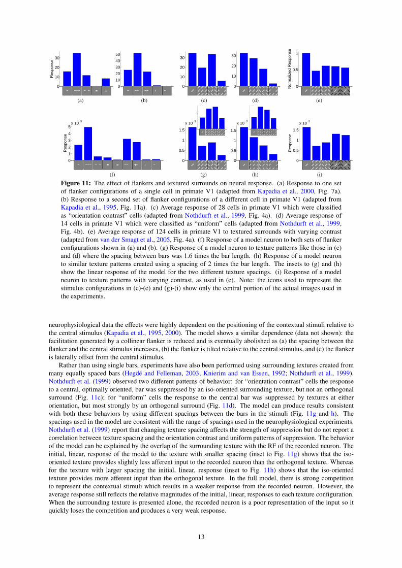
Figure 11: The effect of flankers and textured surrounds on neural response. (a) Response to one setof flanker configurations of a single cell in primate V1 (adapted from Kapadia et al., 2000, Fig. 7a).(b) Response to a second set of flanker configurations of a different cell in primate V1 (adapted fromKapadia et al., 1995, Fig. 11a). (c) Average response of 28 cells in primate V1 which were classifiedas “orientation contrast” cells (adapted from Nothdurft et al., 1999, Fig. 4a). (d) Average response of14 cells in primate V1 which were classified as “uniform” cells (adapted from Nothdurft et al., 1999,Fig. 4b). (e) Average response of 124 cells in primate V1 to textured surrounds with varying contrast(adapted from van der Smagt et al., 2005, Fig. 4a). (f) Response of a model neuron to both sets of flankerconfigurations shown in (a) and (b). (g) Response of a model neuron to texture patterns like those in (c)and (d) where the spacing between bars was 1.6 times the bar length. (h) Response of a model neuronto similar texture patterns created using a spacing of 2 times the bar length. The insets to (g) and (h)show the linear response of the model for the two different texture spacings. (i) Response of a modelneuron to texture patterns with varying contrast, as used in (e). Note: the icons used to represent thestimulus configurations in (c)-(e) and (g)-(i) show only the central portion of the actual images used inthe experiments.

neurophysiological data the effects were highly dependent on the positioning of the contextual stimuli relative tothe central stimulus (Kapadia et al., 1995, 2000). The model shows a similar dependence (data not shown): thefacilitation generated by a collinear flanker is reduced and is eventually abolished as (a) the spacing between theflanker and the central stimulus increases, (b) the flanker is tilted relative to the central stimulus, and (c) the flankeris laterally offset from the central stimulus.

Rather than using single bars, experiments have also been performed using surrounding textures created frommany equally spaced bars (Hegde and Felleman, 2003; Knierim and van Essen, 1992; Nothdurft et al., 1999).Nothdurft et al. (1999) observed two different patterns of behavior: for “orientation contrast” cells the responseto a central, optimally oriented, bar was suppressed by an iso-oriented surrounding texture, but not an orthogonalsurround (Fig. 11c); for “uniform” cells the response to the central bar was suppressed by textures at eitherorientation, but most strongly by an orthogonal surround (Fig. 11d). The model can produce results consistentwith both these behaviors by using different spacings between the bars in the stimuli (Fig. 11g and h). Thespacings used in the model are consistent with the range of spacings used in the neurophysiological experiments.Nothdurft et al. (1999) report that changing texture spacing affects the strength of suppression but do not report acorrelation between texture spacing and the orientation contrast and uniform patterns of suppression. The behaviorof the model can be explained by the overlap of the surrounding texture with the RF of the recorded neuron. Theinitial, linear, response of the model to the texture with smaller spacing (inset to Fig. 11g) shows that the iso-oriented texture provides slightly less afferent input to the recorded neuron than the orthogonal texture. Whereasfor the texture with larger spacing the initial, linear, response (inset to Fig. 11h) shows that the iso-orientedtexture provides more afferent input than the orthogonal texture. In the full model, there is strong competitionto represent the contextual stimuli which results in a weaker response from the recorded neuron. However, theaverage response still reflects the relative magnitudes of the initial, linear, responses to each texture configuration.When the surrounding texture is presented alone, the recorded neuron is a poor representation of the input so itquickly loses the competition and produces a very weak response.

13

Differences between the center and surround along other feature dimensions, such as contrast polarity, havealso been found to diminish the suppression caused by a textured surround (Fig. 11e). Consistent with the empiri-cal data, the model shows (Fig. 11i) that center-surround differences in both dimensions (orientation and contrastpolarity) do not generate a greater reduction in suppression than that generated by a single dimension. In themodel, changing the contrast polarity of the surround only has the effect of changing the identity of those neuronsthat are most strongly activated by that surround. The two sets of neurons activated by the surround at each con-trast polarity both have RFs that overlap with the RF of the recorded neuron to a similar degree, and hence, bothconditions generate a similar degree of suppression in the recorded neuron.

4 DiscussionPrevious work (Rao and Ballard, 1999) has shown that PC is capable of modeling end-stopping behavior (similarto the result shown in Fig. 5b) and texture “pop-out” (similar to the result shown in Fig. 11g). However, thisprevious work did not explore if PC could account for other V1 response properties, perhaps because that workassumed that predictions arise from feedback from extrastriate areas, and hence, are only likely to be involved innon-classical RF properties. The interpretation of PC described in this article assumes that predictions arise withinV1 and that PC can be viewed as a form of competition. This interpretation suggests that PC should also accountfor classical, as well as non-classical, RF properties, as has been demonstrated here.

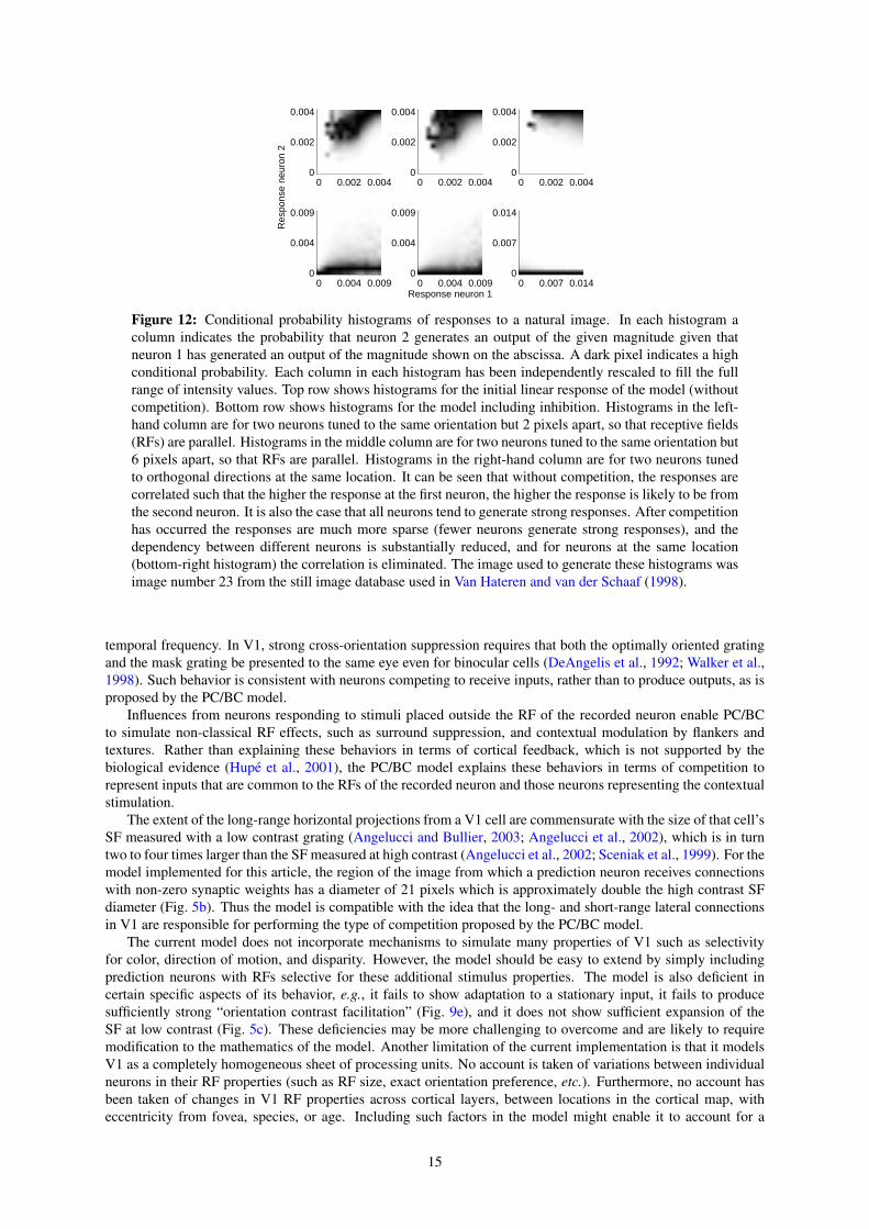
The specific predictive coding model implemented in this article (PC/BC) employs a divisive mechanism tocalculate the residual error between the predictions and the sensory input. This mechanism can be interpreted as aform of divisive normalization like that proposed by the normalization model (Albrecht and Geisler, 1991; Caran-dini and Heeger, 1994; Heeger, 1991, 1992; Wainwright et al., 2001). However, unlike the normalization model,in PC/BC the normalization pool for each neuron is restricted to the population of neurons that have overlappingRFs, and the normalization is applied to the inputs to the population of competing neurons rather than the outputs.The normalization model is capable of simulating a subset of the results presented here (Heeger, 1994; Heegeret al., 1996; Schwartz and Simoncelli, 2001) and has also been recently extended (Reynolds and Heeger, 2009)to model a subset of the attentional data that can be simulated by PC/BC (Spratling, 2008a). However, since theweights used to pool the responses, and so calculate the strength of normalization, are not specified by the nor-malization model it has many more free parameters than PC/BC. As with the normalization model (Schwartz andSimoncelli, 2001; Wainwright et al., 2001), PC/BC reduces redundancy between neural representations (Fig. 12).

There are many other models which can simulate individual results presented here (e.g., Adorjan et al., 1999;Ben-Yishai et al., 1995; Carandini and Ringach, 1997; Dagoi and Sur, 2000; Douglas and Martin, 1991; Somerset al., 1995; Stetter et al., 2000; Troyer et al., 1998, see Ferster and Miller, 2000; Series et al., 2003, for reviews),and many of these models employ mechanisms similar to those used by PC/BC. However, the PC/BC model differsfrom these previous models in providing a computational explanation for the behavior of V1 neurons as well asproviding a unified account of a number of processes that are currently considered, and modeled, in isolation. Themodel also makes testable predictions which are described in the Supplemental Material.

Consistent with previous models and neurophysiological results (Pei et al., 1994; Sompolinsky and Shapley,1997; Xing et al., 2005), orientation tuning in the PC/BC model results from broadly tuned afferent excitationbeing sharpened by intracortical competition. This is also consistent with evidence that blocking inhibitory effectsacross a local population of cortical cells greatly reduces orientation selectivity (Sato et al., 1996; Sillito, 1975;Tsumoto et al., 1979). In the model, blockade of inhibition from neurons with a specific orientation preferenceshould cause neighboring prediction neurons to show increased response to that orientation, rather than simplycausing a general dis-inhibition to all orientations. Such effects have been recorded in V1 (Crook et al., 1998) andanalogous data has been obtained from cortical area TE (Wang et al., 2000). The current model is also consistentwith neurophysiological evidence that the strength of lateral inhibition peaks for stimuli presented at the preferredorientation of the recorded cortical cell (Douglas et al., 1991; Ferster, 1986; Sato et al., 1996; Sompolinsky andShapley, 1997). In the model, the strength of inhibition between any two prediction neurons is proportional to thedegree of overlap between the RFs. Those neurons with orthogonal orientation preferences at a specific locationoverlap less than neurons with similar orientation preferences, and consequently produce less inhibition.

In the PC/BC model inhibition from neurons tuned to near orthogonal orientations is still significant and givesrise to cross-orientation suppression. Evidence that suppression occurs for masks with a high temporal frequencyhas cast doubt on the idea that intracortical inhibition is responsible for cross-orientation suppression (Carandiniet al., 2002). This is because the very weak responses evoked by high frequency stimuli seem insufficient toproduce strong suppression. However, the current model does show strong suppression for masks presentedat high temporal frequencies. This is due to the many neurons weakly activated by the high frequency maskgenerating similar suppression as the few neurons strongly activated by the mask when it is presented at a low

14

0 0.002 0.004

0.004

0.002

00 0.002 0.004

0.004

0.002

00 0.002 0.004

0.004

0.002

0

R

espo

nse

neur

on 2

0 0.004 0.009

0.009

0.004

0

Response neuron 10 0.004 0.009

0.009

0.004

00 0.007 0.014

0.014

0.007

0

Figure 12: Conditional probability histograms of responses to a natural image. In each histogram acolumn indicates the probability that neuron 2 generates an output of the given magnitude given thatneuron 1 has generated an output of the magnitude shown on the abscissa. A dark pixel indicates a highconditional probability. Each column in each histogram has been independently rescaled to fill the fullrange of intensity values. Top row shows histograms for the initial linear response of the model (withoutcompetition). Bottom row shows histograms for the model including inhibition. Histograms in the left-hand column are for two neurons tuned to the same orientation but 2 pixels apart, so that receptive fields(RFs) are parallel. Histograms in the middle column are for two neurons tuned to the same orientation but6 pixels apart, so that RFs are parallel. Histograms in the right-hand column are for two neurons tunedto orthogonal directions at the same location. It can be seen that without competition, the responses arecorrelated such that the higher the response at the first neuron, the higher the response is likely to be fromthe second neuron. It is also the case that all neurons tend to generate strong responses. After competitionhas occurred the responses are much more sparse (fewer neurons generate strong responses), and thedependency between different neurons is substantially reduced, and for neurons at the same location(bottom-right histogram) the correlation is eliminated. The image used to generate these histograms wasimage number 23 from the still image database used in Van Hateren and van der Schaaf (1998).

temporal frequency. In V1, strong cross-orientation suppression requires that both the optimally oriented gratingand the mask grating be presented to the same eye even for binocular cells (DeAngelis et al., 1992; Walker et al.,1998). Such behavior is consistent with neurons competing to receive inputs, rather than to produce outputs, as isproposed by the PC/BC model.

Influences from neurons responding to stimuli placed outside the RF of the recorded neuron enable PC/BCto simulate non-classical RF effects, such as surround suppression, and contextual modulation by flankers andtextures. Rather than explaining these behaviors in terms of cortical feedback, which is not supported by thebiological evidence (Hupe et al., 2001), the PC/BC model explains these behaviors in terms of competition torepresent inputs that are common to the RFs of the recorded neuron and those neurons representing the contextualstimulation.

The extent of the long-range horizontal projections from a V1 cell are commensurate with the size of that cell’sSF measured with a low contrast grating (Angelucci and Bullier, 2003; Angelucci et al., 2002), which is in turntwo to four times larger than the SF measured at high contrast (Angelucci et al., 2002; Sceniak et al., 1999). For themodel implemented for this article, the region of the image from which a prediction neuron receives connectionswith non-zero synaptic weights has a diameter of 21 pixels which is approximately double the high contrast SFdiameter (Fig. 5b). Thus the model is compatible with the idea that the long- and short-range lateral connectionsin V1 are responsible for performing the type of competition proposed by the PC/BC model.

The current model does not incorporate mechanisms to simulate many properties of V1 such as selectivityfor color, direction of motion, and disparity. However, the model should be easy to extend by simply includingprediction neurons with RFs selective for these additional stimulus properties. The model is also deficient incertain specific aspects of its behavior, e.g., it fails to show adaptation to a stationary input, it fails to producesufficiently strong “orientation contrast facilitation” (Fig. 9e), and it does not show sufficient expansion of theSF at low contrast (Fig. 5c). These deficiencies may be more challenging to overcome and are likely to requiremodification to the mathematics of the model. Another limitation of the current implementation is that it modelsV1 as a completely homogeneous sheet of processing units. No account is taken of variations between individualneurons in their RF properties (such as RF size, exact orientation preference, etc.). Furthermore, no account hasbeen taken of changes in V1 RF properties across cortical layers, between locations in the cortical map, witheccentricity from fovea, species, or age. Including such factors in the model might enable it to account for a

15

greater range of empirical data. Despite this the model produces a remarkably good fit to a wide range of data(taken from different species, cortical layers, etc.) suggesting that PC is a ubiquitous property of V1. Anotheromission from the current implementation are feedback connection from extrastriate cortical areas. The model hasoperated without receiving any top-down or contextual predictions from other parts of the cortex. The influenceof such connections is defined by equation 3, and hence, could easily be simulated. The inclusion of predictiveinputs from other parts of the cortex may enable to model to simulate non-classical RF effects which occur forcontextual inputs placed sufficiently far from the recorded neuron’s RF that they can not be explained using themechanisms implemented in the current model.

In conclusion, this article has shown that the mechanism of competition proposed by the predictive codingmodel can account for a very wide range of V1 response properties. This suggests that many of the diverse behav-iors observed in V1 may simply be explained as a consequence of V1 performing predictive coding: minimizingthe error between the observed sensory input and the expectations stored in the synaptic weights of V1 cells.

ReferencesAdorjan, P., Levitt, J. B., Lund, J. S., and Obermayer, K. (1999). A model for the intracortical origin of orientation

preference and tuning in macaque striate cortex. Vis. Neurosci., 16:303–18.Albrecht, D. G. and Geisler, W. S. (1991). Motion selectivity and the contrast-response function of simple cells in

the visual cortex. Vis. Neurosci., 7:531–46.Angelucci, A. and Bullier, J. (2003). Reaching beyond the classical receptive field of V1 neurons: horizontal or

feedback axons? J. Physiol. Paris, 97(2-3):141–54.Angelucci, A., Levitt, J., Walton, E. J. S., Hupe, J.-M., Bullier, J., and Lund, J. S. (2002). Circuits for local and

global signal integration in primary visual cortex. J. Neurosci., 22(19):8633–46.Barlow, H. B. (1994). What is the computational goal of the neocortex? In Koch, C. and Davis, J. L., editors,

Large-Scale Neuronal Theories of the Brain, chapter 1, pages 1–22. MIT Press, Cambridge, MA.Ben-Yishai, R., Bar-Or, R. L., and Sompolinsky, H. (1995). Theory of orientation tuning in visual cortex. Proc.

Natl. Acad. Sci. U.S.A., 92(9):3844–8.Bonds, A. B. (1989). Role of inhibition in the specification of orientation selectivity of cells in the cat striate

cortex. Vis. Neurosci., 2:41–55.Carandini, M. and Heeger, D. J. (1994). Summation and division by neurons in primate visual cortex. Science,

264(5163):1333–6.Carandini, M., Heeger, D. J., and Senn, W. (2002). A synaptic explanation of suppression in visual cortex. J.

Neurosci., 22(22):10053–65.Carandini, M. and Ringach, D. L. (1997). Predictions of a recurrent model of orientation selectivity. Vision Res.,

37(21):3061 – 3071.Cavanaugh, J. R., Bair, W., and Movshon, J. A. (2002a). Nature and interaction of signals from the receptive field

center and surround in macaque V1 neurons. J. Neurophysiol., 88(5):2530–46.Cavanaugh, J. R., Bair, W., and Movshon, J. A. (2002b). Selectivity and spatial distribution of signals from the

receptive field surround in macaque V1 neurons. J. Neurophysiol., 88:2547–56.Crook, J. M., Kisvarday, Z. F., and Eysel, U. T. (1998). Evidence for a contribution of lateral inhibition to orien-

tation tuning and direction selectivity in cat visual cortex: reversible inactivation of functionally characterizedsites combined with neuroanatomical tracing techniques. Eur. J. Neurosci., 10(6):2056–75.

Dagoi, V. and Sur, M. (2000). Dynamic properties of recurrent inhibition in primary visual cortex: contrast andorientation dependence of contextual effects. J. Neurophysiol., 83:1019–30.

Daugman, J. G. (1980). Two-dimensional spectral analysis of cortical receptive field profiles. Vision Res., 20:847–56.

Daugman, J. G. (1988). Complete discrete 2-D Gabor transformations by neural networks for image analysis andcompression. IEEE Transactions on Acoustics, Speech, and Signal Processing, 36(7):1169–79.

De Meyer, K. and Spratling, M. W. (2009). A model of non-linear interactions between cortical top-down andhorizontal connections explains the attentional gating of collinear facilitation. Vision Res., 49(5):533–68.

DeAngelis, G. C., Robson, J. G., Ohzawa, I., and Freeman, R. D. (1992). Organization of suppression in receptivefields of neurons in cat visual cortex. J. Neurophysiol., 68(1):144–63.

Douglas, R. J. and Martin, K. A. C. (1991). A functional microcircuit for cat visual cortex. J. Physiol. (Lond.),440:735–69.

Douglas, R. J., Martin, K. A. C., and Whitteridge, D. (1991). An intracellular analysis of the visual responses ofneurones in cat visual cortex. J. Physiol. (Lond.), 440:659–96.

Ferster, D. (1986). Orientation selectivity of synaptic potentials in neurons of cat primary visual cortex. J.

16

Neurosci., 6:1284–1301.Ferster, D. and Miller, K. D. (2000). Neural mechanisms of orientation selectivity in the visual cortex. Annu. Rev.

Neurosci., 23:441–71.Freeman, T. C. B., Durand, S., Kiper, D. C., and Carandini, M. (2002). Suppression without inhibition in visual

cortex. Neuron, 35(4):759–71.Friston, K. J. (2005). A theory of cortical responses. Philos. Trans. R. Soc. Lond., B, Biol. Sci., 360(1456):815–36.Friston, K. J. (2009). The free-energy principle: a rough guide to the brain? Trends Cogn. Sci., 13(7):293–301.Heeger, D. J. (1991). Nonlinear model of neural responses in cat visual cortex. In Landy, M. S. and Movshon,

J. A., editors, Computational Models of Visual Processing, pages 119–33. MIT Press, Cambridge, MA.Heeger, D. J. (1992). Normalization of cell responses in cat striate cortex. Vis. Neurosci., 9:181–97.Heeger, D. J. (1994). The representation of visual stimuli in primary visual cortex. Curr. Dir. Psychol. Sci.,

3(5):159–63.Heeger, D. J., Simoncelli, E. P., and Movshon, J. A. (1996). Computational models of cortical visual processing.

Proc. Natl. Acad. Sci. U.S.A., 93(2):623–7.Hegde, J. and Felleman, D. J. (2003). How selective are V1 cells for pop-out stimuli? J. Neurosci., 23(31):9968–

80.Hupe, J. M., James, A. C., Girard, P., and Bullier, J. (2001). Response modulations by static texture surround in

area V1 of the macaque monkey do not depend on feedback connections from V2. J. Neurophysiol., 85(1):146–63.

Jehee, J. F. M., Rothkopf, C., Beck, J. M., and Ballard, D. H. (2006). Learning receptive fields using predictivefeedback. J. Physiol. Paris, 100:125–32.

Jones, H. E., Grieve, K. L., Wang, W., and Sillito, A. M. (2001). Surround suppression in primate V1. J.Neurophysiol., 86:2011–28.

Jones, H. E., Wang, W., and Sillito, A. M. (2002). Spatial organization and magnitude of orientation contrastinteractions in primate V1. J. Neurophysiol., 88:2796–808.

Jones, J. P. and Palmer, L. (1987). An evaluation of the two-dimensional gabor filter model of simple receptivefields in cat striate cortex. J. Neurophysiol., 58:1233–58.

Kapadia, M. K., Ito, M., Gilbert, C. D., and Westheimer, G. (1995). Improvement in visual sensitivity by changesin local context: parallel studies in human observers and in V1 of alert monkeys. Neuron, 15(4):843–856.

Kapadia, M. K., Westheimer, G., and Gilbert, C. D. (2000). Spatial distribution of contextual interactions inprimary visual cortex and in visual perception. J. Neurophysiol., 84:2048–62.

Kilner, J. M., Friston, K. J., and Frith, C. D. (2007). Predictive coding: an account of the mirror neuron system.Cogn. Process., 8(3):159–66.

Knierim, J. J. and van Essen, D. C. (1992). Neuronal responses to static texture patterns in area V1 of the alertmacaque monkey. J. Neurophysiol., 67(4):961–980.

Lee, T. S. (1996). Image representation using 2D Gabor wavelets. IEEE Trans. Pattern Anal. Mach. Intell.,18(10):959–71.

Levitt, J. B. and Lund, J. S. (1997). Contrast dependence of contextual effects in primate visual cortex. Nature,387:73–6.

Li, B., Thompson, J. K., Duong, T., Peterson, M. R., and Freeman, R. D. (2006). Origins of cross-orientationsuppression in the visual cortex. J. Neurophysiol., 96:1755–64.

MacEvoy, S. P., Tucker, T. R., and Fitzpatrick, D. (2009). A precise form of divisive suppression supports popu-lation coding in the primary visual cortex. Nat. Neurosci., 12:637–45.

Marcelja, S. (1980). Mathematical description of the responses of simple cortical cells. J. Opt. Soc. Am. A Opt.Image Sci. Vis., 70:1297–1300.

Mumford, D. (1992). On the computational architecture of the neocortex II: the role of cortico-cortical loops.Biol. Cybern., 66:241–51.

Murray, S. O., Schrater, P., and Kersten, D. (2004). Perceptual grouping and the interactions between visualcortical areas. Neural Netw., 17:695–705.

Nothdurft, H.-C., Gallant, J. L., and Van Essen, D. C. (1999). Response modulation by texture surround in primatearea V1: correlates of ‘popout’ under anesthesia. Vis. Neurosci., 16:15–34.

Pei, X., Vidyasagar, T. R., Volgushev, M., and Creutzfeldt, O. (1994). Receptive field analysis and orientationselectivity of postsynaptic potentials of simple cells in cat visual cortex. J. Neurosci., 14(11):7130–40.

Priebe, N. J. and Ferster, D. (2006). The mechanism underlying cross-orientation suppression in cat visual cortex.Nat. Neurosci., 9(4):552–61.

Rao, R. P. N. and Ballard, D. H. (1999). Predictive coding in the visual cortex: a functional interpretation of someextra-classical receptive-field effects. Nat. Neurosci., 2(1):79–87.

Reid, R. C. and Alonso, J. M. (1995). Specificity of monosynaptic connections from thalamus to visual cortex.

17

Nature, 378:281–4.Reynolds, J. H. and Heeger, D. J. (2009). The normalization model of attention. Neuron, 61(2):168–85.Sato, H., Katsuyama, N., Tamura, H., Hata, Y., and Tsumoto, T. (1996). Mechanisms underlying orientation

selectivity in the primary visual cortex of the macaque. J. Physiol. (Lond.), 494(3):757–71.Sceniak, M. P., Ringach, D. L., Hawken, M. J., and Shapley, R. (1999). Contrast’s effect on spatial summation by

macaque V1 neurons. Nat. Neurosci., 2(8).Schwartz, O. and Simoncelli, E. P. (2001). Natural signal statistics and sensory gain control. Nat. Neurosci.,

4:819–25.Series, P., Lorenceau, J., and Fregnac, Y. (2003). The ‘silent’ surround of V1 receptive fields: theory and experi-

ments. J. Physiol. Paris, 97(4-6):453–74.Sillito, A. M. (1975). The contribution of inhibitory mechanisms to the receptive field properties of neurones in

the striate cortex of the cat. J. Physiol. (Lond.), 250:305–29.Skottun, B. C., Bradley, A., Sclar, G., Ohzawa, I., and Freeman, R. D. (1987). The effects of contrast on visual

orientation and spatial frequency discrimination: a comparison of single cells and behavior. J. Neurophysiol.,57:773–86.

Somers, D. C., Nelson, S. B., and Sur, M. (1995). An emergent model of orientation selectivity in cat visualcortical simple cells. J. Neurosci., 15:5448–65.

Sompolinsky, H. and Shapley, R. (1997). New perspectives on the mechanisms for orientation selectivity. Curr.Opin. Neurobiol., 7:514–22.

Spratling, M. W. (2008a). Predictive coding as a model of biased competition in visual selective attention. VisionRes., 48(12):1391–408.

Spratling, M. W. (2008b). Reconciling predictive coding and biased competition models of cortical function.Front. Comput. Neurosci., 2(4):1–8.

Spratling, M. W., De Meyer, K., and Kompass, R. (2009). Unsupervised learning of overlapping image compo-nents using divisive input modulation. Comput. Intell. Neurosci., 2009(381457):1–19.

Stetter, M., Bartsch, H., and Obermayer, K. (2000). A mean-field model for orientation tuning, contrast saturation,and contextual effects in the primary visual cortex. Biol. Cybern., 82(4):291–304.

Troyer, T. W., Krukowski, A. E., Priebe, N. J., and Miller, K. D. (1998). Contrast-invariant orientation tuningin cat visual cortex: thalamocortical input tuning and correlation-based intracortical connectivity. J. Neurosci.,18:5908–27.

Tsumoto, T., Eckart, W., and Creutzfeldt, O. D. (1979). Modification of orientation selectivity of cat visual cortexneurons by removal of GABA mediated inhibition. Exp. Brain Res., 34:351–63.

van der Smagt, M. J., Wehrhahn, C., and Albright, T. D. (2005). Contextual masking of oriented lines: interactionsbetween surface segmentation cues. J. Neurophysiol., 94:576–89.

Van Hateren, J. H. and van der Schaaf, A. (1998). Independent component filters of natural images compared withsimple cells in primary visual cortex. Proc. Biol. Sci., 265:359–66.

Wainwright, M. J., Schwartz, O., and Simoncelli, E. P. (2001). Natural image statistics and divisive normalization:modeling nonlinearities and adaptation in cortical neurons. In Rao, R., Olshausen, B., and Lewicki, M., editors,Statistical Theories of the Brain, pages 203–22. MIT Press, Cambridge, MA.

Walker, G. A., Ohzawa, I., and Freeman, R. D. (1998). Binocular cross-orientation suppression in the cat’s striatecortex. J. Neurophysiol., 79:227–39.

Walker, G. A., Ohzawa, I., and Freeman, R. D. (2002). Disinhibition outside receptive fields in the visual cortex.J. Neurosci., 22(13):5659–68.

Wang, Y., Fujita, I., and Murayama, Y. (2000). Neuronal mechanisms of selectivity for object features revealedby blocking inhibition in inferotemporal cortex. Nat. Neurosci., 3(8):807–13.

Webb, B. S., Dhruv, N. T., Solomon, S. G., Tailby, C., and Lennie, P. (2005). Early and late mechanisms ofsurround suppression in striate cortex of macaque. J. Neurosci., 25:11666–75.

Xing, D., Shapley, R. M., Hawken, M. J., and Ringach, D. L. (2005). Effect of stimulus size on the dynamics oforientation selectivity in macaque V1. J. Neurophysiol., 94:799–812.

Xu, W.-F., Shen, Z.-M., and Li, C.-Y. (2005). Spatial phase sensitivity of V1 neurons in alert monkey. Cereb.Cortex, 15:1697–702.

18

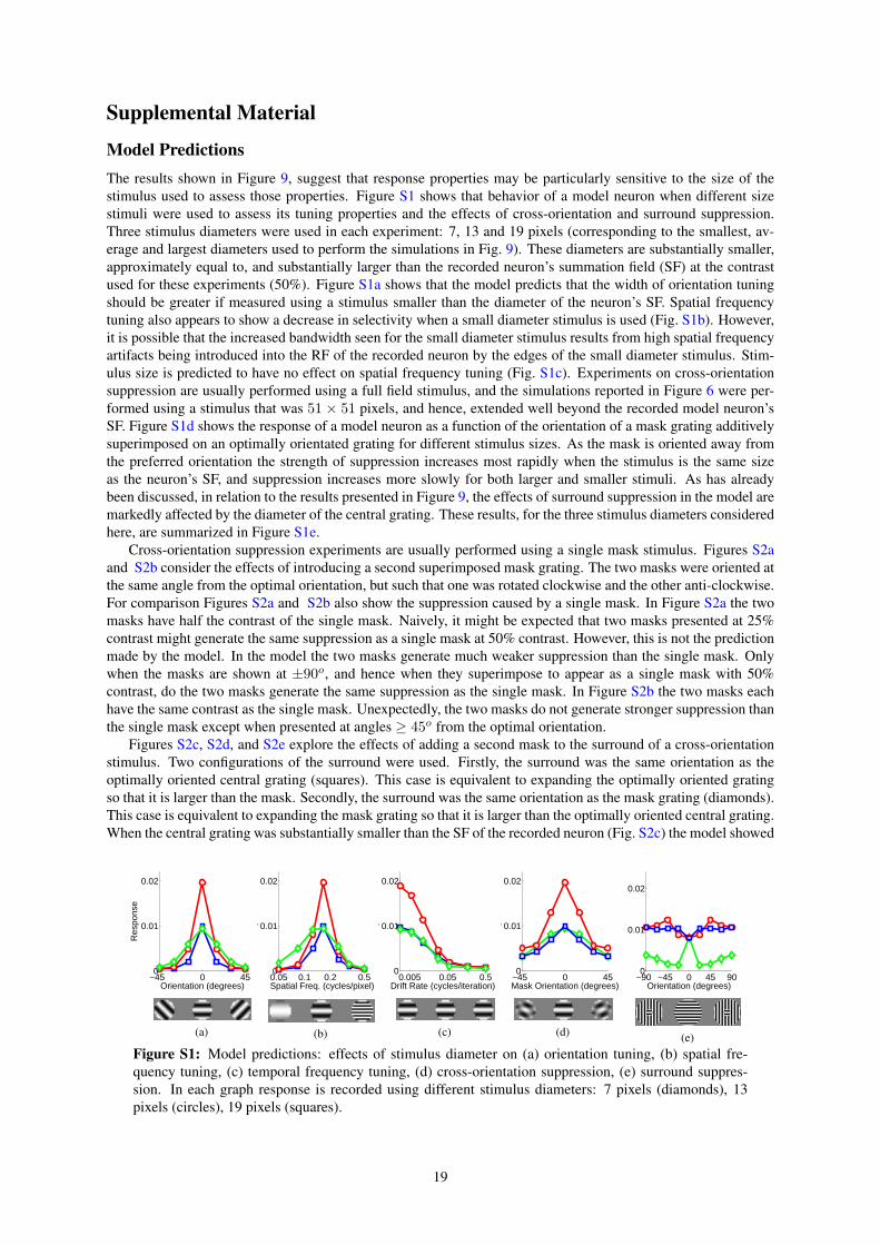
Supplemental Material

Model PredictionsThe results shown in Figure 9, suggest that response properties may be particularly sensitive to the size of thestimulus used to assess those properties. Figure S1 shows that behavior of a model neuron when different sizestimuli were used to assess its tuning properties and the effects of cross-orientation and surround suppression.Three stimulus diameters were used in each experiment: 7, 13 and 19 pixels (corresponding to the smallest, av-erage and largest diameters used to perform the simulations in Fig. 9). These diameters are substantially smaller,approximately equal to, and substantially larger than the recorded neuron’s summation field (SF) at the contrastused for these experiments (50%). Figure S1a shows that the model predicts that the width of orientation tuningshould be greater if measured using a stimulus smaller than the diameter of the neuron’s SF. Spatial frequencytuning also appears to show a decrease in selectivity when a small diameter stimulus is used (Fig. S1b). However,it is possible that the increased bandwidth seen for the small diameter stimulus results from high spatial frequencyartifacts being introduced into the RF of the recorded neuron by the edges of the small diameter stimulus. Stim-ulus size is predicted to have no effect on spatial frequency tuning (Fig. S1c). Experiments on cross-orientationsuppression are usually performed using a full field stimulus, and the simulations reported in Figure 6 were per-formed using a stimulus that was 51 × 51 pixels, and hence, extended well beyond the recorded model neuron’sSF. Figure S1d shows the response of a model neuron as a function of the orientation of a mask grating additivelysuperimposed on an optimally orientated grating for different stimulus sizes. As the mask is oriented away fromthe preferred orientation the strength of suppression increases most rapidly when the stimulus is the same sizeas the neuron’s SF, and suppression increases more slowly for both larger and smaller stimuli. As has alreadybeen discussed, in relation to the results presented in Figure 9, the effects of surround suppression in the model aremarkedly affected by the diameter of the central grating. These results, for the three stimulus diameters consideredhere, are summarized in Figure S1e.

Cross-orientation suppression experiments are usually performed using a single mask stimulus. Figures S2aand S2b consider the effects of introducing a second superimposed mask grating. The two masks were oriented atthe same angle from the optimal orientation, but such that one was rotated clockwise and the other anti-clockwise.For comparison Figures S2a and S2b also show the suppression caused by a single mask. In Figure S2a the twomasks have half the contrast of the single mask. Naively, it might be expected that two masks presented at 25%contrast might generate the same suppression as a single mask at 50% contrast. However, this is not the predictionmade by the model. In the model the two masks generate much weaker suppression than the single mask. Onlywhen the masks are shown at ±90o, and hence when they superimpose to appear as a single mask with 50%contrast, do the two masks generate the same suppression as the single mask. In Figure S2b the two masks eachhave the same contrast as the single mask. Unexpectedly, the two masks do not generate stronger suppression thanthe single mask except when presented at angles ≥ 45o from the optimal orientation.

Figures S2c, S2d, and S2e explore the effects of adding a second mask to the surround of a cross-orientationstimulus. Two configurations of the surround were used. Firstly, the surround was the same orientation as theoptimally oriented central grating (squares). This case is equivalent to expanding the optimally oriented gratingso that it is larger than the mask. Secondly, the surround was the same orientation as the mask grating (diamonds).This case is equivalent to expanding the mask grating so that it is larger than the optimally oriented central grating.When the central grating was substantially smaller than the SF of the recorded neuron (Fig. S2c) the model showed

−45 0 450

0.01

0.02

Orientation (degrees)

Res

pons

e

0.05 0.1 0.2 0.50

0.01

0.02

Spatial Freq. (cycles/pixel)

Res

pons

e

0.005 0.05 0.50

0.01

0.02

Drift Rate (cycles/iteration)

Res

pons

e

−45 0 450

0.01

0.02

Mask Orientation (degrees)

Res

pons

e

−90 −45 0 45 900

0.01

0.02

Orientation (degrees)

Res

pons

e

(a) (b) (c) (d) (e)Figure S1: Model predictions: effects of stimulus diameter on (a) orientation tuning, (b) spatial fre-quency tuning, (c) temporal frequency tuning, (d) cross-orientation suppression, (e) surround suppres-sion. In each graph response is recorded using different stimulus diameters: 7 pixels (diamonds), 13pixels (circles), 19 pixels (squares).

19

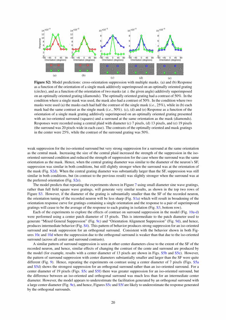
−90 −45 0 45 900

2

4

6

8

10

12

14

Orientation (degrees)

Res

pons

e

x10−3

−90 −45 0 45 900

2

4

6

8

10

12

14

Orientation (degrees)

Res

pons

e

x10−3

−90 −45 0 45 900

2

4

6

8

10

Orientation (degrees)

Res

pons

e

x10−3

−90 −45 0 45 900

2

4

6

8

10

Orientation (degrees)

Res

pons

e

x10−3

−90 −45 0 45 900

2

4

6

8

10

Orientation (degrees)

Res

pons

e

x10−3

(a) (b)(c) (d) (e)

Figure S2: Model predictions: cross-orientation suppression with multiple masks. (a) and (b) Responseas a function of the orientation of a single mask additively superimposed on an optimally oriented grating(circles), and as a function of the orientation of two masks (at± the given angle) additively superimposedon an optimally oriented grating (diamonds). The optimally oriented grating had a contrast of 50%. In thecondition where a single mask was used, the mask also had a contrast of 50%. In the condition where twomasks were used (a) the masks each had half the contrast of the single mask (i.e., 25%), while in (b) eachmask had the same contrast as the single mask (i.e., 50%). (c), (d) and (e) Response as a function of theorientation of a single mask grating additively superimposed on an optimally oriented grating presentedwith an iso-oriented surround (squares) and a surround at the same orientation as the mask (diamonds).Responses were recorded using a central plaid with diameter (c) 7 pixels, (d) 13 pixels, and (e) 19 pixels(the surround was 20 pixels wide in each case). The contrasts of the optimally oriented and mask gratingsin the center were 25%, while the contrast of the surround grating was 50%.

weak suppression for the iso-oriented surround but very strong suppression for a surround at the same orientationas the central mask. Increasing the size of the central plaid increased the strength of the suppression in the iso-oriented surround condition and reduced the strength of suppression for the case where the surround was the sameorientation as the mask. Hence, when the central grating diameter was similar to the diameter of the neuron’s SF,suppression was similar in both conditions, but still slightly stronger when the surround was at the orientation ofthe mask (Fig. S2d). When the central grating diameter was substantially larger than the SF, suppression was stillsimilar in both conditions, but (in contrast to the previous result) was slightly stronger when the surround was atthe preferred orientation (Fig. S2e).

The model predicts that repeating the experiments shown in Figure 7 using small diameter sine wave gratings,rather than full field square wave gratings, will generate very similar results, as shown in the top two rows ofFigure S3. However, if the diameter of the grating is substantially smaller than the SF of the recorded neuron,the orientation tuning of the recorded neuron will be less sharp (Fig. S1a) which will result in broadening of theorientation response curve for gratings containing a single orientation and the response to a pair of superimposedgratings will cease to be the average of the response to each grating in isolation (Fig. S3, bottom row).

Each of the experiments to explore the effects of contrast on surround suppression in the model (Fig. 10a-d)were performed using a center patch diameter of 15 pixels. This is intermediate to the patch diameter used togenerate “Mixed General Suppression” (Fig. 9c) and “Orientation Alignment Suppression” (Fig. 9d), and hence,produces intermediate behavior (Fig. S4). This pattern of behavior produces strong suppression for an iso-orientedsurround and weak suppression for an orthogonal surround. Consistent with the behavior shown in both Fig-ures 10c and 10d where the suppression due to the orthogonal surround is weaker than that due to the iso-orientedsurround (across all center and surround contrasts).

A similar pattern of surround suppression is seen at other center diameters close to the extent of the SF of therecorded neuron, and hence, similar effects of changing the contrast of the cente and surround are produced bythe model (for example, results with a center diameter of 13 pixels are shown in Figs. S5b and S5e). However,the pattern of surround suppression with center diameters substantially smaller and larger than the SF were quitedifferent (Fig. 9). Hence, repeating the experiments on contrast using a center diameter of 7 pixels (Figs. S5aand S5d) shows the strongest suppression for an orthogonal surround rather than an iso-oriented surround. For acenter diameter of 19 pixels (Figs. S5c and S5f) there was greater suppression for an iso-oriented surround, butthe difference between an iso-oriented and orthogonal surround was much less than for an intermediate centerdiameter. However, the model appears to underestimate the facilitation generated by an orthogonal surround witha large center diameter (Fig. 9e), and hence, Figures S5c and S5f are likely to underestimate the response generatedby the orthogonal surrounds.

20

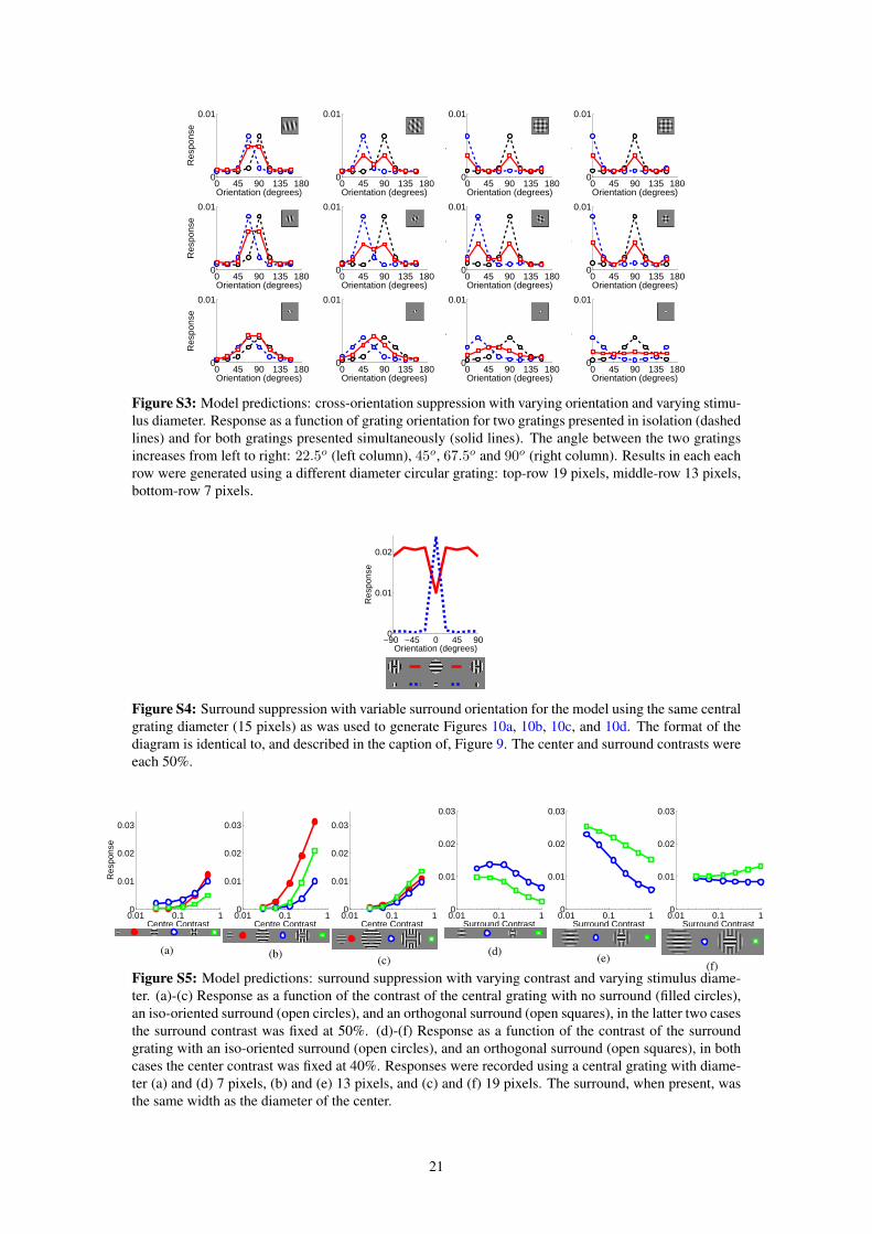
0 45 90 135 1800

0.01

Orientation (degrees)R

espo

nse

0 45 90 135 1800

0.01

Orientation (degrees)

Res

pons

e

0 45 90 135 1800

0.01

Orientation (degrees)

Res

pons

e

0 45 90 135 1800

0.01

Orientation (degrees)

Res

pons

e

0 45 90 135 1800

0.01

Orientation (degrees)

Res

pons

e

0 45 90 135 1800

0.01

Orientation (degrees)

Res

pons

e

0 45 90 135 1800

0.01

Orientation (degrees)

Res

pons

e

0 45 90 135 1800

0.01

Orientation (degrees)

Res

pons

e

0 45 90 135 1800

0.01

Orientation (degrees)

Res

pons

e

0 45 90 135 1800

0.01

Orientation (degrees)

Res

pons

e

0 45 90 135 1800

0.01

Orientation (degrees)

Res

pons

e

0 45 90 135 1800

0.01

Orientation (degrees)

Res

pons

e

Figure S3: Model predictions: cross-orientation suppression with varying orientation and varying stimu-lus diameter. Response as a function of grating orientation for two gratings presented in isolation (dashedlines) and for both gratings presented simultaneously (solid lines). The angle between the two gratingsincreases from left to right: 22.5o (left column), 45o, 67.5o and 90o (right column). Results in each eachrow were generated using a different diameter circular grating: top-row 19 pixels, middle-row 13 pixels,bottom-row 7 pixels.

−90 −45 0 45 900

0.01

0.02

Orientation (degrees)

Res

pons

e

Figure S4: Surround suppression with variable surround orientation for the model using the same centralgrating diameter (15 pixels) as was used to generate Figures 10a, 10b, 10c, and 10d. The format of thediagram is identical to, and described in the caption of, Figure 9. The center and surround contrasts wereeach 50%.

0.01 0.1 10

0.01

0.02

0.03

Centre Contrast

Res

pons

e

0.01 0.1 10

0.01

0.02

0.03

Centre Contrast

Res

pons

e

0.01 0.1 10

0.01

0.02

0.03

Centre Contrast

Res

pons

e

0.01 0.1 10

0.01

0.02

0.03

Surround Contrast

Res

pons

e

0.01 0.1 10

0.01

0.02

0.03

Surround Contrast

Res

pons

e

0.01 0.1 10

0.01

0.02

0.03

Surround Contrast

Res

pons

e

(a) (b) (c)(d) (e)

(f)Figure S5: Model predictions: surround suppression with varying contrast and varying stimulus diame-ter. (a)-(c) Response as a function of the contrast of the central grating with no surround (filled circles),an iso-oriented surround (open circles), and an orthogonal surround (open squares), in the latter two casesthe surround contrast was fixed at 50%. (d)-(f) Response as a function of the contrast of the surroundgrating with an iso-oriented surround (open circles), and an orthogonal surround (open squares), in bothcases the center contrast was fixed at 40%. Responses were recorded using a central grating with diame-ter (a) and (d) 7 pixels, (b) and (e) 13 pixels, and (c) and (f) 19 pixels. The surround, when present, wasthe same width as the diameter of the center.

21

0 5 100

0.01

0.02

0.03

Iteration

Res

pons

e

(a)

0 5 100

0.01

0.02

0.03

Iteration

Res

pons

e

(b)

Figure S6: Comparison or prediction neuron and error-detecting neuron responses. Activation as afunction of time for (a) a prediction neuron and (b) an error-detecting neuron in response to five stimulisimilar to those used in the main experiments (shown on the right of (a)). The stimuli that produce thestrongest to weakest response from the prediction neuron are: a circular grating covering the neuron’ssummation field at the neuron’s preferred orientation; a center-surround stimulus with an orthogonalsurround orientation; a center-surround stimulus with a iso-oriented surround orientation (equivalent toa single circular grating extending beyond the neuron’s summation field); a plaid with an orthogonallyoriented mask grating additively superimposed on an optimally orientated grating; and a circular gratingcovering the neuron’s summation field oriented at 90o to the neuron’s preferred orientation. The error-detecting neuron produces virtually identical responses to all five stimuli. The model does not includefactors such as transmission delays in order to simulate the temporal dynamics of cortical neurons, andhence, these response time profiles should be treated with caution. Furthermore, the transient responseof the error-detecting neuron is exaggerated by setting all neural activity to zero prior to the presentationof each stimulus.

Throughout this article only the response properties of the prediction neurons have been considered. Themodel predicts that the responses of error-detecting neurons would be unselective to different stimuli (Fig. S6).Across the cortical hierarchy the number of prediction neurons and the number of error-detecting neurons shouldbe equal (since the number of units in eSi+1 is equal to the number of units in ySi). However, in any particularcortical area the ratio of error-detecting neurons to prediction neurons could be significantly different from unity.In the model implemented here, for example, error-detecting neurons make up 1

33 of the neurons in the simulatedV1 (see section 2.2). Hence, V1 error-detecting neurons might be rare as well as unselective.

22