predictive model for type 1 diabetes. - automatic … · predictive model for type 1 diabetes. a...

ISSN 0280-5316 ISRN LUTFD2/TFRT--5838--SE

Predictive Model for Type 1 Diabetes. A Case Study

Julia Herget

Department of Automatic Control Lund University

May 2009

Lund University Department of Automatic Control Box 118 SE-221 00 Lund Sweden

Document name MASTER THESIS Date of issue May 2009 Document Number ISRN LUTFD2/TFRT--5838--SE

Author(s)

Julia Herget Supervisor Professor Ulrich Konigorski Technische Univ. Darmstadt, Germany Professor Rolf Johansson Automatic Control, Lund (Examiner) Sponsoring organization

Title and subtitle Predictive Models for Type 1 Diabetes. A Case Study (Prediktiva modeller för typ 1-diabetes. En fallstudie.)

Abstract Linear models were identified from glucose-insulin data of a type 1 diabetic patient. The models were used for simulation and prediction with 10, 30, 60, 90 and 120 min prediction horizon. The predictions were able to track the measured blood glucose, at least for the lower prediction horizons, so that hypo-and hyperglycemic events can be prognosed. The best predictions were achieved with ARX and ARMAX models, predictions for the subspace-based models were not as good as for the autoregressive models. Later a minimum variance controller was developed with an ARMAX model that was identified before. The controller could reduce the variance of the blood glucose concentration as well as eliminate hyperglycemic events. However it introduced the risk for hypoglycemia, which means that there is still some effort to be done. Linear models were identified from glucose-insulin data of a type 1 diabetic patient. The models were used for simulation and prediction with 10, 30, 60, 90 and 120 min prediction horizon. The predictions were able to track the measured blood glucose, at least for the lower prediction horizons, so that hypo-and hyperglycemic events can be prognosed. The best predictions were achieved with ARX and ARMAX models, predictions for the subspace-based models were not as good as for the autoregressive models. Later a minimum variance controller was developed with an ARMAX model that was identified before. The controller could reduce the variance of the blood glucose concentration as well as eliminate hyperglycemic events. However it introduced the risk for hypoglycemia, which means that there is still some effort to be done.

Keywords

Classification system and/or index terms (if any)

Supplementary bibliographical information ISSN and key title 0280-5316

ISBN

Language English

Number of pages 88

Recipient’s notes

Security classification

http://www.control.lth.se/publications/

Contents

1 Introduction 5

2 Medical Background 6

2.1 Glucose . . . . . . . . . . . . . . . . . . . . . . . . . . . . . . 6

2.2 Insulin . . . . . . . . . . . . . . . . . . . . . . . . . . . . . . . 7

2.3 Glucagon . . . . . . . . . . . . . . . . . . . . . . . . . . . . . 7

2.4 Diabetes mellitus . . . . . . . . . . . . . . . . . . . . . . . . . 8

2.5 Link between diabetes mellitus and control theory . . . . . . . 9

3 Previous work, state of the art and research topics 11

3.1 Devices for glucose measuring and insulin administration . . . 11

3.2 Type 1 diabetes modeling . . . . . . . . . . . . . . . . . . . . 12

3.3 Control strategies for type 1 diabetes . . . . . . . . . . . . . . 13

4 Identification 16

4.1 Description of models and evaluation criteria . . . . . . . . . . 16

4.2 Software . . . . . . . . . . . . . . . . . . . . . . . . . . . . . . 18

4.3 Model determination . . . . . . . . . . . . . . . . . . . . . . . 18

4.4 Data used for identification . . . . . . . . . . . . . . . . . . . 20

4.5 Simulation . . . . . . . . . . . . . . . . . . . . . . . . . . . . . 24

4.6 Prediction . . . . . . . . . . . . . . . . . . . . . . . . . . . . . 33

4.7 Identification of models for different times of day . . . . . . . 41

4.8 Discussion . . . . . . . . . . . . . . . . . . . . . . . . . . . . . 47

4.9 Conclusion . . . . . . . . . . . . . . . . . . . . . . . . . . . . . 50

5 Controller 51

5.1 Minimum variance control . . . . . . . . . . . . . . . . . . . . 51

5.2 Structure of the control loop . . . . . . . . . . . . . . . . . . . 52

5.3 Results . . . . . . . . . . . . . . . . . . . . . . . . . . . . . . . 52

5.4 Discussion . . . . . . . . . . . . . . . . . . . . . . . . . . . . . 54

5.5 Conclusion . . . . . . . . . . . . . . . . . . . . . . . . . . . . . 57

6 Conclusion 58

A Tables with identification quality criteria 59

B Utilized model orders for identification 67

C Identified polynomials and matrices for prediction 70

5

D FIT and SDE plots for prediction 74

E Simulations with the controlled system 78

References 80

List of figures 84

List of tables 86

6

1 Introduction

Diabetes mellitus is a wide-spread disease with more than 180 million suffer-ers worldwide [25]. Treatment is based upon insulin injections to force theblood glucose level within a lower and an upper threshold. Crossing theseboundaries leads to hypo- or hyperglycemia with immediate effects like braindamage, coma and potentially death or chronic damages. The appropriatecontrol of blood glucose is therefore of vital importance to the patient.The aim of this thesis was to identify models of the glucose-insulin metabolismon the basis of type 1 diabetes patient data. Various models were comparedwith each other to see how much their structure deviates and which influ-ence different methods have on the models. Later the models were used todevelop a controller for the optimal insulin profile, so that the variations ofthe glucose level and thus the risk for hypo-or hyperglycemia can be reduced.In the following a basic insight into the physiological background of the dis-ease diabetes mellitus will be provided to familiarize the reader with thesubject. On the basis of that a literature survey with regard to previouswork and current research topics will be presented. Section 4 and 5 describethe identification of the models and the control part respectively. The thesiscompletes with a final conclusion.

7

2 Medical Background

To understand the principle of the insulin-glucose-metabolism and the diseasediabetes mellitus a basic insight into glucose, insulin, glucagon and diabetesmellitus will be given.This chapter is based on [10].

2.1 Glucose

Glucose, also known as dextrose or grape sugar, is a monosaccharide andingested into the body by carbohydrate food.Glucose is one of the major energy deliverers in our body. Muscle cells arenot permeable for glucose and therefore use fatty acids as energy sources.However during exercise muscle cells become permeable for glucose and canuse this instead. Another way to enable glucose for entering the cell mem-brane is the availability of insulin which connects with receptors on the cellmembrane. Thus a mechanism is ignited which among other things trans-ports glucose into the cell. The only cells that don’t need insulin to absorbglucose are brain cells, which can hardly use any other energy sources besidesglucose. Therefore it is very important that the blood glucose concentrationstays above a certain level to guarantee the required amount of glucose inthe brain cells.Insulin causes the excess glucose (about 60%), that cannot be taken up incells after a meal, to be stored in the liver as glycogen. Glycogen is turnedinto glucose and secreted in times between meals when the blood glucoselevel is lower. When no further glucose can be stored in the liver as glycogenglucose is turned into fatty acids with the help of insulin and transported tothe adipose cells.

A fasting person normally has a blood glucose concentration in the range of4 − 5 mmol

L blood(70 − 90 mg

dL blood). After breakfast the concentration rises up to

7.8mmol/L (140mg/dL). Two hours after a meal the glucose concentrationshould be within the normal level again.Implications of a hypoglycemic shock, which means a too low blood glucoselevel (< 2.22-2.78mmol/L (40-50 mg/dL)), are nervous irritability, halluci-nations, sweat, fainting, seizures and coma. Immediate treatment have to belarge amounts of glucose or glucagon.Hyperglycemia means too high blood glucose level (more than 7.8mmol/L(140 mg/dL)) and should be avoided, too. A higher glucose level in the bloodthan in the cells causes dehydration in the cells due to osmose. Furthermorea high glucose level in the urine leads to osmotic diuresis by the kidneys and

8

thus more fluids and electrolytes than usual are excreted. High glucose levelshave long-term-effects that can impair tissues like blood vessels and increasethe risk for heart attacks, strokes, end-stage renal diseases and blindness.

2.2 Insulin

Insulin is secreted in the islets of Langerhans in the β-cells in the pancreasand directly ingested into the blood. Insulin is a peptide hormone and has ahalf-life of about five minutes.Whenever the blood glucose level is increasing (e.g. after a meal containingcarbohydrates) insulin is secreted to enable glucose uptake and usage in cells(not in brain cells) and glucose storage. Insulin also prevents glucagon secre-tion and the release of fatty acids so that glucose is used for energy instead.Since insulin causes the surplus glucose to be converted into fat and supportsthe transportation into the fat cells in the same way as the transportation ofglucose into the muscle cells, the storage of fat without insulin is nearly notfeasible.Further positive effects of insulin are the promotion of protein storage andthe transportation of some amino acids into cells. Insulin also helps to pro-duce new proteins and prevents degeneration of proteins.For growth insulin is as important as the growth hormone is.Factors that increase the insulin secretion are increasing blood glucose level,increasing amount of free fatty acids and/or amino acids in the blood andcertain hormones whereas insulin secretion is prevented by decreasing bloodglucose and fasting. Thus insulin is not only controlled by the blood glucoselevel.While the carbohydrates are digested there should be a delay in the insulinsecretion. Otherwise the newly ingested glucose would immediately be usedin the muscles or stored in the liver and there would not be enough glucosefor the brain cells. This is assured by a hormone called somatostatin.

Insulin for insulin-treatment is available in different forms. There is ”regular”insulin which is effective for 3-8 hours and ”long-lasting” insulin which ismixed with protein derivatives to increase the duration for absorption to10-48 hours.

2.3 Glucagon

Glucagon is a peptide hormone and mainly has the opposite effect of that ofinsulin. Like insulin it is produced in islets of Langerhans in the pancreasbut secreted when the blood glucose level is decreasing.

9

Due to glucagon being present in the blood, gluconeogenesis is initiated whichconverts the glycogen in the liver back into glucose and therefore the bloodglucose level is rapidly increased. Glucagon also has an effect on fatty acids,so that these are used by the cells as energy sources.Other causes for glucagon secretion besides a falling glucose level are certainamino acids and exercise. However the impact of exercise on glucagon secre-tion is not yet totally understood.Generally the insulin mechanism is more important than the glucagon mech-anism because glucose cannot be used or stored otherwise, but during timesof starvation or exhaustive exercise the glucagon mechanism gains in impor-tance due to a constantly low glucose level.

2.4 Diabetes mellitus

In diabetics insulin can either not be produced or not be utilized. Thereforeglucose cannot be used nor stored except for the amount of glucose that isused in brain cells. This leads to a raise in blood glucose concentration andin the use of fats and proteins. There are two types of diabetes which willbe explained in the following.

Type 1 Diabetes: In type I diabetic persons there is no insulin secretionand thus insulin has to be injected. Therefore this type is also called insulin-dependent diabetes mellitus (IDDM) or juvenile diabetes mellitus becauseit often occurs in young people. The disability to produce insulin is causedby damaged β-cells of the pancreas or a disease which blocks the insulinproduction. A major factor for type 1 diabetes might be heredity.The blood glucose level in type 1 diabetes patients can be as high as 16-70mmol/L (about 300-1200mg/dL) and is thus much higher than the level ina healthy person (up to 8-10 times higher).The lack of insulin debilitates storage and production of proteins causingextreme weakness and deranged functions of the organs. The absence ofinsulin in the fat metabolism activates the release of fat into the blood andthe usage as energy sources by almost all cells (besides the brain cells). Thisis not as threatening as the lack of insulin in glucose metabolism but possibleconsequential damages are atherosclerosis, heart attacks, cerebral strokes andother vascular accidents.Further symptoms for type 1 diabetes are polyuria, intra-and extracellulardehydration, extreme thirst and weight loss. If not treated the disease canlead to death in a few weeks.In the insulin-therapy usually one dose of long-lasting insulin is given eachday to build up a basal insulin concentration and a bolus injection when a

10

meal is taken to regulate the increased amounts of glucose ingested with themeal.

Type 2 Diabetes: In contrast to type 1 diabetes patients type 2 diabeticsare able to produce insulin. However their bodies are resistant to the effectsof insulin. Large amounts of insulin are being secreted and existing in theblood, but cannot be used.This type is also known as non-insulin-dependent diabetes mellitus (NIDDM)or adult onset diabetes and often appears after the age of 30.Due to the insulin-resistance the amount of insulin in type II diabetics isincreased enormously to compensate for that. Even in the early stages ofthe disease the increased level of insulin does not help to store and use glu-cose after a carbohydrate meal. As a consequences moderate hyperglycemiaoccurs. In later stages when the pancreas is exhausted and cannot producethese excessive amounts of insulin severe hyperglycemia cannot be avoided.Since adiposity is one of the major risks for type 2 diabetes an efficient treat-ment, at least in the early stages, is exercise, caloric diet and weight loss.In later stages when these procedures don’t have any more effect, drugs forincreasing the insulin-sensitivity can be prescribed and if that does not helpany more insulin has to be injected.

2.5 Link between diabetes mellitus and control theory

2.5.1 Conclusion

In non-diabetic persons insulin secretion is controlled by the amount of glu-cose in the blood. An increasing blood glucose level causes the release ofinsulin which supports the usage and storage of glucose and thus preventingthe blood glucose level from rising too high. A decrease in blood glucoselevel prevents the secretion of insulin but promotes the secretion of glucagonto cause an increase in the glucose level again.In Type I Diabetes mellitus patients insulin cannot be produced. Thus in-sulin has to be injected. To figure out the right amount of insulin is a verychallenging task and often causes hyper- or hypoglycemia. A hypoglycemicshock occurs when the blood glucose level falls below a certain threshold.This has immediate effects like fainting and coma. Hyperglycemia insteadrefers to a too high glucose level and often remains unrecognized. Hyper-glycemic effects are long-term consequences like dehydration, risk for strokesand heart-attacks and damages to tissues.

Since brain cells and muscle cells during exercise are able to take up glucosewithout the help of insulin and because the amount of ingested carbohydrates

11

is not easy to estimate, it is hard to figure out the impact of insulin on theblood glucose level.

2.5.2 Why is diabetes mellitus a control theory problem?

Since the glucose-insulin-metabolism in healthy bodies is a control loop in-herently it is only natural to use control theory as a means in therapy fordiabetic persons. To be able to mimic the natural regulation of insulin secre-tion the blood glucose concentration has to be measured and the appropriateamount of insulin has to be administered to the body. For this reason mea-suring devices for glucose level and insulin pumps for the injection of insulinhave been developed.

12

3 Previous work, state of the art and research

topics

3.1 Devices for glucose measuring and insulin admin-

istration

3.1.1 Glucose monitoring

Up to now diabetics measure the blood glucose for insulin therapy severaltimes a day. With a blood glucose meter a drop of blood is tested for theamount of contained blood glucose [27].Continuous glucose monitoring system (CGMS) measures the glucose con-centration every 10 min for a duration up to 3 days. A sensor for measuringthe glucose level is placed in the interstitial fluid in the subcutaneous tissues.Calibration has to be done several times a day with a conventional glucosemeter [14]. CGMS are available in commercial use since 1999 [17].Current research is done on noninvasive methods. The glucose is measured bymeans of for instance infrared light [23] or iontophoresis [31] through the skinwithout causing injury to the body. Noninvasive methods have the advan-tages that they are not causing any pain and that glucose can be measuredcontinuously, but a disadvantage is that the glucose per penetrated tissue ismeasured and not glucose per blood volume [31].

3.1.2 Insulin delivery

Insulin is usually injected into the subcutaneous (SC) tissue with a syringeor an insulin pen. Insulin pumps for continuous subcutaneous insulin infu-sion (CSII) have been developed and allow a continously delivery of insulininstead of several injections a day. The basal insulin can easier be dispensedconstantly than with a long lasting insulin which is injected once a day. Theinsulin boluses which are injected in times of meals can also be administeredwith the pump. However insulin pumps are far more expensive than conven-tional needles or pens and are thus not as widely used [26].Even though the Intravenous (IV) route would be favorable from a controlpoint of view the SC route is much easier to access and advantageous insafety aspects [2]. However the SC route introduces time delays in insulinabsorption.

13

3.2 Type 1 diabetes modeling

A large number of models for the glucose-insulin interaction have been de-veloped. Some models represent the physiological dynamics of glucose andinsulin while others are empirical models. A few examples of both types willbe presented in the following.

3.2.1 Physiological models

In 1981 one of the first physiological model of glucose-insulin dynamics waspublished by Bergman [4]. It is known as the “minimal model” or “Bergmanmodel” and consists of three differential equations which describe the dynam-ics of glucose and insulin in the blood and of insulin in remote compartment.The drawback of this model is however that it does not consider SC insulininjection. For this reason the model has been extended in several studies [8].A much more complex model with 19 compartments representing the glu-cose metabolism in a nondiabetic person was developed by Sorensen in 1985[29]. A simpler model, but yet not as rudimental as the minimal model, wasdesigned by Hovorka et al [16]. In 2002 they developed a nonlinear modelwith three subsystems for glucose kinetics and one subsystem for insulin ac-tion. The subsystems for glucose kinetics consist of two compartments, the“accessible” compartment or plasma compartment and the “non-accessible”compartment. The model was later revised with respect to the insulin ab-sorption so that the model takes fast acting and slow acting insulin intoaccount [14].

3.2.2 Empirical models

Empirical models have been identified both with simulated data from a phys-iological model as in the previous section and with measured data of type 1diabetes patients.In 1994 Bellazzi et al. [3] identified ARX models from type 1 diabetes patientdata. The inputs were meal information (discrete values for low, medium orhigh), physical exercise (in discrete values for low, normal and high), insulininjection (continuous values) and special events (such as hypoglycemia). Themodels were used for predictions with horizons of 2h, 4h and 6h. The authorsnoticed a large variation in the prediction quality of different patients.Five years later Bremer and Gough [5] estimated models from simulated datawith literature models, non-diabetic patient data and type 1 diabetic patientdata. The models were used for prediction of future blood glucose concen-tration. They conclude that even their simple and linear models are ableto warn for hypoglycemia better than it would be possible with unfrequent

14

blood glucose measurements alone. However they attach importance to adaily update of the model’s parameters for receiving reasonable predictions.In 2004 Hovorka and his group [15] used their physiological model for bloodglucose prediction with data from 15 IDDM patients. Since the model pa-rameters vary from patient to patient the parameters were re-estimated ateach control step using Bayesian parameter estimation. They showed thatadaptive nonlinear model predictive control is suitable for glucose control infasting type 1 diabetes patients.Sparacino et al. [30] identified first order polynomial models and first orderAR models from continuously monitored data of 28 type 1 diabetics for thepurpose of prediction. The study demonstrates that it is possible even withsimple models to predict hypoglycemic events 20-25 min ahead in time whichis just early enough to prevent the hypoglycemia by ingesting sugar.Similar studies were accomplished by amongst others Reifman et al. [28] andEren-Oruklu et al. [7].

3.3 Control strategies for type 1 diabetes

Traditional insulin therapy can be viewed as a partially closed-loop control[2]. The physician decides on the insulin dosage in a feed forward controlbased on the patient. A feedback control with blood glucose measurementsspecifies the present amount of insulin to be injected.To improve the current way of insulin administration research is done ondecision support systems and on a fully closed loop control with little needsof interaction by the patient.

3.3.1 Decision support systems

About 20 years ago the development of advisory systems for insulin treat-ment began. Model parameters for glucose-insulin dynamics are identifiedfrom measurements of the patient. Using adaption the parameters are up-dated every day. The ideal insulin amount is then calculated with the modelsand with information about the upcoming meals. Those systems are mostlybased on infrequent glucose measurements with a glucose meter several timesa day [14].The Diabetes Advisory System (DIAS) [13] is based on a compartmentmodel of the glucose metabolism whose parameters are estimated from self-monitored glucose data. Inputs are carbohydrate intake and insulin injection.The system works in three modes. The learning mode is used for estimatingthe parameters, the prediction mode is able to make predictions of the bloodglucose with carbohydrate and insulin data. It is designated for detecting

15

hypo- or hyperglycemia and to see which influence changes in meals or inthe insulin dose can have. The advisory mode should define the ideal insulindosis for the least risk of hypo- or hyperglycemia.The system AIDA (Automated Insulin Dosage Advisor) [22] uses a model ofglucose-insulin interaction combined with a knowledge-based system to makepredictions of the glucose level and to calculate the appropriate insulin dose.UTOPIA (Utilities for optimizing insulin adjustment) [6] collects data inhome measurements so that the physician can adjust the therapy in the nextconsultation.There are also telemedicine systems that consist of a medical unit (MU) anda patient unit (PU). Both units communicate with each other via the inter-net. The PU is supposed to collect data in home measurements and to givedaily proposals on the insulin dose. The physician can correct the therapywith the MU. Examples for these systems are Telematic Management of In-sulin Dependent Diabetes Mellitus (T-IDDM) [1] and DIABTel [11].Because of large paramater and response variations between patients and in-fluences on the glucose metabolism like exercise and stress decision supportsystems are currently rarely used [3].

Besides training programs for teaching diabetic patients how to choose theiramount of insulin dose according to the food have been developed as well[14]. In the 1980s a hospital diabetes teaching and treatment program hadbeen carried out [24]. The program led to an improvement in the glucosecontrol and to less hospitalization. The above mentioned AIDA system isalso able to simulate a set of case studies for educational purposes [22].

3.3.2 Artificial pancreas

The artificial pancreas has been in the interest of research since the 1970s.The first systems were featured with intravenous (IV) glucose sampling andIV insulin infusion. Because of that they were not suitable for use in patients.When CGMS first was available more than 20 years later this was a break-through for the closed loop glucose control. Furthermore the technology ofinsulin pumps had been improved over the years as well [17]. Subcutaneous(SC) insulin infusion however introduced time delays because of the longerinsulin absorption from subcutaneous tissue into the blood. This problemwas solved when fast acting insulin was launched [14].Components of the artificial pancreas are a CGMS, a controller and an in-sulin pump [17]. The closed loop system should be able to work as stand-alone system but might require additional information about meals because

16

of time delays in insulin absorption [18]. Most of the controllers use pole-placement, PID-control (proportional-integral-derivative) or MPC (modelpredictive control) [14]. For testing, the controller is often arranged in a lap-top or a handheld computer. Intensions are to place it in the insulin pumpor in an other handheld device for end product use [17]. Possibilites to usethe artificial pancreas are to only switch it on during the night or to also useit during the day. Since there are no interactions like meal-intake or exercise,the glucose control is easier to achieve during the night [18]. Furthermore ifhypoglycemia occurs during the night it mostly remains unrecognized. [17].Therefore it seems reasonable to focus on an overnight controller first [18].Only very few systems were actually implemented and tested [14]. That isthe reason why there still is no closed loop glucose control system on themarket right now even though research on this area had begun more than 30years ago.

17

4 Identification

A set of carbohydrate, insulin and glucose data was given to the purpose ofmodel identification. Several models and methods were investigated. Simu-lation and prediction of the output obtained with the models was comparedwith the real output.The models and evaluation criteria will be explained below and a descriptionof how to estimate the model order for different models will be given. Afterthat the data set will be examined more closely and finally the identificationresults will be presented and discussed.

4.1 Description of models and evaluation criteria

Different types of models were identified, namely ARX, ARMAX and statespace models. For judging the model’s quality measures such as FIT, varianceaccounted for and standard deviation of simulation/prediction error wereused.

4.1.1 ARX

Autoregressive models with exogenous input (ARX) are described by:

A(z−1)yk = z−nkB(z−1)uk + wk (1)

withA(z−1) = 1 + a1z

−1 + ... + anaz−na (2)

B(z−1) = b0 + b1z−1 + ... + bnb

z−nb+1 (3)

and time-delay nk [21].yk characterizes the model output, uk characterizes the model input and wk

is white noise. na relates to the number of poles and nb to the number ofzeros + 1.

4.1.2 ARMAX

ARMAX models (Autoregressive moving average with exogenous input) havethe following form [21]:

A(z−1)yk = z−nkB(z−1)uk + C(z−1)wk (4)

with A(z−1) and B(z−1) as described in (2) and (3) and

C(z−1) = 1 + c1z−1 + ... + cnc

z−nc (5)

18

As it can be seen easily ARX models are a specialization of ARMAX modelswith C(z−1) = 1 .

4.1.3 State-space-models

State-space-models in innovation form are given by:

xk+1 = Axk + Buk + Kek (6)

yk = Cxk + Duk + ek

where uk ∈ Rm denotes the input, yk ∈ R

p the output, xk ∈ Rn the state

vector and ek ∈ Rp is the innovation, i.e. one-step ahead prediction error

[21].

4.1.4 Evaluation criteria

FITThe FIT-value is calculated as

FIT =

(

1 −‖y − y‖

‖y − y‖

)

· 100% (7)

where y is the predicted output, y is the measured output, ‖y − y‖ denotesthe norm of the error between predicted and measured output and y denotesthe mean of the measured output [19].

VAFVAF means variance accounted for and is calculated by

V AF =

(

1 −var(y − y)

var(y)

)

· 100% (8)

with var(y − y) being the variance of the error between estimated and mea-sured output and var(y) the variance of the measured output [12].

Standard Deviation of simulation/prediction error (SDE)The standard deviation of the simulation/prediction error ek = yk − yk iscalculated as [19]:

σ =

√

√

√

√

1

N − 1

N∑

k=1

(ek − e)2 (9)

with

e =1

n

N∑

k=1

ek (10)

19

4.2 Software

The software used throughout this thesis was Matlab, in particular the Sys-tem Identification Toolbox and the SMI-Toolbox by B. Haverkamp and M.Verhaegen [12].

4.3 Model determination

For each of the models the order was estimated as explained below. ARXmodels were obtained by least-squares-estimation, ARMAX by prediction-error-method. State-space models were identified with the Matlab com-mand “n4sid” and with Multivariable Output-Error State Space Algorithm(MOESP) in the SMI-Toolbox.Tables with the models’ order are in Appendix B. Polynomials and matricesthat were chosen for the prediction part are displayed in Appendix C.

Figure 1: Order Selection for ARX: Identification of Day 1 and Input 1

20

4.3.1 Model order estimation

The Matlab command “delayestimation” was used to estimate the delay thateach input most likely has. With the values that were received from the de-lay estimation the command “modelorderestimation” was applied for ARXmodels with na = 1 : 10, nb1 = 1 : 10 and nb2 = 1 : 10 (see Fig. 1). Withthe suggested orders the number of poles, the number of zeros and the de-lays were adjusted to receive as good results for simulation or prediction aspossible.

Since ARMAX models differ from ARX models only in the description ofthe noise the results for delays and number of poles and zeros from the ARXmodels were used as a starting point to adjust them and the number of zerosfor the noise input to receive as best ARMAX models as possible.

For subspace-based model identification the plot of singular values for differ-ent model orders suggests which model order most likely is the appropriateone (see Fig. 2).

0 2 4 6 8 10 12 14 162

2.5

3

3.5

4

4.5

5

5.5

6

6.5

7

Log o

f S

ingula

r valu

es

Model order

Select model order in command window.

Red: Default Choice

Figure 2: Singular values for the method n4sid for identification of Day 1

21

4.4 Data used for identification

0 10 20 30 40 50 60 70 800

0.5

1

carbohydrate intake

mg

/kg

/min

0 10 20 30 40 50 60 70 800

20

40

60insulin injection

mIU

/L

0 10 20 30 40 50 60 70 800

200

400blood glucose measurement

mg

/dL

t in h

Figure 3: Measurement data used for identification

4.4.1 Description of the dataset

Fig. 3 shows the data used for identification. Input 1 is the appearance ofglucose in plasma. Input 2 is the insulin concentration in the blood. Theoutput are CGMS (continuous glucose monitoring system) measurements.The data was collected from an IDDM patient during a clinical observationfor the duration of 3 days. The patient received standard meals for breakfast(42g carbohydrates) at 8:00, lunch (70g carbohydrates) at 13:00 and dinner(70g carbohydrates) at 19:00. Sampling time of the data is 10 minutes.It can be seen that the patient has a relatively high blood glucose level ofmore than 150mg/dL on the first day. However the patient went into hypo-glycemia on the beginning and at the end of the second day. This can beseen in the low blood glucose level of almost 50mg/dL and on the additionalcarbohydrate intake between breakfast and lunch and after dinner on thesecond day. This could possibly have been extra glucose intakes to prevent

22

a hypoglycemic shock and make the blood glucose level rise again.

4.4.2 Pre-treatment of the data before identification

The time-scale was divided into three parts, so that each part represents oneday. The partitioning can be seen as dotted lines in Fig. 3. Models identifiedfrom data of day 1 were validated with day 2 and models identified from dataof day 2 were validated with day 3.For the purpose of investigating whether the detrending of data has an influ-ence on the quality of the models or not, the mean value of the output wasremoved before identification and added to the simulated/predicted outputafterwards.

The natural logarithm of the data values was taken before identification. De-trending had to take place after the calculation of the logarithm. If the datawas to be detrended first, positive and negative values with a mean valueof zero would have appeared and caused trouble for the calculation of thelogarithm. After the models had been identified the exp-function was appliedto the predicted output to receive the correct output values.First the logarithm was taken for input and output data (part A) and thenfor output data only (part B). Taking the logarithm of input data causedtrouble where the input was zero. In this case the first 48 data samples,where the carbohydrate intake is zero, had to be removed.

4.4.3 Spectral analysis of the data

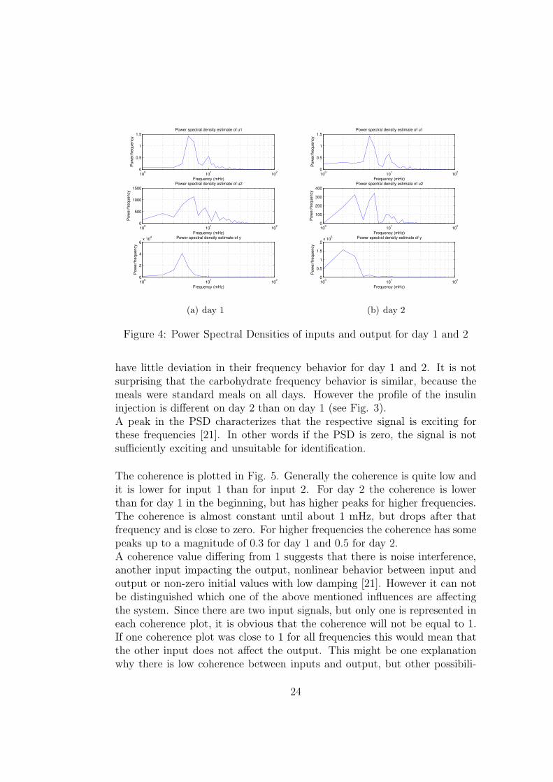
The power spectral densities (PSD) of inputs and output for day 1 and day2 can be seen in Fig. 4. The PSD of input 1 has a peak at 5 mHz and asmaller one at 10 mHz. For frequencies between 10 and 20 mHz there aresome small ripples but these are not as distinctive as the other two peaks.The PSD of input 2 has a peak at 6 mHz and two smaller ones at 9 mHzand at about 12 mHz for day 1. In the PSD of day 2 there are only thoseat 6 and 9 mHz visible and an additional peak at 3 mHz. The PSD of bothdays contain some smaller ripples in the frequency range of 10-20 mHz, likeit was mentioned for input 1 already. This behavior is however not visiblefor the output’s PSD. This has a peak at 4 mHz for day 1 and one at 2 mHzfor day 2.It can be deduced that the carbohydrate intake has similar frequency behav-ior for both days, whereas insulin injection and blood glucose measurement

23

100

101

102

0

0.5

1

1.5

Frequency (mHz)

Po

we

r/fr

eq

ue

ncy

Power spectral density estimate of u1

100

101

102

0

500

1000

1500

Frequency (mHz)

Po

we

r/fr

eq

ue

ncy


100

101

102

0

2

4

6x 10

4

Frequency (mHz)

Po

we

r/fr

eq

ue

ncy

Power spectral density estimate of y

(a) day 1

100

101

102

0

0.5

1

1.5

Frequency (mHz)

Po

we

r/fr

eq

ue

ncy


100

101

102

0

100

200

300

400

Frequency (mHz)

Po

we

r/fr

eq

ue

ncy


100

101

102

0

0.5

1

1.5

2x 10

5

Frequency (mHz)

Po

we

r/fr

eq

ue

ncy

Power spectral density estimate of y

(b) day 2

Figure 4: Power Spectral Densities of inputs and output for day 1 and 2

have little deviation in their frequency behavior for day 1 and 2. It is notsurprising that the carbohydrate frequency behavior is similar, because themeals were standard meals on all days. However the profile of the insulininjection is different on day 2 than on day 1 (see Fig. 3).A peak in the PSD characterizes that the respective signal is exciting forthese frequencies [21]. In other words if the PSD is zero, the signal is notsufficiently exciting and unsuitable for identification.

The coherence is plotted in Fig. 5. Generally the coherence is quite low andit is lower for input 1 than for input 2. For day 2 the coherence is lowerthan for day 1 in the beginning, but has higher peaks for higher frequencies.The coherence is almost constant until about 1 mHz, but drops after thatfrequency and is close to zero. For higher frequencies the coherence has somepeaks up to a magnitude of 0.3 for day 1 and 0.5 for day 2.A coherence value differing from 1 suggests that there is noise interference,another input impacting the output, nonlinear behavior between input andoutput or non-zero initial values with low damping [21]. However it can notbe distinguished which one of the above mentioned influences are affectingthe system. Since there are two input signals, but only one is represented ineach coherence plot, it is obvious that the coherence will not be equal to 1.If one coherence plot was close to 1 for all frequencies this would mean thatthe other input does not affect the output. This might be one explanationwhy there is low coherence between inputs and output, but other possibili-

24

10−4

10−3

10−2

10−1

0

0.2

0.4

0.6

0.8

Frequency (Hz)

Magnitude

Coherence estimate via Welch of u1 and y

10−4

10−3

10−2

10−1

0

0.2

0.4

0.6

0.8

1

Frequency (Hz)

Magnitude


(a) day 1

10−4

10−3

10−2

10−1

0

0.2

0.4

0.6

0.8

Frequency (Hz)

Magnitude


10−4

10−3

10−2

10−1

0

0.2

0.4

0.6

0.8

Frequency (Hz)

Magnitude


(b) day 2

Figure 5: Welch coherence estimates for day 1 and 2

ties like further not regarded inputs, non-linear input-output relationship ornoise cannot be ruled out.

25

4.5 Simulation

Using the input data and the estimated initial state the output was simulatedwith each model and compared to the real output. For comparison the VAFand the standard deviation of the simulation error (SDE) were used.To investigate the influence of the initial state, simulation of the validationday was performed with the estimation of the initial state from identificationdata and from validation data.For ARX and ARMAX models the initial state was estimated with the Mat-lab command “findstates”. For models estimated with the MOESP methodsfrom the SMI toolbox the command ”dinit“ from the same toolbox was used.The initial state for models identified with “n4sid“ were estimated with ”find-states“ and with ”dinit“ to determine which one of the two methods is moresuitable.

4.5.1 Results

VAF and SDE can be seen in Table 1 and 2 in Appendix A. The selectedmodel orders are to be found in Table 15 in Appendix B. For lack of spacethe polynomials and matrices which were identified are not displayed here.They are shown as example for the experiment ”prediction” for the reasonof being compared later.The accordance of simulated output with measured output is ranging fromnot fitting at all (negative VAF or very high standard deviation) to more orless acceptable values (VAF more than 90% and low SDE). However goodfits are mostly only achieved for simulating the same data that was used foridentification.

The simulation results will be exemplified on two models.Fig. 6 and 7 show the simulation of days 2 and 3 with models identifiedby the command ”n4sid“ from detrended data of day 2. In Fig. 6, whereidentification and validation day are the same, it can be seen that the simu-lation basically follows the measured output. The high frequency movementshowever are not caught with the simulation. Still the simulation is one ofthe best ones and trends for running into hypo- or hyperglycemia can berecognized. The VAF for this case is with a value of 93.39% quite high andthe SDE has a relatively low value of 19.53 compared to other simulationstandard deviations, indicating a good model quality.Fig. 7(a), which displays the simulation of the following day with initialstates estimated from day 2, shows that there is a great mismatch between

26

0 50 100 15050

100

150

200

250

300

350identification: day 2, validation: day 2

y2

m2

Figure 6: Simulation of day 2 with 5th order n4sid-model identified from day2 after detrending the data, initial state estimated with dinit

simulated and measured output in the first half of the simulation. This isdue to the wrong initial values. In the second half of the simulation, whenthe effect of the initial values is gone, the simulated output can keep trackof the measured output much better. The VAF is negative here (-175.47%)which is a sign of poor simulation quality and the SDE is much higher thanbefore (56.33).In the case of taking the correct data for estimating the initial state (Fig.7(b)) the first few values are in accordance with the measured output but af-ter a few samples the simulated output is much too high and drops too early.After the second half of the simulation the simulated output looks similar tothe one with wrong initial values. This shows that for longer simulations theeffect of the correct initial states diminishes. The VAF is at least positive(29.03%) but still very low. The SDE is 28.59 and thus takes on only half ofthe value than in the case before.The Bode plots in Fig. 8 show that the models Bode plot try to mimicthe basic trend of the original data’s Bode plot but that they do not coin-cide thoroughly. Especially the Bode plot of the model identified from day1 is not able to follow the high frequency spectrum of the measured data.However the Bode plots shouldn’t be interpreted too much because even the

27

0 20 40 60 80 100 120 14050

100

150

200

250

300identification: day 2, validation: day 3, initial state estimated from day 2

y3

m2

(a) Simulation of day 3, initial state estimated from day 2

0 20 40 60 80 100 120 14060

80

100

120

140

160

180

200

220

240

260identification: day 2, validation: day 3, inital state estimated from day 3

y3

m2

(b) Simulation of day 3, initial state estimated from day 3

Figure 7: Simulation of day 3 with n4sid-model of order 5 identified fromday 2 after detrending the data, initial state estimated with dinit

28

10−4

10−3

10−2

10−1

100

100

102

Am

plit

ud

e

From carbohydrate intake to blood glucose measurement

10−4

10−3

10−2

10−1

100

−200

0

200

400

600

Ph

ase

(d

eg

ree

s)

Frequency (rad/min)

z

m1

m2

(a) input carbohydrates

10−4

10−3

10−2

10−1

100

10−2

100

102

Am

plit

ud

e

From insulin injection to blood glucose measurement

10−4

10−3

10−2

10−1

100

−400

−200

0

200

400

600

Ph

ase

(d

eg

ree

s)

Frequency (rad/min)

z

m1

m2

(b) input insulin

Figure 8: Bode diagram for models identified with n4sid compared to theBode diagram of the measured data (m1 was identified from day 1 and m2from day 2)

29

10−3

10−2

10−1

100

100

102

Am

plit

ud

e


10−3

10−2

10−1

100

−600

−400

−200

0

200

400

600

Ph

ase

(d

eg

ree

s)

Frequency (rad/min)

z

z1

z2

z3

(a) input carbohydrates

10−3

10−2

10−1

100

10−2

100

102

Am

plit

ud

e

From insulin injection to blood glucose measurement

10−3

10−2

10−1

100

−200

0

200

400

600

Ph

ase

(d

eg

ree

s)

Frequency (rad/min)

z

z1

z2

z3

(b) input insulin

Figure 9: Bode diagrams of the original data for the whole sequence and foreach day

30

Bode plots of each day compared to each other deviate quite a lot (see Fig. 9).

Fig. 10(a) shows the simulation of day 1 with an ARX model identified fromday 1. The first values are matched perfectly, this is due to the known ini-tial values. Later the simulation follows the measured output only scarcely.Some peaks are tracked but others are ignored completely. VAF (27.31%)and SDE (27.48) indicate a poor simulation quality. Fig. 10(b) displays thesimulation of day 2 with the same model. Initial states were estimated withday 2. Again the beginning of the simulation is matched exactly becauseof the initial values. However the rest of the simulation does not follow themeasured output at all. In this case the VAF is higher than for the simulationof day 1 (57.27%) but the simulation quality does not look any better thanthat for day 1. This shows that the measurement indicators like VAF do notalways tell the truth. During simulation it occurred several times that theVAF suggested a good model quality but the simulation plot was poor orvice versa. The SDE is with 49.66 quite high, thus indicating bad quality.

An example for the ARMAX simulation can be seen in Fig. 11 and forMOESP models in Fig. 12.

4.5.2 Discussion

Simulation of data for the next day with initial states estimated from theidentification data results in very poor values for VAF and SDE. Using thevalidation data for estimating the initial states provides much better simu-lations. This is obvious because the initial state from the day before mightbe several mg/dL apart from the actual one. The simulation might thenstart much too high or too low. Therefore the initial value does have a greatinfluence on the quality of simulated output and it is essential to estimatethe initial values as close to the real ones as possible. However this is hard toachieve if the data that should be used for simulation are not available be-fore the simulation, like for instance in an online surveillance of blood glucoselevel. In this case a few measurement samples have to be taken to estimatethe initial value first.

The identification of day 2 provides much better results in simulation of day2 than in day 3. This is an effect that will be seen later in the other experi-ments as well.Regarding the detrending of data there can not be seen much improvementsin comparison to not detrending the data. In some cases detrending resultsin better fits, but in others it seems more advisable not to detrend the data.

31

0 50 100 150150

200

250


y2

m1

(a) day 1

0 50 100 15050

100

150

200

250

300


y

m1

(b) day 2

Figure 10: Simulation of day 1 and 2 with ARX model identified from day 1(order: na = 2, nb1 = nb2 = 1, nk1 = 16, nk2 = 30)

32

0 50 100 150150

200

250


y1

m1

(a) day 1

0 50 100 1500

50

100

150

200

250

300


y2

m1

(b) day 2

Figure 11: Simulation of day 1 and 2 with ARMAX model identified fromdetrended data of day 1 (order:na = 2, nb1 = nb2 = 1, nc = 3, nk1 = 16,nk2 = 37)

0 50 100 1500

100

200

300

400

500

600

700

800

900


y2

m1

(a) initial state estimated from day 1

0 50 100 150−100

−50

0

50

100

150

200

250

300


y2

m1

(b) initial state estimated from day 2

Figure 12: Simulation of day 2 with unstable MOESP model of order 4identified from day 1

33

Low-order ARX models lead to unstable models and thus can not be usedfor simulation. Higher-order models (with input delays of around 20) how-ever result in pole-zero-plots with some poles and zeros close to each other.Generally pole-zero-cancelations indicate a too high model order [21]. Stillhigher orders produce very poor simulations. For the first few values simula-tion and real output fit very nicely, this is due to the estimated initial state.After this however the simulation doesn’t follow the real output at all.ARMAX models are not really better than ARX although they are stableeven for low orders.For the n4sid command the estimation of the initial state with ”findstates“is not much different to the one with ”dinit“, though it seems as if the sim-ulations for ”dinit“ generally are a bit better than the others.It was not possible to achieve stable models for all MOESP models. Withthe correct initial values this might not be such a big challenge, but with thewrong initial values the simulation is completely useless (see Fig. 12). Forhigher orders the Bode plots and the standard deviation of the simulationerror was a bit lower, but there were plenty of pole zero cancellations. Sincethere was not much improvement in higher orders, it was tried to keep theorder as low as possible.

The models’ Bode plots try to mimic the general trend of the real Bode plotsbut are not capable of following the higher frequency changes. Mainly themodels’ Bode plots have a magnitude offset and are a bit lower in magnitudethan the original ones.The correlation of residuals mostly stay within the limits (except for MOESPmodels, where the residuals are a bit higher in the beginning but are de-creasing into the limits for increasing lag). If the residuals were much higherthan the margins this would indicate that there is something wrong with themodel. See Fig. 14 as an example for the correlation of the residuals.

It is hard to say which one of the models is the best one. When a modelseems to be best for some days this model produces poor simulations forother days. Furthermore even if VAF and SDE indicate good model qualitythe simulation plot might be of a very poor quality. Taking every aspect intoconsideration ”n4sid“-models seem to be most appropriate for simulation,followed by ARMAX models and finally by ARX and MOESP models.

34

4.6 Prediction

For prediction a Kalman predictor with prediction horizons of 1, 3, 6, 9 and12 steps according to 10, 30, 60, 90 and 120 min was used.

4.6.1 Results

FIT, VAF and standard deviation of prediction error (SDE) were taken foreach prediction and are displayed in Tables 3, 4 and 5 in Appendix A. Theresults for logarithmizing input and output data can be seen in tables 6 -8 and for logarithmizing only output data in tables 9 - 11 in the same ap-pendix. The models’ orders can be found in tables 16 - 18 in Appendix B aswell as the polynomials and A-matrices in Appendix C.

The prediction will be illustrated on the example of a 5th order model iden-tified with n4sid from detrended data of day 1. Fig. 13 shows the 1- and3-step-ahead predictions. For both days the 1-step-ahead prediction is veryclose to the original output. The 3-step-ahead prediction mainly follows theoriginal output, there are however some overshoots and delays. The delayis quite large for the second day (Fig. 13(b)) from sampling steps 50 to 80,covering several sampling steps.Since data and order are the same as in the part simulation the Bode diagramis the one that was already shown in Fig. 8.The correlation of the residuals are displayed in Fig. 14. They are almostentirely in the limits, but don’t have white noise properties.

Fig. 15 - 17 show examples of the predictions with ARX, ARMAX andMOESP models.

There was no difference in taking the mean value first and dividing the datainto three parts afterwards or vice versa.The effect of removing the first order trends was also examined but this didn’tresult in different outcomes than only removing the mean value.

Regarding the calculation of the logarithm the prediction for both parts (partA: taking the logarithm of input and output data, part B: taking the log-arithm of output data) is similar to the one without taking the logarithm.Sometimes normal prediction has better FIT, VAF and SDE values, butsometimes the values for the logarithmized data are better. The mean FITvalues are about 5% higher for normal data up to a prediction horizon of 6

35

0 50 100 150140

160

180

200

220

240

260

280

300

320model identified over day 1, validated over day 1

time in sampling steps

blo

od

glu

co

se

me

asu

rem

en

t

y day 1

model 1 1−step−ahead


(a) day 1

0 50 100 1500

50

100

150

200

250

300



blo

od

glu

co

se

me

asu

rem

en

t

y day 2



(b) day 2

Figure 13: Prediction of day 1 and 2 with 5th order n4sid model identifiedfrom day 1 after detrending the data

36

0 5 10 15 20 25−0.5

0

0.5

1Correlation function of residuals. Output blood glucose measurement

lag

−25 −20 −15 −10 −5 0 5 10 15 20 25−0.2

−0.1

0

0.1

0.2Cross corr. function between input carbohydrate intake and residuals from output blood glucose measurement

lag

(a)

−25 −20 −15 −10 −5 0 5 10 15 20 25−0.2

−0.1

0

0.1

0.2Cross corr. function between input insulin injection and residuals from output blood glucose measurement

lag

0 0.1 0.2 0.3 0.4 0.5 0.6 0.7 0.8 0.9 10

0.2

0.4

0.6

0.8

1

(b)

Figure 14: Correlation of the residuals of day 1 and n4sid model identifiedfrom day 1 after detrending the data

37

0 50 100 150150

200

250



blo

od g

lucose m

easure

ment

y day 1



(a) day 1

0 50 100 15050

100

150

200

250

300



blo

od g

lucose m

easure

ment

y day 2



(b) day 2

Figure 15: Prediction of day 1 and 2 with ARX model identified from day 1(order: na = 2, nb1 = nb2 = 1, nk1 = 16, nk2 = 28)

0 50 100 1500

50

100

150

200

250

300



blo

od g

lucose m

easure

ment

y day 2



(a) day 2

0 20 40 60 80 100 120 14060

80

100

120

140

160

180

200



blo

od g

lucose m

easure

ment

y day 3



(b) day 3

Figure 16: Prediction with ARMAX model identified from detrended dataof day 2 (order: na = 2, nb1 = 2, nb2 = 1, nc = 5, nk1 = 10, nk2 = 34)

38

0 50 100 150140

160

180

200

220

240

260

280

300



blo

od g

lucose m

easure

ment

y day 1



(a) day 1

0 50 100 1500

50

100

150

200

250

300



blo

od g

lucose m

easure

ment

y day 2



(b) day 2

Figure 17: Prediction of day 1 and 2 with 4th order MOESP model identifiedfrom day 1

steps. For larger prediction horizons the FIT values of logarithmized databecome better than those of normal data (Fig. 29(b) in Appendix D).Except for the n4sid models, the FIT values for part A are up to 50% bet-ter than those for part B. For n4sid models the FIT values of part B are5% better than those of part A. For increasing prediction horizons the dif-ference in FIT, VAF and SDE values is rising (see Fig. 29(a) in Appendix D).

4.6.2 Discussion

The FIT values for day 2 are up to 30% better than for day 1 and 3, regard-less of which day was taken for identification (see Fig. 26 in Appendix D asexample). The Bode plots for models identified from day 2 also seemed tobe better fitting than those identified from day 1. This can for instance beseen in the Bode diagram of the ARMAX model (Fig. 18) where the modelidentified from day 1 has a larger offset than that of day 2. A simple reasonfor this phenomenon could be the higher mean value of blood glucose level onthe first day leading to difficulties in prediction for the next day. In takingthe mean value of every day before identification there should however be nodifference between day 1 and 2, but still for detrended data the prediction forday 2 has better results. Probably the reason might be in the data itself. Inday 2 there is an extra carbohydrate intake between breakfast and lunch andone after dinner, leading to a more exciting input signal for carbohydrates.This could be one explanation for the better results for day 2, but there couldas well be plenty of others. To investigate this more data from several dayswould be required.

39

10−4

10−3

10−2

10−1

100

100

102

Am

plit

ud

e


10−4

10−3

10−2

10−1

100

−2000

−1500

−1000

−500

0

500

Ph

ase

(d

eg

ree

s)

Frequency (rad/min)

z

m1

m2

Figure 18: Bode diagram for input 1 with ARMAX model

The magnitude of the model’s Bode plot is too low compared to the dataspectrum. The difference between model 2’s Bode plot and the data’s Bodeplot is 4dB and the difference between model 1’s Bode plot and the system’sis even 12dB (see Fig. 18). For ARX models, higher orders result in slightlybetter matching Bode plots but FIT, VAF, SDE and the prediction plotsare not much better. Furthermore there were some pole-zero cancellationsfor higher order models. To achieve simpler models the smaller order wasprefered.

The fact that the residuals don’t have white noise properties is an indicatorthat there might be some effects not covered by the models. This could forinstance be a too low model order, unaccounted for inputs or nonlinear be-havior [21]. The residuals for input 1 are double as high as for input 2. Thisimplies that input 1 probably is not represented appropriately in the model.

For increasing prediction horizons the quality of the prediction gets worse,as expected. The FIT takes on values of below 50% for prediction horizonsgreater than 3 or 6 steps and the SDE is more than 20 for larger predictionhorizons. An example for FIT and SDE values can be seen in Fig. 27 in Ap-

40

0 50 100 1500

50

100

150

200

250

300



blo

od

glu

co

se

me

asu

rem

en

t

y day 2






Figure 19: Prediction of day 2 with n4sid-model identified from day 2 afterdetrending the data for all investigated prediction horizons

pendix D for models identified from data of day 1 validated on day 2. Fig. 28in Appendix D shows the FIT and SDE values that were obtained by takingthe mean of the FIT and SDE values for models identified from day 1 and 2.In general the detrended models (dotted lines) have higher FIT and mostlylower SDE values and are thus of a bit better quality, except for MOESPmodels where the detrended data led to worse results than the normal data.The difference between detrended or not detrended data becomes strongerwith increasing prediction horizon.ARX and ARMAX models have the best FIT values and are quite close toeach other, ARMAX models are a bit better for detrended data however.n4sid models for detrended data are of better quality for the SDE values.This shows that the quality indicators are not perfect and one should nottrust a single indicator only. For judging the quality all indicators and theplotted output should be taken into consideration.While the values for ARX and ARMAX are very close to each other andn4sid not being so far away, MOESP models have the lowest quality com-pared to the others. The mean FIT values for MOESP models are between5% and 15% lower and the mean SDE values are between 5 and 25 higherthan those of the other models.

41

An explanation for the better results with ARX and ARMAX models mightbe that there can be made more specifications for the order (na, nb1 andnb2) and the most appropriate model can be picked by adjusting all theseparameters for the order. Whereas for the state-space models only the orderof the A-matrix can be changed.Plotting the predicted and the measured output also shows that the qual-ity for higher prediction horizons decreases (see Fig. 19). The larger theprediction horizon, the greater is the delay between prediction and measuredoutput and the less can the prediction follow the high frequency changes. Al-though the VAF is decreasing for increasing prediction horizons this decreaseis not as dramatically as for the other two indicators. This shows again thatthe values for VAF should not be trusted blindly.If the delay is larger than the prediction horizon itself, it is hard for thepatient to react fast enough to occurring hypoglycemia. Since larger pre-diction horizons not only have a bigger mismatch between measured andpredicted output but also a larger delay (see Fig. 19), prediction horizonsof more than 3 or 6 steps (30 or 60 min) should be avoided. On the otherhand, longer prediction horizons would give enough time in case of an up-coming hypoglycemia to take precautions. Even though 30min is enough toprevent hypoglycemia by immediately ingesting carbohydrates a larger leadtime would be much more convenient for the patient.

Regarding the logarithmic analysis it can be concluded that this experimentneither proved nor disproved a logarithmic behavior of the data. It showedat least that logarithmizing does not produce completely meaningless pre-dictions.

42

4.7 Identification of models for different times of day

0 10 20 30 40 50 60 70 800

0.5

1

carbohydrate intake

mg

/kg

/min

0 10 20 30 40 50 60 70 800

20

40

60insulin injection

mIU

/L

0 10 20 30 40 50 60 70 800

200

400blood glucose measurement

mg

/dL

t in h

Figure 20: Division of the data into parts for night, breakfast, lunch anddinner

Since the blood glucose level is not only dependent on carbohydrate intakeand insulin injection, but also on exercise, stress and other factors [26], thetime of the day could play a role in the glucose metabolism. It might bethat the model for breakfast differs from that for dinner because the bodyhas rested during the night but is in motion during the day. To examine ifit is profitable to identify models for different times of the day the data wasdivided into parts for night, breakfast, lunch and dinner for each of the threedays (see Fig. 20).The previous predictions had shown that there was not a remarkable differ-ence between the predictions for detrended data or not detrended data. Thatis why it this experiment was only carried out with detrended data.

43

4.7.1 Results

The quality of the prediction turned out to be very poor, so that only AR-MAX models for day 1 and 2 and n4sid models for day 1 were identified.Models were validated with the corresponding time on the same or the fol-lowing day. If a model e.g. was identified with breakfast data from day 1then the predictions were compared to breakfast data on day 1 and 2.There is no carbohydrate or insulin intake during the night, so the input sig-nals are zero for the night parts. Therefore the input is not exciting enoughto identify models for the night.FIT, VAF and SDE values are displayed in Tables 12 - 14 in Appendix Aand the model orders in Table 19 in Appendix B.

Fig. 21 shows the prediction for breakfast for day 1 and 2 for the ARX modelidentified with day 1. It can be seen that the prediction for day 1 (Fig. 21(a))more or less follows the measured output. However the blood glucose doesnot undergo fast changes for this part and it is thus easier for the predictionto keep track with the measured output. The prediction for the second day(Fig. 21(b)) in contrast has more difficulties to match the measured output.The 1-step-ahead prediction can keep up with the measured data quite wellwith only a few overshoots and little delay. The 3-step-ahead prediction al-ready has a large delay of 5 sampling steps (almost 1h delay) and predictsmuch higher values than they really are. Therewith the 3-step-ahead predic-tion is completely useless for the patient.

In Fig. 22 the prediction for breakfast of day 1 and 2 with the n4sid modelis plotted. The prediction is as bad as for the ARX model.The prediction for dinner time (Fig. 23) is slightly improved, however. Thepredicted output can keep track of the measured output much better, it’sonly the time-delay which is still too high.

4.7.2 Discussion

The division of the data into small parts results in only a few sampling pointsfor each part. For instance the part for breakfast contains only 24 values. Itturned out that higher order models could not be identified because it wasjust not enough data. Furthermore the quality of the lower order modelscan be assumed to be very poor if there is so little information to do theidentification on.

The reason for the predictions for dinner time being closer to the measured

44

0 5 10 15 20 25150

200

250

300model identified over breakfast 1 and validated over breakfast 1


blo

od

glu

co

se

me

asu

rem

en

t

y breakfast 1

model breakfast 1 1−step−ahead


(a) Prediction for breakfast day 1

0 5 10 15 20 2550

60

70

80

90

100

110



blo

od

glu

co

se

me

asu

rem

en

t

y breakfast 2



(b) Prediction for breakfast day 2

Figure 21: Prediction for breakfast with ARX model identified from breakfastday 1

45

0 5 10 15 20 25150

200

250



blo

od

glu

co

se

me

asu

rem

en

t

y breakfast 1



(a) Prediction for breakfast day 1

0 5 10 15 20 2550

60

70

80

90

100

110

120



blo

od

glu

co

se

me

asu

rem

en

t

y breakfast 2



(b) Prediction for breakfast day 2

Figure 22: Prediction for breakfast with n4sid model identified from breakfastday 1

46

0 5 10 15 20 25 30 35 40170

180

190

200

210

220

230

240

250

260

270model identified over dinner 1 and validated over dinner 1


blo

od

glu

co

se

me

asu

rem

en

t

y dinner 1

model supper 1 1−step−ahead


(a) Prediction for dinner day 1

0 5 10 15 20 25 30 35 4060

80

100

120

140

160

180

200

220model identified over dinner 1 and validated over dinner 2


blo

od

glu

co

se

me

asu

rem

en

t

y dinner 2



(b) Prediction for dinner day 2

Figure 23: Prediction for dinner with n4sid model identified from dinner day1

47

output than for breakfast time might be that dinner spreads a time span of40 sampling points, which is nearly double as many as the breakfast time.However even though the predictions for dinner time look better than thosefor breakfast there still is a delay of about 3 steps for 3-step-ahead predic-tions. This means that if for instance hypoglycemia is predicted to occur in30min it occurs already now and the patient does not have any time to takeprecautions for preventing it. Therefore even the predictions for dinner time,which look much better, are not more useful than those for breakfast.

Unfortunately there could not be gained any insights if the models dependon the time of the day or not. To do so more data samples are required. Newmeasurements with a smaller sampling time would have to be taken.

48

4.8 Discussion

The prediction leads to much better results than the simulation. FIT andVAF have much more often values of more than 50% than simulation andthe standard deviation of the error is much smaller than for simulation. Thisis because there is a comparison between predicted and actual output for thecalculation of the next prediction value. Differences can thus much easierbe corrected. Another advantage of this is that also unstable models canproduce good predictions, unlike in simulation.

For simulation n4sid models are those with the best results followed by AR-MAX and then ARX and MOESP. ARX and ARMAX are best for prediction,then n4sid and last are MOESP models. Since there is not a huge differencebetween the quality of ARX and ARMAX models the ARX models are to beprefered because of their simplicity. The method n4sid should be favouredin the identification of state-space-models because models identified withMOESP were not convincing.

Even though the models are quite reasonable for 1 and 3-step ahead predic-tions the quality could be further improved. There are several aspects thatmight have an influence on the models’ quality, but also on the predictionitself.The first aspect is the data. The appearance of glucose in plasma for input1 was procured with a model. Input to the model was the amount of carbo-hydrates in the meal. Since it is hard to estimate the carbohydrate contentsof a meal and since the model used for calculating the plasma glucose mostprobably does not exactly fit the reality, the data obtained for input 1 mightdeviate from the true plasma glucose. Furthermore the insulin concentrationof input 2 was measured, interpolated and resampled. This might lead tofalsified insulin behaviour. For all measurements taken (insulin concentra-tion and monitoring of blood glucose level) there is no information about thesensors and their measuring error available.Any nonconformity in the data first of all leads to erroneous models but sincethe input data is also used for simulation and prediction it has an effect ofthe simulation and prediction, too.In addition there are other influences on the blood glucose concentrationthan carbohydrate intake and insulin concentration, which are not coveredas inputs here. One such influence is exercise. The muscle cells take upglucose without the presence on insulin during heavy exercise. Since it wasa hospital study the patient most probably did not go in for sports, so thatthese influences can be excluded for the identification of the models in this

49

thesis. For applying the models to the patient’s daily life it would however benecessary to consider exercise as input. Yet this is hard to achieve becausethere had to be any means of quantifying the amount of exercise.Besides, only linear models were examined, but it might be that the blood-glucose dynamics are nonlinear.

4.8.1 Comparison of polynomials and matrices of the differentmodels

For the purpose of determining if and how much the different models deviatefrom each other the polynomials and matrices for the part Prediction wereexamined. They are displayed in appendix C.The B-polynomials of the ARX models differ quite much from each other.This is mainly because the input delays were chosen so differently. If onlythose polynomials which have a similar input delay are compared, the factorsfor input 1 cover a range from -1 to -3 and are thus not so different. Thefactors for input 2 however differ from negative to positive values even forsimilar input delays. This might be an indicator for a not correctly choseninput delay for input 2. The A-polynomials for the ARX models of day 1and 2 with and without detrending are quite akin. A mean A-polynomialcould be A(q) ≈ 1 − 1.4q−1 + 0.4q−2.The B-polynomials for the ARMAX models are again hard to compare.Those for input 2 vary strongly, but those for input 1 and day 2 are very close.The A-polynomials are similar except for that of day 1 without detrending.Taking the mean of the A-polynomials leads to A(q) ≈ 1 − 1.7q−1 + 0.7q−2,which is not so much different from the mean ARX-A-polynomial. The C-polynomials for day 1 are very different from each other, but those of day 2are quite close with a mean polynomial of C(q) ≈ 1−0.3q−1−0.4q−2−0.2q−3.

Since it was hard to compare the matrices of the state-space models theeigenvalues were calculated for comparison. The n4sid models for day 1 andday 2 without detrending have different orders, so the number of eigenvaluesis different, too. The eigenvalues of day 2 are however contained in a way inthose of day 1:

0.68 ≈ 0.78 ± 0.5i

0.98 ≈ 0.999

0.93 ≈ 0.95 ± 0.12i

The models for detrended data are comparable to those of not detrended dataexcept that day 2 does only contain one complex pole, but an additional pole

50

at 0.45.The MOESP models for not detrended data are of order 4 and the eigenvaluesof day 1 and 2 are matching with those of the n4sid models.

1.01 ≈ 1

0.87 ≈ 0.8

0.956 ± 0.19i ≈ 0.964 ± 0.19i

The model for day 1 with detrended data also has these eigenvalues. Themodel for day 2 does only have order 2, but the two poles are contained inthose of the other models.

The analysis of the polynomials and matrices showed that n4sid and MOESPdeliver similar poles for models of day 1 and 2 with and without detrendingthe data. Apart from a few exceptions ARX and ARMAX models also havealike poles. Since models for day 1 and day 2 are not really unlike it canbe assumed that the models are not dependant on the days. If each dayrequired a separate model it would be hard to use the models for predictionfor other days than that used for identification. Detrending the data doesalso not seem to have a great influence on the models, which can be seen inthe FIT, VAF and SDE values already. The fact that the models are notvarying highly leads to the conclusion that they are quite reasonable and tryto mimic the reality as good as possible.

51

4.9 Conclusion

• Simulation and prediction of the identified models have been performed.The simulations were rather poor, the simulated output does not followthe measured one at all. Prediction showed much better results.

• It seems as if predictions of more than 3 steps should however beavoided, since the time delay between predicted and measured out-put increases and the prediction quality becomes worse for increasingprediction horizons.

• Despite the fact that ARX models only consider white noise as inputand are thus of less complexity than ARMAX models the quality ofpredictions with ARX models is nevertheless as good as those withARMAX models. For the subspace-based models those predictionsthat were achieved with n4sid-models were better than those achievedwith MOESP-models.

• Detrending the data before identification does not lead to completelydifferent results than not detrending the data. In some cases the resultswere slightly better with detrended data, but it also occured that notdetrended data produced better results. However in general it seemedmore reasonable to detrend the data before identification.

• Identification of the normal data produced better results than takingthe logarithm before identification and applying it back afterwards.

• The attempt to identify models for different times of the day has notbeen followed up after the first results showed that there are not enoughdata points to identify the models properly.

52

5 Controller

5.1 Minimum variance control

Given an ARMAX model for description of input-output system behaviour:

A(z−1)yk = z−dB(z−1)uk + C(z−1)wk (11)

where

A(z−1) = 1 + a1z−1 + ... + ana

z−na (12)

B(z−1) = b0 + b1z−1 + ... + bnb

z−nb+1 (13)

C(z−1) = 1 + c1z−1 + ... + cnc

z−nc (14)

and

y → output

u → control action

w → noise

d → time delay

and solving the Diophantine equation

C(z−1) = A(z−1)F (z−1) + z−dG(z−1) (15)

for the polynomials

F (z−1) = f0 + f1z−1 + ... + fd−1z

−(d−1) (16)

G(z−1) = g0 + g1z−1 + ... + gng

z−ng (17)

where ng is the maximum of (na − 1, nc − 1)

it is possible to compute a control law of the following type:

uk = −G(z−1)

B(z−1)F (z−1)yk (18)

which minimizes the variance of the d-step-ahead output [20].

In this thesis an attempt to control the blood glucose in a type 1 diabeticpatient was to use MV control to reduce the variance of the blood glucoseconcentration. Ideally the blood glucose should then fluctuate around areference value within the limits that are considered as “normoglycemia”in healthy persons. The risk for hyper- and hypoglycemia should thus bereduced.

53

5.2 Structure of the control loop

modelMV controller

noise

carbohydrate intake

insulin

blood glucose

Figure 24: Control loop

The structure of the control loop can be seen in Fig. 24. Inputs to themodel are the carbohydrate data, the calculated amount of insulin and awhite noise sequence. The output is fed back to the controller. Accordingto the control law in (18) the insulin sequence is calculated. Since it is notpossible in reality to have negative insulin values, the insulin value was setto zero whenever a negative value was calculated by the controller.

5.3 Results

To reduce the effort in solving the Diophantine equation an ARMAX modelof order na = nb1 = nb2 = nc = nk1 = nk2 = 1 was chosen as an examplefor the implementation of the controller. The model was identified with datafrom day 2. The reference value for the blood glucose concentration was setto 80 mg/dL, which is in the range of the “normal” blood glucose level inhealthy persons [10]. Unless stated differently the initial value was assumedto match the reference value when the simulation was started.The threshold for hypoglycemia was set at 50 mg/dL and is shown as dottedline in the plots. The blood glucose profile that was achieved with manualinsulin injections in the hospital is drawn as dashed line in the plot for com-parison.

The variance of the measured blood glucose for day 2 was calculated. Ithad a value of 5811 mg2/dL2. Minimum and maximum values of the blood

54

glucose concentration were 52.4 and 310.2 mg/dL. Day 3 had a variance of1812 mg2/dL2 and minimum and maximum values of 0 and 205.6 mg/dL.

Fig. 30(a) in Appendix E shows the simulated blood glucose concentra-tion and the input signals in the ideal case when the noise is disregarded.The blood glucose value is in the immediate vicinity of the reference valuethroughout the whole simulation and does only increase when carbohydratesare ingested. The maximum blood glucose concentration is 113 mg/dL andthe variance is 58.4 mg2/dL2. The insulin profile basically follows the carbo-hydrate profile.Since it is most likely to have noise acting on the process, all following simu-lations were performed with noise as additional input on the model. In Fig.30(b) the simulation with the “ideal” insulin profile, which includes negativevalues, is shown. The blood glucose concentration is fluctuating around thereference value with a variance of 181 mg2/dL2 and minimal and maximalvalues of 46.7 and 118.2 mg/dL respectively.

1400 1600 1800 2000 2200 2400 2600 2800 30000

50

100

150

200

250

300

350

t in min

mg

/dL

blood glucose − day 2

measured

simulated with controller

reference value

1400 1600 1800 2000 2200 2400 2600 2800 30000

0.5

1

1.5carbohydrate intake − day 2

mg

/kg

/min

t in min

1400 1600 1800 2000 2200 2400 2600 2800 30000

10

20

30

40

50

60insulin control signal − day 2

mIU

/L

t in min

(a)

1400 1600 1800 2000 2200 2400 2600 2800 30000

50

100

150

200

250

300

350

t in min

mg

/dL


measured


reference value

1400 1600 1800 2000 2200 2400 2600 2800 30000

0.5

1


mg

/kg

/min

t in min

1400 1600 1800 2000 2200 2400 2600 2800 30000

20

40

60


mIU

/L

t in min

(b)

Figure 25: Simulations for day 3 with controlled insulin signal

Two examples for simulations with noise and only positive insulin values areshown in Fig. 25. Because of the noise the simulations are not repeatable andthe blood glucose trajectory is varying highly in different simulations. Fig.25(a) is an example for one of the best cases that could be achieved. The

55

blood glucose variance is 169.7 mg2/dL2. Minimum and maximum valuesare 43.8 and 121.9 mg/dL. The variance for the much worse example, whichis shown in Fig. 25(b), is much higher with a value of 536.4 mg2/dL2. Theminimum value is calculated to be -0.9 mg/dL, which of course is impossiblein reality. The patient would have already died. The blood glucose exceedsthe threshold of 50 mg/dL longer and more often than in the better case.The maximum value is with 127.5 still in the range of potential values thatcould occur in a healthy person [10].

In Fig. 30(c) and 30(d) the simulation with initial blood glucose values of250 mg/dL and 0 mg/dL can be seen. In the case with the much higherblood glucose value compared to the reference, the blood glucose is correctedrapidly in the range of the reference value. The concentration is then simi-lar to the one with correct initial values. The time until the blood glucosereaches the reference value is much longer for a too low initial value thanwith a too high one.

Since it was prohibited to have negative insulin values there is no means ofincreasing the blood glucose concentration with only an insulin controlledloop except when meals are taken. Therefore negative insulin values werescaled down with a factor to achieve the dimension of the carbohydrate unitand applied as positive values additional to the carbohydrate profile thatwas given with the meals. However the blood glucose concentration did notchange in comparison to the one with only insulin control. An example canbe seen in Fig. 31.

The simulation with the model identified from day 2 was also performed withdata from day 3. The initial blood glucose value was chosen to match that ofthe measured data of day 3. Fig. 32(a) shows an example of one of the bettersimulations with a blood glucose variance of 306.6 mg2/dL2 and minimumand maximum values of 43.0 and 130.7 mg/dL. A rather poor simulationis plotted in Fig. 32(b). The variance is quite high with 1934.2 mg2/dL2,minimum and maximum values are -45.5 and 129.8 mg/dL.

5.4 Discussion

In the ideal case without noise the blood glucose variance could be reducedto 1% of the variance of the measured blood glucose that was achieved inmanual insulin dose determination. For the noisy measurements the variancecould be reduced between 3% and 10% of the measured blood glucose vari-

56

ance for day 2 and between 17% and 107% for day 3.This shows that the variance can be diminished dramatically with the con-troller. However the blood glucose concentration highly depends on the noiseand the variance flutuates a lot subject to the noise. This can be seen verywell on day 3 where there is an improvement in the variance for the bettercase, but a change for the worse in the poor case. It seems crucial to reducethe noise as far as possible. The development of low noise sensors for bloodglucose monitoring might be a step in that direction.The MV control law is designed for applying both a positive and a negativecontrol value, but in this case only positive insulin values are applicable. Thecontroller does not have any knowledge of this contraint of the insulin valuesand can therefore not consider this when calculating the insulin profile. Asa consequence the blood glucose variance might not be the minimal one.Negative blood glucose values, that appear in some simulations, are of coursenot possible in reality. This happens because the controller cannot raise theblood glucose on its own. A real patient would already have taken carbohy-drates or fallen into coma and died in the worst case.While searching for an explanation for extreme low blood glucose valuesbeyound the hypoglycemic threshold, two questions occured: Is this solelycaused by noise or was the calculated insulin dose too high? The fact, thatthis situation does only appear when noise is added, could be an indicatorfor noise beeing the cause. Additionally, a restriction of insulin doses to amaximum value of 20 mIU/L did not result in less hypoglycemia than before,but in increased risk for hyperglycemia.

In the case of a too high initial value this is regulated fastly by setting theinsulin dose to a high value until the blood glucose has reached the referencevalue. For too low initial values the controller does not have a chance toincrease the blood glucose but to wait until the first meal is taken. Due tothe noise it might happen that the blood glucose concentration is even fallingfurther and cannot be raised by the controller alone. However the simulatedscenario with an initial value of 0 mg/dL is rather exaggerated. The patientwould most probably be dead already and even with an initial value between20 and 50 mg/dL an immediate glucose intake can only be recommended.

The modification with altering the carbohydrate input did not lead to im-proved blood glucose concentration compared to only controlling the amountof insulin. Variance and number of overstepping the hypoglycemic thresh-old could not be reduced. Besides it is impractical for the patient havingto ingest carbohydrates all day long whereas the insulin dose can easily beadministered with an insulin pump 24h a day. It seems reasonable to operate

57

the controller with altering the insulin profile only but to ingest additionalcarbohydrates when hypoglycemia should occur.

The simulations for day 3 are in principal comparable to those of day 2.However the variance is higher for day 3. This reflects the fact that the pre-dictions for day 2 also were of higher quality than those of the other days. Tofollow up this matter, data of more days would be required to do simulationson. Furthermore with additional data it could be examined if it is profitableto adjust the model’s parameters adaptively every day as it is suggested by[9] and [15].

For the ideal case, when neglecting the noise, the insulin action is propor-tional to the ingested food. This is because the blood glucose does onlyincrease during mealtimes, but is in accordance with the reference value therest of the time. Therefore the blood glucose just has to be regulated byinsulin when meals are occuring. For some of the other simulations withnoise, e.g. Fig. 30(b) and Fig. 30(c), the insulin dose in times of mealsis not proportional to the carbohydrate intake. The reason for this is thatwhenever the blood glucose is too low, the carbohydrates ingested with themeal are required to raise the blood glucose. A proportional insulin injectionwould only cause the blood glucose to fall even lower.

In spite of reducing the variance, the hypoglycemic threshold is passed moreoften with the controller than without. This is because the controller has nomeans of raising the blood glucose concentration by only having an influenceon the insulin dosis. If the patient took some additional carbohydrates in thecases where the blood glucose is exceeding the hypoglycemic threshold therewill most probably not be so long and intensive hypoglycemic phases as insome of the simulation plots. Therefore the quality of the controlled bloodglucose concentration can most probably be increased in reality.With the controller, hyperglycemia does not occur anymore. The controllercan handle this by increasing the insulin dose. Hence, another way of increas-ing the controller’s quality and decreasing the risk for hypoglycemia might beto raise the reference value to 90 or 100 mg/dL because there is still enoughreserve before reaching hyperglycemia. Besides, a too high blood glucosevalue can easily be dealt with the controller, but not a too low value.

The calculated insulin profile is varying a lot during the day and does notonly contain a few peaks. Therefore it is impracticable to try to achieve thisinsulin profile with single insulin injections. To be able to use a controllerfor the glucose control in a diabetic person, an insulin pump is inevitable.

58

5.5 Conclusion

• By introducing a controller, the blood glucose concentration’s variancecan be reduced. However the blood glucose is highly dependent onnoise. Therefore the controller might lead to a very well regulatedblood glucose profile, but it can as well be of poor quality.

• The controller can reduce the blood glucose by increasing the insulindose, but has no means of raising the glucose level.

• Hyperglycemia can be avoided with the controller, whereas hypoglycemiaseems to appear more often than by defining the insulin dose manually.

• Too high initial values can easily be regulated to the reference value.In the case of too low initial values the controller is powerless and hasto wait for the next food ingestion.

59

6 Conclusion

Even with the utilized linear methods it was possible to make good predic-tions with the identified models for low prediction horizons.The MV controller was able to reduce the variance of the blood glucose con-centration and to eliminate hyperglycemia.

A challenge is that the amount of carbohydrates has to be numbered by thepatient. On the one hand it is hard to estimate the content of carbohydratesin a meal and on the other hand especially snacks and alcohol intake are easyto forget and are then not represented in a meal diary.

Further research could be done on the following topics:

• Since the data that was used for this thesis originates from one patientonly, an approach might be to collect data from different subjects andto identify models for each of these for determining if and how muchthe parameters deviate from patient to patient.

• The risk for hypoglycemia was increased with the controller. Modifi-cations on the controller and a warning system for hypoglycemia arerequired before the controller can be tested on patients.

• Other control methods as PID control or Model Predictive control couldbe examined.

• It could be analyzed if better models and controllers can be achievedwith nonlinear models and methods.

• By taking data for a longer period of time, e.g. more days, it couldbe studied if the models are varying between different days and if itis possible to apply the controller effectively to other days than that,that was used for identification. The effect of adapting the parametersat each day could also be investigated.

• If the data was collected with a smaller sampling time, the attempt toidentify models for different times of the day could be resumed.

• To be able to implement a controller in a diabetic patient, other in-fluences on the glucose level have to be taken into consideration. Forinstance the effect of excercise had to be quantified by some means andadded as input to the model.

60

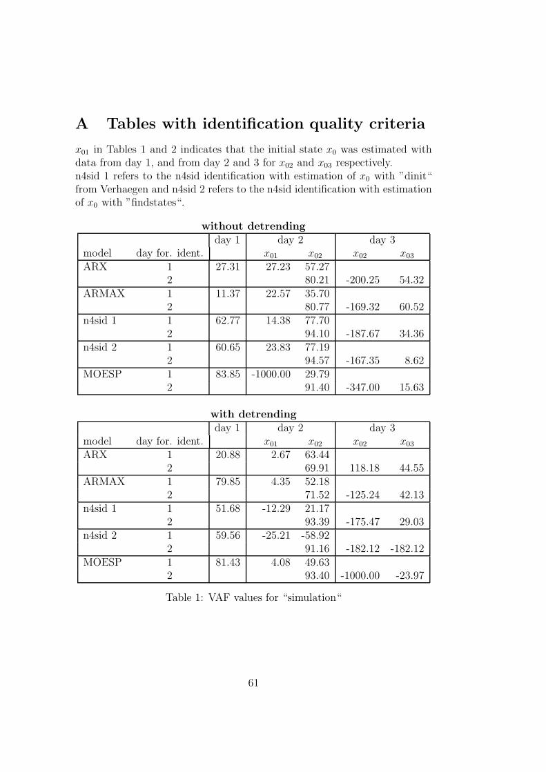
A Tables with identification quality criteria

x01 in Tables 1 and 2 indicates that the initial state x0 was estimated withdata from day 1, and from day 2 and 3 for x02 and x03 respectively.n4sid 1 refers to the n4sid identification with estimation of x0 with ”dinit“from Verhaegen and n4sid 2 refers to the n4sid identification with estimationof x0 with ”findstates“.

without detrendingday 1 day 2 day 3

model day for. ident. x01 x02 x02 x03

ARX 1 27.31 27.23 57.272 80.21 -200.25 54.32

ARMAX 1 11.37 22.57 35.702 80.77 -169.32 60.52

n4sid 1 1 62.77 14.38 77.702 94.10 -187.67 34.36

n4sid 2 1 60.65 23.83 77.192 94.57 -167.35 8.62

MOESP 1 83.85 -1000.00 29.792 91.40 -347.00 15.63

with detrendingday 1 day 2 day 3


ARX 1 20.88 2.67 63.442 69.91 118.18 44.55

ARMAX 1 79.85 4.35 52.182 71.52 -125.24 42.13

n4sid 1 1 51.68 -12.29 21.172 93.39 -175.47 29.03

n4sid 2 1 59.56 -25.21 -58.922 91.16 -182.12 -182.12

MOESP 1 81.43 4.08 49.632 93.40 -1000.00 -23.97

Table 1: VAF values for “simulation“

61

without detrendingday 1 day 2 day 3


ARX 1 27.48 64.81 49.662 33.80 58.81 54.32

ARMAX 1 30.35 66.85 60.922 33.31 55.70 21.33

n4sid 1 1 19.67 70.30 35.882 18.46 57.57 27.50

n4sid 2 1 20.22 66.31 36.282 17.70 55.50 32.45

MOESP 1 12.95 259.56 63.662 22.29 71.76 31.18

with detrendingday 1 day 2 day 3


ARX 1 28.67 74.95 45.932 41.67 50.14 25.27

ARMAX 1 14.47 74.30 52.542 40.54 50.94 25.82

n4sid 1 1 22.41 80.50 67.452 19.53 56.33 28.59

n4sid 2 1 20.50 b 85.01 95.772 22.59 57.01 57.01

MOESP 1 13.89 74.40 53.922 19.52 65919.00 37.79

Table 2: standard deviation of simulation error

62

without detrending

day 1 day 2 day 3

day 1 3 6 9 12 1 3 6 9 12 1 3 6 9 12

ARX 1 78.81 54.29 26.09 5.79 -9.74 90.26 74.11 59.52 48.35 39.58

2 91.07 76.39 66.34 60.88 57.23 86.10 64.31 48.18 43.53 39.02

ARMAX 1 81.27 57.91 29.87 8.32 -7.21 88.47 72.45 58.11 47.17 38.46

2 91.38 78.75 71.86 70.31 70.53 84.86 57.26 36.71 29.83 27.33

n4sid 1 69.94 42.91 25.69 16.92 2.42 87.46 70.60 55.98 46.58 35.94

2 85.96 78.44 74.09 70.96 68.86 65.83 43.87 29.44 23.14 13.93

MOESP 1 66.08 46.47 34.75 25.14 15.56 79.54 61.97 40.38 23.20 12.86

2 86.24 77.44 72.77 69.70 67.54 63.17 32.25 2.71 -12.26 -24.92

with detrending

day 1 day 2 day 3

day 1 3 6 9 12 1 3 6 9 12 1 3 6 9 12

ARX 1 79.30 56.65 33.42 19.91 13.48 90.38 74.35 60.71 52.43 47.06

2 90.99 75.66 64.44 57.75 52.54 85.05 59.24 38.24 35.95 33.10

ARMAX 1 79.85 57.69 34.67 21.06 14.45 90.04 73.70 60.08 50.97 45.02

2 91.38 78.03 70.02 66.91 65.75 85.70 62.09 46.46 45.14 43.04

n4sid 1 72.35 54.15 41.55 30.54 23.44 86.35 70.25 53.21 40.24 30.40

2 86.50 79.07 74.64 70.90 68.89 69.60 48.45 31.58 23.50 16.22

MOESP 1 67.93 47.90 29.47 15.39 4.75 74.57 49.39 21.30 -4.74 -39.69

2 81.07 74.53 69.47 66.04 63.94 56.36 40.25 27.17 20.20 13.56

Table 3: FIT values for ”prediction“

without detrending

day 1 day 2 day 3

day 1 3 6 9 12 1 3 6 9 12 1 3 6 9 12

ARX 1 95.51 79.11 45.39 11.26 -20.42 99.08 93.80 86.34 79.54 73.87

2 99.20 94.43 88.68 84.70 81.72 98.07 87.26 73.14 68.12 62.82

ARMAX 1 96.49 82.28 50.82 15.97 -14.84 98.68 92.63 83.86 75.51 67.98

2 99.26 95.49 92.08 91.19 91.32 97.72 81.90 60.58 51.82 48.55

n4sid 1 90.97 67.45 44.98 31.62 5.67 98.43 91.36 80.63 71.48 58.98

2 98.03 95.35 93.29 91.57 90.31 88.32 68.49 50.26 41.01 25.97

MOESP 1 88.51 71.45 57.90 45.24 30.51 95.89 85.81 65.27 42.69 26.73

2 98.11 94.91 92.59 90.83 89.48 86.52 54.46 6.63 -22.90 -48.84

with detrending

day 1 day 2 day 3

day 1 3 6 9 12 1 3 6 9 12 1 3 6 9 12

ARX 1 95.72 81.22 55.71 35.90 25.16 99.10 93.75 86.11 80.37 76.30

2 99.19 94.11 87.70 82.95 78.69 97.77 83.43 62.15 59.90 56.73

ARMAX 1 95.94 82.11 57.35 37.73 26.84 99.03 93.41 85.86 79.65 75.08

2 99.26 95.18 91.03 89.08 88.30 97.96 85.70 71.57 70.21 67.94

n4sid 1 92.36 78.99 65.94 52.08 41.79 98.15 91.26 78.70 65.69 53.94

2 98.19 95.64 93.59 91.58 90.39 91.10 74.61 56.41 47.46 39.17

MOESP 1 89.74 72.99 50.70 29.44 10.77 93.54 74.39 38.09 -9.61 -94.91

2 96.42 93.51 90.68 88.47 87.00 80.96 64.30 46.97 36.40 25.37

Table 4: VAF values for ”prediction“

63

without detrending

day 1 day 2 day 3

day 1 3 6 9 12 1 3 6 9 12 1 3 6 9 12

ARX 1 6.83 14.73 23.82 30.37 35.38 7.27 18.91 28.08 34.36 38.84

2 6.78 17.93 25.57 29.71 32.48 4.72 12.11 17.59 19.16 20.70

ARMAX 1 6.04 13.57 22.61 29.55 34.55 8.72 20.63 30.52 37.60 42.99

2 6.55 16.14 21.38 22.55 22.38 5.13 14.44 21.31 23.56 24.35

n4sid 1 9.69 18.39 23.91 26.66 31.31 9.53 22.34 33.44 40.57 48.66

2 10.66 16.38 19.68 22.06 23.65 11.60 19.05 23.94 26.07 29.20

MOESP 1 10.93 17.23 20.92 23.86 26.87 15.40 28.62 44.77 57.51 65.03

2 10.45 17.14 20.69 23.00 24.64 12.46 22.90 32.80 37.63 41.41

with detrending

day 1 day 2 day 3

day 1 3 6 9 12 1 3 6 9 12 1 3 6 9 12

ARX 1 6.67 13.97 21.45 25.81 27.89 7.22 18.99 28.31 33.66 36.99

2 6.84 18.43 26.64 31.37 35.07 5.07 13.82 20.88 21.49 22.33

ARMAX 1 6.50 13.64 21.05 25.44 27.57 7.48 19.50 28.57 34.27 37.92

2 6.55 16.69 22.75 25.10 25.99 4.85 12.84 18.10 18.53 19.22

n4sid 1 8.91 14.78 18.81 22.32 24.60 10.34 22.45 35.06 44.50 51.56

2 10.23 15.87 19.23 22.05 23.55 10.13 17.10 22.41 24.60 26.47

MOESP 1 10.33 16.76 22.64 27.08 30.45 19.32 38.45 59.78 79.54 106.06

2 14.38 19.35 23.19 25.80 27.39 14.81 20.28 24.72 27.07 29.32

Table 5: standard deviation of prediction error

without detrending

day 1 day 2 day 3

day 1 3 6 9 12 1 3 6 9 12 1 3 6 9 12

ARX 1 74.84 56.15 42.56 38.04 44.39 81.60 56.84 42.95 32.83 25.64

2 84.21 59.65 46.23 40.99 36.97 81.67 50.17 25.77 24.22 21.16

ARMAX 1 77.98 56.86 40.66 29.49 24.56 81.77 56.07 40.67 30.36 21.37

2 85.22 65.25 57.82 57.10 57.03 82.66 52.77 33.06 27.56 26.27

n4sid 1 52.59 29.33 5.89 -10.29 -16.84 64.94 45.65 29.76 17.74 6.69

2 78.32 62.98 47.84 38.99 31.17 61.02 32.88 11.24 1.96 -6.44

MOESP 1 66.23 35.26 -0.01 -30.27 -48.68 77.77 51.82 33.30 26.18 19.42

2 77.07 54.14 30.27 1.59 -30.50 62.05 15.95 -38.68 -79.15 -138.41

with detrending

day 1 day 2 day 3

day 1 3 6 9 12 1 3 6 9 12 1 3 6 9 12

ARX 1 75.46 61.11 55.27 53.20 53.04 79.17 52.35 37.94 33.31 31.84

2 84.81 62.76 51.21 46.80 44.92 82.24 53.46 34.05 32.53 31.55

ARMAX 1 80.35 66.61 62.12 61.30 62.34 80.92 56.39 46.61 42.78 41.07

2 85.44 66.44 59.11 58.42 58.44 83.26 57.75 45.73 46.86 46.15

n4sid 1 62.36 43.43 28.14 19.89 17.08 65.38 44.96 31.09 22.90 18.89

2 75.04 60.82 51.91 48.20 46.63 66.96 47.42 37.70 36.06 34.61

MOESP 1 70.37 60.30 58.09 57.72 58.60 66.64 39.94 26.92 22.10 17.67

2 76.23 59.70 52.31 49.92 49.11 68.22 43.10 23.98 16.25 12.67

Table 6: FIT for prediction with logarithmizing input and output data

64

without detrending

day 1 day 2 day 3

day 1 3 6 9 12 1 3 6 9 12 1 3 6 9 12

ARX 1 95.09 85.17 73.97 68.92 74.74 98.68 92.34 85.08 79.04 74.69

2 99.12 93.74 86.16 80.27 76.49 97.54 81.31 56.27 54.50 52.13

ARMAX 1 95.49 82.76 67.51 54.53 48.20 98.61 91.09 80.93 71.27 62.34

2 99.20 94.94 91.14 90.22 90.36 97.85 83.39 63.31 54.76 52.77

n4sid 1 78.52 50.92 9.25 -28.21 -47.00 92.44 80.73 61.34 39.24 16.00

2 97.36 91.73 80.89 71.74 64.12 87.75 63.84 36.09 19.45 2.75

MOESP 1 90.10 61.43 -2.54 -89.41 -169.22 97.89 89.47 75.19 64.60 56.80

2 97.15 86.03 50.37 -25.93 -165.99 88.44 42.69 -70.15 -219.91 -554.57

with detrending

day 1 day 2 day 3

day 1 3 6 9 12 1 3 6 9 12 1 3 6 9 12

ARX 1 94.90 86.53 81.94 80.27 80.13 97.05 83.75 71.38 66.96 65.65

2 99.05 93.30 85.75 81.84 80.51 97.54 82.29 63.24 61.87 61.56

ARMAX 1 96.51 90.28 87.47 86.90 87.61 98.46 91.03 85.22 82.40 81.20

2 99.20 95.05 90.96 90.16 90.02 97.88 85.36 73.48 74.06 73.67

n4sid 1 86.63 68.92 47.94 34.70 29.89 90.30 74.99 56.64 44.91 39.36

2 96.27 90.06 82.88 79.28 78.27 91.28 77.71 68.39 67.02 65.35

MOESP 1 92.03 85.16 83.48 82.88 83.45 92.01 73.47 59.41 52.11 44.29

2 97.62 92.97 87.85 84.88 84.73 92.43 75.58 55.35 47.13 43.35

Table 7: VAF for prediction with logarithmizing input and output data

without detrending

day 1 day 2 day 3

day 1 3 6 9 12 1 3 6 9 12 1 3 6 9 12

ARX 1 6.18 10.75 14.24 15.56 14.03 8.74 21.02 29.34 34.78 38.22

2 7.13 19.00 28.27 33.75 36.84 5.32 14.67 22.44 22.89 23.48

ARMAX 1 5.93 11.59 15.91 18.82 20.09 8.96 22.68 33.18 40.72 46.62

2 6.79 17.08 22.61 23.75 23.59 4.98 13.83 20.56 22.83 23.33

n4sid 1 12.93 19.55 26.58 31.60 33.84 20.88 33.35 47.24 59.22 69.63

2 12.34 21.85 33.21 40.38 45.51 11.88 20.41 27.13 30.46 33.47

MOESP 1 8.78 17.33 28.26 38.41 45.79 11.04 24.65 37.84 45.20 49.93

2 12.83 28.39 53.52 85.25 123.90 11.54 25.70 44.27 60.71 86.84

with detrending

day 1 day 2 day 3

day 1 3 6 9 12 1 3 6 9 12 1 3 6 9 12

ARX 1 6.30 10.24 11.86 12.40 12.44 13.06 30.62 40.64 43.67 44.53

2 7.41 19.66 28.68 32.38 33.54 5.33 14.29 20.58 20.96 21.04

ARMAX 1 5.21 8.70 9.88 10.10 9.82 9.44 22.76 29.21 31.87 32.94

2 6.78 16.90 22.84 23.83 24.00 4.94 12.99 17.48 17.29 17.42

n4sid 1 10.21 15.56 20.14 22.55 23.37 23.66 37.99 50.03 56.39 59.16

2 14.67 23.95 31.44 34.58 35.42 10.02 16.02 19.08 19.49 19.98

MOESP 1 7.88 10.75 11.34 11.55 11.35 21.48 39.13 48.40 52.57 56.70

2 11.71 20.14 26.48 29.54 29.69 9.34 16.77 22.68 24.68 25.55

Table 8: SDE for prediction with logarithmizing input and output data

65

without detrending

day 1 day 2 day 3

day 1 3 6 9 12 1 3 6 9 12 1 3 6 9 12

ARX 1 77.42 52.81 24.62 3.96 -12.44 83.69 58.79 43.58 33.80 25.13

2 84.17 59.41 43.64 35.97 30.28 81.73 49.67 23.06 19.05 12.40

ARMAX 1 76.71 51.11 33.00 24.69 19.50 83.94 60.58 46.75 39.97 36.06

2 84.89 63.52 53.45 49.91 48.20 81.48 46.79 21.11 11.68 7.09

n4sid 1 69.39 41.29 19.67 6.32 -10.89 80.17 54.75 40.58 33.14 22.17

2 80.49 64.44 58.02 52.33 47.55 62.25 25.42 7.26 -5.69 -21.79

MOESP 1 62.24 38.49 19.33 3.14 -9.84 70.64 48.24 29.03 17.43 14.06

2 77.25 64.30 62.96 63.59 60.39 59.42 30.23 8.88 2.33 -4.58

with detrending

day 1 day 2 day 3

day 1 3 6 9 12 1 3 6 9 12 1 3 6 9 12

ARX 1 75.90 50.15 30.26 19.41 13.32 83.96 60.25 45.41 37.41 32.62

2 84.63 61.17 48.56 42.74 38.00 82.37 53.24 33.30 31.75 28.95

ARMAX 1 77.18 52.17 31.30 20.34 14.18 83.27 58.94 44.78 37.45 33.00

2 85.08 61.43 46.43 39.04 34.13 81.85 51.89 32.52 28.56 26.36

n4sid 1 70.55 51.44 40.75 35.73 32.19 78.21 56.71 41.55 32.10 26.27

2 79.81 67.53 65.04 63.99 63.62 59.43 29.77 17.43 11.46 6.74

MOESP 1 60.33 39.17 27.97 24.78 24.90 66.93 42.85 17.98 2.44 -2.22

2 71.30 63.56 59.75 56.92 54.30 49.22 33.20 20.11 12.50 4.93

Table 9: FIT for prediction with logarithmizing output data only

without detrending

day 1 day 2 day 3

day 1 3 6 9 12 1 3 6 9 12 1 3 6 9 12

ARX 1 95.42 79.61 46.02 9.08 -25.38 99.04 93.21 84.60 76.31 68.64

2 99.09 93.43 83.76 74.69 68.13 97.53 80.98 53.52 47.39 38.20

ARMAX 1 94.92 78.35 58.64 46.42 38.40 98.89 92.04 81.74 74.84 71.12

2 99.14 94.27 89.13 86.64 85.68 97.37 77.06 46.13 30.45 23.18

n4sid 1 91.02 67.74 42.99 21.50 -12.62 98.51 92.02 82.84 74.59 64.95

2 97.71 91.84 86.98 82.45 79.44 86.95 48.43 19.86 -7.15 -43.51

MOESP 1 86.99 66.89 44.47 19.75 0.50 95.29 83.67 57.63 35.87 39.59

2 97.73 94.16 92.55 92.75 91.06 85.91 54.85 18.04 3.59 -22.18

with detrending

day 1 day 2 day 3

day 1 3 6 9 12 1 3 6 9 12 1 3 6 9 12

ARX 1 94.44 75.55 50.96 32.96 22.10 98.94 92.49 83.38 77.25 73.84

2 99.13 93.43 85.37 79.83 76.05 97.78 83.94 66.36 66.16 64.14

ARMAX 1 94.84 77.14 52.47 34.99 24.47 98.82 91.95 82.75 76.88 73.59

2 99.08 92.73 83.58 77.11 72.77 97.60 83.13 66.40 62.28 60.27

n4sid 1 91.79 78.31 68.05 60.78 55.74 97.55 89.22 76.00 66.00 61.01

2 97.60 93.31 90.98 89.89 89.80 84.74 52.59 33.43 21.69 11.76

MOESP 1 84.84 65.42 52.94 48.97 50.38 93.46 76.98 31.55 -10.16 -3.07

2 95.92 93.17 90.75 89.28 87.91 80.14 65.29 49.57 35.51 13.27

Table 10: VAF for prediction with logarithmizing output data only

66

without detrending

day 1 day 2 day 3

day 1 3 6 9 12 1 3 6 9 12 1 3 6 9 12

ARX 1 6.90 14.56 23.69 30.74 36.10 7.44 19.80 29.81 36.97 42.54

2 7.25 19.48 30.62 38.22 42.89 5.33 14.80 23.14 24.62 26.68

ARMAX 1 7.27 15.00 20.73 23.60 25.30 7.99 21.43 32.46 38.11 40.83

2 7.05 18.18 25.05 27.77 28.75 5.50 16.26 24.91 28.31 29.75

n4sid 1 9.66 18.31 24.34 28.56 34.21 9.27 21.47 31.47 38.29 44.98

2 11.49 21.70 27.41 31.82 34.45 12.26 24.37 30.38 35.13 40.66

MOESP 1 11.63 18.55 24.02 28.88 32.16 16.48 30.70 49.45 60.84 59.05

2 11.45 18.36 20.74 20.46 22.72 12.74 22.81 30.73 33.33 37.52

with detrending

day 1 day 2 day 3

day 1 3 6 9 12 1 3 6 9 12 1 3 6 9 12

ARX 1 7.60 15.94 22.58 26.40 28.45 7.81 20.82 30.97 36.23 38.86

2 7.08 19.47 29.06 34.12 37.18 5.06 13.60 19.69 19.75 20.32

ARMAX 1 7.32 15.41 22.23 25.99 28.02 8.24 21.55 31.56 36.53 39.04

2 7.30 20.49 30.79 36.35 39.64 5.26 13.94 19.68 20.85 21.39

n4sid 1 9.23 15.02 18.22 20.19 21.45 11.88 24.94 37.22 44.30 47.44

2 11.78 19.65 22.81 24.15 24.26 13.26 23.37 27.69 30.04 31.88

MOESP 1 12.55 18.96 22.12 23.03 22.71 19.43 36.45 62.85 79.74 77.13

2 15.35 19.85 23.11 24.87 26.42 15.13 20.00 24.10 27.26 31.61

Table 11: SDE for prediction with logarithmizing output data only

with detrending

day 1 day 2 day 3

day 1 3 6 9 12 1 3 6 9 12 1 3 6 9 12

ARX 1 breakfast 85.95 75.35 62.21 56.49 51.90 24.51 -67.37 -133.54 -203 -263.89

lunch 60.05 30.56 22.34 10.63 3.34 82.54 50.84 16.07 -3.22 -10.00

dinner 65.46 39.95 21.25 10.45 9.94 77.13 50.46 36.49 18.01 -3.14

2 breakfast 38.96 9.82 33.17 38.33 19.23 62.31 15.95 -11.17 -27.74 -43.80

lunch 90.76 76.23 66.14 58.46 52.39 76.58 31.94 -16.79 -38.15 -48.75

dinner 82.14 52.40 37.79 28.32 19.86 62.58 -15.28 -109.76 -149.42 -141.97

n4sid 1 breakfast 83.79 70.27 55.40 51.70 46.56 6.33 -66.30 -70.72 -98.84 -112.38

lunch 62.16 36.92 19.78 1.29 -12.94 70.65 29.78 -14.87 -41.48 -54.16

dinner 63.59 40.27 26.12 19.75 25.39 75.39 51.14 34.99 15.30 -2.59

Table 12: FIT for prediction after identifying different times of the day

67

with detrending

day 1 day 2 day 3

day 1 3 6 9 12 1 3 6 9 12 1 3 6 9 12

ARX 1 breakfast 98.04 94.47 88.88 90.44 93.56 44.27 -154.89 -284.66 -497.40 -619.52

lunch 84.11 52.25 40.36 20.87 7.21 97.13 77.96 38.31 10.68 4.57

dinner 88.09 63.98 38.02 19.82 20.46 94.80 76.19 65.85 48.59 22.75

2 breakfast 62.77 19.11 56.56 62.77 36.44 88.40 48.61 16.07 -11.80 -47.61

lunch 99.16 94.62 90.01 86.13 80.97 94.72 57.72 -18.59 -55.71 -68.18

dinner 96.85 78.34 70.69 69.30 66.38 86.06 -31.32 -330.58 -495.23 -453.53

n4sid 1 breakfast 97.42 91.83 83.98 87.98 91.59 12.28 -174.10 -175.88 -269.42 -288.21

lunch 85.92 61.50 38.75 7.78 -19.18 92.07 55.73 -13.60 -64.50 -80.59

dinner 87.05 65.89 50.01 42.84 50.32 94.19 78.69 70.79 56.85 42.40

Table 13: VAF for prediction after identifying different times of the day

with detrending

day 1 day 2 day 3

day 1 3 6 9 12 1 3 6 9 12 1 3 6 9 12

ARX 1 breakfast 6.48 10.89 15.44 14.32 11.76 8.70 18.60 22.85 28.48 31.25

lunch 5.75 9.97 11.14 12.83 13.90 8.71 24.14 40.40 48.60 50.24

dinner 8.76 15.23 19.98 22.72 22.63 9.18 19.63 23.51 28.84 35.36

2 breakfast 7.11 10.48 7.68 7.11 9.29 6.07 12.78 16.33 18.85 21.66

lunch 4.72 11.93 16.26 19.15 22.44 6.98 19.74 33.06 37.88 39.37

dinner 7.14 18.72 21.78 22.29 23.32 6.39 19.60 35.50 41.74 40.25

n4sid 1 breakfast 7.44 13.24 18.54 16.06 13.43 10.91 19.29 19.35 22.39 22.96

lunch 5.41 8.95 11.29 13.86 15.75 14.48 34.22 54.81 65.96 69.11

dinner 9.13 14.82 17.94 19.19 17.89 9.70 18.57 21.74 26.43 30.53

Table 14: SDE for prediction after identifying different times of the day

68

B Utilized model orders for identification

without detrendingmodel day na nb1 nb2 nc nk1 nk2 model day orderARX 1 2 1 1 16 30 n4sid (dinit) 1 5

2 2 2 2 18 32 2 3ARMAX 1 2 1 1 4 16 28 n4sid (findstate) 1 5

2 2 1 1 2 5 34 2 4MOESP 1 4

2 2

with detrendingmodel day na nb1 nb2 nc nk1 nk2 model day orderARX 1 2 1 1 15 26 n4sid (dinit) 1 5

2 3 1 1 13 17 2 5ARMAX 1 2 1 1 3 16 37 n4sid (findstate) 1 5

2 2 2 1 2 13 20 2 5MOESP 1 3

2 2

Table 15: Orders selected for simulation

69

without detrendingmodel day na nb1 nb2 nc nk1 nk2 model day orderARX 1 2 1 1 16 28 n4sid 1 5

2 3 1 1 9 34 2 3ARMAX 1 2 2 1 4 16 33 MOESP 1 4

2 2 2 1 3 11 37 2 4

with detrendingmodel day na nb1 nb2 nc nk1 nk2 model day orderARX 1 2 1 1 5 36 n4sid 1 5

2 2 1 1 8 38 2 5ARMAX 1 2 1 2 4 6 34 MOESP 1 5

2 2 2 1 5 10 34 2 2

Table 16: Orders selected for prediction


2 2 1 1 16 27 2 4ARMAX 1 2 2 1 3 20 20 MOESP 1 4

2 2 2 1 3 11 33 2 3


2 2 1 1 25 20 2 3ARMAX 1 2 2 1 3 20 32 MOESP 1 4

2 2 2 1 5 20 32 2 2

Table 17: Orders selected for prediction with logarithmized inputs and output

70


2 2 1 1 16 27 2 4ARMAX 1 2 2 1 3 20 20 MOESP 1 4

2 2 2 1 3 11 33 2 4


2 2 1 1 25 20 2 3ARMAX 1 2 2 1 3 20 32 MOESP 1 4

2 2 2 1 5 20 32 2 3

Table 18: Orders selected for prediction with logarithmized output

with detrendingmodel day na nb1 nb2 nk1 nk2 model day orderARX 1 breakfast 2 1 1 0 1 n4sid 1 breakfast 1

lunch 2 1 1 0 0 lunch 1dinner 1 1 1 0 0 dinner 1

2 breakfast 3 2 1 0 0lunch 2 5 2 0 0dinner 2 1 1 0 0

Table 19: Orders selected for prediction after identification of different timesof the day

71

C Identified polynomials and matrices for pre-

diction

For the simulation experiment the polynomials and matrices of the differentmodels are displayed here. m1 stands for models identified from day 1 andm2 from day 2, respectively. For the state-space-models only the A-matrixand the eigenvalues are shown.

ARXwithout detrending:

m1 : A(q) = 1 − 1.358q−1 + 0.372q−2

B1(q) = 4.94q−16

B2(q) = 0.2049q−28

m2 : A(q) = 1 − 1.631q−1 + 0.8141q−2 − 0.1555q−3

B1(q) = −3.036q−9

B2(q) = 0.3756q−34

with detrending:

m1 : A(q) = 1 − 1.341q−1 + 0.3884q−2

B1(q) = −1.904q−5

B2(q) = 0.03228q−36

m2 : A(q) = 1 − 1.57q−1 + 0.5996q−2

B1(q) = −0.9534q−8

B2(q) = −0.01244q−38

72

ARMAXwithout detrending:

m1 : A(q) = 1 − 0.2007q−1 − 0.7812q−2

B1(q) = −27.66q−16 + 34.96q−17

B2(q) = 0.3247q−33

C(q) = 1 + 1.284q−1 + 0.275q−2 + 0.1777q−3 + 0.2771q−4

m2 : A(q) = 1 − 1.884q−1 + 0.8948q−2

B1(q) = −6.663q−11 + 6.385q−12

B2(q) = 0.1358q−37

C(q) = 1 − 0.343q−1 − 0.4313q−2 − 0.1992q−3

with detrending:

m1 : A(q) = 1 − 1.282q−1 + 0.348q−2

B1(q) = −2.464q−6

B2(q) = 0.01755q−34 + 0.01642q−35

C(q) = 1 + 0.0506q−1 − 0.05201q−2 + 0.1848q−3 + 0.1418q−4

m2 : A(q) = 1 − 1.917q−1 + 0.9265q−2

B1(q) = −6.517q−10 + 6.867q−11

B2(q) = −0.02166q−34

C(q) = 1 − 0.3027q−1 − 0.3866q−2 − 0.1632q−3 − 0.003037q−4 − 0.1152q−5

73

n4sidwithout detrending:m1: A =

x1 x2 x3 x4 x5x1 0.97892 -0.038865 0.0077732 -0.020216 0.049224x2 -0.08155 0.99777 -0.10111 -0.20103 -0.16882x3 -0.042255 -0.055858 0.85675 -0.18723 0.35479x4 -0.044346 0.28957 -0.011871 0.79259 0.5214x5 -0.036226 0.085415 -0.24889 -0.26195 0.84069

eig(A) = {0.7843 ± 0.5273i, 0.9991, 0.9495± 0.1185i}

m2: A =x1 x2 x3

x1 1.0007 0.036976 -0.067476x2 -0.019577 0.80441 0.103x3 0.04423 0.15343 0.7917

eig(A) = {0.6828, 0.9845, 0.9295}

with detrending:m1: A =

x1 x2 x3 x4 x5x1 0.95645 -0.1098 0.11809 0.014875 -0.010794x2 0.1716 0.94963 -0.27526 -0.11587 -0.015236x3 -0.008739 0.071186 0.86356 -0.48217 0.31533x4 -0.059194 0.21313 0.30017 0.78549 0.2216x5 0.10605 0.14964 -0.25681 -0.0089214 0.83135

eig(A) = {0.7692 ± 0.5435i, 0.9852± 0.1140i, 0.8776}

m2: A =x1 x2 x3 x4 x5

x1 0.91536 -0.060285 -0.061944 0.10353 -0.09881x2 -0.060813 1.0526 -0.18746 0.048826 -0.03125x3 -0.26525 0.35126 0.59699 0.17414 -0.25403x4 -0.052271 0.29854 -0.25738 0.9032 0.20108x5 -0.05445 -0.13029 0.13037 -0.42713 0.3784

eig(A) = {0.4504, 0.7877± 0.3335i, 0.9235, 0.8972}

74

MOESPwithout detrending:m1: A =

x1 x2 x3 x4x1 1.0254 -0.14544 -0.063307 0.088451x2 0.0029551 0.98245 0.3736 -0.048946x3 0.0034266 -0.096358 0.94281 -0.11816x4 -0.0039834 -0.008023 0.029959 0.84123

eig(A) = {1.0126, 0.8665, 0.9564± 0.1906i}

m2: A =x1 x2 x3 x4

x1 1.0148 -0.15503 -0.067336 0.057644x2 0.013548 0.96089 0.37062 0.077715x3 -0.0026518 -0.065356 0.99643 -0.23293x4 -0.0037382 0.0091471 0.078493 0.76338

eig(A) = {0.7990, 1.0086, 0.9639± 0.1913i}

with detrending:m1: A =

x1 x2 x3 x4 x5x1 0.94672 -0.14594 -0.19888 0.03148 -0.1537x2 0.12258 1.0248 -0.2676 -0.030184 -0.18778x3 0.020241 0.0049067 1.0085 0.17072 0.077289x4 0.0022759 0.014042 -0.1007 0.81523 0.59839x5 0.0099654 -0.030547 -0.010914 -0.5279 0.78855

eig(A) = {0.7996 ± 0.5770i, 0.9630± 0.1499i, 1.0586}

m2: A =x1 x2

x1 1.0111 -0.1639x2 0.01777 0.95163

eig(A) = {0.9814 ± 0.0450i}

75

D FIT and SDE plots for prediction

1 3 6 9 1210

20

30

40

50

60

70

80

90

100FIT values for prediction of ARX models with detrended data

id. day 1, val. day 1




Figure 26: Prediction of day 1, 2 and 3 with ARX model identified from day1 and 2 after detrending the data

76

1 3 6 9 12−40

−20

0

20

40

60

80

100FIT values for prediction of day 2, models identified with day 1

ARX

ARMAX

n4sid

MOESP

ARX detrend

ARMAX detrend

n4sid detrend

MOESP detrend

(a) FIT values

1 3 6 9 120

20

40

60

80

100

120SDE values for prediction of day 2, models identified with day 1

ARX

ARMAX

n4sid

MOESP

ARX detrend

ARMAX detrend

n4sid detrend

MOESP detrend

(b) SDE values

Figure 27: FIT and SDE values for all models with increasing predictionhorizons, models identified with data from day 1 and validated on day 2

77

1 3 6 9 1210

20

30

40

50

60

70

80

90mean FIT values for prediction

ARX

ARMAX

n4sid

MOESP

ARX detrend

ARMAX detrend

n4sid detrend

MOESP detrend

(a) mean FIT values

1 3 6 9 125

10

15

20

25

30

35

40

45

50mean SDE values for prediction

ARX

ARMAX

n4sid

MOESP

ARX detrend

ARMAX detrend

n4sid detrend

MOESP detrend

(b) mean SDE values

Figure 28: mean FIT and SDE values for all models with increasing predic-tion horizons

78

1 3 6 9 1220

30

40

50

60

70

80

90mean FIT values for prediction with logarithmized and detrended data

ARX Part A

ARMAX Part A

n4sid Part A

MOESP Part A

ARX Part B

ARMAX Part B

n4sid Part B

MOESP Part B

(a) part A and part B

1 3 6 9 1210

20

30

40

50

60

70

80

90mean FIT values for prediction with detrended data and with logarithmized and detrended data

ARX

ARMAX

n4sid

MOESP

ARX Part A

ARMAX Part A

n4sid Part A

MOESP Part A

(b) normal data without logarithmizing and part A

Figure 29: comparison of mean FIT values for logarithmized and detrendeddata

79

E Simulations with the controlled system

1400 1600 1800 2000 2200 2400 2600 2800 30000

50

100

150

200

250

300

350

t in min

mg/d

Lblood glucose − day 2

measured


reference value

1400 1600 1800 2000 2200 2400 2600 2800 30000

0.5

1


mg/k

g/m

in

t in min

1400 1600 1800 2000 2200 2400 2600 2800 30000

10

20

30

40


mIU

/L

t in min

(a)

1400 1600 1800 2000 2200 2400 2600 2800 30000

50

100

150

200

250

300

350

t in min

mg/d

L


measured


reference value

1400 1600 1800 2000 2200 2400 2600 2800 30000

0.5

1


mg/k

g/m

in

t in min

1400 1600 1800 2000 2200 2400 2600 2800 3000−50

0


mIU

/Lt in min

(b)

1400 1600 1800 2000 2200 2400 2600 2800 30000

50

100

150

200

250

300

350

t in min

mg/d

L


measured


reference value

1400 1600 1800 2000 2200 2400 2600 2800 30000

0.5

1


mg/k

g/m

in

t in min

1400 1600 1800 2000 2200 2400 2600 2800 30000

50

100

150

200


mIU

/L

t in min

(c)

1400 1600 1800 2000 2200 2400 2600 2800 30000

50

100

150

200

250

300

350

t in min

mg/d

L


measured


reference value

1400 1600 1800 2000 2200 2400 2600 2800 30000

0.5

1


mg/k

g/m

in

t in min

1400 1600 1800 2000 2200 2400 2600 2800 30000

20

40

60


mIU

/L

t in min

(d)

Figure 30: Simulations for day 2 with controlled insulin signal. (a) withoutnoise; (b) with noise, negative insulin values are allowed; (c) with noise,initial value = 250 mg/dL; (d) with noise, initial value = 0 mg/dL

80

1400 1600 1800 2000 2200 2400 2600 2800 30000

50

100

150

200

250

300

350

t in min

mg

/dL


measured


reference value

1400 1600 1800 2000 2200 2400 2600 2800 30000

0.5

1

1.5

1400 1600 1800 2000 2200 2400 2600 2800 30000

10

20

30

40


mIU

/L

t in min

original CHO intake

calculated CHO intake

Figure 31: Simulations for day 2 with controlled insulin and carbohydratesignals

2800 3000 3200 3400 3600 3800 4000 4200 44000

100

200

300

t in min

mg

/dL


measured


reference value

2800 3000 3200 3400 3600 3800 4000 4200 44000

0.5

1


mg

/kg

/min

t in min

2800 3000 3200 3400 3600 3800 4000 4200 44000

20

40

60


mIU

/L

t in min

(a)

2800 3000 3200 3400 3600 3800 4000 4200 4400

0

100

200

300

t in min

mg

/dL


measured


reference value

2800 3000 3200 3400 3600 3800 4000 4200 44000

0.5

1


mg

/kg

/min

t in min

2800 3000 3200 3400 3600 3800 4000 4200 44000

20

40

60


mIU

/L

t in min

(b)

Figure 32: Simulations for day 3 with controlled insulin signal

81

References

[1] R. Bellazzi, C. Larizza, S. Montani, A. Riva, M. Stefanelli,G. d’Annunzio, R. Lorini, E. J. Gomez, E. Hernando, E. Brugues,J. Cermeno, R. Corcoy, A. de Leiva, C. Cobelli, G. Nucci, S. Del Prato,A. Maran, E. Kilkki, and J. Tuominen. A telemedicine support fordiabetes management: the T-IDDM project. Computer Methods and

Programs in Biomedicine, 2002.

[2] R. Bellazzi, G. Nucci, and C. Cobelli. The Subcutaneous Route toInsulin-Dependent Diabetes Therapy. IEEE Engineering in Medicine

and Biology, 2001.

[3] R. Bellazzi, C. Siviero, M. Stefanelli, and G. De Nicolao. Adaptivecontrollers for intelligent monitoring. Artificial Intelligence in Medicine,1995.

[4] R. N. Bergman, L. S. Phillips, and C. Cobelli. Physiologic evaluationof factors controlling glucose tolerance in man: measurement of insulinsensitivity and beta-cell glucose sensitivity from the response to intra-venous glucose. J Clin Invest., 68(6):1456–1467, December 1981.

[5] T. Bremer and D. A. Gough. Is blood glucose predictable from previousvalues? A solicitation for data. Diabetes, 48, 1999.

[6] T. Deutsch, A. V. Roudsari, H. J. Leicester, T. Theodorou, E. R. Carson,and P. H. Sonksen. UTOPIA: a consultation system for visit-by-visitdiabetes management. Medical informatics, 1996.

[7] M. Eren-Oruklu, A. Cinar, L. Quinn, and D. Smith. Estimation ofFuture Glucose Concentrations with Subject-Specific Recursive LinearModels. Diabetes Technology and Therapeutics, 11, April 2009.

[8] D. Finan, H. Zisser, L. Jovanovic, W. Bevier, and D. Seborg. Iden-tification of linear dynamic models for type 1 diabetes: A simulationstudy. In ADCHEM International Symposium on Advanced Control of

Chemical Processes. IFAC, 2006.

[9] U. Fischer, W. Schenk, E. Salzsieder, G. Albrecht, P. Abel, and E.-J.Freyse. Does Physiological Blood Glucose Control Require an Adap-tive Control Strategy? IEEE Transactions on Biomedical Engineering,BME-34(8), 1987.

82

[10] A. C. Guyton and J. E. Hall. Textbook of Medical Physiology, chap-ter Insulin, Glucagon and Diabetes Mellitus, pages 961–977. ElsevierSaunders, 11 edition, 2006.

[11] E. J. Gomez, M. E. Hernando, A. Garcıa, F. Del Pozo, J. Cermeno,R. Corcoy, E. Brugues, and A. De Leiva. Telemedicine as a tool forintensive management of diabetes: the DIABTel experience. Computer

Methods and Programs in Biomedicine, 2002.

[12] B. Haverkamp and M. Verhaegen. Manual for SMI Toolbox Version 1.0.

State Space Model Identification Software for Multivariable Dynamical

Systems. TU Delft, 1997.

[13] O. K. Hejlesen, S. Andreassen, R. Hovorka, and D. A. Gava. DIAS - thediabetes advisory system: an outline of the system and the evaluation re-sults obtained so far. Computer Methods and Programs in Biomedicine,54, 1997.

[14] R. Hovorka. Management of diabetes using adaptive control. Interna-

tional Journal of Adaptive Control and Signal Processing, 2005.

[15] R. Hovorka, V. Canonico, L. J. Chassin, U. Haueter, M. Massi-Benedetti, M. O. Federici, T. R. Pieber, H. C. Schaller, L. Schaupp,T. Vering, and M. E Wilinska. Nonlinear model predictive control ofglucose concentration in subjects with type 1 diabetes. Physiological

Measurement, 25:905–920, 2004.

[16] R. Hovorka, F. Shojaee-Moradie, P. V. Carroll, L. J. Chassin, I. J.Gowrie, N. C. Jackson, R. S. Tudor, A. M. Umpleby, and R. H. Jones.Partitioning glucose distribution/transport, disposal and endogenousproduction during IVGTT. Am J Physiol Endocrinol Metab, 2002.

[17] R. Hovorka, M. Wilinska, L. Chassin, C. Acerini, and D. Dunger. Theartificial pancreas: making headway. Pract Diab Int, 24(2), March 2007.

[18] R. Hovorka, M. Wilinska, L. Chassin, and D. Dunger. Roadmap to theartificial pancreas. Diabetes Research and Clinical Practice, 74:178–182,2006.

[19] The MathWorks Inc. Matlab Documentation.http://www.mathworks.com/access/helpdesk/help/helpdesk.html,May 2009.

[20] R. Johansson. Predictive and Adaptive Control, September 2008.

83

[21] R. Johansson. System Modeling and Identification. KFS i Lund AB,2009.

[22] E. D. Lehmann, T. Deutsch, E. R. Carson, and P. H. Sonksen. AIDA:an interactive diabetes advisor. Computer methods and programs in

biomedicine, 1994.

[23] C. Malchoff, K. Shoukri, J. Landau, and J. Buchert. A novel noninvasiveblood glucose monitor. Diabetes Care, 25(12):2268–75, Dec 2002.

[24] I. Muhlhauser, V. Jorgens, M. Berger, W. Graninger, W. Gurtler,L. Hornke, A. Kunz, G. Schernthaner, V. Scholz, and H. E. Voss. Bi-centric evaluation of a teaching and treatment programme for type 1(insulin-dependent) diabetic patients: improvement of metabolic controland other measures of diabetes care for up to 22 months. Diabetologia,1983.

[25] World Health Organization. Fact sheet N◦312.http://www.who.int/mediacentre/factsheets/fs312/en/, November2008.

[26] C. Palerm, H. Zisser, L. Jovanovic, and F. Doyle III. A run-to-runcontrol strategy to adjust basal insulin infusion rates in type 1 diabtes.Journal of Process Control, 18:258–265, 2008.

[27] M. Percival, W. Bevier, H. Zisser, L. Jovanovic, D. Seborg, and F. DoyleIII. Prediction of Dynamic Glycemic Trends Using Optimal State Esti-mation. In Proceedings of the 17th IFAC World Crongress, pages 422–4227, Seoul, Korea, July 6-11 2008. The International Federation ofAutomatic Control.

[28] J. Reifman, S. Rajaraman, A. Gribok, and W. K. Ward. PredictiveMonitoring for Improved Management of Glucose Levels. Journal of

Diabetes Science and Technology, 1, July 2007.

[29] J. T. Sorensen. A physiologic model of glucose metabolism in man and

its use to design and assess improved insulin therapies for diabetes. PhDthesis, Massachusetts Institute of Technology, 1985.

[30] G. Sparacino, F. Zanderigo, S. Corazza, A. Maran, A. Facchinetti, andC. Cobelli. Glucose Concentration can be Predicted Ahead in TimeFrom Continuous Glucose Monitoring Sensor Time-Series. IEEE Trans-

actions on Biomedical Engineering, 54(5), 2007.

84

[31] M. J. Tierney, J. A. Tamada, R. O. Potts, L. Jovanovic, S. Garg, andCygnus Research Team. Clinical evaluation of the GlucoWatch biogra-pher: a continual, non-invasive glucose monitor for patients with dia-betes. Biosensors and Bioelectronics, 16:621–629, 2001.

85

List of Figures

1 Order Selection for ARX: Identification of Day 1 and Input 1 . 182 Singular values for the method n4sid for identification of Day 1 193 Measurement data used for identification . . . . . . . . . . . . 204 Power Spectral Densities of inputs and output for day 1 and 2 225 Welch coherence estimates for day 1 and 2 . . . . . . . . . . . 236 Simulation of day 2 with 5th order n4sid-model identified from

day 2 after detrending the data, initial state estimated withdinit . . . . . . . . . . . . . . . . . . . . . . . . . . . . . . . . 25

7 Simulation of day 3 with n4sid-model of order 5 identified fromday 2 after detrending the data, initial state estimated withdinit . . . . . . . . . . . . . . . . . . . . . . . . . . . . . . . . 26

8 Bode diagram for models identified with n4sid compared tothe Bode diagram of the measured data (m1 was identifiedfrom day 1 and m2 from day 2) . . . . . . . . . . . . . . . . . 27

9 Bode diagrams of the original data for the whole sequence andfor each day . . . . . . . . . . . . . . . . . . . . . . . . . . . . 28

10 Simulation of day 1 and 2 with ARX model identified fromday 1 (order: na = 2, nb1 = nb2 = 1, nk1 = 16, nk2 = 30) . . . . 30

11 Simulation of day 1 and 2 with ARMAX model identified fromdetrended data of day 1 (order:na = 2, nb1 = nb2 = 1, nc = 3,nk1 = 16, nk2 = 37) . . . . . . . . . . . . . . . . . . . . . . . . 31

12 Simulation of day 2 with unstable MOESP model of order 4identified from day 1 . . . . . . . . . . . . . . . . . . . . . . . 31

13 Prediction of day 1 and 2 with 5th order n4sid model identifiedfrom day 1 after detrending the data . . . . . . . . . . . . . . 34

14 Correlation of the residuals of day 1 and n4sid model identifiedfrom day 1 after detrending the data . . . . . . . . . . . . . . 35

15 Prediction of day 1 and 2 with ARX model identified from day1 (order: na = 2, nb1 = nb2 = 1, nk1 = 16, nk2 = 28) . . . . . . 36

16 Prediction with ARMAX model identified from detrended dataof day 2 (order: na = 2, nb1 = 2, nb2 = 1, nc = 5, nk1 = 10,nk2 = 34) . . . . . . . . . . . . . . . . . . . . . . . . . . . . . 36

17 Prediction of day 1 and 2 with 4th order MOESP model iden-tified from day 1 . . . . . . . . . . . . . . . . . . . . . . . . . 37

18 Bode diagram for input 1 with ARMAX model . . . . . . . . . 3819 Prediction of day 2 with n4sid-model identified from day 2

after detrending the data for all investigated prediction horizons 3920 Division of the data into parts for night, breakfast, lunch and

dinner . . . . . . . . . . . . . . . . . . . . . . . . . . . . . . . 41

86

21 Prediction for breakfast with ARX model identified from break-fast day 1 . . . . . . . . . . . . . . . . . . . . . . . . . . . . . 43

22 Prediction for breakfast with n4sid model identified from break-fast day 1 . . . . . . . . . . . . . . . . . . . . . . . . . . . . . 44

23 Prediction for dinner with n4sid model identified from dinnerday 1 . . . . . . . . . . . . . . . . . . . . . . . . . . . . . . . . 45

24 Control loop . . . . . . . . . . . . . . . . . . . . . . . . . . . . 5225 Simulations for day 3 with controlled insulin signal . . . . . . 5326 Prediction of day 1, 2 and 3 with ARX model identified from

day 1 and 2 after detrending the data . . . . . . . . . . . . . . 7427 FIT and SDE values for all models with increasing prediction

horizons, models identified with data from day 1 and validatedon day 2 . . . . . . . . . . . . . . . . . . . . . . . . . . . . . . 75

28 mean FIT and SDE values for all models with increasing pre-diction horizons . . . . . . . . . . . . . . . . . . . . . . . . . . 76

29 comparison of mean FIT values for logarithmized and de-trended data . . . . . . . . . . . . . . . . . . . . . . . . . . . . 77

30 Simulations for day 2 with controlled insulin signal. (a) with-out noise; (b) with noise, negative insulin values are allowed;(c) with noise, initial value = 250 mg/dL; (d) with noise, ini-tial value = 0 mg/dL . . . . . . . . . . . . . . . . . . . . . . . 78

31 Simulations for day 2 with controlled insulin and carbohydratesignals . . . . . . . . . . . . . . . . . . . . . . . . . . . . . . . 79

32 Simulations for day 3 with controlled insulin signal . . . . . . 79

87

List of Tables

1 VAF values for “simulation“ . . . . . . . . . . . . . . . . . . . 592 standard deviation of simulation error . . . . . . . . . . . . . . 603 FIT values for ”prediction“ . . . . . . . . . . . . . . . . . . . . 614 VAF values for ”prediction“ . . . . . . . . . . . . . . . . . . . 615 standard deviation of prediction error . . . . . . . . . . . . . . 626 FIT for prediction with logarithmizing input and output data 627 VAF for prediction with logarithmizing input and output data 638 SDE for prediction with logarithmizing input and output data 639 FIT for prediction with logarithmizing output data only . . . 6410 VAF for prediction with logarithmizing output data only . . . 6411 SDE for prediction with logarithmizing output data only . . . 6512 FIT for prediction after identifying different times of the day . 6513 VAF for prediction after identifying different times of the day 6614 SDE for prediction after identifying different times of the day 6615 Orders selected for simulation . . . . . . . . . . . . . . . . . . 6716 Orders selected for prediction . . . . . . . . . . . . . . . . . . 6817 Orders selected for prediction with logarithmized inputs and

output . . . . . . . . . . . . . . . . . . . . . . . . . . . . . . . 6818 Orders selected for prediction with logarithmized output . . . 6919 Orders selected for prediction after identification of different

times of the day . . . . . . . . . . . . . . . . . . . . . . . . . . 69

88

predictive model for type 1 diabetes. - automatic … · predictive model for type 1 diabetes. a...

Documents