predictive modeling using dimensionality reduction and
TRANSCRIPT

Predictive Modeling using Dimensionality Reduction andDependency Structures
A DISSERTATION
SUBMITTED TO THE FACULTY OF THE GRADUATE SCHOOL
OF THE UNIVERSITY OF MINNESOTA
BY
Amrudin Agovic
IN PARTIAL FULFILLMENT OF THE REQUIREMENTS
FOR THE DEGREE OF
Doctor of Philosophy
Arindam Banerjee, Maria Gini
July, 2011

c© Amrudin Agovic 2011
ALL RIGHTS RESERVED

Acknowledgements
There are many people that deserve my gratitude. First and foremost I would like to
thank my family for their continued and unconditional support throughout my studies.
I thank my adviser Arindam Banerjee for his patience, support and collaboration over
the last six years. I also thank my adviser Maria Gini for her support, mentoring
and advise that she has given me ever since I have been an undergraduate student. I
am also very grateful to Hanhuai Shan for working with me on Bayesian Multivariate
Regression, and Prof. Snigdhansu Chatterjee from the department of Statistics for his
input on Probabilistic Matrix Addition.
My Mathematics Masters adviser Gilad Lerman deserves my gratitude for exposing
me to dimensionality reduction methods. He made it possible for me attend the IPAM
graduate summer school on “Intelligent Extraction of Information from High Dimen-
sional Data”. As a result of the experience the direction of my subsequent work turned
towards dimensionality reduction.
The work in this thesis has been graciously supported by grants from the Na-
tional Science Foundation (NSF), the National Aeronautics and Space Administration
(NASA), and the Oak Ridge National Laboratory (ORNL).
i

Dedication
To my late father who was a Mathematician himself.
ii

Abstract
As a result of recent technological advances, the availability of collected high dimen-
sional data has exploded in various fields such as text mining, computational biology,
health care and climate sciences. While modeling such data there are two problems that
are frequently faced. High dimensional data is inherently difficult to deal with. The
challenges associated with modeling high dimensional data are commonly referred to as
the “curse of dimensionality.” As the number of dimensions increases the number of
data points necessary to learn a model increases exponentially. A second and even more
difficult problem arises when the observed data exhibits intricate dependencies which
cannot be neglected. The assumption that observations are independently and iden-
tically distributed (i.i.d.) is very widely used in Machine Learning and Data Mining.
Moving away from this simplifying assumption with the goal to model more intricate
dependencies is a challenge and the main focus of this thesis.
In dealing with high dimensional data, dimensionality reduction methods have proven
very useful. Successful applications of non-probabilistic approaches include Anomaly
Detection [1], Face Detection [2], Pose Estimation [3], and Clustering [4]. Probabilistic
approaches have been used in domains such as Visualization [5], Image retrieval [6] and
Topic Modeling [7]. When it comes to modeling intricate dependencies, the i.i.d. as-
sumption is seldomly abandoned as in [8, 9]. As a result of the simplifying assumption
relevant dependencies tend to be broken.
The goal of this work is to address the challenges of dealing with high dimensional
data while capturing intricate dependencies in the context of predictive modeling. In
particular we consider concepts from both non-probabilistic and probabilistic dimen-
sionality reduction approaches.
From the perspective of non-probabilistic dimensionality reduction, we explore semi-
supervised dimensionality reduction methods and their relationship to semi-supervised
predictive methods. The predictive methods that we consider include label propagation
and semi-supervised graph cuts. By introducing a uniform framework for graph-based
semi-supervised learning we illustrate how both label propagation and semi-supervised
graph cuts can be viewed as semi-supervised embedding. In addition to the gained
iii

insights, a new family of label propagation methods is proposed based on existing
dimensionality reduction methods. When it comes to capturing dependencies, non-
probabilistic dimensionality reduction methods tend to utilize a graph Laplacian, a
positive semi-definite matrix which captures relationships between data points only.
The main focus of the thesis is oriented towards concepts from probabilistic dimen-
sionality reduction. In particular we examine to what extent ideas from dimensionality
reduction can be used to create probabilistic multivariate models, capable of capturing
covariance structure across multiple dimensions. Since most data naturally occurs in
form of a matrix, modeling covariance structure within each dimension is relevant in
a wide variety of applications. In essence this means moving away for the i.i.d. as-
sumption. We propose models for multi-label classification, missing value prediction
and topic modeling.
In multi-label classification each data point is associated with possibly multiple la-
bels. Modeling covariances among labels in an effective and scalable manner is one of
the major challenges. We propose Bayesian Multivariate Regression (BMR), as an effi-
cient algorithm for multi-label classification, which takes into consideration covariances
among labels. While it does not explicitly model covariances among data points, it
captures similarities from the feature space by treating the mapping of from features to
labels as an embedding. As illustrated by our empirical evaluations, BMR is a compet-
itive to the state-of-the-art, at the same time it is scalable enough to be applied to very
large data sets.
Making the i.i.d. assumptions in domains such as multi-label classification, missing
value prediction or climate modeling can be expensive in terms of modeling accuracy.
We consider the more general problem of modeling real-valued matrices and propose
Probabilistic Matrix Addition (PMA), a novel model capable of modeling real-valued
matrices of arbitrary size while capturing covariance structure across rows and across
columns of the matrix simultaneously. Unlike approaches which vectorize matrices to
model more intricate dependencies, PMA exhibits a very sparse dependency structure
and has a generative model. As a result scalable inference is possible. We illustrate
the effectiveness of the model in the domains of missing value prediction as well as
multi-label classification.
iv

Lastly we address the problem of modeling multiple covariance structures simul-
taneously in the domain of topic modeling. Topic models are typically implemented
as hierarchical mixture models, whereby a document is represented by a multinomial
distribution over topics, and topics in turn are assumed to be distributions over words.
We propose Gaussian Process Topic Models (GPTM), the first topic model capable of
incorporating a Kernel among documents while capturing covariances among data sets.
This is accomplished by assuming a PMA prior over the latent document-topic matrix.
Experiments on benchmark data sets show that the model is indeed effective.
Part of this work is also the development of an object-oriented machine learning
toolbox for MATLAB. All algorithms in this thesis have been implemented in it. We
briefly summarize its inner workings.
v

Contents
Acknowledgements i
Dedication ii
Abstract iii
List of Tables x
List of Figures xi
1 Introduction 1
1.1 Motivation . . . . . . . . . . . . . . . . . . . . . . . . . . . . . . . . . . 1
1.2 Overview . . . . . . . . . . . . . . . . . . . . . . . . . . . . . . . . . . . 3
1.2.1 Dimensionality Reduction and Semi-Supervised learning . . . . . 3
1.2.2 Bayesian Multi-Variate Regression for Multi-Label Classification 4
1.2.3 Probabilistic Matrix Addition for Modeling Matrices . . . . . . . 4
1.2.4 Capturing Multiple Covariance Structures in Topic Modeling . . 4
1.2.5 Machine Learning Toolbox for MATLAB . . . . . . . . . . . . . 5
1.3 Contributions of the Thesis . . . . . . . . . . . . . . . . . . . . . . . . . 5
2 Literature Review 7
2.1 Non-Probabilistic Methods . . . . . . . . . . . . . . . . . . . . . . . . . 7
2.2 Probabilistic Methods . . . . . . . . . . . . . . . . . . . . . . . . . . . . 10
3 Embeddings, Graph Cuts, and Label Propagation 14
3.1 Introduction . . . . . . . . . . . . . . . . . . . . . . . . . . . . . . . . . . 14
vi

3.2 Background . . . . . . . . . . . . . . . . . . . . . . . . . . . . . . . . . . 16
3.2.1 Graph-based Semi-Supervised Learning . . . . . . . . . . . . . . 16
3.2.2 Graph Laplacians . . . . . . . . . . . . . . . . . . . . . . . . . . . 17
3.3 A Unified View of Label Propagation . . . . . . . . . . . . . . . . . . . . 18
3.3.1 Generalized Label Propagation . . . . . . . . . . . . . . . . . . . 18
3.3.2 Gaussian Fields (GF) . . . . . . . . . . . . . . . . . . . . . . . . 19
3.3.3 Tikhonov Regularization (TIKREG) . . . . . . . . . . . . . . . . 19
3.3.4 Local and Global Consistency (LGC) . . . . . . . . . . . . . . . . 20
3.3.5 Related Methods . . . . . . . . . . . . . . . . . . . . . . . . . . . 21
3.3.6 Label Propagation and Green’s Function . . . . . . . . . . . . . . 24
3.4 Semi-Supervised Graph Cuts . . . . . . . . . . . . . . . . . . . . . . . . 24
3.4.1 Semi-Supervised Unnormalized Cut . . . . . . . . . . . . . . . . 25
3.4.2 Semi-Supervised Ratio Cut . . . . . . . . . . . . . . . . . . . . . 26
3.4.3 Semi-Supervised Normalized Cut . . . . . . . . . . . . . . . . . . 27
3.5 Semi-Supervised Embedding . . . . . . . . . . . . . . . . . . . . . . . . . 28
3.5.1 Non-linear Manifold Embedding . . . . . . . . . . . . . . . . . . 28
3.5.2 Semi-Supervised Embedding . . . . . . . . . . . . . . . . . . . . 29
3.6 Experiments . . . . . . . . . . . . . . . . . . . . . . . . . . . . . . . . . . 31
3.6.1 Experimental Results . . . . . . . . . . . . . . . . . . . . . . . . 32
3.6.2 Semi-Supervised Embedding Methods . . . . . . . . . . . . . . . 33
3.7 Conclusions . . . . . . . . . . . . . . . . . . . . . . . . . . . . . . . . . . 34
4 Bayesian Multi-Variate Regression 42
4.1 Introduction . . . . . . . . . . . . . . . . . . . . . . . . . . . . . . . . . . 42
4.2 Related Work . . . . . . . . . . . . . . . . . . . . . . . . . . . . . . . . . 44
4.3 Bayesian Multivariate Regression . . . . . . . . . . . . . . . . . . . . . . 45
4.3.1 The Model . . . . . . . . . . . . . . . . . . . . . . . . . . . . . . 45
4.3.2 Inference and learning . . . . . . . . . . . . . . . . . . . . . . . . 46
4.3.3 Variational optimization . . . . . . . . . . . . . . . . . . . . . . . 48
4.3.4 Learning With Missing Labels . . . . . . . . . . . . . . . . . . . 49
4.3.5 Prediction . . . . . . . . . . . . . . . . . . . . . . . . . . . . . . . 50
4.4 Empirical Evaluation . . . . . . . . . . . . . . . . . . . . . . . . . . . . . 51
vii

4.4.1 Data Sets . . . . . . . . . . . . . . . . . . . . . . . . . . . . . . . 51
4.4.2 Algorithms . . . . . . . . . . . . . . . . . . . . . . . . . . . . . . 52
4.4.3 Methodology . . . . . . . . . . . . . . . . . . . . . . . . . . . . . 52
4.4.4 Multi-Label Classification . . . . . . . . . . . . . . . . . . . . . . 54
4.4.5 Partially Labeled Data . . . . . . . . . . . . . . . . . . . . . . . . 54
4.4.6 Scalability . . . . . . . . . . . . . . . . . . . . . . . . . . . . . . . 55
4.5 Conclusions . . . . . . . . . . . . . . . . . . . . . . . . . . . . . . . . . . 57
5 Probabilistic Matrix Addition 66
5.1 Introduction . . . . . . . . . . . . . . . . . . . . . . . . . . . . . . . . . . 66
5.2 The Model . . . . . . . . . . . . . . . . . . . . . . . . . . . . . . . . . . 68
5.2.1 Joint and Conditional Distributions . . . . . . . . . . . . . . . . 69
5.2.2 Relationship with LMCs . . . . . . . . . . . . . . . . . . . . . . . 71
5.3 Predicting Missing Values . . . . . . . . . . . . . . . . . . . . . . . . . . 72
5.3.1 Gibbs Sampling . . . . . . . . . . . . . . . . . . . . . . . . . . . . 72
5.3.2 MAP Inference . . . . . . . . . . . . . . . . . . . . . . . . . . . . 74
5.3.3 Experimental Evaluation . . . . . . . . . . . . . . . . . . . . . . 75
5.4 Predicting New Rows . . . . . . . . . . . . . . . . . . . . . . . . . . . . 77
5.4.1 Experimental Evaluation . . . . . . . . . . . . . . . . . . . . . . 78
5.5 Related Work . . . . . . . . . . . . . . . . . . . . . . . . . . . . . . . . . 80
5.6 Conclusions . . . . . . . . . . . . . . . . . . . . . . . . . . . . . . . . . . 82
6 Gaussian Process Topic Models 84
6.1 Introduction . . . . . . . . . . . . . . . . . . . . . . . . . . . . . . . . . . 84
6.2 The Model . . . . . . . . . . . . . . . . . . . . . . . . . . . . . . . . . . 86
6.3 Learning GPTMs . . . . . . . . . . . . . . . . . . . . . . . . . . . . . . . 87
6.3.1 Approximate Inference . . . . . . . . . . . . . . . . . . . . . . . . 89
6.3.2 Parameter Updates . . . . . . . . . . . . . . . . . . . . . . . . . . 90
6.3.3 Inference On New Documents . . . . . . . . . . . . . . . . . . . . 92
6.4 Experimental Evaluation . . . . . . . . . . . . . . . . . . . . . . . . . . . 94
6.4.1 GPTM vs. CTM . . . . . . . . . . . . . . . . . . . . . . . . . . . 96
6.4.2 Variants Of GPTMs . . . . . . . . . . . . . . . . . . . . . . . . . 97
6.4.3 Embeddings . . . . . . . . . . . . . . . . . . . . . . . . . . . . . . 99
viii

6.5 Discussion . . . . . . . . . . . . . . . . . . . . . . . . . . . . . . . . . . . 100
6.5.1 Computational Aspects . . . . . . . . . . . . . . . . . . . . . . . 100
6.5.2 Topic Correlations . . . . . . . . . . . . . . . . . . . . . . . . . . 102
6.6 Conclusions . . . . . . . . . . . . . . . . . . . . . . . . . . . . . . . . . . 103
7 Object-Oriented Machine Learning Toolbox for MATLAB (MALT) 104
7.1 Motivation . . . . . . . . . . . . . . . . . . . . . . . . . . . . . . . . . . 104
7.2 MALT Features . . . . . . . . . . . . . . . . . . . . . . . . . . . . . . . . 106
7.2.1 Unified Passing of Parameters . . . . . . . . . . . . . . . . . . . . 106
7.2.2 Generic Data Sets . . . . . . . . . . . . . . . . . . . . . . . . . . 106
7.2.3 Generic Cross Validation . . . . . . . . . . . . . . . . . . . . . . 106
7.2.4 Incremental Cross Validation and Reruns . . . . . . . . . . . . . 106
7.2.5 Built-in Repositories . . . . . . . . . . . . . . . . . . . . . . . . . 107
7.2.6 Auto-Generated Plots . . . . . . . . . . . . . . . . . . . . . . . . 108
8 Conclusions 110
References 112
ix

List of Tables
4.1 Data sets used for empirical evaluation. . . . . . . . . . . . . . . . . . . 51
4.2 Five-fold cross validation on the ASRS-10000 data set . . . . . . . . . . 56
4.3 Five-fold cross validation on the Mediamill-10000 data set . . . . . . . . 56
4.4 Five-fold cross validation on the Emotions data set . . . . . . . . . . . . 57
4.5 Five-fold cross validation on the Scene data set . . . . . . . . . . . . . . 57
4.6 Error rates for recovering missing labels . . . . . . . . . . . . . . . . . . 58
4.7 Five-fold cross validation on the Emotions and Scene data sets . . . . . 59
5.1 Error rates for recovering missing labels . . . . . . . . . . . . . . . . . . 77
5.2 Data sets used in multi-label classification . . . . . . . . . . . . . . . . . 80
5.3 Five fold cross validation on Scene with 25% of label entries missing . . 80
6.1 Terms of the lower bound for expected loglikelihood . . . . . . . . . . . 90
6.2 Perplexity on hold out test set. . . . . . . . . . . . . . . . . . . . . . . . 96
6.3 Topics extracted by CTM from 20Newsgroup data . . . . . . . . . . . . 96
6.4 Topics extracted by GPTM using K = KNN and the 20Newsgroup data 97
6.5 Topics extracted by GPTM using K = KML and the 20Newsgroup data 98
6.6 Different Variants of GPTM . . . . . . . . . . . . . . . . . . . . . . . . . 98
x

List of Figures
2.1 Graphical model for Latent Dirichlet Allocation. . . . . . . . . . . . . . . . 12
3.1 Five-fold cross validation as increasingly many points are labeled. . . . . 35
3.2 Five-fold cross validation as increasingly many points are labeled. . . . . 36
3.3 Comparison of embedding based label propagation methods . . . . . . . 37
3.4 Performance comparisons with 30 labeled points . . . . . . . . . . . . . 38
3.5 Performance comparisons with 40 labeled points . . . . . . . . . . . . . 38
3.6 Performance comparisons with 50 labeled points . . . . . . . . . . . . . 39
3.7 Embedding based LP methods on Wine corresponding to the Figure 3.8. 40
3.8 Unsupervised and unconstrained semi-supervised embedding on Wine . 41
4.1 Graphical model for Bayesian Multivariate Regression. . . . . . . . . . . . . 46
4.2 Five fold cross validation on ASRS-10000 data set . . . . . . . . . . . . 60
4.3 Five fold cross validation on the Mediamill-10000 data set. . . . . . . . 61
4.4 Five fold cross validation on the Emotions data set. . . . . . . . . . . . 62
4.5 Five fold cross validation on the Scene data set. . . . . . . . . . . . . . . 63
4.6 Computational time to train . . . . . . . . . . . . . . . . . . . . . . . . . 64
4.7 Computational time to make predictions . . . . . . . . . . . . . . . . . . 65
5.1 Graphical model for PMA . . . . . . . . . . . . . . . . . . . . . . . . . . 69
5.2 Five fold cross validation on two artificially created data sets . . . . . . 76
5.3 Five fold cross validation on the Emotions, Yeast and Image data sets . 83
6.1 Gaussian Process Topic Model . . . . . . . . . . . . . . . . . . . . . . . 88
6.2 SVM applied to the outputs of CTM, GPTM and GPLVM . . . . . . . 100
6.3 Embeddings obtained from CTM, GPLVM, and GPTM . . . . . . . . . 101
6.4 Semi-supervised embeddings from GPTM using ML kernel . . . . . . . . 102
7.1 MALT framework . . . . . . . . . . . . . . . . . . . . . . . . . . . . . . . 105
xi

7.2 Unified use of algorithms. . . . . . . . . . . . . . . . . . . . . . . . . . . 107
7.3 Data sets represented by a collection of components. . . . . . . . . . . . 108
7.4 Generic Cross Validation . . . . . . . . . . . . . . . . . . . . . . . . . . . 109
7.5 Repositories represent primitive and easy to use storage containers. . . . 109
xii
Chapter 1
Introduction
While modeling data in most real-world applications there are two challenges that are
frequently faced. Observations have the tendency to be high dimensional, making it
difficult to infer accurate models from a limited number of observations. Another even
bigger problem is the task of capturing intricate dependencies which might be present
within the data. The assumption that observations are independently and identically
distributed is very widely used. Moving away from this simplifying assumption with
the goal to model more intricate dependencies is a challenge. The focus of this work is
to address the issues of high dimensionality and capturing dependencies in the context
of predictive modeling. Specifically, we consider the tasks of classification and missing
value prediction.
1.1 Motivation
In a wide range of applications data tends to have a high dimensional representation.
Images for instance are typically reshaped into long vectors, while text documents tend
to be represented by high dimensional frequency count vectors. The ability to deal with
high dimensional data effectively has become very important. In learning predictive
models the amount of required training data increases exponentially with the number
of feature dimensions. This is also referred to as the “curse of dimensionality.” High
dimensional data can also be problematic from a visualization perspective. In order to
avoid serious problems, the ability to handle high-dimensional data effectively is crucial
1

2
in predictive modeling.
In addition to high dimensionality, an even more challenging issue that one faces
is the modeling of potentially intricate dependencies within the data. Most existing
approaches in Machine Learning and Data Mining make a simplifying assumption that
observations or outputs are independently and identically distributed. While this as-
sumption may lead to simpler models, it neglects potentially relevant relationships.
The domain of multi-label classification can be seen as an illustrative example. In
multi-label classification every data point is assumed to be associated with possibly
multiple labels. The goal is to obtain a predictive model for labels, given feature obser-
vations. In particular, consider the problem of protein function prediction. The input in
this case would be possibly high-dimensional feature vectors representing proteins, indi-
cating their physical structure. The output would be given by a binary vector reflecting
which functions, out of a known set, are associated with the protein. The outputs, as
in many applications, can be represented as a matrix, whereby each row represents a
label vector. In this setting the assumption that label vectors (rows) are drawn i.i.d.,
translates to assuming that relationships between proteins can be neglected. Similarly
assuming that individual labels (columns) are drawn i.i.d. leads to neglecting depen-
dencies between functions. Most multi-label classification approaches will model depen-
dencies in terms of a covariance structures either across data points or across labels.
As it can be seen in the protein function prediction example, neglecting dependencies
translates to discarding potentially relevant information. The main goal of this work is
to examine models which are capable of capturing dependencies across multiple dimen-
sions simultaneously. In the case of protein function prediction this means capturing
the covariance structure across proteins (rows) and functions (columns) simultaneously.
In other words covariances across inputs and outputs are modeled at the same time.
The applicability of models capable of capturing dependencies across multiple di-
mensions stretches far beyond multi-label classification. In particular such models in a
general sense can be used to place priors over arbitrary real-valued matrices, whereby
the covariance across rows and columns is modeled simultaneously. Applicability ex-
tends to any domains which involve the modeling of matrices. In particular climate
modeling across the globe, or missing value prediction problems fall into this category.
In missing value prediction frequently only a fraction of the values are known. Not

3
discarding any relevant structure in terms simplifying modeling assumptions is crucial.
In real-world applications the problems of dealing with high-dimensional data and
capturing dependencies go hand in hand, since frequently observations tend to be pro-
vided in a high-dimensional space. We explore how dependencies can be captured while
dealing with high dimensional data in predictive models.
1.2 Overview
Over the recent years a variety of dimensionality reduction methods have been pro-
posed, both probabilistic and non-probabilistic to address the challenges associated
with high dimensional data. We explore both types of methods in the context of predic-
tive modeling. In particular we examine non-probabilistic approaches in the context of
semi-supervised classification and graph cuts, whereby dependencies across data points
are considered. We then explore probabilistic dimensionality reduction approaches for
modeling more intricate dependency structures.
1.2.1 Dimensionality Reduction and Semi-Supervised learning
Non-probabilistic dimensionality reduction methods tend to be frequently used either
to visualize or preprocess data. Label propagation is a family of graph-based semi-
supervised learning methods, that has proven rather useful over the last decade. Its
relationship to semi-supervised graph cuts is well known. However its interpretation
as semi-supervised embedding has not been explored. In this thesis we examine the
relationship between semi-supervised non-probabilistic dimensionality reduction, label
propagation, and semi-supervised graph cuts. In particular by treating the mapping
from features to labels, as an embedding, we show how label propagation as well as semi-
supervised graph cuts can be understood as semi-supervised dimensionality reduction.
In addition to providing valuable insights, we illustrate how existing embedding methods
can be converted into label propagation algorithms. We propose a new family of label
propagation methods derived from existing manifold embedding approaches [10]. When
it comes to dependencies most graph-based semi-supervised methods rely on graph
Laplacians, which a are positive semi-definite matrices capturing relationships among
data points only.

4
1.2.2 Bayesian Multi-Variate Regression for Multi-Label Classifica-
tion
Up until a few years ago the state-of-the art in multi-label classification was to assume
that individual labels are drawn i.i.d. More recent approaches do take dependencies
among labels into account, however the assumption that each label vector is drawn i.i.d.
typically remains. Driven by the desire to address challenges in dealing with the data
from the Aviation Safety Reporting System (ASRS), we propose Bayesian Multivariate
Regression (BMR) [11], an efficient multi-label classification approach which models
covariance structure across labels. While BMR does not explicitly model covariance
structure across data points, it utilizes an embedding to map relationships from the
higher dimensional feature space to the lower-dimensional label space. We illustrate the
effectiveness of the model on a number of Benchmark data sets including ASRS.
1.2.3 Probabilistic Matrix Addition for Modeling Matrices
We propose Probabilistic Matrix Addition (PMA) [12], a novel model capable of mod-
eling real-valued matrices of arbitrary size while capturing covariance structure across
rows and across columns of the matrix simultaneously. PMA is based on Gaussian
Processes (GP). It assumes a data matrix X to be composed as a sum of two matrices,
where by the first matrix is drawn row-wise from a zero-mean Gaussian Process, and
the second matrix is drawn column-wise from a second zero-mean Gaussian Process.
The entries of the resulting data matrix X have dependencies across both rows and
columns. PMA has a very sparse dependency structure and a generative model. As
a result scalable inference can be devised and the model can naturally be extended to
tensors. If we think of Gaussian Processes as modeling functions of the form f(x), we
can think of PMA as modeling functions of the form f(x, y).
1.2.4 Capturing Multiple Covariance Structures in Topic Modeling
Topic models are typically implemented as hierarchical mixture models, whereby a doc-
ument is represented by a multinomial distribution over topics, and topics in turn are
assumed to be distributions over words. Since the output of topic models are lower

5
dimensional topic representations of documents, they also can be understood as per-
forming dimensionality reduction. In the exiting literature one can find models which are
capable of capturing covariances among topics. However there are no topic models capa-
ble of incorporating covariances among documents and among topics at the same time.
We propose Gaussian Process Topic Models (GPTM) [13]. GPTM is the first topic
model which can incorporate semi-supervised information among documents in form
of a kernel while capturing covariance structure among topics. This is accomplished
by imposing a PMA prior over the latent topic-document matrix. Using benchmark
experiments we illustrate that the proposed model can indeed effectively utilize semi-
supervised information in form of a kernel among documents to influence the resulting
topics. All of this is accomplished without sacrificing the quality and interpret-ability
of extracted topic distributions.
1.2.5 Machine Learning Toolbox for MATLAB
For purposes of conducting experimental evaluations in this thesis, we have developed
MALT an object-oriented machine toolbox for MATLAB. Among other things it pro-
vides a unified user interface for all algorithms, the ability to auto-generate plots, a
generic cross validation procedure as well as the ability to organize results, re-usable
computations and data sets in a primitive database. All experiments and all plots in
this work have been obtained using MALT.
1.3 Contributions of the Thesis
In summary, the contributions of this thesis revolve around using dimensionality reduc-
tion and capturing dependencies in predictive models. The focus is two-fold. For non-
probabilistic dimensionality reduction we provide a unified view of label propagation,
semi-supervised graph cuts and semi-supervised manifold embedding. As a result we
propose a new family of label propagation methods, based on exiting manifold embed-
ding methods. For probabilistic dimensionality reduction methods we note the inability
of exiting approaches to model dependencies across multiple dimensions simultaneously.
To address the problem we propose three models: (1) BMR, a simplistic approach for
multi-label classification which takes the covariance among labels into consideration, (2)

6
PMA, a model for modeling arbitrary real-valued matrices, (3) GPTM, a topic model
with PMA as prior. Lastly we provide an object-oriented machine learning toolbox
(MALT) for conducting experiments.
The rest of this thesis is organized as follows. In Chapter 2 we describe the related
work and background in the area of dimensionality reduction. In Chapter 3 we propose
Bayesian Multivariate Regression, in chapter 4 we introduce Probabilistic Matrix Ad-
dition and in chapter 5 we describe Gaussian Process Topic Models. Finally we draw
conclusions and describe future work in chapter 6.

Chapter 2
Literature Review
Since our work is based on dimensionality reduction, in this chapter we cover a num-
ber exiting approaches from literature, both non-probabilistic approaches as well as
probabilistic ones.
2.1 Non-Probabilistic Methods
Non-probabilistic dimensionality reduction approaches typically formulate the embed-
ding as an optimization problem, whereby the objective function characterizes what
kind of properties are maintained in the lower-dimensional space. Over the last decade
a large number of non-probabilistic dimensionality reduction methods have emerged,
especially from the manifold embedding community. We briefly describe some of the
best known methods, which can be considered as the state-of-the-art. For the purposes
of the discussion let X = {x1, . . . , xn}, where xi ∈ Rd, i = 1, . . . , n, denote data points
in the high dimensional space. The objective in non-probabilistic dimensionality reduc-
tion is to compute n corresponding data points fi ∈ Rm where m < d. For simplicity
and for the sake of the discussion we let m = 1.
Principal Component Analysis (PCA) One of the most well known dimensionality
reduction approaches is Principal Component Analysis. In PCA the objective is to
obtain an embedding while preserving as much of the variance from the original data
set as possible (minimization of squared loss). PCA performs a linear projection, which
is obtained using the top m eigenvectors of the data covariance matrix [14]. Due to
7

8
its linear nature, PCA is generally seen as not well suited for preserving non-linearities
[15, 16, 17]. In recent years, PCA has been extended to work with exponential family
distributions [18] and their corresponding Bregman divergences [19, 20].
Metric Multidimensional Scaling (MDS) Given a n × n dissimilarity matrix D
and a distance measure, the goal of MDS is to perform dimensionality reduction in
a way that will preserve dot products between data points as closely as possible [21].
We consider a particular form of MDS called classical scaling. In classical scaling, the
Euclidean distance measure is used and the following objective function is minimized:
EMDS =∑
i,j,i 6=j
(xTi xj − fTi fj)
2 =∑
i,j,i 6=j
D2ij . (2.1)
The first step of the method is to construct the Gram matrix XXT from D. This can
be accomplished by double-centering D2 [22]:
xTi xj = −1
2
[
D2ij −D2
i. −D2.j +D2
..
]
, (2.2)
where
D2i. =
1
n
n∑
a=1
D2ia, D
2.j =
1
n
n∑
b=1
D2bj , D
2.. =
1
n2
n∑
c=1
n∑
d=1
D2cd .
The minimizer of the objective function is computed from the spectral decomposition of
the Gram matrix. Let V denote the matrix formed with the firstm eigenvectors of XTX
with corresponding eigenvalue matrix Λ that has positive diagonal entries {λi}mj=1. The
projected data point in the lower dimensional space are the rows of V√Λ, i.e.,
√ΛV T = [f1 . . . fn].
The output of classical scaling maximizes the variance in the data set while reducing
dimensionality. Distances that are far apart in the original data set will tend to be far
apart in the projected data set. Since Euclidean distances are used, the output of the
above algorithm is equivalent to the output of PCA [14, 23]. However, other variants
of metric MDS are also possible where, for example, non-Euclidean distance measures
or different objective functions are used.
Locally Linear Embedding (LLE): In LLE [15], the assumption is that each point
in the high-dimensional space can be accurately approximated by a locally linear region.
In particular, the neighborhood dependencies are estimated by solving minW∑
i ||xi −

9∑
j∈Niwijxj ||2, such that
∑
j∈Niwij = 1, where Ni is the set of neighboring points of
xi. Then W is used to reconstruct the points in a lower-dimensional space by solving:
minf∈R
∑
i
||fi −∑
j
wijfj||2 , s.t. f ⊥ 1, ||f ||2 = n . (2.3)
While the computation of W is carried out locally, the reconstruction of the points is
computed globally in one step. As a result, data points with overlapping neighborhoods
are coupled. This way LLE can uncover global structure as well. The constraints
on the optimization problems in the last two steps force the embedding to be scale
and rotation invariant. LLE is a widely used method that has been successfully used on
certain applications [24, 25] and has motivated several methods including supervised [15]
and semi-supervised [26] extensions, as well as other embedding methods [27].
Laplacian Eigenmaps (LE): LE is based on the correspondence between the graph
Laplacian and the Laplace Beltrami operator [28]. The symmetric weights between
neighboring points are typically computed using the RBF kernel as wij = exp(−||xi −xj||2/σ2). Let D be a diagonal matrix with Dii =
∑
j wij.
Then W is used to reconstruct the points in a lower-dimensional space by solving:
minf
1
2
∑
i,j
wij(fi − fj)2 , s.t. f ⊥ D1 , fTDf = I . (2.4)
Local Tangent Space Alignment (LTSA): In LTSA, the tangent space at each
point is approximated using local neighborhoods and a global embedding is obtained by
aligning the local tangent spaces. IfXNi denotes the matrix of neighbors of xi, then it can
be shown [16] that the principal components ofXNi give an approximation to the tangent
space of the embedding fi. Let gi1, . . . , gik be the top k principal components for XNi .
Let Gi = [e/√k, gi1, . . . , gid]
T . If Ni are the indices of the neighbors of xi, submatrices
of the alignment matrix M are computed as M(Ni,Ni) ← M(Ni,Ni) + I − GiGTi for
i = 1, . . . , n. Finally, using M , which is guaranteed to be positive semidefinite, an
embedding is subsequently obtained by minimizing the alignment cost:
minf
fTMf , s.t. f ⊥ 1 , ||f ||2 = n. (2.5)
We refer the reader to [16] for a detailed analysis of LTSA.
Isometric Feature Mapping (ISOMAP): ISOMAP is another graph-based embed-
ding method [29, 30]. The idea behind ISOMAP is to embed points by preserving

10
geodesic distances between data points. The method attempts to preserve the global
structure in the data as closely as possible. Given a graph, geodesic distances are mea-
sured in terms of shortest paths between points. Once geodesic distances are computed
MDS is used to obtain an embedding.
The algorithm consists of three steps. The first step is to construct a graph by
computing k-nearest neighbors. In the second step, one computes pairwise distances
Dij between any two points. This can be done using Dijkstra’s shortest path algorithm.
The last step of ISOMAP is to run the metric MDS algorithm with Dij as input. The
resulting embedding will give ||fi− fj||2 approximately equal to D2ij for any two points.
By using a local neighborhood graph and geodesic distances, the ISOMAP method ex-
ploits both local and global information. In practice, this method works fairly well on a
range of problems. One could prove [30] that as the density of data points is increased
the graph distances converge to the geodesic distances. ISOMAP has been used in a
wide variety of applications [31, 32], and has motivated several extensions in the recent
past [17, 33, 26].
A methodology for converting non-linear dimensionality reduction methods to the semi-
supervised setting was proposed in [26]. To the best of our knowledge none of the existing
literature explores the relationship between dimensionality reduction, label propagation
and semi-supervised graph-cuts.
2.2 Probabilistic Methods
One of the oldest probabilistic dimensionality reduction approaches comes from the
field of Geostatistics and is known as the Linear Model of Corregionalization. More
recent developments include the extension of Gaussian Processes to model dimension-
ality reduction or topic modeling. Topic modeling reduces high dimensional document
representation into lower-dimensional mixtures of topics. Gaussian Processes and Ker-
nel methods generally model covariances among data points. Some approaches in topic
modeling on the other hand capture covariances among the embedded dimensions. Our
work differs from most of the methods in this section in that it models covariances both

11
across data points and across the embedded dimensions simultaneously.
Gaussian Process Latent Variable Model (GPLVM): The Gaussian Process La-
tent Variable Model (GPLVM) [5] is one of the most well known probabilistic embedding
methods. GPLVM assumes that points in the higher dimensional space were generated
using a zero-mean Gaussian Process. The kernel is defined over the lower-dimensional
points and can be chosen depending on application. Using a kernel which is based on
an inner product matrix leads to Probabilistic Principal Component analysis. GPLVM
can be thought as modeling covariances across data points in the form of a kernel.
However it does not model covariances across the latent dimensions. GPLVM has been
applied successfully in several domains including localization [34], pose estimation [35]
and fault detection [36]. Semi-supervised [37] as well as discriminative variants have
been proposed [38].
Latent Dirichlet Allocation (LDA): Latent Dirichlet allocation (LDA) [39] is one
of the most widely used topic modeling algorithms. It is capable of extracting topics
from documents in an unsupervised fashion. In LDA, each document is assumed to be
a mixture of topics, whereby a topic is defined to be a distribution over words. LDA
assumes that each word in a document is drawn from a topic z, which in turn is generated
from a discrete distribution Discrete(π) over topics. Each document is assumed to have
its own distribution Discrete(π), whereby all documents share a common Dirichlet prior
α. The graphical model of LDA is in Figure 2.1, and the generative process for each
document w is as follows:
1. Draw π ∼ Dirichlet(α).
2. For each of m words (wj , [j]m1 ) in w:
(a) Draw a topic zj ∼ Discrete(π).
(b) Draw wj from p(wj |β, zj).
where β = {βi, [i]k1} is a collection of parameters for k topic distributions over totally
V words in the dictionary. The generative process chooses βi corresponding to zj . The
chosen topic distribution βi is subsequently used to generate the word wj. The most
likely words in βi are used as a representation for topic i.

12
α π mn
z
β
k
w
Figure 2.1: Graphical model for Latent Dirichlet Allocation.
Correlated Topic Model (CTM): The Correlated Topic Model [7] is an extension
of Latent Dirichlet allocation to use a Gaussian prior. Rather than using a Dirichlet
prior, the latent variable in CTM is drawn from a Gausian distribution. Unlike in LDA,
the latent variable in CTM is real-valued. To obtain θ, a lognormal transformation is
performed. The remainder of the generative model is identical to LDA. The CTM was
an improvement over LDA in that it models the covariance across topics, leading to a
higher quality model. The resulting covariance matrix can also be used to contract a
”topic graph”, visualizing how topics are related to each other. While CTM captures the
covariance among topics, it does not have a natural way of incorporating semi-supervised
information on the document level in terms of a kernel.
Linear Model of Corregionalization (LMC): Linear Models of Corregionalization
(LMCs) are a broad family of related models widely studied in Geostatistics [8, 9]. LMCs
were first introduced as a dimensionality reduction method. The simplest form of LMC,
also known as the separable model or intrinsic specification [40, 9], works with vectors
X(sj) ∈ Rm at locations sj, j = 1, . . . , n. The objective is to capture associations within
a given location and across locations. Following common notation from Geostatistics [9],
let
X(s) = Aw(s), (2.6)
be a process where A ∈ Rm×m is a full rank matrix and wj(s) ∼ N(0, 1) are i.i.d. pro-
cesses with stationary correlation function ρ(s−s′) = corr(wj(s), wj(s′)) not depending
on j. X(s) is assumed to have zero mean and variance 1. Let T = AAT ∈ Rm×m denote
the local covariance matrix. The cross covariance ΣX(s),X(s′) can then be expressed as
ΣX(s),X(s′) = C(s− s′) = ρ(s − s′)T . (2.7)

13
Thus, by flattening out X as vec(X) ∈ Rmn, the joint distribution of vec(X) ∼
N(0,Σvec(X)) where Σvec(X) = R ⊗ T , Rss′ = ρ(s − s′), and ⊗ denotes the Kronecker
product. More general versions of LMC can be obtained by abandoning the i.i.d. as-
sumption on wj(s) or by considering a nested covariance structure: [41, 9].
C(s− s′) =∑
u
ρu(s − s′)T (u) . (2.8)
Since the component processes are zero mean, the intrinsic formulation of LMC [9] only
requires the specification of the second moment of the differences in measurements,
given by
ΣX(s)−X(s′) = Ψ(s− s′) = C(0)−C(s− s′)
= T − ρ(s− s′)T = γ(s− s′)T .(2.9)
The function γ(s− s′) = ρ(0)− ρ(s− s′), where ρ(0) = 1, is referred to as a variogram.
Learning and inference in LMCs are typically performed by assuming a parametric form
for the variogram [42, 8]. Several recent publications in machine learning [43, 44] can
be seen as special cases of LMCs. Please note that LMC, is also considered to per-
form dimensionality reduction. It is the only existing approach which takes covariances
across multiple dimensions into account. However this is accomplished by vectorizing
the original matrix. As a result dependencies between every entry are modeled. The
drawback of this approach is that it practically does not scale well. The Probabilistic
Matrix Addition approach differs in that it assumes a sparse density structure. Further
our proposed model does not consider the matrix in vectorized form.

Chapter 3
Embeddings, Graph Cuts, and
Label Propagation
In this chapter we explore the relationships between dimensionality reduction, graph-
based semi-supervised learning and semi-supervised graph-cuts.
3.1 Introduction
Semi-supervised learning is becoming a crucial part of data mining, since the gap be-
tween the total amount of data being collected in several problem domains and the
amount of labeled data available for predictive modeling is ever increasing. Semi-
supervised learning methods typically make assumptions about the problem based on
which predictions are made on the unlabeled data [45]. A commonly used assump-
tion, called the smoothness assumption, is that nearby points should have the same
label. The assumption can be instantiated in several ways, and that has lead to several
different algorithms for semi-supervised learning [46, 47, 48].
Graph-based semi-supervised learning algorithms are an instantiation of the smooth-
ness assumption. In such a setting, a graph is constructed where each vertex corresponds
to a point, and the edge connecting two vertices typically has a weight proportional to
the proximity of the two points [46, 47]. Then, labels are “propagated” along the
14

15
weighted edges to get predictions on the unlabeled data. Recent years have seen sig-
nificant interest in the design of label propagation algorithms for graph-based semi-
supervised learning. While interpretations of label propagation methods in terms of
random walks over graphs and semi-supervised graph cuts are not uncommon, the use
of embedding methods for the purpose of label propagation has not been extensively
explored. Further, empirical evaluation and comparison among the methods have been
rather limited. To the extent that it is not quite clear how various existing methods
compare to each other.
This chapter provides three major contributions. The first one is a unified view of
label propagation, semi-supervised graph cuts and semi-supervised non-linear manifold
embedding. A unification of label propagation in terms of a quadratic cost criterion
was provided in [45]. It is no surprise that most existing approaches can be summarized
using a common optimization framework. Unlike [45] the objective of our exposition is
to explicitly draw out connections between various methods, semi-supervised graph cuts
and semi-supervised embedding. This is not done in [45]. Another description of label
propagation approaches is presented in [49]. In particular chapter 5 of [49] presents
methods based on graph cuts, random walks and manifold regularization. These are
presented as three different algorithms, without the connections between them being
described. While we do not claim that our unification introduces previously unknown
connections, to the best of our knowledge no existing literature draws out all of these
connections explicitly. We believe that this exposition will serve as a good reference to
those interested in future label propagation research. We present our unified framework
by introducing a generic form of label propagation (GPL). We show how most existing
label propagation approaches fit into this framework. We further show that both semi-
supervised graph cuts and semi-supervised non-linear embeddings can also be described
in terms of the same framework. Our unified framework has several advantages, includ-
ing the ability to contrast exiting label propagation methods and to interpret them in
terms of semi-supervised graph cuts and semi-supervised embedding.
Having drawn out the connections between semi-supervised non-linear embedding,

16
semi-supervised graph cuts and label propagation, the second contribution of this chap-
ter is to explore existing non-linear embedding methods for the purposes of label prop-
agation. In particular we provide a recipe for converting embedding methods to semi-
supervised label propagation approaches. A novel aspect in this work is the direct ap-
plication of semi-supervised embedding approaches to label propagation. In particular
we introduce a label propagation algorithm based on Local Tangent Space Alignment,
which we call LTSALP.
Finally, we present comprehensive empirical performance evaluation of the existing
label propagation methods as well as the new ones derived from manifold embedding.
Most existing publications on label propagation present very limited empirical evalua-
tions. As a result it is not quite clear how state of the art approaches compare to each
other. We performed extensive experiments. Among other things, we demonstrate that
the new class of embedding-based label propagation methods is competitive on several
datasets.
The rest of the chapter is organized as follows. We review background material in
Section 3.2. In Section 3.3, we introduce the GLP formulation and present an unified
view of existing label propagation methods. In Section 3.4, we show the relationship be-
tween semisupervised graph-cuts and the GLP formulation. We discuss semisupervised
manifold embedding and introduce a set of embedding based label propagation methods
in Section 3.5. We present empirical results in Section 3.6 and conclude in Section 4.5.
3.2 Background
In this section we review necessary background on graph-based semi-supervised learning
and graph Laplacians.
3.2.1 Graph-based Semi-Supervised Learning
Let D = {(x1, y1), . . . , (xℓ, yℓ), xℓ+1, . . . , xℓ+u} be partially labeled dataset for classifi-
cation, where only ℓ out of the n = (ℓ + u) points have labels, and yi ∈ {−1,+1} for
i = 1, . . . , ℓ.1 Let G = (V,E) be an undirected graph over the points, where each
1 While we focus on the 2-class case for ease of exposition, the extensions to multi-class are mostlystraightforward. We report results on multi-class problems in Section 3.6.

17
vertex vi corresponds to a datapoint xi, and each edge in E has a non-negative weight
wij ≥ 0. The weight wij typically reflects the similarity between xi and xj, and is
assumed to be computed in a suitable application dependent manner. Given the par-
tially labeled dataset D and the similarity graph G, our objective is to learn a function
f ∈ Rn, which associates each vertex to a discriminant score fi and a final prediction
sign(fi) for classification. The problem has been extensively studied in the recent past
[50, 48, 45, 46, 47].
3.2.2 Graph Laplacians
Let G = (V,E) be an undirected weighted graph with weights wij ≥ 0, and let D
be a diagonal matrix with Dii =∑
j wij. In the existing literature, there are three
related matrices that are called the graph Laplacian, and there does not appear to be
a consensus on the nomenclature [51]. These three matrices are intimately related, and
we will use all of them in our analysis. The unnormalized graph Laplacian Lu is defined
as:
Lu = D −W . (3.1)
The following property of the unnormalized graph Laplacian is important for our anal-
ysis: For any f ∈ Rn, we have
f tLuf =1
2
∑
i,j
wij(fi − fj)2 . (3.2)
The matrix Lu is a symmetric and positive semidefinite. There are also two normalized
graph Laplacians in the literature [52], respectively given by:
Lr = D−1Lu = I −D−1W , (3.3)
Ls = D−1/2LuD−1/2 = I −D−1/2WD−1/2 . (3.4)
For the symmetrically normalized graph Laplacian, the following property holds: For
any f ∈ Rn, we have
f tLsf =1
2
∑
i,j
wij
(
fi√Dii− fj√
Djj
)2
. (3.5)
We refer the reader to [53, 52, 51] for further details on Laplacians and their properties.

18
3.3 A Unified View of Label Propagation
In this section, we present a unified view of several label propagation formulations as
a constrained optimization problem involving a quadratic form of the Laplacian where
the constraints are obtained from the labeled data.
3.3.1 Generalized Label Propagation
The Generalized Label Propagation (GLP) formulation considers a graph-based semi-
supervised learning setting as described in Section 3.2.1. Let W be the symmetric
weight matrix and L be a corresponding graph Laplacian. Note that L may be any of
the Laplacians discussed in Section 3.2, and we will see how different label propagation
formulations result out of specific choices of the Laplacian. Let f ∈ Rn, where n = ℓ+u,
be the predicted score on each data point xi, i = 1, . . . , n; the predicted label on xi can
be obtained as sign(fi). The generalized label propagation (GLP) problem can be
formulated as follows:
minf∈S
fTLf, s.t.ℓ∑
i=1
(fi − yi)2 ≤ ǫ , (3.6)
where ǫ ≥ 0 is a constant and S ⊆ Rn. For most existing formulations S = R
n whereas
for a few S = {f |f ∈ Rn, f ⊥ 1} where 1 is the all ones vector. The Lagrangian
for the GLP problem is given by L(f, µ) = fTLf + µ∑ℓ
i=1(fi − yi)2, where µ ≥ 0
is the Lagrangian multiplier. Some variants assume yi = 0 for i = (ℓ + 1), . . . , n, so
the constraint will be of the form∑n
i=1(fi − yi)2 ≤ ǫ. Assuming the Laplacian to be
symmetric, which is true for Lu and Ls, the first order necessary conditions are given
by (L+ µI)f = µy, where I is the identity matrix. Several existing methods work with
the special case ǫ = 0, which makes the constraints binding so that∑ℓ
i=1(fi − yi)2 = 0
and fi = yi on the labeled points. The first order conditions for the special case is
given by Lf = 0. In the next several sections, we show how most of the existing label
propagation methods for semi-supervised learning can be derived directly as a special
case of the GLP formulation or closely related to it with special case choices of the
Laplacian L, the constant ǫ, and the subspace S.

19
3.3.2 Gaussian Fields (GF)
Motivated by the assumption that neighboring points in a graph will have similar labels
in Gaussian fields, the following energy function is considered [46]:
E(f) =1
2
n∑
i,j=1
wij(fi − fj)2 . (3.7)
The GF method computes labels by minimizing the energy function E(f) with respect to
f under the contraint that fi = yi for all labeled points. As observed in [46], the energy
function is harmonic, i.e., it is twice continuously differentiable and it satisfies Laplace’s
equation [54]. From the harmonic property of the energy function it follows that the
predicted labels will satisfy: f = D−1Wf . In terms block matrices corresponding to
labeled and unlabeled points we have:[
Dℓℓ 0
0 Duu
][
fℓ
fu
]
=
[
Wℓℓ Wℓu
Wuℓ Wuu
][
fℓ
fu
]
.
Since fℓ = yℓ due to the constraints,2 the above system can be simplified to get a
closed form for fu given by
fu = (Duu −Wuu)−1Wulyl . (3.8)
We can interpret the objective function in Gaussian Fields as a special case of the
GLP problem in (3.6). In particular, using the identity in (3.2) and noting that the
constraints on the labeled points are binding, GF can be seen as a special case of GLP
with L = Lu and ǫ = 0, i.e.,
minf∈Rn
fTLuf , s.t.ℓ∑
i=1
(fi − yi)2 ≤ 0 . (3.9)
3.3.3 Tikhonov Regularization (TIKREG)
Given a partially labeled data set, TIKREG [55] is an algorithm for regularized regres-
sion on graphs, where the objective is to infer a function f over the graph. The objective
function for TIKREG is given by
minf
1
2
n∑
i,j=1
wij(fi − fj)2 +
1
γℓ
ℓ∑
i=1
(fi − yi)2 (3.10)
2 We abuse notation and denote [f1, . . . , fℓ]T by fℓ (similarly for yℓ) and [f(ℓ+1), . . . , fn]
T by fu inthe sequel.
20
with the constraint that f ⊥ 1, i.e., f lies in the orthogonal subspace of 1, the all ones
vector. The parameter γ is assumed to be a real-valued number. A closed form solution
for the above problem is obtained [55] as:
f = (ℓγLu + Ik)−1(y + µ1) (3.11)
where y = (y1, y2, . . . , yl, 0, . . . , 0), Ik = diag(1, . . . , 1, 0, . . . , 0) with the number of ones
equal to the number of labeled points. The orthogonality constraint on f is enforced
through the lagrange multiplier µ, which is optimally computed as:
µ = −1T (ℓγLu + Ik)−1y1T (ℓγLu + Ik)−11 . (3.12)
The objective function can be viewed as a special case of the GLP objective in (3.6). As
before, the first term is fTLuf , where Lu is the unnormalized Laplacian. The second
term corresponds to the constraint∑
i(fi − yi)2 ≤ ǫ, in (3.6) where 1/γℓ is the optimal
Lagrange multiplier corresponding to the constraint. In other words, if ǫ(1/γℓ) is the
constraint value that leads to the optimal Lagrange multiplier of 1/γℓ, the TIKREG
problem can be seen as a special case of GLP:
minf∈Rn,f⊥1 fTLuf , s.t.
ℓ∑
i=1
(fi − yi)2 ≤ ǫ(1/ℓγ) . (3.13)
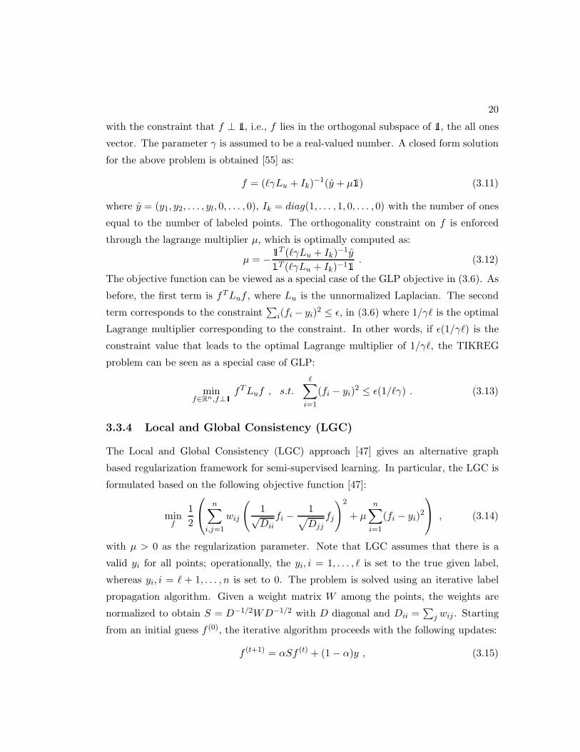
3.3.4 Local and Global Consistency (LGC)
The Local and Global Consistency (LGC) approach [47] gives an alternative graph
based regularization framework for semi-supervised learning. In particular, the LGC is
formulated based on the following objective function [47]:
minf
1
2
n∑
i,j=1
wij
(
1√Dii
fi −1
√
Djj
fj
)2
+ µ
n∑
i=1
(fi − yi)2
, (3.14)
with µ > 0 as the regularization parameter. Note that LGC assumes that there is a
valid yi for all points; operationally, the yi, i = 1, . . . , ℓ is set to the true given label,
whereas yi, i = ℓ + 1, . . . , n is set to 0. The problem is solved using an iterative label
propagation algorithm. Given a weight matrix W among the points, the weights are
normalized to obtain S = D−1/2WD−1/2 with D diagonal and Dii =∑
j wij . Starting
from an initial guess f (0), the iterative algorithm proceeds with the following updates:
f (t+1) = αSf (t) + (1− α)y , (3.15)

21
where α ∈ (0, 1). As shown in [47], this update equation converges to f∗ = (1 −α)(I − αS)−1y, which can be shown to optimize the objective function in (3.14) when
α = 1/(1 + µ). We now show that the LGC formulation is a special case of the GLP
formulation in (3.6). From the identity involving the normalized Laplacian in (3.5),
then the LGC can be seen as a special case of GLP as follows:
minf
fTLsf , s.t.
n∑
i=1
(fi − yi)2 ≤ ǫ(µ) , (3.16)
where ǫ(µ) is the constant corresponding to the optimal Lagrange multiplier µ. Note
that since in LGC, one starts with an initial label yi, i = 1, . . . , n, the constraint involves
terms corresponding to all the points.
3.3.5 Related Methods
We review three other methods, viz cluster kernels, Gaussian random walks, and local
neighborhood propagation for graph-based semi-supervised learning which are closely
related to the GLP framework.
Cluster Kernels (CK)
The main idea in cluster kernels [56] is to embed the data into a lower dimensional
space based on its cluster structure and then subsequently build a classifier on the
low-dimensional data. If K denotes a suitable kernel on the data space, the embedding
method focuses on the k primary eigenvectors of the symmetrized matrix D−1/2KD−1/2.
If K corresponds to the edge weights on the graph G = (V,E) between the points, i.e.,
K = W , then the embedding corresponds to the k eigenvectors of the symmetrized
Laplacian Ls = I −D−1/2WD−1/2 corresponding to the smallest k eigenvalues. In par-
ticular, for k = 1, the embedding is given by the eigenvector corresponding to the small-
est eigenvalue of Ls which is the solution to LGC in absence of any semi-supervision.
CK trains a suitable (linear) classifier on the low-dimensional embedding to obtain the
final predictions.

22
Gaussian Random Walks EM (GWEM)
Consider a random walk on the graph with transition probability P = D−1W . The
GWEM method [50] works with the m-step transition probability matrix Pm so that
the probability of going from xi to xj is given by pm|0(xj |xi) = (Pm)ij . The random walk
is assumed to start with uniform probability from any one of the nodes, so P (xi) = 1/n.
Using Bayes rule, one can obtain the posterior probabilities P0|m(xi|xj). Now, each
point is assumed to have a (possibly unknown) distribution p(y|xi) over the class labels.For any point xj, the posterior probability of class label y is given by P (yj = c|xj) =∑
i P (yi = c|xi)p0|mp(xi|xj). The prediction is based on yj = argmaxc P (yj = c|xj).Now, since P (y|xi) is unknown for the unlabeled points, an EM algorithm can be used
to alternately maximize the log-posterior probability of known labels on the labeled
pointsℓ∑
k=1
log P (yk|xk) =ℓ∑
k=1
logN∑
i=1
P (yi|xi)P0|m(xi|xk).
The EM algorithm alternates between the E step which estimates
P (xi|xk, yk) ∝ P (yk|xi)P0|m(xi|xk) (3.17)
where k denotes an index over labeled points, and the M step, which computes
P (y = c|xi) =∑ℓ
k:yk=c P (xi|xk, yk)∑ℓ
h=1 P (xi|xh, yh).
We now show that GWEM can be interpreted in terms of spectral decomposition
of a suitable asymmetrically normalized Laplacian Lr as in (3.3). For a fixed number
of steps m for the random walk, let ZT = Pm = (D−1W )m. Note that ZT itself is a
transition probability matrix, and Zij = Pm|0(xi|xj). Let DZ be a diagonal matrix such
that DZ,ii =∑
j Zij . Since the prior probability P (xi) = 1/n, by Bayes rule we have
P0|m(xj|xi) =Pm|0(xi|xj)∑
i′ Pm|0(xi′ |j)= (D−1
Z Z)ij.
Let fj = P (yj |xj). When the EM algorithm converges we will have:
f = D−1Z Zf ⇒ (I −D−1
Z Z)f = 0
23
, where fi = yi for the labeled points. Since D−1Z Z is a transition probability matrix,
from (3.3) we note that (I − D−1Z) can be viewed as a asymmetrically normalized
Laplacian Lr so that Lrf = 0. Finally, since DZf = Zf resembles the fixed point
equation for GFs, a block decomposition as in (3.8) yields fu = (Dz,uu − Zuu)−1Zuℓyℓ.
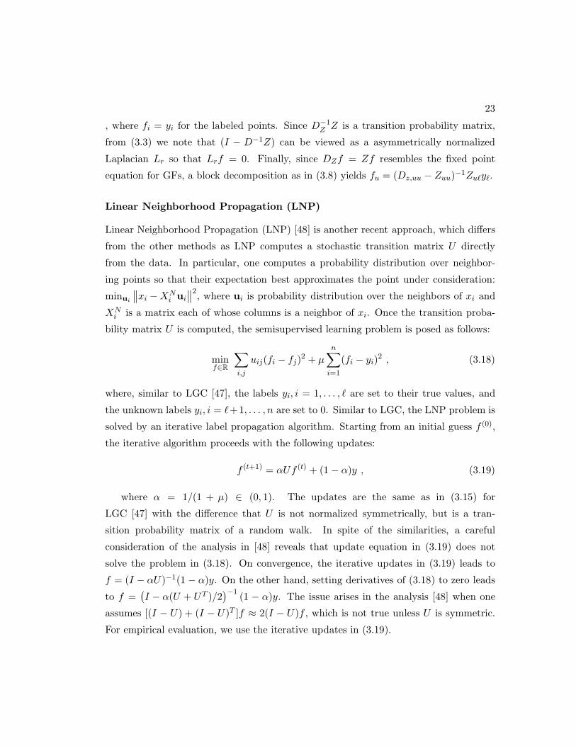
Linear Neighborhood Propagation (LNP)
Linear Neighborhood Propagation (LNP) [48] is another recent approach, which differs
from the other methods as LNP computes a stochastic transition matrix U directly
from the data. In particular, one computes a probability distribution over neighbor-
ing points so that their expectation best approximates the point under consideration:
minui
∥
∥xi −XNi ui
∥
∥
2, where ui is probability distribution over the neighbors of xi and
XNi is a matrix each of whose columns is a neighbor of xi. Once the transition proba-
bility matrix U is computed, the semisupervised learning problem is posed as follows:
minf∈R
∑
i,j
uij(fi − fj)2 + µ
n∑
i=1
(fi − yi)2 , (3.18)
where, similar to LGC [47], the labels yi, i = 1, . . . , ℓ are set to their true values, and
the unknown labels yi, i = ℓ+1, . . . , n are set to 0. Similar to LGC, the LNP problem is
solved by an iterative label propagation algorithm. Starting from an initial guess f (0),
the iterative algorithm proceeds with the following updates:
f (t+1) = αUf (t) + (1− α)y , (3.19)
where α = 1/(1 + µ) ∈ (0, 1). The updates are the same as in (3.15) for
LGC [47] with the difference that U is not normalized symmetrically, but is a tran-
sition probability matrix of a random walk. In spite of the similarities, a careful
consideration of the analysis in [48] reveals that update equation in (3.19) does not
solve the problem in (3.18). On convergence, the iterative updates in (3.19) leads to
f = (I − αU)−1(1 − α)y. On the other hand, setting derivatives of (3.18) to zero leads
to f =(
I − α(U + UT )/2)−1
(1 − α)y. The issue arises in the analysis [48] when one
assumes [(I − U) + (I − U)T ]f ≈ 2(I − U)f , which is not true unless U is symmetric.
For empirical evaluation, we use the iterative updates in (3.19).

24
3.3.6 Label Propagation and Green’s Function
We briefly describe an interesting relationship between label propagation and the dis-
crete Green’s function. Green’s functions are typically used to convert inhomogenous
partial differential equations with boundary conditions into an integral problem. In par-
ticular the inverse Laplace operator with the zero mode removed can be interpreted as
a Green’s function for the discrete Laplace operator [57]. Let G = L† be the generalized
inverse of the Laplacian L. The solutions for both GF and GWEM can be expressed
as: fu = (Duu −Wuu)−1Wulyl = L†
uzu where zu = Wulyl. Discarding the zero mode
of Lu, we have fu ≈ Guzu. As argued in [57], discarding the zero mode is important
to ensure that the Green’s function exists; further, it does not affect the final result.
Then fu can be viewed as a solution to a partial differential equation with boundary
value constraints. The interpretation is intuitive if the labeled points are treated as
electric charges. In particular one assumes labeled points to be postive and negative
charges. Using the Green’s function one then computes the influence of these charges
on unlabeled points [57]. For methods such as LGC and LNP the solution has the form
f = (I −A/(1 + µ))−1 µy/(1 + µ), with A = D−1/2WD−1/2 for LGC and A = U for
LNP. Considering the strong regularization limit as µ→ 0 and removing the zero mode
in L we obtain: f = L†y ≈ Gy.
3.4 Semi-Supervised Graph Cuts
We now demonstrate how label propagation formulations can be viewed as solving a
relaxed version of semi-supervised graph-cut problems. Let G = (V,E) be a weighted
undirected graph with weight matrix W . If V1, V2 is a partitioning of V , i.e., V1 ∩V2 = ∅, V1 ∪ V2 = V , then the value of the cut implied by the partitioning (V1, V2)
is given by: cut(V1, V2) = 12
∑
vi∈V1,vj∈V2wij. The minimum cut problem is to find a
partitioning (V1, V2) such that cut(V1, V2) is minimized. Due to practical reasons, one
often works with a normalized cut objective, such as the ratio-cut [58] or normalized-
cut [59], which encourage the partitions V1, V2 to be more balanced. The objective for
ratio-cut is Rcut(V1, V2) = cut(V1,V2)|V1|
+ cut(V2,V1)|V2|
. The objective for normalized-cut is
similar, however it normalizes cuts by the weight of the edges in each partition. Letting
V ol(V ) =∑
i∈V Dii, we have: Ncut(V1, V2) =cut(V1,V2)V ol(V1)
+ cut(V2,V1)V ol(V2)
.
25
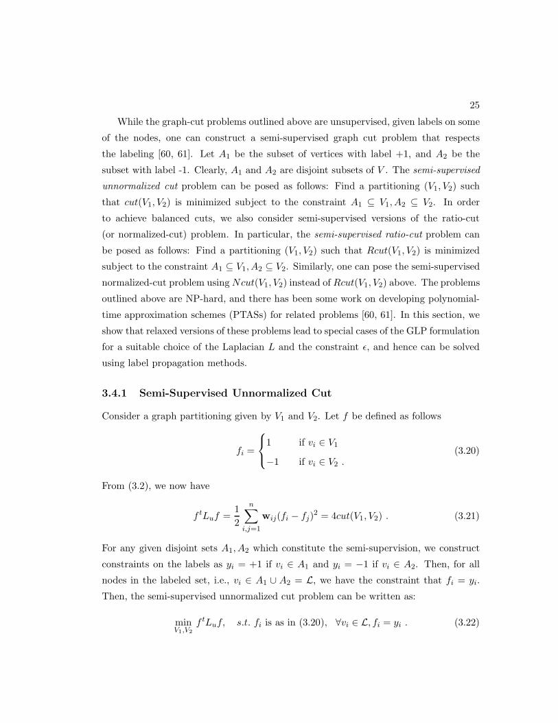
While the graph-cut problems outlined above are unsupervised, given labels on some
of the nodes, one can construct a semi-supervised graph cut problem that respects
the labeling [60, 61]. Let A1 be the subset of vertices with label +1, and A2 be the
subset with label -1. Clearly, A1 and A2 are disjoint subsets of V . The semi-supervised
unnormalized cut problem can be posed as follows: Find a partitioning (V1, V2) such
that cut(V1, V2) is minimized subject to the constraint A1 ⊆ V1, A2 ⊆ V2. In order
to achieve balanced cuts, we also consider semi-supervised versions of the ratio-cut
(or normalized-cut) problem. In particular, the semi-supervised ratio-cut problem can
be posed as follows: Find a partitioning (V1, V2) such that Rcut(V1, V2) is minimized
subject to the constraint A1 ⊆ V1, A2 ⊆ V2. Similarly, one can pose the semi-supervised
normalized-cut problem usingNcut(V1, V2) instead of Rcut(V1, V2) above. The problems
outlined above are NP-hard, and there has been some work on developing polynomial-
time approximation schemes (PTASs) for related problems [60, 61]. In this section, we
show that relaxed versions of these problems lead to special cases of the GLP formulation
for a suitable choice of the Laplacian L and the constraint ǫ, and hence can be solved
using label propagation methods.
3.4.1 Semi-Supervised Unnormalized Cut
Consider a graph partitioning given by V1 and V2. Let f be defined as follows
fi =
1 if vi ∈ V1
−1 if vi ∈ V2 .(3.20)
From (3.2), we now have
f tLuf =1
2
n∑
i,j=1
wij(fi − fj)2 = 4cut(V1, V2) . (3.21)
For any given disjoint sets A1, A2 which constitute the semi-supervision, we construct
constraints on the labels as yi = +1 if vi ∈ A1 and yi = −1 if vi ∈ A2. Then, for all
nodes in the labeled set, i.e., vi ∈ A1 ∪ A2 = L, we have the constraint that fi = yi.
Then, the semi-supervised unnormalized cut problem can be written as:
minV1,V2
f tLuf, s.t. fi is as in (3.20), ∀vi ∈ L, fi = yi . (3.22)

26
By relaxing the problem such that f ∈ Rn and noting that the constraint above is
equivalent to∑ℓ
i=1(fi − yi)2 ≤ 0, we obtain the following formulation:
minf∈Rn
f tLuf, s.t.
ℓ∑
i=1
(fi − yi)2 ≤ 0 (3.23)
Clearly, the objective function is a special case of our GLP formulation using an unnor-
malized graph Laplacian and ǫ = 0. In particular, the above is exactly the same as the
formulation for Gaussian Fields [46] described in section (3.2).
3.4.2 Semi-Supervised Ratio Cut
In the context of the ratio cut problem, consider again a graph partitioning given by V1
and V2. Let f be defined as
fi =
+√
|V2|/|V1| if vi ∈ V1
−√
|V1|/|V2| if vi ∈ V2 .(3.24)
Now, following (3.2), we can express
fTLuf =1
2
∑
i,j
wij(fi − fj)2 = |V |Rcut(V1, V2) (3.25)
where |V | is a constant. From the predefined values of f we can see that fT1 = 0,
and ||f ||2 = n. The objective function for the semi-supervised ratio-cut problem can
therefore be expressed as:
minV1,V2
fTLuf, s.t. f ⊥ 1, ||f ||2 = n, f as in (3.24), ∀vi ∈ L, fi = yi . (3.26)
We relax the problem and perform the optimization over f ∈ Rn such that f ⊥ 1. Note
that in the unsupervised case, i.e., L = ∅, the empty set, the solution to the problem
is simply the second eigenvector of L corresponding to the second smallest eigenvalue.
Now, relaxing the constraint3 on ||f || and allowing fi to mildly deviate from yi on
vi ∈ L, we get the following problem:
minf∈Rn
fTLuf, s.t. f ⊥ 1 ,
ℓ∑
i=1
(fi − yi)2 ≤ ǫ , (3.27)
3 Since the final prediction depends on sign(fi), the norm constraint ||f ||2 = n does not have aneffect on the accuracy.

27
which is exactly the problem TIKREG solves [55]. The key difference between the
relaxed unnormalized formulation in (3.23) and the normalized formulation in (3.27) is
the constraint f ⊥ 1⇒∑
i fi = 1, which ensures f lies in the subspace of Rn orthogonal
to 1. The balancing constraint ensures the total score on positive predictions is the same
as that on the negative predictions.
3.4.3 Semi-Supervised Normalized Cut
In the context of normalized cut, for a graph partitioning given by V1 and V2, let f be
defined as follows
fi =
√
vol(V2)/vol(V1) if vi ∈ V1
−√
vol(V1)/vol(V2) if vi ∈ V2 .(3.28)
Following an analysis similar to that of ratio cut, a semi-supervised normalized cut can
be posed as the following optimization problem:
minV1,V2
f tLuf, s.t. Df ⊥ 1, fTDf = vol(V ) , f as in (3.28),∀vi ∈ L, fi = yi . (3.29)
First, we relax the problem and perform the optimization over f ∈ Rn such that f ⊥ 1.
With g = D1/2f , the relaxed problem is
ming∈Rn
gTD−1/2LuD−1/2g s.t. g ⊥ D1/21, ||g||2 = vol(V ), ∀vi ∈ L, gi = D1/2yi. (3.30)
Note that if L = ∅, then the solution to the problem is simply the second eigenvector
of the symmetrically normalized Laplacian Ls = D−1/2LuD−1/2 corresponding to the
second smallest eigenvalue. Now, relaxing the constraint on ||g|| and allowing gi to
mildly deviate from D1/2yi on vi ∈ L, we get the following problem:
ming∈Rn
gTLsg s.t. g ⊥ D1/21, ℓ∑
i=1
||gi −D1/2yi||2 ≤ ǫ . (3.31)
Algorithms for the above formulation have not been explored in the literature. The for-
mulation is nearest to that of CK, but not the same since CK is a heterogeneous method
which uses the normalized Laplacian for embedding, and then applies a classification
algorithm on the embedding. It is also similar to LGC [47], although the constraint in
LGC includes all points with yi = 0 for i = (ℓ+1), . . . , n and does not involve the D1/2
scaling on yi in the constraint.
28
There has been notable attempts in the literature to directly solve some of the
semi-supervised graph cut problems [60, 61]. Among such methods, the spectral graph
transducer (SGT) [62] solves a problem closely related to the semi-supervised ratio cut
problem, and reduces to TIKREG [55] under certain assumptions.
3.5 Semi-Supervised Embedding
In this section, we show how label propagation methods can be viewed as doing semi-
supervised embedding. The geometric perspective helps in identifying relationships
between existing embedding and label propagation methods, e.g., between Laplacian
Eigenmaps [28] and Gaussian Fields [46]. More generally, we derive a new family of label
propagation methods based on existing embedding methods, including Locally Linear
Embedding (LLE) [63], Local Tangent Space Alignment (LTSA) [16] and Laplacian
Eigenmaps (LE) [28]. While all such methods can be seen as a special case of the GLP
formulation, they differ in the details—in particular, in the choice of the postive semi-
definite matrix L and nature of constraints. Since our exposition is focussed on two
class classification, the embedding will always be on R, a one dimensional space.
3.5.1 Non-linear Manifold Embedding
Manifold embedding methods obtain a lower dimensional representation of a given
dataset such that some suitable neighborhood structures are preserved. In this section
we briefly review three popular embedding methods by formulating them in a similar
form and demonstrate that their semi-supervised generalizations solve a variant of the
GLP formulation.
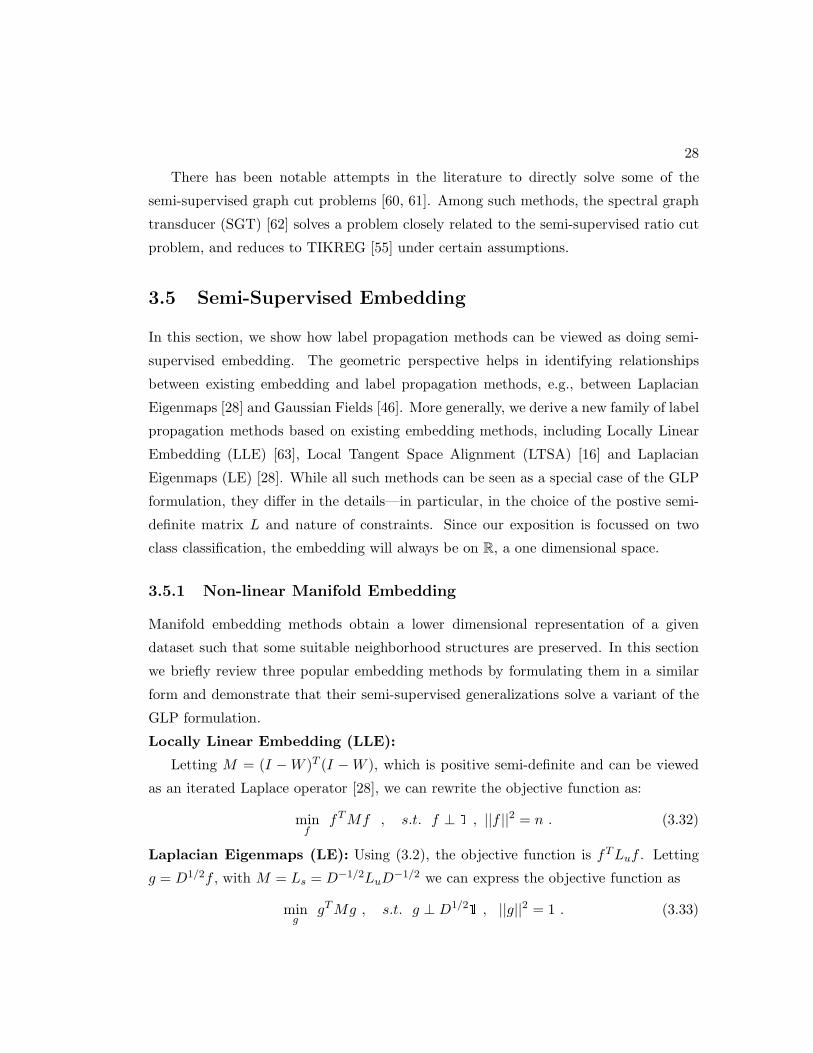
Locally Linear Embedding (LLE):
Letting M = (I −W )T (I −W ), which is positive semi-definite and can be viewed
as an iterated Laplace operator [28], we can rewrite the objective function as:
minf
fTMf , s.t. f ⊥ 1 , ||f ||2 = n . (3.32)
Laplacian Eigenmaps (LE): Using (3.2), the objective function is fTLuf . Letting
g = D1/2f , with M = Ls = D−1/2LuD−1/2 we can express the objective function as
ming
gTMg , s.t. g ⊥ D1/21 , ||g||2 = 1 . (3.33)

29
Local Tangent Space Alignment (LTSA): In LTSA we have:
minf
fTMf , s.t. f ⊥ 1 , ||f ||2 = n. (3.34)
3.5.2 Semi-Supervised Embedding
In this section, we consider two variants of semi-supervised embedding and its applica-
tions to label propagation. The variants differ in whether they consider the constraints
associated with the corresponding unsupervised embedding problem. As discussed in
Section 3.5.1, there are typically two types of constraints: f ⊥ A1, where A = I or
D1/2, and ||f ||2 = c, a constant. Since the prediction is based on sign(fi), the norm
constraint does not play any role in a classification setting, and will be ignored for our
analysis. The two variants we consider are based on whether f ⊥ A1 is enforced or not,
in addition to the constraints coming from the partially labeled data.
Unconstrained Semi-Supervised Embedding
Following [64], we want to obtain an embedding f = [fℓ fu]T , where the exact em-
beddings of the first ℓ points are known and given by yℓ.4 The objective for semi-
supervised embedding is given by
minf
fTMf , s.t fℓ = yℓ , (3.35)
where M is a suitable positive semi-definite matrix. Since fℓ is fixed, the problem can
be cast in terms of block matrices as:
minfu
[
fTℓ fT
u
]
[
Mℓℓ Mℓu
Muℓ Muu
][
fℓ
fu
]
, (3.36)
Setting the first derivative to zero one obtains:
fu = −M−1uu Muℓyℓ . (3.37)
In the context of label propagation for a 2-class classification setting, we will have
yi = +1 or yi = −1 for i = 1, . . . , ℓ. In other words, the labeled points are being em-
bedded to its true class label, and the rest will be embedded while trying to maintain
4 While the constraints can be relaxed to consider∑ℓ
i=1(fi−yi)2 ≤ ǫ, we do not focus on the general
case here.

30
the neighborhood structure. For LLE, M = (I −W )T (I −W ) and we call the corre-
sponding label propagation algorithm LLELP. Similarly, for LTSA, M is as discussed
in Section 3.5.1, and the corresponding algorithm will be called LTSALP. For uncon-
strained LE from (2.4), M = Lu, and the corresponding algorithm will be called LELP.
For LELP, since M = Lu, the unnormalized Laplacian, from (3.37) we have
fu = −L−1uuLuℓyℓ = −(Duu −Wuu)
−1(Duℓ −Wuℓ)yℓ
= (Duℓ −Wuℓ)−1Wuℓyℓ ,
since Duℓ = 0 as D is a diagonal matrix. We note that the solution is exactly the same
as that for GF as in (3.8) implying the equivalence of GF and LELP.
Constrained Semi-Supervised Embedding
In this section, we consider embedding problems when the orthogonality constraint of
the form f ⊥ A1 is enforced. In particular, we consider the following problem
minf
fTMf , s.t.
ℓ∑
i
(fi − yi)2 ≤ ǫ , f ⊥ A1 , (3.38)
where A = I for LLE and LTSA, and A = D1/2 for LE. Let α and µ be the Lagrange
multipliers for the two constraints respectively. The first order necessary conditions
obtained from the Lagrangian corresponding to (3.38) yields
f = (M + αIk)−1(αy + µA1/2) (3.39)
Since 1TAT f = 0, a direct calculation gives the optimal Lagrange multiplier as
µ = −2α 1TAT (M + αIk)−1y1TAT (M + αIk)−1A1 . (3.40)
For LLE, M = (I −W )T (I −W ) and A = I, and we call the corresponding algorithm
LLELPC. For LTSA, M is as discussed in Section 3.5.1 and A = I, and we call the
corresponding algorithm LTSALPC. For LE as in (3.33), M = Lsym = I −D1/2WD1/2
and A = D1/2 and we call the corresponding algorithm LELPC.

31
3.6 Experiments
In this section we provide an empirical evaluation of label propagation methods discussed
in this chapter. To our knowledge, this is the most comprehensive empirical comparison
of the methods till date. Our experiments are divided into two parts: First we compare
seven methods on 14 benchmark data sets in terms of their accuracy; next, we take a
closer look at the performance of the new label propagation methods obtained from the
perspective of semi-supervised manifold embedding. For the first set of experiments, the
methods we consider include 6 standard methods: GF, LNP, CK, GWEM, TIKREG and
LGC, as discussed in Section 3.3. In addition, we include LTSALP, the novel approach
based on semi-supervised LTSA embedding. For the second set of experiments, the
methods we consider are the 6 embedding based methods introduced in Section 3.5.
Methodology: We conducted our experiments on 14 well known benchmark data
sets. They include the following 8 UCI data sets: Hepatitis, Cancer, Pima, Wine, Iris,
Glass, USPS (1-4 only), and Letter (E and F only). In addition we also ran experi-
ments on 6 text datasets, which are all subsets of the 20Newsgroup data set: Differ-
ent100, Similar100, Same100, Different1000 and Same1000 [65]. Each dataset contains
a subset of 3 newsgroups with varying degree of difficulty for classification. Different100
(1000) includes alt.atheism, rec.sport.baseball, and sci.space, which are easy to sepa-
rate; Same100 (1000) includes comp.graphics, comp.os.ms-windows, comp.windows.x,
which are difficult to separate; whereas Similar100 includes talk.politics.guns, talk. pol-
itics.mideast, talk.politics.misc, which are moderately difficult to separate. We also used
the well known Classic-3 benchmark data set containing 3893 documents, whereby 1033
are from medical journals, 1400 are aeronautical system papers and 1460 are information
retrieval papers. For each method and each data set we ran five-fold semi-supervised
cross validation. Specifically, the training points were chosen from four folds and the
test error was measured on the fifth fold. All points were used to construct the neigh-
borhood graph. Further, for each approach involving parameters, e.g., CK using SVMs
with RBF kernel, parameter values were selected by cross-validation.
32
3.6.1 Experimental Results
The performance of the 6 methods from the literature as well as the novel LTSALP in
shown in Figures 3.4, 3.5 and 3.6. All results reported are on the test set. To avoid
clutter, we display the results for the top five methods based on average test-set error
in Figures 3.1 and 3.2 . We make the following observations based on the results:
• There is no dominating method across all datasets. However, there is a set of
methods that seem to be fairly consistently among the top few, and the perfor-
mance of the top few methods is typically close. While across the top methods the
differences typically don’t appear significant, when compared to the worst meth-
ods the improvements do tend to be significant. For instance, if we examine the
results in Figure 4 for the USPS data set we can see that the performance for the
top methods is around 1.5 − 1.8%, while the performance for the worst methods
is between 3.0% and 7.6%. The improvements of the best methods are clearly
significant in comparison to the worst judging by the standard deviation in error.
• Our results also indicate that no given method is always among the best methods
for each data set. For any method we could find at least one data set where
its performance is among the worst. It appears that the assumptions made by
various approaches do not work well across all manifold structures encountered in
various data sets. From an embedding perspective this makes sense, since different
embedding approaches tend to capture slightly different aspects of a manifold.
• The new method LTSALP is among the top performing methods in most of the
UCI datasets. However, it performs poorly on the text datasets, possibly indicat-
ing that the idea of aligning the tangent spaces may have to be suitably modified
for sparse high-dimensional datasets.
• TIKREG is among the most consistent methods on the text datasets. However
its performance is not as consistent on the UCI data sets.
• In spite of an issue with its formulation, LNP is found to be quite competitive
across several UCI and text datasets. Its parameter insensitivity make it rather
easy to tune.

33
• When CK does well, it outperforms all the other methods. However, it does not
have a consistent performance, which probably can be addressed by more thorough
cross-validation over its parameter choices.
• GF seems to be a slow starter, not performing well for small number of labeled
points, but improving significantly as the number of labeled points increases. This
can particularly be seen on the text data sets. As more labeled points are consid-
ered GF becomes the best performing method on several text data sets. Generally
GF is among the consistently well-performing methods.
• GWEM does not demonstrate a consistent performance and seems quite sensitive
to the predefined number of steps in the random walk.
In summary, while several of the methods perform well on some datasets, the embedding-
based proposed method LTSALP seems to be either the best or among the best methods
for 6 out of 8 UCI data sets. Further, GF and TIKREG also stand out as quite consistent
in terms of their performance, GF on both the UCI and text datasets, and TIKREG
mostly on the text data sets.
3.6.2 Semi-Supervised Embedding Methods
We now compare the six label propagation methods based on semi-supervised mani-
fold embedding. In particular we examine both variants of Laplacian Eigenmaps based
Label Propagation (LELP, LELPC), Locally Linear Embedding based Label Propaga-
tion (LLELP, LLELPC), and Local Tangent Space Alignment based Label Propagation
(LTSALP, LTSALPC). Note that LTSALP has already been compared to the existing
methods in Figures 3.1, 3.2, 3.4, 3.5 and 3.6 to serve as a reference. We compare the
methods on the UCI datasets, and show representative plots in Figure 3.3.5 Based
on our experiments, we observe that LELP and LTSALP performed most consistently
well, while LLELP did well only on specific data sets such as Wine. The performance of
LLELP seems to be more sensitive to the geometry of a data set. The effect of the or-
thogonality constraint on these methods can be understood when comparing the restults
for Cancer and Hepatitis in Figure 3.3. While the performance is clearly affected by the
5 We report results on 2-class problems in Figure 3.3. Since Wine is a 3-class dataset, we constructeda 2-class subset Wine(2) for these experiments.

34
constraints, it does not necessarily result in improved performance. For example, the
constraints lead to better performance in Hepatitis but worse performance in Cancer.
For the embedding methods, the quality of semi-supervised label propagation seems
to depend on how well the unsupervised embedding preserves the class separation. Fig-
ure 3.8 illustrates the difference between unsupervised embedding and semi-supervised
embedding on Wine. Note that the unsupervised embedding obtained from LLE and
LTSA maintains the class separation better than LE for this particular dataset. When
semisupervision is added, the embedding obtained from all the methods changes suit-
ably. The class separation is most clear in LLELP followed by LTSALP and LELP, a
fact reflected in the test-set error rates in Figure 3.5 (right panel). In general, label
propagation based on a semi-supervised embedding method works well if the geometric
structure of the class labels is well aligned with the biases of the embedding method.
3.7 Conclusions
In this chapter, we have developed a unified perspective to a large set of graph-based
semi-supervised learning methods. Using our framework we have showed that semi-
supervised approaches to graph-cuts or manifold embeddings lead to the same com-
putational problem. We have provided a recipe for converting embedding methods to
label propagation algorithms. While the individual theoretical connections are known
among experts in the community, unlike existing literature, we uniformly present label
propagation from the perspective of graph cuts and embedding methods. In particu-
lar we provide interpretations of existing approaches both in terms of graph cuts and
semi-supervised embedding methods. Our extensive empirical evaluation reveals that
while there are no clear winners in terms of performance, certain methods seem con-
sistent across several datasets, including some of the new embedding based methods
introduced in this chapter. Our analysis improves our theoretical understanding of an
important class of methods in semi-supervised learning, introduces several new methods
to solve the problem, and, to our knowledge, provides the first comprehensive empirical
performance evaluation of this family of models. The competitive performance of the
embedding-based label propagation methods such as LTSALP provides strong incentive
to investigate the embedding-based family of methods further.

35
0 10 20 30 40 50 60 700.06
0.08
0.1
0.12
0.14
0.16
0.18
0.2
0.22
0.24
Number of Labeled Points
Err
or
Five Fold Cross Validation on the Cancer Data Set
ltsalpgflgclnp
(a) Cancer
0 20 40 60 80 100 1200.25
0.3
0.35
0.4
0.45
0.5
0.55
0.6
Number of Labeled Points
Err
or
Five Fold Cross Validation on the Pima Data Set
gfltsalpmwemlgc
(b) Pima
0 10 20 30 40 50 60 70
0.35
0.4
0.45
0.5
0.55
0.6
0.65
0.7
Number of Labeled Points
Err
or
Five Fold Cross Validation on the Glass Data Set
lnpgflgcmwem
(c) Glass
0 10 20 30 40 50 60 70
0.2
0.25
0.3
0.35
0.4
0.45
0.5
Number of Labeled Points
Err
orFive Fold Cross Validation on the Wine Data Set
ltsalplnptikreggf
(d) Wine
0 20 40 60 80 100 120−0.05
0
0.05
0.1
0.15
0.2
0.25
0.3
0.35
0.4
0.45
Number of Labeled Points
Err
or
Five Fold Cross Validation on the USPS Data Set
gfcktikregltsalp
(e) USPS
0 20 40 60 80 100 1200
0.05
0.1
0.15
0.2
0.25
0.3
0.35
Number of Labeled Points
Err
or
Five Fold Cross Validation on the Letter(EF) Data Set
gflnpltsalplgc
(f) Letter
Figure 3.1: Five-fold cross validation as increasingly many points are labeled.

36
0 10 20 30 40 50 60 700
0.1
0.2
0.3
0.4
0.5
0.6
0.7
Number of Labeled Points
Err
or
Five Fold Cross Validation on the Dif100 Data Set
cktikregmwemlgc
(a) Dif100
0 10 20 30 40 50 60 70
0.2
0.25
0.3
0.35
0.4
0.45
0.5
0.55
0.6
0.65
Number of Labeled Points
Err
or
Five Fold Cross Validation on the Sim100 Data Set
gftikreglnplgc
(b) Sim100
0 10 20 30 40 50 60 70
0.35
0.4
0.45
0.5
0.55
0.6
0.65
Number of Labeled Points
Err
or
Five Fold Cross Validation on the Sam100 Data Set
mwemlgctikreglnp
(c) Sam100
0 20 40 60 80 100 120
0.35
0.4
0.45
0.5
0.55
0.6
0.65
Number of Labeled Points
Err
orFive Fold Cross Validation on the Sam1000 Data Set
tikreglgclnpmwem
(d) Sam1000
0 20 40 60 80 100 1200
0.1
0.2
0.3
0.4
0.5
0.6
0.7
Number of Labeled Points
Err
or
Five Fold Cross Validation on the Dif1000 Data Set
tikreglnpgflgc
(e) Dif1000
0 20 40 60 80 100 120−0.2
−0.1
0
0.1
0.2
0.3
0.4
0.5
0.6
Number of Labeled Points
Err
or
Five Fold Cross Validation on the Classic3 Data Set
cktikregltsalpgf
(f) Classic3
Figure 3.2: Five-fold cross validation as increasingly many points are labeled.

37
10 15 20 25 30 35 40 45 500.05
0.1
0.15
0.2
0.25
0.3
0.35
0.4
0.45
0.5
Number of Labled Points
Err
or
5−fold cross validation on the Cancer data set
lelplelpcltsalpltsalpcllelpllelpc
(a) Cancer
10 15 20 25 30 35 40 45 500.18
0.2
0.22
0.24
0.26
0.28
0.3
0.32
0.34
0.36
0.38
Number of Labled Points
Err
or
5−fold cross validation on the Hepatitis data set
lelplelpcltsalpltsalpcllelpllelpc
(b) Hepatitis
10 15 20 25 30 35 40 45 500
0.1
0.2
0.3
0.4
0.5
0.6
0.7
Number of Labled Points
Err
or
5−fold cross validation on the Wine(12) data set
lelpclelpltsalpltsalpcllelpllelpc
(c) Wine(2)
Figure 3.3: Comparison of embedding based label propagation methods: LELP(C),LTSALP(C), LLELP(C).

38
gf mwem lnp lgc tikreg ck ltsalp
Hepatitis 21.1 ± 0.4 21.4 ± 0.7 25.8 ± 3.0 22.7 ± 1.2 20.8± 0.0 20.8 ± 0.0 24.3 ± 2.5
Cancer 11.2 ± 1.9 12.7 ± 2.5 10.6 ± 1.7 11.1 ± 2.5 10.8 ± 1.9 11.3 ± 1.3 10.3± 1.5
Wine 31.9 ± 1.7 32.2 ± 0.9 29.6 ± 3.5 32.4 ± 2.1 30.7 ± 2.2 30.1 ± 2.2 23.4± 3.0
Iris 5.5 ± 2.5 4.8± 4.1 6.0 ± 2.5 5.3 ± 3.8 5.7 ± 3.4 9.2 ± 1.0 5.3 ± 1.9
Glass 40.8 ± 4.0 41.4 ± 4.1 39.5± 4.2 41.2 ± 5.5 42.8 ± 5.5 49.6 ± 4.5 45.3 ± 4.9
Pima 31.6± 2.5 34.1 ± 3.3 36.0 ± 3.0 34.5 ± 2.5 33.2 ± 2.1 34.8 ± 0.2 32.1 ± 3.2
USPS 2.2 ± 0.4 13.0 ± 2.1 6.3 ± 0.9 4.9 ± 0.7 3.4 ± 1.4 1.5± 0.1 2.4 ± 0.4
Letter(EF) 8.3 ± 2.8 15.4 ± 2.8 8.5 ± 1.0 9.8 ± 2.7 8.3 ± 1.7 48.5 ± 0.5 7.8± 2.6
Dif100 7.3 ± 1.4 12.4 ± 1.3 13.6 ± 2.4 13.0 ± 1.2 11.5 ± 2.6 6.1± 0.6 12.7 ± 2.2
Sim100 27.0± 3.6 34.3 ± 5.3 32.7 ± 5.1 32.6 ± 2.5 32.5 ± 7.0 63.4 ± 2.1 41.0 ± 5.8
Sam100 48.8 ± 8.5 45.9 ± 4.5 47.9 ± 1.9 45.3± 3.6 47.0 ± 2.3 65.7 ± 2.0 51.7 ± 7.6
Dif1000 19.0 ± 13.6 23.3 ± 2.6 16.0 ± 1.9 19.7 ± 3.1 12.0± 1.5 65.8 ± 2.5 28.2 ± 14.6
Sam1000 54.9 ± 8.9 47.0 ± 3.4 47.7 ± 3.6 45.4± 4.0 46.0 ± 3.6 66.4 ± 1.4 61.0 ± 4.7
Classic3 9.3 ± 10.5 12.1 ± 1.7 29.2 ± 1.1 28.8 ± 0.7 5.7 ± 4.1 1.6± 0.1 14.7 ± 10.4
Figure 3.4: Performance comparisons with 30 labeled points on 14 datasets and 7 meth-ods.
gf mwem lnp lgc tikreg ck ltsalp
Hepatitis 21.4 ± 1.7 21.0 ± 1.0 23.8 ± 3.0 22.3 ± 1.8 20.9± 0.6 20.9 ± 0.6 25.4 ± 1.4
Cancer 10.1 ± 1.3 9.5 ± 0.9 9.3 ± 1.3 8.9 ± 1.0 10.6 ± 2.3 12.1 ± 2.3 8.8± 1.2
Wine 31.0 ± 1.6 31.4 ± 1.0 27.0 ± 3.0 31.2 ± 1.5 30.3 ± 2.4 30.1 ± 1.8 22.8± 2.4
Iris 2.5± 2.0 3.1 ± 0.5 6.4 ± 2.7 3.6 ± 1.9 4.0 ± 2.1 9.6 ± 1.4 4.4 ± 2.3
Glass 39.9 ± 1.9 38.7± 3.6 39.1 ± 4.0 40.1 ± 4.1 42.4 ± 2.1 44.4 ± 3.7 41.3 ± 3.8
Pima 31.3 ± 1.6 32.0 ± 2.7 35.0 ± 1.4 33.2 ± 2.5 33.7 ± 2.9 34.8 ± 0.2 31.1± 3.0
USPS 1.9 ± 0.3 9.0 ± 2.1 5.4 ± 1.5 4.0 ± 0.8 3.2 ± 1.8 1.5± 0.1 2.1 ± 0.7
Letter(EF) 8.0 ± 3.5 12.7 ± 2.6 7.7± 2.4 8.6 ± 2.1 7.9 ± 1.5 48.8 ± 0.6 7.8 ± 3.3
Dif100 6.8 ± 1.1 11.3 ± 1.6 13.5 ± 1.7 13.4 ± 1.8 11.4 ± 1.4 6.5± 0.3 11.8 ± 2.3
Sim100 24.5± 3.9 31.6 ± 4.5 29.8 ± 3.7 31.7 ± 3.2 25.8 ± 2.3 60.2 ± 3.0 37.8 ± 6.6
Sam100 41.6 ± 6.0 40.3± 6.3 43.7 ± 2.8 40.5 ± 4.5 44.0 ± 4.6 66.0 ± 2.9 44.3 ± 5.4
Dif1000 13.0 ± 10.2 20.8 ± 1.8 15.2 ± 1.4 17.5 ± 1.3 11.1± 3.2 65.7 ± 2.6 19.6 ± 8.1
Sam1000 48.7 ± 10.9 45.0 ± 3.0 44.6 ± 4.6 42.4± 4.0 42.5 ± 4.1 65.9 ± 1.0 55.4 ± 9.0
Classic3 3.2 ± 2.5 9.2 ± 0.5 28.5 ± 0.2 28.5 ± 0.3 4.1 ± 1.8 1.6± 0.1 4.7 ± 2.1
Figure 3.5: Performance comparisons with 40 labeled points on 14 datasets and 7 meth-ods.

39
gf mwem lnp lgc tikreg ck ltsalp
Hepatitis 22.1 ± 1.0 21.7± 1.2 25.0 ± 2.2 22.1 ± 1.6 21.7 ± 1.2 21.7 ± 1.2 24.8 ± 2.1
Cancer 9.0 ± 1.7 9.0 ± 0.7 9.4 ± 1.6 8.9 ± 0.7 11.3 ± 2.7 10.6 ± 1.8 8.4± 1.0
Wine 29.5 ± 2.4 29.1 ± 1.4 25.9 ± 5.8 30.2 ± 2.6 29.7 ± 3.3 28.0 ± 1.9 22.0± 2.4
Iris 3.2± 1.1 3.8 ± 0.4 6.6 ± 2.9 4.4 ± 1.1 4.2 ± 1.3 9.2 ± 2.3 3.2 ± 1.1
Glass 41.1 ± 1.9 40.4 ± 2.4 39.1± 1.8 39.9 ± 2.3 42.0 ± 2.8 42.9 ± 2.8 42.1 ± 4.4
Pima 31.1 ± 1.6 31.5 ± 2.2 35.3 ± 2.4 32.8 ± 1.9 33.7 ± 2.7 34.8 ± 0.3 30.7± 0.8
USPS 1.8 ± 0.2 7.6 ± 1.6 4.6 ± 1.2 3.6 ± 0.4 3.0 ± 1.4 1.5 ± 0.1 1.8 ± 0.4
Letter(EF) 7.4 ± 2.7 10.8 ± 3.3 6.5 ± 1.9 7.2 ± 1.8 6.2± 2.8 48.8 ± 0.6 7.7 ± 3.1
Dif100 6.9 ± 1.1 9.6 ± 1.6 10.7 ± 2.3 10.0 ± 1.2 7.5 ± 1.9 6.7 ± 1.0 10.2 ± 1.3
Sim100 21.4± 2.1 28.5 ± 3.1 27.3 ± 2.5 28.7 ± 1.3 22.4 ± 2.2 62.6 ± 3.0 30.6 ± 2.6
Sam100 35.6± 3.6 36.0 ± 4.2 40.0 ± 2.7 37.4 ± 3.9 41.1 ± 3.7 65.4 ± 2.0 39.6 ± 5.4
Dif1000 9.1± 7.7 18.9 ± 1.8 14.7 ± 1.2 16.2 ± 1.1 10.2 ± 2.8 63.5 ± 2.5 18.0 ± 6.6
Sam1000 43.0 ± 9.9 43.0 ± 2.1 42.2 ± 2.9 41.1 ± 3.1 39.4± 3.6 65.3 ± 1.4 55.6 ± 5.8
Classic3 2.2 ± 1.1 7.6 ± 1.5 28.5 ± 0.1 28.5 ± 0.4 3.4 ± 1.0 1.6 ± 0.1 3.4 ± 1.2
Figure 3.6: Performance comparisons with 50 labeled points on 14 datasets and 7 meth-ods. LTSALP performs well on UCI datasets, GF performs well on text datasets.

40
0 10 20 30 40 50 60 700.1
0.15
0.2
0.25
0.3
0.35
0.4
0.45
0.5
0.55
0.6
Number of Labeled Points
Err
or
Five Fold Cross Validation on the Wine Data Set
llelpltsalplelp
Figure 3.7: Embedding based LP methods on Wine corresponding to the Figure 3.8.

41
0
0.5
1
1.5
0
0.5
1
0
0.5
1
LELP, 30 labeled points WINE
(a) LELP
−1
0
1
2 −2
−1
0
1
2
−5
0
5
LLELP, 30 labeled points WINE
(b) LLELP
−0.5
0
0.5
1
1.5
−1−0.5
00.5
11.5
−5
0
5
LTSALP, 30 labeled points WINE
(c) LTSALP
−1
−1
−1
−1
−1−1
0
1
2
−2
−1
0
1
LE, WINE
(d) LE
−4
−2
0
2
4−4
−2
0
2
−1.05
−1
−0.95
LLE, WINE
(e) LLE
−0.2
0
0.2
0.4
0.6 −0.1
0
0.1
0.2
0.3
−0.5
0
0.5
LTSA, WINE
(f) LTSA
Figure 3.8: Unsupervised and unconstrained semi-supervised embedding on Wine. Theprediction performance (top) is better if the unsupervised embedding (bottom) keepsthe classes separate.
Chapter 4
Bayesian Multi-Variate
Regression
In this chapter we introduce a scalable algorithm for multi-label classification capable
of modeling the covariance across labels.
4.1 Introduction
Multi-label classification problems, where a data point can have multiple labels, are
becoming important in a variety of domains, such as protein function prediction in
computational biology, image annotation in computer vision, and text categorization
in document analysis [66, 67, 68]. For a problem with K possible labels, there are
M = (2K − 1) distinct categories, so a direct multi-class classification with M classes
would be computationally prohibitive, and may miss out on any covariance among the
labels. Until a few years ago, the convention was to train and apply binary one-vs-rest
classifiers to each label separately. However, even this approach ignores the possibility
of label covariance, which is typically present in real world domains.
In addition to accounting for label covariance, multi-label classification methods
should be scalable and capable of handling partially labeled data. Real-world data sets
tend to be ever-growing. Furthermore, labels are sometimes only partially observed.
While a data point can have any subset of K possible labels, in reality we often know
only some of the labels it has for sure, with no information whatsoever on certain
42

43
other labels. The problem of partial labels is unique to multi-label classification, and is
important in real world applications, such as in protein function prediction [66].
We propose Bayesian Multivariate Regression (BMR), a novel and highly scalable
algorithm for multi-label classification and missing label prediction. The proposed ap-
proach is a probabilistic model based on multi-variate regression. In BMR, every data
point is mapped to a Gaussian distribution, whereby each distribution shares the same
covariance matrix. The resulting distributions are eventually utilized in the generation
of the individual labels. As a result BMR is capable of modeling covariances among
labels while being very efficient and applicable to large data sets. The prediction in
BMR reduces to a mere matrix multiplication. We illustrate the performance of BMR
on a variety of benchmark data sets ranging from 593 to 10,000 in size. The multi-label
classification results indicate a competitive performance across all evaluation measures,
both in terms of prediction and execution time.
In large real-word data sets frequently only partially labeled data are available.
Typically two questions arise: (1) Can we predict the missing labels accurately? (2) Can
we utilize the structure from the partially labeled data to obtain an improved classifier
for future points? We extend the BMR model to handle missing labels. This is done by
utilizing the covariance structure captured by the BMR model. To evaluate performance
on predicting missing labels we compare it to Probabilist Matrix Factorization (PMF)
[69], a well-known state-of-the-art approach. Despite the simplicity of the BMR model,
the results indicate a superior performance. To address the second question we conduct
experiments in which we contrast performance in cases where partially labeled data
is used for training and cases where partially labeled data is discarded. The results
illustrate a significant improvement in performance when partially labeled data are
used.
The rest of the chapter is organized as follows: In Section 4.2, we give a brief
overview on related work. In Section 6.2, we propose our Bayesian Multivariate Regres-
sion approach and a variational inference algorithm to learn the model. We present the
experimental results in Section 4.4, and conclude in Section 4.5.

44
4.2 Related Work
Conventionally, multi-label classification problems are solved by decomposing them into
multiple independent binary classification problems, while ignoring relationships be-
tween labels. In recent years, several approaches have been proposed which attempt to
utilize the correlation structure among labels.
Kernel methods for multi-label classification tend to be extensions of the maximum
margin idea. In [70], a maximum margin approach is proposed which minimizes the
ranking loss. In [71], a method is proposed to learn a kernel which is shared across
labels, to be subsequently used in individual label classifiers. While the ability to handle
kernels is important in several domains, most existing approaches do not have a natural
way of dealing with missing labels and are not probabilistic, i.e., no direct uncertainty
quantification.
A number of probabilistic models have also been proposed for multi-label classifica-
tion. In [68], a mixture model is proposed for text classification. More recently, in [72],
a fully Bayesian model was proposed based on sparse and infinite canonical correlation
analysis. It directly models correlations among labels and is one of few models which
has the flexibility of dealing with missing labels. An extension of Gaussian Process
prediction to the multi-label setting was proposed in [73].
The state-of-the-art also includes two approaches based on the k-nearest neighbor
idea. In [42], label statistics from neighborhoods are used to build a Bayesian classifier.
In [74], features are constructed based on label information from neighborhoods and
subsequently used in logistic regression. In recent years, a family of methods based on
multi-label dimensionality reduction has emerged [75, 76]. Our proposed model also
falls in this category. Another interesting approach is presented in [77], where semi-
supervised multi-label classification is proposed using the Sylvester equation.
There are two major problems with most existing approaches. They have a tendency
not to explicitly model correlations among labels, but rather attempt to indirectly in-
corporate them. The second issue is that most existing approaches are too complex to
be applicable to large scale datasets. Unlike most existing methods, our approach is a
scalable probabilistic method which explicitly models the correlation structure among
labels.

45
4.3 Bayesian Multivariate Regression
In multi-label classification, every data object is associated with a subset of possible
labels. Assuming a total of c possible labels L = {ℓ1, . . . , ℓc}, for any given data object
x, the label information can be captured by a c-length bit vector h ∈ {0, 1}c, wherehs = 1 denotes the membership of x in class s.
4.3.1 The Model
We now introduce our novel approach which we call Bayesian Multivariate Regression
(BMR). Given a real valued feature vector x ∈ Rk we assume a mapping W ∈ R
c×k,
such that µ(x) = Wx. Subsequently we draw a latent label vector representation η
from N(µ(x),Σ), where Σ ∈ Rc×c denotes a covariance matrix among classes. While
the covariance Σ is global in our model, the mean µ(x) differs for every data point. Our
latent variable can alternatively be expressed as
η = Wx+ ε
where ε ∼ N(0,Σ). From this we can see that the empirical covariance of η will not be
solely determined by Σ, but rather jointly by the mean function µ(x) and Σ.
Each entry ηni ∈ R is treated as the natural parameter of a Bernoulli distribu-
tion determining if the data point xn has label ℓi. Thus, the label yni ∈ {0, 1}is generated from the Bernoulli distribution with mean parameterization: θi(ηn) =[
11+exp(ηni)
, exp(ηni)1+exp(ηni)
]
.
Since it does not consider the marginal distribution over x, BMR is a discriminative
model.
Let xn denote a k-dimensional data point, the generative process for each label
c-dimensional label vector yn can be specified as follows:
1. ηn ∼ N(Wxn,Σ).
2. yni ∼ Discrete(θi(ηn)), for i = 1 . . . c.
For convenience, we express the Bernoulli distribution p(yni|ηn) of the labels given
the natural parameterization in standard exponential family form as: p(yni|ηn) =

46
x
W
Σ
yN
η
Figure 4.1: Graphical model for Bayesian Multivariate Regression.
exp {yniηni − ln(1 + expηni)}. With C(ηn) =∑c
i=1 ln(1 + expηni), for yn we have:
p(yn|ηn) =c∏
i=1
p(yni|ηn) = exp{
yTnηn −C(ηn)
}
. (4.1)
The graphical model for BMR is shown in Figure 4.1. Given the model, the likelihood
function of yn is given by
p(yn|xn,Σ,W ) =
∫
ηn
p(ηn,yn|xn,Σ,W )dηn (4.2)
=
∫
ηn
p(ηn|Wxn,Σ)p(yn|ηn)dηn .
= Eηn[p(y|ηn)]
Therefore, for a dataset with N data points X = {xn, [n]N1 } ([n]N1 ≡ n = 1 . . . N) and
Y = {yn, [n]N1 }, the likelihood function is
p(Y |X,Σ,W ) =N∏
n=1
∫
ηn
p(ηn|Wxn,Σ)p(yn|ηn)dηn . (4.3)
=
N∏
n=1
Eηn[p(y|ηn)] .
4.3.2 Inference and learning
For given data points X and corresponding Y , the learning task of BMR involves finding
the model parameters W and Σ, such that the likelihood of p(Y |X,Σ,W ) as in Equation
(4.3) is maximized. A general approach for such a task is to use multivariate optimiza-
tion algorithms. However, the likelihood function in (4.3) is intractable, implying that
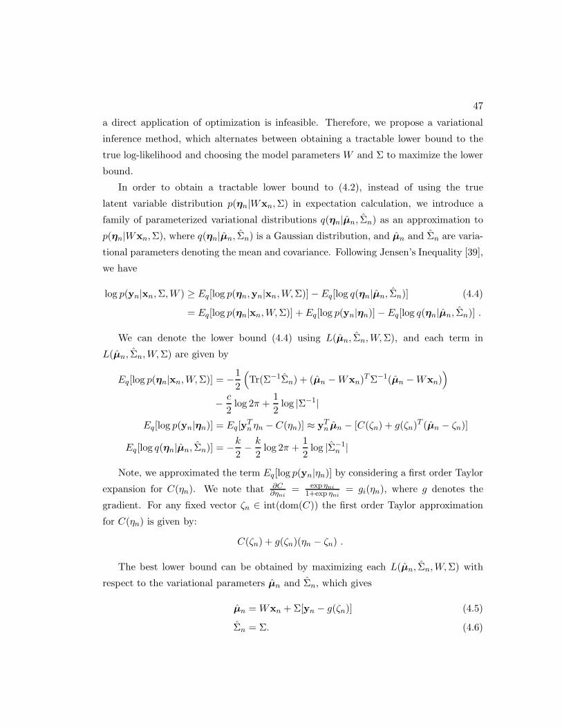
47
a direct application of optimization is infeasible. Therefore, we propose a variational
inference method, which alternates between obtaining a tractable lower bound to the
true log-likelihood and choosing the model parameters W and Σ to maximize the lower
bound.
In order to obtain a tractable lower bound to (4.2), instead of using the true
latent variable distribution p(ηn|Wxn,Σ) in expectation calculation, we introduce a
family of parameterized variational distributions q(ηn|µn, Σn) as an approximation to
p(ηn|Wxn,Σ), where q(ηn|µn, Σn) is a Gaussian distribution, and µn and Σn are varia-
tional parameters denoting the mean and covariance. Following Jensen’s Inequality [39],
we have
log p(yn|xn,Σ,W ) ≥ Eq[log p(ηn,yn|xn,W,Σ)]− Eq[log q(ηn|µn, Σn)] (4.4)
= Eq[log p(ηn|xn,W,Σ)] + Eq[log p(yn|ηn)]− Eq[log q(ηn|µn, Σn)] .
We can denote the lower bound (4.4) using L(µn, Σn,W,Σ), and each term in
L(µn, Σn,W,Σ) are given by
Eq[log p(ηn|xn,W,Σ)] = −1
2
(
Tr(Σ−1Σn) + (µn −Wxn)TΣ−1(µn −Wxn)
)
− c
2log 2π +
1
2log |Σ−1|
Eq[log p(yn|ηn)] = Eq[yTn ηn − C(ηn)] ≈ yT
n µn − [C(ζn) + g(ζn)T (µn − ζn)]
Eq[log q(ηn|µn, Σn)] = −k
2− k
2log 2π +
1
2log |Σ−1
n |
Note, we approximated the term Eq[log p(yn|ηn)] by considering a first order Taylor
expansion for C(ηn). We note that ∂C∂ηni
= exp ηni
1+exp ηni= gi(ηn), where g denotes the
gradient. For any fixed vector ζn ∈ int(dom(C)) the first order Taylor approximation
for C(ηn) is given by:
C(ζn) + g(ζn)(ηn − ζn) .
The best lower bound can be obtained by maximizing each L(µn, Σn,W,Σ) with
respect to the variational parameters µn and Σn, which gives
µn = Wxn +Σ[yn − g(ζn)] (4.5)
Σn = Σ. (4.6)

48
The lower bound of the log-likelihood on the whole dataset Y is given by sum-
ming the lower bound over the individual points∑N
n=1 L(µn, Σn,W,Σ). To obtain the
estimate for model parameters, we use this lower bound function as a surrogate objec-
tive to be maximized. Given a fixed value of (µ∗n, Σ
∗n) from (4.5) and (4.6), the lower
bound function∑N
n=1 L(µ∗n, Σ
∗n,W,Σ) is a function of model parameters (W,Σ). By
maximizing∑N
n=1 L(µ∗n, Σ
∗n,W,Σ) with respect to W and Σ, we have
W =
(
N∑
n=1
µnxTn
)(
N∑
n=1
xnxTn
)−1
(4.7)
Σ =1
N
N∑
n=1
(
Σn + (µn −Wxn)(µn −Wxn)T)
. (4.8)
4.3.3 Variational optimization
Following the update equations in (4.5)-(4.8), we construct a variational optimization al-
gorithm to learn the model. Starting from an initial guess of (W (0),Σ(0)), the algorithm
alternates between the following two steps in each iteration t:
1. Inference-step: Given (W (t−1),Σ(t−1)), for each (xn,yn), find the optimal varia-
tional parameters
(µ(t)n , Σ(t)
n ) = argmax(µn,Σn)
L(µn, Σn,W(t−1),Σ(t−1)) ,
which can be done using (4.5) and (4.6).
2. Optimization-step: Maximizing the aggregate lower bound gives us an improved
estimate of the model parameters:
(W (t),Σ(t)) = argmax(W,Σ)
N∑
n=1
L(µ(t)n , Σ(t)
n ,W,Σ) ,
which can be done following (4.7) and (4.8).

49
After t iterations, the objective function becomes L(µ(t)n , Σ
(t)n ,W (t),Σ(t)). In the (t+1)th
iteration, we have
N∑
n=1
L(µ(t)n , Σ(t)
n ,W (t),Σ(t)) ≤N∑
n=1
L(µ(t+1)n , Σ(t+1)
n ,W (t),Σ(t))
≤N∑
n=1
L(µ(t+1)n , Σ(t+1)
n ,W (t+1),Σ(t+1)) .
The first inequality holds because (µ(t+1)n , Σ
(t+1)n ) maximizes L(µn, Σn,W
(t),Σ(t)) in
the Inference-step. The second inequality holds because (W (t+1),Σ(t+1)) maximizes∑N
n=1 L(µ(t+1)n , Σ
(t+1)n ,W (t+1),Σ(t+1)) in the Optimization-step. Therefore, the objec-
tive function is non-decreasing until convergence.
We note that the computations involved per iteration during training are scalable.
Most operations involved are simple matrix multiplications or matrix-vector products.
There is a matrix inversion involving a d× d matrix in (4.7), but since the matrix only
depends on the feature vectors xn, the inverse can be computed offline, even before
starting the iterations. The algorithm does need to invert Σ in every iteration. Since Σ
is a c×c matrix where c is the number of classes, the inverse can be computed efficiently
even for hundreds of classes.
4.3.4 Learning With Missing Labels
In certain application domains, such as protein function prediction in computational
biology [66], one encounters multi-label classification problems where data points have
partial labels, i.e., instead of knowing y ∈ {0, 1}K , we know only some of the entries
in y, the others being missing. Most existing multi-label approaches were not designed
to handle labels with missing values [70, 42]. However information contained even in
partially observed label vectors is potentially valuable and it is important for a model to
be able to utilize it. Since BMR provides a generative model for labels and it captures
correlations among labels, it can naturally handle data sets with partial labels. The
training of our model when missing labels are present has to be adjusted slightly. From
a generative model perspective, the missing labels are assumed not to be generated by
the model. However, during training, the corresponding µ and all parameters which
depend on it still have to be estimated.

50
To allow learning when some labels are missing for a data point, we need to ad-
just the estimation of µ ∈ RK . We break down the component variables into entries
corresponding to known labels and unknown labels. In particular we let
µ =
[
µl
µu
]
, Σ−1 =
[
Σ−1ll Σ−1
lu
Σ−1ul Σ−1
uu
]
, W =
[
Wl
Wu
]
,
where l denotes set of known labels and u denotes a set of unknown labels. In a similar
fashion we break down all the other parameters: µ and y. For a data point with missing
labels, the problem of estimating µ can be posed as:
maxµl,µu
−1
2
([
µl
µu
]
−[
Wlxn
Wuxn
])T
Σ−1
([
µl
µu
]
−[
Wlxn
Wuxn
])
+yTl µl − g(ζl)
Tµl
}
.
The first order conditions yield the updates:
µl = Wlxn + (Σ−1ll )−1(Σ−1
lu (µu −Wuxn)
+ yl − g(ζl)) (4.9)
µu =(
Σ−1uu
)−1Σ−1ul (µl −Wlxn) +Wuxu . (4.10)
These updates are coupled, therefore we perform them iteratively. The computation of
all other variables/parameters remains the same (in terms of µ) when missing values
are present.
4.3.5 Prediction
Assuming that Σ and W have been estimated from training data, we wish to predict
the label vector h for an unseen data point x. First note that the maximum likelihood
estimate of η, given W and Σ is obtained by η∗ = W x, since η ∼ N(W x,Σ). With η
∗
interpreted as a vector of log odds we can obtain the maximum likelihood estimate for
y, by considering the sign of the individual entries of η∗:
η∗ = W x (4.11)
with
hi =
1 if η∗i > 0
0 otherwise .(4.12)

51
Effectively the prediction task in our model reduces to a matrix multiplication. For this
reason our model can be seen as rather simple, and unlike most existing approaches, it
can be easily used on millions of data points.
4.4 Empirical Evaluation
In this section we present our experimental results on both multi-label classification
and missing label prediction. Our empirical evaluation consists of four parts. We first
evaluate BMR on multi-label classification with fully labeled data. Subsequently we
contrast BMR to PMF on missing label prediction. We then examine to what extent
BMR can take advantage of partially labeled data, when making predictions on unseen
points. Lastly we evaluate the execution time for learning and making predictions.
4.4.1 Data Sets
We evaluated the BMR model using a number of data sets ranging in size from 593 to
10,000 data points. The number of labels in these data sets range from 6 to 374. The
main large data set that we have used, which also motivated the development of BMR
[11] stems from the Aviation Safety Reporting System (ASRS). It encompasses a subset
of 10,000 aviation safety reports assigned to 58 anomaly categories. The ASRS-10000
data set contains 200 features obtained from running Latent Dirichlet Allocation (LDA)
[39] on the original reports. Further data sets that we used include Mediamill-10000. A
subset of 10,000 data points from the Mediamill data set [78]. It includes 120 features
and 101 labels. Two smaller data sets that we used include Scene [79] and Emotions
[80]. In table 5.2 a summary is provided for all of the data sets used.
Data Set Data Points Features Labels
Scene 2407 294 6Emotions 593 72 6
ASRS-10000 10000 200 58Mediamill-10000 10000 120 101
Table 4.1: Data sets used for empirical evaluation.
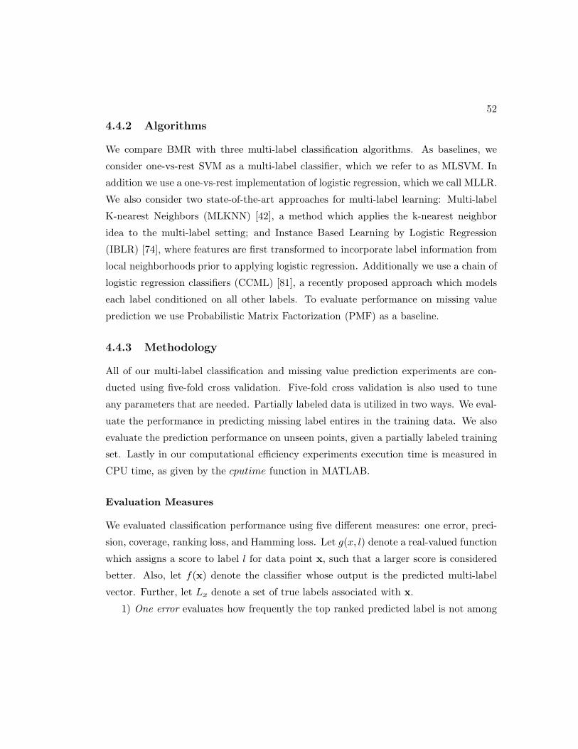
52
4.4.2 Algorithms
We compare BMR with three multi-label classification algorithms. As baselines, we
consider one-vs-rest SVM as a multi-label classifier, which we refer to as MLSVM. In
addition we use a one-vs-rest implementation of logistic regression, which we call MLLR.
We also consider two state-of-the-art approaches for multi-label learning: Multi-label
K-nearest Neighbors (MLKNN) [42], a method which applies the k-nearest neighbor
idea to the multi-label setting; and Instance Based Learning by Logistic Regression
(IBLR) [74], where features are first transformed to incorporate label information from
local neighborhoods prior to applying logistic regression. Additionally we use a chain of
logistic regression classifiers (CCML) [81], a recently proposed approach which models
each label conditioned on all other labels. To evaluate performance on missing value
prediction we use Probabilistic Matrix Factorization (PMF) as a baseline.
4.4.3 Methodology
All of our multi-label classification and missing value prediction experiments are con-
ducted using five-fold cross validation. Five-fold cross validation is also used to tune
any parameters that are needed. Partially labeled data is utilized in two ways. We eval-
uate the performance in predicting missing label entires in the training data. We also
evaluate the prediction performance on unseen points, given a partially labeled training
set. Lastly in our computational efficiency experiments execution time is measured in
CPU time, as given by the cputime function in MATLAB.
Evaluation Measures
We evaluated classification performance using five different measures: one error, preci-
sion, coverage, ranking loss, and Hamming loss. Let g(x, l) denote a real-valued function
which assigns a score to label l for data point x, such that a larger score is considered
better. Also, let f(x) denote the classifier whose output is the predicted multi-label
vector. Further, let Lx denote a set of true labels associated with x.
1) One error evaluates how frequently the top ranked predicted label is not among

53
the true labels. If 1[·] denotes the indicator function, we have:
OneError(g) =1
D
D∑
d=1
1 [argmaxl∈L g(xd, l) 6∈ Lxd] . (4.13)
2) For true labels l ∈ Lx, average precision evaluates the fraction of labels in Lx
that rank at least as high as l according to the scoring rule g on average. For any data
point x and any label l ∈ Lx, let R(x, l) = {l′ ∈ Lx|rankg(x, l′) ≤ rankg(x, l)}, wherethe ranking is among all possible labels. Then, average precision is:
AvePrec(g) =1
D
D∑
d=1
1
|Lxd|∑
l∈Lxd
|R(xd, l)|rankg(xd, l)
. (4.14)
3) Coverage reflects on average how far one needs to go down in the label ranking
to cover all actual labels of an instance:
Coverage(g) =1
D
D∑
d=1
(maxl∈Lxd
rankg(xd, l)− 1) . (4.15)
4) Hamming loss evaluates the fraction of label instance pairs that were misclassified:
HammingLoss(f) =1
D
D∑
d=1
1
c|f(xd)△Lxd
| . (4.16)
where △ denotes the symmetric difference between two sets.
5) Ranking loss reflects the average number of labels that are reversely ordered for a
given instance. Let T (xd) = {(l1, l2) | g(xd, l1) ≤ g(xd, l2), (l1, l2) ∈ Lxd× Lxd
}, whereLxd
denotes the complement of Lxd. Ranking loss is defined as:
RankLoss(g) =1
D
D∑
d=1
|T (xd)||Lxd||Lxd
| . (4.17)
For both Hamming loss and ranking loss, smaller values are better. In particular for
a perfect performance HammingLoss(h) = RankLoss(g) = 0.
The prediction of missing labels within training data is evaluated using Hamming
loss only.

54
4.4.4 Multi-Label Classification
Tables 4.2-4.5 list the prediction results when using five fold cross validation. MLSVM
and MLLR, the two one vs. rest approaches perform the worst, as expected. These
results clearly illustrate that looking at Hamming loss alone is actually quite misleading.
For instance MLSVM has a hamming loss of 11.9% for ASRS-10000, however its one
error is at 85.8%. Even for a degenerate classifier which predicts only zeros, one would
obtain a low hamming loss. For this reason we have opted to evaluate our results using a
range of five different evaluation measures, commonly used in multi-label classification.
Our proposed model performs either better or very competitively compared to all
other approaches, including MLKNN, IBLRML, and the two state-of-the-art methods
across all five evaluation measures. Across all evaluation measures our approach seems to
be followed by MLKNN and then IBLRML. Considering the simplicity of our approach,
these results are quite interesting. After all, the predictive step in our model merely
involves a matrix multiplication, and yet we are outperforming very complex algorithms
such as SVMs or even state-of-the-art multi-label learning methods such as MLKNN
and IBLRML. CCML appears to be more competitive on the larger data sets. However,
overall it does not seem to be standing out.
For the top four algorithms, BMR, MLKNN, CCML and IBLRML, we also examined
what happens when a smaller fraction of the data set is labeled. We omitted the one
vs. rest approaches to prevent clutter, and also since we already established that their
performance is substantially inferior. We ran 5-fold cross validation while gradually
increasing the set of labeled points. The results can be seen in Figures 5.3-4.5. The first
thing that we can note is that overall the performance of IBLRML appears to be worse
than that of MLKNN. CCML seems to perform either worse or as good as IBLRML.
Across all evaluation measures our proposed method, BMR, consistently performs either
competitively or better compared to all three algorithms. This seems to indicate that
our approach is robust, even when the size of the training set is reduced.
4.4.5 Partially Labeled Data
In our first set of experiments involving partially labeled data we evaluate the Hamming
loss in predicting missing labels. The results for the Emotions and Scene data sets are

55
given in Table 4.6. We compare the performance to Probabilistic Matrix Factorization
(PMF), as the percentage of missing values is varied between 10% and 30% of the label
entries. The results are obtained by using again five-fold cross validation. As we can see
across both benchmark data sets BMR outperforms the well-known PMF. Even though
BMR is a rather simplistic model, it performs quite well. While PMF only considers
the label matrix when making predictions, BMR considers both observed labels and
observed features.
The second set of experiments involving partially labeled data examines the predic-
tion performance on unseen points, given a training set with partially labeled data. On
both the Emotions and Scene data sets we set randomly 30% of the label entries to be
missing. We than evaluate the prediction performance on unseen data points. This is
done using five-fold cross validation and all five evaluation measures described earlier.
The performance of BMR is compared to BMR-D, CCML-D, MLKNN-D and IBLRML-
D. The suffix ”D” indicates that partially labeled data in the training set is discarded in
these versions of the algorithms. The point of this experiment is see whether BMR can
benefit from the additional structure provided by partially labeled data. The results
are given in Table 4.7. BMR clearly dominates. The results seem to suggest that BMR
can indeed take advantage of the structure learned from partially labeled data.
4.4.6 Scalability
To contrast the computational cost involved in utilizing MLKNN, IBLRML and BMR
we conducted an experiments in which we tested how long it takes to learn the respective
models and make predictions. We excluded CCML from these experiments due to its
poor performance in the previous evaluations. The number of data points both in the
training set and the test set was varied from 2000 points to 6000 points. The Mediamill
data set with 120 features and 101 labels was used for this purpose. The experiments
were conducted on a 8 core Dell PowerEdge machine, with cores clocked at 2.3 GHz and
32 GB of RAM. The execution time for learning the models can be seen in figure 4.6.
IBLRML clearly takes the longest time to be trained. This can be attributed to the fact
that it requires 101 Logistic Regression models to be learned. MLKNN on the other
hand only needs to be trained once. Overall we can see that BMR is the most efficient
out of the three when it comes to learning.

56
Figure 4.7 illustrates the execution time for making predictions. In this case MLKNN
performs the worst. Even when making predictions it has to compute the K-nearest
neighbors. IBLRML is somewhat better, even though it maintains 101 Logistic Re-
gression models, once they are trained making predictions can be done in a reasonable
time. BMR significantly outperforms both approaches. This can be attributed to the
fact that in BMR making predictions is reduced to a mere matrix multiplication. As a
result BMR can be easily applied to millions of records in less than a second, a property
which is very desirable in many real-world domains.
There appears to be a trade off between IBLRML and MLKNN. While one method
dominates the other for learning, for making predictions the picture is reversed. No such
trade off has to be made with BMR, which is consistently efficient both for learning and
making predictions.
Table 4.2: Five-fold cross validation on the ASRS-10000 data set. BMR clearly outper-forms all the other methods.
BMR CCML MLKNN IBLRML MLLR MLSVM
OneError 39.6± 0.8 47.6 ± 1.3 43.7± 0.8 44.3 ± 1.4 50.7± 1.6 85.8 ± 18.1AvePrec 63.4± 0.7 59.9 ± 0.9 60.1± 0.6 60.3 ± 0.6 57.0± 0.9 33.6 ± 8.2Coverage 7.77± 0.19 10.3 ± 0.5 9.18 ± 0.36 8.39± 0.29 9.63 ± 0.51 13.81 ± 0.87
HammingLoss 4.3± 0.0 4.8 ± 0.1 4.6± 0.1 4.7± 0.0 5.5± 0.1 11.9 ± 1.1RankLoss 5.5± 0.2 8.9 ± 0.8 6.9± 0.3 6.7± 0.3 7.9± 0.6 12.9 ± 1.7
Table 4.3: Five-fold cross validation on the Mediamill-10000 data set. BMR clearlyoutperforms all the other methods.
BMR CCML MLKNN IBLRML MLLR MLSVM
OneError 16.7± 0.6 25.3 ± 5.8 18.2 ± 1.0 28.7 ± 4.3 45.2 ± 2.1 76.7± 9.2AvePrec 67.8± 0.3 62.7 ± 1.4 67.7 ± 0.3 62.3 ± 2.6 58.4 ± 1.3 37.3± 1.9Coverage 17.2± 0.4 29.3 ± 1.8 17.4 ± 0.5 21.4 ± 2.4 22.1 ± 1.0 29.8± 1.3
HammingLoss 3.1± 0.0 3.4± 0.0 3.3 ± 0.0 4.5± 2.0 3.9± 0.0 4.8± 0.5RankLoss 4.8± 0.1 12.9 ± 1.2 5.0 ± 0.2 7.5± 2.5 8.6± 0.6 10.5± 1.0

57
Table 4.4: Five-fold cross validation on the Emotions data set. BMR clearly outperformsall the other methods.
BMR CCML MLKNN IBLRML MLLR MLSVM
OneError 26.7± 0.8 35.9 ± 7.3 38.9 ± 4.3 44.9 ± 5.8 32.2 ± 5.4 70.9± 7.3AvePrec 80.1± 1.4 75.6 ± 4.9 71.0 ± 1.4 67.3 ± 4.3 76.8 ± 2.3 55.0± 5.1Coverage 1.8± 0.1 2.0± 0.2 2.2 ± 0.1 2.4± 0.2 1.9± 0.1 2.8± 0.2
HammingLoss 20.4± 0.8 23.7 ± 3.5 25.8 ± 0.4 36.7 ± 2.4 23.1 ± 1.5 25.1± 2.4RankLoss 16.7± 1.3 20.6 ± 4.5 25.7 ± 1.7 30.0 ± 5.5 18.8 ± 1.7 39.2± 6.2
Table 4.5: Five-fold cross validation on the Scene data set. BMR clearly outperformsall the other methods.
BMR CCML MLKNN IBLRML MLLR MLSVM
OneError 27.1± 0.9 36.1 ± 2.0 23.2± 1.4 29.7 ± 3.0 35.6 ± 2.5 87.3± 6.1AvePrec 83.2± 0.7 75.2 ± 1.2 86.1± 0.6 81.7 ± 1.6 75.0 ± 2.2 48.6± 4.7Coverage 0.6± 0.0 1.0± 0.1 0.5± 0.0 0.7± 0.0 0.9± 0.1 1.6± 0.2
HammingLoss 11.2± 0.6 14.1 ± 0.6 9.0± 0.4 12.7 ± 1.3 14.3 ± 0.3 19.1± 1.9RankLoss 10.0± 0.7 23.9 ± 1.2 8.1± 0.3 11.5 ± 1.0 19.8 ± 2.3 30.6± 4.1
4.5 Conclusions
In this chapter we have proposed Baysian Multivariate Regression (BMR), a rather
simple but effective model for multi-label classification. Our proposed model addresses
three very important challenges when it comes to multi-label data. It models the covari-
ance structure among labels, thereby capturing more intricate dependencies. It is very
scalable, which makes the approach applicable to a wide variety of real-world problems
with ever-growing data sets. The scalability is possible since the learning step only
involves matrix multiplications and inverting small matrices and the prediction step
involves only a matrix multiplication. Lastly, BMR can naturally handle missing labels.
This is especially important for huge data sets where a full labeling is not always avail-
able. For instance when it comes to micro-array data or recommendation systems not
all values might be observed.
Our empirical evaluation shows that BMR is competitive with the state of the art
both in multi-label classification and missing label prediction. We have tested the
approach using a number of different data sets. BMR appears to be rather consistent in
its performance. The most significant improvements can be seen in cases where partially

58
Table 4.6: Error rates for recovering missing labels obtained using five-fold cross valida-tion on the Emotions and Scene data sets. Performance of BMR and PMF is evaluatedwhile an increasing percentage of labels are missing in the training data. Missing La-bels are randomly selected. The error rates reflect the percentage of missing labelsincorrectly recovered.
10% 15% 20% 25% 30%
EmotionsPMA 27.1 ± 5.1 27.1 ± 4.8 26.8 ± 3.0 27.9± 2.0 28.6 ± 1.9BMR 19.8± 4.6 21.1 ± 3.0 21.6± 4.1 24.2± 3.3 24.6± 2.1
ScenePMA 14.6 ± 5.6 13.8 ± 3.0 16.2 ± 3.4 18.5± 2.8 20.1 ± 3.0BMR 11.9± 4.4 13.8 ± 2.3 12.3± 2.4 13.2± 2.0 14.5± 1.6
labeled data is used in training the model. BMR appears to capable of taking advantage
of the additional structure provided by partially labeled training points.

59
Table 4.7: Five-fold cross validation on the Emotions and Scene data sets. BMR clearlyoutperforms all the other methods.
BMR BMR-D CCML-D MLKNN-D IBLRML-D
EmotionsOneError 29.3 ± 1.2 42.8 ± 5.7 49.1± 5.8 52.9 ± 8.6 59.1± 8.4AvePrec 77.9 ± 3.4 70.9 ± 3.3 47.3± 1.0 59.4 ± 4.9 58.5± 5.1Coverage 1.9± 0.2 2.2± 0.3 2.4 ± 0.2 2.9± 0.4 3.1 ± 0.3
HammingLoss 21.2 ± 3.9 28.3 ± 3.1 53.5± 1.0 31.6 ± 1.7 39.7± 4.4RankLoss 18.3 ± 3.5 23.7 ± 3.6 44.9± 5.2 39.1 ± 4.9 40.1± 7.4
SceneOneError 29.6 ± 4.2 37.8 ± 9.3 67.7± 3.2 43.1 ± 8.4 64.4± 9.5AvePrec 82.3 ± 4.3 76.2 ± 5.6 37.4± 1.6 74.9 ± 5.6 53.6± 7.8Coverage 0.6± 0.2 0.8± 0.2 1.4 ± 0.2 0.8± 0.2 1.9 ± 0.3
HammingLoss 12.8 ± 2.3 15.5 ± 3.0 51.7± 2.1 14.6 ± 1.5 28.9± 4.8RankLoss 10.1 ± 3.6 14.8 ± 3.5 48.1± 3.5 14.1 ± 5.2 41.8 ± 10.4

60
2800 3000 3200 3400 3600 3800 4000 42000.35
0.4
0.45
0.5
0.55
0.6
0.65
0.7
Number of Labeled Points
One
Err
orFive Fold Cross Validation on the ASRS−10000 Data Set
mlknniblrmlbmrccml
(a) One Error
2800 3000 3200 3400 3600 3800 4000 42000.48
0.5
0.52
0.54
0.56
0.58
0.6
0.62
0.64
0.66
Number of Labeled Points
Ave
rage
Pre
cisi
on
Five Fold Cross Validation on the ASRS−10000 Data Set
mlknn
iblrml
bmr
ccml
(b) Average Precision
2800 3000 3200 3400 3600 3800 4000 42008
9
10
11
12
13
14
15
16
17
Number of Labeled Points
Cov
erag
e
Five Fold Cross Validation on the ASRS−10000 Data Set
mlknniblrmlbmrccml
(c) Coverage
2800 3000 3200 3400 3600 3800 4000 42000.042
0.044
0.046
0.048
0.05
0.052
0.054
0.056
0.058
0.06
0.062
Number of Labeled Points
Ham
min
g Lo
ss
Five Fold Cross Validation on the ASRS−10000 Data Set
mlknniblrmlbmrccml
(d) Hamming Loss
2800 3000 3200 3400 3600 3800 4000 42000.04
0.06
0.08
0.1
0.12
0.14
0.16
0.18
0.2
Number of Labeled Points
Ran
king
Los
s
Five Fold Cross Validation on the ASRS−10000 Data Set
mlknniblrmlbmrccml
(e) Ranking Loss
Figure 4.2: Five fold cross validation on ASRS-10000 data set. To avoid clutter we onlyinclude the top three algorithms. These plots indicate what happens when a smallerfraction of the data set is labeled. Even in this setting BMR consistently outperformsboth MLKNN and IBLRML.

61
2800 3000 3200 3400 3600 3800 4000 4200
0.2
0.25
0.3
0.35
0.4
Number of Labeled Points
One
Err
or
Five Fold Cross Validation on the Mediamill−10000 Data Set
mlknniblrmlbmrccml
(a) One Error
2800 3000 3200 3400 3600 3800 4000 42000.54
0.56
0.58
0.6
0.62
0.64
0.66
0.68
Number of Labeled Points
Ave
rage
Pre
cisi
on
Five Fold Cross Validation on the Mediamill−10000 Data Set
mlknn
iblrml
bmr
ccml
(b) Average Precision
2800 3000 3200 3400 3600 3800 4000 420016
18
20
22
24
26
28
30
32
34
36
Number of Labeled Points
Cov
erag
e
Five Fold Cross Validation on the Mediamill−10000 Data Set
mlknniblrmlbmrccml
(c) Coverage
2800 3000 3200 3400 3600 3800 4000 42000.025
0.03
0.035
0.04
0.045
0.05
0.055
0.06
0.065
Number of Labeled Points
Ham
min
g Lo
ss
Five Fold Cross Validation on the Mediamill−10000 Data Set
mlknniblrmlbmrccml
(d) Hamming Loss
2800 3000 3200 3400 3600 3800 4000 42000.04
0.06
0.08
0.1
0.12
0.14
0.16
0.18
0.2
Number of Labeled Points
Ran
king
Los
s
Five Fold Cross Validation on the Mediamill−10000 Data Set
mlknniblrmlbmrccml
(e) Ranking Loss
Figure 4.3: Five fold cross validation on the Mediamill-10000 data set.

62
10 20 30 40 50 60 70 80 90 100 1100.2
0.3
0.4
0.5
0.6
0.7
0.8
0.9
1
Number of Labeled Points
One
Err
orFive Fold Cross Validation on the Emotions
Data Set
mlknniblrmlccmlbmr
(a) One Error
10 20 30 40 50 60 70 80 90 100 1100.45
0.5
0.55
0.6
0.65
0.7
0.75
0.8
Number of Labeled Points
Ave
rage
Pre
cisi
on
Five Fold Cross Validation on the Emotions Data Set
mlknn
iblrml
ccml
bmr
(b) Average Precision
10 20 30 40 50 60 70 80 90 100 1101.6
1.8
2
2.2
2.4
2.6
2.8
3
3.2
3.4
3.6
Number of Labeled Points
Cov
erag
e
Five Fold Cross Validation on the Emotions Data Set
mlknniblrmlccmlbmr
(c) Coverage
10 20 30 40 50 60 70 80 90 100 1100.2
0.25
0.3
0.35
0.4
0.45
0.5
0.55
0.6
0.65
Number of Labeled Points
Ham
min
g Lo
ss
Five Fold Cross Validation on the Emotions Data Set
mlknniblrmlccmlbmr
(d) Hamming Loss
10 20 30 40 50 60 70 80 90 100 1100.1
0.2
0.3
0.4
0.5
0.6
0.7
0.8
Number of Labeled Points
Ran
king
Los
s
Five Fold Cross Validation on the Emotions Data Set
mlknniblrmlccmlbmr
(e) Ranking Loss
Figure 4.4: Five fold cross validation on the Emotions data set.
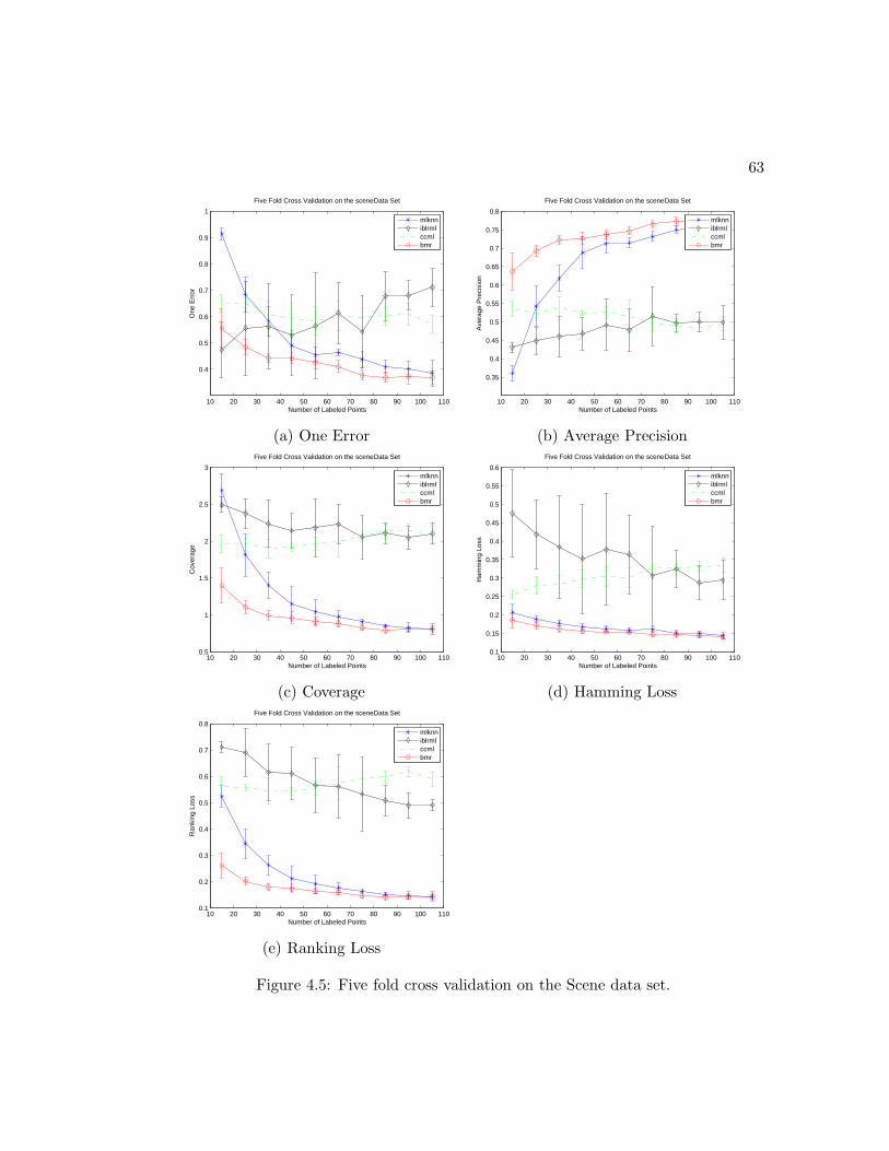
63
10 20 30 40 50 60 70 80 90 100 110
0.4
0.5
0.6
0.7
0.8
0.9
1
Number of Labeled Points
One
Err
orFive Fold Cross Validation on the scene
Data Set
mlknniblrmlccmlbmr
(a) One Error
10 20 30 40 50 60 70 80 90 100 110
0.35
0.4
0.45
0.5
0.55
0.6
0.65
0.7
0.75
0.8
Number of Labeled Points
Ave
rage
Pre
cisi
on
Five Fold Cross Validation on the scene Data Set
mlknniblrmlccmlbmr
(b) Average Precision
10 20 30 40 50 60 70 80 90 100 1100.5
1
1.5
2
2.5
3
Number of Labeled Points
Cov
erag
e
Five Fold Cross Validation on the scene Data Set
mlknniblrmlccmlbmr
(c) Coverage
10 20 30 40 50 60 70 80 90 100 1100.1
0.15
0.2
0.25
0.3
0.35
0.4
0.45
0.5
0.55
0.6
Number of Labeled Points
Ham
min
g Lo
ss
Five Fold Cross Validation on the scene Data Set
mlknniblrmlccmlbmr
(d) Hamming Loss
10 20 30 40 50 60 70 80 90 100 1100.1
0.2
0.3
0.4
0.5
0.6
0.7
0.8
Number of Labeled Points
Ran
king
Los
s
Five Fold Cross Validation on the scene Data Set
mlknniblrmlccmlbmr
(e) Ranking Loss
Figure 4.5: Five fold cross validation on the Scene data set.

64
2000 2500 3000 3500 4000 4500 5000 5500 60000
500
1000
1500
2000
2500
3000Execution Time for Training
Number of Points
Tim
e in
Sec
onds
iblrml
mlknn
bmr
Figure 4.6: Computational time to train the model as more and more data points areconsidered. BMR outperforms MLKNN and IBLRML.

65
2000 2500 3000 3500 4000 4500 5000 5500 60000
5
10
15
20
25
30
35
Number of Points
Tim
e in
Sec
onds
Execution Time to Make Predicitons
bmr
iblrml
mlknn
Figure 4.7: Computational time to make predictions as more and more data points areconsidered. BMR outperforms MLKNN and IBLRML.

Chapter 5
Probabilistic Matrix Addition
In the previous chapter we considered explicitly modeling covariances across one dimen-
sion. In this chapter we propose a model capable of modeling covariances across both
rows and columns of a matrix.
5.1 Introduction
We introduce a novel approach for modeling data matrices which can simultaneously
capture (nonlinear) covariance structures among rows as well as columns. For a n×m
matrix X, existing approaches which consider both covariance structures can be broadly
divided into two categories: Gaussian Process approaches, which suitably modify a
given kernel to incorporate relational information and subsequently draw outputs (rows)
i.i.d. from a single GP [82, 83, 84]; and Linear Models of Corregionalization (LMC) [8, 9],
a widely used family of models from Geostatistics, which effectively flattens out the data
matrix into a long vector, and uses suitable covariance structures over the vectorized
form. As a result, the entries, rows, or columns of the matrix are not independent
as covariances between all entries are modeled. However, the lack of (conditional)
independence can lead to serious scalability problems for inference in LMCs.
In this chapter, we introduce the Probabilistic Matrix Addition (PMA) model which
simultaneously considers two (nonlinear) kernels K1 and K2 corresponding to the rows
and the columns of the matrix respectively. The kernels are utilized in two Gaussian
Processes (GPs), from which we draw two latent matrices with independence along rows
66

67
and along columns respectively. The latent matrices from the two GPs are combined
in an additive fashion to obtain the final matrix, yielding a generative model for real-
valued data matrices of any size. As GPs define priors over functions f(x), PMA can
be viewed as a simple but non-trivial way to define priors over functions f(x, y) which
when instantiated lead to finite sized matrices.
Similar to LMCs, the joint distribution of PMA over the matrix entries does not
factorize over entries, rows, or columns, and thus can capture intricate dependencies
among the entries. Unlike LMC, PMA does not assume stationarity. It exhibits a
conditional independence structure over the latent variables, which allows for fast ap-
proximate inference algorithms. We present two methods for approximate inference in
PMA, respectively based on Gibbs sampling and MAP inference. The Gibbs sampler
is efficient since it takes full advantage of the conditional independence structure, and
precision matrices over the conditioning variables can be computed using a suitable
application of the Sherman-Morrison formula. The MAP inference is obtained by solv-
ing a Sylvester equation [85, 86], where both row and column covariances play a role
in determining a latent variable matrix. For parameter estimation and missing values
prediction, the inference methods are used in a suitable alternating update method.
We illustrate the effectiveness of PMA on two tasks: matrix missing value predic-
tion, where the goal is to infer multiple missing values in a given data matrix; and
multi-label classification, where the goal is to predict an entire new row given a matrix
which may also have missing values. For matrix missing value prediction, we compare
PMA to a single GP capturing covariances either across rows or columns, Probabilistic
Matrix Factorization (PMF) [69] and LMC [9]. PMA clearly outperforms a single GP,
and is competitive or better than PMF and LMC. For multi-label classification, we
compare PMA to three baselines including state-of-the art approaches designed specif-
ically for multi-label classification. Across all evaluation measures and datasets, PMA
consistently outperforms the other methods.
The rest of the chapter is organized as follows. In Section 6.2, we introduce PMA, dis-
cuss its properties, and contrast it with LMCs. We consider the missing value prediction
problem in Section 5.3, propose two inference approaches for PMA, and present empir-
ical evaluation of the ideas. In Section 5.4, we discuss how new rows (or columns) can
be predicted using PMA, and present empirical evaluation on the multi-label prediction
68
problem. We briefly discuss related work in Section 5.5 and conclude in Section 6.6.
5.2 The Model
The Probabilistic Matrix Addition (PMA) model defines distributions over real valued
matrices. Let X be a n×m matrix. We start by outlining a generative model for any
such matrix for arbitrary n and m. Consider two Gaussian processes G1 ≡ GP (0,K1)
with covariance function K1 corresponding to rows and G2 ≡ GP (0,K2) with covariance
function K2 corresponding to columns. For n rows, we get the following distribution
over any column f ∈ Rn from G1:
p(f |G1) =1
(2π)D/2|K1|1/2exp
(
−1
2fTK−1
1 f
)
. (5.1)
Since the matrix will have m columns, we sample f1, . . . , fm ∈ Rn independently fol-
lowing the above distribution. The samples form the following n×m matrix F :
F =[
f1 · · · fm
]
=
f1(1) · · · fm(1)...
. . ....
f1(n) · · · fm(n)
. (5.2)
For m columns, we get the following distribution over any row g ∈ Rm from G2:
p(g|G2) =1
(2π)D/2|K2|1/2exp
(
−1
2gTK−1
2 g
)
. (5.3)
Since the matrix will have n rows, we sample g1, . . . , gn ∈ Rm independently following
the above distribution. The samples form the following n×m matrix G:
G =
gT1...
gTn
=
g1(1) · · · g1(m)...
. . ....
gn(1) · · · gn(m)
. (5.4)
Given the two random matrices F and G, we generate the n×m random matrix X
as
X = F +G . (5.5)
In particular, each entry of X is (Figure 5.1)
xij = fj(i) + gi(j) . (5.6)

69
While the generative process for X is simple, it leads to intricate dependencies between
its entries, in particular capturing (nonlinear) covariance structures along rows as well
as columns.
m
n
X
K
K
1
2g
f
Figure 5.1: Graphical model for PMA: X is generated as the sum of F , sampled bycolumn, and G, and sampled by row.
5.2.1 Joint and Conditional Distributions
Joint Distribution: First, we consider the joint distribution of the components of the
entire matrix X = [xij] ∈ Rm×n. Since fj(i) ∼ N(0,K1,(i,i)) and gi(j) ∼ N(0,K2,(j,j)),
the marginal distribution of xij is a univariate Gaussian: xij ∼ N(0,K1,(i,i) + K2,(j,j)).
To compute the joint covariance, first note that
E[fj(i)fj(ℓ)] = K1(i, ℓ), E[fj(i)fk(ℓ)] = 0 . (5.7)
Similarly,
E[gi(j)gi(k)] = K2(j, k), E[gi(j)gℓ(k)] = 0 . (5.8)
Since E[xij ] = 0, we have Cov(xij , xℓk) = E[xijxℓk]. From (??), for the diagonal
elements we know
E[xijxij ] = K1(i, i) +K2(j, j) .

70
For the off-diagonal entries we have
E[xijxik] = E[(fj(i) + gi(j))(fk(i) + gi(k))]
= E[fj(i)fk(i)] + E[fj(i)gi(k)]
+ E[gi(j)fk(i)] + E[gi(j)gi(k)]
= 0 + 0 + 0 +K2(j, k)
= K2(j, k) .
(5.9)
Similarly,
E[xijxℓj] = K1(i, ℓ) . (5.10)
Further, note that
E[xijxℓk] = E[(fj(i) + gi(j))(fk(ℓ) + gℓ(k))]
= E[fj(i)fk(ℓ)] + E[fj(i)gℓ(k)]
+ E[gi(j)fk(ℓ)] + E[gi(j)gℓ(k)]
= 0 + 0 + 0 + 0
= 0 .
(5.11)
As a result, E[x2ij ] = K1(i, i) +K2(j, j), E[xijxik] = K2(j, k), E[xijxℓj] = K1(i, ℓ),
and E[xijxℓk] = 0. Putting everything together, if vec(X)T = [XT(:,1), . . . ,X
T(:,m)] denotes
the vectorized version ofX, then the joint distribution of vec(X) ∈ Rmn is a multivariate
Gaussian, i.e., vec(X) ∼ N(0,Σvec(X)) where
Σvec(X) = (Im ⊗K1) + (K2 ⊗ In) = K1 ⊕K2. (5.12)
where ⊕ denotes the Kronecker sum [87].
Conditional Distributions: We now consider the conditional distribution of each
fij, gij , and xij given the rest of the latent matrices, i.e., F(−i,−j) and G(−i,−j). Given
F(−i,−j), fj(i) only depends on fj(−i), the other elements of fj. Further, fj(i) is con-
ditionally independent of G(−i,−j) given F(−i,−j). To see this, note that in the PMA
graphical model there are two types of paths connecting fj(i) to elements in G(−i,−j):
paths going through the collider xij and paths going through elements in fj(−i). The
conditional d-separation between fj(i) and G(−i,−j) given F(−i,−j) stems from the fact

71
that there is no conditioning on the collider xij for paths of the first type and condition-
ing on the non-colliders (elements of fj(−i)) for paths of the second type. By a similar
argument, gi(j) depends only on gi(−j), the other elements of gi, and is conditionally
independent of F(−i,−j) given G(−i,−j). As a result, we have
fj(i)|(F(−i,−j), G(−i,−j)) ∼ N(mfj (i), s
fj (i)) ,
gi(j)|(F(−i,−j), G(−i,−j)) ∼ N(mgi (j), s
gi (j)) ,
(5.13)
where
mfj (i) = K1,(i,−i)K−1
1,(−i,−i)fj(−i) ,
sfj (i) = K1,(i,i) −K1,(i,−i)K−11,(−i,−i)K1,(−i,i) ,
mgi (j) = K2,(j,−j)K−1
2,(−j,−j)gi(−j) ,
sgi (j) = K2,(j,j) −K2,(j,−j)K−12,(−j,−j)K2,(−j,j) .
(5.14)
Since xij = fj(i) + gi(j), we have
xij|(F(−i,−j), G(−i,−j)) ∼ N(mij , sij) , (5.15)
where
mij = mfj (i) +mg
i (j) ,sij = sfj (i) + sgi (j) . (5.16)
5.2.2 Relationship with LMCs
Linear Models of Corregionalization (LMCs) are a broad family of related models widely
studied in Geostatistics [8, 9]. We compare and contrast the proposed PMA with LMCs.
The proposed PMA is related to LMCs as is evident from the structure of the joint co-
variance matrices. However, there are important differences between the two models,
including modeling assumptions as well as efficiency of inference algorithms. We briefly
discuss these aspects below. First, LMCs are stationary models where the covariance
depends on (s−s′), whereas PMA does not make such an assumption. Further, generally
LMCs do not have an explicit latent variable based generative model in their specifica-
tion. In particular, the statistical dependency structure of the elements of X tends to be
complete. As a result, inference in LMCs typically involve one or both of the following

72
possible issues: (i) Inverting large covariance matrices, say R(mn−p)×(mn−p) matrices for
p missing entries, which is computationally prohibitive, (ii) Assuming a parametric form
of the variogram which greatly restricts modeling flexibility [9]. In contrast, PMA has
a latent variable based model specification and the statistical dependency structure in
PMA is significantly sparse. The sparsity can be exploited to develop efficient approx-
imate inference algorithms (see Section 5.3). Since the joint distribution is Gaussian,
exact inference can be done in PMA but has the same computational issues as in LMCs.
5.3 Predicting Missing Values
For missing value prediction, we are given a partially observed data matrix X. The
goal is to infer the missing values based on the structure of the known observations. In
this section we outline two approaches for missing value prediction, respectively based
on Gibbs sampling and MAP inference. We conclude the section with an experimental
evaluation of PMA for missing value prediction.
5.3.1 Gibbs Sampling
Let X be a full matrix, where the missing values have been initialized to random values.
For a given (K1,K2), the sampler updates the latent matrices and the missing entries in
X. Since X = F +G, it is sufficient to sample only F or only G—we choose to sample
G. If K1 and/or K2 is unknown, we alternate between sampling (G,X) and estimating
K1 and/or K2.
Sampling G: Given K1,K2, and a full data matrix X, using Bayes rule we have
p(gi(j)|G(−i,−j), X,K1,K2) ∝p(gi(j)|G(−i,−j), X(−i,−j),K1,K2)p(xij |G, X(−i,−j),K1,K2)
= p(gi(j)|G(−i,−j),K2)p(xij − gi(j)|F(−i,−j),K1) ,
due to conditional independence and the fact that F(−i,−j) = X(−i,−j) −G(−i,−j). Note
that the individual distributions are univariate Gaussians as in (5.13) and (5.14). Since
the product of two Gaussians is also a Gaussian, we have
p(gi(j)|G−i,−j ,X,K1,K2) ∝ N(gi(j)|µij , σ2ij) (5.17)

73
where
µij =mg
i (j)sfj (i) +mf
j (i)sgi (j)
sfj (i) + sgi (j), σ2
ij =sfj (i)s
gi (j)
sfj (i) + sgi (j), (5.18)
with mg,mf , sg, sf are from (5.14) with F = X −G.
The sampler involves several matrix inverses, but these can be computed efficiently
from K−11 and K−1
2 . For computations involving F , instead of computing n inverses
of (n − 1) × (n − 1) sub-matrices of K1 (see (5.14)), we can obtain each such inverse
from rank-2 modifications to K1. Assuming that K−11 has been computed, consider the
problem of computing K−11,(−1,−1) = K−1
1,(2 : n,2: n). According to the Sherman-Morrison
formula, we have
(K1 + uvt)−1 = K−11 −
K−11 uvtK−1
1
1 + vtK−11 u
, (5.19)
where 1 + vtK−11 u 6= 0 and u, v ∈ R
n. We construct rank-2 updates to zero out entries
K1,(2 : n,1) and K1,(1,2: n). This can be accomplished in two steps, first we obtain A =
K1 + u1vT1 where u1(1) = 0, u1(2:n) = −K1(2:n,1), v1(1) = 1, v1(2:n) = 0. Then we obtain
B = A + u2vT2 where u(1) = 1, u(2:n) = 0, v(1) = 0, v(2:n) = −K1(1,2:n). Applying the
Sherman-Morrison formula twice we compute B−1 = (K1+u1vT1 +u2v
T2 )
−1. From basic
properties of block matrices it follows: K−11,(−1,−1) = K−1
1,(2 : n,2: n) = B−1(2:n,2:n). We follow
a similar computation for all the n submatrices K1,(−i,−i). Further, for computations
involving G, we can efficiently compute the m inverses of (m−1)× (m−1) sub-matrices
K2,(−j,−j) of K2.
Sampling X: Missing values inX are sampled by extending the sampler and treating
the missing xij as latent variables. In particular, we sample xij conditioned on X(−i,−j)
and one of F and G. Conditioning on F , we have
p(xij |X(−i,−j), F,K1,K2) = N(xij |xij , ζij) (5.20)
where
xij = fj(i) +K2,(i,−i)K−12,(−i,−i)(x−i,j − fj(−i)) ,
ζij = K2,(i,i) −K2,(i,−i)K−12,(−i,−i)K2,(−i,i) . (5.21)
74
Parameter Estimation: IfK1 andK2 are unknown, we initialize K1 ≻ 0, K2 ≻ 0, and
alternate between sampling (G, X) and estimating (K1, K2). We have already outlined
how to sample G and X. Let F = X − G. Then, we have K1 = 1m
∑mi=1 fjf
Tj and
K2 =1n
∑ni=1 gig
Ti .
5.3.2 MAP Inference
As before, we start with a full matrix X , where the missing values have been filled at
random. For given gram matrices (K1,K2), we alternate between estimating F (or G)
and X.
Estimating F : Given X,K1, and K2 the joint log-likelihood over (X,F ) is:
log p(X, F |K1,K2) = log p(F |K1) +
n∑
i=1
log p(xi:|f:(i),K2) .
For a given X , the MAP F can be obtained by maximizing the joint log-likelihood, or
equivalently minimizingn∑
i=1
(xi − F T eni )TK−1
2 (xi − F T eni ) +m∑
j=1
emjTF TK−1
1 Femj ,
where eni ∈ Rn, emj ∈ R
m are vectors of all zeros with the ith and jth position set to one
respectively. A direct calculation shows that the solution has to satisfy the following
Sylvester equation
FK2 +K1F = K1X . (5.22)
A solution to the Sylvester equation exists if and only if no eigenvalue of K1 is equal to
the negative of an eigenvalue of K2 [85]. Since both K1 and K2 are positive definite, the
condition is satisfied, and the solution can be obtained by standard methods [85, 86].
Estimating X: We iteratively update the originally missing entries xij based on the
mode of the distribution p(xij|F, X(−i,−j),K1,K2), given by
xnewij = fj(i) +K2,(j,−j)K−12,(−j,−j)(x−i,j − fj(−i)) . (5.23)
Note that the expression is similar to (5.21), where we sample from the corresponding
distribution.
Parameter Estimation: We initialize K1 ≻ 0, K2 ≻ 0, and the missing values of X
randomly. Then, we alternate between updating (X, F ), and estimating K1, K2. We
have already discussed updates for (X, F ). Let G = X − F . Then K1 = 1m
∑mj=1 fjf
Tj
and K2 =1n
∑ni=1 gig
Ti .

75
5.3.3 Experimental Evaluation
We report results from two sets of experiments for missing value prediction. In the first
set, we compare PMA to Gaussian Process regression (GPR) on simulated datasets.
In the second set, we compare PMA to other algorithms, including GPR, Probabilistic
Matrix Factorization (PMF) [69], and intrinsic LMC (I-LMC) on benchmark datasets.
Datasets and Evaluation: For the first set, we use PMA to generate artificial
datasets, of size 50× 20 and 50× 50. Evaluation is done using mean square error of the
predicted values. For the second set, we use two multi-label classification datasets—
Emotions [80] and Scene [79]. In multi-label classification, for n points and m classes,
class memberships are represented as n×m binary matrix B. We consider a truncated
log-odds matrix X, with xij = c if bij = 1, and xij = −c if bij = 0. For the experiments,
certain entries xij are assumed to be missing. Evaluation is done using class membership
prediction accuracy based on sign(xij).
Methodology: All experiments were conducted using five-fold cross validation.
For the first set, both K1 and K2 are assumed to be unknown, and are estimated from
data. For the second set, K1 is instantiated using the RBF kernel function K1 based on
feature vectors of the data objects, and K2 is estimated from data.
Algorithms: For the first set, we compare PMA to GPR. GPR-D1 treats rows as
data points, while GPR-D2 treats columns as data points. We utilize one implementa-
tion of PMA based on MAP inferece (PMA-MAP) and one based on Gibbs sampling
(PMA-GIBBS). For the second set, we compare six different algorithms: GPR, PMA-
MAP, PMA-GIBBS, PMA-EXACT, PMF, I-LMC and BMR. PMA-EXACT performs
exact prediction by flattening out the matrix X into a vector, assuming a covariance
matrix of the form K1⊕K2. I-LMC corresponds to intrinsic LMC in the prediction step,
whereby we utilize a covariance matrix of the form K1 ⊗ K2. For both PMA-EXACT
and I-LMC we use a provided kernel K1 and K2 as obtained by Gibbs sampling. The
purpose of comparing the latter two algorithms is to see whether PMA suffers by as-
suming a sparser dependency structure. BMR is the Bayesian Multivariate Regression
approach proposed in the previous chapter.
Performance: The results for the first set involving simulated data is in Figure 5.3.
PMA performs better than both GPR-D1 and GPR-D2, suggesting that there is a clear
benefit in modeling both K1 and K2. While not all matrices will necessarily have relevant

76
correlation structure across both dimensions, when this is the case, PMA appears to do
better. PMA-GIBBS and PMA-MAP perform similarly, with PMA-GIBBS appearing
slightly better.
The results for the second set involving benchmark datasets is in Table 5.1. We
make the following observations: (i) PMA clearly outperforms a GPR, illustrating the
value in modeling correlations across both rows and columns; (ii) The differences in
performance between PMA-GIBBS, PMA-EXACT and I-LMC are negligible. The re-
sults indicate that PMA does not suffer by assuming a sparser dependency structure.
Further, PMA-GIBBS is fairly accurate when compared to PMA-EXACT, which can
be computationally prohibitive for large datasets; (iii) PMA-GIBBS appears to perform
slightly but consistently better than PMA-MAP; (iv) PMA is competitive compared to
PMF and BMR. On Emotions, PMF and BMR appear slightly better. On Scene, PMA
is significantly better, suggesting a clear advantage for certain datasets.
20 40 60 80 100 120 140 160 180 200
0.04
0.05
0.06
0.07
0.08
0.09
0.1
Number of Missing Entries
Normalized Root Mean Squared Error
Missing Value Regression on 50x20 matrix
pma-map
pma-gibbs
gpr−d2
gpr−d1
(a) 50x20 Matrix
20 40 60 80 100 120 140 160 180 2000.04
0.05
0.06
0.07
0.08
0.09
0.1
0.11
Number of Missing Entries
Normalized Root Mean Squared Error
Missing Value Regression on 50x50 matrix
pma-map
pma-gibbs
gpr−d2
gpr−d1
(b) 50x50 Matrix
Figure 5.2: Five fold cross validation on two artificially created data sets. PMA clearlybenefits from modeling both covariance structures. The GPR both across rows (GPR-D1) and columns (GPR-D2) is weaker. Gibbs sampling appears to do slightly bettercompared to MAP, when it comes to inference in PMA.
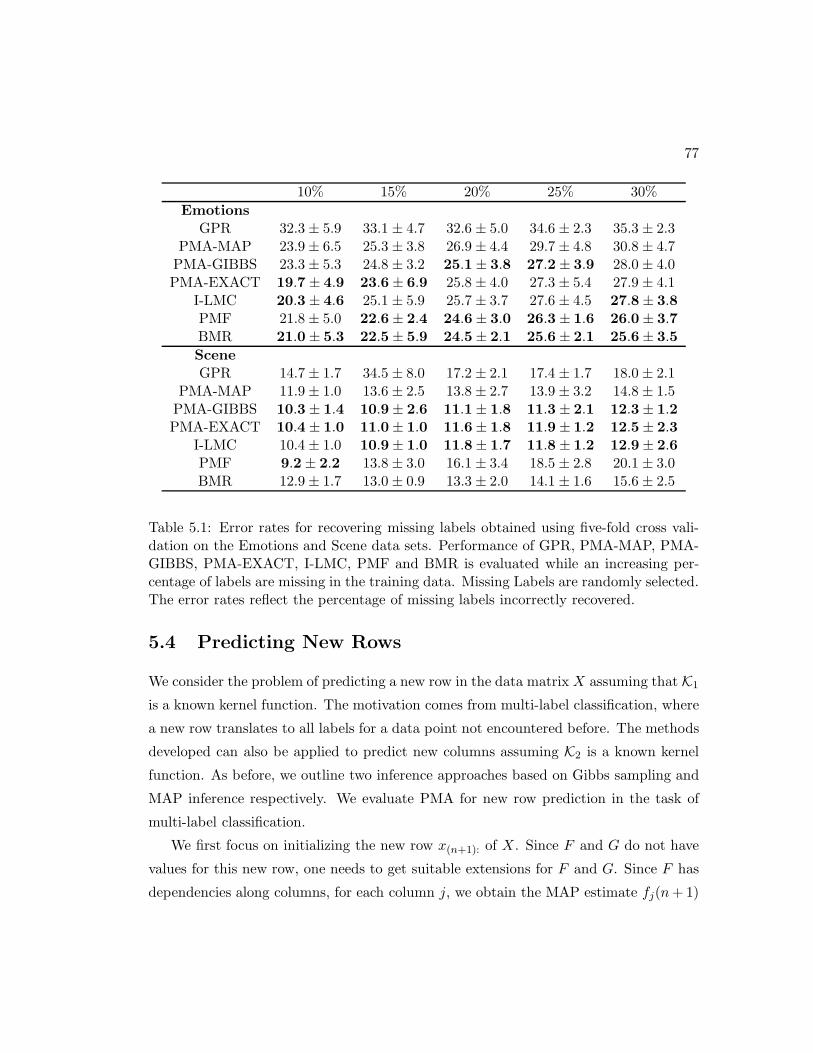
77
10% 15% 20% 25% 30%
EmotionsGPR 32.3± 5.9 33.1 ± 4.7 32.6 ± 5.0 34.6 ± 2.3 35.3 ± 2.3
PMA-MAP 23.9± 6.5 25.3 ± 3.8 26.9 ± 4.4 29.7 ± 4.8 30.8 ± 4.7PMA-GIBBS 23.3± 5.3 24.8 ± 3.2 25.1± 3.8 27.2 ± 3.9 28.0 ± 4.0PMA-EXACT 19.7 ± 4.9 23.6± 6.9 25.8 ± 4.0 27.3 ± 5.4 27.9 ± 4.1
I-LMC 20.3 ± 4.6 25.1 ± 5.9 25.7 ± 3.7 27.6 ± 4.5 27.8± 3.8PMF 21.8± 5.0 22.6± 2.4 24.6± 3.0 26.3 ± 1.6 26.0± 3.7BMR 21.0 ± 5.3 22.5± 5.9 24.5± 2.1 25.6 ± 2.1 25.6± 3.5
SceneGPR 14.7± 1.7 34.5 ± 8.0 17.2 ± 2.1 17.4 ± 1.7 18.0 ± 2.1
PMA-MAP 11.9± 1.0 13.6 ± 2.5 13.8 ± 2.7 13.9 ± 3.2 14.8 ± 1.5PMA-GIBBS 10.3 ± 1.4 10.9± 2.6 11.1± 1.8 11.3 ± 2.1 12.3± 1.2PMA-EXACT 10.4 ± 1.0 11.0± 1.0 11.6± 1.8 11.9 ± 1.2 12.5± 2.3
I-LMC 10.4± 1.0 10.9± 1.0 11.8± 1.7 11.8 ± 1.2 12.9± 2.6PMF 9.2± 2.2 13.8 ± 3.0 16.1 ± 3.4 18.5 ± 2.8 20.1 ± 3.0BMR 12.9± 1.7 13.0 ± 0.9 13.3 ± 2.0 14.1 ± 1.6 15.6 ± 2.5
Table 5.1: Error rates for recovering missing labels obtained using five-fold cross vali-dation on the Emotions and Scene data sets. Performance of GPR, PMA-MAP, PMA-GIBBS, PMA-EXACT, I-LMC, PMF and BMR is evaluated while an increasing per-centage of labels are missing in the training data. Missing Labels are randomly selected.The error rates reflect the percentage of missing labels incorrectly recovered.
5.4 Predicting New Rows
We consider the problem of predicting a new row in the data matrix X assuming that K1
is a known kernel function. The motivation comes from multi-label classification, where
a new row translates to all labels for a data point not encountered before. The methods
developed can also be applied to predict new columns assuming K2 is a known kernel
function. As before, we outline two inference approaches based on Gibbs sampling and
MAP inference respectively. We evaluate PMA for new row prediction in the task of
multi-label classification.
We first focus on initializing the new row x(n+1): of X. Since F and G do not have
values for this new row, one needs to get suitable extensions for F and G. Since F has
dependencies along columns, for each column j, we obtain the MAP estimate fj(n+1)

78
using GP regression and K1 yielding the extended matrix F ∈ R(n+1)×m. Since G does
not have dependencies along columns, we sample a new row gTn+1 ∼ GP (0,K2) yielding
the extended G ∈ R(n+1)×m.
For Gibbs Sampling, we obtain the initial extended matrix as X = F + G. Then we
proceed as in Section 5.3.1, while treating the entire last row of X as latent, in addition
to G and any other missing entries in X . For MAP inference, since gTn+1 is zero mean,
the (n+ 1)st row of F serves directly as an estimate for the new row x(n+1): . In either
setting, if K2 is unknown, we alternate between sampling/estimating X and estimating
K2.
5.4.1 Experimental Evaluation
We compare the performance of PMA (PMA-GIBBS) to existing state-of-the-art meth-
ods for multi-label classification on a number of benchmark data sets. We use the Scene
[79], Emotions [80],Image [88] and YeastProt [89] datasets for evaluation. In table 5.2 a
summary is provided for all of the data sets used. As before, we use truncated log-odds
during learning, and the sign of the predicted score for evaluation.
Algorithms and Methodology: We evaluate PMA-GIBBS against four multi-
label classification algorithms. For PMA-GIBBS, we assume that K1 is an RBF Kernel
over the points, where its parameters are estimated using cross validation, and K2 is
unknown and estimated from the data. The inputs into K1 are given by feature vectors
of the data points. As a baseline, we consider one-vs-rest SVM as a multi-label classifier,
which we refer to as MLSVM. We also consider two state-of-the-art approaches for multi-
label learning: Multi Label K-nearest Neighbors (MLKNN) [42], a method which applies
the k-nearest neighbor idea to the multi-label setting; and Instance Based Learning by
Logistic Regression (IBLR) [74], where features are first transformed to incorporate
label information from local neighborhoods prior to applying logistic regression. In all
multi-label experiments, we utilize an RBF Kernel in PMA, where the parameter σ
is chosen by cross-validation. We also compare performance to Bayesian Multivariate
Regression (BMR), developed in the previous chapter.
We also consider the setting where the training set has partial labels, i.e., missing
entries in X. While PMA and BMR can utilize partial labels, the other algorithms
cannot. Hence, we construct a reduced training set discarding points with partial labels.

79
The corresponding models are called PMA-GIBBS-D, BMR-D MLKNN-D, IBLRML-D
and MLSVM-D.
Evaluation Measures: We evaluated multi-label classification performance using
three different measures: one error, precision, and ranking loss. Let g(x, l) denote a
real-valued function which assigns a score to label l for data point x, such that a larger
score is considered better. Further, let Lx denote a set of true labels associated with x.
1) One error evaluates how frequently the top ranked predicted label is not among
the true labels. If 1[·] denotes the indicator function, we have:
OneError(g) =1
D
D∑
d=1
1 [argmaxl∈L g(xd, l) 6∈ Lxd] .
2) For true labels l ∈ Lx, average precision evaluates the fraction of labels in Lx
that rank at least as high as l according to the scoring rule g on average. For any data
point x and any label l ∈ Lx, let R(x, l) = {l′ ∈ Lx|rankg(x, l′) ≤ rankg(x, l)}, wherethe ranking is among all possible labels. Then, average precision is:
AvePrec(g) =1
D
D∑
d=1
1
|Lxd|∑
l∈Lxd
|R(xd, l)|rankg(x, l)
.
3) Ranking loss reflects the average number of labels that are reversely ordered for a
given instance. Let T (xd) = {(l1, l2) | g(xd, l1) ≤ g(xd, l2), (y1, y2) ∈ Lxd× Lxd
}, whereLxd
denotes the complement of Lxd. Ranking loss is defined as:
RankLoss(g) =1
D
D∑
d=1
|T (xd)||Lxd||Lxd
| .
Thus, for one error and ranking loss, lower is better; for average precision, higher is
better. We evaluate all multi-label algorithms using all performance measures and five
fold cross validation.
Performance: We evaluate performance on both multi-label datasets by consider-
ing an increasing number of labeled points. As seen in Figure 5.3, PMA outperforms
the other four methods on all data sets and for all three performance measures, and
the improvements are in almost all cases significant. Further, all four methods designed
specifically for multi-label classification tend to outperform MLSVMs. Compared to

80
BMR, PMA is slightly better on the Emotions data set and it is significantly better on
the remaining data sets.
We also tested the prediction performance when missing labels are present in the
training data. As seen in Table 5.3, PMA-GIBBS outperforms the other models due to
its ability to leverage partially labeled data. Among algorithms which discard points
with partial labels, PMA-GIBBS-D outperforms the others.
Data Set Points Features Labels
Scene 2407 294 6Emotions 593 72 6Image 2000 135 5
YeastProt 2000 215 138
Table 5.2: Data sets used in multi-label classification
OneError AvePrec Coverage
PMA-GIBBS 29.7± 4.2 82.3± 2.7 10.6 ± 2.3BMR 33.3 ± 4.9 79.9 ± 2.4 11.6 ± 2.0
PMA-GIBBS-D 51.1 ± 7.5 67.5 ± 4.8 22.4 ± 3.7BMR-D 54.7 ± 6.7 64.5 ± 4.6 26.1 ± 3.4
MLKNN-D 70.5 ± 2.0 46.3 ± 4.3 23.7 ± 8.1IBLRML-D 61.9 ± 8.9 36.9 ± 3.9 54.8 ± 3.9MLSVM-D 87.9 ± 2.0 40.9 ± 1.6 83.1 ± 1.4
Table 5.3: Five fold cross validation on the Scene data set with 25% of label entriesmissing. PMA-GIBBS utilizes all available data while training. PMA-GIBBS-D, BMR-D, MLKNN-D,IBLRML-D and MLSVM-D discard data points with missing label entriesin the training stage.
5.5 Related Work
In this section we review work previously done in extending Gaussian Processes to cap-
ture correlations across outputs. We also review work done in multi-label classification.
One of the most popular approaches to capture correlations among outputs of a GP

81
is to utilize convolution processes (CPs) [90, 84]. In CPs each output is represented
as the convolution of a smoothing kernel and a latent function. The outputs of the
convolutions are then modeled by a single Gaussian Process [91], whereby data points
are still assumed to be drawn i.i.d. In our model the i.i.d. assumption is not made.
From a convolution stand point our model also differs. Let Pf (F ) denote the PMA
prior over matrices F , Let Pg(G) denote a prior over matrices G. In PMA we have
P (X) =∫
F Pg(X − F )Pf (F )dF = (Pf ∗ Pg)(X), where Pf and Pg are GP-based priors
over matrices. Please note that in PMA this convolution view point does not hold for
single rows or columns of X, since Pf is defined over columns and Pg over rows.
In [92] a model is proposed which is capable of incorporating relational side informa-
tion in form of a graph, resulting in correlated outputs of a GP. Unlike our approach this
method does not model correlations on two different levels explicitly. In [82] a model is
proposed which assumes latent functions to be the sum of two random variables, one of
which contains relational side information. The resulting model, unlike PMA, is repre-
sented by a single GP with a modified Kernel, from which points are drawn i.i.d. In [83]
an approach is proposed that combines ideas from [92] and [82]. Latent variables are
assumed to be a sum of multiple random variables which encode relational information,
whereby the aggregate latent variables are representable as outputs of a single GP (see
discussion after equation (11) in [83]). Further in [83] unlike in PMA links are modeled
explicitly.
When it comes to multi-label classification the state-of-the art is comprised of meth-
ods which attempt to capture correlations among labels. In recent years several such
methods have been proposed. In [70], a maximum margin approach is proposed which
minimizes the ranking loss. While the ability to handle kernels is important in several
domains, most existing approaches do not have a natural way of providing a direct un-
certainty quantification. A number of probabilistic models have also been proposed for
multi-label classification. In [68], a mixture model is proposed for text classification.
More recently, in [72], a fully Bayesian model was proposed based on sparse and infinite
canonical correlation analysis. Most of the probabilistic models do not have a good way
of incorporating kernels, and if they do as in [73], they do not model correlations among
labels explicitly.
In [42], label statistics from neighborhoods are used to build a Bayesian classifier.

82
In [74], features are constructed based on label information from neighborhoods and
subsequently used in logistic regression. Our model stands out as unique as it is capa-
ble of incorporating a kernel, providing direct uncertainty quantification and modeling
correlation structure among labels explicitly at the same time.
5.6 Conclusions
We have introduced a novel model for matrix data analysis capable of capturing correla-
tions among rows and columns simultaneously. PMA has sparse statistical dependency
structures yielding fast approximate inference algorithms. We have presented prelim-
inary experiments demonstrating the advantage of PMA over single GPs for matrix
analysis, as well as its ability to handle missing data. The ability of PMA to capture
correlations along rows and columns simultaneously appears especially beneficial in do-
mains such as multi-label classification. Our empirical evaluation shows that PMA can
significantly outperform some of the existing multi-label classification algorithms. Fur-
ther, PMA can readily be extended to higher order structures such as tensors which we
plan to investigate in future work.

83
10 20 30 40 50 60 70 80 90 100 1100.2
0.3
0.4
0.5
0.6
0.7
0.8
Number of Labeled Points
One
Err
orFive Fold Cross Validation on the Emotions Data Set
mlknniblrmlmlsvmpma−gibbsbmr
(a) Emotions - OneError
10 20 30 40 50 60 70 80 90 100 1100.4
0.45
0.5
0.55
0.6
0.65
0.7
0.75
Number of Labeled Points
Ave
rage
Pre
cisi
on
Five Fold Cross Validation on the Emotions Data Set
mlknn
iblrml
mlsvm
pma−gibbs
bmr
(b) Emotions - AvePrec
10 20 30 40 50 60 70 80 90 100 110
0.3
0.4
0.5
0.6
0.7
0.8
0.9
Number of Labeled Points
Ran
king
Los
s
Five Fold Cross Validation on the Emotions Data Set
mlknniblrmlmlsvmpma−gibbsbmr
(c) Emotions - Ranking Loss
10 20 30 40 50 60 70 80 90 100 1100.2
0.3
0.4
0.5
0.6
0.7
0.8
0.9
1
Number of Labeled Points
One
Err
or
Five Fold Cross Validation on the scene Data Set
mlknniblrmlmlsvmpma−gibbsbmr
(d) Scene - OneError
10 20 30 40 50 60 70 80 90 100 1100.3
0.4
0.5
0.6
0.7
0.8
0.9
Number of Labeled Points
Ave
rage
Pre
cisi
on
Five Fold Cross Validation on the scene Data Set
mlknn
iblrml
mlsvm
pma−gibbs
bmr
(e) Scene - AvePrec
10 20 30 40 50 60 70 80 90 100 110
0.1
0.2
0.3
0.4
0.5
0.6
0.7
0.8
Number of Labeled Points
Ran
king
Los
s
Five Fold Cross Validation on the scene Data Set
mlknniblrmlmlsvmpma−gibbsbmr
(f) Scene - Ranking Loss
10 20 30 40 50 60 70 80 90 100 1100.4
0.45
0.5
0.55
0.6
0.65
0.7
0.75
0.8
0.85
0.9
Number of Labeled Points
One
Err
or
Five Fold Cross Validation on the Image Data Set
mlknniblrmlmlsvmpma−gibbsbmr
(g) Image - OneError
10 20 30 40 50 60 70 80 90 100 1100.45
0.5
0.55
0.6
0.65
0.7
0.75
Number of Labeled Points
Ave
rage
Pre
cisi
on
Five Fold Cross Validation on the Image Data Set
mlknn
iblrml
mlsvm
pma−gibbs
bmr
(h) Image - AvePrec
10 20 30 40 50 60 70 80 90 100 1100.25
0.3
0.35
0.4
0.45
0.5
0.55
0.6
0.65
0.7
Number of Labeled Points
Ran
king
Los
s
Five Fold Cross Validation on the Image Data Set
mlknniblrmlmlsvmpma−gibbsbmr
(i) Image - Ranking Loss
145 150 155 160 165 170 175 180 185 190 195 2000.8
0.82
0.84
0.86
0.88
0.9
0.92
0.94
0.96
0.98
1
Number of Labeled Points
One Error
Five Fold Cross Validation on the YeastProt Data Set
mlknn
iblrml
mlsvm
pma-gibbs
(j) YeastProt - OneError
140 150 160 170 180 190 200 2100.04
0.06
0.08
0.1
0.12
0.14
0.16
0.18
0.2
0.22
Number of Labeled Points
Ave
rage
Pre
cisi
on
Five Fold Cross Validation on the YeastProt Data Set
mlknn
iblrml
pma−gibbs
mlsvm
bmr
(k) YeastProt - AvePrec
145 150 155 160 165 170 175 180 185 190 195 200
0.3
0.35
0.4
0.45
0.5
0.55
0.6
0.65
0.7
0.75
Five Fold Cross Validation on the YeastProt Data Set
Number of Labeled Points
Ranking Loss
mlknn
iblrml
mlsvm
pma-gibbs
(l) YeastProt - Ranking Loss
Figure 5.3: Five fold cross validation on the Emotions, Yeast and Image data sets usingthree evaluation measures. PMA consistently outperforms the other methods on alldatasets according to all evaluation measures.

Chapter 6
Gaussian Process Topic Models
Having introduced PMA in the previous chapter, we propose a novel topic model capable
of modeling the covariance across topics while incorporating a kernel among documents.
This is accomplished by utilizing PMA as a prior.
6.1 Introduction
In recent years, significant progress has been made in analyzing text documents using
topic models. Statistical topic models such as Latent Dirichlet Allocation (LDA) [93]
and its variants have proven useful and effective. Such topic models allow mixed mem-
berships of documents to several topics, where a topic is represented as a distribution
over words.
In LDA, the topic proportions for each document are drawn from a Dirichlet distri-
bution. As a consequence, LDA does not have the flexibility of modeling correlations
among the topics. Correlated Topic Models (CTMs) [7] were proposed to address this
issue. Instead of a Dirichlet prior, CTMs use a multi-variate normal distribution with
a covariance parameter and map samples from the normal distribution to the topic
simplex using a mean parameterization. The prior model assumes a fixed mean and
covariance parameter for the entire corpus, and the corpus is used to learn these pa-
rameters. Correlations between topics are captured by the resulting covariance matrix.
Frequently one might have additional information about a text corpus, possibly in
the form of additional features/structures, labels, one or more weighted graphs, etc. For
84

85
the purposes of this chapter, we assume that such additional information can be captured
by a suitable kernel defined over the documents. While there has been recent work on
incorporating link structure among documents [94], existing topic models, including
CTM, are unable to leverage such information in form of a kernel. In this chapter,
we propose Gaussian Process Topic Models (GPTMs) which can capture correlations
among topics as well as leverage known similarities among documents using a kernel.
GPTMs can be considered a generalization of CTMs using ideas from Gaussian Process
(GP) embedding and regression. Given a kernel among documents, GPTM defines a
Gaussian Process mapping from a suitable document space into the topic space. While
topic proportions for all documents in CTM are generated from a single mean, the topic
proportions in GPTM are generated from different means. The location of the means
for any document is determined by the Gaussian Process mapping.
Gaussian Processes (GPs) define distributions over function spaces and have been
successfully used for non-linear regression, classification and embedding [95, 96, 5]. The
Gaussian Process Latent Variable Model (GPLVM) [5] is a probabilistic embedding
method which utilizes a GP mapping from the embedded space to the data space.
While GPLVM is powerful non-linear embedding method, current literature does not
have effective models for combining kernel based non-linear embedding models such
as GPLVM with probabilistic topic models such as CTM. One can obtain embeddings
from either family of methods—from LDA/CTM based on the topic structure or from
GPLVM using the kernel and observed features. The proposed GPTM can systemat-
ically leverage both types of information and obtain an embedding based on both the
topic structure and the kernel.
We propose suitable approximate inference algorithms for learning GPTMs and mak-
ing predictions on a test set. The proposed inference algorithm marginalizes the latent
variables in the topic model and maximizes over the latent variables in the embedding,
so we obtain one good embedding. During learning, GPTMs work with two different
positive definite matrices—a topic covariance matrix over the topics and a document
kernel matrix over the documents. Our analysis shows that the two matrices get inte-
grated in an elegant manner to determine the final embedding. In particular, we obtain
a Sylvester equation involving both matrices whose solution gives the final embedding.
While Sylvester equations have been extensively studied in control theory, to the best
86
of our knowledge, their usage in the context of topic models is novel.
The rest of the chapter is organized as follows. We introduce GPTMs in Section 6.2
and discuss learning GPTMs in Section 6.3. We present experimental results in Sec-
tion 6.4, provide a discussion on our model in Section 6.5 and conclude in Section 6.6.
6.2 The Model
Correlated Topic Models (CTMs) [7] are an important recent advance in the realm
of topic models [93, 97]. CTMs have the ability to capture correlation among topics.
However, CTMs were not designed to capture any additional information regarding the
documents, possibly in the form of a kernel over the documents. In this section, we in-
troduce Gaussian Process Topic Models (GPTMs) which are a systematic generalization
of CTMs capable of incorporating knowledge from a kernel over the documents.
The key difference between CTM and the proposed GPTM is how the model samples
mixed memberships over topics for each document. In CTMs, one samples η ∈ RK
from a multivariate Gaussian N(µ,Σ) and maps η to the topic simplex using a mean
parameterization [7]. As a result, E[η] = µ, i.e., apriori all documents have the same
mixing proportions in expectation. In GPTMs, apriori all documents have different
mixing proportions in expectation. The mixing proportions are derived from the kernel
over the documents and, intuitively, similar documents according to the kernel have
similar mixing proportions.
Given a kernel function K over documents, the corresponding GP defines a distribu-
tion over functions over all documents. For a set of D documents, we get a distribution
over f ∈ RD given by
p(f |K) = 1
(2π)D/2|K|1/2 exp
(
−1
2fTK−1f
)
. (6.1)
Assuming there are K topics, we independently sample f1, . . . , fK ∈ RD from the above
distribution, and construct a K ×D matrix F , whose ith row is fTi . Hence p(F |K) =
∏Ki=1 p(fi|K). Now, for each document d = 1, . . . ,D we generate ηd ∈ R
K following
p(ηd|µd,Σ) ∼ N (η|µd,Σ) (6.2)
where Σ denotes a K ×K topic covariance matrix and µd = Fed ∈ RK , where ed ∈ R
D
represents the all zeros vector with only the dth entry 1. Thus, µd ∈ RK is the dth column

87
of F . Each ηd is then mapped to the topic simplex using the mean parameterization:
θ(ηd) =exp(ηd)∑i exp(ηd(i))
. Since the rows of F were drawn independently from the GP with
kernel K, similar documents according to the kernel will implicitly have similar µd, and
hence similar topic proportions apriori. Thus, the GP prior captures global relationships
between documents in determining the apriori mixed memberships.
The entire generative model (Figure 6.1) can be specified as follows:
1. Draw F |K ∼ p(F |K) =∏iN (fi|0,K).
2. For each document d = 1, . . . ,D:
(a) ηd|F,Σ ∼ N (ηd|Fed,Σ).
(b) For each word wn, n = 1, . . . , Nd:
i. Draw a topic zn|ηd ∼ Discrete(θ(ηd)).
ii. Draw a word wn|zn, β1:K ∼ Discrete(βzn).
The joint probability of all observed and latent variables in GPTM is given by:
p(w, z, η, F |K,Σ, β) =K∏
i=1
p(fi|K)D∏
d=1
p(ηd|Fed,Σ)
Nd∏
n=1
p(zn|ηd)p(wn|zn, β) .(6.3)
The proposed GPTM is different from both CTM as well as GPLVM, while drawing
from the strengths of both of these models. Unlike CTM, the apriori topic proportions
of the documents are different and the difference is based on the kernel K. Unlike
GPLVM, GPTM takes topic structure into account. The final embedding will be based
on both the kernel as well as the structure of the documents as determined by the topic
model. As a result, GPTM leverages the strength of both topic models as well as kernel
methods, in particular CTMs and GPs.
6.3 Learning GPTMs
Exact inference in GPTMs is computationally intractable. In this section, we first
explain why some standard approaches to approximate inference may not be desirable

88
Figure 6.1: Gaussian Process Topic Model
and then outline a somewhat non-standard approach for doing approximate inference
in GPTMs. The log-likelihood of the observed words w given (K,Σ, β) is given by:
log p(w|K,Σ, β) = logE(F,η,z)[p(w, z, η, F |K,Σ, β)] , (6.4)
where the expectation is over the distribution on the latent variables (F, η, z). In several
GP-based models [96], one can integrate over all functions f which translates to the dis-
tribution over F in GPTM. Focussing on the terms involving F in the joint distribution,
we haveK∏
i=1
p(fi|K)D∏
d=1
p(ηd|Fed,Σ) =1
|K|k/2|Σ|D/2×
exp
{
−1
2
(
Tr(FK−1F T ) + Tr(F TΣ−1F ))
+Tr(F TΣ−1η)
}
,
where η = [η1 · · · ηD] is the K ×D matrix of means variables ηd. The terms involving
F have both row and column dependencies, one coming from K and the other from Σ.
Hence, exact marginalization over F is difficult. Further, while the apriori marginal over
each entry ηid of η are univariate Gaussians with zero mean and variance Σi,i + Kd,d,
the joint distribution over η will have both row and column dependencies, and hence
exact marginalization of η is also difficult. While variational inference by assuming a
fully factorized distribution over F, η will lead to a variational lower bound, such an
approach to inference undermines a key property of GPTMs, viz dependencies along
both rows and columns. Gibbs sampling based inference is possible for the model but
could be computationally burdensome. It involves inverting (K − 1) × (K − 1) and
(D − 1)× (D − 1) matrices for each entry in η in each sampling iteration.
89
In GPTMs, there are two sets of latent variables to consider: the matrix F , arising
out of the GP, and variables (η, z), which are common in topic models [7]. In light of the
previous discussion, we choose to maximize the log-likelihood over F and variationally
marginalize it over (η, z). As we shall see shortly, the maximum aposteriori (MAP)
inference over F can be done while maintaining the row and column dependencies. In
particular, the first order conditions lead to a Sylvester equation [86, 98] in F involving
both Σ and K. Further, MAP inference over F leads to an embedding of the data points
taking into account both the kernel, the covariance among topics, as well as observed
words. While maximizing over F is unconventional in the context of GPs, related ideas
have been explored in the recent literature in the context of probabilistic embedding
using GPLVMs [5]. In Section 6.4, we compare the embedding performance of GPTMs
to that of GPLVMs as well as CTMs.
6.3.1 Approximate Inference
Our goal in terms of learning is to choose (F,Σ, β) so as to maximize
log p(w,F |K,Σ, β) = logEη,z[p(w, z, η, F |K,Σ, β)] . (6.5)
In principle, one can also optimize over K using kernel learning methods, but we do
not explore this aspect in this chapter. Since computing the expectation over the latent
variables (η, z) is intractable, following [7], we propose a variational inference approach
to lower bound the expectation over (η, z). In particular, for each document, we consider
the family of fully factored variational distributions q as:
q(η1:K , z1:N |λ1:K , ν21:K , φ1:N ) =K∏
i=1
q(ηi|λi, ν2i )
N∏
n=1
q(zn|φn) , (6.6)
where q(ηi|λi, ν2i ) are univariate Gaussian distributions with mean λi and variance ν2i ,
and q(zn|φn) are discrete distributions with parameter φn.
Using Jensen’s inequality [7], for any F we have:
log p(w,F |K,Σ, β)
≥ log p(F |K) +D∑
d=1
{
Eq[log p(ηd|Fed,Σ)]
+ Eq[log p(zd|ηd)] + Eq[log p(wd|zd, β)]}
+H(q)
(6.7)

90Table 6.1: Terms of the lower bound for expected loglikelihood
Term Expression
log p(F |K) K2log |K−1| − KD
2log 2π − 1
2Tr(FK−1F T )
Eq[log p(ηd|Fed,Σ)]12log |Σ−1| − K
2log 2π − 1
2{Tr(diag(ν2)Σ−1) + (λ− Fed)
TΣ−1(λ− Fed)}
Eq(log p(zn|η))∑K
i=1 λiφn,i − ζ−1(
∑K
i=1 exp{λi + ν2i /2}
)
+ 1− log(ζ)
Eq[log p(wn|zn, β)]∑K
i=1 φn,i log βi,wn
H(q)∑K
i=112(log ν2
i + log 2π + 1)−∑N
n=1
∑K
i=1 φn,i log φn,i
We give the exact expressions for each term in Table 6.1. For the derivation of the
last three terms we refer the reader to [7], since these terms are the same as in CTM.
The first two terms are unique to our model and stem from the introduction of F . For
the first term, by definition, we have
log p(F |K)
=K∑
i=1
{
1
2log |K−1| − D
2log 2π − 1
2fTi K−1fi
}
=K
2log |K−1| − KD
2log 2π − 1
2Tr(FK−1F T ) .
For the second term corresponding to each document we have
Eq[log p(ηd|Fed,Σ)] =1
2log |Σ−1| − K
2log 2π
− 1
2Eq[(ηd − Fed)
TΣ−1(ηd − Fed)]
=1
2log |Σ−1| − K
2log 2π +Tr(diag(ν2d)Σ
−1)
+ (λd − Fed)TΣ−1(λd − Fed) ,
where ed ∈ RD is the all zeros vector with only the dth entry as one. Further, note
that the third term Eq[log p(zn|η)] cannot be computed in closed form, and we obtain
a variational lower bound (see Table 6.1) with parameter ζ following [7].
6.3.2 Parameter Updates
The variational lower bound is optimized by updating the variational parameters (λ, ν, φ, ζ)
and the model parameters (F,Σ, β). Since parts of our objective function are similar
to CTM, a number of updates remain the same [7]. In particular, for the parameters

91
corresponding to the topics, we have:
βi,j ∝D∑
d=1
Nd∑
n=1
φdn,iwjdn, (6.8)
φdj,i ∝ exp{λi}βi,j , (6.9)
where wjdn is an indicator that the nth word in the dth document is the jth word in the
vocabulary. Further, for each document, the update for ζ is given by:
ζ =K∑
i=1
exp{λi + ν2i /2} (6.10)
A solution for λi and ν2i cannot be obtained analytically For each document. So gradient
descent is used with gradients
gλ =− Σ−1(λ− Fed) + ΣNn=1φn,1:K
− (N/ζ) exp{λ+ ν2/2}gν2i
=− Σ−1ii /2− (N/2ζ) exp{λi + ν2i /2}+ 1/(2ν2i ) .
We now focus on computation of parameters which are different from CTM. Since these
are unique to our model, we present them in more detail.
Computation of Σ: Unlike in CTM, we have to compute one covariance matrix
given multiple means. Starting with (6.7) we can pose the problem as:
maxΣ
{
D
2log |Σ−1| − 1
2
D∑
d=1
Tr(diag(ν2d)Σ−1)
−1
2Tr[
(L− F )TΣ−1(L− F )
}
,
(6.11)
with L = [λ1 · · · λD] where λd and νd denote the variational parameters associated
with document d. Taking the derivative with respect to Σ, we get
Σ =1
D
(
D∑
d=1
diag(ν2d) +D∑
d=1
(λd − Fed)(λd − Fed)T
)
. (6.12)
Computation of F: The matrix F ∈ RK×D is entirely new in our model. From
(6.7), the optimization problem over F can be posed as:
minF
{
Tr[
(L− F )TΣ−1(L− F )]
+Tr[
FK−1F T]
}
(6.13)
92
Taking derivative with respect to F and setting it to zero, we obtain the following
equation:
ΣF + FK =D∑
d=1
λdeTdK . (6.14)
With A = Σ, B = K and C =∑D
d=1 λdeTdK, the equation is of the form: AF +FB = C.
The equation is known as the Sylvester equation, and it is widely studied in control
theory [85, 86]. A solution to the Sylvester equation exists if and only if no eigenvalue
of A is equal to the negative of an eigenvalue of B. In our case, since A and B are both
positive semi-definite, such a situation can arise only if A and B both have at least one
zero eigen-value. For that to happen, both Σ and K have to be singular, implying Σ−1
and K−1 are not well defined. Since Σ and K both act as covariance matrix/function of
a Gaussian distribution/process, we assume them to be full rank and positive definite.1
As a result, a solution to the Sylvester equation exists and can be obtained using
standard methods [86, 98].
6.3.3 Inference On New Documents
In the learning phase, one obtains the parameters (β,Σ) as well as the best F for the
training set. While applying the model on new documents, (β,Σ) will stay unchanged,
and we do variational inference to obtain parameters (λ, ν, φ, ζ) on the test set. Further,
using the fact that location of the mean µd = Fed is determined by a GP, we can use
GP regression to obtain estimates of document means in the test set.
First, consider one new document, so that the corpus is of size (D + 1). Let F ∈RK×(D+1) denote the matrix containing the means of the entire corpus so that F =
[F F∗], where F∗ denotes the mean for the new document. Let f = [f f∗] denote a
row of F , where f corresponds to the first D documents and f∗ corresponds to the new
document. A kernel for the entire corpus can be expressed as follows:
K =
[
Kf,f Kf,∗
K∗,f K∗,∗
]
,
1 One can generalize the models using pseudo-inserves, but we do not consider such generalizationshere.

93
where K ∈ R(D+1)×(D+1). From GP regression [96], we know that the posterior proba-
bility distribution p(f∗|f) can be expressed as:
p(f∗|f) =1
(2π)1/2|K|1/2exp
(
−(f∗ − f)2
2K
)
, (6.15)
where f ∈ R and K ∈ R+ is given by
K = K∗,∗ −K∗,fK−1f,fKf,∗ (6.16)
f = K∗,fK−1f,ff . (6.17)
Similarly we can obtain a posterior distribution for a collection of M new documents.
Let F∗ ∈ RK×M denote the matrix containing the means of the new documents and
F = [F F∗]. Following the same steps as above, we note that each row fi,∗ of F∗
follows a multi-variate Gaussian distribution with mean equal to the row f i of F , where
FT= K∗,fK−1
f,fFT , and covariance K = K∗,∗ − K∗,fK−1
f,fKf,∗. Since the rows of F∗ are
independent, the probability of the entire matrix is given by
p(F ∗|F, K) =K∏
i=1
p(fi,∗|F, K) =1
(2π)K/2|K|K/2×
exp
{
−1
2Tr[
(F∗ − F )K−1(F∗ − F )T
]
}
.
(6.18)
With the above prior distribution on F∗ on the test set conditioned on the F from the
training set, the rest of the generative model for the test set remains the same as GPTM.
Introducing variational distributions as before, inference on new documents boils down
to optimizing the variational parameters and F∗ over the test set. The optimization
over the variational parameters are same as in the training set. Focussing on the terms
involving F∗, we get the following problem:
minF∗
{
1
2Tr[
(L− F∗)TΣ−1(L− F∗)
]
(6.19)
+1
2Tr[
(F∗ − F )K−1j (F∗ − F )T
]
}
,
where L = [λ1 · · · λM ] is the K ×M matrix of variational parameters λd on the test
set. The first order conditions lead to the following matrix equation:
ΣF∗ + F∗K =
(
D∑
d=1
λdeTd + F
)
K , (6.20)

94
which is again a Sylvester equation. Note that the right hand side is affected by both
observed words in the test set in the form of λd and by the estimated mean F obtained
from training set documents.
6.4 Experimental Evaluation
In this section we evaluate GPTM both as a topic model and as an embedding method,
respectively in comparison to CTM and GPLVM.
Datasets: Our experiments are performed on 6 text data sets. Dif100, Sim100,
and Same100 are subsets of the 20Newsgroup data set, each having 300 data points
from 3 categories; CMU100 is a larger subset which contains 1000 documents from 10
categories. We also report experiments on NASA’s Aviation Safety Reporting System
(ASRS) dataset: ASRS is a subset of 1000 reports from 25 categories, and ASRS3 is a
subset of 788 documents from 3 categories.
Kernel Functions: We consider two kernels for our experiments: an unsupervised
nearest-neighbor kernel derived from the document vectors and a semi-supervised must-
link kernel derived from must-link constraints on some pairs of documents.
Let X = {x1, . . . , xD} denote a set of feature vectors represented by the word counts
in a given document. Let G = (V,E) be a k-nearest neighbor graph which is sym-
metrized by making sure that (xi, xj) ∈ E whenever (xj, xi) ∈ E. The graph neighbors
are determined using cosine similarity among the document vectors. The nearest neigh-
bor (NN) kernel is defined as:
KNN (xi, xj) =
γ exp(
−d(xi,xj)2σ2
)
if (xi, xj) ∈ E
c if i = j
0 otherwise ,
(6.21)
where d(xi, xj) = 1 − xTi xj
‖xi‖‖xj‖, and σ2, γ, c are constant parameters chosen to en-
sure KNN is positive definite. The parameters are tuned for each data set using cross
validation.
While KNN can be used in practice, constructing a kernel based on document vec-
tors may not be conceptually desirable from a generative model perspective. Note
that the experiments using KNN demonstrate the ability of our model to incorporate

95
neighborhood information, which may come from supplemental information regarding
the documents. Further, GPTMs are not tied to the use of KNN . To illustrate the
effectiveness of GPTMs, we consider another kernel constructed purely based on semi-
supervised information, viz must-link constraints between certain pairs of documents,
without utilizing the documents themselves.
In particular, we consider a semi-supervised setting with a set C of must link con-
straints, i.e., if (xi, xj) ∈ C, then the documents are assumed to have the same label.
Using such a must-link constraint set, we define the must-link (ML) kernel as:
KML(xi, xj) =
γ if (xi, xj) ∈ C
c if i = j
0 otherwise ,
(6.22)
where γ > 0 and c is chosen to ensure positive definiteness of KML. The parameters
are tuned per data set using cross validation.
Perplexity Computation: In our experiments we use test-set perplexity to eval-
uate variants of GPTM as well as compare GPTM to CTM. When comparing variants
of GPTM we compute perplexity as:
Perplexityw,F∗= exp
(
−∑M
i=1 log p(wi, F∗)∑M
i=1Ni
)
, (6.23)
based on the joint likelihood of the test documents wi with MAP estimate F∗.
To compare our model to CTM, we compute conditional perplexity for GPTM as
follows:
Perplexityw|F∗= exp
(
−∑M
i=1 log p(wi|F∗)∑M
i=1 Ni
)
(6.24)
Since the conditional distribution p(w|F∗) is a distribution over the space of docu-
ments, which is the same for CTM, the perplexity comparison is meaningful and fair.
We also consider additional measures, including topics inferred, document embeddings
generated, and classification performance using the embeddings, to get a better under-
standing of their comparative performance.

96
Table 6.2: Perplexity on hold out test set.
CTM GPTM KML GPTM KKNN
Dif100 1231 ± 32 1195 ± 49 1183± 36
Sim100 1720 ± 19 1706 ± 22 1684± 21
Same100 761± 6 758 ± 6 755± 12
ASRS 491± 8 488 ± 8 483± 3
News100 2944 ± 83 2943 ± 66 2936± 82
6.4.1 GPTM vs. CTM
We report perplexity results comparing CTMs with GPTMs using both the ML-kernel
and the NN-kernel with neighborhood k = 10 in Table 6.2. Perplexity was evaluated
on a held out test-set using five-fold cross validation and the number of topics set to
three. Compared to CTMs, we observe mild to moderate improvements in perplexity
across all datasets for GPTMs using both kernels. Thus, in terms of perplexity on the
test-set, GPTMs are better or at least as good as CTMs. For GPTMs, the NN-kernel
appears to perform mildly better compared to the ML-kernel.
Table 6.3: Topics extracted by CTM from 20Newsgroup data
Topic 1 Topic 2 Topic 3 Topic 4 Topic 5 Topic 6car plant echo pittsburgh system godoil court list period mac existence
brake scsi motif lemieux files existfluids disk xterm stevens disk islamtires cement set play file standarddot data mailing power comp science
convention ram host njd software atheismabs card mail scorer ftp religion
braking property sun pgh sys religioncars atlantic school islanders macintosh laws
We also qualitatively examined the topics obtained by both models. In Tables
6.3,6.4 and 6.5 we list the 10 most likely words for some of the topics obtained from the
News100 dataset. As is evident, GPTMs returns topics which appear as interpretable
as those obtained by CTM. Taking a closer look, we can see that some of the topics

97
Table 6.4: Topics extracted by GPTM using K = KNN and the 20Newsgroup data
Topic 1 Topic 2 Topic 3 Topic 4 Topic 5 Topic 6car convention drive play system godoil don disk power mac good
brake party hard period files islamfluids people drives pittsburgh disk existtires price bios islanders comp paindot business controller hockey file lawsabs hess floppy scorer software thingcars karl card pts macintosh time
braking institute rom jersey sys existencesystem libertarian scsi good ftp faith
appear more coherent in GPTMs. For example, Topic 1 in CTM contains car part
related words and the word convention. In GPTM with NN-kernel, we have a topic
on car parts (Topic 1), and a topic about the liberterian party convention held at the
Karl Hess business institute (Topic 2). Topic 2 in CTM appears to be memory related,
along with words such as plant, court, cement, and atlantic. While in GPTM with
KNN the corresponding topic (Topic 3) appears only memory related. The two versions
of GPTM produce rather similar topics. With KML the hockey topic appears more
generic, possibly because there are multiple hockey related documents within the same
class. While these are only anecdotal examples, the bottom line is that both CTMs and
GPTMs produce high quality interpretable topics.
6.4.2 Variants Of GPTMs
We compare four variants of GPTMs to understand the value of the topic covariance
matrix Σ and the kernel matrix K. In particular, we consider: (i) GPTM-SI-KI, where
both Σ and K are identity matrices. Since correlation among topics and similarity among
documents are not considered, this model is closest to LDA in spirit; (ii) GPTM-KI,
where K is identity but Σ is learnt from the data. This model is closest in spirit to
CTM; (iii) GPTM-SI, where Σ is identity and K is set to either KNN or KML. This
model is similar to LDA with a kernel over documents; and (iv) GPTM, where Σ is
learned from data and K is either KNN or KML.

98
Table 6.5: Topics extracted by GPTM using K = KML and the 20Newsgroup data
Topic 1 Topic 2 Topic 3 Topic 4 Topic 5 Topic 6car liberation drive team system god
brake committee tape hockey mac moralityoil institute scsi game files atheism
fluids president problem players ftp moraldot hess dos games file existenceabs karl windows play disk existtires business system year comp standard
braking national floppy nhl software faithsystem defense cable player sys goodcars college computer playoffs macintosh true
Table 6.6: Different Variants of GPTM. Performance improves as more informativekernel and covariance matrices are considered.
GP-SIKI GP-KI GP-SI KML GP-SI KKNN GPTM KML GPTM KKNN
Dif100 1264 ± 47 1232 ± 29 1198 ± 46 1138 ± 42 1121 ± 40 1095± 53
Sim100 1778 ± 51 1741 ± 51 1720 ± 46 1656 ± 41 1639 ± 46 1610± 37
Same100 829 ± 21 792 ± 11 745 ± 28 633 ± 14 638 ± 12 608± 10
ASRS 514 ± 11 508 ± 7 472 ± 7 485 ± 9 466± 9 467 ± 7
News100 3093 ± 89 3047 ± 56 2911 ± 65 2877 ± 79 2818 ± 51 2769± 86
Table 6.2 shows the perplexity numbers on a held out test set using five fold cross-
validation. We observe a consistent ordering in terms performance. GPTM-SI-KI per-
forms worst, followed by GPTM-SI, GPTM-KI, and GPTM performs the best. The
fact that GPTM-KI performs better than GPTM-SI-KI is consistent with the observa-
tion that CTM outperforms LDA. The comparison between GPTM-KI and GPTM-SI
shows that GPTM-SI has a consistent better performance possibly implying the kernel
adds more value in terms of perplexity than the topic covariance matrix. Finally, the
full GPTM outperforms all the special cases. The results clearly illustrate the value in
having a suitable kernel over the documents.
Comparing the two different Kernels in GPTM, KNN fairly consistently results in
better perplexity numbers. Interestingly, as far as perplexity is concerned, the nearest
neighbor information appears more valuable compared to must-link constraints among
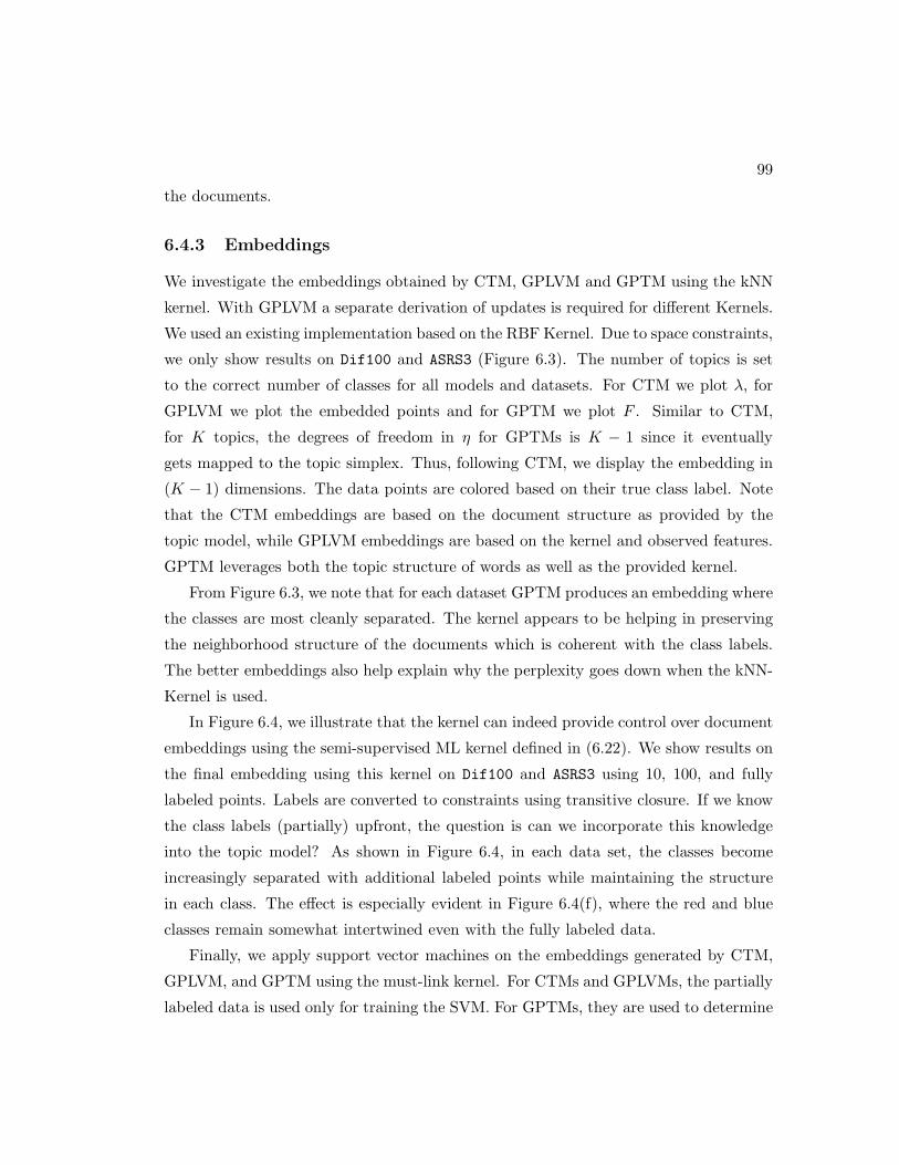
99
the documents.
6.4.3 Embeddings
We investigate the embeddings obtained by CTM, GPLVM and GPTM using the kNN
kernel. With GPLVM a separate derivation of updates is required for different Kernels.
We used an existing implementation based on the RBF Kernel. Due to space constraints,
we only show results on Dif100 and ASRS3 (Figure 6.3). The number of topics is set
to the correct number of classes for all models and datasets. For CTM we plot λ, for
GPLVM we plot the embedded points and for GPTM we plot F . Similar to CTM,
for K topics, the degrees of freedom in η for GPTMs is K − 1 since it eventually
gets mapped to the topic simplex. Thus, following CTM, we display the embedding in
(K − 1) dimensions. The data points are colored based on their true class label. Note
that the CTM embeddings are based on the document structure as provided by the
topic model, while GPLVM embeddings are based on the kernel and observed features.
GPTM leverages both the topic structure of words as well as the provided kernel.
From Figure 6.3, we note that for each dataset GPTM produces an embedding where
the classes are most cleanly separated. The kernel appears to be helping in preserving
the neighborhood structure of the documents which is coherent with the class labels.
The better embeddings also help explain why the perplexity goes down when the kNN-
Kernel is used.
In Figure 6.4, we illustrate that the kernel can indeed provide control over document
embeddings using the semi-supervised ML kernel defined in (6.22). We show results on
the final embedding using this kernel on Dif100 and ASRS3 using 10, 100, and fully
labeled points. Labels are converted to constraints using transitive closure. If we know
the class labels (partially) upfront, the question is can we incorporate this knowledge
into the topic model? As shown in Figure 6.4, in each data set, the classes become
increasingly separated with additional labeled points while maintaining the structure
in each class. The effect is especially evident in Figure 6.4(f), where the red and blue
classes remain somewhat intertwined even with the fully labeled data.
Finally, we apply support vector machines on the embeddings generated by CTM,
GPLVM, and GPTM using the must-link kernel. For CTMs and GPLVMs, the partially
labeled data is used only for training the SVM. For GPTMs, they are used to determine

100
0 10 20 30 40 50 60 70 80 900
0.1
0.2
0.3
0.4
0.5
0.6
0.7
Number of Labeled Points
Err
or
Dif100, SVM 5−fold cross validation
ctmgplvmgptm−ml
(a) Dif100
0 10 20 30 40 50 60 70 80 90
0.2
0.25
0.3
0.35
0.4
0.45
0.5
0.55
0.6
0.65ASRS3, SVM 5−fold cross validation
ctmgplvmgptm−ml
(b) ASRS3
Figure 6.2: The SVM algorithm is applied to the respective outputs of CTM, GPTMand GPLVM.
the ML kernel in GPTM as well as for training the SVM. Due to space constraints, we
show results only on Dif100 and ASRS3 in Figure 6.2. The SVM is trained with an RBF
Kernel, and the parameters are tuned using 5-fold cross validation. The classification
results show that GPTM produces embeddings with the best class separability and
lowest error rates.
6.5 Discussion
In this section we briefly discuss computational aspects in GPTMs and how GPTMs
compare to CTMs in terms of capturing topic correlations.
6.5.1 Computational Aspects
There are two major new computational aspects in our model. One pertains to the
inversion of the D × D kernel matrix during GP regression on the test set, and the
second is the solution of a Sylvester equation.
The inversion of the kernel matrix is something that most GP based models have
to perform [96]. In recent years, progress has been made on making the computation
scalable. For example, several sparsity-based approaches [99, 100] have been developed,

101
−8 −6 −4 −2 0 2 4−8
−6
−4
−2
0
2
4Dif100, CTM
(a) Dif100,CTM
−2 −1.5 −1 −0.5 0 0.5 1 1.5 2 2.5 3
−2
−1.5
−1
−0.5
0
0.5
1
1.5
2
2.5
Dif100, GPLVM
(b) Dif100, GPLVM
−8 −6 −4 −2 0 2 4 6 8 10 12
x 10−4
−8
−6
−4
−2
0
2
4
6
8
10x 10
−4 Dif100, GPTM
(c) Dif100, GPTM
−5 −4 −3 −2 −1 0 1 2 3−8
−6
−4
−2
0
2
4ASRS−3, CTM
(d) ASRS3, CTM
−8 −6 −4 −2 0 2 4 6 8−8
−6
−4
−2
0
2
4
6
8ASRS−3, GPLVM
(e) ASRS3, GPLVM
0.148 0.15 0.152 0.154 0.156 0.158 0.16 0.1620.113
0.114
0.115
0.116
0.117
0.118
0.119
0.12
0.121ASRS−3, GPTM
(f) ASRS3, GPTM
Figure 6.3: Embeddings obtained from CTM, GPLVM, and GPTM without using classlabel information. GPTMs separate the classes better than CTM and GPLVM (Bestviewed in color).
which can be readily leveraged in GPTMs. We will explore such approaches in future
work.
Solving the Sylvester equation repeatedly is an important computational step in
GPTMs. The equation has two matrices: the K × K topic covariance matrix Σ and
the D×D kernel matrix K, where D ≫ K. During learning, the smaller matrix Σ gets
updated iteratively whereas the bigger matrix K is fixed. Using the fact that K does
not change during training, computations involved in solving the Sylvester equation
repeatedly can be speeded up significantly. In the test set, since both Σ and K are fixed
and only the variational parameters λd on the test set get iteratively updated, repeated
solution of the Sylvester equation can also be done efficiently.

102
−6−5−4−3−2−101234−5
−4
−3
−2
−1
0
1
2
3
4Dif100, 10 labeled
(a) Dif100, 10pts labeled
−4−3−2−10123−5
−4
−3
−2
−1
0
1
2
3
4Dif100, 100 labeled
(b) Dif100, 100pts labeled
−6 −5 −4 −3 −2 −1 0 1 2 3 4−4
−3.5
−3
−2.5
−2
−1.5
−1
−0.5
0
0.5
1Dif100, fully labeled
(c) Dif100, fully labeled
−4
−3
−2
−1
0
1
2
3
−4−3−2−101234
ASRS−3, 10 labeled
(d) ASRS3, 10pts labeled
−2
−1.5
−1
−0.5
0
0.5
1
1.5
2
2.5
−3 −2 −1 0 1 2 3
ASRS−3, 100 labeled
(e) ASRS3, 100pts labeled
−3 −2 −1 0 1 2 3−2
−1.5
−1
−0.5
0
0.5
1
1.5
2ASRS−3, fully labeled
(f) ASRS3, fully labeled
Figure 6.4: Semi-supervised embeddings from GPTM using ML kernel. As more la-beled points are considered, GPTM separates the classes better while preserving topicstructure. (Best Viewed in Color)
6.5.2 Topic Correlations
Throughout this chapter we have made comparisons between GPTMs and CTMs. While
both models have a topic covariance matrix Σ, the type of information captured in Σ is
somewhat different in GPTMs, as a result the covariance matrices in these two models
cannot be directly compared.
Consider an example where we model only two topics. A level set of the prior distri-
bution for CTMs is an ellipse over the topic space in R2. In GPTMs, each document has
its own mean in R2 drawn from the GP. As a result, a level set of the prior for GPTMs
involve D ellipses (possibly overlapping/merged) with the same axes but different cen-
troids. In other words, GPTMs consider D different Gaussians with different means but
the same covariance matrix. In principle, one can consider different covariance matrices

103
in different parts of the topic space. Such extensions will be considered in future work.
The topic covariance Σ in CTMs is inferred only based on the observed words. On
the other hand, in GPTMs, the estimated covariance matrix Σ also has a dependency
on F which in turn depends on the kernel K. While Σ in GPTMs may not capture the
exact same information as that in CTMs, as shown in Table 6.6, the performance in
terms of perplexity improves when a non-identity covariance matrix is considered.
6.6 Conclusions
We have introduced a novel family of topic models called GPTMs which can take ad-
vantage of both the topic structure of documents and a given kernel among documents.
GPTMs can be viewed as a systematic generalization of CTMs which leverages a kernel
over documents. The kernel is used to define a GP prior over the topic mixing propor-
tions of documents ensuring that similar documents according to the kernel have similar
mixing proportions apriori. The final topic proportions for each document depend both
on the kernel as well as the observed words. As our experiments illustrate, with a suit-
able kernel choice our model can provide good results both in terms of extracted topics
as well as the resulting embedding. In particular the kernel allows semi-supervised
information to be incorporated into the model, and we illustrate that increased semi-
supervision leads to better class separability in the topic space.

Chapter 7
Object-Oriented Machine
Learning Toolbox for MATLAB
(MALT)
In this chapter we describe MALT, a powerful object-oriented Machine Learning tool-
box, which was developed as a framework for conducting all empirical evaluations in
this thesis.
7.1 Motivation
Most currently available machine learning code is written in terms of non-object oriented
functions. When utilizing other people’s code, several time-consuming challenges may
arise. The code in many instances may not be well-documented or easy to use. Further
the assumed data formats may be very different from algorithm implementation to
implementation.
For instance, if we are interested in running experiments which utilize existing code
for Support Vector Machines (SVMs) and Boosting, we may find ourselves confused as
to what parameters one can use and how to pass them, unless the code is thoroughly
documented. Further we may find that the SVM and Boosting implementations assume
different data formats. As a result utilizing provided code can be very costly. Our
104

105
Figure 7.1: MALT framework. Allows algorithms to be plugged in. Provides unifiedparameter passing, repositories, and generic cross validation.
goal was to provide a framework which unifies how parameters are passed, thereby
minimizing the need to study usage. Further our objective was to introduce a uniform
data format for all algorithms to make comparisons easier.
Challenges can also arise when experiments on self-developed code are conducted.
Every algorithm utilizes different parameters. As a result cross-validation has to be
written over and over again, taking into consideration different usages of different algo-
rithms. Another issue may arise when experiments are conducted on shared resources.
After running cross-validation for 2 weeks, someone may shut down a machine. Our
framework was designed to provide a cross-validation method in a generic sense, mean-
ing that it works with all algorithms, irrespective of what parameters they accept. The
cross-validation method in MALT was also built to withstand interruptions. If compu-
tations are interrupted, they can be resumed.
MALT is an object-oriented MATLAB toolbox, created with the intention to ad-
dress challenges that arise with empirical evaluations in Machine Learning and Data
Mining. It allows a researcher to conduct experiments very efficiently and obtained
auto-generated graphs with little effort.
Currently there is no other Machine Learning package which can accomplish the
same. WEKA is on of the most well known machine learning packages. However, it

106
is written in JAVA. While it works well, setting up experiments, adding self-developed
code and figuring out how to use functions, can take up a lot of time.
Spider is another object-oriented package for MATLAB. It is a very useful package
which illustrates the power of object-oriented design. However, the framework does not
follow object-oriented principles as strictly as MALT. It also does not allow incremental
cross-validation, or the ability to use repositories and arbitrary data sets.
7.2 MALT Features
Rather than describing the design of MALT we will highlight some of its features.
7.2.1 Unified Passing of Parameters
Each algorithm in the MALT framework is invoked in the same fashion and it returns
results in the same way. Parameters are passed within an object, which means the user
does not have to memorize the order of parameters. This unified interface is powerful
because the time one has to spend with reading documentation is minimal.
7.2.2 Generic Data Sets
MALT has its own data set format. Unlike spider however, it allows for arbitrary data
sets to be stored. In text modeling problems features might be represented by word
counts. One might even be interested in knowing what the words are. MALT allows
the user to store arbitrary components of a data set.
7.2.3 Generic Cross Validation
The MALT framework provides a generic cross validation algorithm. The user can plug
in any algorithm into the framework and will be able to produce cross validation results.
7.2.4 Incremental Cross Validation and Reruns
Unlike any existing package, MALT provides the ability to run cross validation incre-
mentally. In other words existing cross validation results can be extended by adding
one algorithm, without having to rerun anything else. Interruptions of experiments, or

107
Figure 7.2: Unified use of algorithms.
the desire to add additional methods to existing results do not pose a problem with
MALT. Another very useful feature is the ability to rerun only one algorithm, given an
existing cross validation result.
7.2.5 Built-in Repositories
Repositories in MALT are objects which represent primitive databases. They allow data
set, result sets, or anything else to be stored. For instance one can create a repository
of datasets used in a particular experiment, and use them conveniently. Repositories
can also be used to speed up algorithms. For example if k-nearest neighbors have to be

108
Figure 7.3: Data sets represented by a collection of components.
repeatedly computed in cross validation, one can precompute them and deposit them
in a repository. This is another useful feature which can only be found in MALT.
7.2.6 Auto-Generated Plots
Results produced by cross validation are objects which can be plotted right away. The
result set object fully labels the graph, making it publication ready.

109
Figure 7.4: Generic Cross Validation
Figure 7.5: Repositories represent primitive and easy to use storage containers.

Chapter 8
Conclusions
In this thesis we have illustrated how the concept of dimensionality reduction can play
a very important role beyond preprocessing and visualizing of data. In the first part
of the thesis we have utilized semi-supervised dimensionality reduction to gain a better
understanding of an entire family of semi-supervised predictive methods. As a result
we have introduced novel label propagation algorithms based on exiting manifold em-
bedding methods. We have also empirically illustrated that the proposed approaches
are competitive in performance with the state-of-the-art methods in label propagation.
The implication is that potential advances in non-probabilistic dimensionality reduction
methods would translate to label propagation.
When it comes to probabilistic dimensionality reduction methods we attack a very
important problem in statistical machine learning, namely modeling of matrices while
capturing covariance dependencies across each dimension. We first introduced BMR, a
very simple and scalable approach for mutli-label classification. The empirical evalua-
tions indicates a number of favorable properties, including a competitive performance
and high scalability.
With Probabilistic Matrix Addition we propose a model for arbitrary size real-valued
matrices. Our model is closely related to the Linear Model of Corregionalization, which
has a rich background in the field of Geostatistics. We illustrate through experimental
evaluation that the PMA is approach is very competitive with the state of the art in
multi-label classification. Further we illustrate competitive performance compared to
Probabilistic Matrix Factorization when it comes to missing value prediction.
110

111
To illustrate the power of PMA and its use as part of a bigger model, we apply PMA
as the prior in a topic model. With it we introduce the first topic model capable of cap-
turing the covariance among topics while modeling the covariance among documents.
The experiments illustrate the ability of the model to incorporate semi-supervised in-
formation without sacrificing the interpretability of topics.
In this thesis we have illustrated how intricate dependencies can be modeled effec-
tively while dealing with high dimensional data. In particular we have introduced a
new family of matrix priors, which move away from the i.i.d assumption and are appli-
cable to a wide variety of applications. Our work is grounded in its relationship to the
research from the field of Geo-statistics, in particular the Linear Model of Corregional-
ization. Furthermore we have illustrated the effectiveness of the idea when applied to
Topic Modeling.
A possible extension of the work presented in this thesis would be to consider higher
dimensional data structures such as tensors. In the case of tensors, for each dimension
one would sample a tensor. The final output would be the sum of all the generated
tensors. Due to the sparse dependency structure in PMA, a tensor extension would not
be problematic.

References
[1] A. Agovic, A. Banerjee, A. Ganguly, and V. Protopopescu. Anomaly detection
using manifold embedding and its applications in transportation corridors. Intell.
Data Anal., 13:435–455, August 2009.
[2] S. Kadoury and M.D. Levine. Face detection in gray scale images using locally
linear embeddings. Comput. Vis. Image Underst., 105:1–20, January 2007.
[3] X. Liu, H. Lu, and D. Zhang. Head pose estimation based on manifold embed-
ding and distance metric learning. In ACCV 09: Proceedings of the 9th Asian
Conference on Computer Vision, pages 61–70, 2009.
[4] G. Alvina and V. Rene. Clustering and dimensionality reduction on riemannian
manifolds. In CVPR 08: Proceedings of the IEEE Conference on Computer Vision
and Pattern Recognition (CVPR), 2008, 2008.
[5] N. Lawrence. Gaussian process latent variable models for visualisation of high
dimensional data. In NIPS 03: Proceedings of the 16th Annual Conference on
Neural Information Processing Systems, 2003.
[6] E. Horster, R. Lienhart, and M. Slaney. Image retrieval on large-scale image
databases. In Proceedings of the 6th ACM international conference on Image and
video retrieval, CIVR ’07, pages 17–24, New York, NY, USA, 2007. ACM.
[7] D. Blei and J. Lafferty. Correlated topic models. NIPS 06: Proceedings of the
19th Annual Conference on Neural Information Processing Systems, 2006.
[8] H. Wackernagel. Multivariate Geostatistics: An Introduction With Applications.
Springer-Verlag Berlin, 2003.
112

113
[9] A. E. Gelfand and S. Banerjee. Multivariate spatial process models. In A. E.
Gelfand, P. Diggle, P. Guttorp, and M. Fuentes, editors, Handbook of Spatial
Statistics. CRC Press, 2010.
[10] A. Agovic and A. Banerjee. A unified view of graph-based semi-supervised learn-
ing: Label propagation, graph-cuts, and embeddings. Technical Report 09-012,
University of Minnesota - Department of Computer Science and Engineering, May
2009.
[11] A. Agovic, H. Shan, and A. Banerjee. Analyzing aviation safety reports: From
topic modeling to scalable multi-label classification. In Proceedings of the 2010
Conference on Intelligent Data Understanding, CIDU 2010, pages 83–97, 2010.
[12] A. Agovic and A. Banerjee. Probabilistic matrix addition. In Proceedings of the
Twenty-Eighth International Conference on Machine Learning, 2011.
[13] A. Agovic and A. Banerjee. Gaussian process topic models. In Proceedings of the
Twenty-Sixth Conference Annual Conference on Uncertainty in Artificial Intelli-
gence (UAI-10), pages 10–19, Corvallis, Oregon, 2010. AUAI Press.
[14] I. Joliffe. Principal Component Analysis. Springer-Verlag, 1996.
[15] D. de Ridder and R. Duin. Locally linear embedding for classification. Technical
Report PH-2002-01, Delft University of Technology, 2002.
[16] Zhenyue Z. and Hongyuan Z. Principal manifolds and nonlinear dimensionality
reduction via tangent space alignment. SIAM J. Sci. Comput., 26(1):313–338,
2005.
[17] H. Zha and Z. Zhang. Isometric embedding and continuum ISOMAP. In Proceed-
ings of the 20th International Conference on Machine Learning, 2003.
[18] M. Collins, S. Dasgupta, and R. Schapire. A generalization of principal component
analysis to the exponential family. In Proc. of the 14th Annual Conference on
Neural Information Processing Systems (NIPS), 2001.

114
[19] J. Forster and M. K. Warmuth. Relative expected instantaneous loss bounds. In
Proc. of the 13th Annual Conference on Computational Learing Theory (COLT),
pages 90–99, 2000.
[20] A. Banerjee, S. Merugu, I. Dhillon, and J. Ghosh. Clustering with Bregman
divergences. Journal of Machine Learning Research, 6:1705–1749, 2005.
[21] I. Borg and P. Groenen. Modern Multi-dimensioanl Scaling. Springer, 1996.
[22] A. M. Andrew. Statistical pattern recognition. Robotica, 18(2):219–223, 2000.
[23] Introduction to Statistical Pattern Recognition. K. Fukunaga. Academic Press,
1990.
[24] S. Roweis and L. Saul. Nonlinear dimensionality reduction by locally linear em-
bedding. Science, 290:2323–2326, 2000.
[25] T. Tangkuampien and T.-J. Chin. Locally linear embedding for markerless human
motion capture using multiple cameras. In Proccedings of Digital Image Comput-
ing: Techniques and Applications, 2005.
[26] X. Yang, H. Fu, H. Zha, and J. Barlow. Semi-supervised nonlinear dimension-
ality reduction. In Proceedings of the 23rd International Conference on Machine
Learning, 2006.
[27] D. Donoho and C. Grimes. Hessian eigenmaps: Locally linear embedding tech-
niques for high-dimensional data. Proceedinsg of the National Academy of Science,
100(10), 2003.
[28] M. Belkin and P. Niyogi. Laplacian eigenmaps for dimensionality reduction and
data representation. Neural Computation, 15(6):1373–1396, June 2003.
[29] J. Tanenbaum, V. de Silva, and J. Langford. A global geometric framework for
nonlinear dimensionality reduction. Science, 290:2319–2323, 2000.
[30] M. Bernstein, V. de Silva, J. Langford, and J. Tenenbaum. Graph approximations
to geodesics on embedded manifolds. Technical report, Stanford University, 2000.

115
[31] D. Kulpinski. Lle and isomap analysis of spectral and color images. Master’s
thesis, Simon Fraser University, 2002.
[32] R. Pless. Image spaces and video trajectories: Using Isomap to explore video
sequences. In Proceedings of IEEE International Conference on Computer Vision,
2003.
[33] O. C. Jenkins and M. J. Mataric. A spatio-temporal extension to Isomap nonlinear
dimensionality reduction. In Proceedings of the 21st International Conference on
Machine Learning, 2004.
[34] B. Ferris, D. Fox, and N. Lawrence. Wifi-slam using gaussian process latent vari-
able models. In IJCAI 07: Proceedings of the 20th International Joint Conference
on Artificial Intelligence, pages 2480–2485, 2007.
[35] C. Ek, P. Torr, and N. Lawrence. Gaussian process latent variable models for
human pose estimation. pages 132–143. 2008.
[36] L. Eciolaza, M. Alkarouri, N.D. Lawrence, V. Kadirkamanathan, and P.J. Flem-
ing. Gaussian process latent variable models for fault detection. pages 287–292,
2007.
[37] X. Wang, X. Gao, Y. Yuan, D. Tao, and J. Li. Semi-supervised gaussian process
latent variable model with pairwise constraints. Neurocomput., 73:2186–2195,
June 2010.
[38] R. Urtasun and T. Darrell. Discriminative gaussian process latent variable model
for classification. In Proceedings of the 24th international conference on Machine
learning, ICML ’07, pages 927–934, New York, NY, USA, 2007. ACM.
[39] D. Blei, A. Ng, and M. Jordan. Latent Dirichlet allocation. Journal of Machine
Learning Research, 3:993–1022, 2003.
[40] K. V. Mardia and C. R. Goodall. Spatial-temporal analysis of multivariate en-
vironmental monitoring data. In Multivariate Environmental Statistics, pages
347–386. Elsevier Science Publishers B.V., 1993.
116
[41] A. Gelfand, A. Schmidt, S. Banerjee, and C. Sirmans. Nonstationary multivariate
process modeling through spatially varying coregionalization. An Official Journal
of the Spanish Society of Statistics and Operations Research, 13(2):263–312, 2004.
[42] M. Zhang and Z. Zhou. ML-KNN: A lazy learning approach to multi-label learn-
ing. Pattern Recognition, 40(7):2038–2048, 2007.
[43] E. Bonilla, K.M. Chai, and C. Williams. Multi-task Gaussian process prediction.
In NIPS 08: Proceedings of the 21st Annual Conference on Neural Information
Processing Systems. 2008.
[44] Y. W. Teh and M. Seeger. Semiparametric latent factor models. In Proceed-
ings of the 10th International Workshop on Artificial Intelligence and Statistics
(AISTATS 2005), 2005.
[45] O. Chapelle, B. Scholkopf, and A. Zien, editors. Semi-Supervised Learning. MIT
Press, 2006.
[46] X. Zhu, Z. Ghahramani, and J. Lafferty. Semi-supervised learning using Gaussian
fields and harmonic functions. In Proceedings of the 20th International Conference
on Machine Learning, 2003.
[47] D. Zhou, O. Bousquet, T. Lal, J. Weston, and B. Scholkopf. Learning with local
and global consistency. In NIPS 03: Proceedings of the 16th Annual Conference
on Neural Information Processing Systems, 2003.
[48] F. Wang and C. Zhang. Label propagation through linear neighborhoods. In
Proceedings of the 23rd International Conference on Machine Learning, 2006.
[49] X. Zhu and A. B. Goldberg. Introduction to Semi-Supervised Learning. Morgan
& Claypool Publishers, 2009.
[50] M. Szummer and T. Jaakkola. Partially labeled classification with markov ran-
dom walks. In NIPS 01: Proceedings of the 14th Annual Conference on Neural
Information Processing Systems, 2001.
[51] U. von Luxburg. A tutorial on spectral clustering. Statistics and Computing,
17(4):395–416, 2007.

117
[52] F. R. K. Chung. Spectral Graph Theory. American Mathematical Society, 1997.
[53] B. Mohar. The laplacian spectrum of graphs. In Graph Theory, Combinatorics,
and Applications, pages 871–898. Wiley, 1991.
[54] P. G. Doyle and L. J. Snell. Random walks and electric networks, Jan 2000.
[55] M. Belkin, I. Matveeva, and P. Niyogi. Regularization and semi-supervised learn-
ing on large graphs. In Proceedings of the 18th Annual Conference on Learning
Theory, 2004.
[56] O. Chapelle, J. Weston, and B. Scholkopf. Cluster kernels for semi-supervised
learning. In NIPS 03: Proceedings of the 16th Annual Conference on Neural
Information Processing Systems, volume 15 of NIPS, pages 585–592, 2003.
[57] C. Ding, H. D. Simon, R. Jin, and T. Li. A learning framework using green’s
function and kernel regularization with application to recommender system. In
KDD ’07: Proceedings of the 13th ACM SIGKDD international conference on
Knowledge discovery and data mining, pages 260–269. ACM, 2007.
[58] L. Hagen and A.B. Kahng. New spectral methods for ratio cut partitioning and
clustering. In Computer-Aided Design of Integrated Circuits and Systems, IEEE
Transactions on, pages 1074–1085, 1992.
[59] J. Shi and J. Malik. Normalized cuts and image segmentation. In CVPR ’97:
Proceedings of the 1997 Conference on Computer Vision and Pattern Recognition
(CVPR ’97), page 731, Washington, DC, USA, 1997. IEEE Computer Society.
[60] A. Blum and S. Chawla. Learning from labeled and unlabeled data using graph
mincuts. In Proc. 18th International Conf. on Machine Learning, pages 19–26.
Morgan Kaufmann, San Francisco, CA, 2001.
[61] A. Blum, J. Lafferty, M. R. Rwebangira, and R. Reddy. Semi-supervised learning
using randomized mincuts. In ICML ’04: Proceedings of the twenty-first interna-
tional conference on Machine learning, page 13. ACM, 2004.
[62] T. Joachims. Transductive learning via spectral graph partitioning. In Proceedings
of the 20th International Conference on Machine Learning, 2003.

118
[63] S. T. Roweis and L. K. Saul. Nonlinear dimensionality reduction by locally linear
embedding. Science, 290(5500):2323–2326, December 2000.
[64] X. Yang, H. Fu, H. Zha, and J. Barlow. Semi-supervised nonlinear dimensionality
reduction. In ICML ’06: Proceedings of the 23rd international conference on
Machine learning, pages 1065–1072. ACM Press, 2006.
[65] A. Banerjee, I. S. Dhillon, J. Ghosh, and S. Sra. Clustering on the unit hypersphere
using von mises-fisher distributions. J. Mach. Learn. Res., 6:1345–1382, 2005.
[66] A. Skabar, D. Wollersheim, and T. Whitfort. Multi-label classification of gene
function using mlps. In IJCNN, 2006.
[67] M. Wang, X. Zhou, and T. Chua. Automatic image annotation via local multi-
label classification. In CIVR, 2008.
[68] A. McCallum. Multi-label text classification with a mixture model trained by EM.
In AAAI Workshop on Text Learning, 1999.
[69] R. Salakhutdinov and A. Mnih. Probabilistic matrix factorization. In NIPS 07:
Proceedings of the 20th Annual Conference on Neural Information Processing Sys-
tems, 2007.
[70] A. Elisseeff and J. Weston. A kernel method for multi-labelled classification. In
ACM SIGIR, 2005.
[71] L. Tang, J. Chen, and J. Ye. On multiple kernel learning with multiple labels. In
IJCAI 09: Proceedings of the 22nd International Joint Conference on Artificial
Intelligence, 2009.
[72] P. Rai and H. Daume. Multi-label prediction via sparse infinite CCA. In NIPS
09: Proceedings of the 22nd Annual Conference on Neural Information Processing
Systems, 2009.
[73] Y. Song, L. Zhang, and L. Giles. A sparse gaussian processes classification frame-
work for fast tag suggestions. In CIKM, 2008.

119
[74] W. Cheng and E. Hullermeier. Combining instance-based learning and logistic
regression for multilabel classification. Mach. Learn., 76(2-3):211–225, 2009.
[75] Y. Zhang and Z. Zhou. Multi-label dimensionality reduction via dependence max-
imization. In AAAI, 2008.
[76] S. Ji and J. Ye. Linear dimensionality reduction for multi-label classification. In
IJCAI 09: Proceedings of the 22nd International Joint Conference on Artificial
Intelligence, 2009.
[77] G. Chen, Y. Song, F. Wang, and C. Zhang. Semi-supervised multi-label learning
by solving a sylvester equation. In SDM, 2008.
[78] C. G. M. Snoek, M. Worring, J. C. Van Gemert, J. Geusebroek, and A. W. M.
Smeulders. The challenge problem for automated detection of 101 semantic con-
cepts in multimedia. In In Proceedings of the ACM International Conference on
Multimedia, pages 421–430. ACM Press, 2006.
[79] M. R. Boutell, J. Luo, X. Shen, and C. M. Brown. Learning multi-label scene
classification. Pattern Recognition, 37(9):1757–1771, 2004.
[80] K. Trohidis, G. Tsoumakas, G. Kalliris, and I. Vlahavas. Multilabel classification
of music into emotions. In ISMIR, 2008.
[81] J. Read, B. Pfahringer, G. Holmes, and E. Frank. Classifier chains for multi-label
classification. In Proc 13th European Conference on Principles and Practice of
Knowledge Discovery in Databases and 20th European Conference on Machine
Learning, 2009.
[82] R. Silva, W. Chu, and Z. Ghahramani. Hidden common cause relations in rela-
tional learning. In NIPS 07: Proceedings of the 20th Annual Conference on Neural
Information Processing Systems, 2007.
[83] Z. Xu, K. Kersting, and V. Tresp. Multi-relational learning with gaussian pro-
cesses. In IJCAI 09: Proceedings of the 22nd International Joint Conference on
Artificial Intelligence, 2009.
120
[84] D. M. Higdon. Space and space-time modelling using process convolutions. In
Quantitative methods for current environmental issues, pages 37–56. Springer-
Verlag, 2002.
[85] G. Golub et al. A Hessenberg-Schur method for the problem AX + XB= C. IEEE
Transactions on Automatic Control, 24(6), 1979.
[86] E. L. Wachspress. Iterative solution of the Lyapunov matrix equation. Applied
Mathematics Letters, 1(1):87–90, 1988.
[87] A. J. Laub. Matrix Analysis for Scientists and Engineers. SIAM, 2005.
[88] Z. Zhou and L. Zhang. Multi-instance multi-label learning with application to
scene classification. In NIPS 06: Proceedings of the 19th Annual Conference on
Neural Information Processing Systems, 2006.
[89] G. Pandey, C. Myers, and V. Kumar. Incorporating functional inter-relationships
into protein function prediction algorithms. BMC Bioinformatics, 10(1):142+,
2009.
[90] P. Boyle and M. Frean. Dependent Gaussian processes. In NIPS 05: Proceed-
ings of the 18th Annual Conference on Neural Information Processing Systems,
volume 17, pages 217–224. MIT Press, 2005.
[91] M. Alvarez and N. D. Lawrence. Sparse convolved gaussian processes for multi-
output regression. In NIPS 08: Proceedings of the 21st Annual Conference on
Neural Information Processing Systems, pages 57–64, 2008.
[92] W. Chu, V. Sindhwani, Z. Ghahramani, and S. Sathiya Keerthi. Relational learn-
ing with Gaussian processes. In NIPS 07: Proceedings of the 20th Annual Con-
ference on Neural Information Processing Systems. 2007.
[93] D. M. Blei et al. Latent dirichlet allocation. Journal of Machine Learning Re-
search, 3:993–1022, January 2003.
[94] J. Chang and D. Blei. Relational topic models for document networks. In Pro-
ceedings of the Twelfth International Conference on Artificial Intelligence and
Statistics, 2009.

121
[95] J. Quinonero Candela and C. E. Rasmussen. A unifying view of sparse approxi-
mate gaussian process regression. Journal of Machine Learning Research, 6:1939–
1959, 2005.
[96] C. Rasmussen and C. Williams. Gaussian Processes for Machine Learning. The
MIT Press, 2005.
[97] T. L. Griffiths and M. Steyvers. Finding scientific topics. Proc Natl Acad Sci U
S A, 101:5228–5235, 2004.
[98] R. H. Bartels and G. W. Stewart. Solution of the matrix equation AX + XB =
C. Commun. ACM, 15(9):820–826, 1972.
[99] N.D. Lawrence, M. Seeger, and R. Herbrich. Fast sparse Gaussian process meth-
ods: The informative vector machine. In NIPS 02: Proceedings of the 15th Annual
Conference on Neural Information Processing Systems, pages 609–616. MIT Press,
2002.
[100] L. Foster, A. Waagen, N. Aijaz, M. Hurley, A. Luis, J. Rinsky, C. Satyavolu,
M.J. Way, P. Gazis, and A. Srivastava. Stable and efficient gaussian process
calculations. J. Mach. Learn. Res., 10:857–882, 2009.