predictive models for 30-day patient readmissions in a
TRANSCRIPT
PREDICTIVE MODELS FOR 30-DAY PATIENT READMISSIONS
IN A SMALL COMMUNITY HOSPITAL
by
Matthew Walter Lovejoy
A thesis submitted in partial fulfillment
of the requirements for the degree
of
Master of Science
in
Industrial and Management Engineering
MONTANA STATE UNIVERSITY
Bozeman, Montana
April 2013

©COPYRIGHT
by
Matthew Walter Lovejoy
2013
All Rights Reserved

ii
APPROVAL
of a thesis submitted by
Matthew Walter Lovejoy
This thesis has been read by each member of the thesis committee and has been
found to be satisfactory regarding content, English usage, format, citation, bibliographic
style, and consistency and is ready for submission to The Graduate School.
Dr. David Claudio
Approved for the Department of Mechanical and Industrial Engineering
Dr. Christopher Jenkins
Approved for The Graduate School
Dr. Ronald W. Larsen

iii
STATEMENT OF PERMISSION TO USE
In presenting this thesis in partial fulfillment of the requirements for a master’s
degree at Montana State University, I agree that the Library shall make it available to
borrowers under rules of the Library.
I have indicated my intention to copyright this thesis by including a copyright
notice page, copying is allowable only for scholarly purposes, consistent with “fair use”
as prescribed in the U.S. Copyright Law. Requests for permission for extended quotation
from or reproduction of this thesis in whole or in parts may be granted only by the
copyright holder.
Matthew Walter Lovejoy
April 2013

iv
DEDICATION
To my loving wife Jennifer, and entire family for their continual support

v
ACKNOWLEDGEMENTS
Investigation of the original context of the research problem and setting at BDHS
was done in conjunction with Kallie Kujawa, a graduate student in the College of
Nursing at Montana State University, Bozeman, Montana. Relevant sections from her
independent professional project are referenced as appropriate in this dissertation.
Bozeman Deaconess Health Services (BDHS) provided the data for this research as
well as supplied resources in the form of people, time and computer access. Special thanks to
Vickie Groeneweg, CNO of BDHS, for advising on this project and for her assistance in the
writing of the application for the Independent Review Board at MSU. Additional special
thanks to Eric Nelson and Julie Kindred from the Information Systems Department for their
time and efforts related to the patient data from the electronic record systems of BDHS.
Dr. David Claudio, Dr. Elizabeth Kinion, Dr. William Schell, Dr. Maria Velazquez
and Dr. Nicholas Ward, have also been critical to the success of this thesis through their
membership in the committee and research guidance. The support and assistance from these
Montana State University (MSU) faculty members, made this research successful. To Dr.
David Claudio special thanks is given for serving as my advisor and committee chair, as well
as offering continual assistance and guidance during all phases of this thesis.

vi
TABLE OF CONTENTS
1. INTRODUCTION ...........................................................................................................1
Background ......................................................................................................................1
United States Readmission Problem ........................................................................1
Legislation................................................................................................................3
Local Problem ..........................................................................................................6
Research Questions ........................................................................................................10
Readmission Predictive Models .....................................................................................16
2. LITERATURE REVIEW ..............................................................................................19
Readmissions .................................................................................................................19
Potential Variables for Readmission Risk Predictors ............................................19
Readmission Risk Predictive Models ............................................................................25
Types of Predictive Models ...................................................................................28
Thesis Research versus Literature Synopsis ..................................................................37
3. METHODOLOGY ........................................................................................................40
Ethical Issues .................................................................................................................40
Patient Population ..........................................................................................................41
Data Acquisition ....................................................................................................42
Desired Patient Variables from EMR ....................................................................43
Data Cleaning.........................................................................................................47
Patient Variables Created for Analysis ..................................................................51
Readmissions .................................................................................................................56
Readmission Type ..................................................................................................58
Determining if a Readmission is Planned versus Unplanned ................................61
Determining if a Readmission is a Related Readmission ......................................62
Identifying PPR and ATR Visits............................................................................66
Intended Models to Develop ..................................................................................68
General Readmission Population Information .......................................................70
Readmission Risk Prediction Models ............................................................................71
Comparison of Models ...........................................................................................72
Testing Issues and Methods Used ..........................................................................74
Binary Logistic Regression Model ........................................................................76
Multivariate Adaptive Regression Splines (MARS) Model ..................................78
Considerable Differences in Modeling Method Capabilities.................................81
4. RESULTS AND DISCUSSION ....................................................................................82

vii
TABLE OF CONTENTS - CONTINUED
General Readmission Patient Population Exploratory Analysis ...................................82
Identified PPR and ATR Visits ..............................................................................82
Exploratory Analysis of General Readmission Sample Cohort
Results and Discussions .........................................................................................83
Top Diagnoses-Related Readmission Results and Discussion .......................................97
Prediction Model Results .............................................................................................101
Individual Diagnoses Type Prediction Model Results and Discussion .................105
General Readmission Prediction Models ..............................................................105
ICD-9 Code 291: Alcoholic Psychoses Prediction Models ..................................106
ICD-9 Code 427: Cardiac Dysrhythmias Prediction Models ...............................108
ICD-9 Code 536: Disorders of the Function of the Stomach
Prediction Models ..................................................................................................111
ICD-9 Code 410: Acute Myocardial Infarction (AMI) Prediction Models ..........113
ICD-9 Code 428: Congestive Heart Failure (CHF) Prediction Models ................116
ICD-9 Code 480-488: Pneumonia Related (PNM) Prediction Models ................118
5. SUMMARY .................................................................................................................121
Overview ......................................................................................................................121
Research Question 1 ..............................................................................................122
Research Question 2 .............................................................................................123
Research Question 3 .............................................................................................124
Contributions to Current Literature ......................................................................125
Limitations ...................................................................................................................126
Future Research and Recommendations for BDHS.....................................................127
REFERENCES CITED ....................................................................................................129
APPENDICES .................................................................................................................136
APPENDIX A: CART Research Information Removed From Thesis Body .....137
APPENDIX B: IRB Application ........................................................................146
APPENDIX C: IRB Approval Letter ...................................................................155
APPENDIX D: IRB Approval Letter for Modifications .....................................157
APPENDIX E: Drug Variable Name Conversion Table .....................................159
APPENDIX F: General Population Final Excel File Variables ...........................165
APPENDIX G: SPSS Methodology ....................................................................177
APPENDIX H: MARS Methodology ..................................................................180
APPENDIX I: MARS Prediction Model Report For ICD-9 Code 427 ...............183
APPENDIX J: SPSS Prediction Model Report Components for 536 .................194
APPENDIX K: MARS Prediction Model Report For ICD-9 Code 536 .............199

viii
TABLE OF CONTENTS - CONTINUED
APPENDIX L: SPSS Prediction Model Report Components for AMI ...............206
APPENDIX M: MARS Prediction Model Report For AMI ................................211
APPENDIX N: MARS Prediction Model Report For CHF ................................217
APPENDIX O: MARS Prediction Model Report For PNM ...............................233
ix
LIST OF TABLES
Table Page
1. Patient Readmission Rates .......................................................................................9
2. Breakdown of Research Collaboration and Contributions ....................................12
3. Literature Supported Predictor Variables ..............................................................24
4. Unavailable and Additional Predictor Variables for Research ..............................44
5. Final List of Desired Variables Available Through BDHS EMR .........................46
6. Original Drug Column Setup .................................................................................52
7. Characteristic 16 Predictor Variables Information ................................................56
8. Readmission Categories .........................................................................................59
9. Relatedness Method Examples ..............................................................................63
10. Relatedness Rubric.................................................................................................65
11. Diagnoses Affiliated ICD-9 Codes for Search Algorithms for Diagnoses
Specific Model Files ..............................................................................................69
12. Diagnoses Specific Dataset Information ..............................................................101
13. Resultant Predictive Models Summary ................................................................104
14. MARS Model Characteristic Predictor Variables for ICD-9: 427.......................111
15. ICD-9: 536 Predictor Variables ...........................................................................113
16. AMI Predictor Variables ......................................................................................115
17. MARS Model Characteristic Predictor Variables for CHF .................................117
18. Model’s Potential Usability for BDHS ................................................................121

x
LIST OF FIGURES
Figure Page
1. Usable Patient Population Breakdown...................................................................50
2. Readmission Focus Summary ................................................................................68
3. Conversion Equation for Logit Predictor Coefficients to
Prediction Probability ............................................................................................78
4. Discharge Month ATR Visit Frequency ................................................................84
5. Length of Stay ATR Visit Frequency ....................................................................85
6. Age (Years) Distribution of ATR Visit Patients ....................................................86
7. Age (5-year Bins) Distribution of ATR Visit Patients...........................................86
8. Marital Status Distribution of ATR Visit Patients .................................................87
9. Discharge Department Distribution of ATR Visits ...............................................88
10. Admission Through ER Distribution of ATR Visits .............................................89
11. Financial Class ATR Visit Distribution .................................................................90
12. Patient Discharge Disposition Distribution of ATR Visits ....................................91
13. Distance to Hospital Distribution of ATR Visits ...................................................91
14. Number of Drugs Prescribed Distribution of ATR Visits .....................................93
15. Number of Drugs Administered Distribution of ATR Visits .................................93
16. Difference between Number of Drugs Prescribed and Administered
Distribution of ATR Visits.....................................................................................94
17. Count of Consults for ATR Visits .........................................................................95
18. Number of ER Visits within Prior 6 Months for ATR Visit Patients ....................96
19. Number of IN Visits within Prior 6 Months for ATR Visit Patients .....................96
xi
LIST OF FIGURES - CONTINUED
Figure Page
20. Top 20 ICD-9 Diagnoses Present in ATR Visits ...................................................98
21. Top 20 Primary Diagnoses Present in ATR Visits ................................................99

xii
NOMENCLATURE
AMI: Acute Myocardial Infarction
ATR: Admit to readmit visit
AUC: Area under the ROC curve (identical to the c-statistic: concordance index)
BDHS: Bozeman Deaconess Hospital Services
CART: Classification and Regression Tree tool from SPM
CHF: Congestive Heart Failure
CMS: Centers for Medicare and Medicaid Services
CV: Cross validation method of testing
EMR: Electronic Medical Record
ER: Emergency Room (Emergency department)
HCERA: Health Care and Education Reconciliation Act
ICD-9: International Classification of Diseases, Ninth Revision, Clinical
Modification
IS: Information Systems department at BDHS
MARS: Multivariate Adaptive Regression Splines tool from SPM
PNM: Pneumonia
PPACA: Patient Protection and Affordable Care Act
PPR: Potentially Preventable Readmission; for this research: an unplanned,
medically related readmission within 30-days of a prior admission.
ROC: Receiver operating characteristic
SPM: Salford Predictive Miner software

xiii
ABSTRACT
Presently, national healthcare initiatives have a strong emphasis on improving patient
quality of care through a reduction in patient readmissions. Current federal regulations created
through the Patient Protection and Affordable Care Act (PPACA); focus on the reduction in
readmissions to improve patient quality of care (Stone & Hoffman, 2010). This legislation
mandates decreased reimbursement for services if a facility has high 30-day patient readmissions
related to the core measures Congestive Heart Failure (CHF), Acute Myocardial Infarction (AMI)
and Pneumonia (PNM).
This research focuses on building predictive models to aid Bozeman Deaconess Health
Services (BDHS), a small community hospital, reduce their readmission rates. Assistance was
performed through identification of patient characteristics influencing patient readmission risk,
along with advanced statistical regression techniques used to develop readmission risk prediction
models. Potential predictor variables and prediction models were obtained through retrospective
analysis of patient readmission data from BDHS during January 2009 through December 2010.
For increased prediction accuracy seven separate readmission dataset types were
developed: General population, and ICD-9 code related populations for AMI, CHF, PNM,
Alcoholic Psychoses (291), Cardiac Dysrhythmias (427) and Disorders of the Function of the
Stomach (536). For the greatest benefit from readmission reduction, analysis focused on
readmissions categorized as Potentially Preventable Readmissions (PPR); defined as unplanned,
medically related readmissions within 30-days of a patient's previous inpatient visit. General
exploratory analysis was performed on the PPR patient data to discover patterns which may
indicate certain variables as good predictors of patient readmission risk. The prediction model
methods compared were binary logistic regression, and multivariate adaptive regression splines
(MARS).
Usable binary logistic regression models for 536 (Nagelkerke R2=0.676) and CHF
(Nagelkerke R2=0.974) were achieved. MARS developed usable models for 427 (Naïve Adj.
R2=0.63288), 536 (Naïve Adj. R
2=0.77395), AMI (Naïve Adj. R
2=0.76705), CHF (Naïve Adj.
R2=0.99385) and PNM (Naïve Adj. R
2=0.82615). Comparison of the modeling methods suggest
MARS is more accurate at developing usable prediction models, however a tradeoff between
model complexity and predictability is present. The usable readmission risk prediction models
developed for BDHS will aid BDHS in reducing their readmissions rates, consequently
improving patient quality of care.

1
INTRODUCTION
Background
Readmissions are increasingly more prevalent in healthcare discussions in the past
decade as an indicator of a healthcare facility success. Readmissions, sometimes referred
to as rehospitalizations, are definitively linked to higher healthcare costs in many studies
and also as potential indicators of a breakdown in quality of care at a facility (Horwitz et
al., 2011; Billings et al., 2012; Jencks et al., 2009). Therefore, readmission rates are
increasingly more accepted as a metric to ascertain a healthcare facility’s quality of
patient care.
United States Readmission Problem
More recently the reduction in healthcare costs and improving quality of care has
been on both government and private sector healthcare organizations impending “to-do”
lists. A renewed focus on improving patient quality was kindled by the Institute of
Medicine (IOM) through the multiple published reports in the past decade calling for
improved quality of patient care. The report To Err Is Human was published by the IOM
in 1999, revealing statistics on medical errors and the number of lives they have cost in
this country (Kohn et al., 1999). From this point forward, healthcare providers and
administrators have been more attentive to quality of care and have been charged with the
enormous task of improving the delivery of care to ensure it is safe, while remaining cost
effective (Stone & Hoffman, 2010). Since, readmissions were illuminated as a potential

2
venue for improvement in quality of care while also reducing healthcare costs (Billings et
al., 2012).
In 2010, “[i]n the United States, the amount of money spent on health care by all
sources, including government, private employers and individuals, is approximately
$7500 a year per person” (Darling & Milstein, 2010). The article further goes on to
discuss that this is approximately three times more than other developed countries, and
does not bring a higher standard of care but rather the opposite. The United States scores
lower in multiple measures of quality of care than other countries. Recently the
increasing costs of healthcare were shown to be disproportional to appropriate costs as
compared to other countries. Therefore searching for methods to reduce these costs is an
increasingly more common goal at healthcare facilities.
In June 2008, the Medicare Payment Advisory Commission (MedPAC) presented
a report to Congress, in which “the commission reported that Medicare expenditures for
potentially preventable rehospitalizations may be as high as $12 billion a year” (Jencks et
al., 2009). This $12 billion per year only is attributed to the “preventable” readmissions,
as well as only for the Medicare patients. Thus the actual costs of readmissions in the
United States annually can easily be seen to be drastically larger than $12 billion.
Healthcare facilities are reimbursed by three major payers which include insurance
companies, employers, and the government (Pappas, 2009). Of these three, the
government makes up the largest percentage, being reported at “46 %” (Pappas, 2009).
Preventable readmissions identifies an area of waste where even small improvements in
readmission rates at healthcare facilities would make substantial cost savings of millions
3
or billions of dollars. It is also important to note that hospitals are those who receive the
largest percentage of healthcare payments from the Centers for Medicare and Medicaid
Services (CMS), the government payer (Pappas, 2009).
The large potential cost savings through reducing readmissions has influenced
new policies to drive readmission rates down in order to cut future incurred healthcare
costs. It is important to understand in order for healthcare costs to enhance and not inhibit
progress for improving quality of care either overall healthcare costs will increase, or
expenditures, such as readmission costs, must decrease (Pappas, 2009). To improve care
while also attempting to reduce costs healthcare reform focuses on eliminating waste in
healthcare. Readmissions which are related to a previous recent admission can be seen as
a non-value-adding occurrence in a patient’s healthcare, because they are a repeated cost
for a problem which potentially should have been addressed the previous admission.
Readmissions thus have become a prime target for both creating increased quality of care
and reducing healthcare costs (Billings et al., 2012).
Legislation
President Obama signed into law, in March of 2010, comprehensive health care
reform legislation, which is referred to as the Patient Protection and Affordable Care Act
(PPACA), later amended by the Health Care and Education Reconciliation Act (HCERA)
(Stone & Hoffman, 2010). This legislation contains a number of provisions that change
Medicare reimbursement in an effort to cut costs for the federal government. “Among
these are provisions intended to reduce preventable hospital readmissions by reducing
Medicare payments to certain hospitals with relatively high preventable readmissions
4
rates” (Stone & Hoffman, 2010). These preventable readmission rates are specifically
related to the three core measures (diagnoses specific readmission rates) which CMS
tracks: Acute Myocardial Infarction (AMI), Pneumonia (PNM) and Congestive Heart
Failure (CHF). The readmission rates for the core measures have been tracked by CMS
for many health care facilities, such as a hospital, and now through the PPACA would be
used as a type of metric to determine a facilities quality of care.
The healthcare reform legislation brings many changes to healthcare but the main
impact related to this research is the establishment of Value-Based Purchasing, and the
Hospital Readmissions Reduction Program where nationwide tracking of readmission
rates at healthcare facilities occurs (Stone & Hoffman, 2010). Both of these reforms were
established due to the increasingly overwhelming healthcare visits and costs in the U.S.
In 2009, more than 7 million Medicare beneficiaries experience more than
12.4 million inpatient hospitalizations … One in three Medicare
beneficiaries who leave the hospital today will be back in the hospital
within a month … Medicare spent an estimated $4.4 billion in 2009 to
care for patients who had been harmed in the hospital, and readmissions
cost Medicare another $26 billion (DPHHS, 2011).
These counts and costs illustrate the severity of need for improvement in healthcare, and
these only represent the Medicare population in healthcare which is less than half the
healthcare population. Thus the government acted to reform components of healthcare.
Overviews of the two components discussed previously are presented below.
Within the PPACA, Value-Based Purchasing is “3,500 hospitals across the
country will be paid for inpatient acute care services based on care quality, not just the
quantity of the services they provide” (DPHHS, 2011). A hospitals ranking of quality of
care would be determined by many factors tracked by CMS and then in fiscal year 2013

5
an estimated $850 million would be distributed to hospitals based on their overall
performance on quality measures (DPHHS, 2011). Furthermore, beginning in October of
2012 CMS would track the preventable, 30-day, readmission rates of the three core
measures AMI, CHF and PNM at each healthcare facility, such as a hospital. Then one
year later in October of 2013 hospitals will receive a payment reduction from Medicare if
they have excess 30-day readmissions for patients with the three core measures, based on
a set allowable threshold calculated by the yearly national average of respective
readmission rates (DPHHS, 2011).
How CMS will justify which readmissions were preventable is somewhat loosely
defined, but will essentially be reported by CMS as the readmission rate for that facility.
Then through a somewhat convoluted calculation a hospital’s Readmission Adjustment
Factor for Medicare payments will be calculated. For more information on these
calculations refer to the PPACA, as well as the CMS website, www.cms.gov. Essentially
a reduction in Medicare payments to a hospital will occur if the hospital is in the worst
tier of readmission rate levels. Therefore a strong emphasis on improving readmission
rates has occurred because hospitals do not want to lose potentially a large portion of
their cost reimbursement from Medicare.
By no way is this description of the rules of PPACA complete. The complexity
and size of the legislation make it extremely difficult to describe, and furthermore
amendments and alterations to the actions and statements of the PPACA are continually
occurring. Therefore even now after enactment of the PPACA there is an ever-changing
6
landscape of the actual legislation related to readmissions, and how they affect a
healthcare facility.
To expound on the economic impact of healthcare costs being addressed through
the PPACA, one only needs to look at the core measure diagnoses being addressed. CHF,
one of three core measures the PPACA legislation monitors, accounts for one of the most
expensive healthcare costs of all diagnoses. According to the Agency for Healthcare
Research and Quality (AHRQ) CHF creates a substantial economic burden on this
country (AHRQ, 2011). In 2006 it was estimated that costs, including managing,
admitting and readmitting patients with CHF in the US, totaled $23 billion for hospitals
alone (Anderson, 2006). In Medicare patients alone, the costs associated with the care of
heart failure patients exceeded those costs associated with myocardial infarction and all
types of cancer combined (Anderson et al., 2006). CHF is not only a substantial
economic burden, it is also the leading cause of hospitalization among older adults, and
according to Healthy People 2020 is the leading cause of death in the United States
(DPHHS, 2012). Furthermore it is reported that almost one-third of CHF patients are
readmitted within 30-days after having been discharged (AHRQ, 2011). The complex and
progressive nature of CHF often results in adverse outcomes for patients, decreasing their
quality of life thus commonly increasing healthcare visits, and eventually increasing
morbidity and mortality rates.
Local Problem
The impact of readmissions has been easily seen on the global level when looking
at the costs and frequencies in the US as a nation, but on a more local level the impact

7
needed to be ascertained. If readmissions are not prevalent in a community or at a
healthcare facility then the time and money spent addressing readmissions is wasted.
Therefore an evaluation of whether readmissions affect the local population of the
research was important. For the local problem healthcare topics related to the core
measures and readmissions are investigated for the local city of Bozeman and Gallatin
County communities, who are serviced by the small community hospital for which this
research was performed.
Bozeman is a small community located in the southwestern region of Montana.
This community’s healthcare needs are currently met by the not-for-profit Bozeman
Deaconess Health Services (BDHS), the only non-critical-access acute care hospital for
almost 100 miles. BDHS has a licensed bed-size of less than 100. Bozeman is located
within Gallatin County. Bozeman’s population in 2010 was 37,280, which was a 35.5%
increase in the total population since 2000 (City-Data, 2012). Median household income
for Gallatin county residents in 2009 was $38,507, with a median resident age of 27.2
years (City-Data, 2012). Primarily, Gallatin County is comprised of a non-Hispanic white
population reported at 91.8% in 2009 (City-Data, 2012).
Gallatin County’s mortality rate associated with heart disease is 96.3 per 100,000
(Overview of Nationwide Inpatient Sample, 2012). When compared with the state
average of 198 per 100,000, it is a little less than half that of the Montana state average.
After reading this information, one might conclude that Gallatin County is doing
something right, but after further investigation, it is noted that people aged 65 and older
comprises only 7.9% of males and 9.6% of females in Gallatin County compared to the

8
state percentages of 12.8% and 15.6% respectively. The remaining population is less than
65 years of age and therefore is at a lower risk for having CHF and heart disease
(Overview of Nationwide Inpatient Sample, 2012). For reference the most expensive
conditions for Montana included bacterial pneumonia, low birth weights, CHF ($22.9
million) and chronic obstructive pulmonary disease (DPHHS, 2012).
Regardless of Gallatin County’s lower rate for mortality associated with heart
disease, it is known that CHF is among the most expensive conditions paid for by
insurance and government organizations. This information alone should help to increase
the urgency and need for reducing the prevalence of CHF and improving the management
of CHF in the community. Other information that helps to determine the importance of
improving management of patients with CHF is the data that shows the prevalence of
modifiable risk factors for developing this condition. According to Healthy People 2020,
modifiable risk factors for developing CHF include hypertension, hyperlipidemia,
smoking tobacco, poor diet, inadequate exercise, and being overweight or obese. In
Gallatin county 75.8% consume inadequate fruit and vegetables, 13.2% report taking zero
leisure time for physical activity, 11.6% are obese, 32.0% are overweight and 14.8%
smoke tobacco. The epidemiological data supports a need for improving the management
of CHF due to the potential for the development of CHF in Gallatin County (DPHHS,
2012).
It is evident that the county is in need of interventions that improve the
management of CHF, but it is difficult to distinguish severity of this issue without using a
comparison technique of some sort. The best way of determining the relevant severity of
9
this problem is to compare the BDHS 30-day readmission rates for the core measure
conditions to the national averages, to see if they are similar. The specific information on
AMI and Pneumonia occurrences in Gallatin County was not as readily available.
However many of the similar characteristics of the population discussed for CHF
illustrate the same conclusion for the other conditions, that to determine the severity of
AMI, and PNM conditions and readmissions the evaluation of readmission rates at BDHS
is necessary.
On the Hospital Compare website run by the Dept. of Health and Human
Services, readmissions and death rates at BDHS for the three core measures of AMI,
PNM, and CHF were no different than U.S. national rates (Hospital Compare, 2012).
This information is helpful to indicate that it appears Gallatin County likely suffers from
the same readmission rates as the national average and thus readmission reduction could
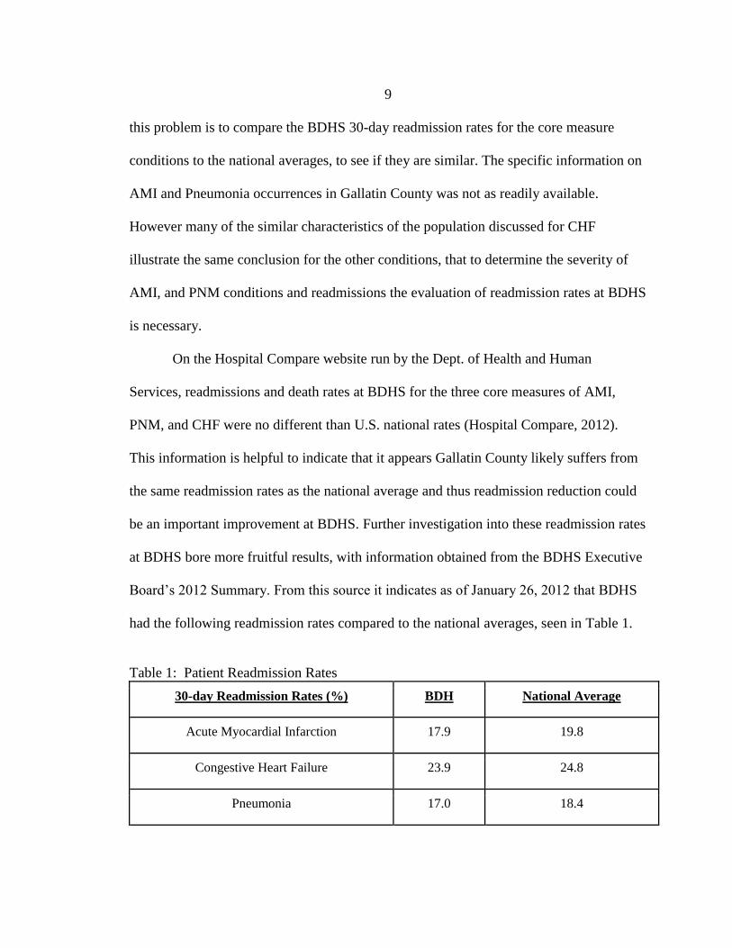
be an important improvement at BDHS. Further investigation into these readmission rates
at BDHS bore more fruitful results, with information obtained from the BDHS Executive
Board’s 2012 Summary. From this source it indicates as of January 26, 2012 that BDHS
had the following readmission rates compared to the national averages, seen in Table 1.
Table 1: Patient Readmission Rates
30-day Readmission Rates (%) BDH National Average
Acute Myocardial Infarction 17.9 19.8
Congestive Heart Failure 23.9 24.8
Pneumonia 17.0 18.4

10
Although these readmission rates indicate that BDHS is slightly below the
national average with respect to these important core measure metrics, this does not allow
for them to be complacent. It is important for BDHS to assess and improve these
readmission rates to stay ahead of the curve for readmission rate levels, so as to ensure
they are never at risk for potential reimbursement repercussions through the PPACA.
Furthermore, investigation into BDHS's readmissions is intended to develop an
understanding of risk contributing factors of readmissions which may be unique to the
BDHS patient population. The identification and understanding of these prediction
factors will be important to BDHS to address the implementation of interventions to
mitigate potential future readmissions. Without understanding the root causes of these
readmissions BDHS will be unable to reduce their readmission rates and could rise above
the national averages if improvements are made elsewhere. For this reason along with
BDHS's drive for continual patient quality of care improvement readmissions are a
problem area for improvement. An immediate focus on developing a thorough
understanding of readmission causation should ensue, with the intention to reduce
readmission rates.
Research Questions
Now that the current problem to be addressed has been established at both a
global level and at the research local level, the specific intentions of this research can be
articulated. With impending new regulations from the recent PPACA legislation
healthcare facilities will be monitored and reimbursed based on their level of quality of

11
care. BDHS as a small community hospital, in a more rural area, is not immune to these
new regulations and must review their current quality of care standing to ensure they are
performing appropriately. With readmission rates of the three core measures being a
primary focus of new regulations, a review of BDHS’s readmission rates suggested
potential improvements could be made. Therefore the primary aim of this project is to aid
in the improvement of the 30-day readmission rates of AMI, PNM, and CHF at BDHS.
For this research the primary champion of this intended improvement at BDHS, is
the Chief Nursing Officer (CNO), Vickie Groeneweg. This project is accompanied by
considerable support from all of the Chief Officers (CEO, CFO, and CMO) and Vice-
Presidents of BDHS, as well as the departmental managers. Finally, support is also
present from the BDHS Research Council, members including Montana State University
Professors, Dr. David Claudio of the College of Engineering, Industrial Engineering
Department and Dr. Elizabeth Kinion of the College of Nursing.
The research was performed in conjunction with Kallie Kujawa, a masters nursing
student at MSU, concurrently working as the Medical and Surgical Floors Clinical Nurse
Educator at BDHS. Joint research into the readmission topic at BDHS was performed
with Kujawa. This collaboration allowed for many components of the research to be
complemented with nursing and engineering thought processes and ideas. All
components of the research added to the breadth and depth of knowledge for this project,
but ultimately diverged to focus on slightly different themes of the research. Kujawa
(2012) focused her final research paper, “A Retrospective Review of 30-Day Patient
Readmissions in a Small Community Hospital to Determine Appropriate Interventions

12
for Improving Readmission Rates”, on the potential interventions possible to reduce
AMI, CHF, and PNM readmissions. A brief overview of the collaboration on this project
is illustrated in Table 2.
Table 2: Breakdown of Research Collaboration and Contributions
Project Component Collaboration
Investigation into US Readmission Topic Performed Jointly
Investigation into Local (BDHS)
Readmission Topic Performed Jointly
Data Acquisition Performed Jointly
Write-up of Research Performed Separately for Each
Individual's Research Focuses
Data Analysis/Methodologies of Research Performed Separately for Each
Individual's Research Focuses
Results and Discussion Performed Separately for Each
Individual's Research Focuses
Project Contribution To Body of
Knowledge Individual
Readmission Interventions Kallie Kujawa
Readmission Predictor Variables Matthew Lovejoy
Readmission Prediction Models Matthew Lovejoy
The primary focus of this thesis will be to aid BDHS in the reduction of
readmission rates by addressing three main research questions deemed important for
BDHS. The corresponding research questions and their hypotheses are described below.
The first research question is:

13
In adults older than 18 years of age who are admitted to BDHS, are there
contributing factors or characteristics of a patient which indicate a change in
likelihood of being readmitted?
Essentially this first question aims to find any variables about a patient which may be
indicators of a patient’s increased or decreased likelihood of readmission. The
corresponding null hypothesis is displayed below.
Hypothesis 1: Upon literature review and exploratory analysis of the general
readmission data from BDHS, no potential predictor variables of patient
readmission risk will be identified.
Then second research question is:
In adults older than 18 years of age who are admitted to BDHS, can they be
identified as being at high or low risk for readmission within 30-days, utilizing a
predictive model prior to their discharge?
This question builds on the first research question, that if factors are found to be
indicative of readmission can they then be used to create a model for future patients,
which could predict the patient's likelihood of readmission prior to their discharge from
their original admission. The corresponding null hypothesis to this research question is
displayed below.
Hypothesis 2: Upon analysis of readmission data from BDHS and the inclusion of
potential readmission risk predictor variables, the development of potentially
usable prediction models for patient readmission risk will not be achieved.
Both research questions will be addressed by the attempted development of readmission
risk prediction models, and the predictive variables indicated as statistically significant
for those final prediction models. Both of these research questions will initially focus on
general, AMI, CHF, and PNM readmission rates, but as research of BDHS’s patient
population is performed other diagnoses to evaluate may be added. Both of these research

14
questions aim to generate answers about readmissions for BDHS, so that they may
improve their patient quality of care and avoid risk of financial reimbursement reduction.
The final research question for this thesis involves the comparison of prediction
models developed by different analysis techniques. Originally in this research evaluation
of the readmission data was only to be performed by one analysis method, binary logistic
regression, however due to modeling difficulties early on for the general readmission data
it was decided prudent to test several analysis methods and compare their resultant
prediction models. The chosen analysis methods to compare were binary logistic
regression, classification and regression trees (CART) and multivariate adaptive
regression splines (MARS). Upon analysis of models the CART method proved
inappropriate and therefore the discussion, methodology and results of this method have
been excluded from the body of this thesis but attached in Appendix A. Therefore the
final research question is:
How do the prediction models developed by the separate analysis methods
compare, and what advantages or disadvantages are present between the models?
With the corresponding null hypothesis;
Hypothesis 3: Upon comparison of the modeling methods, the methods will
perform equally well.
For the modeling methods not only will predictive capabilities be investigated, but also
the appropriateness and ease of potential model implementation. The usability of the
model is an important component of this research for BDHS.
The reasoning for improvement of readmission rates at BDHS, and nationally, has
a two-fold answer. The first being that most healthcare organizations strive for continual

15
improvement in patient care and BDHS has a strong emphasis on this objective. Thus the
intended improvement in readmissions was triggered partially by the advancement for
continual support of BDHS’s mission which is “to improve community health and quality
of life” (Bozeman Deaconess Hospital, 2012). Moreover, the recent emphasis in
healthcare legislature on reducing 30-day patient readmissions has become a paramount
objective for all facilities. The PPACA legislation is the main organizational prompt for
the immediate review of readmissions at BDHS, acting as the primary prompt for this
research’s urgent focus on reducing readmission rates. The federal monitoring of 30-day
readmissions beginning in October 2012, which stems from the PPACA legislation,
began an instantaneous and invigorating push for readmissions to be evaluated, a project
already proposed in the strategic goals at BDHS, and aligned with this research.
In order to develop accurate readmission risk prediction models the patient
process related to a readmission is defined as beginning with an initial admission to
BDHS that later results, within some predefined timeframe, in having a readmission of
the patient back to BDHS. Consequently, the process to be reviewed not only takes into
account the information about the patient on the readmission visit, but also it is important
to know information about the prior admit visit, which resulted in the readmission. The
readmission to be investigated is an unplanned-related readmission. This type of
readmission indicates that a patient has returned to the hospital for the same or similar
medical reason they previously were admitted for, and it was not planned but rather their
health had deteriorated in some manner. This type of readmission has been termed a
Potentially Preventable Readmission (PPR) because during the prior admit or shortly

16
thereafter a gap in quality of care or condition occurred to allow the patient to relapse
with the similar condition requiring hospitalization. PPR's have recently become more of
a focus in healthcare, rather than all readmissions, because they hold the key to
substantial cost reductions and improved quality of care.
Patient visit information and how readmissions were determined will later be
discussed in the Methodology section. The timeframe chosen for evaluating readmissions
was 30-days due to the standard reporting and monitoring of readmission rates by CMS
with this timeframe. The data for this research was obtained by retrospectively assessing
the 30-day readmission patient population data at BDHS for patient visits which had
discharges from January 2009 through December 2010. The goal was then to answer the
two primary research questions through analysis of the historical patient data, striving for
enabling a potential reduction in readmission rates of the core measure at BDHS, to
ensure they remain substantially better than the U.S. national rates.
Readmission Predictive Models
In an attempt to mitigate readmissions a recent strategy is creating models which
can predict a patient’s risk of becoming a readmission. These models can be powerful
tools if implemented correctly and proven to be accurate for the intended population of
the model. The benefit to healthcare facilities from a properly developed predictive
model would be the capability to identify patients at high risk for readmission and to then
mitigate their likelihood of readmission through deliberate interventions (Kujawa, 2012).
Specialized, individualized, readmission risk assessment tools, such as predictive models,

17
are a statistically proven way to determine those patients at higher risk for readmission
(Walraven et al., 2010; Hasan et al., 2009; & Kansagara et al. 2011). Once a prediction
model is available for assessing patients at greatest risk for readmission at BDHS,
resources for reducing the prevalence of readmissions can be efficiently and with fiscal
responsibility directed to those patients who are identified as being at the greatest risk for
readmission. Therefore considerable value to patient quality of care could be created by
functional readmission risk predictive models. These models would allow for the
targeting of the high readmission risk patients with precision, such that resources of a
healthcare facility could be distributed to the patient population where the most benefit to
cost is present.
A brief overview of the prediction models to be investigated is as follows. For
purposes of this study the desired type of readmission to investigate is Potentially
Preventable Readmissions (PPR), defined as readmissions unplanned, medically related
and within a 30-day timeframe of a prior visit. The investigation of "all-condition" or
general readmissions as well as diagnoses specific readmissions will be performed.
Specifics on the type of readmission investigated can be found in the Methodology
section of this paper. For purposes of the readmission risk models patient visits must be
quantified as a readmission and then the admissions to the readmission or "Admit to
Readmit" (ATR) identified. For predictive capabilities the information from the ATR
visits will be used to incorporate patient information known prior to the readmission visit.
The ATR binary variable will be used as the target variable, with predictor variables
being in binary, categorical or continuous form.

18
The methods of prediction model development will be binary logistic regression,
using a forward conditional variable entry method, in IBM SPSS (v. 21); as well as
Multivariate Adaptive Regression Splines (MARS) analysis from Salford Predictive
Miner (v. 6.8). As discussed briefly before classification and regression tree (CART)
analysis method was also performed but removed from this research due to poor
performance, with Appendix A containing the research information related to CART.

19
LITERATURE REVIEW
Readmissions
After assessing and identifying the need for continual improvement of the
readmission rates at BDHS, the literature was searched to locate examples of readmission
risk predictive models. Recently many studies have been conducted on models for the
prediction of readmissions to reduce the rate of readmissions for conditions such as AMI,
CHF and PNM. Articles, descriptive studies, model reviews, presentations and other
literature were located by searches in article and research databases such as Compendex,
Knovel, CINAHL, PubMed, Cochrane Library, and Medline. Search terms included
"preventable readmission", "readmission rates", "readmissions", "30 day readmission
rates", "30-day readmission rates", “reducing readmission rates", "predicting
readmissions", "readmission predictive models", "readmission risk assessment", "Lace
index", "decision tree analysis", "CART models", and "MARS models".
Potential Variables for
Readmission Risk Predictors
In consideration of research question one the investigation in literature for
suggested predictor variables for readmission risk was performed. The literature reveals
many potential causes for general patient readmissions, along with interventions and
strategies for reducing their prevalence. Several factors that influence patient readmission
rates could include the availability and usage of disease management programs and the
bed supply of the local health care systems (Fisher et al., 1994). Disease management

20
programs could include things such as follow-up appointments, and home health services
which may not be available in a more rural community such as Gallatin County. The
Fisher et al. (1994) study compared multiple diagnoses readmission rates for Medicare
beneficiaries in Boston, Massachusetts and New Haven, Connecticut and showed that
these rates were consistently higher in Boston. The researchers found no evidence that
this was due to initial causes of hospitalization or severity of illness They concluded that
the difference in readmission is likely to be dependent on the care delivery system
characteristics, in this case the influence of hospital-bed availability on decisions to admit
patients (Fisher et al., 1994). Several other studies, including Naylor et al. (2004), Rich et
al. (1995), and Phillips et al. (1995), have shown the effects of discharge and follow-up
interventions and programs delivered by nurses on reducing the rates of readmission,
especially for older patients. These findings support the inclusion of variables related to
discharge disposition, family support (possibly marital status) and distance from hospital
because they may impact a patient's ability to get appropriate post-discharge treatment,
thus increasing their chances of readmission.
In the report presented by the Congressional Research Service on Medicare
Hospital Readmissions (Stone & Hoffman, 2010), the authors found seven factors as the
most likely causes of patient readmissions based on collective opinions of policy
researchers and healthcare practitioners. These include an inadequate relay of information
by hospital discharge planners to patients, caregivers, and post-acute care providers; poor
patient compliance with care instructions; inadequate follow-up care from post-acute and
long-term care providers; variation in hospital bed supply; insufficient reliance on family

21
caregivers; the deterioration of a patient’s clinical condition; and medical errors (Stone &
Hoffman, 2010). Almost all of these factors point to the discharge process area as a key
breakdown in quality of care. Therefore obtaining as much information about discharge
characteristics such as location, time of year, disposition, follow-up appointments
planned, etc. should be attempted.
Jencks et al. (2009) states that “although the care that prevents rehospitalizations
occurs largely outside hospitals, it starts in hospitals.” So even though evidence may
indicate post-discharge characteristics as primary readmission risk increasing factors,
readmission risk needs to be addressed within the hospital stay. If an acute care hospital,
such as BDHS, can identify those patients who are more at risk for being readmitted
within 30-days, by readmission risk predictive models, it can then promote better follow-
up care and deploy more interventions at the time of discharge for that particular
population at high risk. Walraven et al. (2010) developed a readmission assessment tool
called the LACE index. Two previous readmission tools have been published and
Walraven et al. (2010) took these existing tools into consideration before designing a new
tool but found that the other tools were impractical to actual clinicians. The previously
published tools used patient characteristic variables that were not readily available in the
patient record and therefore the clinician would have to spend time locating information
to perform an accurate readmission risk assessment. The LACE index incorporated
variables easily identified by clinicians prior to a patient's discharge and was one of the
first pre-discharge readmission risk assessment tools. The statistically significant
variables for assessing readmission risk, according to a 95% confidence interval from the

22
Walraven et al. study, included length of stay, acute emergent admission (the current visit
was an admission through the ER), comorbidity and number of previous emergency room
visits in the past six months. This study supports the use of length of stay (LOS),
admission from the ER and the count of the prior six months emergency room visits as
good variable candidates. Unfortunately it is known that currently BDHS has no tool for
the easy calculation of a comorbidity index such as the Carlson Comorbidity Index, so
comorbidity will not be included but could be a recommendation for future recorded
information.
An informative article by Hasan et al. (2009) examined the literature and grouped
patient variables into four categories: sociodemographic factors, social support, health
condition and healthcare utilization. They then performed a logistic regression analysis
on unplanned readmission within a 30-day timeframe and developed a readmission risk
prediction model. Their study determined variables including insurance type, marital
status, having a regular physician, number of admissions in the past year, Charlson index
and length of stay were statistically significant predictors. Again these are more
appropriate variables to potentially incorporate in analysis of readmissions.
Probably the most informative article on many aspects of readmission prediction
variables and models is a study by Kansagara et al. (2011) which reviewed all
discoverable models through CINAHL, Cochrane Library, and Medline published up to
March 2011 which related to predicting readmissions. They then evaluated article
relevancy based on their parameters including articles having validated readmission
prediction models, and written in English. Their objective was to summarize the validated
23
readmission prediction models, indicating their patient populations, prediction successes,
usability, data collection methods, variable use, and models compared within a
population. They discovered 30 articles with 26 unique models to be systematically
reviewed. From their article commonly used variables categories included (paraphrasing):
specific medical diagnoses, mental health comorbidities, illness severity, prior use of
medical services (hospitalizations-IN, ER, clinic, LOS), overall health and function,
sociodemographic factors (age, sex, race), and social determinants of health (insurance,
marital status, social support, access to care, discharge location) (Kansagara et al., 2011).
Variables in this list were included in discussions of appropriate variables for the BDHS
readmission risk prediction models.
In an article about Medicare rehospitalization by Jencks et al. (2009) the authors
discuss the variables they determined to be predictors for the Medicare patient population
all-cause readmissions. Some of these predictor variables were number of
hospitalizations, length of stay, race, disability, sex and age (Jencks et al. 2009).
Three articles, prepared for CMS, by Krumholz et al. (2008) which are hospital
30-day readmission measure methodologies for AMI, CHF and PNM were also good
resources for variable exploration. The authors suggest and implement the use of
predictor variables of the 189 Hierarchical Condition Category (HCC) clinical
classification systems developed for CMS. The HCC algorithm was develop to group the
15,000+ ICD-9 codes into 804 "diagnoses groups" and then into 189 condition categories
(CC). Krumholz et al. (2008) then uses a 154 subset of these CCs, deemed relevant to
readmissions by experts, grouped again into more condition related groups now
24
representing approximately 95-97 indicator variables as readmission risk predictors,
while only using demographic predictor variables of age and sex, and four ICD-9 code
groups for patient history variables. These reports by Krumholz et al. (2008) were the
only articles found that expressly searched all "conditions" as readmission predictors.
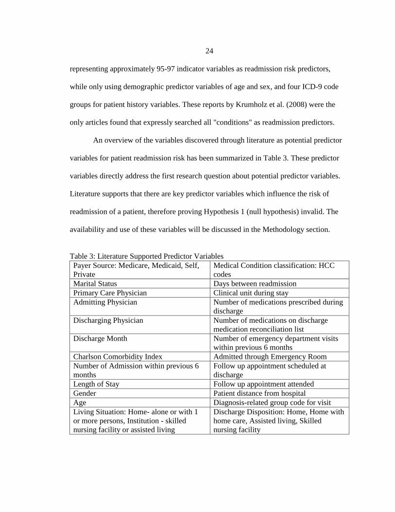
An overview of the variables discovered through literature as potential predictor
variables for patient readmission risk has been summarized in Table 3. These predictor
variables directly address the first research question about potential predictor variables.
Literature supports that there are key predictor variables which influence the risk of
readmission of a patient, therefore proving Hypothesis 1 (null hypothesis) invalid. The
availability and use of these variables will be discussed in the Methodology section.
Table 3: Literature Supported Predictor Variables
Payer Source: Medicare, Medicaid, Self,
Private
Medical Condition classification: HCC
codes
Marital Status Days between readmission
Primary Care Physician Clinical unit during stay
Admitting Physician Number of medications prescribed during
discharge
Discharging Physician Number of medications on discharge
medication reconciliation list
Discharge Month Number of emergency department visits
within previous 6 months
Charlson Comorbidity Index Admitted through Emergency Room
Number of Admission within previous 6
months
Follow up appointment scheduled at
discharge
Length of Stay Follow up appointment attended
Gender Patient distance from hospital
Age Diagnosis-related group code for visit
Living Situation: Home- alone or with 1
or more persons, Institution - skilled
nursing facility or assisted living
Discharge Disposition: Home, Home with
home care, Assisted living, Skilled
nursing facility
25
Readmission Risk Predictive Models
The proposed readmission predictive models for the BDHS data will evaluate
both general readmissions and readmissions linked to specific diagnoses. Furthermore, it
is intended to investigate the type of readmissions that have the best prospective for
reducing costs and improving quality of care. Many versions of readmission predictive
models have been created, addressing different types of readmissions as well as for
different patient populations based on characteristics such as diagnoses, age, and health
insurance provider. Therefore it is appropriate to get a basic understanding of the varying
characteristics of the readmission risk predictive models previously created.
The first characteristic of potential readmissions to review is whether the
readmission was planned or unplanned. A planned readmission was a previously
determined hospital visit based on medical necessity already known during a prior visit.
Therefore planned readmissions rarely can be avoided because there is not a gap in
quality of care. The focus of almost all readmission studies is on unplanned readmissions,
which are also termed "early", "early unplanned", "late unplanned", "potentially
avoidable", "potentially preventable", "shortly after discharge", "short term", or
"unexpected"(Vest et al., 2010). "Unplanned hospital admissions and re-admissions are
regarded as markers of costly, suboptimal healthcare and their avoidance is currently a
priority for policy makers in many countries" (Billings et al., 2012). These readmissions
are commonly categorized as preventable because most of the time these unplanned
readmissions are linked to previous admissions, and therefore can be attributed as a
failure in patient quality of care. Vest et al. (2010) bluntly states "preventable hospital

26
readmissions possess all the hallmark characteristics of healthcare events prime for
intervention and reform." Since BDHS wants to attempt to reform any problem areas in
their healthcare platform, so as to improve patient quality of care and avoid unnecessary
costs or reduced reimbursement, the unplanned readmissions are the appropriate focus.
The article by Vest et al. (2010) evaluated the current literature for "research studies
dealing with unplanned, avoidable, preventable or early readmissions" and found that 37
adult population research studies in the US were present. Similarly to Kansagara et al.
(2011), Vest et al. (2010) investigates the different characteristics of the 37 research
studies investigating unplanned readmissions. Of the 37 research studies nine were
general, all-condition readmission related, 13 were cardiovascular related (CHF,AMI,
etc.), five were surgical related and the remaining five studies were diagnosis specific (2-
Diabetes, PNM, brain injury, and cancer) related readmissions (Vest et al., 2010). This
breakdown indicates the high prevalence of cardiovascular related readmission studies, as
well attempts for general readmission prediction, but minimal studies performed on
potentially preventable readmissions for PNM and other specific diagnoses. Therefore the
proposed predictive models for PNM and any other non-cardiovascular diagnoses
developed will be distinctive.
The next characteristic is the timeframe to review visits as readmission. Many
different timeframes have been used in regression studies ranging from seven days to one
year, but the most common is using a 30-day timeframe (Vest et al., 2010; Kansagara et
al., 2011) From the articles of multiple regression studies review (Vest et al., 2010;
Kansagara et al., 2011) the largest proportion of models (24/37 and 16/26 respectively)
27
use a 30-day timeframe. This is to be expected because CMS reports on 30-day
timeframe readmissions and the PPACA will enforce standards on the same 30-day
readmission rates (Stone & Hoffman, 2010).
When reviewing the data acquisition procedures for readmission information the
prediction models found in literature according to Kansagara et al. (2011) included 14
models which relied on retrospective data, three on administrative data, and 12 models
actually had primary data collection through surveys or chart reviews (Kansagara et al.,
2011). From this it seems using retrospective analysis is the most common method. The
patient population samples used for development and validation of predictive models
varied considerably from several hundred (min=173) to millions (max~ 2.7 million) of
samples per study (Vest et al., 2010; Kansagara et al., 2011). Similarly there was a wide
range of proportional division of the population data used for “train” samples, the data
used to develop models, and “test” samples, the data used for independent validation of
models. These ranged in the literature from a 50/50 split of data to 100% train data either
with no validation or through non-independent validation techniques such as cross
validation (Vest et al., 2010; Kansagara et al., 2011).
Of the 30 studies of risk prediction models for hospitals, evaluated by Kansagara
et al. (2011), 23 of 30 were from the US health care, with 13 of these studies including
only patients 65 and older, with 7 relying solely on Medicare data and 4 using Veterans
Affairs data (Kansagara et al., 2011). Furthermore of all the studies only one indicates a
focus on a small rural community (in Ireland), while all others are either large city, whole
state or nationally related readmission models. Six of the 26 studies compared multiple

28
readmission risk models for a population, all using the C-statistic as the primary form of
comparison (Kansagara et al., 2011).
Upon review of the literature the most commonly studied type of readmissions
risk prediction models had the below patient and readmission characteristics:
30-day timeframe Older population (65+ years) Medicare or Veterans patient population
Large population pool; national, statewide or multi-hospital population Cardiovascular related readmissions or “all-condition” readmissions
General readmission, not PPR because difficulties in effectively defining the PPR
visits
Types of Predictive Models
A wide range of predictive tools are available for evaluating healthcare topics
such as readmissions. To determine what tool is most appropriate for the respective
research is an ever transforming challenge as more is determined and understood about
the patient population and desired outcomes from the predictive models. Two
characteristics, among many, of predictive models to contemplate during selection are
complexity and traditionalism.
Forms of statistical evaluation have ease of understanding ranged in development
from basic-layman understanding to highly complex and expert-knowledge based. One of
the conditions commonly associated with complexity of statistics for a predictive model
is an understandability/prediction success tradeoff. As more complex statistic evaluation
methods are used to develop predictive qualities from data they generally incorporate
more interactions and transformations than the simple models. These interactions and
transformations make it more difficult to understand specific impacts of predictor

29
variables on an individual level but allow for a better prediction success. Conversely a
simple model which may be easily understandable may have poor prediction success.
This tradeoff is influential based on what type of intended audience and capabilities are
desired from the final predictive models
The next characteristic of the readmission predictive models to consider is the
traditionalism, or common practice of use, of the type of models. There is a wide range of
predictive models based from classical statistics to highly advanced theoretically
statistical evaluation models. Commonly predictive model characteristics which are based
in classical statistics are used because these types of models have been more widely
taught and historically proven as reliable or appropriate methods. More modern
prediction model techniques through advanced mathematics and algorithms are also
potential candidates. Since these modern techniques have been introduced only in the
past few decades they are less frequently present in academically mainstream statistics,
but have been proven reliable. Some examples of more classical predictive model choices
are using linear regression or logistical regression, while newer predictive model choices
are decision trees and algorithm based regression models.
Another characteristic of the predictive models is what type of dependent or target
variable will be used. For purposes of readmission risk models patient visits are
commonly quantified as a readmission and then the admissions to the readmission or
"Admit to Readmit" (ATR) is also identified, with either both of these variables having a
yes/no answer. For predictive capabilities the information from the ATR visits will be
used to incorporate patient information known prior to the readmission visit. Therefore

30
since ATR visits will be used to develop the predictive models the ATR identifying
variable will be a binary variable, to be indicated by a "0" for not an ATR visit and a "1"
for an ATR visit. By having a binary target variable as well as the potential for binary
type predictor variable it may be appropriate to consider logistic regression (Johnson &
Wichern, 2002). In the development of appropriate variables for these models it is likely
categorical variables, having discretely defined levels within the variable, will be useful
classifiers.
Due to the presence of categorical variables some viable model options may also
be the newer, computer intensive approach of classification and regression trees (CART),
and the even more complex and novel neural network algorithms (Johnson & Wichern,
2002). Since the early 1990's another method of developing prediction models with
complex categorical variable data became feasible, termed multivariate adaptive
regression splines (MARS). MARS is a procedure for fitting adaptive non-linear
regression that uses piecewise basis functions to define relationships between a response
variable and some set of predictors (Friedman, 1990). These four model types pose some
of the best potential candidates for appropriate modeling of the data available from
BDHS for readmission risk prediction. The last two methods are highly computer
intensive, algorithm search based type methods.
For nearly all readmission prediction studies found in the literature multivariate
statistics were used in evaluation of the readmission visits (Vest et al., 2010). For
medically related models the most common statistical analyses used included multivariate
linear regression, logistic regression, binary logistic regression, decision tree analysis and

31
regression splines. Logistic regression was overwhelmingly the most common prediction
modeling method used for readmission risk, and has been widely accepted in the
healthcare industry as a tool for readmission risk prediction (Vest et al., 2010). Therefore
more of a focus on the use of the less common modeling technique of MARS will be
discussed.
The Multivariate Adaptive Regression Splines tool MARS is a highly advanced
algorithm based regression modeling tool. It claims to be the "world's first truly
successful automated regression modeling tool" (Salford Systems, 2001). The
methodology and non-software components were developed in 1990 by CART co-author
Jerome Friedman in his publication Multivariate Adaptive Regression Splines (Friedman,
1990). The MARS software "enables you to rapidly search through all possible models
and to quickly identify the 'optimal' solution" (Salford Systems, 2001). MARS is
proprietary information and does not completely reveal the algorithms it uses for
intelligent searches but is summarized as "MARS essentially builds flexible models by
fitting piecewise linear regressions; that is the nonlinearity of a model is approximated
through the use of separate regression slopes in distinct intervals for the predictor
variable space" (Salford Systems, 2001). The capability of MARS to not depend on
variable linearity or normality (parametric) assumptions allows for it to be advantageous
for a dataset like the BDHS readmission population. MARS will output many attempted
regression models and illustrate the one which is termed "optimal" based on the smallest
generalized cross validation (GCV) value. The GCV value is not a cross validation in the
typical sense but actually is a penalized version of a mean-squared error due to the

32
inherent degrees of freedom penalty estimations on final model predictor variables. Each
model will show the basis functions entered in a forward stepwise type regression and
then the model found optimal after "pruning back" through backward stepwise
regression. Salford Systems maintains over 500 records of literature related to the use of
their software on their website, www.salford-systems.com, indicating the vast use of
these methods. For specific information on the methods, parameters, uses, capabilities
and components of MARS please refer to either Friedman, (1990) or Salford Systems
(2001).
At the time of this original literature review, spring 2012, no discoverable
readmission risk prediction models by the CART and MARS software was found; rather
only primarily logistic regression models had been attempted. Several articles using
CART or MARS were discovered for predictions of mortality risks, multi-disease risk,
cardiovascular risk, and other models for scientific areas such as Ecology. Since then an
increased focus on readmissions has advanced the pursuit of predictive models and the
potential for new recently published predictive models using CART and MARS is
feasible. A quick literature review search for recently published models revealed two key
new findings. One article "Leveraging derived data elements in data analytic models for
understanding and predicting hospital readmissions" published in November 2012 used
random forests, an advanced CART procedure, to predict risk of readmission through an
automated system linked to EMR data (Cholleti et al., 2012). A presentation dated June
of 2012 predicted hospital readmissions using TreeNet, a Salford Systems advanced
analysis method using CART built models, but indicated the results discussed still as

33
unpublished data (Aronoff, 2012). With minimal findings of CART and MARS
readmission risk prediction models, the performed research for BDHS will be distinct to
previous readmission models. A brief overview of medicine and science related articles
using CART and MARS models will be presented.
A logistic model can be either a general additive logistical model or a linear
logistic model associated with general linear models, based on some of its characteristics.
The binary logistic model commonly used is more related to the GAM models because an
algorithm (i.e. Forward stepwise-conditional) is used for the entrance of variable that
does not presume linearity between the dependent and independent variables. Similarly
CART and MARS models are identified with General Additive Models, classified as
non-linear and non-parametric models. "MARS is a nonparametric logistic regression
analysis that is close procedurally to the simple parametric logistic regression analysis
because of the variable selection through stepwise regression analysis" (Nash &
Bradford, 2001). These models have strong use potential in the medical field where
linearity of a target variable to predictor variables is not commonly true. Furthermore
since the models are non-parametric the predictor variables are not required to fit a
predetermined distribution but rather their form is determined according to information
derived from the data.
In the "Introduction to Salford Predictive Modeler" article some key differences
between logit (logistic regression) and CART models are discussed (Steinberg et al.,
2012). Advantages of CART are automatic analysis, surrogates for missing values and
unaffected outliers, with weaknesses of a discontinuous response and course-grained

34
models meaning CART can only predict as many different probability cases as number of
nodes in the decision tree (Steinberg et al., 2012). Comparatively logit's strengths are
continuous smooth response, can capture global weak effects, and unique predicted
probability for every record, with weaknesses of being sensitive to outliers, requiring
hand-built models and deletion or imputing of missing values (Steinberg et al., 2012).
Logistic Multiple Regression, Principal Component Regression, CART and
MARS were compared for their predictive modeling success by Munoz and Felicisimo
(2004) and their results indicate the MARS and CART models performed best, but the
CART model was difficult to implement due to the high complexity. In Munoz and
Felicismo's study as well as with all the comparative models previously discussed by
Kansagara et al. (2011) the C-statistic or area under the curve (AUC), the curve being the
receiver operating characteristic (ROC) curve, was used as the metric for comparison.
Similarly Gutierrez et al. compared the use of CART and MARS for a predictive model
of gully erosion, showing a better performance by MARS than CART with high AUC
values of 0.98 and 0.97 with validation datasets (Gutierrez, 2009). In the study performed
by Nash and Bradford (2001) they indicate their intention for their report to be "a
reference manual that can be used by investigators for making informed use of logistic
regression using two statistical methods (standard logistic regression and Multivariate
Adaptive Regression Splines (MARS))" (Nash & Bradford, 2001). Their report discusses
how standard regression is quantified as a GLM and MARS as a GAM and that if the
goal is to "examine the structural relationship between a response and independent
variable, especially when there is little or no knowledge about the data, then GAM is the

35
method to use" (Nash & Bradford, 2001). From this it would indicate that likely MARS
will be a better model for the BDHS readmission data since the variable relationship
structure is desired. Their model test results, though for a smaller and non-medical
purpose, indicated no difference in the logistic regression and MARS models (Nash &
Bradford, 2001). The implications of these results may be that the usability of MARS is
only preferred of logistic regression in specific data type scenarios, and a generalization
of MARS superiority to logistic regression is not appropriate.
Five CART or MARS models were discovered for medically related predictions,
including days in bed due to illness, mortality risk (3 models) and disease predictions.
These are discussed below. An informative article by Razi and Athappilly (2005)
indicated the noteworthy improvement in predictive ability of CART and neural networks
(NN) over their logistic regression model:
It is obvious from the study results that NNs and CART models provide
better prediction compared to regression models when the predictor
variables are binary or categorical and the dependent variable
continuous. However, neither NNs nor CART model showed clear
advantage of one over the other. For application standpoint, either one of
NNs and CART models may be used for prediction and would provide
better predictability over regression (Razi & Athappilly, 2005).
From this statement it is evident that since many of the predictor variables for risk of
readmission will be categorical variables, as well as the binary target variable and
potential predictor variables, that CART should be an improved predictive model over
the traditional non-linear, logistic regression.
Three of the medically related CART and MARS prediction models involved the
prediction of a risk of mortality for some a population. Austin compares the predictive

36
capabilities of "regression trees, logistic regression, generalized additive models, and
multivariate adaptive regression splines for predicting AMI mortality" (Austin, 2007).
This study evaluated the different models prediction success and found that regression
trees did not perform as well as logistic regression for predicting mortality following
AMI, and logistic regression had performance comparable to the GAMs and MARS
tested (Austin, 2007). Similarly in a study by Colombet et al. (2000) CART was found to
perform slighlty lower than logistic regression and multilayer perceptron models for
predicting cardiovascular related mortality risk (Colombet et al., 2000).These studies are
interesting because one found essentially no benefit to using a MARS model over
traditional logistic regression and both indicated CART performed worse than logistic
regression. From these results it is feasible that CART and MARS models for the BDHS
data may not be better fits than logistic regression and that is why a comparison of all
three model types should be performed.
The last mortality study tested for the feasibility of a MARS model being used in
predicting in-hospital mortality risk, with no comparisons to other model types. Silke et
al. (2010)determined a feasible MARS model could be developed to predict in-hospital
moratality risk and the model resulted in AUC values of in the 0.92-0.93 level (Silke et
al., 2010).
The final medically related article to use MARS testing attempted to predict
multiple disease risk probability, simultaneously predicting hypertension and
hyperlipidemia. Chang et al. (2011) use common risk factors for hypertension and
hyperlipidemia to build a MARS predictive model which exhibited a 93.07% accuracy

37
(Chang et al., 2011). This paper and all the previously discussed CART and MARS
related articles mainly attribute positive improvement to prediction by the use of CART
or MARS over basic logistic regression techniques. However, several reported studies did
not indicate any benefit to using CART and MARS, thus the proposal still stands to
compare these model types with binary logistic regression for the BDHS data.
Thesis Research versus Literature Synopsis
First a brief overview of the type of variables and prediction models developed in
this research is discussed below and then compared to the current literature. The
reasoning for the chosen variables and prediction model attributes is discussed in the
Methodology section. In reference to potential predictor variables included in the
predictive models the variables presented in Table 3 were attempted for inclusion.
However, several of these variables were unavailable from BDHS and were not included;
these being the Charlson Comorbidity Index, the follow-up care information, and the
medical condition classification by HCCs. In an attempt to emulate the Charlson
Comorbidity Index as well as the medical condition classification HCC variables the
inclusion of primary and secondary diagnoses ICD-9 codes were incorporated. Another
addition of variables for this research was from the inclusion of predictor variables of the
type of drugs prescribed for a patient.
For the readmissions to be evaluated for BDHS the primary characteristics will be
a 30-day timeframe, a PPR visit (unplanned, medically related), the patients come from a
small rural community population. In addition, patients are age 18 and older, all payer

38
types (Financial Classes) and both general and medical condition specific readmissions
will be reviewed.
In comparison to literature the unique contributions of this research are related to
the PPR visit instead of all readmissions being evaluated, and that the patient’s come
from an institute specific small rural population. Also commonly in literature the
Medicare population is payer type population of interest, but for the BDHS data all payer
types will be investigated. The timeframe, age and medical condition types investigated
are similar to those presented in literature. Therefore models developed for BDHS
addressing PPR readmissions, with 18+ patient ages, and hospital specific data of a small
community population will be additively unique to the current readmission predictive
models available.
With respect to modeling techniques, this thesis research will focus on binary
logistic regression and MARS. The literature review depicted logistic regression as the
primary method (developed in SPSS); therefore the inclusion of the MARS method for
model development is a potential contribution to literature. Also the comparison of the
SPSS and MARS models will be another unique contribution of this research to the
literature.
Finally, prediction models were developed for the general and core measures, as
well as for diagnoses specific conditions found prevalent at BDHS of Cardiac
Dysrhythmias (ICD-9 Code 427) and Disorders of the Function of the Stomach (ICD-9
Code 536). Overall the proposed research methods build on the discovered readmission
commonalities in literature, while also having unique qualities.
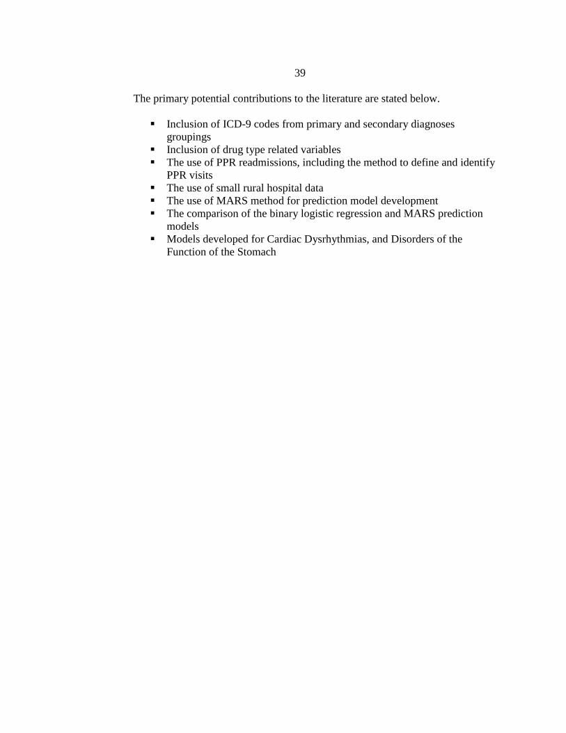
39
The primary potential contributions to the literature are stated below.
Inclusion of ICD-9 codes from primary and secondary diagnoses
groupings
Inclusion of drug type related variables
The use of PPR readmissions, including the method to define and identify
PPR visits
The use of small rural hospital data
The use of MARS method for prediction model development
The comparison of the binary logistic regression and MARS prediction
models
Models developed for Cardiac Dysrhythmias, and Disorders of the
Function of the Stomach

40
METHODOLOGY
The methods used for this research will be discussed in the following sections.
The development of these methods was an iterative process during the beginning phases
of research and literature review when attempting to develop the best understanding of
the readmission topic as well as the most applicable analysis techniques. For this research
it was determined to evaluate readmissions categorized as PPRs, to look at both general
and condition specific readmission populations from BDHS, and to include all patient
payer types and age over 18.The evaluation of the general readmission data for predictor
variables which may indicate readmission risk is also described. In reference to the
prediction models the use of binary logistic regression and MARS methods were
performed and discussed.
Ethical Issues
Prior to beginning any project involving human subjects, it is necessary to
consider ethical issues. One ethical issue related to this project includes privacy concerns
for patient health information and the potential to violate the Health Insurance Portability
and Accountability Act (HIPAA). Since this portion of research will only be looking at
the historical data another ethical concern of potential harm to participating patients’
physical well-being is not an issue. An additional ethical concern is that during this
project there could be room for potential conflicts of interest to arise. A potential conflict
of interest could be if financial or promotional benefits for the researchers were tied with
the successful development of usable predictor variables or prediction models for BDHS.

41
Therefore the primary ethical issue to address is protection of the private patient
health information. To address this ethical concern, researchers have signed HIPAA
agreements through Montana State University and through BDHS; researchers have been
certified in human subject participation; and patient data has been de-identified at BDHS
prior to being analyzed to protect patient identity and privacy. Further effort to protect
patient information was fulfilled by the mandatory application, with multiple addendums,
and approval of research by the Institutional Review Board (IRB) at Montana State
University. The IRB, and legal counsel of BDHS, accepted the application for research
and granted permission for research to be performed on March 5, 2012, based on the
application submitted for “A Retrospective Review of 30-day Patient Readmission in a
Rural Community Hospital”. Slight modifications were made to the IRB in September
2012 and again approved September 20, 2012. The application for sanctioned research to
the IRB can be found in Appendix B, along with the IRB approval letter in Appendix C,
and the approval letter for the modification in Appendix D. Finally conflicts of interest
have been avoided by ensuring that there are no financial or promotional benefits to the
researchers.
Patient Population
The first vital component of this research was to determine the appropriate patient
population to perform readmission analysis on, as well as evaluate population
characteristics. The patient population was determined to be best represented by several
years of historical patient data which was actual patient admissions to BDHS. A critical
42
factor in determining this population data was the availability of records through the
BDHS Electronic Medical Record system (EMR). To understand the availability of this
data and export the necessary population information required collaboration with BDHS's
Information Systems (IS) department.
Data Acquisition
Upon consultation with the IS department a major limiting factor was discovered.
Viable data was limited to only several historical timeframes. This was due to the recent
deployment of the EMR system for BDHS in the past decade, as well as many
modifications to linked electronic record programs throughout the existence of the EMR.
From discussion with Kindred and Nelson it was determined an optimal window of
viable data for research would be the years of 2009 and 2010, because the full EMR
system was in place as well as limited modifications of programs causing interruptions in
potential data entry. Therefore it was decided to use the BDHS historical data of all
patient admissions to the hospital for which patients were discharged during January
2009 through December 2010 timeframe.
This data set would allow for the retrospective review of patient readmissions
during the two-year period of 2009-2010. A critical assumption for this research is that
the patient population of this two year period is similar to the patient populations of
BDHS's future, for which research findings may be utilized to predict readmission risk. It
is assumed the patient population has not altered substantially in the several years
between this historical data and the potential future patients in 2013 that BDHS may

43
attempt to predict readmission risk, because no considerable Gallatin County population
changes have occurred.
Desired Patient Variables from EMR
The EMR system allows for recording of many characteristics and information
about patient visits. Some of this information is pertinent to this research, while a
majority of other data is frivolous or personal information in relation to the research
needs. Therefore the necessary next step to obtain usable data for the research was the
determination of patient characteristics, which the EMR retained, that could be used as
predictors to readmission likelihood. For this step heavy reliance on past literature was
necessary to indicate variables which had the potential to be influencing factors on
readmissions. This section focuses on answering the first research question of this thesis,
the predictor variables potentially impacting readmission risk.
Variables that contribute to the patient’s risk for readmission were discussed and
recorded in the literature review section. The study by Hasan et al. (2009) examined the
literature and grouped patient variables that have been shown to contribute to the risk of
readmission. A second study by Kansagara et al. (2011) also reviewed the many models
related to predicting readmissions, and outlined the most commonly used variables for
these studies. A list of variables was derived using variables discovered from the
discussed studies and the variables used in the LACE model study conducted by
Walraven et al. (2010), Table 3, and from variables discussed as important with BDHS
healthcare professionals (Drug Types added).

44
This variable list was then discussed with the IS department liaisons and was
compared to the available electronic health record information present during a patient’s
current admission at BDHS. Several of these variables, listed in Table 3, were found to
not be retrievable from the BDHS patient data. The Charlson Comorbidity Index (CCI)
takes into account several critical secondary diagnoses or patient history variables when
attempting to model readmissions. Unfortunately it was unavailable for use for the BDHS
data. Therefore to attempt to capture hidden interactions or influence, the inclusion of all
potentially coded ICD-9 codes was chosen. Also the HCCs act as another CMS approved
condition grouping of the ICD-9 codes, but is much less common to most healthcare
facility codes. BDHS did not have patient conditions recorded in the HCC formats but
rather ICD-9 therefore was more practical to include ICD-9 code related variables rather
than attempting to develop the HCCs. Both of these reasons for the inclusion of ICD-9
codes for this research, resulted in the primary and secondary ICD-9 codes listed for the
patient, to be filtered into their respective ICD-9 primary digit groupings and be retained
as variables. The literature supported predictor variables found to be unavailable; along
with the predictor variables added to this research are summarized in Table 4.
Table 4: Unavailable and Additional Predictor Variables for Research
Desired Variables which were
Unavailable
Desired Variables in Addition to
Literature Supported
Charlson Comorbidity Index ICD-9 Code Primary Diagnoses variables
Follow Up Appointment Scheduled
before discharge
ICD-9 Code Secondary Diagnoses variables
Follow Up Appointment attended Drug Type variables: # prescribed, #
administered, Difference of # prescribed vs.
administered, drug type present in patient
admission variables

45
Along with the unavailability of the CCI and the HCC codes, there were two
primary differences from literature in variable inclusion for this research. First it was
desired to include all International Classification of Diseases, Ninth Revision, Clinical
Modification (to be abbreviated ICD-9 for purposes of this paper), primary and secondary
diagnoses codes of the visit as potential variable predictors. This was in the hope to
determine if hidden affects may be missed if they are not included. Previous studies only
sometimes use a specific primary diagnosis or the Charlson Comorbidity Index to attempt
to include potential influence from diagnoses on readmissions. Only in the Krumholz et
al. (2008) studies had something similar to including all ICD-9 code groups been used,
and they used the condition categories (CC), a different grouping system from CMS.
The second difference was developed by the discussion of potential variable
inclusion with other healthcare professionals at BDHS and healthcare academics at MSU
to gain expert opinion, coinciding with literature review. Though this was not a full
Delphi experiment, in determined another type of variables that the stakeholders at
BDHS along with some MSU faculty believed may be important to readmission risk
prediction. From discussions with healthcare professionals it was found that drug type
related information were variables that were not explicitly incorporated in previous
readmission predictive models, but may be affiliated with readmission risk. In several
intervention articles it had been mentioned that potentially too long a list or a different
list from prior hospitalization of prescribed drugs upon discharge may cause patients to
fail to properly medicate and therefore are readmitted (Kujawa, 2012). However,
nowhere in literature was drug type, prescribed or administered, used as a candidate

46
predictor variable. For the BDHS models it will be attempted to use drug information as
predictors and see if this unique aspect brings benefit to the models, this is a potential
contribution to literature of this research. Table 5 illustrates the final variable types
included for this research.
Table 5: Final List of Desired Variables Available Through BDHS EMR
Marital Status:
Divorced
Life partner
Married
Single
Unknown
Widow/widower
Living Situation:
Home
Home health
Skilled nursing home
Hospice-home
Long-term care hospital
Discharge Disposition:
Home
Home health
Skilled nursing home
Against medical advice
Acute care facility
Hospice-home
Other facility
Psych hospital or psych unit
Hospital-medical facility
Long-term care hospital
Payer Source:
Blue Cross
Commercial
Health Maintenance Organization
Medicaid
Medicare
Self-pay
Tricare
Worker’s compensation
Days between readmission Primary Care Physician
Discharging unit location Admitting Physician
Admit From ER Discharging Physician
Patient’s postal code Discharge Date
Number of emergency department visits
within previous 6 months
Number of in-patient admissions within
previous 6 months
Length of Stay ICD-9 Code Primary Diagnoses variables
Gender ICD-9 Code Secondary Diagnoses variables
Age Drug Type variables: # prescribed, #
administered, Difference of # prescribed vs.
administered, drug type present in patient
admission variables
Diagnosis-related group code for visit

47
Once a list of desired available variables was complete the IS computer
programmers, Eric Nelson and Julie Kindred, assisted in writing codes that pulled these
variables from the EMR system into one coherent file about each patient admission. This
was a time consuming and crucial step because many of the different variables were
stored in separate programs of the EMR system, and needed to be synthesized into one
file so analysis could be performed. Parameters for the dates of January 2009 through
December 2010 were put as a filter for the EMR data and a data file, of identifiable data,
was exported in the form of a Microsoft Excel spreadsheet. The identifiable data was then
converted to de-identified data to comply with the IRB approved application, and the
agreements with BDHS, and to also protect patient health information and privacy. The
data spreadsheet was de-identified at the hospital on the IS secure computers, to remove
patient names, medical record numbers and visit numbers. A patient number was
assigned to each patient medical record number, independent of the actual medical record
number, to assure the protection of patient information. The de-identified data was then
saved to a large storage device for use on computers other than at the hospital. The IRB
application included language to support not saving the de-identified data to any
computer other than a hospital computer and to have the data instead stored on a storage
device. The storage device was locked in a cabinet when not in use for this study.
Data Cleaning
The original de-identified data file for this research was a Microsoft Excel
spreadsheet with all patient data for two years, containing 66,011 rows (1 row of column
headings) and 269 columns. Each row represented a visit to BDHS, with a total of 66,010

48
discharged visits during 2009 and 2010. This data included all patient visits within the
entire organization regardless of age, visit, location, etc. Therefore it was necessary to
filter out certain visits (rows) based on their non-relevancy to this research.
To accurately assess the population being readmitted at BDHS, it was necessary
to define which patients or patient visit type appropriate for analysis. The first major filter
on visits was to include only patient visits categorized as "IN" or inpatient visits. A visit
should only be categorized as a readmission if the previous visit and the readmission are
inpatient visits (Pope et al, 2000).This was also suggested by the Compliance Officer at
BDHS, Jennifer McMantis, and then confirmed as appropriate through review of CMS's
standards of assessing readmissions. Reports created for CMS by Yale-New Haven
Hospital-Center for Outcomes Research & Evaluation authors Horvitz et al. and
Krumholz et al., on core measure and all condition readmissions, indicated that
readmissions should only be affiliated with the inpatient population at healthcare
facilities and that is what CMS adopted (Horvitz et al., 2011; Krumholz et al., 2008a;
Krumholz et al., 2008b; Krumholz et al., 2008c). A visit can only be categorized as an
admit prior to a readmission, or a readmission if the patient is quantified as an inpatient at
the healthcare facility. This is an important characteristic of a visit because visits are
billed differently if a patient is considered an inpatient, which is generally categorized as
a patient who had to stay overnight. Thus the other types of visits in the data set were
removed, which included emergency room (ER) visits which did not turn into an
inpatient admission, same-day surgery center (SDC) visits, and inpatient observation
(INO) visits. Jencks et al. (2009) describe defining the population most at risk for

49
readmission as those diagnoses that are primarily medical or surgical in nature. Obstetrics
(OBS) visits were also removed due to their unique qualities of care, and non-
categorization as readmissions by CMS (Stone & Hoffman, 2010).
For HIPPA reasons and relevancy to readmission studies an age parameter was
imposed on the research population in the application submitted to the IRB. Patients only
registered as adults, age 18 and older, were included in the research population approval
in the IRB. Therefore another filter removed all patients age 0-17 years from the analysis
data. These were the primary portions of the original population which were not included
in the analysis data. However, several other exclusions of visits (rows) were necessary for
cleaning the data.
There were three primary types of exclusions which eliminated some visits from
the analysis dataset. The first two exclusion cases were performed due to the
uncontrollable variation in care setting being an unknown factor in contribution to
readmission rates. The first case is any patient visit where the patient was discharged to
another acute care facility, because this then shifts the responsibility of care from BDHS
to the final discharging facility of that patient (Horvitz et al., 2011). Secondly, if a patient
chooses to be discharged "Against Medical Advice" the hospital essentially was not
allowed to perform the care deemed appropriate and cannot be held responsible for
readmissions (Horvitz et al., 2011). Both of these exclusionary cases help to eliminate
patient visits where the healthcare facility was not in control of the complete care of the
patient during their inpatient stay. Finally, the last exclusionary case is simply the
elimination of visits which were accidental duplicate listing in the data set. These cases

50
were where a visit listed was exactly identical in all column variables to a previous visit
and simply was a duplicate entry. A diagram of the filtering and exclusion steps, along
with the count and percentage of each reduction is shown in Figure 3. Now the new
dataset file created from this data cleaning is the data ready for analysis.
Figure 1: Usable Patient Population Breakdown
Hospital Admissions at BDH during January 2009 through
December 2010
(N=66,010)
ER only admissions removed (N=35305, 53.5%)
SDC only admissions removed (N=13816, 20.9%)
INO only admissions removed (N=3911, 5.9%)
Patient Aged 0-17 admissions removed (N=2729, 4.1%)
Obstetrical Floor admissions removed (N=2537, 3.8%)
Final Population Sample Cohort
(N=7451)
EXCLUSIONS
Transferred to ACF/Fed Hospital/Psych Hospital
(N=209, 2.7%)
Discharged Against Medical Advice (N=49, 0.6%)
Incomplete/Duplicate data admissions removed (N=3,
0.039%)
Starting Population Sample Cohort
(N=7712)
51
Applying the discussed filters and exclusions to the BDHS data reduced the count
of patient visits to only about 11% of the original patient visits pulled from the EMR
system for 2009 and 2010. Overall the number of applicable patient visits shifted from
66,010 to a small component of 7,451 visits. The characteristic which removed patient
the most visits was the removal of ER only admissions, accounting for over 50% of all
visits to BDHS during the two years of data. ER only visits, one of the highest cost/visit
events, would be an expected occurrence of around 48 visits/day based on the historical
visit count found in the data. This astonishing count for a small community hospital
represents a causal link to why healthcare costs are out-of-control in the US. After the
other patient visit removals the viable remaining patient visits for analysis is a small
count of visits, as expected from the small size of BDHS. This characteristic may limit
the predictive abilities of developed models, due to not having a large enough population
to formulate validated models.
Patient Variables Created for Analysis
The dataset created through the data cleaning process now had all the appropriate
patient visits, however the column variables in the spreadsheet contained some
unnecessary variables, incorrect desired format variables, and missing desired variables.
To complete the preparation of the dataset for analysis these variable issues needed to be
addressed. This process built on the setup process for desired variables discussed with the
IS department, but now would specify the exact format and nomenclature for the end set
of desired variables. One important aspect for variables is that the variable must be
previously entered into the EMR prior to a patient discharge; otherwise they will not be
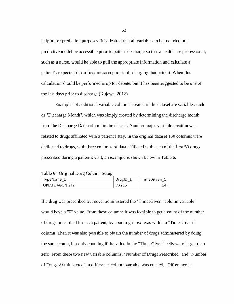
52
helpful for prediction purposes. It is desired that all variables to be included in a
predictive model be accessible prior to patient discharge so that a healthcare professional,
such as a nurse, would be able to pull the appropriate information and calculate a
patient’s expected risk of readmission prior to discharging that patient. When this
calculation should be performed is up for debate, but it has been suggested to be one of
the last days prior to discharge (Kujawa, 2012).
Examples of additional variable columns created in the dataset are variables such
as "Discharge Month", which was simply created by determining the discharge month
from the Discharge Date column in the dataset. Another major variable creation was
related to drugs affiliated with a patient's stay. In the original dataset 150 columns were
dedicated to drugs, with three columns of data affiliated with each of the first 50 drugs
prescribed during a patient's visit, an example is shown below in Table 6.
Table 6: Original Drug Column Setup
TypeName_1 DrugID_1 TimesGiven_1
OPIATE AGONISTS OXYC5 14
If a drug was prescribed but never administered the "TimesGiven" column variable
would have a "0" value. From these columns it was feasible to get a count of the number
of drugs prescribed for each patient, by counting if text was within a "TimesGiven"
column. Then it was also possible to obtain the number of drugs administered by doing
the same count, but only counting if the value in the "TimesGiven" cells were larger than
zero. From these two new variable columns, "Number of Drugs Prescribed" and "Number
of Drugs Administered", a difference column variable was created, "Difference in

53
Number Prescribed versus Number Administered". Furthermore related to the drug
columns it was advantageous to create new variable columns "DrugTypeID:_#" which
are a simple binary variable, and if "DrugTypeID:_52" is present a "1" is present and if
not a "0". It is unnecessary to know the drug type name until it is proven to be a
predictive factor therefore a conversion from using the drug type ID name to a
corresponding number was performed to mitigate large variable name lengths, the table
illustrating the corresponding conversions can be found in Appendix E. This allows for
the comparison of each patient visit to have all drug type information present in their
information, and reduces the number of potential category levels (in the 10's to 100's of
levels) which would have been present for each of the 50 "TypeName" column variables.
In the end the 150 original drug columns were replaced by 204 binary column variables
of the possible drug types and the three separate count variable columns
Another major variable alteration was in reference to the primary and secondary
ICD-9 diagnoses codes listed for each patient. Each patient visit had one primary
diagnosis and up to 15 secondary diagnoses. These diagnoses codes are standard across
healthcare and indicate the disease/symptom a patient is exhibiting. The ICD-9 codes
range from 001-1000, with also some alpha-numeric codes of V01-V89 and E000-E999,
and have many subgroups within each primary three digit code; for example a specific
code could be 560.94. The National Center for Health Statistics (NCHS) and CMS are the
government agencies responsible for overseeing the ICD-9 information in the US, with
the World Health Organization (WHO) being the author of the ICD-9 coding. There are
literally tens of thousands of possible ICD-9 diagnosis codes, and so for purposes of this

54
study these codes were truncated to their first primary digits in front of the decimal point
(WHO, 2010). This reduced the number of feasible category levels but still this value is
in the hundreds. Therefore again similarly to drugs it was advantageous to make new
binary column variables for groupings of the ICD-9 codes. The ICD-9 coding system
already has sub-groupings of similar diagnoses listed at the primary digits level therefore
these 106 sub groupings were used to create the appropriate column variables. For both
the primary diagnoses and all secondary diagnoses the 154 ICD-9 subgroup binary
column variables were created and replaced the 16 columns of numeric ICD-9 code
values. This created 308 diagnoses binary columns compared to 16 columns with
thousands of potential category levels. Some of these variables have no occurrence (i.e.
the whole column is zeroes) and therefore will be deleted as unnecessary.
Another variable viewed as potentially important and added to the data was
"Distance to Hospital". This was accomplished by calculating the approximate distance
between BDHS zip code and the patients listed home residence zip code. This was
performed by using the software Zip Code Distance Wizard created by PC Shareware.
This allowed for calculating the distance between BDHS (zip code: 59715) and the postal
codes listed for the 7451 patients in the analysis data. These distances were then bucketed
into 0-10, 11-30, 31-50, 51-100, 101-200, 201-500, 501-1000, 1000+ miles and
International groups, for a single categorical variable.
Some examples of column variables which were dropped are all the procedure,
surgery, present on admission (POA), and doctor columns. The procedure and surgery
columns were not relevant to information wanted, and the POA columns were both
55
suggested as unreliable and also not necessary when reviewing for readmissions.
Originally it was desired to have the admitting and discharging doctor information but
because these were not de-identified variables it was deemed inappropriate, and an issue
for potential future research if it is desired to determine individual doctor readmission
rates. For the final list of prediction variables the Diagnoses-Related Group (DRG)
variable must also be dropped because it is not added to a patient’s visit record until
sometimes two weeks after the visit, so will not be available before a patient is
discharged.
Any of the created variables which had no instance of occurring (some of the
diagnoses and drug variables) were deleted because they will not be attributes of any
patient population. This procedure will need to be repeated for the diagnosis specific
Excel files to be created later. From the predictor variable types defined as appropriate
for inclusion in Table 5 by literature and discussion with healthcare professionals, and
through the conversion of the reported variable type information in the EMR system, the
final set of specific predictor variables and their variable type (binary, categorical,
continuous) were determined for this research. The final general dataset to be analyzed
consists of a total of 463 predictor column variables. This includes 447 binary variables
composed of 106 variables for primary diagnoses, 137 variables for secondary diagnoses,
204 variables for drugs; and then 16 other variables, to be referred to as “characteristic”
predictor variables. The characteristic predictor variables are the variables of most focus
both as predictors and in models, and exploratory analysis of these variables will be

56
performed. The characteristic variables are shown below in Table 7, and a complete list
of the variables for the general population readmission model is found in Appendix F.
Table 7: Characteristic 16 Predictor Variables Information
Variable Name Variable Type Category Levels
Discharge Month Categorical 12
Length of Stay Scalar NA
Age in Years Scalar NA
Gender (M=0, F=1) Binary 2
Marital Status Categorical 7
Hospital Discharge Dept. Categorical 3
Admit From ER (Y=1) Binary 2
Financial Class Categorical 10
Discharge Disposition Categorical 12
Distance To Hospital Categorical 9
Number of Drugs Prescribed Scalar NA
Number of Drugs Administered Scalar NA
Difference of Number of Drugs
Prescribed vs. Number of Drugs
Administered
Scalar NA
Count of Consults Scalar NA
Prior 6 Month ER Count Scalar NA
Prior 6 Month Inpatient Count Scalar NA
Readmissions
One of the most arduous components of this research was determining which
patient visits in the data are categorized as readmissions. This is because unlike most of
the previous readmission studies, this study developed a method to define and identify

57
readmissions (Vest et al., 2010). This was necessary because readmission tracking is
more of a recent occurrence and unfortunately the historical data from BDHS did not
contain any indicators for if a visit was a readmission. Though readmissions were present
in 2009 and 2010 they were never clearly marked to indicate the visit as a readmission
later. In 2009 and 2010 through the present how a patient visit at BDHS is quantified as a
readmission is a unique and inefficient and non-comprehensive process. At the beginning
of each month the lead case manager in the Case Management Department receives a list
of patient visits from CMS of patients who the prior month were admitted to BDHS
within 30-days of a prior admission. These visits are defined as a "readmission" because
they are a visit within 30-days of a previous visit, but the true question of importance is
whether or not these visits were related medically to a previous visit, making them
"related readmissions". The list from CMS only incorporates the patients who had
government insurance of Medicare and Medicaid, while other insurances may question
about a visit being a readmission on a more case by case basis. Still for this list the lead
case manager then must review the visit, searching through available records, and justify
in writing why or why not each visit is a related readmission. Unfortunately this method
leaves a lot of possibility for bias in the decision of a readmission being related, and has
no real standard metrics to definitively indicate a readmission as medically related to a
previous visit, but rather evaluates each individual case uniquely. Furthermore, after the
written justification for the readmission being related or not is submitted to CMS,
sometimes it can be returned over-ruling the case managers decision and enforcing the
visit as a readmission. This determination is by a separate case worker at CMS making a

58
potentially biased decision, because no clear outline defining relatedness is established.
Once the decision of whether a readmission is related or not is established, it simply is
marked down by CMS to be recorded for the readmission rate statistics, but currently no
documentation of this visit being branded a readmission is recorded by BDHS. This
makes it extremely difficult when retrospectively looking back at patient data to know
which patients are readmissions. Therefore it was necessary to develop some rubric to
quantify a readmission, and establish what type of readmission it is.
Readmission Type
First the type of readmission to investigate is essential to determine; this includes
what timeframe, conditions, relatedness and if planned/unplanned. The easiest component
about readmission type to define was the timeframe in which a second admit would be
considered a readmission. For purposes of this research a 30-day timeframe was chosen,
this is one of the most common timeframes, but more importantly is the timeframe of
which readmission rates are calculated by CMS and will be calculated for the PPACA
legislation. As discussed in the Introduction originally investigation into general, or "all-
condition" readmissions, as well as the three core measures AMI, CHF and PNM, is the
starting point for analysis.
For the patient data at BDHS there is no system in place to indicate if a patient
visit was a planned/unplanned or a related/unrelated readmission. Determining the
relatedness and planned/unplanned aspect of the readmissions to investigate was
influenced by the document written by Stone and Hoffman (2010) that summarizes
Rehospitalization: Understanding the Challenge presentation given by Stephen F. Jencks,

59
M.D., M.P.H, at the National Medicare Readmissions Summit in Washington, DC on
June 1, 2009 (Stone & Hoffman, 2010). Jencks proposed at the Summit that any
readmission within 30 days is a potential cost saving avenue and all readmissions within
30 days should be investigated (Stone & Hoffman, 2010). While this is true the most
potential for cost savings can result in the reduction in readmissions which are
preventable (Halfon, 2002; Jencks et al., 2009). He also stated at the Readmission
Summit in Washington, DC that further classifying readmissions into four proposed
categories could help distinguish which readmissions were potentially preventable, and
thus could be targeted for substantial improvement. The four categories are any variation
of the following combinations: unplanned, planned, related, and unrelated. Table 8 shows
the variations and a brief description of each combination for the classification of
readmissions.
Table 8: Readmission Categories
Planned Unplanned
Related Planned and Related
Readmission is related to initial
hospitalization diagnosis and
Readmission is scheduled or
expected in advance.
Unplanned and Related
Readmission is related to initial
hospitalization diagnosis but is
neither expected nor foreseen.
Unrelated Planned and Unrelated
Readmission is not related to initial
hospitalization diagnosis and
readmission is scheduled or
expected in advance.
Unplanned and Unrelated
Readmission is not related to
initial hospitalization diagnosis
and readmission is neither
expected nor foreseen.

60
Upon further investigation a Planned-Related readmission is essentially
unavoidable and just an extension of the previous care visit. An example of this is a
follow-up inpatient surgery to a previous surgery, to complete more planned work. The
two categories of unrelated readmissions are also not beneficial in reducing costs,
because they are not related to the health issue being addressed at the first visit. For
example, a planned knee surgery 20 days after a hospitalization for Pneumonia is
planned-unrelated readmission because it is within 30 days. An unplanned-unrelated
readmission example would be an admission for injuries sustained from a vehicle
accident 10 days after being hospitalized for Pneumonia.
The final category unplanned-related is the target type of readmission where
improvement could be made. This type of readmission indicates that a patient has
returned to the hospital for the same or similar medical reason they previously were
admitted for, and it was not planned but rather their health had deteriorated in some
manner. This type of readmission has been termed a Potentially Preventable Readmission
(PPR) because during the prior admit or shortly thereafter a gap in quality of care or
condition occurred to allow the patient to relapse with the similar condition requiring
hospitalization. PPR's have recently become more of a focus in healthcare, rather than all
readmissions, because they hold the key to major cost reductions and improved quality of
care.
61
Determining if a Readmission
is Planned versus Unplanned
Now that the type of readmission has been determined the challenge is creating a
method to be able to quantify patient visits as a readmission. This currently is one of the
most difficult topics of readmission, because no proven global appropriate method to
identify relatedness of visits has been formulated since medical interactions and scenarios
are overwhelming complex (Stone & Hoffman, 2010). To electronically decipher the
patient visits which are PPRs a method was devised to identify patient visits as planned
vs. unplanned, and then to use a rules rubric to test if separate visits were related. This
method was developed after considerable discussion with healthcare professionals at
BDHS, as well as being developed similar in structure to the readmission identification
methods found in the Horwitz et al. (2011) and Krumholz et al. (2008) studies performed
for CMS.
Using clinical nursing expertise of Kujawa and others at BDHS, along with some
literature definitions of unplanned being "emergency" hospitalization, planned and
unplanned was determined by whether or not the patient was admitted through the
emergency department. This is because at BDHS if a patient must be admitted to the
hospital without prior scheduling (i.e. planned surgery stay) then even if it is not a life-
threatening emergency the patients still are admitted through the ER. Horwitz et al.
(2011) defines an unplanned visit as those that required “urgent hospital management.”
Thus a visit was unplanned if a patient is admitted through the emergency department and
planned if admitted by some other method. Thus in the dataset a temporary variable of

62
"Unplanned Visit" was created, which represented if the patient visit had originated as an
admission through the ER.
Determining if a Readmission
is a Related Readmission
The method to define if two visits were "related" medically was constructed and
vetted by expert knowledge of nurses, coders, case managers and doctors with whom this
research was discussed. Similarly to determining unplanned/planned, many discussions
on the appropriateness of the developed relatedness method were conducted with BDHS
healthcare professionals. Upon review of this technique the nurses, coders, case managers
and administrators believed this was an appropriate method to identify related
readmissions from historical data. Future vetting of this methodology could be performed
by a panel of experts including parties outside of BDHS, to ensure this methodology for
readmission identification is appropriate. Relatedness will be determined using the ICD-9
codes in primary and secondary diagnoses, as well as Diagnosis-related Group (DRG)
codes used to classify hospital cases (visits) commonly for insurance coding purposes.
The proposed relatedness rubric to be constructed is unique to this research as no proven
substitution for determining relatedness is currently available.
This first and simplest rule to define relatedness was the case where a visit has the
exact DRG as the readmission visit DRG. With identical DRG's for these visits it is
highly probable the patient was readmitted for similar or identical medical issues as
before. The next sets of rules involve relatedness based on the ICD-9 codes and are
appreciably more complicated. Development of the proposed ICD-9 relatedness rules
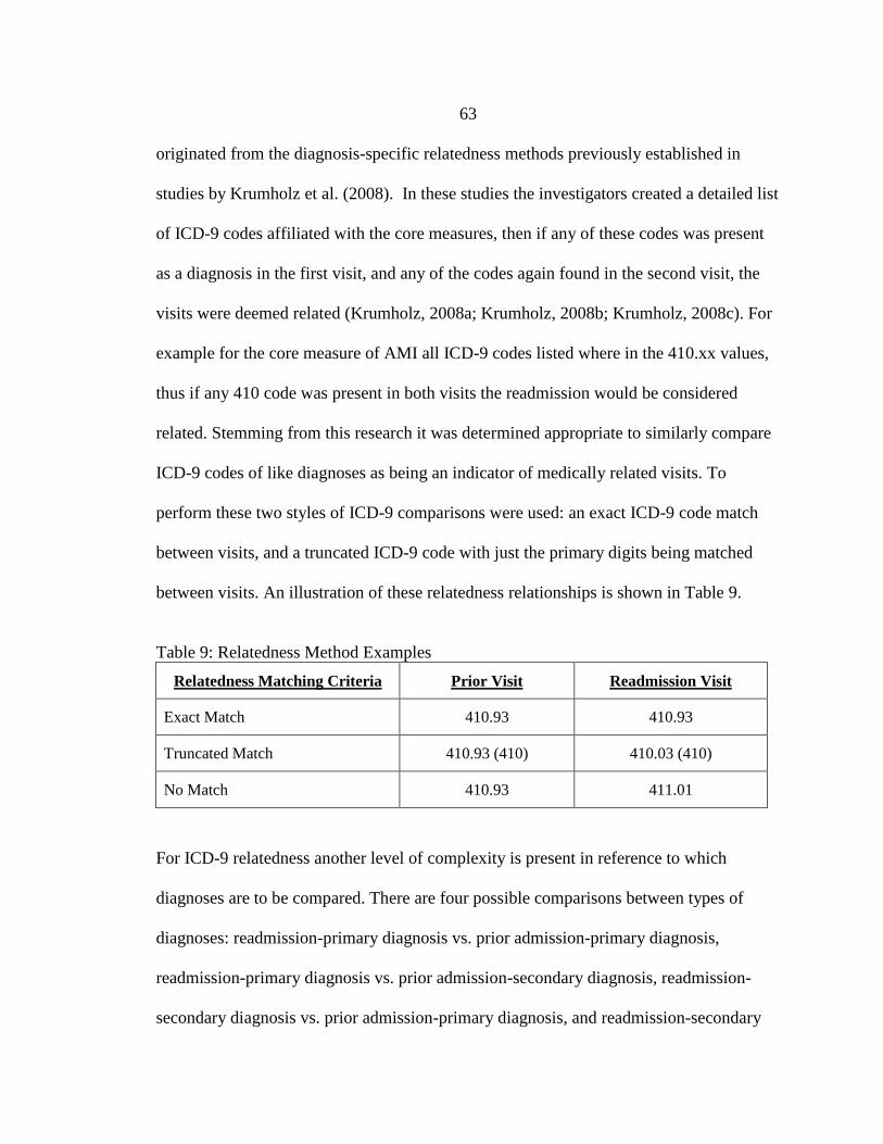
63
originated from the diagnosis-specific relatedness methods previously established in
studies by Krumholz et al. (2008). In these studies the investigators created a detailed list
of ICD-9 codes affiliated with the core measures, then if any of these codes was present
as a diagnosis in the first visit, and any of the codes again found in the second visit, the
visits were deemed related (Krumholz, 2008a; Krumholz, 2008b; Krumholz, 2008c). For
example for the core measure of AMI all ICD-9 codes listed where in the 410.xx values,
thus if any 410 code was present in both visits the readmission would be considered
related. Stemming from this research it was determined appropriate to similarly compare
ICD-9 codes of like diagnoses as being an indicator of medically related visits. To
perform these two styles of ICD-9 comparisons were used: an exact ICD-9 code match
between visits, and a truncated ICD-9 code with just the primary digits being matched
between visits. An illustration of these relatedness relationships is shown in Table 9.
Table 9: Relatedness Method Examples
Relatedness Matching Criteria Prior Visit Readmission Visit
Exact Match 410.93 410.93
Truncated Match 410.93 (410) 410.03 (410)
No Match 410.93 411.01
For ICD-9 relatedness another level of complexity is present in reference to which
diagnoses are to be compared. There are four possible comparisons between types of
diagnoses: readmission-primary diagnosis vs. prior admission-primary diagnosis,
readmission-primary diagnosis vs. prior admission-secondary diagnosis, readmission-
secondary diagnosis vs. prior admission-primary diagnosis, and readmission-secondary

64
diagnosis vs. prior admission-secondary diagnosis. These different comparisons were
then evaluated for their relevance to potentially finding important information about the
readmission. A key aspect to remember is that there is only one primary diagnosis but up
to 15 secondary diagnoses can be listed. Thus to compare one visit to another visit with
secondary diagnoses, each of the secondary ICD-9 codes listed would have to be
compared to a primary diagnoses, or to each of that visits secondary diagnoses. The
primary-primary comparison is important as a relatedness component because this means
for both visits the patient had the same primary ICD-9 diagnosis. Similarly the
readmission-primary to prior-secondary is deemed appropriate to evaluate because this
could indicate a secondary diagnosis present previously that was inadequately treated and
caused the patient readmission. The opposite relationship, readmission-secondary to
prior-primary, could also be indicative of related medical complications because the
reason for the previous visit is still present at a large enough level to be a secondary
diagnosis. These three comparisons all will be included for the relatedness rubric. The
last comparison of secondary-secondary is not appropriate to include because a random
secondary may be listed both times but truly not be influential into why the patient was
rehospitalized.
Furthermore the topic of relatedness increases in complexity because some
patients may have multiple visits with 30-days and therefore each visit within the 30-day
prior window must be tested against each other to determine if they are medically related.
To help view how many previous visits of a patient were within 30 days prior to the visit
being assessed, several simple temporary variables indicating the days since a prior visit

65
were created. Four temporary variables were created testing back to the 4th prior visit
from each visit; at this point no patient had any 4th prior visits within 30 days. Therefore
it is only necessary to compare up to three previous visits if they were within the 30-day
timeframe.
The relatedness rubric development then accounts for relation by exact DRG
code, exact ICD-9 code, and truncated ICD-9 code; while testing up to the third prior
visit within 30-days and comparing primary diagnoses to primary diagnoses, as well as
primary diagnoses to secondary diagnoses. These factors create five different categories
of relatedness, with comparisons occurring with up to 3 different visits, giving 15
possible combinations of relatedness. The visual illustration of these relatedness
combinations is represented in Table 10.
Table 10: Relatedness Rubric
Relatedness: Admit to Readmission Visit
Rea
dm
issi
on
Vis
it
1st Prior Visit 2nd Prior Visit 3rd Prior Visit
Exact DRG - Exact
DRG Rel1-1 Rel1-2 Rel1-3
Exact Primary -
Exact Primary Rel2-1 Rel2-2 Rel2-3
Truncated Primary
- Truncated
Primary
Rel3-1 Rel3-2 Rel3-3
Truncated Primary
- Truncated
Secondary
Rel4-1 Rel4-2 Rel4-3
Truncated
Secondary -
Truncated Primary
Rel5-1 Rel5-2 Rel5-3

66
All degrees of relatedness represented in the rubric were taken into consideration
for readmissions, creating 15 temporary column variables for the identifier, and then
combining all levels of relatedness into a single column variable coded as "Related". To
establish which visits were related, complex search equations in excel were used to
determine if a visit was related by any comparison, then these all had a separate indicator
variable column to show "related" if appropriate.
Identifying PPR and ATR Visits
Finally with an "Unplanned visit" column and "Related" column created the
search for potentially preventable readmissions within 30-days could commence, since a
PPR has been established as an unplanned and related readmission (Stone & Hoffman,
2010). The PPRs are suggested by Jencks et al. (2009) as the type of readmissions that
have the most potential for cost savings and therefore the primary focus of this research.
Determining the PPRs was achieved by searching visit entries for being unplanned,
related and within 30 days of a prior admission. The patient visits which met the
unplanned, related and within 30-day criteria then could be flagged as a "Readmission"
because these are the PPRs to investigate.
An important aspect when developing readmission predictive models is
determining the appropriate patient visit information to evaluate. To predict a
readmission before it occurs use of information available about the patient prior to the
readmission must be used. Therefore the most feasible information to use is the
information from the visit deemed the prior related admission to the readmission. This

67
visit, referred to as “Admit To Readmit” (ATR), is the visit attributed as the theoretical
cause for the rehospitalization based on the PPR readmission criteria.
The ATR visit becomes a crucial component of the research because all the
information about a patient, which can be used to develop predictive variables, should be
found in this visits recorded information. Thus after the PPR readmission visits have been
determined then also the ATR visits must be recorded and given an identifier in an
“AdmitToReadmit” binary column variable. The ATR visits will be the records analyzed
for trends and patterns to attempt to create predictive models for readmissions. This is a
necessary step because this research aims to predict readmission risk and in order to
predict these it is necessary to look at the attributes of the prior related admission to the
readmission and not the readmission itself. Identifying the appropriate AdmitToReadmit
visit was achieved by linking the prior visit number (1, 2 or 3) attached to the relatedness
level corresponding to the visit through the temporary relatedness column variables. It
was possible for a visit to have more than one level of relatedness, as well as being
related to more than one prior visit. Redundancies in counting the number of PPRs was
avoided by only indicating a visit as a readmission once. This was achieve through the
use of "OR" statements in Excel, such that if any of the potential scenarios to mark a visit
as a readmission were true the column variable would be marked "Readmission".
Similarly to mark the AdmitToReadmit visits "OR" statements also were used, again only
singly marking the AdmitToReadmit column variable for the respective visit's row with a
"1" to indicate the patient visit was an admission to a visit marked as a PPR. Please refer
to Figure 2 for an overview on the readmissions focused on for this research.
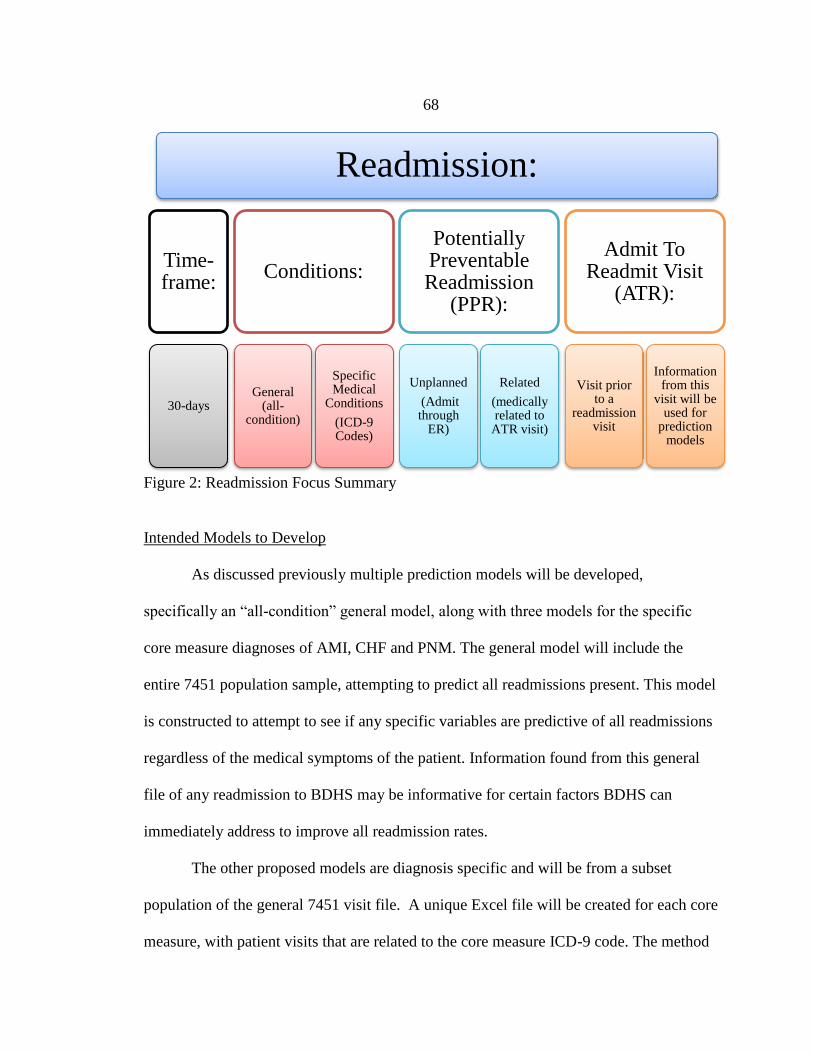
68
Figure 2: Readmission Focus Summary
Intended Models to Develop
As discussed previously multiple prediction models will be developed,
specifically an “all-condition” general model, along with three models for the specific
core measure diagnoses of AMI, CHF and PNM. The general model will include the
entire 7451 population sample, attempting to predict all readmissions present. This model
is constructed to attempt to see if any specific variables are predictive of all readmissions
regardless of the medical symptoms of the patient. Information found from this general
file of any readmission to BDHS may be informative for certain factors BDHS can
immediately address to improve all readmission rates.
The other proposed models are diagnosis specific and will be from a subset
population of the general 7451 visit file. A unique Excel file will be created for each core
measure, with patient visits that are related to the core measure ICD-9 code. The method
Readmission:
Time-frame:
30-days
Conditions:
General (all-
condition)
Specific Medical
Conditions
(ICD-9 Codes)
Potentially Preventable Readmission
(PPR):
Unplanned
(Admit through
ER)
Related
(medically related to
ATR visit)
Admit To Readmit Visit
(ATR):
Visit prior to a
readmission visit
Information from this
visit will be used for
prediction models

69
used to determine if a visit was related to a specific diagnosis consisted of searching the
original 16 ICD-9 primary and secondary diagnoses column variables for the visit to see
if the truncated primary digit code of the diagnosis was present. For example the primary
digit ICD-9 code for CHF is 428, and then this value would be searched for in the
diagnoses columns. In the general Excel file a search algorithm using “OR” statements,
similar to before, was generated to search the 16 diagnoses related cells for each visit;
and if the desired value (i.e. “428”) was found then a “1” would be recorded for a new
temporary column variable indicating if a visit was related to the searched diagnosis. By
this method a column variable for each core measure diagnosis would be created and then
indicate all visits in the general population which were related to these diagnoses. Once
these visits were recorded as related to the respective diagnosis a new file was created
containing only the visits related to the respective diagnosis. Therefore three Excel files
will be created containing visits which are related to the individual AMI, CHF and PNM
diagnoses. In Table 11 the appropriate ICD-9 codes associated with AMI, CHF and PNM
are illustrated.
Table 11: Diagnoses Affiliated ICD-9 Codes for Search Algorithms for Diagnosis
Specific Model Files
Diagnosis Associated Search ICD-9 Primary Digit Code
Acute Myocardial Infarction (AMI) 410
Congestive Heart Failure (CHF) 428
Pneumonia (PNM) 480-488

70
At this point four unique Excel files were created for evaluation of general, AMI, CHF
and PNM related visits and the respective readmissions and readmission predictive
models for each.
Additional models may be developed based on the evaluation of the general
population file. In order to ensure no missing critical diagnoses, that have more
readmissions at BDHS than the core measures, a breakdown, by diagnosis, of the general
readmissions found will be created. Therefore if there is a large representation of
readmissions linked to a separate medical diagnosis other than AMI, CHF and PNM,
diagnosis specific Excel files will be created for these in the same fashion as the core
measures.
General Readmission Population Information
Jencks et al. (2009) state that planning practice changes for improving the
delivery of care and reducing readmissions can only be effective if information about the
readmitted population can be trended for patterns. Therefore it is important to not only
develop the predictive models but to also investigate some of the characteristics of the
general readmission population for patterns.
The first component of analysis to perform is the determination of the count and
proportion of calculated PPRs in the population. For appropriate pattern and prediction
model analysis the data to be reviewed is the ATR visits. Therefore a count and
proportion of ATRs in the population will be performed. These ATR visits will then be
the sub portion of the general data used to search for patterns.

71
To attempt to find patterns in the data the 16 variables listed in Table 7 were
evaluated. The evaluation of each variable for the ATR visits will consist of looking at
the distribution of ATR visits to the respective category levels of the variable. This
evaluation may indicate patterns in the data that then could be correlated to the
incorporated variable in the future readmission predictive models. Evaluating the ATR
visit distribution for these variable levels also will help indicate potential key areas for
readmission prevention for the BDHS population.
The last investigation component for the general readmission will be evaluating
the distribution of ATR visits related to specific diagnosis. This will be performed by
calculating frequency counts of each diagnosis code with respect to their presence in the
ATR visits. First a distribution will be calculated incorporating both primary and
secondary diagnosis codes, this may not be informative on the primary medical reasons a
patient is at the hospital. Therefore a second distribution just using primary diagnoses
affiliated to the ATR visits will be developed, this distribution should indicate the top
diagnoses affiliated with readmissions at BDHS. From this primary diagnoses
distribution of ATR visits it will be determined if diagnoses other than the core measures
should have predictive models created.
Readmission Risk Prediction Models
The healthcare industry is an extremely complex system with high variability in
medical diagnoses, care and patient characteristics. These extreme complexities along
with many unknown aspects of medicine make attempting to create readmission risk

72
prediction models challenging. Almost every patient visit can be viewed as a unique
situation because of so many varying characteristics about the patient and the medical
symptoms, making it difficult to standardize a model that will fit for all patients. Thus a
major challenge when developing the predictive models will be attempting to mitigate or
account for the influence of high-variability factors, and developing reasonably
understandable models.
One of the primary goals of BDHS through this research is to be able to indicate
factors affecting the risk of readmission and then appropriately implement interventions
targeting these specific factors. In order to aid in this goal the predictive models
developed must have understandable results for how individual factors affect the risk of
readmission for patients. Furthermore it is desired that these risk prediction model be
feasibly implemented within an electronic system so as to automatically calculate a
patient’s readmission risk prior to discharge. This is important because knowing a
patient’s risk level prior to discharge should allow staff to enact readmission preventative
measures either during the end of the hospital visit or shortly after discharge. These
preventative measures would be the types of interventions discussed by Kujawa (2012).
Comparison of Models
As discussed previously, in the introduction and literature review, it was deemed
advantageous to create separate types of prediction models for each respective set of
readmission data (general, AMI, CHF, PNM and others as applicable). These model types
will be a binary logistic regression model, and a MARS model. Reviewing the variables
found important to these models will be a reference to research question one. While the

73
development of usable prediction models will be the direct response to research question
two posed earlier. Finally, the comparison between the prediction models attempted and
developed by the different analysis methods will answer research question three. In order
for model comparison to be appropriate a commonly reported metric of prediction
success must be present. The most common metric from literature was the area under the
ROC curve (AUC), equivalent to the concordance index (C-statistic) (Kansagara et al,
2011; Agresti, 2002). Each of these models will also be compared by the models’
prediction successes as indicated by their classification tables (Agresti, 2002). These
classification tables are the same as the concordance index used in most regression
analysis; they directly illustrate the number and percent of events which were
appropriately or inappropriately classified (Agresti, 2002). The direct comparison of R2
values calculated for the model is inappropriate because the modeling methods do not
report the same R2 types (IBM, 2012). The R
2 values can be used as a baseline to whether
or not the model is appropriate for use for that modeling technique (IBM, 2012). With
respect to these R2 values an acceptance threshold lower than theoretical statistical
application is appropriate because real human data is being used which has inherent
variability which cannot be controlled for (Claudio, 2012).
In reviewing the models it was also important to remember the impact of different
types of errors on the practical aspect of the prediction model for BDHS. It was
previously determined, based on discussions with BDHS stakeholders, it was more
important to avoid misclassifications of high readmission risk patients than incorrectly
classifying low risk patients as high risk. The type of error they want to avoid is Type II

74
error, or a “miss”. This is because from BDHS’s perspective missing a patient who is at
high risk of readmission has more dramatic ramifications of increased readmission rates
and sub-optimal quality of care for that patient. Without knowing the exact cost or
weighting ratio for the types of errors it is not possible to directly include penalties for the
misclassification errors in the prediction models. However, a focus on the prediction
success of the visits defined as ATR visits will be important to determine if a large
amount of these visits were missed by the prediction model. Therefore investigation into
both the overall prediction successes and the ATR prediction successes will help to
evaluate the usability of the models more closely to the practical application by BDHS.
Testing Issues and Methods Used
Another topic which affected both models was the type of model testing to
perform. Upon analysis of the patient population sets available for the different model
condition types, it was seen that they were relatively small populations. The populations
being on the several hundred to thousand visit count level did not allow for substantial
data available for analysis with the prediction models. Additionally, the proportion of
visits defined as ATRs is a small proportion of these population sizes, thus compounding
the small size aspect of the target visits which are the primary reason for investigation.
Several attempts to alleviate the small population problem were performed. First the
investigation into more available data from BDHS proved unfortunate, as at the time of
this research no more patient data was available from BDHS due to major EMR
modifications during 2011 and 2012; such that only data from the end of 2012 may be
available. Next the proposition to use an 80/20 or 90/10 split for train/test populations

75
was entertained. However, since there are very small counts of the ATR visits, too small
of a level of the ATR visits would be present in a 10% or 20% test population cohort.
Too small of test datasets was also accompanied by this testing method being not easily
performed in SPSS (when missing variables between the train/test populations were
present). SPSS reports an error and inability to develop the model when the available
variables and their levels are not the same between the train and test populations. This
occurrence made it impractical to split the data into train and test populations for SPSS.
Therefore the best attempt to avoid data count issues was to use 100% of each dataset and
validate using cross validation techniques.
With SPSS cross-validation is performed similarly to a train/test population setup
and again the issue of missing values between the two separate populations made this
testing method infeasible in SPSS because the missing values are handled as a fatal
model error. Therefore for SPSS no model testing will be performed at this time, but
rather the full 100% of data will be used for the train population developing the
prediction models, and then testing will need to be performed in future research with
more BDHS data when available. In comparison MARS was capable of performing cross
validation and handling the cases of missing values. For MARS, based on v-fold cross
validation methodology discussed by Steinberg & Golovnya (2006) it was decided to use
a cross validation technique where the minimal number of target class (ATR) visits
estimated present in each fold would be 5 visits or larger. For consistency purposes a five
fold cross validation technique was used for all models except the AMI models. The AMI
dataset includes a total ATR visit count of only 11, thus to maintain at least 5 visits

76
expected in the testing portion of a fold, a two fold validations was used. Therefore the
analysis of the complete patient population within each of the respective data files will
constitute a "train" population sample, and only in MARS will a "test" population sample
be developed through cross validation testing.
Binary Logistic Regression Model
For creation of the binary logistic regression predictive model the software IBM
SPSS Statistics (v. 21) package was used. Within the software the "Binary Logistic
Regression" and "ROC Curve" analysis methods are used. With this model analysis the
complete model dataset will be used since a small target class (ATR = 1) is present. It is
important to note that this is a limitation to this research. This is important to clarify
because the use of 100% of the available data made all calculated ROC curves and AUC
values representative of the train population, not a test population.
Several other key topics about the use of binary logistic regression analysis in
SPSS are summarized below, with the overview of the step-by-step methodology for
model development being found in Appendix G. The choice of a selection method for
variable entry and removal from the model is the major user decision with this analysis.
For purposes of this research it was determined best to use the "Forward: Conditional"
method which is a forward stepwise algorithm. This was for purposes of ensuring
degrees of freedom rules were not violated, since the algorithm only steps in variables at
each step which show the greatest impact on the model based on the Log Odds Ratio. The
Log Odds Ratio in SPSS is depicted by the exp (β) value which is recorded. Upon review
77
of each of the models the degrees of freedom used by the included variables in the model
can be checked to ensure it is appropriate for the size of the sample population.
Another major component of the analysis is with respect to the inclusion of
interactions. For purposes of this research only the main effects of the variables were
entered into the possible variables allowed to enter the model. This was due to the
necessity of entering in each interaction which should be included prior to running the
model analysis, and without knowledge of potential interactions of the variables the
entrance of thousands of possible interaction possibilities was not viewed appropriate.
The use of only main effects is a substantial handicap of the SPSS models versus their
corresponding MARS models, but at this stage of understanding medical interactions was
unavoidable. This handicap for the SPSS models could be a primary reason for MARS
models greater predictive ability between the models developed.
The output will contain the final stepwise model with the variables it contained
and their respective f-statistical significance level. Also included will be the Nagelkerke
R2 value which is a pseudo R
2 which is an adjusted R
2 value for the Cox and Snell’s R
2,
with a range between 0 and 1 (IBM, 2012). As a true R2
value statistically cannot be
calculated because categorical variables have discrete levels, pseudo R2
values are
common approximations of the R2 value found in linear regression (IBM, 2012). The β
coefficients reported by SPSS are associated with the logit function and will need to be
converted by an equation to calculate the actual probability a patient has for readmission
risk. This conversion equation is shown below in Figure 3.

78
Figure 3: Conversion Equation for Logit Predictor Coefficients to Prediction Probability
A classification table will also be present in the output, indicating how the final
model chosen was able to predict each visit, with specific interest into the ATR visits.
The ROC curve is also computed and represented for the output with the true parameter
of interest the AUC being displayed below the ROC curve. Using the available
information from the model output comparisons to other models can be made as well as
the determination of the significance of individual predictor variables on readmission
risk.
Multivariate Adaptive
Regression Splines (MARS) Model
MARS is a highly computer resource intensive algorithm analysis, searching
expansive numbers of the MARS regression models to find the optimal model. A key
control parameter in MARS is the “Max BF”, which is the maximum number of
allowable basis functions. This value is set by the modeler and directly impacts the length
of time the analysis will take. The Max BF needs to be large enough to allow MARS to
find a good model but not too large so as to take a very long time to evaluate the model.
Therefore it is suggested a “rule of thumb” is the Max BF value must be at least two to
four times larger than the truth for the number of basis functions needed for prediction
(Salford Systems, 2001). Since in most cases “the truth” is not necessarily known after
review of many MARS models it is believed that using three times the number of

79
terminal nodes found in a CART analysis, of the same population, is appropriate for the
Max BF (Salford Systems, 2001). To ensure enough basis functions were included the
Max BF was chosen to be four times larger than the number of terminal nodes found in
the previous CART models which were tested but later removed from the thesis body.
To account for not violating the degrees of freedom associated with a respective
model the MARS User Manual discusses how the method receives a penalty for each
basis function added in the algorithm search. With the addition of each basis function
receiving a specific penalty to equate the entrance of the basis function to the number of
effective parameters investigated in that step of the search algorithm (Salford Systems,
2001). “An ‘effective degrees of freedom’ measure is used to take this exhaustive search
into account” (Salford Systems, 2001). The suggestion from past research using MARS is
that the degrees of freedom charged per knot (basis function entered) should be between
two to five (Friedman, 1990). With the degrees of freedom charged per basis function not
affecting the forward step of MARS but restricts the allowable MARS models once the
backward “pruning” step of MARS is implemented (Salford Systems, 2001). The degrees
of freedom penalty is automatically computed using the cross validation testing technique
discussed; therefore the best estimated penalization for the number of effective
parameters is computed by MARS (Salford Systems, 2001).
The MARS tool will overly construct a regression model, by adding more than an
appropriate number of splines (new main effects or interaction terms) to the model and
then reviews the set of regression models developed and evaluates these with penalization
for over fit models. The comparison of the set of regression models (i.e. the 12 basis

80
function model versus the progressed 15 basis function model, etc.) is performed by
using the generalized cross validation (GCV) value, previously discussed. The GCV
value is a penalized representation of the regression model’s mean squared error (MSE).
It receives a penalization value determined by an increased degrees of freedom (dof)
charge per basis function (knot). Thus the GCV formula charges each basis function with
more than one dof; this penalizes models with higher counts of basis functions, mitigating
the potential of over fitting the data. The modeling techniques and abilities of MARS can
further be investigated in either Salford Systems, 2001 or Friedman, 1990.
For the prediction models it was desired to be more accurate rather than speedy in
the calculation of the MARS models so all parameters related to accuracy were maxed
out, as described in the methodology in Appendix H. The only battery used with MARS
was the MINSPAN battery which checked multiple allowable spans between knots to see
if better models could be developed. More in depth description of the MARS parameters
used in the step-by-step overview of the methodology is found in the MARS
Methodology shown in Appendix H. The MARS methodology will output a set of MARS
models with the illustrated optimal model being the model with the smallest GCV value
(automatically highlighted in pink). The model with the smallest MSE is highlighted in
green but most times is inappropriate for selection because the GCV value accounts more
accurately the approximate error according to Steinberg & Golovnya (2006). The
reported regression models will include the actual model rules, the ROC curve
information and variable importance. Now since MARS uses regression analysis a set of
R2
variables are also displayed. The naïve R2
and the naïve adjusted R2
values are similar

81
to the pseudo R2 values found in SPSS, and R
2 terms found in classical regression
analysis (Nash & Bradford, 2001). The GCV R2
value will always be less than the
previous naïve R2 because it is the metric illustrating a penalization for having degrees of
freedom greater than one for parameters. As discussed previously MARS models can be
compared relative to the AUC train values calculated by SPSS and additionally have
AUC test values reported.
Considerable Differences in
Modeling Method Capabilities
The major differences in the modeling methods were the use of interactions and
the use of testing methods. SPSS prediction models only included main effects compared
to MARS where up to three way interactions were allowed. Furthermore, MARS used
cross validation testing to better illustrate a prediction models success, while SPSS
models only reported train values because 100% of data was used for model
development. Additionally, binary logistic regression models are constrained by the
parametric assumption, while MARS is a non-parametric modeling technique.
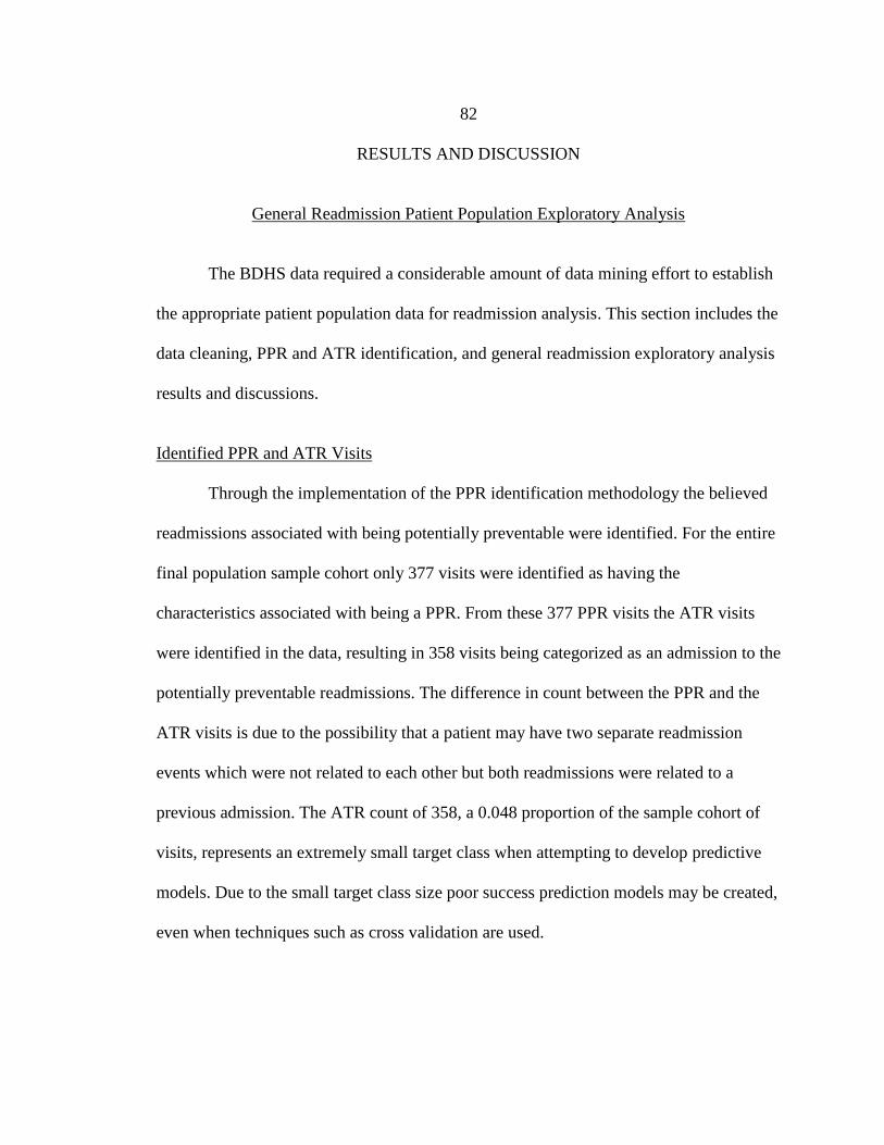
82
RESULTS AND DISCUSSION
General Readmission Patient Population Exploratory Analysis
The BDHS data required a considerable amount of data mining effort to establish
the appropriate patient population data for readmission analysis. This section includes the
data cleaning, PPR and ATR identification, and general readmission exploratory analysis
results and discussions.
Identified PPR and ATR Visits
Through the implementation of the PPR identification methodology the believed
readmissions associated with being potentially preventable were identified. For the entire
final population sample cohort only 377 visits were identified as having the
characteristics associated with being a PPR. From these 377 PPR visits the ATR visits
were identified in the data, resulting in 358 visits being categorized as an admission to the
potentially preventable readmissions. The difference in count between the PPR and the
ATR visits is due to the possibility that a patient may have two separate readmission
events which were not related to each other but both readmissions were related to a
previous admission. The ATR count of 358, a 0.048 proportion of the sample cohort of
visits, represents an extremely small target class when attempting to develop predictive
models. Due to the small target class size poor success prediction models may be created,
even when techniques such as cross validation are used.

83
Exploratory Analysis of General Readmission
Sample Cohort Results and Discussion
The electronically generated retrospective data was trended for emerging patterns
to determine if interventions for select populations could be established. Discovery of
patterns could suggest readmission risk predictor variables in answer to the defined first
research question. Jencks et al. (2009) explicitly stated that planning practice changes for
improving the delivery of care and reducing readmissions can only be effective if
information about the readmitted population can be trended for patterns. Therefore the
resulting ATR visit frequency distributions relating to the 16 predictor variables
discussed in Table 7 are presented. The following figures were created using only the 358
ATR visits and present an enormous amount of information about the patient population,
with potential knowledge from these variable distributions whether the variable could be
a key predictor variable.
The discharge month distribution in Figure 4 portrays an approximately uniform
proportional distribution of ATR visits, with June, May and October representing the
largest frequency values. This fairly uniform distribution of ATR visits helps to rule out
the previous perception that possibly season conditions considerably affect PPR rates.
Some suggestions have been made for Flu season cycles to influence readmission rates
but for the BDHS patient population this does not appear relevant.

84
Figure 4: Discharge Month ATR Visit Frequency
Figure 5 illustrates a possible gamma distribution of ATR visits in relation to the
patient’s LOS, with heavy weighting to the left side of the graph. This skewness does not
definitively indicate a strong potential for LOS to impact risk of readmission, because the
average length of stay of inpatients at BDHS is around 3.1 days. Thus the LOS
distribution for the entire patient population is expected to be right skewed similarly to
what Figure 5 shows.
27, 7%
27, 7%
28, 8%
28, 8%
36, 10%
38, 11% 28, 8%
32, 9%
28, 8%
35, 10%
28, 8%
23, 6%
Distribution of Admit to Readmit Visits by Discharge Month
January
February
March
April
May
June
July
August
September
October

85
Figure 5: Length of Stay ATR Visit Frequency
Age has been shown to be a contributing readmission risk factor in literature and
the Age distributions below in Figures 6 and 7 supports this idea as well. The majority of
patients readmitted to BDHS include those that are in their 50’s, 60’s, 70’s and 80’s.
These decades together make up 65% (232/358) of the readmission population, with the
patients age 50-54 and 80-84 contributing to readmissions appreciably more than other
categories. Several potential factors for this could be the prevalence of cardiovascular
related (CHF and AMI) readmissions being common in people in their 50’s, as well as
the older population, patients in their 80’s being more susceptible to Pneumonia. These
two high national readmission rate medical conditions could explain the prevalent
bimodal distribution found for Age. Patients in their 80’s made up the largest age by
decade category, reported at almost 20% (71/358), according to Figure 7. Gender was an
even split between male and female ATR visits, and therefore was not shown and at least
for general readmissions is not an important risk of readmission predictor.
6
64
82
63 54
28 17
11 10 5 5 1 3 2 1 1 1 1 1 1 1
0
20
40
60
80
100
0 1 2 3 4 5 6 7 8 9 10 11 12 13 15 16 20 21 22 45 54
Fre
qu
en
cy
Days
Distribution of Admit to Readmit Visits by Length of Stay
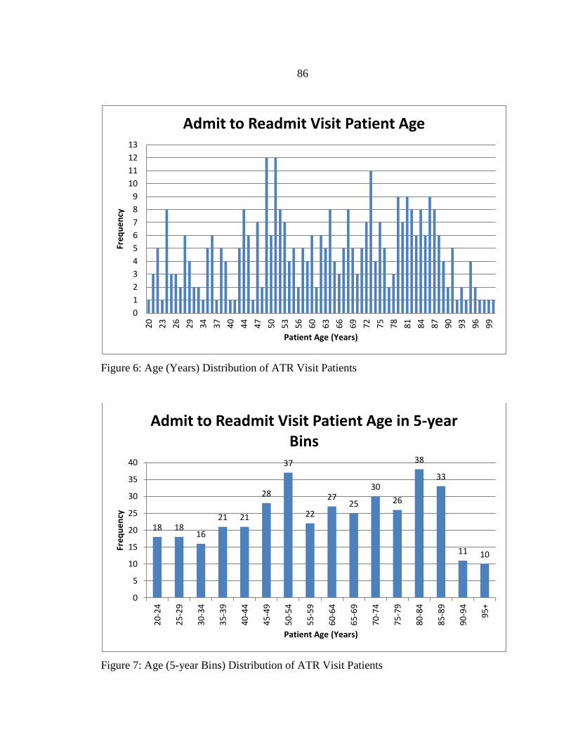
86
Figure 6: Age (Years) Distribution of ATR Visit Patients
Figure 7: Age (5-year Bins) Distribution of ATR Visit Patients
0
1
2
3
4
5
6
7
8
9
10
11
12
13 2
0
23
26
29
34
37
40
44
47
50
53
56
60
63
66
69
72
75
78
81
84
87
90
93
96
99
Fre
qu
en
cy
Patient Age (Years)
Admit to Readmit Visit Patient Age
18 18 16
21 21
28
37
22
27 25
30
26
38
33
11 10
0
5
10
15
20
25
30
35
40
20
-24
25
-29
30
-34
35
-39
40
-44
45
-49
50
-54
55
-59
60
-64
65
-69
70
-74
75
-79
80
-84
85
-89
90
-94
95
+
Fre
qu
en
cy
Patient Age (Years)
Admit to Readmit Visit Patient Age in 5-year Bins

87
Marital status, Figure 8, may look like being married is a potential predictor, this
is proportional to the number of patients at BDHS who were married; and the real reason
for incorporation of this variable is to estimate the readmission patient population who
has close family support at home. Thus of the seven identifiers of marital status, Married
and Life Partner are categorized as indicators of family support, while the other levels do
not. Married and life Partner constitute 43% (155/358) of readmission patients, leaving an
approximate 57% of patients without easily identifiable strong family potential support.
This makes it unlikely a strong predictor will come from Marital Status
Figure 8: Marital Status Distribution of ATR Visit Patients
For hospital discharge department, Figure 9, there appears to be a strong
indication Medical department patients are at the highest risk of readmission. Upon
148
95
66
41
7 1 0
20
40
60
80
100
120
140
160
Fre
qu
en
cy
Marital Status
Distribution of Admit to Readmit Visits by Marital Status

88
further investigation the Medical department accounts for 82% (295/358) ATR visits a
considerably higher proportion than Medical department discharges for the general
population, only 53%. Though more patients are discharged from the Medical department
than any other, they are accounting for a higher than proportional amount of the ATR
visits, this may indicate that Medical floor patients are more likely to be readmitted. In
comparison the Surgical department accounts for only 11% (40/358) of ATRs but for
almost 40% of general population visits. It appears a shift in proportionality from general
to ATR visits by department has occurred. This predictor should be watched when
predictive models are developed.
Figure 9: Discharge Department Distribution of ATR Visits
Overwhelmingly it appears, in Figure 10, that patients who enter through the ER,
89% of ATR visits, are more likely to become an ATR. Thus relating to the PPR not only
23
295
40
0
50
100
150
200
250
300
350
ICU Medical Surgical
Fre
qu
en
cy
Discharge Department
Distribution of Admit to Readmit Visits by Discharge Department
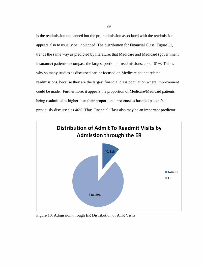
89
is the readmission unplanned but the prior admission associated with the readmission
appears also to usually be unplanned. The distribution for Financial Class, Figure 11,
trends the same way as predicted by literature, that Medicare and Medicaid (government
insurance) patients encompass the largest portion of readmissions, about 61%. This is
why so many studies as discussed earlier focused on Medicare patient related
readmissions, because they are the largest financial class population where improvement
could be made. Furthermore, it appears the proportion of Medicare/Medicaid patients
being readmitted is higher than their proportional presence as hospital patient’s
previously discussed as 46%. Thus Financial Class also may be an important predictor.
Figure 10: Admission through ER Distribution of ATR Visits
40, 11%
318, 89%
Distribution of Admit To Readmit Visits by Admission through the ER
Non-ER
ER

90
Figure 11: Financial Class ATR Visit Distribution
Clinicians at BDHS speculated that local skilled nursing facilities were
contributing substantially to the readmission problem. Contrary to their beliefs according
to Figure 12, only 11% (38/358) of the readmission population was readmitted after
having been previously discharged to a skilled nursing facility Comparatively, 72%
(257/358) of patients who experienced an unplanned and related readmission at BDHS
were discharged home after their initial admission, with another 15% of patient
readmissions having been discharged home with health assistance care available. All
three of these proportions are very similar to the general population proportions for
discharge disposition so unlikely an important predictor.
BlueCross 15%
Commercial 13%
HMO 0%
Medicaid 8% Medicare
53%
Selfpay 11%
Tricare 0%
WorkersComp 0%
Distribution of Admit to Readmit Visits by Financial Class

91
Figure 12: Patient Discharge Disposition Distribution of ATR Visits
Several studies have discussed the potential of inadequate access to follow-up
healthcare and preventative healthcare, like being located in a more rural community, as
being an increased risk factor for readmission. From the distribution presented in Figure
13 there is little distributional evidence to indicate patients more rurally located from
BDHS had considerable increased numbers of readmission. A small spike for 51-100
miles instigated inquisition into if this was just proportionally relative to the general
patient population. Therefore it was determined 7.2% (535/7451) visits from patients
living 51-100 miles from BDHS and this model is almost identically to the 7.26%
(26/358) ATR visits, thus unlikely that distance from hospital is a major predictor of
general readmissions.
257
52 8 1 1
38 1
0
50
100
150
200
250
300
Freq
uen
cy
Discharge Disposition
Distribution of Admit to Readmit Visits by Patient Discharge Disposition

92
Figure 13: Distance to Hospital Distribution of ATR Visits
The three drug related variables in Figures 14, 15 and 16 were included in
exploratory analysis without knowing an expected distribution from these variables. Both
the counts of number of drugs administered, Figure 14, and the number of drugs
prescribed, Figure 15, present normal shape distributions, with the difference between
these variables, Figure 17, appearing to be a right skewed distribution indicating that
generally the number administered was close to the number of drugs prescribed. These
distributions may not give valuable information about readmission risk prediction, but
they give insight into characteristics of the patient population. Several insights to be taken
from the distributions are the averages for the variables. On average an ATR patient is
prescribed about 17 different types of drugs during their stay, with about 12 of those
being administered, leaving the difference of 5 drugs. Though the distributions may not
have unique qualities portraying them as a predictor, it is beneficial to know the
193
95
7 26
8 3 18 8
0
50
100
150
200
250
Freq
uen
cy
Distance
Distribution of Admit to Readmit Visits by Distance to Hospital

93
approximate number of drugs a patient is prescribed at the hospital and whether this
number of drugs if present on the discharging drug list (the variable truly wanted to
investigate but is unavailable) could be a predictor of increased readmission due to the
complexity of medications.
Figure 14: Number of Drugs Prescribed Distribution of ATR Visits
Figure 3: Number of Drugs Administered Distribution of ATR Visits
0 2 4 6 8
10 12 14 16 18 20 22 24 26 28 30
0 4 5 6 7 8 9 10 11 12 13 14 15 16 17 18 19 20 21 22 23 24 25 26 27 28 29 30 31 34 41 47
Fre
qu
en
cy
Number of Drugs Prescribed
Distribution of Admit To Readmit Visits by Number of Drugs Prescribed
0 2 4 6 8
10 12 14 16 18 20 22 24 26 28 30 32 34
0 1 2 3 4 5 6 7 8 9 10 11 12 13 14 15 16 17 18 19 20 21 22 23 24 25 26 27 28 31 34
Fre
qu
en
cy
Number of Drugs Administered
Distribution of Admit To Readmit Visits by Number of Drugs Administered

94
Figure 16: Difference between Number of Drugs Prescribed and Administered for ATR
Visits
A variable which was incorporated due to discussions with healthcare
professional at BDHS, and which may have a potential for readmission risk prediction,
was Count of Consults. This count represents the non-general practice official
consultations the patient received while in BDHS as an inpatient during their visit. Many
times with a major new medical condition causing the onset of a hospitalization it has
been suggested that patients may be discharged from the hospital before they truly have
an understanding of how to manage their medical condition. This is especially true for
CHF, with many studies indicating repeat readmissions since the patient did not change
certain parts of their lifestyle as necessary from the condition. It is believed that by
potentially having a formal consult, say with a cardiologist for CHF, a patient may
become better informed about their medical condition, enabling them to better manage
0
10
20
30
40
50
60
0 1 2 3 4 5 6 7 8 9 10 11 12 13 14 16 17 20 21 23 25 26 30
Fre
qu
en
cy
Difference Between the Number of Drugs Prescribed and Administerd
Distribution of the Difference Between the Number of Drugs Prescribed vs.
Administered for Admit To Readmit Visits

95
their condition after discharge reducing their likelihood of readmission. In Figure 17,
over 57% of patients never had a consult while hospitalized, and 90% of patients only
had one or less consult. Unfortunately after investigation into the general population’s
proportions for this variable it was seen 66% never had a consult and 91% had one or less
consults while hospitalized, therefore it is just a representative proportional distribution.
Figure 4: Count of Consults Distribution for ATR Visits
The remaining two variables evaluated in Figures 18 and 19 were incorporated
with strong support from the literature that these may be risk predictors for readmissions.
Current clinical readmission risk assessment tools, such as LACE, use both the number of
inpatient visits and the number of ER visits within the past six months or a year as
readmission risk predictors. From the distributions shown the expected average number
of ER visits within the prior six months, Figure 18, was approximately 2, while for the
non-readmission population it is less than 0.79, a more than twofold increase in the
number of visits. Similarly for Figure 19, the average number of inpatient visits was seen
to be about 0.83, while the non-readmission population had an estimated average value of
only 0.32, again a more than twofold increase. These values are indicating that these two
205 117
26 8 2 0
200
400
0 1 2 3 4
Freq
uen
cy
Count of Consults
Distribution of Admit To Readmit Visits by Count of Consults

96
variables do appear to have different values between readmission and non-readmission
populations. To be sure of this discovery a statistical means comparison would need to be
performed. This potentially can be future investigations of variable properties for BDHS,
but for now the definite inclusion of these variables in the predictive models and the
inspection for these variables in the final predictive models will be performed.
Figure 5: Number of ER Visits within Prior 6 Months for ATR Visit Patients
Figure 6: Number of IN Visits within Prior 6 Months for ATR Visit Patients
140
87
42
19 23 13 10 7 3 3 3 2 1 2 1 1 1
0
50
100
150
0 1 2 3 4 5 6 7 8 9 10 11 13 20 24 31 32
Fre
qu
en
cy
Number of ER Visits Within Prior 6 Months
Distribution of the Number of ER Visits Within the Prior 6 Months for Admit To Readmit Visits
201
84 41
15 7 4 4 2 0
50
100
150
200
250
0 1 2 3 4 5 6 7
Fre
qu
en
cy
Number of IN Visits Within Prior 6 Months
Distribution of the Number of Inpatient Visits Within the Prior 6 Months for Admit To
Readmit Visits

97
To answer Hypothesis 1, the null hypothesis has been found invalid since it does
appear that some predictor variables included in exploratory analysis show strong
potential for impacting patient readmission risk. From exploratory analysis some factors
which hold promise for being readmission risk predictors are Age, Discharge
Department, Financial Class, Admit from ER, Prior 6-month ER count and Prior 6-month
IN count. These factors should further be investigated for research question 2, by the
inspection of prediction variables present in the prediction models developed for BDHS.
Through further investigation of these six specific predictor variable topics at BDHS,
BDHS may gain more insight into what is affecting patient’s readmission risk and
potential interventions may be applicable.
Top Diagnoses-Related Readmission Results and Discussion
Comparisons of the national and BDHS core measure readmission rates yielded
that BDHS had very similar readmission levels. These three core measures do not
account for most, let alone the entire PPR population. Therefore using the general
readmission file the most prevalent BDHS diagnoses related readmissions were
calculated. Figure 20 illustrates the frequency of presence of ICD-9 codes in the ATR
population; this involved searching both primary and secondary diagnoses variables.

98
Figure 7: Top 20 ICD-9 Diagnoses Present in ATR Visits
This method proved slightly too generic to see potential ICD-9 diagnoses which may be
contributing appreciably to the readmission population. Codes such as 276, 401 and V58
are commonly listed secondary diagnosis variables for many medical conditions and were
evaluated by the medical professionals queried as being inappropriate for readmission
predictive model development. The information gained from this investigation was a
perspective on the medically common conditions affiliated with many hospital
admissions.
117 113
91
77 69 67 66 64 62 62 62 58 57 55 54 54 53 49 47 45
0
20
40
60
80
100
120
140
Fre
qu
en
cy
ICD-9 Diagnoses
Top 20 Diagnoses for Admit To Readmit Visits
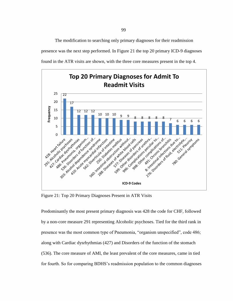
99
The modification to searching only primary diagnoses for their readmission
presence was the next step performed. In Figure 21 the top 20 primary ICD-9 diagnoses
found in the ATR visits are shown, with the three core measures present in the top 4.
Figure 21: Top 20 Primary Diagnoses Present in ATR Visits
Predominantly the most present primary diagnosis was 428 the code for CHF, followed
by a non-core measure 291 representing Alcoholic psychoses. Tied for the third rank in
presence was the most common type of Pneumonia, “organism unspecified”, code 486;
along with Cardiac dysrhythmias (427) and Disorders of the function of the stomach
(536). The core measure of AMI, the least prevalent of the core measures, came in tied
for fourth. So for comparing BDHS’s readmission population to the common diagnoses
22
17
12 12 12 10 10 10 9 9 8 8 8 8 8 7 6 6 6 6
0
5
10
15
20
25
Fre
qu
en
cy
ICD-9 Codes
Top 20 Primary Diagnoses for Admit To Readmit Visits

100
present in the national data reviews, they are very similar. In the report presented to
Congress about Medicare hospital readmissions and the PPACA legislation, by Stone and
Hoffman (2010), the analysts for the Congressional Research Services discuss the
diagnoses present at high 30-day readmission rates “heart failure (26.9%), pneumonia
(20.1%), chronic obstructive pulmonary disease (COPD, 22.6%), psychoses (24.6%), and
gastrointestinal conditions (19.2%)” (Stone & Hoffman, 2010). These almost identically
reflect the top diagnoses related to readmission found for the data in Figure 22, with
alcoholic psychoses linking with psychoses, and disorders of the function of the stomach
linking with gastrointestinal conditions. This comparison is further proof that the same
readmissions conditions at BDHS are the top national readmission conditions, even
though it is a small community hospital surrounded by the rural Gallatin County
community.
The three non-core measure diagnoses present in the top three readmission levels
of the distribution represent potential diagnoses with considerable impact in the
healthcare community nationally. Their strong presence in the BDHS data encourages the
attempt to develop diagnosis specific readmission risk predictive models for them.
Therefore a total of seven unique sets of readmission prediction models were created,
including one general readmission set and six diagnosis specific sets. The data
characteristics for each diagnosis model were generated to illustrate the sample sizes and
ATR visit proportions within the data. These resultant datasets are defined in Table 12.

101
Table 12: Diagnoses Specific Dataset Information
Model Total Sample Count Total ATR Count ATR % of Total Sample
General. 7451 358 4.80%
CHF 800 62 7.75%
PNM 615 30 4.88%
291 189 24 12.69%
427 1188 62 5.22%
536 157 24 15.29%
AMI 225 11 4.89%
After review of the diagnosis specific datasets it is evident to see these are extremely
small data populations and likely will make prediction modeling challenging.
Immediately once this result was discovered it was attempted to see what mitigation
techniques could be used, such as cross validation. Ultimately cross validation testing
was only feasible for the MARS models and the SPSS models are only representative of
the train data success of prediction and will require testing with future BDHS data to
determine their true predictive abilities.
Prediction Model Results
The BDHS visit data has the ability of being suitable for not only the exploration
of general readmission risk predictors, but also investigation into individual condition
specific analysis. In order to attempt to model readmissions more accurately the decision
to break the larger data into six data subset files will allow for the potential creation of up

102
to six prediction tools addressing readmission related to a specific patient medical
condition. The implementation of more targeted prediction models may allow for
multiple different sets of predictor variables to be found significant in the prediction of
ATR visits.
As discussed previously the comparison of the prediction capability of a final
developed prediction model includes the interpretation of many prediction quality metrics
relevant to each structure characteristic model including R2, AUC and prediction success
values. For instance the binary logistic regression models will have pseudo R2 terms
(Nagelkerke), while CART models report Relative Costs (1- R2), and MARS will have
naïve-adjusted R2
values and R2
values representing a penalized prediction value (GCV
R2) based on the complexity of the MARS generated basis functions included. These
values represent the amount of variability in the data used to construct the models (train
data), which is accounted for in the models. Prediction success tables (classification
tables) for the train data will also be used to evaluate the model’s prediction success.
Another metric suggested is the area under the receiver operating characteristic curve, the
previously discussed AUC values. These values are "more informative than the
classification table, since it summarizes predictive power for all possible πo" (Agresti,
2002). Thus comparing the AUC calculated values of the respective SPSS, CART and
MARS prediction models should provide another reasonable metric indicating the
prediction capabilities of different models.
Upon model evaluation of the developed CART models it was apparent that these
models were inappropriate for the BDHS data. With high relative costs (low R2
values)

103
and only the capability to predict a discrete number of patient characteristic scenarios (the
number of terminal nodes) it was decided to not report these values in comparison to the
SPSS and MARS models. For prediction purposes all CART models are inappropriate for
the BDHS data, likely due to the inability of the decision tree to model such complex
potential interactions. However the development of the CART model was used as
exploratory analysis, for establishing estimates of control parameters such as the Max BF
value. Due to the ease and speed of CART as an exploratory analysis technique, it still
should be used prior to MARS to attempt to develop a viable model, as well as to obtain
an estimate value for MARS Max BF value calculation. The key metrics which are
available to aid in model evaluation, for each diagnosis dataset model type, are
summarized and presented in Table 13 for the SPSS and MARS models. The following
discussion of model results directly answers the second and third research questions of
this thesis.
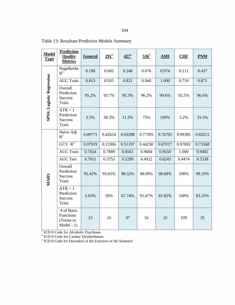
104
Table 13: Resultant Predictive Models Summary
1 ICD-9 Code for Alcoholic Psychoses
2 ICD-9 Code for Cardiac Dysrhythmias
3 ICD-9 Code for Disorders of the Function of the Stomach
Model
Type
Prediction
Quality
Metrics
General 2911
4272
5363
AMI CHF PNM
SP
SS
: L
og
isti
c R
egre
ssio
n
Nagelkerke
R2
0.198 0.605 0.248 0.676 0.974 0.111 0.437
AUC Train 0.813 0.935 0.821 0.940 1.000 0.710 0.871
Overall
Prediction
Success
Train
95.2% 93.7% 95.3% 96.2% 99.6% 92.5% 96.6%
ATR = 1
Prediction
Success
Train
2.5% 58.3% 11.3% 75% 100% 3.2% 33.3%
MA
RS
Naïve Adj.
R2
0.09771 0.42624 0.63288 0.77395 0.76705 0.99385 0.82615
GCV R2 0.07919 0.13306 0.51197 0.44230 0.67017 0.97692 0.73568
AUC Train 0.7654 0.7889 0.8561 0.9684 0.9550 1.000 0.9482
AUC Test 0.7011 0.3753 0.5289 0.4922 0.6243 0.4474 0.5338
Overall
Prediction
Success
Train
95.42% 93.65% 98.32% 98.09% 98.68% 100% 99.19%
ATR = 1
Prediction
Success
Train
5.03% 50% 67.74% 91.67% 81.82% 100% 83.33%
# of Basis
Functions
(Terms in
Model - 1)
23 10 47 16 10 109 35
105
Individual Diagnoses Type Prediction
Model Results and Discussion
The evaluation of the seven datasets fitted for prediction models is presented in an
individual manner. This is due to the semi-subjective analysis necessary to evaluate the
prediction success of these models. Objective prediction metrics have been calculated but
how the two types of models (SPSS and MARS) compare is not a direct “apples to
apples” comparison. The major differences in prediction model creation between these
model types is the validation techniques used and reported coefficient of determination
(R2) values reported. SPSS models only included a train population and model validation
was not performed. MARS used cross validation to formulate results based on both train
and test populations within the datasets. All metric values and percentages discussed
below can be found in Table 11.
General Readmission Prediction Models
By far the dataset with the largest patient visit population, this dataset was the
starting place for the development of all diagnoses specific prediction models. The
dataset containing an ATR visit count of 358 visits, (~5% of data), is a difficult
population characteristic when attempting to develop a prediction model. Since the target
class of ATR visit counts is such a small proportion of the complete population and since
this general model included all-condition readmissions categorized as a PPR, an
enormously complex set of patient characteristics is trying to be modeled with an
insignificant amount of target class data. The expected prediction capability of a general
106
readmission risk prediction model, from any of the three statistical prediction methods,
was not believed to be possible.
These presumptions were confirmed by the prediction models developed in SPSS
and MARS. Though AUC train values were found to be 0.813 and 0.7654 respectively,
these values represent a worse AUC than simply categorizing all visits as not an ATR
visit (~0.95). This is illustrated by the prediction success referring to ATR visits for the
models with prediction capabilities of 2.5% and 5.03% respectively. The only reason the
AUC train values appear to show prediction success is because of the high proportional
difference in ATR versus non-ATR visits. Therefore neither of these models should be
considered appropriate and the variables included in their predictions not investigated.
ICD-9 Code 291: Alcoholic
Psychoses Prediction Models
Similar to the general readmission risk prediction models, models developed for
Alcoholic Psychoses do not appear to have any statistically significant prediction value.
The respective AUC train values 0.935 for binary logistic regression in SPSS appears to
represent a good prediction model. The Nagelkerke R2 value, an adjusted R
2, of 0.605
represents a borderline appropriate level of data variability being accounted for by the
model. After reviewing the fact that this data is real human data, instead of more
variability controlled data such as in clinical trials, this adjusted R2 value becomes more
appealing as potentially reasonable (Claudio, 2012). Due to this research’s use of this
uncontrolled data it was estimated for models with R2 values approximately above 0.6 to
be viewed as reasonable prediction models, if other prediction metrics also indicate

107
positive trends. Evaluating the prediction success of the SPSS model based an
unappealing value of 58.3% for the ATR visits predicted correctly tilts the belief that this
model may be appropriate. The cost of having a patient who is a PPR be falsely classified
as a non-risk of readmission patient is worse than the opposite. This is Type II error, or a
“miss”, and is wanted to be avoided because the miss of a patient at high risk for
readmission is costly, both in potential actual healthcare costs and in the increase to
readmission rates by that patient’s potential readmission. Therefore because this model
presents only borderline ability to effectively predict data variability and ATR visits it is
not appropriate for use at BDHS.
Next in evaluating the MARS model the AUC train values 0.7889 suggest at least
modest prediction ability, but when the Naïve Adjusted R2 and GCV R
2 are viewed the
model is seen to be inappropriate. The R2 values are illustrating a small portion of the
data variability is being properly modeled. Furthermore with MARS an AUC test value is
available from cross validation. With an AUC test of 0.3753 this again points to the
MARS model being inappropriate for use because it truly doesn’t predict the data well.
Therefore again no variables or models for readmission risk predictions could be verified
from this data.
Psychoses related readmissions were only discussed minimally in the literature
and no discussions of potential variables for risk prediction were ever indicated. The poor
ability to predict these types of readmissions may be attributable to an inability to
categorize any common characteristics of alcoholic psychoses related visits, let alone the
readmission visits. Since this diagnosis is so prevalent in the BDHS readmission data in
108
primary ICD-9 conditions for visits (refer to Figure 22), an inspection into the potential
causation for the high number of visits may be appropriate to perform, even though a
prediction model was not developed. Kujawa (2012) discusses potential interventions to
attempt to reduce the readmission rate of the alcohol psychoses patient population.
ICD-9 Code 427: Cardiac
Dysrhythmias Prediction Models
Cardiovascular related readmissions are among the most prevalent readmission
conditions in the US. The inclusion of a third cardiovascular related ICD-9 condition
found on the top 20 list of most prevalent readmission types at BDHS (Figure 22)
supports this finding. AMI and 427 combined accounted for the same frequency of
readmissions as CHF (22, from Figure 22). With the inclusion of CHF these three
cardiovascular related medical conditions pose the largest diagnoses grouped portion of
the readmission population. Unfortunately developing prediction models for 427 was
only mildly successful.
The binary logistic regression prediction model in SPSS reported an AUC train
of 0.821 but had a Nagelkerke value of only 0.248. This R2 value is an indication of poor
variability fit by the model. In reference to the R2 value, basing a model’s prediction
ability solely on the pseudo R2 value developed by Nagelkerke is not advised, because
this value is a transformation of the Cox & Snell pseudo R2 to a 0-1 distribution size.
Furthermore, R-squared values for binary logistic regression, or any other non-parametric
regression analysis including MARS, are created by mathematically supported
estimations of the coefficients of determinations present in the model. Since the predictor
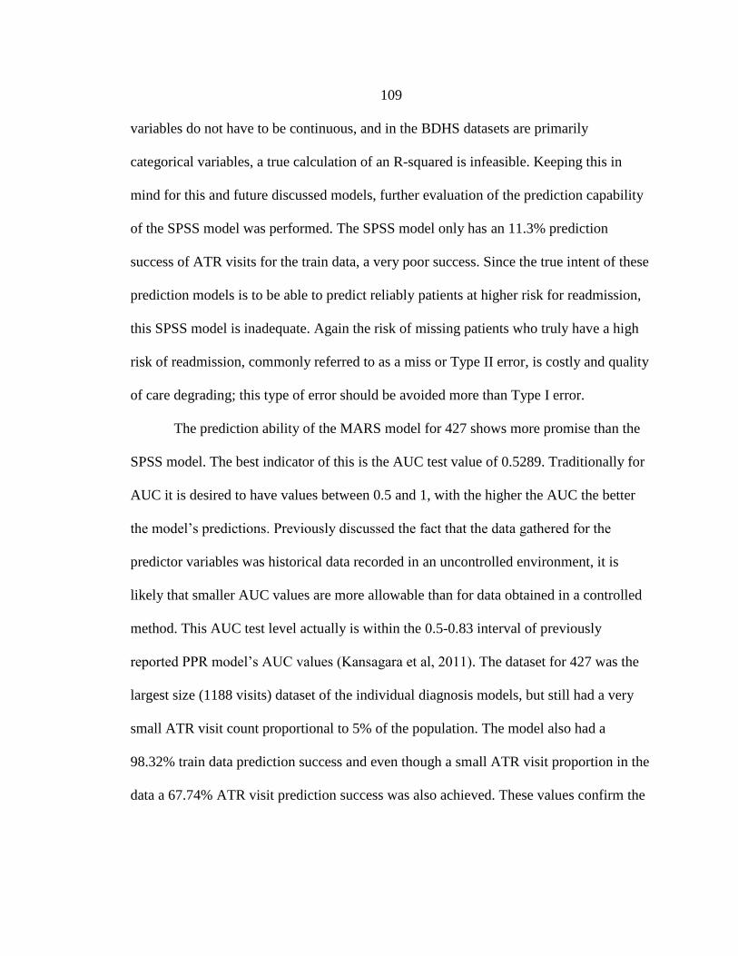
109
variables do not have to be continuous, and in the BDHS datasets are primarily
categorical variables, a true calculation of an R-squared is infeasible. Keeping this in
mind for this and future discussed models, further evaluation of the prediction capability
of the SPSS model was performed. The SPSS model only has an 11.3% prediction
success of ATR visits for the train data, a very poor success. Since the true intent of these
prediction models is to be able to predict reliably patients at higher risk for readmission,
this SPSS model is inadequate. Again the risk of missing patients who truly have a high
risk of readmission, commonly referred to as a miss or Type II error, is costly and quality
of care degrading; this type of error should be avoided more than Type I error.
The prediction ability of the MARS model for 427 shows more promise than the
SPSS model. The best indicator of this is the AUC test value of 0.5289. Traditionally for
AUC it is desired to have values between 0.5 and 1, with the higher the AUC the better
the model’s predictions. Previously discussed the fact that the data gathered for the
predictor variables was historical data recorded in an uncontrolled environment, it is
likely that smaller AUC values are more allowable than for data obtained in a controlled
method. This AUC test level actually is within the 0.5-0.83 interval of previously
reported PPR model’s AUC values (Kansagara et al, 2011). The dataset for 427 was the
largest size (1188 visits) dataset of the individual diagnosis models, but still had a very
small ATR visit count proportional to 5% of the population. The model also had a
98.32% train data prediction success and even though a small ATR visit proportion in the
data a 67.74% ATR visit prediction success was also achieved. These values confirm the
110
potential that this MARS prediction model has prediction capability for readmission risk
in the 427 patient population.
The available dataset with the small target population along with a small total
sample population, in relation to studies previously performed (Kansagara et al. 2011),
are potentially constraining factors to MARS developing a better prediction model.
Before relying on the current prediction model it would be wise to retest this model with
a larger test sample obtained from BDHS.
The MARS prediction model for 427 contained 47 basis functions in the model,
with a constant term also being included to make a total of 48 terms in the final
regression model. The entire MARS report output including a list of prediction variables,
ranking of variables by importance, along with the actual developed basis functions for
the can be found in Appendix I. The MARS model contained 50 predictor variables
forming 48 basis functions. Of the characteristic predictor variables listed in Table 7,
only four were present in some capacity. The remaining predictor variables were ICD-9
diagnoses groupings and drug id variables. For complexity and space purposes these
variables were not explicitly discussed. The key finding about these predictor variables is
that according to this MARS model they represent a considerable (46/50) portion of the
model incorporated predictor variables. The inclusion of ICD-9 and drug related variables
appear to help in the readmission risk prediction for patients with cardiac dysrhythmias
The four predictor variables along with their respective MARS generated level of
variable importance are shown in Table 14. Patient age, as previously expected from the
exploratory analysis of the general readmission values, appeared to have the largest
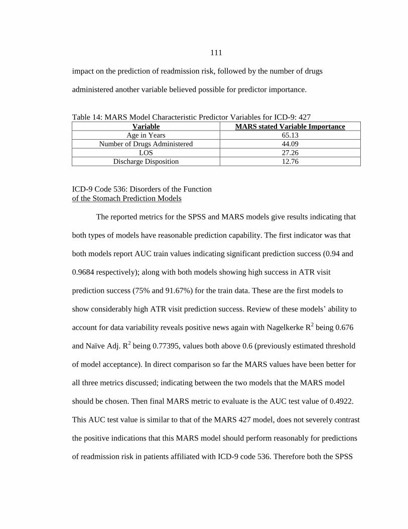
111
impact on the prediction of readmission risk, followed by the number of drugs
administered another variable believed possible for predictor importance.
Table 14: MARS Model Characteristic Predictor Variables for ICD-9: 427
Variable MARS stated Variable Importance
Age in Years 65.13
Number of Drugs Administered 44.09
LOS 27.26
Discharge Disposition 12.76
ICD-9 Code 536: Disorders of the Function
of the Stomach Prediction Models
The reported metrics for the SPSS and MARS models give results indicating that
both types of models have reasonable prediction capability. The first indicator was that
both models report AUC train values indicating significant prediction success (0.94 and
0.9684 respectively); along with both models showing high success in ATR visit
prediction success (75% and 91.67%) for the train data. These are the first models to
show considerably high ATR visit prediction success. Review of these models’ ability to
account for data variability reveals positive news again with Nagelkerke R2 being 0.676
and Naïve Adj. R2 being 0.77395, values both above 0.6 (previously estimated threshold
of model acceptance). In direct comparison so far the MARS values have been better for
all three metrics discussed; indicating between the two models that the MARS model
should be chosen. Then final MARS metric to evaluate is the AUC test value of 0.4922.
This AUC test value is similar to that of the MARS 427 model, does not severely contrast
the positive indications that this MARS model should perform reasonably for predictions
of readmission risk in patients affiliated with ICD-9 code 536. Therefore both the SPSS

112
and MARS prediction models appear to be reasonable models to attempt to predict
readmission risk of 536 affiliated patient visits.
The binary logistic regression model produced in SPSS contained 16 predictor
variables and a constant. The characteristic predictor variables present were patient age in
years, count of consults and prior six month inpatient count. The other 12 predictor
variables included primary diagnoses, secondary diagnoses and drug id predictor
variables. Again this high concentration of these variables being present in these
prediction models supports the idea that the diagnoses and drug related predictor
variables could help account for hidden interactions with readmission risk otherwise
previously missed by the characteristic predictor variables. The complete SPSS primary
component outputs for the prediction model are found in Appendix J, followed by the
model report output of the MARS model in Appendix K. Table 14 lists the variables used
in both models, with the highlighted variables being those both models shared in
common, and the model variables are listed in descending order of variable importance.
The MARS prediction model consists of 18 predictor variables comprising 16
basis functions. The characteristic predictor variables present in the prediction model for
536 were patient financial class and prior six month inpatient visit count. Prior six month
inpatient count was found to be a readmission risk predictor in both models, supporting
the previous studies and LACE tool which have incorporated it as a key predictor.
Furthermore both models have in common five ICD-9 diagnoses related predictors,
shown shaded in Table 15. These common diagnoses related predictors again support the
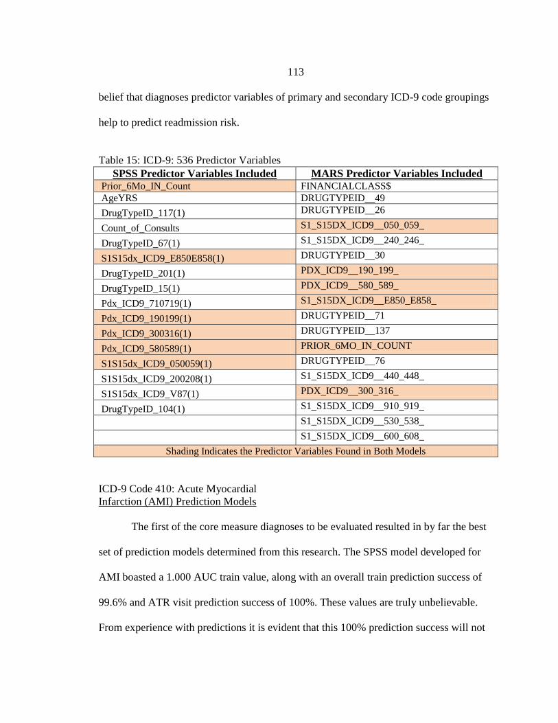
113
belief that diagnoses predictor variables of primary and secondary ICD-9 code groupings
help to predict readmission risk.
Table 15: ICD-9: 536 Predictor Variables
ICD-9 Code 410: Acute Myocardial
Infarction (AMI) Prediction Models
The first of the core measure diagnoses to be evaluated resulted in by far the best
set of prediction models determined from this research. The SPSS model developed for
AMI boasted a 1.000 AUC train value, along with an overall train prediction success of
99.6% and ATR visit prediction success of 100%. These values are truly unbelievable.
From experience with predictions it is evident that this 100% prediction success will not
SPSS Predictor Variables Included MARS Predictor Variables Included Prior_6Mo_IN_Count FINANCIALCLASS$
AgeYRS DRUGTYPEID__49
DrugTypeID_117(1) DRUGTYPEID__26
Count_of_Consults S1_S15DX_ICD9__050_059_
DrugTypeID_67(1) S1_S15DX_ICD9__240_246_
S1S15dx_ICD9_E850E858(1) DRUGTYPEID__30
DrugTypeID_201(1) PDX_ICD9__190_199_
DrugTypeID_15(1) PDX_ICD9__580_589_
Pdx_ICD9_710719(1) S1_S15DX_ICD9__E850_E858_
Pdx_ICD9_190199(1) DRUGTYPEID__71
Pdx_ICD9_300316(1) DRUGTYPEID__137
Pdx_ICD9_580589(1) PRIOR_6MO_IN_COUNT
S1S15dx_ICD9_050059(1) DRUGTYPEID__76
S1S15dx_ICD9_200208(1) S1_S15DX_ICD9__440_448_
S1S15dx_ICD9_V87(1) PDX_ICD9__300_316_
DrugTypeID_104(1) S1_S15DX_ICD9__910_919_
S1_S15DX_ICD9__530_538_
S1_S15DX_ICD9__600_608_
Shading Indicates the Predictor Variables Found in Both Models

114
occur in data tested, but the fact that the train data shows such good predictions based on
the model is promising the tested data will have good predictions as well. The potential
cause for such great prediction success is the incredibly small ATR visit sample size for
AMI with a total of 11 visits. This factor made it necessary to only use a two fold cross
validation level in the MARS model, but in SPSS meant the entire train data only had a
minimal number of visits to categorize.
On par with the SPSS model, the MARS train AUC value is great with a 0.955
value, and 81.82% ATR visit prediction success. The model also proves to test well with
an AUC test AUC test value of 0.6243. This value suggests the MARS prediction model
truly is a highly accurate model of readmission risk for AMI patients. The MARS model
used a cross validation of two folds, which in essence split the data in half and tried to
predict the other half, and then the reverse halves were used in the predicting. Since only
two fold cross validation was used it reduces the inherent validation benefits of cross
validation, however this testing is more appropriate than no test data as performed with
SPSS. Some validity issues to these high prediction success and AUC values may be
attributable to the small ATR visit population, so to confirm the abilities of these models
they really should be tested on a larger AMI population size to get a better approximation
of prediction capability.
Since these models were overwhelmingly supported as good prediction models
based on the train dataset, a better testing of the models will hopefully be verified by
future testing on new BDHS AMI patient data. The SPSS model, using forward stepwise
entry of main affects converged after 16 steps were performed and 10 predictor variables

115
were entered. MARS developed a model having 10 basis functions comprised of 11
prediction variables. Six of the same predictor variables were found present in both
models, seemingly showing the importance of these prediction variables. Table 16 lists
the variables used in the models, with the shaded variables being those both models
shared in common.
Table 16: AMI Predictor Variables
SPSS Predictor Variables Included MARS Predictor Variables Included S1S15dx_ICD9_V10V19 DISCHARGE_MONTH$
DrugTypeID_175 MARITALSTATUS$
Gender S1_S15DX_ICD9__860_869_
S1S15dx_ICD9_V10V19 S1_S15DX_ICD9__V01_V09_
Discharge Month S1_S15DX_ICD9__958_959_
Marital Status DRUGTYPEID__144
Financial Class DRUGTYPEID__40
DrugTypeID_40 DRUGTYPEID__166
DrugTypeID_166 DRUGTYPEID__204
S1S15dx_ICD9_860869 DRUGTYPEID__131
DRUGTYPEID__87
Shading Indicates the Predictor Variables Found in Both Models
Interestingly Discharge Month and Marital Status both variables thought to likely
not affect general readmission risk, appear to impact AMI readmission risk. Also the
remaining variables are secondary diagnoses and drug variables helping to predict the
risk of readmission. Both of these types of variables traditionally have not been included
in readmission prediction but appear to play a role in AMI risk of readmission. These
models indicate the potential importance of these variables as AMI readmission
predictors, but the models must first be more thoroughly tested before it confidently be
stated these variables expressly affect the risk of readmission of AMI visits. More
116
information about these models can be found in Appendix L for SPSS model components
and Appendix M for MARS model output report for AMI.
ICD-9 Code 428: Congestive Heart
Failure (CHF) Prediction Models
For CHF, the most prevalent readmission type at BDHS and nationally, the largest
ATR visit population was found with 62 visits, out of 800. The binary logistic model
developed in SPSS ranked poorly in key metrics, such as only finding a Nagelkerke R2 of
0.111 and only accurately predicting the train ATR visits successfully 3.5% of the time.
This is extremely poor because this was with the use of 100% of the data being used as
train and the logistic regression model could not account for the data variability at any
reasonable level; thus the SPSS model was eliminated as a viable prediction model.
The MARS readmission risk prediction model for CHF was a noteworthy
improvement over SPSS with an AUC train value of 1.000, along with 100% prediction
success for ALL data. The developed MARS model was able to correctly predict all visits
in the train data, but with the test data it was considerably more modest of a prediction
capability with an AUC test of 0.4474. All metrics considered the MARS model still
appears to be a great candidate for predicting readmission risk of CHF patients; though
this would need to be confirmed on a new historical test sample population before
mainstream intended use.
The high prediction ability of this MARS model is feasible from the regression
method. MARS allows for knots to be placed in the regression model essentially forming
a regression graph of a series of piecewise regression lines. This fitting structure allows
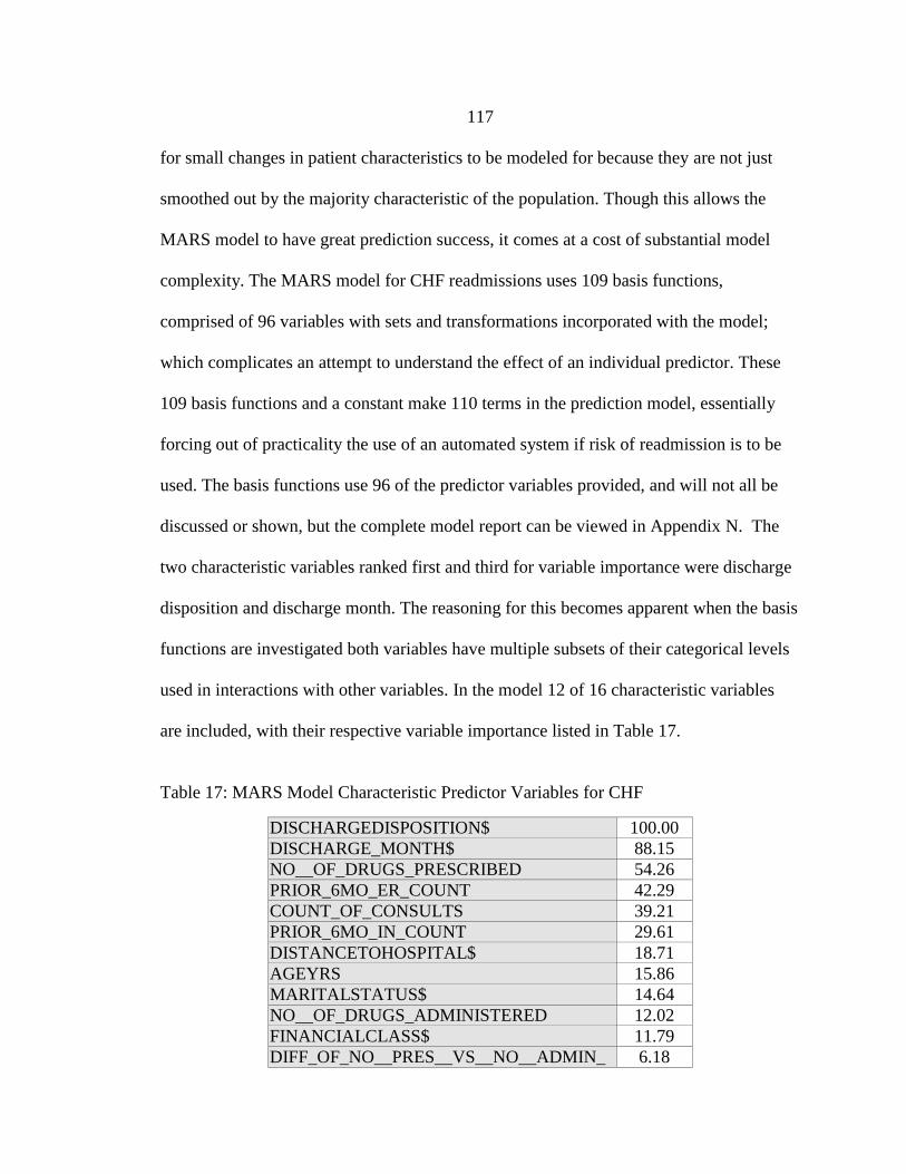
117
for small changes in patient characteristics to be modeled for because they are not just
smoothed out by the majority characteristic of the population. Though this allows the
MARS model to have great prediction success, it comes at a cost of substantial model
complexity. The MARS model for CHF readmissions uses 109 basis functions,
comprised of 96 variables with sets and transformations incorporated with the model;
which complicates an attempt to understand the effect of an individual predictor. These
109 basis functions and a constant make 110 terms in the prediction model, essentially
forcing out of practicality the use of an automated system if risk of readmission is to be
used. The basis functions use 96 of the predictor variables provided, and will not all be
discussed or shown, but the complete model report can be viewed in Appendix N. The
two characteristic variables ranked first and third for variable importance were discharge
disposition and discharge month. The reasoning for this becomes apparent when the basis
functions are investigated both variables have multiple subsets of their categorical levels
used in interactions with other variables. In the model 12 of 16 characteristic variables
are included, with their respective variable importance listed in Table 17.
Table 17: MARS Model Characteristic Predictor Variables for CHF
DISCHARGEDISPOSITION$ 100.00
DISCHARGE_MONTH$ 88.15
NO__OF_DRUGS_PRESCRIBED 54.26
PRIOR_6MO_ER_COUNT 42.29
COUNT_OF_CONSULTS 39.21
PRIOR_6MO_IN_COUNT 29.61
DISTANCETOHOSPITAL$ 18.71
AGEYRS 15.86
MARITALSTATUS$ 14.64
NO__OF_DRUGS_ADMINISTERED 12.02
FINANCIALCLASS$ 11.79
DIFF_OF_NO__PRES__VS__NO__ADMIN_ 6.18

118
Several studies and models in literature for traditional CHF readmission
predictions, using readmission data not necessarily qualified as PPR, have reported model
abilities around the 0.6 AUC validated level (Kansagara et al., 2011). When possible if
this MARS CHF readmission risk model can be tested against a considerably large CHF
related readmission dataset from BDHS, it may yield AUC validated levels foreseeable
larger than the 0.6 level due to its inherent prediction ability discussed from the great
metric values reported. Unfortunately, since this model was developed only using visit
information for PPR readmission of CHF it is an extrapolation to assume that this model
will perform at the same level for all CHF 30-day readmission data, but future
investigation may be worth performing. To be able to help predict accurately this high
readmission rate component of patients would truly be beneficial to the healthcare
industry in reducing costs and improving patient quality of care.
ICD-9 Codes 480-488: Pneumonia
Related (PNM) Prediction Models
The final models to investigate are those affiliated with PNM. PNM is one of the
most prevalent readmissions yet in literature so far only minimal investigation has been
performed on predicting risk of readmission specifically for PNM patients. The visit
complexity of ATR visits for PNM patients, commonly more elderly and with medical
complications other than the primary admitting condition to the hospital, may inhibit the
ability to accurately predict readmission risk for this patient population.
The SPSS prediction model for PNM reported a AUC train of 0.871, however
when looking at the ATR visit prediction success it was only 33.3%, indicating little help
119
in the identification of the target population. Furthermore the Nagelkerke R2 was small at
the 0.437 level. Similarly to previous models the small sample size of visits and small
target population may have adversely affected the construction of a usable model.
The MARS prediction model proved significantly better with an AUC train of
0.9482 and train ATR visit prediction success of 83.3%. The AUC test value of 0.5338 is
the second highest of all the models investigated in this research; along with a Naïve Adj.
R2
and GCV R2
of 0.82615 and 0.73568 respectively. This model poses a good
probability of successfully predicting readmission risk, but should be tested with another
component of PNM related patient visits from BDHS to evaluate its true prediction
potential. The MARS model consists of 35 basis functions comprised of 34 original
predictor variables. This number of basis functions though substantially less than the 109
found in CHF, still presents a fairly complex regression model for the PNM readmission
risk prediction. Similarly to with CHF it is likely the most practical way of implementing
this complex prediction model would have to be through some automated system.
The characteristic predictor variables of most importance were prior six month
ER count and discharge month, being ranked first and second overall. The remaining
characteristic variables included were reported with significantly less importance and are
LOS, count of consults, financial class, age and distance to hospital. The full MARS
model information, including the chosen predictor variable can be found in the model
report in Appendix O. Similarly to previous models a large proportion of predictor
variables, 27 variables, are the ICD-9 and drug related variables. Consistently in each of

120
these models these novel variables have benefited model prediction abilities, with some
of these variables showing high variable importance according to MARS.

121
SUMMARY
Overview
Discussion of some overall important results discovered through the analysis of
the prediction models developed for BDHS is presented. The development of prediction
models for general readmissions was not achievable for the data from BDHS. Similarly
for the Alcoholic Psychoses specific readmissions usable prediction models were not
attained. Also of the usable prediction models developed the MARS method generally
provided more accurate predictions as well as being a test validated technique. The
prediction models developed and their potential usability for BDHS is summarized in
Table 18.
Table 18: Model's Potential Usability for BDHS
Model ICD-9 code: SPSS - Binary Logistic
Regression Analysis
MARS- Regression Spline
Analysis
291 Not Applicable Not Applicable
427 Not Applicable
Appropriate for trial use after
suggested retesting with larger
test sample
536 Appropriate for trial use Appropriate for trial use
AMI
Appropriate for trial use
after suggested retesting
with larger test sample
Appropriate for trial use
CHF Not Applicable Appropriate for trial use
PNM Not Applicable Appropriate for trial use
All-conditions (General) Not Applicable Not Applicable

122
The resulting SPSS models were mostly inappropriate for use due to insufficient
prediction capability, however for 536 and AMI diagnoses specific patient populations
models were developed with feasible applicability into the estimation of patient risk of
readmission. MARS models showed considerably more ability to accurately predict
readmission risk for patients in all model types except the general and 291 readmission
related categories.
There were three primary discoveries from the results of the prediction models.
First was all usable models included a drug type, secondary diagnosis and usually a
primary diagnosis variable. This is an indication of the inclusion of these variables
appears to aid in the prediction of readmission risk. With the potential that secondary
diagnoses and drug type variables playing a similar prediction role to the unavailable
comorbidity indexes used in models of other studies. Secondly where both SPSS and
MARS produced usable models there was a substantial component of the models with
variables in common. This discovery illustrates the strong prediction impact of those
variables found important in both models. The final major discovery was that generally
the MARS models showed better prediction ability, but this appears to be directly linked
to their ability to be complex basis function models with interactions.
Research Question 1
For research question one predictor variables of readmission risk were able to be
developed through investigation of literature review and then further confirmed for
inclusion by exploratory analysis and their presence in individual prediction models. The

123
variables found to be substantially important for readmission risk prediction in
exploratory analysis were:
Patient Age
Patient Financial Class (Payer Type)
Patient Discharge Department
If the patient was admitted through the ER for their ATR visit
Prior 6-month ER visit count
Prior 6-month inpatient visit count
For the individual diagnoses models key predictors relating to the diagnosis specific
readmission were found with the variable importance of the predictors included in the
model illustrated in Tables 11-14.
Research Question 2
Successful development of prediction models for condition specific readmissions
of Cardiac Dysrhythmias (427), Disorders of the Function of the Stomach (536), AMI,
CHF and PNM. Prediction models for general and Alcoholic Psychoses readmissions
were not achieved. The development of potentially usable prediction models for BDHS,
upon success in trial use testing, should allow for the prediction of patient readmission
risk prior to discharge. This then would enable BDHS to target the patients who are
calculated as at high risk for readmission and attempt to mitigate this risk.
Since testing of the SPSS models was not performed the evaluation of the
prediction models on a new set of readmission data from BDHS would allow for direct
comparison of prediction model test successes to be compared between the SPSS and
MARS models. Then the model with the best prediction success, if it is a practically

124
significant improvement for identifying risk, could be developed as a prediction model
within the EMR system that a healthcare professional could use.
Research Question 3
In the comparison of the prediction modeling techniques used, exactly
comparable models were not developed due to restraints in the modeling methodology
from the BDHS data. SPSS was handicapped in comparison to MARS because the
allowance of interactions was restricted, and the necessity to respect the parametric
assumptions was present. However, several comparisons can be made. In reference to the
developed prediction models it is seen that MARS creates more complex models to better
fit the data in comparison to SPSS. Therefore there is a complexity versus predictability
tradeoff between the use of MARS and SPSS models. SPSS models have predictor
variables where the individual impact of the predictor variable can be calculated by the
Log Odds Ratio. While for MARS because the complexity with basis functions involving
interactions and conditionality sets, it is more difficult to understand a predictor variables
impact on readmission risk. Thus SPSS has the advantage for easily understandable and
explained models and the predictor variables present in them.
An advantage of using MARS is that assumptions about predictor variables
interactions with the target variable are not necessary because it is a non-parametric
method. Furthermore MARS can automatically search all interactions possible for a set of
predictor variables, while SPSS the specific interactions to investigate must be entered
manually. Due to medical complexity it is difficult to establish the important interactions
to be included prior to model development. Thus the MARS method’s more “data driven”

125
search method for interactions is valuable for finding interactions affection readmission
risk. A final advantage of the MARS methodology was the capability to use cross
validation testing to alleviate some of the issue of small population and target class
counts present in the BDHS data.
Contributions to Current Literature
The results of this thesis research support the verification of similar prediction
variables present in literature of the Patient Age, Patient Financial Class (Payer Type)
Patient Discharge Department, if the patient was admitted through the ER for their ATR
visit, Prior 6-month ER visit count and Prior 6-month inpatient visit count. As well as
similarities in the type of modeling technique used of binary logistic regression through
SPSS for the prediction models. Additionally the development of usable core measure,
AMI, CHF and PNM models is consistent with models developed in literature.
Multiple unique contributions for literature were developed through this research.
1. The development of a proposed PPR methodology to define and identify
potentially preventable readmissions.
2. The novel prediction models developed for Cardiac Dysrhythmias (427)
and Disorders of the Function of the Stomach (536), not previously found
attempted in literature.
3. The use of institution specific data of a small rural hospital in the US.
4. The inclusion of ICD-9 diagnoses grouping prediction variables related to
the primary and secondary diagnoses affiliated with a patient visit.
5. The inclusion of drug type related prediction variables, related to the drugs
prescribed for a patient during their visit.
6. The use of MARS as a prediction modeling method.
7. The comparison of the prediction models of binary logistic regression and
MARS for readmission risk prediction.

126
Limitations
Two limitations to the research work presented were identified. First, the
included patient visits in the readmission population data were based on the designed
PPR classification of a readmission. Even though the researchers did their best effort to
understand and classify the PPRs according to BDHS definitions, the visits identified as a
PPR and therefore the corresponding visit indicated as an ATR, are not visits proven to
be readmissions since BDHS did not record this information in a direct manner. This use
of data identified as a readmission, when truly it is not confirmable as a readmission by
any other method than an impractical case by case review of every patient visit, allows
for the potential incorporation and exclusion of visits appropriate for the readmission data
population. The uncertainty of the PPR method developed to identify patient visits as
readmissions could be a limitation to the discovered prediction models if the true
readmission population data was not at least reasonably characterized by the proposed
PPR method. Currently BDHS has no system in place to document in a patient's visit
record if the visit was characterized as a readmission. This characterization occurs by the
insuring parties of the patient such as CMS and other private sector insurers. Generally
private sector insurers will characterize a visit as a readmission based on the standard
CMS currently is using for readmission categorization. However, this is not a simple,
unbiased classification process due to the case managers from CMS and BDHS both
subjectively evaluating the patient record to determine if it was a readmission. An
immediate improvement suggestion is to have case managers clearly indicate in a patient
visit record when a visit is determined to be a readmission. This should be a simple

127
process if a checkbox for readmission can be incorporated for the patient visit in the
EMR system, and the case managers immediately enter this information when the
categorization by the insurer and BDHS is in agreement indicating a decision made for
the visit status.
A final limitation to discuss is the small available sample sizes for the creation of
the prediction models. Most of the validated readmission models previously tested in
literature had large population samples in the tens of thousands to millions (Kansagara et
al., 2011). The creation of the prediction models was based on the full population
available due to the small population size and the even smaller target class of ATR visit
population counts. To attempt testing of this data only the method of cross validation was
feasible and even then was at a small level of only five or two folds due to the small
target class counts available. Since the SPSS models have not been validated with
separate test data and the MARS models have only been validated by cross validation the
actual prediction ability of the models for new data, such as new patient visits, is really
unknown. Therefore it is suggested before any models are implemented to perform a
testing of the prediction models with new historical test samples from BDHS, to gauge
the true predictive abilities of the models.
Future Research and Recommendations for BDHS
From this research there were two suggestions for BDHS. For better data
accuracy and more applicability to prediction success it would be important to have
verified readmission patient visit cases, instead of the use of the PPR methodology. This

128
could be performed fairly efficiently. Since case managers are required to justify to CMS
and other insurance why visits occurring within 30-days of each other are or are not a
readmission, this would be the resource to flag the patients visit. Once the disputed visit
is decided as a readmission or not as a readmission the case manager could record in the
EMR system the decision for the visit. This could be as simple as a box to check
indicating a readmission visit in one of the EMR linked software programs. This step
would allow BDHS better tracking of their true readmissions and make data analysis for
readmissions considerably improved, because the sample populations would be
confirmed and not theoretical readmission visits.
Secondly, since it was reviewed that BDHS has similar readmission rates, and the
same readmission conditions are present in the patient population, BDHS should be able
to use readmission risk prediction models developed for national data. Therefore it is
suggested to compare the prediction success of such national risk assessment tools like
the LACE model against the prediction models developed for BDHS. This comparison
should help to understand if the prediction model developed, or the national level generic
risk assessment tool is more appropriate for predicting patient's risk of readmission and in
turn reducing BDHS readmission rate through targeted interventions.

129
REFERENCES CITED

130
Agency for Healthcare Research and Quality (AHRQ). “Transitioning home program to
reduced readmissions for heart failure patients.” Cedar Rapids (IA):Transforming
Care at the Bedside (TCAB); 2011, Retrieved March 9, 2012 from:
http://www.innovations.ahrq.gov/content.aspx?id=2206
Agresti, A. (2002). Categorical Data Analysis, 2nd Ed. New York City, New York,
Wiley Publishing.
Anderson, M., Levsen, J., Dusio, M. Bryant, P., Brown, S., Burr, C., & Benn, C. (2006).
“Evidence-based factors in readmission of patients with heart failure.” Journal Of
Nursing Care Quality, 21(2), 160-167.
Aronoff, R. (2012). "Predicting Hospital Readmission using TreeNet". Retrieved
March12, 2013 from http://www.slideshare.net/salfordsystems/predicting-
hospital-readmission-using-treenet.
Austin, P. (2007). "A comparison of regression trees, logistic regression, generalized
additive models, and multivariate adaptive regression splines for predicting AMI
mortality". Statistics in Medicine, 26 (2007), 2937-2957.
Billings J., Blunt I., Steventon A., et al. (2012). "Development of a predictive model to
identify inpatients at risk of re-admission within 30 days of discharge (PARR-
30)". BMJ Open Group.
Bozeman Deaconess Hospital. Retrieved September 21,2012 from
www.bozemandeaconess.org
Breiman, L., Friedman, J., Olshen, R. and Stone, C. Classification and Regression Trees.
Pacific Grove: Wadsworth, 1984.
City –Data: Montana: Bozeman. Retrieved September 21, 2012 from
http://www.city-data.com/city/Bozeman-Montana.html.
Claudio, D., Ricondo, L., Freivalds, A. and Kremer, G. (2012): “Physiological and
descriptive variables as predictors for the Emergency Severity Index”. IIE
Transactions on Healthcare Systems Engineering, 2:2, 131-141.
Colombet, I., Ruelland, A., Chatellier, G., Gueffier, F., Degoulet, P. and Jaulent,
M.(2000). "Models to predict cardiovascular risk: comparison of CART,
multilayer perceptron and logistic regression", Proceedings of AMIA Symposium,
2000, 156-160.
131
Darling, H., & Milstein, A. (2010) “Better U.S. health care at lower cost; we know what
steps must be taken to improve the performance of the health system. Now we
must develop the political will.” Issues in Science and Technology, 26(2),31+.
Department of Public Health and Human Services (DPHHS) (2008). Data for community
health assessments: Gallatin County. Retrieved February 9, 2012 from
http://www.dphhs.mt.gov/publichealth/epidemiology/documents/GallatinCommu
nityHealthAssessments.pdf
Department of Public Health and Human Services (DPHHS), (2011). “Administration
Implement Affordable Care Act Provision to Improve Care, Lower Costs: Value-
Based Purchasing Will Reward Hospitals Based on Quality of Care for Patients.”
HealthCare.gov, Retrieved September 10, 2012 from:
http://www.healthcare.gov/news/factsheets/2011/04/valuebasedpurchasing042920
11a.html
Department of Public Health and Human Services (DPHHS), (2012). “2020 Topics and
objectives: Heart disease and stroke.” HealthyPeople.gov, Retrieved February 9,
2012 from
http://healthypeople.gov/2020/topicsobjectives2020/overview.aspx?topicid=21
Fisher E., Wennberg J., Stukel T., and Sharp S. (1994). “Hospital readmission rates
for cohorts of Medicare beneficiaries in Boston and New Haven. New England”
Journal of Medicine, 331(15), 989-995.
Friedman, J. (1990). Multivariate Adaptive Regression Splines. Stanford, CA: Stanford
Linear Accelerator Center and Department of Statistics, Stanford University.
Gutierrez, A., Schnabel, S. and Contador, J. (2009). "Using and comparing two
nonparametric methods (CART and MARS) to model the potential distribution of
gullies." Ecological Modelling, 220 (2009), 3630-3637.
Hasan, O., Meltzer, D., Shaykevch, S., Bell, C., Kaboli, P., Auerbach, A., Wetterneck, T.,
Arora, V., Zhang, J. and Schnipper, J. (2009). “Hospital readmission in general
medical patients: A predictive model.” Journal of Internal Medicine, 25(3), 211-
219.
Halfon, P., Eggli, Y., Melle, G., Chevalier, J., Wasserfallen, J. and Burnand, B. (2002).
"Measuring potentially avoidable hospital readmissions." Journal of Clinical
Epidemiology, 55 (2002), 573-587.
Hospital Compare, Department of Health and Human Services (DPHHS), (2012)
Retrieved September 21, 2012 from: http://hospitalcompare.hhs.gov

132
Horwitz, L., Partovian, C., Lin, Z., Herrin, J., Grady, J., Conover, M., Montague, J.,
Dillaway, C., Bartcsak, K., Ross, J., Bernheim, S., Drye, E. and Krumholz, H.
(2011). "Hospital-Wide (All-Condition) 30-Day Risk-Standardized Readmission
Measure." Yale New Haven Health Services Corporation/Center for Outcomes
Research & Evaluation. Retrieved September 10, 2012 from
https://www.cms.gov/Medicare/Quality-Initiatives-Patient-Assessment-
Instruments/MMS/downloads/MMSHospital-WideAll-
ConditionReadmissionRate.pdf
IBM Corporation (2012). SPSS Help Topics. Online help resources for SPSS by IBM,
retrieved March 12th
, 2012 from http://mie-r417-
4:52343/help/index.jsp?topic=/com.ibm.spss.statistics.help/overvw_auto_0.htm
Jencks, F., Williams, M, and Coleman, E. (2009). “Rehospitalizations among
patients in the Medicare fee-for-service program.” New England Journal of
Medicine, 360(14), 1418-1428.
Johnson, R. and Wichern, D. (2002). Applied Multivariate Statistical Analysis (5th Ed.).
Upper Saddle River, New Jersey, Prentice Hall.
Kansagara, Englander, H., Salanitro, A., Kagen, D., Theobald, C., Freeman, M. and
Kripalani, S. (2011). "Risk Prediction Models for Hospital Readmission: A
Systematic Review." Journal of American Medical Association, 306(15), 1688-
1698.
Kohn, L., Corrigan, J. and Donaldson M. (1999). To Err Is Human: Building a Safer
Health System.Institute of Medicine. Washington, D.C.: National Academy Press.
Krumholz, H. Normad, S., Keenan, P., Lin, Z., Drye, E., Bhat, K., Wang, Y., Schuur, J.,
Stauffer, B., Bernheim, S., Epstein, A., Herrin, J., Federer, J., Mattera, J., Wang,
Y., Mulvey, G. and Schreeiner, G. (2008a). Hospital 30-Day Acute Myocardial
Infarction Measure Methodology (Colorado Foundation for Medical Care
#HHSM-500-2005CO001C/CO0018,PM# 419-073). New Haven, CT: Yale
University/Yale-New Haven Hospital-Center for Outcomes Research &
Evaluation.
Krumholz, H. Normad, S., Keenan, P., Lin, Z., Drye, E., Bhat, K., Wang, Y., Schuur, J.,
Stauffer, B., Bernheim, S., Epstein, A., Herrin, J., Federer, J., Mattera, J., Wang,
Y., Mulvey, G. and Schreeiner, G. (2008b). Hospital 30-Day Heart Failure
Measure Methodology (Colorado Foundation for Medical Care #HHSM-500-
2005CO 001C/CO0010, PM# 417-133). New Haven, CT: Yale University/Yale-
New Haven Hospital-Center for Outcomes Research & Evaluation.

133
Krumholz, H. Normad, S., Keenan, P., Lin, Z., Drye, E., Bhat, K., Wang, Y., Schuur, J.,
Stauffer, B., Bernheim, S., Epstein, A., Herrin, J., Federer, J., Mattera, J., Wang,
Y., Mulvey, G. and Schreeiner, G. (2008c). Hospital 30-Day Pneumonia
Readmission Measure Methodology (Colorado Foundation for Medical Care
#HHSM-500-2005CO001C/CO0018,PM# 419-074). New Haven, CT: Yale
University/Yale-New Haven Hospital-Center for Outcomes Research &
Evaluation.
Kujawa, K. (2012). “A Retrospective Review of 30-Day Patient Readmissions in a Small
Community Hospital To Determine Appropriate Interventions for Improving
Readmission Rates.”
Lethwick, J.R., Elith, J. and Hastie, T. (2006). "Comparative performance of generalized
additive models and multivariate adaptive regression splines for statistic
modelling of species distributions". Ecological Modeling, 199 (2006), 188-196.
Munoz, J. and Felicisimo, A. (2004). "Comparison of statistical methods commonly used
in predictive modelling." Journal of Vegetation Science, 15: 285-292.
Nash, M. and Bradford, D. (2001) "Parametric and Nonparametric(MARS; Multivariate
Additive Regression Splines)Logistic Regressions for Prediction of A
Dichotomous Response Variable With an Example for Presence/Absence of an
Amphibian". U.S. Environmental Protection Agency, Office of Research and
Development National Exposure Research Laboratory: Environmental Sciences
Division, EPA/600/R-01/081, October 2001.
Naylor M., Brooten D., Campbell R., Maislin G., McCauley K., and Schwartz J.
(2004). "Transitional care of older adults hospitalized with heart failure: A
randomized, controlled trial". Journal of the American Geriatric Society, 52(5),
675-684.
Nelson, E., Batalden, P. and Godfrey, M. (2007). Quality by design: A clinical
microsystem approach. San Francisco, CA: Jossey-Bass.
Overview of Nationwide Inpatient Sample. Retrieved February 2, 2012 from
http://www.hcup-us.ahrq.gov/nisoverview.jsp
Pappas, S. (2009). “Prophets, prayers and patients: Responding to changes.” Nursing
Management. 40(3), 31-35.
Penner, S (2004). Introductory to health care economics and financial management:
Fundamental concepts with practical application. Philadelphia, PA. Lippincott,
Williams, & Wilkins.

134
Phillips C., Wright S., Kern D., Singa R., Shepperd S., and Rubin H. (2004).
“Comprehensive discharge planning with post discharge support for older patients
with congestive heart failure: A meta-analysis.” Journal of American Medical
Association, 291(11), 1358-1367.
Pope, G. et al. (2000). Diagnostic cost group hierarchical condition category models for
Medicare risk adjustment: Final report (Health Care Financing Administration, #
500-95-048). Retrieved September 29, 2012 from http://www.cms.gov/Research-
Statistics-Data-and-Systems/Statistics-Trends-
andReports/Reports/downloads/pope_2000_2.pdf.
Razi, M. and Athappilly, K. (2005). "A comparative predictive analysis of neural
networks (NN), nonlinear regression and classification and regression tree
(CART) models". Expert Systems with Applications, 29 (2005), 65-74.
Rich M., Beckham V., Wittenberg C., Leven C., Freedland K., and Carney R.
(1995). “A multidisciplinary intervention to prevent the readmission of elderly
patients with congestive heart failure”. New England Journal of Medicine,
333(18), 1190-1195.
Salford Systems. (2001). MARS User Guide. San Diego, CA: Salford Systems.
Silke, B., Kellett, J., Rooney, T., Bennett, K. and O'Riordan, D. (2010) "An improved
medical admissions risk system using multivariable fractional polynomial logistic
regression modelling". Q J Med, 103 (2010), 23-32.
Steinberg, D. and Colla, P.(1997). CART - Classification and Regression Trees. San
Diego, CA: Salford Systems.
Steinberg, D. and Golovnya, M. (2006). CART 6.0 User's Manual. San Diego, CA:
Salford Systems.
Steinberg, D., Cardell, S. and Golovnya, M. (2012). "Introduction into Salford Predictive
Modeler". San Diego, CA: Salford Systems.
Stone, J., & Hoffman, G. (2010). “Medicare Hospital Readmissions: Issues, Policy
Options and PPACA; Congressional Research Service.” Retrieved March 12,
2012from
http://www.hospitalmedicine.org/AM/pdf/advocacy/CRS_Readmissions_Report.p
df
Vest, R., Gamm, L., Oxford, B., Gonzalez, M., and Slawson, K. (2010). "Determinants of
preventable readmissions in the United States: a systematic review".
Implementation Science 2010, 5:88.

135
Walraven, C., Dhalla, I., Bell, C., Etchells, E., Stiell, I, Zarnke, K., Austin, P. and Forster,
A. (2010). “Derivation and validation of an index to predict early death or
unplanned readmission after discharge from hospital to the community.”
Canadian Medical Association Journal, 182(6), 551-557.
Wheeler, E. & Plowfield, L. (2004). “Clinical education initiative in the community:
Caring for patients with congestive heart failure.” Nursing Education
Perspectives, 25(1), 16-21.
World Health Organization (WHO). (2010). ICD-9-CM: International classification of
diseases and related health problems clinical modifications (9th Rev. ed.). Los
Angeles, CA: Practice Management Information Corporation.

136
APPENDICES

137
APPENDIX A
CART RESEARCH INFORMATION REMOVED FROM THESIS BODY

138
CART Models
Classification and regression trees are a decision tree analysis tool. CART is a
proprietary software claiming to be "The CART" which originally started this form of
decision tree analysis as "a robust decision-tree tool for data mining, predictive model,
and data preprocessing" (Steinberg & Golovnya, 2006). The original CART monograph
(book on CART methodology and statistical background) was published in 1984 by
authors and creators Breiman, Friedman, and Olshen. Some of the main claimed strengths
of CART are:
A complete system of reliable data analysis An effective tree-growing methodology A powerful binary-split search approach An effective pruning strategy Automatic self-test procedures Cross validation and repeated cross validation Surrogate splitters intelligently handle missing values Adjustable misclassification penalties help avoid the most costly errors Alternative splitting criteria make progress when other criteria fail (Steinberg &
Golovnya, 2006).
With decision tree analysis developing in the 1980's this form of statistical
analysis is still young compared to some of the "classical" statistics, but decision tree
analysis, and CART specifically, have been shown many times as reliable predictive
modeling tools . Classification decision tree analysis involves the development of a
classification prediction model through variable splits called nodes, with the performance
of a forward stepwise procedure to "overgrow" the decision tree and then use a backward
stepwise procedure to "prune back" the true to the optimal tree. The use of CART can be
seen in almost any data mining, or predictive modeling application from medicine to
stock prices. Salford Systems maintains over 500 records of literature related to the use of

139
their software on their website, www.salford-systems.com, indicating the vast use of
these methods. For specific information on the methods, parameters, uses, capabilities
and components of CART please refer to either Breiman et al. (1984), Steinberg & Colla
(1997) or Steinberg & Golovnya (2006).
Classification and Regression Tree (CART) Model
For creation of the classification and regression trees model the software CART
(v. 6.8) from Salford Systems was used. Similarly to before the complete model dataset
will be used for evaluation, since a small target class (ATR = 1) is likely. Unlike logistic
regression, CART has a testing method, cross validation (CV), available to allow the use
of the complete data set while partitioning it into folds so as to have train and test
samples. When CV is used “for testing you will obtain reliable estimates of the overall
classification accuracy of the tree and a test-based measure of the area under the ROC
curve” (Steinberg & Golovnya, 2006). Furthermore CV is an optimal testing choice for
the BDHS data because “[w]hen you only have a small number of records in an important
target class you should think of your data set as small no matter how many records you
have for other classes. In such circumstances, cross validation may be the only viable
testing method” (Steinberg & Golovnya, 2006). For CV a number of folds to be used is
necessary to determine keeping in mind that “every target class must have at least as
many records as the number of folds in the cross validation. Otherwise the process breaks
down” (Steinberg & Golovnya, 2006). This was pertinent to the BDHS data, as seen in
the results section of this paper, since the target class of interest, ATR = “1”, only
contained very few records comparatively to ATR = “0”. A CV fold number of five was
140
chosen for this reason, and actually had to be reduced to only a two fold testing for the
AMI readmission file. This same CV testing will be also used in MARS with the same
fold values. Using a CV fold of five approximately partitions the data into 80% train and
20% test cohorts, which then are systematically altered a total of 5 times to have each
unique 20% portion of the data be tested once. CART and MARS then combine the
produced results of this validation testing into the best fitting model for the train and test
populations. It is possible that CART indicates a “learn” (train) optimal tree that is not the
same as the tree indicated optimal for the “test” (validated) data. To be consistent the
selection of the best fit model for the learn data was always chosen, in order to allow for
comparison to the logistic regression models which only have a learn population sample.
Other key aspects of the CART prediction model were the use of “Batteries” and
the stackable building method used. To obtain the final CART model three CART
analyses were actually performed. In each prior analysis to the final some aspect of the
CART modeling algorithm was determined optimal and then fixed for the next model
run. This was performed through the use of a “battery” found in CART (and MARS),
which were developed “to automate the most frequently occurring modeling situations
requiring multiple collections of CART runs” (Steinberg & Golovnya, 2006). Essentially
a battery systematically modifies a model parameter based on a defined method so that
several CART runs are performed concurrently so the modeler does not have to iterate
through these models individually. Some batteries can be run in conjunction with each
other, while others must be used individually. The CART batteries used were the RULES
battery for the first CART run, the ATOM and MINCHILD batteries for the second run,

141
and the PRIOR battery with the final run. The RULES battery tested all of the splitting
rules CART can use to choose where variables branch in a decision tree. ATOM and
MINCHILD varied the allowable size of the “parent node” and the “child node” of a
splitting location. For example testing the rule that a parent node must contain at least 10
visit records and the smallest child node could be a single record (this being the default
node restrictions. And the PRIOR battery manipulates the sensitivity versus specificity
tradeoff for a model, essentially acting similar to a difference in error penalty being
enforced on the different target variable class levels. For more detailed explanation of
batteries, testing methods and other components of the CART software refer to Steinberg
& Golovnya, 2006. The detailed methodology developed for the CART models is shown
below.
CART Methodology:
1) Use data file with 100% of Data
2) Data file opened
3) Model Setup
a) Model Tab
i) Analysis Method: CART
ii) Variables
(1) Target: Admit To Readmit
(2) Excluded from Predictors: RANDOMNUMBERGENERATOR and
READMIT_VISIT$
(3) All other variables marked as Predictors
(4) Categorical Variables: ADMITTOREADMIT, DISCHARGE_MONTH$,
GENDER_M_0_F_1, MARITALSTATUS$, HOSPDISCHARGEDEPT$,
ADMITFROMER_YES_1, FINANCIALCLASS$,
DISCHARGEDISPOSITION$, and DISTANCETOHOSPITAL$

142
iii) Tree Type: Classification
iv) Automatic Best Predictor Discovery: Off
b) Method Tab
i) No modifications from default: (Gini, Favor Even Splits: 0.00)
c) Advance Tab
i) Check to ensure train and test sample sizes match at least the full available
sample of that data file (this should be automatic but sometimes glitches after
continual different model runs)
ii) Check “Data Set Size Warning Limit for Cross Validation” to ensure greater
than number of samples in file
d) Categorical Tab
i) Search Intensity set to 400
ii) Ensure all Variable listed previously as “Categorical Variables” are present in
the list
iii) Leave default of 15 Threshold level for enabling intelligent categorical split
search (the maximum levels of any of the categorical variables present is 12)
e) Force Split Tab
i) No modifications from default
f) Costs Tab
i) No modifications from default (1 to 1 costs)
g) Priors Tab
i) No modifications from default (Priors Equal)
h) Constraints Tab
i) No modifications from default
i) Penalty Tab
i) No modifications from default
j) Testing Tab
i) Choose “V-fold cross validation:”
(1) Set to: 5 (except if 5 fold would decrease average expected number of
target class below and approximate value of 5 samples in each fold, i.e. if

143
it was below 25 target class samples in the data. AMI for example is only
11 target units and should be reduced to a fold of 2 so as to have about 5
target samples in each fold)
k) Select Cases Tab
i) No modifications from default (blank)
l) Battery Tab
i) Add battery: RULES
(1) RULES Battery: leave default
m) Best Tree Tab
i) No modifications from default (Minimum cost tree regardless of size, All
surrogates count equally, 5 and 5 for surrogates and competitors to track)
n) Choose “Start”
4) Results for Model Analysis and all Classification Trees and their respective result
values are presented.
a) Find the model which best fits the Learn data, and note the splitting rule used.
b) Next re-construct the model with the chosen splitting rule, as well as all the
previous steps for Model setup, except the batteries.
i) For batteries now choose ATOM and MINCHILD Battery
(1) ATOM Battery: leave default values.
(2) MINCHILD Battery: leave default values
c) Choose “Start” (This will now create a model based on the best model created
previously and now taking into account the best splitting rule)
5) Results for Model Analysis and all Classification Trees and their respective result
values are presented.
a) Find the model which best fits the Learn data, and note the splitting rule, parent
and terminal nodes used.
b) Next re-construct the model with the chosen best model parent and terminal node
sizes and the previous best splitting rule, as well as all the previous steps for
Model setup, except the batteries.
i) For batteries now choose the Prior Battery
144
(1) PRIOR Battery: Choose Class 1, then set increment range from 0.1 to 0.9,
by increments of 0.1
c) Choose “Start” (This will now create a model based on the best model created
previously and now taking into account priors (weighting or putting costs on the
different misclassifications)
6) Results for Model Analysis and all Classification Trees and their respective result
values are presented. These are the final classification trees to choose the best model
from.
a) Note the number of terminal nodes for a calculation number for maximum basis
functions in MARS
The above methodology will output a CART model with an optimal decision tree with
nodes that are predictor variables. Since a node can only be split into two child nodes
there is always a variable splitting rule which segregates the data down either of the two
feasible branches from the node. The output will contain the final decision tree deemed
“optimal” based on the lowest relative cost or best ROC values. The decision tree may
have multiple options for the number of terminal nodes but the model with the smallest
relative cost value will be indicated as the unique optimal tree. Information available in
the output includes the physical construct of the tree, with the corresponding rule based
model (with coefficients and values of the variables included in the decision tree node
splitting criteria), a classification table, ROC information and variable importance
information. No R2
values are computed for CART because of the model structure
therefore the AUC value will be the comparison metric in relation to the other models.
For clarification in both the output of CART and MARS when they say “ROC Train:” or
“ROC Test:” these values actually represent the AUC values and not the ROC. Since
cross validation was used a representative AUC value for test data is calculated, which

145
represents how well the model developed as the optimal decision tree worked when
predicting the test data. For comparison between models the train AUC value will be
compared to both the logistic regression and MARS predictive models, while the test
AUC value can also be compared to the respective value calculated by MARS.
An important characteristic of the CART model to retain is the number of
terminal nodes in the developed model. This is because CART is a good exploratory
analysis method to produce control parameters that aid in the development of optimal
MARS models. Thus the number of terminal nodes found in the CART model will be
used in the setup of the respective MARS model maximum allowable basis functions.
Summarization of CART results:
Model
Type
Prediction
Quality
Variables
291 427 536 AMI CHF PNM General
CA
RT
Rel. Cost
(≈1-R2)
.983 .832 .672 .707 .878 .799 .7
Approx. R2 .017 .268 .328 .293 .122 .201 .3
ROC
Train* 0.7154 0.8469 0.8775 0.8454 0.8824 0.918 0.7288
ROC Test* 0.4646 0.6134 0.6646 0.6466 0.578 0.5986 0.6869
OPS
Train+ 63.49% 70.79% 81.53% 74.67% 78% 83.09% 59.54%
ATR=1
PS+ Train
75% 91.94% 91.67% 90.91% 95.16% 100% 80.73%
OPS Test+
60.85% 70.37% 71.97% 73.78% 66.75% 81.14% 62.23%
ATR=1
PS+ Test
37.5% 43.55% 58.33% 54.55% 43.55% 36.67% 66.48%
# of
Terminal
Nodes
4 12 6 3 21 12 6

146
APPENDIX B
IRB APPLICATION

147
MONTANA STATE UNIVERSITY
Institutional Review Board Application for Review
(revised 10/14/11)
***********************************************************************************************************************
THIS AREA IS FOR INSTITUTIONAL REVIEW BOARD USE ONLY. DO NOT WRITE IN THIS AREA
Application Number: Approval Date: Disapproved: IRB Chair's Signature: ****************************************************************************************************
****************** Date: February 28, 2012 I. Investigators and Associates (list all investigators involved; application will be filed under name of first person listed) NAME: Vickie Groeneweg TITLE: Vice President of Patient Services/Chief Nursing Officer DEPT: Administration PHONE #: 406-585-1033 COMPLETE ADDRESS: 915 Highland Blvd. Bozeman, MT 59715 E-MAIL ADDRESS: [email protected] DATE TRAINING COMPLETED: __February, 2012__
NAME: Elizabeth S. Kinion TITLE: Professor and Bozeman Campus Director DEPT: College of Nursing PHONE #:406-994-2725 COMPLETE ADDRESS: 204 Sherrick Hall, Bozeman, MT 59717-3560 E-MAIL ADDRESS: [email protected] DATE TRAINING COMPLETED: __10/12/10______________ NAME: David Claudio TITLE: Assistant Professor DEPT: Mechanical and Industrial Engineering PHONE #: 406-994-5943 COMPLETE ADDRESS: 220 Roberts Hall, Bozeman, MT 59717-3800 E-MAIL ADDRESS: [email protected] DATE TRAINING COMPLETED: ____09/23/11____________
NAME: Matt Lovejoy TITLE: MSU IE Graduate Student DEPT: 220 Roberts Hall, Bozeman, MT 59717-3800 PHONE #: 406-531-3781 COMPLETE ADDRESS: 220 Roberts Hall, Bozeman, MT 59717 E-MAIL ADDRESS: [email protected] DATE TRAINING COMPLETED: ___03/29/11_____________
NAME: Kallie R. Kujawa TITLE: MSU CNL Student, Clinical Nurse Educator at
Bozeman Deaconess Hospital DEPT: MSU College of Nursing, Bozeman Deaconess Hospital, Medical and Surgical Units
PHONE #: 406-585-1057

148
COMPLETE ADDRESS: 915 Highland Blvd., Bozeman, MT 59715 E-MAIL ADDRESS: [email protected]; [email protected] DATE TRAINING COMPLETED: _09/23/11_______ Do you as PI, any family member or any of the involved researchers or their family members have consulting agreements, management responsibilities or substantial equity (greater than $10,000 in value or greater than 5% total equity) in the sponsor, subcontractor or in the technology, or serve on the Board of the Sponsor? _____ YES __X__ NO If you answered Yes, you will need to contact Pamela Merrell, Assistant Legal Counsel-JD at 406-994-3480.
II. Title of Proposal: A Retrospective Review of 30-day Patient Readmission in a Rural
Community Hospital
III. Beginning Date for Use of Human Subjects: No human subjects. Beginning date to look at
historical data will be immediately after IRB is approved.
IV. Type of Grant and/or Project (if applicable)
Research Grant: Contract: Training Grant: Classroom Experiments/Projects:
Thesis Project: Other (Specify): Collaborative research project with the Bozeman Deaconess Hospital
Research Council, MSU faculty and MSU graduate students.
V. Name of Funding Agency to which Proposal is Being Submitted (if applicable): In-
kind support for the research project is provided by Bozeman Deaconess Hospital, MSU College of Nursing, and MSU Department of Mechanical and Industrial Engineering.
VI. Signatures Submitted by Investigator Typed Name: David Claudio Signature: Date: 02/28/12
149
VII. Summary of Activity. Provide answers to each section and add space as needed.
Do not refer to an accompanying grant or contract proposal. A. RATIONALE AND PURPOSE OF RESEARCH (What question is being asked?)
Almost one fifth of Medicare beneficiaries in 2003, who had been discharged from a hospital, were rehospitalized within thirty days (Jencks et al., 2009). It has been reported that the costs associated with these readmissions may be as high as $12 billion per year (Jencks et al., 2009). In an effort to reduce costs, Medicare currently withholds financial reimbursements for patient readmissions within 24 hours. It has been proposed that policies may be enacted that reduce payments to hospitals with the highest rates of readmissions within thirty days (Allaudeen et al., 2011). In a recent study by Darling & Milstein (2010), 5 major waste areas in the healthcare systems were identified. According to them, one of the opportunity areas consists on reducing readmissions from illnesses that occur from previous hospitalizations (Darling & Milstein, 2010). The purpose of this research is to investigate possible causes for patient readmission at the Bozeman Deaconess Hospital and propose alternatives to reduce the incidence rate. The primary objective is to collect and analyze baseline data from a rural hospital concerning 30-day patient readmission post discharge. The research question is: what are the critical variables associated with readmissions to the hospital within 30 days of discharge. The researchers will also look at patient readmissions within seven days after having been discharged in order to identify appropriate interventions for reducing their prevalence.
B. RESEARCH PROCEDURES INVOLVED. Provide a short description of
sequence and methods of procedures that will be performed with human subjects. Include details of painful or uncomfortable procedures, frequency of procedures, time involved, names of psychological tests, questionnaires, restrictions on usual life patterns, and follow up procedures.
As part of the procedures, a team of researchers will look at past historical data
to investigate potential root causes for patient readmissions over the last year. The data will be obtained from the patients’ medical records via chart audits and record reviews. The patients’ names and any other identifiers will be coded to protect and will be coded to protect the patients’ privacy.
The data will consist of patients readmitted with one of the following diagnosis:
acute MI, Congestive heart failure, and Pneumonia. The data to be used is from November 2010 through November 2011. The information to be collected will be divided into two categories: patient-related variables and system-related variables.
150
The patient related variables consist of:
Age
Payer Source (coded)
Medical Diagnosis (DRG code)
Physician (coded)
Days between discharge and readmission
Length of stay pre discharge and readmission
Follow-up appointment?
Kept follow-up appointment?
Type of readmission (observation vs. inpatient)
Date and time of discharge
Location of admission (surgical vs. medical)
Where are patients been discharged to? (home, homecare, etc.- coded)
Patient residence origin (coded)
Vocation (employed vs. retired)
The system-related variables consist of:
Discharge process
Patient education process After all the data is collected a root cause analysis will be conducted to delineate all the possible reasons for patient readmissions. This preliminary data will serve as a foundation for future research studies.
C. DECEPTION - If any deception (withholding of complete information) is required
for the validity of this activity, explain why this is necessary and attach debriefing statement.
N/A D. SUBJECTS 1. Approximate number and ages How Many Subjects: The coded data is populated with approximately 400 participants Age Range of Subjects: 18-95 How Many Normal/Control: N/A Age Range of Normal/Control: N/A 2. Criteria for selection: Anyone discharged and readmitted from BDHS within
30 days, 18 and older. The data to be used is from November 2010 through November 2011.
3. Criteria for exclusion: Pediatrics, newborn, neonatal, and patients younger
than 18 years old.

151
4. Source of Subjects (including patients): 30-day Coded Readmission
Database from BDH. Subjects will be de-identified. 5. Who will approach subjects and how? Explain steps taken to avoid coercion. There will be no contact or approach to patients. The data will be obtained
from the 30-day Coded Readmission Database.
6. Will subjects receive payments, service without charge, or extra course credit? Yes or No (If yes, what amount and how? Are there other ways to receive similar benefits?)
7. Location(s) where procedures will be carried out. Review and analysis of the data will take place at the Bozeman Deaconess
Hospital. E. RISKS AND BENEFITS (ADVERSE EFFECTS) 1. Describe nature and amount of risk and/or adverse effects (including side
effects), substantial stress, discomfort, or invasion of privacy involved. All variables will be reported as an aggregate data. Data will be kept in a
locked file or password protected computer. 2. Will this study preclude standard procedures (e.g., medical or psychological
care, school attendance, etc.)? If yes, explain. No 3. Describe the expected benefits for individual subjects and/or society. Expected benefits include:
Improvement in patient safety and quality.
Improved coordination of care.
Improvement of discharge process.
Improved patient outcomes. F. ADVERSE EFFECTS 1. How will possible adverse effects be handled?
This research will be conducted with the authorization of the Compliance and Risk Department at BDHS and the MSU IRB. All the investigators have signed a Confidentiality Agreement with the hospital and have taken HIPPA training as well as the Behavioral Sciences Module for Human Subject Research.

152
For any questions the MSU IRB will be contacted at: 994-
2. Are facilities/equipment adequate to handle possible adverse effects? Yes
or No (If no, explain.)
Data will be coded and placed in a password protected computer. Data will not leave the premises of the hospital.
3. Describe arrangements for financial responsibility for any possible adverse
effects. MSU compensation (explain): No Sponsoring agency insurance: No Subject is responsible: No Other (explain): Not known G. CONFIDENTIALITY OF RESEARCH DATA 1. Will data be coded? Yes or No 2. Will master code be kept separate from data? Yes or No 3. Will any other agency have access to identifiable data? Yes or No (If yes, explain.)
4. How will documents, data be stored and protected? Locked file: Yes (and in a secured area at BDH)
Computer with restricted password: Yes (only investigators will have access to the coded area)
Other (explain): VIII. Checklist to be completed by Investigator(s) A. Will any group, agency, or organization be involved? Yes or No (If yes, please confirm that appropriate permissions have been obtained.) The investigators are in the process of obtaining permission from the MSU IRB, the
Bozeman Deaconess Hospital Ethics Committee and Compliance and Risk Department.
B. Will materials with potential radiation risk be used (e.g. x-rays, radioisotopes)?
Yes or No 1. Status of annual review by MSU Radiation Sources Committee (RSC).
Pending or Approved (If approved, attach one copy of approval notice.)
2. Title of application submitted to MSU RSC (if different).

153
C. Will human blood be utilized in your proposal? Yes or No (If yes, please answer the following)
1. Will blood be drawn? Yes or No (If yes, who will draw the blood and how is the individual qualified to draw blood? What procedure will be utilized?)
2. Will the blood be tested for HIV? Yes or No 3. What disposition will be made of unused blood? 4. Has the MSU Occupational Health Officer been contacted? Yes or No D. Will non-investigational drugs or other substances be used for purposes of the
research? Yes or No Name: Dose: Source: How Administered: Side effects: E. Will any investigational new drug or other investigational substance be used?
Yes or No [If yes, provide information requested below and one copy of: 1) available toxicity data; 2) reports
of animal studies; 3) description of studies done in humans; 4) concise review of the literature prepared by the investigator(s); and 5) the drug protocol.]
Name: Dose: Source: How Administered: IND Number: Phase of Testing: F. Will an investigational device be used? Yes or No (If yes, provide name, source description of purpose, how used, and status with the
U.S. Food and Drug Administration FDA). Include a statement as to whether or not device poses a significant risk. Attach any relevant material.)
G. Will academic records be used? Yes or No H. Will this research involve the use of: Medical, psychiatric and/or psychological records Yes or No Health insurance records Yes or No Any other records containing information regarding personal health and illness Yes

154
or No If you answered "Yes" to any of the items under "H.", you must complete the HIPAA worksheet. I. Will audio-visual or tape recordings or photographs be made? Yes or No J. Will written consent form(s) be used? (Yes or No. If no, explain.) (Please use
accepted format from our website. Be sure to indicate that participation is voluntary. Provide a stand-alone copy; do not include the form here.)
No consent forms will be used since investigators are only going to look at historical data.
References Allaudeen, N. Vidyarthi, A. Maselli, J. and Auerbach, A. (2011). Redefining readmission risk factors for general medicine patients. Journal of Hospital Medicine, 6(2), 54-60. Darling, H., & Milstein, A. (2010). Better U.S. health care at lower cost; we know what steps must be taken to improve the performance of the health system. Now we must develop the political will. Issues in Science and Technology, 26(2),31-41. Jencks S.F., Williams M.V., Coleman E.A. (2009) .Rehospitalizations among patients in the Medicare fee-for-service program. New England Journal of Medicine, 360(14),1418–1428.

155
APPENDIX C
IRB APPROVAL LETTER

156

157
APPENDIX D
IRB APPROVAL LETTER FOR MODIFICATIONS
158

159
APPENDIX E
DRUG VARIABLE NAME CONVERSION TABLE
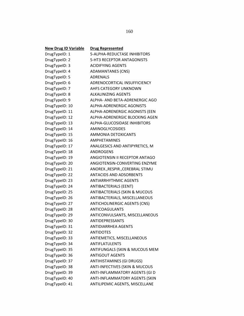
160
New Drug ID Variable Drug Represented
DrugTypeID: 1 5-ALPHA-REDUCTASE INHIBITORS
DrugTypeID: 2 5-HT3 RECEPTOR ANTAGONISTS
DrugTypeID: 3 ACIDIFYING AGENTS
DrugTypeID: 4 ADAMANTANES (CNS)
DrugTypeID: 5 ADRENALS
DrugTypeID: 6 ADRENOCORTICAL INSUFFICIENCY
DrugTypeID: 7 AHFS CATEGORY UNKNOWN
DrugTypeID: 8 ALKALINIZING AGENTS
DrugTypeID: 9 ALPHA- AND BETA-ADRENERGIC AGO
DrugTypeID: 10 ALPHA-ADRENERGIC AGONISTS
DrugTypeID: 11 ALPHA-ADRENERGIC AGONISTS (EEN
DrugTypeID: 12 ALPHA-ADRENERGIC BLOCKING AGEN
DrugTypeID: 13 ALPHA-GLUCOSIDASE INHIBITORS
DrugTypeID: 14 AMINOGLYCOSIDES
DrugTypeID: 15 AMMONIA DETOXICANTS
DrugTypeID: 16 AMPHETAMINES
DrugTypeID: 17 ANALGESICS AND ANTIPYRETICS, M
DrugTypeID: 18 ANDROGENS
DrugTypeID: 19 ANGIOTENSIN II RECEPTOR ANTAGO
DrugTypeID: 20 ANGIOTENSIN-CONVERTING ENZYME
DrugTypeID: 21 ANOREX.,RESPIR.,CEREBRAL STIMU
DrugTypeID: 22 ANTACIDS AND ADSORBENTS
DrugTypeID: 23 ANTIARRHYTHMIC AGENTS
DrugTypeID: 24 ANTIBACTERIALS (EENT)
DrugTypeID: 25 ANTIBACTERIALS (SKIN & MUCOUS
DrugTypeID: 26 ANTIBACTERIALS, MISCELLANEOUS
DrugTypeID: 27 ANTICHOLINERGIC AGENTS (CNS)
DrugTypeID: 28 ANTICOAGULANTS
DrugTypeID: 29 ANTICONVULSANTS, MISCELLANEOUS
DrugTypeID: 30 ANTIDEPRESSANTS
DrugTypeID: 31 ANTIDIARRHEA AGENTS
DrugTypeID: 32 ANTIDOTES
DrugTypeID: 33 ANTIEMETICS, MISCELLANEOUS
DrugTypeID: 34 ANTIFLATULENTS
DrugTypeID: 35 ANTIFUNGALS (SKIN & MUCOUS MEM
DrugTypeID: 36 ANTIGOUT AGENTS
DrugTypeID: 37 ANTIHISTAMINES (GI DRUGS)
DrugTypeID: 38 ANTI-INFECTIVES (SKIN & MUCOUS
DrugTypeID: 39 ANTI-INFLAMMATORY AGENTS (GI D
DrugTypeID: 40 ANTI-INFLAMMATORY AGENTS (SKIN
DrugTypeID: 41 ANTILIPEMIC AGENTS, MISCELLANE
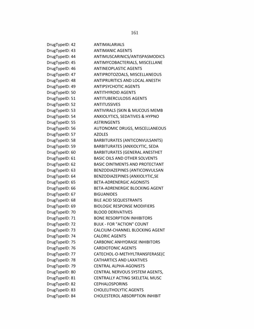
161
DrugTypeID: 42 ANTIMALARIALS
DrugTypeID: 43 ANTIMANIC AGENTS
DrugTypeID: 44 ANTIMUSCARINICS/ANTISPASMODICS
DrugTypeID: 45 ANTIMYCOBACTERIALS, MISCELLANE
DrugTypeID: 46 ANTINEOPLASTIC AGENTS
DrugTypeID: 47 ANTIPROTOZOALS, MISCELLANEOUS
DrugTypeID: 48 ANTIPRURITICS AND LOCAL ANESTH
DrugTypeID: 49 ANTIPSYCHOTIC AGENTS
DrugTypeID: 50 ANTITHYROID AGENTS
DrugTypeID: 51 ANTITUBERCULOSIS AGENTS
DrugTypeID: 52 ANTITUSSIVES
DrugTypeID: 53 ANTIVIRALS (SKIN & MUCOUS MEMB
DrugTypeID: 54 ANXIOLYTICS, SEDATIVES & HYPNO
DrugTypeID: 55 ASTRINGENTS
DrugTypeID: 56 AUTONOMIC DRUGS, MISCELLANEOUS
DrugTypeID: 57 AZOLES
DrugTypeID: 58 BARBITURATES (ANTICONVULSANTS)
DrugTypeID: 59 BARBITURATES (ANXIOLYTIC, SEDA
DrugTypeID: 60 BARBITURATES (GENERAL ANESTHET
DrugTypeID: 61 BASIC OILS AND OTHER SOLVENTS
DrugTypeID: 62 BASIC OINTMENTS AND PROTECTANT
DrugTypeID: 63 BENZODIAZEPINES (ANTICONVULSAN
DrugTypeID: 64 BENZODIAZEPINES (ANXIOLYTIC,SE
DrugTypeID: 65 BETA-ADRENERGIC AGONISTS
DrugTypeID: 66 BETA-ADRENERGIC BLOCKING AGENT
DrugTypeID: 67 BIGUANIDES
DrugTypeID: 68 BILE ACID SEQUESTRANTS
DrugTypeID: 69 BIOLOGIC RESPONSE MODIFIERS
DrugTypeID: 70 BLOOD DERIVATIVES
DrugTypeID: 71 BONE RESORPTION INHIBITORS
DrugTypeID: 72 BULK - FOR "ACTION" COUNT
DrugTypeID: 73 CALCIUM-CHANNEL BLOCKING AGENT
DrugTypeID: 74 CALORIC AGENTS
DrugTypeID: 75 CARBONIC ANHYDRASE INHIBITORS
DrugTypeID: 76 CARDIOTONIC AGENTS
DrugTypeID: 77 CATECHOL-O-METHYLTRANSFERASE(C
DrugTypeID: 78 CATHARTICS AND LAXATIVES
DrugTypeID: 79 CENTRAL ALPHA-AGONISTS
DrugTypeID: 80 CENTRAL NERVOUS SYSTEM AGENTS,
DrugTypeID: 81 CENTRALLY ACTING SKELETAL MUSC
DrugTypeID: 82 CEPHALOSPORINS
DrugTypeID: 83 CHOLELITHOLYTIC AGENTS
DrugTypeID: 84 CHOLESTEROL ABSORPTION INHIBIT

162
DrugTypeID: 85 CORTICOSTEROIDS (EENT)
DrugTypeID: 86 DEVICES
DrugTypeID: 87 DEVICES SUCH AS IV SETS
DrugTypeID: 88 DIABETES MELLITUS
DrugTypeID: 89 DIGESTANTS
DrugTypeID: 90 DIHYDROPYRIDINES
DrugTypeID: 91 DIRECT VASODILATORS
DrugTypeID: 92 DIRECT-ACTING SKELETAL MUSCLE
DrugTypeID: 93 DISEASE-MODIFYING ANTIRHEUMATI
DrugTypeID: 94 DOPAMINE PRECURSORS
DrugTypeID: 95 DOPAMINE RECEPTOR AGONISTS
DrugTypeID: 96 ECHINOCANDINS
DrugTypeID: 97 EENT ANTI-INFECTIVES, MISCELLA
DrugTypeID: 98 EENT DRUGS, MISCELLANEOUS
DrugTypeID: 99 EENT NONSTEROIDAL ANTI-INFLAM.
DrugTypeID: 100 ENZYMES
DrugTypeID: 101 ESTROGEN AGONIST-ANTAGONISTS
DrugTypeID: 102 ESTROGENS
DrugTypeID: 103 ETHANOLAMINE DERIVATIVES
DrugTypeID: 104 EXPECTORANTS
DrugTypeID: 105 FIBRIC ACID DERIVATIVES
DrugTypeID: 106 FIRST GEN. ANTIHIST. DERIVATIV
DrugTypeID: 107 FUNGI
DrugTypeID: 108 GABA-DERIVATIVE SKELETAL MUSCL
DrugTypeID: 109 GALLBLADDER FUNCTION
DrugTypeID: 110 GASTROINTESTINAL DRUGS
DrugTypeID: 111 GENERAL ANESTHETICS, MISCELLAN
DrugTypeID: 112 GENITOURINARY SMOOTH MUSCLE RE
DrugTypeID: 113 GLYCOGENOLYTIC AGENTS
DrugTypeID: 114 HEMATOPOIETIC AGENTS
DrugTypeID: 115 HEMORRHEOLOGIC AGENTS
DrugTypeID: 116 HEMOSTATICS
DrugTypeID: 117 HISTAMINE H2-ANTAGONISTS
DrugTypeID: 118 HMG-COA REDUCTASE INHIBITORS
DrugTypeID: 119 HYDANTOINS
DrugTypeID: 120 IMMUNOSUPPRESSIVE AGENTS
DrugTypeID: 121 INHALATION ANESTHETICS
DrugTypeID: 122 INSULINS
DrugTypeID: 123 IRON PREPARATIONS
DrugTypeID: 124 IRRIGATING SOLUTIONS
DrugTypeID: 125 KERATOLYTIC AGENTS
DrugTypeID: 126 KIDNEY FUNCTION
DrugTypeID: 127 LEUKOTRIENE MODIFIERS

163
DrugTypeID: 128 LOCAL ANESTHETICS (EENT)
DrugTypeID: 129 LOCAL ANESTHETICS (PARENTERAL)
DrugTypeID: 130 LOCAL ANTI-INFECTIVES, MISCELL
DrugTypeID: 131 LOOP DIURETICS
DrugTypeID: 132 MACROLIDES
DrugTypeID: 133 MEGLITINIDES
DrugTypeID: 134 MESSAGE (order entry)
DrugTypeID: 135 MINERALOCORTICOID (ALDOSTERONE
DrugTypeID: 136 MISC. SKIN AND MUCOUS MEMBRANE
DrugTypeID: 137 MISCELLANEOUS B-LACTAM ANTIBIO
DrugTypeID: 138 MONOAMINE OXIDASE B INHIBITORS
DrugTypeID: 139 MOUTHWASHES AND GARGLES
DrugTypeID: 140 MUCOLYTIC AGENTS
DrugTypeID: 141 MULTIVITAMIN PREPARATIONS
DrugTypeID: 142 MYDRIATICS
DrugTypeID: 143 NEURAMINIDASE INHIBITORS
DrugTypeID: 144 NEUROMUSCULAR BLOCKING AGENTS
DrugTypeID: 145 NITRATES AND NITRITES
DrugTypeID: 146 NON FORMULARY
DrugTypeID: 147 NONSTEROIDAL ANTI-INFLAMMATORY
DrugTypeID: 148 NUCLEOSIDES AND NUCLEOTIDES
DrugTypeID: 149 OPIATE AGONISTS
DrugTypeID: 150 OPIATE ANTAGONISTS
DrugTypeID: 151 OPIATE PARTIAL AGONISTS
DrugTypeID: 152 OSMOTIC DIURETICS
DrugTypeID: 153 OTHER MISCELLANEOUS THERAPEUTI
DrugTypeID: 154 OVER-THE-COUNTER
DrugTypeID: 155 OXYTOCICS
DrugTypeID: 156 PARASYMPATHOMIMETIC (CHOLINERG
DrugTypeID: 157 PARATHYROID
DrugTypeID: 158 PENICILLINS
DrugTypeID: 159 PHARMACEUTICAL AIDS
DrugTypeID: 160 PHENOTHIAZINE DERIVATIVES
DrugTypeID: 161 PHOSPHATE-REMOVING AGENTS
DrugTypeID: 162 PITUITARY
DrugTypeID: 163 PITUITARY FUNCTION
DrugTypeID: 164 PLATELET-AGGREGATION INHIBITOR
DrugTypeID: 165 POLYENES
DrugTypeID: 166 POTASSIUM-REMOVING AGENTS
DrugTypeID: 167 POTASSIUM-SPARING DIURETICS
DrugTypeID: 168 PROGESTINS
DrugTypeID: 169 PROKINETIC AGENTS
DrugTypeID: 170 PROPYLAMINE DERIVATIVES

164
DrugTypeID: 171 PROSTAGLANDIN ANALOGS
DrugTypeID: 172 PROTECTANTS
DrugTypeID: 173 PROTECTIVE AGENTS
DrugTypeID: 174 PROTON-PUMP INHIBITORS
DrugTypeID: 175 QUINOLONES
DrugTypeID: 176 REPLACEMENT PREPARATIONS
DrugTypeID: 177 RESPIRATORY SMOOTH MUSCLE RELA
DrugTypeID: 178 ROENTGENOGRAPHY
DrugTypeID: 179 SCLEROSING AGENTS
DrugTypeID: 180 SECOND GENERATION ANTIHISTAMIN
DrugTypeID: 181 SELECTIVE SEROTONIN AGONISTS
DrugTypeID: 182 SERUMS
DrugTypeID: 183 SKELETAL MUSCLE RELAXANTS, MIS
DrugTypeID: 184 SKIN AND MUCOUS MEMBRANE AGENT
DrugTypeID: 185 SULFONAMIDES (SYSTEMIC)
DrugTypeID: 186 SULFONYLUREAS
DrugTypeID: 187 TETRACYCLINES
DrugTypeID: 188 THIAZIDE DIURETICS
DrugTypeID: 189 THIAZIDE-LIKE DIURETICS
DrugTypeID: 190 THIAZOLIDINEDIONES
DrugTypeID: 191 THROMBOLYTIC AGENTS
DrugTypeID: 192 THYROID AGENTS
DrugTypeID: 193 TOXOIDS
DrugTypeID: 194 TUBERCULOSIS
DrugTypeID: 195 TYPE CSN
DrugTypeID: 196 URICOSURIC AGENTS
DrugTypeID: 197 URINARY ANTI-INFECTIVES
DrugTypeID: 198 VACCINES
DrugTypeID: 199 VASOCONSTRICTORS
DrugTypeID: 200 VASODILATING AGENTS, MISCELLAN
DrugTypeID: 201 VITAMIN B COMPLEX
DrugTypeID: 202 VITAMIN C
DrugTypeID: 203 VITAMIN D
DrugTypeID: 204 VITAMIN E
DrugTypeID: 205 VITAMIN K ACTIVITY

165
APPENDIX F
GENERAL POPULATION FINAL EXCEL FILE VARIABLES

166
Variable Name Variable
Type Category
Levels Target/Predictor
AdmitToReadmit Binary 2 Target
Discharge_Month Categorical 12 Predictor
LOS Scalar NA Predictor
AgeYRS Scalar NA Predictor
Gender_M_0_F_1 Binary 2 Predictor
MaritalStatus Categorical 7 Predictor
HospDischargeDept Categorical 3 Predictor
AdmitFromEr_Yes_1 Binary 2 Predictor
FinancialClass Categorical 10 Predictor
DischargeDisposition Categorical 12 Predictor
DistanceToHospital Categorical 9 Predictor
Pdx_ICD9_(001-009) Binary 2 Predictor
Pdx_ICD9_(010-018) Binary 2 Predictor
Pdx_ICD9_(030-041) Binary 2 Predictor
Pdx_ICD9_(042) Binary 2 Predictor
Pdx_ICD9_(045-049) Binary 2 Predictor
Pdx_ICD9_(050-059) Binary 2 Predictor
Pdx_ICD9_(070-079) Binary 2 Predictor
Pdx_ICD9_(080-088) Binary 2 Predictor
Pdx_ICD9_(110-118) Binary 2 Predictor
Pdx_ICD9_(140-149) Binary 2 Predictor
Pdx_ICD9_(150-159) Binary 2 Predictor
Pdx_ICD9_(160-165) Binary 2 Predictor
Pdx_ICD9_(170-176) Binary 2 Predictor
Pdx_ICD9_(179-189) Binary 2 Predictor
Pdx_ICD9_(190-199) Binary 2 Predictor
Pdx_ICD9_(200-208) Binary 2 Predictor
Pdx_ICD9_(209) Binary 2 Predictor
Pdx_ICD9_(210-229) Binary 2 Predictor
Pdx_ICD9_(230-234) Binary 2 Predictor
Pdx_ICD9_(235-238) Binary 2 Predictor
Pdx_ICD9_(239) Binary 2 Predictor
Pdx_ICD9_(240-246) Binary 2 Predictor
Pdx_ICD9_(249-259) Binary 2 Predictor
Pdx_ICD9_(260-269) Binary 2 Predictor
Pdx_ICD9_(270-279) Binary 2 Predictor
Pdx_ICD9_(280-289) Binary 2 Predictor
Pdx_ICD9_(290-294) Binary 2 Predictor
Pdx_ICD9_(295-299) Binary 2 Predictor
Pdx_ICD9_(300-316) Binary 2 Predictor
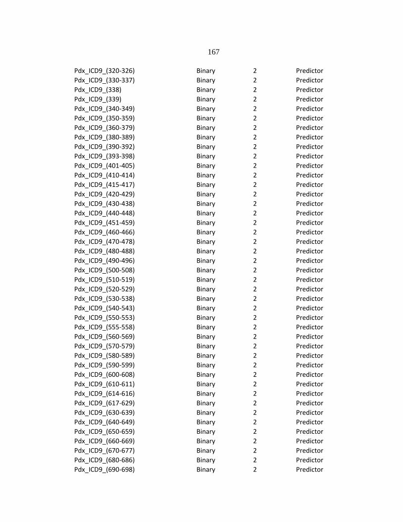
167
Pdx_ICD9_(320-326) Binary 2 Predictor
Pdx_ICD9_(330-337) Binary 2 Predictor
Pdx_ICD9_(338) Binary 2 Predictor
Pdx_ICD9_(339) Binary 2 Predictor
Pdx_ICD9_(340-349) Binary 2 Predictor
Pdx_ICD9_(350-359) Binary 2 Predictor
Pdx_ICD9_(360-379) Binary 2 Predictor
Pdx_ICD9_(380-389) Binary 2 Predictor
Pdx_ICD9_(390-392) Binary 2 Predictor
Pdx_ICD9_(393-398) Binary 2 Predictor
Pdx_ICD9_(401-405) Binary 2 Predictor
Pdx_ICD9_(410-414) Binary 2 Predictor
Pdx_ICD9_(415-417) Binary 2 Predictor
Pdx_ICD9_(420-429) Binary 2 Predictor
Pdx_ICD9_(430-438) Binary 2 Predictor
Pdx_ICD9_(440-448) Binary 2 Predictor
Pdx_ICD9_(451-459) Binary 2 Predictor
Pdx_ICD9_(460-466) Binary 2 Predictor
Pdx_ICD9_(470-478) Binary 2 Predictor
Pdx_ICD9_(480-488) Binary 2 Predictor
Pdx_ICD9_(490-496) Binary 2 Predictor
Pdx_ICD9_(500-508) Binary 2 Predictor
Pdx_ICD9_(510-519) Binary 2 Predictor
Pdx_ICD9_(520-529) Binary 2 Predictor
Pdx_ICD9_(530-538) Binary 2 Predictor
Pdx_ICD9_(540-543) Binary 2 Predictor
Pdx_ICD9_(550-553) Binary 2 Predictor
Pdx_ICD9_(555-558) Binary 2 Predictor
Pdx_ICD9_(560-569) Binary 2 Predictor
Pdx_ICD9_(570-579) Binary 2 Predictor
Pdx_ICD9_(580-589) Binary 2 Predictor
Pdx_ICD9_(590-599) Binary 2 Predictor
Pdx_ICD9_(600-608) Binary 2 Predictor
Pdx_ICD9_(610-611) Binary 2 Predictor
Pdx_ICD9_(614-616) Binary 2 Predictor
Pdx_ICD9_(617-629) Binary 2 Predictor
Pdx_ICD9_(630-639) Binary 2 Predictor
Pdx_ICD9_(640-649) Binary 2 Predictor
Pdx_ICD9_(650-659) Binary 2 Predictor
Pdx_ICD9_(660-669) Binary 2 Predictor
Pdx_ICD9_(670-677) Binary 2 Predictor
Pdx_ICD9_(680-686) Binary 2 Predictor
Pdx_ICD9_(690-698) Binary 2 Predictor

168
Pdx_ICD9_(700-709) Binary 2 Predictor
Pdx_ICD9_(710-719) Binary 2 Predictor
Pdx_ICD9_(720-724) Binary 2 Predictor
Pdx_ICD9_(725-729) Binary 2 Predictor
Pdx_ICD9_(730-739) Binary 2 Predictor
Pdx_ICD9_(740-759) Binary 2 Predictor
Pdx_ICD9_(780-789) Binary 2 Predictor
Pdx_ICD9_(790-796) Binary 2 Predictor
Pdx_ICD9_(797-799) Binary 2 Predictor
Pdx_ICD9_(800-804) Binary 2 Predictor
Pdx_ICD9_(805-809) Binary 2 Predictor
Pdx_ICD9_(810-819) Binary 2 Predictor
Pdx_ICD9_(820-829) Binary 2 Predictor
Pdx_ICD9_(830-839) Binary 2 Predictor
Pdx_ICD9_(840-848) Binary 2 Predictor
Pdx_ICD9_(850-854) Binary 2 Predictor
Pdx_ICD9_(860-869) Binary 2 Predictor
Pdx_ICD9_(870-879) Binary 2 Predictor
Pdx_ICD9_(880-887) Binary 2 Predictor
Pdx_ICD9_(890-897) Binary 2 Predictor
Pdx_ICD9_(900-904) Binary 2 Predictor
Pdx_ICD9_(910-919) Binary 2 Predictor
Pdx_ICD9_(920-924) Binary 2 Predictor
Pdx_ICD9_(925-929) Binary 2 Predictor
Pdx_ICD9_(930-939) Binary 2 Predictor
Pdx_ICD9_(940-949) Binary 2 Predictor
Pdx_ICD9_(950-957) Binary 2 Predictor
Pdx_ICD9_(958-959) Binary 2 Predictor
Pdx_ICD9_(960-979) Binary 2 Predictor
Pdx_ICD9_(980-989) Binary 2 Predictor
Pdx_ICD9_(990-995) Binary 2 Predictor
Pdx_ICD9_(996-999) Binary 2 Predictor
Pdx_ICD9_(V50-V59) Binary 2 Predictor
Pdx_ICD9_(V60-V69) Binary 2 Predictor
S1-S15dx_ICD9_(001-009) Binary 2 Predictor
S1-S15dx_ICD9_(030-041) Binary 2 Predictor
S1-S15dx_ICD9_(050-059) Binary 2 Predictor
S1-S15dx_ICD9_(070-079) Binary 2 Predictor
S1-S15dx_ICD9_(080-088) Binary 2 Predictor
S1-S15dx_ICD9_(090-099) Binary 2 Predictor
S1-S15dx_ICD9_(110-118) Binary 2 Predictor
S1-S15dx_ICD9_(130-136) Binary 2 Predictor
S1-S15dx_ICD9_(137-139) Binary 2 Predictor

169
S1-S15dx_ICD9_(140-149) Binary 2 Predictor
S1-S15dx_ICD9_(150-159) Binary 2 Predictor
S1-S15dx_ICD9_(160-165) Binary 2 Predictor
S1-S15dx_ICD9_(170-176) Binary 2 Predictor
S1-S15dx_ICD9_(179-189) Binary 2 Predictor
S1-S15dx_ICD9_(190-199) Binary 2 Predictor
S1-S15dx_ICD9_(200-208) Binary 2 Predictor
S1-S15dx_ICD9_(209) Binary 2 Predictor
S1-S15dx_ICD9_(210-229) Binary 2 Predictor
S1-S15dx_ICD9_(230-234) Binary 2 Predictor
S1-S15dx_ICD9_(235-238) Binary 2 Predictor
S1-S15dx_ICD9_(239) Binary 2 Predictor
S1-S15dx_ICD9_(240-246) Binary 2 Predictor
S1-S15dx_ICD9_(249-259) Binary 2 Predictor
S1-S15dx_ICD9_(260-269) Binary 2 Predictor
S1-S15dx_ICD9_(270-279) Binary 2 Predictor
S1-S15dx_ICD9_(280-289) Binary 2 Predictor
S1-S15dx_ICD9_(290-294) Binary 2 Predictor
S1-S15dx_ICD9_(295-299) Binary 2 Predictor
S1-S15dx_ICD9_(300-316) Binary 2 Predictor
S1-S15dx_ICD9_(317-319) Binary 2 Predictor
S1-S15dx_ICD9_(320-326) Binary 2 Predictor
S1-S15dx_ICD9_(330-337) Binary 2 Predictor
S1-S15dx_ICD9_(338) Binary 2 Predictor
S1-S15dx_ICD9_(339) Binary 2 Predictor
S1-S15dx_ICD9_(340-349) Binary 2 Predictor
S1-S15dx_ICD9_(350-359) Binary 2 Predictor
S1-S15dx_ICD9_(360-379) Binary 2 Predictor
S1-S15dx_ICD9_(380-389) Binary 2 Predictor
S1-S15dx_ICD9_(393-398) Binary 2 Predictor
S1-S15dx_ICD9_(401-405) Binary 2 Predictor
S1-S15dx_ICD9_(410-414) Binary 2 Predictor
S1-S15dx_ICD9_(415-417) Binary 2 Predictor
S1-S15dx_ICD9_(420-429) Binary 2 Predictor
S1-S15dx_ICD9_(430-438) Binary 2 Predictor
S1-S15dx_ICD9_(440-448) Binary 2 Predictor
S1-S15dx_ICD9_(451-459) Binary 2 Predictor
S1-S15dx_ICD9_(460-466) Binary 2 Predictor
S1-S15dx_ICD9_(470-478) Binary 2 Predictor
S1-S15dx_ICD9_(480-488) Binary 2 Predictor
S1-S15dx_ICD9_(490-496) Binary 2 Predictor
S1-S15dx_ICD9_(500-508) Binary 2 Predictor
S1-S15dx_ICD9_(510-519) Binary 2 Predictor

170
S1-S15dx_ICD9_(520-529) Binary 2 Predictor
S1-S15dx_ICD9_(530-538) Binary 2 Predictor
S1-S15dx_ICD9_(540-543) Binary 2 Predictor
S1-S15dx_ICD9_(550-553) Binary 2 Predictor
S1-S15dx_ICD9_(555-558) Binary 2 Predictor
S1-S15dx_ICD9_(560-569) Binary 2 Predictor
S1-S15dx_ICD9_(570-579) Binary 2 Predictor
S1-S15dx_ICD9_(580-589) Binary 2 Predictor
S1-S15dx_ICD9_(590-599) Binary 2 Predictor
S1-S15dx_ICD9_(600-608) Binary 2 Predictor
S1-S15dx_ICD9_(610-611) Binary 2 Predictor
S1-S15dx_ICD9_(614-616) Binary 2 Predictor
S1-S15dx_ICD9_(617-629) Binary 2 Predictor
S1-S15dx_ICD9_(640-649) Binary 2 Predictor
S1-S15dx_ICD9_(650-659) Binary 2 Predictor
S1-S15dx_ICD9_(660-669) Binary 2 Predictor
S1-S15dx_ICD9_(670-677) Binary 2 Predictor
S1-S15dx_ICD9_(680-686) Binary 2 Predictor
S1-S15dx_ICD9_(690-698) Binary 2 Predictor
S1-S15dx_ICD9_(700-709) Binary 2 Predictor
S1-S15dx_ICD9_(710-719) Binary 2 Predictor
S1-S15dx_ICD9_(720-724) Binary 2 Predictor
S1-S15dx_ICD9_(725-729) Binary 2 Predictor
S1-S15dx_ICD9_(730-739) Binary 2 Predictor
S1-S15dx_ICD9_(740-759) Binary 2 Predictor
S1-S15dx_ICD9_(760-763) Binary 2 Predictor
S1-S15dx_ICD9_(780-789) Binary 2 Predictor
S1-S15dx_ICD9_(790-796) Binary 2 Predictor
S1-S15dx_ICD9_(797-799) Binary 2 Predictor
S1-S15dx_ICD9_(800-804) Binary 2 Predictor
S1-S15dx_ICD9_(805-809) Binary 2 Predictor
S1-S15dx_ICD9_(810-819) Binary 2 Predictor
S1-S15dx_ICD9_(820-829) Binary 2 Predictor
S1-S15dx_ICD9_(830-839) Binary 2 Predictor
S1-S15dx_ICD9_(840-848) Binary 2 Predictor
S1-S15dx_ICD9_(850-854) Binary 2 Predictor
S1-S15dx_ICD9_(860-869) Binary 2 Predictor
S1-S15dx_ICD9_(870-879) Binary 2 Predictor
S1-S15dx_ICD9_(880-887) Binary 2 Predictor
S1-S15dx_ICD9_(890-897) Binary 2 Predictor
S1-S15dx_ICD9_(900-904) Binary 2 Predictor
S1-S15dx_ICD9_(905-909) Binary 2 Predictor
S1-S15dx_ICD9_(910-919) Binary 2 Predictor

171
S1-S15dx_ICD9_(920-924) Binary 2 Predictor
S1-S15dx_ICD9_(930-939) Binary 2 Predictor
S1-S15dx_ICD9_(940-949) Binary 2 Predictor
S1-S15dx_ICD9_(950-957) Binary 2 Predictor
S1-S15dx_ICD9_(958-959) Binary 2 Predictor
S1-S15dx_ICD9_(960-979) Binary 2 Predictor
S1-S15dx_ICD9_(980-989) Binary 2 Predictor
S1-S15dx_ICD9_(990-995) Binary 2 Predictor
S1-S15dx_ICD9_(996-999) Binary 2 Predictor
S1-S15dx_ICD9_(V01-V09) Binary 2 Predictor
S1-S15dx_ICD9_(V10-V19) Binary 2 Predictor
S1-S15dx_ICD9_(V20-V29) Binary 2 Predictor
S1-S15dx_ICD9_(V40-V49) Binary 2 Predictor
S1-S15dx_ICD9_(V50-V59) Binary 2 Predictor
S1-S15dx_ICD9_(V60-V69) Binary 2 Predictor
S1-S15dx_ICD9_(V70-V82) Binary 2 Predictor
S1-S15dx_ICD9_(V83-V84) Binary 2 Predictor
S1-S15dx_ICD9_(V85) Binary 2 Predictor
S1-S15dx_ICD9_(V86) Binary 2 Predictor
S1-S15dx_ICD9_(V87) Binary 2 Predictor
S1-S15dx_ICD9_(V88) Binary 2 Predictor
S1-S15dx_ICD9_(E001-E030) Binary 2 Predictor
S1-S15dx_ICD9_(E810-E819) Binary 2 Predictor
S1-S15dx_ICD9_(E820-E825) Binary 2 Predictor
S1-S15dx_ICD9_(E826-E829) Binary 2 Predictor
S1-S15dx_ICD9_(E840-E845) Binary 2 Predictor
S1-S15dx_ICD9_(E846-E849) Binary 2 Predictor
S1-S15dx_ICD9_(E850-E858) Binary 2 Predictor
S1-S15dx_ICD9_(E860-E869) Binary 2 Predictor
S1-S15dx_ICD9_(E870-E876) Binary 2 Predictor
S1-S15dx_ICD9_(E878-E879) Binary 2 Predictor
S1-S15dx_ICD9_(E880-E888) Binary 2 Predictor
S1-S15dx_ICD9_(E890-E899) Binary 2 Predictor
S1-S15dx_ICD9_(E900-E909) Binary 2 Predictor
S1-S15dx_ICD9_(E910-E915) Binary 2 Predictor
S1-S15dx_ICD9_(E916-E928) Binary 2 Predictor
S1-S15dx_ICD9_(E929) Binary 2 Predictor
S1-S15dx_ICD9_(E930-E949) Binary 2 Predictor
S1-S15dx_ICD9_(E950-E959) Binary 2 Predictor
S1-S15dx_ICD9_(E960-E969) Binary 2 Predictor
S1-S15dx_ICD9_(E980-E989) Binary 2 Predictor
S1-S15dx_ICD9_(E990-E999) Binary 2 Predictor
DrugTypeID:_1 Binary 2 Predictor

172
DrugTypeID:_2 Binary 2 Predictor
DrugTypeID:_3 Binary 2 Predictor
DrugTypeID:_4 Binary 2 Predictor
DrugTypeID:_5 Binary 2 Predictor
DrugTypeID:_6 Binary 2 Predictor
DrugTypeID:_7 Binary 2 Predictor
DrugTypeID:_8 Binary 2 Predictor
DrugTypeID:_9 Binary 2 Predictor
DrugTypeID:_10 Binary 2 Predictor
DrugTypeID:_11 Binary 2 Predictor
DrugTypeID:_12 Binary 2 Predictor
DrugTypeID:_13 Binary 2 Predictor
DrugTypeID:_14 Binary 2 Predictor
DrugTypeID:_15 Binary 2 Predictor
DrugTypeID:_16 Binary 2 Predictor
DrugTypeID:_17 Binary 2 Predictor
DrugTypeID:_18 Binary 2 Predictor
DrugTypeID:_19 Binary 2 Predictor
DrugTypeID:_20 Binary 2 Predictor
DrugTypeID:_21 Binary 2 Predictor
DrugTypeID:_22 Binary 2 Predictor
DrugTypeID:_23 Binary 2 Predictor
DrugTypeID:_24 Binary 2 Predictor
DrugTypeID:_25 Binary 2 Predictor
DrugTypeID:_26 Binary 2 Predictor
DrugTypeID:_27 Binary 2 Predictor
DrugTypeID:_28 Binary 2 Predictor
DrugTypeID:_29 Binary 2 Predictor
DrugTypeID:_30 Binary 2 Predictor
DrugTypeID:_31 Binary 2 Predictor
DrugTypeID:_32 Binary 2 Predictor
DrugTypeID:_33 Binary 2 Predictor
DrugTypeID:_34 Binary 2 Predictor
DrugTypeID:_35 Binary 2 Predictor
DrugTypeID:_36 Binary 2 Predictor
DrugTypeID:_37 Binary 2 Predictor
DrugTypeID:_38 Binary 2 Predictor
DrugTypeID:_39 Binary 2 Predictor
DrugTypeID:_40 Binary 2 Predictor
DrugTypeID:_41 Binary 2 Predictor
DrugTypeID:_42 Binary 2 Predictor
DrugTypeID:_43 Binary 2 Predictor
DrugTypeID:_44 Binary 2 Predictor

173
DrugTypeID:_45 Binary 2 Predictor
DrugTypeID:_46 Binary 2 Predictor
DrugTypeID:_47 Binary 2 Predictor
DrugTypeID:_48 Binary 2 Predictor
DrugTypeID:_49 Binary 2 Predictor
DrugTypeID:_50 Binary 2 Predictor
DrugTypeID:_51 Binary 2 Predictor
DrugTypeID:_52 Binary 2 Predictor
DrugTypeID:_53 Binary 2 Predictor
DrugTypeID:_54 Binary 2 Predictor
DrugTypeID:_55 Binary 2 Predictor
DrugTypeID:_56 Binary 2 Predictor
DrugTypeID:_57 Binary 2 Predictor
DrugTypeID:_58 Binary 2 Predictor
DrugTypeID:_59 Binary 2 Predictor
DrugTypeID:_60 Binary 2 Predictor
DrugTypeID:_61 Binary 2 Predictor
DrugTypeID:_62 Binary 2 Predictor
DrugTypeID:_63 Binary 2 Predictor
DrugTypeID:_64 Binary 2 Predictor
DrugTypeID:_65 Binary 2 Predictor
DrugTypeID:_66 Binary 2 Predictor
DrugTypeID:_67 Binary 2 Predictor
DrugTypeID:_68 Binary 2 Predictor
DrugTypeID:_69 Binary 2 Predictor
DrugTypeID:_70 Binary 2 Predictor
DrugTypeID:_71 Binary 2 Predictor
DrugTypeID:_72 Binary 2 Predictor
DrugTypeID:_73 Binary 2 Predictor
DrugTypeID:_74 Binary 2 Predictor
DrugTypeID:_75 Binary 2 Predictor
DrugTypeID:_76 Binary 2 Predictor
DrugTypeID:_77 Binary 2 Predictor
DrugTypeID:_78 Binary 2 Predictor
DrugTypeID:_79 Binary 2 Predictor
DrugTypeID:_80 Binary 2 Predictor
DrugTypeID:_81 Binary 2 Predictor
DrugTypeID:_82 Binary 2 Predictor
DrugTypeID:_83 Binary 2 Predictor
DrugTypeID:_84 Binary 2 Predictor
DrugTypeID:_85 Binary 2 Predictor
DrugTypeID:_86 Binary 2 Predictor
DrugTypeID:_87 Binary 2 Predictor

174
DrugTypeID:_88 Binary 2 Predictor
DrugTypeID:_89 Binary 2 Predictor
DrugTypeID:_90 Binary 2 Predictor
DrugTypeID:_91 Binary 2 Predictor
DrugTypeID:_92 Binary 2 Predictor
DrugTypeID:_93 Binary 2 Predictor
DrugTypeID:_94 Binary 2 Predictor
DrugTypeID:_95 Binary 2 Predictor
DrugTypeID:_96 Binary 2 Predictor
DrugTypeID:_97 Binary 2 Predictor
DrugTypeID:_98 Binary 2 Predictor
DrugTypeID:_99 Binary 2 Predictor
DrugTypeID:_100 Binary 2 Predictor
DrugTypeID:_101 Binary 2 Predictor
DrugTypeID:_102 Binary 2 Predictor
DrugTypeID:_103 Binary 2 Predictor
DrugTypeID:_104 Binary 2 Predictor
DrugTypeID:_105 Binary 2 Predictor
DrugTypeID:_106 Binary 2 Predictor
DrugTypeID:_108 Binary 2 Predictor
DrugTypeID:_109 Binary 2 Predictor
DrugTypeID:_110 Binary 2 Predictor
DrugTypeID:_111 Binary 2 Predictor
DrugTypeID:_112 Binary 2 Predictor
DrugTypeID:_113 Binary 2 Predictor
DrugTypeID:_114 Binary 2 Predictor
DrugTypeID:_115 Binary 2 Predictor
DrugTypeID:_116 Binary 2 Predictor
DrugTypeID:_117 Binary 2 Predictor
DrugTypeID:_118 Binary 2 Predictor
DrugTypeID:_119 Binary 2 Predictor
DrugTypeID:_120 Binary 2 Predictor
DrugTypeID:_121 Binary 2 Predictor
DrugTypeID:_122 Binary 2 Predictor
DrugTypeID:_123 Binary 2 Predictor
DrugTypeID:_124 Binary 2 Predictor
DrugTypeID:_125 Binary 2 Predictor
DrugTypeID:_126 Binary 2 Predictor
DrugTypeID:_127 Binary 2 Predictor
DrugTypeID:_128 Binary 2 Predictor
DrugTypeID:_129 Binary 2 Predictor
DrugTypeID:_130 Binary 2 Predictor
DrugTypeID:_131 Binary 2 Predictor

175
DrugTypeID:_132 Binary 2 Predictor
DrugTypeID:_133 Binary 2 Predictor
DrugTypeID:_134 Binary 2 Predictor
DrugTypeID:_135 Binary 2 Predictor
DrugTypeID:_136 Binary 2 Predictor
DrugTypeID:_137 Binary 2 Predictor
DrugTypeID:_138 Binary 2 Predictor
DrugTypeID:_139 Binary 2 Predictor
DrugTypeID:_140 Binary 2 Predictor
DrugTypeID:_141 Binary 2 Predictor
DrugTypeID:_142 Binary 2 Predictor
DrugTypeID:_143 Binary 2 Predictor
DrugTypeID:_144 Binary 2 Predictor
DrugTypeID:_145 Binary 2 Predictor
DrugTypeID:_146 Binary 2 Predictor
DrugTypeID:_147 Binary 2 Predictor
DrugTypeID:_148 Binary 2 Predictor
DrugTypeID:_149 Binary 2 Predictor
DrugTypeID:_150 Binary 2 Predictor
DrugTypeID:_151 Binary 2 Predictor
DrugTypeID:_152 Binary 2 Predictor
DrugTypeID:_153 Binary 2 Predictor
DrugTypeID:_154 Binary 2 Predictor
DrugTypeID:_155 Binary 2 Predictor
DrugTypeID:_156 Binary 2 Predictor
DrugTypeID:_157 Binary 2 Predictor
DrugTypeID:_158 Binary 2 Predictor
DrugTypeID:_159 Binary 2 Predictor
DrugTypeID:_160 Binary 2 Predictor
DrugTypeID:_161 Binary 2 Predictor
DrugTypeID:_162 Binary 2 Predictor
DrugTypeID:_163 Binary 2 Predictor
DrugTypeID:_164 Binary 2 Predictor
DrugTypeID:_165 Binary 2 Predictor
DrugTypeID:_166 Binary 2 Predictor
DrugTypeID:_167 Binary 2 Predictor
DrugTypeID:_168 Binary 2 Predictor
DrugTypeID:_169 Binary 2 Predictor
DrugTypeID:_170 Binary 2 Predictor
DrugTypeID:_171 Binary 2 Predictor
DrugTypeID:_172 Binary 2 Predictor
DrugTypeID:_173 Binary 2 Predictor
DrugTypeID:_174 Binary 2 Predictor

176
DrugTypeID:_175 Binary 2 Predictor
DrugTypeID:_176 Binary 2 Predictor
DrugTypeID:_177 Binary 2 Predictor
DrugTypeID:_178 Binary 2 Predictor
DrugTypeID:_179 Binary 2 Predictor
DrugTypeID:_180 Binary 2 Predictor
DrugTypeID:_181 Binary 2 Predictor
DrugTypeID:_182 Binary 2 Predictor
DrugTypeID:_183 Binary 2 Predictor
DrugTypeID:_184 Binary 2 Predictor
DrugTypeID:_185 Binary 2 Predictor
DrugTypeID:_186 Binary 2 Predictor
DrugTypeID:_187 Binary 2 Predictor
DrugTypeID:_188 Binary 2 Predictor
DrugTypeID:_189 Binary 2 Predictor
DrugTypeID:_190 Binary 2 Predictor
DrugTypeID:_191 Binary 2 Predictor
DrugTypeID:_192 Binary 2 Predictor
DrugTypeID:_193 Binary 2 Predictor
DrugTypeID:_194 Binary 2 Predictor
DrugTypeID:_195 Binary 2 Predictor
DrugTypeID:_196 Binary 2 Predictor
DrugTypeID:_197 Binary 2 Predictor
DrugTypeID:_198 Binary 2 Predictor
DrugTypeID:_199 Binary 2 Predictor
DrugTypeID:_200 Binary 2 Predictor
DrugTypeID:_201 Binary 2 Predictor
DrugTypeID:_202 Binary 2 Predictor
DrugTypeID:_203 Binary 2 Predictor
DrugTypeID:_204 Binary 2 Predictor
DrugTypeID:_205 Binary 2 Predictor
No._of_Drugs_Prescribed Scalar NA Predictor
No._of_Drugs_Administered Scalar NA Predictor
Diff_of_No._Pres._vs._No._Admin. Scalar NA Predictor
Count_of_Consults Scalar NA Predictor
Prior_6Mo_ER_Count Scalar NA Predictor
Prior_6Mo_IN_Count Scalar NA Predictor

177
APPENDIX G
SPSS METHODOLOGY
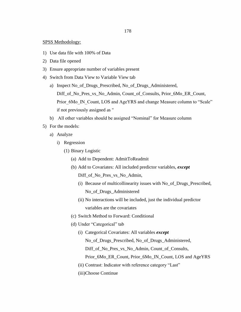
178
SPSS Methodology:
1) Use data file with 100% of Data
2) Data file opened
3) Ensure appropriate number of variables present
4) Switch from Data View to Variable View tab
a) Inspect No_of_Drugs_Prescribed, No_of_Drugs_Administered,
Diff_of_No_Pres_vs_No_Admin, Count_of_Consults, Prior_6Mo_ER_Count,
Prior_6Mo_IN_Count, LOS and AgeYRS and change Measure column to “Scale”
if not previously assigned as "
b) All other variables should be assigned “Nominal” for Measure column
5) For the models:
a) Analyze
i) Regression
(1) Binary Logistic
(a) Add to Dependent: AdmitToReadmit
(b) Add to Covariates: All included predictor variables, except
Diff_of_No_Pres_vs_No_Admin,
(i) Because of multicollinearity issues with No_of_Drugs_Prescribed,
No_of_Drugs_Administered
(ii) No interactions will be included, just the individual predictor
variables are the covariates
(c) Switch Method to Forward: Conditional
(d) Under “Categorical” tab
(i) Categorical Covariates: All variables except
No_of_Drugs_Prescribed, No_of_Drugs_Administered,
Diff_of_No_Pres_vs_No_Admin, Count_of_Consults,
Prior_6Mo_ER_Count, Prior_6Mo_IN_Count, LOS and AgeYRS
(ii) Contrast: Indicator with reference category “Last”
(iii)Choose Continue

179
(e) Under “Save” tab
(i) Predicted Values
1. Check "Probabilities"
a. These will be used to construct the ROC curve for the data
(ii) Choose Continue
(f) Under “Options” tab
(i) Statistics and Plots
1. Check “Hosmer-Lemeshow goodness-of-fit" and “CI for
exp(B):”
a. Leave “CI for exp(B):” set to 95%
(ii) Display
1. Change to “At last step”
(iii)Probability for Stepwise
1. Entry: 0.05
2. Removal: 0.10
(iv) Classification cutoff: 0.5
(v) Maximum Iterations: 20
(vi) Choose Continue
(g) Back in Logistic Regression screen choose "OK"
ii) After regression analysis complete choose ROC Curve
(1) Add to Test Variable: the prediction probabilities previously saved from
the binary logistic regression, these should be found as the last column of
data in the SPSS dataset
(2) Add to State Variable: "AdmitToReadmit"
(a) Set Value of State Variable: 1
(3) Check all Display category boxes
(4) Choose Ok
The above methodology will output a binary logistic regression model with some number
of steps used to bring in predictors.

180
APPENDIX H
MARS METHODOLOGY
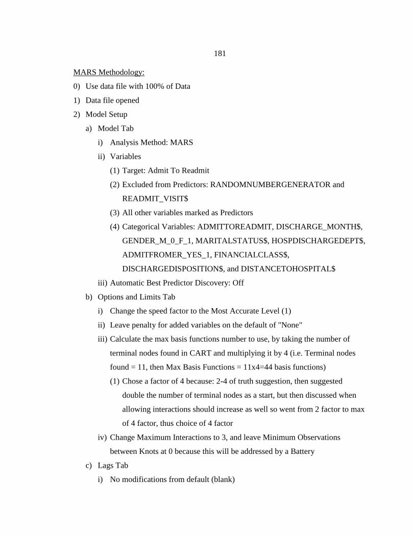
181
MARS Methodology:
0) Use data file with 100% of Data
1) Data file opened
2) Model Setup
a) Model Tab
i) Analysis Method: MARS
ii) Variables
(1) Target: Admit To Readmit
(2) Excluded from Predictors: RANDOMNUMBERGENERATOR and
READMIT_VISIT$
(3) All other variables marked as Predictors
(4) Categorical Variables: ADMITTOREADMIT, DISCHARGE_MONTH$,
GENDER_M_0_F_1, MARITALSTATUS$, HOSPDISCHARGEDEPT$,
ADMITFROMER_YES_1, FINANCIALCLASS$,
DISCHARGEDISPOSITION$, and DISTANCETOHOSPITAL$
iii) Automatic Best Predictor Discovery: Off
b) Options and Limits Tab
i) Change the speed factor to the Most Accurate Level (1)
ii) Leave penalty for added variables on the default of "None"
iii) Calculate the max basis functions number to use, by taking the number of
terminal nodes found in CART and multiplying it by 4 (i.e. Terminal nodes
found = 11, then Max Basis Functions = 11x4=44 basis functions)
(1) Chose a factor of 4 because: 2-4 of truth suggestion, then suggested
double the number of terminal nodes as a start, but then discussed when
allowing interactions should increase as well so went from 2 factor to max
of 4 factor, thus choice of 4 factor
iv) Change Maximum Interactions to 3, and leave Minimum Observations
between Knots at 0 because this will be addressed by a Battery
c) Lags Tab
i) No modifications from default (blank)

182
d) Testing Tab
i) Choose “V-fold cross validation:”
(1) Set to: 5 (except if 5 fold would decrease average expected number of
target class below and approximate value of 5 samples in each fold, i.e. if
it was below 25 target class samples in the data. AMI for example is only
11 target units and should be reduced to a fold of 2 so as to have about 5
target samples in each)
e) Select Cases Tab
i) No modifications from default (blank)
f) Battery Tab
i) Add battery MINSPAN
(1) MINSPAN Battery: Add other levels for testing of the minimum span
between knots, include levels 0, 1, 2, 3, 4, 5, 10, 15, 20, 25, 50
g) Penalty Tab
i) No modifications from default
h) Choose “Start”
3) Results for Model Analysis and all MARS Models and their respective result values
are presented. These are the final MARS models to choose the best model from.
4) Review Model Accuracy and Error Profiles to choose most appropriate model
a) Threshold value for prediction success can be altered with discretion
The above methodology will output a set of MARS models with the illustrated optimal
model being the model with the smallest GCV value (automatically highlighted in pink).
The model with the smallest MSE is highlighted in green but most times is inappropriate
for selection because the GCV value accounts more accurately the approximate error
according to Steinberg & Golovnya (2006).

183
APPENDIX I
MARS PREDICTION MODEL REPORT FOR ICD-9 CODE 427

184
MARS 1 Results: ICD-9 Code 427, 47 Basis Functions
Dataset: 427-FinalMethodology-Basic-AnalysisReady-ModelSetup.xlsx
Predictor Variables: DISCHARGE_MONTH$, GENDER_M_0_F_1, MARITALSTATUS$,
HOSPDISCHARGEDEPT$,
ADMITFROMER_YES_1, FINANCIALCLASS$,
DISCHARGEDISPOSITION$,
DISTANCETOHOSPITAL$, LOS, AGEYRS, PDX_ICD9__001_009_,
PDX_ICD9__030_041_, PDX_ICD9__050_059_, PDX_ICD9__110_118_,
PDX_ICD9__140_149_, PDX_ICD9__150_159_, PDX_ICD9__160_165_,
PDX_ICD9__170_176_, PDX_ICD9__179_189_, PDX_ICD9__190_199_,
PDX_ICD9__200_208_, PDX_ICD9__209_, PDX_ICD9__210_229_,
PDX_ICD9__235_238_, PDX_ICD9__239_, PDX_ICD9__240_246_,
PDX_ICD9__249_259_, PDX_ICD9__260_269_, PDX_ICD9__270_279_,
PDX_ICD9__280_289_, PDX_ICD9__290_294_, PDX_ICD9__300_316_,
PDX_ICD9__330_337_, PDX_ICD9__338_, PDX_ICD9__340_349_,
PDX_ICD9__350_359_, PDX_ICD9__360_379_, PDX_ICD9__390_392_,
PDX_ICD9__393_398_, PDX_ICD9__401_405_, PDX_ICD9__410_414_,
PDX_ICD9__415_417_, PDX_ICD9__420_429_, PDX_ICD9__430_438_,
PDX_ICD9__440_448_, PDX_ICD9__451_459_, PDX_ICD9__460_466_,
PDX_ICD9__480_488_, PDX_ICD9__490_496_, PDX_ICD9__500_508_,
PDX_ICD9__510_519_, PDX_ICD9__530_538_, PDX_ICD9__540_543_,
PDX_ICD9__550_553_, PDX_ICD9__555_558_, PDX_ICD9__560_569_,
PDX_ICD9__570_579_, PDX_ICD9__580_589_, PDX_ICD9__590_599_,
PDX_ICD9__600_608_, PDX_ICD9__617_629_, PDX_ICD9__680_686_,
PDX_ICD9__700_709_, PDX_ICD9__710_719_, PDX_ICD9__720_724_,
PDX_ICD9__725_729_, PDX_ICD9__730_739_, PDX_ICD9__780_789_,
PDX_ICD9__790_796_, PDX_ICD9__797_799_, PDX_ICD9__800_804_,
PDX_ICD9__805_809_, PDX_ICD9__810_819_, PDX_ICD9__820_829_,
PDX_ICD9__840_848_, PDX_ICD9__850_854_, PDX_ICD9__860_869_,
PDX_ICD9__870_879_, PDX_ICD9__880_887_, PDX_ICD9__900_904_,
PDX_ICD9__920_924_, PDX_ICD9__958_959_, PDX_ICD9__960_979_,
PDX_ICD9__980_989_, PDX_ICD9__990_995_, PDX_ICD9__996_999_,
PDX_ICD9__V50_V59_, S1_S15DX_ICD9__001_009_,
S1_S15DX_ICD9__030_041_,
S1_S15DX_ICD9__050_059_, S1_S15DX_ICD9__070_079_,
S1_S15DX_ICD9__090_099_, S1_S15DX_ICD9__110_118_,
S1_S15DX_ICD9__130_136_, S1_S15DX_ICD9__137_139_,
S1_S15DX_ICD9__140_149_, S1_S15DX_ICD9__150_159_,
S1_S15DX_ICD9__160_165_, S1_S15DX_ICD9__170_176_,
S1_S15DX_ICD9__179_189_, S1_S15DX_ICD9__190_199_,
S1_S15DX_ICD9__200_208_, S1_S15DX_ICD9__209_,
S1_S15DX_ICD9__210_229_,
S1_S15DX_ICD9__230_234_, S1_S15DX_ICD9__235_238_,
S1_S15DX_ICD9__240_246_, S1_S15DX_ICD9__249_259_,
S1_S15DX_ICD9__260_269_, S1_S15DX_ICD9__270_279_,
S1_S15DX_ICD9__280_289_, S1_S15DX_ICD9__290_294_,
S1_S15DX_ICD9__295_299_, S1_S15DX_ICD9__300_316_,
S1_S15DX_ICD9__320_326_, S1_S15DX_ICD9__330_337_,

185
S1_S15DX_ICD9__338_, S1_S15DX_ICD9__340_349_,
S1_S15DX_ICD9__350_359_,
S1_S15DX_ICD9__360_379_, S1_S15DX_ICD9__380_389_,
S1_S15DX_ICD9__393_398_, S1_S15DX_ICD9__401_405_,
S1_S15DX_ICD9__410_414_, S1_S15DX_ICD9__415_417_,
S1_S15DX_ICD9__420_429_, S1_S15DX_ICD9__430_438_,
S1_S15DX_ICD9__440_448_, S1_S15DX_ICD9__451_459_,
S1_S15DX_ICD9__460_466_, S1_S15DX_ICD9__470_478_,
S1_S15DX_ICD9__480_488_, S1_S15DX_ICD9__490_496_,
S1_S15DX_ICD9__500_508_, S1_S15DX_ICD9__510_519_,
S1_S15DX_ICD9__520_529_, S1_S15DX_ICD9__530_538_,
S1_S15DX_ICD9__550_553_, S1_S15DX_ICD9__555_558_,
S1_S15DX_ICD9__560_569_, S1_S15DX_ICD9__570_579_,
S1_S15DX_ICD9__580_589_, S1_S15DX_ICD9__590_599_,
S1_S15DX_ICD9__600_608_, S1_S15DX_ICD9__610_611_,
S1_S15DX_ICD9__614_616_, S1_S15DX_ICD9__617_629_,
S1_S15DX_ICD9__680_686_, S1_S15DX_ICD9__690_698_,
S1_S15DX_ICD9__700_709_, S1_S15DX_ICD9__710_719_,
S1_S15DX_ICD9__720_724_, S1_S15DX_ICD9__725_729_,
S1_S15DX_ICD9__730_739_, S1_S15DX_ICD9__740_759_,
S1_S15DX_ICD9__780_789_, S1_S15DX_ICD9__790_796_,
S1_S15DX_ICD9__797_799_, S1_S15DX_ICD9__800_804_,
S1_S15DX_ICD9__805_809_, S1_S15DX_ICD9__810_819_,
S1_S15DX_ICD9__820_829_, S1_S15DX_ICD9__840_848_,
S1_S15DX_ICD9__850_854_, S1_S15DX_ICD9__860_869_,
S1_S15DX_ICD9__870_879_, S1_S15DX_ICD9__880_887_,
S1_S15DX_ICD9__890_897_, S1_S15DX_ICD9__905_909_,
S1_S15DX_ICD9__910_919_, S1_S15DX_ICD9__920_924_,
S1_S15DX_ICD9__930_939_, S1_S15DX_ICD9__950_957_,
S1_S15DX_ICD9__958_959_, S1_S15DX_ICD9__960_979_,
S1_S15DX_ICD9__980_989_, S1_S15DX_ICD9__990_995_,
S1_S15DX_ICD9__996_999_, S1_S15DX_ICD9__V01_V09_,
S1_S15DX_ICD9__V10_V19_, S1_S15DX_ICD9__V40_V49_,
S1_S15DX_ICD9__V50_V59_, S1_S15DX_ICD9__V60_V69_,
S1_S15DX_ICD9__V85_, S1_S15DX_ICD9__V87_,
S1_S15DX_ICD9__E001_E030_,
S1_S15DX_ICD9__E810_E819_, S1_S15DX_ICD9__E820_E825_,
S1_S15DX_ICD9__E826_E829_, S1_S15DX_ICD9__E840_E845_,
S1_S15DX_ICD9__E846_E849_, S1_S15DX_ICD9__E850_E858_,
S1_S15DX_ICD9__E860_E869_, S1_S15DX_ICD9__E870_E876_,
S1_S15DX_ICD9__E878_E879_, S1_S15DX_ICD9__E880_E888_,
S1_S15DX_ICD9__E890_E899_, S1_S15DX_ICD9__E900_E909_,
S1_S15DX_ICD9__E910_E915_, S1_S15DX_ICD9__E916_E928_,
S1_S15DX_ICD9__E929_, S1_S15DX_ICD9__E930_E949_,
S1_S15DX_ICD9__E950_E959_, S1_S15DX_ICD9__E960_E969_,
S1_S15DX_ICD9__E980_E989_, S1_S15DX_ICD9__E990_E999_,
DRUGTYPEID__1, DRUGTYPEID__2, DRUGTYPEID__4,
DRUGTYPEID__5,
DRUGTYPEID__6, DRUGTYPEID__7, DRUGTYPEID__8,
DRUGTYPEID__9,
DRUGTYPEID__10, DRUGTYPEID__11, DRUGTYPEID__12,
DRUGTYPEID__14,
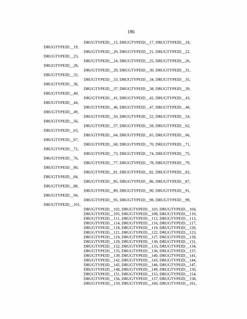
186
DRUGTYPEID__15, DRUGTYPEID__17, DRUGTYPEID__18,
DRUGTYPEID__19,
DRUGTYPEID__20, DRUGTYPEID__21, DRUGTYPEID__22,
DRUGTYPEID__23,
DRUGTYPEID__24, DRUGTYPEID__25, DRUGTYPEID__26,
DRUGTYPEID__28,
DRUGTYPEID__29, DRUGTYPEID__30, DRUGTYPEID__31,
DRUGTYPEID__32,
DRUGTYPEID__33, DRUGTYPEID__34, DRUGTYPEID__35,
DRUGTYPEID__36,
DRUGTYPEID__37, DRUGTYPEID__38, DRUGTYPEID__39,
DRUGTYPEID__40,
DRUGTYPEID__41, DRUGTYPEID__42, DRUGTYPEID__43,
DRUGTYPEID__44,
DRUGTYPEID__46, DRUGTYPEID__47, DRUGTYPEID__48,
DRUGTYPEID__49,
DRUGTYPEID__50, DRUGTYPEID__52, DRUGTYPEID__54,
DRUGTYPEID__56,
DRUGTYPEID__57, DRUGTYPEID__58, DRUGTYPEID__62,
DRUGTYPEID__63,
DRUGTYPEID__64, DRUGTYPEID__65, DRUGTYPEID__66,
DRUGTYPEID__67,
DRUGTYPEID__68, DRUGTYPEID__70, DRUGTYPEID__71,
DRUGTYPEID__72,
DRUGTYPEID__73, DRUGTYPEID__74, DRUGTYPEID__75,
DRUGTYPEID__76,
DRUGTYPEID__77, DRUGTYPEID__78, DRUGTYPEID__79,
DRUGTYPEID__80,
DRUGTYPEID__81, DRUGTYPEID__82, DRUGTYPEID__83,
DRUGTYPEID__84,
DRUGTYPEID__85, DRUGTYPEID__86, DRUGTYPEID__87,
DRUGTYPEID__88,
DRUGTYPEID__89, DRUGTYPEID__90, DRUGTYPEID__91,
DRUGTYPEID__94,
DRUGTYPEID__95, DRUGTYPEID__98, DRUGTYPEID__99,
DRUGTYPEID__101,
DRUGTYPEID__102, DRUGTYPEID__103, DRUGTYPEID__104,
DRUGTYPEID__105, DRUGTYPEID__108, DRUGTYPEID__110,
DRUGTYPEID__111, DRUGTYPEID__112, DRUGTYPEID__113,
DRUGTYPEID__114, DRUGTYPEID__116, DRUGTYPEID__117,
DRUGTYPEID__118, DRUGTYPEID__119, DRUGTYPEID__120,
DRUGTYPEID__121, DRUGTYPEID__122, DRUGTYPEID__123,
DRUGTYPEID__124, DRUGTYPEID__127, DRUGTYPEID__128,
DRUGTYPEID__129, DRUGTYPEID__130, DRUGTYPEID__131,
DRUGTYPEID__132, DRUGTYPEID__133, DRUGTYPEID__134,
DRUGTYPEID__135, DRUGTYPEID__136, DRUGTYPEID__137,
DRUGTYPEID__139, DRUGTYPEID__140, DRUGTYPEID__141,
DRUGTYPEID__142, DRUGTYPEID__143, DRUGTYPEID__144,
DRUGTYPEID__145, DRUGTYPEID__146, DRUGTYPEID__147,
DRUGTYPEID__148, DRUGTYPEID__149, DRUGTYPEID__150,
DRUGTYPEID__151, DRUGTYPEID__153, DRUGTYPEID__154,
DRUGTYPEID__156, DRUGTYPEID__157, DRUGTYPEID__158,
DRUGTYPEID__159, DRUGTYPEID__160, DRUGTYPEID__161,
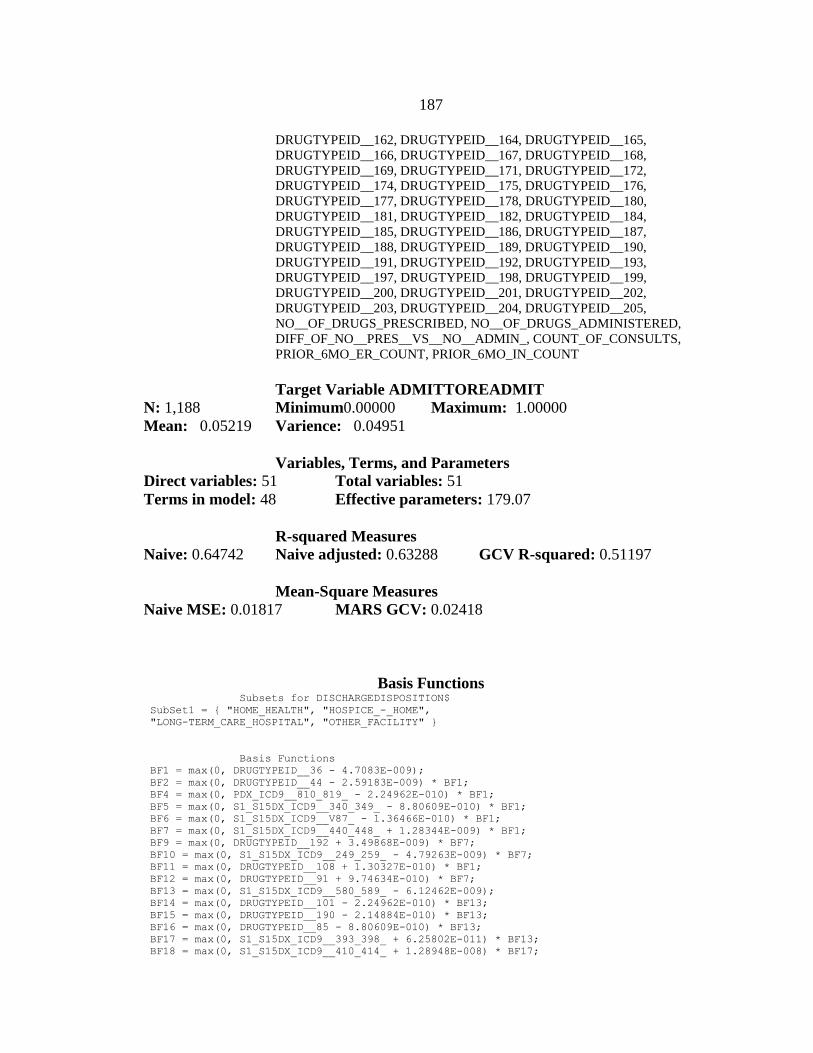
187
DRUGTYPEID__162, DRUGTYPEID__164, DRUGTYPEID__165,
DRUGTYPEID__166, DRUGTYPEID__167, DRUGTYPEID__168,
DRUGTYPEID__169, DRUGTYPEID__171, DRUGTYPEID__172,
DRUGTYPEID__174, DRUGTYPEID__175, DRUGTYPEID__176,
DRUGTYPEID__177, DRUGTYPEID__178, DRUGTYPEID__180,
DRUGTYPEID__181, DRUGTYPEID__182, DRUGTYPEID__184,
DRUGTYPEID__185, DRUGTYPEID__186, DRUGTYPEID__187,
DRUGTYPEID__188, DRUGTYPEID__189, DRUGTYPEID__190,
DRUGTYPEID__191, DRUGTYPEID__192, DRUGTYPEID__193,
DRUGTYPEID__197, DRUGTYPEID__198, DRUGTYPEID__199,
DRUGTYPEID__200, DRUGTYPEID__201, DRUGTYPEID__202,
DRUGTYPEID__203, DRUGTYPEID__204, DRUGTYPEID__205,
NO__OF_DRUGS_PRESCRIBED, NO__OF_DRUGS_ADMINISTERED,
DIFF_OF_NO__PRES__VS__NO__ADMIN_, COUNT_OF_CONSULTS,
PRIOR_6MO_ER_COUNT, PRIOR_6MO_IN_COUNT
Target Variable ADMITTOREADMIT
N: 1,188 Minimum0.00000 Maximum: 1.00000
Mean: 0.05219 Varience: 0.04951
Variables, Terms, and Parameters
Direct variables: 51 Total variables: 51
Terms in model: 48 Effective parameters: 179.07
R-squared Measures
Naive: 0.64742 Naive adjusted: 0.63288 GCV R-squared: 0.51197
Mean-Square Measures
Naive MSE: 0.01817 MARS GCV: 0.02418
Basis Functions Subsets for DISCHARGEDISPOSITION$
SubSet1 = { "HOME_HEALTH", "HOSPICE_-_HOME",
"LONG-TERM_CARE_HOSPITAL", "OTHER_FACILITY" }
Basis Functions
BF1 = max(0, DRUGTYPEID__36 - 4.7083E-009);
BF2 = max(0, DRUGTYPEID__44 - 2.59183E-009) * BF1;
BF4 = max(0, PDX_ICD9__810_819_ - 2.24962E-010) * BF1;
BF5 = max(0, S1_S15DX_ICD9__340_349_ - 8.80609E-010) * BF1;
BF6 = max(0, S1_S15DX_ICD9__V87_ - 1.36466E-010) * BF1;
BF7 = max(0, S1_S15DX_ICD9__440_448_ + 1.28344E-009) * BF1;
BF9 = max(0, DRUGTYPEID__192 + 3.49868E-009) * BF7;
BF10 = max(0, S1_S15DX_ICD9__249_259_ - 4.79263E-009) * BF7;
BF11 = max(0, DRUGTYPEID__108 + 1.30327E-010) * BF1;
BF12 = max(0, DRUGTYPEID__91 + 9.74634E-010) * BF7;
BF13 = max(0, S1_S15DX_ICD9__580_589_ - 6.12462E-009);
BF14 = max(0, DRUGTYPEID__101 - 2.24962E-010) * BF13;
BF15 = max(0, DRUGTYPEID__190 - 2.14884E-010) * BF13;
BF16 = max(0, DRUGTYPEID__85 - 8.80609E-010) * BF13;
BF17 = max(0, S1_S15DX_ICD9__393_398_ + 6.25802E-011) * BF13;
BF18 = max(0, S1_S15DX_ICD9__410_414_ + 1.28948E-008) * BF17;
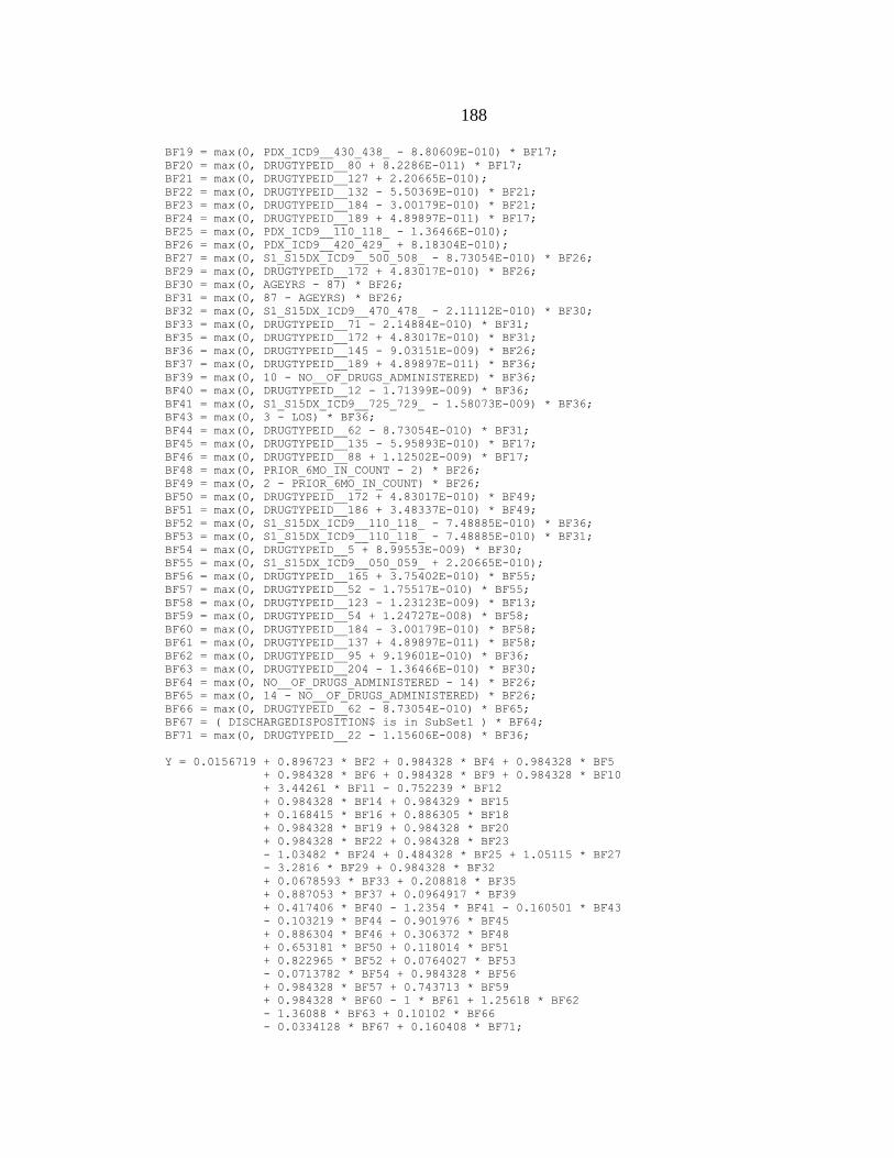
188
BF19 = max(0, PDX_ICD9__430_438_ - 8.80609E-010) * BF17;
BF20 = max(0, DRUGTYPEID__80 + 8.2286E-011) * BF17;
BF21 = max(0, DRUGTYPEID__127 + 2.20665E-010);
BF22 = max(0, DRUGTYPEID__132 - 5.50369E-010) * BF21;
BF23 = max(0, DRUGTYPEID__184 - 3.00179E-010) * BF21;
BF24 = max(0, DRUGTYPEID__189 + 4.89897E-011) * BF17;
BF25 = max(0, PDX_ICD9__110_118_ - 1.36466E-010);
BF26 = max(0, PDX_ICD9__420_429_ + 8.18304E-010);
BF27 = max(0, S1_S15DX_ICD9__500_508_ - 8.73054E-010) * BF26;
BF29 = max(0, DRUGTYPEID__172 + 4.83017E-010) * BF26;
BF30 = max(0, AGEYRS - 87) * BF26;
BF31 = max(0, 87 - AGEYRS) * BF26;
BF32 = max(0, S1_S15DX_ICD9__470_478_ - 2.11112E-010) * BF30;
BF33 = max(0, DRUGTYPEID__71 - 2.14884E-010) * BF31;
BF35 = max(0, DRUGTYPEID__172 + 4.83017E-010) * BF31;
BF36 = max(0, DRUGTYPEID__145 - 9.03151E-009) * BF26;
BF37 = max(0, DRUGTYPEID__189 + 4.89897E-011) * BF36;
BF39 = max(0, 10 - NO__OF_DRUGS_ADMINISTERED) * BF36;
BF40 = max(0, DRUGTYPEID__12 - 1.71399E-009) * BF36;
BF41 = max(0, S1_S15DX_ICD9__725_729_ - 1.58073E-009) * BF36;
BF43 = max(0, 3 - LOS) * BF36;
BF44 = max(0, DRUGTYPEID__62 - 8.73054E-010) * BF31;
BF45 = max(0, DRUGTYPEID__135 - 5.95893E-010) * BF17;
BF46 = max(0, DRUGTYPEID__88 + 1.12502E-009) * BF17;
BF48 = max(0, PRIOR_6MO_IN_COUNT - 2) * BF26;
BF49 = max(0, 2 - PRIOR_6MO_IN_COUNT) * BF26;
BF50 = max(0, DRUGTYPEID__172 + 4.83017E-010) * BF49;
BF51 = max(0, DRUGTYPEID__186 + 3.48337E-010) * BF49;
BF52 = max(0, S1_S15DX_ICD9__110_118_ - 7.48885E-010) * BF36;
BF53 = max(0, S1_S15DX_ICD9__110_118_ - 7.48885E-010) * BF31;
BF54 = max(0, DRUGTYPEID__5 + 8.99553E-009) * BF30;
BF55 = max(0, S1_S15DX_ICD9__050_059_ + 2.20665E-010);
BF56 = max(0, DRUGTYPEID__165 + 3.75402E-010) * BF55;
BF57 = max(0, DRUGTYPEID__52 - 1.75517E-010) * BF55;
BF58 = max(0, DRUGTYPEID__123 - 1.23123E-009) * BF13;
BF59 = max(0, DRUGTYPEID__54 + 1.24727E-008) * BF58;
BF60 = max(0, DRUGTYPEID__184 - 3.00179E-010) * BF58;
BF61 = max(0, DRUGTYPEID__137 + 4.89897E-011) * BF58;
BF62 = max(0, DRUGTYPEID__95 + 9.19601E-010) * BF36;
BF63 = max(0, DRUGTYPEID__204 - 1.36466E-010) * BF30;
BF64 = max(0, NO__OF_DRUGS_ADMINISTERED - 14) * BF26;
BF65 = max(0, 14 - NO__OF_DRUGS_ADMINISTERED) * BF26;
BF66 = max(0, DRUGTYPEID__62 - 8.73054E-010) * BF65;
BF67 = ( DISCHARGEDISPOSITION$ is in SubSet1 ) * BF64;
BF71 = max(0, DRUGTYPEID__22 - 1.15606E-008) * BF36;
Y = 0.0156719 + 0.896723 * BF2 + 0.984328 * BF4 + 0.984328 * BF5
+ 0.984328 * BF6 + 0.984328 * BF9 + 0.984328 * BF10
+ 3.44261 * BF11 - 0.752239 * BF12
+ 0.984328 * BF14 + 0.984329 * BF15
+ 0.168415 * BF16 + 0.886305 * BF18
+ 0.984328 * BF19 + 0.984328 * BF20
+ 0.984328 * BF22 + 0.984328 * BF23
- 1.03482 * BF24 + 0.484328 * BF25 + 1.05115 * BF27
- 3.2816 * BF29 + 0.984328 * BF32
+ 0.0678593 * BF33 + 0.208818 * BF35
+ 0.887053 * BF37 + 0.0964917 * BF39
+ 0.417406 * BF40 - 1.2354 * BF41 - 0.160501 * BF43
- 0.103219 * BF44 - 0.901976 * BF45
+ 0.886304 * BF46 + 0.306372 * BF48
+ 0.653181 * BF50 + 0.118014 * BF51
+ 0.822965 * BF52 + 0.0764027 * BF53
- 0.0713782 * BF54 + 0.984328 * BF56
+ 0.984328 * BF57 + 0.743713 * BF59
+ 0.984328 * BF60 - 1 * BF61 + 1.25618 * BF62
- 1.36088 * BF63 + 0.10102 * BF66
- 0.0334128 * BF67 + 0.160408 * BF71;
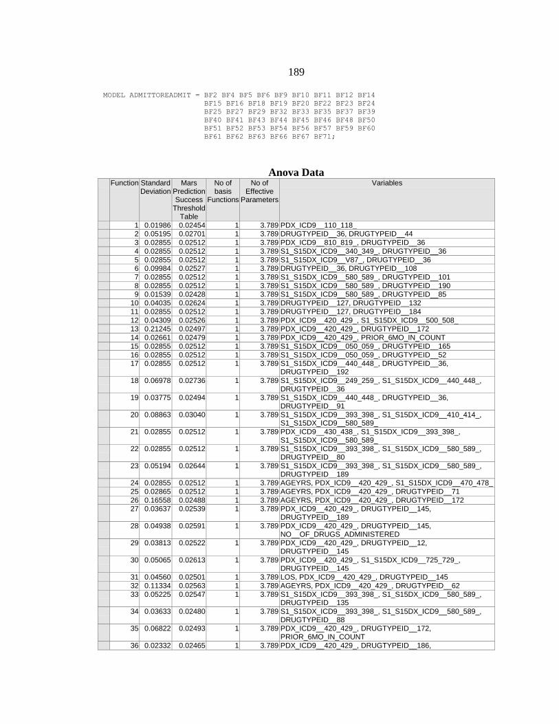
189
MODEL ADMITTOREADMIT = BF2 BF4 BF5 BF6 BF9 BF10 BF11 BF12 BF14
BF15 BF16 BF18 BF19 BF20 BF22 BF23 BF24
BF25 BF27 BF29 BF32 BF33 BF35 BF37 BF39
BF40 BF41 BF43 BF44 BF45 BF46 BF48 BF50
BF51 BF52 BF53 BF54 BF56 BF57 BF59 BF60
BF61 BF62 BF63 BF66 BF67 BF71;
Anova Data Function Standard
Deviation
Mars Prediction Success
Threshold Table
No of basis
Functions
No of Effective
Parameters
Variables
1 0.01986 0.02454 1 3.789 PDX_ICD9__110_118_
2 0.05195 0.02701 1 3.789 DRUGTYPEID__36, DRUGTYPEID__44
3 0.02855 0.02512 1 3.789 PDX_ICD9__810_819_, DRUGTYPEID__36
4 0.02855 0.02512 1 3.789 S1_S15DX_ICD9__340_349_, DRUGTYPEID__36
5 0.02855 0.02512 1 3.789 S1_S15DX_ICD9__V87_, DRUGTYPEID__36
6 0.09984 0.02527 1 3.789 DRUGTYPEID__36, DRUGTYPEID__108
7 0.02855 0.02512 1 3.789 S1_S15DX_ICD9__580_589_, DRUGTYPEID__101
8 0.02855 0.02512 1 3.789 S1_S15DX_ICD9__580_589_, DRUGTYPEID__190
9 0.01539 0.02428 1 3.789 S1_S15DX_ICD9__580_589_, DRUGTYPEID__85
10 0.04035 0.02624 1 3.789 DRUGTYPEID__127, DRUGTYPEID__132
11 0.02855 0.02512 1 3.789 DRUGTYPEID__127, DRUGTYPEID__184
12 0.04309 0.02526 1 3.789 PDX_ICD9__420_429_, S1_S15DX_ICD9__500_508_
13 0.21245 0.02497 1 3.789 PDX_ICD9__420_429_, DRUGTYPEID__172
14 0.02661 0.02479 1 3.789 PDX_ICD9__420_429_, PRIOR_6MO_IN_COUNT
15 0.02855 0.02512 1 3.789 S1_S15DX_ICD9__050_059_, DRUGTYPEID__165
16 0.02855 0.02512 1 3.789 S1_S15DX_ICD9__050_059_, DRUGTYPEID__52
17 0.02855 0.02512 1 3.789 S1_S15DX_ICD9__440_448_, DRUGTYPEID__36, DRUGTYPEID__192
18 0.06978 0.02736 1 3.789 S1_S15DX_ICD9__249_259_, S1_S15DX_ICD9__440_448_, DRUGTYPEID__36
19 0.03775 0.02494 1 3.789 S1_S15DX_ICD9__440_448_, DRUGTYPEID__36, DRUGTYPEID__91
20 0.08863 0.03040 1 3.789 S1_S15DX_ICD9__393_398_, S1_S15DX_ICD9__410_414_, S1_S15DX_ICD9__580_589_
21 0.02855 0.02512 1 3.789 PDX_ICD9__430_438_, S1_S15DX_ICD9__393_398_, S1_S15DX_ICD9__580_589_
22 0.02855 0.02512 1 3.789 S1_S15DX_ICD9__393_398_, S1_S15DX_ICD9__580_589_, DRUGTYPEID__80
23 0.05194 0.02644 1 3.789 S1_S15DX_ICD9__393_398_, S1_S15DX_ICD9__580_589_, DRUGTYPEID__189
24 0.02855 0.02512 1 3.789 AGEYRS, PDX_ICD9__420_429_, S1_S15DX_ICD9__470_478_
25 0.02865 0.02512 1 3.789 AGEYRS, PDX_ICD9__420_429_, DRUGTYPEID__71
26 0.16558 0.02488 1 3.789 AGEYRS, PDX_ICD9__420_429_, DRUGTYPEID__172
27 0.03637 0.02539 1 3.789 PDX_ICD9__420_429_, DRUGTYPEID__145, DRUGTYPEID__189
28 0.04938 0.02591 1 3.789 PDX_ICD9__420_429_, DRUGTYPEID__145, NO__OF_DRUGS_ADMINISTERED
29 0.03813 0.02522 1 3.789 PDX_ICD9__420_429_, DRUGTYPEID__12, DRUGTYPEID__145
30 0.05065 0.02613 1 3.789 PDX_ICD9__420_429_, S1_S15DX_ICD9__725_729_, DRUGTYPEID__145
31 0.04560 0.02501 1 3.789 LOS, PDX_ICD9__420_429_, DRUGTYPEID__145
32 0.11334 0.02563 1 3.789 AGEYRS, PDX_ICD9__420_429_, DRUGTYPEID__62
33 0.05225 0.02547 1 3.789 S1_S15DX_ICD9__393_398_, S1_S15DX_ICD9__580_589_, DRUGTYPEID__135
34 0.03633 0.02480 1 3.789 S1_S15DX_ICD9__393_398_, S1_S15DX_ICD9__580_589_, DRUGTYPEID__88
35 0.06822 0.02493 1 3.789 PDX_ICD9__420_429_, DRUGTYPEID__172, PRIOR_6MO_IN_COUNT
36 0.02332 0.02465 1 3.789 PDX_ICD9__420_429_, DRUGTYPEID__186,
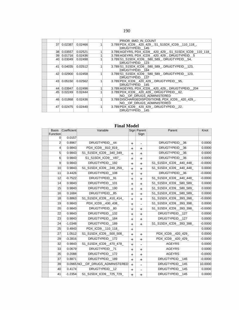
190
PRIOR_6MO_IN_COUNT
37 0.02387 0.02466 1 3.789 PDX_ICD9__420_429_, S1_S15DX_ICD9__110_118_, DRUGTYPEID__145
38 0.03557 0.02521 1 3.789 AGEYRS, PDX_ICD9__420_429_, S1_S15DX_ICD9__110_118_
39 0.01716 0.02436 1 3.789 AGEYRS, PDX_ICD9__420_429_, DRUGTYPEID__5
40 0.03049 0.02498 1 3.789 S1_S15DX_ICD9__580_589_, DRUGTYPEID__54, DRUGTYPEID__123
41 0.04035 0.02512 1 3.789 S1_S15DX_ICD9__580_589_, DRUGTYPEID__123, DRUGTYPEID__184
42 0.02900 0.02458 1 3.789 S1_S15DX_ICD9__580_589_, DRUGTYPEID__123, DRUGTYPEID__137
43 0.05150 0.02562 1 3.789 PDX_ICD9__420_429_, DRUGTYPEID__95, DRUGTYPEID__145
44 0.03947 0.02496 1 3.789 AGEYRS, PDX_ICD9__420_429_, DRUGTYPEID__204
45 0.02249 0.02444 1 3.789 PDX_ICD9__420_429_, DRUGTYPEID__62, NO__OF_DRUGS_ADMINISTERED
46 0.01868 0.02436 1 3.789 DISCHARGEDISPOSITION$, PDX_ICD9__420_429_, NO__OF_DRUGS_ADMINISTERED
47 0.02475 0.02440 1 3.789 PDX_ICD9__420_429_, DRUGTYPEID__22, DRUGTYPEID__145
Final Model
Basis Function
Coefficient Variable Sign Parent Sign
Parent Knot
0 0.0157
2 0.8967 DRUGTYPEID__44 + - DRUGTYPEID__36 0.0000
4 0.9843 PDX_ICD9__810_819_ + + DRUGTYPEID__36 0.0000
5 0.9843 S1_S15DX_ICD9__340_349_ + + DRUGTYPEID__36 0.0000
6 0.9843 S1_S15DX_ICD9__V87_ + + DRUGTYPEID__36 0.0000
9 0.9843 DRUGTYPEID__192 + + S1_S15DX_ICD9__440_448_ -0.0000
10 0.9843 S1_S15DX_ICD9__249_259_ + + S1_S15DX_ICD9__440_448_ 0.0000
11 3.4426 DRUGTYPEID__108 + + DRUGTYPEID__36 -0.0000
12 -0.7522 DRUGTYPEID__91 + + S1_S15DX_ICD9__440_448_ -0.0000
14 0.9843 DRUGTYPEID__101 + + S1_S15DX_ICD9__580_589_ 0.0000
15 0.9843 DRUGTYPEID__190 + + S1_S15DX_ICD9__580_589_ 0.0000
16 0.1684 DRUGTYPEID__85 + + S1_S15DX_ICD9__580_589_ 0.0000
18 0.8863 S1_S15DX_ICD9__410_414_ + + S1_S15DX_ICD9__393_398_ -0.0000
19 0.9843 PDX_ICD9__430_438_ + - S1_S15DX_ICD9__393_398_ 0.0000
20 0.9843 DRUGTYPEID__80 + + S1_S15DX_ICD9__393_398_ -0.0000
22 0.9843 DRUGTYPEID__132 + + DRUGTYPEID__127 0.0000
23 0.9843 DRUGTYPEID__184 + + DRUGTYPEID__127 0.0000
24 -1.0348 DRUGTYPEID__189 + + S1_S15DX_ICD9__393_398_ -0.0000
25 0.4843 PDX_ICD9__110_118_ + 0.0000
27 1.0512 S1_S15DX_ICD9__500_508_ + + PDX_ICD9__420_429_ 0.0000
29 -3.2816 DRUGTYPEID__172 + + PDX_ICD9__420_429_ -0.0000
32 0.9843 S1_S15DX_ICD9__470_478_ + - AGEYRS 0.0000
33 0.0679 DRUGTYPEID__71 + + AGEYRS 0.0000
35 0.2088 DRUGTYPEID__172 + + AGEYRS -0.0000
37 0.8871 DRUGTYPEID__189 + + DRUGTYPEID__145 -0.0000
39 0.0965 NO__OF_DRUGS_ADMINISTERED + - DRUGTYPEID__145 10.0000
40 0.4174 DRUGTYPEID__12 + - DRUGTYPEID__145 0.0000
41 -1.2354 S1_S15DX_ICD9__725_729_ + + DRUGTYPEID__145 0.0000

191
43 -0.1605 LOS + + DRUGTYPEID__145 3.0000
44 -0.1032 DRUGTYPEID__62 + + AGEYRS 0.0000
45 -0.9020 DRUGTYPEID__135 + + S1_S15DX_ICD9__393_398_ 0.0000
46 0.8863 DRUGTYPEID__88 - + S1_S15DX_ICD9__393_398_ -0.0000
48 0.3064 PRIOR_6MO_IN_COUNT + + PDX_ICD9__420_429_ 2.0000
50 0.6532 DRUGTYPEID__172 + + PRIOR_6MO_IN_COUNT -0.0000
51 0.1180 DRUGTYPEID__186 + + PRIOR_6MO_IN_COUNT -0.0000
52 0.8230 S1_S15DX_ICD9__110_118_ + + DRUGTYPEID__145 0.0000
53 0.0764 S1_S15DX_ICD9__110_118_ + + AGEYRS 0.0000
54 -0.0714 DRUGTYPEID__5 + + AGEYRS -0.0000
56 0.9843 DRUGTYPEID__165 + + S1_S15DX_ICD9__050_059_ -0.0000
57 0.9843 DRUGTYPEID__52 - + S1_S15DX_ICD9__050_059_ 0.0000
59 0.7437 DRUGTYPEID__54 + + DRUGTYPEID__123 -0.0000
60 0.9843 DRUGTYPEID__184 + + DRUGTYPEID__123 0.0000
61 -1.0000 DRUGTYPEID__137 + + DRUGTYPEID__123 -0.0000
62 1.2562 DRUGTYPEID__95 - + DRUGTYPEID__145 -0.0000
63 -1.3609 DRUGTYPEID__204 + + AGEYRS 0.0000
66 0.1010 DRUGTYPEID__62 + + NO__OF_DRUGS_ADMINISTERED 0.0000
67 -0.0334 DISCHARGEDISPOSITION$ + + NO__OF_DRUGS_ADMINISTERED SubSet1
71 0.1604 DRUGTYPEID__22 + + DRUGTYPEID__145 0.0000
MARS Learn Gains for Class 0
Gains Data Bin Cases
Tgt.Class % of Bin Tgt.Class
% Tgt.Class
Cum % Tgt.Class
Cum % Pop
% Pop
Cases in Bin
Cum Lift
Lift Pop
1 27 100.00 2.40 2.40 2.27 2.27 27 1.06 1.06 2 26 100.00 2.31 4.71 4.46 2.19 26 1.06 1.06 3 759 98.19 67.41 72.11 69.53 65.07 773 1.04 1.04 4 196 99.49 17.41 89.52 86.11 16.58 197 1.04 1.05 5 59 98.33 5.24 94.76 91.16 5.05 60 1.04 1.04 6 23 100.00 2.04 96.80 93.10 1.94 23 1.04 1.06 7 22 95.65 1.95 98.76 95.03 1.94 23 1.04 1.01
0
20
40
60
80
100
0 20 40 60 80 100
% C
lass
% Population

192
8 14 70.00 1.24 100.00 96.72 1.68 20 1.03 0.74 9 0 0.00 0.00 100.00 98.40 1.68 20 1.02 0.00
10 0 0.00 0.00 100.00 100.00 1.60 19 1.00 0.00
Variable Importance
Variable Score S1_S15DX_ICD9__580_589_ 100.00 ||||||||||||||||||||||||||||||||||||
|||||| DRUGTYPEID__36 95.78 ||||||||||||||||||||||||||||||||||||
|||| PDX_ICD9__420_429_ 92.11 ||||||||||||||||||||||||||||||||||||
||| S1_S15DX_ICD9__393_398_ 82.73 ||||||||||||||||||||||||||||||||||| S1_S15DX_ICD9__410_414_ 74.83 ||||||||||||||||||||||||||||||| DRUGTYPEID__145 72.93 |||||||||||||||||||||||||||||| AGEYRS 65.13 ||||||||||||||||||||||||||| S1_S15DX_ICD9__440_448_ 60.33 ||||||||||||||||||||||||| S1_S15DX_ICD9__249_259_ 53.50 |||||||||||||||||||||| DRUGTYPEID__127 51.76 ||||||||||||||||||||| DRUGTYPEID__44 50.53 ||||||||||||||||||||| DRUGTYPEID__189 46.73 ||||||||||||||||||| NO__OF_DRUGS_ADMINISTERED 44.09 |||||||||||||||||| DRUGTYPEID__132 43.08 |||||||||||||||||| S1_S15DX_ICD9__725_729_ 41.88 ||||||||||||||||| DRUGTYPEID__184 40.99 ||||||||||||||||| S1_S15DX_ICD9__050_059_ 40.99 ||||||||||||||||| DRUGTYPEID__123 37.20 ||||||||||||||| S1_S15DX_ICD9__110_118_ 36.71 ||||||||||||||| DRUGTYPEID__95 35.97 |||||||||||||| PRIOR_6MO_IN_COUNT 35.85 |||||||||||||| DRUGTYPEID__135 34.06 |||||||||||||| DRUGTYPEID__62 33.87 |||||||||||||| DRUGTYPEID__108 31.36 |||||||||||| S1_S15DX_ICD9__500_508_ 31.20 |||||||||||| DRUGTYPEID__12 30.57 |||||||||||| DRUGTYPEID__71 29.12 |||||||||||| PDX_ICD9__430_438_ 29.11 |||||||||||| PDX_ICD9__810_819_ 29.11 |||||||||||| S1_S15DX_ICD9__340_349_ 29.11 |||||||||||| S1_S15DX_ICD9__470_478_ 29.11 |||||||||||| S1_S15DX_ICD9__V87_ 29.11 |||||||||||| DRUGTYPEID__52 29.11 |||||||||||| DRUGTYPEID__80 29.11 |||||||||||| DRUGTYPEID__101 29.11 |||||||||||| DRUGTYPEID__165 29.11 |||||||||||| DRUGTYPEID__190 29.11 |||||||||||| DRUGTYPEID__192 29.11 |||||||||||| LOS 27.26 ||||||||||| DRUGTYPEID__54 26.86 ||||||||||| DRUGTYPEID__204 26.56 |||||||||| DRUGTYPEID__91 26.22 |||||||||| DRUGTYPEID__172 24.81 |||||||||| DRUGTYPEID__88 23.56 ||||||||| DRUGTYPEID__186 20.57 |||||||| DRUGTYPEID__137 18.95 ||||||| PDX_ICD9__110_118_ 18.06 ||||||| DRUGTYPEID__22 14.08 ||||| DISCHARGEDISPOSITION$ 12.76 |||| DRUGTYPEID__5 12.66 |||| DRUGTYPEID__85 9.30 |||

193
Prediction Success
Actual Class
Total Class
Percent Correct
Class 0 N=1144
Class 1 N=44
Class 0 1,126 99.91 1,125 1 Class 1 62 69.35 19 43
Total: 1,188.00
Average: 84.63
Overall % Correct:
98.32

194
APPENDIX J
SPSS PREDICTION MODEL REPORT COMPONENTS FOR 536

195
Block 1: Method = Forward Stepwise (Conditional)
Omnibus Tests of Model Coefficients
Chi-square df Sig.
Step 18
Step 3.235 1 .072
Block 77.245 16 .000
Model 77.245 16 .000
Model Summary
Step -2 Log likelihood Cox & Snell R
Square
Nagelkerke R
Square
18 57.036a .389 .676
a. Estimation terminated at iteration number 20 because
maximum iterations has been reached. Final solution cannot be
found.
Hosmer and Lemeshow Test
Step Chi-square df Sig.
18 9.249 8 .322
Classification Tablea
Observed Predicted
AdmitToReadmit Percentage
Correct .0 1.0
Step 18 AdmitToReadmit
.0 133 0 100.0
1.0 6 18 75.0
Overall Percentage 96.2
a. The cut value is .500

196
Variables in the Equation
B S.E. Wald df Sig.
Step 18a
AgeYRS -.147 .046 10.124 1 .001
Pdx_ICD9_190199(1) -30.031 40193.107 .000 1 .999
Pdx_ICD9_300316(1) -28.636 40193.099 .000 1 .999
Pdx_ICD9_580589(1) -29.177 40193.110 .000 1 .999
Pdx_ICD9_710719(1) -4.668 2.613 3.192 1 .074
S1S15dx_ICD9_050059(1) -23.165 28315.926 .000 1 .999
S1S15dx_ICD9_200208(1) -33.478 40193.109 .000 1 .999
S1S15dx_ICD9_V87(1) -26.288 40193.102 .000 1 .999
S1S15dx_ICD9_E850E858(1) -4.430 1.695 6.834 1 .009
DrugTypeID_15(1) -2.411 1.299 3.446 1 .063
DrugTypeID_67(1) -3.380 1.300 6.760 1 .009
DrugTypeID_104(1) -25.487 40193.016 .000 1 .999
DrugTypeID_117(1) -4.549 1.467 9.616 1 .002
DrugTypeID_201(1) -5.916 2.409 6.028 1 .014
Count_of_Consults 1.393 .474 8.622 1 .003
Prior_6Mo_IN_Count .854 .258 10.989 1 .001
Constant 221.375 102443.719 .000 1 .998
Variables in the Equation
Exp(B) 95% C.I.for EXP(B)
Lower Upper
Step 18a
AgeYRS .864 .789 .945
Pdx_ICD9_190199(1) .000 .000 .
Pdx_ICD9_300316(1) .000 .000 .
Pdx_ICD9_580589(1) .000 .000 .
Pdx_ICD9_710719(1) .009 .000 1.573
S1S15dx_ICD9_050059(1) .000 .000 .
S1S15dx_ICD9_200208(1) .000 .000 .
S1S15dx_ICD9_V87(1) .000 .000 .
S1S15dx_ICD9_E850E858(1) .012 .000 .330
DrugTypeID_15(1) .090 .007 1.144

197
DrugTypeID_67(1) .034 .003 .435
DrugTypeID_104(1) .000 .000 .
DrugTypeID_117(1) .011 .001 .188
DrugTypeID_201(1) .003 .000 .303
Count_of_Consults 4.025 1.589 10.197
Prior_6Mo_IN_Count 2.349 1.418 3.891
Constant 1.386E+096
a. Variable(s) entered on step 18: DrugTypeID_15.
Step Summarya,b
Step Improvement Model Correct
Class %
Variable
Chi-
square
df Sig. Chi-
square
df Sig.
1 7.659 1 .006 7.659 1 .006 86.0% IN:
S1S15dx_ICD9_050059
2 6.672 1 .010 14.330 2 .001 84.7% IN: Prior_6Mo_IN_Count
3 4.842 1 .028 19.172 3 .000 85.4% IN: Pdx_ICD9_300316
4 5.027 1 .025 24.200 4 .000 86.0% IN:
S1S15dx_ICD9_200208
5 5.232 1 .022 29.432 5 .000 86.6% IN: S1S15dx_ICD9_V87
6 5.458 1 .019 34.890 6 .000 88.5% IN: Pdx_ICD9_190199
7 4.799 1 .028 39.689 7 .000 89.2% IN: Pdx_ICD9_580589
8 2.760 1 .097 42.448 8 .000 89.8% IN:
S1S15dx_ICD9_690698
9 3.806 1 .051 46.255 9 .000 87.9% IN: Count_of_Consults
10 3.883 1 .049 50.138 10 .000 87.3% IN: DrugTypeID_104
11 6.004 1 .014 56.142 11 .000 87.3% IN: AgeYRS
12 -2.458 1 .117 53.684 10 .000 87.9% OUT:
S1S15dx_ICD9_690698
13 4.424 1 .035 58.108 11 .000 88.5% IN: DrugTypeID_117
14 3.478 1 .062 61.586 12 .000 89.8% IN:
S1S15dx_ICD9_E850E858
15 3.773 1 .052 65.359 13 .000 90.4% IN: DrugTypeID_201
16 4.986 1 .026 70.345 14 .000 94.9% IN: DrugTypeID_67
17 3.665 1 .056 74.010 15 .000 94.9% IN: Pdx_ICD9_710719
18 3.235 1 .072 77.245 16 .000 96.2% IN: DrugTypeID_15

198
ROC Curve
Case Processing Summary
AdmitToReadmit Valid N (listwise)
Positivea 24
Negative 133
Larger values of the test result
variable(s) indicate stronger evidence
for a positive actual state.
a. The positive actual state is 1.0.
Area Under the Curve
Test Result Variable(s): Predicted probability
Area Std. Errora Asymptotic Sig.
b Asymptotic 95% Confidence
Interval
Lower Bound Upper Bound
.940 .028 .000 .885 .994

199
APPENDIX K
MARS PREDICTION MODEL REPORT FOR ICD-9 CODE 536

200
MARS 1 Results: 536, 16 Basis Functions
Dataset: 536-FinalMethodology-Basic-AnalysisReady-ModelSetup.xlsx
Predictor Variables: DISCHARGE_MONTH$, GENDER_M_0_F_1, MARITALSTATUS$,
HOSPDISCHARGEDEPT$,
ADMITFROMER_YES_1, FINANCIALCLASS$,
DISCHARGEDISPOSITION$,
DISTANCETOHOSPITAL$, LOS, AGEYRS, PDX_ICD9__001_009_,
PDX_ICD9__190_199_, PDX_ICD9__249_259_, PDX_ICD9__270_279_,
PDX_ICD9__280_289_, PDX_ICD9__300_316_, PDX_ICD9__338_,
PDX_ICD9__401_405_, PDX_ICD9__420_429_, PDX_ICD9__430_438_,
PDX_ICD9__451_459_, PDX_ICD9__480_488_, PDX_ICD9__490_496_,
PDX_ICD9__500_508_, PDX_ICD9__530_538_, PDX_ICD9__550_553_,
PDX_ICD9__555_558_, PDX_ICD9__560_569_, PDX_ICD9__570_579_,
PDX_ICD9__580_589_, PDX_ICD9__590_599_, PDX_ICD9__680_686_,
PDX_ICD9__710_719_, PDX_ICD9__720_724_, PDX_ICD9__780_789_,
PDX_ICD9__790_796_, PDX_ICD9__805_809_, PDX_ICD9__810_819_,
PDX_ICD9__850_854_, PDX_ICD9__996_999_, S1_S15DX_ICD9__001_009_,
S1_S15DX_ICD9__030_041_, S1_S15DX_ICD9__050_059_,
S1_S15DX_ICD9__070_079_, S1_S15DX_ICD9__110_118_,
S1_S15DX_ICD9__140_149_, S1_S15DX_ICD9__150_159_,
S1_S15DX_ICD9__160_165_, S1_S15DX_ICD9__170_176_,
S1_S15DX_ICD9__179_189_, S1_S15DX_ICD9__190_199_,
S1_S15DX_ICD9__200_208_, S1_S15DX_ICD9__210_229_,
S1_S15DX_ICD9__235_238_, S1_S15DX_ICD9__240_246_,
S1_S15DX_ICD9__249_259_, S1_S15DX_ICD9__260_269_,
S1_S15DX_ICD9__270_279_, S1_S15DX_ICD9__280_289_,
S1_S15DX_ICD9__290_294_, S1_S15DX_ICD9__295_299_,
S1_S15DX_ICD9__300_316_, S1_S15DX_ICD9__330_337_,
S1_S15DX_ICD9__338_, S1_S15DX_ICD9__340_349_,
S1_S15DX_ICD9__350_359_,
S1_S15DX_ICD9__360_379_, S1_S15DX_ICD9__380_389_,
S1_S15DX_ICD9__393_398_, S1_S15DX_ICD9__401_405_,
S1_S15DX_ICD9__410_414_, S1_S15DX_ICD9__415_417_,
S1_S15DX_ICD9__420_429_, S1_S15DX_ICD9__430_438_,
S1_S15DX_ICD9__440_448_, S1_S15DX_ICD9__451_459_,
S1_S15DX_ICD9__460_466_, S1_S15DX_ICD9__470_478_,
S1_S15DX_ICD9__480_488_, S1_S15DX_ICD9__490_496_,
S1_S15DX_ICD9__500_508_, S1_S15DX_ICD9__510_519_,
S1_S15DX_ICD9__520_529_, S1_S15DX_ICD9__530_538_,
S1_S15DX_ICD9__550_553_, S1_S15DX_ICD9__555_558_,
S1_S15DX_ICD9__560_569_, S1_S15DX_ICD9__570_579_,
S1_S15DX_ICD9__580_589_, S1_S15DX_ICD9__590_599_,
S1_S15DX_ICD9__600_608_, S1_S15DX_ICD9__610_611_,
S1_S15DX_ICD9__680_686_, S1_S15DX_ICD9__690_698_,
S1_S15DX_ICD9__700_709_, S1_S15DX_ICD9__710_719_,
S1_S15DX_ICD9__720_724_, S1_S15DX_ICD9__725_729_,
S1_S15DX_ICD9__730_739_, S1_S15DX_ICD9__740_759_,
S1_S15DX_ICD9__780_789_, S1_S15DX_ICD9__790_796_,
S1_S15DX_ICD9__797_799_, S1_S15DX_ICD9__805_809_,
S1_S15DX_ICD9__820_829_, S1_S15DX_ICD9__840_848_,
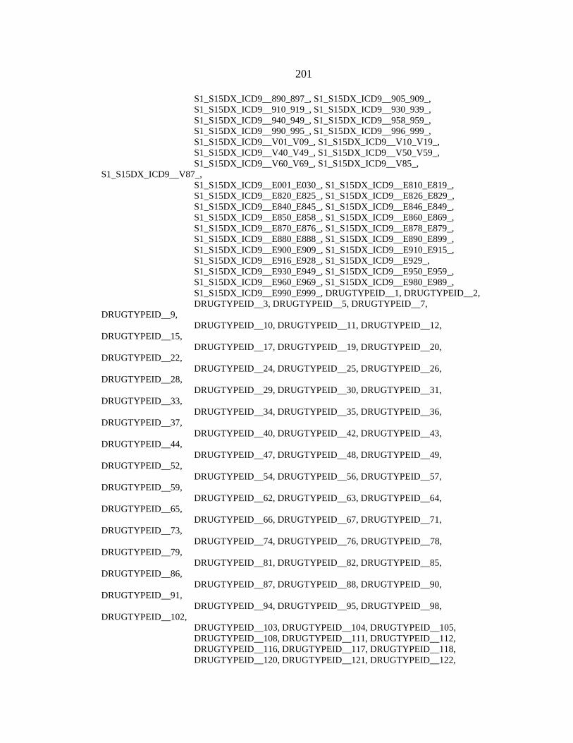
201
S1_S15DX_ICD9__890_897_, S1_S15DX_ICD9__905_909_,
S1_S15DX_ICD9__910_919_, S1_S15DX_ICD9__930_939_,
S1_S15DX_ICD9__940_949_, S1_S15DX_ICD9__958_959_,
S1_S15DX_ICD9__990_995_, S1_S15DX_ICD9__996_999_,
S1_S15DX_ICD9__V01_V09_, S1_S15DX_ICD9__V10_V19_,
S1_S15DX_ICD9__V40_V49_, S1_S15DX_ICD9__V50_V59_,
S1_S15DX_ICD9__V60_V69_, S1_S15DX_ICD9__V85_,
S1_S15DX_ICD9__V87_,
S1_S15DX_ICD9__E001_E030_, S1_S15DX_ICD9__E810_E819_,
S1_S15DX_ICD9__E820_E825_, S1_S15DX_ICD9__E826_E829_,
S1_S15DX_ICD9__E840_E845_, S1_S15DX_ICD9__E846_E849_,
S1_S15DX_ICD9__E850_E858_, S1_S15DX_ICD9__E860_E869_,
S1_S15DX_ICD9__E870_E876_, S1_S15DX_ICD9__E878_E879_,
S1_S15DX_ICD9__E880_E888_, S1_S15DX_ICD9__E890_E899_,
S1_S15DX_ICD9__E900_E909_, S1_S15DX_ICD9__E910_E915_,
S1_S15DX_ICD9__E916_E928_, S1_S15DX_ICD9__E929_,
S1_S15DX_ICD9__E930_E949_, S1_S15DX_ICD9__E950_E959_,
S1_S15DX_ICD9__E960_E969_, S1_S15DX_ICD9__E980_E989_,
S1_S15DX_ICD9__E990_E999_, DRUGTYPEID__1, DRUGTYPEID__2,
DRUGTYPEID__3, DRUGTYPEID__5, DRUGTYPEID__7,
DRUGTYPEID__9,
DRUGTYPEID__10, DRUGTYPEID__11, DRUGTYPEID__12,
DRUGTYPEID__15,
DRUGTYPEID__17, DRUGTYPEID__19, DRUGTYPEID__20,
DRUGTYPEID__22,
DRUGTYPEID__24, DRUGTYPEID__25, DRUGTYPEID__26,
DRUGTYPEID__28,
DRUGTYPEID__29, DRUGTYPEID__30, DRUGTYPEID__31,
DRUGTYPEID__33,
DRUGTYPEID__34, DRUGTYPEID__35, DRUGTYPEID__36,
DRUGTYPEID__37,
DRUGTYPEID__40, DRUGTYPEID__42, DRUGTYPEID__43,
DRUGTYPEID__44,
DRUGTYPEID__47, DRUGTYPEID__48, DRUGTYPEID__49,
DRUGTYPEID__52,
DRUGTYPEID__54, DRUGTYPEID__56, DRUGTYPEID__57,
DRUGTYPEID__59,
DRUGTYPEID__62, DRUGTYPEID__63, DRUGTYPEID__64,
DRUGTYPEID__65,
DRUGTYPEID__66, DRUGTYPEID__67, DRUGTYPEID__71,
DRUGTYPEID__73,
DRUGTYPEID__74, DRUGTYPEID__76, DRUGTYPEID__78,
DRUGTYPEID__79,
DRUGTYPEID__81, DRUGTYPEID__82, DRUGTYPEID__85,
DRUGTYPEID__86,
DRUGTYPEID__87, DRUGTYPEID__88, DRUGTYPEID__90,
DRUGTYPEID__91,
DRUGTYPEID__94, DRUGTYPEID__95, DRUGTYPEID__98,
DRUGTYPEID__102,
DRUGTYPEID__103, DRUGTYPEID__104, DRUGTYPEID__105,
DRUGTYPEID__108, DRUGTYPEID__111, DRUGTYPEID__112,
DRUGTYPEID__116, DRUGTYPEID__117, DRUGTYPEID__118,
DRUGTYPEID__120, DRUGTYPEID__121, DRUGTYPEID__122,

202
DRUGTYPEID__123, DRUGTYPEID__124, DRUGTYPEID__127,
DRUGTYPEID__128, DRUGTYPEID__129, DRUGTYPEID__131,
DRUGTYPEID__132, DRUGTYPEID__134, DRUGTYPEID__135,
DRUGTYPEID__136, DRUGTYPEID__137, DRUGTYPEID__140,
DRUGTYPEID__141, DRUGTYPEID__142, DRUGTYPEID__144,
DRUGTYPEID__145, DRUGTYPEID__146, DRUGTYPEID__147,
DRUGTYPEID__149, DRUGTYPEID__151, DRUGTYPEID__156,
DRUGTYPEID__158, DRUGTYPEID__160, DRUGTYPEID__164,
DRUGTYPEID__165, DRUGTYPEID__166, DRUGTYPEID__167,
DRUGTYPEID__169, DRUGTYPEID__171, DRUGTYPEID__172,
DRUGTYPEID__174, DRUGTYPEID__175, DRUGTYPEID__176,
DRUGTYPEID__178, DRUGTYPEID__180, DRUGTYPEID__181,
DRUGTYPEID__184, DRUGTYPEID__185, DRUGTYPEID__186,
DRUGTYPEID__187, DRUGTYPEID__188, DRUGTYPEID__190,
DRUGTYPEID__191, DRUGTYPEID__192, DRUGTYPEID__198,
DRUGTYPEID__201, DRUGTYPEID__202, DRUGTYPEID__203,
DRUGTYPEID__205, NO__OF_DRUGS_PRESCRIBED,
NO__OF_DRUGS_ADMINISTERED,
DIFF_OF_NO__PRES__VS__NO__ADMIN_, COUNT_OF_CONSULTS,
PRIOR_6MO_ER_COUNT, PRIOR_6MO_IN_COUNT
Target Variable ADMITTOREADMIT
N: 157 Minimum0.00000 Maximum: 1.00000
Mean: 0.15287 Varience: 0.13033
Variables, Terms, and Parameters
Direct variables: 18 Total variables: 18
Terms in model: 17 Effective parameters: 62.91
R-Square Measures
Naive: 0.79713 Naive adjusted: 0.77395 GCV R-square: 0.44230
Mean-Square Measures
Naive MSE: 0.02946 MARS GCV: 0.07315
Basis Functions Subsets for FINANCIALCLASS$
SubSet1 = { "HMO", "Medicare", "Selfpay", "Tricare", "WorkersComp" }
SubSet2 = { "BlueCross", "Commercial", "Medicaid" }
Basis Functions
BF1 = ( FINANCIALCLASS$ is in SubSet1 );
BF2 = ( FINANCIALCLASS$ is in SubSet2 );
BF3 = max(0, DRUGTYPEID__26 + 1.82144E-009) * BF2;
BF4 = max(0, DRUGTYPEID__49 - 8.26983E-009) * BF2;
BF5 = max(0, S1_S15DX_ICD9__050_059_ - 4.94944E-011);
BF6 = max(0, DRUGTYPEID__71 - 1.01897E-010) * BF1;
BF7 = max(0, PDX_ICD9__580_589_ - 1.01897E-010) * BF1;
BF8 = max(0, PDX_ICD9__190_199_ - 1.01897E-010) * BF1;
BF9 = max(0, PDX_ICD9__300_316_ - 1.01897E-010) * BF2;
BF10 = max(0, S1_S15DX_ICD9__440_448_ + 1.82144E-009) * BF2;
BF11 = max(0, S1_S15DX_ICD9__E850_E858_ + 4.72525E-010) * BF2;
BF12 = max(0, DRUGTYPEID__137 - 5.31255E-010) * BF2;
BF14 = max(0, PRIOR_6MO_IN_COUNT - 2);
BF16 = max(0, DRUGTYPEID__76 - 1.01897E-010) * BF2;

203
BF17 = max(0, S1_S15DX_ICD9__910_919_ - 1.01897E-010);
BF18 = max(0, DRUGTYPEID__30 - 7.94443E-009) * BF2;
BF19 = max(0, S1_S15DX_ICD9__240_246_ + 2.52024E-009) * BF18;
BF20 = max(0, S1_S15DX_ICD9__530_538_ + 7.05768E-009) * BF18;
BF21 = max(0, S1_S15DX_ICD9__600_608_ + 1.82144E-009) * BF18;
Y = 0.00741154 + 1.02029 * BF3 + 0.865519 * BF4 + 0.922275 * BF5
+ 0.992588 * BF6 + 0.992588 * BF7 + 0.992588 * BF8
+ 0.851962 * BF9 + 0.851962 * BF10
+ 0.992588 * BF11 + 0.963834 * BF12
- 0.111873 * BF14 - 1.01356 * BF16
- 0.789812 * BF17 + 0.761543 * BF19
+ 0.140627 * BF20 + 0.422275 * BF21;
MODEL ADMITTOREADMIT = BF3 BF4 BF5 BF6 BF7 BF8 BF9 BF10 BF11
BF12 BF14 BF16 BF17 BF19 BF20 BF21;
Anova Data Function Standard
Deviation
Mars Prediction Success
Threshold Table
No of basis
Functions
No of Effective
Parameters
Variables
1 0.10343 0.09458 1 3.870 S1_S15DX_ICD9__050_059_
2 0.09930 0.08176 1 3.870 PRIOR_6MO_IN_COUNT
3 0.06283 0.07668 1 3.870 S1_S15DX_ICD9__910_919_
4 0.13968 0.11675 1 3.870 FINANCIALCLASS$, DRUGTYPEID__26
5 0.22996 0.13752 1 3.870 FINANCIALCLASS$, DRUGTYPEID__49
6 0.07896 0.08346 1 3.870 FINANCIALCLASS$, DRUGTYPEID__71
7 0.07896 0.08346 1 3.870 FINANCIALCLASS$, PDX_ICD9__580_589_
8 0.07896 0.08346 1 3.870 FINANCIALCLASS$, PDX_ICD9__190_199_
9 0.06778 0.07889 1 3.870 FINANCIALCLASS$, PDX_ICD9__300_316_
10 0.06778 0.07889 1 3.870 FINANCIALCLASS$, S1_S15DX_ICD9__440_448_
11 0.07896 0.08346 1 3.870 FINANCIALCLASS$, S1_S15DX_ICD9__E850_E858_
12 0.07668 0.08204 1 3.870 FINANCIALCLASS$, DRUGTYPEID__137
13 0.08063 0.08158 1 3.870 FINANCIALCLASS$, DRUGTYPEID__76
14 0.10426 0.09375 1 3.870 FINANCIALCLASS$, S1_S15DX_ICD9__240_246_, DRUGTYPEID__30
15 0.05912 0.07445 1 3.870 FINANCIALCLASS$, S1_S15DX_ICD9__530_538_, DRUGTYPEID__30
16 0.04736 0.07316 1 3.870 FINANCIALCLASS$, S1_S15DX_ICD9__600_608_, DRUGTYPEID__30
Final Model Basis
Function
Coefficient Variable Sign Parent Sign
Parent Knot
0 0.0074
3 1.0203 DRUGTYPEID__26 + - FINANCIALCLASS$ -0.0000
4 0.8655 DRUGTYPEID__49 - - FINANCIALCLASS$ 0.0000
5 0.9223 S1_S15DX_ICD9__050_059_ + 0.0000
6 0.9926 DRUGTYPEID__71 + + FINANCIALCLASS$ 0.0000
7 0.9926 PDX_ICD9__580_589_ + - FINANCIALCLASS$ 0.0000
8 0.9926 PDX_ICD9__190_199_ + + FINANCIALCLASS$ 0.0000
9 0.8520 PDX_ICD9__300_316_ + + FINANCIALCLASS$ 0.0000
10 0.8520 S1_S15DX_ICD9__440_448_ + + FINANCIALCLASS$ -0.0000
11 0.9926 S1_S15DX_ICD9__E850_E858_ + + FINANCIALCLASS$ -0.0000
12 0.9638 DRUGTYPEID__137 + + FINANCIALCLASS$ 0.0000

204
14 -0.1119 PRIOR_6MO_IN_COUNT + 2.0000
16 -1.0136 DRUGTYPEID__76 + + FINANCIALCLASS$ 0.0000
17 -0.7898 S1_S15DX_ICD9__910_919_ + 0.0000
19 0.7615 S1_S15DX_ICD9__240_246_ + - DRUGTYPEID__30 -0.0000
20 0.1406 S1_S15DX_ICD9__530_538_ - - DRUGTYPEID__30 -0.0000
21 0.4223 S1_S15DX_ICD9__600_608_ + + DRUGTYPEID__30 -0.0000
MARS Learn Gains for Class 0
Gains Data Bin Cases
Tgt.Class % of Bin Tgt.Class
% Tgt.Class
Cum % Tgt.Class
Cum % Pop
% Pop
Cases in Bin
Cum Lift
Lift Pop
1 5 100.00 3.76 3.76 3.18 3.18 5 1.18 1.18 2 5 100.00 3.76 7.52 6.37 3.18 5 1.18 1.18 3 74 98.67 55.64 63.16 54.14 47.77 75 1.17 1.16 4 26 100.00 19.55 82.71 70.70 16.56 26 1.17 1.18 5 4 100.00 3.01 85.71 73.25 2.55 4 1.17 1.18 6 14 93.33 10.53 96.24 82.80 9.55 15 1.16 1.10 7 5 62.50 3.76 100.00 87.90 5.10 8 1.14 0.74 8 0 0.00 0.00 100.00 92.36 4.46 7 1.08 0.00 9 0 0.00 0.00 100.00 96.18 3.82 6 1.04 0.00
10 0 0.00 0.00 100.00 100.00 3.82 6 1.00 0.00
Variable Importance
Variable Score FINANCIALCLASS$ 100.00 ||||||||||||||||||||||||||||||||||||
|||||| DRUGTYPEID__49 99.85 ||||||||||||||||||||||||||||||||||||
|||||| DRUGTYPEID__26 82.18 |||||||||||||||||||||||||||||||||| S1_S15DX_ICD9__050_059_ 57.60 |||||||||||||||||||||||| S1_S15DX_ICD9__240_246_ 56.49 ||||||||||||||||||||||| DRUGTYPEID__30 55.09 ||||||||||||||||||||||| PDX_ICD9__190_199_ 39.96 |||||||||||||||| PDX_ICD9__580_589_ 39.96 ||||||||||||||||
0
20
40
60
80
100
0 20 40 60 80 100
% C
lass
% Population
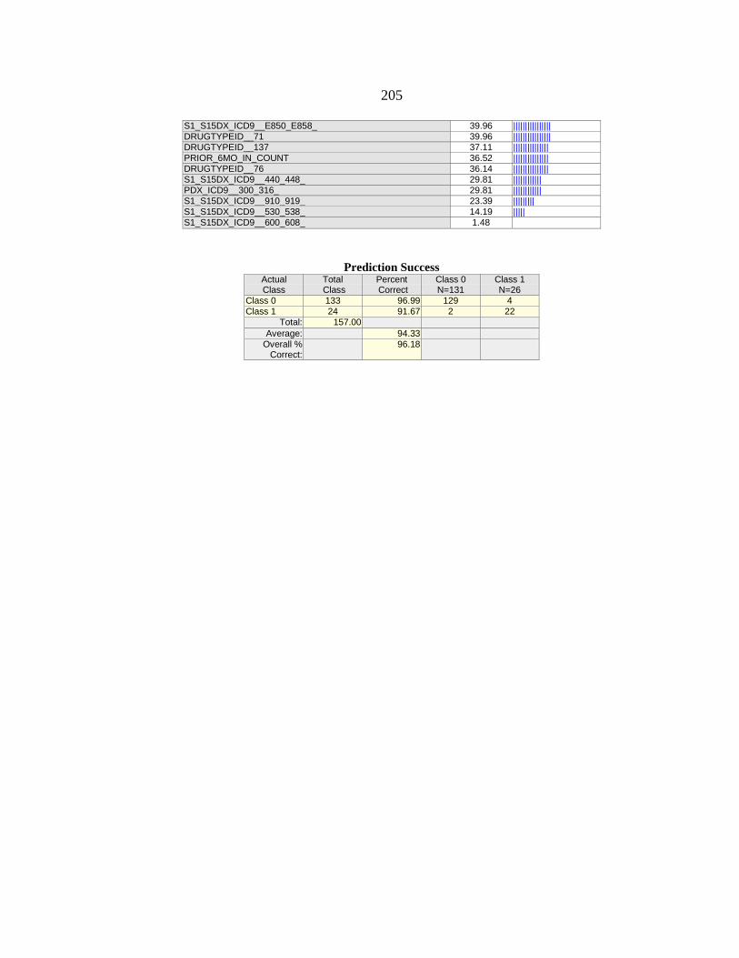
205
S1_S15DX_ICD9__E850_E858_ 39.96 |||||||||||||||| DRUGTYPEID__71 39.96 |||||||||||||||| DRUGTYPEID__137 37.11 ||||||||||||||| PRIOR_6MO_IN_COUNT 36.52 ||||||||||||||| DRUGTYPEID__76 36.14 ||||||||||||||| S1_S15DX_ICD9__440_448_ 29.81 |||||||||||| PDX_ICD9__300_316_ 29.81 |||||||||||| S1_S15DX_ICD9__910_919_ 23.39 ||||||||| S1_S15DX_ICD9__530_538_ 14.19 ||||| S1_S15DX_ICD9__600_608_ 1.48
Prediction Success
Actual Class
Total Class
Percent Correct
Class 0 N=131
Class 1 N=26
Class 0 133 96.99 129 4 Class 1 24 91.67 2 22
Total: 157.00
Average: 94.33
Overall % Correct:
96.18
206
APPENDIX L
SPSS PREDICTION MODEL REPORT COMPONENTS FOR AMI

207
Block 1: Method = Forward Stepwise (Conditional)
Omnibus Tests of Model Coefficients
Chi-square df Sig.
Step 16a
Step .000 1 1.000
Block 85.081 29 .000
Model 85.081 29 .000
a. A negative Chi-squares value indicates that the Chi-squares
value has decreased from the previous step.
Model Summary
Step -2 Log likelihood Cox & Snell R
Square
Nagelkerke R
Square
16 2.773a .315 .974
a. Estimation terminated at iteration number 20 because
maximum iterations has been reached. Final solution cannot be
found.
Hosmer and Lemeshow Test
Step Chi-square df Sig.
16 .000 8 1.000
Classification Tablea
Observed Predicted
AdmitToReadmit Percentage
Correct .0 1.0
Step 16 AdmitToReadmit
.0 213 1 99.5
1.0 0 11 100.0
Overall Percentage 99.6
a. The cut value is .500
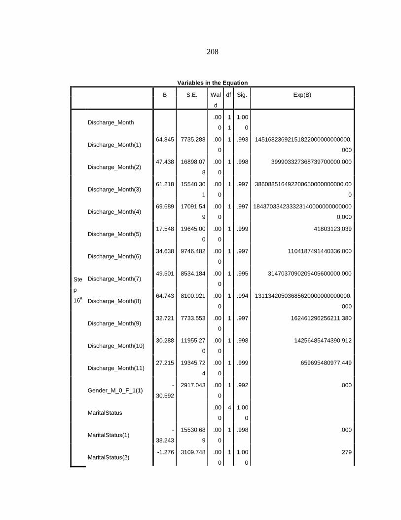
208
Variables in the Equation
B S.E. Wal
d
df Sig. Exp(B)
Ste
p
16a
Discharge_Month
.00
0
1
1
1.00
0
Discharge_Month(1) 64.845 7735.288 .00
0
1 .993 14516823692151822000000000000.
000
Discharge_Month(2) 47.438 16898.07
8
.00
0
1 .998 399903327368739700000.000
Discharge_Month(3) 61.218 15540.30
1
.00
0
1 .997 386088516492200650000000000.00
0
Discharge_Month(4) 69.689 17091.54
9
.00
0
1 .997 184370334233323140000000000000
0.000
Discharge_Month(5) 17.548 19645.00
0
.00
0
1 .999 41803123.039
Discharge_Month(6) 34.638 9746.482 .00
0
1 .997 1104187491440336.000
Discharge_Month(7) 49.501 8534.184 .00
0
1 .995 3147037090209405600000.000
Discharge_Month(8) 64.743 8100.921 .00
0
1 .994 13113420503685620000000000000.
000
Discharge_Month(9) 32.721 7733.553 .00
0
1 .997 162461296256211.380
Discharge_Month(10) 30.288 11955.27
0
.00
0
1 .998 14256485474390.912
Discharge_Month(11) 27.215 19345.72
4
.00
0
1 .999 659695480977.449
Gender_M_0_F_1(1) -
30.592
2917.043 .00
0
1 .992 .000
MaritalStatus
.00
0
4 1.00
0
MaritalStatus(1) -
38.243
15530.68
9
.00
0
1 .998 .000
MaritalStatus(2) -1.276 3109.748 .00
0
1 1.00
0
.279

209
MaritalStatus(3) 30.608 24529.81
9
.00
0
1 .999 19635832012505.227
MaritalStatus(4) 31.585 5081.283 .00
0
1 .995 52155551094788.460
FinancialClass
.00
0
7 1.00
0
FinancialClass(1) 11.674 23821.74
6
.00
0
1 1.00
0
117535.674
FinancialClass(2) -
19.624
18730.26
7
.00
0
1 .999 .000
FinancialClass(3) 88.787 44629.39
3
.00
0
1 .998 3.627E+038
FinancialClass(4) 129.69
7
25091.89
7
.00
0
1 .996 2.122E+056
FinancialClass(5) 28.141 19436.13
3
.00
0
1 .999 1665273817761.869
FinancialClass(6) 57.832 44291.88
5
.00
0
1 .999 13067101617014609000000000.000
FinancialClass(7) 42.864 20751.92
4
.00
0
1 .998 4125877245123476000.000
S1S15dx_ICD9_86086
9(1)
-
66.269
290662.7
94
.00
0
1 1.00
0
.000
S1S15dx_ICD9_V01V0
9(1)
-
94.674
5741.989 .00
0
1 .987 .000
S1S15dx_ICD9_V10V1
9(1)
33.638 4427.004 .00
0
1 .994 406130626526814.500
DrugTypeID_40(1) -
30.075
9797.632 .00
0
1 .998 .000
DrugTypeID_166(1) -
64.468
43433.04
4
.00
0
1 .999 .000
DrugTypeID_175(1) -
32.655
2914.730 .00
0
1 .991 .000
Constant 145.27
6
293496.1
79
.00
0
1 1.00
0
1.237E+063
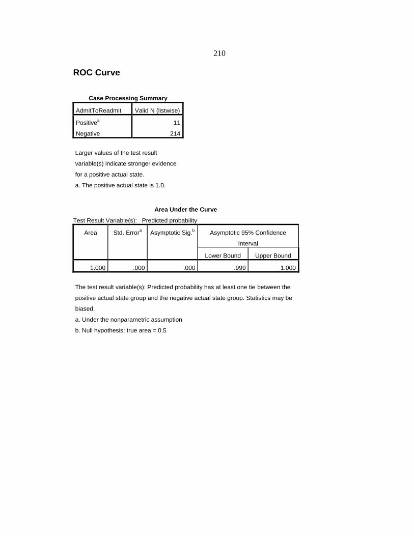
210
ROC Curve
Case Processing Summary
AdmitToReadmit Valid N (listwise)
Positivea 11
Negative 214
Larger values of the test result
variable(s) indicate stronger evidence
for a positive actual state.
a. The positive actual state is 1.0.
Area Under the Curve
Test Result Variable(s): Predicted probability
Area Std. Errora Asymptotic Sig.
b Asymptotic 95% Confidence
Interval
Lower Bound Upper Bound
1.000 .000 .000 .999 1.000
The test result variable(s): Predicted probability has at least one tie between the
positive actual state group and the negative actual state group. Statistics may be
biased.
a. Under the nonparametric assumption
b. Null hypothesis: true area = 0.5

211
APPENDIX M
MARS PREDICTION MODEL REPORT FOR AMI

212
MARS 2 Results: AMI, 10 Basis Functions
Dataset: AMI-FinalMethodology-Basic-AnalysisReady-ModelSetup.xlsx
Predictor Variables: DISCHARGE_MONTH$, GENDER_M_0_F_1, MARITALSTATUS$,
HOSPDISCHARGEDEPT$,
ADMITFROMER_YES_1, FINANCIALCLASS$,
DISCHARGEDISPOSITION$,
DISTANCETOHOSPITAL$, LOS, AGEYRS, PDX_ICD9__001_009_,
PDX_ICD9__030_041_, PDX_ICD9__190_199_, PDX_ICD9__249_259_,
PDX_ICD9__280_289_, PDX_ICD9__350_359_, PDX_ICD9__401_405_,
PDX_ICD9__410_414_, PDX_ICD9__420_429_, PDX_ICD9__430_438_,
PDX_ICD9__451_459_, PDX_ICD9__480_488_, PDX_ICD9__500_508_,
PDX_ICD9__510_519_, PDX_ICD9__530_538_, PDX_ICD9__560_569_,
PDX_ICD9__570_579_, PDX_ICD9__710_719_, PDX_ICD9__780_789_,
PDX_ICD9__960_979_, PDX_ICD9__996_999_, PDX_ICD9__V50_V59_,
S1_S15DX_ICD9__001_009_, S1_S15DX_ICD9__030_041_,
S1_S15DX_ICD9__050_059_, S1_S15DX_ICD9__070_079_,
S1_S15DX_ICD9__110_118_, S1_S15DX_ICD9__130_136_,
S1_S15DX_ICD9__170_176_, S1_S15DX_ICD9__179_189_,
S1_S15DX_ICD9__190_199_, S1_S15DX_ICD9__200_208_,
S1_S15DX_ICD9__235_238_, S1_S15DX_ICD9__240_246_,
S1_S15DX_ICD9__249_259_, S1_S15DX_ICD9__260_269_,
S1_S15DX_ICD9__270_279_, S1_S15DX_ICD9__280_289_,
S1_S15DX_ICD9__290_294_, S1_S15DX_ICD9__295_299_,
S1_S15DX_ICD9__300_316_, S1_S15DX_ICD9__330_337_,
S1_S15DX_ICD9__338_, S1_S15DX_ICD9__340_349_,
S1_S15DX_ICD9__350_359_,
S1_S15DX_ICD9__360_379_, S1_S15DX_ICD9__380_389_,
S1_S15DX_ICD9__393_398_, S1_S15DX_ICD9__401_405_,
S1_S15DX_ICD9__410_414_, S1_S15DX_ICD9__415_417_,
S1_S15DX_ICD9__420_429_, S1_S15DX_ICD9__430_438_,
S1_S15DX_ICD9__440_448_, S1_S15DX_ICD9__451_459_,
S1_S15DX_ICD9__460_466_, S1_S15DX_ICD9__470_478_,
S1_S15DX_ICD9__480_488_, S1_S15DX_ICD9__490_496_,
S1_S15DX_ICD9__500_508_, S1_S15DX_ICD9__510_519_,
S1_S15DX_ICD9__520_529_, S1_S15DX_ICD9__530_538_,
S1_S15DX_ICD9__550_553_, S1_S15DX_ICD9__555_558_,
S1_S15DX_ICD9__560_569_, S1_S15DX_ICD9__570_579_,
S1_S15DX_ICD9__580_589_, S1_S15DX_ICD9__590_599_,
S1_S15DX_ICD9__600_608_, S1_S15DX_ICD9__610_611_,
S1_S15DX_ICD9__617_629_, S1_S15DX_ICD9__680_686_,
S1_S15DX_ICD9__690_698_, S1_S15DX_ICD9__700_709_,
S1_S15DX_ICD9__710_719_, S1_S15DX_ICD9__720_724_,
S1_S15DX_ICD9__725_729_, S1_S15DX_ICD9__730_739_,
S1_S15DX_ICD9__740_759_, S1_S15DX_ICD9__780_789_,
S1_S15DX_ICD9__790_796_, S1_S15DX_ICD9__797_799_,
S1_S15DX_ICD9__860_869_, S1_S15DX_ICD9__905_909_,
S1_S15DX_ICD9__910_919_, S1_S15DX_ICD9__930_939_,
S1_S15DX_ICD9__958_959_, S1_S15DX_ICD9__960_979_,
S1_S15DX_ICD9__990_995_, S1_S15DX_ICD9__996_999_,

213
S1_S15DX_ICD9__V01_V09_, S1_S15DX_ICD9__V10_V19_,
S1_S15DX_ICD9__V40_V49_, S1_S15DX_ICD9__V50_V59_,
S1_S15DX_ICD9__V60_V69_, S1_S15DX_ICD9__V85_,
S1_S15DX_ICD9__V87_,
S1_S15DX_ICD9__E846_E849_, S1_S15DX_ICD9__E850_E858_,
S1_S15DX_ICD9__E860_E869_, S1_S15DX_ICD9__E870_E876_,
S1_S15DX_ICD9__E878_E879_, S1_S15DX_ICD9__E880_E888_,
S1_S15DX_ICD9__E890_E899_, S1_S15DX_ICD9__E900_E909_,
S1_S15DX_ICD9__E910_E915_, S1_S15DX_ICD9__E916_E928_,
S1_S15DX_ICD9__E929_, S1_S15DX_ICD9__E930_E949_,
S1_S15DX_ICD9__E950_E959_, S1_S15DX_ICD9__E960_E969_,
S1_S15DX_ICD9__E980_E989_, S1_S15DX_ICD9__E990_E999_,
DRUGTYPEID__1, DRUGTYPEID__2, DRUGTYPEID__5,
DRUGTYPEID__8,
DRUGTYPEID__9, DRUGTYPEID__10, DRUGTYPEID__12,
DRUGTYPEID__15,
DRUGTYPEID__17, DRUGTYPEID__19, DRUGTYPEID__20,
DRUGTYPEID__22,
DRUGTYPEID__23, DRUGTYPEID__25, DRUGTYPEID__26,
DRUGTYPEID__28,
DRUGTYPEID__29, DRUGTYPEID__30, DRUGTYPEID__31,
DRUGTYPEID__33,
DRUGTYPEID__34, DRUGTYPEID__35, DRUGTYPEID__36,
DRUGTYPEID__37,
DRUGTYPEID__40, DRUGTYPEID__41, DRUGTYPEID__44,
DRUGTYPEID__46,
DRUGTYPEID__47, DRUGTYPEID__49, DRUGTYPEID__52,
DRUGTYPEID__54,
DRUGTYPEID__56, DRUGTYPEID__57, DRUGTYPEID__63,
DRUGTYPEID__64,
DRUGTYPEID__65, DRUGTYPEID__66, DRUGTYPEID__67,
DRUGTYPEID__68,
DRUGTYPEID__71, DRUGTYPEID__73, DRUGTYPEID__74,
DRUGTYPEID__76,
DRUGTYPEID__78, DRUGTYPEID__79, DRUGTYPEID__80,
DRUGTYPEID__82,
DRUGTYPEID__84, DRUGTYPEID__85, DRUGTYPEID__86,
DRUGTYPEID__87,
DRUGTYPEID__88, DRUGTYPEID__90, DRUGTYPEID__91,
DRUGTYPEID__95,
DRUGTYPEID__98, DRUGTYPEID__102, DRUGTYPEID__103,
DRUGTYPEID__104, DRUGTYPEID__105, DRUGTYPEID__111,
DRUGTYPEID__112, DRUGTYPEID__117, DRUGTYPEID__118,
DRUGTYPEID__119, DRUGTYPEID__121, DRUGTYPEID__122,
DRUGTYPEID__123, DRUGTYPEID__124, DRUGTYPEID__127,
DRUGTYPEID__128, DRUGTYPEID__129, DRUGTYPEID__130,
DRUGTYPEID__131, DRUGTYPEID__132, DRUGTYPEID__134,
DRUGTYPEID__135, DRUGTYPEID__136, DRUGTYPEID__137,
DRUGTYPEID__141, DRUGTYPEID__142, DRUGTYPEID__144,
DRUGTYPEID__145, DRUGTYPEID__146, DRUGTYPEID__147,
DRUGTYPEID__148, DRUGTYPEID__149, DRUGTYPEID__150,
DRUGTYPEID__153, DRUGTYPEID__155, DRUGTYPEID__156,
DRUGTYPEID__158, DRUGTYPEID__159, DRUGTYPEID__160,

214
DRUGTYPEID__161, DRUGTYPEID__162, DRUGTYPEID__164,
DRUGTYPEID__166, DRUGTYPEID__167, DRUGTYPEID__169,
DRUGTYPEID__171, DRUGTYPEID__172, DRUGTYPEID__174,
DRUGTYPEID__175, DRUGTYPEID__176, DRUGTYPEID__177,
DRUGTYPEID__178, DRUGTYPEID__180, DRUGTYPEID__184,
DRUGTYPEID__185, DRUGTYPEID__186, DRUGTYPEID__187,
DRUGTYPEID__188, DRUGTYPEID__189, DRUGTYPEID__190,
DRUGTYPEID__191, DRUGTYPEID__192, DRUGTYPEID__198,
DRUGTYPEID__199, DRUGTYPEID__200, DRUGTYPEID__201,
DRUGTYPEID__202, DRUGTYPEID__203, DRUGTYPEID__204,
NO__OF_DRUGS_PRESCRIBED, NO__OF_DRUGS_ADMINISTERED,
DIFF_OF_NO__PRES__VS__NO__ADMIN_, COUNT_OF_CONSULTS,
PRIOR_6MO_ER_COUNT, PRIOR_6MO_IN_COUNT
Target Variable ADMITTOREADMIT
N: 225 Minimum0.00000 Maximum: 1.00000
Mean: 0.04889 Varience: 0.04671
Variables, Terms, and Parameters
Direct variables: 11 Total variables: 11
Terms in model: 11 Effective parameters: 41.00
R-squared Measures
Naive: 0.77745 Naive adjusted: 0.76705 GCV R-squared: 0.67017
Mean-Square Measures
Naive MSE: 0.01088 MARS GCV: 0.01547
Basis Functions Subsets for DISCHARGE_MONTH$
SubSet1 = { "March" }
SubSet2 = { "April", "August", "December", "February", "January",
"July", "June", "May", "November", "October", "September" }
Subsets for MARITALSTATUS$
SubSet1 = { "Married", "NotSpecified" }
SubSet2 = { "Divorced", "Single", "Widow/Widower" }
Basis Functions
BF1 = max(0, DRUGTYPEID__166 - 3.31652E-010);
BF2 = max(0, DRUGTYPEID__204 - 3.31652E-010);
BF3 = max(0, S1_S15DX_ICD9__V01_V09_ - 6.29565E-010);
BF4 = ( DISCHARGE_MONTH$ is in SubSet1 );
BF5 = ( DISCHARGE_MONTH$ is in SubSet2 );
BF6 = max(0, DRUGTYPEID__131 + 7.63378E-009) * BF4;
BF7 = max(0, DRUGTYPEID__144 + 2.11715E-010) * BF4;
BF8 = max(0, S1_S15DX_ICD9__860_869_ - 7.79243E-012);
BF9 = max(0, S1_S15DX_ICD9__958_959_ - 3.31652E-010) * BF5;
BF11 = max(0, DRUGTYPEID__87 + 4.96769E-009) * BF4;
BF12 = ( MARITALSTATUS$ is in SubSet1 );
BF13 = ( MARITALSTATUS$ is in SubSet2 );
BF14 = max(0, S1_S15DX_ICD9__V01_V09_ - 6.29565E-010) * BF12;
BF15 = max(0, DRUGTYPEID__40 - 3.09083E-011) * BF13;
Y = 0.00495982 + 0.99504 * BF1 + 0.99504 * BF2 + 0.661706 * BF3
+ 0.998118 * BF6 - 1.33145 * BF7 + 0.99504 * BF8
- 1 * BF9 + 0.328373 * BF11 - 0.666324 * BF14

215
+ 0.99504 * BF15;
MODEL ADMITTOREADMIT = BF1 BF2 BF3 BF6 BF7 BF8 BF9 BF11 BF14
BF15;
Anova Data Function Standard
Deviation
Mars Prediction Success
Threshold Table
No of basis Functions
No of Effective
Parameters
Variables
1 0.06619 0.02109 1 4.000 DRUGTYPEID__166
2 0.06619 0.02109 1 4.000 DRUGTYPEID__204
3 0.15984 0.02306 1 4.000 S1_S15DX_ICD9__V01_V09_
4 0.09340 0.02109 1 4.000 S1_S15DX_ICD9__860_869_
5 0.13189 0.03151 1 4.000 DISCHARGE_MONTH$, DRUGTYPEID__131
6 0.08857 0.02141 1 4.000 DISCHARGE_MONTH$, DRUGTYPEID__144
7 0.06652 0.01801 1 4.000 DISCHARGE_MONTH$, S1_S15DX_ICD9__958_959_
8 0.04339 0.01685 1 4.000 DISCHARGE_MONTH$, DRUGTYPEID__87
9 0.14368 0.02129 1 4.000 MARITALSTATUS$, S1_S15DX_ICD9__V01_V09_
10 0.06619 0.02109 1 4.000 MARITALSTATUS$, DRUGTYPEID__40
Final Model Basis
Function Coefficient Variable Sign Parent
Sign Parent Knot
0 0.0050
1 0.9950 DRUGTYPEID__166 + 0.0000
2 0.9950 DRUGTYPEID__204 + 0.0000
3 0.6617 S1_S15DX_ICD9__V01_V09_ + 0.0000
6 0.9981 DRUGTYPEID__131 + - DISCHARGE_MONTH$ -0.0000
7 -1.3315 DRUGTYPEID__144 - - DISCHARGE_MONTH$ -0.0000
8 0.9950 S1_S15DX_ICD9__860_869_ + 0.0000
9 -1.0000 S1_S15DX_ICD9__958_959_ + + DISCHARGE_MONTH$ 0.0000
11 0.3284 DRUGTYPEID__87 + - DISCHARGE_MONTH$ -0.0000
14 -0.6663 S1_S15DX_ICD9__V01_V09_ + + MARITALSTATUS$ 0.0000
15 0.9950 DRUGTYPEID__40 + + MARITALSTATUS$ 0.0000

216
MARS Learn Gains for Class 0
Gains Data Bin Cases
Tgt.Class % of Bin Tgt.Class
% Tgt.Class
Cum % Tgt.Class
Cum % Pop
% Pop
Cases in Bin
Cum Lift
Lift Pop
1 1 100.00 0.47 0.47 0.44 0.44 1 1.05 1.05 2 1 100.00 0.47 0.93 0.89 0.44 1 1.05 1.05 3 9 100.00 4.21 5.14 4.89 4.00 9 1.05 1.05 4 200 99.50 93.46 98.60 94.22 89.33 201 1.05 1.05 5 2 66.67 0.93 99.53 95.56 1.33 3 1.04 0.70 6 1 33.33 0.47 100.00 96.89 1.33 3 1.03 0.35 7 0 0.00 0.00 100.00 97.78 0.89 2 1.02 0.00 8 0 0.00 0.00 100.00 98.22 0.44 1 1.02 0.00 9 0 0.00 0.00 100.00 99.56 1.33 3 1.00 0.00
10 0 0.00 0.00 100.00 100.00 0.44 1 1.00 0.00
Variable Importance
Variable Score DISCHARGE_MONTH$ 100.00 |||||||||||||||||||||||||||||||||||||||||| DRUGTYPEID__131 97.35 ||||||||||||||||||||||||||||||||||||||||| MARITALSTATUS$ 80.43 |||||||||||||||||||||||||||||||||| S1_S15DX_ICD9__V01_V09_ 62.68 |||||||||||||||||||||||||| DRUGTYPEID__144 59.22 |||||||||||||||||||||||| S1_S15DX_ICD9__860_869_ 57.63 |||||||||||||||||||||||| DRUGTYPEID__40 57.63 |||||||||||||||||||||||| DRUGTYPEID__166 57.63 |||||||||||||||||||||||| DRUGTYPEID__204 57.63 |||||||||||||||||||||||| S1_S15DX_ICD9__958_959_ 38.68 |||||||||||||||| DRUGTYPEID__87 28.53 |||||||||||
Prediction Success
Actual Class
Total Class
Percent Correct
Class 0 N=215
Class 1 N=10
Class 0 214 99.53 213 1 Class 1 11 81.82 2 9
Total: 225.00
Average: 90.68
Overall % Correct:
98.67
0
20
40
60
80
100
0 20 40 60 80 100
% C
lass
% Population

217
APPENDIX N
MARS PREDICTION MODEL REPORT FOR CHF

218
MARS 2 Results: CHF, 109 Basis Functions
Dataset: CHF-FinalMethodology-Basic-AnalysisReady-ModelSetup.xlsx
Predictor Variables: DISCHARGE_MONTH$, GENDER_M_0_F_1, MARITALSTATUS$,
HOSPDISCHARGEDEPT$,
ADMITFROMER_YES_1, FINANCIALCLASS$,
DISCHARGEDISPOSITION$,
DISTANCETOHOSPITAL$, LOS, AGEYRS, PDX_ICD9__001_009_,
PDX_ICD9__030_041_, PDX_ICD9__045_049_, PDX_ICD9__110_118_,
PDX_ICD9__150_159_, PDX_ICD9__170_176_, PDX_ICD9__179_189_,
PDX_ICD9__190_199_, PDX_ICD9__200_208_, PDX_ICD9__240_246_,
PDX_ICD9__249_259_, PDX_ICD9__270_279_, PDX_ICD9__280_289_,
PDX_ICD9__290_294_, PDX_ICD9__300_316_, PDX_ICD9__330_337_,
PDX_ICD9__338_, PDX_ICD9__340_349_, PDX_ICD9__350_359_,
PDX_ICD9__393_398_, PDX_ICD9__401_405_, PDX_ICD9__410_414_,
PDX_ICD9__415_417_, PDX_ICD9__420_429_, PDX_ICD9__430_438_,
PDX_ICD9__440_448_, PDX_ICD9__451_459_, PDX_ICD9__480_488_,
PDX_ICD9__490_496_, PDX_ICD9__500_508_, PDX_ICD9__510_519_,
PDX_ICD9__530_538_, PDX_ICD9__540_543_, PDX_ICD9__550_553_,
PDX_ICD9__555_558_, PDX_ICD9__560_569_, PDX_ICD9__570_579_,
PDX_ICD9__580_589_, PDX_ICD9__590_599_, PDX_ICD9__600_608_,
PDX_ICD9__680_686_, PDX_ICD9__700_709_, PDX_ICD9__710_719_,
PDX_ICD9__720_724_, PDX_ICD9__725_729_, PDX_ICD9__730_739_,
PDX_ICD9__740_759_, PDX_ICD9__780_789_, PDX_ICD9__790_796_,
PDX_ICD9__805_809_, PDX_ICD9__810_819_, PDX_ICD9__820_829_,
PDX_ICD9__840_848_, PDX_ICD9__850_854_, PDX_ICD9__860_869_,
PDX_ICD9__900_904_, PDX_ICD9__920_924_, PDX_ICD9__960_979_,
PDX_ICD9__996_999_, S1_S15DX_ICD9__001_009_,
S1_S15DX_ICD9__030_041_,
S1_S15DX_ICD9__050_059_, S1_S15DX_ICD9__070_079_,
S1_S15DX_ICD9__110_118_, S1_S15DX_ICD9__130_136_,
S1_S15DX_ICD9__137_139_, S1_S15DX_ICD9__150_159_,
S1_S15DX_ICD9__160_165_, S1_S15DX_ICD9__170_176_,
S1_S15DX_ICD9__179_189_, S1_S15DX_ICD9__190_199_,
S1_S15DX_ICD9__200_208_, S1_S15DX_ICD9__210_229_,
S1_S15DX_ICD9__235_238_, S1_S15DX_ICD9__240_246_,
S1_S15DX_ICD9__249_259_, S1_S15DX_ICD9__260_269_,
S1_S15DX_ICD9__270_279_, S1_S15DX_ICD9__280_289_,
S1_S15DX_ICD9__290_294_, S1_S15DX_ICD9__295_299_,
S1_S15DX_ICD9__300_316_, S1_S15DX_ICD9__320_326_,
S1_S15DX_ICD9__330_337_, S1_S15DX_ICD9__338_,
S1_S15DX_ICD9__340_349_,
S1_S15DX_ICD9__350_359_, S1_S15DX_ICD9__360_379_,
S1_S15DX_ICD9__380_389_, S1_S15DX_ICD9__393_398_,
S1_S15DX_ICD9__401_405_, S1_S15DX_ICD9__410_414_,
S1_S15DX_ICD9__415_417_, S1_S15DX_ICD9__420_429_,
S1_S15DX_ICD9__430_438_, S1_S15DX_ICD9__440_448_,
S1_S15DX_ICD9__451_459_, S1_S15DX_ICD9__460_466_,
S1_S15DX_ICD9__470_478_, S1_S15DX_ICD9__480_488_,
S1_S15DX_ICD9__490_496_, S1_S15DX_ICD9__500_508_,
219
S1_S15DX_ICD9__510_519_, S1_S15DX_ICD9__520_529_,
S1_S15DX_ICD9__530_538_, S1_S15DX_ICD9__550_553_,
S1_S15DX_ICD9__555_558_, S1_S15DX_ICD9__560_569_,
S1_S15DX_ICD9__570_579_, S1_S15DX_ICD9__580_589_,
S1_S15DX_ICD9__590_599_, S1_S15DX_ICD9__600_608_,
S1_S15DX_ICD9__610_611_, S1_S15DX_ICD9__614_616_,
S1_S15DX_ICD9__617_629_, S1_S15DX_ICD9__680_686_,
S1_S15DX_ICD9__690_698_, S1_S15DX_ICD9__700_709_,
S1_S15DX_ICD9__710_719_, S1_S15DX_ICD9__720_724_,
S1_S15DX_ICD9__725_729_, S1_S15DX_ICD9__730_739_,
S1_S15DX_ICD9__740_759_, S1_S15DX_ICD9__780_789_,
S1_S15DX_ICD9__790_796_, S1_S15DX_ICD9__797_799_,
S1_S15DX_ICD9__800_804_, S1_S15DX_ICD9__805_809_,
S1_S15DX_ICD9__810_819_, S1_S15DX_ICD9__820_829_,
S1_S15DX_ICD9__840_848_, S1_S15DX_ICD9__850_854_,
S1_S15DX_ICD9__860_869_, S1_S15DX_ICD9__870_879_,
S1_S15DX_ICD9__880_887_, S1_S15DX_ICD9__890_897_,
S1_S15DX_ICD9__905_909_, S1_S15DX_ICD9__910_919_,
S1_S15DX_ICD9__920_924_, S1_S15DX_ICD9__930_939_,
S1_S15DX_ICD9__958_959_, S1_S15DX_ICD9__960_979_,
S1_S15DX_ICD9__990_995_, S1_S15DX_ICD9__996_999_,
S1_S15DX_ICD9__V01_V09_, S1_S15DX_ICD9__V10_V19_,
S1_S15DX_ICD9__V40_V49_, S1_S15DX_ICD9__V50_V59_,
S1_S15DX_ICD9__V60_V69_, S1_S15DX_ICD9__V85_,
S1_S15DX_ICD9__V87_,
S1_S15DX_ICD9__E001_E030_, S1_S15DX_ICD9__E810_E819_,
S1_S15DX_ICD9__E820_E825_, S1_S15DX_ICD9__E826_E829_,
S1_S15DX_ICD9__E840_E845_, S1_S15DX_ICD9__E846_E849_,
S1_S15DX_ICD9__E850_E858_, S1_S15DX_ICD9__E860_E869_,
S1_S15DX_ICD9__E870_E876_, S1_S15DX_ICD9__E878_E879_,
S1_S15DX_ICD9__E880_E888_, S1_S15DX_ICD9__E890_E899_,
S1_S15DX_ICD9__E900_E909_, S1_S15DX_ICD9__E910_E915_,
S1_S15DX_ICD9__E916_E928_, S1_S15DX_ICD9__E929_,
S1_S15DX_ICD9__E930_E949_, S1_S15DX_ICD9__E950_E959_,
S1_S15DX_ICD9__E960_E969_, S1_S15DX_ICD9__E980_E989_,
S1_S15DX_ICD9__E990_E999_, DRUGTYPEID__1, DRUGTYPEID__2,
DRUGTYPEID__5, DRUGTYPEID__6, DRUGTYPEID__7,
DRUGTYPEID__8,
DRUGTYPEID__9, DRUGTYPEID__10, DRUGTYPEID__11,
DRUGTYPEID__12,
DRUGTYPEID__14, DRUGTYPEID__15, DRUGTYPEID__17,
DRUGTYPEID__18,
DRUGTYPEID__19, DRUGTYPEID__20, DRUGTYPEID__21,
DRUGTYPEID__22,
DRUGTYPEID__23, DRUGTYPEID__24, DRUGTYPEID__25,
DRUGTYPEID__26,
DRUGTYPEID__28, DRUGTYPEID__29, DRUGTYPEID__30,
DRUGTYPEID__31,
DRUGTYPEID__32, DRUGTYPEID__33, DRUGTYPEID__34,
DRUGTYPEID__35,
DRUGTYPEID__36, DRUGTYPEID__37, DRUGTYPEID__39,
DRUGTYPEID__40,
220
DRUGTYPEID__41, DRUGTYPEID__42, DRUGTYPEID__44,
DRUGTYPEID__46,
DRUGTYPEID__47, DRUGTYPEID__48, DRUGTYPEID__49,
DRUGTYPEID__52,
DRUGTYPEID__54, DRUGTYPEID__55, DRUGTYPEID__56,
DRUGTYPEID__57,
DRUGTYPEID__58, DRUGTYPEID__62, DRUGTYPEID__63,
DRUGTYPEID__64,
DRUGTYPEID__65, DRUGTYPEID__66, DRUGTYPEID__67,
DRUGTYPEID__68,
DRUGTYPEID__71, DRUGTYPEID__72, DRUGTYPEID__73,
DRUGTYPEID__74,
DRUGTYPEID__75, DRUGTYPEID__76, DRUGTYPEID__77,
DRUGTYPEID__78,
DRUGTYPEID__79, DRUGTYPEID__80, DRUGTYPEID__81,
DRUGTYPEID__82,
DRUGTYPEID__83, DRUGTYPEID__84, DRUGTYPEID__85,
DRUGTYPEID__86,
DRUGTYPEID__87, DRUGTYPEID__88, DRUGTYPEID__89,
DRUGTYPEID__90,
DRUGTYPEID__91, DRUGTYPEID__92, DRUGTYPEID__94,
DRUGTYPEID__95,
DRUGTYPEID__98, DRUGTYPEID__99, DRUGTYPEID__101,
DRUGTYPEID__102, DRUGTYPEID__103, DRUGTYPEID__104,
DRUGTYPEID__105, DRUGTYPEID__108, DRUGTYPEID__110,
DRUGTYPEID__111, DRUGTYPEID__112, DRUGTYPEID__113,
DRUGTYPEID__114, DRUGTYPEID__117, DRUGTYPEID__118,
DRUGTYPEID__119, DRUGTYPEID__120, DRUGTYPEID__121,
DRUGTYPEID__122, DRUGTYPEID__123, DRUGTYPEID__124,
DRUGTYPEID__127, DRUGTYPEID__128, DRUGTYPEID__129,
DRUGTYPEID__130, DRUGTYPEID__131, DRUGTYPEID__132,
DRUGTYPEID__133, DRUGTYPEID__134, DRUGTYPEID__135,
DRUGTYPEID__136, DRUGTYPEID__137, DRUGTYPEID__139,
DRUGTYPEID__140, DRUGTYPEID__141, DRUGTYPEID__142,
DRUGTYPEID__143, DRUGTYPEID__144, DRUGTYPEID__145,
DRUGTYPEID__146, DRUGTYPEID__147, DRUGTYPEID__148,
DRUGTYPEID__149, DRUGTYPEID__150, DRUGTYPEID__151,
DRUGTYPEID__152, DRUGTYPEID__153, DRUGTYPEID__154,
DRUGTYPEID__156, DRUGTYPEID__157, DRUGTYPEID__158,
DRUGTYPEID__159, DRUGTYPEID__160, DRUGTYPEID__161,
DRUGTYPEID__162, DRUGTYPEID__164, DRUGTYPEID__165,
DRUGTYPEID__166, DRUGTYPEID__167, DRUGTYPEID__168,
DRUGTYPEID__169, DRUGTYPEID__171, DRUGTYPEID__172,
DRUGTYPEID__174, DRUGTYPEID__175, DRUGTYPEID__176,
DRUGTYPEID__177, DRUGTYPEID__178, DRUGTYPEID__180,
DRUGTYPEID__181, DRUGTYPEID__182, DRUGTYPEID__184,
DRUGTYPEID__185, DRUGTYPEID__186, DRUGTYPEID__187,
DRUGTYPEID__188, DRUGTYPEID__189, DRUGTYPEID__190,
DRUGTYPEID__191, DRUGTYPEID__192, DRUGTYPEID__194,
DRUGTYPEID__196, DRUGTYPEID__197, DRUGTYPEID__198,
DRUGTYPEID__199, DRUGTYPEID__200, DRUGTYPEID__201,
DRUGTYPEID__202, DRUGTYPEID__203, DRUGTYPEID__204,

221
DRUGTYPEID__205, NO__OF_DRUGS_PRESCRIBED,
NO__OF_DRUGS_ADMINISTERED,
DIFF_OF_NO__PRES__VS__NO__ADMIN_, COUNT_OF_CONSULTS,
PRIOR_6MO_ER_COUNT, PRIOR_6MO_IN_COUNT
Target Variable ADMITTOREADMIT
N: 800 Minimum0.00000 Maximum: 1.00000
Mean: 0.07750 Varience: 0.07158
Variables, Terms, and Parameters
Direct variables: 96 Total variables: 96
Terms in model: 110 Effective parameters: 416.70
R-Square Measures
Naive: 0.99469 Naive adjusted: 0.99385 GCV R-square: 0.97692
Mean-Square Measures
Naive MSE: 0.00044 MARS GCV: 0.00165
Basis Functions Subsets for DISCHARGEDISPOSITION$
SubSet1 = { "HOME_HEALTH" }
SubSet2 = { "EXPIRED", "HOME", "HOSPICE_-_HOME",
"HOSPICE_-_MEDICAL_FACILITY", "LONG-TERM_CARE_HOSPITAL",
"OTHER_FACILITY", "REHAB_FACILITY", "SKILLED_NURSING_HOME",
"SWING_BED" }
SubSet3 = { "HOME", "HOME_HEALTH" }
Subsets for DISCHARGE_MONTH$
SubSet1 = { "May", "October" }
SubSet2 = { "April", "August", "December", "February", "January",
"July", "June", "March", "November", "September" }
SubSet3 = { "April", "December", "February", "June", "November" }
SubSet4 = { "August", "January", "July", "March", "May", "October",
"September" }
SubSet5 = { "January", "July" }
SubSet6 = { "April" }
Subsets for DISTANCETOHOSPITAL$
SubSet1 = { "0-10_miles", "1001+_miles", "11-30_miles", "31-50_miles",
"51-100_miles" }
Subsets for MARITALSTATUS$
SubSet1 = { "NotSpecified", "Single" }
Subsets for FINANCIALCLASS$
SubSet1 = { "Medicare", "Tricare" }
Basis Functions
BF1 = max(0, PDX_ICD9__740_759_ + 4.94148E-011);
BF2 = ( DISCHARGEDISPOSITION$ is in SubSet1 );
BF3 = ( DISCHARGEDISPOSITION$ is in SubSet2 );
BF4 = ( DISCHARGE_MONTH$ is in SubSet1 ) * BF2;
BF5 = ( DISCHARGE_MONTH$ is in SubSet2 ) * BF2;
BF6 = max(0, PDX_ICD9__280_289_ - 1.34122E-010) * BF2;
BF8 = max(0, PDX_ICD9__430_438_ - 1.6079E-009) * BF2;
BF9 = max(0, S1_S15DX_ICD9__030_041_ + 4.94193E-010) * BF4;
BF11 = max(0, 1 - PRIOR_6MO_ER_COUNT) * BF4;
BF12 = max(0, DRUGTYPEID__146 - 5.74666E-009) * BF4;

222
BF13 = max(0, DRUGTYPEID__145 + 7.13155E-009) * BF4;
BF14 = max(0, DRUGTYPEID__5 + 1.68958E-008);
BF15 = max(0, S1_S15DX_ICD9__700_709_ - 1.66759E-009) * BF14;
BF17 = max(0, S1_S15DX_ICD9__530_538_ - 1.35502E-008) * BF15;
BF18 = max(0, S1_S15DX_ICD9__E880_E888_ + 7.27331E-010) * BF14;
BF19 = max(0, S1_S15DX_ICD9__V50_V59_ + 3.70638E-009) * BF18;
BF20 = max(0, NO__OF_DRUGS_PRESCRIBED - 14) * BF2;
BF21 = max(0, 14 - NO__OF_DRUGS_PRESCRIBED) * BF2;
BF23 = max(0, PDX_ICD9__249_259_ - 4.35738E-010) * BF20;
BF25 = max(0, DRUGTYPEID__12 + 2.30342E-010) * BF20;
BF26 = max(0, PDX_ICD9__420_429_ - 3.50468E-009);
BF27 = max(0, S1_S15DX_ICD9__820_829_ - 1.0165E-010) * BF26;
BF28 = max(0, DRUGTYPEID__124 - 1.72902E-010) * BF26;
BF29 = max(0, S1_S15DX_ICD9__260_269_ - 2.856E-009) * BF26;
BF30 = ( DISCHARGE_MONTH$ is in SubSet3 ) * BF26;
BF31 = ( DISCHARGE_MONTH$ is in SubSet4 ) * BF26;
BF32 = max(0, DRUGTYPEID__91 + 5.41182E-010) * BF30;
BF34 = ( DISTANCETOHOSPITAL$ is in SubSet1 ) * BF30;
BF36 = max(0, DRUGTYPEID__122 - 1.13516E-009) * BF21;
BF37 = max(0, DRUGTYPEID__95 + 7.37284E-010) * BF30;
BF38 = max(0, DRUGTYPEID__73 + 8.34751E-010) * BF4;
BF39 = max(0, DRUGTYPEID__23 + 1.20146E-009) * BF30;
BF40 = max(0, DRUGTYPEID__127 + 5.52188E-010) * BF15;
BF41 = max(0, DRUGTYPEID__36 - 8.19628E-009) * BF3;
BF42 = max(0, S1_S15DX_ICD9__470_478_ - 2.01211E-010) * BF41;
BF43 = max(0, PDX_ICD9__996_999_ - 1.6079E-009) * BF41;
BF44 = max(0, S1_S15DX_ICD9__470_478_ - 2.01211E-010) * BF30;
BF48 = max(0, PDX_ICD9__490_496_ - 2.34093E-009) * BF15;
BF49 = max(0, S1_S15DX_ICD9__680_686_ - 9.59531E-010) * BF14;
BF51 = max(0, S1_S15DX_ICD9__340_349_ - 1.3803E-009) * BF41;
BF53 = max(0, PDX_ICD9__410_414_ + 1.01672E-010) * BF21;
BF54 = max(0, DRUGTYPEID__128 - 2.34093E-009) * BF14;
BF55 = max(0, DRUGTYPEID__20 + 1.34862E-008) * BF54;
BF56 = max(0, DRUGTYPEID__56 - 1.36896E-009) * BF54;
BF57 = max(0, DRUGTYPEID__76 - 4.78485E-009) * BF30;
BF58 = max(0, DRUGTYPEID__174 - 2.96E-008) * BF30;
BF59 = max(0, S1_S15DX_ICD9__110_118_ - 2.04076E-009) * BF30;
BF60 = max(0, PRIOR_6MO_IN_COUNT - 1) * BF30;
BF61 = max(0, 1 - PRIOR_6MO_IN_COUNT) * BF30;
BF62 = max(0, S1_S15DX_ICD9__740_759_ - 1.6079E-009) * BF30;
BF63 = max(0, S1_S15DX_ICD9__235_238_ - 1.36896E-009) * BF30;
BF64 = max(0, S1_S15DX_ICD9__415_417_ - 4.29662E-009) * BF30;
BF65 = max(0, DRUGTYPEID__31 - 6.95593E-009) * BF30;
BF67 = max(0, DRUGTYPEID__75 + 2.49218E-010) * BF31;
BF68 = max(0, DRUGTYPEID__34 - 4.35738E-010) * BF26;
BF69 = max(0, DRUGTYPEID__12 + 2.30342E-010) * BF5;
BF70 = ( DISCHARGEDISPOSITION$ is in SubSet3 ) * BF30;
BF72 = max(0, DRUGTYPEID__189 - 1.92743E-009) * BF14;
BF73 = max(0, DRUGTYPEID__190 - 2.01211E-010) * BF3;
BF74 = max(0, DRUGTYPEID__151 - 1.72902E-010) * BF73;
BF75 = max(0, DRUGTYPEID__132 + 2.73106E-009) * BF73;
BF76 = max(0, S1_S15DX_ICD9__235_238_ - 1.36896E-009) * BF21;
BF77 = max(0, PDX_ICD9__580_589_ - 2.01211E-010) * BF20;
BF79 = max(0, PDX_ICD9__600_608_ - 1.0165E-010) * BF2;
BF80 = max(0, PDX_ICD9__490_496_ - 2.34093E-009) * BF41;
BF82 = max(0, PDX_ICD9__560_569_ - 4.58505E-010) * BF41;
BF84 = max(0, 2 - DIFF_OF_NO__PRES__VS__NO__ADMIN_) * BF41;
BF85 = max(0, S1_S15DX_ICD9__680_686_ - 9.59531E-010) * BF30;
BF86 = max(0, S1_S15DX_ICD9__520_529_ + 9.93033E-011) * BF30;
BF87 = max(0, DRUGTYPEID__132 + 2.73106E-009) * BF26;
BF88 = max(0, DRUGTYPEID__190 - 2.01211E-010) * BF5;
BF89 = max(0, DRUGTYPEID__8 - 1.086E-010) * BF14;
BF90 = max(0, DRUGTYPEID__79 - 2.34093E-009) * BF3;
BF91 = max(0, COUNT_OF_CONSULTS - 1) * BF90;
BF93 = max(0, S1_S15DX_ICD9__996_999_ + 1.01672E-010) * BF90;
BF94 = max(0, NO__OF_DRUGS_ADMINISTERED - 22) * BF90;
BF96 = max(0, DRUGTYPEID__201 + 5.59613E-010) * BF90;
BF97 = max(0, DRUGTYPEID__12 + 2.30342E-010) * BF4;

223
BF98 = max(0, DRUGTYPEID__90 + 2.74787E-009) * BF30;
BF100 = max(0, 15 - NO__OF_DRUGS_PRESCRIBED) * BF41;
BF101 = max(0, S1_S15DX_ICD9__430_438_ + 2.06265E-009) * BF41;
BF102 = max(0, S1_S15DX_ICD9__V60_V69_ + 2.20407E-009) * BF87;
BF103 = max(0, DRUGTYPEID__178 - 1.39299E-009) * BF30;
BF104 = max(0, S1_S15DX_ICD9__295_299_ - 4.35738E-010) * BF3;
BF105 = max(0, DRUGTYPEID__164 - 3.44748E-009) * BF104;
BF106 = max(0, COUNT_OF_CONSULTS - 2) * BF41;
BF108 = max(0, DRUGTYPEID__40 + 1.98656E-010) * BF41;
BF109 = max(0, DRUGTYPEID__105 - 2.01211E-010) * BF41;
BF110 = max(0, S1_S15DX_ICD9__990_995_ + 2.58874E-009) * BF41;
BF111 = max(0, PDX_ICD9__030_041_ - 6.89908E-010) * BF15;
BF112 = max(0, DRUGTYPEID__189 - 1.92743E-009) * BF18;
BF113 = max(0, PDX_ICD9__249_259_ - 4.35738E-010) * BF21;
BF114 = max(0, DRUGTYPEID__49 - 1.18154E-009) * BF30;
BF115 = ( DISCHARGE_MONTH$ is in SubSet5 ) * BF3;
BF117 = max(0, PRIOR_6MO_IN_COUNT - 2) * BF115;
BF119 = max(0, DRUGTYPEID__171 - 1.36896E-009) * BF115;
BF123 = ( MARITALSTATUS$ is in SubSet1 ) * BF30;
BF125 = max(0, DRUGTYPEID__94 - 6.89908E-010) * BF90;
BF126 = ( FINANCIALCLASS$ is in SubSet1 ) * BF30;
BF128 = max(0, AGEYRS - 94) * BF30;
BF129 = max(0, 94 - AGEYRS) * BF30;
BF130 = max(0, S1_S15DX_ICD9__600_608_ - 1.33236E-009) * BF26;
BF131 = max(0, S1_S15DX_ICD9__350_359_ + 2.74787E-009) * BF130;
BF132 = max(0, DRUGTYPEID__192 - 1.21727E-008) * BF130;
BF133 = max(0, S1_S15DX_ICD9__550_553_ + 9.88223E-011) * BF130;
BF134 = max(0, S1_S15DX_ICD9__V85_ - 2.04076E-009) * BF115;
BF135 = max(0, S1_S15DX_ICD9__700_709_ - 1.66759E-009) * BF30;
BF136 = max(0, DRUGTYPEID__88 - 9.45594E-010) * BF30;
BF137 = max(0, DRUGTYPEID__177 + 4.94148E-011);
BF138 = max(0, PDX_ICD9__170_176_ + 4.94148E-011) * BF115;
BF139 = ( DISCHARGE_MONTH$ is in SubSet6 ) * BF26;
BF141 = max(0, DRUGTYPEID__66 - 3.78194E-008) * BF87;
BF143 = max(0, DRUGTYPEID__29 - 8.0147E-009) * BF90;
BF144 = max(0, DRUGTYPEID__198 - 1.4178E-009) * BF104;
BF145 = max(0, PDX_ICD9__480_488_ - 1.88521E-009) * BF90;
BF146 = max(0, S1_S15DX_ICD9__V85_ - 2.04076E-009) * BF130;
BF147 = max(0, S1_S15DX_ICD9__200_208_ - 2.01211E-010) * BF30;
BF148 = max(0, S1_S15DX_ICD9__580_589_ - 4.30706E-010) * BF30;
BF149 = max(0, COUNT_OF_CONSULTS - 3.05396E-008) * BF30;
BF150 = max(0, DRUGTYPEID__189 - 1.92743E-009) * BF30;
BF151 = max(0, PDX_ICD9__420_429_ - 3.50468E-009) * BF54;
BF152 = max(0, PDX_ICD9__560_569_ - 4.58505E-010) * BF20;
BF153 = max(0, S1_S15DX_ICD9__290_294_ - 1.59748E-009) * BF30;
BF154 = max(0, DRUGTYPEID__156 + 7.37284E-010) * BF30;
BF155 = max(0, DRUGTYPEID__85 - 1.4178E-009) * BF30;
BF156 = max(0, DRUGTYPEID__23 + 1.20146E-009) * BF21;
Y = -0.000142368 + 1.00014 * BF1 + 0.994801 * BF4
+ 1.00507 * BF6 + 1.00014 * BF8 + 2.01394 * BF9
- 0.994567 * BF11 + 1.01038 * BF12
- 1.00465 * BF13 + 1.00014 * BF17
+ 0.968046 * BF19 + 0.333381 * BF23
+ 0.0449169 * BF25 + 1.00014 * BF27
+ 0.448872 * BF28 + 1.00246 * BF29
+ 0.795341 * BF30 + 0.71096 * BF32
- 0.339687 * BF34 + 0.324942 * BF36
+ 1.13848 * BF37 - 0.998011 * BF38
+ 0.687947 * BF39 + 1.00014 * BF40
+ 1.00014 * BF42 + 1.00014 * BF43
+ 1.99022 * BF44 - 1 * BF48 + 1.00014 * BF49
+ 1.79145 * BF51 + 0.333381 * BF53
+ 1.00014 * BF55 - 1 * BF56 - 0.238137 * BF57
- 0.262429 * BF58 + 0.456925 * BF59
- 0.179485 * BF60 - 0.0972393 * BF61
- 0.846112 * BF62 + 0.756034 * BF63
- 0.405159 * BF64 + 0.988855 * BF65

224
- 0.442439 * BF67 - 1.00232 * BF68
- 0.24885 * BF69 + 0.2254 * BF70
+ 0.55906 * BF72 + 1.00014 * BF74
+ 1.00014 * BF75 + 0.123097 * BF76
- 0.0283174 * BF77 + 0.187109 * BF79
- 0.63566 * BF80 + 0.998258 * BF82
+ 0.0786267 * BF84 - 0.224447 * BF85
- 0.589501 * BF86 - 0.141937 * BF87
- 0.804255 * BF88 + 0.514244 * BF89
+ 0.503421 * BF91 - 1.32906 * BF93
+ 0.0805532 * BF94 - 0.503279 * BF96
- 0.205063 * BF97 + 0.247746 * BF98
- 0.0176785 * BF100 + 0.787688 * BF101
+ 0.560455 * BF102 + 0.375385 * BF103
+ 1.00014 * BF105 - 1.15753 * BF106
- 0.998116 * BF108 - 0.789428 * BF109
- 0.571185 * BF110 - 0.558917 * BF111
- 0.526963 * BF112 - 0.3248 * BF113
+ 0.222185 * BF114 + 0.500071 * BF117
+ 1.00014 * BF119 - 0.219694 * BF123
+ 0.483416 * BF125 - 0.234129 * BF126
+ 0.0822306 * BF128 - 0.00503231 * BF129
- 0.67755 * BF131 - 0.119887 * BF132
+ 0.677693 * BF133 + 1.00014 * BF134
+ 0.185115 * BF135 + 0.335483 * BF136
- 0.514101 * BF137 - 0.514101 * BF138
- 0.155886 * BF139 - 0.417942 * BF141
- 0.241517 * BF143 - 1 * BF144
- 0.758482 * BF145 - 0.322449 * BF146
+ 0.394076 * BF147 + 0.104647 * BF148
- 0.0900198 * BF149 + 0.179474 * BF150
- 0.994801 * BF151 + 0.0258467 * BF152
- 0.101996 * BF153 + 0.166241 * BF154
- 0.159635 * BF155 - 0.25339 * BF156;
MODEL ADMITTOREADMIT = BF1 BF4 BF6 BF8 BF9 BF11 BF12 BF13 BF17
BF19 BF23 BF25 BF27 BF28 BF29 BF30 BF32
BF34 BF36 BF37 BF38 BF39 BF40 BF42 BF43
BF44 BF48 BF49 BF51 BF53 BF55 BF56 BF57
BF58 BF59 BF60 BF61 BF62 BF63 BF64 BF65
BF67 BF68 BF69 BF70 BF72 BF74 BF75 BF76
BF77 BF79 BF80 BF82 BF84 BF85 BF86 BF87
BF88 BF89 BF91 BF93 BF94 BF96 BF97 BF98
BF100 BF101 BF102 BF103 BF105 BF106 BF108
BF109 BF110 BF111 BF112 BF113 BF114 BF117
BF119 BF123 BF125 BF126 BF128 BF129 BF131
BF132 BF133 BF134 BF135 BF136 BF137 BF138
BF139 BF141 BF143 BF144 BF145 BF146 BF147
BF148 BF149 BF150 BF151 BF152 BF153 BF154
BF155 BF156;
Anova Data Function Standard
Deviation
Mars Prediction Success
Threshold Table
No of basis
Functions
No of Effective
Parameters
Variables
1 0.03534 0.00695 1 3.814 PDX_ICD9__740_759_
2 0.01816 0.00252 1 3.814 DRUGTYPEID__177
3 0.16268 0.01857 1 3.814 DISCHARGE_MONTH$, DISCHARGEDISPOSITION$
4 0.05019 0.00999 1 3.814 DISCHARGEDISPOSITION$, PDX_ICD9__280_289_
5 0.03534 0.00695 1 3.814 DISCHARGEDISPOSITION$, PDX_ICD9__430_438_
6 0.03534 0.00695 1 3.814 PDX_ICD9__420_429_, S1_S15DX_ICD9__820_829_
7 0.01586 0.00237 1 3.814 PDX_ICD9__420_429_, DRUGTYPEID__124
8 0.09974 0.01770 1 3.814 PDX_ICD9__420_429_, S1_S15DX_ICD9__260_269_

225
9 0.24106 0.00600 2 7.628 DISCHARGE_MONTH$, PDX_ICD9__420_429_
10 0.03534 0.00695 1 3.814 S1_S15DX_ICD9__680_686_, DRUGTYPEID__5
11 0.03542 0.00564 1 3.814 PDX_ICD9__420_429_, DRUGTYPEID__34
12 0.05563 0.00622 1 3.814 DRUGTYPEID__5, DRUGTYPEID__189
13 0.00934 0.00186 1 3.814 DISCHARGEDISPOSITION$, PDX_ICD9__600_608_
14 0.01653 0.00173 1 3.814 PDX_ICD9__420_429_, DRUGTYPEID__132
15 0.04437 0.00407 1 3.814 DRUGTYPEID__5, DRUGTYPEID__8
16 0.10057 0.02287 1 3.814 DISCHARGE_MONTH$, DISCHARGEDISPOSITION$, S1_S15DX_ICD9__030_041_
17 0.13041 0.01403 1 3.814 DISCHARGE_MONTH$, DISCHARGEDISPOSITION$, PRIOR_6MO_ER_COUNT
18 0.05046 0.00706 1 3.814 DISCHARGE_MONTH$, DISCHARGEDISPOSITION$, DRUGTYPEID__146
19 0.07918 0.00826 1 3.814 DISCHARGE_MONTH$, DISCHARGEDISPOSITION$, DRUGTYPEID__145
20 0.06113 0.01756 1 3.814 S1_S15DX_ICD9__530_538_, S1_S15DX_ICD9__700_709_, DRUGTYPEID__5
21 0.06828 0.01591 1 3.814 S1_S15DX_ICD9__V50_V59_, S1_S15DX_ICD9__E880_E888_, DRUGTYPEID__5
22 0.03717 0.00732 2 7.628 DISCHARGEDISPOSITION$, PDX_ICD9__249_259_, NO__OF_DRUGS_PRESCRIBED
23 0.06301 0.00377 1 3.814 DISCHARGEDISPOSITION$, DRUGTYPEID__12, NO__OF_DRUGS_PRESCRIBED
24 0.03550 0.00489 1 3.814 DISCHARGE_MONTH$, PDX_ICD9__420_429_, DRUGTYPEID__91
25 0.10191 0.00408 1 3.814 DISCHARGE_MONTH$, DISTANCETOHOSPITAL$, PDX_ICD9__420_429_
26 0.03805 0.00705 1 3.814 DISCHARGEDISPOSITION$, DRUGTYPEID__122, NO__OF_DRUGS_PRESCRIBED
27 0.04023 0.00711 1 3.814 DISCHARGE_MONTH$, PDX_ICD9__420_429_, DRUGTYPEID__95
28 0.07039 0.00880 1 3.814 DISCHARGE_MONTH$, DISCHARGEDISPOSITION$, DRUGTYPEID__73
29 0.06845 0.01150 1 3.814 DISCHARGE_MONTH$, PDX_ICD9__420_429_, DRUGTYPEID__23
30 0.06113 0.01227 1 3.814 S1_S15DX_ICD9__700_709_, DRUGTYPEID__5, DRUGTYPEID__127
31 0.04994 0.01227 1 3.814 DISCHARGEDISPOSITION$, S1_S15DX_ICD9__470_478_, DRUGTYPEID__36
32 0.03534 0.00695 1 3.814 DISCHARGEDISPOSITION$, PDX_ICD9__996_999_, DRUGTYPEID__36
33 0.07032 0.01234 1 3.814 DISCHARGE_MONTH$, PDX_ICD9__420_429_, S1_S15DX_ICD9__470_478_
34 0.03533 0.00518 1 3.814 PDX_ICD9__490_496_, S1_S15DX_ICD9__700_709_, DRUGTYPEID__5
35 0.08946 0.01114 1 3.814 DISCHARGEDISPOSITION$, S1_S15DX_ICD9__340_349_, DRUGTYPEID__36
36 0.03534 0.00695 1 3.814 DISCHARGEDISPOSITION$, PDX_ICD9__410_414_, NO__OF_DRUGS_PRESCRIBED
37 0.07054 0.01227 1 3.814 DRUGTYPEID__5, DRUGTYPEID__20, DRUGTYPEID__128
38 0.03533 0.00518 1 3.814 DRUGTYPEID__5, DRUGTYPEID__56, DRUGTYPEID__128
39 0.03626 0.00405 1 3.814 DISCHARGE_MONTH$, PDX_ICD9__420_429_, DRUGTYPEID__76
40 0.05065 0.00593 1 3.814 DISCHARGE_MONTH$, PDX_ICD9__420_429_, DRUGTYPEID__174
41 0.02793 0.00369 1 3.814 DISCHARGE_MONTH$, PDX_ICD9__420_429_, S1_S15DX_ICD9__110_118_
42 0.03556 0.00264 2 7.628 DISCHARGE_MONTH$, PDX_ICD9__420_429_, PRIOR_6MO_IN_COUNT
43 0.06668 0.00652 1 3.814 DISCHARGE_MONTH$, PDX_ICD9__420_429_, S1_S15DX_ICD9__740_759_
44 0.03775 0.00522 1 3.814 DISCHARGE_MONTH$, PDX_ICD9__420_429_, S1_S15DX_ICD9__235_238_
45 0.07317 0.01127 1 3.814 DISCHARGE_MONTH$, PDX_ICD9__420_429_, S1_S15DX_ICD9__415_417_
46 0.06044 0.00915 1 3.814 DISCHARGE_MONTH$, PDX_ICD9__420_429_,

226
DRUGTYPEID__31
47 0.01563 0.00224 1 3.814 DISCHARGE_MONTH$, PDX_ICD9__420_429_, DRUGTYPEID__75
48 0.03626 0.00251 2 7.628 DISCHARGE_MONTH$, DISCHARGEDISPOSITION$, DRUGTYPEID__12
49 0.06244 0.00327 1 3.814 DISCHARGE_MONTH$, DISCHARGEDISPOSITION$, PDX_ICD9__420_429_
50 0.03534 0.00695 1 3.814 DISCHARGEDISPOSITION$, DRUGTYPEID__151, DRUGTYPEID__190
51 0.03534 0.00695 1 3.814 DISCHARGEDISPOSITION$, DRUGTYPEID__132, DRUGTYPEID__190
52 0.03506 0.00687 1 3.814 DISCHARGEDISPOSITION$, S1_S15DX_ICD9__235_238_, NO__OF_DRUGS_PRESCRIBED
53 0.01501 0.00228 1 3.814 DISCHARGEDISPOSITION$, PDX_ICD9__580_589_, NO__OF_DRUGS_PRESCRIBED
54 0.03174 0.00361 1 3.814 DISCHARGEDISPOSITION$, PDX_ICD9__490_496_, DRUGTYPEID__36
55 0.07041 0.00773 1 3.814 DISCHARGEDISPOSITION$, PDX_ICD9__560_569_, DRUGTYPEID__36
56 0.01325 0.00192 1 3.814 DISCHARGEDISPOSITION$, DRUGTYPEID__36, DIFF_OF_NO__PRES__VS__NO__ADMIN_
57 0.01769 0.00235 1 3.814 DISCHARGE_MONTH$, PDX_ICD9__420_429_, S1_S15DX_ICD9__680_686_
58 0.02083 0.00292 1 3.814 DISCHARGE_MONTH$, PDX_ICD9__420_429_, S1_S15DX_ICD9__520_529_
59 0.02842 0.00384 1 3.814 DISCHARGE_MONTH$, DISCHARGEDISPOSITION$, DRUGTYPEID__190
60 0.05616 0.00706 1 3.814 DISCHARGEDISPOSITION$, DRUGTYPEID__79, COUNT_OF_CONSULTS
61 0.04696 0.00489 1 3.814 DISCHARGEDISPOSITION$, S1_S15DX_ICD9__996_999_, DRUGTYPEID__79
62 0.02771 0.00265 1 3.814 DISCHARGEDISPOSITION$, DRUGTYPEID__79, NO__OF_DRUGS_ADMINISTERED
63 0.01778 0.00270 1 3.814 DISCHARGEDISPOSITION$, DRUGTYPEID__79, DRUGTYPEID__201
64 0.02465 0.00309 1 3.814 DISCHARGE_MONTH$, PDX_ICD9__420_429_, DRUGTYPEID__90
65 0.00571 0.00170 1 3.814 DISCHARGEDISPOSITION$, DRUGTYPEID__36, NO__OF_DRUGS_PRESCRIBED
66 0.04815 0.00543 1 3.814 DISCHARGEDISPOSITION$, S1_S15DX_ICD9__430_438_, DRUGTYPEID__36
67 0.03426 0.00377 1 3.814 PDX_ICD9__420_429_, S1_S15DX_ICD9__V60_V69_, DRUGTYPEID__132
68 0.02648 0.00310 1 3.814 DISCHARGE_MONTH$, PDX_ICD9__420_429_, DRUGTYPEID__178
69 0.03534 0.00695 1 3.814 DISCHARGEDISPOSITION$, S1_S15DX_ICD9__295_299_, DRUGTYPEID__164
70 0.07075 0.00655 1 3.814 DISCHARGEDISPOSITION$, DRUGTYPEID__36, COUNT_OF_CONSULTS
71 0.03527 0.00447 1 3.814 DISCHARGEDISPOSITION$, DRUGTYPEID__36, DRUGTYPEID__40
72 0.03942 0.00389 1 3.814 DISCHARGEDISPOSITION$, DRUGTYPEID__36, DRUGTYPEID__105
73 0.02852 0.00327 1 3.814 DISCHARGEDISPOSITION$, S1_S15DX_ICD9__990_995_, DRUGTYPEID__36
74 0.01975 0.00284 1 3.814 PDX_ICD9__030_041_, S1_S15DX_ICD9__700_709_, DRUGTYPEID__5
75 0.01862 0.00249 1 3.814 S1_S15DX_ICD9__E880_E888_, DRUGTYPEID__5, DRUGTYPEID__189
76 0.02587 0.00241 1 3.814 DISCHARGE_MONTH$, PDX_ICD9__420_429_, DRUGTYPEID__49
77 0.03534 0.00695 1 3.814 DISCHARGE_MONTH$, DISCHARGEDISPOSITION$, PRIOR_6MO_IN_COUNT
78 0.03534 0.00695 1 3.814 DISCHARGE_MONTH$, DISCHARGEDISPOSITION$, DRUGTYPEID__171
79 0.03076 0.00314 1 3.814 DISCHARGE_MONTH$, MARITALSTATUS$,

227
PDX_ICD9__420_429_
80 0.01708 0.00253 1 3.814 DISCHARGEDISPOSITION$, DRUGTYPEID__79, DRUGTYPEID__94
81 0.06905 0.00262 1 3.814 DISCHARGE_MONTH$, FINANCIALCLASS$, PDX_ICD9__420_429_
82 0.03580 0.00339 2 7.628 DISCHARGE_MONTH$, AGEYRS, PDX_ICD9__420_429_
83 0.04779 0.00407 1 3.814 PDX_ICD9__420_429_, S1_S15DX_ICD9__350_359_, S1_S15DX_ICD9__600_608_
84 0.00846 0.00182 1 3.814 PDX_ICD9__420_429_, S1_S15DX_ICD9__600_608_, DRUGTYPEID__192
85 0.02395 0.00285 1 3.814 PDX_ICD9__420_429_, S1_S15DX_ICD9__550_553_, S1_S15DX_ICD9__600_608_
86 0.07054 0.00695 1 3.814 DISCHARGE_MONTH$, DISCHARGEDISPOSITION$, S1_S15DX_ICD9__V85_
87 0.01724 0.00236 1 3.814 DISCHARGE_MONTH$, PDX_ICD9__420_429_, S1_S15DX_ICD9__700_709_
88 0.01675 0.00228 1 3.814 DISCHARGE_MONTH$, PDX_ICD9__420_429_, DRUGTYPEID__88
89 0.01816 0.00252 1 3.814 DISCHARGE_MONTH$, DISCHARGEDISPOSITION$, PDX_ICD9__170_176_
90 0.04408 0.00250 1 3.814 PDX_ICD9__420_429_, DRUGTYPEID__66, DRUGTYPEID__132
91 0.01476 0.00186 1 3.814 DISCHARGEDISPOSITION$, DRUGTYPEID__29, DRUGTYPEID__79
92 0.03533 0.00429 1 3.814 DISCHARGEDISPOSITION$, S1_S15DX_ICD9__295_299_, DRUGTYPEID__198
93 0.02680 0.00255 1 3.814 DISCHARGEDISPOSITION$, PDX_ICD9__480_488_, DRUGTYPEID__79
94 0.01139 0.00181 1 3.814 PDX_ICD9__420_429_, S1_S15DX_ICD9__600_608_, S1_S15DX_ICD9__V85_
95 0.01392 0.00208 1 3.814 DISCHARGE_MONTH$, PDX_ICD9__420_429_, S1_S15DX_ICD9__200_208_
96 0.02081 0.00226 1 3.814 DISCHARGE_MONTH$, PDX_ICD9__420_429_, S1_S15DX_ICD9__580_589_
97 0.02658 0.00245 1 3.814 DISCHARGE_MONTH$, PDX_ICD9__420_429_, COUNT_OF_CONSULTS
98 0.01548 0.00221 1 3.814 DISCHARGE_MONTH$, PDX_ICD9__420_429_, DRUGTYPEID__189
99 0.03515 0.00454 1 3.814 PDX_ICD9__420_429_, DRUGTYPEID__5, DRUGTYPEID__128
100 0.01553 0.00191 1 3.814 DISCHARGEDISPOSITION$, PDX_ICD9__560_569_, NO__OF_DRUGS_PRESCRIBED
101 0.01240 0.00195 1 3.814 DISCHARGE_MONTH$, PDX_ICD9__420_429_, S1_S15DX_ICD9__290_294_
102 0.01016 0.00190 1 3.814 DISCHARGE_MONTH$, PDX_ICD9__420_429_, DRUGTYPEID__156
103 0.00976 0.00186 1 3.814 DISCHARGE_MONTH$, PDX_ICD9__420_429_, DRUGTYPEID__85
104 0.00895 0.00178 1 3.814 DISCHARGEDISPOSITION$, DRUGTYPEID__23, NO__OF_DRUGS_PRESCRIBED
Final Model Basis Functio
n
Coefficient
Variable Sign
Parent
Sign
Parent Knot
0 -0.0001
1 1.0001 PDX_ICD9__740_759_ + -0.0000
4 0.9948 DISCHARGE_MONTH$ + - DISCHARGEDISPOSITION$ SubSet1
6 1.0051 PDX_ICD9__280_289_ - - DISCHARGEDISPOSITION$ 0.0000
8 1.0001 PDX_ICD9__430_438_ + + DISCHARGEDISPOSITION$ 0.0000
9 2.0139 S1_S15DX_ICD9__030_041_ - + DISCHARGE_MONTH$ -0.0000
11 -0.9946 PRIOR_6MO_ER_COUNT + + DISCHARGE_MONTH$ 1.0000
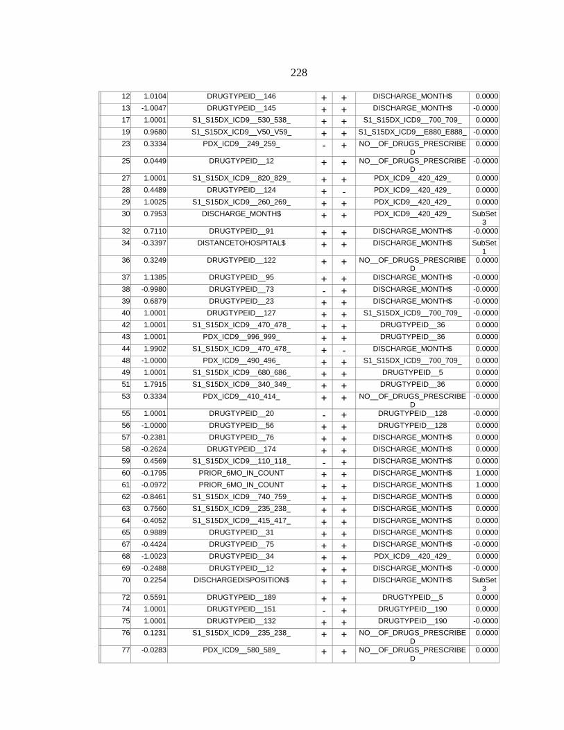
228
12 1.0104 DRUGTYPEID__146 + + DISCHARGE_MONTH$ 0.0000
13 -1.0047 DRUGTYPEID__145 + + DISCHARGE_MONTH$ -0.0000
17 1.0001 S1_S15DX_ICD9__530_538_ + + S1_S15DX_ICD9__700_709_ 0.0000
19 0.9680 S1_S15DX_ICD9__V50_V59_ + + S1_S15DX_ICD9__E880_E888_ -0.0000
23 0.3334 PDX_ICD9__249_259_ - + NO__OF_DRUGS_PRESCRIBED
0.0000
25 0.0449 DRUGTYPEID__12 + + NO__OF_DRUGS_PRESCRIBED
-0.0000
27 1.0001 S1_S15DX_ICD9__820_829_ + + PDX_ICD9__420_429_ 0.0000
28 0.4489 DRUGTYPEID__124 + - PDX_ICD9__420_429_ 0.0000
29 1.0025 S1_S15DX_ICD9__260_269_ + + PDX_ICD9__420_429_ 0.0000
30 0.7953 DISCHARGE_MONTH$ + + PDX_ICD9__420_429_ SubSet3
32 0.7110 DRUGTYPEID__91 + + DISCHARGE_MONTH$ -0.0000
34 -0.3397 DISTANCETOHOSPITAL$ + + DISCHARGE_MONTH$ SubSet1
36 0.3249 DRUGTYPEID__122 + + NO__OF_DRUGS_PRESCRIBED
0.0000
37 1.1385 DRUGTYPEID__95 + + DISCHARGE_MONTH$ -0.0000
38 -0.9980 DRUGTYPEID__73 - + DISCHARGE_MONTH$ -0.0000
39 0.6879 DRUGTYPEID__23 + + DISCHARGE_MONTH$ -0.0000
40 1.0001 DRUGTYPEID__127 + + S1_S15DX_ICD9__700_709_ -0.0000
42 1.0001 S1_S15DX_ICD9__470_478_ + + DRUGTYPEID__36 0.0000
43 1.0001 PDX_ICD9__996_999_ + + DRUGTYPEID__36 0.0000
44 1.9902 S1_S15DX_ICD9__470_478_ + - DISCHARGE_MONTH$ 0.0000
48 -1.0000 PDX_ICD9__490_496_ + + S1_S15DX_ICD9__700_709_ 0.0000
49 1.0001 S1_S15DX_ICD9__680_686_ + + DRUGTYPEID__5 0.0000
51 1.7915 S1_S15DX_ICD9__340_349_ + + DRUGTYPEID__36 0.0000
53 0.3334 PDX_ICD9__410_414_ + + NO__OF_DRUGS_PRESCRIBED
-0.0000
55 1.0001 DRUGTYPEID__20 - + DRUGTYPEID__128 -0.0000
56 -1.0000 DRUGTYPEID__56 + + DRUGTYPEID__128 0.0000
57 -0.2381 DRUGTYPEID__76 + + DISCHARGE_MONTH$ 0.0000
58 -0.2624 DRUGTYPEID__174 + + DISCHARGE_MONTH$ 0.0000
59 0.4569 S1_S15DX_ICD9__110_118_ - + DISCHARGE_MONTH$ 0.0000
60 -0.1795 PRIOR_6MO_IN_COUNT + + DISCHARGE_MONTH$ 1.0000
61 -0.0972 PRIOR_6MO_IN_COUNT + + DISCHARGE_MONTH$ 1.0000
62 -0.8461 S1_S15DX_ICD9__740_759_ + + DISCHARGE_MONTH$ 0.0000
63 0.7560 S1_S15DX_ICD9__235_238_ + + DISCHARGE_MONTH$ 0.0000
64 -0.4052 S1_S15DX_ICD9__415_417_ + + DISCHARGE_MONTH$ 0.0000
65 0.9889 DRUGTYPEID__31 + + DISCHARGE_MONTH$ 0.0000
67 -0.4424 DRUGTYPEID__75 + + DISCHARGE_MONTH$ -0.0000
68 -1.0023 DRUGTYPEID__34 + + PDX_ICD9__420_429_ 0.0000
69 -0.2488 DRUGTYPEID__12 + + DISCHARGE_MONTH$ -0.0000
70 0.2254 DISCHARGEDISPOSITION$ + + DISCHARGE_MONTH$ SubSet3
72 0.5591 DRUGTYPEID__189 + + DRUGTYPEID__5 0.0000
74 1.0001 DRUGTYPEID__151 - + DRUGTYPEID__190 0.0000
75 1.0001 DRUGTYPEID__132 + + DRUGTYPEID__190 -0.0000
76 0.1231 S1_S15DX_ICD9__235_238_ + + NO__OF_DRUGS_PRESCRIBED
0.0000
77 -0.0283 PDX_ICD9__580_589_ + + NO__OF_DRUGS_PRESCRIBED
0.0000

229
79 0.1871 PDX_ICD9__600_608_ + + DISCHARGEDISPOSITION$ 0.0000
80 -0.6357 PDX_ICD9__490_496_ + + DRUGTYPEID__36 0.0000
82 0.9983 PDX_ICD9__560_569_ + + DRUGTYPEID__36 0.0000
84 0.0786 DIFF_OF_NO__PRES__VS__NO__ADMIN_
+ + DRUGTYPEID__36 2.0000
85 -0.2244 S1_S15DX_ICD9__680_686_ + + DISCHARGE_MONTH$ 0.0000
86 -0.5895 S1_S15DX_ICD9__520_529_ + + DISCHARGE_MONTH$ -0.0000
87 -0.1419 DRUGTYPEID__132 + + PDX_ICD9__420_429_ -0.0000
88 -0.8043 DRUGTYPEID__190 + + DISCHARGE_MONTH$ 0.0000
89 0.5142 DRUGTYPEID__8 + + DRUGTYPEID__5 0.0000
91 0.5034 COUNT_OF_CONSULTS + + DRUGTYPEID__79 1.0000
93 -1.3291 S1_S15DX_ICD9__996_999_ - + DRUGTYPEID__79 -0.0000
94 0.0806 NO__OF_DRUGS_ADMINISTERED + + DRUGTYPEID__79 22.0000
96 -0.5033 DRUGTYPEID__201 + + DRUGTYPEID__79 -0.0000
97 -0.2051 DRUGTYPEID__12 + + DISCHARGE_MONTH$ -0.0000
98 0.2477 DRUGTYPEID__90 + + DISCHARGE_MONTH$ -0.0000
100 -0.0177 NO__OF_DRUGS_PRESCRIBED + + DRUGTYPEID__36 15.0000
101 0.7877 S1_S15DX_ICD9__430_438_ + + DRUGTYPEID__36 -0.0000
102 0.5605 S1_S15DX_ICD9__V60_V69_ + + DRUGTYPEID__132 -0.0000
103 0.3754 DRUGTYPEID__178 + + DISCHARGE_MONTH$ 0.0000
105 1.0001 DRUGTYPEID__164 + + S1_S15DX_ICD9__295_299_ 0.0000
106 -1.1575 COUNT_OF_CONSULTS - + DRUGTYPEID__36 2.0000
108 -0.9981 DRUGTYPEID__40 + + DRUGTYPEID__36 -0.0000
109 -0.7894 DRUGTYPEID__105 + + DRUGTYPEID__36 0.0000
110 -0.5712 S1_S15DX_ICD9__990_995_ + + DRUGTYPEID__36 -0.0000
111 -0.5589 PDX_ICD9__030_041_ + + S1_S15DX_ICD9__700_709_ 0.0000
112 -0.5270 DRUGTYPEID__189 + + S1_S15DX_ICD9__E880_E888_ 0.0000
113 -0.3248 PDX_ICD9__249_259_ + + NO__OF_DRUGS_PRESCRIBED
0.0000
114 0.2222 DRUGTYPEID__49 + + DISCHARGE_MONTH$ 0.0000
117 0.5001 PRIOR_6MO_IN_COUNT + + DISCHARGE_MONTH$ 2.0000
119 1.0001 DRUGTYPEID__171 + + DISCHARGE_MONTH$ 0.0000
123 -0.2197 MARITALSTATUS$ + + DISCHARGE_MONTH$ SubSet1
125 0.4834 DRUGTYPEID__94 + + DRUGTYPEID__79 0.0000
126 -0.2341 FINANCIALCLASS$ + + DISCHARGE_MONTH$ SubSet1
128 0.0822 AGEYRS - + DISCHARGE_MONTH$ 94.0000
129 -0.0050 AGEYRS + + DISCHARGE_MONTH$ 94.0000
131 -0.6776 S1_S15DX_ICD9__350_359_ + + S1_S15DX_ICD9__600_608_ -0.0000
132 -0.1199 DRUGTYPEID__192 + + S1_S15DX_ICD9__600_608_ 0.0000
133 0.6777 S1_S15DX_ICD9__550_553_ + + S1_S15DX_ICD9__600_608_ -0.0000
134 1.0001 S1_S15DX_ICD9__V85_ + + DISCHARGE_MONTH$ 0.0000
135 0.1851 S1_S15DX_ICD9__700_709_ + + DISCHARGE_MONTH$ 0.0000
136 0.3355 DRUGTYPEID__88 + + DISCHARGE_MONTH$ 0.0000
137 -0.5141 DRUGTYPEID__177 - -0.0000
138 -0.5141 PDX_ICD9__170_176_ + + DISCHARGE_MONTH$ -0.0000
139 -0.1559 DISCHARGE_MONTH$ + + PDX_ICD9__420_429_ SubSet6
141 -0.4179 DRUGTYPEID__66 - + DRUGTYPEID__132 0.0000

230
143 -0.2415 DRUGTYPEID__29 + + DRUGTYPEID__79 0.0000
144 -1.0000 DRUGTYPEID__198 + + S1_S15DX_ICD9__295_299_ 0.0000
145 -0.7585 PDX_ICD9__480_488_ + + DRUGTYPEID__79 0.0000
146 -0.3224 S1_S15DX_ICD9__V85_ + + S1_S15DX_ICD9__600_608_ 0.0000
147 0.3941 S1_S15DX_ICD9__200_208_ - + DISCHARGE_MONTH$ 0.0000
148 0.1046 S1_S15DX_ICD9__580_589_ + + DISCHARGE_MONTH$ 0.0000
149 -0.0900 COUNT_OF_CONSULTS + + DISCHARGE_MONTH$ 0.0000
150 0.1795 DRUGTYPEID__189 + + DISCHARGE_MONTH$ 0.0000
151 -0.9948 PDX_ICD9__420_429_ + + DRUGTYPEID__128 0.0000
152 0.0258 PDX_ICD9__560_569_ + + NO__OF_DRUGS_PRESCRIBED
0.0000
153 -0.1020 S1_S15DX_ICD9__290_294_ + + DISCHARGE_MONTH$ 0.0000
154 0.1662 DRUGTYPEID__156 - + DISCHARGE_MONTH$ -0.0000
155 -0.1596 DRUGTYPEID__85 + + DISCHARGE_MONTH$ 0.0000
156 -0.2534 DRUGTYPEID__23 + + NO__OF_DRUGS_PRESCRIBED
-0.0000
MARS Learn Gains for Class 0
Gains Data Bin Cases
Tgt.Class % of Bin Tgt.Class
% Tgt.Class
Cum % Tgt.Class
Cum % Pop
% Pop
Cases in Bin
Cum Lift
Lift Pop
1 54 100.00 7.32 7.32 6.75 6.75 54 1.08 1.08 2 15 100.00 2.03 9.35 8.63 1.88 15 1.08 1.08 3 107 100.00 14.50 23.85 22.00 13.38 107 1.08 1.08 4 479 100.00 64.91 88.75 81.88 59.88 479 1.08 1.08 5 12 100.00 1.63 90.38 83.38 1.50 12 1.08 1.08 6 26 100.00 3.52 93.90 86.63 3.25 26 1.08 1.08 7 27 100.00 3.66 97.56 90.00 3.38 27 1.08 1.08 8 18 22.78 2.44 100.00 99.88 9.88 79 1.00 0.25 9 0 0.00 0.00 100.00 100.00 0.13 1 1.00 0.00
0
20
40
60
80
100
0 20 40 60 80 100
% C
lass
% Population
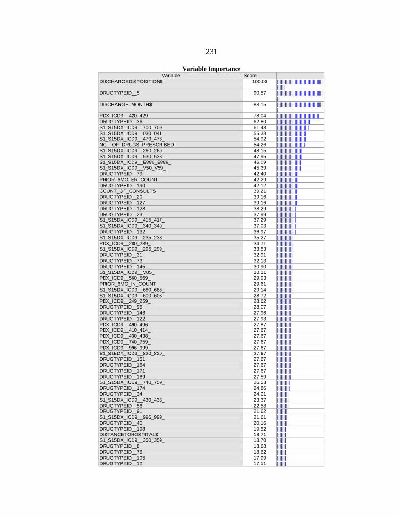
231
Variable Importance
Variable Score DISCHARGEDISPOSITION$ 100.00 ||||||||||||||||||||||||||||||||||||
|||||| DRUGTYPEID__5 90.57 ||||||||||||||||||||||||||||||||||||
|| DISCHARGE_MONTH$ 88.15 ||||||||||||||||||||||||||||||||||||
| PDX_ICD9__420_429_ 78.04 ||||||||||||||||||||||||||||||||| DRUGTYPEID__36 62.80 |||||||||||||||||||||||||| S1_S15DX_ICD9__700_709_ 61.48 ||||||||||||||||||||||||| S1_S15DX_ICD9__030_041_ 55.38 ||||||||||||||||||||||| S1_S15DX_ICD9__470_478_ 54.92 ||||||||||||||||||||||| NO__OF_DRUGS_PRESCRIBED 54.26 |||||||||||||||||||||| S1_S15DX_ICD9__260_269_ 48.15 |||||||||||||||||||| S1_S15DX_ICD9__530_538_ 47.95 |||||||||||||||||||| S1_S15DX_ICD9__E880_E888_ 46.09 ||||||||||||||||||| S1_S15DX_ICD9__V50_V59_ 45.39 ||||||||||||||||||| DRUGTYPEID__79 42.40 ||||||||||||||||| PRIOR_6MO_ER_COUNT 42.29 ||||||||||||||||| DRUGTYPEID__190 42.12 ||||||||||||||||| COUNT_OF_CONSULTS 39.21 |||||||||||||||| DRUGTYPEID__20 39.16 |||||||||||||||| DRUGTYPEID__127 39.16 |||||||||||||||| DRUGTYPEID__128 38.29 ||||||||||||||| DRUGTYPEID__23 37.99 ||||||||||||||| S1_S15DX_ICD9__415_417_ 37.29 ||||||||||||||| S1_S15DX_ICD9__340_349_ 37.03 ||||||||||||||| DRUGTYPEID__132 36.97 ||||||||||||||| S1_S15DX_ICD9__235_238_ 35.27 |||||||||||||| PDX_ICD9__280_289_ 34.71 |||||||||||||| S1_S15DX_ICD9__295_299_ 33.53 ||||||||||||| DRUGTYPEID__31 32.91 ||||||||||||| DRUGTYPEID__73 32.13 ||||||||||||| DRUGTYPEID__145 30.90 |||||||||||| S1_S15DX_ICD9__V85_ 30.31 |||||||||||| PDX_ICD9__560_569_ 29.93 |||||||||||| PRIOR_6MO_IN_COUNT 29.61 |||||||||||| S1_S15DX_ICD9__680_686_ 29.14 |||||||||||| S1_S15DX_ICD9__600_608_ 28.72 ||||||||||| PDX_ICD9__249_259_ 28.62 ||||||||||| DRUGTYPEID__95 28.07 ||||||||||| DRUGTYPEID__146 27.96 ||||||||||| DRUGTYPEID__122 27.93 ||||||||||| PDX_ICD9__490_496_ 27.87 ||||||||||| PDX_ICD9__410_414_ 27.67 ||||||||||| PDX_ICD9__430_438_ 27.67 ||||||||||| PDX_ICD9__740_759_ 27.67 ||||||||||| PDX_ICD9__996_999_ 27.67 ||||||||||| S1_S15DX_ICD9__820_829_ 27.67 ||||||||||| DRUGTYPEID__151 27.67 ||||||||||| DRUGTYPEID__164 27.67 ||||||||||| DRUGTYPEID__171 27.67 ||||||||||| DRUGTYPEID__189 27.59 ||||||||||| S1_S15DX_ICD9__740_759_ 26.53 |||||||||| DRUGTYPEID__174 24.86 |||||||||| DRUGTYPEID__34 24.01 ||||||||| S1_S15DX_ICD9__430_438_ 23.37 ||||||||| DRUGTYPEID__56 22.58 ||||||||| DRUGTYPEID__91 21.62 |||||||| S1_S15DX_ICD9__996_999_ 21.61 |||||||| DRUGTYPEID__40 20.16 |||||||| DRUGTYPEID__198 19.52 ||||||| DISTANCETOHOSPITAL$ 18.71 ||||||| S1_S15DX_ICD9__350_359_ 18.70 ||||||| DRUGTYPEID__8 18.68 ||||||| DRUGTYPEID__76 18.62 ||||||| DRUGTYPEID__105 17.99 ||||||| DRUGTYPEID__12 17.51 |||||||

232
S1_S15DX_ICD9__V60_V69_ 17.47 ||||||| S1_S15DX_ICD9__110_118_ 17.17 |||||| AGEYRS 15.86 |||||| S1_S15DX_ICD9__990_995_ 15.28 |||||| MARITALSTATUS$ 14.64 ||||| DRUGTYPEID__178 14.43 ||||| DRUGTYPEID__90 14.40 ||||| S1_S15DX_ICD9__520_529_ 13.50 ||||| S1_S15DX_ICD9__550_553_ 13.12 ||||| PDX_ICD9__030_041_ 13.12 ||||| DRUGTYPEID__201 12.32 |||| NO__OF_DRUGS_ADMINISTERED 12.02 |||| FINANCIALCLASS$ 11.79 |||| PDX_ICD9__480_488_ 11.39 |||| DRUGTYPEID__94 11.28 |||| DRUGTYPEID__177 11.17 |||| PDX_ICD9__170_176_ 11.17 |||| DRUGTYPEID__66 11.04 |||| DRUGTYPEID__49 10.46 ||| DRUGTYPEID__124 10.14 ||| PDX_ICD9__580_589_ 9.53 ||| DRUGTYPEID__88 9.48 ||| S1_S15DX_ICD9__580_589_ 9.38 ||| DRUGTYPEID__75 9.17 ||| S1_S15DX_ICD9__200_208_ 7.80 || S1_S15DX_ICD9__290_294_ 6.48 || DIFF_OF_NO__PRES__VS__NO__ADMIN_ 6.18 || DRUGTYPEID__156 5.90 || DRUGTYPEID__29 5.46 | PDX_ICD9__600_608_ 5.43 | DRUGTYPEID__85 5.42 | DRUGTYPEID__192 4.87 |
Prediction Success
Actual Class
Total Class
Percent Correct
Class 0 N=738
Class 1 N=62
Class 0 738 100.00 738 0 Class 1 62 100.00 0 62
Total: 800.00
Average: 100.00
Overall % Correct:
100.00

233
APPENDIX O
MARS PREDICTION MODEL REPORT FOR PNM

234
MARS 3 Results: PNM, 35 Basis Functions
Dataset: PNM-FinalMethodology-Basic-AnalysisReady-ModelSetup.xlsx
Predictor Variables: DISCHARGE_MONTH$, GENDER_M_0_F_1, MARITALSTATUS$,
HOSPDISCHARGEDEPT$,
ADMITFROMER_YES_1, FINANCIALCLASS$,
DISCHARGEDISPOSITION$,
DISTANCETOHOSPITAL$, LOS, AGEYRS, PDX_ICD9__001_009_,
PDX_ICD9__030_041_, PDX_ICD9__045_049_, PDX_ICD9__110_118_,
PDX_ICD9__160_165_, PDX_ICD9__190_199_, PDX_ICD9__200_208_,
PDX_ICD9__210_229_, PDX_ICD9__249_259_, PDX_ICD9__260_269_,
PDX_ICD9__270_279_, PDX_ICD9__280_289_, PDX_ICD9__295_299_,
PDX_ICD9__338_, PDX_ICD9__390_392_, PDX_ICD9__401_405_,
PDX_ICD9__410_414_, PDX_ICD9__415_417_, PDX_ICD9__420_429_,
PDX_ICD9__430_438_, PDX_ICD9__480_488_, PDX_ICD9__490_496_,
PDX_ICD9__500_508_, PDX_ICD9__510_519_, PDX_ICD9__530_538_,
PDX_ICD9__540_543_, PDX_ICD9__550_553_, PDX_ICD9__555_558_,
PDX_ICD9__560_569_, PDX_ICD9__570_579_, PDX_ICD9__580_589_,
PDX_ICD9__590_599_, PDX_ICD9__640_649_, PDX_ICD9__680_686_,
PDX_ICD9__710_719_, PDX_ICD9__720_724_, PDX_ICD9__725_729_,
PDX_ICD9__730_739_, PDX_ICD9__740_759_, PDX_ICD9__780_789_,
PDX_ICD9__790_796_, PDX_ICD9__805_809_, PDX_ICD9__820_829_,
PDX_ICD9__840_848_, PDX_ICD9__850_854_, PDX_ICD9__860_869_,
PDX_ICD9__900_904_, PDX_ICD9__920_924_, PDX_ICD9__960_979_,
PDX_ICD9__990_995_, PDX_ICD9__996_999_, PDX_ICD9__V50_V59_,
S1_S15DX_ICD9__001_009_, S1_S15DX_ICD9__030_041_,
S1_S15DX_ICD9__050_059_, S1_S15DX_ICD9__070_079_,
S1_S15DX_ICD9__080_088_, S1_S15DX_ICD9__110_118_,
S1_S15DX_ICD9__130_136_, S1_S15DX_ICD9__137_139_,
S1_S15DX_ICD9__140_149_, S1_S15DX_ICD9__150_159_,
S1_S15DX_ICD9__160_165_, S1_S15DX_ICD9__170_176_,
S1_S15DX_ICD9__179_189_, S1_S15DX_ICD9__190_199_,
S1_S15DX_ICD9__200_208_, S1_S15DX_ICD9__209_,
S1_S15DX_ICD9__210_229_,
S1_S15DX_ICD9__235_238_, S1_S15DX_ICD9__240_246_,
S1_S15DX_ICD9__249_259_, S1_S15DX_ICD9__260_269_,
S1_S15DX_ICD9__270_279_, S1_S15DX_ICD9__280_289_,
S1_S15DX_ICD9__290_294_, S1_S15DX_ICD9__295_299_,
S1_S15DX_ICD9__300_316_, S1_S15DX_ICD9__320_326_,
S1_S15DX_ICD9__330_337_, S1_S15DX_ICD9__338_,
S1_S15DX_ICD9__340_349_,
S1_S15DX_ICD9__350_359_, S1_S15DX_ICD9__360_379_,
S1_S15DX_ICD9__380_389_, S1_S15DX_ICD9__393_398_,
S1_S15DX_ICD9__401_405_, S1_S15DX_ICD9__410_414_,
S1_S15DX_ICD9__415_417_, S1_S15DX_ICD9__420_429_,
S1_S15DX_ICD9__430_438_, S1_S15DX_ICD9__440_448_,
S1_S15DX_ICD9__451_459_, S1_S15DX_ICD9__460_466_,
S1_S15DX_ICD9__470_478_, S1_S15DX_ICD9__480_488_,
S1_S15DX_ICD9__490_496_, S1_S15DX_ICD9__500_508_,
S1_S15DX_ICD9__510_519_, S1_S15DX_ICD9__520_529_,

235
S1_S15DX_ICD9__530_538_, S1_S15DX_ICD9__540_543_,
S1_S15DX_ICD9__550_553_, S1_S15DX_ICD9__555_558_,
S1_S15DX_ICD9__560_569_, S1_S15DX_ICD9__570_579_,
S1_S15DX_ICD9__580_589_, S1_S15DX_ICD9__590_599_,
S1_S15DX_ICD9__600_608_, S1_S15DX_ICD9__617_629_,
S1_S15DX_ICD9__640_649_, S1_S15DX_ICD9__670_677_,
S1_S15DX_ICD9__680_686_, S1_S15DX_ICD9__690_698_,
S1_S15DX_ICD9__700_709_, S1_S15DX_ICD9__710_719_,
S1_S15DX_ICD9__720_724_, S1_S15DX_ICD9__725_729_,
S1_S15DX_ICD9__730_739_, S1_S15DX_ICD9__740_759_,
S1_S15DX_ICD9__780_789_, S1_S15DX_ICD9__790_796_,
S1_S15DX_ICD9__797_799_, S1_S15DX_ICD9__805_809_,
S1_S15DX_ICD9__810_819_, S1_S15DX_ICD9__820_829_,
S1_S15DX_ICD9__840_848_, S1_S15DX_ICD9__860_869_,
S1_S15DX_ICD9__870_879_, S1_S15DX_ICD9__880_887_,
S1_S15DX_ICD9__905_909_, S1_S15DX_ICD9__910_919_,
S1_S15DX_ICD9__920_924_, S1_S15DX_ICD9__930_939_,
S1_S15DX_ICD9__958_959_, S1_S15DX_ICD9__960_979_,
S1_S15DX_ICD9__980_989_, S1_S15DX_ICD9__990_995_,
S1_S15DX_ICD9__996_999_, S1_S15DX_ICD9__V01_V09_,
S1_S15DX_ICD9__V10_V19_, S1_S15DX_ICD9__V40_V49_,
S1_S15DX_ICD9__V50_V59_, S1_S15DX_ICD9__V60_V69_,
S1_S15DX_ICD9__V85_, S1_S15DX_ICD9__V87_, S1_S15DX_ICD9__V88_,
S1_S15DX_ICD9__E001_E030_, S1_S15DX_ICD9__E810_E819_,
S1_S15DX_ICD9__E820_E825_, S1_S15DX_ICD9__E826_E829_,
S1_S15DX_ICD9__E840_E845_, S1_S15DX_ICD9__E846_E849_,
S1_S15DX_ICD9__E850_E858_, S1_S15DX_ICD9__E860_E869_,
S1_S15DX_ICD9__E870_E876_, S1_S15DX_ICD9__E878_E879_,
S1_S15DX_ICD9__E880_E888_, S1_S15DX_ICD9__E890_E899_,
S1_S15DX_ICD9__E900_E909_, S1_S15DX_ICD9__E910_E915_,
S1_S15DX_ICD9__E916_E928_, S1_S15DX_ICD9__E929_,
S1_S15DX_ICD9__E930_E949_, S1_S15DX_ICD9__E950_E959_,
S1_S15DX_ICD9__E960_E969_, S1_S15DX_ICD9__E980_E989_,
S1_S15DX_ICD9__E990_E999_, DRUGTYPEID__1, DRUGTYPEID__2,
DRUGTYPEID__3, DRUGTYPEID__5, DRUGTYPEID__6,
DRUGTYPEID__8,
DRUGTYPEID__9, DRUGTYPEID__10, DRUGTYPEID__11,
DRUGTYPEID__12,
DRUGTYPEID__14, DRUGTYPEID__15, DRUGTYPEID__16,
DRUGTYPEID__17,
DRUGTYPEID__19, DRUGTYPEID__20, DRUGTYPEID__21,
DRUGTYPEID__22,
DRUGTYPEID__23, DRUGTYPEID__24, DRUGTYPEID__25,
DRUGTYPEID__26,
DRUGTYPEID__28, DRUGTYPEID__29, DRUGTYPEID__30,
DRUGTYPEID__31,
DRUGTYPEID__32, DRUGTYPEID__33, DRUGTYPEID__34,
DRUGTYPEID__35,
DRUGTYPEID__36, DRUGTYPEID__37, DRUGTYPEID__39,
DRUGTYPEID__40,
DRUGTYPEID__41, DRUGTYPEID__42, DRUGTYPEID__43,
DRUGTYPEID__44,
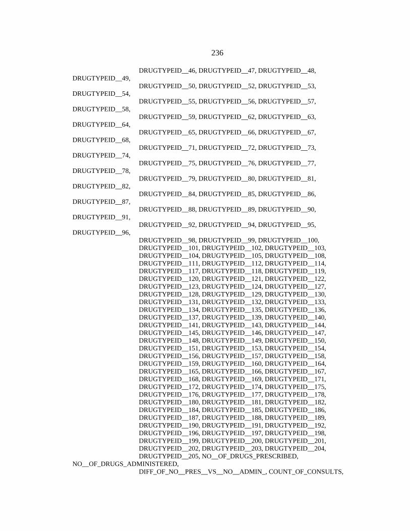
236
DRUGTYPEID__46, DRUGTYPEID__47, DRUGTYPEID__48,
DRUGTYPEID__49,
DRUGTYPEID__50, DRUGTYPEID__52, DRUGTYPEID__53,
DRUGTYPEID__54,
DRUGTYPEID__55, DRUGTYPEID__56, DRUGTYPEID__57,
DRUGTYPEID__58,
DRUGTYPEID__59, DRUGTYPEID__62, DRUGTYPEID__63,
DRUGTYPEID__64,
DRUGTYPEID__65, DRUGTYPEID__66, DRUGTYPEID__67,
DRUGTYPEID__68,
DRUGTYPEID__71, DRUGTYPEID__72, DRUGTYPEID__73,
DRUGTYPEID__74,
DRUGTYPEID__75, DRUGTYPEID__76, DRUGTYPEID__77,
DRUGTYPEID__78,
DRUGTYPEID__79, DRUGTYPEID__80, DRUGTYPEID__81,
DRUGTYPEID__82,
DRUGTYPEID__84, DRUGTYPEID__85, DRUGTYPEID__86,
DRUGTYPEID__87,
DRUGTYPEID__88, DRUGTYPEID__89, DRUGTYPEID__90,
DRUGTYPEID__91,
DRUGTYPEID__92, DRUGTYPEID__94, DRUGTYPEID__95,
DRUGTYPEID__96,
DRUGTYPEID__98, DRUGTYPEID__99, DRUGTYPEID__100,
DRUGTYPEID__101, DRUGTYPEID__102, DRUGTYPEID__103,
DRUGTYPEID__104, DRUGTYPEID__105, DRUGTYPEID__108,
DRUGTYPEID__111, DRUGTYPEID__112, DRUGTYPEID__114,
DRUGTYPEID__117, DRUGTYPEID__118, DRUGTYPEID__119,
DRUGTYPEID__120, DRUGTYPEID__121, DRUGTYPEID__122,
DRUGTYPEID__123, DRUGTYPEID__124, DRUGTYPEID__127,
DRUGTYPEID__128, DRUGTYPEID__129, DRUGTYPEID__130,
DRUGTYPEID__131, DRUGTYPEID__132, DRUGTYPEID__133,
DRUGTYPEID__134, DRUGTYPEID__135, DRUGTYPEID__136,
DRUGTYPEID__137, DRUGTYPEID__139, DRUGTYPEID__140,
DRUGTYPEID__141, DRUGTYPEID__143, DRUGTYPEID__144,
DRUGTYPEID__145, DRUGTYPEID__146, DRUGTYPEID__147,
DRUGTYPEID__148, DRUGTYPEID__149, DRUGTYPEID__150,
DRUGTYPEID__151, DRUGTYPEID__153, DRUGTYPEID__154,
DRUGTYPEID__156, DRUGTYPEID__157, DRUGTYPEID__158,
DRUGTYPEID__159, DRUGTYPEID__160, DRUGTYPEID__164,
DRUGTYPEID__165, DRUGTYPEID__166, DRUGTYPEID__167,
DRUGTYPEID__168, DRUGTYPEID__169, DRUGTYPEID__171,
DRUGTYPEID__172, DRUGTYPEID__174, DRUGTYPEID__175,
DRUGTYPEID__176, DRUGTYPEID__177, DRUGTYPEID__178,
DRUGTYPEID__180, DRUGTYPEID__181, DRUGTYPEID__182,
DRUGTYPEID__184, DRUGTYPEID__185, DRUGTYPEID__186,
DRUGTYPEID__187, DRUGTYPEID__188, DRUGTYPEID__189,
DRUGTYPEID__190, DRUGTYPEID__191, DRUGTYPEID__192,
DRUGTYPEID__196, DRUGTYPEID__197, DRUGTYPEID__198,
DRUGTYPEID__199, DRUGTYPEID__200, DRUGTYPEID__201,
DRUGTYPEID__202, DRUGTYPEID__203, DRUGTYPEID__204,
DRUGTYPEID__205, NO__OF_DRUGS_PRESCRIBED,
NO__OF_DRUGS_ADMINISTERED,
DIFF_OF_NO__PRES__VS__NO__ADMIN_, COUNT_OF_CONSULTS,

237
PRIOR_6MO_ER_COUNT, PRIOR_6MO_IN_COUNT
Target Variable ADMITTOREADMIT
N: 615 Minimum0.00000 Maximum: 1.00000
Mean: 0.04878 Varience: 0.04648
Variables, Terms, and Parameters
Direct variables: 34 Total variables: 34
Terms in model: 36 Effective parameters: 131.45
R-squared Measures
Naive: 0.83606 Naive adjusted: 0.82615 GCV R-squared: 0.73568
Mean-Square Measures
Naive MSE: 0.00808 MARS GCV: 0.01230
Basis Functions Subsets for DISCHARGE_MONTH$
SubSet1 = { "December", "March", "May" }
SubSet2 = { "April", "February", "January", "July", "March" }
SubSet3 = { "August", "December", "June", "May", "November",
"October", "September" }
Subsets for FINANCIALCLASS$
SubSet1 = { "Medicaid", "Medicare", "Selfpay" }
Subsets for DISTANCETOHOSPITAL$
SubSet1 = { "101-200_miles" }
Basis Functions
BF1 = max(0, PDX_ICD9__860_869_ - 8.30065E-011);
BF2 = max(0, DRUGTYPEID__58 - 8.30065E-011);
BF3 = max(0, DRUGTYPEID__124 + 2.34799E-010);
BF4 = max(0, PRIOR_6MO_ER_COUNT - 5.18256E-008);
BF5 = max(0, S1_S15DX_ICD9__710_719_ + 4.96736E-009) * BF4;
BF6 = ( DISCHARGE_MONTH$ is in SubSet1 ) * BF5;
BF8 = max(0, PDX_ICD9__570_579_ - 2.4696E-010) * BF4;
BF9 = max(0, DRUGTYPEID__160 + 1.64387E-009) * BF4;
BF10 = max(0, S1_S15DX_ICD9__393_398_ + 2.71494E-010) * BF4;
BF11 = max(0, S1_S15DX_ICD9__580_589_ + 2.02463E-009) * BF10;
BF12 = max(0, S1_S15DX_ICD9__160_165_ - 3.3843E-010) * BF9;
BF13 = ( DISCHARGE_MONTH$ is in SubSet2 );
BF14 = ( DISCHARGE_MONTH$ is in SubSet3 );
BF15 = max(0, S1_S15DX_ICD9__470_478_ + 1.44288E-009) * BF13;
BF16 = max(0, LOS - 2.25452E-007) * BF15;
BF17 = max(0, PRIOR_6MO_ER_COUNT - 1) * BF15;
BF18 = max(0, 1 - PRIOR_6MO_ER_COUNT) * BF15;
BF19 = max(0, S1_S15DX_ICD9__V85_ - 1.60297E-009) * BF4;
BF20 = max(0, DRUGTYPEID__180 + 1.95269E-009) * BF19;
BF21 = ( FINANCIALCLASS$ is in SubSet1 ) * BF5;
BF23 = max(0, S1_S15DX_ICD9__V01_V09_ + 1.73961E-009) * BF13;
BF24 = max(0, DRUGTYPEID__146 - 5.53822E-010) * BF23;
BF25 = max(0, DRUGTYPEID__57 + 1.44288E-009) * BF23;
BF26 = max(0, COUNT_OF_CONSULTS - 2) * BF23;
BF27 = max(0, 2 - COUNT_OF_CONSULTS) * BF23;
BF29 = max(0, DRUGTYPEID__124 + 2.34799E-010) * BF14;
BF30 = max(0, DRUGTYPEID__205 - 9.90418E-010);
BF31 = max(0, S1_S15DX_ICD9__190_199_ - 1.32509E-009) * BF30;
BF32 = max(0, S1_S15DX_ICD9__209_ + 2.38685E-010) * BF13;
BF33 = max(0, PDX_ICD9__270_279_ - 6.18295E-010) * BF5;

238
BF34 = max(0, PDX_ICD9__270_279_ - 6.18295E-010) * BF13;
BF35 = max(0, S1_S15DX_ICD9__920_924_ + 5.91698E-010) * BF13;
BF36 = max(0, S1_S15DX_ICD9__860_869_ + 5.91698E-010) * BF14;
BF37 = max(0, S1_S15DX_ICD9__958_959_ - 5.06252E-011) * BF14;
BF38 = max(0, AGEYRS - 79) * BF15;
BF40 = max(0, PDX_ICD9__410_414_ + 2.34799E-010) * BF10;
BF41 = max(0, S1_S15DX_ICD9__338_ + 2.01808E-009) * BF13;
BF42 = max(0, S1_S15DX_ICD9__725_729_ - 1.32509E-009) * BF41;
BF43 = max(0, DRUGTYPEID__52 + 1.42219E-009) * BF41;
BF44 = max(0, DRUGTYPEID__158 - 5.53822E-010) * BF23;
BF45 = ( DISTANCETOHOSPITAL$ is in SubSet1 ) * BF13;
BF47 = max(0, AGEYRS - 88) * BF5;
Y = 0.0039682 + 1.93709 * BF1 + 0.996032 * BF2 + 0.996031 * BF3
- 0.179024 * BF5 + 0.194943 * BF6 + 0.498084 * BF8
+ 0.0397034 * BF9 + 0.166005 * BF11
+ 0.209304 * BF12 - 0.620571 * BF15
+ 0.339733 * BF16 - 0.766353 * BF17
- 0.462228 * BF18 + 0.498016 * BF20
+ 0.178956 * BF21 + 0.912048 * BF23
+ 0.764697 * BF24 - 1.2269 * BF25 - 0.916016 * BF26
- 0.453809 * BF27 - 0.999999 * BF29
+ 0.996032 * BF31 + 0.996031 * BF32
- 1.52424 * BF33 + 0.329365 * BF34
+ 0.329365 * BF35 + 0.999999 * BF36
- 1.00397 * BF37 + 0.0409675 * BF38
+ 0.166005 * BF40 + 0.996032 * BF42
+ 0.96656 * BF43 - 0.945487 * BF44
+ 0.196032 * BF45 - 0.0152565 * BF47;
MODEL ADMITTOREADMIT = BF1 BF2 BF3 BF5 BF6 BF8 BF9 BF11 BF12
BF15 BF16 BF17 BF18 BF20 BF21 BF23 BF24
BF25 BF26 BF27 BF29 BF31 BF32 BF33 BF34
BF35 BF36 BF37 BF38 BF40 BF42 BF43 BF44
BF45 BF47;
Anova Data Function Standard
Deviation
Mars Prediction Success
Threshold Table
No of basis
Functions
No of Effective
Parameters
Variables
1 0.07805 0.01700 1 3.727 PDX_ICD9__860_869_
2 0.04013 0.01468 1 3.727 DRUGTYPEID__58
3 0.08007 0.01468 1 3.727 DRUGTYPEID__124
4 0.10121 0.01288 1 3.727 S1_S15DX_ICD9__710_719_, PRIOR_6MO_ER_COUNT
5 0.04014 0.01457 1 3.727 PDX_ICD9__570_579_, PRIOR_6MO_ER_COUNT
6 0.03969 0.01456 1 3.727 DRUGTYPEID__160, PRIOR_6MO_ER_COUNT
7 0.08225 0.01298 1 3.727 DISCHARGE_MONTH$, S1_S15DX_ICD9__470_478_
8 0.15373 0.01520 1 3.727 DISCHARGE_MONTH$, S1_S15DX_ICD9__V01_V09_
9 0.06967 0.01384 1 3.727 DISCHARGE_MONTH$, DRUGTYPEID__124
10 0.05671 0.01724 1 3.727 S1_S15DX_ICD9__190_199_, DRUGTYPEID__205
11 0.05671 0.01468 1 3.727 DISCHARGE_MONTH$, S1_S15DX_ICD9__209_
12 0.02648 0.01296 1 3.727 DISCHARGE_MONTH$, PDX_ICD9__270_279_
13 0.02295 0.01296 1 3.727 DISCHARGE_MONTH$, S1_S15DX_ICD9__920_924_
14 0.05693 0.01384 1 3.727 DISCHARGE_MONTH$, S1_S15DX_ICD9__860_869_
15 0.04045 0.01316 1 3.727 DISCHARGE_MONTH$, S1_S15DX_ICD9__958_959_
16 0.01760 0.01261 1 3.727 DISCHARGE_MONTH$, DISTANCETOHOSPITAL$
17 0.08238 0.01676 1 3.727 DISCHARGE_MONTH$, S1_S15DX_ICD9__710_719_, PRIOR_6MO_ER_COUNT
18 0.04484 0.01468 1 3.727 S1_S15DX_ICD9__393_398_, S1_S15DX_ICD9__580_589_, PRIOR_6MO_ER_COUNT
19 0.03373 0.01388 1 3.727 S1_S15DX_ICD9__160_165_, DRUGTYPEID__160, PRIOR_6MO_ER_COUNT
20 0.17296 0.01623 1 3.727 DISCHARGE_MONTH$, LOS, S1_S15DX_ICD9__470_478_
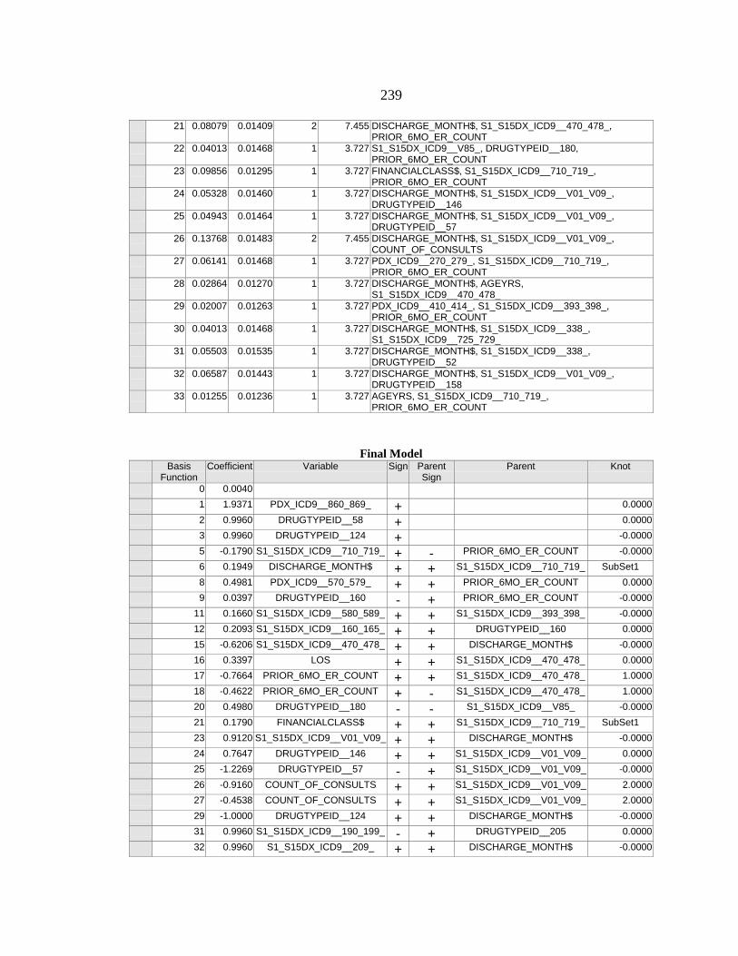
239
21 0.08079 0.01409 2 7.455 DISCHARGE_MONTH$, S1_S15DX_ICD9__470_478_,
PRIOR_6MO_ER_COUNT
22 0.04013 0.01468 1 3.727 S1_S15DX_ICD9__V85_, DRUGTYPEID__180, PRIOR_6MO_ER_COUNT
23 0.09856 0.01295 1 3.727 FINANCIALCLASS$, S1_S15DX_ICD9__710_719_, PRIOR_6MO_ER_COUNT
24 0.05328 0.01460 1 3.727 DISCHARGE_MONTH$, S1_S15DX_ICD9__V01_V09_, DRUGTYPEID__146
25 0.04943 0.01464 1 3.727 DISCHARGE_MONTH$, S1_S15DX_ICD9__V01_V09_, DRUGTYPEID__57
26 0.13768 0.01483 2 7.455 DISCHARGE_MONTH$, S1_S15DX_ICD9__V01_V09_, COUNT_OF_CONSULTS
27 0.06141 0.01468 1 3.727 PDX_ICD9__270_279_, S1_S15DX_ICD9__710_719_, PRIOR_6MO_ER_COUNT
28 0.02864 0.01270 1 3.727 DISCHARGE_MONTH$, AGEYRS, S1_S15DX_ICD9__470_478_
29 0.02007 0.01263 1 3.727 PDX_ICD9__410_414_, S1_S15DX_ICD9__393_398_, PRIOR_6MO_ER_COUNT
30 0.04013 0.01468 1 3.727 DISCHARGE_MONTH$, S1_S15DX_ICD9__338_, S1_S15DX_ICD9__725_729_
31 0.05503 0.01535 1 3.727 DISCHARGE_MONTH$, S1_S15DX_ICD9__338_, DRUGTYPEID__52
32 0.06587 0.01443 1 3.727 DISCHARGE_MONTH$, S1_S15DX_ICD9__V01_V09_, DRUGTYPEID__158
33 0.01255 0.01236 1 3.727 AGEYRS, S1_S15DX_ICD9__710_719_, PRIOR_6MO_ER_COUNT
Final Model Basis
Function
Coefficient Variable Sign Parent Sign
Parent Knot
0 0.0040
1 1.9371 PDX_ICD9__860_869_ + 0.0000
2 0.9960 DRUGTYPEID__58 + 0.0000
3 0.9960 DRUGTYPEID__124 + -0.0000
5 -0.1790 S1_S15DX_ICD9__710_719_ + - PRIOR_6MO_ER_COUNT -0.0000
6 0.1949 DISCHARGE_MONTH$ + + S1_S15DX_ICD9__710_719_ SubSet1
8 0.4981 PDX_ICD9__570_579_ + + PRIOR_6MO_ER_COUNT 0.0000
9 0.0397 DRUGTYPEID__160 - + PRIOR_6MO_ER_COUNT -0.0000
11 0.1660 S1_S15DX_ICD9__580_589_ + + S1_S15DX_ICD9__393_398_ -0.0000
12 0.2093 S1_S15DX_ICD9__160_165_ + + DRUGTYPEID__160 0.0000
15 -0.6206 S1_S15DX_ICD9__470_478_ + + DISCHARGE_MONTH$ -0.0000
16 0.3397 LOS + + S1_S15DX_ICD9__470_478_ 0.0000
17 -0.7664 PRIOR_6MO_ER_COUNT + + S1_S15DX_ICD9__470_478_ 1.0000
18 -0.4622 PRIOR_6MO_ER_COUNT + - S1_S15DX_ICD9__470_478_ 1.0000
20 0.4980 DRUGTYPEID__180 - - S1_S15DX_ICD9__V85_ -0.0000
21 0.1790 FINANCIALCLASS$ + + S1_S15DX_ICD9__710_719_ SubSet1
23 0.9120 S1_S15DX_ICD9__V01_V09_ + + DISCHARGE_MONTH$ -0.0000
24 0.7647 DRUGTYPEID__146 + + S1_S15DX_ICD9__V01_V09_ 0.0000
25 -1.2269 DRUGTYPEID__57 - + S1_S15DX_ICD9__V01_V09_ -0.0000
26 -0.9160 COUNT_OF_CONSULTS + + S1_S15DX_ICD9__V01_V09_ 2.0000
27 -0.4538 COUNT_OF_CONSULTS + + S1_S15DX_ICD9__V01_V09_ 2.0000
29 -1.0000 DRUGTYPEID__124 + + DISCHARGE_MONTH$ -0.0000
31 0.9960 S1_S15DX_ICD9__190_199_ - + DRUGTYPEID__205 0.0000
32 0.9960 S1_S15DX_ICD9__209_ + + DISCHARGE_MONTH$ -0.0000
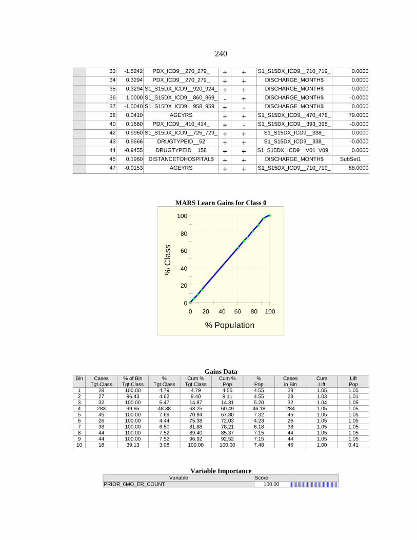
240
33 -1.5242 PDX_ICD9__270_279_ + + S1_S15DX_ICD9__710_719_ 0.0000
34 0.3294 PDX_ICD9__270_279_ + + DISCHARGE_MONTH$ 0.0000
35 0.3294 S1_S15DX_ICD9__920_924_ + + DISCHARGE_MONTH$ -0.0000
36 1.0000 S1_S15DX_ICD9__860_869_ - + DISCHARGE_MONTH$ -0.0000
37 -1.0040 S1_S15DX_ICD9__958_959_ + - DISCHARGE_MONTH$ 0.0000
38 0.0410 AGEYRS + + S1_S15DX_ICD9__470_478_ 79.0000
40 0.1660 PDX_ICD9__410_414_ + - S1_S15DX_ICD9__393_398_ -0.0000
42 0.9960 S1_S15DX_ICD9__725_729_ + + S1_S15DX_ICD9__338_ 0.0000
43 0.9666 DRUGTYPEID__52 + + S1_S15DX_ICD9__338_ -0.0000
44 -0.9455 DRUGTYPEID__158 + + S1_S15DX_ICD9__V01_V09_ 0.0000
45 0.1960 DISTANCETOHOSPITAL$ + + DISCHARGE_MONTH$ SubSet1
47 -0.0153 AGEYRS + + S1_S15DX_ICD9__710_719_ 88.0000
MARS Learn Gains for Class 0
Gains Data Bin Cases
Tgt.Class % of Bin Tgt.Class
% Tgt.Class
Cum % Tgt.Class
Cum % Pop
% Pop
Cases in Bin
Cum Lift
Lift Pop
1 28 100.00 4.79 4.79 4.55 4.55 28 1.05 1.05 2 27 96.43 4.62 9.40 9.11 4.55 28 1.03 1.01 3 32 100.00 5.47 14.87 14.31 5.20 32 1.04 1.05 4 283 99.65 48.38 63.25 60.49 46.18 284 1.05 1.05 5 45 100.00 7.69 70.94 67.80 7.32 45 1.05 1.05 6 26 100.00 4.44 75.38 72.03 4.23 26 1.05 1.05 7 38 100.00 6.50 81.88 78.21 6.18 38 1.05 1.05 8 44 100.00 7.52 89.40 85.37 7.15 44 1.05 1.05 9 44 100.00 7.52 96.92 92.52 7.15 44 1.05 1.05
10 18 39.13 3.08 100.00 100.00 7.48 46 1.00 0.41
Variable Importance
Variable Score PRIOR_6MO_ER_COUNT 100.00 ||||||||||||||||||||||||||||||||||||
0
20
40
60
80
100
0 20 40 60 80 100
% C
lass
% Population

241
||||||
DISCHARGE_MONTH$ 95.17 ||||||||||||||||||||||||||||||||||||||||
S1_S15DX_ICD9__710_719_ 66.93 |||||||||||||||||||||||||||| S1_S15DX_ICD9__V01_V09_ 56.07 ||||||||||||||||||||||| S1_S15DX_ICD9__338_ 48.99 |||||||||||||||||||| S1_S15DX_ICD9__470_478_ 48.46 |||||||||||||||||||| S1_S15DX_ICD9__190_199_ 47.13 ||||||||||||||||||| DRUGTYPEID__205 47.13 ||||||||||||||||||| PDX_ICD9__860_869_ 45.97 ||||||||||||||||||| S1_S15DX_ICD9__393_398_ 45.87 ||||||||||||||||||| DRUGTYPEID__160 45.26 |||||||||||||||||| LOS 42.02 ||||||||||||||||| DRUGTYPEID__52 37.02 ||||||||||||||| COUNT_OF_CONSULTS 33.70 ||||||||||||| S1_S15DX_ICD9__209_ 32.72 ||||||||||||| S1_S15DX_ICD9__580_589_ 32.72 ||||||||||||| S1_S15DX_ICD9__725_729_ 32.72 ||||||||||||| S1_S15DX_ICD9__V85_ 32.72 ||||||||||||| DRUGTYPEID__58 32.72 ||||||||||||| DRUGTYPEID__180 32.72 ||||||||||||| DRUGTYPEID__57 32.43 ||||||||||||| DRUGTYPEID__146 32.17 ||||||||||||| PDX_ICD9__570_579_ 31.96 ||||||||||||| PDX_ICD9__270_279_ 31.94 ||||||||||||| DRUGTYPEID__124 31.16 |||||||||||| DRUGTYPEID__158 30.95 |||||||||||| S1_S15DX_ICD9__160_165_ 26.67 |||||||||| S1_S15DX_ICD9__860_869_ 26.33 |||||||||| S1_S15DX_ICD9__958_959_ 19.63 ||||||| S1_S15DX_ICD9__920_924_ 17.12 |||||| FINANCIALCLASS$ 17.04 |||||| AGEYRS 14.14 ||||| PDX_ICD9__410_414_ 12.12 |||| DISTANCETOHOSPITAL$ 11.73 ||||
Prediction Success
Actual Class
Total Class
Percent Correct
Class 0 N=590
Class 1 N=25
Class 0 585 100.00 585 0 Class 1 30 83.33 5 25
Total: 615.00
Average: 91.67
Overall % Correct:
99.19