Mach Learn (2012) 89:123–156DOI 10.1007/s10994-012-5313-8

Preference-based reinforcement learning:a formal framework and a policy iteration algorithm

Johannes Fürnkranz · Eyke Hüllermeier ·Weiwei Cheng · Sang-Hyeun Park

Received: 7 November 2011 / Revised: 28 June 2012 / Accepted: 6 July 2012 /Published online: 10 August 2012© The Author(s) 2012

Abstract This paper makes a first step toward the integration of two subfields of machinelearning, namely preference learning and reinforcement learning (RL). An important mo-tivation for a preference-based approach to reinforcement learning is the observation thatin many real-world domains, numerical feedback signals are not readily available, or aredefined arbitrarily in order to satisfy the needs of conventional RL algorithms. Instead, wepropose an alternative framework for reinforcement learning, in which qualitative rewardsignals can be directly used by the learner. The framework may be viewed as a generaliza-tion of the conventional RL framework in which only a partial order between policies isrequired instead of the total order induced by their respective expected long-term reward.

Therefore, building on novel methods for preference learning, our general goal is to equipthe RL agent with qualitative policy models, such as ranking functions that allow for sortingits available actions from most to least promising, as well as algorithms for learning suchmodels from qualitative feedback. As a proof of concept, we realize a first simple instanti-ation of this framework that defines preferences based on utilities observed for trajectories.To that end, we build on an existing method for approximate policy iteration based on roll-outs. While this approach is based on the use of classification methods for generalizationand policy learning, we make use of a specific type of preference learning method called

Editors: Dimitrios Gunopulos, Donato Malerba, and Michalis Vazirgiannis.

J. Fürnkranz (�) · S.-H. ParkDepartment of Computer Science, TU Darmstadt, Darmstadt, Germanye-mail: juffi@ke.tu-darmstadt.de

S.-H. Parke-mail: park@ke.tu-darmstadt.de

E. Hüllermeier · W. ChengDepartment of Mathematics and Computer Science, Marburg University, Marburg, Germany

E. Hüllermeiere-mail: eyke@mathematik.uni-marburg.de

W. Chenge-mail: cheng@mathematik.uni-marburg.de

124 Mach Learn (2012) 89:123–156

label ranking. Advantages of preference-based approximate policy iteration are illustratedby means of two case studies.

Keywords Reinforcement learning · Preference learning

1 Introduction

Standard methods for reinforcement learning (RL) assume feedback to be specified in theform of real-valued rewards. While such rewards are naturally generated in some applica-tions, there are many domains in which precise numerical information is difficult to extractfrom the environment, or in which the specification of such information is largely arbitrary.The quest for numerical information, even if accomplishable in principle, may also com-promise efficiency in an unnecessary way. In a game playing context, for example, a shortlook-ahead from the current state may reveal that an action a is most likely superior to anaction a′; however, the precise numerical gains are only known at the end of the game.Moreover, external feedback, which is not produced by the environment itself but, say, by ahuman expert (e.g., “In this situation, action a would have been better than a′”), is typicallyof a qualitative nature, too.

In order to make RL more amenable to qualitative feedback, we build upon formal con-cepts and methods from the rapidly growing field of preference learning (Fürnkranz andHüllermeier 2010). Roughly speaking, we consider the RL task as a problem of learning theagent’s preferences for actions in each possible state, that is, as a problem of contextualizedpreference learning (with the context given by the state). In contrast to the standard approachto RL, the agent’s preferences are not necessarily expressed in terms of a utility function.Instead, more general types of preference models, as recently studied in preference learning,can be envisioned, such as total and partial order relations.

Interestingly, this approach is in a sense in-between the two extremes that have been stud-ied in RL so far, namely learning numerical utility functions for all actions (e.g., Watkinsand Dayan 1992) and, on the other hand, directly learning a policy which predicts a singlebest action in each state (e.g., Lagoudakis and Parr 2003). One may argue that the former ap-proach is unnecessarily complex, since precise utility degrees are actually not necessary fortaking optimal actions, whereas the latter approach is not fully effectual, since a predictionin the form of a single action does neither suggest alternative actions nor offer any meansfor a proper exploration. An order relation on the set of actions seems to provide a reason-able compromise, as it supports the exploration of acquired knowledge (i.e., the selectionof presumably optimal actions), but at the same time also provides information about whichalternatives are more promising than others.

The main contribution of this paper is a formal framework for preference-based rein-forcement learning. Its key idea is the observation that, while a numerical reward signalinduces a total order on the set of trajectories, a qualitative reward signal only induces apartial order on this set. This makes the problem considerably more difficult, because cru-cial steps such as the comparison of policies, which can be realized in a numerical settingby estimating their expected reward, are becoming more complex. In this particular case,we propose a solution based on stochastic dominance between probability distributions onthe space of trajectories. Once having defined preferences of trajectories, we can also de-duce preferences between states and actions. The proposed framework is quite related tothe approach of Akrour et al. (2011). As we will discuss in more detail in Sect. 8, the maindifferences are that their approach works with preferences over policies, and uses this infor-mation to directly learn to rank policies, whereas we learn to rank actions.

Mach Learn (2012) 89:123–156 125

We will start the paper with a discussion on the importance of qualitative feedback forreinforcement learning (Sect. 2), which we motivate with an example from the domain ofchess, where annotated game traces provide a source for feedback in the form of actionand state preferences. We then show how such preferences can be embedded into a formalframework for preference-based reinforcement learning, which is based on preferences be-tween trajectories (Sect. 3). For a first instantiation of this algorithm, we build upon a policylearning approach called approximate policy iteration, which reduces the problem to itera-tively learning a policy in the form of a classifier that predicts the best action in a state. Weintroduce a preference-based variant of this algorithm by replacing the classifier with a labelranker, which is able to make better use of the information provided by roll-out evaluationsof all actions in a state. Preference learning and label ranking are briefly recapitulated inSect. 4, and their use for policy iteration is introduced in Sect. 5. While the original ap-proach is based on the use of classification methods for generalization and policy learning,we employ label ranking algorithms for incorporating preference information. Advantagesof this preference-based approximate policy iteration method are illustrated by means of twocase studies presented in Sects. 6 and 7. In the last two sections, we discuss our plans forfuture work and conclude the paper.1

2 Reinforcement learning and qualitative feedback

In this section, we will informally introduce a framework for reinforcement learning fromqualitative feedback. We will start with a brief recapitulation of conventional reinforcementlearning (Sect. 2.1) and then discuss our alternative proposal, which can be seen as a gen-eralization that does not necessarily require a numerical feedback signal but is also able toexploit qualitative feedback (Sect. 2.2). Finally, we illustrate this setting using the game ofchess as an example domain (Sect. 2.3).

2.1 Reinforcement learning

Conventional reinforcement learning assumes a scenario in which an agent moves througha (finite) state space by taking different actions. Occasionally, the agent receives feedbackabout its actions in the form of a reward signal. The goal of the agent is to choose its actionsso as to maximize its expected total reward. Thus, reinforcement learning may be consideredto be half-way between unsupervised learning (where the agent does not receive any formof feedback) and supervised learning (where the agent would be told the correct action incertain states).

The standard formalization of a reinforcement learning problem builds on the notion ofa Markov Decision Process (MDP; Puterman 2005) and consists of

– a set of states S = {s1, . . . , sn} in which the agent operates; normally, a state does nothave an internal structure, though it may be described in terms of a set of features (whichallows, for example, functional representations of policies);

– a (finite) set of actions A = {a1, . . . ,ak} the agent can perform; sometimes, only a subsetA(si ) ⊂ A of actions is applicable in a state si ;

– a Markovian state transition function δ : S × A → P(S), where P(S) denotes the set ofprobability distributions over S; thus, τ(s,a, s′) = δ(s,a)(s′) is the probability that actiona in state s leads the agent to state s′.

1A preliminary version of this paper appeared as Cheng et al. (2011).

126 Mach Learn (2012) 89:123–156

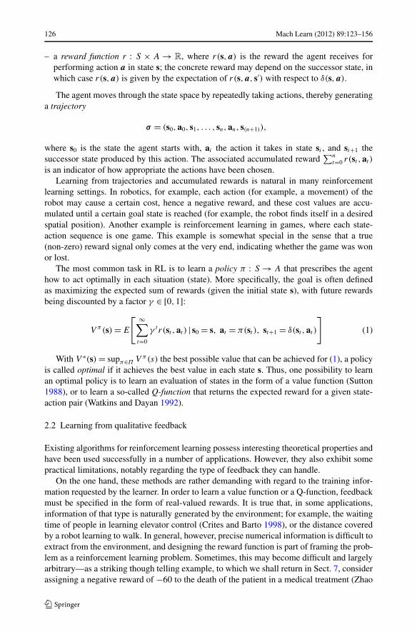
– a reward function r : S × A → R, where r(s,a) is the reward the agent receives forperforming action a in state s; the concrete reward may depend on the successor state, inwhich case r(s,a) is given by the expectation of r(s,a, s′) with respect to δ(s,a).

The agent moves through the state space by repeatedly taking actions, thereby generatinga trajectory

σ = (s0,a0, s1, . . . , sn,an, s(n+1)),

where s0 is the state the agent starts with, ai the action it takes in state si , and si+1 thesuccessor state produced by this action. The associated accumulated reward

∑n

t=0 r(st ,at )

is an indicator of how appropriate the actions have been chosen.Learning from trajectories and accumulated rewards is natural in many reinforcement

learning settings. In robotics, for example, each action (for example, a movement) of therobot may cause a certain cost, hence a negative reward, and these cost values are accu-mulated until a certain goal state is reached (for example, the robot finds itself in a desiredspatial position). Another example is reinforcement learning in games, where each state-action sequence is one game. This example is somewhat special in the sense that a true(non-zero) reward signal only comes at the very end, indicating whether the game was wonor lost.

The most common task in RL is to learn a policy π : S → A that prescribes the agenthow to act optimally in each situation (state). More specifically, the goal is often definedas maximizing the expected sum of rewards (given the initial state s), with future rewardsbeing discounted by a factor γ ∈ [0,1]:

V π(s) = E

[ ∞∑

t=0

γ t r(st ,at ) | s0 = s, at = π(st ), st+1 = δ(st ,at )

]

(1)

With V ∗(s) = supπ∈Π V π(s) the best possible value that can be achieved for (1), a policyis called optimal if it achieves the best value in each state s. Thus, one possibility to learnan optimal policy is to learn an evaluation of states in the form of a value function (Sutton1988), or to learn a so-called Q-function that returns the expected reward for a given state-action pair (Watkins and Dayan 1992).

2.2 Learning from qualitative feedback

Existing algorithms for reinforcement learning possess interesting theoretical properties andhave been used successfully in a number of applications. However, they also exhibit somepractical limitations, notably regarding the type of feedback they can handle.

On the one hand, these methods are rather demanding with regard to the training infor-mation requested by the learner. In order to learn a value function or a Q-function, feedbackmust be specified in the form of real-valued rewards. It is true that, in some applications,information of that type is naturally generated by the environment; for example, the waitingtime of people in learning elevator control (Crites and Barto 1998), or the distance coveredby a robot learning to walk. In general, however, precise numerical information is difficult toextract from the environment, and designing the reward function is part of framing the prob-lem as a reinforcement learning problem. Sometimes, this may become difficult and largelyarbitrary—as a striking though telling example, to which we shall return in Sect. 7, considerassigning a negative reward of −60 to the death of the patient in a medical treatment (Zhao

Mach Learn (2012) 89:123–156 127

et al. 2009). Likewise, in (robot) soccer, a corner ball is not as good as a goal but better thana throw-in; again, however, it is difficult to quantify the differences in terms of real numbers.

The main objective of this paper is to define a reinforcement learning framework that isnot restricted to numerical, quantitative feedback, but also able to handle qualitative feed-back expressed in the form of preferences over states, actions, or trajectories. Feedbackof this kind is more natural and less difficult to acquire in many applications. As will beseen later on, comparing pairs of actions, states or trajectories instead of evaluating themnumerically does also have a number of advantages from a learning point of view. Beforedescribing our framework more formally in Sect. 3, we discuss the problem of chess playingas a concrete example for illustrating the idea of qualitative feedback.

2.3 Example: qualitative feedback in chess

In games like chess, reinforcement learning algorithms have been successfully employedfor learning meaningful evaluation functions (Baxter et al. 2000; Beal and Smith 2001;Droste and Fürnkranz 2008). These approaches have all been modeled after the successof TD-Gammon (Tesauro 2002), a learning system that uses temporal-difference learning(Sutton 1988) for training a game evaluation function (Tesauro 1992). However, all thesealgorithms were trained exclusively on self-play, entirely ignoring human feedback that isreadily available in annotated game databases.

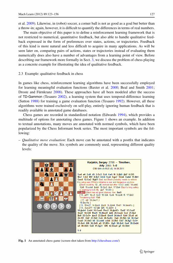
Chess games are recorded in standardized notation (Edwards 1994), which provides amultitude of options for annotating chess games. Figure 1 shows an example. In additionto textual annotations, many moves are annotated with normed symbols, which have beenpopularized by the Chess Informant book series. The most important symbols are the fol-lowing:

– Qualitative move evaluation: Each move can be annotated with a postfix that indicatesthe quality of the move. Six symbols are commonly used, representing different qualitylevels:

Fig. 1 An annotated chess game (screen-shot taken from http://chessbase.com/)

128 Mach Learn (2012) 89:123–156

– blunder (??),– bad move (?),– dubious move (?!),– interesting move (!?),– good move (!),– excellent move (!!).

– Qualitative position evaluation: Each position can be annotated with a symbol that indi-cates the qualitative value of this position:– white has decisive advantage (+−),– white has the upper hand (±),– white is better (+ =),– equal chances for both sides (=),– black is better (= +),– black has the upper hand (∓),– black has decisive advantage (−+),– the evaluation is unclear (∞).

For example, the left-hand side of Fig. 1 shows the game position after the 13th moveof white. Here, black made a mistake (13. . . g6?), but he is already in a difficult position.From the alternative moves, 13. . .a5?! is somewhat better, but even here white has the upperhand at the end of the variation (18. ec1!±). On the other hand, 13. . . ×c2?? is an evenworse choice, ending in a position that is clearly lost for black (+−).

It is important to note that this feedback is of qualitative nature, i.e., it is not clear whatthe expected reward is in terms of, e.g., percentage of won games from a position withevaluation ±. However, it is clear that positions with evaluation ± are preferable to positionswith evaluation + = or worse (=, = +, ∓, −+).

Also note that the feedback for positions typically applies to the entire sequence of movesthat has been played up to reaching this position. The qualitative position evaluations maybe viewed as providing an evaluation of the trajectory that lead to this particular position,whereas the qualitative move evaluations may be viewed as evaluations of the expected valueof a trajectory that starts at this point.

Note, however, that even though there is a certain correlation between these two typesof annotations (good moves tend to lead to better positions and bad moves tend to lead toworse positions), they are not interchangeable. A very good move may be the only movethat saves the player from imminent doom, but must not necessarily lead to a very goodposition. Conversely, a bad move may be a move that misses a chance to mate the opponentright away, but the resulting position may still be good for the player.

3 A formal framework for preference-based reinforcement learning

In this section, we define our framework in a more rigorous way. To this end, we first intro-duce a preference relation on trajectories. Based on this relation, we then derive a preferenceorder on policies, and eventually on states and actions.

3.1 Preferences over trajectories

Our point of departure is preferences over trajectories, that is, over the set Σ of all con-ceivable trajectories that may be produced by an RL agent in a certain environment.2

2Note that if S is countable and all trajectories are finite, then Σ is countable, too.

Mach Learn (2012) 89:123–156 129

Thus, our main assumption is that, given two trajectories σ ,σ ′ ∈ Σ (typically thoughnot necessarily both starting in the same initial state), a user is able to compare them interms of preference. In conventional RL, this comparison is reduced to the comparison ofthe associated (discounted) cumulative rewards: σ = (s0,a0, s1,a1, s2, . . .) is preferred toσ ′ = (s′

0,a′0, s′

1,a′1, s′

2, . . .) if the rewards accumulated along σ are higher than those accu-mulated along σ ′, that is, if

∑

t

γ t r(st ,at ) >∑

t

γ t r(s′t ,a′

t

).

The comparison of trajectories in terms of cumulative rewards immediately induces a to-tal order on Σ . Given that our qualitative framework does not necessarily allow for mappingtrajectories to real numbers, we have to relax the assumption of completeness, that is, theassumption that each pair of trajectories can be compared with each other. Instead, we onlyassume Σ to be equipped with a partial order relation , where σ σ ′ signifies that σ isat least as good as σ ′. Since the weak preference relation is only partial, it allows for theincomparability of two trajectories. More specifically, it induces a strict preference (�), anindifference (∼) and an incomparability (⊥) relation as follows:

σ � σ ′ ⇔ (σ σ ′) ∧ ¬(

σ ′ σ)

σ ∼ σ ′ ⇔ (σ σ ′) ∧ (

σ ′ σ)

σ ⊥ σ ′ ⇔ ¬(σ σ ′) ∧ ¬(

σ ′ σ)

To illustrate the idea of incomparability, consider the case where an RL agent pursues sev-eral goals simultaneously. This can be captured by means of a vector-valued reward functionmeasuring multiple instead of a single criterion, a setting known as multiobjective reinforce-ment learning (Gábor et al. 1998; Mannor and Shimkin 2004). An example of this kind willbe studied in Sect. 7 in the context of medical therapy planning. Since a trajectory σ can bebetter than a trajectory σ ′ in terms of one objective but worse with respect to another, sometrajectories may be incomparable in this setting.

3.2 Preferences over policies

What we are eventually interested in, of course, is preferences over actions or, more gen-erally, policies. Note that a policy π (together with an initial state or an initial probabilitydistribution over states) induces a probability distribution over the set Σ of trajectories. Infact, fixing a policy π means fixing a state transition function, which means that trajectoriesare produced by a simple Markov process.

What is needed, therefore, is a preference relation over P(Σ), the set of all probabilitydistributions over Σ . Again, the standard setting of RL is quite reductionistic in this regard:

1. First, trajectories are mapped to real numbers (accumulated rewards), so that the com-parison of probability distributions over Σ is reduced to the comparison of distributionsover R.

2. This comparison is further simplified by mapping probability distributions to their ex-pected value. Thus, a policy π is preferred to a policy π ′ if the expected accumulatedreward of the former is higher than the one of the latter.

130 Mach Learn (2012) 89:123–156

Since the first reduction step (mapping trajectories to real numbers) is not feasible in oursetting, we have to compare probability distributions over Σ directly. What we can exploit,nevertheless, is the order relation on Σ . Indeed, recall that a common way to compareprobability distributions on totally ordered domains is stochastic dominance. More formally,if X is equipped with a total order ≥, and P and P ′ are probability distributions on X, then P

dominates (is preferred to) P ′ if P (Xa) ≥ P ′(Xa) for all a ∈ X, where Xa = {x ∈ X |x ≥ a}.Or, to put it in words, the probability to reach a or something better is always as high underP as it is under P ′.

However, since is only a partial order, stochastic dominance cannot be applied imme-diately. What is needed, therefore, is a generalization of this concept to the case of partial or-ders: What does it mean for P to dominate P ′ if both distributions are defined on a partiallyordered set? This question is interesting and non-trivial, especially since both distributionsmay allocate probability mass on elements that are not comparable. Somewhat surprisingly,it seems that the generalization of stochastic dominance to distributions over partial ordershas not received much attention in the literature so far, with a few notable exceptions.

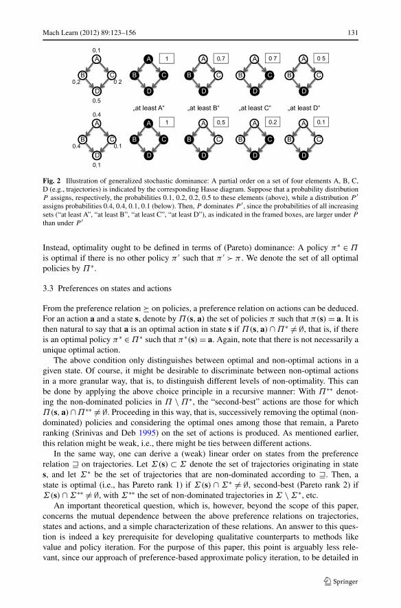
We adopt a generalization proposed by Massey (1987). Roughly speaking, the idea ofthis approach is to find a proper replacement for the (half-open) intervals Xa that are usedto define stochastic dominance in the case of total orders. To this end, he makes use of thenotion of an increasing set. For any subset Γ ⊂ Σ , let

Γ ↑ = {σ ∈ Σ |σ σ ′ for some σ ′ ∈ Γ

}.

Then, a set Γ is called an increasing set if Γ = Γ ↑. Informally speaking, this means that Γ

is an increasing set if it is closed under addition of “better” elements: For no element in Γ ,there is an element which, despite being at least as good, is not yet included.

The idea, then, is to say that a probability distribution P on Σ stochastically dominatesa distribution P ′, if P (Γ ) ≥ P ′(Γ ) for all Γ ∈ I(Σ), where I(Σ) is a suitable family ofincreasing sets of Σ . One reasonable choice of such a family, resembling the “pointwise”generation of (half-open) intervals Xa in the case of total orders through the elements a ∈ X,is

I(Σ) = {{σ }↑ |σ ∈ Σ} ∪ {Σ,∅}.

See Fig. 2 for a simple illustration.Recalling that policies are associated with probability distributions over Σ , it is clear that

a dominance relation on such distributions immediately induces a preference relation � onthe class Π of policies: π � π ′ if the probability distribution associated with π dominatesthe one associated with π ′. It is also obvious that this relation is reflexive and antisymmetric.An important question, however, is whether it is also transitive, and hence a partial order.This is definitely desirable, and in fact already anticipated by the interpretation of � as apreference relation.

Massey (1987) shows that the above dominance relation is indeed transitive, providedthe family I(Σ) fulfills two technical requirements. First, it must be strongly separating,meaning that whenever σ � σ ′, there is some Γ ∈ I(Σ) such that σ ′ ∈ Γ and σ �∈ Γ (thatis, if σ ′ is not worse than σ , then it can be separated from σ ). The second condition is thatI (Σ) is a determining class, which, roughly speaking, means that it is sufficiently rich, sothat each probability measure is uniquely determined by its values on the sets in I (Σ).

In summary, provided these technical conditions are met, the partial order on the setof trajectories Σ that we started with induces a partial order � on the set of policies Π .Of course, since � is only a partial order, there is not necessarily a unique optimal policy.

Mach Learn (2012) 89:123–156 131

Fig. 2 Illustration of generalized stochastic dominance: A partial order on a set of four elements A, B, C,D (e.g., trajectories) is indicated by the corresponding Hasse diagram. Suppose that a probability distributionP assigns, respectively, the probabilities 0.1, 0.2, 0.2, 0.5 to these elements (above), while a distribution P ′assigns probabilities 0.4, 0.4, 0.1, 0.1 (below). Then, P dominates P ′ , since the probabilities of all increasingsets (“at least A”, “at least B”, “at least C”, “at least D”), as indicated in the framed boxes, are larger under P

than under P ′

Instead, optimality ought to be defined in terms of (Pareto) dominance: A policy π∗ ∈ Π

is optimal if there is no other policy π ′ such that π ′ � π . We denote the set of all optimalpolicies by Π∗.

3.3 Preferences on states and actions

From the preference relation � on policies, a preference relation on actions can be deduced.For an action a and a state s, denote by Π(s,a) the set of policies π such that π(s) = a. It isthen natural to say that a is an optimal action in state s if Π(s,a) ∩ Π∗ �= ∅, that is, if thereis an optimal policy π∗ ∈ Π∗ such that π∗(s) = a. Again, note that there is not necessarily aunique optimal action.

The above condition only distinguishes between optimal and non-optimal actions in agiven state. Of course, it might be desirable to discriminate between non-optimal actionsin a more granular way, that is, to distinguish different levels of non-optimality. This canbe done by applying the above choice principle in a recursive manner: With Π∗∗ denot-ing the non-dominated policies in Π \ Π∗, the “second-best” actions are those for whichΠ(s,a) ∩ Π∗∗ �= ∅. Proceeding in this way, that is, successively removing the optimal (non-dominated) policies and considering the optimal ones among those that remain, a Paretoranking (Srinivas and Deb 1995) on the set of actions is produced. As mentioned earlier,this relation might be weak, i.e., there might be ties between different actions.

In the same way, one can derive a (weak) linear order on states from the preferencerelation on trajectories. Let Σ(s) ⊂ Σ denote the set of trajectories originating in states, and let Σ∗ be the set of trajectories that are non-dominated according to . Then, astate is optimal (i.e., has Pareto rank 1) if Σ(s) ∩ Σ∗ �= ∅, second-best (Pareto rank 2) ifΣ(s) ∩ Σ∗∗ �= ∅, with Σ∗∗ the set of non-dominated trajectories in Σ \ Σ∗, etc.

An important theoretical question, which is, however, beyond the scope of this paper,concerns the mutual dependence between the above preference relations on trajectories,states and actions, and a simple characterization of these relations. An answer to this ques-tion is indeed a key prerequisite for developing qualitative counterparts to methods likevalue and policy iteration. For the purpose of this paper, this point is arguably less rele-vant, since our approach of preference-based approximate policy iteration, to be detailed in

132 Mach Learn (2012) 89:123–156

Sect. 5, is explicitly based on the construction and evaluation of trajectories through roll-outs. The idea, then, is to learn the above linear order (ranking) of actions (as a function ofthe state) from these trajectories. A suitable learning method for doing so will be introducedin Sect. 5.

Finally, we note that learning a ranking function of the above kind is also a viable optionin the standard setting where rewards are numerical, and policies can therefore be evaluatedin terms of expected cumulative rewards (instead of being compared in terms of generalizedstochastic dominance). In fact, the case study presented in Sect. 6 will be of that type.

4 Preference learning and label ranking

The topic of preference learning has attracted considerable attention in machine learningin recent years (Fürnkranz and Hüllermeier 2010). Roughly speaking, preference learning isabout inducing predictive preference models from empirical data, thereby establishing a linkbetween machine learning and research fields related to preference modeling and decisionmaking.

4.1 Utility Functions vs. preference relations

There are two main approaches to representing preferences, namely in terms of

– utility functions evaluating individual alternatives, and– preference relations comparing pairs of competing alternatives.

The first approach is quantitative in nature, in the sense that a utility function is normallya mapping from alternatives to real numbers. This approach is in line with the standardRL setting: A value V (s) assigned to a state s by a value function V can be seen as autility of that state. Likewise, a Q-function assigns a degree of utility to an action, namely,Q(s,a) is the utility of choosing action a in state s. The second approach, on the otherhand, is qualitative in nature, as it is based on comparing alternatives in terms of qualitativepreference relations.3 The main idea of our paper is to exploit such a qualitative approach inthe context of RL.

From a machine learning point of view, the two approaches give rise to two kinds oflearning problems: learning utility functions and learning preference relations. The latterdeviates more strongly than the former from conventional problems like classification andregression, as it involves the prediction of complex structures, such as rankings or partialorder relations, rather than single values. Moreover, training input in preference learningwill not, as it is usually the case in supervised learning, be offered in the form of completeexamples but may comprise more general types of information, such as relative preferencesor different kinds of indirect feedback and implicit preference information.

4.2 Label ranking

Among the problems in the realm of preference learning, the task of “learning to rank” hasprobably received the most attention in the machine learning literature so far. In general, apreference learning task consists of some set of items for which preferences are known, and

3Although the valuation of such relations is possible, too.

Mach Learn (2012) 89:123–156 133

the task is to learn a function that predicts preferences for a new set of items, or for the sameset of items in a different context. The preferences can be among a set of objects, in whichcase we speak of object ranking (Kamishima et al. 2011), or among a set of labels that areattached to a set of objects, in which case we speak of label ranking (Vembu and Gärtner2011).

The task of a policy is to pick one of a set of available actions for a given state. Thissetting can be nicely represented as a label ranking problem, where the task is to rank a setof actions (labels) in dependence of a state description (object). More formally, assume to begiven an instance space X and a finite set of labels Y = {y1, y2, . . . , yk}. In label ranking, thegoal is to learn a “label ranker” in the form of an X → SY mapping, where the output spaceSY is given by the set of all total orders (permutations) of the set of labels Y . Thus, labelranking can be seen as a generalization of conventional classification, where a completeranking of all labels

yτ−1

x (1)�x y

τ−1x (2)

�x · · · �x yτ−1

x (k)

is associated with an instance x instead of only a single class label. Here, τx is a permutationof {1,2, . . . , k} such that τx(i) is the position of label yi in the ranking associated with x.

The training data E used to induce a label ranker typically consists of a set of pairwisepreferences of the form yi �x yj , suggesting that, for instance x, yi is preferred to yj . Inother words, a single “observation” consists of an instance x together with an ordered pairof labels (yi, yj ).

4.3 Learning by pairwise comparison

Several methods for label ranking have already been proposed in the literature; we refer toVembu and Gärtner (2011) for a comprehensive survey. In this paper, we chose learning bypairwise comparison (LPC; Hüllermeier et al. 2008), but other choices would be possible.The key idea of LPC is to train a separate model Mi,j for each pair of labels (yi, yj ) ∈ Y ×Y ,1 ≤ i < j ≤ k; thus, a total number of k(k − 1)/2 models is needed. At prediction time, aquery x is submitted to all models, and each prediction Mi,j (x) is interpreted as a votefor a label. More specifically, assuming scoring classifiers that produce normalized scoresfi,j = Mi,j (x) ∈ [0,1], the weighted voting technique interprets fi,j and fj,i = 1 − fi,j asweighted votes for classes yi and yj , respectively, and orders the labels according to theaccumulated voting mass F(yi) = ∑

j �=i fi,j .Note that the total complexity for training the quadratic number of classifiers of the LPC

approach is only linear in the number of observed preferences (Hüllermeier et al. 2008).More precisely, the learning complexity of LPC is O(n × d), where n is the number oftraining examples, and d is the average number of preferences that have been observed perstate. In the worst case (for each training example we observe a total order of the labels), d

can be as large as k · (k − 1)/2 (k being the number of labels). However, in many practicalproblems, it is considerably smaller.

Querying the quadratic number of classifiers can also be sped up considerably so thatthe best label y∗ = arg maxy F (y) can be determined after querying only approximatelyk · log(k) classifiers (Park and Fürnkranz 2012). Thus, the main obstacle for tackling large-scale problems with LPC is the memory required for storing the quadratic number of classi-fiers. Nevertheless, Loza Mencía et al. (2010) have shown that it is applicable to multilabelproblems with up to half a million examples and up to 1000 labels.

We refer to Hüllermeier et al. (2008) for a more detailed description of LPC in generaland a theoretical justification of the weighted voting procedure in particular. We shall use

134 Mach Learn (2012) 89:123–156

label ranking techniques in order to realize our idea of preference-based approximate policyiteration, which is described in the next section.

5 Preference-based approximate policy iteration

In Sect. 3, we have shown that qualitative feedback based on preferences over trajectoriesmay serve as a theoretical foundation of preference-based reinforcement learning. Morespecifically, our point of departure is a preference relation on trajectories: σ � σ ′ indicatesthat trajectory σ is preferred to σ ′, and we assume that preference information of that kindcan be obtained from the environment. From preferences over trajectories, we then derivedpreferences over policies and preferences over actions given states.

Within this setting, different variants of preference-based reinforcement learning are con-ceivable. For example, tracing observed preferences on trajectories back to preferences oncorresponding policies, it would be possible to search the space of policies directly or, morespecifically, to train a ranking function that sorts policies according to their preference as inAkrour et al. (2011).

Here, we tackle the problem in a different way. Instead of learning preferences on policiesdirectly, we seek to learn (local) preferences on actions given states. What is needed, there-fore, is training information of the kind a �s a′, suggesting that in state s, action a is betterthan a′. Following the idea of approximate policy iteration (Sect. 5.1), we induce such pref-erences from preferences on trajectories via simulation (called “roll-outs” later on): Takings as an initial state, we systematically compare the trajectories generated by taking action afirst (and following a given policy thereafter) with the trajectories generated by taking actiona′ first; this is possible thanks to the preference relation � on trajectories that we assume tobe given (Sect. 5.3).

The type of preference information thus produced, a �s a′, exactly corresponds to thetype of training information assumed by a label ranker (Sect. 4.2). Indeed, our idea is totrain a ranker of that kind, that is, a mapping from states to rankings over the set of actions(Sect. 5.2). This can be seen as a generalization of the original approach to approximatepolicy iteration, in which a classifier is trained that maps states to single actions. As will beshown later on, by replacing a classifier with a label ranker, our preference-based variantof approximate policy iteration enjoys a number of advantages compared to the originalversion.

5.1 Approximate policy iteration

Instead of determining optimal actions indirectly through learning the value function or theQ-function, one may try to learn a policy directly in the form of a mapping from states toactions. We will briefly review such approaches in Sects. 8.1 and 8.2. Our work is basedon approximate policy iteration (Lagoudakis and Parr 2003; Dimitrakakis and Lagoudakis2008). The key idea of this approach is to iteratively train a policy using conventional ma-chine learning algorithms. This approach assumes access to a generative model E of theunderlying process, i.e., a model which takes a state s and an action a as input and returns asuccessor state s′ and the reward r(s,a). The key idea, then, is to use this generative modelto perform simulations—so-called roll-outs—that in turn allow for approximating the valueof an action in a given state (Algorithm 1). To this end, the action is performed, resulting ina state s1 = δ(s,a). This is repeated K times, and the average reward over these K roll-outsis used to approximate the Q-value Q̃π (s0,a) for taking action a in state s0 (leading to s1)and following policy π thereafter.

Mach Learn (2012) 89:123–156 135

Algorithm 1 ROLLOUT(E, s1, γ,π,K,L): Estimation of state valuesRequire: generative environment model E, sample state s1, discount factor γ , policy π ,

number of trajectories/roll-outs K , max. length/horizon of each trajectory L

for k = 1 to K dos ← s1, Q̃k ← 0, t ← 1while t < L and ¬TERMINALSTATE(s) do

(s′, r) ← SIMULATE(E, s,π(s))Q̃k ← Q̃k + γ t r

s ← s′, t ← t + 1end while

end for

Q̃ = 1K

∑K

k=1 Q̃k

return Q̃

Algorithm 2 Multi-class variant of Approx. Policy Iteration with Roll-Outs (Lagoudakisand Parr 2003)Require: generative environment model E, sample states S ′, discount factor γ , initial (ran-

dom) policy π0, number of trajectories/roll-outs K , max. length/horizon of each trajec-tory L, max. number of policy iterations p

1: π ′ ← π0, i ← 02: repeat3: π ← π ′, E ← ∅4: for all s ∈ S ′ do5: for all a ∈ A do6: (s′, r) ← SIMULATE(E, s,a) {do (possibly off-policy) action a}7: Q̃π (s,a) ← ROLLOUT(E, s′, γ,π,K,L) + r {estimate state-action value}8: end for

9: a∗ ← arg maxa∈A Q̃π (s,a)

10: if Q̃π (s,a∗) >L Q̃π(s,a) for all a ∈ A,a �= a∗ then {please see text for >L}11: E ← E ∪ {(s,a∗)}12: end if

13: end for14: π ′ ← LEARN(E ), i ← i + 115: until STOPPINGCRITERION(E,π,π ′,p, i)

These roll-outs are used in a policy iteration loop (Algorithm 2), which iterates througheach state in a set of sample states S ′ ⊂ S, simulates all actions in this state, and determinesthe action a∗ that promises the highest Q-value. If a∗ is significantly better than all alternativeactions in this state, (indicated with the symbol >L in line 10), a training example (s,a∗)is added to a training set E . Eventually, E is used to directly learn a mapping from states toactions, which forms the new policy π ′. This process is repeated several times, until somestopping criterion is met (e.g., if the policy does not improve from one iteration to the next).

The choice of the sampling procedure to generate the state sample S ′ is not a trivial taskas discussed in Lagoudakis and Parr (2003), Dimitrakakis and Lagoudakis (2008). Choices

136 Mach Learn (2012) 89:123–156

Algorithm 3 Preference-Based Approximate Policy Iteration.

Require: sample states S ′, initial (random) policy π0, max. number of policy iterations p,procedure EVALUATEPREFERENCE for determining the preference between a pair ofactions for a given policy in a given state.

1: π ′ ← π0, i ← 02: repeat3: π ← π ′, E ← ∅4: for all s ∈ S ′ do5: for all (ak,aj ) ∈ A × A do6: EVALUATEPREFERENCE(s,ak,aj , π)

7: if ak �s aj then8: E ← E ∪ {(s,ak � aj )}9: end if

10: end for11: end for12: π ′ ← LEARNLABELRANKER(E ), i ← i + 113: until STOPPINGCRITERION(π,π ′,p, i)

of procedures range from simple uniform sampling of the state space to sampling schemesincorporating domain-expert knowledge and other more sophisticated schemes. We empha-size that we do not contribute to this aspect and will use in this work rather simple samplingschemes, which will be described in detail in the experimental sections.

We should note some minor differences between the version presented in Algorithm 2and the original formulation (Lagoudakis and Parr 2003). Most notably, the training set hereis formed as a multi-class training set, whereas in Lagoudakis and Parr (2003) it was formedas a binary training set, learning a binary policy predicate π̂ : S × A → {0,1}. We chosethe more general multi-class representation because, as we will see in the following, it lendsitself to an immediate generalization to a ranking scenario.

5.2 Preference-based approximate policy iteration

Following our idea of preference-based RL, we propose to train a label ranker instead ofa classifier: Using the notation from Sect. 4.2 above, the instance space X is given by thestate space S, and the set of labels Y corresponds to the set of actions A. Thus, the goalis to learn a mapping S → SA, which maps a given state to a total order (permutation) ofthe available actions. In other words, the task of the learner is to learn a function that isable to rank all available actions in a state. The training information is provided in the formof binary action preferences of the form (s,ak � aj ), indicating that in state s, action ak ispreferred to action aj .

Algorithm 3 shows a high-level view of the preference-based approximate policy itera-tion algorithm PBPI. Like Algorithm 2, it starts with a random policy π0 and continuouslyimproves this policy by collecting experience on a set of sample states S ′ ⊂ S. However,in each state s, PBPI does not evaluate each individual action a, but pairs of preferences(ak,aj ). For each such pair of preferences, we then call a routine EVALUATEPREFERENCE

which determines whether ak � aj holds in state s or not. If it holds, the training example(s,ak � aj ) is added to the training set E . If all states in S ′ have been evaluated in that way,a new policy in the form of a label ranker is learned from E . This process is iterated until thepolicies converge or a predetermined number p of iterations has been reached.

Mach Learn (2012) 89:123–156 137

Note that in practice, looping through all pairs of actions may not be necessary. Forexample, in our motivating chess example, preferences may only be available for a fewaction pairs per state, and it might be more appropriate to directly enumerate the preferences.Thus, the complexity of this algorithm is essentially O(|S ′| · d), where d is the averagenumber of observed preferences per state (the constant number of iterations is hidden in theO(.) notation). This complexity directly corresponds to the complexity of LPC as discussedin Sect. 4.3. If a total order of actions is observed in each state (as is the case in the studyin Sect. 6), the complexity may become as bad as linear in the number of visited statesand quadratic in the number of actions. However, if only a few preferences per state can beobserved (as is e.g., the case in our motivating chess example), the complexity is only linearin the number of visited states |S ′| and essentially independent of the number of actions(e.g. if we only compare a single pair of actions for each state). Of course, in the latter case,we might need considerably more iterations to converge, but this cannot be solved withthe choice of a different label ranking algorithm. Thus, we recommend the use of LPC forsettings where very few action preferences are observed per state. Its use is not advisablefor problems with very large action spaces, because the storage of a quadratic number ofclassifiers may become problematic in such cases.

5.3 Using roll-out-based preferences

The key point of the algorithm is the implementation of EVALUATEPREFERENCE, whichdetermines the preference between two actions in a state. We follow the work on approxi-mate policy iteration and choose a roll-out based approach. Recall the scenario described atthe end of Sect. 5.1, where the agent has access to a generative model E, which takes a states, and an action a as input and returns a successor state s′ and the reward r(s,a). Lagoudakisand Parr (2003) use this setting for generating training examples via roll-outs, i.e., by usingthe generative model and the current policy π for generating a training set E , which is inturn used for training a multi-class classifier that can be used as a policy. Instead of traininga classifier on the optimal action in each state, we can instead use the PBPI algorithm totrain a label ranker on all pairwise comparisons of actions in each state.

Note that generating roll-out based training information for PBPI is no more expensivethan generating the training information for API, because in both cases all actions in a statehave to be run for a number of iterations. On the contrary, we argue that from a trainingpoint of view, a key advantage of this approach is that pairwise preferences are much easierto elicit than examples for unique optimal actions. Our experiments in Sects. 6 and 7 utilizethis in different ways.

The preference relation over actions can be derived from the roll-outs in different ways.In particular, we can always reduce the conventional utility-based setting to this particularcase by defining the preference ak �s aj as “in state s, policy π gives a higher expectedreward for ak than for aj ”. This is the approach that we evaluate in Sect. 6.

An alternative approach is to count the success of each of the two actions ak and aj instate s, and perform a sign test for determining the overall preference. This approach allowsto entirely omit the aggregation of utility values and instead only aggregates preferences. Inpreliminary experiments, we noted essentially the same qualitative results as those reportedbelow. The results are, however, not directly comparable to the results of approximate policyiteration, because the sign test is more conservative than the t -test, which is used in API.However, the key advantage of this approach is that we can also use it in cases of non-numerical rewards. This is crucial for the experiments reported in Sect. 7, where we takethis approach.

138 Mach Learn (2012) 89:123–156

Section 6 demonstrates that a comparison of only two actions is less difficult than “prov-ing” the optimality of one among a possibly large set of actions, and that, as a result, ourpreference-based approach better exploits the gathered training information. Indeed, the pro-cedure proposed by Lagoudakis and Parr (2003) for forming training examples is very waste-ful with this information. An example (s,a∗) is only generated if a∗ is “provably” the bestaction among all candidates, namely if it is (significantly) better than all other actions in thegiven state. Otherwise, if this superiority is not confirmed by a statistical hypothesis test,all information about this state is ignored. In particular, no training examples would be gen-erated in states where multiple actions are optimal, even if they are clearly better than allremaining actions.4 For the preference-based approach, on the other hand, it suffices if onlytwo possible actions ak and aj yield a clear preference (either ak � aj or aj � ak) in order toobtain (partial) training information about that state. Note that a corresponding comparisonmay provide useful information even if both actions are suboptimal.

In Sect. 7, an example will be shown in which actions are not necessarily comparable,since the agent seeks to optimize multiple criteria at the same time (and is not willing toaggregate them into a one-dimensional target). In general, this means that, while at leastsome of the actions will still be comparable in a pairwise manner, a unique optimal actiondoes not exist.

Regarding the type of prediction produced, it was already mentioned earlier that aranking-based reinforcement learner can be seen as a reasonable compromise between theestimation of a numerical utility function (like in Q-learning) and a classification-based ap-proach which provides only information about the optimal action in each state: the agenthas enough information to determine the optimal action, but can also rely on the ranking inorder to look for alternatives, for example to steer the exploration towards actions that areranked higher. We will briefly return to this topic at the end of the next section. Before that,we will discuss the experimental setting in which we evaluate the utility of the additionalranking-based information.

6 Case study I: exploiting action preferences

In this section, we compare three variants of approximate policy iteration following Algo-rithms 2 and 3. They only differ in the way in which they use the information gathered fromthe performed roll-outs.

Approximate Policy Iteration (API) generates one training example (s,a∗) if a∗ is the bestavailable action in s, i.e., if Q̃π (s,a∗) >L Q̃π(s,a) for all a �= a∗. If there is no action thatis better than all alternatives, no training example is generated for this state.

Pairwise Approximate Policy Iteration (PAPI) works in the same way as API, but the under-lying base learning algorithm is replaced with a label ranker. This means that each trainingexample (s,a∗) of API is transformed into a − 1 training examples of the form (s,a∗ � a)

for all a �= a∗.Preference-Based Approximate Policy Iteration (PBPI) is trained on all available pairwise

preferences, not only those involving the best action. Thus, whenever Q̃π (s,ak) >L

Q̃π(s,al ) holds for a pair of actions (ak,al ), PBPI generates a corresponding training ex-ample (s,ak � al ).

4In the original formulation as a binary problem, it is still possible to produce negative examples, whichindicate that the given action is certainly not the best action (because it was significantly worse than the bestaction).

Mach Learn (2012) 89:123–156 139

Fig. 3 Comparing actions in terms of confidence intervals on expected rewards: Although a best actioncannot be identified uniquely, pairwise preferences like a1 � a3 and a2 � a4 can still be derived

Note that, in the last setting, an example (s,ak � al ) can be generated although ak isnot the best action. In particular, in contrast to PAPI, it is not necessary that there is a clearbest action in order to generate training examples. Consequently, from the same roll-outs,PBPI will typically generate more training information than PAPI or API (see Fig. 3). Thisis actually an interesting illustration of the increased flexibility of preference-based traininginformation: Even if there might be no obvious “correct” alternative, some options may stillbe preferred to others.

The problems we are going to tackle in this section do still fall into the standard frame-work of reinforcement learning. Thus, rewards are numerical, trajectories are evaluated byaccumulated rewards, and policies by expected cumulative discounted rewards. The reasonis that, otherwise, it is not possible to compare with the original approach to approximatepolicy iteration. Nevertheless, as will be seen, preference-based learning from qualitativefeedback can even be useful in this setting.

6.1 Application Domains

Following Dimitrakakis and Lagoudakis (2008), we evaluated these variants on two well-known problems, inverted pendulum and mountain car. We will briefly recapitulate thesetasks, which were used in their default setting, unless stated otherwise.

In the inverted pendulum problem, the task is to push or pull a cart so that it balances anupright pendulum. The available actions are to apply a force of fixed strength of 50 Newtonto the left (−1), to the right (+1) or to apply no force at all (0). The mass of the pole is 2 kgand of the cart 9 kg. The pole has a length of 0.5 m and each time step is set to 0.1 seconds.Following Dimitrakakis and Lagoudakis (2008), we describe the state of the pendulum usingonly the angle and angular velocity of the pole, ignoring the position and the velocity of cart.For each time step, where the pendulum is above the horizontal line, a reward of 1 was given,else 0. A policy was considered sufficient, if it is able to balance the pendulum longer than1000 steps (100 sec). The random samples S in this setting were generated by simulating auniform random number (max 100) of uniform random actions from the initial state (polestraight up, no velocity for cart and pole). If the pendulum fell within this sequence, theprocedure was repeated.

In the mountain car problem, the task is to drive a car out of a steep valley. To do so, ithas to repeatedly go up on each side of the hill, gaining momentum by going down and upto the other side, so that eventually it can get out. Again, the available actions are (−1) forleft or backward and (+1) for right or forward and (0) for a fixed level of throttle. The statesor feature vectors consist of the horizontal position and the current velocity of the car. Here,the agent received a reward of −1 in each step until the goal was reached. A policy whichneeded less than 75 steps to reach the goal was considered as sufficient. For this setting,the random samples S were generated by uniform sampling over valid horizontal positions(excluding the goal state) and valid velocities.

140 Mach Learn (2012) 89:123–156

6.2 Experimental setup

In addition to these conventional formulations using three actions in each state, we also usedversions of these problems with 5, 9, and 17 actions, because in these cases it becomes lessand less likely that a unique best actions can be found, and the benefit from being able toutilize information from states where no clear winner emerges increases. The range of theoriginal action set {−1,0,1} was partitioned equidistantly into the given number of actions,for e.g., using 5 actions, the set of action signals is {−1,−0.5,0,0.5,1}. Also, a uniformnoise term in [−0.2,0.2] was added to the action signal, such that all state transitions arenon-deterministic. For training the label ranker we used LPC (cf. Sect. 4.2) and for all threeconsidered variants simple multi-layer perceptrons (as implemented in the Weka machinelearning library (Hall et al. 2009) with its default parameters) was used as (base) learningalgorithm. The discount factor for both settings was set to 1 and the maximal length of thetrajectory for the inverted pendulum task was set to 1500 steps and 1000 for the mountaincar task. The policy iteration algorithms terminated if the learned policy was sufficient orif the policy performance decreased or if the number of policy iterations reached 10. Forthe evaluation of the policy performance, 100 simulations beginning from the correspond-ing initial states were utilized. Furthermore, for statistical testing unpaired t-tests assumingequal variance (homoscedastic t-test) were used.

For each task and method, the following parameter settings were evaluated:

– five numbers of state samples |S| ∈ {10,20,50,100,200},– five maximum numbers of roll-outs K ∈ {10,20,50,100,200},– three levels of significance c ∈ {0.025,0.05,0.1}.Each of the 5 × 5 × 3 = 75 parameter combinations was evaluated ten times, such that thetotal number of experiments per learning task was 750. We tested both domains, mountaincar and inverted pendulum, with |A| ∈ {3,5,9,17} different actions each.

6.3 Evaluation

Our prime evaluation measure is the success rate (SR), i.e., the percentage of learned suf-ficient policies. Following Dimitrakakis and Lagoudakis (2008), we plot a cumulative dis-tribution of the success rates of all different parameter settings over a measure of learningcomplexity, where each point (x, y) indicates the minimum complexity x needed to reach asuccess rate of y. However, while Dimitrakakis and Lagoudakis (2008) simply use the num-ber of roll-outs (i.e., the number of sampled states) as a measure of learning complexity, weuse the number of performed actions over all roll-outs, which is a more fine-grained com-plexity measure. The two would coincide if all roll-outs are performed a constant number oftimes. However, this is typically not the case, as some roll-outs may stop earlier than others.Thus, we generated graphs by sorting all successful runs over all parameter settings (i.e.,runs which yielded a sufficient policy) in increasing order regarding the number of appliedactions and by plotting these runs along the x-axis with a y-value corresponding to its cu-mulative success rate. This visualization can be interpreted roughly as the development ofthe success rate in dependence of the applied learning complexity.

6.4 Complete state evaluations

Figure 4 shows the results for the inverted pendulum and the mountain car tasks. One canclearly see that for an increasing number of actions, PBPI reaches a significantly higher

Mach Learn (2012) 89:123–156 141

Fig. 4 Comparison of API, PAPI and PBPI for the inverted pendulum task (left) and the mountain car task(right). The number of actions is increasing from top to bottom

142 Mach Learn (2012) 89:123–156

Table 1 Training information generation for API, PAPI and PBPI. For each algorithm, we show the fractionof training states that could be used, as well as the fraction of the 1

2 · |A| · (|A| − 1) possible preferences thatcould on average be generated from a training state. Note that the values for PAPI are only approximatelytrue (the measures are taken from the API experiments and may differ slightly due to random issues)

|A| API/PAPI PBPI

States Preferences States Preferences

IP 3 0.589 ± 0.148 0.393 ± 0.099 0.736 ± 0.108 0.631 ± 0.119

5 0.400 ± 0.162 0.160 ± 0.065 0.759 ± 0.101 0.581 ± 0.128

9 0.273 ± 0.154 0.061 ± 0.034 0.776 ± 0.087 0.543 ± 0.124

MC 3 0.316 ± 0.218 0.211 ± 0.145 0.453 ± 0.245 0.349 ± 0.229

5 0.231 ± 0.181 0.093 ± 0.072 0.510 ± 0.263 0.311 ± 0.216

9 0.149 ± 0.125 0.033 ± 0.028 0.539 ± 0.273 0.281 ± 0.201

success rate than the two alternative approaches, and it typically also has a much fasterlearning curve, i.e., it needs to take fewer actions to reach a given success rate. Anotherinteresting point is that the maximum success level decreases with an increasing number ofactions for API and PAPI, but it remains essentially constant for PBPI. Overall, these resultsclearly demonstrate that the additional information about comparisons of lower-ranked ac-tion pairs, which is ignored in API and PAPI, can be put to effective use when approximatepolicy iteration is extended to use a label ranker instead of a mere classifier.

Part of the problem is that API and PAPI are very wasteful with sample states. The thirdcolumn of Table 1 shows the fraction of states for which a training example could be gen-erated, i.e., for which one action turned out to be significantly better than all other actions.It can be clearly seen that this fraction decreases with the number of available actions ineach problem (shown in the second column). It is not surprising that the number of trainingstates from which PBPI could generate at least a training preference (column 5 of Table 1) ishigher than API and PAPI in all cases. PBPI can generate some training information from astate when at least one pair of actions yields a significant difference, whereas API and PAPIonly uses a state if one action is better than all other actions. Thus, this quantity is at least theamount of API/PAPI. The result that this quantity for PBPI is non-decreasing for increasingnumber of actions may be explained by the fact that to some extent a found preference fora given number of actions |A| for a particular state is also existent in the next setting with ahigher number of actions |A′|. Here, the set of possible preferences of A is a subset of thepossible preferences of A′.

However, even if we instead look at the fraction of possible preferences that could beused, we see that there is only a small decay for the PBPI. This decay can be explained bythe fact that the more actions we have in the mountain car and inverted pendulum problems,the more similar they are to each other and the more likely it is that we can detect actionspairs that have approximately the same quality and cannot be discriminated via roll-outs.For API and PAPI, on the other hand, the decay in the number of generated preferences isthe same as with the number of usable states, because each usable training state producesexactly |A| − 1 preferences.5 Thus, the fourth column differs from the third by a factorof |A|/2.

5Strictly speaking, only the best action for each state is generated and used within API, but for the sake ofcomparison in terms of preferences this directly relates to |A| − 1 preferences involving the best action.

Mach Learn (2012) 89:123–156 143

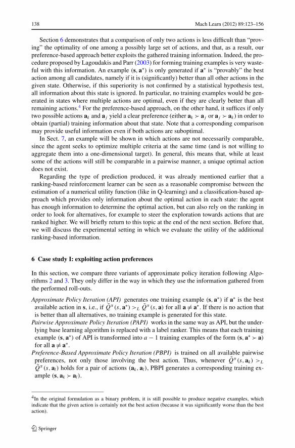
Fig. 5 Comparison of complete state evaluation (PBPI) with partial state evaluation in three variants(PBPI-1, PBPI-2, PBPI-3)

6.5 Partial state evaluations

So far, based on the API strategy, we always evaluated all possible actions at each state,and generated preferences from their pairwise comparisons. A possible advantage of thepreference-based approach is that it does not need to evaluate all options at a given state.In fact, one could imagine to select only two actions for a state and compare them via roll-outs. While such a partial state evaluation will, in general, not be sufficient for generating atraining example for API, it suffices to generate a training preference for PBPI. Thus, sucha partial PBPI strategy also allows for considering a far greater number of states, using thesame number of roll-outs, at the expense that not all actions of each state will be explored.Such an approach may thus be considered to be orthogonal to recent approaches for roll-outallocation strategies (cf. Sect. 8.2).

In order to investigate this effect, we also experimented with three partial variants ofPBPI, which only differ in the number of states that they are allowed to visit. The first(PBPI-1) allows the partial PBPI variant to visit only the same total number of states as PBPI.The second (PBPI-2) adjusts the number of visited sample states by multiplying it with |A|

2 ,to account for the fact that the partial variant performs only 2 action roll-outs in each state, asopposed to |A| action roll-outs for PBPI. Thus, the total number of action roll-outs in PBPIand PBPI-2 is constant. Finally, for the third variant (PBPI-3), we assume that the numberof preferences that are generated from each state is constant. While PBPI generates up to|A|(|A|−1)

2 preferences from each visited state, partial PBPI generates only one preferenceper state, and is thus allowed to visit |A|(|A|−1)

2 as many states. These modifications wereintegrated into Algorithm 2 by adapting Line 5 to iterate only over two randomly chosenactions and changing the number of considered sample states S to the values as describedabove.

Figure 5 shows the results for the inverted pendulum with five different actions (theresults for the other problems are quite similar). The left graph shows the success rate overthe total number of taken actions, whereas the right graph shows the success rate over thetotal number of training preferences. From the right graph, no clear differences can be seen.In particular, the curves for PBPI-3 and PBPI almost coincide. This is not surprising, becauseboth generate the same number of preference samples, albeit for different random states.However, the left graph clearly shows that the exploration policies that do not generate allaction roll-outs for each state are more wasteful with respect to the total number of actionsthat have to be taken in the roll-outs. Again, this is not surprising, because evaluating all

144 Mach Learn (2012) 89:123–156

five actions in a state may generate up to 10 preferences for a single state, or, in the case ofPBPI-2, only a total of 5 preferences if 2 actions are compared in each of 5 states.

Nevertheless, the results demonstrate that partial state evaluation is feasible. This mayform the basis of novel algorithms for exploring the state space. We will briefly return tothis issue in Sect. 8.2.

7 Case study II: learning from qualitative feedback

In a second experiment, we applied preference-based reinforcement learning to a simulationof optimal therapy design in cancer treatment, using a model that was recently proposedin Zhao et al. (2009). In this domain, it is arguably more natural to define preferences thatinduce a partial order between states than to define an artificial numerical reward functionthat induces a total order between states.

7.1 Cancer clinical trials domain

The model proposed in Zhao et al. (2009) captures a number of essential factors in cancertreatment: (i) the tumor growth during the treatment; (ii) the patient’s (negative) wellness,measured in terms of the level of toxicity in response to chemotherapy; (iii) the effect ofthe drug in terms of its capability to reduce the tumor size while increasing toxicity; (iv)the interaction between the tumor growth and patient’s wellness. The two state variables,the tumor size Y and the toxicity X, are modeled using a system of difference equations:Yt+1 = Yt + ΔYt and Xt+1 = Xt + ΔXt , where the time variable t denotes the number ofmonths after the start of the treatment and assumes values t = 0,1, . . . ,6. The terms ΔY

and ΔX indicate the increments of the state variables that depend on the action, namelythe dosage level D, which is a number between 0 and 1 (minimum and maximum dosage,respectively):

ΔYt = [a1 · max(Xt ,X0) − b1 · (Dt − d1)

] × 1(Yt > 0)

ΔXt = a2 · max(Yt , Y0) + b2 · (Dt − d2)(2)

These changing rates produce a piecewise linear model over time. We fix the parametervalues following the recommendation of Zhao et al. (2009): a1 = 0.15, a2 = 0.1, b1 = b2 =1.2 and d1 = d2 = 0.5. By using the indicator term 1(Yt > 0), the model assumes that oncethe patient has been cured, namely the tumor size is reduced to 0, there is no recurrence. Notethat this system does not reflect a specific cancer but rather models the generic developmentof the chemotherapy process.

The possible death of a patient in the course of a treatment is modeled by means of ahazard rate model. For each time interval (t − 1, t], this rate is defined as a function oftumor size and toxicity: λ(t) = exp(c0 + c1Yt + c2Xt), where c0, c1, c2 are cancer-dependentconstants. Again following Zhao et al. (2009), we let c0 = −4, c1 = c2 = 1. By setting c1 =c2, the tumor size and the toxicity have an equally important influence on patient’s survival.The probability of the patient’s death during the time interval (t − 1, t] is calculated as

Pdeath = 1 − exp

[

−∫ t

t−1λ(x)dx

]

.

Mach Learn (2012) 89:123–156 145

7.2 A preference-based approach

The problem is to learn an optimal treatment policy π mapping states (Y,X) to actions inthe form of a dosage level D (recall that this is a number between 0 and 1). In Zhao et al.(2009), the authors tackle this problem by means of RL, and indeed obtained interestingresults. However, using standard RL techniques, there is a need to define a numerical re-ward function depending on the tumor size, wellness, and possibly the death of a patient.More specifically, four threshold values and eight utility scores are needed, and the authorsthemselves notice that these quantities strongly influence the results.

We consider this as a key disadvantage of the approach, since in a medical context, anumerical function of that kind is extremely hard to specify and will always be subject todebate. Just to give a striking example, the authors defined a negative reward of −60 for thedeath of a patient, which, of course, is a rather arbitrary number. As an interesting alternative,we tackle the problem using a more qualitative approach.

To this end, we treat the criteria (tumor size, wellness, death) independently of each other,without the need to aggregate them in a mathematical way; in fact, the question of how to“compensate” or trade off one criterion against another one is always difficult, especially infields like medicine. Instead, as outlined in Sect. 3, we proceed from a preference relationon trajectories, that is, we compare trajectories in a qualitative way. More specifically, tra-jectories σ and σ ′ are compared as follows: σ σ ′ if the patient survives under σ but notunder σ ′, and both policies are incomparable if the patient does neither survive under σ norunder σ ′. Otherwise, if the patient survives under both policies, let CX denote the maximaltoxicity during the 6 months of treatment under σ and, correspondingly, C ′

X under treatmentσ ′. Likewise, let CY and C ′

Y denote the respective size of the tumor at the end of the therapy.Then, we define preference via Pareto dominance as

σ σ ′ ⇔ (CX ≤ C ′X) and (CY ≤ C ′

Y ) (3)

It is important to remark that thus defined, as well as the induced preference order �on policies, are only partial order relations. In other words, it is thoroughly possible thattwo trajectories (policies) are incomparable. For our preference learning framework, thismeans that less pairwise comparisons may be generated as training examples. However, incontrast to standard RL methods as well as the classification approach of Lagoudakis andParr (2003), this is not a conceptual problem. In fact, since these approaches are based ona numerical reward function and, therefore, implicitly assume a total order among policies(and actions in a state), they are actually not even applicable in the case of a partial order.

7.3 Experimental setup

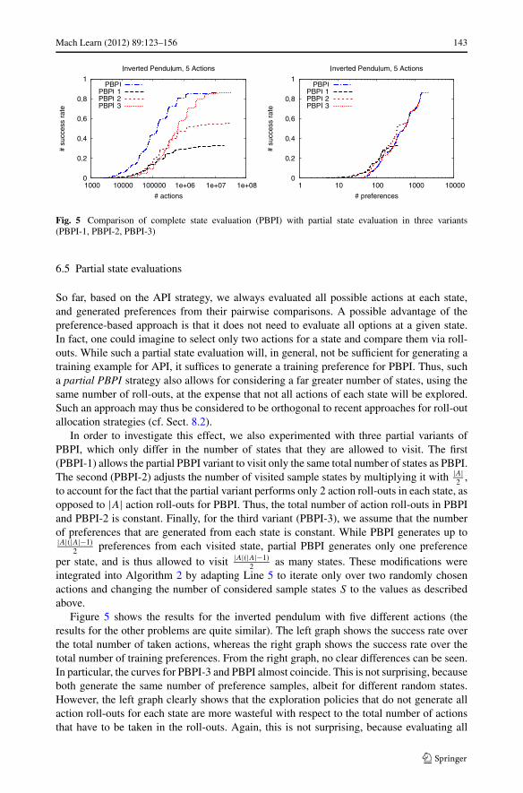
For training, we generate 1000 patients at random. That is, we simulate 1000 patients ex-periencing the treatment based on model (2). The initial state of each patient, Y0 and X0,are generated independently and uniformly from (0,2). Then, for the following 6 months,the patient receives a monthly chemotherapy with a dosage level taken from one of fourdifferent values (actions) 0.1 (low), 0.4 (medium), 0.7 (high) and 1.0 (extreme), where 1.0corresponds to the maximum acceptable dose.6 As an illustration, Fig. 6 shows the treatment

6We exclude the value 0, as it is a common practice to let the patient keep receiving certain level of chemother-apy agent during the treatment in order to prevent the tumor relapsing.

146 Mach Learn (2012) 89:123–156

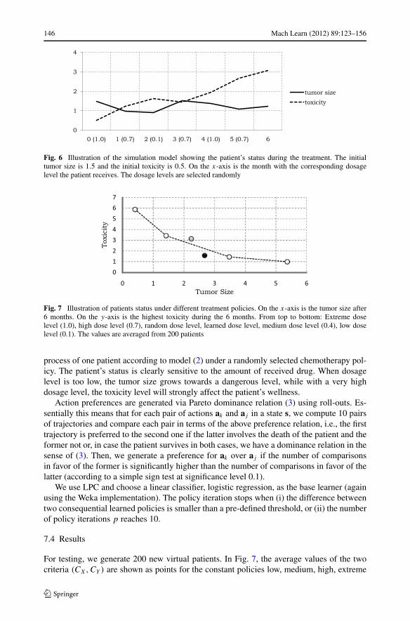
Fig. 6 Illustration of the simulation model showing the patient’s status during the treatment. The initialtumor size is 1.5 and the initial toxicity is 0.5. On the x-axis is the month with the corresponding dosagelevel the patient receives. The dosage levels are selected randomly

Fig. 7 Illustration of patients status under different treatment policies. On the x-axis is the tumor size after6 months. On the y-axis is the highest toxicity during the 6 months. From top to bottom: Extreme doselevel (1.0), high dose level (0.7), random dose level, learned dose level, medium dose level (0.4), low doselevel (0.1). The values are averaged from 200 patients

process of one patient according to model (2) under a randomly selected chemotherapy pol-icy. The patient’s status is clearly sensitive to the amount of received drug. When dosagelevel is too low, the tumor size grows towards a dangerous level, while with a very highdosage level, the toxicity level will strongly affect the patient’s wellness.

Action preferences are generated via Pareto dominance relation (3) using roll-outs. Es-sentially this means that for each pair of actions ak and aj in a state s, we compute 10 pairsof trajectories and compare each pair in terms of the above preference relation, i.e., the firsttrajectory is preferred to the second one if the latter involves the death of the patient and theformer not or, in case the patient survives in both cases, we have a dominance relation in thesense of (3). Then, we generate a preference for ak over aj if the number of comparisonsin favor of the former is significantly higher than the number of comparisons in favor of thelatter (according to a simple sign test at significance level 0.1).

We use LPC and choose a linear classifier, logistic regression, as the base learner (againusing the Weka implementation). The policy iteration stops when (i) the difference betweentwo consequential learned policies is smaller than a pre-defined threshold, or (ii) the numberof policy iterations p reaches 10.

7.4 Results

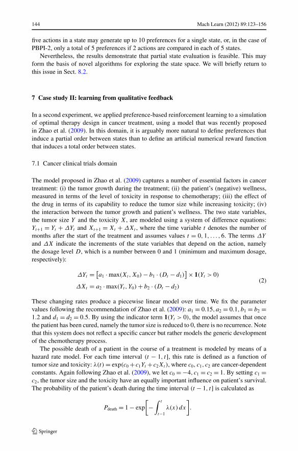
For testing, we generate 200 new virtual patients. In Fig. 7, the average values of the twocriteria (CX,CY ) are shown as points for the constant policies low, medium, high, extreme

Mach Learn (2012) 89:123–156 147

Fig. 8 Average ranks of thepolicies according to death rates.CD stands for the criticaldifference of ranks derived froma Nemenyi test at α = 0.05

(i.e., the policies prescribing a constant dosage regardless of the state). As can be seen, allfour policies are Pareto-optimal, which is hardly surprising in light of the fact that toxicityand tumor size are conflicting criteria: A reduction of the former tends to increase the latter,and vice versa. The figure also shows the convex hull of the Pareto-optimal policies.

Finally, we add the results for two other policies, namely the policy learned by ourpreference-based approach and a random policy, which, in each state, picks a dose levelat random. Although these two policies are again both Pareto-optimal, it is interesting tonote that our policy is outside the convex hull of the constant policies, whereas the randompolicy falls inside. Recalling the interpretation of the convex hull in terms of randomizedstrategies, this means that the random policy can be outperformed by a randomization of theconstant policies, whereas our policy can not.

In a second evaluation, we focus on the death rate—which, after all, is a function oftoxicity and tumor size. In each test trial, we now compute a patient’s probability to surviveduring the whole treatment. Averaging over all patients, we rank the policies accordingto this criterion. The average ranks of policies are shown in Fig. 8. As can be seen, thetreatments produced by our preference-based RL method have a lower death rate than theother polices. In fact, the Nemenyi test even indicates that the differences are statisticallysignificant at a significance level of α = 0.05 (Dems̆ar 2006).

8 Related work

In this section, we give an overview of existing work which is, in one way or the other,related to the idea of preference-based reinforcement learning as introduced in this paper.In Sect. 8.1, we start with policy search approaches that use the reinforcement signal for di-rectly modifying the policy. The preference-based approach of Akrour et al. (2011) may beviewed in this context. Preference-based policy iteration is, on the other hand, closer relatedto approaches that use supervised learning algorithms for learning a policy (Sect. 8.2). InSect. 8.3, we discuss the work of Maes (2009), which tackles a quite similar learning prob-lem, albeit in a different context and having other goals in mind. Our work is also related tomulti-objective reinforcement learning, because in both learning settings, trajectories maynot be comparable (Sect. 8.4). Finally we also discuss alternative approaches for incorporat-ing external advice (Sect. 8.5) and for handling qualitative information (Sect. 8.6).

8.1 Preference-based policy search

Akrour et al. (2011) propose a framework that is quite similar to ours. In their architecture,the learning agent shows a set of policies to a domain expert who gives feedback in the formof pairwise preferences between the policies. This information is then used in order to learnto estimate the value of parametrized policies in a way that is consistent with the preferences

148 Mach Learn (2012) 89:123–156

provided by the expert. Based on the new estimates, the agent selects another set of policiesfor the expert, and the process is repeated until a termination criterion is met.

Thus, just like in our approach, the key idea of Akrour et al. (2011) is to combine prefer-ence learning and reinforcement learning, taking qualitative preferences between trajectoriesas a point of departure.7 What is different, however, is the type of (preference) learning prob-lem that is eventually solved: Akrour et al. (2011) seek to directly learn a ranking functionin the policy space from global preferences on the level of complete trajectories, whereas wepropose to proceed from training information in the form of local preferences on actions ina given state. Correspondingly, they solve an object ranking problem, with objects given byparametrized policies, making use of standard learning-to-rank methods (Kamishima et al.2011).

In a way, the approach of Akrour et al. (2011) may be viewed as a preference-basedvariant of policy search. Just as so-called policy gradient methods search for a good param-eter setting in a space of parametrized policies by using the reinforcement signal to derivethe direction into which the policy should be corrected, the above-mentioned approach usesa qualitative preference signal for driving the policy learner towards better policies. Nu-merical policy gradients can be computed in closed form from a parametrized policy (Ngand Jordan 2000), be estimated empirically from action samples of the policy (Williams1992), or learned by regression (Kersting and Driessens 2008). In the actor-critic frame-work, where algorithms learn both the value function (the critic) and an explicit policy(the actor) simultaneously (Barto et al. 1983), the policy gradient can be estimated fromthe predicted values of the value function (Konda and Tsitsiklis 2003; Sutton et al. 2000).A particularly interesting policy gradient approach is the natural actor-critic (Peters andSchaal 2008a). The key idea of this approach is to fight the large variance in conventionalgradient approaches by the use of the natural gradient, i.e., the gradient that does not as-sume that the parameter space is Euclidean but takes its structure into account (Amari 1998;Kakade 2001). Good surveys of current work in this area can be found in Bhatnagar et al.(2009), Peters and Schaal (2008b).

Not all approaches to direct policy search use policy gradients. For example, Mannoret al. (2003) suggest the use of the Cross Entropy for finding an optimal policy. Other meth-ods include EM-like methods (Peters and Schaal 2007; Kober and Peters 2011) or the gen-eralized path integral control approach (Theodorou et al. 2010).

8.2 Supervised policy learning

The above-mentioned approaches use the (qualitative or quantitative) reinforcement signalto directly optimize the policy, whereas preference-based approximate policy iteration isquite related to approaches that use supervised learning algorithms to learn a policy. Inparticular, our work directly builds upon approximate policy iteration (Lagoudakis and Parr2003), which had the goal of using modern classifiers to learn the policy. In general, thekey idea of such approaches is to learn a policy in the form of a P-function, which directlymaps states to optimal actions (Tadepalli et al. 2004). The P-function can be representedin commonly used concept representations such as relational decision trees (Džeroski et al.2001), decision lists (Fern et al. 2006), support vector machines (Lagoudakis and Parr 2003),etc. As the P-function needs to capture less information than the Q-function (it does not need

7We assume here that policies are demonstrated to the user in the form of “representative” trajectories, butthis is not entirely clear from the description in Akrour et al. (2011).

Mach Learn (2012) 89:123–156 149

to perfectly fit the Q-values), the hope is that it leads to more compact representations andto a faster convergence.

A key issue for such approaches is the strategy used for generating examples for thesupervised learning algorithm. The original roll-out strategy proposed by Lagoudakis andParr (2003) is rather wasteful with respect to the performed number of roll-outs, andseveral authors have tried to address this problem (Dimitrakakis and Lagoudakis 2008;Gabillon et al. 2010). First, the number of necessary roll-outs in a state, which we assumedto be a constant number K , can be dynamically adjusted so that the roll-outs are stopped assoon as a winning action clearly emerges. Hoeffding or Bernstein races can be used to deter-mine the best action with a minimal number of roll-outs (Heidrich-Meisner and Igel 2009),elimination algorithms iteratively remove the worst action until a single winner emerges(Even-Dar et al. 2003; Audibert et al. 2010), and the UCB algorithm, which trades off ex-ploration and exploitation in multi-armed bandit problems (Auer et al. 2002), can also beadapted to this setting (Dimitrakakis and Lagoudakis 2008). Recently, Gabillon et al. (2011)proposed to improve finite-horizon roll-out estimates by enhancing them with a critic whichlearns to estimate the value of the iterations beyond the horizon. All these approaches are,in a way, orthogonal to our approach, in that they all focus on the best action. In all of them,additional pairwise comparisons can emerge as a by-product of sampling for the best action,and the experiments of Sect. 6 show that it can be beneficial to use them.

A second approach for optimizing the use of roll-outs is to define a state exploration strat-egy. For example, it was suggested that a policy-based generation of states may be preferableto a random selection (Fern et al. 2006). While this may clearly lead to faster convergencein some domains, it may also fail to find optimal solutions in other cases (Lagoudakis andParr 2003). Again, such approaches can be straight-forwardly combined with our proposal.Moreover, preference-based approximate policy iteration provides a natural focus on thecomparison between pairs of actions instead of sets of actions. This allows the use of fewerroll-outs for getting some information (one preference) from a state, and thus allows to movemore quickly from state to state. For example, selecting a pair of actions and following thebetter one may be a simple but effective way of trading off exploration and exploitation forstate sampling. Whether and how this additional flexibility can be used for more efficientexploration strategies is subject of future work.

Finally, Lazaric et al. (2010) propose direct policy iteration, which improves approximatepolicy iteration (Lagoudakis and Parr 2003), upon which our work builds, by optimizing aloss function that is based on the difference between the roll-out estimate of the actionchosen by a policy and the maximum value obtainable by any action.

8.3 Reinforcement learning for structured output prediction

Maes (2009) solves a learning problem quite similar to ours, namely “policy learning asaction ranking”, and even makes use of pairwise learning techniques. More specifically, helearns a function called “action-ranking function” that ranks actions given states.

The context and the purpose of the approach, however, are quite different. The idea is totackle structured output prediction problems with reinforcement learning: instead of predict-ing a structured output (such as a sequence or a tree) right away, the output is constructedstep by step. This stepwise construction is modeled as following a path in a properly definedstate space and, thus, can be cast as a reinforcement learning problem.

Apart from this difference, Maes (2009) makes use of ranking methods (instead of re-gression learning of action-value functions) for other reasons. While still making use ofquantitative information about the costs of actions in a given state, he is mainly interested infacilitating the learning process and making it more efficient.

150 Mach Learn (2012) 89:123–156

8.4 Multi-objective reinforcement learning

In multi-objective reinforcement learning (MORL), the agent seeks to achieve two or moreobjectives at the same time, each with its own associated reward signal. Thus, unlike in stan-dard RL, where the reward is a scalar, it is now a vector (Vamplew et al. 2010). Typically,the different objectives are in conflict with each other and cannot easily be optimized si-multaneously. Instead, a policy must either optimize only one objective while neglecting theothers, or try to find a trade-off between the conflicting criteria. What is sought, therefore,is a policy that is optimal in a Pareto sense.

MORL shares an important property with our approach to preference-based reinforce-ment learning, namely the fact that trajectories (policies) are not necessarily comparablewith each other. On the other hand, the reward signals in MORL are still numerical, thusmaking the problem amenable to other types of learning algorithms. In other words, MORLcan be seen as a special case of our general framework; as such, it can be tackled by special-ized algorithms that are presumably more effective than general algorithms for preference-based reinforcement learning.

8.5 External advice and off-policy learning

In addition to numerical reward functions, some authors have investigated ways for incor-porating other forms of feedback, most notably external advice. For example, Maclin andShavlik (1996) proposed an approach in which user-generated advice in the form of rules istransferred to the same neural network used by the reinforcement learning agent for learningthe Q-function. Maclin et al. (2005) propose user-provided advice in the form of preferencesover actions and use them for training a reinforcement learner via kernel-based regression.The constraints compare two actions, but are still quantitative in the sense of specifying alower bound on the difference of the Q-values of two actions. These constraints can thenbe directly incorporated into the kernelized optimization algorithm. This form of advicehas later been adapted for transfer learning (Torrey et al. 2005). A good survey of transferlearning in RL and its relation to advice-taking is given by Taylor and Stone (2009).

An alternative technique is to encode advice in the form of a reasonable starting policy,which can then be used to generate training examples for a relational reinforcement learner(Driessens and Džeroski 2004). Such examples could, e.g., also be generated by a humancontroller. Auer et al. (1995) consider the multi-armed bandit problem in the presence ofexperts, each of which instructs the learner on a particular arm to pull. Langford and Zhang(2008) consider a more general case where any contextual information can be consideredin addition to the reward. For example, in a news recommender system, the context coulddescribe news articles and user information (Li et al. 2010). Another approach for advice-taking with reinforcement learning has been tried by Fürnkranz et al. (2000). The key ideaof this paper is tuning the weights of several advice-givers instead of the weights of anevaluation function.

The above is related to off-policy learning, where the learner does not have to follow thepolicy it tries to optimize. In the simplest case, when the value function is simply representedas a look-up table, off-policy learning is well understood. In fact, Q-learning is an off-policylearner. In the general case, however, when the state space is so complex that the valuefunction has to be approximated, off-policy learning is known to become unstable even forlinear function approximators (Precup et al. 2001; Maei et al. 2010). Recently, Langfordet al. (2008) discuss how policies can be evaluated using off-line experience.

Preference-based reinforcement learning is also related to inverse reinforcement learning(Ng and Russell 2000; Abbeel and Ng 2010). In this framework, the idea is to learn a reward

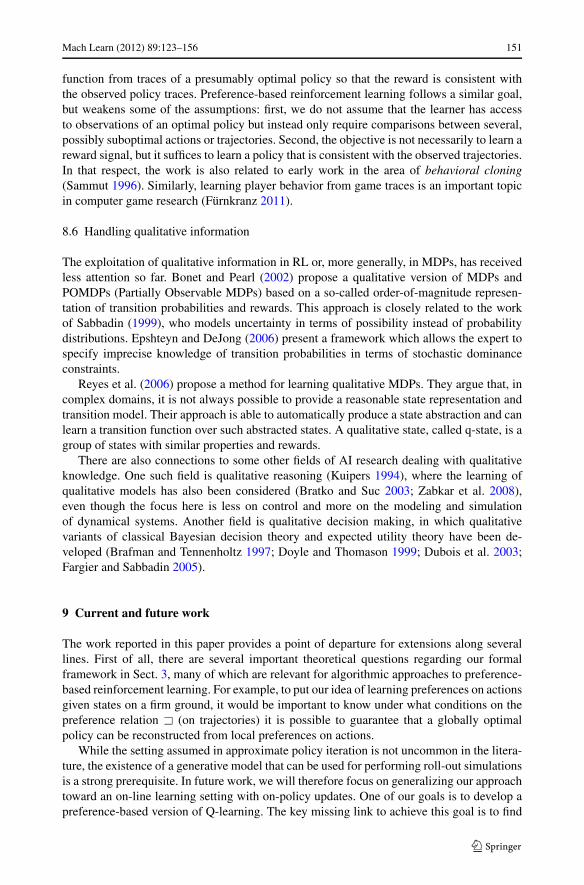
Mach Learn (2012) 89:123–156 151

function from traces of a presumably optimal policy so that the reward is consistent withthe observed policy traces. Preference-based reinforcement learning follows a similar goal,but weakens some of the assumptions: first, we do not assume that the learner has accessto observations of an optimal policy but instead only require comparisons between several,possibly suboptimal actions or trajectories. Second, the objective is not necessarily to learn areward signal, but it suffices to learn a policy that is consistent with the observed trajectories.In that respect, the work is also related to early work in the area of behavioral cloning(Sammut 1996). Similarly, learning player behavior from game traces is an important topicin computer game research (Fürnkranz 2011).

8.6 Handling qualitative information

The exploitation of qualitative information in RL or, more generally, in MDPs, has receivedless attention so far. Bonet and Pearl (2002) propose a qualitative version of MDPs andPOMDPs (Partially Observable MDPs) based on a so-called order-of-magnitude represen-tation of transition probabilities and rewards. This approach is closely related to the workof Sabbadin (1999), who models uncertainty in terms of possibility instead of probabilitydistributions. Epshteyn and DeJong (2006) present a framework which allows the expert tospecify imprecise knowledge of transition probabilities in terms of stochastic dominanceconstraints.

Reyes et al. (2006) propose a method for learning qualitative MDPs. They argue that, incomplex domains, it is not always possible to provide a reasonable state representation andtransition model. Their approach is able to automatically produce a state abstraction and canlearn a transition function over such abstracted states. A qualitative state, called q-state, is agroup of states with similar properties and rewards.

There are also connections to some other fields of AI research dealing with qualitativeknowledge. One such field is qualitative reasoning (Kuipers 1994), where the learning ofqualitative models has also been considered (Bratko and Suc 2003; Zabkar et al. 2008),even though the focus here is less on control and more on the modeling and simulationof dynamical systems. Another field is qualitative decision making, in which qualitativevariants of classical Bayesian decision theory and expected utility theory have been de-veloped (Brafman and Tennenholtz 1997; Doyle and Thomason 1999; Dubois et al. 2003;Fargier and Sabbadin 2005).

9 Current and future work

The work reported in this paper provides a point of departure for extensions along severallines. First of all, there are several important theoretical questions regarding our formalframework in Sect. 3, many of which are relevant for algorithmic approaches to preference-based reinforcement learning. For example, to put our idea of learning preferences on actionsgiven states on a firm ground, it would be important to know under what conditions on thepreference relation � (on trajectories) it is possible to guarantee that a globally optimalpolicy can be reconstructed from local preferences on actions.

While the setting assumed in approximate policy iteration is not uncommon in the litera-ture, the existence of a generative model that can be used for performing roll-out simulationsis a strong prerequisite. In future work, we will therefore focus on generalizing our approachtoward an on-line learning setting with on-policy updates. One of our goals is to develop apreference-based version of Q-learning. The key missing link to achieve this goal is to find

152 Mach Learn (2012) 89:123–156

a preference-based equivalent to the Bellman equation, which allows to transfer informationabout action preferences from one state to the other.

A first step in that direction is to define and evaluate a ranking-based exploration strategy.The results on partial state evaluations (Sect. 6.5) indicate that an exploration strategy that isbased on picking the better one of a pair of actions may be an interesting approach to try. Itseems clear that information provided by a ranking gives more information than uninformedexploration strategies like ε-greedy strategies, and we believe that the loss of informationthat we suffer from only having a ranking instead of expected utilities or action probabilitiesis only minor. This, however, needs to be properly evaluated.

We are currently working on applying preference-based reinforcement learning to thechess domain that we have used to motivate our framework in Sect. 2.3. The main obstaclethat we have to solve here is that preference-based policy iteration as proposed in this paperis for on-line learning, whereas the preferences that we want to learn from are only avail-able off-line. An interesting way for solving this strategy could be an integration of off-lineadvice with on-line experience. This can be easily done in Algorithm 3 by merging prefer-ences from off-line data with preferences that have been generated via roll-out analysis withthe current policy. A problem here is that roll-out analysis with imperfect policies tendsto be considerably less reliable for chess than for games like Go (Ramanujan et al. 2010;Arenz 2012), which is one of the motivations for resorting to game annotations in this do-main. We are also aiming at lifting inverse reinforcement learning (Ng and Russell 2000;Abbeel and Ng 2010) to a preference-based formulation.

10 Conclusions

The main contribution of this work is a framework for preference-based reinforcement learn-ing, which allows for lifting RL into a qualitative setting, where reward is not available onan absolute, numerical scale. Instead, comparative reward functions can be used to decidewhich of two actions is preferable in a given state, or, more generally, which of two trajec-tories is preferable.

To cope with this type of training information, we proposed an algorithm for preference-based policy iteration, which only depends on the availability of preference informationbetween two actions. As a proof-of-concept, we instantiated this algorithm into a version ofapproximate policy iteration, where the preference information is determined via roll-outs.Whereas the original algorithm essentially reduces reinforcement learning to classification,we tackle the problem by means of a preference learning method called label ranking. Inthis setting, a policy is represented by a ranking function that maps states to total orders ofall available actions.

To demonstrate the feasibility of this approach, we performed two case studies. In the firststudy, we showed that additional training information about lower-ranked actions can be suc-cessfully used for improving the learned policies. The second case study demonstrated oneof the key advantages of a qualitative policy iteration approach, namely that a comparisonof pairs of actions is often more feasible than the quantitative evaluation of single actions.

Acknowledgements We would like to thank the anonymous reviewers for their careful reading of ourmanuscript and many suggestions that helped to improve the paper. We also thank Robert Busa-Fekete forseveral useful comments and discussions, Jan Peters for advice on policy search, and the Frankfurt Centerfor Scientific Computing for providing computational resources. This research was supported by the GermanScience Foundation (DFG).

Mach Learn (2012) 89:123–156 153

References

Abbeel, P., & Ng, A. Y. (2010). Inverse reinforcement learning. In C. Sammut & G. I. Webb (Eds.), Encyclo-pedia of machine learning (pp. 554–558). Berlin: Springer.

Akrour, R., Schoenauer, M., & Sebag, M. (2011). Preference-based policy learning. In D. Gunopulos, T. Hof-mann, D. Malerba, & M. Vazirgiannis (Eds.), Proceedings of the European conference on machinelearning and knowledge discovery in databases (ECML-PKDD-11), part I, Athens, Greece (pp. 12–27).Berlin: Springer.

Amari, S. (1998). Natural gradient works efficiently in learning. Neural Computation, 10(2), 251–276.Arenz, O. (2012). Monte-Carlo chess. Bachelor’s thesis. TU Darmstadt: Knowledge Engineering Group.Audibert, J.-Y., Bubeck, S., & Munos, R. (2010). Best arm identification in multi-armed bandits. In A. T.

Kalai & M. Mohri (Eds.), Proceedings of the 23rd conference on learning theory (COLT-10), Haifa,Israel (pp. 41–53). Hawthorne: Omnipress.

Auer, P., Cesa-Bianchi, N., Freund, Y., & Schapire, R. E. (1995). Gambling in a rigged casino: the adversarialmulti-arm bandit problem. In Proceedings of the 36th annual symposium on foundations of computerscience (pp. 322–331). Los Alamitos: IEEE Computer Society Press.

Auer, P., Cesa-Bianchi, N., & Fischer, P. (2002). Finite-time analysis of the multiarmed bandit problem.Machine Learning, 47(2–3), 235–256.

Barto, A. G., Sutton, R. S., & Anderson, C. (1983). Neuron-like elements that can solve difficult learningcontrol problems. IEEE Transactions on Systems, Man and Cybernetics, 13, 835–846.

Baxter, J., Tridgell, A., & Weaver, L. (2000). Learning to play chess using temporal differences. MachineLearning, 40(3), 243–263.

Beal, D. F., & Smith, M. C. (2001). Temporal difference learning applied to game playing and the results ofapplication to Shogi. Theoretical Computer Science, 252(1–2), 105–119. Special Issue on Papers fromthe Computers and Games 1998 Conference.

Bhatnagar, S., Sutton, R. S., Ghavamzadeh, M., & Lee, M. (2009). Natural actor-critic algorithms. Automat-ica, 45(11), 2471–2482.

Bonet, B., & Pearl, J. (2002). Qualitative mdps and pomdps: an order-of-magnitude approximation. In Proc.18th conference in uncertainty in artificial intelligence (UAI-02), Alberta, Canada (pp. 61–68).

Brafman, R. I., & Tennenholtz, M. (1997). Modeling agents as qualitative decision makers. Artificial Intelli-gence, 94(1–2), 217–268.

Bratko, I., & Suc, D. (2003). Learning qualitative models. AI Magazine, 24(4), 107–119.Cheng, W., Fürnkranz, J., Hüllermeier, E., & Park, S.-H. (2011). Preference-based policy iteration: leveraging

preference learning for reinforcement learning. In D. Gunopulos, T. Hofmann, D. Malerba, & M. Vazir-giannis (Eds.), Proceedings of the European conference on machine learning and knowledge discoveryin databases (ECML-PKDD-11), part I, Athens, Greece (pp. 312–327). Berlin: Springer.

Crites, R., & Barto, A. (1998). Elevator group control using multiple reinforcement learning agents. MachineLearning, 33, 235–262.

Dems̆ar, J. (2006). Statistical comparisons of classifiers over multiple data sets. Journal of Machine LearningResearch, 7, 1–30.

Dimitrakakis, C., & Lagoudakis, M. G. (2008). Rollout sampling approximate policy iteration. MachineLearning, 72(3), 157–171.

Doyle, J., & Thomason, R. (1999). Background to qualitative decision theory. AI Magazine, 20(2), 55–68.Driessens, K., & Džeroski, S. (2004). Integrating guidance into relational reinforcement learning. Machine

Learning, 57(3), 271–304.Droste, S., & Fürnkranz, J. (2008). Learning the piece values for three chess variants. International Computer

Games Association Journal, 31(4), 209–233.Dubois, D., Fargier, H., & Perny, P. (2003). Qualitative decision theory with preference relations and com-

parative uncertainty: an axiomatic approach. Artificial Intelligence, 148(1–2), 219–260.Džeroski, S., De Raedt, L., & Driessens, K. (2001). Relational reinforcement learning. Machine Learning,

43(1–2), 7–52.Edwards, S. J. (1994). Portable game notation. http://folk.uio.no/andreio/docs/pgnspec.pdf.Epshteyn, A., & DeJong, G. (2006). Qualitative reinforcement learning. In W. Cohen & A. Moore (Eds.),

Proceedings of the 23rd international conference on machine learning (ICML-06), Pittsburgh, Pennsyl-vania, USA (pp. 305–312).

Even-Dar, E., Mannor, S., & Mansour, Y. (2003). Action elimination and stopping conditions for reinforce-ment learning. In T. Fawcett & N. Mishra (Eds.), Proceedings of the 20th international conference onmachine learning (ICML-03), Washington, DC (pp. 162–169). Menlo Park: AAAI Press.

Fargier, H., & Sabbadin, R. (2005). Qualitative decision under uncertainty: back to expected utility. ArtificialIntelligence, 164(1–2), 245–280.

154 Mach Learn (2012) 89:123–156

Fern, A., Yoon, S. W., & Givan, R. (2006). Approximate policy iteration with a policy language bias: solvingrelational Markov decision processes. The Journal of Artificial Intelligence Research, 25, 75–118.

Fürnkranz, J. (2011). Machine learning and game playing. In C. Sammut & G. I. Webb (Eds.), Encyclopediaof machine learning (pp. 633–637). Berlin: Springer.

Fürnkranz, J. & Hüllermeier, E. (Eds.) (2010). Preference learning. Berlin: Springer.Fürnkranz, J., Pfahringer, B., Kaindl, H., & Kramer, S. (2000). Learning to use operational advice. In

W. Horn (Ed.), Proceedings of the 14th European conference on artificial intelligence (ECAI-00), Berlin(pp. 291–295). Amsterdam: IOS press.

Gabillon, V., Lazaric, A., & Ghavamzadeh, M. (2010). Rollout allocation strategies for classification-basedpolicy iteration. In P. Auer, S. Kaski, & C. Szepesvàri (Eds.), Proceedings of the ICML-10 workshop onreinforcement learning and search in very large spaces.

Gabillon, V., Lazaric, A., Ghavamzadeh, M., & Scherrer, B. (2011). Classification-based policy iteration witha critic. In L. Getoor & T. Scheffer (Eds.), Proceedings of the 28th international conference on machinelearning (ICML-11), New York, NY, USA (pp. 1049–1056). New York: ACM Press.

Gábor, Z., Kalmár, Z., & Szepesvàri, C. (1998). Multi-criteria reinforcement learning. In Proceedings of the15th international conference on machine learning (ICML-98), Madison, WI (pp. 197–205). San Mateo:Morgan Kaufmann.

Hall, M., Frank, E., Holmes, G., Pfahringer, B., Reutemann, P., & Witten, I. H. (2009). The weka data miningsoftware: an update. SIGKDD Explorations, 11(1), 10–18.

Heidrich-Meisner, V., & Igel, C. (2009). Hoeffding and Bernstein races for selecting policies in evolutionarydirect policy search. In A. P. Danyluk, L. Bottou, & M. L. Littman (Eds.), ACM international conferenceproceeding series: Proceedings of the 26th international conference on machine learning (ICML-09),Montreal, Canada (pp. 401–408).

Hüllermeier, E., Fürnkranz, J., Cheng, W., & Brinker, K. (2008). Label ranking by learning pairwise prefer-ences. Artificial Intelligence, 172, 1897–1916.

Kakade, S. (2001). A natural policy gradient. In T. G. Dietterich, S. Becker, & Z. Ghahramani (Eds.), Ad-vances in neural information processing systems 14 (NIPS-2001), Vancouver, British Columbia, Canada(pp. 1531–1538). Cambridge: MIT Press.

Kamishima, T., Kazawa, H., & Akaho, S. (2011). A survey and empirical comparison of object rankingmethods. In J. Fürnkranz & E. Hüllermeier (Eds.), Preference leaning (pp. 181–201). Berlin: Springer.

Kersting, K., & Driessens, K. (2008). Non-parametric policy gradients: a unified treatment of propositionaland relational domains. In W. W. Cohen, A. McCallum, & S. T. Roweis (Eds.), Proceedings of the 25thinternational conference on machine learning (ICML 2008), Helsinki, Finland (pp. 456–463). NewYork: ACM Press.

Kober, J., & Peters, J. (2011). Policy search for motor primitives in robotics. Machine Learning, 84(1–2),171–203.

Konda, V. R., & Tsitsiklis, J. N. (2003). On actor-critic algorithms. SIAM Journal on Control and Optimiza-tion, 42(4), 1143–1166.

Kuipers, B. (1994). Qualitative reasoning. Cambridge: MIT Press.Lagoudakis, M. G., & Parr, R. (2003). Reinforcement learning as classification: leveraging modern classifiers.

In T. E. Fawcett & N. Mishra (Eds.), Proceedings of the 20th international conference on machinelearning (ICML-03), Washington, DC, USA: (pp. 424–431). Menlo Park: AAAI Press.

Langford, J., & Zhang, T. (2008). The epoch-greedy algorithm for multi-armed bandits with side information.In J. C. Platt, D. Koller, Y. Singer, & S. T. Roweis (Eds.), Advances in neural information processingsystems 20 (NIPS-21), Vancouver, Canada. Cambridge: MIT Press

Langford, J., Strehl, A. L., & Wortman, J. (2008). Exploration scavenging. In W. W. Cohen, A. McCallum, &S. T. Roweis (Eds.), ACM international conference proceeding series: Vol. 307. Proceedings of the 25thinternational conference on machine learning (ICML-08), Helsinki, Finland (pp. 528–535). New York:ACM Press.

Lazaric, A., Ghavamzadeh, M., & Munos, R. (2010). Analysis of a classification-based policy iteration al-gorithm. In J. Fürnkranz & T. Joachims (Eds.), Proceedings of the 27th international conference onmachine learning (ICML-10) (pp. 607–614). Hawthorne: Omnipress.

Li, L., Chu, W., Langford, J., & Schapire, R. E. (2010). A contextual-bandit approach to personalized newsarticle recommendation. In M. Rappa, P. Jones, J. Freire, & S. Chakrabarti (Eds.), Proceedings of the19th international conference on world wide web (WWW-10), Raleigh, North Carolina (pp. 661–670).New York: ACM Press.

Loza Mencía, E., Park, S.-H., & Fürnkranz, J. (2010). Efficient voting prediction for pairwise multilabelclassification. Neurocomputing, 73(7–9), 1164–1176.

Maclin, R., & Shavlik, J. W. (1996). Creating advice-taking reinforcement learners. Machine Learning,22(1–3), 251–281.

Mach Learn (2012) 89:123–156 155

Maclin, R., Shavlik, J. W., Torrey, L., Walker, T., & Wild, E. W. (2005). Giving advice about preferred actionsto reinforcement learners via knowledge-based kernel regression. In M. M. Veloso & S. Kambhampati(Eds.), Proceedings of the 20th national conference on artificial intelligence (AAAI-05), Pittsburgh,Pennsylvania (pp. 819–824). Menlo Park/Cambridge: AAAI Press/MIT Press.

Maei, H. R., Szepesvàri, C., Bhatnagar, S., & Sutton, R. S. (2010). Toward off-policy learning control withfunction approximation. In J. Fürnkranz & T. Joachims (Eds.), Proceedings of the 27th internationalconference on machine learning (ICML-10), Haifa, Israel (pp. 719–726). Hawthorne: Omnipress.

Maes, F. (2009). Learning in Markov decision processes for structured prediction. PhD thesis, UniversityPierre et Marie Curie, Paris, France.

Mannor, S., & Shimkin, N. (2004). A geometric approach to multi-criterion reinforcement learning. Journalof Machine Learning Research, 5, 325–360.

Mannor, S., Rubinstein, R. Y., & Gat, Y. (2003). The cross entropy method for fast policy search. In T. Fawcett& N. Mishra (Eds.), Proceedings of the 20th international conference on machine learning (ICML-03),Washington, DC (pp. 512–519). Menlo Park: AAAI Press.

Massey, W. A. (1987). Stochastic orderings for Markov processes on partially ordered spaces. Mathematicsof Operations Research, 12(2), 350–367.

Ng, A. Y., & Jordan, M. I. (2000). Pegasus: a policy search method for large mdps and pomdps. In C. Boutilier& M. Goldszmidt (Eds.), Proceedings of the 16th conference in uncertainty in artificial intelligence(UAI-00), Stanford University, Stanford, California (pp. 406–415). San Mateo: Morgan Kaufmann.

Ng, A. Y., & Russell, S. (2000). Algorithms for inverse reinforcement learning. In P. Langley (Ed.), Pro-ceedings of the 17th international conference on machine learning (ICML-00), Stanford University,Stanford, California (pp. 663–670). San Mateo: Morgan Kaufmann.

Park, S.-H., & Fürnkranz, J. (2012). Efficient prediction algorithms for binary decomposition techniques.Data Mining and Knowledge Discovery, 24(1), 40–77.

Peters, J., & Schaal, S. (2007). Reinforcement learning by reward-weighted regression for operational spacecontrol. In Z. Ghahramani (Ed.), Proceedings of the 24th international conference on machine learning(ICML-07), Corvallis, Oregon, USA (pp. 745–750).

Peters, J., & Schaal, S. (2008a) Natural actor-critic. Neurocomputing, 71(7–9), 1180–1190.Peters, J., & Schaal, S. (2008b). Reinforcement learning of motor skills with policy gradients. Neural Net-

works, 21(4), 682–697.Precup, D., Sutton, R. S., & Dasgupta, S. (2001). Off-policy temporal difference learning with function ap-

proximation. In C. E. Brodley & A. P. Danyluk (Eds.), Proceedings of the 18th international conferenceon machine learning (ICML-01), Williams College, Williamstown, MA (pp. 417–424). San Mateo: Mor-gan Kaufmann.

Puterman, M. L. (2005). Markov decision processes: discrete stochastic dynamic programming (2nd edn.).New York: Wiley.

Ramanujan, R., Sabharwal, A., & Selman, B. (2010). On adversarial search spaces and sampling-based plan-ning. In R. I. Brafman, H. Geffner, J. Hoffmann, & H. A. Kautz (Eds.), Proceedings of 20th interna-tional conference on automated planning and scheduling (ICAPS-10), Toronto, Ontario, Canada (pp.242–245).

Reyes, A., Ibarguengoytia, P., Sucar, L., & Morales, E. (2006). Abstraction and refinement for solving con-tinuous Markov decision processes. In Proc. 3rd European workshop on probabilistic graphical models,Prague, Czech Republic (pp. 263–270).

Sabbadin, R. (1999). A possibilistic model for qualitative sequential decision problems under uncertainty inpartially observable environments. In Proc. UAI, 15th conference on uncertainty in artificial intelligence,Stockholm, Sweden (pp. 567–574).

Sammut, C. (1996). Automatic construction of reactive control systems using symbolic machine learning.Knowledge Engineering Review, 11(1), 27–42.

Srinivas, N., & Deb, K. (1995). Multiobjective optimization using nondominant sorting in genetic algorithms.Evolutionary Computation, 2(3), 221–248.

Sutton, R. S. (1988). Learning to predict by the methods of temporal differences. Machine Learning, 3, 9–44.Sutton, R. S., McAllester, D. A., Singh, S. P., & Mansour, Y. (2000). Policy gradient methods for reinforce-

ment learning with function approximation. In S. A. Solla, T. K. Leen, & K.-R. Müller (Eds.), Advancesin neural information processing systems 12 (NIPS-99), Denver, Colorado, USA (pp. 1057–1063). Cam-bridge: MIT Press.

Tadepalli, P., Givan, R., & Driessens, K. (2004). Relational reinforcement learning: an overview. In P. Tade-palli, R. Givan, & K. Driessens (Eds.), Proceedings of the ICML’04 workshop on relational reinforce-ment learning (pp. 1–9).

Taylor, M. E., & Stone, P. (2009). Transfer learning for reinforcement learning domains: a survey. Journal ofMachine Learning Research, 10, 1633–1685.

Tesauro, G. (1992). Practical issues in temporal difference learning. Machine Learning, 8, 257–278.

156 Mach Learn (2012) 89:123–156

Tesauro, G. (2002). Programming backgammon using self-teaching neural nets. Artificial Intelligence,134(1–2), 181–199. Special Issue on Games, Computers and Artificial Intelligence.

Theodorou, E., Buchli, J., & Schaal, S. (2010). A generalized path integral control approach to reinforcementlearning. Journal of Machine Learning Research, 11, 3137–3181.

Torrey, L., Walker, T., Shavlik, J. W., & Maclin, R. (2005). Using advice to transfer knowledge acquired inone reinforcement learning task to another. In J. Gama, R. Camacho, P. Brazdil, A. Jorge, & L. Torgo(Eds.), Proceedings of the 16th European conference on machine learning (ECML-05), Porto, Portugal(pp. 412–424). Berlin: Springer.

Vamplew, P., Dazeley, R., Berry, A., Issabekov, R., & Dekker, E. (2010). Empirical evaluation methods formultiobjective reinforcement learning algorithms. Machine Learning, 84(1–2), 51–80.

Vembu, S., & Gärtner, T. (2011). Label ranking algorithms: a survey. In J. Fürnkranz & E. Hüllermeier (Eds.),Preference leaning (pp. 45–64). Berlin: Springer.

Watkins, C. J., & Dayan, P. (1992) Q-learning. Machine Learning, 8, 279–292.Williams, R. J. (1992). Simple statistical gradient-following algorithms for connectionist reinforcement learn-

ing. Machine Learning, 8, 229–256.Zabkar, J., Bratko, I., & Mohan, A. (2008). Learning qualitative models by an autonomous robot. In Proc.

22nd international workshop on qualitative reasoning, Boulder, Colorado.Zhao, Y., Kosorok, M., & Zeng, D. (2009). Reinforcement learning design for cancer clinical trials. Statistics

in Medicine, 28, 3295–3315.