0  

Macroeconomic Shocks and Their Propagation

Valerie A. Ramey

University of California, San Diego and NBER

April 8, 2015

PreliminaryandVeryIncomplete

I wish to thank Neville Francis, Arvind Krishnamurthy, Karel Mertens, and Johannes Wieland for helpful discussions. I would also like to express appreciation to the American Economic Association for requiring that all data and programs for published articles be posted. In addition, I am grateful to researchers who publish in journals without that requirement but still post their data and programs on their websites.

 

1  

Table of Contents

1. Introduction

2. Methods for Identifying Shocks and Estimating Impulse Responses 2.1 Overview: What is a Shock? 2.2 Illustrative Framework 2.3 Common Identification Methods

2.3.1 Cholesky Decompositions 2.3.2 Structural VARs (SVARs) 2.3.3 Factor Augmented VARs (FAVARs) 2.3.4 Narrative Methods 2.3.5 High Frequency Identification 2.3.6 External Instruments/Proxy SVARs 2.3.7 Restrictions at Longer Horizons 2.3.8 Sign Restrictions 2.3.9 Estimated DSGE Models

2.4 Estimating Impulse Responses 2.5 The Problem of Foresight 2.6 The Problem of Trends 2.7 DSGE Monte Carlos

3. Monetary Policy Shocks

3.1 A Brief History Through 1999 3.2 A Brief Overview of Findings Since 2000

3.2.1 Regime Switching Models 3.2.2Time-Varying Effects of Monetary Policy 3.2.3 Summary of Recent Estimates

3.3 A Discussion of Two Leading External Instruments 3.3.1 Romer and Romer’s Greenbook/Narrative 3.3.2 Gertler and Karadi’s HFI/Proxy SVAR

3.4 New Results Based on Two Leading External Instruments 3.4.1 Explorations with Romer and Romer’s Shock 3.4.2 Explorations with Gertler and Karadi’s Shock

3.5 Summary

4. Fiscal Shocks 4.1 The Effects of Government Spending Shocks 4.1.1 SVAR and Narrative Methods 4.1.2 Summary of the Main Results from the Literature 4.2 The Effects of Tax Shocks

2  

4.2.1 SVAR and Narrative Methods 4.2.2 Anticipated versus Unanticipated 4.3 Summary of Fiscal Results

5. Technology Shocks 5.1 Neutral Technology Shocks 5.2 Investment-Specific Technology Shocks

6. News Shocks

7. Oil Shocks

8. Sectoral Shocks in Networks

9. Summary and Conclusions

3  

1. Introduction

At the beginning of the 20th Century, economists seeking to explain business cycle

fluctuations recognized the importance of both impulses and propagations as components of the

explanations. A key question was how to explain regular fluctuations in a model with dampened

oscillations. In 1927, the Russian statistician Eugen Slutsky published a paper titled “The

Summation of Random Causes as a Source of Cyclic Processes.” In this paper, Slutsky

demonstrated the (then) surprising result that moving sums of random variables could produce

time series that looked very much like the movements of economic time series – “sequences of

rising and falling movements, like waves…with marks of certain approximate uniformities and

regularities.”1 This insight, developed independently by British mathematician Yule in 1926

and extended by Frisch (1933) in his paper “Propagation Problems and Impulse Problems in

Dynamic Economics,” revolutionized the study of business cycles. Their insights shifted the

focus of research from developing mechanisms to support a metronomic view of business cycles,

in which each boom created conditions leading to the next bust, to a search for the sources of the

random shocks. Since then economists have offered numerous candidates for these “random

causes,” such as crop failures, wars, technological innovation, animal spirits, government

actions, and commodity shocks.

Research from the 1940s through the 1970s emphasized fiscal and monetary policy shocks,

identified from large-scale econometric models or single equation analyses. The 1980s

witnessed two important innovations that fundamentally changed the direction of the research.

First, Sims’ (1980) paper “Macroeconomics and Reality” revolutionized the identification of

shocks and the analysis of their effects by introducing vector autoregressions (VARs). Sims’

                                                            1 Page 105 of the 1937 English version of the article published in Econometrica. 

4  

VARs made the link between exogenous shocks and forecast errors, and used Cholesky

decompositions to identify the economic shocks from the reduced form residuals. Using his

method, it became easier to talk about identification assumptions, impulse response functions,

and to do innovation accounting using forecast error decompositions. The second important

innovation was the expansion of the inquiry beyond policy shocks to consider important non-

policy shocks, such as technology shocks (Kydland and Prescott (1982) and oil shocks (Hamilton

(1983).

These innovations led to a flurry of research on shocks and their effects. In his 1994 paper

“Shocks,” John Cochrane took stock of the state of knowledge at that time by using the by-then

standard VAR techniques to conduct a fairly comprehensive search for the shocks that drove

economic fluctuations. Surprisingly, he found that none of the popular candidates could account

for the bulk of economic fluctuations. He proffered the rather pessimistic possibility that “we

will forever remain ignorant of the fundamental causes of economic fluctuations.” (Cochrane

(1994), abstract)

Are we destined to remain forever ignorant of the fundamental causes of economic

fluctuations? Are Slutsky’s “random causes” unknowable? In this chapter, I will summarize the

new methodological innovations and what their application has revealed about the propagation of

the leading candidates for macroeconomic shocks and their importance in explaining economic

fluctuations since Cochrane’s speculation.

5  

2. Methods for Identifying Shocks and Estimating Impulse Responses

2.1.Overview

Before discussing details of methodology, it is useful to consider more carefully what exactly

a “shock” is and why macroeconomists focus on them. Perhaps the best way to answer this

question is to compare how many microeconomists approach empirical research to how

macroeconomists approach empirical research. One rarely hears an applied microeconomist,

particularly the majority who estimate reduced forms, talk about shocks. For example, Angrist

and Pischke’s (2010) article “The Credibility Revolution in Empirical Economics: How Better

Research Design is Taking the Con out of Econometrics” only mentions the word “shocks” when

describing a few papers in macro that use narrative methods. They only talk about these papers

as being examples of “some rays of sunlight pok(ing) through the grey clouds of dynamic

stochastic general equilibrium.” (p. 18). Alas, Angrist and Pischke seemed to miss the

distinction between the empirical investigations of many applied microeconomisst and those of

macroeconomists. Many investigations in applied microeconomics focus on measuring a causal,

though rarely structural, effect of variable X on variable Y in a static setting, ignoring general

equilibrium, and rarely incorporating expectations. Often, these investigations apply insights

from standard theories and do not attempt to estimate deep structural parameters of preferences

or technology that might be used to test the theories.

In stark contrast, macroeconomists ask questions for which dynamics are all-important,

general equilibrium effects are crucial, and expectations have powerful effects. Moreover, in

contrast to microeconomics, the two-way flow between theory and empirics in macroeconomics

is very active. Prescott (1986) argued that business cycle theory in the mid-1980s was “ahead of

business cycle measurement” and that theory should be used to obtain better measures of key

6  

economic series. Prescott did not use “ahead” to mean “superior,” but rather meant that theory

had made more progress on these questions as of that time. Because of this constant interplay

between theory and empirics in macroeconomics, most top macroeconomists have pushed both

the theoretical and empirical frontiers in macroeconomics. Most empirical macroeconomists are

closely guided by theory, either directly or indirectly, and most theoretical macroeconomists are

disciplined by the empirical estimates.

Thus, what are the shocks that we seek to estimate empirically? They are the exact empirical

counterpart to the shocks we discuss in our theories: shocks to technology, monetary policy,

fiscal policy, etc. The empirical counterpart of the shocks in our theories must satisfy three

conditions in order for us to be able to make proper inference about their effects: (1) They must

be exogenous with respect to the other current and lagged endogenous variables in the model; (2)

They must be uncorrelated with other exogenous shocks; otherwise, we cannot identify the

unique causal effects of one exogenous shock relative to another; and (3) They must be

unanticipated.

2.2. Illustrative Framework

To illustrate the relationship between some of the methods, it is useful to consider a simple

trivariate model with three endogenous variables, X1, X2, and XP and suppose that we are trying

to identify the shocks to XP. In the monetary context, the first two variables could be industrial

production and a price index, and XP could be the federal funds rate; in the fiscal context, the

first two could be real GDP and government purchases and XP could be tax revenue; in the

technology shock context, the first two variables could be output and consumption and XP could

be labor productivity. I will call XP the “policy variable” for short, but it should be understood

7  

that it can represent any variable from which we want to extract a shock component. Let Xt =

[X1t, X2t, XPt] be the vector of endogenous variables. Following the standard procedure, let us

model the dynamics with a structural VAR,

(2.1)

where A(L) is a polynomial in the lag operator and ∑ . , ,

is the vector of the normalized structural shocks. We assume that 0, and

that 0 . We can write the reduced form VAR as:

(2.2) ⋯

where . , , is the vector of reduced form residuals, which are related

to the underlying structural shocks as follows:

Following the set-up of Mertens and Ravn (2013), we can express the reduced form errors as:

(2.3)

8  

The parameters and represent the endogenous response of the “policy” variable to X1 and

X2. The and parameterize the contemporaneous effect of the structural shocks to the two

endogenous variables on the policy variable. The σs are the standard deviations of the

(unnormalized) structural shocks.

2.3 Common Identification Methods

Let n be the number of variables in the system, in this case three. The requirement

that ′ provides n(n+1)/2 = 6 identifying restrictions for the equations in (2.3),

but we require three more identifying restrictions to obtain all nine elements. We can now

discuss various schemes for identifying the shock in the context of this model, as well as

several other schemes that go beyond this simple model.

2.3.1 Cholesky Decompositions

The most commonly used identification method imposes alternative sets of recursive zero

restrictions on the contemporaneous coefficients to identify the shock . The following are two

widely-used alternatives.

A. The “policy” variable does not respond within the period to the other endogenous

variables. This could be motivated by decision lags on the part policymakers or other

adjustment costs. This scheme involves constraining = = 0, which is equivalent to

ordering the policy variable first in the Cholesky ordering. For example, Blanchard and

Perotti (2002) impose this constraint to identify the shock to government spending; they

9  

assume that government spending does not respond to the contemporaneous movements

in output or taxes.

B. The other endogenous variables do not respond to the “policy” variable within the period.

This could be motivated by sluggish responses of the other endogenous variables to

shocks to the policy variable. This scheme involves constraining = = 0, which is

equivalent to ordering the policy variable last in the Cholesky ordering. For example,

Bernanke and Blinder (1992) were the first to identify shocks to the federal funds rate as

monetary policy shocks and used this type of identification. This is now the most

standard way to identify monetary policy shocks.

2.3.2 Structural VARs

Another more general approach (that nests the Cholesky decomposition) is what is known

as a Structural VAR, or SVAR, introduced by Blanchard and Watson (1986) and Bernanke

(1986). This approach uses either economic theory or outside estimates to constrain parameters.

For example, Blanchard and Perotti (2002) identify shocks to net taxes (the XP in the system

above) by setting = 2.08, an outside estimate of the cyclical sensitivity of net taxes. As noted

above, they used standard zero restrictions to identify the government spending shock . In

conjunction with the assumed value of they are able to identify the tax shock, .

2.3.3 Factor Augmented VARs

A perennial concern in identifying shocks is that the variables included in the VAR do

not capture all of the relevant information. The comparison of price responses in monetary

10  

VARs with and without commodity prices is one example of the difference a variable exclusion

can make. To address this issue more broadly, Bernanke, Boivin, and Eliasz (2005) developed

the Factor Augmented VARs (FAVARS) based on earlier dynamic factor models developed by

Stock and Watson (2002) and others. The FAVAR, which typically contains over one hundred

series, has the benefit that it is much more likely to condition on relevant information for

identifying shocks. In most implementations, though, it still typically relies on a Cholesky

decomposition.

2.3.4 Narrative Methods

Narrative methods involve constructing a series from historical documents to identify the

reason and/or the quantities associated with a particular change in a variable. The first use of

narrative methods for identification was Hamilton (1985) for oil shocks, which was further

extended by Hoover and Perez (1994). These papers isolated political events that led to

disruptions in world oil markets. Other examples of the use of narrative methods are Romer and

Romer’s (1989, 2004) monetary shock series based on FOMC minutes, Ramey and Shapiro

(1998) and Ramey’s (2011) series of expected changes in future government spending caused by

military events gleaned from periodicals such as Business Week, and Romer and Romer’s (2010)

narrative series of tax changes based on reading various legislative documents.

Until recently, these series were used either as exogenous shocks in sets of dynamic

single equation regressions or ordered first in a Cholesky decomposition. For example, in the

framework above, we would set XP to be the narrative series and we would constrain = = 0.

As the next section details, recent innovations have led to an improved method for incorporating

these series.

11  

A cautionary note on the potential of narrative series to identify exogenous shocks is in

order. Some of the follow-up research has operated on the principle that the narrative alone

provides exogeneity. This is not true. Leeper (1997) made this point for monetary policy

shocks. Another example is in the fiscal literature. A series on fiscal consolidations, quantified

by narrative evidence on the expected size of these consolidations, is not necessarily exogenous.

If the series includes fiscal consolidations adopted in response to bad news about the future

growth of the economy, the series cannot be used to establish a causal effect of the fiscal

consolidation on future output.

2.3.5 High Frequency Identification

Research by Bagliano and Favero (1999), Kuttner (2001), Cochrane and Piazzesi (2002),

Faust, Swanson, and Wright (2004), Gürkaynak et al. (2005), Piazzesi and Swanson (2008),

Gertler and Karadi (2015) and others has used high frequency data (such as news announcements

around FOMC dates) and the movement of federal funds futures to identify unexpected Fed

policy actions. This identification is also based in part on timing, but because the timing is so

high frequency (daily or higher), the assumptions are more plausible than those employed at the

monthly or quarterly frequency. As I will discuss in the foresight section below, the financial

futures data is ideal for ensuring that a shock is unanticipated.

It should be noted, however, that without additional assumptions the unanticipated shock

is not necessarily exogenous to the economy. For example, if the implementation does not

adequately control for the Fed’s private information about the future state of the economy, which

12  

might be driving its policy changes, these shocks cannot be used to estimate a causal effect of

monetary policy on macroeconomic variables.

2.3.6 External Instruments/Proxy SVARs

The external instrument, or “proxy SVAR,” method is a promising new approach for

incorporating external series for identification. Major elements of this idea appeared earlier in

Hamilton (2003) and Evans and Marshall (2005, 2009), but the full application was developed

independently by Stock and Watson (2012) and Mertens and Ravn (2013). This approach takes

advantage of information developed from “outside” the VAR, such as series based on narrative

evidence, shocks from estimated DSGE models, or high frequency information. The idea is that

these external series are noisy measures of the true shock.

Suppose that Zt represents one of these external series. Then this series is a valid

instrument for identifying the shock if the following two conditions hold:

(2.4a) 0,

(2.4b) 0 i = 1, 2

Condition (2.4a) is the instrument relevance condition: the external instrument must be

contemporaneously correlated with the structural policy shock. Condition (2.4b) is the

instrument exogeneity condition: the external instrument must be contemporaneously

uncorrelated with the other structural shocks. If the external instrument satisfies these two

conditions, it can be used to identify the shock .

13  

The procedure is very straightforward and takes place with the following steps.2

Step 1: Estimate the reduced form system to obtain estimates of the reduced form

residuals, ut.

Step 2: Regress and on using the external instrument Zt as the instrument.

These regressions yield unbiased estimates of and . Define the residuals of

these regressions to be and .

Step 3: Regress on and , using the and estimated in Step 2 as the

instruments. This yields unbiased estimates of and . Define the residual of this

regression to be .

Step 4: Estimate from the variance of .

As an example, Mertens and Ravn (2013a) reconcile Romer and Romer’s (2010) estimates of the

effects of tax shocks with the Blanchard and Perotti (2002) estimates by using the Romer’s

narrative tax shock series as an external instrument Z to identify the structural tax shock, .

Thus, they do not need to impose parameter restrictions, such as the cyclical elasticity of taxes to

output. As I will discuss in section 2.3 below, Ramey and Zubairy (2014) extend this external

instrument approach to estimating impulse responses by combining it with Jordà’s (2005)

method.

                                                            2 This exposition follows Merten and Ravn (2013a, online appendix).  See Mertens and Ravn (2013a,b) and the associated online appendices for generalizations to additional external instruments and to larger systems.  

14  

2.3.7 Restrictions at Longer Horizons

Rather than constraining the contemporaneous responses, one can instead identify a

shock by imposing long-run restrictions. The most common is an infinite horizon long-run

restriction, first used by Shapiro and Watson (1988), Blanchard and Quah (1989), and King,

Plosser, Stock and Watson (1991). To see how this identification works, rewrite the system

above as:

(2.5)

where . Suppose we wanted to identify a technology shock as the only shock

that affects labor productivity in the long-run. In this case, the “policy” variable would be the

growth rate of labor productivity and the other variables would also be transformed to induce

stationary (e.g. first-differenced). Letting denote the (i,j) element of the C matrix and

1 denote the lag polynomial with L = 1, we impose the long-run restriction by setting

1 = 0 and 1 = 0. This restriction constrains the unit root in the policy variable (e.g.

labor productivity) to emanate only from the shock that we are calling the technology shock.

This is the identification used by Galí (1999).

An equivalent way of imposing this restriction is to use the estimation method suggested

by Shapiro and Watson (1988). Let XP denote the first-difference of the log of labor

productivity and X1 and X2 be the stationary transformations of two other variables (such as

hours). Then, imposing the long-run restriction is equivalent to identifying the error term in the

following equation as the technology shock:

15  

(2.6) ∑ , ∑ , ∑ ,

We have imposed the restriction by specifying that only the differences of the other stationary

variables enter this equation. Because the current values of those differences might also be

affected by the technology shock and therefore correlated with the error term, we use lags one

through p of X1 and X2 as instruments for the terms involving the current and lagged values of

those variables. The estimated residual is the identified technology shock. We can then identify

the other shocks, if desired, by orthogonalizing the error terms with respect to the technology

shock.

This equivalent way of imposing long-run identification restrictions highlights some of the

problems that can arise with this method. First, identification depends on the relevance of the

instruments. Second, it requires additional identifying restrictions in the form of assumptions

about unit roots. If, for example, hours have a unit root, then in order to identify the technology

shock one would have to impose that only the second difference of hours entered in equation

(2.6).3

Another issue is the behavior of infinite horizon restrictions in small samples (e.g. Faust

and Leeper (1997)). Recently, researchers have introduced new methods that overcome these

problems. For example, Francis, Owyang, Roush, and DeCecio (2014) identify the technology

shock as the shock that maximizes the forecast error variance share of labor productivity at some

finite horizon h. A variation by Barsky and Sims (2011) identifies the shock as the one that

maximizes the sum of the forecast error variances up to some horizon h. Both of these methods

operate off of the moving average representation in equation (2.5).

                                                            3 To be clear, all of the X variables in equation (2.6) must be trend stationary.  If hours have a unit root, then X1 must take the form of Δhourst  , so the constraint in (2.6) would take the form Δ2hourst . 

16  

2.3.8 Sign Restrictions

A number of authors had noted the circularity in some of the reasoning analyzing VAR

specifications in practice. In particular, whether a specification or identification method is

deemed correct is often judged by whether the impulses they produce are “reasonable,” i.e.

consistent with the researcher’s priors. Uhlig (2005) developed a new method to incorporate

“reasonableness” without undercutting scientific inquiry by investigating the effects of a shock

on variable Y, where the shock was identified by sign restrictions on the responses of other

variables (excluding variable Y).

Uhlig’s sign restriction method has been used in many contexts, such as monetary policy,

fiscal policy and technology shocks. Recently, however, two contributions by Arias, Rubio-

Ramirez, and Waggoner (2013) and by Baumeister and Hamilton (2014) have highlighted some

potential problems with sign restriction methods. The Arias et al paper demonstrates problems

with particular implementations and offers new computational methods to overcome those

problems. Baumeister and Hamilton develop Bayesian methods that highlight and link the

relationship between the priors used for identification and the outcomes.

2.3.9 Estimated DSGE Models

An entirely different approach to identification is the estimated DSGE model, introduced

by Smets and Wouters (2003, 2007). This method involves estimating a fully-specified model (a

New Keynesian model with many frictions and rigidities in the case of Smets and Wouters) and

extracting a full set of implied shocks from those estimates. In the case of Smets and Wouters,

many shocks are estimated including technology shocks, monetary shocks, government spending

17  

shocks, wage markup shocks, and risk premium shocks. One can then trace out the impulse

responses to these shocks as well as to do innovation accounting. Other examples of this method

include Justiano, Primiceri, Tambolotti (2010, 2011) and Schmitt-Grohe and Uribe (2012).

Christiano, Eichenbaum and Evans (2005) took a different estimation approach by first

estimating impulse responses to a monetary shock in a standard SVAR and then estimating the

parameters of the DSGE model by matching the impulse responses from the model to those of

the data.

These models achieve identification by imposing structure based on theory. It should be

noted that identification is less straightforward in these types of models. Work by Canova and

Sala (2009), Komunjer and Ng (2011), and others highlight some of the potential problems with

identification in DSGE models.

2.4 Estimating Impulse Responses

Suppose that one has identified the economic shock through one of the methods

discussed above. How do we measure the effects on the endogenous variables of interest? The

most common way to estimate the impulse responses to a shock uses nonlinear (at horizons

greater than one) functions of the estimated VAR parameters. In particular, estimation of the

reduced form system and imposition of the necessary identification assumptions to identify

provides the elements of the moving average representation matrix, ,in equation (2.5).

Writing out C(L) = C0 + C1L + C2L2 + C3L

3 + …, and denoting Ch = [cijh], we can express the

impulse response of variable Xi at horizon t+h to a shock to as:

18  

(2.7) ,

,

These cijk parameters are nonlinear functions of the VAR parameters.

If the VAR adequately captures the data generating process, this method is optimal at all

horizons. If the VAR is mispecified, however, then the specification errors will be compounded

at each horizon. To address this problem, Jordà (2005) introduced a local projection method for

estimating impulse responses. The comparison between his procedure and the standard

procedure has an analogy with direct forecasting versus iterated forecasting (e.g. Marcellino,

Stock, and Watson (2006)). In the forecasting context, one can forecast future values of a

variable using either a horizon-specific regression (“direct” forecasting) or iterating on a one-

period ahead estimated model (“iterated” forecasting). Jordà’s method is analogous to the direct

forecasting whereas the standard VAR method is analogous to the iterated forecasting method.

To see how Jordà’s method works, suppose that has been identified by one of the

methods discussed in the previous section. Then, the impulse response of Xi at horizon h can be

estimated from the following single regression:

(2.8) , , ∙

, is the estimate of the impulse response of Xi at horizon h to a shock to . The control

variables do not have to include the other X’s as long as is exogenous to those other X’s.

Typically, the control variables include deterministic terms (constant, time trends), lags of the Xi,

and lags of other variables that are necessary to “mop up;” the specification can be chosen using

information criteria. One estimates a separate regression for each horizon and the control

19  

variables do not necessarily need to be the same for each regression. Note that except for

horizon h = 0, the error term will be serially correlated because it will be a moving average

of the forecast errors from t to t+h. Thus, the standard errors need to incorporate corrections for

serial correlation, such as a Newey-West (1987) correction.

Because the Jordà method for calculating impulse response functions imposes fewer

restrictions, the estimates are often less precisely estimated and are sometimes erratic.

Nevertheless, this procedure is more robust than standard methods, so it can be very useful as a

heuristic check on the standard methods. Moreover, it is much easier to incorporate state-

dependence (e.g. Auerbach and Gorodnichenko (2013)).

Ramey and Zubairy (2014) recently proposed a new use for the Jordà method that merges

the insights from the external instrument/proxy SVAR literature. To see this, modify equation

(2.8) as follows:

(2.9) , , ∙ ,

As discussed above, Xp is the policy variable, but may be partly endogenous so it will be

correlated with . We can easily deal with this issue, however, by estimating this equation

using the external instrument Zt as an instrument for Xp,t. For example, if Xi is real output and

Xp,t is the federal funds rate, we can use Romer and Romer’s (2004) narrative-based monetary

shock series as an instrument. As I will discuss below, in some cases there are multiple potential

external instruments. We can easily incorporate these in this framework by using multiple

instruments for Xp . In fact, these overidentifying restrictions can be used to test the restrictions

of the model (using a Hansen’s J-statistic, for example).

20  

2.5 The Problem of Foresight

A potential identification problem highlighted recently in multiple literatures is the issue of

news or policy foresight.4 For example, Beaudry and Portier (2006) explicitly take into account

that news about future technology may have effects today even though it does not show up in

current productivity. Ramey (2011) argues that the results of Ramey and Shapiro (1998) and

Blanchard and Perotti (2002) differ because most of the latter’s identified shocks to government

spending are actually anticipated. Leeper, Walker, and Yang (2013) work out the econometrics

of “fiscal foresight” for taxes, showing that foresight can lead to a non-fundamental moving

average representation.

The principal method for dealing with this problem is to try to measure the expectations with

data or time series restrictions. For example, Beaudry and Portier (2006) extracted news about

future technology from stock prices, Ramey (2011) created a series of news about future

government spending by reading Business Week and other periodicals, Fisher and Peters (2010)

created news about government spending by extracting information from stock returns of defense

contractors, Leeper, Richter, Walker (2012) used information from the spread between federal

and municipal bond yields for news about future tax changes, and Mertens and Ravn (2012)

decomposed Romer and Romer’s (2010) narrative tax series into one series in which

implementation was within the quarter (“unanticipated”) and another series in which

implementation was delayed (“news”). In the monetary shock literature, many papers use

financial futures prices to try to extract the anticipated versus unanticipated component of

                                                            4 The general problem was first recognized and discussed decades ago.  For example, Sims (1980) states: “It is my view,  however,  that  rational  expectations  is  more  deeply  subversive  of  identification  than  has  yet  been recognized.”    

21  

interest rates changes (e.g. Rudebusch (1998), Bagliano and Favero (1999), Kuttner (2001), and

Gertler and Karadi (2014)).

The typical way that news has been incorporated in VARs is by adding the news series to a

standard VAR. Perotti (2011) has called these “EVARs” for “Expectational VARs.” Note that

in general one cannot use news as an external instrument in Mertens and Ravn’s proxy SVAR

framework. The presence of foresight invalidates the interpretation of the VAR reduced form

residuals as prediction errors, since the conditioning variables may not span the information set

of forward looking agents (Mertens and Ravn (2013, 2014)).

On the other hand, one can use a news series as an instrument in the Jordà framework in

certain instances. Owyang, Ramey, and Subairy (2013) and Ramey and Zubairy (2014) estimate

what is essentially an instrumental variables regression, but in two steps. In particular, they (i)

regress the change in output from t-1 to t+h for various horizons h on current military news; (ii)

regress the change in government spending from t-1 to t+h for various horizons h on current

military news; and then (iii) estimate the government spending multiplier as the integral of the

output responses up to some horizon H divided by the integral of the government spending

responses up to some horizon H. They perform their estimation in two steps because of the

complexities of the state dependent model they estimate. In a linear model, one can obtain

identical results by estimating the model in one step. To do this, one must first transform the

endogenous variables to be integrals of responses up to horizon H, i.e., the changes in output

from t-1 to t+h summed from h = 0 to h = H and the similar transformation for government

spending. Call each of these ∑ , . Then one estimates the following equation using news

in period t as an instrument for ∑ , :

22  

(2.9) ∑ , , ∙ ∑ ,

In the government spending example, Xi is output, Xp is government spending, and Z is military

news derived from narrative methods.

2.6 The Problem of Trends

Most macroeconomic variables are nonstationary, exhibiting behavior consistent with

either deterministic trends or stochastic trends. A key question is how to specify an SVAR when

many of the variables may be trending. Sims, Stock and Watson (1990) demonstrate that even

when variables might have stochastic trends and might be cointegrated, the log levels

specification will give consistent estimates. While one might be tempted to pretest the variables

and impose the unit root and cointegration relationships, Elliott (1998) shows that such a

procedure can lead to large size distortions in theory. More recently, Gospodinov, Herrera, and

Pesavento (2013) have demonstrated how large the size distortions can be in practice.

Thus, the safest method is to estimate the SVAR in log levels (perhaps also including

some deterministic trends) as long as the imposition of stationarity is not required for

identification. If desired, one can then explore whether the imposition of unit roots and

cointegration lead to similar results but increase the precision of the estimates. For years, it was

common to include a linear time trend in macroeconomic equations. Many analyses now include

a broken trend or a quadratic trend to capture features such as the productivity slowdown in 1974

or the effect of the baby boom moving through the macroeconomic variables (e.g. Perron (1989),

Francis and Ramey (2009)).

23  

2.7 DSGE Monte Carlos

Much empirical macroeconomics is linked to testing theoretical models. A question that

arises is whether shocks identified in SVARs, often with minimal theoretical restrictions, are

capable of capturing the true shocks. This question has been asked most in the literature on the

effects of technology shocks. Erceg, Guerrieri, and Gust (2005) were perhaps the first to subject

an SVAR involving long-run restrictions to what I will term a “DSGE Monte Carlo.” In

particular, they generated artificial data from a calibrated DSGE model and applied SVARS with

long-restrictions to the data to see if the implied impulse responses matched those of the

underlying model.

This method has now been used in several settings. Chari, Kehoe, and McGrattan (2008)

used this method to argue against SVARs’ ability to test the RBC model, Ramey (2009) used it

to show how standard SVARs could be affected by anticipated government spending changes,

and Francis, Owyang, Roush, and DiCecio (2014) used this method to verify the applicability of

their new finite horizon restrictions method. This method seems to be a very useful tool for

judging the ability of SVARs to test DSGE models. Of course, like any Monte Carlo, the

specification of the model generating the artificial data is all important.

24  

3. Monetary Policy Shocks

This section reviews the main issues and results from the empirical literature seeking to

identify and estimate the effects of monetary policy shocks. I begin by with a brief overview of

the research before and after Christiano, Eichenbaum, and Evan’s (1999) Handbook of

Macroeconomics chapter on the subject. I then focus on two leading externally identified

monetary policy shocks, Romer and Romer’s (2004) narrative/Greenbook shock and Gertler and

Karadi’s (2015) shock identified using fed funds futures. I focus on these two shocks in part

because they both imply very similar effects of monetary policy on output, despite using

different identification methods and different samples. In an empirical exploration of the effects

of those shocks in systems that impose fewer restrictions, though, I discovered that relaxing

some key over-identifying assumptions yields estimated responses of output and prices that are

very different from the standard story.

Before beginning, it is important to clarify why we are interested in monetary policy

shocks. Because monetary policy is typically guided by a rule, most movements in monetary

policy instruments are due to the systematic component of monetary policy rather than to

deviations from that rule. Why, then, do we care about identifying shocks? We care about

identifying shocks for a variety of reasons, the most important of which is to be able to estimate

causal effects of money on macroeconomic variables. As Sims (1998) argued in his discussion

of Rudebusch’s (1998) critique of standard VAR methods, because we are trying to identify

structural parameters, we need instruments that shift key relationships. Analogous to the supply

and demand framework where we need demand shift instruments to identify the parameters of

the supply curve, in the monetary policy context we require monetary rule shift instruments to

identify the response of the economy to monetary policy.

25  

It should be kept in mind, though, that a finding that monetary shocks themselves

contribute little to a standard forecast error variance decomposition does not imply that monetary

policy is unimportant for macroeconomic outcomes. Rather, such a finding would be consistent

with the notion that the monetary authority pursues systematic policy in an effort to stabilize the

economy and is rarely itself a source of macroeconomic volatility.

3.1 A Brief History through 1999

The effect of monetary policy on the economy is one of the most studied empirical

questions in all of macroeconomics. The most important early evidence was Friedman and

Schwartz’s path-breaking 1963 contribution in the form of historical case studies and analysis of

historical data. The rational expectations revolution of the late 1960s and 1970s highlighted the

importance of distinguishing the part of policy that was part of a rule versus shocks to that rule,

as well as anticipated versus unanticipated parts of the change in the policy variable. Sims

(1972, 1980a, 1980b) developed modern time series methods that allowed for that distinction

while investigating the effects of monetary policy. During the 1970s and much of the 1980s,

shocks to monetary policy were measured as shocks to the stock of money (e.g. Sims (1972),

Barro (1977, 1978)). This early work offered evidence that (i) money was (Granger-) causal for

income; and (ii) that fluctuations in the stock of money could explain an important fraction of

output fluctuations. Later, however, Sims (1980b) and Litterman and Weis (1985) discovered

that the inclusion of interest rates in the VAR significantly reduced the importance of shocks to

the money stock for explaining output, and many concluded that monetary policy was not

important for understanding economic fluctuations.5

                                                            5 Of course, this view was significantly strengthened by Kydland and Prescott’s (1982) seminal demonstration that business cycles could be explained with technology shocks. 

26  

There were two important rebuttals to the notion that monetary policy was not important

for understanding fluctuations. The first rebuttal was by Romer and Romer (1989), who

developed a narrative series on monetary policy shocks in the spirit of Friedman and Schwarz’s

(1963) work. Combing through FOMC minutes, they identified dates at which the Federal

Reserve “attempted to exert a contractionary influence on the economy in order to reduce

inflation” (p. 134). They found that industrial production decreased significantly after one of

these “Romer Dates.” The Romers’ series rapidly gained acceptance as an indicator of monetary

policy shocks.6 A few years later, though, Shapiro (1994) and Leeper (1997) showed that the

Romers’ dummy variable was, in fact, predictable from lagged values of output (or

unemployment) and inflation. Both argued that the narrative method used by the Romers did not

adequately separate exogenous shocks to monetary policy, necessary for establishing the strength

of the causal channel, from the endogenous response of monetary policy to the economy.

The second rebuttal to the Sims and Litterman and Weiss argument was by Bernanke and

Blinder (1992). Building on an earlier idea by McCallum (1983), Bernanke and Blinder turned

the money supply vs. interest rate evidence on its head by arguing that interest rates, and in

particular the federal funds rate, were the key indicators of monetary policy.7 They showed that

both in Granger-causality tests and in variance decompositions of forecast errors, the federal

                                                            6 Boschen and Mills (1995) also extended the Romers’ dummy variables to a more continuous indicator. 7 Younger readers not familiar with monetary history might be surprised that anyone would think that monetary policy was conducted by targeting the money stock rather than the  interest rate.   To understand the thinking of that time, one must remember that Milton Friedman had argued in his 1968 Presidential Address that the central bank could not peg  interest rates, and prescribed targeting the growth rate of the money stock  instead.    In fact, the evidence suggests  that  the Fed has almost always  targeted  interest  rates.   The only possible exception was from late 1979 through 1982, when the Fed said it was targeting nonborrowed reserves.  Interest rates spiked up twice during that period, and it was convenient to suggest that those movements were beyond the Fed’s control.  Subsequent  research has shown  that  in  fact most of  the movements  in  the Federal  funds  rate even during  that period were directly guided by  the  Fed  (e.g. Cook  (1989), Goodfriend  (1991)).   The Fed’s  claim  that  they were targeting  the money  supply  not  interest  rates  gave  them  political  cover  for  undertaking  the  necessary  rise  in interest rates to fight inflation.  

27  

funds rate outperformed both M1 and M2, as well as the three-month Treasury bill and the 10-

month Treasury bond for most variables.

The 1990s saw numerous papers that devoted attention to the issue of the correct

specification of the monetary policy function. These papers used prior information on the

monetary authority’s operating procedures to specify the policy function in order to identify

correctly the shocks to policy. For example, Christiano and Eichenbaum (1992) used

nonborrowed reserves, Strongin (1995) suggested the part of nonborrowed reserves orthogonal to

total reserves, and Bernanke and Mihov (1998) generalized these ideas by allowing for regime

shifts in monetary policy rules.8 Another issue that arose during this period was the “Price

Puzzle,” a term coined by Eichenbaum (1992) to describe the common result that a

contractionary shock to monetary policy appeared to raise the price level in the short-run. Sims

(1992) conjectured that the Federal Reserve used more information about future movements in

inflation than was commonly included in the VAR. He showed that the price puzzle was

substantially reduced if commodity prices, often a harbinger of future inflation, were included in

the VAR.

Christiano, Eichenbaum, and Evans’ 1999 Handbook of Macroeconomics chapter

“Monetary Policy Shocks: What Have We Learned and To What End?” summarized and

explored the implications of many of the 1990 innovations in studying monetary policy shocks.

Perhaps the most important message of the chapter was the robustness of the finding that

monetary policy shocks, however measured, had significant effects on output. On the other

hand, the pesky price puzzle continued to pop up in many specifications.

                                                            8 An important part of this literature was addressed to the “liquidity puzzle,” that is, the failure of some measures of money supply shocks to produce a negative short‐run correlation between the supply of money and interest rates. 

28  

3.2 A Brief Overview of Findings Since 2000

In this section, I will begin by briefly overviewing two important departures from the

time-invariant linear modeling that constitutes the bulk of the research. I will then summarize

the findings of the most current results from the literature in terms of the effect on output.

3.2.1 Regime Switching Models

In addition to the switch between interest rate targeting and nonborrowed reserve

targeting (discussed by Bernanke and Mihov (1998)), several papers have estimated regime

switching models of monetary policy. The idea in these models is that monetary policy is driven

not just by shocks but also by changes in the policy parameters. In an early contribution to this

literature, Owyang and Ramey (2004) estimate a regime switching model in which the Fed’s

preference parameters can switch between “hawk” and “dove” regimes. They find that the onset

of a dove regime leads to a steady increase in prices, followed by decline in output after

approximately a year. Primiceri (2005) investigates the roles of changes in systematic monetary

policy versus shocks to policy in the outcomes in the last 40 years. While he finds evidence for

changes in systematic monetary policy, he concludes that they are not an important part of the

explanation of fluctuations in inflation and output. Sims and Zha (2006) also consider regime

switching models and find evidence of regime switches that correspond closely to changes in the

Fed chairmanship. Nevertheless, they also conclude that changes in monetary policy regimes do

not explain much of economic fluctuations.

3.2.2 Time-Varying Effects of Monetary Policy

29  

In their excellent summary of the monetary policy literature in their chapter in the

Handbook of Monetary Economics, Boivin, Kiley, and Mishkin (2010) focus on time variation in

the effects of monetary policy. I refer the reader to their excellent survey for more detail. I will

highlight two sets of results that emerge from their estimation of a factor-augmented VAR

(FAVAR), using the standard Cholesky identification method. First, they confirm some earlier

finds that the responses of real GDP were greater in the pre-1979Q3 period than in the post-

1984Q1 period. For example, they find that for the earlier period, a 100 basis point increase in

the federal funds rate leads to a decline of industrial production of 1.6 percent troughing at 8

months. In the later period, the same increase in the funds rate leads to a -0.7 percent decline

troughing at 24 months. The second set of results concerns the price puzzle. They find that in a

standard VAR the results for prices are very sensitive to the specification. Inclusion of a

commodity price index does not resolve the price puzzle, but inclusion of a measure of expected

inflation does resolve it in the post-1984:1 period. In contrast, there is no price puzzle in the

results from their FAVAR estimation. This time-variation in the strength of the effect of

monetary shocks across periods had also been noted previously, such as by Faust (1998) and

Barth and Ramey (2001).

Barakchian and Crowe (2013) estimate many of the standard models, such as Bernanke

and Mihov (1998), CEE (1999), Romer and Romer (2004), and Sims and Zha (2006b), splitting

the estimation sample in the 1980s and showing that the impulse response functions change

dramatically. In particular, most of the specifications estimated from 1988 – 2008 show that a

positive shock to the federal funds rate raises output and prices in most cases.

Another source of time variation is state-dependent or sign-dependent effects of monetary

shocks on the economy. Cover (1992) was one of the first to present evidence that negative

30  

monetary policy shocks had bigger effects (in absolute value) than positive monetary shocks.

Follow-up papers such as by Thoma (1994) and Weisse (1999) found similar results. Recent

work by Angrist, Jordà, and Kuersteiner (2013) finds related evidence that monetary policy is

more effective in slowing economic activity than it is in stimulating economic activity. Tenreyro

and Thwaites (2014) also find that monetary shocks seem to be less powerful during recessions.

3.2.3 Summary of Recent Estimates

Table 3.1 summarizes some of the main results from the literature in terms of the impact

of the identified monetary shock on output, the contribution of monetary shocks to output

fluctuations, and whether the price puzzle is present. Rather than trying to be encyclopedic in

listing all results, I have chosen leading examples obtained with the various identifying

assumptions.

As the table shows, the some key results from research that uses linear models and the

identification methods described in section 2.1. As the table shows, the standard CEE (1999)

SVAR, the Faust, Swanson, Wright (2004) high frequency identification, Uhlig’s (2005) sign

restrictions, Smets and Wouters’ (2007) estimated DSGE model, and Bernanke, Boivin and

Eliasz’s (2005) FAVAR all produce rather small effects of monetary policy shocks. Also, most

are plagued by the price puzzle to greater or lesser degree. On the other hand, Romer and Romer

(2004), Coibion (2012), and Gertler-Karadi (2015) all find larger impacts of a given shock on

output. The Romers’ estimates are particularly large.

I will also summarize the effects on other variables from some of the leading analyses. A

particularly comprehensive examination for many variables is conducted by Boivin, Kiley, and

Mishkin’s (2010) with their FAVAR. Recall that they obtained different results for the pre-

31  

versus post-1980 period. For the period from 1984m1 – 2008m12, they found that a positive

shock to the federal funds rate leads to declines in a number of variables, including employment,

consumption expenditures, investment, housing starts, and capacity utilization.

3.3 A Discussion of Two Leading External Instruments

3.3.1 Romer and Romer’s Narrative/Greenbook Method

In a 2000 paper, Romer and Romer presented evidence suggesting that the Fed had

superior information when constructing inflation forecasts compared to the private sector.

Romer and Romer (2004) builds on this result and introduces a new measure of monetary policy

shocks that seeks to correct some of the limitations of their earlier monetary policy measure.

They construct their new measure as follows. First, they derive a series of intended federal funds

rate changes around FOMC meetings using narrative methods. Second, in order to separate the

endogenous response of policy to the economy from the exogenous shock, they regress the

intended funds rate change on the current rate and on the Greenbook forecasts of output growth

and inflation over the next two quarters. They then use the estimated residuals in dynamic

regressions for output and other variables. They find very large effects of these shocks on

output.

John Cochrane’s (2004) NBER EFG discussion of the Romer and Romer paper highlights

how their method can not only overcome the identification problem but can also provide us a

coherent notion of what a shock to monetary policy really is. In a number of papers, Cochrane

has questioned even the existence of a “shock” to monetary policy. He notes that the Fed never

“rolls the dice;” every Fed action is a response to something. How then can one identify

movements in monetary policy instruments that are exogenous to the error term of the model?

32  

As Cochrane (2004) argues, the Romers’ method might provide an answer. If the

Greenbook forecast of future GDP growth contains all of the information that the FOMC uses to

make its decisions, then that forecast is a “sufficient statistic.” Any movements in the target

funds rate that are not predicted by the Greenbook forecast of GDP growth can be used as an

instrument to identify the causal effect of monetary policy on output. Analogously, any

movements in the target funds rate that are not predicted by the Greenbook forecast of inflation

can be used as an instrument to identify the causal effect of monetary policy on inflation. The

idea is that if the Fed responds to a shock for reasons other than its effect on future output or

future inflation, that response can be used as an instrument for output or inflation. Cochrane

states the following proposition in his discussion:

Proposition 1: To measure the effects of monetary policy on output it is enough that the

shock is orthogonal to output forecasts. The shock does not have to be orthogonal to

price, exchange rate, or other forecasts. It may be predictable from time t information; it

does not have to be a shock to the agent’s or the Fed’s entire information set. (Cochrane

(2004)).

This conceptualization of the issue of interpreting and identifying shocks developed by the

Romers and Cochrane is an important step forward. In addition to giving us a way to construct

exogenous shocks, it offers an interpretation of monetary policy shocks as a rational response of

the Fed rather than as an arbitrary roll of the dice.

I have one practical concern about the implementation of the idea, though. Because of

the data limitations and the preference not to limit their sample too much, Romer and Romer

33  

(2004) use forecasts of GDP and inflation only as far as two quarters ahead. This means that the

Greenbook forecasts are only a Cochrane “sufficient statistic” for establishing the causal effect

for the next two quarters. It seems plausible (as outlined in the news section of this chapter) that

the Romer-Romer shocks could include the endogenous response to news about changes in

inflation and GDP at longer horizons. In fact, the impulse responses from their shocks have no

significant negative effect on output and inflation for the first several quarters and then begin to

have effects later (often with the wrong sign on inflation). This result is consistent with the

traditional "long and variable lags" causal story, but it is also consistent with the following

alternative. Suppose that there are no real effects of monetary policy shocks on the real

economy. Instead, monetary policy reacts now to news about inflation and output at longer

horizons and the effects we are seeing on both the funds rate and the economy is the news rather

than a causal effect. This alternative story would also answer the question as to how a very

temporary shock to the federal funds could have such persistent effects on output. Perhaps we

can only be confident of estimates of the effects of a monetary policy shock on output at horizon

h if we have controlled for forecasts of output at horizon h when constructing the shocks. I will

investigate this issue more below.

Separately, Coibion (2012) has explored puzzle concerning the Romers’ estimates. He

notes that the Romers’ main estimates produce much larger effects than the shocks identified in

a standard VAR, i.e. one in which the monetary policy shock is identified as the residual to the

equation for the effective federal funds rate (ordered last). This distinction is important because

it implies a very different accounting of the role of monetary policy in historical business cycles.

Coibion explores many possible reasons for the differences and provides very satisfactory and

revealing answers. In particular, he finds that the Romers’ main results, based on measuring the

34  

effect of their identified shock using a single dynamic equation, is very sensitive to the inclusion

of the period of nonborrowed reserves targeting, 1979 – 1982 and the number of lags (the

estimated impact on output is monotonically increasing in the number of lags included in the

specification). In addition, their large effects on output are linked to the more persistent effects

of their shock on the funds rate. In contrast, the Romers’ hybrid VAR specification, in which

they substituted their (cumulative) shocks for the federal funds rate (ordered last) in a standard

VAR, produces results implying that monetary policy shocks have “medium” effects. Coibion

(2012) goes on to show that the hybrid model results are consistent with numerous other

specifications, such as GARCH estimates of Taylor Rules (as suggested by Hamilton (2010) and

Sims-Zha (2006a)) and time-varying parameter models as in Boivin (2006) and Coibion and

Gorodnichenko (2011). Thus, he concludes that monetary policy shocks have “medium” effects.

In particular, a 100 basis point rise in the federal funds rate leads industrial production to fall 2 –

3 percent at its trough at around 18 months.

3.3.2 Gertler and Karadi’s HFI/Proxy SVAR Method

A recent paper by Gertler and Karadi (2014) combines high frequency identification

methods (HFI) with traditional VAR methods. They have two motivations for using these

methods. First, they seek to study the effect of monetary policy on variables measuring financial

frictions, such as interest rate spreads. The usual Cholesky ordering with the federal funds rate

ordered last imposes the restriction that no variables ordered earlier respond to the funds rate

shocks within the period. This is clearly an untenable assumption for financial market rates.

Second, they want to capture the fact that over time the Fed has increasingly relied on

35  

communication to influence market beliefs about the future path of interest rates (“forward

guidance”).

A key additional methodological feature of Gertler and Karadi’s work is the use of the

“external instrument” or “proxy SVAR” methods discussed in section 2. The advantage of this

method is that one does not need to resort to Cholesky orderings, as long as the external

instrument satisfies the key relevance and exogeneity properties. Following Mertens and Ravn

(2013), Gertler and Karadi estimate the reduced form residuals from their VARS and then use

their HFI series to identify the structural shocks from the reduced form residuals. These shocks

are used to calculate the usual VAR impulse responses.

In the implementation, Gertler and Karadi estimate the residuals using monthly data from

1979 to 2012, but then execute the proxy SVAR from 1991-2012 since the instruments are only

available for that sample. Their baseline results imply that a monetary policy shock that leads to

a 100 basis point increase in the federal funds rate results in a decline of industrial production of

-2.2 percent at its trough 18 months later and a small but statistically insignificant decline in the

consumer price index.9

3.4 New Results Based on Linking Some Recent Innovations

I now explore the effects of monetary policy in more detail using the two leading external

instruments – the Romers’ shocks and Gertler and Karadi’s shocks - and I will also discuss links

between them.10

                                                            9 The authors’ baseline results are for a shock that results in a 25 basis point increase in the one‐year bond.  I combined the information in Figure 1 and 3 to construct the estimates given in the text to facilitate comparison with other studies. 10 Smets and Wouter’s (2007) monetary shock estimate is another leading candidate for an external instrument.  I did not include their shock only because I am working with monthly data, and their shock is estimated on a 

36  

3.4.1 Explorations with Romer and Romer’s Shock

I begin by extending Coibion’s (2012) analysis of the Romer and Romer (2004) shocks

and consider the effects of employing an instrumental variables approach. There are two

reasons that an instrumental variables approach is better than the hybrid VAR. First, Romer and

Romer’s hybrid VAR embeds a cumulative measure of their shocks in a VAR, ordered last in a

Cholesky decomposition and thereby imposes a zero restriction on the contemporaneous effects.

While it is useful “exogeneity insurance” to purge the Romer’s measure from any predictive

power based on lagged variables, there is no reason to impose the additional contemporaneous

zero restriction. Second, one would expect all external instruments to be noisy measures of the

underlying shock, as Stock and Watson (2012) and Mertens and Ravn (2013) have argued. For

these two reasons the instrumental variables approach is preferred.

In the first extension, I use Mertens and Ravn (2013) proxy SVAR method. In the second

version, I use Ramey and Zubairy’s (2014) external instrument – Jordà (2005) local projection

method.

Coibion estimated his systems from 1969 to 1996, whereas I extend the sample through

2007. To determine whether the extended sample changes the results of Romer and Romer’s

hybrid VAR I first re-estimate Coibion’s small hybrid VAR system with the log of industrial

production, unemployment, the log of a commodity price index, the log of CPI, and the

cumulative Romer shock in a VAR with 12 monthly lags included. The data are monthly

                                                                                                                                                                                                quarterly frequency.  I will use their other shocks in later sections when I examine shocks that are usually estimated on a quarterly basis. 

37  

updated from 1969m1 through 2007m12.11 Following their procedure, I order the cumulative

shock last in the VAR and use the Cholesky decomposition.

Figure 3.1A shows the estimated impulse responses, with the shaded areas are 90 percent

confidence bands. The results are very similar to those reported by Romer and Romer (2004)

and Coibion (2012). After a positive shock to the funds rate, industrial production shows no

response for several months and then begins to fall. The point estimates imply that a shock that

leads to a peak response of the funds rate of 100 basis points leads to a decline in industrial

production of -1 percent at its trough. This response is somewhat smaller in magnitude than

those found by Coibion for the shorter sample, where the fall was -1.6 percent. The

overshooting of production after three years does not appear in Romer and Romer’s estimates,

but does appear in Coibion’s estimates. The unemployment rate does nothing for ten months

after the shock and then finally rises. Prices do not move for 10 months and then begin to fall.

Thus, the responses are roughly similar even in the updated data through 2007. The estimates

are less precise, though.

As I discussed in Section 3.3, there is substantial evidence that there might have been a

structural break in the 1980s, both in the way that monetary policy was conducted and the impact

of monetary policy shocks on the economy. Therefore, I explore the results from estimating the

system on a sample that begins in 1983. I use Wieland and Yang’s (2015) updated Romer and

Romer Greenbook data and re-estimate the Romers’ policy rule for 1983 to 2007 to create a new

series of shocks. I then re-estimate the model for this shortened period.

Figure 3.1B shows the impulses responses from the hybrid VAR estimated over the post-

1983 period. The signs of most of the results change. Interest rates rise, of course, but industrial

                                                            11 I am grateful to Johannes Wieland for sharing his update of the Romer‐Romer shocks and the underlying data used in Wieland and Yang (2015). 

38  

production also rises persistently, unemployment falls, and the price index falls. The estimates

are not very precise, but are nonetheless worrying.

I next estimate a proxy SVAR. In particular, I estimate the reduced form of Coibion’s

system with the federal funds rate instead of the cumulative Romer shock and instead use Romer

and Romer’s monetary policy shock as an external instrument following Mertens and Ravn’s

(2013) proxy SVAR method (see Section 2 for a description).

Figure 3.2A shows the results for the sample from 1969 through 2007. The shaded areas

are 90% confidence bands using Mertens and Ravn’s wild bootstrap. A shock to monetary

policy raises the federal funds rate, which peaks at 1.4 percent by the month after the shock and

falls slowly to 0 thereafter. As Coibion has noted, this drawn-out federal funds rate response is a

feature of the Romer-Romer shocks. The response of industrial production is different from the

one obtained using the hybrid VAR. In particular, industrial production now rises significantly

for about 10 months, then begins falling, hitting a trough at about 29 months. Normalizing the

funds rate peak, the results imply that a shock that raises the funds rate to a peak of 100 basis

points, first raises industrial production by 0.5 percent at its peak a few months after the shock

and then lowers it by -0.9 percent by 29 months. The unemployment rate exhibits the same

pattern in reverse. After a contractionary monetary policy shock, it falls by 0.2 percentage points

in the first year, then begins rising, hitting a peak of about 0.25 percentage points at month 30.

The behavior of the CPI shows a pronounced, statistically significant prize puzzle.

Thus, relaxing the zero restriction imposed by Romer and Romer’s hybrid VAR leads to

very different results. A contractionary monetary policy shock is now expansionary in its first

year and the price puzzle is very pronounced.

39  

In fact, Romer and Romer’s zero restriction is rejected by their instrument. A regression

of industrial production on the current change in the federal funds rate, instrumented by the

Romers’ shock, including 12 lags of industrial production, unemployment, CPI, commodity

prices and the funds rate, yields a coefficient on the change in the federal funds rate of 0.4 with a

robust standard error of 0.2. Similarly, the same regression for unemployment yields a

coefficient on the change in the federal funds rate of -0.12 with a robust standard error of 0.06.

Thus, Romer and Romer’s hybrid VAR imposes a restriction that is rejected by their own

instrument.

I re-estimated their hybrid VAR, but this time placing their cumulative shock first in the

ordering. This is the more natural way to run a Cholesky decomposition if one believes that their

shock is exogenous. When I do this, I find results (not shown) similar to the proxy SVAR

results. In particular, the shock has an expansionary effect on industrial production and

unemployment in the first 10 months. There is virtually no price puzzle, though.

The impulse responses for the proxy SVAR estimated for the post-1983 sample are

shown in Figure 3.2B. Curiously, the results become more consistent with the standard

monetary shock results. For example, the response of the federal funds rate is less persistent.

Output starts to fall after only three months, and troughs after 18 months. However, the

pointwise estimates are not statistically different from zero.12 Normalizing for a 100 basis point

increase in the funds rate, the decrease in output is -1 percent at the trough. The unemployment

rate also behaves more consistently with standard results, doing little for the first 10 months, and

then rising during the second year. Some of the pointwise unemployment estimates are

                                                            12 Since we care more about the statistical significance of the general pattern, we should test the integral of the response for statistical significance rather than each point.  I have not yet had time to work out this extension of Mertens and Ravn’s wild bootstrap. 

40  

statistically different from zero. Prices rise in this shortened sample, though less so than for the

full sample and they are not statistically significant.

A concern I discussed earlier is whether the Romer and Romer shocks control for

sufficiently long horizons. Recall the discussion above of Cochrane’s proposition about the

Greenbook forecasts being a sufficient statistic for creating a shock that could be used to make

causal statements about monetary shocks on the economy. I pointed out that since the Romers

were able to control for Greenbook forecasts of output and inflation for up to two quarters ahead,

one could make causal statements using their shocks only for the horizon covered by the

Greenbook forecasts. The Romers did not control for longer horizons because those projections

were not available in the early part of their sample. For the shortened sample I am now

considering, longer horizon projections are available. Thus, as a robustness check, I estimate

new Romer shocks, adding controls for the projections for growth of GDP and the GDP deflator

at the longest horizon available at the time of the FOMC meeting.13 The dashed lines in Figure

3.2B, which are barely distinguishable from the solid lines, show the impulse responses using

this alternative measure. Thus, this quick robustness check suggests that including longer

horizon projections does not change the results. This offers an additional degree of confidence

that the Romer shock can be used to make causal statements at horizons of a year of more.

I now investigate using the Romer shocks as an external instrument in a system that

estimates the impulses using Jordà’s (2005) local projection method. As discussed above, the

Jordà method puts fewer restrictions on the impulse responses. As discussed above, rather than

estimating impulse responses based on nonlinear functions of the reduced form parameters, the

Jordà method estimates regressions of the dependent variable at horizon t+h on the shock in

                                                            13 This method is not ideal since the horizon varies over time.  Sometimes the longest projection is four quarters ahead, sometimes it is five or six quarters ahead.  It would be useful to investigate some fixed longer horizon in further research.   

41  

period t and uses the coefficient on the shock as the impulse response estimate. In my

specification, the control variables included are a constant term plus two lags of the Romer

shock, the funds rate, log industrial production, log CPI, and the unemployment rate. The point

estimates are similar if more lags are included.14

Figure 3.3A shows the impulse responses for the full sample.15 The results show a

pattern that is very similar to the one using the proxy SVAR, where the impulse responses are

nonlinear functions of the reduced form parameters. It continues to show that industrial

production rises significantly for several months before falling. Once we normalize for the peak

response of the funds rate, the magnitude the effects are very similar to those from the proxy

SVAR: a shock leading to a rise of the funds rate by 100 basis points results in output falling by

1 percent at its trough.

Figure 3.3B shows the results for the sample starting in 1983. Here the results look more

like those from the hybrid VAR on the reduced sample. Industrial production now rises

significantly at every horizon and the unemployment rate falls at every horizon. Prices change

little until the third year, when they begin to fall. The strange results are not due to low

instrument relevance, since the first-stage F-statistics are very high. Furthermore, I tried a few

specification changes, such as adding more lags or including a deterministic quadratic trend.

None of these changed the basic results.

I would not be so concerned about these results if the confidence bands included zero in

all cases. Because the Jordà method imposes fewer restrictions, the impulse estimates are often

less precise and more erratic. However, the confidence bands shown, which incorporate Newey-

                                                            14 If I include too many lags, warning messages appear from the STATA ivreg2 command about the covariance matrix.  I think the issue is the correction for serial correlation at longer horizons. 15 Note that the confidence bands are based on a HAC procedure that is different from the Mertens and Ravn wild bootstrap used for the proxy SVARs, so the confidence bands should not be compared across procedures.  

42  

West corrections, often don’t include zero and thus suggest that the estimates are statistically

different from zero.

This exploration highlights the importance of additional restrictions imposed in standard

monetary models, as well as the importance of the sample period. Of the six specifications

shown, including the hybrid VAR used by Coibion and Romer and Romer, only three

specifications do not suggest an expansionary effect of monetary policy in the first year. Three

do not display a significant price puzzle. The new puzzle with respect to real variables, however,

is much more concerning.

3.4.2 Explorations with Gertler and Karadi’s Shock

I now explore specifications using Gertler and Karadi’s (2015) shock based on high

frequency identification (HFI). I first consider it in isolation and then examine its relationship to

the my late sample version of the Romer’s shock.

Gertler and Karadi were able to take advantage of the new proxy SVAR method since

their paper is very recent. Figure 3.4A replicates the results from the baseline proxy SVAR they

run for Figure 1 of their paper.16 This system uses the three-month ahead fed funds futures

(ff4_tc) as the shock and the one year government bond rate as the policy instrument. The other

variables included are log of industrial production, log CPI, and the Gilchrist-Zakrajsek (2012)

excess bond premium spread. Note that Gertler and Karadi estimate their reduced from model

from 1979:6 through 2012:6, but then use the instruments when they are available starting in the

1990s. The results show that a shock raises the one-year rate, significantly lowers industrial

production, does little to the CPI for the first year, and raises the excess bond premium. In order

to put the results on the same basis as other results, I also estimated the effect of their shock on                                                             16 The only difference is that I used 90% confidence intervals to be consistent with my other graphs. 

43  

the funds rate. The results imply that a shock that raises the federal funds rate to a peak of 100

basis points lowers industrial production by about -2 percent.

To explore the robustness of the results, I then use Gertler and Karadi’s shocks as

instruments in a Jordà local projection framework, as described above for the exercise I

conducted using the Romer shocks as instruments. Again, I include two lags of all variables as

control variables. Figure 3.4B shows the results. We see the same pattern we saw with the later

sample Romer results using this method. The only statistically significant response is the interest

rate response, and again, the effects are much more persistent than in the proxy SVAR

framework. Output does little for a year and then rises, though not significantly. None of the

other responses is statistically significant.

I briefly investigated several alternative specifications to see if the patterns would

change. For example, rather than estimating the model only from 1990s on, I estimated it

starting in 1979:6 and set the missing instrument values to 0. The results were similar. I also

explored the reduced form regressions of variables such as industrial production on the shock

itself in the Jordà framework, allowing for 12 lags of variables. Again, if anything, the positive

effects on industrial production started becoming more precisely estimated.

The fewer restrictions imposed by the Jordà method result in imprecise estimates. Thus,

an obvious next step is to use both the Romer shocks and the Gertler and Karadi shocks as

instruments. I first set out to see how they were related in the sample in which both were

available, 1990:1 – 2007:12.17 The correlation between the shocks is 0.26. This suggests that

each instrument might contain information not contained by the other, though noise in both

instruments is another possibility. I then conducted some further investigations of the Gertler-

Karadi shock. Several features emerge. First, the shock is not zero mean. The mean is -0.013                                                             17 I use my new version of the Romer shocks estimated from 1983 through 2007. 

44  

and is statistically different from zero. Second, it seems to be serially correlated; if I regress it on

its lagged value the coefficient is 0.31 with a robust standard error of 0.11. This is surprising

since it is supposed to capture only unanticipated movements in interest rates. Third, if I regress

it on all of the Greenbook variables that the Romers used to create their shock, I can reject that

the coefficients are jointly zero with a p-value of 0.00. Furthermore, the R-squared of the

regression is 0.265. Thus, the Gertler-Karadi variable is predicted by Greenbook projections.

Gertler and Karadi also worried about this issue, but they performed a robustness check based

only on the difference between private forecasts and Greenbook forecasts. They found a much

lower R-squared (see their Table 4). When they use their purged measure, they find greater falls

in industrial production. I have not investigated the effect of using my purged version of their

measure.

I then re-estimated the Jordà specification using both the Romer shock and the Gertler-

Karadi shock as instruments. I used the variables from Coibion’s system (federal funds rate,

industrial production, unemployment, CPI, and commodity prices). Two lags of each variable

(including the instruments) were included as control variables. The joint instrumentation passed

two key diagnostics. First, the first-stage F-statistics were very high, indicating instrument

relevance.18 Second, the Hansen J-statistic test for identifying restrictions were low, with high p-

values, suggesting that one cannot reject the overidentifying restrictions.

Figure 3.5 shows the resulting impulse response estimates. The estimates indicate that

the federal funds rate stays above normal for all four years. In response, the unemployment rate

falls significantly and industrial production rises during the first year, falls slightly in the second

year, and then rises again afterward. Moreover, some simple changes to the specification, such

                                                            18 Olea and Pflueger (2013) show that the thresholds can be higher when the errors are serially correlated, as is the case with the Jordà method.  However, even with those adjustments, the tests indicate high levels of instrument relevance. 

45  

as adding more lags or including a quadratic trend did not noticeably change these results. The

results are quite perplexing from the standpoint of many researchers’ priors.

3.5 Summary

The literature exploring the effects of monetary shocks has made substantial progress in

the last 15 years. Researchers now take instrument identification and relevance much more

seriously when estimating monetary policy shocks. New methods, such as FAVARs and

Greenbook forecasts, have improved the conditioning set for estimating monetary policy shocks.

Structural VARS, sign restrictions and regime switching models have provided alternatives to

the usual Cholesky decomposition. Moreover, new measures of monetary shocks have been

developed using rich external data, such as narrative data, Greenbook projections, and high

frequency information from financial markets. Recently published work using shocks estimated

with external data results in similar conclusions. In particular, Coibion’s (2012) reconciliation of

the Romer results with the VAR results suggests that a 100 basis point rise in federal funds rate

lowers industrial production by about -2 percent at 18 months. Those results are based on data

from 1969 through 1996. Gertler and Karadi’s (2015) research uses high frequency

identification from fed funds futures and Mertens and Ravn’s (2013) proxy SVAR method to

find very similar results – a fall in industrial production of about -2 percent at 18 months – for

the period 1990 through 2012.

This rosy reconciliation picture disappears, however, when the specifications are

subjected to some robustness tests. In particular, my new results suggest that the Coibion

reconciliation results are dependent on the imposition of the typical Cholesky zero restriction.

When I instead use the Romer shocks as external instruments in a proxy SVAR, the results imply

46  

a significant price puzzle and expansionary effects of monetary contractions. When I use Romer

and Romer’s shock and/or Gertler and Karadi’s (2015) HFI shock in a Jordà local projection

framework, I again often find expansionary effects of contractionary monetary policy.

As a result, I end this section on the same pessimistic note that Cochrane (1994) ended

his explorations. There is still a lot of uncertainty about the effects of monetary policy shocks.

47  

4. Fiscal Shocks

This section reviews the main issues and results from the empirical literature seeking to

identify and estimate the effects of fiscal policy shocks. In contrast to the case of a monetary

policy shock, a fiscal shock is much better defined in theory. Because the legislative and

executive branches of government often make tax and spending decisions based on concerns that

are orthogonal to the current state of the macroeconomy, the notion of fiscal policy shocks makes

much more sense than a monetary policy shock.

Measuring the empirical effects of changes in government spending and taxes on aggregate

GDP and its components was an active research area for a number of decades. The large

Keynesian models of the 1960s included fiscal variables, and numerous academic papers

estimated their effects in behavioral equations. For several decades afterwards, though, research

on the aggregate effects of tax and spending shocks experienced a lull, punctuated by only a few

papers. Most empirical research on shocks during this time instead focused on monetary policy.

With the onset of the Great Recession and the zero lower bound, however, research energy

immediately shifted to the effects of fiscal policy. The recent literature has built on and

extending the strides made by the few authors working on the topic during the long dormant

period.

The following sections will discuss some of the literature since 1990 that has sought to

analyze the effects of fiscal shocks. I will begin by considering government spending shocks and

then discuss tax shocks.

48  

4.1 The Effects of Government Spending Shocks

4.1.1 SVAR and Narrative Methods

In this section, I will discuss SVAR and narrative methods in detail because these are the

two most widely used methods. In the section summarizing the results, I will also discuss

several other methods that have been used.

Perhaps the first example of what looks like a VAR-type analysis of the effects of fiscal

shocks is Rotemberg and Woodford’s (1992) analysis of the effects of military spending and

employment on macroeconomic variables. Their purpose was to provide evidence in favor of

their counter-cyclical markup model, showing that a “demand” shock would lead to

countercyclical markups. To do this, they estimated systems with military spending, military

employment, and a macroeconomic variable of interest (such as private value added and private

hours worked). They included lags of the variables in the system, but restricted the VAR so that

there was no feedback of the macroeconomic variables onto the military variables. In their

system, identification was achieved as follows. To identify government spending shocks that

were exogenous to the economy, they followed Hall (1980, 1986) and Barro (1981) who argued

that defense spending is driven by military events rather than macroeconomic events. To

identify unanticipated shocks, they regressed the military variables on their own lags and used

the residuals. This identification assumes that all relevant information for predicting military

spending and employment is contained in lags of military spending and employment. They

showed that shocks to defense spending raised real wages.

In a paper analyzing the effects of sectoral shifts in the presence of costly mobility of

capital across sectors, Ramey and Shapiro (1998) used narrative techniques to create a dummy

49  

variable capturing major military buildups. We read through Business Week in order to isolate

the political events that led to the buildups in order to create a series that was exogenous to the

current state of the economy. We also used this narrative approach to ensure that the shock was

unanticipated. We stated: “We believe this approach gives a clearer indicator of unanticipated

shifts in defense spending than the usual VAR approach, since many of the disturbances in the

VAR approach are due solely to timing effects on military contracts and do not represent

unanticipated changes in military spending. “ (Ramey and Shapiro (1998), p. 175.) Ramey and

Shapiro (1998) estimated the effects of one of our “war dates” by estimating single dynamic

equations for each variable of interest, including current values and lags of the war dates and lags

of the left hand side variable. A number of follow-up papers embedded the war dates in VARs,

ordered first in the Cholesky decomposition. These include Edelberg, Eichenbaum, and Fisher

(1999), Burnside, Eichenbaum, and Fisher (2004), and Cavallo 2005). Most applications

typically found that while government spending raised GDP and hours, it lowered investment,

consumption and real wages. Most of these papers did not specifically estimate a multiplier,

though one can typically back out the implied multiplier from the impulse response.

In contrast, Blanchard and Perotti (2002) used a structural VAR (SVAR) to explore the

effects of both government spending and taxes. They assumed that government spending was

predetermined within the quarter, and identified the shock to government spending using a

standard Cholesky decomposition with government spending ordered first. They found that

government spending shocks raised not only GDP, but also hours, consumption and real wages.

Follow-up work, such as by Fatás and Mihov (2001), Perotti (2005), Pappa (2005) and Galí,

López-Salido, and Vallés (2007), found similar results. Mountford and Uhlig (2009) used sign

restrictions and find only weak effects on GDP and no significant effect on consumption.

50  

In Ramey (2011a), I sought to reconcile why the war dates were producing different

results from the SVARs that used Cholesky decompositions. I argued that most government

spending is anticipated at least several quarters in advance, so that the standard SVAR method

was not identifying unanticipated shocks. In support of this idea, I showed that the shocks from

an SVAR were indeed Granger-caused by the Ramey and Shapiro (1998) war dates. To create a

richer narrative variable to capture the “news” part of government spending shocks, I read

Business Week starting in 1939 and created a quantitative series of estimates of changes in the

expected present value of government spending, caused by military events. I then embedded the

news series in a standard VAR, with the news ordered first in the Cholesky decomposition. In

that work, I found results that were broadly consistent with the estimates based on the simple war

dates.

In follow-up work, Owyang, Ramey,and Zubairy (2013) and Ramey and Zubairy (2014)

extended the military news series back to 1889. The military news variable tends to have low

instrument relevance for samples that begin after the early 1950s, though. In Ramey (2011), I

augmented my analysis by also considering shocks that were orthogonal to professional

forecasts of future government spending. Fisher and Peters (2010) created an alternative series

of news based on the excess returns of defense contractor stocks for the period starting in 1958.

All of these measures of anticipations have weaknesses, though. All of them suffer from low

first-stage F-statistics in some reduced samples, and there is always an issue of whether there are

confounding events (e.g. rationing during WWII, the effects of exports of military equipment on

military stock returns, etc.)

Thus, there are two main differences in the shocks identified across these two classes of

models. First, the SVAR shocks are more likely to be plagued by foresight problems. As I

51  

discussed in section 2, this problem of foresight can be a serious flaw in SVARs. Second, the

news alternatives are not rich enough in some subsamples and there may be confounding

influences.

4.1.2 Summary of the Main Results from the Literature

Typically, the literature on government spending has sought to answer one or both of two

main questions: (1) Are the empirical results consistent with standard DSGE models? (2) What

are the government spending multipliers?

Let us begin by considering results that shed light on the first question. Most versions of

standard neoclassical theory and standard new Keynesian theory predict that a rise in

government spending (financed with deficits or lump-sum taxes and not spent on public

infrastructure, etc.) should raise GDP and hours, but should decrease consumption and real

wages. Whether investment initially rises or falls depends on the persistence of the increase in

government spending. It is only when one adds extra elements, such as rule-of-thumb

consumers and off-the-labor supply behavior of workers that one can produce rises in

consumption and real wages in a model (e.g. Galí, López-Salido, Vallés (2006)).

Both SVARs and expectational VARs (EVARs) that use a news variable produce

qualitative similar results for some variables. For example, both typically estimate an increase

in GDP and hours and a fall in investment (at least after the first year) in response to a positive

government spending shock. In contrast, the SVAR typically implies a rise in consumption and

real wages whereas the EVAR predicts a fall in consumption and real wages.

One might assume from this set of results that SVARs produce bigger multipliers. They

don’t. In Ramey (2013a), I compared the effects of government spending on private spending,

52  

i.e. GDP minus government spending, of the different shocks based on the various identification

methods. If the government spending multiplier is greater than unity, then private spending must

increase.

Figure 4.1 reproduces the graphs for the period 1947q1 – 2008q4 for the Blanchard-

Perotti SVAR and two versions of the EVAR, one that uses my military news series and the

other that uses the Fisher-Peters’ (2010) stock return-based news series. The Fisher-Peters

estimates start in 1958q1 due to data availability. The SVAR specification orders government

purchases first in a system that also includes private spending, the Barro and Redlick (2011)

average marginal tax rate, and the interest rate on three-month Treasury bills. Four lags are

included, as is a quadratic time trend. The two EVARs add the relevant news variable, ordered

first, and use shocks to news as the identified shock.

The left hand column shows the response of the log of government spending and the right

hand column shows the response of the log private spending, i.e., GDP minus government

purchases. Consider first the responses of government spending. The shock identified with the

Cholesky decomposition in Blanchard and Perotti’s framework results in an immediate jump in

government spending. It rises for a few more quarters and then gradually declines. In contrast,

the impact effect of a Ramey news shock or a Fisher-Peters shock on government spending is

zero (or slightly negative). These are exactly the results one would expect if these two series

really do indicate news about future changes in government spending. In response to the Ramey

news shock, government spending gradually increases, hitting a peak about six quarters after the

news arrives. In response to the Fisher-Peters shock, government spending rises and stays high

for at least five years.

53  

Now consider the responses of private spending shown in the right panel of Figure 4.1.

Given that the Blanchard and Perotti shock usually implies an increase in consumption whereas

the Ramey news shock implies a decrease in consumption, it is ironic that when one considers all

private spending, the Blanchard and Perotti shock implies a bigger decline in private spending.

The trough in private spending occurs at the same time as the peak in government spending. In

contrast, the Ramey news shock initially raises private spending. The reason is (as shown in

Ramey (2011)), GDP jumps when the news arrives even though government spending has not

risen yet. As government spending begins to rise, private spending falls slightly below zero.

The Fisher-Peters shock appears to lead to oscillations in private spending that only become

significantly negative after the third year. The comparison of the private spending responses

shows that, contrary to many researcher’s impressions, the Blanchard and Perotti SVAR shocks

do not imply greater multipliers than the Ramey news shock.19 The DSGE Monte Carlo

analyzed in Ramey (2009b) shows that when government spending is anticipated, a standard

SVAR will miss the initial rise in output. Thus, this provides an explanation for why the SVAR

would end up predicting lower multipliers.

I will briefly summarize the responses of subcomponents of private spending and of other

variables. When the military news shocks are used, consumer nondurables, consumer durables,

investment, and real wages tend to fall after a positive news shock.20 Furthermore, real interest

rates tend to fall for several quarters before returning to normal. The fall in real interest rates is

puzzling from the standpoint of any model. In contrast, when the Blanchard and Perotti shock is

                                                            19 These impulse responses only show the within quarter multiplier.  As discussed below, the correct way to calculate multipliers is to take the ratio of the cumulative response of output to the cumulative response of government spending.  Calculated this way, the SVAR system also produces smaller multipliers.  See, for example, the robustness checks in Ramey and Zubairy (2014). 20 See, for example, Figures X and XI of Ramey (2011).  Ramey and Shapiro (1998) present similar results using the war dummy variables. 

54  

used, nondurable consumption and real wages tend to rise. Furthermore, real interest rates

display a significant rise for the first several quarters. Thus, the two types of identification give

very different results for some key economic variables.

Owyang, Ramey, and Zubairy (2013) and Ramey and Zubairy (2014) estimate impulse

responses using the Jordà (2005) local projection method discussed in Section 2. The results for

output are robust to this alternative way of estimating impulse responses. Ramey and Zubairy

(2014) also investigated the first-stage F-statistics of the extended military shock relative to the

standard Blanchard-Perotti shock. They found that the Blanchard-Perotti shock had very high

first-stage F-statistics for the first few quarters, but then quickly fell to zero. In contrast, the

military shock had low first-stage F-statistics during the first few quarters (as expected, since the

instrument is news about future changes in government spending), but then rose for medium

horizons.

Smets and Wouters (2003, 2007) use an estimated DSGE model to assess the effect of

shocks to government spending (as well as many other shocks) on macroeconomic variables.

Their results imply that a positive shock to government spending raises output and hours, but

lowers consumption and investment.21 Thus, their results imply multipliers that are less than

unity.

The second question the literature seeks to answer is the size of “the” government

spending multiplier. Unfortunately, most estimates are not for pure deficit financed multipliers

since most rises in government spending are accompanied by a rise in distortionary taxes,

typically with a lag. This caveat should be kept in mind in the subsequent discussion of

multiplier estimates.

                                                            21 Smets and Wouters (2007) do not show all of the impulse responses in their published paper.  They show these additional results in a not‐for‐publication supplement. 

55  

In my survey of the literature on multipliers, Ramey (2011b), I found that most estimates

of the government spending multiplier in aggregate data were between 0.8 and 1.2. The only

multipliers that were larger were (1) those estimated on states or regions; and (2) some of those

estimated allowing state-dependence. As suggested in my survey, and as shown formally by

Nakamura and Steinsson (2014) and Farhi and Werning (2012), the link between estimates of

multipliers in a fiscal union (e.g. across U.S. states or regions) for aggregate multipliers are not

entirely clear. Usually, the cross-section or panel multipliers from a fiscal union will be higher

than the aggregate multipliers. I will discuss the issue of state dependence in more detail

momentarily.

Since writing that survey, I realized that there were two potential biases in the way that

many researchers calculated their multiplier, and as a result many reported estimates are not

comparable. First, many researchers followed Blanchard and Perotti’s (2002) lead and

calculated multipliers by comparing the peak output response to the initial government spending

impact effect. While comparing values of impulse responses at peaks or troughs is a useful way

to compare impulse responses, it is not a good way to calculate a multiplier. As argued by

Mountford and Uhlig (2009), Uhlig (2010) and Fisher and Peters (2010), multipliers should

instead be calculated as the integral of the output response divided by the integral government

spending response. The integral multipliers address the relevant policy question because they

measure the cumulative GDP gain relative to the cumulative government spending during a

given period. In many cases, Blanchard and Perotti’s method gives a higher number for the

multiplier than the integral method. Second, most researchers estimating VARs use logarithms

of variables. To convert the estimates to multipliers, they usually multiply the estimates by the

sample mean of GDP to government spending ratio. As Owyang, Ramey,and Zubairy (2013)

56  

point out, this can lead to serious biases in some samples. In the few cases where I have been

able to adjust the estimates of multipliers to be integral multipliers, I have found that the

multipliers are often below one.

With this additional caveat in mind, Table 4.1 shows a summary of a few of the estimates

of multipliers. Even with the variety of ways of calculating multipliers from the estimated

impulse response functions, the values fall in a relatively tight band around unity. Gechert

(forthcoming) conducts a meta-analysis of 104 studies of multiplier effects, including many

different types of analyses from reduced form empirical to estimated DSGE models. With the

caveat that the context and experiment varies across studies, Gechert finds that public spending

multipliers are close to one, while public investment multipliers are around 1.5. In contrast, tax

and transfer multipliers tend to be around 0.6 to 0.7.

A number of researchers and policy-makers have suggested that multipliers may be state

dependent. Auerbach and Gorodnichenko (2012) use a smooth transition vector autoregression

model (STVAR) and find evidence of larger multipliers in recessions. Ramey and Zubairy

(2014) use the Jordà (2005) method (also used by Auerbach and Gorodnichenko (2013) in a

panel of countries) and find little evidence of state dependence, based on recessions, elevated

unemployment rates or the zero lower bound. They argue that their different finding is not so

much due to the underlying parameter estimates but rather to the additional assumptions that

Auerbach and Gorodnichenko (2012) made when transforming those estimates into multipliers.

4.2 The Effects of Tax Shocks

4.2.1 SVAR and Narrative Methods for Unanticipated Tax Shocks

57  

One of the first systematic analyses of macroeconomic tax effects outside of the large

Keynesian empirical models was Blanchard and Perotti’s (2002) analysis. They used a structural

VAR approach in which they identified tax shocks by imposing the elasticity of net taxes to GDP

estimated from other studies. The value of the elasticity they imposed was 2.08. Their results

implied “multipliers” of -0.78. I put quotes around “multiplier” because this is not a standard

multiplier; it is calculated as the trough of GDP relative to the initial shock to taxes. In section

4.1.2, I argued that government spending multipliers should be calculated as the integral of the

response of output divided by the integral of the response of government spending because

policymakers want to compare cumulative effects to cumulative spending. The issue is more

difficult for taxes because there is so much feedback of the output response back onto the tax

revenue response. In some cases, a tax cut raises the tax base so much that tax revenue does not

change.

Mountford and Uhlig (2009) instead use sign restrictions to identify tax and spending

shocks. Their results imply a multiplier of 5 at 12 quarters for a deficit-financed tax cut, when

the multiplier is calculated as the ratio of the present value of the impulse response functions. In

order to compare their results to Blanchard and Perotti, they also calculate “impact multipliers,”

meaning the value of the GDP response at a certain quarter to the initial shock impact on the

fiscal variable. They find that whereas the Blanchard and Perotti method implies a peak-to-

impact multiplier of 1.3 at quarter 7, Mountford and Uhlig’s results imply a peak-to-impact

multiplier of 3.6. Recent work by Arias, Rubio-Ramírez, and Waggoner (2013), however, has

discovered some potential problems with the implementation of sign restrictions. They suggest

that some of the procedures used can result in biased estimates and misleadingly small

confidence intervals.

58  

In the context of the Blanchard and Perotti (2002) set-up, Caldara and Kamps (2012)

demonstrate how the estimated multiplier depends crucially on their assumption about the

elasticity of net tax revenue to GDP. Particularly important is their demonstration of how a

small change in the assumed cyclical elasticity parameter can result in large changes in the

estimated tax multiplier; to wit, this seems to be a case of a “multiplier multiplier” on the

assumed elasticity! Caldara and Kamps (2012) propose a new method, which involves imposing

probability restrictions on the output elasticities of taxes and spending. When they implement

this method, they find peak-to-impact multipliers of 0.65 for tax shocks and peak-to-impact

multipliers greater than unity for government spending shocks.

Barro and Redlick (2011) construct a new series of average marginal tax rates using IRS

data and analyze its effects in a system that also considers government spending in annual data

extending back to 1917. In their baseline specification, they find that an increase in the average

marginal tax rate of one percentage point lowers GDP by 0.5 percent. Their calculations indicate

a tax multiplier of -1.1.

Romer and Romer (2010) use narrative methods to identify tax shocks. Based on

presidential speeches and congressional reports, they construct several series of legislated tax

changes and distinguish those series based on the motivation for enacting them. They argue that

tax changes motivated by a desire to pay down the deficit or long-run growth considerations can

be used to establish the causal effect of tax changes on output. When they estimate their

standard dynamic single equation regression of output growth on its lags and on current and

lagged values of the “exogenous” tax changes, they obtain estimates implying tax multipliers of -

2.5 to -3 at three years. Leigh et al (2010) use a similar narrative method to study fiscal

59  

consolidations across countries.22 Cloyne (2013) uses this method to identify exogenous tax

shocks in the U.K.

Favero and Giavazzi (2012) embed the Romers’ series in a somewhat restricted VAR and

find smaller multipliers. In a series of papers, Mertens and Ravn (2011b, 2012, 2013, 2014)

exploit the Romer and Romer narrative tax information in a way that significantly expands our

understanding of the effects of tax shocks on the economy. I will focus on several of their

contributions in this subsection and discuss the others in the next subsection. First, Mertens and

Ravn (2011b, 2012) split the Romers’ series into anticipated versus unanticipated shocks based

on the delay between the passing of the legislation and the implementation of the legislation.

Romer and Romer had timed all of their shocks to coincide with the implementation rather the

legislation. I will discuss the findings using unanticipated shocks here and discuss the findings

using anticipated shocks below. Second, in their 2013 paper, Mertens and Ravn (2013)

decomposed the unanticipated parts of the Romer series into personal income tax changes and

corporate income tax changes and showed the differences in the two types of cuts on the

economy. In their 2014 paper, Mertens and Ravn (2014) reconciled the Blanchard and Perotti

SVAR estimates with the narrative estimates by introducing the proxy SVAR method discussed

in detail in previous sections.

Let’s consider the fiscal version of the trivariate model discussed in equation (2.3) in

Section 2. Let Y denote variables associated with output, G, government spending, and T, tax

revenues.23 The reduced form residuals, u, are related to the structural shocks, ε, as follows:

                                                            22 The Leigh et al attempts to address measurement concerns in the very large literature on the effects of fiscal consolidations across countries, perhaps best exemplified by Giavazzi and Pagano (1990, 1996), Alesina and Perotti (1995, 1997), and Alesina and Ardagna (1998, 2010). 

60  

(2.3)

Blanchard and Perotti identification makes the following two sets of assumptions. First, they

assume that government spending does not respond within the period to output or to other fiscal

shocks (due to decision and recognition lags): 0. Thus, the reduced form residual in

the government spending equation is identified to consist entirely of the government spending

shock. Second, they calibrate the value of the cyclical sensitivity of net taxes are calibrated to

outside estimates: 2.08.

As discussed in Section 2.3.6, Mertens and Ravn’s (2014) proxy SVAR provides a new

method to identify shocks using external instruments. In particular, they regress from

equation (2.3) above on , using the Romer shock as an instrument. This leads to an unbiased

estimate of . We can then use the estimated residual from that regression as one of the

instruments in the regression of on and . (The additional instrument depends on how

the government spending shock is identified.) This regression identifies and . The

standard deviation of the residual from this regression provides an estimate of . When they

implement their method, they estimate 3.13with a 95% confidence band of (2.73, 3.55).

                                                                                                                                                                                                23 Blanchard and Perotti actually used net taxes, meaning taxes less transfers.  I follow Mertens and Ravn and use taxes.  One could augment the system to include transfers as a fourth variable and use Romer and Romer’s (2014) narrative‐based transfer shock series as an external instrument. 

61  

Thus, their results suggest that Blanchard and Perotti’s preset estimate of is too low. Setting

the tax elasticity to output too low results in estimated tax shocks that include a reverse causality

components (i.e. there is a positive correlation between the cyclical components of taxes and

output because of the positive causal effect of output on tax revenues). This is also an excellent

example of Caldara and Kamps’ (2012) insight on the link between the assumed tax elasticity

and multipliers.

It is useful to investigate these results in more detail. To do this, I use Mertens and Ravn

(2014) specification, data, and sample. The specification is a trivariate SVAR with government

spending, output, and tax revenue, all in real per capita logarithms. The SVAR includes four

lags of the variables in addition to a quadratic trend and a dummy variable for the second quarter

of 1975 (following Blanchard and Perotti (2002)). The tax shock is Mertens and Ravn’s

unanticipated shocks extracted from the Romer narrative, demeaned as they describe.

Figure 4.2A shows the impulse responses for tax revenue and output from their proxy

SVAR using their programs.24 The results show that a positive Romer tax shock that has an

impact effect on tax revenues equal to one percent of GDP raises tax revenue for several

quarters, and then lowers it below zero (though not statistically different). Output falls

significantly on impact and troughs around -3 after a year. The magnitude of the results are

similar to those found by Romer and Romer (2010) with their entire exogenous series.

When estimating this system, though, I noticed several important features. First, the first

stage regression of tax revenue on the unanticipated tax shock (controlling for the lags of the

other variables in the VAR) has an F-statistic of 1.7 (based on robust standard errors), which

                                                            24 This is the same as Mertens and Ravn (2014) Figure 4 with the signs reversed to examine the effect of a tax increase. 

62  

suggests a possible problem with instrument relevance.25 26 Stock and Watson (2012) also

noticed problems with first-stage F-statistics of some of these external instruments in their

dynamic factor model. The theoretical results suggest that running IV with instruments that are

weak biases estimates toward the OLS estimates. When I estimate the effect of a change in

current tax revenues on current output using OLS (and controlling for the other lagged variables

in the VAR), I estimate a coefficient of 0.17 with a robust standard error of 0.028. When I

estimate the same coefficient using the Romer tax shock as the instrument, I estimate a

coefficient of -0.34 with a robust standard error of 0.35. Thus, the IV estimate is very far from

the OLS estimate. In contrast, the Blanchard and Perotti identified shock has a huge first stage

F-statistic. When I use their identified tax shock as the instrument, I estimate a coefficient of -

0.084 with a robust standard error of 0.036. Thus, the Blanchard-Perotti shock gives an estimate

that is closer to the OLS estimate (though still very far). When I use both as instruments for tax

revenues, I overwhelmingly reject the overidentifying restrictions and obtain an estimate that is

similar to the Blanchard-Perotti estimate. If one just focuses on the results using the Romer

shocks, but takes into account that the low relevance may be biasing the estimates toward the

positive OLS estimate, this means that the effect of taxes on output may be even more negative

than estimated by Mertens and Ravn.

A second issue is the precision of the impulse responses. Mertens and Ravn’s (2014)

confidence bands do not appear to take into account the sampling uncertainty of the effect of the

estimated shock on tax revenue; note that their tax revenue impulse response looks like a “moray

                                                            25 Stock, Wright, and Yogo (2002) recommend a threshold for the first‐stage F‐statistic of 10 to be confident that there is not a weak instrument problem. 26 If I don’t use robust standard errors, the F‐statistic is 4. 

63  

eel,” meaning that the confidence band is equal to the point estimate at horizon 0.27 Thus, their

confidence bands could be over-stating the precision of the result.

To investigate these issues more closely, I re-estimated their specification using the Jordà

local projection method and the Romer tax shock. I first estimate the reduced forms. As

discussed earlier, this involves regressing the dependent variable at t+h on the shock at t,

controlling for lags of other variables. To be consistent with Mertens and Ravn’s specification, I

use the same lags and variables in their proxy svar. Figure 4.2B shows the impulse responses

from the reduced form. Tax revenue increases in response to the shock initially and then falls

below normal. The confidence bands are wider, both because the Jordà method imposes fewer

restrictions on the dynamics and because they incorporate the uncertainty about the impact of

the tax shock on tax revenue. In response to the tax shock, output falls on impact and then

declines further to about -2 at two years, before beginning to recover. As usual, though, the

Jordà method produces more erratic point estimates and wider confidence bands. Also, as noted

by Ramey (2013b), the Jordà method sometimes produces strange oscillations at longer horizons.

However, the point estimates for output for the first few years are broadly consistent with both

Romer and Romer’s (2010) original results and Mertens and Ravn’s (2014) proxy SVAR.28

As Mertens and Ravn (2014) note, however, external instruments tend to have

measurement error, so they should not be used directly in an SVAR. A natural way to adjust for

this in the Jordà set-up is to estimate things as an IV (as in Ramey and Zubairy (2014)). Thus, in

a second specification I regress output at t+h on the change in tax revenue at t, instrumented with

                                                            27 The term “moray eel” confidence bands was coined by Lawrence Christiano (2014) in an NBER Macroeconomics discussion. 28 If I use the Jordà method on the Romer’s original specification and tax shock, I obtain results that are very close to theirs.  This is as one would expect since the do not calculate impulses from a VAR. 

64  

the unanticipated part of the Romer tax shock, also controlling for the same variables as in the

proxy SVAR (four lags of output, tax revenue, and government spending, as well as the

deterministic terms). Figure 4.2C shows the estimated impulse response of output for this

specification. The graph only shows the response up through quarter 12 because the confidence

bands became very wide after that point and showing them would distort the scale of the graph.

The point estimates for these results look very similar to those for output in panel B. The

difference is that the confidence intervals are very wide, always encompassing zero. Moreover,

when I test whether the integral of the response for the first 12 quarters is different from zero, I

cannot reject that it is zero.29

In sum, my robustness checks on Mertens and Ravn’s reconciliation estimates suggest

that the point estimates are robust to less restrictive ways of estimating the systems. My results

support their findings of multipliers (calculated relative to the impact effect on tax revenue) of -2

to -3. My additional robustness checks suggest that instrument relevance may not be as high as

one would like and that the confidence bands may not be as narrow as their results indicate.

Nevertheless, I conclude that these results are quite robust.

Mertens and Ravn (2013) split the unanticipated Romer shocks into changes in personal

income tax rates versus corporate income tax rates. They find that cuts in either tax rate have

positive effects on output, employment, hours, and the tax base. Interestingly, a cut in the

corporate tax rate does not decrease corporate tax revenues because the corporate income tax

base responds so robustly. Personal income tax cuts tend to raise consumption and investment

more than corporate income tax cuts do. See Figures 2, 9, and 10 of Mertens and Ravn (2013)

for more detail.

                                                            29 Reducing the number of lags or control variables changes the results little. 

65  

4.2.2 Anticipated Tax Shocks

Theory predicts that anticipated tax changes should have very different effects from

unanticipated tax shocks. If agents know that tax rates will increase in the future, they should

respond by intertemporally substituting taxable activity into the present. Moreover, as discussed

in Section 2, foresight about future tax changes can lead to identification problems in a standard

SVAR. I will now review some recent results on the effects of anticipated tax changes on

aggregate outcomes.

House and Shapiro (2006) consider the effects of the 2001 and 2003 tax law changes that

phased in changes in the marginal tax rates. They simulate a DSGE model to predict the effects

of the law and compare it to the behavior of macro data during the early 2000s. Their analysis

indicates that the phased-in tax cuts had substantial effects on macroeconomic variables, such as

output, labor and investment. Their analysis suggests that the slow recovery from the 2001

recession was due, in part, to the phased-in nature of the tax cuts.

Mertens and Ravn (2011b, 2012) explore the effects of anticipated tax changes by

splitting the Romers’ narrative tax shock series into anticipated versus unanticipated shocks

based on the delay between the passing of the legislation and the implementation of the

legislation. Romer and Romer had timed all of their shocks to coincide with the implementation

rather the legislation. Mertens and Ravn argue that the response of macroeconomic variables

should be very different for anticipated versus unanticipated shocks.

Mertens and Ravn separate out the tax changes that were legislated more than 90 days

before they were implemented. Because there are not a large number of these kinds of tax

changes and because the lags between legislation and implementation vary significantly, Mertens

and Ravn preserve the degrees of freedom in their estimation by combining various anticipated

66  

tax shocks according to the number of quarters left before implementation. Thus, their study

does not trace out the effect of “news” per se; rather, it is more similar to an event study of the

behavior of variables before and after the tax changes are implemented.

Figure 4.3 shows Mertens and Ravn’s (2011) estimates of the effects of Romer tax

shocks that were anticipated. Quarter 0 is the date of the implementation, negative quarters are

quarters between the arrival of the news and before the implementation, and positive quarters are

after the implementation. The graphs show clear evidence of anticipation effects and

intertemporal substitution. Most variables, including output, hours, investment, and durable

goods consumption expenditures, are higher than average in the interval between the

announcement of a tax increase and its actual implementation. After implementation, all

variables fall below normal, including nondurable consumption. Thus, the behavior of the data

is very consistent with the theory.

Leeper, Richter and Walker (2011) (LRW) construct an alternative measure of expected

tax changes based on the spread between federal bonds and municipal bonds. They use their

new series to inform their theoretical model, but do not estimate effects of shocks to their series

directly from the data. In the unpublished supplement to their 2013 Econometrica paper, Leeper,

Walker, Yang (2013) investigate the effect of their measure on output and show that expectations

of a future tax increase raise output when the news arrives. To see how the results compare to

Mertens and Ravn’s results, I analyze the effects of LRW’s measure of average expected future

tax rates from one to five years forward (AFTR15). Using a Jordà local projection, I estimate

several sets of regressions at each horizon. In particular, I regress the endogenous variable of

interest at t+h on AFTR15 in period t, as well as on four lags of AFTR15, four lags of the

endogenous variable and four lags of the average federal tax rate (total federal receipts divided

67  

by GDP) . Because I do not orthogonalize the shock with respect to current values of any of the

other variables, this identification scheme is similar to the one used by Leeper, Walker, Yang,

where they order the tax news first in the Cholesky decomposition.

Figure 4.4 shows the estimated responses to “news” that future tax rates will rise. Even

though the anticipation variable is from a completely difference source and the model is

estimated as responses to news rather than as an event study around the implementation, the

results are remarkably similar to those of Mertens and Ravn’s results. Output, hours and

investment start rising when the news arrives at period 0 that tax rates will increase in the

interval between one and five years. The variables remain high for awhile and then fall below

normal after a year or so.

In sum, perhaps the strongest and most robust findings in the fiscal literature are those

associated with news about future tax changes. Expectations that future tax rates will increase

leads to boom now. This is perhaps some of the strongest evidence that “news” can drive

economic fluctuations.

4.3 Summary of Fiscal Results

In this section, I have summarized some of the main methods and findings concerning the

effects of fiscal shocks. For both government spending and taxes, the methods that use external

narrative series tend to find bigger effects on output than the more traditional SVAR method.

For both government spending and taxes, anticipation effects are found to be very important.

Some of the literature has studied the effects of government spending and tax shocks

jointly and made statements about “which” multiplier is larger. Some find larger government

68  

spending multipliers, others find larger tax multipliers. Because of all of the issues discussed

here, I do not think we have overcome enough of the weaknesses in our methods (fiscal

foresight, instruments with high relevance, the joint movement of government spending and

taxes, etc.) to be able to give sufficiently precise estimates to make this comparison.

5. Technology Shocks 6.

5.1 Neutral Technology Shocks

In 1982, Kydland and Prescott (1982) demonstrated the (then) surprising result that one could

produce business cycle movements of key variables from a dynamic stochastic general

equilibrium growth model beset by only one type of shock: variations in the growth rate of

exogenous total factor productivity (TFP). Several empirical regularities supported their

hypothesis. First, Solow (1957) showed that 87 percent of the growth in average labor

productivity from 1909 to 1949 was due to TFP growth. If TFP growth was so important for

growth, why not also for business cycles? Second, at the time that Kydland and Prescott

published their article, a long-standing stylzed fact was the procyclicality of labor productivity.

In fact, this stylized fact was a problem for Keynesian “aggregate demand” explanations of

business cycles, since diminishing returns would predict countercyclical labor productivity.

Typically, the aggregate demand driven-business cycle literature had to resort to stories of labor

hoarding or increasing returns to explain the procyclicality of labor productivity.

In follow-up work, Prescott (1986) used the Solow residual as his measure of exogenous TFP

and used the standard deviation of that series along with his model to argue that the bulk of

business cycle fluctuations could be explained by technology shocks. Beginning in the 1990s,

69  

though, several new results emerged that cast doubt on using the Solow residual as an exogenous

technological progress for the purpose of business cycle analysis. First, Evans (1992) showed

that variables such as money, interest rates, and government spending Granger-caused the Solow

residual. Second, Hall (1988, 1990) developed a generalization of the Solow residual framework

that relaxed the assumptions of competition and constant returns to scale. This framework

demonstrated how endogenous components could enter the Solow Residual. Third, a number of

papers, such as Shapiro (1993), Burnside, Eichenbaum, and Rebelo (1995), Basu and Kimball,

(1997) used proxies such as the workweek of capital, electricity, or average hours to adjust the

Solow residual for variations in utilization of labor and/or capital. They found that much of the

procyclicality of the Solow residual disappeared once it was adjusted.

Two approaches called into question whether technology shocks even led to business-cycle

like movements. Galí (1999) and Basu, Fernald, Kimball (2006) used different methods but both

found results suggesting that a positive technology shock led to a decline in labor inputs, such as

hours. I will discuss each of the approaches with the follow-up work in turn.

Galí (1999) used long-run restrictions to identify technology shocks. He argued that a

standard real business cycle (RBC) model predicted that technology shocks were the only shocks

that could have permanent effects on labor productivity. Referring back to the discussion of

long-run restrictions in section 2.3.7, Galí (1999) estimated a bivariate VAR with labor

productivity and hours (or employment) and imposed the long-run restriction that technology

shocks were the only shocks that could have a permanent effect on labor productivity. Francis

and Ramey (2005) derived additional long-run restrictions from the theory and used them as an

overidentification test and found that one could not reject the over-identifying restrictions.

70  

Galí (1999) and Francis and Ramey (2005) both assumed that both (log) labor productivity

and hours had a unit root and that there were first differences were stationary. As Section 2.3.7

above demonstrated, imposing long-run restrictions also requires the imposition of assumptions

on stationarity. Christiano, Eichenbaum and Vigfusson (2003 argued that it makes no sense to

model hours per capita as having a unit root since it is bounded above and below. They show

that if instead one assumes that hours are stationary and then impose the Galí long-run

restriction, a positive technology shock leads to a rise in hours worked. Fernald (2007) noted the

structural break in labor productivity growth, and when he allowed for that complication, he

found that hours fell after a positive technology shock. Francis and Ramey (2009) argued that

the baby boom led to low frequency (though not necessarily unit root) movements in both labor

productivity growth and hours worked per capita and that failure to correct for these led to the

positive correlations found by Christiano et al. When they corrected for demographics, they

found that a positive technology shock led to a decrease in hours. Gospodinov, Maynard and

Pesavento (2011) discuss various econometric issues that arise in this setting with low frequency

movements.

Francis, Owyang, Rousch, DeCiccio (2014) introduced a new method of imposing long-

run restrictions that overcame many of these problems. They identify the technology shock as

the shock that maximizes the forecast error variance share of labor productivity at some finite

horizon h. Using that scheme, they find that their identified technology leads to a fall in hours

worked. A variation by Barsky and Sims (2011) identifies the technology shock as the one that

maximizes the sum of the forecast error variances up to some horizon h.

Several papers have questioned Galí’s (1999) basic identifying assumption that

technology shocks are the only shocks that have a long-run effect on labor productivity. Uhlig

71  

(2004) argues that capital taxation and shifts in preferences involving “leisure in the workplace”

can also have long-run effects on labor productivity. He also introduces a “medium run”

identification procedure that anticipates the horizon h procedures discussed above. He finds that

the impact effect on hours is zero and that there is a small rise afterward. Mertens and Ravn (

Basu, Fernald and Kimball (2006) found that technology shocks were contractionary using a

completely different method. Employing insights from Basu and Kimball (1997), they adjusted

the Solow residual for utilization using hours per worker as a proxy. When they examined

shocks to this purged Solow residual, they found that positive shocks to technology led to a

decline in hours worked.

Alexopoulos (2011) analyzed the effects of technology shocks by creating an entirely

new data series for measuring technology. She created annual counts of book publications for

several types of technologies and then studied their effects on several macroeconomic series.

To be continued.

72  

References

Alexopoulos, Michelle. "Read all about it!! What happens following a technology shock?." The American Economic Review 101.4 (2011): 1144-1179.

Angrist, Joshua D. and Jorn-Steffen Pischke, "The Credibility Revolution in Empirical Economics: How Better Research Design is Taking the Con out of Econometrics," Journal of Economic Perspectives, 24 (Spring 2010): 3-30.

Alesina, Alberto, and Silvia Ardagna, 1998, “Tales of Fiscal Adjustment,” Economic Policy, Vol. 13, No. 27, pp. 487–545.

Alesina, Alberto, and Silvia Ardagna, 2010, “Large Changes in Fiscal Policy: Taxes versus Spending,” Tax Policy and the Economy, Vol. 24, ed. by Jeffrey R. Brown (Cambridge, Massachusetts: National Bureau of Economic Research).

Alesina, Alberto, and Roberto Perotti, 1995, “Fiscal Expansions and Fiscal Adjustments in OECD Countries,” Economic Policy, Vol. 10, No. 21, pp. 205–248.

Alesina, Alberto, and Roberto Perotti, 1997, “Fiscal Adjustments in OECD Countries: Composition and Macroeconomic Effects,” IMF Staff Papers, Vol. 44 (June), pp. 210–48.

Angrist, Joshua D. and Jorn-Steffen Pischke, "The Credibility Revolution in Empirical Economics: How Better Research Design is Taking the Con out of Econometrics," Journal of Economic Perspectives, 24 (Spring 2010): 3-30.

Angrist, Joshua D., Òscar Jordà, and Guido Kuersteiner (2013), “Semiparametric Estimates of Monetary Policy Effects: String Theory Revisited,” NBER working paper 19355.

Arias, Jonas E., Juan F. Rubio-Ramirez, and Daniel F. Waggoner, “Inference Based on SVARs Identified with Sign and Zero Restrictions: Theory and Applications,” Board of Governors of the Federal Reserve System International Finance Discussion Papers Number 1100, April 2014.

Auerbach, Alan and Yuriy Gorodnichenko. 2012. “Measuring the Output Responses to Fiscal Policy.” American Economic Journal: Economic Policy 4 (2): 1-27.

Auerbach, Alan and Yuriy Gorodnichenko. 2013. “Fiscal Multipliers in Recession and Expansion” Fiscal Policy After the Financial Crisis, eds. Alberto Alesina and Francesco Giavazzi, University of Chicago Press.

Bagliano, Fabio C., and Carlo A. Favero. 1999. “Information from Financial Markets and VAR Measures of Monetary Policy.” European Economic Review 43 (4–6): 825–37.

73  

Barakchian, S. Mahdi and Christopher Crowe, “Monetary Policy Matters: Evidence from New Shocks,” Journal of Monetary Economics, Volume 60, Issue 8, November 2013, Pages 950–966

Barro, Robert J., “Unanticipated Money Growth and Unemployment in the United States.” The American Economic Review Vol. 67, No. 2 (Mar., 1977), pp. 101-115.

Barro, Robert J., “Unanticipated Money, Output, and the Price Level in the United States.” Journal of Political Economy Vol. 86, No. 4 (Aug., 1978), pp. 549-580.

Barro, Robert J., and Charles J. Redlick. 2011. “Macroeconomic Effects from Government Purchases and Taxes.” Quarterly Journal of Economics 126 (1): 51-102.

Barsky, R. B., and E. R. Sims (2011): “News shocks and business cycles," Journal of Monetary Economics, 58(3), 273-289.

Barsky, Robert. B. and Eric Sims, “Information, Animal Spirits, and the Meaning of Innovations in Consumer Confidence," American Economic Review, 102(4), 2012.

Basu, Susanto, and Miles S. Kimball. Cyclical productivity with unobserved input variation. No. w5915. National Bureau of Economic Research, 1997.

Basu, Susanto, John G. Fernald, and Miles S. Kimball. "Are Technology Improvements Contractionary?." The American Economic Review (2006): 1418-1448.

Baumeister, Christiane and James D. Hamilton (2014), “Sign Restrictions, Structural Vector Autoregressions, and Useful Prior Information,” working paper.

Beaudry, Paul and Frank Portier, “Stock Prices, News, and Economic Fluctuations," American Economic Review, 2006, 96(4), 1293-1307.

Beaudry, Paul and Frank Portier, ”News Driven Business Cycles: Insights and Challenges,” Journal of Economic Literature 2014, 52(4), 993–1074.

Bernanke, Ben S. “Alternative explanations of the money-income correlation” Carnegie-Rochester Conference Series on Public Policy, Volume 25, Autumn 1986, Pages 49–99

Bernanke, Ben S. and Alan S. Blinder, “The Federal Funds Rate and the Channels of Monetary Transmission,” The American Economic Review Vol. 82, No. 4 (Sep., 1992), pp. 901-921.

Bernanke, Ben S. and Ilian Mihov, “Measuring Monetary Policy,” The Quarterly Journal of Economics Vol. 113, No. 3 (Aug., 1998), pp. 869-902.

74  

Bernanke, Ben S., Jean Boivin and Piotr Eliasz, “Measuring the Effects of Monetary Policy: A Factor-Augmented Vector Autoregressive (FAVAR) Approach,” Quarterly Journal of Economics, Volume 120, Issue 1, 2002, Pp. 387-422.

Blanchard, Olivier and Mark W. Watson, “Are All Business Cycles Alike?” in The American Business Cycle: Continuity and Change, ed. Robert J. Gordon, NBER 1986.

Blanchard, Olivier and Danny Quah, “The Dynamic Effects of Aggregate Demand and Supply Disturbances,” American Economic Review, 79 (4): September 1989, 655-673.

Blanchard, Olivier, and Roberto Perotti, “An Empirical Characterization of the Dynamic Effects of Changes in Government Spending and Taxes on Output,” Quarterly Journal of Economics, 117 (2002), 1329-1368.

Blanchard, Olivier J., and Daniel Leigh. 2013. "Growth Forecast Errors and Fiscal Multipliers." American Economic Review, 103(3): 117-20.

Blanchard, Olivier J., Jean-Paul L'Huillier, Guido Lorenzoni, 2013. "News, Noise, and Fluctuations: An Empirical Exploration," American Economic Review, vol. 103(7), pages 3045-70, December.

Boivin, Jean. 2006. “Has U.S. Monetary Policy Changed? Evidence from Drifting Coef"cients and Real-Time Data.” Journal of Money, Credit, and Banking 38 (5): 1149–73.

Boivin, Jean, Michael T. Kiley, and Frederick S. Mishkin, “How Has the Monetary Transmission Mechanism Evolved Over Time?” Handbook of Monetary Economics. 2010.

Boschen, John F. and Leonard O. Mills (1995). “The Relation between Narrative and Money Market Indicators of Monetary Policy,” Economic Inquiry, Volume 33, Issue 1, pages 24–44.

Burnside, Craig, Martin Eichenbaum, and Sergio Rebelo. "Capital utilization and returns to scale." In NBER Macroeconomics Annual 1995, Volume 10, pp. 67-124. MIT Press, 1995.

Burnside, Craig, Martin Eichenbaum, and Jonas Fisher, “Fiscal Shocks and their Consequences,” Journal of Economic Theory, 115 (2004), 89-117.

Caldara, Dario and Christophe Kamps, “The Analytics of SVARs: A Unified Framework to Measure Fiscal Multipliers,” Finance and Economics Discussion Series Divisions of Research & Statistics and Monetary Affairs Federal Reserve Board, Washington, D.C., 2012-20.

Canova, Fabio and Luca Sala, “Back to Square One: Identification Issues in DSGE Models,” Journal of Monetary Economics 56 (May 2009): 431-449.

75  

Chari, VV, Patrick J. Kehoe, and Ellen R. McGrattan, “Are structural VARs with long-run restrictions useful in developing business cycle theory?” Journal of Monetary Economics, 2008.

Christiano, Lawrence J, Martin Eichenbaum, Charles L. Evans, “What Have We Learned and To What End?” in Handbook of Macroeconomics, ed. Michael Woodford and John D. Taylor, 1999.

Christiano, Lawrence J, Martin Eichenbaum, Charles L. Evans, “Nominal Rigidities and the Dynamic Effects of a Shock to Monetary Policy,” Journal of Political Economy, Vol. 113, No. 1, February 2005.

Christiano, Lawrence J., Martin Eichenbaum, and Robert Vigfusson. 2003. "What Happens after a Technology Shock?" NBER Working Paper Series 9819. Cambridge, MA: National Bureau of Economic Research.

Cloyne, James, “Discretionary Tax Changes and the Macroeconomy: New Narrative Evidence from the United Kingdom,” The American Economic Review, Volume 103, Number 4, June 2013, pp. 1507-1528(22)

Cochrane, John, “Shocks,” Carnegie-Rochester Conference Series on Public Policy, 41 (December 1994): 295-364.

Cochrane, John, “Comments on ‘A new measure of monetary shocks: Derivation and implications’ By Christina Romer and David Romer.” July 17 2004, presented at NBER EFG meeting

http://faculty.chicagobooth.edu/john.cochrane/research/papers/talk_notes_new_measure_2.pdf  

Cochrane, John and Monika Piazzesi, 2002. "The Fed and Interest Rates - A High-Frequency Identification." American Economic Review, 92(2): 90-95.

Coibion, Olivier, and Yuriy Gorodnichenko. 2011. “Monetary Policy, Trend Inflation, and the Great Moderation: An Alternative Interpretation.” American Economic Review 101 (1): 341–70.

Coibion, Olivier, “Are the Effects of Monetary Policy Shocks Big or Small?”   American Economic Journal: Macroeconomics, Volume 4, Number 2, April 2012, pp. 1-32(32) 

Cook, Timothy., (1989). “Deterrminants of the Federal Funds Rate: 1979-1982,” Federal Reserve Bank of Richmond Economic Review, 75: 3-19.

Cook, Timothy. and T.Hahn (1989). “The Effect of Changes in the Federal FundsRate Target on Market Interest Rates in the 1970s, Journal of Monetary Economics, 24: 331-351.

76  

Cover, James Peery, “Asymmetric Effects of Positive and Negative Money-Supply Shocks,” The Quarterly Journal of Economics Vol. 107, No. 4 (Nov., 1992), pp. 1261-1282 .

Crafts, Nicholas and Terence C. Mills. 2012. “Rearmament to the Rescue? New Estimates of the Impact of ‘Keynesian’ Policies in 1930s’ Britain.” October Working Paper.

Crouzet, Nicolas and Oh, Hyunseung, “What Do Inventories tell us about News-Driven Business Cycles?” Columbia University, November 2013.

Eichenbaum, Martin S. (1992) “Comment on Interpreting the Macroeconomic Time Series Facts: The Effects of Monetary Policy,” European Economic Review 36(5): 1001-1011.

Elliott, Graham. "On the robustness of cointegration methods when regressors almost have unit roots." Econometrica (1998): 149-158.

Erceg, Christopher J., Luca Guerrieri, and Christopher Gust, “Can Long-Run Restrictions Identify Technology Shocks?” Journal of the European Economic Association, Volume 3, Issue 6, pages 1237–1278, December 2005.

Evans, Charles L. and David A. Marshall, “Fundamental Economic Shocks and the Macroeconomy,” Journal of Money, Credit and Banking, Vol. 41, No. 8 (December 2009).

Farhi,, Emmanuel and Iván Werning, “Fiscal Multipliers: Liquidity Traps and Currency Unions,” NBER Working Paper No. 18381, September 2012.

Faust, Jon and Eric M. Leeper, “When Do Long-Run Identifying Restrictions Give Reliable Results?” Journal of Business & Economic Statistics Volume 15, Issue 3, 1997

Faust, Jon. (1998). “The Robustness of Identified VAR Conclusions about Money. Carnegie-Rochester Conference Series on Public Policy 49:207-244.

Faust, Jon, Eric T. Swanson, and Jonathan H. Wright (2004), “Identifying VARS based on high frequency futures data,” Journal of Monetary Economics, Volume 51, Issue 6, September 2004, Pages 1107–113.

Favero,Carlo,Giavazzi,Francesco,2012.”Measuring Tax Multipliers: The Narrative Method in Fiscal VARs,” American Economic Journal: Economic Policy 4(2), 69–94.

Fernald, John G. "Trend breaks, long-run restrictions, and contractionary technology improvements." Journal of Monetary Economics 54.8 (2007): 2467-2485.

Fisher, Jonas D.M., and Ryan Peters, “Using Stock Returns to Identify Government Spending Shocks,” The Economic Journal, 120 (May 2010): 414-436.

77  

Francis, Neville, and Valerie A. Ramey. "Is the technology-driven real business cycle hypothesis dead? Shocks and aggregate fluctuations revisited." Journal of Monetary Economics 52.8 (2005): 1379-1399.

Francis, Neville, and Valerie A. Ramey. "Measures of per Capita Hours and Their Implications for the Technology‐Hours Debate." Journal of Money, credit and Banking 41.6 (2009): 1071-1097.

Francis, Neville, Michael T. Owyang, Jennifer E. Rousch, and Ricardo DeCiccio, “A Flexible Finite-Horizon Alternative to Long-Run Restrictions with an Application to Technology Shocks,” The Review of Economics and Statistics, October 2014, 96(4): 638–647.

Friedman, Milton and Anna Schwartz, A Monetary History of the United States: 1867-1960, National Bureau of Economic Research, 1963.

Friedman, Milton, “The Role of Monetary Policy, ”American Economic Review, 58(1): (March 1968).

Frisch, Ragnar, “Propagation Problems and Impulse Problems in Dynamic Economics,” Economic essays in honor of Gustav Cassel (1933), pp. 171–205 (London).

Galí, J., 1999. Technology, employment, and the business cycle: Do technology shocks explain aggregate fluctuations, American Economic Review 89, 249-271.

Gechert, Sebastian, “What Fiscal Policy is Most Effective? A Meta Regression Analysis,”

forthcoming Oxford Economic Papers. Gertler, Mark and Peter Karadi, “Monetary Policy Surprises, Credit Costs, and Economic

Activity,” American Economic Journal: Macroeconomics, 7(1) (January 2015) 44–76.

Giavazzi, Francesco, and Marco Pagano, 1990, “Can Severe Fiscal Consolidations Be Expansionary? Tales of Two Small European Countries,” NBER Macroeconomics Annual, Vol. 5 (Cambridge, Massachusetts: National Bureau of Economic Research).

Giavazzi, Francesco, and Marco Pagano, 1996, “Non-Keynesian Effects of Fiscal Policy Changes: International Evidence and the Swedish Experience,” Swedish Economic Policy Review, Vol. 3, No. 1, pp. 67–103.

Gilchrist, Simon, and Egon Zakrajšek. 2012. “Credit spreads and business cycle fluctuations.” American Economic Review 102 (4): 1692–1720.

Goodfriend, Marvin, “Interest Rates and the Conduct of Monetary Policy,” Carnegie-Rochester Conference Series on Public Policy 34 (1991) 7-30.

78  

Gospodinov, Nikolay, Ana María Herrera, and Elena Pesavento. "Unit Roots, Cointegration, and Pretesting in Var Models." VAR Models in Macroeconomics–New Developments and Applications: Essays in Honor of Christopher A. Sims. Emerald Group Publishing Limited, 2013. 81-115.

Gordon, Robert J. and Robert Krenn. 2010. “The End of the Great Depression: VAR Insight on the Roles of Monetary and Fiscal Policy,” NBER Working Paper 16380, September.

Granger, C.W.J., “Investigating Causal Relations by Econometric Models and Cross-spectral Methods,” Econometrica Vol. 37, No. 3 (Aug., 1969), pp. 424-438 .

Gürkaynak, Refet S., Brian Sack and Eric Swanson, “The Sensitivity of Long-Term Interest Rates to Economic News: Evidence and Implications for Macroeconomic Models,” American Economic Review, Vol. 95, No. 1 (Mar., 2005), pp. 425-436.

Hall, Robert E., “The Relation between Price and Marginal Cost in U.S. Industry,” JPE, October 1988, 96(5), 921-947.

Hall, Robert E., “Invariance Properties of Solow’s Productivity Residual,” in Peter Diamond (ed.), Growth/ Productivity/Unemployment: Essays to Celebrate Bob Solow’s Birthday, MIT Press, 71-112, 1990.

Hall, Robert E. 2009. “By How Much Does GDP Rise If the Government Buys More Output?” Brookings Papers on Economic Activity, 2 (2009): 183-231.

Hamilton, James D., "Oil and the Macroeconomy Since World War II," Journal of Political Economy, April 1983, pp. 228-248.

Hamilton, James D., "Historical Causes of Postwar Oil Shocks and Recessions," Energy Journal, January 1985, pp. 97-116.

Hamilton, James D. “What Is an Oil Shock?” Journal of Econometrics, April 2003, vol. 113, pp. 363-398.

Hamilton, James D. “Macroeconomics and ARCH.” In Volatility and Time Series Econometrics: Essays in Honor of Robert Engle, edited by Tim Bollerslev, Jeffrey Russell, and Mark Watson, 79-96, Oxford: Oxford University Press.

Hoover, Kevin D. and Stephen J. Perez, “Post hoc ergo propter once more an evaluation of ‘does monetary policy matter?’ in the spirit of James Tobin,” Journal of Monetary Economics, Volume 34, Issue 1, August 1994, Pages 47–74

House, Christopher L., and Matthew D. Shapiro. 2006. "Phased-In Tax Cuts and Economic Activity." American Economic Review, 96(5): 1835-1849.

79  

Ilzetski, Ethan, Enrique G. Mendoza, Carlos A. Végh, "How Big (Small?) are Fiscal Multipliers?" 2013. "How big (small?) are fiscal multipliers?," Journal of Monetary Economics, Elsevier, vol. 60(2), pages 239-254.

Jaimovich, Nir and Sergio Rebelo, “Can News about the Future Drive the Business Cycle?" American Economic Review, 99(4) 2009, 1097-1118.

Jordà, Òscar. 2005. “Estimation and Inference of Impulse Responses by Local Projections.” American Economic Review 95 (1): 161-82.

Justiniano, Alejandro, Giorgio E. Primiceri, and Andrea Tambalotti, “Investment shocks and business cycles,” Journal of Monetary Economics, Volume 57, Issue 2, March 2010, Pages 132–145.

Justiniano, Alejandro, Giorgio E. Primiceri, and Andrea Tambalotti, “Investment shocks and the relative price of investment,” Review of Economic Dynamics, Volume 14, Issue 1, January 2011, Pages 102–121

King, Robert, Charles Plosser, James Stock and Mark W. Watson (1991), “Stochastic Trends and Economic Fluctuations,” American Economic Review, 81 (4) September 1991, 819-840.

Komunjer, Ivana and Serena Ng, “Dynamic Identification of DSGE Models,”Econometrica, Vol. 79, No. 6 (November, 2011), 1995-2032.

Kurmann, André and Elmar Mertens, “Stock Prices, News, and Economic Fluctuations: Comment,” American Economic Review " 104.4 (2014): 1439-1445.

Kuttner, Kenneth N., “Monetary policy surprises and interest rates: Evidence from the Fed funds futures market,” Journal of Monetary Economics Volume 47, Issue 3, June 2001, Pages 523–544.

Kydland, Finn E. and Edward C. Prescott, “Time to Build and Aggregate Fluctuations,” Econometrica Vol. 50, No. 6 (Nov., 1982), pp. 1345-1370.

Leeper, Eric M., “Narrative and VAR Approaches to Monetary Policy: Common Identification Problems,” Journal of Monetary Economics 40 (1997): 641-657.

Leeper, Eric M., Alexander Richter, and Shu-Chun Susan Yang, “Quantitative Effects of Fiscal Foresight,” American Economic Journal: Economic Policy 4 (2): 1-27.

Leeper, Eric M., Todd B. Walker, Shu-Chun Susan Yang, “Fiscal Foresight and Information Flows,” Econometrica 81 (3) May 2013: 1115-1145. (Also, unpublished supplement at: https://www.econometricsociety.org/sites/default/files/8337_extensions_0.pdf

80  

Leigh, Daniel, P.Devries, C.Freedman, Jaime.Guajardo, D.Laxton, Andrea.Pescatori "Will It Hurt? Macroeconomic Effects of Fiscal Consolidation" Chapter 3, World Economic Outlook, IMF, October 2010.

Litterman, Robert B. and Laurence Weiss, “Money, Real Interest Rates, and Output: A Reinterpretation of Post-War Data,” Econometrica, Vol. 53, No. 1 (Jan., 1985), pp. 129-156.

Marcellino, Massimo, James H. Stock, and Mark W. Watson, “A comparison of direct and iterated multistep AR methods for forecasting macroeconomic time series,” Journal of Econometrics, 2006

McCallum, Bennett T., "A Reconsideration of Sims' Evidence Concerning Monetarism," Economics Letters, 1983, 13 (2-3), 167-71.

Mertens, Karel, and Morten O. Ravn, 2011a “Technology-Hours Redux: Tax Changes and the Measurement of Technology Shocks,” NBER International Seminar on Macroeconomics 2010.

Mertens, Karel, and Morten O. Ravn, 2011b, “Understanding the Aggregate Effects of Anticipated and Unanticipated Tax Policy Shocks,” Review of Economic Dynamics, Volume 14:1, January 2011.

Mertens, Karel, and Morten O. Ravn. 2012. "Empirical Evidence on the Aggregate Effects of Anticipated and Unanticipated US Tax Policy Shocks." American Economic Journal: Economic Policy, 4(2): 145-81.

Mertens, Karel, and Morten O. Ravn. 2013. "The Dynamic Effects of Personal and Corporate Income Tax Changes in the United States." American Economic Review, 103(4): 1212-47.

Mertens, Karel, and Morten O. Ravn., “A Reconciliation of SVAR and Narrative Estimates of Tax Multipliers,” Journal of Monetary Economics 68 (2014): S1-S19.

Miyamoto, Wataru and Nguyen, Thuy Lan, “News Shocks and Business Cycles: Evidence from Forecast Data,” Columbia University, Nov. 2013.

Mountford, Andrew and Harald Uhlig, “What are the Effects of Fiscal Policy Shocks? Journal of Applied Econometrics 24 (September/October 2009): 960-992.

Nakamura, Emi, and Steinsson, Jon. (2014). Fiscal Stimulus in a Monetary Union: Evidence from US Regions. The American Economic Review, 104(3), 753-792.

81  

Newey, Whitney K. and Kenneth D. West, “A simple, positive semi-definite, heteroskedasticity and autocorrelation consistent covariance matrix,” Econometrica, 1987, vol. 55, 3, pp. 703-708.

Olea, Jose Luis Montiel and Carolin Pflueger, 2013. “A Robust Test for Weak Instruments.” Journal of Business & Economic Statistics 31(3): 358–369.

Owyang, Michael and Garey Ramey, “Regime switching and monetary policy measurement,” Journal of Monetary Economics, Volume 51, Issue 8, November 2004, Pages 1577–1597.

Perotti, Roberto, “Expectations and Fiscal Policy: An Empirical Investigation,” 2011 Bocconi working paper.

Perron, Pierre. "The great crash, the oil price shock, and the unit root hypothesis." Econometrica: Journal of the Econometric Society (1989): 1361-1401.

Piazzesi, Monika and Eric T. Swanson (2008), “Futures prices as risk-adjusted forecasts of monetary policy,” Journal of Monetary Economics, Volume 55, Issue 4, May 2008, Pages 677–691.

Prescott, Edward C., “Theory Ahead of Business-Cycle Measurement,” Carnegie-Rochester Conference Series on Public Policy, Volume 25, Autumn 1986, Pages 11–44.

Primiceri, Giorgio, “Time Varying Structural Vector Autoregressions and Monetary Policy,” Review of Economic Studies (2005) 72 (3): 821-852.

Ramey, Valerie A. and Matthew Shapiro, “Costly Capital Reallocation and the Effects of Government Spending,” Carnegie Rochester Conference on Public Policy (1998).

Ramey, Valerie A., “Defense News Shocks, 1939-2008: An Analysis Based on News Sources,” UCSD manuscript, 2009a. http://econ.ucsd.edu/~vramey/research/Defense_News_Narrative.pdf .

Ramey, Valerie A., “Identifying Government Spending Shocks: It’s All in the Timing,” NBER Working Paper No. 15464, October 2009. 2009b

Ramey, Valerie A., “Identifying Government Spending Shocks: It’s All in the Timing,” Quarterly Journal of Economics, 126 (February 2011): 1-50.

Ramey, Valerie A. Government Spending and Private Activity, Fiscal Policy After the Financial Crisis eds. Alberto Alesina and Francesco Giavazzi, University of Chicago Press. 2013a,

Ramey, Valerie A., “Discussion of ‘Roads to Prosperity or Bridges to Nowhere? Theory and Evidence on the Impact of Public Infrastructure Investment’” by Sylvain Leduc and Daniel Wilson 2012 NBER Macroeconomics Annual Conference, 2013b

82  

Ramey, Valerie A. and Sarah Zubairy, “Government Spending Multipliers in Good Times and in Bad: Evidence from 20th Century Historical Data,” November 2014 working paper.

Romer, Christina D. and David H. Romer, “Does Monetary Policy Matter? A New Test in the Spirit of Friedman and Schwartz,” NBER Macroeconomic Annual 1989.

Romer, Christina D., and David H. Romer, “Federal Reserve Information and the Behavior of Interest Rates.” American Economic Review, June 2000, 90(3), pp. 429–57.

Romer, Christina D., and David H. Romer, “A New Measure of Monetary Policy Shocks: Derivation and Implications,” American Economic Review, 94(4) (September 2004): 1055-84 .

Romer, Christina D., and David H. Romer, “The Macroeconomic Effects of Tax Changes: Estimates Based on a New Measure of Fiscal Shocks,” American Economic Review, 100 (June 2010): 763-801 .

Rotemberg, Julio, and Woodford, Michael, “Oligopolistic Pricing and the Effects of Aggregate Demand on Economic Activity,” Journal of Political Economy, 100 (1992), 1153–1297.

Rudebusch, Glenn, “Do Measures of Monetary Policy in a VAR Make Sense?” International Economic Review , Vol. 39, No. 4, Symposium on Forecasting and Empirical Methods in Macroeconomics and Finance (Nov., 1998), pp. 907-931

Schmitt-Grohe, Stephanie and Martin Uribe (2012), “What’s News in Business Cycles?” Econometrica, Volume 80, Issue 6, pages 2733–2764, November 2012

Slutzky, Eugen, “The Summation of Random Causes as the Source of Cyclic Processes,” Econometrica, Vol. 5, No. (2) (April 1937), pp. 105-146.

Shapiro, Matthew D. and Mark W. Watson (1988), “The Sources of Business Cycle Fluctuations,” NBER Macroeconomics Annual 1988.

Shapiro, Matthew D. "Cyclical productivity and the workweek of capital." The American Economic Review (1993): 229-233.

Shapiro, Matthew D., “Federal Reserve Policy: Cause and Effect,” in Monetary Policy ed. N. Gregory Mankiw, National Bureau of Economic Research, 1994.

Sims, Christopher A. “Money, Income, and Causality,” American Economic Review, Vol. 62, No. 4 (Sep., 1972), pp. 540-552

Sims, Christopher A. 1980a. “Macroeconomics and Reality,” Econometrica. 48, pp. 1-48.

83  

Sims, Christopher A. 1980b. “Comparison of Interwar and Postwar Business Cycles: Monetarism Reconsidered,” The American Economic Review Vol. 70, No. 2, (May, 1980), pp. 250-257.

Sims, Christopher A., James H. Stock, and Mark W. Watson. "Inference in linear time series models with some unit roots." Econometrica: Journal of the Econometric Society (1990): 113-144.

Sims, Christopher A. and Tao Zha, (2006a) “Were there Regime Switches in U.S. Monetary Policy?” American Economic Review, Vol. 96, No. 1 (Mar., 2006), pp. 54-81.

Sims, Christopher A. and Tao Zha, (2006b), “Does Monetary Policy Generate Recessions?” Macroeconomic Dynamics, 10 (2) April 2006: 231-272.

Smets, Frank and Raf Wouters, “An Estimated Dynamic Stochastic General Equilibrium Model of the Euro Area,” Journal of the European Economics Association, Volume 1, Issue 5, pages 1123–1175, September 2003.

Smets, Frank and Raf Wouters, “Shocks and Frictions in U.S. Business Cycles: A Bayesian DSGE Approach,” American Economic Review, 97(3) June 2007: 586-606.

Solow, Robert M., “Technical Change and the Aggregate Production Function,” The Review of Economics and Statistics Vol. 39, No. 3 (Aug., 1957), pp. 312-320.

Stock, James H. and Mark W. Watson, “Forecasting Using Principal Components From a Larg Number of Predictors,” Journal of the American Statistical Association Volume 97, Issue 460, 2002

Stock, James H. and Mark W. Watson, “Disentangling the Channels of the 2007–09 Recession,” Brookings Papers on Economic Activity, Spring 2012.

Stock, James H., Jonathan H. Wright, and Motohiro Yogo. 2002. “A survey of weak instruments and weak identification in generalized method of moments.” Journal of Business & Economic Statistics 20 (4): 518–29.

Strongin, Steven, “The identification of monetary policy disturbances explaining the liquidity puzzle,” Journal of Monetary Economics, Volume 35, Issue 3, June 1995, Pages 463–497

Tenreyro, Silvana and Gregory Thwaites, Gregory (2013) “Pushing on a string: US monetary policy is less powerful in recessions,” CEP Discussion Papers, CEPDP1218. Centre for Economic Performance, London School of Economics and Political Science, London, UK.

Thoma, Mark A., “Subsample instability and asymmetries in money-income causality,” Journal of Econometrics, Volume 64, Issues 1–2, September–October 1994, Pages 279–306.

84  

Weise, Charles L.,“The Asymmetric Effects of Monetary Policy: A Nonlinear Vector Autoregression Approach,” Journal of Money, Credit and Banking, Vol. 31, No. 1 (Feb., 1999), pp. 85-108.

Uhlig, Harald, “Economics and Reality,” Journal of Macroeconomics 34 (March 2012): 29-41.

85  

Tables and Figures

All confidence bands shown on impulse responses are 90% confidence bands.

86  

Table 3.1. Summary of Some Effects of Identified Monetary Shocks

Paper Method, sample Impact of 100 basis point increase in funds rate

% of output explained by shock

Price Puzzle?

Christiano, Eichenbaum, Evans (1999) – FFR identification

SVAR, 1965q3 – 1995q3 -0.7% at 8 quarters. 44% at 2 years Yes, but very small

Faust, Swanson, Wright (2004)

HFI, 1991m2 – 2001m7 -0.6% at 10 months

Romer and Romer (2004)

Narrative/Greenbook 1970m1 – 1996m12

-4.3% at 24 months Major part No, but prices don’t change until 22 months

Uhlig (2005) Sign restrictions, 1965m1 – 1996m12

Positive, but not statistically different from 0

5 – 10% at all horizons. No (by construction)

Bernanke, Boivin, and Eliasz (2005)

FAVAR, 1959m1 – 2001m7

-0.6% at 18 months 5% at 5 years Yes

Smets-Wouters (2007) Estimated DSGE model 1966Q1 – 2004Q4

-1.8 at 4 quarter trough 10% at 1 year (trough) No

Boivin, Kiley, Mishkin (2010)

FAVAR, 1962m1-79m9, 1984m1-2008m12

-1.6% at 8 months in early period, -0.7% at 24 months in later period

Only in the early period.

Coibion (2012)

“Robust” Romer-Romer methods, 1970m1 – 1996m12

-2 % at 18 months “Medium” part Yes, sometimes

Gertler-Karadi (2015) HFI-Proxy SVAR, 1979m7 – 2012m6 (1991m1-2012m6 for instruments)

-2.2 % at 18 months ? No

87  

Table 4.1. Summary of Some Government Spending Multiplier Estimates for the Aggregate U.S. Study Sample Identification Implied spending

multiplier Barro (1981), Hall (1986), Hall (2009), Barro-Redlick (2011)

Annual, various samples, some going back to 1889

Use military spending as instrument for government spending.

0.6 - 1

Rotemberg-Woodford (1992) Quarterly, 1947 - 1989

Shocks are residuals from regression of military spending on own lags and lags of military employment

1.25

Ramey-Shapiro (1998), Edelberg, Eichenbaum, and Fisher (1999), Eichenbaum-Fisher (2005), Cavallo (2005)

Quarterly, 1947 – late 1990s or 2000s

Dynamic simulations or VARs using Ramey-Shapiro dates, which are based on narrative evidence of anticipated military buildups

0.6 – 1.2, depending on sample and whether calculated as cumulative or peak.

Blanchard-Perotti (2002) Quarterly, 1960 - 1997

SVARS, Choleski decomposition with G ordered first

0.9 to 1.29, depending on assumptions about trends.

Mountford-Uhlig (2009) Quarterly, 1955 - 2000

Sign restrictions on a VAR 0.65 for a deficit-financed increase in spending.

Romer-Bernstein (2009) Quarterly Average multipliers from FRB/US model and a private forecasting firm model

Rising to 1.57 by the 8th quarter

Cogan, Cwik, Taylor, Wieland (2010)

Quarterly, 1966 – 2004

Estimated Smets-Wouters Model 0.64 at peak

Ramey (2011) Quarterly, 1939 - 2008 and subsamples

VAR using shocks to the expected present discounted value of government spending caused by military events, based on narrative evidence

0.6 to 1.2, depending on sample.

Fisher-Peters (2010) Quarterly, 1960 – 2007

VAR using shocks to the excess stock returns of military contractors

1.5 based on cumulative effects.

Auerbach-Gorodnichenko (2011) Quarterly, 1947 - 2008

SVAR that controls for professional forecasts, Ramey news. Key innovation is regime switching model

Expansion: -0.3 to 0.8 Recession: 1 to 3.6 (uses a variety of ways to calculate multiplers)

88  

 

Table 4.2. Summary of Some Tax Multiplier Estimates for the Aggregate U.S.  

Study Main sample Identification Implied tax multiplier Evans (1969) Quarterly, 1966-1974 Based on estimates of equations

of Wharton, Klein-Goldberger, and Brookings models

-0.5 to -1.7, depending on horizon, type of tax, and model

Blanchard-Perotti (2002) Quarterly, 1960 - 1997 Assumed output elasticities in an SVAR. “Taxes” are actually taxes less transfers.

-0.78 to -1.33

Mountford-Uhlig (2009) Quarterly, 1955 - 2000 Sign restrictions on a VAR. Use same variables as BP.

-5 for a tax increase that reduces the deficit.

Romer-Romer (2010) Quarterly, 1947 – 2007 Legislated tax changes driven by an inherited government budget deficit or to promote future growth, based on narrative evidence.

-3, based on peak effect. Romer-Romer (2009) show that these tax shocks do not raise government spending significantly, so these are close to pure tax shocks.

Barro-Redlick (2011) Annual, 1917 - 2006 and subsamples

Average marginal income tax rate

-1.1

Favero-Giavazzi (2011) Quarterly, 1950-2006 Romer-Romer shocks embedded in an SVAR

-0.5

Mertens-Ravn (2014) Quarterly, 1950 – 2006 Proxy SVAR using Romer-Romer unanticipated shocks

-3 at 6 quarters

89  

Figure 3.1A. Romer Hybrid Monetary VAR, 1969m1 – 2007m12 (90% confidence intervals)

Figure 3.1B. Romer Hybrid Monetary VAR, 1983m1 – 2007m12 (90% confidence intervals)

0.1

.2.3

0 10 20 30 40 50

Federal Funds Rate

-.5

0.5

1

0 10 20 30 40 50

Industrial Production

-.15

-.1-

.05

0.0

5.1

0 10 20 30 40 50

Unemployment

-.8

-.6

-.4

-.2

0

0 10 20 30 40 50

CPI

-.05

0.0

5.1

.15

0 10 20 30 40 50

Federal Funds Rate

-.2

0.2

.4.6

0 10 20 30 40 50

Industrial Production

-.1

-.05

0.0

5

0 10 20 30 40 50

Unemployment

-.3

-.2

-.1

0.1

0 10 20 30 40 50

CPI

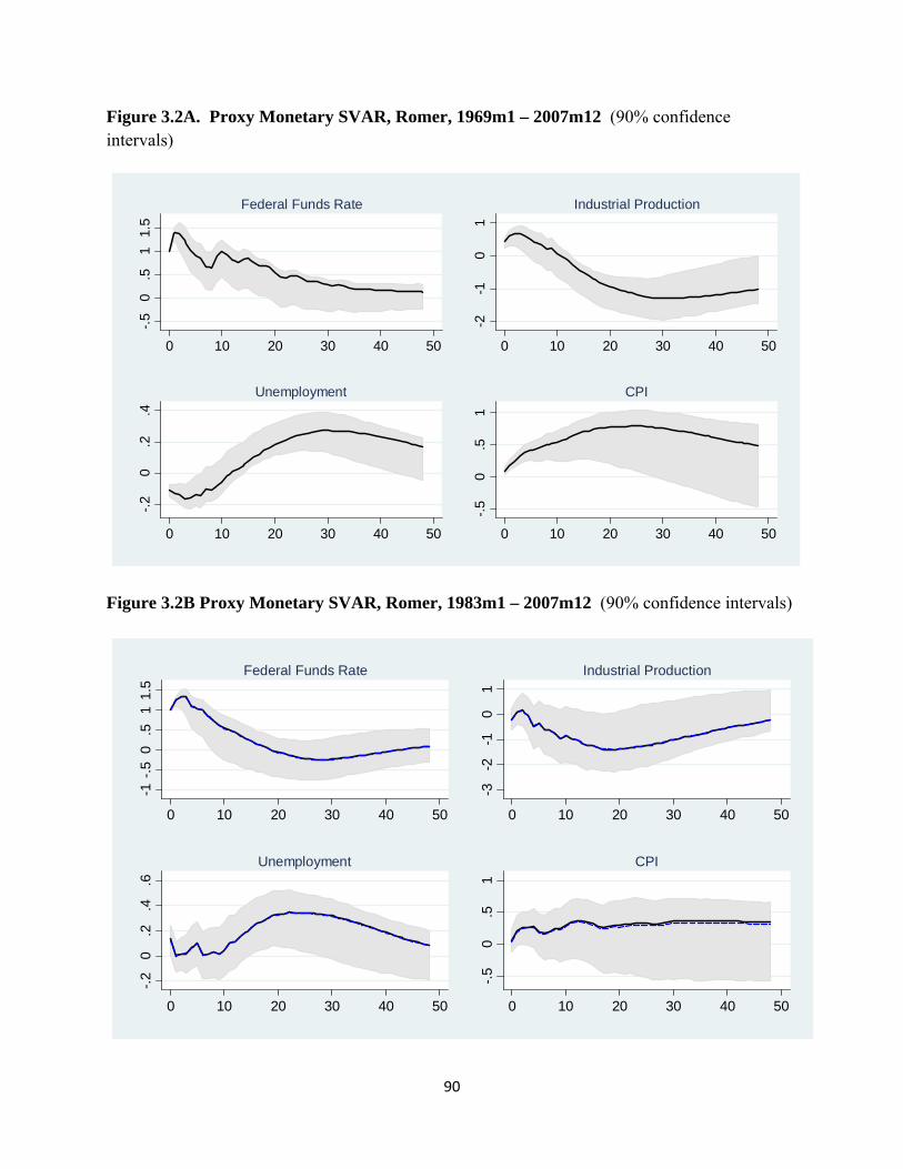
90  

Figure 3.2A. Proxy Monetary SVAR, Romer, 1969m1 – 2007m12 (90% confidence intervals)

Figure 3.2B Proxy Monetary SVAR, Romer, 1983m1 – 2007m12 (90% confidence intervals)

-.5

0.5

11.

5

0 10 20 30 40 50

Federal Funds Rate

-2-1

01

0 10 20 30 40 50

Industrial Production

-.2

0.2

.4

0 10 20 30 40 50

Unemployment

-.5

0.5

1

0 10 20 30 40 50

CPI

-1-.

50

.51

1.5

0 10 20 30 40 50

Federal Funds Rate

-3-2

-10

1

0 10 20 30 40 50

Industrial Production

-.2

0.2

.4.6

0 10 20 30 40 50

Unemployment

-.5

0.5

1

0 10 20 30 40 50

CPI

91  

Figure 3.3A. Monetary Jordà IV, Romer, 1969m1 – 2007m12 (90% confidence intervals)

Figure 3.3B. Monetary Jordà IV, Romer, 1983m1 – 2007m12 (90% confidence intervals)

-20

24

0 10 20 30 40 50

Federal Funds Rate

-6-4

-20

2

0 10 20 30 40 50

Industrial Production

-.5

0.5

1

0 10 20 30 40 50

Unemployment

-2-1

01

2

0 10 20 30 40 50

CPI

-20

24

0 10 20 30 40 50

Federal Funds Rate

-50

510

0 10 20 30 40 50

Industrial Production

-1.5

-1-.

50

.51

0 10 20 30 40 50

Unemployment

-4-2

02

0 10 20 30 40 50

CPI

92  

Figure 3.4A Monetary Proxy SVAR, Gertler-Karadi, 1990m1 – 2012m6 (90% confidence intervals)

Figure 3.4B Monetary Jordà IV, Gertler-Karadi, 1990m1 – 2012m6 (90% confidence intervals)

-.2

-.1

0.1

.2.3

0 10 20 30 40 50

One Year Rate

-.6

-.4

-.2

0.2

0 10 20 30 40 50

Industrial Production

-.05

0.0

5.1

.15

0 10 20 30 40 50

Excess Bond Premium

-.2-

.15-

.1-.

050

.05

0 10 20 30 40 50

CPI

-20

24

6

0 10 20 30 40 50

One Year Rate

-50

510

15

0 10 20 30 40 50

Industrial Production

-3-2

-10

12

0 10 20 30 40 50

Excess Bond Premium

-4-2

02

0 10 20 30 40 50

CPI

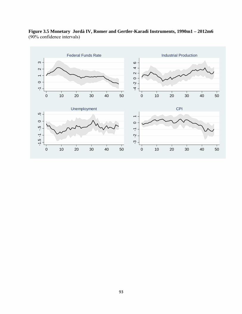
93  

Figure 3.5 Monetary Jordà IV, Romer and Gertler-Karadi Instruments, 1990m1 – 2012m6 (90% confidence intervals)

-10

12

3

0 10 20 30 40 50

Federal Funds Rate

-4-2

02

46

0 10 20 30 40 50

Industrial Production

-1.5

-1-.

50

.5

0 10 20 30 40 50

Unemployment

-3-2

-10

1

0 10 20 30 40 50

CPI

94  

Figure 4.1 Comparison of the Effects of Government Spending Shocks (1947q1 – 2008q4, except for Fisher-Peters, 1958q1 – 2008q4. 90% confidence intervals)

0.5

11.

5

0 4 8 12 16 20quarter

Blanchard-Perotti

-1.5

-1-.

50

.50 4 8 12 16 20

quarter

Blanchard-Perotti

-.5

0.5

11.

5

0 4 8 12 16 20quarter

Ramey News

-1-.

50

.51

0 4 8 12 16 20quarter

Ramey News

-.5

0.5

11.

5

0 4 8 12 16 20quarter

Fisher-Peters News

-4-2

02

0 4 8 12 16 20quarter

Fisher-Peters News

Government Spending Private Spending

95  

Figure 4.2 Effect of Unanticipated Romer Tax Shock, Trivariate VAR, 1950q1 – 2006q4 (90% confidence intervals)

A. Mertens-Ravn (2014) Proxy SVAR

B. Jordà Local Projection, Reduced Form

C. Jordà Local Projection, IV Regression of Output on Tax Revenue

-50

510

0 5 10 15 20

Tax Revenue

-5-2

.50

2.5

0 5 10 15 20

Output

-10

-50

510

0 5 10 15 20

Tax Revenue-4

-20

2

0 5 10 15 20

Output

-6-4

-20

2

0 5 10 15 20

Output

96  

Figure 4.3 Effect of Anticipated Romer Tax Increase, Mertens-Ravn (2011) Estimates 1950q1 – 2006q4 (90% confidence intervals)

-3-2

-10

12

-5 0 5 10 15 20

Output

-2-1

01

-5 0 5 10 15 20

Nondurable Consumption

-4-2

02

4

-5 0 5 10 15 20

Hours-1

5-10-

50

51

0

-5 0 5 10 15 20

Investment

-15-1

0-5

05

-5 0 5 10 15 20

Durable Consumption

97  

Figure 4.4 Effect of News of Future Tax Increase, Leeper, Richter, Walker (2011) Measure

-.2

-.1

0.1

0 5 10 15 20

Output

-.15

-.1-.

050

.05.

1

0 5 10 15 20

Nondurable Consumption

-.2

-.1

0.1

.2

0 5 10 15 20

Hours-.

20

.2.4

.6

0 5 10 15 20

Investment

-.6-

.4-.

20

.2.4

0 5 10 15 20

Durable Consumption