preliminary dynamic modeling of the hanford waste .../67531/metadc719079/m2/1/high... · aspen...
TRANSCRIPT
WSRC-TR-2001-000140, Rev. 0SRT-RPP-2001-00031
Preliminary Dynamic Modeling of the HanfordWaste Treatment Plant Melter Offgas Systems (U)
Frank G. Smith, III
August 15, 2001
UNCLASSIFIEDDOES NOT CONTAIN
UNCLASSIFIED CONTROLLEDNUCLEAR INFORMATION
ADC &ReviewingOfficial:
(Name and Title)
Date:
Westinghouse Savannah River CompanySavannah River SiteAiken, SC 29808
Prepared for the U.S. Department of Energy under Contract No. DE-AC09-96SR18500
This document was prepared in conjunction with work accomplished under Contract No.DE-AC09-96SR18500 with the U.S. Department of Energy.
DISCLAIMER
This report was prepared as an account of work sponsored by an agency of the United States Government.Neither the United States Government nor any agency thereof, nor any of their employees, makes anywarranty, express or implied, or assumes any legal liability or responsibility for the accuracy,completeness, or usefulness of any information, apparatus, product or process disclosed, or represents thatits use would not infringe privately owned rights. Reference herein to any specific commercial product,process or service by trade name, trademark, manufacturer, or otherwise does not necessarily constitute orimply its endorsement, recommendation, or favoring by the United States Government or any agencythereof. The views and opinions of authors expressed herein do not necessarily state or reflect those of theUnited States Government or any agency thereof.
This report has been reproduced directly from the best available copy.
Available for sale to the public, in paper, from: U.S. Department of Commerce, National TechnicalInformation Service, 5285 Port Royal Road, Springfield, VA 22161, phone: (800)553-6847, fax: (703) 605-6900, email: [email protected] online ordering:http://www.ntis.gov/ordering.htm
Available electronically at http://www.doe.gov/bridge
Available for a processing fee to U.S. Department of Energy and its contractors, in paper, from: U.S.Department of Energy, Office of Scientific and Technical Information, P.O. Box 62, Oak Ridge, TN37831-0062, phone: (865 ) 576-8401, fax: (865) 576-5728, email: [email protected]

August 15, 2001 WSRC-TR-2001-000140, Rev. 0SRT-RPP-2001-00031
iii
Keywords: Dynamic ModelMelter OffgasPressure Drop
Aspen Custom Modeler
Retention: Permanent
Preliminary Dynamic Modeling of the HanfordWaste Treatment Plant Melter Offgas Systems (U)
Frank G. Smith, III
Publication Date: August 15, 2001
Westinghouse Savannah River CompanySavannah River SiteAiken, SC 29808
Prepared for the U.S. Department of Energy under Contract No. DE-AC09-96SR18500

August 15, 2001 WSRC-TR-2001-000140, Rev. 0SRT-RPP-2001-00031
iv
Approvals
F. G. Smith, III, AuthorSRTC, Immobilization Technology
M. V. Gregory, Technical ReviewerSRTC, Engineering Development
C. T. Randall, Program Integration ManagerSRTC, Immobilization Technology
D. A. Crowley, L4 ManagerSRTC, Immobilization Technology

August 15, 2001 WSRC-TR-2001-000140, Rev. 0SRT-RPP-2001-00031
v
Table of Contents
Introduction.....................................................................................................................1HLW System Flowsheet..................................................................................................2LAW System Flowsheet..................................................................................................6Model Components .......................................................................................................10
Gas Physical Properties .............................................................................................10Gas Sources...............................................................................................................12Orifice.......................................................................................................................13Air Duct ....................................................................................................................15
Laminar Flow Regime ...........................................................................................16Turbulent Flow Regime .........................................................................................16Transition Flow Regime ........................................................................................17
Gas Volumes.............................................................................................................21Air Filter ...................................................................................................................25Wet Electrostatic Precipitator ....................................................................................29Submerged Bed Scrubber ..........................................................................................31HEPA Preheater ........................................................................................................34PID Controller...........................................................................................................37Control Valve............................................................................................................39Caustic Scrubber .......................................................................................................40Exhaust Blower .........................................................................................................44
HLW Primary and Stack Exhaust Blowers.............................................................44LAW Exhaust Blowers ..........................................................................................46
Thermal Catalytic Oxidizer Unit................................................................................48Thermal Catalytic Oxidizer/Selective Catalytic Reducer............................................49Heat Exchanger .........................................................................................................51Flow Splitting ...........................................................................................................53Fan Speed Control.....................................................................................................53List of System Models...............................................................................................54
Calculation Basis...........................................................................................................55HLW Offgas System Calculations.................................................................................57
HLW Steady-State Operation ....................................................................................57HLW Startup Transient .............................................................................................59HLW Steam Surge ....................................................................................................60
LAW Offgas System Calculations.................................................................................63LAW Steady-State Operation ....................................................................................63LAW Startup Transient .............................................................................................63LAW Steam Surge ....................................................................................................67
Conclusions...................................................................................................................71Nomenclature................................................................................................................73
Greek Symbols..........................................................................................................74Subscripts..................................................................................................................74
References.....................................................................................................................75Appendix A: Derivation of Loss Coefficient Relationship .............................................77
August 15, 2001 WSRC-TR-2001-000140, Rev. 0SRT-RPP-2001-00031
vi
Table of Figures
Figure 1. ACM model of HLW melter offgas system......................................................4Figure 2. Schematic illustration of vessel model. ............................................................5Figure 3a. ACM model of three LAW melter systems. ...................................................8Figure 3b. ACM model of common LAW melter offgas system. ....................................9Figure 4. Calculation of water vapor pressure. ..............................................................11Figure 5. Specification of gas flow profiles...................................................................12Figure 6. Comparison of orifice pressure functions.......................................................14Figure 7. Schematic diagram of pipe model. .................................................................15Figure 8. Friction factor correlation developed for dynamic model. ..............................18Figure 9. Schematic representation of flow through tank gas space...............................22Figure 10. Schematic representation of general filter model..........................................25Figure 11. Fit to manufacturer’s data for HEME pressure drop. ....................................26Figure 12. Illustration of gas flow through cylindrical HEME.......................................28Figure 13. Schematic diagram of WESP model. ...........................................................29Figure 14. Schematic diagram of Submerged Bed Scrubber model. ..............................31Figure 15. Correlation of SBS pressure oscillation amplitude as a function of gas
velocity..................................................................................................................33Figure 16. Schematic diagram of Heater model. ...........................................................34Figure 17. Pressure drop correlation for flow across tube bank. ....................................35Figure 18. Schematic diagram of caustic scrubber model..............................................40Figure 19. Pressure drop correlation for flow through mesh demister............................42Figure 20. Correlations for HLW blower operating curves............................................45Figure 21. Operating curves for LAW primary blower..................................................46Figure 22. Schematic illustration of fan operating curves..............................................47Figure 23. Schematic diagram of Thermal Catalytic Oxidizer Unit. ..............................48Figure 24. Schematic diagram of catalytic unit model...................................................49Figure 25. Schematic diagram of plate heat exchanger model. ......................................51Figure 26. HLW melter steam surge and ADS steam fluctuations.................................56Figure 27. LAW melter steam surge and ADS steam fluctuations.................................56Figure 28. HLW melter pressure during startup and 7X steam surge.............................61Figure 29. HLW control valve operation at 92% full blower speed. ..............................61Figure 30. HLW melter pressure during startup and 7X steam surge.............................62Figure 31. HLW control valve operation at 100% full blower speed. ............................62Figure 32. LAW Melter 1 pressure during startup and 4X steam surge with pressure
control. ..................................................................................................................69Figure 33. LAW Melter 1 pressure during startup and 4X steam surge with design basis
flow and pressure control.......................................................................................69Figure 34. LAW SBS gas flow during startup and 4X steam surge in Melter 1 with
design basis flow and pressure control. ..................................................................70Figure 35. LAW control valve action during startup and 4X steam surge in Melter 1 with
design basis flow and pressure control. ..................................................................70
August 15, 2001 WSRC-TR-2001-000140, Rev. 0SRT-RPP-2001-00031
vii
Table of Tables
Table 1. Gas Sources to HLW Offgas System Model......................................................2Table 2. Gas Sources to LAW Offgas System Model......................................................6Table 3. Model Fittings and Loss Coefficients..............................................................15Table 4. HLW Offgas Air Duct Parameters ..................................................................19Table 5. LAW Offgas Air Duct Parameters ..................................................................20Table 6. Duct Entrance and Exit Loss Coefficient Calculation......................................20Table 7. Characteristics of Gas Space Models...............................................................21Table 8. Dynamic Gas Volumes in System Models ......................................................24Table 9. PID Controller Settings...................................................................................38Table 10. Caustic Scrubber model parameters. .............................................................42Table 11. List of ACM Models.....................................................................................54Table 12. HLW Steady-State Unit Outlet Pressures and Gas Flows ..............................58Table 13. HLW Steady-State Duct Pressure Drops .......................................................59Table 14. LAW Steady-State Unit Outlet Pressures and Gas Flows ..............................65Table 15. LAW Steady-State Duct Pressure Drops .......................................................66
Acronyms
ACM..............Aspen Custom ModelerADS...............Air Displacement SlurryHEME............High Efficiency Mist EliminatorHEPA.............High Efficiency Particle AirHLW..............High Level WasteLAW..............Low Activity WasteLP ..................Low PressureMT.................Metric TonsPID ................Proportional Integral DerivativeRPP................River Protection ProjectSBS................Submerged Bed ScrubberSCR ...............Selective Catalytic ReducerTCO...............Thermal Catalytic OxidizerVVS...............Vessel Ventilation SystemWESP ............Wet Electrostatic PrecipitatorWTP ..............Waste Treatment Plant
August 15, 2001 WSRC-TR-2001-000140, Rev. 0SRT-RPP-2001-00031
1
Preliminary Dynamic Modeling of the HanfordWaste Treatment Plant Melter Offgas Systems (U)
Introduction
Dynamic models of the High Level Waste (HLW) and Low Activity Waste (LAW)melter offgas systems for the proposed River Protection Project (RPP) Waste TreatmentPlant (WTP) at the Hanford Site have been developed using Aspen Custom Modeler(ACM Version 10.2) software from Aspen Technology, Inc. This report documentspreliminary versions of the models that include the components of the offgas systemsfrom the melters through the exhaust stacks and the vessel ventilation systems. Themodels consider only the two major chemical species in the offgas stream: air and steamor water vapor. Model mass and energy balance calculations are designed to show thedynamic behavior of gas pressure and flow throughout the offgas systems in response totransient driving forces. As such, the models are structured to give accurate pressuredrop calculations throughout the offgas systems. Detailed calculations of the steady-statepressure drop through the offgas systems have been performed separately by Hanforddesign engineers (see references). The dynamic models are largely based on thesecalculations and incorporate the most significant factors identified by the steady-stateanalysis. While they do not contain all of the details included in the steady-statecalculations, the models have previously been shown to accurately reproduce the steady-state system pressure profiles when run under identical conditions. These comparisons tothe independent steady-state solution serve as a validation of the dynamic models.
This report is titled preliminary modeling because some aspects of the offgas systemshave not yet been included in the models at this point. However, it was determined thatthe project should provide a preliminary description of the work and some results ofsample calculations to assist the Hanford design work and planning for further modelingwork. Known modeling omissions are listed in the conclusion section of this report. Thecalculated results are also termed preliminary since neither the model nor the input datahave been formally checked. Nevertheless, this report provides an accurate description ofthe models as they now exist, lists some of the model input parameters, and providescalculated results that, at a minimum, indicate the computational capabilities of thedynamic models.
This report covers model development work performed between May, 2000 and April,2001. In April, 2001 the modeling work was temporarily stopped pending a review bynew RPP-WTP project management. Prior to the work stoppage, it was requested by thecustomer that a draft report be written describing the status of the dynamic offgasmodeling work. This report formally issues that draft report incorporating reviewcomments received from the customer.

August 15, 2001 WSRC-TR-2001-000140, Rev. 0SRT-RPP-2001-00031
2
HLW System Flowsheet
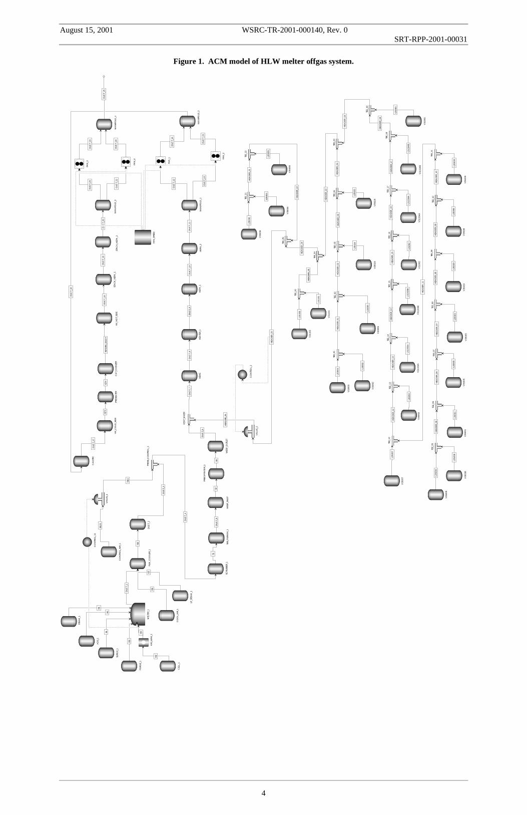
Figure 1 shows a schematic diagram of the flowsheet used to model the HLW melteroffgas system. The flowsheet is based on the system description given by Rouse (2000a).The flowsheet diagram was printed directly from the ACM model representation of thesystem. Solid lines in the figure indicate gas flow paths while dashed lines show controlsignals. Gas lines labeled Duct_xx, Header_xx, or L3xxxx are models of actual gasducting where pressure drop calculations are performed. Other gas lines labeled Sxx orISxx are simply connecting lines that transfer gas from the source point to the destinationbut where no pressure drop calculation is performed.
The melter gas plenum (Melter_1) is the starting point for the HLW model. There arefive sources of gas flow into the meter plenum including air inleakage from the melt cell(Cell_1) through an orifice (Air_Leak_1). From the melter plenum, the gas passesthrough a film cooler where it is mixed with cool air and (possibly) low pressure steam.From the film cooler, the gas flows to the pressure control point where control air,metered through Valve_1, is added to control the melter pressure. Control_11 uses themelter pressure to set the control valve stem position. Sources of gas flow into the HLWsystem are listed in Table 1 (Rouse, 2000m). The fixed values shown in the table arenominal steady-state operating flows. Fluctuations in the melter steam flow caused byslurry feed through variable rate Air Displacement Slurry (ADS) pumps are modeled bysetting a time varying profile in feed stream ADS_1. Half of the total steam is assumedto be generated by a constant flow and half by the transient profile. Similarly, to modelsteam surges, the melter surge flow is ramped through a transient profile defined throughthe model input. The steam surge is added to the nominal steam flow. Therefore, a 7Xsteam surge is interpreted as the total steam flow through the melter increasing to 7 timesthe nominal value which requires a surge flow 6 times nominal. The control air flow rateis set by the control scheme which attempts to maintain a constant melter pressure of –5inches of water relative to the melter cell pressure of –1 inches water.
Table 1. Gas Sources to HLW Offgas System Model
Gas Source Stream Description Flow (kg/s)
Steam_1 Constant steam flow in melter 0.047
ADS_1 Time varying steam flow in melter 0.047
Surge_1 7X steam surge in melter 0.566 (+6X)
Purge_1 Purge air flow to melter 0.031
Cell_1 Air inleakage to melter through orifice Variable
Cool_Air_1 Air flow to film cooler 0.183
LP_Steam_1 Low pressure steam flow to film cooler 0
Control_Air_1 Air flow to melter pressure control mixer Variable
26 VVS Tanks Air flow into vessel ventilation system tanks Fixed + Variable
August 15, 2001 WSRC-TR-2001-000140, Rev. 0SRT-RPP-2001-00031
3
From the pressure control mixer, gas flow passes through a Submerged Bed Scrubber(SBS), Scrubber_1 and Wet Electrostatic Precipitator (WESP), Precipitator_1. The SBSplenum, WESP inlet, and WESP outlet units model significant gas volumes associatedwith the offgas equipment. Following the WESP, the gas flow enters the vent mixerwhere it is mixed with the offgas from the vessel ventilation system. The vesselventilation system is modeled by the 26 vessels, 26 laterals, 25 headers and 25 mixingtees arranged in the flow network shown in the lower half of the Figure 1. Control_2attempts to maintain a constant pressure in Header_25 by adjusting the valve stemposition in Valve_2. Fixed air and steam flows into the HLW vessels were set to nominalvalues reported by Meeuwsen (2001) for the preliminary calculations presented in thisreport.
Each “vessel” shown in the Vessel Ventilation System (VVS) network is a compositemodel as illustrated in Figure 2. The model, ACM model Vessel_System, includes afixed source of gas flow into the vessel gas space representing purge air and otheradditions to the vessel, a variable gas source representing air inleakage into the vesselfrom the surrounding cell, an orifice, and the vessel gas space. Air inleakage is modeledas flow through an orifice that is a function of the pressure difference between the vesselgas space and the surrounding cell.
After mixing with the vessel ventilation gas, the offgas stream flows through a HighEfficiency Mist Eliminator (HEME), a preheater, and two banks of High EfficiencyParticle Air (HEPA) filters. The stream is then split between two identical booster fans.Both fans are modeled to allow calculating fan failure accident scenarios. Exiting thefans, the gas streams are recombined before passing through a caustic scrubber. From thecaustic scrubber, the offgas passes through a thermal catalytic oxidizer unit. The oxidizerhas been broken down into its individual parts for modeling purposes. These parts are:cold side of the heat exchanger, preheater, catalytic oxidizer, and hot side of the heatexchanger. From the thermal catalytic oxidizer, the gas passes through another two setsof HEPA filters and is again split into two streams for two identical stack fans. After thestack fans, the offgas streams are recombined and exit the system at the discharge ofDuct_25.
The calculations performed in each of the individual models of the offgas system unitsare described in detail below. Further details of the dimensions and construction of theHLW offgas system are also provided in the discussion below.
August 15, 2001 WSRC-TR-2001-000140, Rev. 0SRT-RPP-2001-00031
4
Figure 1. ACM model of HLW melter offgas system.
CEL
L_1
AIR
_LEA
K_1
MEL
TER
_1FI
LM_C
OO
LER
_1D
UC
T_2
PR
ESS_
CO
NTR
OL_
1
SCR
UBB
ER_1
PR
ECIP
ITA
TOR
_1
VEN
T_M
IXER
HEA
TER
_1H
EPA
_1M
AN
IFO
LD_1
FAN
_1 FAN
_2
MA
NIF
OLD
_2
HX
_CO
LD_S
IDE
PR
EHEA
TER
CA
T_O
XID
IZER
HX
_HO
T_SI
DE
CA
UST
ICC
ON
TRO
L_11
CO
NTR
OL_
AIR
_1
VA
LVE_
1
CO
NTR
OL_
2
VA
LVE_
2
V33
002
V33
005
V35
024
V35
025
V35
003
V35
005
V35
001
V35
038
V33
003
V35
009
TEE_
01TE
E_02
TEE_
03TE
E_04
TEE_
08TE
E_07
TEE_
06TE
E_05
SBS_
PLE
NU
M_1
STEA
M_1
PU
RG
E_1
SUR
GE_
1
AD
S_1
CO
OL_
AIR
_1
LP_S
TEA
M_1
HEP
A_2
HEM
E
STA
CK
_HEP
A_1
STA
CK
_HEP
A_2
MA
NIF
OLD
_3
FAN
_3
FAN
_4
MA
NIF
OLD
_4
TEE_
23
V35
029
TEE_
09
V35
008
TEE_
10
V35
039
TEE_
11
V35
007
TEE_
12
V35
002
TEE_
13
V31
333A
TEE_
14
V31
333B
TEE_
15
V31
002
TEE_
16
V31
334A
TEE_
17
V31
334B
TEE_
18
V31
001
TEE_
19
V31
102
V31
101
TEE_
20
TEE_
24
V35
036
V35
004
TEE_
21
V35
006
TEE_
22
TEE_
25
WES
P_I
NLE
TW
ESP
_OU
TLET
FAN
_SP
EED
IS0
IS1
IS2
IS3
IS6
IS7
IS8
IS11
IS73
IS74
IS12
1
DU
CT_
1
DU
CT_
4
DU
CT_
6
DU
CT_
8D
UC
T_9
DU
CT_
11
DU
CT_
12
DU
CT_
13
DU
CT_
16
RET
UR
N_D
UC
TD
UC
T_18
HEA
DER
_01
HEA
DER
_02
HEA
DER
_03
HEA
DER
_04
HEA
DER
_19
HEA
DER
_07
HEA
DER
_06
HEA
DER
_05
HEA
DER
_23
HEA
DER
_26
DU
CT_
5
L330
02
L330
03
L330
05
L350
24L3
5025
L350
38
L350
09
L350
01L3
5005
L350
03
DU
CT_
3
S1
S4S5
DU
CT_
14
DU
CT_
15
DU
CT_
10D
UC
T_7
DU
CT_
17
DU
CT_
19D
UC
T_20
DU
CT_
21
DU
CT_
22
DU
CT_
23
DU
CT_
24
DU
CT_
25
HEA
DER
_08
L350
29
HEA
DER
_09
L350
08
HEA
DER
_10
L350
39
HEA
DER
_11
L350
07H
EAD
ER_1
2
L350
02
HEA
DER
_13
L313
33A
HEA
DER
_14
L313
33B
HEA
DER
_15
L310
02
HEA
DER
_16
L313
34A
HEA
DER
_17
L313
34B
HEA
DER
_18
L310
01
L311
02
L311
01
HEA
DER
_20
L350
36
L350
04
HEA
DER
_21
L350
06
HEA
DER
_24
HEA
DER
_22
HEA
DER
_25
S2S3

August 15, 2001 WSRC-TR-2001-000140, Rev. 0SRT-RPP-2001-00031
5
Purge Air
Orifice
GasSpace
LiquidVolume
Lateral Piping
AirInleakage
Figure 2. Schematic illustration of vessel model.

August 15, 2001 WSRC-TR-2001-000140, Rev. 0SRT-RPP-2001-00031
6
LAW System Flowsheet
Figures 3a and 3b show schematic diagrams of the flowsheet used to model the LAWmelter offgas system. The flowsheet is largely based on the system descriptions given byAnderson and Berrios (1999), Berrios (2000), and Rouse (2000a) although it includessome modifications of the original design. As for the HLW system, the LAW processflow diagrams have been printed directly from the ACM model to provide an accuratepicture of how the system has been simulated.
As shown in Figure 3a, the LAW system consists of three melters with dedicated controlsystems, film coolers, submerged bed scrubbers, and wet electrostatic precipitatorsconnected to a common offgas train. The LAW melter systems have essentially the sameconfiguration as that described for the HLW system with the exception that a secondcontrol loop that attempts to maintain a constant gas flow out of the SBS has been added.Sources of gas flow into the LAW system are listed in Table 2 (Rouse, 2000m). Thefixed values shown in the table are nominal steady-state operating flows. Fluctuations inthe melter steam flow caused by slurry feed through variable rate air displacement pumpsare modeled by setting a time varying profile in streams ADS_1, ADS_2, and ADS_3.To model steam surges, the melter surge flow is ramped through a transient profiledefined through the model input. The control air flow rate is set by the control schemewhich attempts to maintain a negative melter pressure of –5 inches of water relative tothe melter cell pressure of –1.5 inches water or controls for constant SBS gas flow.
Table 2. Gas Sources to LAW Offgas System Model
Gas Source Stream Description Flow (kg/s)
Steam_1,3 Constant steam flow in melter 0.038
ADS_1,3 Time varying steam flow in melter 0.038
Surge_1,3 4X steam surge in melter 0.229 (+3X)
Purge_1,3 Purge air flow to melter 0.061
Cell_1,3 Air inleakage to melter through orifice Variable
Cool_Air_1,3 Air flow to film cooler 0.092
LP_Steam_1,3 Low pressure steam flow to film cooler 0.056
Control_Air_1,3 Air flow to melter pressure control mixer Variable
12 VVS Tanks Air flow into vessel ventilation system tanks Fixed + Variable
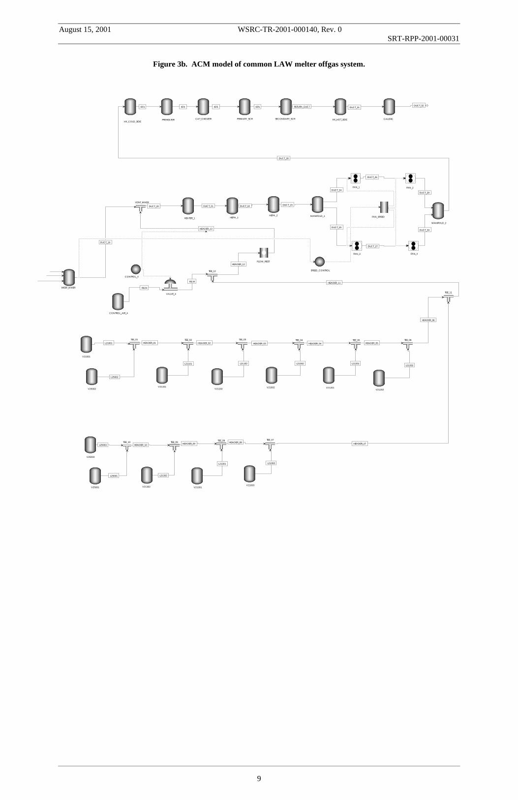
As shown in Figure 3b, gas flow from the vessel ventilation system is mixed with themelter offgas downstream of the point where the offgas streams from the three melterscombine. The vessel ventilation system is modeled by 12 vessels, 12 laterals, 13 headersand 12 mixing tees arranged in the flow network shown in the lower half of the Figure3b. As before, each vessel in the network is the composite model illustrated in Figure 2including a fixed source of gas flow into the vessel gas space and air inleakage into thevessel from the surrounding cell. Control_4 attempts to maintain a constant gas flow inHeader_13 by adjusting the valve stem position in Valve_4. Fixed air and steam flows
August 15, 2001 WSRC-TR-2001-000140, Rev. 0SRT-RPP-2001-00031
7
into the LAW vessels were set to the nominal values reported by Fergestrom andMeeuwsen (2000) for the preliminary calculations presented in this report.
After mixing with the vessel ventilation gas, the offgas stream flows through a preheater,and two banks of HEPA filters. The stream is then split between two parallel sets of twoidentical booster fans operating in series. All four fans are explicitly modeled to allowcalculating fan failure accident scenarios. Exiting the fans, the gas streams arerecombined before passing through a thermal catalytic oxidizer unit. As in the HLWsystem, the oxidizer has been broken down into its individual parts for modelingpurposes. These parts are: cold side of the heat exchanger, preheater, catalytic oxidizer,primary catalytic reduction unit, secondary catalytic reduction unit, and hot side of theheat exchanger. From the thermal catalytic oxidizer, the gas passes through a causticscrubber and then exits the system at the discharge of Duct_32.
The calculations performed in each of the individual models of the offgas system unitsare described in detail below. Further details of the dimensions and construction of theLAW offgas system are also provided in the discussion below.

August 15, 2001 WSRC-TR-2001-000140, Rev. 0SRT-RPP-2001-00031
8
Figure 3a. ACM model of three LAW melter systems.
CELL_1
AIR_LEAK_1
MELTER_1FILM_COOLER_1
DUCT_2 PRESS_CONTROL_1 SCRUBBER_1 PRECIPITATOR_1
CELL_2
AIR_LEAK_2
MELTER_2 FILM_COOLER_2 DUCT_8PRESS_CONTROL_2
SCRUBBER_2PRECIPITATOR_2
CELL_3
AIR_LEAK_3MELTER_3
FILM_COOLER_3DUCT_14
PRESS_CONTROL_3 SCRUBBER_3PRECIPITATOR_3
WESP_MIXER
CONTROL_11
CONTROL_12
PROCESSOR_1
CONTROL_AIR_1
VALVE_1
CONTROL_21
CONTROL_22
PROCESSOR_2
CONTROL_AIR_2
VALVE_2
CONTROL_31
CONTROL_32
PROCESSOR_3
CONTROL_AIR_3
VALVE_3
SBS_PLENUM_1
SBS_PLENUM_2
SBS_PLENUM_3
SURGE_2
SURGE_3
STEAM_1
PURGE_1
SURGE_1
ADS_1
STEAM_2
ADS_2
PURGE_2
COOL_AIR_1
COOL_AIR_2
LP_STEAM_1
LP_STEAM_2
STEAM_3
ADS_3
PURGE_3
COOL_AIR_3
LP_STEAM_3
WESP_1_INLETWESP_1_OUTLET
WESP_2_INLETWESP_2_OUTLET
WESP_3_INLET WESP_3_OUTLET
IS0
IS1
IS2
IS3
IS6
IS7
IS8
IS11
IS17
IS18
IS19
IS20
IS23
IS24
IS25
IS28
IS34
IS35
IS36
IS37
IS40
IS41
IS42
IS45
IS121
IS122
IS123
DUCT_1
DUCT_4
DUCT_6
DUCT_7DUCT_10
DUCT_12
DUCT_13
DUCT_16
DUCT_18
DUCT_5
DUCT_11
DUCT_17
DUCT_3
DUCT_9
DUCT_15
S1
S2
S3
S4S5
S7
S8S9
S10
S6S11
S12 S13
S14 S15
August 15, 2001 WSRC-TR-2001-000140, Rev. 0SRT-RPP-2001-00031
9
Figure 3b. ACM model of common LAW melter offgas system.
WESP_MIXER
VENT_MIXER
HEATER_1 HEPA_1MANIFOLD_1
FAN_1
FAN_3
MANIFOLD_2
HX_COLD_SIDEPREHEATER CAT_OXIDIZER PRIMARY_SCR SECONDARY_SCR HX_HOT_SIDE CAUSTIC
CONTROL_4
CONTROL_AIR_4
VALVE_4
V21001
V21101V21102 V21002 V21201
V21202
V21003V21301V21302V25001
V25002
V25003
TEE_01 TEE_02 TEE_03 TEE_04 TEE_05 TEE_06
TEE_07TEE_08TEE_09TEE_10
TEE_11
TEE_12
FLOW_REST
FAN_2
FAN_4
HEPA_2
SPEED_CONTROL
FAN_SPEED
IS73 IS74 IS75 IS76
IS116
IS124
DUCT_19
DUCT_20 DUCT_21 DUCT_23
DUCT_24
DUCT_25
DUCT_28
DUCT_29
DUCT_30
RETURN_DUCT DUCT_31DUCT_32
HEADER_01 HEADER_02 HEADER_03 HEADER_04 HEADER_05
HEADER_06
HEADER_07HEADER_08HEADER_09HEADER_10
HEADER_12
HEADER_11
HEADER_13
L21001
L25002
L21101 L21102 L21002 L21201L21202
L25001
L25003
L21302
L21301 L21003
DUCT_26
DUCT_27
DUCT_22

August 15, 2001 WSRC-TR-2001-000140, Rev. 0SRT-RPP-2001-00031
10
Model Components
In this section of the report, gas physical property calculations and the individual modelsdeveloped to describe the various components of the melter offgas system are described.
Gas Physical Properties
The gas is treated as an ideal mixture of air and water and the gas density is calculatedfrom the ideal gas relationship:
( )273TRNVP g += or ( )273TR
MP
g
avgg +
=ρ . (1)
The average molecular weight of the gas mixture is calculated as:
waterwaterairairavg MyMyM += , (2)
where yair and ywater are the gas phase mole fractions of air and water. The molecularweights of air and water are taken to be 29.0 and 18.0, respectively.
Gas viscosity, in units of Pa-s, is calculated for each of the components in the gas mixtureusing the equations recommended by Rouse (2000g):
2g
11g
86air T10161.3T10183.51013.17 −−− ⋅⋅⋅ −+=µ , (3a)
2g
11g
86water T10000.2T10113.31012.9 −−− ⋅⋅⋅ ++=µ . (3b)
A mixture viscosity is calculated as the mass average of the component values:
waterwaterairairg xx µµµ += (3c)
where xair and xwater are the mass fractions of air and water in the gas phase, respectively.
Gas specific enthalpy, in units of kJ/kg, is calculated for each of the components in themixture using the temperature functions developed by Rouse as reported by Meeuwsen(2001):
2g
3gair T10077.1T991.0h −⋅+= , (4a)
2g
4gwater T10144.3T818.1h −⋅+= . (4b)
The enthalpy of air is the average of the equations for oxygen and nitrogen weighted bythe respective mass fractions. A mixture enthalpy is calculated as the mass average of thecomponent values:
waterwaterairairg hxhxh += . (4c)
August 15, 2001 WSRC-TR-2001-000140, Rev. 0SRT-RPP-2001-00031
11
The saturation vapor pressure of water is calculated as a function of gas temperatureusing the Antoinne equation provided by Holland (1981):
( ) ( )[ ]228T2.3841344.18exp760101325p gsat +−= . (5)
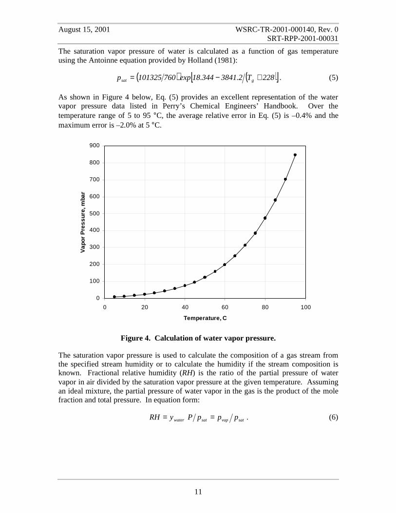
As shown in Figure 4 below, Eq. (5) provides an excellent representation of the watervapor pressure data listed in Perry’s Chemical Engineers’ Handbook. Over thetemperature range of 5 to 95 °C, the average relative error in Eq. (5) is –0.4% and themaximum error is –2.0% at 5 °C.
Figure 4. Calculation of water vapor pressure.
The saturation vapor pressure is used to calculate the composition of a gas stream fromthe specified stream humidity or to calculate the humidity if the stream composition isknown. Fractional relative humidity (RH) is the ratio of the partial pressure of watervapor in air divided by the saturation vapor pressure at the given temperature. Assumingan ideal mixture, the partial pressure of water vapor in the gas is the product of the molefraction and total pressure. In equation form:
satvapsatwater pppPyRH == . (6)
0
100
200
300
400
500
600
700
800
900
0 20 40 60 80 100
Temperature, C
Vap
or P
ress
ure,
mba
r
August 15, 2001 WSRC-TR-2001-000140, Rev. 0SRT-RPP-2001-00031
12
Gas Sources
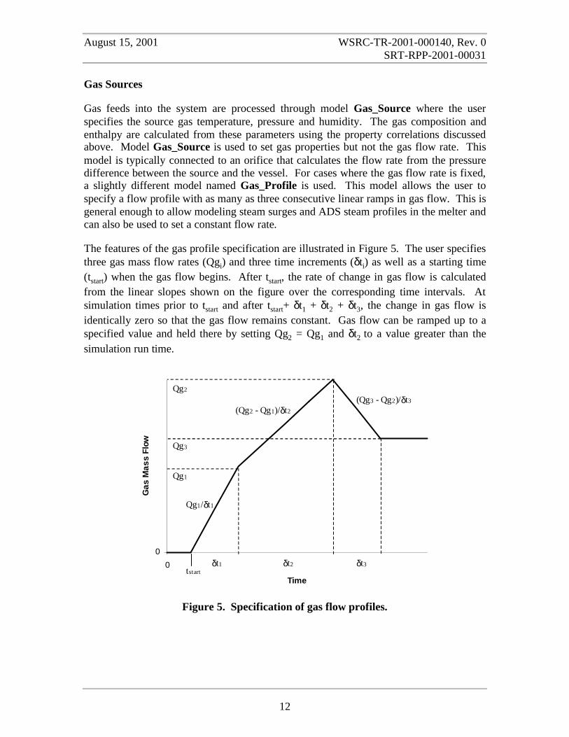
Gas feeds into the system are processed through model Gas_Source where the userspecifies the source gas temperature, pressure and humidity. The gas composition andenthalpy are calculated from these parameters using the property correlations discussedabove. Model Gas_Source is used to set gas properties but not the gas flow rate. Thismodel is typically connected to an orifice that calculates the flow rate from the pressuredifference between the source and the vessel. For cases where the gas flow rate is fixed,a slightly different model named Gas_Profile is used. This model allows the user tospecify a flow profile with as many as three consecutive linear ramps in gas flow. This isgeneral enough to allow modeling steam surges and ADS steam profiles in the melter andcan also be used to set a constant flow rate.
The features of the gas profile specification are illustrated in Figure 5. The user specifiesthree gas mass flow rates (Qgi) and three time increments (δti) as well as a starting time(tstart) when the gas flow begins. After tstart, the rate of change in gas flow is calculatedfrom the linear slopes shown on the figure over the corresponding time intervals. Atsimulation times prior to tstart and after tstart+ δt1 + δt2 + δt3, the change in gas flow isidentically zero so that the gas flow remains constant. Gas flow can be ramped up to aspecified value and held there by setting Qg2 = Qg1 and δt2 to a value greater than thesimulation run time.
Figure 5. Specification of gas flow profiles.
0
0
Time
Gas
Mas
s Fl
ow
δt1 δt2 δt3
Qg1
Qg3
Qg2
(Qg3 - Qg2)/δt3
(Qg2 - Qg1)/δt2
Qg1/δt1
tstart
August 15, 2001 WSRC-TR-2001-000140, Rev. 0SRT-RPP-2001-00031
13
Orifice
Following Rouse (1999), model Orifice calculates flow through an orifice using the basicequation:
pDCQm g2ovggg ∆== ρρ& . (7)
The orifice loss coefficient Cv and the orifice diameter are specified through the inputsection of the code. Nominally we use the value Cv = 0.5715. Air inleakage to the melterand VVS vessels is calculated as flow through an orifice and the model is also used forthe restricting orifice in the LAW vessel ventilation system.
A difficulty arises in applying Eq. (7) since the numerical solution technique requirescalculating the derivatives of the variables with respect to all dependent variables.Taking the derivative of gas flow with respect to pressure difference in Eq. (7) gives:
( )p
1DC
2
1
p
mg
2ov
g
∆=
∆∂∂
ρ&
. (8)
At a pressure drop of zero, Eq. (8) becomes singular and the solution fails. To overcomethis problem, Eq. (7) is first rearranged into the form:
( )pf
pDCm g
2ovg ∆
∆= ρ& . (9)
To recover Eq.(7) would require the function of the pressure difference in thedenominator of Eq. (9) to be:
( ) ppf ∆=∆ . (10a)
Note that using Eqs. (9) and (10a) instead of Eq. (7) allows the correct assignment of theflow direction from the sign of the pressure difference. To avoid an infinite slope at zeropressure drop, Eq. (10a) is replaced with the alternative form:
( ) ( )p101.0ppf ∆++∆≡∆ . (10b)
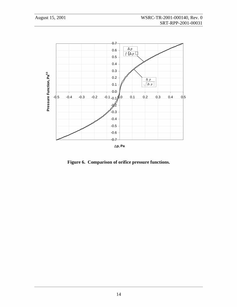
The behavior of this functional form is compared to that obtained from Eq. (10a) inFigure 6. The second term under the square root in Eq. (10b) ranges from 0.01 at smallpressure drops to essentially zero as the pressure difference increases from zero toward alarge value. For the purposes of the melter offgas system calculations, this function isindistinguishable from the square root of the pressure difference.
August 15, 2001 WSRC-TR-2001-000140, Rev. 0SRT-RPP-2001-00031
14
Figure 6. Comparison of orifice pressure functions.
-0.7
-0.6
-0.5
-0.4
-0.3
-0.2
-0.1
0.0
0.1
0.2
0.3
0.4
0.5
0.6
0.7
-0.5 -0.4 -0.3 -0.2 -0.1 0.0 0.1 0.2 0.3 0.4 0.5
∆p, Pa
Pre
ssur
e Fu
nctio
n, P
a0.5
p
p
∆∆
( )pf
p
∆∆

August 15, 2001 WSRC-TR-2001-000140, Rev. 0SRT-RPP-2001-00031
15
Air Duct
Air ducts in the system are modeled as gas flow through pipes having flow resistanceswith the model Pipe_Flow and in the stream Gas_Pipe. Some of the nomenclature usedin discussing the pipe flow model is illustrated in Figure 7.
Dp DoutDin θoutθin
Lp
Figure 7. Schematic diagram of pipe model.
The pressure drop across the pipe is calculated from the equation:
( ) gggextextententaddf
ffp
p0 uuKCKCKCn
D
Lf
2
1p ρ
++
++=∆ ∑ . (11)
Loss coefficients for the fittings listed in Table 3 have been automatically included in thepressure drop calculation. The user must only specify the number of each fitting (nf) inthe duct through the tabular data entry for each section of piping. The parameter Kadd isincluded to allow the used to specify additional loss coefficients to account for non-standard hardware configurations. This formulation is basically identical to that used byRouse (2000g, 2000j).
Table 3. Model Fittings and Loss Coefficients
Fitting Loss Coefficient Cf
45° Elbow 16
90° Elbow 30
Branch Tee 60
Flow Through Tee 20
Butterfly Valve 51.4 –52.36 Dp
Note that Eq. (11) uses the friction factor multiplied by gas velocity to the first power.The other fluid velocity that would normally appear in Eq. (11) has been incorporatedinto the definition of the friction factor f0. This modified formulation is convenient fordealing with both laminar and turbulent flow regimes as shown below.
The friction factor in Eq. (11) is calculated as a function of the flow Reynolds numberthat is defined by the relationship:

August 15, 2001 WSRC-TR-2001-000140, Rev. 0SRT-RPP-2001-00031
16
gp
g
g
ggpRe D
m4uDN
µπµρ &
=≡ . (12)
The second equality in Eq. (12) is derived from the definition of mass flow:
fggg Aum ρ=& , (13)
and by using the calculation of the flow area from 4DA 2pf π= .
Laminar Flow Regime
At low fluid velocity, the laminar friction factor is calculated as:
gp
gg
Relam0 D
64u
N
64f
ρµ
=≡ . (14)
By defining the friction factor to include the gas velocity, the laminar flow calculationavoids a numerical singularity in calculating the value of the friction factor at no flowconditions (ug = 0). The last equality in Eq. (14) is used to calculate the modifiedlaminar flow friction factor for all cases and Eq. (11) then correctly calculates a pressuredrop of zero at no flow without the use of special logic tests. No flow conditions canoccur during startup and during flow reversal.
Turbulent Flow Regime
In the turbulent flow regime, the friction factor is calculated using an explicitapproximation to the Colebrook-White equation originally due to Jain (1976) andreported by Blevins (1984). This correlation, multiplied by the gas velocity, can bewritten as:
2
9.0Rep
s10gturb0
N
74.5
D7.3
klog2uf
−
+= , (15)
which is identical in form to that used by Rouse (2000j). In practice, we have scaled theReynolds number defined in Eq. (12) by dividing by 1000 and added a small value (0.01)to it to avoid a division by zero when the Reynolds number is identically zero. Thesemodifications give the functional form for the turbulent friction factor that is coded intothe model:
( )
2
9.0Rep
s10gturb0
01.0N
01145.0
D7.3
klog2uf
−
++= . (15a)
August 15, 2001 WSRC-TR-2001-000140, Rev. 0SRT-RPP-2001-00031
17
Transition Flow Regime
To obtain a smooth transition between the laminar and turbulent flow regimes, the overallfriction factor is calculated using the exponential interpolation scheme shown in Eq. (16):
( ) ( )[ ]{ } ( )3N2expfff
3N2exp1f3N2expff
Returb0lam0turb0
Returb0Relam00
−−+=
−−+−=. (16)
Clearly in the limit of the Reynolds number approaching zero Eq. (16) approaches thelaminar flow friction factor and in the limit of a large Reynolds number the turbulentflow friction factor dominates. Figure 8 shows the friction factor approximation over therange of Reynolds number from 10 to 105. The friction factor begins to transition fromthe laminar correlation at a Reynolds number of approximately 200 and is essentiallyusing the turbulent friction factor at Reynolds numbers of 4000 and higher. As indicatedon the figure, the transition flow regime is normally assumed to occur between Reynoldsnumbers of 2000 and 4000. However, if the laminar friction factor is followed to aReynolds number of 2000 it will increase during the transition to turbulent flow. For agiven pressure gradient, this increase in the friction factor will decrease the gas velocityand drive the flow back toward the laminar regime and the solution will have difficultyconverging. Similar arguments apply when the flow is decreasing from turbulent flow tolaminar. In either case, if the same value of the friction factor can be obtained with morethan one value of gas velocity the code will have difficulty converging. The interpolationscheme in Eq. (16) eliminates this problem by creating a single valued function for thefriction factor that monotonically decreases as the Reynolds number increases. Thefactor of 2/3 in the exponential was chosen by trial and error to find a smoothing functionthat was both monotonic and accurately reproduced the friction factor in the turbulentregime where the gas flow predominantly occurs.

August 15, 2001 WSRC-TR-2001-000140, Rev. 0SRT-RPP-2001-00031
18
Figure 8. Friction factor correlation developed for dynamic model.
Table 4 lists parameters for the air ducts modeled in the HLW offgas system (Rouse,2000k, Appendix c.3) while Table 5 gives parameters for the LAW offgas system ducts(Rouse, 2000l, Appendix c.3). The added resistances in Duct 4 in the HLW system andDucts 4, 10 and 16 in the LAW system account for the presence of non-standard elbowsin those lines (Rouse, 2000g). The dynamic model uses a duct to connect the melter tothe film cooler where, in reality, the film cooler is placed directly on the melter offgasport. Therefore, Duct 1 in the HLW model and Ducts 1, 7 and 13 in the LAW model areused to account for entrance losses into the film cooler with a small length of duct thatoffers negligible additional flow resistance. Duct 2 represents pressure losses through thefilm cooler itself. The entrance contraction in the first duct in the system represents thesudden contraction from the melter plenum into the duct which is assumed to be anabrupt change in duct diameter. Similarly, the expansion at the end represents flow outthe stack and is again assumed to be an abrupt expansion. These sudden expansions andcontractions are flagged by specifying a reducer angle of 180°. All other expansions andcontractions in the system are assumed to be gradual changes in duct diameter with areducer angle of 30°.
Entrance and exit losses in Eq. (11) are calculated using the following method. The userinputs diameters of inlet (Din) and outlet (Dout) fittings to the duct and inlet and outlet
0.01
0.10
1.00
10.00
0.01 0.10 1.00 10.00 100.00
Re/1000
fric
tio
n fa
cto
r
laminar
turbulent
interpolatedcorrelation
transitionregion
standardtransition

August 15, 2001 WSRC-TR-2001-000140, Rev. 0SRT-RPP-2001-00031
19
reducer angles. The code then checks whether there is an expansion or contraction at theinlet and outlet and calculates the corresponding loss coefficient using the equationsgiven by Rouse (2000g) as reproduced in Table 6. The coefficients in Table 6 apply forsudden contractions or expansions. If reducer angles (θin and θout) less than 180° arespecified, the model adjusts the loss coefficients by multiplying by factors of
( )360sin6.2 θπ for a gradual expansion or ( )360sin6.1 θπ for a gradual contraction.This calculation is also used to account for the sudden contraction losses between themelter and film cooler and sudden expansion losses at the exit of the offgas system intothe stack.
Table 4. HLW Offgas Air Duct Parameters
Duct ks(mx104)
Lp(m)
IDp(m)
n45 n90 nbt nft nbv Exp Con Kadd
1 9.1440 0.0305 0.2027 0 0 0 0 0 0 1 0
2 9.1440 0.3048 0.2027 0 0 0 1 0 0 0 0
3 9.1440 1.0668 0.2027 0 0 1 0 0 0 0 0
4 9.1440 2.7432 0.2027 0 0 0 0 0 0 0 36.05
5 0.4572 16.1544 0.2027 1 3 0 0 0 0 0 0
6 0.4572 19.8120 0.2027 0 3 0 0 0 1 0 0
7 0.4572 21.9456 0.2125 0 3 1 1 1 0 0 0
8 0.4572 13.4112 0.2125 1 2 0 0 0 0 0 0
9 0.4572 17.0688 0.3048 0 2 0 0 0 0 0 0
10 0.4572 6.0960 0.3048 0 4 0 0 0 0 0 0
11 0.4572 60.9600 0.3048 0 12 0 1 1 0 0 0
12, 13 0.4572 3.3528 0.2027 0 2 0 1 1 0 1 0
14, 15 0.4572 3.0480 0.2027 0 2 1 0 1 1 0 0
16 0.4572 25.6032 0.2125 0 6 0 1 1 0 0 0
17 0.4572 32.9184 0.2125 0 6 0 1 2 0 0 0
18 0.4572 24.3840 0.3048 0 3 0 0 0 0 0 0
19 0.4572 6.0960 0.3048 0 4 0 0 0 0 0 0
20 0.4572 15.2400 0.3048 0 3 0 1 0 0 0 0
21, 22 0.4572 3.0480 0.2027 0 3 1 0 0 0 1 0
23, 24 0.4572 3.0480 0.2027 0 3 0 1 0 1 0 0
25 0.4572 112.7760 0.3048 0 4 1 0 0 1 0 0

August 15, 2001 WSRC-TR-2001-000140, Rev. 0SRT-RPP-2001-00031
20
Table 5. LAW Offgas Air Duct Parameters
Duct ks(mx104)
Lp(m)
Dp(m)
n45 n90 nbt nft nbv Exp Con Kadd
1, 7, 13 9.1440 0.0305 0.2454 0 0 0 0 0 0 1 0
2, 8, 14 9.1440 0.3048 0.2454 0 0 0 1 0 0 0 0
3, 9, 15 9.1440 1.2192 0.2454 0 0 1 0 0 0 0 0
4, 10, 16 9.1440 3.3528 0.2454 0 0 0 0 0 0 0 36.05
5, 11, 17 0.4572 16.1544 0.2454 1 3 0 0 0 0 0 0
6, 12, 18 0.4572 15.2400 0.2454 0 2 0 0 0 0 0 0
19 0.4572 12.4968 0.4286 0 0 1 1 0 1 0 0
20 0.4572 5.4864 0.4778 0 1 0 0 0 0 0 0
21 0.4572 41.1480 0.4778 0 6 0 0 0 0 0 0
22 0.4572 3.0480 0.4778 0 4 1 2 0 0 0 0
23 0.4572 31.3944 0.4778 0 5 0 0 1 0 1 0
24, 25 0.4572 5.7912 0.3334 0 1 0 0 1 1 0 0
26, 27 0.4572 3.6576 0.3334 0 2 0 0 0 0 0 0
28, 29 0.4572 5.7912 0.3334 0 3 1 0 0 0 0 0
30 0.4572 21.6408 0.4286 0 8 0 1 0 0 0 0
31 0.4572 96.6216 0.5746 2 6 0 0 0 0 0 0
32 0.4572 83.8200 0.4286 0 8 0 0 0 1 0 0
Table 6. Duct Entrance and Exit Loss Coefficient Calculation
Test Case Loss Coefficient
Din < Dp Entrance expansion ( )[ ]22pinent DD1K −=
Din > Dp Entrance contraction ( )[ ]2inpent DD15.0K −=
Dout < Dp Exit contraction ( )[ ]2poutext DD15.0K −=
Dout > Dp Exit expansion ( )[ ]22outpext DD1K −=
August 15, 2001 WSRC-TR-2001-000140, Rev. 0SRT-RPP-2001-00031
21
Gas Volumes
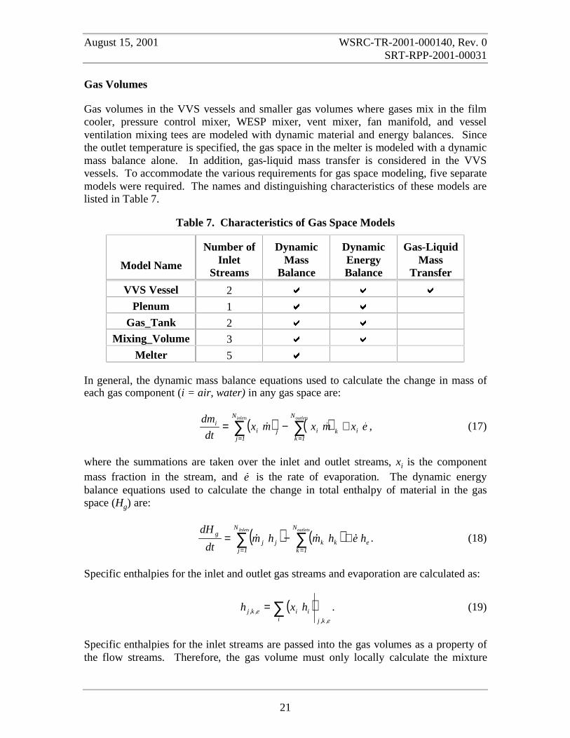
Gas volumes in the VVS vessels and smaller gas volumes where gases mix in the filmcooler, pressure control mixer, WESP mixer, vent mixer, fan manifold, and vesselventilation mixing tees are modeled with dynamic material and energy balances. Sincethe outlet temperature is specified, the gas space in the melter is modeled with a dynamicmass balance alone. In addition, gas-liquid mass transfer is considered in the VVSvessels. To accommodate the various requirements for gas space modeling, five separatemodels were required. The names and distinguishing characteristics of these models arelisted in Table 7.
Table 7. Characteristics of Gas Space Models
Model Name
Number ofInlet
Streams
DynamicMass
Balance
DynamicEnergyBalance
Gas-LiquidMass
Transfer
VVS Vessel 2 a a a
Plenum 1 a a
Gas_Tank 2 a a
Mixing_Volume 3 a a
Melter 5 a
In general, the dynamic mass balance equations used to calculate the change in mass ofeach gas component (i = air, water) in any gas space are:
( ) ( ) exmxmxdt
dmi
N
1kki
N
1jji
ioutletsinlets
&&& +−= ∑∑==
, (17)
where the summations are taken over the inlet and outlet streams, xi is the componentmass fraction in the stream, and e& is the rate of evaporation. The dynamic energybalance equations used to calculate the change in total enthalpy of material in the gasspace (Hg) are:
( ) ( ) e
N
1kkk
N
1jjj
g hehmhmdt
dH outletsInlets
&&& +−= ∑∑==
. (18)
Specific enthalpies for the inlet and outlet gas streams and evaporation are calculated as:
( )e,k,ji
iie,k,j hxh ∑= . (19)
Specific enthalpies for the inlet streams are passed into the gas volumes as a property ofthe flow streams. Therefore, the gas volume must only locally calculate the mixture
August 15, 2001 WSRC-TR-2001-000140, Rev. 0SRT-RPP-2001-00031
22
specific enthalpy which is the same as the outlet enthalpy assuming a well mixed volume.Evaporation is assumed to add water vapor to the gas phase at the liquid temperature.We assume that the heat of evaporation is supplied by the large mass of water in theliquid phase. The total enthalpy in the gas mixture is calculated as total mass multipliedby the mixture specific enthalpy:
( )
= ∑∑
iii
iig hxmH . (20)
Equations (18) and (20) are solved for the temperature in the gas space. The gas spacesare assumed to be well-mixed volumes so that the gas composition, temperature andenthalpy in the outlet stream are the same as that within the volume.
In the VVS vessels, the evaporation of water from the liquid in the vessel into the gasphase is modeled. The rate of evaporation is calculated as:
( )( )273TR
ppMkAe
g
vapsatwatercs +
−=& . (21)
In Eq. (21), As is the surface area of the liquid ( 4d 2tπ ), kc is the mass transfer
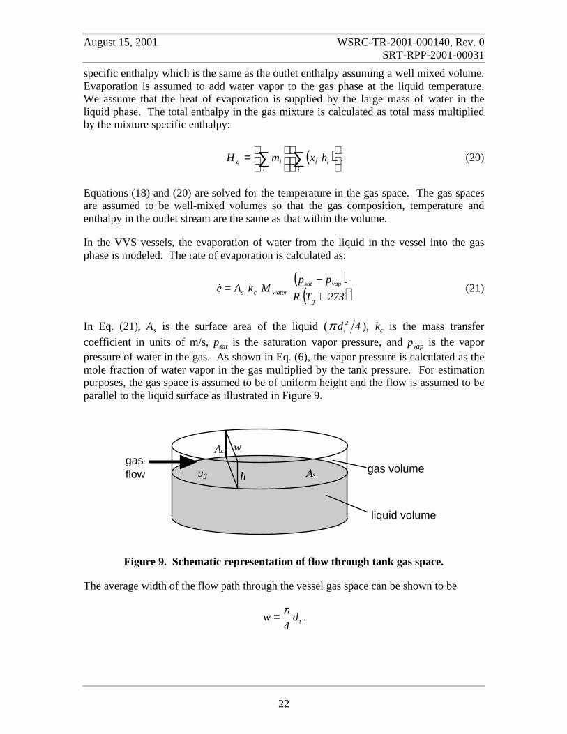
coefficient in units of m/s, psat is the saturation vapor pressure, and pvap is the vaporpressure of water in the gas. As shown in Eq. (6), the vapor pressure is calculated as themole fraction of water vapor in the gas multiplied by the tank pressure. For estimationpurposes, the gas space is assumed to be of uniform height and the flow is assumed to beparallel to the liquid surface as illustrated in Figure 9.
gasflow gas volume
liquid volume
h Asug
Ac w
Figure 9. Schematic representation of flow through tank gas space.
The average width of the flow path through the vessel gas space can be shown to be
td4
wπ= .
August 15, 2001 WSRC-TR-2001-000140, Rev. 0SRT-RPP-2001-00031
23
The average cross-sectional flow area (Ac) is the average flow width multiplied by theheight of the gas layer (h). The height of the gas layer is the gas volume divided by thetank surface area. Also, the average gas velocity is the volumetric flow (Q) divided bythe average flow area. Combining these definitions gives the relationships:
tstc d
V
A
Vd
4hwA === π
and V
dQu t
g = .
To evaluate the mass transfer coefficient, a characteristic Reynolds number for flowacross the liquid surface must be defined. We assume that the correct length scale for theflow is the tank diameter and define the flow Reynolds number as:
g
ggtRe
udN
µρ
= . (22)
A rough calculation using the above relationships indicates that gas flow across thesurface of the tank will be in the laminar flow regime under any reasonable flowconditions. Therefore the laminar flow correlation in Eq. (23) for flow across a flat plateis used to estimate the mass transfer coefficient (Foust et al., 1967):
( ) 5.0
Re
5.0Reg
c
01.0N
0206.0
N
65.0
u
k
+≅= . (23)
The second equality in Eq. (23) is obtained by scaling the Reynolds number by a factor of1000 ( 3
ReRe 10NN −⋅= ) and adding the constant 0.01 to avoid a division by zero when
there is no gas flow through the tank.
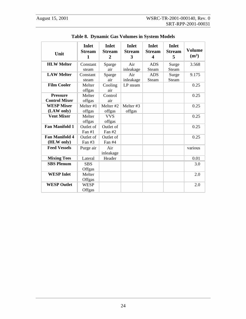
Inlet streams and mixing volumes used in the system models are shown in Table 8 forboth the LAW system and the HLW system. Gas volumes in the VVS vessels, themelter, and the SBS and WESP plenums were obtained from the reports by Rouse(2000m), Fergestrom and Meeuwsen, (2000), and Meeuwsen (2001). Other gas spacevolumes in the model are arbitrary and do not fully account for the gas volume of theoffgas system.
August 15, 2001 WSRC-TR-2001-000140, Rev. 0SRT-RPP-2001-00031
24
Table 8. Dynamic Gas Volumes in System Models
Unit
InletStream
1
InletStream
2
InletStream
3
InletStream
4
InletStream
5Volume
(m3)
HLW Melter Constantsteam
Spargeair
Airinleakage
ADSSteam
SurgeSteam
3.568
LAW Melter Constantsteam
Spargeair
Airinleakage
ADSSteam
SurgeSteam
9.175
Film Cooler Melteroffgas
Coolingair
LP steam 0.25
PressureControl Mixer
Melteroffgas
Controlair
0.25
WESP Mixer(LAW only)
Melter #1offgas
Melter #2offgas
Melter #3offgas
0.25
Vent Mixer Melteroffgas
VVSoffgas
0.25
Fan Manifold 1 Outlet ofFan #1
Outlet ofFan #2
0.25
Fan Manifold 4(HLW only)
Outlet ofFan #3
Outlet ofFan #4
0.25
Feed Vessels Purge air Airinleakage
various
Mixing Tees Lateral Header 0.01SBS Plenum SBS
Offgas3.0
WESP Inlet MelterOffgas
2.0
WESP Outlet WESPOffgas
2.0

August 15, 2001 WSRC-TR-2001-000140, Rev. 0SRT-RPP-2001-00031
25
Air Filter
The generic model Filter was developed to calculate the pressure drop across both a HighEfficiency Particle Air (HEPA) Filter and a High Efficiency Mist Eliminator (HEME).Rouse (2000e) has shown that essentially the entire pressure drop across a HEME iscreated by flow through the filter elements with smaller contributions from a suddenexpansion at the entrance and a sudden contraction at the discharge. Steady-statecalculations by Rouse (2000h) also show that the pressure drop across HEPA filters is acombination of losses from a sudden expansion at the inlet, a sudden contraction at theentrance to the filter elements, and a sudden contraction at the outlet. Smallercontributions to the HEPA filter pressure loss come from the flow through the filterelements themselves and flow through the filter housing sections. The generic modelconsiders pressure losses from an inlet expansion, outlet contraction, contraction at thefilter entrance, and flow through the filter elements. The model neglects losses from flowthrough the filter housing. A schematic representation of the filter model is shown inFigure 10.
Ns
Outlet
dout
Inlet
din
Filter Pack
UpperHousing
LowerHousing
dup dlowdfilter
Np
Filter Pack
UpperHousing
LowerHousing
dup dlowdfilter
Np
Figure 10. Schematic representation of general filter model.
Loss coefficients for the inlet expansion and outlet contraction are calculated as:
( )[ ]22upinin dd1K −= and ( )[ ]2
lowoutout dd12
1K −= , (24)
where dup and dlow are the upper and lower filter housing diameters at the inlet and outletsides, respectively. In the code input, these diameters are entered separately and need notbe the same value. Similarly, the loss coefficient for a sudden contraction at the entranceto the filter element is:
( )[ ]2upfilterent dd1
2
1K −= , (25)
where dfilter is the diameter of a single filter unit.

August 15, 2001 WSRC-TR-2001-000140, Rev. 0SRT-RPP-2001-00031
26
The pressure drop across a filter element is calculated by fitting data supplied by themanufacturer to an empirical equation of the form:
2gg2fgg1f
2g2g1f uK
2
1uKucucp ρρ +=+=∆ , (26)
where g11f cK ρ≡ and g22f c2K ρ≡ . (27)
Rouse (2000e) has provided limited data for the pressure drop across the HEME for theHLW melter offgas system. The fit to this data is shown in Figure 11. Although the datais very limited, the assumed form of Eq. (27) appears to accurately represent the datatrend. While the exact gas density at which the data was taken is not known, assuming agas temperature of 50° C to match the steady-state HEME calculation, ρg is 0.86 for airand the data fit implies equation coefficients of Kf 1 = 19550 and Kf 2 = 88900.
Figure 11. Fit to manufacturer’s data for HEME pressure drop.
It is convenient for calculation purposes to convert from the gas velocity to the mass flowrate of gas as defined in Eq. (13) since this is a constant. Substituting Eq. (13) into Eq.(26) gives:
2fg
2
2ff
1ff A
mK
2
1
A
mKp
ρ&&
+=∆ . (28)
Combining the second term in Eq. (28) with the entrance and exit loss coefficients fromEqs. (24) and (25) an overall loss coefficient can be written as:
∆p = 38217ug2 + 16814ug
R2 = 0.9997
0
1000
2000
3000
4000
5000
6000
0 0.05 0.1 0.15 0.2 0.25
Gas Velocity (m/s)
Pre
ssur
e D
rop
(Pa)
August 15, 2001 WSRC-TR-2001-000140, Rev. 0SRT-RPP-2001-00031
27
+
++=
2out
out2f
2f
2fe
ents2
in
inv
A
K
A
K
A
KN
A
K
2
1K . (29)
In Eq. (29), Afe is the total area of the filter elements in the flow direction and Ns is thenumber of filter banks in series. The area of the filter elements in the flow direction is:
4
dNA
2filter
pfe π= , (30)
where Np is the number of filter elements in parallel. The overall pressure drop across thefilter unit is then calculated using the equation:
2
g
v
f
1fs m
Km
A
KNp &&
ρ+=∆ . (31)
The flow area within the filters is designed to be much larger than the area of theelements. The filter model has been generalized to accept filters having either arectangular or cylindrical cross-sectional area. The type of cross-sectional area isspecified through the input parameter Shape where a value of 1 selects a cylindrical filterand any value other than 1 selects a rectangular filter. For cylindrical filters, such as theHEME, the flow area through the filter media is calculated as (Rouse, 2000e):
( ) fffilterpf Ht2dNA −= π , (32)
where tf is the filter element thickness and Hf is the height of the filter elements.Equation (32) bases the gas flow through the filter medium on the inner surface area ofthe filter element as shown in Figure 12.
For rectangular filters, such as the HEPA filters, the flow area is calculated by:
fpf HNA = . (33)
Equation (33) is simply used to specify the area of a single filter through the value of theinput parameter Hf.
Rouse (2000h) provides an equation to calculate the loss coefficient for flow through aHEPA filter as a function of the dust loading L of the form:
0l1l2
2l2f cLcLcK ++= . (34)
Rouse further defines the HEPA filter equation coefficients to be:
,, 123c6.33c 1l2l == and 6490c 0l = .

August 15, 2001 WSRC-TR-2001-000140, Rev. 0SRT-RPP-2001-00031
28
The filter model uses this general functional form to calculate the filter loss coefficient.Following Rouse, we have used a dust loading of 10 g/m2 for the HEPA filters. For theHEME we simply set:
,, 0c0c 1l2l == and 88900c 0l =
to recover the appropriate loss coefficient from the data correlation.
H
dfilter
InletGas Flow
FilterMedium
OutletGas Flow
OutletGas Flow
t
Figure 12. Illustration of gas flow through cylindrical HEME.
We note that the functional form of Eq. (31) is very convenient. The presence of thelinear term avoids the singular derivative problems discussed in conjunction with Eqs. (7)and (8). To use Eq. (31) for HEPA filters as well as a HEME, we assign the smallarbitrary value to the linear coefficient of Kf1 = 100. This value will have little effect onthe pressure drop calculation except at very low gas flows.
From the steady state calculations performed by Rouse (2000e, 2000h), the filter modelshould account for essentially 100% of the pressure drop across a HEME and at least90% of the pressure drop across HEPA filters. There is some additional frictional lossfrom the flow through the upper housing in HEPA filters that has been neglected in thismodel.
August 15, 2001 WSRC-TR-2001-000140, Rev. 0SRT-RPP-2001-00031
29
Wet Electrostatic Precipitator
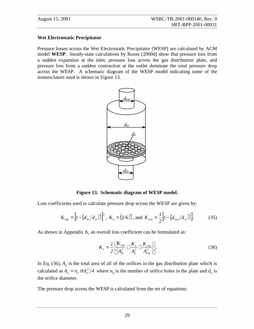
Pressure losses across the Wet Electrostatic Precipitator (WESP) are calculated by ACMmodel WESP. Steady-state calculations by Rouse (2000d) show that pressure loss froma sudden expansion at the inlet, pressure loss across the gas distribution plate, andpressure loss from a sudden contraction at the outlet dominate the total pressure dropacross the WESP. A schematic diagram of the WESP model indicating some of thenomenclature used is shown in Figure 13.
dout
dw
do
din
Figure 13. Schematic diagram of WESP model.
Loss coefficients used to calculate pressure drop across the WESP are given by:
( )[ ]22winexp dd1K −= , ( )2
o 61K = , and ( )[ ]2woutcon dd1
2
1K −= . (35)
As shown in Appendix A, an overall loss coefficient can be formulated as:
++=
2out
con2o
o2in
expv A
K
A
K
A
K
2
1K . (36)
In Eq. (36), Ao is the total area of all of the orifices in the gas distribution plate which is
calculated as 4dnA 2ooo π= where no is the number of orifice holes in the plate and do is
the orifice diameter.
The pressure drop across the WESP is calculated from the set of equations:
August 15, 2001 WSRC-TR-2001-000140, Rev. 0SRT-RPP-2001-00031
30
minggminv pp,mpKp ∆≤∆∆=∆ &ρ (37a)
( ) mingggv pp,mmKp ∆>∆=∆ &&ρ . (37b)
The calculation of pressure difference across the WESP by the method shown in Eqs.(37a) and (37b) linearizes the calculation for pressure drops near zero. A minimumpressure drop ( minp∆ ) of 1.0 Pa is used in the evaluation. Squaring Eq. (37a) and
dividing through by the minimum pressure drop leads to the alternative form:
( ) mingggvmin
pp,mmKp
pp∆≤∆=
∆∆∆
&&ρ . (37c)
Steady-state calculations by Rouse (2000d) also consider pressure drops in the WESPassociated with: contraction of the gas entering the electrode tubes, frictional loses fromflow in the electrode tubes, and sudden expansion of the gas as it exits the electrodetubes. However, the total of these losses associated with the WESP electrode tubes isonly 0.35 Pa for both the HLW and LAW systems. The overall pressure drop across theWESP is on the order of 254 Pa. Therefore, these losses, which represent less than0.15% of the total, have been neglected in the dynamic calculation.

August 15, 2001 WSRC-TR-2001-000140, Rev. 0SRT-RPP-2001-00031
31
Submerged Bed Scrubber
The pressure drop across the Submerged Bed Scrubber (SBS) is calculated as the total ofthe static head created by the liquid in and above the bed plus the frictional loss from gasflow through the gas distribution plate and the packed bed. ACM model SBS calculatesthe pressure drop across the scrubber. The gas exiting the scrubber is assumed to besaturated air at the liquid temperature. Figure 14 shows a schematic diagram of the SBSmodel.
GasDistribution
Plate
Packed Bed
Gas OutletGas Inlet
Downcomer
Figure 14. Schematic diagram of Submerged Bed Scrubber model.
The static liquid head is calculated using the expression:
llH Hgp ρ=∆ , (38)
where Hl is the liquid depth in the scrubber in meters. The liquid depth is the sum of thebed height plus the bed submergence. The code user specifies these parameters and theliquid density through the input. When the offgas system is started from conditions ofuniform pressure and no flow, the static head across the SBS must be overcome beforesignificant gas flow starts.
Pressure drop from gas flow through the packed bed is calculated using the data basedempirical equation:
24.1gB u5650p =∆ . (39)
In equation (39), ug is the superficial gas velocity based on the cross-sectional area of thepacked bed and the pressure drop is in Pascals.

August 15, 2001 WSRC-TR-2001-000140, Rev. 0SRT-RPP-2001-00031
32
The basis for Eq. (39) is data from experiments on a prototypical SBS conducted at theVitreous State Laboratories as reported by Rouse (2000c). The data correlation includesthe contribution to the pressure drop from flow across the SBS gas distribution plate. Themodel neglects pressure losses through the downcomer pipe and the offgas dischargetube. Rouse (2000c) has shown that these losses amount to less than 2% of the totalpressure loss across the SBS.
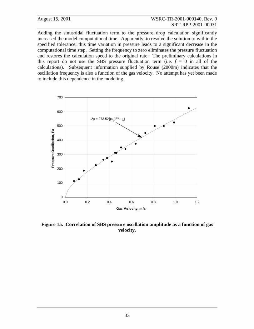
Measurements on experimental Submerged Bed Scrubbers show significant pressurefluctuations across the bed. The amplitude of the oscillations increases as the gas flowincreases. Experimental data on the oscillation amplitude supplied by Rouse (2000m)was fit with a single adjustable parameter using the empirical equation:
( )ggo uu52.273p +=∆ . (40)
The data fit is shown in Figure 15. The pressure fluctuations have been observed to havea frequency of approximately 2 Hz. The overall pressure drop across the SBS includingpressure fluctuations is then calculated by combining Eqs. (38) through (40) as:
( ) ( )tf2sinuu52.273u5650Hgp gg24.1
gll πρ +++=∆ . (41)
In Eq. (41), f is the oscillation frequency and t is time in seconds. Subtracting out thestatic pressure head, Eq. (41) can be rewritten in the equivalent form:
( ) ( )tf2sinuucucpHgp gg2ag1dll πρ ++=∆=−∆ . (41a)
In practice, to implement Eq. (41), we use the following logic:
• If 0pd ≤∆ then ug = 0. This prevents backflow of gas through the scrubber.
• If mind pp δ≤∆ , a linearized version of Eq. (41a) without the oscillating
component is employed where ( ) ga/1
min1mind upcpp δδ=∆ . This relationship is
derived by first evaluating Eq. (41a) for the gas velocity at the minimum pressuredifference obtaining:
( ) a/11minming cpu δ=
and then using the ratio
minggmind uupp =∆ δ
to linearize the relationship between pressure difference and gas velocity.
• If mind pp δ>∆ , the full version of Eq. (41a) is used to solve for the gas velocity
through the scrubber. The minimum pressure difference is set to be 1.0 Pa.
August 15, 2001 WSRC-TR-2001-000140, Rev. 0SRT-RPP-2001-00031
33
Adding the sinusoidal fluctuation term to the pressure drop calculation significantlyincreased the model computational time. Apparently, to resolve the solution to within thespecified tolerance, this time variation in pressure leads to a significant decrease in thecomputational time step. Setting the frequency to zero eliminates the pressure fluctuationand restores the calculation speed to the original rate. The preliminary calculations inthis report do not use the SBS pressure fluctuation term (i.e. f = 0 in all of thecalculations). Subsequent information supplied by Rouse (2000m) indicates that theoscillation frequency is also a function of the gas velocity. No attempt has yet been madeto include this dependence in the modeling.
Figure 15. Correlation of SBS pressure oscillation amplitude as a function of gasvelocity.
0
100
200
300
400
500
600
700
0.0 0.2 0.4 0.6 0.8 1.0 1.2
Gas Velocity, m/s
Pre
ssu
re O
scill
atio
n, P
a
δp = 273.52{(ug)0.5+ug}
August 15, 2001 WSRC-TR-2001-000140, Rev. 0SRT-RPP-2001-00031
34
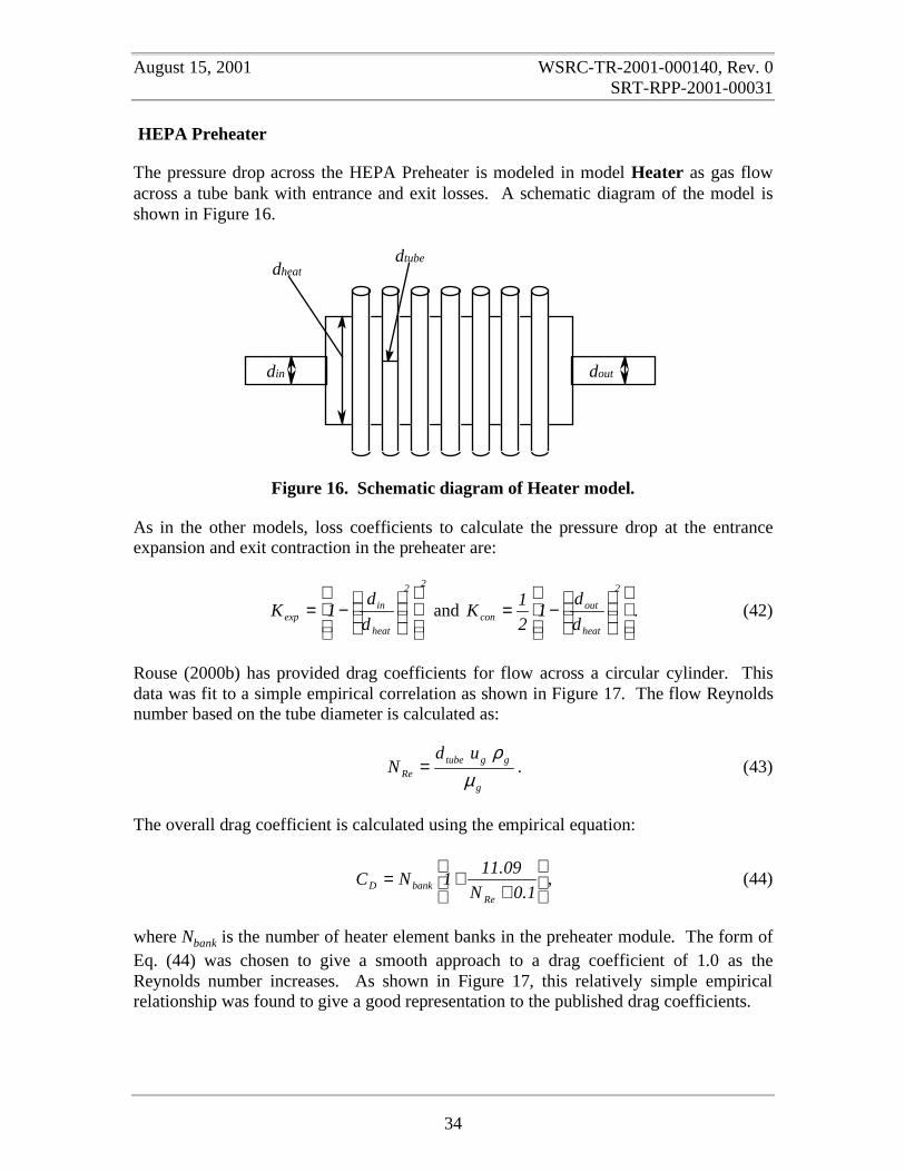
HEPA Preheater
The pressure drop across the HEPA Preheater is modeled in model Heater as gas flowacross a tube bank with entrance and exit losses. A schematic diagram of the model isshown in Figure 16.
din dout
dtubedheat
Figure 16. Schematic diagram of Heater model.
As in the other models, loss coefficients to calculate the pressure drop at the entranceexpansion and exit contraction in the preheater are:
22
heat
inexp d
d1K
−= and
−=
2
heat
outcon d
d1
2
1K . (42)
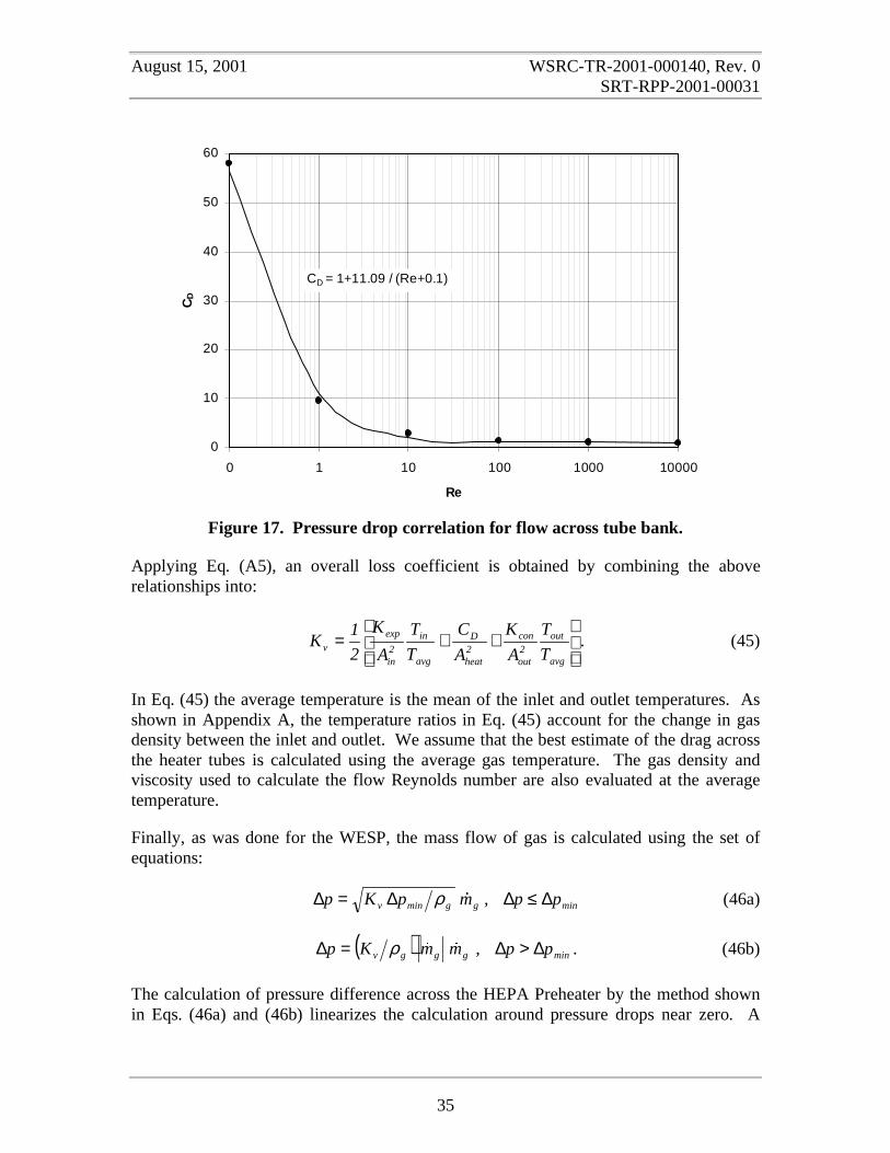
Rouse (2000b) has provided drag coefficients for flow across a circular cylinder. Thisdata was fit to a simple empirical correlation as shown in Figure 17. The flow Reynoldsnumber based on the tube diameter is calculated as:
g
ggtubeRe
udN
µρ
= . (43)
The overall drag coefficient is calculated using the empirical equation:
+
+=1.0N
09.111NC
RebankD , (44)
where Nbank is the number of heater element banks in the preheater module. The form ofEq. (44) was chosen to give a smooth approach to a drag coefficient of 1.0 as theReynolds number increases. As shown in Figure 17, this relatively simple empiricalrelationship was found to give a good representation to the published drag coefficients.
August 15, 2001 WSRC-TR-2001-000140, Rev. 0SRT-RPP-2001-00031
35
Figure 17. Pressure drop correlation for flow across tube bank.
Applying Eq. (A5), an overall loss coefficient is obtained by combining the aboverelationships into:
++=
avg
out2out
con2heat
D
avg
in2in
expv T
T
A
K
A
C
T
T
A
K
2
1K . (45)
In Eq. (45) the average temperature is the mean of the inlet and outlet temperatures. Asshown in Appendix A, the temperature ratios in Eq. (45) account for the change in gasdensity between the inlet and outlet. We assume that the best estimate of the drag acrossthe heater tubes is calculated using the average gas temperature. The gas density andviscosity used to calculate the flow Reynolds number are also evaluated at the averagetemperature.
Finally, as was done for the WESP, the mass flow of gas is calculated using the set ofequations:
minggminv pp,mpKp ∆≤∆∆=∆ &ρ (46a)
( ) mingggv pp,mmKp ∆>∆=∆ &&ρ . (46b)
The calculation of pressure difference across the HEPA Preheater by the method shownin Eqs. (46a) and (46b) linearizes the calculation around pressure drops near zero. A
0
10
20
30
40
50
60
0 1 10 100 1000 10000
Re
CD
CD = 1+11.09 / (Re+0.1)

August 15, 2001 WSRC-TR-2001-000140, Rev. 0SRT-RPP-2001-00031
36
minimum pressure drop ( minp∆ ) of 1.0 Pa is used in the evaluation. Squaring Eq. (46a)
and dividing through by the minimum pressure drop leads to the alternative form:
( ) mingggvmin
pp,mmKp
pp∆≤∆=
∆∆∆
&&ρ . (46c)
Equations (46b) and (46c) were used for the model calculations. These two equationsgive the identical result when minpp ∆=∆ .
The development presented above neglects pressure losses from gas flow through theheater housing. As shown by Rouse (2000b), at steady state, these losses are very smallrepresenting less than 1% of the total pressure drop across the preheater.
Neglecting the heat capacity of the gas within the heater, a steady-state enthalpy balanceis used to calculate the heat addition (∆hg) according to the equation:
g
iniiiin
outiiiout hhxmhxm ∆=
−
∑∑ && . (47)
The summations in Eq. (47) are taken over the air and steam components of the inlet andoutlet gas streams. The model is run specifying the outlet gas temperature with the modelthen calculating the required heat addition to the gas. Alternatively, with no change tothe model, the heat addition could be specified and the outlet gas temperature calculated.
August 15, 2001 WSRC-TR-2001-000140, Rev. 0SRT-RPP-2001-00031
37
PID Controller
The model of a Proportional-Integral-Derivative (PID) controller, coded in modelPID_Controller, is a simplified model of the action of a proportional-integral-derivativecontroller. The basic equation to calculate controller output is:
++= ∫ dt
eddte
1eGC d
iout τ
τ. (48)
The following nomenclature is used in Eq. (48):
Cout.......................Controller output.G.......................Controller gain.e.......................Error.τi.......................Integral time constant.
τd.......................Derivative time constant.
The error is defined to be equal to the difference between the input to the controller (Cin)and the controller set point (Pset) divided by the allowed input range:
−−
≡mininmaxin
setin
CC
PCe ψ . (49)
The input parameter ψ in Eq. (49) is an on off switch used to initiate the control action.With 0=ψ the controller is off while setting 1=ψ turns the controller on.
The rate of change of the error is approximated using the equation
e
ee
dt
ed
τ−= . (50)
where τe is an error time constant. Integrating Eq. (50) assuming a constant error leads tothe relationship
( ) ( )e0 texpeeee τ−−=− , (51)
which demonstrates that e will approach e at long times under some conditions.
The controller model clips the input signal to lie between maximum and minimum valuesspecified by the used through model input. The output signal is automatically clipped tolie in the range ±1. The model also applies a time lag to the output response using theequation:

August 15, 2001 WSRC-TR-2001-000140, Rev. 0SRT-RPP-2001-00031
38
( )l
outC
dt
d
τσσ −
= , (52)
where σ is the final controller output and τl is the time constant for the lag.
A controller is used on each melter to control the pressure. There are also controllers inthe HLW and LAW systems that control airflow out of the vessel ventilation systems.The LAW system has additional controllers on SBS flow and fan speed. Table 9 lists theparameters used for all of controllers in the model calculations. These parameters arerather arbitrary at this time and can have a significant influence on the transient responseof the offgas system. Future model development will work to improve the simulation byproviding more realistic parameters for the control systems.
Table 9. PID Controller Settings
HLW System LAW SystemParameter Pressure VVS Pressure SBS Flow Fan Speed VVS
Gain 10 10 10 10 5 5
Integral TimeConstant (s)
1000 1000 1000 1000 100 10
Derivative TimeConstant (s)
0.1 0.1 0.1 0.1 0.1 0.1
Error TimeConstant (s)
1 1 1 1 1 1
Delay TimeConstant (s)
1 1 1 5 1 1
Units mbar mbar mbar m3/s mbar m3/s
Set Point 985.0 990.0 983.75 0.685 870.0 0.25
Input Min. 975.0 980.0 978.75 0.370 850.0 0.00
Input Max. 995.0 1000.0 988.75 1.000 890.0 0.50
August 15, 2001 WSRC-TR-2001-000140, Rev. 0SRT-RPP-2001-00031
39
Control Valve
As shown in the flowsheet schematics, control valves are used only in conjunction withthe controllers. The operation of these control valves is modeled using ACM modelControl_Valve. The flow stream being controlled passes through the valve and the valvecharacteristics and the controller response determine the flowrate out of the valve. Afixed valve coefficient (Cv) is specified through the code input. The mass flow throughthe valve is then calculated as a function of the pressure difference across the valve using:
( )pf
pCm gv ∆
∆= ρφ& . (53)
In Eq. (53), φ is the relative (0 to 1) valve stem position and the function ( )pf ∆ is thefunction defined in Eq. (10b) to approximate the square root of the pressure difference.
The change in the valve stem position (φ) is governed by a control signal (σ) which is theoutput of the associated PID controller and by the valve time constant τv through theequation:
vdt
d
τσφ = . (54)
Equation (54) adjusts the valve open position until the control signal reaches zero at arate governed by the valve time constant. The function of Eq. (54) is augmented by twologic tests to keep the valve position in the physically meaningful range of zero to one. Ifthe valve position is zero (fully closed) and the control signal is still trying to close thevalve, the rate of change in valve position is set to zero. Similarly, if the valve position isone (fully opened) and the control signal is still trying to open the valve, the rate ofchange in the valve position is set to zero. Symbolically,
≥=≤=
=0and1
0and0if0
dt
d
σφσφφ
.
As a further check, the value of the valve position calculated by Eq. (54) is clipped to fallbetween zero and one before it is used in Eq. (53). All of the control valve time constantswere arbitrarily set to one second for the preliminary model calculations reported here.As more information about the offgas control system becomes available, the valveparameters can be easily modified.
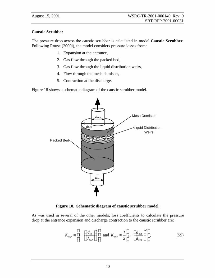
August 15, 2001 WSRC-TR-2001-000140, Rev. 0SRT-RPP-2001-00031
40
Caustic Scrubber
The pressure drop across the caustic scrubber is calculated in model Caustic Scrubber.Following Rouse (2000i), the model considers pressure losses from:
1. Expansion at the entrance,
2. Gas flow through the packed bed,
3. Gas flow through the liquid distribution weirs,
4. Flow through the mesh demister,
5. Contraction at the discharge.
Figure 18 shows a schematic diagram of the caustic scrubber model.
din
dout
dbed
Packed Bed
Mesh Demister
Liquid DistributionWeirs
Figure 18. Schematic diagram of caustic scrubber model.
As was used in several of the other models, loss coefficients to calculate the pressuredrop at the entrance expansion and discharge contraction to the caustic scrubber are:
22
bed
inexp d
d1K
−= and
−=
2
bed
outcon d
d1
2
1K , (55)

August 15, 2001 WSRC-TR-2001-000140, Rev. 0SRT-RPP-2001-00031
41
where dbed is the diameter of the packed bed. A loss coefficient for gas flow through theliquid distribution weirs is calculated by:
( )2o 61K = . (56)
Rouse (2000i) has provided a correlation for the gas phase pressure loss in two-phaseflow through a packed bed in the form:
( )lL
g
2
pb 10G
hp ρφ
ργ &
&
=∆ . (57)
In Eq. (57), h is the height of the packed bed, γ and φ are bed constants, G& is thesuperficial gas mass velocity, L& is the superficial liquid mass velocity, and ρl is theliquid density. The superficial gas mass velocity is defined to be:
ggbed
gg uA
QG ρ
ρ==& . (58)
Using Eq. (58), Eq. (57) can be conveniently cast into the same form as that forcalculating the pressure drop from flow through a resistance:
2ggbedpb uK
2
1p ρ=∆ with ( )[ ]lbed L10lnexpgh2K ρφγ &≡ . (59)
The loss coefficient Kbed defined in Eq. (59) has been converted into an exponential formto facilitate the model calculations. Rouse (2000i) has provided a table of bedcoefficients, γ and φ, in English units. When converted to SI, the coefficient γ has unitsof s2/m2. Since the loss coefficient must be dimensionless, the gravitational constant ghas been introduced into the definition of Kbed to make the product γgh dimensionless.To simplify the calculations and model input slightly, it is then convenient to combine theproduct γg into a modified γ coefficient and ( )φ10ln into a modified φ coefficient. The
ratio lL ρ& in the exponential term in Eq. (59) can also be replaced with Ql /Abed. Making
these changes, the bed loss coefficient can be written in the equivalent form:
[ ]bedlbed AQexph2K φγ ′′≡ . (60)
Required model inputs are the bed height (h), the bed diameter which is used to calculatethe cross-sectional area, and the liquid volumetric flowrate (Ql). A list of parameters forboth the HLW and LAW caustic scrubbers is given in Table 10.

August 15, 2001 WSRC-TR-2001-000140, Rev. 0SRT-RPP-2001-00031
42
Table 10. Caustic Scrubber model parameters.
Parameter LAW System HLW System
γ ′ (m−1) 82.02 164.05
φ ′ (s/m) 62.55 76.15
dbed (m) 1.3208 1.0668
h (m) 2.6412 5.1562
Ql (m3/s) 1.89 7.57
Tl (C) 66 25
Rouse (2000i) also provides manufacturer’s data on the pressure drop across the meshdemister as a function of gas velocity. These data can be fit using a quadratic polynomialas shown in Figure 19.
Figure 19. Pressure drop correlation for flow through mesh demister.
To be compatible with the other pressure drop calculations, we assume that the pressuredrop across the demister can be correlated using the equation:
2gg2dgg1d
2g2g1dm uK
2
1uKucucp ρρ +=+=∆ , (61)
∆p = 49.971ug2 + 70.318ug
R2 = 0.9964
0
50
100
150
200
250
300
350
0.00 0.25 0.50 0.75 1.00 1.25 1.50 1.75 2.00
Gas Velocity (m/s)
∆p
(Pas
cal)
August 15, 2001 WSRC-TR-2001-000140, Rev. 0SRT-RPP-2001-00031
43
where g11d cK ρ≡ and g22d c2K ρ≡ . (62)
Assuming a gas density of approximately 1.0 kg/m3, the data correlation implies demisterloss coefficients of Kd1 = 70.318 and Kd2 = 99.942.
As shown in Appendix A, an overall loss coefficient can be used to combine all of thepressure losses that are quadratic in the gas velocity. This overall coefficient iscalculated as:
++++=
2out
con2bed
2d2o
o2bed
bed2in
expv A
K
A
K
A
K
A
K
A
K
2
1K . (63)
In Eq. (63), Ao is the total area of all of the orifices in the liquid distribution plate which
is calculated as 4dnA 2ooo π= where no is the number of orifice holes in the plate and do
is the orifice diameter. Finally, the overall pressure drop across the caustic scrubber iscalculated using the equation:
2
g
v
bed
1d mK
mA
Kp &&
ρ+=∆ . (64)
Equation (64) is particularly convenient to use since the linear term prevents singularbehavior in the derivative when the gas flow is identically zero. With this pressurerelationship no special logic is required to treat the case of no gas flow.
The gas exiting the scrubber is assumed to be saturated air at the liquid temperature. Thisassumption fixes the exit gas composition, temperature and enthalpy. We also assumethat the liquid in the scrubber is saturated with air so that the mass flows of air enteringand exiting the scrubber are the same.
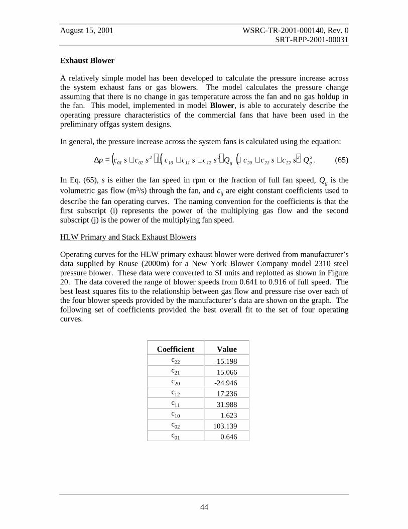
August 15, 2001 WSRC-TR-2001-000140, Rev. 0SRT-RPP-2001-00031
44
Exhaust Blower
A relatively simple model has been developed to calculate the pressure increase acrossthe system exhaust fans or gas blowers. The model calculates the pressure changeassuming that there is no change in gas temperature across the fan and no gas holdup inthe fan. This model, implemented in model Blower, is able to accurately describe theoperating pressure characteristics of the commercial fans that have been used in thepreliminary offgas system designs.
In general, the pressure increase across the system fans is calculated using the equation:
( ) ( ) ( ) 2g
2222120g
2121110
20201 QscsccQscsccscscp +++++++=∆ . (65)
In Eq. (65), s is either the fan speed in rpm or the fraction of full fan speed, Qg is thevolumetric gas flow (m3/s) through the fan, and cij are eight constant coefficients used todescribe the fan operating curves. The naming convention for the coefficients is that thefirst subscript (i) represents the power of the multiplying gas flow and the secondsubscript (j) is the power of the multiplying fan speed.
HLW Primary and Stack Exhaust Blowers
Operating curves for the HLW primary exhaust blower were derived from manufacturer’sdata supplied by Rouse (2000m) for a New York Blower Company model 2310 steelpressure blower. These data were converted to SI units and replotted as shown in Figure20. The data covered the range of blower speeds from 0.641 to 0.916 of full speed. Thebest least squares fits to the relationship between gas flow and pressure rise over each ofthe four blower speeds provided by the manufacturer’s data are shown on the graph. Thefollowing set of coefficients provided the best overall fit to the set of four operatingcurves.
Coefficient Valuec22 -15.198c21 15.066c20 -24.946c12 17.236c11 31.988c10 1.623c02 103.139c01 0.646

August 15, 2001 WSRC-TR-2001-000140, Rev. 0SRT-RPP-2001-00031
45
Figure 20. Correlations for HLW blower operating curves.
0
10
20
30
40
50
60
70
80
90
100
110
120
0.0 0.2 0.4 0.6 0.8 1.0 1.2 1.4 1.6 1.8
Volumetric Flow, m3/s
Fan
Sta
tic P
resu
re, m
bar
s = 0.916
s = 0.825
s = 0.733
s = 0.641

August 15, 2001 WSRC-TR-2001-000140, Rev. 0SRT-RPP-2001-00031
46
LAW Exhaust Blowers
Operating curves for the primary LAW exhaust blower were derived from manufacturer’sdata referenced by Bustamante (2000) in his report on sizing the LAW exhaust blower.The recommendation from that report is to use type HP pressure blowers manufacturedby the New York Blower Co. in the LAW offgas system. The reference report providescopies of some of the manufacturer’s data and operating curves for Type HP pressureblowers with steel wheels operating at 3550 rpm. These data were used to develop thefan operating curves for the LAW dynamic model calculations.
Manufacturers performance curves for Type HP pressure blowers operating at 3550 rpm,are reproduced on page 47 of Bustamante (2000). These curves indicate a quadraticrelationship between inlet airflow and static pressure across the blower. Nineteen datapoints were read from the operating curve for a Model Number 29012 blower (290 wheeldiameter size with a 12 inch outlet), converted to SI units and plotted as shown in Figure21.
Figure 21. Operating curves for LAW primary blower.c01 = 4.5662, c10 = -1000, c11 = 0.8612, c20 = -746.14
∆p = -746.14 Q2 + 2057.2 Q + 16210R2 = 0.999
0
2000
4000
6000
8000
10000
12000
14000
16000
18000
20000
0.0 0.5 1.0 1.5 2.0 2.5 3.0 3.5 4.0 4.5 5.0 5.5 6.0 6.5
Q (m3/s)
∆p
(Pa)
3550 rpm
2500 rpm1500 rpm500 rpm

August 15, 2001 WSRC-TR-2001-000140, Rev. 0SRT-RPP-2001-00031
47
As shown in Figure 21, a least squares quadratic equation gives an excellent fit to thesedata points (R2 = 0.999). To model system startup and the system response to variationsin the blower speed, performance curves at other operating speeds are required. Sincethis data was not available, it was assumed that the constant term in the least squares fit tothe data at 3550 rpm was a linear function of blower speed. This assumption leads to anestimation of the coefficient 5662.4355016210c01 == .
Initially it was assumed that the coefficient on the gas flow to the first power in the leastsquares fit was also a simple linear function of blower speed. However, with this model,the code repeatedly failed to converge at the point of flow breakthrough in the SBS. Itwas observed that the fan curves in the successful HLW blower model had a negativeslope at the breakthrough point whereas the LAW blower curves had a positive slope.This difference is illustrated in Figure 22 where the arrows indicate the apparent stablesolution path. The characteristic LAW fan curves were modified to give a negative slopeat the point of flow breakthrough by setting the coefficient 1000c10 −= . With this
adjustment, the model was able to successfully compute through the flow breakthroughpoint. Using the set of coefficients listed in the caption to Figure 21, Eq. (69) was used togenerate blower performance curves at the other fan speeds as shown in the figure.
Figure 22. Schematic illustration of fan operating curves.
-1 0 1
Flow
∆p
positive slope
negative slope
increasingfan speed

August 15, 2001 WSRC-TR-2001-000140, Rev. 0SRT-RPP-2001-00031
48
Thermal Catalytic Oxidizer Unit
As described above, both offgas systems have Thermal Catalytic Oxidizer units withsomewhat different configurations. A more detailed schematic diagram of the trueconfiguration of this unit is shown in Figure 23 (Berrios, 2000).
Preheater
Return Duct
Heat ExchangerCold Side
Heat ExchangerHot Side
PrimarySCR
SecondarySCR
LAW Only
TCO
Figure 23. Schematic diagram of Thermal Catalytic Oxidizer Unit.
In both systems, the gas flow enters on the cold side of a plate type heat exchanger. Afterthe heat exchanger, the gas passes through a preheater, the Thermal Catalytic Oxidizer(TCO), through a return duct, and then through the hot side of the heat exchanger.Following the TCO in the LAW system, the gas also passes through two SelectiveCatalytic Reduction (SCR) units to remove ammonia, nitric oxide, and nitrogen dioxidefrom the stream. For calculation purposes, the entire unit is modeled as a series of sub-process units as shown in Figures 1 and 3b. The existing Heater and Pipe_Flow modelsare used to model the gas flow through the preheater and return duct, respectively. Tocomplete the description of this unit, models of gas flow through a plate heat exchanger,the TCO, and the SCR were developed. The heat exchanger model was applied twice toseparately calculate the pressure drop across the hot and cold sides of the heat exchanger.The heat exchanger model does not treat the coupled heat transfer between the hot andcold sides but uses a specified outlet temperature to estimate the heat load.

August 15, 2001 WSRC-TR-2001-000140, Rev. 0SRT-RPP-2001-00031
49
Thermal Catalytic Oxidizer/Selective Catalytic Reducer
Pressure losses across the Thermal Catalytic Oxidizer and the Selective CatalyticReducer are both calculated using the model Catalytic. Gas flow through the catalystmonolith is modeled as flow through small channels (Rouse, 2000f). The catalyst iscontained inside a housing so there are pressure losses from contraction as the flow entersthe catalyst channels and expansion as the flow exits the channels. Since the catalystchannels are small it is assumed that the gas flow within the channels is laminar. Figure24 shows a schematic diagram of the catalytic unit model where dh is the diameter of thehousing and dcat is the diameter of a single flow channel through the catalyst.
dh
dcat
Figure 24. Schematic diagram of catalytic unit model.
Loss coefficients for the pressure drop at the entrance contraction and dischargeexpansion to the catalyst bed are calculated as:
−=
2
h
catcon d
d1
2
1K and
22
h
catexp d
d1K
−= . (66)
Since both pressure losses are based on the flow through the catalyst, a relatively simpleoverall loss coefficient can be written as:
[ ]expcon2cat
v KKA2
1K += . (67)
Following Rouse (2000f), the total flow area through the catalyst is estimated as:
catmonmonmoncat WHNA φ= with 2
catcat
catcat td
d
+
=φ . (68)
In Eq. (68), Nmon is the number of catalyst monoliths stacked in the flow direction, Hmon isthe height of a single monolith, Wmon is the monolith width and φcat is the fraction of the
August 15, 2001 WSRC-TR-2001-000140, Rev. 0SRT-RPP-2001-00031
50
surface area occupied by catalyst pores. The fraction of catalyst surface occupied bypores in both linear directions is estimated as the ratio of the pore diameter to the sum ofthe pore diameter and the thickness of the catalyst solid (tcat).
Since we can assume laminar flow through the catalyst channels, the friction factor isgiven by:
gcat
g
lam0 d
64f
ρµ
= . (69)
The total pressure loss across the catalytic unit is then calculated as:
2g
g
v
cat
g
cat
catlam0
lay mK
A
m
d
Lf
2
Np &
&
ρ+=∆ . (70)
In Eq. (70), Lcat is the length of a catalyst monolith and Nlay is the number of catalystlayers in series. The laminar contribution to the pressure drop is linear in gas flowrate.Therefore, no special logic is required to assure that the calculation is well behaved atzero flow.
Both the TCO and SCR units can be modeled using the same general form if onlypressure losses are required. As a future extension of the offgas system model it isanticipated that other species will be added to the gas phase and the chemical reactions inthe TCO and SCR units accounted for. In this eventuality, the models would have to beseparated to include individual reaction mechanisms.
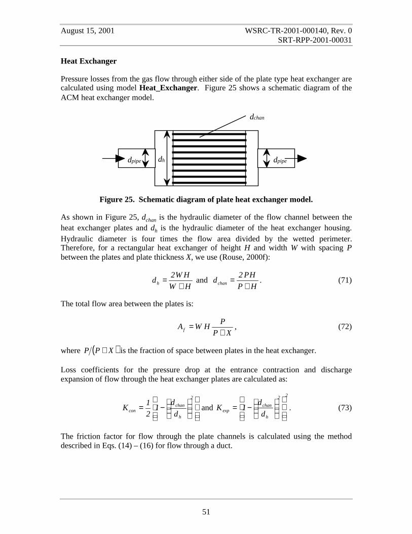
August 15, 2001 WSRC-TR-2001-000140, Rev. 0SRT-RPP-2001-00031
51
Heat Exchanger
Pressure losses from the gas flow through either side of the plate type heat exchanger arecalculated using model Heat_Exchanger. Figure 25 shows a schematic diagram of theACM heat exchanger model.
dpipe dpipedh
dchan
Figure 25. Schematic diagram of plate heat exchanger model.
As shown in Figure 25, dchan is the hydraulic diameter of the flow channel between theheat exchanger plates and dh is the hydraulic diameter of the heat exchanger housing.Hydraulic diameter is four times the flow area divided by the wetted perimeter.Therefore, for a rectangular heat exchanger of height H and width W with spacing Pbetween the plates and plate thickness X, we use (Rouse, 2000f):
HW
HW2dh +
= and HP
HP2dchan +
= . (71)
The total flow area between the plates is:
XP
PHWAf +
= , (72)
where ( )XPP + is the fraction of space between plates in the heat exchanger.
Loss coefficients for the pressure drop at the entrance contraction and dischargeexpansion of flow through the heat exchanger plates are calculated as:
−=
2
h
chancon d
d1
2
1K and
22
h
chanexp d
d1K
−= . (73)
The friction factor for flow through the plate channels is calculated using the methoddescribed in Eqs. (14) – (16) for flow through a duct.
August 15, 2001 WSRC-TR-2001-000140, Rev. 0SRT-RPP-2001-00031
52
As shown in Figure 25, the hot side of the heat exchanger has a contraction loss fromflow exiting the unit while the cold side has an expansion loss from flow entering theunit. Including the temperature correction, these losses are calculated as:
avg
out
2
h
pipeout T
T
d
d1
2
1K
−= and
avg
in
22
h
pipein T
T
d
d1K
−= . (74)
An integer flag is specified through the input to select which of the loss coefficients fromEq. (74) is applied. Combining the loss terms defined above, an overall pressure losscoefficient is calculated as
either
++=
avg
out2f
exp
avg
in2f
con2pipe
inv T
T
A
K
T
T
A
K
A
K
2
1K (75a)
or
++=
avg
out2f
exp
avg
in2f
con2pipe
outv T
T
A
K
T
T
A
K
A
K
2
1K (75b)
at the inlet and outlet, respectively. The pressure drop from gas flow through one side ofthe heat exchanger is calculated using the relationship:
2g
g
v
f
g
chan
chan0 m
K
A
m
d
Lf
2
1p &
&
ρ+=∆ . (76)
The flow friction factor is calculated using the method described in the Air Duct sectionfor model Pipe_Flow to capture both laminar and turbulent flow regimes.
The model is run specifying outlet gas temperatures on both the hot and cold sides. Themodel calculates the heat addition to or the heat removal from the gas. Alternatively, theheat input could be specified and the outlet gas temperature calculated. Neglecting theheat capacity of the gas within the heater, a steady-state enthalpy balance is used tocalculate the heat addition (∆hg) according to the steady-state equation:
g
iniiiin
outiiiout hhxmhxm ∆=
−
∑∑ && . (77)
The summations in Eq. (77) are taken over the air and steam components of the inlet andoutlet streams.
August 15, 2001 WSRC-TR-2001-000140, Rev. 0SRT-RPP-2001-00031
53
Flow Splitting
An additional unit operation is required at the inlet to the exhaust blowers where the gasstream splits into two streams to enter the parallel blowers. The ACM model Flow_Splittakes the inlet gas stream and splits it into two outlet streams. The model requires almostno computations since the composition, temperature, pressure and enthalpy of the gas inthe outlet streams are equal to the inlet values. The model does calculate the gas densityand inlet volumetric flow since this is used as a control variable in the HLW system. Theflow split is determined by pressure balances around the system and is not specifieddirectly in the model. The model only sets the sum of the mass flows in the outletstreams to equal the inlet mass flow to conserve mass.
Fan Speed Control
Another small model used in the package to set the blower fan speed is ACM modelSpeed_Set. Starting at time zero, this model ramps the fan speed from zero to themaximum speed at a linear rate of increase. The user sets the rate of increase in fanspeed and the time over which the ramp is applied thereby indirectly specifying themaximum speed. At times greater than the ramp time, the model calculates the change infan speed as the product of a time constant and a control signal. This allows the LAWsystem to attempt to control fan speed in response to the system pressure at the pointwhere the three melter offgas streams combine while the control signal can be set to zeroin the HLW system to maintain a constant fan speed. This model can also be used tosimulate a fan failure accident by using the time constant or control signal for a particularfan to ramp down the blower speed and turn off the blower. The Task structure in ACMcan be conveniently used to adjust coefficient values, such as the blower time constant, atspecific times in the simulation to model accident scenarios.

August 15, 2001 WSRC-TR-2001-000140, Rev. 0SRT-RPP-2001-00031
54
List of System Models
There are a total of 23 individual models of specific unit operations in the simulationpackage. A listing of the model names and a brief description of the units they model isprovided in Table 11. In addition, there are four submodels used to evaluate gas physicalproperties also listed in Table 11.
Table 11. List of ACM Models
Model Name Unit Modeled1 Blower Exhaust and stack blowers2 Catalytic Selective Catalytic Reducers3 Caustic_Scrubber Caustic scrubbers4 Control_Valve Control valves5 Filter HEME and HEPA filters6 Flow_Split Inlet fan manifolds7 Gas_Profile Time dependent feed streams8 Gas_Source Constant feed streams9 Gas_Tank Tees and junctions
10 Heat_Exchanger Heat exchangers11 Heater HEPA preheaters12 Melter Melters13 Mixing_Volume Tees and junctions14 Orifice Air leaks and restricting orifices15 PID_Controller PID controllers16 Pipe_Flow Film cooler17 Plenum Equipment gas volumes18 SBS Submerged Bed Scrubbers19 Speed_Set Blower speed control20 Vessel VVS vessels21 Vessel_System VVS Vessel, gas source, and orifice22 WESP Wet Electrostatic Precipitators23 Gas_Pipe Air ducts24 P_Sat Saturation vapor pressure25 Vapor_Density Gas mixture density26 Vapor_Enthalpy Gas mixture enthalpy27 Vapor_Viscosity Gas mixture viscosity

August 15, 2001 WSRC-TR-2001-000140, Rev. 0SRT-RPP-2001-00031
55
Calculation Basis
Three calculations were run for both the HLW and LAW melter offgas systems:
1. Steady-state operating conditions,
2. Startup transient,
3. Best estimate melter steam surges.
As specified by Rouse (2000m), for all of the calculations, the ambient atmosphericpressure at the Hanford Site is assumed to be 100,000 Pa. The HLW melter cell pressureis taken to be 99,750 Pa which is approximately –1.0 inch water from ambient while theLAW melter cell pressure is assumed to be 99,625 Pa or approximately –1.5 incheswater. Cell air conditions on the high-pressure side of the melter air inleakage orifice areassumed to be 45 °C and 50% relative humidity. The humidity is used to calculate theinleakage gas composition by applying Eqs. (5) and (6).
Since no detailed startup sequence has been specified for the melter systems, assumptionsused for the startup transient are rather arbitrary in this preliminary calculation. Thecalculation is intended to demonstrate the model capability to perform this particularcalculation rather than to present an accurate picture of how the actual system startup willtake place. Starting up the offgas system from conditions of uniform pressure and noflow is a particularly challenging calculation that forces model parameters to change overa wide range and exercises the flow regime logic. The ability of the models to make hiscalculation demonstrates that the models are relatively robust and stable.
Figure 26 shows the melter steam surge assumed to take place in the HLW melter. Thenominal 7X surge profile was obtained from Peters (2000). Also shown on Figure 26 arethe fluctuations in the HLW melter steam flow caused by the Air Displacement Slurry(ADS) pumps. Figure 27 shows the LAW melter steam surge transient that was assumedto occur in the model calculations. The nominal 4X surge profile was obtained from agraph provided by Rouse (2000m) for a 10 MT/day LAW melter. The calculationsassume that the surge occurs in only one of the three LAW melters (specifically in LAWMelter #1). Also shown on Figure 27 are the fluctuations in the LAW melter steam flowcaused by the ADS pumps. For both systems, the ADS fluctuations are controlledthrough an ACM Task that increments the starting time for the specified gas profile tocreate a uniformly repeating pattern of gas flow.
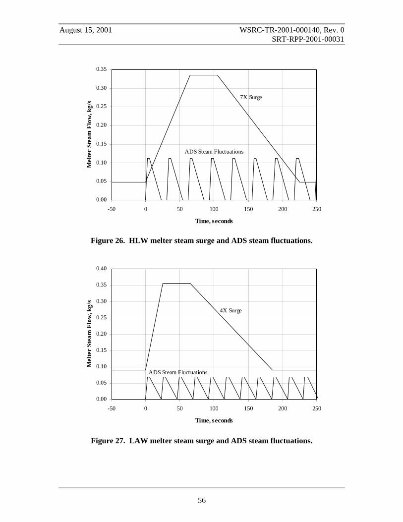
August 15, 2001 WSRC-TR-2001-000140, Rev. 0SRT-RPP-2001-00031
56
Figure 26. HLW melter steam surge and ADS steam fluctuations.
Figure 27. LAW melter steam surge and ADS steam fluctuations.
0.00
0.05
0.10
0.15
0.20
0.25
0.30
0.35
-50 0 50 100 150 200 250
Time, seconds
Mel
ter
Stea
m F
low
, kg/
s7X Surge
ADS Steam Fluctuations
0.00
0.05
0.10
0.15
0.20
0.25
0.30
0.35
0.40
-50 0 50 100 150 200 250
Time, seconds
Mel
ter
Stea
m F
low
, kg/
s
4X Surge
ADS Steam Fluctuations

August 15, 2001 WSRC-TR-2001-000140, Rev. 0SRT-RPP-2001-00031
57
HLW Offgas System Calculations
For the calculations in this report, the orifice diameter for melter air inleakage is taken tobe 3.0 inches and an orifice coefficient of 0.5715 is used (Rouse, 2000m). Air and steamflows into the HLW VVS vessels were set to the nominal flows specified by Meeuwsen(2001).
HLW Steady-State Operation
The model was first run through a startup scenario and melter surge transient. Followingthese calculations, the model was allowed to run for an additional 300 seconds ofsimulated time until a steady-state operation was reached. At this point, the pressures andgas flows recorded in Tables 12 and 13 were observed. One difference between thesteady-state and the usual dynamic calculation was that the fluctuating ADS flow wasreplaced with a constant average value to obtain the steady-state results reported in thetables. Table 12 compares the pressures, mass flows, and volumetric flows calculated bythe HLW dynamic model to the values reported on the material and energy balanceflowsheet provided by Rouse (2000k, Appendix A). The lower part of Table 12 gives thesystem gauge pressures in inches of water. The two sets of calculations are in fairagreement. The largest difference between the calculations appears to be that thedynamic ACM model is predicting a significantly smaller control air flow than was usedin the spreadsheet calculation. The source of this discrepancy has not been identified.Steady-state pressure drops calculated across the HLW system ducts by the dynamicmodel are reported in Table 13. The dynamic model predicts a total system pressure dropof about 18.4 inches water.
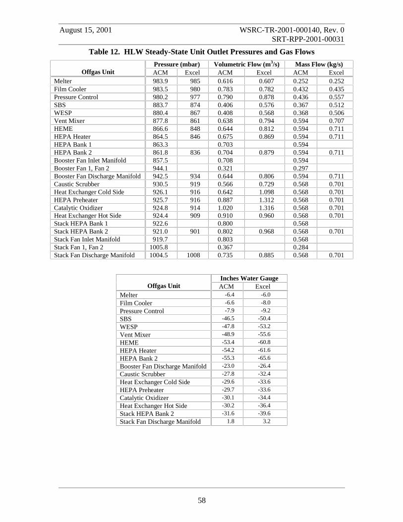
August 15, 2001 WSRC-TR-2001-000140, Rev. 0SRT-RPP-2001-00031
58
Table 12. HLW Steady-State Unit Outlet Pressures and Gas Flows
Pressure (mbar) Volumetric Flow (m3/s) Mass Flow (kg/s)Offgas Unit ACM Excel ACM Excel ACM Excel
Melter 983.9 985 0.616 0.607 0.252 0.252Film Cooler 983.5 980 0.783 0.782 0.432 0.435Pressure Control 980.2 977 0.790 0.878 0.436 0.557SBS 883.7 874 0.406 0.576 0.367 0.512WESP 880.4 867 0.408 0.568 0.368 0.506Vent Mixer 877.8 861 0.638 0.794 0.594 0.707HEME 866.6 848 0.644 0.812 0.594 0.711HEPA Heater 864.5 846 0.675 0.869 0.594 0.711HEPA Bank 1 863.3 0.703 0.594HEPA Bank 2 861.8 836 0.704 0.879 0.594 0.711Booster Fan Inlet Manifold 857.5 0.708 0.594Booster Fan 1, Fan 2 944.1 0.321 0.297Booster Fan Discharge Manifold 942.5 934 0.644 0.806 0.594 0.711Caustic Scrubber 930.5 919 0.566 0.729 0.568 0.701Heat Exchanger Cold Side 926.1 916 0.642 1.098 0.568 0.701HEPA Preheater 925.7 916 0.887 1.312 0.568 0.701Catalytic Oxidizer 924.8 914 1.020 1.316 0.568 0.701Heat Exchanger Hot Side 924.4 909 0.910 0.960 0.568 0.701Stack HEPA Bank 1 922.6 0.800 0.568Stack HEPA Bank 2 921.0 901 0.802 0.968 0.568 0.701Stack Fan Inlet Manifold 919.7 0.803 0.568Stack Fan 1, Fan 2 1005.8 0.367 0.284Stack Fan Discharge Manifold 1004.5 1008 0.735 0.885 0.568 0.701
Inches Water GaugeOffgas Unit ACM Excel
Melter -6.4 -6.0
Film Cooler -6.6 -8.0
Pressure Control -7.9 -9.2
SBS -46.5 -50.4
WESP -47.8 -53.2
Vent Mixer -48.9 -55.6
HEME -53.4 -60.8
HEPA Heater -54.2 -61.6
HEPA Bank 2 -55.3 -65.6
Booster Fan Discharge Manifold -23.0 -26.4
Caustic Scrubber -27.8 -32.4
Heat Exchanger Cold Side -29.6 -33.6
HEPA Preheater -29.7 -33.6
Catalytic Oxidizer -30.1 -34.4
Heat Exchanger Hot Side -30.2 -36.4
Stack HEPA Bank 2 -31.6 -39.6
Stack Fan Discharge Manifold 1.8 3.2
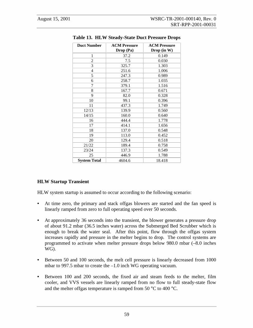
August 15, 2001 WSRC-TR-2001-000140, Rev. 0SRT-RPP-2001-00031
59
Table 13. HLW Steady-State Duct Pressure Drops
Duct Number ACM PressureDrop (Pa)
ACM PressureDrop (in W)
1 37.2 0.1492 7.5 0.0303 325.7 1.3034 251.6 1.0065 247.3 0.9896 258.7 1.0357 379.1 1.5168 167.7 0.6719 82.0 0.328
10 99.1 0.39611 437.3 1.749
12/13 139.9 0.56014/15 160.0 0.640
16 444.4 1.77817 414.1 1.65618 137.0 0.54819 113.0 0.45220 129.4 0.518
21/22 189.4 0.75823/24 137.3 0.549
25 446.9 1.788System Total 4604.6 18.418
HLW Startup Transient
HLW system startup is assumed to occur according to the following scenario:
• At time zero, the primary and stack offgas blowers are started and the fan speed islinearly ramped from zero to full operating speed over 50 seconds.
• At approximately 36 seconds into the transient, the blower generates a pressure dropof about 91.2 mbar (36.5 inches water) across the Submerged Bed Scrubber which isenough to break the water seal. After this point, flow through the offgas systemincreases rapidly and pressure in the melter begins to drop. The control systems areprogrammed to activate when melter pressure drops below 980.0 mbar (–8.0 inchesWG).
• Between 50 and 100 seconds, the melt cell pressure is linearly decreased from 1000mbar to 997.5 mbar to create the –1.0 inch WG operating vacuum.
• Between 100 and 200 seconds, the fixed air and steam feeds to the melter, filmcooler, and VVS vessels are linearly ramped from no flow to full steady-state flowand the melter offgas temperature is ramped from 50 °C to 400 °C.

August 15, 2001 WSRC-TR-2001-000140, Rev. 0SRT-RPP-2001-00031
60
• At 200 seconds the ADS steam flow in the melter is started. Once ADS flow isinitiated, the system will not operate at steady-state.
• Between 200 and 300 seconds, the model is run without changing the input to allow anominal operating condition to be reached.
HLW Steam Surge
Figure 28 shows model calculated results for the melter pressure during startup followedby a nominal 7X steam surge with the offgas blowers operating at 92% maximum fanspeed. The steam surge starts at time 300 seconds on the graph. One inch of water isvery closely approximated as 2.5 mbar. Therefore, each grid division on the pressurescale represents 1.0 inch water. The melt cell vacuum of –1 inch WG (997.5 mbar) andthe melter pressure set point of –5 inches WG with respect to the melt cell (985.0 mbar)are indicated on the figure. During startup, SBS breakthrough occurs at about 40 secondsand the melter pressure reaches a minimum of about –9 inches WG within a few secondsof breakthrough. The control system returns the pressure to the set point of 985 mbar. At100 seconds, the system is perturbed as gas flows to the melter, film cooler, and HLWVVS vessels are ramped in. At 200 seconds, the ADS steam flow starts and the systemthereafter operates in a transient fashion. The ADS steam fluctuations create melterpressure disturbances of from +4 inches to –1 inch so that the melter reaches a maximumpressure of about –2 inches WG during the ADS cycle. At 300 seconds, the melterexperiences the start of the 7X steam surge. During the surge, the melter pressureincreases +5 inches to about –1 inch and briefly exceeds the cell pressure at two pointswhere maximums in the ADS surges superimpose on the maximum in the steam surge.
Figure 29 shows stem position of the two control valves during the transient. The controlvalve on VVS flow, shown by the darker line, is able to maintain a relatively constantposition at about 20% full open during the transient. However, once gas flows areestablished in the system, the melter pressure control valve is operating at the lower endof its range and is shutting off during the ADS surges. During the melter steam surge, thevalve shuts off almost immediately and does not recover any control function until theend of the surge. Therefore, under the assumptions used in this calculation, the melter isoperating without pressure control during the steam surge.
As shown in Figures 30 and 31, the control action is improved by operating the blowersat 100% capacity. Under this condition, ADS steam fluctuations cause melter pressuredisturbances of from +2.5 inches to –3 inches. During the steam surge, melter pressureincreases by a maximum of 3.5 inches leaving a margin of 1.5 inches between the melterand the cell. Figure 31 shows that the melter pressure control valve is now normallyoperating at an average of 20% capacity and looses control function only briefly at thepeak of the steam surge.
All of these results depend on control system and control valve parameters that have notbeen specified by the Hanford design team at this point and certainly are not optimized inthese calculations. Therefore, the results should be taken as only a preliminary indicationof the system behavior pending refinement of the models.
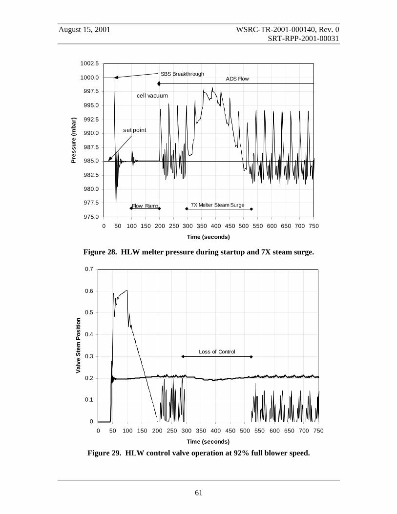
August 15, 2001 WSRC-TR-2001-000140, Rev. 0SRT-RPP-2001-00031
61
Figure 28. HLW melter pressure during startup and 7X steam surge.
Figure 29. HLW control valve operation at 92% full blower speed.
0
0.1
0.2
0.3
0.4
0.5
0.6
0.7
0 50 100 150 200 250 300 350 400 450 500 550 600 650 700 750
Time (seconds)
Val
ve S
tem
Pos
ition
Loss of Control
975.0
977.5
980.0
982.5
985.0
987.5
990.0
992.5
995.0
997.5
1000.0
1002.5
0 50 100 150 200 250 300 350 400 450 500 550 600 650 700 750
Time (seconds)
Pre
ssur
e (m
bar)
SBS BreakthroughADS Flow
Flow Ramp 7X Melter Steam Surge
cell vacuum
set point
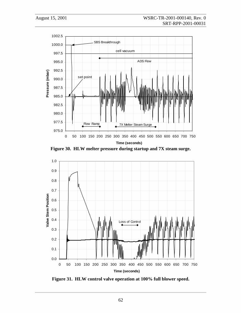
August 15, 2001 WSRC-TR-2001-000140, Rev. 0SRT-RPP-2001-00031
62
Figure 30. HLW melter pressure during startup and 7X steam surge.
Figure 31. HLW control valve operation at 100% full blower speed.
0.0
0.1
0.2
0.3
0.4
0.5
0.6
0.7
0.8
0.9
1.0
0 50 100 150 200 250 300 350 400 450 500 550 600 650 700 750
Time (seconds)
Val
ve S
tem
Pos
ition
Loss of Control
975.0
977.5
980.0
982.5
985.0
987.5
990.0
992.5
995.0
997.5
1000.0
1002.5
0 50 100 150 200 250 300 350 400 450 500 550 600 650 700 750
Time (seconds)
Pre
ssur
e (m
bar)
SBS Breakthrough
Flow Ramp 7X Melter Steam Surge
ADS Flow
cell vacuum
set point

August 15, 2001 WSRC-TR-2001-000140, Rev. 0SRT-RPP-2001-00031
63
LAW Offgas System Calculations
For the calculations described in this report, the orifice diameters for melter air inleakageare taken to be (Rouse, 2000m):
LAW Melter #1 – 3.00 inches
LAW Melter #2 – 3.75 inches
LAW Melter #3 – 4.25 inches
Variable orifice diameters were used to reflect the uncertainty and range of air inleakageexpected for the three LAW melters. An orifice coefficient of 0.5715 is used. Air andsteam flows into the LAW vessels were set to the nominal flows specified by Fergestromand Meeuwsen (2000).
LAW Steady-State Operation
As described below, the model was run through a startup scenario and melter surgetransient. Following these calculations, the model was allowed to run for an additional300 seconds of simulated time until steady-state operation was reached. At this point, thepressures and gas flows recorded in Tables 14 and 15 were observed. As in the HLWsteady-state calculation, the fluctuating ADS flow was replaced with a constant averagevalue to obtain the LAW steady-state results reported in the tables. Table 14 comparespressures, mass flows, and volumetric flows calculated by the LAW dynamic model tothose reported on the material and energy balance flowsheet provided by Rouse (2000l,Appendix A). The lower part of Table 14 gives the system gauge pressures in inches ofwater. The two sets of calculations are in reasonably good agreement. As opposed to theHLW model, the LAW dynamic model predicts essentially the same control air flow. Asource of significant difference between the two sets of calculations is the assumed VVSgas flow. The Excel spreadsheet calculation is adding about twice the gas flow from theVVS as is predicted at nominal vessel flow by the dynamic model. However, thedynamic model has more air coming out of the combined melter systems which offsetsthe lower VVS flow. Steady-state pressure drops calculated across the LAW systemducts are reported in Table 15. Comparable steady-state calculations from the Hanfordspreadsheets were not available for comparison. From previous comparisons, it isexpected that if both sets of calculations were made under identical conditions therewould be good agreement between the results. The dynamic model predicts a total systempressure drop (through Melter #2 and the common offgas train) of about 21.5 incheswater.
LAW Startup Transient
LAW system startup is assumed to occur according to the following scenario:
• At time zero, the offgas blowers are started and the fan speed is linearly ramped fromzero to full operating speed of 3000 rpm over 100 seconds.
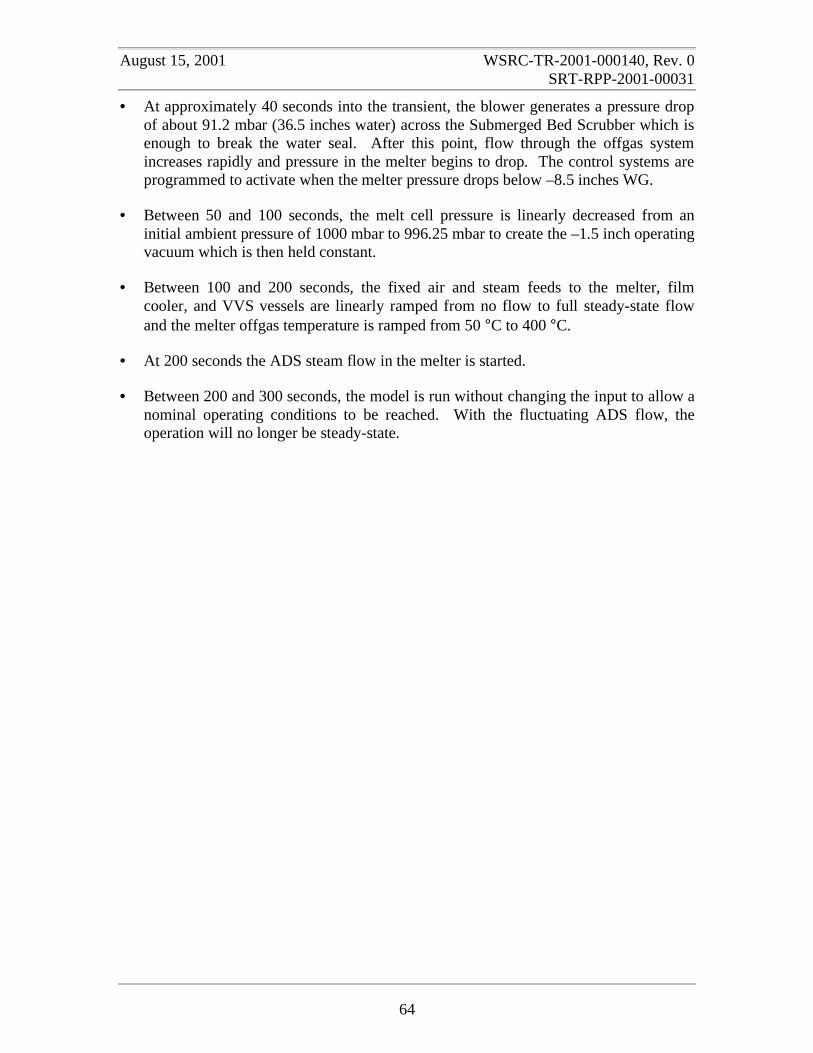
August 15, 2001 WSRC-TR-2001-000140, Rev. 0SRT-RPP-2001-00031
64
• At approximately 40 seconds into the transient, the blower generates a pressure dropof about 91.2 mbar (36.5 inches water) across the Submerged Bed Scrubber which isenough to break the water seal. After this point, flow through the offgas systemincreases rapidly and pressure in the melter begins to drop. The control systems areprogrammed to activate when the melter pressure drops below –8.5 inches WG.
• Between 50 and 100 seconds, the melt cell pressure is linearly decreased from aninitial ambient pressure of 1000 mbar to 996.25 mbar to create the –1.5 inch operatingvacuum which is then held constant.
• Between 100 and 200 seconds, the fixed air and steam feeds to the melter, filmcooler, and VVS vessels are linearly ramped from no flow to full steady-state flowand the melter offgas temperature is ramped from 50 °C to 400 °C.
• At 200 seconds the ADS steam flow in the melter is started.
• Between 200 and 300 seconds, the model is run without changing the input to allow anominal operating conditions to be reached. With the fluctuating ADS flow, theoperation will no longer be steady-state.
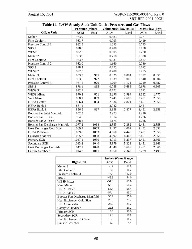
August 15, 2001 WSRC-TR-2001-000140, Rev. 0SRT-RPP-2001-00031
65
Table 14. LAW Steady-State Unit Outlet Pressures and Gas FlowsPressure (mbar) Volumetric Flow (m3/s) Mass Flow (kg/s)
Offgas Unit ACM Excel ACM Excel ACM ExcelMelter 1 983.9 0.583 0.271Film Cooler 1 983.7 0.793 0.419Pressure Control 1 982.5 1.093 0.743SBS 1 878.8 0.788 0.708WESP 1 872.6 0.805 0.720Melter 2 983.9 0.718 0.338Film Cooler 2 983.7 0.931 0.487Pressure Control 2 982.0 1.160 0.730SBS 2 878.4 0.771 0.692WESP 2 872.5 0.788 0.705Melter 3 983.9 975 0.825 0.804 0.392 0.357Film Cooler 3 983.6 972 1.039 1.000 0.540 0.504Pressure Control 3 981.5 970 1.209 1.171 0.719 0.687SBS 3 878.1 865 0.755 0.685 0.678 0.605WESP 3 872.7 0.772 0.691WESP Mixer 870.2 861 2.396 1.994 2.132 1.777Vent Mixer 868.1 859 2.741 2.603 2.451 2.358HEPA Heater 866.4 854 2.834 2.821 2.451 2.358HEPA Bank 1 861.1 2.942 2.451HEPA Bank 2 856.5 837 2.958 2.877 2.451 2.358Booster Fan Inlet Manifold 852.3 2.973 1.226Booster Fan 1, Fan 3 964.5 1.314 1.226Booster Fan 2, Fan 4 1078.2 1.175 1.226Booster Fan Discharge Manifold 1077.2 1064 2.353 2.382 2.451 2.358Heat Exchanger Cold Side 1069.9 1063 3.497 4.067 2.451 2.358HEPA Preheater 1059.8 1063 4.660 4.448 2.451 2.358Catalytic Oxidizer 1055.2 1058 4.692 4.468 2.451 2.358Primary SCR 1047.1 1050 4.713 5.237 2.451 2.366Secondary SCR 1043.2 1040 5.879 5.323 2.451 2.366Heat Exchanger Hot Side 1042.1 1028 4.848 3.699 2.451 2.366Caustic Scrubber 1014.2 1011 3.660 2.349 2.729 2.495
Inches Water GaugeOffgas Unit ACM Excel
Melter 3 -6.4 -10.0
Film Cooler 3 -6.6 -11.2
Pressure Control 3 -7.4 -12.0
SBS 3 -48.8 -54.0
WESP Mixer -51.9 -55.6
Vent Mixer -52.8 -56.4
HEPA Heater -53.4 -58.4
HEPA Bank 2 -57.4 -65.2
Booster Fan Discharge Manifold 30.9 25.6
Heat Exchanger Cold Side 28.0 25.2
HEPA Preheater 23.9 25.2
Catalytic Oxidizer 22.1 23.2
Primary SCR 18.8 20.0
Secondary SCR 17.3 16.0
Heat Exchanger Hot Side 16.8 11.2
Caustic Scrubber 5.7 4.4
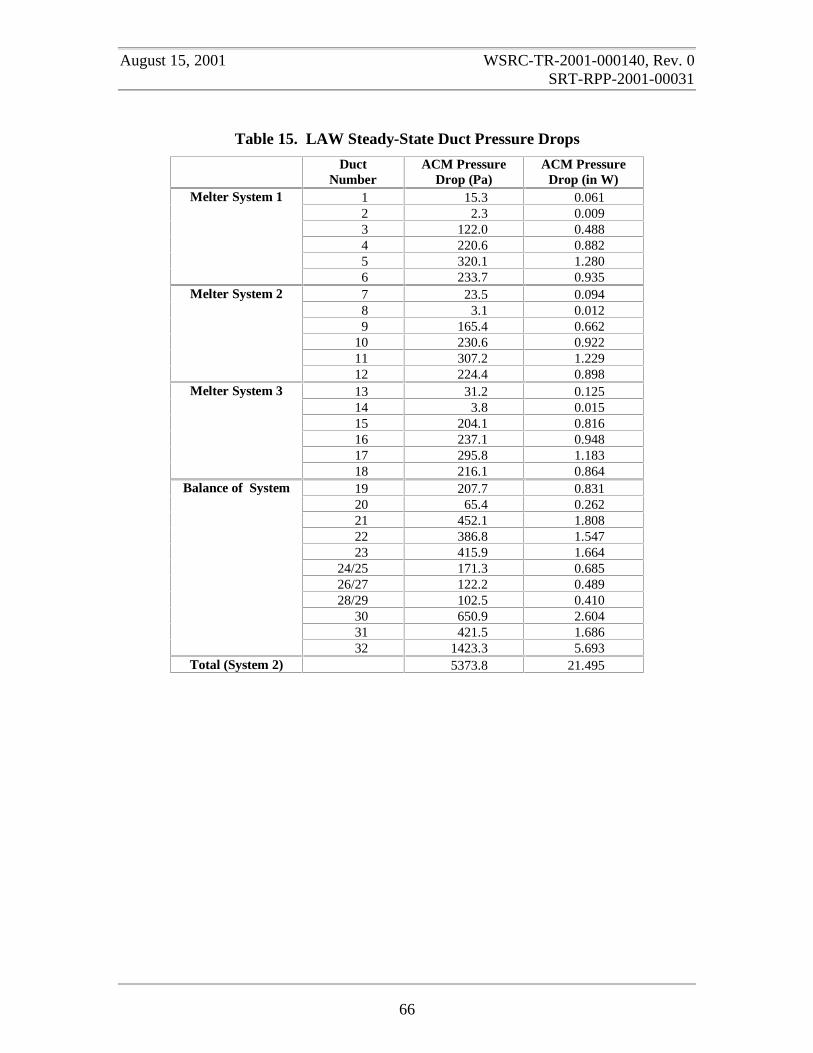
August 15, 2001 WSRC-TR-2001-000140, Rev. 0SRT-RPP-2001-00031
66
Table 15. LAW Steady-State Duct Pressure Drops
DuctNumber
ACM PressureDrop (Pa)
ACM PressureDrop (in W)
1 15.3 0.0612 2.3 0.0093 122.0 0.4884 220.6 0.8825 320.1 1.280
Melter System 1
6 233.7 0.9357 23.5 0.0948 3.1 0.0129 165.4 0.662
10 230.6 0.92211 307.2 1.229
Melter System 2
12 224.4 0.89813 31.2 0.12514 3.8 0.01515 204.1 0.81616 237.1 0.94817 295.8 1.183
Melter System 3
18 216.1 0.86419 207.7 0.83120 65.4 0.26221 452.1 1.80822 386.8 1.54723 415.9 1.664
24/25 171.3 0.68526/27 122.2 0.48928/29 102.5 0.410
30 650.9 2.60431 421.5 1.686
Balance of System
32 1423.3 5.693Total (System 2) 5373.8 21.495
August 15, 2001 WSRC-TR-2001-000140, Rev. 0SRT-RPP-2001-00031
67
LAW Steam Surge
It has proved difficult to emulate the intended LAW control system function. Asproposed, the LAW control system will hold the gas flow out of the SBS constant as longas melter pressure is within ±2.0 inch WG of the set point. Outside this range, the systemwill control melter pressure directly. It was attempted to model this by using acombination of control signals from SBS gas flow and melter pressure to operate a singlecontrol valve. Both control signals were sampled and, within the flow control region, theflow control signal was used exclusively. Within 0.5 inch WG of the flow control regiona polynomial transition to pressure control was attempted. However, in practice, thisscheme did not work well since almost always the control signals tried to drive thecontrol valve in opposing directions. That is, an increase in melter pressure decreases airinleakage and consequently flow out of the SBS. Therefore, as melter pressure increases,the flow control wants to open the control valve to increase flow while the pressurecontrol signals to shut the valve to decrease melter pressure. These opposing signalscombine to create a point where the composite signal is zero and the system no longerresponds. The issue of LAW control is still unresolved so two sets of calculations weremade for the LAW system: (1) a calculation with the melter under pressure control onlyand (2) a calculation using the combined pressure and flow control scheme.
Figure 32 shows model calculated results for the melter pressure during system startupand a nominal 4X steam surge (the surge is assumed to occur in Melter 1 only) usingpressure control alone. As before, each grid division on the pressure scale represents 1.0inch WG. During startup, SBS breakthrough occurs at about 40 seconds and the melterpressure reaches a minimum of about –9.0 inch WG within 10 seconds of breakthrough.The control system returns the pressure to the set point of 983.75 mbar at about 100seconds into the transient. At 100 seconds, the system is perturbed as gas flows to themelter, film cooler, and LAW VVS vessels are started. At 200 seconds, the ADS steamflow starts and the system begins to operate in a constantly transient fashion. The ADSsteam fluctuations create melter pressure disturbances of approximately ±1.0 inch WG.The steam surge starts at time 300 seconds on the graph. At 300 seconds, the melterexperiences the start of the 4X steam surge. During the surge, the melter pressurefluctuations increases to about ±1.5 inch WG. This relatively small increase in thepressure fluctuations is similar to that observed in the HLW system. In the LAW system,the pressure control valve continues to operate during the surge and does not loosecontrol function as was observed in the HLW system with a larger steam surge.
Figure 33 shows model calculated results for the melter pressure during system startupand a nominal 4X steam surge in Melter 1 using combined flow and pressure control.Event timing is identical to that described for Figure 32. Melter pressure is simplyfloating between the upper (988.75 mbar) and lower (978.75 mbar) bounds of the controlrange depending on whether the gas flow out of the SBS is below or above its set point.This creates a smooth pressure profile with the ADS pressure fluctuations clearly visibleas superimposed pressure spikes on the profile. However, as discussed above, the controlscheme is actually not functioning since the opposing signals are canceling out to give anet control signal of zero which the system interprets as being in the desired condition.

August 15, 2001 WSRC-TR-2001-000140, Rev. 0SRT-RPP-2001-00031
68
During the meter steam surge, the pressure peaks at about –5.0 inch WG which is wellbelow the cell vacuum of –1.5 inch WG.
Figure 34 shows the SBS outlet gas flow profile for the design basis case of combinedflow and pressure control. The gas flow is not being controlled with any precision by themodel control scheme. Note that when the flow crosses the set point of 0.685 m3/s atabout 70 seconds and again at about 250 seconds, the melter pressure simply flips frommaximum to minimum and back to the maximum value. Figure 35 shows the response ofthe melter pressure control valves for the case of combined flow and pressure control.The valves are able to respond to the ADS fluctuations although, for the parameter valuesassumed in this calculation, the valve is operating undesirably close to a fully closedposition. The 4X steam surge has minimal effect on valve operation. At long times, thevolumetric flow does reach a roughly steady-state condition at the correct SBS gas flowbut melter vacuum remains higher than desirable.
These results show that control of the LAW melter plenum vacuum is difficult to achievewith the proposed control system design. The function of the LAW melter pressurecontrol system is to maintain melter plenum vacuum in the range of –6.5 ± 2.5 in. WGand to control the offgas flow downstream of the SBS at a constant flowrate. Asproposed, it would accomplish this through two competing control loops with the flowcontrol being the dominant response when the melter vacuum is within the specifiedpressure range. However, because of the competing control loops and the transientnature of the offgas system, the proposed LAW melter pressure control scheme does notappear to be able to control either the SBS discharge flow or the melter plenum vacuum.The melter plenum vacuum simply bounces between the upper and lower break pointsbetween the two competing control loops. At the break points, the two control loopscancel each other out resulting in no control response at all. The SBS discharge flowdoes converge to the desired setpoint at long times in the simulation but during strongsystem transients the flow is not controlled and varies based on the amount of offgasbeing generated or added.
As with the HLW system, all of these results strongly depend on control system andcontrol valve parameters that have not been specified by the Hanford design team at thispoint and are not optimized in these calculations. Therefore, the results should be takenas only a preliminary indication of the system behavior pending refinement of themodels.

August 15, 2001 WSRC-TR-2001-000140, Rev. 0SRT-RPP-2001-00031
69
Figure 32. LAW Melter 1 pressure during startup and 4X steam surge withpressure control.
Figure 33. LAW Melter 1 pressure during startup and 4X steam surge with designbasis flow and pressure control.
975.0
977.5
980.0
982.5
985.0
987.5
990.0
992.5
995.0
997.5
1000.0
1002.5
0 50 100 150 200 250 300 350 400 450 500 550 600 650 700 750
Time (seconds)
Pre
ssur
e (m
bar)
Flow Ramp
ADS Flow
4X Melter Surge
SBS Breakthrough
cell vacuum
set point
975.0
977.5
980.0
982.5
985.0
987.5
990.0
992.5
995.0
997.5
1000.0
1002.5
0 50 100 150 200 250 300 350 400 450 500 550 600 650 700 750
Time (seconds)
Pre
ssur
e (m
bar)
SBS Breakthrough
ADS Flow
Flow Ramp 4X Melter Surge
cell vacuum
set point

August 15, 2001 WSRC-TR-2001-000140, Rev. 0SRT-RPP-2001-00031
70
Figure 34. LAW SBS gas flow during startup and 4X steam surge in Melter 1 withdesign basis flow and pressure control.
Figure 35. LAW control valve action during startup and 4X steam surge in Melter 1with design basis flow and pressure control.
0
0.1
0.2
0.3
0.4
0.5
0.6
0.7
0.8
0 50 100 150 200 250 300 350 400 450 500 550 600 650 700 750
Time (seconds)
Val
ve P
ositi
on
Melter 1
Melter 2
Melter 3
0
0.1
0.2
0.3
0.4
0.5
0.6
0.7
0.8
0.9
1
1.1
0 50 100 150 200 250 300 350 400 450 500 550 600 650 700 750
Time (seconds)
Vol
umet
ric
Flow
(m3 /s
)Melter 1
Melter 2
Melter 3
set point
August 15, 2001 WSRC-TR-2001-000140, Rev. 0SRT-RPP-2001-00031
71
Conclusions
Dynamic models of the High Level Waste and Low Activity Waste melter offgas systemsfor the proposed River Protection Project Waste Treatment Plant at the Hanford Site havebeen developed. The models treat the systems from the melters through the offgas stacksand include the vessel ventilation systems. The models have been applied to makecalculations of steady-state operation, melter startup, and melter surge scenarios. Whilethese calculations were successfully completed, the resulting pressure transients dependon the operation of the control systems, which have not been completely defined.Preliminary comparisons of model calculated pressures and gas flows to independentsteady-state calculations show good agreement.
The modeling assumes that, in all cases, the offgas leaving the Submerged Bed Scrubberis saturated air at 50 °C. That assumption means that gas flow past the scrubber actuallyfalls as steam surges in the melter. The steam surge increases melter pressure which actsto decreases the air inleakage. Since the scrubber is assumed to completely absorb thesteam a decrease in gas flow is seen downstream of the scrubber during steam surges inthe melter. Without variation in the melter steam flow caused by the ADS pumps, themodel runs very quickly requiring on the order of 60 seconds of CPU time for a completetransient calculation of system startup through a melter surge and back to steady-stateoperation. With the ADS fluctuations included, model run time increased significantly torequire on the order of 10 minutes for a 10 minute transient simulation.
As noted in the introduction, modeling was stopped before all of the planned work couldbe completed. However, the modeling is sufficiently complete that meaningful resultscan be generated. To fully complete the offgas system modeling, the following itemsneed to be included:
1. Offgas pressure control interlocks.
2. Standby offgas duct between melter and SBS.
3. HLW control valve Cv curve. Manufacturer’s data is available for thecontrol valve in the HLW VVS but it has not been incorporated intothe model.
4. SBS pressure fluctuations. Preliminary trials indicate that this may bedifficult to include in the models.
5. Offgas equipment gas volumes. Gas volumes for the SBS and WESPplenums, which represent the largest gas volumes, were included in themodel. However, gas volumes in the filters, caustic scrubber, andcatalyst skids have not been included. Including significant gasvolume in equipment will more accurately model surge suppressionand time delays in the system.
In addition, control system parameters have not been tuned and the model has notbeen independently verified or completely validated.
August 15, 2001 WSRC-TR-2001-000140, Rev. 0SRT-RPP-2001-00031
72
For quality assurance, electronic copies of the files used to generate the results inthis report have been archive. The archived material includes all Excelspreadsheets used to develop pressure drop correlations used in the models, theACM model files, and an electronic copy of this report. The material is archivedin the site DFS file storage system in folder
dce.srs.gov/project/rpp/smith/offgas.
The two ACM models named:
hlw_mog_v1.acmf and law_mog_v1.acmf
are in folders HLW Model and LAW Model, respectively. These acmf filescontain all of the input parameters, individual unit models, and the offgasflowsheet. An additional copy of the project files resides on the author’s personalcomputer in folder
E:\Hanford RPP\Off Gas
These files will be frozen and new working versions of the ACM models, reportsand Excel spreadsheets used to provide input to the ACM model will be createdfor future revisions.

August 15, 2001 WSRC-TR-2001-000140, Rev. 0SRT-RPP-2001-00031
73
Nomenclature
Af....................Flow area, m2
CD ..................Loss coefficient for tube bankCf ...................Loss coefficient for pipe fittingCv ...................Orifice coefficientD, d ................Equivalent diameter of flow path, me .....................Controller error signale& ....................Evaporation rate, kg/sf......................Frequency, Hzf0 ....................Friction factorg.....................Gravitational constant, 9.8 m/s2
G ....................Controller gainG& ..................Superficial gas mass velocity, kg/m2-sh.....................Enthalpy of gas stream, kJ/moleH, h ................Height of flow path, mHl ...................Height of liquid in scrubber, mH ....................Total gas enthalpy, kJkc....................Mass transfer coefficient, m/sks ....................Pipe roughness, mKf1, Kf2............Filter loss coefficientsK, Kv ..............Loss coefficientL ....................Fractional filter loadingL ....................Length of flow path, mL& ...................Superficial liquid mass velocity, kg/m2-sm ....................Mass, kgm& ..................Mass flow, kg/sM ...................Molecular weightnf ....................Number of fittingsno ...................Number of orifice holes in gas distribution plateN ....................MolesNRe .................Reynolds numberNs ...................Number of filter banks in seriesp, P ................Pressure, PaP ....................Heat exchanger plate spacing, mQ ....................Volumetric flow, m3/sR ....................Gas constant, 8314 J/kg-CRH .................Relative humiditys .....................Blower speed as rpm or fraction of maximum speedt......................Time, stf .....................Filter thickness, mT ....................Temperature, Cu.....................Velocity, m/sV ....................Volume, m3
w ....................Width of flow path, m

August 15, 2001 WSRC-TR-2001-000140, Rev. 0SRT-RPP-2001-00031
74
xi ....................Mass fraction of component i in gas mixtureX ....................Heat exchanger plate thickness, myi ....................Mole fraction of component i in gas mixture
Greek Symbolsγ, φ .................Scrubber constantsφ.....................Fractional valve openingφcat .................Fraction of catalyst surface occupied by poresµ ....................Viscosity, Pa-sψ ....................Controller on/off switchρ.....................Density, kg/m3
σ ....................Control output signal, 0 to 1τ .....................Time constant, sθ.....................Angle, degrees
Subscriptsavg .................Averagebed .................Scrubber bedc .....................Cross-sectioncat ..................Catalystchan ...............Flow channelcon .................Contractionexp .................Expansionent ..................Entranceext ..................Exitg.....................Gasin....................Pipe or unit inletl......................Liquidlam .................Laminar flowlay ..................Catalyst layerslow .................Lower filter housingmon ................Catalyst monolitho.....................Orificeout..................Pipe or unit outletp, pipe ............Pipes .....................Surfacesat ..................Saturationturb ................Turbulent flowup...................Upper filter housingvap .................Vaporw ....................Internal flow area
August 15, 2001 WSRC-TR-2001-000140, Rev. 0SRT-RPP-2001-00031
75
References
Anderson, T, and Berrios, E., “LAW Melter Offgas System Design Basis,” Draft A,January 22, 1999, BNFL Inc., Richland, Washington.
Berrios, E., 2000, “Systems 231, 232, 233 and 234: LAW Melter Offgas SystemDescription,” SD-W375LV-PR00004, Rev. E, BNFL Inc., Richland, Washington.
Blevins, R. D., 1984, Applied Fluid Dynamics Handbook, Van Nostrand Reinhold, NewYork.
Bustamante, I., 2000, “Sizing of the LAW Exhauster Booster Fans,” CALC-W375LV-PR00017, Rev. 1, February 7, 2000, BNFL Inc., Richland, Washington.
Fergestrom, L., and W. Meeuwsen, 2000, “LAW Vessel Ventilation Calculation,”CALC-W375LV-PR00022, Rev. 1, November 6, 2000, CH2MHill Hanford Group, Inc.,Richland, Washington.
Foust, A. S., L. A. Wenzel, C. W. Clump, L. Maus, and L. B. Andersen, 1967, Principlesof Unit Operations, John Wiley & Sons, New York, pp. 160-182.
Holland, C. D., 1981, Fundamentals of Multicomponent Distillation, McGraw-Hill, NewYork, p. 608.
Jain, A. K., 1976, “Accurate Explicit Equation for Friction Factor,” ASCE J. HydraulicsDiv. 102, pp. 674-677.
Meeuwsen, W., 2001, “HLW Vessel Ventilation Calculation,” CALC-W375HV-PR00033, Rev. 1, January 29, 2001, CH2MHill Hanford Group, Inc., Richland,Washington.
Peters, R., 2000, “Technical Basis for HLW Melter Pressure Control,” RPT-W375HV-PR00004, Rev. 0, May 24, 2000, BNFL Inc., Richland Washington.
Rouse, J. K., 1999, “Prediction of Melter Air Inleakage Based on Plenum Vacuum,”CALC-W375HV-PR00062, Rev. 0, November 30, 1999, BNFL Inc., Richland,Washington.
Rouse, J. K., 2000a, “System 231: HLW Vitrification Offgas Treatment SystemDescription,” SD-W375HV-PR00002, Rev. C, January 21, 2000, BNFL Inc., Richland,Washington.
Rouse, J. K., 2000b, “High Efficiency Particulate Air Filter Electric Preheater OverallPressure Drop Determination,” CALC-W375HV-PR00023, Rev. 0, May 3, 2000, BNFLInc., Richland, Washington.
August 15, 2001 WSRC-TR-2001-000140, Rev. 0SRT-RPP-2001-00031
76
Rouse, J. K., 2000c, “Submerged Bed Scrubber Overall Pressure Drop Determination,”CALC-W375HV-PR00065, Rev. 0, March 23, 2000, BNFL Inc., Richland, Washington.
Rouse, J. K., 2000d, “Wet Electrostatic Precipitator Overall Pressure DropDetermination,” CALC-W375HV-PR00074, Rev. 0, March 23, 2000, BNFL Inc.,Richland, Washington.
Rouse, J. K., 2000e, “High Efficiency Mist Eliminator Overall Pressure DropDetermination,” CALC-W375HV-PR00075, Rev. 0, March 23, 2000, BNFL Inc.,Richland, Washington.
Rouse, J. K., 2000f, “Thermal Catalytic Oxidizer/Nox SCR Overall Pressure DropDetermination,” CALC-W375HV-PR00078, Rev. 0, May 3, 2000, BNFL Inc., Richland,Washington.
Rouse, J. K., 2000g, “Offgas Ducting Overall Pressure Drop Determination,” CALC-W375HV-PR00079, Rev. 0, May 3, 2000, BNFL Inc., Richland, Washington.
Rouse, J. K., 2000h, “High Efficiency Particulate Air Filter Overall Pressure DropDetermination,” CALC-W375HV-PR00089, Rev. 0, March 23, 2000, BNFL Inc.,Richland, Washington.
Rouse, J. K., 2000i, “Caustic Scrubber Overall Pressure Drop Determination,” CALC-W375HV-PR00090, Rev. 0, May 3, 2000, BNFL Inc., Richland, Washington.
Rouse, J. K., 2000j, “Definition of Fundamental Equations to Predict Offgas PressureLosses,” CALC-W375HV-PR00091, Rev. 0, March 14, 2000, BNFL Inc., Richland,Washington.
Rouse, J. K., 2000k, “HLW Melter Offgas Material and Heat Balance,” CALC-W375HV-PR00014, Rev. 1, June 28, 2000, BNFL Inc., Richland, Washington.
Rouse, J. K., 2000l, “LAW Melter Offgas Material and Heat Balance,” CALC-W375LV-PR00029, Rev. 1, July 20, 2000, BNFL Inc., Richland, Washington.
Rouse, J. K., 2000m, “Dynamic Pressure Modeling Revised Assumptions,”memorandum, December 21, 2000.
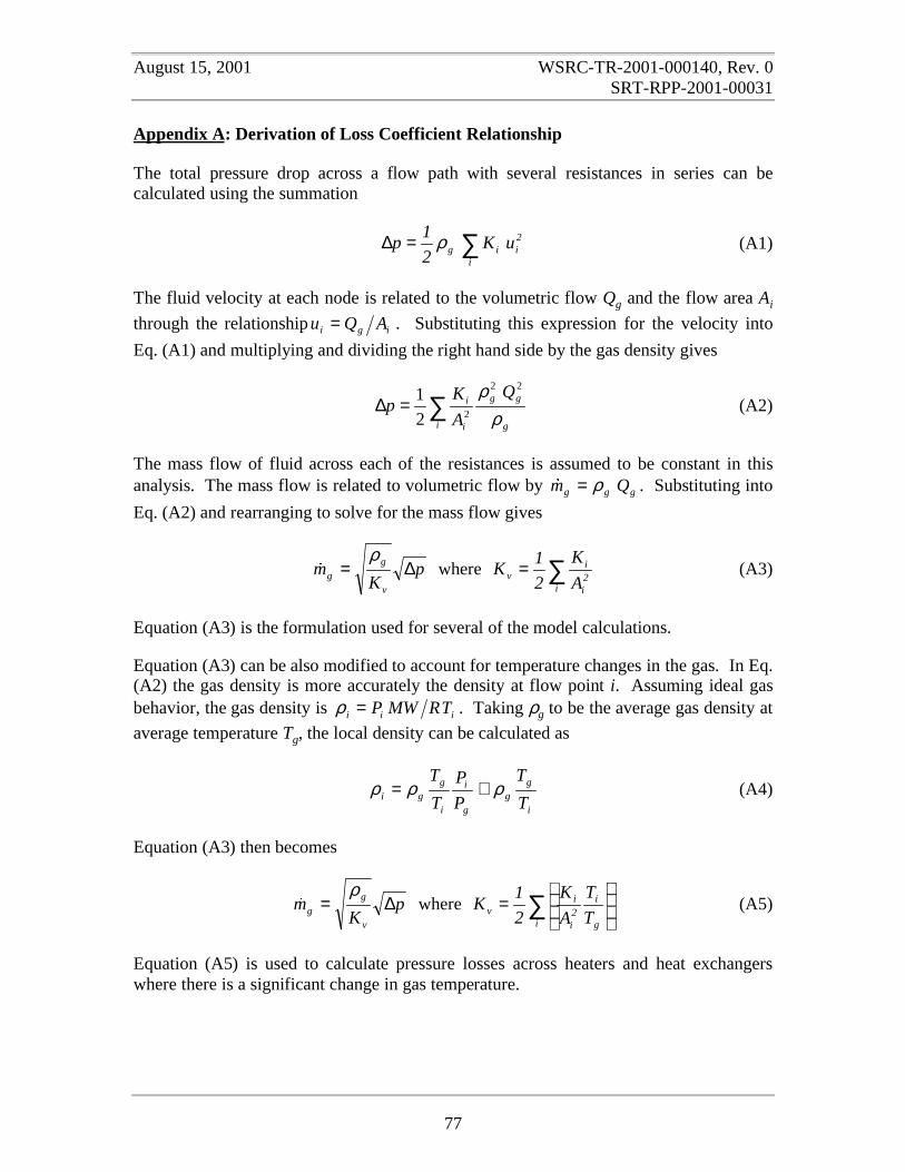
August 15, 2001 WSRC-TR-2001-000140, Rev. 0SRT-RPP-2001-00031
77
Appendix A: Derivation of Loss Coefficient Relationship
The total pressure drop across a flow path with several resistances in series can becalculated using the summation
∑=∆i
2iig uK
2
1p ρ (A1)
The fluid velocity at each node is related to the volumetric flow Qg and the flow area Ai
through the relationship igi AQu = . Substituting this expression for the velocity into
Eq. (A1) and multiplying and dividing the right hand side by the gas density gives
g
gg
i i
iQ
A
Kp
ρρ 22
22
1 ∑=∆ (A2)
The mass flow of fluid across each of the resistances is assumed to be constant in thisanalysis. The mass flow is related to volumetric flow by ggg Qm ρ=& . Substituting into
Eq. (A2) and rearranging to solve for the mass flow gives
pK
mv
gg ∆=
ρ& where ∑=
i2i
iv A
K
2
1K (A3)
Equation (A3) is the formulation used for several of the model calculations.
Equation (A3) can be also modified to account for temperature changes in the gas. In Eq.(A2) the gas density is more accurately the density at flow point i. Assuming ideal gasbehavior, the gas density is iii TRMWP=ρ . Taking ρg to be the average gas density at
average temperature Tg, the local density can be calculated as
i
gg
g
i
i
ggi T
T
P
P
T
Tρρρ ≅= (A4)
Equation (A3) then becomes
pK
mv
gg ∆=
ρ& where ∑
=
i g
i2i
iv T
T
A
K
2
1K (A5)
Equation (A5) is used to calculate pressure losses across heaters and heat exchangerswhere there is a significant change in gas temperature.