preliminary investigation of fine sediment...
TRANSCRIPT

PRELIMINARY INVESTIGATION OF FINE SEDIMENT DYNAMICS IN
CUMBARJUA CANAL, GOA, INDIA
by
A. J. Mehta
E. J. Hayter
Coastal and Oceanographic Engineering Department
University of Florida
UFL/COEL-81/012
December, 1981

ABSTRACT
Sediment management in estuaries requires an understanding of fine,cohesive sediment transport processes which typically characterize theestuarine regime. A preliminary field investigation was carried out inCumbarjua Canal, Goa, India, where the sediment is almost entirely in
the fine range and the flows are primarily tide-induced. In a 10.4 km
reach of the canal, data on currents, tides, sediments and wind were
obtained. The hydrodynamic and the sedimentary regimes of the canal
under fair weather conditions is distinct from the regimes in monsoon.
In fair weather the flow is vertically mixed with a small longitudinalsalinity gradient. Under the typically moderate tides, the suspended
sediment concentrations are low, the shearing rates in the flow are low
to moderate, and aggregation of the flocculated kaolinitic sediment
occurs, but the order of aggregation is low, and small diameter
aggregates with low settling velocities are formed in suspension.
Consequently the waters do not clarify at slack. There appears to be a
net flux of sediment from Zuari River towards the Tonca-Surlafonda
region where consolidated shoals have formed. During monsoon the flow
is stratified, and under increased freshwater flow the salinity drops to
near-zero levels. Under these conditions, sediment load in the lower
layers of the flow is probably enhanced, and it is likely that there is
a net transport of the sediment towards Zuari River. Wind-induced waves
appear to play a role in contributing to the suspended sediment load.
The overall sediment balance is determined by the cumulative
contributions to the transport during fair weather and during monsoon.
The canal appears to be well suited for further work in elucidating the
mechanisms characterizing suspended cohesive sediment transport in tidal
waterways.
ACKNOWLEDGEMENT
The field measurement program was carried out with support from the
National Institute of Oceanography, Goa, India, while the first author
was a Visiting Scientist at the Institute, in the Ocean Engineering
Division. Encouragement given by Dr. S. Z. Qasim, Director and Dr. B.
U. Nayak, Head of the Ocean Engineering Division, made the field
investigation possible. The study was completed at the University of
Florida during the period when related cohesive sediment transport
studies were supported by the U.S. Environmental Protection Agency
(Grant No. R806684010) and the U.S. Geological Survey.
-ii-

TABLES OF CONTENTS
Page
ABSTRACT........................................................... ii
ACKNOWLEDGEMENT..................................................... ii
LIST OF TABLES...................................................... v
LIST OF FIGURES.................................................... vi
CHAPTER
I. INTRODUCTION......................... ............... ........ 1
1.1 Estuarine Fine Sediment Dynamics....................... 1
1.2 Scope of the Present Investigation...................... 6
II. FIELD INVESTIGATION ........... ............................. 9
2.1 Cumbarjua Canal........................................ 9
2.2 Field Measurements........................... ........... 14
2.2.1 Bathymetry..................................... 14
2.2.2 Tides ........................................... . 21
2.2.3 Discharge........................................ . 21
2.2.4 Time-Velocity Records............................. 21
2.2.5 Wind........................................... . 25
2.2.6 Sediment...... .......................... . .. ... 25
III. CONSIDERATIONS ON SEDIMENTARY PROCESSES ..................... 33
3.1 Scope................................................... 33
3.2 Bottom Sediment Analysis................................ 33
3.2.1 Grain Size....................................... 33
3.2.2 Minerals .. ......................................... 35
3.2.3 Organic Matter................................... 35
3.2.4 Cation Exchange Capacity......................... 36
3.2.5 Fluid Composition.. ............................. 36
3.3 Bed Roughness and Time-discharge Relationship........... 37
3.4 Mechanisms Controlling the Rate of Aggregation.......... 40
3.5 Order of Aggregation and Transport...................... 43
3.6 Shearing Rates in the Canal............................ 49
3.7 Settling Velocity...................................... 52
-iii-
TABLE OF CONTENTS (Continued) Page
3.8 Sediment Transport Rate................................. 56
3.9 Wind Effect............................................. 57
3.10 Mode of Transport in the Canal.......................... 59
IV. RECOMMENDATIONS FOR FURTHER WORK............................. 62
V. REFERENCES................................................... 65
-iv-

LIST OF TABLES
Table Title Page
2-1 Canal End Widths and Depths.................................. 9
2-2 Estimated Monthly Fresh Water Outflows....................... 11
2-3 Maximum Currents and Salinity................................ 12
2-4 Suspended Sediment Loads in the Canal (after
Rao, et al., 1976)........................................... 14
2-5 Measurement Stations........................................ 17
2-6 Dimensions of the Four Cross-Sections........................ 20
2-7 Current Profiles for Discharge Measurement................... 20
2-8 Measured Discharge.......................................... 20
3-1 Properties of Brunswick Harbor Sediment (after Krone, 1963).. 44
3-2 Computation of u* using Eq. 3-17 ............................. 53
3-3 Parameters for Eq. 3-16 and Computed Values of w............. 53
3-4 Sediment Transport Rates at Station 1........................ 57
-v-

LIST OF FIGURES
FIGURE Page
1.1 Schematic Representation of Transport and Shoaling
Processes in the Mixing Zone of the Estuary, including
Ebb Predominance Factors.................................... 4
1.2 Longitudinal Salinity and Suspended Sediment
Concentrations in the Hooghly River Estuary (India).......... 7
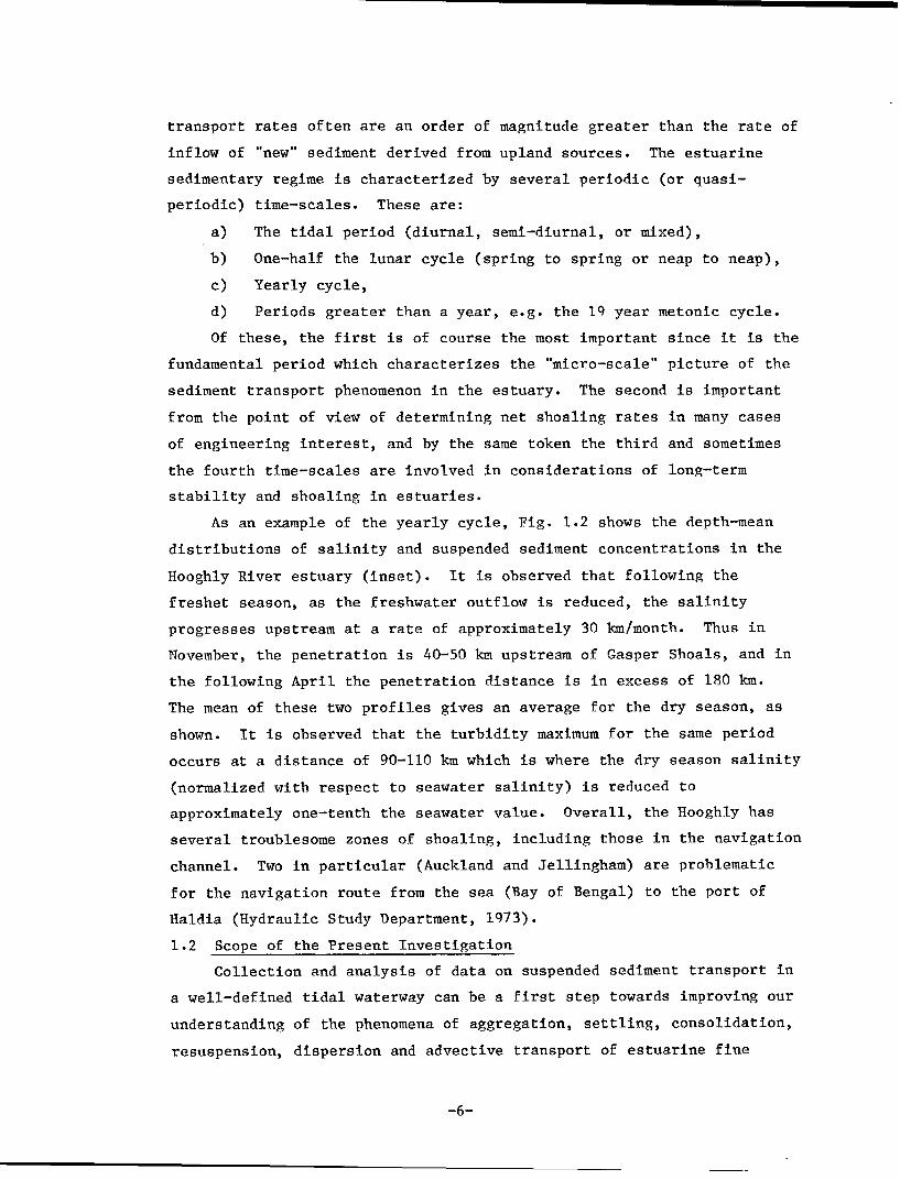
2.1 Cumbarjua Canal Connecting the Mandovi River and
the Zuari River, Goa........................................ 10
2.2 Monthly Salinity Distributions in the Canal; -- Ebb,
---- Flood (after Rao, et al., 1976)......................... 13
2.3 Selected Stations for Field Investigation.................... 15
2.4 Centerline Depth Profile in the Canal........................ 16
2.5 Canal Cross-sections at Stations 1, 2, 3 and 4............... 18
2.6 View of the Canal near Station 2................t............ 19
2.7 Tidal Measurements at Stations 1, 2, 3 and 4 on
Feb. 27, 1980 ........................................... ........ 22
2.8 Vertical Velocity Profiles at Station 1 for
Discharge Determination..................................... 23
2.9 Vertical Profiles at Station 4 for Discharge
Determination.............. ...... ......... ..... .... .... ... 23
2.10 Time-Velocity Records at Stations 1, 2, 3 and 4.............. 24
2.11 Wind Record at Station 1, Feb. 27, 1980...................... 24
2.12 Vertical Velocity Profiles at a Fixed Lateral
Position at Station 1, 0845-1200 on Feb. 27, 1980............ 26
2.13 Vertical Velocity Profiles at a Fixed Lateral
Position at Station 1, 1230-1530 on Feb. 27, 1980............ 26
2.14 Vertical Velocity Profiles at a Fixed Lateral
Position at Station 1, 1600-1700 on Feb. 27, 1980............ 27
2.15 Time-Suspended Sediment Concentration Profiles
over Depth at Station 1, Feb. 27, 1980....................... 29
2.16 Surficial Time-Suspended Sediment Concentration
Profiles at Stations 1, 2, 3 and 4........................... 30
2.17 Typical Canoe used in the Field Program...................... 32
3.1 Grain Size Distribution of Bottom Sediment from
Station 3.................................................... 34
-vi-

LIST OF FIGURES (Continued) Page
3.2 Computed Time-Discharge Relationships for
Feb. 27, 1980: a) Station 1, b) Station 4.................... 41
3.3 Typical Variation of the Depth-mean Velocity Over
a Tidal Cycle in an Estuary ................................. 47
3.4 Shearing Rate as a Function of Elevation above
the Bed Over a Tidal Cycle - An Illustrative Example......... 47
3.5 Bed Shear Stress and Aggregate Shear Strength -
An Illustrative Example...................................... 47
3.6 a) Laterally Averaged Bed Shear Stress Variation with
Time in the Canal, Station 1, Feb. 27, 1980
b) Shearing Rates in the Canal at Elevations
z/h = 0.1, 0.5 and 0.9, Station 1............................ 50
3.7 a) Laterally Averaged Bed Shear Stress Variation with
Time in the Canal, Station 4, Feb. 27, 1980
b) Shearing Rates in the Canal at Elevations
z/h = 0.1, 0.5 and 0.9, Station 4............................ 51
3.8 Normalized Suspended Sediment Concentration Profiles
in the Canal (based on data obtained on Feb. 27, 1980)....... 54
3.9 Transport of Bank-derived Suspended Sediment in the
Presence of Wind-generated Waves............................. 54
3.10 Normalized Suspended Sediment Concentration in the
Presence of Wind............................................. 58
3.11 Sediment Entrainment near East Bank.......................... 58
-vii-
I. INTRODUCTION
1.1 Estuarine Fine Sediment Dynamics
Cohesive sediments are comprised largely of terrigenous clay-sized
particles plus fine silts. The remainder includes biogenic detritus,
algae, organic matter, waste materials and sometimes small quantities of
very fine sand. Although in water with very low salt concentrations
(less than 1-2 parts per thousand) the sediment particles can be found
in a dispersed state, small amounts of salts are sufficient to cause the
electrochemical surface forces on these particles to become attractive,
with the result that the particles aggregate to form flocculated units
which possess settling velocities that are much larger than those of the
individual particles. The transport properties of the aggregates of a
given sediment are affected both by the hydraulic conditions and by the
chemical composition of the fluid. Most estuaries contain abundant
quantities of cohesive sediments which usually occur in the flocculated
form in various degrees of aggregation. Therefore, an understanding of
the transport properties of cohesive sediments in estuaries requires a
knowledge of the manner in which the aggregates are transported in these
waters. Sediment movement in estuaries is an integral component of the
natural phenomena which are characteristic of these water bodies. The
necessity of improving the current level of understanding of this
phenomenon is evident upon examination of the effects of these sediments
on the following two factors involved in estuarial management.
The first pertains to water quality for aquatic biota. The effects
of sediments on water quality for aquatic biota include limitation of
the penetration of sunlight and the sorption of toxic compounds from
solution. The concentrations of nutrients for algae in some estuaries
are often sufficient to cause excessive algae blooms. The rate of
multiplication of algae in such estuarial waters is limited by a reduced
light supply resulting from high turbidity caused by suspended sediment
particles. Estuarial waters are often used by industries as convenient
dump sites for waste products. Pollutants such as heavy metals,
pesticides, herbicides, and organics are often found sorbed on sediment
materials with equilibrium between dissolved and sorbed materials
frequently favoring the sorbed phase (Ariathurai, MacArthur and Krone,
1977). Due to their property of cohesion, these sediments appear to
-1-

provide a large assimilative capacity as well as the transporting
mechanism for such toxic compounds. Storage of river waters upstream
and their diversion for agricultural, urban and industrial uses will
sharply reduce sediment inflows as water resources become scarce.
Therefore, it will be necessary to predict the effects of reduced
sediment inflows to ascertain the minimum waste management needed to
achieve and maintain desirable water quality. Several aspects of water
quality problems related to sediment contamination have been discussed
in a series of papers edited by Baker (1980).
The second factor concerns the maintenance of navigable
waterways. Under low flow velocities, sometimes coupled with hydraulic
conditions which favor the formation of large aggregates, cohesive
sediments have a tendency to deposit in areas such as dredged cuts or
navigations channels, basins such as harbors and marinas, and behind
pilings placed in water. In addition, as described later, the mixing
zone between upland freshwater and seawater in estuaries is a favorable
site for bottom sediment accumulation. Inasmuch as estuaries are often
utilized as commerce routes to the sea, it is desirable to be able to
accurately estimate the amount of dredging required to maintain
navigable depths in these water bodies, and also to predict the effect
of new estuarial development projects such as the construction of a port
facility or dredging of additional navigation channels.
Indian estuaries are uniquely characterized by two distinct regimes
- one during the months of monsoon and the other in fair weather. Muddy
sediments predominate these coastal features (Ahmad, 1972). During
monsoon the suspended loads typically are high, under comparatively
large freshwater outflows. In fair weather the loads are lower and the
flows primarily tide-induced. For example, in the Hooghly River, the
average suspended sediment concentration upstream of Naihati (500 km
upstream of Garden Reach) increases from a value which is less than 0.2
gm/liter in dry season to a value in excess of 1 gm/liter in the freshet
season, which is a five-fold or more increase in magnitude (Hydraulic
Study Department, 1973). As a result of the large amounts of sediments
which deposit in the docks, turning basins and navigation channels at
many Indian ports on both the coasts, prediction of the rate of shoaling
under existing as well as under altered physical conditions is an
important consideration in port design.
-2-

The transport of fine sediments in estuaries is a complex process
involving a strong coupling between the baroclinic flow field and the
aggregated sediment. This process has been described extensively
elsewhere (Postma, 1967; Partheniades, 1971; Krone, 1972, Kranck,
1980). In Fig. 1.1, a schematic description is given. The case
considered is one in which the estuary is stratified, and a stationary
saline wedge is as shown. Various phases of suspended fine sediment
transport are shown, assuming a quasi-steady state, i.e. a tidally-
averaged situation. In the case of a partially mixed estuary, the
description will be modified, but since relatively steep vertical
salinity gradients are usually present even in this case, the sediment
transport processes will generally remain the same as depicted in Fig.
1.1.
The vertical variation of the horizontal flows on a tidally-
averaged basis can be conveniently described by computing the ebb
predominance factor, EPF, defined as
TEOE u(z,t)dt
EPF = (1-1)
T TF
fEu(zt)dt + J0 u(z,t)dt
Where u(z,t) = instantaneous longitudinal current velocity at an
elevation z above the bed, TE = ebb period and TF = flood period, noting
that T = TE + TF, where T = tidal period. If the strengths of flood and
ebb were the same throughout the water column, EPF would be equal to 0.5
over the entire depth of flow. This is almost never the case, and
usually EPF < 0.5 near the bottom, particularly in the wedge, and EPF >
0.5 in the upper layers. The net upstream bottom current is due to the
characteristic nature of flow circulation induced by the presence of the
wedge, which means that the strength of this current will decrease as
the limit of seawater intrusion is approached, and is theoretically zero
at the limit (node) itself (Keulegan, 1966). Distributions of EPF at
three locations - at the mouth, in the wedge and at the node, will
qualitatively appear as shown in Fig. 1.1. When interpreted in terms of
the tidal flows, these distributions correspond to the general
observation that in the mixing zone of the estuary (i.e. the region
-3-

where seawater mixes with fresh water) flood flows landward at the
bottom and ebb flows seaward at the surface.
The trends indicated by the EPF distributions suggest the
dominating influence of flow hydrodynamics on sediment movement. As
noted in Fig. 1.1, riverborne sediments from upstream sources arrive in
the mixing zone of the estuary. The comparatively high degree of
turbulence and associated shearing rates will cause the aggregates to
grow in size as a result of frequent interparticle collisions, and the
large aggregates will settle out because of their high fall
velocities. This material will eventually be carried upstream near the
bottom to a point where the bed shear stresses at the peak flow velocity
are unable to resuspend the material deposited during slack. The
sediment will consolidate here and shoals will be formed. Some fine
material will be re-entrained through-out most of the length of the
mixing zone to levels above the salt water-fresh water interface and
will be transported downstream to form larger aggregates once again, and
these will settle to the lower portion of the water column as before.
At the seaward end some material may be transported out of the system, a
portion or all of which could return ultimately with the net upstream
current. The strength of this upstream current is often enhanced by the
inequality between the flood and the ebb flows induced by the usually
observed distortion of the tidal wave. Inasmuch as the low water depth
is often significantly less than the depth at high water, the speed of
the propagating tidal wave, being proportional to the square root of the
depth, is higher at high water than at low water. This typically
results in a higher peak flood velocity than peak ebb velocity and a
shorter flood period than ebb period. Such a situation tends to enhance
the strength of the upstream bottom current, and the sediment is
sometimes transported to regions upstream of the limit of seawater
intrusion.
The shoals formed in the mixing zone may be periodically scoured by
high freshwater discharges (e.g. during the monsoon period in India),
and the material will deposit near the estuarine mouth or in the sea.
During periods of low freshwater discharge, the sediment will slowly
return to the shoal area with the net upstream current. In a typical
estuary the sediment residence time in the mixing zone is large, and the
-5-
transport rates often are an order of magnitude greater than the rate of
inflow of "new" sediment derived from upland sources. The estuarine
sedimentary regime is characterized by several periodic (or quasi-
periodic) time-scales. These are:
a) The tidal period (diurnal, semi-diurnal, or mixed),
b) One-half the lunar cycle (spring to spring or neap to neap),
c) Yearly cycle,
d) Periods greater than a year, e.g. the 19 year metonic cycle.
Of these, the first is of course the most important since it is the
fundamental period which characterizes the "micro-scale" picture of the
sediment transport phenomenon in the estuary. The second is important
from the point of view of determining net shoaling rates in many cases
of engineering interest, and by the same token the third and sometimes
the fourth time-scales are involved in considerations of long-term
stability and shoaling in estuaries.
As an example of the yearly cycle, Fig. 1.2 shows the depth-mean
distributions of salinity and suspended sediment concentrations in the
Hooghly River estuary (inset). It is observed that following the
freshet season, as the freshwater outflow is reduced, the salinity
progresses upstream at a rate of approximately 30 km/month. Thus in
November, the penetration is 40-50 km upstream of Gasper Shoals, and in
the following April the penetration distance is in excess of 180 km.
The mean of these two profiles gives an average for the dry season, as
shown. It is observed that the turbidity maximum for the same period
occurs at a distance of 90-110 km which is where the dry season salinity
(normalized with respect to seawater salinity) is reduced to
approximately one-tenth the seawater value. Overall, the Hooghly has
several troublesome zones of shoaling, including those in the navigation
channel. Two in particular (Auckland and Jellingham) are problematic
for the navigation route from the sea (Bay of Bengal) to the port of
Haldia (Hydraulic Study Department, 1973).
1.2 Scope of the Present Investigation
Collection and analysis of data on suspended sediment transport in
a well-defined tidal waterway can be a first step towards improving our
understanding of the phenomena of aggregation, settling, consolidation,
resuspension, dispersion and advective transport of estuarine fine
-6-

sediments. It was felt that the development of a major field
measurement program at the National Institute of Oceanography, Goa, for
the purpose of obtaining parameters relevant to estuarine suspended
sediment transport necessitated an initial effort at a chosen site in
the commutable proximity of the Institute. Cumbarjua Canal offers three
advantages, namely: 1) it has a reasonably well-defined, "two-
dimensional" geometry, 2) the bottom sediment is predominantly in the
fine size range, and 3) it is at a commutable distance from the
Institute. Provided appropriate instruments for measurement are
available, this canal appears to be a suitably located body of water for
carrying out extensive field investigations. To that end, a preliminary
effort was carried out during February, 1980, and the results are
reported here. The main objective was to characterize the sediment
transport regime in a 10.4 km reach of the canal, so as to facilitate
the design of future, more comprehensive data collection experiments.
-8-

II. FIELD INVESTIGATION
2.1 Cumbarjua Canal
Cumbarjua Canal (Figure 2.1) connects the Mandovi River estuary
with the Zuari River estuary at upstream distances of 14 km and 11 km
from their mouths in the Arabian Sea, respectively. The canal is 17 km
long, and is wider and deeper at the Zuari end than at the Mandovi
end. The dimensions are as followsl:
Table 2-1
Canal End Widths and Depths
Location Width at Mean Mean Depth Below
Tide Level (m) Mean Tide Level (m)
Zuari end 210 7.5
Mandovi end 25 3.5
At distances of 1.3 km and 4.0 km from the Mandovi end, the canal
bifurcates; consequently, the flow pattern near these two junction is
somewhat more complicated than in the remainder of the canal (Rao, et
al., 1976). The navigable route is utilized for the transport of iron
and manganese ore which is carried on 500 DWT barges between the mines
in the Bicholim area and Mormugao harbor. The traffic is comparatively
heavy during the monsoon period, when the build-up of the Aguada Bar
blocks the flow connection between Mandovi River and the Arabian Sea,
causing a complete diversion of the barge traffic through the canal. A
major segment of the canal has been dredged recently to accommodate
larger (1,000 DWT) barges.
The tidal range measured at the Zuari end during three days in
1969-70 varied from 0.54 m to 1.72 m, and the corresponding variation at
the Mandovi end was 0.36 m to 2.00 m, with a dominant semi-diurnal
constituent (Das, et al., 1972). Considering the tide at Marmagao
1Data for the Mandovi end of the canal are based on survey in the early
seventies (Rao, et al., 1976). Data for the Zuari end are based on a
1980 survey, carried out as a part of the present investigation.
-9-
73 E 4p 5P' !' 74o
R
GOAB A
AGU PPANJIM Monsoon j ~N ,u ABANASTARIM
AGUADA AGUADA BARBAY
A ABOPrimaryFair
SWeather a *CUNDAIM0 Route ----
*SURLAFONDA
Z14 R1 *TONCA25 -25
2 MARMAGAO BAY
SPORT
E
A
20 2015 15
S730 45 5'' 5'5' 74
Fig. 2.1 Cumbarjua Canal Connecting the Mandovi River and the Zuari River, Goa. o

Harbor to be the representative sea tide at the mouths of the two
estuaries, the narrower width of the Mandovi and the longer travel
distance to the canal through Mandovi in comparison with the Zuari
causes the arrival of the tidal wave at the Mandovi end of the canal to
lag the arrival at the Zuari end. The corresponding time lags with
respect to Marmagao Harbor are 1 hr and 0.5 hr (Rao et al., 1976). In
order words, the time of arrival of high or low water at the Mandovi end
lags that at the Zuari end by 0.5 hr, which provides a driving force for
the tidal motions in the canal.
Inasmuch as the Mandovi has a larger tributary system than the
Zuari, the salinity at the Mandovi end of the canal is consistently
lower than at the Zuari end. This condition becomes more pronounced
during the monsoon period (June-September), when a portion of the
Mandovi River freshwater outflow which flows through the canal has a
marked influence on the salinity distribution in the canal.
Magnitudes of fresh water flow through the canal are not
available. However, Table 2-2 gives estimates of the outflows through
the Zuari and the Mandovi on a monthly basis (Mehta, 1981). The rates
are observed to be substantial during July-August, and it is not
surprising that the canal becomes a complete, or near-complete fresh
water body, since it may be expected that a significant amount of the
flow is diverted through the canal. Recorded variations in the currents
and salinity at the two ends of the canal are given in Table 2-3 (Rao,
et al., 1976).
Table 2-2Estimated Monthly Fresh Water Outflows
Month Outflow(m 3/sec)
Zuari River Mandovi River
June 20 40July 170 340August 250 500September 80 160
October 30 60
November-May Negligible Negligible
-11-

Table 2-3Maximum Currents and Salinity
Location Max. Current Salinity(m/sec) (ppt)
Flood Ebb
Non-monsoon:Zuari end 0.60 0.60 34.0-35.4Mandovi end 0.60 0.15 29.0-35.0
Monsoon:Zuari end 0.90 1.10 16-29.6Mandovi end 0.50 0.75 0-8.5
The data in Table 2-2 indicate a high degree of correlation between
ebb dominated currents due to freshwater outflow in the monsoon period
and the corresponding reduction in canal salinity. The canal is
essentially "flushed out" by the fresh water from Mandovi River. The
vertical and the spatial distributions of salinity are shown in Fig. 2.2
on a monthly basis (Rao, et al., 1976). These data illustrate the
rather substantial variations in salinity which typically occur over a
year. The measurements, which were obtained in 1972, show two signifi-
cant trends. First, there appears to be a measurable longitudinal
movement of the vertical salinity gradients with tide. The length scale
of this movement appears to be on the order to 1-2 km. Second, there is
also a significant seasonal variation of salinity. Peak, spatially-
averaged salinity occurs in May, which is the driest month, whereas
during July-August much of the canal water has negligible salinity.
Following August, as the freshwater outflows from the Mandovi and the
Zuari begin to decrease, the salinity begins to rise, and continues to
increase until it attains another maximum during the following May. The
vertical structure of the flow is correspondingly affected. Thus,
during monsoon it may be expected that the flow would be stratified due
to the contribution from fresh water flows. During pre-monsoon months,
the flow is vertically mixed (Rao, et al., 1976). In Fig. 2.2, some
stratification is observed in the October distribution, whereas during
the March-June period, except for the region near the Mandovi, the
vertical variation in canal salinity does not appear to be significant.
-12-

Table 2-4Suspended Sediment Loads in the Canal (after Rao, et al., 1976)
Month Suspended Sediment Load(mg/liter)
During ebb During flood
January 10-50 10-40February 10-50 20-70March 20-80 20-100May 20-100 40-120June 30-65July 50-80 20-60August 70-120 60-90October 10-60 10-50
Measured suspended sediment loads (Rao, et al., 1976) during the
year are given in Table 2-4. It is noted that the load in May (and
possibly in June, during flood), is greater than the load in October and
January (and possibly in November and December). The observed
magnitudes in February (10-50 mg/liter during ebb and 20-70 mg/liter)
are comparable to those reported in this study.
Coupled with salinity changes, water temperature variations can
also have a marked effect on cohesive sediment transport rates since
increasing the fluid temperature tends to weaken the interparticle
bonding forces. At Cumbarjua Canal, however, the yearly variation is
comparatively small, ranging between 270C and 320C. The influence of
temperature is thus likely to be of secondary importance only.
2.2 Field Measurements
Measurements were carried out during February of 1980. Four
stations were selected as shown in Fig. 2.3. These are identified in
Table 2-5.
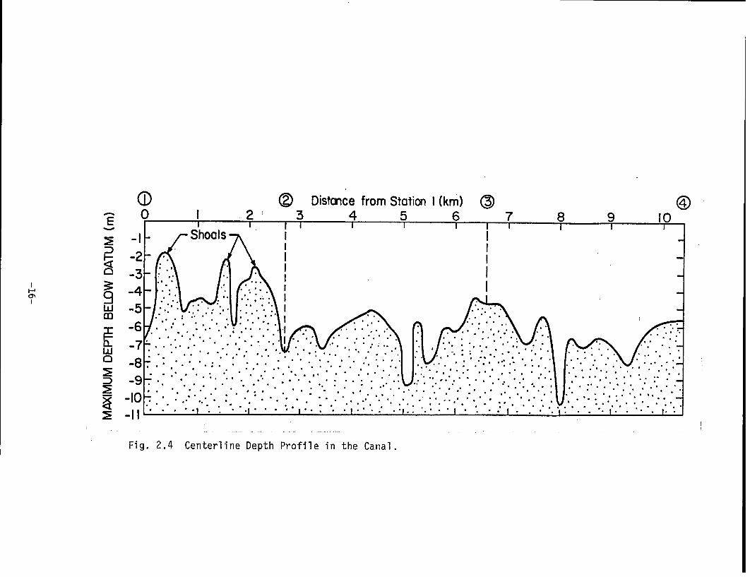
2.2.1 Bathymetry
Fig. 2.4 shows the centerline depth profile of the 10.4 km reach of
the canal between stations 1 and 4. It is noteworthy that the stretch
between stations 3 and 4 is characterized by the presence of significant
shoals. At low tide, and in the presence of wind-generated waves, these
shoals are likely to contribute measurably to the suspended sediment
load in the canal. It should be noted that these shoals do not in
-14-

Gandaulim )) oCombarjua Org
SOOld Goa
Banastarim
N 0 Corlim 0 Adcalna
/ 3.8 km
SBoma
Dongrim®O 3• 9kr Cundaim
~T 9 kSurlafonda
( 2.7 km
D Tonca 0 I 2 3 4 5km
E Agacaim
Fig. 2.3 Selected Stations for Field Investigation.
-15-
( © Distance from Station I (km) @S0 I 2 3 4 5 6 7 8 9 10SI I I I I I iI I I I
S-I /- Shoals I
-2 I-3 - -.
N -4 :. Iw -5
-6
6. " .,,' " ." ,-,.,,-.,
• . ... . .. .. .. . ., .. ... .Fig.e Dh P e in te
Fig. 2.4 Centerline Depth Profile in the Canal.

Table 2-5Measurement Stations
Station Location Distance from Station 1
(m)
1 Tonca 02 Surlafonda 2.73 Cundaim 6.64 Banastarim 10.4
general extend laterally along the entire width of the canal. Thus the
observed depths over the shoals should not be confused with the
controlling depths in the navigable channel which does not necessarily
run along the canal centerline everywhere. The presence of these shoals
near the Zuari end of the canal is an indication that the primary source
of sediment in the reach of the canal under consideration is the Zuari
River.
Cross-sections at 1, 2, 3 and 4 are shown in Fig. 2.5. Of
particular interest is the comparatively wide section at 1. Here, the
western bank is shallow and stretches over a distance of approximately
150 m. A consequence is that as the tide rises above the low water
level during flood, i.e. when the flow is towards the Mandovi, the
waterline travels this distance of 150 m within minutes, giving the
appearance of a much wider canal when it is "bankfull" than the width of
its deeper section, which is comparatively narrow. Fig. 2.6 shows the
canal near station 2. At low tide when the muddy bottom is exposed,
small holes made by various types of burrowing animals are observed
everywhere (see Fig. 3.11). Apart from the fact that these biota
actively participate in the reworking of the benthic sediments, the
perforated bed surface resulting from the presence of these organisms
would be expected to influence the bottom roughness, tending to enhance
the form drag and.hence the energy dissipation at the bed.
Water level datum indicated in Fig. 2.5 is the mean tidal elevation
derived from water surface profiles obtained on February 27, 1980. This
datum should not be confused with the hydrographic datum, which is not
considered here. Dimensions of the four cross-sections are given in
Table 2-6.
-17-

East Bank Datum Instantaneous w.s. during Discharge Measurement West Bank
I
Current I SECTION IProfile ISECTION
-Float -Datum
SECTION 2
I
i Float _ Datum
SECTION 3
Datum Float
-n Instantaneous w.s. during Discharge Measurement
I I j/ SECTION 4
S'0 10 I203040 50 km
I I m Scales2m
Fig. 2.5 Canal Cross-sections at Stations 1, 2, 3 and 4.

Fig. 2.6 View of the Canal near station 2

Table 2-6Dimensions of the Four Cross-Sections*
Section Mean Depth Maximum Depth Width Area
(m) (m) (m) (m2)
1 2.54 6.1 315 8002 3.23 7.1 153 4943 2.68 4.3 194 520
4 3.63 6.1 103 374
*Relative to selected mean tidal datum
Table 2-7Current Profiles for Discharge Measurement
Station Date Stage Time Number ofPeriod Profiles
1 Feb. 14, 1980 ebb 1130-1157 6
4 Feb. 26, 1980 ebb* 1210-1245 5
*close to slack
Table 2-8Measured Discharge
Station Date Stage Time Discharge(m3/sec)
1 Feb. 14, 1980 ebb 1144 247
4 Feb. 26, 1980 ebb 1228 61
-20-

2.2.2 Tides
Tidal measurements at the four stations obtained on February 27,
1980, are shown in Fig. 2.7. At each station, the water level was
recorded on a graduated pole installed near the east bank and leveled
with reference to a temporary bench mark. The selected datum for each
station is the mean tide level applicable only to the corresponding
record shown. Its relationship to the local hydrographic station, or2
the relationship between the four selected datums, are not known . The
tidal range is observed to be approximately 1.3 m, and the time between
high and low waters is approximately 9 hrs, indicating that the tide was
probably of a mixed type on this day. Low water at station 4 is
observed to lag the low water at station 1 by approximately 1.2 hr.
2.2.3 Discharge
For discharge determination, vertical velocity profiles were
obtained at stations 1 and 4, using a small Savonius rotor-type current
meter designed at the National Institute of Oceanography.
Characteristics of the measurements are given in Table 2-7.
Because of the comparatively short duration over which the velocity
profiles were obtained at each section, they may be construed to yield
the instantaneous discharges. The profile positions, and the position
of the instantaneous water surface are shown in Fig. 2.5. Profiles
themselves are given in Figs. 2.8 and 2.9. At station 1, no flow was
recorded at the position of profile 6. At station 4, although surface
currents were ebbing, a current reversal is observed to have had
occurred near the bottom. Discharges computed on the basis of these
profiles are given in Table 2-8.
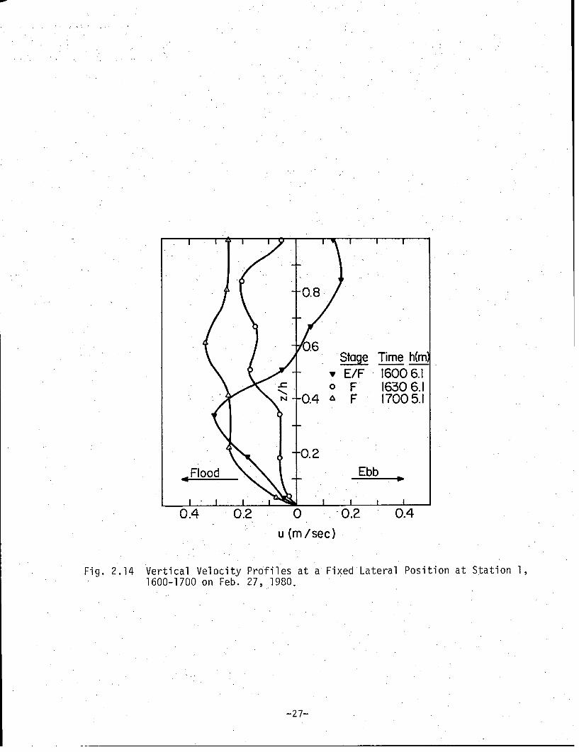
2.2.4 Time-Velocity Records
Time-velocity records were obtained at the four stations on
February 27, 1980 and are shown in Fig. 2.10. Whereas surface floats
(float sphere diameter was 30 cm) were employed at stations 2, 3 and 4,
a Savonius rotor current meter was used at station 1. Lateral position
of the float at each station is shown in Fig. 2.5. A metal cross-piece
2Attempts to tie the mean tide datum with the hydrographic datum
recorded on two benchmarks, one on a road bridge at Banastarim and the
other in the Tonca vicinity yielded apparently spurious results.
-21-

S/' . Tide at Stations 1,2,3 and 4, Feb. 27, 1980E 0.6
1 04-C-,
w 0.2
-J
o 9 10 II 12 15 16 17 18 19w. - . TIME (hrs)
o 0 -0.2-
z -0.4o0
J -0.6-
S-0.8
Fig. 2.7 Tidal Measurements at Stations 1, 2, 3 and 4 on Feb. 27, 1980.

I Oi - 1- I^ e i --- i - ' -- -- -
1.0 Velocity Profiles at I for_ Discharge, Feb. 14,1980
Position Time h(m)0.8 I 1130 4.25
2 1140 6.25o 3 1145 5.75-* 4 1152 425
0.6- o 5 1157 1.50
€-
0.4-
zh0.2
Ebb
0 0.2 0.4 0.6 0.8 1.0u (m/sec)
Fig. 2.8 Vertical Velocity Profiles at Station 1 for Discharge Determination.
Velocity Profiles at '4for Discharge,Feb.26,1980
Position Time h(m)T I 1010 32008a 2 1220 5.20o 3 12302.20* 4 12355.20o 5 12455.20
0.6-
0.4
Flood Ebb
0.4 0.2 0 0.2 0.4u( m/sec)
Fig. 2.9 Vertical Profiles at Station 4 for Discharge Determination.
-23-

Currents at Stations 1,2,3 and4, Feb. 27, 1980. Section
S- -- I 5.0m above bed(current meter)S 0.4 --- 2 0.5m below instantaneous w.s.(float)
- -- 3 0.5m below instantaneous w.s.(float)o o 4 I.Om below instantaneous w.s. (float)
0.2-2 - t
- 0
SI I I I I I I"0 4 - ®•--® -
0 Wind at Station I, Feb.27,19804 - Elev. 1.5 m above w.s. /
E Direction: along Canal Axis /
a2
TIME (hrs)
Fig. 2.11 Wind Record at Station 1, Feb. 27, 1980.
-24--24-

was attached to the float at station 4 (each of the four fins of the
cross-piece was 28 cm long, 20.5 cm wide and 1 cm thick). The effective
depth at which this float may be considered to have recorded the current
velocity was 1 m. At station 1, the current meter was used to obtain
"instantaneous" velocity profiles at a position shown in Fig. 2.5. The
profiles themselves are plotted in Figs. 2.12, 2.13 and 2.14.
Fig. 2.10 indicates that the maximum ebb velocities were on the
order of 0.4 to 0.5 m/sec. Low water slack at station 4 lagged the low
water at station 1 by 0.75 hr.
2.2.5 Wind
Wind was recorded at station 1 using a hand-held anemometer (made
by OTA Keiki Seisakusho (OTH), Japan) on February 27, 1980 (Fig.
2.11). Wind direction was approximately along the axis of the canal
(and therefore normal to the cross-section), and into the canal.
Although no wind speed was recorded at stations 2, 3 and 4, the general
observation was that the wind speed decreased from station 1 to 4, and
infact at 4, there was very little wind. It is noted that the speed at
station 1 reached a maximum of 4.5 m/sec at 1430 hr. The observed
temporal distribution is characteristic of the onshore wind during this
part of the year.
During those times when the wind speed was appreciable, a wave
generation, growth and breaking phenomenon was observed, particularly at
stations 1 and 2, and especially after the flow reversed in the late
afternoon, at the onset of flood flow. The waves reached heights of the
order of 0.15 m at breaking, causing a noticeable degree of sediment
resuspension along the eastern bank, where the breaking was most
pronounced.
2.2.6 Sediment
One of the main objectives of the field investigation was the
measurement of the suspended sediment load in the canal. Suspended
sediment concentrations were obtained at the four stations on February
27, 1980, simultaneously with measurements of tides, currents and
wind. At station 1, the measurements were obtained with a van Dorn
bottle (of 2 liter capacity) at three elevations - "surface," "mid-
depth" and "bottom." The samples were stored in 2 liter plastic
bottles. Each sample was dried, filtered through 0.45 micron Millipore
-25-

I Stage Time h(m)
0.2- - zh
Flood EbbO I 0
I I I I i _ __ _ _ _
0.4 0.2 0 0.2 0.4 0.6 0.8 1.0
Fig. 2.12 Vertical Velocity Profiles at a Fixed LateralnI -4 - C4 .-4-4-- no C I onn -Y6 1 "E 0 non
\ / o E 0940 7.1SE 1040 7.10 E 1100 7.1
0.6 * E 1130 6.1a E 1200 6.1
0.4
A?-UII ° oG,. , UO u,-iU U r. .muO.
1.00.2 -
Ebb
I I I I .. IJ
0 0.2 0.4 0.6 0.8 1.0
u(m/sec)
Fig. 2.13 Vertical Velocity Profiles at a Fixed Lateral Position
at Station 1, 1230-1530 on Feb. 27, 1980.
Stage Time h(m)v E- 1230 6.1o E 1330 6.1
0.6- E 1400 6.1-o E 1430 6.1
- E 1500 6.1-N a E 1530 6.1
04-,
0.8
0.6Stage Time h(m
S-E/F 16006.1o F 1630 6.1
S-0.4 F 17005.1
0.2
Flood Ebb
I II I I I
0.4 0.2 0 0.2 0.4
u (m/sec)
Fig. 2.14 Vertical Velocity Profiles at a Fixed Lateral Position at Station 1,1600-1700 on Feb. 27, 1980.
-27-
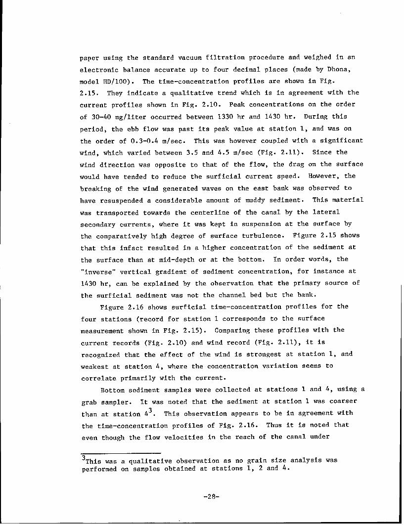
paper using the standard vacuum filtration procedure and weighed in an
electronic balance accurate up to four decimal places (made by Dhona,
model HD/100). The time-concentration profiles are shown in Fig.
2.15. They indicate a qualitative trend which is in agreement with the
current profiles shown in Fig. 2.10. Peak concentrations on the order
of 30-40 mg/liter occurred between 1330 hr and 1430 hr. During this
period, the ebb flow was past its peak value at station 1, and was on
the order of 0.3-0.4 m/sec. This was however coupled with a significant
wind, which varied between 3.5 and 4.5 m/sec (Fig. 2.11). Since the
wind direction was opposite to that of the flow, the drag on the surface
would have tended to reduce the surficial current speed. However, the
breaking of the wind generated waves on the east bank was observed to
have resuspended a considerable amount of muddy sediment. This material
was transported towards the centerline of the canal by the lateral
secondary currents, where it was kept in suspension at the surface by
the comparatively high degree of surface turbulence. Figure 2.15 shows
that this infact resulted in a higher concentration of the sediment at
the surface than at mid-depth or at the bottom. In order words, the
"inverse" vertical gradient of sediment concentration, for instance at
1430 hr, can be explained by the observation that the primary source of
the surficial sediment was not the channel bed but the bank.
Figure 2.16 shows surficial time-concentration profiles for the
four stations (record for station 1 corresponds to the surface
measurement shown in Fig. 2.15). Comparing these profiles with the
current records (Fig. 2.10) and wind record (Fig. 2.11), it is
recognized that the effect of the wind is strongest at station 1, and
weakest at station 4, where the concentration variation seems to
correlate primarily with the current.
Bottom sediment samples were collected at stations 1 and 4, using a
grab sampler. It was noted that the sediment at station 1 was coarser
than at station 4 . This observation appears to be in agreement with
the time-concentration profiles of Fig. 2.16. Thus it is noted that
even though the flow velocities in the reach of the canal under
3This was a qualitative observation as no grain size analysis was
performed on samples obtained at stations 1, 2 and 4.
-28-

50 I I ISuspended Sediment at Station I, Feb. 27,1980
40-S' Bottom
E30-
z
Mid-depth
r20 -z
S0-
O 1 0 ! I I I I I I I
8 10 12 14 16 18
TIME (hrs)
Fig. 2.15 Time-Suspended Sediment Concentration Profiles over Depth at Station 1; Feb. 27, 1980.

- . **a.g I-I- I I I I--, I
Suspended Sediment at Stations 1,2,3 and 4, Feb. 27,1980I 0.25m depth below instantaneous w.s.
40- 2E 3 0.5 m depth below instantaneous w.s
4S30-
W 20 "-.
.100o
0 I I I I I I I I
8 10 12 14 16 18TIME (hrs)
Fig,. 2.16 Surficial :,Time-Susp2nded Sediment Concentrationn Profiles at Stations 1, 2, 3 and 4.
investigation were of the same order of magnitude (Fig. 2.10), the
concentration in suspension at station 1 was generally lower than that
at station 4 until about 1330 hr. This may be attributed to the larger
grain size of the bed material at station 1, causing it to be
resuspended with greater difficulty than that at station 4. The rather
rapid increase in the concentration after 1330 hr is likely to be due to
the transport of comparatively finer material derived from the banks, as
noted previously4
Locally available canoes were utilized in the field program, for
current and sediment measurements. The small draft makes such a vessel
useful in canals such as Cumbarjua, where the small depths in the
shallower portion of the flow cross-section limit the use of boats with
outboard engines. Fig. 2.17 shows one such canoe.
4Caution is warranted when interpreting the degree of resuspension interms of grain size alone. When the bed material is cohesionless, it isa reasonable expectation that the larger the grain size, the lower theamount of material in suspension. When the material is a mixture ofcohesionless and cohesive sediments, the same interpretation isapplicable to the cohesionless portion of the sediment, when the latteris the predominant constituent by weight. With increasing fraction ofthe cohesive component, the mixture has a tendency to behave as acomposite cohesive unit, and increasing consideration must be given tothe flocculation characteristics of the sediment, and therefore to thesize and shear strengths of the aggregates composing the bed.Individual grain size will be of even lesser significance when thematerial is primarily in the clay range. Aggregation is discussed inChapter III, briefly.
-31-

r

III. CONSIDERATIONS ON SEDIMENTARY PROCESSES
3.1 Scope
The limited data collected in this study enable a cursory appraisal
of the sedimentary processes in the canal. A detailed description must
await a comprehensive data collection program which covers periods of
spring, mean and neap tides, at least once in fair weather and once
during monsoon. Such a measurement program will be of particular
importance in elucidating the mechanism for the observed long-term
shoaling in the canal. Some of the important features relevant to fine
sediment transport are highlighted in the sequel. In Section 3.2
certain physical and physico-chemical properties of the bottom sediment
collected at station 3 are described. In Section 3.3 bottom roughness
and time-discharge relationships are derived for stations 1 and 4 based
on, 1) instantaneous discharge measurements at the two stations (see
also Section 2.2.3) and 2) time-velocity data obtained at these stations
(see also Section 2.2.4). Following this a brief description of the
mechanisms which influence the rate of particle aggregation is given in
Section 3.4. In Section 3.5, the role of aggregation in characterizing
the transport of fine sediments is illustrated by a hypothetical
(typical) example which is further highlighted by computations based on
the canal data in Section 3.6. In Section 3.7 an attempt has been made
to obtain a few representative values of the settling velocity of the
suspended aggregates, and in Section 3.8 the role of wind in influencing
the vertical distribution of the suspended sediment concentration (and
therefore the settling rates) is briefly discussed. Finally in Section
3.9 a tentative description of the overall transport process is
attempted.
3.2 Bottom Sediment Analysis
3.2.1 Grain Size
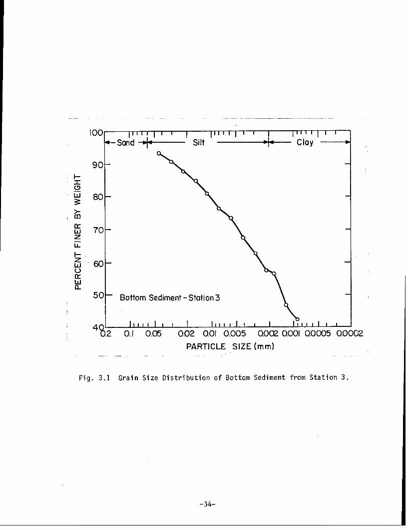
Fig. 3.1 shows the grain size distribution of the dispersed
sediment. It is noted that the percentage of particles greater than
0.06 mm, i.e. in the sand range, is no more than about 5, indicating
that at station 3, where the sample was collected, the material is
almost entirely in the fine range. Fifty-seven percent of the material
is clayey and the remaining is in the silt size range. This type of
material is generally very cohesive.
-33-
100 I I ' I 1 '*- Sand ---- Silt -- Clay
90-
I-
w 80-
w 70zLL.Z
w 60
Qa-50 Bottom Sediment-Station 3
I0II I , ! I 1, ',i, ,, I i ,11 1 l ii4.2 0.1 0.05 0.02 0.01 0.005 0.002 0.001 0.0005 0.0002
PARTICLE SIZE (mm)
Fig. 3.1 Grain Size Distribution of Bottom Sediment from Station 3.
-34-

The size distribution was determined by the standard hydrometer
test (Bauer and Thornburn, 1958) with the modification that the sample
was not dried initially for obtaining the total dry weight of the
material used in the test. This was done in accordance with the
observation made by Krone (1962), and confirmed in the present
investigation, that if the sample is dried, it is likely that it will
not redisperse completely even when a sufficient amount of the
dispersing agent (sodium hexa-metaphosphate) is added. This in turn
means that the subsequently measured size distribution will indicate
larger particle sizes in comparison with those obtained by using the
original wet sample. For this reason, the total dry weight of the
sample was obtained from a separate sub-sample, and the corresponding
value for the test sample was calculated by assuming that both samples
had the same water content.
3.2.2 Minerals
X-ray diffraction analysis of 1) the bulk sample, 2) less than 2
micron sample and 3) glycolated, less than 2 micron sample indicated the
presence of clay minerals kaolinite (as predominant constituent), illite
and montmorillonite. Among non-clay minerals, quartz was identified.
Traces of other clay and non-clay minerals appear to be present as well,
but their identification requires further confirmatory tests.
It may be expected that although the percentage of coarse material
varies spatially in the stretch of the canal under investigation (see
Section 2.2.6), the clay mineral constituents are likely to be well-
mixed inasmuch as the canal is relatively short and their relative
amounts are probably invariant throughout. Reworked fine sediments in
estuaries tend to exhibit such a uniformity, as in San Francisco Bay
(Krone, 1962).
3.2.3 Organic Matter
The sediment sample was found to contain 6.9% organic matter by
weight using the Walkley-Black procedure (Allison, 1965). It is likely
that the organic content shows a spatial as well as seasonal
variation. A comprehensive sediment sampling program is required to
confirm (or reject) this hypothesis. Sorption of organic molecules on a
clay surface has a considerable influence on the clay behavior in
suspension. The subject matter is vastly complicated by the variability
-35-
in the type of clay and in the composition of the organic matter. An
additional time-dependent factor arises from biodegradation which
markedly influences the stability of dilute, fine sediment suspensions
(Luh and Baker, 1970).
3.2.4 Cation Exchange Capacity
The cation exchange capacity, CEC, is a useful property of fine
sediment, clay minerals in particular, and is defined as the number of
(exchangeable) cations from the pore fluid that are attracted to the
negatively charged surfaces of clay particles per unit surface area or
per unit weight of the sediment. The CEC value as well as the kind of
exchangeable cations present have an important influence on the sediment
behavior. It is usually measured in terms of milliequivalents per 100
gm. The sediment sample analyzed was determined to have a CEC value of
94 meq/100 gm using the procedure described in the USDA Soil Survey
Investigations Report No. 1, 1972. This high value, which falls within
the range of CEC values typically found for montmorillonitic clay
minerals, indicates that the sediment sample analyzed has a high level
of activity. Since it was found that the sediment contains a larger
quantity of kaolinite (which has a reported range of 3-15 meq/100 gm)
than montmorillonite, it is believed that the high CEC value obtained is
at least partially attributable to the organic matter present in the
sediment, as CEC values ranging from 150 to 500 meq/100 gm have been
reported for the organic fraction of some soils (Grim, 1968).
3.2.5 Fluid Composition
A sample (9 ml) of the supernatant fluid associated with the
sediment was collected with the help of a pipette and subjected to
analysis for pH, Na+, K+, Ca+ , Mg+, Mn+, Fe+. and C1-, with the
following results: pH = 7.8, Na+ = 2,800 ppm, K = 115.0 ppm, Ca =
56.0 ppm, Mg+ = 189.0 ppm, Mn+ = 2.8 ppm, Fe - = 0.2 ppm, and Cl =
1,200 ppm. The total salt concentration was measured to be 30,500+ t 4+ +
ppm. The relative abundance of the cations Na , Ca and Mg , which
typically (and in the present case as well with the exception of K+ ) are
dominant in the fluids associated with soils, may be characterized by
the Sodium Adsorption Ratio, SAR, defined as:
Na+
SAR = (3-1)
S(Ca + + + Mg +)]/2
-36-

where the concentrations are in milliequivalents per liter
(Arunlanandan, 1975). The above values of the concentrations of Na+,
Ca+ + and Mg++ yield SAR = 28. The pH indicates that the fluid was
slightly basic.
The magnitude of SAR in the pore fluid signifies the degree of
flocculation of the sediment. As SAR increases, soil flocculation
decreases, with inter-particle bonds weakening and surface soil
particles detaching more easily. It must however be assumed that in
Cumbarjua Canal, the surficial sediment deposit is periodically
resuspended, and since during fair weather the salinity does not vary
significantly with time, it may be expected that the pore and the
eroding fluids have similar ionic compositions. Experimental evidence
using distilled water as the eroding fluid (Arulanandan et al., 1973)
indicates that for a given pore fluid SAR in the neighborhood of the
value measured in this study (i.e. 28), increasing the salinity (NaC1)
in the eroding fluid suppresses the erodibility of the soil. Therefore,
whereas based on the pore fluid SAR = 28 one may be tempted to conclude
that at this relatively high value of SAR the soil may possess a low
degree of flocculation and therefore relatively high erodibility, it is
essential to refrain from arriving at such a conclusion inasmuch as the
influence of the eroding fluid composition on erodibility must also be
taken into consideration. At the present time there appears to be no
realistic substitute for testing the sediment in a laboratory flume in
order to measure the critical shear stress and the rates of erosion
under applied bed shear stresses, for characterizing the sediment
erosion potential.
In the present study the eroding fluid composition was not measured
directly. However, it is reasonable to assume that the sediment in the
surficial bed layers is in equilibrium, or at least quasi-equilibrium,
with the eroding fluid. The measured pore fluid salt concentration of
30,500 ppm is likely to be close to the salt concentration in the
eroding fluid. With reference to Fig. 2.2, the measured value appears
to be in agreement with previous measurements during the month of
February.
3.3 Bed Roughness and Time-discharge Relationship
Computation of bed roughness and the determination of the time-
discharge relationship from velocity measurements are part of a general
-37-

procedure which was reported by Mehta, Hayter and Christensen (1977)
previously. The following steps are involved:
a. At the selected cross-section, the instantaneous discharge, Qmis measured.
b. Qm is equated to the discharge Q computed analytically from the
following expressions:
i=mQ = ) AQ (3-2)
i=1
with
3/22.5 VgS(dm) /2AW I
AQ m i i iS1- i (3-2a)
Ki-'i ) (l-Di) i
and
k 1-2Ki( s( m --i1 29.7(d)i 29.7(d ) ( 3 i
i = en { [ k +1] +1 } (l-w) dw (3-2b)D si
where the cross-section has been divided into m sub-sections
and i refers to the i-th sub-section. Here, Ki is defined as
the degree of fullness of the sub-section (K = 1 if the sub-
section bottom is horizontal), AW = width of the sub-section,
AQ = discharge through the sub-section, dmi, dmi- = the two
end depths of the sub-section, Di = dmi-1/dmi, w = dummy
variable, S = slope of the energy grade line (assumed to be
invariant across the section) and ks = Nikuradse bed roughness
of the cross-section. Two basic assumptions inherent in the
derivation of Eqs. 3-2,a,b are: 1) the time-mean value of the
bed shear stess is proportional to the local depth, and 2) the
velocity profiles are logarithmic in the vertical. The flow is
considered to be in the hydraulically fully rough range. To
the extent that these assumptions are constrained in any given
situation, the method considers the system to be an equivalent
idealized open channel. The unknown in Eqs. 3-2a,b, when Q is
matched with Qm, is ks, whose value can thus be computed
through a numerical iterative procedure.
-38-

c. At some suitable position in the cross-section, a current meter
is installed for recording the variation of the velocity, uc,
with time, t, together with a tide gage for obtaining the
corresponding record of the water surface elevation, n(t).
d. Knowing uc(t), n(t) and ks, the following equations are
utilized to yield Q(t):
Q(t) = E(t).Uc(t) (3-3)
where
i-m 3/2
S(dm)i AWiii=1
E= (3-3a)1/2 29.7pd cd I £n( k + 1 )
and
AllA •' = l_-i
1 1-K.
K Ki (3-3b)( )i (1-Di)
I< i
where dc(t) is the water depth at the site of the meter, p = rc/de
and rc = elevation of the meter above the bed. Application of the
method to shallow waterways similar to Cumbarjua Canal has yielded
reasonably good results which have been verified through independent
measurements of discharge (Mehta and Sheppard, 1979).
As noted in Section 2.2.3, Qm = 247 m3/sec and 61 m3/sec were
obtained at stations 1 and 4, respectively. These yield corresponding
values of ks = 0.172 m and 0.01 m. The comparatively high value at
station 1 appears to be consistent with the presence of shoals in the
vicinity, which appear to have altered the flow boundary layer in such a
way as to indicate an effectively higher degree of bed resistance to the
flow at this station. Next, with these values of ks, and uc(t) and n(t)
derived from data given in Figs. 2.10 and 2.7, respectively, Q(t) is
computed as per the described method. It should be noted that while
uc(t) should correspond to current measured at a fixed elevation above
the bed, the data given in Fig. 2.10 for station 4 were derived from
float observations. Since the float elevation above the bed varied with
-39-

the water surface elevation, it became necessary to obtain a
corresponding record of flow velocity at a fixed elevation above the
bed, as required. Assuming a logarithmic velocity distribution in the
vertical, the measured current um(t) can be converted to uc(t) utilizing
the following relationship:
r
An(29.7 -+ 1)
u (t) = su m(t) (3-4)
z (t)
Xn(29.7 + 1)s
where zm(t) is the float elevation above the bed. A complete
description of the programming effort and examples have been given
elsewhere (Hayter, 1979). The time-discharge plots for stations 1 and 4
are shown in Fig. 3.2a, b. The peak ebb discharge was 253 m 3/sec at
station 1 and 151 m 3/sec at station 4 on February 27, 1980. The flow
reduction over the 10.4 km distance appears to be significant and must
be attributed to energy dissipation at the bed.
3.4 Mechanisms Controlling the Rate of Aggregation
Under estuarine conditions, suspended particles in the clay size
range, and to a lesser degree in the silt range, become cohesive as a
result of the mutually attractive electro-chemical surface forces on the
particles. When subjected to repeated collisions the particles combine
to form comparatively large aggregates, each consisting of perhaps
thousands or even millions of individual particles. The size, the
strength and the density of the resultant aggregates play an important
role in characterizing the transport of cohesive sediments under tidal
conditions.
There are three principal mechanisms of inter-particle collision in
suspension, and these influence the rate at which particle aggregation
occurs (Ariathurai, MacArthur and Krone, 1977; Hunt, 1980). The first
is due to Brownian motion resulting from thermal motions of molecules of
the suspending ambient medium. The frequency of collision, I, on a
given particle by other particles has been given by Whytlaw-Gray and
Patterson (1932) as:
I = 4kTn (3-5)3p
-40-

150 II I I I i
STATION I100- k =0.172m
50
0OEmx o---------I
-
C -50-
I -100
' -150
-200
-250
-300 I l II I8 10 12 14 16 18
TIME (Hours)
(a)
100 T I III I ISTATION 4
S50 s = 0.010m
0
oL -500
-50
S- 100 -
U)
5 -150-
-200 1I I I I I I18 10 12 14 16 18
TIME (Hours)
(b)
Fig. 3.2 Computed Time-Discharge Relationships for Feb. 27, 1980:a) Station 1, b) Station 4.
-41-

where k = Boltzmann constant, T = absolute temperature, n = number
concentration of suspended particles and y = dynamic viscosity of the
fluid (water). Under typical conditions at 200 C, I = 5 x 10⁻¹ 2n
collisions per second. Generally, aggregation rates by this mechanism
are too slow to be significant in estuaries unless the suspended
sediment concentration exceeds 10 gm/liter. Aggregates formed by this
mechanism are weak, with a lace-like structure, and are easily dispersed
by shearing in the flow or are crushed easily when deposited
(Ariathurai, MacArthur and Krone, 1977).
The second mechanism of inter-particle collision is that due to
internal shearing produced by the local velocity gradients in the
fluid. Collision will occur if the paths of the particle centers in the
velocity gradient are displaced by a distance which is less than the sum
of their radii which is referred to as the collision radius, Rij,
between i-size and j-size particles. The frequency of collision, J, on
a suspended spherical particle was derived by Smoluchowski (1917) as
4 3J = - n R G (3-6)
where G is the local velocity gradient. Aggregates produced by this
mechanism tend to be spherical, and are relatively dense and strong
because only those bonds that are strong enough to resist the internal
shearing due to local velocity gradients can survive. The3
product n Rij is large when aggregates are mixed with a large number of
dispersed particles, as in the case of an estuarial mixing region.
The third mechanism of inter-particle collision results from the
fact that particles of different sizes have different settling
velocities. Thus a larger particle, due to its higher settling
velocity, will collide with smaller, more slowly settling particles
along its path and will have the tendency to "pick up" these particles
on its way down. The frequency of collision, H, due to this mechanism
has been obtained by Fuchs (1964) as
2H = rER nAW' (3-7)
-42-

where E = a capture coefficient and AW' = relative velocity between
particles. This mechanism produces relatively weak aggregates and
contributes to the often observed rapid clarification of estuarial
waters at slack.
All three mechanisms operate in an estuary, with J and H generally
being dominant in the water column excluding perhaps the high density
near-bed layer, where Brownian motion is likely to contribute
significantly as a collision mechanism. Then again, J is probably more
important than H during times excluding those near slack, when collision
and coherence due to differential settling would be expected to be the
main mechanism controlling the rate of aggregation.
3.5 Order of Aggregation and Transport
Given the mechanisms which influence the rate of particle
aggregation in the estuary the order of aggregation, which characterizes
the packing arrangement, density and shear strength of the aggregates,
is determined by the following factors: 1) sediment type, 2) fluid
composition, 3) local shear field, and 4) concentration of particles
available for aggregation.
Primary or 0-order aggregates consist of highly packed arrangements
of primary particles, with each aggregate consisting of perhaps as many
as a million particles. Typical values of the void ratio (volume of
pore water divided by volume of "solids") have been estimated to be on
the order of 1.2. This is equivalent to a porosity of 0.55, which is a
more "open" structure than commonly occurs in cohesionless sediments
(Krone, 1963). Continued aggregation under favorable shear gradients can
result in the formation of loosely packed arrays of 0-order
aggregates. Each succeeding order consists of aggregates of lower
density and lower shear strength. Experimental observations (Krone,
1963; 1978) tend to indicate the following approximate relationship
between the shear strength, Ts, and floc density, Pf, for many (although
not all) sediments
Ts = a(pf-1) (3-8)
where a and B are coefficients which must be determined experimentally
for each sediment. As a result of the fact that the shear field in the
-43-

estuary exhibits significant spatial and temporal variations, a range of
aggregates of different shear strengths and densities are formed, and
the highest order is determined by the prevailing shearing rate,
provided that the sediment and the fluid composition remain invariant,
and given that sufficient number of suspended particles are available
for promoting aggregation.
The determination of Ts and pf corresponding to each sediment-fluid
mixture can be carried out through rheological diagrams of applied shear
stress against the shearing rate, du/dz. Such plots were developed by
Krone (1963; 1978) with the help of a specially designed annular
viscometer. Each order of aggregation corresponds to a given volume
fraction of the aggregates (volume occupied by the aggregates divided by
the total volume of the suspension) which in turn can be shown to be
related to the relative differential viscosity, i.e. the viscosity of
the suspension divided by the viscosity of the suspending medium
(water). Given the viscosity of the suspending medium, the relative
differential viscosity is determined from the slope of the rheological
diagram, and hence the volume fraction can be calculated, pf is then
computed from the volume fraction. The intercept on the applied shear
stress axis of the rheological diagram corresponds to Ts .
Table 3-1 gives the order of aggregations, shear strength and
density of Brunswick Harbor, Georgia sediment aggregates. The
mineralogical composition of this sediment is similar to the one from
Cumbarjua Canal.
Table 3-1Properties of Brunswick Harbor Sediment (after Krone, 1963)
Order of Density Shear Strength
Aggregation pf(gm/cm3 ) Ts(N/m2 )
0 1.164 3.401 1.090 0.412 1.067 0.123 1.056 0.062
-44-

The average internal shearing in a fluid, G, is obtained from
'iG =d• (3-9)
where P = energy dissipated per unit volume of the fluid, y = dynamic
viscosity and T = shear at any elevation z above the bed. This
relationship is obtained by considering the balance of forces and
conservation of energy for a differential fluid element (Streeter and
Wylie, 1975). In the laminar case, G = du/dz, whereas in the turbulent
case Eq. 3-9 is an approximation (Friedlander, 1977). In the
rheological experiments of Krone (1963), shearing was produced at
relatively low speeds at which viscous forces were dominant. Eq. 3-9 can
be utilized to calculate the shearing rate which can be withstood by an
aggregate of a given order, by equating the aggregate shear strength
with the viscous shear stress which is equal to the dynamic viscosity of
the fluid multiplied by the shearing rate. For example, the shearing
rate which can be withstood by 0-order aggregates in Table 3-1 is 3,370-i
sec , whereas 3-order aggregates will be severed when the shearing rate-lexceeds 61 sec - .
Assuming the existence of a Prandtl-von Karman logarithmic vertical
velocity distribution, T is related to z according to
2 zT =pu (1 -) (3-10)
and
du u,du _z u(3-11)dz KZ
where u* = friction velocity, p = fluid density, h = depth of flow and K
= Karman constant. Substitution of Eqs. 3-10 and 3-11 into Eq. 3-9
yields
3/2
u 1/2G U/ (1 -1 )1/2 (3-12)
1/2 1/2 z/h
( -4) 5-
-45-

Fig. 3.3 exemplifies the time-variation of the depth-mean velocity,
u, as would occur in an estuary. As a result of the distortion that a
progressive tidal wave typically experiences, the peak flood velocity is
shown to be higher than the peak ebb velocity, and the flood period is
shorter than the ebb period. Fresh water discharge is assumed to be
negligible. Since
f 1/2 _u* = u (3-13)
where f = Darcy-Weisbach friction factor, Eq. 3-12 can be written as
3/4,3/2 ,
G (f8) u (-1)1/2 (3-14)1/2 1/2 z/h
(Ky) h
For the purpose of illustration,the time-variation of G is plotted in
Fig. 3.4 for values of z/h = 0.1 (near-bed), 0.5 (mid-depth) and 0.9
(near-surface), given assumed values of f = 0.025, h = 4.6 m, v =
1.06x10 - 6 m2/sec and K = 0.3 (for sediment-laden flows). Also given in
the figure are typical shearing rates which can be withstood by 3-, 2-
and 1-order aggregates. The following observations can be made:
1. The magnitude of the shearing rate, G, varies both temporally
and spatially quite significantly. The increase in G with
depth means that, once formed, aggregates of a given "base"
order will survive near the surface in preference to the
bottom layers where they will be broken up more easily. There
will therefore be a tendency for the comparatively large
aggregates to settle downward (due to their high settling
velocities), and for smaller aggregates to move upward by
diffusion, thus setting up a vertical sediment circulation
cell. The strength of this circulation will, in general, vary
temporally as well.
2. During flood only 0- and 1-order aggregates will be able to
withstand the level of shearing at the strength of flow
(assuming the shearing rate at z/h = 0.1 to be representative
of the near-bed shearing regime), whereas during ebb 0-, 1-
-46-

in
' 0.6 II I I
3 0.
0 Q3
O
- 10 ' '- 'der - _ , - _ , _8 -0 2 4 6 8 10 12
TIME (Hours)
Fig. 3.3 Typical Variation of the Depth-mean Velocity Over a TidalCycle in an Estuary.
I - order303 0 - . z/h= 0.1
?' z/h=0.5' 20 S/ z/h =0.9- _2-order---
3 - order, 10 -- ---
< 2 2-order
S- order
0 2 4 6 8 10 12
TIME (Hours)
Fig. 3.4 Shearing Rate as a Function of Elevation above the BedOver a Tidal Cycle - An Illustrative Example.
0-order3 -S2-
E I- - order
I - / \ //-2-order
S3- 3-ordeorder
LUJ \o 2- order2 --- I - order
L -3 - •-O-order
0 2 4 6 8 10 12
TIME (Hours)
Fig. 3.5 Bed Shear Stress and Aggregate Shear Strength - AnIllustrative Example.
-47-

and 2-order aggregates can occur, as the shearing rates are
observed to be insufficient to break up 2- order aggregates.
The implication is that the aggregates deposited at slack
after flood will tend to be an order lower than those
deposited at slack after ebb.
It has been found that freshly deposited mud will consist of
aggregates which can be one order higher than the order of aggregates
forming the bed by deposition (Krone, 1972). However, after a layer of
2-3 cm thickness is formed, the aggregate volume fraction underneath is
reduced due to consolidation by overburden, and aggregates one order
lower are formed. Consequently the shear strength of the deposit will
increase with depth up to a limiting value corresponding to the lowest
order aggregates which occur in the lower layers of the deposit.
The critical shear stress and the rate of resuspension of the
deposited sediment are dependent on the shear strength of the aggregates
in the deposit and on the applied shear stress. In Fig. 3.5, the bed
shear stress, T , for the same illustrative example is plotted as a0
function of time. Also given are typical magnitudes of the shear
strength, Ts, of the aggregates, as would be determined experimen-
tally. It is observed that whereas during flood aggregates of all
orders are resuspended, the ebb shear stresses are too weak to allow the
resuspension of 0-order aggregates. Therefore, the amount of the
material resuspended will be less during ebb than during flood. Given a
greater inequality between flood and ebb flows, a situation can arise
whereby the bed material is resuspended during flood only, with the
result that a predominantly upstream sediment transport will occur.
Such a "rectification" of the transport has been observed for instance
during neap tides in Savannah Harbor (Krone, 1972). Flood dominance
near the bottom is typically enhanced in estuaries as a result of
vertical salinity gradients which will augment the rectified
transport. Indeed rectification of sediment transport is the mechanism
by which shoaling in estuaries occurs. A full description of this
phenomenon at Cumbarjua Canal remains to be verified, pending future
investigations in which data during fair weather as well as during
monsoon must be collected.
-48-

3.6 Shearing Rates in the Canal
Fig. 3.6a shows the time-variation of the bed shear stress at
station 1 on February 27, 1980. The shear stress is based on the cross-
sectional mean flow velocity and is essentially a laterally averaged
quantity. The corresponding shearing rate, G, at relative elevations
z/h = 0.1, 0.5 and 0.9 are given in Fig. 3.6b. The rates are
comparatively low throughout most of the water column, although at
elevations of the order of a few aggregate diameters, above the bed, G
values exceeding 1,000 sec - can occur. If the depth-averaged velocity
in the deepest part of the cross-section is used instead of the cross-
sectional average velocity, a peak value of G = 14 sec-1 at z/h = 0.1
can be estimated, as compared with G = 9.4 from Fig. 3.6b.
Figs. 3.7a,b correspond to the same information as in Fig. 3.6a,b,
but for station 4. Here the G values are higher, and it can be shown
that a peak value of G = 34 sec-1, as opposed to G = 16 sec - at z/h =
0.1 can be estimated in the deepest part of the cross-section. In
general, it may be concluded that on the day of the observations, the
shearing rates were low to moderate. Higher shearing rates often occur
in larger estuaries such as Savannah Harbor (Krone, 1972).
Krone (1963) has shown that the maximum shear on a floc surface due
to drag from rotation can be calculated by considering the viscous drag
on the edge of a thin disc at the equator. This yields
1 du (3T = -8 7 (3-15)
where T = maximum shear stress on a suspended floc, U = dynamic
viscosity of the fluid and du/dz = shearing rate. As an example,
considering the shearing rate of relative elevation z/h = 0.1, the
maximum shearing rate of 34 sec- 1 at station 4 would correspond to T =
0.0046 N/M2 . Assuming the canal sediment to have properties similar to
those given in Table 3-1, it is seen that aggregates of all three orders
can easily exist over most of the water column. This of course will be
the case provided that a sufficient amount of suspended sediment is
available for the rate of aggregation to be high. Inasmuch as the
suspended sediment load in the canal is very low, aggregation is likely
to proceed at a slow rate, and the order of aggregation is probably low
-49-
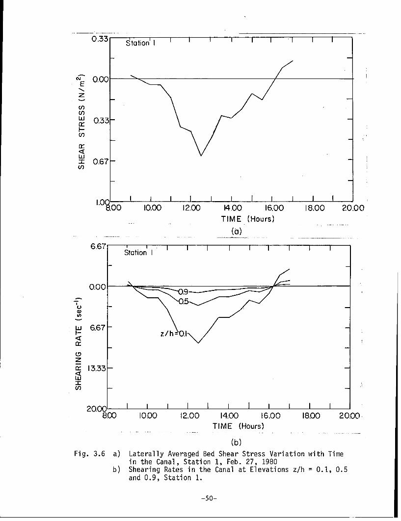
.33 " Station' I
W" 0.00 -ET H
z
U,U,W 0.33I-
iU,
I 0.67-U)
I I I I I I-
.00 10.00 12.00 14.00 16.00 18.00 20.00TIME (Hours)
(a)
6.67n I I II I IStation I
0.00-
w 6.67, z/h .1^
z
x 13.33
Ic,
20.20.00-I I I I I - -I-I-I-I
8.00 10.00 12.00 14.00 16.00 18.00 20.00TIME (Hours)
(b)Fig. 3.6 a) Laterally Averaged Bed Shear Stress Variation with Time
in the Canal, Station 1, Feb. 27, 1980b) Shearing Rates in the Canal at Elevations z/h = 0.1, 0.5
and 0.9, Station 1.
-50-

0.33 iI IStation 4
E 0.00• o.oo -- '\ ---------- "---
z
or
0.67 -
I 1.00 I II I I I0.00 2.00 4.00 6.00 8.00 1000 1200
TIME (Hours)
(n
0.67- TIME (Hours)g. 3.7 a) Latally Aveaged(d)_ _B Se Stess V wt Tm
6.67 n th , iC a S io I Fb 27 1980-Station 4
0.00-
00
S6.67 -
rl _ z/h=0.1
S13.33-I-
20.0 I I I I I I I I I2.00 8.00 10.00 12.00 14.00 16.00 18.00 ,
TIME (Hours)
(b)
Fig. 3.7 a) Laterally Averaged Bed Shear Stress Variation with Timein the Canal, Station 4, Feb. 27, 1980b) Shearing Rates in the Canal at Elevations z/h = 0.1,0.5 and 0.9, Station 4.
-51-

as well. This hypothesis appears to be corroborated by the settling
velocity estimates.
3.7 Settling Velocity
The assumption of steady state conditions for transport under a
fully developed turbulent flow results in the following expression for
the vertical distribution of suspended sediment concentration, C
(Vanoni, 1975):wKU
C(z) = [a(h - z) * (3-16
C z(h - a) (3-16)a
where Ca = concentration at a reference elevation, a, above the bed, h =
depth of flow, z = elevation above the bed, w = settling velocity, K =
Karman constant and u* = friction velocity. Application of Eq. 3-16 to
the present case can be justified on the grounds that the temporal
variations induced by the tide are of a comparatively low frequency, and
that the suspended sediment concentration is too low for hindered
settling to occur. Concentration profiles are significantly influenced
by the hindered settling of the settling aggregate "network" when
concentrations exceed 10-15 mg/liter (Krone, 1962).
Suspended sediment concentration profiles given in Fig. 2.16 at
station 1 can be utilized for the application of Eq. 3-16. Profiles at
0845, 1230 and 1330 are of a nature where C(z) increases monotonically
from surface to bottom, and are suitable for the determination of w.
The surface values are considered to correspond to C at a depth of 0.3
mbelow the instantaneous water surface, and the bottom values 0.3 m
above the bed.
The friction velocity, u*, can be computed from
u = L}1 u (3-17)
C2Rz
where g = acceleration due to gravity, h = instantaneous depth at the
site of the measurement Cz = Chezy coefficient, R = instantaneous
hydraulic radius of the cross-section and u = cross-sectional mean
instantaneous flow velocity. The data and the computed values of u* are
given in Table 3-2.
-52-

Table 3-2Computation of u* using Eq. 3-17
Time Cz R h u,
(m/sec) (ml/2/sec) (m) (m) (m/sec)
0845 0.025 42.8 3.00 6.7 0.0181230 0.267 40.3 2.19 6.2 0.2221330 0.153 39.9 2.06 5.8 0.127
Suspended sediment concentration profiles at 0845, 1230, and 1330
are plotted in Fig. 3.8. These profiles are normalized according to
Eq. 3-16, using the values of u*, h, a and Ca, given in Tables 3-2 and
3-3. The reference elevation, a, is considered to be 0.3 m, which means
that the corresponding concentration Ca is taken to be the measured
bottom concentration. The ratio a/h is noted to be 0.045, 0.048 and
0.052 which is reasonably close to the usually recommended value of 0.05
(Vanoni, 1975).
Table 3-3Parameters for Eq. 3-16 and Computed Values of w
Time h a Ca w
(m) (m) (mg/liter) (m/sec)
0845 6.7 0.3 42.5 0.001011230 6.2 0.3 18.5 0.004301330 5.8 0.3 33.0 0.00557
The slopes of the lines of Fig. 3.8 yield values of w which are
reported in Table 3-3. When analyzing data from Savannah Harbor in a
similar manner, Krone (1972) obtained values of w ranging from 0.0037 to
0.046 m/sec which indicates that the presently obtained values are
somewhat lower. The mean settling velocity is 0.0036 m/sec. The
corresponding Stokes' diameter, d, is obtained from
d = 18i1w 1/2 (3-18)
-53-

1.0
0.5 MainFlow -
SedimentSTransport
0.05- I
S * 0845 -x 1230
o 1330o Bank Erosion0.01- by Waves - - -
SecondaryFlow
0.005 -SWave-induced Surficial
o -Turbulence and Mixing
SSediment0.001 Transport
0.1 0.5 1.0
C/C a
Fig. 3.8 Normalized Suspended Sediment Con- Fig. 3.9 Transport of Bank-derived Suspendedcentration Profiles in the Canal (based Sediment in the Presence of Wind-on data obtained on Feb. 27, 1980). generated Waves.

where p = dynamic viscosity of the suspension, ys = unit weight of the
aggregates and y = unit weight of the fluid. Eq. 3-18 yields a value of
0.29 mm corresponding to w = 0.0036 m/sec. This is nearly one-half the
value of 0.6 mm (first order aggregate) determined for Savannah Harbor,
and indicates the presence of small and probably lower order aggregates
at Cumbarjua in comparison with those at Savannah Harbor. This
conclusion appears to be in agreement with the nature of the suspended
sediment profiles of Fig. 2.16. There it is observed that during
periods close to slack (0910 hr and 1515 hr) at station 1, clarification
of the fluid resulting from a rapid deposition of the suspended sediment
is not nearly as pronounced as at Savannah Harbor, where the majority of
the suspended load deposited at slack. The same observation is apparent
from the data from the three other stations shown in Fig. 2.15. In
fact, the data collected in this study indicate comparatively minor
temporal changes produced by deposition and resuspension, and it is felt
that another investigation carried out when the tides are likely to be
much stronger would be expected to yield more information concerning the
transport process in the canal than is possible to derive from the
available information. Furthermore, the present information is limited
by the unavailability of data during a flood flow.
An interesting observation concerns the role of salinity in
influencing the rate and the order of aggregation of the sediment. At
very low salt concentrations, the electro-chemical surface forces become
repulsive, and the material will disperse. When the salt concentration
is less than 1-2 parts per thousand, flocculation is generally
incomplete, and weak aggregates, which can be easily broken up, are
formed. If this indeed occurs under the high freshwater flows during
monsoon (see Fig. 2.2), the transport rates would be strongly influenced
by the salinity, under a given hydrodynamic regime in the canal. The
influence of salinity on aggregate structure has been clearly
demonstrated previously (Krone, 1963). If the material disperses, the
turbidity level could increase significantly, and the sediment will
behave essentially as wash load. A device such as the in situ settling
velocity measuring tube developed by Owen (1971) can be a useful
apparatus for ascertaining the degree of flocculation of the sediment in
monsoon.
-55-

3.8 Sediment Transport Rate
The instantaneous sediment transport rate per unit width over the
depth of flow, qs, at any given vertical in a channel cross section is
given by
h
q = f C(z)u(z)dz (3-19)
where 6 = interface elevation above the bed between bed-load and
suspended load, and u(z) = time mean flow velocity at an elevation z
about the bed. The analytic expression used for C(z) is that given in
Eq. 3-16. The expression utilized for u(z) was that of Christensen
(1972). Substituting these in Eq. 3-19 yields
wh Cau iKU
qs = (h- j *n(29.7 - +1)dz (3-20)6 s
with 0.05h being the usually recommended value for 6.
For illustrative purposes, values of qs were determined by
numerical integration of Eq. 3-20 for Station 1 verticals at 0845, 1230
and 1330 hr on February 27, 1980. The values given in Tables 3-2 and
3-3 for h, u,, a, Ca and w at the three times were used in evaluating
Eq. 3-20, with K = 0.30 and ks = 0.172 m and 6 = 0.05h as given
previously. For 0845, 1230 and 1330 hr, the following values were
determined: qs = 8.9, 69.4 and 54.3 gm/m/sec respectively. As
expected, the lowest value was obtained at the time closest to slack
(0845 hr). An estimate of the total transport rate, Qs, through Station
1 can be made using the following approximation:
q Bh
Qs - (3-21)s h
where B = instantaneous canal width and h = instantaneous cross-
sectional average depth. Values for B and h, determined using Fig. 2.5,
qs and Qs are given in Table 3-4.
-56-

Table 3-4Sediment Transport Rates at Station 1
Time B h qs Qs
(m) (m) (gm/m/sec) (gm/sec)
0845 330 2.62 8.9 11501230 315 2.55 69.4 89901330 305 2.50 54.3 7140
3.9 Wind Effect
The role of wind appears to be dual, and is particularly
significant near station 1, where onshore wind from the sea is diverted
into the canal during afternoons in fair weather. First, wind affects
the flow distribution by generating a surface current (whose magnitude
will approximately be 3 percent of the wind speed at 10 m elevation)
plus relatively high frequency gravity as well as surface tension
controlled waves. Second, when the gravity controlled waves break on
the banks, additional sediment is brought into suspension. Since a
tidal current of sufficient strength is generally present, this bank-
derived material is transported both longitudinally with the main
current and laterally with the secondary currents towards the center of
the canal. Settling of the finer portion of this material could be
hindered by the relatively high degree of surficial turbulence and
mixing due to the presence of the wind-generated waves. If during this
period resuspension of the bottom sediment is limited by the magnitude
of the prevailing bed shear stress, a situation could arise wherein the
surficial suspended sediment concentration is greater than that near the
bottom. Fig. 3.9 schematically depicts the contribution to the
suspended sediment load made by sediment derived from bank erosion. The
resulting situation is highlighted by the suspended sediment
concentration data at station 1, between 1330 and 1500 (Fig. 2.16). In
Fig. 3.10, the normalized concentration, C/Ca, is plotted against
normalized elevation, z/h. Here Ca refers to "bottom" concentration.
The wind velocity (in m/sec) corresponding to the time at which each
profile was measured is also given. Two noteworthy observations can be
made. First, it is noted that the surficial concentration relative to
-57-

1.0 I I I I I I
3.6m/s /0.80 4. I m/s -S4. 3 m/s
4.6m/s
0.6
N Time0.4- 1330
x 1400
0.2- 1430
a 1500
0 0.4 0.8 1.2 1.6 2.0
C/Ca
Fig. 3.10 Normalized Suspended Sediment Concentration in thePresence of Wind.
Fig. 3.11 Sediment Entrainment near East Banks.
-58-

that at the bottom increases with increasing wind speed. Second, as the
wind speed increases, the shape of the profile deviates from what
normally occurs in open channels under steady flows, namely a monotomic
decrease in sediment load with elevation above the bed. Thus it is
observed that a situation exists wherein the surficial sediment load is
greater than that at the bottom, or mid-depth of both. It is postulated
that bank erosion due to waves is the causative factor. As noted in
Chapter II, erosion of the eastern bank due to 0.15 m breaking waves was
recorded. Fig. 3.11 shows the bank with entrained sediment.
At low tide, the shoals in the canal between stations 1 and 2 are
no more than 0.5 to 1 m below the water surface. Hence, particularly
when wind is present, it would be expected that the contribution to the
suspended load from this source may not be insignificant during times
close to low water.
3.10 Mode of Transport in the Canal
The following description of the sediment transport in the 10.4 km
reach of the canal from Tonca to Banastarim is tentative, pending
further investigations.
The sediment is predominantly in the fine size range (silt plus
clay). The fine sand portion, which constitutes less than 5% by weight
of the sediment near the upstream end of the study segment (i.e.
Cundaim-Banastarim), increases somewhat in the direction from Banastarim
to the Zuari end of the canal. Near the Zuari end (Surlafonda-Tonca)
shoals are present, and the navigation channel is somewhat tortuous.
The primary source of sediment in the shoals appears to be the Zuari
River. The sediment, which is composed of kaolinte plus some illite,
montmorillonite and quartz, contains varying amounts of organic matter
(probably 5-15%). Burrowing marine creatures abound in the bottom
sediment. The fluid is slightly basic and the salinity varies from
near-zero to as much as 36 parts per thousand, depending on the season.
Sediment transport in the canal is almost entirely as suspended
load rather than as bed-load, which occurs only when cohesionless
sediment is present. The sediment in suspension is primarily bed
material with the possible exception of a portion of the organic
material, but the transport regime is such that a portion of the bed
material load exhibits apparent characteristics of wash load. Suspended
-59-

sediment concentration varies from 10 mg/liter to 120 mg/liter or more
depending on the season. Fair weather concentrations are lower than
those during monsoon.
The transport is primarily tide-induced, but with measurable
contribution from wind-induced effects, and from high freshwater flow
effects during monsoon. In general, the transport regime can be divided
into two categories - normal or fair weather regime and monsoon
regime. These regimes, taken together, essentially characterize the
long-term processes in the canal.
The normal hydrodynamic regime is characterized by moderate tides
(-1 m), low freshwater flow and low to moderate winds which result in a
wind-induced surface current plus waves and associated turbulent mixing
in the surficial water layer. The flow is vertically mixed, but a small
longitudinal gradient of salinity (which decreases by 2 to 4 ppt over
the 10.4 km distance) exists. The total salt concentration (23-36 ppt)
is however well above the minimum (1-2 ppt) required to complete
flocculation and above the limit (~10 ppt) below which aggregation is
influenced by the amount of salt present. Under the bed shear stresses
induced by the prevailing moderate tidal conditions, the bed sediment
appears to be resistant to erosion. This is suggested by the rather low
suspended sediment concentrations measured in the canal (-10-120
mg/liter). Except during slack, it is likely that the available
sediment rapidly aggregates in the near-bed layer of thickness ranging
from a few aggregate diameters to perhaps 1-2 cm where high shearing
rates prevail. This near-bed layer will be saturated with aggregates of
the base, i.e. lowest, order that can be formed in the system (probably
0-order in the present case), and a high density suspension layer with a
density of the order of 1.6 gms/cm3 will exist most of the time5 .
During the period of increasing bed shear stress when resuspension of
the deposit will occur, this high density suspension will gain sediment
from the bed deposit by erosion of the bed, and will lose sediment to
the fluid column above, where the shearing rates are low to moderate.
5Such a suspension was not noted in the canal because special sensorsare required for their detection (Parker and Kirby, 1977). The
transport rates given in Table 3-4 do not include contribution from thenear-bed layer.
-60-
Under a quasi-steady state condition, the rates of gain and loss of the
sediment will be nearly equal, but since the rate of gain, being equal
to the rate of erosion of the bed deposit, appears to be limited, it can
be postulated that the rate at which sediment escapes the high density
suspension to the upper layers is correspondingly small. This in turn
means that inspite of the mechanisms available for collision to occur,
the base order aggregates do not aggregate further (e.g. to second or
third order) to any significant extent due to the presence of
insufficient number of aggregates in suspension. The canal thus
contains low order aggregates of relatively small diameters (-0.3 mm)
and low settling velocities (~0.0036 m/sec). Consequently the
difference between the maximum and minimum sediment concentration during
a tidal cycle remains moderate (20-30 mg/liter), and the waters are not
clarified at slack. The aggregates with low settling velocities plus
the organic matter contribute to the observed turbidity of the canal
even during times close to slack. The existence of a longitudinal
salinity gradient however implies that there is likely to be a small net
upsteam transport of sediment which enters from Zuari and proceeds
towards Banastarim. It is possible that some of this sediment is
transported by the near-bed high density suspension.
The monsoon regime is more severe as a result of high freshwater
flow, wind and direct precipitation. The flow becomes vertically
stratified, and in July-August the salinity drops to near-zero values.
It is likely that suspended sediment is "trapped" in the relatively more
saline lower layer, and that sediment entrained in the upper layers is
carried by the freshwater flow to the Zuari River. There is likely to
be a net depletion of the bottom sediment from the canal, but the total
amount depleted is probably equal to or less than the net amount trans-
ported into the canal during fair weather, as the lower consolidated
layers of the Tonca-Surlafonda shoals are believed to be resistant to
erosion. Under such a mechanism, and particularly when dredging is
carried out, there will be a tendency for the canal to "fill up" to some
equilibrium depth when the net influx of sediment balances the net
outflux. Evidence corroborating this effect can be obtained from a
series of accurate post-dredging surveys of the canal.
-61-

IV. RECOMMENDATIONS FOR FURTHER WORK
Cumbarjua Canal does not appear to currently pose any engineering
problems which cannot be solved by available technology. The purpose of
the investigation reported herein was to identify important aspects of
the fine sediment transport regime for future research-related needs,
rather than the proposal of a solution for a particular sedimentation
problem. Along these lines, the following relevant points may be noted:
1. It is emphasized that the canal is well suited for a more in-depth
investigation of the basic aspects of fine sediment transport in
tidal waterways.
2. As a prerequisite for such a comprehensive study, it will be
necessary to characterize the canal hydrodynamics in greater
detail. This can be achieved in the following manner:
a. An accurate bathymetric survey of the 10.4 km reach of the
canal between station 1 and 4 should be performed during the fair
weather season (in monsoon this is desirable as well, but may be
impractical).
b. Either a tide gage (preferably) or a tide staff should be
installed and leveled into the local tidal datum at each of the
four stations. During both fair weather and monsoon, water surface
elevation, current, wind velocity, electrical conductivity (or
salinity) and temperature profiles should be measured at each of
the four stations at least once, preferably during a spring tide.
The data collection period should be at least 14 hours. Both
vertical (over the local water depth) and lateral (spanning the
canal width) profiles of the current, conductivity and temperature
should be obtained. Where the flow depth allows, these
measurements should be made at a minimum of three depths over each
vertical: one-half meter below the water surface, mid-depth and
one-half meter above the bottom.
c. This data set will be utilized for the calibration of a
numerical hydrodynamic model, which will then be used to predict
the temporal and spatial distributions of flow and salinity under
the range of tides and freshwater discharges which occur during a
"normal" year.
-62-

3. The above set of measurements must be repeated during the following
year, with three sets of measurements - under spring, mean and neap
tides - collected during each season. In order to properly
characterize the sediment regime, suspended sediment concentrations
must as well be measured at each of the four stations simultaneously
with the other parameters. It is recommended that fluid-suspended
sediment samples be collected at the points over the vertical and
lateral station dimensions used previously by pumping in small
volumes of the fluid-sediment mixture via a small battery operated
pump with an intake tube which can be lowered to any desired
depth. In addition, in order to adequately characterize both the
existing (consolidated) bed and any new (unconsolidated) deposits,
at least six undisturbed five inch diameter sediment cores (at least
one meter in length) should be obtained at each of the four
stations. The six cores should be taken at approximately equally
spaced locations across the width of the canal at each station.
4. The purpose for obtaining these sediment cores is to determine the
following sediment-related properties: modes of sediment
aggregation, settling velocity, minimum applied shear stress at
which deposition will occur, the shear strength, bulk density, rate
of erosion, and thickness of each stratum of both the existing bed
and new deposit, and the consolidation characteristics of the new
deposit. In addition, the average CEC value as well as the chemical
composition of the pore fluid in each of the sediment cores should
be determined.
5. Beyond this point, investigations can proceed along a number of
different lines depending upon research priorities. It is however
recommended that the data collected in the second series of
experiments, i.e. those including sediment measurements, be utilized
for the purpose of calibrating a numerical fine sediment transport
model such as the one developed by Ariathurai, MacArthur and Krone
(1977), which will enable a reasonably accurate estimation of the
suspended sediment transport rates through the canal under various
hydrodynamic conditions. In turn this will allow for the prediction
of reshoaling rates in the canal after any potential dredging. Much
greater utility of the application of such a comprehensive field
-63-

program/modeling effort lies in other, larger potential problem
areas involving port construction and management, in terms of
cost/benefit computations when heavy shoaling or sediment
redistribution of the sediment in channels is likely to occur.
-64-

V. REFERENCES
Allison, L. E., Organic Carbon, Part II, American Society of Agronomy,
Madison, Wisconsin, 1965.
Ahmad, E., Coastal Geomorphology of India, Orient Longman Limited, New
Delhi, India, 1972.
Ariathurai, R., MacArthur, R. C. and Krone, R. B., "Mathematical Model
for Estuarial Sediment Transport," DMRP Technical Report D-77-12,
U.S. Army Engineer Waterways Experiment Station, Vicksburg, MS,
December 1977.
Arulanandan, K., "Fundamental Aspects of Erosion of Cohesive Soils,"
Journal of the Hydraulics Division, ASCE, Vol. 101, NO.HY5, May,
1975, pp. 635-639.
Arulanandan, K., Sargunam, A., Loganathan, P., and Krone, R. B.,
"Application of Chemical and Electrical Parameters to Prediction of
Erodibility," in Soil Erosion: Causes and Mechanisms, Prevention and
Control, Highway Research Board Special Report 135, Washington,
D.C., 1973, pp. 42-51.
Baker, R. A., Editor, Contaminants and Sediments Volume 1 - Fate and
Transport, Case Studies, Modeling, Toxicity, Ann Arbor Science,
1980.
Bauer, E. E., and Thornburn, T. H., Introductory Soil and Bituminous
Testing, Stipes Publishing Co., Champaign, IL, 1958.
Christensen, B. A., "Incipient Motion on Cohesionless Channel Banks,"
Ch. 4, in, Sedimentation Symposium to Honor H. A. Einstein, H. W.
Shen, Ed., Fort Collins, Colorado, 1972, pp 4.1-4.22.
Das, P. K. Murty, C. S. and Varadachari, V. V. R., "Flow Characteristics
of Cumbarjua Canal Connecting Mandovi and Zuari Estuaries," Indian
Journal of Marine Studies, Vol. 1, December 1972, pp. 92-102.
Friedlander, S. K., Smoke, Dust and Haze: Fundamentals of Aerosol
Behavior, Wiley-Interscience, New York, 1977.
Fuchs, N. A., The Mechanics of Aerosols, Pergamon, New York, 1964.
Grim, R. E., Clay Mineralogy, McGraw-Hill Book Company, New York, N. Y.,
1968.
Hayter, E. J., "Verification of the Hydrodynamic Regime of a Tidal
Waterway Network," M.S. Thesis, University of Florida, Gainesville,
1979.
-65-

Hunt, J. R., "Prediction of Oceanic Particle Size Distributions from
Coagulation and Sedimentation Mechanisms," in Advances in Chemistry
Series No. 189 - Particulates in Water, Ch. 11, M. C. Kavanaugh and
J. 0. Leckie Editors, American Chemical Society, 1980, pp. 243-257.
Hydraulic Study Department, "The Study of the Hooghly Estuary and the
Project for Training Measures below Diamond Harbor," Report,
Calcutta Port Commissioners, Calcutta, July, 1973.
Keulegan, G. H., "The Mechanism of an Arrested Saline Wedge," Ch.ll, in,
Estuary and Coastline Hydrodynamics, A. T. Ippen Editor, MaGraw-
Hill, New York, 1966, pp. 546-574.
Kranck, K., "Sedimentation Processes in the Sea," in The Handbook of
Environmental Chemistry, Vol. 2, Part A, 0. Hutzinger Editor,
Springer-Verlag, Berlin, 1980, pp. 61-75.
Krone, R. B., "Flume Studies of the Transport of Sediment on Estuarial
Shoaling Processes," Final Report, Hydraulic Engineering Laboratory
and Sanitary Engineering Research Laboratory, University of
California, Berkeley, June, 1962.
Krone, R. B., "A Study of Rheological Properties of Estuarial
Sediments," Technical Bulletin No. 7, Committee on Tidal Hydraulics,
U.S. Army Corps of Engineers, Vicksburg, MS, September, 1963.
Krone, R. B., "A Field Study of Flocculation as a Factor in Estuarial
Shoaling Processes," Technical Report 19, Committee on Tidal
Hydraulics, U.S. Army Corps of Engineers, Vicksburg, MS, June 1972.
Krone, R. B., "Aggregation of Suspended Particles in Estuaries," in
Estuarine Transport Processes B. Kjerfve Editor, the Belle W. Baruch
Library in Marine Science, Number 7, University of South Carolina
Press, Columbia, SC, 1978, pp. 177-190.
Luh, M-D., and Baker, R. A., "Organic Sorption from Aqueous Solution by
Two Clays, " Proceedings of 25th Purdue Industrial Waste Conference,
Purdue, Indiana, May, 1970, pp. 534-542.
Mehta, A. J., "Considerations on the Stability of Aguada Bar Channel at
Mandovi Estuary, Goa," Technical Report 01-81, Ocean Engineering
Division, National Institute of Oceanography, Goa, April 1981.
Mehta, A. J., Hayter, E. J., and Christensen, B. A., "A Generalized
Point-Velocity Method for Discharge Computations in Tidal
Waterways," Proceedings of Hydraulics in the Coastal Zone, ASCE,
College Station, TX, August, 1977, pp. 10-12.
-66-

Mehta, A. J., and Sheppard, D. M., "Performance Study at Matanzas
Closure," UF/COEL-79/007, Coastal and Oceanographic Engineering
Laboratory, University of Florida, Gainesville, October, 1979.
Owen, M. W., "The Effect of Turbulence on the Settling Velocities of
Silt Flocs," Proceedings of 14th Congress of I.A.H.R., Vol. 4,
Paris, August, 1971, pp. 27-32.
Parker, W. R. and Kirby, R., "Fine Sediment Studies Relevant to Dredging
Practice and Control," Second International Symposium on Dredging
Technology, BHRA Fluid Engineering Paper B2, Texas A & M University,
College Station, TX, November, 1977.
Partheniades, E., "Salinity Intrusion in Estuaries and its Effect on
Shoaling," Ch. 26, in River Mechanics, Vol. II, H. W. Shen Editor,
Fort Collins, CO, 1971.
Postma, H., "Sediment Transport and Sedimentation in the Estuarine
Environment," in, Estuaries, G. H. Lauff Editor, American
Association for Advancement of Science, Washington, D. C., 1967, pp.
158-179.
Rao, L V. G., Cherian, T., Varma, K. K., and Varadachari, V. V. R.,
"Hydrographic Conditions and Flow Pattern in Cumbarjua Canal, Goa,"
Indian Journal of Marine Sciences, Vol. 5, December, 1976, pp. 163-
168.
Smoluchowski, von M., "Versuch einer mathematischen Theorie der
Koagulationskinetik Kolloider Losungen," Zeitschrift Fur
Physikalische Chemie, Vol. 92, 1917, pp. 129-168.
Soil Survey Laboratory Methods and Procedures for Collecting Soil
Samples, Soil Survey Investigations Report No. 1, Soil Conservation
Service, USDA, Washington, D.C., April, 1972.
Streeter, V. L., and Wylie, E. B. Fluid Mechanics, Sixth Ed., McGraw-
Hill, 1975.
Vanoni, V. A. (editor), Sedimentation Engineering, ASCE Manuals and
Reports on Engineering Practice NO. 54, 1975.
Whytlaw-Gray, R., and Patterson, H. W., Smoke, A Study of Aerial
Disperse Systems, Edward Arnold & Co., London, 1932.
-67-