preliminary investigation of methods for correcting

Technical Report NREL/TP-520-47277 March 2010

Preliminary Investigation of Methods for Correcting for Variations in Solar Spectrum under Clear Skies B. Marion

National Renewable Energy Laboratory 1617 Cole Boulevard, Golden, Colorado 80401-3393 303-275-3000 • www.nrel.gov

NREL is a national laboratory of the U.S. Department of Energy Office of Energy Efficiency and Renewable Energy Operated by the Alliance for Sustainable Energy, LLC

Contract No. DE-AC36-08-GO28308

Technical Report NREL/TP-520-47277 March 2010

Preliminary Investigation of Methods for Correcting for Variations in Solar Spectrum under Clear Skies B. Marion

Prepared under Task No. PVD9.1460

NOTICE

This report was prepared as an account of work sponsored by an agency of the United States government. Neither the United States government nor any agency thereof, nor any of their employees, makes any warranty, express or implied, or assumes any legal liability or responsibility for the accuracy, completeness, or usefulness of any information, apparatus, product, or process disclosed, or represents that its use would not infringe privately owned rights. Reference herein to any specific commercial product, process, or service by trade name, trademark, manufacturer, or otherwise does not necessarily constitute or imply its endorsement, recommendation, or favoring by the United States government or any agency thereof. The views and opinions of authors expressed herein do not necessarily state or reflect those of the United States government or any agency thereof.

Available electronically at http://www.osti.gov/bridge

Available for a processing fee to U.S. Department of Energy and its contractors, in paper, from:

U.S. Department of Energy Office of Scientific and Technical Information P.O. Box 62 Oak Ridge, TN 37831-0062 phone: 865.576.8401 fax: 865.576.5728 email: mailto:[email protected]

Available for sale to the public, in paper, from: U.S. Department of Commerce National Technical Information Service 5285 Port Royal Road Springfield, VA 22161 phone: 800.553.6847 fax: 703.605.6900 email: [email protected] online ordering: http://www.ntis.gov/ordering.htm

Printed on paper containing at least 50% wastepaper, including 20% postconsumer waste

http://www.osti.gov/bridge�

mailto:[email protected]�

mailto:[email protected]�

http://www.ntis.gov/ordering.htm�

iii

Acknowledgements

This work was performed under DOE Contract No. DE-AC36-08GO28308 and Task No. PVD9.1460. The author acknowledges the efforts of Jose Rodriguez, Ed Gelak, and Matt Muller at the National Renewable Energy Laboratory (NREL) for installation and operation of the test equipment; the efforts of Gobind Atmaram and Jim Roland at the Florida Solar Energy Center for coordinating the collection of data at their location; and the efforts of Chris Gueymard (Solar Consulting Services), David King (Sandia National Laboratories-Retired), Joshua Stein (Sandia National Laboratories), Kevin Fok (United Solar Ovonic), Joe del Cueto (NREL), and Matt Muller (NREL) for reviewing this report and providing helpful suggestions.

iv

List of Acronyms and Abbreviations

AM air mass

AM absolute air mass a

ASTM American Society for Testing and Materials

CREST Centre for Renewable Energy Systems Technology

f(AM) function of air mass

FSEC Florida Solar Energy Center

I short-circuit current sc

NREL National Renewable Energy Laboratory

POA plane-of-array

PV photovoltaic

SAM Solar Advisor Model

SRC Standard Reporting Conditions

T PV module temperature pv

v

Abstract

Two types of methods were evaluated for correcting the short-circuit current of photovoltaic (PV) modules for variations in the solar spectrum under clear skies: (1) empirical relationships based on air mass, and (2) use of spectral irradiance models and PV module spectral response data. Methods of the first type were the Sandia absolute air-mass function, or f(AMa

For predicting the short-circuit current for a multi-crystalline silicon PV module and an amorphous silicon PV module, the methods using spectral irradiance models and PV module spectral response data performed better than the empirical air mass methods. This is attributed to the empirical air mass methods not accounting for variations of aerosols and water vapor. For the multi-crystalline silicon PV module, applying a correction with any of the methods was not significantly beneficial when compared to not applying a correction.

), and the CREST air-mass function, or f(AM). The second type used SEDES2 and SMARTS spectral irradiance models. The methods were evaluated using data recorded during June, September, and December 2008 at the National Renewable Energy Laboratory and during June 2008 at the Florida Solar Energy Center.

vi

Table of Contents

Acknowledgements ...................................................................................................................... iiiList of Acronyms and Abbreviations ......................................................................................... ivAbstract .......................................................................................................................................... vTable of Contents ......................................................................................................................... viList of Tables ............................................................................................................................... viiList of Figures .............................................................................................................................. vii1 Introduction ......................................................................................................................... 12 Spectral Correction Methods ............................................................................................. 2

2.1 Empirical Methods Using Air Mass ............................................................................. 22.1.1 Sandia Method .......................................................................................................... 22.1.2 CREST Method ......................................................................................................... 4

2.2 Method Using Spectral Irradiance Models and PV Module Spectral Response .......... 52.2.1 Spectral Mismatch Correction .................................................................................. 52.2.2 SEDES2 Model 6 ......................................................................................................... 2.2.3 SMARTS Model ....................................................................................................... 62.2.4 PV Module Spectral Response .................................................................................. 72.2.5 Method Variation for Multi-Junction PV Modules .................................................. 7

3 Design of Experiment and Data ......................................................................................... 93.1 Equipment ..................................................................................................................... 93.2 Solar Geometry ............................................................................................................. 93.3 Data Screening ............................................................................................................ 123.4 Temperature Corrections ............................................................................................ 133.5 Additional Data for Spectral Models .......................................................................... 13

3.5.1 SMARTS Model ..................................................................................................... 133.5.2 SEDES2 Model ....................................................................................................... 15

4 Results ................................................................................................................................ 165 Analysis of Results ............................................................................................................. 27

5.1 Variations in Solar Spectrum ...................................................................................... 275.1.1 Influence of Air Mass ............................................................................................. 275.1.2 Influence of Aerosols .............................................................................................. 285.1.3 Influence of Water Vapor ....................................................................................... 295.1.4 Influence of Aerosol and Water Vapor Combinations ........................................... 305.1.5 Geographical and Seasonal Considerations ............................................................ 31

5.2 Comparison of Air Mass Function and Spectral Mismatch ....................................... 325.3 Effects of Diffuse Radiation on AM Functions .......................................................... 35

6 Summary ............................................................................................................................ 367 References .......................................................................................................................... 38Appendix A: Plots ...................................................................................................................... 40

vii

List of Tables Table 2-1. Sandia AMa

Polynomial Coefficients for a Multi-Crystalline Silicon and an a-Si/a-Si/a-

Si:Ge PV Module ....................................................................................................................... 3Table 3-1. Summary of Days Used for Model Evaluations ................................................................... 12Table 3-2. Isc Correction Factors for PV Module Temperature ............................................................. 13Table 3-3. Additional Input Values for the SMARTS Model .................................................................. 14Table 4-1. Results of Least-Square-Fits of Temperature Corrected Isc

Versus Effective Irradiance

When Using Various Spectral Correction Methods. ............................................................ 26 List of Figures Figure 2-1. Sandia AMa

function for a multi-crystalline silicon and an a-Si/a-Si/a-Si:Ge PV module

as a function of the pressure corrected air mass. ................................................................................... 3Figure 2-2. PVSYST spectral correction as a function of air mass and clearness for amorphous silicon PV modules. .................................................................................................................................... 4Figure 2-3. Spectral response for the multi-crystalline silicon PV module and the G-173-03 reference spectrum. .................................................................................................................................... 8Figure 2-4. Spectral response for the top, middle, and bottom cells of the a-Si/a-Si/a-Si:Ge PV module, and the G-173-03 reference spectrum. ....................................................................................... 8Figure 3-1. Relationship between air mass (pressure corrected) and the PV module’s angle-of-incidence of the direct beam radiation for the test dates at NREL and FSEC and the PV module tilt angles from horizontal. ............................................................................................................................. 10Figure 3-2. BP Solar model SX5M (top) and UNI-SOLAR model US-11 (bottom) PV modules with plane-of-array pyranometer at NREL for June 7-9, 2008. PV modules are south-facing and tilted 12° from the horizontal. The enclosure behind the PV modules contains the data logger. .............. 11Figure 3-3. BP Solar model SX5M and UNI-SOLAR model US-11 PV modules with plane-of-array pyranometer at FSEC for June 14-19, 2008. PV modules are mounted horizontal and viewed from the north. .................................................................................................................................................... 11Figure 4-1. Temperature-corrected Isc

versus POA irradiance, without spectral correction, multi-

crystalline silicon PV module. ................................................................................................................. 17Figure 4-2. Fit slopes of individual data sets for temperature-corrected Isc

versus POA irradiance,

without spectral correction, multi-crystalline silicon PV module. ....................................................... 17Figure 4-3. Temperature-corrected Isc versus POA irradiance corrected with Sandia AMa

function,

multi-crystalline silicon PV module. ....................................................................................................... 18Figure 4-4. Fit slopes of individual data sets for temperature-corrected Isc versus POA irradiance corrected with Sandia AMa function, multi-crystalline silicon PV module. ........................................ 18Figure 4-5. Temperature-corrected Isc

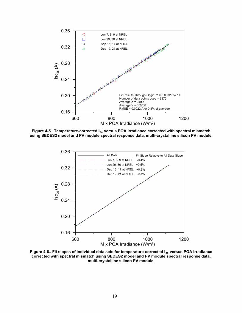
versus POA irradiance corrected with spectral mismatch using SEDES2 model and PV module spectral response data, multi-crystalline silicon PV module. .................................................................................................................................................................... 19Figure 4-6.. Fit slopes of individual data sets for temperature-corrected Isc

versus POA irradiance corrected with spectral mismatch using SEDES2 model and PV module spectral response data, multi-crystalline silicon PV module. ....................................................................................................... 19Figure 4-7. Temperature-corrected Isc

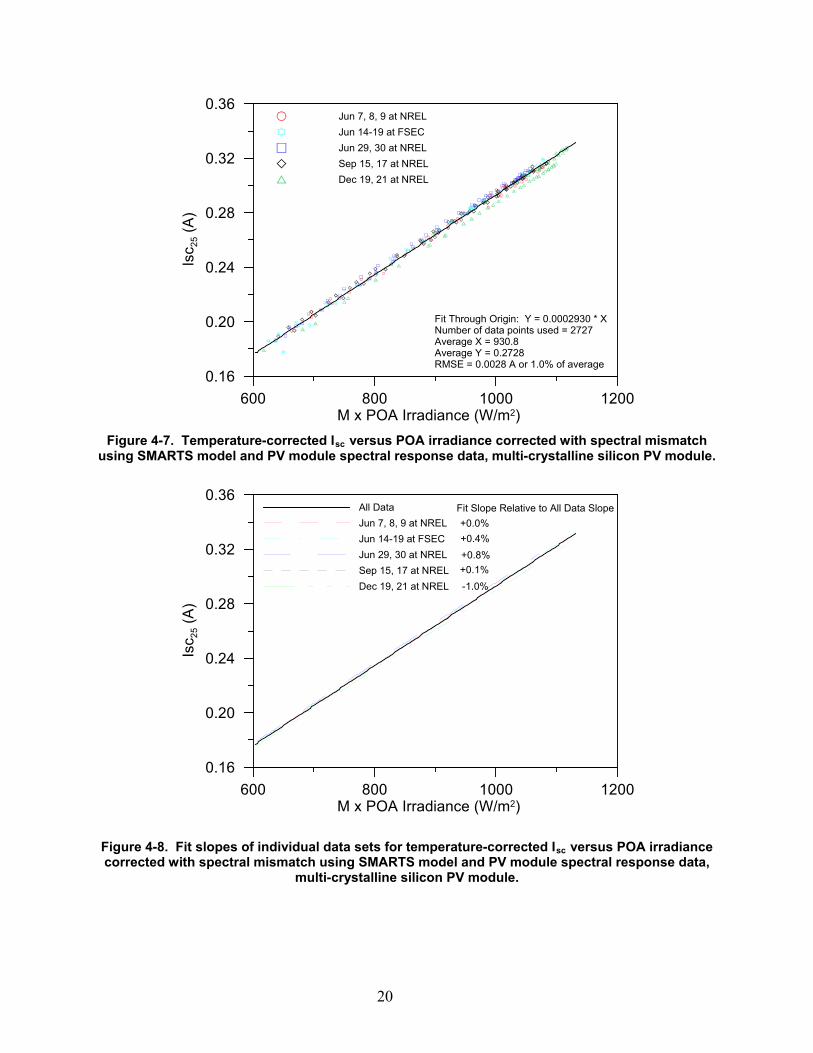
versus POA irradiance corrected with spectral mismatch using SMARTS model and PV module spectral response data, multi-crystalline silicon PV module. ....................................................................................................................................................... 20Figure 4-8. Fit slopes of individual data sets for temperature-corrected Isc

versus POA irradiance corrected with spectral mismatch using SMARTS model and PV module spectral response data, multi-crystalline silicon PV module. ....................................................................................................... 20

viii

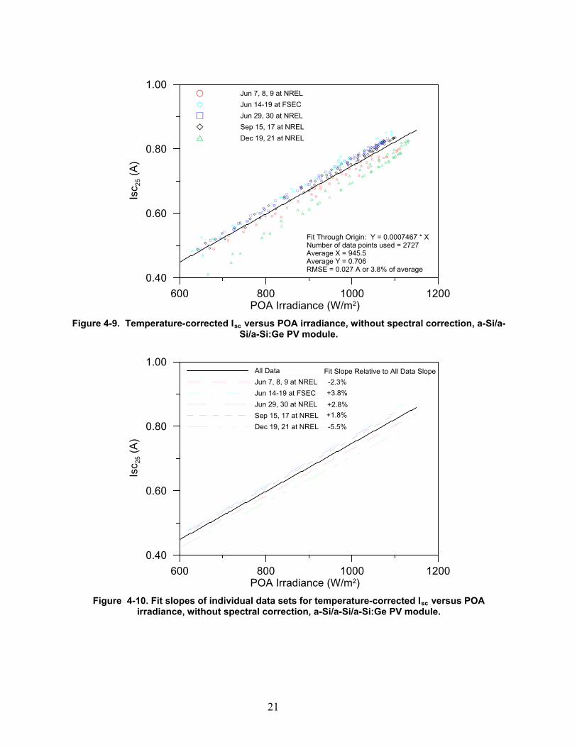
Figure 4-9. Temperature-corrected Isc

versus POA irradiance, without spectral correction, a-Si/a-Si/a-Si:Ge PV module. ............................................................................................................................... 21Figure 4-10. Fit slopes of individual data sets for temperature-corrected Isc

versus POA

irradiance, without spectral correction, a-Si/a-Si/a-Si:Ge PV module. ................................................ 21Figure 4-11. Temperature-corrected Isc versus POA irradiance corrected with Sandia AMa

function, a-Si/a-Si/a-Si:Ge PV module. ................................................................................................... 22Figure 4-12. Fit slopes of individual data sets for temperature-corrected Isc versus POA irradiance corrected with Sandia AMa function, a-Si/a-Si/a-Si:Ge PV module. .................................................... 22Figure 4-13. Temperature-corrected Isc

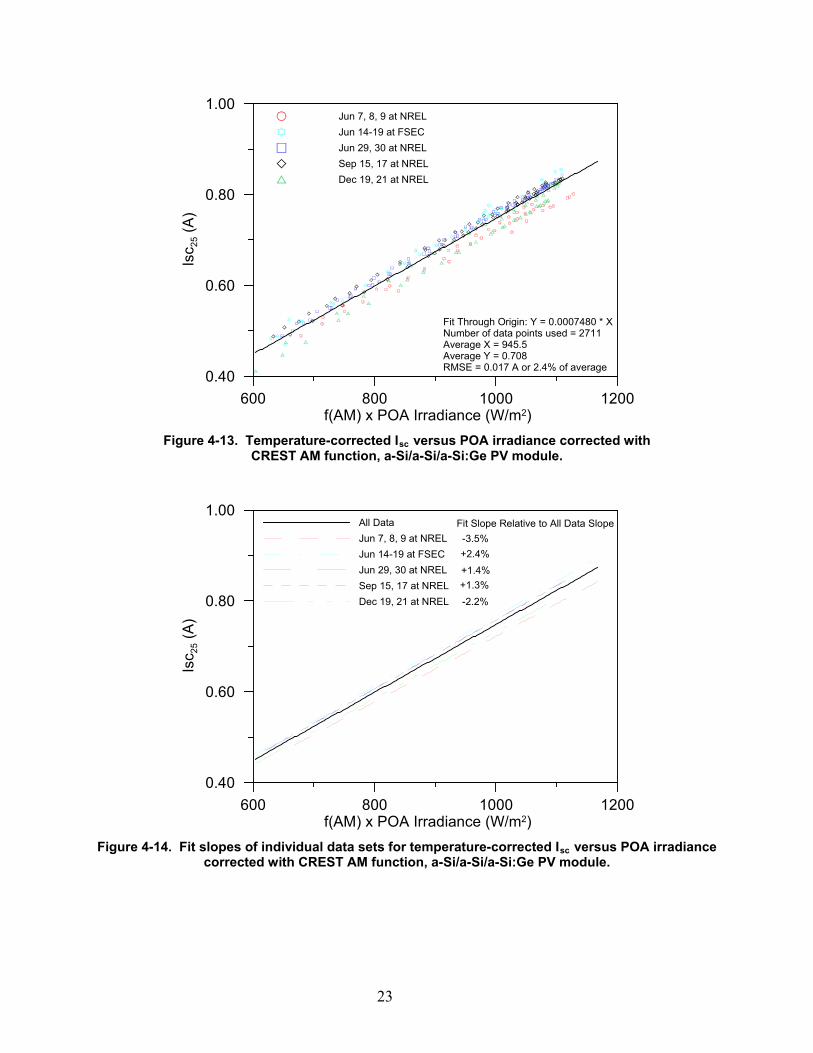
versus POA irradiance corrected with CREST AM

function, a-Si/a-Si/a-Si:Ge PV module. ................................................................................................... 23Figure 4-14. Fit slopes of individual data sets for temperature-corrected Isc

versus POA irradiance

corrected with CREST AM function, a-Si/a-Si/a-Si:Ge PV module. ...................................................... 23Figure 4-15. Temperature-corrected Isc

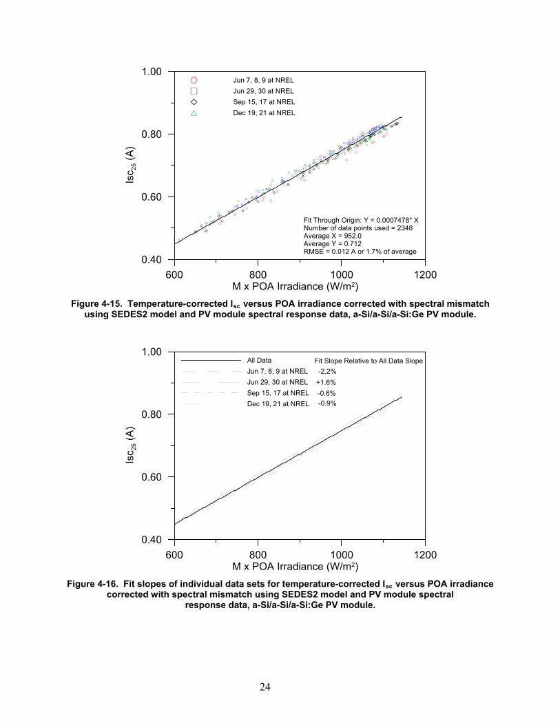
versus POA irradiance corrected with spectral mismatch

using SEDES2 model and PV module spectral response data, a-Si/a-Si/a-Si:Ge PV module. ......... 24Figure 4-16. Fit slopes of individual data sets for temperature-corrected Isc

versus POA irradiance corrected with spectral mismatch using SEDES2 model and PV module spectral response data, a-Si/a-Si/a-Si:Ge PV module. ....................................................................................................................... 24Figure 4-17. Temperature-corrected Isc

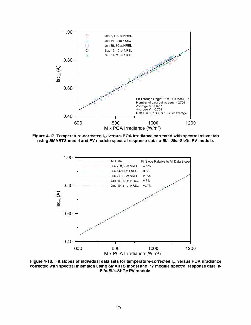
versus POA irradiance corrected with spectral mismatch

using SMARTS model and PV module spectral response data, a-Si/a-Si/a-Si:Ge PV module. ........ 25Figure 4-18. Fit slopes of individual data sets for temperature-corrected Isc

versus POA irradiance corrected with spectral mismatch using SMARTS model and PV module spectral response data, a-Si/a-Si/a-Si:Ge PV module. ....................................................................................................................... 25Figure 5-1. Comparison of spectra for air mass values 1.0 and 2.0 with the G173-03 hemispherical spectrum. Other model inputs are the same as that for the G173-03 hemispherical spectrum. ...... 28Figure 5-2. Comparison of spectra for aerosol optical depth values of 0.055 and 0.300 with the G173-03 hemispherical spectrum. Other model inputs are the same as that for the G173-03 hemispherical spectrum. .......................................................................................................................... 29Figure 5-3. Comparison of spectra for precipitable water vapor amounts of 0.2 cm and 3.4 cm with the G173-03 hemispherical spectrum. Other model inputs are the same as that for the G173-03 hemispherical spectrum. ..................................................................................................................... 30Figure 5-4. Comparison of two spectra with the G173-03 hemispherical spectrum. One spectra with an aerosol optical depth of 0.055 and a precipitable water vapor amount of 0.2 cm, and the other spectra with an aerosol optical depth of 0.300 and a precipitable water vapor amount of 3.4 cm. Other model inputs are the same as that for the G173-03 hemispherical spectrum. ................. 31Figure 5-5. Sandia AMa function and spectral mismatch, calculated using SMARTS model, versus AMa for the multi-crystalline silicon PV module. ................................................................................... 33Figure 5-6. Sandia AMa function and spectral mismatch, calculated using SMARTS model, versus AMa for the a-Si/a-Si/a-Si:Ge silicon PV module. ................................................................................... 33Figure 5-7. Spectral mismatch for the a-Si/a-Si/a-Si:Ge PV module and each of its cells for June 14-19 at FSEC. Performance is limited by the middle cell. ................................................................... 34Figure 5-8. Spectral mismatch for the a-Si/a-Si/a-Si:Ge PV module and each of its cells for December 19 and 21 at NREL. Performance is limited by the top cell. ............................................... 34Figure 5-9. Sandia AMa function and spectral mismatch values, calculated using SMARTS modeled direct normal spectra, versus AMa for the a-Si/a-Si/a-Si:Ge silicon PV module. ............... 35

1

1 Introduction

This report presents results of a preliminary investigation of methods for correcting the short-circuit current (Isc

The performance of a PV module is rated at Standard Reporting Conditions (SRC), where one of the conditions stipulates that the spectral distribution of the solar radiation conforms to the American Society for Testing and Materials (ASTM) standard for hemispherical spectrum, ASTM G 173-03.

) of photovoltaic (PV) modules for variations in the solar spectrum. Correcting PV output for variations in the solar spectrum is included in certain PV performance software applications, and is under consideration for developing energy rating standards.

1 However, PV modules perform under a variety of conditions where the spectral distribution varies from the ASTM spectrum. Spectral distribution is primarily influenced by the path length through the atmosphere and the amounts of atmospheric water vapor and aerosols. These factors cause diurnal, seasonal, and geographic variations in spectral distribution that can increase or decrease Isc

Variations in spectral distribution are more likely to impact the performance of PV modules that respond to a narrower wavelength range of solar radiation, such as amorphous silicon, than those that respond to a wider wavelength range of solar radiation, such as crystalline silicon. This work evaluated methods that represent two approaches for correcting for variations in spectral distribution: (1) empirical relationships based on air mass (AM) or path length through the atmosphere, and (2) use of spectral irradiance models and PV module spectral response data.

from expected values when spectral effects are not considered.

The methods were evaluated using data recorded at the National Renewable Energy Laboratory (NREL) and the Florida Solar Energy Center (FSEC) for a range of air mass, water vapor, and aerosol values under mostly clear sky conditions. The data included one-minute average values of Isc and PV module temperature (Tpv

The following sections of this report describe the methods for correcting for variations in spectrum, the design of the experiment and data, the results, and analysis of the results.

) for both a multi-crystalline silicon PV module and a triple-junction amorphous silicon PV module, along with coincident measurements of the plane-of-array (POA) solar irradiance with a pyranometer.

2

2 Spectral Correction Methods

As mentioned previously, this work considered two approaches for correcting for variations in spectral distribution: (1) empirical relationships based on air mass or path length through the atmosphere, and (2) use of spectral irradiance models with PV module spectral response data.

2.1 Empirical Methods Using Air Mass Two empirical air mass methods were evaluated for correcting for spectral variations: (1) the Sandia method developed by King et al.2, 3 and (2) the Centre for Renewable Energy Systems Technology (CREST) method developed by Betts et al.4

2.1.1 Sandia Method

This method uses an empirically based correction factor based on air mass, with polynomial coefficients that are determined using one or more days of outdoor performance measurements. The PV module is mounted on a two-axis tracker alongside a thermopile pyranometer. Isc

and irradiance data are recorded from sunrise to sunset, thereby providing data for determining the polynomial coefficients that define the correction factor function. To determine a correction factor with this method, air mass is determined with Equation 1 and adjusted for altitude (pressure) with Equation 2 to give an absolute value.

( ) ( )[ ] 1634.1ss Z08.965057.0ZcosAM

−−−⋅+= (1) ( ) AMeAM h0001184.0

a ⋅= ⋅− (2) where:

Zs

h = site altitude, m.

= zenith angle of the sun, degrees

The correction factor as a function of absolute air mass, or f(AMa

) is then given by Equation 3.

( ) ( ) ( ) ( )4a43

a32

a2a10a AMaAMaAMaAMaaAMf ⋅+⋅+⋅+⋅+= (3) where:

a0, a1, a2, a3, a4

This correction assumes that variations in spectrum are predominantly influenced by the path length through the atmosphere, and that variations in clouds, aerosols, and water vapor with season or location are of less influence. The correction has a value of one for AM

= empirically derived polynomial coefficients.

a

For the two PV modules in this study, polynomial coefficients for similar PV modules of the same manufacturer from the Sandia module data base

= 1.5.

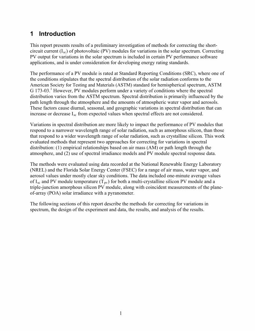
5 were used. The values of the coefficients are provided in Table 2-1 and the resulting functions of absolute air mass are shown graphically in Figure 2-1. The air mass functions exhibit different air mass dependencies for these two modules, with dependency values increasing along with increasing air mass for the multi-crystalline silicon PV module. However, dependency values decreased with increasing air mass for the a-Si/a-Si/a-Si:Ge PV module. These results are consistent with the theory that increasing

3

the air mass shifts the spectral distribution to longer wavelengths, which are more beneficial to crystalline silicon PV modules than to amorphous silicon PV modules that are more responsive to shorter wavelengths (especially for multi-junction amorphous silicon PV modules).

Table 2-1. Sandia AMa

PV Module

Polynomial Coefficients for a Multi-Crystalline Silicon and an a-Si/a-Si/a-Si:Ge PV Module

a a0 a1 a2 a3 BP SX3150

4 0.9415 0.05272800 -0.009588 0.00067629 -1.8111E-05

Uni-Solar US-21

1.0470 0.00082115 -0.025900 0.00317360 0.00011026

Air mass function values greater than 1.0 indicate spectral distributions that are more favorable than for the AMa = 1.5 condition. The values also indicate that the Isc will be proportionally greater than expected based on the integrated spectral or broadband irradiance, such as measured by a thermopile pyranometer. (The converse applies if air mass function values are less than 1.0.) To apply a spectral correction, the broadband irradiance is multiplied by the air mass function value to obtain an “effective irradiance” where Isc

is considered proportional to the “effective irradiance” if the PV temperature is constant. The “effective irradiance” may also include a multiplier to account for angle-of-incidence effects. But to examine spectral effects more precisely for this work, the analysis restricted angle-of-incidences to less than 50° where angle-of-incidence effects are small or nonexistent.

Figure 2-1. Sandia AMa

Sandia has developed air mass polynomial coefficients for numerous PV modules and technologies, and several PV system design and/or performance software applications use this

function for a multi-crystalline silicon and an a-Si/a-Si/a-Si:Ge PV module as a function of the pressure corrected air mass.

0 1 2 3 4 5 6Air Mass (pressure corrected)

0.6

0.7

0.8

0.9

1.0

1.1

Sand

ia A

Ma F

unct

ion

m-Si

a-Si/a-Si/a-Si:Ge

4

method to correct for variations in spectral distribution. These software applications include: PV-DesignPro by Maui Solar Energy Software Corporation6; NREL’s Solar Advisor Model (SAM)7; and the University of Wisconsin-Madison’s 5-Parameter model8 which is used by the California Energy Commission’s PV Calculator.9

2.1.2 CREST Method

Unlike the other two applications, the 5-Parameter model uses coefficients for a multi-crystalline PV module for all PV modules and technologies because the results obtained from using module and technology-specific coefficients did not show significant differences.

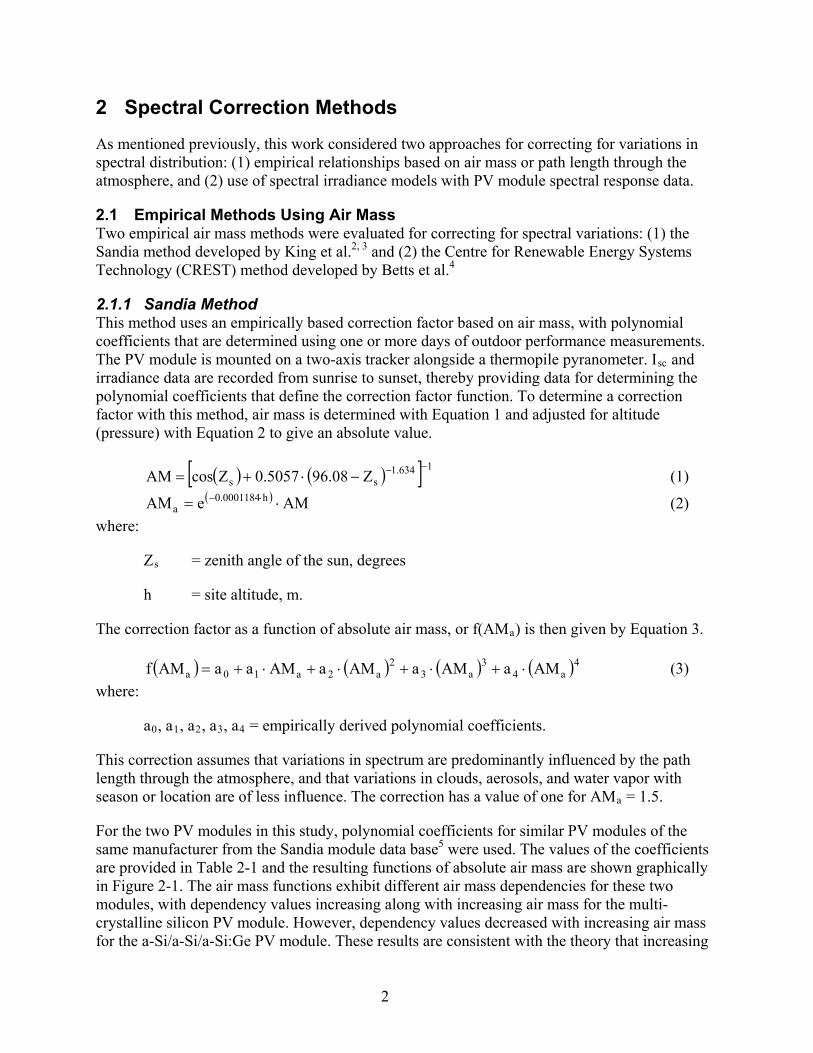
This method also uses an empirically based correction factor. Using a year of spectroradiometer measurements for a south-facing latitude-tilt (52°) orientation, CREST parameterized the spectral correction as a function of air mass (optical, per Eqn. 1) and clearness, where clearness is the ratio of global radiation to the global radiation for clear skies. This approach for correcting for spectral distribution is used by the PV system software package PVSYST.10 For amorphous silicon, the PVSYST spectral correction is shown in Figure 2-2. The same correction for amorphous silicon can also be selected in PVSYST for cadmium telluride (CdTe) PV modules. Betts et al.4

at CREST did not see an improvement in error statistics when applying spectral corrections for crystalline silicon PV modules; consequently, PVSYST does not apply spectral corrections for these PV modules.

Figure 2-2. PVSYST spectral correction as a function of air mass and clearness for amorphous silicon PV modules.

Because only data recorded under primarily clear skies were used for this study, only the empirical function for a clear sky (Ktcd = 1.0) was evaluated. It is similar to the Sandia air mass function in that it has a value of 1.0 for an air mass of 1.5, but different in that it is a function of

5

optical air mass instead of pressure-corrected air mass and its rate of change with respect to air mass is only about half that of the Sandia method. For cloudy skies, the values of the function are increased. This seems reasonable because the presence of clouds shifts the diffuse spectrum to shorter wavelengths,11

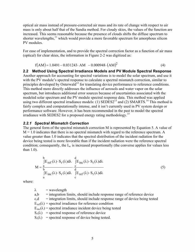
For ease of implementation, and to provide the spectral correction factor as a function of air mass (optical) for clear skies, the information in Figure 2-2 was digitized as:

which would provide a more favorable spectrum for amorphous silicon PV modules.

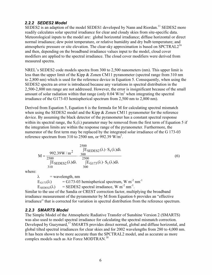
( ) ( )2AM000948.0AM031243.00491.1AMf ⋅−⋅−= (4) 2.2 Method Using Spectral Irradiance Models and PV Module Spectral Response Another approach for accounting for spectral variations is to model the solar spectrum, and use it with the PV module’s spectral response to calculate a spectral mismatch correction, similar to principles developed by Osterwald12 for translating device performance to reference conditions. This method more directly addresses the influence of aerosols and water vapor on the solar spectrum, but introduces additional error sources because of uncertainties associated with the modeled solar spectrum and the PV module spectral response data. This method was applied using two different spectral irradiance models: (1) SEDES213 and (2) SMARTS.14 This method is fairly complex and computationally intense, and it isn’t currently used in PV system design or performance software. However, it has been recommended in the past to model the spectral irradiance with SEDES2 for a proposed energy rating methodology.

2.2.1 Spectral Mismatch Correction

15

The general form of the spectral mismatch correction M is represented by Equation 5. A value of M = 1.0 indicates that there is no spectral mismatch with regard to the reference spectrum. A value greater than 1.0 indicates that the spectral distribution of the incident radiation for the device being tested is more favorable than if the incident radiation were the reference spectral condition; consequently, the Isc

∫ λλ⋅λ

∫ λλ⋅λ⋅

∫ λλ⋅λ

∫ λλ⋅λ= d

ctref

d

ctinc

b

arinc

b

arref

d)(S)(E

d)(S)(E

d)(S)(E

d)(S)(EM

is increased proportionally (the converse applies for values less than 1.0).

(5)

where:

λ = wavelength a,b = integration limits, should include response range of reference device c,d = integration limits, should include response range of device being tested Eref

E(λ) = spectral irradiance for reference condition

inc

S(λ) = spectral irradiance incident device being tested

r

S(λ) = spectral response of reference device

t

(λ) = spectral response of device being tested.

6

SEDES2 is an adaption of the model SEDES1 developed by Nann and Riordan.11 SEDES2 more readily calculates solar spectral irradiance for clear and cloudy skies from site-specific data. Meteorological inputs to the model are: global horizontal irradiance; diffuse horizontal or direct normal irradiance; dew point temperature, or relative humidity and dry bulb temperature; and atmospheric pressure or site elevation. The clear-sky approximation is based on SPCTRAL216

NREL’s SEDES2 code models spectra from 300 to 2,500 nanometers (nm). This upper limit is less than the upper limit of the Kipp & Zonen CM11 pyranometer (spectral range from 310 nm to 2,800 nm) which is used for the reference device in Equation 5. Consequently, when using the SEDES2 spectra an error is introduced because any variations in spectral distribution in the 2,500-2,800 nm range are not addressed. However, the error is insignificant because of the small amount of solar radiation within that range (only 0.04 W/m

and then, depending on the broadband irradiance values input to the model, cloud cover modifiers are applied to the spectral irradiance. The cloud cover modifiers were derived from measured spectra.

2

Derived from Equation 5, Equation 6 is the formula for M for calculating spectral mismatch when using the SEDES2 model and the Kipp & Zonen CM11 pyranometer for the reference device. By assuming the black detector of the pyranometer has a constant spectral response within its spectral range, the S

when integrating the spectral irradiance of the G173-03 hemispherical spectrum from 2,500 nm to 2,800 nm).

r(λ) parameter may be removed from the first term of Equation 5 if the integration limits are within the response range of the pyranometer. Furthermore, the numerator of the first term may be replaced by the integrated solar irradiance of the G 173-03 reference spectrum from 310 to 2500 nm, or 992.39 W/m2

∫ λλ⋅λ

∫ λλ⋅λ⋅

∫ λλ= 2500

300t173G

2500

300t2SEDES

2500

3102SEDES

2

d)(S)(E

d)(S)(E

d)(E

m/W39.992M

.

(6)

where: λ = wavelength, nm EG173(λ) = G173-03 hemispherical spectrum, W m-2 nmE

-1 SEDES2(λ) = SEDES2 spectral irradiance, W m-2 nm-1

Similar to the use of the Sandia or CREST correction factor, multiplying the broadband irradiance measurement of the pyranometer by M from Equation 6 provides an “effective irradiance” that is corrected for variation in spectral distribution from the reference spectrum.

.

2.2.3 SMARTS Model The Simple Model of the Atmospheric Radiative Transfer of Sunshine Version 2 (SMARTS) was also used to model spectral irradiance for calculating the spectral mismatch correction. Developed by Gueymard,17 SMARTS provides direct normal, global and diffuse horizontal, and global tilted spectral irradiances for clear skies and for 2002 wavelengths from 280 to 4,000 nm. It has been shown to be more accurate than the SPCTRAL2 model, and as accurate as more complex models such as Air Force MODTRAN.18

2.2.2 SEDES2 Model

7

SMARTS allows nearly 30 input parameters for defining atmospheric constituents and site and application conditions. This work uses SMARTS Version 2.9.5. An earlier Version 2.9.2 was used to develop the G173-03 reference solar spectral irradiances. Compared to Version 2.9.2, the primary difference is that Version 2.9.5 allows the use of a more up-to-date extraterrestrial spectrum. This increases the spectral irradiance by a few percent from 400 nm to 550 nm and decreases it by a few percent from 550 nm to 700 nm and from 850 to 1,300 nm. Algorithms for diffuse irradiance were also streamlined in Version 2.9.5.

Similar to the derivation of the spectral mismatch correction when using the SEDES2 model, Equation 7 is the formula for M for calculating spectral mismatch when using the SMARTS model and the Kipp & Zonen CM11 pyranometer for the reference device. The numerator of the first term, 992.43 W/m2

∫ λλ⋅λ

∫ λλ⋅λ⋅

∫ λλ= 4000

280t173G

4000

280t2SMARTS

2800

3102SMARTS

2

d)(S)(E

d)(S)(E

d)(E

m/W43.992M

, is the integrated solar irradiance of the G 173-03 reference spectrum from 310 to 2,800 nm, which includes the complete spectral range of the Kipp and Zonen pyranometer..

(7)

where: ESMARTS(λ) = SMARTS spectral irradiance, W m-2 nm-1

2.2.4 PV Module Spectral Response

.

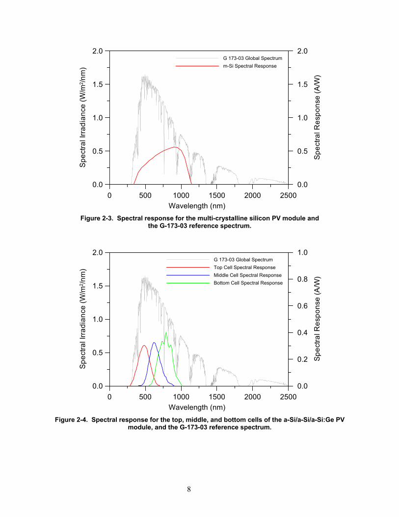
The spectral response data for the multi-crystalline PV module and the a-Si/a-Si/a-Si:Ge PV module were selected from previous measurements at NREL, rather than from performing spectral response measurements of the individual PV modules. The data were judged as being representative of the technology and manufacture. Figures 2-3 and 2-4 provide the spectral response data used for the multi-crystalline PV module and the a-Si/a-Si/a-Si:Ge PV module, respectively.

2.2.5 Method Variation for Multi-Junction PV Modules For series-connected multi-junction PV modules where one junction may limit the current of another, the Isc of the PV module is considered to be the Isc provided by the junction that produces the least current. Consequently, for the a-Si/a-Si/a-Si:Ge PV module, the second term of Equations 6 and 7 is evaluated by using the spectral response of the cell that gives the smallest numerator (current at test conditions) for the numerator. The spectral response of the cell that gives the smallest denominator (current at reference conditions) is used for the denominator. Depending on test conditions, the numerator and denominator may require spectral responses of different cells.

8

Figure 2-3. Spectral response for the multi-crystalline silicon PV module and

the G-173-03 reference spectrum.

Figure 2-4. Spectral response for the top, middle, and bottom cells of the a-Si/a-Si/a-Si:Ge PV

module, and the G-173-03 reference spectrum.

0 500 1000 1500 2000 2500Wavelength (nm)

0.0

0.5

1.0

1.5

2.0

Spe

ctra

l Irra

dian

ce (W

/m2 /n

m)

G 173-03 Global Spectrumm-Si Spectral Response

0.0

0.5

1.0

1.5

2.0

Spec

tral R

espo

nse

(A/W

)

0 500 1000 1500 2000 2500Wavelength (nm)

0.0

0.5

1.0

1.5

2.0

Spe

ctra

l Irra

dian

ce (W

/m2 /n

m)

G 173-03 Global SpectrumTop Cell Spectral Response Middle Cell Spectral ResponseBottom Cell Spectral Response

0.0

0.2

0.4

0.6

0.8

1.0

Spec

tral R

espo

nse

(A/W

)

9

3 Design of Experiment and Data

Impacts of the spectral distribution on PV module Isc were measured to show geographic variations (i.e., NREL in Golden, Colorado versus FSEC in Cocoa, Florida) and seasonal variations (summer, fall, and winter at NREL). To provide consistent measurements, the same PV modules and data acquisition equipment were used for both locations and all time periods. Additionally, data were screened to remove times with unstable irradiance and times when reflection losses at high incidence angles of the direct beam radiation could be confused with changes in Isc

3.1 Equipment

caused by variations in spectral distribution.

The two PV modules used for the experiment were:

• A multi-crystalline silicon PV module – BP Solar Model SX5M, S/N C1020522 2146292

• An a-Si/a-Si/a-Si:Ge PV module – UNI-SOLAR Model US-11, S/N US-11-015754.

The a-Si/a-Si/a-Si:Ge PV module had been sun-exposed for several years; consequently, the initial light-induced degradation occurred prior to this experiment. Seasonal changes in the efficiency of amorphous silicon PV modules occur from temperature-induced annealing, but the changes primarily affect the fill-factor, not the Isc.19

I

Furthermore, the deployment times were minimized in order to minimize any exposure or aging effects.

sc

3.2 Solar Geometry

values were measured with current shunts connected to the module leads. PV module temperatures were measured with type T “cement-on” thermocouples taped to the module back-surface, near the center. The plane-of-array irradiance was measured with a Kipp & Zonen CM11 pyranometer. A Campbell Scientific datalogger performed measurements every second and stored the data as one-minute averages.

The PV modules were deployed with a south-facing fixed-tilt orientation, with the tilt angle adjusted, for a particular period and location, so that the angle-of-incidence of the direct beam radiation would be near zero at solar noon. This was to ensure that the sun’s position with respect to the PV modules was as similar as possible for all locations and test periods, thereby facilitating the comparison of test data.

10

Figure 3-1 presents the relationship between the pressure-corrected air mass and the PV module’s angle-of-incidence of the direct beam radiation. Except for the December dates, adjusting the tilt angle provided very similar air mass versus angle-of-incidence relationships. In Figure 3-1, the distance between symbols represents one hour, with the leftmost symbol coinciding with solar noon.

Figure 3-1. Relationship between air mass (pressure corrected) and the PV module’s

angle-of-incidence of the direct beam radiation for the test dates at NREL and FSEC and the PV module tilt angles from horizontal.

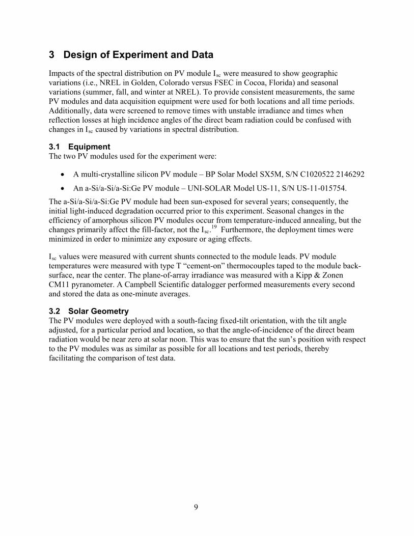
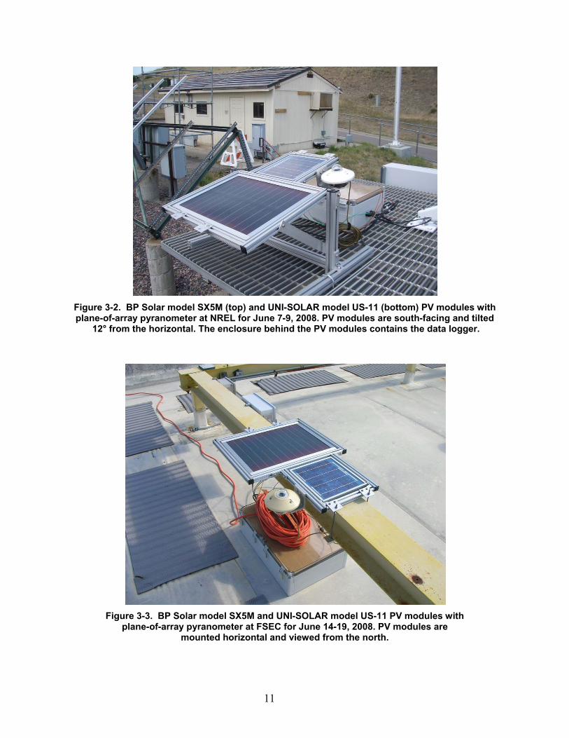
Figures 3-2 and 3-3 show the PV modules deployed at NREL June 7-9, 2008 and at FSEC June 14-19, 2008. To have similar solar geometries with respect to the PV modules, the tilt angles for the two deployments differ by 12° to accommodate their difference in latitude.

0 20 40 60 80 100Angle-of-Incidence of Direct Beam Radiation (°)

0

2

4

6

8

10

Air

Mas

s (p

ress

ure

corr

ecte

d)

Tilt Angles and Dates of Data CollectionJun 7, 8, and 9 at NREL, 12° tiltJun 14-19 at FSEC, 0° tiltJun 29, 30 at NREL, 12° tiltSep 15, 17 at NREL, 40° tiltDec 19, 21 NREL, 60° tilt

11

Figure 3-2. BP Solar model SX5M (top) and UNI-SOLAR model US-11 (bottom) PV modules with plane-of-array pyranometer at NREL for June 7-9, 2008. PV modules are south-facing and tilted

12° from the horizontal. The enclosure behind the PV modules contains the data logger.

Figure 3-3. BP Solar model SX5M and UNI-SOLAR model US-11 PV modules with

plane-of-array pyranometer at FSEC for June 14-19, 2008. PV modules are mounted horizontal and viewed from the north.

12

3.3 Data Screening Prior to analysis, the data were screened to remove data with the potential to create errors in the results. The removed data included: (a) data with an angle-of-incidence of direct beam radiation greater than 50°, (b) data with a plane-of-array irradiance below 600 W/m2 or greater than 1,150 W/m2, and (c) data where the plane-of-array irradiance had changed by more than 5 W/m2

For angle-of-incidences greater than 50°, I

from the previous minute’s value.

sc is reduced because of increased reflection losses. By limiting data to angle-of-incidences of 50° or less, effects of variations in spectral distribution on Isc

Calibration records for the pyranometer show its responsitivity varying less than 1% for angles-of-incidence of 50° or less, using both morning and afternoon calibration data. The “b” and “c” criteria ensured that data are for mostly clear-sky conditions and conditions are reasonably stable with respect to the plane-of-array irradiance. A rapidly changing irradiance might impact results because the response of the thermopile detector in the pyranometer is significantly slower than that of the PV modules.

may be considered separately from the effects of angle-of-incidence, which can be considerably larger. This also ensured that irradiance measurements using the Kipp & Zonen CM11 pyranometer were accurate.

The deployments at NREL afforded the opportunity to collect data for a two- to three-week period, and then select two or three days that typified clear-sky conditions, to which the screening criteria were then applied. The FSEC deployment was of shorter duration, and screening criteria were applied to all recorded data. Table 3-1 summarizes the measurement days selected for model evaluation. Appendix A shows data passing selection and screening criteria.

Table 3-1. Summary of Days Used for Model Evaluations

Location Period Tilt Angle (°)

NREL June 7-9, 2008 12 FSEC June 14-19, 2008 0 NREL June 29-30, 2008 12 NREL Sept 15 and17,

2008 40

NREL Dec 19 and 21, 2008

60

13

3.4 Temperature Corrections Besides spectral and angle-of-incidence effects, Isc is also dependent on PV module temperature. To prevent temperature effects from impacting the study, the Isc measurements were corrected for temperature by using Equation 8 to translate Isc values at the measured PV module temperature to Isc

°−⋅

°+α+÷= C25E

m/W1000C5.2T1II 2pvscsc25

values for a temperature of 25°C.

(8)

where: α = Isc correction factor for PV module temperature, °C

T-1

pv E = plane-of-array irradiance, W/m

= PV module back-surface temperature, °C 2

In Equation 8, the middle term within the parentheses accounts for the temperature gradient that exists from the PV module back-surface to the PV cell. Values of α for similar PV modules of the same manufacturer from the Sandia module data base

.

5

Table 3-2. I

were used. The values of the coefficients are provided in Table 3-2.

sc

PV Module Correction Factors for PV Module Temperature

Technology α (°C-1

BP SX3150 )

multi-crystalline silicon 0.000404 Uni-Solar US-21

a-Si/a-Si/a-Si:Ge 0.000850

3.5 Additional Data for Spectral Models The empirical air mass methods may be implemented by calculating the sun’s position and resulting air mass. Sun position may be determined from the site coordinates and the date and time. Air mass is determined from Equation 1, or with Equation 2 if pressure corrected. The methods using the spectral irradiance models require additional information for modeling the spectral irradiance. This additional information is described in the following paragraphs.

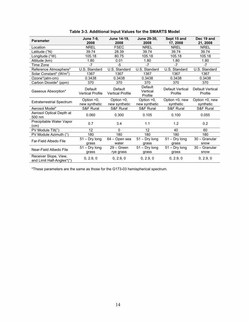
3.5.1 SMARTS Model Like the air mass methods, the spectral irradiance models use the site coordinates and the date and time to calculate the sun’s position. SMARTS allows additional input parameters for defining atmospheric constituents and site and application conditions. Besides date and time, the inputs that we used with SMARTS Version 2.9.5 are listed in Table 3-3.

14

Table 3-3. Additional Input Values for the SMARTS Model

Parameter June 7-9, 2008

June 14-19, 2008

June 29-30, 2008

Sept 15 and 17, 2008

Dec 19 and 21, 2008

Location NREL FSEC NREL NREL NREL Latitude (°N) 39.74 28.39 39.74 39.74 39.74 Longitude (°W) 105.18 80.75 105.18 105.18 105.18 Altitude (km) 1.80 0.01 1.80 1.80 1.80 Time Zone -7 -5 -7 -7 -7 Reference Atmosphere* U.S. Standard U.S. Standard U.S. Standard U.S. Standard U.S. Standard Solar Constant* (W/m2 1367 ) 1367 1367 1367 1367 Ozone*(atm-cm) 0.3438 0.3438 0.3438 0.3438 0.3438 Carbon Dioxide* (ppm) 370 370 370 370 370

Gaseous Absorption* Default Vertical Profile

Default Vertical Profile




Extraterrestrial Spectrum Option =0, new synthetic

Option =0, new synthetic




Aerosol Model* S&F Rural S&F Rural S&F Rural S&F Rural S&F Rural Aerosol Optical Depth at 500 nm 0.060 0.300 0.105 0.100 0.055

Precipitable Water Vapor (cm) 0.7 3.4 1.1 1.2 0.2

PV Module Tilt(°) 12 0 12 40 60 PV Module Azimuth (°) 180 180 180 180 180

Far-Field Albedo File 51 – Dry long grass

64 – Open sea water

51 – Dry long grass


30 – Granular snow

Near-Field Albedo File 51 – Dry long grass

29 – Green rye grass



30 – Granular snow

Receiver Slope, View, and Limit Half-Angles*(°) 0, 2.9, 0 0, 2.9, 0 0, 2.9, 0 0, 2.9, 0 0, 2.9, 0

*These parameters are the same as those for the G173-03 hemispherical spectrum.

15

In Table 3-3, parameters that are the same as for the G173-03 hemispherical spectrum are identified with an asterisk. Precipitable water vapor amounts were determined from the daytime average dew point temperatures and the method of Wright et al.,20 except for the December NREL data, which are precipitable water data that were available from NREL’s Solar Radiation Research Laboratory21 (SRRL). Aerosol optical depth data for the NREL location and test periods were also from SRRL, and average daytime values for the period. For the FSEC location, no aerosol optical depth data were available. Consequently, it was estimated using information from the National Solar Radiation Data Base.22

3.5.2 SEDES2 Model

In hindsight, a far-field albedo for the FSEC location should have included a mix of green grass or trees and water, rather than just water. The near-field albedo is of no consequence for the horizontal PV modules at FSEC.

Compared to SMARTS, SEDES2 has a reduced set of allowable inputs. Besides the site coordinates and the date and time to calculate the sun’s position, the input requirements are: global horizontal irradiance; diffuse horizontal or direct normal irradiance; and dew point temperature, or relative humidity and dry bulb temperature. For NREL, nearby SRRL data were used to provide global horizontal, diffuse horizontal, and direct normal irradiance data. These data were not available for FSEC; consequently, the SEDES2 model was not evaluated using the FSEC data. In place of dew point temperature, SEDES2 code was modified to use the precipitable water vapor amounts from Table 3-3, instead of calculating it internal to SEDES2 from dew-point temperature. This allowed identical precipitable water vapor amounts to be used by both SMARTS and SEDES2.

16

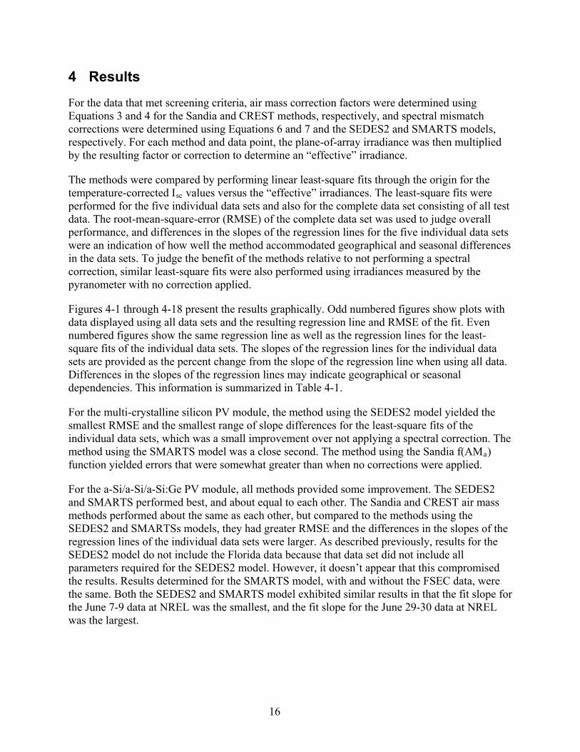
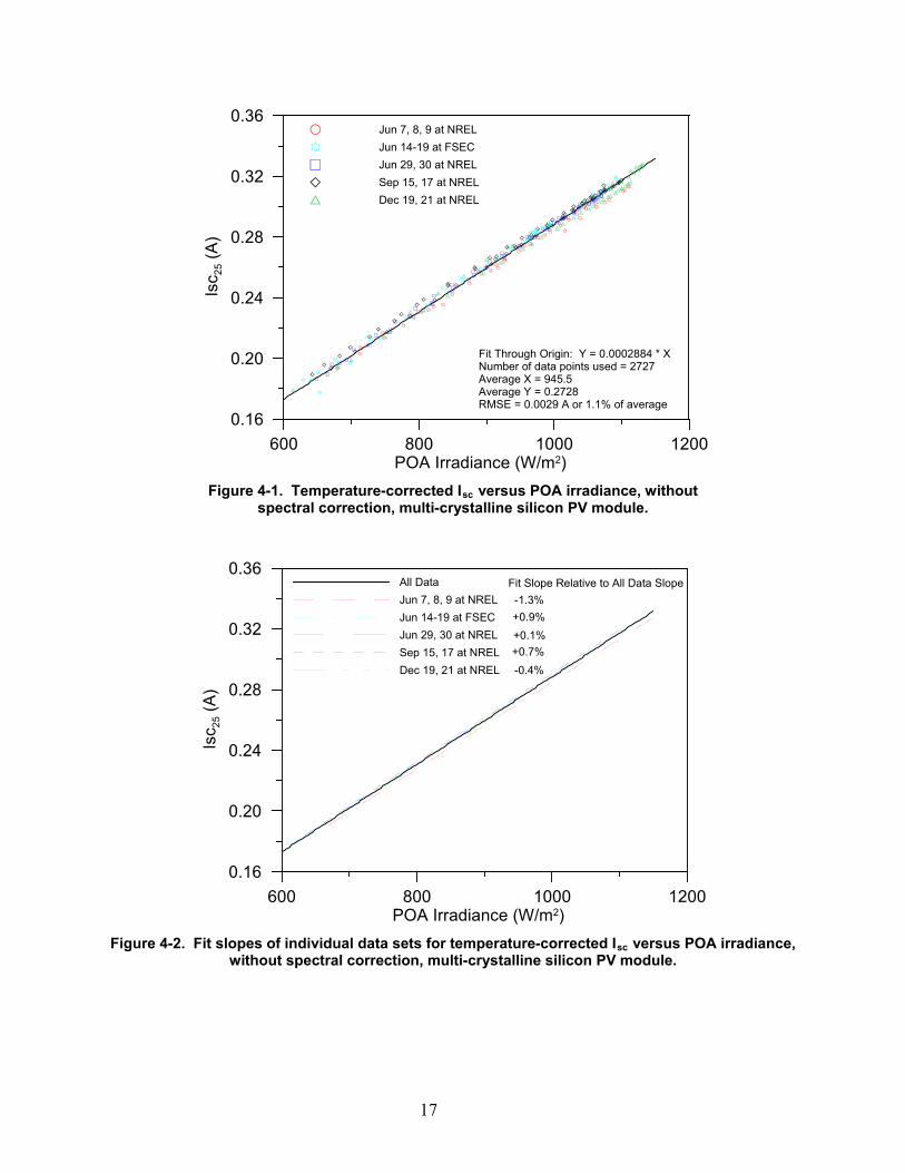
4 Results

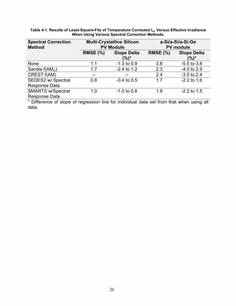
For the data that met screening criteria, air mass correction factors were determined using Equations 3 and 4 for the Sandia and CREST methods, respectively, and spectral mismatch corrections were determined using Equations 6 and 7 and the SEDES2 and SMARTS models, respectively. For each method and data point, the plane-of-array irradiance was then multiplied by the resulting factor or correction to determine an “effective” irradiance.

The methods were compared by performing linear least-square fits through the origin for the temperature-corrected Isc

Figures 4-1 through 4-18 present the results graphically. Odd numbered figures show plots with data displayed using all data sets and the resulting regression line and RMSE of the fit. Even numbered figures show the same regression line as well as the regression lines for the least-square fits of the individual data sets. The slopes of the regression lines for the individual data sets are provided as the percent change from the slope of the regression line when using all data. Differences in the slopes of the regression lines may indicate geographical or seasonal dependencies. This information is summarized in Table 4-1.

values versus the “effective” irradiances. The least-square fits were performed for the five individual data sets and also for the complete data set consisting of all test data. The root-mean-square-error (RMSE) of the complete data set was used to judge overall performance, and differences in the slopes of the regression lines for the five individual data sets were an indication of how well the method accommodated geographical and seasonal differences in the data sets. To judge the benefit of the methods relative to not performing a spectral correction, similar least-square fits were also performed using irradiances measured by the pyranometer with no correction applied.

For the multi-crystalline silicon PV module, the method using the SEDES2 model yielded the smallest RMSE and the smallest range of slope differences for the least-square fits of the individual data sets, which was a small improvement over not applying a spectral correction. The method using the SMARTS model was a close second. The method using the Sandia f(AMa

For the a-Si/a-Si/a-Si:Ge PV module, all methods provided some improvement. The SEDES2 and SMARTS performed best, and about equal to each other. The Sandia and CREST air mass methods performed about the same as each other, but compared to the methods using the SEDES2 and SMARTSs models, they had greater RMSE and the differences in the slopes of the regression lines of the individual data sets were larger. As described previously, results for the SEDES2 model do not include the Florida data because that data set did not include all parameters required for the SEDES2 model. However, it doesn’t appear that this compromised the results. Results determined for the SMARTS model, with and without the FSEC data, were the same. Both the SEDES2 and SMARTS model exhibited similar results in that the fit slope for the June 7-9 data at NREL was the smallest, and the fit slope for the June 29-30 data at NREL was the largest.

) function yielded errors that were somewhat greater than when no corrections were applied.

17


versus POA irradiance, without spectral correction, multi-crystalline silicon PV module.

Figure 4-2. Fit slopes of individual data sets for temperature-corrected Isc

600 800 1000 1200POA Irradiance (W/m2)

0.16

0.20

0.24

0.28

0.32

0.36

Isc 2

5 (A

)

Jun 7, 8, 9 at NRELJun 14-19 at FSECJun 29, 30 at NRELSep 15, 17 at NRELDec 19, 21 at NREL

Fit Through Origin: Y = 0.0002884 * XNumber of data points used = 2727Average X = 945.5Average Y = 0.2728RMSE = 0.0029 A or 1.1% of average

versus POA irradiance, without spectral correction, multi-crystalline silicon PV module.


0.16

0.20

0.24

0.28

0.32

0.36

Isc 2

5 (A

)

All DataJun 7, 8, 9 at NRELJun 14-19 at FSECJun 29, 30 at NRELSep 15, 17 at NRELDec 19, 21 at NREL

Fit Slope Relative to All Data Slope-1.3%+0.9%+0.1%+0.7%-0.4%

18

Figure 4-3. Temperature-corrected Isc versus POA irradiance corrected with Sandia AMa

function, multi-crystalline silicon PV module.

Figure 4-4. Fit slopes of individual data sets for temperature-corrected Isc versus POA irradiance

corrected with Sandia AMa

600 800 1000 1200f(AMa) x POA Irradiance (W/m2)

0.16

0.20

0.24

0.28

0.32

0.36

Isc 2

5 (A

)



function, multi-crystalline silicon PV module.


0.16

0.20

0.24

0.28

0.32

0.36

Isc 2

5 (A

)



19


versus POA irradiance corrected with spectral mismatch using SEDES2 model and PV module spectral response data, multi-crystalline silicon PV module.

Figure 4-6.. Fit slopes of individual data sets for temperature-corrected Isc

600 800 1000 1200M x POA Irradiance (W/m2)

0.16

0.20

0.24

0.28

0.32

0.36

Isc 2

5 (A

)

Jun 7, 8, 9 at NRELJun 29, 30 at NRELSep 15, 17 at NRELDec 19, 21 at NREL

Fit Results Through Origin: Y = 0.0002924 * XNumber of data points used = 2375Average X = 940.5Average Y = 0.2750RMSE = 0.0022 A or 0.8% of average

versus POA irradiance corrected with spectral mismatch using SEDES2 model and PV module spectral response data,

multi-crystalline silicon PV module.


0.16

0.20

0.24

0.28

0.32

0.36

Isc 2

5 (A

)

All DataJun 7, 8, 9 at NRELJun 29, 30 at NRELSep 15, 17 at NRELDec 19, 21 at NREL

Fit Slope Relative to All Data Slope-0.4%

+0.5%+0.2%-0.3%

20


versus POA irradiance corrected with spectral mismatch using SMARTS model and PV module spectral response data, multi-crystalline silicon PV module.


versus POA irradiance corrected with spectral mismatch using SMARTS model and PV module spectral response data,

multi-crystalline silicon PV module.


0.16

0.20

0.24

0.28

0.32

0.36

Isc 2

5 (A

)




0.16

0.20

0.24

0.28

0.32

0.36

Isc 2

5 (A

)


Fit Slope Relative to All Data Slope+0.0%+0.4%+0.8%+0.1%-1.0%

21


versus POA irradiance, without spectral correction, a-Si/a-Si/a-Si:Ge PV module.


versus POA irradiance, without spectral correction, a-Si/a-Si/a-Si:Ge PV module.


0.40

0.60

0.80

1.00

Isc 2

5 (A

)




0.40

0.60

0.80

1.00

Isc 2

5 (A

)



22

Figure 4-11. Temperature-corrected Isc versus POA irradiance corrected with

Sandia AMa

function, a-Si/a-Si/a-Si:Ge PV module.

Figure 4-12. Fit slopes of individual data sets for temperature-corrected Isc versus POA irradiance

corrected with Sandia AMa


0.40

0.60

0.80

1.00

Isc 2

5 (A

)



function, a-Si/a-Si/a-Si:Ge PV module.


0.40

0.60

0.80

1.00

Isc 2

5 (A

)



23


versus POA irradiance corrected with CREST AM function, a-Si/a-Si/a-Si:Ge PV module.


versus POA irradiance corrected with CREST AM function, a-Si/a-Si/a-Si:Ge PV module.

600 800 1000 1200f(AM) x POA Irradiance (W/m2)

0.40

0.60

0.80

1.00

Isc 2

5 (A

)



600 800 1000 1200f(AM) x POA Irradiance (W/m2)

0.40

0.60

0.80

1.00

Isc 2

5 (A

)



24


versus POA irradiance corrected with spectral mismatch using SEDES2 model and PV module spectral response data, a-Si/a-Si/a-Si:Ge PV module.



0.40

0.60

0.80

1.00

Isc 2

5 (A

)

Jun 7, 8, 9 at NRELJun 29, 30 at NRELSep 15, 17 at NRELDec 19, 21 at NREL

Fit Through Origin: Y = 0.0007478* XNumber of data points used = 2348Average X = 952.0Average Y = 0.712RMSE = 0.012 A or 1.7% of average

versus POA irradiance corrected with spectral mismatch using SEDES2 model and PV module spectral

response data, a-Si/a-Si/a-Si:Ge PV module.


0.40

0.60

0.80

1.00

Isc 2

5 (A

)

All DataJun 7, 8, 9 at NRELJun 29, 30 at NRELSep 15, 17 at NRELDec 19, 21 at NREL

Fit Slope Relative to All Data Slope-2.2%

+1.6%-0.6%-0.9%

25


versus POA irradiance corrected with spectral mismatch using SMARTS model and PV module spectral response data, a-Si/a-Si/a-Si:Ge PV module.


versus POA irradiance corrected with spectral mismatch using SMARTS model and PV module spectral response data, a-

Si/a-Si/a-Si:Ge PV module.


0.40

0.60

0.80

1.00

Isc 2

5 (A

)




0.40

0.60

0.80

1.00

Isc 2

5 (A

)


Fit Slope Relative to All Data Slope-2.2%-0.6%+1.5%-0.7%+0.7%

26

Table 4-1. Results of Least-Square-Fits of Temperature Corrected Isc

Spectral Correction Method

Versus Effective Irradiance When Using Various Spectral Correction Methods.

Multi-Crystalline Silicon PV Module

a-Si/a-Si/a-Si:Ge PV module

RMSE (%) Slope Delta (%)*

RMSE (%) Slope Delta (%)*

None 1.1 -1.3 to 0.9 3.8 -5.5 to 3.8 Sandia f(AMa 1.7 ) -2.4 to 1.2 2.3 -4.0 to 2.9 CREST f(AM) -- -- 2.4 -3.5 to 2.4 SEDES2 w/ Spectral Response Data

0.8 -0.4 to 0.5 1.7 -2.2 to 1.6

SMARTS w/Spectral Response Data

1.0 -1.0 to 0.8 1.8 -2.2 to 1.5

* Difference of slope of regression line for individual data set from that when using all data.

27

5 Analysis of Results

From the results presented in Section 4, the methods using spectral irradiance models and PV module spectral response data performed better than the empirical air mass methods. This is attributed to the spectral models accounting for the influence of aerosols and water vapor on the distribution of the spectral irradiance, but also may be a consequence of how the empirical air mass functions are determined and implemented.

5.1 Variations in Solar Spectrum For clear skies, variations in spectrum are predominantly influenced by the air mass, aerosols, and water vapor. To illustrate their effects, the SMARTS model was used to model spectra to compare with the G173-03 hemispherical spectrum. The same inputs used to model the G173-03 hemispherical spectrum were used, except air mass, aerosol, and water vapor amounts were varied singularly and in combination to show their effects. Like the G173-03 hemispherical spectrum, the spectra modeled with SMARTS include both the direct and diffuse solar radiation components.

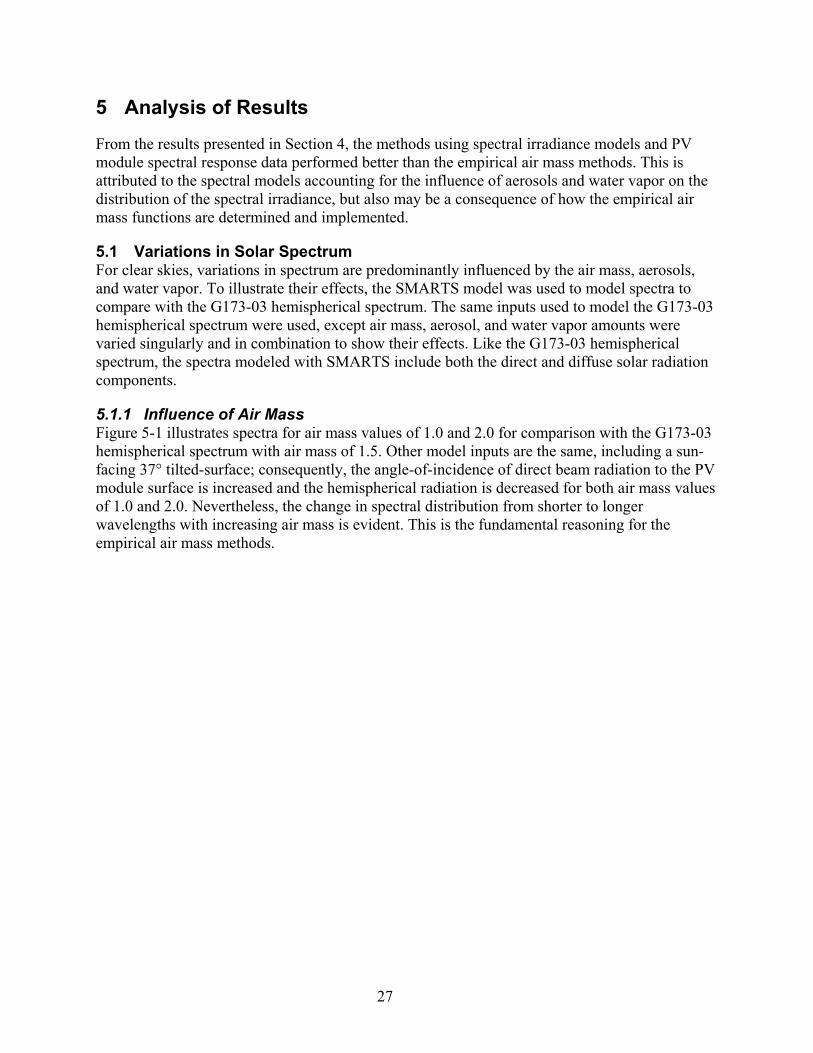
5.1.1 Influence of Air Mass Figure 5-1 illustrates spectra for air mass values of 1.0 and 2.0 for comparison with the G173-03 hemispherical spectrum with air mass of 1.5. Other model inputs are the same, including a sun-facing 37° tilted-surface; consequently, the angle-of-incidence of direct beam radiation to the PV module surface is increased and the hemispherical radiation is decreased for both air mass values of 1.0 and 2.0. Nevertheless, the change in spectral distribution from shorter to longer wavelengths with increasing air mass is evident. This is the fundamental reasoning for the empirical air mass methods.

28

Figure 5-1. Comparison of spectra for air mass values 1.0 and 2.0 with the G173-03 hemispherical

spectrum. Other model inputs are the same as that for the G173-03 hemispherical spectrum.

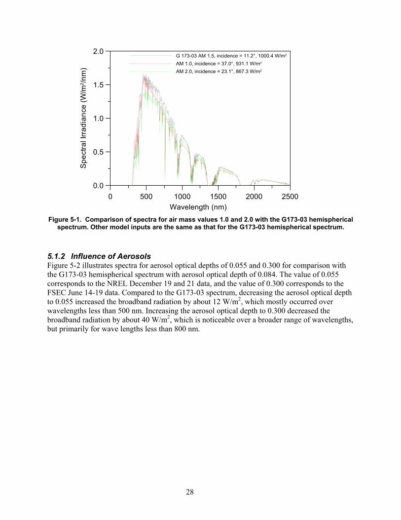
5.1.2 Influence of Aerosols Figure 5-2 illustrates spectra for aerosol optical depths of 0.055 and 0.300 for comparison with the G173-03 hemispherical spectrum with aerosol optical depth of 0.084. The value of 0.055 corresponds to the NREL December 19 and 21 data, and the value of 0.300 corresponds to the FSEC June 14-19 data. Compared to the G173-03 spectrum, decreasing the aerosol optical depth to 0.055 increased the broadband radiation by about 12 W/m2, which mostly occurred over wavelengths less than 500 nm. Increasing the aerosol optical depth to 0.300 decreased the broadband radiation by about 40 W/m2

0 500 1000 1500 2000 2500Wavelength (nm)

0.0

0.5

1.0

1.5

2.0

Spe

ctra

l Irra

dian

ce (W

/m2 /n

m)

G 173-03 AM 1.5, incidence = 11.2°, 1000.4 W/m2

AM 1.0, incidence = 37.0°, 931.1 W/m2 AM 2.0, incidence = 23.1°, 867.3 W/m2

, which is noticeable over a broader range of wavelengths, but primarily for wave lengths less than 800 nm.

29

Figure 5-2. Comparison of spectra for aerosol optical depth values of 0.055 and 0.300

with the G173-03 hemispherical spectrum. Other model inputs are the same as that for the G173-03 hemispherical spectrum.

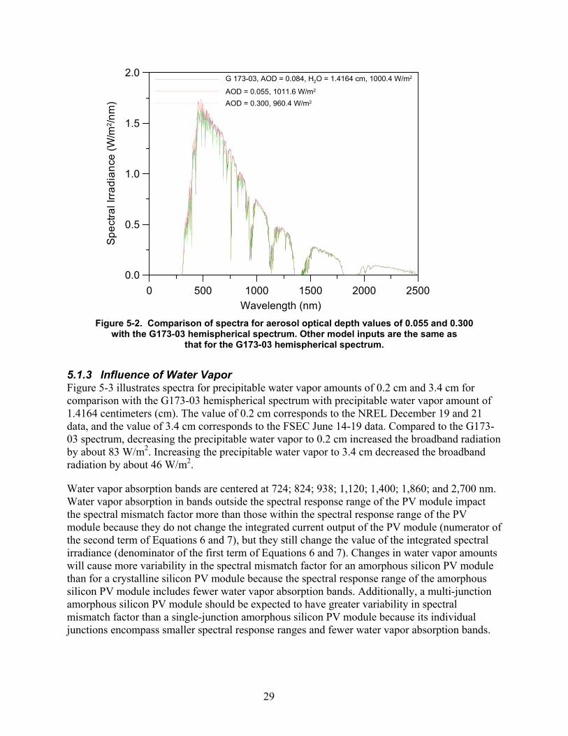
5.1.3 Influence of Water Vapor Figure 5-3 illustrates spectra for precipitable water vapor amounts of 0.2 cm and 3.4 cm for comparison with the G173-03 hemispherical spectrum with precipitable water vapor amount of 1.4164 centimeters (cm). The value of 0.2 cm corresponds to the NREL December 19 and 21 data, and the value of 3.4 cm corresponds to the FSEC June 14-19 data. Compared to the G173-03 spectrum, decreasing the precipitable water vapor to 0.2 cm increased the broadband radiation by about 83 W/m2. Increasing the precipitable water vapor to 3.4 cm decreased the broadband radiation by about 46 W/m2

Water vapor absorption bands are centered at 724; 824; 938; 1,120; 1,400; 1,860; and 2,700 nm. Water vapor absorption in bands outside the spectral response range of the PV module impact the spectral mismatch factor more than those within the spectral response range of the PV module because they do not change the integrated current output of the PV module (numerator of the second term of Equations 6 and 7), but they still change the value of the integrated spectral irradiance (denominator of the first term of Equations 6 and 7). Changes in water vapor amounts will cause more variability in the spectral mismatch factor for an amorphous silicon PV module than for a crystalline silicon PV module because the spectral response range of the amorphous silicon PV module includes fewer water vapor absorption bands. Additionally, a multi-junction amorphous silicon PV module should be expected to have greater variability in spectral mismatch factor than a single-junction amorphous silicon PV module because its individual junctions encompass smaller spectral response ranges and fewer water vapor absorption bands.

.

0 500 1000 1500 2000 2500Wavelength (nm)

0.0

0.5

1.0

1.5

2.0

Spe

ctra

l Irr

adia

nce

(W/m

2 /nm

)

G 173-03, AOD = 0.084, H2O = 1.4164 cm, 1000.4 W/m2

AOD = 0.055, 1011.6 W/m2 AOD = 0.300, 960.4 W/m2

30

Figure 5-3. Comparison of spectra for precipitable water vapor amounts of 0.2 cm and 3.4 cm with the G173-03 hemispherical spectrum. Other model inputs are the same as

that for the G173-03 hemispherical spectrum.

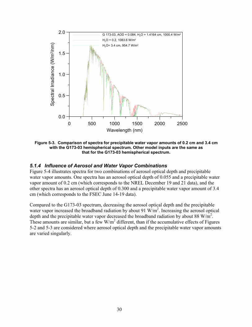
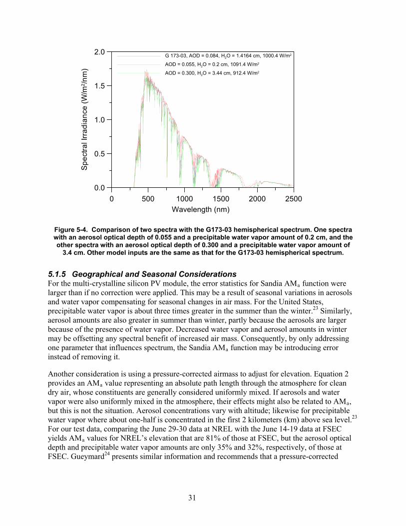
5.1.4 Influence of Aerosol and Water Vapor Combinations Figure 5-4 illustrates spectra for two combinations of aerosol optical depth and precipitable water vapor amounts. One spectra has an aerosol optical depth of 0.055 and a precipitable water vapor amount of 0.2 cm (which corresponds to the NREL December 19 and 21 data), and the other spectra has an aerosol optical depth of 0.300 and a precipitable water vapor amount of 3.4 cm (which corresponds to the FSEC June 14-19 data).

Compared to the G173-03 spectrum, decreasing the aerosol optical depth and the precipitable water vapor increased the broadband radiation by about 91 W/m2. Increasing the aerosol optical depth and the precipitable water vapor decreased the broadband radiation by about 88 W/m2. These amounts are similar, but a few W/m2

0 500 1000 1500 2000 2500Wavelength (nm)

0.0

0.5

1.0

1.5

2.0

Spe

ctra

l Irra

dian

ce (W

/m2 /n

m)

G 173-03, AOD = 0.084, H2O = 1.4164 cm, 1000.4 W/m2

H2O = 0.2, 1083.6 W/m2

H2O= 3.4 cm, 954.7 W/m2

different, than if the accumulative effects of Figures 5-2 and 5-3 are considered where aerosol optical depth and the precipitable water vapor amounts are varied singularly.

31

Figure 5-4. Comparison of two spectra with the G173-03 hemispherical spectrum. One spectra with an aerosol optical depth of 0.055 and a precipitable water vapor amount of 0.2 cm, and the other spectra with an aerosol optical depth of 0.300 and a precipitable water vapor amount of

3.4 cm. Other model inputs are the same as that for the G173-03 hemispherical spectrum.

5.1.5 Geographical and Seasonal Considerations For the multi-crystalline silicon PV module, the error statistics for Sandia AMa function were larger than if no correction were applied. This may be a result of seasonal variations in aerosols and water vapor compensating for seasonal changes in air mass. For the United States, precipitable water vapor is about three times greater in the summer than the winter.23 Similarly, aerosol amounts are also greater in summer than winter, partly because the aerosols are larger because of the presence of water vapor. Decreased water vapor and aerosol amounts in winter may be offsetting any spectral benefit of increased air mass. Consequently, by only addressing one parameter that influences spectrum, the Sandia AMa

Another consideration is using a pressure-corrected airmass to adjust for elevation. Equation 2 provides an AM

function may be introducing error instead of removing it.

a value representing an absolute path length through the atmosphere for clean dry air, whose constituents are generally considered uniformly mixed. If aerosols and water vapor were also uniformly mixed in the atmosphere, their effects might also be related to AMa, but this is not the situation. Aerosol concentrations vary with altitude; likewise for precipitable water vapor where about one-half is concentrated in the first 2 kilometers (km) above sea level.23 For our test data, comparing the June 29-30 data at NREL with the June 14-19 data at FSEC yields AMa values for NREL’s elevation that are 81% of those at FSEC, but the aerosol optical depth and precipitable water vapor amounts are only 35% and 32%, respectively, of those at FSEC. Gueymard24

0 500 1000 1500 2000 2500Wavelength (nm)

0.0

0.5

1.0

1.5

2.0

Spe

ctra

l Irra

dian

ce (W

/m2 /n

m)

G 173-03, AOD = 0.084, H2O = 1.4164 cm, 1000.4 W/m2

AOD = 0.055, H2O = 0.2 cm, 1091.4 W/m2

AOD = 0.300, H2O = 3.44 cm, 912.4 W/m2

presents similar information and recommends that a pressure-corrected

32

airmass not be used because the extinction of solar radiation by aerosols, water vapor, or ozone is not proportional to pressure.

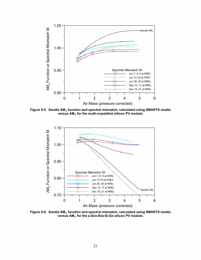
5.2 Comparison of Air Mass Function and Spectral Mismatch Figures 5-5 and 5-6 compare the Sandia AMa function for the multi-crystalline silicon PV module and the a-Si/a-Si/a-Si:Ge PV module with spectral mismatch values calculated for each set of test data using the SMARTS model and the PV module spectral response data. For comparison, spectral mismatch values are plotted versus AMa

In general, for the NREL and FSEC data sets the calculated spectral mismatch values change less with AM

.

a than the Sandia AMa functions, and while the Sandia AMa functions equal 1 when the AMa

For the a-Si/a-Si/a-Si:Ge PV module, only the spectral mismatch values for the NREL December 19 and 21 data resembled the Sandia AM

equals 1.5, the spectral mismatch is less than 1 for the multi-crystalline silicon PV module (from 0.98 to 0.995) and greater than 1 for the a-Si/a-Si/a-Si:Ge PV module (from 1.025 to 1.07).

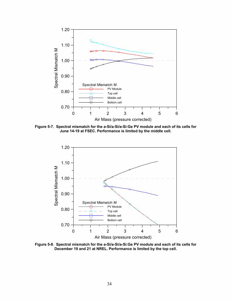
a function. This is likely a consequence of which cell in the multi-junction construction was limiting the performance. Figures 5-7 and 5-8 provide the spectral mismatch for the PV module and each of its cells for two data sets: June 14-19 at FSEC and December 19 and 21 at NREL. For June at FSEC, the mismatch for the middle cell in Figure 5-7 has the same profile as the mismatch for the PV module; consequently, the middle cell is determining performance. (Performance is determined by the cell producing the least current, but current is not shown in the figures.) For December at NREL, the top cell in Figure 5-8 is limiting performance, which provided results similar to the Sandia AMa

function.

33

Figure 5-5. Sandia AMa function and spectral mismatch, calculated using SMARTS model,

versus AMa

for the multi-crystalline silicon PV module.

Figure 5-6. Sandia AMa function and spectral mismatch, calculated using SMARTS model,

versus AMa

for the a-Si/a-Si/a-Si:Ge silicon PV module.


0.90

0.95

1.00

1.05

AMa F

unct

ion

or S

pect

ral M

ism

atch

M

Spectral Mismatch MJun 7, 8, 9 at NRELJun 14-19 at FSECJun 29, 30 at NRELSep 15, 17 at NRELDec 19, 21 at NREL

Sandia AMa


0.70

0.80

0.90

1.00

1.10

AMa F

unct

ion

or S

pect

ral M

ism

atch

M


Sandia AMa

34

Figure 5-7. Spectral mismatch for the a-Si/a-Si/a-Si:Ge PV module and each of its cells for

June 14-19 at FSEC. Performance is limited by the middle cell.

Figure 5-8. Spectral mismatch for the a-Si/a-Si/a-Si:Ge PV module and each of its cells for

December 19 and 21 at NREL. Performance is limited by the top cell.


0.70

0.80

0.90

1.00

1.10

1.20

Spe

ctra

l Mis

mat

ch M

Spectral Mismatch MPV ModuleTop cellMiddle cellBottom cell


0.70

0.80

0.90

1.00

1.10

1.20

Spe

ctra

l Mis

mat

ch M

Spectral Mismatch MPV ModuleTop cellMiddle cellBottom cell

35

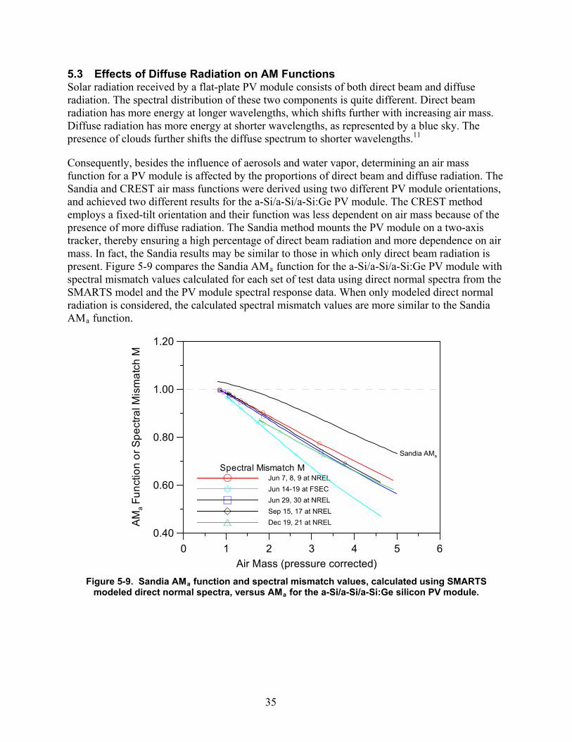
5.3 Effects of Diffuse Radiation on AM Functions Solar radiation received by a flat-plate PV module consists of both direct beam and diffuse radiation. The spectral distribution of these two components is quite different. Direct beam radiation has more energy at longer wavelengths, which shifts further with increasing air mass. Diffuse radiation has more energy at shorter wavelengths, as represented by a blue sky. The presence of clouds further shifts the diffuse spectrum to shorter wavelengths.

Consequently, besides the influence of aerosols and water vapor, determining an air mass function for a PV module is affected by the proportions of direct beam and diffuse radiation. The Sandia and CREST air mass functions were derived using two different PV module orientations, and achieved two different results for the a-Si/a-Si/a-Si:Ge PV module. The CREST method employs a fixed-tilt orientation and their function was less dependent on air mass because of the presence of more diffuse radiation. The Sandia method mounts the PV module on a two-axis tracker, thereby ensuring a high percentage of direct beam radiation and more dependence on air mass. In fact, the Sandia results may be similar to those in which only direct beam radiation is present. Figure 5-9 compares the Sandia AM

11

a function for the a-Si/a-Si/a-Si:Ge PV module with spectral mismatch values calculated for each set of test data using direct normal spectra from the SMARTS model and the PV module spectral response data. When only modeled direct normal radiation is considered, the calculated spectral mismatch values are more similar to the Sandia AMa

function.

Figure 5-9. Sandia AMa function and spectral mismatch values, calculated using SMARTS modeled direct normal spectra, versus AMa

for the a-Si/a-Si/a-Si:Ge silicon PV module.


0.40

0.60

0.80

1.00

1.20

AMa F

unct

ion

or S

pect

ral M

ism

atch

M


Sandia AMa

36

6 Summary

This report presents the results of a preliminary investigation of methods for correcting the Isc of PV modules for variations in solar spectrum under clear skies. We evaluated two types of methods: (1) empirical relationships based on air mass, and (2) use of spectral irradiance models and PV module spectral response data. Methods of the first type were the Sandia f(AMa

The methods were evaluated using data recorded during June, September, and December, 2008 at NREL and during June, 2008 at FSEC. The data included one-minute average values of I

) function and the CREST f(AM) function. The second type used SEDES2 and SMARTS spectral irradiance models.

sc

Data used for analysis were screened to remove data when the presence of clouds or large angle-of-incidences of direct beam radiation created the potential for errors in the results. The angle-of-incidence screening limited data to within about three or three and one-half hours either side of solar noon, the peak energy producing part of the day. AM

and PV module temperature for both a multi-crystalline silicon PV module and an a-Si/a-Si/a-Si:Ge PV module, along with coincident measurements of the plane-of-array solar irradiance with a pyranometer. The same equipment was used for all measurements at both locations. The PV modules were deployed south-facing at a fixed-tilt, with the tilt angle adjusted, for a test period and location, so that the angle-of-incidence of the direct beam radiation would be near zero at solar noon.

a

For predicting I

values of the screened data ranged from 0.8 to 1.5 for the June and September data, and from 1.8 to 3.3 for the December data.

sc, the methods using spectral irradiance models and PV module spectral response data performed better than the empirical air mass methods. This is attributed to the empirical air mass methods not accounting for variations of aerosols and water vapor, which have also been identified by Emery et al.25

For the multi-crystalline silicon PV module, the Sandia f(AM

as a limitation of these methods.

a

A satisfactory solution might be to apply a general derate factor of 0.98 or 0.99 to bring the performance with the reference spectrum closer to these experimental results. (Interestingly, PV modules with conventional bulk silicon cells rated under the G173-03 hemispherical spectrum have their I

) function yielded errors that were somewhat greater than when no corrections were applied. Decreased water vapor and aerosol amounts in winter may have offset any spectral benefit from increased air mass predicted by the method. The methods using spectral irradiance models improved results compared to when not applying a spectral correction, but not significantly when considering the larger modeling errors that can exist with plane-of-array irradiance models or PV module temperature models.

sc increased 0.6% to 1.0% when compared to a rating under the previous reference spectrum.26

For the a-Si/a-Si/a-Si:Ge PV module, all methods provided some improvement compared to no spectral correction. The SEDES2 and SMARTS performed best, and about equal to each other. The Sandia and CREST air mass functions performed about the same as each other, but with increased error. Not properly accounting for diffuse radiation by these methods may have

Consequently, the previous reference spectrum would give a general derate factor closer to one for this PV module.)

37

influenced results. This module’s f(AMa

Future work will evaluate the use of a spectral irradiance model and PV module spectral response data for other PV technologies and for all sky conditions. The SEDES2 model already accommodates the influence of clouds and can be used without modification. The SMARTS models spectra for only clear skies, but the ability to provide spectra for direct and diffuse components may afford the opportunity to extend its capabilities, or cloud cover modifiers similar to that used for SEDES2 might be derived.

) function was strongly dependent on air mass and indicated that performance was top cell limited, consistent with a characterization performed on a tracker with a large direct beam component. However, the test data were for fixed-tilt operation with a smaller direct beam component and a larger diffuse component. For the June data, the method using the SMARTS model, which accounts for the proportions of direct and diffuse components, indicated only a small sensitivity to air mass and that performance was limited by the middle cell.

A worthwhile effort might also be to perform an inter-comparison between SEDES2, SMARTS, and experimental data using spectroradiometer measurements at NREL. Better input data to the models might also improve results. For example, this study used the same ozone amount as the G173-03 spectrum, but satellite-derived amounts are available that would provide seasonal and location-specific values.

Work is also underway at NREL to provide better estimates of aerosol and water vapor amounts, which could improve spectral modeling results. Detailed spectral albedo measurements have also been identified by Gueymard as important for modeling spectral irradiances for steeply tilted surfaces.

27

38

7 References

1. American Society for Testing and Materials, ASTM G 173-03. Standard Tables for Reference

Solar Spectral Irradiances: Direct Normal and Hemispherical for a 37° Tilted Surface, West Conshohocken, PA: American Society for Testing and Materials, 2003.

2. D. King; W. Boyson; J. Kratochvil. Photovoltaic Array Performance Model, SAND2004-3535, Albuquerque, NM: Sandia National Laboratories, 2004.

3. D. King; J. Kratochvil; W. Boyson. “Field Experience with a New Performance Characterization Procedure for Photovoltaic Arrays,” 2nd

4. T. R. Betts; R. Gottschalg; D. G. Infield. “Spectral Irradiance Correction for PV System Yield Calculations.” Proceedings of the 19

World Conference on PV Solar Energy Conversion, Vienna, 1998, pp. 1947-1952.

th

5. “Sandia Database of Photovoltaic Module Performance Parameters,”

European Photovoltaic Solar Energy Conference, Paris, 2004.

http://photovoltaics.sandia.gov/docs/Database.htm. Accessed August 19, 2009. 6. Maui Solar Energy Software Corporation, http://www.mauisolarsoftware.com/. Accessed

August 19, 2009. 7. N. Blair; C. Christensen; M. Mehos; S. Janzou. “Cost and Performance Solar Analysis

Model for All Solar Technologies,” Proceedings of the 2005 International Solar Energy Conference (ISEC2005), August 6-12, 2005, Orlando, Florida.

8. W. De Soto; S.A. Klein; W.A. Beckman. Improvement and Validation of a Model for Photovoltaic Array Performance, Solar Energy 2006; 80: 78-88.

9. “CECPV Calculator Version 2.3,” http://www.gosolarcalifornia.ca.gov/nshpcalculator/download_calculator.html. Accessed August 19, 2009.

10. “PVSYST 4.37 – Software for photovoltaic Systems”, http://www.pvsyst.com/ch/index.php. Accessed August 19, 2009.

11. S. Nann; C. Riordan. “Solar Spectral Irradiance Under Clear and Cloudy Skies: Measurements and a Semi-Empirical Model.” Journal of Applied Meteorology, 30(4), pp. 477-462, 1991.

12. C. Osterwald. Translation of Device Performance Measurements to Reference Conditions, Solar Cells 1986; 18: 269-279.

13. S. Nann; K. Emergy, “Spectral Effects on PV-Device Rating.” Solar Energy Materials and Solar Cells, 27, pp.189-216, 1992.

14. C. Gueymard. User’s Manual—SMARTS Code, Version 2.9.5 for Windows. USA: Solar Consulting Services, 2005.

15. B. Marion; B. Kroposki; K. Emery; J. del Cueto; D. Myers; C. Osterwald. Validation of a Photovoltaic Module Energy Ratings Procedure at NREL, NREL/TP-520-26909, Golden, CO: National Renewable Energy Laboratory, 1999.

16. R. Bird; C. Riordan. “Simple Solar Spectral Model for Direct and Diffuse Insolation on Horizontal and Tilted Planes at the Earth’s Surface for Cloudless Atmospheres.” Journal of Climate and Applied Meteorology, 25, pp. 87-97, 1986.

17. C. Gueymard. “Updated Transmittance Functions for Use in Fast Spectral Direct Beam Irradiance Models.” Proceedings of the 1994 Annual Conference-American Solar Energy Society, June 27-30, 1994, San Jose, California, pp. 355-360.

http://photovoltaics.sandia.gov/docs/Database.htm�

http://www.mauisolarsoftware.com/�

http://www.gosolarcalifornia.ca.gov/nshpcalculator/download_calculator.html�

http://www.pvsyst.com/ch/index.php�

39

18. D. Myers; K. Emery, ;C. Gueymard. “Terrestrial Solar Spectral Modeling Tools and Applications for Photovoltaic Devices.” Proceedings of the 29th

19. R. Gottschalg; J. del Cueto; T. Betts; S. Williams; D. Infield. “Investigating the Seasonal Performance of Amorphous Silicon Single- and Multi-Junction Modules.” Third WCPEC, Osaka, 2003.

IEEE PV Specialist Conference, May 20-24, 2002, New Orleans, Louisiana.

20. J. Wright, R. Perez; J. Michalsky. Luminous Efficacy of Direct Irradiance: Variations with Insolation and Moisture Conditions, Solar Energy 1989; 42: 387-394.

21. NREL Solar Radiation Research Laboratory, http://www.nrel.gov/midc/srrl_bms/. Accessed August 19, 2009.

22. NSRDB—Vol. 1 (1992). User’s Manual—National Solar Radiation Data Base (1961-1990). Version 1.0. Golden, CO: National Renewable Energy Laboratory and Asheville, NC: National Climatic Data Center.

23. Iqbal, M. An Introduction to Solar Radiation. New York: Academic Press, 1983; pp. 92-93. 24. C. Gueymard. “Daily Spectral Effects on Concentrating PV Solar Cells as Affected by

Realistic Aerosol Optical Depth and Other Atmospheric Conditions.” Proceedings of SPIE Conference #7410, Optical Modeling and Measurements for Solar Energy Systems III, August 2-6, 2009. San Diego, California.

25. K. Emery; J. Del Cueto; W. Zaaiman. “Spectral Corrections Based on Optical Air Mass.” Proceedings of the 29th

26. M. Green; K. Emery; Y. Hishikawa; and W. Warta. Solar Cell Efficiency Tables (Version 33), Progress in Photovoltaics: Research and Applications 2009; 17: 85-94.

IEEE PV Specialist Conference, May 20-24, 2002, New Orleans, Louisiana.

27. C. Gueymard. Prediction and Validation of Cloudless Shortwave Solar Spectra Incident on Horizontal, Tilted, and Tracking Surfaces, Solar Energy 2008: 82: 260-271.

http://www.nrel.gov/midc/srrl_bms/�

40

Appendix A: Plots This appendix contains plots of the plane-of-array irradiance versus time of day for data passing the screening criteria for the days selected for the model evaluations. For ease of view, only every fifth data point is displayed in the figures.

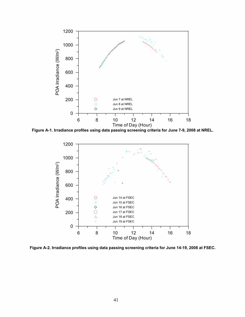
41

Figure A-1. Irradiance profiles using data passing screening criteria for June 7-9, 2008 at NREL.

Figure A-2. Irradiance profiles using data passing screening criteria for June 14-19, 2008 at FSEC.

6 8 10 12 14 16 18Time of Day (Hour)

0

200

400

600

800

1000

1200

PO

A Ir

radi

ance

(W/m

2 )

Jun 7 at NRELJun 8 at NRELJun 9 at NREL

6 8 10 12 14 16 18Time of Day (Hour)

0

200

400

600

800

1000

1200

PO

A Ir

radi

ance

(W/m

2 )

Jun 14 at FSECJun 15 at FSECJun 16 at FSECJun 17 at FSECJun 18 at FSECJun 19 at FSEC

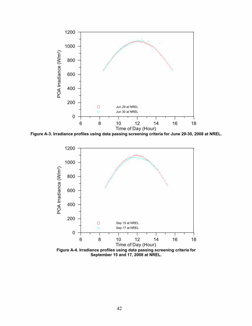
42

Figure A-3. Irradiance profiles using data passing screening criteria for June 29-30, 2008 at NREL.

Figure A-4. Irradiance profiles using data passing screening criteria for

September 15 and 17, 2008 at NREL.

6 8 10 12 14 16 18Time of Day (Hour)

0

200

400

600

800

1000

1200

PO

A Ir

radi

ance

(W/m

2 )

Jun 29 at NRELJun 30 at NREL

6 8 10 12 14 16 18Time of Day (Hour)

0

200

400

600

800

1000

1200

PO

A Ir

radi

ance

(W/m

2 )

Sep 15 at NRELSep 17 at NREL

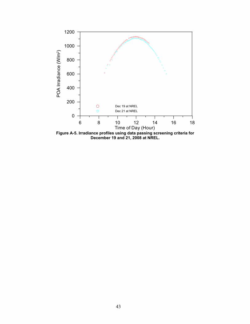
43

Figure A-5. Irradiance profiles using data passing screening criteria for

December 19 and 21, 2008 at NREL.

6 8 10 12 14 16 18Time of Day (Hour)

0

200

400

600

800

1000

1200

PO

A Ir

radi

ance

(W/m

2 )

Dec 19 at NRELDec 21 at NREL

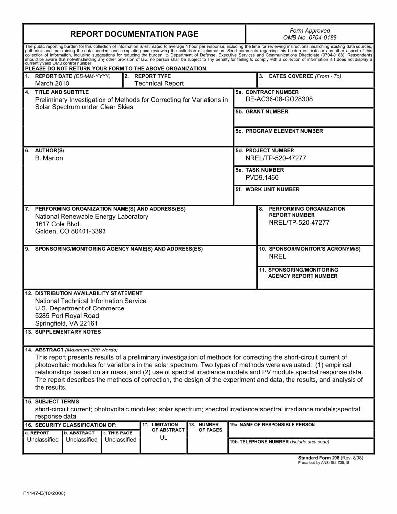
F1147-E(10/2008)

REPORT DOCUMENTATION PAGE Form Approved OMB No. 0704-0188

The public reporting burden for this collection of information is estimated to average 1 hour per response, including the time for reviewing instructions, searching existing data sources, gathering and maintaining the data needed, and completing and reviewing the collection of information. Send comments regarding this burden estimate or any other aspect of this collection of information, including suggestions for reducing the burden, to Department of Defense, Executive Services and Communications Directorate (0704-0188). Respondents should be aware that notwithstanding any other provision of law, no person shall be subject to any penalty for failing to comply with a collection of information if it does not display a currently valid OMB control number. PLEASE DO NOT RETURN YOUR FORM TO THE ABOVE ORGANIZATION. 1. REPORT DATE (DD-MM-YYYY)

March 2010 2. REPORT TYPE

Technical Report 3. DATES COVERED (From - To)

4. TITLE AND SUBTITLE

Preliminary Investigation of Methods for Correcting for Variations in Solar Spectrum under Clear Skies

5a. CONTRACT NUMBER DE-AC36-08-GO28308

5b. GRANT NUMBER

5c. PROGRAM ELEMENT NUMBER

6. AUTHOR(S) B. Marion

5d. PROJECT NUMBER NREL/TP-520-47277

5e. TASK NUMBER PVD9.1460

5f. WORK UNIT NUMBER

7. PERFORMING ORGANIZATION NAME(S) AND ADDRESS(ES) National Renewable Energy Laboratory 1617 Cole Blvd. Golden, CO 80401-3393

8. PERFORMING ORGANIZATION REPORT NUMBER NREL/TP-520-47277

9. SPONSORING/MONITORING AGENCY NAME(S) AND ADDRESS(ES)

10. SPONSOR/MONITOR'S ACRONYM(S) NREL

11. SPONSORING/MONITORING AGENCY REPORT NUMBER

12. DISTRIBUTION AVAILABILITY STATEMENT National Technical Information Service U.S. Department of Commerce 5285 Port Royal Road Springfield, VA 22161

13. SUPPLEMENTARY NOTES

14. ABSTRACT (Maximum 200 Words) This report presents results of a preliminary investigation of methods for correcting the short-circuit current of photovoltaic modules for variations in the solar spectrum. Two types of methods were evaluated: (1) empirical relationships based on air mass, and (2) use of spectral irradiance models and PV module spectral response data. The report describes the methods of correction, the design of the experiment and data, the results, and analysis of the results.

15. SUBJECT TERMS short-circuit current; photovoltaic modules; solar spectrum; spectral irradiance;spectral irradiance models;spectral response data

16. SECURITY CLASSIFICATION OF: 17. LIMITATION OF ABSTRACT

UL

18. NUMBER OF PAGES

19a. NAME OF RESPONSIBLE PERSON a. REPORT

Unclassified b. ABSTRACT Unclassified

c. THIS PAGE Unclassified 19b. TELEPHONE NUMBER (Include area code)

Standard Form 298 (Rev. 8/98) Prescribed by ANSI Std. Z39.18

preliminary investigation of methods for correcting

Documents