preliminary notions about particlespolypaganini/ch1.pdf · p.paganini ecole polytechnique physique...

Chapter 1

Preliminary notions about particles

Few references:Andre Rouge, “Introduction a la physique subatomique”, Chapter 3, 6 and 7, Les editions del’Ecole polytechniqueD. Gri�ths, “Introduction to elementary particles”, Chapter 3 and 4, Harper & Row, 1987

In this first chapter, I give some reminders about Special Relativity and Quan-tum Mechanics that are relevant for particle physics. No real justifications willbe given. At the end of the chapter, we derive very useful formulas to computedecay rates and branching ratio of particles.

1.1 Covariance, contravariance and 4-vector notation

An event is defined in a given frame of the spacetime thanks to 4 numbers (ct, x, y, z). Havinga standard basis ~eµ, the vector “event” is then ~X =

Pxµ~eµ = xµ~eµ where in the last equation

the summation on µ is implict (Einstein notation). The xµ are the contravariant coordinates ofthe 4-vector position:

xµ = (x0 = ct, x1 = x, x2 = y, x3 = z) = (ct, ~x) (1.1)

Let us now define a scalar product of 2 vectors ~X = xµ~eµ and ~Y = yµ~eµ:

~X.~Y = xµy⌫~eµ.~e⌫

We wish this scalar product to be consistent with the definition of the spacetime interval of theSpecial Relativity:

�s2 = ( ~X1

� ~X2

).( ~X1

� ~X2

) = c2(t1

� t2

)2 � (x1

� x2

)2 � (y1

� y2

)2 � (z1

� z2

)2

Recall that the spacetime interval is basically the relativistic equivalent of the (squared) Eu-clidian distance. �s2 can be positive, negative or null. Since the celerity of light is assumed tobe constant (at c) in any frame, �s2 = 0 for light-like interval, positive for time-like interval(meaning that the 2 events can be causally related), and negative for space-like interval (the 2events cannot be causally related). Hence, by writing gµ⌫ = ~eµ.~e⌫ , the scalar product of two4-vectors consistent with the spacetime interval is then:

~X.~Y = gµ⌫xµy⌫ (1.2)

9

10 Preliminary notions about particles

where gµ⌫ , the so-called metric tensor of the Minkowski space is:

gµ⌫ =

0BB@

1 0 0 00 �1 0 00 0 �1 00 0 0 �1

1CCA (1.3)

We can define a new set of numbers:xµ = gµ⌫x

⌫ (1.4)

that are called covariant coordinates with:

xµ = (ct, �~x) (1.5)

xµ can be expressed from xµ by writing:

xµ = gµ⌫x⌫ (1.6)

wheregµ⌫ = gµ⌫ (1.7)

Thus, a scalar product is defined by:

~X.~Y ⌘ x.y = gµ⌫xµy⌫ = gµ⌫xµy⌫ = xµyµ = xµyµ (1.8)

More rigorously, xµ are the components of the dual vector ~X? of ~X in the dual basis and are

called covariant coordinates of ~X while xµ components are contravariant coordinates1. Lowerand upper indices indicate always covariant and contravariant coordinates, respectively.

From now on, we will write a 4-vector without the arrow and using as a symbol indi↵erentlythe name of the 4-vector or its components (it’s a common abuse of language). Ex: the 4-vectorposition can be written simply x or xµ.

1.2 Lorentz transformation

A Lorentz transformation conserves the scalar product, and hence the spacetime interval between2 events.

x0µ = ⇤µ⌫x

⌫ (1.9)

where ⇤ is a matrix of Lorentz transformation. Using matrix notation with g the matrix repre-sentation of the Minkowski tensor:

x02 = x2 ) (⇤x)tg(⇤x) = xtgx) xt⇤tg⇤x = xtgx

Since the equality is true for any x, one has ⇤tg⇤ = g. Taking the determinant, it comesdet(⇤t)det(⇤) = 1 ) det2(⇤) = 1, and so ⇤ has a determinant of ±1. When det(⇤) = 1,the Lorentz transformation conserves the space-time orientation and is called proper Lorentztransformation. Furthermore, if ⇤0

0

� 1, it is orthochronous, meaning that time direction isconserved. A proper-orthochronous transformation consists purely of boosts and rotations in3D space, and forms the special (or restricted) Lorentz group.

1In mathematics, any vector space, V, has a corresponding dual space consisting of all linear functionals on V.

P.Paganini Ecole Polytechnique Physique des particules

Special Lorentz transformation 11

1.2.1 Special Lorentz transformation

In the framework of special relativity, the Lorentz transformations correspond to the law ofchange of inertial (or Galilean) reference frame, for which the physics equations must be pre-served and the speed of light must be the same for any Galilean frame while preserving theorientations of space and time. With these assumptions, one can derive the following Lorentzmatrix (see any Special relativity course):

0BB@

x00

x01

x02

x03

1CCA =

0BB@

� �� 0 0�� 0 0

0 0 1 00 0 0 1

1CCA0BB@

x0 = ctx1 = xx2 = yx3 = z

1CCA (1.10)

where x0µ are the coordinates in the <0 frame moving at v along the x axis with respect to < (xand x0 being aligned) and

� =v

c, � =

1p1 � �2

(1.11)

� being called the boost of the Lorentz transformation. The coordinates in < are deduced fromthe ones in <0 by replacing � ! ��. In case of an arbitrary direction of the <0 frame ~� = ~v/c,the general special Lorentz transformation becomes:

x00 = �(x0 � ~�.~x)~x0 = ~x + (� � 1)(~�.~x)

~��2

� ~��x0

(1.12)

where ~x = (x1, x2, x3). In terms of matrix representation, it corresponds to:

0BB@

x00

x01

x02

x03

1CCA =

0BBBB@

� ��x� ��y� ��z�

��x� 1 + (� � 1)�2

x�2

(� � 1)�x�y�2

(� � 1)�x�z�2

��y� (� � 1)�y�x�2

1 + (� � 1)�2

y

�2

(� � 1)�y�z�2

��z� (� � 1)�z�x�2

(� � 1)�z�y�2

1 + (� � 1)�2

z�2

1CCCCA

0BB@

x0 = ctx1 = xx2 = yx3 = z

1CCA (1.13)

1.2.2 Proper time

In the center-of-mass frame of a particle, the space-time distance ds2 is simply reduced to itsproper time contribution c2d⌧2 when the particle decays, while in the lab frame it is c2dt2 �dx2 � dy2 � dz2 = c2dt2(1 � v2/c2), and hence d⌧ =

p(1 � v2/c2)dt i.e:

d⌧ =dt

�(1.14)

The proper time of a particle (namely the lifetime in the center-of-mass frame) is always shorterthan its lifetime measured in another frame.

1.2.3 Useful 4-vectors

So far, only the 4-vector position was considered. But any 4 numbers that follow the sametransformation as the 4-vector position in a change of frame is by definition a 4-vector.

P.Paganini Ecole Polytechnique Physique des particules avancee


1.2.3.1 Derivative

For instance, if F is a scalar function, the quantity:

dF =@F

@xµdxµ

is a scalar as well, so that the 4 components of :

@µ =@

@xµ= (

1

c

@

@t,@

@x,@

@y,@

@z) (1.15)

are covariant components. And equivalently:

@µ =@

@xµ= (

1

c

@

@t, � @

@x, � @

@y, � @

@z) (1.16)

so that:

@µ@µ = @µ@µ = ⇤ =

1

c2

@2

@t2� @2

@x2

� @2

@y2

� @2

@z2

(1.17)

is the d’Alembertian operator.

1.2.3.2 4-velocity

In order to define the relativistic velocity 4-vector uµ , one has to divide the increase of the4-vector position by a time interval. The obvious choice is to use the proper time since it isindependent of the choice of the reference frame. Hence,

uµ =dxµ

d⌧= �

dxµ

dt= �(c,~v) (1.18)

As expected, one can easily check that u2 = c2.

1.2.3.3 4-momentum

The mass m being a 4-scalar2, the 4-momentum:

pµ = muµ = (�mc, �m~v) = (E/c, ~p) (1.19)

is still a 4-vector with a norm p2 = m2u2 = m2c2. Since p2 is also E2/c2 � |~p|2, one has:

E2 = |~p|2c2 + m2c4 (1.20)

A particle satisfying p2 = m2 is said to be on mass-shell. Equation 1.20 is usually called themass-shell condition. Incidentally, we notice that equality 1.19 implies:

p =�

cE (1.21)

which is valid for any mass. When � = 1, p = E/c which injected in 1.20 implies m = 0.

2There is sometimes a source of confusion in some old textbooks (an historical artifact of special relativity),where it is sometimes said that the mass increases as the velocity of the particle. This approach is now completelyobsolete and better to avoid: the mass is invariant, but not the energy and the momentum which do increase withthe velocity. For more details about the mass, see section 7.4.1.


Useful 4-vectors 13

1.2.3.4 4-acceleration

Following the same argument as for the 4-velocity, one has:

�µ =duµ

d⌧= �(

d�

dtc,

d�

dt~v + �~a) (1.22)

1.2.3.5 4-current

We wish to combine the charge density ⇢ with the current density ~j in a 4-vector. Let us considera point-like charge having a constant density ⇢ in the small element of volume dV and movingat velocity ~v. The current density is thus ~j = ⇢~v while the charge q = ⇢dV . The charge beingan intrinsic property of the particle must not depend on the reference frame (so be a 4-scalar)and we must have ⇢dV = ⇢0dV 0. In a frame <, during dt the particle moves (in the spacetime)by dxµ = (cdt, d~r) which is obviously a 4-vector. So the quantity ⇢dV dxµ = ⇢dtdV (dxµ/dt) =⇢(d⌦/c)(dxµ/dt) is a 4-vector as well, where d⌦ = cdtdV is a small “volume” (in 4 D) of thespacetime, considered between 2 infinitely close moments. d⌦ being a 4-scalar (see exercise 1.1),⇢(dxµ/dt) must be a 4-vector. The 4-current is then defined as:

jµ = ⇢dxµ

dt= (c⇢,~j) (1.23)

We will see in chapter 3 the importance of the 4-current for the description of the interactionbetween charged particles and photons.

1.2.3.6 Electromagnetic 4-potential

In classical electrodynamic, the electric field ~E and magnetic field ~B are solution of the Maxwell’sequations:

(1) ~r. ~E = ⇢/✏0

(3) ~r. ~B = 0

(2) @ ~B@t + ~r ⇥ ~E = 0 (4) ~r ⇥ ~B � 1

c2@ ~E@t = µ

0

~j

!(1.24)

where ⇢ and ~j are respectively the charge density and current density. Let us define the 4-potential:

Aµ = (V/c, ~A) (1.25)

with V the scalar potential and ~A the vector potential. Now defining the electromagnetic tensorof rank 2 by:

Fµ⌫ = @µA⌫ � @⌫Aµ (1.26)

we will see that we can easily recover the Maxwell’s equations. The main interest of usingthe expression of Maxwell’s equations with Fµ⌫ is that the formalism is explicitly covariant.We notice first that Fµ⌫ is obviously antisymmetric and hence depends on only 6 independentparameters. Developing:

F 01 = @0A1 � @1A0 = 1/c(@Ax/@t + @V/@x)F 02 = @0A2 � @2A0 = 1/c(@Ay/@t + @V/@y)F 03 = @0A3 � @3A0 = 1/c(@Az/@t + @V/@z)

we can set F 01 = 1/c(�Ex), F 02 = 1/c(�Ey), F 03 = 1/c(�Ez) with ~E verifying:

~E = �@~A

@t� ~rV (1.27)



where we call ~E the electric field. We can set the 3 other independent parameters:

F 12 = �(@Ax/@y � @Ay/@x) ⌘ �Bz

F 13 = �(@Ax/@z � @Az/@x) ⌘ By

F 23 = �(@Ay/@z � @Az/@y) ⌘ �Bx

the components of the magnetic field ~B satisfying

~B = ~r ⇥ ~A (1.28)

Fµ⌫ then reads:

Fµ⌫ =

0BB@

0 �Ex/c �Ey/c �Ez/cEx/c 0 �Bz By

Ey/c Bz 0 �Bx

Ez/c �By Bx 0

1CCA (1.29)

Calculating @ ~B@t + ~r ⇥ ~E from equ. 1.27 and 1.28 we do check that it is 0 ie the Maxwell’s

equation (2). And the same for ~r. ~B = 0 (equation (3)). In order to find (1) and (4) we justhave to write:

@µFµ⌫ = µ0

j⌫ (1.30)

j⌫ being the 4-current. Let us check:

@µFµ0 = µ0

j0 ) 0 +1

c

@Ex

@x+

1

c

@Ey

@y+

1

c

@Ez

@z= µ

0

c⇢ , ~r. ~E = ⇢/✏0

(using ✏0

µ0

= 1/c2). For the other component:

@µFµ1 = µ0

j1 ) � 1

c2

@Ex

@t+@Bz

@y� @By

@z= µ

0

jx

and similar result for @µFµ2 and @µFµ3 (with permuted x, y and z) so that one actually findsequation (4).

It is easy to realize that the electric field and magnetic field are entangled. Suppose forexample A0 = 0 and A1,2,3 = (0, 0, sin!t). According to 1.28 and 1.27: ~B = 0 and ~E =(0, 0,! cos!t). Since Aµ is a 4-vector with no component along the x-axis, in a frame movingat � with respect to the x-axis, we have A0µ = Aµ. However, in this frame the magnetic fieldis now3 ~B0 = ~r0 ⇥ ~A0 = (0, ��! cos!t, 0) 6= 0. A pure electric field can be seen as a magneticfield (or a mix of electric and magnetic fields) in another frame and vice-versa. Both are clearlyentangled and inseparable. A well-known result.

1.2.4 Rapidity

The rapidity ⇣ is given by:

⇣ = tanh�1 � ) � = cosh ⇣ , �� = sinh ⇣ (1.31)

The rapidities of 2 Lorentz transformations just add up: ⇣<00/< = ⇣<00/<0 + ⇣<0/< (assuming thatthe two frames <0 and <” are moving in the same direction with respect to <). That means

3Alternatively one may transform the electromagnetic tensor F 0µ⌫ = ⇤µ⇢⇤

⌫�F

⇢� = ⇤µ⇢(⇤

t)�⌫F⇢� =

⇤µ⇢F

⇢�(⇤t)�⌫ ) F 0 = ⇤F⇤t to deduce the new components of the electric and magnetic fields.


Rapidity 15

that if the rapidity is known in a given frame, the value in another frame moving at � will justbe translated: ⇣ 0 = ⇣ + tanh�1 (�). In other words, d⇣ 0 = d⇣ is Lorentz invariant and so therapidity distribution dN/d⇣ as well. The addition of rapidities gives an easy way to rememberthe addition of relativistic velocities: �<00/< = tanh(tanh�1 �<00/<0 + tanh�1 �<0/<) leading to:

�<00/< =�<00/<0 + �<0/<1 + �<00/<0�<0/<

(1.32)

Knowing that � = tanh ⇣ = (e⇣ � e�⇣)/(e⇣ + e�⇣), equation 1.31 can be rewritten:

⇣ =1

2ln

✓1 + �

1 � �

◆

Hence, at low velocity,

⇣ =1

2[ln(1 + �) � ln(1 � �)] ⇡ � (� ⌧ 1)

rapidity converges to velocity. We recover the usual Euclidian addition of velocities at lowvelocity.

Now, let us consider a non zero mass particle moving at � = v/c. Combining E = �mc2 andp = �mv, the rapidity becomes:

⇣ =1

2ln

✓E + pc

E � pc

◆

However, experimental particle physicists often use a modified definition of rapidity relative toa beam axis where pL is the longitudinal component of momentum along the beam axis:

⇣ =1

2ln

✓E + pLc

E � pLc

◆(1.33)

Any Lorentz transformation along the beam axis will just add a term tanh�1 �. This is typicallythe case of asymmetric collisions such as with fixed-target experiments or in hadron colliderswhere the elements colliding (so called partons) take a varying fraction of the initial hadrons’energy. Hence, with this definition, the rapidity distribution dN/d⇣ is the same in the center ofmass frame of the collision or in the lab frame.

In formula 1.33, the mass of the particle has to be known (or both E and pL have to bemeasured independently). However, as soon as E � mc2, E ' pc, pL = p cos ✓ ) pLc ' E cos ✓and the previous definition becomes

⇣ ' ⌘ =1

2ln

✓1 + cos ✓

1 � cos ✓

◆=

1

2ln

cos2 ✓

2

sin2

✓2

!) ⌘ = � ln

✓tan

✓

2

◆

where ⌘ is called the pseudorapidity. The advantage of the pseudorapidity is that it doesn’tdepend on the mass, and thus on the nature of the particle which is usually unknown in exper-iments. When ✓ is close to zero (on the beam axis), ⌘ diverges to the infinity. ⌘ and ⇣ are veryclose as soon as E � mc2 and the angle of the particle w.r.t beam axis is large enough. A noteof caution with the pseudorapidity: while the behavior of the rapidity is clear under a Lorentzboost (⇣ 0

2

� ⇣ 01

= ⇣2

� ⇣1

), it is not the case for the pseudorapidity where ⌘02

� ⌘01

6= ⌘2

� ⌘1

.



1.3 Units

The two fundamental constants in High Energy Physics are the speed of light c = 2.998 ⇥108 ms�1 and the Plank constant ~ = h

2⇡ = 1.0546 ⇥ 10�34 Js (reflecting that we usually dealwith relativistic quantum objets). In the rest of the document, we are going to use the so-callednatural units with c = ~ = 1, so that length units are equivalent to time units and energy unitsequivalent to mass or inverse of time. Hence:

~ = 1 )1 GeV�1 ⌘ 6.58 ⇥ 10�25 s (1.34)

~c = 1 )1 fm ⌘ 5 GeV�1 ⇡ (1/5 GeV)�1 = (197 MeV)�1 (1.35)

This will strongly simplify the formulas.

1.4 Angular momentum of particles

The purpose of this section is to remind the reader of important properties of the angularmomentum in quantum mechanics that are often used in particle physics. They will not bejustified, the reader can refer to any quantum mechanics book (for example [2] or [3]).

1.4.1 Orbital angular momentum in quantum mechanics

In classical mechanics, the angular momentum is defined as ~L = ~r ^ ~p. It depends on 6 numbersrx, ry, rz, px, py and pz. In quantum mechanics, due to the Heisenberg uncertainty principle, it’snot possible to measure simultaneously these 6 numbers with an arbitrary precision. It turns outthat the best that one can do is to simultaneously measure both the magnitude of the angularmomentum vector and its component along one axis. The angular momentum is quantized andis defined as an operator (symbolˆbelow) acting on the wave function. Its expression is:

~L = ~r ^ ~p = �i~ ~r ^ ~r (1.36)

where we used the correspondence principle stating that ~p = �i~~r (see next chapter). Itsatisfies the following canonical commutation relations expressing the impossibility to measuresimultaneously all the angular momentum components:

[Lx, Ly] = i~Lz, [Ly, Lz] = i~Lx, [Lz, Ly] = i~Ly (1.37)

which can be simply written [Li, Lj ] = i~✏ijkLk, ✏ijk being the antisymmetric Levi-Civita symbol.

Then, one can easily show that L2 = L2

x + L2

y + L2

z satisfies:

[L2, Lx,y,z] = 0 (1.38)

Thus, one can find a basis of eigenvectors of L2 and Lz4. One can show that the eigenvectors

|l,mi satisfy:L2 |l,mi = l(l + 1)~2 |l,miLz |l,mi = m~ |l,mi , m 2 [�l, l]

(1.39)

where l is the quantum number of the orbital momentum and m is the quantum number of theprojection of the orbital momentum on the Z-axis. In case of orbital angular momentum, l,mare integers.

4Z axis is chosen by convention.


Spin angular momentum 17

Using the cylindrical coordinates (x = r sin ✓ cos�, y = r sin ✓ sin�, z = r cos ✓ with ✓ and �the polar and azimuthal angles), we have from 1.36:

L2 = �~2

✓@2

@✓2

+1

tan ✓

@

@✓+

1

sin2 ✓

@2

@�2

◆

and

Lz = �i~ @

@�

The spherical harmonics Y ml (✓,�) = h✓,�|l,mi are eigenfunctions of the orbital angular momen-

tum and thus satisfy the equation 1.39 i.e.:

L2 Y ml (✓,�) = l(l + 1)~2 Y m

l (✓,�)Lz Y m

l (✓,�) = m~ Y ml (✓,�), m 2 [�l, l]

The expression of the most useful spherical harmonics is given in the table below.

l/m 0 1 2

0q

1

4⇡

q3

4⇡ cos ✓q

5

4⇡

�3

2

cos2 ✓ � 1

2

�

1q

3

8⇡ sin ✓ei� �q

15

8⇡ sin ✓ cos ✓ei�

2 1

4

q15

2⇡ sin2 ✓e2i�

Table 1.1: Spherical harmonics Y ml .

The two following properties of the Y ml are useful:

Y �ml (✓,�) = (�1)m [Y m

l (✓,�)]⇤ m > 0

Y ml (⇡ � ✓,�+ ⇡) = (�1)l Y m

l (✓,�)

The last property explains why under parity transformation (which inverts all spatial coordinatesand thus ✓ ! ⇡ � ✓ and � ! �+ ⇡), the orbital angular momentum gets an extra factor (�1)l.

1.4.2 Spin angular momentum

As the name suggests, spin was originally conceived as the rotation of a particle about its axis.This name is very unfortunate: elementary particles are described as point-like objects for which“rotation about its axis” is meaningless. One has to resign with the classical picture and justadmit that spin is a kind of angular momentum in the sense that it obeys the same mathematicallaws as quantized orbital angular momenta do i.e.:

S2 |s, mi = s(s + 1)~2 |s, miSz |s, mi = m~ |s, mi , m 2 [�s, s]

(1.40)

However, spins have some peculiar properties that distinguish them from orbital angular mo-menta. Spin quantum number s may take an half-odd-integer positive values (for fermions).



Spin is usually presented as the intrinsic angular momentum suggesting that it is the residualangular momentum that still remains even if the particle is at rest (and hence p = 0) or if therestframe of the particle is used. This image is obviously not appropriate for massless particlealways propagating at the velocity of light.

A case of most importance is the spin 1/2. A particle having a spin 1/2 has two possibleprojections |1

2

, +1

2

i and |12

, �1

2

i that can be gathered into a 2-component notation named Paulispinor:

|12, +

1

2i =

✓10

◆= |"i , |1

2, �1

2i =

✓01

◆= |#i

with:

Sz |"i =1

2|"i , Sz |#i = �1

2|#i

while the projection on the two other axis gives (see for instance [2, p. 252]):

Sx |"i =1

2|#i , Sx |#i =

1

2|"i , Sy |"i = i

1

2|#i , Sy |#i = �i

1

2|"i

where we have dropped the ~. We see that the mean value of the spin on the x and y-axes fora system prepared in |"i or |#i gives 0 as expected (h" |Sx| "i = h# |Sx| #i = 0). In general, thestate of a spin 1/2 is a linear combination of the 2 spin-up |"i and spin-down |#i eigenstates:

↵ |"i + � |#i =

✓↵�

◆

so that the probability to find after the measurement of the z-axis the spin-up state is |↵|2 and|�|2 for the spin-down one (with |↵|2 + |�|2 = 1). We see that using the spinor notation, theprojection on the di↵erent axes is obtained with 2 ⇥ 2 matrices, called the Pauli matrices:

~S =1

2~� (1.41)

meaning:

Sx =1

2�1 , Sy =

1

2�2 , Sz =

1

2�3

where �i=1,2,3 are given by:

�1 =

✓0 11 0

◆, �2 =

✓0 �ii 0

◆, �3 =

✓1 00 �1

◆(1.42)

~S verifies the commutation relations:

[Sx, Sy] = iSz

Moreover, we do have, as eigenstates of S2 = S2

x + S2

y + S2

z , the spin-up and spin-down states

with the expected value s(s + 1) with s = 1

2

. Conclusion: the ~S operators made with the Paulimatrices verify all the conditions of the quantum mechanical angular momentum operators, withS = 1

2

, ie the spin. They represent the operators for spin 1

2

.


Total angular momentum and addition of angular momenta 19

1.4.3 Total angular momentum and addition of angular momenta

As for classical mechanics, the total angular momentum is the sum of the orbital angular orbital

momentum and spin (which in classical mechanics is the rotation of the object on itself): ~J =~L + ~S, J satisfying:

J2 |j, mi = j(j + 1)~2 |j, miJz |j, mi = m~ |j, mi , m 2 [�j, j]

(1.43)

j and m being integers or half-odd-integers.The spin of composite particles is usually understood to mean the total angular momentum.

This is the sum of the spins and orbital angular momenta of the constituent particles5 and isunderstood to refer to the spin of the lowest-energy internal state of the composite particle (i.e.,a given spin and orbital configuration of the constituents).

The dimension of the Hilbert space H(j) generated by the states of the angular momentumJ is 2j + 1. When two angular momenta ~J

1

and ~J2

are added, the new space is the tensorialproduct H

1

(j1

) ⌦ H2

(j2

) of dimension (2j1

+ 1) ⇥ (2j2

+ 1) for which a complete basis can bedenoted by the following eigenvectors:

|j1

, j2

, m1

, m2

i ⌘ |j1

, m1

i ⌦ |j2

, m2

i

The eigenvectors obviously satisfy:

J2

1

|j1

, j2

, m1

, m2

i = j1

(j1

+ 1)~2 |j1

, j2

, m1

, m2

i , J1z |j

1

, j2

, m1

, m2

i = m1

~ |j1

, j2

, m1

, m2

iJ2

2

|j1

, j2

, m1

, m2

i = j2

(j2

+ 1)~2 |j1

, j2

, m1

, m2

i , J2z |j

1

, j2

, m1

, m2

i = m2

~ |j1

, j2

, m1

, m2

i

One can show that there exists another complete basis of this space which corresponds to thetotal angular momentum ~J = ~J

1

+ ~J2

. This basis is generated by the eigenvectors of J2

1

, J2

2

, J2,and Jz:

|j1

, j2

, j, mi with j 2 j1

+ j2

, j1

+ j2

� 1, · · · , |j1

� j2

| and m = m1

+ m2

2 [�j, j]

and thus satisfy:

J2

1

|j1

, j2

, j, mi = j1

(j1

+ 1)~2 |j1

, j2

, j, mi , J2

2

|j1

, j2

, j, mi = j2

(j2

+ 1)~2 |j1

, j2

, j, miJ2 |j

1

, j2

, j, mi = j(j + 1)~2 |j1

, j2

, j, mi , Jz |j1

, j2

, j, mi = m~ |j1

, j2

, j, mi

In other words, the resulting space is decomposed as:

H1

(j1

)O

H2

(j2

) =j1

+j2M

j=|j1

�j2

|

H(j)

The relationship between the basis |j1

, j2

j, mi and |j1

, j2

, m1

, m2

i is given by the Clebsch-Gordancoe�cients (chosen as real numbers and denoted below as hj

1

, j2

, m1

, m2

|j1

, j2

, j, mi):

|j1

, j2

, j, mi =j1X

m1

=�j1

j2X

m2

=�j2

hj1

, j2

, m1

, m2

|j1

, j2

, j, mi |j1

, j2

, m1

, m2

i

where only coe�cients for which m = m1

+ m2

are non-zero. The most useful coe�cients forparticle physics are given in a concise way in figure 1.1. Looking for example at the table labelled

5The notion of constituent is here very large: for instance, it includes valence quarks of hadrons as well asquarks or gluon from quantum fluctuations. It is known now that the spin of the proton cannot be explained bythe contribution of the valence quarks only.



40. Clebsch-Gordan coe�cients 1

40. CLEBSCH-GORDAN COEFFICIENTS, SPHERICAL HARMONICS,

AND d FUNCTIONS

Note: A square-root sign is to be understood over every coe�cient, e.g., for �8/15 read �p

8/15.

Y 0

1

=

r3

4⇡cos ✓

Y 1

1

= �r

3

8⇡sin ✓ ei�

Y 0

2

=

r5

4⇡

⇣3

2cos2 ✓ � 1

2

⌘

Y 1

2

= �r

15

8⇡sin ✓ cos ✓ ei�

Y 2

2

=1

4

r15

2⇡sin2 ✓ e2i�

Y �m� = (�1)mY m⇤

� hj1

j2

m1

m2

|j1

j2

JMi= (�1)J�j

1

�j2hj

2

j1

m2

m1

|j2

j1

JMid �m,0 =

r4⇡

2� + 1Y m

� e�im�

d jm�,m = (�1)m�m�

d jm,m� = d j

�m,�m� d 1

0,0 = cos ✓ d1/2

1/2,1/2

= cos✓

2

d1/2

1/2,�1/2

= � sin✓

2

d 1

1,1 =1 + cos ✓

2

d 1

1,0 = � sin ✓p2

d 1

1,�1

=1 � cos ✓

2

d3/2

3/2,3/2

=1 + cos ✓

2cos

✓

2

d3/2

3/2,1/2

= �p

31 + cos ✓

2sin

✓

2

d3/2

3/2,�1/2

=p

31 � cos ✓

2cos

✓

2

d3/2

3/2,�3/2

= �1 � cos ✓

2sin

✓

2

d3/2

1/2,1/2

=3 cos ✓ � 1

2cos

✓

2

d3/2

1/2,�1/2

= �3 cos ✓ + 1

2sin

✓

2

d 2

2,2 =⇣1 + cos ✓

2

⌘2

d 2

2,1 = �1 + cos ✓

2sin ✓

d 2

2,0 =

p6

4sin2 ✓

d 2

2,�1

= �1 � cos ✓

2sin ✓

d 2

2,�2

=⇣1 � cos ✓

2

⌘2

d 2

1,1 =1 + cos ✓

2(2 cos ✓ � 1)

d 2

1,0 = �r

3

2sin ✓ cos ✓

d 2

1,�1

=1 � cos ✓

2(2 cos ✓ + 1) d 2

0,0 =⇣3

2cos2 ✓ � 1

2

⌘

Figure 40.1: The sign convention is that of Wigner (Group Theory, Academic Press, New York, 1959), also used by Condon and Shortley (TheTheory of Atomic Spectra, Cambridge Univ. Press, New York, 1953), Rose (Elementary Theory of Angular Momentum, Wiley, New York, 1957),and Cohen (Tables of the Clebsch-Gordan Coe�cients, North American Rockwell Science Center, Thousand Oaks, Calif., 1974).

Figure 1.1: The Clebsch-Gordan coe�cients, spherical harmonics and d-functions. From [19].

1/2 ⇥ 1/2, it is easy to check that the addition of 2 spins 1

2

(j1

= j2

= 1

2

) gives the well-knownresult:

|12

, 1

2

, 1, 1i = |12

, 1

2

, +1

2

, +1

2

i ⌘ |""i|12

, 1

2

, 1, 0i = 1p2

|12

, 1

2

, +1

2

, �1

2

i + 1p2

|12

, 1

2

, �1

2

, +1

2

i ⌘ 1p2

|"#i + 1p2

|#"i|12

, 1

2

, 0, 0i = 1p2

|12

, 1

2

, +1

2

, �1

2

i � 1p2

|12

, 1

2

, �1

2

, +1

2

i ⌘ 1p2

|"#i � 1p2

|#"i|12

, 1

2

, 1, �1i = |12

, 1

2

, �1

2

, �1

2

i ⌘ |##i


E↵ect of rotations on angular momentum states 21

1.4.4 E↵ect of rotations on angular momentum states

Consider a rotation of a quantum mechanic system. A rotation in general is defined by 3numbers: they could be the two polar coordinates �, ✓ of the rotation axis ~n and the rotationangle ⇥ around the axis or they could be the three Euler angles �, ✓, respectively around thez, y and z axes as shown in figure 1.2 [33]. In the former definition, the rotation is defined by

Physique des particules M1 HEP X Pascal Paganini LLR-IN2P3-CNRS 34

4) Angular momentum of particles�

Figure 1.2: The 3 Euler angles for an extrinsic rotation (i.e. with respect to fixed axes).

the operator6:

R(n, ⇥) = e�i⇥

~ ~n.ˆ~J (1.44)

while in the later definition:

R(�, ✓, ) = e�i�~ˆJze�i ✓~

ˆJye�i ~ˆJz (1.45)

When applied to the angular momentum states, the norm j remains unchanged but the projec-tion on an axis is obviously a↵ected -since the frame (passive transformation) or the angularmomentum (active transformation) is rotated-, and hence:

R |j, mi =Pj

m0=�j |j, m0i hj, m0|R|j, mi

=Pj

m0=�j |j, m0i Dj

m0,m

(1.46)

where Djm0,m (which depend on the angles) are the so-called Wigner rotation D-functions. The

interpretation of D-functions in case of a passive transformation is easier: in equation 1.46, theleft hand side ket is an eigenvector of Jz (with eigenvalue m~) where the z-axis is the rotatedaxis. The right hand-side ket is an eigenvector of Jz (with eigenvalue m0~) where now the z-axisis the original axis. Thus, Dj

m0,m is simply the amplitude to measure the value m0~ along thez-axis when the angular momentum points in the direction of the rotated axis with componentm~. Using the Euler angle rotation 1.45, the expression of Dj

m0,m can be simplified since |j, miand |j, m0i are eigenvector of Jz:

Djm0,m(�, ✓, ) = hj, m0|e�i�~

ˆJze�i ✓~ˆJye�i ~

ˆJz |j, mi= e�i�m0

djm0,m(✓) e�i m

(1.47)

where the d-functions:dj

m0,m(✓) = hj, m0|e�i ✓~ˆJy |j, mi (1.48)

are reduced rotation matrices and the most useful expressions are given in figure 1.1. Since weare interested in the angular momentum, only rotations that a↵ect the z-axis matter. Therefore,

6The angular momentum operators are the (infinitesimal) generators of the rotations.



we can simply ignore the rotation with the angle i.e. choose = 0 (it is the usual convention):such rotation R(�, ✓, 0) would bring the z-axis in the same position as R(�, ✓, ) (only x andy-axes would di↵er). Consequently, equation 1.47 finally reduces to:

Djm0,m(�, ✓, 0) = e�i�m0

djm0,m(✓) (1.49)

As an example, it is interesting to consider a spin 1/2. Using formulae in figure 1.1, we find:

D1

2

1

2

, 12

= e�i�2 cos ✓

2

, D1

2

� 1

2

, 12

= e+i�2 sin ✓

2

, D1

2

1

2

,� 1

2

= �e�i�2 sin ✓

2

, D1

2

� 1

2

,� 1

2

= e+i�2 cos ✓

2

,

and thus:

R |12

, 1

2

i = |12

, �1

2

i D1

2

� 1

2

, 12

+ |12

, 1

2

i D1

2

1

2

, 12

= |12

, �1

2

i e+i�2 sin ✓

2

+ |12

, 1

2

i e�i�2 cos ✓

2

R |12

, �1

2

i = |12

, �1

2

i D1

2

� 1

2

,� 1

2

+ |12

, 1

2

i D1

2

1

2

,� 1

2

= |12

, �1

2

i e+i�2 cos ✓

2

� |12

, 1

2

i e�i�2 sin ✓

2

Using the spinor notation introduced in section 1.4.2, the previous equation reads:

R

✓10

◆= e�i�

2 cos ✓2

✓10

◆+ e+i�

2 sin ✓2

✓01

◆=

e�i�

2 cos ✓2

e+i�2 sin ✓

2

!

R

✓01

◆= �e�i�

2 sin ✓2

✓10

◆+ e+i�

2 cos ✓2

✓01

◆=

�e�i�

2 sin ✓2

e+i�2 cos ✓

2

!

meaning that R corresponds to the matrix representation7:

R(✓,�) =

e�i�

2 cos ✓2

�e�i�2 sin ✓

2

e+i�2 sin ✓

2

e+i�2 cos ✓

2

!

Let us see the e↵ect of the rotation R of angles ✓ = 2⇡ and � = 0 which brings back the systemin its original position:

R(2⇡, 0) = � l1

where l1 denotes the identity matrix. We find the famous result R(2⇡, 0) | i = � | i: forspin 1/2 particles, a rotation of 2⇡ is not enough to recover the initial state (that would haveincidence on interferences properties), but 2 turns (4⇡) are actually needed. There is a directconnection with the spin-statistic theorem: interchanging two particles is topologically the sameas rotating either one of them by 360 degrees as shown in figure 1.3. Thus, we see that theinterchange of two spin 1/2 particles will generate a minus sign. For example, if (1)�(2)describes particle 1 in state and particle 2 in state �, then the particle interchange must bedescribed by � (2)�(1) and since both particles are identical, the correct wave-function is thelinear superposition (1)�(2) � (2)�(1) which is antisymmetric as expected for fermions. Thereader can check that with spin 1 particles, only one turn is enough to recover the initial state.

7The reader could have found directly this result by expanding the formula e�i�~ ˆSze�i ✓~ ˆSy with Sz and Sy

given by the Pauli matrix (equation 1.41).


Collisions 23

Physique des particules M1 HEP X Pascal Paganini LLR-IN2P3-CNRS 36

21 2 1

Figure 1.3: The rotation with an angle 2⇡ of one of the 2 particles is equivalent to the interchange ofthe 2 particles.

1.5 Collisions

1.5.1 4-momentum conservation

In physics, the invariance of spacetime by translation implies that an isolated system has a 4-momentum which is conserved. For a system consisted of particles without interaction, the globalmomentum of the system is just the addition of the individual particles momenta. However, forparticles in interaction with fields, the situation is more complicated and one should take intoaccount the momenta of the fields themselves which can be complicated. Fortunately, in case ofcollision of particles, one makes the assumption that the initial state is described by particleswithout interaction, which then interact and produce a final state in which the particles areconsidered again without interaction. Hence, even if we don’t try to describe what happensduring the collision (the dynamic of the process), we can still write that the sum of particles’momenta of the initial state is equal to the sum of particles’ momenta of the final state.

1.5.2 Two-particles scattering and Mandelstam variables

Let us consider the collision sketched on figure 1.4: (1) + (2) ! (3) + (4) with 4-momentap1

, p2

, p3

, p4

. The amplitude (-probability) of the process must not depend on the frame,

(2) p2

(1) p1

(4) p4

(3) p3

Figure 1.4: A scattering with two particles.

so only 4-scalar must be involved i.e. scalar product of 4-momenta. There are 10 possiblecombinations but, because of momentum conservation and the on mass-shell constraint, only 2independent combination remain. It is often convenient to express the amplitude as function of



other Lorentz-invariant variables called Mandelstam variables and defined as:

s = (p1

+ p2

)2 = (p3

+ p4

)2

t = (p1

� p3

)2 = (p4

� p2

)2

u = (p1

� p4

)2 = (p3

� p2

)2(1.50)

where s is the square of the center-of-mass energy (in the center-of-mass frame8 ~p⇤1

+ ~p⇤2

= 0,

thus (p⇤1

+ p⇤2

)2 = (E⇤1

+ E⇤2

)2 � (~p⇤1

+ ~p⇤2

)2 = (E⇤1

+ E⇤2

)2) and t the square of the 4-momentumtransfer (trivial in case of elastic scattering). By developing the expressions of equation 1.50,and using the relation p

1

+ p2

= p3

+ p4

, one finds

s + t + u =4X1

m2

i (1.51)

reflecting that only 2 variables are indeed really independent.

1.5.2.1 Determination of center-of-mass variables

Let us find now the momentum and energy in the center-of-mass frame (labelled CM in whatfollows) where |~p⇤

1

| = |~p⇤2

| = |~p⇤|:E⇤2

1

= m2

1

+ ~p⇤2 ) ~p⇤2 = E⇤2

1

� m2

1

E⇤2

2

= m2

2

+ ~p⇤2 ) E⇤2

2

= m2

2

+ E⇤2

1

� m2

1ps = E⇤

1

+ E⇤2

) ps = E⇤

1

+p

m2

2

� m2

1

+ E⇤2

1

) (p

s � E⇤1

)2 = m2

2

� m2

1

+ E⇤2

1

Finally:

E⇤1

=s + m2

1

� m2

2

2p

s(1.52)

And thus:

E⇤2

=p

s � E⇤1

) E⇤2

=s + m2

2

� m2

1

2p

s(1.53)

And:

~p⇤2 = E⇤2

1

� m2

1

=(s + m2

1

� m2

2

)2

4s� m2

1

=s2 + m4

1

+ m4

2

� 2m2

1

m2

2

� 2sm2

1

� 2sm2

2

4s

~p⇤2 =�(s, m2

1

, m2

2

)

4s=

[s � (m1

+ m2

)2][s � (m1

� m2

)2]

4s(1.54)

with �(x, y, z) the triangle function (also known as the Kallen function):

�(x, y, z) = x2 + y2 + z2 � 2xy � 2xz � 2yz = [x � (p

y +p

z)2][x � (p

y �p

z)2] (1.55)

For the energies and momenta of the particles in the final state, one has just to replace m1

! m3

and m2

! m4

in equ. 1.52, 1.53 and 1.54. In case of elastic scattering where m1

= m3

andm

2

= m4

the final and initial quantities in the CM are obviously the same.One should notice that formulas 1.52, 1.53 or 1.54 do not depend on the final state. Hence,

they are valid whatever the number of particles in the final state. Inversely, the 3 correspondingformulas for the final state are independent of the initial state and are valid whatever the numberof particles in the initial state.

8In center-of-mass frame, the quantities are labelled with a *.


Crossed reactions 25

1.5.2.2 Case of fixed target

We can apply these formulas in case of a collision of a particle (1) to a nucleus of fixed target (2).We have ~p

2

= 0 and hence E2

= m2

. Therefore s = (p1

+p2

)2 = m2

1

+m2

2

+2E1

m2

and includingthis result in the numerator of 1.54, we get ~p⇤2 = [2E

1

m2

� 2m1

m2

][2E1

m2

+ 2m1

m2

]/4s =m2

2

(E2

1

� m2

1

)/s. Since E2

1

� m2

1

= ~p2

1

, it remains9:

|~p⇤| = m2

|~p1

|ps

, s = m2

1

+ m2

2

+ 2E1

m2

(1.56)

Usually, E1

� m1

, m2

, so thatp

s 'p

2E1

m2

. For example, when the Tevatron collider (nearChicago, USA) ran with fixed target mode with E

1

= 980 GeV and m2

' 1 GeV, we haveps ' 44 GeV to be compared to the collider mode where

ps = 2 ⇥ 980 = 1960 GeV.

1.5.3 Crossed reactions

So far, the 3 Mandelstam variables were simply presented as a combination of 4-momenta withs being the squared energy in the CM, t the squared transfer momenta and u without a clearphysical meaning. However, we can go further as soon as we re-interprete the negative signs inequations 1.50. We will see in the chapter devoted to Quantum ElectroDynamic that a particlewith 4-momentum �pµ is interpreted as an antiparticle:

pµ ⌘ �pµ (1.57)

so that the amplitude M (a complex function which completely describes the scattering pro-cess) involving an antiparticle can be described by the amplitude of the reaction involving theparticle but using instead �pµ. Actually, this is a general property of Quantum Field Theorythat the amplitude involving a particle in the initial state with 4-momentum pµ is identical tothe amplitude of the otherwise same process but with an antiparticle in the final state withmomentum �pµ. Hence, the amplitudes of the following reactions can be derived from the sameamplitude:

(1) + (2) ! (3) + (4) (1.58)

(1) + (3) ! (2) + (4) (1.59)

(1) + (4) ! (3) + (2) (1.60)

and even for (1) ! (2) + (3) + (4). However, even if the amplitude would be the same, it doesnot mean that all these reactions are allowed: conservation of 4-momentum must be respected,or in other words the kinematics must be adequate.

M depends on the four 4-momenta which are not independent because of the energy-momentum conservation. Equivalently, M depends on s, t, u. Let us denote by M(s = (p

1

+p2

)2, t = (p1

� p3

)2, u = (p1

� p4

)2) the amplitude of 1.58 and M0(s0 = (p1

+ p¯

3

)2, t0 = (p1

�p¯

2

)2, u0 = (p1

� p4

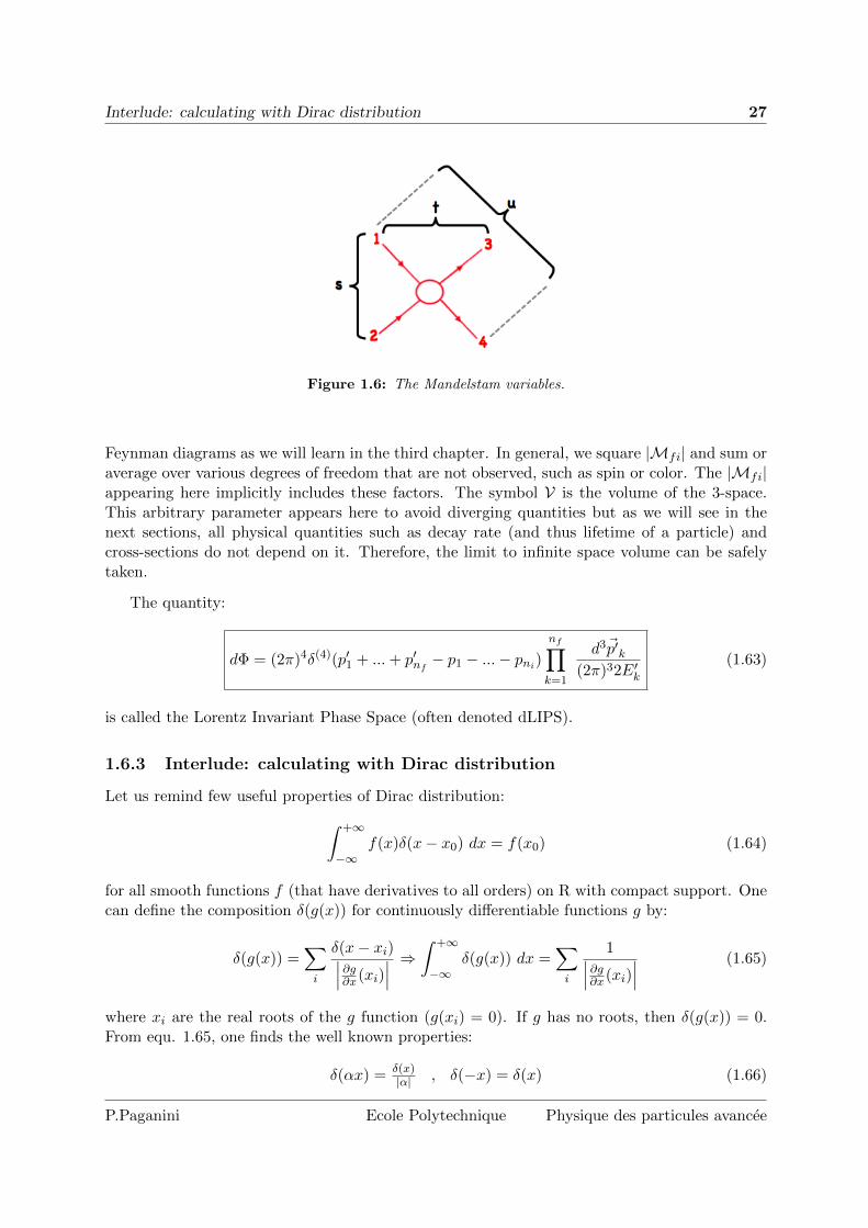
)2) the amplitude of 1.59. Applying 1.57 rule, we see on figure 1.5 that t = s0,s = t0 and u = u0. Hence, the amplitude of reaction 1.59 is just M0(s0, t0, u0) = M(t0, s0, u0).Similarly for reaction 1.60, we have M(u0, t0, s0). The 3 processes in which s, t, u are the squaredCM energy are called respectively s, t, and u-channel and are displayed in figure 1.6. Reaction1.59 and 1.60 are then respectively the t and u-channel of reaction 1.58. A summary of thesituation is given in the following table:

9you can find this result by using a Lorentz transformation.



(2) p2

(1) p1

(4) p4

(3) p3

(3) �p3

(1) p1

(4) p4

(2) �p2

(4) �p4

(1) p1

(2) �p2

(3) p3

Figure 1.5: Crossed-reactions: the middle and right reactions are respectively the t-channel and u-channel of the reaction on the left.

channel reaction s-variable t-variable u-variable

s-channel (1) + (2) ! (3) + (4) s t u

t-channel (1) + (3) ! (2) + (4) t s u

u-channel (1) + (4) ! (3) + (2) u t s

Table 1.2: The Mandelstam variables as function of the channels of the reaction (1) + (2) ! (3) + (4).

1.6 Elementary particles dynamics

1.6.1 Phase space

Let us consider the following reaction with ni particles in the initial state and nf in the finalstate:

p1

+ p2

+ ... + pni ! p01

+ p02

+ ... + p0nf

(1.61)

The particles are considered on mass shell: E2 = p2 +m2 so that the final state is represented by4nf �nf = 3nf parameters. Because of the conservation of the 4-momemtum between the initialand final state, there are 3nf � 4 independent parameters. A given reaction will correspond toa single point on an hyper-surface of dimension 3nf � 4 of the space of dimension 3nf . Thishyper-surface is the phase space: it corresponds to all possible values of 4-momenta componentsof the particles in the final state involved in a reaction.

1.6.2 Transition rate

In chapter 3, we will show that the general formula of the elementary transition rate (probabilityper unit time) from an initial state |ii made of ni particles to a final state |fi made of nf particlesis given by10:

d�i!f = V1�ni(2⇡)4�(4)(p01

+ ... + p0nf

� p1

� ... � pni)|Mfi|2niY

k=1

1

2Ek

nfYk=1

d3~p0k

(2⇡)32E0k

(1.62)

where the prime symbols denote final states quantities and Mfi is the invariant scatteringamplitude (or probability amplitude or often called matrix element) that can be computed with

10We also provide in appendix A a “classical” justification of this formula based on quantum mechanics andnot on quantum fields theory.


Interlude: calculating with Dirac distribution 27

Figure 1.6: The Mandelstam variables.

Feynman diagrams as we will learn in the third chapter. In general, we square |Mfi| and sum oraverage over various degrees of freedom that are not observed, such as spin or color. The |Mfi|appearing here implicitly includes these factors. The symbol V is the volume of the 3-space.This arbitrary parameter appears here to avoid diverging quantities but as we will see in thenext sections, all physical quantities such as decay rate (and thus lifetime of a particle) andcross-sections do not depend on it. Therefore, the limit to infinite space volume can be safelytaken.

The quantity:

d� = (2⇡)4�(4)(p01

+ ... + p0nf

� p1

� ... � pni)

nfYk=1

d3~p0k

(2⇡)32E0k

(1.63)

is called the Lorentz Invariant Phase Space (often denoted dLIPS).

1.6.3 Interlude: calculating with Dirac distribution

Let us remind few useful properties of Dirac distribution:

Z+1

�1f(x)�(x � x

0

) dx = f(x0

) (1.64)

for all smooth functions f (that have derivatives to all orders) on R with compact support. Onecan define the composition �(g(x)) for continuously di↵erentiable functions g by:

�(g(x)) =X

i

�(x � xi)�� @g@x(xi)

�� )Z

+1

�1�(g(x)) dx =

Xi

1�� @g@x(xi)

�� (1.65)

where xi are the real roots of the g function (g(xi) = 0). If g has no roots, then �(g(x)) = 0.From equ. 1.65, one finds the well known properties:

�(↵x) = �(x)

|↵| , �(�x) = �(x) (1.66)



Applying equ. 1.65 to p2�m2 with g(p0) = (p0)2� |~p|2�m2 = (p0)2�E2 = (p0�E)(p0+E),one gets: Z

+1

�1�(p2 � m2) dp0 =

1

E

But since �(p2 � m2) is an even function versus p0, we have:

Z+1

�1�(p2 � m2) dp0 = 2

Z+1

0

�(p2 � m2) dp0 = 2

Z+1

�1�(p2 � m2)✓(p0) dp0

✓ being the Heaviside function. Hence:

Z+1

�1�(p2 � m2)✓(p0) dp0 =

1

2E(1.67)

Thus, one has the useful equivalence:

Z+1

�1d4p �(p2 � m2)✓(p0) =

Z+1

�1

d3~p

2E(1.68)

Applying the Fourier transformations with the following convention ˆf(⇠) =R

+1�1 f(x)e�i⇠xdx ,

f(x) = 1

2⇡

R+1�1

ˆf(⇠)ei⇠xd⇠ to the Dirac distribution

� = 1 , �(x) =1

2⇡

Z+1

�1ei⇠xd⇠ ) �(n)(x) =

1

(2⇡)n

Zei⇠.xdn⇠ (1.69)

1.6.4 Decay width and lifetime

We apply equ. 1.62 with ni = 1 and nf = n particles:

d�1!n = (2⇡)4�(4)(p0

1

+ ... + p0n � p

1

)|M|2 1

2E1

nYk=1

d3~p0k

(2⇡)32E0k

And hence the transition rate to a set of particles is obtained by integrating over the phasespace:

�1!n = (2⇡)4

1

2E1

Z�(4)(p0

1

+ ... + p0n � p

1

)|M|2nY

k=1

d3~p0k

(2⇡)32E0k

(1.70)

The rate is in s�1, and so equivalent to GeV in natural unit. We call it the partial decaywidth. The total decay width (or total transition rate) is obtained by summing up on allpossible decays:

�tot =X

�1!fi (1.71)

and the branching ratio which represents the fraction of decay in a given channel is simply:

BR1!fi =

�1!fi

�tot(1.72)


Cross-sections 29

A particle that decays has a given lifetime. When a particle is stable, we can write its wavefunction as (t) = (0)e�iEt, so that | (t)|2 = | (0)|2. When the particle is unstable, we expect| (t)|2 = | (0)|2e�t/⌧ , ⌧ being the lifetime. Let us write:

E = E0

� i�/2 ) | (t)|2 = | (0)|2e��t

Clearly, the particle lifetime has to be identified as the inverse of the total decay width:

⌧ =1

�tot(1.73)

But there is another consequence: in order to find the probability of finding the particle statewith energy E, let us take the Fourier transform:

(E) =1p2⇡

Z+1

�1dteiEt (t) =

(0)p2⇡

Z+1

0

dtei(E�E0

)t��

2

t =i (0)p

2⇡

1

(E � E0

) + i�

2

where (t < 0) = 0 (the particle doesn’t exist yet). The probability of finding the energy E isthen:

| (E)|2 =| (0)|2

2⇡

1

(E � E0

)2 + �

2

4

The distribution of the energy (or mass) follows a Breit-wigner law with a spread of energiesgiven by the decay width. The relationship between lifetime and decay-width can be found againvia the Heisenberg’s uncertainty principle:

�tot � ~/⌧

The greater the mass (or energy) is shifted from its nominal value, the shorter the particle lives.Note that according to 1.70, the lifetime depends on E

1

and so on the reference frame. Byconvention, the lifetime is measured in the particle’s rest frame.

1.6.5 Cross-sections

In particle physics, cross-sections are measured in barns = 10�24 cm2, a unit of surface area, byreference to the image of a particle (1) having a radius r

1

impinging on the surface S of a targetmade of particle (2) of radius r

2

and containing n2

particles per unit of volume. Two particlescan hit only if the distance between their centre is below r

1

+ r2

. If around each target particle,we draw a disc of area � = ⇡(r

1

+ r2

)2, the probability of interaction is given by the numberof particles (2) seen by (1) times the ratio of � over the surface of the target. If the particle(1) travels at speed |~v

1

|, during dt, (1) is going to go through a region of the target containingn

2

S|~v1

|dt particles of the target so that the probability of interaction is:

dP =�

Sn

2

S|~v1

|dt = �n2

|~v1

|dt

which leads to the rate:

� =dP

dt= �n

2

|~v1

|

Now, instead of a single particle, we have a beam, larger than the surface S of the target witha density of n

1

particle per unit of volume. Considering a volume V of the target, the rate willbe multiplied by the number of particle of the beam that can interact in that volume:

� = �n2

|~v1

| n1

V = �n2

V n1

|~v1

| = �N2

� (1.74)



where � = n1

|~v1

| is the flux of incident particles and N2

the number of particles considered inthe target. If particles (2) are also in a beam moving at ~v

2

, the flux becomes: � = n1

|~v1

� ~v2

|.According to 1.74, the cross section is defined as:

� =�

N2

�

Let us apply this definition to the experiments in particle physics where we are interested in theinteraction between two single particles. In that case, the cross section, � has to be understoodas an e↵ective area. The flux of the incoming particle is � = 1

V |~v1

�~v2

| (using n1

= 1/V), leadingto the cross-section formula:

� =number of interactions per unit time

flux incident particles=

�

�

Applying equ. 1.62 with ni = 2 and nf = n particles to get the number of interaction per unittime:

d�2!n =

1

V (2⇡)4�(4)(p01

+ ... + p0n � p

1

� p2

)|M|2 1

2E1

1

2E2

nYk=1

d3~p0k

(2⇡)32E0k

so that the cross section is:

d� =1

4|~v1

� ~v2

|E1

E2

(2⇡)4�(4)(p01

+ ... + p0n � p

1

� p2

)|M|2nY

k=1

d3~p0k

(2⇡)32E0k

Let us denote by F , the flux factor: F = |~v1

� ~v2

|E1

E2

. In general , it is not Lorentz invariantwhereas the rest of the previous equation is. However, if we consider only cases of 2 collinearbeams, then F is Lorentz invariant. Rearranging F , it’s going to be clear:

F = |~v1

� ~v2

|E1

E2

= | ~p1

E1

� ~p2

E2

|E1

E2

= ( |~p1

|E

1

+ |~p2

|E

2

)E1

E2

= (|~p1

|E2

+ |~p2

|E1

)) F 2 = |~p

1

|2E2

2

+ |~p2

|2E2

1

+ 2|~p1

|E2

|~p2

|E1

But p1

p2

= E1

E2

+ |~p1

||~p2

| ) (p1

p2

)2 = E2

1

E2

2

+ |~p1

|2|~p2

|2 + 2E1

E2

|~p1

||~p2

| and hence:

F 2 � (p1

p2

)2 = |~p1

|2(E2

2

� |~p2

|2) + E2

1

(|~p2

|2 � E2

2

) = |~p1

|2m2

2

� E2

1

m2

2

= �m2

1

m2

2

Therefore:

F = E1

E2

✓|~p

1

|E

1

+|~p

2

|E

2

◆=p

(p1

.p2

)2 � (m1

m2

)2 (1.75)

which is obviously Lorentz invariant. The elementary cross-section is finally:

d�2!n = 1

4

p(p

1

.p2

)

2�(m1

m2

)

2

(2⇡)4�(4)(p01

+ ... + p0n � p

1

� p2

)|M|2Qn

k=1

d3~p0k

(2⇡)

3

2E0k

= |M|24F d�

(1.76)

If the 2 beams are not collinear, the cross section is by definition the one that would be measuredin the rest-frame of the 2 particles.


Decomposition of the phase space 31

1.6.6 Decomposition of the phase space

Let us denote by P the 4-momentum of the initial state (potentially made of several particles)and p

1

, p2

, · · · , pn the ones of the n particles in the final state. For simplicity, we will startwith n = 3. The Lorentz invariant phase space (equ. 1.63) corresponds to:

d�(P ! p1

p2

p3

) = (2⇡)4�(4)(p1

+ p2

+ p3

� P )d3~p

1

(2⇡)32E1

d3~p2

(2⇡)32E2

d3~p3

(2⇡)32E3

The particles in the final state are often produced via intermediate resonances and sometimes,it simplifies the calculation to make it appear explicitly. For example let us suppose that thereaction is actually P ! q

12

p3

! p1

p2

p3

where q12

denotes the 4-momentum of the intermediatestate which further decays in p

1

p2

. One can always introduce the 2 identity integrals:

1 =

Zd4q

12

�(4)(q12

� p1

� p2

)✓(q0

12

) , 1 =

Zdm2

12

�(m2

12

� q2

12

)

m2

12

being the mass-squared of the particle described by the 4-momentum q12

. Putting togetherthese 2 identity integrals and using the equivalence of equ. 1.68 gives:

1 =

ZZd4q

12

�(4)(q12

� p1

� p2

)✓(q0

12

) dm2

12

�(m2

12

� q2

12

) =

ZZd3~q

12

2E12

�(4)(q12

� p1

� p2

) dm2

12

And hence:

d�(P ! p1

p2

p3

) = (2⇡)4�(4)(q12

+ p3

� P ) d3~p1

(2⇡)

3

2E1

d3~p2

(2⇡)

3

2E2

d3~p3

(2⇡)

3

2E3

d3~q12

2E12

�(4)(q12

� p1

� p2

) dm2

12

=dm2

12

2⇡ (2⇡)4�(4)(q12

+ p3

� P ) d3~p3

(2⇡)

3

2E3

d3~q12

(2⇡)

3

2E12

⇥(2⇡)4�(4)(q12

� p1

� p2

) d3~p1

(2⇡)

3

2E1

d3~p2

(2⇡)

3

2E2

where the integral sign is implicit. Thus, we have decomposed the 3 particles phase space intosmaller (2-body) phase spaces:

d�(P ! p1

p2

p3

) =dm2

12

2⇡d�(P ! q

12

p3

) d�(q12

! p1

p2

) (1.77)

Note that the number of degrees of freedom stays the same: initially, we had 3 ⇥ 3 (the 33-momenta) reduced by the delta function to 3 ⇥ 3 � 4 = 5. Each 2-body phase space has2 ⇥ 3 � 4 = 2 degrees of freedom, and thus 2 + 2 + 1 = 5 (1 being due to dm2

12

).

The decomposition of the 3-particles final state can be easily extended to larger states con-taining n particles:

d�(P ! p1

· · · pn) =dm2

[1···j]2⇡

d�(P ! q[1···j]pj+1

· · · pn) d�(q[1···j] ! p

1

· · · pj) (1.78)

with m2

[1···j] = (p1

+ · · · pj)2 = q2

[1···j]. Since each d� is Lorentz invariant, they can be evaluatedin di↵erent frames. The fact that the particle described by q is a real resonance or not does notmatter in this decomposition. q can correspond to any sum of 4-momenta final state particles.However, in case of a resonance, q2 distribution follows a Breit-Wigner as seen previously.



1.6.7 Few applications

1.6.7.1 Decay to 2 particles

(i) ! (1) + (2)

Let us denote by p = (E, ~p) the initial particle 4-momenta and pf=1,2 = (Ef , ~pf ) the two4-momenta of the decay products. Applying equ. 1.70:

�1!2

= (2⇡)41

2E

Z�(4)(p

1

+ p2

� p)|M|2 d3~p1

(2⇡)32E1

d3~p2

(2⇡)32E2

In the initial particle’s rest frame, we have:

~p1

+ ~p2

= 0, p = (m, 0), p1

= (q

|~p⇤|2 + m2

1

, ~p⇤), p2

= (q

|~p⇤|2 + m2

2

, �~p⇤)

Integrating over ~p2

, we get:

�1!2

= (2⇡)�2

1

2m

Z�(q

|~p⇤|2 + m2

1

+q

|~p⇤|2 + m2

2

� m)|M|2 d3~p⇤

2p

|~p⇤|2 + m2

1

1

2p

|~p⇤|2 + m2

2

where now |M| depends on ~p⇤. Using spherical coordinates d3~p⇤ = p⇤2 sin ✓ dp⇤ d✓ d� =p⇤2 dp⇤ d⌦:

�1!2

=1

32⇡2m

Zd⌦

Z+1

0

dp⇤ �(p

p⇤2 + m2

1

+p

p⇤2 + m2

2

� m)pp⇤2 + m2

1

pp⇤2 + m2

2

p⇤2|M|2

We could use the formula 1.65 to perform the integration over p⇤ but it is simpler to make thechange of variables:

E =q

p⇤2 + m2

1

+q

p⇤2 + m2

2

) dE =Ep⇤p

p⇤2 + m2

1

pp⇤2 + m2

2

dp⇤

E representing the total energyp

s. Then it comes:

�1!2

=1

32⇡2m

Zd⌦

Z+1

m1

+m2

dE

E�(E � m)p⇤|M|2

�1!2

=|~p⇤|

32⇡2m2

Zd⌦|M|2 if m > m

1

+ m2

, 0 otherwise (1.79)

p⇤ satisfying m =p

p⇤2 + m2

1

+p

p⇤2 + m2

2

and corresponds to the momentum in the rest-frameand hence, its expression is the one we calculated previously in equ. 1.54. M must be evaluatedat ~p

1

= ~p⇤ and ~p2

= �~p⇤. This result is general, no assumptions were made on the detailedshape of M. If, we assume in addition that the initial particle is spinless, by symmetry, theamplitude M cannot depend on the solid angle. Then

Rsin ✓d✓ d� = 4⇡ and finally we get:

�1!2

=|~p⇤|

8⇡m2

|M|2 if m > m1

+ m2

, 0 otherwise

Following the same kind of calculations the phase space for the 2-body is easy to obtain.Looking at formula 1.79, it is simply:

d�(p ! p1

p2

) = d�1!2

2E

|M|2 =) d�(p ! p1

p2

) =|~p⇤

1

|16⇡2m

12

d⌦⇤1

(1.80)


Few applications 33

where m2 has been changed to m2

12

to be more general, E = m12

and all variables have to beunderstood in the rest frame of particles 1 and 2 and denoted with a star index. Finally, usingformula 1.54 for |~p⇤

1

|, it gives:

d�(p ! p1

p2

) =

s1 � 2

(m2

1

+ m2

2

)

m2

12

+(m2

1

� m2

2

)2

m4

12

d⌦⇤1

32⇡2

(1.81)

1.6.7.2 Scattering cross section 2 ! 2

(1) + (2) ! (10) + (20)

We apply the formula 1.76 with nf = 2:

d�2!2

=1

4p

(p1

.p2

)2 � (m1

m2

)2(2⇡)4�(4)(p0

1

+ p02

� p1

� p2

)|M|2 d3~p01

(2⇡)32E01

d3~p02

(2⇡)32E02

(1.82)

In the Center-of-mass frame, p1

= (E⇤1

=p

|~p⇤|+m2

1

, ~p⇤) and p2

= (E2

=p

|~p⇤|+m2

2

, �~p⇤) withE

1

+ E2

=p

s. Hence F simplifies to F = (E1

+ E2

)|~p⇤| (using 1.75) and thus:

d�2!2

=1

4p

s|~p⇤|(2⇡)2�(E0

1

+ E02

�p

s)�(3)(~p01

+ ~p02

)|M|2 d3~p01

2E01

d3~p02

2E02

(1.83)

which gives the cross-section for a process in which ~p01,2 lies in the range d3~p0

1,2. In general,we are interested in the probability of observing one of the final products in certain directionwithin an element of the solid angle d⌦⇤ = sin ✓⇤d✓⇤d�⇤. Let us integrate over the other decayproduct, let us say ~p0

2

:

d�2!2

=1

4p

s|~p⇤|(2⇡)2�(E0⇤

1

+ E0⇤2

�p

s)|M|2 | ~p0⇤|2d| ~p0⇤|d⌦⇤

2E0⇤1

1

2E0⇤2

(1.84)

Replacing E0⇤i by

q| ~p0⇤|2 + m0

i2:

d�2!2

d⌦

⇤ = 1

16

ps|~p⇤|(2⇡)

2

R+10

�

✓q|~p⇤|2 + m0

1

2 +q

|~p⇤|2 + m02

2 � ps

◆|M|2

⇥ | ~p0⇤|2d| ~p0⇤|p|~p⇤|2+m0

1

2

p|~p⇤|2+m0

2

2

(1.85)

Using the variable E⇤ =q

|~p⇤|2 + m01

2 +q

|~p⇤|2 + m02

2, we have

dE⇤ = d| ~p0⇤|| ~p0⇤|

q|~p⇤|2 + m0

1

2 +q

|~p⇤|2 + m02

2

q|~p⇤|2 + m0

1

2

q|~p⇤|2 + m0

2

2

so that:d�

2!2

d⌦⇤ =1

16p

s|~p⇤|(2⇡)2

Z+1

m01

+m02

��E⇤ �

ps�|M|2 dE⇤

E⇤ |~p0⇤|

and thus the di↵erential cross-section is:

d�2!2

d⌦⇤ =1

64⇡2s|M|2 |~p0⇤|

|~p⇤| ifp

s > m01

+ m02

, 0 otherwise (1.86)



where |~p0⇤| and |~p⇤| have been calculated with equ. 1.54. To calculate the total cross sec-tion (which is Lorentz invariant with collinear beams), it is su�cient to integrate the pre-vious expression. However, it is not so useful for the di↵erential cross-section, since thisformula is only available in the CM frame. We can go a bit further by expressing d⌦⇤ asfunction of the Mandelstam variable t = (p

1

� p01

)2 = m2

1

+ m021

� 2E⇤1

E0⇤1

+ 2~p⇤1

.~p0⇤1

. With

~p⇤ = (0, 0, |~p⇤|) and ~p0⇤ = (|~p0⇤| sin ✓⇤, 0, |~p0⇤| cos ✓⇤), t = m2

1

+ m021

� 2E⇤1

E0⇤1

+ 2|~p⇤||~p0⇤| cos ✓⇤,

giving dt = 2|~p⇤||~p0⇤|d(cos ✓⇤) and since d⌦⇤ = d(cos ✓⇤)d� (the sign doesn’t matter), one has:

d�2!2

dt=

d�2!2

d⌦⇤d⌦⇤

dt=

1

64⇡2s|M|2 |~p0⇤|

|~p⇤|d�

2|~p⇤||~p0⇤|=

1

128⇡2s|M|2 d�

|~p⇤|2 (1.87)

Let us assume M doesn’t depend on � (it’s not systematically true because the symmetry isbroken by the beam axis). After integration over the angle:

d�2!2

dt=

1

64⇡s

|M|2|~p⇤|2 (1.88)

which gives a formula valid in all frames with |~p⇤| from 1.54.

1.6.7.3 The three particles final state: Dalitz plots

Let us consider the decay of a particle with a mass m and 4-momentum p into 3 particleswith mass mi=[1,3]

and 4-momenta pi=[1,3]

. Using the rest-frame of the decaying particle, thedi↵erential decay rate is given by (equ. 1.70):

d�1!3

= (2⇡)41

2m�(4)(p

1

+ p2

+ p3

� p)|M|2 d3~p1

(2⇡)32E1

d3~p2

(2⇡)32E2

d3~p3

(2⇡)32E3

Integrating over ~p3

, it gives:

d�1!3

=1

16m(2⇡)5�(E

1

+ E2

+ E3

� m)|M|2 |~p1

|2d|~p1

|d⌦1

E1

|~p2

|2d|~p2

|d⌦2

E2

1

E3

Let us assume that we are not interested by the angular distributions and that the matrix elementdoes not depend on them (in other words, we suppose that there is no spin polarization). Thenthe integration over all angles except the one between particle 1 and 2 will give:

Rd⌦

1

= 4⇡and d⌦

2

= 2⇡d(cos ✓12

) leading to:

d�1!3

=1

8m(2⇡)3�(E

1

+ E2

+ E3

� m)|M|2 |~p1

|2|~p2

|2d|~p1

|d|~p2

|d(cos ✓12

)

E1

E2

E3

Since E2

i = m2

i + |~pi|2, we have EidEi = |~pi|d|~pi|. In addition, |~p3

|2 = |~p1

+ ~p2

|2 = |~p1

|2 + |~p2

|2 +2|~p

1

||~p2

| cos ✓12

and thus E3

dE3

= |~p3

|d|~p3

| = |~p1

||~p2

|d(cos ✓12

). The di↵erential decay width isthen reduced to:

d�1!3

=1

8m(2⇡)3�(E

1

+ E2

+ E3

� m)|M|2dE1

dE2

dE3

which simply gives after integration over E3

:

d�1!3

=1

8m(2⇡)3|M|2dE

1

dE2


Exercises 35

The 3-body decay is then described by 2 variables, here E1

and E2

. The Dalitz plot is a planeshowing the density (i.e. relative frequency) of these two variables, with one variable on thex-axis and the other on the y-axis. Traditionally, instead of the energies, the squares of themasses of two pairs of the decay products are used. It has the advantage not to depend on the

frame. Since m2

13

= (p1

+ p3

)2 = (p � p2

)2 = m2 + m2

2

� 2mE2

, we have dE2

= �dm2

13

2m and

similarly dE1

= �dm2

23

2m leading to:

d�1!3

=1

32m3(2⇡)3|M|2dm2

13

dm2

23

If the matrix element |M|2 is a constant, then the plan (m2

13

, m2

23

) should be uniformly pop-ulated. In this case, the di↵erential decay width only depends on the phase space and thecontour of the Dalitz plot is shaped by the energy-momentum conservation and the masses ofthe particles involved in the reaction. However, as soon as there are departures from a uniformdensity, it is a sign of a underlying dynamic in the process: |M|2 depends on m2

13

or m2

23

. Thisis the case for example when the 3-body reaction occurs via an intermediate resonance (|M|2depending on a Breit-Wigner).

An example of Dalitz plot is shown on figure 1.7 in which the reaction K�+p ! ⇤+⇡++⇡�

was studied [34]. Clearly, the density is not uniform in the distorded ellipse. An accumulationof data is seen in horizontal and vertical bands for masses m

⇤⇡+ ⇡ m⇤⇡� ⇡ 1.38 GeV. This

accumulation turns out to be due to the presence of the ⌃±(1385) resonance having a mass of1385 MeV. The reaction was actually: K� +p ! ⌃+ +⇡� ! ⇤+⇡+ +⇡� (and the C-conjugatereaction)

1.7 Exercises

Exercise 1.1 Using Lorentz transformation, show that d⌦ = cdtdV is a 4-scalar. Hint: do notforget the jacobian of the transformation!

Exercise 1.2 What is the appropriate factor to convert cross-sections expressed in natural units( GeV�2) to µb?

Exercise 1.3 ⇡+ decay in µ+⌫µ

Consider N0

= 600 ⇡+ (spin 0, m ⇡ 140 MeV/c2) with a kinetic energy of 140 MeV. The ⇡+’sdecay in µ+⌫µ (mµ ⇡ 106 MeV/c2, m⌫ ⇡ 0).

1. Determine the angular distribution dNd cos ✓⇤ of the µ in the ⇡ rest frame? (✓⇤ is the angle

between the ⇡ direction and µ in the ⇡ rest frame)

2. What are the energy and momentum of the µ in the ⇡ rest frame?

3. What is the minimum and maximum energy of the µ in the lab frame?

4. Draw the shape of the energy distribution dNdEµ

of the µ in the lab frame assuming a binningof 1 MeV.

Exercise 1.4 �0 production and decayThe �0 resonance has a spin 3/2 and an intrinsic parity +1. The reaction ⇡�p ! �0 ! ⇡0n



VOLUME 10, NUMBER 5 PHYSICAL REVIEW LETTERS 1 MARCH 1963

reactions are produced according to phase space andthat the effect of Zo contamination in the Y&* peak isnegligible.SR. H. Dalitz, Brookhaven National Laboratory Report

BNL 735 (T-264) (unpublished).

~OJ. W. Cronin and D. E. Overseth, International Con-ference on High-Energy Nuclear Physics, Geneva, 1962(CERN Scientific Information Service, Geneva, Switzer-land, 1962), p. 453.~D. Colley et al. , Phys. Rev. 128, 1930 (1962).

SPIN AND PARITY OF THE 1385-MeV Y,* RESONANCE~Janice B. Shafer, Joseph J. Murray, and Darrell O. Huwe

Lawrence Radiation Laboratory, University of California, Berkeley, California(Received 24 January 1963)

Study of the reaction

at a momentum of 1.22 BeVy'c has shown conclu-sively that the spin of the 1385-MeV Y,* is «&3,

as reported earlier by Ely et al. ', it has also in-dicated that the Y,* state is P» (even Y~ —Aparity) rather than D» (odd parity). These con-clusions result from the angular distribution ofthe lambda and the angular dependence of thelambda polar ization.The events were obtained through the use of

the 72-inch hydrogen bubble chamber placed ina beam of high-energy K mesons extracted fromthe Bevatron. The momentum spread of the beamwas +2. 5 $, and the pion background was about10$Approximately 1650 events were analyzed which

satisfied the E +p —A+ n++ n hypothesis. Someresults from a partial sample were reportedearlier. The events were identified by kine-matic fitting, first at the decay vertex and thenat the production vertex, with the IBM-7090 pro-gram "PACKAGE, " After this two-step fitting,the number of ambiguous events that might havebeen F' production rather than lambda productionwas approximately 1 $ of the total. Almost com-plete separation of the Z n+v from the Av+nevents was accomplished by examination of theratio y2(Am~) j2y'(Zmw) for each event, the Z'vvy' being weighted by a factor of two because ofthe difference in average g' values. The finalAm+a- sample included about 93 $ of the true Annevents and about 5$ of the true Zo~m events. TheA3v events were excluded from the Ann sampleby eliminating all events with y2(A3w) less than 10.The cross section for production of the A~+~

final state by 1.22-BeV/c Z mesons was de-termined by comparison with the observed num-ber of tau decays in the same film sample; its

value is 2. 2~0. 2 mb. The angular distributionsof Y*+ and Y~ production were found similar tothat of Y*+ production in the work of Ely et al. '(see reference 3).The Dalitz plot for the Av v events is shown

in Fig. 1. Projection onto the Av+ mass axis isdisplayed; the Am projection (not shown) is sim-ilar. These mass spectra of the A~+ and the Avsystems are well fitted by Y*+ and Y~ reso-nance curves alone, without background; valuesof M(Y*) = 1385 MeV and f' = 50 MeV are required.The production ratio of Y*+ to Y* is 0.80. Back-ground of 5 to 10$ cannot be ruled out.On the basis of these mass spectra, the limits

1340 MeV ~M(Y*) ~ 1430 MeV were utilized inthe analysis discussed below. Only events withlarge production angles in the center of mass

Mass of Aw- pair fMeV)I 300 l 400 l 500 l600 1700

—0Q. ~

C4

V0

0l.50 2.00 2.50

Mass squared of A~- pair (BeV2j3.00

0OgCO

0 a0 ~0~0 o

EA

OX00Number per l0 MeV

FIG. 1. Dalitz plot of A~ m events from E P inter-actions at 1.22 BeV/c. The square of A&+ effectivemass is plotted against the square of Ax effective mass.Scales giving the masses in MeV are also shown. Pro-jection of the events onto the A~+ mass axis is displayedto the right of the figure; the curve represents the fittingof Breit-Wigner resonance expressions to the An+ andAm systems.

Figure 1.7: The Dalitz plot of the reaction K� + p ! ⇤ + ⇡+ + ⇡�. From [34].

is considered. The decay occurs via the strong interaction which conserves the parity. We recallthat both the proton and the neutron have spin 1/2 and parity +1 while the pion has a spin 0and parity -1.

1. Considering the Z axis as the direction of the ⇡�, show that the angular momentum con-servation imposes that the projection of the �0 spin is Sz(�0) = ±1

2

.

2. What is the value of the orbital angular momentum l of the final system ⇡0n?

3. Assuming Sz(�0) = +1

2

, show that the neutron angular distribution is (1+3 cos

2 ✓)8⇡ . Hint:

consider successively the neutron in the spin-up and spin-down state and determine thecorresponding angular distribution. Use the figure 1.1 for the Clebsch-Gordan coe�cientsand the expression of the spherical harmonics.

4. Same question if Sz(�0) = �1

2

. Can you guess the answer without any calculation?

Exercise 1.5 Show that the Lorentz invariant phase space:

d� = (2⇡)4�(4)(p01

+ ... + p0nf

� p1

� ... � pni)

nfYk=1

d3~p0k

(2⇡)32E0k

is indeed Lorentz invariant. Hint: for the �-Dirac function, use Fourier transformation.

Exercise 1.6 Decompose the phase space of a 4-particles final state into product of 2-particlesfinal states.


preliminary notions about particlespolypaganini/ch1.pdf · p.paganini ecole polytechnique physique...

Documents