preliminary ratio study analysis2
TRANSCRIPT
Preliminary Ratio Study Analysis Values as of September 2009
*****
Prepared for Montana Department of Revenue
*****
Almy, Gloudemans, Jacobs & Denne
April 25, 2010
Contents 1. Executive Summary ................................................................................................................. 1 2. Methodology ............................................................................................................................ 4
2.1 Data Assembly ................................................................................................................. 4 2.2 Price Trend Analysis ........................................................................................................ 4 2.3 Treatment of Outliers ....................................................................................................... 5 2.4 Statistical Analyses .......................................................................................................... 6
3. Improved Residential Analyses .............................................................................................. 9 3.1 Residential Price Trends ................................................................................................... 9 3.2 Residential Outlier Analysis ............................................................................................. 9 3.3 Residential Sales Ratio Analysis .................................................................................... 10
4. Vacant Residential Analyses ................................................................................................. 12 4.1 Vacant Residential Price Trends .................................................................................... 12 4.2 Vacant Residential Outlier Analysis .............................................................................. 13 4.3 Vacant Residential Sales Ratio Analysis ....................................................................... 13
5. Commercial Analyses ............................................................................................................ 16 5.1 Commercial Price Trends ............................................................................................... 16 5.2 Commercial Outlier Analysis ......................................................................................... 16 5.3 Commercial Sales Ratio Analysis .................................................................................. 17
Appendix A-1: Residential Price Trend Plots .............................................................................. 21 Appendix A-2: Improved Residential Ratios by Economic Area and Property Type ................. 26 Appendix A-3: Scatter Plots of Residential Ratios with Value ................................................... 28 Appendix B-1: Vacant Residential Price Trend Plots .................................................................. 34 Appendix B-2: Plots of Vacant Residential Ratios with Value ................................................... 41 Appendix C-1: Commercial Price Trend Plots ............................................................................ 47 Appendix C-2: Plots of Commercial Ratios with Value .............................................................. 57
Preliminary Ratio Study Analysis: Values as of September 2009
1. Executive Summary The Montana Department of Revenue commissioned Almy, Gloudemans, Jacobs & Denne to conduct a series of market price trend and sales ratio studies to monitor assessment levels and related performance measures subsequent to the 2009 revaluation. The studies are designed to measure assessment performance at various points in time and help formulate assessment policies and strategies until the next general revaluation, including possible indexing of values to recognize changing market conditions. This is our second study in the series. The first study compared 2009 assessed values against sales prices adjusted to January 1, 2009. This study compares 2009 assessed values against sales prices adjusted to September 2009. Like the first study, it produces estimates of assessment levels and various assessment uniformity measures for each major property type (improved residential, vacant residential, and commercial) in each of the State’s nine major economic areas (see table and map at the end of this section). Results are further stratified by property subtypes within each of these three major property types. Subsequent studies will apply additional geographic stratification based on market areas, which generally conform to geographic groupings used in valuation analysis. The studies are based on assessed values, sale price data, and other property data supplied by the Department. Sales data used in this study are generally current through September 2009. The vacant and improved residential studies are based on sales from January 2007 through September 2009 (33 months). To ensure adequate sample sizes, the commercial study uses sales from January 2004 through September 2009 (69 months). Although the analyses underlying this study are similar to those used in the prior study, procedures to identify and trim outliers and measure price-related bias have been refined and improved. Section 2 describes the methodology used in the study. Section 3 reports results for improved residential property, section 4 for residential vacant land, and section 5 for commercial property (both vacant and improved). Sections 3-5 are each further divided into subsections: price trend analyses, treatment of outliers, and ratio study analyses and results. Since the market generally changed little during the first nine months of 2009, overall assessment levels also changed little. Overall median assessment levels as of January 1, 2009 in the prior and as of September 2009 in the current study are as follows:
Median Ratio: 1 Jan 2009 Median Ratio: Sep 2009 Residential Improved .998 .996 Residential Vacant .963 .989 Commercial .965 .979
As the table indicates, overall results for all three property types are closely centered on market value, which also implies good overall equity among property types. Because of the comparatively large volume of sales, results for residential properties are the most reliable of the three major property types. Results to be presented in section 3 indicate that median ratios range from 0.904 to 1.023, all within the range of 0.90 to 1.10 recommended by the International Association of Assessing Officers (IAAO). Assessment equity or uniformity is also generally good, particularly given the wide range of economic conditions and residences found across the State.

Estimating performance for vacant land and commercial properties is more difficult. Median ratios for vacant residential land in six of nine market areas range between 0.901 and 1.001, while two median ratios are below 0.90 and one, where values have declined the most, is 1.265. Uniformity in values is generally good with some exceptions as noted in section 4. Median ratios for commercial properties all range from 0.942 to 1.033, indicating that values remain close to market values with good uniformity among the nine areas. With some exceptions discussed in section 5, uniformity of values within each area is also reasonably good. In general, the most problematic areas are those where appraisal challenges are the most difficult, that is, sparsely populated rural or recreation areas or areas with relatively thin or depressed markets and often volatile sales prices. In urban and more active markets, assessment performance appears reasonably good in most cases. Our next study will break down results by appraisal “market areas” wherever there are sufficient sales to produce meaningful results. It will employ sales through June 2010 and, in effect, provide a snapshot of assessment performance as it stands on July 1, 2010, two years subsequent to the valuation date used in the 2009 revaluation.
Montana Economic Areas 81 Flathead, Lake 82 Blaine, Cascade, Chouteau, Fergus, Glacier, Hill, Judith Basin, Liberty, Pondera, Teton, Toole, 84 Missoula, Ravalli 85 Beaverhead, Gallatin, Madison, Park 87 Big Horn, Carter, Custer, Daniels, Dawson, Fallon, Garfield, McCone, Petroleum, Phillips,
Powder River, Prairie, Richland, Roosevelt, Rosebud, Sheridan, Treasure, Valley, Wibaux 88 Carbon, Golden Valley, Meagher, Musselshell, Stillwater, Sweet Grass, Wheatland, Yellowstone 89 Broadwater, Jefferson, Lewis & Clark, 90 Anaconda - Deer Lodge, Butte - Silver Bow, Granite, Powell 91 Lincoln, Mineral, Sanders


2. Methodology Ratio studies are the chief means by which assessment performance is measured. In a ratio study, assessed values are compared against surrogates for market value, usually in the form of sales prices. If assessment performance is good, assessed values should be closely related to sales prices. Ratio studies measure the degree of relationship.
Ratio = Assessed Value ÷ Sale Price Ideally the middle or average ratio should be near 1.0, and the individual ratios should be relatively uniform or consistent. The primary guideline on how to perform such studies is the Standard on Ratio Studies (IAAO 2007). Our study follows the methodology outlined in the IAAO standard. This section describes our procedures and methodology. 2.1 Data Assembly The Montana Department of Revenue provided all the data used in our study. Department staff regularly screens sales as valid or invalid for appraisal and sales ratio analyses. It provided us those sales coded as valid, although not all had been verified with a party to the transfer. The data were provided on three files: (1) residential improved; (2) residential vacant; and (3) commercial vacant and improved. We converted the data to the statistical package, SPSS (Statistical Package for the Social Sciences) for analysis. Multiple-parcel commercial sales were aggregated to a single record by summing the assessed values to match with the sale price. Residential sales ranged from January 2007 through September 2009. Commercial sales ranged from January 2005 through September 2009. The ending sale dates are six months more recent than sales available for our prior (February 2010) study. The data were edited to remove invalid or otherwise unusable or atypical records. The primary edits in this regard were as follows:
Exempt property or easements. Sale type does not match property type, for example, a vacant land sale for a subsequently
improved property. Missing or abnormally low sale price. Missing or abnormally low assessed value. Year built greater than sale year. Improved property sale with little building value (generally less than 30% of total value). Sales classified as vacant land sales but with the majority of value in improvements. Atypical or difficult-to-analyze commercial properties (e.g., amusement parks, feed lots, parking
garages, and hotels/motels) where a significant portion of the sale price can be attributable to non-real estate components.
2.2 Price Trend Analysis The base or target date in our analysis is September 2009, the most recent date for which sales were available. Because sales occurred at different dates spanning several years, it is important that all sales be adjusted to their equivalent price as of this date. As in prior analyses, price trends were developed using sales ratio trend analysis, which is likely the most common method used by mass appraisers to track and quantify price trends. In the method, sales prices over the time frame selected for analysis are compared against assessed values for the most recent assessment year. Since the assessments reflect a common, fixed date and the sales prices reflect transaction dates, an upward trend in sale/assessment (S/A) ratios
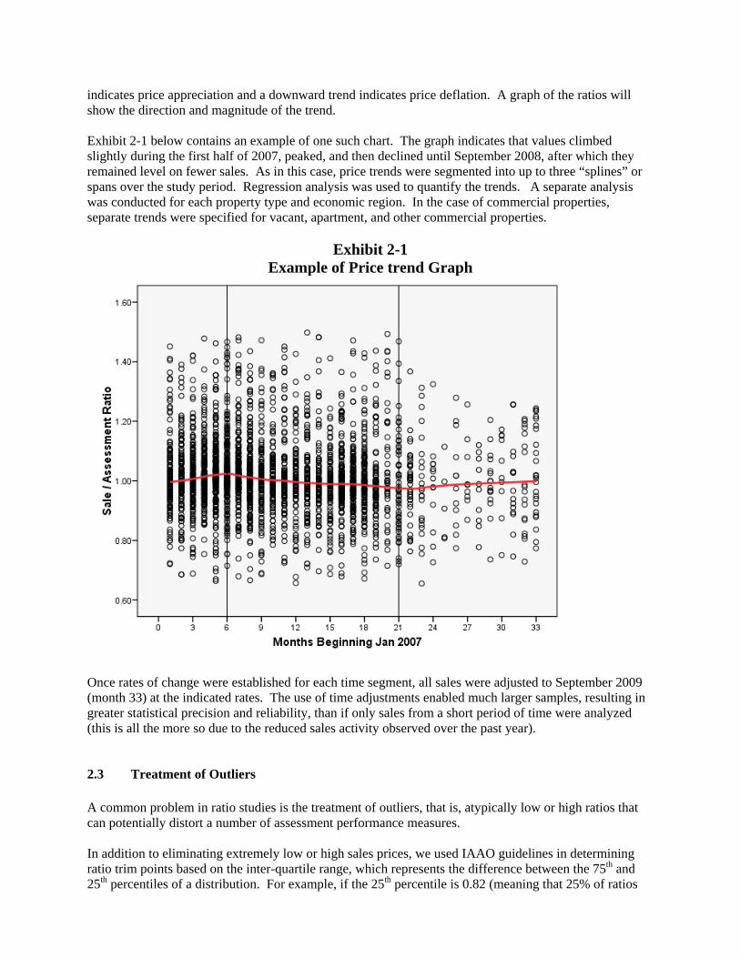
indicates price appreciation and a downward trend indicates price deflation. A graph of the ratios will show the direction and magnitude of the trend. Exhibit 2-1 below contains an example of one such chart. The graph indicates that values climbed slightly during the first half of 2007, peaked, and then declined until September 2008, after which they remained level on fewer sales. As in this case, price trends were segmented into up to three “splines” or spans over the study period. Regression analysis was used to quantify the trends. A separate analysis was conducted for each property type and economic region. In the case of commercial properties, separate trends were specified for vacant, apartment, and other commercial properties.
Exhibit 2-1 Example of Price trend Graph
Once rates of change were established for each time segment, all sales were adjusted to September 2009 (month 33) at the indicated rates. The use of time adjustments enabled much larger samples, resulting in greater statistical precision and reliability, than if only sales from a short period of time were analyzed (this is all the more so due to the reduced sales activity observed over the past year). 2.3 Treatment of Outliers A common problem in ratio studies is the treatment of outliers, that is, atypically low or high ratios that can potentially distort a number of assessment performance measures. In addition to eliminating extremely low or high sales prices, we used IAAO guidelines in determining ratio trim points based on the inter-quartile range, which represents the difference between the 75th and 25th percentiles of a distribution. For example, if the 25th percentile is 0.82 (meaning that 25% of ratios

are less than 0.82) and the 75th percentile is 1.14 (meaning that 75% of ratios are lower than 1.14 and 25% are higher), the inter-quartile range (IQR) is:
IQR = 1.14 – 0.82 = 0.32 Subtracting 1.5 IQR from the 25% percentile and adding 1.5 IQR to the 75% percentile gives the bounds used to identify statistical “outliers”. In our example, 1.5 x 0.32 = 0.48 and the cut points for identifying outliers is:
Lower bound = 0.82 – 0.48 = 0.34; Upper bound = 1.14 + 0.48 = 1.62 Thus any ratios below 0.34 or greater than 1.62 are outliers and potentially could be excluded. Similarly, adding and subtracting three IQR identifies “extremes”. In our example, 3 x 0.32 = 0.96 and the cut points for identifying extreme ratios is:
Lower bound = 0.82 – 0.96 = -0.14; Upper bound = 1.14 + 0.96 = 2.10 Since assessed value and assessment ratios cannot be negative, the lower bound defaults to 0. Trimming based on logarithms of ratios (which is equivalent to working with percentages) avoids cases like this and results in a more even balance of low and high outlier and extreme ratios. This is the approach we followed. Of course, one does not have to use exactly 1.5 or 3.0 IQRs to identify appropriate trim points, which can vary with the nature of the data distribution. Nevertheless, as a general rule, when working with logarithms of the ratios, trimming based on 1.5 IQR usually excludes less than 10% of ratios and trimming based on 3.0 IQR usually excludes less than 5% of the data. With these guidelines in mind, we determined trim points for each property type and economic area based on an examination of ratio distributions. Trim points generally range between 2.5 to 3 IQRs for residential properties and 1.5 to 2.5 IQRs for vacant land and commercial properties, where outliers were more common. Specific trim points are based on logical break points in the data. Specific trimming procedures and the percentage of sales excluded are discussed in conjunction with the ratio analyses conducted for each property type. 2.4 Statistical Analyses There are two primary aspects of assessment performance: level and uniformity. Assessment level relates to how close overall assessments are to market value. Uniformity relates to the consistency or equity of assessed values. Three measures of central tendency are used in ratio studies: the median, the mean, and the weighted mean.
Median. The median is the middle ratio when the ratios are arrayed from smallest to largest. There are an equal number of ratios above and below the median. Since it simply represents the middle ratio, the median is no more affected by extreme or “outlier” ratios than any other ratio in the sample. In other words, each ratio is afforded equal weight. The median is the most appropriate measure of central tendency when gauging whether assessments are centered on market value. According to IAAO standards, median ratios should fall between 0.90 and 1.10. A 95% confidence interval can be constructed about the calculated median to determine whether

one can conclude with 95% confidence that that the recommended standard has not been achieved.
Mean. The mean is ratio is simply the average ratio. It is computed by summing the ratios and dividing by the number of ratios. Like the median, the mean assigns equal weight to each sale; however, it is more impacted by outliers than the median. For this reason, and because it has no offsetting advantages, the mean enjoys little prominence in ratio studies. We do not report it.
Weighted Mean. The weighted mean weights each ratio based on its sale price; for example a $1 million sale has 10 times the weight of a $100,000 sale (and a $5,000,000 sale has the same weight as 100 sales of $50,000 each). Because of this weighting feature, the weighted mean is the most appropriate measure for estimating the total value of property in a jurisdiction. However, the weighted mean can be disproportionately influenced by outlier ratios, particularly if they occur for high-value sales. In our studies, the weighted mean should be viewed as a secondary, dollar-weighted measure of the assessment level.
The primary measure of assessment uniformity is the coefficient of dispersion (COD), which expresses the average percentage deviation of ratios around the median. For example, a COD of 15 means that, on average, ratios differ from the median by 15%. In general, lower CODs indicate better assessment uniformity. However, as properties become more complex and heterogeneous and as markets become thin or unstable, good CODs are more difficult (or impossible) to achieve. The IAAO offers the following guidelines for the COD:
Residential properties. CODs should be 10 or less in newer, homogeneous areas; 15 or less in older or heterogeneous areas; and 20 or less in rural, recreational, or seasonal areas. The standard of 15 could be applied to largely urban economic areas and 20 to the other economic areas covered in the present study.
Commercial properties. CODs should be 15 or less in larger, urban areas and 20 or less in rural or depressed areas with less market activity.
Vacant land. CODs should be 25 or less.
In addition to uniformity within property groups, it is important that each group be assessed at a similar percentage of market value. This aspect of assessment uniformity is termed horizontal equity. One can evaluate horizontal equity by comparing medians among property groups. A final aspect of assessment uniformity, known as vertical equity, relates to uniformity between low and high value properties. Ideally, of course, both should be assessed at a similar percentage of market value. A long-standing measure of vertical equity is the price-related differential (PRD), which is the mean assessment ratio divided by the weighted mean assessment ratio:
PRD = mean ÷ weighted mean When high value properties are under-assessed relative to other properties, the weighted mean falls below the mean and the PRD climbs above 1.00, signaling “assessment regressivity”. When high value properties are relatively over-assessed, the weighted mean exceeds the mean and the PRD falls below 1.00, signaling “assessment progressivity”. Because the mean and weighted mean are both impacted by outliers and because the weighted mean is highly sensitive to ratios for the highest value properties, the PRD provides only a crude, inadequate gauge of price-related bias. In addition, the PRD lacks intuitive appeal as one can only say that PRDs near 1.00 are preferred to PRDs farther from 1.00.
We report a superior measure obtained by regressing percentage differences from the median assessment ratio on percentage differences from the median value1. The coefficient from the regression quantifies the relationship (if any) between property values and assessment levels. For example, a coefficient of -0.05 indicates that a doubling of values (an increase of 100%) is associated with a 5% decline in assessment level. Regression analysis also quantifies the statistical strength or significance of the relationship. If no price-related bias is present, the coefficient from the regression will not be significantly different from zero. We suggest that price-related bias should be noted when (a) the regression coefficient is less than -0.03 or greater than 0.03 and (b) the relationship is statistically significant at the 95% confidence level. Regression coefficients below -0.05 should be viewed with concern, again assuming they are significant at the 95% confidence level.
1 The dependent variable in the analysis is (Sale Ratio – Median Ratio)/Median Ratio. The independent variable is: Ln(Property Value/Median Value)/0.693. The use of logarithms converts the analysis to percentages and division by 0.693 (the natural logarithm of 2) permits each doubling of value to be associated with an increment of 1 (i.e. transforms the logs from natural logs to base 2 logs). Thus, for example, a coefficient of -0.024 means that the assessment level falls by 2.4% whenever value doubles (and increases by 2.4% whenever values are halved). For technical reasons, value is computed as ½ of time-adjusted sale price plus ½ of assessed value to avoid statistical bias that would overstate the degree of regressivity (or understate the degree of progressivity).

3. Improved Residential Analyses
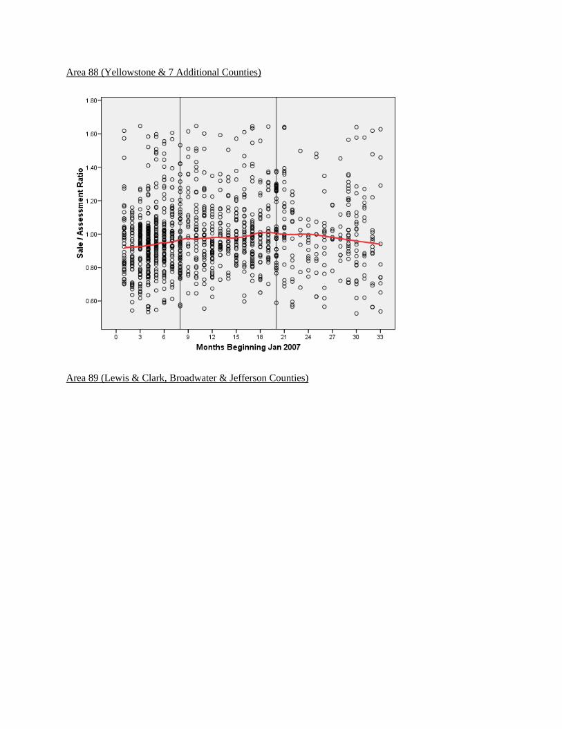
3.1 Residential Price Trends Sales from 2007 through September of 2009 were analyzed to develop the price trends shown in Exhibit 3-1 below. Exhibit 3-2 shows the trends graphically. Appendix A-1 contains graphs of the underlying data in each economic area.
Exhibit 3-1 Improved Residential Price Trend Periods and Factors
Area Start End Rate Start End Rate Start End Rate
81 Jan 07 Jul 07 0.004 Aug 07 Jan 08 ‐0.006 Feb 08 Sep 09 0.000
82 Jan 07 Jul 07 0.008 Aug 07 Jan 08 0.000 Feb 08 Sep 09 0.003
84 Jan 07 Aug 07 0.005 Sep 07 Aug 08 ‐0.001 Sep 08 Sep 09 ‐0.002
85 Jan 07 Jun 07 0.004 Jul 07 Sep 08 ‐0.003 Oct 08 Sep 09 0.000
87 Jan 07 Dec 07 0.008 Jan 08 Aug 08 0.000 Sep 08 Sep 09 0.004
88 Jan 07 Jul 07 0.006 Aug 07 Oct 08 0.002 Nov 08 Sep 09 0.000
89 Jan 07 Jun 07 0.011 Jul 07 May 08 0.000 Jun 08 Sep 09 ‐0.003
90 Jan 07 Jul 07 0.018 Aug 07 Jun 08 0.005 Jul 08 Sep 09 0.000
91 Jan 07 Jul 07 0.016 Aug 07 Jun 08 ‐0.004 Jul 08 Sep 09 0.000
Exhibit 3-2 Graph of Improved Residential Price Trends
3.2 Residential Outlier Analysis
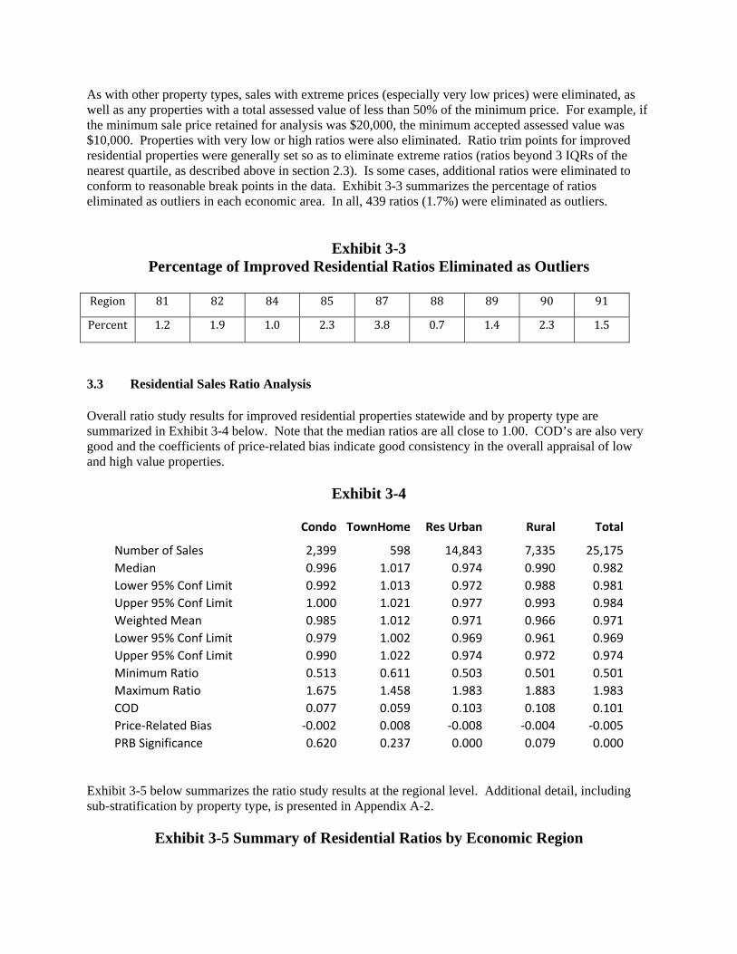
As with other property types, sales with extreme prices (especially very low prices) were eliminated, as well as any properties with a total assessed value of less than 50% of the minimum price. For example, if the minimum sale price retained for analysis was $20,000, the minimum accepted assessed value was $10,000. Properties with very low or high ratios were also eliminated. Ratio trim points for improved residential properties were generally set so as to eliminate extreme ratios (ratios beyond 3 IQRs of the nearest quartile, as described above in section 2.3). Is some cases, additional ratios were eliminated to conform to reasonable break points in the data. Exhibit 3-3 summarizes the percentage of ratios eliminated as outliers in each economic area. In all, 439 ratios (1.7%) were eliminated as outliers.
Exhibit 3-3 Percentage of Improved Residential Ratios Eliminated as Outliers
Region 81 82 84 85 87 88 89 90 91
Percent 1.2 1.9 1.0 2.3 3.8 0.7 1.4 2.3 1.5
3.3 Residential Sales Ratio Analysis Overall ratio study results for improved residential properties statewide and by property type are summarized in Exhibit 3-4 below. Note that the median ratios are all close to 1.00. COD’s are also very good and the coefficients of price-related bias indicate good consistency in the overall appraisal of low and high value properties.
Exhibit 3-4
Condo TownHome Res Urban Rural Total
Number of Sales 2,399 598 14,843 7,335 25,175
Median 0.996 1.017 0.974 0.990 0.982
Lower 95% Conf Limit 0.992 1.013 0.972 0.988 0.981
Upper 95% Conf Limit 1.000 1.021 0.977 0.993 0.984
Weighted Mean 0.985 1.012 0.971 0.966 0.971
Lower 95% Conf Limit 0.979 1.002 0.969 0.961 0.969
Upper 95% Conf Limit 0.990 1.022 0.974 0.972 0.974
Minimum Ratio 0.513 0.611 0.503 0.501 0.501
Maximum Ratio 1.675 1.458 1.983 1.883 1.983
COD 0.077 0.059 0.103 0.108 0.101
Price‐Related Bias ‐0.002 0.008 ‐0.008 ‐0.004 ‐0.005
PRB Significance 0.620 0.237 0.000 0.079 0.000 Exhibit 3-5 below summarizes the ratio study results at the regional level. Additional detail, including sub-stratification by property type, is presented in Appendix A-2.
Exhibit 3-5 Summary of Residential Ratios by Economic Region

Region 81 82 84 85 87 88 89 90 91
Number of Sales 2,610 3,699 3,949 3,390 1,361 6,263 2,138 1,339 426
Median 1.004 0.953 1.020 1.023 0.904 0.966 0.980 0.920 0.963
Lower 95% Conf Limit 1.000 0.949 1.016 1.020 0.893 0.964 0.972 0.908 0.949
Upper 95% Conf Limit 1.008 0.955 1.023 1.027 0.912 0.968 0.988 0.931 0.983
Weighted Mean 0.979 0.949 1.002 0.990 0.889 0.961 0.960 0.898 0.926
Lower 95% Conf Limit 0.970 0.945 0.997 0.981 0.879 0.959 0.953 0.887 0.906
Upper 95% Conf Limit 0.988 0.953 1.007 1.000 0.899 0.964 0.967 0.910 0.945
Minimum Ratio 0.562 0.552 0.601 0.501 0.506 0.554 0.534 0.509 0.508
Maximum Ratio 1.475 1.686 1.491 1.555 1.746 1.499 1.787 1.983 1.528
COD 0.080 0.091 0.079 0.095 0.163 0.075 0.115 0.203 0.128
Price‐Related Bias ‐0.022 ‐0.018 ‐0.023 ‐0.011 ‐0.057 ‐0.014 ‐0.029 ‐0.111 ‐0.036
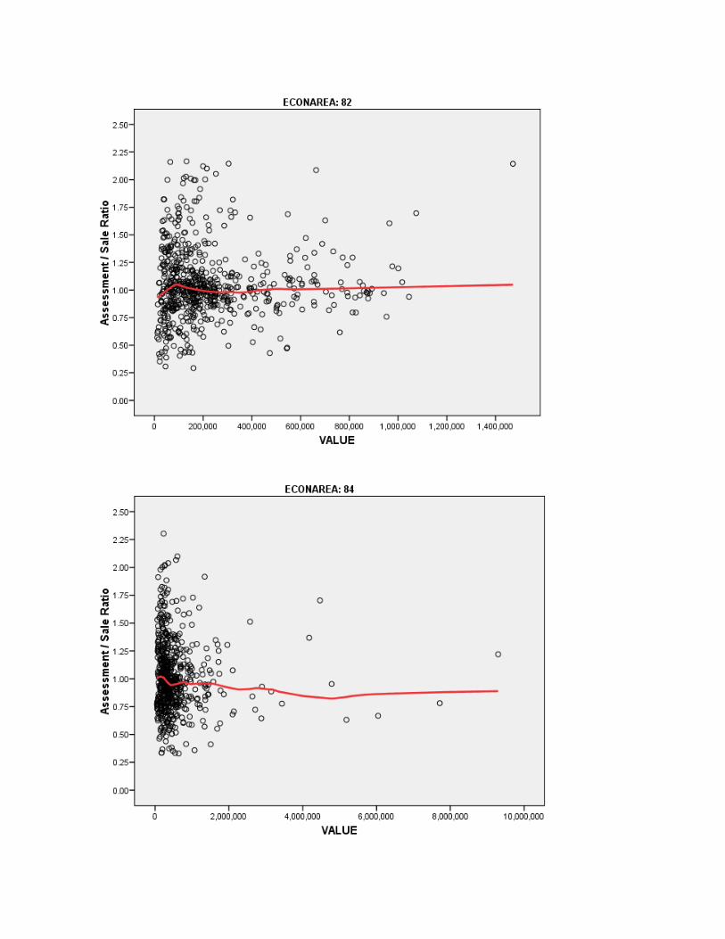
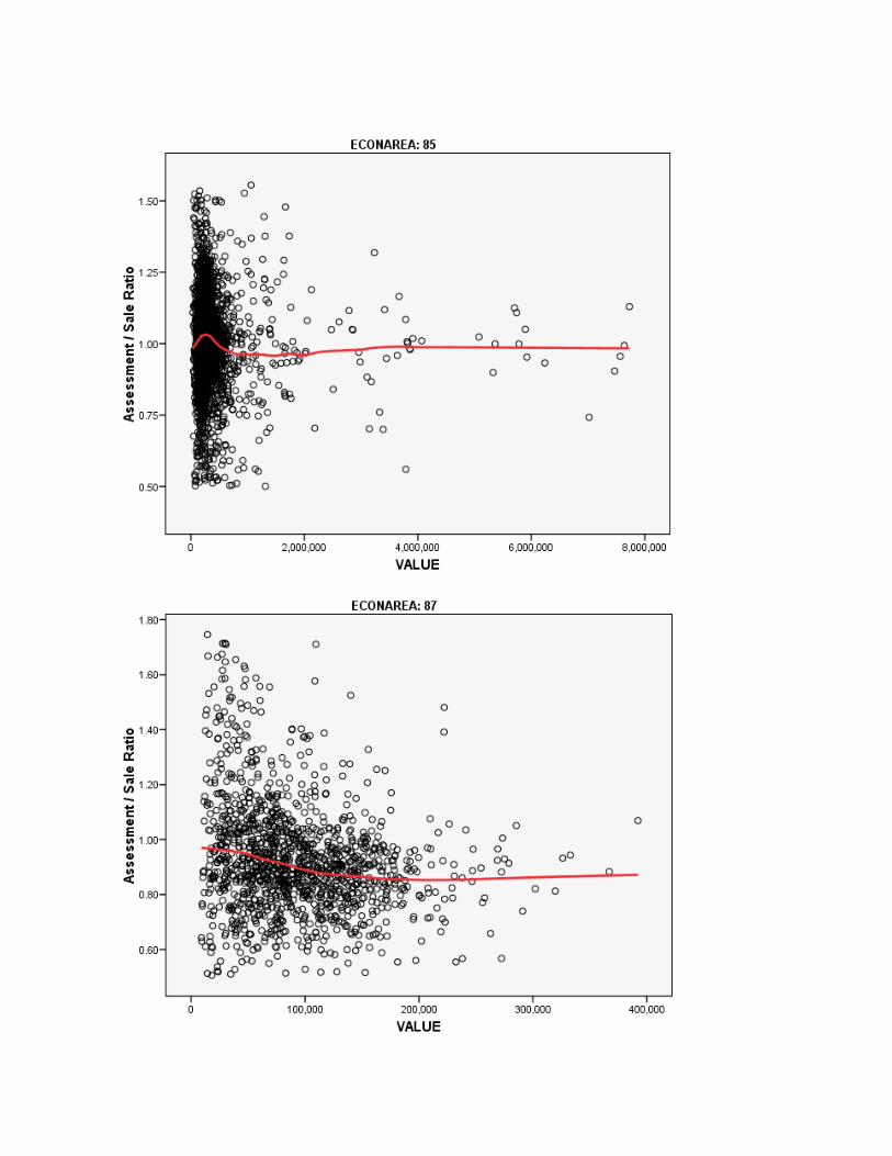
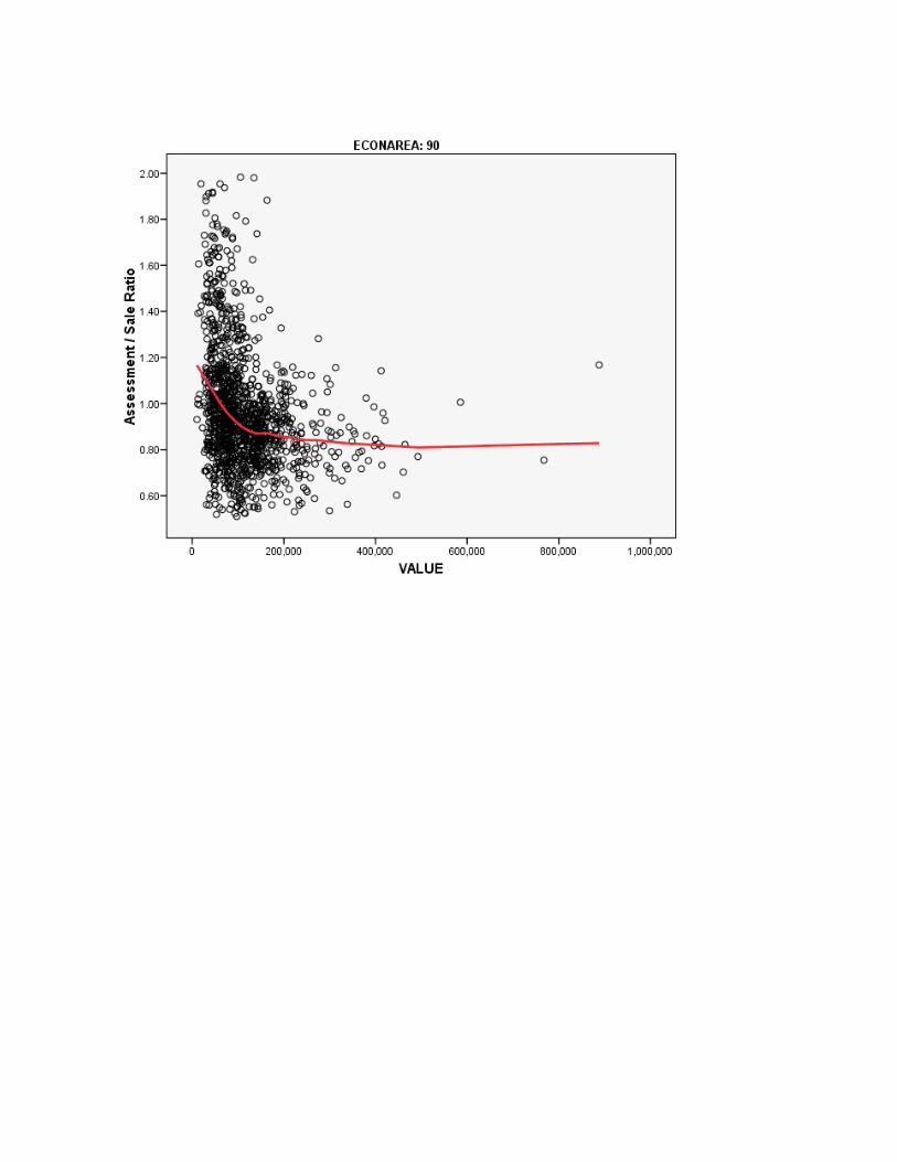
PRB Significance 0.000 0.000 0.000 0.000 0.000 0.000 0.000 0.000 0.001 Note that median ratios for all nine economic areas range between 0.904 and 1.023, indicating that assessment ratios are closely centered on market value. All fall within the range of 0.90 to 1.10 recommended by IAAO. Coefficients of dispersion (CODs), which measure the average percentage deviation from the median, are less than 15% in seven of the nine economic areas, and 10% or less in five areas, indicating excellent uniformity in values. The COD of 16.3% for area 87 is reasonable for this diverse group of rural counties (largely eastern Montana) and complies with the recommended IAAO standard of 20% for rural areas. The most problematic COD is 20.3% for area 90 (Butte-Silver Bow, Powell, Anaconda-Deer Lodge, Granite counties), which is arguably the most difficult of the nine areas because the age and generally low value of properties. A review of the sales ratio graph for this area in Appendix A-3 will reveal a large number of high ratios for the lowest value properties, which are too numerous to be dismissed as outliers. If sales below $50,000 are omitted, the COD improves to 17.6%, and the coefficient of price-related bias improves to -0.060 (still outside of the recommended range). The coefficient of price-related bias (PRB) is negative in all nine areas, meaning that ratios tend to decline with value. However, the coefficients are within the recommended range of -0.03 to +.03 in six of the nine areas and below -0.05 in only areas 87 and 90. A review of the ratio graphs for these areas in Appendix A-3 will reveal that this is largely a function of high ratios for the lowest value properties (particularly in area 90, as discussed above). Overall, residential ratios remain good as of September 2009. Assessment levels are reasonably close to 1.00 and, with a few problematic areas noted above, uniformity in values is good.
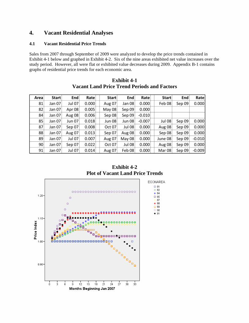
4. Vacant Residential Analyses 4.1 Vacant Residential Price Trends Sales from 2007 through September of 2009 were analyzed to develop the price trends contained in Exhibit 4-1 below and graphed in Exhibit 4-2. Six of the nine areas exhibited net value increases over the study period. However, all were flat or exhibited value decreases during 2009. Appendix B-1 contains graphs of residential price trends for each economic area.
Exhibit 4-1 Vacant Land Price Trend Periods and Factors
Area Start End Rate Start End Rate Start End Rate
81 Jan 07 Jul 07 0.000 Aug 07 Jan 08 0.000 Feb 08 Sep 09 0.000
82 Jan 07 Apr 08 0.005 May 08 Sep 09 0.000
84 Jan 07 Aug 08 0.006 Sep 08 Sep 09 ‐0.010
85 Jan 07 Jun 07 0.018 Jun 08 Jun 08 ‐0.007 Jul 08 Sep 09 0.000
87 Jan 07 Sep 07 0.008 Oct 07 Jul 08 0.000 Aug 08 Sep 09 0.000
88 Jan 07 Aug 07 0.013 Sep 07 Aug 08 0.000 Sep 08 Sep 09 0.000
89 Jan 07 Jul 07 0.007 Aug 07 May 08 0.000 June 08 Sep 09 ‐0.010
90 Jan 07 Sep 07 0.022 Oct 07 Jul 08 0.000 Aug 08 Sep 09 0.000
91 Jan 07 Jul 07 0.014 Aug 07 Feb 08 0.000 Mar 08 Sep 09 ‐0.009
Exhibit 4-2 Plot of Vacant Land Price Trends

4.2 Vacant Residential Outlier Analysis
Sales with very low and a few very high time-adjusted sales prices were removed, as well as any properties with a total assessed value of less than 50% of the minimum retained price. This was followed by an analysis of ratio outliers. Ratios more than 1.5 IQR (inter-quartile range) were identified and further scrutinized so as to set cut point at logical break points. Exhibit 4-3 shows the percentage of properties deleted as ratio outliers in each economic area. A total of 446 sales (6.7%) were eliminated in this manner. The percentage is much greater than for residential properties (1.7%) because of the much wider dispersion in the data.
Exhibit 4-3 Percentage of Vacant Residential Ratios Eliminated as Outliers
Region 81 82 84 85 87 88 89 90 91
Percent 5.1 8.3 6.3 5.5 9.7 5.9 9.0 11.3 5.5
4.3 Vacant Residential Sales Ratio Analysis Exhibit 4-4 below shows vacant residential ratios for urban and rural properties. The overall median ratio of 0.989 indicates that assessed values are closely centered on market value. There is also very good overall equity between urban and rural vacant land as indicated by their similar medians: 0.977 and 0.994, respectively. The COD statistics are reasonably good for vacant land and fall within the IAAO recommended upper limit of 0.250. Overall, there is no price-related bias for urban land and minimal regressivity for rural land.
Exhibit 4-4 Vacant Residential Sales Ratios
2192 .977 .925 .301 1.943 .197 .008 .059
3973 .994 .953 .288 2.320 .241 -.017 .000
6165 .989 .945 .288 2.320 .226 -.002 .456
Group1 Urban
2 Rural
Overall
Sales Median Wtd Mean Minimum Maximum COD Coefficient Significance
Price-Related Bias
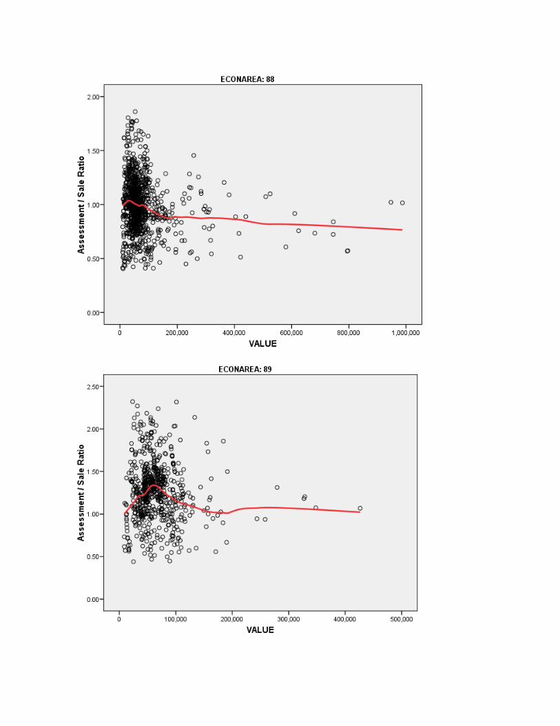
Exhibit 4-5 below presents vacant residential ratio statistics by economic area. Median ratios in areas 87 and 89 fall below the IAAO recommended lower limit of 0.90. However, in both areas the upper 95% confidence limit exceeds 0.95, although barely so in area 90. The median ratio in area 89 (Broadwater, Jefferson, and Lewis & Clark counties) is 1.265, well above the IAAO recommended upper limit of 1.10, and the lower 95% confidence limit of 1.240 is also well above 1.10. This area had a median ratio of 1.103 in our prior study and, as indicated in Exhibit 4-1 and shown graphically in Appendix A-2, has continued to depreciate at a rate of 1.0 per month since June 2008. To confirm the reasonability of the estimated median ratio of 1.265, ratios were run for area 89 using unadjusted sales prices from 2009 only. The median ratio for 61 such sales is 1.259.
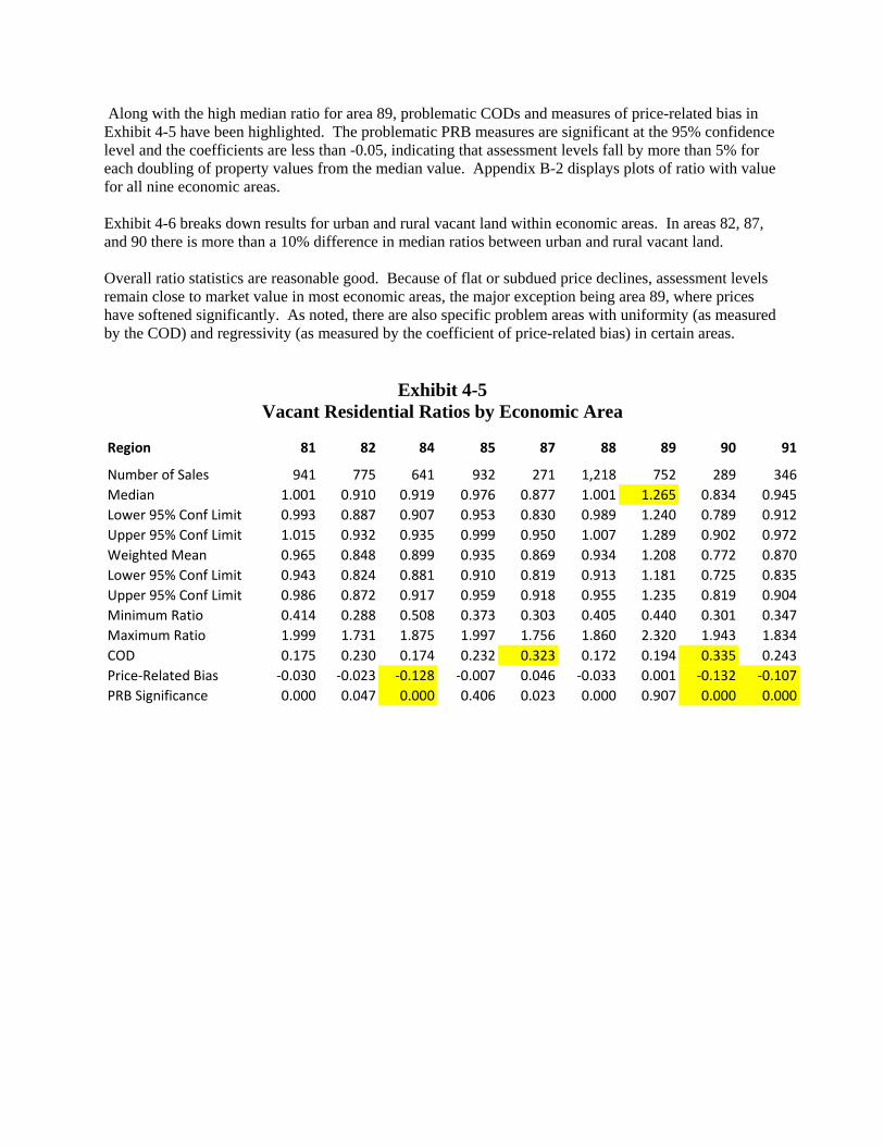
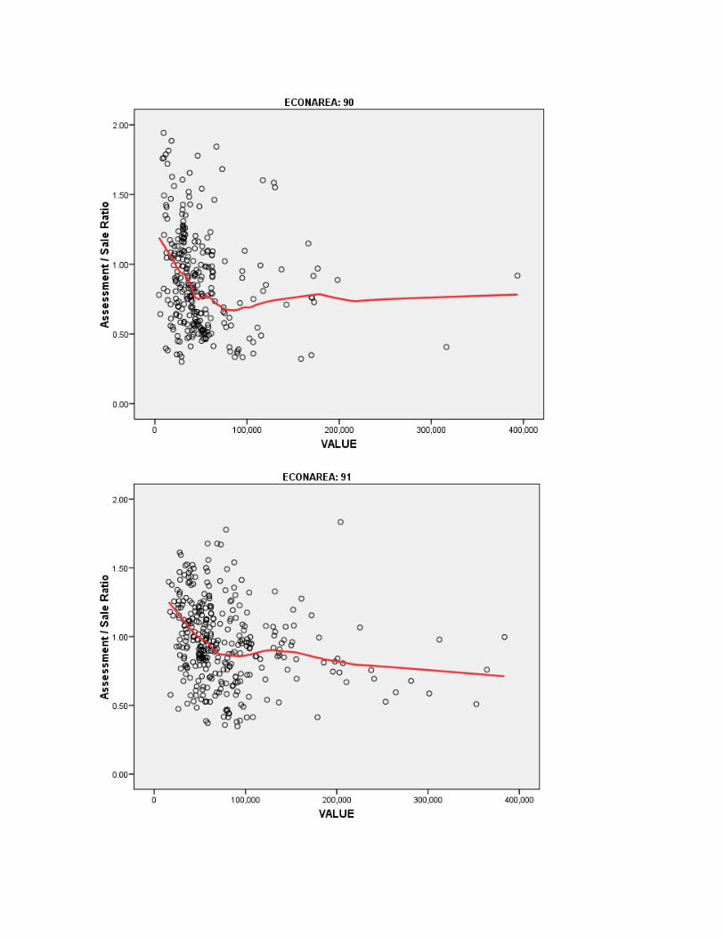
Along with the high median ratio for area 89, problematic CODs and measures of price-related bias in Exhibit 4-5 have been highlighted. The problematic PRB measures are significant at the 95% confidence level and the coefficients are less than -0.05, indicating that assessment levels fall by more than 5% for each doubling of property values from the median value. Appendix B-2 displays plots of ratio with value for all nine economic areas. Exhibit 4-6 breaks down results for urban and rural vacant land within economic areas. In areas 82, 87, and 90 there is more than a 10% difference in median ratios between urban and rural vacant land. Overall ratio statistics are reasonable good. Because of flat or subdued price declines, assessment levels remain close to market value in most economic areas, the major exception being area 89, where prices have softened significantly. As noted, there are also specific problem areas with uniformity (as measured by the COD) and regressivity (as measured by the coefficient of price-related bias) in certain areas.
Exhibit 4-5 Vacant Residential Ratios by Economic Area
Region 81 82 84 85 87 88 89 90 91
Number of Sales 941 775 641 932 271 1,218 752 289 346
Median 1.001 0.910 0.919 0.976 0.877 1.001 1.265 0.834 0.945
Lower 95% Conf Limit 0.993 0.887 0.907 0.953 0.830 0.989 1.240 0.789 0.912
Upper 95% Conf Limit 1.015 0.932 0.935 0.999 0.950 1.007 1.289 0.902 0.972
Weighted Mean 0.965 0.848 0.899 0.935 0.869 0.934 1.208 0.772 0.870
Lower 95% Conf Limit 0.943 0.824 0.881 0.910 0.819 0.913 1.181 0.725 0.835
Upper 95% Conf Limit 0.986 0.872 0.917 0.959 0.918 0.955 1.235 0.819 0.904
Minimum Ratio 0.414 0.288 0.508 0.373 0.303 0.405 0.440 0.301 0.347
Maximum Ratio 1.999 1.731 1.875 1.997 1.756 1.860 2.320 1.943 1.834
COD 0.175 0.230 0.174 0.232 0.323 0.172 0.194 0.335 0.243
Price‐Related Bias ‐0.030 ‐0.023 ‐0.128 ‐0.007 0.046 ‐0.033 0.001 ‐0.132 ‐0.107
PRB Significance 0.000 0.047 0.000 0.406 0.023 0.000 0.907 0.000 0.000
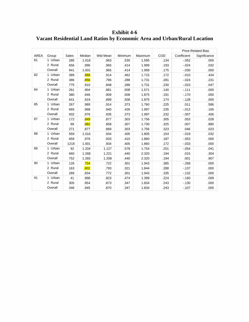
Exhibit 4-6 Vacant Residential Land Ratios by Economic Area and Urban/Rural Location
285 1.018 .963 .530 1.595 .134 -.052 .000
656 .996 .965 .414 1.999 .193 -.024 .032
941 1.001 .965 .414 1.999 .175 -.030 .000
389 .968 .914 .462 1.715 .172 -.010 .434
386 .856 .796 .288 1.731 .281 -.024 .231
775 .910 .848 .288 1.731 .230 -.023 .047
261 .904 .881 .508 1.571 .140 -.111 .000
380 .946 .909 .508 1.875 .191 -.170 .000
641 .919 .899 .508 1.875 .174 -.128 .000
267 .989 .914 .373 1.760 .225 .011 .586
665 .968 .940 .426 1.997 .235 -.012 .165
932 .976 .935 .373 1.997 .232 -.007 .406
172 .849 .877 .303 1.756 .305 .053 .028
99 .982 .858 .307 1.730 .325 .007 .880
271 .877 .869 .303 1.756 .323 .046 .023
559 1.016 .934 .405 1.805 .154 -.019 .032
659 .976 .933 .410 1.860 .187 -.053 .000
1218 1.001 .934 .405 1.860 .172 -.033 .000
92 1.204 1.127 .578 1.754 .201 -.054 .041
660 1.268 1.221 .440 2.320 .194 .015 .304
752 1.265 1.208 .440 2.320 .194 .001 .907
126 .754 .722 .301 1.943 .385 -.268 .000
163 .902 .793 .321 1.844 .288 -.137 .000
289 .834 .772 .301 1.943 .335 -.132 .000
41 .898 .823 .474 1.399 .224 -.160 .009
305 .954 .873 .347 1.834 .243 -.130 .000
346 .945 .870 .347 1.834 .243 -.107 .000
Group1 Urban 2 Rural Overall
1 Urban 2 Rural Overall
1 Urban 2 Rural Overall
1 Urban 2 Rural Overall
1 Urban 2 Rural Overall
1 Urban 2 Rural Overall
1 Urban 2 Rural Overall
1 Urban 2 Rural Overall
1 Urban 2 Rural Overall
AREA81
82
84
85
87
88
89
90
91
Sales Median Wtd Mean Minimum Maximum COD Coefficient Significance
Price-Related Bias

5. Commercial Analyses 5.1 Commercial Price Trends To obtain adequate data for analysis, sales from 2005 through September 2009 were used for commercial properties. As with other property types, all sales were adjusted to September 2009. Price trends were developed by property type (vacant, apartment, and other commercial) where possible. Five of the nine areas showed no discernable difference among property types. In several areas the apartment market peaked earlier than the commercial market. In areas 87 and 89 values continued to appreciate to the end of the period. The other areas turned flat or, in the case of apartments in area 85, declined in value after peaking in 2008 or before. Exhibit 5-1 below summarizes price trends for each economic area and property type. Appendix C-1 contains price trend graphs for each economic area. 5.2 Commercial Outlier Analysis Very low and a few very high time-adjusted sales prices, as well as any properties with a total assessed value of less than 50% of the minimum retained price, were removed. An analysis of ratio outliers was also conducted. Ratios more than 1.5 IQR (inter-quartile range) were identified and further scrutinized so as to set cut point at logical breaks. The table below shows the number and percentage of sales removed as ratio outliers in each economic area.
Econ Area 81 82 84 85 87 88 89 90 91 81
Number 50 64 57 50 22 44 35 32 15 369
Percent 9.4 8.8 7.9 7.8 5.6 6.1 10.6 9.8 11.4 8.15 In all, 369 sales (8.1%) were removed as outlier ratios.

Exhibit 5-1
Commercial Price Trend Periods and Factors Region 81 Start End Rate Start End Rate Start End Rate
Vacant Jan 05 Sep 07 0.006 Oct 07 Jun 08 0 Jul 08 Sep 09 0
Apartment Jan 05 Sep 07 0.006 Oct 07 Jun 08 0 Jul 08 Sep 09 0
Commercial Jan 05 Sep 07 0.006 Oct 07 Jun 08 0 Jul 08 Sep 09 0
Region 82 Start End Rate Start End Rate
Vacant Jan 05 Jul 05 0 Aug 05 Dec 07 0.005 Jan 08 Sep 09 0
Apartment Jan 05 Jul 05 0 Aug 05 Dec 07 0.005 Jan 08 Sep 09 0
Commercial Jan 05 Jul 05 0 Aug 05 Dec 07 0.005 Jan 08 Sep 09 0
Region 84 Start End Rate Start End Rate
Vacant Jan 05 Dec 07 0.004 Jan 08 Sep 09 0
Apartment Jan 05 Oct 07 0.003 Nov 07 Sep 09 0
Commercial Jan 05 Dec 05 0 Jan 06 Oct 06 0.013 Nov 06 Sep 09 0
Region 85 Start End Rate Start End Rate
Vacant Jan 05 Mar 09 0.008 Apr 09 Sep 09 0
Apartment Jan 05 Aug 06 0.010 Sep 06 Sep 09 ‐0.003
Commercial Jan 05 Mar 06 0.020 Apr 06 Apr 08 0.003 May 08 Sep 09 0
Region 87 Start End Rate Start End Rate
Vacant Jan 05 Sep 09 0.005
Apartment Jan 05 Sep 09 0.005
Commercial Jan 05 Sep 09 0.005
Region 88 Start End Rate Start End Rate
Vacant Jan 05 Apr 08 0.010 Apr 08 Sep 09 0
Apartment Jan 05 Sep 09 0
Commercial Jan 05 Dec 08 0.006 Jan 09 Sep 09 0
Region 89 Start End Rate Start End Rate
Vacant Jan 05 Jun 06 0.012 Jul 06 Sep 09 0.002
Apartment Jan 05 Jun 06 0.012 Jul 06 Sep 09 0.002
Commercial Jan 05 Jun 06 0.012 Jul 06 Sep 09 0.002
Region 90 Start End Rate Start End Rate
Vacant Jan 05 Mar 08 0.0095 Apr 08 Sep 09 0
Apartment Jan 05 Dec 07 0.006 Jan 08 Jan 09 0
Commercial Jan 05 Mar 08 0.0095 Apr 08 Sep 09 0
Region 91 Start End Rate Start End Rate Start End Rate
Vacant Jan 05 Sep 05 0 Oct 05 Jun 07 0.016 Jul 07 Sep 09 0
Apartment Jan 05 Sep 05 0 Oct 05 Jun 07 0.016 Jul 07 Sep 09 0
Commercial Jan 05 Sep 05 0 Oct 05 Jun 07 0.016 Jul 07 Sep 09 0 5.3 Commercial Sales Ratio Analysis
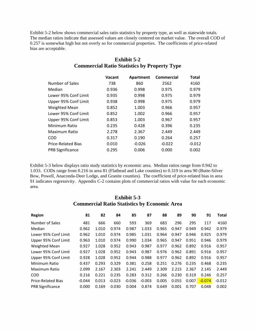
Exhibit 5-2 below shows commercial sales ratio statistics by property type, as well as statewide totals. The median ratios indicate that assessed values are closely centered on market value. The overall COD of 0.257 is somewhat high but not overly so for commercial properties. The coefficients of price-related bias are acceptable.
Exhibit 5-2 Commercial Ratio Statistics by Property Type
Vacant Apartment Commercial Total
Number of Sales 738 860 2562 4160
Median 0.936 0.998 0.975 0.979
Lower 95% Conf Limit 0.935 0.998 0.975 0.979
Upper 95% Conf Limit 0.938 0.998 0.975 0.979
Weighted Mean 0.852 1.003 0.966 0.957
Lower 95% Conf Limit 0.852 1.002 0.966 0.957
Upper 95% Conf Limit 0.853 1.003 0.967 0.957
Minimum Ratio 0.235 0.428 0.396 0.235
Maximum Ratio 2.278 2.367 2.449 2.449
COD 0.317 0.190 0.264 0.257
Price‐Related Bias 0.010 ‐0.026 ‐0.022 ‐0.012
PRB Significance 0.295 0.006 0.000 0.002 Exhibit 5-3 below displays ratio study statistics by economic area. Median ratios range from 0.942 to 1.033. CODs range from 0.216 in area 81 (Flathead and Lake counties) to 0.319 in area 90 (Butte-Silver Bow, Powell, Anaconda-Deer Lodge, and Granite counties). The coefficient of price-related bias in area 91 indicates regressivity. Appendix C-2 contains plots of commercial ratios with value for each economic area.
Exhibit 5-3 Commercial Ratio Statistics by Economic Area
Region 81 82 84 85 87 88 89 90 91 Total
Number of Sales 481 666 660 593 369 683 296 295 117 4160
Median 0.962 1.010 0.974 0.987 1.033 0.965 0.947 0.949 0.942 0.979
Lower 95% Conf Limit 0.962 1.010 0.974 0.985 1.031 0.964 0.947 0.946 0.925 0.979
Upper 95% Conf Limit 0.963 1.010 0.974 0.990 1.034 0.965 0.947 0.951 0.946 0.979
Weighted Mean 0.927 1.028 0.952 0.943 0.987 0.977 0.962 0.892 0.916 0.957
Lower 95% Conf Limit 0.927 1.028 0.952 0.943 0.987 0.976 0.962 0.891 0.916 0.957
Upper 95% Conf Limit 0.928 1.028 0.952 0.944 0.988 0.977 0.962 0.892 0.916 0.957
Minimum Ratio 0.437 0.293 0.329 0.381 0.258 0.251 0.276 0.235 0.468 0.235
Maximum Ratio 2.099 2.167 2.303 2.241 2.449 2.309 2.215 2.367 2.145 2.449
COD 0.216 0.221 0.235 0.283 0.312 0.266 0.230 0.319 0.246 0.257
Price‐Related Bias ‐0.044 0.013 ‐0.023 ‐0.036 ‐0.003 0.005 0.055 0.007 ‐0.074 ‐0.012
PRB Significance 0.000 0.169 0.030 0.004 0.874 0.649 0.001 0.707 0.048 0.002

Exhibit 5-4 presents ratio statistics by property types within economic areas. Median and weighted mean ratios for vacant land are below 0.90 in areas 81, 85, 90, and 91. Vacant land CODs are above 0.350 in areas 84, 87, and 90. Problematic coefficients of price-related bias have also been highlighted. Aside from these specific problems, commercial ratios look reasonably good for such a heterogeneous and difficult-to-value property type. Except for vacant land in certain areas, overall levels of appraisal consistently range from 0.90 to 1.00, indicating good uniformity in the appraisal of residential and commercial properties.
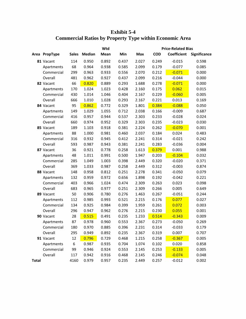
Exhibit 5-4 Commercial Ratios by Property Type within Economic Area
Wtd Price‐Related Bias
Area PropType Sales Median Mean Min Max COD Coefficient Significance
81 Vacant 114 0.950 0.892 0.437 2.027 0.249 ‐0.015 0.598
Apartments 68 0.964 0.938 0.585 2.099 0.179 ‐0.077 0.085
Commercial 299 0.963 0.933 0.556 2.070 0.212 ‐0.071 0.000
Overall 481 0.962 0.927 0.437 2.099 0.216 ‐0.044 0.000
82 Vacant 66 0.820 0.889 0.293 1.688 0.278 ‐0.071 0.000
Apartments 170 1.024 1.023 0.428 2.160 0.175 0.062 0.015
Commercial 430 1.014 1.046 0.404 2.167 0.229 ‐0.060 0.005
Overall 666 1.010 1.028 0.293 2.167 0.221 0.013 0.169
84 Vacant 95 0.862 0.772 0.329 1.801 0.384 ‐0.088 0.050
Apartments 149 1.029 1.055 0.712 2.038 0.166 ‐0.009 0.687
Commercial 416 0.957 0.944 0.537 2.303 0.233 ‐0.028 0.024
Overall 660 0.974 0.952 0.329 2.303 0.235 ‐0.023 0.030
85 Vacant 189 1.103 0.918 0.381 2.224 0.262 ‐0.070 0.001
Apartments 88 1.000 0.981 0.460 2.037 0.184 0.024 0.483
Commercial 316 0.932 0.945 0.412 2.241 0.314 ‐0.021 0.242
Overall 593 0.987 0.943 0.381 2.241 0.283 ‐0.036 0.004
87 Vacant 36 0.921 0.778 0.258 1.613 0.379 0.001 0.988
Apartments 48 1.011 0.991 0.500 1.947 0.203 ‐0.104 0.032
Commercial 285 1.049 1.003 0.398 2.449 0.320 ‐0.020 0.371
Overall 369 1.033 0.987 0.258 2.449 0.312 ‐0.003 0.874
88 Vacant 148 0.958 0.812 0.251 2.278 0.341 ‐0.050 0.079
Apartments 132 0.959 0.972 0.656 1.898 0.192 ‐0.042 0.221
Commercial 403 0.966 1.024 0.474 2.309 0.263 0.023 0.098
Overall 683 0.965 0.977 0.251 2.309 0.266 0.005 0.649
89 Vacant 50 0.906 0.780 0.276 1.463 0.267 ‐0.051 0.244
Apartments 112 0.985 0.993 0.521 2.215 0.176 0.077 0.027
Commercial 134 0.925 0.984 0.399 1.959 0.261 0.072 0.003
Overall 296 0.947 0.962 0.276 2.215 0.230 0.055 0.001
90 Vacant 28 0.515 0.491 0.235 1.233 0.514 ‐0.343 0.009
Apartments 87 0.978 0.960 0.553 2.367 0.273 ‐0.050 0.269
Commercial 180 0.970 0.885 0.396 2.231 0.314 ‐0.033 0.179
Overall 295 0.949 0.892 0.235 2.367 0.319 0.007 0.707
91 Vacant 12 0.796 0.729 0.468 1.215 0.258 ‐0.367 0.005
Apartments 6 0.987 0.935 0.704 1.074 0.102 0.020 0.858
Commercial 99 0.946 0.924 0.553 2.145 0.253 ‐0.133 0.005
Overall 117 0.942 0.916 0.468 2.145 0.246 ‐0.074 0.048
Total 4160 0.979 0.957 0.235 2.449 0.257 ‐0.012 0.002

Appendix A-1: Residential Price Trend Plots
Area 81 (Flathead & Lake Counties)
Months Beginning Jan 200733302724211815129630
Sal
e / A
sses
smen
t R
atio
1.40
1.30
1.20
1.10
1.00
0.90
0.80
0.70
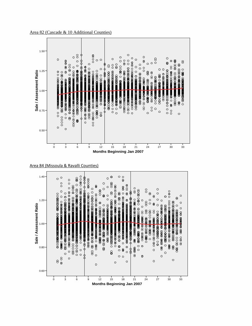
Area 82 (Cascade & 10 Additional Counties)
Months Beginning Jan 200733302724211815129630
Sal
e / A
sses
smen
t R
atio
1.50
1.25
1.00
0.75
0.50
Area 84 (Missoula & Ravalli Counties)
Months Beginning Jan 200733302724211815129630
Sal
e / A
sses
smen
t R
atio
1.40
1.20
1.00
0.80
0.60

Area 85 (Gallatin, Madison, Beaver, Park Counties)
Months Beginning Jan 2007
33302724211815129630
Sal
e / A
sses
smen
t R
atio
1.60
1.40
1.20
1.00
0.80
0.60
Area 87 (Custer & 17 Additional Counties)
Months Beginning Jan 200733302724211815129630
Sal
e / A
sses
smen
t R
atio
1.50
1.25
1.00
0.75
0.50

Area 88 (Yellowstone & 7 Additional Counties)
Months Beginning Jan 200733302724211815129630
Sal
e / A
sses
smen
t R
atio
1.60
1.40
1.20
1.00
0.80
0.60
Area 89 (Lewis & Clark, Broadwater & Jefferson Counties)
Months Beginning Jan 200733302724211815129630
Sal
e / A
sses
smen
t R
atio
1.60
1.40
1.20
1.00
0.80
0.60

Area 90 (Butte-Silver Bow, Powell, Anaconda-Deer Lodge, Granite Counties)
Months Beginning Jan 200733302724211815129630
Sal
e / A
sses
smen
t R
atio
1.50
1.25
1.00
0.75
0.50
Area 91 (Sanders, Mineral & Lincoln Counties)
Months Beginning Jan 200733302724211815129630
Sal
e / A
sses
smen
t R
atio
1.60
1.40
1.20
1.00
0.80
0.60

Appendix A-2: Improved Residential Ratios by Economic Area and Property Type
Area Property Type Sales MedianLower Bound
Upper Bound
Wtd Mean
Lower Bound
Upper Bound Min Max COD
PRB Coef.
PRB Sig.
81 Condo Urban 204 1.00 0.98 1.01 0.97 0.95 0.99 0.60 1.35 0.08 ‐0.027 0.003
81 Thome Urban 254 1.01 1.01 1.02 1.01 0.99 1.02 0.61 1.28 0.05 ‐0.008 0.387
81 Res Urban 952 1.00 1.00 1.01 0.97 0.95 0.99 0.56 1.47 0.08 ‐0.035 0.000
81 Res Rural 1200 1.00 1.00 1.01 0.98 0.97 0.99 0.56 1.48 0.09 ‐0.020 0.000
81 OVERALL 2610 1.00 1.00 1.01 0.98 0.97 0.99 0.56 1.48 0.08 -0.022 0.000
82 Condo Urban 228 0.94 0.94 0.95 0.94 0.93 0.95 0.72 1.18 0.05 0.009 0.224
82 Thome Urban 15 0.93 0.90 0.96 0.92 0.89 0.95 0.86 1.05 0.04 ‐0.025 0.204
82 Res Urban 3017 0.95 0.95 0.96 0.95 0.95 0.96 0.56 1.69 0.09 ‐0.020 0.000
82 Res Rural 439 0.95 0.93 0.96 0.93 0.91 0.94 0.55 1.67 0.13 ‐0.005 0.650
82 OVERALL 3699 0.95 0.95 0.96 0.95 0.94 0.95 0.55 1.69 0.09 -0.018 0.000
84 Condo Urban 345 1.02 1.01 1.03 0.99 0.98 1.01 0.64 1.46 0.08 ‐0.039 0.014
84 Thome Urban 118 1.03 1.02 1.03 1.03 1.01 1.04 0.87 1.25 0.04 0.026 0.022
84 Res Urban 1817 1.02 1.02 1.03 1.01 1.01 1.02 0.63 1.49 0.08 ‐0.016 0.003
84 Res Rural 1669 1.01 1.01 1.02 0.99 0.98 1.00 0.60 1.45 0.08 ‐0.040 0.000
84 OVERALL 3949 1.02 1.02 1.02 1.00 1.00 1.01 0.60 1.49 0.08 -0.023 0.000
85 Condo Urban 643 1.03 1.02 1.03 1.01 1.00 1.02 0.52 1.52 0.07 ‐0.024 0.003
85 Thome Urban 157 1.04 1.02 1.05 1.02 1.00 1.05 0.62 1.46 0.07 ‐0.020 0.218
85 Res Urban 1281 1.02 1.02 1.03 1.01 1.00 1.02 0.50 1.52 0.10 0.003 0.543
85 Res Rural 1309 1.02 1.01 1.03 0.98 0.96 0.99 0.50 1.56 0.11 ‐0.011 0.008
85 OVERALL 3390 1.02 1.02 1.03 0.99 0.98 1.00 0.50 1.56 0.10 -0.011 0.000
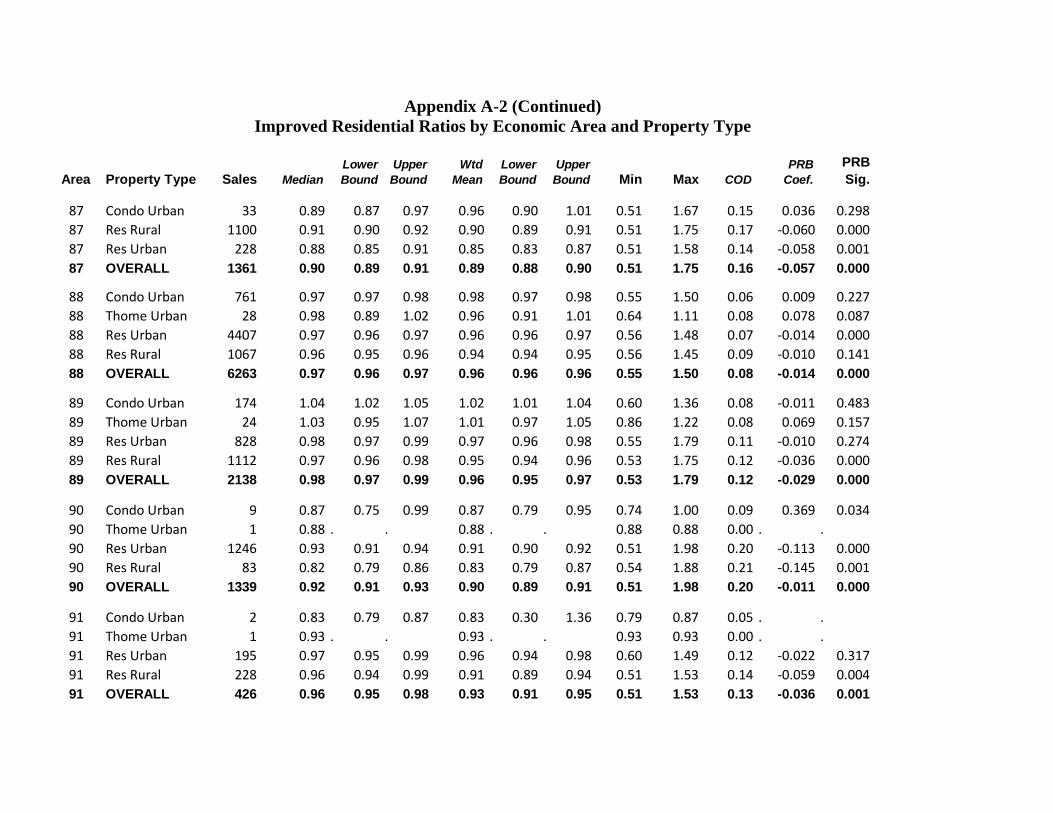
Appendix A-2 (Continued) Improved Residential Ratios by Economic Area and Property Type
Area Property Type Sales MedianLower Bound
Upper Bound
Wtd Mean
Lower Bound
Upper Bound Min Max COD
PRB Coef.
PRB Sig.
87 Condo Urban 33 0.89 0.87 0.97 0.96 0.90 1.01 0.51 1.67 0.15 0.036 0.298
87 Res Rural 1100 0.91 0.90 0.92 0.90 0.89 0.91 0.51 1.75 0.17 ‐0.060 0.000
87 Res Urban 228 0.88 0.85 0.91 0.85 0.83 0.87 0.51 1.58 0.14 ‐0.058 0.001
87 OVERALL 1361 0.90 0.89 0.91 0.89 0.88 0.90 0.51 1.75 0.16 -0.057 0.000
88 Condo Urban 761 0.97 0.97 0.98 0.98 0.97 0.98 0.55 1.50 0.06 0.009 0.227
88 Thome Urban 28 0.98 0.89 1.02 0.96 0.91 1.01 0.64 1.11 0.08 0.078 0.087
88 Res Urban 4407 0.97 0.96 0.97 0.96 0.96 0.97 0.56 1.48 0.07 ‐0.014 0.000
88 Res Rural 1067 0.96 0.95 0.96 0.94 0.94 0.95 0.56 1.45 0.09 ‐0.010 0.141
88 OVERALL 6263 0.97 0.96 0.97 0.96 0.96 0.96 0.55 1.50 0.08 -0.014 0.000
89 Condo Urban 174 1.04 1.02 1.05 1.02 1.01 1.04 0.60 1.36 0.08 ‐0.011 0.483
89 Thome Urban 24 1.03 0.95 1.07 1.01 0.97 1.05 0.86 1.22 0.08 0.069 0.157
89 Res Urban 828 0.98 0.97 0.99 0.97 0.96 0.98 0.55 1.79 0.11 ‐0.010 0.274
89 Res Rural 1112 0.97 0.96 0.98 0.95 0.94 0.96 0.53 1.75 0.12 ‐0.036 0.000
89 OVERALL 2138 0.98 0.97 0.99 0.96 0.95 0.97 0.53 1.79 0.12 -0.029 0.000
90 Condo Urban 9 0.87 0.75 0.99 0.87 0.79 0.95 0.74 1.00 0.09 0.369 0.034
90 Thome Urban 1 0.88 . . 0.88 . . 0.88 0.88 0.00 . .
90 Res Urban 1246 0.93 0.91 0.94 0.91 0.90 0.92 0.51 1.98 0.20 ‐0.113 0.000
90 Res Rural 83 0.82 0.79 0.86 0.83 0.79 0.87 0.54 1.88 0.21 ‐0.145 0.001
90 OVERALL 1339 0.92 0.91 0.93 0.90 0.89 0.91 0.51 1.98 0.20 -0.011 0.000
91 Condo Urban 2 0.83 0.79 0.87 0.83 0.30 1.36 0.79 0.87 0.05 . .
91 Thome Urban 1 0.93 . . 0.93 . . 0.93 0.93 0.00 . .
91 Res Urban 195 0.97 0.95 0.99 0.96 0.94 0.98 0.60 1.49 0.12 ‐0.022 0.317
91 Res Rural 228 0.96 0.94 0.99 0.91 0.89 0.94 0.51 1.53 0.14 ‐0.059 0.004
91 OVERALL 426 0.96 0.95 0.98 0.93 0.91 0.95 0.51 1.53 0.13 -0.036 0.001
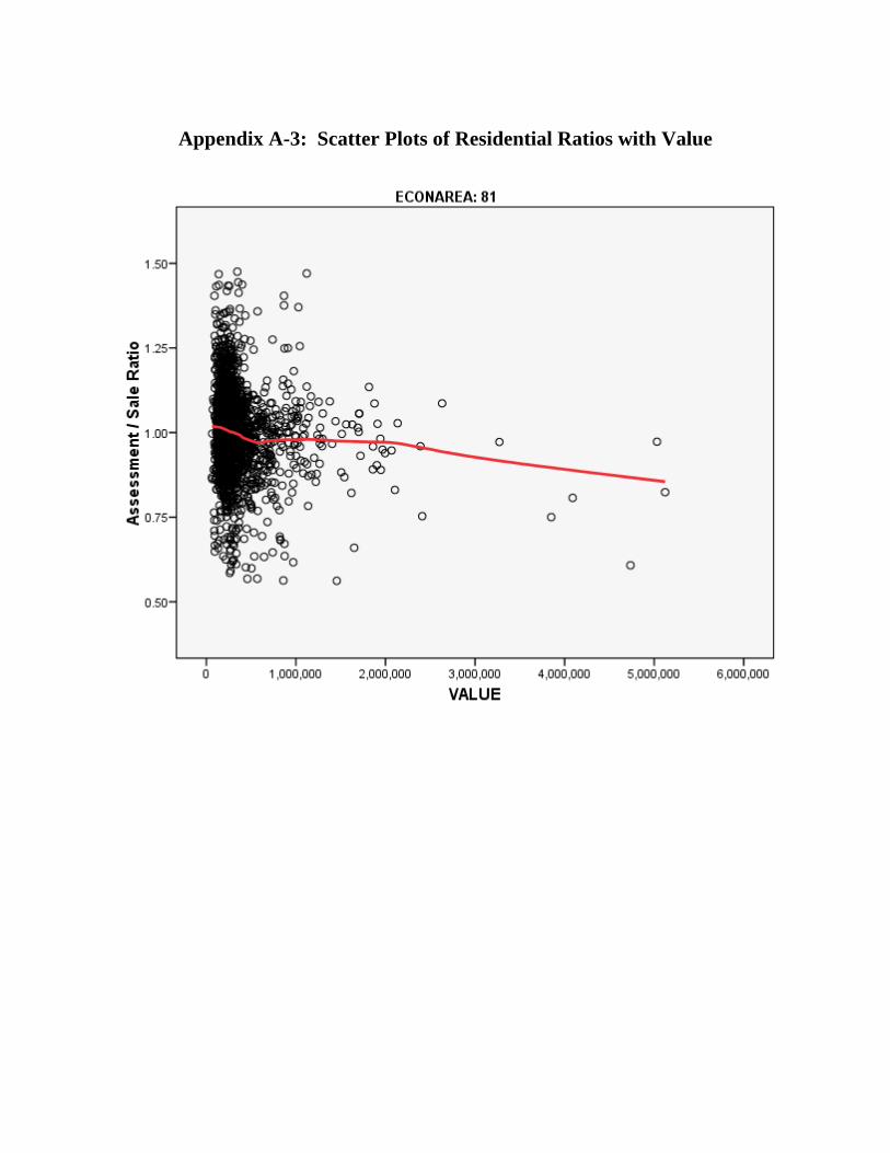
Appendix A-3: Scatter Plots of Residential Ratios with Value


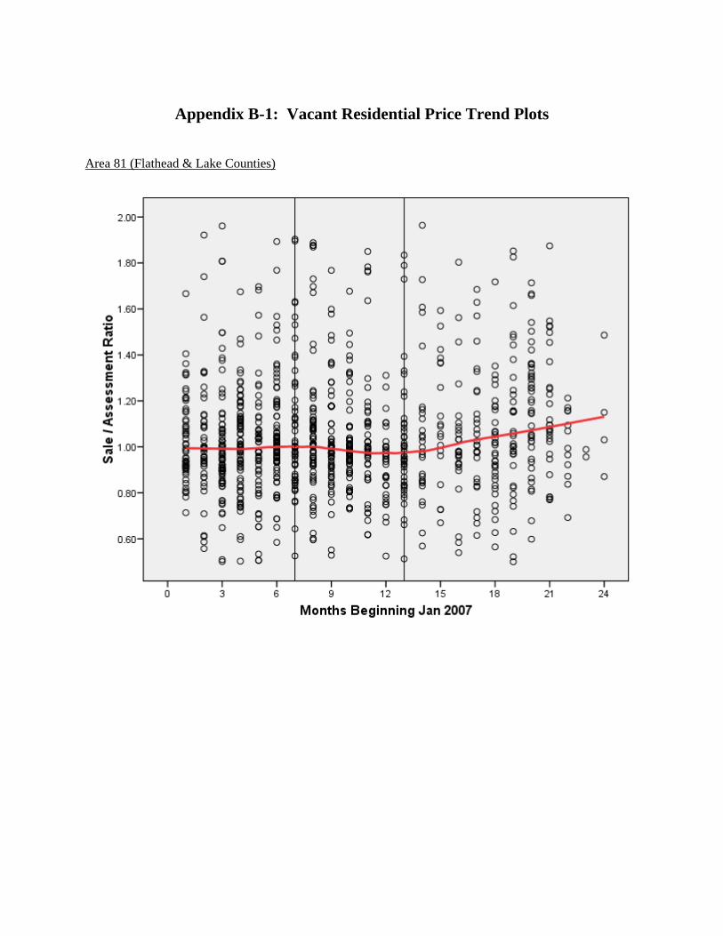
Appendix B-1: Vacant Residential Price Trend Plots
Area 81 (Flathead & Lake Counties)
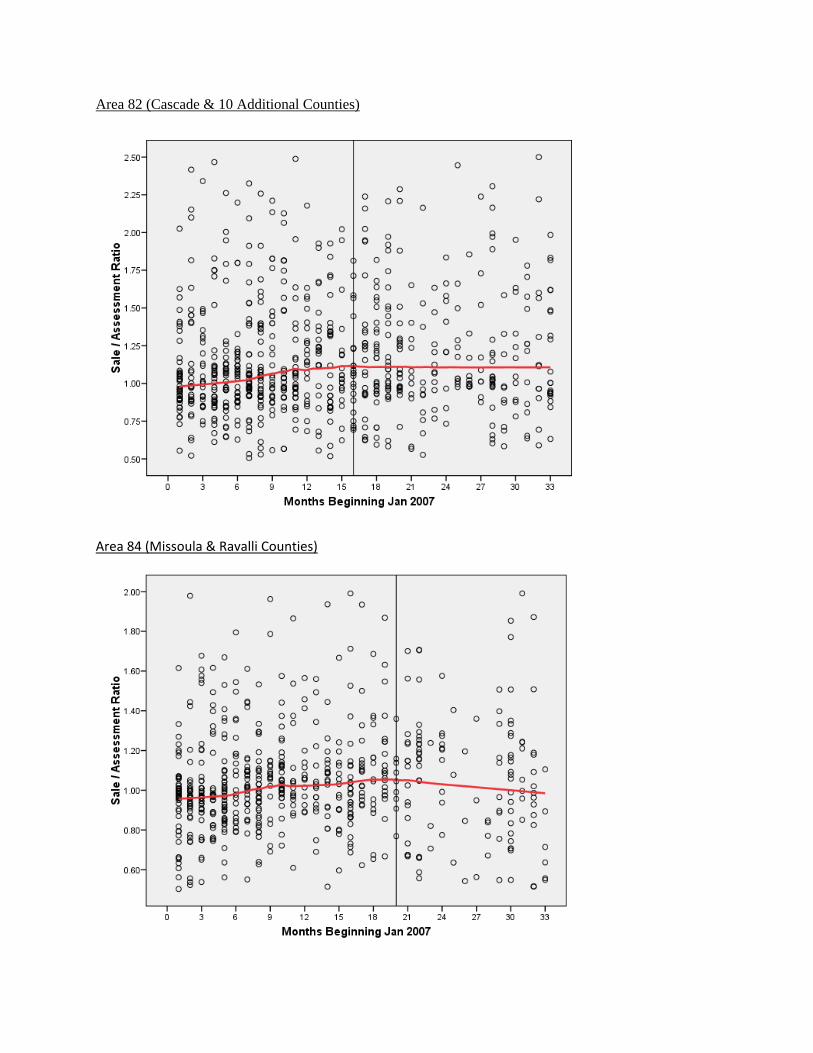
Area 82 (Cascade & 10 Additional Counties)
Area 84 (Missoula & Ravalli Counties)
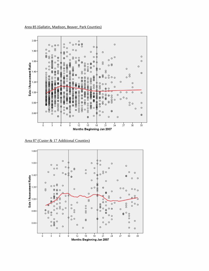
Area 85 (Gallatin, Madison, Beaver, Park Counties)
Area 87 (Custer & 17 Additional Counties)

Area 88 (Yellowstone & 7 Additional Counties)
Area 89 (Lewis & Clark, Broadwater & Jefferson Counties)

Area 90 (Butte-Silver Bow, Powell, Anacondo-Deer Lodge, Granite Counties)
Area 91 (Sanders, Mineral & Lincoln Counties)

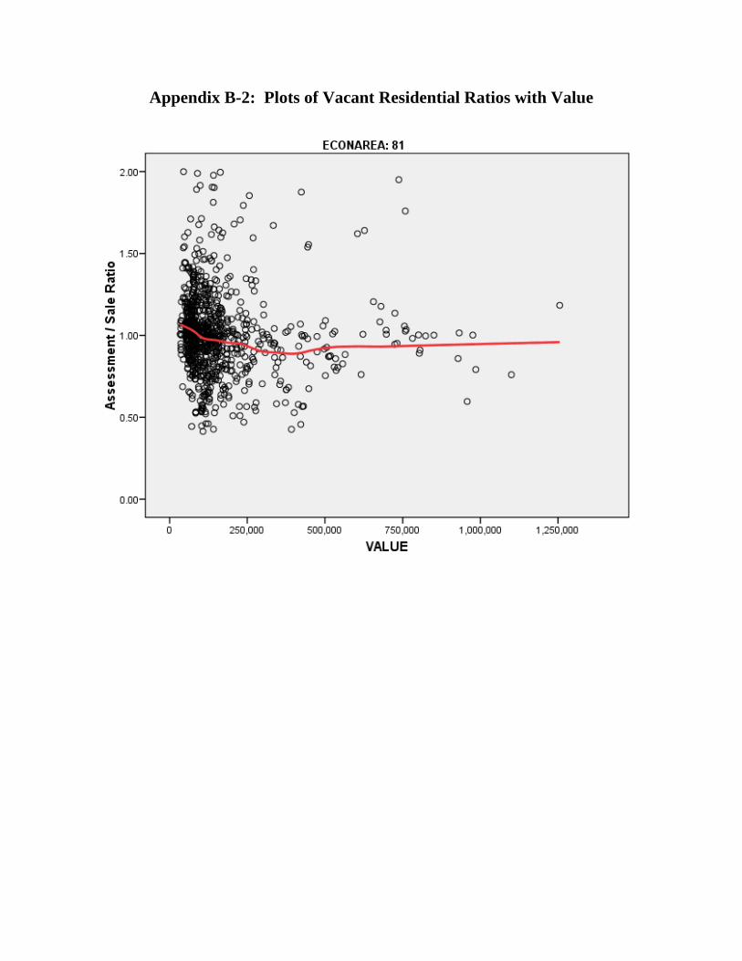
Appendix B-2: Plots of Vacant Residential Ratios with Value


Appendix C-1: Commercial Price Trend Plots Area 81 (Flathead & Lake Counties)

Area 82 (Cascade & 10 Additional Counties)
Area 84 (Missoula & Ravalli Counties): Commercial Improved
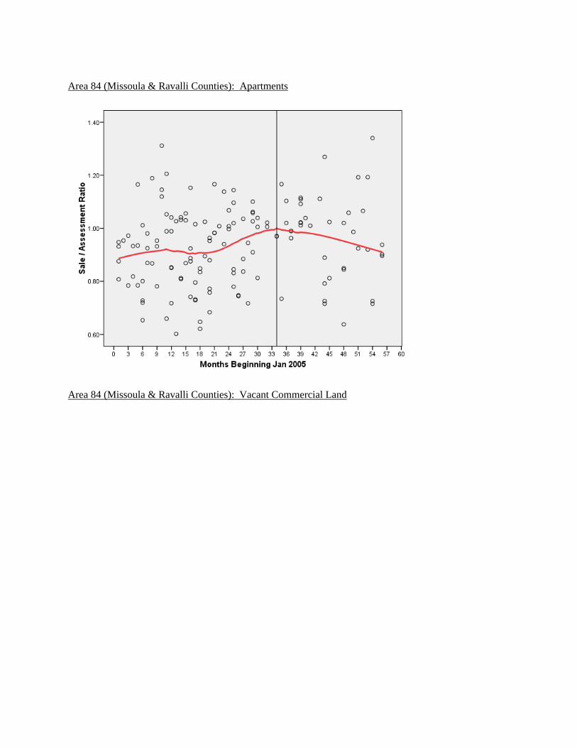
Area 84 (Missoula & Ravalli Counties): Apartments
Area 84 (Missoula & Ravalli Counties): Vacant Commercial Land

Area 85 (Gallatin, Madison, Beaver, Park Counties): Commercial Improved
Area 85 (Gallatin, Madison, Beaver, Park Counties): Apartments
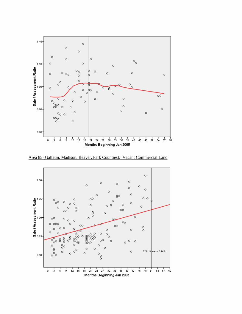
Area 85 (Gallatin, Madison, Beaver, Park Counties): Vacant Commercial Land

Area 87 (Custer & 17 Additional Counties)
Area 88 (Yellowstone & 7 Additional Counties): Commercial Improved
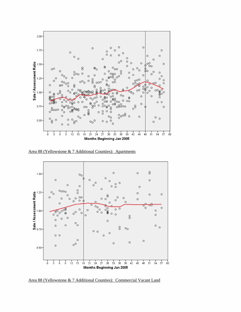
Area 88 (Yellowstone & 7 Additional Counties): Apartments
Area 88 (Yellowstone & 7 Additional Counties): Commercial Vacant Land
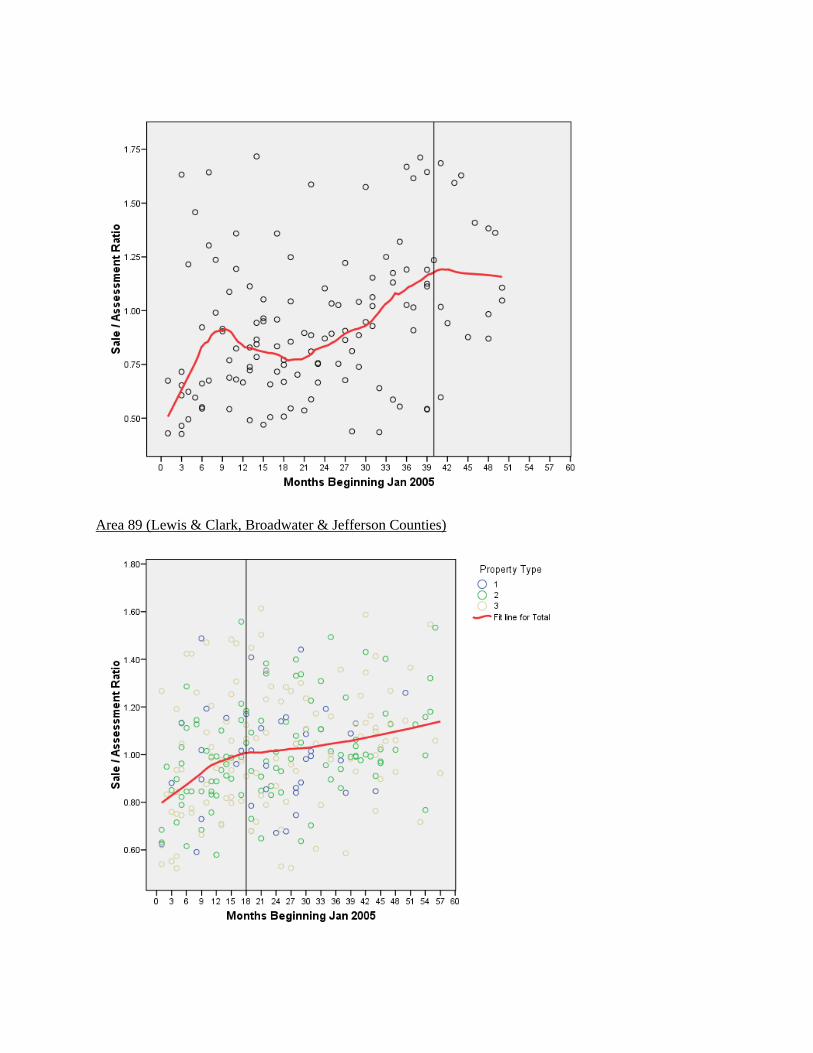
Area 89 (Lewis & Clark, Broadwater & Jefferson Counties)

Area 90 (Butte-Silver Bow, Powell, Anaconda-Deer Lodge, Granite): Commercial Vacant & Improved
Area 90 (Butte-Silver Bow, Powell, Anaconda-Deer Lodge, Granite): Apartments

Area 91 (Sanders, Mineral & Lincoln Counties)

Appendix C-2: Plots of Commercial Ratios with Value