1

7KH���UG�(XURSHDQ�&RQJUHVV�RI�WKH�5HJLRQDO�6FLHQFH�$VVRFLDWLRQ���

-\YlVN\Ol��)LQODQG���$XJXVW����WR�$XJXVW����������

�

0XOWLSOH�5HJLPHV�LQ�&URVV�5HJLRQ�*URZWK�5HJUHVVLRQV�ZLWK�

6SDWLDO�'HSHQGHQFH��$�3DUDPHWULF�DQG�D�6HPL�SDUDPHWULF�

$SSURDFK

(preliminary version)

Roberto Basile, Sergio de Nardis and Marianna Mantuano

(ISAE, Institute of Studies and Economic Analysis)

Rome, Italy

Abstract

Since the beginning of the nineties, the issue of income convergence has received considerable attention in regional economic analysis. Nevertheless, little attention has been given to the treatment of the spatial dependence and spatial heterogeneity (or spatial regimes). In this paper, we propose a semi-parametric model of regional growth in Europe to simultaneously identify the presence of multiple regimes and deal with the problem of spatial dependence. We do this in a new specification of the convergence model which allows to take into account the different effects of labour productivity and employment rates on development gaps. We also verify the degree of coincidence between the multiple regime structure “endogenously” identified through the semi-parametric model and the Core-Periphery structure used by economic geographers.

.H\�ZRUGV: Regional Convergence, Europe, Spatial Econometrics, Multiple Regimes,

semi-parametric models

-(/�&ODVVLILFDWLRQ: O40, O52, R11, C13, C14

$GGUHVV� IRU� FRUUHVSRQGHQFH�� Roberto Basile, ISAE (Institute for Studies and Economic

Analyses), P.zza Indipendenza, 4, 00191 Rome, Italy. Tel. +39-06-44482874, E-mail: r.basile@isae.it.

2

���,QWURGXFWLRQ�

Regional convergence studies have recently experienced an increase of interest due

to the issues raised in Europe by the unification process. Since large differentials in per

capita GDP across regions are regarded as an impediment to the completion of the

economic and monetary union, the narrowing of regional disparities (so called

cohesion, in the EC jargon) is indeed regarded as a fundamental objective for the

European Union policy. Hence, the problem of testing convergence among the member

States of the Union emerges as fundamental in policy evaluation.

From a methodological point of view, testing regional convergence hypothesis

involves important technical issues. The problem arises of finding the best data to test

the theory and the best estimators for the associated modelling. In the literature, a

number of related econometric concepts have been applied and developed.

Nevertheless, little attention has been given to the treatment of the spatial dependence

and spatial heterogeneity.

As regards spatial dependence, we argue that regional data cannot be regarded as

independently generated because of the presence of spatial similarities among

neighbouring regions (Anselin, 1988; Anselin and Bera, 1998). As a consequence, the

standard estimation procedures employed in many empirical studies can be invalid and

lead to serious biases and inefficiencies in the estimates of the convergence rate.

However, few empirical studies have recently used the spatial econometric framework

for testing regional convergence (see, for example, Rey and Montouri, 1998; Arbia,

Basile and Salvatore, 2002).

As far as spatial heterogeneity is concerned, the bulk of empirical studies on

European regional growth has implicitly assumed that all regions obey a common linear

specification, disregarding the possibility of non-linearities or multiple steady states in

per capita income. The issue of multiple regimes has been instead raised in some cross-

country growth studies (Durlauf and Johnson, 1995; Liu and Stengos, 1999; Durlauf,

Kourtellos and Minkin, 2001). The basic idea underlying the multiple regime analysis

is that the level of per capita GDP on which each economy converges depends on some

initial conditions (such as initial per capita GDP or initial level of schooling), so that,

for example, regions with an initial per capita GDP lower than a certain threshold level

converge to one steady state level while regions above the threshold converge to a

different level.

3

A problem with multiple-regime analysis is that the threshold level cannot be (and

must not be) exogenously imposed. In order to identify economies whose growth

behaviour obeys a common statistical model, it is necessary to allow the data to

determine the location of the different regimes. The above-mentioned cross-country

studies, indeed, make use of non-parametric or semi-parametric approaches to model

the regression function. In some circumstances, the hypothesis of linearity has been

abandoned in some cross region studies in Europe by assuming the presence of

“threshold effects” automatically produced by the belonging of each region to one

group or another, according to “exogenous” criteria, such as geographical criteria (e.g.

Centre versus Periphery) or policy criteria (e.g. Objective 1 versus non Objective 1)

(see, for example, Basile, de Nardis and Girardi, 2003).

The aim of this paper is to reconcile the critical points raised in the current debate

on spatial dependence and multiple regimes. Thus, we propose a semi-parametric

model of regional growth behaviour in Europe to simultaneously identify the presence

of multiple regimes and take accounts of the problem of spatial dependence. We also

try to verify how similar are the multiple regime structure “endogenously” identified

through the additive model and the Core-Periphery structure adopted by economic

geographers like Keeble, Offord and Walzer (1988) and Copus (1999).

Regional development is measured in terms of both per capita GDP and its basic

components: labour productivity and employment ratio. Following Boldrin and Canova,

2001), we claim that, given the strong imperfections in the local labour markets in

Europe, this decomposition is an essential feature of the regional development analysis

in the Union: looking just at the behaviour of regional per capita GDP doesn’t allow to

say much. Thus, we specify an empirical growth model where, instead of the initial per

capita GDP, we introduce the initial level of the two components as well as their

interaction.

The layout of the paper is the following. In Section 2, we introduce the statistical

decomposition of per capita GDP that we use throughout the paper and report some

descriptive analysis of regional developments in Europe. In Section 3, we present a

review of spatial econometric techniques that incorporate spatial dependence and

spatial heterogeneity within the contest of a b-convergence modelling. In Section 4, we

report the results of a parametric analysis of regional convergence based on a data set of

about 160 EU-15 NUTS-2 regions for the period 1988-1999. In Section 5, we report the

results of a semi-parametric analysis. Some conclusions are reported in Section 6.

4

���6RPH�GHVFULSWLYH�VWDWLVWLFV�RI�(XURSHDQ�UHJLRQDO�GHYHORSPHQW�

Our analysis is based on the dataset compiled by Cambridge Econometrics on GDP,

population and employment for about 160 European NUTS-2 regions over the period

1988-1999. The level of per capita GDP, measured in PPP, is the main economic

indicator adopted by the European Commission, as well as by other international

institutions (World Bank, IMF, OECD, United Nations), to compare the development

levels of different countries and regions. In this paper too, the evaluation of EU

region’s development is based upon the examination of per capita GDP (or incomes).

However since we are interested in regional real growth and real convergence, per

capita GDP of European regions are computed at 1995 prices and converted in the

PPP’s of the same year.

As it is well known, the observed inequalities in regional income levels can be

accounted for by a combination of three factors: differences in labour productivity,

differences in employment rates and the interaction between productivity and

employment rates. These relations are based on the following identity:

3

/

/

<

3

<�� (1)

where < is the value added; 3 indicates the population; ( is the employment level.

In logarithms, it takes up an additive form:

OQ�<�3�� �OQ�<�(����OQ�(�3�� ������

By applying the variance operator to both members, one obtains:

YDU>OQ�<�3�@� �YDU>OQ�<�(�@���YDU>OQ�(�3�@����FRY>OQ�<�(��OQ�(�3�@� ������

This expression shows that the variability of per capita incomes depends on labor

productivity and employment rates variance and on the covariance between

productivity and employment rates. The combination of these three effects may

determine either convergence, or divergence or invariance in the regional distribution

of per capita incomes.

On the basis of this relationship, the analysis of convergence takes into account not

only per capita GDP of the European regions, but also labor productivity and

employment rates. In addition, in observance to the Core/Periphery concept developed

by the New Economic Geography (from now on, NEG) models, European regions have

been divided into two groups. Some simple indexes have been calculated for the initial

5

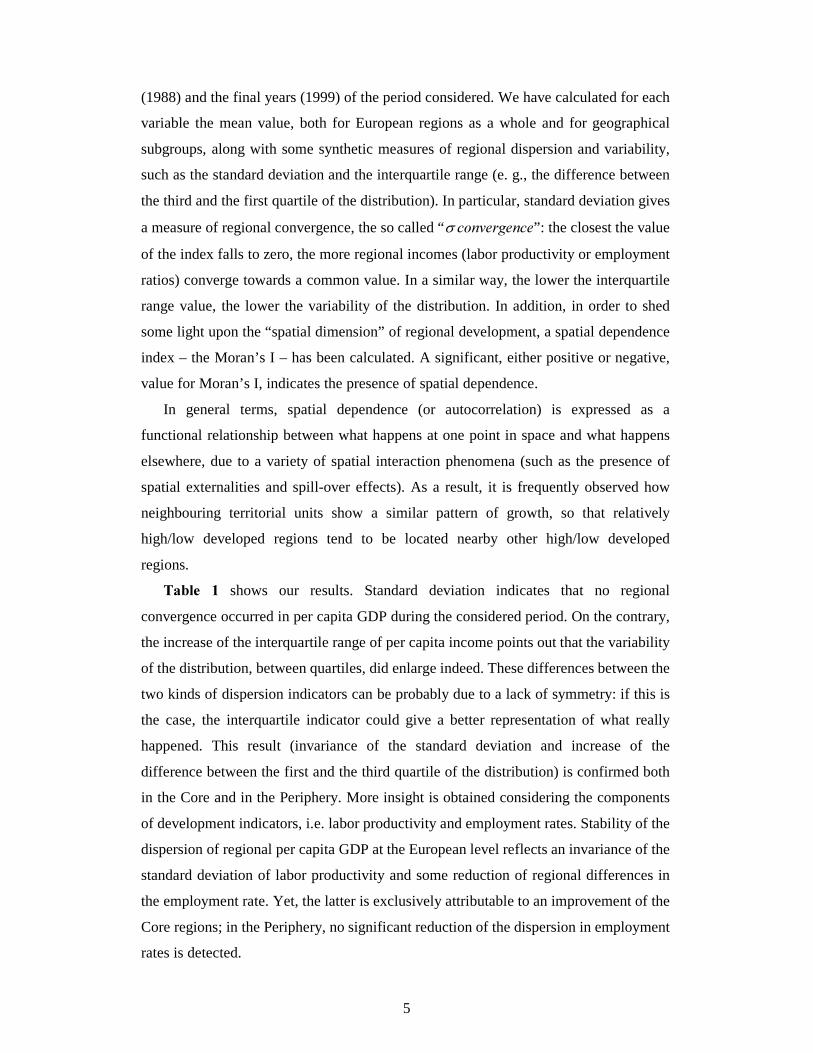
(1988) and the final years (1999) of the period considered. We have calculated for each

variable the mean value, both for European regions as a whole and for geographical

subgroups, along with some synthetic measures of regional dispersion and variability,

such as the standard deviation and the interquartile range (e. g., the difference between

the third and the first quartile of the distribution). In particular, standard deviation gives

a measure of regional convergence, the so called “s�FRQYHUJHQFH”: the closest the value

of the index falls to zero, the more regional incomes (labor productivity or employment

ratios) converge towards a common value. In a similar way, the lower the interquartile

range value, the lower the variability of the distribution. In addition, in order to shed

some light upon the “spatial dimension” of regional development, a spatial dependence

index – the Moran’s I – has been calculated. A significant, either positive or negative,

value for Moran’s I, indicates the presence of spatial dependence.

In general terms, spatial dependence (or autocorrelation) is expressed as a

functional relationship between what happens at one point in space and what happens

elsewhere, due to a variety of spatial interaction phenomena (such as the presence of

spatial externalities and spill-over effects). As a result, it is frequently observed how

neighbouring territorial units show a similar pattern of growth, so that relatively

high/low developed regions tend to be located nearby other high/low developed

regions.

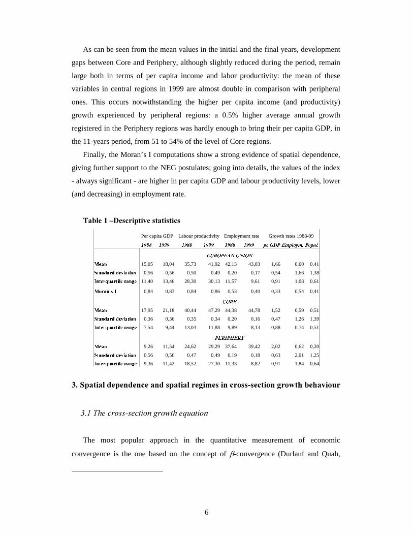
7DEOH� �� shows our results. Standard deviation indicates that no regional

convergence occurred in per capita GDP during the considered period. On the contrary,

the increase of the interquartile range of per capita income points out that the variability

of the distribution, between quartiles, did enlarge indeed. These differences between the

two kinds of dispersion indicators can be probably due to a lack of symmetry: if this is

the case, the interquartile indicator could give a better representation of what really

happened. This result (invariance of the standard deviation and increase of the

difference between the first and the third quartile of the distribution) is confirmed both

in the Core and in the Periphery. More insight is obtained considering the components

of development indicators, i.e. labor productivity and employment rates. Stability of the

dispersion of regional per capita GDP at the European level reflects an invariance of the

standard deviation of labor productivity and some reduction of regional differences in

the employment rate. Yet, the latter is exclusively attributable to an improvement of the

Core regions; in the Periphery, no significant reduction of the dispersion in employment

rates is detected.

6

As can be seen from the mean values in the initial and the final years, development

gaps between Core and Periphery, although slightly reduced during the period, remain

large both in terms of per capita income and labor productivity: the mean of these

variables in central regions in 1999 are almost double in comparison with peripheral

ones. This occurs notwithstanding the higher per capita income (and productivity)

growth experienced by peripheral regions: a 0.5% higher average annual growth

registered in the Periphery regions was hardly enough to bring their per capita GDP, in

the 11-years period, from 51 to 54% of the level of Core regions.

Finally, the Moran’s I computations show a strong evidence of spatial dependence,

giving further support to the NEG postulates; going into details, the values of the index

- always significant - are higher in per capita GDP and labour productivity levels, lower

(and decreasing) in employment rate.

7DEOH���±'HVFULSWLYH�VWDWLVWLFV�

Per capita GDP Labour productivity Employment rate Growth rates 1988-99

������� ������� ������� ������� ������� ������� ����� ������� ������� �������� �

������ ! "��#�$%�&$�'( �$

)+*(,�-15,05 18,04 35,73 41,92 42,13 43,03 1,66 0,60 0,41 .�/ ,�-10�,�23040�*35�6 , / 6 7�-

0,56 0,56 0,50 0,49 0,20 0,17 0,54 1,66 1,38 89- / *(23:�;�,�2 / 6 < *�23,�-�=�*11,40 13,46 28,30 30,13 11,57 9,61 0,91 1,08 0,61

)+7�2>,�-�? @!80,84 0,83 0,84 0,86 0,53 0,40 0,33 0,54 0,41

A !�!�)+*(,�-17,95 21,18 40,44 47,29 44,38 44,78 1,52 0,59 0,51 .�/ ,�-10�,�23040�*35�6 , / 6 7�-

0,36 0,36 0,35 0,34 0,20 0,16 0,47 1,26 1,39 89- / *(23:�;�,�2 / 6 < *�23,�-�=�*7,54 9,44 13,03 11,88 9,89 8,13 0,88 0,74 0,51

&�!�!'9 "BC�!�ED

)+*(,�-9,26 11,54 24,62 29,29 37,64 39,42 2,02 0,62 0,20 .�/ ,�-10�,�23040�*35�6 , / 6 7�-0,56 0,56 0,47 0,49 0,19 0,18 0,63 2,01 1,25 89- / *(23:�;�,�2 / 6 < *�23,�-�=�*9,36 11,42 18,52 27,30 11,33 8,82 0,91 1,84 0,64

���6SDWLDO�GHSHQGHQFH�DQG�VSDWLDO�UHJLPHV�LQ�FURVV�VHFWLRQ�JURZWK�EHKDYLRXU�

�

����7KH�FURVV�VHFWLRQ�JURZWK�HTXDWLRQ�

The most popular approach in the quantitative measurement of economic

convergence is the one based on the concept of b-convergence (Durlauf and Quah,

7

1999 for a review). It moves from the neoclassical Solow-Swan growth model,

assuming exogenous saving rates and a production function based on decreasing

productivity of (physical and human) capital and constant returns to scale. On this basis

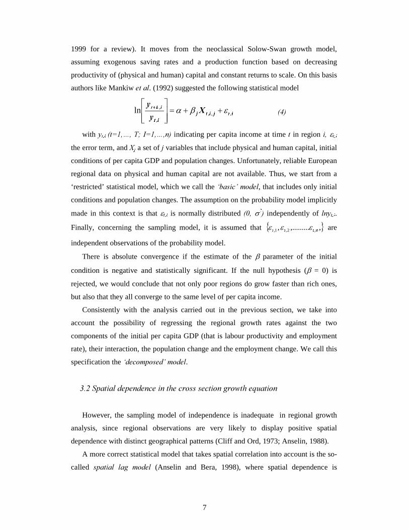
authors like Mankiw HW�DO. (1992) suggested the following statistical model

FGHFGHFGFIG

;\

\,,,

,

,ln eba ++=ßßà

Þ

ÏÏÐ

ΠJ� � ���

with \ K L M �W ��«��7��, ��«�Q� indicating per capita income at time W in region L��e K L M the error term, and ;N �a set of M�variables that include physical and human capital, initial

conditions of per capita GDP and population changes. Unfortunately, reliable European

regional data on physical and human capital are not available. Thus, we start from a

‘restricted’ statistical model, which we call the µEDVLF¶�PRGHO, that includes only initial

conditions and population changes. The assumption on the probability model implicitly

made in this context is that e K L M is normally distributed ����sO�� independently of OQ\ K L M .

Finally, concerning the sampling model, it is assumed that { },,........., ,2,1, PQQQ eee are

independent observations of the probability model.

There is absolute convergence if the estimate of the b parameter of the initial

condition is negative and statistically significant. If the null hypothesis (b = 0) is

rejected, we would conclude that not only poor regions do grow faster than rich ones,

but also that they all converge to the same level of per capita income.

Consistently with the analysis carried out in the previous section, we take into

account the possibility of regressing the regional growth rates against the two

components of the initial per capita GDP (that is labour productivity and employment

rate), their interaction, the population change and the employment change. We call this

specification the µGHFRPSRVHG¶�PRGHO.

����6SDWLDO�GHSHQGHQFH�LQ�WKH�FURVV�VHFWLRQ�JURZWK�HTXDWLRQ�

However, the sampling model of independence is inadequate in regional growth

analysis, since regional observations are very likely to display positive spatial

dependence with distinct geographical patterns (Cliff and Ord, 1973; Anselin, 1988).

A more correct statistical model that takes spatial correlation into account is the so-

called VSDWLDO� ODJ� PRGHO� (Anselin and Bera, 1998), where spatial dependence is

8

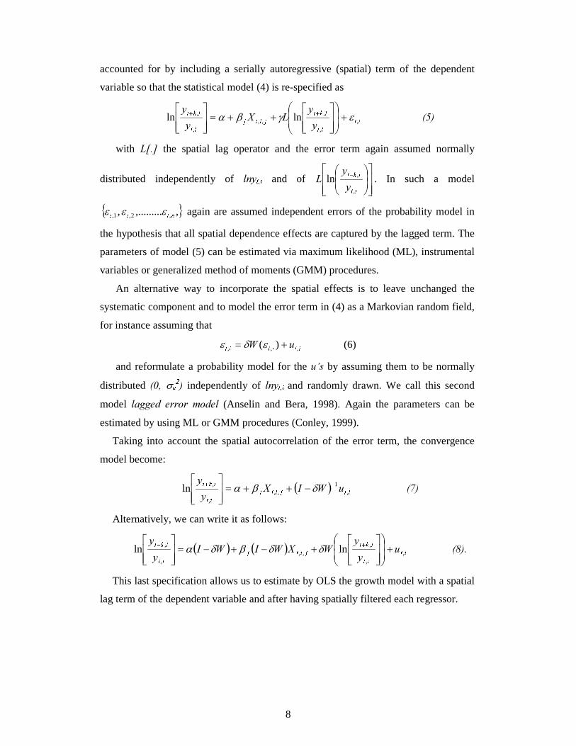
accounted for by including a serially autoregressive (spatial) term of the dependent

variable so that the statistical model (4) is re-specified as

RSRSRTSURSU

RSRTS

\

\/;

\

\,

,

,,,

,

, lnln egba +ÜÜ

Ý

Û

ÌÌ

Í

Ë

ßßà

Þ

ÏÏÐ

Î++=

ßßà

Þ

ÏÏÐ

ΠVV�� � ����

with />�@� the spatial lag operator and the error term again assumed normally

distributed independently of OQ\ K L M and of ßßà

Þ

ÏÏÐ

ÎÜÜÝ

ÛÌÌÍ

Ë WXYXZY

\

\/

,

,ln . In such a model

{ },,........., ,2,1, [\\\ eee again are assumed independent errors of the probability model in

the hypothesis that all spatial dependence effects are captured by the lagged term. The

parameters of model (5) can be estimated via maximum likelihood (ML), instrumental

variables or generalized method of moments (GMM) procedures.

An alternative way to incorporate the spatial effects is to leave unchanged the

systematic component and to model the error term in (4) as a Markovian random field,

for instance assuming that

]^]^]^ X: ,,, )( += ede (6)

and reformulate a probability model for the X¶V�by assuming them to be normally

distributed ����s _O� independently of OQ\ K L M and randomly drawn. We call this second

model ODJJHG� HUURU� PRGHO (Anselin and Bera, 1998). Again the parameters can be

estimated by using ML or GMM procedures (Conley, 1999).

Taking into account the spatial autocorrelation of the error term, the convergence

model become:

( ) `ab`ab`a`ca

X:,;\

\,

1,,

,

,ln de

-++=ßßà

Þ

ÏÏÐ

Îdba �� � ����

Alternatively, we can write it as follows:

( ) ( ) fgfgfhgifgi

fgfhg

X\

\:;:,:,

\

\,

,

,,,

,

, lnln +ÜÜ

Ý

Û

ÌÌ

Í

Ë

ßßà

Þ

ÏÏÐ

Î+-+-=

ßßà

Þ

ÏÏÐ

Πjjddbda �� � �����

This last specification allows us to estimate by OLS the growth model with a spatial

lag term of the dependent variable and after having spatially filtered each regressor.

9

����6SDWLDO�UHJLPHV�DQG�QRQ�OLQHDULWLHV�LQ�WKH�FURVV�VHFWLRQ�JURZWK�HTXDWLRQ�

The spatial econometric literature raises also the problem of spatial heterogeneity,

that is the lack of stability over space of the behavioural or other relationships under

study (Anselin, 1988). This implies that functional forms and parameters vary with

location and are not homogenous throughout the data set. With regard to the cross-

section growth analysis, the bulk of empirical studies has implicitly assumed that all

economies (countries or regions) obey a common linear specification, disregarding the

possibility of non-linearities or multiple locally stable steady states in per capita

income. Notable exception are Durlauf and Johnson (1995), Liu and Stengos (1999)

and Durlauf, Kourtellos and Minkin (2001).

The basic idea underlying the multiple regime analysis is that the level of per capita

GDP on which each economy converges depends on some initial conditions (such as

initial per capita GDP) and that, according to these characteristics some economies

converge to one level and others converge to another. A common specification that is

used to test this hypothesis considers a modification of the systematic component in

model (4) that takes the form:

klmklmklknl

;\

\,,,11

,

,ln eba ++=ßßà

Þ

ÏÏÐ

Î o LI [; pqr <,, (4’)

stustustsvt

;\

\,,,22

,

,ln eba ++=ßßà

Þ

ÏÏÐ

Î w LI [; xyz �,,

where [ is a threshold that determines whether or not region L belongs to the first or

second regime. The same adjustment can be applied to the systematic component in the

spatial dependence models.

A problem with multiple regime analysis is that the threshold level cannot be (and

must not be) exogenously imposed. In order to identify economies whose growth

behaviour obeys a common statistical model, we must allow the data to determine the

location of the different regimes. We argue that a non-parametric specification of the

cross-region growth function goes a long away in addressing the issue of multiple

regimes. By using a particular version of the non-parametric regression model that

allows for additive non-parametric components, the additive model (see, Beck and

Jackman, 1997), we are able to obtain graphical representations of these components

10

that shed light on non-linear behaviour of some of the basic variables. The non-

parametric additive model can be written as:

( ) {|}| ~ {}{|{�|

;J\

\,,

,

,ln e+=ßßà

Þ

ÏÏÐ

Î � (9)

In particular, instead of imposing a linearity hypothesis on the functional form of

the relationship between per capita GDP growth rates and each term in ;, we use the

much more flexible ORFDOO\� ZHLJKWHG� UHJUHVVLRQ� VPRRWKHU, that is a particular

specification of the polynomial local regression model (Cleveland, 1979; Cleveland e

Devlin, 1988).

In order to incorporate spatial dependence within the additive model, we can use

both a nonparametric spatial lag (NP-SL) and a nonparametric spatial error (NP-SE)

specification, as follows:

NP-SL ( ) ��������� � ��

�����

\

\/J;J

\

\,

,

,,

,

, lnln e+ÜÜ

Ý

Û

ÌÌ

Í

Ë

ÜÜ

Ý

Û

ÌÌ

Í

Ë

ßßà

Þ

ÏÏÐ

Î+=

ßßà

Þ

ÏÏÐ

�� (9)

NP-SE ( ) �����������

�����

\

\/J;:,J

\

\,

,

,,,

,

, lnln ed +ÜÜ

Ý

Û

ÌÌ

Í

Ë

ÜÜ

Ý

Û

ÌÌ

Í

Ë

ßßà

Þ

ÏÏÐ

Î+-=

ßßà

Þ

ÏÏÐ

�� (10).

���3DUDPHWULF�UHJUHVVLRQV�

This section reports the results of the parametric regressions of the cross-region

growth equation. The starting point is the µEDVLF¶ model of growth behaviour without

taking into account the issue of spatial dependence and spatial heterogeneity. Secondly,

the model is implemented by decomposing the initial condition into its different terms

(labour productivity, employment rate and their interaction). Thirdly, the hypothesis of

multiple regimes is tested by imposing a Core-Periphery structure to the data. Finally,

the results of spatial error and spatial lag models are discussed.

4.1 �%DVLF�DQG�GHFRPSRVHG�PRGHOV��2/6�UHVXOWV�

We start from the OLS estimates of the µEDVLF¶�PRGHO of b-convergence and test

for the presence of different possible sources of misspecification (spatial

11

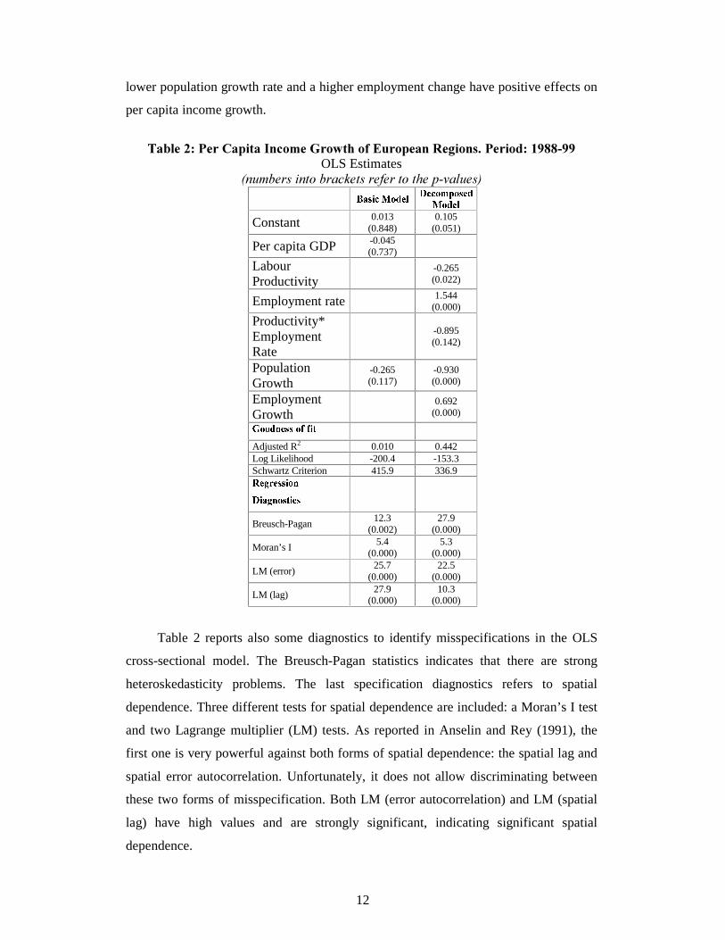
heteroskedasticity and spatial autocorrelation). 7DEOH� �� (Columns labelled “Basic

Model”) displays the cross-sectional OLS estimates of convergence for the 160 EU15

NUTS-2 regions. The dependent variable is the growth rate of region’s per capita

income, while the predictors introduced are the log of the initial level of per-capita

income and the log of population growth rate. All variables are scaled to the EU15

average. The model is estimated for the period (1988-1999) covering the new phase of

reformed Structural Funds.

Our results appear very much in line with the previous findings on the

development of European regions. The coefficient of the initial per capita GDP is –

0.045 and non-significant, suggesting lack of convergence. The coefficient of the

population growth rate is also non-significantly different from zero.

The Column labelled “Decomposed Model” in Table 2 reports the results of the

regression estimation with a different specification: instead of the initial level of per

capita GDP, we introduce the initial level of labour productivity, the initial level

employment rate and their interaction; the employment growth rate is also introduced

along with the population growth rate [The decomposition of per capita GDP in the two

components represented by labor productivity and employment rate implies we control for employment

growth. Actually, a more correct specification would require to control for both employment growth and

the rate of change of the reciprocal of the employment rate (i.e. the rate of change of the ratio of

population over employment). In this version of the paper we just consider population and employment

growth rates, intending to refine the estimates in a subsequent version].

Again, all variables are in logs and scaled to the EU15 average. The improvement

obtained with this alternative specification is apparent: while the ‘basic’ model is not

able to explain the variability of regional growth rates, the ‘decomposed’ model

explains about 44%! The change in the Schwartz statistics is coherent with the strong

increase of the adjusted R2 statistics: all parameters, but the interaction term, appear

strongly significant. In particular, we observe a converging effect of the labour

productivity (labour productivity grows faster among low productivity regions) and a

diverging effect of the employment rate (employment rates grow faster among regions

with high employment rates). These two opposite effects may help us to understand the

lack of a global regional convergence in terms of per capita GDP levels over the

examined period. The interaction term is negative but not significant. Population and

employment changes have also significant effects on per capita income growth rates: a

12

lower population growth rate and a higher employment change have positive effects on

per capita income growth.

7DEOH����3HU�&DSLWD�,QFRPH�*URZWK�RI�(XURSHDQ�5HJLRQV��3HULRG����������

OLS Estimates �QXPEHUV�LQWR�EUDFNHWV�UHIHU�WR�WKH�S�YDOXHV��

� �C�1�>� ���%���&���� �������������3���

�%���&���Constant 0.013

(0.848) 0.105

(0.051)

Per capita GDP -0.045 (0.737)

Labour Productivity

-0.265 (0.022)

Employment rate 1.544

(0.000)

Productivity* Employment Rate

-0.895 (0.142)

Population Growth

-0.265 (0.117)

-0.930 (0.000)

Employment Growth

0.692

(0.000) � ���1���&���>���1�!��� �

Adjusted R2 0.010 0.442 Log Likelihood -200.4 -153.3 Schwartz Criterion 415.9 336.9   ��¡�¢����3�3� ���� � ��¡1�����9� � ���

Breusch-Pagan 12.3

(0.002) 27.9

(0.000)

Moran’s I 5.4

(0.000) 5.3

(0.000)

LM (error) 25.7

(0.000) 22.5

(0.000)

LM (lag) 27.9

(0.000) 10.3

(0.000)

Table 2 reports also some diagnostics to identify misspecifications in the OLS

cross-sectional model. The Breusch-Pagan statistics indicates that there are strong

heteroskedasticity problems. The last specification diagnostics refers to spatial

dependence. Three different tests for spatial dependence are included: a Moran’s I test

and two Lagrange multiplier (LM) tests. As reported in Anselin and Rey (1991), the

first one is very powerful against both forms of spatial dependence: the spatial lag and

spatial error autocorrelation. Unfortunately, it does not allow discriminating between

these two forms of misspecification. Both LM (error autocorrelation) and LM (spatial

lag) have high values and are strongly significant, indicating significant spatial

dependence.

13

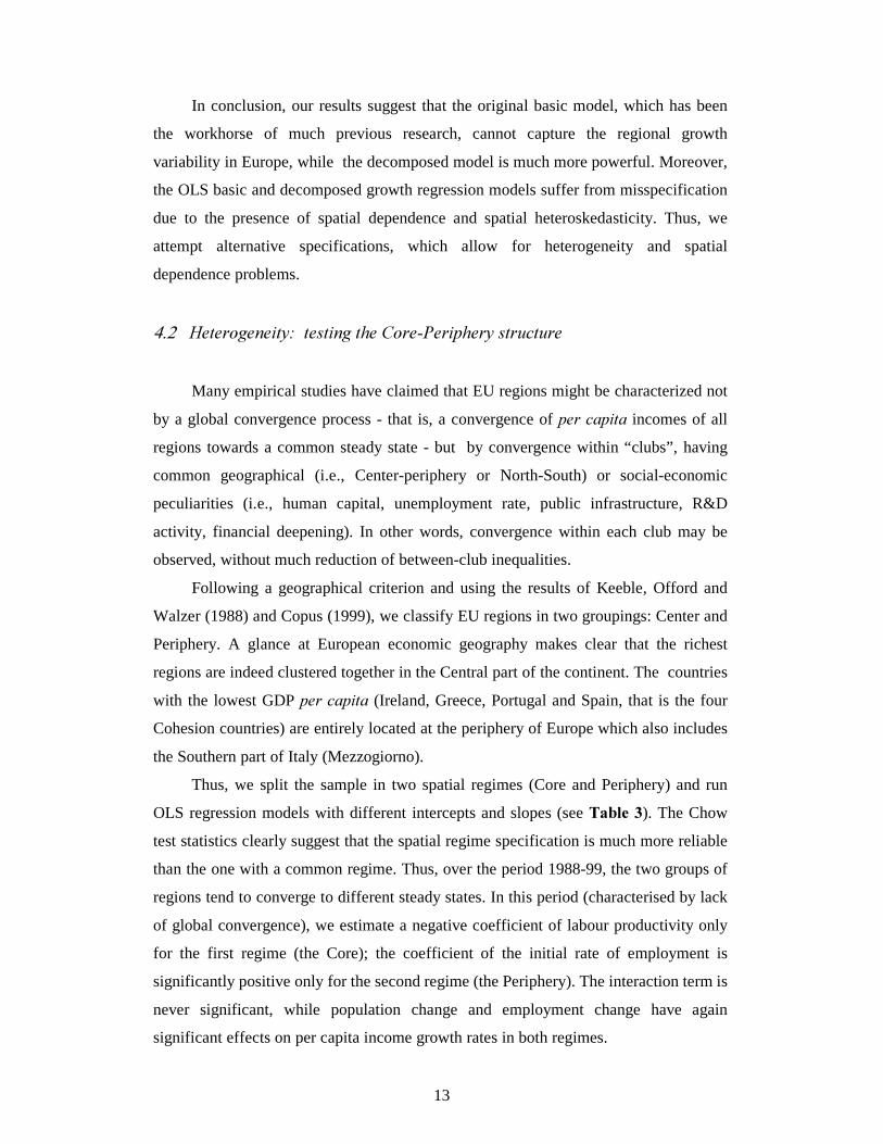
In conclusion, our results suggest that the original basic model, which has been

the workhorse of much previous research, cannot capture the regional growth

variability in Europe, while the decomposed model is much more powerful. Moreover,

the OLS basic and decomposed growth regression models suffer from misspecification

due to the presence of spatial dependence and spatial heteroskedasticity. Thus, we

attempt alternative specifications, which allow for heterogeneity and spatial

dependence problems.

4.2 �+HWHURJHQHLW\���WHVWLQJ�WKH�&RUH�3HULSKHU\�VWUXFWXUH��

Many empirical studies have claimed that EU regions might be characterized not

by a global convergence process - that is, a convergence of SHU�FDSLWD incomes of all

regions towards a common steady state - but by convergence within “clubs”, having

common geographical (i.e., Center-periphery or North-South) or social-economic

peculiarities (i.e., human capital, unemployment rate, public infrastructure, R&D

activity, financial deepening). In other words, convergence within each club may be

observed, without much reduction of between-club inequalities.

Following a geographical criterion and using the results of Keeble, Offord and

Walzer (1988) and Copus (1999), we classify EU regions in two groupings: Center and

Periphery. A glance at European economic geography makes clear that the richest

regions are indeed clustered together in the Central part of the continent. The countries

with the lowest GDP SHU�FDSLWD (Ireland, Greece, Portugal and Spain, that is the four

Cohesion countries) are entirely located at the periphery of Europe which also includes

the Southern part of Italy (Mezzogiorno).

Thus, we split the sample in two spatial regimes (Core and Periphery) and run

OLS regression models with different intercepts and slopes (see 7DEOH��). The Chow

test statistics clearly suggest that the spatial regime specification is much more reliable

than the one with a common regime. Thus, over the period 1988-99, the two groups of

regions tend to converge to different steady states. In this period (characterised by lack

of global convergence), we estimate a negative coefficient of labour productivity only

for the first regime (the Core); the coefficient of the initial rate of employment is

significantly positive only for the second regime (the Periphery). The interaction term is

never significant, while population change and employment change have again

significant effects on per capita income growth rates in both regimes.

14

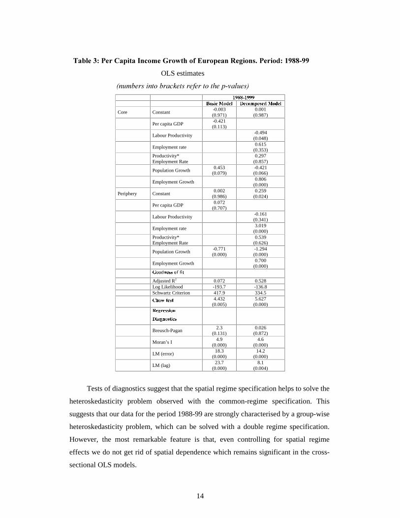
7DEOH����3HU�&DSLWD�,QFRPH�*URZWK�RI�(XURSHDQ�5HJLRQV��3HULRG����������

OLS estimates

�QXPEHUV�LQWR�EUDFNHWV�UHIHU�WR�WKH�S�YDOXHV��

£(¤�¥�¥�¦�£(¤�¤�¤ §�¨�©�ª «�¬®­�¯1°(±³²�°(«>­�´¶µ1­�©9°>¯4¬+­�¯�°>±Core Constant

-0.003 (0.971)

0.001 (0.987)

Per capita GDP

-0.421 (0.113)

Labour Productivity

-0.494 (0.048)

Employment rate

0.615 (0.353)

Productivity* Employment Rate

0.297

(0.857)

Population Growth 0.453

(0.079) -0.421 (0.066)

Employment Growth 0.806 (0.000)

Periphery Constant 0.002

(0.986) 0.259

(0.024) Per capita GDP 0.072

(0.707)

Labour Productivity

-0.161 (0.341)

Employment rate 3.019 (0.000)

Productivity* Employment Rate

0.539

(0.626)

Population Growth -0.771 (0.000)

-1.294 (0.000)

Employment Growth

0.700 (0.000) · ­�­�¯�¸�°>©9©�­�¹&¹ ª º

Adjusted R2 0.072 0.528 Log Likelihood -193.7 -136.8 Schwartz Criterion 417.9 334.5 »�¼ ­�½¾º °>©�º 4.432

(0.005) 5.627

(0.000) ¿�°>À�Á3°>©9©�ª ­�¸²�ª ¨�À�¸�­�©�º ª «>©

Breusch-Pagan

2.3 (0.131)

0.026 (0.872)

Moran’s I

4.9 (0.000)

4.6 (0.000)

LM (error)

18.3 (0.000)

14.2 (0.000)

LM (lag)

23.7 (0.000)

8.1 (0.004)

Tests of diagnostics suggest that the spatial regime specification helps to solve the

heteroskedasticity problem observed with the common-regime specification. This

suggests that our data for the period 1988-99 are strongly characterised by a group-wise

heteroskedasticity problem, which can be solved with a double regime specification.

However, the most remarkable feature is that, even controlling for spatial regime

effects we do not get rid of spatial dependence which remains significant in the cross-

sectional OLS models.

15

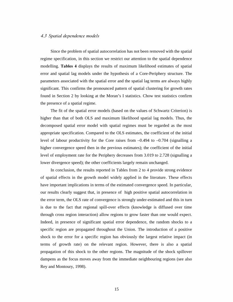
4.3 6SDWLDO�GHSHQGHQFH�PRGHOV�

Since the problem of spatial autocorrelation has not been removed with the spatial

regime specification, in this section we restrict our attention to the spatial dependence

modelling. 7DEOHV� �� displays the results of maximum likelihood estimates of spatial

error and spatial lag models under the hypothesis of a Core-Periphery structure. The

parameters associated with the spatial error and the spatial lag terms are always highly

significant. This confirms the pronounced pattern of spatial clustering for growth rates

found in Section 2 by looking at the Moran’s I statistics. Chow test statistics confirm

the presence of a spatial regime.

The fit of the spatial error models (based on the values of Schwartz Criterion) is

higher than that of both OLS and maximum likelihood spatial lag models. Thus, the

decomposed spatial error model with spatial regimes must be regarded as the most

appropriate specification. Compared to the OLS estimates, the coefficient of the initial

level of labour productivity for the Core raises from –0.494 to –0.704 (signalling a

higher convergence speed then in the previous estimates); the coefficient of the initial

level of employment rate for the Periphery decreases from 3.019 to 2.728 (signalling a

lower divergence speed); the other coefficients largely remain unchanged.

In conclusion, the results reported in Tables from 2 to 4 provide strong evidence

of spatial effects in the growth model widely applied in the literature. These effects

have important implications in terms of the estimated convergence speed. In particular,

our results clearly suggest that, in presence of high positive spatial autocorrelation in

the error term, the OLS rate of convergence is strongly under-estimated and this in turn

is due to the fact that regional spill-over effects (knowledge is diffused over time

through cross region interaction) allow regions to grow faster than one would expect.

Indeed, in presence of significant spatial error dependence, the random shocks to a

specific region are propagated throughout the Union. The introduction of a positive

shock to the error for a specific region has obviously the largest relative impact (in

terms of growth rate) on the relevant region. However, there is also a spatial

propagation of this shock to the other regions. The magnitude of the shock spillover

dampens as the focus moves away from the immediate neighbouring regions (see also

Rey and Montoury, 1998).

16

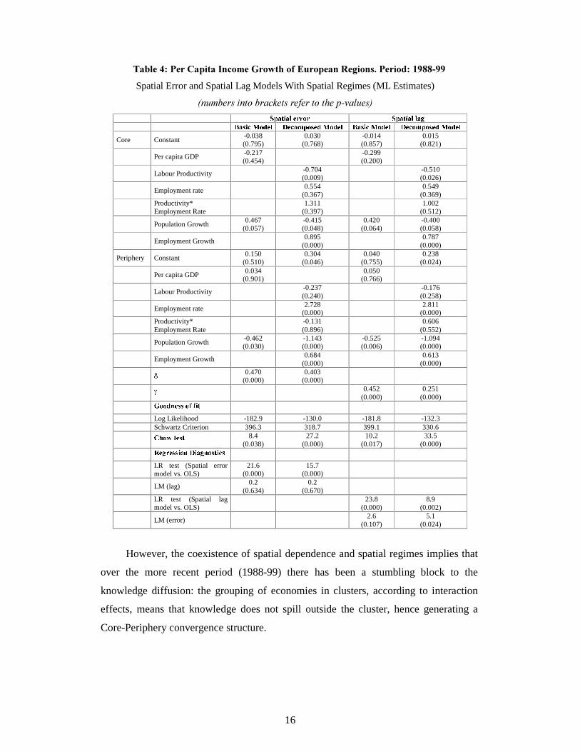
7DEOH����3HU�&DSLWD�,QFRPH�*URZWK�RI�(XURSHDQ�5HJLRQV��3HULRG����������

Spatial Error and Spatial Lag Models With Spatial Regimes (ML Estimates)

�QXPEHUV�LQWR�EUDFNHWV�UHIHU�WR�WKH�S�YDOXHV�� µ�¨�º ª ¨�±1°(Á>Á>­�Á  µ1¨�º ª ¨�±1± ¨�À

§�¨�©9ª «�¬+­�¯�°>± ²�°>«(­�´Ãµ�­�©�°(¯E¬®­�¯1°(±Ä§�¨�©�ª «�¬®­�¯1°(± ²�°>«>­�´¶µ�­�©�°>¯4¬+­�¯�°>±Core Constant

-0.038 (0.795)

0.030 (0.768)

-0.014 (0.857)

0.015 (0.821)

Per capita GDP -0.217 (0.454)

-0.299 (0.200)

Labour Productivity

-0.704 (0.009)

-0.510 (0.026)

Employment rate

0.554 (0.367)

0.549

(0.369) Productivity*

Employment Rate

1.311 (0.397)

1.002

(0.512)

Population Growth 0.467

(0.057) -0.415 (0.048)

0.420 (0.064)

-0.400 (0.058)

Employment Growth

0.895 (0.000)

0.787

(0.000)

Periphery Constant 0.150

(0.510) 0.304

(0.046) 0.040

(0.755) 0.238

(0.024) Per capita GDP 0.034

(0.901) 0.050

(0.766)

Labour Productivity

-0.237 (0.240)

-0.176 (0.258)

Employment rate 2.728 (0.000)

2.811 (0.000)

Productivity* Employment Rate

-0.131 (0.896)

0.606

(0.552) Population Growth -0.462

(0.030) -1.143 (0.000)

-0.525 (0.006)

-1.094 (0.000)

Employment Growth

0.684 (0.000)

0.613

(0.000) Å

0.470 (0.000)

0.403 (0.000)

Æ

0.452 (0.000)

0.251 (0.000) · ­�­�¯�¸�°>©�©�­�¹&¹ ª º

Log Likelihood -182.9 -130.0 -181.8 -132.3 Schwartz Criterion 396.3 318.7 399.1 330.6 »�¼ ­�½¾º °>©�º 8.4

(0.038) 27.2

(0.000) 10.2

(0.017) 33.5

(0.000) ¿�°>À�Á>°>©�©�ª ­�¸E²�ª ¨�À�¸�­�©�º ª «>©

LR test (Spatial error model vs. OLS)

21.6 (0.000)

15.7 (0.000)

LM (lag)

0.2 (0.634)

0.2 (0.670)

LR test (Spatial lag model vs. OLS)

23.8 (0.000)

8.9 (0.002)

LM (error)

2.6 (0.107)

5.1 (0.024)

However, the coexistence of spatial dependence and spatial regimes implies that

over the more recent period (1988-99) there has been a stumbling block to the

knowledge diffusion: the grouping of economies in clusters, according to interaction

effects, means that knowledge does not spill outside the cluster, hence generating a

Core-Periphery convergence structure.

17

���6HPL�SDUDPHWULF�UHJUHVVLRQV�

The parametric estimation results of the cross-region growth models discussed above

highlighted the emergence of a Core-Periphery structure over the nineties. However,

such evidence does not necessarily imply that the Core-Periphery classification is the

best one to identify the presence of multiple regimes. In other words, the choice of this

geographical taxonomy may result to be arbitrary and other forms of non-linearities

may characterise regional development patterns in Europe.

In this section, we try to identify non-linearities in European regions’ growth

behaviour by using semi-parametric techniques which allow non linear behaviours to

emerge endogenously from the data. We use only the “GHFRPSRVHG” specification of

the regional growth model and introduce a spatial lagged term of the dependent variable

(spatial lag model) as well as spatially filtered independent variables (spatial error

model). Firstly, we model the regional per capita income growth rate semi-

parametrically, specifying a linear regression-like fits on the initial level of employment

rate, on the population growth and on the lag of the dependent variableand a local linear

regression fit on labour productivity and a local quadratic fit on the employment rate.

Then, we model the regional growth rates, specifying a local linear fit over the

combination of labour productivity and employment rates. The globally linear terms are

always significant and with the expected sign, coherently with the globally parametric

results (VHH�7DEOH���DQG��).

18

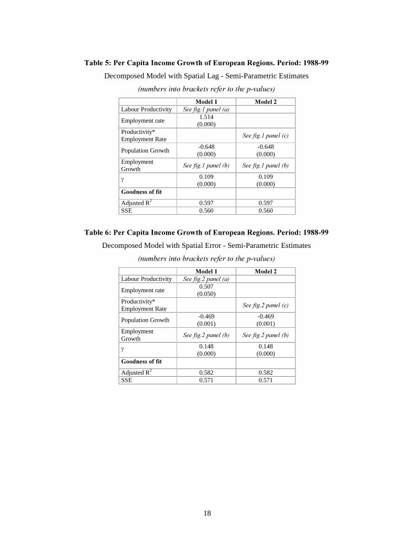
7DEOH����3HU�&DSLWD�,QFRPH�*URZWK�RI�(XURSHDQ�5HJLRQV��3HULRG����������

Decomposed Model with Spatial Lag - Semi-Parametric Estimates

�QXPEHUV�LQWR�EUDFNHWV�UHIHU�WR�WKH�S�YDOXHV��

� 0RGHO��� 0RGHO���

Labour Productivity 6HH�ILJ���SDQHO��D��

Employment rate 1.514

(0.000)

Productivity* Employment Rate

6HH�ILJ���SDQHO��F��

Population Growth -0.648 (0.000)

-0.648 (0.000)

Employment Growth

6HH�ILJ���SDQHO��E�� 6HH�ILJ���SDQHO��E��

g 0.109 (0.000)

0.109 (0.000)

*RRGQHVV�RI�ILW�

Adjusted R2 0.597 0.597 SSE 0.560 0.560

7DEOH����3HU�&DSLWD�,QFRPH�*URZWK�RI�(XURSHDQ�5HJLRQV��3HULRG����������

Decomposed Model with Spatial Error - Semi-Parametric Estimates

�QXPEHUV�LQWR�EUDFNHWV�UHIHU�WR�WKH�S�YDOXHV��

� 0RGHO��� 0RGHO���

Labour Productivity 6HH�ILJ���SDQHO��D��

Employment rate 0.507

(0.050)

Productivity* Employment Rate

6HH�ILJ���SDQHO��F��

Population Growth -0.469 (0.001)

-0.469 (0.001)

Employment Growth

6HH�ILJ���SDQHO��E�� 6HH�ILJ���SDQHO��E��

g 0.148 (0.000)

0.148 (0.000)

*RRGQHVV�RI�ILW�

Adjusted R2 0.582 0.582 SSE 0.571 0.571

19

5.1 6SDWLDO�ODJ�VHPL�SDUDPHWULF�PRGHO�

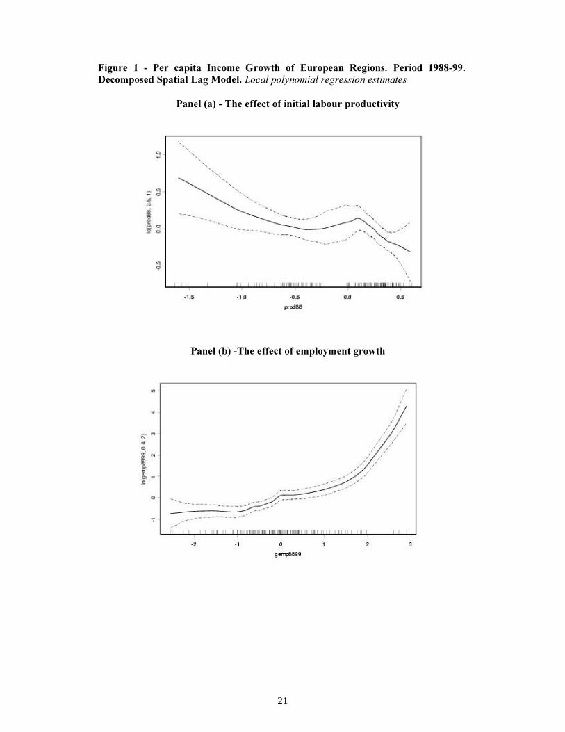
In )LJXUHV� �, we report the graphical output of the fitted smooth functions (solid

lines) and the 95% confidence intervals (dotted lines). The graphical output allows us to

identify a strong non-linearity between the levels of labour productivity and subsequent

regional growth rates (SDQHO� D). F tests overwhelming reject the null hypothesis of

linearity in favour of the local regression fit, with p<0.01. The figure clearly shows that

there is a weak effect of initial labour productivity on per capita income growth rates

until the level of productivity exceeds by 0.1 the EU average level. But once exceeded

that threshold, there is a strong negative relationship (i.e. a convergence path) between

the two variables. The linear model (with a common regime) is therefore strongly

misleading. Instead, the parametric results with two regimes revealed a negative

coefficient of the level of labour productivity for Core regions and a non-significant

coefficient for Peripheral regions. Moreover, it is important to say that more than 70%

of the regions with a relative productivity level equal or lower than 0.1 are in the

Periphery; while more than 90% of regions with a relative productivity level higher

than 0.1 are in the Core and about 10% in the Periphery. Thus, we can conclude that the

exogenous Core-Periphery structure captures an important of the non-linear effect of

labour productivity on regional growth behaviour properly identified by the semi-

parametric estimation, although with some approximation (particularly as far as

peripheral regions are concerned).

The effect of employment change on per capita income growth is strongly

significant and monotonically increasing. Only at relative employment growth rates

lower than about –1 it is not observed any positive relation between the two variables;

above that threshold we can easily distinguish between a slow (if the relative

employment growth rate is between –1 and 0), a medium (if the relative employment

growth rate is between 0 and 2) and a high (if the relative employment growth rate is

higher than 2) employment growth effect. Again, it is interesting to note that about 85%

of the regions with a relative employment growth rate lower than -1 are in the

Periphery, while 70% of regions with a slow, a medium or a high employment growth

effect are in the Core. Actually, the parametric results showed a stronger employment

growth effect for the Core regions than for the Peripheral regions.

Thus, according to these first results of the semi-parametric model, we might

conclude that the parametric “decomposed” model with a Core-Periphery double

20

regime allows us to capture the strong non-linearities identified in a properly specified

smoothed fashion for the most relevant variables (i.e. the initial of labour productivity

and the employment growth rate), with a low - even if not negligible - margin of error.

Table 5 reports also the results of a semi parametric regression model specified with

a local linear fit over the combination of labour productivity and employment rates. As

shown above, the parametric regression model did not revealed any significant effect of

the interaction between the two variables on per capita income growth rates. On the

contrary, an F test clearly indicates that the smooth of the interaction term belongs to

the semi-parametric specification, and is superior to a specification with only linear and

multiplicative terms in “labour productivity” and “employment rates”.

As already emphasised, the two terms of the interaction have significant opposite

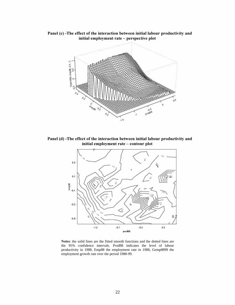
effects on the expected regional growth rate. The 2-dimensional lowess smooth gives

more information about the role of each initial condition on regional growth. Figure 1

panel (c) reports the 3-dimensional perspective plot, with the two initial conditions on

the [ and \ axes and the smoothed impact on growth plotted on the ] (vertical) axis. The

correspondent contour plot is shown in panel (d). The merit of this analysis is to asses

whether each initial condition matters, or whether only one of the two variables is

important. Looking at the perspective plot, we can clearly see that our model predicts

higher growth rates for regions with an initial employment rate higher than the EU

average, whatever the initial level of labour productivity. Also when both the

employment rate and the productivity level are lower than the EU average, income

growth rates are positive, but decreasing in the initial level of both productivity and

employment rate; in other words, when both initial conditions are low, any increase in

either initial level tends to decrease the expected rate of growth, signalling a movement

toward convergence within the group of these laggard regions; this movement

(reduction of the expected growth rate of per capita GDP) is much more pronounced in

correspondence of a rise in productivity than in the employment rate. This can also be

seen in the contours in panel (d): in the South West part of the figure, these contours are

negatively sloped 45° lines and their height is decreasing as they move outward..

Finally, for high levels of labour productivity and low employment rates, our model

predicts low income growth rates.

21

)LJXUH� �� �� 3HU� FDSLWD� ,QFRPH� *URZWK� RI� (XURSHDQ� 5HJLRQV�� 3HULRG� ���������

'HFRPSRVHG�6SDWLDO�/DJ�0RGHO��/RFDO�SRO\QRPLDO�UHJUHVVLRQ�HVWLPDWHV��

3DQHO��D����7KH�HIIHFW�RI�LQLWLDO�ODERXU�SURGXFWLYLW\�

�

3DQHO��E���7KH�HIIHFW�RI�HPSOR\PHQW�JURZWK�

22

�

3DQHO��F���7KH�HIIHFW�RI�WKH�LQWHUDFWLRQ�EHWZHHQ�LQLWLDO�ODERXU�SURGXFWLYLW\�DQG�

LQLWLDO�HPSOR\PHQW�UDWH�±�SHUVSHFWLYH�SORW�

�

�

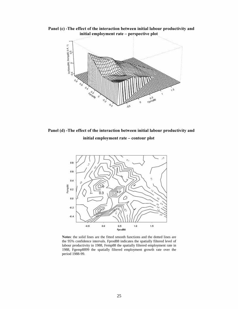
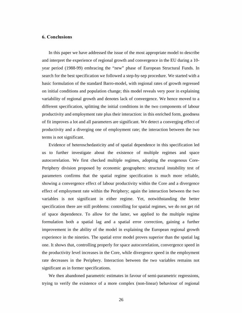
3DQHO��G���7KH�HIIHFW�RI�WKH�LQWHUDFWLRQ�EHWZHHQ�LQLWLDO�ODERXU�SURGXFWLYLW\�DQG�

LQLWLDO�HPSOR\PHQW�UDWH�±�FRQWRXU�SORW�

�

1RWHV: the solid lines are the fitted smooth functions and the dotted lines are the 95% confidence intervals. Prod88 indicates the level of labour productivity in 1988, Emp88 the employment rate in 1988, Gemp8899 the employment growth rate over the period 1988-99.

23

5.2 6SDWLDO�HUURU�VHPL�SDUDPHWULF�PRGHO�

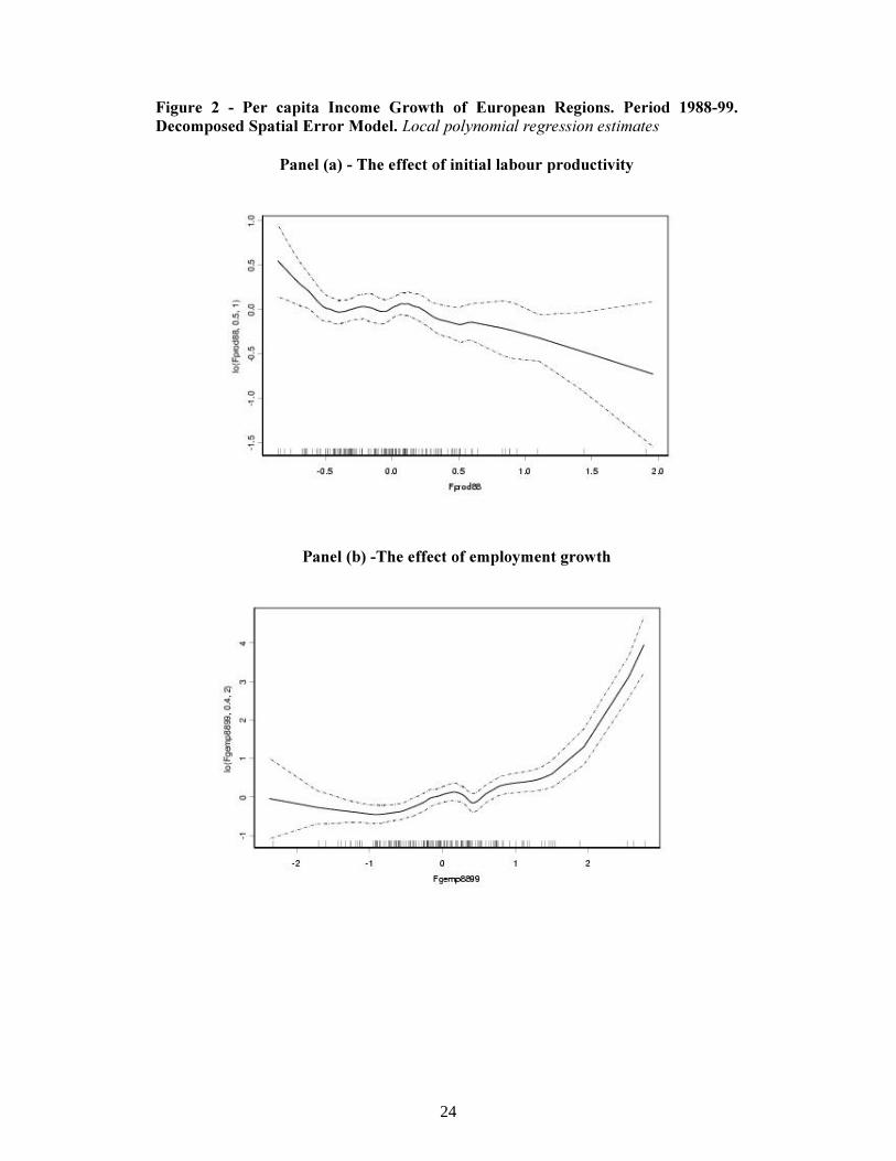
Table 6 reports the results of a semi parametric regression model specified in the

same way as in Table 5 but with the covariates (initial level of labour productivity,

initial employment rate, their interaction and population and employment growth)

measured as spatially filtered variables. In other words, we specified a semi-parametric

spatial error model of growth behaviour. Figure 2 reports the graphical output of the

fitted smooth functions (solid lines) and the 95% confidence intervals (dotted lines).

The most remarkable difference from the results of the semi-parametric spatial lag

model is observable for the interaction term. As it has been shown above, under the

hypothesis of ‘spatial lag’, that is when the spatial dependence problem is controlled for

by the inclusion of the spatial lagged term of the dependent variable, at high initial

employment rates the expected income growth rate is always higher than the EU

average. This feature disappears under the hypothesis of ‘spatial error’, that is when the

spatial dependence problem is controlled for not only by the inclusion of the spatial

lagged term of the dependent variable, but also by using spatially filtered variables of

each covariate, included the initial employment rate. The 3-dimensional perspective

plot in Figure 2 panel (c) and its correspondent contour plot in panel (d) clearly show

that when both employment rate and labour productivity are initially high, the expected

income growth rate is lower than EU average and decreasing in the productivity level

(signalling a tendency toward convergence for this kind of regions). Moreover, at initial

productivity levels close to or below the UE average, an increase from very low levels

of the employment rate leads, up to a point, to a decrease of the predicted growth rate of

per capita GDP; this movement reverses when the regional employment rates become

higher than the EU average; from that point onwards, a rising employment rates is

accompanied by an increase of the expected growth of per capita income. Such

important differences in the prediction of the two models are probably due to the fact

that the positive effect of employment rate on regional income growth (the divergence

effect) is highly related to a strong spatial dependence in regional job creation.

24

)LJXUH� �� �� 3HU� FDSLWD� ,QFRPH� *URZWK� RI� (XURSHDQ� 5HJLRQV�� 3HULRG� ���������

'HFRPSRVHG�6SDWLDO�(UURU�0RGHO��/RFDO�SRO\QRPLDO�UHJUHVVLRQ�HVWLPDWHV��

3DQHO��D����7KH�HIIHFW�RI�LQLWLDO�ODERXU�SURGXFWLYLW\�

�

3DQHO��E���7KH�HIIHFW�RI�HPSOR\PHQW�JURZWK�

25

3DQHO��F���7KH�HIIHFW�RI�WKH�LQWHUDFWLRQ�EHWZHHQ�LQLWLDO�ODERXU�SURGXFWLYLW\�DQG�

LQLWLDO�HPSOR\PHQW�UDWH�±�SHUVSHFWLYH�SORW�

�

3DQHO��G���7KH�HIIHFW�RI�WKH�LQWHUDFWLRQ�EHWZHHQ�LQLWLDO�ODERXU�SURGXFWLYLW\�DQG�

LQLWLDO�HPSOR\PHQW�UDWH�±�FRQWRXU�SORW�

�1RWHV: the solid lines are the fitted smooth functions and the dotted lines are the 95% confidence intervals. Fprod88 indicates the spatially filtered level of labour productivity in 1988, Femp88 the spatially filtered employment rate in 1988, Fgemp8899 the spatially filtered employment growth rate over the period 1988-99.

26

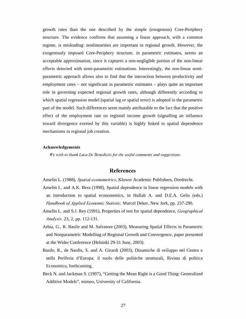
���&RQFOXVLRQV�

In this paper we have addressed the issue of the most appropriate model to describe

and interpret the experience of regional growth and convergence in the EU during a 10-

year period (1988-99) embracing the “new” phase of European Structural Funds. In

search for the best specification we followed a step-by-sep procedure. We started with a

basic formulation of the standard Barro-model, with regional rates of growth regressed

on initial conditions and population change; this model reveals very poor in explaining

variability of regional growth and denotes lack of convergence. We hence moved to a

different specification, splitting the initial conditions in the two components of labour

productivity and employment rate plus their interaction: in this enriched form, goodness

of fit improves a lot and all parameters are significant. We detect a converging effect of

productivity and a diverging one of employment rate; the interaction between the two

terms is not significant.

Evidence of heteroschedasticity and of spatial dependence in this specification led

us to further investigate about the existence of multiple regimes and space

autocorrelation. We first checked multiple regimes, adopting the exogenous Core-

Periphery division proposed by economic geographers: structural instability test of

parameters confirms that the spatial regime specification is much more reliable,

showing a convergence effect of labour productivity within the Core and a divergence

effect of employment rate within the Periphery; again the interaction between the two

variables is not significant in either regime. Yet, notwithstanding the better

specification there are still problems: controlling for spatial regimes, we do not get rid

of space dependence. To allow for the latter, we applied to the multiple regime

formulation both a spatial lag and a spatial error correction, gaining a further

improvement in the ability of the model in explaining the European regional growth

experience in the nineties. The spatial error model proves superior than the spatial lag

one. It shows that, controlling properly for space autocorrelation, convergence speed in

the productivity level increases in the Core, while divergence speed in the employment

rate decreases in the Periphery. Interaction between the two variables remains not

significant as in former specifications.

We then abandoned parametric estimates in favour of semi-parametric regressions,

trying to verify the existence of a more complex (non-linear) behaviour of regional

27

growth rates than the one described by the simple (exogenous) Core-Periphery

structure. The evidence confirms that assuming a linear approach, with a common

regime, is misleading: nonlinearities are important in regional growth. However, the

exogenously imposed Core-Periphery structure, in parametric estimates, seems an

acceptable approximation, since it captures a non-negligible portion of the non-linear

effects detected with semi-parametric estimations. Interestingly, the non-linear semi-

parametric approach allows also to find that the interaction between productivity and

employment rates – not significant in parametric estimates – plays quite an important

role in governing expected regional growth rates, although differently according to

which spatial regression model (spatial lag or spatial error) is adopted in the parametric

part of the model. Such differences seem mainly attributable to the fact that the positive

effect of the employment rate on regional income growth (signalling an influence

toward divergence exerted by this variable) is highly linked to spatial dependence

mechanisms in regional job creation.

$FNQRZOHGJHPHQWV�

:H�ZLVK�WR�WKDQN�/XFD�'H�%HQHGLFWLV�IRU�WKH�XVHIXO�FRPPHQWV�DQG�VXJJHVWLRQV��

5HIHUHQFHV�

Anselin L. (1988), 6SDWLDO�HFRQRPHWULFV, Kluwer Academic Publishers, Dordrecht.

Anselin L. and A.K. Bera (1998), Spatial dependence in linear regression models with

an introduction to spatial econometrics, in Hullah A. and D.E.A. Gelis (eds.)

+DQGERRN�RI�$SSOLHG�(FRQRPLF�6WDWLVWLF��Marcel Deker, New Jork, pp. 237-290.

Anselin L. and S.J. Rey (1991), Properties of test for spatial dependence, *HRJUDSKLFDO�

$QDO\VLV��23, 2, pp. 112-131.

Arbia, G., R. Basile and M. Salvatore (2003), Measuring Spatial Effects in Parametric

and Nonparametric Modelling of Regional Growth and Convergence, paper presented

at the Wider Conference (Helsinki 29-31 June, 2003).

Basile, R., de Nardis, S. and A. Girardi (2003), Dinamiche di sviluppo nel Centro e

nella Periferia d’Europa: il ruolo delle politiche strutturali, Rivista di politica

Economica, forthcoming.

Beck N. and Jackman S. (1997), “Getting the Mean Right is a Good Thing: Generalized

Additive Models”, mimeo, University of California.

28

Boldrin M. and F. Canova (2001), Europe’s Regions: Income Disparities and Regional

Policies, (FRQRPLF�3ROLF\, 32, pp. 207-53.

Cleveland W.S., “Robust Locally-Weighted Regression and Scatterplot Smoothing”,

-RXUQDO�RI�WKH�$PHULFDQ�6WDWLVWLFDO�$VVRFLDWLRQ, n.74, 1979.

Cleveland W.S. and Devlin S.J., “Locally-Weighted Regression: an Approach to

Regression Analysis by Local Fitting”, -RXUQDO� RI� WKH� $PHULFDQ� 6WDWLVWLFDO�

$VVRFLDWLRQ, n.83, 1988.

Cliff A.D. and J. K. Ord (1973), 6SDWLDO�DXWRFRUUHODWLRQ, Pion, London.

Conley T. (1999), GMM estimation with cross sectional dependence, -RXUQDO� RI�

(FRQRPHWULFV, 92, 1, pp. 1-45.

Copus A. (1999), “A New Peripherality Index for the NUTS III Regions of the

European Union”, (XURSHDQ�&RPPLVVLRQ, ERDF/FEDER Study 98/00/27/130.

Durlauf S.N., A. Kourtellos and A. Minkin (2001), The Local Solow Growth Model,

(XURSHDQ�(FRQRPLF�5HYLHZ��n. 45.

Durlauf S.N. and D.T. Quah (1999), The New Empirics of Economic Growth, in J.B.

Taylor and M. Woodford (eds.), +DQGERRN� RI� 0DFURHFRQRPLFV�� vol. IA, Cap. 4,

North-Holland, Amsterdam.

Durlauf S.N. and P. Johnson (1995), Multiple Regimes and Cross-Country Growth

Behavior, -RXUQDO�RI�$SSOLHG�(FRQRPHWULFV, n. 10.

Keeble D., Offord J. and S. Walker (1988), 3HULSKHUDO� 5HJLRQV� LQ� D�&RPPXQLW\� RI�

7ZHOYH�0HPEHU�6WDWHV, Office for Official Publications of the E.C., Luxemburg.

Liu Z. and T. Stengos (1999), Non-Linearities in Cross-Country Growth Regressions: a

Semiparametric Approach, -RXUQDO�RI�$SSOLHG�(FRQRPHWULFV, n. 14.

Mankiw N. G., Romer D. and D.N. Weil (1992), A contribution to the empirics of

economic growth, 4XDUWHUO\�-RXUQDO�RI�HFRQRPLFV��May, pp. 407-437.

Rey S.J. and B.D. Montouri (1998), US regional income convergence: a spatial

econometric perspective, 5HJLRQDO�6WXGLHV��33, 2, pp. 143-156.