preparation of high-dimensional biomedical data with a
TRANSCRIPT

Preparation of high-dimensional biomedicaldata with a focus on prediction and error
estimation
Roman Hornung
Munchen 2016


Preparation of high-dimensional biomedicaldata with a focus on prediction and error
estimation
Roman Hornung
Dissertation
an der Fakultat fur Mathematik, Informatik und Statistik
der Ludwig–Maximilians–Universitat
Munchen
vorgelegt von
Roman Hornung
aus Augsburg
Munchen, den 19. September 2016

Erstgutachter: Prof. Dr. Anne-Laure Boulesteix
Zweitgutachter: Prof. Dr. David Causeur
Drittgutachter: Dr. Marie-Laure Martin-Magniette
Tag der mundlichen Prufung: 15.12.2016

Summary
This thesis is based on three projects in which specific aspects of the preparation ofhigh-dimensional biomedical data play a central role.
The first project is concerned with the question of whether it is necessary to includedata preparation steps in cross-validation procedures in situations where such proce-dures are followed to estimate the prediction error of biomedical prediction rules. Inpractice many data preparation steps are, in most cases, not repeated within cross-validation on the training datasets, but rather performed beforehand on the entiredataset. Thereby, the training data and test data are not entirely separated, which,for some data preparation steps, can lead to a relevant underestimation of the pre-diction error. However, it is mostly unknown for which of these data preparationsteps there is a danger of severe underestimation of this kind. In this project, first ageneral measure is developed to assess the magnitude of this underestimation. Next,this measure is applied to real datasets in extensive analyses in order to determinewhether it is necessary to include two data preparation steps—normalization andprincipal component analysis—in cross-validation procedures.
In the second project an innovative method for batch effect adjustment is developedusing which parts of a dataset that are systematically distorted, can be homogenized.This new method differs from others in that it removes both differences in terms ofmeans and variances among the different dataset parts and corresponding differencesin terms of the dependence structures of the variables. Using simulated data and realdata, the performance of the new method is compared to that of popular alternativemethods.
In the third project the possibility of employing batch effect adjustment and nor-malization to assimilate new data to the training data before prediction in order toachieve greater prediction accuracy is explored. In applications, the data to whicha prediction rule is intended to be applied most often have, for various reasons, aslightly different distribution than the data on which the rule was derived. This oftenleads to increase in prediction error in practice. Therefore, it is desirable to adjustthe distribution of new observations to that of the training observations prior to pre-diction. Here, both batch effect adjustment and normalization methods are suitablein partly modified forms; however, it is not clear which of these methods actuallylead to greater prediction accuracy in practice. Therefore, with the help of a largenumber of real datasets, in the third project several of these methods are comparedwith respect to the prediction accuracies obtained from their use.


Zusammenfassung
Diese Arbeit basiert auf drei Projekten, in denen bestimmte Aspekte der Vorverar-beitung hoch-dimensionaler biomedizinischer Daten eine zentrale Rolle spielen.
Das erste Projekt befasst sich mit der Frage nach der Notwendigkeit des Einschlus-ses von Vorverarbeitungsschritten in Kreuzvalidierungsverfahren, wenn letztere zurSchatzung des Vorhersagefehlers von biomedizinischen Pradiktionsregeln verwendetwerden. In der Praxis werden viele Vorverarbeitungsschritte zumeist nicht innerhalbder Kreuzvalidierung auf den Trainingsdatensatzen wiederholt, sondern vorher aufdem ganzen Datensatz durchgefuhrt. Fur manche Vorverarbeitungsschritte kann die-ses Vorgehen durch die damit verbundene Aufhebung der vollstandigen Trennung vonTrainings- und Testdaten zu einer relevanten Unterschatzung des Vorhersagefehlersfuhren. Es ist jedoch weitestgehend unbekannt, fur welche Vorverarbeitungsschrit-te eine derartige Unterschatzung zu befurchten ist. Deshalb wird in dieser Arbeitzunachst ein allgemeines Maß zur Abschatzung des Ausmaßes dieser Unterschatzungentwickelt. Dieses Maß wird anschließend in ausfuhrlichen Analysen auf echte Da-ten angewendet, um die Frage nach der Notwendigkeit des Einschlusses der beidenVorverarbeitungsschritte Normalisierung und Hauptkomponentanalyse in Kreuzvali-dierungsverfahren abschließend zu beantworten.
Im zweiten Projekt wird eine innovative Methode zur sogenannten Batcheffektent-fernung entwickelt, anhand derer sich systematisch verzerrte Teile eines Datensatzeshomogenisieren lassen. Die Besonderheit der neuen Methode gegenuber existieren-den Alternativen besteht darin, dass sie sowohl Unterschiede in den Mittelwertenund Varianzen zwischen den verschiedenen Teilen des Datensatzes beseitigt als auchentsprechende Unterschiede in der Abhangigkeitsstruktur der Variablen. Die Perfor-manz der neuen Methode wird anhand simulierter und echter Daten mit popularen,alternativen Methoden verglichen.
Das dritte Projekt befasst sich schließlich mit der Moglichkeit, mit Hilfe von Bat-cheffektentfernung und Normalisierung vor der Anwendung von Pradiktionsregeln,die zu pradiktierenden Daten an die Trainingsdaten anzupassen, um eine großereVorhersagegenauigkeit zu erzielen. In Anwendungen folgen die Daten auf die einePradiktionsregel angewendet wird, aus diversen Grunden zumeist einer leicht ande-ren Verteilung als die Daten auf denen sie gelernt wurde. Das fuhrt dazu, dass derVorhersagefehler von Pradiktionsregeln in der Praxis haufig erhoht ist. Deshalb istes wunschenswert die Verteilung der Daten der zu pradiktierenden Beobachtungenan die Verteilung der Trainingsdaten anzupassen. Hierzu bieten sich Batcheffektent-fernungsmethoden und Normalisierungsmethoden in teils abgewandelter Form an.Allerdings ist unklar, welche solcher Methoden in der Praxis tatsachlich zu einergroßeren Vorhersagenauigkeit fuhren. Deshalb werden im letzten der drei Projekteeinige dieser Methoden anhand einer großen Zahl echter Datensatze hinsichtlich deraus ihrer Verwendung jeweils resultierenden Vorhersagegenauigkeiten verglichen.


Acknowledgments
First and foremost, I would like to thank very warmly my thesis adviser Prof. Dr.Anne-Laure Boulesteix. She has pointed me in suitable directions and was alwaysavailable for questions and helpful discussions. Moreover, she created an excellentencouraging collegial atmosphere in which I always felt secure during the preparationof the dissertation.
I would also like to extend my sincere thank to Prof. Dr. David Causeur. Duringmy three research stays in Rennes I always felt very welcome. He pointed me insuitable directions as well, and in our many helpful discussions I was able to gainvaluable insights.
Moreover, I am very grateful to my “periodical” colleagues at the Applied Mathe-matics Department at Agrocampus Ouest in Rennes, who amicably took care of meduring my research stays in Britanny, for work as well as leisure.
Many thanks also to my colleagues at the Department of Medical Informatics,Biometry and Epidemiology for the great atmosphere.
Last but not least, I would like to thank my parents and my friends for their con-tinued support and encouragement inside and outside of work.
Munich, in September 2016 Roman Hornung


Contents
1. Introduction 1
2. Measuring the impact of CV incompleteness with respect to data prepa-ration steps 132.1. Background . . . . . . . . . . . . . . . . . . . . . . . . . . . . . . . . 132.2. Methods . . . . . . . . . . . . . . . . . . . . . . . . . . . . . . . . . . 15
2.2.1. Data material . . . . . . . . . . . . . . . . . . . . . . . . . . . 152.2.2. Addon procedures . . . . . . . . . . . . . . . . . . . . . . . . . 172.2.3. (Addon) normalization . . . . . . . . . . . . . . . . . . . . . . 182.2.4. (Addon) principal component analysis . . . . . . . . . . . . . 192.2.5. The CV incompleteness impact measure (CVIIM) . . . . . . . 192.2.6. Global CVIIM . . . . . . . . . . . . . . . . . . . . . . . . . . . 212.2.7. Illustration . . . . . . . . . . . . . . . . . . . . . . . . . . . . 222.2.8. Study design . . . . . . . . . . . . . . . . . . . . . . . . . . . 24
2.3. Results . . . . . . . . . . . . . . . . . . . . . . . . . . . . . . . . . . . 252.3.1. Normalization . . . . . . . . . . . . . . . . . . . . . . . . . . . 252.3.2. Principal Component Analysis . . . . . . . . . . . . . . . . . . 26
2.4. Discussion . . . . . . . . . . . . . . . . . . . . . . . . . . . . . . . . . 292.4.1. Alternative measures of CV incompleteness . . . . . . . . . . . 292.4.2. Outlook: other preparation steps . . . . . . . . . . . . . . . . 302.4.3. Simulation study . . . . . . . . . . . . . . . . . . . . . . . . . 372.4.4. Combination of several steps . . . . . . . . . . . . . . . . . . . 382.4.5. Further issues . . . . . . . . . . . . . . . . . . . . . . . . . . . 40
2.5. Conclusions . . . . . . . . . . . . . . . . . . . . . . . . . . . . . . . . 44
3. Combining location-and-scale batch effect adjustment with data clean-ing by latent factor adjustment 453.1. Background . . . . . . . . . . . . . . . . . . . . . . . . . . . . . . . . 453.2. Methods . . . . . . . . . . . . . . . . . . . . . . . . . . . . . . . . . . 49
3.2.1. Description of existing batch-effect adjustment methods . . . . 493.2.2. FAbatch . . . . . . . . . . . . . . . . . . . . . . . . . . . . . . 533.2.3. Addon adjustment of independent batches . . . . . . . . . . . 573.2.4. Comparison of FAbatch to other methods . . . . . . . . . . . 61
3.3. Results . . . . . . . . . . . . . . . . . . . . . . . . . . . . . . . . . . . 683.3.1. Ability to adjust for batch effects . . . . . . . . . . . . . . . . 683.3.2. Application in cross-batch prediction . . . . . . . . . . . . . . 753.3.3. Artificial increase in measured class signal by applying SVA . 80
3.4. Discussion . . . . . . . . . . . . . . . . . . . . . . . . . . . . . . . . . 823.5. Conclusions . . . . . . . . . . . . . . . . . . . . . . . . . . . . . . . . 83

xii Contents
4. Improving cross-study prediction through addon batch effect adjust-ment or addon normalization 854.1. Background . . . . . . . . . . . . . . . . . . . . . . . . . . . . . . . . 854.2. Methods . . . . . . . . . . . . . . . . . . . . . . . . . . . . . . . . . . 88
4.2.1. Data material . . . . . . . . . . . . . . . . . . . . . . . . . . . 884.2.2. (Addon) Batch effect adjustment and (addon) quantile normal-
ization . . . . . . . . . . . . . . . . . . . . . . . . . . . . . . . 884.2.3. Cross-study validation . . . . . . . . . . . . . . . . . . . . . . 904.2.4. Study design . . . . . . . . . . . . . . . . . . . . . . . . . . . 90
4.3. Results . . . . . . . . . . . . . . . . . . . . . . . . . . . . . . . . . . . 914.3.1. Addon quantile normalization . . . . . . . . . . . . . . . . . . 924.3.2. Addon batch effect adjustment . . . . . . . . . . . . . . . . . 93
4.4. Discussion . . . . . . . . . . . . . . . . . . . . . . . . . . . . . . . . . 974.4.1. Reasons for no benefit from combining the two approaches . . 974.4.2. Random forest: impaired performance in the presence of dif-
fering class frequencies between training data and test data . . 984.4.3. Boosting as a (potentially) robust method to avoid overfitting
in the context of cross-study prediction . . . . . . . . . . . . . 994.4.4. Further possibilities for application . . . . . . . . . . . . . . . 100
4.5. Conclusions . . . . . . . . . . . . . . . . . . . . . . . . . . . . . . . . 101
5. Conclusions and outlook 103
A. Appendices to Chapter 2 115A.1. Simulation study for the example of supervised variable selection . . . 115A.2. Methodological background . . . . . . . . . . . . . . . . . . . . . . . 122
A.2.1. Prediction rules, prediction errors, and their estimation . . . . 122A.2.2. Incomplete opposed to full CV . . . . . . . . . . . . . . . . . . 124A.2.3. Behavior of CVIIMs,n,K for small εfull(ntrain,K) values . . . . . 125
B. Appendices to Chapter 3 127B.1. Plots used in verification of model assumptions . . . . . . . . . . . . 127B.2. Target variables of datasets used in comparison study . . . . . . . . . 133B.3. Reasons for batch effect structures of datasets used in comparison study134B.4. Boxplots of the metric values for simulated datasets for each method
and simulation scenario . . . . . . . . . . . . . . . . . . . . . . . . . . 135B.5. Tables showing the means of the metric values and of the corresponding
ranks in simulated datasets by method and by scenario . . . . . . . . 142
C. Appendices to Chapter 4 149C.1. Plots of the MCCrule values . . . . . . . . . . . . . . . . . . . . . . . 149

1. Introduction
The analysis of modern, high-dimensional, biomedical data usually involves special
preliminary data preparation steps, for example normalization or filtering by variance,
which are performed before addressing the questions of thematic interest. With tra-
ditional medical datasets preprocessing usually is more straightforward and easier to
conduct. Preliminary steps in this field may involve standardizing the variables or im-
puting missing variables. Given the increasingly important role of high-dimensional
biomedical data in medical research, data preparation can be expected to gain atten-
tion in the scientific literature.
This thesis consists of three parts, in each of which, preparation of high-dimensional
biomedical data plays a central role. In the first part the impact of excluding specific
data preparation from cross-validation on the estimated error is analyzed with the aid
of the cross-validation incompleteness impact measure (CVIIM) developed specially
for this purpose. In the second part, a new batch-effect adjustment method for high-
dimensional data is presented, which, in addition to adjusting for location-and-scale
batch effects, adjusts for batch effects evident in the correlation structures within the
batches. In the third part, a compendium of microarray datasets is used to determine
the extent to which, and under which circumstances, cross-study prediction can be
improved with the aid of addon batch effect adjustment and addon normalization.
Background
In the following, several terms which play a crucial role in the thesis are explained.
High-dimensional data
This term describes datasets featuring more variables than observations. High-
throughput datasets are specific types of high-dimensional datasets featuring many—
often many thousands of—biomolecular variables. In this context, each variable often
corresponds to the behavior of a certain gene. Traditional statistical analysis meth-
ods such as linear or logistic regression are not applicable to high-dimensional data.

2 1. Introduction
However, in the last few decades many methods have been developed that are special-
ized for this data format. Many of these methods were used in the analyses presented
in this thesis.
Data preparation step
In general, this term is used for any analysis step performed before conducting anal-
ysis steps that deliver the final result of the study. However, in this thesis there
is a difference between data preparation steps performed observation by observa-
tion, such as background correction in microarray data, and data preparation steps
which use information across observations. Examples of the latter steps are quantile
normalization of microarray data, batch effect adjustment (see below), and variable
selection. In this thesis only steps of the second kind are considered, which is why in
the following, the term data preparation step refers to this kind of data preparation.
Normalization
Various factors influencing raw high-throughput data lead to differences among obser-
vations. Such differences are due to elements beyond the biological signal of interest.
Therefore, the distributions of the raw values generally are made similar across obser-
vations by employing a normalization method. Due to differences among the various
high-throughput data structures, each data type requires the use of a specific normal-
ization method. An important method is the quantile normalization method (Bolstad
et al.; 2003), which is used in this thesis. After employing this method, the empirical
distributions of the data values are identical across the different observations.
Prediction rule
A central application field of high-throughput data is the prediction of disease states
of patients. To this end, prediction rules are used. A prediction rule is an algorithm
that uses the values of a number of variables in a patient (covariates) to predict the
unknown value of a specific phenotype variable of interest (target variable). Such
prediction rules are obtained, or learned, using the data on a series of patients for
whom the covariate values and the values of the target variable are known. These
data are commonly denoted as training data. The algorithm that is used for learning
the prediction rule is specific to the latter. This thesis is concerned with prediction
rules for high-dimensional data with binary target variables. A prediction rule of this
kind may, for example, be obtained by applying the random forest (RF) algorithm
(Breiman; 2001), which involves constructing a large number of classification trees

3
using the training data. The application of the learned prediction rule then involves
applying the classification trees constituting the constructed RF to the data on a
new patient and aggregating the results to obtain a prediction of his/her value of the
target variable.
When applying prediction rules in practice one is confronted with the raw covariate
data on new patients. Therefore, here, as a preliminary step, any data preparation
steps that have been taken while learning the prediction rule have to be taken for
the data on new patients as well. It is impossible to obtain a prediction based on the
patients’ raw covariate data, because the learning algorithm which delivered the final
prediction rule has used the form of the training data obtained after preparation.
Due to the widespread use of data preparation steps, this issue can be expected to
be equally widespread in practice. However, this issue seems widely overlooked in
the scientific literature. In this thesis the following definition of prediction rules is
given: A prediction rule comprises not only the algorithm specific to the method
outputting the predictions based on the preprocessed data, for example the RF, but
also any data preparation steps to be performed before the preprocessed data can be
committed to this algorithm. In accordance with this definition, the algorithm used
for learning such a prediction rule comprises all data preparation steps.
Estimation of the error of a prediction rule
Before applying a prediction rule, it is important to assess how accurately it can
predict the values of the target variable of independent patients. If the error frequency
of a prediction rule is too high, it should not be applied in practice. This is because
doctors and patients would be misinformed too frequently if such a rule were used for
diagnosis. A naıve and very problematic approach to estimate the error frequency
would be the following: Apply the prediction rule to the training data with which
it was learned and calculate the frequency of which the prediction rule delivers an
incorrect prediction for this data. It is well-known that this can lead to a severe
underestimation of the error frequency to be expected for independent data. The
reason for this is that the prediction rule tends to be better adjusted to its training
data than to the independent data for which it is intended. Therefore, as a general
rule the data used to estimate the error frequency, the test data, should be different
from those used to learn the prediction rule. Here it is possible to discern two cases: 1)
The test data are distinct from the training data but originate from the same dataset
as the training data, referred to as internal validation; 2) The test data stem from
an independent dataset, referred to as external validation. As the data to which the
prediction rule is intended to be applied, usually originate from an entirely different

4 1. Introduction
dataset than that of the training data, external validation results in more realistic
error estimates than internal validation. As data from different datasets other than
from where the training data originate, generally behave more differently than those
from the same datasets, external validation results in higher error estimates (see e.g.
Bernau et al. (2014)).
K-fold cross-validation
The most prominent method for estimating the error frequency to be expected in
internal validation is K-fold cross-validation or short cross-validation (CV). High-
throughput datasets are often quite small; therefore, splitting the dataset into training
data and test data usually leads to at least one of the following two problems: 1) The
test dataset is too small to provide an acceptable accuracy of the error estimate; 2)
The training dataset is too small to ascertain a level of prediction performance similar
to that which results when using the entire dataset as a training dataset. K-fold CV
addresses these issues first by re-performing the error estimation for different splits
of the entire dataset into training data and test data and second by choosing a large
enough amount of training data. Precisely, K-fold CV is conducted as follows: 1)
Split the dataset randomly into K (approximately) equally sized parts, denoted as
folds ; 2) For k ∈ {1, . . . , K}: estimate the error frequency using fold k as test data
and the rest of the dataset as training data; 3) Take the average of the error estimates
from 2). To reduce further the variance of the error estimation, in practice K-fold
CV should be repeated multiple times. Although K-fold CV is less variable than
error estimates obtained when using single splits into training data and test data, its
variance is still high (Efron and Tibshirani; 1997). Ostensibly, no widely accepted
guidelines exist for choosing the number of folds K.
Batch effects
Traditional clinical data most often directly mirror the biological phenomena of in-
terest such as age or sex. By contrast, the data values from microarray-based data
types constitute measurements of the respective biological phenomena such as gene
expression. These measurements are unwantedly influenced by external conditions.
There are numerous external factors that can influence microarray data, such as the
laboratory in which the data are produced, the technician treating the data and
even the time of data generation. As a result, data of observations which have the
same or similar biological characteristics and, thus, should behave similarly, can be
distributed very differently when stemming from different datasets. Such effects gen-

5
erally are known as batch effects. The totality of data from a specific source is denoted
as a batch. Batch effects lead to limited comparability of data from different sources,
which can negatively influence analyses being performed using the combined data.
In contrast to microarray-based data types, which require measuring the underlying
biological phenomena, more modern high-throughput data types such as RNA-Seq
data allow direct investigation of the underlying biological phenomena. Nevertheless,
data collection in the case of these modern high-throughput data types is prone to
error and batch effects have been found to be a problem with these data as well
(Hansen and Irizarry; 2012).
In this thesis, the definition of batch effects comprises not only effects caused by
external conditions of the data generation process but also by differences in data
cohorts due to differing study populations, as long as these differences do not affect
the biological phenomena to be studied with the aid of the data.
Batch effect adjustment
Given that batch effects can influence analyses negatively, it is desirable to re-
move such effects beforehand by assimilating the distributions of the data across
the batches. A method with such an aim is called a batch effect adjustment or batch
effect removal method. A number of such methods exist. Some of them are very
simple, for example, zero-mean centering of the variable values in the batches, while
others are more sophisticated, for example, adjusting for location-and-scale differ-
ences across batches as performed by ComBat (Johnson et al.; 2007). Note that
batch effect adjustment is a data preparation step.
Cross-study prediction
As mentioned above, a prediction rule is applied in practice to data stemming from
entirely different sources than those of the training data. This procedure is referred
to as cross-study prediction in this thesis.

6 1. Introduction
Contents
In this section the three projects presented in the thesis are described in order to
provide an initial overview of the work.
Chapter 2: Measuring the impact of CV incompleteness with
respect to data preparation steps
As stated above, in CV the prediction rule is learned repeatedly using different subsets
of the available dataset. The learning process of obtaining a prediction rule also
comprises the data preparation steps involved according to the definition of prediction
rules given above. Therefore, from a formal standpoint, data preparation should be
re-performed using the training data in each iteration of the CV. Performing data
preparation on the entire dataset before performing error estimation is equivalent to
learning part of the prediction rule using both training data and test data. This can
have negative implications. Above it was stated that the prediction rule is better
adjusted to the data on which it was learned. If these data comprise the test data for
part of the learning process, as done when performing data preparation on the entire
dataset, it can be expected that the test data are better adjusted to the prediction
rule than truly independent data are. Again, this may lead to underestimation of the
error frequency. Chapter 2 is concerned with the latter phenomenon.
In fact, for various reasons, it is common practice to perform certain data prepara-
tion steps, for example, quantile normalization, using the entire dataset before CV.
The extent of underestimation of the error frequency resulting from this, that is, the
impact of such an incomplete CV, differs among data preparation steps. Steps mak-
ing use of the target variable more frequently are associated with a stronger impact
on the estimated error through incomplete CV. However, as will be shown in the
analyses in Chapter 2, there also are steps which use only the covariate values but
nevertheless should not be performed on the entire dataset before error estimation to
warrant against underestimating the error frequency.
The work presented in Chapter 2 resulted from the following three considerations:
1) The impact of incomplete CV depends on the data preparation step under consider-
ation; 2) It is not clear which data preparation steps have to be performed within CV
to prevent a relevant optimistic bias; 3) Someone confronted with a dataset cannot be
expected to decide for his/her specific analysis whether or not he/she should include
a data preparation step in CV. These considerations necessitate the formulation of
empirically based guidelines for individual data preparation steps that state whether
or not these steps generally can be conducted on the entire dataset before CV. When

7
formulating such guidelines based on real datasets, it is convenient, if not required,
to use a measure of the impact of incomplete CV. In Chapter 2 such a measure is
provided with the CV incompleteness impact measure (CVIIM ) which depends on
the distribution underlying the dataset used for estimating it. Therefore, in addition
to CVIIM, with the global CVIIM a measure is provided that does not depend on a
specific data distribution. The estimation of this measure requires several datasets.
With the aid of CVIIM and global CVIIM and through using large collections of
real high-throughput datasets, guidelines for the following two commonly used data
preparation steps are developed: normalization and principal component analysis
(PCA). These guidelines state that while normalization can be performed beforehand
on the entire dataset, PCA should be included in CV. Corresponding empirically
based guidelines ostensibly were previously available only for the data preparation
step “supervised variable selection”. In addition to the guidelines for normalization
and PCA, preliminary results obtained for other common data preparation steps are
provided.
Chapter 3: Combining location-and-scale batch effect adjustment
with data cleaning by latent factor adjustment
Due to the wide variety of factors leading to batch effects, the latter are equally
diverse in nature. Therefore a batch effect adjustment method intended to work well
for various datasets should do at least one of the following: 1) address coarse types
of batch effects that are present in all datasets affected by batch effects. Examples
of methods of this kind are mean-centering, standardization, ratio-A, ratio-G (Luo
et al.; 2010), and ComBat; 2) adjust to the specific kind of batch effects of the dataset
being analyzed. An example of a method of this kind is surrogate variable analysis
(SVA) (Leek and Storey; 2007).
Methods of the first kind may miss important characteristics of batch effects present
in the specific dataset being analyzed, for example, sophisticated dependence struc-
tures induced by batch effects. By contrast, methods of the second kind may miss
simple batch effect structures which can easily be addressed, for example, mean-
differences of the variables across batches. In Chapter 3 a method is presented with
FAbatch that addresses coarse features of batch effects and adjusts to sophisticated
batch effect patterns specific to the individual dataset being studied. FAbatch repre-
sents an extension of ComBat, that is, adjustment for location-and-scale differences of
the variables across batches. With FAbatch, in addition to location-and-scale adjust-
ment, the data are adjusted for latent factor influences associated with batch effects
within the individual batches. This has the effect of reducing excess heterogeneity

8 1. Introduction
within batches, that is, variations in the observations not attributable to the biolog-
ical signal of interest are addressed, which is very similar to the approach followed
by SVA. However, in contrast to FAbatch, SVA was developed for situations where
it is not known which observation belongs to which batch. The primary goal of the
adjustment for latent factor influences performed by SVA is to remove heterogene-
ity resulting from observations belonging to different batches. The adjustment for
latent factor influences performed by FAbatch within batches, by contrast, should
capture sophisticated properties of the batches specific to the dataset being studied.
In the estimation of the latent factor models, it is important that the biological sig-
nal of interest be protected. Otherwise, not only unwanted differences among the
observations attributable to batch effects would be removed, but also would desired
differences attributable to the biological signal. SVA uses a specific procedure for
protecting the biological signal. This procedure can lead to a dangerous exaggeration
of the biological signal, as will be discussed in detail in Chapter 3. By contrast, with
FAbatch the signal exaggeration is mitigated by using predicted class probabilities
instead of the actual classes in the protection of the biological signal.
In Chapter 3, using a large collection of real high-throughput datasets, FAbatch is
extensively compared to commonly used competitors with respect to several metrics.
These metrics measure either the homogeneity of the data across batches after batch
effect adjustment or the performance of analyses performed using the batch effect
adjusted data. Here, FAbatch proves to be equal to the other methods in many
situations and superior in some situations.
Moreover, for illustrative purposes FAbatch and its competitors are applied in a
prediction context. In prediction, batch effect adjustment can be employed to render
data to which the prediction rule is to be applied more similar to the training data. In
this thesis, reference is made to addon batch effect adjustment when applying batch
effect adjustment in this way. Addon batch effect adjustment is properly defined in
Chapter 3 and will be at the center of Chapter 4.
Chapter 4: Improving cross-study prediction through addon batch
effect adjustment or addon normalization
When obtaining prediction rules, it is implicitly assumed that the data to which the
rule is intended to be applied follow the same distribution as that underlying the
training data. However, this assumption is—due to batch effects—not given in many
cases when applying prediction rules in practice. Consequently, the true error of a
prediction rule will be greater than the error estimate obtained through CV. Given
the need for similarity between the data to which a prediction rule is applied and the

9
training data, it is a natural goal to transform the new data before prediction in such
a way that they follow the same distribution as the training data. In the following
the term test data will be used for the data to which a prediction rule is applied. Note
that this term also is used for the data used to estimate the error rate of a prediction
rule. However, there is no likelihood of confusion between the two meanings because
the correct meaning of this term will be clear from the respective context.
As noted above, batch effect adjustment can be performed to transform the test
data in order to adjust them to the training data. Many batch effect adjustment
methods can be applied to this end without the need for alteration. Others have to
be adjusted in such a way that the training data are not changed in the process of
considering varying test datasets. However, the latter is not a difficult task using
the general blueprint for determining the addon procedure for a specific batch effect
adjustment method introduced in Chapter 3.
The aim of batch effect adjustment is to assimilate the distributions of the individ-
ual variables across different data subparts. The aim of normalization is quite similar:
to adjust the marginal distributions of the data values across observations. Thus, nor-
malization also can be used in adjusting the test data to the training data. Here, as
with batch effect adjustment, it has to be warranted that the training data are not
altered when transforming the test data. A normalization procedure that fulfills this
is termed addon normalization in the following. The only difference between a nor-
malization procedure and an addon normalization procedure is the following: In an
addon normalization procedure, those parameters involved which are not observation-
specific are estimated using the training data only, sparing out the test data. The
addon normalization procedure for robust multi-array average (RMA) normalization
was developed by Kostka and Spang (2008). Addon procedures can be determined for
any data preparation steps that involve considering information across observations
(see Chapter 2).
From an intuitive point of view, it is clear that both addon batch effect adjust-
ment and addon normalization should lead to better prediction results when the test
data follow a different distribution from that of the training data before adjustment.
However, in Chapter 4 a large study of real data is conducted to investigate the value
of these procedures in a prediction context for the following two main reasons: 1)
Even though an improvement is expected, it is not clear whether there is indeed a
notable gain in prediction performance by applying these procedures in practice; 2)
There are various batch effect adjustment methods and it is not clear whether all of
them lead to an improvement. In this extensive study 25 real microarray datasets are
considered, where “sex” is used as a binary target variable. For each setting studied,
all 25 datasets are considered once as a training dataset and all other 24 datasets as

10 1. Introduction
test sets.
From the results of this extensive study of real data the following conclusions can
be drawn: 1) There is an improvement both by addon batch effect adjustment and
addon normalization; 2) Addon batch effect adjustment generally is more effective
than addon normalization; 3) There is no advantage of combining addon batch effect
adjustment and addon normalization over using addon batch effect adjustment alone;
4) While addon batch effect adjustment is recommendable in principle, it should be
applied only when the test datasets are not too small and when the distribution of
the target variable is similar in training data and test data; 5) Only those batch effect
adjustment methods that address coarse batch effects seem to be appropriate. Other
kinds of methods impaired performance in the analyses.
Publications and submitted articles
The works described in Chapters 2, 3, and 4 have been published in the journals
BMC Medical Research Methodology, BMC Bioinformatics, and Bioinformatics, re-
spectively:
• Hornung, R., Bernau, C., Truntzer, C., Wilson, R., Stadler, T., and Boulesteix,
A.-L. (2015). A measure of the impact of CV incompleteness on prediction
error estimation with application to PCA and normalization. BMC Medical
Research Methodology, 15, 95.
• Hornung, R., Boulesteix, A.-L., and Causeur, D. (2016). Combining location-
and-scale batch effect adjustment with data cleaning by latent factor adjust-
ment. BMC Bioinformatics, 17, 27.
• Hornung, R., Causeur, D., Bernau, C., and Boulesteix, A.-L. (2016). Improving
cross-study prediction through addon batch effect adjustment or addon normal-
ization. Bioinformatics, doi: 10.1093/bioinformatics/btw650.
Moreover, the R package bapred was developed in the context of the project pre-
sented in Chapter 3. This package allows batch effect adjustment and addon batch
effect adjustment using the new method FAbatch and various other common batch
effect adjustment methods. Further, it provides various metrics for assessing the
success of batch effect adjustment. The package was extended in the context of the
project presented in Chapter 4 by addon quantile normalization and addon RMA
normalization.

11
Contributions to chapters
Chapters 1 and 5 were written by me without any contributions by others. Moreover,
I was the main contributor of the manuscripts of the papers underlying Chapters 2
to 4.
I wrote, by far, the greatest part of the manuscript of the paper underlying Chapter
2. The co-authors helped with revising the manuscript, setting up the study design
of the empirical study presented in section 2.2.8 and implementing the simulation
study presented in Appendix A.1 and in section 2.4.3.
The manuscript of the paper underlying Chapter 3 was written also almost com-
pletely by me. The co-authors helped with revising the manuscript, setting up the
design of the empirical comparison study presented in section 3.2.4 and contributed
to the concept of the FAbatch method.
I also wrote the manuscript of the paper underlying Chapter 4 almost completely
by myself. The co-authors helped with revising the manuscript.
With the exception of the help I received in implementing the simulation study for
the manuscript of the paper underlying Chapter 2, I performed all analyses presented
in the thesis by myself.


2. Measuring the impact of CV
incompleteness with respect to
data preparation steps
2.1. Background
In supervised statistical learning, it is widely recognized that prediction models should
not be constructed and evaluated using the same dataset. While the training dataset
is used for all steps towards obtaining the prediction rule, the test dataset is used to
evaluate its prediction error and, ideally, should not be at all involved in the training
phase. CV and related procedures involve considering several divisions into training
data and test data and averaging the estimated prediction errors of the respective
prediction rules constructed in each iteration (see also Chapter 1). In this chapter
K-fold CV is used, but all ideas and procedures can be extended to other resampling
techniques used for prediction error estimation.
In the following the term incomplete CV (Simon et al.; 2003) refers to CV proce-
dures in which some analysis steps are performed beforehand using the entire dataset.
With incomplete CV, at each iteration the excluded fold acting as test data may af-
fect the prediction rule derived, since it was used preliminarily for data preparation
which contradicts the principle of test data requiring perfect separation (Daumer
et al.; 2008). In contrast, if all steps leading to the prediction rules are performed in
each CV iteration using only the corresponding training set, the CV procedure is full
CV.
The problems resulting from incomplete CV have been studied extensively with
regard to preliminary variable selection for classification based on high-dimensional
microarray data (Simon et al.; 2003; Ambroise and McLachlan; 2002; Wood et al.;
2007; Zhu et al.; 2008). If performed before splitting the dataset into K folds, super-
vised variable selection often leads to strongly, downwardly biased error estimates.
The now widely adopted procedure to avoid this problem involves conducting anew
the variable selection step in each CV iteration using the training dataset only (Si-

14 2. Measuring the impact of CV incompleteness
mon et al.; 2003; Ambroise and McLachlan; 2002), that is, considering it part of the
classifier construction process. Similarly, it has been suggested that parameter tuning
should be performed using the training dataset only (Varma and Simon; 2006; Bernau
et al.; 2013; Boulesteix and Strobl; 2009). However, the bias resulting from incomplete
CV with respect to parameter tuning ostensibly has never been investigated.
Variable selection and parameter tuning are—by far—not the only procedures of-
ten performed in practice before CV. For example, raw data from high-throughput
biological experiments such as microarrays have to be normalized before high-level
analyses such as predictive modeling can be conducted. The selection of features ex-
hibiting considerable variability across the observations is another example of a data
preparation step often performed when analyzing microarray data. Further examples
relevant to any type of data include imputation of missing values, dichotomization,
and non-linear transformations of the features. Preparation steps are not limited to
these few examples. The analysis of increasingly complex biomedical data (including,
e.g., imaging or sequencing data) requires the use of evermore sophisticated prepro-
cessing steps for making raw data analyzable. Note again that the question of the
impact of CV incompleteness is not relevant to those steps which prepare the obser-
vations independently of each other, such as background correction for microarray
data.
Although it is known that incomplete CV is problematic in the case of variable
selection, it is unknown which other preparation steps lead to underestimation of
the prediction error if performed before splitting the dataset into K folds. To date
there seems to be no consensus on whether it is necessary to include all steps in CV:
Some authors postulate that all steps are required to be included (Westerhuis et al.;
2008), which seems to be done rarely, regardless; others only suggest this procedure
for variable selection (Ambroise and McLachlan; 2002) or, generally, for supervised
steps (Hastie et al.; 2009).
Some practical problems which deter researchers from performing full CV include
the computational effort often needed to repeat time-intensive preparation steps, the
fact that some preparation steps such as variable selection are sometimes conducted
“in the lab” before the data are given to the statistician (Zhu et al.; 2006), and the
lack of (user-friendly) implementations of addon procedures allowing the adequate
preparation of the excluded fold when the preparation step has been conducted us-
ing the training folds only (see section 2.2.2 for more details on addon procedures).
Another practical problem occurs in the context of genotype calling in genetic asso-
ciation studies: It is common practice to use not only the entire dataset of interest,
but also additional datasets to improve genotype calling accuracy.
In the context of high-dimensional data, two further important preparation steps

2.2 Methods 15
often performed using the entire dataset are dimension reduction procedures such as
PCA and normalization—for example normalization using the RMA method (Irizarry
et al.; 2003) for microarray gene expression data. It is not clear whether the prediction
error estimate that results is optimistically biased if one applies these two methods
to the entire dataset before splitting the data into K folds. In an effort to answer this
question, a measure is presented in this chapter which enables the quantification of
the impact of incomplete CV with regard to steps of interest, the CV incompleteness
impact measure (CVIIM). It is based on the ratio of the CV prediction error which
results when the preparation steps investigated are applied only once using the entire
dataset to the CV prediction error which results when they are incorporated into
CV. The latter means that, within CV, in addition to performing the investigated
preparation steps on each training dataset anew they are applied to the excluded fold
through addon procedures.
The goal of this chapter is two-fold: (i) to present the new measure CVIIM, which is
intended to be used by methodology researchers or statisticians working on statistical
learning applications to determine whether a particular preparation step should, in
general, be trained in each CV iteration successively or whether it can be performed
safely as a preliminary step on the entire dataset without generating a relevant opti-
mistic bias; and (ii) to apply this new measure to answer this question for two impor-
tant preparation steps, PCA and normalization, in order to provide corresponding
guidelines for these steps.
This chapter is structured as follows: In section 2.2 first the microarray gene ex-
pression datasets used in the empirical studies described below, the concept of addon
procedures, and the two methods, normalization and PCA, are presented. Then
CVIIM is introduced and its use and behavior in the well investigated case of vari-
able selection are briefly illustrated using four datasets. Finally, the designs of the
studies on the impact of CV incompleteness with respect to normalization and PCA
are described. In section 2.3 the results of these studies are presented. In section
2.4 preliminary results obtained for other data preparation steps are presented and
further issues are discussed. In section 2.5 the main conclusions drawn from this
chapter are summarized.
2.2. Methods
2.2.1. Data material
A wide range of publicly available, high-dimensional, mostly transcriptomic datasets
were used in the real data analyses. See Table 2.1 for an overview.

16 2. Measuring the impact of CV incompleteness
Study Label/ Num. of Num. of Prop. smaller Data type IDacc. number observ. variables class
Normalization E-GEOD-10320 100 22283 0.42 transcription 1
Normalization E-GEOD-47552 74 32321 0.45 transcription 2
Normalization E-GEOD-25639 57 54675 0.46 transcription 3
Normalization E-GEOD-29044 54 54675 0.41 transcription 4
Normalization E-MTAB-57 47 22283 0.47 transcription 5
Normalization E-GEOD-19722 46 54675 0.39 transcription 6
Normalization E-MEXP-3756 40 54675 0.50 transcription 7
Normalization E-GEOD-34465 26 32321 0.35 transcription 8
Normalization E-GEOD-30174 20 54675 0.50 transcription 9
Normalization E-GEOD-39683 20 32321 0.40 transcription 10
Normalization E-GEOD-40744 20 20706 0.50 transcription 11
Normalization E-GEOD-46053 20 54675 0.40 transcription 12
PCA E-GEOD-37582 121 48766 0.39 transcription 13
PCA ProstatecTranscr 102 12625 0.49 transcription 14
PCA GSE20189 100 22277 0.49 transcription 15
PCA E-GEOD-57285 77 27578 0.45 DNA methyl. 16
PCA E-GEOD-48153 71 23232 0.48 proteomic 17
PCA E-GEOD-42826 68 47323 0.24 transcription 18
PCA E-GEOD-31629 62 13737 0.35 transcription 19
PCA E-GEOD-33615 60 45015 0.35 transcription 20
PCA E-GEOD-39046 57 392 0.47 transcription 21
PCA E-GEOD-32393 56 27578 0.41 DNA methyl. 22
PCA E-GEOD-42830 55 47323 0.31 transcription 23
PCA E-GEOD-39345 52 22184 0.38 transcription 24
PCA GSE33205 50 22011 0.50 transcription 25
PCA E-GEOD-36769 50 54675 0.28 transcription 26
PCA E-GEOD-43329 48 887 0.40 transcription 27
PCA E-GEOD-42042 47 27578 0.49 DNA methyl. 28
PCA E-GEOD-25609 41 1145 0.49 transcription 29
PCA GSE37356 36 47231 0.44 transcription 30
PCA E-GEOD-49641 36 33297 0.50 transcription 31
PCA E-GEOD-37965 30 485563 0.50 DNA methyl. 32
Table 2.1.: Overview of the datasets used in the studies on normalization and PCA.The following information is given: accession number, number of observations, number ofvariables, proportion of observations in the smaller class, data type. NCBI GEO accessionnumbers have the prefix GSE.

2.2 Methods 17
With the exception of ProstatecTranscr all datasets were downloaded from the
ArrayExpress database (www.ebi.ac.uk/arrayexpress) (Kolesnikov et al.; 2015)
or the NCBI GEO database (www.ncbi.nlm.nih.gov/geo) (Barrett et al.; 2013).
All datasets feature a binary target variable and are of human origin. Details
on the biological background of the datasets may be obtained online with the re-
spective accession numbers available in Table 2.1 and via the R scripts written
for the preparation of the individual datasets for analysis. The latter are avail-
able at http://www.ibe.med.uni-muenchen.de/organisation/mitarbeiter/070_
drittmittel/hornung/cviim_suppfiles/index.html and can be used to download
and prepare the individual datasets automatically. The dataset ProstatecTranscr
appeared in Singh et al. (2002) and is available in the form of an Rda-file at the above
link as well. Here, R scripts also are provided for reproducing all analyses presented
in this chapter.
In the search for suitable datasets those which featured a strong class imbalance or
would have been difficult to handle from a computational point of view were excluded.
2.2.2. Addon procedures
In this section a brief overview is given of the concept of addon procedures. When
a data preparation step has been conducted on the training data only, the test data
must be prepared equivalently: To not do so might render the test data nonsensical
with regard to, or even incompatible with, the prediction rule derived from the train-
ing data. A naıve but straightforward procedure in the case of steps which do not
involve the response variable (unsupervised steps) such as normalization (see section
2.2.3) is to prepare the test data completely independently, that is, without using any
information from the preparation of the training data. For the prediction of exter-
nal data such a separate data preparation procedure may be suitable for some steps
when the external data behave very differently from the training data: By separate
processing the data preparation procedure can adjust itself to the peculiarities of the
external data (see e.g. Bin et al. (2014)). However, in many situations this approach
may lead to greater prediction error particularly in the case of small test datasets
due to the larger variance of the output of preparation steps. Test datasets of size
one (corresponding to, for example, patients examined one at a time) are an extreme
case in which this approach is even unfeasible. Moreover, for some preparation steps
such as variable filtering by variance this naıve approach cannot be applied because
it would lead to the selection of different variables in the training datasets and test
datasets and thus make the application of the prediction rule impossible.
Another straightforward approach is to “train” the preparation step on the training

18 2. Measuring the impact of CV incompleteness
data and to use the output of the preparation step to prepare the test data. In the
following, this is referred to as an addon procedure. This term originally was intro-
duced in the specific case of normalization for microarray data (Kostka and Spang;
2008) but is employed here for all types of data preparation steps. In this thesis, the
following definition is used: An addon procedure for a data preparation step prepares
an observation in the test data precisely as it would prepare a corresponding obser-
vation in the training data, where, however, the parameter estimates involved have
been obtained exclusively on the training data. This, of course, excludes parameters
specific to the individual observations. These parameters are still estimated using
the data of the corresponding observations. Note that by performing a preliminary
step the following is meant in the context of this chapter: 1) Conduct the preparation
step on the data considered; 2) Store all information necessary for addon preparation
of new observations. Addon procedures are trivial in some cases, for instance, that
for dichotomization according to cutpoints determined from the training data (one
simply uses the training-data-derived cutpoint to dichotomize the test data) or that
of variable selection (selecting precisely those variables in the test data which were
selected based on the training data). However, in other cases, such as normalization
of microarray data or imputation of missing values, this task is more complex.
2.2.3. (Addon) normalization
Normalization of microarray data essentially is the transformation of the data in such
a way as to eliminate or reduce systematic differences among observations unrelated
to biological differences. In this chapter two methods of microarray data normaliza-
tion are considered: 1) RMA and 2) RMA where the quantile-normalization step is
expanded by variance stabilization normalization (VSN) (Huber et al.; 2002) with-
out calibration (RMAglobalVSN) (Huber; 2014). RMA consists of three steps: 1)
background correction, 2) quantile normalization (Bolstad et al.; 2003), and 3) sum-
marization. Background correction and summarization are performed on an array-by-
array basis, which is why no addon strategies are necessary for these procedures. The
quantile normalization step is performed conceptionally as follows: Let xsort,i∗j be the
j-th smallest variable value of array i∗. Then for each array i ∈ {1, . . . , n} the j-th
smallest value is determined and the average xsort,j over these n values taken. Finally
xsort,i∗j is replaced by xsort,j. By performing this procedure for all variable values, the
empirical distributions of all arrays become equal. When normalizing the test obser-
vations using addon quantile normalization (Kostka and Spang; 2008) the averages of
the j-th smallest values are obtained using the training data only, that is, excluding
the corresponding test observations. As a consequence the scale of the normalized

2.2 Methods 19
test observations is consistent with that of the normalized training observations with-
out the latter having been changed during the procedure. VSN transforms the gene
expression values in such a way that the variance of the differences between values
of different observations is rather constant across the entire intensity range. In the
vignette of the Bioconductor package vsn, Huber (2014) presents a version of VSN
in which no calibration is performed, that is, only a global variance stabilization
transformation is conducted. In contrast to standard VSN this procedure does not
involve any observation-specific parameters, so it is possible to determine an addon
procedure: The global VSN parameters estimated on the training data are used to
transform the test data.
2.2.4. (Addon) principal component analysis
PCA is an unsupervised dimension reduction method commonly used in the con-
text of high-dimensional data analysis. The principal components are calculated
using a singular value decomposition (SVD) of the centered data matrix. The ad-
don procedure is as follows: 1) Center the values of each variable by subtracting
the corresponding variable mean estimated from the training data; 2) Multiply the
matrix resulting from 1) by the PCA loading matrix derived from the training data
to obtain the principal components. The principal components with highest variance
can be viewed as a summary of the data in fewer dimensions and often are used in
practice for graphical representation of the data. In the context of classification using
high-dimensional data, it is common to fit a prediction rule with a prediction method
such as discriminant analysis using principal components as predictors instead of the
original variables (Dai et al.; 2006).
2.2.5. The CV incompleteness impact measure (CVIIM)
In the following, CVIIM, the new measure to determine the extent of bias induced
by incomplete CV with respect to a data preparation step of interest, is presented.
Let s be the available dataset from which a prediction rule is to be derived. s is
assumed to be an i.i.d. sample of size n with observations drawn from the distribution
P , where P is the joint distribution of predictors and a response variable. Note
that the assumption of i.i.d. observations made here is owing to the fact that this
chapter is concerned with CV, that is, dataset internal validation. With external
validation this assumption generally is not appropriate. Further, let efull,K(s) be the
prediction error estimated by fullK-fold CV, that is, all steps leading to the prediction
rule, including data preparation steps, are performed anew at each CV iteration

20 2. Measuring the impact of CV incompleteness
based on the training dataset only. Similarly, let eincompl,K(s) be the prediction error
estimated by incomplete K-fold CV, that is, the data preparation step(s) of interest
is/are performed before CV, using the entire dataset. For simplicity of notation, it
is assumed that efull,K(s) and eincompl,K(s) are obtained by averaging over a large
number of CV runs, that is, over a large number of random partitions, and can thus
be treated as deterministic.
For S ∼ P n, the measure CVIIM is defined as:
CVIIMP,n,K :=
1 − E[eincompl,K(S)]
E[efull,K(S)]if E[eincompl,K(S)] < E[efull,K(S)]
and E[efull,K(S)] > 0
0 otherwise.
(2.1)
Note that CVIIMP,n,K is defined as a theoretical quantity, not calculable, but
possible to estimate from real data. It is estimated simply by replacing the expected
CV errors with their empirical counterparts eincompl,K(s) and efull,K(s):
CVIIMs,n,K :=
1 − eincompl,K(s)
efull,K(s)if eincompl,K(s) < efull,K(s)
and efull,K(s) > 0
0 otherwise.
(2.2)
Clearly, CVIIMP,n,K ∈ [0, 1]. The same holds for the estimator CVIIMs,n,K . CVIIM
is based on the ratio of the incomplete CV error to the full CV error, which is more
revealing than their difference as a measure of the impact of CV incompleteness.
Indeed, the latter would depend heavily on the value of the error (large error values
leading to large differences), as suggested by the results shown in section 2.4.1 and
by the simulation presented in section 2.4.3 and in Appendix A.1. Truncation at
zero prevents CVIIM from being negative in the unlikely case that the incomplete
CV error is larger than the full CV error. A large value of CVIIM indicates that CV
incompleteness results in a large underestimation of the prediction error.
The discrepancy between eincompl,K(s) and efull,K(s) depends on the extent to which
the specific preliminary step conducted on the entire dataset increases the homogene-
ity of the covariate values across observations and (for supervised preparation steps)
the empirical association between the covariate values and the values of the target
variable.
The interpretation of CVIIMs,n,K and results from real data together with expecta-
tions regarding the impact of specific data preparation steps give rise to the following

2.2 Methods 21
tentative rules of thumb for categorizing the computed values in terms of the impact
of CV incompleteness with regard to the considered step(s): [0, 0.02] ∼ no impact,
]0.02, 0.1] ∼ weak, ]0.1, 0.2] ∼ medium, ]0.2, 0.4] ∼ strong, ]0.4, 1] ∼ very strong.
In the following an artificial example is outlined to demonstrate, step by step,
a possible application of CVIIMP,n,K . The interest lies in measuring the extent of
overoptimism connected with performing the quantile normalization step of RMA
before CV in gene-expression-based classification. Suppose there is a dataset with
gene expression measurements from 32 patients suffering from breast cancer and from
22 disease-free patients. For each patient there are measurements of the expression
of 54675 genes. As a classification method the nearest shrunken centroids (NSC) are
used (Tibshirani et al.; 2002). The error eincompl,5(s), as estimated by incomplete
5-fold CV, is computed by conducting RMA normalization beforehand on the entire
dataset and performing 5-fold CV on the normalized dataset. In this procedure only
the fitting of NSC is repeated in each CV iteration on the training datasets. The
CV is repeated 300 times to obtain more stable results. The full CV error efull,5(s)
is computed by performing a 5-fold CV in which the quantile normalization step of
RMA (as well as the fitting of the NSC) is re-performed in each CV iteration on
the respective training set, with addon normalization of the corresponding test set
through the addon procedure by Kostka and Spang (2008). This procedure is repeated
another 300 times. If eincompl,5(s) = 0.15 and efull,5(s) = 0.1503 were obtained, then
CVIIMs,n,K = 1 − 0.15/0.1503 ∼ 0.002. According to the aforementioned rules of
thumb this would indicate no impact on the estimated error.
This result obtained for a specific dataset and specific classifier, may not be rep-
resentative of all datasets and classifiers in the field of gene-expression-based classi-
fication. It is necessary to study several datasets and several analysis settings rep-
resentative of the considered field in order to formulate recommendations regarding
incomplete CV for a particular step. Alternatively, specific guidelines could be for-
mulated for particular settings and data types within the considered field; however,
this could result in overly complicated guidelines.
For a detailed formal introduction to the concepts presented in this section such
as prediction rules, prediction error, and its estimation via full and incomplete CV,
consult Appendices A.2.1 and A.2.2.
2.2.6. Global CVIIM
Clearly, the value of CVIIMs,n,K depends on the specific dataset. For a general assess-
ment of the bias attributable to a specific step a more global measure summarizing
the results obtained for several datasets is needed: The global CVIIM is defined as

22 2. Measuring the impact of CV incompleteness
the quantity resulting when replacing E[eincompl,K(S)] and E[efull,K(S)] in Eq. (2.1)
by quantities very similar to their means over the universe of datasets from the area
of interest (see Boulesteix et al. (2015) for a more formal description of this concept
in another context). Consider the following example: At this time the standard ap-
proach to microarray data analysis is to perform quantile normalization of RMA on
the entire dataset before performing CV. Suppose that the prediction error is, on
average, 0.2 over all datasets from the area of interest, but if full CV were performed
with respect to quantile normalization it would equal 0.201. The global CVIIM in
this scenario would be 1− 0.2/0.201 ∼ 0.005, a negligible overall bias.
To estimate the global CVIIM the plug-in estimator can be used, which functions
by replacing eincompl,K(s) and efull,K(s) in Eq. (2.2) with the averages of their values
obtained for several datasets from the considered area of application:
CVIIMglobals(1),...,s(L);K :=1 −
1L
∑Ll=1 eincompl,K(s(l))
1L
∑Ll=1 efull,K(s(l))
if 1L
∑Ll=1 eincompl,K(s(l)) <
1L
∑Ll=1 efull,K(s(l))
and 1L
∑Ll=1 efull,K(s(l)) > 0
0 otherwise,
(2.3)
where s(1), . . . , s(L) are the datasets used. Note that this estimator is not affected
considerably by individual extreme CVIIM estimates, which can occur in the case of
very small values of E[efull,K(S)]. For a detailed discussion on this phenomenon, see
Appendix A.2.3.
2.2.7. Illustration
To give a preliminary illustration of the application of CVIIM as a proof of concept, it
was applied to supervised variable selection, which was expected to yield high CVIIM
values. The following datasets were used: ProstatecTranscr, GSE33205, GSE20189,
and GSE37356. These also were considered in the PCA study; see Table 2.1.
For each variable a two-sample t-test was conducted to test the equality of the
means of the two groups. The variables with the smallest p-values were selected.
Because the result was expected to depend substantially on the number of selected
variables, the analysis was repeated for different numbers of variables: 5, 10, 20, and
half of the total number p of variables. After selecting 5, 10, and 20 variables, linear

2.2 Methods 23
discriminant analysis (LDA) was used as a classification method. When selecting half
of the variables, LDA could not be applied because the empirical covariance matrices
involved are not well behaved in general when the number of variables is higher than
the number of observations. In this case, diagonal linear discriminant analysis was
used, that is, LDA under the simplifying assumption that within the two classes the
variables are independent; see Hastie et al. (2009).
In all the analyses performed in this chapter, eincompl,K(s) and efull,K(s) were ob-
tained by averaging the results from B = 300 runs of K-fold CV, where K takes the
values 3, 5, and 10 successively.
14 14 14
25
252515 15 15
30 30 30
1414 14
25 25 25
15 15 15
30 30 30
14 14 14
2525
2515 15 15
30
3030
14 14 1425 25 25
15 15 15
30 30 30
psel = 5 psel = 10
psel = 20 psel = p/2
0.00
0.25
0.50
0.75
1.00
0.00
0.25
0.50
0.75
1.00
K = 3 K = 5 K = 10 K = 3 K = 5 K = 10
CV
IIMs,
n,K
Figure 2.1.: CVIIMs,n,K values from variable selection study. The numbers distinguishthe datasets. psel denotes the number of selected variables.
The CVIIMs,n,K values obtained for all settings are displayed in Figure 2.1. In the
plots the error bars represent the 25% and 75% quartiles (computed over the B =
300 iterations) of the iterationwise non-truncated incompleteness measure estimates
(INIMEs) CVIIMs,n,K,b := 1 − eincompl,K(s)b/efull,K(s)b, where the index b indicates
that these errors were obtained for run b (with b = 1, . . . , B). It is important to
bear in mind that the error bars should be used for comparisons between each other
only, since their absolute lengths have no relevant interpretation. Note that due to

24 2. Measuring the impact of CV incompleteness
number of sel. K = 3 K = 5 K = 10variables5 0.5777 0.5927 0.612610 0.5557 0.5617 0.550520 0.3971 0.4706 0.4511p/2 0.2720 0.2702 0.2824
Table 2.2.: Estimates of global CVIIM from variable selection study
the unboundedness of the INIMEs, the error bars—as opposed to the CVIIMs,n,K
values—are not bound by zero.
While CVIIMs,n,K is especially large for small numbers of selected variables, rel-
atively large values also are observed when half of the variables are selected (with
the exception of the dataset with the fewest variables). Although the differences in
CVIIMs,n,K for the selection of 5, 10, and 20 variables are not large, the estimates
of the global CVIIM given in Table 2.2 indicate that the bias induced by incomplete
CV tends to decrease with an increasing number of selected variables.
Dataset 30 stands out through its noticeably larger CVIIMs,n,K values in all plots.
This dataset comprises only 36 observations but 47231 variables (see Table 2.1), which
at least may explain in part the larger values. Extreme values above 0.9, however,
are surprising.
In this illustrative analysis, employing the new measure CVIIM the following con-
clusion previously obtained in the literature could be confirmed: Performing super-
vised variable selection before CV leads to a strong bias of the resulting error estimate.
2.2.8. Study design
The investigation of normalization is based on the first 12 microarray datasets listed
in Table 2.1. Here, the two variants of normalization described in section 2.2.3
were used. Two classification methods were employed successively to derive pre-
diction rules: NSC and LDA performed on partial least squares components (PLS-
LDA)(Boulesteix; 2004). For NSC the shrinkage intensity ∆ was chosen from the
grid {0.05, 0.1, 0.25, 0.5, 1, 1.5} and for PLS-LDA the number of components ncomp
was chosen from the grid {1, 2, . . . , 10}. Parameter choice was done in the following
way. For each considered training dataset, 3-fold internal CV was performed for each
candidate parameter value from the grid. The candidate parameter value yielding
the smallest 3-fold CV error was selected.
The study of PCA is based on the last 20 microarray datasets listed in Table
2.1. The constructed principal components were used as predictors in LDA and RF,
successively. For RF, the crucial parameter mtry, denoting the number of predictors

2.3 Results 25
considered as candidates in the splits of the trees, was chosen by 3-fold internal CV
from the grid {1, 2, 3, 5, 10}. Since the results can be assumed to depend heavily on
the number of principal components used as predictors, the analyses were repeated
for four numbers: 2, 5, 10, and 15.
2.3. Results
2.3.1. Normalization
Figure 2.2 depicts the CVIIMs,n,K values from the normalization study together with
the estimates of global CVIIM. The latter are given in Table 2.3.
●
●
●
●
●
●
●
●●
●
●
●●
●
●
●
●
●
●
●
●●
●
●
●
●
●
●●
●
●
●
●
●
RMA, NSC RMA, PLS−LDA
RMAglobalVSN, NSC RMAglobalVSN, PLS−LDA
0.00
0.01
0.02
0.03
0.04
0.00
0.01
0.02
0.03
0.04
K = 3 K = 5 K = 10 K = 3 K = 5 K = 10
CV
IIMs,
n,K
Figure 2.2.: CVIIMs,n,K values from normalization study. The grey lines connect thevalues corresponding to the same datasets. The diamonds depict the estimates of globalCVIIM.

26 2. Measuring the impact of CV incompleteness
Normalization Classification K = 3 K = 5 K = 10method methodRMA NSC 0.0000 0.0000 0.0000
PLS-LDA 0.0030 0.0064 0.0000RMAglobalVSN NSC 0.0000 < 0.0001 0.0000
PLS-LDA 0.0000 0.0030 0.0000
Table 2.3.: Estimates of global CVIIM from the normalization study
For both normalization approaches the CVIIMs,n,K values are very small for all
datasets and both classifiers. In the majority of cases the measure estimates suggest
no bias resulting from incomplete CV for normalization as defined by the rules of
thumb given on page 21. The global CVIIM estimates seem to confirm that in
general there is no bias. Slightly higher values are obtained for PLS-LDA than for
NSC, but the difference is not noteworthy.
For the individual datasets there is no visible dependence of the measure estimates
on K, although in general a negative dependence is expected; see section 2.4.5 for a
discussion on this topic. The fact that such a decrease with K is not observed for nor-
malization likely can be explained by the small values of the estimates: eincompl,K(s)
and efull,K(s) are very similar here. Therefore, the non-systematic fluctuations across
the different K values are attributable to small—probably random—fluctuations of
eincompl,K(s) and efull,K(s) over K, which could overshadow a potential dependence
on K.
In contrast to section 2.2.7, no iteration-based error bars for the individual CVIIMs,n,K
values are presented here. When depicting the results of a study with a larger number
of datasets, individual error bars make the corresponding plots increasingly unclear.
In this situation it is possible to focus on the distribution of the CVIIMs,n,K values
across datasets; the results for individual datasets are less important. Nevertheless,
extreme individual results should be examined more closely.
Given the small CVIIM estimates it can be concluded that RMA and RMAglob-
alVSN can be performed safely before CV without the danger of inducing a relevant
bias in the resulting error estimate.
2.3.2. Principal Component Analysis
Figure 2.3 and Table 2.4 show the results of the PCA study. Note that the scale
of Figure 2.3 is much larger than that of the corresponding plot for normalization
(Figure 2.2). Globally, the results suggest a weak but existing underestimation of
the true error E[efull,K(S)] when performing PCA before CV. Exceptions are LDA
in those instances where the number of components is greater than five, where zero

2.3 Results 27
Classification number of K = 3 K = 5 K = 10method componentsLDA 2 0.0974 0.0805 0.0582
5 0.0397 0.0371 0.035410 0.0000 0.0000 0.000015 0.0000 0.0000 0.0000
RF 2 0.0855 0.0747 0.06595 0.0686 0.0558 0.051610 0.0907 0.0613 0.036815 0.1117 0.0988 0.0794
Table 2.4.: Estimates of global CVIIM from the PCA study
values of the global CVIIM estimates are obtained.
For LDA the impact of incomplete CV seems to diminish with an increasing number
of components in PCA. The global CVIIM estimates generally are larger for RF than
for LDA. While the overall effects of performing PCA before CV seem to be weak,
Figure 2.3 reveals that there are several settings in which the CVIIM estimates suggest
a strong bias, according to the rules of thumb given on page 21, for a non-neglible
number of datasets. Therefore, these results strongly favor the use of full CV over
incomplete CV with respect to PCA.
A closer look at Table 2.4 reveals that, in general, the global CVIIM estimates
decrease with an increasing value of K (for all settings with non-zero values). For
example, this decrease is noticeable for LDA with ncomp = 2 and RF with ncomp =
10. This suggests that the estimates of global CVIIM are overly high in these cases
due to the greater upward bias of efull,K(s) compared to eincompl,K(s) as detailed in
section 2.4.5. The global CVIIM estimates depend on the means of the efull,K(s)
and the eincompl,K(s) values calculated over the included datasets. The decrease with
larger values of K is induced by the mean of the efull,K(s) values becoming more
similar to the mean of the eincompl,K(s) values with increasing value of K. For most
settings there is no substantial decrease in the global CVIIM estimates. This suggests
that the two cases for which the decrease with K was strong are connected to aberrant
results for individual datasets, which was confirmed by inspecting more closely the
individual values obtained for each setting and each dataset.
More precisely, a simple type of sensitivity analysis was performed. First, for each
of the two settings that dataset displaying the largest difference between efull,3(s)
and efull,10(s) was omitted and the global CVIIM values were re-estimated. For the
LDA with ncomp = 2 the results were 0.0812 (K = 3), 0.0681 (K = 5), and 0.0524
(K = 10), and for RF with ncomp = 10 the following values were obtained: 0.0590
(K = 3), 0.0351 (K = 5), and 0.0222 (K = 10). The values are obviously more
similar across the three different K values for both settings than the results obtained

28 2. Measuring the impact of CV incompleteness
●●
●●●
●●
●●●
●●●●●●
●
●
●
●
●
●
●
●●
●
●
●
●
●
●
●
●
●
●
●
●●
●
●
●
●
●
●
●
●
●
●
●●
●
●
●
●
●
●
●
●
●●
●
●
●●
●
●
●
●●
●●
●
●
●
●●
●●
●
●
●
●
LDA, ncomp = 2 LDA, ncomp = 5
LDA, ncomp = 10 LDA, ncomp = 15
RF, ncomp = 2 RF, ncomp = 5
RF, ncomp = 10 RF, ncomp = 15
0.00
0.25
0.50
0.75
1.00
0.00
0.25
0.50
0.75
1.00
0.00
0.25
0.50
0.75
1.00
0.00
0.25
0.50
0.75
1.00
K = 3 K = 5 K = 10 K = 3 K = 5 K = 10
CV
IIMs,
n,K
Figure 2.3.: CVIIMs,n,K values from PCA study. The grey lines connect the values corre-sponding to the same datasets. The diamonds depict the estimates of global CVIIM.

2.4 Discussion 29
when using all 20 datasets; see Table 2.4. This is especially noticeable in the case
of the values for K = 5 and K = 10 in “LDA with ncomp = 2”; nevertheless, there
still are substantial differences. Therefore, as a second step the same procedure was
repeated. However, this time the three datasets with the largest differences between
efull,3(s) and efull,10(s) were omitted. The results were as follows: 0.0676 (K = 3),
0.0575 (K = 5), and 0.0499 (K = 10) for LDA with ncomp = 2, and 0.0067 (K = 3),
0.0000 (K = 5), and 0.0000 (K = 10) for RF with ncomp = 10. For the former setting
the similarity across K values obviously has increased, but the size of the values has
not decreased very much. The (almost) zero values for the second setting are quite
striking given that values as high as 0.0907 for K = 3 were observed when using all
20 datasets. The same analysis also was performed for all other settings (results not
shown): The global CVIIM estimates in these settings tended to be more robust to
the removal of datasets than the ones of the settings presented here. Such results,
especially those obtained for the setting “RF with ncomp = 10”, illustrate that a
large decrease in global CVIIM estimates with an increasing value of K should be
interpreted with caution. In such cases it is recommendable to conduct a sensitivity
analysis of the same kind as the one conducted here.
2.4. Discussion
In the following, first, possible alternative measures of CV incompleteness are exam-
ined and why they are less appropriate than the new measure CVIIM is discussed.
Then, as an outlook some preliminary results obtained for additional data prepa-
ration steps beyond normalization and PCA are presented. Finally, various further
issues related to CVIIM are explored.
2.4.1. Alternative measures of CV incompleteness
An important question with respect to the definition of CVIIM is whether it depends
on E[efull,K(S)]. Such dependence is undesirable because CVIIM should not be a
measure of the error but rather of the impact of CV incompleteness. To examine
this in the context of the PCA study, the upper panel of Figure 2.4 shows a plot of
the CVIIMs,n,K- against the efull,K(s) values, where the different analysis settings
for a given dataset are represented using the same color and number, and the mean
over the values for each dataset is represented with a black point. This plot suggests
no relevant dependence of CVIIMs,n,K on the full CV error efull,K(s). For two of
the smallest errors, extreme CVIIM estimates resulting from random fluctuations in
the error estimates as discussed in Appendix A.2.3 can be observed. However, this

30 2. Measuring the impact of CV incompleteness
problem—concerning only two values of 480 error values in total—seems to be neg-
ligible. The lower panel of Figure 2.4 displays the zero-truncated difference between
efull,K(s) and eincompl,K(s) against efull,K(s). This plot clearly suggests a compara-
tively strong dependence of the estimates of this measure on the full CV error, as
also observed in the results obtained in the simulation study presented in Appendix
A.1, and thus provides evidence supporting the use of a ratio-based measure rather
than a difference-based measure. Analogous plots give a very similar picture in the
case of normalization; see Figure 2.5.
An obvious, but less insightful, way of visualizing the impact of CV incompleteness
is simply to plot efull,K(s) and eincompl,K(s) for the individual datasets. Figure 2.6
shows such a plot for the PCA study. Without closer inspection, it appears that in
some cases eincompl,K(s) is considerably smaller than efull,K(s), indicating the strong
bias already suggested by the CVIIMs,n,K values.
However, this visualization has two crucial disadvantages. First, in contrast to
the plot of the CVIIM estimates, it does not show values which allow immediate
interpretation of the extent of overoptimism for the individual datasets. Second, it
draws attention to the different sizes of the errors across individual datasets rather
than highlight the discrepancies between the efull,K(s) and eincompl,K(s) values, which
should be the focus.
2.4.2. Outlook: other preparation steps
Additional analyses were performed for additional data preparation steps, however,
with fewer datasets and fewer analysis settings than in the studies for normalization
and PCA. These preparation steps included optimization of tuning parameters, vari-
able filtering by variance, and imputation of missing values. In the following, the
study designs and detailed results of these analyses are described.
Optimization of tuning parameters An important data preparation step is choos-
ing tuning parameter values. Seven classification methods were considered succes-
sively, each with one tuning parameter of interest optimized from a grid through
internal CV as described in section 2.2.8: the number of iterations mstop in componen-
twise boosting with logistic loss function (LogitBoost) (grid: {50, 100, 200, 500, 1000})(Buhlmann and Yu; 2003), the number of neighbors in the k-Nearest Neighbors al-
gorithm (kNN) (grid: {1, 2, . . . , 10}), the shrinkage intensity in L1-penalized logistic
regression expressed as the fraction of the coefficient L1-norm compared to the maxi-
mum possible L1-norm (grid: {0.1, 0.2, . . . , 0.9}) (Young-Park and Hastie; 2007), the
shrinkage intensity for the class centroids in NSC (grid: {0.1, 0.25, 0.5, 1, 2, 5}), the

2.4 Discussion 31
291922
20
26
13 32
21
24
28
18
23
27
17
3116
15
25
30
14
29
19
22
20
26 13 322124 28
18
23
2717
31
161525 30
14
29
19
22
20
26
13
322124
28
1823
271731 1615
25
30
14 29192220 26
13
32
2124
28
18 23 271731 16152530
14
29
19
2220
2613
3221
24
28
18
23
27
17
31
16
1525
30
1429
1922
20 261332
21
24
2818
23
27
17
31
161525
30
1429
19
22
20 2613 3221
24
28
18
23 2717
31
1615
25
30
14
2919
22
20 2613 3221
24
28
18
23
27
1731
1615
25
30
14 2919
222026
13 32
21
24
28
18
23
2717
3116
15
25
30
14 29
19
22
20
26 13 32212428
18
23
2717
31
16152530
14
29
19
22
20
26
13
322124
28
18 23 271731
161525
30
14 29192220 26
13 32
2124
28
1823 271731 161525
30
14
29
19
22
2026
13
3221
24
2818
23
2717
31
16
1525
30
14
29
19
22
20 2613 3221
24
28
18
23
27
17
31
161525
30
14 29
1922
20 2613 322124
28
1823
2717
31
1615
25
30
14 29
19
22
20 261332
2124
28
18
23
27
1731
1615
2530
14 2919
222026
13 32
21
24
28
1823
2717 31
16
1525
30
1429
19
22
20
26 13 32212428
1823
2717
31
16152530
14
29
19
22
20
26
13
322124
28
18 23 2717
31
161525
30
14 29192220 26
13
32
2124
28
18 23 2717
31 161525
30
14
29
19
22
20
2613
3221
24
28
18
23
2717
31
16
1525
30
14
29
19
22
20 2613 3221
2428
18
23
27
17
31
161525
30
14 29
19
2220 2613 322124
28
18
23
27
17
31
1615
25
30
14 29
19
22
20 261332
2124
28
18
23
27
17
31
1615
2530
14 ●●●
●
●● ●
●
●
●
●
●
●●
●●
●
●
●
●
●
●
●
●
● ● ●●● ●
●●
●●●
●●● ●
●
●●
●
●
●
●
●●●
●
●● ●●● ●●●●
● ●●●●●●
●
●●
●
●● ●●● ●●●●
●
●
●●●
●●
●●
●
●●
●
●●
●
●
●●
●
● ●
●●
●●● ●●
●
●●
●
●●
●
●●●
●
● ●●
●● ●● ●●
●
●
●● ●●
●
●●
●
●
●●●
●
● ●● ●●
●
●
●●
●
●●
●●
●
●
● ●●●●● ● ●
●
●
●
●
●●
● ●●
●●
●
● ●
●
●
●
● ● ●●●●
●●
●●
●
●●●●
●
●●
●
●
●
●
●●●
●
●● ●●●
●●●●
● ●●●●●
● ●
●●
●
●● ●●● ●●●
●
●
●
●
●
● ●●
●●
●
●●
●
●●
●
●●●
●
●●
●●
●●● ●●
●
●
●
●●
●
●
●●●
●
● ●●●
●●● ●●●
●
● ● ●●
●
●●
●
●
● ●●
●
● ●● ●●●
●
●●
●
●●
●●
●●
● ●●●●●● ●
●
●
●●
●●● ●●
●●
●
●●
●
●
●
● ● ●●●●
●●
●●
●
●●● ●
●
●
●
●
●
●
●
●●●
●
●● ●●●
●●●
●
● ●●●●●
●●
●●
●
●● ●●● ●●●
●
●
●
●
●
●●●
●●
●
●●
●
●●
●
●
●●
●
●●
●●
●●● ●●
● ●
●
●
●●
●
●●●
●
● ●●
●●●● ●●●
●
●
●●
●
●
●●
●
●
● ●
●●
●●● ●●●
●
●
●
●
●
●
●●
● ●
●●
●●
●
●
●●●
●
●
●
●
●●
●
●●
●
●
●
0.00
0.25
0.50
0.75
1.00
0.00 0.25 0.50 0.75efull, K(s)
CV
IIMs,
n,K
2919
22
2026 13
32
21
24
28
18 23
27
17
3116
15
25
30
14
29
19
2220
26 13 32212428
1823
2717
31
161525
3014
29
19
222026
13
32
2124
28
18 23 271731 16
15
25
30
14 29192220 2613
32
2124
28
18 23 271731 161525
30
14
29
19
2220 261332
21
24
2818
23
27
17
31
16
15
25
30
14 2919
22
20 2613
32
21
24
28
18
23
27
17
31
161525
30
14
2919
2220 2613 3221
24
28
18 23
2717
31
1615
25
30
14
29
1922
20 261332
21
24
28
18 23
27
17
31
1615
25
30
14 29
19
222026 1332
21
24
28
1823
27
17 31
16
15
25
30
14 29
19
2220
26 13 322124
281823
27
17
31
161525
30
14
29
19
22202613
322124
28
18 23 271731
161525
30
14 29192220 2613
32
2124
28
1823 271731 161525
30
14
29
19
22
20 2613
32
21
24
2818
23
2717
31
16
15
25
30
14
29
19
22
20 2613 3221
24
28
18
23 27
17
31
161525
30
14 2919
2220 2613 322124
28
18
2327
17
31
1615
25
30
14 29
1922
20 2613
32
2124
28
18
23
27
17
31
1615
25
30
14 2919
222026 13 32
21
24
28
18 23
2717
31
16
15
25
30
14
29
19
222026 13 322124
28182327
17
31
161525
30
14
29
19
22202613
322124
28
18 23 2717
31
161525
30
14 29192220 2613
32
2124
28
18 23 2717
31 161525
30
14
29
19
22
202613 32
21
24
2818
23
2717
31
16
15
25
30
14
29
19
22
20 2613 3221
24
28
18
23 27
17
31
16
1525
30
14 2919
2220 2613 322124
28
18
2327
17
31
1615
25
30
14 29
1922
20 2613
32
2124
28
18
23
27
17
31
1615
25
30
14 ●●●●● ●
●
●
●
●
● ●
●●
●●
●
●
●
●
●
●
●●● ● ●●●●●
●●●
●●●●
●●
●
●
●●●●
●
●●
●
●● ●●● ●●
●
●
● ●●●●●●
●
●●
●
●● ●●● ●●●
●
●
●
●●●●● ●●
●
●●
●
●●
●
●
●
●
●
● ●●
●●●●
●
●
●
●●
●●
●
●
●●●
●
●
●●●● ●● ●●
●
●
● ●●●
●
●●
●
●
●
●●●
● ●●●
●●
●
● ●●
●
●
●●
●
●
● ●●
●●● ● ●
●
●
●
● ●●
● ●●
●
●
●
● ●
●
●●● ● ●●●●●● ●
●
●
●●●
●●
●
●
●●●●
●●●
●
●● ●●●
●●●
●
● ●●●●●●
●
●●
●
●● ●●● ●●●
●
●
●
●●
● ●●●
●
●
●●
●
●●
●
●
●
●
●
●●
●
●●●● ●●
●●
●
● ●
●
●
●●●
●
● ●●●●●● ●●●
●
●●
●●
●
●●●
●
● ●●●
● ●●
●
●●
●
●●
●
●
●
●●
●
●
● ●●
●●●● ●●
●●
● ●●
●
●
●
●
●
●
●
●
●
●●● ● ●●●
●●● ●●
●
●●●●
●
●
●
●●●● ●●●
●
●● ●●●
●●●
●
● ●●●●●●
●
●●
●
●● ●●
● ●●●
●
●
●
●●
●●● ●●
●
●●
●
●●
●
●
●
●
●
●
●
●
●●●● ●●
●
●
●
● ●
●
●
●●●
●
● ●●
●●●● ●●●
●
●
● ●
●
●
●●
●
●
● ●
●●●●●
●
●●
●
●
●
●
●
●
●●
●
●
●
●●
●● ●●
●
●
●
●
●
●
●
●
●
●
●●
●
●
0.00
0.05
0.10
0.15
0.20
0.00 0.25 0.50 0.75efull, K(s)
max
( e f
ull,
K(s
) −
ein
com
pl, K
(s),
0 )
Figure 2.4.: Dependence on CV errors in PCA study. Upper panel: CVIIMs,n,K values ver-sus efull,K(s) values for all settings; Lower panel: Zero-truncated differences of efull,K(s)values and eincompl,K(s) values against efull,K(s) values for all settings. The colors andnumbers distinguish the different datasets. The filled black circles depict the respectivemeans over the results of all settings obtained for the specific datasets.

32 2. Measuring the impact of CV incompleteness
1
116
6
6
3
3
3 4
4
4 22
2
7
7
7 99
9
8
8
8
101010 111111121212
5
5
5 1
1
16
6
63
33
4
44
2
2
2
7
7
79
9
9
8
88 10
10
10 11
11
11
12
12
125
5
5
111
6
6
6
33
3
4
4
4
222
77
7 9
9
98
8
8
10
1010
111111
12
12125
55
1
1
16663
3
3 44
4
2
2
2 7
7
7
9
9
9
888 101010 1111
11
1212125
5
5 ●●●
●
●
●
●●● ●
●
● ●●
●
●●● ●●
●●
●
●
●●● ●●●●●●
●
●
● ●
●
●●
●
●●
●●●
●●
●
●
●
●
●
● ●
●
●
●
●● ●
●
● ●
●
●
●
●
●●
●
●
●●●
●
●
●
●●●
●
●
●
●●●●●
● ●
●
●●
●
●
●
●●
●●●
●
●●●
●●
●●
●●●●●
●
● ●●●
●
●
● ●
●
●
●●
●
●●● ●●● ●●
●
●●●●
●
●●
●
●●
●
●●
●
●
●●
●
0.00
0.01
0.02
0.03
0.04
0.1 0.2 0.3 0.4 0.5efull, K(s)
CV
IIMs,
n,K
1
11
6
66
333 4
4
4 22
2
777 99
9
8
88
101010 111111121212
5
5
5 1
1
16
6
6333
444
2
2
27
7
7
9
9
9888 10
10
10 11
11
11
12
12
125
5
5
11
1
6
6
6
333
4
44
222
77
7 9
9
9888
10
1010
111111
12
12125
551
1
16663
3
3 444
2
2
2 7
7
7
9
9
9
888 101010 1111
11
1212125
5
5 ●●●
●●●
●●● ●●● ●●
●●●● ●●
●●●●
●●● ●●●●●●●
●
● ●
●
●●
●●●●● ●●●
●●
● ●
●
●
●
●
●●●● ●
●
● ●
●
●
●
●
●●
●●
●●●
●
●
●
●●●●●●
●●●●●
● ●
●
●●●● ●
●●
●●●
●
●●●●●
●●
●●●●●
●
● ●●●●
●
● ●
●
●
●
●
●
●●● ●●● ●●
●
●●●●
●
●●
●
● ●●
●
●
● ●
●
●●
0.000
0.004
0.008
0.012
0.1 0.2 0.3 0.4 0.5efull, K(s)
max
( e f
ull,
K(s
) −
ein
com
pl, K
(s),
0 )
Figure 2.5.: Dependence on CV errors in normalization study. Upper panel: CVIIMs,n,K
values against efull,K(s) values for all settings; Lower panel: Zero-truncated differencesof efull,K(s) values and eincompl,K(s) values against efull,K(s) values for all settings. Thecolors and numbers distinguish the datasets. The filled black circles depict the respectivemeans over the results of all settings obtained for the specific datasets.

2.4 Discussion 33
●●
●
●●
●
●
●
●
●
●
●
●
●
●
●●
●
●
●
●●
●
●●●
●
●
●
●
●
●
●
●
●
●●
●
●
●
●●
●
●●●
●
●
●
●
●
●
●
●
●
●●
●
●
●
●
●
●●●
●
●
●●
●
●●
●●
●
●●
●
●
●
●
●
●●●
●
●
●●
●
●●
●●
●
●●
●
●
●
●
●
●●●
●
●
●●
●
●●
●●
●
●●
●
●
●
●
●
●
●●●
●
●●●
●●
●●
●
●
●
●
●
●
●
●
●●●●
●
●●
●
●●
●●
●
●
●
●
●
●
●
●
●●●●
●
●●
●
●●
●●
●
●
●
●
●
●
●
●
●
●
●●
●
●●●
●●
●
●
●
●
●
●
●
●
●
●
●
●
●●
●
●●●●●
●
●
●
●
●
●
●
●
●
●
●
●
●●
●
●●●
●●
●●
●
●●
●
●
●
●●
●
●●●
●
●
●
●
●
●
●
●
●
●●
●
●
●
●●
●●●●
●
●
●
●
●●
●
●
●
●●
●
●
●
●●
●●●●
●
●
●
●
●●
●
●●
●●
●
●
●
●
●
●●●●
●
●
●
●
●
●
●
●
●
●●
●
●
●
●
●
●●●●
●
●
●
●
●
●
●
●
●
●●
●
●
●
●
●
●●
●●
●
●
●
●
●
●
●
●
●
●●
●
●
●
●
●
●
●
●●
●
●
●●●
●
●
●
●
●●
●
●
●
●
●
●
●
●●
●
●
●●●
●
●●
●
●●
●
●
●
●
●●
●
●●
●
●
●●●
●
●●
●
●●
●
●
●
●
●
●●
●●
●
●
●●●
●
●
●●
●●
●
●
●
●
●
●●
●●
●
●
●●●
●
●
●
●
●●
●
●
●
●
●
●●
●●
●
●
●●●
●
●
●
●
●●
●
●
●
LDA, ncomp = 2 LDA, ncomp = 5
LDA, ncomp = 10 LDA, ncomp = 15
RF, ncomp = 2 RF, ncomp = 5
RF, ncomp = 10 RF, ncomp = 15
0.00
0.25
0.50
0.75
0.00
0.25
0.50
0.75
0.00
0.25
0.50
0.75
0.00
0.25
0.50
0.75
K = 3 K = 5 K = 10 K = 3 K = 5 K = 10
repe
ated
CV
err
or e
stim
ates
Figure 2.6.: Errors in PCA study. efull,K(s) values (filled triangles) and eincompl,K(s)values (filled circles) for all datasets and settings from the PCA study
.

34 2. Measuring the impact of CV incompleteness
number of components in PLS-LDA (grid: {1, 2, . . . , 10}) (Boulesteix and Strimmer;
2007), the number mtry of variables randomly sampled as candidates at each split in
RF (grid: {1, 5, 10, 50, 100, 500}) (Breiman; 2001), and the cost of constraints viola-
tion in support vector machines (SVMs) with linear kernel (grid: {10−5 · 40k/7 : k =
0, . . . , 7}) (Scholkopf and Smola; 2002).
The same four example datasets were used as in the illustrative application of
CVIIM to supervised variable selection presented in section 2.2.7. Figure 2.7 and
Table 2.5 show the results. None of the methods exhibit large CVIIMs,n,K values.
According to the rules of thumb given on page 21, only one result is classified as a
medium effect, namely tuning of the number of components in PLS-LDA for dataset
GSE33205 and the rest are classified as weak effects.
Researchers applying CV to optimize tuning parameters in the way described here
may be tempted to use as an error estimate of the prediction rule the CV error esti-
mate for the ultimately chosen tuning parameter value obtained during optimization,
that is, the smallest one. The optimistic bias of this estimate has been studied in the
literature (Varma and Simon; 2006; Bernau et al.; 2013; Boulesteix and Strobl; 2009).
Given a large enough number of repetitions of the CV used in the optimization, this
optimistic bias becomes equivalent to the bias resulting from performing the opti-
mization before CV, as studied here. This is because the dependence of the CV error
estimates, that is, those of the optimization process, on the specific training/test set
divisions diminishes with an increasing number of repetitions. As a result, the ad-
ditional distortion of the estimate studied by Varma and Simon (2006) and Bernau
et al. (2013), which was due to the impact of optimally selecting the smallest error
estimate, and the distortion of the incomplete CV estimate studied here, decrease in
the same way.
An effort was made to choose reasonable parameter grids in the above analysis;
however, the results are likely grid-dependent. Moreover, for methods such as RF
involving several important tuning parameters, it would be interesting to investigate
the bias induced by incomplete CV when optimizing two or more tuning parameters
simultaneously.
Variable filtering by variance Here, for each variable the empirical variance was
calculated and half of the variables with the largest variances were selected. Such
procedures are common in the context of gene expression data analysis. The aim of
these procedures is to eliminate genes exhibiting little variation in their profile and
therefore generally are not of interest (Soreq et al.; 2012). Again, diagonal linear
discriminant analysis was used as a classification method and the same four example
datasets were considered as in the case of supervised variable selection and tuning.

2.4 Discussion 35
14 1414
25 25 25
15 15 1530 3030
14 14 1425 25 2515 15 1530 3030
14 14 142525 25
15 15 1530 30 30
1414
1425 25 25
15 15 1530 30 30
14 1414
2525 25
15 15 1530 30 30
14 14 1425 25 2515 15 1530 30 30
14 14 142525
2515 15 1530 30 30
Boosting kNN
Lasso NSC
PLS−LDA RF
SVM
−0.2
0.0
0.2
−0.2
0.0
0.2
−0.2
0.0
0.2
−0.2
0.0
0.2
K = 3 K = 5 K = 10
CV
IIMs,
n,K
Figure 2.7.: CVIIMs,n,K values from tuning study. The numbers distinguish the datasets.

36 2. Measuring the impact of CV incompleteness
number of sel. K = 3 K = 5 K = 10variablesBoosting 0.0385 0.0415 0.0591kNN 0.0227 0.0309 0.0465Lasso 0.0124 0.0134 0.0126NSC 0.0554 0.0472 0.0501PLS-LDA 0.0456 0.0343 0.0486RF 0.0097 0.0014 0.0025SVM 0.0350 0.0330 0.0417
Table 2.5.: Estimates of global CVIIM from the tuning study
Here, only zero or almost zero values are observed, see Figure 2.8. The global
CVIIM estimates are correspondingly zero or (for K = 3) almost zero. These results
suggest that the selection of a large number of variables in an unsupervised fashion
might be performed outside CV in contrast to supervised variable selection.
1414 14
2525 25
15 15 15
30
30
30
−0.04
0.00
0.04
K = 3 K = 5 K = 10
CV
IIMs,
n,K
Figure 2.8.: CVIIMs,n,K values from variable filtering study. The numbers distinguish thedatasets.
Imputation of missing values The k-Nearest Neighbors imputation procedure
(Wong; 2013) was applied. The latter commonly is used for the analysis of high-
dimensional microarray data. Prior to imputation, the variables were centered and
scaled, and the estimated means and standard deviations were stored. After imputing
the values, they were rescaled using the stored standard deviations, and the stored

2.4 Discussion 37
means were added to retransform the data to the original level. The result of the
imputation may depend heavily on the number k of nearest neighbors considered.
Therefore, to optimize this parameter on the grid {1, 2, 3, 5, 10, 15} again 3-fold CV
was employed. For correct addon imputation, the means and standard deviations es-
timated from the training data were used and only the training data were examined
when searching for the k nearest neighbors.
First a collection of five example datasets was considered, GenitInfCow, contain-
ing measurements on 51 cows, 36 of which were suffering from a major genital infec-
tion. Each dataset (IDs 33 - 37 in Table 2.1) contains measurements from a specific
week and comprises between 21 and 27 variables. These datasets had been obtained
with great thanks through personal communication with Michael Schmaußer. RF
was used as a classification method here. The second example dataset used was
ProstatecMethyl (ID 38 in Table 2.1), containing 222 variables obtained through
DNA methylation profiling of 70 patients, 29 of whom were suffering from metastatic
prostate cancer. This dataset was obtained with great thanks from Thomas Stadler,
the fifth author of Hornung et al. (2015). NSC was used as a classification method
for this dataset. The shrinkage intensity (for NSC) and mtry (for RF) were chosen
by 3-fold CV.
The results, shown in Figure 2.9, suggest that in this setting it is irrelevant whether
the considered imputation procedure is trained on the entire dataset or based on the
training datasets only. The GenitInfCow datasets contain proportions of missing val-
ues between∼ 8% and∼ 19% with tendentiously lower proportions for more advanced
weeks. This pattern also is reflected by the CVIIMs,n,K values, where increasingly
smaller values are observed for more advanced weeks, with the highest values be-
ing observed for Dataset 33, that with the greatest number of missing values. The
high-dimensional dataset ProstatecMethyl yields CVIIMs,n,K values of zero for all
K values. In this dataset only ∼ 3% of values were missing, which is, although small
compared to the GenitInfCow datasets, a proportion within the range of proportions
likely to occur in practice.
2.4.3. Simulation study
In addition to the real data studies presented above, a simulation study was con-
ducted to investigate general statistical properties of CVIIMs,n,K . Here, super-
vised variable selection was used as a preparation step, which displayed the largest
CVIIMs,n,K values in the real data analyses. The data-driven simulation study uses
the ProstatecTranscr dataset and involves 2000 correlated normally distributed
predictors. The methods and detailed results are presented in the Appendix A.1.

38 2. Measuring the impact of CV incompleteness
3333 33
3434 34
35 35 35
36
36 3637
373738 38 38
−0.05
0.00
0.05
0.10
K = 3 K = 5 K = 10
CV
IIMs,
n,K
Figure 2.9.: CVIIMs,n,K values from imputation study. The numbers distinguish thedatasets.
Briefly, in the simulations the variance of CVIIMs,n,K as an estimator of CVIIMP,n,K
was relatively high and decreased with decreasing CVIIMP,n,K values. The bias
was negligible. When displaying the CVIIMs,n,K values graphically in sections 2.2.7
and 2.4.2 error bars were added representing the variability in the (untruncated)
CVIIMP,n,K estimates from individual repetitions of CV. The assumption made there
that this variability measure also reflects the actual variance of CVIIMs,n,K was con-
firmed by the simulation, whereby this similarity in behavior was most pronounced
for K = 3. This indicates that the error bars obtained for the small K values—of all
considered values of K (see section 2.4.5)—are the most appropriate for comparing
the variability in individual CVIIMs,n,K values.
2.4.4. Combination of several steps
In practice, data preparation frequently involves a combination of several preliminary
steps, often performed in a natural order. For example, normalization of microarray
data has to be performed before variable selection. However, there also are cases
with no predefined order. For example, dichotomization can be conducted before or
after variable selection. Given a specific order of the steps, if one step is performed
during CV, for obvious technical reasons one also has to perform all subsequent steps

2.4 Discussion 39
during CV. Of course it also is possible to compute CVIIM globally for the entire
combination of steps. In the following an example of such a combination is presented.
The following combination of steps was considered: imputation of missing values,
supervised variable selection, and optimization of tuning parameters. For imputation
the algorithm described in section 2.4.2 was used. For supervised variable selection
the 10 variables with the smallest p-values from Wilcoxon’s two-sample tests were
chosen. As a classification method RF was used with mtry as a tuning parameter.
Here, mtry was optimized from the grid {1, 2, . . . , 5} through internal CV as described
in section 2.2.8.
In addition to efull,K(s) (where all three preparation steps are conducted on the
training datasets and addon procedures are used to prepare the test datasets) and
eincompl,K(s) (where all three steps are conducted on the entire dataset), for each
step the step-specific incomplete CV error (stspincCVerr) was calculated. The value
of this measure is obtained when the considered step is performed using the entire
dataset and the others are performed within CV. StspincCVerr values are calculated
to investigate the contribution of the individual steps to the discrepancy between
efull,K(s) and eincompl,K(s).
In the following the procedures performed to obtain the stspincCVerrs are de-
scribed. For the first step (imputation), the stspincCVerrs simply were computed by
performing the considered step using the entire dataset and then starting the CV
repetitions, that is, all subsequent steps were included in the repeated CV. For steps
not performed when starting data preparation, different actions must be taken to
obtain a stspincCVerr. In fact, each preceding step changes the data. Therefore,
it is not feasible to employ ordinary CV in the process of calculating the stspinc-
CVerrs because it is not possible to perform the considered step only once on the
entire dataset. Instead, to obtain a stspincCVerr value in these cases, the follow-
ing CV-like procedure was applied, using a random partition of the dataset into K
equally sized folds as in ordinary CV. For k ∈ {1, . . . , K} the following steps were
taken: 1) Perform all steps up to the considered step on the k-th training set, each
time adjusting the corresponding test set with the appropriate addon procedure; 2)
Merge the training set and test set and perform the considered step on the resulting
concatenated dataset; 3) Split the result from 2) into the division of training set and
test data again; 4) Perform all remaining data preparation steps on the training set,
again, each time adjusting the test set with the appropriate addon procedure; and
5) Calculate the misclassification error of the prediction rule on the test set. Note
that the only goal of this procedure is to assess the impact of the individual steps
within the combinations. It has no other meaningful application in error estimation
in practice.

40 2. Measuring the impact of CV incompleteness
As in the analyses of single steps, here also B = 300 repetitions of the CV(-like)
procedures were performed. The dataset ProstatecMethyl was used.
The CVIIMs,n,K values are 0.2846, 0.3121, and 0.3442 for K = 3, K = 5, and
K = 10, respectively. When calculating the stspincCVerr values (Figure 2.10) it
is interesting to notice that when performing only supervised variable selection on
the entire dataset the error is virtually identical as when performing all steps on the
entire dataset. Correspondingly, incomplete CV based on each of the other steps alone
yields results almost no different to those from full CV. Therefore in this example the
supervised variable selection is almost completely responsible alone for the difference
between the correct and incorrect CV procedures.
In summary, individual influential steps can play a dominating role within com-
binations of several steps; however, the analysis presented in this section should be
considered an illustration. The results described here cannot be generalized because
they can depend heavily on the specific setting and dataset used.
0.30
0.35
0.40
0.45
K = 3 K = 5 K = 10
Err
or e
stim
ates
Figure 2.10.: efull,K(s) (−−) and eincompl,K(s) values (−−) as well as stspincCVerr valuesfor imputation (−−), variable selection (−−), and tuning (−−).
2.4.5. Further issues
For producing the results presented in section 2.4.2 a limited number of datasets
were used in the analyses and therefore these results should not be over-interpreted.
In contrast, the results from the normalization and PCA analyses were based on 12
and 20 datasets respectively, and thus are more reliable. As a rule of thumb at least

2.4 Discussion 41
10 datasets should be analyzed to evaluate the impact of CV incompleteness for a
particular preparation step. However, the number of datasets to consider depends on
the heterogeneity of the datasets. Generally, variability in the relative performances
of different classification methods across different datasets has been found to be large
in previous studies (Boulesteix et al.; 2015; Boulesteix; 2013). Frequently analogous
observations can be made with respect to the distribution of the CVIIM estimates
over datasets. When studying these distributions, implicit variability inherent in
individual CVIIM estimates also is observable. This variability probably is difficult
to estimate given that the estimator involves a fraction of two CV estimates, the
variance of which is very difficult to estimate (Bengio and Grandvalet; 2004).
In CV the training sets are necessarily smaller than the entire dataset and the CV
error estimate is, thus, an upwardly biased estimator of the error of the prediction
rule fit on the entire dataset. This type of bias also affects the relationship between
E[efull,K(S)] and E[eincompl,K(S)]. Since in E[eincompl,K(S)] the considered analysis
step(s) is/are performed on the entire dataset, the corresponding parameters are
estimated more accurately than in E[efull,K(S)] due to the difference in sample sizes.
This leads to a greater upward bias of efull,K(s) compared to eincompl,K(s) with respect
to the prediction error of the prediction rule fit on the entire dataset. Occasionally,
this can result in increased CVIIMs,n,K values. A strong decrease in the CVIIM
estimates with increasing value of K is an indication of the presence of this problem.
This is because as the value of K increases, the size of the training sets gets closer
to the full sample size, thereby diminishing the additional upward inherent bias of
efull,K(s). For the latter, see Appendix A.2.1. In most of the analyses performed
above no substantial dependence on K was observable. Nevertheless, CVIIM should
be estimated for several values of K as a form of sensitivity analysis, as done in the
analyses presented in this chapter.
For larger datasets the result of any preliminary step is expected to be more stable,
and in fact results become deterministic as the sample size tends to infinity. Therefore,
with larger sample sizes the result of a preliminary step will differ less, depending
on whether it is performed on the entire dataset or correctly, separating training and
test data. Thus CVIIM depends negatively on the sample size. In Figures 2.11,
2.12, and 2.13 for each preparation step investigated the dataset-specific means of
the CVIIM estimates over all respective settings are plotted against the sample sizes
of the datasets. Here, such a dependence is observable: For large datasets (n ∼ 100)
the CVIIM estimates were much smaller in most cases. This also was observed in the
simulation study.
CVIIM in its current form is applicable to binary classification problems only.
However, it can be easily adjusted to many other regression problems by replacing

42 2. Measuring the impact of CV incompleteness
1
6
3
4
2
7
9
8
10
11
12
5
0.000
0.002
0.004
0.006
20 40 60 80 100
n
Mea
n of
CV
IIMs,
n,K v
alue
s 1
6
3
4 2
7
9
8
10
11
12
5
0.0
0.1
0.2
0.3
0.4
20 40 60 80 100
nM
ean
of e
full,
K(s
) val
ues
Figure 2.11.: Normalization study: Dataset-specific means of the CVIIMs,n,K andefull,K(s) values plotted against the sample sizes of the datasets. The solid lines areLOESS curves.
29
19
22
20
26
13
32 21
24
28
18
23
27
17
31
16
15
25
30
14
0.0
0.1
0.2
50 75 100 125
n
Mea
n of
CV
IIMs,
n,K v
alue
s
29
19
22
2026 13
32
21
24
28
18
23
271731
16 15
25
30
14
0.0
0.2
0.4
0.6
50 75 100 125
n
Mea
n of
efu
ll, K
(s) v
alue
s
Figure 2.12.: PCA study: Dataset-specific means of the CVIIMs,n,K and efull,K(s) valuesplotted against the sample sizes of the datasets. The solid lines are LOESS curves.

2.4 Discussion 43
15
25
30 14
0.00
0.02
0.04
0.06
40 60 80 100n
CVIIM
15
25
30
14
0.0
0.1
0.2
0.3
0.4
40 60 80 100n
Est. error
Optimization of tuning parameters
15
25
30
14
0.0000
0.0025
0.0050
0.0075
40 60 80 100n
CVIIM
15
25
30
14
0.0
0.1
0.2
0.3
0.4
40 60 80 100n
Est. error
Variable filtering by variance
33
34
35
36
37
380.00
0.01
0.02
0.03
55 60 65 70n
CVIIM
33
343536
37
38
0.0
0.1
0.2
0.3
0.4
55 60 65 70n
Est. error
Imputation of missing values
15
25
30
14
0.0
0.2
0.4
0.6
0.8
40 60 80 100n
CVIIM
15
25
30
14
0.0
0.1
0.2
0.3
0.4
0.5
40 60 80 100n
Est. error
Supervised variable selection
Figure 2.13.: Dataset-specific means of the CVIIMs,n,K and efull,K(s) values plottedagainst the sample sizes of the datasets

44 2. Measuring the impact of CV incompleteness
the misclassification errors in Eq. (2.1) with alternative error measures. The only
requirement is that the loss function associated with the respective error type has
a positive range. Most common loss functions fulfill this requirement, for example,
the quadratic or absolute loss for linear regression, the integrated Brier score for
survival data, the check function in the case of quantile regression, and the negative
log-likelihood as an alternative to the error rate when the response variable is discrete.
Because CV provides dataset-internal error estimation, it estimates the error ex-
pected on observations following the same distribution as the training data. When a
different dataset is used for evaluating the prediction rule as done in external valida-
tion, the error can be expected to be higher (Bernau et al.; 2014) (see also Chapter
4). CV can be used in the process of obtaining an adequate prediction rule when no
external data are available; however, before ultimately applying a prediction rule in
medical practice, it should be validated externally (Simon; 2004; Collins et al.; 2014).
2.5. Conclusions
In conclusion, the results of the empirical study in which the new measure of CV
incompleteness is used suggest that 1) RMA and RMAglobalVSN can be performed
safely as preliminary data preparation steps on the entire dataset since they yielded
very small CVIIM values for all 12 real datasets analyzed, and 2) PCA has to be
performed anew in each CV iteration, that is, re-trained on each training set, to
avoid a potential optimistic bias, since it yielded large CVIIM values in some of
the 20 real datasets analyzed. The latter result indicates that non-supervised data
preparation steps also can lead to over-optimistic error estimation if performed before
CV. Given the widespread use of RMA in microarray analysis, it is reassuring that
the common practice of performing RMA before CV is not harmful.
Due to the complexity of modern biological data, traditional model assessment tools
often are not appropriate or even employable and CV is the method of choice in eval-
uating prediction models. Thus, it is especially important to have reliable guidelines
for its application. Moreover, data preparation is becoming increasingly important,
especially for data generated by high-throughput technologies. The need to evaluate
empirically the impact of CV incompleteness with regard to these data preparation
steps likewise increases. In this chapter, through its application to important data
preparation steps, CVIIM was shown to be a useful tool in this endeavor.

3. Combining location-and-scale
batch effect adjustment with data
cleaning by latent factor
adjustment
3.1. Background
In practical data analysis, groups of observations included in a dataset sometimes
form distinct batches; for example, measured at different times, under different con-
ditions, by different people, or even in different laboratories. Such batch data are
common in the context of high-throughput molecular data analysis, where experi-
mental conditions typically have a high impact on the measurements and only few
patients are considered at a time. Further, different batches may represent different
studies concerned with the same biological question of interest. In this thesis all
systematic differences between batches of data unattributable to the biological signal
of interest are denoted as batch effects regardless of the context. If ignored when
conducting analyses of the combined data, batch effects can lead to distorted and
less precise results.
It is clear that batch effects are more severe when the sources from which the
individual batches originate are more disparate. Batch effects, as explained in the
definition above and as stated in Chapter 1, also may include systematic differences
between batches due to biological differences among the respective populations un-
related to the biological signal of interest. This conception of batch effects is related
to an assumption made about the distribution of the data on recruited patients in
randomized controlled clinical trials (see, e.g., Matthews (2006)). This assumption
is that the distribution of the (metric) outcome variable may be different for the
actual recruited patients than for the patients eligible for the trial, that is, there may
be biological differences, with one important restriction: The difference between the
means in treatment and control group must be the same for recruited patients and

46 3. Location-and-scale batch effect adjustment with data cleaning
for eligible patients. Here, the population of recruited patients and the population of
eligible patients can be perceived as two batches (ignoring that the former is a—very
small—subset of the latter) and the difference between the means of the treatment
and control group would correspond to the biological signal.
Throughout this chapter it is assumed that the data of interest are high-dimensional,
that is, there are more variables than observations, and that all measurements are
(quasi-)continuous. Possible present clinical variables are excluded from batch effect
adjustment. Various methods have been developed to correct for batch effects (see
e.g., Lazar et al. (2012) for a general overview and Luo et al. (2010) for an overview
of methods suitable in applications involving prediction). Two of the most commonly
used methods are ComBat (Johnson et al.; 2007), a location-and-scale batch effect
adjustment method and SVA (Leek and Storey; 2007; Parker et al.; 2014), a non-
parametric method in which the batch effects are assumed to be induced by latent
factors. Even though the assumed form of batch effects underlying a location-and-
scale adjustment as done by ComBat is rather simple, this method reduces batch
effects (Chen et al.; 2011) considerably. However, a location-and-scale model often is
too simplistic to account for more complicated batch effects. SVA is, unlike ComBat,
concerned with situations where it is unknown which observations belong to which
batches. The aim of this method is to remove inhomogeneities within the dataset that
distort its correlation structure. These inhomogeneities are assumed to be caused by
latent factors. When the batch variable is known, it is natural to take this important
information into account when correcting for batch effects. Also, it is reasonable here
to make use of the data-cleaning ability of the latent-factor adjustment by applying it
within batches. This has the effect of reducing such inhomogeneities within batches
which are unrelated to the biological signal of interest. By doing so it can be expected
that the homogeneity of the data is further increased across batches as well.
In this chapter, a new method is introduced, denoted as FAbatch, where FA stands
for factor adjustment. The method combines the location-and-scale adjustment (as
performed by ComBat) with data cleaning by latent factor adjustment (as performed
by SVA). Care has to be taken in the latent factor estimation in the context of data
cleaning. Inhomogeneities within the dataset are induced not only by sources of un-
wanted noise but also by the biological signal of interest. If this interference between
batch effects and signal would not be taken into account, removing the corresponding
estimated latent factor loadings would lead to removing a large part of the biolog-
ical signal of interest. An obvious, yet problematic, way of protecting the signal of
interest would be to remove it temporarily before estimating the latent factors by
regressing each of the variables in the dataset on the variable representing the bio-
logical signal. However, this can lead to an artificially increased signal, as outlined in

3.1 Background 47
section 3.2.2. A solution in the case of a binary variable representing the biological
signal is realized by FAbatch. Here, first, preliminary L2-penalized logistic regression
models are fitted to predict the probabilities of the individual observations to belong
to the first class and to the second class. Second, these predicted probabilities are
used in place of the actual values of the binary variable when protecting the signal
of interest during latent factor estimation (see section 3.2.2 for details). Thus, in its
current form FAbatch is applicable only when the signal variable is binary; however,
extensions to other types of variables are possible (see section 3.4).
As an illustration, Figure 3.1 shows plots of the first two principal components
obtained by PCA on a raw dataset (upper-left) and after running the three differ-
ent batch effect adjustment methods described above. The dataset, composed of
two batches, contains the gene expressions of 20 alcoholics and 19 healthy controls
(downloadable from ArrayExpress (Kolesnikov et al.; 2015), accession number: E-
GEOD-44456). After ComBat adjustment, the centers of gravity of the first principal
components separated into the two batches become very similar (upper-right panel).
However, the shapes of the point clouds corresponding to the two batches do not
change substantially in comparison to the results obtained for the raw data (upper-
left panel) and the two clouds do not fully overlap. After SVA adjustment, as with
ComBat, the two batch centers are similar (lower-left panel), and the forms of the
point clouds change considerably more than those with ComBat. Nevertheless, there
still are regions in the plots with suboptimal overlap between the two clouds. The
two batch centers are not distinguishable in the plot showing the result obtained after
applying FAbatch (lower-right panel). Moreover, there is great overlap between the
two clouds. This illustrative example suggests that the adjustment for batch effects
can be improved by combining location-and-scale adjustment with data cleaning by
factor adjustment.
As stated before, the prediction of phenotypes by means of prediction rules is an
important area of application for high-throughput molecular data. In practice, the
training data used to obtain the prediction rule often stem from a source different from
that of the test data to which the prediction rule is applied. Batch-effect adjustment
can be performed to render the test data more similar to the training data before
applying a prediction rule that previously had been fitted on the training data. This
will be empirically studied in depth in a realistic setting in Chapter 4. Note again
that this kind of batch effect adjustment is not specific to FAbatch, but represents
a general concept denoted as “addon batch effect adjustment”: First, batch effect
adjustment is conducted on the original dataset. Some methods require the values of
the target variable to be known in the dataset under investigation. Second, batch-
effect adjustment for independent batches is performed. To facilitate this, several

48 3. Location-and-scale batch effect adjustment with data cleaning
1
2
121
22
1
1
21
12 2
1
2
2
2
2
2
2
12 1
2
1
2
1
1
1
2
1
2
21
2 1
1
1
−60
−40
−20
0
20
−50 −25 0 25 50 75PC 1
PC
2
Without batch effect adjustment
1
2
12
1
22
1
1
21
12
2
1
2
2
2
2
2
2
12 1
2
1
2
1
1
1
2
1
2
21
2 1
1
1
−40
−20
0
20
−60 −30 0 30 60PC 1
PC
2
ComBat
1
2
1
2
1
22
11
21
12
2
1
2
2
22
22
12
1
2
1
2
111
2
1
2
2
1
2
1
1
1
−30
−20
−10
0
10
20
−40 −20 0 20PC 1
PC
2
SVA
1
2
1
2
122
1
12
11
2
2
1
2
2
2
2
2
2
1
2
1
2
12
1
1
1
21
2 2
1
2
1
1
1
−40
−20
0
20
−25 0 25PC 1
PC
2
FAbatch
Figure 3.1.: Visualization of batch effect adjustment. First two principal components fromPCA performed on the covariate matrix of a microarray dataset studying alcoholism: raw,after batch-effect adjustment according to ComBat, SVA using three factors, and FAbatchusing three factors. The first batch is depicted in bold and the numbers distinguish the twoclasses “alcoholic” (2) versus “healthy control” (1) . The contour lines represent batch-wise two-dimensional kernel estimates and the diamonds represent the batch-wise centersof gravities of the points.

3.2 Methods 49
observations from each batch must be available simultaneously (in general, however
not in the case of frozen SVA (fSVA), see section 3.2.3). This second phase does not
affect the data prepared during the first phase (see section 3.2.3 for details). Such
scenarios are referred to as cross-batch prediction in the rest of this chapter.
The structure of this chapter is as follows: Section 3.2 begins with an overview
of the ComBat method, the SVA method, as well as other batch-effect adjustment
methods. Subsequently, the new method is introduced and shown to be able to be
seen as an extension of ComBat by batchwise adjustment for latent factor influences
with this adjustment being similar to the application of SVA within batches. More-
over, how to adjust for batch effects a posteriori in independent observations for
the purpose of cross-batch prediction is explained. The corresponding procedure is
outlined in general and for the specific batch-effect adjustment methods considered
in this chapter. In the subsequent subsection the design of an extensive comparison
study based on simulations and real data applications is presented. In this study, FA-
batch is compared with commonly used competitors with respect to diverse metrics
measuring the effectiveness of batch-effect adjustment (Lazar et al.; 2012; Lee et al.;
2014). While the main aim here is to study the performance of FAbatch, the results
of this comparison study also can be used to aid researchers in choosing appropriate
batch-effect adjustment methods for their applications. The methods considered are
FAbatch (fabatch), ComBat (combat), SVA (sva), mean-centering (meanc), stan-
dardization (stand), ratio-A (ratioa), and ratio-G (Luo et al.; 2010) (ratiog).
The results of this study are described in section 3.3, which also contains an analysis
of the use of batch-effect adjustment methods in cross-batch prediction. Moreover, it
is argued that SVA can lead to an artificial increase of the biological signal of interest.
The latter is demonstrated using simulated data. In section 3.4 the models behind
FAbatch and other approaches are reviewed, and in section 3.5 important conclusions
drawn from the results presented in this chapter are summarized.
3.2. Methods
3.2.1. Description of existing batch-effect adjustment methods
ComBat
This method assumes the following model for the data observed xijg:
xijg = αg + aTijβg + γjg + δjgεijg, εijg ∼ N(0, σ2
g). (3.1)

50 3. Location-and-scale batch effect adjustment with data cleaning
Here i is the index for the observation, j the index for the batch, and g the index for
the variable. The term aTijβg parametrizes the effect of experimental conditions or, in
general, any factors of interest aij on the measurements of variable g. In the context
of this chapter, aij is a dummy variable representing the binary variable of interest
yij, with aij = 1 if yij = 2 and aij = 0 if yij = 1. The term εijg represents random
noise unaffected by batch effects. The term γjg corresponds to the shift in location of
variable g in the j-th batch; to the unobserved—hypothetical—data x∗ijg unaffected
by batch effects. The term δjg corresponds to the scale shift of the residuals for
variable g in the j-th batch. Note that the restriction to binary target variables,
which is not necessary in general for the application of ComBat, is required for the
application of FAbatch (in its present form).
The unobserved counterpart x∗ijg of xijg not affected by batch effects is assumed to
be
x∗ijg = αg + aTijβg + εijg, εijg ∼ N(0, σ2
g). (3.2)
The goal of batch effect correction via ComBat is to estimate these unobserved x∗ijg
values. The following transformation of the observed xijg values would provide the
true x∗ijg values:
√Var(x∗ijg)
(xijg − E(xijg)√
Var(xijg)
)+ E(x∗ijg) (3.3)
= σg
(xijg − (αg + aT
ijβg + γjg)
δjgσg
)+ αg + aT
ijβg (3.4)
= αg + aTijβg + εijg = x∗ijg. (3.5)
In practice, however, the parameters involved in Eq. (3.4) are unknown and have to
be estimated. In particular, γjg/σg and δjg are estimated using empirical Bayes to
obtain more robust results (see Johnson et al. (2007) for details on the estimation
procedure). Note that in the analyses performed and presented in this chapter the
term aTijβg is not included in the adjustment. The first reason for this is that in
section 3.3.2 cross-batch prediction is used—the class values aij are not known in the
test data when performing cross-batch prediction. The second reason is that using
the class values aij with the estimates of βg may lead to an artificially increased
class signal because the estimates of βg depend on the class values aij. This kind of
mechanism is discussed in detail, but in slightly other contexts, in sections 3.2.2 and
3.3.3.

3.2 Methods 51
SVA
The model for the observed data is given by:
xijg = αg + aTijβg +
m∑l=1
bglZijl + εijg, (3.6)
Var(εijg) = σ2g . (3.7)
Here αg and aTijβg are as in the previous subsection and Zij1, . . . , Zijm are random
latent factors with loadings bg1, . . . , bgm.
The unobserved, corresponding, batch-free data are:
x∗ijg = αg + aTijβg + εijg, Var(εijg) = σ2
g . (3.8)
Note again that in the SVA model batch membership is assumed to be unknown.
To judge the appropriateness of the SVA algorithm it is important to specify the
model underlying SVA as precisely as possible. From the following two facts it
can be deduced that the distribution of the latent factors can be different for each
observation—in the extreme case. First, the assumed form of the batch-free data in
Eq. (3.8) implies that the distortions between the batches are induced fully by the
latent factors. Second, each observation may come from a different batch with its
own mean structure, covariance structure, and correlation structure.
The SVA batch-effect adjustment is performed by substracting∑m
l=1 bglZijl from
xijg:
xijg −m∑l=1
bglZijl = αg + aTijβg + εijg = x∗ijg. (3.9)
The latent factors are estimated as the first m right singular vectors from a SVD. In
section 3.1 it was stressed that inhomogeneities in datasets are due not only to batch
effects, but also to the biological signal of interest, that is, the term aTijβg in Eq.
(3.6) and (3.8). Therefore, it was noted that the biological signal of interest has to
be protected during factor estimation in FAbatch. In SVA, to protect the biological
signal, before performing the SVD on the transposed covariate matrix, the variable
values are weighted by the estimated probability that the corresponding variables are
associated with unmeasured confounders but not with the binary variable represent-
ing the biological signal. The factor loadings are estimated by linear models. An
extension of SVA (Leek and Storey; 2007) developed for the purpose of prediction is
the fSVA procedure (Parker et al.; 2014), which will be explained in section 3.2.3.

52 3. Location-and-scale batch effect adjustment with data cleaning
Further batch effect adjustment methods considered in comparison studies
In the following, further batch-effect adjustment methods are presented which are
less closely related to FAbatch than ComBat and SVA are, but they will be used in
the analyses presented in this chapter and in Chapter 4.
Mean-centering From each measurement the mean of the values of the correspond-
ing variable in the corresponding batch is substracted:
x∗ijg = xijg − µjg, (3.10)
where µjg = (1/nj)∑
i xijg.
Standardization The values of each variable are centered and scaled for each batch:
x∗ijg =xijg − µjg√
σ2jg
, (3.11)
where µjg as in (3.10) and σ2jg = [1/(nj − 1)]
∑i(xijg − µjg)
2.
Ratio-A Each measurement is divided by the arithmetic mean of the values of the
variable in the corresponding batch:
x∗ijg =xijgµjg
, (3.12)
where µjg is the same as in (3.10).
Ratio-G Each measurement is divided by the geometric mean of the values of the
variable in the corresponding batch:
x∗ijg =xijg
µg,geom
, (3.13)
where µg,geom = nj
√∏nj
i xijg.

3.2 Methods 53
3.2.2. FAbatch
Model
The following model is assumed for the data observed xijg:
xijg = αg + aTijβg + γjg +
mj∑l=1
bjglZijl + δjgεijg, (3.14)
Zij1, . . . , Zijmj∼ N(0, 1), εijg ∼ N(0, σ2
g),
Here, all parameters involved are the same as those in section 3.2.1. As in the
SVA model, Zijl are random latent factors. In contrast to the SVA model, in the
FAbatch model the distribution of the latent factors is the same for all observations.
However, since the loadings bjgl of the latent factors are batch-specific, they induce
batch effects in the FAbatch model as well. More precisely, they lead to varying
correlation structures in the batches. In the SVA model, by contrast, all batch effects
are induced by the latent factors. Without the summand∑mj
l=1 bjglZijl model (3.14)
would equal the model underlying the ComBat method (see Eq. (3.1)).
The unobserved data x∗ijg unaffected by batch effects are assumed to have the
following form:
x∗ijg = αg + aTijβg + εijg, εijg ∼ N(0, σ2
g). (3.15)
Using estimated probabilities instead of actual classes
As noted in section 3.1, a further peculiarity of FAbatch is that the actual classes are
not used when protecting the biological signal of interest in the estimation algorithm.
Instead, probabilities of the observations to belong to either class are estimated and
these are used in place of the actual classes.
The FAbatch procedure has two major advantages. First, it makes the batch-effect
correction method applicable to prediction problems involving new test observations
with unknown classes. Second, using the actual classes might lead to an artificial
increase in separation between the two classes in the dataset. This is because, as
will be seen in the next subsection, it is necessary to use the estimated class-specific
means for centering the data before conducting factor estimation. Due to sampling
variance, these estimated class-specific means often lie further away from each other
than the true means, in particular for variables for which the true means lie close to
each other. Subtracting the estimated influences of the factors leads to a reduction
of the variance. If the variable values within the classes are centered before factor
estimation is conducted, removing the estimated influences of factors would lead to
a reduction in the variance around the respective estimated class-specific means. In

54 3. Location-and-scale batch effect adjustment with data cleaning
those—frequently occurring—cases, in which the estimated class-specific means lie
further from each other than the corresponding true means, this would lead to an
artificial increase in the discriminatory power of the corresponding variable in the
adjusted dataset.
All analyses concerned with the discriminatory power of the covariate variables
with respect to the target variable would be biased if performed on data adjusted
in this way. More precisely, the discriminatory power would be overestimated. This
mechanism is similar conceptually to the over-fitting of prediction rules to the data
on which they were obtained. SVA suffers from a very similar kind of bias also related
to using class information in protecting the biological signal (see section 3.3.3 for a
detailed description of this phenomenon and the results of a small simulation study
performed to assess the impact of this bias on data analysis in practice).
The probabilities of the individual observations to belong to the first and to the
second class that are considered in FAbatch are estimated using models fitted from
data other than the corresponding observations. Using these estimated probabilities
instead of the actual classes attenuates the artificial increase in the class signal de-
scribed above. The idea underlying the protection of the signal of interest is to center
xijg before conducting factor estimation by subtracting the term
E(αg + aTijβg + γjg|xij1,, . . . , xijp) =
Pr(yij = 1|xij1,, . . . , xijp) (αg + γjg)+
Pr(yij = 2|xij1,, . . . , xijp) (αg + βg + γjg). (3.16)
Note that this adjustment is performed slightly differently in the FAbatch estimation
algorithm.
Estimation
In the following, the estimation procedure of FAbatch is outlined:
1. Standardize the values xijg per batch:
xijg,S :=xijg − µjg√
σ2jg
, (3.17)
where µjg = (1/nj)∑
i xijg and σ2jg = [1/(nj − 1)]
∑i(xijg − µjg)
2. Here, the
number of observations in batch j is denoted as nj.
2. Using L2-penalized logistic regression, estimate the probability of each obser-

3.2 Methods 55
vation to belong to the second class:
πij := Pr(yij = 2|xij1,S, . . . , xijp,S). (3.18)
Here, the following CV-related procedure is employed. For batch j ∈ {1, . . . , J}:1) Fit a L2-penalized logistic regression model using all observations except
those in batch j; 2) Use the model fitted in step 1) to predict the probabilities
πij of the observations from batch j. By using observations for fitting the models
different from those used for predicting the probability overfitting is avoided in
terms of the problems occurring when the actual classes are used as described
in the previous subsection. The reason cross-batch prediction is performed here
for estimating the probabilities instead of ordinary CV is that the resulting
batch-adjusted data can be expected to be more suitable for the application in
cross-batch prediction (see section 3.2.3). Here, to estimate the probabilities in
the test batch a prediction model fitted on other batches has to be used. If the
probabilities in the training data are estimated using ordinary CV, they will
be more optimistic—that is, closer to zero and one, respectively—than those in
the test data. This is because in ordinary CV observations from the same batch
can be in training data and test data. By conducting cross-batch prediction
for the estimation of the πij the situation encountered in cross-batch prediction
applications is mimicked. The only, but important, exception where ordinary
CV is performed to estimate the πij is when the data come from one batch only
(this occurs in the context of cross-batch prediction when the training data
consist of one batch, see also Chapter 4, where the latter occurs in the context
of cross-study prediction).
The shrinkage intensity tuning parameter of the L2-penalized logistic regres-
sion model is optimized with the aid of CV (Hsu et al.; 2010). For computa-
tional efficiency this optimization is not repeated in each iteration of the cross-
batch prediction. Instead, it is performed beforehand on the complete dataset.
Overoptimism resulting from this procedure compared to that resulting from
“nested cross-batch prediction” is assumed to be negligible in the considered
context.
3. Calculate the class adjusted values xijg,S,CA, which should contain considerably
less class signal than xijg,S:
xijg,S,CA := xijg,S − (1− πij)µg,S(1) − πijµg,S
(2), (3.19)

56 3. Location-and-scale batch effect adjustment with data cleaning
where µg,S(c) = (1/#Lc)
∑{i∗,j∗}∈Lc
xi∗j∗g,S with Lc = {{i, j} : yij = c, i ∈{1, . . . , nj}, j ∈ {1, . . . , J}} and c ∈ {1, 2}.
4. Using xijg,S,CA, estimate the latent factors Z∗ijmjand their loadings b∗jgmj
by
the EM algorithm presented in Rubin and Thayer (1982), again considered by
Friguet et al. (2009) in a specific context for microarray data. For the estimation
of the number of factors see Friguet et al. (2009).
5. Subsequently the estimated factor contributions are removed:
xijg,S,FA := xijg,S − b∗jg1Z∗ij1 − · · · − b∗jgmjZ∗ijmj
, (3.20)
where b∗jg1, . . . , b∗jgmj
are the estimated, batch-specific factor loadings and
Z∗ij1, . . . , Z∗ijmj
are the estimated latent factors. Note that only the factor con-
tributions as a whole are identifiable, not the individual factors and their coef-
ficients.
6. Finally, in each batch the xijg,S,FA values are transformed to have the global
means and pooled variances estimated before batch effect adjustment:
x∗ijg =
xijg,S,FA − µg,S,FA√σ2g,S,FA
√σ2g + µg, (3.21)
where µg,S,FA =(
1/∑j
nj
)∑j
∑i
xijg,S,FA,
σ2g,S,FA =
[1/(∑
j
nj − 1)]
∑j
∑i
(xijg,S,FA − µg,S,FA)2,
µg =(
1/∑j
nj
)∑j
∑i
xijg
and σ2g =
[1/(∑
j
nj − 1)]∑
j
∑i
(xijg − µg)2.
Note that by forcing the empirical variances in the batches to be equal to the
pooled variances estimated before batch effect adjustment the residual variances
σ2g in (3.14) are overestimated. This is because it is not taken into account
that the variance is reduced by the adjustment for latent factors. However,
unbiasedly estimating σ2g appears to be difficult due to scaling before estimation
of the latent factor contributions.

3.2 Methods 57
Verification of model assumptions on real data
Due to the flexibility of its model FAbatch should—from a theoretical point of view—
adapt well to real datasets. Nevertheless, it is important to test its validity on real
data because the behavior of high-dimensional biomedical data does not become
apparent through mere theoretical considerations. Therefore, in the following it is
demonstrated that the model underlying FAbatch is indeed suited for real data using
the dataset BreastCancerConcatenation presented in Table 3.1. This dataset was
chosen because the batches involved are independent datasets in themselves and so
the batch effects can be expected to be especially strong. When analyzing other
datasets than BreastCancerConcatenation the same conclusions as for this dataset
could be drawn (results not shown). Because the FAbatch model is an extension of
the ComBat model by the addition of batch-specific latent factor contributions, the
model fit of FAbatch is in the following compared to that of ComBat.
Figures B.1 and B.2 show a plot of the data values for each batch against the
corresponding fitted values of FAbatch and ComBat. While there seem to be no
deviations in the mean for either method, the association between data values and
predictions is a bit stronger for FAbatch, except in the case of batch 4. This stronger
association between fitted values and predictions for FAbatch can be explained by
the fact that the factor contributions absorb part of the variance of the data values.
In the case of batch 4, the estimated number of factors was zero, which explains why
here the association is not stronger for FAbatch than for ComBat. Figures B.3 and
B.4 correspond to the previous two figures, except that here the deviations from the
fitted values instead of the data values are plotted against the corresponding fitted
values. As illustrated, for batches 2, 3, and 5 the variance of these residuals depends
slightly less on the mean for FAbatch than on the mean for ComBat. Batchwise
density estimates of these residuals divided by their standard deviations are shown
in Figures B.5 and B.6 for FAbatch and ComBat, respectively. For both methods
outliers are observed. However, the distributions of the residuals differ between the
two methods. In the case of ComBat the distributions are skewed for part of the
batches, slightly for batches 3 and 5 and more strongly for batch 2. In the case of
FAbatch the distributions are symmetric. A probable reason for the skewness of the
distributions in the case of ComBat is that the residuals still contain the biological
signal, as it is not included in the fixed part of the model.
3.2.3. Addon adjustment of independent batches
As described in section 3.1, an important feature of batch-effect adjustment meth-
ods is that they offer the possibility of making test data more similar to training

58 3. Location-and-scale batch effect adjustment with data cleaning
data of the same kind when studying the same biological issue of interest. Here, the
training data and the test data both may consist of different batches. This feature
of batch-effect adjustment can be used for prediction purposes in particular. In the
following, first, an explanation is given of how batch effect adjustment is conception-
ally performed to incorporate independent batches in general. Second, the respective
procedures for the particular methods considered in this chapter are outlined.
General procedure
A batch-effect adjustment method (implicitly or explicitly) assumes a specific model
for the data being observed. One part of the parameters involved in this model is
connected with the data observed within the batches xijg and the other part with
the unobserved batch-effect-free data x∗ijg. While the values of the former kind of
parameters in most cases depend on the individual batches, the values of the latter
kind are the same for all observations, that is, they are batch-unspecific. When
incorporating independent batches after having adjusted the training data, it is of
interest to transform the data in the independent batches in such a way that their
distribution becomes similar to those in the already adjusted training data without
having to change the adjusted training data. This can be achieved by performing the
same kind of transformation on the independent batches with the peculiarity that
for the batch-unspecific parameters involved the estimates obtained for the training
data are used. These procedures are referred to as addon batch effect adjustment
procedures in the following.
Following the above definition, the batch effect adjustment methods which do not
involve batch-unspecific parameters remain unchanged in addon batch effect adjust-
ment. From the batch effect adjustment methods considered in this thesis, this is
the case for mean-centering, standardization, ratio-A and ratio-G. In these methods
the batch effect adjustment is performed batch by batch. The adjustment according
to ComBat, FAbatch, and SVA does, by contrast, involve estimated batch-unspecific
parameters.
ComBat
For ComBat, Luo et al. (2010) present the addon procedure for the situation of having
only one batch in the training data. The addon batch effect adjustment with ComBat
involves applying the standard ComBat adjustment to the validation data without
the term aTijβg and with all batch-unspecific parameters αg, σ
2g and βg estimated
using the training data.
M-ComBat (Stein et al.; 2015) is a similar method applicable in the situation

3.2 Methods 59
of having one batch in the training data. This method can be used to perform a
location-and-scale adjustment of the validation data, that is, in contrast to original
ComBat this method does not involve shrinkage by empirical Bayes. Thus, accord-
ing to the aforementioned definition of addon batch effect adjustment, M-ComBat
represents the addon batch effect adjustment procedure for location-and-scale batch
effect adjustment with one batch in the training data.
FAbatch
Adjustment with FAbatch involves estimates of the same batch-unspecific parameters
as those with ComBat (according to Eq. (3.4)): αg, σ2g and βg. However, unlike
in adjustment with ComBat, in FAbatch the term aTijβg also is considered. This
is achieved, basically, by estimating E(aij|xij1,, . . . , xijp) and βg using L2-penalized
logistic regression (see section 3.2.2 for details). The addon procedure for FAbatch is
derived straightforwardly from the general definition of addon procedures given above:
The estimation scheme in section 3.2.2 is performed with the peculiarity that for all
occurring batch-unspecific parameters, the estimates obtained in the adjustment of
the training data are used.
SVA
There is a specific procedure for SVA denoted as fSVA (Parker et al.; 2014) for prepar-
ing independent data for prediction. More precisely, Parker et al. (2014) describe two
versions of fSVA: the exact fSVA algorithm and the fast fSVA algorithm. The bgl- and
the βg values are two of the batch-unspecific parameters involved in SVA adjustment.
The βg values are implicitly involved, namely when multiplying the variable values
by the estimated probabilities that the corresponding variable is associated with un-
measured confounders, but not with the binary variable representing the biological
signal. In both fSVA algorithms, when adjusting for batch effects in new observa-
tions the estimates of the bgl values obtained for the training data are used. Also, for
multiplying the variable values of a new observation by the estimated probabilities
that the corresponding variable is associated with unmeasured confounders but not
with the target variable, both algorithms use the estimates obtained for the training
data. The distinguishing feature between the two algorithms is the way estimates of
the factors Zijl for new observations are obtained.
In the first fSVA algorithm, denoted as exact fSVA algorithm in Parker et al. (2014),
the latent factor vector for a new observation is estimated in the following way: 1)
Combine the training data with the values of the new observation and multiply by the
probabilities estimated on the training data; 2) Re-perform the SVD on the combined

60 3. Location-and-scale batch effect adjustment with data cleaning
data from 1) and use the right singular vector corresponding to the new observation as
the estimate of its vector of latent factors. This algorithm is not an addon procedure.
In this algorithm, the estimate of the latent factor vector for the test observation
originates from a SVD different from that from which the estimated latent factors
of the training observations originate. Therefore, this new estimated latent factor
behaves, at least to some extent, differently than those of the training data. As
a consequence, when adjusting the new observation, a feature of addon procedures
is not given: The same kind of transformation must be performed for independent
batches. This problem can be assumed to have a lower impact for larger training
datasets. Here, the latent factor model estimated on the training data depends less
on whether or not a single new observation is included in the SVD. A solution to the
problem of differently behaving latent factor estimates in training data and test data
would be the following: To adjust the training data use the estimates of the latent
factors (and their loadings) obtained in the second SVD performed after including the
test observation. However, this again would not correspond to an addon procedure
because the adjusted training data would change each time a new observation is
included, which is not allowed, as stated in the definition of addon procedures given
in section 3.2.3.
The second fSVA algorithm, denoted as fast fSVA algorithm in Parker et al. (2014)
takes a different approach. Here, the SVD is not re-performed entirely on the com-
bination of the training data and the new observation. Instead, basically a SVD is
performed in order to calculate the right singular vector corresponding to the new
observation under the restriction that the left singular vectors and singular values are
fixed to the values of the parameters obtained from the SVA performed on the training
data. Thus in this adjustment, it is taken into account that the left singular vectors
and singular values are batch-unspecific parameters. The resulting estimated latent
factor vector of the new observation behaves in the same way as that of the training
data, because here it originates from the same SVD. This algorithm does correspond
to an addon procedure because the same kind of transformation is performed for
independent batches, or rather independent observations in the SVA model, without
the need to change the training data.
The fSVA algorithms initially seem intuitive. However, when using the estimated
factor loadings (and other information in the case of the fast fSVA algorithm) from
the training data the same sources of heterogeneity must be present in the training
data and test data, which might not be true in case of a test data batch from a
different source. Thus, fSVA is fully applicable only when training data and test
data are similar, as stated by Parker et al. (2014). Nevertheless, in section 3.3.2 it
is applied in cross-batch prediction to obtain indications of whether the prediction

3.2 Methods 61
performance of classifiers might even deteriorate through the use of fSVA when the
training data and test data are very different.
Above, I have presented the addon procedures for the batch effect adjustment
methods considered in this thesis. However, adhering to the general definition of
addon procedures, such algorithms can be derived readily for other methods as well.
3.2.4. Comparison of FAbatch to other methods
A comprehensive evaluation of the ability of FAbatch to adjust for batch effects in
comparison to its competitors was performed, using both simulated datasets and real
datasets. Simulation makes it possible to study the performance subject to basic
settings and to use a large number of datasets. Nevertheless, simulated data never
can capture all properties found in real datasets from the area of the application.
Therefore, in addition, 14 publicly available real datasets were studied, each consisting
of at least two batches.
The value of batch effect adjustment contains various aspects connected with the
adjusted data or with the quality of results of analyses performed using the adjusted
data. Therefore, when comparing batch effect adjustment methods, it is necessary to
consider several criteria, each of which must be concerned with a certain aspect. Seven
metrics were calculated to measure the performance of each batch effect adjustment
method on each simulated dataset and each real dataset.
In the following, first, the seven metrics considered in the comparison study de-
scribed above are outlined. Second, the simulation designs are explained and basic
information on the real datasets is provided. Third, the results of these analyses are
interpreted and presented in section 3.3.1.
Performance metrics
In this section the performance metrics used to assess batch effect adjustment are
described. Several of them are, in their original form, restricted to the case of two
batches only. For datasets with more than two batches they are extended as follows:
1) Calculate the original metric for all possible pairs of batches and 2) calculate the
weighted average of the values in 1) with weights proportional to the sum of the
sample sizes in the two respective batches.
Separation score (sepscore) This metric was derived from the mixture score pre-
sented in Lazar et al. (2012), which was inapplicable here because it depends on the
relative sizes of the two involved batches j and j∗. Generally, the mixture score mea-
sures the degree of mixing between the observations belonging to the two batches

62 3. Location-and-scale batch effect adjustment with data cleaning
after batch effect adjustment. By contrast, the separation score measures the de-
gree of separation between the two batches. First, for each observation in j, its k
nearest neighbors are determined in both batches simultaneously with respect to the
euclidean distance. Here, the proportion of nearest neighbors belonging to batch j∗
is calculated. Then, the average, denoted as MSj, is taken of the nj proportions
obtained in this way. This value is the mixture score as presented in Lazar et al.
(2012). To obtain a measure for the separation of the two batches the absolute dif-
ference between MSj and its value expected in the absence of batch effects is taken:
|MSj −nj∗/(nj + nj∗ − 1)|. The separation score is defined as the simple average of
this absolute difference and the corresponding quantity when the roles of j and j∗
are switched. The number of k nearest neighbors considered was set to 10. Smaller
values of the separation score are better.
Average minimal distance to other batch (avedist) A very similar metric for
two batches is the average minimal distance to the other batch after batch effect ad-
justment (see also Lazar et al. (2012)). For each observation in batch j the euclidean
distance to the nearest observation in batch j∗ is calculated. Consecutively, the roles
of j and j∗ are switched and finally the average is computed over all nj +nj∗ minimal
distances. To obtain a metric independent of the scale, the variables are standardized
before the calculation to have a zero mean and uniform variance. Here, smaller values
are better.
Kullback-Leibler divergence between density of within- and between-batch pair-
wise distances (klmetr) This metric, used in Lee et al. (2014) in a similar form is,
again, based on the distances of the observations within and between batches. First,
the distances between all pairs of observations in batch j, denoted as {distj}, and
the distances between all such pairs in batch j∗, denoted as {distj∗}, are calculated.
Then, for each observation in j the distances to all observations in j∗ are calculated,
resulting in nj × nj∗ distances denoted as {distjj∗}. Consecutively, the Kullback-
Leibler divergence is estimated between the densities of {distj} and {distjj∗} and
between the densities of {distj∗} and {distjj∗}, using the k-Nearest Neighbors-based
method by Boltz et al. (2009) with k = 5. Finally, the weighted mean of the values
of these two divergences is calculated, with weights proportional to nj and nj∗ . As
in the case of avedist the variables are standardized before the calculation to make
the metric independent of scale. Smaller values of this metric are better.
Skewness divergence score (skewdiv) This metric presented in Shabalin et al.
(2008) is concerned with the values of the skewness of the observation-wise empirical

3.2 Methods 63
distributions of the data. Because batch effect adjustment should make the distri-
bution of the data similar for all batches, these skewness values should not differ
substantially across batches after a successful batch effect adjustment. The metric is
obtained as follows for two batches j and j∗ after batch effect adjustment: 1) For each
observation in batch j and for each observation in batch j∗ calculate the difference
between the mean and the median of the data as a measure for the skewness of the
distribution of the data values; 2) Determine the area between the two batch-wise
empirical cumulative density functions of the values obtained from 1). The value ob-
tained in 2) can be regarded as a measure for the disparity of the batches with respect
to the skewness of the observation-wise empirical distributions. Again, standardiza-
tion is conducted before the calculation. Smaller values indicate a more successful
batch effect adjustment with respect to the homogeneity of the skewness values.
Proportion of variation induced by class signal estimated by principal variance
component analysis (pvca) Principal variance component analysis (Li et al.; 2009)
allows the estimation of the contributions of several sources of variability. Here, first
PCA is performed on the n × n covariance matrix between the observations. Then,
using a random effects model, the principal components are regressed on arbitrary
factors of variability, such as “batch” and “(phenotype) class”. Ultimately, estimated
proportions of variance induced by each factor, and that of the residual variance are
obtained; for details see Li et al. (2009). The following factors were included into
the model: “batch”, “class” and the interaction of “batch” and “class”. As a metric
the proportion of variance explained by “class” was used. Naturally, higher values of
this metric indicate a better preservation or exposure, respectively, of the biological
signal of interest.
Performance of differential expression analysis (diffexpr) This metric is similar
to the idea presented in Lazar et al. (2012) which involves comparing the list of
genes deemed differentially expressed the strongest when using a batch effect adjusted
dataset to the corresponding list obtained using an independent dataset. Having no
independent data available here, a slightly different approach was taken: 1) Omit
each batch j and perform batch effect adjustment on the remaining batches. Derive
two lists of the 5% of variables deemed differentially expressed the strongest (see next
paragraph for details): one using the batch effect adjusted dataset, where batch j
was omitted, and one using the data from batch j. Calculate the number of variables
appearing in both lists and divide this number by the length of the lists. 2) Calculate
a weighted average of the values obtained in 1) with weights proportional to the
number of observations in the corresponding omitted batches. Note that in the case

64 3. Location-and-scale batch effect adjustment with data cleaning
of the simulated datasets it would have been possible to estimate the true discovery
rate instead of calculating the metric described above. However, for the sake of
comparability, the procedure described above was followed for the simulated data as
well.
In the following the procedure performed to estimate the 5% of variables most
differentially expressed is described. The original idea to use the p-values of simple
two-sample t-tests between the two classes was soon discarded. The reason for this
was that this procedure might have favoured batch effect adjustment methods that
produce more normally distributed values of the variables. The p-values of classical
non-parametric tests, such as the Mann-Whitney-Wilcoxon rank sum test also would
have been unsuitable here because here the p-values can adopt a limited number of
possible values only. Therefore, it would have occurred in many cases that more
than 5% of the variables adopt the smallest of possible p-values, making a selection
of 5% of variables with the smallest p-values impossible. As a solution, for each
variable a randomized p-value from the Whitney-Wilcoxon rank sum test was drawn
(see Geyer and Meeden (2005) for details). These randomized p-values can adopt
any possible value between zero and one and therefore were suitable for ordering the
variables according to their degree of differential expression between the two classes.
Ultimately, the 5% of variables that were associated with the smallest p-values were
considered. Higher values of this metric are better.
Mean Pearson’s correlation of the variable values before and after batch ef-
fect adjustment (corbeaf) This metric suggested by Lazar et al. (2012) is not a
measure for the performance of batch effect adjustment. However, it may be used
occasionally to decide between two methods performing similarly: In such cases the
method that least affects the data (i.e., that with smaller corbeaf values) could be
preferred (Lazar et al.; 2012).
Simulation design
Three basic scenarios were considered: 1) Common correlation structure in all batches
(ComCor); 2) Batch-specific correlation structures (BatchCor); 3) Batch- and class-
specific correlation structures (BatchClassCor). For each of these three scenarios the
correlations were induced in two ways (see below for details): 1) simulating from a
latent factor model with normally distributed residuals and 2) drawing from multi-
variate normal distributions with specified correlation matrices. The second scheme
was considered to avoid favoring FAbatch and SVA by restricting the simulation to
factor-based data generation mechanisms. Each simulated dataset consisted of four

3.2 Methods 65
batches with 25 observations each. The number of variables was 1000. For each of the
six (3×2) settings 500 datasets were simulated. The values of the parameters occur-
ring in the simulation models were based on corresponding estimates obtained from
two publicly available microarray datasets: a dataset also used in the real data study,
denoted as AutismTranscr (Table 3.1), and a dataset on colon cancer, denoted as
ColoncbTranscr. The latter is downloadable from ArrayExpress (Kolesnikov et al.;
2015), accession number: E-GEOD-44861.
All six settings can be expressed using the following general model:
xij = α+ aijβ + γj + ε∗ij,
ε∗ij ∼MVN(0,Σj,aij), (3.22)
with xij = (xij1, . . . , xijp)T , α = (α1, . . . , αp)
T , aij ∈ {0, 1}, β = (β1, . . . , βp)T ,
γj = (γj1, . . . , γjp)T , ε∗ij = (ε∗ij1, . . . , ε
∗ijp)
T , j ∈ {1, . . . , K} and p = 1000.
The elements of α and γj (j ∈ {1, . . . , K}) were drawn from normal distribu-
tions with means and variances based on corresponding estimates obtained from
ColoncTranscr (for details see the corresponding commented R code at the following
link: http://www.ibe.med.uni-muenchen.de/organisation/mitarbeiter/070_
drittmittel/hornung/fabatchpaper_suppfiles/index.html). The vector of the
class differences β contained 300 (30%) non-zero values. Half of these were negative
and half positive. The values were drawn from gamma distributions, where the choice
of parameters was, again, based on ColoncTranscr. Here, in the case of the negative
entries of β, the sign of the originally drawn values was changed.
The six settings differed with respect to the specification of Σj,aij. The differences
are outlined in the following.

66 3. Location-and-scale batch effect adjustment with data cleaning
Design A: Simulating from latent factor model The residuals of the fixed part of
the model ε∗ij were simulated in the following ways for the corresponding scenarios:
1. ComCor: ε∗ijg :=5∑
m=1
b0gmZijm + δjgεijg (3.23)
2. BatchCor: ε∗ijg :=5∑
m=1
b0gmZijm+
5∑m=1
bjgm∗Zijm + δjgεijg (3.24)
3. BatchClassCor: ε∗ijg :=5∑
m=1
b0gmZijm+
5∑m=1
baijgmZijm+
5∑m=1
bjgm∗Zijm + δjgεijg, (3.25)
where εijgiid∼ N(0, σ2
g) and Zijm,∗Zijm
iid∼ N(0, 1). b0gm, bjgm and baijgm were drawn
from normal distributions and δ2jg and σ2g from inverse gamma distributions. Again,
the parameters of the latter distributions were based on corresponding estimates
obtained from ColoncTranscr.
In Eq. (3.23), (3.24), and (3.25) factors Zij1, . . . , Zij5 model the biological corre-
lation between the variables. Factors∗Zij1, . . . ,
∗Zij5 in Eq. (3.24) and (3.25) model
distortions that affect the correlation in the batches. In the ComCor setting all ob-
servations have the same correlation structure—independent of the batch. In the
BatchCor setting the correlation structure is different in each batch due to the batch-
specific loadings of factors∗Zij1, . . . ,
∗Zij5. In the third setting, BatchClassCor, the
correlations differ not only by batch but also according to which of the two classes
the observations are in, that is, there are batch- and class-specific correlations. In
each setting the variances are different in the batches.
Design B: Drawing from multivariate distributions with specified correlation
matrices In Design B, all correlation matrices appearing in the three scenarios
were estimated using real data. First, using the R function cor() an approximate
positive definite correlation matrix was estimated and then the R function nearPD()
from the R package Matrix was applied to the result to calculate the nearest positive
definite correlation matrix. The 1000 genes from the AutismTranscr dataset showing

3.2 Methods 67
themselves to be the most related to the binary outcome according to variable-wise
two-sample t-tests were used. Before estimating the correlation matrices, the data
were further centered by class in each batch to adjust for excess correlations due to
class differences. The variances are the same in all three scenarios. They were set to
be equal to those in the ComCor setting of Design A, that is,∑5
m=1 b20gm + δ2jgσ
2g .
The correlation matrices were obtained as follows for the three settings:
1. ComCor: A single correlation matrix was used for all batches and was estimated
from the data of a single batch in AutismTranscr.
2. BatchCor: A separate correlation matrix was used for each batch, each esti-
mated from the data of a batch in AutismTranscr.
3. BatchClassCor: A separate correlation matrix was used for each combination
of batch and class, where each was estimated on a corresponding batch-class
combination in AutismTranscr.
After obtaining the correlation matrices, the corresponding covariance matrices
were calculated by multiplying each entry in the correlation matrices with the re-
spective pair of standard deviations.
Datasets
Fourteen high-dimensional datasets with a binary target variable and with at least
two batches were downloaded from the ArrayExpress database (Kolesnikov et al.;
2015) and the NCBI GEO database (Barrett et al.; 2013). In searching for suitable
datasets on ArrayExpress and NCBI GEO, the search term “batch” was entered
and the search hits were surveyed manually. This procedure was chosen in order to
maximize the number of possibly eligible datasets. Exclusion criteria were as follows:
not enough samples, no batch variable, and no possibility to form a suitable binary
target variable. The selection of the datasets was not in any way based on the results
they yielded with the different methods, thus following Rule 4 from Boulesteix (2015):
“do not fish for datasets”.
Three datasets featured too many variables to be manageable from a computa-
tional point of view. Therefore, in these cases, 50,000 variables were randomly se-
lected. When missing values occurred in a dataset the following approach was taken.
First, variables with too many missing values were excluded. Second, the remaining
missing values were imputed by the median of the observed values of the correspond-
ing variable in the corresponding batch. This simplistic imputation procedure can
be justified by the very low numbers of variables with missing values in all datasets.

68 3. Location-and-scale batch effect adjustment with data cleaning
Outlier analysis was performed by visually inspecting the principal components of
the PCA applied to the individual datasets and suspicious samples were removed.
Figure 3.2 shows the first two principal components of PCA applied to each of the
datasets used after imputation and outlier removal.
Table 3.1 gives an overview on the datasets. Information on the nature of the
binary target variable for each dataset is given in Appendix B.2. The dataset
BreastCancerConcatenation is a concatenation of five independent breast cancer
datasets. For the remaining 13 datasets the reason for the batch structure could be
ascertained in four cases only. In three of these, batches were the result of hybridiza-
tion and in one case labeling (for details see Appendix B.3).
Details regarding the background of the datasets can be found online on the Array-
Express webpage using the corresponding accession numbers. Moreover, correspond-
ing R scripts written for preparation of the datasets can be obtained from the follow-
ing link: http://www.ibe.med.uni-muenchen.de/organisation/mitarbeiter/
070_drittmittel/hornung/fabatchpaper_suppfiles/index.html. Here, the R
code necessary to reproduce all analyses performed in this chapter also is provided.
3.3. Results
3.3.1. Ability to adjust for batch effects
Figures B.7 to B.13 show the values of the individual metrics obtained for the sim-
ulated data and Figure 3.3 shows the corresponding results obtained for the 14 real
datasets. Tables B.1 to B.7 for the simulated data and Tables 3.2 and 3.3 for the
real data show the means of the metric values separated by method (and simulation
scenario) together with the mean ranks of the methods with respect to the individual
metrics. In most cases, results of the study of the simulated data differ only slightly
between the settings with respect to the ranking of the methods by their performance.
Therefore, only occasionally will the scenarios in the interpretations be differentiated.
In addition, analyses of the simulated data and real data often yield similar results.
Differences will be discussed whenever relevant.
According to the values of the separation score (Figures B.7 and 3.3, Tables B.1
and 3.2) ComBat, FAbatch, and standardization seem to lead to the best mixing of
the observations across the batches. For the real datasets, however, standardization
was only slightly better on average than other methods.
The results with respect to avedist are less clear. For Design A the results of
the simulation indicate that FAbatch and SVA are associated with greater minimal
distances to neighboring batches than are the other methods. However, for Design

3.3 Results 69
2 1
21
1
1
2
1 2
2
12
2
22 2
111
1
1
222
2
2
1
1
22
2
2
1
22
1
2
2
22
2
2
2
1
12
2
122
221
1
2
2
2
2
SarcoidosisTranscr
PC 1
PC
2
11
2
12
1
2
1
2
122
12
2121112
1
22111
1
11
221
21122
1
2
1
1
111
11
1
12
1
1
12
2
22
2
22
1
222
2
2212
2
2
1
22
212
22
1
1
1
11
2
11
2
1
1
1
1
1
1
1
1
121 11
22
1
211
11121
1
2
22
1
1
21
1
121
11
22
1
11
21
22211
2
1
11
1
2
1
1
122
22 1
1
2
11
1
11
2
11
2
22 21111
11
11
21
1
1
1
1
2
22 2
1
11
2
2
1
1
21
11
2
2
21
2
222222
2
2222
2
2 222
22
22 222 2
22
22
2
2
22
11
1
2
2
11
2
1
2
1
AgeDichotomTranscr
PC 1
PC
2
222
12
1
11
2
2
21
2
1
1
221
2
1
1
122
2211
1
212
2
1121
121
1 221
21
121 221
21
2
12221
121
2
21111 2
2
21 11 22212 1
121
2
21
112 1
221
BipolardisorderMethyl
PC 1
PC
2
1
2
121
22
1
12
11
2 2
1
2
22
2
2
2
12 1
21
2
11
1
2
1
2
212 1
1
1
AlcoholismTranscr
PC 1
PC
2
11
1
11
1
1
1
1 1
1
1
1
1
11
1
11
1
1
2
2
22
2
22
2
22
2
2
22
2
22
2
WestNileVirusTranscr
PC 1
PC
2 1
1
1
1
1
111
1 11
11
11
11
1 122 2
2 2
222
2
2
2 222
2 2 2 22
2
22
2
22
2
2
2
2
2 2
22
2222 22
22
2
22
IBSTranscr
PC 1
PC
2
2
2222
222
2
22
222
2
2
2
2
2
2
22
2
22
2
22
222
2
2
222
2
2
22
22
2
2
22
22
2
2
11
1111
11
1
11
1
1
1
11
1
1
1
11
11
111111
1
1
1
11
1
1
11
1
111
1
ColonGastricEsophagealcSNPArray
PC 1
PC
2
1 2122
22
2
2 11
1
11 2
22
11
2 11 2
2
12
21
1
1122
22
2
111 221 1
1
2
1 21
21
2
2
1211
1
2
221
12
1112
12
11 21
1 212
2
21
2
12
121
2
2
2
2
1
122
2
121111
221
21
11
12
1
2
2
21 2 2
2
11 11
1
11
11 11 1
1
1 1
EthnicityMethyl
PC 1
PC
2 1
2
2
2
1
2111
11
1 2
1221 1
1
12
1
1 2
1
2
111
2
1
2 12
11
22
1
22
22 1
2
1
12
2 2
PostpartumDepressionMethyl
PC 1
PC
2
1
11
1
11
1
11
1111111112
2
2
2
2
22
2
2
2
222222222222222222222
pSSTranscr
PC 1
PC
2 21212
2 1
1
2212222222222222
222
221
122 221222
2 1
22 22 122221
22
21212
121212122121
2121
2
111211222
11112
22
12
12122121 21212212
21212
112
21211
11212 2221121
212
1
21212121112121
21
21212112112212122
12
2211
2
22 11111
2 1111
2
212
12
21
21
2221 2112
1
21212112
22
1
122
21
2
2
1 1 2
22
1
12212121
2122
2
21
121
2
12
21
2
2111121212121212
1 22
122 2
2
121
1
2
12111212112
11
2
111222211122
2
1111221
2111122
2
11211
2 121
1
121
1
2
1
1212121
1
122
12 11
12
12
21
121
2
22
22 11
112221221
1111
22212111122112
1
22
12
21211122
12
21
2122
111
222
22
2 1122
11
2AutismTranscr
PC 1
PC
2
2
12
1
1
2
221
2
1
1
21
1
1
2
2
21
12
1
1
11
11
1
1
1
2
2
2
221
12
11
1
21
1
111
1
2
21
21
21
22 2
2
11 221
11
112
22
2
2 11
22
2
2
1
1
2 2 11
2
2
21 22
2
2
2
1
1
1
1
1
2 211
2
2
1 122 1
22
22
1
2
2
12 1
12
12
22
2212
2
22
2
1
21
2
2
1 2
1
1
1
1 21
2
2
2
2
12
1
11
21
1
12
1
1 1
1
1
1
1 2
12
1
2
12
1
2 1
2
11
12
1
2
111
12 2
1
1
2 12
12
2
122
1
11
1
1 1
21111
21
1 2
12
2
11 11
1
2
2
2
1 1
1
1111
2
22
2
222
2
12
212
212
21
2
2
2
12
21
221
22 2
2
2 1
22
1
2
2
22 12
221
2 1
1
21
21
21
2 112
2
2 2
2
1
11
212
2
2
1
22
1
11
2
1
2
22
2
1
1
1
11 1
2
1
2
11
1
21
212
11
21
1
221
2 11
2
21
2
2
12 1
2
12
12
21
2 1
2
1 1
1
211
21
2
12
22
12
2
1 1
2
1
12
1
212
22
1
121
11
12
221
1
1
2
2
2
2
BreastcTranscr
PC 1
PC
2
2
2112
121 21
1
12
2
2
1
2
1
11
1
22
1
112
21
2
1
21
12
1
11
1
1
2
121
2
1
2
1
1
1
112
21211
212
11
21
12
IUGRTranscr
PC 1
PC
2
11 1111111122222222221111111111111111 111122222 22222222222222222222222 22222222222
2222222
111112222222
212 22112
22
1
2
2 22
22
2222222222111111 1111
1
11111
1 111
2
22
222 222
22222 2
BreastCancerConcatenation
PC 1
PC
2
Figure 3.2.: Each subplot shows the first two principal components out of PCA performedon the covariate matrix of one of the datasets used. In each case the colors distinguishthe batches, and the numbers distinguish the two classes “diseased” (2) versus “healthycontrol” (1). The contour lines represent batch-wise two-dimensional kernel estimates andthe diamonds represent the batch-wise centers of gravities of the points. The plots arearranged in ascending order according to the strength of batch effects with respect to thefollowing criterion: average over the euclidean distances between all possible pairs of pointsin the plot from different batches divided by the analoguous mean over all such pairs fromthe same batches.

70 3. Location-and-scale batch effect adjustment with data cleaning
Lab
elN
um
.of
Nu
m.
of
Nu
m.
of
Pro
p.
with
Data
typ
eS
ource
(Acc.n
um
.)ob
serv.
batch
esva
riab
lesd
isease
Colon
GastricE
sop
hagea
lcSN
PA
rray93
350000
0.5
4co
mp
ara
tivegen
omic
hyb
ridization
Array
Exp
r.:E
-GE
OD
-36458A
geDich
otom
Tran
scr243
15
27568
0.4
9D
NA
meth
ylation
profi
ling
Array
Exp
r.:E
-GE
OD
-36194E
thn
icityM
ethyl
1333
50000
0.4
5D
NA
meth
ylation
profi
ling
Array
Exp
r.:E
-GE
OD
-39672B
ipolard
isorderM
ethyl
94
227537
0.5
0D
NA
meth
ylation
profi
ling
Array
Exp
r.:E
-GE
OD
-38873P
ostpartu
mD
epression
Meth
yl
505
50000
0.4
6D
NA
meth
ylation
profi
ling
Array
Exp
r.:E
-GE
OD
-44132A
utism
Tra
nscr
439
524526
0.5
3tran
scription
profi
ling
Array
Exp
r.:E
-GE
OD
-37772B
reastcTran
scr410
23
20180
0.5
0tran
scription
profi
ling
Array
Exp
r.:E
-GE
OD
-44281B
reastCan
cerCon
caten
ation
168
522277
0.6
5tran
scription
profi
ling
Array
Exp
r.:E
-GE
OD
-27562,E
-GE
OD
-21422,E
-GE
OD
-22544,E
-GE
OD
-20266,E
-TA
BM
-276IU
GR
Tra
nscr
672
48701
0.4
0tran
scription
profi
ling
Array
Exp
r.:E
-GE
OD
-35574IB
ST
ran
scr63
654671
0.7
0tran
scription
profi
ling
Array
Exp
r.:E
-GE
OD
-36701S
arcoid
osisT
ranscr
58
354675
0.6
6tran
scription
profi
ling
NC
BI
GE
O:
GS
E19314
pS
ST
ranscr
493
54675
0.6
3tran
scription
profi
ling
Array
Exp
r.:E
-GE
OD
-40611A
lcoh
olism
Tran
scr39
228869
0.5
1tran
scription
profi
ling
Array
Exp
r.:E
-GE
OD
-44456W
estNileV
irusT
ran
scr39
247323
0.4
6tran
scription
profi
ling
Array
Exp
r.:E
-GE
OD
-43190
Ta
ble
3.1
.:O
verview
of
datasets
used
inem
pirical
stud
ies.T
he
followin
gin
formation
isgiv
en:
nu
mb
erof
observation
s,nu
mb
erof
batch
es,nu
mb
erof
variables,
prop
ortion
of
ob
servations
with
disease
(y=
2),b
iomolecu
lard
ataty
pe,
accessionnu
mb
er.

3.3 Results 71
B this is not clearly observed other than for the setting with common correlations.
Results for the real data also indicate no clear ordering of the methods with respect
to this metric (see in particular the means over the datasets in Table 3.2). The values
of this metric were not appreciably improved by batch effect adjustment in general
on the real datasets.
The values of klmetric, which conceptionally is very similar to the separation
score, allow a very similar conclusion to be drawn as that from the latter metric
(Figures B.9 and 3.3, Tables B.3 and 3.2): ComBat, FAbatch, and standardization
performed the best. While this conclusion could be drawn about both simulated data
and real data, other results of the simulation scenarios and the real data analyses
differed: SVA performed considerably worse for Design A than for Design B and
mean-centering performed better on the simulated data in general.
The estimates of the proportions of the variation explained by the class signals ob-
tained through principal variance component analysis (pvca) are depicted in Figures
B.10 and 3.3 and summarized in Tables B.4 and 3.2. SVA appears to be associated
with the highest proportion of variation induced by the class signal; however, com-
parison to the other methods is unfair here: SVA makes use of the target variable
and therefore is associated with an artificially increased class signal (see section 3.3.3
for details on this mechanism related to overoptimism). FAbatch performed well on
the simulated data but not on the real datasets, where it had the lowest mean value
with the exception of no batch effect adjustment. Figure 3.3 reveals that those three
datasets for which pvca was considerably smaller after batch effect adjustment using
FAbatch were, at the same time, the three datasets with the highest pvca values
before batch effect adjustment. Datasets with high pvca values are datasets where
the biological signal is relatively strong in comparison to the batch effects. The re-
sults suggest that for such datasets, batch effect adjustment with FAbatch might
be counterproductive. The distinguishing feature of FAbatch as opposed to a mere
location-and-scale adjustment as performed by ComBat is that it aims to adjust ad-
ditionally for batch effects not explainable by location or scale shifts. While FAbatch
aims to protect the biological signal in the factor estimation, this signal cannot be
protected entirely here due to the uncertainty in the estimation of the class proba-
bilities. When reducing the total heterogeneity by FAbatch in cases of weak batch
effects, the merit of removing heterogeneity due to batch effects becomes smaller in
comparison to the harm that affects the signal. ComBat performed better than other
methods here on the real data (with the exception of SVA as mentioned before).
For the performance metric related to differential expression analysis diffexpr
(Figures B.11 and 3.3, Tables B.5 and 3.3) the results for FAbatch and SVA dif-
fered substantially between simulated data and real data. In the simulation, these

72 3. Location-and-scale batch effect adjustment with data cleaning
●●
●
●●
●
●
● ●
●
●
●
●
●
● ●
●
●
●
●
●●
●
●
●
● ●
●
●
●
●
●
●
●
●
●
●
●
●
●
●
● ●
●
●
●
●
●
●
●
●
●
●
●
●
●
●
●
●
●
●
●
●
●
●
●
●●●
●
●●
●●●
●
●●
sepscore avedist
klmetr pvca
diffexpr skewdiv
corbeaf
0.0
0.1
0.2
0.3
0.4
0.5
160
200
240
280
320
0.0
2.5
5.0
7.5
10.0
0.00
0.05
0.10
0.15
0.1
0.2
0.3
0.0
0.1
0.2
0.4
0.6
0.8
1.0
none
fabat
ch
com
bat
sva
mea
ncsta
ndra
tiog
ratio
a
Figure 3.3.: Metric values in real datasets. Boxplots of values for all 14 datasets sepa-rated by method for the following metrics: sepscore, avedist, klmetr, pvca, diffexpr,skewdiv, and corbeaf. The grey lines connect values corresponding to the same datasets.

3.3 Results 73
sep
score
mea
nva
lues
com
bat
fab
atc
hst
an
dsv
am
ean
cra
tiog
rati
oa
non
e0.
0989
50.1
0227
0.1
3238
0.1
5217
0.1
5807
0.1
6618
0.1
8314
0.2
806
mea
nra
nks
com
bat
fab
atc
hst
an
dsv
am
ean
cra
tiog
rati
oa
non
e2.
2857
13.3
5714
3.7
1429
4.4
2857
4.6
4286
4.7
8571
5.9
2857
6.8
5714
aved
ist
mea
nva
lues
mea
nc
rati
ogra
tioa
com
bat
stan
dfa
batc
hsv
an
on
e23
3.32
619
235.
2732
1235.3
9525
235.5
2757
237.8
6855
239.5
3197
240.5
5365
243.1
0948
mea
nra
nks
mea
nc
com
bat
rati
og
rati
oa
fab
atc
hst
an
dn
on
esv
a3.
0714
33.
5714
33.5
7143
3.5
7143
5.1
4286
5.2
1429
5.7
8571
6.0
7143
klm
etr
mea
nva
lues
fab
atc
hco
mb
atst
an
dsv
am
ean
cra
tioa
rati
og
non
e0.3
2312
0.33
748
0.3
5524
1.0
8835
1.1
3029
1.1
5025
1.2
3577
2.8
5956
mea
nra
nks
com
bat
fab
atc
hst
an
dsv
am
ean
cra
tioa
rati
og
non
e2.
8571
43
3.1
4286
4.5
7143
4.7
1429
4.9
2857
5.4
2857
7.3
5714
pvca
mea
nva
lues
sva
com
bat
mea
nc
rati
oa
rati
og
stan
dfa
batc
hn
on
e0.
0636
40.
0601
50.0
5636
0.0
502
0.0
4933
0.0
4741
0.0
4569
0.0
4477
mea
nra
nks
sva
com
bat
mea
nc
rati
oa
stan
dra
tiog
fab
atc
hn
on
e2.
9285
73.
1428
63.5
7143
55.0
7143
5.2
1429
5.3
5714
5.7
1429
Ta
ble
3.2
.:M
ean
sof
the
met
ric
valu
esan
dof
the
corr
esp
ond
ing
ran
ks
amon
gth
eva
riou
sm
eth
od
sfo
rth
e14
dat
aset
sse
par
ated
by
met
hod
for
the
foll
owin
gm
etri
cs:sepscore,avedist,klmetr,
andpvca.
Inea
chro
wth
ere
sult
sar
eli
sted
ind
esce
nd
ing
ord
erac
cord
ing
tom
ean
per
form
an
cein
term
sof
the
ori
gin
al
valu
esan
dth
eir
ran
ks.

74 3. Location-and-scale batch effect adjustment with data cleaning
diff
exp
r
mea
nvalu
escom
bat
stan
dra
tioa
mea
nc
ratio
gn
one
svafa
batch
0.11044
0.1
0958
0.1
0891
0.1
088
0.1
0796
0.105260.09517
0.0
9364
mea
nran
ks
comb
at
stan
dra
tioa
mea
nc
non
eratiog
fab
atch
sva3.285
71
3.5
7143
3.7
8571
4.1
4286
4.5
4.642865.8
5714
6.21429
skew
div
mea
nvalu
esfa
batch
svasta
nd
com
bat
ratio
aratiog
mean
cn
one
0.0
1724
0.0
2206
0.0
2377
0.0
2688
0.0
2875
0.032570.03671
0.05041
mea
nran
ks
svafa
batch
com
bat
stan
dm
ean
cratioa
ratiogn
one
2.21429
2.9
2857
4.2
8571
4.7
8571
5.0
7143
5.428575.5
5.78571
corb
eaf
mea
nvalu
esn
one
com
bat
mea
nc
ratio
ara
tiog
stand
svafa
batch
10.8
6857
0.8
6742
0.8
5516
0.8
4931
0.827540.69313
0.6
7795
mea
nran
ks
non
eco
mb
at
mea
nc
ratio
gra
tioa
stand
svafa
batch
12.9
2857
2.9
2857
4.2
1429
4.3
5714
5.857147.14286
7.5
7143
Ta
ble
3.3
.:M
ean
sof
the
metric
valu
esan
dof
the
correspon
din
gran
ks
amon
gth
evariou
sm
ethods
forth
e14
datasets
separated
by
meth
od
forth
efo
llowin
gm
etrics:diffexpr,skewdiv
andcorbeaf.
Ineach
rowth
eresu
ltsare
listedin
descen
din
gord
eraccord
ing
tom
eanp
erforman
cein
terms
of
the
original
valu
esan
dth
eirra
nks.

3.3 Results 75
two methods performed best (with the exception of FAbatch for Design B with com-
mon correlation). However, for the real data they performed worst—even worse than
no batch effect adjustment in the mean. For FAbatch those datasets were examined
which yielded substantially worse diffexpr values after batch effect adjustment than
before. As can be seen in Figure 3.3, two of these datasets contain data with high
diffexpr values before batch effect adjustment. This implies that for these datasets
the biological signal is well preserved in the batches—in other words they seem to
be less affected by batch effects. A possible reason FAbatch performs worse for mild
batch effects has been outlined above. The other datasets connected with diffexpr
values worse than “no batch effect adjustment” in the case of FAbatch were those
for which some “outlying” batches were very different from the others—according to
the PCA plots given in Figure 3.2. In this case, pooling the data of the outlying
batch(es) with the other batches and estimating the L2-penalized logistic regression
model can result in a predictor with bad performance. The combined data might be
too heterogeneous for the L2-penalized logistic regression model, which assumes that
all observations follow the same distribution. If the predictions of the class probabil-
ities by the L2-penalized logistic regression rule are bad, the biological signal is less
protected in the latent factor estimation. Therefore, the removal of the estimated
latent factor influences will affect the biological signal more. There were no notewor-
thy differences between the other methods with respect to diffexpr. For the real
datasets none of the methods showed an advantage over no batch effect adjustment.
This indicates that differential expression analysis might not benefit from batch effect
adjustment in general.
For the skewness divergence score skewdiv (Figures B.12 and 3.3, Tables B.6 and
3.3) no clear ranking of the methods is seen in the case of the simulated data. How-
ever, for the real datasets, SVA and FAbatch clearly outperform the other methods
with respect to this metric.
Finally, for both the simulated data and real data, FAbatch and SVA have consid-
erably lower corbeaf values (Figures B.13 and 3.3, Tables B.7 and 3.3), which is not
very surprising considering their high level of complexity.
3.3.2. Application in cross-batch prediction
In this illustrative analysis all batch effect adjustment methods outlined above were
applied in cross-batch prediction together with the corresponding addon procedures
described in section 3.2.3. A real data analysis as well as a simulation were performed.
Luo et al. (2010) conducted a more extensive real data study. They used several
datasets to compare all of the methods considered here, except for fSVA and FAbatch,

76 3. Location-and-scale batch effect adjustment with data cleaning
with respect to their performance in cross-batch prediction.
In the present analyis, the dataset IUGRTranscr was used because it features a
relatively strong class signal and at the same time is strongly affected by batch
effects, judging from the PCA plot in Figure 3.2. This dataset contains miRNA
measurements obtained from 67 human placentas using the Illumina Human-6 v2
Expression BeadChip. Of these 67 samples, 27 were obtained from placentas of
embryos suffering from intrauterine growth restriction (IUGR); the remaining 40
samples were obtained from placentas of healthy embryos. The dataset consists of
one batch of 20 samples and another batch of 47 samples. In the first batch 9 (45%)
samples and in the second batch 18 (≈ 38%) samples originate from IUGR embryos.
As a classification algorithm for the dependent variable “IUGR (yes vs. no)” PLS-
LDA was chosen, where the number of components used was tuned on the grid 1, 2,
. . . , 10 employing 3-fold CV.
Just as in the extensive real data study of Luo et al. (2010), Matthews correlation
coefficient (MCC) was used as a performance metric. This measure has an advantage
over the more commonly considered misclassification error rate in that it is indepen-
dent of the class frequencies in the test data. It takes values in [−1, 1], where a MCC
value of 1 would indicate a perfect prediction, a MCC value of 0 would correspond
to a completely random prediction and a MCC value of -1 to a total disagreement
between prediction and reality. The MCC is calculated as follows:
MCC =TP × TN − FP × FN√
(TP + FP )(TP + FN)(TN + FP )(TN + FN), (3.26)
where TP designates the number of true positive predictions, TN the number of true
negatives, FP the number of false positives, and FN the number of false negatives.
Figure 3.4 depicts the MCC values that result from applying the different batch
effect adjustment methods in predicting from one batch to the other and then switch-
ing the training set and test set roles between the two batches. When training on
the first batch, only ComBat, mean-centering, and FAbatch lead to a higher MCC
value than does no batch effect adjustment. The two fSVA algorithms and standard-
ization lead to a substantial deterioration in prediction performance, where the fast
fSVA algorithm is slightly better than the exact fSVA algorithm. When training on
the second batch, the prediction performance without batch effect adjustment corre-
sponds to random guessing as indicated by the MCC value of zero here. Except for
standardization and the exact fSVA algorithm, all methods lead to an improvement
of prediction performance here. The ranking of the methods is almost entirely the
same as that when training on the first batch.
In Figures 3.1 and 3.2 PCA plots were used to visualize batch effects in data after

3.3 Results 77
●
●
●
●
●
●
●
●●
●
●
●
●
●
●
●
●●
Training on the first batch
Training on the second batch
0.0
0.1
0.2
0.3
0.4
0.5
0.0
0.1
0.2
0.3
0.4
0.5
none
fabat
ch
com
bat
fsva_
f
fsva_
e
mea
ncsta
ndra
tiog
ratio
a
MC
C
Figure 3.4.: Cross-batch prediction—MCC values. MCC values from using the individ-ual batch effect adjustment methods in cross-batch prediction when training on the firstand second batch. fsva f and fsva e denote the fast and the exact fSVA algorithm,respectively.
batch effect adjustment and in raw data, respectively. In this section such plots are
utilized for a slightly different purpose: to study the extent to which the test batch is
similar to the training batch after addon batch effect adjustment using the different
batch effect adjustment methods. In each panel of Figure 3.5 the training batch is
depicted in bold. In each case PCA was applied to the following data matrix: the
training batch after batch effect adjustment combined with the test batch after addon
batch effect adjustment using the method indicated in each case. The stronger the
two point clouds overlap, the closer the test batch is to the training batch after addon
batch effect adjustment. Before batch effect adjustment the two batches obviously
are grossly disparate. While the shapes of the point clouds are rather similar, their
locations differ considerably. FAbatch leads to the greatest overlap between the train-
ing and test batches, here. ComBat and standardization are in second place. Note
that despite the decent overlap between training and test batches using standard-

78 3. Location-and-scale batch effect adjustment with data cleaning
ization, this method produced poor MCC values in the analysis above. In Chapter
4 it will be seen that, in general, when using PLS-LDA as a classification method,
standardization leads to a poor prediction performance when employed to assimilate
the validation data to the training data. Mean-centering, ratio-A, and ratio-G are
connected with a worse overlap here and the point clouds hardly differ among these
methods. The two fSVA algorithms make the two point clouds even more disparate
than before batch effect adjustment. The poor performance of fSVA observed here
indicates that in this example it seems inappropriate to assume that the same sources
of heterogeneity operate in the two batches—an assumption required for the applica-
tion of fSVA. In section 3.2.3 it was noted that for mean-centering, standardization,
ratio-A, and ratio-G methods no specific addon batch effect adjustment methods are
required because they treat each batch independently of the others. Therefore, for
each of these methods, in the two corresponding subplots of Figure 3.5 the point
clouds are identical, irrespective of which batch is used as the training batch and test
batch.
Note again that the above real data analysis is illustrative only. Simulations give
more accurate results and allow the study of the impact of specific aspects of the
underlying data distribution. In the simulation presented in the following the main
interest lied in demonstrating that FAbatch is best suited in situations with correlated
predictors. Four simulation settings were considered: the three settings of Design B
presented in section 3.2.4 and an additional setting in which no correlation among
the predictors was induced. Design B was chosen instead of Design A in order to
prevent a possible optimistic bias with respect to FAbatch and fSVA, since these
involve adjustment for latent factor influences. The additional fourth setting was
generated by simply setting the correlations in Design B to zero. For each setting
100 datasets were simulated and proceeded as in the analysis of the real dataset
presented above—with two differences. The first difference was that in the simulation
there were(42
)× 2 = 12 instead of two combinations of training batches and test
batches per dataset, because the simulated datasets featured four batches instead of
only two. The second difference concerns the evaluation of the results, because the
MCC values could not be calculated in cases where the denominator in Eq. (3.26) was
zero. Therefore for each combination of setting and batch effect adjustment method
the TP , the TN , the FP , and the FN values were separately totaled up over all
prediction iterations in all 100 datasets and the MCC value then was calculated
using the standard formula. Figure 3.6 shows the results. In many respects the
simulation results concur with the results obtained using the real dataset. The most
striking difference is that standardization is best here although it was bad for the real
data analysis. However, the good performance of standardization in the simulation

3.3 Results 79
2
2112
121 21
1
12
2
2
1
2
1
11
1
221
112
212
1
21
12
1
11
1
1
2
121
2
1
2
11
1
112
21211
212
11
21
12
PC 1
PC
2
1
221
112
212
1
21
12
1
11
1
1
2
121
2
1
2
11
1
11221211
212
11
21
12
2
2112
121 21
1
12
2
2
1
2
1
11
PC 1
PC
2
none
22
11
2
1
2
1
2 1
1
1
2
22
1
2 1
1
1 1
2
2 111
2
2
1
2
12
11
21
1
1
112
1
21
21
2
1
11
1
1 221
2112
1
2
1
12
11
2
PC 1
PC
2
1
22
1
1
1 2
21
2
1
21
1
2
111
1
12 1
2
12
1
2
11
1
11
2
2
1
2
1 1
2
1211
2
1
1
2
22 11
21
2
121
1 1
22
212
11
1
PC 1
PC
2
fabatch
2
21
1
2
1
2
12 11
1
22
2 1
2 11
1 1
2 2
11
12
21
21 21
1
2
11
11
12 1
2
1
2
1
2
11 1
1
12
2
1
2
11
21 2 1
1
21 12
PC 1
PC
2
1
22
11
1 2
21
2
121
1
2
11
11
121
2
1
2
1
2
111
11
2
21
2
11
2121
1
211
2
2
21
1
2
1
2
121 1
1
22
21
21 11
PC 1
PC
2combat
2211
21
21211122212111
1
22
11
12
21
2
121
1
211
111
2
1
2
1
2
121
1
111
2
21
2
11
2121
1
211
2
PC 1
PC
2
1221112212121121111121212121111 1221211212112112
2
2112
12
12
11
12
22
1
2
1
11
PC 1
PC
2
fsva_f
22112121211122212111
1
22
1
112
21
2
1
2
1
12
1 11
11
2
12
12
1 211
1
1122
12
11212
11
21
12
PC 1
PC
2
122111221212112111112121212111112212112121121122
21
1
21
21
2
1
1
12221
211
1
PC 1
PC
2
fsva_e
2
21
1
2
1
2
12
111
22
21
2 111 1
2 2
11
12
21
2
1 21
1
2
11
11
12 1
2
1
21
2
11 1
11
2
21
2
11
212
1
1
21 1
2
PC 1
PC
2 1
2 2
11
12
21
2
1 21
1
2
11
11
12 1
2
1
21
2
11 1
11
2
21
2
11
212
1
1
21 1
2
2
21
1
2
1
2
12
111
22
21
2 111
PC 1
PC
2
meanc
2
2
1
1
2
1
2
121
112 2
2
1 2
11
11
22
11
1 2
21
212 11
2
11
11
1
21
2
1
2 1
2
1 11
11
22
1
2
11
2 12
1
121
12
PC 1
PC
2
122
11
1 2
21
212 11
2
11
11
1
21
2
1
2 1
2
1 11
11
22
1
2
11
2 12
1
121
12
2
2
1
1
2
1
2
121
112 2
2
1 2
11
1
PC 1
PC
2
stand
2
21
1
2
1
2
1211 1
22
2
12 111 1
22
11
12
21
2
1 211
2
11
1 1
1
2 1
2
1
21
2
11
1
11
2
21
2
11
21 21
121
1
2
PC 1
PC
2 1
22
11
12
21
2
1 211
2
11
1 1
1
2 1
2
1
21
2
11 1
11
2
21
2
11
21 21
121
1
2
2
21
1
2
1
2
121
1 1
22
2
12 111
PC 1
PC
2ratiog
2
21
1
2
1
2
1211 1
22
2
12 111 1
22
11
12
21
2
1 211
2
11
1 1
1
2 1
2
1
21
2
11
1
11
2
21
2
11
21 21
121
1
2
PC 1
PC
2 1
22
11
12
21
2
1 211
2
11
1 1
1
2 1
2
1
21
2
11 1
11
2
21
2
11
21 21
121
1
2
2
21
1
2
1
2
121
1 1
22
2
12 111
PC 1
PC
2
ratioa
Figure 3.5.: Visualization of the assimilation of test batch to training batch after batcheffect adjustment. First two principal components of PCA performed on the followingdata matrix: the training batch after batch effect adjustment combined with the testbatch after addon batch effect adjustment. The training batch in each subplot is depictedin bold and the numbers distinguish the two classes “IUGR yes” (2) versus “IUGR no” (1).The contour lines represent batch-wise two-dimensional kernel estimates and the diamondsrepresent the batch-wise centers of gravities of the points.

80 3. Location-and-scale batch effect adjustment with data cleaning
should not be over-interpreted as it is the least performant method in the study
of Luo et al. (2010). Moreover, as noted above, in Chapter 4 it is revealed that
standardization performs poorly when used in combination with PLS-LDA. FAbatch
is the second-best method in all settings except for the setting without correlation
between the predictors. In the latter setting, FAbatch is outperformed by ComBat
and mean-centering. This confirms that FAbatch is best suited in situations with
more correlated variables. Ratio-G performs poorly here—other than in the study by
Luo et al. (2010) and in the real-data analysis above. Both fSVA algorithms perform
poorly here as well.
●
●
●
●
●
●
●
●
●
●
●
●
●
●
●
●
●
●
●
●
●
●
●
●
●
●
●
●
●
●
●●
●
●
●
●
0.2
0.3
0.4
0.5
0.6
NoCor ComCor BatchCor BatchClassCor
MC
C
Figure 3.6.: MCC values from simulation study. The colors differentiate the methods:none ( ), fabatch ( ), combat ( ), fsva f ( ), fsva e ( ), meanc ( ), stand ( ), ratiog( ), ratioa ( ). For better interpretability the results corresponding to the same methodsare connected.
3.3.3. Artificial increase in measured class signal by applying SVA
In section 3.2.2 it was explained in detail why using the actual values of the target
variable in protecting the biological signal during the latent factor estimation of FA-
batch would lead to an artificially increased class signal. SVA uses the values of the
target variable and indeed suffers from the problem of an artificially increased class
signal. In the following, the reason SVA suffers from this problem will be outlined. A
serious problem with the weighting of the variable values by the estimated probabil-
ities that the corresponding variable is associated with unmeasured confounders but

3.3 Results 81
not with the target variable is the following: These estimated probabilities depend on
the values of the target variable, particularly for smaller datasets. Naturally, due to
the variability in the data, for some variables the two classes are, by chance, mixed to
a much lesser degree. Such variables, for which the observed separation between the
classes is greater than the actual—biologically motivated—separation, are connected
with smaller estimated weights. This means that such variables are affected less by
the removal of the estimated latent factor influences than are variables not connected
with such a randomly increased separation. Phrased differently, the stronger the
apparent—not the actual—signal of a variable is, the less its values are affected by
the adjustment of latent factors. As a result, after applying SVA the classes are
separated to a greater degree than they would be if biological differences among the
classes were the only source of separation—as is required in a meaningful analysis.
This phenomenon is pronounced more strongly in smaller datasets. The reason for
this is that for larger datasets the measured signals of the variables approach the
actual signals, which is why the overoptimism due to working with the apparent
signals instead of the actual signals becomes less pronounced here. Accordingly, in
the example with real data in the previous subsection fSVA performed considerably
worse when using the smaller batch as training data.
Using datasets with artificially increased signals in analyses can lead to over-
optimistic results, which can have serious consequences. For example, when the
result of CV is over-optimistic, this may lead to overestimating the discriminatory
power of a poor prediction rule. Another example is when searching for differen-
tially expressed genes, where an artificially increased class signal could lead to an
abundance of false positive results.
The observed deterioration of the MCC values in the real data example by perform-
ing fSVA when training on the smaller batch, admittedly, also may be due to random
error. To determine whether the effects originating from the mechanism of artificially
increasing the discriminative power of datasets by performing SVA are strong enough
to have actual implications in data analysis, a small simulation study was conducted.
Datasets with 40 observations were generated, each of which featured 1000 variables,
two equally sized batches, standard normally distributed variable values, and a bi-
nary target variable with equal class probabilities. Note that there was no class
signal in these data. Then, to each simulated dataset 5-fold CV repeated twice was
applied to estimate the misclassification error rate of PLS-LDA. Consecutively, SVA
was applied to the data and the misclassification error rates were estimated using the
same procedure. This procedure was repeated for the following numbers of factors
to estimate: 1, 2, and 3. In each case 50 datasets were simulated. The mean of
the misclassification error rates was 0.504 for the raw datasets and 0.431, 0.356, and

82 3. Location-and-scale batch effect adjustment with data cleaning
0.306 after applying SVA with 1, 2, and 3 factors. These results confirm that the
artificial increase in the class signal by performing SVA can be large enough to have
implications in data analysis. Moreover, the problem seems to be more severe for a
higher number of factors estimated. The same analysis also was done with FAbatch,
again using 1, 2, and 3 factors, where the following misclassification error rates were
obtained: 0.505, 0.521, and 0.509, respectively. The results indicate that FAbatch
does not suffer from this problem in the context investigated.
3.4. Discussion
In this chapter, FAbatch, a general batch effect adjustment method, was introduced.
It is applicable in situations where the batch membership is known and accounts for
two kinds of batch effects simultaneously: 1) coarse, easily observable batch effects
expressed as location and scale shifts of the variable values across the different batches;
2) more complicated batch effects, modelled by latent factor influences which affect
the correlations among the variables in the batches. The model behind FAbatch is
an extension of the model underlying ComBat, the latter of which is designed to
address the first kind of batch effects described above. In FAbatch latent factors
are used to model batch effects in the spirit of SVA. In contrast to SVA, however,
FAbatch assumes that the batch membership of the observations is known and that
the latent factor models are batch-specific, that is, that in each batch different sources
of heterogeneity may operate. In section 3.2.1 it was shown that in the SVA model
it is implicitly assumed that the distribution of the vector of latent factors may be
different for each observation. This is a very broad assumption. However, it is unclear
how well SVA can deal with specific datasets originating from such a general model
because the link between the SVD used in the estimation and this model is not
evident. By contrast, the estimation algorithm of FAbatch was motivated explicitly
by its underlying model, which is quite general and reasonable. In cases in which
the data in question are generally uniform with this model, FAbatch should perform
reasonably well. In the form presented here, FAbatch is applicable in the presence
of a binary target variable only. However, it also can be extended to other types of
target variables. For example, when having a metric target variable, ridge regression
could be used instead of L2-penalized logistic regression when protecting the biological
signal of interest in the factor estimation.
In an illustrative analysis the batch effect adjustment methods previously studied
in the main analyses were applied in the important case of cross-batch prediction.
FAbatch—unlike fSVA—performed reasonably well in this example. Moreover, by a

3.5 Conclusions 83
small simulation study evidence was obtained that the artificial increase in the mea-
sured biological signal of interest faced when performing SVA can have noticeable
negative effects in applications. In FAbatch, this artificial increase is prevented by
employing the following: For each observation the parameters involved in the trans-
formations performed for protecting the biological signal are estimated using training
data, which does not contain the respective observation to be transformed. This idea
also may be applied to protect the biological signal of SVA, that is, when multiplying
the variable values by the estimated probabilities that the corresponding variables
are associated with unmeasured confounders but not with the binary variable repre-
senting the biological signal. More precisely, these probabilities could be estimated
in a CV procedure—taking up, again, the idea used in FAbatch.
It can be dangerous to combine data from several studies to analyze a biological
phenomenon of interest, independent of whether or not batch effect adjustment is
used to assimilate the different datasets. In the context of clinical studies Shenhav
et al. (2015) observed that often the biological signal of interest exists in only one of
the investigated studies. The fact that there is signal in one of the studies considered
can be due to the specific population under investigation in the respective study or
to a particular study design. In such situations there is no signal in the population
considered in the analysis. However, a strong signal in one of the individual studies
can dominate the behavior of the data combined from several studies. Therefore, false
positive results can be easily obtained when analyzing data from combined studies.
All batch effect adjustment methods considered in this chapter, together with the
corresponding addon procedures and all metrics used in the comparisons of the meth-
ods, were implemented in or adopted into the new R package bapred available online
from CRAN (Hornung and Causeur; 2015).
3.5. Conclusions
FAbatch leads to a good mix of observations across the batches, which is reassuring
given the diversity of batch effect structures in real datasets. In the case of very
weak batch effects and in the case of strongly outlying batches, the observed biolog-
ical signal may be slightly altered by FAbatch. In an extensive comparison study of
existing and new batch effect adjustment methods, no method was found to be best
with respect to all metrics. Thus, it is difficult to formulate general recommenda-
tions: The choice of method may depend primarily on the goal of the researcher as
reflected by the choice of the metric. Performing no batch effect correction at all is
not recommended in any case.

84 3. Location-and-scale batch effect adjustment with data cleaning
This chapter was concerned mainly with situations in which batch effects are
present in an available dataset. In such situations, batch effect adjustment can be
performed prior to the analysis of interest to mitigate batch effects and, in conse-
quence, to obtain more accurate and/or less biased results. The next chapter is
concerned with a different situation: A specific dataset is used as training data for
a prediction rule that is consecutively applied to varying external test datasets. In
such a situation, batch effect adjustment can be employed differently, namely for ad-
justing the behavior of the test datasets to that of the training dataset by performing
addon batch effect adjustment to improve prediction accuracy. Addon batch effect
adjustment was described in section 3.2.3 and applied in section 3.3.2 in the context
of cross-batch prediction.

4. Improving cross-study prediction
through addon batch effect
adjustment or addon normalization
4.1. Background
As seen in the previous chapters, a wide variety of modern classification methods
can be used to construct prediction rules about the presence of diseases or disease
outcomes of interest on the basis of high-dimensional, molecular data. Not only are
such prediction rules used extensively in this thesis, but they very frequently appear
in the literature. Although, to date, they seldom are applied in daily medical prac-
tice, potentially they could be established as useful tools to assist medical doctors in
their decision making (van’t Veer and Bernards; 2008). In addition to governmental
policies, a major obstacle to broader application of such methods is batch effects,
which lead to lack of comparability of patients’ data needed for prediction, that is,
the test data, to that the prediction rules are constructed on, the training data. High-
dimensional bio-molecular measurements are highly sensitive to external conditions
of the data generation procedure (Scheerer; 2009). Moreover, different datasets used
to study the same biological phenomenon vary in terms of the study population.
Thus, prediction rules can be expected to perform worse or considerably worse in
practice than is suggested by the results of dataset-internal error estimation through
CV (Castaldi et al.; 2011; Bernau et al.; 2014). Apart from the dissimilarity among
datasets used to study the same biological signal of interest due to batch effects,
an important reason for external validation is the following: Often while particular
datasets feature a strong biological signal of interest, other datasets from the field of
application do not (Shenhav et al.; 2015), as explained in section 3.4. Researchers
may be inclined to build prediction rules using datasets that feature a strong bio-
logical signal precisely because of the fact that they do feature a strong signal. A
prediction rule created using such a training dataset admittedly features a small CV
error estimate, but performs poorly when applied to independent datasets in which

86 4. Improving cross-study prediction
the strong signal found in the training dataset is not present. This poor performance
on independent datasets would, however, go unnoticed without performing external
validation. As stated in Chapter 1, the term cross-study prediction is used to refer
to situations where a prediction rule is learned using data from a study and then is
applied to independent external data from another study.
It is a desirable goal to reduce the error frequency of prediction rules applied
in cross-study settings. Batch effect adjustment methods frequently are used to
make the distributions of different datasets more similar not only within a study but
also across studies. However, it is far less acknowledged that these methods also
can be applied to make test data more similar to the training data in the context
of prediction. In Chapter 3, specifically in section 3.2.3, this addon batch effect
adjustment was discussed in detail.
Independent from addon batch effect adjustment, by normalizing the training data
and test data simultaneously, the severity of batch effects would be greatly reduced.
However, in the context of prediction the prediction rule must not depend on the
test data. This condition would not be fulfilled when normalizing training data and
test data together, because the training data would change each time new test data
arrived. This pitfall is circumvented by addon normalization, which was discussed
in Chapter 2 in a different context: Normalization of the training data is done with-
out considering the test data. When normalizing observations in the test data, for
those parameters of the normalization procedure which do not entirely depend on the
individual samples, estimates obtained from the training data only are used.
In this chapter the potential improvement of cross-study prediction yielded by the
use of addon normalization, addon batch effect adjustment, and the combination of
these two is investigated through their application to 25 raw microarray datasets of
the same chiptype. This large-scale neutral comparison study follows the recommen-
dations made by Boulesteix et al. (2013) and Boulesteix (2013). Beyond the small
illustrative (and often biased) real data studies provided in the great majority of pa-
pers presenting new methods, such neutral comparison studies yield crucial evidence
to guide data analysis practice (Boulesteix; 2013; Gatto et al.; 2016). The large num-
ber of datasets considered in these studies increases the reliability of the conclusions
substantially (Boulesteix et al.; 2015). In the study presented in this chapter, seven
batch effect adjustment methods and the addon normalization procedure for RMA
by Kostka and Spang (2008) are considered. The target variable considered for all
datasets is “sex”. CV delivers error rates close to zero here because the biological
signal present in gene expression for explaining “sex” is very strong. However, the er-
ror rate estimated by cross-study validation will be seen to be much higher, although
from a biological point of view, it should be possible to predict “sex” accurately based

4.1 Background 87
on microarray gene expression data in cross-study settings as well. This illustrates
that batch effects can deteriorate the accuracy of prediction considerably in this con-
text and that CV does not reflect the true error rate to be expected when applying
a prediction rule to an external dataset in practice.
Note that it is not meaningful to predict “sex” from a clinical point of view. How-
ever, for the purpose of the systematic large-scale study performed here it is important
to analyze a large number of datasets with the same phenotype target variable and
collected using the same chiptype, which was possible only for the target variable
“sex”. Despite the fact that the biological signal present in gene data explaining
“sex” is very strong, “sex” can be seen as a substitute for a meaningful phenotype
target variable. Moreover, “sex” has the advantage of being a clearly defined tar-
get variable. By contrast, for clinically relevant target variables it often is difficult to
find several datasets featuring the same two biological groups, and definitions may be
ambiguous. Keeping in mind that prediction performance is usually better for “sex”
than for most other target variables, in the study presented in this chapter the abso-
lute sizes of the performance measure values will not be examined; deliberate focus
will be on the effect of addon batch effect adjustment and addon normalization.
Modern next generation sequencing (NGS) data is commonly associated with con-
siderably reduced variability compared to microarray data (Bullard et al.; 2010),
which is why batch effects should be weaker for NGS data. Nevertheless, as stated
in Chapter 1, batch effects have been found to pose a problem for NGS data as well
(Hansen and Irizarry; 2012). The question investigated in the study presented here
is, thus, relevant beyond the special case of traditional microarray data.
Unlike in this study, where cross-study prediction is investigated, in the study by
Luo et al. (2010) of addon batch effect adjustment cross-batch prediction within the
same study is considered. In their paper, batches are parts of a common dataset
which are uncomparable for reasons unrelated to the biological signal of interest.
Since their batches originate from the same study, they share certain characteristics,
for example, the laboratory used for data generation or the personnel involved may
be the same for all batches. However, such similarities between training data and
test data generally are not present in cross-study settings when a prediction rule is
made publicly available and applied by other teams around the world. Therefore,
the analysis design used in this study reflects practically relevant situations better.
Moreover, by considering a large number of datasets, more stable results are obtained
than in Luo et al. (2010).
This chapter is structured as follows: In section 4.2 a description of the data ma-
terial is provided and the analyses performed in the cases of cross-study prediction
using addon batch effect adjustment and addon normalization are explained. In sec-

88 4. Improving cross-study prediction
tion 4.3 important features of the results of the large-scale comparison study are
described. In section 4.4 several of the findings are interpreted and further oppor-
tunities for application of the methodology are proposed. In section 4.5 practically
relevant conclusions from the chapter are drawn.
4.2. Methods
4.2.1. Data material
All datasets were obtained from ArrayExpress (Kolesnikov et al.; 2015). As a pre-
liminary step datasets meeting the following criteria were sought: availability of a
variable denoted as “sex” in the phenotypic data, availability of the raw data (neces-
sary for (addon) normalization), number of samples between 30 to 500, human origin
of the samples, and samples of microarray chip type Affymetrix HGU GeneChip HG-
U133PLUS2. From the corresponding search results initially the 39 most recently
published datasets meeting these criteria were considered. Subsequently, for each
dataset an investigation was made into whether there were repeated measurements
and if so, one sample per patient was chosen randomly. Following this, any datasets
containing duplicates from other datasets were excluded. Moreover, datasets featur-
ing fewer than 20 observations after removal of repeated measurements were excluded.
After excluding further datasets seen to contain repeated measurements, ultimately
25 datasets for use in the analysis were obtained. Table 4.1 provides basic information
on these datasets after removal of repeated measurements.
4.2.2. (Addon) Batch effect adjustment and (addon) quantile
normalization
The seven batch effect adjustment methods investigated were the same as those
considered in Chapter 3: ComBat, fSVA, mean-centering, standardization, ratio-A,
ratio-G, and FAbatch. Both variants of fSVA presented in Parker et al. (2014) were
considered: the exact fSVA algorithm and the fast fSVA algorithm (see also section
3.2.3). See Chapter 3 for a detailed discussion about addon batch effect adjustment.
In the analysis presented in this chapter, all methods were used in exactly the same
ways as in Chapter 3.
RMA normalization (Irizarry et al.; 2003) together with the addon quantile normal-
ization procedure by Kostka and Spang (2008), which also was considered in Chapter
2, was used (see section 2.2.3 for a description).

4.2 Methods 89
Accession number Number of Proportion of Year ofobservations female patients publication
E-GEOD-19722 46 0.33 2014
E-GEOD-28654 112 0.41 2015
E-GEOD-29623 65 0.38 2014
E-GEOD-39084 70 0.50 2014
E-GEOD-45216 31 0.19 2014
E-GEOD-45670 38 0.16 2014
E-GEOD-46474 40 0.35 2014
E-GEOD-48278 57 0.51 2015
E-GEOD-48350 58 0.52 2014
E-GEOD-48780 49 0.84 2014
E-GEOD-49243 73 0.48 2014
E-GEOD-50774 21 0.38 2014
E-GEOD-53224 53 0.60 2015
E-GEOD-53890 41 0.51 2014
E-GEOD-54543 30 0.27 2015
E-GEOD-54837 226 0.35 2014
E-GEOD-58697 124 0.64 2015
E-GEOD-59312 79 0.33 2014
E-GEOD-60028 24 0.67 2014
E-GEOD-61804 325 0.45 2014
E-GEOD-63626 63 0.62 2014
E-GEOD-64415 209 0.47 2015
E-GEOD-64857 81 0.42 2015
E-GEOD-67851 31 0.42 2015
E-GEOD-68720 97 0.44 2015
Table 4.1.: Overview of datasets used in the empirical study.

90 4. Improving cross-study prediction
4.2.3. Cross-study validation
Bernau et al. (2014) recommend cross-study validation to obtain estimates of the error
expected when applying prediction rules to external data. This procedure requires I
datasets that study the same biological phenomenon. The prediction rule of interest
is learned iteratively on each of the I datasets and its error evaluated on every other
dataset. This results in I(I − 1) error estimates which are more realistic than CV
error estimates as far as the application of prediction to external data in practice is
concerned.
This procedure was slightly altered to fit the purposes of the study at hand. Instead
of an error estimator a performance metric was considered, namely the MCC men-
tioned in section 3.3.2. The absolute size of the latter is interpretable analogously to
that of the well known Bravais-Pearson correlation coefficient used with metric data.
For this reason, it was favoured over the more common misclassification error rate.
In the calculations, female patients and male patients are considered “positives” and
“negatives”, respectively. Again, as in section 3.3.2 the MCC values according to
formula (3.26) would not have been calculable in cases where the denominator in the
calculation of the MCC value was zero. Therefore, first, for each of the I training
sets the TP , the TN , the FP , and the FN values were totaled up over the I − 1
test set evaluations. Second, formula (3.26) was applied to the totaled TP , TN , FP ,
and FN values. Here, in some cases formula (3.26) was not applicable because the
denominator was zero also in case of the totaled TP , TN , FP , and FN values. In
each of these cases, the corresponding prediction rule either classified all observations
as negative or all observations as positive so that TP + FP or TN + FN was zero.
Such prediction rules, which simply assign all observations to one class, are no more
effective than random guessing. Therefore, a MCC value of zero was assigned in these
rare cases where either TP + FP or TN + FN was zero. The MCC values calcu-
lated using the totaled TP , TN , FP , and FN values are denoted as MCCrule. This
measure reflects the mean cross-study prediction performance of a specific prediction
rule evaluated on test datasets from the setting under consideration.
4.2.4. Study design
Five parameters were varied in the analyses:
• normalization type: addon normalization (addon), separate normalization
(separate)
• batch effect adjustment method: No batch effect adjustment (none), ComBat
(combat), mean-centering (meanc), standardization (stand), ratio-G (ratiog),

4.3 Results 91
ratio-A (ratioa), fast fSVA (fsva f), exact fSVA (fsva e), FAbatch (fabatch)
• Training set size: original size of dataset, but with a maximum of 70 observa-
tions (trainlarge), 20 observations (trainsmall)
• Test set size: original size of dataset, but with a maximum of 70 observations
(testlarge), 20 observations (testsmall), 5 observations (testverysmall)
• Classification method: PLS-LDA (PLS-LDA), PLS-LDA using the 2000 variables
with the smallest p-values from two-sample t-tests (PLS-LDAvarsel), Logit-
Boost (Boosting), Boosting using the 2000 variables with the smallest p-values
from two-sample t-tests (Boostingvarsel), NSC (NSC), RF (RF), kNN using the
2000 variables with the smallest p-values from two-sample t-tests (kNNvarsel)
After applying (addon) RMA normalization and (addon) batch effect adjustment
to each training and test dataset pair, the data were used to build and apply the
respective classifier. For kNN initial variable selection was performed because unlike
the other classification methods used in the analysis, kNN classification does not
weigh the variables by importance; its performance thus depends very much on the
quality of the variables included (Pohjalainen et al.; 2015). All possible combinations
of the values of these parameters were considered, leading to a total of 756 settings
(2 × 9 × 2 × 3 × 7). In cases where subsetting was necessary, random samples were
drawn from the datasets. Here, except in the case of testverysmall, it was ensured
that the smaller class was represented by at least five observations. Because all
possible pairs of training datasets and test datasets were considered, for each setting
there were 25 MCCrule values, each corresponding to a specific training dataset.
The R code written to produce and evaluate the results is available at the following
link: http://www.ibe.med.uni-muenchen.de/organisation/mitarbeiter/070_
drittmittel/hornung/icsv_suppfiles/index.html.
4.3. Results
Figures C.1 to C.7 show boxplots of theMCCrule values for each classification method,
separated by batch effect adjustment method, normalization type, training dataset
size, and test dataset size. In the following, unless otherwise stated, the description
of the results of the study is based on these plots.

92 4. Improving cross-study prediction
●
●●
●
●
●●
●
●
●
●
●
●
●
●
●●
●
●●●
●
●
●
●●
●●
●
●
●
●
●
●
●
●
●
●
●
●●●
●
●
●
●●
●
●
●
●
●
●
●
●
●
●
●
●
●
●●
●
●
●
●
●
●●
●
●●
●
●
●
●
●
●
●
●
●
●
●
●●
●
●●
●●
●
●●
●
●
●
●
●●
●
● ●
●
●
●●
●
●
●
●
●●
●
●
●
●
trainlarge
testlarge
trainlarge
testsmall
trainlarge
testverysmall
trainsmall
testlarge
trainsmall
testsmall
trainsmall
testverysmall
0.00
0.25
0.50
0.75
0.00
0.25
0.50
0.75
PLS−L
DA
PLS−L
DAvars
el
Boosti
ng
Boosti
ngva
rsel
NSC RF
kNNva
rsel
PLS−L
DA
PLS−L
DAvars
el
Boosti
ng
Boosti
ngva
rsel
NSC RF
kNNva
rsel
PLS−L
DA
PLS−L
DAvars
el
Boosti
ng
Boosti
ngva
rsel
NSC RF
kNNva
rsel
classification method
MC
Cru
le
Figure 4.1.: MCCrule values for the 25 datasets for each setting without addon batch effectadjustment. The red and the cyan boxplots indicate the results when using addon andseparate normalization, respectively.
4.3.1. Addon quantile normalization
In most of the settings without addon batch effect adjustment, addon normalization
improved performance and in no setting did it lead to a decline in classification per-
formance (see Figure 4.1). While addon batch effect adjustment, if applicable, usually
is more effective than addon normalization, in some situations it impairs performance
(see further down). Because performance was not impaired by addon normalization
in any of the settings studied, the following generally should be done: Addon nor-
malization should be performed whenever test observations are unavailable in groups
and addon batch effect adjustment is, thus, impossible, and it should be performed
when addon batch effect adjustment tends not to improve results (see further down).
While both approaches improve performance, there is no advantage to using addon
batch effect adjustment in combination with addon normalization over using addon
batch effect adjustment alone. Instead, in some cases the performance deteriorates
slightly by additional addon normalization (see also section 4.4). Therefore, in the
following, the results obtained for the combination of addon normalization and ad-
don batch effect adjustment will not be examined; only the results obtained for either
addon normalization or addon batch effect adjustment will be explored. Note that

4.3 Results 93
addon quantile normalization is, however, not necessary in the case of rank-based
classifiers, that is, classifiers which exclusively use the orderings of the variable values
of the individual observations. The top scoring pairs classifier (Geman et al.; 2004;
Tan et al.; 2005) is an example of such a method that has been found to perform
comparably well to standard classification methods for high-dimensional molecular
data (Geman et al.; 2008).
4.3.2. Addon batch effect adjustment
Influence of training set and test set size
As expected, the MCCrule values tended to be smaller for the setting with smaller
training datasets. A striking observation is that RF delivered useful predictions in the
setting with larger training datasets only. Sonka et al. (2014) previously noted that
RFs do not generalize well when using small datasets as training data. While the size
of the training dataset does influence the cross-study prediction performance, it has
almost no influence on the benefit yielded by addon normalization and addon batch
effect adjustment. For the sake of clarity, the descriptions in the following will focus
on the setting with large training datasets only.
Figure 4.2 shows the median MCCrule values for all settings with large training
datasets and separate normalization. Generally, there were hardly any differences
in the results for addon batch effect adjustment when using a large dataset and
when using a small test dataset. However, when using a very small test dataset
(five observations), the MCCrule values tended to become considerably smaller. This
frequently led to a small deterioration from addon batch effect adjustment. Therefore,
as a general rule, for addon batch effect adjustment to be effective very small test
datasets should be avoided.
Specific classification methods
Given a test dataset comprising several observations, whether or not batch effect ad-
justment considerably improved results depended on the classification method used.
For most classification methods an improvement through certain addon batch effect
adjustment methods is observed (see the next subsection for details), the exceptions
being Boosting (Figure C.3), Boostingvarsel (Figure C.4), and RF (Figure C.6).
In the case of RF the boxplots corresponding to combat, meanc, stand, ratiog, and
ratioa have a very similar form. These methods all assimilate the means between the
training data and the test data. Upon closer inspection of the results, the small 25%
quartiles of the MCCrule values displayed in the boxplots (Figure C.6) were found

94 4. Improving cross-study prediction
●
● ●
●
● ●
● ●
●
●
●●
●
● ●
●
●●
● ● ●●
● ●● ●
●
● ● ● ●● ●
● ●
●
●
●●
● ● ●
● ●
●
● ●
● ●● ●
●
● ●
●
● ●
●
● ●
●
●
●
PLS−LDA PLS−LDAvarsel
Boosting Boostingvarsel
NSC RF
kNNvarsel
0.00
0.25
0.50
0.75
0.00
0.25
0.50
0.75
0.00
0.25
0.50
0.75
0.00
0.25
0.50
0.75
none
com
bat
mea
ncsta
ndra
tiogra
tioa
fsva_
f
fsva_
e
fabat
ch
batch effect adjustment method
Med
ian
of M
CC
rule
val
ues
Figure 4.2.: Medians of the MCCrule values over the 25 datasets for each setting with alarge training dataset and separate normalization. The red lines, green lines, and blue linesindicate the results obtained when using a large, a small, and a very small test dataset,respectively.

4.3 Results 95
to be attributable to the results of two training datasets, namely E-GEOD-46474 and
E-GEOD-54543 (see Table 4.1). Here, the prediction accuracy was quite strong without
addon batch effect adjustment. However, by applying the methods mentioned above,
the results worsened to a substantially greater degree than was the case for other
datasets for which deterioration was observed. These two problematic datasets were
seen to be imbalanced with the frequencies of the smaller classes being 35% and 26.7%.
For six of the remaining 23 datasets the frequency of the smaller class was below
35%. Five of these were associated with very small MCCrule values not only with,
but also without, addon batch effect adjustment. The fact that the performance was
poor already without addon batch effect adjustment for the majority of imbalanced
datasets explains why a substantial decline in performance through addon batch effect
adjustment was observed for the two datasets mentioned but not for all imbalanced
datasets. It is not surprising that RF performed poorly for many of the imbalanced
datasets. RF is well known to predict overly frequently the class that is more frequent
in the training dataset (see e.g. Janitza et al. (2013)). The deterioration in prediction
performance through addon batch effect adjustment for the two datasets mentioned
above is not directly due to the fact that in these cases the class frequencies are
imbalanced in the training data. Instead, the reason is that the class frequencies in the
test data tend to be very different from the class frequencies in the training data if the
latter are imbalanced. The mechanism by which RF in particular suffers by differing
class frequencies between training data and test data when used in combination
with batch effect adjustment methods involving assimilation of the means between
training data and test data will be explained in section 4.4.2. When excluding the
two datasets for which substantial deterioration was observed, the boxplots showed a
relatively strong improvement in the prediction accuracy of RF by addon batch effect
adjustment (results not shown).
Both Boosting and Boostingvarsel performed very well without addon batch
effect adjustment. Here, the MCCrule values were very high and had almost zero
variance apart from a few outliers (Figure 4.1; see the discussion section for an ex-
planation why boosting may be especially suitable in cross-study prediction). Upon
closer inspection of the results the small variance of the MCCrule values observed for
boosting without batch effect adjustment could be explained as follows: There were
two to three datasets which performed poorly as training datasets and test datasets,
while the other datasets exhibited an almost perfect performance. This had the effect
that the MCCrule values for the good training datasets were very similar because in
these cases the totaled values used to calculate the MCCrule values were almost the
same: The corresponding prediction rules classified the observations from the good
test datasets almost perfectly and those from the bad test datasets equally as badly.

96 4. Improving cross-study prediction
The outliers in the lower domain mentioned above show the results obtained when
using the bad datasets as training datasets. In conclusion, other than when con-
sidering the problematic datasets as training datasets or as test datasets, boosting
without addon batch effect adjustment delivered almost perfect predictions. This
explains why none of the batch effect adjustment methods led to an improvement
here. For combat, ratiog, and ratioa there was substantial deterioration by batch
effect adjustment for several training datasets, which seems surprising given that
these methods performed well in other settings of the study (see next subsection).
However, the training datasets for which substantial deterioration was observed for
these methods were seen to feature, unexceptionally, the greatest degrees of class
imbalance. Thus it can be concluded that boosting, as RF, can suffer from differing
class distributions between training data and test data when used in combination
with addon batch effect adjustment. Another factor that could contribute to the
worse results for addon batch effect adjustment observed here is the variability that
is associated with batch effect adjustment. This variability may be responsible for
some differences in the predictions compared to when no addon batch effect adjust-
ment is used. Such changes necessarily lead to errors when the predictions are almost
perfect, as was the case for boosting.
Apart from the level of class imbalance in the training datasets, another factor
that might influence the degree of improvement obtained through addon batch effect
adjustment is the level of heterogeneity of the observations in the training data. To
study whether the degree of heterogeneity in the training data is indeed a relevant
factor, it was proceeded as follows. First, PCA was applied to each of the 25 datasets
and in each case the first two principal components plotted against each other. Us-
ing these plots the datasets that featured a considerable level of heterogeneity were
identified. Second, the results of the study obtained when using these heterogeneous
datasets as training datasets were compared to the corresponding results obtained
using the remaining datasets for training. Here, there were no clear indications that
prediction rules obtained using heterogeneous training datasets may benefit less from
addon batch effect adjustment.
For boosting, pre-selection of influencing variables performed with Boostingvarsel
did not further improve results (Figure 4.1). By contrast, PLS-LDA seems to be
improved by initial supervised variable selection, which also was found by Li et al.
(2007).

4.4 Discussion 97
Performance of individual batch effect adjustment methods
As seen above, the settings in which addon batch effect adjustment was not valuable
were marked down. In those settings where it did improve performance there were
several well performing methods with no clear ranking among them (Figure 4.2). Four
methods always were among the best here: combat, meanc, ratiog, and ratioa.
While stand also was frequently among the best methods, it was inferior in the
cases of PLS-LDA, PLS-LDAvarsel, and kNNvarsel. Thus, the value of this method
depends heavily on the classifier used, which is why it cannot be recommended. In
contrast to the findings of Luo et al. (2010) in the present study ratioa and ratiog
were not found to be preferable over the other well performing methods. fsva f,
fsva e, and fabatch did not improve performance in any of the settings and, more
importantly, these methods often were harmful and therefore should not be used for
cross-study prediction. Note again that as explained in section 3.2.3 fSVA relies on
similarity between training data and test data, an assumption most often not given
in cross-study prediction. Results of the present study indicate that fSVA can impair
performance when the assumption of similarity cannot be made.
The results of the illustrative real-data cross-batch prediction analysis presented in
section 3.3.2 differed in the following ways: fabatch was among the best methods;
ratiog and ratioa were not. Apart from the fact that in cross-batch prediction the
training datasets and test datasets are more similar than in cross-study prediction,
the differing results are likely due to the fact that in the illustrative cross-batch
prediction analysis only a single dataset was used. In the cross-batch prediction
simulation performed and reported on in section 3.3.2 FAbatch was, again, among
the best methods. However, the simulation design used there was based on two real
datasets. Therefore, the simulation results may as well depend in part on the behavior
of these datasets used in designing the simulation.
4.4. Discussion
4.4.1. Reasons for no benefit from combining the two approaches
Used separately, addon normalization and addon batch effect adjustment both im-
proved the performance of cross-study prediction under the conditions outlined in the
previous section. However, there was no additional gain in prediction performance
by using addon batch effect adjustment in combination with addon normalization in
comparison to using addon batch effect adjustment alone. Two explanations for this
could be the following: 1) The assimilation of the distribution of the test data to that

98 4. Improving cross-study prediction
of the training data by addon batch effect adjustment is not substantially improved by
a preceding addon normalization. Generally, addon batch effect adjustment leads to
a stronger assimilation of the distribution of the test data to that of the training data
than addon normalization. The reason for this is that addon batch effect adjustment
explicitly assimilates the distributions of the individual variables in the test data to
those in the training data. By contrast, addon normalization merely assimilates the
marginal distributions of the values belonging to the individual observations. The
latter is, however, implicitly performed by addon batch effect adjustment as well;
2) the variability connected with the adjustment is increased by combining the two
procedures.
4.4.2. Random forest: impaired performance in the presence of
differing class frequencies between training data and test
data
When the classes were imbalanced in the training data, the performance of RF was
impaired to the same extent by all addon batch effect adjustment methods, which in-
volve an assimilation of the variable means between training data and test data. This
was attributed to the fact that if classes are imbalanced in the training data, there
tends to be a difference in class frequencies between the test data and the training
data. In the context of conventional batch effect adjustment, Nygaard and Rødland
(2016) noted that mean-centering reduces class differences when the classes are un-
evenly represented in the different batches. While all classifiers can be expected
to suffer to some extent from variable mean adjustment, if there is a difference in
class frequencies between training data and test data, this is probably particularly
problematic for RFs. In the following the mechanism responsible for this will be de-
scribed. The classification trees constituting a RF iteratively divide the observations
into subgroups of decreasing sizes. More precisely, in each iteration the subgroups
are split into two smaller subgroups based on a threshold of an individual variable.
That threshold among all possible thresholds of the variables (in the randomly chosen
subset) is used that leads to the strongest separation of the two classes through the
two resulting subgroups according to a specific criterion. As a result, the splits are
performed in each case using the variable (from the candidates) that has the great-
est discriminatory power. The stronger the discriminatory power of a variable, the
greater it suffers from an adjustment of the means between training data and test
data if the class frequencies of the two are different. Here, the mean adjustment leads
to the split point in the test data, which actually is the best, meaning that which
separates the two classes in the test observations best, being strongly shifted away

4.4 Discussion 99
from the best split point in the training data. The best split points in the test data
are always shifted into the direction of the same class, namely that which is more
frequent in the training data than in the test data. Thus, when splitting the test
observations according to the split points found in the training data, many of the
test observations belonging to the class less frequent in the training data are placed
into the wrong subnodes. These wrong decisions accumulate as the test observations
reach lower layers of the classification trees. In the extreme case, the RF ultimately
classifies all test observations as the class which is more frequent in the training data
than in the test data. For the two problematic training datasets mentioned above, it
was investigated whether this phenomenon can be observed in the case of ComBat.
Here, indeed ComBat led to classifying almost all test observations as the class over-
represented in the training data. This was not the case without addon batch effect
adjustment.
4.4.3. Boosting as a (potentially) robust method to avoid
overfitting in the context of cross-study prediction
As seen in section 4.3.2 Boosting without batch effect adjustment almost perfectly
predicted the class values across datasets. It has been noted in the literature that
boosting is quite resistant to overfitting, that is, to an over-adjustment to the training
dataset, in classification settings in particular (Buhlmann and Hothorn; 2007). While
LogitBoost can be prone to overfitting, this can be efficiently inhibited by stopping
the boosting iterations early (Buhlmann and Yu; 2008), as performed in this study.
Conventionally the term overfitting refers to the phenomenon that a classifier is
overly adjusted to the specific observations in the training data. This can have
the effect that the classifier features an increased error frequency when applied to
independent test observations following the same distribution as the training data. In
the context of cross-study prediction, however, independent test observations follow
a distribution different from that of the training data, which is due to batch effects,
as already mentioned. Therefore, a different kind of overfitting has to be considered
here. A classifier may be overly adjusted not only to the specific observations in the
training data, but also to the distribution of the training data. Such a classifier, which
is adjusted too much to the particular behavior of the training data, may feature a
poor generalizability to different, albeit similar, data distributions. A classifier of this
kind would have a low level of CV error but a high level of cross-study prediction error.
By contrast a classifier which does not overfit the training data distribution could
have quite a high level of CV error but a low level of cross-study prediction error.
Accordingly, Bernau et al. (2014) found only a weak positive correlation between CV

100 4. Improving cross-study prediction
and cross-study validation error in their study.
The strong performance of boosting with early stopping suggests that this method
may be resistant not only to overfitting the training observations, but also to over-
fitting the distribution of the training observations. Early stopping of the boosting
iterations has the effect that only strong, coarse properties of the relationship be-
tween covariates and response in the training data are taken into account. These
properties can be expected not to be induced by batch effects but to be common to
all datasets on the biological phenomenon of interest. As the number of boosting
iterations increases, the classifier is increasingly well adjusted to the training data
distribution. This, together with the fact that boosting is more prone to overfitting
for other prediction settings than classification could explain why the CoxBoost al-
gorithm was less suitable for cross-study prediction in the study by Bernau et al.
(2014) than LogitBoost was here. Similar to the number of iterations in boosting,
other classification methods also feature tuning parameters which control the degree
to which the algorithm adjusts itself to the training observations and consequently
also to the distribution of the training data. Examples include the shrinkage param-
eter ∆ of NSC and the penalization parameter λ in L1- and L2-penalized logistic
regression. Further research could focus on the influence of such parameters on the
cross-study prediction performance of these methods. The number of iterations in
boosting could be especially useful in this context. First, this parameter has been seen
to influence the performance considerably (see e.g. Seibold et al. (2016)). Second, in
each iteration the influence of only one variable is updated, which is why boosting is
not heavily dependent on the specific correlation structure of the dataset. Instead,
new variables are consecutively taken into the model based on their importance with
respect to explaining the target variable, and the iterations are stopped as soon as
the model is deemed complex enough.
4.4.4. Further possibilities for application
ComBat holds a special place among the four well performing batch effect adjustment
methods because of the peculiarity that the training data are not altered in any way
by the adjustment. As a consequence, ComBat addon adjustment could be employed
to improve the prediction performance of already existing prediction rules provided
the following requirements are met: The training data used to learn the prediction
rule must be available and the observations to predict must be available in groups of
sufficient sizes.
In the analysis performed in this study quantile normalization was considered as
part of RMA for Affymetrix data. However, quantile normalization also is used for

4.5 Conclusions 101
many other biomolecular data types (Okoniewski and Miller; 2008; Schmid et al.;
2010; Bullard et al.; 2010; Staaf et al.; 2008; ’t Hoen et al.; 2008). Therefore, addon
quantile normalization can be used for data types other than Affymetrix data to
improve the cross-study performance of prediction rules obtained from these data
types. Note that quantile normalization can be used with normalized data as well.
This is important in view of clinical settings, in which raw data are not available on
a standard basis.
4.5. Conclusions
Assimilating the test data to the training data before applying prediction rules ob-
tained from gene expression data can improve the accuracy of prediction consider-
ably. In this endeavor, both addon normalization and addon batch effect adjustment
are in principle recommendable, but not the combination of these two approaches.
Nevertheless, there are two requirements for the application of addon batch effect
adjustment: 1) the test observations are available in groups of sufficient sizes; 2)
the class frequencies must not differ strongly between training data and test data.
If these requirements are met, addon batch effect adjustment with an appropriate
method is preferable to addon normalization. The following addon batch effect ad-
justment methods are recommended and perform comparably well: combat, meanc,
ratiog, and ratioa. All methods for assimilating training data and test data ap-
plied in the study are available in the R package bapred, version 1.0 (Hornung and
Causeur; 2016), available from CRAN.


5. Conclusions and outlook
This thesis addressed specific aspects of preparation of high-dimensional biomedical
data from a statistical point of view. Such focus on data preparation seems relatively
unusual in (bio-)statistical research, which usually is immediately concerned with
methodology for high-level analyses, which directly tackle specific questions of interest
in the field of application. In the following, the most important conclusions drawn in
Chapters 2 to 4 will be summarized, additional points within the context of this thesis
not covered in the chapters will be discussed, and suggestions for future research on
the topics explored in the thesis will be made.
Chapter 2 was concerned with investigating the reduction of the error estimated by
CV procedures through performing data preparation steps before CV instead of in-
cluding them in CV. Accordingly, the new CVIIM measure was defined as the relative
reduction in the expected error obtained by CV by performing a data preparation
step under consideration before CV. As the extent of underestimation by incomplete
CV is not the same for each dataset, CVIIM depends on the underlying data distri-
bution. With the global CVIIM a measure was introduced, which in contrast, does
not depend on the underlying data distribution, but rather only on the specific data
preparation step and potentially on the specific design of the analysis used in con-
structing the prediction rule. However, naturally it is dangerous to rely on global
CVIIM alone, because without considering CVIIM for individual datasets, important
situations where incomplete CV does lead to a relevant underestimation of the error
of prediction rules can be overlooked. The plug-in estimator of CVIIM features a
negligible bias but a relatively large variance, which is smaller for smaller CVIIM
values.
With the aid of CVIIM and large collections of real biomolecular datasets, the fol-
lowing conclusions could be drawn in Chapter 2: RMA and RMAglobalVSN can be
performed before CV using the entire dataset, but PCA should be included into CV
through its addon procedure. If PCA is performed on the entire dataset before CV,
there is a risk of severe underestimation of the misclassification error. More precisely,
there is a risk of underestimating the misclassification error expected when applying
the corresponding prediction rule to test data following the same distribution as the
training data using the addon procedure for PCA. Preliminary results were obtained

104 5. Conclusions and outlook
for the following steps: CV-based optimization of tuning parameters, variable filter-
ing by variance, and k-Nearest Neighbors imputation. These results are considered
preliminary because only a limited number of datasets were used to obtain them. To
draw valid conclusions from real data analyses about whether excluding specific steps
from CV can be warranted, larger collections of datasets are required, which might
deter researchers from studying the impact of a step under consideration. However,
depending on the step of interest it may be meaningful to use simulated data instead
of real datasets because simulated data may reduce the effort associated with studies
in which the impact of data preparation steps concerning CV incompleteness is eval-
uated. Here, it would be important to set up several reasonably realistic simulation
settings in order to ensure that common situations leading to large CVIIM values for
the step under investigation are not overlooked. Data preparation steps for which
the simulation approach would not be appropriate are, for example, normalization,
because raw microarray data are difficult to simulate (see Nykter et al. (2006) for a
sophisticated simulation procedure for this data type) and imputation, because the
missing data mechanism is unknown in applications.
Throughout the thesis it was assumed that the prediction rule must remain fixed
when new test data arrive. Under this presumption it is not possible to include the
test data when performing unsupervised data preparation steps, that is, steps that
do not take the target variable into account. However, for unsupervised steps that
tend to feature high CVIIM values, the eincompl,K(s) values by definition tend to be
much lower than the efull,K(s) values, which is why the prediction error would be
greatly reduced by including the test data before performing the respective steps.
In general, unsupervised data preparation steps originally were not intended to be
used in combination with addon procedures for the purpose of including new test
observations. For some of these steps, the estimates of the parameters necessary for
addon preparation may depend too much on the specific set of observations in the
training data, which is why they may not be well suited for independent observations.
This would explain high CVIIM values for this category of steps. Depending on the
gain in prediction performance to be expected by performing a specific step under
the inclusion of the test data, it might be worthwhile sometimes to refrain from the
requirement of fixing the prediction rule.
A possible explanation why, in the specific case of PCA, large CVIIM values fre-
quently were obtained is given in the following. With PCA, a separate loading of
each variable is estimated for each component. Therefore, from a statistical point of
view, many parameters have to be estimated for each component in the case of high-
dimensional datasets. In their entirety, the estimates of these parameters depend
heavily on the training dataset used. This is similar to the overfitting of statistical

105
models for explaining a target variable in the presence of high-dimensional covari-
ate data, occurring, for example when using penalization parameters that are too
small in penalized regression approaches. As a consequence of considering such a
multitude of parameters for each component, the factor loadings in their entirety
are suited much better for an observation that is added to the training data before
performing PCA, in particular for heterogeneous data. This would explain why, for
several datasets, high CVIIM values were obtained, but for the majority of datasets
only small values were obtained.
Note that also in the case of fSVA a multitude of parameters have to be estimated.
This fact, as well as the fact that the training datasets and test datasets behave quite
differently, may contribute to the poor performance of fSVA observed in cross study-
prediction. In a potential, sparse version of SVA, a smaller number of parameters
would have to be estimated. Therefore, the cross-batch prediction performance might
be improved by such a modification to the method.
In all analyses of the impact of CV incompleteness with respect to specific steps
and in the definition of CVIIM, the target variable was binary. The impact of CV
incompleteness may be stronger for metric target variables. In general, the infor-
mation contained in a metric variable is more detailed than that in a binary target
variable. Therefore, a prediction rule for a metric variable generally could be better
adjusted to the training data than a respective prediction rule for a binary variable.
Consequently, a prediction rule for a metric target variable could be more sensitive
to the impact of CV incompleteness, which would lead to higher CVIIM values than
in the case of a comparable prediction rule for a binary target variable. However,
this is merely a presumption that was not in any way empirically investigated.
As stated in Chapter 4 batch effects are weaker for modern NGS data. Because
modern biomolecular measurements are becoming increasingly accurate and studies
increasingly homogeneous through improved coordination in the information age,
batch effects will become less important in the future. Therefore, from a technical
point of view, in more and more applications it may become less crucial to validate
prediction rules externally before using them in practice. As a consequence, in many
cases only CV error estimates might be reported instead of error estimates obtained
using external data.
When relying on CV alone for error estimation, it is especially important that
this procedure be conducted in such a way that it is not connected with a relevant
optimistic bias. Here, it will be valuable to perform empirical studies using CVIIM
to ensure that no data preparation steps, which lead to a strong underestimation of
the prediction error, are performed on the entire dataset before CV.
Another consequence of a decrease in batch effects would be that addon procedures

106 5. Conclusions and outlook
for data preparation steps play a more important role. This is because the application
of addon procedures made necessary by performing corresponding data preparation
steps in the construction of prediction rules, in general, requires the test data to follow
the same distribution as the training data. Given the expected increase in importance
of addon procedures, it is worthwhile to derive and implement the addon procedures
for several important data preparation steps. Availability of these procedures would
allow researchers to integrate the data preparation steps used in their analyses into
their prediction rules and present the latter, for example, in the form of a Shiny-based
user interface available online. Here, users of the prediction rules could simply upload
the raw data of new patients and automatically obtain predictions. These practical
aspects of integrating data preparation steps into prediction rules are discussed in an
upcoming paper that I am co-authoring (Boulesteix et al.; in prep).
The new FAbatch method introduced in Chapter 3 extends location-and-scale ad-
justment of the batches as performed with ComBat by adjustment for latent factor
influences within batches. Figure 3.5 on page 79 shows that FAbatch—in contrast to
fSVA—performs well in assimilating the distribution of the test data to that of the
training data. However, while FAbatch performed quite well in cross-batch prediction,
it impaired performance for cross-study prediction. It is not certain why this is the
case. A crucial point is that in the latent factor estimation with FAbatch the biologi-
cal signal is not entirely protected, neither in the training data nor in the test data. It
could be worthwhile to compare FAbatch thoroughly with a mere location-and-scale
adjustment of the batches and to inspect more closely those test dataset observations
that are correctly predicted with location-and-scale adjustment but falsely with FA-
batch. Thereby specific properties of test observations that are difficult to classify
when using FAbatch could be revealed and FAbatch could be adjusted accordingly
to improve its performance with respect to classifying these observations.
In protecting the biological signal in the training data, with FAbatch rather than
with fSVA the actual classes are not used; instead, class probabilities are estimated
through CV. The reasons for this are the following: 1) If the actual classes were used,
the biological signal would be exaggerated in the training data; 2) In the adjustment
of the test data, the actual classes cannot be used because they are unknown; and
3) Using the actual classes in the training data, but not in the test data, would not
correspond to an addon batch effect adjustment procedure as defined in section 3.2.3.
An advantage of using the actual classes in the training data would be that there
would be no risk of the biological signal in the training data being diminished by the
adjustment for latent factors. However, as noted above, if the actual classes are used,
the signal is exaggerated. One might investigate whether the latter disadvantage of
using the actual classes in the training data is outweighed by the former advantage in

107
the sense that a better cross-study prediction performance might be achieved when
using the actual classes. This is contradicted, however, by the fact that FAbatch
performed poorly in the real data analysis presented in Chapter 4 even though in
this analysis the biological signal was very strong and the respective estimated class
probabilities in the training datasets were consecutively close to zero and one.
The large real data study performed and reported on in Chapter 4 revealed that un-
der some conditions, cross-study prediction can, indeed, be improved through certain
addon batch effect adjustment procedures and addon normalization but not through
the combination of these two approaches. It is questionable as to whether a batch
effect adjustment method can be developed which performs considerably better in
cross-study prediction than the four best-performing methods discussed in Chapter
4—combat, meanc, ratiog, and ratioa. A new, considerably better batch effect ad-
justment method may not be possible, because although the approaches underlying
these best-performing methods are reasonably different, their median performances
are surprisingly similar. On the other hand, there is nonetheless room for improve-
ment.
For stand performance depended heavily on the classification method used: When
using PLS-LDA, PLS-LDAvarsel, and kNNvarsel this method performed considerably
worse than for the other classifiers, where it was among the best methods. An impor-
tant reason for the poor performance of PLS-LDA, PLS-LDAvarsel, and kNNvarsel
when used in combination with standardization could be that they probably favor
variables with a high level of variance when predicting new observations. Highly vari-
able genes are known to be frequently associated with phenotypes (Li et al.; 2010;
Alemu et al.; 2014), thus these are good candidates for differentially expressed genes,
in particular with respect to a generic target variable such as “sex”, which was consid-
ered in the analysis in Chapter 4. The euclidean distances between observations that
are considered in the kNN algorithm are dominated by variables with high variances,
which is why such variables influence the choice of the k nearest neighbors more than
variables with low variance. Due to regression towards the mean, variables with a
high level of empirical variance in the training data are likely to have a lower level
of empirical variance in the test data. This in turn has the effect that the estimated
loadings used to construct the PLS components in PLS-LDA are overly large for the
values in the test data in the case of highly variable genes. Consequently, these genes
play a more dominant role when predicting the values of the components in the test
data than do genes with small variances.
In Chapter 4 it was seen that if in cross-study prediction the class frequencies in
the test data differ substantially from those in the training data, addon batch effect
adjustment can impair the performance substantially. In these cases the variable

108 5. Conclusions and outlook
values in the test data are shifted too far into the direction of the class that is more
frequent in the training data than in the test data. In practice, the training data often
are more balanced than the test data are. This is because, in general, the incidence of
the disease under consideration is higher in the study from which the prediction rules
are constructed than in the population to which they are intended to be applied. In
many situations in practice the approximate percentage of individuals affected by a
specific disease is known. This information could be used in the assimilation of the
test data to the training data. For example, for adjusting the variable means in the
test data to that of the training data, the following could be done: 1) Center the
variable values in the test data to have zero means; 2) Instead of adding the variable
means of the training data to the values resulting from 1) add to these values for each
variable the weighted mean of the two class-specific variable means of the training
data with weights proportional to the proportions of individuals of the respective
classes in the population from which the test data originates. This would prevent the
variable values in the test data from being shifted too far in the direction of the class
more frequent in the training data than in the test data.
Not only was there no single best performing addon batch effect adjustment method
in the case of cross-study prediction, also in the more general comparisons of the
batch effect adjustment methods discussed in Chapter 3, there was no method that
was best in terms of all aspects investigated. This suggests that an omnipotent batch
effect adjustment method performing well in all respects may not exist. FAbatch was
particularly effective for mixing together observations from different batches, but
failed to preserve the biological signal of interest when there were extremely outlying
batches and when the batch effects were very weak compared to the biological signal.
Although none of the batch effect adjustment methods studied was omnipotent,
the methods differ with respect to different aspects of measuring the performance of
batch effect adjustment. Therefore, it could be fruitful to develop methods targeted
to individual analysis goals. For example, focus could be on developing a batch effect
adjustment method that is particularly efficient with respect to the identification of
influential variables in multiple testing.
A potential method in this context could be based on the ComBat algorithm. Al-
though, just as the other methods considered, ComBat lead to no improvement in the
diffexpr values for the real datasets it was best with respect to pvca here (see Figure
3.3). This suggests that ComBat is particularly effective with regard to preserving
the biological signal of interest. Although the aim of standardization just as that of
ComBat is to assimilate the means and variances of the variables across batches, the
pvca values for standardization were smaller than those obtained in the case of Com-
Bat. This suggests that the reason for the good performance of ComBat observed

109
here, lies in the empirical Bayes-based shrinkage this method performs. More pre-
cisely, with ComBat the empirical means and variances within batches are not made
exactly equal to, but only shrunken towards, the overall means and variances (see
Johnson et al. (2007) for details). As a consequence, larger deviations in the batches
in terms of means and variances, which might not be explainable entirely by batch
effects but might be due to biologically relevant differences among the batches, are
only partially removed. This mechanism is probably responsible for the better preser-
vation of the biological signal with ComBat than with the other methods. The degree
of shrinkage performed by ComBat is determined by the empirical Bayes procedure.
However, it might be possible to choose a degree of shrinkage that is particularly
effective for the application of multiple testing, for example one that leads to a very
small false discovery rate.
An interesting aspect related to prediction, but not to data preparation, that was
touched upon in section 4.4.3 is the potential improvement in cross-study prediction
by choosing different values of important tuning parameters of conventional classifi-
cation methods. In classic settings, where it is assumed that the test data follow the
same distribution as the training data, the purpose of tuning parameters is to inhibit
an overly strong or even a perfect adaption of the respective model to the specific ob-
servations constituting the training data. Naturally, tuning also fulfills this function
in cross-study prediction—in some cases the corresponding models would not even
be estimable without the constraints imposed by the tuning parameters.
In addition to inhibiting over-adaptation to the observations in the training data,
tuning may be suitable in cross-study prediction settings for inhibiting an over-
adaptation of the model to the distribution of the training data, not only to the
specific observations in the training data. The value of a tuning parameter optimal
for cross-study prediction can be expected to lead to a simpler prediction rule. This
is because a prediction rule optimal in the context of cross-study prediction should
generalize well to independent datasets, which tend to share only coarse properties
with the training data.
In the following an illustration is given of the discrepancy between conventional
tuning and tuning for cross-study prediction by means of a fictional example. Predic-
tion rule A obtained using the NSC algorithm on a specific dataset features optimal
generalizability to observations from the same source when the shrinkage parameter
∆ takes the value 1. When performing shrinkage using the tuning parameter value
of 1, 100 genes are influential in the resulting prediction rule A. The prediction rule
B obtained when using a large shrinkage parameter value, namely ∆ = 3, features
optimal generalizability to sources outside of the training data in the mean. For
prediction rule B the shrinkage leads to only 10 influential genes. Although this

110 5. Conclusions and outlook
number of genes is smaller, the influence of the genes is robust in the sense that it
is so strong that it exists in any data from studies of the biological phenomenon of
interest—despite batch effects.
Conventionally, tuning parameters are optimized using CV, which is suitable when
the test data follow the same distribution as the training data but not in the case
of cross-study prediction settings. While it certainly is desirable to choose proper
values of the tuning parameters for cross-study prediction scenarios, it is unclear how
this can be performed. If in addition to the training dataset there are several other
datasets available featuring the same covariates and target variable, the respective
tuning parameter could be optimized simply by minimizing the prediction error rate
obtained for the other datasets. While this procedure certainly would be optimal, it
is hardly ever practicable for a prediction problem at hand, because in practice the
required independent datasets are almost never available.
In many situations there is one independent test dataset from a different source
available. When such an independent dataset is at hand, the following would be
possible: All parameters of the corresponding model are estimated using the training
data with the exception of the tuning parameter, for which, using grid search, the
value that minimizes the prediction error rate obtained for the independent test
dataset is chosen. The goal of this procedure is to obtain a prediction rule that is
general enough to apply well to sources different from that of the training data.
Note that when the independent test dataset is used both for tuning and for es-
timating the prediction error rate, the resulting error rate estimate underestimates
the error rate to be expected in the case of new observations. The reason for the
overoptimism of this estimate is that the value of the optimized tuning parameter
is overly strongly adapted to the independent test dataset used for error estimation.
Nevertheless, the degree of this overoptimism might be small enough to be negligible
in practice. Otherwise, such overoptimism could be prevented by considering a sec-
ond independent dataset and using this only to estimate the prediction error of the
prediction rule, optimizing the tuning parameter using the first independent dataset.
However, in practical situations it is probably rare that two independent datasets
are available. If it becomes apparent that the approach of tuning using external
data described above works considerably better than the conventional approach, the
following would be possible to obtain a conservative error estimate: Perform conven-
tional tuning using the training dataset, apply the resulting prediction rule to the
test dataset and use the error rate obtained there as an error estimate. Note that
although conventional tuning would be performed for error estimation here, the final
prediction rule nevertheless would be obtained using tuning with external data.
A drawback of the approach of using a different dataset for tuning might be that

111
the tuning parameter value optimized using the independent dataset might not be
appropriate for other independent datasets from the application field under consid-
eration. Extensive studies would be necessary to refute that this risk is substantial.
Another way to obtain tuning parameter values suitable for cross-study prediction
could be to provide empirically motivated rules of thumb for the choice of these pa-
rameters, for example “use two times the optimized value of ∆ in NSC if weak batch
effects are expected and three times this value if strong batch effects are expected”.
In addition to the examples mentioned in section 4.4.3, another interesting tuning
parameter could be the terminal node size of the classification trees constituting a
RF, where larger terminal node sizes would correspond to a weaker adaptation of the
classifier to the training data distribution. RFs generally are known to be able to
capture complex dependence patterns present in the data; consequently, they could
be prone to overfitting the training data distribution. Basically, the individual clas-
sification trees constituting a RF feature a high level of variability, but a small bias
with respect to rendering the actual dependence structure of the target variable on
the covariates. The high variability inherent in the individual classification trees is
remedied in the final classifications by aggregating the individual trees, where the
advantage of the small bias of the individual trees with respect to the true depen-
dence structure is still retained. The ability of RFs potentially to reveal important
aspects of the actual dependence structure underlying specific datasets makes them
very appealing for complex modern biomolecular data. The working group “Compu-
tational Molecular Medicine” at the Department of Medical Informatics, Biometry
and Epidemiology, University of Munich, to which I belong to, has conducted and
will continue to conduct research on extensions of the RF methodology.
In the FAbatch estimation algorithm, the shrinkage parameter of the L2-penalized
logistic regression models was optimized using CV. The cross-batch and cross-study
prediction performance of FAbatch might be improved by a tuning procedure of the
shrinkage parameter that takes into account that the estimations of the class proba-
bilities are made across batches or datasets. More precisely, the following procedure
might be considered: using grid search choose the tuning parameter value that delivers
the smallest error of the CV-related procedure used to estimate the class probabili-
ties. See again the second step of the FAbatch estimation algorithm (section 3.2.2)
for a description of this CV-related procedure. However, this procedure requires more
than one batch to be present in the training data.
The idea of using external data in the construction of prediction rules has been
realized by Xiao et al. (2014), who introduce a modification of RF in which the
individual trees are weighted based on their performance of predicting the external
data. This approach makes even more use of the test data than the approach of tuning

112 5. Conclusions and outlook
using external data described above, because the influence of variables relevant in the
training data only and not in the test data is directly reduced and the influence of
variables relevant in both training data and test data increases. By contrast, the
aim of prediction with tuning using external data is to retain only variables whose
influence is strong enough to be both relevant in training data and test data. Here
it is assumed that variables with strong influences also are relevant to datasets other
than the training data, while weaker influences correspond to artifacts specific to the
training data. However, there also may be variables which, due to confounding with
clinical covariates, exhibit a strong apparent relationship to the target variable in
the training data that cannot be generalized to other datasets. Nevertheless, since it
uses more information from the external dataset, the approach by Xiao et al. (2014)
might result in a prediction rule that is overly adjusted to the specific external dataset
used to be valuable in cross-study prediction. Variables relevant in the training data,
but not in the specific test dataset at hand, might be relevant for other external
data. Conversely, variables that are relevant in the test data at hand might be less
influential for other external data. Prediction with tuning using external data, by
contrast, requires less information from the specific external dataset used and thus
might generalize better to other external datasets.
In the empirical study on cross-study prediction, all 25 publicly available datasets
used had been collected using the traditional microarray data chip type HG-
U133PLUS2. As previously stated, batch effects are stronger when using such tradi-
tional microarrays than when using more modern biomolecular data types. It cannot
be precluded that addon batch effect adjustment is not beneficial or even slightly
harmful when considering prediction rules based on other data types. Batch effect
adjustment is, by necessity, connected with some variability, because the parameters
involved are unknown and have to be estimated. In the case of very weak batch
effects, there may not be much benefit from addon batch effect adjustment. Here,
the variability connected with estimating the parameters involved in batch effect ad-
justment might lead to a small deterioration in prediction performance. With the aid
of a real data analysis, whether this problem exists in actual applications to modern
biomolecular data types can be studied. For this purpose, one could use the same
analysis design as that presented in Chapter 4, replacing the datasets used there by
datasets of a more modern type, for example by RNA-Seq datasets. Note that in
section 3.3.2 it was reported that addon batch effect adjustment had been successfully
applied to a dataset of a more modern data type in cross-batch prediction, namely
miRNA measurements, using the Illumina Human-6 v2 Expression BeadChip. Nev-
ertheless, the analysis outlined in section 3.3.2 can be regarded as illustrative only,
since only a single dataset was considered there.

113
Just as batch effect adjustment is connected with variability, so is normalization;
this is because in normalization the parameters involved have to be estimated from
the data as well. Frozen RMA (McCall et al.; 2010) is an extension of RMA in which
for normalizing the data at hand, the parameters involved are estimated using large
amounts of data from publicly available databases. Frozen RMA performs addon
quantile normalization, where the training of the quantile normalization is performed
on the publicly available data. Frozen RMA has the advantage over RMA with addon
normalization that no parameters have to be estimated using the data investigated,
which is why this procedure is more robust. On the other hand, RMA with addon
normalization has the advantage of being sensitive to the specific behavior of the
training dataset.
The performance of prediction rules obtained when using frozen RMA as the nor-
malization method has been compared to that of prediction rules obtained when us-
ing separate RMA normalization. Frozen RMA achieved slightly better results (see
Parker and Leek (2012) for details); however, the batch effects in the two datasets
considered in the study by Parker and Leek were only mild. It still might be inter-
esting to compare frozen RMA and RMA with addon quantile normalization with
respect to their performance in cross-study prediction in an extensive real data study
comparable to that outlined in Chapter 4. Nevertheless large differences are not
expected between these two approaches in case of the practically more interesting
setting with large training datasets because here the result of RMA on the training
datasets should be quite stable.
In all three main projects conducted in the context of this thesis, large collections
of real datasets were used to evaluate the behavior of statistical methods in actual ap-
plications. For two analyses, in addition to studying real datasets, simulations were
performed, namely for the large comparison study of the batch effect adjustment
methods (sections 3.2.4 and 3.3.1) and for the comparison study of these methods in
the context of cross-batch prediction (section 3.3.2). Although in most cases conclu-
sions drawn from the simulation also were observable in the real data analysis, there
sometimes were critical differences, for example with respect to the performance
of standardization in cross-batch prediction. This illustrates that, as discussed in
Boulesteix et al. (2015), it can be dangerous to rely completely on simulations. It is
likely that in many papers in which empirical results based on simulations only are
presented, false conclusions are drawn. Therefore, it seems like a valid strategy to
study real datasets as well as simulated datasets to avoid drawing misleading con-
clusions from simulated data. Note, however, that in order to base conclusions on
real data alone, a sufficiently large number of datasets are needed (see e.g. Boulesteix
et al. (2015)).


A. Appendices to Chapter 2
A.1. Simulation study for the example of supervised
variable selection
As described in section 2.4.3, a simulation study was conducted to investigate basic
statistical properties of CVIIMs,n,K .
Simulation design
To make the simulation design representative of high-dimensional biomedical data,
the transcriptomic dataset ProstatecTranscr was employed to estimate realistic
parameters to be used in the data-generating process. Datasets of sizes n = 50 and
n = 100 were generated with p = 2000 continuous variables and a binary target
variable with balanced class frequencies.
Two settings were considered for the mean and covariance structure MeanCov for
the classes:
1. Scenario with strong signal:
2000 correlated variables were generated, 200 of which were informative, and
had class-specific means and covariances. First, 2000 of the 12625 variables of
ProstatecTranscr were selected, namely those yielding the smallest p-values
from two-sample t-tests between the observations from the two classes. From
these again the 200 variables corresponding to the smallest p-values were se-
lected: they were taken as the informative variables, and the remaining 1800
as the non-informative. For each informative variable the difference was cal-
culated between the mean of the observations belonging to class 2 and that of
the observations belonging to class 1, resulting in the vector δ of length 200.
Furthermore the empirical covariance matrix of the informative variables was
calculated separately for classes 1 and 2, denoted as Σclass1 and as Σclass2, re-
spectively. In the simulation, the vector of the informative variables was drawn
from N(0200, Σclass1) for observations from class 1 and from N(δ, Σclass2) for

116 A. Appendices to Chapter 2
observations from class 2. Theoretically it would be possible to draw the val-
ues of all 1800 non-informative variables at once from a multivariate normal
distribution with a covariance matrix estimated from the data. However, this
is computationally intractable. Therefore, the 1800 non-informative variables
were split into blocks of 200 variables, and for each of these blocks the empirical
covariance matrix Σ0j , j = 1, . . . , 9, was calculated. In the simulation a vector
from N(0200, Σ0j) was drawn for j = 1, . . . , 9 and subsequently these vectors
were combined. Thus, the covariance matrix of the non-informative variables
is block-diagonal with a block size of 200.
2. Scenario with weak signal:
This scenario is conceptually equivalent to the previous one but is different
in the following ways: Only 100 variables are informative, the entries in the
mean vector δ for class 2 from scenario 1, corresponding to the 100 informative
variables, were multiplied by 0.7 and the block sizes for the non-informative
variables were reduced from 200 to 100.
For the supervised variable selection two numbers of selected variables psel were
considered: psel = 10 and psel = 1000. The variables yielding the smallest p-
values from two-sample t-tests between the observations from the two classes were
selected. Linear discriminant analysis was the classification method employed with
psel = 10 variables and diagonal linear discriminant analysis was the classification
method employed with psel = 1000. Again, the following commonly used splitting
ratios between the sizes of the training sets and test sets were considered: 2:1 (3-fold
CV), 4:1 (5-fold CV) and 9:1 (10-fold CV). Again, K in the following denotes the
number of folds in the CV.
The simulation was performed for each possible combination of MeanCov, n, psel
and K, leading to 24 simulation settings in total. For each setting 2000 datasets
were simulated and for each the estimate CVIIMs,n,K was calculated. As with the
real-data analyses presented in Chapter 2 the full and incomplete CV was repeated
300 times for each simulated dataset.
For approximating the true measure CVIIMP,n,K both E[efull,K(S)] and
E[eincompl,K(S)] were approximated based on 105 simulated datasets of size n. Each
dataset was randomly split into a training set of size ntrain := dn(K − 1)/Ke and
a test set of size n − ntrain. In the b-th iteration (b = 1, . . . , 105) the approxima-
tion was done as follows: For E[efull,K(S)] the variable selection and the training of
the classifier were performed on the training set only and the resulting classifier was
subsequently applied to the test set to calculate the error rate. The same procedure
was followed for E[eincompl,K(S)] with the exception that the variable selection was

A.1 Simulation study 117
performed on the entire dataset. By averaging over the 105 simulated datasets, close
approximations of the true values of E[efull,K(S)] and E[eincompl,K(S)] are expected.
Results
Figure A.1 shows boxplots of the CVIIMs,n,K values for all simulation settings. The
bias with respect to the true measure values CVIIMP,n,K is negligible in all settings.
However, the variance around the true values is relatively large in many of the set-
tings. Note that when computing CVIIM over multiple datasets, as one would in an
extensive real-data analysis, the variability within the given distribution (as examined
in this simulation study) and the variability across the datasets are measured.
The dependence of CVIIMP,n,K on the individual simulation parameters can be
assessed better by examining Figure A.2. The number of observations n has a negative
effect on CVIIM in all cases. An important and slightly surprising observation is that
the results suggest no or only a slight dependence on the number of folds K. Higher
values of CVIIM are observed when selecting 1000 variables, but this should not
be over-interpreted since it may result from the specific simulation design. In the
supervised variable selection analyses on real datasets performed in Chapter 2 this
observation was not made. The influence of the mean-covariance structure MeanCov
depends on psel (see Figure A.1). For psel = 10 smaller CVIIMs,n,K values are
observed in the scenario with weak effects than in the scenario with strong effects;
for psel = 1000 it is the reverse. This might be explained by the fact that in the
scenario with weak effects there are only 100 informative variables. When selecting
1000 variables more noise variables are selected, impacting E[efull,K(S)]—causing the
error to be larger—much more than E[eincompl,K(S)].
The dependence of the variance of CVIIMs,n,K on the simulation parameters and
on CVIIMP,n,K is visualized in Figure A.3. Unsurprisingly, the variance decreases
with increasing n and increases with the number of folds K. The latter can be
explained as follows: CVIIMs,n,K involves the fraction of two CV estimators which,
with increasing K, become increasingly dataset-dependent—due to the training sets
sharing more observations with the entire dataset—and therefore more variable. In
the scenario with the stronger effects generally larger variances are observed. When
selecting only psel = 10 variables, the variances are much higher than for psel = 1000.
For the scenario with psel = 10 a strong dependence of the variance on the true
value of the measure can be observed, with smaller measure values leading to smaller
variances. This dependence cannot be seen as clearly in the case of psel = 1000: A
possible explanation is that the measure values are generally higher in this setting,
obscuring the dependence at the relatively smaller CVIIM values.
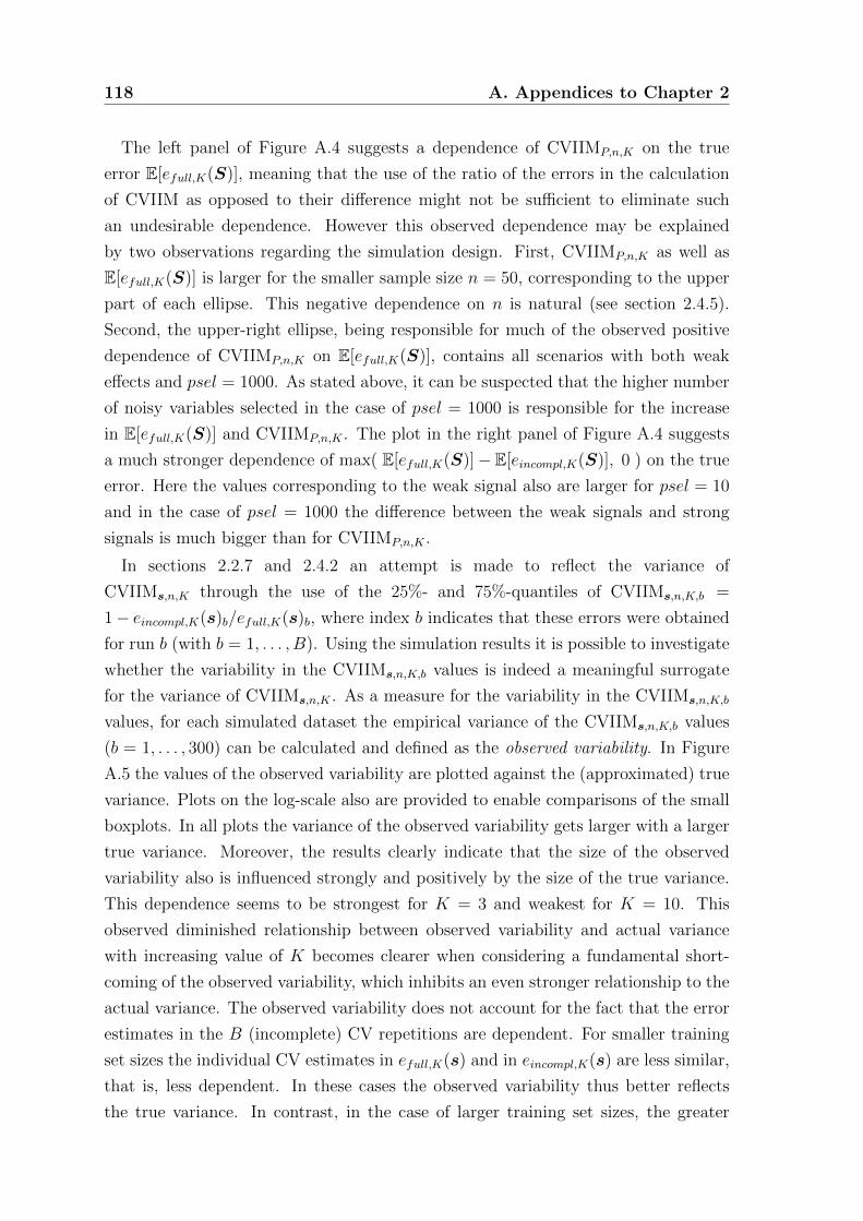
118 A. Appendices to Chapter 2
The left panel of Figure A.4 suggests a dependence of CVIIMP,n,K on the true
error E[efull,K(S)], meaning that the use of the ratio of the errors in the calculation
of CVIIM as opposed to their difference might not be sufficient to eliminate such
an undesirable dependence. However this observed dependence may be explained
by two observations regarding the simulation design. First, CVIIMP,n,K as well as
E[efull,K(S)] is larger for the smaller sample size n = 50, corresponding to the upper
part of each ellipse. This negative dependence on n is natural (see section 2.4.5).
Second, the upper-right ellipse, being responsible for much of the observed positive
dependence of CVIIMP,n,K on E[efull,K(S)], contains all scenarios with both weak
effects and psel = 1000. As stated above, it can be suspected that the higher number
of noisy variables selected in the case of psel = 1000 is responsible for the increase
in E[efull,K(S)] and CVIIMP,n,K . The plot in the right panel of Figure A.4 suggests
a much stronger dependence of max( E[efull,K(S)]−E[eincompl,K(S)], 0 ) on the true
error. Here the values corresponding to the weak signal also are larger for psel = 10
and in the case of psel = 1000 the difference between the weak signals and strong
signals is much bigger than for CVIIMP,n,K .
In sections 2.2.7 and 2.4.2 an attempt is made to reflect the variance of
CVIIMs,n,K through the use of the 25%- and 75%-quantiles of CVIIMs,n,K,b =
1− eincompl,K(s)b/efull,K(s)b, where index b indicates that these errors were obtained
for run b (with b = 1, . . . , B). Using the simulation results it is possible to investigate
whether the variability in the CVIIMs,n,K,b values is indeed a meaningful surrogate
for the variance of CVIIMs,n,K . As a measure for the variability in the CVIIMs,n,K,b
values, for each simulated dataset the empirical variance of the CVIIMs,n,K,b values
(b = 1, . . . , 300) can be calculated and defined as the observed variability. In Figure
A.5 the values of the observed variability are plotted against the (approximated) true
variance. Plots on the log-scale also are provided to enable comparisons of the small
boxplots. In all plots the variance of the observed variability gets larger with a larger
true variance. Moreover, the results clearly indicate that the size of the observed
variability also is influenced strongly and positively by the size of the true variance.
This dependence seems to be strongest for K = 3 and weakest for K = 10. This
observed diminished relationship between observed variability and actual variance
with increasing value of K becomes clearer when considering a fundamental short-
coming of the observed variability, which inhibits an even stronger relationship to the
actual variance. The observed variability does not account for the fact that the error
estimates in the B (incomplete) CV repetitions are dependent. For smaller training
set sizes the individual CV estimates in efull,K(s) and in eincompl,K(s) are less similar,
that is, less dependent. In these cases the observed variability thus better reflects
the true variance. In contrast, in the case of larger training set sizes, the greater

A.1 Simulation study 119
dependence makes the behavior of the actual variance more different from that of the
observed variability. These results suggest that the error bars obtained for the small
K values are most appropriate for comparing the variability in individual CVIIMs,n,K
values.
●
●
●
●
●●
●●
●
●●●●●
●
●
●
●
●
●
●
●
●
●
●
●
●
●●●●●●●●●●●●●●●
●●
●
●
●●●●
●
●● ●
●
●●●●●
●●
●●
●
●●●
●●
●
●
●
●●●●●●
●
●●●●●
●
●●
●●
●●
●
●●
●●
●●●●●
●●●
●
●
●
●
●
●
●
●
●
●
●
●●●●●
●
●●
●
●●
●
●
●
●●
●
●
●
●●●●
●
●●●
●
●●●
●
●
●
●●
●
●
●●
●●●●
●
●●●●●●●●
●●
●
●●●
●
●●●
●●
●
●●
●●●●
●●●
●●
●
●
●
●
●
●●
●
●●
●
●
●
●
●
●
●●
●●●
●
●
●●●
●
●
●●●
●
●
●
●●●●●
●
●
●
●●
●
●
●
●●
●
●
●●●
●●●
●
●
●
●●●
●
●●●●●●
●
●●●●
●
●●●●●
●
●
●●●
●●
●
●
●
●
●●●
●
●●●●●
●●●
●
●
●●●
●
●
●
●●
●
●
●●●
●
●
●●●●
●
●
●
●●●
●
●
●●●●●●●●
●●
●
●●●●
●
●●●
●●●
●●
●
●●●●
●
●●●
●
●●●
●●
●
●
●
●●●
●
●
●●●
●
●●
●●●●●
●
●
●
●
●●●●
●
●●
●●
●●
●
●
●●●
●
●
●
●
●
●●●
●●●●●
●●●
●
●
●●
●●●
●
●
●●●●●●●
●●
●●
●●
●●
●●●
●
●●●●
●
●●●●●●●
●●●●
●
●
●●
●
●
●
●
●
●
●●●
●
●●●●●
●●
●●●
K = 3, psel = 10 K = 3, psel = 1000
K = 5, psel = 10 K = 5, psel = 1000
K = 10, psel = 10 K = 10, psel = 1000
0.00
0.25
0.50
0.75
1.00
0.00
0.25
0.50
0.75
1.00
0.00
0.25
0.50
0.75
1.00
strong eff.n = 50
weak eff.n = 50
strong eff.n = 100
weak eff.n = 100
strong eff.n = 50
weak eff.n = 50
strong eff.n = 100
weak eff.n = 100
CV
IIMs,
n,K
Figure A.1.: Estimated CVIIMs,n,K values from all simulation iterations (means depictedwith broken blue lines) and true CVIIMP,n,K values (depicted with solid red lines)

120 A. Appendices to Chapter 2
●●●
●●●
●●●
●●●●
●●
●●●
●●●
●●●
0.2
0.3
0.4
n = 50 n = 100
CV
IIMP,
n,K
n
●● ●
●●
●
● ● ●
●●
●●● ●
● ● ●
● ● ●
● ● ●
0.2
0.3
0.4
K = 3 K = 5 K = 10
CV
IIMP,
n,K
K
●●●
●●●
●●●
●●● ●
●●
●●●
●●●
●●●
0.2
0.3
0.4
strong signal weak signal
CV
IIMP,
n,K
MeanCov
●●●
●●●
●●●
●●●●
●●
●●●
●●●
●●●
0.2
0.3
0.4
psel = 10 psel = 1000
CV
IIMP,
n,K
psel
Figure A.2.: CVIIMP,n,K values for parameter settings, grouped according to n (top left),K (top right), MeanCov (bottom left), and psel (bottom right)
●
●
●
●●
● ●●
●
●●●
●
●
●
●
●
●
●●
●
●●●
0.01
0.02
0.03
n = 50 n = 100
Var
(CV
IIMs,
n,K)
n
●
●
●
●●
●●●
●
● ● ●
●
●
●
●
●
●
● ●
●
●● ●
0.01
0.02
0.03
K = 3 K = 5 K = 10
Var
(CV
IIMs,
n,K)
K
●
●
●
●●
●●●
●
●●●
●
●
●
●
●
●
●●
●
●●●
0.01
0.02
0.03
strong signal weak signal
Var
(CV
IIMs,
n,K)
MeanCov
●
●
●
●●
●●●
●
●●●
●
●
●
●
●
●
●●
●
●●●
0.01
0.02
0.03
psel = 10 psel = 1000
Var
(CV
IIMs,
n,K)
psel
●
●
●
●●
●
●
●
●
●●
●
0.01
0.02
0.03
0.2 0.3 0.4CVIIMP,n,K
Var
(CV
IIMs,
n,K)
Figure A.3.: (Approximated) true variances of CVIIMs,n,K for parameter settings, groupedaccording to n, K, MeanCov, and psel, and scatterplot of the variance of CVIIMs,n,K
versus the true CVIIMP,n,K values. The true variances are approximated by the empiricalvariances over the 2000 simulation iterations. The points corresponding to the setting withpsel = 10 and psel = 1000 are depicted as red circles and cyan plus signs, respectively

A.1 Simulation study 121
.
●●●
●●●
●
●●
●●●
0.1
0.2
0.3
0.4
0.5
0.1 0.2 0.3E[efull, K(S)]
CV
IIMP,
n,K
●●●
●●●
●
●●
●●●
0.05
0.1
0.15
0.1 0.2 0.3E[efull, K(S)]
max
( E
[efu
ll, K
(S)]
− E
[ein
com
pl, K
(S)]
, 0 )
Figure A.4.: Values of CVIIMP,n,K (left) and E[efull,K(S)]−E[eincompl,K(S)] (right) plottedagainst true errors. Each solid ellipse contains values corresponding to the strong signaland each dashed ellipse contains values corresponding to the weak signal. The pointscorresponding to the setting with psel = 10 and psel = 1000 are depicted as red circlesand cyan plus signs, respectively
K = 3
K = 5
K = 10
0.0
0.1
0.2
0.3
0.0
0.1
0.2
0.3
0.0
0.1
0.2
0.3
0.00 0.01 0.02 0.03
Var(CVIIMs,n,K)
Obs
erve
d V
aria
bilit
y
K = 3
K = 5
K = 10
−6
−4
−2
−6
−4
−2
−6
−4
−2
−6 −5 −4
log(Var(CVIIMs,n,K))
log(
Obs
erve
d V
aria
bilit
y)
Figure A.5.: (Log-) values of the observed variability plotted against the actual (log-)variance of CVIIMs,n,K for different values of K. The boxplots corresponding to thesetting with psel = 10 and psel = 1000 are red and cyan, respectively

122 A. Appendices to Chapter 2
.A.2. Methodological background
A.2.1. Prediction rules, prediction errors, and their estimation
Let X ⊂ Rp denote the predictor space and Y = {1, 2} the space of the response
variable. Note that this notation also allows for categorical covariates, for example,
X = {0, 1}p ⊂ Rp in the case of dummy-coded categorical predictors. Let S =
{(X1, Y1), . . . , (Xn, Yn)} be an i.i.d. random sample with observations drawn from
distribution P . Most importantly, here x ∈ X denotes the “raw” data, meaning that
these predictors may be subject to data preparation steps (possibly modifying their
number or scale of measurement) before being used as predictors in classification.
A classification function g : X 7→ Y , x 7→ g(x) takes the vector x as an argu-
ment and returns a prediction y of the value y of the response variable. For example,
in a classification task where, based on microarray samples, patients are classified
as having cancer or not having cancer using the NSC approach, the corresponding
function g would take the pre-normalized expression values as an argument, perform
normalization, and classify the sample using a certain value of the shrinkage param-
eter. These steps are assumed to be performed in an ideal way, where all occurring
parameters are estimated or optimized using a hypothetical dataset with sample size
tending to infinity.
In practice g is estimated from the available data. Therefore gS : X 7→ Y ,
x 7→ gS(x) is defined as the classification function estimated from S. In the
example outlined above, this means that the parameters involved in the normalization
procedure and the averages and variances involved in the nearest shrunken centroids
classifier are estimated from S and that the shrinkage parameter also is chosen based
on S. The estimated classification function gS then can be used to predict y for a
new observation.
Note that, as outlined in section 2.2.2, depending on the procedures involved in the
estimation, it may not be straightforward to construct such a function gS that can
be applied to predict independent data. However, from here on, it will be assumed
that the necessary addon procedures (see section 2.2.2) are available and, thus, that
the function gS can be constructed.
It is important to assess the prediction error of gS, which is defined as
ε[gS] := E(X,Y )∼P [L(gS(X), Y )] =
∫X×Y
L(gS(x), y) dP (x, y), (A.1)
where L(·, ·) is an appropriate loss function, for example, the indicator loss yielding
the misclassification error rate, as used in Chapter 2. The error defined in Eq. (A.1) is

A.2 Methodological background 123
commonly termed conditional because it refers to the specific sample S. The average
error across all samples following P n is referred to as the unconditional error and
denoted by ε(n) := ES∼Pn [ ε[gS] ].
Let s = {(x1, y1), . . . , (xn, yn)} denote a realization of the random sample S. If a
large independent sample were available, ε[gs] could be estimated directly by com-
paring the true values of the response variable in these data to the predictions made
by gs. Having only s available, a naıve approach would be to estimate ε[gs] using s
itself as test data. This approach yields the apparent error or resubstitution error,
which is known to be downwardly biased (i.e., too optimistic) as an estimator of ε[gs]
since estimation of the classification function and error estimation are conducted on
the same data. Resampling-based error estimation can be performed to address this
issue. The sample s is split iteratively into non-overlapping training datasets and
test datasets. In each iteration function g is estimated based on the training set, and
the error of this estimated function is assessed based on the test set. In the following
K-fold CV, the most widely used of these resampling-based approaches, is treated.
Given a random partition of the dataset s into K approximately equally sized folds
s1, . . . , sK , the K-fold CV error estimate is given as
1
K
K∑k=1
1
#sk
∑j ∈ {i : (xi,yi) ∈ sk}
L(gs\sk(xj), yj), (A.2)
where # represents the cardinality, s \ sk is the training set in iteration k and sk is
the test set. Since this estimate depends heavily on the considered random partition
of the sample s into K folds, it is recommended to repeat this procedure B > 1 times
and average the error estimates across the B repetitions. With sb1, . . . , sbK denoting
the folds considered in the b-th repetition, the repeated K-fold CV error estimate is
given as
eK(s) =1
B
B∑b=1
1
K
K∑k=1
1
#sbk
∑j ∈ {i : (xi,yi) ∈ sbk}
L(gs\sbk(xj), yj). (A.3)
If, for simplicity, it is assumed that the sb1, . . . , sbK (b = 1, . . . , B) are equally sized
with size ntrain,K := #s \ sbk for b ∈ {1, . . . , B} and k ∈ {1, . . . , K}, it easily can
be seen that eK(s) is an unbiased estimator of ε(ntrain,K) and therefore an upwardly
biased estimator of ε(n). This bias is called the inherent bias of CV in Varma and
Simon (2006). Note that the notation eK(s) does not reflect the fact that the repeated
K-fold CV error estimate depends on the random partitions in the B iterations. For
purposes here, B is assumed to be large enough that this dependence can be ignored.

124 A. Appendices to Chapter 2
A.2.2. Incomplete opposed to full CV
With the issue of incomplete CV in mind, the following notation is introduced
ga2a1
: X 7→ Y x 7→ ga2a1
(x) a1 ⊆ a2 ⊆ s (A.4)
to denote an estimated classification function estimated based in part on a sample
a2 and in part on a possibly smaller subsample a1 (i.e., one or several steps may
be performed on a bigger sample). Returning to the example of microarray-based
classification, it is common practice to run the normalization procedure, and often
also the parameter tuning, based on the entire dataset s but to perform the training
of the classifier within CV, that is, based only on the training set s \ sbk in each
iteration k of each repetition b. In this scenario a2 would be the entire dataset s and
in each CV iteration a1 would be the training set s \ sbk.
With a1 = s \ sbk and a2 = s for b = 1, . . . , B and k = 1, . . . , K, we obtain
the incomplete CV error estimate, which is downwardly biased as an estimator of
ε(ntrain,K):
eincompl,K(s) :=1
B
B∑b=1
1
K
K∑k=1
1
#sbk
∑j ∈ {i : (xi,yi) ∈ sbk}
L(gss\sbk(xj), yj), (A.5)
where the index “incompl” indicates that the entire sample s is used for
at least part of the data analysis steps required for the estimation of g,
and that the resulting CV procedure is, thus, incomplete. The estima-
tor eincompl,K(s) is unbiased as an estimator of the average incomplete error
εincompl(ntrain,K ;n) := ES∼Pn [L(gSStrain,K(Xntrain,K+1), Yntrain,K+1)], with Strain,K =
{(X1, Y1), . . . , (Xntrain,K, Yntrain,K
)} and (Xntrain,K+1, Yntrain,K+1) playing the role of
an arbitrary test set observation in S. Here, exchangeability of the random observa-
tions in S is assumed.
Furthermore, since by definition gs\sbks\sbk = gs\sbk , the usual repeated K-fold error
estimate from Eq. (A.3) is obtained if a1 = a2 = s \ sbk is set for k = 1, . . . , K, and
b = 1, . . . , B. This estimator is denoted by efull,K(s):
efull,K(s) := eK(s) =1
B
B∑b=1
1
K
K∑k=1
1
#sbk
∑j ∈ {i : (xi,yi) ∈ sbk}
L(gs\sbks\sbk (xj), yj), (A.6)
where index “full” underlines that all steps of prediction rule construction are con-
ducted within the CV procedure, that is, using the training sets only.
For easier interpretation, in Chapter 2 and in other sections of this Appendix

A.2 Methodological background 125
E[efull,K(S)] is written for ε(ntrain,K) and E[eincompl,K(S)] for εincompl(ntrain,K ;n).
A.2.3. Behavior of CVIIMs,n,K for small εfull(ntrain,K) values
For very small values of εfull(ntrain,K), extreme CVIIM estimates can occur (either
zero or very high values). For very small values of efull,K(s), the CVIIM estimate
is highly sensitive to relatively small differences between eincompl,K(s) and efull,K(s),
which may be due at least partly to random fluctuations. For example, suppose
that efull,K(s) = 0.01 and eincompl,K(s) = 0.001, then there would be CVIIMs,n,K =
0.9. Note, however, that such extremely large results are expected to be rare due
to a mechanism related to regression toward the mean: Considering the high level
of variance of CV estimates, in many cases very small values of efull,K(s) are an
underestimation of εfull(ntrain,K). In this case it is unlikely that εincompl(ntrain,K ;n)
is considerably more affected by underestimation. Thus, in such a situation it is
unlikely that eincompl,K(s) is much smaller than efull,K(s). Instead, the incomplete
CV error estimator eincompl,K(s) is more likely to be closer to its mean than efull,K(s),
thereby preventing an overly large CVIIM estimate.


B. Appendices to Chapter 3
B.1. Plots used in verification of model assumptions
●
●
●
●
●
●
●
●
●
●●
●
●
●
●
●
●
●
●
●
●
●
●
●
●●
●
●
●
●
●
●
●
●●
●
●
●
●
●
●
●●
●
●
●
●
●
●
●●
●
●●
●
●
●
●
●
●●
●
●●
●
●
●
●
●
●●
●
●●
●
●
●
●
●
●
●
●
●
●
●
●
●
●●●
●
●
●
●
●
●
●
●
●
●
●●●
●
●
●●
●
●
●
●
●
●●
●●
●
●
●
●●
●
●●
●
●
●
●
●
●
●
●
●
●
●
●
●●
●●●
●
●●●
●
●
●
●
●
●
●
●
●●
●
●
●
●●
●
●●
●
●
●
●●
● ●
●
●
●
●●
●
●
●
●
●
●●
●
●
●
● ●
●
●●
●
●
●
●
●
●●
●
●●
●
●
●
●
●
●
●
●●
●
●
●
●
●
●
●
● ●●
●●
●
●
●
●
●
●
●
●
●
●
●●
●●
●
●●
●●
●
●●
●
●
●
●
●
●
●
●
●●
●
●
● ●●
●
●
●
●
●
●
●
●
●●
●
●●
●
●●●
●
●●●
●
●
●
●
●●
●
●
●●●
●
●
●
●
●
●
●●
●
●
●
●●
●
●
●●
●
●
●
●●
●
●
●●
●
●
●
●
●
●●●
●
●
●
●●●
●●
●
●
●●
●
●
●
●
●
●
●
●●
●
●
●
●
●
●
●
●●
●●
●
●
●
●
●
●
●
●
●
●
●
●
●
●●
●
●
●●
●
●
●
●
●
●
●
●
●●
●●
●●
●●
●●
●●
●●
●●
●
●
●●●
●
●
●
●
●
●
●
●●
●
●
●
●
●
●
●●
●
●
●
●
●
●
●
●
●
●
●
●
●
●●
●
●
●●
●
●
●
●●
●
●
●
●
●●
●
●●
●●●
●
●
●
●●
●●
●
●
●
●
●●
●
●
●
●●
●
●
●
●●
●●●
●
●
●
●●
●●
●
●
●
●
●
●
●
●
●
●
●
●
●
●
●
●●●
●
●
●
●
●
●
●●
● ●●
●
●
●
●
●●
●
●
●
●
●
●
●
●
●
●
●
●
●●
●
●
●
●●●
●
●
●
●●
●
●
●
● ●●
●
●●
● ●
●
●
●
●
●
●
●
●
●
●
●
●
●
●
●
●
●
●●●
●
●
●
●
●
●
●●
●
●
●
●●
●
●
●
●●
●
●
●
●
●
●
●
●
●
●
●
●
●
●
●
●●
●
●
●●●
●
●
●
●
●
●
●
●
●
●
●
●
●
●
●●
●●
●
●
●●●
●
●●
●
●
●
●
●●
●●
●●●
●
●●
●
●
●●
●
● ●
●
●
●●
●
●
●
●
●
●
●
●
●
●●
●
●
●
●
●
●●●
●
●
●●
●
●●●
●●
●
●
●
●●●
●
●●
●
●
●
●●
●
●●
●●
●●●●
●●
●
●●●●
●
●
●●
●
●●
●
●
●
●
●●
●
●
●
●
●
●●
●
●●
●
●
●
●
●
●
●
●
●
●
●
●
●
●
●●●
●
●
●
●
●
●
●
●
●
●●●
●
●
●
●
●
●●
●
●●
●
●
●
●●
●
●
●
●
●
●
●
●
●
●
●●
●
●●
●
●
●
●
●●●
●●●
●●
●
●
●
●
●●
●
●
●●
●
●
●●●
●
●
●
●
●
●●
●
●
●
●
●
●
●
●
●
●
●
●
●
●
●
●
●
●
● ●●
●
●
●
●●●●
●
● ●
●●●
●
●
●
●
●
●●
●
●
●
●
●
●
●●●
●
●
●
●
●●
●
●●
●
●●● ●
● ●
●●
●
●
●
●
●
●●●
●
●
●
●
●
●
● ●●
●●
●
●
●
●
●●
● ●
●●
●
●
●
●●
●
●
●
●
●
●●
●
●
●
●●
●
●●●●
●●
●
●●
●●
●
●
●
●
●●
●
●
●
●
●●
●
●
●
●
●
●
●
●
●●
●
●
●
● ●
●●
●
●
●
●
●
●
●
●●
●
●
●
●●
●
●
●
●
●
● ●
●
●
●
●
●●
●●
●
●●
●
●
●
●
●
●
●
●
●
●●
●
●
●
●●
●
●
●
●
●
●
●
●
●
●
●
●
●
●
●
●
●
●
●●
●
●●
●
●●
●
●
●●
●●
●
●
●
●
●
●
●
● ●
●
●●
●●
●
●
●
● ●
●
●●
●
●●
●●●
●●
●●●
●
●
●
●
●
●
●
●●
●
●
●
●●
●
●
●●
●
● ●
●●●
●●
●●
●●
●
●●
●
●
●
●●●
●
●
●
●●
●
●
●
●
●
●●
●
●●
●
●
●●
●
● ●
●
●
●
● ●
●
●●
●
●
●
●
●
●●
●
●
●
●
●
●●
●●
●
●
●
●
●●
●
●●
●
●
●
●
●
●
●
●
●
●●
●●
●
●
●
●
●
●
●●
●
●
●
●
●
●
●
●
●
●
●
●
●
●
●
●
●
●
●
●●●
●●
●
●●
●
●
●
●
●
●
●
●●
●
●●
●
●
●
●●●
●
●
●●
●
●
●
●
●
●
●
●
●●
● ●
●
●
●
●
●
●
●
●
●
●
●
●●
●
●
●●●
●●
●●
●
●
●●
●
● ●
●●
●
●●●
●
●●
●
●
●
●
●
●
●
●●
●
●
●
●●
●
●●
●
●
●
●
●
●
●●
●
●
●
●
●
●
●
●
●
●
●
●
●
●
●
●
●●
●
●
●
●
●
●
●
●●
●●
●
●
●
●
●
●
●
●
●
●
●●
●
●
●
●
●
●●
●●
●
●
●
●
●
●
●
●●
●
●●
●
●
●
●
●
●
●
●
●
●
●
●
●
●●
●●
●
●
●●
●●●
●
●
●
●
●
●
●
●
●
●
●
●
●●
●
●
●
●
●
●
●
●
●
●
●
●●
●●
●
● ●
●
●
●
●
●
●
●
●
●●
●●●●●
●
●
●
●●
●
●●
●
●
●●
●
●
●
●
●
●
●
●
●
●
●
●
●●
●
●
●
●
●
●
●
●
●
●●
●●●
●
●
●●
●
●●
●
●
●
●●●
●
●
●
●
●
●
●
●
●
●●
●
●
●
●●
●●
●
●●
●
●
●
●●
●
●●●
●
●
●●
●
●
●
●
●
●
●
●
●
●
●
●
●
●
●
●
●
●
●
●
●
●
●
●
●
●
●●
●
●●
●
●●
●
●●
●
●
●
●
●
● ●
●●
●●
●
●
●
●
●
●
●●
●
●
●
●
●●
●
●
●
●
●
●●
●
●●
●
●
●●
●●●●
●
●●
●●
●
●
●
●●
●
●●●
●
●
●
●
●
●
●
●
●
●
●
●●
●● ●
●●●
●
●
●
●
●
●
●
●●●
●
●
●●
●
●
●
●●●
●
●●
●
●
●
●
●
●
●
●
●
●
●
●●
●
●
●
●●
●
●
●
●
●
●
●
●●
●
●
●
●
●
●●
●●
●
●
●
●
●
●
●
●
●
●
●
●
●
●● ●
●
●
●●
●
●●
●
●
●●
●
●● ●
●●
●
●
●
●
●
●
●●
●●
●
●
●●
●●
●
●
●
●
●
●●
●
●●
●●
●
●●
●
●
●
●
●●
●
●
●
●
●●
●●
●●
●●
●●
●●●
●●
●●
●
●
●
●●
●
●
● ●●
●
●
●
●
●
●
●
●
●
●
●
●
●●
●●
●
●
●
●●●
●
●●
●
●
●
●
●●
●●
●
●
●
●
●
●
●●
●
●● ●●
●●
●
●
●
●
●
●
●●
●
●
●
●
●
●
●
●
●
●
●
●
●●
●●
●
●
●
●●
●
●
●
●
●
●
●
●
●
●
●
●
●
●
●
●
●
●
●
●
● ●
●
●
●
●
●
●●
●
●
●
●
●
●
●
●●
●
●●
●●
●●
●
●●
●●
●
●
●
●●
●
●
●
●
●
●
●
●
●
●
● ●
●
●●
●●
●
●
●
●
●
●
●
●
●
●
●
●●
●
●
●
●
●
●
●
●
●
●
●●
●
●
●
●
●
●
●
●
●
●
●
●
●
●
●
●
●
●
●
●
●
●
●
●
●
●
●
●
●
●
●
●
●
●
●
●
●●●
●●
●
●
●●
●
●
●
●
●
●
●●
●●
●●
●
●
●
●
●
●
●
●
●
●
●●
●●
●
●
●
●●
●
●
●
●
●●
●
●
●●
●●
●
●
●
●
●
●
●
●
●
●
●
●
●●
●
●
●
●
●
●
●
●●
●
●
●
●
●
●●
●
●●
●
●
●
●
●●●
●
●
●●
●
●
●
●
●
●●
●
●
●
●
●
●
●●
●●
●
●
●
●
●
●
●
●●
●
●
●
●
●●
●●
●
● ●
●
●
●
●●
●
●●
●
●●●●
● ●
●●●
●
●●
●
●
●
●
●
●
●
●
●●
●
●
●●
●● ●
●
●
●
●
●●
●
●●
● ●●
●●
●
●
●
●●
●
●
●
●
●
●
●
●
●
●
●
●●
●
●
●●
●
●
●●
●
●●
●
●
●●
●●
●
●●
●
●
●
●●●●
●
●●●●
●
●
●●
●
●
●
●
●
●
●
●
●
●●
●
●
●● ●
●●●
●●
●
●
●
●
●●
●●●
●
●
●●
●
●
●●
●
●
●
●
●
●
●●
●
●
●●
●
●
●
●
●
●●●
●
●
●●
●●
●●
●
●
●●
●●
●
●
●
●
● ●
●
●
●●
●
●
●
●
●
●
●●
●
●●
●
●
●●
●
●
●●
●●●
●
●
●
●
●
●
●
●●
●
●
●
●
●
●
●
●
●●
●
●
●
●
●
●
●
●
●●
●
●
●
●
●
●
●
●
●
●
●
●
●
●
●
●
●
●
●
●
●●●●
●
●
●
●
●
●●●
●
●●
●
●
●
●
●
●
●●
●
●
●
●●
●●
●
●●
●
●
●
●●
●
●
●
●
●
●
●
●
●●
●
●●
●
●
●
●
●
●
●
●●
●
●
●
●
●
●
●●
●
●
●
●
●●
●
●
●
●
●
●●
●
●
●
●
● ●●
●
●
●
●●
●
●
●
●
●
●
●
●●
●
●●
●●
●
●●●
●
●●
●
●
●
●
●●
●
●
●
●
●●
●●
●
●
●●
●
●
●
●
●
●
●
●●
●
●
●
●
●
●
●
●●
●
●
●
●
●
●
●
●
●
●
●
●●
●●
●
●
●
●
●●● ●●
●●
●
●
●
●
●
●
●●
●
●
●
●●
● ●●
●
●
●
●
●
●●
●
●
● ●
●●
●
●
●
●●●
●
●
●
●●
●
●
●●
●●
●●
●
●●
●
●
●
●
●
●
●
●● ●
●●●
●
●●
●
●
●
●●
●
●
●●
●●●
●●●
●●
●
●
●
●●
●
●
●
●●
●●●
●
●
●
●
●
●
●
●
●
●
●
●
●●
●
●
●
●
●●
●
●
●
●
●
●
●
●
●
●
●
●●
●●
●●●
●
●●
●
●
●●
●
●●
●
●●
●●
●
●●
●
●
●
●
●
●
●
●
●
● ●
●
●
●
●
●●●
●●
●
●●
●●
●
●●●
●
●●
●
●●
●
●
●
●
●●
●
●
●
●
●
●●
●
●
●
●
●
●
●
●
●
●
●●
●
●
●
●●
●
● ●
●
●
●
●
●●●
●
●
●●●
●
●
●●
●
●
●
●
●
●
●●
●
●
●●
●
●●
●●●
●
●
●
●
●
●
●
●
●●●
●
●
●
●
●●
●●
●
●●
●
●
●●
●●
●
●● ●
●
●
●●
●
●
●
●●
●
●
●
●
●
●
●
● ●●
●
●
●
●
●
●
●
●
●
●●
●
●
●●
●
●
●
●
● ●
●
●
●
●
●
●
●
●●
● ●
●
●
●
●
● ●
●
●
● ●●
●
●
●
●
●●
●
●
●
●
●
●
● ●
●●
●●
●●
●
●
●
●
●
●●
●
●●
●●
●
●
●●
●●
●
● ●
●●
●
●
●●●
● ●
●
●●
●
●
●
●
●
●●●
●
●
●
●●
●
●
●●
●
●
●
●
●●
●● ●● ●● ●
●
●
●
●●
●
●
●●●
●
●
●
●●
●●
●
●
●●
●
●
●
●●
●●●
●●
●
●●
●
●●
● ●●
●
●
●
●
●
●
●
●
●●● ●
● ●
●
●●
●●
●
●● ●
● ●
●
●
●●●
●
●
●
●
●
●
●
●●
●●
●●
●
●
●●
●●
●●
● ●●●
●
●
●● ●
●
●●●
●
●
●
● ●● ●
●
●●
●
●
●
●●
●
●
●
● ●
●
●
●
●
●
●
●
●
●
●
●●
●
●
●
●
●
●
●
●
●
●
●●
●
●●
●
●●
●
●
●● ●
●
●
●●● ●
●
●
●
●
●
●
●
● ●●●
●
●
●
●
●
●
●
●
●●●
●
●●
●
●
●
●●
●
●
●
●●
●
●●
●
●●
● ●
●●
●
●
●
●●
●●●
●
●●
●●●
●
●
●
●● ●
●●●
●
●
● ●●
●
●●
●
●
●●
●
●
●
●
●
● ●
●
●
●
●●
●
●
●●
●
●
●
●
●●
●●
●
●
●
●●
●
●●
●
●
●
●
●●
●●
●●
●
●
●●
●
●
●
●●
●●
●
●
●
●●
●
●
●
●
●
●
●
●
●
●●
●
●
●●
●●●●
●
●
●
●
●
●
●
●
●
● ●●
●●●
●
●
●●
●
●●
●● ●
●
●
●
●
●
●●
●
●
●
●
● ●●
●
●
●
● ●●
●
●
●
●
●
●
●●●
●●
●
●
●
●●
●●
●
●
●●
●
●
●
●
●●
●
●
●●
●
●
●
●
●●●
●
● ●●
●●
●
●
●
●
●
●
●
●●
●
●
●
●
●
●
●●
●
●●
●●
●
●
●
●●
●
● ●
●
●
●●
●
●
●
●
●
● ●
●
●
● ●
● ●●
●
●
●
●
●
●
●
●●
●
●
●●
●
●
● ●
●
●
●●
●●
●
●
●
●●
●
● ●
●●● ●●●
●
● ●
●
●●●●
●
●
●●
●
●
●
●
●
●●
●
●
●
●●
●●
●
●
●
●
●●
●
●
●●
●
●
●●
●●
●●
●
●
●
●
●
●
●
●
●
●●
●
● ●
●
●●
●
●
●●
●
●
●
●
●
●●
●
●
●
●
● ●
●●
●● ●
●
●
●
●
●
●●
●
●●
●
●●
●
●
●
●●
●
●●
●
●
●●
●
● ●
●
●
●
●
●
●
●●
●
● ●●
●
●
●
●
●●
●
●
●●
●
●
●
●
●
●● ●
●
●
●●●
●
●
●
●
●●
●
●
●
●
●
●
●
●●●
●
●●
●
●
●●
●
●
● ●
●
●●
●
●
●
●
●
●
●●●
●●
●●
●●
●
●
●
●
●
●●
●
●
●
●
●●
●
●
●
●
●
●
●
●
●
●
●
●
●● ●
●
●●
●●
●
●
●
●
●●
●
●● ●
●
●
● ●
●
●
●
●●
●
●
●●
●
●
●
●
●
●
●●
●
●
●
●
●
●
●●
●
●
●●
●
●
●
●
●
●●
●
●
●
●
●
●
●
●
●
●●●
●●
●
●
●●
●
●
●●
●
●
●
●●
●
●
●
●
● ●
●
●●
●●●●●
●
●
●●
●
● ●
●
●
●
●
●●●
●
●
●●
●
●
●
●
● ●
●●
●●
●
●●
●
●●
●
●
●
●
●
●
● ●●
●
●
●
●
●
●
●
●
●●●
●
●
●●
●
●
●
●
●●●
●●
●
●●
●
●
●●
●●●
●
●
●●
● ●
●● ●●
●
● ●
●●
●
●
●●
●
●
●●●
●
●
●
●●●
●
●
●
●
●●
●
●●
●
●●●●
●●●
●
●
●
●
●
●
●
●
●
●
●
●
●
●
●●
●
●
●
●
●
●
●
●
●
●●
●
●
●
●
●
●
●
●
●
●
●
●
●
●
●●
●
●
●
●
●
●
●
●
●
●
●
●
●●
●
●
●
●
●
●
●
●
●
●
●
●●
●
●
●●
●
●●
●
●
●
●
●
● ●
●
●● ●●
●
●
●
●
●
●
● ●
●
●
●
●
●
●
●
●
●
●
●● ●
●●
●
●
●
●
●
●
●
●
●
●
●
●
●●
● ●
●
●●
●
●●
●●
●
●
●
●●
●
●●●
●
●
●●
●
●
●●
●
●
●
●
●●●
●
●
●
●
●●
●
●
●
●
●
●
●
●
●
●
●●
●
●
●
●
●
●
●
●
●
●●
●
●
●
●●●●
●
●
●
●
●
●
●
●
●●
●
●●
●
●
●
●
●
●
●
●●
●
●
●●
●
●
●
●
●
●●
●
●●
●
●●
●●
●
●●
●
●
●
●●●
● ●●●
●
●●
●
●
●●●
●●
●●
●●●
●
●●●
●
●
●
●●
●
●
●●
●
●●
●
●
●●●
●
●
●
●
●
●
●●
●
●●●
●
●●
●●
●
●●
●●
●
●●
●
●●●●
●
●●
●
●
●●●
●
●●
●
●
●
●
●
●
●●
●
●
●
●
●
●
●
●
● ●
●● ●●●
●
● ●
●
●
●●●
●
●
● ●
●
● ●●
●
●●
● ●
●
●
●●
●
●
●
●
●
●
●
●
●●
●●
●
●
●
●
●●
●●
●
●
●
●
●
●●
●
●
●
●
●
●
●●
●
●
●
●
●
●
●●
●
●
●
●
●●
●
●
●
●
●
●
●
●
●
●
●
●
●●●
●
● ●
●
●
●● ●
●
●● ●
●●
●●
●
●
●
●●
●●
●
●
●
●
● ●
●●
●
● ●
●
●
●●
●●
●
●●
●
●●
●
●
●
●
●
●
●
●
●
●
●●
●
●●●
●
●
●
●
●
●
●
●
●
●●
●
●
●
●
●
●
●
●
●
●●
●
●
●
●●
●
●●
●
●
●
●●
●
●●
●●
●
●
●
●
●
●
●
●
●
●
●
●
●● ●
●
●
●
●
●
●
●
●
●●
●
●
●
●
●
●
●●●
●
●
●
●
●
●
●●
●
●
●
●
●
●
● ●
●●
●
●
●
●
●
●
●
●
●●●
●
●
●
●
●●●
●●●
●
●●
●
●
●
●
●
●
●
●
●
●
●
●
●
●
●
●●
●
●
●
●●
●
●●●●
●●
●
●
●●
●
●
●
●
●
●
●
●●
●
●
●
●
●
●●
●
●
●
●●
●
●
●
●
●●●
●
●
●
●
●
●
●
●
●
●●●
●
●
●
●●
●●
●●
●
●●
●●
●
●
●
●
●
●
●
●●
●
●
●
●●
●
●
●
●●●
●●
●●
●
●
●
●
●●
●
●●
●
●
●●
●
●●●
●
●
●●
●
●
●
●●●
●
●
●
●
●
●
●●
●
●
●●
●●
●
●●
●
●●●
●
●
●
●●
●
●
●
●●
●●
●
●
●
● ●
●
●
●
●
●
●
●
●●
●●
●
●●
●●
●
●
●
●
●●
●
●
●
●
●●
●
●
● ● ●
●
●
●
●
●●
●
●●
●
●
●
●
●
●
●●●
●
●●
●
●
●
●
●
●
●
●
●
●
●
●
●
●
●
●●
● ●
●
●
●
●
●
●
●
● ●
●●
●
●●
●●
●
●
●
●
●
●
●
●
●●
●
●
●
●
● ●●
●
●
●●
●
●
●
●
●
●
●
●
●
●
●
●
●
●
●
●●
●●
●
●●
●●
●
●
●
●●●
●●
●
●
●● ●
● ●
●
●●
●
●
●
●
●
●
●
●●
●●
●
●
●
●
●
●●
●
●●
●
●
●
●
●
●●
●
●
●
●
●
●●
●●
● ●
●
●
●●●
●
●
●●
●
●
●●●
●
●●
●
●
●
●
●
●
batch 1 batch 2
batch 3 batch 4
batch 5
0
5
10
15
0
5
10
15
0
5
10
15
0 5 10 15fitted values (given factors)
data
val
ues
Figure B.1.: Data values against corresponding fitted values resulting from the FAbatchmethod. The contour lines represent two-dimensional kernel density estimates. The brokenlines mark the bisectors and the red lines are LOESS estimates of the associations. Thegrey dots in each case are random subsets of size 1000 of all values.

128 B. Appendices to Chapter 3
●
●
●
●
●●● ●
●
●
●●
●
●●
●
●
●
●
●
●
●
●
●●
●
●
● ●
●
●
●
●
●
●
●
●
●
●
●
●
●
●
●●
● ●●
●●
●
●
●
●●
●●
●
● ●●
●
●
●
●
●
●
● ●
●●
●●
●●●●●
●
●
●
●
●
●
●
●
●
●
●●
●
● ●●
● ●
●
●
●
●●
●
●●
●
●
●
●
●
●
● ●
●
●
●
●
●
●●●
●
●
●●
●●
●●
●
●
●
●
●
●
●
●
●
●
●
●
●
●
●
●
●●
●●
●
●
●
●
●
●
●
●
●
●
●
●●
●
●
●
● ●
●
●●
●
●
●●
● ●
●
●●
● ●
●
●
●
●
●
●
●
●
●
●●
●
●
●
●
●
●
●
●
●
●
●
●●
●
●
●
●
●●
●
●
●
●●●
●
● ●
●
●
●
●●
●●●●
●
●
●
●
●
●
●
●
●
●
●
●
●
●
●
●
●
●●
● ●●●●
●
●
●
●
●
●
●
●●
●
●
●●
●●
●
●●
● ●●
●
●
●●
●●
●
●●
●●
●
●
●
●
●
●
●
●
●●
●
●●●
●●●●●
●
●
●
●
●
●●
●
●●
●●
●●
●
●
●
●
●
●
●
●
●
●
●
●
●
●
●
●
●
●
●
●
●
●
●
●
●●
●
●●
●
●●
●
●
●
●
●
●
●●●
●
●
●
●●
●
●
●
●
●
●●
●
●
●
●
●
●
●
●
●
●
●
●
●
●
●
●
●
●
●
●●●
●
●
●
●
●●
●
●
●
●
●
●●●
●
●
●
●●
●
●●
●
●●
●
●●
●
●
●●
●●
●
●●●●
●
●
●
●
●●
●●
●
●
●
●
●
●●
●
●
●
●
●
●
●
●
●
●
●
●
●
●
●●●
●
●
●●
●
●
●
●
●
●
●
●
●●
●
●●
●
●
●
●
●
●●
●
●
●
●
●
●
●
●
●●
●
●
●
●
●
●
●
●
●
●●
●
●
●
●
●
●● ●
●
●
●●
●
●●
●
●
●●●
●●
●●
●
●
●
●
●
●
●
●
●
●
●
●
●●
●
●
●
●
●
●
●
●●
●
●
●
●
●
●
●
●
●●
●
●●
●
●●
●
●
●
●
●●●
●
●
●
●
●
● ●
●
●
●
●
●
●●
●●●
●
●●
●
●
●●
●
●
●
●
● ●
●
●
●●
●
●
● ● ●
●●
●
●
●
●
●
●
●
●
● ●
●●
●
●
●
●
●
●
●
●
●
●
●
●
●●
●
●
●
●
●
●
●
●
●
●
●
●
●
●●
●
●●
●
●
●
●
●
●
●
●
●
●
●
●●
●
●● ●
●
●
●
●
●
●●
●
●
●
●
●
●
●
●
●●
●
●
●●
●
●
●
●●
●
●
●
●
●
●
●●
●
●
●
●
●
●
●
●
●
●
●●
●
●
●●
●
●
●
●
●
●● ●●
●
●
●●
●
●
●
●
●
●
●
●
●
● ●
●
●
●
●
●
●●
●
●
●
●
●
●●
●
●
●
●●
●
●●
●
●
●
●
●
●
●
●
●
●
●
●
●
●
●
●
● ●
●
●
●
●
●
●
●
●
●
●●
●●
●
●
●
●●
●
●
●
●
●
●
●●
●●
●
●
●
●
●
●
●
●
●
●●
●
●
●
●
●
●●
●
●
●
●
●
●
●
●
●●●
●●●
●
●
●
●
●
●
●●●
●
●
●●
●
●
●
●
●
●●
●
●
● ●●●
●
●
●
●
●●
●
●
●
●
●
●
●
●
●
●
●
●
●
●
●●
●
●
●
●
●
●
●●
● ●
●
●
●
●●
●
●
●
●
●
●
●
●●
●
●
●
●●
●
●
●
●
●
●
●
●
●●
●
●
●
●
●
●
●
●●
●
●●
●
●
●
●●
●
●
●
●
●
●
●
●
●
●
●
●●
●
●●
●
●
●●
●●
●
●
●
●
●●
●
●
●●●
●
●
●
●
●
●
●
●
●
●
● ●
●
●
●●
●
●
●
●
●
●●
●
●
●
●
●
●
●
●
●
●
● ●
●
●
●
●●
●
●
●
●
●
●
●
●
●
●
● ●
●
●
●
●●●
●
●
●
●
●
●●
●
●
●
●●
●
●
●
●
●●
●
●
●
●
●●
●
●●
●●●●
● ●
●
●
●●
●
●
●
●
●●
●
●
●
●
●
●
●
●
●
● ●
●
●● ●●
●
●●
●
●
●
●
●
●
●
●
●
●
●●●
●
●
●
●
●
●
●
●
●
●
●
●
●
●
●
●●
●
●
●
●●
●
●
●
●●
●
●
●
●
●
●
●
●●
●
●
●
●
●
●
●
●
●
●
●
●
●●●
● ●
●
●
●●
●
●
●
●
●●
●
●●
●
●
●●
●
●
●
●
●
●●
●
●
●
●
●
●
●
●●
●
●
●
●
●
●
●
●
●●●
●
●
●
●●
●
●
●
●●
●
●●
●●
●
●
●
●●
●
●
●
●
●
●
●
●● ●
●●●
●
●
●
●●
●
●●●
●
●
●
●
●
●
● ●
●●●●
●
●
●
●
●
●●
●
●
●●
●
●
●
●
●
●●
●
●
●
● ●
●
●●●
●
●
●
●
●
●
●
●
●
●
●
●●
●
●●●
●
●
●
●●
●
●
●
●
●
●
●
●
●
●
●
●
●
●
●
●
●
●
●●
●
●
●
●
●
●
● ●
●
●
●
●
●
●
●
●●
● ●●●
●
●●
●
●●
●
●
●
●
●
●
●
●●
●
●●
●
●
●
●
●
●
●
●
●
●
●
●
●
●
●
●●
●
●
●
●
●
●
●
●
●
●
●
●
●
●
●
●●
●
● ●
●
●
●
●●
●
●
●
● ●
●
●
●
●
●
●
●
●
●
●
●
●
●
●
●
●
●
●
●●
●
●
●
●
●
●
●
●
●
●
●
●
●
●
●
●
●
●
●
●●
●
●
●
●
●●
●
●●
●●
●
●●
●
●
●
●
●
●●●
●
●
●
●
●
●
●
●●
●●
●
●
●●
●
●
●
●
●
●
●
●
●
●
●
●
●●
●●●
●●
●●
●
●
●
●
●
●
●
●
●
●●
●
●
●
●●
●● ●● ●
●
●
●
●
●
●●
●
●
●
●
●
●
●
●
●
●
●
●
●
●●
●
●
●
●
●
●
●
●
●
●●
●
●
●
●
●
●●
●
●●
●
●●
●
●●● ●
●
●
●
●
●
●
●
●
●
●
●
●
●
●
●
●
●
●
●
●
●
●
●
●
●
●
●
●
●
●
●
●
●
●
●
●●
●
●
●
●
●
●
●
●
●
●
●
●
●
●
●●
●
●
●
●
●
●
●
●
●●
●
●
●
●
●
●
●
●
●●
●
●
●
●
●●●
●
●
●
●
●
●●
●
●
●●
●●●
●
●
●
●
●
●
●
●●●●
●
●
●
●●●
●
●
● ●
●
●●●
●
●●●
●
●
●
●
●
●
●●
●
●●
●
●
●
●●●
●
●
●●●
●
●
●
●●●
●
●●
● ●
●
●
●
●
●●
●
●
●
●
●●
●
●
●
●●
●
●
●
●
●
●●●
●
●
●
●●
●
●
●
●
●
●
●
●
●
●
●
●
●
●
●
●
●
●
●
●
●
●
●
●●
●
●●
●
●
●
●
●
●
●
●
●
●●
●
●
●●
●
●
●
●
●
●
●
●
●
● ●
●
●●
●
●
●
●
●
●
●●
●
●
●
●
●
●
●
●●
●
●●
●
●
●
●●
●
●●
●
●
●
●
●
●●
●
●
●
●
●
●
●●
●
●
●
●
●
●
●●
●
●
●
●
●
●
●
●
●●
●
●
●
●●
●
●●
●●●
●
●●
●
●●
●
●
●
●
●
●
●
●
●
●
●
●
●●
●
●
●●
●●
●● ●●
●●●
●●
●
●
●
●
●
●●
●
●
●●
●
●
●
●
●
●
●
●● ●
●
●
●●
●
●
●●
●● ●
●
●
●●
●
●
●
●●
●
●●
●
●
●
●
●
●●●
●
●
●
●
●
●●
●
●
●
●
●●
●●
●
●
●
●
●
●
●
●●
●
●
●
●
●
● ●●
●
●
●
●
●
●
●●
●
●
●
●
●
●●
●
●
●
●
●
●
●●
●
●
●
●
●
●●
●
●
●
●
●
●
●●
●
●
●
●
●
●
●
●
●
●
●
●
●
●
●
●
●
●
●
●
●
●
●
●
●
●
●
●
●
●
●
●
●
●
●
●
●
●
●
●
●
●
●
●
● ●
●
●
●
●
●●
●
●
●●
●
●
●
●
●
●●
●
●
●
●
●
●●
●
●
●
●
●
●
●
● ●
●
●
●
●
●
●
●
●
●
●
●
●
●
●●
●●
●●
●
●
●
●●
●●
●
●
●
●
● ●
●
●
●●
●
●
●●
●
● ●
●
●
●●
●
●●
●
●
●
● ●
●
●
●
●
●
●
●●
●●
●
●
●
●
●
●
●
●●
●
●
●
●
●●
● ●
●
●
●
●
● ●
●
●
●
●
●
●
●●●●
●
●●
●
●
●●
●●
●
●
●
● ●●●
● ●
●
●
●
●
●●●● ●
●●●●●
●
●●
●
●●
●
●
●●
●
●
●
●
●
●●
●
●●
●
●
●●
●
●●●
●●●
●●
●●●●
●
●
●
●
●
●
●
●
●
●
● ●●
●
●● ●
●
●
●●●
●
●
●
●
●
●
●●
●
●●
●
●
●
●
●
●
●
●
●
●
●
●
●
●●
●
●
●
●
●
●
●
●
●
●
●
●
●
●
●●
●
●
●
●
●
●
●
●
●
●●
●
●
●
●
●
●
●
●
●
●
●
● ●
●
●
●
●●●
●
●
●
●
●
●
●
●●●
●
●
●
●●
●
●
●
●
●●
●
●
●
●
●●●●
●
●
●●
●
●
●
●
●
●
●
●
●●
●
●
●
●
●
●
●
●
●
●●
●●
●
●●
●
●
●
●
●
●
●●
●
●
●
●
●
●●
●
●
●
●
●
●
●
●
●
●
●●
●●
●
●
●
●
●
●
●●●
●
●
●
●●
●●
●
●
●
●
●
●
●
●
●
●
●
●
●
●
●
●
●
●
●
●●
●
●
●
●
●
●●
●●
●
●
●
●
●
●
●
●
●
●
●
●
●
●
●
●
●●
●
●
●
●
●
●●
●
●
●
●
●
●
●
●
●
●
●●● ●
●
●
●
●
●
●
●
●
●
●
●
●
●
●
●
●
●
●
●
●
●
●●
●
●
●
●
●
●
●
●
●
●
●●
●
●
●
● ●●
●●
●
●
●
●●
●
●
●
●
●
●
●●
●●
●
●●●
●
●
●
●
●
●●
●
●●
●●
●
●●
●●●
●
●●
●
●
●
●
●
●
●●
●
●
●
●
●
●●
●
●
●
●
●
●
●
●
●
●
●●
●●
●●
●●
●
●
●●
●●
●
●
●
●
●●●
●
●
●●
●
●●
●
● ●
●
●●● ●
●
●●
●● ●
●
●
●●
●
●
●
●●
●
●
●
●
●
●
●●
●
●
●
●
●●●
●
●
●
●
●
●
●
●
●
●
●
●
●
●●
●
●
●
● ●
● ●
● ●
●
●
●●
●
●
●
●●
●
●
●●
●
●
●
●
●
●
●
●
●
●
●
●
●
●
●●
●
●
●
●
●
●
●
●
●
●
●
●●●
●
●
●
●
●●
●●
●
●
●
●
●
●
●
●
●
●
●
●
●
●
●
●
●
●●●
●
●
●
●
●●
●
●
●
●
●●
●
●
●
●
●●
●●
●●●
●●●
●
●
●
●
●
●
●●
●
●
●
●
●
●
●
●
●
●●
●
●
●●●●
●●●
●
●
●
●●●
●
●●
●
●
●
●
●
●
●●
●
●
●
●
●●
●●
●
●
●
●
●
●
●
●●
●
●
●
●●
●
●●
●●
●
●
●
●
●
●
●
●
●
●
●
●
●
●
●
●
●
●
●
●
●
●
●
●
●
●●
●
●
●
●
●
●
●
●
●
●
●
●
●
●
●●
●
●
●
●
●●
●
●
●
●●
●●
●
●
●
●●
●
● ●
●
●
●●
●
●●
●●
●●●
●●
●
●
●●
●
●
●
●●
● ●
●
●
●
●
●
●
●● ●●
●
●
●
●
●
●
●
●
●
●
●●●
● ●
●
●
●
●
●●
●●
●
●●
●
●
●●
●●
●
●
●
●●
●
●
●
●
●
●●
●●
●●
●
●
●
●
●●
● ●
●●
●
●
●
●
●●
●
●●
●●●
●●
●●
●●
●
●
●
● ●●
●
●
●
●●
●
●
●●
●
●●
●
●
●
●
●●
●
●●●
●
●
●●
●
●●
●●
●●
●
●
●
● ●
●●
●●
●●●
●
●
●●
●●●●
●
●
●
●
●
●
●
● ●●
●
●
●
●● ●●
●
●
●
●
●
●
●
●
●
●
●●
●●
●
●
●●●
●
●
●●
●
●
●●
●
●
●
●
●●
●
●
● ●
●
●●
●
●
● ●●
●●
●
●
●
●
●
●
● ●
●
●
●
●●
●
●
●
●
●
●●
●
●
●
●
●●●
●●●
●
●
●
●
●
●
●
●
●
●
●●
●●
●
●
●●
●
●●
●
●
●
●
●
●
●
●
●
●●
●
●
●
●●
●
●
●●
●
●●
●
●
●
● ●
●●●
●
●
●●
●
●
●
●
●●
●
●
●
●
●
● ●●
●
●●
●●
●● ●
●
●
●●●
●
●
●
●
●●
●●
●
●
●
●
●
●●
●
●
●
●●
●
●
●●
●
●
●
●
●
●●
●
●● ●
●
● ●●
●
●
●
●●
●
● ●
●●
●
●●
●●
●
●●
●
●
●
●
●
●
●
●
●●
●●
●
●●●
●
●
●● ●●●
● ●
●●
●
●●
●
●
●●
●
●
●
● ●●●
●
●
●●
●●
●●
●●
●
●
● ●●
●
●●●●
●
●
●
●
●
●
●
●
● ●
●
●
●
●
●
●
●●●
●●
●
●
●●
●●
●
●
●
●
●
●●
●● ●
●
●●
●
●●
●
●
●
●
●
●●
●
●
●●
●
●●●
●●●
●
●●
●
●
●
●
●●
●
●●●
●
●
●
●
●
●●
●
●
●
●
●
●
●
●
●
●●
●
●
●
●●
●
●
●
●
●
●
●
●
●
●
●
●
●
●
●
●
●
●
●
●
●
●●
●
●
● ●●●
●
●
●
●●
●
●
●●
●●
●●
●
●
●
●
●
●
●
●
●
● ●
●
●●
●
●
●●
●
●
●
●
●
●
●
●
●
●
●
●
●
●
●
●
●
●
●●
●●
●●
●
●
●●
●
●●
●
●●
●
●
●●●
●●
●
●●
●
●
●
●●
●
●●
●
●
●
●
●●
●
●
●
●●
●● ●●
●
●●
●
●
●
●
● ●
●●
●
●
●
● ●
●
●●
●
●
●
● ●
●
●
●
●
●
●
●
●
●●
●
●
●●●
●
●●
●
●
●
●
● ●● ●
●●
●
●●
●●
●
●
●
●
●
●
●
●
●
●
●
● ●●
●
●
●
●
●
●●
●●
●
●
●
●
●●
●
●
●
●●
●
● ●
●●●
●
●
●●
●
●
●●
●
●
●●
●●
●
●●
●
●●
●
●
●
●
●
●
●●
●
●
●
●
●
●
●
● ●
●
●
●●
●
●
●
●
●
●
● ●
●
●
●
●
●
●●
●
●
●
●
●
●●
● ●
●
●
●
●
●
●●
●●
●
●
●●
●●
●●●
●
●●
●
●●
●●
●
●
●
●●
●
●
●● ●●
●
●●
●
●
●
●●
●
●
●
●
●
●
●
●
●
● ● ●
●
●
●● ●
●
● ●●●
●
● ●
●
●
●●
●
●
●
●●
●
●●
●
●
●
●●
●
●
●
●
●
●
●
●
●
●
●
●
●
●
●●
●●
●●
●
● ●
●●
●
●●
●
●
●
●
●
●
●
●
●
●
●●
●
●
●
●
●
●
●
●
●
●
●
●
●
●
●
●
●
●
●
●
●
●
●
●
●
●
●
●
●
●
●
●●
●
●
●
●
●
●●
●
●
● ●
●
●
●
●
●
●●
●●●
●
●
●
●
●●
●
●
●
●
●
●
●
●●
●
●
● ●
●
●●
●
●
●
●
●
●
●
●
●●
●
●
●
●
● ●
●
●
●
●
●
●
●●
●
●
●
●
●
●
●
●
●
●
● ●●
●
●
●
●
●
●
●
●●
●
●●
●●
●
●
●
●
●●
●
●
●
●
●
●
●
●
●
●
●
●
●●
●
●
●●
●
●
●●
●
●
●
●●
●
●
●
●
●
●
●
●
●
●
●
●
●
●
●
●
●
●
●
●
●●
●
●
●
●
●●
●●
●
●
● ●
●
●
●
●
●
●
●
●
●
●
●
●
●
●
●
●
●
●
●●●
●
●
●
●
●●
●
●
●
●
●●
●
●
●
●●
●
●●
●
●
●●
●
●
●
●
●
●
●
●
●●
●●
●●
●
●
●
●
●
●
●
●●● ●
●
●
●
●
●●
●
●
●●●
●●
●●
●
●
●
●
●●
●
●
●
●
●
●
●
●
●
●
●●
●
●●
●
● ●
●
● ●
●
●
●
●
●
●
●
●
●
●
●
●
●●
●
●
●
●
●
●●●
●●
●
●
●
●●
●
●
●●
●
●●
●
●
●
●●●
●
●
●
● ●
● ●
●
●
●
●
●
●
●
●●
●
●●
●
●
● ●
●●
●●
●
● ●
●
●●
●
●
●
●
●
●●
●●●
●
●
●
●●
●
● ●
●
●
●●
●
●
●
●●
●
●●
●●●
●●
●
●
●
●
●
●
●●
●
●●
●
●
●
● ●●
●
●●
●
●
●
●
●
●
●
●
●
●●
●
●
●
●
●
●
●
●
●
●
●
●
●
● ●
●
●
●
●
●
●
●●
●
●
●
●
●
●
●
●● ●
●
●
●
●●
●
●
●
●
●
●
●
●
●
●
●
●
●
●
●
●
●
●
●
●
●
●
●●
●
●
●●
●
●
●
●
●
●
●
●
●●
●●
●
●
●●
●
●
●
●
●●
●
●
●
●
●●
●
●
●●
●●
●
●
●
●
●
●
●
●
●
●●
●
●
●
●
●●●
●
●
●●
● ●
●
●●
●
●
●
●
●
●
●
●●●
●
●
●●●
●●
●
●●
●
●
●
●
●
●
●
●
●●
●
●
●
●●
●
●
●
●
●
●
●
●
●
●
●
●
●
●
●●
●
●
●
●●
●
●
●
●●
●
●
●
●
●
●
●
●
●●
●●
●
●
●
●●
●
●
●
● ●
●●●
●
●●
●
●
●
●●
●
●
●
●
●
●
●●
●
●
●
●
●
●●
●●
●
●
●
●●
●
●
●
●
●●
●●
●
●
●●
●
●
●●
●●
●
●●
●
●
●
●●
●●●
●
●●
●
●
●
●●
●
●●
●
●
●
●●
●●
●●
●
●
●
●●●
●●
●
●
●
●
●
●●
●
● ●
●
●
●●
●
●
●
●
●
●●
●● ●
●
●
●
●
●
●
●●
●
●●
●
●●
●
●
●
●
●
●●
●●
●
●
●
●
●
●●
●
●
●
●●
●
●
●
●●
●
●
●
●
●
●
●
●●
●
● ●
●
●●
●
●●
●
●
●
●
● ●
●●
●
●
●
●
● ●
●
●●●
●
●
●
●●●
●
●●
●
●●
●
●
●
●●
●●
●
●
●
●
●●
●
●
●
●
●
●
● ●
●●
●
●
●
●
●
●
●●
●
●
●
●
●●
●
●
●
●●
●
●
●
●●●
●
●
●
●
●
●●
●
●
●
●
●●
●
●
●
●
●
●
●●
●
●
●
●●
●
●
●
●
●●
●●●
●
●
●
●
●
●
●
●●
●
●
●
●
●
●●
● ●
●
●●
●
●
●
●
●
●●
●
●
●
●
●
●
●
●
●
●●
●
●●
●
●
●
●●
●
●●
●●
●
●
●
●
●
●
●
●
●
●●
batch 1 batch 2
batch 3 batch 4
batch 5
5
10
15
5
10
15
5
10
15
5 10 15fitted values
data
val
ues
Figure B.2.: Data values against corresponding fitted values resulting from the ComBatmethod. The contour lines represent two-dimensional kernel density estimates. The brokenlines mark the bisectors and the red lines are LOESS estimates of the associations. Thegrey dots in each case are random subsets of size 1000 of all values.

B.1 Plots used in verification of model assumptions 129
● ●●●
●●
●
●
●
●
● ●●● ●● ●
●●
●
●●●
●●●
●● ●●
●●
● ●● ●● ●●
●
●●●●
●
●●●
●●●
●
●
●●● ●
●
● ●●●●
● ●
●●
●●●● ●●● ●●●
●
●
●●
●●
● ●●
● ●● ●●● ●● ●
●●
●●
● ●●●
●
●●
●● ●
● ●● ●● ●
●●●
●●
●●
● ●
●
●● ● ●●●
●
● ●●
●●
●●
●●
●
●● ●
●●
●●● ●●● ●
●●● ● ●
●
●
●●
●● ●●
●● ●●
●
●●●
●
●● ●
●●
●
●
●
●
●●
● ●●● ●●
●●
●
●●
●● ●●● ●
●
● ●●
●●
●●
●
●●
●● ●
●
●●
●
●
●●●
●●●
●
●●●
●●
●
●● ●●● ●
●● ●
●●
●
●●●
●● ●
●●
●● ●● ●●
●
●●
● ●●●● ●
●●
●●
●●● ●
●●
●●
●
●●●●
●●● ●
●
● ●●●
●
● ●
●●
●●
●
●
●
●●
●●
●
●●
●●● ●
●●
● ●● ●●●●
●●●● ●●
●●
●●●
●●● ●
●●●
●● ●● ●
●● ●● ●● ●●
●
●●
●●● ●
●
●●
●●●●●
●●
●●●
●●
●●
●● ●
●●
●
●●
●
●●●● ●● ● ●
●●● ●● ●
●
●● ●●●● ●● ●
● ●●
● ●● ●●●
●●
● ●●●
●
●●
● ●●●●● ● ● ●
● ●●●●● ●
●●
●● ●
●●
●●
●●●
●●●●
●
● ●●
●● ●●
●●●●●●
●●● ●
●●●●
●●
●● ●●●
●●
●
●
●●●
●
●
●
●
●
●●●
●
●
●● ●● ● ● ●●
●
● ●
●
●●
● ●●●●● ●●
●● ● ● ●
● ●● ●●● ●
●
●
●●
●●●●● ●
●●●●
●
●
●●● ●●
●●
●●●
●●
●●
●●
●●● ●●
●
●●● ●
●●
●
●● ●
●
●●
●●
●
● ●●
●●●
●
●
●●●
●
●
●
●●
●
●●● ●
●
●● ●●
●
● ●● ●●●
●●
●●●
●●●
● ● ●● ●●
●
●● ●
●
●●
●●●●
●●●● ● ●●
● ●●
●●
●
●●●
●● ●
●
●● ●
●●
●●●
● ●●
●●●
●
●●
●
●●● ●●● ●
●
●●
●●
●●●
●● ●
●
●●
●
●
●
●●
●●
●●●
●●
●●
●
● ●●●
●
●●
●
●●
●●
● ●●
●
●●
●●
●
●
● ●● ●
●
● ●●
●●●
●
●●●●●● ●
●
●● ●● ●
●●● ●
●
●● ●● ●●
●
●● ●●●● ●
● ●●●
●●● ●●
●●
●● ●●● ●
●●
●●
● ●●●●
● ●
●
● ● ●●● ●
●●●
●● ●
●
● ●●
●
●
●●
●● ●●
●●
●●● ●●
●
●●
●● ●
●●●●
●●●
●
●
●
●
●●
●● ●
● ●● ●●
●●
●● ●●● ●● ●● ●
● ●●
●
●
●
●
●●
● ●●●
●
●
●●● ● ●●
●● ●●
●●●
●● ●● ●
●
● ●●
●● ● ●●●
●●
●●
●
●●
●●
●
●
●
● ●●●●
●
● ●●● ●● ●
●
●●
●
●● ●
●
●●●●
●●
●●
●● ●
●●●
●●
●
●●
●●
●●● ●●●
●
●
●
●●●
●●
●●
●
●
●●●●
●
●
●●
●
● ●●
●
●●
●
●● ●●●
●● ●
●
●●●
●
●●
●
● ●
●
●
●●
●
●●
●
●●
●● ●●●
●
●●
●
●
●
●●
●● ●●
●
●●●● ● ●●●
●●
●
●
●
●
●●
●●
●●
●
●
●
●
●●
●●
●●
●
●
●●
●
●
●
●
●
●●
●
●
●●●● ●
●●
●●●
●●
●●
● ●●
●
●●
●●●● ●
●●
●●
●
● ●
●
●●●●
●● ●
●
●
●
● ● ●●
●● ●
●●●
●
●
●●
●●
●
●
●
●●
●
●●
●● ●●
●●●●
●
●●
●
●●
●●
●
●●
●
● ●●
●●●
●
●
●●
●
● ●●●
● ● ●
●●
●
●
● ●●
●
●
●●
●●●●
●●● ●
●● ●●
●●● ●● ●●
●●●
●●
●
●●
●
●● ●●●
●● ●●● ●
●●●
●● ● ●●
●●
●●
●●
●●●
●●
●●●● ●●●
●
●
●
●●● ●● ● ●
●
●
●
●●
●
●
●●
●●
●●● ●● ●
●● ● ●
●●● ●
● ●●●● ● ●●●
●
●●
●●
●
● ●
●
●● ●●
●●
●● ●● ●●
●
●
●
●
●●
●
●
●
●
●
●●
●
●●●
●●●
●
●
●
●
●●
●●
●●
●●●●
●●
●
●
●●● ● ●●●
●●
●
●●
●● ●
●●
●●
●
●
● ●● ●●
●
●●●●
●●● ●
●
●● ●
●
●●●●
●●
●●●
●●
●●
●● ●
●
● ●●
●
●●●
●●●
● ●●
●●
●●●
● ●
●
● ●● ●●
●●
●●●
●● ●●
● ●●
●
●
●
●
●
●●
●● ●
● ●
●
●●●
●●
●●●
●●
●
●
● ●●●●● ●
●●
●●
●●
●●
●●
●
●● ●
●●
● ●
●●
●●
●
●●
●
●
●●● ●●●● ● ●●●●
●●
● ●
●
●●
●
●
●
●●● ●● ●
●●
●
●
● ●
●
●●
●
●●●
●
●
●●●
● ●●●
●
●●
●
● ●
●
●●●
●
●●
●
●
● ●●● ● ●●
●
●
●
●● ●
●● ● ● ●
●● ●
●
● ●●
●
●
●●
●●
●
●
●
●●●
●
● ●●●
● ●●
●●●
●●
●
●
●
●●●●
●●
●●●●●
●●●●
●●
● ●
●
● ●●
●●
●●
●●
●●● ● ●●●
●
●
●
● ●● ●●
●
●●
●●
●
● ●●● ●●●
●
●
●● ●●
●●
●●● ●● ●●●
●● ●●●●
● ●●
● ● ●●
● ●
●●
●●●●
●●
●
●●
●
●● ●●
●
●●
●●
●● ● ●
● ●●
● ●●
●
●
●●●
●
●
●
● ●
●
●●
●●
●●●
●●
●●●
●●
●●
●
●●
●●
●
● ● ●●● ●●
●●●●
●
●●●
●●
●
●
●●
●●
●
●
●●●●●
●
●●
●●
●● ●
●
●●
●● ●
●●
●
●●● ●
●● ●●
●●
●
● ●
●
●● ●
●
●●
●
●●● ● ●●●
●●●
●●
●●●
●●
●●●
●●●
●●
●●●
●●●
●
●●●● ●●
●●
●
●
● ● ●
●● ●
●
●●●
●
●
●●
●●
●
●
●
●●
●
●●
●
●●
●
●●
●
●
●●●
●●
●
●●
●●●●
●●
●
●●● ●
● ●●
● ●●
●●●
●●●
●
●●
●
●●
●
●
●●
●●●
●
●
●
●
●
●●
●●
●
●
●●
● ●
●
● ●
●
●
●
●●
●
●
● ●
●
● ●● ●
●●
●
●
●
●● ●
● ●●
●
●
●●
●●●
●
●●
●
●
●
●
●
●●
●●
●
●
●
●●●
●
● ●
●●
●
●
●
● ●
●● ●
●
●
● ●
●
●
●
●
●
●●
●●
●
●
●
●●
● ●●●
●
●
●●
●
●●
●
●
●
●
●
●
●
●
●
●
●
●
●
●
●
●
●
● ●●
●●
●
●●
●
●
●
●
●
●
●
●
● ●●
●●
●
●●
●
●
●
●
●
●
●●
● ●
●●
●
●●●
●●
● ●●●●
●
●●
●
●
●
●
●
● ●
● ●●
●●
●
●●
●●
● ●●●
●
●
●
●
●
●
●
●
● ●
●
●●
●●
●
●
●
●
●
●●●
●
●
●
●●●
●● ●● ●
●
●●●
●●
● ●●
●
●
●
●
●●
●
●●●
●●
●
●
●●
●●
●●
●
●●
●
●
●●
●
●
●
●●●
●●
●
● ●●●●
●●
●●
●
●
●●
●● ●●
● ●
●
●●●
●●●●
●
●●
●●
●
● ●●
●●
● ●
●●
●
●
●
●● ●● ●
●
●
●
●
●●●
●
●
●
●
●
●●
●
●
●●
●
●●
●
●
●●
●
●
●●●
●
●●
●●●
●●
●
●●
●
●
●
●●
● ●
●
●
●●
●●
●●
●
●
●
●
●●
●●●
●
●
●●
●●●●
●
●
●
●
●●
●
●
●
●
●
● ●●●
●
●
●● ●●
●
●
● ●●
●
●●
●
●●
●● ●●
●● ●●
●●
●● ●
●
●● ●
● ●●
●● ●
● ●●●●
●●●
●
●
●
●
●
●●
●
●
●
●
●
●●
●
●
●● ●●
●
●
●
●●
●●
●
●
●●
●● ●●
●
● ●● ●
●
●
●●
●
●
●●●
●●
●
●●
●
●●
● ●●
●
●●
●
●●
●
●●
●
●
●●
●
●●
●
●
●●
●
●
●
●●
●
●● ●●●●● ●
●
●
●
●●● ●
●
●
●●
●
●
●●●
●
●
●
●●●
●●●
●
●
●● ●● ●
●
●●
●
●
●
●
●●●
●
●
●●
●
●
●
●
●
●
●●●
●
●
●
●
●
● ●●
●●
●
●● ● ●●
● ● ●●● ●
●●●
●●
●
●
●●●
●
● ●
●●
● ●● ●
●●●
●●●●
●
●●
●●●● ●●
●
● ●
●● ●●●
●●●
●
●●● ●●
●●
●●● ●
●●●●
●
●●
●● ●
●
●●
● ●●
●●●
●
●
●
●
●● ●●
● ●
●● ●●
●● ●
●●●
● ●●
●
●●●
●●●
●●
●● ●
●● ●●
●
●●● ●●●
● ●●●
●●
●●
●
●
● ●
●● ●
●
●
●
●●
●
●
●
●
●
●
●●● ●
●●
● ● ●●●
●●
●●
●●
● ●●
●
●
●
●
●●
●
●● ●●
●● ●
●
●
●●
●
●●
●●
●
●
●
●●
●
●
●● ●
●●
●●
●●
●●
●
●
●●
●●●●
●
●●
●●
●
●●
●
●●
●
●●●
●
●
●●●
●
●
●
●
●
● ●
●
●●
●● ●
●●
●●
●
●
●
●
●
●●
●● ●●●
●
●
●●●
●●●
● ●●
● ●●
●
●
●
●●●●
●
●● ●● ●
●
●
●● ●●●●
●●
●
●●●
●●●
●
●
●
●●
●● ●●●
●● ●
●●● ●●
●
● ●
●
●
●
●
●
●●
●●
●
●
● ●
●
●●
●
●
●
●●●● ●
●
●
●
●
●
●
●●
● ●●
●●
●●
●
●●
●
●
●
●
●
●● ●
●
●
●
●
●
●●
●●
●
●
●
●●●
●
●
●
●
●
●
●
●
●
●
●
●●
●●
●●●
●
●
●
●
●
●
●
●
●
●●
●
●
●
●●
●
●●
●
●
●
●
●● ●
● ●
●
●●
●
●●
●●
● ●
● ●●
●
●
●●
●●
●●●
●
●●
●
●
●●
●
●
●●
●
●
●●
●
●
●●
●●
●●
●
●
●●
●
●
●
●
●
●
●
●
●●
●
●
●
●
●
●
●●
●●●
●●
●
●
●● ●
●
●
●
●
●
●
●
●
●
●
●
●●
●●
●
●
●●
●
●●
●
●●
●●
●●
●
●
●
●
●
●●
●●
●
●●
●
●
●
●
●
●
●●
●
●●
●●
●
●
●
●
●
●●
●●
●
●
●
●
●
●●
●
●
●
●
●
●
●
●●
●
●
●
●
●●
●
●
●
●
●
●
●
●
●
●
●●
● ●
●
●
●
●●●
●●
●
●
●
●
●
●●●
●●
●
●
●
●
●
●
●●
● ●
●●
●
●●
●
●
●
●
●
●
●
●
●
●
●
●
●
●
●
●
●
●●
●
●
●
●
●
●
●
●
●
●
●
●
●
●
●
●
●
●
●
●
●
●●
●●
●
●
●●
●
●●
● ●
●
●
●
●
●
●
●
●
●
●
●
●
●
●
●
●●
●●●
●
●
● ●●
●
●●
●
●
●
●
●
●● ●
●
●
●
●
●
●
●
●
●
●
●
●● ●
●
●
●●
● ●
●
●
●
●
●
●●
●●
●●
●
●
●●
●
●
●
●
●●
●
●
●
● ●●
●●
●
●
●
●
●
●
●
●●
●
●
●
●
●
● ●●
●
●
●
●
●
●●
●
●●●
●
●
●
●
●
●
●
●
●
●
●
●
●
●●
●
●
●
●●
●
●●●
●●●
●
●
●
●
●
●●
●
●
●
●
●
●●
●
●●
●●
●
●
●
●
●
●●
●●●
●
●●
●
●
●
●
●
●
●
●●
●
●
●
●
●
●●
●
●
●
●●
●
●
●
●●
●
●
●
●
●
●●
●●
●
●
●●
● ●
●●
●
● ●
●●
●
●
●
●
●●●
●●
●
●
●●
●
●
●
●
● ●
●
●●
●
●
●●●
●
●
●●
●
●
●●
●
●
●
●●
●
●●
●
●●●
●●
●
●
●
●
● ●
●●
●
●
●●
●
●
●
●
●
●●
●● ●
●●
●
●
●● ●
●
● ●
●
●
●●
●
●
●
●
●
●
●
●●
●
●
●
●●
●
●
●
●
●
●● ●
●
●●
●
●
●
●
●
●
●
● ●
●●
● ●
●
●
●
●●
●●
●
● ● ●
●
●
● ●●
●
●●
● ●●
●
●
●
●
●
●
●
●
●
●
●
●
●
●
●
●●
●
●
●●
●
●
●
●●
●
●
●●
●
●
●
●
● ●●
●
● ●
●●
● ●●
●
●
●
●
●
●
●
●
●
●
●
●
●●
●●
●
●
● ●●
●●
●
●●●
●
●
●
●
●
●
● ●●
●●
●
●
●●
●
●
●
●●
●
●●
● ●
●
●●●
●
●
●
●
●
●●
●●
●
●
●
●
●●
●
●●
●
●
●●
●
●
●
●
●
●
●
●
●
●
●
●
●
●
●
●
●
●
●●
●
●●
●●
●
● ●
●
●
●
●
●
●
●
●
●●
●
● ●
●
●●
●●●
●
●
●
●
●
●●
●●
●●
●
●
●
●
●
●
●
●●●
●
●●
●
●
●●
●
●
●
●
●
●
●
●
●●
●
●
●
●
●
●
●
●●
●●
●
●
●
●●
●
●
●
●
●
●
●
●
●
●
●●
●●●
●
●
●
●●
●● ●
●●
●
●
●
●●
●
●●
●
● ●●
●
●●
●●
●●
●
●●
●●
●
●
●
●
●●●
●●
●
●
●
●
●●
● ●●
●●
●
●●
●
●●
●●
●
●
●
●● ●
● ● ●
●
●● ●
● ●
●
●
●
●
●
●●
●●
●●●
● ●●
●●●
●
● ●
●●
●
●
●
●●
●
●● ●●
●
●
●
●●●
●●
●●
●●●
●● ●●
●● ●●
●●●
● ●●
●●
●●●
●●
●
●●
●
●
●
●
●●●
●
●
●
●●●
●
●
●●
●
●
● ●
●●
●
●●●
●
●●
●
●
●●
●
●●
●●
●●●
●●
●
●
●
● ●●
●
●
●●
●
●
●●
●
●●
●
●●
●
● ●●
●
●
●
●● ●●
●
●
●
●
●
●●●
●
●●●
●
●
●● ●●●
●
●
●
●●●
●● ●
●●●
●●
●●
●● ● ●●
●●●
●
●
●
●
●
●
●●
●●●
●●
●
●●●●
●
●
●
●●
●
●●
●
●●
●●
●
●
●
●
● ●● ●●
●●
●
●
●
● ●
●●
●
●
● ●●
●
● ●
●
●●
●●
●●
●●
●●
●
● ●●
●
● ●
●●
●
●
●
●● ●
●
●●
●
●●
●●
●●
●●
●
●●
●●●●
●
●
● ●
●●
●
● ●
● ●●●
●●
●
●
●
●●
● ●●
●
●●
●●
●●●
●●●
●●
●
●●
●●
●●●
●●
●●
●●
●
●
●
●
●
●●
●
●
●●
●●
●
●● ●
●●● ●
●
●
●●●
●
●●
●
●●
●
●
●
●
●
●
●
●
●
●
●●
●●●
●●
●
●
●●● ●
●
●
●●
●●●●
●
●●
●
●
●●
● ●●●
●●
●● ●● ●
●● ●
●
●
●
●●
●
●
●
● ●●●
●
●
●
●
●●
●●
●●●●
●● ●●●
●
● ● ●● ●
●●● ●
●
●●
●●
●●
● ●● ● ●
●● ●
●
● ●
●
●
●
● ●●
●●● ●
●
●
●
●
●●
●
●
● ●●
●●
●●
●
●●
●
●
●●
● ●●
●
●●
●
●●●●
●
●●
●
●
●
●
●● ● ●
●
●
●
●
●●
●●●
●
●●●●
●
●●
●●
●●
●
●
●
●
●
●●
●
● ●●●
●
● ●
●
●
●
●
●●
●
●
●●
●
●●
● ●●● ●
●● ●●
●
●●●●● ●
●●● ●●
●●
●●
●●
●●
●
●
●●
●●●
●●●
●●
●● ●
●●● ●●
●
●●●●
● ●●
●●
●●
●
●
●●
● ● ●
●●
●
● ● ●
●●
●
●●
●
● ●●●●● ● ●
●●● ● ●●
●●●
●
●
●● ●●
●
●●
●●
●●● ● ●
●
●●
●● ●
●
●
●●
● ●
●●
●●
● ●
● ●●●
●
● ●
● ●
●
●
●
●
●
●●●
●●
●
●
●
●●
●
●●● ●
●●● ●
●
●
●● ●
●●
●
●
●
●
●
●
●
●
●●
●
●● ●
●
●
●● ●
●
●
●●●
●●
● ●●●
●
●●
●● ●● ●
●
●
●●
●● ●● ●
●●●
●
●
●
●
●●●
●●●●
●
●● ● ● ●●
●
●
●
●●
●
●
●
●●●
●●●
●● ● ●
●●● ●●
●●
●●
●
●
● ●●
●
● ●●
●
● ●● ●
●●
●
● ●
●
●●●
●●
●●
●●
● ●●
●●
●
●
●
●● ●
●●
●
●● ●●
●●●●
●
●●●● ●
●●
●
●
●●
●
●●●●
●
●
●●
●
●
●
●
● ● ●●●
●●
●
●●●
●●
●●
●
●●● ●●
●●
●
●●
●●●●●
●
●●
●●●
●●
●
●●
●
●
batch 1 batch 2
batch 3 batch 4
batch 5
−4
−2
0
2
4
−4
−2
0
2
4
−4
−2
0
2
4
0 5 10 15fitted values (given factors)
resi
dual
s
Figure B.3.: Deviations from fitted values resulting from the FAbatch method againstcorresponding fitted values. The contour lines represent two-dimensional kernel densityestimates. The broken lines mark the horizontal zero lines and the red lines are LOESSestimates of the associations. The grey dots in each case are random subsets of size 1000of all values.

130 B. Appendices to Chapter 3
●
● ●● ● ●●
●
●●
●●● ●
●
● ●●● ●●
●● ●●●
●
●
●●
●● ● ●●
●●
●●
●● ●● ●
●●
●●
●
●
●
●●
●
●
● ●
●
● ●
●●
● ●● ●●
●● ●●
●
●
●●●
●
●
●
●
●
●●
●
●
●●
●●
●●
● ● ●
●
●
●
●●
●
●
●
●
●
●
●
●
●
●● ● ●●●
●●
● ●●●
● ●
●
●●
●
●
●
●
●
●
●
●
● ●●●
●●
● ●
●
●●
●
●●
●●
●●
●●
●●
● ●● ●
● ●
●
●● ●●
●●
●●●
●●
●
●● ●
●●
●●
●●
●●
●
●
●●
●●
●●
●● ●●
●●
●●
● ● ●
●
●●●
●●
●
●
● ●●
●
●● ●
●●
●● ●●
●
●
●
●
●●● ●●● ●
●● ●
●
●
●●
● ●
●
●
●
●●● ●●●●● ●
●●● ●●●●
●
● ●●
●●
●
●
●●
● ●
●
●●
●● ●
●●
●●●
●●
●●
●
●●● ●●
●●● ●●● ●●●
●
●● ●
● ●●
●●
●●●
● ●● ●● ●
●
●● ●●● ●●
●●
●●
●
● ●
●
●●
●●
●
●
●
● ●●
●●
●
●
● ●
●●
● ●
●
● ●●
●
●
●●
●
●●
●●
●● ● ●
●
● ●
●
●●
● ●
● ●
●
●
●
●●
●●
●●
●● ●●●●
●
●●
●●
● ●
●
●
●● ●
●●
● ●
● ●
●●
●● ●
●●
●●
●●
●
● ●
●●●
●
●
●
●
●●
●●
● ● ●●
●
●
●
●
●
●
●●
●●
●
●●
●●●●
●
●●
●
●
●●●
●
● ●●
●●●
●● ●
●●
●●●●● ●●
● ●● ●
●●
●●●
●
●
●
● ●●●
●
●
●
● ●●
●●
●●
●
●●●
●●●
●
● ●●
●
●
●●●●●
●
●●
●
●
●
●
●
●
●
●●
●●●
●
● ●
●
●
● ●●
●
●
●●●
●
●
●
●●
● ● ●●●
● ●●●
●●
●●●
●
●● ●
●
●●
●●
●●
●
●● ●
●
●●●●
●
●●●
●
●●●
● ●●
●●
●●
● ●●
●●● ●
●●
●●●
●
● ●●
●
●●
●● ●● ●
●
●● ● ●●
●●
●● ●
●
●
●●
●● ●●
●●●●●
●●●
●
●●● ●●
●
●●●●
● ●● ●
●●
●
●● ●●
●●
●●
●
●● ●
●
●●●
●
● ●●●
● ●●
●
●●● ●●
●
●●●●●●
●●
●● ● ● ●
●
● ●●●
● ●●●●
●●
●
● ●● ●
●
●●●●●
● ● ●●●
●●●
●●
●
●●●
●●
●●
●
●
● ●
●
●
●
●
●
●●●
●●
●
●
●
●
●●●
●
●
●
●●
●● ●
●●
●
●
●●●
●●
●
●●
●
● ●● ●●●●
●●
●●
●
● ●●
●
●
●
●
●●●
●
●
●
●
●●
●
●
●●
● ●
●
●
●●
●
●
●
●●●
●
●●●
●
●
●
●
●●
●
●
●●● ●
● ●●
●●
●●
●
●
●
●●●
●●● ● ●●
●●
●●●
●
●
●
●
●
●●●●
●●●●
●●●●
● ●●
●●●
●●●
●●
●
●●
●
●
●
●
● ●●
●●●
●●
●
●
●
●
● ●
● ●
● ●
●●
●●
●
●●
●
●● ●●
●●
●
●●
●
● ●●●
●●●
●● ●●●●
●●
● ●●●
●
●●●
● ●
●●
●
●
●
●● ●
●
●
●
●
●●
●
●
●
●
●
●
●
●●● ●
●● ●
● ●
●
●●●
●●
●
●
●
●●
●
●
●●
●●
●
●
●
●
●●
●●
●●●
●
● ●
●
●
●
●
●
●●
●●
●
●
●
● ●●
●
●
●
●●
●●●
●●
●
●●
●●●
●
●
●●
● ●● ●● ●
●
●●● ●
●
● ●
●●
●●
●
●
●
●
●●
●
●●
●●
●
●
●
●
●●
●
●
●
●
●●
●
●●
●●●
●
●
●
●
●
●
●
●
●
●
●
●
●
●
●
●
●
●
●●
●
● ● ●●●
●
●
●●●
●
●●
●
●●
●●
●
●
●
●
●●●
●
●●
●
●
● ●
●
●
●
●
●●●
●
●●●
●
●●●
●
●●
●●
●
●
●●●●
●
●● ●
●
●
●
●
● ● ●
●
●●
●●
●
●
●●●
●
● ● ●
●
●●
●
● ●●
●
●●
●
●
●●●
●
●
●
●
●
●●●
●
● ●●● ●●
●
●● ●● ●
●
●
●
●
●
●
●
● ● ●●
●
●●
●
●●
●
●●● ●●
●
●
●●
●
●
●●
●● ●●●
●
●
●●
●●●●
●●
●● ●●●
●
●● ●● ●
●● ●●●
●
●
●●
●
●●
●●●
●
●
●●●●
● ●
●
●●●●
●
● ●●●
● ●
●
●
●
●
●
●
●
●
●
●
●●
●●
●
●
●
●
●
●
●
●
●
● ●●
● ●●
●
● ●
●● ●●●
●
●
●●
●
●
●● ●
●●
●
●●● ●●
●
●
●
●
●
●
●●●
●
●
●●●
●
●●● ●
●
●
●● ●●
●●
●
●
●● ●
●●●
●●●●
●
●●
● ●
●
●
●
●
●
●
●
●●●
● ●●●
●
●
●●
●
●
● ●● ●
●● ●
●
●
● ●
●
●
●●
●
●
●
●
●
●
●
●●●
●
●
●
●
●
●
●
●
●
●
●
●●●
●●●
●● ●
●
●●
●
●
●
●
●
●
●●
●●
●
●● ● ●
●
●
●●
●
●
●
●●
●●
●
●
● ●●
●
●●
●
●
●
●
●
●●
●
●●
●
●●
●
●●
●
●
●
●●
●●
●●●
● ●● ●●
●
●●
●●
● ●
●
●
●
●●●●
● ●
●
●●
●
●●
●
●●
●●
●
●
●
●
●
●●
●
●●
●●●
●
●●
●
●●●●●●● ●
●●
●
●●
● ●
●
●●
●●
●
●● ●●●●
●●
●
●●●
●
●●●● ●
● ●
●
●
●● ●●
●●
●●
●●●●
●
●●
●
●●
●●
●●
●●
●
●
●●
●
●●
●
● ●●
● ●●
●●
● ●●
●●●
●● ●
●
● ●●
●●● ●●
●●●●●
●● ●
●●● ●
●●
●● ●● ●● ●
●
●
●
●●
●
●
●
● ●
● ●
●
●
● ●
●
●●
●
●
●●
●
●●
●
●
●
●
●
●
●●●
●
●
●
●●●
●
●●
●●
●
●
●
●
●
●●
●
●●
●
●● ●
●
●
●● ●
●● ●
●
●●
●
●
●
●●
●
●
●●
●
●
●
●●
●
●
●
●●
●
●
●
●●●
●●
●
●●
●●
●
●
●●
●●
●●
●●
●●●
●
●● ●●
●●
●
●
●
●
●●●●
●
●
●
● ●
●
●●●
●●● ●● ●●●●
●
●●
● ●●
●
●●
●●
●●
●
●●●
●
●
●
●
●●
●●
●●
●●●●
●●
●
●●
●●
●
●
●
●● ●
●●
●●
●● ●● ●
●●
●
●●●
●
●
●●
●●●● ●
●
●●
●●
● ●
●
●
●
●●●
●●●
●
●
●
●
●
●
●●
●
●
●●
●
●●●
●
●
●●
●
●
●
●
● ●●
●●
●
●●
●
●
●
●
●●
●
●
●
●
●
●
●
●● ●●
●
●
●
●
●
●
●
●
●
●● ●
●●
●●
●
●
●
●
● ●●●
●●●
●●●
●
●
●
●
●
●
●
●
●
●
●
●●
●
●●●
●
●
●
●
●
●
●
●
●●
●●●
●
●●
●
●
●
●
●
●● ●
●
●●
●
●
●
●
●
●
●
●
●
●
●
●
●
● ●
●
●●
●●
●
●
●
●
●
●●
●●●●
●
●
●●
●
●● ●
●
●
● ●
●●
●
●
●
●
●
●●
● ●
●
●
●
●
●
●
●
●
●
●
●●
●●
●
● ●
●
●
●
●
●
●
●
●
●
●
●
●
●
●
●
●
●
●
●
●
●
●
●
●
●
●
●
●
● ●●
●●
● ●
● ●●
●
●●
●
●
●●●
● ●●
●
●
●
●
●●●
●
●
●
●
●●●●●●
●
●
●
●
●●
●●
●
●
●
●
●
●
●
●
●
●
●●●●
●●●●
●
●
●●●
●●
●
●
●
●
●
●
●
●
●
●
●
●
●●
●●
●
●
●●
●●
●
●
●
●●
●
●● ● ●●
●
●
●
●
●
●
●
●
●
●
●●●
●
●●
●●
●●
●
●
●●
●● ●
●
●●
●●
●
●
●
●●
●
●●
●
●
●
●●
●
●
●
●
●
●●●
●
●●
●●●
●●
●●●
●
●
●
●
●
●
●
●
● ●
●
●●
●●
●
●
●●
●
●
●●
●
●
●
●
●
●●
●
●
●
●
●●
●●
●
●
●
●
●
●
●
●●
●
●●
●
●
●●
●
●
●
●●
●
●● ●
●
●●●
●● ●
●●
●
●
●
●●
●
●●●
● ●●●
●
●
● ●●
●●●
●
●
●●●
●●● ● ●●
●
●●
●
●
●
●●
●
●
●●
●
●
●
● ●●●
●
●
●
●
●●
●●
●
●
●
●
●●
●●
●●
●
●
●●
●
●
●
●
● ●
●
●●
●
●●
● ●●
●
●
●
●
●
●
●
●
●
●●●
●
●
●
●●
●●
●
●
●
●● ●
●
●
●
●
●●
●
●
●
●●●
●
●●
●
●
●
●
●●
●●
●
●
●
●● ●
●
● ●
●
●
●●
●
●●●
●
●
●●
●
●
●
●
●● ●
●
●
●
●
●
●
●●●
●●●●
●● ●●
●●●
●●
●
●
●●●
●●
●● ●●
●
●●●●●
●●
●●●
●
● ●
●
●
●
●
●●
● ●●
●
●
●
●
●● ●
●
●
●
●
●
● ●● ●● ●
●
● ● ●●● ●●
●
●●
●● ●● ●
●
●●●
●●
●
●
●●
●●●
●●●
●
●
●
●
●●● ● ●
●●
●●
●
●
●●
●
●●
● ●
●●
●●
●●●●
●
●
● ●
●
● ●
●
●●
●
●
●
●●
● ●
●●
●
●
●●
●
●
●
●
●
●
●
●●●
●●
●
●●
● ●
●
●
●
●
●
●
●
●●●
●
●●
●
●
● ●
●
●●
●
●
●
●
●
●●
●
●
●
●
●
●
●●●
●
●
●
●
●● ●
●
●●
●
●
●
● ●●
●
●
●
●
●
●●
●
●●● ●
●●
●
●
●●
●●
●
●
●
●●
●
●
●
●
●
●●
●●
●
●
●
●
●
●●
●
●
●●
●
●
●
●●●
●● ●
●●
●
●
●●●
●● ●
●●
●
●●
●● ●
●● ●
● ●
●
●●
● ●
●
●
● ● ●
●● ●
●
● ●
●
●
●
●●
●
●
●●●●
●●
●
●●
●
●● ●● ●●
●
●
●
●● ●
●
●
●
●
● ●
●
●●
●
●●
●
●
●
●●
●●
●
●
●●●
●●
●
●
●●
●
●●
●
●
●●
●●
●
●
●
●
●
●
●
●●
●
●
●●
●
●
●
●●
●
●●●
●
●●
●●
●
●
●●
●
●
●
●
●
●
●
●●
●
●
●
●
●
●●
●
●●
●
●
●
● ●
●
●
●●
●
●
●
●●
●
●
●
●●
●
●
●
●●
●
●
●
●●
●
●
●
●
●
●
●
●
●
●
●
●
●
●
●●●
●
●
●
●
●
●
●●
●
●
●
●
●
●
●●
●
●
●
●
●●
●
●
● ●
●
●
●●
●
●
●●
●
●●
●●
●
●●●●
●●
●●
●
●
●
●
●
●●
●
●
●
●
●
●
●
●
●
●
●
●
●
●●
●
● ●
●●
●
●
●
● ●●
●
●●
●
●
●
●●
●●
●
●
●
●
●
●
●
●●
●
●
●
●
●
●
●
●
●
●
●
●
●
●●
●●
●
●
●
●
●
●
●●
●
●
●
●●
●
●
● ●
●
●
●● ●●
● ●
● ●
●
●
●
● ●●
●
●
●
●
●
●
●●
●
●
●●
●
●
● ●●
●
●
●
●
●
●
●
●●
●
● ●●●
●●
● ● ●
●●
●
●
●
●
●
●
●●
●
●●
●
●
●
●
●
●
●
●
●
●● ●
●
●
●
●
●
●
●●
● ● ●
●
● ●●
●
●
●
● ●
●●
●●
● ●●●
●
●
●●
●●
●
●
●
●
●●
●
●●●
●
●
●
●●
●
●
●●
●
●
●
●
●
●
●
●
●
●●
●
●
●
●
●●
●
●●
●●
●
●
●●●
●●
● ●
●
●
●●
●
●
●●
●
●●
●●
●●
●
●
● ●
● ●
●●
●●
●●
●●
●
●
●
● ●● ●
●●
●
●
●
●
●
● ●
●●
●●
●
●
●●
● ●
●
●●
●
●
●
●
●
●
●
●
●●●
●
●
●
●
●
●
●
●
●●●
●
●●
●
●
●●
●●●
●●
●
●
●
●
●
●
●
●
●
●
●
●●
●
●
●
●
●
●
●
●●
●
●
●
●
●
●
●
●
●
●
●
●●
●
●
●●
●
●
● ●
●
●
●●●
●
●
●
●
●
●
●
●
●
●●
●
●
●●
●
●
●●
●
●
●
●●
●
●
●
●
●
●
●
●
●●●
●
●
●
●
●
● ●
●
●
●
●●● ●
●
●
●
●
●
●
●
●
●
●
●
●
●
●●●
●
● ●●●
●
●
●
●●
●
●
●
●
●
●
●●
●
●●
●
●
●
●
●●
●
●●
●
●
●
●
●
●
●
●●●
●
● ●
●
●●
●
●
●
●
●
●●
●
●●
●
●●
●
●
●
●●
●●
●
●
●
●
●
● ●●
●
●
●●
●
●
●●
●●
●
●
●
●●
●
●
●
●
●
●
●
●
●●
●●
● ●
●
●●
●●
●
●
●●
●
●
●
●
●
●
●
●
●
●●
●
●
● ●
●
●
●
●
●●
●
●
●
●
●
●●
●
●
●
●
●
●●
●
●
●
●
●
●
●●
●
●
●
●●
●
●●
●●
●
●
●●
● ●
● ●
●●
●
●
●
●
●
●
●●●
●
●
●
●●
●●
●●
●●
●●
●
●
●●
●
●●
●
●
●
●●
●
●●
●●
●●
●
●
●●
●
●●
●
●
●
●
●
●
●
●
●
●
●
●
●
●●
●●
●
●
●
●
●
●
●
●
●
●
●
●●
●●
●
●
●
●
●●
● ●
●
●
●
●
●●●●
●
●
●
●
●
●
●
●●●●
●●
●
●●
●
●●
● ●
●
●
●
●
●
●
●
●
●●●
●
●
●
●
●
●
●
●
●
●
●
●
●●● ●
●●
●
●
●●
●
●
●
●●
●
●
●
●
●
●
● ●
●●
●
●●
● ●
●
●
●●
●●
●
●
●●
●●
●
●●
●
●●
●
●
●
●
●● ●●
● ●
●
●
●
●
● ●●
●●
●
●
●
●
●
●●
●●●
●
●
●
● ●●
●
●
●●
●
●
●
●
●
●
●
●
●●
●●
●
●
●●
●
●●
●
●
●
●●●
●
●
●
●
●
●
●●
●
●● ●●
●
●
●●
●
●
●
●
●
●
●
●
●●
●
●
●
●
●
●
●
●●●
● ●●
●
●
●
●
●
●
●
●
●●
●
●
●
●●●
●
●
●● ●
●
●
●
●●●
●
●
●●
●●
●
●
●●● ●
●
●
●
●
●
●● ●
●
●
●
●
●●●
●
●●●
●●● ●
●
●
●●
●
●
●●
●
●
●
●
●● ●
●●●
●
●●
●
● ●
●●
●
●
●●
●
●●
●
●
●
●
●
●●
●
●
●
●
●
●
●
●
●
●
●
●
●●
●
●
●●
●
●
●
●●
● ●
●
●
●●
●
●
●
●
●
●
●
●
●●
●●
●●
●●
●●
●●
●
●
●
● ●
●●
●
●
●
●
●
●
●
●
●
●●
●
●●●
●●
●
●
●●
●
●
●●●
●●●
●
●
●●
●
● ●●
●
●●
●
●● ●
●
●
●●
● ●
●
●
●●●
●●
●
●
●●●●
● ●●
●●●
●●●
●
●●
●●
●
●●
●●
●
●●
●
●
●●
●
●
●●
●
●
●
●
●
●
●●●
●●●
●● ●
●
●
● ●
●
●●
●
●●
●●
●
●
●● ● ● ●● ●
●●●
●
●
●
●
●
●
●
●
●
●
●
●
●
●
●●
●
●●
●●
●
●
●
●●
●
●
●
●●
●
●
●
●
●
●●
●
●
●
●
●
●
●●
●
●
●
● ●
●
●
●
●
●
●●●
●●
●
●
●
●
●
●
●
●
●●
●
●
●●
●●● ●
●
●
●
●
●
●
●
●● ●
● ●●
●●
●
●
●
●●
●
●
●●
●
● ●●
●
●●
●
●
●
●
●
●
●
● ●●
●
●
●●
●
●
●●
●
●
●
●
●
●
●
●
●
●●
●● ●●
●●
●
●
●●
●
●
●
●
●
●●
●
●●
●
●
●●
●
●
●
●
●●
●
●
●
●
●
●
●
●
●
●
●
●●
●● ●
●
●
●
●
●●●
●
●
●
●●●
●
●
●
●
●
● ●
●
●
●●
●
●●
●
●
●●
●
●
●
●●
●
●
●●
●
●
●
●
●
●
●
●●●
●
●●●
●●●
●
●● ●●
● ●
●●
●
●●
●
●
●
●●●
●
●
●
●
●
●● ●●
●●
●
●●
●
●●
●●●●
●●
●
●
●
●
●
●
●
●●
●
● ● ●●●
●
●●●
●●● ●●
●
●
●●●
●
●
●●
●●
●
●
●
●●
●
●
●●
● ●●
●●
●
●
●
●● ●●
●●●
● ●●
●
●
●
●
●●
●
●
●
●●
●●
●
●
●
●
●●
●●
●●
●●
●
●●
●●●
●
●
● ●●●
●
●
●
●
●●
●
●●
●
●●
●
●
●
●
●●
●
●
●● ●
●●
●
●
●●●
●● ●
●
●
●
●
●
●
●●
●
●
●
●●
●
●
●
●●●
●
●
●● ●
●
●●
●
●●
● ●
●
●●●●●
●
●●
●
●
●
●
●
●
●
●
●
●
●
●
●
●
●
●
●●
●●
● ●
●
●
● ●● ●
●●
●
●●
●●
●
●
●
●
●
●
●
●●
●●
●
●
● ●●
●
●
●
●
● ●
●
●
● ●●● ●
●
● ●
●
●
●●
●●● ●●
●
●
●●●
●● ●● ●
●●●
●
●
●
●●
●
●●
● ●●●
● ●● ●●
●
●
●
●●
●
●
●
●
●
●
●●
●●
●
●●
●●
●
●
●●●
●
●
●●
●
●
●●
●●
●●
●●●
●●
●
●
●
●
●
●●
● ●
●●●
●
●●
●
●
●●
●
●●●
● ●
●
●
●
batch 1 batch 2
batch 3 batch 4
batch 5
−2.5
0.0
2.5
−2.5
0.0
2.5
−2.5
0.0
2.5
5 10 15fitted values
resi
dual
s
Figure B.4.: Deviations from fitted values resulting from the ComBat method againstcorresponding fitted values. The contour lines represent two-dimensional kernel densityestimates. The broken lines mark the horizontal lines and the red lines are LOESS esti-mates of the associations. The grey dots in each case are random subsets of size 1000 ofall values.

B.1 Plots used in verification of model assumptions 131
batch 1 batch 2
batch 3 batch 4
batch 5
0.0
0.1
0.2
0.3
0.4
0.0
0.1
0.2
0.3
0.4
0.0
0.1
0.2
0.3
0.4
−5 0 5
dens
ity
Figure B.5.: Density estimates of the deviations from the fitted values divided by theirstandard deviations for the FAbatch method. The broken lines mark the vertical zero lines.

132 B. Appendices to Chapter 3
batch 1 batch 2
batch 3 batch 4
batch 5
0.0
0.1
0.2
0.3
0.4
0.0
0.1
0.2
0.3
0.4
0.0
0.1
0.2
0.3
0.4
−5 0 5
dens
ity
Figure B.6.: Density estimates of the deviations from the fitted values divided by theirstandard deviations for the ComBat method. The broken lines mark the vertical zero lines.

B.2 Target variables of datasets used in comparison study 133
B.2. Target variables of datasets used in comparison
study
ColonGastricEsophagealcSNPArray: “gastric cancer” (y = 2) versus “healthy”
(y = 1)
AgeDichotomTranscr: “older than the median age of patients” (y = 2) versus
“younger than or the same age as the median age of patients” (y = 1)
EthnicityMethyl: “Caucasian, from Utah and of European ancestry” (y = 2) versus
“Yorubian, from Ibadan Nigeria” (y = 1)
BipolardisorderMethyl: “bipolar disorder” (y = 2) versus “healthy” (y = 1)
PostpartumDepressionMethyl: “depression post partum” (y = 2) versus “healthy”
(y = 1)
AutismTranscr: “autistic” (y = 2) versus “healthy” (y = 1)
BreastcTranscr: “breast cancer” (y = 2) versus “healthy” (y = 1)
BreastCancerConcatenation: “breast cancer” (y = 2) versus “healthy” (y = 1)
IUGRTranscr: “intrauterine growth restriction” (y = 2) versus “healthy” (y = 1)
IBSTranscr: “constipation-predominant/diarrhoea-predominant irritable bowel syn-
drome” (y = 2) versus “healthy” (y = 1)
SarcoidosisTranscr: “sarcoidosis” (y = 2) versus “healthy” (y = 1)
pSSTranscr: “Sjogren’s/sicca syndrome” (y = 2) versus “healthy” (y = 1)
AlcoholismTranscr: “chronic alcoholic” (y = 2) versus “healthy” (y = 1)
WestNileVirusTranscr: “severe West Nile virus infection” (y = 2) versus “asymp-
tomatic West Nile virus infection” (y = 1)

134 B. Appendices to Chapter 3
B.3. Reasons for batch effect structures of datasets
used in comparison study
EthnicityMethyl: “To limit the potential bias due to experimental batches, samples
were randomized by population identity and hybridized in three batches.” (Moen
et al.; 2013)
BreastcTranscr: “To minimize possible processing and chip lot effects, samples were
assigned to processing batches of seven to nine pairs, and batches had similar dis-
tributions of age, race, and date of enrollment. For array hybridization, each batch
was assigned to one of two different chip lots (’A’ and ’B’) in a manner designed to
ensure a balance of these same characteristics. [. . . ] Laboratory personnel were blind
to case control status and other phenotype information.” (Godfrey et al.; 2013)
BreastCancerConcatenation: Concatenation of five independent datasets.
IUGRTranscr: Citation from the description on the ArrayExpress website: “[. . . ]
were collected during the years of 2004-2008 and hybridized in two batches to mi-
croarrays. Samples were randomized across arrays to control for array and batch
variability.” (ArrayExpress website)
AlcoholismTranscr: The batch variable in the sdrf.txt file is designated as “labeling
batch”, from which it was deduced that the batch structure is due to labeling for this
dataset.

B.4 Boxplots of the metric values for simulated datasets 135
B.4. Boxplots of the metric values for simulated
datasets for each method and simulation scenario
●
●●
●
●●●●●●●●●●●
●●●●●●
●
●●
●
●●●●
●●●
●
●
●●
●●●●●
●●
●●
●
●
●●●●●●●●●●
●
●●
●
●
●
●●
●●●●●●
●●
●
●
●
●
●●●
●
●●●●
●●
●
●
●●●●●
●
●
●●
●
●●●●●●●●●●●
●●
●
●
●
●
●
●●●●●●●●●●●●
●●●●●●●●●●
●●●●●●●
●
●
●●
●●
●
●
●
●●
●
●●●●●●
●
●●●●●●●●●●
●●●●
●
●
●●
●
●●
●●●
●
●
●
●●
●
●
●●
●●
●
●●
●●●●●
●●
●
●●●
●●●●●●●●●●● ●●●
●●
●
●●●
●●●
●
●
●
●●
●
●●●●
●●●●●●●●●●●
●
●
●
●
●
●●●
●
●
●●
●●●●
●
●●
●
●
●
●
●●
●
●●
●●●●
●
●●
●●●
●●
●
●●
Design A − ComCor Design B − ComCor
Design A − BatchCor Design B − BatchCor
Design A − BatchClassCor Design B − BatchClassCor
0.0
0.1
0.2
0.3
0.4
0.5
0.0
0.1
0.2
0.3
0.4
0.5
0.0
0.1
0.2
0.3
0.4
0.5
none
fabat
ch
com
bat
sva
mea
ncsta
ndra
tiog
ratio
ano
ne
fabat
ch
com
bat
sva
mea
ncsta
ndra
tiog
ratio
a
Figure B.7.: Values of metric sepscore for all simulated datasets separated by simulationscenario and by method.

136 B. Appendices to Chapter 3
●●●●●
●●●●●●●
●●●●●
●
●●
●●
●●●●●●●●●●
●●●●●
●●● ●
●●●
●
●●●●●●
●
●●●●●●●●
●
●
●
●●
●●●
●
●
● ●
●
● ●
●
●●
●
●
●●
●●
●
●●●●●●
●●●●
●●●●●●
●
●●●●
●●●
●●●● ●●
●
● ●●
●
●
●
●●●●●
●●●●●●●●●● ●
●
●●●●
●●●●●
●
●
●●●●
●
●●●
●●●●
●
●●●● ●●●●●●
●
●●●●
●●●●
●●
●●●●
●●●●
●
●●
●●●
●●●●
●●
●
●
●●●
●●
●●●
●
●
●
●●●●●
●
●
●●
●●
●
●
●
●
●●
●● ●
●●
●
●
Design A − ComCor Design B − ComCor
Design A − BatchCor Design B − BatchCor
Design A − BatchClassCor Design B − BatchClassCor
38
40
42
38
40
42
38
40
42
none
fabat
ch
com
bat
sva
mea
ncsta
ndra
tiog
ratio
ano
ne
fabat
ch
com
bat
sva
mea
ncsta
ndra
tiog
ratio
a
Figure B.8.: Values of metric avedist for all simulated datasets separated by simulationscenario and by method.

B.4 Boxplots of the metric values for simulated datasets 137
●
●●
●●
●●●●●●
●
●●●
●●●
●
●
●●●●●●●●●●
●●●●●●●●●●●●●
●●●●●●●●
●
●●●●
●●
●●●●
●●
●●●●●●●●●●●●●● ●●●●●
●●
●
●●●
●●●●
●●●●●
●●
●●
●
●●
●●●
●
●●●
●●●●●
●●●
●● ●●●
●●
●
●
●●
●
●●
●
●
●●
●●●●●●●
●●●●●●
●●●●●
●●
●●●●●●
●
●●
●●●●
●●●●●●●
●●
●
●●●
●
●●●●●●●●
●●●●
●●
●●●●●●●●●●●●●●●
●
●●●●
●
●
●
●●●●●●●●
●
●
●●●●●●
●
●
●●
●●●●●●●
●
●●●●●●
●●●●●●
●●●●
Design A − ComCor Design B − ComCor
Design A − BatchCor Design B − BatchCor
Design A − BatchClassCor Design B − BatchClassCor
0
2
4
0
2
4
0
2
4
none
fabat
ch
com
bat
sva
mea
ncsta
ndra
tiog
ratio
ano
ne
fabat
ch
com
bat
sva
mea
ncsta
ndra
tiog
ratio
a
Figure B.9.: Values of metric klmetr for all simulated datasets separated by simulationscenario and by method.

138 B. Appendices to Chapter 3
●
●
●●
●
●●●●●
●
●●●●●●
●
●
●
●
●
●●
●
●●●
●
●
●
●
●●
●
●●
●
●
●●●●●
●
●
●
●
●
●
●
●
●●
●
●●
●
●●
●●●●
●
●
●●
●
●●
●
●
●
●●
●
●
●
●●
●●
●
●●●
●
●●
●●
●
●●●
●
●●●
●
●
●●
●●
●
●●●
●
●●●
●
●
●
●●
●●●●
●
●
●
●
●
●
●●
●
●
●●
●
●
●
●
●
●●
●●●●
●●
●
●
●
●●●
●●●● ●
●
●●
●●●
●●
●●
●
●
●
●
●●
●●
●
●●●●●●●●●●●
●●●
●
●●
●
●
●●●●●●●●
●
●
●●
●
●
●●
●
●
●●●●●●●●●●
●
●●●
●
●● ●
●
●
●●●●●
●
●●
●●
●
●
●
●
●●
●
●
●
●
●
●
●
●
●
●
●
●
●
●
●●
●●●
●●
●●●●
●
●
●
●●●
●●●
●●
●
●
●
●●
●●
●
●
●●●●
●
●
●●●●
●
●●●
●
●●●●●●
●
●●●
●
●●
●
●
●●
●
●
●●
●●
●
●
●●
●
●
●
●
●
●●●
●
●
●●●●●●●
●
●●
●
●●●●●
●
●
●●
●●
●
●
●●●●●
●
●
●
●●
●
●
●●
●
●
●
●
●●
●
●●
●
●
●
●
●●●
●●
●●●●
●
●
●
●
●●●●
●
●
●
●●
●
●
●
●●
●
●
●●●
●
●●
●
●●●●
●
●
●●
●
●●●●
●
●
●
●
●●●●
●
●
●
●●
●
●
●●
●
●●
●●
●
●
●●●●●
●
●
●●●●
●
●
●●
●
●●●
Design A − ComCor Design B − ComCor
Design A − BatchCor Design B − BatchCor
Design A − BatchClassCor Design B − BatchClassCor
0.00
0.02
0.04
0.06
0.00
0.02
0.04
0.06
0.00
0.02
0.04
0.06
none
fabat
ch
com
bat
sva
mea
ncsta
ndra
tiog
ratio
ano
ne
fabat
ch
com
bat
sva
mea
ncsta
ndra
tiog
ratio
a
Figure B.10.: Values of metric pvca for all simulated datasets separated by simulationscenario and by method.

B.4 Boxplots of the metric values for simulated datasets 139
●●●●
●
●
●●●●
●
●
●
●●
●
●●●●●
●
●●●
●●●●●
●
●●●
●
●
●
●
●
●
●
●
●
●
●●
●
●●●●●●●
●
●
● ●
●●
●
●●
●
●●
●
●
●
●
●●●●●●●●
●
●
●
●
●
●
●
●
●
●●●●
●
●●●●●●
●
●●●
●
●●●●
●
●●
●●●●
●
●
●●●
● ●●
●●
●
●
●
●
●●●
●
●●
●
●●●●
●
●●●●
●●
●
●●● ●
●
●● ●
●●
●
●●
●●
● ●
●
●
●●
●
●●
●
●
●●
●●
●
●
●
●
●●
●●
●●●●
●
●●
●
●●●
●
●
●
●●
●
●
●●●●●● ●
●
● ●●●●
●
●
●
●
●
●
●
●●●
●
●●
●
●●●
●
●
●
●
Design A − ComCor Design B − ComCor
Design A − BatchCor Design B − BatchCor
Design A − BatchClassCor Design B − BatchClassCor
0.1
0.2
0.1
0.2
0.1
0.2
none
fabat
ch
com
bat
sva
mea
ncsta
ndra
tiog
ratio
ano
ne
fabat
ch
com
bat
sva
mea
ncsta
ndra
tiog
ratio
a
Figure B.11.: Values of metric diffexpr for all simulated datasets separated by simulationscenario and by method.

140 B. Appendices to Chapter 3
●●
●
●●
●
●
●●
●●● ●
●
●●●●●●●●● ●●
●
●●●
●●●●●
●
●●●
●●●●●●●●●●
●
●
●●●●●●
●●●●●
●
●
●
●●●●●●●●
●
●●●
●●●●●●●●
●
●
●
●●●
●
●●●
●
●
●●
●●●●
●●●
●
●●●
●●●
●●
●●●
●●●●●
●
●
●
●●●●
●●
●●
●●
●
●● ●●
●
●●●●●●●●●●●
●
●
●
●●●
●●●●●
●● ●●
●
● ●●●●●●
●●●●●
●●●●●●
●●
●●●●●●●●●●
●●●●●●
●
●●
●●●●● ●●
●●●●
●●●●
●
●●
●●●●
●
●●●● ●
●●●●
●●●
Design A − ComCor Design B − ComCor
Design A − BatchCor Design B − BatchCor
Design A − BatchClassCor Design B − BatchClassCor
0.00
0.01
0.02
0.03
0.04
0.00
0.01
0.02
0.03
0.04
0.00
0.01
0.02
0.03
0.04
none
fabat
ch
com
bat
sva
mea
ncsta
ndra
tiog
ratio
ano
ne
fabat
ch
com
bat
sva
mea
ncsta
ndra
tiog
ratio
a
Figure B.12.: Values of metric skewdiv for all simulated datasets separated by simulationscenario and by method.

B.4 Boxplots of the metric values for simulated datasets 141
●
●
●●●
●
●●
●●●
●
●●
●
●●●
●●
●
●
●●●●
●●●
●●
●●●●
●●
●●●
●
●●●●
●
●●
●
●●●●●●●
●
●
●
●
●●
●
●●●●
●●●●
●●●
●
●
●●●
●
●●●●
●
●
●
●
●
●
●●
●●
●●
●●●●
●●
●●
●
●
●●●
●●
●
●
●●●●●●
●
●●
●●
●
●●
●
●
●●●
●●●●
●
●●
Design A − ComCor Design B − ComCor
Design A − BatchCor Design B − BatchCor
Design A − BatchClassCor Design B − BatchClassCor
0.5
0.6
0.7
0.8
0.9
1.0
0.5
0.6
0.7
0.8
0.9
1.0
0.5
0.6
0.7
0.8
0.9
1.0
none
fabat
ch
com
bat
sva
mea
ncsta
ndra
tiog
ratio
ano
ne
fabat
ch
com
bat
sva
mea
ncsta
ndra
tiog
ratio
a
Figure B.13.: Values of metric corbeaf for all simulated datasets separated by simulationscenario and by method.

142 B. Appendices to Chapter 3
B.5. Tables showing the means of the metric values
and of the corresponding ranks in simulated
datasets by method and by scenario
Table
B.1.:
Mea
ns
of
the
valu
esof
met
ricsepscore
and
of
thei
rra
nks
am
ong
the
diff
eren
tm
ethods
over
all
sim
ula
ted
data
sets
separa
ted
by
sim
ula
tion
scen
ari
oand
by
met
hod.
Inea
chro
wth
ere
sult
sare
list
edin
des
cendin
gord
erby
mea
np
erfo
rmance
as
itre
late
sto
the
ori
gin
al
valu
esand
thei
rre
spec
tive
ranks.
Fac
tor-
ind
uce
dco
rrel
atio
ns
-C
omm
onco
rrel
atio
ns
mea
nva
lues
fab
atc
hco
mb
atst
and
mea
nc
rati
ogra
tioa
sva
non
e0.0
4259
0.10
329
0.109
830.
2642
50.
3454
50.
3603
30.
4036
80.
4127
2
mea
nra
nks
fab
atc
hco
mb
atst
and
mea
nc
rati
ogra
tioa
sva
non
e1
2.2
722.
728
4.01
25.
159
5.85
17.
236
7.74
2
Fac
tor-
ind
uce
dco
rrel
atio
ns
-B
atch
-sp
ecifi
cco
rrel
atio
ns
mea
nva
lues
fab
atc
hco
mb
atst
and
mea
nc
rati
ogsv
ara
tioa
non
e0.0
3983
0.06
467
0.070
550.
2652
0.33
873
0.34
239
0.35
290.
3767
mea
nra
nks
fab
atc
hco
mb
atst
and
mea
nc
rati
ogsv
ara
tioa
non
e1.1
84
2.1
682.
648
4.02
25.
807
5.81
86.
485
7.86
8
Fact
or-i
nd
uce
dco
rrel
ati
ons
-B
atch
-cla
ss-s
pec
ific
corr
elat
ion
s
mea
nva
lues
fab
atc
hco
mb
atst
and
mea
nc
rati
ogsv
ara
tioa
non
e0.0
4157
0.06
515
0.071
270.
263
0.33
364
0.34
064
0.34
989
0.37
793
mea
nra
nks
fab
atc
hco
mb
atst
and
mea
nc
rati
ogsv
ara
tioa
non
e1.2
12.1
382.
652
4.02
45.
698
5.84
16.
515
7.92
2
Corr
elat
ion
ses
tim
ated
onre
ald
ata
-C
omm
onco
rrel
atio
ns
mea
nva
lues
com
bat
fab
atc
hst
and
sva
mea
nc
rati
ogra
tioa
non
e0.0
902
40.0
9931
0.11
938
0.17
365
0.21
915
0.32
436
0.33
918
0.41
279
mea
nra
nks
com
bat
fab
atc
hst
and
sva
mea
nc
rati
ogra
tioa
non
e1.
252
1.8
25
2.93
94.
056
4.92
86.
215
6.78
58
Corr
elati
on
ses
tim
ated
on
real
dat
a-
Bat
ch-s
pec
ific
corr
elat
ion
s
mea
nva
lues
fab
atc
hco
mb
atst
and
mea
nc
sva
rati
ogra
tioa
non
e0.0
8246
0.09
017
0.103
970.
1685
10.
2641
60.
3254
70.
3413
90.
4614
2
mea
nra
nks
fab
atc
hco
mb
atst
and
mea
nc
sva
rati
ogra
tioa
non
e1.5
22
1.7
422.
806
3.93
25.
068
6.09
86.
832
8
Cor
rela
tion
ses
tim
ate
don
real
dat
a-
Bat
ch-c
lass
-sp
ecifi
cco
rrel
atio
ns
mea
nva
lues
com
bat
stan
dfa
batc
hm
ean
cra
tioa
rati
ogsv
an
one
0.1
0634
0.1
1988
0.1
3248
0.14
60.
2842
10.
2921
60.
3061
90.
4478
9
mea
nra
nks
com
bat
stan
dfa
batc
hm
ean
cra
tioa
rati
ogsv
an
one
1.4
44
2.61
62.8
09
3.13
95.
574
6.07
26.
346
8

B.5 Tables of the metric values for simulated datasets 143
Table
B.2.:
Mea
ns
of
the
valu
esof
met
ricavedist
and
of
thei
rra
nks
am
ong
the
diff
eren
tm
ethods
over
all
sim
ula
ted
data
sets
separa
ted
by
sim
ula
tion
scen
ari
oand
by
met
hod.
Inea
chro
wth
ere
sult
sare
list
edin
des
cendin
gord
erby
mea
np
erfo
rmance
as
itre
late
sto
the
ori
gin
al
valu
esand
thei
rre
spec
tive
ranks.
Fact
or-
ind
uce
dco
rrel
atio
ns
-C
omm
onco
rrel
atio
ns
mea
nva
lues
stan
dco
mb
atm
ean
cra
tioa
rati
ogfa
batc
hn
one
sva
37.
4238
237.
5344
137
.581
2137
.593
5437
.691
0640.4
9195
40.9
5461
42.1
0377
mea
nra
nks
stan
dco
mb
atm
ean
cra
tioa
rati
ogfa
batc
hn
one
sva
1.0
162.
212
3.35
43.
446
4.97
26.1
98
6.80
28
Fac
tor-
ind
uce
dco
rrel
atio
ns
-B
atch
-sp
ecifi
cco
rrel
atio
ns
mea
nva
lues
rati
oam
ean
cst
and
rati
ogco
mb
atn
one
fab
atc
hsv
a37
.408
3437
.507
4937
.508
2837
.523
0637
.579
9139
.766
439.9
0564
41.5
4491
mea
nra
nks
rati
oast
and
mea
nc
rati
ogco
mb
atn
one
fab
atc
hsv
a1.2
282.
768
2.93
43.
448
4.62
26.
354
6.6
46
8
Fact
or-
ind
uce
dco
rrel
atio
ns
-B
atch
-cla
ss-s
pec
ific
corr
elat
ion
s
mea
nva
lues
rati
oam
ean
cst
and
rati
ogco
mb
atn
one
fab
atc
hsv
a37
.395
7737
.495
3337
.499
4637
.512
37.5
7149
39.7
8901
39.9
3852
41.5
8123
mea
nra
nks
rati
oast
and
mea
nc
rati
ogco
mb
atn
one
fab
atc
hsv
a1.2
282.
752
2.87
83.
498
4.64
46.
358
6.6
42
8
Corr
elat
ion
ses
tim
ated
onre
ald
ata
-C
omm
onco
rrel
atio
ns
mea
nva
lues
stan
dra
tioa
mea
nc
com
bat
rati
ogfa
batc
hsv
an
one
37.9
8839
37.9
8975
38.0
1252
38.0
5134
38.0
9271
39.4
9123
39.8
2755
40.8
1266
mea
nra
nks
stan
dra
tioa
mea
nc
com
bat
rati
ogfa
batc
hsv
an
one
1.7
642.
064
2.59
83.
982
4.59
26.0
44
6.95
68
Cor
rela
tion
ses
tim
ated
onre
ald
ata
-B
atch
-sp
ecifi
cco
rrel
atio
ns
mea
nva
lues
rati
oara
tiog
mea
nc
stan
dco
mb
atfa
batc
hsv
an
one
39.7
4457
39.8
2068
39.9
5839
40.1
671
40.1
761
40.3
8741
40.4
4444
42.6
2075
mea
nra
nks
rati
oara
tiog
mea
nc
stan
dco
mb
atfa
batc
hsv
an
one
1.13
2.15
23.
112
4.82
5.02
45.7
36
6.02
68
Cor
rela
tion
ses
tim
ated
onre
ald
ata
-B
atch
-cla
ss-s
pec
ific
corr
elat
ion
s
mea
nva
lues
rati
oara
tiog
mea
nc
com
bat
fab
atc
hst
and
sva
non
e38.
2629
238.
3701
38.6
6762
38.9
3779
38.9
477
38.9
7117
39.2
8459
41.7
9299
mea
nra
nks
rati
oara
tiog
mea
nc
fab
atc
hco
mb
atst
and
sva
non
e1.
174
2.21
83.
354
4.6
94.
946
5.46
86.
158

144 B. Appendices to Chapter 3
Table
B.3.:
Mea
ns
of
the
valu
esof
met
ricklmetr
and
of
thei
rra
nks
am
ong
the
diff
eren
tm
ethods
over
all
sim
ula
ted
data
sets
separa
ted
by
sim
ula
tion
scen
ari
oand
by
met
hod.
Inea
chro
wth
ere
sult
sare
list
edin
des
cendin
gord
erby
mea
np
erfo
rmance
as
itre
late
sto
the
ori
gin
al
valu
esand
thei
rre
spec
tive
ranks.
Fac
tor-
ind
uce
dco
rrel
atio
ns
-C
omm
onco
rrel
atio
ns
mea
nva
lues
com
bat
stan
dfa
batc
hm
ean
cra
tioa
rati
ogsv
an
one
0.06
141
0.07
561
0.3
2144
0.42
421.
3491
71.
4487
43.
7863
63.
9608
8
mea
nra
nks
com
bat
stan
dfa
batc
hm
ean
cra
tioa
rati
ogsv
an
one
1.3
441.
656
3.1
64
3.83
65.
002
5.99
87.
342
7.65
8
Fact
or-i
nd
uce
dco
rrel
atio
ns
-B
atch
-sp
ecifi
cco
rrel
atio
ns
mea
nva
lues
com
bat
stan
dfa
batc
hm
ean
cra
tioa
rati
ogsv
an
one
0.02
796
0.03
953
0.2
5008
0.45
892
1.41
785
1.56
052
1.66
582
2.65
573
mea
nra
nks
com
bat
stan
dfa
batc
hm
ean
cra
tioa
rati
ogsv
an
one
1.3
441.
656
3.0
36
3.96
45.
198
6.37
66.
426
8
Fact
or-i
nd
uce
dco
rrel
atio
ns
-B
atch
-cla
ss-s
pec
ific
corr
elat
ion
s
mea
nva
lues
com
bat
stan
dfa
batc
hm
ean
cra
tioa
rati
ogsv
an
one
0.03
325
0.04
196
0.2
5189
0.44
475
1.41
077
1.55
757
1.61
859
2.61
917
mea
nra
nks
com
bat
stan
dfa
batc
hm
ean
cra
tioa
sva
rati
ogn
one
1.3
941.
606
3.0
53.
955.
26.
382
6.41
88
Cor
rela
tion
ses
tim
ated
onre
ald
ata
-C
omm
onco
rrel
atio
ns
mea
nva
lues
com
bat
stan
dfa
batc
hsv
am
ean
cra
tioa
rati
ogn
one
0.03
725
0.06
081
0.0
9927
0.27
584
0.33
733
1.32
624
1.44
356
3.86
244
mea
nra
nks
com
bat
stan
dfa
batc
hsv
am
ean
cra
tioa
rati
ogn
one
1.2
781.
938
2.7
94
4.28
64.
704
67
8
Cor
rela
tion
ses
tim
ated
onre
ald
ata
-B
atch
-sp
ecifi
cco
rrel
atio
ns
mea
nva
lues
com
bat
stan
dfa
batc
hm
ean
csv
ara
tioa
rati
ogn
one
0.17
189
0.19
011
0.2
3987
0.44
967
0.69
586
1.40
077
1.53
715
4.57
746
mea
nra
nks
com
bat
stan
dfa
batc
hm
ean
csv
ara
tioa
rati
ogn
one
1.3
821.
888
2.7
48
4.06
64.
922
5.99
47
8
Cor
rela
tion
ses
tim
ated
onre
ald
ata
-B
atch
-cla
ss-s
pec
ific
corr
elat
ions
mea
nva
lues
com
bat
stan
dfa
batc
hm
ean
csv
ara
tioa
rati
ogn
one
0.14
284
0.16
164
0.2
3314
0.35
449
0.66
427
0.94
171
1.03
813.
7518
2
mea
nra
nks
com
bat
stan
dfa
batc
hm
ean
csv
ara
tioa
rati
ogn
one
1.3
721.
874
2.8
94
3.88
25.
218
5.85
66.
904
8

B.5 Tables of the metric values for simulated datasets 145
Table
B.4.:
Mea
ns
of
the
valu
esof
met
ricpvca
and
of
thei
rra
nks
am
ong
the
diff
eren
tm
ethods
over
all
sim
ula
ted
data
sets
separa
ted
by
sim
ula
tion
scen
ari
oand
by
met
hod.
Inea
chro
wth
ere
sult
sare
list
edin
des
cendin
gord
erby
mea
np
erfo
rmance
as
itre
late
sto
the
ori
gin
al
valu
esand
thei
rre
spec
tive
ranks.
Fac
tor-
ind
uce
dco
rrel
atio
ns
-C
omm
onco
rrel
atio
ns
mea
nva
lues
sva
fab
atc
hco
mb
atm
ean
cra
tioa
stan
dn
on
era
tiog
0.0
417
40.0
4079
0.03
155
0.03
139
0.03
047
0.0
297
20.
026
430.0
263
4
mea
nra
nks
sva
fab
atc
hco
mb
atm
ean
cra
tioa
stan
dra
tiog
non
e1.6
91.8
83.
874
4.08
64.
752
5.386
7.044
7.288
Fac
tor-
ind
uce
dco
rrel
atio
ns
-B
atch
-sp
ecifi
cco
rrel
ati
ons
mea
nva
lues
sva
fab
atc
hst
and
com
bat
mea
nc
rati
oa
non
era
tiog
0.0
4362
0.0
4099
0.03
228
0.02
981
0.02
956
0.027
430.0
243
20.
022
09
mea
nra
nks
sva
fab
atc
hst
and
com
bat
mea
nc
rati
oa
non
era
tiog
1.4
82
1.8
68
3.21
24.
372
4.69
65.
626
7.122
7.622
Fact
or-i
nd
uce
dco
rrel
atio
ns
-B
atch
-cla
ss-s
pec
ific
corr
elat
ion
s
mea
nva
lues
sva
fab
atc
hst
and
com
bat
mea
nc
rati
oa
non
era
tiog
0.0
4376
0.0
4053
0.03
172
0.02
988
0.02
964
0.027
710.0
245
90.
022
54
mea
nra
nks
sva
fab
atc
hst
and
com
bat
mea
nc
rati
oa
non
era
tiog
1.37
1.9
86
3.43
64.
362
4.60
45.
568
7.154
7.52
Corr
elat
ion
ses
tim
ated
onre
ald
ata
-C
omm
onco
rrel
atio
ns
mea
nva
lues
sva
fab
atc
hst
and
com
bat
mea
nc
rati
oa
rati
ogn
on
e0.0
4484
0.0
3385
0.03
010.
0252
80.
0250
50.
024
20.
020
650.0
192
1
mea
nra
nks
sva
fab
atc
hst
and
com
bat
mea
nc
rati
oa
rati
ogn
on
e1.0
32
2.3
94
2.93
24.
804
5.03
25.
276
6.96
7.57
Corr
elati
ons
esti
mat
edon
real
dat
a-
Bat
ch-s
pec
ific
corr
elat
ion
s
mea
nva
lues
sva
stan
dfa
batc
hco
mb
atm
ean
cra
tioa
rati
og
non
e0.0
4494
0.03
349
0.0
3294
0.02
878
0.02
822
0.0
270
20.
022
90.0
227
6
mea
nra
nks
sva
stan
dfa
batc
hco
mb
atm
ean
cra
tioa
rati
og
non
e1.0
08
2.54
2.8
88
4.47
44.
965.4
17.
248
7.47
2
Cor
rela
tion
ses
tim
ated
onre
ald
ata
-B
atch
-cla
ss-s
pec
ific
corr
elat
ions
mea
nva
lues
sva
fab
atc
hst
and
com
bat
mea
nc
rati
oa
rati
ogn
on
e0.0
4893
0.0
3542
0.03
463
0.03
010.
0296
50.0
286
20.
024
970.0
235
1
mea
nra
nks
sva
stan
dfa
batc
hco
mb
atm
ean
cra
tioa
rati
og
non
e1.0
08
2.66
22.7
64.
602
5.00
25.3
37.
042
7.59
4

146 B. Appendices to Chapter 3
Table
B.5.:
Mea
ns
of
the
valu
esof
met
ricdiffexpr
and
of
thei
rra
nks
am
ong
the
diff
eren
tm
ethods
over
all
sim
ula
ted
data
sets
separa
ted
by
sim
ula
tion
scen
ari
oand
by
met
hod.
Inea
chro
wth
ere
sult
sare
list
edin
des
cendin
gord
erby
mea
np
erfo
rmance
as
itre
late
sto
the
ori
gin
al
valu
esand
thei
rre
spec
tive
ranks.
Fac
tor-
ind
uce
dco
rrel
atio
ns
-C
omm
onco
rrel
atio
ns
mea
nva
lues
sva
fab
atc
hco
mb
atst
and
mea
nc
rati
oara
tiog
non
e0.1
697
10.1
6407
0.16
098
0.16
097
0.16
030.
159
570.1
592
40.
152
15
mea
nra
nks
sva
fab
atc
hco
mb
atst
and
mea
nc
rati
oara
tiog
non
e3.
192
3.9
26
4.27
34.
361
4.55
84.
753
4.844
6.093
Fact
or-i
nd
uce
dco
rrel
atio
ns
-B
atch
-sp
ecifi
cco
rrel
ati
ons
mea
nva
lues
sva
fab
atc
hco
mb
atst
and
mea
nc
rati
oara
tiog
non
e0.1
424
10.1
3769
0.13
267
0.13
246
0.13
195
0.1
309
40.
130
740.1
261
5
mea
nra
nks
sva
fab
atc
hco
mb
atst
and
mea
nc
rati
oara
tiog
non
e3.
202
3.8
21
4.44
24.
448
4.54
84.
849
4.898
5.792
Fac
tor-
ind
uce
dco
rrel
atio
ns
-B
atch
-cla
ss-s
pec
ific
corr
elat
ion
s
mea
nva
lues
sva
fab
atc
hst
and
com
bat
mea
nc
rati
ogra
tioa
non
e0.1
414
0.1
3553
0.12
975
0.12
949
0.12
902
0.1
279
80.
127
770.1
236
7
mea
nra
nks
sva
fab
atc
hst
and
com
bat
mea
nc
rati
ogra
tioa
non
e2.
936
3.8
01
4.47
74.
508
4.61
84.
909
5.015
5.736
Cor
rela
tion
ses
tim
ated
onre
ald
ata
-C
omm
onco
rrel
atio
ns
mea
nva
lues
sva
stan
dco
mb
atm
ean
cfa
batc
hra
tioa
rati
ogn
one
0.16
337
0.15
697
0.15
680.
1558
70.1
5579
0.155
540.1
552
0.1
481
7
mea
nra
nks
sva
stan
dco
mb
atm
ean
cfa
batc
hra
tioa
rati
ogn
one
3.6
24.
134
4.16
34.
433
4.5
64.
572
4.64
5.8
78
Corr
elat
ion
ses
tim
ated
onre
ald
ata
-B
atch
-sp
ecifi
cco
rrel
ati
ons
mea
nva
lues
sva
fab
atc
hco
mb
atst
and
mea
nc
rati
ogra
tioa
non
e0.1
608
60.1
6064
0.15
724
0.15
721
0.15
659
0.1
559
80.
155
950.1
480
2
mea
nra
nks
fab
atc
hsv
aco
mb
atst
and
mea
nc
rati
ogra
tioa
non
e3.7
72
3.79
14.
236
4.29
94.
448
4.6
28
4.6
35
6.1
91
Corr
elati
on
ses
tim
ated
onre
ald
ata
-B
atch
-cla
ss-s
pec
ific
corr
elati
ons
mea
nva
lues
sva
fab
atc
hst
and
com
bat
mea
nc
rati
oara
tiog
non
e0.
16286
0.1
6221
0.15
80.
1579
20.
1571
10.
156
370.1
562
10.
149
18
mea
nra
nks
sva
fab
atc
hst
and
com
bat
mea
nc
rati
oara
tiog
non
e3.5
83.6
89
4.23
54.
314
4.52
84.
755
4.803
6.096

B.5 Tables of the metric values for simulated datasets 147
Table
B.6.:
Mea
ns
of
the
valu
esof
met
ricskewdiv
and
of
thei
rra
nks
am
ong
the
diff
eren
tm
ethods
over
all
sim
ula
ted
data
sets
separa
ted
by
sim
ula
tion
scen
ari
oand
by
met
hod.
Inea
chro
wth
ere
sult
sare
list
edin
des
cendin
gord
erby
mea
np
erfo
rmance
as
itre
late
sto
the
ori
gin
al
valu
esand
thei
rre
spec
tive
ranks.
Fact
or-i
nd
uce
dco
rrel
atio
ns
-C
omm
onco
rrel
atio
ns
mea
nva
lues
sva
rati
oam
ean
cco
mb
atfa
batc
hst
and
rati
ogn
one
0.0
053
50.
0054
0.00
547
0.00
550.0
0571
0.00
573
0.00
651
0.02
865
mea
nra
nks
rati
oa
mea
nc
sva
com
bat
fab
atc
hst
and
rati
ogn
one
3.51
43.
696
3.83
23.
852
4.1
24
4.25
24.
738
Fact
or-i
nd
uce
dco
rrel
atio
ns
-B
atch
-sp
ecifi
cco
rrel
atio
ns
mea
nva
lues
rati
oa
mea
nc
sva
stan
dfa
batc
hco
mb
atra
tiog
non
e0.0
050
90.
0051
90.
0052
40.
0054
30.0
0544
0.00
556
0.00
701
0.02
46
mea
nra
nks
rati
oa
mea
nc
sva
fab
atc
hst
and
com
bat
rati
ogn
one
3.40
23.
612
3.72
23.9
74
4.08
5.21
48
Fact
or-i
nd
uce
dco
rrel
atio
ns
-B
atch
-cla
ss-s
pec
ific
corr
elat
ion
s
mea
nva
lues
rati
oa
mea
nc
sva
com
bat
fab
atc
hst
and
rati
ogn
one
0.0
051
50.
0052
70.
0052
80.
0054
40.0
0548
0.00
550.
0071
20.
0234
9
mea
nra
nks
rati
oa
mea
nc
sva
fab
atc
hco
mb
atst
and
rati
ogn
one
3.48
63.
724
3.79
63.8
72
3.89
4.02
25.
218
Cor
rela
tion
ses
tim
ated
onre
ald
ata
-C
omm
onco
rrel
atio
ns
mea
nva
lues
sva
fab
atc
hm
ean
cra
tioa
stan
dco
mb
atra
tiog
non
e0.0
054
50.0
0571
0.00
692
0.00
695
0.00
716
0.00
722
0.00
751
0.02
868
mea
nra
nks
sva
fab
atc
hm
ean
cra
tioa
com
bat
stan
dra
tiog
non
e3.
072
3.2
66
4.06
24.
094
4.42
64.
432
4.64
88
Cor
rela
tion
ses
tim
ated
onre
ald
ata
-B
atch
-sp
ecifi
cco
rrel
atio
ns
mea
nva
lues
sva
rati
oafa
batc
hm
ean
cco
mb
atst
and
rati
ognon
e0.0
055
20.
0057
20.0
0574
0.00
584
0.00
591
0.00
608
0.00
659
0.02
892
mea
nra
nks
rati
oa
sva
mea
nc
fab
atc
hco
mb
atst
and
rati
ogn
one
3.59
23.
762
3.83
23.8
48
3.95
64.
474.
548
Corr
elat
ion
ses
tim
ated
onre
ald
ata
-B
atch
-cla
ss-s
pec
ific
corr
elat
ion
s
mea
nva
lues
sva
fab
atc
hra
tioa
mea
nc
stan
dco
mb
atra
tiog
non
e0.
00547
0.0
0573
0.00
573
0.00
581
0.00
601
0.00
602
0.00
674
0.02
85
mea
nra
nks
rati
oa
sva
mea
nc
fab
atc
hco
mb
atst
and
rati
ogn
one
3.56
63.
626
3.87
63.9
54.
074
4.22
24.
686
8

148 B. Appendices to Chapter 3
Table
B.7.:
Mea
ns
ofth
eva
lues
ofm
etri
ccorbeaf
and
ofth
eir
ranks
am
ong
the
diff
eren
tm
ethods
over
all
sim
ula
ted
data
sets
separa
ted
by
sim
ula
tion
scen
ari
oand
by
met
hod.
Inea
chro
wth
ere
sult
sare
list
edin
des
cendin
gord
erby
mea
np
erfo
rmance
as
itre
late
sto
the
ori
gin
al
valu
esand
thei
rre
spec
tive
ranks.
Fac
tor-
ind
uce
dco
rrel
atio
ns
-C
omm
onco
rrel
atio
ns
mea
nva
lues
non
eco
mb
atm
ean
cra
tioa
stan
dra
tiog
sva
fab
atc
h1
0.86
018
0.84
427
0.83
774
0.83
067
0.8
144
60.6
612
40.6
2064
mea
nra
nks
non
eco
mb
atm
ean
cra
tioa
stan
dra
tiog
sva
fab
atc
h1
23
45
67
8
Fac
tor-
ind
uce
dco
rrel
atio
ns
-B
atch
-sp
ecifi
cco
rrel
atio
ns
mea
nva
lues
non
eco
mb
atm
ean
cra
tioa
stan
dra
tiog
sva
fab
atc
h1
0.87
781
0.86
351
0.85
656
0.84
845
0.8
268
20.6
411
10.5
9071
mea
nra
nks
non
eco
mb
atm
ean
cra
tioa
stan
dra
tiog
sva
fab
atc
h1
23
45
67.
006
7.9
94
Fact
or-i
nd
uce
dco
rrel
atio
ns
-B
atch
-cla
ss-s
pec
ific
corr
elati
ons
mea
nva
lues
non
eco
mb
atm
ean
cra
tioa
stan
dra
tiog
sva
fab
atc
h1
0.87
943
0.86
510.
8581
60.
8500
60.8
28
0.642
630.5
9331
mea
nra
nks
non
eco
mb
atm
ean
cra
tioa
stan
dra
tiog
sva
fab
atc
h1
23
45
67.
006
7.9
94
Corr
elat
ion
ses
tim
ated
onre
ald
ata
-C
omm
onco
rrel
atio
ns
mea
nva
lues
non
eco
mb
atm
ean
cra
tioa
stan
dra
tiog
fab
atc
hsv
a1
0.86
037
0.84
442
0.83
790.
8308
60.
814
680.7
2987
0.6
499
4
mea
nra
nks
non
eco
mb
atm
ean
cra
tioa
stan
dra
tiog
fab
atc
hsv
a1
23
45
67
8
Corr
elati
ons
esti
mat
edon
real
dat
a-
Bat
ch-s
pec
ific
corr
elat
ion
s
mea
nva
lues
non
eco
mb
atm
ean
cra
tioa
stan
dra
tiog
fab
atc
hsv
a1
0.86
035
0.84
433
0.83
781
0.83
078
0.8
145
80.7
6653
0.6
969
1
mea
nra
nks
non
eco
mb
atm
ean
cra
tioa
stan
dra
tiog
fab
atc
hsv
a1
23
45
67.0
02
7.9
98
Cor
rela
tion
ses
tim
ated
onre
ald
ata
-B
atch
-cla
ss-s
pec
ific
corr
elat
ions
mea
nva
lues
non
eco
mb
atm
ean
cra
tioa
stan
dra
tiog
fab
atc
hsv
a1
0.86
023
0.84
423
0.83
771
0.83
071
0.8
144
60.7
5314
0.6
892
4
mea
nra
nks
non
eco
mb
atm
ean
cra
tioa
stan
dra
tiog
fab
atc
hsv
a1
23
45
6.002
7.0
24
7.9
74

C. Appendices to Chapter 4
C.1. Plots of the MCCrule values
●●●●
●
●
●
Large training dataset Small training dataset
−0.3
0.0
0.3
0.6
0.9
none
com
bat
mea
ncsta
ndra
tiog
ratio
a
fsva_
f
fsva_
e
fabat
chno
ne
com
bat
mea
ncsta
ndra
tiog
ratio
a
fsva_
f
fsva_
e
fabat
ch
batch effect adjustment method
MC
Cru
le
Large test dataset
●
●
●
●●●●●
●
●●
Large training dataset Small training dataset
−0.3
0.0
0.3
0.6
0.9
none
com
bat
mea
ncsta
ndra
tiog
ratio
a
fsva_
f
fsva_
e
fabat
chno
ne
com
bat
mea
ncsta
ndra
tiog
ratio
a
fsva_
f
fsva_
e
fabat
ch
batch effect adjustment method
MC
Cru
le
Small test dataset
●
● ●
●
Large training dataset Small training dataset
−0.3
0.0
0.3
0.6
0.9
none
com
bat
mea
ncsta
ndra
tiog
ratio
a
fsva_
f
fsva_
e
fabat
chno
ne
com
bat
mea
ncsta
ndra
tiog
ratio
a
fsva_
f
fsva_
e
fabat
ch
batch effect adjustment method
MC
Cru
le
Very small test dataset
Figure C.1.: MCCrule values for each setting and batch effect adjustment method whenusing PLS-LDA as the classification method. The red and the cyan boxplots show theresults when using addon and separate normalization, respectively.

150 C. Appendices to Chapter 4
●
●
●
●
●
●
●
●
●
●
●
●●
●●
●●
●
●
●●●
●
●
●
●
●
●
●
●
●
●●●
●
●●
●
●
●●
●
●
●●
●
●
●
●
●
●
●●
●●
●
●
●
●
●
●
●●
●
●
●
●
●
●
●
●
●
Large training dataset Small training dataset
0.00
0.25
0.50
0.75
none
com
bat
mea
ncsta
ndra
tiog
ratio
a
fsva_
f
fsva_
e
fabat
chno
ne
com
bat
mea
ncsta
ndra
tiog
ratio
a
fsva_
f
fsva_
e
fabat
ch
batch effect adjustment method
MC
Cru
le
Large test dataset
●●
●
●
●
●
●
●
●●
● ●
●●●
●
●
●
●●
●
●
●
●●
●
●●●
●
●●
●
●
●
●
●
●
●
●
●
●
●
●
●
●
●
●
●●
●●
●
●
●
●
●
●●
●●
●
●
●
●
●
●
●●
●
●●
Large training dataset Small training dataset
0.00
0.25
0.50
0.75
none
com
bat
mea
ncsta
ndra
tiog
ratio
a
fsva_
f
fsva_
e
fabat
chno
ne
com
bat
mea
ncsta
ndra
tiog
ratio
a
fsva_
f
fsva_
e
fabat
ch
batch effect adjustment method
MC
Cru
le
Small test dataset
●
●
●
●
●
●
● ●●●
●●
● ●●
● ●
●●
●
●
Large training dataset Small training dataset
0.00
0.25
0.50
0.75
none
com
bat
mea
ncsta
ndra
tiog
ratio
a
fsva_
f
fsva_
e
fabat
chno
ne
com
bat
mea
ncsta
ndra
tiog
ratio
a
fsva_
f
fsva_
e
fabat
ch
batch effect adjustment method
MC
Cru
le
Very small test dataset
Figure C.2.: MCCrule values for each setting and batch effect adjustment method whenusing PLS-LDAvarsel as the classification method. The red and the cyan boxplots showthe results when using addon and separate normalization, respectively.

C.1 Plots of the MCCrule values 151
●
●●
●
●
●
●●
●
●
●
●
●
●
●
●
●
●
●●
●
●●
●●
●
●
●
●●
●●
●
●
●
●●
●
●
●
●
●
●
●
●
●
●
●
●
●●
●
●
●
●
●
●
●
●
●
●
●●●
●
●
●
●
●
●●
●
●
●●
●
●
●
●
●
●
●●
●
●
●
●
●●
●●
●
●
●●
●
●
●
●
●
●●
●
●●●
●
●●●
●
●
●
●
●●
●●
●
●
●●
●
●
●
●
●●
●
●●●
●
●
Large training dataset Small training dataset
−0.25
0.00
0.25
0.50
0.75
none
com
bat
mea
ncsta
ndra
tiog
ratio
a
fsva_
f
fsva_
e
fabat
chno
ne
com
bat
mea
ncsta
ndra
tiog
ratio
a
fsva_
f
fsva_
e
fabat
ch
batch effect adjustment method
MC
Cru
le
Large test dataset
●●●
●●
●
●●
●
●
●●
●
●
●
●
● ●
●●
●
●
●●●
●
●
●
●●
●
●●
●
●
●
●
●
●
●●
●
●
●
●
●
●
●
●
●
● ●
●
●
● ●
●
●
●
●
●
●
●●
●
●●
●●
●
●
●●
●
●
●●
●
●
●
●
●●
●●
●
●●
●
●
●
●●
●
●●●
●
●
●●
●
●
●
●
●
●
●●
●●
●
●
●●
●
●
●
●
●
●
●
●
●●●
●
●
Large training dataset Small training dataset
−0.25
0.00
0.25
0.50
0.75
none
com
bat
mea
ncsta
ndra
tiog
ratio
a
fsva_
f
fsva_
e
fabat
chno
ne
com
bat
mea
ncsta
ndra
tiog
ratio
a
fsva_
f
fsva_
e
fabat
ch
batch effect adjustment method
MC
Cru
le
Small test dataset
●●●
●
●
●
●●
●●
●●
●
●
●● ●
●●
●
●
● ●●
●
●●
●
●
●
●
●
●
●
●●
●
●●
●
●●
●●
●
●
●
●
●●●
●
●●
●
●●
●
●
●●
●
●
● ●
●●
●
●
●
●
●
●●
●
●
●●
●
●
●●
●●
●
●●
●
●
●
●●
●
●●
●
●●
●
●
●●●
Large training dataset Small training dataset
−0.25
0.00
0.25
0.50
0.75
none
com
bat
mea
ncsta
ndra
tiog
ratio
a
fsva_
f
fsva_
e
fabat
chno
ne
com
bat
mea
ncsta
ndra
tiog
ratio
a
fsva_
f
fsva_
e
fabat
ch
batch effect adjustment method
MC
Cru
le
Very small test dataset
Figure C.3.: MCCrule values for each setting and batch effect adjustment method whenusing Boosting as the classification method. The red and the cyan boxplots show theresults when using addon and separate normalization, respectively.

152 C. Appendices to Chapter 4
●
●●
●
●
●
●●
●
●●
●
●
●
●
●
●
●
●●
●●●
●●
●●
●
●
●
●
●
●
●●
● ●●
●
●
●
●
●●
●
●●
●●
●
●●
●●
●
●
●
●
●
●
●
●
●●
●
●
●●
●
●●
●
●
●●
●
●
●
●
●●
●●
●
●●
●
●
●
●●
●
●
●●
●
●●●
●
●
●●●
●●
●
●
●
●●
●
●●●
●
●
●
●●
●
●
●●●●
●
●
●
Large training dataset Small training dataset
−0.25
0.00
0.25
0.50
0.75
none
com
bat
mea
ncsta
ndra
tiog
ratio
a
fsva_
f
fsva_
e
fabat
chno
ne
com
bat
mea
ncsta
ndra
tiog
ratio
a
fsva_
f
fsva_
e
fabat
ch
batch effect adjustment method
MC
Cru
le
Large test dataset
●●
●●
●
●
●
●
●●
●
●
●
●
● ●
●●
●
●
●●●
●
●
●●
● ●●
●
●
●
●●
●
●●
●●
●
●
●
●
●
●
●
●
●
●
●●
●
●
●●●
●
●●
●
●
●●
●
●
●●
●●
●● ●
●
●
●
●
●
●
●
●
●●●
●
●
●●●
●
●●
●
●
●
●
●●
●●
●
●
●●●
●
●
●
●●●
●●●●
●
●
●
Large training dataset Small training dataset
−0.25
0.00
0.25
0.50
0.75
none
com
bat
mea
ncsta
ndra
tiog
ratio
a
fsva_
f
fsva_
e
fabat
chno
ne
com
bat
mea
ncsta
ndra
tiog
ratio
a
fsva_
f
fsva_
e
fabat
ch
batch effect adjustment method
MC
Cru
le
Small test dataset
●●
●
●
●
●
●
●●
●
●
●● ●
●●
●
●●
●● ●
●
●
●●
●
●
●
●
●
●
●
●
●
●
●●
●●
●
●
●●
●
●●
●
●
●
●● ●
●
●●
●
●
●
●
●●
●
●
●
●
●
●
●
●
●
●
●●
●
●
●●●
●
●●
●
●● ●
●●
●
●
●●●
Large training dataset Small training dataset
−0.25
0.00
0.25
0.50
0.75
none
com
bat
mea
ncsta
ndra
tiog
ratio
a
fsva_
f
fsva_
e
fabat
chno
ne
com
bat
mea
ncsta
ndra
tiog
ratio
a
fsva_
f
fsva_
e
fabat
ch
batch effect adjustment method
MC
Cru
le
Very small test dataset
Figure C.4.: MCCrule values for each setting and batch effect adjustment method whenusing Boostingvarsel as the classification method. The red and the cyan boxplots showthe results when using addon and separate normalization, respectively.

C.1 Plots of the MCCrule values 153
●
●
● ●
●
●
●
●
●●
●
●
●
●
Large training dataset Small training dataset
−0.25
0.00
0.25
0.50
0.75
none
com
bat
mea
ncsta
ndra
tiog
ratio
a
fsva_
f
fsva_
e
fabat
chno
ne
com
bat
mea
ncsta
ndra
tiog
ratio
a
fsva_
f
fsva_
e
fabat
ch
batch effect adjustment method
MC
Cru
le
Large test dataset
●
●
●
●
● ●●●
●
● ●
●●
Large training dataset Small training dataset
−0.25
0.00
0.25
0.50
0.75
none
com
bat
mea
ncsta
ndra
tiog
ratio
a
fsva_
f
fsva_
e
fabat
chno
ne
com
bat
mea
ncsta
ndra
tiog
ratio
a
fsva_
f
fsva_
e
fabat
ch
batch effect adjustment method
MC
Cru
le
Small test dataset
●
●
●●
●●●
●
●
●
●
●
●
●
Large training dataset Small training dataset
−0.25
0.00
0.25
0.50
0.75
none
com
bat
mea
ncsta
ndra
tiog
ratio
a
fsva_
f
fsva_
e
fabat
chno
ne
com
bat
mea
ncsta
ndra
tiog
ratio
a
fsva_
f
fsva_
e
fabat
ch
batch effect adjustment method
MC
Cru
le
Very small test dataset
Figure C.5.: MCCrule values for each setting and batch effect adjustment method whenusing NSC as the classification method. The red and the cyan boxplots show the resultswhen using addon and separate normalization, respectively.

154 C. Appendices to Chapter 4
●
●● ●●●● ●● ●●
● ●
●●
●●
● ●
●
●
●●●
●
Large training dataset Small training dataset
0.00
0.25
0.50
0.75
none
com
bat
mea
ncsta
ndra
tiog
ratio
a
fsva_
f
fsva_
e
fabat
chno
ne
com
bat
mea
ncsta
ndra
tiog
ratio
a
fsva_
f
fsva_
e
fabat
ch
batch effect adjustment method
MC
Cru
le
Large test dataset
●● ●
● ●●●
●●
●●
●●
●●
●●
●
●
●●
Large training dataset Small training dataset
0.00
0.25
0.50
0.75
none
com
bat
mea
ncsta
ndra
tiog
ratio
a
fsva_
f
fsva_
e
fabat
chno
ne
com
bat
mea
ncsta
ndra
tiog
ratio
a
fsva_
f
fsva_
e
fabat
ch
batch effect adjustment method
MC
Cru
le
Small test dataset
●●
● ●●●
●●●●●●
●●
●●
●●
●● ●
Large training dataset Small training dataset
0.00
0.25
0.50
0.75
none
com
bat
mea
ncsta
ndra
tiog
ratio
a
fsva_
f
fsva_
e
fabat
chno
ne
com
bat
mea
ncsta
ndra
tiog
ratio
a
fsva_
f
fsva_
e
fabat
ch
batch effect adjustment method
MC
Cru
le
Very small test dataset
Figure C.6.: MCCrule values for each setting and batch effect adjustment method whenusing RF as the classification method. The red and the cyan boxplots show the resultswhen using addon and separate normalization, respectively.

C.1 Plots of the MCCrule values 155
●●
●
●
●●
●
●
●
●●
●
●●
●●
●
●
●
●
●
●●
●●
●
●
●●
●
●
●●
● ●
●
●
●
●
●
●
● ●●
●
●
●
●
●
●
●
●
●
●
●
●●
●
●●
●
●●●
●
●
●
●
●
●
●
●
●
●●
●
●
●
●
●●
Large training dataset Small training dataset
−0.25
0.00
0.25
0.50
0.75
none
com
bat
mea
ncsta
ndra
tiog
ratio
a
fsva_
f
fsva_
e
fabat
chno
ne
com
bat
mea
ncsta
ndra
tiog
ratio
a
fsva_
f
fsva_
e
fabat
ch
batch effect adjustment method
MC
Cru
le
Large test dataset
●
●
●
●
● ● ●
●
●
●
●
●●
●
●
●●●●
●
●●
●
●
●
●
●
●
●
●
●
●●
● ●●
●●
●
●
●●
●
●
●
●
●●
●
●●
●
●●●
●
●
●
●
●
●
●●
●
●
●
●●●
Large training dataset Small training dataset
−0.25
0.00
0.25
0.50
0.75
none
com
bat
mea
ncsta
ndra
tiog
ratio
a
fsva_
f
fsva_
e
fabat
chno
ne
com
bat
mea
ncsta
ndra
tiog
ratio
a
fsva_
f
fsva_
e
fabat
ch
batch effect adjustment method
MC
Cru
le
Small test dataset
●
●
●
●
●
●
●
●
●
● ●
●
●
●●●
●
●
●
●
●
●
●●
●●
●
●
●●
●
●●
●●●●●
● ●●
●
●●
●
●
Large training dataset Small training dataset
−0.25
0.00
0.25
0.50
0.75
none
com
bat
mea
ncsta
ndra
tiog
ratio
a
fsva_
f
fsva_
e
fabat
chno
ne
com
bat
mea
ncsta
ndra
tiog
ratio
a
fsva_
f
fsva_
e
fabat
ch
batch effect adjustment method
MC
Cru
le
Very small test dataset
Figure C.7.: MCCrule values for each setting and batch effect adjustment method whenusing kNNvarsel as the classification method. The red and the cyan boxplots show theresults when using addon and separate normalization, respectively.


Bibliography
Alemu, E. Y., Carl Jr, J. W., Bravo, H. C. and Hannenhalli, S. (2014). Determinantsof expression variability, Nucleic Acids Research 42: 3503–3514.
Ambroise, C. and McLachlan, G. J. (2002). Selection bias in gene extraction on thebasis of microarray gene-expression data, Proceedings of the National Academy ofSciences of the United States of America 99: 6562–6566.
Barrett, T., Wilhite, S. E., Ledoux, P., Evangelista, C., Kim, I. F., Tomashevsky, M.,Marshall, K. A., Phillippy, K. H., Sherman, P. M., Holko, M., Yefanov, A., Lee,H., Zhang, N., Robertson, C. L., Serova, N. et al. (2013). NCBI GEO: archive forfunctional genomics data sets–update, Nucleid Acids Research 41: D991–D995.
Bengio, Y. and Grandvalet, Y. (2004). No unbiased estimator of the variance ofK-fold cross-validation, The Journal of Machine Learning Research 5: 1089–1105.
Bernau, C., Augustin, T. and Boulesteix, A.-L. (2013). Correcting the optimalresampling-based error rate by estimating the error rate of wrapper algorithms,Biometrics 69: 693–702.
Bernau, C., Riester, M., Boulesteix, A.-L., Parmigiani, G., Huttenhower, C., Wal-dron, L. and Trippa, L. (2014). Cross-study validation for the assessment of pre-diction algorithms, Bioinformatics 30: i105–i112.
Bin, R. D., Herold, T. and Boulesteix, A.-L. (2014). Added predictive value of omicsdata: specific issues related to validation illustrated by two case studies, BMCMedical Research Methodology 117: 14.
Bolstad, B. M., Irizarry, R. A., Astrand, M. and Speed, T. P. (2003). A comparisonof normalization methods for high density oligonucleotide array data based onvariance and bias, Bioinformatics 19: 185–193.
Boltz, S., Debreuve, E. and Barlaud, M. (2009). High-dimensional statistical measurefor region-of-interest tracking, Transactions in Image Processing 18: 1266–1283.
Boulesteix, A.-L. (2004). PLS dimension reduction for classification with microarraydata, Statistical Applications in Genetics and Molecular Biology 3: 33.
Boulesteix, A.-L. (2013). On representative and illustrative comparisons with realdata in bioinformatics: response to the letter to the editor by Smith et al., Bioin-formatics 29: 2664–2666.
Boulesteix, A.-L. (2015). Ten simple rules for reducing overoptimistic report-ing in methodological computational research, PLoS Computational Biology11: e1004191.

158 Bibliography
Boulesteix, A.-L., Hable, R., Lauer, S. and Eugster, M. J. A. (2015). A statisticalframework for hypothesis testing in real data comparison studies, The AmericanStatistician 69: 201–212.
Boulesteix, A.-L., Janitza, S., Hornung, R., Probst, P., Busen, H., Bischl, B. andHapfelmeier, A. (in prep). Applicability of prediction rules presented in the litera-ture: a survey on random forest and logistic regression, Technical report, Depart-ment of Statistics, LMU.
Boulesteix, A.-L., Lauer, S. and Eugster, M. J. (2013). A plea for neutral comparisonstudies in computational sciences, PLoS ONE 8: e61562.
Boulesteix, A.-L. and Strimmer, K. (2007). Partial least squares: A versatile tool forthe analysis of high-dimensional genomic data, Briefings in Bioinformatics 8: 32–44.
Boulesteix, A.-L. and Strobl, C. (2009). Optimal classifier selection and negative biasin error rate estimation: an empirical study on high-dimensional prediction, BMCMedical Research Methodology 85: 9.
Breiman, L. (2001). Random forests, Machine Learning 45: 5–32.
Buhlmann, P. and Hothorn, T. (2007). Boosting algorithms: regularization, predic-tion and model fitting, Statistical Science 22: 477–505.
Buhlmann, P. and Yu, B. (2003). Boosting with the L2-loss: regression and classifi-cation, Journal of the American Statistical Association 98: 324–339.
Buhlmann, P. and Yu, B. (2008). Response to Mease and Wyner, evidence contrary tothe statistical view of boosting, Journal of Machine Learning Research 9: 187–194.
Bullard, J. H., Purdom, E., Hansen, K. D. and Dudoit, S. (2010). Evaluation ofstatistical methods for normalization and differential expression in mRNA-Seq ex-periments, BMC Bioinformatics 11: 94.
Castaldi, P. J., Dahabreh, I. J. and Ioannidis, J. P. (2011). An empirical assessment ofvalidation practices for molecular classifiers, Briefings in Bioinformatics 12: 189–202.
Chen, C., Grennan, K., Badner, J., Zhang, D., Gershon, E., Jin, L. and Liu, C. (2011).Removing batch effects in analysis of expression microarray data: An evaluationof six batch adjustment methods, PLoS ONE 6: e17238.
Collins, G. S., de Groot, J. A., Dutton, S., Omar, O., Shanyinde, M., Tajar, A., Voy-sey, M., Wharton, R., Yu, L.-M., Moons, K. G. and Altman, D. G. (2014). Externalvalidation of multivariable prediction models: a systematic review of methodolog-ical conduct and reporting, BMC Medical Research Methodology 40: 14.
Dai, J. J., Lieu, L. and Rocke, D. (2006). Dimension reduction for classification withgene expression microarray data, Statistical Applications in Genetics and MolecularBiology 5: 6.

Bibliography 159
Daumer, M., Held, U., Ickstadt, K., Heinz, M., Schach, S. and Ebers, G. (2008).Reducing the probability of false positive research findings by pre-publicationvalidation—experience with a large multiple sclerosis database, BMC Medical Re-search Methodology 18: 8.
Efron, B. and Tibshirani, R. (1997). Improvements on cross-validation: the .632+bootstrap method, Journal of the American Statistical Association 92: 548–560.
Friguet, C., Kloareg, M. and Causeur, D. (2009). A factor model approach to mul-tiple testing under dependence, Journal of the American Statistical Association104: 1406–1415.
Gatto, L., Hansen, K. D., Hoopmann, M. R., Hermjakob, H., Kohlbacher, O. andBeyer, A. (2016). Testing and validation of computational methods for mass spec-trometry, Journal of Proteome Research 15: 809–814.
Geman, D., Afsari, B., Tan, A. C. and Naiman, D. Q. (2008). Microarray clas-sification from several two-gene expression comparisons, in M. A. Wani, X. W.Chen, D. Casasent, L. A. Kurgan, T. Hu and K. Hafeez (eds), ICMLA. San Diego,pp. 583–585.
Geman, D., d’Avignon, C., Naiman, D. Q. and Winslow, R. L. (2004). Classifyinggene expression profiles from pairwise mRNA comparisons, Statistical Applicationsin Genetics and Molecular Biology 3: Article 19.
Geyer, C. J. and Meeden, G. D. (2005). Fuzzy and randomized confidence intervalsand p-values (with discussion), Statistical Science 20: 358–387.
Godfrey, A. C., Xu, Z., Weinberg, C. R., Getts, R. C., Wade, P. A., DeRoo, L. A.,Sandler, D. P. and Taylor, J. A. (2013). Serum microRNA expression as an earlymarker for breast cancer risk in prospectively collected samples from the SisterStudy cohort, Breast Cancer Research 15: R42.
Hansen, K. D. and Irizarry, R. A. (2012). Removing technical variability in RNA-seqdata using conditional quantile normalization, Biostatistics 13: 204–216.
Hastie, T., Tibshirani, R. and Friedman, J. (2009). The Elements of StatisticalLearning: Data Mining, Inference and Prediction, Springer, New York.
Hornung, R., Bernau, C., Truntzer, C., Wilson, R., Stadler, T. and Boulesteix, A.-L. (2015). A measure of the impact of CV incompleteness on prediction errorestimation with application to PCA and normalization, BMC Medical ResearchMethodology 15: 95.
Hornung, R. and Causeur, D. (2015). bapred: Batch Effect Removal (in PhenotypePrediction using Gene Data). R package version 0.1.URL: http://cran.r-project.org/package=bapred
Hornung, R. and Causeur, D. (2016). bapred: Batch effect removal and addon nor-malization (in phenotype prediction using gene data). R package version 1.0.URL: http://cran.r-project.org/package=bapred

160 Bibliography
Hsu, C.-W., Chang, C.-C. and Lin, C.-J. (2010). A practical guide to support vectorclassification, Technical report, National Taiwan University.
Huber, W. (2014). Introduction to robust calibration and variance stabilisationwith VSN. Vignette. http://www.bioconductor.org/packages/release/bioc/
vignettes/vsn/inst/doc/vsn.pdf. Accessed 13 Feb 2015.
Huber, W., von Heydebreck, A., Sultmann, H., Poustka, A. and Vingron, M. (2002).Variance stabilization applied to microarray data calibration and to the quantifi-cation of differential expression, Bioinformatics 18: S96–S104.
Irizarry, R. A., Hobbs, B., Collin, F., Beazer-Barclay, Y. D., Antonellis, K. J., Scherf,U. and Speed, T. P. (2003). Exploration, normalization, and summaries of highdensity oligonucleotide array probe level data, Biostatistics 4: 249–264.
Janitza, S., Strobl, C. and Boulesteix, A.-L. (2013). An AUC-based permutationvariable importance measure for random forests, BMC Bioinformatics 14: 119.
Johnson, W. E., Rabinovic, A. and Li, C. (2007). Adjusting batch effects in microar-ray expression data using empirical Bayes methods, Biostatistics 8: 118–127.
Kolesnikov, N., Hastings, E., Keays, M., Melnichuk, O., Tang, Y. A., Williams, E.,Dylag, M., Kurbatova, N., Brandizi, M., Burdett, T., Megy, K., Pilicheva, E.,Rustici, G., Tikhonov, A., Parkinson, H. et al. (2015). ArrayExpress update–simplifying data submissions, Nucleid Acid Research 43: D1113–D1116.
Kostka, D. and Spang, R. (2008). Microarray based diagnosis profits from betterdocumentation of gene expression signatures, PLoS Computational Biology 4: e22.
Lazar, C., Meganck, S., Taminau, J., Steenhoff, D., Coletta, A., Molter, C., Weiss-Solıs, D. Y., Duque, R., Bersini, H. and Nowe, A. (2012). Batch effect removalmethods for microarray gene expression data integration: a survey, Briefings inBioinformatics 14: 469–490.
Lee, J. A., Dobbin, K. K. and Ahn, J. (2014). Covariance adjustment for batch effectin gene expression data, Statistics in Medicine 33: 2681–2695.
Leek, J. T. and Storey, J. D. (2007). Capturing heterogeneity in gene expressionstudies by surrogate variable analysis, PLoS Genetics 3: 1724–1735.
Li, G.-Z., Zeng, X.-Q., Yang, J. Y. and Yang, M. Q. (2007). Partial least squares baseddimension reduction with gene selection for tumor classification, in J. Y. Yang,M. Q. Yang, M. M. Zhu, Y. Zhang, H. R. Arabnia, Y. Deng and N. G. Bourbakis(eds), Proceedings of the 7th IEEE International Conference on Bioinformatics andBioengineering. Boston, pp. 1439–1444.
Li, J., Bushel, P., Chu T-M and Wolfinger, R. D. (2009). Principal variance com-ponents analysis: Estimating batch effects in microarray gene expression data, inA. Scherer (ed.), Batch Effects and Noise in Microarray Experiments: Sources andSolutions, John Wiley & Sons, Chichester, UK, pp. 141–154.

Bibliography 161
Li, J., Liu, Y., Kim, T., Min, R. and Zhang, Z. (2010). Gene expression variabilitywithin and between human populations and implications toward disease suscepti-bility, PLoS Computational Biology 6: e1000910.
Luo, J., Schumacher, M., Scherer, A., Sanoudou, D., Megherbi, D., Davison, T., Shi,T., Tong, W., Shi, L., Hong, H., Zhao, C., Elloumi, F., Shi, W., Thomas, R., Lin,S. et al. (2010). A comparison of batch effect removal methods for enhancementof prediction performance using MAQC-II microarray gene expression data, ThePharmacogenomics Journal 10: 278–291.
Matthews, J. N. S. (2006). Introduction to Randomized Controlled Clinical Trials,Chapman & Hall, London, UK.
McCall, M. N., Bolstad, B. M. and Irizarry, R. A. (2010). Frozen robust multiarrayanalysis (fRMA), Biostatistics 11: 242–253.
Moen, E. L., Zhang, X., Mu, W., Delaney, S. M., Wing, C., McQuade, J., Myers, J.,Godley, L. A., Dolan, M. E. and Zhang, W. (2013). Genome-wide variation of cyto-sine modifications between European and African populations and the implicationsfor complex traits, Genetics 194: 987–996.
Nygaard, V. and Rødland, E. A. (2016). Methods that remove batch effects whileretaining group differences may lead to exaggerated confidence in downstream anal-yses, Biostatistics 17: 29–39.
Nykter, M., Aho, T., Ahdesmaki, M., Ruusuvuori, P., Lehmussola, A. and Yli-Harja,O. (2006). Simulation of microarray data with realistic characteristics, BMC Bioin-formatics 7: 349.
Okoniewski, M. J. and Miller, C. J. (2008). Comprehensive analysis of Affymetrixexon arrays using BioConductor, PLoS Computational Biology 4: e6.
Parker, H. S., Bravo, H. C. and Leek, J. T. (2014). Removing batch effects forprediction problems with frozen surrogate variable analysis, PeerJ 2: e561.
Parker, H. S. and Leek, J. T. (2012). The practical effect of batch on genomicprediction, Statistical Applications in Genetics and Molecular Biology 11: Article10.
Pohjalainen, J., Rasanen, O. and Kadioglu, S. (2015). Feature selection methods andtheir combinations in high-dimensional classification of speaker likability, intelligi-bility and personality traits, Computer Speech & Language 29: 145–171.
Rubin, D. B. and Thayer, D. T. (1982). EM algorithms for ML factor analysis,Psychometrika 47: 69–76.
Scheerer, A. (ed.) (2009). Batch Effects and Noise in Microarray Experiments:Sources and Solutions, Wiley Series in Probability and Statistics, Wiley, Hobo-ken.

162 Bibliography
Schmid, R., Baum, P., Ittrich, C., Fundel-Clemens, K., Huber, W., Brors, B., Eils,R., Weith, A., Mennerich, D. and Quast, K. (2010). Comparison of normalizationmethods for Illumina BeadChip HumanHT-12 v3, BMC Genomics 11: 349.
Scholkopf, B. and Smola, A. J. (2002). Learning with Kernels, MIT Press, CambridgeMA, England.
Seibold, H., Bernau, C., Boulesteix, A.-L. and De Bin, R. (2016). On the choiceand influence of the number of boosting steps, Technical report 188, Departmentof Statistics, LMU.
Shabalin, A. A., Tjelmeland, H., Fan, C., Perou, C. M. and Nobel, A. B. (2008).Merging two gene-expression studies via cross-platform normalization, Bioinfor-matics 24: 1154–1160.
Shenhav, L., Heller, R. and Benjamini, Y. (2015). Quantifying replicability in sys-tematic reviews: the r-value, arXiv:1502.00088 [stat.AP] .URL: http://arxiv.org/abs/1502.00088
Simon, R. (2004). When is a genomic classifier ready for prime time?, Nature ClinicalPractice 1: 4–5.
Simon, R., Radmacher, M. D., Dobbin, K. and McShane, L. M. (2003). Pitfalls in theuse of DNA microarray data for diagnostic and prognostic classification, Journalof the National Cancer Institute 95: 14–18.
Singh, D., Febbo, P. G., Ross, K., Jackson, D. G., Manola, J., Ladd, C., Tamayo, P.,Renshaw, A. A., D’Amico, A. V., Richie, J. P., Lander, E. S., Loda, M., Kantoff,P. W., Golub, T. R. and Sellers, W. R. (2002). Gene expression correlates of clinicalprostate cancer behavior, Cancer Cell 1: 203–209.
Sonka, M., Hlavac, V. and Boyle, R. (eds) (2014). Image Processing, Analysis, andMachine Vision, Cengage Learning, Boston.
Soreq, L., Ben-Shaul, Y., Israel, Z., Bergman, H. and Soreq, H. (2012). Meta-analysisof genetic and environmental Parkinson’s disease models reveals a common role ofmitochondrial protection pathways, Neurobiology of Disease 45: 1018–1030.
Staaf, J., Vallon-Christersson, J., Lindgren, D., Juliusson, G., Rosenquist, R.,Hoglund, M., Borg, A. and Ringner, M. (2008). Normalization of Illumina Infiniumwhole-genome SNP data improves copy number estimates and allelic intensity ra-tios, BMC Bioinformatics 9: 409.
Stein, C. K., Qu, P., Epstein, J., Buros, A., Rosenthal, A., Crowley, J., Morgan, G.and Barlogie, B. (2015). Removing batch effects from purified plasma cell geneexpression microarrays with modified ComBat, BMC Bioinformatics 16: 63.
’t Hoen, P. A. C., Ariyurek, Y., Thygesen, H. H., Vreugdenhil, E., Vossen, R. H.,de Menezes, R. X., Boer, J. M., van Ommen, G. J. and den Dunnen, J. T. (2008).Deep sequencing-based expression analysis shows major advances in robustness,resolution and inter-lab portability over five microarray platforms, Nucleic AcidsResearch 36: e141.

163
Tan, A. C., Naiman, D. Q., Xu, L., Winslow, R. L. and Geman, D. (2005). Simpledecision rules for classifying human cancers from gene expression profiles, Bioin-formatics 21: 3896–3904.
Tibshirani, R., Hastie, T., Narasimhan, B. and Chu, G. (2002). Diagnosis of multiplecancer types by shrunken centroids of gene expression, Proceedings of the NationalAcademy of Sciences of the United States of America 99: 6567–6572.
van’t Veer, L. J. and Bernards, R. (2008). Enabling personalized cancer medicinethrough analysis of gene-expression patterns, Nature 452: 564–570.
Varma, S. and Simon, R. (2006). Bias in error estimation when using cross-validationfor model selection, BMC Bioinformatics 7: 91.
Westerhuis, J. A., Hoefsloot, H. C. J., Smit, S., Vis, D. J., Smilde, A. K., van Velzen,E. J. J., van Duijnhoven, J. P. M. and van Dorsten, F. A. (2008). Assessment ofPLSDA cross validation, Metabolomics 4: 81–89.
Wong, J. (2013). imputation. R package version 2.0.1.URL: http://CRAN.R-project.org/package=imputation
Wood, I. A., Visscher, P. M. and Mengersen, K. L. (2007). Classification based upongene expression data: bias and precision of error rates, Bioinformatics 23: 1363–1370.
Xiao, G., Ma, S., Minna, J. and Xie, Y. (2014). Adaptive prediction model in prospec-tive molecular signature-based clinical studies, Clinical Cancer Research 20: 531–539.
Young-Park, M. and Hastie, T. (2007). L1-regularization path algorithm for gener-alized linear models, Journal of the Royal Statistical Society B 69: 659–577.
Zhu, J. X., McLachlan, G. J., Jones, L. B.-T. and Wood, I. A. (2008). On selectionbiases with prediction rules formed from gene expression data, Journal of StatisticalPlanning and Inference 138: 374–386.
Zhu, X., Ambroise, C. and McLachlan, G. J. (2006). Selection bias in working withthe top genes in supervised classification of tissue samples, Statistical Methodology3: 29–41.


Eidesstattliche Versicherung
(Siehe Promotionsordnung vom 12.07.2011, § 8, Abs. 2 Pkt. .5.)
Hiermit erklare ich an Eidesstatt, dass die Dissertation von mir selbststandig, ohneunerlaubte Beihilfe angefertigt ist.
Munchen, den 19.09.2016
Roman Hornung