Preprocessing of Lifelog

September 18, 2008

Sung-Bae Cho

1

• Motivation

• Preprocessing techniques

– Data cleaning

– Data integration and transformation

– Data reduction

– Discretization

• Preprocessing examples

– Accelerometer data

– GPS data

Agenda

Data Types & Forms

• Attribute-value data:

• Data types

– Numeric, categorical (see the hierarchy for its relationship)

– Static, dynamic (temporal)

• Other kinds of data

– Distributed data

– Text, web, meta data

– Images, audio/video

A1 A2 … An C

3

Why Data Preprocessing?

• Data in the real world is dirty

– Incomplete: missing attribute values, lack of certain attributes of interest, or containing only aggregate data

• e.g., occupation=“ ”

– Noisy: containing errors or outliers

• e.g., Salary=“-10”

– Inconsistent: containing discrepancies in codes or names

• e.g., Age=“42” Birthday=“03/07/1997”

• e.g., Was rating “1,2,3”, now rating “A, B, C”

• e.g., discrepancy between duplicate records

4

Why Is Data Preprocessing Important?

• No quality data, no quality results!

– Quality decisions must be based on quality data

• e.g., duplicate or missing data may cause incorrect or even misleading statistics

• Data preparation, cleaning, and transformation comprises the majority of the work in a lifelog application (90%)

5

Multi-Dimensional Measure of Data Quality

• A well-accepted multi-dimensional view:

– Accuracy

– Completeness

– Consistency

– Timeliness

– Believability

– Value added

– Interpretability

– Accessibility

6

Major Tasks in Data Preprocessing

• Data cleaning

– Fill in missing values, smooth noisy data, identify or remove outliers and noisy data, and resolve inconsistencies

• Data integration

– Integration of multiple sources of information, or sensors

• Data transformation

– Normalization and aggregation

• Data reduction

– Obtains reduced representation in volume but produces the same or similar analytical results

• Data discretization (for numerical data)

– Part of data reduction but with particular importance, especially for numerical data

7

• Motivation

• Preprocessing techniques

– Data cleaning

– Data integration and transformation

– Data reduction

– Discretization

• Preprocessing examples

– Accelerometer data

– GPS data

Agenda

Data Cleaning

• Importance

– “Data cleaning is the number one problem in data processing & management”

• Data cleaning tasks

– Fill in missing values

– Identify outliers and smooth out noisy data

– Correct inconsistent data

– Resolve redundancy caused by data integration

9

Missing Data

• Data is not always available

– e.g., many tuples have no recorded values for several attributes, such as GPS log inside a building

• Missing data may be due to

– Equipment malfunction

– Inconsistent with other recorded data and thus deleted

– Data not entered due to misunderstanding

– Certain data may not be considered important at the time of entry

– Not register history or changes of the data

10

How to Handle Missing Data?

• Ignore the tuple

• Fill in missing values manually: tedious + infeasible?

• Fill in it automatically with

– a global constant : e.g., “unknown”, a new class?!

– the attribute mean

– the most probable value: inference-based such as Bayesian formula, decision tree, or EM algorithm

11

Noisy Data

• Noise: random error or variance in a measured variable

• Incorrect attribute values may due to

– Faulty data collection instruments

– Data entry problems

– Data transmission problems

– Technology limitation

– Inconsistency in naming convention

• Other data problems which require data cleaning

– Duplicate records

– Incomplete data

– Inconsistent data

12

How to Handle Noisy Data?

• Binning method:

– First sort data and partition into (equi-depth) bins

– Then one can smooth by bin means, smooth by bin median, smooth by bin boundaries, etc

• Clustering

– Detect and remove outliers

• Combined computer and human inspection

– Detect suspicious values and check by human

• e.g., deal with possible outliers

• Regression

– Smooth by fitting the data into regression functions

13

Binning

• Attribute values (for one attribute, e.g., age):

– 0, 4, 12, 16, 16, 18, 24, 26, 28

• Equi-width binning – for bin width of e.g., 10:

– Bin 1: 0, 4 [ -, 10 ) bin

– Bin 2: 12, 16, 16, 18 [10, 20) bin

– Bin 3: 24, 26, 28 [20, + ) bin

– Denote negative infinity, + positive infinity

• Equi-frequency binning – for bin density of e.g., 3:

– Bin 1: 0, 4, 12 [ -, 14) bin

– Bin 2: 16, 16, 18 [14, 21) bin

– Bin 3: 24, 26, 28 [21, + ] bin

14

Clustering

• Partition data set into clusters, and one can store cluster representation only

• Can be very effective if data is clustered but not if data is “scattered”

• There are many choices of clustering definitions and clustering algorithms.

15

• Motivation

• Preprocessing techniques

– Data cleaning

– Data integration and transformation

– Data reduction

– Discretization

• Preprocessing examples

– Accelerometer data

– GPS data

Agenda

Data Integration

• Data integration:

– Combines data from multiple sources

• Schema integration

– Integrate metadata from different sources

– Entity identification problem: identify real world entities from multiple data sources

• e.g., A.cust-id B.cust-#

• Detecting and resolving data value conflicts

– For the same real world entity, attribute values from different sources are different

• e.g., different scales, metric vs. British units

– Possible reasons: different representations, different scales

• e.g., metric vs. British units

• Removing duplicates and redundant data17

Data Transformation

• Smoothing

– Remove noise from data

• Normalization

– Scaled to fall within a small, specified range

• Attribute/feature construction

– New attributes constructed from the given ones

• Aggregation

– Summarization

• Generalization

– Concept hierarchy climbing

18

Data Transformation: Normalization

• Min-max normalization

• Z-score normalization

• Normalization by decimal scaling

AAA

AA

A

minnewminnewmaxnewminmax

minvv _)__('

A

A

devstand

meanvv

_'

j

vv

10' where j is the smallest integer such that Max(| |)<1'v

19

• Motivation

• Preprocessing techniques

– Data cleaning

– Data integration and transformation

– Data reduction

– Discretization

• Preprocessing examples

– Accelerometer data

– GPS data

Agenda

Data Reduction Strategies

• Data is too big to work with

• Data reduction

– Obtain a reduced representation of the data set that is much smaller in volume but yet produce the same (or almost the same) analytical results

• Data reduction strategies

– Dimensionality reduction — remove unimportant attributes

– Aggregation and clustering

– Sampling

– Numerosity reduction

– Discretization and concept hierarchy generation

21

Dimensionality Reduction

• Feature selection (i.e., attribute subset selection)

– Select a minimum set of attributes (features) that is sufficient for the lifelog management task

• Heuristic methods (due to exponential # of choices)

– Step-wise forward selection

– Step-wise backward elimination

– Combining forward selection and backward elimination

– Decision-tree induction

22

Example of Decision Tree Induction

Initial attribute set:{A1, A2, A3, A4, A5, A6}

A4 ?

A1? A6?

Class 1 Class 2 Class 1 Class 2

Reduced attribute set: {A1, A4, A6}

23

Histograms

• A popular data reduction technique

• Divide data into buckets and store average (sum) for each bucket

• Can be constructed optimally in one dimension using dynamic programming

• Related to quantization problems

0

5

10

15

20

25

30

35

40

10000 30000 50000 70000 90000

24

Data Compression

• String compression

– There are extensive theories and well-tuned algorithms

– Typically lossless

– But only limited manipulation is possible without expansion

• Audio/video compression

– Typically lossy compression, with progressive refinement

– Sometimes small fragments of signal can be reconstructed without reconstructing the whole

• Time sequence is not audio

– Typically short and vary slowly with time

26

Data Compression

Original Data Compressed Data

lossless

Original DataApproximated

lossy

27

Numerosity Reduction

• Parametric methods

– Assume the data fits some model, estimate model parameters, store only the parameters, and discard the data (except possible outliers)

– Log-linear models:

• obtain value at a point in m-D space as the product on appropriate marginal subspaces

• Non-parametric methods

– Do not assume models

– Major families: histograms, clustering, sampling

28

Regression & Log-Linear Models

• Linear regression: Data are modeled to fit a straight line

– Often uses the least-square method to fit the line

• Multiple regression:

– Allows a response variable Y to be modeled as a linear function of multidimensional feature vector

• Log-linear model:

– Approximates discrete multidimensional probability distributions

29

Regress Analysis & Log-Linear Models

• Linear regression: Y = + X

– Two parameters , and specify the line and are to be estimated by using the data at hand

– using the least squares criterion to the known values of Y1, Y2, …, X1, X2, ….

• Multiple regression: Y = b0 + b1 X1 + b2 X2

– Many nonlinear functions can be transformed into the above

• Log-linear models:

– The multi-way table of joint probabilities is approximated by a product of lower-order tables

– Probability: p(a, b, c, d) = ab acad bcd

30

Sampling

• Choose a representative subset of the data

– Simple random sampling may have poor performance in the presence of skew

• Develop adaptive sampling methods

– Stratified sampling:

• Approximate the percentage of each class (or subpopulation of interest) in the overall database

• Used in conjunction with skewed data

Raw Data Cluster/Stratified Sample

31

• Motivation

• Preprocessing techniques

– Data cleaning

– Data integration and transformation

– Data reduction

– Discretization

• Preprocessing examples

– Accelerometer data

– GPS data

Agenda

Discretization

• Three types of attributes

– Nominal — values from an unordered set

– Ordinal — values from an ordered set

– Continuous — real numbers

• Discretization

– Divide the range of a continuous attribute into intervals because some data analysis algorithms only accept categorical attributes

• Some techniques

– Binning methods – equal-width, equal-frequency

– Entropy-based methods

33

Hierarchical Reduction

• Use multi-resolution structure with different degrees of reduction

• Hierarchical clustering is often performed but tends to define partitions of data sets rather than “clusters”

• Parametric methods are usually not amenable to hierarchical representation

• Hierarchical aggregation

– An index tree hierarchically divides a data set into partitions by value range of some attributes

– Each partition can be considered as a bucket

– Thus an index tree with aggregates stored at each node is a hierarchical histogram

34

Discretization & Concept Hierarchy

• Discretization

– Reduce the number of values for a given continuous attribute by dividing the range of the attribute into intervals. Interval labels can then be used to replace actual data values

• Concept hierarchies

– Reduce the data by collecting and replacing low level concepts (such as numeric values for the attribute age) by higher level concepts (such as young, middle-aged, or senior)

35

Discretization & Concept Hierarchy Generation

• Binning

• Histogram analysis

• Clustering analysis

• Entropy-based discretization

• Segmentation by natural partitioning

36

Entropy-based Discretization

• Given a set of samples S, if S is partitioned into two intervals S1 and S2 using boundary T, the entropy after partitioning is

• The boundary that minimizes the entropy function over all possible boundaries is selected as a binary discretization

• The process is recursively applied to partitions obtained until some stopping criterion is met, e.g.,

• Experiments show that it may reduce data size and improve classification accuracy

E S TS

EntS

EntS S S S( , )| |

| |( )

| |

| |( ) 1

12

2

Ent S E T S( ) ( , )

37

• Motivation

• Preprocessing techniques

– Data cleaning

– Data integration and transformation

– Data reduction

– Discretization

• Preprocessing examples

– Accelerometer data

– GPS data

Agenda

Accelerometer Sensor Data

• Geometrical Calculation

– Acceleration

– Energy

– Frequency domain entropy

– Correlation

– Vibration

• Parameter tuning of accelerometer

– Adjusting parameters for surroundings

39

Acceleration Calculation

• 3D acceleration(ax, ay, az) and gravity (G)

• Acceleration (a)

– Vector combination: (ax, ay, az)

– Considering gravity (G)

• a = ax + ay + az – g

• γ = a + g = ax + ay + az

40

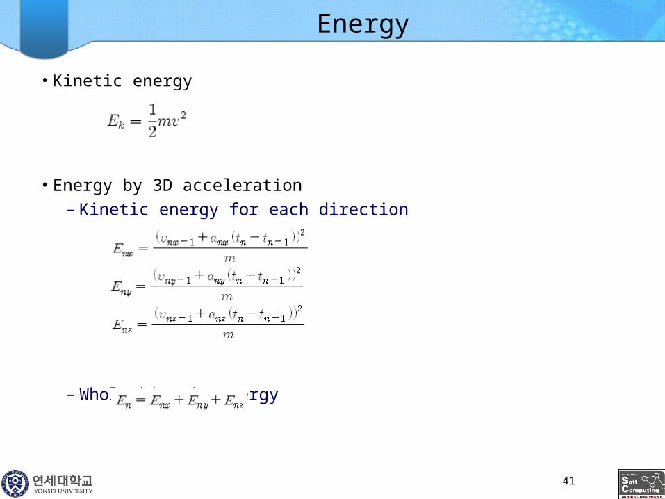
Energy

• Kinetic energy

• Energy by 3D acceleration

– Kinetic energy for each direction

– Whole kinetic energy

41

Why Energy?

• For classification of sedentary activity

• For consideration bias by the body weight

Moderate intensity activities

(walking, typing)

Vigorous activities (running)

vs.

Same activity &heavy man 1

Same activity &light man 2vs

.

F1>F2, E1 = E2 ∵ force ∝ weight

42

Frequency-domain Entropy

• Converted value from time scale x(t) to frequency scale X(f)

• Normalize by entropy calculation

• Fourier transform

– Continuous Fourier Transform

– Discrete Fourier Transform

• Fast Fourier Transform algorithms

I(X) is the information content or

self-information of X, which is itself a random variable

43

Vibration

• The variation of distance of acceleration (ax, ay, az) from origin

– Static condition: ax2 + ay

2 + az2 = g2

– In action: ax2 + ay

2 + az2 ≠ g2

– Vibration calculation (Δ)

44

Sensor Parameter Tuning

• Acceleration variables (ax, ay, az) can be tuned by a linear function

• Setting the values kx, bx by test sample data (vx1, vx2)

– Measuring on a static condition

– Gravity g is generally 9.8

45

LPSDB

LabelingInterface

LocationDB

PlaceSelection

LabelInference

GPS Data Preprocessing

• Mapping from GPS coordinates to place

• Place:

– A human readable labeling of positions [Hightower ' 03]

• Place Mapping Process

Scalability?

46

Outlier Elimination

• To get rid of the peculiar GPS data from its normal boundary

– ti is the time of the ith GPS data

– da,b means the distance between the ath and bth coordinates

– pi is the ith GPS coordinates

– kv denotes the threshold for outlier clearing.)(THEN)

--(IF

1

1,

1

,1iv

ii

iiv

ii

ii pDisregardktt

dORk

tt

d

47

Missing Data Correction

• Regression for filling missing data

– ti is the time of the ith GPS data

– pi is the ith GPS coordinates

Gray dots

)-(-

-11

11

11

ii

ii

iiii pp

tt

ttpp

48

Mapping Example of Yonsei Univ.

• Divided the domain area into a lattice and then labeled each region

49

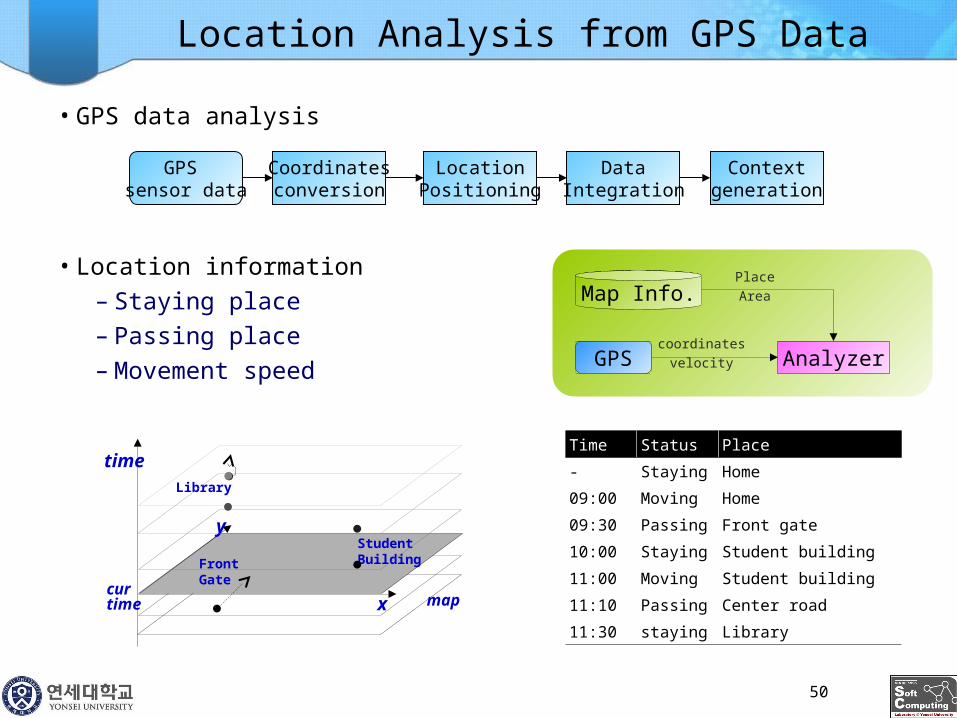
Location Analysis from GPS Data

• GPS data analysis

• Location information

– Staying place

– Passing place

– Movement speed

Time Status Place

- Staying Home

09:00 Moving Home

09:30 Passing Front gate

10:00 Staying Student building

11:00 Moving Student building

11:10 Passing Center road

11:30 staying Library

GPS sensor data

Coordinatesconversion

LocationPositioning

DataIntegration

Contextgeneration

AnalyzerGPScoordinates

velocity

Map Info.Place

Area

x

y

time

FrontGate

StudentBuilding

Library

curtime map

50

Location Positioning

• Place detection methods

– Polygon area based: Accurate, difficult to make DB

– Center point based: easy to manage, inaccurate

Polygon basedPolygon based

Center basedCenter based

51

Summary

• Data preprocessing is a big issue for data management

• Data preprocessing includes

– Data cleaning and data integration

– Data reduction and feature selection

– Discretization

• Many methods have been proposed but still an active area of research

52