prescription opioids and labor market...

Prescription Opioids and Labor Market Pains:The Effect of Schedule II Opioids on Labor Force Participation and Unemployment∗

Matthew C. Harris1, Lawrence M. Kessler†1, Matthew N. Murray1 and M. Elizabeth Glenn1

1Department of Economics and Boyd Center for Business and Economic Research,

University of Tennessee.

March 28, 2018

Abstract

We examine the effect of prescription opioids on county labor market outcomes, using data

from the Prescription Drug Monitoring Programs of ten U.S. states and labor data from the

Bureau of Labor Statistics. We achieve causal identification by exploiting plausibly exogenous

variation in the concentration of high-volume prescribers as instruments (using Medicare Part D

prescriber data). We find strong adverse effects on labor force participation rates, employment-

to-population ratios, and unemployment rates. Notably, a 10 percent increase in prescriptions

causes a 0.56 percentage point reduction in labor force participation, similar to the drop at-

tributed to the 1984 liberalization of Disability Insurance.

Keywords: Prescription Opioids, Unemployment, Regional Labor Markets

∗We are grateful to the states who shared data from their PDMP or CSMD. All errors are our own.†Corresponding Author: 719 Stokely Management Center, 916 Volunteer Boulevard, Knoxville, TN 37996-0570;

[email protected], (865) 974-6078

1

1 Introduction

The use and abuse of prescription opioids in the United States has become sufficiently ubiq-

uitous to be labeled an epidemic. The number of opioid prescriptions written and dispensed

in the U.S. has grown more than three-fold from 76 million in 1991 to almost 245 million in

2014, roughly equivalent to one opioid prescription per adult in the U.S. (Volkow, 2014; Volkow

and McLellan, 2016). Prescription growth has been accompanied by a host of adverse outcomes

including higher rates of opioid overdose, abuse, addiction, diversion, emergency room visits,

and neonatal abstinence syndrome (SAMHSA, 2011; Patrick et al., 2012; Nelson et al., 2015;

Chou et al., 2015). While much of the focus on the opioid epidemic has centered on how opioid

use affects users’ health, their families, and communities, little is known about how the rise in

opioid prescriptions has impacted labor outcomes at the individual or aggregate level.

In this paper we use variation in provider-prescribing behavior per county to estimate the

causal effect of per capita opioid prescriptions on county labor market outcomes including un-

employment rates, labor force participation rates, and employment-to-population ratios. While

the vast majority of labor economics research is conducted using individual-level data, in our

context county data yield three distinct advantages. First, diversion of prescriptions presents

a significant challenge in evaluating the effects of prescription opioids. Most illegal opioids are

not purchased from street corners, but received from friends and family. Similarly, a substantial

share of prescribed opioids is diverted to friends, family, or illegal markets rather than being

consumed by the patient who received the prescription.1 In practice, diversion within immedi-

ate social circles would be impossible to track using individual-level prescription data, which is

currently not available in the U.S. Therefore, county-level analysis better enables us to capture

the net effects of all per capita opioid prescriptions (both legitimate and diverted) on labor

force participation and employment. Second, counties represent a common region for policies to

promote labor force engagement and mitigate problems associated with substance abuse. The

former includes workforce development and training initiatives and the latter includes public

health programs that seek to mitigate substance use and abuse. A third advantage is that

aggregate data allow isolation of net impacts on the labor market.

Because opioids have both a therapeutic use in treating pain as well as a narcotic effect

1In 2013 and 2014, on average 25.2 percent of misused prescription drugs (i.e. using a prescription drug that wasnot prescribed to you or taken solely for the euphoric feeling it caused) were from doctors, 66.3 percent were froma friend or relative (a category including drugs offered free, sold, or stolen), and only 8.5 percent were from drugdealers or other strangers (Lipari and Hughes, 2017). Other estimates on diversion rates range from 5 percent to 50percent (Garnier et al., 2010; Surratt et al., 2014).

2

and high risk of dependency, prescription opioids may have both beneficial and adverse effects

on labor force participation and unemployment rates. On the positive side, opioids have a

therapeutic purpose for pain treatment and may help individuals continue or resume work.

Garthwaite (2012) and Butikofer and Skira (2017) examine the effects of Cox-2 inhibitors (which

also treat a specific sort of pain) and found positive effects on workplace attendance. However,

Cox-2 inhibitors do not have the potential for dependence, addiction, or use as an intoxicant,

all of which can lead to adverse labor market outcomes.

While most prior work on the relationship between intoxicants and labor market outcomes

has focused on alcohol or illegal drug use, the relationship between prescription opioids and

labor market outcomes may fundamentally differ from that of alcohol or illicit drugs (Cook and

Moore, 1993; French and Zarkin, 1995; Mullahy and Sindelar, 1993, 1996; Buchmueller and Zu-

vekas, 1998; Zarkin et al., 1998; DeSimone, 2002; Auld, 2005; Bray, 2005). The aforementioned

therapeutic potential implies that prescription opioids may positively affect employment out-

comes in moderation, but negatively affect employment when taken for illegitimate purposes or

in excess.2 Additionally, the social context of prescription drug use differs fundamentally from

alcohol and other illicit substances. Prescription opioids are initially dispensed by a health care

provider, are legal, and are sanctioned by the health community for private use. While alcohol

and prescription opioids are legal, the use of prescription opioids is arguably less acceptable in

social settings. These contextual differences likely imply that individuals who select into pre-

scription opioid use will differ in both observable and unobservable characteristics from those

who select into heavy alcohol or illicit drug use.3 These differences suggest that prescription

opioids may affect labor market outcomes differently than alcohol or other illicit substances.

To empirically examine the relationship between prescription opioids and labor market out-

comes, we use an unbalanced panel of county-year data on per capita opioid prescriptions from

the prescription drug monitoring program (PDMP) databases of 10 U.S. states from 2010 to

2015 and county labor market data from the Bureau of Labor Statistics (BLS).4 Because it is

2Papers such as Mullahy and Sindelar (1993) have documented a similar phenomenon for alcohol. However, asalcohol has no medical therapeutic use, this is viewed as somewhat of a puzzle. Similar findings would be lesssurprising for opioids.

3Demographically, prescription opioid use may be more concentrated in different segments of the populationthan either alcohol or other illicit substances. For example, McCabe et al. (2007) finds that race/ethnicity was not asignificant predictor of prescription drug misuse among college students, but was a significant predictor for illicit druguse (most common among White and Hispanic students). Alcohol use is also most common among Whites (Office ofthe Surgeon General, 2016). There is evidence to suggest that prescription opioid misuse is also significantly relatedto age. A 2014 report by the Substance Abuse and Mental Health Services Agency finds that the two younger agebrackets, 18 to 24 year olds and 25 to 34 year olds, were the most likely to be admitted for prescription opioid abusetreatment. There were no gender differences except at the oldest age bracket (65 or older), where women were morelikely than men to be admitted (SAMHSA, 2014).

4PDMPs are used to collect, monitor, and analyze prescribing and dispensing data submitted electronically by

3

impossible to distinguish between legitimate and illegitimate uses of prescription opioids, we

interpret these results as a net effect of both types of use. We partially control for medical

necessity by including controls for the supply of primary care doctors and cancer mortality

rates.

Our model is identified through variation in provider practices between counties, specifically

the number of high-volume opioid prescribers per capita in a given county. We merge data

on opioid prescriptions by physician from the Medicare Part D summary claims database to

identify the concentration of providers in each county in the nation’s top-five percent of opioid

prescriptions written and the nation’s top-one percent of doses prescribed.5 Previous research

has used the top-five percent as a cut-off to define high-volume prescribers (Betses and Brennan,

2013; Daubresse et al., 2017), while the top-one percent was chosen as a secondary measure of

even heavier prescribers. While Medicare Part D data do not cover all prescriptions, it covers

most providers. According to a Kaiser Family Foundation survey of primary care doctors,

93 percent accept Medicare patients (Boccuti et al., 2015). Additionally, roughly two thirds of

primary care physicians who accept Medicare patients report that less than half of their patients

have Medicare, suggesting that the majority of prescribers in the Medicare Part D database have

a mix of older and relatively younger patients. Essentially, the thought experiment behind our

instruments is the following: suppose we subtract a high volume prescriber from a given county,

while opioids per capita prescribed in that county will likely decrease, the unobservable factors

that affect the labor market will not.

Prior work has found that providers have considerable autonomy in the way they conduct

their practices. Therefore, a considerable share of the variation in medical practice is attributable

directly to the provider (Davis et al., 2000; Grytten and Sorensen, 2003; Wang and Pauly, 2005).6

Our identification strategy relies on the exogeneity of the heterogeneity in provider practices to

labor market outcomes. While it is certainly true that patients’ demand affects the equilibrium

number of prescriptions written, this is only an issue in our context if preferences among the

patients of the heavy prescribers is correlated with the unobservable factors that affect county

pharmacies and prescribing practitioners (e.g., physicians or nurse practitioners) in an effort to combat prescriptiondrug misuse, abuse, and diversion. Currently all PDMPs are operated at the state level, and PDMPs have beenauthorized or established in all 50 states and Washington D.C.

5We use the national distribution so that our measure of per-capita heavy prescribers is comparable across states.We also verify that the performance of our instrumental variables and our second-stage results are not sensitive tothe thresholds at the top-one and top-five percent. We verify that our results are similar in instrument strength,instrument validity, and estimated effect when using several delineations of ‘heavy prescribers.’ Results are availablein Appendix Table A2.

6Recent work by Sacarny et al. (2017) suggests that high-volume prescribers are aware that they are heavyprescribers and may be reluctant to change.

4

labor outcomes. We address these concerns in two ways. First, any correlation between the

concentration of heavy prescribers and unobservable factors related to county labor market out-

comes (e.g., patient appropriateness for opioids, proportion of the population with legitimate

pain problems, etc.) will result in violations of the orthogonality condition for our instruments.

Because our model is over-identified, we are able to directly test our instruments using Hansen’s

J-test, and find no evidence to support concerns regarding the orthogonality of our instruments

to unobservable labor market factors. Second, we estimate the model with alternative instru-

ments, including the number of prescriptions written for Schedule IV non-opioids written (per

capita) by high-volume opioid prescribers and the number of high-volume Schedule IV pre-

scribers in a county.7 These instruments perform well and our results are unchanged under the

alternative strategies. In demonstrating that our findings are robust when instrumenting for

opioid prescriptions with prescriptions of non-opioids, we provide additional evidence that the

variation behind our identification strategy stems from heterogeneity in provider practices.

We find that prescription opioids adversely impact county-level labor market indicators.

Our preferred model indicates that a 10 percent increase in per capita opioid prescriptions

leads to a 0.61 percentage point reduction in the employment-to-population ratio. For a given

population, a decrease in the employment-to-population ratio could occur if more people leave

their jobs either voluntarily or involuntarily. If these individuals continue looking for work, the

unemployment rate will increase. Alternatively, if these individuals were to exit the labor force

entirely, the labor force participation rate will decrease. We find that a 10 percent increase in per

capita opioid prescriptions leads to a 0.56 percentage point drop in the labor force participation

rate,8 and a 0.1 percentage point increase in the county unemployment rate, though the latter

is only marginally significant.

Finding that prescription opioids have a strong negative effect on the labor force participation

rate but only a marginal adverse effect on the unemployment rate suggests that prescription

opioids are primarily leading people to exit the labor force entirely. These results contrast

sharply with the positive labor market effects found for Cox 2 inhibitors, which were also used to

treat pain but not used for recreational purposes (Garthwaite, 2012; Butikofer and Skira, 2017).

7Schedule IV drugs include benzodiazepines such as alprazolam (Xanax) and diazepam (Valium) as well as anumber of sleeping pills such as zolpidem (Ambien) and eszopiclone (Lunesta). Our results are robust to the in-clusion/exclusion of Schedule IV opioids (tramadol and dextropropoxyphene) of any analysis involving Schedule IVdrugs. High-volume Schedule IV prescribers were defined in a similar fashion as the high-volume opioid prescribers –those in the nation’s top-five percent of Schedule IV prescriptions written and the nation’s top-one percent of dosessupplied.

8This is comparable to the reduction in labor force participation among high school dropouts that is attributedto the 1984 liberalization of the federal Disability Insurance program (Autor and Duggan, 2003).

5

While prescription opioids may have therapeutic value which could help individuals suffering

from pain to continue or return to work, our findings imply that for a regional labor market

the adverse effects of opioids dominate any positive labor market effects from therapeutic use.

These outcomes reflect both individual behavior and firm dynamics of hiring and termination.

To supplement the county-level analysis, we also examine the relationship between prescrip-

tion opioids and labor force engagement at the regional level using data from the Drug Enforce-

ment Administration’s Automated Reports and Consolidated Orders System (ARCOS), which

contains data from 2000 to 2016 for all U.S. states and Washington D.C.. While the ARCOS

data cover all 50 states and more years than our 10-state PDMP data, they are reported at the

generally larger area defined by 3-digit zip codes.9 Thus, while we view the county as the prefer-

able unit of observation for labor market outcomes, we acknowledge that the ARCOS data may

have more complete information on prescription opioids. Therefore, there is useful information

in both the county PDMP and the regional ARCOS analysis. Our results are highly similar

when using opioid data from either source, indicating that imperfections in either variable of

interest are not responsible for our findings.

Using quantile regressions, we also investigate whether the labor market effects of prescription

opioids vary by the vitality of the county labor market. Our results indicate that prescription

opioids have the strongest measurable adverse effects in counties with higher labor force par-

ticipation rates and employment-to-population ratios and lower unemployment rates. We also

find that the marginal effects of prescription opioids on county labor market indicators do not

substantively differ between relatively rural and non-rural counties.

To our knowledge, this is the first paper to examine the direct causal linkage between pre-

scription opioids and labor market outcomes at the county level. The question of how opioid

use affects labor market outcomes is relatively new in the economics literature, and the early

evidence is somewhat mixed. Hollingsworth et al. (2017) show that higher unemployment rates

are associated with higher opioid-related death and overdose rates. Laird and Neilson (2016)

examine the effects of physician-prescribing behaviors on labor market outcomes in Denmark,

and find that increases in physician prescribing rates are associated with a slight decrease in

the probability of labor force participation. However, Laird and Neilson estimate the effect of

changes in the prescriber environment rather than the direct effects of opioids prescribed on

labor market outcomes. Conversely, Kilby (2015) finds evidence consistent with the therapeutic

value of opioids: the introduction of PDMPs leads to a decrease in opioid prescriptions and an

9For example, Tennessee has 95 counties, but only 15 3-digit zip code regions.

6

increase in absence rates for short-term disabled and injured workers. However, Kilby (2015)

does not examine rates of labor force participation or unemployment.

The remainder of the paper is organized as follows: Section 2 provides background on the

opioid epidemic. Section 3 describes both the county-level data that we have acquired from

a number of U.S. states and the ARCOS regional-level data on all U.S. states, and Section 4

outlines the empirical framework. Section 5 presents the results, and Section 6 concludes with

a brief discussion.

2 Background

Several factors have contributed to the increased prevalence of prescription opioid use, in-

cluding changes in how opioids are viewed by the American medical community and the rapid

development and Federal Drug Administration (FDA) approval of new types of opioids in the

mid-1990s and 2000s.10 In 1999 the National Pain Society launched a campaign to treat pain

as a “fifth vital sign,” and minimizing pain through opioid use, without comprehensive evidence

of either the effectiveness or consequences of long-term use became commonplace (Meldrum,

2003; Mularski et al., 2006).11 This regime change in the rationale for opioid use dovetailed

with the rollout of extended-release opioids, which can impart psychoactive effects for up to

twelve hours from a single dose. When the first of these, MS Contin (morphine sulfate), was

approved by the FDA in 1987, no significant increase in opioid misuse followed. In 1995 the third

extended-release opioid, OxyContin (oxycodone controlled-release), was approved and marketed

aggressively to physicians.12 The rollout of OxyContin appears to have been a watershed mo-

ment in the emergence of the opioid epidemic, with emergency room visits from prescription

drug misuse increasing substantially in the early 2000s (FDA, 2017b). Extended-release opioids,

such as OxyContin, are associated with a higher risk of addiction and overdose, and two decades

after OxyContin’s release there were 52 extended-release opioids with FDA approval on the mar-

ket (FDA, 2017a). From 1999-2015, the percentage of drug overdoses involving opioids more

10For a comprehensive overview of the way chronic pain has been treated by the American medical system fromthe 1970s to present, and how opioids fit into this history, see Tompkins et al. (2017).

11The ubiquitous pain metric scales in doctors offices which ask patients to rate their pain on a scale from 0 to10 are the culmination of this campaign. Ballantyne and Sullivan (2015) note that “[for patients with chronic pain]maintaining low pain scores requires continuous or escalating doses of opioids at the expense of worsening functionand quality of life” (p. 2098).

12OxyContin’s parent company, Purdue Pharmacy, was sent a warning letter by the FDA in 2003 because itsmedical journal advertisements neglected to mention addiction as a possible negative side effect of OxyContin use(FDA, 2017). In 2007 the company and three executives pleaded guilty to criminal charges that they misled regulators,doctors, and patients about the drug’s risk of addiction, and the company paid out $600 million in fines and settlementpayments (Meier, 2010).

7

than doubled from 30 to 63.1 percent, and in 2015 alone, opioids were involved in 33,091 drug

overdose deaths in the U.S. (Department of Health and Human Services, 2013; Rudd, 2016).

In 2014 there were an estimated 2.5 million adults affected by opioid addiction in the U.S.

(Volkow and McLellan, 2016). Boscarino et al. (2010) found evidence to suggest that 26 percent

of patients who received long-term opioid therapy (four or more opioid prescriptions in a 12-

month period) from a primary physician would struggle with opioid dependence. Furthermore,

Shah et al. (2017) found that the probability of long-term opioid use increases most dramatically

during the first days of therapy. Specifically, the likelihood of chronic opioid use increases

with each additional day of medication supplied, but the sharpest increases occurred after

the 5th and 31st day, or after receiving just one prescription refill. While the path to opioid

dependence and/or chronic use differs across these two studies, both highlight the addictive

nature of prescription opioids and the role of provider behavior (in the amount prescribed) in

the risk of dependence.

The U.S. labor force participation rate has been on a steady decline since 2000, which coin-

cides with large increases in prescription opioid use for both medical and non-medical reasons.13

For earlier years, Zacny et al. (2003) show that the number of people using a prescription opioid

for a non-medical reason increased five-fold from 400,000 people per year in the mid-1980s to

roughly 2 million in 2000.14 The authors also find evidence to suggest that the prevalence of

non-medical prescription opioid use was steady from 1999 to 2000, but increased significantly

from 2000 to 2001. Moreover, Compton et al. (2016) estimate that this figure has ballooned in

recent years, with over 10.3 million Americans using prescription opioids for non-medical pur-

poses in 2014. Similarly, Gilson et al. (2004) show that the total medical use of Oxycodone and

Fentanyl, two popular prescription opioids, increased by over 402.9 percent and 226.7 percent

respectively from 1997 to 2002. However, the extent to which prescription opioids have affected

labor force engagement is unclear. Krueger (2015) finds that out of 571 nonworking men, close

to one third reported taking prescription pain medication. Krueger also examined data from the

American Time Use Survey Well-being Supplement (ATUS-WB) and found that 44 percent of

prime-age men who were out of the labor force had reported taking pain medication the previous

day, which was more than double the rates for employed and unemployed men. However, it is

important to note that the survey did not differentiate between non-prescription (e.g. Tylenol,

13The labor force participation rate of men has been in decline since the 1940s while the labor force participationrate of women peaked in 2000 and has since declined. There are many possible explanations for these trends. Forexample, see Autor (2015).

14Non-medical use was defined as using a prescription drug even once, that was not prescribed for you, or that youtook only for the experience or feeling it caused (Zancy et al., 2003).

8

Advil, etc.) and prescription pain medication. It is also unclear from these surveys whether

individuals are not employed because of pain medication use or whether they are unemployed

and using pain medication because of a health condition.

Table I reports data from the 2014 National Survey of Drug Use and Health (NSDUH), a

survey of 55,271 people aged 12 and over. The survey asks questions about drug use behavior

as well as demographic data. We use this data to compare the observable characteristics of

individuals who report ever using prescription opioids for a nonmedical reason to individuals

who report ever using other intoxicants. We compare family income, race, age, gender, and

education levels for both groups. Age is restricted to those 24 and over for the education

comparison but unrestricted for other comparisons. Compared to other intoxicants, users of

prescription opioids (non-medically) are a relatively young, male, working class subset of the

population. They are less likely to have graduated college and less likely to earn at least $75,000

per year compared to users of other substances (except heroin). Additionally, 47 percent of

prescription opioid users are younger than age 35, while only 38 percent of marijuana users are

under age 35.

In summary, the opioid epidemic has coincided with mounting concerns regarding declining

economy-wide labor force participation, despite the absence of direct evidence. Importantly, pre-

scription opioids represent a substance that differs socially, demographically, and pharmacologi-

cally from other substances whose impacts on the labor force have been previously documented.

The limited evidence does not offer clarity on the extent to which opioid use may affect individ-

ual and aggregate engagement with the labor market. We therefore focus on county-level opioid

prescriptions to determine whether dispensation has a material effect on economy-wide labor

market outcomes, as measured by traditional and observable metrics like participation rates,

unemployment rates and employment-to-population ratios. Our causally-identified estimates,

based on data from 10 U.S. states, reveal large and statistically significant adverse impacts on

the labor market.

3 Data

County-level data on opioid prescriptions were acquired directly from 10 U.S. states –

Arkansas, California, Colorado, Florida, Massachusetts, Michigan, Ohio, Oregon, Tennessee

and Texas – by request through their respective Controlled Substance Monitoring Database

(CSMD) or PDMP database. These data form an unbalanced panel from 2010 to 2015. We

use the total number of Schedule II opioid prescriptions filled per county in a given year as our

9

Table I: Summary Comparison of Prescription Drug Misuse and Use of Other Illicit Drugs

Percent of Respondents Who Ever Use a Specific DrugPain Relievers Alcohol Marijuana Cocaine Heroin

(Non-medically)

EducationLess Than High School 13.34 10.86 9.61 11.94 20.22

High School 27.72 27.51 27.15 28.24 27.26Some College 30.57 27.01 28.88 31.30 35.22

College Graduate 28.36 34.62 34.36 28.52 17.31

Family Income< $20,000 20.77 16.59 17.32 18.94 32.94

$20,000 - $49,999 31.71 30.12 28.95 29.36 33.02$50,000 - $74,999 16.28 17.22 16.72 16.63 13.36

≥ $75,000 31.25 36.07 37.00 35.07 20.68

RaceWhite 71.77 67.97 71.62 75.53 76.55Black 9.96 11.02 11.47 7.58 9.95

Hispanic 12.77 14.45 11.68 11.97 8.43

Age12-17 Years 5.04 3.40 3.49 0.59 0.8318-25 Years 19.19 13.40 15.85 9.92 14.5326-34 Years 22.86 15.84 17.97 17.15 25.5235-49 Years 25.76 24.90 25.79 29.33 24.6250-64 Years 22.37 25.51 28.47 37.28 28.29≥ 65 Years 4.77 16.95 8.42 5.73 6.21

GenderMale 56.66 49.91 54.23 61.44 71.60

Female 43.34 50.09 45.77 38.56 28.40

Authors’ calculations from the National Survey on Drug Use and Health, 2014.Age is restricted to 24 and over for the education comparison but unrestricted otherwise.

10

measure of ‘opioid prescriptions’. The Drug Enforcement Administration (DEA) classifies drugs

into five categories based on the drug’s acceptable medical use and abuse potential.15 Schedule

I is reserved for drugs with no acceptable medical use and a high potential for abuse, such as

heroin and lysergic acid diethylamide (LSD). Schedules II-V have accepted medical uses and

decreasing potential for psychological or physical dependence. Most of the ongoing conversation

about ‘prescription opioids’ focuses on Schedule II opioids (e.g., Hydrocodone, OxyContin, Oxy-

codone, Fentanyl), which have acceptable medical use but high potential for abuse. These drugs

must be prescribed in writing and refills are prohibited in the absence of a new prescription from

the provider. Our empirical analysis focuses on the dispensing of all Schedule II prescription

opioids, as the goal of the paper is to model the effects of increased prescriptions in this pivotal

class of drugs.16,17 We convert prescriptions to per capita measures to facilitate comparisons

across counties and states.

Table II reports state-level data as evidence of the representativeness of these ten states.

(These are 2012 data, the only year for which state-level opioid prescription data are available

for all states.) The ten states together accounted for 41.4 percent of the U.S. population in

2012. The average unemployment rate for the ten states is slightly higher than the national

average (8.5% vs 8.1%) and the labor force participation rate is slightly lower (63.1% vs 63.8%).

Average opioid prescriptions per capita for the U.S. were 0.82 compared to 0.78 for our ten states

in 2012. Tennessee held the second-highest prescription rate in the nation while California had

the lowest among all U.S. states.

We obtained data on prescribers from the 2013-2015 Medicare Part D Prescriber database

housed by the Centers for Medicare and Medicaid Services. From these data, we identify the

number of practitioners in each county in the top-five and top-one percent of opioid prescribers

in the nation, as measured by the number of opioid prescriptions written and the number of

doses prescribed, respectively. We use the number of high-volume prescribers per-capita in a

county-year, to identify the causal effects of per capita opioid prescriptions on labor market

outcomes. Previous work has shown that the majority of prescription drugs in a given state

are prescribed by a small percentage of practitioners (Dhalla et al., 2011; Department of Health

15https://www.dea.gov/druginfo/ds.shtml16A small number of prescription opioids are classified as Schedule III narcotics (drugs with acceptable medical use

and low potential for dependence), including some cough syrups and Tylenol mixed with less than 90 milligrams ofcodeine per dosage.

17The prescription opioids data provided by Colorado and Ohio measured all opioid prescriptions and not justSchedule II opioids, thus over-counting the number of Schedule II opioid prescriptions coming from these two states.In the subsequent regression analysis, this is accounted for through unique metropolitan statistical area (MSA) fixedeffects that differ across states.

11

and Human Services, 2013). For example, an analysis of Oregon’s PDMP indicated that the

top 4.1 percent of prescribers were responsible for 60 percent of all Schedule II-IV controlled

substances dispensed in a six month period (Oregon Health Authority, 2012). Similarly, data

from California suggest that 3 percent of the prescribing physicians account for 55 percent of all

Schedule II prescriptions (Swedlow et al., 2011). Furthermore, Powell et al. (2015) show that

increases in opioid prescriptions are associated with diversions to non-medical uses, while Laird

and Neilson (2016) find that a higher concentration of high-prescribing general practitioners

leads to increases in individual opioid use. The intuition behind our identification strategy is

that individuals who are in close proximity to one (or more) of these high-volume prescribers,

by virtue of living in the same county, will face lower time and transportation costs and less

difficulty in accessing prescription opioids within family and social circles.

Table III shows how opioid prescriptions per capita vary across states and time.18 Because

the data necessary for our identification strategy are only available from 2013-2015, we restrict

our analytical sample to those years. Average per capita opioid prescriptions over the analytic

sample are also presented as a map in Figure 1. Prescription opioids data were available for

eight of the 10 states in all three years, and all 10 states in 2014 and 2015. In all three years,

Tennessee had the highest average number of per capita opioid prescriptions, with roughly

1.4 prescriptions per person. If there is an average of 60 opioid doses per prescription, this is

equivalent to prescribing 80 opioid doses to every man, woman, and child in Tennessee each year.

Conversely, Texas and Massachusetts had the fewest per capita opioid prescriptions, averaging

0.4 and 0.5 prescriptions per person respectively. In the Analysis section, we perform a number

of robustness checks to account for data reporting heterogeneity across the 10 states and examine

whether our results are sensitive to the exclusion of certain states.

Table IV reports county-level data on the average number of high-volume opioid prescribers

per 100,000 population at the county level in each state. Tennessee had the highest number

of heavy opioid prescribers among the 10 states in our sample, averaging 18.0 prescribers per

100,000 population per county in the nation’s top-five percent and 4.3 per county in the top-one

18In 2014 Hydrocodone, one of the most heavily prescribed opioids was rescheduled from Schedule III to the morerestrictive Schedule II category (Laxmaiah Manchikanti et al., 2012; Drug Enforcement Administration, 2014). Moststates in our dataset counted Hydrocodone prescriptions as a Schedule II opioid, even before the schedule change, asthere was no uptick in Schedule II opioids after the schedule change (in 2014). Michigan was the exception, and asa result we have added Hydrocodone prescriptions to the Schedule II count for Michigan. Without this correctionMichigan averaged only 0.26 prescription opioids per person in 2013, but in 2014, the year that Hydrocodone wasrescheduled, per capita opioid prescriptions increased more than 3-fold to 0.93 prescriptions per person. Adding theSchedule III Hydrocodone prescriptions to the Michigan data completely removes this uptick, leads to much morestable prescription opioids per capita over time, and results in summary statistics that are more comparable to theother states in our sample (see Table III). In the Analysis section, we also perform robustness checks by excludingthe Schedule III Hydrocodone prescriptions from the Michigan counties to see if this changes any of our results.

12

percent. In contrast, the counties in Colorado and Massachusetts averaged the fewest high-

volume prescribers with only 2.9 and 3.0 practitioners per 100,000 people in the top-five percent

of national prescribers respectively, and approximately 0.2 practitioners per 100,000 people in

the top-one percent.

County-level labor force, employment, and unemployment rate data were collected from the

Bureau of Labor Statistics (BLS), and county population and demographic data (age, gender,

race, and ethnicity) were taken from U.S. Census Bureau. The percentage of the county pop-

ulation that is classified as rural is based on the 2010 U.S. Census. Additional health-related

variables such as the number of cancer deaths and the number of primary care physicians per

county were drawn from the Centers for Disease Control and Prevention (CDC) and the Ameri-

can Medical Associations (AMA) Physician Masterfile respectively. Each county is matched to a

unique BLS-defined metropolitan statistical area (MSA) or regional nonmetropolitan area (e.g.

East Tennessee nonmetropolitan area). County-level data on the number of marijuana-related

arrests were collected from the U.S. Department of Justice’s Uniform Crime Reporting (USR)

database. Data on the number of liquor stores and bars were gathered from the U.S. Census

Bureau’s County Business Patterns database. Finally, data on the number of adults receiving

disability benefits were taken from the Social Security Administration (SSA).

Table V reports summary statistics for the full sample (2010-2015) as well as the analytic

sample (2013-2015), and shows that the two samples are fairly similar. The unemployment rate

is higher in the full sample, which is not surprising given that the full sample contains more years

closer to the Great Recession. In the analytic sample there were 2,167 county-level observations,

with 505 counties observed in 2013, 830 in 2014, and 832 counties in 2015.19 This increase in

observations was due to the additions of Arkansas and Texas in 2014.

In addition to the county-level analysis, we also obtain regional-level opioid prescriptions

data from the Drug Enforcement Administration’s Automated Reports and Consolidated Or-

ders System (ARCOS) from 2000 to 2016 for all U.S. states and Washington D.C. ARCOS is

an automated data system that tracks the flow of controlled substances starting at the drug

manufacturer and ending at the point of sale or distribution (i.e. hospitals, retail pharmacies,

practitioners, etc.). The ARCOS reports contain data on the total number of grams of all

Schedule I and Schedule II substances, and select Schedule III narcotics sold or distributed.

For consistency with our county-level analysis, we examine prescriptions of Schedule II opioids

19In the analytic sample 6 observations were dropped in 2014 and 2 were dropped in 2015, all from Texas, for havinglabor force participation rates greater than one: Loving County (2014 and 2015), King County (2014), McMullenCounty (2014 and 2015), and Kennedy County (2014).

13

Table II: State Profiles, 2012

State Populationa Unemployment Labor Force Opioid PrescriptionsRateb Participation Rateb Per Capitac

Arkansas 2,950,685 0.076 0.594 1.16California 38,011,074 0.104 0.629 0.57Colorado 5,189,867 0.079 0.688 0.71Florida 19,344,156 0.085 0.606 0.73Massachusetts 6,658,008 0.067 0.651 0.71Michigan 9,887,238 0.091 0.599 1.07Ohio 11,550,839 0.074 0.632 1.00Oregon 3,899,116 0.088 0.631 0.89Tennessee 6,454,306 0.078 0.616 1.43Texas 26,071,655 0.067 0.656 0.74

10 State Aggregate 130,016,940 0.085 0.631 0.78U.S. 313,998,379 0.081 0.638 0.82a Source: U.S. Census Bureaub Source: Bureau of Labor Statisticsc Source: Paulozzi et al. (2014)

and hydrocodone. While the ARCOS data are measured in terms of grams, opioid doses are

generally measured in milligrams (mg), for example hydrocodone dosages range from 5mg up

to 10mg. Thus, a 60-pill prescription of 10mg hydrocodone would total 600mg or 0.6 grams.

Therefore, in many cases, 1 gram of opioids is much larger than a full prescription.20

However, our PDMP data are measured in prescriptions, and in most cases we do not

have sufficient information on dosages to convert to MME’s (Morphine milligram equivalents).

Therefore, it is difficult to make direct comparisons between the ARCOS data and the PDMP

data. When we compare the magnitudes of our results from regressions using opioids as measured

by PDMP or ARCOS data, we use the sample means for a common basis of comparison. As

noted earlier, the ARCOS data cover a larger sample than the PDMP data described above (in

both N and T ). However, the ARCOS data are reported at the more aggregated regional level,

as measured by 3-digit zip codes and are not directly comparable to the BLS labor market data.

In the subsequent ARCOS analysis, we convert the county-level labor force, employment, and

unemployment data to the regional level using residential weights provided by the Department of

Housing and Urban Development (HUD). Similar conversions are performed for the population,

demographic, and health-related data as well. Appendix Table A1 presents summary statistics

for the ARCOS full sample (2000-2016) and the analytic sample (2013-2015).

20This is not always the case with some of the stronger opioids such as oxycodone, with dosage ranges from 10mgup to 80mg. Here, a 60-pill prescription of 80mg oxycodone would equal 4,800mg or 4.8 grams.

14

Table III: Opioid Prescriptions Per Capita by State and Year

State 2010 2011 2012 2013 2014 2015 All Years

Arkansas 1.28 0.85 1.06(0.22) (0.16) (0.29)

California 0.92 0.92 0.95 0.92 0.93 0.92 0.93(0.36) (0.36) (0.37) (0.36) (0.35) (0.33) (0.35)

Colorado 0.82 0.87 0.86 0.83 0.82 0.79 0.83(0.19) (0.19) (0.19) (0.18) (0.17) (0.16) (0.18)

Florida 0.83 0.81 0.78 0.75 0.80(0.26) (0.25) (0.24) (0.23) (0.25)

Massachusetts 0.45 0.45 0.47 0.46 0.45 0.55 0.47(0.11) (0.10) (0.10) (0.10) (0.10) (0.11) (0.10)

Michigan 0.83 0.91 0.96 0.96 0.93 0.87 0.91(0.20) (0.22) (0.23) (0.24) (0.24) (0.21) (0.23)

Ohio 1.18 1.18 1.21 1.19 1.16 1.09 1.17(0.36) (0.34) (0.33) (0.32) (0.32) (0.30) (0.33)

Oregon 1.01 1.06 1.02 0.96 1.01(0.21) (0.22) (0.23) (0.21) (0.22)

Tennessee 1.42 1.38 1.32 1.37(0.39) (0.37) (0.36) (0.36)

Texas 0.26 0.50 0.38(0.08) (0.17) (0.18)

Full Sample 0.93 0.96 0.96 1.04 0.81 0.82 0.89(0.34) (0.33) (0.32) (0.38) (0.47) (0.35) (0.39)

A blank indicates no opioid data were available from that state year.Standard deviations in parenthesis.Data from CO and OH are on all opioid prescriptions and are now limited to Schedule II opioids.Ohio data were only available as the number of doses prescribed. The number of prescriptionswere estimated as doses divided by 60.

15

Table IV: Summary Statistics: County-level Concentration of High-Volume Prescribers by State

State Top 5 Claim Top 1 Supply

Arkansas 13.31 2.11(8.44) (3.42)

California 7.06 1.00(5.94) (1.48)

Colorado 2.90 0.25(4.96) (0.91)

Florida 7.04 2.06(4.42) (1.97)

Massachusetts 3.00 0.21(2.24) (0.35)

Michigan 10.94 1.41(8.38) (2.70)

Ohio 7.43 1.00(5.48) (1.29)

Oregon 8.06 0.44(5.74) (0.95)

Tennessee 17.98 4.31(11.09) (4.92)

Texas 4.33 0.51(6.54) (1.15)

For a given county, Top 5 Claim is calculated as the num-ber of prescribers in the top-5 percent of Part D opioidclaims per 100,000 people. Top 1 Supply is the number ofprescribers in the top-1 percent of opioid doses suppliedper 100,000 people.Standard deviations in parenthesis.

16

Table V: Summary Statistics

Variable Full Sample Analytic Sample(2010-2015) (2013-2015)

Opioids Per Capita 0.894 0.867(0.39) (0.42)

Employment-to-Population Ratio 0.527 0.525(0.08) (0.08)

Unemployment Rate 0.078 0.067(0.03) (0.02)

Labor Force Participation Rate 0.571 0.562(0.08) (0.08)

Percent Male 0.504 0.504(0.03) (0.03)

Percent Female 0.496 0.496(0.03) (0.03)

Percent Black 0.087 0.088(0.12) (0.12)

Percent Hispanic 0.142 0.155(0.18) (0.19)

Percent Rural 0.51 0.524(0.32) (0.31)

Percent under 15 Years Old 0.182 0.182(0.03) (0.03)

Percent 15 through 19 Years Old 0.065 0.064(0.01) (0.01)






Percent Aged 65+ 0.173 0.179(0.05) (0.05)

Total Population 189,522 170,258(573,849) (525,751)

Number of Primary Care Physicians per Thousand People 0.58 0.34(0.32) (0.37)

Number of Cancer Deaths per 100,000 People 234.4 127.6(68.1) (129.8)

Top 1 Supply per 100,000 Population 1.43(2.75)

Top 5 Claim per 100,000 Population 8.36(8.55)

Number of Liquor Stores 21.92(65.73)

Number of Bars 24.8(58.53)

Number of Marijuana-Related Arrests (Sales) 35.10(117.75)

Number of Marijuana-Related Arrests (Possession) 155.32(483.22)

Number of Observations 3,191 2,167

Standard deviations in parenthesis.

17

Figure 1: Average Per Capita Opioid Prescriptions, 2013-2015

4 Empirical Specification

We estimate the relationship between opioid prescriptions and labor market outcomes using

the following equation:

Yist = β0 + β1Oist + β2Xist + β3Ris + γ2s + δ2t + ε2ist (1)

where Yist, is the outcome variable (the unemployment rate, labor force participation rate

and employment-to-population ratio) in county i, MSA/non-metro area s, in year t; Oist mea-

sures the number of Schedule II opioid prescriptions per capita written by practitioners in the

same county; and Xist is a vector of explanatory variables including measures of the county’s

demographic composition (i.e. age, gender, race, and ethnicity). We include the number of

primary care physicians per thousand residents and the number of cancer deaths per hundred

thousand people as proxies for the health status of the county and the overall amount of care

being provided. Ris measures the percentage of the county’s population that is denoted as rural

18

in the 2010 Census.21 Finally, γ2s and δ2t represent metropolitan statistical area (MSA) and year

fixed effects respectively.22,23

There are multiple reasons to be concerned about an endogenous relationship between pre-

scription opioids and employment outcomes. Opioid prescriptions may be correlated with un-

observed factors that also impact labor market outcomes, which could potentially bias the

estimates from Equation (1). Counties experiencing declining labor market conditions may also

be experiencing worsening population health. If a county population is trending towards both

poorer health and economic decline, a spurious relationship between prescription opioid use and

labor market outcomes could arise. Second, there is the prospect of reverse causality. If declining

economic opportunities in a county lead individuals to engage in increased patterns of substance

use, as is shown in Hollingsworth et al. (2017), estimates on β1 will be biased. To address these

concerns, we implement an instrumental variables approach using the per capita concentration of

high-volume prescribers as exclusion restrictions. The first-stage equation specifies the number

of opioid prescriptions per capita as follows:

Oist = α0 + α1Xist + α2Ris + α3Zist + γ1s + δ1t + ε1ist (2)

As described above, we rely on two instrumental variables, both of which measure the number

of high-volume opioid prescribing practitioners in a county (or region for the ARCOS analysis):

the per capita number of practitioners in a county (region) that are in the nation’s top-five

percent of opioid prescriptions written, and the per capita number of practitioners in a county

(region) that are in the nation’s top-one percent of opioid doses prescribed.24 To check for

simultaneity bias, we also estimate a 2SLS model with Oi,t−1 as the variable of interest and Zi,t−1

as the instruments. For our instrumental variables approach to work, our instruments must be

relevant and orthogonal to the errors in the second stage, (i.e., E[Z ′ε] = 0). Any concerns

about instrument validity, such as whether the concentration of heavy-prescribing providers is

correlated with unobserved health or cultural factors that affect labor market outcomes, will

result in violations of the orthogonality conditions. Because our model is overidentified, we can

directly test the validity of our orthogonality assumption using tests developed by Sargan (1958)

and Hansen (1982). We find no evidence that our instruments are invalid, with p-values ranging

21County-level data on rural population were only available for 2010. We therefore assume a constant share of therural population from 2010 to 2015. Our results are also robust to assuming a constant rural population.

22Because 96 percent of the total variation of prescription opioids per capita is between county means, models withcounty fixed effects essentially remove all of the variation in the variable of interest. We therefore rely on uniqueMSA fixed effects to absorb geographic heterogeneity in labor markets.

23In the regional analysis, we modify Equation 1 so that i and s index regions and states respectively.24We use the national distribution so that our measure of per-capita heavy prescribers is comparable across states.

19

between 0.4 and 0.8.

We also examine how the treatment effect of opioids varies by the health of the regional

economy. To that end, we employ a quantile regression specification to examine the effects

of prescription opioids across the distributions of the employment-to-population ratio, labor

force participation rate, and unemployment rate (Firpo et al., 2009). We acknowledge that our

approach does not account for county-to-county drug flows, due to data limitations. However,

over 91 percent of misused opioids are either attained from a provider or a friend/family member,

and prior work has shown that, among friends, the majority of face-to-face contacts occur within

five miles of an individual’s home (Tilly, 1982; Huckfeldt, 1983; Eagles et al., 2004; Mok et al.,

2007, 2010). Furthermore, given the lack of any credible data on county-to-county drug flows,

treating each county as an ‘opioid island’ is a reasonable starting point for identifying the effects

of opioids on labor markets.

5 Results

Table VI reports the estimates from the first-stage equation. These first-stage results indicate

that as the number of high-volume opioid-prescribing practitioners in a county increases, per

capita opioid prescriptions also increase. The estimated coefficients on the two variables intended

to capture the concentration of heavy-prescribing practitioners are both positive and statistically

significant at the 5 percent level.25 A joint significance test of the instruments produces an F-

statistic of 17.16, which is above the benchmark value of 10 for instrument strength as outlined

in Staiger and Stock (1997). Given that our chosen instruments are similar to one another, we

also perform a redundancy test based on Breusch et al. (1999) and Baum et al. (2007) and find

that both instruments are contributing to the estimation. Finally, we perform overidentification

tests on the validity of our instruments using the Sargan-Hansen test. Results support the

validity of our instruments.

We also conduct sensitivity analysis with respect to the definition of ‘high-volume opioid

prescribers.’ We repeat our analysis with several alternative definitions of ‘heavy opioid pre-

scribers’ including the number of providers per 100,000 people who wrote opioid prescriptions (or

doses) greater than 1.5, 2.0, and 2.5 standard deviations above the national mean. In all cases,

we use one instrument for heavy prescriber with respect to opioid prescriptions (i.e. claims)

25We also find that the black and teenage proportions of the population are negatively related to per capita opioidprescriptions in a given county. The rural proportion and number of cancer-related deaths in a county are associatedwith higher levels of per capita opioid prescriptions. The results for the black population variable are consistent withprevious research on racial trends in opioid prescribing (Green et al., 2003; Burgess et al., 2008; Shavers et al., 2010).

20

and one with respect to opioid doses. Results are available in Appendix Table A2. Column 1

repeats our main specification, with the other columns using alternative definitions for high-

volume prescribers. Under all specifications of high-volume opioid prescribers, our instruments

are jointly strong (F-statistics greater than 10) and under no specification do our instruments

fail the validity test. Additionally, our second stage results are all within one standard error of

our preferred specification, reported in Column 1.

Table VII presents the main empirical results on the effects of per capita opioid prescriptions

on county labor market outcomes. In each panel, the first column reports the baseline results

(without instruments) for the full sample (2010-2015) and the second column presents the base-

line results for the analytic sample (the years for which instruments are available, 2013-2015).

The third column contains second-stage results from our preferred IV specification. For the

specification in the fourth column, we report the results of an IV specification that includes

controls for the number of liquor stores, bars, and marijuana-related arrests per county. We

include Column 4 as evidence that our findings are attributable to opioid use specifically, rather

than an overall pattern of substance use. However, the potentially endogenous relationship

between marijuana arrests and opioid use makes Column 3 our preferred specification. In all

three panels, we find that the baseline estimates of the full sample are very similar to those of

the analytic sample (comparing Columns 1 and 2), mitigating concerns about restricting our

analysis to 2013-2015. Panel A reports results with the county-level employment-to-population

ratio as the dependent variable. Per capita opioid prescriptions have a strong negative impact

on the employment-to-population ratio in the baseline models, and the estimated effects are

even larger in the preferred IV specifications. The baseline estimates in Panel A show that

a one-unit increase in per capita opioid prescriptions leads to a 6.4 to 6.5 percentage point

drop in the employment-to-population ratio, while the IV models estimate a 7.0 to 7.8 per-

centage point reduction in the employment-to-population ratio. While these estimated effects

are quite large, a one-unit increase in opioids per-capita would imply more than doubling the

number of opioids in the average county in our sample. For the effects of a more modest in-

crease in prescription opioids, predictions based on the model in Column 3 indicate that a 10

percent increase in per capita prescription opioids leads to a 0.61 percentage point drop in the

employment-to-population ratio.

Panels B and C in Table VII explore whether the effect on the employment-to-population

ratio operates through the labor force participation rate or the unemployment rates. Our es-

timates suggest that prescription opioid use affects both. In our preferred IV specification, a

21

Table VI: First-stage Estimates

Opioids Per Capita

Providers in Top 5 percent Opioid Prescriptions/100,000 Population. 0.0074**(0.0037)

Providers in Top 1 Percent Opioid Doses/100,000 Population 0.006***(0.001)

Percent Female 0.692(0.614)

Percent Black -0.382***(0.108)

Percent Hispanic 0.0423(0.128)

Percent Rural 0.125**(0.057)

Percent under 15 Years Old -0.147(0.867)

Percent 15 through 19 Years Old -3.816***(1.166)

Percent 20 through 24 Years Old -0.027(1.056)




Percent Aged 65+ 0.107(0.832)

Number of Primary Care Physicians/1,000 Population -0.04(0.033)

Number of Cancer Deaths/100,000 Population 0.001***(0.0002)

F-statistic (exclusions) 17.16Observations 2,167

Includes unique MSA and year fixed effects.Robust standard errors (in parenthesis) are clustered at the MSA/non-MSA regional level with 186clusters.∗ p < 0.10, ∗∗ p < 0.05, ∗∗∗ p < 0.01.

22

one-unit increase in per capita opioid prescriptions leads to a 6.5 percentage point drop in the

labor force participation rate. Alternatively, these estimates imply that a 10 percent increase

in per capita opioid prescriptions leads to a 0.56 percentage point reduction in the labor force

participation rate. The magnitude of these effects suggests that over 80 percent of the opioid-

induced change in the employment-to-population ratio is driven by individuals exiting the labor

force. All else the same, a declining labor force participation rate would mean a falling un-

employment rate. However, we find that increases in per capita opioid prescriptions increase

the unemployment rate as well. In Panel C, our IV results indicate that a one-unit increase in

per capita opioid prescriptions leads to a 1.2 percentage point increase in the unemployment

rate, though this effect is only marginally significant. Scaling the size of the change in opioids,

the model predicts that a 10 percent increase in per capita opioid prescriptions would lead to

a 0.1 percentage point increase in the unemployment rate. Our results therefore indicate that

high levels of per capita opioid prescriptions have significant adverse labor market effects at the

county level, and this is primarily driven through workers exiting the labor force.

We subject the results from our preferred IV specification to a number of robustness checks

in Table VIII. Column 1 reports our main specification to facilitate comparison. Column 2

contains a specification using lagged values of opioids per capita (and lagged instruments) to

address concerns about simultaneity bias. The estimates in Column 2 are less precise due to

the loss of observations, but the results are qualitatively similar to the main specification. We

also conduct a series of regressions excluding certain states to verify that our main results are

not driven by between-state heterogeneity in data reporting or the aggregation of opioids. The

sample for Column 3 excludes the Schedule III Hydrocodone prescriptions from Michigan but

this does not substantively change the results. Column 4 examines whether our results are

driven by the counties with unusually high opioid prescription rates by excluding all counties

from the three states with the highest average per capita opioid prescriptions: Arkansas, Ohio,

and Tennessee. Our results actually strengthen when we exclude the high-opioid states. That

is, an increase in per capita opioid prescriptions will impact labor markets more adversely in

areas with (currently) lower levels of per capita opioid prescriptions. Perhaps suggesting that

the proverbial damage has already been done in the high-opioid states. The results in Column

5 are from a sample that excludes Colorado and Ohio, the two states where opioid prescriptions

are not limited to those in the Schedule II category. The results do not change substantively,

thus this reporting difference is not responsible for our findings. In Column 6, we check that our

results are robust to excluding Texas, as opioids per capita in Texas were reportedly very low

23

Table VII: Effects of Opioid Prescriptions Per Capita on County Labor Market Outcomes

Full Sample Analytic Sample Analytic Sample Analytic SampleFixed Effects Fixed Effects FE-IV FE-IV

Incl. Drugs/Alcohol

Panel A: Employment-to-Population Ratio(1) (2) (3) (4)

Opioids Per Capita -0.064*** -0.065*** -0.070** -0.078***(0.008) (0.008) (0.033) (0.030)

N 3,191 2,167 2,167 2,167F-statistic (exclusions) 17.16 17.84Hansen J-Statistic p-value 0.399 0.466

Panel B: Labor Force Participation Rate(1) (2) (3) (4)

Opioids per capita -0.057*** -0.059*** -0.065** -0.073**(0.007) (0.008) (0.033) (0.030)


Panel C: Unemployment Rate(1) (2) (3) (4)

Opioids per capita 0.019*** 0.017*** 0.012* 0.013*(0.003) (0.002) (0.007) (0.007)


Includes unique MSA and year fixed effects.Robust standard errors (in parenthesis) are clustered at the MSA/non-MSA regional level with 186 clusters.∗ p < 0.10, ∗∗ p < 0.05, ∗∗∗ p < 0.01.

24

in 2014 but nearly doubled the year after; our results are again virtually unchanged. For some

instances where we exclude states, our estimates on the effect of opioids on unemployment rates

lose precision (and significance), though the point estimates are largely unchanged. This loss of

precision does reinforce the conclusion that the primary effect on the employment-to-population

ratio is through labor force participation. Finally, in poorer labor markets, more people using

prescription opioids may also be receiving disability benefits. Therefore, in Panel B Column 8 we

measure the dependent variable as the labor force participation rate conditional on the county’s

disability rate and find results similar to our main specification. This suggests that higher

disability rates are not spuriously generating our main result, but we nevertheless highlight that

we cannot separately identify the effects of disability rates and prescription opioids. We discuss

this issue in greater detail in the discussion section, but a deeper exploration into the joint

relationships between disability, prescription opioids, and labor force participation remains an

area for future work.

While our IV specifications using heavy prescribers as exclusion restrictions perform well, it

is possible that this variation is driven in part by patient demand for opioids. If this unobservable

demand among the patients of these heavy prescribers is correlated with unobservable factors

that affect county labor market outcomes, it threatens the validity of our instruments. We

therefore repeat our main IV specification with alternative instruments, the results of which

are contained in Table IX. Column 1 contains results from a specification where we use the

number of prescribers (per capita) in the nation’s top 5 percent of claims and top 1 percent of

doses of Schedule IV non-opioid narcotics as instruments for per-capita Schedule II opioids. This

specification serves primarily as a reference point for the rest of the table. These instruments are

relatively weakly correlated with opioid prescriptions, with a first stage joint F-statistic of 7.31.

However, they do pass Hansen’s J-test, suggesting that they do not violate the orthogonality

conditions. Moreover, the estimated opioid effects are similar to our main findings, although

the unemployment rate effects are larger in magnitude.

Column 2 contains results where we instrument for per-capita Schedule II opioid prescriptions

with the per-capita number of prescriptions for Schedule IV non-opioid narcotics written by the

heavy opioid prescribers. When we use these providers’ prescribing behavior for other drugs

to instrument for Scheduled II opioids, our first stage F-statistics increase to 30.34 and second

stage estimates change only slightly. The key feature of this instrument is that we are using

the prescribing behavior with regards to other non-opioid drugs of the previously identified

high-volume prescription opioid providers. The prescribing behavior of non-opioid drugs should

25

Table VIII: Robustness Checks: Effects of Opioid Prescriptions Per Capita on County Labor MarketOutcomes

Main Ot−1 No MI No AR, No CO, OH No TX No FL Non-OH, TN Disabled

Pop OnlyPanel A: Employment-to-Population Ratio

(1) (2) (3) (4) (5) (6) (7)

Opioids Per Capita -0.070** -0.062* -0.071** -0.119** -0.071* -0.069** -0.069**(0.033) (0.036) (0.033) (0.058) (0.038) (0.029) (0.033)

N 2,167 1,330 2,167 1,468 1,711 1,665 1,966F-statistic (exclusions) 17.16 16.56 19.68 18.13 12.74 22.20 15.52Hansen J-Statistic p-value 0.399 0.714 0.500 0.788 0.340 0.510 0.415

Panel B: Labor Force Participation Rate(1) (2) (3) (4) (5) (6) (7) (8)

Opioids Per Capita -0.065** -0.055 -0.066** -0.114** -0.067* -0.062** -0.063* -0.076**(0.032) (0.035) (0.032) (0.058) (0.038) (0.029) (0.033)

(0.032)

N 2,167 1,330 2,167 1,468 1,711 1,665 1,966 1,993F-statistic (exclusions) 17.16 16.56 19.68 18.13 12.74 22.20 15.52 19.17Hansen J-Statistic p-value 0.374 0.742 0.464 0.872 0.313 0.466 0.408 0.981

Panel C: Unemployment Rate(1) (2) (3) (4) (5) (6) (7)

Opioids Per Capita 0.012* 0.013* 0.012 0.013 0.011 0.016** 0.012(0.007) (0.007) (0.008) (0.016) (0.008) (0.008) (0.007)


Excluded Data Schedule III AR, OH, CO, OH TX FLHydrocodone TNprescriptions

from MI


26

not be driven by unobservable demand for opioids. Because we use these providers’ prescribing

behavior for non-opioids as instruments for per-capita opioid prescriptions, we contend that

these instruments are driven by provider behavior and are much less likely to be determined by

the general equilibrium process that produces opioid consumption and labor market outcomes.

However, it is still possible that the variation that links the Schedule IV prescriptions of the

heavy Schedule II prescribers is driven by the presence of the Schedule II prescribers, not the

Schedule IV prescriptions. To address those concerns, we include the specifications in Columns 3

and 4, which include the number of heavy opioid prescribers (defined by prescriptions or claims)

and the Schedule IV prescriptions of those prescribers. The first stage results are presented

in Appendix Table A3 and show that while both instruments in both specifications predict

increases in opioids per capita, the strength comes from the Schedule IV prescribing behavior

rather than the presence of the heavy Schedule II prescribers. In both Column 3 and Column 4

the F-statistics of the instruments are greater than 10 and we do not reject the null that these

exclusion restrictions are valid using the J-test. For all four alternative instrument sets, the

second stage results are highly similar to the main findings in Table VII.

Next, we examine how the relationship between per capita opioid prescriptions and county

labor market outcomes varies over the support of the dependent variables. While our conditional

mean results presented above robustly show that per-capita opioid prescriptions adversely affect

county labor markets, there is clear potential for heterogeneous treatment effects. Media reports

often associate heavy opioid use with the more rural and economically distressed counties. How-

ever, it is ex ante unclear whether the marginal effects of prescription opioids on labor market

outcomes are worse in these areas or in areas with tighter labor markets (i.e., higher labor force

participation and lower unemployment rates) (Kliff, 2017; Semuels, 2017). To address this issue

we estimate quantile regressions to examine the effects of prescription opioids at the 20th, 40th,

60th, and 80th percentiles of each dependent variable. These estimates are presented in Table

X. For each outcome of interest, we present both a descriptive model using our baseline speci-

fication, as well as our preferred IV specification. We find that the effects of per capita opioid

prescriptions on unemployment rates, labor force participation, and employment-to-population

ratios are most pronounced in counties with stronger labor markets. While anecdotal reporting

on the effects of the opioid epidemic has focused on areas with slack labor markets, these re-

sults suggest that perhaps the opioid-related damage has already been done in areas with low

labor force participation. These findings are also consistent with the larger marginal effects

found in Table VIII Column 4. This interpretation is consistent with the associative findings in

27

Table IX: Robustness Checks: Effects Opioids Per Capita on County Labor Market OutcomesUsing Alternative Instruments


Opioids Per Capita -0.079* -0.077** -0.077** -0.084**(0.045) (0.036) (0.036) (0.034)

N 2,167 2,167 2,167 2,167F-statistic (exclusions) 7.31 30.34 15.76 16.09Hansen J-Statistic p-value 0.24 NA 0.86 0.32


Opioids Per Capita -0.068 -0.069* -0.075** -0.075**(0.045) (0.036) (0.038) (0.034)



Opioids Per Capita 0.021*** 0.021*** 0.020*** 0.020***(0.008) (0.006) (0.006) (0.006)


Instruments 1. Top 1 supply of non-opioid 1. Non-opioid Schedule IV 1. Non-opioid Schedule IV 1. Non-opioid Schedule IVSchedule IV narcotics prescriptions per capita prescriptions per capita prescriptions per capita

2. Top 5 claim of non-opioid among high opioid among high opioid among high opioidSchedule IV narcotics prescribers prescribers prescribers

2. Top 5 claim opioids 2. Top 5 supply opioids


28

Hollingsworth et al. (2017). Individuals may be using more opioids in depressed rural counties,

but some of these individuals may have already left the labor force. Hence, we find that opioids

have the largest marginal effect when labor markets are tighter.

We also examine whether the labor market effects of prescription opioids differ between rural

and non-rural counties, as delineated by the BLS metropolitan and nonmetropolitan definitions.

These results, reported for the baseline model only, are presented in Table XI. Consistent with

our main findings, we find statistically significant negative effects for both rural and non-rural

counties. While the estimated effects are slightly larger in magnitude for rural counties, the

estimates are not significantly different from one another.

Finally, we utilize the ARCOS data to examine the relationship between prescription opioids

and labor market outcomes at the regional level. These results are presented in Table XII. The

results again indicate that opioids have a strong adverse effect on the labor market. Column

1 presents results for the baseline model on the full sample of all U.S. states from 2000 to

2016. These results show that a one gram increase in prescription opioids per capita leads to

reductions in both the employment-to-population ratio and labor force participation rate as

well as an increase in the unemployment rate. However, these effects are smaller than those

found in Table VII. In Column 2, we repeat the full sample analysis with the addition of an

indicator variable for whether there was a PDMP in place in that area in the year of observation.

The results are nearly identical to those found in Column 1.26 Column 3 presents the baseline

results for the analytic sample (2013-2015, the years for which instruments are available) and

the results are very similar to results derived using PDMP data (Table VII Column 2). Column

4 reports the IV results for the analytic sample, which indicate an even larger adverse opioid

effects on all regional labor market outcomes. Specifically, a one gram increase in prescription

opioids per capita leads to a 13.5 percentage point reduction in the labor force participation

rate, a 12.7 percentage point drop in the employment-to-population ratio, and a 3.2 percentage

point increase in the unemployment rate.

Differences in scale between the ARCOS and PDMP data can be misleading, and it is difficult

to convert one to the other. To compare the regional ARCOS analysis with the estimated county

PDMP effects from earlier, next we calculate the estimated effects with respect to their analytic

sample means. For this exercise, we focus on the IV results from Table VII Column 3 and Table

XII Column 4. Using results from the PDMP analysis, doubling opioids per capita at the sample

26The results remain unchanged regardless of whether we use a dummy variable for the implementation of allPDMPs or for the implementation of ‘must access’ PDMPs where physicians are required to check the PDMPdatabase and view the patient’s prescribing history before providing an opioid prescription, as defined in Buchmuellerand Carey (2017).

29

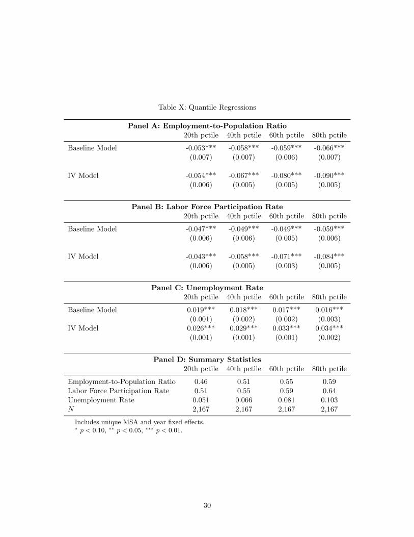
Table X: Quantile Regressions

Panel A: Employment-to-Population Ratio20th pctile 40th pctile 60th pctile 80th pctile

Baseline Model -0.053*** -0.058*** -0.059*** -0.066***(0.007) (0.007) (0.006) (0.007)

IV Model -0.054*** -0.067*** -0.080*** -0.090***(0.006) (0.005) (0.005) (0.005)

Panel B: Labor Force Participation Rate20th pctile 40th pctile 60th pctile 80th pctile

Baseline Model -0.047*** -0.049*** -0.049*** -0.059***(0.006) (0.006) (0.005) (0.006)

IV Model -0.043*** -0.058*** -0.071*** -0.084***(0.006) (0.005) (0.003) (0.005)

Panel C: Unemployment Rate20th pctile 40th pctile 60th pctile 80th pctile

Baseline Model 0.019*** 0.018*** 0.017*** 0.016***(0.001) (0.002) (0.002) (0.003)

IV Model 0.026*** 0.029*** 0.033*** 0.034***(0.001) (0.001) (0.001) (0.002)

Panel D: Summary Statistics20th pctile 40th pctile 60th pctile 80th pctile

Employment-to-Population Ratio 0.46 0.51 0.55 0.59Labor Force Participation Rate 0.51 0.55 0.59 0.64Unemployment Rate 0.051 0.066 0.081 0.103N 2,167 2,167 2,167 2,167

Includes unique MSA and year fixed effects.∗ p < 0.10, ∗∗ p < 0.05, ∗∗∗ p < 0.01.

30

Table XI: Robustness Checks: Effects of Opioid Prescriptions Per Capita on County Labor MarketOutcomes. Baseline Model

Unemp. Unemp. LFP LFP Emp/Pop Emp/PopNon-Rural Rural Non-Rural Rural Non-Rural Rural

Opioids Per Capita 0.016*** 0.017*** -0.046*** -0.058*** -0.052*** -0.064***(0.004) (0.003) (0.008) (0.009) (0.009) (0.010)

N 888 1,279 888 1,279 888 1,279

Includes unique MSA and year fixed effects.

Robust standard errors (in parenthesis) are clustered at the MSA/non-MSA regional level with186 clusters.

∗ p < 0.10, ∗∗ p < 0.05, ∗∗∗ p < 0.01.

mean (a 0.867 unit increase) would lead to a 6.1 percentage point drop in the employment-to-

population ratio, a 5.6 percentage point fall in labor force participation, and a 1.0 percentage

point increase in the unemployment rate. While in the ARCOS analysis, doubling opioids

per capita at the sample mean (a 0.521 gram increase) would lead to a 7.1 percentage point

reduction in the employment-to-population ratio, a 6.7 percentage point drop in the labor force

participation rate, and a 1.7 percentage point increase in the unemployment rate. Thus, the

adverse opioid effects are slightly larger in magnitude for the regional analysis, but they are still

very similar to those from the county-level analysis at the unconditional mean.

6 Conclusion

This is the first paper to examine the causal effects of per capita opioid prescriptions on

highly-visible county and regional labor market outcomes. We exploit plausibly exogenous

variation in the concentration of high-volume opioid prescribers as measured by the number of

prescriptions written and number of doses prescribed to identify the causal effects. Our findings

indicate that prescription opioids have very strong negative effects on employment-to-population

ratios and labor force participation rates, and a marginally adverse impact on unemployment

rates. We also find that while popular perception associates the opioid epidemic with counties

with slack labor markets, the marginal effects of opioids per capita on county labor markets are

strongest in counties where the labor markets are tight.

These results are not intended to suggest that all restrictions on the supply of prescription

opioids will necessarily improve labor market outcomes or welfare. First, if individuals are

31

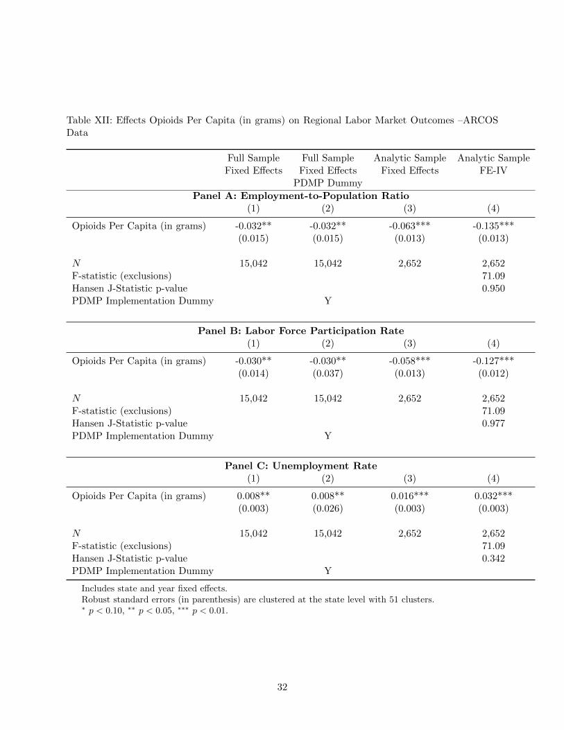
Table XII: Effects Opioids Per Capita (in grams) on Regional Labor Market Outcomes –ARCOSData

Full Sample Full Sample Analytic Sample Analytic SampleFixed Effects Fixed Effects Fixed Effects FE-IV

PDMP Dummy


Opioids Per Capita (in grams) -0.032** -0.032** -0.063*** -0.135***(0.015) (0.015) (0.013) (0.013)

N 15,042 15,042 2,652 2,652F-statistic (exclusions) 71.09Hansen J-Statistic p-value 0.950PDMP Implementation Dummy Y


Opioids Per Capita (in grams) -0.030** -0.030** -0.058*** -0.127***(0.014) (0.037) (0.013) (0.012)



Opioids Per Capita (in grams) 0.008** 0.008** 0.016*** 0.032***(0.003) (0.026) (0.003) (0.003)


Includes state and year fixed effects.Robust standard errors (in parenthesis) are clustered at the state level with 51 clusters.∗ p < 0.10, ∗∗ p < 0.05, ∗∗∗ p < 0.01.

32

leaving the labor force because of opioid dependence, restricting the availability of opioids may

lead individuals to substitute to heroin or other substances rather than snapping back to work

(Compton et al., 2016). Second, if individuals have valid medical conditions for which pain

management is necessary, severe restrictions on prescription opioids may make it more difficult

for individuals to work, as in Kilby (2015). Determining the extent to which these findings reflect

legitimate and/or illegitimate use(s) of opioids is an area for future work with individual-level

data. If the results reflect legitimate uses, then society should be informed of the labor market

costs associated with the opioid approach to pain management; if the results reflect illegitimate

uses, the labor market consequences should be well identified to help motivate public health

interventions that can minimize abuse.

One important caveat from these findings involves disability rates. While we show that

our results hold when restricting the denominator of the labor force participation rate to non-

disabled individuals, the relationship between opioid use, labor market outcomes, and disability

rates is more complicated. Previous research has shown that adverse labor market conditions

may contribute to higher disability rates (Black et al., 2002; Autor and Duggan, 2003; Erceg and

Levin, 2014; Hall, 2015). Similarly, as chronic diagnosed pain is by itself grounds for disability,

the direction of causation between opioid use and disability may run in either direction (GAO,

2011; Morden et al., 2014; Meara et al., 2016; Buchmueller and Carey, 2017; Song, 2017).27

With the data currently available, we do not have the ability to separately identify the effects

of disability and opioid use on labor market outcomes. While the statistical tests for validity of

our preferred instruments and robustness checks using alternative instruments provide support

for our findings, disentangling the importance of disability from prescription opioids remains an

area for future work.

Our hope is that these findings contribute towards our fledgling understanding of the com-

prehensive economic impact of the prescription opioid epidemic. The finding that prescription

opioids are subtracting individuals from the labor market means that the opioid epidemic is af-

fecting economic growth, the tax bases of local economies, and the amount of resources available

for households to invest in the next generation. Hopefully, these results are useful in garnering

resources for further research, as well as for prevention, treatment, and recovery.

27Moreover, people who use prescription opioids may also receive disability benefits at a higher rate and longerduration (Mahmud et al., 2000; Webster et al., 2007; Franklin et al., 2008; Kidner et al., 2009; Ashworth et al., 2013).

33

References

Ashworth, J., D. J. Green, K. M. Dunn, and K. P. Jordan (2013). Opioid use among low back

pain patients in primary care: Is opioid prescription associated with disability at 6-month

follow-up? PAIN R© 154 (7), 1038–1044.

Auld, M. C. (2005). Smoking, drinking, and income. Journal of Human Resources 40, 505–518.

Autor, D. (2015). Why are there still so many jobs. Journal of Economic Perspectives 29 (3),

3–30.

Autor, D. H. and M. G. Duggan (2003). The rise in the disability rolls and the decline in

unemployment. The Quarterly Journal of Economics 118 (1), 157–206.

Ballantyne, J. and M. Sullivan (2015). Intensity of chronic pain - the wrong metric? New

England Journal of Medicine 373 (22), 2098–2099.

Baum, C. F., M. E. Schaffer, and S. Stillman (2007). Enhanced routines for instrumental

variables/gmm estimation and testing. Stata Journal 7 (4), 465–506.

Betses, M. and T. Brennan (2013). Abusive prescribing of controlled substancesa pharmacy

view. New England Journal of Medicine 369 (11), 989–991.

Black, D., K. Daniel, and S. Sanders (2002). The impact of economic conditions on participation

in disability programs: Evidence from the coal boom and bust. The American Economic

Review 92 (1), 27.

Boccuti, C., C. Fields, G. Casillas, and L. Hamel (2015). Primary care physicians accepting

medicare: A snapshot.

Boscarino, J. A., M. Rukstalis, S. N. Hoffman, P. M. Han, J. J.and Erlich, G. S. Gerhard, and

W. F. Stewart (2010). Risk factors for drug dependence among outpatients on opioid therapy

in a large us health care system. Addiction 105 (10), 1776–1782.

Bray, J. W. (2005). Alcohol use, human capital, and wages. Journal of Labor Economics 23,

279–312.

Breusch, T., H. Qian, P. Schmidt, and D. Wyhowski (1999). Redundancy of moment conditions.

Journal of Econometrics 91 (1), 89–111.

34

Buchmueller, T. C. and C. Carey (2017). The effect of prescription drug monitoring programs

on opioid utilization in medicare. American Economic Journal: Economic Policy .

Buchmueller, T. C. and S. H. Zuvekas (1998). Drug use, drug abuse, and labor market outcomes.

Health Economics 7 (3), 229–245.

Burgess, D. J., M. Crowley-Matoka, S. Phelan, J. F. Dovidio, R. Kerns, C. Roth, S. Saha, and

M. vanRyn (2008). Patient race and physicians’ decisions to prescribe opioids for chronic low

back pain. Social Science and Medicine 67 (11), 1852–1860.

Butikofer, A. and M. M. Skira (2017). Missing work is a pain: The effect of cox-2 inhibitors on

sickness absence and disability pension receipt. Journal of Human Resources, Forthcoming.

Chou, R., J. A. Turner, E. B. Devine, R. N. Hansen, S. D. Sullivan, I. Blazina, T. Dana,

C. Bougatsos, and R. A. Deyo (2015). The effectiveness and risks of long-term opioid therapy

for chronic pain: a systematic review for a national institutes of health pathways to prevention

workshop. Annals of Internal Medicine 162 (4), 276–286.

Compton, W. M., C. M. Jones, and G. Baldwin (2016). Relationship between nonmedical

prescription-opioid use and heroin use. New England Journal of Medicine 374, 154–163.

Cook, P. and M. J. Moore (1993). Drinking and schooling. Journal of Health Economics 12,

411–429.

Daubresse, M., B. Saloner, H. A. Pollack, and G. Caleb Alexander (2017). Non-buprenorphine

opioid utilization among patients using buprenorphine. Addiction.

Davis, P., B. Gribben, A. Scott, and R. Lay-Yee (2000). The “supply hypothesis’ and medical

practice variation in primary care: testing economic and clinical models of inter-practitioner

variation. Social Science & Medicine 50 (3), 407–418.

Department of Health and Human Services (2013). Addressing prescription drug abuse in the

united states: Current and future opportunities.

DeSimone, J. (2002). Illegal drug use and employment. Journal of Labor Economics 20 (4),

952–977.

Dhalla, I. A., M. M. Mamdani, T. Gomes, and D. N. Juurlink (2011). Clustering of opioid

prescribing and opioid-related mortality among family physicians in ontario. Canadian Family

Physician 57 (3), e92–e96.

35

Drug Enforcement Administration (2014). Schedules of controlled substances: rescheduling

of hydrocodone combination products from schedule III to schedule II. Final rule. Federal

Register 79 (163), 49661.

Eagles, M., P. Belanger, and H. W. Calkins (2004). The spatial structure of urban politi-

cal discussion networks. In M. F. Janelle (Ed.), Spatially Integrated Social Science. Oxford

University Press.

Erceg, C. J. and A. T. Levin (2014). Labor force participation and monetary policy in the wake

of the great recession. Journal of Money, Credit and Banking 46 (S2), 3–49.

FDA (2017a). Introduction for the fda blueprint for prescriber education for extended-release

and long-acting opioid analgesics.

FDA (2017b). Timeline of selected fda activities and significant events addressing opioid misuse

and abuse.

Firpo, S., N. M. Fortin, and T. Lemieux (2009). Unconditional quantile regressions. Economet-

rica 77 (3), 953–973.

Franklin, G. M., B. D. Stover, J. A. Turner, D. Fulton-Kehoe, and T. M. Wickizer (2008). Early

opioid prescription and subsequent disability among workers with back injuries: the disability

risk identification study cohort. Spine 33 (2), 199–204.

French, M. T. and G. A. Zarkin (1995). Is moderate alcohol use related to wages? Journal of

Health Economics 14, 319–344.

GAO (2011). Instances of questionable access to prescription drugs.

Garnier, L. M., A. M. Arria, K. M. Caldeira, K. B. Vincent, K. E. O’Grady, and E. D. Wish

(2010). Sharing and selling of prescription medications in a college student sample. Journal

of Clinical Psychiatry 71 (3), 262–269.

Garthwaite, C. (2012). The economic benefits of pharmaceutical innovations: The case of cox-2

inhibitors. American Economic Journal: Applied Economics 4 (3), 116–137.

Gilson, A. M., K. M. Ryan, D. E. Joranson, and J. L. Dahl (2004). A reassessment of trends

in the medical use and abuse of opioid analgesics and implications for diversion control:

19972002. Journal of Pain and Symptom Management 28 (2), 176–188.

36

Green, C. R., K. O. Anderson, T. A. Baker, L. C. Campbell, S. Decker, R. B. Fillingim, D. A.

Kaloukalani, K. E. Lasch, C. Myers, and R. C. Tait (2003). The unequal burden of pain:

confronting racial and ethnic disparities in pain. Pain Medicine 4 (3), 277–294.

Grytten, J. and R. Sorensen (2003). Practice variation and physician-specific effects. Journal

of Health Economics 22 (3), 403–418.

Hall, R. E. (2015). Quantifying the lasting harm to the us economy from the financial crisis.

NBER Macroeconomics Annual 29 (1), 71–128.

Hansen, L. P. (1982). Large sample properties of generalized method of moments estimators.

Econometrica 50, 1029–1054.

Hollingsworth, A., C. J. Ruhm, and K. Simon (2017). Macroeconomic conditions and opioid

abuse. NBER Working Paper, #23192.

Huckfeldt, R. R. (1983). Social contexts, social networks, and urban neighborhoods; environ-

mental constrains on friendship choice. American Journal of Sociology 89, 651–669.

Kidner, C. L., T. G. Mayer, and R. J. Gatchel (2009). Higher opioid doses predict poorer

functional outcome in patients with chronic disabling occupational musculoskeletal disorders.

The Journal of Bone and Joint Surgery. American volume. 91 (4), 919.

Kilby, A. E. (2015). Opioids for the masses: Welfare tradeoffs in the regulation of narcotic pain

medications. Working Paper, Northeastern University.

Kliff, S. (2017). The opioid crisis changed how doctors think about pain. Vox .

Krueger, A. B. (2015). Where Have All the Workers Gone? Working Paper, Boston Federal

Reserve.

Laird, J. and T. Neilson (2016). The effects of physician prescribing behaviors on prescription

drug use and labor supply: evidence from movers in denmark. Harvard University Working

Papers.

Laxmaiah Manchikanti, M., I. Standiford Helm, and J. W. J. MA (2012). Opioid epidemic in

the United States. Pain Physician 15, 2150–1149.

Lipari, R. N. and A. Hughes (2017). How people obtain the prescription pain relievers they

misuse. Technical report, Center for Behavioral Health Statistics and Quality, Substance

Abuse and Mental Health Services Administration.

37

Mahmud, M. A., B. S. Webster, T. K. Courtney, S. Matz, J. A. Tacci, and D. C. Christiani

(2000). Clinical management and the duration of disability for work-related low back pain.

Journal of Occupational and Environmental Medicine 42 (12), 1178–1187.

McCabe, S. E., M. Morales, J. A. Cranford, J. Delva, M. D. McPherson, and C. J. Boyd (2007).

Race/ethnicity and gender differences in drug use and abuse among college students. Journal

of Ethnicity in Substance Abuse 6 (2), 75–95.

Meara, E., J. R. Horwitz, W. Powell, L. McClelland, W. Zhou, A. J. O’malley, and N. E.

Morden (2016). State legal restrictions and prescription-opioid use among disabled adults.

New England Journal of Medicine 375 (1), 44–53.

Meier, B. (2010). In guilty plea, oxycontin maker to pay $600 million. New York Times.

Meldrum, M. L. (2003). A capsule history of pain management. Journal of the American Medical

Association 290 (18), 2470–2475.

Mok, W., B. Wellman, and R. Basu (2007). Did distance matter before the internet? Social

Networks 29 (3), 430–461.

Mok, W., B. Wellman, and J. A. Carrasco (2010). Does distance matter in the age of the

internet? Urban Studies 47 (3), 2747–2783.

Morden, N. E., J. C. Munson, C. H. Colla, J. S. Skinner, J. P. Bynum, W. Zhou, and E. R. Meara

(2014). Prescription opioid use among disabled medicare beneficiaries: Intensity, trends and

regional variation. Medical care 52 (9), 852.

Mularski, R. A., F. White-Chu, D. Oberbay, L. Miller, S. M. Asch, and L. Ganzini (2006).

Measuring pain as the 5th vital sign does not improve quality of pain management. Journal

of General Internal Medicine 21 (6), 607–612.

Mullahy, J. and J. Sindelar (1993). Alcoholism, work, and income. Journal of Health Eco-

nomics 11 (3), 494–520.

Mullahy, J. and J. Sindelar (1996). Employment, unemployment, and problem drinking. Journal

of Health Economics 15 (4), 409–434.

Nelson, L., D. Juurlink, and J. Perrone (2015). Addressing the opioid epidemic. Journal of the

American Medical Association 314 (14), 1453–1454.

38

Oregon Health Authority (2012). Prescription drug dispensing in Oregon, October 2011-March

2012. Technical report, Oregon Health Authority.

Patrick, S. W., R. E. Schumacher, B. D. Benneyworth, E. E. Krans, J. M. McAllister, and

M. M. Davis (2012). Neonatal abstinence syndrome and associated health care expenditures:

United States, 2000-2009. Journal of the American Medical Association 307 (18), 1934–1940.

Paulozzi, L. J., K. A. Mack, and J. M. Hockenberry (2014). Vital signs: variation among states

in prescribing of opioid pain relievers and benzodiazepinesunited states, 2012. MMWR Morb

Mortal Wkly Rep 63 (26), 563–8.

Powell, D., R. Pacula, and E. Taylor (2015). How increasing medical access to opioids contributes

to the opioid epidemic: evidence from medicare part d. NBER Working Paper, #21072.

Rudd, R. A. (2016). Increases in drug and opioid-involved overdose deaths - United States,

2010-2015. MMWR. Morbidity and mortality weekly report 65.

Sacarny, A., D. Yokum, and S. Agrawal (2017). Government-academic partnerships in random-

ized evaluations: The case of inappropriate prescribing. American Economic Review Papers

& Proceedings 107, 466–470.

SAMHSA (2011). Drug abuse warning network, 2011: National estimates of drug-related emer-

gency department visits, sma13-4760. Technical report, Substance Abuse and Mental Health

Services Administration.

SAMHSA (2014). The TEDS report: Gender differences in primary substances of abuse across

age groups. Technical report, Center for Behavioral Health Statistics and Quality, Substance

Abuse and Mental Health Services Administration.

Sargan, J. D. (1958). The estimation of economic relationships using instrumental variables.

Econometrica 26, 393–415.

Semuels, A. (2017). The lonely women of the rust belt. The Atlantic.

Shah, A., C. Hayes, and B. Martin (2017). Characteristics of initial prescription episodes and

likelihood of long-term opioid use - United States, 2006-2015. MMWR Morbidity and Mortality

Weekly Report .

Shavers, V. L., A. Bakos, and V. B. Sheppard (2010). Race, ethnicity, and pain among the U.S.

adult population. Journal of Health Care for the Poor and Underserved 21 (1), 177–220.

39

Song, Z. (2017). Mortality quadrupled among opioid-driven hospitalizations, notably within

lower-income and disabled white populations. Health Affairs 36 (12), 2054–2061.

Staiger, D. and J. H. Stock (1997). Instrumental variables regression with weak instruments.

Econometrica 65 (3), 557–586.

Surratt, H. L., C. O’Grady, S. P. Kurtz, Y. Stivers, T. J. Cicero, R. C. Dart, and M. Chen

(2014). Reductions in prescription opioid diversion following recent legislative interventions

in Florida. Pharmacoepidemiology 23, 314–320.

Swedlow, A., J. Ireland, and G. Johnson (2011). Prescribing patterns of schedule II opioids in

California workers’ compensation.

Tilly, C. (1982). To Dwell among Friends: Personal Networks in Town and City. Chicago:

University of Chicago Press.

Tompkins, D. A., J. G. Hobelmann, and P. Compton (2017). Providing chronic pain management

in the fifth vital sign era: Historical and treatment perspectives on a modern-day medical

dilemma. Drug and Alcohol Dependence 173, S11–S21.

Volkow, N. D. (2014). Americas addiction to opioids: Heroin and prescription drug abuse.

Technical report, Senate Caucus on International Narcotics Control.

Volkow, N. D. and A. T. McLellan (2016). Opioid abuse in chronic pain - misconceptions and

mitigation strategies. New England Journal of Medicine 374, 1253–1263.

Wang, Y. R. and M. V. Pauly (2005). Spillover effects of restrictive drug formularies on physician

prescribing behavior. Journal of Economics and Management Strategies 14, 755–773.

Webster, B. S., S. K. Verma, and R. J. Gatchel (2007). Relationship between early opioid

prescribing for acute occupational low back pain and disability duration, medical costs, sub-

sequent surgery and late opioid use. Spine 32 (19), 2127–2132.

Zacny, J., G. Bigelow, P. Compton, K. Foley, M. Iguchi, and C. Sannerud (2003). College on

problems of drug dependence taskforce on prescription opioid non-medical use and abuse:

position statement. Drug and Alcohol Dependence 69, 215–232.

Zarkin, G. A., M. T. French, T. A. Mroz, and J. W. Bray (1998). Alcohol and wages: New

results from the national household survey on drug abuse. Journal of Health Economics 17,

53–68.

40

7 Appendix

41

Table A1: Summary Statistics - ARCOS Data

Variable Full Sample Analytic Sample(2000-2016) (2013-2015)

Opioids Per Capita (in grams) 0.423 0.521(0.29) (0.25)

Employment-to-Population Ratio 0.579 0.559(0.07) (0.07)

Unemployment Rate 0.061 0.063(0.02) (0.02)

Labor Force Participation Rate 0.616 0.596(0.06) (0.06)

Percent Male 0.493 0.495(0.01) (0.01)

Percent Female 0.506 0.504(0.01) (0.01)

Percent Black 0.099 0.102(0.12) (0.12)

Percent Hispanic 0.109 0.122(0.14) (0.14)

Percent Rural 0.34 0.327(0.24) (0.24)

Percent under 15 Years Old 0.196 0.188(0.02) (0.02)







Percent Aged 65+ 0.143 0.157(0.03) (0.03)

Total Population 342,587 360,167(365,485) (525,751)

Number of Primary Care Physicians per Thousand People 0.712 0.720(0.23) (0.23)

Number of Cancer Deaths per 100,000 People 207.7 208.8(47.9) (49.2)

Top 1 Supply per 100,000 Population 1.43(2.10)

Top 5 Claim per 100,000 Population 7.79(6.40)

Number of Observations 15,042 2,652

Standard deviations in parenthesis.

42

Table A2: Instrument Sensitivity Analysis: Effects of Opioid Prescriptions Per Capita on CountyLabor Market Outcomes using Different Instruments

Panel A: Employment-to-Population Ratio(1) (2) (3) (4) (5) (6) (7)

Opioids Per Capita -0.070** -0.075** -0.060* -0.064* -0.75** -0.063* -0.082**(0.032) (0.035) (0.033) (0.035) (0.35) (0.034) (0.036)


Panel B: Labor Force Participation Rate(1) (2) (3) (4) (5) (6) (7)

Opioids Per Capita -0.065** -0.070* -0.055* -0.060* -0.69** -0.057* -0.077**(0.033) (0.035) (0.032) (0.035) (0.35) (0.034) (0.036)


Panel C: Unemployment Rate(1) (2) (3) (4) (5) (6) (7)

Opioids Per Capita 0.012* 0.011 0.009 0.009 0.014 0.014* 0.013(0.007) (0.008) (0.007) (0.008) (0.008) (0.008) (0.008)


Instruments top 1 supply plus 2.0SD supply top1supply plus 2.5SD supply plus 1.5SD supply plus 2.5SD supply plus 1.5SD supplytop 5 claim top 5 claim plus 1.5SD claim plus 1.5SD claim plus 2.0SD claim plus 2.0SD claim plus 2.5SD claim

For a given county, “plus xSD supply” represents the number of practitioners per 100,000 population with opioiddoses supplied that are x standard deviations above the national average, and “plus xSD claim” is the number ofprescribers with opioid claims that are x standard deviations above the national average.Includes unique MSA and year fixed effects.Robust standard errors (in parenthesis) are clustered at the MSA/non-MSA regional level with 186 clusters.∗ p < 0.10, ∗∗ p < 0.05, ∗∗∗ p < 0.01.

43

Table A3: First-stage Estimates - Alternative Instruments

Opioids Per Capita

Exclusions

Providers in Top 5 Percent Non-Opioid 0.010**Schedule IV Prescriptions/100,000 Population (0.004)

Providers in Top 1 Percent Non-Opioid 0.005**Schedule IV Doses/100,000 Population (0.002)

Non-Opioid Schedule IV Prescriptions Per 1.020*** 0.928*** 0.779***Capita Among High Opioid Prescribers (0.185) (0.288) (0.264)

Providers in Top 5 percent Opioid 0.0009Prescriptions/100,000 Population (0.002)

Providers in Top 5 Percent Opioid 0.003Doses/100,000 Population (0.002)

F-statistic (exclusions) 7.31 30.34 15.76 16.09Observations 2,167 2,167 2,167 2,167

Includes unique MSA and year fixed effects.Robust standard errors (in parenthesis) are clustered at the MSA/non-MSA regional level with 186clusters.∗ p < 0.10, ∗∗ p < 0.05, ∗∗∗ p < 0.01.

44

prescription opioids and labor market...

Documents