presentation of r

8/8/2019 Presentation of R

http://slidepdf.com/reader/full/presentation-of-r 1/109

An Introduction to R


John Verzani

CUNY/College of Staten Island Department of Mathematics

NYC ASA, CUNY Ed. Psych/May 24, 2005

http://find/

http://goback/




OutlineWhat is R?The many faces of RData

Manipulating dataApplying functions to data

Vectorization of dataGraphics

Model formulasInference

Significance testsconfidence intervals

ModelsSimple linear regressionMultiple linear regression

Analysis of variance modelsLogistic regression models

http://find/




What is R?

R is an open-source statistical computing environment

R is available from http://www.r-project.org R is a computing language, based on S and S-Plus, which is

well suited for statistical calculations

R has the ability to produce excellent graphics for statisticalexplorations and publications

http://www.r-project.org/


http://find/




What is R?

The structure of R

RKernel

Library

Base

base

grid

stats

stats4

...

Recommended

MASS

nlme

...

MASS

nlme

Contrib. (CRAN)UsingR

gregmisc

...

UsingR

gregmisc

library()

CLIBatch

DCOM,...

text graphicsdevice

http://find/

http://goback/




The many faces of R

The many faces of R

R is ported to most modern computing platforms: Windows,MAC OS X, Unix with X11 (linux), ...

R has an interface that varies depending on the installation:

http://find/

http://goback/




The many faces of R

Windows interface

Figure: Windows gui

http://find/




The many faces of R

Mac OS X interface

Figure: Mac OS X gui

http://find/

http://goback/




The many faces of R

X11 interface – the command line

Figure: There is no standard GUI for X11 implementations. A“typical”usage may look like this screenshot. Also of interest is ESS package for(X)Emacs users.

http://find/

http://goback/




The many faces of R

The command line interface (CLI)

In R the typical means of interacting with the software is at thecommand line.

Commands are typed at the prompt >

Continuation lines are indicated with a +

ENTER sends the commands off to the interpreter

2 + 2

> 2 + 2

[1] 4

A I d i R

http://find/




Data

Data types

In statistics data comes in different types: numeric,categorical, univariate, bivariate, multivariate, etc.

R has different data types or classes to accommodate thesedifferent types of data sets.

Some basic storage types are:

A I t d ti t R

http://find/




Data

numeric vectors: created with c(), etc.

> somePrimes = c(2, 3, 5, 7, 11, 13, 17)

> somePrimes

[1] 2 3 5 7 11 13 17

> odds = seq(1, 15, 2)

> odds

[1] 1 3 5 7 9 11 13 15

> ones = rep(1, 10)

> ones

[1] 1 1 1 1 1 1 1 1 1 1

An Introd ction to R

http://find/

http://goback/




Data

Character strings are indicated by using matching quote, double of single.

Character variables

> character = c("Homer", "Marge", "Bart", "Lisa",

+ "Maggie")

> gender = c("Male", "Female", "Male", "Female",

+ "Male")


http://find/

http://goback/




Data

Categorical variables – factors

> gender = factor(c("Male", "Female", "Male",

+ "Female", "Male"))

> gender

[1] Male Female Male Female Male

Levels: Female Male

Factors have an extra attribute a fixed set of levels that requiresome care. (E.g., you can’t add new levels without some work.)Factors are used instead of character vectors, as this allows R toidentify certain types of data. (Storage space is smaller as well.)


http://find/

http://goback/




Data

Logical vectors: vectors of TRUE or FALSE

> somePrimes

[1] 2 3 5 7 11 13 17

> somePrimes < 10 [1] TRUE TRUE TRUE TRUE FALSE FALSE FALSE

> somePrimes %in% c(3, 5, 7)

[1] FALSE TRUE TRUE TRUE FALSE FALSE FALSE

> somePrimes == 2 | somePrimes >= 10

[1] TRUE FALSE FALSE FALSE TRUE TRUE TRUE


http://find/




Data

Matrices

defining matrices:matrix(), rbind(), ...

> M = rbind(c(1, 1), c(0, 1))> M

[,1] [,2]

[1,] 1 1

[2,] 0 1


http://find/



u

Data

Matrices, cont.

Operations: multiplication. (* is entry-by-entry

> M % * % M

[,1] [,2]

[1,] 1 2[2,] 0 1

Inverse is found by“solving”Ax

=b

,b

an indentity matrix> solve(M)

[,1] [,2]

[1,] 1 -1

[2,] 0 1


http://find/



Data

Matrices, cont.

Least squares regression coefficients the hard way

> x = 1 : 5

> y = c(2, 3, 1, 4, 5)> ones = rep(1, length(x))

> X = cbind(ones, x)

> solve(t(X) %*% X, t(X) %*% y)

[,1]ones 0.9

x 0.7


http://find/



Data

Lists

Lists are recursive structures with each level made up of components.

List components can be other data types, functions, additionallists, etc.

Lists are used often as return values of functions in R. Theprint method is set to show only part of the values contained

in the list.


http://find/



Data

Defining lists

> lst = list(a = somePrimes, b = M, c = mean)

> lst

$a

[1] 2 3 5 7 11 13 17

$b

[,1] [,2]

[1,] 1 1

[2,] 0 1

$c

function (x, ...)

UseMethod("mean")

<environment: namespace:base>


http://find/



Data

Other data types

Data can be given extra attributes, such as a time series:

Time series have regular date information

> google = c(100.2, 132.6, 196, 180, 202.7,

+ 191.9, 186.1, 180)> ts(google, start = c(2004, 9), frequency = 12)

Jan Feb Mar Apr May Jun Jul Aug Sep

2004 100.2

2005 202.7 191.9 186.1 180.0Oct Nov Dec

2004 132.6 196.0 180.0

2005


http://find/



Data

Tables – an extension of an matrix or array

The table() function (also xtabs, ftable,...)

> table(gender)

gender

Female Male2 3

> satisfaction = c(3, 4, 3, 5, 4, 3)

> category = c("a", "a", "b", "b", "a", "a")> table(category, satisfaction)

satisfaction

category 3 4 5

a 2 2 0

b 1 0 1


http://find/



Data

Data frames

The most common data-storage format is a data frame

Stores rectangular data: each column a variable, typically eachrow data for one subject

Columns have names for easy reference

May be manipulated like a matrix or a list (each variable a

top-level component)


http://find/



Data

Relationship between vector, matrix, data frame, list

Matrix

q q q

q q q

q q q

q q q

Vector

q q q

Data frame List


D

http://find/

http://goback/



Data

Data frame examples

> role = c("Comic relief", "Parent", "troublemaker",

+ "Goody two-shoes", "Cute baby")

> theSimpsons = data.frame(name = character,

+ gender = gender, role = role)

> theSimpsons

name gender role

1 Homer Male Comic relief

2 Marge Female Parent

3 Bart Male troublemaker

4 Lisa Female Goody two-shoes

5 Maggie Male Cute baby


D t

http://find/



Data

Reading in data

Data can be built-in, entered in at the keyboard, or read in fromexternal files. These may be formatted using fixed width format,commas separated values, tables, etc. For instance, this commandreads in a data set from a url:

Reading urls

> f = "http://www.math.csi.cuny.edu/st/R/crackers.csv"

> crackers = read.csv(f)

> names(crackers)

[1] "Company" "Product"

[3] "Crackers" "Grams"

[5] "Calories" "Fat.Calories"

[7] "Fat.Grams" "Saturated.Fat.Grams"

[9] "Sodium" "Carbohydrates"[11] "Fiber"


Data

http://find/

http://goback/



Data

Manipulating data

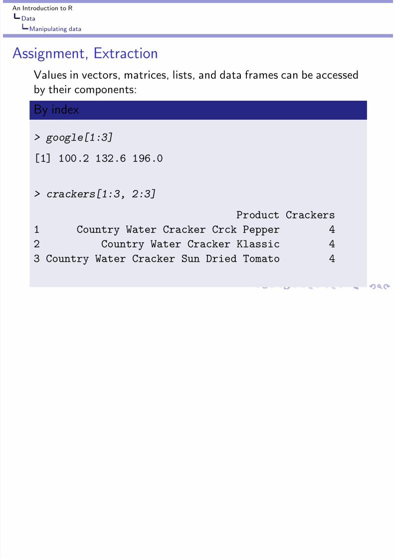
Assignment, Extraction

Values in vectors, matrices, lists, and data frames can be accessedby their components:

By index

> google[1:3][1] 100.2 132.6 196.0

> crackers[1:3, 2:3]

Product Crackers

1 Country Water Cracker Crck Pepper 4

2 Country Water Cracker Klassic 4

3 Country Water Cracker Sun Dried Tomato 4


Data

http://find/



Data

Manipulating data

By index cont.

> M[1, ]

[1] 1 1

> lst[[1]]

[1] 2 3 5 7 11 13 17


Data

http://find/



Data

Manipulating data

Access by name

by name

> crackers[1:3, c("Product", "Crackers")]

Product Crackers

1 Country Water Cracker Crck Pepper 42 Country Water Cracker Klassic 4

3 Country Water Cracker Sun Dried Tomato 4

> theSimpsons[["role"]][1] Comic relief Parent troublemaker

[4] Goody two-shoes Cute baby

5 Levels: Comic relief Cute baby ... troublemaker


Data

http://find/



Data

Manipulating data

Access by logical expressions

logical questions answered TRUE or FALSE

> somePrimes < 10 [1] TRUE TRUE TRUE TRUE FALSE FALSE FALSE

> somePrimes[somePrimes < 10]

[ 1 ] 2 3 5 7


Data

http://find/



ata

Manipulating data

Recycling values

When making assignments in R we might have a situation wheremany values are replaced by 1, or a few. R has a means of recycling the values in the assignment to fill in the size mismatch.

replace coded values with NA

> x = c(1, 1, 0, 1, 99, 0, 1, 99, 0, 1, 99)

> x[x == 99] = NA

> x[x == 1] = "Yes"

> x[x == 0] = "No"

> x

[1] "Yes" "Yes" "No" "Yes" NA "No" "Yes" NA

[9] "No" "Yes" NA


Data

http://goforward/

http://find/

http://goback/



Applying functions to data


Finding the mean

> fat = crackers$Fat.Grams

> mean(fat)

[1] 3.679

The median

> median(fat)

[1] 3.25


Data

http://find/




Extra arguments to find trimmed mean

> mean(fat, trim = 0.2)

[1] 3.482

missing data – coded NA

> shuttleFailures = c(0, 1, 0, NA, 0, 0, 0)

> mean(shuttleFailures, na.rm = TRUE)

[1] 0.1667


Data

http://find/




Functions

Functions are called by name with a matching pair of ()

Arguments may be indicated by position or name

Named arguments can (and usually do) have reasonabledefaults

A special role is played by the first argument


Data

http://find/




generic functions

Interacting with R from the command line requires one toremember a lot of function names, although R helps outsomewhat. In practice, many tasks may be viewed generically:E.g.,“print”the values of an object,“summarize”values of an

object,“plot”the object. Of course, different objects should yielddifferent representations.R has methods (S3, S4) to declare a function to be generic. Thisallows different functions to be“dispatched”based on the“class”of the first argument.

A basic template is:

methodName( object, extraArguments)

Some common generic functions are print() (the default action),summary() (for summaries), plot() (for basic plots).


Data

http://find/




summary() function called on a number and factor

> summary(somePrimes)

Min. 1st Qu. Median Mean 3rd Qu. Max.

2.00 4.00 7.00 8.29 12.00 17.00

> summary(gender)

Female Male

2 3


Data

http://find/



Vectorization of data

R, like MATLAB, is naturally vectorized. For instance, to find thesample variance, (n−1)−1∑(x i − x̄ )2 by hand involves:

sample variance (also var())

> x = c(2, 3, 5, 7, 11, 13)

> fractions(x - mean(x))

[1] -29/6 -23/6 -11/6 1/6 25/6 37/6

> fractions((x - mean(x))^2)

[1] 841/36 529/36 121/36 1/36 625/36 1369/36

> fractions(sum((x - mean(x))^2)/(length(x) -

+ 1))

[1] 581/30


Data

http://find/




Example: simulating a sample distribution

A simulation of the sampling distribution of x̄ from a randomsample of size 10 taken from an exponential distribution withparameter 1 naturally lends itself to a“for loop:”

for loop simulation

> res = c()

> for (i in 1:200) {

+ res[i] = mean(rexp(10, rate = 1))

+ }> summary(res)

Min. 1st Qu. Median Mean 3rd Qu. Max.

0.392 0.786 0.946 1.000 1.220 2.440


Data

V i i f d

http://find/




Vectorizing a simulation

It is often faster in R to vectorize the simulation above bygenerating all of the random data at once, and then applying the mean() function to the data. The natural way to store the data isa matrix.

Simulation using a matrix

> m = matrix(rexp(200 * 10, rate = 1), ncol = 200)

> res = apply(m, 2, mean)

> summary(res)Min. 1st Qu. Median Mean 3rd Qu. Max.

0.308 0.800 1.010 1.020 1.190 1.830


Graphics

http://find/



Graphics

R has many built-in graphic-producing functions, and facilities tocreate custom graphics. Some standard ones include:

histogram and density estimate

> hist(fat, probability = TRUE, col = "goldenrod")

> lines(density(fat), lwd = 3)


Graphics

http://goforward/

http://find/

http://goback/



histogram and density estimate

Histogram of fat

fat

D e n s i t y

0 2 4 6 8

0 . 0

0

0 . 0 5

0 . 1

0

0 . 1

5

0 . 2

0


Graphics

http://find/



Graphics: cont.

Quantile-Quantile plots

> qqnorm(fat)

Boxplots

> boxplot(MPG.highway ~ Type, data = Cars93)

plot() is generic, last one also with

> plot(MPG.highway ~ Type, data = Cars93)


Graphics

http://find/



Quantile-Quantile plot

qqq

qq

q

q

qq

q

q

q

q

q

q

q

q

q

q

q

q

q

q

q

qqq

q

q

q

qq

qqq

qq

q

q

q

q

qq

q

q

q

q

qq

qq

q

q

q

qq

q

q

q

q

qq

q

q

qqq

q

q

q

qq

q

q

q

q

q

q

qqqq

q

q

q

q

q

q

q

q

qq

−2 −1 0 1 2

0

2

4

6

8

Normal Q−Q Plot

Theoretical Quantiles

S a m p l e Q u a n t i l e s


Graphics

http://find/



Boxplots

q

q

Compact Large Midsize Small Sporty Van

2 0

2 5

3 0

3 5

4 0

4 5

5 0


Graphics

http://find/



Fancy examples from upcoming book of P. Murrell

0.0 0.2 0.4 0.6 0.8 1.0

0

5 0

1 0 0

1 5 0

2 0 0

2 5

0

3 0 0

3 5 0

234 (65%)

159 (44%)

1.2

N u m b e r o f V e s s e l s

Sampling Fraction

C o m p l e t e n e s s

1 . 0

1 . 2

1 . 4

1 . 6

1 . 8

2 . 0

N = 360 brokenness = 0.5


Graphics

http://find/



3-d graphics

X1

X2 X3

X2 X3

X1


Graphics

Model formulas

http://find/



Model formula notation

The boxplot example illustrates R’s model formula. Many genericfunctions have a method to handle this type of input, allowing foreasier usage with multivariate data objects.

Example with xtabs – tables

> df = data.frame(cat = category, sat = satisfaction)

> xtabs(~cat + sat, df)

sat

c a t 3 4 5a 2 2 0

b 1 0 1

An Introduction to RGraphics

Model formulas

http://find/



Model formula cont.

Suppose x, y are numeric variables, and f is a factor. The basicmodel formulas have these interpretations:

y ~ 1 y i = β0 + εi y ~ x y i = β0 + β1x i + εi y ~ x - 1 y i = β1x i + εi remove the intercepty ~ x | f y i = β0 + β1x i + εi grouped by levels of f y ~ f y ij = τi + εij

The last usage suggests storing multivariate data in two variables –a numeric variable with the measurements, and a factor indicatingthe treatment.


Model formulas

http://find/



Lattice graphics

Lattice graphics can effectively display multivariate data that arenaturally defined by some grouping variable. (Slightly morecomplicated than need be to show groupedData() function in

nlme package.)

lattice graphics

> cars = groupedData(MPG.highway ~ Weight |

+ Type, Cars93)> plot(cars)


Model formulas

http://find/



Weight

M P G . h

i g h w a y

2000 3000 4000

20

25

30

35

40

45

50

q

qq

qq

qq

Van

q

qq

q

q

q

qq

qq

Large

2000 3000 4000

q

q

q

q

q

q

q

q

q

qq

qqq

q

q

q

q

qq

Midsize

q

q

q

qq

q

q

qq

q

q

q

Compact

2000 3000 4000

q

qq

q

q

q

q

q

q

q

q

q

Sporty

20

25

30

35

40

45

50

q

q

q

q

q

q

q

q

q

qq

q q

q

qq

q

q

q

q

Small


Model formulas

http://find/

http://goback/



more lattice graphics (Murrell’s book)

Barley Yield (bushels/acre)

20 30 40 50 60

SvansotaNo. 462

ManchuriaNo. 475

VelvetPeatlandGlabronNo. 457

Wisconsin No. 38Trebi

q

q

q

q

q

q

q

q

q

q

Grand RapidsSvansota

No. 462Manchuria

No. 475Velvet

PeatlandGlabronNo. 457


q

q

q

q

q

q

q

q

q

q

DuluthSvansota

No. 462Manchuria

No. 475Velvet



q

q

q

q

q

q

q

q

q

q

University FarmSvansota

No. 462Manchuria

No. 475Velvet



q

q

q

q

q

q

q

q

q

q

MorrisSvansota

No. 462Manchuria

No. 475Velvet



q

q

q

q

q

q

q

q

q

q

CrookstonSvansota

No. 462Manchuria

No. 475Velvet



q

q

q

q

q

q

q

q

q

q

Waseca

19321931

q

An Introduction to RInference

Significance tests

http://find/

http://goback/



Significance tests

There are several functions for performing classical statistical testsof significance: t.test(), prop.test(), oneway.test(),wilcox.test(), chisq.test(), ...These produce a p -value, and summaries of the computations.


Significance tests

http://find/



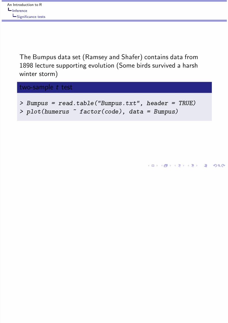
The Bumpus data set (Ramsey and Shafer) contains data from1898 lecture supporting evolution (Some birds survived a harshwinter storm)

two-sample t test

> Bumpus = read.table("Bumpus.txt", header = TRUE)

> plot(humerus ~ factor(code), data = Bumpus)


Significance tests

http://find/



Diagnostic plot

q

q

1 2

6 6 0

6 8 0

7 0 0

7 2 0

7 4 0

7 6 0

7 8 0

factor(code)

h u m e r u s


Significance tests

http://find/

http://goback/



t.test() output

> t.test(humerus ~ code, data = Bumpus)

Welch Two Sample t-test

data: humerus by codet = -1.721, df = 43.82, p-value = 0.09236

alternative hypothesis: true difference in means is not eq

95 percent confidence interval:

-21.895 1.728

sample estimates: mean in group 1 mean in group 2

727.9 738.0


Significance tests

http://find/

http://goback/



The SchizoTwins data set (R&S) contains data on 15 pairs of monozygotic twins. Measured values are of volume of lefthippocampus.

t -tests: paired

> twins = read.table("SchizoTwins.txt", header = TRUE)

> plot(affected ~ unaffected, data = twins)> attach(twins)

> t.test(affected - unaffected)$p.value

[1] 0.006062

> t.test(affected, unaffected, paired = TRUE)$p.value

[1] 0.006062

> detach(twins)


Significance tests

http://find/



Diagnostic plot

q

q

q

q

q

q

q

q

q

q

q

q

q

q

q

1.4 1.6 1.8 2.0

1 .

0

1 .

2

1 .

4

1 .

6

1 .

8

2 .

0

unaffected

a f f e c t e d


confidence intervals

http://find/



Confidence intervals

Confidence intervals are computed as part of the output of manyof these functions. The default is to do 95% CIs, which may beadjusted using conf.level=.

95% CI humerus length overall

> t.test(Bumpus$humerus)

...

95 percent confidence interval:728.2 739.6

...



http://find/



Chi-square tests

Goodness of fit tests are available through chisq.test() andothers. For instance, data from Rosen and Jerdee (1974, fromR&S) on the promotion of candidates based on gender:

gender data

> rj = rbind(c(21, 3), c(14, 10))

> dimnames(rj) = list(gender = c("M", "F"),

+ promoted = c("Y", "N"))

> rj

promotedgender Y N

M 21 3

F 14 10



http://find/



sieveplot(rj)

Sieve diagram

promoted

g e n d e r

F

Y N

M



http://find/



chi-squared test p -value

> chisq.test(rj)$p.value

[1] 0.05132

Fischer’s exact test

> fisher.test(rj, alt = "greater")$p.value

[1] 0.02450

An Introduction to RModels

Simple linear regression

http://find/



Fitting linear models

Linear models are fit using lm():

This function uses the syntax for model formula Model objects are reticent – you need to ask them for more

information

This is done with extractor functions: summary(), resid(),fitted(), coef(), predict(), anova(), deviance(),...



http://find/



Body fat data set

> source("http://www.math.csi.cuny.edu/st/R/fat.R")

> names(fat)

[1] "case" "body.fat" "body.fat.siri"[4] "density" "age" "weight"

[7] "height" "BMI" "ffweight"

[10] "neck" "chest" "abdomen"

[13] "hip" "thigh" "knee"

[16] "ankle" "bicep" "forearm"[19] "wrist"



http://find/



Fitting a simple linear regression model

Basic fit is done with lm: response ˜ predictor(s)

> res = lm(body.fat ~ BMI, data = fat)

> res

Call:

lm(formula = body.fat ~ BMI, data = fat)

Coefficients:

(Intercept) BMI

-20.41 1.55

http://find/



Scatterplot with regression line

q

q

q

q

q

q

q

q

q

q

qq

q qq

q

q

q

q

q

q

q

q

q

q

q

q

q

q

q

q

q

q

q

q

q

q

q

q

qq

q

q

q

q

q

q

q

q

q

q

q

q

q

q

q

q

q

qq

q

q

q

q

q

q

q

q

qq

q

q

q

q

qq

q

q

q

q

qq q

q

q

q

q

q

q

q

q

q

q

qq

q

qq

qq

q

q

q

qq

q

q

q

q

qq

q

q

q

q

q

q

q

q

q

q

q

q

q

q

q

q

q

qq

q

q

q

q

q

q

q

q

q

q

qq

q

q

q

q

q

q

q

q

q

q

q

q

q

q

q

q

q

q

q

q

q

q

q

q

q

q

q

q

q

q

q

q

q

q

q

q

q

qq

q

q

q

q

q

q

q

q

q

q

q

q

q

q

q

q

q

q

q

q

q

q

q

q

q

q

qq

q

q

q

q

q

q

q

q

q

q

q

q

q

q

q

q

qq

qq

q

q

q

q

q

q

q

q

q

q

q

q

q

q

q

q

q

20 25 30 35 40 45 50

0

1

0

2 0

3 0

4 0

BMI

b o d y .

f a t

BMI predicting body fat

least−squares

lqs



()

http://find/



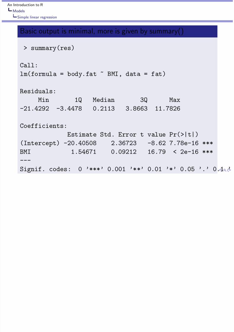
Basic output is minimal, more is given by summary()

> summary(res)

Call:

lm(formula = body.fat ~ BMI, data = fat)

Residuals:

Min 1Q Median 3Q Max

-21.4292 -3.4478 0.2113 3.8663 11.7826

Coefficients:Estimate Std. Error t value Pr(>|t|)

(Intercept) -20.40508 2.36723 -8.62 7.78e-16 ***

BMI 1.54671 0.09212 16.79 < 2e-16 ***

---

Signif. codes: 0 ’***’ 0.001 ’**’ 0.01 ’*’ 0.05 ’.’ 0.1 ’



http://find/



summary() output cont.

Residual standard error: 5.324 on 250 degrees of freedomMultiple R-Squared: 0.53, Adjusted R-squared: 0.5281

F-statistic: 281.9 on 1 and 250 DF, p-value: < 2.2e-16



E f i d i f i

http://find/



Extractor functions used to extract information

extractor functions

> coef(res)

(Intercept) BMI

-20.405 1.547

> summary(residuals(res))

Min. 1st Qu. Median Mean 3rd Qu.

-2.14e+01 -3.45e+00 2.11e-01 3.52e-17 3.87e+00Max.

1.18e+01



http://find/



Residual plots to test model assumptions

> plot(fitted(res), resid(res))

> qqnorm(resid(res))



R id l l t

http://find/



Residual plots

q

q

q

q

q

q

q

q

q

q

q

q

q

q

q

q

q

q

q

q

q

q

q

q

q

q

q

q

q

q

q

q

q

q

q

q

q

q

q

q

q

q

q

q

q

q

q

q

q

q

qq

q

q

q

q

q

q

q

qq

q

qq

q

q

q

q

q

q

q

q

q

q

q

q

q

q

q

q

q

qq

q

q

q

q

q

q

q

q

q

q

q

qq

qq

q

qq

q

qq

q

q

q

q

q

q

q

q

q

q

q

q

q

q

q

q

q

q

q

q

q q

q

q

q

q

q

q

q

q

q

q

q

q

q

qq

q

q

q

q

qq

q

q

q

q

qq

q

q

q

q

qq

q

q

q

q

q

q

q

q

q

q

q

qq

qq

q

q

q

q

qq

q

q

q

q

q

q

q

q

q

q

q

q

q

q

q

q

q

q

q

q

q

q

q

q

q

q

q

qq

q

q

q

q

q

q

q

q

q

q

q

q

q

q

q

q

q

q

q

q

q

q

q

qq

q

q

q

q

q

q

q

q

q

q

q

q

q

10 20 30 40 50

− 2 0

− 1 5

− 1 0

− 5

0

5

1 0

fitted(res)

r e s i d ( r e s )

q

q

q

q

q

q

q

q

q

q

q

q

q

q

qq

q

q

q

q

q

q

q

q

q

q

q

q

q

q

q

q

q

q

q

q

q

q

q

q

q

q

q

q

q

q

q

q

q

q

q

qqq

q

q

q

q

q

q

q

qq

q

qq

q

q

q

q

q

q

q

q

q

q

q

q

q

q

q

q

q

qq

q

q

q

q

q

q

q

q

q

q

q

qq

qqq

q

qq

q

qq

q

q

q

q

q

q

q

q

q

q

q

q

q

q

q

q

q

q

q

q

qq

q

q

q

q

q

q

qq

q

q

q

q

q

q

qq

q

q

q

q

qq

q

q

q

q

qq

q

q

q

q

qq

q

q

q

q

q

q

q

q

q

q

q

qq

qq

q

q

q

q

q

q

q

q

q

q

q

q

q

q

q

q

q

q

q

q

q

q

q

q

q

q

q

q

q

q

q

q

qq

q

q

q

q

q

q

q

q

q

q

q

q

q

q

q

q

q

q

qq

q

q

q

q

qq

q

q

q

q

q

q

q

q

q

q

q

q

q

−3 −2 −1 0 1 2 3

− 2 0

− 1 5

− 1 0

− 5

0

5

1 0

Normal Q−Q Plot

Theoretical Quantiles

S a m p l e Q u a n t i l e s


Models


D f lt di g sti l ts

http://find/



Default diagnostic plots

Model objects, such as the output of lm(), have default plotsassociated with them. For lm() there are four plots.

plot(res)

> par(mfrow = c(2, 2))

> plot(res)

http://find/




Models




Predictions done using the predict() extractor function

> vals = seq(15, 35, by = 2)

> names(vals) = vals

> predict(res, newdata = data.frame(BMI = vals))15 17 19 21 23 25 27

2.796 5.889 8.982 12.076 15.169 18.263 21.356

29 31 33 35

24.450 27.543 30.636 33.730


Models

Multiple linear regression

Multiple regression

http://find/



Multiple regression

Multiple regression models are modeled with lm() as well. Extracovariates are specified using the following notations:

+ adds terms (- subtracts them, such as -1)

Math expressions can (mostly) be used as is: log, exp,...

I() used to insulate certain math expressions

a:b adds an interaction between a and b. Also, *, ^ areshortcuts for more complicated interactions

To illustrate, we model the body.fat variable, by measurementsthat are easy to compute


Models


Modeling body fat

http://find/



Modeling body fat

> res = lm(body.fat ~ age + weight + height + + chest + abdomen + hip + thigh, data = fat)

> res

Call:lm(formula = body.fat ~ age + weight + height + chest + ab

Coefficients:

(Intercept) age weight height

-33.27351 0.00986 -0.12846 -0.09557chest abdomen hip thigh

-0.00150 0.89851 -0.17687 0.27132


Models


http://find/



Model selection using AIC

> stepAIC(res, trace = 0)

Call:

lm(formula = body.fat ~ weight + abdomen + thigh, data = f

Coefficients:

(Intercept) weight abdomen thigh

-48.039 -0.170 0.917 0.209

(Set trace=1 to get diagnostic output.)


Models


http://find/



Model selection using F -statistic

> res.sub = lm(body.fat ~ weight + height +

+ abdomen, fat)

> anova(res.sub, res)

Analysis of Variance Table

Model 1: body.fat ~ weight + height + abdomen

Model 2: body.fat ~ age + weight + height + chest + abdome

Res.Df RSS Df Sum of Sq F Pr(>F)

1 248 42062 244 4119 4 88 1.3 0.27


Models

Analysis of variance models


http://find/




A simple one-way analysis of variance test is done using,oneway.test() with a model formula of the type y ~ f.For instance, we look at data on the lifetime of mice who have

been given a type of diet (R&S).

read in data, make plot

> mice = read.table("mice-life.txt", header = TRUE)

> plot(lifetime ~ treatment, data = mice, ylab = "Months")


Models


Plot of months survived by diet

http://find/



Plot of months survived by diet

qq

qq

q

q

qq

q

q

q

q

N/N85 N/R40 N/R50 NP R/R50 lopro

1 0

2 0

3 0

4

0

5 0

treatment

M o n t h s


Models


http://find/



One way test of equivalence of means

> oneway.test(lifetime ~ treatment, data = mice,

+ var.equal = TRUE)

One-way analysis of means

data: lifetime and treatment

F = 57.1, num df = 5, denom df = 343, p-value <

2.2e-16

(var.equal=TRUE for assumption of equal variances, not default)


Models


Using lm() for ANOVA

http://find/



Us g () o O

Modeling is usually done with a modeling function. The lm()

function can also fit a one-way ANOVA, again with the samemodel formula

Using lm()

> res = lm(lifetime ~ treatment, data = mice)> anova(res)

Analysis of Variance Table

Response: lifetimeDf Sum Sq Mean Sq F value Pr(>F)

treatment 5 12734 2547 57.1 <2e-16 ***

Residuals 343 15297 45

---

Si nif codes: 0 ’***’ 0 001 ’**’ 0 01 ’*’ 0 05 ’ ’ 0 1 ’


Models


Following Ramsey and Schafer we ask: Does lifetime on 50kcal/wkd h f 85 k l/ h? W k d f h

http://goback/

http://find/

http://goback/



exceed that of 85 kcal/month? We can take advantage of the use

of treatment contrasts to investigate this (difference in mean fromfirst level is estimated).

Treatment contrasts, set β1

> treat = relevel(mice$treatment, "N/R50")

> res = lm(lifetime ~ treat, data = mice)

> coef(summary(res))

Estimate Std. Error t value Pr(>|t|)

(Intercept) 42.30 0.8 53.37 3.4e-168

treatN/N85 -9.61 1.2 -8.09 1.1e-14treatN/R40 2.82 1.2 2.41 1.7e-02

treatNP -14.90 1.2 -12.01 5.7e-28

treatR/R50 0.59 1.2 0.49 6.2e-01

treatlopro -2.61 1.2 -2.19 2.9e-02


Models

Logistic regression models

logistic regression

http://find/



g g

Logistic regression extends the linear regression framework tobinary response variables. It may be seen as a special case of ag eneralized l inear model which consists of:

A response y and covariates x 1,x

2, . . . ,x

p A linear predictor η = β1x 1 + · · ·+βp x p .

A specific family of distributions which describe the randomvariable y with mean response, µy |x , related to η through alink function, m−1, where

µy |x = m(η), or η = m−1( µy |x )


Models


logistic regression example

http://find/



g g p

Linear regression would be m being the identity and thedistribution being the normal distribution.

For logistic regression, the response variable is Bernoulli, sothe mean is also the probability of success. The link functionis the logit , or log-odds, function and the family is Bernoulli, aspecial case of the binomial.

We illustrate the implementation in R with an example from

Devore on the failure of space shuttle rings (a binary responsevariable) in terms of take off temperature.


Models


Space shuttle data

http://find/



read in data, diagnostic plot

> shuttle = read.table("shuttle.txt", header = TRUE)

> dotplot(~Temperature | Failure, data = shuttle,

+ layout = c(1, 2))


Models


Lift-off temperature by O-Ring failure/success (Y/N)

http://goforward/

http://find/

http://goback/



y g / ( / )

Temperature

55 60 65 70 75 80

q q q q q q q q q q q q q q

N

q q q q q

Y


Models


Fitting a logistic model

http://find/



We need to specify the formula, the family , and the link to theglm() function:

Specify model, family, optional link

> res.glm = glm(Failure ~ Temperature, data = shuttle,+ family = binomial(link = logit))

> coef(summary(res.glm))

Estimate Std. Error z value Pr(>|z|)

(Intercept) 11.7464 6.0214 1.951 0.05108

Temperature -0.1884 0.0891 -2.115 0.03443

(Actually, link=logit is default for binomial family.)


Models

Random effects models

mixed effects

http://find/



Mixed-effects models are fit using the nlme package (or its newreplacement lmer which can also do logistic regression).

Need to specify the fixed and random effects Can optionally specify structure beyond independence for the

error terms.

The implemention is well documented in Pinheiro and Bates(2000)


Models


Mixed-effects example

http://find/



We present an example from Piheiro and Bates on a data setinvolving a dental measurement taken over time for the same set of subjects – longitudinal data.

The key variables Orthodont the data frame containing:

distance – measurement

age – age of subject at time of measurement

Sex – gender of subject subject – subject code


Models


Fit model with lm(), check

http://find/



The simple regression model is

y i = β0 +β1x i + εi ,

where εi is N (0,σ2).

model using lm()

> res.lm = lm(distance ~ I(age - 11), Orthodont)

> res.lm

> bwplot(getGroups(Orthodont) ~ resid(res.lm))

Call:

lm(formula = distance ~ I(age - 11), data = Orthodont)

Coefficients:

(Intercept) I(age - 11)

24 02 0 66


Models


Boxplots of residuals by group

http://find/



resid(res.lm)

−5 0 5

M16

M05

M02

M11

M07

M08

M03

M12

M13

M14

M09

M15

M06

M04

M01

M10

F10

F09

F06

F01

F05

F07

F02

F08

F03

F04

F11

q

q

q

q

q

q

q

q

q

q

q

q

q

q

q

q

q

q

q

q

q

q

q

q

q

q

q


Models


Fit each group

http://find/



A linear model fit for each group is this model

y ij = βi 0 +βi 1x ij + εij ,

where εij are N (0,

σ2).

fit each group with lmList()

> res.lmlist = lmList(distance ~ I(age - 11) |

+ Subject, data = Orthodont)> plot(intervals(res.lmlist))

http://find/




Models


Fit with random effect



This fits the model

y ij = (β0 + b 0i ) + (β1 + b 1i )x ij + εij ,

with b ·i N (0,Ψ). εij N (0,σ2).

fit with lme()

> res.lme = lme(distance ~ I(age - 11), data = Orthodont,

+ random = ~I(age - 11) | Subject)

> plot(augPred(res.lme))> plot(res.lme, resid(.) ~ fitted(.) | Sex)


Models


Predictions based on random-effects model

http://find/



Age (yr)

D i s t a n c e f r o m p

i t u i t a r y t o p t e r y g o m a x i l l a r y f i s s u r e ( m m )

8 9 10 11 12 13 14

20

25

30

qq

q

q

M16

q

qq

q

M05

8 9 10 11 12 13 14

qq

q

q

M02

q qq

q

M11

8 9 10 11 12 13 14

q q

q

q

M07

q

q

qq

M08

qq

q

q

M03

q

qq

q

M12

q

q

q

q

M13

q

q qq

M14

q

q

q

q

M09

20

25

30

q

q

q

q

M15

20

25

30

qq

q

q

M06

q

qq

q

M04

qq

q

q

M01

qq

qq

M10

q

q qq

F10

qq

qq

F09

qq q

q

F06

qq

q

q

F01

q

qq

q

F05

qq

q

q

F07

qq

q

q

F02

20

25

30

q qq

q

F08

20

25

30

q

qq

q

F03

8 9 10 11 12 13 14

qq

q

q

F04

qq

q q

F11


Models


Residuals by gender, subject

http://find/



Fitted values (mm)

R e s i d u a l s ( m m )

20 25 30

−4

−2

0

2

4

q

q

q

q

q

q

q

qq

qq

qq

q

q

q

q

q

qq

q q q

q

q

q

q

q

qq

q

q

q

q

q

q

q

q

q

q

q

qq

q

q

q

q

q

q

q

q

q

q

q

qq

q

q

q

q

q

q

Male

20 25 30

q

q

q

qq

q

qq

q

q

q q

q

q

qq

q

q

q q

q q

q

q

qq

q

q

q

q

q

q

qqq

qq

q

q

q

q

q

q

q

Female


Models


Adjust the variance

http://find/



Adjust the variance for different groups is done by specifying aformula to the weights= argument:

Adjust σ for each gender

> res.lme2 = update(res.lme, weights = varIdent(form = ~1

+ Sex))

> plot(compareFits(ranef(res.lme), ranef(res.lme2)))

> plot(comparePred(res.lme, res.lme2))


Models


Compare random effects BLUPs for two models

http://find/

http://goback/



−4 −2 0 2 4

M16

M05

M02

M11

M07

M08

M03

M12

M13

M14

M09

M15

M06

M04

M01

M10

F10

F09

F06

F01

F05

F07

F02

F08

F03

F04

F11

q

q

q

q

q

q

q

q

q

q

q

q

q

q

q

q

q

q

q

q

q

q

q

q

q

q

q

(Intercept)

−0.2 0.0 0.2 0.4

q

q

q

q

q

q

q

q

q

q

q

q

q

q

q

q

q

q

q

q

q

q

q

q

q

q

q

I(age − 11)

q ranef(res.lme) ranef(res.lme2)


Models


Compare the different predictions

http://find/



Age (yr)

D i s t a n c e f r o m p

i t u i t a r y t o p t e r y g o m a x i l l a r y f i s s u r

e ( m m )

8 9 10 11 12 13 14

20

25

30

qq

q

q

M16

q

qq

q

M05

8 9 10 11 12 13 14

qq

q

q

M02

q qq

q

M11

8 9 10 11 12 13 14

q q

q

q

M07

q

q

qq

M08

qq

q

q

M03

q

qq

q

M12

q

q

q

q

M13

q

q qq

M14

q

q

q

q

M09

20

25

30

q

q

q

q

M15

20

25

30

qq

q

q

M06

q

qq

q

M04

qq

q

q

M01

qq

qq

M10

q

q qq

F10

qq

qq

F09

qq q

q

F06

qq

q

q

F01

q

qq

q

F05

qq

q

q

F07

qq

q

q

F02

20

25

30

q qq

q

F08

20

25

30

q

qq

q

F03

8 9 10 11 12 13 14

qq

q

q

F04

qq

q q

F11

res.lme res.lme2


Models


compare models using anova()

http://find/



These nested models can be formally compared using a likelihoodratio test. The details are carried out by the anova() method:

compare nested models

> anova(res.lme, res.lme2)Model df AIC BIC logLik Test L.Ratio

res.lme 1 6 454.6 470.6 -221.3

res.lme2 2 7 435.6 454.3 -210.8 1 vs 2 20.99

p-value

res.lme

res.lme2 <.0001


Extras

Extending R: writing functions

http://find/



R can be extended by writing functions. These may be defined inseparate files and read into R, or defined within an R session. Forinstance, how to create the following diagram?


Extras

Pizza and pepperoni

http://find/




Extras

http://find/



helper functions

plotCircle = function(x,radius=1,...) {

t = seq(0,2*pi,length=100)

polygon(x[1]+ radius*cos(t), x[2]+radius*sin(t), ...)

}

doPlot = function(x,r,R,...) {

if(sqrt(sum(x^2))+r < R) plotCircle(x,r=r,...)

}


Extras

Key points

http://find/



functions are defined using function()

Arguments are matched by position or name

Named arguments may be abbreviated

The special argument ... is used to pass along extraarguments

Command blocks are indicated using braces

Functions can be defined on the command line, usedanonymously, or be stored in files to be sourced in.


Extras

Calling function

http://find/



g

plotPizza = function(n,R=n,r=0.2) {

par(mai=c(0,0,0,0))

plot.new();plot.window(xlim=c(-n,n),ylim=c(-n,n),asp=1)

plotCircle(c(0,0),radius=R,lwd=2)

x = rep(-n:n,rep(2*n+1,2*n+1))

y = rep(-n:n,length.out=(2*n+1)^2)

apply(cbind(x,y),1,function(x) doPlot(x,r,R,col=gray(.5)

}

plotPizza(5)


Extras

Extending R with add-on packages

Extending R: add-on packages

http://find/



One can extend R using add-on packages. Some are built-in(≈ 10), over 400 contributed packages are hosted on CRAN(http://cran.r-project.org), others are on author’s websites.For instance, neglecting issues with permissions, to download andinstall a basic GUI for R can be done with the command

Installing a package

> install.packages("Rcmdr")

This GUI, available for the three main platforms, allows one toselect variables, and fill in function arguments with a mouse.The command install.packages() allows one to browse theavailable packages.


ExtrasExtending R with add-on packages

Learning more

http://cran.r-project.org/

http://cran.r-project.org/

http://find/



R has several different ways that you can learn more:The built in help pages. Some key fuctions are

help.start() – to start web interface ?functionName – to find specific help for the named function

apropos("word") To search through searchlist for a word

help.search() matches in more places than apropos()



More free documentation

http://find/



The accompanying manuals Included with R are 5 manuals in pdf or html form. An Introduction to R contains lots of information.

Contributed documentation Contributed documentation: On the R

project webpage http://www.r-project.org is alink to contributed documentation. There are quite afew documents of significant size, including a fewthat have made it into book form.

The R mailing list The R mailing list is full of information.Questions should only be asked after a reading of theFAQ or you are likely to have a rather terse response.



Books on R (Also numerous S-plus titles)



http://find/



200 400 600

Verzani, Using R for Introductory Statistics

Dalgaard, Introductory Statistics with R

Maindonald and Braun, Data Analysis and Graphics Using R

Fox, An R and S−Plus Companion to Applied Regression

Faraway, Linear Models with R

Heiberger and Holland, Statistical Analysis and Data Display...

Venables and Ripley, Modern Applied Statistics with S

Pinheiro and Bates, Mixed−Effects Models in S and S−Plus

Venables and Ripley, S Programming

Chambers and Hastie, Statistical Models in S.

Chambers, Programming with Data

Paul Murrell, R Graphics

http://find/

presentation of r

Documents