presidential energy program - description, impact and ... · - certain very poor gersons, spch as...
TRANSCRIPT

The original documents are located in Box 8 folder ldquoPresidential Energy Program - Description Impact and Comments on Alternatives (2)rdquo of the Frank Zarb Papers at the
Gerald R Ford Presidential Library
Copyright Notice The copyright law of the United States (Title 17 United States Code) governs the making of photocopies or other reproductions of copyrighted material Frank Zarb donated to the United States of America his copyrights in all of his unpublished writings in National Archives collections Works prepared by US Government employees as part of their official duties are in the public domain The copyrights to materials written by other individuals or organizations are presumed to remain with them If you think any of the information displayed in the PDF is subject to a valid copyright claim please contact the Gerald R Ford Presidential Library
Digitized from Box 8 of the Frank Zarb Papers at the Gerald R Ford Presidential Library
bull bull
I
1-
ANALYSIS OF GASOLDrs RlTIONING
-
(~
-
Energy Conservation and Environment Federal Energy Administration
January 24 1975
1
TABLE OF CONTENTS
Summary
Page
1
Description of Coupon Rationing System 5
Gasoline Use Data 9
Problems with Gasoline Rationing 11
ComparisonProgram
of Gas Rationing and Presidents 15
~
(
1
~~~~f~~gt~ -gt middotcmiddot 11 ~
~
- 1 shy
Description of Rationinq Svsten
o Each licensedraquo driver in the coulltry lQuld receive an e~ual monthly allot~ent of coupons entitling him to purchase 36 gallonsmonth at the controlled price These coupons could be freely traded or sold The couon market would permit those drivers with needs qreater than t~ose represented by the monthly allotment to purchase ~dditional cotipons from those lvho use less than their monthly amount
o COTTII71ercial users would receive coupon allotments equivalent to 90 percent of their consumption during the 1973 base peri9d
o For that limited class of users for whose special needs the coupon resale market is not a reasonable solutidn 3 of the coupons ~ould be set aside and distributed by the state This distribution would be based primarily on emergency or hardship
o Coupons would be picked UP in person at POSt Offices by ~ach eligible individu~l They will b~ jn~alidaf~~
( at the pump at time of purchase and deposited by --- retailers with banks in a special coupon account
Gasoline deliveries to suppliers will be made to retailers only for amounts equivalent to coupons co llected
Gasoline Use Data
o Estimated consumption in 1975 is 64 million barrels per day or 270 millions of gallons per day (MGD)
o Number of licensed drivers in 1974 Has 1251 million There Hill be all increase of up to 15 million anticipated if coupon rationinq is put into effect
o Without rationing each driver would use 50 gallons per Gorth
1middot
0 IIJi th the exp9cted increase lr licensed ari vers and s ll ly lini ted by 1 millian b2rrels P2r d2Y by rutiotirmiddotg ( allowance for each licensed driver vollie he per day = 12 92110ns
per ~onth = 36 qallons per year = 4J2 gallons
- 2 shy
foblems with Gasoline ~ationi~q
-shyGallons per month and price of Gasoline
o To save 1 million b~rrels per day while assuring adequate feel for business will ~ean limiting each licensed driver to about 36 gallons per month compared to curren~ average of 50 galloDsmonth It is eXD2cted that the COUDons Imiddotiill sell for about $120 per gallon Hence tor those who must purchase nore than their basic ration the effective_orice of gasoline (pump plus coupon price) is estimated at $175gallo~
Inpact on National Energy Goals
omiddot Gasoline rationing while it may limit consumption in the short run I makes no cotributionmiddot to our midshyand long-term goals of energy indeoendencebecause it provides ~o incentives for i~creasinq suply
- o Gasoline consumption is only 40 of total petroleum
use Residual and fuel oil comprise a substantial amount of total oetroleuPl imports Bv concentrating exclusively on private vehicles and gasoline othe~-fruitful areas for energy co~servation shyare not addressed -- such as irtoroved industrial efficiency and better construct~d and i~sulated buildings In the poundi~al analysis we cannot be independent unless these other petroleum uses are also reduced dramatically
Potential for Inequities
o Each person receives an equal number of coupons but use of gasoline varies widely amon0 drivers Thus rationing inevitably leads to inequities Some exa~les are
- A widcmiddoted secretary wi th tHO children Ii ving in the suburbs rho COTtTllutes 16 miles each day to work In a car tat gets 12 rrpg lill experience a fi8S increase L1 her cO-C1uting costs r bec2us she fcQSt purchase 17 addi tional coupon) each GJ1 th at an a~erag2 C03t of $120 Der qal1on This a~ouDts to about S2~5year in additional costs
- A b l L12- cnllar 0 rlt e r Idho O7S a ca r that gets only 9 rl~pg can cL_~i~re jL1St ()t(r 320 T~iLc~I~Gr~th C 11S bJsic ration and c8uld ~ot easily a~ford to ourch~se a new mor~ effici0~t autc~nbilc On the other hand cn aEflLH~t I~is~_~or- C~middot~l rc~dil~ ~~-2LI(_~ i~-t li~ 0Ci~~Cllly in(~fficier~ 01(1 21-- ~o tJljrclc~~r~ o~c S--=~t~ing b2t~f_~r
i _ h
-- 3
than 22 ~g This allows his to drive over 7908i125 on the saDe allotment of COuoons
raquo
- Sub5t2~tial regional i~equities ~o~ld exist The averase driver in sose rural states sush as r1o~tara tcsels r22rly 600 Tties er flonth versus about 3JO in less rurab states suc~ cis Xew York and New Jersey Simil~r disparities exist between city cve llers and suburbani tes Under- rationing each would receive the same gallonage
- Certain very poor gersons spch as migrants drive large distances eac~ year They can neither afford to buy additional Coupons normiddot are alternative methods of transoortation available to them
- The recreation and tourism industrv oula be very heavily im[)acted as lQuld the auto industry Autoshymobile sales could decrease 355 from ~middothat they would othenise be
Increase Bureaucracy and Complexity -
o The C-oJernment would be inJolJed in ma1Y ne aSDects of Olr eve r-i day Ii pound2 addinq an inescutable portion of bureaucracy co~lexity and inconvenience
o The Goverent ould decide
if a new business should get fuel exa~ding businesses deserve mare f~el specific indiv~du213 would qualify eor
more coupcms beccltse of h2rCishiDS
o Gasoline rationing can be i~olem2nted but it is cODple~ eX~2nsive and at b2St a S~0rt t~rm solution It takes 4-6 ~onth3 to is12~ent 2~out l~ to 25000 full-tiDe eo~le a~d $2 billion in Fed2r~1 costs uses 00)) I)ost Cic-ices for ci=tributioI1 and reauires 3000 st~t~ and 10201 board5 to handle exceptions
o PecCl us 2 CJ c)cm s 1-2 tc-C) 1 S 2 -cj 1 co J tn 2 Sto D i cled up by e2C~ d~iv2r i~ 82rso~ ~J~r~2r~V 2t Post Offices Lmiddot8r1g li-~23 ald cL~l(1ys ~_~2 ir~~-Ytcdl)12
o GdS stati~ it middot~~litC)~l clr5ti ~ ~middoto 5=11 argt unl i~oL r-l in el Lmiddotmiddotngt- Utu ~) ~~ )s 1irri t2ci
- shy J t ~~ ~ c1 (
(--
4 shy
b Use of allocation a~d rationing to reduce imports by one million barrels per day could create a drop of nearly 13 billion dollars in the GNP and place several hu-dred thousand more ~lorkers on unemployment rolls Also rationing would have an inflationary impact due to the significantly hig~er clearing price of gasoline Coupons sold by those having excess Coupons
Comparison of Gas Rationing and Pres~dents Program
o Each option has major regional impacts rationing hits the mountain states the southwest a~d the mid-west hardest The Presidents program affects New England and the east coast
omiddot Rationing will reduce consumption in the short term but is inadequate as long term solution The Presidents program is effective in both the short and long run
o Both rationinq and the Presidents orogram trans fei about $2 billion to Door families in the firstyea~ ~
o Rationing is costly and complex the Presidents program is inexpensive and easy to administer
o Rationing raises the cpr by over 25 percentage points the Presidents program by about 25 points
o Rationing could cost the country $13 billion in GNP and a substantial increase in unemployrent the Presidents program Hould have negligible effects middotin each area
bull 1
- 5 -
DEseRI 7IC~r OF COOJN R1r~NrNG SYSTE~-------___ -------~---
At the time of the 1973 embargo an effort was begun to design a rationing plan After much analysis regarding various possible approqches that effort culminated in the development of a prooosed rationinq oroqram and the ourchase of 48 billion coupons A description of that propose~ plan is outlined belmv
I SYSTEH OPERTION
A Entitlements -
bull
o An estimated 140 million licensed drivers receive an equal monthly coupon allotment (estimated at 36 gallons per month) These coupons could be freely traded and
-~ sold
o Comnercial users receive a coupon allotment equivalent to a percentage of base period consumption estimated at 10 less than 1973 consurnotion-shy
o State set-aside for special cases (3 of available supply) ie miqrants the handicapped etc
o Government and non-profit organizations included ln commerc ial sector
o Coupons for first quarter are all of the samp denomina- tion and are not serialized Changes could be made in subsequent quarters
B Distribution
o Postal Service WOuld distribute coupons at the 40000 Post Offices four times a year
o Estimated that 48 billion coupons would be needed ln first quarter (amount currently in storage)
o Under special conditions a~ agent could pick up Coupons for those not able to do so themselves
o Users would pav a fee of $300 per quarter-amouting to middot$15 billion (Ihis would cover most of estiDated
program cost)
o Local Boards throughout the states would handle secial appeals fro~ state residents with emergency or ~ardshipgasoline needs
o In first quarter individu21s ~ould turn in selfshyexecutc~c1 crJlic(~~~i~1 for a tllcir Post OEic2 P-c3l crl~ 10 ~r -~ --= l c l11(J ~ 1 ~_ L (1(-l c ( ~) 1 i c ~l t i C1 1 C~-- (Jr1 iI1 (~ c111 d rt~~ r dLic~~~~ J-iconS~f ~l1d iSSl~_ ~atiorl CC)Ll JOllS
r
- 6 shy
o I~ subs2~~~nt quarters licensed drivers would receive state-iss~~d authorization cards in the mail entitling them to pick up ration cou~ons at their post offices
o For first quarter commercial users would submit an PEA for~ to their bank which would issue them an allot~ent in the form of a coupon draft These drafts would be exchanged for cou9~ns at the Post Office Forms lOuld be fcniarded by banks to FE] so that FEA could issue coupon drafts for the second and follmving quarter~
o Forms retained for audi t purposes
o U~ Smiddot agencies ~vould apply directly to FEA for coupon allotments __ _
c Banking System
o Commercial banks would be mainstay of coupon redemption mechanism
o Initially gas stations take deposit ration coupons received from motorists to local banks and receivamp
gasoline drafts (in gallons) enabling them to pur- chase addi tional gasoline from their supplier
~ o In subsequent quarters a COmplete ration banking
system lOuld be established in ~hich cO-Ul1ercial government and non-profit users along with gas statio~s and suppliers would participate
o FEA Processing Centers would handle initial appli shycations and maintain records of all cor~ercial users These centers would issue drafts for ration coupons in subsequent quarters through the mail
D Coupon Resale Market
0 Unused coupons vould be freely traded or sold Those with excess coupons could sell them to those willing to pay the price
o Fedf-ral Comiddotvfrnr12nt vlould Iake no at tellpt to co trol or regulate trade in coupcns except to identify and prohibit pr2ctices which inhibit natural intershyplay of market forces
o It is CStilCl( tcc1 thu-c excecc couoon~ dould be so-lgh t ~ by more th211 C12 1E11f of illl use-s
middot1
- 7 shy
E State Set-Aside
o State set-aside of coupons (a~out 3) would be available to recognize claims of users for whom the resale market is not a vehicle for their speclal needs
o About 3000 local boards throughout the states would administer the set-asides replying to applications
o The State set-aside will also be used for organizashytions or governmental units perror3ing essential public health or safety services
o Federal Government could provide quidelines to assure uniform application of eligiDility criteria
F Enforcement Svstem
o Vigorous enforcement program Hould be required to prevent widespread abuses
o The audit progra~ would focus on cowmercial gnd non-profit users to detect overstatement of base
( period volTh~es and on gasoline suppliers to ~ detect illegal shipments of gasoline
o There would also be a system to detect multiple applications by individuals
II PRELEIINARY ESTH1ATE OF RESOU~CS P-EQUIRED (STEADY-STATS
A Perso~nel Resources
( 1) Federal
FEA Headquarters - 625 positions
PEA Regions - 3250positio~s (1200 Opli 2000 enforc~~)
middotUS Post Office -- unknmvn
Non-FEA Enforcement - 2500 positions
(2) StJte and Local
3000 local boards 10 each (15000 volunteers 0
15000 support s~aff)
51 LL~1)2middott-cnt uf lnCc-=- V2hic2~ 20 c2ch - 5100 pas j tiolS
- 8 shy
(-- B Costs
uSPS Distribution $160 per transaction
USPS shi9ping costs
Coupon printing serialized
Forms printing
ADP system
Public Education Materials
Direct Salaries
o Federal (6375 20K)
0 State and local (20100 20K)
GRk1D TOTAL (~
(million $)
845
50
195
30
200
10
1330
1275
402 -
186 billion
shy ~-~
- 9 shy
GASOLINE USE DATA
Use Data
A Estimated consumption in 1975 Billions of barrels per day (H3D) 64 MBDNillions of gallons per day (l-1GD) 270 r1GD
B End use categories - volume (MGD) and percent
Private use 205 76 BusinessCommercial 57 21 Government 8 3
c~ Number of registered vehicles in 1975 13075million
D Number of licensed drivers in 1974 1251 million(increase of up to 15 million anticipated if coupon rationing is put into effect)
Programmatic Assumptions for Rationing
A Nill achieve 1 MBD saving through reduction in gasoline consumption
-
B Business will receive 90 of 1973 gasolineconsumption
C Coupons will be provided to licensed dri vers as opposed to allocations based on registeredvehicles
Key Parameters of Data and Assumntions
A Savings target (1 million BD) 42 rlGD
B Business and Government Allowance o Estimated 1975 cons~~ption 65 HGD o Less 10 of 1973 Consumntion 6 MGDo Allowance 59 rlGD
C Private Use Allowance o Estinated 1975 cons~~ntion 20 - J l~v
0 Less redlction 36 NGDo Allmvance 169 rmiddotlGD
D Al1oh~ance for Each Licensed Driver Gallo1s Per day = 1 2
per munth = 36 per YC2r = 432
- JU shy
E Private Use of Automobiles by Trip Purpose
Work trip 31
Recreational trip 31
Family business 34
-
---- (
1
- 11 shy
Gallons per -Ion-=h a1d Price of Gasoline
o To save 1 million barrels per day while assuring adequate fuel for business will mean limitinq each licensed drivermiddotto about 36 gallons per ~onth bompared to 6urrent average of 50 gallonsmonth and restricting businesses to 10 less than their last years use It is expected that the COUpon will sell for about $120 per gallon during the first year Hence for those who must purchase more than their basic ratlon the effective price of gasoline (Dumn plus coupon Drice) is estimated at $1 75gallon - shy
Impact on Enerqv Conservation Goals
o Gasoline rationing while it may limit consumption in the short run makes no contrihution to our mid- and long-term goals of energy independence
o Rationing limits the conslli~ption of gasoline not thrJugh price but through proscription Thus an artificial shortage is created inciting people to attempt to beat the system rather than to ~conserve - fuel
o Moreover because of the inherent comolexities in even the most carefully designed rationinq system and the fluid nature of Americ~n society a rationing scheme is probably limited to a useful life of no
more than two years Thus even as a conservation tool it has a limited utility
o Rationing provides no incentive for increasing do~estic petroleum supply or bri~gi~q on alternate energy sources
o Gasoline consumption is only 40 of total petroleum use Residual and fuel oil compronise a substantial amount o~ total petroleum imorts By concentrating exclusively on private vehicles many other fruitful areas for energy conservation are not addressed __ such as iDproved industrial efficiency better co~str~ct~0
and insulated buildings less wasteful use of electricitx and natural gas In the final analysis we cannot be
independent unless those other oetrolcu~ uses are also reduced dramatically
Potc n ~ i a 1 f 0 In em i tie s
o Each prs~n receives an equal nu~h2r of coupons but use of g3soline variGs ~id21v Cuvcrnshy
- 12 shy
mental decisions will be based on statistical averages and broad objective criteria they can~ot possibly take into account most of the differences in individual needs and preferences Thus rationing i~evitably leads to inequities Some examples are
- A vidmved secretary with two children living in the suburbs who comrnutes 16 mi les each -lay to work in a car that gets 12 mpg will experience a 68 increase in her co~~uting costs because she must purchase 17 additional coupons each month at an average cost of $120 per gallon each This amounts to about $245year in additional costs
- A blue-collar worker who owns a car that gets only 9 milesgallon can drive just over 320 -lilesmonth on his basic ration and could not easily afford to purchasemiddot a new more efficient auto~obile On the other hand an affluent neighbor can readily trade in his equally inefficient old car to purchase--one getting better than 22 mpg This allows him to drive over 790 miles on the same allotment of coupons
- A single individual with a mid-size car (14 mpg) _ could drive up to 17 milesday If he vanted to take_ a 500 mile trip over a long 4-day weekend he could shyonly use his car for that four-day period during that month He would have to arrange for ot~er transportashytion for the remaining 26 days of the ~onth or purchase additional coupons
- A Congressman living in GeorgetmmiddotTI has enough gas to drive his 10 mpg car to work by himself 5 days a week and still travel 54 miles on the wRekend
- Substantial regional inequities llould exist The average driver in some rural states suc~ as Montana travels nearly 600 miles per month versus about 300 in less rural states such as New York and New Jersey Similar dis~arities exist bet~een city d-middotlellers and suburbani tes Under rationing- each middotQu2d receive the sarre gallonage
- A fClmily of 4 -7ith bvo licensed criers and one car which gets 15 mpg moves from New York to California This reove middotQuld take 2-31 months of tcs ==rilys coupons 012 out of eJery five Llilies roves every year
- Certain very poor persons such as si~r~~ts drive lClrge dis~lnC83 each ~e~tc Th~r c~-r ~~~=~2~~ 2=rord to buy Q~di~ional couoo~s nor are alter~=tive nethods oft r c1 ~- ) iJ 0 _- t ~~ t 5_ C) ~1 ==-~ ~ i 1 ~-~ 1) ~~ t C) t h ~ ~~ bull
L
- 13 shy - A family in which the husband wife and two(~ teenage children all drive would receive sufficient coupons to drive approximately 2160 miles per month while the next door neigh~or with only one licensed driver coul~ drive only 540 miles per month asslli~ing both u~n cars which get 15 mpg
- The recreation and tourism industry ~lOuld be very heavily i~~acted a~ would the auto industry Autoshymobile sales would decrease 35 from what they roulel otheTVise be shy
- A small successful Midwestern sales firm which had increased its business and sales area 50 since 1973 would have the market area it can cover reduced ~O under its basic rationing allot2ent
~ -- -- -
Increased Bureaucracy and Comolexitv t
o The Government would be inVOlved in many new aspects of our everyday life adding an inescapable portion of bureaucracy complexity a~d inconvenience
o Gasoline rationing can be irrplerented bUt it is _ complex expensive and at best a short term solution It takes 4-6 months to implement about 15 to 25000 full-time people and $2 billion in Federal costs uses 40000 Post Offices for distri~ution and requires 3000 state wid local boards to handle exceptions
o The Government would decide
if a new business s~auld get fueli if expanding businesses deserve nore fuel if specific individuals would qualify for more coupons because of hardshis
o Because coupons are transferable they must be picked up by each driver in person quarterly at Post Offices Long lines and delays are inevitable
o G s middot t d quan~l~12S--- L se l~ areas t a~lons W1Ln Llmle LO l I unlii~ly to nlaintain Eore tha1 the mas t -lirlited
servic2 hours Evening and weekend closings are almost a certainty
o The longe~ a raticning progran is In place the more likc-ly collusi ve and ill(gt~Tal b2i1vior becQ[1ps I $uch as counterfeiting or pil~2r2ge of coupc~s
L
a Use of
- 14 shy
1allocation and rationing to reduce imports by one million barrels per day would create a drop of nearly 13 billion dollars in the GNP and place several hundred tftousand more JOrkers on uneTT1loyment rolls Also rationing would have an inflationary impact due to the significantly higher market clearing price of gasoline (pump plus coupon) resulting from reduced supplies
o Rationing leads to distortions in the marketplace as adjustments in business inJestrents modes of distribution and purchases are made based on artificial rationing-imposed coits
Impact on Poor
o Low inco~e people are like ly to dri ve less than average and thus have excess coupons to sell If speculators buy large quantities of couons from the poor at 1007 prices in order to resell them at high prices to the more affluent the potential income benefits of the rationing program will beshygarnered by these entrepreneurs rather than by - the poor
~Effects on Refiring Runs
o A reduction of 1 million barrels per day in the use of gasoline through rationing would have the following effects on refining production
- 1500000 bid crude oil i~oorts
+ 500000 bid product imoorts (made up of approximately 300000 bid residual oil products and 200000 bid middle distillates)
o Such a reduction is likely to reduce domestic petroleun related employ~ent increase the costl barrel of domestic p~oduction and decrease tll~ p=9ductiol rate cu)j efficiency of uS refiners
- 15 shy
COMPARISON OF GAS RATIO~ING AND PRESIDENTS PROGR~~
-
There are two principal options for reducing petroleum imports in the short to mid-term They include the Presidents program of a petroleQ~ tariff and decontrol of domestic oil prices and a cap on iElports ~lith gasoline rationing and petroleum allocashytion This paper briefly describes these options and discusses the impact of each on reducing imports regional equitYI inflashytionary impact impact on the poor administrative complexity and cost and impact on the recessionand employment
OPTION A IHPORT CAPRATIONING
o A vollli~etric limit would be placed on imports equivalent to the reductionscalled for in the Presidents nrooram A reduction of 1 million barrels per day cannot feasibly be allocated without rationingo The current system of price controls for petroleum would be strengthened including control of new domestic crude thus an artificial shortage_would_be created
o Since price is not used to determine distribution of petroleum products the goverrment ~JOuld mainshytain its system of allocating to retailers based essentially on historical use for products other than gasoline The government vould also control refinery yields
o To prevent long gas lines COUDon rationing would be introduced Such a program would include as its basic features
1) Each licensed driver would receive an equal monthly coupon allotment these COupons could be freely traded or sold The COUpon market (the white market) permits those drivers with needs greater than those represented by the monthl allotent to purchase acitioaal
1 Cou~ons from thos~ who use less than their mon~hly a~ount Thus the market rather than the government is r2s90nsibl~ ior assessing need for g2so1ine above the basic minimum ration Failure to orovice a ~hite market would invite a black market and increase the incquitiesect_
-16 shy
2) Commercial users whether they buy in bulk or at the pump would receive coupon allotments equivalent to a percentage of their consumption during ~he 1973 base period
3) For that limited class of users (migrants handicapped etc) for whose special needs the coupon resale market is not a reasonable solushytion a proportion of coupons would be set aside and distributed by the state This disshytribution would be based primarily on emergency or hardship needs
4) Coupons would be picked up in person at Post Offices by each eligible individual They will be invalidated at the pump at the time of purshychase and deposited by retailers with banks in a special coupon account Gasoline deliveries to suppliers will be made to retailers only for amounts equivalent to coupons collected
OPTION B PRESIDE~IT S PROGRN-I OF TARIFF TAX DECONTROLshyAim REBATE -
~ 0 After April 1975 this program ould consist of an additional tariff on petroleum irmorts of $2 perbarrel and an excise tax of $2 per barrel on all domestic petroleum
o Domestic oil prices will be decontrolled and a windshyfall profits tax implemented to ensure that the revenue generated will accrue to the government not the oil companies This will raise the overall price of petrolelli~ by $2 a barrel The tariff taxes and decontrol then will add $4 to the price of a barrel of oil
o In addition an excise tax on natural gas equivalent to $2 a bar=el would be adopted and new natural gas prices dereglla ted to equaJ 1ze the impact on oi 1 and natural gas consu~ers and decrease natural g2s conshysumption
o $30 billion will be collect~d by the government from the tariff and t~xes These reve~ues will all be rebated to c~n~US2rs and govern~2nts
~-
17 shy
(~ Regional Disnarities
o Bo~h options have major regional ispacts There are substantialregional variations in per capita gasoline use Those in the Middle Atlantic states use less than two-thirds the gasoline or those in the t10untain states Gasoline rationing as the attached chart shows weighs more heavily on residents of the mountain states sout1vest and mid--est than on other citizens
o Reliance on gasoline to bear the brunt petroleQ~ cutbacks also discriminates against rural dwellers and in favor of those in cities In the aggregate rural dwellers use almost twice the gasolineyearof city dwellers
o The Presidents program which includes oil natural gas and electricity generated from petroleum imoacts most heaVily on the New England West North Cential West South Central and Mountain states
-
Petroleum and Natural Gas Use bv Reqions of the United States Petroleul1
Natural Gas Petroleum amp Per Household Cons 11i11 0 t iO1
per Year (bb1) Cons urrrption Natural Gas (i1CF J (BTU)
united States Total 74402 3307 -73848
12057 a 71 73J74
Hid-Atlantic 8581 156 62586
East North Central 6619 326
West North Centra~ 7412 386 7961
So 1J th At 1 2I1 tic 8862 164 64980
East South C2ntral 623J 299 640761
~est South Central 97 89 1153 169487
467 90781
6707 bull 2 80 65237
OJ -1
GOO
375
w )30 r shy
) 5 6 r 1
CI shy)25-u 531 c o 500 I-- shy--i bull e- SOt r 475 02tshy
shy459
Avorilqe Consumrti m per c
- 450
bullpilu~12 S I (J
10 (j 421
) 37gt c () 350 JJ Of 32) ~1
c Jon~) rLU ~uw Middle ~as t West South E South VJ Sblt-JC Enql~nd Atlunticc North North Atluntie Central Central (~leNI Vt (NY NJ Central Central (Del Md (Ky Tenn (Ark La
~l)sSRI Pa)H n (Ohio l Ind (Ninn Iowa DC Va AI Miss) Ok Tx)0 Conn ) Ill Mieh Mo ND YVl NC v Wise ) SD Ncb SC Gu
15841 I
-8 ~~ I
)un tili n P iJCl f l-c (tmiddotont Idaho (- 0-0101
VY Colo N Cil -llt1)(u
10lt A1 HilViaii) ULll Nev)
Kansus) Fla)
) ) J
- 19 shy
Effectiveness in Reducing Imports in Sho~t and Long Te~
o In the mid to long term the elasticity for gasoline is Imver than tha t for othe~ petroleuITl products This is because the~e are fewer substitutes for gasoline than there a~e for other fuels This means that an increase in the price of all petroleum products (Presidents progr~u) will reduce imports more than an equal increase in the price (gasoline tax) of gasoline In the short term this is not the case
o The reduction in imports from the President1s proshygram option is 900jOOO barrels per day in 1975 l6 million in 1977 and 21 in 1985 This esti~ mate is not a guaranteed saying but is based on econometric studies
o The rationingallocation option could obviously be adjusted to any level desired The level considered in this paper is 1 million barrels per day in 1975 moving to 1S million in 1977 Because of the complexity of the administration and the dimited ~ ability of a rationing progra~ to adjust to-changes
~ in the economy (eg people ~oving new businesses shy ~s r-J-l-1 -=gt ~J-l started) lOt
-- 1J -~~J1 ~d-1- - -- IJ JtlJJL~ v r-
-~~~
LVJ-Lv
more than one or two years Hence it-is notreally a feasible part of a mid or long term program Moreshyover the longer the system lasts the more exceptions are made the more people learn how to evade the rules and the greater are the opportunities fer countershyfeiting and abuse
o If we are to reduce significantly our vulnerability to imports in the mid and long term -G wust ldapt an option to reduce cons~~ption of petroleum that can be effective in 1980 and 1985
Inco~e Effect
o Gasoline rationing would have so~e beneficial impact _f as lo~er ince~2 pearle sell their excess coupons to
those with higher income who in general use more gasoline This e fEect O~~ ld fC sorr2lmiddothCl t limited by the plan to di5tribute coupons only ~o licensed drivers The actual inco~e t~ansfer effects depend on th~ size of the ~~ortag2 an~ the marginal price of the coupons
- ~D-
I~ Private sector demand for gasoline in 1975 is esti shymated to be approxi~ately 206 MGD Reducing daily petroleum consurnption by 1 l-IJBD solely through reductions in ga~oline would result in a 17 pershycent reduction in supplies The equilibrilli~ price of gasoline would be about $175 per gallon ($56gal Plli~p price plus $119coupon)
The average poor householdconsLL7les 4047 gallons of gasoline per y~ar per vehicle while the II lower middle II and well-off households average 6322 8231 and 8008 gallons per year per vehicle respectively The average number of gallons of gasoline consumed per vehicle is 7278 The surplusshortageof gasoline per household group and the potential income transfer can be calculated by comparing the individual household conslli~ption rates wit~ the average COnSliL11ption rate The table shows the average gasoline use by household income the surplusshortage of gasoline and the net income transfer likely to occur through the sale of coupons
GASOLINE CONSUHPTION ~ AND INCOYlE TRANSFER
(5000- (l2OOO-Income (O-SOOO) 12000) 16000) ll~OOO+)
GalVeh 4047 6322 8231 8008
Net Surplus +1994 -281 -2190 -1967Shortage
bull (GalVeh)
Net Income Transfer +220 - bull 20 -92 -108($Billions)
1
- 21 shy
The ~(ormiddot household Hold have surplus coupons for 1852 billion g~llons of gasoline The coupons for p~rchase of gasoline would trade at Sl19 gallnn Jhich ould r2s111t in d net tr1nsfer of 220 billiQn dollars to the poor categoryopound households in the Ii rs t year
o Similarly the Presidents progra~ would transfer roughly 52 billion from those with incoQes above $12 000 to those middoti th 10llt1er incomes preliminary calculations indicate~
Income ($1000)
0-5 5-12 12-16 16+
Additional Cost 725 8200 2900 7500 of Energy (S~1il)
Rebated Revenue~ 3520 7350 3610 4520 (SMil)
Net Transfer +136 -1 06+044 -74 ($8i11ioos)
-
AcTIinistrative Complexity and Cost~
o The cost and number of people re~uired to iQplementmiddot the Presidents system of t~riffs taxes and rebates is estimated at about $50 million and 400-500 addishytional people on the government payroll
o The complexity of administering gasoline rationing and allocation is considerably greater than the other option both because of the printing distribution collection and control of ltQupons and because of the exceptions process for the poor neCe3SJry in every state and local community Rationing vill require an additional 17000 government employees and approxishymately $2 billion per year to adminisLei
Tncla~lmiddotonr I-n1~ r I lt-l __-___l~~~
(
0 A S2barrel import tariff plus eXClse taxes on dCr1esti~ petroleum Clnd natural 92S would increase the Consumer Price Index b J about 25 percentaglt3 points in 1975 Agoinr these fees would be return~d to consumers so th2t the Oera 11 Ie vel of dispasoble income would not b~ changed
r o Under utioning the cost of buying un Lldditiol1ul ~
I
coupon should stabilize at the lllLlrct cleLlriIlg
1eve 1 0 f $ 1 1 9 h us the r e 10 U J d be un 10 in pound 1u _ ~ tionilry imp1c t of ove r 25 pcrccr tage poin ts on the Consumermiddot Price Index in 1975
f
I
To SClve 1~1BDof petroleum imports in 1975 could be accornlished I
by reducing market supplies of gClsolinc distillates residual etc in varing amounts The a~ount of gusolice that would be available for private use and the co~ts of gasoline would depend on the amount of petroleum saving that is loltlded C1to ltcsoline The table show~ the amount of gasoline per registered driver the percent reduction of gasoline s~pply and the estimated cost of coupons under 100 I 70 and 50 percent~ application of petroleum
saving to gasoline shy
of IH1BD Gasoline Cost of Applied to per driverHk Gasoline per driver coupon
__~g~a_s o_l_i_n_e ~(~g~a_l s~)__________~p~e_r __ __~(g~a_l_s~)__ __________ __ __m_o__~ t_h ________~(~$~p~r~gal)
i1100 84 t36 11970 91 3950 95 41
64
38
A siDilar computltltion for a rutioning program lasting through 1977 and equaling the impact 6pound the Presidents tax ~acJ~ag2 (lG middot~l13D savings of petroleum imports) can be made
of l~J)mD Applied to gasoline
Gasoline per driverHk
(gals) Gasoline per driver per month (q()ls)
Cost of Coupon
($ pcr gol)
100 70 50
75 82 8bull 8
32 35 38
70
41
26
middot1
Fc~ru~ry 4 1975 COll[crvJtioll dIll
Environment
ALLOCATIm~ JI~D PRICE CONTROLS AS A SOLUTION TO THE ENERGY PEOBLE~l
Introductiol
Alloca tLm 1S one method 0 [ distribu tinr] [~ L 1-0 lcum products throughout the US economj It docs not oC itself reduce demand it merely provides l set of rules lt1d ll(~c~dni~lll~ to pass out vlhutever quantity of petroleuPl suplliL~ drc ~lvclLlablc Allocation has been linked with price control~ and 1)1] _no doubt continnc to be This pclpcr discusses the poible usc ot a_ mechlnism consisting of l~ import cap price COlltro]s dnJ al~ocashytio1 lS i1n alternutive to ihe President I s pn~rlrn to reduce 1111shy
ports It assumes that the import ClP lil] be used to Jeduce petrol(~um iIllports by one r-il1ion bl1rrlls ~ ~~lY chlt lr1ces wlll not then be allowed to rise to market cle~rlns levels llnd thus a shortuge will be created and that this shortlgc will be gall shyaged by an allocation ~rcg~am similar in most respects to that which ilas been in effect Slnce January 1974
This should not be confused with the Presidents program to limit imports The Presidents proposal ltiould r~ot create a shortage in fuel and hence does not depend on an allocation mechanism to distribute the shortage around the country Instead the Presidents program by increasing the price for petroleum relative to other goods and services would cause individuals and industry to reduce their demand for petroleum products thereby reducing the need for import-ed oil
~ Present Allocation Program
The Emergency Petrole~~ Allocation Act of 1973 provides for the mandatory allocation of crude oil residual fuel oil and certain refined petroleum products and for price controls for the producer refiner reseller and - ret-ailer levels of the petroleum marketing chain Major features of the present program are
bull First sales of domestic crude oil are subject to a two-tier pricing system Old oil (crude oil produced in amounts up to 1972 levels from a particular property) is priced at an average of $525 per barrel Oil produced from a property in exces~ of 1972 levels and oil from a property which produced less than 10 barrels per well per day may be sold at free market prices The price of imported crude oil is also uncontrolled
bull In general refiners may pass along their increased crude oil costs and some limited non-product cost increases but may not generally increase profit margins These same rules apply down the marketing chain a dollar-far-dollar pnss-through of increased product costs and some addition~l limited increases in selling prices to reflect non-product cost increnses
2
bull rhe reguLltions provide for Cl crudc oil supp] y progrClm for small ClIHl inc1l~penJen t rc [incrs utilizing a freeze as of December 11973 ormiddot supplier-purchaser re la tionships fOJ- crude oi 1 and a buysell list under -hieh th-~ 15 l1~ll01 oil corporations Circ reqJirccl to sell l~~ci[ie(i oltllcs of crude oil to Ll~(O sr-~111 tnC irl-l~lt rt~finers There icgt ~lsc 0 i~C(~-1 middotllicll pru1~ - - ~iJlLlnLi~ll cqualizltic 0 avcr(1ge crude oil priclo 1rHJ I1J -c-fincrs by the purchase ancl Sa lc of en ti t lC1(rl 1s Lu run cheap price-controlled old oil in th8 SacC natjomvic1c proshyportion at all refineries
e Refined products are distributed to ultimate users in accordrtnce vitl the allocation regulations except for gasoline 1-here the IClandatory allocation chain ends at the retail station and bulk purchaser Three general classes of users are established
_ Those users who are authorized to receive their current requirements - essentially whatever they request -- and are not subject to any allocation fraction This inclu~es Department of Defense agriculture and space heating for hospitals
Those who receive their current requirements but are subject to an allocation fraction -- emergency services energy production etc
Those who receive some percentage of their historical consumption or base period volume (usually based on 1972) and are subject to an allocation fraction
These class definitions and further percentage delineations within the third class are decided by the government and are spelled out in detail in regulations Their effect is to limit each user to a specific monthly or for some fuels quarterly authorized amount the usercategory scheme varies from one petroleum product to another
bull A supplier must continue to supply the same customers he serviced during the base period If he haS sufficient product to meet the sum of all his customers authorized amounts h~ delivers thisamotint to eltlch If not he reduces each purchltlsers share on a pre rata basis by applying his allocltion fraction equal Lo his totltll supply over the sum of his customers authoriZations and delivers this percentage of authoriZation to each customer
3
bull A port ion 0 f the product is reservcc1 for clell s tLl tc to usc f 1 c x i b 1Y toe 1 i minaLe hJ r d ~ ~ 1tl ) S bull T11 is ~ tgtl t e set-aside is administered by sLILmiddot (~ller(JY offices
e A detJiJed case handling ilnd appc~1s process has been establi~hed to hCll1dle ad ju~lr(i1L_ of base period usc to Jccount for changed circunLlI1ccs or unusuJl groith and other applic~l t i ()11~~ for c-(CPshy
tions and assignment of supplier
Positive As~)C~cts of an Import Cap and Allocttion Froqram
lhere are at least four positive Clccomplishlc1cnts thJt can be expected from a cap on imports and allocation
o The level of reduction in petroleum imports can be established with certainty There is no depeRdence on price elasticities of energy for achieving conshyservation results
bull Prices can be kept from rising thus minimizing any increase in the consumer price index
4
bull l]Lhouqh the i1Jlocatiol1 proqr1I11 (I()(~ not 1( (nCIltJY it can ~[Jrc(]cl tllouncl tlll~ 1111 ion t IH i1olt HW Cdll~lll
by thc import CZ1r thus temperinltJ th6 r0qionl impzlcts of such Zl procJrltlIn
bull The Government CZlr) milke qross ch()iCl 1 to Ihich s0ctor of the (conomy shoul(l he II ()(1tltd LI1( qrfdt t port-iOl ()[ the l1ortaltw lor (lt11111)1 fuel CLln bo made ilVLliL1])Je to tlle illclwiri11 sector Zlt thp expense of horne hllinq fuel or gasoljno for Zlutomobiles
o Undo r an allocation program the qOV(~ rnmen t n-~) lLlcCs the market in distributing encrcjV ouppJ ics Several significil1t problems arise with such Ll ub~jitution
-- An Llilocation system crc~pends on Zl governrnent determination of a persons need for fuol and yet need is almost imp6ssible to dc(ine The standards currently employed for making this determination rely on historical use and a governshyment judgment on priorities (eg agriculture should get all the fuel it needs) Unfortunately in thousands of cases the amount of fuel an individual or firm used two years ago may have little or no relation to how much fuel he currently needs Thus an exceptions process must be created and administrative judgment and procedures used to supplement the historical use standard There simply are not enough Solomons around to make such a system work well
In addition any system that classifies users according to government-determined priorities shifts the struggle for market advantage from the marketshyplace to the offices of those who write definitions and regulations The political pressures to give groups special preference become very great Should tobacco growing be made part of agriculture and thus tobacco growers be made eligible for the same priority as wheat fZlrmers What about green houses growing flowers lre portable toilets pZlrt of sanitZltion services Those who are most effective in these political bZlttles are not necessarily those who would be the most effective in a competitive market situZltion but for each the decision reqZlrding
L
5
their allocation priority cem Il1ab the di rrCHnce as to whether the businl~~ tllLi V(~ ()J ~lrr(rs
Because th(~ ~1l1ocClticgtn of pltr(llcIIIl1 uroducts under Cln allocation sYctcnl is plJrnrmld hy the Federal Clnd State ~lovernmcnt~ J1t 11()- t h-I) 1) th~ market public costs arc incurrLcl lll()(~ltil)n durin g the recon t ernhJrqo requi nmiddotd U1l 11 1-[- ime efforts of about l1OOO pcoplc dlH C()~-[ 1~1)-(J--imi1tely $100 million in addition su)slilt j)] r-cord kecpinc] reports (1nd (1uc1i ts 1erc l-l(lU i rcJ CJ~ the privale sector
-- An allocation systcI1 asumcs UuL ntLilcrs will distribute suppli(~s accordincr Lo rU]lS oet by th~ government In practice however it is impossib Ie to en force these rulc~) cC~1i tab Jy alOng thousands of gas station ODerators and fuel oil dealers Thus practices ~uch as prepounderc~tial treatment for special customers car washgasoline fill-up schemes pre-paid gasoline contracts and even direct black market operations quickly spring up bull
bull Allocation does not aid in solving mid- or longshyterm energy problems An allocation program hile it is useful in managing a shortaqe created by embargo or a cap on imports makes no contribushytion to our mid- and long-term gOals of energy independence because it provides no incentive for increasing domestic energy supply
bull Choosing the base period in an allOCation system is an especially difficult problem On the one hand choosing an early base period such as 1972 for which complete data are available means making numerous individual changes in the system to mirror current consumption since thousands of new businesses have begun old ones failed and many people moved in the intervening years Using a more recen1 base period however penali zes those who conserved during this period while rewarding those in the sam~ allocation cJtegory who did not curtail wasteful fuel use during the base period bull
bull AllocCltion has a retardinq effect on GNP growth and employment A reduction of 1 million bnrrcls a day through e111 import C(1P and (1llocation -Jill reduce GNP by an estimnted G billion dollars Jnd place 250000 more people on uven~loy~ent rolls
6
This occurs b(CdW~C an allocatioll IlroqldTll TllWt
spread fuel Llcross the vilrious ~c~ctoc of Lh( economy ltlccordinq to ltl ~cL of n-L1LivIlv inlcxible and cOIllplicLlh~d nLltiondl rtllts llhrqy lhll~ I
made aVltlilablc for both morc (fri(~il1t mc ll~~s
efficient uscs On the 0 Hlcr limd n~ J idl1Cl on higher price ltlnd the mikct to dtll with d
shortLlqc meun on the wholc a di~triblltj()ll or fuel to those Vho vLlluc it most 1l is llHn morc likely to )c usee ([ficienLJ~ r(lt pn)ducl iL
purposes resulting in a hiCJher C~Jgt ewci qrcatcr employrnen l
bull While iln allocation and price control proqrClm would 1 imi t di roct incrc ases in fue 1 cost~ it docs corry wi til it other costs J~xcllnplc abound reduced air line s c1cdu] Cc~ and thus reduced mobil i ty sales of petroleum prodllct~s linJed to contracts or sales of other goods and services drastjcally limited service hours and above all continuing uncertainty as to supply uvailability vhich makes planning impossible for businesses Llnd individual citizens In this regard the major cost to the consumer will likely be the inconvenience of gasshyoline lines To minimize the negative impact of the shortage on the economy and jobs mos t 0 f the ~eduction in consumption would probably have to come from private auto usc of gltlsoline Thus a substantial reduction in imports is likely to result in a recurrence of last years long gas-o line lines
o Even the best designed allocation program generates unforeseeable effects During the recent embargo for example people took few long trips Thus rural gasoline consumption was down relative to urban consumption since allocations to gasoline stations were based on historical consumption urban stations were unable to supply the unexpected increased demand resulting from this changed consumption bull
bull An allocation program is not an e f fecti ve consershyvation tool and has limited utility as a means of distributing products in short supply due to a cap on imports Because of the inherent complexshyities in even Ll cLlrefully desiqnecl allocCltion system and the fluid nature of lmc~ricun society the lltlrger the shortuqc the shorter the useful life of such Ll system
Revised Base Case Forecast and The Presidents ProgramForecast
National Petroleum Product Supply and Demand
Technical Report 75-2
Office of Quantitative Methods
February 5 1975
Federal Energy Adm ill istration
Washington DC 20461
NATIONAL PETROLEUM PRODUCT SUPPLY -m J~-lto
REVISED MSE CASE FORECtST fiJ
IHE PRESIDENTS PROGRN-l FORECS~
Technical Report 75-2
FEA~ - EATR - 75-2
February 5 1975
Short Range Modeling and Forecasting Division
Office of Quantitative Methods
Federal Energy Administration
This Technical Report replaces Technical Report 75-1 Comparison of Forecasts of Petroleum Product ~n2Jld Illustrating the Effects of Prices and other Factors FEA January 16 1970
SUMMARY
For 1975 as a whole it lS estimJted that thc Prc=idcnts program will
reduce aggregatc petroleum demand by 548 MBD
mcrease domestic production by 101 MBD
reduce petroleum imports by 649 MBD
The effects of each component of the Presidents program grow over time As a result for the fourth quarter 1975 the impact will be greater than when averaged over the entire year For fourth quarter 1975
aggregate petroleum demand will be reduced by 880 MBD
--domestic production ~vill be increased by 160 MBD
-- petroleum imports will be reduced by 1040 MBD
By December 1975 the Presidents goal of reducing petroleum imports by one million barrels per day will be surpassed under the Presidents program For December under the program
-- aggregate petroleum demanq will be reduced by 934 MBD
--domestic production will be increased by 160 MBD
- petrolelllTI imports will be reduced by 1094 MBD
The import savings in December 1975 are accounted for as follows (MBD)
160 Elk Hills development 98 conversion to coal
147 suspension of gas curtailments 689 effects of higher prices 1094
middotmiddotThe reductions in petroleum demand by product in December 1975 will be (in MBD)
rrotor gasoline -278 distillate - -238 residual -310 all other products -108
Total -934
INTRODUTIO
This Tltchnical ~port flI ltcnts the CClllt~ r un km(r -~r FEAs s-Jrt ter-- tJe-colelXn product supplyckrTLU1~ )dlnCl~ i~ L~~ion under t--J s-s =~ as~l1ption3 a Base Case 3ccnali) illi 1 ~ccnt3 petrolezn I=-cltu- su-gtlym derrBrld using a currcnt 1~lt~Jmiddot_~c siInula~n -=-~J ~X2-C price and weather data ~Jr_ 1 ~middotoli= J~)n Scenali- ~-~ -1 =--ampccrmiddot~~aL~S t~c pCirtictllars of t~middot) ~~~r~=j j-r-- s ~Tlergy prograr ~Lt ~~Je S3se Case scerlario rThe supply ~~~J ~cnm~ 01-22dStS
presentC rCCe 22 sight2y iferent from those -lc~uec 1shy
Decernbec 197~ 3 ea-ly January 1975 in that
the par-iculars of the Presidents program (rather than its general stC-lcture) are accoun~ed for explicitly
more recent ffi2croeconomic forecasts are available arid
price and weather data have been updated
The impact of the President I s program on a~cregate petrgtleum deIlEI1d and etrcleum imports or 1975 as a whole fou1h qU2rter 1975 and Dec2J-IDer 1973 are presented in a s~ section Othel~ sections of -he CeuroporL present the scenarios and associatec su~ly and derrand orec2sts the derivation of the effec~ of the Fres~Gentls program on 2troewn prices and the derivation of forecast inventory policies Zle forecasting procedure utilized for this repc~~ ~s docwrented I1 cional Petroleum Product Supply aitd Derrand October 197~ ~~ou~~ 1975 Tew~ical Report 74-5 rEA Nov8ber 8 1974
Appendices present a comparison of alternative forecasts documenting the effects of prices and other import~~t factors alternative elasticiy estimates and factors influencing a determination of the price of imported crude oil
1
SUPPLYDGlN m PllANCE SCOWUOS NID rORITASTHlG RlSULTS
Two supply dem=md balance scenarios arc presented 1 Plt~se CClse and a Policy Option Scenario The two scenarios dIC JPecificd as follows
Base Case The petroleum product demand simulation documented in Technical Report 7q-5 as utilicci Based upon rfcent economic indicators a DIU ITBcroeconomic simulation prepared in December vIas incorporate in Lhe cemm-i fOtecast this sirnulation projected relatively weak consumer dem-IDd over 1975 with a decline in real GtJP of 3 5 percent over the year The relative prices of the products were held constant at their last observed level
POlicy Option Case This case differs from the Base Case through the incorporation of the Presidents energy policy as given in the State of the Union Message
The price assumptions occasioned by the imposition of import fees and deregulation are given below in the section on prlces In addition it was
I assumed that
--- domestic production increqses by 160 MBD by the end of 1975 due to the development of Elk Hills
petroleUm derIBJ1d is reduced by 98 MBD due to switching from oil to coal
petroleum derIBJ1d due to natural gas curtailments ceases after May 1 1975 due to the deregulation of new natural gas at the wellhead
-- price changes due to the Presidents policies are held constant in real terms at their May 1975 levels
The Base Case supplyderIBJ1d balance scenario is presented in Table I and the Policy Option scenario in Table II Tables III through VII itemize the impact ofmiddot the various components of the Presidents program by pluduct for each quarter of 1975 and for 1975 as a whole
2
Table I
Base Case 025) Supply and Deman2 Forecast
(MBD)
Forecast without Implementation of the Presidents Program
D MOGAS
E Distillate M Residual A Keroj e t N Naphthajet D Petrochemicals
LPG Other products
a1 all products-shy
S Domestic Crude U P NGL P L Gain Y
Total Domestic Supply
Change in inventories
Imports
Total all products
~lQ 1975 2Q 3Q
6178 6715 b ~ 0 VUv
3916 2546 2215 2654 2 rJ iS35
769 812 815 211 248 244 333 338 337
1560 1076 1025 2029 2127 2383
17650 15872 15834
8663 8622 8575
1676 1E57 1650
413 399 357
10752 10678 10582
-229 +165 +323
6669 5359 5575
17650 15872 15834
4Q Year
6 C 1 6597 3 t~ 57 3034 2I01 2250
838 809 276 245 350 339
1470 1283 2178 2179
17583 16735
8540 8600
1656 1660
407 393
10603 10653
-260 0
6720 6082
17583 16735
3
Table II
Supply and Demand Forecast with the PresiJcnts Prog~arn
(HBD)
Forecast with full I
Implementation of the 1975
Presidents Program lQ 2Q 3Q
D MOGAS 6139 6489 6603 E Distillate 3915 2462 2055 M Residual 2625 187~ 1718 A Kerojet 767 803 797 N Nap hthaj e t 211 245 238 D Petrochemicals 332 330 322
LPG 1559 1068 1009 Other products 2027 2108 2344
~a1 all products 17575 15383 15085
S Domestic Crude I 8703 8702 8695 U P NGL 1676 1657 1650 P L Gain 413 399 357 Y
Tot a 1 Dom est i c Supply 10792 10758 10702
Change in inventories -229 +165 +323
Imports 6554 4790 4706
Total all products 17575 15383 15085middot
4Q Year
6336 6392 3243 2919 2118 2085
816 796 269 241 333 329
1445 1270 2143 2155
16703 16137
S70n R 7()1
1556 1 fl flO
407 393
10763 10754
-260 a
5680 54~3
16703 16187
4
Table III
Impact of the PresiJents Program First Quarter 1~7j
(HBD)
-39 - 1 - 4 - 1 - 1
1 - 1 - 2
~ otal all Products 49 o II- -75
Elk Hills Development 40
Current change in consu~ption Demand for petroleum imports
-5
---
Table IV
Impact of the Presidents Program Second Quarter 1975
(MBD)
Demand Changes
SuspensionPrice Coal of gasEffectsProduct Conversion Curtailments
I
~ Total
lOG S -227 0 0 -227Distillate - 20 -0 -62 - 82Resi2ual - 48 -49 -34 -131Kerojet - 9 0 0 - 9Naphtajet - 3 0 0 - 3Petrochemicals - 8 0 0 - 8LPG - 9 0 0 - 9Other - 20 0 0 - 20i
I Iotal all Products 3441 -49 -96- ~ -489
Elk Hills Dev~10prnent
Current change in consumption =Demand for petroleum imports
6
Table V
Impact of the President s Program Third Quarter 1975
(MBD)
Product
~WGAS -278Distillate -160Residual -217Kerojet 19Naphtajet 6Petrochemicals 15LPG 16Other - 38
==t=-========~=======---=-======~=============-_~ -(otal all Prod uc t s--r -525 -7 4 r-~~50 -749
i I
Elk Hills Deyelopment 120
Current change in consumption = Demand for petroleum imports
L 7
~lOGlt S Discil2ate Resi2 Kerojet Xaphtajet PetrocheTicals LPG Other
Table VI
Impact of the Presidents lr~srlm
Fourth Quarter 1975 (HBD)
-278 0 0 -120 0 -94 -214 -131 -98 -53 -282 - 22 0 0 22
7 0 0 I shy 7- 17 0 0 I 17 25 0 0 i shy 25
- 35 middot0 0 35
8 O_1_1__ -_6_3_5 __________~1__ p_r_o_d__~_c_t_S~__ ______-L~~-_9_8_-______________-_1_4_7 -ri_-_8_____
Elk Hills Development 160
Current change in consu~ption =Demand for petroleum imports
8
Table VII
Impact of the Presidents Program Annual 1975
(HBD)
-------~---I-- Dcm~~C h~~~l(C_~ II 5 pC n-s-~ 0 11 r--shyPrice Coal of gas E f f e c ti i
I
Conv e r 5 i 0 i1 C l r t a i 1m en t S I
~
r 0 t 31Product I ----- --------- -- shy~----- shy
~lOGAS -205 0 0 -205 Distillate - 52 0 -63 -115 Residuel - 69 -61 -35 -165 Keroj e t - 13 0 0 - 13 Naphtajet 4 0 0 4 Petrochemicals 10- 0 0 - 10 LPG - 12 0 0 - 12 Other 24 0 0 24
~ Products)total ll 1 -389 -61 -98 -SZ8I
Elk Hills Developrent I 101
Current change in consumption = Demand for petroleum imports
9
PRICE ASSLlMPIIOIIS
The petroleum [leaduct dcmmd simulation d[plLcc [)ticr elasticity asumptions to deflated w101csaLc prio inlic~ few Lin products except rrotor [ls01ine For motor [clsolinc [wicmiddot _ rTect are rrcasured in terms of the deflateI- cx- tax lcLlil ptic(c PlT gallon For all prnducts ecept motol~ Sdsoline the tL~n (~[fccts are lagged lith respect to how long a price ch(m~I i-~ _~SSllITCd to be sustained This IGf3 structUl~e (2ssuJniIlC consLm cl~~tc~itics) is given for a one tvo ill1d three quarter dUlation T1C LlsJUJi1Cci elasticities are
Product lQ 2Q 3Q
Distillate -09 -12 -12 Residual -15 -18 -21 Kerojet -06 -07 -08 Naphthajet -06 -07 -08 LPG -04 -04 -05 Petrochemicals -12 -14 -16 Other products -05 -05 -05
For motor gasoline the relationship between market price and demand was included as part of the regression estirrating the deITand forecasting equation ~~e specification of the forecastL~g equation is such that the price elasticity of motor gasoline deITand varies sorrewhat depending upon the values of price a1d quantity demanded at which it is Feasured Generally for the year 1975 the price elasticity of motor gasoline is -15
Using the results of analyses conducted with the Office of Economic Impact FEA the implication of the Presidents policy of import fees and deregulation was traced for nominal prices measured by rronth for January through May 1975 These norninal prices were then converted into the appropriate indexed and deflated format for incorporation into the petroleum product derrand simulation The derivation of the nominal price time series is given below
10
The end of year 19711 crude oil priccwl~ dlliv l tolJow~
$84425 75 [5 x Old Oil Price + LI x New Oil [tic ] + 25 x Imported Oil Feice
~middotr(ntiuLJwhere 75 proportion of crude S d()riC~ t i- l~ 1 n)(JuceC
25 proportion of cruce S iCL impoctclt - ~ j6 CllIYent proportion of cll)mcstic bull ~ ~j that 18 Old Oil
4 current proportion of dornc~)tic ~~l~)ply lldt lS 0lcw Oil
Old Oil Price $525 per bcJrrel New Oil ~iice $11 00 per barrel Imported Oil Price $11 00 per baJTel
The May 1 1975 crude price was obtained by equdting The Old Price to the New Oil rice and the IIIl[)~ted Oil rice LO $13 to account for decontrol the domestic excise tax and the ~Tport fee It was asswned that the price of NGL would be equivalent to The price of crude oil even if a smaller SIU equivalent tax here to be placed on it After Hay 11975 all petroleum prices Jere asscJned to rise nominally by the rate of inflation that is not to change in real terms
The refined product average was constructed using the crude oil series plus estj~aTes of refining costs and other cost factors The distillate and residual price series were constructed from the crude series with the rule that increases in the domestically produced distillate and residual would equal increases in average crude prices Iwported residual and distillate were ass~poundd to increase in price by an amount equalmiddot to the import fee The average price indices constructed for the procucts are the weighted by their domestic to imported ratios Since nearly all gasoline is domestically produced its price increases only reflect crude increases
These rules produce straight pass through of costs to Droducts without shifting costs from one product to another As an alternative to this simple pro-rata cost pass through price construction historical price relationships were also euroxamined Historical ratios of the various product prices to the refined products average were used to forecast prices The results of forecasting prices on the basis of historical ratios was little different from that given by the simple pass throuu~ assumptions Since it is expected that regulations will be enforced to equalize product price increases the equalized cost pass throuf~ with immediate adjustment was used to forecast prices TI1e nominal price forecast assumed is given in Table VIII
Although hiGher imported oil prices ~LrC quoted $11 is the estimate of the average economic cost of imports to refiners See Appendix B
11
For tte tr3J1si-ri()n period February 1 to pri 1 30 l~n 5 the folloH l11g ric(s wccc used
The ~ltr b-rrel increascs in crude prices HI FclJLll)middot tlclrd1 and April reflcct -he $~ $2 $3 import fce on irTlpcwU~d C~~dL 0clIlLsticdily produced-ldc is st~J- averce undel th~ Old-ll~IrJ ui - ~C21LJne 1he product c~C2[ lC2 cJudl dlstlllate dIlcl tl~( 1llJlC r _gt_~ dUllJ12
this k-2ric re~cct the ch~mge in crude plices due tu -tL 1 $ 2 $ 3 crude ir~--t fEo lr_ the $0 GOcent $1 20[12 OIl lITljX)lt ~ ~loduc ts as weI as the rati J )f dornestically produced to imp0c---2C products
These rats a-e dssUJed to be
Petrc=eum rDG1Ct tverage Drnesticcly rDdlced Jnported coo Product
82
18
Resic-al Drnesticclly Produced Imported ~s Product
35
65
Distillate Domestically Produced Imported as Product
85
15
Gasoline - All I))rnestically Produce_d
Product prices are calculated as follows
Petroleum Product Average = $1015h Wholesale Price 82 (Average Change LTl Crude Oil Price)
18 (Change in Product Import Fee)
Residual ~lJholesale Price = $ 775 35 (Average Change In Crude Oil Price) -65 (Change in Product Import Fee)
Distillate Wholesale Price= $11 98 + 85 (Average Change in Crude Oil Price) 15 (Change in Product Import Fee)
Gasoline Retail Price = $041 + Average Change in Crude Oil Price per gallon
) See The Itllitt Ik1use Fact Sheet (January 15 1975) 111e Presidents State of the Union rk~sc1Ge p 33 items (A) Ha) and (A) lCc) 111C system of rebates (n prDducts nullifies the Febrvary fee on products
) Latest observed price per barrel - except gasoline (per gallon)~
12
+
+
+
Crude
All Products
Distillate
Residual
Gtsoline
Jan
844
1015
1198
775
41
Wholesale prices per barrel
Table VIII
Price Assumptions
Feb
899
1060
1244
794
423
March
954
1116
1300
852
436
Anrilshy~
1009
1172
1356
910
449
gticlrcn
1300
1425
1615
1064
Retailmiddot price per gallon excluding taxes The natural average for gasoline taxes is 12-14cent
13
519
INVENTORY MJUSTHUflS ror~ 1375
A cornpLlri~on ol [orecLlst Llnd observeci inverl LI Y lX) 11 (llS fc)l Lhc months of Oc tober 110vcInbcr ill1d Dlccmber 1~ 7q Ld rev lt1 1 ( r j hi ~lll Lnn forecast stock level~ In fact the stock leveL ()IJticd It Ll1t~ beginninr of Ceccrrber 1971f arc believed to b-~ neeI Llll ~ inill trys sustainable capacity dS that capelcity was mCdsurcd in i1lt3111xr 1373 As a result the inventory profiles assumed for th ul[lymiddotlcnnnci simulations piesent~r hcrmiddot -Jere chm~ec in tilt 1~middot~t(I t( be consistent Vlith rec~~t coservations A mop~ c~rculnl Ly~i of expected prociuct 00 ~middot)~)(L inventory behavior i11 L~ -lOlOrat~d l~
the implem~ntTtion (j~ C- r2gionali=2o shortfclll runirni=il1 SdfplyrdcmJIld simulation tmiddot) be pnpared in Fctru2cj 1975
Stated siInply the inventory char1Ges projected for 1975 in Technical Report 74-5 and subsequent applicJTiors of tl1at I2Ort shotJed a net drawdo~I1 ~I 1975 of over 200 rrSD Iur 1975 as 2 Hhole The estimate of this redllC1ion in inventories arises iiom the imposition of miniJIl~L opeurorable as coml3red to historic211y normal bounds on major procJct inventories Tile inclusion of more traditional inventory piufiles will be reflected in the results of the neXT application of the full regional ITcdel
For the forecasts given above the following assumptions were imposed upon the aggregate ~Iventory profile assumed
a zero net ~~nge in aggregate stock levels over 1975
inventory build-up lf1 the second and third quarter 1975 was constrained such that the largest assUmed aggregate stock level was that observed on December 1 1974
the relative rate of first quarter to fourth quarter drawdown and second quarter to third quarter build-up was set at that given by the Base Case simulation in Teclmical Report 74-5
The assumed inventory profile for 1975 is as follows (in MBD)
Quarter Stock Change
19751Q -229 19752Q +165 19753Q +323 19754Q -260
te Such an inventory policy is lppropriate to a periodof embcn~~ related shortlgcs but not appropriate to the CUIlnt supply sltudtion
tete Aggregate inv61tories are estimated to have ~~ed by-770 MBD during December 1974
14
APPENDlcr~S
Appendix A Comparis)ns)f Fcxccst-lt Petroleura rcduct DCJand Illu-ltir1s the Effects of Prices and Oth1 Fc1ctors
Appendix B klmestic New Oi_l and Imported Crude Prices
15
APPHIDIX
Comparisons of Forecasts of Pc trD11 tnl
Product DeBld Illlstratir1pound the tlcls of Prices and Other F octors
The time serES descrilirs the consumption crnci oss)ciated wi-h four difercrrt ~~ets c ss--=pic)n= ~ere de~_--=1-~~1C~ l~-=-~i~[ t~e pe-rolcum product fOlecas i~s P-2cscre (dOC1JJCle1leG in lmiddot~ch1ic31 Report 7Lf-5) 11e s3imr)1S 323231e incoe Jld lt2dtlr efects from p~ice efiects from tre e-d of 1973 tfLYQugh 1J75 fct~al data is used for all the t1-le seies for all periods liJl to the fourth quarter of 1973 The parTicular assurrp-cicns fellow
Series I re-S~argo Forecast
This series proj ects COI1s~-lption der1ind for the focv-th quarter 1973 and for -che leaS lS7w 2nd 1975 ~lder cc1_e ass1llTption that the severe econoIYic d-rrtJ-11 id no-c occur tht the relative price of petroleum products did not increase qid that nOI~al weather prevailed The macroecono17ic forecast assumed was prepared in December 1973
Series II Income and Weather 7ffects
This series simulates consumption derrand from fourth qu~rrter 1973 throug1-j 1974 using observed values for the rracroeconornic variables and the weather NOYl1El weather was asswed for 1975 The ffi3croeconomic forecast for 1975 vlas prepared in December 1974 The differences beuveen Series I a~d II are attributable entirely to income and weather effects Tne relative price of petroleum products was held at its third quarter 1973 level
Series_ III Price Effects
Series III differs from Series II in that the effects of the increase in petroleum prices are incorporated in the sirnulation For 1975 the relative price of petroleu~ products was assumed to remain at its present level For 1974 Series III represents expected consumption as determined by the forecasting procedure For 1975 Series III is the current b3se case forecast without accounting for the Presidents program
16
Secies IV pGrtrays actual clemmel durin 1ltJ71~ tr~ pC3c--s he de~rarj orcS-3 t ssociatecl Hith th~ Prc~iJcnt 11 Jb~ sectl i- _(~le -ed abcle
T1e fO=-~CviZ f~ures present recent col1su-c~lt 1( ~--C~--_-2 anc for2as- 2on3lpcion for each of the assumpti-n e -~C __ -
for eac-- 0 --DtCc gasoline distillJte and resiucl =-Je 8 anc all petr82eu- rocucts taken together
o the four time series are illustrated or the period 1969-1975 and separately for 1974 and 1975 on a larger scale
o the four time series are expressed in percentage terms with Series I = 100 The three remaining series are plotted in percentage terms with respect to Series I
For 1974 actual consumption fell below those levels wch ers anticipated befoe the economic downturn and higher rices (as given in Series 1) tven when higher prices and lower iJlcCne are -2~~en into account fis1 quarter demand lS still lower thCJl exe21e iI
due to the elbargo In the SlUIlffier of 1974 a surge 0 post-2lb~go pent u derranc l1By be noted However in the last quart2 of 1974 deIlE11d returns to expected levels determined by the forec2st i 1g procedure
A brief discussion of alternative elasticity estiITBtes lS provided as the last section of the Appendix
17
Series
I II
y--
L
C()in)iRI~)Oti~ or LOTi[ n~c)J)UCT [)i~]i)
(Imi)
21000-+shyI I
200001shy
190001 I
180COt
17000j
16000shy
1 15000
14000
bull
t I I X~ I r~I
bull bull
bull I
13000shy -t--t---t----t--I---t------ l~o~ 1970 1971 197a 1973 1974 1975
Prc-Dnl_urgo ForccCts t ~-------
Incorr2 cmd -e~lthcr effects - - - - - - -l1iee Effects added to Income clnd ltcdthcr Effcots Actual 19711 Pn2sicl~nts PrDgral1l 1975 - - - -
~r _ bullbull Lmiddot
18
~
---- _shy
J i
COHlAhISIH ()i LulM j-UDL~~ IJi) (l1 t~[) )
22000 -I
cH00Co+ I t
i 200C0-t-
I I
19000~
l~ I bull I 18000
i I bull
I ~ I ~
I - shy
I I I
I I I
I
170001
160001 ~
I bull I
I v- bullbullbull
15000
1974
-
1975
I
~ _______ __ - _~___ __ bull _______bullbullbull - _______ ______bullbull ~__ ______ ~_ _ ____ 0
Series
I II
Pre-Dnbcugo Forecast Income c1I1d Jeather L-f---l-~C-C--ts------------- -
Price Iffccts ilddcd to Income Clnd kalhcr Effects Actual 197LJ Presidents Prorr~1J~ 1975 - - - - bull
____ _ _- - ---- -- - or -~ ~~ -~ --or ---r~-_~________ 0_
19
CU)~~f~()l~~ ~l~ l~lt1 ~middot(~ll~(I ~~ (i1l ~~ l(~lL lmiddot ~ LI j~)
lC2-T
lOOT I
I J bull
g8i -
I
Ii
96-Tshy
I I I 01 bullbull I94--- i ~ I ~
92--- I
9C i 881
I 86
84 ----
82shy
1975
Series
I rn~-Lbarfgto Fot~(Cl3t II IncQl~ and J~lthcr E1-tc-~lS - - - shy
I-1ice Effects ~lddcj to Incorrc and ~~L1thcr Effects Actual 19711 PresiJcnt s Pl)D~Clffi 195 - 0 - 00 - 0 shy
~- --_-_ - - --- ----1middot- - ~middotmiddotmiddot1-- ~~
20
Series I Series II Series II Series iV
Series I Series II Series III Series IV
COMPARISO~JS OF TOTL [FODlICI )r~IJ 1
(MBD)
~ -- 1 - -~- -- -+ bull -
-l 1 ~ ~ -4 (I ~_ bull ~ 1- L~ ~~ 1 ~=- ~ 1 i~ l -+ bull --~ ~ 1 -- 2 1 bull (i 1 -t 1 ~~ bull 1 4 ( (i bull=i 1 S C 1 ~ ~ - 11 ~ ~ bull 7~ ~- 1 ~ cmiddot r 4 ~ r
1~74 1~75
17879S~1 19046637 17613112 1782S4G~
16771089 1~734724 1626297 16186571
21
---~----
COf1JlniJj ClI tlC)[(j (JXl[[ ltjjl
(fmiddot1EI))
7500
I
7000-r
i 65001
I 6000-r
I I
I I
5500+
til
bull
5000shy _ -shy 1-- --l- middotmiddot----middotr--middot-t----+----t----I 1909 97 1971 1972 1973 1974 1975
shy - - ___ _ _shy __ - --shy -- --
Series
I Pre-Dnbargo Forecwst II Income i-md -leather EmiddotE~ro--e-c--ts------------ -
III Price Effects added to Incorn~ wIld leather Effects IV Actuli 19711 Presicknts Pr)~nlIn 1975 - --
r~ bull r~ ~ ~-~- ~r-~ ~-1-~- -~ ~~T-- -~ ~~~ vr-~ bullbullr- ~~-
22 ~ ~---~
bull bull
bull bull
(iIi))
760O I
7400-fshy
i
7200-i 1
I 70001 I
JY ~ I bull
1 ~
Imiddot 6seej I I
bullbull ~
~ ~ I 6600 bull I
I bull bull l I I bull I
6400-4-
I I I
F _- r bull 1 bull f I
6200 I s J6000
I 5800
H~7 1975
Series
I Pre-Dnb-lrrO ForecClst ~~-------------II Inconc anu -Jelthcl- Effects - - - - - - shy
Price rffccts aJdLcl to Income cmd veJthcr Effects Actual 19711 Presidents Prq~tun 1975 - - - -
_____ --__ _ __ - ___ __ _r_______ _ _ -- _ ___ bull - - -~ - - -- --
23
_r_
COilPMISjgtI OE iIJl(lmiddot~ Cmiddotlrri id~~[) (Ln plrt-~llcl(gt _middott~~~)
102- I
i i
100--_~-------------------------------------- bull
98-- I -s~~~ bull - - bull --IP- -
I -----shy ---96~ shy
I J ~- 94 _ - 1
1 - --- --- I
Sla-+
- - shy_ --------4-----------lss-+-shy1974 1975
---- - -- - -- ---~-- -- -__ -~- -- - --shySeries
Pre-DnhlI~(TO ForeccJst lt i I tl lt~0
II IncOolc (Inc -J(~athcr Lffccts - - - - - - - t
Price lffccts added to lnconc and -JeClthcr Effects U Actln1 19711 Presidents PrDir-eul1 1975 - - - -
If-----~bullbull ~~-~-_
L
Series I Series II Series III Series IV
Series I Series II Series III Series IV
COMPNUSOtJS
5 ~~ l ~ bullC ti t 0 c Ur
5S~~206
52 ~ 2 I)~
1974
689155 6746946 6467523 6496869
or nUlUI- CJsoLIr~r DI iI (HG))
- 1 bull + ( - n1 ~ bull 1 1 -= 4 1 bull ~ t 4 bull (1 ~
= - 1 bull 1 7 I 1 ~=- 1 ~- 1 ~ 1 bull 2 --+ r_~ bull ( 57~1 476 ~Olc15 6~~1 24~ 662S~
5( = 1 bull 4 ( t ~ Ci 1~ bull 1 1 Co = ~ 1 bull ~ 4 - 1 bull 254bull
1375
7076738 6S65342 6596793 6391458
25
middot
cmu[I~OilS or DJ STILlAn DI -~o~[) (i1HO)
5000-y-
I 45001 4000J
I
- shy bull --shy --shy -
Series
I II
III IV
3500
I
3000~
2000
1500 -t-_--tmiddot_--middotmiddott--i 1969 97~ g7 ~7a 1~73 1974 1975
-~-- _ _ - _ ___ o_ bullbullbullbull _ bull __
Pre-Dnbar~o Forecast ~--~~~------
Income and He1thcr Effects - - - - -Price Efftcts added to Income and Ieather Effects ActnJ1 197L~ Jresidents PrUrnU11 1975 - - - -
~
--~ -
CC)fF~I~(XJS or DISTI [[ ATL gt LU (HBD)
I
4500-middot
4000-+
I 3500-+
30130 I
2500
2000
I
1 I
11 I I
11 II I
1 bullbullbull bull
_
1500-r-------------+-----------~--~ 1975
- __ _--_ - - _-----_ -- __ -- ----shy -~----~ ---~-- ~ ------- o
Ser-ies
I II
Prc-DnbJrfo Forecls t ~---------------
Incorni~ mcl ]lJtlk~ Effects Price Effects adi -c1 tu Inox~ and euthcr Effects ActU11 19711 F11~sidcnts PrOtnun 1975 - - -
~- __ __~__ -- _ --- __ _~~ __ __ ~_~-~ middot middot~--middot bullmiddot 1--middotmiddot
COtil-WL 0 (JL [) I I LI lL ilJ~ Ji) (ill ~)(I((liLt LlJIIL)
1013--shy
shy 1 eo-~----~
I
~
shy9S-T t ~
se
bull ~
~ l - ~
I
I
7S-+-shy
1975
Sepjes
I Prc-Dllburgo Forerd~ t ~--~----------II I11C0112 cUlll vcllhc~l l~frccts - - - - - - shy
Price Ef1cts Jedcd to Income nne Wcalhl~r Effects Actual 19711 Presidcnts Prognun 1975 - - shy
_ ___ - I ~4~
8
COr1fARISOrJ~ or DL3T[LLJTi DlVjj[i
Series I Series II Series III Series IV
Series I Series II Series III Series IV
= 4 - 1 -
J - 1 bull 471 5= 24 i 1 bull (l5~
1374
3224843 3161426 301S302 2399126
(HBD)
1970
2 -- -1- t bull ( 1- 2 4 bull (i 1 ~
St 4 bull i)1 -
4 4 bull (I 1
1375
34~1 554 3227345 303~582 2918757
29
1~71
2~rt ~ bull - CI ~ -- _~ -1-
2~~ - ~ ( - bull I
- bull I -t
~ ~ bull 1~1J (
Series
I II
III
- - ~
COmiddot1i Ar l~U r~ ()l I ~ mU([ [)[ Emiddot iU WHO)
4eo-middotI
I i
I
3500-r
3000~
2500
2000
I Ibull
1500 _-_t--t--shy
1
I I
I I middot r~ I V I
~ I I t I I Ib bull v 1 I I
1 bull I
bull bull 1 I I
t 1 I I
10middotbullf I
196~ 1970 lS7 1972 1973 1974 1975
~~-- - ~-- __---shy -~- ~--- --- -----~ -_ ~~ -- --~
Pre-Embar~o Forecust Inco( and ctither [irects - - - - - - -Price Effects added to Income clnu hcathcr rffect~
T Aetu1l197LI Prcsjc1enls ProgYun 1975 _ _ _ _ ~ -y-- 1 bullbull~ -~ - - -middotmiddot--Il~---~-lt f+ ~~ ~r__-----~___ ~_middot
30
~-
j1 bullbull
bull I
I3500-shy
middotL_~-middot _ -____
I II f
I 14 I I I bullbull
bull I bull bull
I bullbullbull
1- - aS00 bull bull I bull bull t bull bull
I til bull _ t
2000
I
shy1500-+-shy
197~ 1975
Series
I Pre-Dnbar[o ForecClst ~~------------II Income and -]_1 thoI F ffCcts - - - - - - shy
III Price poundffcc ts added to Incoc and H-~dther Effects IV AetLll1 19711 Flgt2sidcnts P1D3ram 1975 - - -
- -- ~ r bullbull ~_
31
bullbull --
t ii t l)l I ~)[ ) eli ~iIJ
(in lT((~llt We 1tlC)
1ec----~------+~---------------
I I - I --
i i
I
9~-+ bullbull e bull
~ 80
~bullbull
bullbull ~- ~
til ~70 -----
bull
G0 - -
50+--------t------l 1975
Series
I Prc-Ln8~r~O rorec~st
II Incon imJ t-1lhct effects - - - - - - shyIII Price Effects 1dcl-J to InC(Xll(~ LInd Weather [Ffect
TI ActLlCl1 107 l l FnsiJetlts PloUdm 1975 - ~
32
COMfARISCgtJS OF [middotTSHJJL DGlinl (1BD)
Series I 1~7~ =4 ~c (Ibull - ishy
Series II 1 ~ ~ -- ~~ -=~ r--~ bull - (t -Series T7T
---1~ rmiddot~~-middot~middot ~middot4 ~ l~ - Cl~Series IV 19964 22u~0~
174 1975
Series I 2930882 244806Series II ~a1743~ 27J5381Series III 2503294 224994SSeries IV 2749009 2094824
33
c~~ ~I I L~middot4 bull I~ 1 ~ t bull I~~ ~c ~~ - I~ ~ ~bull - I I 1 -=- 4- 5 ~~ ~ -= ~ -_r~4 I~I ~ I 2 ~~ i ~ 1 ( bull
2~~~8~~ ~S4~~Gl
bull
C011PARISOi or SELICno S (TlCl T
The short run elasticity estirmtcs LcOl1Xr 1 t~(( in thc El short-tenn orcc2stirL6 procccicrc arc difficult t(1 ~Liut particularly in -hc case of dislggregcltcc] pDXJllC t --i tctorit-s Represe1tativ~ e ~Lic~ty estirrldtt2S plusmnnJm cl~ tC~l C 3 U_ P
presented L1 3b~c ~ for ptlrposes of corparison to icc l LC 1C
general plac3~biJi[y of the figures usee in the ClC2OLS 1iO2rer~ the precise interpretaTion or applicatio of th2S CSCLCS should not be attertcdout of conteAt of the Tilcdels in ihid) thoj ctYe
developed the til1e frames to Hhieh they are applie 0 -he definitions used L~ L~eir computation lhe elastici-ies ~rese~ted are calculated 0 a consistent basis but are intencec to be only summary indicators of the price sensitivicy of the alcen1ace ~dels 1m accurate staternent of the price response of other oGels 1middotolJld require direct application of the full model to price amp10 other changes
34
TIBLE AI
ESTHilTES or r1 rnrr rUISTICTTY or rEr~rrm --~---prTEonllfl~I)-f)ilaquo)I)IJll~lF-- shy
------ ~- -
SflOI r IU~l (Upmiddot(omiddotr YCcl r )
Houthukker Vcr 1 (Hj C) [ Hudson-
fEI1 Sheehan3 Ph 1i 1S~ Jo rgc ns Ot~lj___---J _____ __
All Pe tro1~ uamp1 -10 -10 -10 -11
Gasolinel -10 (-15) -09 (- 14) -07 (-11) - 13 (-20) Distillute -12 Residual -21
bullKerojet -08 Naphthajet -08 LPG -05 Petrochemi ca1s - 16 Other Products -05 - 1middot Estimates of gasoline elasticity relate to retail prices extax shmmiddotm in parentheses - All other estimates relate to wholesale prices or have been converted to wholesale
prices under the assumption that cost pass-throughs occur without proportional markups
2 Consensus estimate by Troika CEA Treasury OMB and FEA - 1974 3 Prepared by EPA and CEQ - December 1973
Phlips L IIA Dynamic Version of the Linear Expenditure ~~odel II The Reviemiddot of Economics and Statistics Vol LIV No 4 (Nov 1972) pp 450-465- shy
DR Energy Forecast January 1975 Chase Econometric Analysis January 24 1975 For Ford Foundation - 1974 All elasticities relate to wholesale prices except that in the case of gasoline the second figure in () relates to the retail price before excise taxes In judging the relative degree to which different products respond to price the wholesale figures provide the best indication They indictlte thtlt gClso1ine is less responsive than some other product
The eltlsticity figu)e is hi~Jhcr fo) the retail pricr thun for the lho1fs11e price That is beclluse the elasticity is the ratio bet((n~ thp f)(I-~P~lt~HJ~) Clhln~Jl in COI1shy lTlpti on and the Eecent-~~l~ change in pri ce A 10c Chl))(Jl for eXdflp Ie JOul d )H~
W~~ change in a 2c 11010stl10 price but only a 251 chan(j( in J lt10( rotdil pIice ishy
-a1us the denominator of the ~lasticily figlwe Ou1d be gn~i1lr~I in the Ci1e of the wholesale price than in the case of the retail price lIovewl if the chJngc in actucl1 consumption - the numerator remains the same the elastiCity figurcchlngcs 35--
NlLilDL l)
Ibrrcstic Ncw Oil Clnd Importcri Crude l)rj (
The current avc~~[e prJcc of irl-Ortcd crude r(T)~t-d tc the FEA for the cost pJ~thrCJlJrj j ~12 53 per bdrrel C~r~~Jt)
New oil prices currcntly wcnlge Jbout $1083 per brt~l lUS
appendix c~iscLsses eli ferenccs be t1tJeen tl1C declaredmiddot ~ middotCTOUC
price of cruce
One important reason for the difference is the rrehoc of valuatLTlg in~orted oil for the cost passthrough Current~ thele are thrce basic types of purc1ases of foreign crude eqJity participation and third party Equity oil is that oil roduced and ovmed by the concessionaire (e g Fpoundamco) under a~eent ith the host country Since the concessionaire olaquos the oil there is no purchase price per se However the host country charges the concessionaire taxes a1d royalties on this oil The sum of these taxes and royalties plus the cost of producing the oil is the tax paid cost and represents the real cost of the oil to the concessionaire Although there have been increases in tax and royalty rates in recent months during 1974 tax paid costs were lower than the price of crude sold to non-concessionaires
The second type of purchase pa-rtlclpation oil is that oil produced by the concessionaire vIhich the host COW1try owns as a result of a participation agre~~ent and which the host government sells to the concessionaire at a negotiated price For exarr~le sixty percent of the oil produced by Aramco is owned by Saudi Arabia
and Saudi Arabia sells the rrajor portion of this oil back to companies of Ararnco at the buyback price which currently is $1046 per barrel
The third type of purchase third party purchases is oil purchased by any company either from the host government or the concessionaire This price may be viewed as a free market price although this price will vary depending upon purchase terms (ie quantity and date of delivery) During 1974 at times third party purchase prices were higher than both government ta~ paid costs and buyback prices During the first quarter some third party purchases ran in excess of $2000 per barrel
36
lor puq)O~CS of the cu~t-Pd~~~tltn)u(~h rCdJl~tmiddot~ VdllJC tgtl1VI)d~k oiJ and thirCl Jgtdrty [gttJrchltl~c oil dL purcfldC IWlCC [Lue IlmiddotI[p)dILiull co~ l ~md fcc
However for equity crude refiners Ire pcnn-i t tcd t() (( t
value on the i r (qui ty crucic hhich JouLd ptev Ii] if trwy 11 1 III with their elft i liatul -lltiLimiddot clt arm -Jellith In (middotfilet (Iii means that tIle rcCjncY ITny _harrc hinlJcl~ (i plicc e)I Iii ltqui lj crude whicil l([IIL thc lhi~j i)cilLj llllldld( twice The l~J fj-ewc for imp)YtcJ erucic inchclc C(luity cnldc middothic1 i~ llIC(
above its Clilcll CO~3t 10 the rcfincr Al30 then i [hI il factor of tlle U s trcutln(~rlt of tucs pc1id c)n C(lltiL~l ClU( Jc~ fdCS
paid to hos t g()verrJTlent~ ~lre the basis for foreiGn t2X C1cclit) and this may reduce the real costs of equity crude In this sense the $1253 figure overstates -he real costs of iJljJOrtcd ClUJC 0
the refiner Thus the difference between the pcices of neVI oil and impcrted oil reported for the cost p~stht)J~Jl dues not
necessarily reflect the difference in nal costs to the refiner
The real difference in cost is difficult to determine New Oil prices are still rising and have not stabilized but it is safe to assume that they will stabilize at sonE price below $1253 which would represent an equilibrium between the real costs of impcrted oil and the price of new oil
Although institutional complexities complicate the determination of impcrted crude prices the equilibrium price of ned domestic crude and the oppcrtunity cost of acquiring imported crude will be the same Therefore the analysis ill this study assumes an imported oil price of $11 per barrel the approximate price of New Oil
37
I
- 002500064-2
- 002500064-2
-
bull bull
I
1-
ANALYSIS OF GASOLDrs RlTIONING
-
(~
-
Energy Conservation and Environment Federal Energy Administration
January 24 1975
1
TABLE OF CONTENTS
Summary
Page
1
Description of Coupon Rationing System 5
Gasoline Use Data 9
Problems with Gasoline Rationing 11
ComparisonProgram
of Gas Rationing and Presidents 15
~
(
1
~~~~f~~gt~ -gt middotcmiddot 11 ~
~
- 1 shy
Description of Rationinq Svsten
o Each licensedraquo driver in the coulltry lQuld receive an e~ual monthly allot~ent of coupons entitling him to purchase 36 gallonsmonth at the controlled price These coupons could be freely traded or sold The couon market would permit those drivers with needs qreater than t~ose represented by the monthly allotment to purchase ~dditional cotipons from those lvho use less than their monthly amount
o COTTII71ercial users would receive coupon allotments equivalent to 90 percent of their consumption during the 1973 base peri9d
o For that limited class of users for whose special needs the coupon resale market is not a reasonable solutidn 3 of the coupons ~ould be set aside and distributed by the state This distribution would be based primarily on emergency or hardship
o Coupons would be picked UP in person at POSt Offices by ~ach eligible individu~l They will b~ jn~alidaf~~
( at the pump at time of purchase and deposited by --- retailers with banks in a special coupon account
Gasoline deliveries to suppliers will be made to retailers only for amounts equivalent to coupons co llected
Gasoline Use Data
o Estimated consumption in 1975 is 64 million barrels per day or 270 millions of gallons per day (MGD)
o Number of licensed drivers in 1974 Has 1251 million There Hill be all increase of up to 15 million anticipated if coupon rationinq is put into effect
o Without rationing each driver would use 50 gallons per Gorth
1middot
0 IIJi th the exp9cted increase lr licensed ari vers and s ll ly lini ted by 1 millian b2rrels P2r d2Y by rutiotirmiddotg ( allowance for each licensed driver vollie he per day = 12 92110ns
per ~onth = 36 qallons per year = 4J2 gallons
- 2 shy
foblems with Gasoline ~ationi~q
-shyGallons per month and price of Gasoline
o To save 1 million b~rrels per day while assuring adequate feel for business will ~ean limiting each licensed driver to about 36 gallons per month compared to curren~ average of 50 galloDsmonth It is eXD2cted that the COUDons Imiddotiill sell for about $120 per gallon Hence tor those who must purchase nore than their basic ration the effective_orice of gasoline (pump plus coupon price) is estimated at $175gallo~
Inpact on National Energy Goals
omiddot Gasoline rationing while it may limit consumption in the short run I makes no cotributionmiddot to our midshyand long-term goals of energy indeoendencebecause it provides ~o incentives for i~creasinq suply
- o Gasoline consumption is only 40 of total petroleum
use Residual and fuel oil comprise a substantial amount of total oetroleuPl imports Bv concentrating exclusively on private vehicles and gasoline othe~-fruitful areas for energy co~servation shyare not addressed -- such as irtoroved industrial efficiency and better construct~d and i~sulated buildings In the poundi~al analysis we cannot be independent unless these other petroleum uses are also reduced dramatically
Potential for Inequities
o Each person receives an equal number of coupons but use of gasoline varies widely amon0 drivers Thus rationing inevitably leads to inequities Some exa~les are
- A widcmiddoted secretary wi th tHO children Ii ving in the suburbs rho COTtTllutes 16 miles each day to work In a car tat gets 12 rrpg lill experience a fi8S increase L1 her cO-C1uting costs r bec2us she fcQSt purchase 17 addi tional coupon) each GJ1 th at an a~erag2 C03t of $120 Der qal1on This a~ouDts to about S2~5year in additional costs
- A b l L12- cnllar 0 rlt e r Idho O7S a ca r that gets only 9 rl~pg can cL_~i~re jL1St ()t(r 320 T~iLc~I~Gr~th C 11S bJsic ration and c8uld ~ot easily a~ford to ourch~se a new mor~ effici0~t autc~nbilc On the other hand cn aEflLH~t I~is~_~or- C~middot~l rc~dil~ ~~-2LI(_~ i~-t li~ 0Ci~~Cllly in(~fficier~ 01(1 21-- ~o tJljrclc~~r~ o~c S--=~t~ing b2t~f_~r
i _ h
-- 3
than 22 ~g This allows his to drive over 7908i125 on the saDe allotment of COuoons
raquo
- Sub5t2~tial regional i~equities ~o~ld exist The averase driver in sose rural states sush as r1o~tara tcsels r22rly 600 Tties er flonth versus about 3JO in less rurab states suc~ cis Xew York and New Jersey Simil~r disparities exist between city cve llers and suburbani tes Under- rationing each would receive the same gallonage
- Certain very poor gersons spch as migrants drive large distances eac~ year They can neither afford to buy additional Coupons normiddot are alternative methods of transoortation available to them
- The recreation and tourism industrv oula be very heavily im[)acted as lQuld the auto industry Autoshymobile sales could decrease 355 from ~middothat they would othenise be
Increase Bureaucracy and Complexity -
o The C-oJernment would be inJolJed in ma1Y ne aSDects of Olr eve r-i day Ii pound2 addinq an inescutable portion of bureaucracy co~lexity and inconvenience
o The Goverent ould decide
if a new business should get fuel exa~ding businesses deserve mare f~el specific indiv~du213 would qualify eor
more coupcms beccltse of h2rCishiDS
o Gasoline rationing can be i~olem2nted but it is cODple~ eX~2nsive and at b2St a S~0rt t~rm solution It takes 4-6 ~onth3 to is12~ent 2~out l~ to 25000 full-tiDe eo~le a~d $2 billion in Fed2r~1 costs uses 00)) I)ost Cic-ices for ci=tributioI1 and reauires 3000 st~t~ and 10201 board5 to handle exceptions
o PecCl us 2 CJ c)cm s 1-2 tc-C) 1 S 2 -cj 1 co J tn 2 Sto D i cled up by e2C~ d~iv2r i~ 82rso~ ~J~r~2r~V 2t Post Offices Lmiddot8r1g li-~23 ald cL~l(1ys ~_~2 ir~~-Ytcdl)12
o GdS stati~ it middot~~litC)~l clr5ti ~ ~middoto 5=11 argt unl i~oL r-l in el Lmiddotmiddotngt- Utu ~) ~~ )s 1irri t2ci
- shy J t ~~ ~ c1 (
(--
4 shy
b Use of allocation a~d rationing to reduce imports by one million barrels per day could create a drop of nearly 13 billion dollars in the GNP and place several hu-dred thousand more ~lorkers on unemployment rolls Also rationing would have an inflationary impact due to the significantly hig~er clearing price of gasoline Coupons sold by those having excess Coupons
Comparison of Gas Rationing and Pres~dents Program
o Each option has major regional impacts rationing hits the mountain states the southwest a~d the mid-west hardest The Presidents program affects New England and the east coast
omiddot Rationing will reduce consumption in the short term but is inadequate as long term solution The Presidents program is effective in both the short and long run
o Both rationinq and the Presidents orogram trans fei about $2 billion to Door families in the firstyea~ ~
o Rationing is costly and complex the Presidents program is inexpensive and easy to administer
o Rationing raises the cpr by over 25 percentage points the Presidents program by about 25 points
o Rationing could cost the country $13 billion in GNP and a substantial increase in unemployrent the Presidents program Hould have negligible effects middotin each area
bull 1
- 5 -
DEseRI 7IC~r OF COOJN R1r~NrNG SYSTE~-------___ -------~---
At the time of the 1973 embargo an effort was begun to design a rationing plan After much analysis regarding various possible approqches that effort culminated in the development of a prooosed rationinq oroqram and the ourchase of 48 billion coupons A description of that propose~ plan is outlined belmv
I SYSTEH OPERTION
A Entitlements -
bull
o An estimated 140 million licensed drivers receive an equal monthly coupon allotment (estimated at 36 gallons per month) These coupons could be freely traded and
-~ sold
o Comnercial users receive a coupon allotment equivalent to a percentage of base period consumption estimated at 10 less than 1973 consurnotion-shy
o State set-aside for special cases (3 of available supply) ie miqrants the handicapped etc
o Government and non-profit organizations included ln commerc ial sector
o Coupons for first quarter are all of the samp denomina- tion and are not serialized Changes could be made in subsequent quarters
B Distribution
o Postal Service WOuld distribute coupons at the 40000 Post Offices four times a year
o Estimated that 48 billion coupons would be needed ln first quarter (amount currently in storage)
o Under special conditions a~ agent could pick up Coupons for those not able to do so themselves
o Users would pav a fee of $300 per quarter-amouting to middot$15 billion (Ihis would cover most of estiDated
program cost)
o Local Boards throughout the states would handle secial appeals fro~ state residents with emergency or ~ardshipgasoline needs
o In first quarter individu21s ~ould turn in selfshyexecutc~c1 crJlic(~~~i~1 for a tllcir Post OEic2 P-c3l crl~ 10 ~r -~ --= l c l11(J ~ 1 ~_ L (1(-l c ( ~) 1 i c ~l t i C1 1 C~-- (Jr1 iI1 (~ c111 d rt~~ r dLic~~~~ J-iconS~f ~l1d iSSl~_ ~atiorl CC)Ll JOllS
r
- 6 shy
o I~ subs2~~~nt quarters licensed drivers would receive state-iss~~d authorization cards in the mail entitling them to pick up ration cou~ons at their post offices
o For first quarter commercial users would submit an PEA for~ to their bank which would issue them an allot~ent in the form of a coupon draft These drafts would be exchanged for cou9~ns at the Post Office Forms lOuld be fcniarded by banks to FE] so that FEA could issue coupon drafts for the second and follmving quarter~
o Forms retained for audi t purposes
o U~ Smiddot agencies ~vould apply directly to FEA for coupon allotments __ _
c Banking System
o Commercial banks would be mainstay of coupon redemption mechanism
o Initially gas stations take deposit ration coupons received from motorists to local banks and receivamp
gasoline drafts (in gallons) enabling them to pur- chase addi tional gasoline from their supplier
~ o In subsequent quarters a COmplete ration banking
system lOuld be established in ~hich cO-Ul1ercial government and non-profit users along with gas statio~s and suppliers would participate
o FEA Processing Centers would handle initial appli shycations and maintain records of all cor~ercial users These centers would issue drafts for ration coupons in subsequent quarters through the mail
D Coupon Resale Market
0 Unused coupons vould be freely traded or sold Those with excess coupons could sell them to those willing to pay the price
o Fedf-ral Comiddotvfrnr12nt vlould Iake no at tellpt to co trol or regulate trade in coupcns except to identify and prohibit pr2ctices which inhibit natural intershyplay of market forces
o It is CStilCl( tcc1 thu-c excecc couoon~ dould be so-lgh t ~ by more th211 C12 1E11f of illl use-s
middot1
- 7 shy
E State Set-Aside
o State set-aside of coupons (a~out 3) would be available to recognize claims of users for whom the resale market is not a vehicle for their speclal needs
o About 3000 local boards throughout the states would administer the set-asides replying to applications
o The State set-aside will also be used for organizashytions or governmental units perror3ing essential public health or safety services
o Federal Government could provide quidelines to assure uniform application of eligiDility criteria
F Enforcement Svstem
o Vigorous enforcement program Hould be required to prevent widespread abuses
o The audit progra~ would focus on cowmercial gnd non-profit users to detect overstatement of base
( period volTh~es and on gasoline suppliers to ~ detect illegal shipments of gasoline
o There would also be a system to detect multiple applications by individuals
II PRELEIINARY ESTH1ATE OF RESOU~CS P-EQUIRED (STEADY-STATS
A Perso~nel Resources
( 1) Federal
FEA Headquarters - 625 positions
PEA Regions - 3250positio~s (1200 Opli 2000 enforc~~)
middotUS Post Office -- unknmvn
Non-FEA Enforcement - 2500 positions
(2) StJte and Local
3000 local boards 10 each (15000 volunteers 0
15000 support s~aff)
51 LL~1)2middott-cnt uf lnCc-=- V2hic2~ 20 c2ch - 5100 pas j tiolS
- 8 shy
(-- B Costs
uSPS Distribution $160 per transaction
USPS shi9ping costs
Coupon printing serialized
Forms printing
ADP system
Public Education Materials
Direct Salaries
o Federal (6375 20K)
0 State and local (20100 20K)
GRk1D TOTAL (~
(million $)
845
50
195
30
200
10
1330
1275
402 -
186 billion
shy ~-~
- 9 shy
GASOLINE USE DATA
Use Data
A Estimated consumption in 1975 Billions of barrels per day (H3D) 64 MBDNillions of gallons per day (l-1GD) 270 r1GD
B End use categories - volume (MGD) and percent
Private use 205 76 BusinessCommercial 57 21 Government 8 3
c~ Number of registered vehicles in 1975 13075million
D Number of licensed drivers in 1974 1251 million(increase of up to 15 million anticipated if coupon rationing is put into effect)
Programmatic Assumptions for Rationing
A Nill achieve 1 MBD saving through reduction in gasoline consumption
-
B Business will receive 90 of 1973 gasolineconsumption
C Coupons will be provided to licensed dri vers as opposed to allocations based on registeredvehicles
Key Parameters of Data and Assumntions
A Savings target (1 million BD) 42 rlGD
B Business and Government Allowance o Estimated 1975 cons~~ption 65 HGD o Less 10 of 1973 Consumntion 6 MGDo Allowance 59 rlGD
C Private Use Allowance o Estinated 1975 cons~~ntion 20 - J l~v
0 Less redlction 36 NGDo Allmvance 169 rmiddotlGD
D Al1oh~ance for Each Licensed Driver Gallo1s Per day = 1 2
per munth = 36 per YC2r = 432
- JU shy
E Private Use of Automobiles by Trip Purpose
Work trip 31
Recreational trip 31
Family business 34
-
---- (
1
- 11 shy
Gallons per -Ion-=h a1d Price of Gasoline
o To save 1 million barrels per day while assuring adequate fuel for business will mean limitinq each licensed drivermiddotto about 36 gallons per ~onth bompared to 6urrent average of 50 gallonsmonth and restricting businesses to 10 less than their last years use It is expected that the COUpon will sell for about $120 per gallon during the first year Hence for those who must purchase more than their basic ratlon the effective price of gasoline (Dumn plus coupon Drice) is estimated at $1 75gallon - shy
Impact on Enerqv Conservation Goals
o Gasoline rationing while it may limit consumption in the short run makes no contrihution to our mid- and long-term goals of energy independence
o Rationing limits the conslli~ption of gasoline not thrJugh price but through proscription Thus an artificial shortage is created inciting people to attempt to beat the system rather than to ~conserve - fuel
o Moreover because of the inherent comolexities in even the most carefully designed rationinq system and the fluid nature of Americ~n society a rationing scheme is probably limited to a useful life of no
more than two years Thus even as a conservation tool it has a limited utility
o Rationing provides no incentive for increasing do~estic petroleum supply or bri~gi~q on alternate energy sources
o Gasoline consumption is only 40 of total petroleum use Residual and fuel oil compronise a substantial amount o~ total petroleum imorts By concentrating exclusively on private vehicles many other fruitful areas for energy conservation are not addressed __ such as iDproved industrial efficiency better co~str~ct~0
and insulated buildings less wasteful use of electricitx and natural gas In the final analysis we cannot be
independent unless those other oetrolcu~ uses are also reduced dramatically
Potc n ~ i a 1 f 0 In em i tie s
o Each prs~n receives an equal nu~h2r of coupons but use of g3soline variGs ~id21v Cuvcrnshy
- 12 shy
mental decisions will be based on statistical averages and broad objective criteria they can~ot possibly take into account most of the differences in individual needs and preferences Thus rationing i~evitably leads to inequities Some examples are
- A vidmved secretary with two children living in the suburbs who comrnutes 16 mi les each -lay to work in a car that gets 12 mpg will experience a 68 increase in her co~~uting costs because she must purchase 17 additional coupons each month at an average cost of $120 per gallon each This amounts to about $245year in additional costs
- A blue-collar worker who owns a car that gets only 9 milesgallon can drive just over 320 -lilesmonth on his basic ration and could not easily afford to purchasemiddot a new more efficient auto~obile On the other hand an affluent neighbor can readily trade in his equally inefficient old car to purchase--one getting better than 22 mpg This allows him to drive over 790 miles on the same allotment of coupons
- A single individual with a mid-size car (14 mpg) _ could drive up to 17 milesday If he vanted to take_ a 500 mile trip over a long 4-day weekend he could shyonly use his car for that four-day period during that month He would have to arrange for ot~er transportashytion for the remaining 26 days of the ~onth or purchase additional coupons
- A Congressman living in GeorgetmmiddotTI has enough gas to drive his 10 mpg car to work by himself 5 days a week and still travel 54 miles on the wRekend
- Substantial regional inequities llould exist The average driver in some rural states suc~ as Montana travels nearly 600 miles per month versus about 300 in less rural states such as New York and New Jersey Similar dis~arities exist bet~een city d-middotlellers and suburbani tes Under rationing- each middotQu2d receive the sarre gallonage
- A fClmily of 4 -7ith bvo licensed criers and one car which gets 15 mpg moves from New York to California This reove middotQuld take 2-31 months of tcs ==rilys coupons 012 out of eJery five Llilies roves every year
- Certain very poor persons such as si~r~~ts drive lClrge dis~lnC83 each ~e~tc Th~r c~-r ~~~=~2~~ 2=rord to buy Q~di~ional couoo~s nor are alter~=tive nethods oft r c1 ~- ) iJ 0 _- t ~~ t 5_ C) ~1 ==-~ ~ i 1 ~-~ 1) ~~ t C) t h ~ ~~ bull
L
- 13 shy - A family in which the husband wife and two(~ teenage children all drive would receive sufficient coupons to drive approximately 2160 miles per month while the next door neigh~or with only one licensed driver coul~ drive only 540 miles per month asslli~ing both u~n cars which get 15 mpg
- The recreation and tourism industry ~lOuld be very heavily i~~acted a~ would the auto industry Autoshymobile sales would decrease 35 from what they roulel otheTVise be shy
- A small successful Midwestern sales firm which had increased its business and sales area 50 since 1973 would have the market area it can cover reduced ~O under its basic rationing allot2ent
~ -- -- -
Increased Bureaucracy and Comolexitv t
o The Government would be inVOlved in many new aspects of our everyday life adding an inescapable portion of bureaucracy complexity a~d inconvenience
o Gasoline rationing can be irrplerented bUt it is _ complex expensive and at best a short term solution It takes 4-6 months to implement about 15 to 25000 full-time people and $2 billion in Federal costs uses 40000 Post Offices for distri~ution and requires 3000 state wid local boards to handle exceptions
o The Government would decide
if a new business s~auld get fueli if expanding businesses deserve nore fuel if specific individuals would qualify for more coupons because of hardshis
o Because coupons are transferable they must be picked up by each driver in person quarterly at Post Offices Long lines and delays are inevitable
o G s middot t d quan~l~12S--- L se l~ areas t a~lons W1Ln Llmle LO l I unlii~ly to nlaintain Eore tha1 the mas t -lirlited
servic2 hours Evening and weekend closings are almost a certainty
o The longe~ a raticning progran is In place the more likc-ly collusi ve and ill(gt~Tal b2i1vior becQ[1ps I $uch as counterfeiting or pil~2r2ge of coupc~s
L
a Use of
- 14 shy
1allocation and rationing to reduce imports by one million barrels per day would create a drop of nearly 13 billion dollars in the GNP and place several hundred tftousand more JOrkers on uneTT1loyment rolls Also rationing would have an inflationary impact due to the significantly higher market clearing price of gasoline (pump plus coupon) resulting from reduced supplies
o Rationing leads to distortions in the marketplace as adjustments in business inJestrents modes of distribution and purchases are made based on artificial rationing-imposed coits
Impact on Poor
o Low inco~e people are like ly to dri ve less than average and thus have excess coupons to sell If speculators buy large quantities of couons from the poor at 1007 prices in order to resell them at high prices to the more affluent the potential income benefits of the rationing program will beshygarnered by these entrepreneurs rather than by - the poor
~Effects on Refiring Runs
o A reduction of 1 million barrels per day in the use of gasoline through rationing would have the following effects on refining production
- 1500000 bid crude oil i~oorts
+ 500000 bid product imoorts (made up of approximately 300000 bid residual oil products and 200000 bid middle distillates)
o Such a reduction is likely to reduce domestic petroleun related employ~ent increase the costl barrel of domestic p~oduction and decrease tll~ p=9ductiol rate cu)j efficiency of uS refiners
- 15 shy
COMPARISON OF GAS RATIO~ING AND PRESIDENTS PROGR~~
-
There are two principal options for reducing petroleum imports in the short to mid-term They include the Presidents program of a petroleQ~ tariff and decontrol of domestic oil prices and a cap on iElports ~lith gasoline rationing and petroleum allocashytion This paper briefly describes these options and discusses the impact of each on reducing imports regional equitYI inflashytionary impact impact on the poor administrative complexity and cost and impact on the recessionand employment
OPTION A IHPORT CAPRATIONING
o A vollli~etric limit would be placed on imports equivalent to the reductionscalled for in the Presidents nrooram A reduction of 1 million barrels per day cannot feasibly be allocated without rationingo The current system of price controls for petroleum would be strengthened including control of new domestic crude thus an artificial shortage_would_be created
o Since price is not used to determine distribution of petroleum products the goverrment ~JOuld mainshytain its system of allocating to retailers based essentially on historical use for products other than gasoline The government vould also control refinery yields
o To prevent long gas lines COUDon rationing would be introduced Such a program would include as its basic features
1) Each licensed driver would receive an equal monthly coupon allotment these COupons could be freely traded or sold The COUpon market (the white market) permits those drivers with needs greater than those represented by the monthl allotent to purchase acitioaal
1 Cou~ons from thos~ who use less than their mon~hly a~ount Thus the market rather than the government is r2s90nsibl~ ior assessing need for g2so1ine above the basic minimum ration Failure to orovice a ~hite market would invite a black market and increase the incquitiesect_
-16 shy
2) Commercial users whether they buy in bulk or at the pump would receive coupon allotments equivalent to a percentage of their consumption during ~he 1973 base period
3) For that limited class of users (migrants handicapped etc) for whose special needs the coupon resale market is not a reasonable solushytion a proportion of coupons would be set aside and distributed by the state This disshytribution would be based primarily on emergency or hardship needs
4) Coupons would be picked up in person at Post Offices by each eligible individual They will be invalidated at the pump at the time of purshychase and deposited by retailers with banks in a special coupon account Gasoline deliveries to suppliers will be made to retailers only for amounts equivalent to coupons collected
OPTION B PRESIDE~IT S PROGRN-I OF TARIFF TAX DECONTROLshyAim REBATE -
~ 0 After April 1975 this program ould consist of an additional tariff on petroleum irmorts of $2 perbarrel and an excise tax of $2 per barrel on all domestic petroleum
o Domestic oil prices will be decontrolled and a windshyfall profits tax implemented to ensure that the revenue generated will accrue to the government not the oil companies This will raise the overall price of petrolelli~ by $2 a barrel The tariff taxes and decontrol then will add $4 to the price of a barrel of oil
o In addition an excise tax on natural gas equivalent to $2 a bar=el would be adopted and new natural gas prices dereglla ted to equaJ 1ze the impact on oi 1 and natural gas consu~ers and decrease natural g2s conshysumption
o $30 billion will be collect~d by the government from the tariff and t~xes These reve~ues will all be rebated to c~n~US2rs and govern~2nts
~-
17 shy
(~ Regional Disnarities
o Bo~h options have major regional ispacts There are substantialregional variations in per capita gasoline use Those in the Middle Atlantic states use less than two-thirds the gasoline or those in the t10untain states Gasoline rationing as the attached chart shows weighs more heavily on residents of the mountain states sout1vest and mid--est than on other citizens
o Reliance on gasoline to bear the brunt petroleQ~ cutbacks also discriminates against rural dwellers and in favor of those in cities In the aggregate rural dwellers use almost twice the gasolineyearof city dwellers
o The Presidents program which includes oil natural gas and electricity generated from petroleum imoacts most heaVily on the New England West North Cential West South Central and Mountain states
-
Petroleum and Natural Gas Use bv Reqions of the United States Petroleul1
Natural Gas Petroleum amp Per Household Cons 11i11 0 t iO1
per Year (bb1) Cons urrrption Natural Gas (i1CF J (BTU)
united States Total 74402 3307 -73848
12057 a 71 73J74
Hid-Atlantic 8581 156 62586
East North Central 6619 326
West North Centra~ 7412 386 7961
So 1J th At 1 2I1 tic 8862 164 64980
East South C2ntral 623J 299 640761
~est South Central 97 89 1153 169487
467 90781
6707 bull 2 80 65237
OJ -1
GOO
375
w )30 r shy
) 5 6 r 1
CI shy)25-u 531 c o 500 I-- shy--i bull e- SOt r 475 02tshy
shy459
Avorilqe Consumrti m per c
- 450
bullpilu~12 S I (J
10 (j 421
) 37gt c () 350 JJ Of 32) ~1
c Jon~) rLU ~uw Middle ~as t West South E South VJ Sblt-JC Enql~nd Atlunticc North North Atluntie Central Central (~leNI Vt (NY NJ Central Central (Del Md (Ky Tenn (Ark La
~l)sSRI Pa)H n (Ohio l Ind (Ninn Iowa DC Va AI Miss) Ok Tx)0 Conn ) Ill Mieh Mo ND YVl NC v Wise ) SD Ncb SC Gu
15841 I
-8 ~~ I
)un tili n P iJCl f l-c (tmiddotont Idaho (- 0-0101
VY Colo N Cil -llt1)(u
10lt A1 HilViaii) ULll Nev)
Kansus) Fla)
) ) J
- 19 shy
Effectiveness in Reducing Imports in Sho~t and Long Te~
o In the mid to long term the elasticity for gasoline is Imver than tha t for othe~ petroleuITl products This is because the~e are fewer substitutes for gasoline than there a~e for other fuels This means that an increase in the price of all petroleum products (Presidents progr~u) will reduce imports more than an equal increase in the price (gasoline tax) of gasoline In the short term this is not the case
o The reduction in imports from the President1s proshygram option is 900jOOO barrels per day in 1975 l6 million in 1977 and 21 in 1985 This esti~ mate is not a guaranteed saying but is based on econometric studies
o The rationingallocation option could obviously be adjusted to any level desired The level considered in this paper is 1 million barrels per day in 1975 moving to 1S million in 1977 Because of the complexity of the administration and the dimited ~ ability of a rationing progra~ to adjust to-changes
~ in the economy (eg people ~oving new businesses shy ~s r-J-l-1 -=gt ~J-l started) lOt
-- 1J -~~J1 ~d-1- - -- IJ JtlJJL~ v r-
-~~~
LVJ-Lv
more than one or two years Hence it-is notreally a feasible part of a mid or long term program Moreshyover the longer the system lasts the more exceptions are made the more people learn how to evade the rules and the greater are the opportunities fer countershyfeiting and abuse
o If we are to reduce significantly our vulnerability to imports in the mid and long term -G wust ldapt an option to reduce cons~~ption of petroleum that can be effective in 1980 and 1985
Inco~e Effect
o Gasoline rationing would have so~e beneficial impact _f as lo~er ince~2 pearle sell their excess coupons to
those with higher income who in general use more gasoline This e fEect O~~ ld fC sorr2lmiddothCl t limited by the plan to di5tribute coupons only ~o licensed drivers The actual inco~e t~ansfer effects depend on th~ size of the ~~ortag2 an~ the marginal price of the coupons
- ~D-
I~ Private sector demand for gasoline in 1975 is esti shymated to be approxi~ately 206 MGD Reducing daily petroleum consurnption by 1 l-IJBD solely through reductions in ga~oline would result in a 17 pershycent reduction in supplies The equilibrilli~ price of gasoline would be about $175 per gallon ($56gal Plli~p price plus $119coupon)
The average poor householdconsLL7les 4047 gallons of gasoline per y~ar per vehicle while the II lower middle II and well-off households average 6322 8231 and 8008 gallons per year per vehicle respectively The average number of gallons of gasoline consumed per vehicle is 7278 The surplusshortageof gasoline per household group and the potential income transfer can be calculated by comparing the individual household conslli~ption rates wit~ the average COnSliL11ption rate The table shows the average gasoline use by household income the surplusshortage of gasoline and the net income transfer likely to occur through the sale of coupons
GASOLINE CONSUHPTION ~ AND INCOYlE TRANSFER
(5000- (l2OOO-Income (O-SOOO) 12000) 16000) ll~OOO+)
GalVeh 4047 6322 8231 8008
Net Surplus +1994 -281 -2190 -1967Shortage
bull (GalVeh)
Net Income Transfer +220 - bull 20 -92 -108($Billions)
1
- 21 shy
The ~(ormiddot household Hold have surplus coupons for 1852 billion g~llons of gasoline The coupons for p~rchase of gasoline would trade at Sl19 gallnn Jhich ould r2s111t in d net tr1nsfer of 220 billiQn dollars to the poor categoryopound households in the Ii rs t year
o Similarly the Presidents progra~ would transfer roughly 52 billion from those with incoQes above $12 000 to those middoti th 10llt1er incomes preliminary calculations indicate~
Income ($1000)
0-5 5-12 12-16 16+
Additional Cost 725 8200 2900 7500 of Energy (S~1il)
Rebated Revenue~ 3520 7350 3610 4520 (SMil)
Net Transfer +136 -1 06+044 -74 ($8i11ioos)
-
AcTIinistrative Complexity and Cost~
o The cost and number of people re~uired to iQplementmiddot the Presidents system of t~riffs taxes and rebates is estimated at about $50 million and 400-500 addishytional people on the government payroll
o The complexity of administering gasoline rationing and allocation is considerably greater than the other option both because of the printing distribution collection and control of ltQupons and because of the exceptions process for the poor neCe3SJry in every state and local community Rationing vill require an additional 17000 government employees and approxishymately $2 billion per year to adminisLei
Tncla~lmiddotonr I-n1~ r I lt-l __-___l~~~
(
0 A S2barrel import tariff plus eXClse taxes on dCr1esti~ petroleum Clnd natural 92S would increase the Consumer Price Index b J about 25 percentaglt3 points in 1975 Agoinr these fees would be return~d to consumers so th2t the Oera 11 Ie vel of dispasoble income would not b~ changed
r o Under utioning the cost of buying un Lldditiol1ul ~
I
coupon should stabilize at the lllLlrct cleLlriIlg
1eve 1 0 f $ 1 1 9 h us the r e 10 U J d be un 10 in pound 1u _ ~ tionilry imp1c t of ove r 25 pcrccr tage poin ts on the Consumermiddot Price Index in 1975
f
I
To SClve 1~1BDof petroleum imports in 1975 could be accornlished I
by reducing market supplies of gClsolinc distillates residual etc in varing amounts The a~ount of gusolice that would be available for private use and the co~ts of gasoline would depend on the amount of petroleum saving that is loltlded C1to ltcsoline The table show~ the amount of gasoline per registered driver the percent reduction of gasoline s~pply and the estimated cost of coupons under 100 I 70 and 50 percent~ application of petroleum
saving to gasoline shy
of IH1BD Gasoline Cost of Applied to per driverHk Gasoline per driver coupon
__~g~a_s o_l_i_n_e ~(~g~a_l s~)__________~p~e_r __ __~(g~a_l_s~)__ __________ __ __m_o__~ t_h ________~(~$~p~r~gal)
i1100 84 t36 11970 91 3950 95 41
64
38
A siDilar computltltion for a rutioning program lasting through 1977 and equaling the impact 6pound the Presidents tax ~acJ~ag2 (lG middot~l13D savings of petroleum imports) can be made
of l~J)mD Applied to gasoline
Gasoline per driverHk
(gals) Gasoline per driver per month (q()ls)
Cost of Coupon
($ pcr gol)
100 70 50
75 82 8bull 8
32 35 38
70
41
26
middot1
Fc~ru~ry 4 1975 COll[crvJtioll dIll
Environment
ALLOCATIm~ JI~D PRICE CONTROLS AS A SOLUTION TO THE ENERGY PEOBLE~l
Introductiol
Alloca tLm 1S one method 0 [ distribu tinr] [~ L 1-0 lcum products throughout the US economj It docs not oC itself reduce demand it merely provides l set of rules lt1d ll(~c~dni~lll~ to pass out vlhutever quantity of petroleuPl suplliL~ drc ~lvclLlablc Allocation has been linked with price control~ and 1)1] _no doubt continnc to be This pclpcr discusses the poible usc ot a_ mechlnism consisting of l~ import cap price COlltro]s dnJ al~ocashytio1 lS i1n alternutive to ihe President I s pn~rlrn to reduce 1111shy
ports It assumes that the import ClP lil] be used to Jeduce petrol(~um iIllports by one r-il1ion bl1rrlls ~ ~~lY chlt lr1ces wlll not then be allowed to rise to market cle~rlns levels llnd thus a shortuge will be created and that this shortlgc will be gall shyaged by an allocation ~rcg~am similar in most respects to that which ilas been in effect Slnce January 1974
This should not be confused with the Presidents program to limit imports The Presidents proposal ltiould r~ot create a shortage in fuel and hence does not depend on an allocation mechanism to distribute the shortage around the country Instead the Presidents program by increasing the price for petroleum relative to other goods and services would cause individuals and industry to reduce their demand for petroleum products thereby reducing the need for import-ed oil
~ Present Allocation Program
The Emergency Petrole~~ Allocation Act of 1973 provides for the mandatory allocation of crude oil residual fuel oil and certain refined petroleum products and for price controls for the producer refiner reseller and - ret-ailer levels of the petroleum marketing chain Major features of the present program are
bull First sales of domestic crude oil are subject to a two-tier pricing system Old oil (crude oil produced in amounts up to 1972 levels from a particular property) is priced at an average of $525 per barrel Oil produced from a property in exces~ of 1972 levels and oil from a property which produced less than 10 barrels per well per day may be sold at free market prices The price of imported crude oil is also uncontrolled
bull In general refiners may pass along their increased crude oil costs and some limited non-product cost increases but may not generally increase profit margins These same rules apply down the marketing chain a dollar-far-dollar pnss-through of increased product costs and some addition~l limited increases in selling prices to reflect non-product cost increnses
2
bull rhe reguLltions provide for Cl crudc oil supp] y progrClm for small ClIHl inc1l~penJen t rc [incrs utilizing a freeze as of December 11973 ormiddot supplier-purchaser re la tionships fOJ- crude oi 1 and a buysell list under -hieh th-~ 15 l1~ll01 oil corporations Circ reqJirccl to sell l~~ci[ie(i oltllcs of crude oil to Ll~(O sr-~111 tnC irl-l~lt rt~finers There icgt ~lsc 0 i~C(~-1 middotllicll pru1~ - - ~iJlLlnLi~ll cqualizltic 0 avcr(1ge crude oil priclo 1rHJ I1J -c-fincrs by the purchase ancl Sa lc of en ti t lC1(rl 1s Lu run cheap price-controlled old oil in th8 SacC natjomvic1c proshyportion at all refineries
e Refined products are distributed to ultimate users in accordrtnce vitl the allocation regulations except for gasoline 1-here the IClandatory allocation chain ends at the retail station and bulk purchaser Three general classes of users are established
_ Those users who are authorized to receive their current requirements - essentially whatever they request -- and are not subject to any allocation fraction This inclu~es Department of Defense agriculture and space heating for hospitals
Those who receive their current requirements but are subject to an allocation fraction -- emergency services energy production etc
Those who receive some percentage of their historical consumption or base period volume (usually based on 1972) and are subject to an allocation fraction
These class definitions and further percentage delineations within the third class are decided by the government and are spelled out in detail in regulations Their effect is to limit each user to a specific monthly or for some fuels quarterly authorized amount the usercategory scheme varies from one petroleum product to another
bull A supplier must continue to supply the same customers he serviced during the base period If he haS sufficient product to meet the sum of all his customers authorized amounts h~ delivers thisamotint to eltlch If not he reduces each purchltlsers share on a pre rata basis by applying his allocltion fraction equal Lo his totltll supply over the sum of his customers authoriZations and delivers this percentage of authoriZation to each customer
3
bull A port ion 0 f the product is reservcc1 for clell s tLl tc to usc f 1 c x i b 1Y toe 1 i minaLe hJ r d ~ ~ 1tl ) S bull T11 is ~ tgtl t e set-aside is administered by sLILmiddot (~ller(JY offices
e A detJiJed case handling ilnd appc~1s process has been establi~hed to hCll1dle ad ju~lr(i1L_ of base period usc to Jccount for changed circunLlI1ccs or unusuJl groith and other applic~l t i ()11~~ for c-(CPshy
tions and assignment of supplier
Positive As~)C~cts of an Import Cap and Allocttion Froqram
lhere are at least four positive Clccomplishlc1cnts thJt can be expected from a cap on imports and allocation
o The level of reduction in petroleum imports can be established with certainty There is no depeRdence on price elasticities of energy for achieving conshyservation results
bull Prices can be kept from rising thus minimizing any increase in the consumer price index
4
bull l]Lhouqh the i1Jlocatiol1 proqr1I11 (I()(~ not 1( (nCIltJY it can ~[Jrc(]cl tllouncl tlll~ 1111 ion t IH i1olt HW Cdll~lll
by thc import CZ1r thus temperinltJ th6 r0qionl impzlcts of such Zl procJrltlIn
bull The Government CZlr) milke qross ch()iCl 1 to Ihich s0ctor of the (conomy shoul(l he II ()(1tltd LI1( qrfdt t port-iOl ()[ the l1ortaltw lor (lt11111)1 fuel CLln bo made ilVLliL1])Je to tlle illclwiri11 sector Zlt thp expense of horne hllinq fuel or gasoljno for Zlutomobiles
o Undo r an allocation program the qOV(~ rnmen t n-~) lLlcCs the market in distributing encrcjV ouppJ ics Several significil1t problems arise with such Ll ub~jitution
-- An Llilocation system crc~pends on Zl governrnent determination of a persons need for fuol and yet need is almost imp6ssible to dc(ine The standards currently employed for making this determination rely on historical use and a governshyment judgment on priorities (eg agriculture should get all the fuel it needs) Unfortunately in thousands of cases the amount of fuel an individual or firm used two years ago may have little or no relation to how much fuel he currently needs Thus an exceptions process must be created and administrative judgment and procedures used to supplement the historical use standard There simply are not enough Solomons around to make such a system work well
In addition any system that classifies users according to government-determined priorities shifts the struggle for market advantage from the marketshyplace to the offices of those who write definitions and regulations The political pressures to give groups special preference become very great Should tobacco growing be made part of agriculture and thus tobacco growers be made eligible for the same priority as wheat fZlrmers What about green houses growing flowers lre portable toilets pZlrt of sanitZltion services Those who are most effective in these political bZlttles are not necessarily those who would be the most effective in a competitive market situZltion but for each the decision reqZlrding
L
5
their allocation priority cem Il1ab the di rrCHnce as to whether the businl~~ tllLi V(~ ()J ~lrr(rs
Because th(~ ~1l1ocClticgtn of pltr(llcIIIl1 uroducts under Cln allocation sYctcnl is plJrnrmld hy the Federal Clnd State ~lovernmcnt~ J1t 11()- t h-I) 1) th~ market public costs arc incurrLcl lll()(~ltil)n durin g the recon t ernhJrqo requi nmiddotd U1l 11 1-[- ime efforts of about l1OOO pcoplc dlH C()~-[ 1~1)-(J--imi1tely $100 million in addition su)slilt j)] r-cord kecpinc] reports (1nd (1uc1i ts 1erc l-l(lU i rcJ CJ~ the privale sector
-- An allocation systcI1 asumcs UuL ntLilcrs will distribute suppli(~s accordincr Lo rU]lS oet by th~ government In practice however it is impossib Ie to en force these rulc~) cC~1i tab Jy alOng thousands of gas station ODerators and fuel oil dealers Thus practices ~uch as prepounderc~tial treatment for special customers car washgasoline fill-up schemes pre-paid gasoline contracts and even direct black market operations quickly spring up bull
bull Allocation does not aid in solving mid- or longshyterm energy problems An allocation program hile it is useful in managing a shortaqe created by embargo or a cap on imports makes no contribushytion to our mid- and long-term gOals of energy independence because it provides no incentive for increasing domestic energy supply
bull Choosing the base period in an allOCation system is an especially difficult problem On the one hand choosing an early base period such as 1972 for which complete data are available means making numerous individual changes in the system to mirror current consumption since thousands of new businesses have begun old ones failed and many people moved in the intervening years Using a more recen1 base period however penali zes those who conserved during this period while rewarding those in the sam~ allocation cJtegory who did not curtail wasteful fuel use during the base period bull
bull AllocCltion has a retardinq effect on GNP growth and employment A reduction of 1 million bnrrcls a day through e111 import C(1P and (1llocation -Jill reduce GNP by an estimnted G billion dollars Jnd place 250000 more people on uven~loy~ent rolls
6
This occurs b(CdW~C an allocatioll IlroqldTll TllWt
spread fuel Llcross the vilrious ~c~ctoc of Lh( economy ltlccordinq to ltl ~cL of n-L1LivIlv inlcxible and cOIllplicLlh~d nLltiondl rtllts llhrqy lhll~ I
made aVltlilablc for both morc (fri(~il1t mc ll~~s
efficient uscs On the 0 Hlcr limd n~ J idl1Cl on higher price ltlnd the mikct to dtll with d
shortLlqc meun on the wholc a di~triblltj()ll or fuel to those Vho vLlluc it most 1l is llHn morc likely to )c usee ([ficienLJ~ r(lt pn)ducl iL
purposes resulting in a hiCJher C~Jgt ewci qrcatcr employrnen l
bull While iln allocation and price control proqrClm would 1 imi t di roct incrc ases in fue 1 cost~ it docs corry wi til it other costs J~xcllnplc abound reduced air line s c1cdu] Cc~ and thus reduced mobil i ty sales of petroleum prodllct~s linJed to contracts or sales of other goods and services drastjcally limited service hours and above all continuing uncertainty as to supply uvailability vhich makes planning impossible for businesses Llnd individual citizens In this regard the major cost to the consumer will likely be the inconvenience of gasshyoline lines To minimize the negative impact of the shortage on the economy and jobs mos t 0 f the ~eduction in consumption would probably have to come from private auto usc of gltlsoline Thus a substantial reduction in imports is likely to result in a recurrence of last years long gas-o line lines
o Even the best designed allocation program generates unforeseeable effects During the recent embargo for example people took few long trips Thus rural gasoline consumption was down relative to urban consumption since allocations to gasoline stations were based on historical consumption urban stations were unable to supply the unexpected increased demand resulting from this changed consumption bull
bull An allocation program is not an e f fecti ve consershyvation tool and has limited utility as a means of distributing products in short supply due to a cap on imports Because of the inherent complexshyities in even Ll cLlrefully desiqnecl allocCltion system and the fluid nature of lmc~ricun society the lltlrger the shortuqc the shorter the useful life of such Ll system
Revised Base Case Forecast and The Presidents ProgramForecast
National Petroleum Product Supply and Demand
Technical Report 75-2
Office of Quantitative Methods
February 5 1975
Federal Energy Adm ill istration
Washington DC 20461
NATIONAL PETROLEUM PRODUCT SUPPLY -m J~-lto
REVISED MSE CASE FORECtST fiJ
IHE PRESIDENTS PROGRN-l FORECS~
Technical Report 75-2
FEA~ - EATR - 75-2
February 5 1975
Short Range Modeling and Forecasting Division
Office of Quantitative Methods
Federal Energy Administration
This Technical Report replaces Technical Report 75-1 Comparison of Forecasts of Petroleum Product ~n2Jld Illustrating the Effects of Prices and other Factors FEA January 16 1970
SUMMARY
For 1975 as a whole it lS estimJted that thc Prc=idcnts program will
reduce aggregatc petroleum demand by 548 MBD
mcrease domestic production by 101 MBD
reduce petroleum imports by 649 MBD
The effects of each component of the Presidents program grow over time As a result for the fourth quarter 1975 the impact will be greater than when averaged over the entire year For fourth quarter 1975
aggregate petroleum demand will be reduced by 880 MBD
--domestic production ~vill be increased by 160 MBD
-- petroleum imports will be reduced by 1040 MBD
By December 1975 the Presidents goal of reducing petroleum imports by one million barrels per day will be surpassed under the Presidents program For December under the program
-- aggregate petroleum demanq will be reduced by 934 MBD
--domestic production will be increased by 160 MBD
- petrolelllTI imports will be reduced by 1094 MBD
The import savings in December 1975 are accounted for as follows (MBD)
160 Elk Hills development 98 conversion to coal
147 suspension of gas curtailments 689 effects of higher prices 1094
middotmiddotThe reductions in petroleum demand by product in December 1975 will be (in MBD)
rrotor gasoline -278 distillate - -238 residual -310 all other products -108
Total -934
INTRODUTIO
This Tltchnical ~port flI ltcnts the CClllt~ r un km(r -~r FEAs s-Jrt ter-- tJe-colelXn product supplyckrTLU1~ )dlnCl~ i~ L~~ion under t--J s-s =~ as~l1ption3 a Base Case 3ccnali) illi 1 ~ccnt3 petrolezn I=-cltu- su-gtlym derrBrld using a currcnt 1~lt~Jmiddot_~c siInula~n -=-~J ~X2-C price and weather data ~Jr_ 1 ~middotoli= J~)n Scenali- ~-~ -1 =--ampccrmiddot~~aL~S t~c pCirtictllars of t~middot) ~~~r~=j j-r-- s ~Tlergy prograr ~Lt ~~Je S3se Case scerlario rThe supply ~~~J ~cnm~ 01-22dStS
presentC rCCe 22 sight2y iferent from those -lc~uec 1shy
Decernbec 197~ 3 ea-ly January 1975 in that
the par-iculars of the Presidents program (rather than its general stC-lcture) are accoun~ed for explicitly
more recent ffi2croeconomic forecasts are available arid
price and weather data have been updated
The impact of the President I s program on a~cregate petrgtleum deIlEI1d and etrcleum imports or 1975 as a whole fou1h qU2rter 1975 and Dec2J-IDer 1973 are presented in a s~ section Othel~ sections of -he CeuroporL present the scenarios and associatec su~ly and derrand orec2sts the derivation of the effec~ of the Fres~Gentls program on 2troewn prices and the derivation of forecast inventory policies Zle forecasting procedure utilized for this repc~~ ~s docwrented I1 cional Petroleum Product Supply aitd Derrand October 197~ ~~ou~~ 1975 Tew~ical Report 74-5 rEA Nov8ber 8 1974
Appendices present a comparison of alternative forecasts documenting the effects of prices and other import~~t factors alternative elasticiy estimates and factors influencing a determination of the price of imported crude oil
1
SUPPLYDGlN m PllANCE SCOWUOS NID rORITASTHlG RlSULTS
Two supply dem=md balance scenarios arc presented 1 Plt~se CClse and a Policy Option Scenario The two scenarios dIC JPecificd as follows
Base Case The petroleum product demand simulation documented in Technical Report 7q-5 as utilicci Based upon rfcent economic indicators a DIU ITBcroeconomic simulation prepared in December vIas incorporate in Lhe cemm-i fOtecast this sirnulation projected relatively weak consumer dem-IDd over 1975 with a decline in real GtJP of 3 5 percent over the year The relative prices of the products were held constant at their last observed level
POlicy Option Case This case differs from the Base Case through the incorporation of the Presidents energy policy as given in the State of the Union Message
The price assumptions occasioned by the imposition of import fees and deregulation are given below in the section on prlces In addition it was
I assumed that
--- domestic production increqses by 160 MBD by the end of 1975 due to the development of Elk Hills
petroleUm derIBJ1d is reduced by 98 MBD due to switching from oil to coal
petroleum derIBJ1d due to natural gas curtailments ceases after May 1 1975 due to the deregulation of new natural gas at the wellhead
-- price changes due to the Presidents policies are held constant in real terms at their May 1975 levels
The Base Case supplyderIBJ1d balance scenario is presented in Table I and the Policy Option scenario in Table II Tables III through VII itemize the impact ofmiddot the various components of the Presidents program by pluduct for each quarter of 1975 and for 1975 as a whole
2
Table I
Base Case 025) Supply and Deman2 Forecast
(MBD)
Forecast without Implementation of the Presidents Program
D MOGAS
E Distillate M Residual A Keroj e t N Naphthajet D Petrochemicals
LPG Other products
a1 all products-shy
S Domestic Crude U P NGL P L Gain Y
Total Domestic Supply
Change in inventories
Imports
Total all products
~lQ 1975 2Q 3Q
6178 6715 b ~ 0 VUv
3916 2546 2215 2654 2 rJ iS35
769 812 815 211 248 244 333 338 337
1560 1076 1025 2029 2127 2383
17650 15872 15834
8663 8622 8575
1676 1E57 1650
413 399 357
10752 10678 10582
-229 +165 +323
6669 5359 5575
17650 15872 15834
4Q Year
6 C 1 6597 3 t~ 57 3034 2I01 2250
838 809 276 245 350 339
1470 1283 2178 2179
17583 16735
8540 8600
1656 1660
407 393
10603 10653
-260 0
6720 6082
17583 16735
3
Table II
Supply and Demand Forecast with the PresiJcnts Prog~arn
(HBD)
Forecast with full I
Implementation of the 1975
Presidents Program lQ 2Q 3Q
D MOGAS 6139 6489 6603 E Distillate 3915 2462 2055 M Residual 2625 187~ 1718 A Kerojet 767 803 797 N Nap hthaj e t 211 245 238 D Petrochemicals 332 330 322
LPG 1559 1068 1009 Other products 2027 2108 2344
~a1 all products 17575 15383 15085
S Domestic Crude I 8703 8702 8695 U P NGL 1676 1657 1650 P L Gain 413 399 357 Y
Tot a 1 Dom est i c Supply 10792 10758 10702
Change in inventories -229 +165 +323
Imports 6554 4790 4706
Total all products 17575 15383 15085middot
4Q Year
6336 6392 3243 2919 2118 2085
816 796 269 241 333 329
1445 1270 2143 2155
16703 16137
S70n R 7()1
1556 1 fl flO
407 393
10763 10754
-260 a
5680 54~3
16703 16187
4
Table III
Impact of the PresiJents Program First Quarter 1~7j
(HBD)
-39 - 1 - 4 - 1 - 1
1 - 1 - 2
~ otal all Products 49 o II- -75
Elk Hills Development 40
Current change in consu~ption Demand for petroleum imports
-5
---
Table IV
Impact of the Presidents Program Second Quarter 1975
(MBD)
Demand Changes
SuspensionPrice Coal of gasEffectsProduct Conversion Curtailments
I
~ Total
lOG S -227 0 0 -227Distillate - 20 -0 -62 - 82Resi2ual - 48 -49 -34 -131Kerojet - 9 0 0 - 9Naphtajet - 3 0 0 - 3Petrochemicals - 8 0 0 - 8LPG - 9 0 0 - 9Other - 20 0 0 - 20i
I Iotal all Products 3441 -49 -96- ~ -489
Elk Hills Dev~10prnent
Current change in consumption =Demand for petroleum imports
6
Table V
Impact of the President s Program Third Quarter 1975
(MBD)
Product
~WGAS -278Distillate -160Residual -217Kerojet 19Naphtajet 6Petrochemicals 15LPG 16Other - 38
==t=-========~=======---=-======~=============-_~ -(otal all Prod uc t s--r -525 -7 4 r-~~50 -749
i I
Elk Hills Deyelopment 120
Current change in consumption = Demand for petroleum imports
L 7
~lOGlt S Discil2ate Resi2 Kerojet Xaphtajet PetrocheTicals LPG Other
Table VI
Impact of the Presidents lr~srlm
Fourth Quarter 1975 (HBD)
-278 0 0 -120 0 -94 -214 -131 -98 -53 -282 - 22 0 0 22
7 0 0 I shy 7- 17 0 0 I 17 25 0 0 i shy 25
- 35 middot0 0 35
8 O_1_1__ -_6_3_5 __________~1__ p_r_o_d__~_c_t_S~__ ______-L~~-_9_8_-______________-_1_4_7 -ri_-_8_____
Elk Hills Development 160
Current change in consu~ption =Demand for petroleum imports
8
Table VII
Impact of the Presidents Program Annual 1975
(HBD)
-------~---I-- Dcm~~C h~~~l(C_~ II 5 pC n-s-~ 0 11 r--shyPrice Coal of gas E f f e c ti i
I
Conv e r 5 i 0 i1 C l r t a i 1m en t S I
~
r 0 t 31Product I ----- --------- -- shy~----- shy
~lOGAS -205 0 0 -205 Distillate - 52 0 -63 -115 Residuel - 69 -61 -35 -165 Keroj e t - 13 0 0 - 13 Naphtajet 4 0 0 4 Petrochemicals 10- 0 0 - 10 LPG - 12 0 0 - 12 Other 24 0 0 24
~ Products)total ll 1 -389 -61 -98 -SZ8I
Elk Hills Developrent I 101
Current change in consumption = Demand for petroleum imports
9
PRICE ASSLlMPIIOIIS
The petroleum [leaduct dcmmd simulation d[plLcc [)ticr elasticity asumptions to deflated w101csaLc prio inlic~ few Lin products except rrotor [ls01ine For motor [clsolinc [wicmiddot _ rTect are rrcasured in terms of the deflateI- cx- tax lcLlil ptic(c PlT gallon For all prnducts ecept motol~ Sdsoline the tL~n (~[fccts are lagged lith respect to how long a price ch(m~I i-~ _~SSllITCd to be sustained This IGf3 structUl~e (2ssuJniIlC consLm cl~~tc~itics) is given for a one tvo ill1d three quarter dUlation T1C LlsJUJi1Cci elasticities are
Product lQ 2Q 3Q
Distillate -09 -12 -12 Residual -15 -18 -21 Kerojet -06 -07 -08 Naphthajet -06 -07 -08 LPG -04 -04 -05 Petrochemicals -12 -14 -16 Other products -05 -05 -05
For motor gasoline the relationship between market price and demand was included as part of the regression estirrating the deITand forecasting equation ~~e specification of the forecastL~g equation is such that the price elasticity of motor gasoline deITand varies sorrewhat depending upon the values of price a1d quantity demanded at which it is Feasured Generally for the year 1975 the price elasticity of motor gasoline is -15
Using the results of analyses conducted with the Office of Economic Impact FEA the implication of the Presidents policy of import fees and deregulation was traced for nominal prices measured by rronth for January through May 1975 These norninal prices were then converted into the appropriate indexed and deflated format for incorporation into the petroleum product derrand simulation The derivation of the nominal price time series is given below
10
The end of year 19711 crude oil priccwl~ dlliv l tolJow~
$84425 75 [5 x Old Oil Price + LI x New Oil [tic ] + 25 x Imported Oil Feice
~middotr(ntiuLJwhere 75 proportion of crude S d()riC~ t i- l~ 1 n)(JuceC
25 proportion of cruce S iCL impoctclt - ~ j6 CllIYent proportion of cll)mcstic bull ~ ~j that 18 Old Oil
4 current proportion of dornc~)tic ~~l~)ply lldt lS 0lcw Oil
Old Oil Price $525 per bcJrrel New Oil ~iice $11 00 per barrel Imported Oil Price $11 00 per baJTel
The May 1 1975 crude price was obtained by equdting The Old Price to the New Oil rice and the IIIl[)~ted Oil rice LO $13 to account for decontrol the domestic excise tax and the ~Tport fee It was asswned that the price of NGL would be equivalent to The price of crude oil even if a smaller SIU equivalent tax here to be placed on it After Hay 11975 all petroleum prices Jere asscJned to rise nominally by the rate of inflation that is not to change in real terms
The refined product average was constructed using the crude oil series plus estj~aTes of refining costs and other cost factors The distillate and residual price series were constructed from the crude series with the rule that increases in the domestically produced distillate and residual would equal increases in average crude prices Iwported residual and distillate were ass~poundd to increase in price by an amount equalmiddot to the import fee The average price indices constructed for the procucts are the weighted by their domestic to imported ratios Since nearly all gasoline is domestically produced its price increases only reflect crude increases
These rules produce straight pass through of costs to Droducts without shifting costs from one product to another As an alternative to this simple pro-rata cost pass through price construction historical price relationships were also euroxamined Historical ratios of the various product prices to the refined products average were used to forecast prices The results of forecasting prices on the basis of historical ratios was little different from that given by the simple pass throuu~ assumptions Since it is expected that regulations will be enforced to equalize product price increases the equalized cost pass throuf~ with immediate adjustment was used to forecast prices TI1e nominal price forecast assumed is given in Table VIII
Although hiGher imported oil prices ~LrC quoted $11 is the estimate of the average economic cost of imports to refiners See Appendix B
11
For tte tr3J1si-ri()n period February 1 to pri 1 30 l~n 5 the folloH l11g ric(s wccc used
The ~ltr b-rrel increascs in crude prices HI FclJLll)middot tlclrd1 and April reflcct -he $~ $2 $3 import fce on irTlpcwU~d C~~dL 0clIlLsticdily produced-ldc is st~J- averce undel th~ Old-ll~IrJ ui - ~C21LJne 1he product c~C2[ lC2 cJudl dlstlllate dIlcl tl~( 1llJlC r _gt_~ dUllJ12
this k-2ric re~cct the ch~mge in crude plices due tu -tL 1 $ 2 $ 3 crude ir~--t fEo lr_ the $0 GOcent $1 20[12 OIl lITljX)lt ~ ~loduc ts as weI as the rati J )f dornestically produced to imp0c---2C products
These rats a-e dssUJed to be
Petrc=eum rDG1Ct tverage Drnesticcly rDdlced Jnported coo Product
82
18
Resic-al Drnesticclly Produced Imported ~s Product
35
65
Distillate Domestically Produced Imported as Product
85
15
Gasoline - All I))rnestically Produce_d
Product prices are calculated as follows
Petroleum Product Average = $1015h Wholesale Price 82 (Average Change LTl Crude Oil Price)
18 (Change in Product Import Fee)
Residual ~lJholesale Price = $ 775 35 (Average Change In Crude Oil Price) -65 (Change in Product Import Fee)
Distillate Wholesale Price= $11 98 + 85 (Average Change in Crude Oil Price) 15 (Change in Product Import Fee)
Gasoline Retail Price = $041 + Average Change in Crude Oil Price per gallon
) See The Itllitt Ik1use Fact Sheet (January 15 1975) 111e Presidents State of the Union rk~sc1Ge p 33 items (A) Ha) and (A) lCc) 111C system of rebates (n prDducts nullifies the Febrvary fee on products
) Latest observed price per barrel - except gasoline (per gallon)~
12
+
+
+
Crude
All Products
Distillate
Residual
Gtsoline
Jan
844
1015
1198
775
41
Wholesale prices per barrel
Table VIII
Price Assumptions
Feb
899
1060
1244
794
423
March
954
1116
1300
852
436
Anrilshy~
1009
1172
1356
910
449
gticlrcn
1300
1425
1615
1064
Retailmiddot price per gallon excluding taxes The natural average for gasoline taxes is 12-14cent
13
519
INVENTORY MJUSTHUflS ror~ 1375
A cornpLlri~on ol [orecLlst Llnd observeci inverl LI Y lX) 11 (llS fc)l Lhc months of Oc tober 110vcInbcr ill1d Dlccmber 1~ 7q Ld rev lt1 1 ( r j hi ~lll Lnn forecast stock level~ In fact the stock leveL ()IJticd It Ll1t~ beginninr of Ceccrrber 1971f arc believed to b-~ neeI Llll ~ inill trys sustainable capacity dS that capelcity was mCdsurcd in i1lt3111xr 1373 As a result the inventory profiles assumed for th ul[lymiddotlcnnnci simulations piesent~r hcrmiddot -Jere chm~ec in tilt 1~middot~t(I t( be consistent Vlith rec~~t coservations A mop~ c~rculnl Ly~i of expected prociuct 00 ~middot)~)(L inventory behavior i11 L~ -lOlOrat~d l~
the implem~ntTtion (j~ C- r2gionali=2o shortfclll runirni=il1 SdfplyrdcmJIld simulation tmiddot) be pnpared in Fctru2cj 1975
Stated siInply the inventory char1Ges projected for 1975 in Technical Report 74-5 and subsequent applicJTiors of tl1at I2Ort shotJed a net drawdo~I1 ~I 1975 of over 200 rrSD Iur 1975 as 2 Hhole The estimate of this redllC1ion in inventories arises iiom the imposition of miniJIl~L opeurorable as coml3red to historic211y normal bounds on major procJct inventories Tile inclusion of more traditional inventory piufiles will be reflected in the results of the neXT application of the full regional ITcdel
For the forecasts given above the following assumptions were imposed upon the aggregate ~Iventory profile assumed
a zero net ~~nge in aggregate stock levels over 1975
inventory build-up lf1 the second and third quarter 1975 was constrained such that the largest assUmed aggregate stock level was that observed on December 1 1974
the relative rate of first quarter to fourth quarter drawdown and second quarter to third quarter build-up was set at that given by the Base Case simulation in Teclmical Report 74-5
The assumed inventory profile for 1975 is as follows (in MBD)
Quarter Stock Change
19751Q -229 19752Q +165 19753Q +323 19754Q -260
te Such an inventory policy is lppropriate to a periodof embcn~~ related shortlgcs but not appropriate to the CUIlnt supply sltudtion
tete Aggregate inv61tories are estimated to have ~~ed by-770 MBD during December 1974
14
APPENDlcr~S
Appendix A Comparis)ns)f Fcxccst-lt Petroleura rcduct DCJand Illu-ltir1s the Effects of Prices and Oth1 Fc1ctors
Appendix B klmestic New Oi_l and Imported Crude Prices
15
APPHIDIX
Comparisons of Forecasts of Pc trD11 tnl
Product DeBld Illlstratir1pound the tlcls of Prices and Other F octors
The time serES descrilirs the consumption crnci oss)ciated wi-h four difercrrt ~~ets c ss--=pic)n= ~ere de~_--=1-~~1C~ l~-=-~i~[ t~e pe-rolcum product fOlecas i~s P-2cscre (dOC1JJCle1leG in lmiddot~ch1ic31 Report 7Lf-5) 11e s3imr)1S 323231e incoe Jld lt2dtlr efects from p~ice efiects from tre e-d of 1973 tfLYQugh 1J75 fct~al data is used for all the t1-le seies for all periods liJl to the fourth quarter of 1973 The parTicular assurrp-cicns fellow
Series I re-S~argo Forecast
This series proj ects COI1s~-lption der1ind for the focv-th quarter 1973 and for -che leaS lS7w 2nd 1975 ~lder cc1_e ass1llTption that the severe econoIYic d-rrtJ-11 id no-c occur tht the relative price of petroleum products did not increase qid that nOI~al weather prevailed The macroecono17ic forecast assumed was prepared in December 1973
Series II Income and Weather 7ffects
This series simulates consumption derrand from fourth qu~rrter 1973 throug1-j 1974 using observed values for the rracroeconornic variables and the weather NOYl1El weather was asswed for 1975 The ffi3croeconomic forecast for 1975 vlas prepared in December 1974 The differences beuveen Series I a~d II are attributable entirely to income and weather effects Tne relative price of petroleum products was held at its third quarter 1973 level
Series_ III Price Effects
Series III differs from Series II in that the effects of the increase in petroleum prices are incorporated in the sirnulation For 1975 the relative price of petroleu~ products was assumed to remain at its present level For 1974 Series III represents expected consumption as determined by the forecasting procedure For 1975 Series III is the current b3se case forecast without accounting for the Presidents program
16
Secies IV pGrtrays actual clemmel durin 1ltJ71~ tr~ pC3c--s he de~rarj orcS-3 t ssociatecl Hith th~ Prc~iJcnt 11 Jb~ sectl i- _(~le -ed abcle
T1e fO=-~CviZ f~ures present recent col1su-c~lt 1( ~--C~--_-2 anc for2as- 2on3lpcion for each of the assumpti-n e -~C __ -
for eac-- 0 --DtCc gasoline distillJte and resiucl =-Je 8 anc all petr82eu- rocucts taken together
o the four time series are illustrated or the period 1969-1975 and separately for 1974 and 1975 on a larger scale
o the four time series are expressed in percentage terms with Series I = 100 The three remaining series are plotted in percentage terms with respect to Series I
For 1974 actual consumption fell below those levels wch ers anticipated befoe the economic downturn and higher rices (as given in Series 1) tven when higher prices and lower iJlcCne are -2~~en into account fis1 quarter demand lS still lower thCJl exe21e iI
due to the elbargo In the SlUIlffier of 1974 a surge 0 post-2lb~go pent u derranc l1By be noted However in the last quart2 of 1974 deIlE11d returns to expected levels determined by the forec2st i 1g procedure
A brief discussion of alternative elasticity estiITBtes lS provided as the last section of the Appendix
17
Series
I II
y--
L
C()in)iRI~)Oti~ or LOTi[ n~c)J)UCT [)i~]i)
(Imi)
21000-+shyI I
200001shy
190001 I
180COt
17000j
16000shy
1 15000
14000
bull
t I I X~ I r~I
bull bull
bull I
13000shy -t--t---t----t--I---t------ l~o~ 1970 1971 197a 1973 1974 1975
Prc-Dnl_urgo ForccCts t ~-------
Incorr2 cmd -e~lthcr effects - - - - - - -l1iee Effects added to Income clnd ltcdthcr Effcots Actual 19711 Pn2sicl~nts PrDgral1l 1975 - - - -
~r _ bullbull Lmiddot
18
~
---- _shy
J i
COHlAhISIH ()i LulM j-UDL~~ IJi) (l1 t~[) )
22000 -I
cH00Co+ I t
i 200C0-t-
I I
19000~
l~ I bull I 18000
i I bull
I ~ I ~
I - shy
I I I
I I I
I
170001
160001 ~
I bull I
I v- bullbullbull
15000
1974
-
1975
I
~ _______ __ - _~___ __ bull _______bullbullbull - _______ ______bullbull ~__ ______ ~_ _ ____ 0
Series
I II
Pre-Dnbcugo Forecast Income c1I1d Jeather L-f---l-~C-C--ts------------- -
Price Iffccts ilddcd to Income Clnd kalhcr Effects Actual 197LJ Presidents Prorr~1J~ 1975 - - - - bull
____ _ _- - ---- -- - or -~ ~~ -~ --or ---r~-_~________ 0_
19
CU)~~f~()l~~ ~l~ l~lt1 ~middot(~ll~(I ~~ (i1l ~~ l(~lL lmiddot ~ LI j~)
lC2-T
lOOT I
I J bull
g8i -
I
Ii
96-Tshy
I I I 01 bullbull I94--- i ~ I ~
92--- I
9C i 881
I 86
84 ----
82shy
1975
Series
I rn~-Lbarfgto Fot~(Cl3t II IncQl~ and J~lthcr E1-tc-~lS - - - shy
I-1ice Effects ~lddcj to Incorrc and ~~L1thcr Effects Actual 19711 PresiJcnt s Pl)D~Clffi 195 - 0 - 00 - 0 shy
~- --_-_ - - --- ----1middot- - ~middotmiddotmiddot1-- ~~
20
Series I Series II Series II Series iV
Series I Series II Series III Series IV
COMPARISO~JS OF TOTL [FODlICI )r~IJ 1
(MBD)
~ -- 1 - -~- -- -+ bull -
-l 1 ~ ~ -4 (I ~_ bull ~ 1- L~ ~~ 1 ~=- ~ 1 i~ l -+ bull --~ ~ 1 -- 2 1 bull (i 1 -t 1 ~~ bull 1 4 ( (i bull=i 1 S C 1 ~ ~ - 11 ~ ~ bull 7~ ~- 1 ~ cmiddot r 4 ~ r
1~74 1~75
17879S~1 19046637 17613112 1782S4G~
16771089 1~734724 1626297 16186571
21
---~----
COf1JlniJj ClI tlC)[(j (JXl[[ ltjjl
(fmiddot1EI))
7500
I
7000-r
i 65001
I 6000-r
I I
I I
5500+
til
bull
5000shy _ -shy 1-- --l- middotmiddot----middotr--middot-t----+----t----I 1909 97 1971 1972 1973 1974 1975
shy - - ___ _ _shy __ - --shy -- --
Series
I Pre-Dnbargo Forecwst II Income i-md -leather EmiddotE~ro--e-c--ts------------ -
III Price Effects added to Incorn~ wIld leather Effects IV Actuli 19711 Presicknts Pr)~nlIn 1975 - --
r~ bull r~ ~ ~-~- ~r-~ ~-1-~- -~ ~~T-- -~ ~~~ vr-~ bullbullr- ~~-
22 ~ ~---~
bull bull
bull bull
(iIi))
760O I
7400-fshy
i
7200-i 1
I 70001 I
JY ~ I bull
1 ~
Imiddot 6seej I I
bullbull ~
~ ~ I 6600 bull I
I bull bull l I I bull I
6400-4-
I I I
F _- r bull 1 bull f I
6200 I s J6000
I 5800
H~7 1975
Series
I Pre-Dnb-lrrO ForecClst ~~-------------II Inconc anu -Jelthcl- Effects - - - - - - shy
Price rffccts aJdLcl to Income cmd veJthcr Effects Actual 19711 Presidents Prq~tun 1975 - - - -
_____ --__ _ __ - ___ __ _r_______ _ _ -- _ ___ bull - - -~ - - -- --
23
_r_
COilPMISjgtI OE iIJl(lmiddot~ Cmiddotlrri id~~[) (Ln plrt-~llcl(gt _middott~~~)
102- I
i i
100--_~-------------------------------------- bull
98-- I -s~~~ bull - - bull --IP- -
I -----shy ---96~ shy
I J ~- 94 _ - 1
1 - --- --- I
Sla-+
- - shy_ --------4-----------lss-+-shy1974 1975
---- - -- - -- ---~-- -- -__ -~- -- - --shySeries
Pre-DnhlI~(TO ForeccJst lt i I tl lt~0
II IncOolc (Inc -J(~athcr Lffccts - - - - - - - t
Price lffccts added to lnconc and -JeClthcr Effects U Actln1 19711 Presidents PrDir-eul1 1975 - - - -
If-----~bullbull ~~-~-_
L
Series I Series II Series III Series IV
Series I Series II Series III Series IV
COMPNUSOtJS
5 ~~ l ~ bullC ti t 0 c Ur
5S~~206
52 ~ 2 I)~
1974
689155 6746946 6467523 6496869
or nUlUI- CJsoLIr~r DI iI (HG))
- 1 bull + ( - n1 ~ bull 1 1 -= 4 1 bull ~ t 4 bull (1 ~
= - 1 bull 1 7 I 1 ~=- 1 ~- 1 ~ 1 bull 2 --+ r_~ bull ( 57~1 476 ~Olc15 6~~1 24~ 662S~
5( = 1 bull 4 ( t ~ Ci 1~ bull 1 1 Co = ~ 1 bull ~ 4 - 1 bull 254bull
1375
7076738 6S65342 6596793 6391458
25
middot
cmu[I~OilS or DJ STILlAn DI -~o~[) (i1HO)
5000-y-
I 45001 4000J
I
- shy bull --shy --shy -
Series
I II
III IV
3500
I
3000~
2000
1500 -t-_--tmiddot_--middotmiddott--i 1969 97~ g7 ~7a 1~73 1974 1975
-~-- _ _ - _ ___ o_ bullbullbullbull _ bull __
Pre-Dnbar~o Forecast ~--~~~------
Income and He1thcr Effects - - - - -Price Efftcts added to Income and Ieather Effects ActnJ1 197L~ Jresidents PrUrnU11 1975 - - - -
~
--~ -
CC)fF~I~(XJS or DISTI [[ ATL gt LU (HBD)
I
4500-middot
4000-+
I 3500-+
30130 I
2500
2000
I
1 I
11 I I
11 II I
1 bullbullbull bull
_
1500-r-------------+-----------~--~ 1975
- __ _--_ - - _-----_ -- __ -- ----shy -~----~ ---~-- ~ ------- o
Ser-ies
I II
Prc-DnbJrfo Forecls t ~---------------
Incorni~ mcl ]lJtlk~ Effects Price Effects adi -c1 tu Inox~ and euthcr Effects ActU11 19711 F11~sidcnts PrOtnun 1975 - - -
~- __ __~__ -- _ --- __ _~~ __ __ ~_~-~ middot middot~--middot bullmiddot 1--middotmiddot
COtil-WL 0 (JL [) I I LI lL ilJ~ Ji) (ill ~)(I((liLt LlJIIL)
1013--shy
shy 1 eo-~----~
I
~
shy9S-T t ~
se
bull ~
~ l - ~
I
I
7S-+-shy
1975
Sepjes
I Prc-Dllburgo Forerd~ t ~--~----------II I11C0112 cUlll vcllhc~l l~frccts - - - - - - shy
Price Ef1cts Jedcd to Income nne Wcalhl~r Effects Actual 19711 Presidcnts Prognun 1975 - - shy
_ ___ - I ~4~
8
COr1fARISOrJ~ or DL3T[LLJTi DlVjj[i
Series I Series II Series III Series IV
Series I Series II Series III Series IV
= 4 - 1 -
J - 1 bull 471 5= 24 i 1 bull (l5~
1374
3224843 3161426 301S302 2399126
(HBD)
1970
2 -- -1- t bull ( 1- 2 4 bull (i 1 ~
St 4 bull i)1 -
4 4 bull (I 1
1375
34~1 554 3227345 303~582 2918757
29
1~71
2~rt ~ bull - CI ~ -- _~ -1-
2~~ - ~ ( - bull I
- bull I -t
~ ~ bull 1~1J (
Series
I II
III
- - ~
COmiddot1i Ar l~U r~ ()l I ~ mU([ [)[ Emiddot iU WHO)
4eo-middotI
I i
I
3500-r
3000~
2500
2000
I Ibull
1500 _-_t--t--shy
1
I I
I I middot r~ I V I
~ I I t I I Ib bull v 1 I I
1 bull I
bull bull 1 I I
t 1 I I
10middotbullf I
196~ 1970 lS7 1972 1973 1974 1975
~~-- - ~-- __---shy -~- ~--- --- -----~ -_ ~~ -- --~
Pre-Embar~o Forecust Inco( and ctither [irects - - - - - - -Price Effects added to Income clnu hcathcr rffect~
T Aetu1l197LI Prcsjc1enls ProgYun 1975 _ _ _ _ ~ -y-- 1 bullbull~ -~ - - -middotmiddot--Il~---~-lt f+ ~~ ~r__-----~___ ~_middot
30
~-
j1 bullbull
bull I
I3500-shy
middotL_~-middot _ -____
I II f
I 14 I I I bullbull
bull I bull bull
I bullbullbull
1- - aS00 bull bull I bull bull t bull bull
I til bull _ t
2000
I
shy1500-+-shy
197~ 1975
Series
I Pre-Dnbar[o ForecClst ~~------------II Income and -]_1 thoI F ffCcts - - - - - - shy
III Price poundffcc ts added to Incoc and H-~dther Effects IV AetLll1 19711 Flgt2sidcnts P1D3ram 1975 - - -
- -- ~ r bullbull ~_
31
bullbull --
t ii t l)l I ~)[ ) eli ~iIJ
(in lT((~llt We 1tlC)
1ec----~------+~---------------
I I - I --
i i
I
9~-+ bullbull e bull
~ 80
~bullbull
bullbull ~- ~
til ~70 -----
bull
G0 - -
50+--------t------l 1975
Series
I Prc-Ln8~r~O rorec~st
II Incon imJ t-1lhct effects - - - - - - shyIII Price Effects 1dcl-J to InC(Xll(~ LInd Weather [Ffect
TI ActLlCl1 107 l l FnsiJetlts PloUdm 1975 - ~
32
COMfARISCgtJS OF [middotTSHJJL DGlinl (1BD)
Series I 1~7~ =4 ~c (Ibull - ishy
Series II 1 ~ ~ -- ~~ -=~ r--~ bull - (t -Series T7T
---1~ rmiddot~~-middot~middot ~middot4 ~ l~ - Cl~Series IV 19964 22u~0~
174 1975
Series I 2930882 244806Series II ~a1743~ 27J5381Series III 2503294 224994SSeries IV 2749009 2094824
33
c~~ ~I I L~middot4 bull I~ 1 ~ t bull I~~ ~c ~~ - I~ ~ ~bull - I I 1 -=- 4- 5 ~~ ~ -= ~ -_r~4 I~I ~ I 2 ~~ i ~ 1 ( bull
2~~~8~~ ~S4~~Gl
bull
C011PARISOi or SELICno S (TlCl T
The short run elasticity estirmtcs LcOl1Xr 1 t~(( in thc El short-tenn orcc2stirL6 procccicrc arc difficult t(1 ~Liut particularly in -hc case of dislggregcltcc] pDXJllC t --i tctorit-s Represe1tativ~ e ~Lic~ty estirrldtt2S plusmnnJm cl~ tC~l C 3 U_ P
presented L1 3b~c ~ for ptlrposes of corparison to icc l LC 1C
general plac3~biJi[y of the figures usee in the ClC2OLS 1iO2rer~ the precise interpretaTion or applicatio of th2S CSCLCS should not be attertcdout of conteAt of the Tilcdels in ihid) thoj ctYe
developed the til1e frames to Hhieh they are applie 0 -he definitions used L~ L~eir computation lhe elastici-ies ~rese~ted are calculated 0 a consistent basis but are intencec to be only summary indicators of the price sensitivicy of the alcen1ace ~dels 1m accurate staternent of the price response of other oGels 1middotolJld require direct application of the full model to price amp10 other changes
34
TIBLE AI
ESTHilTES or r1 rnrr rUISTICTTY or rEr~rrm --~---prTEonllfl~I)-f)ilaquo)I)IJll~lF-- shy
------ ~- -
SflOI r IU~l (Upmiddot(omiddotr YCcl r )
Houthukker Vcr 1 (Hj C) [ Hudson-
fEI1 Sheehan3 Ph 1i 1S~ Jo rgc ns Ot~lj___---J _____ __
All Pe tro1~ uamp1 -10 -10 -10 -11
Gasolinel -10 (-15) -09 (- 14) -07 (-11) - 13 (-20) Distillute -12 Residual -21
bullKerojet -08 Naphthajet -08 LPG -05 Petrochemi ca1s - 16 Other Products -05 - 1middot Estimates of gasoline elasticity relate to retail prices extax shmmiddotm in parentheses - All other estimates relate to wholesale prices or have been converted to wholesale
prices under the assumption that cost pass-throughs occur without proportional markups
2 Consensus estimate by Troika CEA Treasury OMB and FEA - 1974 3 Prepared by EPA and CEQ - December 1973
Phlips L IIA Dynamic Version of the Linear Expenditure ~~odel II The Reviemiddot of Economics and Statistics Vol LIV No 4 (Nov 1972) pp 450-465- shy
DR Energy Forecast January 1975 Chase Econometric Analysis January 24 1975 For Ford Foundation - 1974 All elasticities relate to wholesale prices except that in the case of gasoline the second figure in () relates to the retail price before excise taxes In judging the relative degree to which different products respond to price the wholesale figures provide the best indication They indictlte thtlt gClso1ine is less responsive than some other product
The eltlsticity figu)e is hi~Jhcr fo) the retail pricr thun for the lho1fs11e price That is beclluse the elasticity is the ratio bet((n~ thp f)(I-~P~lt~HJ~) Clhln~Jl in COI1shy lTlpti on and the Eecent-~~l~ change in pri ce A 10c Chl))(Jl for eXdflp Ie JOul d )H~
W~~ change in a 2c 11010stl10 price but only a 251 chan(j( in J lt10( rotdil pIice ishy
-a1us the denominator of the ~lasticily figlwe Ou1d be gn~i1lr~I in the Ci1e of the wholesale price than in the case of the retail price lIovewl if the chJngc in actucl1 consumption - the numerator remains the same the elastiCity figurcchlngcs 35--
NlLilDL l)
Ibrrcstic Ncw Oil Clnd Importcri Crude l)rj (
The current avc~~[e prJcc of irl-Ortcd crude r(T)~t-d tc the FEA for the cost pJ~thrCJlJrj j ~12 53 per bdrrel C~r~~Jt)
New oil prices currcntly wcnlge Jbout $1083 per brt~l lUS
appendix c~iscLsses eli ferenccs be t1tJeen tl1C declaredmiddot ~ middotCTOUC
price of cruce
One important reason for the difference is the rrehoc of valuatLTlg in~orted oil for the cost passthrough Current~ thele are thrce basic types of purc1ases of foreign crude eqJity participation and third party Equity oil is that oil roduced and ovmed by the concessionaire (e g Fpoundamco) under a~eent ith the host country Since the concessionaire olaquos the oil there is no purchase price per se However the host country charges the concessionaire taxes a1d royalties on this oil The sum of these taxes and royalties plus the cost of producing the oil is the tax paid cost and represents the real cost of the oil to the concessionaire Although there have been increases in tax and royalty rates in recent months during 1974 tax paid costs were lower than the price of crude sold to non-concessionaires
The second type of purchase pa-rtlclpation oil is that oil produced by the concessionaire vIhich the host COW1try owns as a result of a participation agre~~ent and which the host government sells to the concessionaire at a negotiated price For exarr~le sixty percent of the oil produced by Aramco is owned by Saudi Arabia
and Saudi Arabia sells the rrajor portion of this oil back to companies of Ararnco at the buyback price which currently is $1046 per barrel
The third type of purchase third party purchases is oil purchased by any company either from the host government or the concessionaire This price may be viewed as a free market price although this price will vary depending upon purchase terms (ie quantity and date of delivery) During 1974 at times third party purchase prices were higher than both government ta~ paid costs and buyback prices During the first quarter some third party purchases ran in excess of $2000 per barrel
36
lor puq)O~CS of the cu~t-Pd~~~tltn)u(~h rCdJl~tmiddot~ VdllJC tgtl1VI)d~k oiJ and thirCl Jgtdrty [gttJrchltl~c oil dL purcfldC IWlCC [Lue IlmiddotI[p)dILiull co~ l ~md fcc
However for equity crude refiners Ire pcnn-i t tcd t() (( t
value on the i r (qui ty crucic hhich JouLd ptev Ii] if trwy 11 1 III with their elft i liatul -lltiLimiddot clt arm -Jellith In (middotfilet (Iii means that tIle rcCjncY ITny _harrc hinlJcl~ (i plicc e)I Iii ltqui lj crude whicil l([IIL thc lhi~j i)cilLj llllldld( twice The l~J fj-ewc for imp)YtcJ erucic inchclc C(luity cnldc middothic1 i~ llIC(
above its Clilcll CO~3t 10 the rcfincr Al30 then i [hI il factor of tlle U s trcutln(~rlt of tucs pc1id c)n C(lltiL~l ClU( Jc~ fdCS
paid to hos t g()verrJTlent~ ~lre the basis for foreiGn t2X C1cclit) and this may reduce the real costs of equity crude In this sense the $1253 figure overstates -he real costs of iJljJOrtcd ClUJC 0
the refiner Thus the difference between the pcices of neVI oil and impcrted oil reported for the cost p~stht)J~Jl dues not
necessarily reflect the difference in nal costs to the refiner
The real difference in cost is difficult to determine New Oil prices are still rising and have not stabilized but it is safe to assume that they will stabilize at sonE price below $1253 which would represent an equilibrium between the real costs of impcrted oil and the price of new oil
Although institutional complexities complicate the determination of impcrted crude prices the equilibrium price of ned domestic crude and the oppcrtunity cost of acquiring imported crude will be the same Therefore the analysis ill this study assumes an imported oil price of $11 per barrel the approximate price of New Oil
37
I
- 002500064-2
- 002500064-2
-
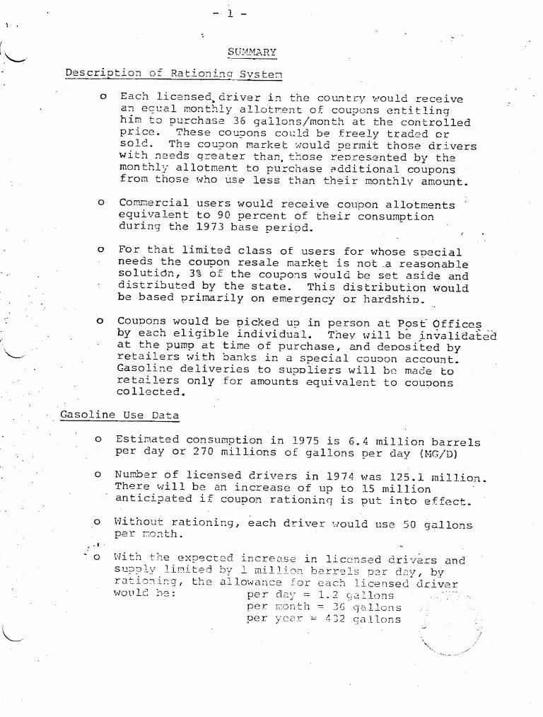
middot1
- 7 shy
E State Set-Aside
o State set-aside of coupons (a~out 3) would be available to recognize claims of users for whom the resale market is not a vehicle for their speclal needs
o About 3000 local boards throughout the states would administer the set-asides replying to applications
o The State set-aside will also be used for organizashytions or governmental units perror3ing essential public health or safety services
o Federal Government could provide quidelines to assure uniform application of eligiDility criteria
F Enforcement Svstem
o Vigorous enforcement program Hould be required to prevent widespread abuses
o The audit progra~ would focus on cowmercial gnd non-profit users to detect overstatement of base
( period volTh~es and on gasoline suppliers to ~ detect illegal shipments of gasoline
o There would also be a system to detect multiple applications by individuals
II PRELEIINARY ESTH1ATE OF RESOU~CS P-EQUIRED (STEADY-STATS
A Perso~nel Resources
( 1) Federal
FEA Headquarters - 625 positions
PEA Regions - 3250positio~s (1200 Opli 2000 enforc~~)
middotUS Post Office -- unknmvn
Non-FEA Enforcement - 2500 positions
(2) StJte and Local
3000 local boards 10 each (15000 volunteers 0
15000 support s~aff)
51 LL~1)2middott-cnt uf lnCc-=- V2hic2~ 20 c2ch - 5100 pas j tiolS
- 8 shy
(-- B Costs
uSPS Distribution $160 per transaction
USPS shi9ping costs
Coupon printing serialized
Forms printing
ADP system
Public Education Materials
Direct Salaries
o Federal (6375 20K)
0 State and local (20100 20K)
GRk1D TOTAL (~
(million $)
845
50
195
30
200
10
1330
1275
402 -
186 billion
shy ~-~
- 9 shy
GASOLINE USE DATA
Use Data
A Estimated consumption in 1975 Billions of barrels per day (H3D) 64 MBDNillions of gallons per day (l-1GD) 270 r1GD
B End use categories - volume (MGD) and percent
Private use 205 76 BusinessCommercial 57 21 Government 8 3
c~ Number of registered vehicles in 1975 13075million
D Number of licensed drivers in 1974 1251 million(increase of up to 15 million anticipated if coupon rationing is put into effect)
Programmatic Assumptions for Rationing
A Nill achieve 1 MBD saving through reduction in gasoline consumption
-
B Business will receive 90 of 1973 gasolineconsumption
C Coupons will be provided to licensed dri vers as opposed to allocations based on registeredvehicles
Key Parameters of Data and Assumntions
A Savings target (1 million BD) 42 rlGD
B Business and Government Allowance o Estimated 1975 cons~~ption 65 HGD o Less 10 of 1973 Consumntion 6 MGDo Allowance 59 rlGD
C Private Use Allowance o Estinated 1975 cons~~ntion 20 - J l~v
0 Less redlction 36 NGDo Allmvance 169 rmiddotlGD
D Al1oh~ance for Each Licensed Driver Gallo1s Per day = 1 2
per munth = 36 per YC2r = 432
- JU shy
E Private Use of Automobiles by Trip Purpose
Work trip 31
Recreational trip 31
Family business 34
-
---- (
1
- 11 shy
Gallons per -Ion-=h a1d Price of Gasoline
o To save 1 million barrels per day while assuring adequate fuel for business will mean limitinq each licensed drivermiddotto about 36 gallons per ~onth bompared to 6urrent average of 50 gallonsmonth and restricting businesses to 10 less than their last years use It is expected that the COUpon will sell for about $120 per gallon during the first year Hence for those who must purchase more than their basic ratlon the effective price of gasoline (Dumn plus coupon Drice) is estimated at $1 75gallon - shy
Impact on Enerqv Conservation Goals
o Gasoline rationing while it may limit consumption in the short run makes no contrihution to our mid- and long-term goals of energy independence
o Rationing limits the conslli~ption of gasoline not thrJugh price but through proscription Thus an artificial shortage is created inciting people to attempt to beat the system rather than to ~conserve - fuel
o Moreover because of the inherent comolexities in even the most carefully designed rationinq system and the fluid nature of Americ~n society a rationing scheme is probably limited to a useful life of no
more than two years Thus even as a conservation tool it has a limited utility
o Rationing provides no incentive for increasing do~estic petroleum supply or bri~gi~q on alternate energy sources
o Gasoline consumption is only 40 of total petroleum use Residual and fuel oil compronise a substantial amount o~ total petroleum imorts By concentrating exclusively on private vehicles many other fruitful areas for energy conservation are not addressed __ such as iDproved industrial efficiency better co~str~ct~0
and insulated buildings less wasteful use of electricitx and natural gas In the final analysis we cannot be
independent unless those other oetrolcu~ uses are also reduced dramatically
Potc n ~ i a 1 f 0 In em i tie s
o Each prs~n receives an equal nu~h2r of coupons but use of g3soline variGs ~id21v Cuvcrnshy
- 12 shy
mental decisions will be based on statistical averages and broad objective criteria they can~ot possibly take into account most of the differences in individual needs and preferences Thus rationing i~evitably leads to inequities Some examples are
- A vidmved secretary with two children living in the suburbs who comrnutes 16 mi les each -lay to work in a car that gets 12 mpg will experience a 68 increase in her co~~uting costs because she must purchase 17 additional coupons each month at an average cost of $120 per gallon each This amounts to about $245year in additional costs
- A blue-collar worker who owns a car that gets only 9 milesgallon can drive just over 320 -lilesmonth on his basic ration and could not easily afford to purchasemiddot a new more efficient auto~obile On the other hand an affluent neighbor can readily trade in his equally inefficient old car to purchase--one getting better than 22 mpg This allows him to drive over 790 miles on the same allotment of coupons
- A single individual with a mid-size car (14 mpg) _ could drive up to 17 milesday If he vanted to take_ a 500 mile trip over a long 4-day weekend he could shyonly use his car for that four-day period during that month He would have to arrange for ot~er transportashytion for the remaining 26 days of the ~onth or purchase additional coupons
- A Congressman living in GeorgetmmiddotTI has enough gas to drive his 10 mpg car to work by himself 5 days a week and still travel 54 miles on the wRekend
- Substantial regional inequities llould exist The average driver in some rural states suc~ as Montana travels nearly 600 miles per month versus about 300 in less rural states such as New York and New Jersey Similar dis~arities exist bet~een city d-middotlellers and suburbani tes Under rationing- each middotQu2d receive the sarre gallonage
- A fClmily of 4 -7ith bvo licensed criers and one car which gets 15 mpg moves from New York to California This reove middotQuld take 2-31 months of tcs ==rilys coupons 012 out of eJery five Llilies roves every year
- Certain very poor persons such as si~r~~ts drive lClrge dis~lnC83 each ~e~tc Th~r c~-r ~~~=~2~~ 2=rord to buy Q~di~ional couoo~s nor are alter~=tive nethods oft r c1 ~- ) iJ 0 _- t ~~ t 5_ C) ~1 ==-~ ~ i 1 ~-~ 1) ~~ t C) t h ~ ~~ bull
L
- 13 shy - A family in which the husband wife and two(~ teenage children all drive would receive sufficient coupons to drive approximately 2160 miles per month while the next door neigh~or with only one licensed driver coul~ drive only 540 miles per month asslli~ing both u~n cars which get 15 mpg
- The recreation and tourism industry ~lOuld be very heavily i~~acted a~ would the auto industry Autoshymobile sales would decrease 35 from what they roulel otheTVise be shy
- A small successful Midwestern sales firm which had increased its business and sales area 50 since 1973 would have the market area it can cover reduced ~O under its basic rationing allot2ent
~ -- -- -
Increased Bureaucracy and Comolexitv t
o The Government would be inVOlved in many new aspects of our everyday life adding an inescapable portion of bureaucracy complexity a~d inconvenience
o Gasoline rationing can be irrplerented bUt it is _ complex expensive and at best a short term solution It takes 4-6 months to implement about 15 to 25000 full-time people and $2 billion in Federal costs uses 40000 Post Offices for distri~ution and requires 3000 state wid local boards to handle exceptions
o The Government would decide
if a new business s~auld get fueli if expanding businesses deserve nore fuel if specific individuals would qualify for more coupons because of hardshis
o Because coupons are transferable they must be picked up by each driver in person quarterly at Post Offices Long lines and delays are inevitable
o G s middot t d quan~l~12S--- L se l~ areas t a~lons W1Ln Llmle LO l I unlii~ly to nlaintain Eore tha1 the mas t -lirlited
servic2 hours Evening and weekend closings are almost a certainty
o The longe~ a raticning progran is In place the more likc-ly collusi ve and ill(gt~Tal b2i1vior becQ[1ps I $uch as counterfeiting or pil~2r2ge of coupc~s
L
a Use of
- 14 shy
1allocation and rationing to reduce imports by one million barrels per day would create a drop of nearly 13 billion dollars in the GNP and place several hundred tftousand more JOrkers on uneTT1loyment rolls Also rationing would have an inflationary impact due to the significantly higher market clearing price of gasoline (pump plus coupon) resulting from reduced supplies
o Rationing leads to distortions in the marketplace as adjustments in business inJestrents modes of distribution and purchases are made based on artificial rationing-imposed coits
Impact on Poor
o Low inco~e people are like ly to dri ve less than average and thus have excess coupons to sell If speculators buy large quantities of couons from the poor at 1007 prices in order to resell them at high prices to the more affluent the potential income benefits of the rationing program will beshygarnered by these entrepreneurs rather than by - the poor
~Effects on Refiring Runs
o A reduction of 1 million barrels per day in the use of gasoline through rationing would have the following effects on refining production
- 1500000 bid crude oil i~oorts
+ 500000 bid product imoorts (made up of approximately 300000 bid residual oil products and 200000 bid middle distillates)
o Such a reduction is likely to reduce domestic petroleun related employ~ent increase the costl barrel of domestic p~oduction and decrease tll~ p=9ductiol rate cu)j efficiency of uS refiners
- 15 shy
COMPARISON OF GAS RATIO~ING AND PRESIDENTS PROGR~~
-
There are two principal options for reducing petroleum imports in the short to mid-term They include the Presidents program of a petroleQ~ tariff and decontrol of domestic oil prices and a cap on iElports ~lith gasoline rationing and petroleum allocashytion This paper briefly describes these options and discusses the impact of each on reducing imports regional equitYI inflashytionary impact impact on the poor administrative complexity and cost and impact on the recessionand employment
OPTION A IHPORT CAPRATIONING
o A vollli~etric limit would be placed on imports equivalent to the reductionscalled for in the Presidents nrooram A reduction of 1 million barrels per day cannot feasibly be allocated without rationingo The current system of price controls for petroleum would be strengthened including control of new domestic crude thus an artificial shortage_would_be created
o Since price is not used to determine distribution of petroleum products the goverrment ~JOuld mainshytain its system of allocating to retailers based essentially on historical use for products other than gasoline The government vould also control refinery yields
o To prevent long gas lines COUDon rationing would be introduced Such a program would include as its basic features
1) Each licensed driver would receive an equal monthly coupon allotment these COupons could be freely traded or sold The COUpon market (the white market) permits those drivers with needs greater than those represented by the monthl allotent to purchase acitioaal
1 Cou~ons from thos~ who use less than their mon~hly a~ount Thus the market rather than the government is r2s90nsibl~ ior assessing need for g2so1ine above the basic minimum ration Failure to orovice a ~hite market would invite a black market and increase the incquitiesect_
-16 shy
2) Commercial users whether they buy in bulk or at the pump would receive coupon allotments equivalent to a percentage of their consumption during ~he 1973 base period
3) For that limited class of users (migrants handicapped etc) for whose special needs the coupon resale market is not a reasonable solushytion a proportion of coupons would be set aside and distributed by the state This disshytribution would be based primarily on emergency or hardship needs
4) Coupons would be picked up in person at Post Offices by each eligible individual They will be invalidated at the pump at the time of purshychase and deposited by retailers with banks in a special coupon account Gasoline deliveries to suppliers will be made to retailers only for amounts equivalent to coupons collected
OPTION B PRESIDE~IT S PROGRN-I OF TARIFF TAX DECONTROLshyAim REBATE -
~ 0 After April 1975 this program ould consist of an additional tariff on petroleum irmorts of $2 perbarrel and an excise tax of $2 per barrel on all domestic petroleum
o Domestic oil prices will be decontrolled and a windshyfall profits tax implemented to ensure that the revenue generated will accrue to the government not the oil companies This will raise the overall price of petrolelli~ by $2 a barrel The tariff taxes and decontrol then will add $4 to the price of a barrel of oil
o In addition an excise tax on natural gas equivalent to $2 a bar=el would be adopted and new natural gas prices dereglla ted to equaJ 1ze the impact on oi 1 and natural gas consu~ers and decrease natural g2s conshysumption
o $30 billion will be collect~d by the government from the tariff and t~xes These reve~ues will all be rebated to c~n~US2rs and govern~2nts
~-
17 shy
(~ Regional Disnarities
o Bo~h options have major regional ispacts There are substantialregional variations in per capita gasoline use Those in the Middle Atlantic states use less than two-thirds the gasoline or those in the t10untain states Gasoline rationing as the attached chart shows weighs more heavily on residents of the mountain states sout1vest and mid--est than on other citizens
o Reliance on gasoline to bear the brunt petroleQ~ cutbacks also discriminates against rural dwellers and in favor of those in cities In the aggregate rural dwellers use almost twice the gasolineyearof city dwellers
o The Presidents program which includes oil natural gas and electricity generated from petroleum imoacts most heaVily on the New England West North Cential West South Central and Mountain states
-
Petroleum and Natural Gas Use bv Reqions of the United States Petroleul1
Natural Gas Petroleum amp Per Household Cons 11i11 0 t iO1
per Year (bb1) Cons urrrption Natural Gas (i1CF J (BTU)
united States Total 74402 3307 -73848
12057 a 71 73J74
Hid-Atlantic 8581 156 62586
East North Central 6619 326
West North Centra~ 7412 386 7961
So 1J th At 1 2I1 tic 8862 164 64980
East South C2ntral 623J 299 640761
~est South Central 97 89 1153 169487
467 90781
6707 bull 2 80 65237
OJ -1
GOO
375
w )30 r shy
) 5 6 r 1
CI shy)25-u 531 c o 500 I-- shy--i bull e- SOt r 475 02tshy
shy459
Avorilqe Consumrti m per c
- 450
bullpilu~12 S I (J
10 (j 421
) 37gt c () 350 JJ Of 32) ~1
c Jon~) rLU ~uw Middle ~as t West South E South VJ Sblt-JC Enql~nd Atlunticc North North Atluntie Central Central (~leNI Vt (NY NJ Central Central (Del Md (Ky Tenn (Ark La
~l)sSRI Pa)H n (Ohio l Ind (Ninn Iowa DC Va AI Miss) Ok Tx)0 Conn ) Ill Mieh Mo ND YVl NC v Wise ) SD Ncb SC Gu
15841 I
-8 ~~ I
)un tili n P iJCl f l-c (tmiddotont Idaho (- 0-0101
VY Colo N Cil -llt1)(u
10lt A1 HilViaii) ULll Nev)
Kansus) Fla)
) ) J
- 19 shy
Effectiveness in Reducing Imports in Sho~t and Long Te~
o In the mid to long term the elasticity for gasoline is Imver than tha t for othe~ petroleuITl products This is because the~e are fewer substitutes for gasoline than there a~e for other fuels This means that an increase in the price of all petroleum products (Presidents progr~u) will reduce imports more than an equal increase in the price (gasoline tax) of gasoline In the short term this is not the case
o The reduction in imports from the President1s proshygram option is 900jOOO barrels per day in 1975 l6 million in 1977 and 21 in 1985 This esti~ mate is not a guaranteed saying but is based on econometric studies
o The rationingallocation option could obviously be adjusted to any level desired The level considered in this paper is 1 million barrels per day in 1975 moving to 1S million in 1977 Because of the complexity of the administration and the dimited ~ ability of a rationing progra~ to adjust to-changes
~ in the economy (eg people ~oving new businesses shy ~s r-J-l-1 -=gt ~J-l started) lOt
-- 1J -~~J1 ~d-1- - -- IJ JtlJJL~ v r-
-~~~
LVJ-Lv
more than one or two years Hence it-is notreally a feasible part of a mid or long term program Moreshyover the longer the system lasts the more exceptions are made the more people learn how to evade the rules and the greater are the opportunities fer countershyfeiting and abuse
o If we are to reduce significantly our vulnerability to imports in the mid and long term -G wust ldapt an option to reduce cons~~ption of petroleum that can be effective in 1980 and 1985
Inco~e Effect
o Gasoline rationing would have so~e beneficial impact _f as lo~er ince~2 pearle sell their excess coupons to
those with higher income who in general use more gasoline This e fEect O~~ ld fC sorr2lmiddothCl t limited by the plan to di5tribute coupons only ~o licensed drivers The actual inco~e t~ansfer effects depend on th~ size of the ~~ortag2 an~ the marginal price of the coupons
- ~D-
I~ Private sector demand for gasoline in 1975 is esti shymated to be approxi~ately 206 MGD Reducing daily petroleum consurnption by 1 l-IJBD solely through reductions in ga~oline would result in a 17 pershycent reduction in supplies The equilibrilli~ price of gasoline would be about $175 per gallon ($56gal Plli~p price plus $119coupon)
The average poor householdconsLL7les 4047 gallons of gasoline per y~ar per vehicle while the II lower middle II and well-off households average 6322 8231 and 8008 gallons per year per vehicle respectively The average number of gallons of gasoline consumed per vehicle is 7278 The surplusshortageof gasoline per household group and the potential income transfer can be calculated by comparing the individual household conslli~ption rates wit~ the average COnSliL11ption rate The table shows the average gasoline use by household income the surplusshortage of gasoline and the net income transfer likely to occur through the sale of coupons
GASOLINE CONSUHPTION ~ AND INCOYlE TRANSFER
(5000- (l2OOO-Income (O-SOOO) 12000) 16000) ll~OOO+)
GalVeh 4047 6322 8231 8008
Net Surplus +1994 -281 -2190 -1967Shortage
bull (GalVeh)
Net Income Transfer +220 - bull 20 -92 -108($Billions)
1
- 21 shy
The ~(ormiddot household Hold have surplus coupons for 1852 billion g~llons of gasoline The coupons for p~rchase of gasoline would trade at Sl19 gallnn Jhich ould r2s111t in d net tr1nsfer of 220 billiQn dollars to the poor categoryopound households in the Ii rs t year
o Similarly the Presidents progra~ would transfer roughly 52 billion from those with incoQes above $12 000 to those middoti th 10llt1er incomes preliminary calculations indicate~
Income ($1000)
0-5 5-12 12-16 16+
Additional Cost 725 8200 2900 7500 of Energy (S~1il)
Rebated Revenue~ 3520 7350 3610 4520 (SMil)
Net Transfer +136 -1 06+044 -74 ($8i11ioos)
-
AcTIinistrative Complexity and Cost~
o The cost and number of people re~uired to iQplementmiddot the Presidents system of t~riffs taxes and rebates is estimated at about $50 million and 400-500 addishytional people on the government payroll
o The complexity of administering gasoline rationing and allocation is considerably greater than the other option both because of the printing distribution collection and control of ltQupons and because of the exceptions process for the poor neCe3SJry in every state and local community Rationing vill require an additional 17000 government employees and approxishymately $2 billion per year to adminisLei
Tncla~lmiddotonr I-n1~ r I lt-l __-___l~~~
(
0 A S2barrel import tariff plus eXClse taxes on dCr1esti~ petroleum Clnd natural 92S would increase the Consumer Price Index b J about 25 percentaglt3 points in 1975 Agoinr these fees would be return~d to consumers so th2t the Oera 11 Ie vel of dispasoble income would not b~ changed
r o Under utioning the cost of buying un Lldditiol1ul ~
I
coupon should stabilize at the lllLlrct cleLlriIlg
1eve 1 0 f $ 1 1 9 h us the r e 10 U J d be un 10 in pound 1u _ ~ tionilry imp1c t of ove r 25 pcrccr tage poin ts on the Consumermiddot Price Index in 1975
f
I
To SClve 1~1BDof petroleum imports in 1975 could be accornlished I
by reducing market supplies of gClsolinc distillates residual etc in varing amounts The a~ount of gusolice that would be available for private use and the co~ts of gasoline would depend on the amount of petroleum saving that is loltlded C1to ltcsoline The table show~ the amount of gasoline per registered driver the percent reduction of gasoline s~pply and the estimated cost of coupons under 100 I 70 and 50 percent~ application of petroleum
saving to gasoline shy
of IH1BD Gasoline Cost of Applied to per driverHk Gasoline per driver coupon
__~g~a_s o_l_i_n_e ~(~g~a_l s~)__________~p~e_r __ __~(g~a_l_s~)__ __________ __ __m_o__~ t_h ________~(~$~p~r~gal)
i1100 84 t36 11970 91 3950 95 41
64
38
A siDilar computltltion for a rutioning program lasting through 1977 and equaling the impact 6pound the Presidents tax ~acJ~ag2 (lG middot~l13D savings of petroleum imports) can be made
of l~J)mD Applied to gasoline
Gasoline per driverHk
(gals) Gasoline per driver per month (q()ls)
Cost of Coupon
($ pcr gol)
100 70 50
75 82 8bull 8
32 35 38
70
41
26
middot1
Fc~ru~ry 4 1975 COll[crvJtioll dIll
Environment
ALLOCATIm~ JI~D PRICE CONTROLS AS A SOLUTION TO THE ENERGY PEOBLE~l
Introductiol
Alloca tLm 1S one method 0 [ distribu tinr] [~ L 1-0 lcum products throughout the US economj It docs not oC itself reduce demand it merely provides l set of rules lt1d ll(~c~dni~lll~ to pass out vlhutever quantity of petroleuPl suplliL~ drc ~lvclLlablc Allocation has been linked with price control~ and 1)1] _no doubt continnc to be This pclpcr discusses the poible usc ot a_ mechlnism consisting of l~ import cap price COlltro]s dnJ al~ocashytio1 lS i1n alternutive to ihe President I s pn~rlrn to reduce 1111shy
ports It assumes that the import ClP lil] be used to Jeduce petrol(~um iIllports by one r-il1ion bl1rrlls ~ ~~lY chlt lr1ces wlll not then be allowed to rise to market cle~rlns levels llnd thus a shortuge will be created and that this shortlgc will be gall shyaged by an allocation ~rcg~am similar in most respects to that which ilas been in effect Slnce January 1974
This should not be confused with the Presidents program to limit imports The Presidents proposal ltiould r~ot create a shortage in fuel and hence does not depend on an allocation mechanism to distribute the shortage around the country Instead the Presidents program by increasing the price for petroleum relative to other goods and services would cause individuals and industry to reduce their demand for petroleum products thereby reducing the need for import-ed oil
~ Present Allocation Program
The Emergency Petrole~~ Allocation Act of 1973 provides for the mandatory allocation of crude oil residual fuel oil and certain refined petroleum products and for price controls for the producer refiner reseller and - ret-ailer levels of the petroleum marketing chain Major features of the present program are
bull First sales of domestic crude oil are subject to a two-tier pricing system Old oil (crude oil produced in amounts up to 1972 levels from a particular property) is priced at an average of $525 per barrel Oil produced from a property in exces~ of 1972 levels and oil from a property which produced less than 10 barrels per well per day may be sold at free market prices The price of imported crude oil is also uncontrolled
bull In general refiners may pass along their increased crude oil costs and some limited non-product cost increases but may not generally increase profit margins These same rules apply down the marketing chain a dollar-far-dollar pnss-through of increased product costs and some addition~l limited increases in selling prices to reflect non-product cost increnses
2
bull rhe reguLltions provide for Cl crudc oil supp] y progrClm for small ClIHl inc1l~penJen t rc [incrs utilizing a freeze as of December 11973 ormiddot supplier-purchaser re la tionships fOJ- crude oi 1 and a buysell list under -hieh th-~ 15 l1~ll01 oil corporations Circ reqJirccl to sell l~~ci[ie(i oltllcs of crude oil to Ll~(O sr-~111 tnC irl-l~lt rt~finers There icgt ~lsc 0 i~C(~-1 middotllicll pru1~ - - ~iJlLlnLi~ll cqualizltic 0 avcr(1ge crude oil priclo 1rHJ I1J -c-fincrs by the purchase ancl Sa lc of en ti t lC1(rl 1s Lu run cheap price-controlled old oil in th8 SacC natjomvic1c proshyportion at all refineries
e Refined products are distributed to ultimate users in accordrtnce vitl the allocation regulations except for gasoline 1-here the IClandatory allocation chain ends at the retail station and bulk purchaser Three general classes of users are established
_ Those users who are authorized to receive their current requirements - essentially whatever they request -- and are not subject to any allocation fraction This inclu~es Department of Defense agriculture and space heating for hospitals
Those who receive their current requirements but are subject to an allocation fraction -- emergency services energy production etc
Those who receive some percentage of their historical consumption or base period volume (usually based on 1972) and are subject to an allocation fraction
These class definitions and further percentage delineations within the third class are decided by the government and are spelled out in detail in regulations Their effect is to limit each user to a specific monthly or for some fuels quarterly authorized amount the usercategory scheme varies from one petroleum product to another
bull A supplier must continue to supply the same customers he serviced during the base period If he haS sufficient product to meet the sum of all his customers authorized amounts h~ delivers thisamotint to eltlch If not he reduces each purchltlsers share on a pre rata basis by applying his allocltion fraction equal Lo his totltll supply over the sum of his customers authoriZations and delivers this percentage of authoriZation to each customer
3
bull A port ion 0 f the product is reservcc1 for clell s tLl tc to usc f 1 c x i b 1Y toe 1 i minaLe hJ r d ~ ~ 1tl ) S bull T11 is ~ tgtl t e set-aside is administered by sLILmiddot (~ller(JY offices
e A detJiJed case handling ilnd appc~1s process has been establi~hed to hCll1dle ad ju~lr(i1L_ of base period usc to Jccount for changed circunLlI1ccs or unusuJl groith and other applic~l t i ()11~~ for c-(CPshy
tions and assignment of supplier
Positive As~)C~cts of an Import Cap and Allocttion Froqram
lhere are at least four positive Clccomplishlc1cnts thJt can be expected from a cap on imports and allocation
o The level of reduction in petroleum imports can be established with certainty There is no depeRdence on price elasticities of energy for achieving conshyservation results
bull Prices can be kept from rising thus minimizing any increase in the consumer price index
4
bull l]Lhouqh the i1Jlocatiol1 proqr1I11 (I()(~ not 1( (nCIltJY it can ~[Jrc(]cl tllouncl tlll~ 1111 ion t IH i1olt HW Cdll~lll
by thc import CZ1r thus temperinltJ th6 r0qionl impzlcts of such Zl procJrltlIn
bull The Government CZlr) milke qross ch()iCl 1 to Ihich s0ctor of the (conomy shoul(l he II ()(1tltd LI1( qrfdt t port-iOl ()[ the l1ortaltw lor (lt11111)1 fuel CLln bo made ilVLliL1])Je to tlle illclwiri11 sector Zlt thp expense of horne hllinq fuel or gasoljno for Zlutomobiles
o Undo r an allocation program the qOV(~ rnmen t n-~) lLlcCs the market in distributing encrcjV ouppJ ics Several significil1t problems arise with such Ll ub~jitution
-- An Llilocation system crc~pends on Zl governrnent determination of a persons need for fuol and yet need is almost imp6ssible to dc(ine The standards currently employed for making this determination rely on historical use and a governshyment judgment on priorities (eg agriculture should get all the fuel it needs) Unfortunately in thousands of cases the amount of fuel an individual or firm used two years ago may have little or no relation to how much fuel he currently needs Thus an exceptions process must be created and administrative judgment and procedures used to supplement the historical use standard There simply are not enough Solomons around to make such a system work well
In addition any system that classifies users according to government-determined priorities shifts the struggle for market advantage from the marketshyplace to the offices of those who write definitions and regulations The political pressures to give groups special preference become very great Should tobacco growing be made part of agriculture and thus tobacco growers be made eligible for the same priority as wheat fZlrmers What about green houses growing flowers lre portable toilets pZlrt of sanitZltion services Those who are most effective in these political bZlttles are not necessarily those who would be the most effective in a competitive market situZltion but for each the decision reqZlrding
L
5
their allocation priority cem Il1ab the di rrCHnce as to whether the businl~~ tllLi V(~ ()J ~lrr(rs
Because th(~ ~1l1ocClticgtn of pltr(llcIIIl1 uroducts under Cln allocation sYctcnl is plJrnrmld hy the Federal Clnd State ~lovernmcnt~ J1t 11()- t h-I) 1) th~ market public costs arc incurrLcl lll()(~ltil)n durin g the recon t ernhJrqo requi nmiddotd U1l 11 1-[- ime efforts of about l1OOO pcoplc dlH C()~-[ 1~1)-(J--imi1tely $100 million in addition su)slilt j)] r-cord kecpinc] reports (1nd (1uc1i ts 1erc l-l(lU i rcJ CJ~ the privale sector
-- An allocation systcI1 asumcs UuL ntLilcrs will distribute suppli(~s accordincr Lo rU]lS oet by th~ government In practice however it is impossib Ie to en force these rulc~) cC~1i tab Jy alOng thousands of gas station ODerators and fuel oil dealers Thus practices ~uch as prepounderc~tial treatment for special customers car washgasoline fill-up schemes pre-paid gasoline contracts and even direct black market operations quickly spring up bull
bull Allocation does not aid in solving mid- or longshyterm energy problems An allocation program hile it is useful in managing a shortaqe created by embargo or a cap on imports makes no contribushytion to our mid- and long-term gOals of energy independence because it provides no incentive for increasing domestic energy supply
bull Choosing the base period in an allOCation system is an especially difficult problem On the one hand choosing an early base period such as 1972 for which complete data are available means making numerous individual changes in the system to mirror current consumption since thousands of new businesses have begun old ones failed and many people moved in the intervening years Using a more recen1 base period however penali zes those who conserved during this period while rewarding those in the sam~ allocation cJtegory who did not curtail wasteful fuel use during the base period bull
bull AllocCltion has a retardinq effect on GNP growth and employment A reduction of 1 million bnrrcls a day through e111 import C(1P and (1llocation -Jill reduce GNP by an estimnted G billion dollars Jnd place 250000 more people on uven~loy~ent rolls
6
This occurs b(CdW~C an allocatioll IlroqldTll TllWt
spread fuel Llcross the vilrious ~c~ctoc of Lh( economy ltlccordinq to ltl ~cL of n-L1LivIlv inlcxible and cOIllplicLlh~d nLltiondl rtllts llhrqy lhll~ I
made aVltlilablc for both morc (fri(~il1t mc ll~~s
efficient uscs On the 0 Hlcr limd n~ J idl1Cl on higher price ltlnd the mikct to dtll with d
shortLlqc meun on the wholc a di~triblltj()ll or fuel to those Vho vLlluc it most 1l is llHn morc likely to )c usee ([ficienLJ~ r(lt pn)ducl iL
purposes resulting in a hiCJher C~Jgt ewci qrcatcr employrnen l
bull While iln allocation and price control proqrClm would 1 imi t di roct incrc ases in fue 1 cost~ it docs corry wi til it other costs J~xcllnplc abound reduced air line s c1cdu] Cc~ and thus reduced mobil i ty sales of petroleum prodllct~s linJed to contracts or sales of other goods and services drastjcally limited service hours and above all continuing uncertainty as to supply uvailability vhich makes planning impossible for businesses Llnd individual citizens In this regard the major cost to the consumer will likely be the inconvenience of gasshyoline lines To minimize the negative impact of the shortage on the economy and jobs mos t 0 f the ~eduction in consumption would probably have to come from private auto usc of gltlsoline Thus a substantial reduction in imports is likely to result in a recurrence of last years long gas-o line lines
o Even the best designed allocation program generates unforeseeable effects During the recent embargo for example people took few long trips Thus rural gasoline consumption was down relative to urban consumption since allocations to gasoline stations were based on historical consumption urban stations were unable to supply the unexpected increased demand resulting from this changed consumption bull
bull An allocation program is not an e f fecti ve consershyvation tool and has limited utility as a means of distributing products in short supply due to a cap on imports Because of the inherent complexshyities in even Ll cLlrefully desiqnecl allocCltion system and the fluid nature of lmc~ricun society the lltlrger the shortuqc the shorter the useful life of such Ll system
Revised Base Case Forecast and The Presidents ProgramForecast
National Petroleum Product Supply and Demand
Technical Report 75-2
Office of Quantitative Methods
February 5 1975
Federal Energy Adm ill istration
Washington DC 20461
NATIONAL PETROLEUM PRODUCT SUPPLY -m J~-lto
REVISED MSE CASE FORECtST fiJ
IHE PRESIDENTS PROGRN-l FORECS~
Technical Report 75-2
FEA~ - EATR - 75-2
February 5 1975
Short Range Modeling and Forecasting Division
Office of Quantitative Methods
Federal Energy Administration
This Technical Report replaces Technical Report 75-1 Comparison of Forecasts of Petroleum Product ~n2Jld Illustrating the Effects of Prices and other Factors FEA January 16 1970
SUMMARY
For 1975 as a whole it lS estimJted that thc Prc=idcnts program will
reduce aggregatc petroleum demand by 548 MBD
mcrease domestic production by 101 MBD
reduce petroleum imports by 649 MBD
The effects of each component of the Presidents program grow over time As a result for the fourth quarter 1975 the impact will be greater than when averaged over the entire year For fourth quarter 1975
aggregate petroleum demand will be reduced by 880 MBD
--domestic production ~vill be increased by 160 MBD
-- petroleum imports will be reduced by 1040 MBD
By December 1975 the Presidents goal of reducing petroleum imports by one million barrels per day will be surpassed under the Presidents program For December under the program
-- aggregate petroleum demanq will be reduced by 934 MBD
--domestic production will be increased by 160 MBD
- petrolelllTI imports will be reduced by 1094 MBD
The import savings in December 1975 are accounted for as follows (MBD)
160 Elk Hills development 98 conversion to coal
147 suspension of gas curtailments 689 effects of higher prices 1094
middotmiddotThe reductions in petroleum demand by product in December 1975 will be (in MBD)
rrotor gasoline -278 distillate - -238 residual -310 all other products -108
Total -934
INTRODUTIO
This Tltchnical ~port flI ltcnts the CClllt~ r un km(r -~r FEAs s-Jrt ter-- tJe-colelXn product supplyckrTLU1~ )dlnCl~ i~ L~~ion under t--J s-s =~ as~l1ption3 a Base Case 3ccnali) illi 1 ~ccnt3 petrolezn I=-cltu- su-gtlym derrBrld using a currcnt 1~lt~Jmiddot_~c siInula~n -=-~J ~X2-C price and weather data ~Jr_ 1 ~middotoli= J~)n Scenali- ~-~ -1 =--ampccrmiddot~~aL~S t~c pCirtictllars of t~middot) ~~~r~=j j-r-- s ~Tlergy prograr ~Lt ~~Je S3se Case scerlario rThe supply ~~~J ~cnm~ 01-22dStS
presentC rCCe 22 sight2y iferent from those -lc~uec 1shy
Decernbec 197~ 3 ea-ly January 1975 in that
the par-iculars of the Presidents program (rather than its general stC-lcture) are accoun~ed for explicitly
more recent ffi2croeconomic forecasts are available arid
price and weather data have been updated
The impact of the President I s program on a~cregate petrgtleum deIlEI1d and etrcleum imports or 1975 as a whole fou1h qU2rter 1975 and Dec2J-IDer 1973 are presented in a s~ section Othel~ sections of -he CeuroporL present the scenarios and associatec su~ly and derrand orec2sts the derivation of the effec~ of the Fres~Gentls program on 2troewn prices and the derivation of forecast inventory policies Zle forecasting procedure utilized for this repc~~ ~s docwrented I1 cional Petroleum Product Supply aitd Derrand October 197~ ~~ou~~ 1975 Tew~ical Report 74-5 rEA Nov8ber 8 1974
Appendices present a comparison of alternative forecasts documenting the effects of prices and other import~~t factors alternative elasticiy estimates and factors influencing a determination of the price of imported crude oil
1
SUPPLYDGlN m PllANCE SCOWUOS NID rORITASTHlG RlSULTS
Two supply dem=md balance scenarios arc presented 1 Plt~se CClse and a Policy Option Scenario The two scenarios dIC JPecificd as follows
Base Case The petroleum product demand simulation documented in Technical Report 7q-5 as utilicci Based upon rfcent economic indicators a DIU ITBcroeconomic simulation prepared in December vIas incorporate in Lhe cemm-i fOtecast this sirnulation projected relatively weak consumer dem-IDd over 1975 with a decline in real GtJP of 3 5 percent over the year The relative prices of the products were held constant at their last observed level
POlicy Option Case This case differs from the Base Case through the incorporation of the Presidents energy policy as given in the State of the Union Message
The price assumptions occasioned by the imposition of import fees and deregulation are given below in the section on prlces In addition it was
I assumed that
--- domestic production increqses by 160 MBD by the end of 1975 due to the development of Elk Hills
petroleUm derIBJ1d is reduced by 98 MBD due to switching from oil to coal
petroleum derIBJ1d due to natural gas curtailments ceases after May 1 1975 due to the deregulation of new natural gas at the wellhead
-- price changes due to the Presidents policies are held constant in real terms at their May 1975 levels
The Base Case supplyderIBJ1d balance scenario is presented in Table I and the Policy Option scenario in Table II Tables III through VII itemize the impact ofmiddot the various components of the Presidents program by pluduct for each quarter of 1975 and for 1975 as a whole
2
Table I
Base Case 025) Supply and Deman2 Forecast
(MBD)
Forecast without Implementation of the Presidents Program
D MOGAS
E Distillate M Residual A Keroj e t N Naphthajet D Petrochemicals
LPG Other products
a1 all products-shy
S Domestic Crude U P NGL P L Gain Y
Total Domestic Supply
Change in inventories
Imports
Total all products
~lQ 1975 2Q 3Q
6178 6715 b ~ 0 VUv
3916 2546 2215 2654 2 rJ iS35
769 812 815 211 248 244 333 338 337
1560 1076 1025 2029 2127 2383
17650 15872 15834
8663 8622 8575
1676 1E57 1650
413 399 357
10752 10678 10582
-229 +165 +323
6669 5359 5575
17650 15872 15834
4Q Year
6 C 1 6597 3 t~ 57 3034 2I01 2250
838 809 276 245 350 339
1470 1283 2178 2179
17583 16735
8540 8600
1656 1660
407 393
10603 10653
-260 0
6720 6082
17583 16735
3
Table II
Supply and Demand Forecast with the PresiJcnts Prog~arn
(HBD)
Forecast with full I
Implementation of the 1975
Presidents Program lQ 2Q 3Q
D MOGAS 6139 6489 6603 E Distillate 3915 2462 2055 M Residual 2625 187~ 1718 A Kerojet 767 803 797 N Nap hthaj e t 211 245 238 D Petrochemicals 332 330 322
LPG 1559 1068 1009 Other products 2027 2108 2344
~a1 all products 17575 15383 15085
S Domestic Crude I 8703 8702 8695 U P NGL 1676 1657 1650 P L Gain 413 399 357 Y
Tot a 1 Dom est i c Supply 10792 10758 10702
Change in inventories -229 +165 +323
Imports 6554 4790 4706
Total all products 17575 15383 15085middot
4Q Year
6336 6392 3243 2919 2118 2085
816 796 269 241 333 329
1445 1270 2143 2155
16703 16137
S70n R 7()1
1556 1 fl flO
407 393
10763 10754
-260 a
5680 54~3
16703 16187
4
Table III
Impact of the PresiJents Program First Quarter 1~7j
(HBD)
-39 - 1 - 4 - 1 - 1
1 - 1 - 2
~ otal all Products 49 o II- -75
Elk Hills Development 40
Current change in consu~ption Demand for petroleum imports
-5
---
Table IV
Impact of the Presidents Program Second Quarter 1975
(MBD)
Demand Changes
SuspensionPrice Coal of gasEffectsProduct Conversion Curtailments
I
~ Total
lOG S -227 0 0 -227Distillate - 20 -0 -62 - 82Resi2ual - 48 -49 -34 -131Kerojet - 9 0 0 - 9Naphtajet - 3 0 0 - 3Petrochemicals - 8 0 0 - 8LPG - 9 0 0 - 9Other - 20 0 0 - 20i
I Iotal all Products 3441 -49 -96- ~ -489
Elk Hills Dev~10prnent
Current change in consumption =Demand for petroleum imports
6
Table V
Impact of the President s Program Third Quarter 1975
(MBD)
Product
~WGAS -278Distillate -160Residual -217Kerojet 19Naphtajet 6Petrochemicals 15LPG 16Other - 38
==t=-========~=======---=-======~=============-_~ -(otal all Prod uc t s--r -525 -7 4 r-~~50 -749
i I
Elk Hills Deyelopment 120
Current change in consumption = Demand for petroleum imports
L 7
~lOGlt S Discil2ate Resi2 Kerojet Xaphtajet PetrocheTicals LPG Other
Table VI
Impact of the Presidents lr~srlm
Fourth Quarter 1975 (HBD)
-278 0 0 -120 0 -94 -214 -131 -98 -53 -282 - 22 0 0 22
7 0 0 I shy 7- 17 0 0 I 17 25 0 0 i shy 25
- 35 middot0 0 35
8 O_1_1__ -_6_3_5 __________~1__ p_r_o_d__~_c_t_S~__ ______-L~~-_9_8_-______________-_1_4_7 -ri_-_8_____
Elk Hills Development 160
Current change in consu~ption =Demand for petroleum imports
8
Table VII
Impact of the Presidents Program Annual 1975
(HBD)
-------~---I-- Dcm~~C h~~~l(C_~ II 5 pC n-s-~ 0 11 r--shyPrice Coal of gas E f f e c ti i
I
Conv e r 5 i 0 i1 C l r t a i 1m en t S I
~
r 0 t 31Product I ----- --------- -- shy~----- shy
~lOGAS -205 0 0 -205 Distillate - 52 0 -63 -115 Residuel - 69 -61 -35 -165 Keroj e t - 13 0 0 - 13 Naphtajet 4 0 0 4 Petrochemicals 10- 0 0 - 10 LPG - 12 0 0 - 12 Other 24 0 0 24
~ Products)total ll 1 -389 -61 -98 -SZ8I
Elk Hills Developrent I 101
Current change in consumption = Demand for petroleum imports
9
PRICE ASSLlMPIIOIIS
The petroleum [leaduct dcmmd simulation d[plLcc [)ticr elasticity asumptions to deflated w101csaLc prio inlic~ few Lin products except rrotor [ls01ine For motor [clsolinc [wicmiddot _ rTect are rrcasured in terms of the deflateI- cx- tax lcLlil ptic(c PlT gallon For all prnducts ecept motol~ Sdsoline the tL~n (~[fccts are lagged lith respect to how long a price ch(m~I i-~ _~SSllITCd to be sustained This IGf3 structUl~e (2ssuJniIlC consLm cl~~tc~itics) is given for a one tvo ill1d three quarter dUlation T1C LlsJUJi1Cci elasticities are
Product lQ 2Q 3Q
Distillate -09 -12 -12 Residual -15 -18 -21 Kerojet -06 -07 -08 Naphthajet -06 -07 -08 LPG -04 -04 -05 Petrochemicals -12 -14 -16 Other products -05 -05 -05
For motor gasoline the relationship between market price and demand was included as part of the regression estirrating the deITand forecasting equation ~~e specification of the forecastL~g equation is such that the price elasticity of motor gasoline deITand varies sorrewhat depending upon the values of price a1d quantity demanded at which it is Feasured Generally for the year 1975 the price elasticity of motor gasoline is -15
Using the results of analyses conducted with the Office of Economic Impact FEA the implication of the Presidents policy of import fees and deregulation was traced for nominal prices measured by rronth for January through May 1975 These norninal prices were then converted into the appropriate indexed and deflated format for incorporation into the petroleum product derrand simulation The derivation of the nominal price time series is given below
10
The end of year 19711 crude oil priccwl~ dlliv l tolJow~
$84425 75 [5 x Old Oil Price + LI x New Oil [tic ] + 25 x Imported Oil Feice
~middotr(ntiuLJwhere 75 proportion of crude S d()riC~ t i- l~ 1 n)(JuceC
25 proportion of cruce S iCL impoctclt - ~ j6 CllIYent proportion of cll)mcstic bull ~ ~j that 18 Old Oil
4 current proportion of dornc~)tic ~~l~)ply lldt lS 0lcw Oil
Old Oil Price $525 per bcJrrel New Oil ~iice $11 00 per barrel Imported Oil Price $11 00 per baJTel
The May 1 1975 crude price was obtained by equdting The Old Price to the New Oil rice and the IIIl[)~ted Oil rice LO $13 to account for decontrol the domestic excise tax and the ~Tport fee It was asswned that the price of NGL would be equivalent to The price of crude oil even if a smaller SIU equivalent tax here to be placed on it After Hay 11975 all petroleum prices Jere asscJned to rise nominally by the rate of inflation that is not to change in real terms
The refined product average was constructed using the crude oil series plus estj~aTes of refining costs and other cost factors The distillate and residual price series were constructed from the crude series with the rule that increases in the domestically produced distillate and residual would equal increases in average crude prices Iwported residual and distillate were ass~poundd to increase in price by an amount equalmiddot to the import fee The average price indices constructed for the procucts are the weighted by their domestic to imported ratios Since nearly all gasoline is domestically produced its price increases only reflect crude increases
These rules produce straight pass through of costs to Droducts without shifting costs from one product to another As an alternative to this simple pro-rata cost pass through price construction historical price relationships were also euroxamined Historical ratios of the various product prices to the refined products average were used to forecast prices The results of forecasting prices on the basis of historical ratios was little different from that given by the simple pass throuu~ assumptions Since it is expected that regulations will be enforced to equalize product price increases the equalized cost pass throuf~ with immediate adjustment was used to forecast prices TI1e nominal price forecast assumed is given in Table VIII
Although hiGher imported oil prices ~LrC quoted $11 is the estimate of the average economic cost of imports to refiners See Appendix B
11
For tte tr3J1si-ri()n period February 1 to pri 1 30 l~n 5 the folloH l11g ric(s wccc used
The ~ltr b-rrel increascs in crude prices HI FclJLll)middot tlclrd1 and April reflcct -he $~ $2 $3 import fce on irTlpcwU~d C~~dL 0clIlLsticdily produced-ldc is st~J- averce undel th~ Old-ll~IrJ ui - ~C21LJne 1he product c~C2[ lC2 cJudl dlstlllate dIlcl tl~( 1llJlC r _gt_~ dUllJ12
this k-2ric re~cct the ch~mge in crude plices due tu -tL 1 $ 2 $ 3 crude ir~--t fEo lr_ the $0 GOcent $1 20[12 OIl lITljX)lt ~ ~loduc ts as weI as the rati J )f dornestically produced to imp0c---2C products
These rats a-e dssUJed to be
Petrc=eum rDG1Ct tverage Drnesticcly rDdlced Jnported coo Product
82
18
Resic-al Drnesticclly Produced Imported ~s Product
35
65
Distillate Domestically Produced Imported as Product
85
15
Gasoline - All I))rnestically Produce_d
Product prices are calculated as follows
Petroleum Product Average = $1015h Wholesale Price 82 (Average Change LTl Crude Oil Price)
18 (Change in Product Import Fee)
Residual ~lJholesale Price = $ 775 35 (Average Change In Crude Oil Price) -65 (Change in Product Import Fee)
Distillate Wholesale Price= $11 98 + 85 (Average Change in Crude Oil Price) 15 (Change in Product Import Fee)
Gasoline Retail Price = $041 + Average Change in Crude Oil Price per gallon
) See The Itllitt Ik1use Fact Sheet (January 15 1975) 111e Presidents State of the Union rk~sc1Ge p 33 items (A) Ha) and (A) lCc) 111C system of rebates (n prDducts nullifies the Febrvary fee on products
) Latest observed price per barrel - except gasoline (per gallon)~
12
+
+
+
Crude
All Products
Distillate
Residual
Gtsoline
Jan
844
1015
1198
775
41
Wholesale prices per barrel
Table VIII
Price Assumptions
Feb
899
1060
1244
794
423
March
954
1116
1300
852
436
Anrilshy~
1009
1172
1356
910
449
gticlrcn
1300
1425
1615
1064
Retailmiddot price per gallon excluding taxes The natural average for gasoline taxes is 12-14cent
13
519
INVENTORY MJUSTHUflS ror~ 1375
A cornpLlri~on ol [orecLlst Llnd observeci inverl LI Y lX) 11 (llS fc)l Lhc months of Oc tober 110vcInbcr ill1d Dlccmber 1~ 7q Ld rev lt1 1 ( r j hi ~lll Lnn forecast stock level~ In fact the stock leveL ()IJticd It Ll1t~ beginninr of Ceccrrber 1971f arc believed to b-~ neeI Llll ~ inill trys sustainable capacity dS that capelcity was mCdsurcd in i1lt3111xr 1373 As a result the inventory profiles assumed for th ul[lymiddotlcnnnci simulations piesent~r hcrmiddot -Jere chm~ec in tilt 1~middot~t(I t( be consistent Vlith rec~~t coservations A mop~ c~rculnl Ly~i of expected prociuct 00 ~middot)~)(L inventory behavior i11 L~ -lOlOrat~d l~
the implem~ntTtion (j~ C- r2gionali=2o shortfclll runirni=il1 SdfplyrdcmJIld simulation tmiddot) be pnpared in Fctru2cj 1975
Stated siInply the inventory char1Ges projected for 1975 in Technical Report 74-5 and subsequent applicJTiors of tl1at I2Ort shotJed a net drawdo~I1 ~I 1975 of over 200 rrSD Iur 1975 as 2 Hhole The estimate of this redllC1ion in inventories arises iiom the imposition of miniJIl~L opeurorable as coml3red to historic211y normal bounds on major procJct inventories Tile inclusion of more traditional inventory piufiles will be reflected in the results of the neXT application of the full regional ITcdel
For the forecasts given above the following assumptions were imposed upon the aggregate ~Iventory profile assumed
a zero net ~~nge in aggregate stock levels over 1975
inventory build-up lf1 the second and third quarter 1975 was constrained such that the largest assUmed aggregate stock level was that observed on December 1 1974
the relative rate of first quarter to fourth quarter drawdown and second quarter to third quarter build-up was set at that given by the Base Case simulation in Teclmical Report 74-5
The assumed inventory profile for 1975 is as follows (in MBD)
Quarter Stock Change
19751Q -229 19752Q +165 19753Q +323 19754Q -260
te Such an inventory policy is lppropriate to a periodof embcn~~ related shortlgcs but not appropriate to the CUIlnt supply sltudtion
tete Aggregate inv61tories are estimated to have ~~ed by-770 MBD during December 1974
14
APPENDlcr~S
Appendix A Comparis)ns)f Fcxccst-lt Petroleura rcduct DCJand Illu-ltir1s the Effects of Prices and Oth1 Fc1ctors
Appendix B klmestic New Oi_l and Imported Crude Prices
15
APPHIDIX
Comparisons of Forecasts of Pc trD11 tnl
Product DeBld Illlstratir1pound the tlcls of Prices and Other F octors
The time serES descrilirs the consumption crnci oss)ciated wi-h four difercrrt ~~ets c ss--=pic)n= ~ere de~_--=1-~~1C~ l~-=-~i~[ t~e pe-rolcum product fOlecas i~s P-2cscre (dOC1JJCle1leG in lmiddot~ch1ic31 Report 7Lf-5) 11e s3imr)1S 323231e incoe Jld lt2dtlr efects from p~ice efiects from tre e-d of 1973 tfLYQugh 1J75 fct~al data is used for all the t1-le seies for all periods liJl to the fourth quarter of 1973 The parTicular assurrp-cicns fellow
Series I re-S~argo Forecast
This series proj ects COI1s~-lption der1ind for the focv-th quarter 1973 and for -che leaS lS7w 2nd 1975 ~lder cc1_e ass1llTption that the severe econoIYic d-rrtJ-11 id no-c occur tht the relative price of petroleum products did not increase qid that nOI~al weather prevailed The macroecono17ic forecast assumed was prepared in December 1973
Series II Income and Weather 7ffects
This series simulates consumption derrand from fourth qu~rrter 1973 throug1-j 1974 using observed values for the rracroeconornic variables and the weather NOYl1El weather was asswed for 1975 The ffi3croeconomic forecast for 1975 vlas prepared in December 1974 The differences beuveen Series I a~d II are attributable entirely to income and weather effects Tne relative price of petroleum products was held at its third quarter 1973 level
Series_ III Price Effects
Series III differs from Series II in that the effects of the increase in petroleum prices are incorporated in the sirnulation For 1975 the relative price of petroleu~ products was assumed to remain at its present level For 1974 Series III represents expected consumption as determined by the forecasting procedure For 1975 Series III is the current b3se case forecast without accounting for the Presidents program
16
Secies IV pGrtrays actual clemmel durin 1ltJ71~ tr~ pC3c--s he de~rarj orcS-3 t ssociatecl Hith th~ Prc~iJcnt 11 Jb~ sectl i- _(~le -ed abcle
T1e fO=-~CviZ f~ures present recent col1su-c~lt 1( ~--C~--_-2 anc for2as- 2on3lpcion for each of the assumpti-n e -~C __ -
for eac-- 0 --DtCc gasoline distillJte and resiucl =-Je 8 anc all petr82eu- rocucts taken together
o the four time series are illustrated or the period 1969-1975 and separately for 1974 and 1975 on a larger scale
o the four time series are expressed in percentage terms with Series I = 100 The three remaining series are plotted in percentage terms with respect to Series I
For 1974 actual consumption fell below those levels wch ers anticipated befoe the economic downturn and higher rices (as given in Series 1) tven when higher prices and lower iJlcCne are -2~~en into account fis1 quarter demand lS still lower thCJl exe21e iI
due to the elbargo In the SlUIlffier of 1974 a surge 0 post-2lb~go pent u derranc l1By be noted However in the last quart2 of 1974 deIlE11d returns to expected levels determined by the forec2st i 1g procedure
A brief discussion of alternative elasticity estiITBtes lS provided as the last section of the Appendix
17
Series
I II
y--
L
C()in)iRI~)Oti~ or LOTi[ n~c)J)UCT [)i~]i)
(Imi)
21000-+shyI I
200001shy
190001 I
180COt
17000j
16000shy
1 15000
14000
bull
t I I X~ I r~I
bull bull
bull I
13000shy -t--t---t----t--I---t------ l~o~ 1970 1971 197a 1973 1974 1975
Prc-Dnl_urgo ForccCts t ~-------
Incorr2 cmd -e~lthcr effects - - - - - - -l1iee Effects added to Income clnd ltcdthcr Effcots Actual 19711 Pn2sicl~nts PrDgral1l 1975 - - - -
~r _ bullbull Lmiddot
18
~
---- _shy
J i
COHlAhISIH ()i LulM j-UDL~~ IJi) (l1 t~[) )
22000 -I
cH00Co+ I t
i 200C0-t-
I I
19000~
l~ I bull I 18000
i I bull
I ~ I ~
I - shy
I I I
I I I
I
170001
160001 ~
I bull I
I v- bullbullbull
15000
1974
-
1975
I
~ _______ __ - _~___ __ bull _______bullbullbull - _______ ______bullbull ~__ ______ ~_ _ ____ 0
Series
I II
Pre-Dnbcugo Forecast Income c1I1d Jeather L-f---l-~C-C--ts------------- -
Price Iffccts ilddcd to Income Clnd kalhcr Effects Actual 197LJ Presidents Prorr~1J~ 1975 - - - - bull
____ _ _- - ---- -- - or -~ ~~ -~ --or ---r~-_~________ 0_
19
CU)~~f~()l~~ ~l~ l~lt1 ~middot(~ll~(I ~~ (i1l ~~ l(~lL lmiddot ~ LI j~)
lC2-T
lOOT I
I J bull
g8i -
I
Ii
96-Tshy
I I I 01 bullbull I94--- i ~ I ~
92--- I
9C i 881
I 86
84 ----
82shy
1975
Series
I rn~-Lbarfgto Fot~(Cl3t II IncQl~ and J~lthcr E1-tc-~lS - - - shy
I-1ice Effects ~lddcj to Incorrc and ~~L1thcr Effects Actual 19711 PresiJcnt s Pl)D~Clffi 195 - 0 - 00 - 0 shy
~- --_-_ - - --- ----1middot- - ~middotmiddotmiddot1-- ~~
20
Series I Series II Series II Series iV
Series I Series II Series III Series IV
COMPARISO~JS OF TOTL [FODlICI )r~IJ 1
(MBD)
~ -- 1 - -~- -- -+ bull -
-l 1 ~ ~ -4 (I ~_ bull ~ 1- L~ ~~ 1 ~=- ~ 1 i~ l -+ bull --~ ~ 1 -- 2 1 bull (i 1 -t 1 ~~ bull 1 4 ( (i bull=i 1 S C 1 ~ ~ - 11 ~ ~ bull 7~ ~- 1 ~ cmiddot r 4 ~ r
1~74 1~75
17879S~1 19046637 17613112 1782S4G~
16771089 1~734724 1626297 16186571
21
---~----
COf1JlniJj ClI tlC)[(j (JXl[[ ltjjl
(fmiddot1EI))
7500
I
7000-r
i 65001
I 6000-r
I I
I I
5500+
til
bull
5000shy _ -shy 1-- --l- middotmiddot----middotr--middot-t----+----t----I 1909 97 1971 1972 1973 1974 1975
shy - - ___ _ _shy __ - --shy -- --
Series
I Pre-Dnbargo Forecwst II Income i-md -leather EmiddotE~ro--e-c--ts------------ -
III Price Effects added to Incorn~ wIld leather Effects IV Actuli 19711 Presicknts Pr)~nlIn 1975 - --
r~ bull r~ ~ ~-~- ~r-~ ~-1-~- -~ ~~T-- -~ ~~~ vr-~ bullbullr- ~~-
22 ~ ~---~
bull bull
bull bull
(iIi))
760O I
7400-fshy
i
7200-i 1
I 70001 I
JY ~ I bull
1 ~
Imiddot 6seej I I
bullbull ~
~ ~ I 6600 bull I
I bull bull l I I bull I
6400-4-
I I I
F _- r bull 1 bull f I
6200 I s J6000
I 5800
H~7 1975
Series
I Pre-Dnb-lrrO ForecClst ~~-------------II Inconc anu -Jelthcl- Effects - - - - - - shy
Price rffccts aJdLcl to Income cmd veJthcr Effects Actual 19711 Presidents Prq~tun 1975 - - - -
_____ --__ _ __ - ___ __ _r_______ _ _ -- _ ___ bull - - -~ - - -- --
23
_r_
COilPMISjgtI OE iIJl(lmiddot~ Cmiddotlrri id~~[) (Ln plrt-~llcl(gt _middott~~~)
102- I
i i
100--_~-------------------------------------- bull
98-- I -s~~~ bull - - bull --IP- -
I -----shy ---96~ shy
I J ~- 94 _ - 1
1 - --- --- I
Sla-+
- - shy_ --------4-----------lss-+-shy1974 1975
---- - -- - -- ---~-- -- -__ -~- -- - --shySeries
Pre-DnhlI~(TO ForeccJst lt i I tl lt~0
II IncOolc (Inc -J(~athcr Lffccts - - - - - - - t
Price lffccts added to lnconc and -JeClthcr Effects U Actln1 19711 Presidents PrDir-eul1 1975 - - - -
If-----~bullbull ~~-~-_
L
Series I Series II Series III Series IV
Series I Series II Series III Series IV
COMPNUSOtJS
5 ~~ l ~ bullC ti t 0 c Ur
5S~~206
52 ~ 2 I)~
1974
689155 6746946 6467523 6496869
or nUlUI- CJsoLIr~r DI iI (HG))
- 1 bull + ( - n1 ~ bull 1 1 -= 4 1 bull ~ t 4 bull (1 ~
= - 1 bull 1 7 I 1 ~=- 1 ~- 1 ~ 1 bull 2 --+ r_~ bull ( 57~1 476 ~Olc15 6~~1 24~ 662S~
5( = 1 bull 4 ( t ~ Ci 1~ bull 1 1 Co = ~ 1 bull ~ 4 - 1 bull 254bull
1375
7076738 6S65342 6596793 6391458
25
middot
cmu[I~OilS or DJ STILlAn DI -~o~[) (i1HO)
5000-y-
I 45001 4000J
I
- shy bull --shy --shy -
Series
I II
III IV
3500
I
3000~
2000
1500 -t-_--tmiddot_--middotmiddott--i 1969 97~ g7 ~7a 1~73 1974 1975
-~-- _ _ - _ ___ o_ bullbullbullbull _ bull __
Pre-Dnbar~o Forecast ~--~~~------
Income and He1thcr Effects - - - - -Price Efftcts added to Income and Ieather Effects ActnJ1 197L~ Jresidents PrUrnU11 1975 - - - -
~
--~ -
CC)fF~I~(XJS or DISTI [[ ATL gt LU (HBD)
I
4500-middot
4000-+
I 3500-+
30130 I
2500
2000
I
1 I
11 I I
11 II I
1 bullbullbull bull
_
1500-r-------------+-----------~--~ 1975
- __ _--_ - - _-----_ -- __ -- ----shy -~----~ ---~-- ~ ------- o
Ser-ies
I II
Prc-DnbJrfo Forecls t ~---------------
Incorni~ mcl ]lJtlk~ Effects Price Effects adi -c1 tu Inox~ and euthcr Effects ActU11 19711 F11~sidcnts PrOtnun 1975 - - -
~- __ __~__ -- _ --- __ _~~ __ __ ~_~-~ middot middot~--middot bullmiddot 1--middotmiddot
COtil-WL 0 (JL [) I I LI lL ilJ~ Ji) (ill ~)(I((liLt LlJIIL)
1013--shy
shy 1 eo-~----~
I
~
shy9S-T t ~
se
bull ~
~ l - ~
I
I
7S-+-shy
1975
Sepjes
I Prc-Dllburgo Forerd~ t ~--~----------II I11C0112 cUlll vcllhc~l l~frccts - - - - - - shy
Price Ef1cts Jedcd to Income nne Wcalhl~r Effects Actual 19711 Presidcnts Prognun 1975 - - shy
_ ___ - I ~4~
8
COr1fARISOrJ~ or DL3T[LLJTi DlVjj[i
Series I Series II Series III Series IV
Series I Series II Series III Series IV
= 4 - 1 -
J - 1 bull 471 5= 24 i 1 bull (l5~
1374
3224843 3161426 301S302 2399126
(HBD)
1970
2 -- -1- t bull ( 1- 2 4 bull (i 1 ~
St 4 bull i)1 -
4 4 bull (I 1
1375
34~1 554 3227345 303~582 2918757
29
1~71
2~rt ~ bull - CI ~ -- _~ -1-
2~~ - ~ ( - bull I
- bull I -t
~ ~ bull 1~1J (
Series
I II
III
- - ~
COmiddot1i Ar l~U r~ ()l I ~ mU([ [)[ Emiddot iU WHO)
4eo-middotI
I i
I
3500-r
3000~
2500
2000
I Ibull
1500 _-_t--t--shy
1
I I
I I middot r~ I V I
~ I I t I I Ib bull v 1 I I
1 bull I
bull bull 1 I I
t 1 I I
10middotbullf I
196~ 1970 lS7 1972 1973 1974 1975
~~-- - ~-- __---shy -~- ~--- --- -----~ -_ ~~ -- --~
Pre-Embar~o Forecust Inco( and ctither [irects - - - - - - -Price Effects added to Income clnu hcathcr rffect~
T Aetu1l197LI Prcsjc1enls ProgYun 1975 _ _ _ _ ~ -y-- 1 bullbull~ -~ - - -middotmiddot--Il~---~-lt f+ ~~ ~r__-----~___ ~_middot
30
~-
j1 bullbull
bull I
I3500-shy
middotL_~-middot _ -____
I II f
I 14 I I I bullbull
bull I bull bull
I bullbullbull
1- - aS00 bull bull I bull bull t bull bull
I til bull _ t
2000
I
shy1500-+-shy
197~ 1975
Series
I Pre-Dnbar[o ForecClst ~~------------II Income and -]_1 thoI F ffCcts - - - - - - shy
III Price poundffcc ts added to Incoc and H-~dther Effects IV AetLll1 19711 Flgt2sidcnts P1D3ram 1975 - - -
- -- ~ r bullbull ~_
31
bullbull --
t ii t l)l I ~)[ ) eli ~iIJ
(in lT((~llt We 1tlC)
1ec----~------+~---------------
I I - I --
i i
I
9~-+ bullbull e bull
~ 80
~bullbull
bullbull ~- ~
til ~70 -----
bull
G0 - -
50+--------t------l 1975
Series
I Prc-Ln8~r~O rorec~st
II Incon imJ t-1lhct effects - - - - - - shyIII Price Effects 1dcl-J to InC(Xll(~ LInd Weather [Ffect
TI ActLlCl1 107 l l FnsiJetlts PloUdm 1975 - ~
32
COMfARISCgtJS OF [middotTSHJJL DGlinl (1BD)
Series I 1~7~ =4 ~c (Ibull - ishy
Series II 1 ~ ~ -- ~~ -=~ r--~ bull - (t -Series T7T
---1~ rmiddot~~-middot~middot ~middot4 ~ l~ - Cl~Series IV 19964 22u~0~
174 1975
Series I 2930882 244806Series II ~a1743~ 27J5381Series III 2503294 224994SSeries IV 2749009 2094824
33
c~~ ~I I L~middot4 bull I~ 1 ~ t bull I~~ ~c ~~ - I~ ~ ~bull - I I 1 -=- 4- 5 ~~ ~ -= ~ -_r~4 I~I ~ I 2 ~~ i ~ 1 ( bull
2~~~8~~ ~S4~~Gl
bull
C011PARISOi or SELICno S (TlCl T
The short run elasticity estirmtcs LcOl1Xr 1 t~(( in thc El short-tenn orcc2stirL6 procccicrc arc difficult t(1 ~Liut particularly in -hc case of dislggregcltcc] pDXJllC t --i tctorit-s Represe1tativ~ e ~Lic~ty estirrldtt2S plusmnnJm cl~ tC~l C 3 U_ P
presented L1 3b~c ~ for ptlrposes of corparison to icc l LC 1C
general plac3~biJi[y of the figures usee in the ClC2OLS 1iO2rer~ the precise interpretaTion or applicatio of th2S CSCLCS should not be attertcdout of conteAt of the Tilcdels in ihid) thoj ctYe
developed the til1e frames to Hhieh they are applie 0 -he definitions used L~ L~eir computation lhe elastici-ies ~rese~ted are calculated 0 a consistent basis but are intencec to be only summary indicators of the price sensitivicy of the alcen1ace ~dels 1m accurate staternent of the price response of other oGels 1middotolJld require direct application of the full model to price amp10 other changes
34
TIBLE AI
ESTHilTES or r1 rnrr rUISTICTTY or rEr~rrm --~---prTEonllfl~I)-f)ilaquo)I)IJll~lF-- shy
------ ~- -
SflOI r IU~l (Upmiddot(omiddotr YCcl r )
Houthukker Vcr 1 (Hj C) [ Hudson-
fEI1 Sheehan3 Ph 1i 1S~ Jo rgc ns Ot~lj___---J _____ __
All Pe tro1~ uamp1 -10 -10 -10 -11
Gasolinel -10 (-15) -09 (- 14) -07 (-11) - 13 (-20) Distillute -12 Residual -21
bullKerojet -08 Naphthajet -08 LPG -05 Petrochemi ca1s - 16 Other Products -05 - 1middot Estimates of gasoline elasticity relate to retail prices extax shmmiddotm in parentheses - All other estimates relate to wholesale prices or have been converted to wholesale
prices under the assumption that cost pass-throughs occur without proportional markups
2 Consensus estimate by Troika CEA Treasury OMB and FEA - 1974 3 Prepared by EPA and CEQ - December 1973
Phlips L IIA Dynamic Version of the Linear Expenditure ~~odel II The Reviemiddot of Economics and Statistics Vol LIV No 4 (Nov 1972) pp 450-465- shy
DR Energy Forecast January 1975 Chase Econometric Analysis January 24 1975 For Ford Foundation - 1974 All elasticities relate to wholesale prices except that in the case of gasoline the second figure in () relates to the retail price before excise taxes In judging the relative degree to which different products respond to price the wholesale figures provide the best indication They indictlte thtlt gClso1ine is less responsive than some other product
The eltlsticity figu)e is hi~Jhcr fo) the retail pricr thun for the lho1fs11e price That is beclluse the elasticity is the ratio bet((n~ thp f)(I-~P~lt~HJ~) Clhln~Jl in COI1shy lTlpti on and the Eecent-~~l~ change in pri ce A 10c Chl))(Jl for eXdflp Ie JOul d )H~
W~~ change in a 2c 11010stl10 price but only a 251 chan(j( in J lt10( rotdil pIice ishy
-a1us the denominator of the ~lasticily figlwe Ou1d be gn~i1lr~I in the Ci1e of the wholesale price than in the case of the retail price lIovewl if the chJngc in actucl1 consumption - the numerator remains the same the elastiCity figurcchlngcs 35--
NlLilDL l)
Ibrrcstic Ncw Oil Clnd Importcri Crude l)rj (
The current avc~~[e prJcc of irl-Ortcd crude r(T)~t-d tc the FEA for the cost pJ~thrCJlJrj j ~12 53 per bdrrel C~r~~Jt)
New oil prices currcntly wcnlge Jbout $1083 per brt~l lUS
appendix c~iscLsses eli ferenccs be t1tJeen tl1C declaredmiddot ~ middotCTOUC
price of cruce
One important reason for the difference is the rrehoc of valuatLTlg in~orted oil for the cost passthrough Current~ thele are thrce basic types of purc1ases of foreign crude eqJity participation and third party Equity oil is that oil roduced and ovmed by the concessionaire (e g Fpoundamco) under a~eent ith the host country Since the concessionaire olaquos the oil there is no purchase price per se However the host country charges the concessionaire taxes a1d royalties on this oil The sum of these taxes and royalties plus the cost of producing the oil is the tax paid cost and represents the real cost of the oil to the concessionaire Although there have been increases in tax and royalty rates in recent months during 1974 tax paid costs were lower than the price of crude sold to non-concessionaires
The second type of purchase pa-rtlclpation oil is that oil produced by the concessionaire vIhich the host COW1try owns as a result of a participation agre~~ent and which the host government sells to the concessionaire at a negotiated price For exarr~le sixty percent of the oil produced by Aramco is owned by Saudi Arabia
and Saudi Arabia sells the rrajor portion of this oil back to companies of Ararnco at the buyback price which currently is $1046 per barrel
The third type of purchase third party purchases is oil purchased by any company either from the host government or the concessionaire This price may be viewed as a free market price although this price will vary depending upon purchase terms (ie quantity and date of delivery) During 1974 at times third party purchase prices were higher than both government ta~ paid costs and buyback prices During the first quarter some third party purchases ran in excess of $2000 per barrel
36
lor puq)O~CS of the cu~t-Pd~~~tltn)u(~h rCdJl~tmiddot~ VdllJC tgtl1VI)d~k oiJ and thirCl Jgtdrty [gttJrchltl~c oil dL purcfldC IWlCC [Lue IlmiddotI[p)dILiull co~ l ~md fcc
However for equity crude refiners Ire pcnn-i t tcd t() (( t
value on the i r (qui ty crucic hhich JouLd ptev Ii] if trwy 11 1 III with their elft i liatul -lltiLimiddot clt arm -Jellith In (middotfilet (Iii means that tIle rcCjncY ITny _harrc hinlJcl~ (i plicc e)I Iii ltqui lj crude whicil l([IIL thc lhi~j i)cilLj llllldld( twice The l~J fj-ewc for imp)YtcJ erucic inchclc C(luity cnldc middothic1 i~ llIC(
above its Clilcll CO~3t 10 the rcfincr Al30 then i [hI il factor of tlle U s trcutln(~rlt of tucs pc1id c)n C(lltiL~l ClU( Jc~ fdCS
paid to hos t g()verrJTlent~ ~lre the basis for foreiGn t2X C1cclit) and this may reduce the real costs of equity crude In this sense the $1253 figure overstates -he real costs of iJljJOrtcd ClUJC 0
the refiner Thus the difference between the pcices of neVI oil and impcrted oil reported for the cost p~stht)J~Jl dues not
necessarily reflect the difference in nal costs to the refiner
The real difference in cost is difficult to determine New Oil prices are still rising and have not stabilized but it is safe to assume that they will stabilize at sonE price below $1253 which would represent an equilibrium between the real costs of impcrted oil and the price of new oil
Although institutional complexities complicate the determination of impcrted crude prices the equilibrium price of ned domestic crude and the oppcrtunity cost of acquiring imported crude will be the same Therefore the analysis ill this study assumes an imported oil price of $11 per barrel the approximate price of New Oil
37
I
- 002500064-2
- 002500064-2
-
L
a Use of
- 14 shy
1allocation and rationing to reduce imports by one million barrels per day would create a drop of nearly 13 billion dollars in the GNP and place several hundred tftousand more JOrkers on uneTT1loyment rolls Also rationing would have an inflationary impact due to the significantly higher market clearing price of gasoline (pump plus coupon) resulting from reduced supplies
o Rationing leads to distortions in the marketplace as adjustments in business inJestrents modes of distribution and purchases are made based on artificial rationing-imposed coits
Impact on Poor
o Low inco~e people are like ly to dri ve less than average and thus have excess coupons to sell If speculators buy large quantities of couons from the poor at 1007 prices in order to resell them at high prices to the more affluent the potential income benefits of the rationing program will beshygarnered by these entrepreneurs rather than by - the poor
~Effects on Refiring Runs
o A reduction of 1 million barrels per day in the use of gasoline through rationing would have the following effects on refining production
- 1500000 bid crude oil i~oorts
+ 500000 bid product imoorts (made up of approximately 300000 bid residual oil products and 200000 bid middle distillates)
o Such a reduction is likely to reduce domestic petroleun related employ~ent increase the costl barrel of domestic p~oduction and decrease tll~ p=9ductiol rate cu)j efficiency of uS refiners
- 15 shy
COMPARISON OF GAS RATIO~ING AND PRESIDENTS PROGR~~
-
There are two principal options for reducing petroleum imports in the short to mid-term They include the Presidents program of a petroleQ~ tariff and decontrol of domestic oil prices and a cap on iElports ~lith gasoline rationing and petroleum allocashytion This paper briefly describes these options and discusses the impact of each on reducing imports regional equitYI inflashytionary impact impact on the poor administrative complexity and cost and impact on the recessionand employment
OPTION A IHPORT CAPRATIONING
o A vollli~etric limit would be placed on imports equivalent to the reductionscalled for in the Presidents nrooram A reduction of 1 million barrels per day cannot feasibly be allocated without rationingo The current system of price controls for petroleum would be strengthened including control of new domestic crude thus an artificial shortage_would_be created
o Since price is not used to determine distribution of petroleum products the goverrment ~JOuld mainshytain its system of allocating to retailers based essentially on historical use for products other than gasoline The government vould also control refinery yields
o To prevent long gas lines COUDon rationing would be introduced Such a program would include as its basic features
1) Each licensed driver would receive an equal monthly coupon allotment these COupons could be freely traded or sold The COUpon market (the white market) permits those drivers with needs greater than those represented by the monthl allotent to purchase acitioaal
1 Cou~ons from thos~ who use less than their mon~hly a~ount Thus the market rather than the government is r2s90nsibl~ ior assessing need for g2so1ine above the basic minimum ration Failure to orovice a ~hite market would invite a black market and increase the incquitiesect_
-16 shy
2) Commercial users whether they buy in bulk or at the pump would receive coupon allotments equivalent to a percentage of their consumption during ~he 1973 base period
3) For that limited class of users (migrants handicapped etc) for whose special needs the coupon resale market is not a reasonable solushytion a proportion of coupons would be set aside and distributed by the state This disshytribution would be based primarily on emergency or hardship needs
4) Coupons would be picked up in person at Post Offices by each eligible individual They will be invalidated at the pump at the time of purshychase and deposited by retailers with banks in a special coupon account Gasoline deliveries to suppliers will be made to retailers only for amounts equivalent to coupons collected
OPTION B PRESIDE~IT S PROGRN-I OF TARIFF TAX DECONTROLshyAim REBATE -
~ 0 After April 1975 this program ould consist of an additional tariff on petroleum irmorts of $2 perbarrel and an excise tax of $2 per barrel on all domestic petroleum
o Domestic oil prices will be decontrolled and a windshyfall profits tax implemented to ensure that the revenue generated will accrue to the government not the oil companies This will raise the overall price of petrolelli~ by $2 a barrel The tariff taxes and decontrol then will add $4 to the price of a barrel of oil
o In addition an excise tax on natural gas equivalent to $2 a bar=el would be adopted and new natural gas prices dereglla ted to equaJ 1ze the impact on oi 1 and natural gas consu~ers and decrease natural g2s conshysumption
o $30 billion will be collect~d by the government from the tariff and t~xes These reve~ues will all be rebated to c~n~US2rs and govern~2nts
~-
17 shy
(~ Regional Disnarities
o Bo~h options have major regional ispacts There are substantialregional variations in per capita gasoline use Those in the Middle Atlantic states use less than two-thirds the gasoline or those in the t10untain states Gasoline rationing as the attached chart shows weighs more heavily on residents of the mountain states sout1vest and mid--est than on other citizens
o Reliance on gasoline to bear the brunt petroleQ~ cutbacks also discriminates against rural dwellers and in favor of those in cities In the aggregate rural dwellers use almost twice the gasolineyearof city dwellers
o The Presidents program which includes oil natural gas and electricity generated from petroleum imoacts most heaVily on the New England West North Cential West South Central and Mountain states
-
Petroleum and Natural Gas Use bv Reqions of the United States Petroleul1
Natural Gas Petroleum amp Per Household Cons 11i11 0 t iO1
per Year (bb1) Cons urrrption Natural Gas (i1CF J (BTU)
united States Total 74402 3307 -73848
12057 a 71 73J74
Hid-Atlantic 8581 156 62586
East North Central 6619 326
West North Centra~ 7412 386 7961
So 1J th At 1 2I1 tic 8862 164 64980
East South C2ntral 623J 299 640761
~est South Central 97 89 1153 169487
467 90781
6707 bull 2 80 65237
OJ -1
GOO
375
w )30 r shy
) 5 6 r 1
CI shy)25-u 531 c o 500 I-- shy--i bull e- SOt r 475 02tshy
shy459
Avorilqe Consumrti m per c
- 450
bullpilu~12 S I (J
10 (j 421
) 37gt c () 350 JJ Of 32) ~1
c Jon~) rLU ~uw Middle ~as t West South E South VJ Sblt-JC Enql~nd Atlunticc North North Atluntie Central Central (~leNI Vt (NY NJ Central Central (Del Md (Ky Tenn (Ark La
~l)sSRI Pa)H n (Ohio l Ind (Ninn Iowa DC Va AI Miss) Ok Tx)0 Conn ) Ill Mieh Mo ND YVl NC v Wise ) SD Ncb SC Gu
15841 I
-8 ~~ I
)un tili n P iJCl f l-c (tmiddotont Idaho (- 0-0101
VY Colo N Cil -llt1)(u
10lt A1 HilViaii) ULll Nev)
Kansus) Fla)
) ) J
- 19 shy
Effectiveness in Reducing Imports in Sho~t and Long Te~
o In the mid to long term the elasticity for gasoline is Imver than tha t for othe~ petroleuITl products This is because the~e are fewer substitutes for gasoline than there a~e for other fuels This means that an increase in the price of all petroleum products (Presidents progr~u) will reduce imports more than an equal increase in the price (gasoline tax) of gasoline In the short term this is not the case
o The reduction in imports from the President1s proshygram option is 900jOOO barrels per day in 1975 l6 million in 1977 and 21 in 1985 This esti~ mate is not a guaranteed saying but is based on econometric studies
o The rationingallocation option could obviously be adjusted to any level desired The level considered in this paper is 1 million barrels per day in 1975 moving to 1S million in 1977 Because of the complexity of the administration and the dimited ~ ability of a rationing progra~ to adjust to-changes
~ in the economy (eg people ~oving new businesses shy ~s r-J-l-1 -=gt ~J-l started) lOt
-- 1J -~~J1 ~d-1- - -- IJ JtlJJL~ v r-
-~~~
LVJ-Lv
more than one or two years Hence it-is notreally a feasible part of a mid or long term program Moreshyover the longer the system lasts the more exceptions are made the more people learn how to evade the rules and the greater are the opportunities fer countershyfeiting and abuse
o If we are to reduce significantly our vulnerability to imports in the mid and long term -G wust ldapt an option to reduce cons~~ption of petroleum that can be effective in 1980 and 1985
Inco~e Effect
o Gasoline rationing would have so~e beneficial impact _f as lo~er ince~2 pearle sell their excess coupons to
those with higher income who in general use more gasoline This e fEect O~~ ld fC sorr2lmiddothCl t limited by the plan to di5tribute coupons only ~o licensed drivers The actual inco~e t~ansfer effects depend on th~ size of the ~~ortag2 an~ the marginal price of the coupons
- ~D-
I~ Private sector demand for gasoline in 1975 is esti shymated to be approxi~ately 206 MGD Reducing daily petroleum consurnption by 1 l-IJBD solely through reductions in ga~oline would result in a 17 pershycent reduction in supplies The equilibrilli~ price of gasoline would be about $175 per gallon ($56gal Plli~p price plus $119coupon)
The average poor householdconsLL7les 4047 gallons of gasoline per y~ar per vehicle while the II lower middle II and well-off households average 6322 8231 and 8008 gallons per year per vehicle respectively The average number of gallons of gasoline consumed per vehicle is 7278 The surplusshortageof gasoline per household group and the potential income transfer can be calculated by comparing the individual household conslli~ption rates wit~ the average COnSliL11ption rate The table shows the average gasoline use by household income the surplusshortage of gasoline and the net income transfer likely to occur through the sale of coupons
GASOLINE CONSUHPTION ~ AND INCOYlE TRANSFER
(5000- (l2OOO-Income (O-SOOO) 12000) 16000) ll~OOO+)
GalVeh 4047 6322 8231 8008
Net Surplus +1994 -281 -2190 -1967Shortage
bull (GalVeh)
Net Income Transfer +220 - bull 20 -92 -108($Billions)
1
- 21 shy
The ~(ormiddot household Hold have surplus coupons for 1852 billion g~llons of gasoline The coupons for p~rchase of gasoline would trade at Sl19 gallnn Jhich ould r2s111t in d net tr1nsfer of 220 billiQn dollars to the poor categoryopound households in the Ii rs t year
o Similarly the Presidents progra~ would transfer roughly 52 billion from those with incoQes above $12 000 to those middoti th 10llt1er incomes preliminary calculations indicate~
Income ($1000)
0-5 5-12 12-16 16+
Additional Cost 725 8200 2900 7500 of Energy (S~1il)
Rebated Revenue~ 3520 7350 3610 4520 (SMil)
Net Transfer +136 -1 06+044 -74 ($8i11ioos)
-
AcTIinistrative Complexity and Cost~
o The cost and number of people re~uired to iQplementmiddot the Presidents system of t~riffs taxes and rebates is estimated at about $50 million and 400-500 addishytional people on the government payroll
o The complexity of administering gasoline rationing and allocation is considerably greater than the other option both because of the printing distribution collection and control of ltQupons and because of the exceptions process for the poor neCe3SJry in every state and local community Rationing vill require an additional 17000 government employees and approxishymately $2 billion per year to adminisLei
Tncla~lmiddotonr I-n1~ r I lt-l __-___l~~~
(
0 A S2barrel import tariff plus eXClse taxes on dCr1esti~ petroleum Clnd natural 92S would increase the Consumer Price Index b J about 25 percentaglt3 points in 1975 Agoinr these fees would be return~d to consumers so th2t the Oera 11 Ie vel of dispasoble income would not b~ changed
r o Under utioning the cost of buying un Lldditiol1ul ~
I
coupon should stabilize at the lllLlrct cleLlriIlg
1eve 1 0 f $ 1 1 9 h us the r e 10 U J d be un 10 in pound 1u _ ~ tionilry imp1c t of ove r 25 pcrccr tage poin ts on the Consumermiddot Price Index in 1975
f
I
To SClve 1~1BDof petroleum imports in 1975 could be accornlished I
by reducing market supplies of gClsolinc distillates residual etc in varing amounts The a~ount of gusolice that would be available for private use and the co~ts of gasoline would depend on the amount of petroleum saving that is loltlded C1to ltcsoline The table show~ the amount of gasoline per registered driver the percent reduction of gasoline s~pply and the estimated cost of coupons under 100 I 70 and 50 percent~ application of petroleum
saving to gasoline shy
of IH1BD Gasoline Cost of Applied to per driverHk Gasoline per driver coupon
__~g~a_s o_l_i_n_e ~(~g~a_l s~)__________~p~e_r __ __~(g~a_l_s~)__ __________ __ __m_o__~ t_h ________~(~$~p~r~gal)
i1100 84 t36 11970 91 3950 95 41
64
38
A siDilar computltltion for a rutioning program lasting through 1977 and equaling the impact 6pound the Presidents tax ~acJ~ag2 (lG middot~l13D savings of petroleum imports) can be made
of l~J)mD Applied to gasoline
Gasoline per driverHk
(gals) Gasoline per driver per month (q()ls)
Cost of Coupon
($ pcr gol)
100 70 50
75 82 8bull 8
32 35 38
70
41
26
middot1
Fc~ru~ry 4 1975 COll[crvJtioll dIll
Environment
ALLOCATIm~ JI~D PRICE CONTROLS AS A SOLUTION TO THE ENERGY PEOBLE~l
Introductiol
Alloca tLm 1S one method 0 [ distribu tinr] [~ L 1-0 lcum products throughout the US economj It docs not oC itself reduce demand it merely provides l set of rules lt1d ll(~c~dni~lll~ to pass out vlhutever quantity of petroleuPl suplliL~ drc ~lvclLlablc Allocation has been linked with price control~ and 1)1] _no doubt continnc to be This pclpcr discusses the poible usc ot a_ mechlnism consisting of l~ import cap price COlltro]s dnJ al~ocashytio1 lS i1n alternutive to ihe President I s pn~rlrn to reduce 1111shy
ports It assumes that the import ClP lil] be used to Jeduce petrol(~um iIllports by one r-il1ion bl1rrlls ~ ~~lY chlt lr1ces wlll not then be allowed to rise to market cle~rlns levels llnd thus a shortuge will be created and that this shortlgc will be gall shyaged by an allocation ~rcg~am similar in most respects to that which ilas been in effect Slnce January 1974
This should not be confused with the Presidents program to limit imports The Presidents proposal ltiould r~ot create a shortage in fuel and hence does not depend on an allocation mechanism to distribute the shortage around the country Instead the Presidents program by increasing the price for petroleum relative to other goods and services would cause individuals and industry to reduce their demand for petroleum products thereby reducing the need for import-ed oil
~ Present Allocation Program
The Emergency Petrole~~ Allocation Act of 1973 provides for the mandatory allocation of crude oil residual fuel oil and certain refined petroleum products and for price controls for the producer refiner reseller and - ret-ailer levels of the petroleum marketing chain Major features of the present program are
bull First sales of domestic crude oil are subject to a two-tier pricing system Old oil (crude oil produced in amounts up to 1972 levels from a particular property) is priced at an average of $525 per barrel Oil produced from a property in exces~ of 1972 levels and oil from a property which produced less than 10 barrels per well per day may be sold at free market prices The price of imported crude oil is also uncontrolled
bull In general refiners may pass along their increased crude oil costs and some limited non-product cost increases but may not generally increase profit margins These same rules apply down the marketing chain a dollar-far-dollar pnss-through of increased product costs and some addition~l limited increases in selling prices to reflect non-product cost increnses
2
bull rhe reguLltions provide for Cl crudc oil supp] y progrClm for small ClIHl inc1l~penJen t rc [incrs utilizing a freeze as of December 11973 ormiddot supplier-purchaser re la tionships fOJ- crude oi 1 and a buysell list under -hieh th-~ 15 l1~ll01 oil corporations Circ reqJirccl to sell l~~ci[ie(i oltllcs of crude oil to Ll~(O sr-~111 tnC irl-l~lt rt~finers There icgt ~lsc 0 i~C(~-1 middotllicll pru1~ - - ~iJlLlnLi~ll cqualizltic 0 avcr(1ge crude oil priclo 1rHJ I1J -c-fincrs by the purchase ancl Sa lc of en ti t lC1(rl 1s Lu run cheap price-controlled old oil in th8 SacC natjomvic1c proshyportion at all refineries
e Refined products are distributed to ultimate users in accordrtnce vitl the allocation regulations except for gasoline 1-here the IClandatory allocation chain ends at the retail station and bulk purchaser Three general classes of users are established
_ Those users who are authorized to receive their current requirements - essentially whatever they request -- and are not subject to any allocation fraction This inclu~es Department of Defense agriculture and space heating for hospitals
Those who receive their current requirements but are subject to an allocation fraction -- emergency services energy production etc
Those who receive some percentage of their historical consumption or base period volume (usually based on 1972) and are subject to an allocation fraction
These class definitions and further percentage delineations within the third class are decided by the government and are spelled out in detail in regulations Their effect is to limit each user to a specific monthly or for some fuels quarterly authorized amount the usercategory scheme varies from one petroleum product to another
bull A supplier must continue to supply the same customers he serviced during the base period If he haS sufficient product to meet the sum of all his customers authorized amounts h~ delivers thisamotint to eltlch If not he reduces each purchltlsers share on a pre rata basis by applying his allocltion fraction equal Lo his totltll supply over the sum of his customers authoriZations and delivers this percentage of authoriZation to each customer
3
bull A port ion 0 f the product is reservcc1 for clell s tLl tc to usc f 1 c x i b 1Y toe 1 i minaLe hJ r d ~ ~ 1tl ) S bull T11 is ~ tgtl t e set-aside is administered by sLILmiddot (~ller(JY offices
e A detJiJed case handling ilnd appc~1s process has been establi~hed to hCll1dle ad ju~lr(i1L_ of base period usc to Jccount for changed circunLlI1ccs or unusuJl groith and other applic~l t i ()11~~ for c-(CPshy
tions and assignment of supplier
Positive As~)C~cts of an Import Cap and Allocttion Froqram
lhere are at least four positive Clccomplishlc1cnts thJt can be expected from a cap on imports and allocation
o The level of reduction in petroleum imports can be established with certainty There is no depeRdence on price elasticities of energy for achieving conshyservation results
bull Prices can be kept from rising thus minimizing any increase in the consumer price index
4
bull l]Lhouqh the i1Jlocatiol1 proqr1I11 (I()(~ not 1( (nCIltJY it can ~[Jrc(]cl tllouncl tlll~ 1111 ion t IH i1olt HW Cdll~lll
by thc import CZ1r thus temperinltJ th6 r0qionl impzlcts of such Zl procJrltlIn
bull The Government CZlr) milke qross ch()iCl 1 to Ihich s0ctor of the (conomy shoul(l he II ()(1tltd LI1( qrfdt t port-iOl ()[ the l1ortaltw lor (lt11111)1 fuel CLln bo made ilVLliL1])Je to tlle illclwiri11 sector Zlt thp expense of horne hllinq fuel or gasoljno for Zlutomobiles
o Undo r an allocation program the qOV(~ rnmen t n-~) lLlcCs the market in distributing encrcjV ouppJ ics Several significil1t problems arise with such Ll ub~jitution
-- An Llilocation system crc~pends on Zl governrnent determination of a persons need for fuol and yet need is almost imp6ssible to dc(ine The standards currently employed for making this determination rely on historical use and a governshyment judgment on priorities (eg agriculture should get all the fuel it needs) Unfortunately in thousands of cases the amount of fuel an individual or firm used two years ago may have little or no relation to how much fuel he currently needs Thus an exceptions process must be created and administrative judgment and procedures used to supplement the historical use standard There simply are not enough Solomons around to make such a system work well
In addition any system that classifies users according to government-determined priorities shifts the struggle for market advantage from the marketshyplace to the offices of those who write definitions and regulations The political pressures to give groups special preference become very great Should tobacco growing be made part of agriculture and thus tobacco growers be made eligible for the same priority as wheat fZlrmers What about green houses growing flowers lre portable toilets pZlrt of sanitZltion services Those who are most effective in these political bZlttles are not necessarily those who would be the most effective in a competitive market situZltion but for each the decision reqZlrding
L
5
their allocation priority cem Il1ab the di rrCHnce as to whether the businl~~ tllLi V(~ ()J ~lrr(rs
Because th(~ ~1l1ocClticgtn of pltr(llcIIIl1 uroducts under Cln allocation sYctcnl is plJrnrmld hy the Federal Clnd State ~lovernmcnt~ J1t 11()- t h-I) 1) th~ market public costs arc incurrLcl lll()(~ltil)n durin g the recon t ernhJrqo requi nmiddotd U1l 11 1-[- ime efforts of about l1OOO pcoplc dlH C()~-[ 1~1)-(J--imi1tely $100 million in addition su)slilt j)] r-cord kecpinc] reports (1nd (1uc1i ts 1erc l-l(lU i rcJ CJ~ the privale sector
-- An allocation systcI1 asumcs UuL ntLilcrs will distribute suppli(~s accordincr Lo rU]lS oet by th~ government In practice however it is impossib Ie to en force these rulc~) cC~1i tab Jy alOng thousands of gas station ODerators and fuel oil dealers Thus practices ~uch as prepounderc~tial treatment for special customers car washgasoline fill-up schemes pre-paid gasoline contracts and even direct black market operations quickly spring up bull
bull Allocation does not aid in solving mid- or longshyterm energy problems An allocation program hile it is useful in managing a shortaqe created by embargo or a cap on imports makes no contribushytion to our mid- and long-term gOals of energy independence because it provides no incentive for increasing domestic energy supply
bull Choosing the base period in an allOCation system is an especially difficult problem On the one hand choosing an early base period such as 1972 for which complete data are available means making numerous individual changes in the system to mirror current consumption since thousands of new businesses have begun old ones failed and many people moved in the intervening years Using a more recen1 base period however penali zes those who conserved during this period while rewarding those in the sam~ allocation cJtegory who did not curtail wasteful fuel use during the base period bull
bull AllocCltion has a retardinq effect on GNP growth and employment A reduction of 1 million bnrrcls a day through e111 import C(1P and (1llocation -Jill reduce GNP by an estimnted G billion dollars Jnd place 250000 more people on uven~loy~ent rolls
6
This occurs b(CdW~C an allocatioll IlroqldTll TllWt
spread fuel Llcross the vilrious ~c~ctoc of Lh( economy ltlccordinq to ltl ~cL of n-L1LivIlv inlcxible and cOIllplicLlh~d nLltiondl rtllts llhrqy lhll~ I
made aVltlilablc for both morc (fri(~il1t mc ll~~s
efficient uscs On the 0 Hlcr limd n~ J idl1Cl on higher price ltlnd the mikct to dtll with d
shortLlqc meun on the wholc a di~triblltj()ll or fuel to those Vho vLlluc it most 1l is llHn morc likely to )c usee ([ficienLJ~ r(lt pn)ducl iL
purposes resulting in a hiCJher C~Jgt ewci qrcatcr employrnen l
bull While iln allocation and price control proqrClm would 1 imi t di roct incrc ases in fue 1 cost~ it docs corry wi til it other costs J~xcllnplc abound reduced air line s c1cdu] Cc~ and thus reduced mobil i ty sales of petroleum prodllct~s linJed to contracts or sales of other goods and services drastjcally limited service hours and above all continuing uncertainty as to supply uvailability vhich makes planning impossible for businesses Llnd individual citizens In this regard the major cost to the consumer will likely be the inconvenience of gasshyoline lines To minimize the negative impact of the shortage on the economy and jobs mos t 0 f the ~eduction in consumption would probably have to come from private auto usc of gltlsoline Thus a substantial reduction in imports is likely to result in a recurrence of last years long gas-o line lines
o Even the best designed allocation program generates unforeseeable effects During the recent embargo for example people took few long trips Thus rural gasoline consumption was down relative to urban consumption since allocations to gasoline stations were based on historical consumption urban stations were unable to supply the unexpected increased demand resulting from this changed consumption bull
bull An allocation program is not an e f fecti ve consershyvation tool and has limited utility as a means of distributing products in short supply due to a cap on imports Because of the inherent complexshyities in even Ll cLlrefully desiqnecl allocCltion system and the fluid nature of lmc~ricun society the lltlrger the shortuqc the shorter the useful life of such Ll system
Revised Base Case Forecast and The Presidents ProgramForecast
National Petroleum Product Supply and Demand
Technical Report 75-2
Office of Quantitative Methods
February 5 1975
Federal Energy Adm ill istration
Washington DC 20461
NATIONAL PETROLEUM PRODUCT SUPPLY -m J~-lto
REVISED MSE CASE FORECtST fiJ
IHE PRESIDENTS PROGRN-l FORECS~
Technical Report 75-2
FEA~ - EATR - 75-2
February 5 1975
Short Range Modeling and Forecasting Division
Office of Quantitative Methods
Federal Energy Administration
This Technical Report replaces Technical Report 75-1 Comparison of Forecasts of Petroleum Product ~n2Jld Illustrating the Effects of Prices and other Factors FEA January 16 1970
SUMMARY
For 1975 as a whole it lS estimJted that thc Prc=idcnts program will
reduce aggregatc petroleum demand by 548 MBD
mcrease domestic production by 101 MBD
reduce petroleum imports by 649 MBD
The effects of each component of the Presidents program grow over time As a result for the fourth quarter 1975 the impact will be greater than when averaged over the entire year For fourth quarter 1975
aggregate petroleum demand will be reduced by 880 MBD
--domestic production ~vill be increased by 160 MBD
-- petroleum imports will be reduced by 1040 MBD
By December 1975 the Presidents goal of reducing petroleum imports by one million barrels per day will be surpassed under the Presidents program For December under the program
-- aggregate petroleum demanq will be reduced by 934 MBD
--domestic production will be increased by 160 MBD
- petrolelllTI imports will be reduced by 1094 MBD
The import savings in December 1975 are accounted for as follows (MBD)
160 Elk Hills development 98 conversion to coal
147 suspension of gas curtailments 689 effects of higher prices 1094
middotmiddotThe reductions in petroleum demand by product in December 1975 will be (in MBD)
rrotor gasoline -278 distillate - -238 residual -310 all other products -108
Total -934
INTRODUTIO
This Tltchnical ~port flI ltcnts the CClllt~ r un km(r -~r FEAs s-Jrt ter-- tJe-colelXn product supplyckrTLU1~ )dlnCl~ i~ L~~ion under t--J s-s =~ as~l1ption3 a Base Case 3ccnali) illi 1 ~ccnt3 petrolezn I=-cltu- su-gtlym derrBrld using a currcnt 1~lt~Jmiddot_~c siInula~n -=-~J ~X2-C price and weather data ~Jr_ 1 ~middotoli= J~)n Scenali- ~-~ -1 =--ampccrmiddot~~aL~S t~c pCirtictllars of t~middot) ~~~r~=j j-r-- s ~Tlergy prograr ~Lt ~~Je S3se Case scerlario rThe supply ~~~J ~cnm~ 01-22dStS
presentC rCCe 22 sight2y iferent from those -lc~uec 1shy
Decernbec 197~ 3 ea-ly January 1975 in that
the par-iculars of the Presidents program (rather than its general stC-lcture) are accoun~ed for explicitly
more recent ffi2croeconomic forecasts are available arid
price and weather data have been updated
The impact of the President I s program on a~cregate petrgtleum deIlEI1d and etrcleum imports or 1975 as a whole fou1h qU2rter 1975 and Dec2J-IDer 1973 are presented in a s~ section Othel~ sections of -he CeuroporL present the scenarios and associatec su~ly and derrand orec2sts the derivation of the effec~ of the Fres~Gentls program on 2troewn prices and the derivation of forecast inventory policies Zle forecasting procedure utilized for this repc~~ ~s docwrented I1 cional Petroleum Product Supply aitd Derrand October 197~ ~~ou~~ 1975 Tew~ical Report 74-5 rEA Nov8ber 8 1974
Appendices present a comparison of alternative forecasts documenting the effects of prices and other import~~t factors alternative elasticiy estimates and factors influencing a determination of the price of imported crude oil
1
SUPPLYDGlN m PllANCE SCOWUOS NID rORITASTHlG RlSULTS
Two supply dem=md balance scenarios arc presented 1 Plt~se CClse and a Policy Option Scenario The two scenarios dIC JPecificd as follows
Base Case The petroleum product demand simulation documented in Technical Report 7q-5 as utilicci Based upon rfcent economic indicators a DIU ITBcroeconomic simulation prepared in December vIas incorporate in Lhe cemm-i fOtecast this sirnulation projected relatively weak consumer dem-IDd over 1975 with a decline in real GtJP of 3 5 percent over the year The relative prices of the products were held constant at their last observed level
POlicy Option Case This case differs from the Base Case through the incorporation of the Presidents energy policy as given in the State of the Union Message
The price assumptions occasioned by the imposition of import fees and deregulation are given below in the section on prlces In addition it was
I assumed that
--- domestic production increqses by 160 MBD by the end of 1975 due to the development of Elk Hills
petroleUm derIBJ1d is reduced by 98 MBD due to switching from oil to coal
petroleum derIBJ1d due to natural gas curtailments ceases after May 1 1975 due to the deregulation of new natural gas at the wellhead
-- price changes due to the Presidents policies are held constant in real terms at their May 1975 levels
The Base Case supplyderIBJ1d balance scenario is presented in Table I and the Policy Option scenario in Table II Tables III through VII itemize the impact ofmiddot the various components of the Presidents program by pluduct for each quarter of 1975 and for 1975 as a whole
2
Table I
Base Case 025) Supply and Deman2 Forecast
(MBD)
Forecast without Implementation of the Presidents Program
D MOGAS
E Distillate M Residual A Keroj e t N Naphthajet D Petrochemicals
LPG Other products
a1 all products-shy
S Domestic Crude U P NGL P L Gain Y
Total Domestic Supply
Change in inventories
Imports
Total all products
~lQ 1975 2Q 3Q
6178 6715 b ~ 0 VUv
3916 2546 2215 2654 2 rJ iS35
769 812 815 211 248 244 333 338 337
1560 1076 1025 2029 2127 2383
17650 15872 15834
8663 8622 8575
1676 1E57 1650
413 399 357
10752 10678 10582
-229 +165 +323
6669 5359 5575
17650 15872 15834
4Q Year
6 C 1 6597 3 t~ 57 3034 2I01 2250
838 809 276 245 350 339
1470 1283 2178 2179
17583 16735
8540 8600
1656 1660
407 393
10603 10653
-260 0
6720 6082
17583 16735
3
Table II
Supply and Demand Forecast with the PresiJcnts Prog~arn
(HBD)
Forecast with full I
Implementation of the 1975
Presidents Program lQ 2Q 3Q
D MOGAS 6139 6489 6603 E Distillate 3915 2462 2055 M Residual 2625 187~ 1718 A Kerojet 767 803 797 N Nap hthaj e t 211 245 238 D Petrochemicals 332 330 322
LPG 1559 1068 1009 Other products 2027 2108 2344
~a1 all products 17575 15383 15085
S Domestic Crude I 8703 8702 8695 U P NGL 1676 1657 1650 P L Gain 413 399 357 Y
Tot a 1 Dom est i c Supply 10792 10758 10702
Change in inventories -229 +165 +323
Imports 6554 4790 4706
Total all products 17575 15383 15085middot
4Q Year
6336 6392 3243 2919 2118 2085
816 796 269 241 333 329
1445 1270 2143 2155
16703 16137
S70n R 7()1
1556 1 fl flO
407 393
10763 10754
-260 a
5680 54~3
16703 16187
4
Table III
Impact of the PresiJents Program First Quarter 1~7j
(HBD)
-39 - 1 - 4 - 1 - 1
1 - 1 - 2
~ otal all Products 49 o II- -75
Elk Hills Development 40
Current change in consu~ption Demand for petroleum imports
-5
---
Table IV
Impact of the Presidents Program Second Quarter 1975
(MBD)
Demand Changes
SuspensionPrice Coal of gasEffectsProduct Conversion Curtailments
I
~ Total
lOG S -227 0 0 -227Distillate - 20 -0 -62 - 82Resi2ual - 48 -49 -34 -131Kerojet - 9 0 0 - 9Naphtajet - 3 0 0 - 3Petrochemicals - 8 0 0 - 8LPG - 9 0 0 - 9Other - 20 0 0 - 20i
I Iotal all Products 3441 -49 -96- ~ -489
Elk Hills Dev~10prnent
Current change in consumption =Demand for petroleum imports
6
Table V
Impact of the President s Program Third Quarter 1975
(MBD)
Product
~WGAS -278Distillate -160Residual -217Kerojet 19Naphtajet 6Petrochemicals 15LPG 16Other - 38
==t=-========~=======---=-======~=============-_~ -(otal all Prod uc t s--r -525 -7 4 r-~~50 -749
i I
Elk Hills Deyelopment 120
Current change in consumption = Demand for petroleum imports
L 7
~lOGlt S Discil2ate Resi2 Kerojet Xaphtajet PetrocheTicals LPG Other
Table VI
Impact of the Presidents lr~srlm
Fourth Quarter 1975 (HBD)
-278 0 0 -120 0 -94 -214 -131 -98 -53 -282 - 22 0 0 22
7 0 0 I shy 7- 17 0 0 I 17 25 0 0 i shy 25
- 35 middot0 0 35
8 O_1_1__ -_6_3_5 __________~1__ p_r_o_d__~_c_t_S~__ ______-L~~-_9_8_-______________-_1_4_7 -ri_-_8_____
Elk Hills Development 160
Current change in consu~ption =Demand for petroleum imports
8
Table VII
Impact of the Presidents Program Annual 1975
(HBD)
-------~---I-- Dcm~~C h~~~l(C_~ II 5 pC n-s-~ 0 11 r--shyPrice Coal of gas E f f e c ti i
I
Conv e r 5 i 0 i1 C l r t a i 1m en t S I
~
r 0 t 31Product I ----- --------- -- shy~----- shy
~lOGAS -205 0 0 -205 Distillate - 52 0 -63 -115 Residuel - 69 -61 -35 -165 Keroj e t - 13 0 0 - 13 Naphtajet 4 0 0 4 Petrochemicals 10- 0 0 - 10 LPG - 12 0 0 - 12 Other 24 0 0 24
~ Products)total ll 1 -389 -61 -98 -SZ8I
Elk Hills Developrent I 101
Current change in consumption = Demand for petroleum imports
9
PRICE ASSLlMPIIOIIS
The petroleum [leaduct dcmmd simulation d[plLcc [)ticr elasticity asumptions to deflated w101csaLc prio inlic~ few Lin products except rrotor [ls01ine For motor [clsolinc [wicmiddot _ rTect are rrcasured in terms of the deflateI- cx- tax lcLlil ptic(c PlT gallon For all prnducts ecept motol~ Sdsoline the tL~n (~[fccts are lagged lith respect to how long a price ch(m~I i-~ _~SSllITCd to be sustained This IGf3 structUl~e (2ssuJniIlC consLm cl~~tc~itics) is given for a one tvo ill1d three quarter dUlation T1C LlsJUJi1Cci elasticities are
Product lQ 2Q 3Q
Distillate -09 -12 -12 Residual -15 -18 -21 Kerojet -06 -07 -08 Naphthajet -06 -07 -08 LPG -04 -04 -05 Petrochemicals -12 -14 -16 Other products -05 -05 -05
For motor gasoline the relationship between market price and demand was included as part of the regression estirrating the deITand forecasting equation ~~e specification of the forecastL~g equation is such that the price elasticity of motor gasoline deITand varies sorrewhat depending upon the values of price a1d quantity demanded at which it is Feasured Generally for the year 1975 the price elasticity of motor gasoline is -15
Using the results of analyses conducted with the Office of Economic Impact FEA the implication of the Presidents policy of import fees and deregulation was traced for nominal prices measured by rronth for January through May 1975 These norninal prices were then converted into the appropriate indexed and deflated format for incorporation into the petroleum product derrand simulation The derivation of the nominal price time series is given below
10
The end of year 19711 crude oil priccwl~ dlliv l tolJow~
$84425 75 [5 x Old Oil Price + LI x New Oil [tic ] + 25 x Imported Oil Feice
~middotr(ntiuLJwhere 75 proportion of crude S d()riC~ t i- l~ 1 n)(JuceC
25 proportion of cruce S iCL impoctclt - ~ j6 CllIYent proportion of cll)mcstic bull ~ ~j that 18 Old Oil
4 current proportion of dornc~)tic ~~l~)ply lldt lS 0lcw Oil
Old Oil Price $525 per bcJrrel New Oil ~iice $11 00 per barrel Imported Oil Price $11 00 per baJTel
The May 1 1975 crude price was obtained by equdting The Old Price to the New Oil rice and the IIIl[)~ted Oil rice LO $13 to account for decontrol the domestic excise tax and the ~Tport fee It was asswned that the price of NGL would be equivalent to The price of crude oil even if a smaller SIU equivalent tax here to be placed on it After Hay 11975 all petroleum prices Jere asscJned to rise nominally by the rate of inflation that is not to change in real terms
The refined product average was constructed using the crude oil series plus estj~aTes of refining costs and other cost factors The distillate and residual price series were constructed from the crude series with the rule that increases in the domestically produced distillate and residual would equal increases in average crude prices Iwported residual and distillate were ass~poundd to increase in price by an amount equalmiddot to the import fee The average price indices constructed for the procucts are the weighted by their domestic to imported ratios Since nearly all gasoline is domestically produced its price increases only reflect crude increases
These rules produce straight pass through of costs to Droducts without shifting costs from one product to another As an alternative to this simple pro-rata cost pass through price construction historical price relationships were also euroxamined Historical ratios of the various product prices to the refined products average were used to forecast prices The results of forecasting prices on the basis of historical ratios was little different from that given by the simple pass throuu~ assumptions Since it is expected that regulations will be enforced to equalize product price increases the equalized cost pass throuf~ with immediate adjustment was used to forecast prices TI1e nominal price forecast assumed is given in Table VIII
Although hiGher imported oil prices ~LrC quoted $11 is the estimate of the average economic cost of imports to refiners See Appendix B
11
For tte tr3J1si-ri()n period February 1 to pri 1 30 l~n 5 the folloH l11g ric(s wccc used
The ~ltr b-rrel increascs in crude prices HI FclJLll)middot tlclrd1 and April reflcct -he $~ $2 $3 import fce on irTlpcwU~d C~~dL 0clIlLsticdily produced-ldc is st~J- averce undel th~ Old-ll~IrJ ui - ~C21LJne 1he product c~C2[ lC2 cJudl dlstlllate dIlcl tl~( 1llJlC r _gt_~ dUllJ12
this k-2ric re~cct the ch~mge in crude plices due tu -tL 1 $ 2 $ 3 crude ir~--t fEo lr_ the $0 GOcent $1 20[12 OIl lITljX)lt ~ ~loduc ts as weI as the rati J )f dornestically produced to imp0c---2C products
These rats a-e dssUJed to be
Petrc=eum rDG1Ct tverage Drnesticcly rDdlced Jnported coo Product
82
18
Resic-al Drnesticclly Produced Imported ~s Product
35
65
Distillate Domestically Produced Imported as Product
85
15
Gasoline - All I))rnestically Produce_d
Product prices are calculated as follows
Petroleum Product Average = $1015h Wholesale Price 82 (Average Change LTl Crude Oil Price)
18 (Change in Product Import Fee)
Residual ~lJholesale Price = $ 775 35 (Average Change In Crude Oil Price) -65 (Change in Product Import Fee)
Distillate Wholesale Price= $11 98 + 85 (Average Change in Crude Oil Price) 15 (Change in Product Import Fee)
Gasoline Retail Price = $041 + Average Change in Crude Oil Price per gallon
) See The Itllitt Ik1use Fact Sheet (January 15 1975) 111e Presidents State of the Union rk~sc1Ge p 33 items (A) Ha) and (A) lCc) 111C system of rebates (n prDducts nullifies the Febrvary fee on products
) Latest observed price per barrel - except gasoline (per gallon)~
12
+
+
+
Crude
All Products
Distillate
Residual
Gtsoline
Jan
844
1015
1198
775
41
Wholesale prices per barrel
Table VIII
Price Assumptions
Feb
899
1060
1244
794
423
March
954
1116
1300
852
436
Anrilshy~
1009
1172
1356
910
449
gticlrcn
1300
1425
1615
1064
Retailmiddot price per gallon excluding taxes The natural average for gasoline taxes is 12-14cent
13
519
INVENTORY MJUSTHUflS ror~ 1375
A cornpLlri~on ol [orecLlst Llnd observeci inverl LI Y lX) 11 (llS fc)l Lhc months of Oc tober 110vcInbcr ill1d Dlccmber 1~ 7q Ld rev lt1 1 ( r j hi ~lll Lnn forecast stock level~ In fact the stock leveL ()IJticd It Ll1t~ beginninr of Ceccrrber 1971f arc believed to b-~ neeI Llll ~ inill trys sustainable capacity dS that capelcity was mCdsurcd in i1lt3111xr 1373 As a result the inventory profiles assumed for th ul[lymiddotlcnnnci simulations piesent~r hcrmiddot -Jere chm~ec in tilt 1~middot~t(I t( be consistent Vlith rec~~t coservations A mop~ c~rculnl Ly~i of expected prociuct 00 ~middot)~)(L inventory behavior i11 L~ -lOlOrat~d l~
the implem~ntTtion (j~ C- r2gionali=2o shortfclll runirni=il1 SdfplyrdcmJIld simulation tmiddot) be pnpared in Fctru2cj 1975
Stated siInply the inventory char1Ges projected for 1975 in Technical Report 74-5 and subsequent applicJTiors of tl1at I2Ort shotJed a net drawdo~I1 ~I 1975 of over 200 rrSD Iur 1975 as 2 Hhole The estimate of this redllC1ion in inventories arises iiom the imposition of miniJIl~L opeurorable as coml3red to historic211y normal bounds on major procJct inventories Tile inclusion of more traditional inventory piufiles will be reflected in the results of the neXT application of the full regional ITcdel
For the forecasts given above the following assumptions were imposed upon the aggregate ~Iventory profile assumed
a zero net ~~nge in aggregate stock levels over 1975
inventory build-up lf1 the second and third quarter 1975 was constrained such that the largest assUmed aggregate stock level was that observed on December 1 1974
the relative rate of first quarter to fourth quarter drawdown and second quarter to third quarter build-up was set at that given by the Base Case simulation in Teclmical Report 74-5
The assumed inventory profile for 1975 is as follows (in MBD)
Quarter Stock Change
19751Q -229 19752Q +165 19753Q +323 19754Q -260
te Such an inventory policy is lppropriate to a periodof embcn~~ related shortlgcs but not appropriate to the CUIlnt supply sltudtion
tete Aggregate inv61tories are estimated to have ~~ed by-770 MBD during December 1974
14
APPENDlcr~S
Appendix A Comparis)ns)f Fcxccst-lt Petroleura rcduct DCJand Illu-ltir1s the Effects of Prices and Oth1 Fc1ctors
Appendix B klmestic New Oi_l and Imported Crude Prices
15
APPHIDIX
Comparisons of Forecasts of Pc trD11 tnl
Product DeBld Illlstratir1pound the tlcls of Prices and Other F octors
The time serES descrilirs the consumption crnci oss)ciated wi-h four difercrrt ~~ets c ss--=pic)n= ~ere de~_--=1-~~1C~ l~-=-~i~[ t~e pe-rolcum product fOlecas i~s P-2cscre (dOC1JJCle1leG in lmiddot~ch1ic31 Report 7Lf-5) 11e s3imr)1S 323231e incoe Jld lt2dtlr efects from p~ice efiects from tre e-d of 1973 tfLYQugh 1J75 fct~al data is used for all the t1-le seies for all periods liJl to the fourth quarter of 1973 The parTicular assurrp-cicns fellow
Series I re-S~argo Forecast
This series proj ects COI1s~-lption der1ind for the focv-th quarter 1973 and for -che leaS lS7w 2nd 1975 ~lder cc1_e ass1llTption that the severe econoIYic d-rrtJ-11 id no-c occur tht the relative price of petroleum products did not increase qid that nOI~al weather prevailed The macroecono17ic forecast assumed was prepared in December 1973
Series II Income and Weather 7ffects
This series simulates consumption derrand from fourth qu~rrter 1973 throug1-j 1974 using observed values for the rracroeconornic variables and the weather NOYl1El weather was asswed for 1975 The ffi3croeconomic forecast for 1975 vlas prepared in December 1974 The differences beuveen Series I a~d II are attributable entirely to income and weather effects Tne relative price of petroleum products was held at its third quarter 1973 level
Series_ III Price Effects
Series III differs from Series II in that the effects of the increase in petroleum prices are incorporated in the sirnulation For 1975 the relative price of petroleu~ products was assumed to remain at its present level For 1974 Series III represents expected consumption as determined by the forecasting procedure For 1975 Series III is the current b3se case forecast without accounting for the Presidents program
16
Secies IV pGrtrays actual clemmel durin 1ltJ71~ tr~ pC3c--s he de~rarj orcS-3 t ssociatecl Hith th~ Prc~iJcnt 11 Jb~ sectl i- _(~le -ed abcle
T1e fO=-~CviZ f~ures present recent col1su-c~lt 1( ~--C~--_-2 anc for2as- 2on3lpcion for each of the assumpti-n e -~C __ -
for eac-- 0 --DtCc gasoline distillJte and resiucl =-Je 8 anc all petr82eu- rocucts taken together
o the four time series are illustrated or the period 1969-1975 and separately for 1974 and 1975 on a larger scale
o the four time series are expressed in percentage terms with Series I = 100 The three remaining series are plotted in percentage terms with respect to Series I
For 1974 actual consumption fell below those levels wch ers anticipated befoe the economic downturn and higher rices (as given in Series 1) tven when higher prices and lower iJlcCne are -2~~en into account fis1 quarter demand lS still lower thCJl exe21e iI
due to the elbargo In the SlUIlffier of 1974 a surge 0 post-2lb~go pent u derranc l1By be noted However in the last quart2 of 1974 deIlE11d returns to expected levels determined by the forec2st i 1g procedure
A brief discussion of alternative elasticity estiITBtes lS provided as the last section of the Appendix
17
Series
I II
y--
L
C()in)iRI~)Oti~ or LOTi[ n~c)J)UCT [)i~]i)
(Imi)
21000-+shyI I
200001shy
190001 I
180COt
17000j
16000shy
1 15000
14000
bull
t I I X~ I r~I
bull bull
bull I
13000shy -t--t---t----t--I---t------ l~o~ 1970 1971 197a 1973 1974 1975
Prc-Dnl_urgo ForccCts t ~-------
Incorr2 cmd -e~lthcr effects - - - - - - -l1iee Effects added to Income clnd ltcdthcr Effcots Actual 19711 Pn2sicl~nts PrDgral1l 1975 - - - -
~r _ bullbull Lmiddot
18
~
---- _shy
J i
COHlAhISIH ()i LulM j-UDL~~ IJi) (l1 t~[) )
22000 -I
cH00Co+ I t
i 200C0-t-
I I
19000~
l~ I bull I 18000
i I bull
I ~ I ~
I - shy
I I I
I I I
I
170001
160001 ~
I bull I
I v- bullbullbull
15000
1974
-
1975
I
~ _______ __ - _~___ __ bull _______bullbullbull - _______ ______bullbull ~__ ______ ~_ _ ____ 0
Series
I II
Pre-Dnbcugo Forecast Income c1I1d Jeather L-f---l-~C-C--ts------------- -
Price Iffccts ilddcd to Income Clnd kalhcr Effects Actual 197LJ Presidents Prorr~1J~ 1975 - - - - bull
____ _ _- - ---- -- - or -~ ~~ -~ --or ---r~-_~________ 0_
19
CU)~~f~()l~~ ~l~ l~lt1 ~middot(~ll~(I ~~ (i1l ~~ l(~lL lmiddot ~ LI j~)
lC2-T
lOOT I
I J bull
g8i -
I
Ii
96-Tshy
I I I 01 bullbull I94--- i ~ I ~
92--- I
9C i 881
I 86
84 ----
82shy
1975
Series
I rn~-Lbarfgto Fot~(Cl3t II IncQl~ and J~lthcr E1-tc-~lS - - - shy
I-1ice Effects ~lddcj to Incorrc and ~~L1thcr Effects Actual 19711 PresiJcnt s Pl)D~Clffi 195 - 0 - 00 - 0 shy
~- --_-_ - - --- ----1middot- - ~middotmiddotmiddot1-- ~~
20
Series I Series II Series II Series iV
Series I Series II Series III Series IV
COMPARISO~JS OF TOTL [FODlICI )r~IJ 1
(MBD)
~ -- 1 - -~- -- -+ bull -
-l 1 ~ ~ -4 (I ~_ bull ~ 1- L~ ~~ 1 ~=- ~ 1 i~ l -+ bull --~ ~ 1 -- 2 1 bull (i 1 -t 1 ~~ bull 1 4 ( (i bull=i 1 S C 1 ~ ~ - 11 ~ ~ bull 7~ ~- 1 ~ cmiddot r 4 ~ r
1~74 1~75
17879S~1 19046637 17613112 1782S4G~
16771089 1~734724 1626297 16186571
21
---~----
COf1JlniJj ClI tlC)[(j (JXl[[ ltjjl
(fmiddot1EI))
7500
I
7000-r
i 65001
I 6000-r
I I
I I
5500+
til
bull
5000shy _ -shy 1-- --l- middotmiddot----middotr--middot-t----+----t----I 1909 97 1971 1972 1973 1974 1975
shy - - ___ _ _shy __ - --shy -- --
Series
I Pre-Dnbargo Forecwst II Income i-md -leather EmiddotE~ro--e-c--ts------------ -
III Price Effects added to Incorn~ wIld leather Effects IV Actuli 19711 Presicknts Pr)~nlIn 1975 - --
r~ bull r~ ~ ~-~- ~r-~ ~-1-~- -~ ~~T-- -~ ~~~ vr-~ bullbullr- ~~-
22 ~ ~---~
bull bull
bull bull
(iIi))
760O I
7400-fshy
i
7200-i 1
I 70001 I
JY ~ I bull
1 ~
Imiddot 6seej I I
bullbull ~
~ ~ I 6600 bull I
I bull bull l I I bull I
6400-4-
I I I
F _- r bull 1 bull f I
6200 I s J6000
I 5800
H~7 1975
Series
I Pre-Dnb-lrrO ForecClst ~~-------------II Inconc anu -Jelthcl- Effects - - - - - - shy
Price rffccts aJdLcl to Income cmd veJthcr Effects Actual 19711 Presidents Prq~tun 1975 - - - -
_____ --__ _ __ - ___ __ _r_______ _ _ -- _ ___ bull - - -~ - - -- --
23
_r_
COilPMISjgtI OE iIJl(lmiddot~ Cmiddotlrri id~~[) (Ln plrt-~llcl(gt _middott~~~)
102- I
i i
100--_~-------------------------------------- bull
98-- I -s~~~ bull - - bull --IP- -
I -----shy ---96~ shy
I J ~- 94 _ - 1
1 - --- --- I
Sla-+
- - shy_ --------4-----------lss-+-shy1974 1975
---- - -- - -- ---~-- -- -__ -~- -- - --shySeries
Pre-DnhlI~(TO ForeccJst lt i I tl lt~0
II IncOolc (Inc -J(~athcr Lffccts - - - - - - - t
Price lffccts added to lnconc and -JeClthcr Effects U Actln1 19711 Presidents PrDir-eul1 1975 - - - -
If-----~bullbull ~~-~-_
L
Series I Series II Series III Series IV
Series I Series II Series III Series IV
COMPNUSOtJS
5 ~~ l ~ bullC ti t 0 c Ur
5S~~206
52 ~ 2 I)~
1974
689155 6746946 6467523 6496869
or nUlUI- CJsoLIr~r DI iI (HG))
- 1 bull + ( - n1 ~ bull 1 1 -= 4 1 bull ~ t 4 bull (1 ~
= - 1 bull 1 7 I 1 ~=- 1 ~- 1 ~ 1 bull 2 --+ r_~ bull ( 57~1 476 ~Olc15 6~~1 24~ 662S~
5( = 1 bull 4 ( t ~ Ci 1~ bull 1 1 Co = ~ 1 bull ~ 4 - 1 bull 254bull
1375
7076738 6S65342 6596793 6391458
25
middot
cmu[I~OilS or DJ STILlAn DI -~o~[) (i1HO)
5000-y-
I 45001 4000J
I
- shy bull --shy --shy -
Series
I II
III IV
3500
I
3000~
2000
1500 -t-_--tmiddot_--middotmiddott--i 1969 97~ g7 ~7a 1~73 1974 1975
-~-- _ _ - _ ___ o_ bullbullbullbull _ bull __
Pre-Dnbar~o Forecast ~--~~~------
Income and He1thcr Effects - - - - -Price Efftcts added to Income and Ieather Effects ActnJ1 197L~ Jresidents PrUrnU11 1975 - - - -
~
--~ -
CC)fF~I~(XJS or DISTI [[ ATL gt LU (HBD)
I
4500-middot
4000-+
I 3500-+
30130 I
2500
2000
I
1 I
11 I I
11 II I
1 bullbullbull bull
_
1500-r-------------+-----------~--~ 1975
- __ _--_ - - _-----_ -- __ -- ----shy -~----~ ---~-- ~ ------- o
Ser-ies
I II
Prc-DnbJrfo Forecls t ~---------------
Incorni~ mcl ]lJtlk~ Effects Price Effects adi -c1 tu Inox~ and euthcr Effects ActU11 19711 F11~sidcnts PrOtnun 1975 - - -
~- __ __~__ -- _ --- __ _~~ __ __ ~_~-~ middot middot~--middot bullmiddot 1--middotmiddot
COtil-WL 0 (JL [) I I LI lL ilJ~ Ji) (ill ~)(I((liLt LlJIIL)
1013--shy
shy 1 eo-~----~
I
~
shy9S-T t ~
se
bull ~
~ l - ~
I
I
7S-+-shy
1975
Sepjes
I Prc-Dllburgo Forerd~ t ~--~----------II I11C0112 cUlll vcllhc~l l~frccts - - - - - - shy
Price Ef1cts Jedcd to Income nne Wcalhl~r Effects Actual 19711 Presidcnts Prognun 1975 - - shy
_ ___ - I ~4~
8
COr1fARISOrJ~ or DL3T[LLJTi DlVjj[i
Series I Series II Series III Series IV
Series I Series II Series III Series IV
= 4 - 1 -
J - 1 bull 471 5= 24 i 1 bull (l5~
1374
3224843 3161426 301S302 2399126
(HBD)
1970
2 -- -1- t bull ( 1- 2 4 bull (i 1 ~
St 4 bull i)1 -
4 4 bull (I 1
1375
34~1 554 3227345 303~582 2918757
29
1~71
2~rt ~ bull - CI ~ -- _~ -1-
2~~ - ~ ( - bull I
- bull I -t
~ ~ bull 1~1J (
Series
I II
III
- - ~
COmiddot1i Ar l~U r~ ()l I ~ mU([ [)[ Emiddot iU WHO)
4eo-middotI
I i
I
3500-r
3000~
2500
2000
I Ibull
1500 _-_t--t--shy
1
I I
I I middot r~ I V I
~ I I t I I Ib bull v 1 I I
1 bull I
bull bull 1 I I
t 1 I I
10middotbullf I
196~ 1970 lS7 1972 1973 1974 1975
~~-- - ~-- __---shy -~- ~--- --- -----~ -_ ~~ -- --~
Pre-Embar~o Forecust Inco( and ctither [irects - - - - - - -Price Effects added to Income clnu hcathcr rffect~
T Aetu1l197LI Prcsjc1enls ProgYun 1975 _ _ _ _ ~ -y-- 1 bullbull~ -~ - - -middotmiddot--Il~---~-lt f+ ~~ ~r__-----~___ ~_middot
30
~-
j1 bullbull
bull I
I3500-shy
middotL_~-middot _ -____
I II f
I 14 I I I bullbull
bull I bull bull
I bullbullbull
1- - aS00 bull bull I bull bull t bull bull
I til bull _ t
2000
I
shy1500-+-shy
197~ 1975
Series
I Pre-Dnbar[o ForecClst ~~------------II Income and -]_1 thoI F ffCcts - - - - - - shy
III Price poundffcc ts added to Incoc and H-~dther Effects IV AetLll1 19711 Flgt2sidcnts P1D3ram 1975 - - -
- -- ~ r bullbull ~_
31
bullbull --
t ii t l)l I ~)[ ) eli ~iIJ
(in lT((~llt We 1tlC)
1ec----~------+~---------------
I I - I --
i i
I
9~-+ bullbull e bull
~ 80
~bullbull
bullbull ~- ~
til ~70 -----
bull
G0 - -
50+--------t------l 1975
Series
I Prc-Ln8~r~O rorec~st
II Incon imJ t-1lhct effects - - - - - - shyIII Price Effects 1dcl-J to InC(Xll(~ LInd Weather [Ffect
TI ActLlCl1 107 l l FnsiJetlts PloUdm 1975 - ~
32
COMfARISCgtJS OF [middotTSHJJL DGlinl (1BD)
Series I 1~7~ =4 ~c (Ibull - ishy
Series II 1 ~ ~ -- ~~ -=~ r--~ bull - (t -Series T7T
---1~ rmiddot~~-middot~middot ~middot4 ~ l~ - Cl~Series IV 19964 22u~0~
174 1975
Series I 2930882 244806Series II ~a1743~ 27J5381Series III 2503294 224994SSeries IV 2749009 2094824
33
c~~ ~I I L~middot4 bull I~ 1 ~ t bull I~~ ~c ~~ - I~ ~ ~bull - I I 1 -=- 4- 5 ~~ ~ -= ~ -_r~4 I~I ~ I 2 ~~ i ~ 1 ( bull
2~~~8~~ ~S4~~Gl
bull
C011PARISOi or SELICno S (TlCl T
The short run elasticity estirmtcs LcOl1Xr 1 t~(( in thc El short-tenn orcc2stirL6 procccicrc arc difficult t(1 ~Liut particularly in -hc case of dislggregcltcc] pDXJllC t --i tctorit-s Represe1tativ~ e ~Lic~ty estirrldtt2S plusmnnJm cl~ tC~l C 3 U_ P
presented L1 3b~c ~ for ptlrposes of corparison to icc l LC 1C
general plac3~biJi[y of the figures usee in the ClC2OLS 1iO2rer~ the precise interpretaTion or applicatio of th2S CSCLCS should not be attertcdout of conteAt of the Tilcdels in ihid) thoj ctYe
developed the til1e frames to Hhieh they are applie 0 -he definitions used L~ L~eir computation lhe elastici-ies ~rese~ted are calculated 0 a consistent basis but are intencec to be only summary indicators of the price sensitivicy of the alcen1ace ~dels 1m accurate staternent of the price response of other oGels 1middotolJld require direct application of the full model to price amp10 other changes
34
TIBLE AI
ESTHilTES or r1 rnrr rUISTICTTY or rEr~rrm --~---prTEonllfl~I)-f)ilaquo)I)IJll~lF-- shy
------ ~- -
SflOI r IU~l (Upmiddot(omiddotr YCcl r )
Houthukker Vcr 1 (Hj C) [ Hudson-
fEI1 Sheehan3 Ph 1i 1S~ Jo rgc ns Ot~lj___---J _____ __
All Pe tro1~ uamp1 -10 -10 -10 -11
Gasolinel -10 (-15) -09 (- 14) -07 (-11) - 13 (-20) Distillute -12 Residual -21
bullKerojet -08 Naphthajet -08 LPG -05 Petrochemi ca1s - 16 Other Products -05 - 1middot Estimates of gasoline elasticity relate to retail prices extax shmmiddotm in parentheses - All other estimates relate to wholesale prices or have been converted to wholesale
prices under the assumption that cost pass-throughs occur without proportional markups
2 Consensus estimate by Troika CEA Treasury OMB and FEA - 1974 3 Prepared by EPA and CEQ - December 1973
Phlips L IIA Dynamic Version of the Linear Expenditure ~~odel II The Reviemiddot of Economics and Statistics Vol LIV No 4 (Nov 1972) pp 450-465- shy
DR Energy Forecast January 1975 Chase Econometric Analysis January 24 1975 For Ford Foundation - 1974 All elasticities relate to wholesale prices except that in the case of gasoline the second figure in () relates to the retail price before excise taxes In judging the relative degree to which different products respond to price the wholesale figures provide the best indication They indictlte thtlt gClso1ine is less responsive than some other product
The eltlsticity figu)e is hi~Jhcr fo) the retail pricr thun for the lho1fs11e price That is beclluse the elasticity is the ratio bet((n~ thp f)(I-~P~lt~HJ~) Clhln~Jl in COI1shy lTlpti on and the Eecent-~~l~ change in pri ce A 10c Chl))(Jl for eXdflp Ie JOul d )H~
W~~ change in a 2c 11010stl10 price but only a 251 chan(j( in J lt10( rotdil pIice ishy
-a1us the denominator of the ~lasticily figlwe Ou1d be gn~i1lr~I in the Ci1e of the wholesale price than in the case of the retail price lIovewl if the chJngc in actucl1 consumption - the numerator remains the same the elastiCity figurcchlngcs 35--
NlLilDL l)
Ibrrcstic Ncw Oil Clnd Importcri Crude l)rj (
The current avc~~[e prJcc of irl-Ortcd crude r(T)~t-d tc the FEA for the cost pJ~thrCJlJrj j ~12 53 per bdrrel C~r~~Jt)
New oil prices currcntly wcnlge Jbout $1083 per brt~l lUS
appendix c~iscLsses eli ferenccs be t1tJeen tl1C declaredmiddot ~ middotCTOUC
price of cruce
One important reason for the difference is the rrehoc of valuatLTlg in~orted oil for the cost passthrough Current~ thele are thrce basic types of purc1ases of foreign crude eqJity participation and third party Equity oil is that oil roduced and ovmed by the concessionaire (e g Fpoundamco) under a~eent ith the host country Since the concessionaire olaquos the oil there is no purchase price per se However the host country charges the concessionaire taxes a1d royalties on this oil The sum of these taxes and royalties plus the cost of producing the oil is the tax paid cost and represents the real cost of the oil to the concessionaire Although there have been increases in tax and royalty rates in recent months during 1974 tax paid costs were lower than the price of crude sold to non-concessionaires
The second type of purchase pa-rtlclpation oil is that oil produced by the concessionaire vIhich the host COW1try owns as a result of a participation agre~~ent and which the host government sells to the concessionaire at a negotiated price For exarr~le sixty percent of the oil produced by Aramco is owned by Saudi Arabia
and Saudi Arabia sells the rrajor portion of this oil back to companies of Ararnco at the buyback price which currently is $1046 per barrel
The third type of purchase third party purchases is oil purchased by any company either from the host government or the concessionaire This price may be viewed as a free market price although this price will vary depending upon purchase terms (ie quantity and date of delivery) During 1974 at times third party purchase prices were higher than both government ta~ paid costs and buyback prices During the first quarter some third party purchases ran in excess of $2000 per barrel
36
lor puq)O~CS of the cu~t-Pd~~~tltn)u(~h rCdJl~tmiddot~ VdllJC tgtl1VI)d~k oiJ and thirCl Jgtdrty [gttJrchltl~c oil dL purcfldC IWlCC [Lue IlmiddotI[p)dILiull co~ l ~md fcc
However for equity crude refiners Ire pcnn-i t tcd t() (( t
value on the i r (qui ty crucic hhich JouLd ptev Ii] if trwy 11 1 III with their elft i liatul -lltiLimiddot clt arm -Jellith In (middotfilet (Iii means that tIle rcCjncY ITny _harrc hinlJcl~ (i plicc e)I Iii ltqui lj crude whicil l([IIL thc lhi~j i)cilLj llllldld( twice The l~J fj-ewc for imp)YtcJ erucic inchclc C(luity cnldc middothic1 i~ llIC(
above its Clilcll CO~3t 10 the rcfincr Al30 then i [hI il factor of tlle U s trcutln(~rlt of tucs pc1id c)n C(lltiL~l ClU( Jc~ fdCS
paid to hos t g()verrJTlent~ ~lre the basis for foreiGn t2X C1cclit) and this may reduce the real costs of equity crude In this sense the $1253 figure overstates -he real costs of iJljJOrtcd ClUJC 0
the refiner Thus the difference between the pcices of neVI oil and impcrted oil reported for the cost p~stht)J~Jl dues not
necessarily reflect the difference in nal costs to the refiner
The real difference in cost is difficult to determine New Oil prices are still rising and have not stabilized but it is safe to assume that they will stabilize at sonE price below $1253 which would represent an equilibrium between the real costs of impcrted oil and the price of new oil
Although institutional complexities complicate the determination of impcrted crude prices the equilibrium price of ned domestic crude and the oppcrtunity cost of acquiring imported crude will be the same Therefore the analysis ill this study assumes an imported oil price of $11 per barrel the approximate price of New Oil
37
I
- 002500064-2
- 002500064-2
-
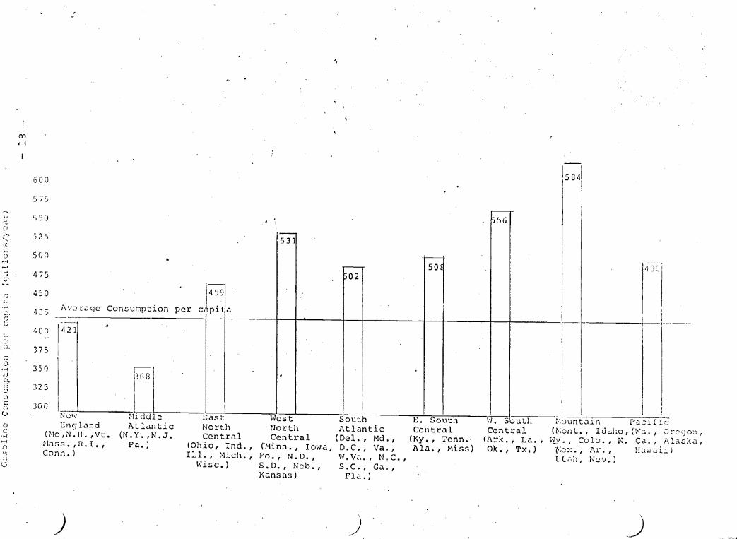
2
bull rhe reguLltions provide for Cl crudc oil supp] y progrClm for small ClIHl inc1l~penJen t rc [incrs utilizing a freeze as of December 11973 ormiddot supplier-purchaser re la tionships fOJ- crude oi 1 and a buysell list under -hieh th-~ 15 l1~ll01 oil corporations Circ reqJirccl to sell l~~ci[ie(i oltllcs of crude oil to Ll~(O sr-~111 tnC irl-l~lt rt~finers There icgt ~lsc 0 i~C(~-1 middotllicll pru1~ - - ~iJlLlnLi~ll cqualizltic 0 avcr(1ge crude oil priclo 1rHJ I1J -c-fincrs by the purchase ancl Sa lc of en ti t lC1(rl 1s Lu run cheap price-controlled old oil in th8 SacC natjomvic1c proshyportion at all refineries
e Refined products are distributed to ultimate users in accordrtnce vitl the allocation regulations except for gasoline 1-here the IClandatory allocation chain ends at the retail station and bulk purchaser Three general classes of users are established
_ Those users who are authorized to receive their current requirements - essentially whatever they request -- and are not subject to any allocation fraction This inclu~es Department of Defense agriculture and space heating for hospitals
Those who receive their current requirements but are subject to an allocation fraction -- emergency services energy production etc
Those who receive some percentage of their historical consumption or base period volume (usually based on 1972) and are subject to an allocation fraction
These class definitions and further percentage delineations within the third class are decided by the government and are spelled out in detail in regulations Their effect is to limit each user to a specific monthly or for some fuels quarterly authorized amount the usercategory scheme varies from one petroleum product to another
bull A supplier must continue to supply the same customers he serviced during the base period If he haS sufficient product to meet the sum of all his customers authorized amounts h~ delivers thisamotint to eltlch If not he reduces each purchltlsers share on a pre rata basis by applying his allocltion fraction equal Lo his totltll supply over the sum of his customers authoriZations and delivers this percentage of authoriZation to each customer
3
bull A port ion 0 f the product is reservcc1 for clell s tLl tc to usc f 1 c x i b 1Y toe 1 i minaLe hJ r d ~ ~ 1tl ) S bull T11 is ~ tgtl t e set-aside is administered by sLILmiddot (~ller(JY offices
e A detJiJed case handling ilnd appc~1s process has been establi~hed to hCll1dle ad ju~lr(i1L_ of base period usc to Jccount for changed circunLlI1ccs or unusuJl groith and other applic~l t i ()11~~ for c-(CPshy
tions and assignment of supplier
Positive As~)C~cts of an Import Cap and Allocttion Froqram
lhere are at least four positive Clccomplishlc1cnts thJt can be expected from a cap on imports and allocation
o The level of reduction in petroleum imports can be established with certainty There is no depeRdence on price elasticities of energy for achieving conshyservation results
bull Prices can be kept from rising thus minimizing any increase in the consumer price index
4
bull l]Lhouqh the i1Jlocatiol1 proqr1I11 (I()(~ not 1( (nCIltJY it can ~[Jrc(]cl tllouncl tlll~ 1111 ion t IH i1olt HW Cdll~lll
by thc import CZ1r thus temperinltJ th6 r0qionl impzlcts of such Zl procJrltlIn
bull The Government CZlr) milke qross ch()iCl 1 to Ihich s0ctor of the (conomy shoul(l he II ()(1tltd LI1( qrfdt t port-iOl ()[ the l1ortaltw lor (lt11111)1 fuel CLln bo made ilVLliL1])Je to tlle illclwiri11 sector Zlt thp expense of horne hllinq fuel or gasoljno for Zlutomobiles
o Undo r an allocation program the qOV(~ rnmen t n-~) lLlcCs the market in distributing encrcjV ouppJ ics Several significil1t problems arise with such Ll ub~jitution
-- An Llilocation system crc~pends on Zl governrnent determination of a persons need for fuol and yet need is almost imp6ssible to dc(ine The standards currently employed for making this determination rely on historical use and a governshyment judgment on priorities (eg agriculture should get all the fuel it needs) Unfortunately in thousands of cases the amount of fuel an individual or firm used two years ago may have little or no relation to how much fuel he currently needs Thus an exceptions process must be created and administrative judgment and procedures used to supplement the historical use standard There simply are not enough Solomons around to make such a system work well
In addition any system that classifies users according to government-determined priorities shifts the struggle for market advantage from the marketshyplace to the offices of those who write definitions and regulations The political pressures to give groups special preference become very great Should tobacco growing be made part of agriculture and thus tobacco growers be made eligible for the same priority as wheat fZlrmers What about green houses growing flowers lre portable toilets pZlrt of sanitZltion services Those who are most effective in these political bZlttles are not necessarily those who would be the most effective in a competitive market situZltion but for each the decision reqZlrding
L
5
their allocation priority cem Il1ab the di rrCHnce as to whether the businl~~ tllLi V(~ ()J ~lrr(rs
Because th(~ ~1l1ocClticgtn of pltr(llcIIIl1 uroducts under Cln allocation sYctcnl is plJrnrmld hy the Federal Clnd State ~lovernmcnt~ J1t 11()- t h-I) 1) th~ market public costs arc incurrLcl lll()(~ltil)n durin g the recon t ernhJrqo requi nmiddotd U1l 11 1-[- ime efforts of about l1OOO pcoplc dlH C()~-[ 1~1)-(J--imi1tely $100 million in addition su)slilt j)] r-cord kecpinc] reports (1nd (1uc1i ts 1erc l-l(lU i rcJ CJ~ the privale sector
-- An allocation systcI1 asumcs UuL ntLilcrs will distribute suppli(~s accordincr Lo rU]lS oet by th~ government In practice however it is impossib Ie to en force these rulc~) cC~1i tab Jy alOng thousands of gas station ODerators and fuel oil dealers Thus practices ~uch as prepounderc~tial treatment for special customers car washgasoline fill-up schemes pre-paid gasoline contracts and even direct black market operations quickly spring up bull
bull Allocation does not aid in solving mid- or longshyterm energy problems An allocation program hile it is useful in managing a shortaqe created by embargo or a cap on imports makes no contribushytion to our mid- and long-term gOals of energy independence because it provides no incentive for increasing domestic energy supply
bull Choosing the base period in an allOCation system is an especially difficult problem On the one hand choosing an early base period such as 1972 for which complete data are available means making numerous individual changes in the system to mirror current consumption since thousands of new businesses have begun old ones failed and many people moved in the intervening years Using a more recen1 base period however penali zes those who conserved during this period while rewarding those in the sam~ allocation cJtegory who did not curtail wasteful fuel use during the base period bull
bull AllocCltion has a retardinq effect on GNP growth and employment A reduction of 1 million bnrrcls a day through e111 import C(1P and (1llocation -Jill reduce GNP by an estimnted G billion dollars Jnd place 250000 more people on uven~loy~ent rolls
6
This occurs b(CdW~C an allocatioll IlroqldTll TllWt
spread fuel Llcross the vilrious ~c~ctoc of Lh( economy ltlccordinq to ltl ~cL of n-L1LivIlv inlcxible and cOIllplicLlh~d nLltiondl rtllts llhrqy lhll~ I
made aVltlilablc for both morc (fri(~il1t mc ll~~s
efficient uscs On the 0 Hlcr limd n~ J idl1Cl on higher price ltlnd the mikct to dtll with d
shortLlqc meun on the wholc a di~triblltj()ll or fuel to those Vho vLlluc it most 1l is llHn morc likely to )c usee ([ficienLJ~ r(lt pn)ducl iL
purposes resulting in a hiCJher C~Jgt ewci qrcatcr employrnen l
bull While iln allocation and price control proqrClm would 1 imi t di roct incrc ases in fue 1 cost~ it docs corry wi til it other costs J~xcllnplc abound reduced air line s c1cdu] Cc~ and thus reduced mobil i ty sales of petroleum prodllct~s linJed to contracts or sales of other goods and services drastjcally limited service hours and above all continuing uncertainty as to supply uvailability vhich makes planning impossible for businesses Llnd individual citizens In this regard the major cost to the consumer will likely be the inconvenience of gasshyoline lines To minimize the negative impact of the shortage on the economy and jobs mos t 0 f the ~eduction in consumption would probably have to come from private auto usc of gltlsoline Thus a substantial reduction in imports is likely to result in a recurrence of last years long gas-o line lines
o Even the best designed allocation program generates unforeseeable effects During the recent embargo for example people took few long trips Thus rural gasoline consumption was down relative to urban consumption since allocations to gasoline stations were based on historical consumption urban stations were unable to supply the unexpected increased demand resulting from this changed consumption bull
bull An allocation program is not an e f fecti ve consershyvation tool and has limited utility as a means of distributing products in short supply due to a cap on imports Because of the inherent complexshyities in even Ll cLlrefully desiqnecl allocCltion system and the fluid nature of lmc~ricun society the lltlrger the shortuqc the shorter the useful life of such Ll system
Revised Base Case Forecast and The Presidents ProgramForecast
National Petroleum Product Supply and Demand
Technical Report 75-2
Office of Quantitative Methods
February 5 1975
Federal Energy Adm ill istration
Washington DC 20461
NATIONAL PETROLEUM PRODUCT SUPPLY -m J~-lto
REVISED MSE CASE FORECtST fiJ
IHE PRESIDENTS PROGRN-l FORECS~
Technical Report 75-2
FEA~ - EATR - 75-2
February 5 1975
Short Range Modeling and Forecasting Division
Office of Quantitative Methods
Federal Energy Administration
This Technical Report replaces Technical Report 75-1 Comparison of Forecasts of Petroleum Product ~n2Jld Illustrating the Effects of Prices and other Factors FEA January 16 1970
SUMMARY
For 1975 as a whole it lS estimJted that thc Prc=idcnts program will
reduce aggregatc petroleum demand by 548 MBD
mcrease domestic production by 101 MBD
reduce petroleum imports by 649 MBD
The effects of each component of the Presidents program grow over time As a result for the fourth quarter 1975 the impact will be greater than when averaged over the entire year For fourth quarter 1975
aggregate petroleum demand will be reduced by 880 MBD
--domestic production ~vill be increased by 160 MBD
-- petroleum imports will be reduced by 1040 MBD
By December 1975 the Presidents goal of reducing petroleum imports by one million barrels per day will be surpassed under the Presidents program For December under the program
-- aggregate petroleum demanq will be reduced by 934 MBD
--domestic production will be increased by 160 MBD
- petrolelllTI imports will be reduced by 1094 MBD
The import savings in December 1975 are accounted for as follows (MBD)
160 Elk Hills development 98 conversion to coal
147 suspension of gas curtailments 689 effects of higher prices 1094
middotmiddotThe reductions in petroleum demand by product in December 1975 will be (in MBD)
rrotor gasoline -278 distillate - -238 residual -310 all other products -108
Total -934
INTRODUTIO
This Tltchnical ~port flI ltcnts the CClllt~ r un km(r -~r FEAs s-Jrt ter-- tJe-colelXn product supplyckrTLU1~ )dlnCl~ i~ L~~ion under t--J s-s =~ as~l1ption3 a Base Case 3ccnali) illi 1 ~ccnt3 petrolezn I=-cltu- su-gtlym derrBrld using a currcnt 1~lt~Jmiddot_~c siInula~n -=-~J ~X2-C price and weather data ~Jr_ 1 ~middotoli= J~)n Scenali- ~-~ -1 =--ampccrmiddot~~aL~S t~c pCirtictllars of t~middot) ~~~r~=j j-r-- s ~Tlergy prograr ~Lt ~~Je S3se Case scerlario rThe supply ~~~J ~cnm~ 01-22dStS
presentC rCCe 22 sight2y iferent from those -lc~uec 1shy
Decernbec 197~ 3 ea-ly January 1975 in that
the par-iculars of the Presidents program (rather than its general stC-lcture) are accoun~ed for explicitly
more recent ffi2croeconomic forecasts are available arid
price and weather data have been updated
The impact of the President I s program on a~cregate petrgtleum deIlEI1d and etrcleum imports or 1975 as a whole fou1h qU2rter 1975 and Dec2J-IDer 1973 are presented in a s~ section Othel~ sections of -he CeuroporL present the scenarios and associatec su~ly and derrand orec2sts the derivation of the effec~ of the Fres~Gentls program on 2troewn prices and the derivation of forecast inventory policies Zle forecasting procedure utilized for this repc~~ ~s docwrented I1 cional Petroleum Product Supply aitd Derrand October 197~ ~~ou~~ 1975 Tew~ical Report 74-5 rEA Nov8ber 8 1974
Appendices present a comparison of alternative forecasts documenting the effects of prices and other import~~t factors alternative elasticiy estimates and factors influencing a determination of the price of imported crude oil
1
SUPPLYDGlN m PllANCE SCOWUOS NID rORITASTHlG RlSULTS
Two supply dem=md balance scenarios arc presented 1 Plt~se CClse and a Policy Option Scenario The two scenarios dIC JPecificd as follows
Base Case The petroleum product demand simulation documented in Technical Report 7q-5 as utilicci Based upon rfcent economic indicators a DIU ITBcroeconomic simulation prepared in December vIas incorporate in Lhe cemm-i fOtecast this sirnulation projected relatively weak consumer dem-IDd over 1975 with a decline in real GtJP of 3 5 percent over the year The relative prices of the products were held constant at their last observed level
POlicy Option Case This case differs from the Base Case through the incorporation of the Presidents energy policy as given in the State of the Union Message
The price assumptions occasioned by the imposition of import fees and deregulation are given below in the section on prlces In addition it was
I assumed that
--- domestic production increqses by 160 MBD by the end of 1975 due to the development of Elk Hills
petroleUm derIBJ1d is reduced by 98 MBD due to switching from oil to coal
petroleum derIBJ1d due to natural gas curtailments ceases after May 1 1975 due to the deregulation of new natural gas at the wellhead
-- price changes due to the Presidents policies are held constant in real terms at their May 1975 levels
The Base Case supplyderIBJ1d balance scenario is presented in Table I and the Policy Option scenario in Table II Tables III through VII itemize the impact ofmiddot the various components of the Presidents program by pluduct for each quarter of 1975 and for 1975 as a whole
2
Table I
Base Case 025) Supply and Deman2 Forecast
(MBD)
Forecast without Implementation of the Presidents Program
D MOGAS
E Distillate M Residual A Keroj e t N Naphthajet D Petrochemicals
LPG Other products
a1 all products-shy
S Domestic Crude U P NGL P L Gain Y
Total Domestic Supply
Change in inventories
Imports
Total all products
~lQ 1975 2Q 3Q
6178 6715 b ~ 0 VUv
3916 2546 2215 2654 2 rJ iS35
769 812 815 211 248 244 333 338 337
1560 1076 1025 2029 2127 2383
17650 15872 15834
8663 8622 8575
1676 1E57 1650
413 399 357
10752 10678 10582
-229 +165 +323
6669 5359 5575
17650 15872 15834
4Q Year
6 C 1 6597 3 t~ 57 3034 2I01 2250
838 809 276 245 350 339
1470 1283 2178 2179
17583 16735
8540 8600
1656 1660
407 393
10603 10653
-260 0
6720 6082
17583 16735
3
Table II
Supply and Demand Forecast with the PresiJcnts Prog~arn
(HBD)
Forecast with full I
Implementation of the 1975
Presidents Program lQ 2Q 3Q
D MOGAS 6139 6489 6603 E Distillate 3915 2462 2055 M Residual 2625 187~ 1718 A Kerojet 767 803 797 N Nap hthaj e t 211 245 238 D Petrochemicals 332 330 322
LPG 1559 1068 1009 Other products 2027 2108 2344
~a1 all products 17575 15383 15085
S Domestic Crude I 8703 8702 8695 U P NGL 1676 1657 1650 P L Gain 413 399 357 Y
Tot a 1 Dom est i c Supply 10792 10758 10702
Change in inventories -229 +165 +323
Imports 6554 4790 4706
Total all products 17575 15383 15085middot
4Q Year
6336 6392 3243 2919 2118 2085
816 796 269 241 333 329
1445 1270 2143 2155
16703 16137
S70n R 7()1
1556 1 fl flO
407 393
10763 10754
-260 a
5680 54~3
16703 16187
4
Table III
Impact of the PresiJents Program First Quarter 1~7j
(HBD)
-39 - 1 - 4 - 1 - 1
1 - 1 - 2
~ otal all Products 49 o II- -75
Elk Hills Development 40
Current change in consu~ption Demand for petroleum imports
-5
---
Table IV
Impact of the Presidents Program Second Quarter 1975
(MBD)
Demand Changes
SuspensionPrice Coal of gasEffectsProduct Conversion Curtailments
I
~ Total
lOG S -227 0 0 -227Distillate - 20 -0 -62 - 82Resi2ual - 48 -49 -34 -131Kerojet - 9 0 0 - 9Naphtajet - 3 0 0 - 3Petrochemicals - 8 0 0 - 8LPG - 9 0 0 - 9Other - 20 0 0 - 20i
I Iotal all Products 3441 -49 -96- ~ -489
Elk Hills Dev~10prnent
Current change in consumption =Demand for petroleum imports
6
Table V
Impact of the President s Program Third Quarter 1975
(MBD)
Product
~WGAS -278Distillate -160Residual -217Kerojet 19Naphtajet 6Petrochemicals 15LPG 16Other - 38
==t=-========~=======---=-======~=============-_~ -(otal all Prod uc t s--r -525 -7 4 r-~~50 -749
i I
Elk Hills Deyelopment 120
Current change in consumption = Demand for petroleum imports
L 7
~lOGlt S Discil2ate Resi2 Kerojet Xaphtajet PetrocheTicals LPG Other
Table VI
Impact of the Presidents lr~srlm
Fourth Quarter 1975 (HBD)
-278 0 0 -120 0 -94 -214 -131 -98 -53 -282 - 22 0 0 22
7 0 0 I shy 7- 17 0 0 I 17 25 0 0 i shy 25
- 35 middot0 0 35
8 O_1_1__ -_6_3_5 __________~1__ p_r_o_d__~_c_t_S~__ ______-L~~-_9_8_-______________-_1_4_7 -ri_-_8_____
Elk Hills Development 160
Current change in consu~ption =Demand for petroleum imports
8
Table VII
Impact of the Presidents Program Annual 1975
(HBD)
-------~---I-- Dcm~~C h~~~l(C_~ II 5 pC n-s-~ 0 11 r--shyPrice Coal of gas E f f e c ti i
I
Conv e r 5 i 0 i1 C l r t a i 1m en t S I
~
r 0 t 31Product I ----- --------- -- shy~----- shy
~lOGAS -205 0 0 -205 Distillate - 52 0 -63 -115 Residuel - 69 -61 -35 -165 Keroj e t - 13 0 0 - 13 Naphtajet 4 0 0 4 Petrochemicals 10- 0 0 - 10 LPG - 12 0 0 - 12 Other 24 0 0 24
~ Products)total ll 1 -389 -61 -98 -SZ8I
Elk Hills Developrent I 101
Current change in consumption = Demand for petroleum imports
9
PRICE ASSLlMPIIOIIS
The petroleum [leaduct dcmmd simulation d[plLcc [)ticr elasticity asumptions to deflated w101csaLc prio inlic~ few Lin products except rrotor [ls01ine For motor [clsolinc [wicmiddot _ rTect are rrcasured in terms of the deflateI- cx- tax lcLlil ptic(c PlT gallon For all prnducts ecept motol~ Sdsoline the tL~n (~[fccts are lagged lith respect to how long a price ch(m~I i-~ _~SSllITCd to be sustained This IGf3 structUl~e (2ssuJniIlC consLm cl~~tc~itics) is given for a one tvo ill1d three quarter dUlation T1C LlsJUJi1Cci elasticities are
Product lQ 2Q 3Q
Distillate -09 -12 -12 Residual -15 -18 -21 Kerojet -06 -07 -08 Naphthajet -06 -07 -08 LPG -04 -04 -05 Petrochemicals -12 -14 -16 Other products -05 -05 -05
For motor gasoline the relationship between market price and demand was included as part of the regression estirrating the deITand forecasting equation ~~e specification of the forecastL~g equation is such that the price elasticity of motor gasoline deITand varies sorrewhat depending upon the values of price a1d quantity demanded at which it is Feasured Generally for the year 1975 the price elasticity of motor gasoline is -15
Using the results of analyses conducted with the Office of Economic Impact FEA the implication of the Presidents policy of import fees and deregulation was traced for nominal prices measured by rronth for January through May 1975 These norninal prices were then converted into the appropriate indexed and deflated format for incorporation into the petroleum product derrand simulation The derivation of the nominal price time series is given below
10
The end of year 19711 crude oil priccwl~ dlliv l tolJow~
$84425 75 [5 x Old Oil Price + LI x New Oil [tic ] + 25 x Imported Oil Feice
~middotr(ntiuLJwhere 75 proportion of crude S d()riC~ t i- l~ 1 n)(JuceC
25 proportion of cruce S iCL impoctclt - ~ j6 CllIYent proportion of cll)mcstic bull ~ ~j that 18 Old Oil
4 current proportion of dornc~)tic ~~l~)ply lldt lS 0lcw Oil
Old Oil Price $525 per bcJrrel New Oil ~iice $11 00 per barrel Imported Oil Price $11 00 per baJTel
The May 1 1975 crude price was obtained by equdting The Old Price to the New Oil rice and the IIIl[)~ted Oil rice LO $13 to account for decontrol the domestic excise tax and the ~Tport fee It was asswned that the price of NGL would be equivalent to The price of crude oil even if a smaller SIU equivalent tax here to be placed on it After Hay 11975 all petroleum prices Jere asscJned to rise nominally by the rate of inflation that is not to change in real terms
The refined product average was constructed using the crude oil series plus estj~aTes of refining costs and other cost factors The distillate and residual price series were constructed from the crude series with the rule that increases in the domestically produced distillate and residual would equal increases in average crude prices Iwported residual and distillate were ass~poundd to increase in price by an amount equalmiddot to the import fee The average price indices constructed for the procucts are the weighted by their domestic to imported ratios Since nearly all gasoline is domestically produced its price increases only reflect crude increases
These rules produce straight pass through of costs to Droducts without shifting costs from one product to another As an alternative to this simple pro-rata cost pass through price construction historical price relationships were also euroxamined Historical ratios of the various product prices to the refined products average were used to forecast prices The results of forecasting prices on the basis of historical ratios was little different from that given by the simple pass throuu~ assumptions Since it is expected that regulations will be enforced to equalize product price increases the equalized cost pass throuf~ with immediate adjustment was used to forecast prices TI1e nominal price forecast assumed is given in Table VIII
Although hiGher imported oil prices ~LrC quoted $11 is the estimate of the average economic cost of imports to refiners See Appendix B
11
For tte tr3J1si-ri()n period February 1 to pri 1 30 l~n 5 the folloH l11g ric(s wccc used
The ~ltr b-rrel increascs in crude prices HI FclJLll)middot tlclrd1 and April reflcct -he $~ $2 $3 import fce on irTlpcwU~d C~~dL 0clIlLsticdily produced-ldc is st~J- averce undel th~ Old-ll~IrJ ui - ~C21LJne 1he product c~C2[ lC2 cJudl dlstlllate dIlcl tl~( 1llJlC r _gt_~ dUllJ12
this k-2ric re~cct the ch~mge in crude plices due tu -tL 1 $ 2 $ 3 crude ir~--t fEo lr_ the $0 GOcent $1 20[12 OIl lITljX)lt ~ ~loduc ts as weI as the rati J )f dornestically produced to imp0c---2C products
These rats a-e dssUJed to be
Petrc=eum rDG1Ct tverage Drnesticcly rDdlced Jnported coo Product
82
18
Resic-al Drnesticclly Produced Imported ~s Product
35
65
Distillate Domestically Produced Imported as Product
85
15
Gasoline - All I))rnestically Produce_d
Product prices are calculated as follows
Petroleum Product Average = $1015h Wholesale Price 82 (Average Change LTl Crude Oil Price)
18 (Change in Product Import Fee)
Residual ~lJholesale Price = $ 775 35 (Average Change In Crude Oil Price) -65 (Change in Product Import Fee)
Distillate Wholesale Price= $11 98 + 85 (Average Change in Crude Oil Price) 15 (Change in Product Import Fee)
Gasoline Retail Price = $041 + Average Change in Crude Oil Price per gallon
) See The Itllitt Ik1use Fact Sheet (January 15 1975) 111e Presidents State of the Union rk~sc1Ge p 33 items (A) Ha) and (A) lCc) 111C system of rebates (n prDducts nullifies the Febrvary fee on products
) Latest observed price per barrel - except gasoline (per gallon)~
12
+
+
+
Crude
All Products
Distillate
Residual
Gtsoline
Jan
844
1015
1198
775
41
Wholesale prices per barrel
Table VIII
Price Assumptions
Feb
899
1060
1244
794
423
March
954
1116
1300
852
436
Anrilshy~
1009
1172
1356
910
449
gticlrcn
1300
1425
1615
1064
Retailmiddot price per gallon excluding taxes The natural average for gasoline taxes is 12-14cent
13
519
INVENTORY MJUSTHUflS ror~ 1375
A cornpLlri~on ol [orecLlst Llnd observeci inverl LI Y lX) 11 (llS fc)l Lhc months of Oc tober 110vcInbcr ill1d Dlccmber 1~ 7q Ld rev lt1 1 ( r j hi ~lll Lnn forecast stock level~ In fact the stock leveL ()IJticd It Ll1t~ beginninr of Ceccrrber 1971f arc believed to b-~ neeI Llll ~ inill trys sustainable capacity dS that capelcity was mCdsurcd in i1lt3111xr 1373 As a result the inventory profiles assumed for th ul[lymiddotlcnnnci simulations piesent~r hcrmiddot -Jere chm~ec in tilt 1~middot~t(I t( be consistent Vlith rec~~t coservations A mop~ c~rculnl Ly~i of expected prociuct 00 ~middot)~)(L inventory behavior i11 L~ -lOlOrat~d l~
the implem~ntTtion (j~ C- r2gionali=2o shortfclll runirni=il1 SdfplyrdcmJIld simulation tmiddot) be pnpared in Fctru2cj 1975
Stated siInply the inventory char1Ges projected for 1975 in Technical Report 74-5 and subsequent applicJTiors of tl1at I2Ort shotJed a net drawdo~I1 ~I 1975 of over 200 rrSD Iur 1975 as 2 Hhole The estimate of this redllC1ion in inventories arises iiom the imposition of miniJIl~L opeurorable as coml3red to historic211y normal bounds on major procJct inventories Tile inclusion of more traditional inventory piufiles will be reflected in the results of the neXT application of the full regional ITcdel
For the forecasts given above the following assumptions were imposed upon the aggregate ~Iventory profile assumed
a zero net ~~nge in aggregate stock levels over 1975
inventory build-up lf1 the second and third quarter 1975 was constrained such that the largest assUmed aggregate stock level was that observed on December 1 1974
the relative rate of first quarter to fourth quarter drawdown and second quarter to third quarter build-up was set at that given by the Base Case simulation in Teclmical Report 74-5
The assumed inventory profile for 1975 is as follows (in MBD)
Quarter Stock Change
19751Q -229 19752Q +165 19753Q +323 19754Q -260
te Such an inventory policy is lppropriate to a periodof embcn~~ related shortlgcs but not appropriate to the CUIlnt supply sltudtion
tete Aggregate inv61tories are estimated to have ~~ed by-770 MBD during December 1974
14
APPENDlcr~S
Appendix A Comparis)ns)f Fcxccst-lt Petroleura rcduct DCJand Illu-ltir1s the Effects of Prices and Oth1 Fc1ctors
Appendix B klmestic New Oi_l and Imported Crude Prices
15
APPHIDIX
Comparisons of Forecasts of Pc trD11 tnl
Product DeBld Illlstratir1pound the tlcls of Prices and Other F octors
The time serES descrilirs the consumption crnci oss)ciated wi-h four difercrrt ~~ets c ss--=pic)n= ~ere de~_--=1-~~1C~ l~-=-~i~[ t~e pe-rolcum product fOlecas i~s P-2cscre (dOC1JJCle1leG in lmiddot~ch1ic31 Report 7Lf-5) 11e s3imr)1S 323231e incoe Jld lt2dtlr efects from p~ice efiects from tre e-d of 1973 tfLYQugh 1J75 fct~al data is used for all the t1-le seies for all periods liJl to the fourth quarter of 1973 The parTicular assurrp-cicns fellow
Series I re-S~argo Forecast
This series proj ects COI1s~-lption der1ind for the focv-th quarter 1973 and for -che leaS lS7w 2nd 1975 ~lder cc1_e ass1llTption that the severe econoIYic d-rrtJ-11 id no-c occur tht the relative price of petroleum products did not increase qid that nOI~al weather prevailed The macroecono17ic forecast assumed was prepared in December 1973
Series II Income and Weather 7ffects
This series simulates consumption derrand from fourth qu~rrter 1973 throug1-j 1974 using observed values for the rracroeconornic variables and the weather NOYl1El weather was asswed for 1975 The ffi3croeconomic forecast for 1975 vlas prepared in December 1974 The differences beuveen Series I a~d II are attributable entirely to income and weather effects Tne relative price of petroleum products was held at its third quarter 1973 level
Series_ III Price Effects
Series III differs from Series II in that the effects of the increase in petroleum prices are incorporated in the sirnulation For 1975 the relative price of petroleu~ products was assumed to remain at its present level For 1974 Series III represents expected consumption as determined by the forecasting procedure For 1975 Series III is the current b3se case forecast without accounting for the Presidents program
16
Secies IV pGrtrays actual clemmel durin 1ltJ71~ tr~ pC3c--s he de~rarj orcS-3 t ssociatecl Hith th~ Prc~iJcnt 11 Jb~ sectl i- _(~le -ed abcle
T1e fO=-~CviZ f~ures present recent col1su-c~lt 1( ~--C~--_-2 anc for2as- 2on3lpcion for each of the assumpti-n e -~C __ -
for eac-- 0 --DtCc gasoline distillJte and resiucl =-Je 8 anc all petr82eu- rocucts taken together
o the four time series are illustrated or the period 1969-1975 and separately for 1974 and 1975 on a larger scale
o the four time series are expressed in percentage terms with Series I = 100 The three remaining series are plotted in percentage terms with respect to Series I
For 1974 actual consumption fell below those levels wch ers anticipated befoe the economic downturn and higher rices (as given in Series 1) tven when higher prices and lower iJlcCne are -2~~en into account fis1 quarter demand lS still lower thCJl exe21e iI
due to the elbargo In the SlUIlffier of 1974 a surge 0 post-2lb~go pent u derranc l1By be noted However in the last quart2 of 1974 deIlE11d returns to expected levels determined by the forec2st i 1g procedure
A brief discussion of alternative elasticity estiITBtes lS provided as the last section of the Appendix
17
Series
I II
y--
L
C()in)iRI~)Oti~ or LOTi[ n~c)J)UCT [)i~]i)
(Imi)
21000-+shyI I
200001shy
190001 I
180COt
17000j
16000shy
1 15000
14000
bull
t I I X~ I r~I
bull bull
bull I
13000shy -t--t---t----t--I---t------ l~o~ 1970 1971 197a 1973 1974 1975
Prc-Dnl_urgo ForccCts t ~-------
Incorr2 cmd -e~lthcr effects - - - - - - -l1iee Effects added to Income clnd ltcdthcr Effcots Actual 19711 Pn2sicl~nts PrDgral1l 1975 - - - -
~r _ bullbull Lmiddot
18
~
---- _shy
J i
COHlAhISIH ()i LulM j-UDL~~ IJi) (l1 t~[) )
22000 -I
cH00Co+ I t
i 200C0-t-
I I
19000~
l~ I bull I 18000
i I bull
I ~ I ~
I - shy
I I I
I I I
I
170001
160001 ~
I bull I
I v- bullbullbull
15000
1974
-
1975
I
~ _______ __ - _~___ __ bull _______bullbullbull - _______ ______bullbull ~__ ______ ~_ _ ____ 0
Series
I II
Pre-Dnbcugo Forecast Income c1I1d Jeather L-f---l-~C-C--ts------------- -
Price Iffccts ilddcd to Income Clnd kalhcr Effects Actual 197LJ Presidents Prorr~1J~ 1975 - - - - bull
____ _ _- - ---- -- - or -~ ~~ -~ --or ---r~-_~________ 0_
19
CU)~~f~()l~~ ~l~ l~lt1 ~middot(~ll~(I ~~ (i1l ~~ l(~lL lmiddot ~ LI j~)
lC2-T
lOOT I
I J bull
g8i -
I
Ii
96-Tshy
I I I 01 bullbull I94--- i ~ I ~
92--- I
9C i 881
I 86
84 ----
82shy
1975
Series
I rn~-Lbarfgto Fot~(Cl3t II IncQl~ and J~lthcr E1-tc-~lS - - - shy
I-1ice Effects ~lddcj to Incorrc and ~~L1thcr Effects Actual 19711 PresiJcnt s Pl)D~Clffi 195 - 0 - 00 - 0 shy
~- --_-_ - - --- ----1middot- - ~middotmiddotmiddot1-- ~~
20
Series I Series II Series II Series iV
Series I Series II Series III Series IV
COMPARISO~JS OF TOTL [FODlICI )r~IJ 1
(MBD)
~ -- 1 - -~- -- -+ bull -
-l 1 ~ ~ -4 (I ~_ bull ~ 1- L~ ~~ 1 ~=- ~ 1 i~ l -+ bull --~ ~ 1 -- 2 1 bull (i 1 -t 1 ~~ bull 1 4 ( (i bull=i 1 S C 1 ~ ~ - 11 ~ ~ bull 7~ ~- 1 ~ cmiddot r 4 ~ r
1~74 1~75
17879S~1 19046637 17613112 1782S4G~
16771089 1~734724 1626297 16186571
21
---~----
COf1JlniJj ClI tlC)[(j (JXl[[ ltjjl
(fmiddot1EI))
7500
I
7000-r
i 65001
I 6000-r
I I
I I
5500+
til
bull
5000shy _ -shy 1-- --l- middotmiddot----middotr--middot-t----+----t----I 1909 97 1971 1972 1973 1974 1975
shy - - ___ _ _shy __ - --shy -- --
Series
I Pre-Dnbargo Forecwst II Income i-md -leather EmiddotE~ro--e-c--ts------------ -
III Price Effects added to Incorn~ wIld leather Effects IV Actuli 19711 Presicknts Pr)~nlIn 1975 - --
r~ bull r~ ~ ~-~- ~r-~ ~-1-~- -~ ~~T-- -~ ~~~ vr-~ bullbullr- ~~-
22 ~ ~---~
bull bull
bull bull
(iIi))
760O I
7400-fshy
i
7200-i 1
I 70001 I
JY ~ I bull
1 ~
Imiddot 6seej I I
bullbull ~
~ ~ I 6600 bull I
I bull bull l I I bull I
6400-4-
I I I
F _- r bull 1 bull f I
6200 I s J6000
I 5800
H~7 1975
Series
I Pre-Dnb-lrrO ForecClst ~~-------------II Inconc anu -Jelthcl- Effects - - - - - - shy
Price rffccts aJdLcl to Income cmd veJthcr Effects Actual 19711 Presidents Prq~tun 1975 - - - -
_____ --__ _ __ - ___ __ _r_______ _ _ -- _ ___ bull - - -~ - - -- --
23
_r_
COilPMISjgtI OE iIJl(lmiddot~ Cmiddotlrri id~~[) (Ln plrt-~llcl(gt _middott~~~)
102- I
i i
100--_~-------------------------------------- bull
98-- I -s~~~ bull - - bull --IP- -
I -----shy ---96~ shy
I J ~- 94 _ - 1
1 - --- --- I
Sla-+
- - shy_ --------4-----------lss-+-shy1974 1975
---- - -- - -- ---~-- -- -__ -~- -- - --shySeries
Pre-DnhlI~(TO ForeccJst lt i I tl lt~0
II IncOolc (Inc -J(~athcr Lffccts - - - - - - - t
Price lffccts added to lnconc and -JeClthcr Effects U Actln1 19711 Presidents PrDir-eul1 1975 - - - -
If-----~bullbull ~~-~-_
L
Series I Series II Series III Series IV
Series I Series II Series III Series IV
COMPNUSOtJS
5 ~~ l ~ bullC ti t 0 c Ur
5S~~206
52 ~ 2 I)~
1974
689155 6746946 6467523 6496869
or nUlUI- CJsoLIr~r DI iI (HG))
- 1 bull + ( - n1 ~ bull 1 1 -= 4 1 bull ~ t 4 bull (1 ~
= - 1 bull 1 7 I 1 ~=- 1 ~- 1 ~ 1 bull 2 --+ r_~ bull ( 57~1 476 ~Olc15 6~~1 24~ 662S~
5( = 1 bull 4 ( t ~ Ci 1~ bull 1 1 Co = ~ 1 bull ~ 4 - 1 bull 254bull
1375
7076738 6S65342 6596793 6391458
25
middot
cmu[I~OilS or DJ STILlAn DI -~o~[) (i1HO)
5000-y-
I 45001 4000J
I
- shy bull --shy --shy -
Series
I II
III IV
3500
I
3000~
2000
1500 -t-_--tmiddot_--middotmiddott--i 1969 97~ g7 ~7a 1~73 1974 1975
-~-- _ _ - _ ___ o_ bullbullbullbull _ bull __
Pre-Dnbar~o Forecast ~--~~~------
Income and He1thcr Effects - - - - -Price Efftcts added to Income and Ieather Effects ActnJ1 197L~ Jresidents PrUrnU11 1975 - - - -
~
--~ -
CC)fF~I~(XJS or DISTI [[ ATL gt LU (HBD)
I
4500-middot
4000-+
I 3500-+
30130 I
2500
2000
I
1 I
11 I I
11 II I
1 bullbullbull bull
_
1500-r-------------+-----------~--~ 1975
- __ _--_ - - _-----_ -- __ -- ----shy -~----~ ---~-- ~ ------- o
Ser-ies
I II
Prc-DnbJrfo Forecls t ~---------------
Incorni~ mcl ]lJtlk~ Effects Price Effects adi -c1 tu Inox~ and euthcr Effects ActU11 19711 F11~sidcnts PrOtnun 1975 - - -
~- __ __~__ -- _ --- __ _~~ __ __ ~_~-~ middot middot~--middot bullmiddot 1--middotmiddot
COtil-WL 0 (JL [) I I LI lL ilJ~ Ji) (ill ~)(I((liLt LlJIIL)
1013--shy
shy 1 eo-~----~
I
~
shy9S-T t ~
se
bull ~
~ l - ~
I
I
7S-+-shy
1975
Sepjes
I Prc-Dllburgo Forerd~ t ~--~----------II I11C0112 cUlll vcllhc~l l~frccts - - - - - - shy
Price Ef1cts Jedcd to Income nne Wcalhl~r Effects Actual 19711 Presidcnts Prognun 1975 - - shy
_ ___ - I ~4~
8
COr1fARISOrJ~ or DL3T[LLJTi DlVjj[i
Series I Series II Series III Series IV
Series I Series II Series III Series IV
= 4 - 1 -
J - 1 bull 471 5= 24 i 1 bull (l5~
1374
3224843 3161426 301S302 2399126
(HBD)
1970
2 -- -1- t bull ( 1- 2 4 bull (i 1 ~
St 4 bull i)1 -
4 4 bull (I 1
1375
34~1 554 3227345 303~582 2918757
29
1~71
2~rt ~ bull - CI ~ -- _~ -1-
2~~ - ~ ( - bull I
- bull I -t
~ ~ bull 1~1J (
Series
I II
III
- - ~
COmiddot1i Ar l~U r~ ()l I ~ mU([ [)[ Emiddot iU WHO)
4eo-middotI
I i
I
3500-r
3000~
2500
2000
I Ibull
1500 _-_t--t--shy
1
I I
I I middot r~ I V I
~ I I t I I Ib bull v 1 I I
1 bull I
bull bull 1 I I
t 1 I I
10middotbullf I
196~ 1970 lS7 1972 1973 1974 1975
~~-- - ~-- __---shy -~- ~--- --- -----~ -_ ~~ -- --~
Pre-Embar~o Forecust Inco( and ctither [irects - - - - - - -Price Effects added to Income clnu hcathcr rffect~
T Aetu1l197LI Prcsjc1enls ProgYun 1975 _ _ _ _ ~ -y-- 1 bullbull~ -~ - - -middotmiddot--Il~---~-lt f+ ~~ ~r__-----~___ ~_middot
30
~-
j1 bullbull
bull I
I3500-shy
middotL_~-middot _ -____
I II f
I 14 I I I bullbull
bull I bull bull
I bullbullbull
1- - aS00 bull bull I bull bull t bull bull
I til bull _ t
2000
I
shy1500-+-shy
197~ 1975
Series
I Pre-Dnbar[o ForecClst ~~------------II Income and -]_1 thoI F ffCcts - - - - - - shy
III Price poundffcc ts added to Incoc and H-~dther Effects IV AetLll1 19711 Flgt2sidcnts P1D3ram 1975 - - -
- -- ~ r bullbull ~_
31
bullbull --
t ii t l)l I ~)[ ) eli ~iIJ
(in lT((~llt We 1tlC)
1ec----~------+~---------------
I I - I --
i i
I
9~-+ bullbull e bull
~ 80
~bullbull
bullbull ~- ~
til ~70 -----
bull
G0 - -
50+--------t------l 1975
Series
I Prc-Ln8~r~O rorec~st
II Incon imJ t-1lhct effects - - - - - - shyIII Price Effects 1dcl-J to InC(Xll(~ LInd Weather [Ffect
TI ActLlCl1 107 l l FnsiJetlts PloUdm 1975 - ~
32
COMfARISCgtJS OF [middotTSHJJL DGlinl (1BD)
Series I 1~7~ =4 ~c (Ibull - ishy
Series II 1 ~ ~ -- ~~ -=~ r--~ bull - (t -Series T7T
---1~ rmiddot~~-middot~middot ~middot4 ~ l~ - Cl~Series IV 19964 22u~0~
174 1975
Series I 2930882 244806Series II ~a1743~ 27J5381Series III 2503294 224994SSeries IV 2749009 2094824
33
c~~ ~I I L~middot4 bull I~ 1 ~ t bull I~~ ~c ~~ - I~ ~ ~bull - I I 1 -=- 4- 5 ~~ ~ -= ~ -_r~4 I~I ~ I 2 ~~ i ~ 1 ( bull
2~~~8~~ ~S4~~Gl
bull
C011PARISOi or SELICno S (TlCl T
The short run elasticity estirmtcs LcOl1Xr 1 t~(( in thc El short-tenn orcc2stirL6 procccicrc arc difficult t(1 ~Liut particularly in -hc case of dislggregcltcc] pDXJllC t --i tctorit-s Represe1tativ~ e ~Lic~ty estirrldtt2S plusmnnJm cl~ tC~l C 3 U_ P
presented L1 3b~c ~ for ptlrposes of corparison to icc l LC 1C
general plac3~biJi[y of the figures usee in the ClC2OLS 1iO2rer~ the precise interpretaTion or applicatio of th2S CSCLCS should not be attertcdout of conteAt of the Tilcdels in ihid) thoj ctYe
developed the til1e frames to Hhieh they are applie 0 -he definitions used L~ L~eir computation lhe elastici-ies ~rese~ted are calculated 0 a consistent basis but are intencec to be only summary indicators of the price sensitivicy of the alcen1ace ~dels 1m accurate staternent of the price response of other oGels 1middotolJld require direct application of the full model to price amp10 other changes
34
TIBLE AI
ESTHilTES or r1 rnrr rUISTICTTY or rEr~rrm --~---prTEonllfl~I)-f)ilaquo)I)IJll~lF-- shy
------ ~- -
SflOI r IU~l (Upmiddot(omiddotr YCcl r )
Houthukker Vcr 1 (Hj C) [ Hudson-
fEI1 Sheehan3 Ph 1i 1S~ Jo rgc ns Ot~lj___---J _____ __
All Pe tro1~ uamp1 -10 -10 -10 -11
Gasolinel -10 (-15) -09 (- 14) -07 (-11) - 13 (-20) Distillute -12 Residual -21
bullKerojet -08 Naphthajet -08 LPG -05 Petrochemi ca1s - 16 Other Products -05 - 1middot Estimates of gasoline elasticity relate to retail prices extax shmmiddotm in parentheses - All other estimates relate to wholesale prices or have been converted to wholesale
prices under the assumption that cost pass-throughs occur without proportional markups
2 Consensus estimate by Troika CEA Treasury OMB and FEA - 1974 3 Prepared by EPA and CEQ - December 1973
Phlips L IIA Dynamic Version of the Linear Expenditure ~~odel II The Reviemiddot of Economics and Statistics Vol LIV No 4 (Nov 1972) pp 450-465- shy
DR Energy Forecast January 1975 Chase Econometric Analysis January 24 1975 For Ford Foundation - 1974 All elasticities relate to wholesale prices except that in the case of gasoline the second figure in () relates to the retail price before excise taxes In judging the relative degree to which different products respond to price the wholesale figures provide the best indication They indictlte thtlt gClso1ine is less responsive than some other product
The eltlsticity figu)e is hi~Jhcr fo) the retail pricr thun for the lho1fs11e price That is beclluse the elasticity is the ratio bet((n~ thp f)(I-~P~lt~HJ~) Clhln~Jl in COI1shy lTlpti on and the Eecent-~~l~ change in pri ce A 10c Chl))(Jl for eXdflp Ie JOul d )H~
W~~ change in a 2c 11010stl10 price but only a 251 chan(j( in J lt10( rotdil pIice ishy
-a1us the denominator of the ~lasticily figlwe Ou1d be gn~i1lr~I in the Ci1e of the wholesale price than in the case of the retail price lIovewl if the chJngc in actucl1 consumption - the numerator remains the same the elastiCity figurcchlngcs 35--
NlLilDL l)
Ibrrcstic Ncw Oil Clnd Importcri Crude l)rj (
The current avc~~[e prJcc of irl-Ortcd crude r(T)~t-d tc the FEA for the cost pJ~thrCJlJrj j ~12 53 per bdrrel C~r~~Jt)
New oil prices currcntly wcnlge Jbout $1083 per brt~l lUS
appendix c~iscLsses eli ferenccs be t1tJeen tl1C declaredmiddot ~ middotCTOUC
price of cruce
One important reason for the difference is the rrehoc of valuatLTlg in~orted oil for the cost passthrough Current~ thele are thrce basic types of purc1ases of foreign crude eqJity participation and third party Equity oil is that oil roduced and ovmed by the concessionaire (e g Fpoundamco) under a~eent ith the host country Since the concessionaire olaquos the oil there is no purchase price per se However the host country charges the concessionaire taxes a1d royalties on this oil The sum of these taxes and royalties plus the cost of producing the oil is the tax paid cost and represents the real cost of the oil to the concessionaire Although there have been increases in tax and royalty rates in recent months during 1974 tax paid costs were lower than the price of crude sold to non-concessionaires
The second type of purchase pa-rtlclpation oil is that oil produced by the concessionaire vIhich the host COW1try owns as a result of a participation agre~~ent and which the host government sells to the concessionaire at a negotiated price For exarr~le sixty percent of the oil produced by Aramco is owned by Saudi Arabia
and Saudi Arabia sells the rrajor portion of this oil back to companies of Ararnco at the buyback price which currently is $1046 per barrel
The third type of purchase third party purchases is oil purchased by any company either from the host government or the concessionaire This price may be viewed as a free market price although this price will vary depending upon purchase terms (ie quantity and date of delivery) During 1974 at times third party purchase prices were higher than both government ta~ paid costs and buyback prices During the first quarter some third party purchases ran in excess of $2000 per barrel
36
lor puq)O~CS of the cu~t-Pd~~~tltn)u(~h rCdJl~tmiddot~ VdllJC tgtl1VI)d~k oiJ and thirCl Jgtdrty [gttJrchltl~c oil dL purcfldC IWlCC [Lue IlmiddotI[p)dILiull co~ l ~md fcc
However for equity crude refiners Ire pcnn-i t tcd t() (( t
value on the i r (qui ty crucic hhich JouLd ptev Ii] if trwy 11 1 III with their elft i liatul -lltiLimiddot clt arm -Jellith In (middotfilet (Iii means that tIle rcCjncY ITny _harrc hinlJcl~ (i plicc e)I Iii ltqui lj crude whicil l([IIL thc lhi~j i)cilLj llllldld( twice The l~J fj-ewc for imp)YtcJ erucic inchclc C(luity cnldc middothic1 i~ llIC(
above its Clilcll CO~3t 10 the rcfincr Al30 then i [hI il factor of tlle U s trcutln(~rlt of tucs pc1id c)n C(lltiL~l ClU( Jc~ fdCS
paid to hos t g()verrJTlent~ ~lre the basis for foreiGn t2X C1cclit) and this may reduce the real costs of equity crude In this sense the $1253 figure overstates -he real costs of iJljJOrtcd ClUJC 0
the refiner Thus the difference between the pcices of neVI oil and impcrted oil reported for the cost p~stht)J~Jl dues not
necessarily reflect the difference in nal costs to the refiner
The real difference in cost is difficult to determine New Oil prices are still rising and have not stabilized but it is safe to assume that they will stabilize at sonE price below $1253 which would represent an equilibrium between the real costs of impcrted oil and the price of new oil
Although institutional complexities complicate the determination of impcrted crude prices the equilibrium price of ned domestic crude and the oppcrtunity cost of acquiring imported crude will be the same Therefore the analysis ill this study assumes an imported oil price of $11 per barrel the approximate price of New Oil
37
I
- 002500064-2
- 002500064-2
-
3
bull A port ion 0 f the product is reservcc1 for clell s tLl tc to usc f 1 c x i b 1Y toe 1 i minaLe hJ r d ~ ~ 1tl ) S bull T11 is ~ tgtl t e set-aside is administered by sLILmiddot (~ller(JY offices
e A detJiJed case handling ilnd appc~1s process has been establi~hed to hCll1dle ad ju~lr(i1L_ of base period usc to Jccount for changed circunLlI1ccs or unusuJl groith and other applic~l t i ()11~~ for c-(CPshy
tions and assignment of supplier
Positive As~)C~cts of an Import Cap and Allocttion Froqram
lhere are at least four positive Clccomplishlc1cnts thJt can be expected from a cap on imports and allocation
o The level of reduction in petroleum imports can be established with certainty There is no depeRdence on price elasticities of energy for achieving conshyservation results
bull Prices can be kept from rising thus minimizing any increase in the consumer price index
4
bull l]Lhouqh the i1Jlocatiol1 proqr1I11 (I()(~ not 1( (nCIltJY it can ~[Jrc(]cl tllouncl tlll~ 1111 ion t IH i1olt HW Cdll~lll
by thc import CZ1r thus temperinltJ th6 r0qionl impzlcts of such Zl procJrltlIn
bull The Government CZlr) milke qross ch()iCl 1 to Ihich s0ctor of the (conomy shoul(l he II ()(1tltd LI1( qrfdt t port-iOl ()[ the l1ortaltw lor (lt11111)1 fuel CLln bo made ilVLliL1])Je to tlle illclwiri11 sector Zlt thp expense of horne hllinq fuel or gasoljno for Zlutomobiles
o Undo r an allocation program the qOV(~ rnmen t n-~) lLlcCs the market in distributing encrcjV ouppJ ics Several significil1t problems arise with such Ll ub~jitution
-- An Llilocation system crc~pends on Zl governrnent determination of a persons need for fuol and yet need is almost imp6ssible to dc(ine The standards currently employed for making this determination rely on historical use and a governshyment judgment on priorities (eg agriculture should get all the fuel it needs) Unfortunately in thousands of cases the amount of fuel an individual or firm used two years ago may have little or no relation to how much fuel he currently needs Thus an exceptions process must be created and administrative judgment and procedures used to supplement the historical use standard There simply are not enough Solomons around to make such a system work well
In addition any system that classifies users according to government-determined priorities shifts the struggle for market advantage from the marketshyplace to the offices of those who write definitions and regulations The political pressures to give groups special preference become very great Should tobacco growing be made part of agriculture and thus tobacco growers be made eligible for the same priority as wheat fZlrmers What about green houses growing flowers lre portable toilets pZlrt of sanitZltion services Those who are most effective in these political bZlttles are not necessarily those who would be the most effective in a competitive market situZltion but for each the decision reqZlrding
L
5
their allocation priority cem Il1ab the di rrCHnce as to whether the businl~~ tllLi V(~ ()J ~lrr(rs
Because th(~ ~1l1ocClticgtn of pltr(llcIIIl1 uroducts under Cln allocation sYctcnl is plJrnrmld hy the Federal Clnd State ~lovernmcnt~ J1t 11()- t h-I) 1) th~ market public costs arc incurrLcl lll()(~ltil)n durin g the recon t ernhJrqo requi nmiddotd U1l 11 1-[- ime efforts of about l1OOO pcoplc dlH C()~-[ 1~1)-(J--imi1tely $100 million in addition su)slilt j)] r-cord kecpinc] reports (1nd (1uc1i ts 1erc l-l(lU i rcJ CJ~ the privale sector
-- An allocation systcI1 asumcs UuL ntLilcrs will distribute suppli(~s accordincr Lo rU]lS oet by th~ government In practice however it is impossib Ie to en force these rulc~) cC~1i tab Jy alOng thousands of gas station ODerators and fuel oil dealers Thus practices ~uch as prepounderc~tial treatment for special customers car washgasoline fill-up schemes pre-paid gasoline contracts and even direct black market operations quickly spring up bull
bull Allocation does not aid in solving mid- or longshyterm energy problems An allocation program hile it is useful in managing a shortaqe created by embargo or a cap on imports makes no contribushytion to our mid- and long-term gOals of energy independence because it provides no incentive for increasing domestic energy supply
bull Choosing the base period in an allOCation system is an especially difficult problem On the one hand choosing an early base period such as 1972 for which complete data are available means making numerous individual changes in the system to mirror current consumption since thousands of new businesses have begun old ones failed and many people moved in the intervening years Using a more recen1 base period however penali zes those who conserved during this period while rewarding those in the sam~ allocation cJtegory who did not curtail wasteful fuel use during the base period bull
bull AllocCltion has a retardinq effect on GNP growth and employment A reduction of 1 million bnrrcls a day through e111 import C(1P and (1llocation -Jill reduce GNP by an estimnted G billion dollars Jnd place 250000 more people on uven~loy~ent rolls
6
This occurs b(CdW~C an allocatioll IlroqldTll TllWt
spread fuel Llcross the vilrious ~c~ctoc of Lh( economy ltlccordinq to ltl ~cL of n-L1LivIlv inlcxible and cOIllplicLlh~d nLltiondl rtllts llhrqy lhll~ I
made aVltlilablc for both morc (fri(~il1t mc ll~~s
efficient uscs On the 0 Hlcr limd n~ J idl1Cl on higher price ltlnd the mikct to dtll with d
shortLlqc meun on the wholc a di~triblltj()ll or fuel to those Vho vLlluc it most 1l is llHn morc likely to )c usee ([ficienLJ~ r(lt pn)ducl iL
purposes resulting in a hiCJher C~Jgt ewci qrcatcr employrnen l
bull While iln allocation and price control proqrClm would 1 imi t di roct incrc ases in fue 1 cost~ it docs corry wi til it other costs J~xcllnplc abound reduced air line s c1cdu] Cc~ and thus reduced mobil i ty sales of petroleum prodllct~s linJed to contracts or sales of other goods and services drastjcally limited service hours and above all continuing uncertainty as to supply uvailability vhich makes planning impossible for businesses Llnd individual citizens In this regard the major cost to the consumer will likely be the inconvenience of gasshyoline lines To minimize the negative impact of the shortage on the economy and jobs mos t 0 f the ~eduction in consumption would probably have to come from private auto usc of gltlsoline Thus a substantial reduction in imports is likely to result in a recurrence of last years long gas-o line lines
o Even the best designed allocation program generates unforeseeable effects During the recent embargo for example people took few long trips Thus rural gasoline consumption was down relative to urban consumption since allocations to gasoline stations were based on historical consumption urban stations were unable to supply the unexpected increased demand resulting from this changed consumption bull
bull An allocation program is not an e f fecti ve consershyvation tool and has limited utility as a means of distributing products in short supply due to a cap on imports Because of the inherent complexshyities in even Ll cLlrefully desiqnecl allocCltion system and the fluid nature of lmc~ricun society the lltlrger the shortuqc the shorter the useful life of such Ll system
Revised Base Case Forecast and The Presidents ProgramForecast
National Petroleum Product Supply and Demand
Technical Report 75-2
Office of Quantitative Methods
February 5 1975
Federal Energy Adm ill istration
Washington DC 20461
NATIONAL PETROLEUM PRODUCT SUPPLY -m J~-lto
REVISED MSE CASE FORECtST fiJ
IHE PRESIDENTS PROGRN-l FORECS~
Technical Report 75-2
FEA~ - EATR - 75-2
February 5 1975
Short Range Modeling and Forecasting Division
Office of Quantitative Methods
Federal Energy Administration
This Technical Report replaces Technical Report 75-1 Comparison of Forecasts of Petroleum Product ~n2Jld Illustrating the Effects of Prices and other Factors FEA January 16 1970
SUMMARY
For 1975 as a whole it lS estimJted that thc Prc=idcnts program will
reduce aggregatc petroleum demand by 548 MBD
mcrease domestic production by 101 MBD
reduce petroleum imports by 649 MBD
The effects of each component of the Presidents program grow over time As a result for the fourth quarter 1975 the impact will be greater than when averaged over the entire year For fourth quarter 1975
aggregate petroleum demand will be reduced by 880 MBD
--domestic production ~vill be increased by 160 MBD
-- petroleum imports will be reduced by 1040 MBD
By December 1975 the Presidents goal of reducing petroleum imports by one million barrels per day will be surpassed under the Presidents program For December under the program
-- aggregate petroleum demanq will be reduced by 934 MBD
--domestic production will be increased by 160 MBD
- petrolelllTI imports will be reduced by 1094 MBD
The import savings in December 1975 are accounted for as follows (MBD)
160 Elk Hills development 98 conversion to coal
147 suspension of gas curtailments 689 effects of higher prices 1094
middotmiddotThe reductions in petroleum demand by product in December 1975 will be (in MBD)
rrotor gasoline -278 distillate - -238 residual -310 all other products -108
Total -934
INTRODUTIO
This Tltchnical ~port flI ltcnts the CClllt~ r un km(r -~r FEAs s-Jrt ter-- tJe-colelXn product supplyckrTLU1~ )dlnCl~ i~ L~~ion under t--J s-s =~ as~l1ption3 a Base Case 3ccnali) illi 1 ~ccnt3 petrolezn I=-cltu- su-gtlym derrBrld using a currcnt 1~lt~Jmiddot_~c siInula~n -=-~J ~X2-C price and weather data ~Jr_ 1 ~middotoli= J~)n Scenali- ~-~ -1 =--ampccrmiddot~~aL~S t~c pCirtictllars of t~middot) ~~~r~=j j-r-- s ~Tlergy prograr ~Lt ~~Je S3se Case scerlario rThe supply ~~~J ~cnm~ 01-22dStS
presentC rCCe 22 sight2y iferent from those -lc~uec 1shy
Decernbec 197~ 3 ea-ly January 1975 in that
the par-iculars of the Presidents program (rather than its general stC-lcture) are accoun~ed for explicitly
more recent ffi2croeconomic forecasts are available arid
price and weather data have been updated
The impact of the President I s program on a~cregate petrgtleum deIlEI1d and etrcleum imports or 1975 as a whole fou1h qU2rter 1975 and Dec2J-IDer 1973 are presented in a s~ section Othel~ sections of -he CeuroporL present the scenarios and associatec su~ly and derrand orec2sts the derivation of the effec~ of the Fres~Gentls program on 2troewn prices and the derivation of forecast inventory policies Zle forecasting procedure utilized for this repc~~ ~s docwrented I1 cional Petroleum Product Supply aitd Derrand October 197~ ~~ou~~ 1975 Tew~ical Report 74-5 rEA Nov8ber 8 1974
Appendices present a comparison of alternative forecasts documenting the effects of prices and other import~~t factors alternative elasticiy estimates and factors influencing a determination of the price of imported crude oil
1
SUPPLYDGlN m PllANCE SCOWUOS NID rORITASTHlG RlSULTS
Two supply dem=md balance scenarios arc presented 1 Plt~se CClse and a Policy Option Scenario The two scenarios dIC JPecificd as follows
Base Case The petroleum product demand simulation documented in Technical Report 7q-5 as utilicci Based upon rfcent economic indicators a DIU ITBcroeconomic simulation prepared in December vIas incorporate in Lhe cemm-i fOtecast this sirnulation projected relatively weak consumer dem-IDd over 1975 with a decline in real GtJP of 3 5 percent over the year The relative prices of the products were held constant at their last observed level
POlicy Option Case This case differs from the Base Case through the incorporation of the Presidents energy policy as given in the State of the Union Message
The price assumptions occasioned by the imposition of import fees and deregulation are given below in the section on prlces In addition it was
I assumed that
--- domestic production increqses by 160 MBD by the end of 1975 due to the development of Elk Hills
petroleUm derIBJ1d is reduced by 98 MBD due to switching from oil to coal
petroleum derIBJ1d due to natural gas curtailments ceases after May 1 1975 due to the deregulation of new natural gas at the wellhead
-- price changes due to the Presidents policies are held constant in real terms at their May 1975 levels
The Base Case supplyderIBJ1d balance scenario is presented in Table I and the Policy Option scenario in Table II Tables III through VII itemize the impact ofmiddot the various components of the Presidents program by pluduct for each quarter of 1975 and for 1975 as a whole
2
Table I
Base Case 025) Supply and Deman2 Forecast
(MBD)
Forecast without Implementation of the Presidents Program
D MOGAS
E Distillate M Residual A Keroj e t N Naphthajet D Petrochemicals
LPG Other products
a1 all products-shy
S Domestic Crude U P NGL P L Gain Y
Total Domestic Supply
Change in inventories
Imports
Total all products
~lQ 1975 2Q 3Q
6178 6715 b ~ 0 VUv
3916 2546 2215 2654 2 rJ iS35
769 812 815 211 248 244 333 338 337
1560 1076 1025 2029 2127 2383
17650 15872 15834
8663 8622 8575
1676 1E57 1650
413 399 357
10752 10678 10582
-229 +165 +323
6669 5359 5575
17650 15872 15834
4Q Year
6 C 1 6597 3 t~ 57 3034 2I01 2250
838 809 276 245 350 339
1470 1283 2178 2179
17583 16735
8540 8600
1656 1660
407 393
10603 10653
-260 0
6720 6082
17583 16735
3
Table II
Supply and Demand Forecast with the PresiJcnts Prog~arn
(HBD)
Forecast with full I
Implementation of the 1975
Presidents Program lQ 2Q 3Q
D MOGAS 6139 6489 6603 E Distillate 3915 2462 2055 M Residual 2625 187~ 1718 A Kerojet 767 803 797 N Nap hthaj e t 211 245 238 D Petrochemicals 332 330 322
LPG 1559 1068 1009 Other products 2027 2108 2344
~a1 all products 17575 15383 15085
S Domestic Crude I 8703 8702 8695 U P NGL 1676 1657 1650 P L Gain 413 399 357 Y
Tot a 1 Dom est i c Supply 10792 10758 10702
Change in inventories -229 +165 +323
Imports 6554 4790 4706
Total all products 17575 15383 15085middot
4Q Year
6336 6392 3243 2919 2118 2085
816 796 269 241 333 329
1445 1270 2143 2155
16703 16137
S70n R 7()1
1556 1 fl flO
407 393
10763 10754
-260 a
5680 54~3
16703 16187
4
Table III
Impact of the PresiJents Program First Quarter 1~7j
(HBD)
-39 - 1 - 4 - 1 - 1
1 - 1 - 2
~ otal all Products 49 o II- -75
Elk Hills Development 40
Current change in consu~ption Demand for petroleum imports
-5
---
Table IV
Impact of the Presidents Program Second Quarter 1975
(MBD)
Demand Changes
SuspensionPrice Coal of gasEffectsProduct Conversion Curtailments
I
~ Total
lOG S -227 0 0 -227Distillate - 20 -0 -62 - 82Resi2ual - 48 -49 -34 -131Kerojet - 9 0 0 - 9Naphtajet - 3 0 0 - 3Petrochemicals - 8 0 0 - 8LPG - 9 0 0 - 9Other - 20 0 0 - 20i
I Iotal all Products 3441 -49 -96- ~ -489
Elk Hills Dev~10prnent
Current change in consumption =Demand for petroleum imports
6
Table V
Impact of the President s Program Third Quarter 1975
(MBD)
Product
~WGAS -278Distillate -160Residual -217Kerojet 19Naphtajet 6Petrochemicals 15LPG 16Other - 38
==t=-========~=======---=-======~=============-_~ -(otal all Prod uc t s--r -525 -7 4 r-~~50 -749
i I
Elk Hills Deyelopment 120
Current change in consumption = Demand for petroleum imports
L 7
~lOGlt S Discil2ate Resi2 Kerojet Xaphtajet PetrocheTicals LPG Other
Table VI
Impact of the Presidents lr~srlm
Fourth Quarter 1975 (HBD)
-278 0 0 -120 0 -94 -214 -131 -98 -53 -282 - 22 0 0 22
7 0 0 I shy 7- 17 0 0 I 17 25 0 0 i shy 25
- 35 middot0 0 35
8 O_1_1__ -_6_3_5 __________~1__ p_r_o_d__~_c_t_S~__ ______-L~~-_9_8_-______________-_1_4_7 -ri_-_8_____
Elk Hills Development 160
Current change in consu~ption =Demand for petroleum imports
8
Table VII
Impact of the Presidents Program Annual 1975
(HBD)
-------~---I-- Dcm~~C h~~~l(C_~ II 5 pC n-s-~ 0 11 r--shyPrice Coal of gas E f f e c ti i
I
Conv e r 5 i 0 i1 C l r t a i 1m en t S I
~
r 0 t 31Product I ----- --------- -- shy~----- shy
~lOGAS -205 0 0 -205 Distillate - 52 0 -63 -115 Residuel - 69 -61 -35 -165 Keroj e t - 13 0 0 - 13 Naphtajet 4 0 0 4 Petrochemicals 10- 0 0 - 10 LPG - 12 0 0 - 12 Other 24 0 0 24
~ Products)total ll 1 -389 -61 -98 -SZ8I
Elk Hills Developrent I 101
Current change in consumption = Demand for petroleum imports
9
PRICE ASSLlMPIIOIIS
The petroleum [leaduct dcmmd simulation d[plLcc [)ticr elasticity asumptions to deflated w101csaLc prio inlic~ few Lin products except rrotor [ls01ine For motor [clsolinc [wicmiddot _ rTect are rrcasured in terms of the deflateI- cx- tax lcLlil ptic(c PlT gallon For all prnducts ecept motol~ Sdsoline the tL~n (~[fccts are lagged lith respect to how long a price ch(m~I i-~ _~SSllITCd to be sustained This IGf3 structUl~e (2ssuJniIlC consLm cl~~tc~itics) is given for a one tvo ill1d three quarter dUlation T1C LlsJUJi1Cci elasticities are
Product lQ 2Q 3Q
Distillate -09 -12 -12 Residual -15 -18 -21 Kerojet -06 -07 -08 Naphthajet -06 -07 -08 LPG -04 -04 -05 Petrochemicals -12 -14 -16 Other products -05 -05 -05
For motor gasoline the relationship between market price and demand was included as part of the regression estirrating the deITand forecasting equation ~~e specification of the forecastL~g equation is such that the price elasticity of motor gasoline deITand varies sorrewhat depending upon the values of price a1d quantity demanded at which it is Feasured Generally for the year 1975 the price elasticity of motor gasoline is -15
Using the results of analyses conducted with the Office of Economic Impact FEA the implication of the Presidents policy of import fees and deregulation was traced for nominal prices measured by rronth for January through May 1975 These norninal prices were then converted into the appropriate indexed and deflated format for incorporation into the petroleum product derrand simulation The derivation of the nominal price time series is given below
10
The end of year 19711 crude oil priccwl~ dlliv l tolJow~
$84425 75 [5 x Old Oil Price + LI x New Oil [tic ] + 25 x Imported Oil Feice
~middotr(ntiuLJwhere 75 proportion of crude S d()riC~ t i- l~ 1 n)(JuceC
25 proportion of cruce S iCL impoctclt - ~ j6 CllIYent proportion of cll)mcstic bull ~ ~j that 18 Old Oil
4 current proportion of dornc~)tic ~~l~)ply lldt lS 0lcw Oil
Old Oil Price $525 per bcJrrel New Oil ~iice $11 00 per barrel Imported Oil Price $11 00 per baJTel
The May 1 1975 crude price was obtained by equdting The Old Price to the New Oil rice and the IIIl[)~ted Oil rice LO $13 to account for decontrol the domestic excise tax and the ~Tport fee It was asswned that the price of NGL would be equivalent to The price of crude oil even if a smaller SIU equivalent tax here to be placed on it After Hay 11975 all petroleum prices Jere asscJned to rise nominally by the rate of inflation that is not to change in real terms
The refined product average was constructed using the crude oil series plus estj~aTes of refining costs and other cost factors The distillate and residual price series were constructed from the crude series with the rule that increases in the domestically produced distillate and residual would equal increases in average crude prices Iwported residual and distillate were ass~poundd to increase in price by an amount equalmiddot to the import fee The average price indices constructed for the procucts are the weighted by their domestic to imported ratios Since nearly all gasoline is domestically produced its price increases only reflect crude increases
These rules produce straight pass through of costs to Droducts without shifting costs from one product to another As an alternative to this simple pro-rata cost pass through price construction historical price relationships were also euroxamined Historical ratios of the various product prices to the refined products average were used to forecast prices The results of forecasting prices on the basis of historical ratios was little different from that given by the simple pass throuu~ assumptions Since it is expected that regulations will be enforced to equalize product price increases the equalized cost pass throuf~ with immediate adjustment was used to forecast prices TI1e nominal price forecast assumed is given in Table VIII
Although hiGher imported oil prices ~LrC quoted $11 is the estimate of the average economic cost of imports to refiners See Appendix B
11
For tte tr3J1si-ri()n period February 1 to pri 1 30 l~n 5 the folloH l11g ric(s wccc used
The ~ltr b-rrel increascs in crude prices HI FclJLll)middot tlclrd1 and April reflcct -he $~ $2 $3 import fce on irTlpcwU~d C~~dL 0clIlLsticdily produced-ldc is st~J- averce undel th~ Old-ll~IrJ ui - ~C21LJne 1he product c~C2[ lC2 cJudl dlstlllate dIlcl tl~( 1llJlC r _gt_~ dUllJ12
this k-2ric re~cct the ch~mge in crude plices due tu -tL 1 $ 2 $ 3 crude ir~--t fEo lr_ the $0 GOcent $1 20[12 OIl lITljX)lt ~ ~loduc ts as weI as the rati J )f dornestically produced to imp0c---2C products
These rats a-e dssUJed to be
Petrc=eum rDG1Ct tverage Drnesticcly rDdlced Jnported coo Product
82
18
Resic-al Drnesticclly Produced Imported ~s Product
35
65
Distillate Domestically Produced Imported as Product
85
15
Gasoline - All I))rnestically Produce_d
Product prices are calculated as follows
Petroleum Product Average = $1015h Wholesale Price 82 (Average Change LTl Crude Oil Price)
18 (Change in Product Import Fee)
Residual ~lJholesale Price = $ 775 35 (Average Change In Crude Oil Price) -65 (Change in Product Import Fee)
Distillate Wholesale Price= $11 98 + 85 (Average Change in Crude Oil Price) 15 (Change in Product Import Fee)
Gasoline Retail Price = $041 + Average Change in Crude Oil Price per gallon
) See The Itllitt Ik1use Fact Sheet (January 15 1975) 111e Presidents State of the Union rk~sc1Ge p 33 items (A) Ha) and (A) lCc) 111C system of rebates (n prDducts nullifies the Febrvary fee on products
) Latest observed price per barrel - except gasoline (per gallon)~
12
+
+
+
Crude
All Products
Distillate
Residual
Gtsoline
Jan
844
1015
1198
775
41
Wholesale prices per barrel
Table VIII
Price Assumptions
Feb
899
1060
1244
794
423
March
954
1116
1300
852
436
Anrilshy~
1009
1172
1356
910
449
gticlrcn
1300
1425
1615
1064
Retailmiddot price per gallon excluding taxes The natural average for gasoline taxes is 12-14cent
13
519
INVENTORY MJUSTHUflS ror~ 1375
A cornpLlri~on ol [orecLlst Llnd observeci inverl LI Y lX) 11 (llS fc)l Lhc months of Oc tober 110vcInbcr ill1d Dlccmber 1~ 7q Ld rev lt1 1 ( r j hi ~lll Lnn forecast stock level~ In fact the stock leveL ()IJticd It Ll1t~ beginninr of Ceccrrber 1971f arc believed to b-~ neeI Llll ~ inill trys sustainable capacity dS that capelcity was mCdsurcd in i1lt3111xr 1373 As a result the inventory profiles assumed for th ul[lymiddotlcnnnci simulations piesent~r hcrmiddot -Jere chm~ec in tilt 1~middot~t(I t( be consistent Vlith rec~~t coservations A mop~ c~rculnl Ly~i of expected prociuct 00 ~middot)~)(L inventory behavior i11 L~ -lOlOrat~d l~
the implem~ntTtion (j~ C- r2gionali=2o shortfclll runirni=il1 SdfplyrdcmJIld simulation tmiddot) be pnpared in Fctru2cj 1975
Stated siInply the inventory char1Ges projected for 1975 in Technical Report 74-5 and subsequent applicJTiors of tl1at I2Ort shotJed a net drawdo~I1 ~I 1975 of over 200 rrSD Iur 1975 as 2 Hhole The estimate of this redllC1ion in inventories arises iiom the imposition of miniJIl~L opeurorable as coml3red to historic211y normal bounds on major procJct inventories Tile inclusion of more traditional inventory piufiles will be reflected in the results of the neXT application of the full regional ITcdel
For the forecasts given above the following assumptions were imposed upon the aggregate ~Iventory profile assumed
a zero net ~~nge in aggregate stock levels over 1975
inventory build-up lf1 the second and third quarter 1975 was constrained such that the largest assUmed aggregate stock level was that observed on December 1 1974
the relative rate of first quarter to fourth quarter drawdown and second quarter to third quarter build-up was set at that given by the Base Case simulation in Teclmical Report 74-5
The assumed inventory profile for 1975 is as follows (in MBD)
Quarter Stock Change
19751Q -229 19752Q +165 19753Q +323 19754Q -260
te Such an inventory policy is lppropriate to a periodof embcn~~ related shortlgcs but not appropriate to the CUIlnt supply sltudtion
tete Aggregate inv61tories are estimated to have ~~ed by-770 MBD during December 1974
14
APPENDlcr~S
Appendix A Comparis)ns)f Fcxccst-lt Petroleura rcduct DCJand Illu-ltir1s the Effects of Prices and Oth1 Fc1ctors
Appendix B klmestic New Oi_l and Imported Crude Prices
15
APPHIDIX
Comparisons of Forecasts of Pc trD11 tnl
Product DeBld Illlstratir1pound the tlcls of Prices and Other F octors
The time serES descrilirs the consumption crnci oss)ciated wi-h four difercrrt ~~ets c ss--=pic)n= ~ere de~_--=1-~~1C~ l~-=-~i~[ t~e pe-rolcum product fOlecas i~s P-2cscre (dOC1JJCle1leG in lmiddot~ch1ic31 Report 7Lf-5) 11e s3imr)1S 323231e incoe Jld lt2dtlr efects from p~ice efiects from tre e-d of 1973 tfLYQugh 1J75 fct~al data is used for all the t1-le seies for all periods liJl to the fourth quarter of 1973 The parTicular assurrp-cicns fellow
Series I re-S~argo Forecast
This series proj ects COI1s~-lption der1ind for the focv-th quarter 1973 and for -che leaS lS7w 2nd 1975 ~lder cc1_e ass1llTption that the severe econoIYic d-rrtJ-11 id no-c occur tht the relative price of petroleum products did not increase qid that nOI~al weather prevailed The macroecono17ic forecast assumed was prepared in December 1973
Series II Income and Weather 7ffects
This series simulates consumption derrand from fourth qu~rrter 1973 throug1-j 1974 using observed values for the rracroeconornic variables and the weather NOYl1El weather was asswed for 1975 The ffi3croeconomic forecast for 1975 vlas prepared in December 1974 The differences beuveen Series I a~d II are attributable entirely to income and weather effects Tne relative price of petroleum products was held at its third quarter 1973 level
Series_ III Price Effects
Series III differs from Series II in that the effects of the increase in petroleum prices are incorporated in the sirnulation For 1975 the relative price of petroleu~ products was assumed to remain at its present level For 1974 Series III represents expected consumption as determined by the forecasting procedure For 1975 Series III is the current b3se case forecast without accounting for the Presidents program
16
Secies IV pGrtrays actual clemmel durin 1ltJ71~ tr~ pC3c--s he de~rarj orcS-3 t ssociatecl Hith th~ Prc~iJcnt 11 Jb~ sectl i- _(~le -ed abcle
T1e fO=-~CviZ f~ures present recent col1su-c~lt 1( ~--C~--_-2 anc for2as- 2on3lpcion for each of the assumpti-n e -~C __ -
for eac-- 0 --DtCc gasoline distillJte and resiucl =-Je 8 anc all petr82eu- rocucts taken together
o the four time series are illustrated or the period 1969-1975 and separately for 1974 and 1975 on a larger scale
o the four time series are expressed in percentage terms with Series I = 100 The three remaining series are plotted in percentage terms with respect to Series I
For 1974 actual consumption fell below those levels wch ers anticipated befoe the economic downturn and higher rices (as given in Series 1) tven when higher prices and lower iJlcCne are -2~~en into account fis1 quarter demand lS still lower thCJl exe21e iI
due to the elbargo In the SlUIlffier of 1974 a surge 0 post-2lb~go pent u derranc l1By be noted However in the last quart2 of 1974 deIlE11d returns to expected levels determined by the forec2st i 1g procedure
A brief discussion of alternative elasticity estiITBtes lS provided as the last section of the Appendix
17
Series
I II
y--
L
C()in)iRI~)Oti~ or LOTi[ n~c)J)UCT [)i~]i)
(Imi)
21000-+shyI I
200001shy
190001 I
180COt
17000j
16000shy
1 15000
14000
bull
t I I X~ I r~I
bull bull
bull I
13000shy -t--t---t----t--I---t------ l~o~ 1970 1971 197a 1973 1974 1975
Prc-Dnl_urgo ForccCts t ~-------
Incorr2 cmd -e~lthcr effects - - - - - - -l1iee Effects added to Income clnd ltcdthcr Effcots Actual 19711 Pn2sicl~nts PrDgral1l 1975 - - - -
~r _ bullbull Lmiddot
18
~
---- _shy
J i
COHlAhISIH ()i LulM j-UDL~~ IJi) (l1 t~[) )
22000 -I
cH00Co+ I t
i 200C0-t-
I I
19000~
l~ I bull I 18000
i I bull
I ~ I ~
I - shy
I I I
I I I
I
170001
160001 ~
I bull I
I v- bullbullbull
15000
1974
-
1975
I
~ _______ __ - _~___ __ bull _______bullbullbull - _______ ______bullbull ~__ ______ ~_ _ ____ 0
Series
I II
Pre-Dnbcugo Forecast Income c1I1d Jeather L-f---l-~C-C--ts------------- -
Price Iffccts ilddcd to Income Clnd kalhcr Effects Actual 197LJ Presidents Prorr~1J~ 1975 - - - - bull
____ _ _- - ---- -- - or -~ ~~ -~ --or ---r~-_~________ 0_
19
CU)~~f~()l~~ ~l~ l~lt1 ~middot(~ll~(I ~~ (i1l ~~ l(~lL lmiddot ~ LI j~)
lC2-T
lOOT I
I J bull
g8i -
I
Ii
96-Tshy
I I I 01 bullbull I94--- i ~ I ~
92--- I
9C i 881
I 86
84 ----
82shy
1975
Series
I rn~-Lbarfgto Fot~(Cl3t II IncQl~ and J~lthcr E1-tc-~lS - - - shy
I-1ice Effects ~lddcj to Incorrc and ~~L1thcr Effects Actual 19711 PresiJcnt s Pl)D~Clffi 195 - 0 - 00 - 0 shy
~- --_-_ - - --- ----1middot- - ~middotmiddotmiddot1-- ~~
20
Series I Series II Series II Series iV
Series I Series II Series III Series IV
COMPARISO~JS OF TOTL [FODlICI )r~IJ 1
(MBD)
~ -- 1 - -~- -- -+ bull -
-l 1 ~ ~ -4 (I ~_ bull ~ 1- L~ ~~ 1 ~=- ~ 1 i~ l -+ bull --~ ~ 1 -- 2 1 bull (i 1 -t 1 ~~ bull 1 4 ( (i bull=i 1 S C 1 ~ ~ - 11 ~ ~ bull 7~ ~- 1 ~ cmiddot r 4 ~ r
1~74 1~75
17879S~1 19046637 17613112 1782S4G~
16771089 1~734724 1626297 16186571
21
---~----
COf1JlniJj ClI tlC)[(j (JXl[[ ltjjl
(fmiddot1EI))
7500
I
7000-r
i 65001
I 6000-r
I I
I I
5500+
til
bull
5000shy _ -shy 1-- --l- middotmiddot----middotr--middot-t----+----t----I 1909 97 1971 1972 1973 1974 1975
shy - - ___ _ _shy __ - --shy -- --
Series
I Pre-Dnbargo Forecwst II Income i-md -leather EmiddotE~ro--e-c--ts------------ -
III Price Effects added to Incorn~ wIld leather Effects IV Actuli 19711 Presicknts Pr)~nlIn 1975 - --
r~ bull r~ ~ ~-~- ~r-~ ~-1-~- -~ ~~T-- -~ ~~~ vr-~ bullbullr- ~~-
22 ~ ~---~
bull bull
bull bull
(iIi))
760O I
7400-fshy
i
7200-i 1
I 70001 I
JY ~ I bull
1 ~
Imiddot 6seej I I
bullbull ~
~ ~ I 6600 bull I
I bull bull l I I bull I
6400-4-
I I I
F _- r bull 1 bull f I
6200 I s J6000
I 5800
H~7 1975
Series
I Pre-Dnb-lrrO ForecClst ~~-------------II Inconc anu -Jelthcl- Effects - - - - - - shy
Price rffccts aJdLcl to Income cmd veJthcr Effects Actual 19711 Presidents Prq~tun 1975 - - - -
_____ --__ _ __ - ___ __ _r_______ _ _ -- _ ___ bull - - -~ - - -- --
23
_r_
COilPMISjgtI OE iIJl(lmiddot~ Cmiddotlrri id~~[) (Ln plrt-~llcl(gt _middott~~~)
102- I
i i
100--_~-------------------------------------- bull
98-- I -s~~~ bull - - bull --IP- -
I -----shy ---96~ shy
I J ~- 94 _ - 1
1 - --- --- I
Sla-+
- - shy_ --------4-----------lss-+-shy1974 1975
---- - -- - -- ---~-- -- -__ -~- -- - --shySeries
Pre-DnhlI~(TO ForeccJst lt i I tl lt~0
II IncOolc (Inc -J(~athcr Lffccts - - - - - - - t
Price lffccts added to lnconc and -JeClthcr Effects U Actln1 19711 Presidents PrDir-eul1 1975 - - - -
If-----~bullbull ~~-~-_
L
Series I Series II Series III Series IV
Series I Series II Series III Series IV
COMPNUSOtJS
5 ~~ l ~ bullC ti t 0 c Ur
5S~~206
52 ~ 2 I)~
1974
689155 6746946 6467523 6496869
or nUlUI- CJsoLIr~r DI iI (HG))
- 1 bull + ( - n1 ~ bull 1 1 -= 4 1 bull ~ t 4 bull (1 ~
= - 1 bull 1 7 I 1 ~=- 1 ~- 1 ~ 1 bull 2 --+ r_~ bull ( 57~1 476 ~Olc15 6~~1 24~ 662S~
5( = 1 bull 4 ( t ~ Ci 1~ bull 1 1 Co = ~ 1 bull ~ 4 - 1 bull 254bull
1375
7076738 6S65342 6596793 6391458
25
middot
cmu[I~OilS or DJ STILlAn DI -~o~[) (i1HO)
5000-y-
I 45001 4000J
I
- shy bull --shy --shy -
Series
I II
III IV
3500
I
3000~
2000
1500 -t-_--tmiddot_--middotmiddott--i 1969 97~ g7 ~7a 1~73 1974 1975
-~-- _ _ - _ ___ o_ bullbullbullbull _ bull __
Pre-Dnbar~o Forecast ~--~~~------
Income and He1thcr Effects - - - - -Price Efftcts added to Income and Ieather Effects ActnJ1 197L~ Jresidents PrUrnU11 1975 - - - -
~
--~ -
CC)fF~I~(XJS or DISTI [[ ATL gt LU (HBD)
I
4500-middot
4000-+
I 3500-+
30130 I
2500
2000
I
1 I
11 I I
11 II I
1 bullbullbull bull
_
1500-r-------------+-----------~--~ 1975
- __ _--_ - - _-----_ -- __ -- ----shy -~----~ ---~-- ~ ------- o
Ser-ies
I II
Prc-DnbJrfo Forecls t ~---------------
Incorni~ mcl ]lJtlk~ Effects Price Effects adi -c1 tu Inox~ and euthcr Effects ActU11 19711 F11~sidcnts PrOtnun 1975 - - -
~- __ __~__ -- _ --- __ _~~ __ __ ~_~-~ middot middot~--middot bullmiddot 1--middotmiddot
COtil-WL 0 (JL [) I I LI lL ilJ~ Ji) (ill ~)(I((liLt LlJIIL)
1013--shy
shy 1 eo-~----~
I
~
shy9S-T t ~
se
bull ~
~ l - ~
I
I
7S-+-shy
1975
Sepjes
I Prc-Dllburgo Forerd~ t ~--~----------II I11C0112 cUlll vcllhc~l l~frccts - - - - - - shy
Price Ef1cts Jedcd to Income nne Wcalhl~r Effects Actual 19711 Presidcnts Prognun 1975 - - shy
_ ___ - I ~4~
8
COr1fARISOrJ~ or DL3T[LLJTi DlVjj[i
Series I Series II Series III Series IV
Series I Series II Series III Series IV
= 4 - 1 -
J - 1 bull 471 5= 24 i 1 bull (l5~
1374
3224843 3161426 301S302 2399126
(HBD)
1970
2 -- -1- t bull ( 1- 2 4 bull (i 1 ~
St 4 bull i)1 -
4 4 bull (I 1
1375
34~1 554 3227345 303~582 2918757
29
1~71
2~rt ~ bull - CI ~ -- _~ -1-
2~~ - ~ ( - bull I
- bull I -t
~ ~ bull 1~1J (
Series
I II
III
- - ~
COmiddot1i Ar l~U r~ ()l I ~ mU([ [)[ Emiddot iU WHO)
4eo-middotI
I i
I
3500-r
3000~
2500
2000
I Ibull
1500 _-_t--t--shy
1
I I
I I middot r~ I V I
~ I I t I I Ib bull v 1 I I
1 bull I
bull bull 1 I I
t 1 I I
10middotbullf I
196~ 1970 lS7 1972 1973 1974 1975
~~-- - ~-- __---shy -~- ~--- --- -----~ -_ ~~ -- --~
Pre-Embar~o Forecust Inco( and ctither [irects - - - - - - -Price Effects added to Income clnu hcathcr rffect~
T Aetu1l197LI Prcsjc1enls ProgYun 1975 _ _ _ _ ~ -y-- 1 bullbull~ -~ - - -middotmiddot--Il~---~-lt f+ ~~ ~r__-----~___ ~_middot
30
~-
j1 bullbull
bull I
I3500-shy
middotL_~-middot _ -____
I II f
I 14 I I I bullbull
bull I bull bull
I bullbullbull
1- - aS00 bull bull I bull bull t bull bull
I til bull _ t
2000
I
shy1500-+-shy
197~ 1975
Series
I Pre-Dnbar[o ForecClst ~~------------II Income and -]_1 thoI F ffCcts - - - - - - shy
III Price poundffcc ts added to Incoc and H-~dther Effects IV AetLll1 19711 Flgt2sidcnts P1D3ram 1975 - - -
- -- ~ r bullbull ~_
31
bullbull --
t ii t l)l I ~)[ ) eli ~iIJ
(in lT((~llt We 1tlC)
1ec----~------+~---------------
I I - I --
i i
I
9~-+ bullbull e bull
~ 80
~bullbull
bullbull ~- ~
til ~70 -----
bull
G0 - -
50+--------t------l 1975
Series
I Prc-Ln8~r~O rorec~st
II Incon imJ t-1lhct effects - - - - - - shyIII Price Effects 1dcl-J to InC(Xll(~ LInd Weather [Ffect
TI ActLlCl1 107 l l FnsiJetlts PloUdm 1975 - ~
32
COMfARISCgtJS OF [middotTSHJJL DGlinl (1BD)
Series I 1~7~ =4 ~c (Ibull - ishy
Series II 1 ~ ~ -- ~~ -=~ r--~ bull - (t -Series T7T
---1~ rmiddot~~-middot~middot ~middot4 ~ l~ - Cl~Series IV 19964 22u~0~
174 1975
Series I 2930882 244806Series II ~a1743~ 27J5381Series III 2503294 224994SSeries IV 2749009 2094824
33
c~~ ~I I L~middot4 bull I~ 1 ~ t bull I~~ ~c ~~ - I~ ~ ~bull - I I 1 -=- 4- 5 ~~ ~ -= ~ -_r~4 I~I ~ I 2 ~~ i ~ 1 ( bull
2~~~8~~ ~S4~~Gl
bull
C011PARISOi or SELICno S (TlCl T
The short run elasticity estirmtcs LcOl1Xr 1 t~(( in thc El short-tenn orcc2stirL6 procccicrc arc difficult t(1 ~Liut particularly in -hc case of dislggregcltcc] pDXJllC t --i tctorit-s Represe1tativ~ e ~Lic~ty estirrldtt2S plusmnnJm cl~ tC~l C 3 U_ P
presented L1 3b~c ~ for ptlrposes of corparison to icc l LC 1C
general plac3~biJi[y of the figures usee in the ClC2OLS 1iO2rer~ the precise interpretaTion or applicatio of th2S CSCLCS should not be attertcdout of conteAt of the Tilcdels in ihid) thoj ctYe
developed the til1e frames to Hhieh they are applie 0 -he definitions used L~ L~eir computation lhe elastici-ies ~rese~ted are calculated 0 a consistent basis but are intencec to be only summary indicators of the price sensitivicy of the alcen1ace ~dels 1m accurate staternent of the price response of other oGels 1middotolJld require direct application of the full model to price amp10 other changes
34
TIBLE AI
ESTHilTES or r1 rnrr rUISTICTTY or rEr~rrm --~---prTEonllfl~I)-f)ilaquo)I)IJll~lF-- shy
------ ~- -
SflOI r IU~l (Upmiddot(omiddotr YCcl r )
Houthukker Vcr 1 (Hj C) [ Hudson-
fEI1 Sheehan3 Ph 1i 1S~ Jo rgc ns Ot~lj___---J _____ __
All Pe tro1~ uamp1 -10 -10 -10 -11
Gasolinel -10 (-15) -09 (- 14) -07 (-11) - 13 (-20) Distillute -12 Residual -21
bullKerojet -08 Naphthajet -08 LPG -05 Petrochemi ca1s - 16 Other Products -05 - 1middot Estimates of gasoline elasticity relate to retail prices extax shmmiddotm in parentheses - All other estimates relate to wholesale prices or have been converted to wholesale
prices under the assumption that cost pass-throughs occur without proportional markups
2 Consensus estimate by Troika CEA Treasury OMB and FEA - 1974 3 Prepared by EPA and CEQ - December 1973
Phlips L IIA Dynamic Version of the Linear Expenditure ~~odel II The Reviemiddot of Economics and Statistics Vol LIV No 4 (Nov 1972) pp 450-465- shy
DR Energy Forecast January 1975 Chase Econometric Analysis January 24 1975 For Ford Foundation - 1974 All elasticities relate to wholesale prices except that in the case of gasoline the second figure in () relates to the retail price before excise taxes In judging the relative degree to which different products respond to price the wholesale figures provide the best indication They indictlte thtlt gClso1ine is less responsive than some other product
The eltlsticity figu)e is hi~Jhcr fo) the retail pricr thun for the lho1fs11e price That is beclluse the elasticity is the ratio bet((n~ thp f)(I-~P~lt~HJ~) Clhln~Jl in COI1shy lTlpti on and the Eecent-~~l~ change in pri ce A 10c Chl))(Jl for eXdflp Ie JOul d )H~
W~~ change in a 2c 11010stl10 price but only a 251 chan(j( in J lt10( rotdil pIice ishy
-a1us the denominator of the ~lasticily figlwe Ou1d be gn~i1lr~I in the Ci1e of the wholesale price than in the case of the retail price lIovewl if the chJngc in actucl1 consumption - the numerator remains the same the elastiCity figurcchlngcs 35--
NlLilDL l)
Ibrrcstic Ncw Oil Clnd Importcri Crude l)rj (
The current avc~~[e prJcc of irl-Ortcd crude r(T)~t-d tc the FEA for the cost pJ~thrCJlJrj j ~12 53 per bdrrel C~r~~Jt)
New oil prices currcntly wcnlge Jbout $1083 per brt~l lUS
appendix c~iscLsses eli ferenccs be t1tJeen tl1C declaredmiddot ~ middotCTOUC
price of cruce
One important reason for the difference is the rrehoc of valuatLTlg in~orted oil for the cost passthrough Current~ thele are thrce basic types of purc1ases of foreign crude eqJity participation and third party Equity oil is that oil roduced and ovmed by the concessionaire (e g Fpoundamco) under a~eent ith the host country Since the concessionaire olaquos the oil there is no purchase price per se However the host country charges the concessionaire taxes a1d royalties on this oil The sum of these taxes and royalties plus the cost of producing the oil is the tax paid cost and represents the real cost of the oil to the concessionaire Although there have been increases in tax and royalty rates in recent months during 1974 tax paid costs were lower than the price of crude sold to non-concessionaires
The second type of purchase pa-rtlclpation oil is that oil produced by the concessionaire vIhich the host COW1try owns as a result of a participation agre~~ent and which the host government sells to the concessionaire at a negotiated price For exarr~le sixty percent of the oil produced by Aramco is owned by Saudi Arabia
and Saudi Arabia sells the rrajor portion of this oil back to companies of Ararnco at the buyback price which currently is $1046 per barrel
The third type of purchase third party purchases is oil purchased by any company either from the host government or the concessionaire This price may be viewed as a free market price although this price will vary depending upon purchase terms (ie quantity and date of delivery) During 1974 at times third party purchase prices were higher than both government ta~ paid costs and buyback prices During the first quarter some third party purchases ran in excess of $2000 per barrel
36
lor puq)O~CS of the cu~t-Pd~~~tltn)u(~h rCdJl~tmiddot~ VdllJC tgtl1VI)d~k oiJ and thirCl Jgtdrty [gttJrchltl~c oil dL purcfldC IWlCC [Lue IlmiddotI[p)dILiull co~ l ~md fcc
However for equity crude refiners Ire pcnn-i t tcd t() (( t
value on the i r (qui ty crucic hhich JouLd ptev Ii] if trwy 11 1 III with their elft i liatul -lltiLimiddot clt arm -Jellith In (middotfilet (Iii means that tIle rcCjncY ITny _harrc hinlJcl~ (i plicc e)I Iii ltqui lj crude whicil l([IIL thc lhi~j i)cilLj llllldld( twice The l~J fj-ewc for imp)YtcJ erucic inchclc C(luity cnldc middothic1 i~ llIC(
above its Clilcll CO~3t 10 the rcfincr Al30 then i [hI il factor of tlle U s trcutln(~rlt of tucs pc1id c)n C(lltiL~l ClU( Jc~ fdCS
paid to hos t g()verrJTlent~ ~lre the basis for foreiGn t2X C1cclit) and this may reduce the real costs of equity crude In this sense the $1253 figure overstates -he real costs of iJljJOrtcd ClUJC 0
the refiner Thus the difference between the pcices of neVI oil and impcrted oil reported for the cost p~stht)J~Jl dues not
necessarily reflect the difference in nal costs to the refiner
The real difference in cost is difficult to determine New Oil prices are still rising and have not stabilized but it is safe to assume that they will stabilize at sonE price below $1253 which would represent an equilibrium between the real costs of impcrted oil and the price of new oil
Although institutional complexities complicate the determination of impcrted crude prices the equilibrium price of ned domestic crude and the oppcrtunity cost of acquiring imported crude will be the same Therefore the analysis ill this study assumes an imported oil price of $11 per barrel the approximate price of New Oil
37
I
- 002500064-2
- 002500064-2
-
4
bull l]Lhouqh the i1Jlocatiol1 proqr1I11 (I()(~ not 1( (nCIltJY it can ~[Jrc(]cl tllouncl tlll~ 1111 ion t IH i1olt HW Cdll~lll
by thc import CZ1r thus temperinltJ th6 r0qionl impzlcts of such Zl procJrltlIn
bull The Government CZlr) milke qross ch()iCl 1 to Ihich s0ctor of the (conomy shoul(l he II ()(1tltd LI1( qrfdt t port-iOl ()[ the l1ortaltw lor (lt11111)1 fuel CLln bo made ilVLliL1])Je to tlle illclwiri11 sector Zlt thp expense of horne hllinq fuel or gasoljno for Zlutomobiles
o Undo r an allocation program the qOV(~ rnmen t n-~) lLlcCs the market in distributing encrcjV ouppJ ics Several significil1t problems arise with such Ll ub~jitution
-- An Llilocation system crc~pends on Zl governrnent determination of a persons need for fuol and yet need is almost imp6ssible to dc(ine The standards currently employed for making this determination rely on historical use and a governshyment judgment on priorities (eg agriculture should get all the fuel it needs) Unfortunately in thousands of cases the amount of fuel an individual or firm used two years ago may have little or no relation to how much fuel he currently needs Thus an exceptions process must be created and administrative judgment and procedures used to supplement the historical use standard There simply are not enough Solomons around to make such a system work well
In addition any system that classifies users according to government-determined priorities shifts the struggle for market advantage from the marketshyplace to the offices of those who write definitions and regulations The political pressures to give groups special preference become very great Should tobacco growing be made part of agriculture and thus tobacco growers be made eligible for the same priority as wheat fZlrmers What about green houses growing flowers lre portable toilets pZlrt of sanitZltion services Those who are most effective in these political bZlttles are not necessarily those who would be the most effective in a competitive market situZltion but for each the decision reqZlrding
L
5
their allocation priority cem Il1ab the di rrCHnce as to whether the businl~~ tllLi V(~ ()J ~lrr(rs
Because th(~ ~1l1ocClticgtn of pltr(llcIIIl1 uroducts under Cln allocation sYctcnl is plJrnrmld hy the Federal Clnd State ~lovernmcnt~ J1t 11()- t h-I) 1) th~ market public costs arc incurrLcl lll()(~ltil)n durin g the recon t ernhJrqo requi nmiddotd U1l 11 1-[- ime efforts of about l1OOO pcoplc dlH C()~-[ 1~1)-(J--imi1tely $100 million in addition su)slilt j)] r-cord kecpinc] reports (1nd (1uc1i ts 1erc l-l(lU i rcJ CJ~ the privale sector
-- An allocation systcI1 asumcs UuL ntLilcrs will distribute suppli(~s accordincr Lo rU]lS oet by th~ government In practice however it is impossib Ie to en force these rulc~) cC~1i tab Jy alOng thousands of gas station ODerators and fuel oil dealers Thus practices ~uch as prepounderc~tial treatment for special customers car washgasoline fill-up schemes pre-paid gasoline contracts and even direct black market operations quickly spring up bull
bull Allocation does not aid in solving mid- or longshyterm energy problems An allocation program hile it is useful in managing a shortaqe created by embargo or a cap on imports makes no contribushytion to our mid- and long-term gOals of energy independence because it provides no incentive for increasing domestic energy supply
bull Choosing the base period in an allOCation system is an especially difficult problem On the one hand choosing an early base period such as 1972 for which complete data are available means making numerous individual changes in the system to mirror current consumption since thousands of new businesses have begun old ones failed and many people moved in the intervening years Using a more recen1 base period however penali zes those who conserved during this period while rewarding those in the sam~ allocation cJtegory who did not curtail wasteful fuel use during the base period bull
bull AllocCltion has a retardinq effect on GNP growth and employment A reduction of 1 million bnrrcls a day through e111 import C(1P and (1llocation -Jill reduce GNP by an estimnted G billion dollars Jnd place 250000 more people on uven~loy~ent rolls
6
This occurs b(CdW~C an allocatioll IlroqldTll TllWt
spread fuel Llcross the vilrious ~c~ctoc of Lh( economy ltlccordinq to ltl ~cL of n-L1LivIlv inlcxible and cOIllplicLlh~d nLltiondl rtllts llhrqy lhll~ I
made aVltlilablc for both morc (fri(~il1t mc ll~~s
efficient uscs On the 0 Hlcr limd n~ J idl1Cl on higher price ltlnd the mikct to dtll with d
shortLlqc meun on the wholc a di~triblltj()ll or fuel to those Vho vLlluc it most 1l is llHn morc likely to )c usee ([ficienLJ~ r(lt pn)ducl iL
purposes resulting in a hiCJher C~Jgt ewci qrcatcr employrnen l
bull While iln allocation and price control proqrClm would 1 imi t di roct incrc ases in fue 1 cost~ it docs corry wi til it other costs J~xcllnplc abound reduced air line s c1cdu] Cc~ and thus reduced mobil i ty sales of petroleum prodllct~s linJed to contracts or sales of other goods and services drastjcally limited service hours and above all continuing uncertainty as to supply uvailability vhich makes planning impossible for businesses Llnd individual citizens In this regard the major cost to the consumer will likely be the inconvenience of gasshyoline lines To minimize the negative impact of the shortage on the economy and jobs mos t 0 f the ~eduction in consumption would probably have to come from private auto usc of gltlsoline Thus a substantial reduction in imports is likely to result in a recurrence of last years long gas-o line lines
o Even the best designed allocation program generates unforeseeable effects During the recent embargo for example people took few long trips Thus rural gasoline consumption was down relative to urban consumption since allocations to gasoline stations were based on historical consumption urban stations were unable to supply the unexpected increased demand resulting from this changed consumption bull
bull An allocation program is not an e f fecti ve consershyvation tool and has limited utility as a means of distributing products in short supply due to a cap on imports Because of the inherent complexshyities in even Ll cLlrefully desiqnecl allocCltion system and the fluid nature of lmc~ricun society the lltlrger the shortuqc the shorter the useful life of such Ll system
Revised Base Case Forecast and The Presidents ProgramForecast
National Petroleum Product Supply and Demand
Technical Report 75-2
Office of Quantitative Methods
February 5 1975
Federal Energy Adm ill istration
Washington DC 20461
NATIONAL PETROLEUM PRODUCT SUPPLY -m J~-lto
REVISED MSE CASE FORECtST fiJ
IHE PRESIDENTS PROGRN-l FORECS~
Technical Report 75-2
FEA~ - EATR - 75-2
February 5 1975
Short Range Modeling and Forecasting Division
Office of Quantitative Methods
Federal Energy Administration
This Technical Report replaces Technical Report 75-1 Comparison of Forecasts of Petroleum Product ~n2Jld Illustrating the Effects of Prices and other Factors FEA January 16 1970
SUMMARY
For 1975 as a whole it lS estimJted that thc Prc=idcnts program will
reduce aggregatc petroleum demand by 548 MBD
mcrease domestic production by 101 MBD
reduce petroleum imports by 649 MBD
The effects of each component of the Presidents program grow over time As a result for the fourth quarter 1975 the impact will be greater than when averaged over the entire year For fourth quarter 1975
aggregate petroleum demand will be reduced by 880 MBD
--domestic production ~vill be increased by 160 MBD
-- petroleum imports will be reduced by 1040 MBD
By December 1975 the Presidents goal of reducing petroleum imports by one million barrels per day will be surpassed under the Presidents program For December under the program
-- aggregate petroleum demanq will be reduced by 934 MBD
--domestic production will be increased by 160 MBD
- petrolelllTI imports will be reduced by 1094 MBD
The import savings in December 1975 are accounted for as follows (MBD)
160 Elk Hills development 98 conversion to coal
147 suspension of gas curtailments 689 effects of higher prices 1094
middotmiddotThe reductions in petroleum demand by product in December 1975 will be (in MBD)
rrotor gasoline -278 distillate - -238 residual -310 all other products -108
Total -934
INTRODUTIO
This Tltchnical ~port flI ltcnts the CClllt~ r un km(r -~r FEAs s-Jrt ter-- tJe-colelXn product supplyckrTLU1~ )dlnCl~ i~ L~~ion under t--J s-s =~ as~l1ption3 a Base Case 3ccnali) illi 1 ~ccnt3 petrolezn I=-cltu- su-gtlym derrBrld using a currcnt 1~lt~Jmiddot_~c siInula~n -=-~J ~X2-C price and weather data ~Jr_ 1 ~middotoli= J~)n Scenali- ~-~ -1 =--ampccrmiddot~~aL~S t~c pCirtictllars of t~middot) ~~~r~=j j-r-- s ~Tlergy prograr ~Lt ~~Je S3se Case scerlario rThe supply ~~~J ~cnm~ 01-22dStS
presentC rCCe 22 sight2y iferent from those -lc~uec 1shy
Decernbec 197~ 3 ea-ly January 1975 in that
the par-iculars of the Presidents program (rather than its general stC-lcture) are accoun~ed for explicitly
more recent ffi2croeconomic forecasts are available arid
price and weather data have been updated
The impact of the President I s program on a~cregate petrgtleum deIlEI1d and etrcleum imports or 1975 as a whole fou1h qU2rter 1975 and Dec2J-IDer 1973 are presented in a s~ section Othel~ sections of -he CeuroporL present the scenarios and associatec su~ly and derrand orec2sts the derivation of the effec~ of the Fres~Gentls program on 2troewn prices and the derivation of forecast inventory policies Zle forecasting procedure utilized for this repc~~ ~s docwrented I1 cional Petroleum Product Supply aitd Derrand October 197~ ~~ou~~ 1975 Tew~ical Report 74-5 rEA Nov8ber 8 1974
Appendices present a comparison of alternative forecasts documenting the effects of prices and other import~~t factors alternative elasticiy estimates and factors influencing a determination of the price of imported crude oil
1
SUPPLYDGlN m PllANCE SCOWUOS NID rORITASTHlG RlSULTS
Two supply dem=md balance scenarios arc presented 1 Plt~se CClse and a Policy Option Scenario The two scenarios dIC JPecificd as follows
Base Case The petroleum product demand simulation documented in Technical Report 7q-5 as utilicci Based upon rfcent economic indicators a DIU ITBcroeconomic simulation prepared in December vIas incorporate in Lhe cemm-i fOtecast this sirnulation projected relatively weak consumer dem-IDd over 1975 with a decline in real GtJP of 3 5 percent over the year The relative prices of the products were held constant at their last observed level
POlicy Option Case This case differs from the Base Case through the incorporation of the Presidents energy policy as given in the State of the Union Message
The price assumptions occasioned by the imposition of import fees and deregulation are given below in the section on prlces In addition it was
I assumed that
--- domestic production increqses by 160 MBD by the end of 1975 due to the development of Elk Hills
petroleUm derIBJ1d is reduced by 98 MBD due to switching from oil to coal
petroleum derIBJ1d due to natural gas curtailments ceases after May 1 1975 due to the deregulation of new natural gas at the wellhead
-- price changes due to the Presidents policies are held constant in real terms at their May 1975 levels
The Base Case supplyderIBJ1d balance scenario is presented in Table I and the Policy Option scenario in Table II Tables III through VII itemize the impact ofmiddot the various components of the Presidents program by pluduct for each quarter of 1975 and for 1975 as a whole
2
Table I
Base Case 025) Supply and Deman2 Forecast
(MBD)
Forecast without Implementation of the Presidents Program
D MOGAS
E Distillate M Residual A Keroj e t N Naphthajet D Petrochemicals
LPG Other products
a1 all products-shy
S Domestic Crude U P NGL P L Gain Y
Total Domestic Supply
Change in inventories
Imports
Total all products
~lQ 1975 2Q 3Q
6178 6715 b ~ 0 VUv
3916 2546 2215 2654 2 rJ iS35
769 812 815 211 248 244 333 338 337
1560 1076 1025 2029 2127 2383
17650 15872 15834
8663 8622 8575
1676 1E57 1650
413 399 357
10752 10678 10582
-229 +165 +323
6669 5359 5575
17650 15872 15834
4Q Year
6 C 1 6597 3 t~ 57 3034 2I01 2250
838 809 276 245 350 339
1470 1283 2178 2179
17583 16735
8540 8600
1656 1660
407 393
10603 10653
-260 0
6720 6082
17583 16735
3
Table II
Supply and Demand Forecast with the PresiJcnts Prog~arn
(HBD)
Forecast with full I
Implementation of the 1975
Presidents Program lQ 2Q 3Q
D MOGAS 6139 6489 6603 E Distillate 3915 2462 2055 M Residual 2625 187~ 1718 A Kerojet 767 803 797 N Nap hthaj e t 211 245 238 D Petrochemicals 332 330 322
LPG 1559 1068 1009 Other products 2027 2108 2344
~a1 all products 17575 15383 15085
S Domestic Crude I 8703 8702 8695 U P NGL 1676 1657 1650 P L Gain 413 399 357 Y
Tot a 1 Dom est i c Supply 10792 10758 10702
Change in inventories -229 +165 +323
Imports 6554 4790 4706
Total all products 17575 15383 15085middot
4Q Year
6336 6392 3243 2919 2118 2085
816 796 269 241 333 329
1445 1270 2143 2155
16703 16137
S70n R 7()1
1556 1 fl flO
407 393
10763 10754
-260 a
5680 54~3
16703 16187
4
Table III
Impact of the PresiJents Program First Quarter 1~7j
(HBD)
-39 - 1 - 4 - 1 - 1
1 - 1 - 2
~ otal all Products 49 o II- -75
Elk Hills Development 40
Current change in consu~ption Demand for petroleum imports
-5
---
Table IV
Impact of the Presidents Program Second Quarter 1975
(MBD)
Demand Changes
SuspensionPrice Coal of gasEffectsProduct Conversion Curtailments
I
~ Total
lOG S -227 0 0 -227Distillate - 20 -0 -62 - 82Resi2ual - 48 -49 -34 -131Kerojet - 9 0 0 - 9Naphtajet - 3 0 0 - 3Petrochemicals - 8 0 0 - 8LPG - 9 0 0 - 9Other - 20 0 0 - 20i
I Iotal all Products 3441 -49 -96- ~ -489
Elk Hills Dev~10prnent
Current change in consumption =Demand for petroleum imports
6
Table V
Impact of the President s Program Third Quarter 1975
(MBD)
Product
~WGAS -278Distillate -160Residual -217Kerojet 19Naphtajet 6Petrochemicals 15LPG 16Other - 38
==t=-========~=======---=-======~=============-_~ -(otal all Prod uc t s--r -525 -7 4 r-~~50 -749
i I
Elk Hills Deyelopment 120
Current change in consumption = Demand for petroleum imports
L 7
~lOGlt S Discil2ate Resi2 Kerojet Xaphtajet PetrocheTicals LPG Other
Table VI
Impact of the Presidents lr~srlm
Fourth Quarter 1975 (HBD)
-278 0 0 -120 0 -94 -214 -131 -98 -53 -282 - 22 0 0 22
7 0 0 I shy 7- 17 0 0 I 17 25 0 0 i shy 25
- 35 middot0 0 35
8 O_1_1__ -_6_3_5 __________~1__ p_r_o_d__~_c_t_S~__ ______-L~~-_9_8_-______________-_1_4_7 -ri_-_8_____
Elk Hills Development 160
Current change in consu~ption =Demand for petroleum imports
8
Table VII
Impact of the Presidents Program Annual 1975
(HBD)
-------~---I-- Dcm~~C h~~~l(C_~ II 5 pC n-s-~ 0 11 r--shyPrice Coal of gas E f f e c ti i
I
Conv e r 5 i 0 i1 C l r t a i 1m en t S I
~
r 0 t 31Product I ----- --------- -- shy~----- shy
~lOGAS -205 0 0 -205 Distillate - 52 0 -63 -115 Residuel - 69 -61 -35 -165 Keroj e t - 13 0 0 - 13 Naphtajet 4 0 0 4 Petrochemicals 10- 0 0 - 10 LPG - 12 0 0 - 12 Other 24 0 0 24
~ Products)total ll 1 -389 -61 -98 -SZ8I
Elk Hills Developrent I 101
Current change in consumption = Demand for petroleum imports
9
PRICE ASSLlMPIIOIIS
The petroleum [leaduct dcmmd simulation d[plLcc [)ticr elasticity asumptions to deflated w101csaLc prio inlic~ few Lin products except rrotor [ls01ine For motor [clsolinc [wicmiddot _ rTect are rrcasured in terms of the deflateI- cx- tax lcLlil ptic(c PlT gallon For all prnducts ecept motol~ Sdsoline the tL~n (~[fccts are lagged lith respect to how long a price ch(m~I i-~ _~SSllITCd to be sustained This IGf3 structUl~e (2ssuJniIlC consLm cl~~tc~itics) is given for a one tvo ill1d three quarter dUlation T1C LlsJUJi1Cci elasticities are
Product lQ 2Q 3Q
Distillate -09 -12 -12 Residual -15 -18 -21 Kerojet -06 -07 -08 Naphthajet -06 -07 -08 LPG -04 -04 -05 Petrochemicals -12 -14 -16 Other products -05 -05 -05
For motor gasoline the relationship between market price and demand was included as part of the regression estirrating the deITand forecasting equation ~~e specification of the forecastL~g equation is such that the price elasticity of motor gasoline deITand varies sorrewhat depending upon the values of price a1d quantity demanded at which it is Feasured Generally for the year 1975 the price elasticity of motor gasoline is -15
Using the results of analyses conducted with the Office of Economic Impact FEA the implication of the Presidents policy of import fees and deregulation was traced for nominal prices measured by rronth for January through May 1975 These norninal prices were then converted into the appropriate indexed and deflated format for incorporation into the petroleum product derrand simulation The derivation of the nominal price time series is given below
10
The end of year 19711 crude oil priccwl~ dlliv l tolJow~
$84425 75 [5 x Old Oil Price + LI x New Oil [tic ] + 25 x Imported Oil Feice
~middotr(ntiuLJwhere 75 proportion of crude S d()riC~ t i- l~ 1 n)(JuceC
25 proportion of cruce S iCL impoctclt - ~ j6 CllIYent proportion of cll)mcstic bull ~ ~j that 18 Old Oil
4 current proportion of dornc~)tic ~~l~)ply lldt lS 0lcw Oil
Old Oil Price $525 per bcJrrel New Oil ~iice $11 00 per barrel Imported Oil Price $11 00 per baJTel
The May 1 1975 crude price was obtained by equdting The Old Price to the New Oil rice and the IIIl[)~ted Oil rice LO $13 to account for decontrol the domestic excise tax and the ~Tport fee It was asswned that the price of NGL would be equivalent to The price of crude oil even if a smaller SIU equivalent tax here to be placed on it After Hay 11975 all petroleum prices Jere asscJned to rise nominally by the rate of inflation that is not to change in real terms
The refined product average was constructed using the crude oil series plus estj~aTes of refining costs and other cost factors The distillate and residual price series were constructed from the crude series with the rule that increases in the domestically produced distillate and residual would equal increases in average crude prices Iwported residual and distillate were ass~poundd to increase in price by an amount equalmiddot to the import fee The average price indices constructed for the procucts are the weighted by their domestic to imported ratios Since nearly all gasoline is domestically produced its price increases only reflect crude increases
These rules produce straight pass through of costs to Droducts without shifting costs from one product to another As an alternative to this simple pro-rata cost pass through price construction historical price relationships were also euroxamined Historical ratios of the various product prices to the refined products average were used to forecast prices The results of forecasting prices on the basis of historical ratios was little different from that given by the simple pass throuu~ assumptions Since it is expected that regulations will be enforced to equalize product price increases the equalized cost pass throuf~ with immediate adjustment was used to forecast prices TI1e nominal price forecast assumed is given in Table VIII
Although hiGher imported oil prices ~LrC quoted $11 is the estimate of the average economic cost of imports to refiners See Appendix B
11
For tte tr3J1si-ri()n period February 1 to pri 1 30 l~n 5 the folloH l11g ric(s wccc used
The ~ltr b-rrel increascs in crude prices HI FclJLll)middot tlclrd1 and April reflcct -he $~ $2 $3 import fce on irTlpcwU~d C~~dL 0clIlLsticdily produced-ldc is st~J- averce undel th~ Old-ll~IrJ ui - ~C21LJne 1he product c~C2[ lC2 cJudl dlstlllate dIlcl tl~( 1llJlC r _gt_~ dUllJ12
this k-2ric re~cct the ch~mge in crude plices due tu -tL 1 $ 2 $ 3 crude ir~--t fEo lr_ the $0 GOcent $1 20[12 OIl lITljX)lt ~ ~loduc ts as weI as the rati J )f dornestically produced to imp0c---2C products
These rats a-e dssUJed to be
Petrc=eum rDG1Ct tverage Drnesticcly rDdlced Jnported coo Product
82
18
Resic-al Drnesticclly Produced Imported ~s Product
35
65
Distillate Domestically Produced Imported as Product
85
15
Gasoline - All I))rnestically Produce_d
Product prices are calculated as follows
Petroleum Product Average = $1015h Wholesale Price 82 (Average Change LTl Crude Oil Price)
18 (Change in Product Import Fee)
Residual ~lJholesale Price = $ 775 35 (Average Change In Crude Oil Price) -65 (Change in Product Import Fee)
Distillate Wholesale Price= $11 98 + 85 (Average Change in Crude Oil Price) 15 (Change in Product Import Fee)
Gasoline Retail Price = $041 + Average Change in Crude Oil Price per gallon
) See The Itllitt Ik1use Fact Sheet (January 15 1975) 111e Presidents State of the Union rk~sc1Ge p 33 items (A) Ha) and (A) lCc) 111C system of rebates (n prDducts nullifies the Febrvary fee on products
) Latest observed price per barrel - except gasoline (per gallon)~
12
+
+
+
Crude
All Products
Distillate
Residual
Gtsoline
Jan
844
1015
1198
775
41
Wholesale prices per barrel
Table VIII
Price Assumptions
Feb
899
1060
1244
794
423
March
954
1116
1300
852
436
Anrilshy~
1009
1172
1356
910
449
gticlrcn
1300
1425
1615
1064
Retailmiddot price per gallon excluding taxes The natural average for gasoline taxes is 12-14cent
13
519
INVENTORY MJUSTHUflS ror~ 1375
A cornpLlri~on ol [orecLlst Llnd observeci inverl LI Y lX) 11 (llS fc)l Lhc months of Oc tober 110vcInbcr ill1d Dlccmber 1~ 7q Ld rev lt1 1 ( r j hi ~lll Lnn forecast stock level~ In fact the stock leveL ()IJticd It Ll1t~ beginninr of Ceccrrber 1971f arc believed to b-~ neeI Llll ~ inill trys sustainable capacity dS that capelcity was mCdsurcd in i1lt3111xr 1373 As a result the inventory profiles assumed for th ul[lymiddotlcnnnci simulations piesent~r hcrmiddot -Jere chm~ec in tilt 1~middot~t(I t( be consistent Vlith rec~~t coservations A mop~ c~rculnl Ly~i of expected prociuct 00 ~middot)~)(L inventory behavior i11 L~ -lOlOrat~d l~
the implem~ntTtion (j~ C- r2gionali=2o shortfclll runirni=il1 SdfplyrdcmJIld simulation tmiddot) be pnpared in Fctru2cj 1975
Stated siInply the inventory char1Ges projected for 1975 in Technical Report 74-5 and subsequent applicJTiors of tl1at I2Ort shotJed a net drawdo~I1 ~I 1975 of over 200 rrSD Iur 1975 as 2 Hhole The estimate of this redllC1ion in inventories arises iiom the imposition of miniJIl~L opeurorable as coml3red to historic211y normal bounds on major procJct inventories Tile inclusion of more traditional inventory piufiles will be reflected in the results of the neXT application of the full regional ITcdel
For the forecasts given above the following assumptions were imposed upon the aggregate ~Iventory profile assumed
a zero net ~~nge in aggregate stock levels over 1975
inventory build-up lf1 the second and third quarter 1975 was constrained such that the largest assUmed aggregate stock level was that observed on December 1 1974
the relative rate of first quarter to fourth quarter drawdown and second quarter to third quarter build-up was set at that given by the Base Case simulation in Teclmical Report 74-5
The assumed inventory profile for 1975 is as follows (in MBD)
Quarter Stock Change
19751Q -229 19752Q +165 19753Q +323 19754Q -260
te Such an inventory policy is lppropriate to a periodof embcn~~ related shortlgcs but not appropriate to the CUIlnt supply sltudtion
tete Aggregate inv61tories are estimated to have ~~ed by-770 MBD during December 1974
14
APPENDlcr~S
Appendix A Comparis)ns)f Fcxccst-lt Petroleura rcduct DCJand Illu-ltir1s the Effects of Prices and Oth1 Fc1ctors
Appendix B klmestic New Oi_l and Imported Crude Prices
15
APPHIDIX
Comparisons of Forecasts of Pc trD11 tnl
Product DeBld Illlstratir1pound the tlcls of Prices and Other F octors
The time serES descrilirs the consumption crnci oss)ciated wi-h four difercrrt ~~ets c ss--=pic)n= ~ere de~_--=1-~~1C~ l~-=-~i~[ t~e pe-rolcum product fOlecas i~s P-2cscre (dOC1JJCle1leG in lmiddot~ch1ic31 Report 7Lf-5) 11e s3imr)1S 323231e incoe Jld lt2dtlr efects from p~ice efiects from tre e-d of 1973 tfLYQugh 1J75 fct~al data is used for all the t1-le seies for all periods liJl to the fourth quarter of 1973 The parTicular assurrp-cicns fellow
Series I re-S~argo Forecast
This series proj ects COI1s~-lption der1ind for the focv-th quarter 1973 and for -che leaS lS7w 2nd 1975 ~lder cc1_e ass1llTption that the severe econoIYic d-rrtJ-11 id no-c occur tht the relative price of petroleum products did not increase qid that nOI~al weather prevailed The macroecono17ic forecast assumed was prepared in December 1973
Series II Income and Weather 7ffects
This series simulates consumption derrand from fourth qu~rrter 1973 throug1-j 1974 using observed values for the rracroeconornic variables and the weather NOYl1El weather was asswed for 1975 The ffi3croeconomic forecast for 1975 vlas prepared in December 1974 The differences beuveen Series I a~d II are attributable entirely to income and weather effects Tne relative price of petroleum products was held at its third quarter 1973 level
Series_ III Price Effects
Series III differs from Series II in that the effects of the increase in petroleum prices are incorporated in the sirnulation For 1975 the relative price of petroleu~ products was assumed to remain at its present level For 1974 Series III represents expected consumption as determined by the forecasting procedure For 1975 Series III is the current b3se case forecast without accounting for the Presidents program
16
Secies IV pGrtrays actual clemmel durin 1ltJ71~ tr~ pC3c--s he de~rarj orcS-3 t ssociatecl Hith th~ Prc~iJcnt 11 Jb~ sectl i- _(~le -ed abcle
T1e fO=-~CviZ f~ures present recent col1su-c~lt 1( ~--C~--_-2 anc for2as- 2on3lpcion for each of the assumpti-n e -~C __ -
for eac-- 0 --DtCc gasoline distillJte and resiucl =-Je 8 anc all petr82eu- rocucts taken together
o the four time series are illustrated or the period 1969-1975 and separately for 1974 and 1975 on a larger scale
o the four time series are expressed in percentage terms with Series I = 100 The three remaining series are plotted in percentage terms with respect to Series I
For 1974 actual consumption fell below those levels wch ers anticipated befoe the economic downturn and higher rices (as given in Series 1) tven when higher prices and lower iJlcCne are -2~~en into account fis1 quarter demand lS still lower thCJl exe21e iI
due to the elbargo In the SlUIlffier of 1974 a surge 0 post-2lb~go pent u derranc l1By be noted However in the last quart2 of 1974 deIlE11d returns to expected levels determined by the forec2st i 1g procedure
A brief discussion of alternative elasticity estiITBtes lS provided as the last section of the Appendix
17
Series
I II
y--
L
C()in)iRI~)Oti~ or LOTi[ n~c)J)UCT [)i~]i)
(Imi)
21000-+shyI I
200001shy
190001 I
180COt
17000j
16000shy
1 15000
14000
bull
t I I X~ I r~I
bull bull
bull I
13000shy -t--t---t----t--I---t------ l~o~ 1970 1971 197a 1973 1974 1975
Prc-Dnl_urgo ForccCts t ~-------
Incorr2 cmd -e~lthcr effects - - - - - - -l1iee Effects added to Income clnd ltcdthcr Effcots Actual 19711 Pn2sicl~nts PrDgral1l 1975 - - - -
~r _ bullbull Lmiddot
18
~
---- _shy
J i
COHlAhISIH ()i LulM j-UDL~~ IJi) (l1 t~[) )
22000 -I
cH00Co+ I t
i 200C0-t-
I I
19000~
l~ I bull I 18000
i I bull
I ~ I ~
I - shy
I I I
I I I
I
170001
160001 ~
I bull I
I v- bullbullbull
15000
1974
-
1975
I
~ _______ __ - _~___ __ bull _______bullbullbull - _______ ______bullbull ~__ ______ ~_ _ ____ 0
Series
I II
Pre-Dnbcugo Forecast Income c1I1d Jeather L-f---l-~C-C--ts------------- -
Price Iffccts ilddcd to Income Clnd kalhcr Effects Actual 197LJ Presidents Prorr~1J~ 1975 - - - - bull
____ _ _- - ---- -- - or -~ ~~ -~ --or ---r~-_~________ 0_
19
CU)~~f~()l~~ ~l~ l~lt1 ~middot(~ll~(I ~~ (i1l ~~ l(~lL lmiddot ~ LI j~)
lC2-T
lOOT I
I J bull
g8i -
I
Ii
96-Tshy
I I I 01 bullbull I94--- i ~ I ~
92--- I
9C i 881
I 86
84 ----
82shy
1975
Series
I rn~-Lbarfgto Fot~(Cl3t II IncQl~ and J~lthcr E1-tc-~lS - - - shy
I-1ice Effects ~lddcj to Incorrc and ~~L1thcr Effects Actual 19711 PresiJcnt s Pl)D~Clffi 195 - 0 - 00 - 0 shy
~- --_-_ - - --- ----1middot- - ~middotmiddotmiddot1-- ~~
20
Series I Series II Series II Series iV
Series I Series II Series III Series IV
COMPARISO~JS OF TOTL [FODlICI )r~IJ 1
(MBD)
~ -- 1 - -~- -- -+ bull -
-l 1 ~ ~ -4 (I ~_ bull ~ 1- L~ ~~ 1 ~=- ~ 1 i~ l -+ bull --~ ~ 1 -- 2 1 bull (i 1 -t 1 ~~ bull 1 4 ( (i bull=i 1 S C 1 ~ ~ - 11 ~ ~ bull 7~ ~- 1 ~ cmiddot r 4 ~ r
1~74 1~75
17879S~1 19046637 17613112 1782S4G~
16771089 1~734724 1626297 16186571
21
---~----
COf1JlniJj ClI tlC)[(j (JXl[[ ltjjl
(fmiddot1EI))
7500
I
7000-r
i 65001
I 6000-r
I I
I I
5500+
til
bull
5000shy _ -shy 1-- --l- middotmiddot----middotr--middot-t----+----t----I 1909 97 1971 1972 1973 1974 1975
shy - - ___ _ _shy __ - --shy -- --
Series
I Pre-Dnbargo Forecwst II Income i-md -leather EmiddotE~ro--e-c--ts------------ -
III Price Effects added to Incorn~ wIld leather Effects IV Actuli 19711 Presicknts Pr)~nlIn 1975 - --
r~ bull r~ ~ ~-~- ~r-~ ~-1-~- -~ ~~T-- -~ ~~~ vr-~ bullbullr- ~~-
22 ~ ~---~
bull bull
bull bull
(iIi))
760O I
7400-fshy
i
7200-i 1
I 70001 I
JY ~ I bull
1 ~
Imiddot 6seej I I
bullbull ~
~ ~ I 6600 bull I
I bull bull l I I bull I
6400-4-
I I I
F _- r bull 1 bull f I
6200 I s J6000
I 5800
H~7 1975
Series
I Pre-Dnb-lrrO ForecClst ~~-------------II Inconc anu -Jelthcl- Effects - - - - - - shy
Price rffccts aJdLcl to Income cmd veJthcr Effects Actual 19711 Presidents Prq~tun 1975 - - - -
_____ --__ _ __ - ___ __ _r_______ _ _ -- _ ___ bull - - -~ - - -- --
23
_r_
COilPMISjgtI OE iIJl(lmiddot~ Cmiddotlrri id~~[) (Ln plrt-~llcl(gt _middott~~~)
102- I
i i
100--_~-------------------------------------- bull
98-- I -s~~~ bull - - bull --IP- -
I -----shy ---96~ shy
I J ~- 94 _ - 1
1 - --- --- I
Sla-+
- - shy_ --------4-----------lss-+-shy1974 1975
---- - -- - -- ---~-- -- -__ -~- -- - --shySeries
Pre-DnhlI~(TO ForeccJst lt i I tl lt~0
II IncOolc (Inc -J(~athcr Lffccts - - - - - - - t
Price lffccts added to lnconc and -JeClthcr Effects U Actln1 19711 Presidents PrDir-eul1 1975 - - - -
If-----~bullbull ~~-~-_
L
Series I Series II Series III Series IV
Series I Series II Series III Series IV
COMPNUSOtJS
5 ~~ l ~ bullC ti t 0 c Ur
5S~~206
52 ~ 2 I)~
1974
689155 6746946 6467523 6496869
or nUlUI- CJsoLIr~r DI iI (HG))
- 1 bull + ( - n1 ~ bull 1 1 -= 4 1 bull ~ t 4 bull (1 ~
= - 1 bull 1 7 I 1 ~=- 1 ~- 1 ~ 1 bull 2 --+ r_~ bull ( 57~1 476 ~Olc15 6~~1 24~ 662S~
5( = 1 bull 4 ( t ~ Ci 1~ bull 1 1 Co = ~ 1 bull ~ 4 - 1 bull 254bull
1375
7076738 6S65342 6596793 6391458
25
middot
cmu[I~OilS or DJ STILlAn DI -~o~[) (i1HO)
5000-y-
I 45001 4000J
I
- shy bull --shy --shy -
Series
I II
III IV
3500
I
3000~
2000
1500 -t-_--tmiddot_--middotmiddott--i 1969 97~ g7 ~7a 1~73 1974 1975
-~-- _ _ - _ ___ o_ bullbullbullbull _ bull __
Pre-Dnbar~o Forecast ~--~~~------
Income and He1thcr Effects - - - - -Price Efftcts added to Income and Ieather Effects ActnJ1 197L~ Jresidents PrUrnU11 1975 - - - -
~
--~ -
CC)fF~I~(XJS or DISTI [[ ATL gt LU (HBD)
I
4500-middot
4000-+
I 3500-+
30130 I
2500
2000
I
1 I
11 I I
11 II I
1 bullbullbull bull
_
1500-r-------------+-----------~--~ 1975
- __ _--_ - - _-----_ -- __ -- ----shy -~----~ ---~-- ~ ------- o
Ser-ies
I II
Prc-DnbJrfo Forecls t ~---------------
Incorni~ mcl ]lJtlk~ Effects Price Effects adi -c1 tu Inox~ and euthcr Effects ActU11 19711 F11~sidcnts PrOtnun 1975 - - -
~- __ __~__ -- _ --- __ _~~ __ __ ~_~-~ middot middot~--middot bullmiddot 1--middotmiddot
COtil-WL 0 (JL [) I I LI lL ilJ~ Ji) (ill ~)(I((liLt LlJIIL)
1013--shy
shy 1 eo-~----~
I
~
shy9S-T t ~
se
bull ~
~ l - ~
I
I
7S-+-shy
1975
Sepjes
I Prc-Dllburgo Forerd~ t ~--~----------II I11C0112 cUlll vcllhc~l l~frccts - - - - - - shy
Price Ef1cts Jedcd to Income nne Wcalhl~r Effects Actual 19711 Presidcnts Prognun 1975 - - shy
_ ___ - I ~4~
8
COr1fARISOrJ~ or DL3T[LLJTi DlVjj[i
Series I Series II Series III Series IV
Series I Series II Series III Series IV
= 4 - 1 -
J - 1 bull 471 5= 24 i 1 bull (l5~
1374
3224843 3161426 301S302 2399126
(HBD)
1970
2 -- -1- t bull ( 1- 2 4 bull (i 1 ~
St 4 bull i)1 -
4 4 bull (I 1
1375
34~1 554 3227345 303~582 2918757
29
1~71
2~rt ~ bull - CI ~ -- _~ -1-
2~~ - ~ ( - bull I
- bull I -t
~ ~ bull 1~1J (
Series
I II
III
- - ~
COmiddot1i Ar l~U r~ ()l I ~ mU([ [)[ Emiddot iU WHO)
4eo-middotI
I i
I
3500-r
3000~
2500
2000
I Ibull
1500 _-_t--t--shy
1
I I
I I middot r~ I V I
~ I I t I I Ib bull v 1 I I
1 bull I
bull bull 1 I I
t 1 I I
10middotbullf I
196~ 1970 lS7 1972 1973 1974 1975
~~-- - ~-- __---shy -~- ~--- --- -----~ -_ ~~ -- --~
Pre-Embar~o Forecust Inco( and ctither [irects - - - - - - -Price Effects added to Income clnu hcathcr rffect~
T Aetu1l197LI Prcsjc1enls ProgYun 1975 _ _ _ _ ~ -y-- 1 bullbull~ -~ - - -middotmiddot--Il~---~-lt f+ ~~ ~r__-----~___ ~_middot
30
~-
j1 bullbull
bull I
I3500-shy
middotL_~-middot _ -____
I II f
I 14 I I I bullbull
bull I bull bull
I bullbullbull
1- - aS00 bull bull I bull bull t bull bull
I til bull _ t
2000
I
shy1500-+-shy
197~ 1975
Series
I Pre-Dnbar[o ForecClst ~~------------II Income and -]_1 thoI F ffCcts - - - - - - shy
III Price poundffcc ts added to Incoc and H-~dther Effects IV AetLll1 19711 Flgt2sidcnts P1D3ram 1975 - - -
- -- ~ r bullbull ~_
31
bullbull --
t ii t l)l I ~)[ ) eli ~iIJ
(in lT((~llt We 1tlC)
1ec----~------+~---------------
I I - I --
i i
I
9~-+ bullbull e bull
~ 80
~bullbull
bullbull ~- ~
til ~70 -----
bull
G0 - -
50+--------t------l 1975
Series
I Prc-Ln8~r~O rorec~st
II Incon imJ t-1lhct effects - - - - - - shyIII Price Effects 1dcl-J to InC(Xll(~ LInd Weather [Ffect
TI ActLlCl1 107 l l FnsiJetlts PloUdm 1975 - ~
32
COMfARISCgtJS OF [middotTSHJJL DGlinl (1BD)
Series I 1~7~ =4 ~c (Ibull - ishy
Series II 1 ~ ~ -- ~~ -=~ r--~ bull - (t -Series T7T
---1~ rmiddot~~-middot~middot ~middot4 ~ l~ - Cl~Series IV 19964 22u~0~
174 1975
Series I 2930882 244806Series II ~a1743~ 27J5381Series III 2503294 224994SSeries IV 2749009 2094824
33
c~~ ~I I L~middot4 bull I~ 1 ~ t bull I~~ ~c ~~ - I~ ~ ~bull - I I 1 -=- 4- 5 ~~ ~ -= ~ -_r~4 I~I ~ I 2 ~~ i ~ 1 ( bull
2~~~8~~ ~S4~~Gl
bull
C011PARISOi or SELICno S (TlCl T
The short run elasticity estirmtcs LcOl1Xr 1 t~(( in thc El short-tenn orcc2stirL6 procccicrc arc difficult t(1 ~Liut particularly in -hc case of dislggregcltcc] pDXJllC t --i tctorit-s Represe1tativ~ e ~Lic~ty estirrldtt2S plusmnnJm cl~ tC~l C 3 U_ P
presented L1 3b~c ~ for ptlrposes of corparison to icc l LC 1C
general plac3~biJi[y of the figures usee in the ClC2OLS 1iO2rer~ the precise interpretaTion or applicatio of th2S CSCLCS should not be attertcdout of conteAt of the Tilcdels in ihid) thoj ctYe
developed the til1e frames to Hhieh they are applie 0 -he definitions used L~ L~eir computation lhe elastici-ies ~rese~ted are calculated 0 a consistent basis but are intencec to be only summary indicators of the price sensitivicy of the alcen1ace ~dels 1m accurate staternent of the price response of other oGels 1middotolJld require direct application of the full model to price amp10 other changes
34
TIBLE AI
ESTHilTES or r1 rnrr rUISTICTTY or rEr~rrm --~---prTEonllfl~I)-f)ilaquo)I)IJll~lF-- shy
------ ~- -
SflOI r IU~l (Upmiddot(omiddotr YCcl r )
Houthukker Vcr 1 (Hj C) [ Hudson-
fEI1 Sheehan3 Ph 1i 1S~ Jo rgc ns Ot~lj___---J _____ __
All Pe tro1~ uamp1 -10 -10 -10 -11
Gasolinel -10 (-15) -09 (- 14) -07 (-11) - 13 (-20) Distillute -12 Residual -21
bullKerojet -08 Naphthajet -08 LPG -05 Petrochemi ca1s - 16 Other Products -05 - 1middot Estimates of gasoline elasticity relate to retail prices extax shmmiddotm in parentheses - All other estimates relate to wholesale prices or have been converted to wholesale
prices under the assumption that cost pass-throughs occur without proportional markups
2 Consensus estimate by Troika CEA Treasury OMB and FEA - 1974 3 Prepared by EPA and CEQ - December 1973
Phlips L IIA Dynamic Version of the Linear Expenditure ~~odel II The Reviemiddot of Economics and Statistics Vol LIV No 4 (Nov 1972) pp 450-465- shy
DR Energy Forecast January 1975 Chase Econometric Analysis January 24 1975 For Ford Foundation - 1974 All elasticities relate to wholesale prices except that in the case of gasoline the second figure in () relates to the retail price before excise taxes In judging the relative degree to which different products respond to price the wholesale figures provide the best indication They indictlte thtlt gClso1ine is less responsive than some other product
The eltlsticity figu)e is hi~Jhcr fo) the retail pricr thun for the lho1fs11e price That is beclluse the elasticity is the ratio bet((n~ thp f)(I-~P~lt~HJ~) Clhln~Jl in COI1shy lTlpti on and the Eecent-~~l~ change in pri ce A 10c Chl))(Jl for eXdflp Ie JOul d )H~
W~~ change in a 2c 11010stl10 price but only a 251 chan(j( in J lt10( rotdil pIice ishy
-a1us the denominator of the ~lasticily figlwe Ou1d be gn~i1lr~I in the Ci1e of the wholesale price than in the case of the retail price lIovewl if the chJngc in actucl1 consumption - the numerator remains the same the elastiCity figurcchlngcs 35--
NlLilDL l)
Ibrrcstic Ncw Oil Clnd Importcri Crude l)rj (
The current avc~~[e prJcc of irl-Ortcd crude r(T)~t-d tc the FEA for the cost pJ~thrCJlJrj j ~12 53 per bdrrel C~r~~Jt)
New oil prices currcntly wcnlge Jbout $1083 per brt~l lUS
appendix c~iscLsses eli ferenccs be t1tJeen tl1C declaredmiddot ~ middotCTOUC
price of cruce
One important reason for the difference is the rrehoc of valuatLTlg in~orted oil for the cost passthrough Current~ thele are thrce basic types of purc1ases of foreign crude eqJity participation and third party Equity oil is that oil roduced and ovmed by the concessionaire (e g Fpoundamco) under a~eent ith the host country Since the concessionaire olaquos the oil there is no purchase price per se However the host country charges the concessionaire taxes a1d royalties on this oil The sum of these taxes and royalties plus the cost of producing the oil is the tax paid cost and represents the real cost of the oil to the concessionaire Although there have been increases in tax and royalty rates in recent months during 1974 tax paid costs were lower than the price of crude sold to non-concessionaires
The second type of purchase pa-rtlclpation oil is that oil produced by the concessionaire vIhich the host COW1try owns as a result of a participation agre~~ent and which the host government sells to the concessionaire at a negotiated price For exarr~le sixty percent of the oil produced by Aramco is owned by Saudi Arabia
and Saudi Arabia sells the rrajor portion of this oil back to companies of Ararnco at the buyback price which currently is $1046 per barrel
The third type of purchase third party purchases is oil purchased by any company either from the host government or the concessionaire This price may be viewed as a free market price although this price will vary depending upon purchase terms (ie quantity and date of delivery) During 1974 at times third party purchase prices were higher than both government ta~ paid costs and buyback prices During the first quarter some third party purchases ran in excess of $2000 per barrel
36
lor puq)O~CS of the cu~t-Pd~~~tltn)u(~h rCdJl~tmiddot~ VdllJC tgtl1VI)d~k oiJ and thirCl Jgtdrty [gttJrchltl~c oil dL purcfldC IWlCC [Lue IlmiddotI[p)dILiull co~ l ~md fcc
However for equity crude refiners Ire pcnn-i t tcd t() (( t
value on the i r (qui ty crucic hhich JouLd ptev Ii] if trwy 11 1 III with their elft i liatul -lltiLimiddot clt arm -Jellith In (middotfilet (Iii means that tIle rcCjncY ITny _harrc hinlJcl~ (i plicc e)I Iii ltqui lj crude whicil l([IIL thc lhi~j i)cilLj llllldld( twice The l~J fj-ewc for imp)YtcJ erucic inchclc C(luity cnldc middothic1 i~ llIC(
above its Clilcll CO~3t 10 the rcfincr Al30 then i [hI il factor of tlle U s trcutln(~rlt of tucs pc1id c)n C(lltiL~l ClU( Jc~ fdCS
paid to hos t g()verrJTlent~ ~lre the basis for foreiGn t2X C1cclit) and this may reduce the real costs of equity crude In this sense the $1253 figure overstates -he real costs of iJljJOrtcd ClUJC 0
the refiner Thus the difference between the pcices of neVI oil and impcrted oil reported for the cost p~stht)J~Jl dues not
necessarily reflect the difference in nal costs to the refiner
The real difference in cost is difficult to determine New Oil prices are still rising and have not stabilized but it is safe to assume that they will stabilize at sonE price below $1253 which would represent an equilibrium between the real costs of impcrted oil and the price of new oil
Although institutional complexities complicate the determination of impcrted crude prices the equilibrium price of ned domestic crude and the oppcrtunity cost of acquiring imported crude will be the same Therefore the analysis ill this study assumes an imported oil price of $11 per barrel the approximate price of New Oil
37
I
- 002500064-2
- 002500064-2
-

L
5
their allocation priority cem Il1ab the di rrCHnce as to whether the businl~~ tllLi V(~ ()J ~lrr(rs
Because th(~ ~1l1ocClticgtn of pltr(llcIIIl1 uroducts under Cln allocation sYctcnl is plJrnrmld hy the Federal Clnd State ~lovernmcnt~ J1t 11()- t h-I) 1) th~ market public costs arc incurrLcl lll()(~ltil)n durin g the recon t ernhJrqo requi nmiddotd U1l 11 1-[- ime efforts of about l1OOO pcoplc dlH C()~-[ 1~1)-(J--imi1tely $100 million in addition su)slilt j)] r-cord kecpinc] reports (1nd (1uc1i ts 1erc l-l(lU i rcJ CJ~ the privale sector
-- An allocation systcI1 asumcs UuL ntLilcrs will distribute suppli(~s accordincr Lo rU]lS oet by th~ government In practice however it is impossib Ie to en force these rulc~) cC~1i tab Jy alOng thousands of gas station ODerators and fuel oil dealers Thus practices ~uch as prepounderc~tial treatment for special customers car washgasoline fill-up schemes pre-paid gasoline contracts and even direct black market operations quickly spring up bull
bull Allocation does not aid in solving mid- or longshyterm energy problems An allocation program hile it is useful in managing a shortaqe created by embargo or a cap on imports makes no contribushytion to our mid- and long-term gOals of energy independence because it provides no incentive for increasing domestic energy supply
bull Choosing the base period in an allOCation system is an especially difficult problem On the one hand choosing an early base period such as 1972 for which complete data are available means making numerous individual changes in the system to mirror current consumption since thousands of new businesses have begun old ones failed and many people moved in the intervening years Using a more recen1 base period however penali zes those who conserved during this period while rewarding those in the sam~ allocation cJtegory who did not curtail wasteful fuel use during the base period bull
bull AllocCltion has a retardinq effect on GNP growth and employment A reduction of 1 million bnrrcls a day through e111 import C(1P and (1llocation -Jill reduce GNP by an estimnted G billion dollars Jnd place 250000 more people on uven~loy~ent rolls
6
This occurs b(CdW~C an allocatioll IlroqldTll TllWt
spread fuel Llcross the vilrious ~c~ctoc of Lh( economy ltlccordinq to ltl ~cL of n-L1LivIlv inlcxible and cOIllplicLlh~d nLltiondl rtllts llhrqy lhll~ I
made aVltlilablc for both morc (fri(~il1t mc ll~~s
efficient uscs On the 0 Hlcr limd n~ J idl1Cl on higher price ltlnd the mikct to dtll with d
shortLlqc meun on the wholc a di~triblltj()ll or fuel to those Vho vLlluc it most 1l is llHn morc likely to )c usee ([ficienLJ~ r(lt pn)ducl iL
purposes resulting in a hiCJher C~Jgt ewci qrcatcr employrnen l
bull While iln allocation and price control proqrClm would 1 imi t di roct incrc ases in fue 1 cost~ it docs corry wi til it other costs J~xcllnplc abound reduced air line s c1cdu] Cc~ and thus reduced mobil i ty sales of petroleum prodllct~s linJed to contracts or sales of other goods and services drastjcally limited service hours and above all continuing uncertainty as to supply uvailability vhich makes planning impossible for businesses Llnd individual citizens In this regard the major cost to the consumer will likely be the inconvenience of gasshyoline lines To minimize the negative impact of the shortage on the economy and jobs mos t 0 f the ~eduction in consumption would probably have to come from private auto usc of gltlsoline Thus a substantial reduction in imports is likely to result in a recurrence of last years long gas-o line lines
o Even the best designed allocation program generates unforeseeable effects During the recent embargo for example people took few long trips Thus rural gasoline consumption was down relative to urban consumption since allocations to gasoline stations were based on historical consumption urban stations were unable to supply the unexpected increased demand resulting from this changed consumption bull
bull An allocation program is not an e f fecti ve consershyvation tool and has limited utility as a means of distributing products in short supply due to a cap on imports Because of the inherent complexshyities in even Ll cLlrefully desiqnecl allocCltion system and the fluid nature of lmc~ricun society the lltlrger the shortuqc the shorter the useful life of such Ll system
Revised Base Case Forecast and The Presidents ProgramForecast
National Petroleum Product Supply and Demand
Technical Report 75-2
Office of Quantitative Methods
February 5 1975
Federal Energy Adm ill istration
Washington DC 20461
NATIONAL PETROLEUM PRODUCT SUPPLY -m J~-lto
REVISED MSE CASE FORECtST fiJ
IHE PRESIDENTS PROGRN-l FORECS~
Technical Report 75-2
FEA~ - EATR - 75-2
February 5 1975
Short Range Modeling and Forecasting Division
Office of Quantitative Methods
Federal Energy Administration
This Technical Report replaces Technical Report 75-1 Comparison of Forecasts of Petroleum Product ~n2Jld Illustrating the Effects of Prices and other Factors FEA January 16 1970
SUMMARY
For 1975 as a whole it lS estimJted that thc Prc=idcnts program will
reduce aggregatc petroleum demand by 548 MBD
mcrease domestic production by 101 MBD
reduce petroleum imports by 649 MBD
The effects of each component of the Presidents program grow over time As a result for the fourth quarter 1975 the impact will be greater than when averaged over the entire year For fourth quarter 1975
aggregate petroleum demand will be reduced by 880 MBD
--domestic production ~vill be increased by 160 MBD
-- petroleum imports will be reduced by 1040 MBD
By December 1975 the Presidents goal of reducing petroleum imports by one million barrels per day will be surpassed under the Presidents program For December under the program
-- aggregate petroleum demanq will be reduced by 934 MBD
--domestic production will be increased by 160 MBD
- petrolelllTI imports will be reduced by 1094 MBD
The import savings in December 1975 are accounted for as follows (MBD)
160 Elk Hills development 98 conversion to coal
147 suspension of gas curtailments 689 effects of higher prices 1094
middotmiddotThe reductions in petroleum demand by product in December 1975 will be (in MBD)
rrotor gasoline -278 distillate - -238 residual -310 all other products -108
Total -934
INTRODUTIO
This Tltchnical ~port flI ltcnts the CClllt~ r un km(r -~r FEAs s-Jrt ter-- tJe-colelXn product supplyckrTLU1~ )dlnCl~ i~ L~~ion under t--J s-s =~ as~l1ption3 a Base Case 3ccnali) illi 1 ~ccnt3 petrolezn I=-cltu- su-gtlym derrBrld using a currcnt 1~lt~Jmiddot_~c siInula~n -=-~J ~X2-C price and weather data ~Jr_ 1 ~middotoli= J~)n Scenali- ~-~ -1 =--ampccrmiddot~~aL~S t~c pCirtictllars of t~middot) ~~~r~=j j-r-- s ~Tlergy prograr ~Lt ~~Je S3se Case scerlario rThe supply ~~~J ~cnm~ 01-22dStS
presentC rCCe 22 sight2y iferent from those -lc~uec 1shy
Decernbec 197~ 3 ea-ly January 1975 in that
the par-iculars of the Presidents program (rather than its general stC-lcture) are accoun~ed for explicitly
more recent ffi2croeconomic forecasts are available arid
price and weather data have been updated
The impact of the President I s program on a~cregate petrgtleum deIlEI1d and etrcleum imports or 1975 as a whole fou1h qU2rter 1975 and Dec2J-IDer 1973 are presented in a s~ section Othel~ sections of -he CeuroporL present the scenarios and associatec su~ly and derrand orec2sts the derivation of the effec~ of the Fres~Gentls program on 2troewn prices and the derivation of forecast inventory policies Zle forecasting procedure utilized for this repc~~ ~s docwrented I1 cional Petroleum Product Supply aitd Derrand October 197~ ~~ou~~ 1975 Tew~ical Report 74-5 rEA Nov8ber 8 1974
Appendices present a comparison of alternative forecasts documenting the effects of prices and other import~~t factors alternative elasticiy estimates and factors influencing a determination of the price of imported crude oil
1
SUPPLYDGlN m PllANCE SCOWUOS NID rORITASTHlG RlSULTS
Two supply dem=md balance scenarios arc presented 1 Plt~se CClse and a Policy Option Scenario The two scenarios dIC JPecificd as follows
Base Case The petroleum product demand simulation documented in Technical Report 7q-5 as utilicci Based upon rfcent economic indicators a DIU ITBcroeconomic simulation prepared in December vIas incorporate in Lhe cemm-i fOtecast this sirnulation projected relatively weak consumer dem-IDd over 1975 with a decline in real GtJP of 3 5 percent over the year The relative prices of the products were held constant at their last observed level
POlicy Option Case This case differs from the Base Case through the incorporation of the Presidents energy policy as given in the State of the Union Message
The price assumptions occasioned by the imposition of import fees and deregulation are given below in the section on prlces In addition it was
I assumed that
--- domestic production increqses by 160 MBD by the end of 1975 due to the development of Elk Hills
petroleUm derIBJ1d is reduced by 98 MBD due to switching from oil to coal
petroleum derIBJ1d due to natural gas curtailments ceases after May 1 1975 due to the deregulation of new natural gas at the wellhead
-- price changes due to the Presidents policies are held constant in real terms at their May 1975 levels
The Base Case supplyderIBJ1d balance scenario is presented in Table I and the Policy Option scenario in Table II Tables III through VII itemize the impact ofmiddot the various components of the Presidents program by pluduct for each quarter of 1975 and for 1975 as a whole
2
Table I
Base Case 025) Supply and Deman2 Forecast
(MBD)
Forecast without Implementation of the Presidents Program
D MOGAS
E Distillate M Residual A Keroj e t N Naphthajet D Petrochemicals
LPG Other products
a1 all products-shy
S Domestic Crude U P NGL P L Gain Y
Total Domestic Supply
Change in inventories
Imports
Total all products
~lQ 1975 2Q 3Q
6178 6715 b ~ 0 VUv
3916 2546 2215 2654 2 rJ iS35
769 812 815 211 248 244 333 338 337
1560 1076 1025 2029 2127 2383
17650 15872 15834
8663 8622 8575
1676 1E57 1650
413 399 357
10752 10678 10582
-229 +165 +323
6669 5359 5575
17650 15872 15834
4Q Year
6 C 1 6597 3 t~ 57 3034 2I01 2250
838 809 276 245 350 339
1470 1283 2178 2179
17583 16735
8540 8600
1656 1660
407 393
10603 10653
-260 0
6720 6082
17583 16735
3
Table II
Supply and Demand Forecast with the PresiJcnts Prog~arn
(HBD)
Forecast with full I
Implementation of the 1975
Presidents Program lQ 2Q 3Q
D MOGAS 6139 6489 6603 E Distillate 3915 2462 2055 M Residual 2625 187~ 1718 A Kerojet 767 803 797 N Nap hthaj e t 211 245 238 D Petrochemicals 332 330 322
LPG 1559 1068 1009 Other products 2027 2108 2344
~a1 all products 17575 15383 15085
S Domestic Crude I 8703 8702 8695 U P NGL 1676 1657 1650 P L Gain 413 399 357 Y
Tot a 1 Dom est i c Supply 10792 10758 10702
Change in inventories -229 +165 +323
Imports 6554 4790 4706
Total all products 17575 15383 15085middot
4Q Year
6336 6392 3243 2919 2118 2085
816 796 269 241 333 329
1445 1270 2143 2155
16703 16137
S70n R 7()1
1556 1 fl flO
407 393
10763 10754
-260 a
5680 54~3
16703 16187
4
Table III
Impact of the PresiJents Program First Quarter 1~7j
(HBD)
-39 - 1 - 4 - 1 - 1
1 - 1 - 2
~ otal all Products 49 o II- -75
Elk Hills Development 40
Current change in consu~ption Demand for petroleum imports
-5
---
Table IV
Impact of the Presidents Program Second Quarter 1975
(MBD)
Demand Changes
SuspensionPrice Coal of gasEffectsProduct Conversion Curtailments
I
~ Total
lOG S -227 0 0 -227Distillate - 20 -0 -62 - 82Resi2ual - 48 -49 -34 -131Kerojet - 9 0 0 - 9Naphtajet - 3 0 0 - 3Petrochemicals - 8 0 0 - 8LPG - 9 0 0 - 9Other - 20 0 0 - 20i
I Iotal all Products 3441 -49 -96- ~ -489
Elk Hills Dev~10prnent
Current change in consumption =Demand for petroleum imports
6
Table V
Impact of the President s Program Third Quarter 1975
(MBD)
Product
~WGAS -278Distillate -160Residual -217Kerojet 19Naphtajet 6Petrochemicals 15LPG 16Other - 38
==t=-========~=======---=-======~=============-_~ -(otal all Prod uc t s--r -525 -7 4 r-~~50 -749
i I
Elk Hills Deyelopment 120
Current change in consumption = Demand for petroleum imports
L 7
~lOGlt S Discil2ate Resi2 Kerojet Xaphtajet PetrocheTicals LPG Other
Table VI
Impact of the Presidents lr~srlm
Fourth Quarter 1975 (HBD)
-278 0 0 -120 0 -94 -214 -131 -98 -53 -282 - 22 0 0 22
7 0 0 I shy 7- 17 0 0 I 17 25 0 0 i shy 25
- 35 middot0 0 35
8 O_1_1__ -_6_3_5 __________~1__ p_r_o_d__~_c_t_S~__ ______-L~~-_9_8_-______________-_1_4_7 -ri_-_8_____
Elk Hills Development 160
Current change in consu~ption =Demand for petroleum imports
8
Table VII
Impact of the Presidents Program Annual 1975
(HBD)
-------~---I-- Dcm~~C h~~~l(C_~ II 5 pC n-s-~ 0 11 r--shyPrice Coal of gas E f f e c ti i
I
Conv e r 5 i 0 i1 C l r t a i 1m en t S I
~
r 0 t 31Product I ----- --------- -- shy~----- shy
~lOGAS -205 0 0 -205 Distillate - 52 0 -63 -115 Residuel - 69 -61 -35 -165 Keroj e t - 13 0 0 - 13 Naphtajet 4 0 0 4 Petrochemicals 10- 0 0 - 10 LPG - 12 0 0 - 12 Other 24 0 0 24
~ Products)total ll 1 -389 -61 -98 -SZ8I
Elk Hills Developrent I 101
Current change in consumption = Demand for petroleum imports
9
PRICE ASSLlMPIIOIIS
The petroleum [leaduct dcmmd simulation d[plLcc [)ticr elasticity asumptions to deflated w101csaLc prio inlic~ few Lin products except rrotor [ls01ine For motor [clsolinc [wicmiddot _ rTect are rrcasured in terms of the deflateI- cx- tax lcLlil ptic(c PlT gallon For all prnducts ecept motol~ Sdsoline the tL~n (~[fccts are lagged lith respect to how long a price ch(m~I i-~ _~SSllITCd to be sustained This IGf3 structUl~e (2ssuJniIlC consLm cl~~tc~itics) is given for a one tvo ill1d three quarter dUlation T1C LlsJUJi1Cci elasticities are
Product lQ 2Q 3Q
Distillate -09 -12 -12 Residual -15 -18 -21 Kerojet -06 -07 -08 Naphthajet -06 -07 -08 LPG -04 -04 -05 Petrochemicals -12 -14 -16 Other products -05 -05 -05
For motor gasoline the relationship between market price and demand was included as part of the regression estirrating the deITand forecasting equation ~~e specification of the forecastL~g equation is such that the price elasticity of motor gasoline deITand varies sorrewhat depending upon the values of price a1d quantity demanded at which it is Feasured Generally for the year 1975 the price elasticity of motor gasoline is -15
Using the results of analyses conducted with the Office of Economic Impact FEA the implication of the Presidents policy of import fees and deregulation was traced for nominal prices measured by rronth for January through May 1975 These norninal prices were then converted into the appropriate indexed and deflated format for incorporation into the petroleum product derrand simulation The derivation of the nominal price time series is given below
10
The end of year 19711 crude oil priccwl~ dlliv l tolJow~
$84425 75 [5 x Old Oil Price + LI x New Oil [tic ] + 25 x Imported Oil Feice
~middotr(ntiuLJwhere 75 proportion of crude S d()riC~ t i- l~ 1 n)(JuceC
25 proportion of cruce S iCL impoctclt - ~ j6 CllIYent proportion of cll)mcstic bull ~ ~j that 18 Old Oil
4 current proportion of dornc~)tic ~~l~)ply lldt lS 0lcw Oil
Old Oil Price $525 per bcJrrel New Oil ~iice $11 00 per barrel Imported Oil Price $11 00 per baJTel
The May 1 1975 crude price was obtained by equdting The Old Price to the New Oil rice and the IIIl[)~ted Oil rice LO $13 to account for decontrol the domestic excise tax and the ~Tport fee It was asswned that the price of NGL would be equivalent to The price of crude oil even if a smaller SIU equivalent tax here to be placed on it After Hay 11975 all petroleum prices Jere asscJned to rise nominally by the rate of inflation that is not to change in real terms
The refined product average was constructed using the crude oil series plus estj~aTes of refining costs and other cost factors The distillate and residual price series were constructed from the crude series with the rule that increases in the domestically produced distillate and residual would equal increases in average crude prices Iwported residual and distillate were ass~poundd to increase in price by an amount equalmiddot to the import fee The average price indices constructed for the procucts are the weighted by their domestic to imported ratios Since nearly all gasoline is domestically produced its price increases only reflect crude increases
These rules produce straight pass through of costs to Droducts without shifting costs from one product to another As an alternative to this simple pro-rata cost pass through price construction historical price relationships were also euroxamined Historical ratios of the various product prices to the refined products average were used to forecast prices The results of forecasting prices on the basis of historical ratios was little different from that given by the simple pass throuu~ assumptions Since it is expected that regulations will be enforced to equalize product price increases the equalized cost pass throuf~ with immediate adjustment was used to forecast prices TI1e nominal price forecast assumed is given in Table VIII
Although hiGher imported oil prices ~LrC quoted $11 is the estimate of the average economic cost of imports to refiners See Appendix B
11
For tte tr3J1si-ri()n period February 1 to pri 1 30 l~n 5 the folloH l11g ric(s wccc used
The ~ltr b-rrel increascs in crude prices HI FclJLll)middot tlclrd1 and April reflcct -he $~ $2 $3 import fce on irTlpcwU~d C~~dL 0clIlLsticdily produced-ldc is st~J- averce undel th~ Old-ll~IrJ ui - ~C21LJne 1he product c~C2[ lC2 cJudl dlstlllate dIlcl tl~( 1llJlC r _gt_~ dUllJ12
this k-2ric re~cct the ch~mge in crude plices due tu -tL 1 $ 2 $ 3 crude ir~--t fEo lr_ the $0 GOcent $1 20[12 OIl lITljX)lt ~ ~loduc ts as weI as the rati J )f dornestically produced to imp0c---2C products
These rats a-e dssUJed to be
Petrc=eum rDG1Ct tverage Drnesticcly rDdlced Jnported coo Product
82
18
Resic-al Drnesticclly Produced Imported ~s Product
35
65
Distillate Domestically Produced Imported as Product
85
15
Gasoline - All I))rnestically Produce_d
Product prices are calculated as follows
Petroleum Product Average = $1015h Wholesale Price 82 (Average Change LTl Crude Oil Price)
18 (Change in Product Import Fee)
Residual ~lJholesale Price = $ 775 35 (Average Change In Crude Oil Price) -65 (Change in Product Import Fee)
Distillate Wholesale Price= $11 98 + 85 (Average Change in Crude Oil Price) 15 (Change in Product Import Fee)
Gasoline Retail Price = $041 + Average Change in Crude Oil Price per gallon
) See The Itllitt Ik1use Fact Sheet (January 15 1975) 111e Presidents State of the Union rk~sc1Ge p 33 items (A) Ha) and (A) lCc) 111C system of rebates (n prDducts nullifies the Febrvary fee on products
) Latest observed price per barrel - except gasoline (per gallon)~
12
+
+
+
Crude
All Products
Distillate
Residual
Gtsoline
Jan
844
1015
1198
775
41
Wholesale prices per barrel
Table VIII
Price Assumptions
Feb
899
1060
1244
794
423
March
954
1116
1300
852
436
Anrilshy~
1009
1172
1356
910
449
gticlrcn
1300
1425
1615
1064
Retailmiddot price per gallon excluding taxes The natural average for gasoline taxes is 12-14cent
13
519
INVENTORY MJUSTHUflS ror~ 1375
A cornpLlri~on ol [orecLlst Llnd observeci inverl LI Y lX) 11 (llS fc)l Lhc months of Oc tober 110vcInbcr ill1d Dlccmber 1~ 7q Ld rev lt1 1 ( r j hi ~lll Lnn forecast stock level~ In fact the stock leveL ()IJticd It Ll1t~ beginninr of Ceccrrber 1971f arc believed to b-~ neeI Llll ~ inill trys sustainable capacity dS that capelcity was mCdsurcd in i1lt3111xr 1373 As a result the inventory profiles assumed for th ul[lymiddotlcnnnci simulations piesent~r hcrmiddot -Jere chm~ec in tilt 1~middot~t(I t( be consistent Vlith rec~~t coservations A mop~ c~rculnl Ly~i of expected prociuct 00 ~middot)~)(L inventory behavior i11 L~ -lOlOrat~d l~
the implem~ntTtion (j~ C- r2gionali=2o shortfclll runirni=il1 SdfplyrdcmJIld simulation tmiddot) be pnpared in Fctru2cj 1975
Stated siInply the inventory char1Ges projected for 1975 in Technical Report 74-5 and subsequent applicJTiors of tl1at I2Ort shotJed a net drawdo~I1 ~I 1975 of over 200 rrSD Iur 1975 as 2 Hhole The estimate of this redllC1ion in inventories arises iiom the imposition of miniJIl~L opeurorable as coml3red to historic211y normal bounds on major procJct inventories Tile inclusion of more traditional inventory piufiles will be reflected in the results of the neXT application of the full regional ITcdel
For the forecasts given above the following assumptions were imposed upon the aggregate ~Iventory profile assumed
a zero net ~~nge in aggregate stock levels over 1975
inventory build-up lf1 the second and third quarter 1975 was constrained such that the largest assUmed aggregate stock level was that observed on December 1 1974
the relative rate of first quarter to fourth quarter drawdown and second quarter to third quarter build-up was set at that given by the Base Case simulation in Teclmical Report 74-5
The assumed inventory profile for 1975 is as follows (in MBD)
Quarter Stock Change
19751Q -229 19752Q +165 19753Q +323 19754Q -260
te Such an inventory policy is lppropriate to a periodof embcn~~ related shortlgcs but not appropriate to the CUIlnt supply sltudtion
tete Aggregate inv61tories are estimated to have ~~ed by-770 MBD during December 1974
14
APPENDlcr~S
Appendix A Comparis)ns)f Fcxccst-lt Petroleura rcduct DCJand Illu-ltir1s the Effects of Prices and Oth1 Fc1ctors
Appendix B klmestic New Oi_l and Imported Crude Prices
15
APPHIDIX
Comparisons of Forecasts of Pc trD11 tnl
Product DeBld Illlstratir1pound the tlcls of Prices and Other F octors
The time serES descrilirs the consumption crnci oss)ciated wi-h four difercrrt ~~ets c ss--=pic)n= ~ere de~_--=1-~~1C~ l~-=-~i~[ t~e pe-rolcum product fOlecas i~s P-2cscre (dOC1JJCle1leG in lmiddot~ch1ic31 Report 7Lf-5) 11e s3imr)1S 323231e incoe Jld lt2dtlr efects from p~ice efiects from tre e-d of 1973 tfLYQugh 1J75 fct~al data is used for all the t1-le seies for all periods liJl to the fourth quarter of 1973 The parTicular assurrp-cicns fellow
Series I re-S~argo Forecast
This series proj ects COI1s~-lption der1ind for the focv-th quarter 1973 and for -che leaS lS7w 2nd 1975 ~lder cc1_e ass1llTption that the severe econoIYic d-rrtJ-11 id no-c occur tht the relative price of petroleum products did not increase qid that nOI~al weather prevailed The macroecono17ic forecast assumed was prepared in December 1973
Series II Income and Weather 7ffects
This series simulates consumption derrand from fourth qu~rrter 1973 throug1-j 1974 using observed values for the rracroeconornic variables and the weather NOYl1El weather was asswed for 1975 The ffi3croeconomic forecast for 1975 vlas prepared in December 1974 The differences beuveen Series I a~d II are attributable entirely to income and weather effects Tne relative price of petroleum products was held at its third quarter 1973 level
Series_ III Price Effects
Series III differs from Series II in that the effects of the increase in petroleum prices are incorporated in the sirnulation For 1975 the relative price of petroleu~ products was assumed to remain at its present level For 1974 Series III represents expected consumption as determined by the forecasting procedure For 1975 Series III is the current b3se case forecast without accounting for the Presidents program
16
Secies IV pGrtrays actual clemmel durin 1ltJ71~ tr~ pC3c--s he de~rarj orcS-3 t ssociatecl Hith th~ Prc~iJcnt 11 Jb~ sectl i- _(~le -ed abcle
T1e fO=-~CviZ f~ures present recent col1su-c~lt 1( ~--C~--_-2 anc for2as- 2on3lpcion for each of the assumpti-n e -~C __ -
for eac-- 0 --DtCc gasoline distillJte and resiucl =-Je 8 anc all petr82eu- rocucts taken together
o the four time series are illustrated or the period 1969-1975 and separately for 1974 and 1975 on a larger scale
o the four time series are expressed in percentage terms with Series I = 100 The three remaining series are plotted in percentage terms with respect to Series I
For 1974 actual consumption fell below those levels wch ers anticipated befoe the economic downturn and higher rices (as given in Series 1) tven when higher prices and lower iJlcCne are -2~~en into account fis1 quarter demand lS still lower thCJl exe21e iI
due to the elbargo In the SlUIlffier of 1974 a surge 0 post-2lb~go pent u derranc l1By be noted However in the last quart2 of 1974 deIlE11d returns to expected levels determined by the forec2st i 1g procedure
A brief discussion of alternative elasticity estiITBtes lS provided as the last section of the Appendix
17
Series
I II
y--
L
C()in)iRI~)Oti~ or LOTi[ n~c)J)UCT [)i~]i)
(Imi)
21000-+shyI I
200001shy
190001 I
180COt
17000j
16000shy
1 15000
14000
bull
t I I X~ I r~I
bull bull
bull I
13000shy -t--t---t----t--I---t------ l~o~ 1970 1971 197a 1973 1974 1975
Prc-Dnl_urgo ForccCts t ~-------
Incorr2 cmd -e~lthcr effects - - - - - - -l1iee Effects added to Income clnd ltcdthcr Effcots Actual 19711 Pn2sicl~nts PrDgral1l 1975 - - - -
~r _ bullbull Lmiddot
18
~
---- _shy
J i
COHlAhISIH ()i LulM j-UDL~~ IJi) (l1 t~[) )
22000 -I
cH00Co+ I t
i 200C0-t-
I I
19000~
l~ I bull I 18000
i I bull
I ~ I ~
I - shy
I I I
I I I
I
170001
160001 ~
I bull I
I v- bullbullbull
15000
1974
-
1975
I
~ _______ __ - _~___ __ bull _______bullbullbull - _______ ______bullbull ~__ ______ ~_ _ ____ 0
Series
I II
Pre-Dnbcugo Forecast Income c1I1d Jeather L-f---l-~C-C--ts------------- -
Price Iffccts ilddcd to Income Clnd kalhcr Effects Actual 197LJ Presidents Prorr~1J~ 1975 - - - - bull
____ _ _- - ---- -- - or -~ ~~ -~ --or ---r~-_~________ 0_
19
CU)~~f~()l~~ ~l~ l~lt1 ~middot(~ll~(I ~~ (i1l ~~ l(~lL lmiddot ~ LI j~)
lC2-T
lOOT I
I J bull
g8i -
I
Ii
96-Tshy
I I I 01 bullbull I94--- i ~ I ~
92--- I
9C i 881
I 86
84 ----
82shy
1975
Series
I rn~-Lbarfgto Fot~(Cl3t II IncQl~ and J~lthcr E1-tc-~lS - - - shy
I-1ice Effects ~lddcj to Incorrc and ~~L1thcr Effects Actual 19711 PresiJcnt s Pl)D~Clffi 195 - 0 - 00 - 0 shy
~- --_-_ - - --- ----1middot- - ~middotmiddotmiddot1-- ~~
20
Series I Series II Series II Series iV
Series I Series II Series III Series IV
COMPARISO~JS OF TOTL [FODlICI )r~IJ 1
(MBD)
~ -- 1 - -~- -- -+ bull -
-l 1 ~ ~ -4 (I ~_ bull ~ 1- L~ ~~ 1 ~=- ~ 1 i~ l -+ bull --~ ~ 1 -- 2 1 bull (i 1 -t 1 ~~ bull 1 4 ( (i bull=i 1 S C 1 ~ ~ - 11 ~ ~ bull 7~ ~- 1 ~ cmiddot r 4 ~ r
1~74 1~75
17879S~1 19046637 17613112 1782S4G~
16771089 1~734724 1626297 16186571
21
---~----
COf1JlniJj ClI tlC)[(j (JXl[[ ltjjl
(fmiddot1EI))
7500
I
7000-r
i 65001
I 6000-r
I I
I I
5500+
til
bull
5000shy _ -shy 1-- --l- middotmiddot----middotr--middot-t----+----t----I 1909 97 1971 1972 1973 1974 1975
shy - - ___ _ _shy __ - --shy -- --
Series
I Pre-Dnbargo Forecwst II Income i-md -leather EmiddotE~ro--e-c--ts------------ -
III Price Effects added to Incorn~ wIld leather Effects IV Actuli 19711 Presicknts Pr)~nlIn 1975 - --
r~ bull r~ ~ ~-~- ~r-~ ~-1-~- -~ ~~T-- -~ ~~~ vr-~ bullbullr- ~~-
22 ~ ~---~
bull bull
bull bull
(iIi))
760O I
7400-fshy
i
7200-i 1
I 70001 I
JY ~ I bull
1 ~
Imiddot 6seej I I
bullbull ~
~ ~ I 6600 bull I
I bull bull l I I bull I
6400-4-
I I I
F _- r bull 1 bull f I
6200 I s J6000
I 5800
H~7 1975
Series
I Pre-Dnb-lrrO ForecClst ~~-------------II Inconc anu -Jelthcl- Effects - - - - - - shy
Price rffccts aJdLcl to Income cmd veJthcr Effects Actual 19711 Presidents Prq~tun 1975 - - - -
_____ --__ _ __ - ___ __ _r_______ _ _ -- _ ___ bull - - -~ - - -- --
23
_r_
COilPMISjgtI OE iIJl(lmiddot~ Cmiddotlrri id~~[) (Ln plrt-~llcl(gt _middott~~~)
102- I
i i
100--_~-------------------------------------- bull
98-- I -s~~~ bull - - bull --IP- -
I -----shy ---96~ shy
I J ~- 94 _ - 1
1 - --- --- I
Sla-+
- - shy_ --------4-----------lss-+-shy1974 1975
---- - -- - -- ---~-- -- -__ -~- -- - --shySeries
Pre-DnhlI~(TO ForeccJst lt i I tl lt~0
II IncOolc (Inc -J(~athcr Lffccts - - - - - - - t
Price lffccts added to lnconc and -JeClthcr Effects U Actln1 19711 Presidents PrDir-eul1 1975 - - - -
If-----~bullbull ~~-~-_
L
Series I Series II Series III Series IV
Series I Series II Series III Series IV
COMPNUSOtJS
5 ~~ l ~ bullC ti t 0 c Ur
5S~~206
52 ~ 2 I)~
1974
689155 6746946 6467523 6496869
or nUlUI- CJsoLIr~r DI iI (HG))
- 1 bull + ( - n1 ~ bull 1 1 -= 4 1 bull ~ t 4 bull (1 ~
= - 1 bull 1 7 I 1 ~=- 1 ~- 1 ~ 1 bull 2 --+ r_~ bull ( 57~1 476 ~Olc15 6~~1 24~ 662S~
5( = 1 bull 4 ( t ~ Ci 1~ bull 1 1 Co = ~ 1 bull ~ 4 - 1 bull 254bull
1375
7076738 6S65342 6596793 6391458
25
middot
cmu[I~OilS or DJ STILlAn DI -~o~[) (i1HO)
5000-y-
I 45001 4000J
I
- shy bull --shy --shy -
Series
I II
III IV
3500
I
3000~
2000
1500 -t-_--tmiddot_--middotmiddott--i 1969 97~ g7 ~7a 1~73 1974 1975
-~-- _ _ - _ ___ o_ bullbullbullbull _ bull __
Pre-Dnbar~o Forecast ~--~~~------
Income and He1thcr Effects - - - - -Price Efftcts added to Income and Ieather Effects ActnJ1 197L~ Jresidents PrUrnU11 1975 - - - -
~
--~ -
CC)fF~I~(XJS or DISTI [[ ATL gt LU (HBD)
I
4500-middot
4000-+
I 3500-+
30130 I
2500
2000
I
1 I
11 I I
11 II I
1 bullbullbull bull
_
1500-r-------------+-----------~--~ 1975
- __ _--_ - - _-----_ -- __ -- ----shy -~----~ ---~-- ~ ------- o
Ser-ies
I II
Prc-DnbJrfo Forecls t ~---------------
Incorni~ mcl ]lJtlk~ Effects Price Effects adi -c1 tu Inox~ and euthcr Effects ActU11 19711 F11~sidcnts PrOtnun 1975 - - -
~- __ __~__ -- _ --- __ _~~ __ __ ~_~-~ middot middot~--middot bullmiddot 1--middotmiddot
COtil-WL 0 (JL [) I I LI lL ilJ~ Ji) (ill ~)(I((liLt LlJIIL)
1013--shy
shy 1 eo-~----~
I
~
shy9S-T t ~
se
bull ~
~ l - ~
I
I
7S-+-shy
1975
Sepjes
I Prc-Dllburgo Forerd~ t ~--~----------II I11C0112 cUlll vcllhc~l l~frccts - - - - - - shy
Price Ef1cts Jedcd to Income nne Wcalhl~r Effects Actual 19711 Presidcnts Prognun 1975 - - shy
_ ___ - I ~4~
8
COr1fARISOrJ~ or DL3T[LLJTi DlVjj[i
Series I Series II Series III Series IV
Series I Series II Series III Series IV
= 4 - 1 -
J - 1 bull 471 5= 24 i 1 bull (l5~
1374
3224843 3161426 301S302 2399126
(HBD)
1970
2 -- -1- t bull ( 1- 2 4 bull (i 1 ~
St 4 bull i)1 -
4 4 bull (I 1
1375
34~1 554 3227345 303~582 2918757
29
1~71
2~rt ~ bull - CI ~ -- _~ -1-
2~~ - ~ ( - bull I
- bull I -t
~ ~ bull 1~1J (
Series
I II
III
- - ~
COmiddot1i Ar l~U r~ ()l I ~ mU([ [)[ Emiddot iU WHO)
4eo-middotI
I i
I
3500-r
3000~
2500
2000
I Ibull
1500 _-_t--t--shy
1
I I
I I middot r~ I V I
~ I I t I I Ib bull v 1 I I
1 bull I
bull bull 1 I I
t 1 I I
10middotbullf I
196~ 1970 lS7 1972 1973 1974 1975
~~-- - ~-- __---shy -~- ~--- --- -----~ -_ ~~ -- --~
Pre-Embar~o Forecust Inco( and ctither [irects - - - - - - -Price Effects added to Income clnu hcathcr rffect~
T Aetu1l197LI Prcsjc1enls ProgYun 1975 _ _ _ _ ~ -y-- 1 bullbull~ -~ - - -middotmiddot--Il~---~-lt f+ ~~ ~r__-----~___ ~_middot
30
~-
j1 bullbull
bull I
I3500-shy
middotL_~-middot _ -____
I II f
I 14 I I I bullbull
bull I bull bull
I bullbullbull
1- - aS00 bull bull I bull bull t bull bull
I til bull _ t
2000
I
shy1500-+-shy
197~ 1975
Series
I Pre-Dnbar[o ForecClst ~~------------II Income and -]_1 thoI F ffCcts - - - - - - shy
III Price poundffcc ts added to Incoc and H-~dther Effects IV AetLll1 19711 Flgt2sidcnts P1D3ram 1975 - - -
- -- ~ r bullbull ~_
31
bullbull --
t ii t l)l I ~)[ ) eli ~iIJ
(in lT((~llt We 1tlC)
1ec----~------+~---------------
I I - I --
i i
I
9~-+ bullbull e bull
~ 80
~bullbull
bullbull ~- ~
til ~70 -----
bull
G0 - -
50+--------t------l 1975
Series
I Prc-Ln8~r~O rorec~st
II Incon imJ t-1lhct effects - - - - - - shyIII Price Effects 1dcl-J to InC(Xll(~ LInd Weather [Ffect
TI ActLlCl1 107 l l FnsiJetlts PloUdm 1975 - ~
32
COMfARISCgtJS OF [middotTSHJJL DGlinl (1BD)
Series I 1~7~ =4 ~c (Ibull - ishy
Series II 1 ~ ~ -- ~~ -=~ r--~ bull - (t -Series T7T
---1~ rmiddot~~-middot~middot ~middot4 ~ l~ - Cl~Series IV 19964 22u~0~
174 1975
Series I 2930882 244806Series II ~a1743~ 27J5381Series III 2503294 224994SSeries IV 2749009 2094824
33
c~~ ~I I L~middot4 bull I~ 1 ~ t bull I~~ ~c ~~ - I~ ~ ~bull - I I 1 -=- 4- 5 ~~ ~ -= ~ -_r~4 I~I ~ I 2 ~~ i ~ 1 ( bull
2~~~8~~ ~S4~~Gl
bull
C011PARISOi or SELICno S (TlCl T
The short run elasticity estirmtcs LcOl1Xr 1 t~(( in thc El short-tenn orcc2stirL6 procccicrc arc difficult t(1 ~Liut particularly in -hc case of dislggregcltcc] pDXJllC t --i tctorit-s Represe1tativ~ e ~Lic~ty estirrldtt2S plusmnnJm cl~ tC~l C 3 U_ P
presented L1 3b~c ~ for ptlrposes of corparison to icc l LC 1C
general plac3~biJi[y of the figures usee in the ClC2OLS 1iO2rer~ the precise interpretaTion or applicatio of th2S CSCLCS should not be attertcdout of conteAt of the Tilcdels in ihid) thoj ctYe
developed the til1e frames to Hhieh they are applie 0 -he definitions used L~ L~eir computation lhe elastici-ies ~rese~ted are calculated 0 a consistent basis but are intencec to be only summary indicators of the price sensitivicy of the alcen1ace ~dels 1m accurate staternent of the price response of other oGels 1middotolJld require direct application of the full model to price amp10 other changes
34
TIBLE AI
ESTHilTES or r1 rnrr rUISTICTTY or rEr~rrm --~---prTEonllfl~I)-f)ilaquo)I)IJll~lF-- shy
------ ~- -
SflOI r IU~l (Upmiddot(omiddotr YCcl r )
Houthukker Vcr 1 (Hj C) [ Hudson-
fEI1 Sheehan3 Ph 1i 1S~ Jo rgc ns Ot~lj___---J _____ __
All Pe tro1~ uamp1 -10 -10 -10 -11
Gasolinel -10 (-15) -09 (- 14) -07 (-11) - 13 (-20) Distillute -12 Residual -21
bullKerojet -08 Naphthajet -08 LPG -05 Petrochemi ca1s - 16 Other Products -05 - 1middot Estimates of gasoline elasticity relate to retail prices extax shmmiddotm in parentheses - All other estimates relate to wholesale prices or have been converted to wholesale
prices under the assumption that cost pass-throughs occur without proportional markups
2 Consensus estimate by Troika CEA Treasury OMB and FEA - 1974 3 Prepared by EPA and CEQ - December 1973
Phlips L IIA Dynamic Version of the Linear Expenditure ~~odel II The Reviemiddot of Economics and Statistics Vol LIV No 4 (Nov 1972) pp 450-465- shy
DR Energy Forecast January 1975 Chase Econometric Analysis January 24 1975 For Ford Foundation - 1974 All elasticities relate to wholesale prices except that in the case of gasoline the second figure in () relates to the retail price before excise taxes In judging the relative degree to which different products respond to price the wholesale figures provide the best indication They indictlte thtlt gClso1ine is less responsive than some other product
The eltlsticity figu)e is hi~Jhcr fo) the retail pricr thun for the lho1fs11e price That is beclluse the elasticity is the ratio bet((n~ thp f)(I-~P~lt~HJ~) Clhln~Jl in COI1shy lTlpti on and the Eecent-~~l~ change in pri ce A 10c Chl))(Jl for eXdflp Ie JOul d )H~
W~~ change in a 2c 11010stl10 price but only a 251 chan(j( in J lt10( rotdil pIice ishy
-a1us the denominator of the ~lasticily figlwe Ou1d be gn~i1lr~I in the Ci1e of the wholesale price than in the case of the retail price lIovewl if the chJngc in actucl1 consumption - the numerator remains the same the elastiCity figurcchlngcs 35--
NlLilDL l)
Ibrrcstic Ncw Oil Clnd Importcri Crude l)rj (
The current avc~~[e prJcc of irl-Ortcd crude r(T)~t-d tc the FEA for the cost pJ~thrCJlJrj j ~12 53 per bdrrel C~r~~Jt)
New oil prices currcntly wcnlge Jbout $1083 per brt~l lUS
appendix c~iscLsses eli ferenccs be t1tJeen tl1C declaredmiddot ~ middotCTOUC
price of cruce
One important reason for the difference is the rrehoc of valuatLTlg in~orted oil for the cost passthrough Current~ thele are thrce basic types of purc1ases of foreign crude eqJity participation and third party Equity oil is that oil roduced and ovmed by the concessionaire (e g Fpoundamco) under a~eent ith the host country Since the concessionaire olaquos the oil there is no purchase price per se However the host country charges the concessionaire taxes a1d royalties on this oil The sum of these taxes and royalties plus the cost of producing the oil is the tax paid cost and represents the real cost of the oil to the concessionaire Although there have been increases in tax and royalty rates in recent months during 1974 tax paid costs were lower than the price of crude sold to non-concessionaires
The second type of purchase pa-rtlclpation oil is that oil produced by the concessionaire vIhich the host COW1try owns as a result of a participation agre~~ent and which the host government sells to the concessionaire at a negotiated price For exarr~le sixty percent of the oil produced by Aramco is owned by Saudi Arabia
and Saudi Arabia sells the rrajor portion of this oil back to companies of Ararnco at the buyback price which currently is $1046 per barrel
The third type of purchase third party purchases is oil purchased by any company either from the host government or the concessionaire This price may be viewed as a free market price although this price will vary depending upon purchase terms (ie quantity and date of delivery) During 1974 at times third party purchase prices were higher than both government ta~ paid costs and buyback prices During the first quarter some third party purchases ran in excess of $2000 per barrel
36
lor puq)O~CS of the cu~t-Pd~~~tltn)u(~h rCdJl~tmiddot~ VdllJC tgtl1VI)d~k oiJ and thirCl Jgtdrty [gttJrchltl~c oil dL purcfldC IWlCC [Lue IlmiddotI[p)dILiull co~ l ~md fcc
However for equity crude refiners Ire pcnn-i t tcd t() (( t
value on the i r (qui ty crucic hhich JouLd ptev Ii] if trwy 11 1 III with their elft i liatul -lltiLimiddot clt arm -Jellith In (middotfilet (Iii means that tIle rcCjncY ITny _harrc hinlJcl~ (i plicc e)I Iii ltqui lj crude whicil l([IIL thc lhi~j i)cilLj llllldld( twice The l~J fj-ewc for imp)YtcJ erucic inchclc C(luity cnldc middothic1 i~ llIC(
above its Clilcll CO~3t 10 the rcfincr Al30 then i [hI il factor of tlle U s trcutln(~rlt of tucs pc1id c)n C(lltiL~l ClU( Jc~ fdCS
paid to hos t g()verrJTlent~ ~lre the basis for foreiGn t2X C1cclit) and this may reduce the real costs of equity crude In this sense the $1253 figure overstates -he real costs of iJljJOrtcd ClUJC 0
the refiner Thus the difference between the pcices of neVI oil and impcrted oil reported for the cost p~stht)J~Jl dues not
necessarily reflect the difference in nal costs to the refiner
The real difference in cost is difficult to determine New Oil prices are still rising and have not stabilized but it is safe to assume that they will stabilize at sonE price below $1253 which would represent an equilibrium between the real costs of impcrted oil and the price of new oil
Although institutional complexities complicate the determination of impcrted crude prices the equilibrium price of ned domestic crude and the oppcrtunity cost of acquiring imported crude will be the same Therefore the analysis ill this study assumes an imported oil price of $11 per barrel the approximate price of New Oil
37
I
- 002500064-2
- 002500064-2
-
6
This occurs b(CdW~C an allocatioll IlroqldTll TllWt
spread fuel Llcross the vilrious ~c~ctoc of Lh( economy ltlccordinq to ltl ~cL of n-L1LivIlv inlcxible and cOIllplicLlh~d nLltiondl rtllts llhrqy lhll~ I
made aVltlilablc for both morc (fri(~il1t mc ll~~s
efficient uscs On the 0 Hlcr limd n~ J idl1Cl on higher price ltlnd the mikct to dtll with d
shortLlqc meun on the wholc a di~triblltj()ll or fuel to those Vho vLlluc it most 1l is llHn morc likely to )c usee ([ficienLJ~ r(lt pn)ducl iL
purposes resulting in a hiCJher C~Jgt ewci qrcatcr employrnen l
bull While iln allocation and price control proqrClm would 1 imi t di roct incrc ases in fue 1 cost~ it docs corry wi til it other costs J~xcllnplc abound reduced air line s c1cdu] Cc~ and thus reduced mobil i ty sales of petroleum prodllct~s linJed to contracts or sales of other goods and services drastjcally limited service hours and above all continuing uncertainty as to supply uvailability vhich makes planning impossible for businesses Llnd individual citizens In this regard the major cost to the consumer will likely be the inconvenience of gasshyoline lines To minimize the negative impact of the shortage on the economy and jobs mos t 0 f the ~eduction in consumption would probably have to come from private auto usc of gltlsoline Thus a substantial reduction in imports is likely to result in a recurrence of last years long gas-o line lines
o Even the best designed allocation program generates unforeseeable effects During the recent embargo for example people took few long trips Thus rural gasoline consumption was down relative to urban consumption since allocations to gasoline stations were based on historical consumption urban stations were unable to supply the unexpected increased demand resulting from this changed consumption bull
bull An allocation program is not an e f fecti ve consershyvation tool and has limited utility as a means of distributing products in short supply due to a cap on imports Because of the inherent complexshyities in even Ll cLlrefully desiqnecl allocCltion system and the fluid nature of lmc~ricun society the lltlrger the shortuqc the shorter the useful life of such Ll system
Revised Base Case Forecast and The Presidents ProgramForecast
National Petroleum Product Supply and Demand
Technical Report 75-2
Office of Quantitative Methods
February 5 1975
Federal Energy Adm ill istration
Washington DC 20461
NATIONAL PETROLEUM PRODUCT SUPPLY -m J~-lto
REVISED MSE CASE FORECtST fiJ
IHE PRESIDENTS PROGRN-l FORECS~
Technical Report 75-2
FEA~ - EATR - 75-2
February 5 1975
Short Range Modeling and Forecasting Division
Office of Quantitative Methods
Federal Energy Administration
This Technical Report replaces Technical Report 75-1 Comparison of Forecasts of Petroleum Product ~n2Jld Illustrating the Effects of Prices and other Factors FEA January 16 1970
SUMMARY
For 1975 as a whole it lS estimJted that thc Prc=idcnts program will
reduce aggregatc petroleum demand by 548 MBD
mcrease domestic production by 101 MBD
reduce petroleum imports by 649 MBD
The effects of each component of the Presidents program grow over time As a result for the fourth quarter 1975 the impact will be greater than when averaged over the entire year For fourth quarter 1975
aggregate petroleum demand will be reduced by 880 MBD
--domestic production ~vill be increased by 160 MBD
-- petroleum imports will be reduced by 1040 MBD
By December 1975 the Presidents goal of reducing petroleum imports by one million barrels per day will be surpassed under the Presidents program For December under the program
-- aggregate petroleum demanq will be reduced by 934 MBD
--domestic production will be increased by 160 MBD
- petrolelllTI imports will be reduced by 1094 MBD
The import savings in December 1975 are accounted for as follows (MBD)
160 Elk Hills development 98 conversion to coal
147 suspension of gas curtailments 689 effects of higher prices 1094
middotmiddotThe reductions in petroleum demand by product in December 1975 will be (in MBD)
rrotor gasoline -278 distillate - -238 residual -310 all other products -108
Total -934
INTRODUTIO
This Tltchnical ~port flI ltcnts the CClllt~ r un km(r -~r FEAs s-Jrt ter-- tJe-colelXn product supplyckrTLU1~ )dlnCl~ i~ L~~ion under t--J s-s =~ as~l1ption3 a Base Case 3ccnali) illi 1 ~ccnt3 petrolezn I=-cltu- su-gtlym derrBrld using a currcnt 1~lt~Jmiddot_~c siInula~n -=-~J ~X2-C price and weather data ~Jr_ 1 ~middotoli= J~)n Scenali- ~-~ -1 =--ampccrmiddot~~aL~S t~c pCirtictllars of t~middot) ~~~r~=j j-r-- s ~Tlergy prograr ~Lt ~~Je S3se Case scerlario rThe supply ~~~J ~cnm~ 01-22dStS
presentC rCCe 22 sight2y iferent from those -lc~uec 1shy
Decernbec 197~ 3 ea-ly January 1975 in that
the par-iculars of the Presidents program (rather than its general stC-lcture) are accoun~ed for explicitly
more recent ffi2croeconomic forecasts are available arid
price and weather data have been updated
The impact of the President I s program on a~cregate petrgtleum deIlEI1d and etrcleum imports or 1975 as a whole fou1h qU2rter 1975 and Dec2J-IDer 1973 are presented in a s~ section Othel~ sections of -he CeuroporL present the scenarios and associatec su~ly and derrand orec2sts the derivation of the effec~ of the Fres~Gentls program on 2troewn prices and the derivation of forecast inventory policies Zle forecasting procedure utilized for this repc~~ ~s docwrented I1 cional Petroleum Product Supply aitd Derrand October 197~ ~~ou~~ 1975 Tew~ical Report 74-5 rEA Nov8ber 8 1974
Appendices present a comparison of alternative forecasts documenting the effects of prices and other import~~t factors alternative elasticiy estimates and factors influencing a determination of the price of imported crude oil
1
SUPPLYDGlN m PllANCE SCOWUOS NID rORITASTHlG RlSULTS
Two supply dem=md balance scenarios arc presented 1 Plt~se CClse and a Policy Option Scenario The two scenarios dIC JPecificd as follows
Base Case The petroleum product demand simulation documented in Technical Report 7q-5 as utilicci Based upon rfcent economic indicators a DIU ITBcroeconomic simulation prepared in December vIas incorporate in Lhe cemm-i fOtecast this sirnulation projected relatively weak consumer dem-IDd over 1975 with a decline in real GtJP of 3 5 percent over the year The relative prices of the products were held constant at their last observed level
POlicy Option Case This case differs from the Base Case through the incorporation of the Presidents energy policy as given in the State of the Union Message
The price assumptions occasioned by the imposition of import fees and deregulation are given below in the section on prlces In addition it was
I assumed that
--- domestic production increqses by 160 MBD by the end of 1975 due to the development of Elk Hills
petroleUm derIBJ1d is reduced by 98 MBD due to switching from oil to coal
petroleum derIBJ1d due to natural gas curtailments ceases after May 1 1975 due to the deregulation of new natural gas at the wellhead
-- price changes due to the Presidents policies are held constant in real terms at their May 1975 levels
The Base Case supplyderIBJ1d balance scenario is presented in Table I and the Policy Option scenario in Table II Tables III through VII itemize the impact ofmiddot the various components of the Presidents program by pluduct for each quarter of 1975 and for 1975 as a whole
2
Table I
Base Case 025) Supply and Deman2 Forecast
(MBD)
Forecast without Implementation of the Presidents Program
D MOGAS
E Distillate M Residual A Keroj e t N Naphthajet D Petrochemicals
LPG Other products
a1 all products-shy
S Domestic Crude U P NGL P L Gain Y
Total Domestic Supply
Change in inventories
Imports
Total all products
~lQ 1975 2Q 3Q
6178 6715 b ~ 0 VUv
3916 2546 2215 2654 2 rJ iS35
769 812 815 211 248 244 333 338 337
1560 1076 1025 2029 2127 2383
17650 15872 15834
8663 8622 8575
1676 1E57 1650
413 399 357
10752 10678 10582
-229 +165 +323
6669 5359 5575
17650 15872 15834
4Q Year
6 C 1 6597 3 t~ 57 3034 2I01 2250
838 809 276 245 350 339
1470 1283 2178 2179
17583 16735
8540 8600
1656 1660
407 393
10603 10653
-260 0
6720 6082
17583 16735
3
Table II
Supply and Demand Forecast with the PresiJcnts Prog~arn
(HBD)
Forecast with full I
Implementation of the 1975
Presidents Program lQ 2Q 3Q
D MOGAS 6139 6489 6603 E Distillate 3915 2462 2055 M Residual 2625 187~ 1718 A Kerojet 767 803 797 N Nap hthaj e t 211 245 238 D Petrochemicals 332 330 322
LPG 1559 1068 1009 Other products 2027 2108 2344
~a1 all products 17575 15383 15085
S Domestic Crude I 8703 8702 8695 U P NGL 1676 1657 1650 P L Gain 413 399 357 Y
Tot a 1 Dom est i c Supply 10792 10758 10702
Change in inventories -229 +165 +323
Imports 6554 4790 4706
Total all products 17575 15383 15085middot
4Q Year
6336 6392 3243 2919 2118 2085
816 796 269 241 333 329
1445 1270 2143 2155
16703 16137
S70n R 7()1
1556 1 fl flO
407 393
10763 10754
-260 a
5680 54~3
16703 16187
4
Table III
Impact of the PresiJents Program First Quarter 1~7j
(HBD)
-39 - 1 - 4 - 1 - 1
1 - 1 - 2
~ otal all Products 49 o II- -75
Elk Hills Development 40
Current change in consu~ption Demand for petroleum imports
-5
---
Table IV
Impact of the Presidents Program Second Quarter 1975
(MBD)
Demand Changes
SuspensionPrice Coal of gasEffectsProduct Conversion Curtailments
I
~ Total
lOG S -227 0 0 -227Distillate - 20 -0 -62 - 82Resi2ual - 48 -49 -34 -131Kerojet - 9 0 0 - 9Naphtajet - 3 0 0 - 3Petrochemicals - 8 0 0 - 8LPG - 9 0 0 - 9Other - 20 0 0 - 20i
I Iotal all Products 3441 -49 -96- ~ -489
Elk Hills Dev~10prnent
Current change in consumption =Demand for petroleum imports
6
Table V
Impact of the President s Program Third Quarter 1975
(MBD)
Product
~WGAS -278Distillate -160Residual -217Kerojet 19Naphtajet 6Petrochemicals 15LPG 16Other - 38
==t=-========~=======---=-======~=============-_~ -(otal all Prod uc t s--r -525 -7 4 r-~~50 -749
i I
Elk Hills Deyelopment 120
Current change in consumption = Demand for petroleum imports
L 7
~lOGlt S Discil2ate Resi2 Kerojet Xaphtajet PetrocheTicals LPG Other
Table VI
Impact of the Presidents lr~srlm
Fourth Quarter 1975 (HBD)
-278 0 0 -120 0 -94 -214 -131 -98 -53 -282 - 22 0 0 22
7 0 0 I shy 7- 17 0 0 I 17 25 0 0 i shy 25
- 35 middot0 0 35
8 O_1_1__ -_6_3_5 __________~1__ p_r_o_d__~_c_t_S~__ ______-L~~-_9_8_-______________-_1_4_7 -ri_-_8_____
Elk Hills Development 160
Current change in consu~ption =Demand for petroleum imports
8
Table VII
Impact of the Presidents Program Annual 1975
(HBD)
-------~---I-- Dcm~~C h~~~l(C_~ II 5 pC n-s-~ 0 11 r--shyPrice Coal of gas E f f e c ti i
I
Conv e r 5 i 0 i1 C l r t a i 1m en t S I
~
r 0 t 31Product I ----- --------- -- shy~----- shy
~lOGAS -205 0 0 -205 Distillate - 52 0 -63 -115 Residuel - 69 -61 -35 -165 Keroj e t - 13 0 0 - 13 Naphtajet 4 0 0 4 Petrochemicals 10- 0 0 - 10 LPG - 12 0 0 - 12 Other 24 0 0 24
~ Products)total ll 1 -389 -61 -98 -SZ8I
Elk Hills Developrent I 101
Current change in consumption = Demand for petroleum imports
9
PRICE ASSLlMPIIOIIS
The petroleum [leaduct dcmmd simulation d[plLcc [)ticr elasticity asumptions to deflated w101csaLc prio inlic~ few Lin products except rrotor [ls01ine For motor [clsolinc [wicmiddot _ rTect are rrcasured in terms of the deflateI- cx- tax lcLlil ptic(c PlT gallon For all prnducts ecept motol~ Sdsoline the tL~n (~[fccts are lagged lith respect to how long a price ch(m~I i-~ _~SSllITCd to be sustained This IGf3 structUl~e (2ssuJniIlC consLm cl~~tc~itics) is given for a one tvo ill1d three quarter dUlation T1C LlsJUJi1Cci elasticities are
Product lQ 2Q 3Q
Distillate -09 -12 -12 Residual -15 -18 -21 Kerojet -06 -07 -08 Naphthajet -06 -07 -08 LPG -04 -04 -05 Petrochemicals -12 -14 -16 Other products -05 -05 -05
For motor gasoline the relationship between market price and demand was included as part of the regression estirrating the deITand forecasting equation ~~e specification of the forecastL~g equation is such that the price elasticity of motor gasoline deITand varies sorrewhat depending upon the values of price a1d quantity demanded at which it is Feasured Generally for the year 1975 the price elasticity of motor gasoline is -15
Using the results of analyses conducted with the Office of Economic Impact FEA the implication of the Presidents policy of import fees and deregulation was traced for nominal prices measured by rronth for January through May 1975 These norninal prices were then converted into the appropriate indexed and deflated format for incorporation into the petroleum product derrand simulation The derivation of the nominal price time series is given below
10
The end of year 19711 crude oil priccwl~ dlliv l tolJow~
$84425 75 [5 x Old Oil Price + LI x New Oil [tic ] + 25 x Imported Oil Feice
~middotr(ntiuLJwhere 75 proportion of crude S d()riC~ t i- l~ 1 n)(JuceC
25 proportion of cruce S iCL impoctclt - ~ j6 CllIYent proportion of cll)mcstic bull ~ ~j that 18 Old Oil
4 current proportion of dornc~)tic ~~l~)ply lldt lS 0lcw Oil
Old Oil Price $525 per bcJrrel New Oil ~iice $11 00 per barrel Imported Oil Price $11 00 per baJTel
The May 1 1975 crude price was obtained by equdting The Old Price to the New Oil rice and the IIIl[)~ted Oil rice LO $13 to account for decontrol the domestic excise tax and the ~Tport fee It was asswned that the price of NGL would be equivalent to The price of crude oil even if a smaller SIU equivalent tax here to be placed on it After Hay 11975 all petroleum prices Jere asscJned to rise nominally by the rate of inflation that is not to change in real terms
The refined product average was constructed using the crude oil series plus estj~aTes of refining costs and other cost factors The distillate and residual price series were constructed from the crude series with the rule that increases in the domestically produced distillate and residual would equal increases in average crude prices Iwported residual and distillate were ass~poundd to increase in price by an amount equalmiddot to the import fee The average price indices constructed for the procucts are the weighted by their domestic to imported ratios Since nearly all gasoline is domestically produced its price increases only reflect crude increases
These rules produce straight pass through of costs to Droducts without shifting costs from one product to another As an alternative to this simple pro-rata cost pass through price construction historical price relationships were also euroxamined Historical ratios of the various product prices to the refined products average were used to forecast prices The results of forecasting prices on the basis of historical ratios was little different from that given by the simple pass throuu~ assumptions Since it is expected that regulations will be enforced to equalize product price increases the equalized cost pass throuf~ with immediate adjustment was used to forecast prices TI1e nominal price forecast assumed is given in Table VIII
Although hiGher imported oil prices ~LrC quoted $11 is the estimate of the average economic cost of imports to refiners See Appendix B
11
For tte tr3J1si-ri()n period February 1 to pri 1 30 l~n 5 the folloH l11g ric(s wccc used
The ~ltr b-rrel increascs in crude prices HI FclJLll)middot tlclrd1 and April reflcct -he $~ $2 $3 import fce on irTlpcwU~d C~~dL 0clIlLsticdily produced-ldc is st~J- averce undel th~ Old-ll~IrJ ui - ~C21LJne 1he product c~C2[ lC2 cJudl dlstlllate dIlcl tl~( 1llJlC r _gt_~ dUllJ12
this k-2ric re~cct the ch~mge in crude plices due tu -tL 1 $ 2 $ 3 crude ir~--t fEo lr_ the $0 GOcent $1 20[12 OIl lITljX)lt ~ ~loduc ts as weI as the rati J )f dornestically produced to imp0c---2C products
These rats a-e dssUJed to be
Petrc=eum rDG1Ct tverage Drnesticcly rDdlced Jnported coo Product
82
18
Resic-al Drnesticclly Produced Imported ~s Product
35
65
Distillate Domestically Produced Imported as Product
85
15
Gasoline - All I))rnestically Produce_d
Product prices are calculated as follows
Petroleum Product Average = $1015h Wholesale Price 82 (Average Change LTl Crude Oil Price)
18 (Change in Product Import Fee)
Residual ~lJholesale Price = $ 775 35 (Average Change In Crude Oil Price) -65 (Change in Product Import Fee)
Distillate Wholesale Price= $11 98 + 85 (Average Change in Crude Oil Price) 15 (Change in Product Import Fee)
Gasoline Retail Price = $041 + Average Change in Crude Oil Price per gallon
) See The Itllitt Ik1use Fact Sheet (January 15 1975) 111e Presidents State of the Union rk~sc1Ge p 33 items (A) Ha) and (A) lCc) 111C system of rebates (n prDducts nullifies the Febrvary fee on products
) Latest observed price per barrel - except gasoline (per gallon)~
12
+
+
+
Crude
All Products
Distillate
Residual
Gtsoline
Jan
844
1015
1198
775
41
Wholesale prices per barrel
Table VIII
Price Assumptions
Feb
899
1060
1244
794
423
March
954
1116
1300
852
436
Anrilshy~
1009
1172
1356
910
449
gticlrcn
1300
1425
1615
1064
Retailmiddot price per gallon excluding taxes The natural average for gasoline taxes is 12-14cent
13
519
INVENTORY MJUSTHUflS ror~ 1375
A cornpLlri~on ol [orecLlst Llnd observeci inverl LI Y lX) 11 (llS fc)l Lhc months of Oc tober 110vcInbcr ill1d Dlccmber 1~ 7q Ld rev lt1 1 ( r j hi ~lll Lnn forecast stock level~ In fact the stock leveL ()IJticd It Ll1t~ beginninr of Ceccrrber 1971f arc believed to b-~ neeI Llll ~ inill trys sustainable capacity dS that capelcity was mCdsurcd in i1lt3111xr 1373 As a result the inventory profiles assumed for th ul[lymiddotlcnnnci simulations piesent~r hcrmiddot -Jere chm~ec in tilt 1~middot~t(I t( be consistent Vlith rec~~t coservations A mop~ c~rculnl Ly~i of expected prociuct 00 ~middot)~)(L inventory behavior i11 L~ -lOlOrat~d l~
the implem~ntTtion (j~ C- r2gionali=2o shortfclll runirni=il1 SdfplyrdcmJIld simulation tmiddot) be pnpared in Fctru2cj 1975
Stated siInply the inventory char1Ges projected for 1975 in Technical Report 74-5 and subsequent applicJTiors of tl1at I2Ort shotJed a net drawdo~I1 ~I 1975 of over 200 rrSD Iur 1975 as 2 Hhole The estimate of this redllC1ion in inventories arises iiom the imposition of miniJIl~L opeurorable as coml3red to historic211y normal bounds on major procJct inventories Tile inclusion of more traditional inventory piufiles will be reflected in the results of the neXT application of the full regional ITcdel
For the forecasts given above the following assumptions were imposed upon the aggregate ~Iventory profile assumed
a zero net ~~nge in aggregate stock levels over 1975
inventory build-up lf1 the second and third quarter 1975 was constrained such that the largest assUmed aggregate stock level was that observed on December 1 1974
the relative rate of first quarter to fourth quarter drawdown and second quarter to third quarter build-up was set at that given by the Base Case simulation in Teclmical Report 74-5
The assumed inventory profile for 1975 is as follows (in MBD)
Quarter Stock Change
19751Q -229 19752Q +165 19753Q +323 19754Q -260
te Such an inventory policy is lppropriate to a periodof embcn~~ related shortlgcs but not appropriate to the CUIlnt supply sltudtion
tete Aggregate inv61tories are estimated to have ~~ed by-770 MBD during December 1974
14
APPENDlcr~S
Appendix A Comparis)ns)f Fcxccst-lt Petroleura rcduct DCJand Illu-ltir1s the Effects of Prices and Oth1 Fc1ctors
Appendix B klmestic New Oi_l and Imported Crude Prices
15
APPHIDIX
Comparisons of Forecasts of Pc trD11 tnl
Product DeBld Illlstratir1pound the tlcls of Prices and Other F octors
The time serES descrilirs the consumption crnci oss)ciated wi-h four difercrrt ~~ets c ss--=pic)n= ~ere de~_--=1-~~1C~ l~-=-~i~[ t~e pe-rolcum product fOlecas i~s P-2cscre (dOC1JJCle1leG in lmiddot~ch1ic31 Report 7Lf-5) 11e s3imr)1S 323231e incoe Jld lt2dtlr efects from p~ice efiects from tre e-d of 1973 tfLYQugh 1J75 fct~al data is used for all the t1-le seies for all periods liJl to the fourth quarter of 1973 The parTicular assurrp-cicns fellow
Series I re-S~argo Forecast
This series proj ects COI1s~-lption der1ind for the focv-th quarter 1973 and for -che leaS lS7w 2nd 1975 ~lder cc1_e ass1llTption that the severe econoIYic d-rrtJ-11 id no-c occur tht the relative price of petroleum products did not increase qid that nOI~al weather prevailed The macroecono17ic forecast assumed was prepared in December 1973
Series II Income and Weather 7ffects
This series simulates consumption derrand from fourth qu~rrter 1973 throug1-j 1974 using observed values for the rracroeconornic variables and the weather NOYl1El weather was asswed for 1975 The ffi3croeconomic forecast for 1975 vlas prepared in December 1974 The differences beuveen Series I a~d II are attributable entirely to income and weather effects Tne relative price of petroleum products was held at its third quarter 1973 level
Series_ III Price Effects
Series III differs from Series II in that the effects of the increase in petroleum prices are incorporated in the sirnulation For 1975 the relative price of petroleu~ products was assumed to remain at its present level For 1974 Series III represents expected consumption as determined by the forecasting procedure For 1975 Series III is the current b3se case forecast without accounting for the Presidents program
16
Secies IV pGrtrays actual clemmel durin 1ltJ71~ tr~ pC3c--s he de~rarj orcS-3 t ssociatecl Hith th~ Prc~iJcnt 11 Jb~ sectl i- _(~le -ed abcle
T1e fO=-~CviZ f~ures present recent col1su-c~lt 1( ~--C~--_-2 anc for2as- 2on3lpcion for each of the assumpti-n e -~C __ -
for eac-- 0 --DtCc gasoline distillJte and resiucl =-Je 8 anc all petr82eu- rocucts taken together
o the four time series are illustrated or the period 1969-1975 and separately for 1974 and 1975 on a larger scale
o the four time series are expressed in percentage terms with Series I = 100 The three remaining series are plotted in percentage terms with respect to Series I
For 1974 actual consumption fell below those levels wch ers anticipated befoe the economic downturn and higher rices (as given in Series 1) tven when higher prices and lower iJlcCne are -2~~en into account fis1 quarter demand lS still lower thCJl exe21e iI
due to the elbargo In the SlUIlffier of 1974 a surge 0 post-2lb~go pent u derranc l1By be noted However in the last quart2 of 1974 deIlE11d returns to expected levels determined by the forec2st i 1g procedure
A brief discussion of alternative elasticity estiITBtes lS provided as the last section of the Appendix
17
Series
I II
y--
L
C()in)iRI~)Oti~ or LOTi[ n~c)J)UCT [)i~]i)
(Imi)
21000-+shyI I
200001shy
190001 I
180COt
17000j
16000shy
1 15000
14000
bull
t I I X~ I r~I
bull bull
bull I
13000shy -t--t---t----t--I---t------ l~o~ 1970 1971 197a 1973 1974 1975
Prc-Dnl_urgo ForccCts t ~-------
Incorr2 cmd -e~lthcr effects - - - - - - -l1iee Effects added to Income clnd ltcdthcr Effcots Actual 19711 Pn2sicl~nts PrDgral1l 1975 - - - -
~r _ bullbull Lmiddot
18
~
---- _shy
J i
COHlAhISIH ()i LulM j-UDL~~ IJi) (l1 t~[) )
22000 -I
cH00Co+ I t
i 200C0-t-
I I
19000~
l~ I bull I 18000
i I bull
I ~ I ~
I - shy
I I I
I I I
I
170001
160001 ~
I bull I
I v- bullbullbull
15000
1974
-
1975
I
~ _______ __ - _~___ __ bull _______bullbullbull - _______ ______bullbull ~__ ______ ~_ _ ____ 0
Series
I II
Pre-Dnbcugo Forecast Income c1I1d Jeather L-f---l-~C-C--ts------------- -
Price Iffccts ilddcd to Income Clnd kalhcr Effects Actual 197LJ Presidents Prorr~1J~ 1975 - - - - bull
____ _ _- - ---- -- - or -~ ~~ -~ --or ---r~-_~________ 0_
19
CU)~~f~()l~~ ~l~ l~lt1 ~middot(~ll~(I ~~ (i1l ~~ l(~lL lmiddot ~ LI j~)
lC2-T
lOOT I
I J bull
g8i -
I
Ii
96-Tshy
I I I 01 bullbull I94--- i ~ I ~
92--- I
9C i 881
I 86
84 ----
82shy
1975
Series
I rn~-Lbarfgto Fot~(Cl3t II IncQl~ and J~lthcr E1-tc-~lS - - - shy
I-1ice Effects ~lddcj to Incorrc and ~~L1thcr Effects Actual 19711 PresiJcnt s Pl)D~Clffi 195 - 0 - 00 - 0 shy
~- --_-_ - - --- ----1middot- - ~middotmiddotmiddot1-- ~~
20
Series I Series II Series II Series iV
Series I Series II Series III Series IV
COMPARISO~JS OF TOTL [FODlICI )r~IJ 1
(MBD)
~ -- 1 - -~- -- -+ bull -
-l 1 ~ ~ -4 (I ~_ bull ~ 1- L~ ~~ 1 ~=- ~ 1 i~ l -+ bull --~ ~ 1 -- 2 1 bull (i 1 -t 1 ~~ bull 1 4 ( (i bull=i 1 S C 1 ~ ~ - 11 ~ ~ bull 7~ ~- 1 ~ cmiddot r 4 ~ r
1~74 1~75
17879S~1 19046637 17613112 1782S4G~
16771089 1~734724 1626297 16186571
21
---~----
COf1JlniJj ClI tlC)[(j (JXl[[ ltjjl
(fmiddot1EI))
7500
I
7000-r
i 65001
I 6000-r
I I
I I
5500+
til
bull
5000shy _ -shy 1-- --l- middotmiddot----middotr--middot-t----+----t----I 1909 97 1971 1972 1973 1974 1975
shy - - ___ _ _shy __ - --shy -- --
Series
I Pre-Dnbargo Forecwst II Income i-md -leather EmiddotE~ro--e-c--ts------------ -
III Price Effects added to Incorn~ wIld leather Effects IV Actuli 19711 Presicknts Pr)~nlIn 1975 - --
r~ bull r~ ~ ~-~- ~r-~ ~-1-~- -~ ~~T-- -~ ~~~ vr-~ bullbullr- ~~-
22 ~ ~---~
bull bull
bull bull
(iIi))
760O I
7400-fshy
i
7200-i 1
I 70001 I
JY ~ I bull
1 ~
Imiddot 6seej I I
bullbull ~
~ ~ I 6600 bull I
I bull bull l I I bull I
6400-4-
I I I
F _- r bull 1 bull f I
6200 I s J6000
I 5800
H~7 1975
Series
I Pre-Dnb-lrrO ForecClst ~~-------------II Inconc anu -Jelthcl- Effects - - - - - - shy
Price rffccts aJdLcl to Income cmd veJthcr Effects Actual 19711 Presidents Prq~tun 1975 - - - -
_____ --__ _ __ - ___ __ _r_______ _ _ -- _ ___ bull - - -~ - - -- --
23
_r_
COilPMISjgtI OE iIJl(lmiddot~ Cmiddotlrri id~~[) (Ln plrt-~llcl(gt _middott~~~)
102- I
i i
100--_~-------------------------------------- bull
98-- I -s~~~ bull - - bull --IP- -
I -----shy ---96~ shy
I J ~- 94 _ - 1
1 - --- --- I
Sla-+
- - shy_ --------4-----------lss-+-shy1974 1975
---- - -- - -- ---~-- -- -__ -~- -- - --shySeries
Pre-DnhlI~(TO ForeccJst lt i I tl lt~0
II IncOolc (Inc -J(~athcr Lffccts - - - - - - - t
Price lffccts added to lnconc and -JeClthcr Effects U Actln1 19711 Presidents PrDir-eul1 1975 - - - -
If-----~bullbull ~~-~-_
L
Series I Series II Series III Series IV
Series I Series II Series III Series IV
COMPNUSOtJS
5 ~~ l ~ bullC ti t 0 c Ur
5S~~206
52 ~ 2 I)~
1974
689155 6746946 6467523 6496869
or nUlUI- CJsoLIr~r DI iI (HG))
- 1 bull + ( - n1 ~ bull 1 1 -= 4 1 bull ~ t 4 bull (1 ~
= - 1 bull 1 7 I 1 ~=- 1 ~- 1 ~ 1 bull 2 --+ r_~ bull ( 57~1 476 ~Olc15 6~~1 24~ 662S~
5( = 1 bull 4 ( t ~ Ci 1~ bull 1 1 Co = ~ 1 bull ~ 4 - 1 bull 254bull
1375
7076738 6S65342 6596793 6391458
25
middot
cmu[I~OilS or DJ STILlAn DI -~o~[) (i1HO)
5000-y-
I 45001 4000J
I
- shy bull --shy --shy -
Series
I II
III IV
3500
I
3000~
2000
1500 -t-_--tmiddot_--middotmiddott--i 1969 97~ g7 ~7a 1~73 1974 1975
-~-- _ _ - _ ___ o_ bullbullbullbull _ bull __
Pre-Dnbar~o Forecast ~--~~~------
Income and He1thcr Effects - - - - -Price Efftcts added to Income and Ieather Effects ActnJ1 197L~ Jresidents PrUrnU11 1975 - - - -
~
--~ -
CC)fF~I~(XJS or DISTI [[ ATL gt LU (HBD)
I
4500-middot
4000-+
I 3500-+
30130 I
2500
2000
I
1 I
11 I I
11 II I
1 bullbullbull bull
_
1500-r-------------+-----------~--~ 1975
- __ _--_ - - _-----_ -- __ -- ----shy -~----~ ---~-- ~ ------- o
Ser-ies
I II
Prc-DnbJrfo Forecls t ~---------------
Incorni~ mcl ]lJtlk~ Effects Price Effects adi -c1 tu Inox~ and euthcr Effects ActU11 19711 F11~sidcnts PrOtnun 1975 - - -
~- __ __~__ -- _ --- __ _~~ __ __ ~_~-~ middot middot~--middot bullmiddot 1--middotmiddot
COtil-WL 0 (JL [) I I LI lL ilJ~ Ji) (ill ~)(I((liLt LlJIIL)
1013--shy
shy 1 eo-~----~
I
~
shy9S-T t ~
se
bull ~
~ l - ~
I
I
7S-+-shy
1975
Sepjes
I Prc-Dllburgo Forerd~ t ~--~----------II I11C0112 cUlll vcllhc~l l~frccts - - - - - - shy
Price Ef1cts Jedcd to Income nne Wcalhl~r Effects Actual 19711 Presidcnts Prognun 1975 - - shy
_ ___ - I ~4~
8
COr1fARISOrJ~ or DL3T[LLJTi DlVjj[i
Series I Series II Series III Series IV
Series I Series II Series III Series IV
= 4 - 1 -
J - 1 bull 471 5= 24 i 1 bull (l5~
1374
3224843 3161426 301S302 2399126
(HBD)
1970
2 -- -1- t bull ( 1- 2 4 bull (i 1 ~
St 4 bull i)1 -
4 4 bull (I 1
1375
34~1 554 3227345 303~582 2918757
29
1~71
2~rt ~ bull - CI ~ -- _~ -1-
2~~ - ~ ( - bull I
- bull I -t
~ ~ bull 1~1J (
Series
I II
III
- - ~
COmiddot1i Ar l~U r~ ()l I ~ mU([ [)[ Emiddot iU WHO)
4eo-middotI
I i
I
3500-r
3000~
2500
2000
I Ibull
1500 _-_t--t--shy
1
I I
I I middot r~ I V I
~ I I t I I Ib bull v 1 I I
1 bull I
bull bull 1 I I
t 1 I I
10middotbullf I
196~ 1970 lS7 1972 1973 1974 1975
~~-- - ~-- __---shy -~- ~--- --- -----~ -_ ~~ -- --~
Pre-Embar~o Forecust Inco( and ctither [irects - - - - - - -Price Effects added to Income clnu hcathcr rffect~
T Aetu1l197LI Prcsjc1enls ProgYun 1975 _ _ _ _ ~ -y-- 1 bullbull~ -~ - - -middotmiddot--Il~---~-lt f+ ~~ ~r__-----~___ ~_middot
30
~-
j1 bullbull
bull I
I3500-shy
middotL_~-middot _ -____
I II f
I 14 I I I bullbull
bull I bull bull
I bullbullbull
1- - aS00 bull bull I bull bull t bull bull
I til bull _ t
2000
I
shy1500-+-shy
197~ 1975
Series
I Pre-Dnbar[o ForecClst ~~------------II Income and -]_1 thoI F ffCcts - - - - - - shy
III Price poundffcc ts added to Incoc and H-~dther Effects IV AetLll1 19711 Flgt2sidcnts P1D3ram 1975 - - -
- -- ~ r bullbull ~_
31
bullbull --
t ii t l)l I ~)[ ) eli ~iIJ
(in lT((~llt We 1tlC)
1ec----~------+~---------------
I I - I --
i i
I
9~-+ bullbull e bull
~ 80
~bullbull
bullbull ~- ~
til ~70 -----
bull
G0 - -
50+--------t------l 1975
Series
I Prc-Ln8~r~O rorec~st
II Incon imJ t-1lhct effects - - - - - - shyIII Price Effects 1dcl-J to InC(Xll(~ LInd Weather [Ffect
TI ActLlCl1 107 l l FnsiJetlts PloUdm 1975 - ~
32
COMfARISCgtJS OF [middotTSHJJL DGlinl (1BD)
Series I 1~7~ =4 ~c (Ibull - ishy
Series II 1 ~ ~ -- ~~ -=~ r--~ bull - (t -Series T7T
---1~ rmiddot~~-middot~middot ~middot4 ~ l~ - Cl~Series IV 19964 22u~0~
174 1975
Series I 2930882 244806Series II ~a1743~ 27J5381Series III 2503294 224994SSeries IV 2749009 2094824
33
c~~ ~I I L~middot4 bull I~ 1 ~ t bull I~~ ~c ~~ - I~ ~ ~bull - I I 1 -=- 4- 5 ~~ ~ -= ~ -_r~4 I~I ~ I 2 ~~ i ~ 1 ( bull
2~~~8~~ ~S4~~Gl
bull
C011PARISOi or SELICno S (TlCl T
The short run elasticity estirmtcs LcOl1Xr 1 t~(( in thc El short-tenn orcc2stirL6 procccicrc arc difficult t(1 ~Liut particularly in -hc case of dislggregcltcc] pDXJllC t --i tctorit-s Represe1tativ~ e ~Lic~ty estirrldtt2S plusmnnJm cl~ tC~l C 3 U_ P
presented L1 3b~c ~ for ptlrposes of corparison to icc l LC 1C
general plac3~biJi[y of the figures usee in the ClC2OLS 1iO2rer~ the precise interpretaTion or applicatio of th2S CSCLCS should not be attertcdout of conteAt of the Tilcdels in ihid) thoj ctYe
developed the til1e frames to Hhieh they are applie 0 -he definitions used L~ L~eir computation lhe elastici-ies ~rese~ted are calculated 0 a consistent basis but are intencec to be only summary indicators of the price sensitivicy of the alcen1ace ~dels 1m accurate staternent of the price response of other oGels 1middotolJld require direct application of the full model to price amp10 other changes
34
TIBLE AI
ESTHilTES or r1 rnrr rUISTICTTY or rEr~rrm --~---prTEonllfl~I)-f)ilaquo)I)IJll~lF-- shy
------ ~- -
SflOI r IU~l (Upmiddot(omiddotr YCcl r )
Houthukker Vcr 1 (Hj C) [ Hudson-
fEI1 Sheehan3 Ph 1i 1S~ Jo rgc ns Ot~lj___---J _____ __
All Pe tro1~ uamp1 -10 -10 -10 -11
Gasolinel -10 (-15) -09 (- 14) -07 (-11) - 13 (-20) Distillute -12 Residual -21
bullKerojet -08 Naphthajet -08 LPG -05 Petrochemi ca1s - 16 Other Products -05 - 1middot Estimates of gasoline elasticity relate to retail prices extax shmmiddotm in parentheses - All other estimates relate to wholesale prices or have been converted to wholesale
prices under the assumption that cost pass-throughs occur without proportional markups
2 Consensus estimate by Troika CEA Treasury OMB and FEA - 1974 3 Prepared by EPA and CEQ - December 1973
Phlips L IIA Dynamic Version of the Linear Expenditure ~~odel II The Reviemiddot of Economics and Statistics Vol LIV No 4 (Nov 1972) pp 450-465- shy
DR Energy Forecast January 1975 Chase Econometric Analysis January 24 1975 For Ford Foundation - 1974 All elasticities relate to wholesale prices except that in the case of gasoline the second figure in () relates to the retail price before excise taxes In judging the relative degree to which different products respond to price the wholesale figures provide the best indication They indictlte thtlt gClso1ine is less responsive than some other product
The eltlsticity figu)e is hi~Jhcr fo) the retail pricr thun for the lho1fs11e price That is beclluse the elasticity is the ratio bet((n~ thp f)(I-~P~lt~HJ~) Clhln~Jl in COI1shy lTlpti on and the Eecent-~~l~ change in pri ce A 10c Chl))(Jl for eXdflp Ie JOul d )H~
W~~ change in a 2c 11010stl10 price but only a 251 chan(j( in J lt10( rotdil pIice ishy
-a1us the denominator of the ~lasticily figlwe Ou1d be gn~i1lr~I in the Ci1e of the wholesale price than in the case of the retail price lIovewl if the chJngc in actucl1 consumption - the numerator remains the same the elastiCity figurcchlngcs 35--
NlLilDL l)
Ibrrcstic Ncw Oil Clnd Importcri Crude l)rj (
The current avc~~[e prJcc of irl-Ortcd crude r(T)~t-d tc the FEA for the cost pJ~thrCJlJrj j ~12 53 per bdrrel C~r~~Jt)
New oil prices currcntly wcnlge Jbout $1083 per brt~l lUS
appendix c~iscLsses eli ferenccs be t1tJeen tl1C declaredmiddot ~ middotCTOUC
price of cruce
One important reason for the difference is the rrehoc of valuatLTlg in~orted oil for the cost passthrough Current~ thele are thrce basic types of purc1ases of foreign crude eqJity participation and third party Equity oil is that oil roduced and ovmed by the concessionaire (e g Fpoundamco) under a~eent ith the host country Since the concessionaire olaquos the oil there is no purchase price per se However the host country charges the concessionaire taxes a1d royalties on this oil The sum of these taxes and royalties plus the cost of producing the oil is the tax paid cost and represents the real cost of the oil to the concessionaire Although there have been increases in tax and royalty rates in recent months during 1974 tax paid costs were lower than the price of crude sold to non-concessionaires
The second type of purchase pa-rtlclpation oil is that oil produced by the concessionaire vIhich the host COW1try owns as a result of a participation agre~~ent and which the host government sells to the concessionaire at a negotiated price For exarr~le sixty percent of the oil produced by Aramco is owned by Saudi Arabia
and Saudi Arabia sells the rrajor portion of this oil back to companies of Ararnco at the buyback price which currently is $1046 per barrel
The third type of purchase third party purchases is oil purchased by any company either from the host government or the concessionaire This price may be viewed as a free market price although this price will vary depending upon purchase terms (ie quantity and date of delivery) During 1974 at times third party purchase prices were higher than both government ta~ paid costs and buyback prices During the first quarter some third party purchases ran in excess of $2000 per barrel
36
lor puq)O~CS of the cu~t-Pd~~~tltn)u(~h rCdJl~tmiddot~ VdllJC tgtl1VI)d~k oiJ and thirCl Jgtdrty [gttJrchltl~c oil dL purcfldC IWlCC [Lue IlmiddotI[p)dILiull co~ l ~md fcc
However for equity crude refiners Ire pcnn-i t tcd t() (( t
value on the i r (qui ty crucic hhich JouLd ptev Ii] if trwy 11 1 III with their elft i liatul -lltiLimiddot clt arm -Jellith In (middotfilet (Iii means that tIle rcCjncY ITny _harrc hinlJcl~ (i plicc e)I Iii ltqui lj crude whicil l([IIL thc lhi~j i)cilLj llllldld( twice The l~J fj-ewc for imp)YtcJ erucic inchclc C(luity cnldc middothic1 i~ llIC(
above its Clilcll CO~3t 10 the rcfincr Al30 then i [hI il factor of tlle U s trcutln(~rlt of tucs pc1id c)n C(lltiL~l ClU( Jc~ fdCS
paid to hos t g()verrJTlent~ ~lre the basis for foreiGn t2X C1cclit) and this may reduce the real costs of equity crude In this sense the $1253 figure overstates -he real costs of iJljJOrtcd ClUJC 0
the refiner Thus the difference between the pcices of neVI oil and impcrted oil reported for the cost p~stht)J~Jl dues not
necessarily reflect the difference in nal costs to the refiner
The real difference in cost is difficult to determine New Oil prices are still rising and have not stabilized but it is safe to assume that they will stabilize at sonE price below $1253 which would represent an equilibrium between the real costs of impcrted oil and the price of new oil
Although institutional complexities complicate the determination of impcrted crude prices the equilibrium price of ned domestic crude and the oppcrtunity cost of acquiring imported crude will be the same Therefore the analysis ill this study assumes an imported oil price of $11 per barrel the approximate price of New Oil
37
I
- 002500064-2
- 002500064-2
-
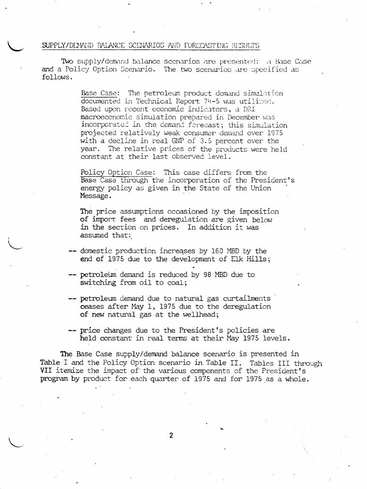
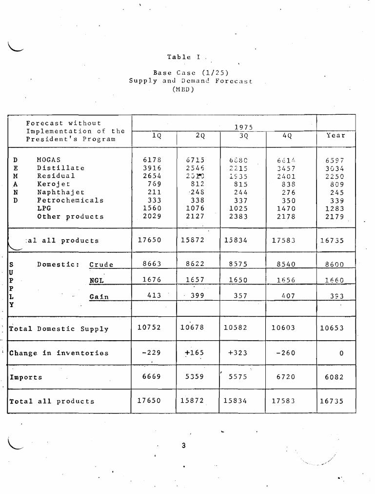
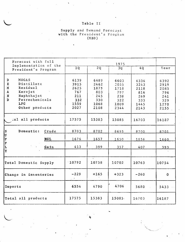
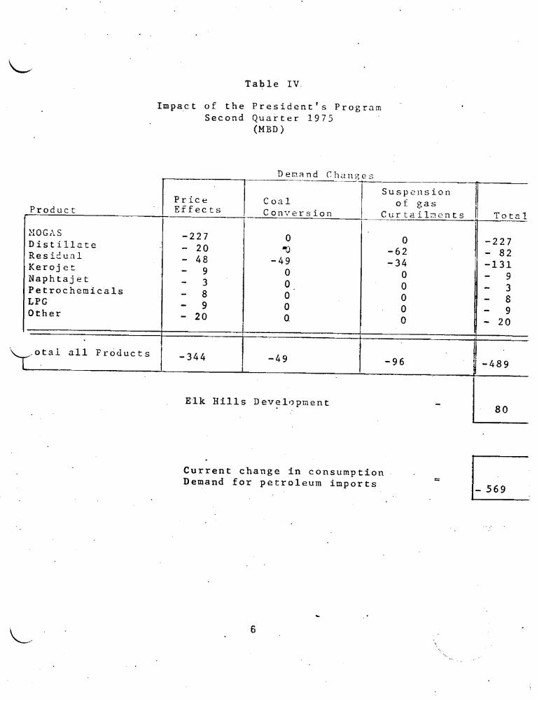
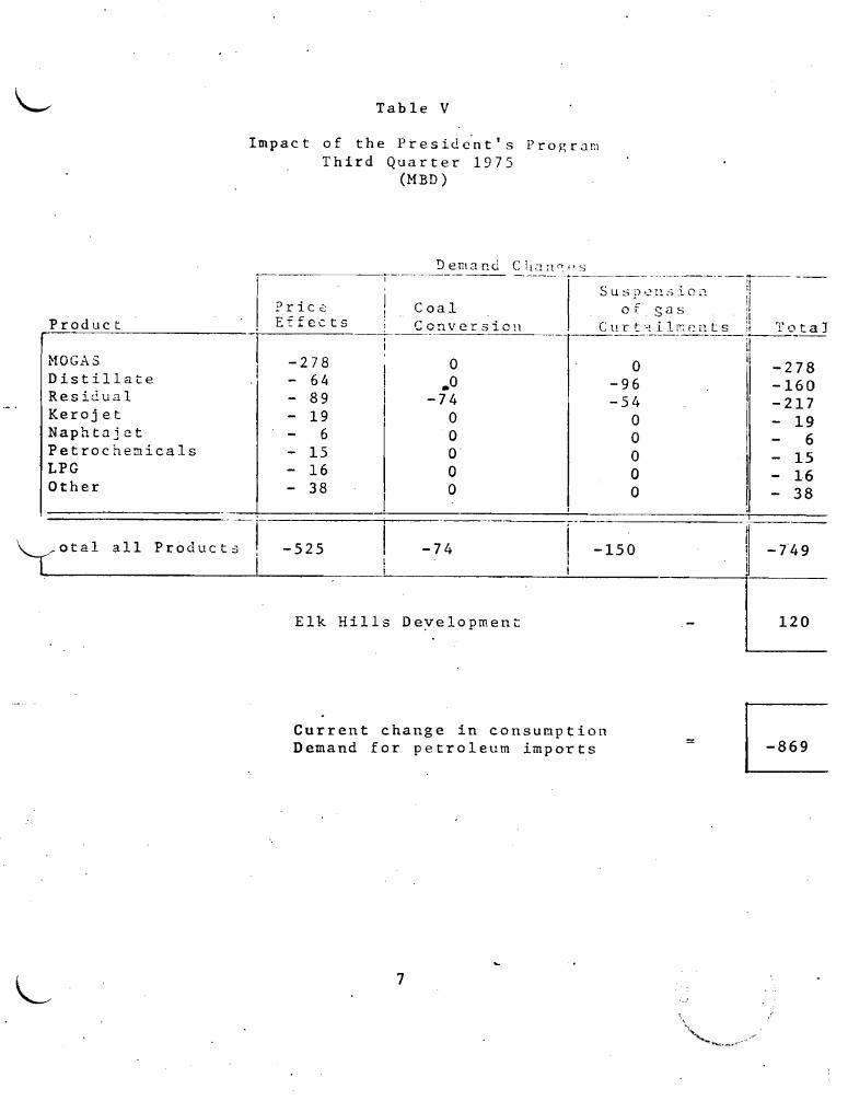
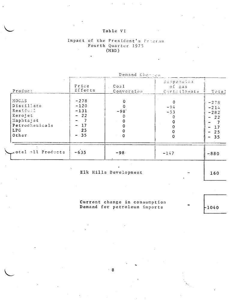
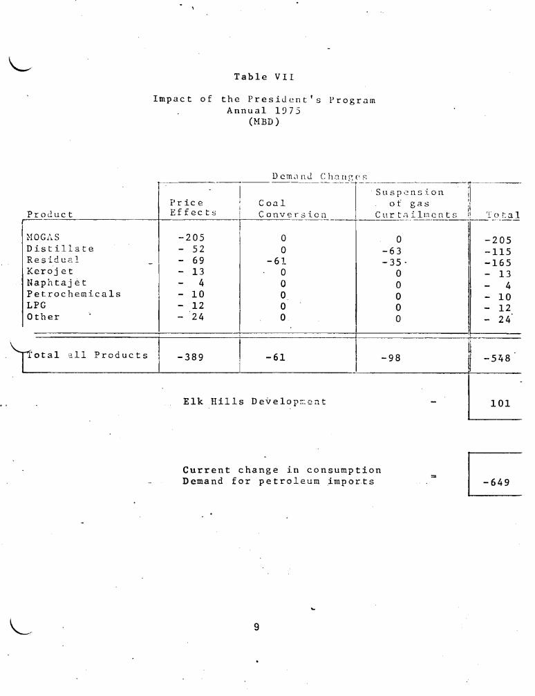
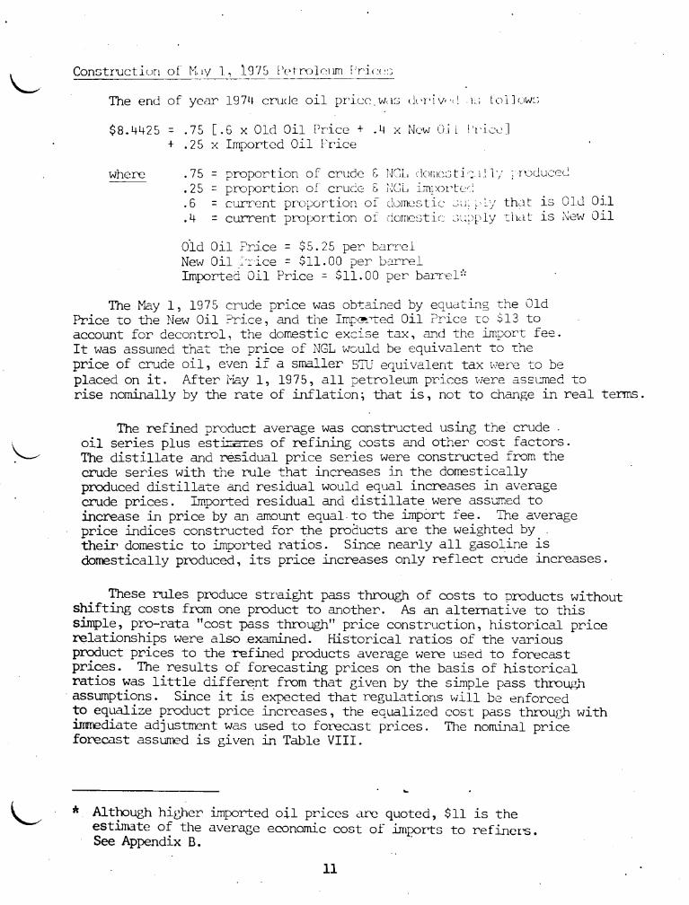
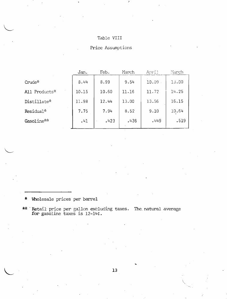
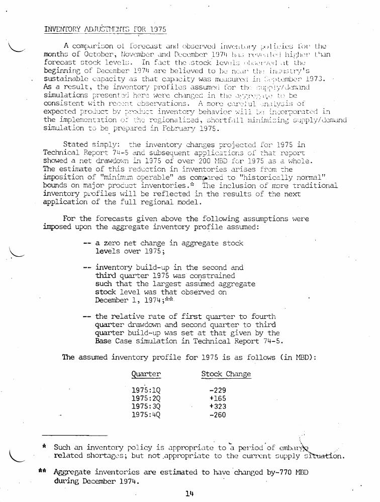
Series
I II
y--
L
C()in)iRI~)Oti~ or LOTi[ n~c)J)UCT [)i~]i)
(Imi)
21000-+shyI I
200001shy
190001 I
180COt
17000j
16000shy
1 15000
14000
bull
t I I X~ I r~I
bull bull
bull I
13000shy -t--t---t----t--I---t------ l~o~ 1970 1971 197a 1973 1974 1975
Prc-Dnl_urgo ForccCts t ~-------
Incorr2 cmd -e~lthcr effects - - - - - - -l1iee Effects added to Income clnd ltcdthcr Effcots Actual 19711 Pn2sicl~nts PrDgral1l 1975 - - - -
~r _ bullbull Lmiddot
18
~
---- _shy
J i
COHlAhISIH ()i LulM j-UDL~~ IJi) (l1 t~[) )
22000 -I
cH00Co+ I t
i 200C0-t-
I I
19000~
l~ I bull I 18000
i I bull
I ~ I ~
I - shy
I I I
I I I
I
170001
160001 ~
I bull I
I v- bullbullbull
15000
1974
-
1975
I
~ _______ __ - _~___ __ bull _______bullbullbull - _______ ______bullbull ~__ ______ ~_ _ ____ 0
Series
I II
Pre-Dnbcugo Forecast Income c1I1d Jeather L-f---l-~C-C--ts------------- -
Price Iffccts ilddcd to Income Clnd kalhcr Effects Actual 197LJ Presidents Prorr~1J~ 1975 - - - - bull
____ _ _- - ---- -- - or -~ ~~ -~ --or ---r~-_~________ 0_
19
CU)~~f~()l~~ ~l~ l~lt1 ~middot(~ll~(I ~~ (i1l ~~ l(~lL lmiddot ~ LI j~)
lC2-T
lOOT I
I J bull
g8i -
I
Ii
96-Tshy
I I I 01 bullbull I94--- i ~ I ~
92--- I
9C i 881
I 86
84 ----
82shy
1975
Series
I rn~-Lbarfgto Fot~(Cl3t II IncQl~ and J~lthcr E1-tc-~lS - - - shy
I-1ice Effects ~lddcj to Incorrc and ~~L1thcr Effects Actual 19711 PresiJcnt s Pl)D~Clffi 195 - 0 - 00 - 0 shy
~- --_-_ - - --- ----1middot- - ~middotmiddotmiddot1-- ~~
20
Series I Series II Series II Series iV
Series I Series II Series III Series IV
COMPARISO~JS OF TOTL [FODlICI )r~IJ 1
(MBD)
~ -- 1 - -~- -- -+ bull -
-l 1 ~ ~ -4 (I ~_ bull ~ 1- L~ ~~ 1 ~=- ~ 1 i~ l -+ bull --~ ~ 1 -- 2 1 bull (i 1 -t 1 ~~ bull 1 4 ( (i bull=i 1 S C 1 ~ ~ - 11 ~ ~ bull 7~ ~- 1 ~ cmiddot r 4 ~ r
1~74 1~75
17879S~1 19046637 17613112 1782S4G~
16771089 1~734724 1626297 16186571
21
---~----
COf1JlniJj ClI tlC)[(j (JXl[[ ltjjl
(fmiddot1EI))
7500
I
7000-r
i 65001
I 6000-r
I I
I I
5500+
til
bull
5000shy _ -shy 1-- --l- middotmiddot----middotr--middot-t----+----t----I 1909 97 1971 1972 1973 1974 1975
shy - - ___ _ _shy __ - --shy -- --
Series
I Pre-Dnbargo Forecwst II Income i-md -leather EmiddotE~ro--e-c--ts------------ -
III Price Effects added to Incorn~ wIld leather Effects IV Actuli 19711 Presicknts Pr)~nlIn 1975 - --
r~ bull r~ ~ ~-~- ~r-~ ~-1-~- -~ ~~T-- -~ ~~~ vr-~ bullbullr- ~~-
22 ~ ~---~
bull bull
bull bull
(iIi))
760O I
7400-fshy
i
7200-i 1
I 70001 I
JY ~ I bull
1 ~
Imiddot 6seej I I
bullbull ~
~ ~ I 6600 bull I
I bull bull l I I bull I
6400-4-
I I I
F _- r bull 1 bull f I
6200 I s J6000
I 5800
H~7 1975
Series
I Pre-Dnb-lrrO ForecClst ~~-------------II Inconc anu -Jelthcl- Effects - - - - - - shy
Price rffccts aJdLcl to Income cmd veJthcr Effects Actual 19711 Presidents Prq~tun 1975 - - - -
_____ --__ _ __ - ___ __ _r_______ _ _ -- _ ___ bull - - -~ - - -- --
23
_r_
COilPMISjgtI OE iIJl(lmiddot~ Cmiddotlrri id~~[) (Ln plrt-~llcl(gt _middott~~~)
102- I
i i
100--_~-------------------------------------- bull
98-- I -s~~~ bull - - bull --IP- -
I -----shy ---96~ shy
I J ~- 94 _ - 1
1 - --- --- I
Sla-+
- - shy_ --------4-----------lss-+-shy1974 1975
---- - -- - -- ---~-- -- -__ -~- -- - --shySeries
Pre-DnhlI~(TO ForeccJst lt i I tl lt~0
II IncOolc (Inc -J(~athcr Lffccts - - - - - - - t
Price lffccts added to lnconc and -JeClthcr Effects U Actln1 19711 Presidents PrDir-eul1 1975 - - - -
If-----~bullbull ~~-~-_
L
Series I Series II Series III Series IV
Series I Series II Series III Series IV
COMPNUSOtJS
5 ~~ l ~ bullC ti t 0 c Ur
5S~~206
52 ~ 2 I)~
1974
689155 6746946 6467523 6496869
or nUlUI- CJsoLIr~r DI iI (HG))
- 1 bull + ( - n1 ~ bull 1 1 -= 4 1 bull ~ t 4 bull (1 ~
= - 1 bull 1 7 I 1 ~=- 1 ~- 1 ~ 1 bull 2 --+ r_~ bull ( 57~1 476 ~Olc15 6~~1 24~ 662S~
5( = 1 bull 4 ( t ~ Ci 1~ bull 1 1 Co = ~ 1 bull ~ 4 - 1 bull 254bull
1375
7076738 6S65342 6596793 6391458
25
middot
cmu[I~OilS or DJ STILlAn DI -~o~[) (i1HO)
5000-y-
I 45001 4000J
I
- shy bull --shy --shy -
Series
I II
III IV
3500
I
3000~
2000
1500 -t-_--tmiddot_--middotmiddott--i 1969 97~ g7 ~7a 1~73 1974 1975
-~-- _ _ - _ ___ o_ bullbullbullbull _ bull __
Pre-Dnbar~o Forecast ~--~~~------
Income and He1thcr Effects - - - - -Price Efftcts added to Income and Ieather Effects ActnJ1 197L~ Jresidents PrUrnU11 1975 - - - -
~
--~ -
CC)fF~I~(XJS or DISTI [[ ATL gt LU (HBD)
I
4500-middot
4000-+
I 3500-+
30130 I
2500
2000
I
1 I
11 I I
11 II I
1 bullbullbull bull
_
1500-r-------------+-----------~--~ 1975
- __ _--_ - - _-----_ -- __ -- ----shy -~----~ ---~-- ~ ------- o
Ser-ies
I II
Prc-DnbJrfo Forecls t ~---------------
Incorni~ mcl ]lJtlk~ Effects Price Effects adi -c1 tu Inox~ and euthcr Effects ActU11 19711 F11~sidcnts PrOtnun 1975 - - -
~- __ __~__ -- _ --- __ _~~ __ __ ~_~-~ middot middot~--middot bullmiddot 1--middotmiddot
COtil-WL 0 (JL [) I I LI lL ilJ~ Ji) (ill ~)(I((liLt LlJIIL)
1013--shy
shy 1 eo-~----~
I
~
shy9S-T t ~
se
bull ~
~ l - ~
I
I
7S-+-shy
1975
Sepjes
I Prc-Dllburgo Forerd~ t ~--~----------II I11C0112 cUlll vcllhc~l l~frccts - - - - - - shy
Price Ef1cts Jedcd to Income nne Wcalhl~r Effects Actual 19711 Presidcnts Prognun 1975 - - shy
_ ___ - I ~4~
8
COr1fARISOrJ~ or DL3T[LLJTi DlVjj[i
Series I Series II Series III Series IV
Series I Series II Series III Series IV
= 4 - 1 -
J - 1 bull 471 5= 24 i 1 bull (l5~
1374
3224843 3161426 301S302 2399126
(HBD)
1970
2 -- -1- t bull ( 1- 2 4 bull (i 1 ~
St 4 bull i)1 -
4 4 bull (I 1
1375
34~1 554 3227345 303~582 2918757
29
1~71
2~rt ~ bull - CI ~ -- _~ -1-
2~~ - ~ ( - bull I
- bull I -t
~ ~ bull 1~1J (
Series
I II
III
- - ~
COmiddot1i Ar l~U r~ ()l I ~ mU([ [)[ Emiddot iU WHO)
4eo-middotI
I i
I
3500-r
3000~
2500
2000
I Ibull
1500 _-_t--t--shy
1
I I
I I middot r~ I V I
~ I I t I I Ib bull v 1 I I
1 bull I
bull bull 1 I I
t 1 I I
10middotbullf I
196~ 1970 lS7 1972 1973 1974 1975
~~-- - ~-- __---shy -~- ~--- --- -----~ -_ ~~ -- --~
Pre-Embar~o Forecust Inco( and ctither [irects - - - - - - -Price Effects added to Income clnu hcathcr rffect~
T Aetu1l197LI Prcsjc1enls ProgYun 1975 _ _ _ _ ~ -y-- 1 bullbull~ -~ - - -middotmiddot--Il~---~-lt f+ ~~ ~r__-----~___ ~_middot
30
~-
j1 bullbull
bull I
I3500-shy
middotL_~-middot _ -____
I II f
I 14 I I I bullbull
bull I bull bull
I bullbullbull
1- - aS00 bull bull I bull bull t bull bull
I til bull _ t
2000
I
shy1500-+-shy
197~ 1975
Series
I Pre-Dnbar[o ForecClst ~~------------II Income and -]_1 thoI F ffCcts - - - - - - shy
III Price poundffcc ts added to Incoc and H-~dther Effects IV AetLll1 19711 Flgt2sidcnts P1D3ram 1975 - - -
- -- ~ r bullbull ~_
31
bullbull --
t ii t l)l I ~)[ ) eli ~iIJ
(in lT((~llt We 1tlC)
1ec----~------+~---------------
I I - I --
i i
I
9~-+ bullbull e bull
~ 80
~bullbull
bullbull ~- ~
til ~70 -----
bull
G0 - -
50+--------t------l 1975
Series
I Prc-Ln8~r~O rorec~st
II Incon imJ t-1lhct effects - - - - - - shyIII Price Effects 1dcl-J to InC(Xll(~ LInd Weather [Ffect
TI ActLlCl1 107 l l FnsiJetlts PloUdm 1975 - ~
32
COMfARISCgtJS OF [middotTSHJJL DGlinl (1BD)
Series I 1~7~ =4 ~c (Ibull - ishy
Series II 1 ~ ~ -- ~~ -=~ r--~ bull - (t -Series T7T
---1~ rmiddot~~-middot~middot ~middot4 ~ l~ - Cl~Series IV 19964 22u~0~
174 1975
Series I 2930882 244806Series II ~a1743~ 27J5381Series III 2503294 224994SSeries IV 2749009 2094824
33
c~~ ~I I L~middot4 bull I~ 1 ~ t bull I~~ ~c ~~ - I~ ~ ~bull - I I 1 -=- 4- 5 ~~ ~ -= ~ -_r~4 I~I ~ I 2 ~~ i ~ 1 ( bull
2~~~8~~ ~S4~~Gl
bull
C011PARISOi or SELICno S (TlCl T
The short run elasticity estirmtcs LcOl1Xr 1 t~(( in thc El short-tenn orcc2stirL6 procccicrc arc difficult t(1 ~Liut particularly in -hc case of dislggregcltcc] pDXJllC t --i tctorit-s Represe1tativ~ e ~Lic~ty estirrldtt2S plusmnnJm cl~ tC~l C 3 U_ P
presented L1 3b~c ~ for ptlrposes of corparison to icc l LC 1C
general plac3~biJi[y of the figures usee in the ClC2OLS 1iO2rer~ the precise interpretaTion or applicatio of th2S CSCLCS should not be attertcdout of conteAt of the Tilcdels in ihid) thoj ctYe
developed the til1e frames to Hhieh they are applie 0 -he definitions used L~ L~eir computation lhe elastici-ies ~rese~ted are calculated 0 a consistent basis but are intencec to be only summary indicators of the price sensitivicy of the alcen1ace ~dels 1m accurate staternent of the price response of other oGels 1middotolJld require direct application of the full model to price amp10 other changes
34
TIBLE AI
ESTHilTES or r1 rnrr rUISTICTTY or rEr~rrm --~---prTEonllfl~I)-f)ilaquo)I)IJll~lF-- shy
------ ~- -
SflOI r IU~l (Upmiddot(omiddotr YCcl r )
Houthukker Vcr 1 (Hj C) [ Hudson-
fEI1 Sheehan3 Ph 1i 1S~ Jo rgc ns Ot~lj___---J _____ __
All Pe tro1~ uamp1 -10 -10 -10 -11
Gasolinel -10 (-15) -09 (- 14) -07 (-11) - 13 (-20) Distillute -12 Residual -21
bullKerojet -08 Naphthajet -08 LPG -05 Petrochemi ca1s - 16 Other Products -05 - 1middot Estimates of gasoline elasticity relate to retail prices extax shmmiddotm in parentheses - All other estimates relate to wholesale prices or have been converted to wholesale
prices under the assumption that cost pass-throughs occur without proportional markups
2 Consensus estimate by Troika CEA Treasury OMB and FEA - 1974 3 Prepared by EPA and CEQ - December 1973
Phlips L IIA Dynamic Version of the Linear Expenditure ~~odel II The Reviemiddot of Economics and Statistics Vol LIV No 4 (Nov 1972) pp 450-465- shy
DR Energy Forecast January 1975 Chase Econometric Analysis January 24 1975 For Ford Foundation - 1974 All elasticities relate to wholesale prices except that in the case of gasoline the second figure in () relates to the retail price before excise taxes In judging the relative degree to which different products respond to price the wholesale figures provide the best indication They indictlte thtlt gClso1ine is less responsive than some other product
The eltlsticity figu)e is hi~Jhcr fo) the retail pricr thun for the lho1fs11e price That is beclluse the elasticity is the ratio bet((n~ thp f)(I-~P~lt~HJ~) Clhln~Jl in COI1shy lTlpti on and the Eecent-~~l~ change in pri ce A 10c Chl))(Jl for eXdflp Ie JOul d )H~
W~~ change in a 2c 11010stl10 price but only a 251 chan(j( in J lt10( rotdil pIice ishy
-a1us the denominator of the ~lasticily figlwe Ou1d be gn~i1lr~I in the Ci1e of the wholesale price than in the case of the retail price lIovewl if the chJngc in actucl1 consumption - the numerator remains the same the elastiCity figurcchlngcs 35--
NlLilDL l)
Ibrrcstic Ncw Oil Clnd Importcri Crude l)rj (
The current avc~~[e prJcc of irl-Ortcd crude r(T)~t-d tc the FEA for the cost pJ~thrCJlJrj j ~12 53 per bdrrel C~r~~Jt)
New oil prices currcntly wcnlge Jbout $1083 per brt~l lUS
appendix c~iscLsses eli ferenccs be t1tJeen tl1C declaredmiddot ~ middotCTOUC
price of cruce
One important reason for the difference is the rrehoc of valuatLTlg in~orted oil for the cost passthrough Current~ thele are thrce basic types of purc1ases of foreign crude eqJity participation and third party Equity oil is that oil roduced and ovmed by the concessionaire (e g Fpoundamco) under a~eent ith the host country Since the concessionaire olaquos the oil there is no purchase price per se However the host country charges the concessionaire taxes a1d royalties on this oil The sum of these taxes and royalties plus the cost of producing the oil is the tax paid cost and represents the real cost of the oil to the concessionaire Although there have been increases in tax and royalty rates in recent months during 1974 tax paid costs were lower than the price of crude sold to non-concessionaires
The second type of purchase pa-rtlclpation oil is that oil produced by the concessionaire vIhich the host COW1try owns as a result of a participation agre~~ent and which the host government sells to the concessionaire at a negotiated price For exarr~le sixty percent of the oil produced by Aramco is owned by Saudi Arabia
and Saudi Arabia sells the rrajor portion of this oil back to companies of Ararnco at the buyback price which currently is $1046 per barrel
The third type of purchase third party purchases is oil purchased by any company either from the host government or the concessionaire This price may be viewed as a free market price although this price will vary depending upon purchase terms (ie quantity and date of delivery) During 1974 at times third party purchase prices were higher than both government ta~ paid costs and buyback prices During the first quarter some third party purchases ran in excess of $2000 per barrel
36
lor puq)O~CS of the cu~t-Pd~~~tltn)u(~h rCdJl~tmiddot~ VdllJC tgtl1VI)d~k oiJ and thirCl Jgtdrty [gttJrchltl~c oil dL purcfldC IWlCC [Lue IlmiddotI[p)dILiull co~ l ~md fcc
However for equity crude refiners Ire pcnn-i t tcd t() (( t
value on the i r (qui ty crucic hhich JouLd ptev Ii] if trwy 11 1 III with their elft i liatul -lltiLimiddot clt arm -Jellith In (middotfilet (Iii means that tIle rcCjncY ITny _harrc hinlJcl~ (i plicc e)I Iii ltqui lj crude whicil l([IIL thc lhi~j i)cilLj llllldld( twice The l~J fj-ewc for imp)YtcJ erucic inchclc C(luity cnldc middothic1 i~ llIC(
above its Clilcll CO~3t 10 the rcfincr Al30 then i [hI il factor of tlle U s trcutln(~rlt of tucs pc1id c)n C(lltiL~l ClU( Jc~ fdCS
paid to hos t g()verrJTlent~ ~lre the basis for foreiGn t2X C1cclit) and this may reduce the real costs of equity crude In this sense the $1253 figure overstates -he real costs of iJljJOrtcd ClUJC 0
the refiner Thus the difference between the pcices of neVI oil and impcrted oil reported for the cost p~stht)J~Jl dues not
necessarily reflect the difference in nal costs to the refiner
The real difference in cost is difficult to determine New Oil prices are still rising and have not stabilized but it is safe to assume that they will stabilize at sonE price below $1253 which would represent an equilibrium between the real costs of impcrted oil and the price of new oil
Although institutional complexities complicate the determination of impcrted crude prices the equilibrium price of ned domestic crude and the oppcrtunity cost of acquiring imported crude will be the same Therefore the analysis ill this study assumes an imported oil price of $11 per barrel the approximate price of New Oil
37
I
- 002500064-2
- 002500064-2
-
bull bull
bull bull
(iIi))
760O I
7400-fshy
i
7200-i 1
I 70001 I
JY ~ I bull
1 ~
Imiddot 6seej I I
bullbull ~
~ ~ I 6600 bull I
I bull bull l I I bull I
6400-4-
I I I
F _- r bull 1 bull f I
6200 I s J6000
I 5800
H~7 1975
Series
I Pre-Dnb-lrrO ForecClst ~~-------------II Inconc anu -Jelthcl- Effects - - - - - - shy
Price rffccts aJdLcl to Income cmd veJthcr Effects Actual 19711 Presidents Prq~tun 1975 - - - -
_____ --__ _ __ - ___ __ _r_______ _ _ -- _ ___ bull - - -~ - - -- --
23
_r_
COilPMISjgtI OE iIJl(lmiddot~ Cmiddotlrri id~~[) (Ln plrt-~llcl(gt _middott~~~)
102- I
i i
100--_~-------------------------------------- bull
98-- I -s~~~ bull - - bull --IP- -
I -----shy ---96~ shy
I J ~- 94 _ - 1
1 - --- --- I
Sla-+
- - shy_ --------4-----------lss-+-shy1974 1975
---- - -- - -- ---~-- -- -__ -~- -- - --shySeries
Pre-DnhlI~(TO ForeccJst lt i I tl lt~0
II IncOolc (Inc -J(~athcr Lffccts - - - - - - - t
Price lffccts added to lnconc and -JeClthcr Effects U Actln1 19711 Presidents PrDir-eul1 1975 - - - -
If-----~bullbull ~~-~-_
L
Series I Series II Series III Series IV
Series I Series II Series III Series IV
COMPNUSOtJS
5 ~~ l ~ bullC ti t 0 c Ur
5S~~206
52 ~ 2 I)~
1974
689155 6746946 6467523 6496869
or nUlUI- CJsoLIr~r DI iI (HG))
- 1 bull + ( - n1 ~ bull 1 1 -= 4 1 bull ~ t 4 bull (1 ~
= - 1 bull 1 7 I 1 ~=- 1 ~- 1 ~ 1 bull 2 --+ r_~ bull ( 57~1 476 ~Olc15 6~~1 24~ 662S~
5( = 1 bull 4 ( t ~ Ci 1~ bull 1 1 Co = ~ 1 bull ~ 4 - 1 bull 254bull
1375
7076738 6S65342 6596793 6391458
25
middot
cmu[I~OilS or DJ STILlAn DI -~o~[) (i1HO)
5000-y-
I 45001 4000J
I
- shy bull --shy --shy -
Series
I II
III IV
3500
I
3000~
2000
1500 -t-_--tmiddot_--middotmiddott--i 1969 97~ g7 ~7a 1~73 1974 1975
-~-- _ _ - _ ___ o_ bullbullbullbull _ bull __
Pre-Dnbar~o Forecast ~--~~~------
Income and He1thcr Effects - - - - -Price Efftcts added to Income and Ieather Effects ActnJ1 197L~ Jresidents PrUrnU11 1975 - - - -
~
--~ -
CC)fF~I~(XJS or DISTI [[ ATL gt LU (HBD)
I
4500-middot
4000-+
I 3500-+
30130 I
2500
2000
I
1 I
11 I I
11 II I
1 bullbullbull bull
_
1500-r-------------+-----------~--~ 1975
- __ _--_ - - _-----_ -- __ -- ----shy -~----~ ---~-- ~ ------- o
Ser-ies
I II
Prc-DnbJrfo Forecls t ~---------------
Incorni~ mcl ]lJtlk~ Effects Price Effects adi -c1 tu Inox~ and euthcr Effects ActU11 19711 F11~sidcnts PrOtnun 1975 - - -
~- __ __~__ -- _ --- __ _~~ __ __ ~_~-~ middot middot~--middot bullmiddot 1--middotmiddot
COtil-WL 0 (JL [) I I LI lL ilJ~ Ji) (ill ~)(I((liLt LlJIIL)
1013--shy
shy 1 eo-~----~
I
~
shy9S-T t ~
se
bull ~
~ l - ~
I
I
7S-+-shy
1975
Sepjes
I Prc-Dllburgo Forerd~ t ~--~----------II I11C0112 cUlll vcllhc~l l~frccts - - - - - - shy
Price Ef1cts Jedcd to Income nne Wcalhl~r Effects Actual 19711 Presidcnts Prognun 1975 - - shy
_ ___ - I ~4~
8
COr1fARISOrJ~ or DL3T[LLJTi DlVjj[i
Series I Series II Series III Series IV
Series I Series II Series III Series IV
= 4 - 1 -
J - 1 bull 471 5= 24 i 1 bull (l5~
1374
3224843 3161426 301S302 2399126
(HBD)
1970
2 -- -1- t bull ( 1- 2 4 bull (i 1 ~
St 4 bull i)1 -
4 4 bull (I 1
1375
34~1 554 3227345 303~582 2918757
29
1~71
2~rt ~ bull - CI ~ -- _~ -1-
2~~ - ~ ( - bull I
- bull I -t
~ ~ bull 1~1J (
Series
I II
III
- - ~
COmiddot1i Ar l~U r~ ()l I ~ mU([ [)[ Emiddot iU WHO)
4eo-middotI
I i
I
3500-r
3000~
2500
2000
I Ibull
1500 _-_t--t--shy
1
I I
I I middot r~ I V I
~ I I t I I Ib bull v 1 I I
1 bull I
bull bull 1 I I
t 1 I I
10middotbullf I
196~ 1970 lS7 1972 1973 1974 1975
~~-- - ~-- __---shy -~- ~--- --- -----~ -_ ~~ -- --~
Pre-Embar~o Forecust Inco( and ctither [irects - - - - - - -Price Effects added to Income clnu hcathcr rffect~
T Aetu1l197LI Prcsjc1enls ProgYun 1975 _ _ _ _ ~ -y-- 1 bullbull~ -~ - - -middotmiddot--Il~---~-lt f+ ~~ ~r__-----~___ ~_middot
30
~-
j1 bullbull
bull I
I3500-shy
middotL_~-middot _ -____
I II f
I 14 I I I bullbull
bull I bull bull
I bullbullbull
1- - aS00 bull bull I bull bull t bull bull
I til bull _ t
2000
I
shy1500-+-shy
197~ 1975
Series
I Pre-Dnbar[o ForecClst ~~------------II Income and -]_1 thoI F ffCcts - - - - - - shy
III Price poundffcc ts added to Incoc and H-~dther Effects IV AetLll1 19711 Flgt2sidcnts P1D3ram 1975 - - -
- -- ~ r bullbull ~_
31
bullbull --
t ii t l)l I ~)[ ) eli ~iIJ
(in lT((~llt We 1tlC)
1ec----~------+~---------------
I I - I --
i i
I
9~-+ bullbull e bull
~ 80
~bullbull
bullbull ~- ~
til ~70 -----
bull
G0 - -
50+--------t------l 1975
Series
I Prc-Ln8~r~O rorec~st
II Incon imJ t-1lhct effects - - - - - - shyIII Price Effects 1dcl-J to InC(Xll(~ LInd Weather [Ffect
TI ActLlCl1 107 l l FnsiJetlts PloUdm 1975 - ~
32
COMfARISCgtJS OF [middotTSHJJL DGlinl (1BD)
Series I 1~7~ =4 ~c (Ibull - ishy
Series II 1 ~ ~ -- ~~ -=~ r--~ bull - (t -Series T7T
---1~ rmiddot~~-middot~middot ~middot4 ~ l~ - Cl~Series IV 19964 22u~0~
174 1975
Series I 2930882 244806Series II ~a1743~ 27J5381Series III 2503294 224994SSeries IV 2749009 2094824
33
c~~ ~I I L~middot4 bull I~ 1 ~ t bull I~~ ~c ~~ - I~ ~ ~bull - I I 1 -=- 4- 5 ~~ ~ -= ~ -_r~4 I~I ~ I 2 ~~ i ~ 1 ( bull
2~~~8~~ ~S4~~Gl
bull
C011PARISOi or SELICno S (TlCl T
The short run elasticity estirmtcs LcOl1Xr 1 t~(( in thc El short-tenn orcc2stirL6 procccicrc arc difficult t(1 ~Liut particularly in -hc case of dislggregcltcc] pDXJllC t --i tctorit-s Represe1tativ~ e ~Lic~ty estirrldtt2S plusmnnJm cl~ tC~l C 3 U_ P
presented L1 3b~c ~ for ptlrposes of corparison to icc l LC 1C
general plac3~biJi[y of the figures usee in the ClC2OLS 1iO2rer~ the precise interpretaTion or applicatio of th2S CSCLCS should not be attertcdout of conteAt of the Tilcdels in ihid) thoj ctYe
developed the til1e frames to Hhieh they are applie 0 -he definitions used L~ L~eir computation lhe elastici-ies ~rese~ted are calculated 0 a consistent basis but are intencec to be only summary indicators of the price sensitivicy of the alcen1ace ~dels 1m accurate staternent of the price response of other oGels 1middotolJld require direct application of the full model to price amp10 other changes
34
TIBLE AI
ESTHilTES or r1 rnrr rUISTICTTY or rEr~rrm --~---prTEonllfl~I)-f)ilaquo)I)IJll~lF-- shy
------ ~- -
SflOI r IU~l (Upmiddot(omiddotr YCcl r )
Houthukker Vcr 1 (Hj C) [ Hudson-
fEI1 Sheehan3 Ph 1i 1S~ Jo rgc ns Ot~lj___---J _____ __
All Pe tro1~ uamp1 -10 -10 -10 -11
Gasolinel -10 (-15) -09 (- 14) -07 (-11) - 13 (-20) Distillute -12 Residual -21
bullKerojet -08 Naphthajet -08 LPG -05 Petrochemi ca1s - 16 Other Products -05 - 1middot Estimates of gasoline elasticity relate to retail prices extax shmmiddotm in parentheses - All other estimates relate to wholesale prices or have been converted to wholesale
prices under the assumption that cost pass-throughs occur without proportional markups
2 Consensus estimate by Troika CEA Treasury OMB and FEA - 1974 3 Prepared by EPA and CEQ - December 1973
Phlips L IIA Dynamic Version of the Linear Expenditure ~~odel II The Reviemiddot of Economics and Statistics Vol LIV No 4 (Nov 1972) pp 450-465- shy
DR Energy Forecast January 1975 Chase Econometric Analysis January 24 1975 For Ford Foundation - 1974 All elasticities relate to wholesale prices except that in the case of gasoline the second figure in () relates to the retail price before excise taxes In judging the relative degree to which different products respond to price the wholesale figures provide the best indication They indictlte thtlt gClso1ine is less responsive than some other product
The eltlsticity figu)e is hi~Jhcr fo) the retail pricr thun for the lho1fs11e price That is beclluse the elasticity is the ratio bet((n~ thp f)(I-~P~lt~HJ~) Clhln~Jl in COI1shy lTlpti on and the Eecent-~~l~ change in pri ce A 10c Chl))(Jl for eXdflp Ie JOul d )H~
W~~ change in a 2c 11010stl10 price but only a 251 chan(j( in J lt10( rotdil pIice ishy
-a1us the denominator of the ~lasticily figlwe Ou1d be gn~i1lr~I in the Ci1e of the wholesale price than in the case of the retail price lIovewl if the chJngc in actucl1 consumption - the numerator remains the same the elastiCity figurcchlngcs 35--
NlLilDL l)
Ibrrcstic Ncw Oil Clnd Importcri Crude l)rj (
The current avc~~[e prJcc of irl-Ortcd crude r(T)~t-d tc the FEA for the cost pJ~thrCJlJrj j ~12 53 per bdrrel C~r~~Jt)
New oil prices currcntly wcnlge Jbout $1083 per brt~l lUS
appendix c~iscLsses eli ferenccs be t1tJeen tl1C declaredmiddot ~ middotCTOUC
price of cruce
One important reason for the difference is the rrehoc of valuatLTlg in~orted oil for the cost passthrough Current~ thele are thrce basic types of purc1ases of foreign crude eqJity participation and third party Equity oil is that oil roduced and ovmed by the concessionaire (e g Fpoundamco) under a~eent ith the host country Since the concessionaire olaquos the oil there is no purchase price per se However the host country charges the concessionaire taxes a1d royalties on this oil The sum of these taxes and royalties plus the cost of producing the oil is the tax paid cost and represents the real cost of the oil to the concessionaire Although there have been increases in tax and royalty rates in recent months during 1974 tax paid costs were lower than the price of crude sold to non-concessionaires
The second type of purchase pa-rtlclpation oil is that oil produced by the concessionaire vIhich the host COW1try owns as a result of a participation agre~~ent and which the host government sells to the concessionaire at a negotiated price For exarr~le sixty percent of the oil produced by Aramco is owned by Saudi Arabia
and Saudi Arabia sells the rrajor portion of this oil back to companies of Ararnco at the buyback price which currently is $1046 per barrel
The third type of purchase third party purchases is oil purchased by any company either from the host government or the concessionaire This price may be viewed as a free market price although this price will vary depending upon purchase terms (ie quantity and date of delivery) During 1974 at times third party purchase prices were higher than both government ta~ paid costs and buyback prices During the first quarter some third party purchases ran in excess of $2000 per barrel
36
lor puq)O~CS of the cu~t-Pd~~~tltn)u(~h rCdJl~tmiddot~ VdllJC tgtl1VI)d~k oiJ and thirCl Jgtdrty [gttJrchltl~c oil dL purcfldC IWlCC [Lue IlmiddotI[p)dILiull co~ l ~md fcc
However for equity crude refiners Ire pcnn-i t tcd t() (( t
value on the i r (qui ty crucic hhich JouLd ptev Ii] if trwy 11 1 III with their elft i liatul -lltiLimiddot clt arm -Jellith In (middotfilet (Iii means that tIle rcCjncY ITny _harrc hinlJcl~ (i plicc e)I Iii ltqui lj crude whicil l([IIL thc lhi~j i)cilLj llllldld( twice The l~J fj-ewc for imp)YtcJ erucic inchclc C(luity cnldc middothic1 i~ llIC(
above its Clilcll CO~3t 10 the rcfincr Al30 then i [hI il factor of tlle U s trcutln(~rlt of tucs pc1id c)n C(lltiL~l ClU( Jc~ fdCS
paid to hos t g()verrJTlent~ ~lre the basis for foreiGn t2X C1cclit) and this may reduce the real costs of equity crude In this sense the $1253 figure overstates -he real costs of iJljJOrtcd ClUJC 0
the refiner Thus the difference between the pcices of neVI oil and impcrted oil reported for the cost p~stht)J~Jl dues not
necessarily reflect the difference in nal costs to the refiner
The real difference in cost is difficult to determine New Oil prices are still rising and have not stabilized but it is safe to assume that they will stabilize at sonE price below $1253 which would represent an equilibrium between the real costs of impcrted oil and the price of new oil
Although institutional complexities complicate the determination of impcrted crude prices the equilibrium price of ned domestic crude and the oppcrtunity cost of acquiring imported crude will be the same Therefore the analysis ill this study assumes an imported oil price of $11 per barrel the approximate price of New Oil
37
I
- 002500064-2
- 002500064-2
-
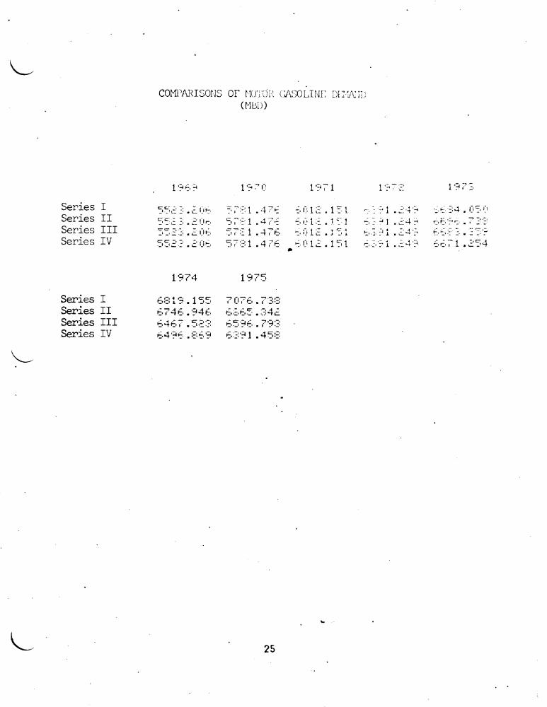
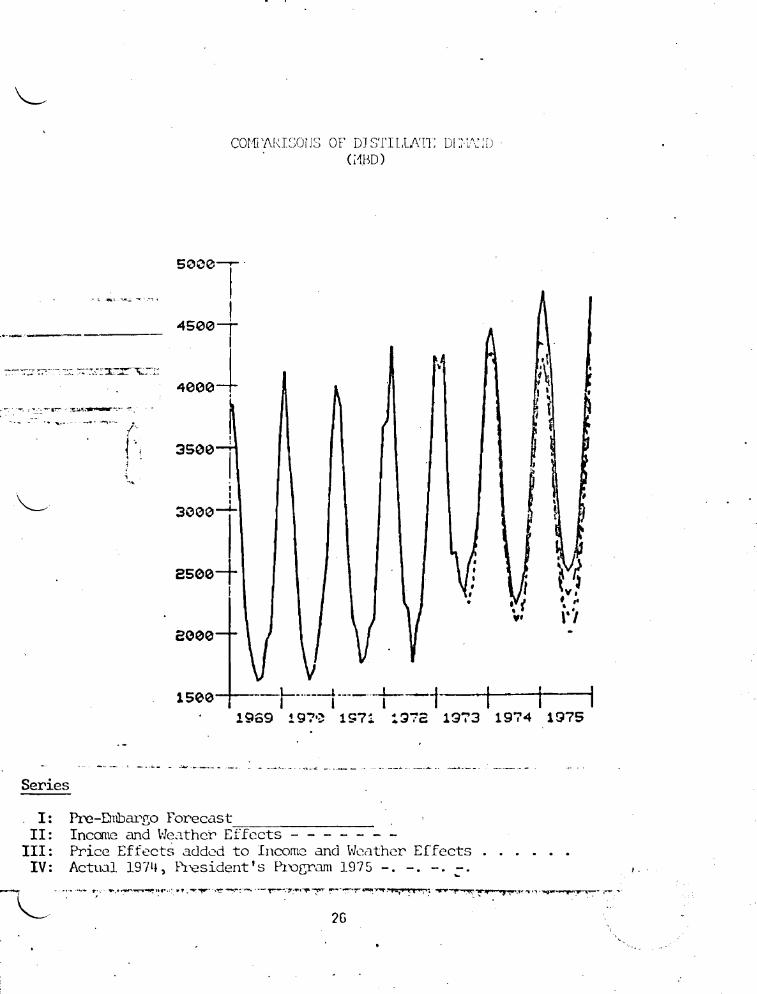
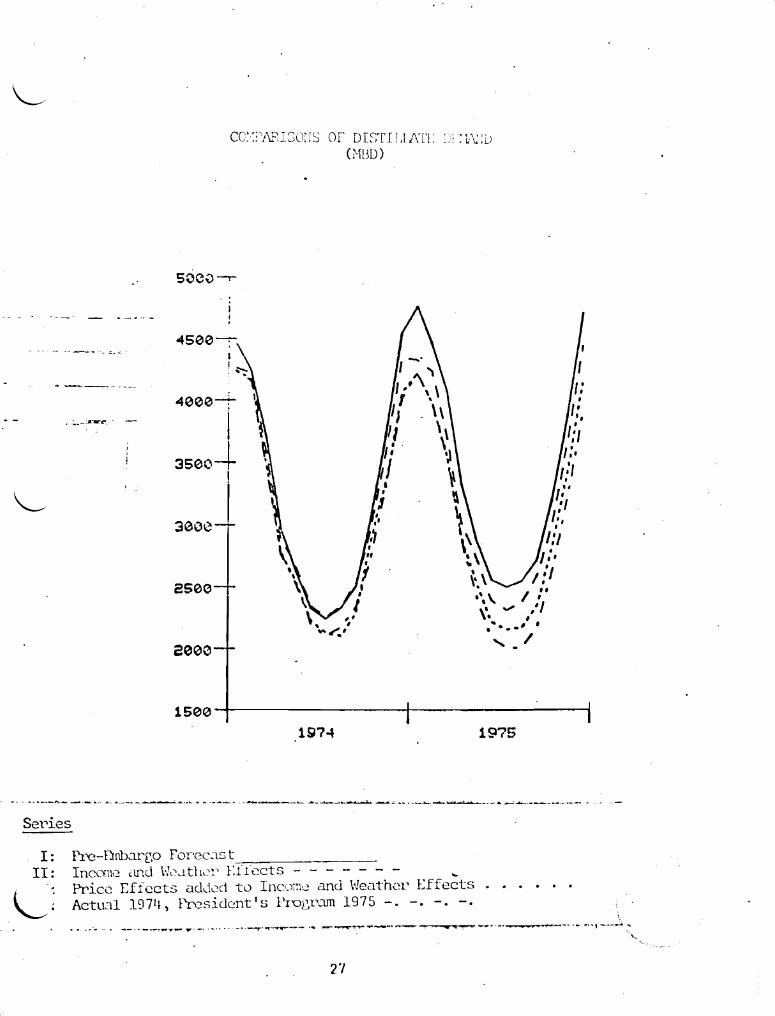

Series
I II
III
- - ~
COmiddot1i Ar l~U r~ ()l I ~ mU([ [)[ Emiddot iU WHO)
4eo-middotI
I i
I
3500-r
3000~
2500
2000
I Ibull
1500 _-_t--t--shy
1
I I
I I middot r~ I V I
~ I I t I I Ib bull v 1 I I
1 bull I
bull bull 1 I I
t 1 I I
10middotbullf I
196~ 1970 lS7 1972 1973 1974 1975
~~-- - ~-- __---shy -~- ~--- --- -----~ -_ ~~ -- --~
Pre-Embar~o Forecust Inco( and ctither [irects - - - - - - -Price Effects added to Income clnu hcathcr rffect~
T Aetu1l197LI Prcsjc1enls ProgYun 1975 _ _ _ _ ~ -y-- 1 bullbull~ -~ - - -middotmiddot--Il~---~-lt f+ ~~ ~r__-----~___ ~_middot
30
~-
j1 bullbull
bull I
I3500-shy
middotL_~-middot _ -____
I II f
I 14 I I I bullbull
bull I bull bull
I bullbullbull
1- - aS00 bull bull I bull bull t bull bull
I til bull _ t
2000
I
shy1500-+-shy
197~ 1975
Series
I Pre-Dnbar[o ForecClst ~~------------II Income and -]_1 thoI F ffCcts - - - - - - shy
III Price poundffcc ts added to Incoc and H-~dther Effects IV AetLll1 19711 Flgt2sidcnts P1D3ram 1975 - - -
- -- ~ r bullbull ~_
31
bullbull --
t ii t l)l I ~)[ ) eli ~iIJ
(in lT((~llt We 1tlC)
1ec----~------+~---------------
I I - I --
i i
I
9~-+ bullbull e bull
~ 80
~bullbull
bullbull ~- ~
til ~70 -----
bull
G0 - -
50+--------t------l 1975
Series
I Prc-Ln8~r~O rorec~st
II Incon imJ t-1lhct effects - - - - - - shyIII Price Effects 1dcl-J to InC(Xll(~ LInd Weather [Ffect
TI ActLlCl1 107 l l FnsiJetlts PloUdm 1975 - ~
32
COMfARISCgtJS OF [middotTSHJJL DGlinl (1BD)
Series I 1~7~ =4 ~c (Ibull - ishy
Series II 1 ~ ~ -- ~~ -=~ r--~ bull - (t -Series T7T
---1~ rmiddot~~-middot~middot ~middot4 ~ l~ - Cl~Series IV 19964 22u~0~
174 1975
Series I 2930882 244806Series II ~a1743~ 27J5381Series III 2503294 224994SSeries IV 2749009 2094824
33
c~~ ~I I L~middot4 bull I~ 1 ~ t bull I~~ ~c ~~ - I~ ~ ~bull - I I 1 -=- 4- 5 ~~ ~ -= ~ -_r~4 I~I ~ I 2 ~~ i ~ 1 ( bull
2~~~8~~ ~S4~~Gl
bull
C011PARISOi or SELICno S (TlCl T
The short run elasticity estirmtcs LcOl1Xr 1 t~(( in thc El short-tenn orcc2stirL6 procccicrc arc difficult t(1 ~Liut particularly in -hc case of dislggregcltcc] pDXJllC t --i tctorit-s Represe1tativ~ e ~Lic~ty estirrldtt2S plusmnnJm cl~ tC~l C 3 U_ P
presented L1 3b~c ~ for ptlrposes of corparison to icc l LC 1C
general plac3~biJi[y of the figures usee in the ClC2OLS 1iO2rer~ the precise interpretaTion or applicatio of th2S CSCLCS should not be attertcdout of conteAt of the Tilcdels in ihid) thoj ctYe
developed the til1e frames to Hhieh they are applie 0 -he definitions used L~ L~eir computation lhe elastici-ies ~rese~ted are calculated 0 a consistent basis but are intencec to be only summary indicators of the price sensitivicy of the alcen1ace ~dels 1m accurate staternent of the price response of other oGels 1middotolJld require direct application of the full model to price amp10 other changes
34
TIBLE AI
ESTHilTES or r1 rnrr rUISTICTTY or rEr~rrm --~---prTEonllfl~I)-f)ilaquo)I)IJll~lF-- shy
------ ~- -
SflOI r IU~l (Upmiddot(omiddotr YCcl r )
Houthukker Vcr 1 (Hj C) [ Hudson-
fEI1 Sheehan3 Ph 1i 1S~ Jo rgc ns Ot~lj___---J _____ __
All Pe tro1~ uamp1 -10 -10 -10 -11
Gasolinel -10 (-15) -09 (- 14) -07 (-11) - 13 (-20) Distillute -12 Residual -21
bullKerojet -08 Naphthajet -08 LPG -05 Petrochemi ca1s - 16 Other Products -05 - 1middot Estimates of gasoline elasticity relate to retail prices extax shmmiddotm in parentheses - All other estimates relate to wholesale prices or have been converted to wholesale
prices under the assumption that cost pass-throughs occur without proportional markups
2 Consensus estimate by Troika CEA Treasury OMB and FEA - 1974 3 Prepared by EPA and CEQ - December 1973
Phlips L IIA Dynamic Version of the Linear Expenditure ~~odel II The Reviemiddot of Economics and Statistics Vol LIV No 4 (Nov 1972) pp 450-465- shy
DR Energy Forecast January 1975 Chase Econometric Analysis January 24 1975 For Ford Foundation - 1974 All elasticities relate to wholesale prices except that in the case of gasoline the second figure in () relates to the retail price before excise taxes In judging the relative degree to which different products respond to price the wholesale figures provide the best indication They indictlte thtlt gClso1ine is less responsive than some other product
The eltlsticity figu)e is hi~Jhcr fo) the retail pricr thun for the lho1fs11e price That is beclluse the elasticity is the ratio bet((n~ thp f)(I-~P~lt~HJ~) Clhln~Jl in COI1shy lTlpti on and the Eecent-~~l~ change in pri ce A 10c Chl))(Jl for eXdflp Ie JOul d )H~
W~~ change in a 2c 11010stl10 price but only a 251 chan(j( in J lt10( rotdil pIice ishy
-a1us the denominator of the ~lasticily figlwe Ou1d be gn~i1lr~I in the Ci1e of the wholesale price than in the case of the retail price lIovewl if the chJngc in actucl1 consumption - the numerator remains the same the elastiCity figurcchlngcs 35--
NlLilDL l)
Ibrrcstic Ncw Oil Clnd Importcri Crude l)rj (
The current avc~~[e prJcc of irl-Ortcd crude r(T)~t-d tc the FEA for the cost pJ~thrCJlJrj j ~12 53 per bdrrel C~r~~Jt)
New oil prices currcntly wcnlge Jbout $1083 per brt~l lUS
appendix c~iscLsses eli ferenccs be t1tJeen tl1C declaredmiddot ~ middotCTOUC
price of cruce
One important reason for the difference is the rrehoc of valuatLTlg in~orted oil for the cost passthrough Current~ thele are thrce basic types of purc1ases of foreign crude eqJity participation and third party Equity oil is that oil roduced and ovmed by the concessionaire (e g Fpoundamco) under a~eent ith the host country Since the concessionaire olaquos the oil there is no purchase price per se However the host country charges the concessionaire taxes a1d royalties on this oil The sum of these taxes and royalties plus the cost of producing the oil is the tax paid cost and represents the real cost of the oil to the concessionaire Although there have been increases in tax and royalty rates in recent months during 1974 tax paid costs were lower than the price of crude sold to non-concessionaires
The second type of purchase pa-rtlclpation oil is that oil produced by the concessionaire vIhich the host COW1try owns as a result of a participation agre~~ent and which the host government sells to the concessionaire at a negotiated price For exarr~le sixty percent of the oil produced by Aramco is owned by Saudi Arabia
and Saudi Arabia sells the rrajor portion of this oil back to companies of Ararnco at the buyback price which currently is $1046 per barrel
The third type of purchase third party purchases is oil purchased by any company either from the host government or the concessionaire This price may be viewed as a free market price although this price will vary depending upon purchase terms (ie quantity and date of delivery) During 1974 at times third party purchase prices were higher than both government ta~ paid costs and buyback prices During the first quarter some third party purchases ran in excess of $2000 per barrel
36
lor puq)O~CS of the cu~t-Pd~~~tltn)u(~h rCdJl~tmiddot~ VdllJC tgtl1VI)d~k oiJ and thirCl Jgtdrty [gttJrchltl~c oil dL purcfldC IWlCC [Lue IlmiddotI[p)dILiull co~ l ~md fcc
However for equity crude refiners Ire pcnn-i t tcd t() (( t
value on the i r (qui ty crucic hhich JouLd ptev Ii] if trwy 11 1 III with their elft i liatul -lltiLimiddot clt arm -Jellith In (middotfilet (Iii means that tIle rcCjncY ITny _harrc hinlJcl~ (i plicc e)I Iii ltqui lj crude whicil l([IIL thc lhi~j i)cilLj llllldld( twice The l~J fj-ewc for imp)YtcJ erucic inchclc C(luity cnldc middothic1 i~ llIC(
above its Clilcll CO~3t 10 the rcfincr Al30 then i [hI il factor of tlle U s trcutln(~rlt of tucs pc1id c)n C(lltiL~l ClU( Jc~ fdCS
paid to hos t g()verrJTlent~ ~lre the basis for foreiGn t2X C1cclit) and this may reduce the real costs of equity crude In this sense the $1253 figure overstates -he real costs of iJljJOrtcd ClUJC 0
the refiner Thus the difference between the pcices of neVI oil and impcrted oil reported for the cost p~stht)J~Jl dues not
necessarily reflect the difference in nal costs to the refiner
The real difference in cost is difficult to determine New Oil prices are still rising and have not stabilized but it is safe to assume that they will stabilize at sonE price below $1253 which would represent an equilibrium between the real costs of impcrted oil and the price of new oil
Although institutional complexities complicate the determination of impcrted crude prices the equilibrium price of ned domestic crude and the oppcrtunity cost of acquiring imported crude will be the same Therefore the analysis ill this study assumes an imported oil price of $11 per barrel the approximate price of New Oil
37
I
- 002500064-2
- 002500064-2
-
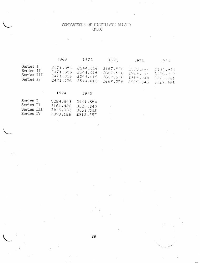
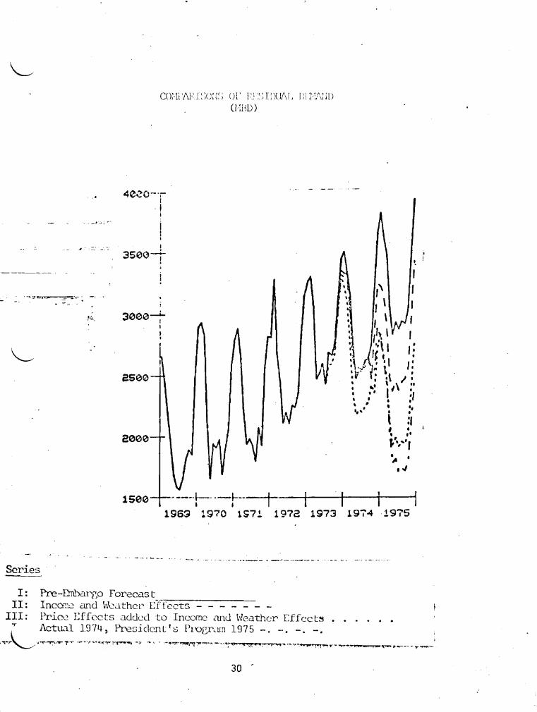
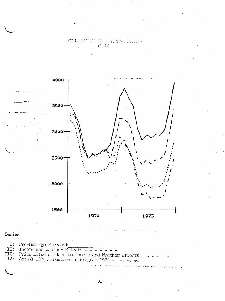
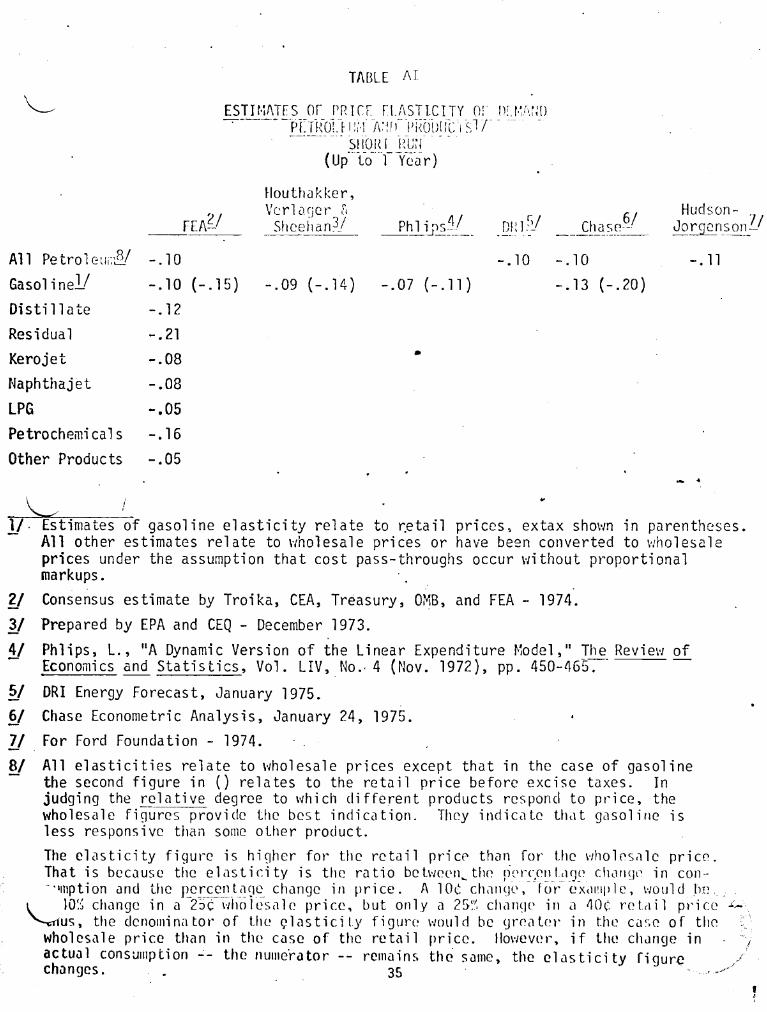