pressure fluctuations as a diagnostic tool for fluidized beds/67531/metadc673151/m2/1/high... ·...

i

Pressure Fluctuations as a Diagnostic Tool for Fluidized Beds

Final Technical ReportDOE Award No.: DE-FG22-94PC94210--15

Principal Investigator: Robert C. BrownGraduate Assistants: Ethan Brue, Joel R. Schroeder, and Ramon De La Cruz

Department of Mechanical EngineeringIowa State University

Ames, IA 50011

May 30, 1998

Disclaimer

This report was prepared as an account of work sponsored by anagency of the United States Government. Neither the United StatesGovernment nor any agency thereof, nor any of their employees,makes any warranty, express or implied, or assumes any legal liabilityor responsibility for the accuracy, completeness, or usefulness of anyinformation, apparatus, product, or process disclosed, or representsthat its use would not infringe privately owned rights. Referenceherein to any specific commercial product, process, or service by tradename, trademark, manufacturer, or otherwise does not necessarilyconstitute or imply its endorsement, recommendation, or favoring bythe United States Government or any agency thereof. The views andopinions of authors expressed herein do not necessarily state or reflectthose of the United States Government or any agency thereof.

iii

Table of Contents

Disclaimer……………………………………………………………………………………...iiTable of Contents……………………………………………………………………………...iiiAbstract………………………………………………………………………………………..ivObjective..……………………………………………………………………………………...1Motivation for Similitude Study……………………………………………………………….1Motivation for Studies in Bubbling Fluidized Beds……………………………………………2

Experimental Apparatus and Procedures: Bubbling Fluidized BedsBubbling Bed…………………………………………………………………………...3

Results and Discussion: Bubbling Fluidized BedsMeasurement of Pressure Fluctuations in BFB Systems……………………………… 7The Nature of Bubbling Fluidized Bed Pressure Fluctuations………………………...15BFB Pressure Fluctuations as a Global Phenomena………………………………… 23Evaluation of the Global Theories of Fluidized Bed Oscillations…………………….23Derivation of a Modified-Hiby Model for Bubbling Fluidized Bed Dynamics……….38Surface Waves in Fluidized Bed Systems…………………………………………….45The Use of Pressure Fluctuations to Validate Similitude Parameters………………...46BFB Similitude……………………………………………………………………….46Transition Regime Fluctuations………………………………………………………49Validation of BFB similitude parameters……………………………………………..51BFB Combustor Similitude Verification……………………………………………...54Bubbling Bed Sensitivity Study………………………………………………………61

Experimental Apparatus and Procedures: Circulating Fluidized BedCirculating Fluidized Bed…………………………………………………………….80Solids Flux Measurement……………………………………………………………. 80

Results and Discussion: Circulating Fluidized BedGlobal Theory of Pressure Fluctuations……………………………………………...83CFB Similitude Background………………………………………………………….86Fast Fluidization Fluctuations - General characteristics……………………………...87Discussion of Voidage Wave Phenomenon in CFBs…………………………………87Discussion of Surface Wave Frequency Phenomena in CFBs………………………...94Summary of CFB Pressure Fluctuations……………………………………………...94Investigation of CFB Similitude Parameters………………………………………….95L-valve Flow Characteristics…………………………………………………………98ISU Power Plant CFB Boilers………………………………………………………110Fluctuations in Lower Regions of CFB Boiler………………………………………110Fluctuations in Upper Region of CFB Boiler………………………………………..116

Conclusions………………………………………………………………………………...120

iv


Final Technical ReportDOE Award No.: DE-FG22-94PC94210

Principal Investigator: Robert C. BrownResearch Assistants: Ethan Brue and Joel R. Schroeder

Department of Mechanical EngineeringIowa State University

Ames, IA 50011

Abstract

The purpose of this project was to investigate the origin of pressure fluctuations in

fluidized bed systems. The study assessed the potential for using pressure fluctuations as an

indicator of fluidized bed hydrodynamics in both laboratory scale cold-models and industrial scale

boilers. Both bubbling fluidized beds and circulating fluidized beds were evaluated. Testing

including both cold-flow models and laboratory and industrial-scale combustors operating at

elevated temperatures.

The study yielded several conclusions on the relationship of pressure fluctuations and

hydrodynamic behavior in fluidized beds. The study revealed the importance of collecting

sufficiently long data sets to capture low frequency (on the order of 1 Hz) pressure phenomena in

fluidized beds. Past research has tended toward truncated data sets collected with high frequency

response transducers, which miss much of the spectral structure of fluidized bed hydrodynamics.

As a result, many previous studies have drawn conclusions concerning hydrodynamic similitude

between model and prototype fluidized beds that is insupportable from the low resolution data

presented.

Using appropriate data collection and analysis, this study was able to verify that a set of

dimensionless parameters derived by other researchers can be used to achieve hydrodynamic

similitude between cold –flow model and prototype bubbling fluidized beds. On the other hand, a

related set of dimensionless parameters developed by other researchers for circulating fluidized

beds were not able to accurately predict similitude between model and prototype. The present

study was successful in slightly modifying this set of dimensionless parameters to correctly predict

v

similitude between cold-flow models. Similitude tests between a cold-flow bubbling fluidized bed

model and a high temperature bubbling fluidized bed combustor were less successful. Although

qualitative agreement in spectral plots of pressure fluctuations was obtained, the data was not

sufficiently quantitative to permit its use in predicting the existence of similitude between cold

model and hot prototype. Similitude tests between a cold-flow circulating fluidized bed and a

hot-flow circulating fluidized bed combustor were also unsuccessful, but for different reasons.

The circulating fluidized bed combustor, an industrial-scale boiler, presented unique data filtering

problems that were never overcome. Modulated air dampers produced pressure fluctuations that

propagated into the fluidized bed where they overwhelmed pressure fluctuations associated with

the hydrodynamics of the particulate-gas mixture.

The study developed models of pressure fluctations in the circulating fluidized beds in an

attempt to understand the nature of the fluctuations. As dynamical systems, circulating fluidized

beds proved to be surprisingly complicated. Linear models were constructed from spectral plots

of pressure fluctuations, but they proved of limited use in deriving physical insight into

hydrodynamic behavior. A variety of acoustical and wave phenomena were used as the basis for

explaining pressure fluctuations in the fluidized bed but with little success.

1


Robert C. Brown, Ethan Brue, and Joel R. Schroeder

Objective

The purpose of this project is to investigate the origin of pressure fluctuations in fluidized

bed systems. The study will asses the potential for using pressure fluctuations as an indicator of

fluidized bed hydrodynamics in both laboratory scale cold-models and industrial scale boilers.

Motivation for Similitude Study

Similitude theory has the potential to become an important tool for fluidized bed design

and operation, since the complexity of fluidized bed hydrodynamics makes the development of

general theoretical relations difficult. Using dimensional analysis and non-dimensional equations

of motion, Glicksman and others derived similitude parameters for bubbling fluidized bed systems

[1]. Glicksman extends his analysis to circulating fluidized beds by adding a dimensionless solids

flux group to the required similitude parameters [2]. Numerous researchers have matched these

parameters in geometrically similar cold-model fluidized beds or have tried to match model

conditions in larger scale fluidized bed combustors. Researchers have used a number of

techniques to verify that the matching of similitude parameters results in similar hydrodynamics.

Typically for CFBs, axial voidage profiles are created from static pressure measurements along

the riser. If these axial voidage profiles match, the local solids concentration at any location in the

riser should be equal. Other studies have used the probability density function (PDF) of static

pressure measurements in fluidized beds to match the distribution of pressure measurements

obtained at various locations in the bed [3].

A number of similitude studies have compared the structure of pressure fluctuations in

fluidized beds using Bode plots and power spectral density (PSD) functions to verify that

hydrodynamic similitude has been achieved [4-6]. However, the validity of pressure fluctuation

analysis for verifying similitude in fluidized bed models and industrial scale boilers cannot be

assumed until a better understanding of the complex structure of pressure fluctuations is achieved.

This study focuses on pressure fluctuation analysis as a method for similitude verification,

2

outlining how pressure fluctuations should be analyzed and qualitatively describing the

hydrodynamic information contained in these fluctuations.

Motivation for Studies in Bubbling Fluidized Beds

The primary goal of this research is to study the nature of pressure fluctuations in

circulating fluidized beds in order to asses how they can be used as a design tool (e.g. model

scale-up) or diagnostic tool (e.g. boiler control) in industrial scale CFB combustors. In order to

achieve this objective, it is necessary to have an adequate understanding of bubbling fluidized bed

pressure fluctuations prior to studying similar fluctuations in CFBs for a number of reasons.

First, the majority of previous research on this subject of fluidized bed fluctuations, has been

conducted in bubbling fluidized beds. This existing data is useful in validating the experimental

methods developed in the present study. Secondly, there are similarities in the structure of

pressure fluctuations in bubbling fluidized beds and circulating fluidized beds. The fluctuations in

the lower dense region of the CFB exhibit a similar frequency response profile as those observed

in bubbling fluidized beds. Also, oscillatory second order system dynamics are observed in the

fluctuation structure of all fluidization systems. Finally, fluidized bed similitude relations were

first applied to bubbling beds and then extended to CFBs. Before the relations for CFB similitude

can be validated using pressure fluctuations, the validity of using bubbling bed fluctuations to

verify the achievement of BFB similitude must be addressed.

Despite the wealth of published research dealing with bubbling fluidized bed fluctuations

there is still no consensus as to the phenomena that governs pressure fluctuations. This

fundamental question is a difficult one for a number of reasons. First of all, experimental data

suggests that multiple phenomena acting simultaneously may be responsible for fluctuations in

fluidized bed systems. This being the case, the problem is not that previous studies have derived

entirely incorrect theories for the appearance of periodic behavior in fluidized bed systems, but

rather that they have composed an incomplete picture of a more complex system. Fluidized bed

systems cannot always be characterized by a single frequency observed in the frequency spectrum.

The characteristic frequency (or frequencies) of pressure fluctuations is not observed as a well

defined single peak in the frequency response plots. Spectral analysis of fluidized bed fluctuations

typically yields a broad distribution of frequencies centered around a dominant frequency.

3

Therefore, any quantitative description of the fluctuation structure inherently contains a great deal

of uncertainty. When multiple frequency phenomena are observed, this quantitative assessment

becomes even more difficult. In addition to the complexity of the fluctuation signal, the

configuration of the pressure measurement system plays a significant part in the information that

can be obtained from pressure fluctuation measurements.

Experimental Apparatus and Procedures: Bubbling Fluidized Beds

Bubbling Bed

Experiments on bubbling fluidized beds was performed with three fluidized beds with

diameters of 5.08 cm, 10.2 cm, and 20.32 cm. The column heights of the three beds in order of

increasing diameter are 32 cm, 64 cm, and 190 cm. The smallest two beds were constructed of

Plexiglas.

The largest bed, illustrated in Figure 1, is constructed of mild steel with a ceramic liner

that allows high temperature combustion tests to be performed. In addition, a water jacket

surrounds the ceramic wall to remove heat generated during combustion. Natural gas or coal can

be burned in the combustor. An Accurate mechanical auger is used to feed coal above the

surface of the combustor. Fluidization air is provided from compressed air and controlled with a

manually operated ball valve. Air flow rate in the combustor is measured with an orifice plate

flow meter, while air flow rates in the cold models is measured with a calibrated rotameter. All

BFBs are equipped with pressure taps for spectral analysis.

The 5.08 cm and 10.16 cm diameter fluidized beds are illustrated in Figure 2. Table 1 lists

the distance above the distributor plate for each pressure tap. The 10.16 cm bed has pressure taps

located on three sides of the bed as illustrated in Figure 2. Distributor plates were constructed to

preserve geometric similitude among the various fluidized beds. In addition, several distributor

plates were constructed to evaluate the effect of distributor plate design on hydrodynamic

behavior of the beds. These designs are described in Table 2. All distributor plate are drilled in a

square grid pattern.

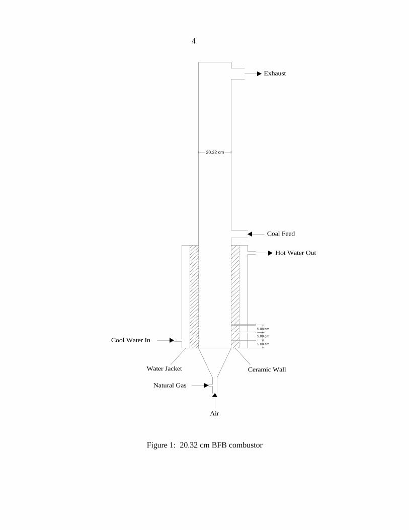
4

Exhaust

Coal Feed

Hot Water Out

Cool Water In

Natural Gas

Air

20.32 cm

Ceramic WallWater Jacket

5.08 cm

5.08 cm

5.08 cm

Figure 1: 20.32 cm BFB combustor

5

Distributor Plate

Air In

Plenum

Pressure Tap

(a) (b)

5.08 cm

2.54 cm

2.54 cm2.54 cm

10.16 cm

5.08 cm

5.08 cm

Figure 2: (a) 10.16 cm BFB, (b) 5.08 cm BFB

6

Table 1: Bed tap locations

20.32 cm combustor 10.16 cm BFB 5.08 cm BFB5.1 cm 3.8 cm 5.08 cm 2.5 cm 1.3

10.2 cm 6.4 cm 10.16 cm 7.6 cm 3.815.2 cm 8.9 cm 12.7 cm 6.4

17.8 cm 8.922.9 cm

Table 2: Distributor plate designs

Plate Designation Bed Size Hole Diameter Square Grid SizeA 5.08 cm 0.6 mm 3.5 mmB 5.08 cm 3.2 mm 9.0 mmC 10.16 cm 1.2 mm 7.0 mmD 10.16 cm 3.2 mm 9.0 mmE 10.16 cm 2.4 mm 14.0 mmF 20.32 cm 2.4 mm 14.0 mm

7

Results and Discussion: Bubbling Fluidized Beds

Measurement of Pressure Fluctuations in BFB Systems

As shown by Davidson for bubbling beds [7] and by Brue for circulating beds [2],

differential pressure measurements and absolute pressure measurements can yield distinctly

different periodic structure. The differential measurement typically reveals a dominant frequency

in the spectrum that is at a higher frequency than the dominant frequency measured by absolute

pressure measurement. While the differential pressure is a function of the fluctuations in the

voidage between two pressure taps, absolute pressure measurements record the pressure drop

from the tap position to the upper bed surface. Consequently, absolute pressure measurement

represents a change in the amount of material above the point of measurement. The absolute

measurement could be considered a differential pressure measurement with the upper tap

positioned at the bed surface (assuming a non-pressurized BFB). Consequently, the difference

between the resulting absolute and differential signals is essentially a difference arising from an

increased tap spacing, which will be discussed in more detail later.

As long as the measurement configuration remains the same (i.e. differential or absolute),

the position of the observed frequency will not vary as the elevation of the pressure fluctuation

measurement changes within the bed. This does not mean that the relative magnitude of each

dominant frequency observed will not change. Figures 3 and 4 compare the frequency spectrum

of pressure fluctuations measured simultaneously in a 20 cm deep bed at a bed elevations of 5.1

cm and 15.2 cm respectively. In the 5.1 cm measurement, both the 3.5 Hz frequency phenomena

and the 2.2 Hz frequency behavior can be observed. While the 3.5 Hz frequency spike is not

detected in the spectrum of the upper bed, the lower frequency phenomena is evident. This

dominant lower frequency that appears at 2.2 Hz will be observed very near 2.2 Hz at all

elevations. The Bode plots of fluctuations at all elevations are indicative of second order

dynamics. Even above the bed a second order phenomena is observed in the gas fluctuations

exiting the bed surface, although it is obvious that fluctuations are significantly damped out at this

position (see Figure 5). This observation will be discussed further in connection with turbulent

and fast fluidization.

8

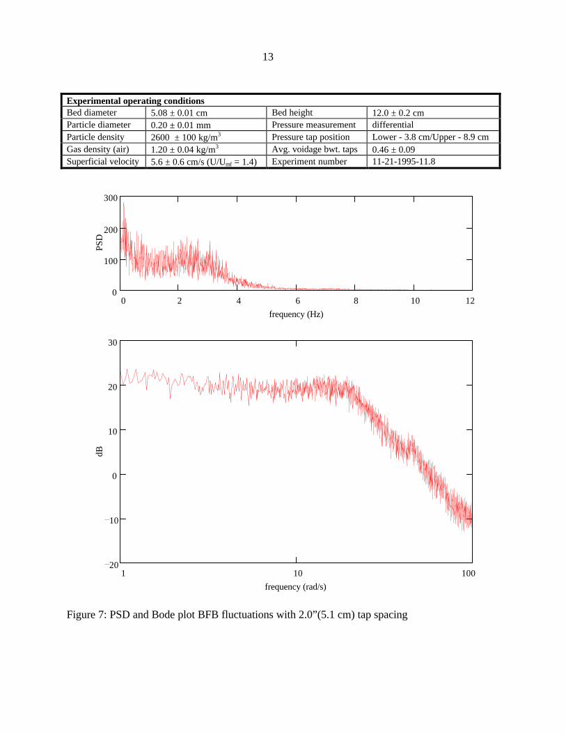
Not only does the elevation at which the pressure fluctuations are measured effect the

appearance of the Bode plot profiles, but the spacing of pressure taps can also complicate the

observed results. Figures 6 and 7 show the how the tap spacing can distort the observed results.

In these figures simultaneous fluctuation measurements were recorded in a BFB at tap spacing of

2.5 cm and 5.1 cm, respectively. These two Bode plots appear fundamentally different. In the

case of the 2.5 cm spacing, a very dominant high frequency peak appears at around 5.5 Hz along

with a highly damped 3.1 Hz phenomena that can be observed in the Bode plot. The dominant

frequency virtually disappears in fluctuations from the 5.1 cm differential measurement, and a

broad 2.2 - 3.1 Hz dominant frequency is observed.

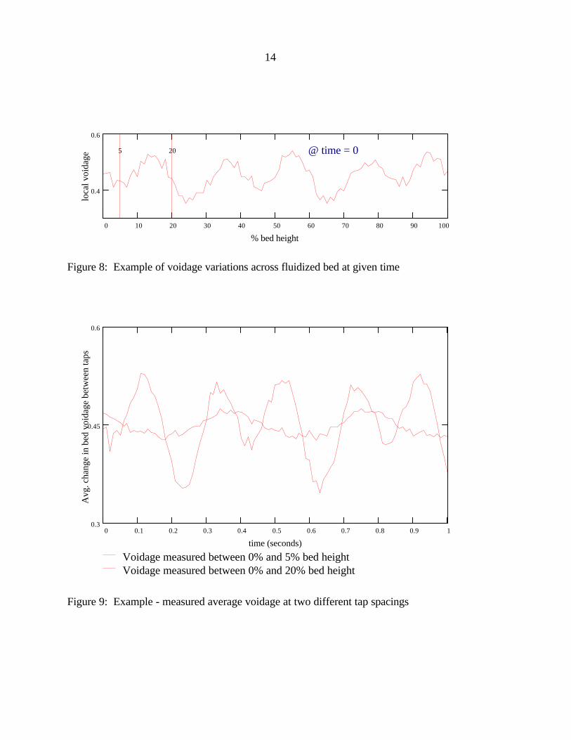
A possible explanation for these apparent inconsistencies in the fluctuation spectrum is

that the increased distance between the pressure taps introduces what could be considered spatial

aliasing to the observed signal. An example using the simulated signals of Figures 7 and 8 best

illustrates this concept. Figure 8 shows a possible distribution of local voidages across the height

of a fluidized bed. This voidage distribution can be thought of as a series of bubble layers passing

up through the fluidized bed. Differential pressure measurements record the average pressure or

voidage between the taps. By averaging the local voidage measurements between the two tap

configurations in Figure 8 (taps across 0-5% and 0-20% bed height), as the wave propagates

upwards through the bed, the resulting voidage signal measured for both cases is shown in Figure

9. It is evident that the dominant frequency of the signal measured by the taps between 0-20%

bed height is half of that observed in the taps that are closer. If such spatial aliasing was occurring

in the bubbling bed system shown in Figure 7, the 5.5 Hz phenomena should be observed as a 2.2

Hz phenomena. Close inspection of Figure 7 confirms this. Locating the two pressure taps used

in the differential measurement close together will decrease the chances of spatial aliasing effects.

Although, if the taps are placed too close to one another the magnitude of the fluctuation will not

be large enough to be accurately recorded by most transducers and noise may begin to mask the

system dynamics.

9

Experimental operating conditionsBed diameter 10.16 ± 0.01 cm Bed height 20.0 ± 0.2 cmParticle diameter 0.30 ± 0.01 mm Pressure measurement differentialParticle density 2600 ± 100 kg/m3 Pressure tap position Lower - 2.5 cm/Upper - 7.6 cmGas density (air) 1.20 ± 0.04 kg/m3 Avg. voidage bwt. taps 0.48 ± 0.06Superficial velocity 12.7 ± 0.6 cm/s (U/Umf = 1.4) Experiment number 6-21-1995-14.1

0 2 4 6 8 10 120

2000

4000

6000

frequency (Hz)

PSD

1 10 10010

0

10

20

30

40

frequency (rad/s)

dB

Figure 3: PSD and Bode plot of BFB fluctuations in the lower bed region

10

Experimental operating conditionsBed diameter 10.16 ± 0.01 cm Bed height 20.0 ± 0.2 cmParticle diameter 0.30 ± 0.01 mm Pressure measurement differentialParticle density 2600 ± 100 kg/m3 Pressure tap position Lower-12.7 cm/Upper-17.8 cmGas density (air) 1.20 ± 0.04 kg/m3 Avg. voidage bwt. taps 0.47 ± 0.06Superficial velocity 12.7 ± 0.6 cm/s (U/Umf = 1.4) Experiment number 6-21-1995-14.1

0 2 4 6 8 10 120

1 104

2 104

3 104

frequency (Hz)

PSD

1 10 10010

0

10

20

30

40

50

frequency (rad/s)

dB

Figure 4: PSD and Bode plot of BFB fluctuations in the upper bed region

11

Experimental operating conditionsBed diameter 10.16 ± 0.01 cm Bed height 20.0 ± 0.2 cmParticle diameter 0.30 ± 0.01 mm Pressure measurement differentialParticle density 2600 ± 100 kg/m3 Pressure tap position Lower-22.9 cm/Upper-27.9 cmGas density (air) 1.20 ± 0.04 kg/m3 Avg. voidage bwt. taps No particles bwt. tapsSuperficial velocity 12.7 ± 0.6 cm/s (U/Umf = 1.4) Experiment number 6-21-1995-14.1

0 2 4 6 8 10 120

0.2

0.4

0.6

frequency (Hz)

PSD

1 10 10040

35

30

25

20

15

10

5

0

frequency (rad/s)

dB

Figure 5: PSD and Bode plot of BFB fluctuations above the bed

12


0 2 4 6 8 10 120

200

400

frequency (Hz)

PSD

1 10 10010

0

10

20

30

frequency (rad/s)

dB

Figure 6: PSD and Bode plot BFB fluctuations with 1.0”(2.5 cm) tap spacing

13


0 2 4 6 8 10 120

100

200

300

frequency (Hz)

PSD

1 10 10020

10

0

10

20

30

frequency (rad/s)

dB

Figure 7: PSD and Bode plot BFB fluctuations with 2.0”(5.1 cm) tap spacing

14

0 10 20 30 40 50 60 70 80 90 100

0.4

0.6

% bed height

loca

l voi

dage

5 20 @ time = 0

Figure 8: Example of voidage variations across fluidized bed at given time

0 0.1 0.2 0.3 0.4 0.5 0.6 0.7 0.8 0.9 10.3

0.45

0.6

Voidage measured between 0% and 5% bed heightVoidage measured between 0% and 20% bed height

time (seconds)

Avg

. cha

nge

in b

ed v

oida

ge b

etw

een

taps

Figure 9: Example - measured average voidage at two different tap spacings

15

Considering that both the method of pressure fluctuation measurement and the method of

pressure fluctuation analysis make a significant difference in the observed results, it is not

surprising that there is still no consensus as to the phenomena governing pressure fluctuations.

The Nature of Bubbling Fluidized Bed Pressure Fluctuations

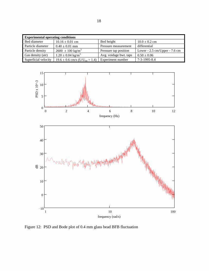
A number of general characteristics of bubbling fluidized bed pressure fluctuations have

been observed by previous researchers and in the present study as well. Under conditions of low

to moderate velocity bubbling fluidization, the particle size does not have a significant effect on

the overall dynamic character of the fluctuations. Figures 10 - 12 show three Bode plots of

fluctuations taken from similar beds of 0.2 mm, 0.3 mm, and 0.4 mm glass beads fluidized at

U/Umf = 1.4. The profiles for each particle size are identical. Any slight variations in the

dominant frequency as the particle diameter is changed, are likely due to variations in bubble

properties or bed voidage. For further verification that particle diameter does not strongly

influence the frequency of the system see Figures 12-15 and Figure 18.

Bed diameter has a significant effect on the Bode plot profiles, although it is important to

emphasize that bed diameter does not effect the position at which dominant system frequencies

observed until the bubbling regime approaches slugging or turbulent conditions. Figures 16 and

17 show the Bode plots of the 10.2 and 5.1 cm diameter beds respectively. In both beds the

particle size, bed height, tap height & spacing, and superficial velocity are identical. It is evident

that changes is the diameter can significantly effect the frequency response, changing the degree

of damping of the observed frequency. Despite the increased damping, the natural frequencies at

which the bed operates under do not change. In both figures, dominant frequencies appear at 3.1

and 5.5 Hz, although the higher (5.5Hz) frequency dominates as the bed diameter decreases.

As shown in Figures 12 - 15, for U/Umf > 1.2, changes in the superficial velocity does not

effect the dominant frequency in the bubbling fluidization regime. At the onset of fluidization, the

dominant frequency increases only slightly and then levels off as the superficial velocity is

increased above U/Umf > 1.2. It should again be emphasized that the superficial velocity will not

change the characteristic period of oscillation of the system, but it may dictate the damping of the

observed frequencies in the spectrum.

16


0 2 4 6 8 10 120

2000

4000

6000

frequency (Hz)

PSD

1 10 10010

0

10

20

30

40

frequency (rad/s)

dB

Figure 10: PSD and Bode plot of 0.2 mm glass bead BFB fluctuations

17


0 2 4 6 8 10 120

10

20

frequency (Hz)

PSD

x 1

0^-3

1 10 1000

10

20

30

40

50

frequency (rad/s)

dB

Figure 11: PSD and Bode plot of 0.3 mm glass bead BFB fluctuations

18


0 2 4 6 8 10 120

5

10

15

frequency (Hz)

PSD

x 1

0^-3

1 10 10010

0

10

20

30

40

50

frequency (rad/s)

dB

Figure 12: PSD and Bode plot of 0.4 mm glass bead BFB fluctuation

19

1 1.5 2 2.5 3 3.50

2

4

6

dp = 0.2 mmdp = 0.3 mmdp = 0.4 mm

U/Umf

freq

uenc

y (H

z)

Figure 13: Fluctuation frequency versus U/Umf for 10.0 cm bed height

1 1.5 2 2.5 3 3.51

2

3

4

Taps @ 1" & 3 " - first peakTaps @ 1" & 3" - second peakTaps @ 5" & 7"

U/Umf

freq

uenc

y (H

z)

Figure 14: Fluctuation frequency versus U/Umf for 20 cm bed height and dp = 0.2 mm

20

1 1.5 2 2.5 3 3.51

2

3

4


U/Umf

freq

uenc

y (H

z)


1 1.2 1.4 1.6 1.8 2 2.2 2.4 2.6 2.8 31

2

3

4


U/Umf

freq

uenc

y (H

z)


21


0 2 4 6 8 10 120

200

400

frequency (Hz)

PSD

1 10 10010

0

10

20

30

frequency (rad/s)

dB

Figure 17: PSD and Bode plot of BFB fluctuations in 5.1 cm diameter bed

22


0 2 4 6 8 10 120

100

200

300

frequency (Hz)

PSD

1 10 10010

5

0

5

10

15

20

25

frequency (rad/s)

dB

Figure 18: PSD and Bode plot of BFB fluctuations in 10.2 cm diameter bed

23

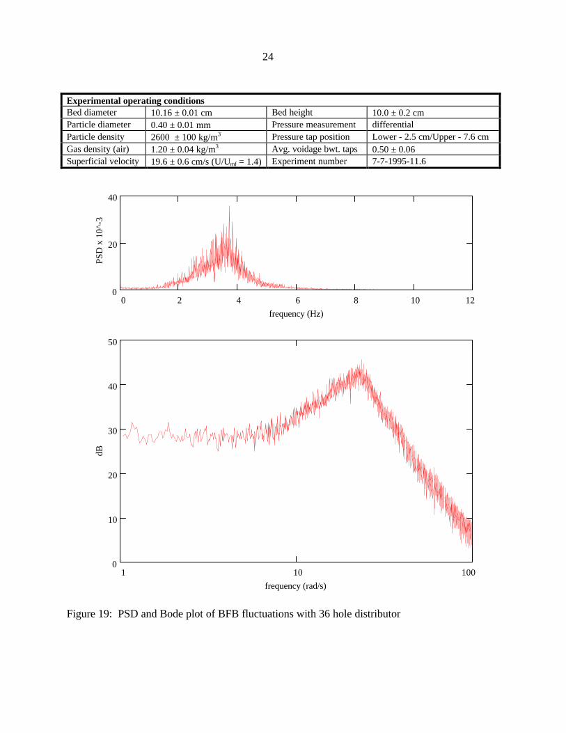
BFB Pressure Fluctuations as a Global Phenomena

Our work suggests that two different types of global phenomena are responsible for

pressure fluctuations in bubbling fluidized beds. Our research has led us to dismiss the possibility

of random local phenomena (such as bubbles) being the explanation of pressure fluctuations in

bubbling beds for two reasons. Static pressure measurements in a BFB were simultaneously

recorded from the center of the bed and at the bed wall. The Bode plot profiles of the

fluctuations at these two locations were identical. If the passage of local bubbles were solely

responsible for pressure fluctuations, the hydrodynamics at the center of the bed would produce a

different fluctuation structure, since the majority of bubbles rise to the surface through the center

of the bed. Further evidence of the global nature of pressure fluctuations was obtained from an

experiment in which two different drilled hole distributor plates were tested under identical

operating conditions. The two distributor plates had the same total hole-area, but one had 72

holes while the other had only 36 holes. Since bubbles form at the distributor plate holes, the 72

hole plate would produce more bubbles than the 36 hole plate. As is shown in Figures 19 - 20,

the Bode plots of the pressure fluctuations from the two different distributor plate cases are

identical, suggesting that random bubble passage in the vicinity of the region of pressure

measurement is not a sufficient explanation for the fluctuations. This argument does not lead to

the conclusion that bubbles are not responsible for pressure fluctuation phenomena, but rather that

the global phenomena that dictates fluidized bed hydrodynamics may also govern the periodic

production of bubbles.

Evaluation of the Global Theories of Fluidized Bed Oscillations

Three different categories of global phenomena are highlighted by Roy and Davidson [8]:

a natural frequency of oscillation of the entire bed; a surface phenomena that propagates pressure

fluctuations down through the bed; and a plenum compression wave phenomena exhibited in

fluidized beds with low resistance distributor plates. This third phenomena is not of interest in

this study. To eliminate the effect of this phenomena, high resistance distributor plates are used.

It is hypothesized that two global fluidization phenomena are responsible for the structure of

fluctuations. These two phenomena will be generally referred to as the natural frequency and the

surface frequency.

24


0 2 4 6 8 10 120

20

40

frequency (Hz)

PSD

x 1

0^-3

1 10 1000

10

20

30

40

50

frequency (rad/s)

dB

Figure 19: PSD and Bode plot of BFB fluctuations with 36 hole distributor

25


0 2 4 6 8 10 120

5

10

15

frequency (Hz)

PSD

x 1

0^-3

1 10 10010

0

10

20

30

40

50

frequency (rad/s)

dB

Figure 20: PSD and Bode plot of BFB fluctuations with 72 hole distributor plate

26

When evaluating potential theories for the origin of fluctuations in bubbling beds, two

requirements must be considered. The first requirement is that the theory must be able to account

for the second order system behavior observed in fluidized bed systems. The Bode plots of all

fluidized bed systems exhibit a final asymptotic slope of -40 dB/decade. Figures 21 and 22 show

examples of simple second order systems. In many cases, a single second order system is not

sufficient to describe fluidization hydrodynamics. Experiments suggest that the dynamics of

fluidization can be described by a model that assumes multiple second order systems acting

concurrently within the fluidized bed system. Second order systems acting in parallel will also

yield -40 dB/decade final Bode plot roll off (as shown by example in Figure 23). Secondly, the

theory must be able to predict the observed dominant frequencies accurately and explain why at

low bed heights they appear to be inversely proportional to the square root of bed height.

There are three researchers who have proposed mechanisms that meet these two

requirements. The first two researchers to present mechanisms for fluctuations were Hiby [9] and

Verloop [10]. Fundamentally the mechanism proposed by both these researchers is the

same,although the derivations differ slightly. While Verloop maintains that the entire incipiently

fluidized bed oscillates in phase, Hiby proposes a system of oscillating layers being “pulled into

tune.” The changes in bed voidage as the bed lifts and returns to its initial position result in the

fluctuations of static pressure drop across the bed. While Verloop focuses on shallow incipiently

fluidized beds, Hiby extends this phenomena to explain layers of bubble production which

coincide with the natural oscillations of the bed.

Baskakov [11] takes a different approach to fluidized bed dynamics. He proposes a direct

analogy between fluidized bed dynamics and a hydraulic pendulum (e.g. U-tube manometer). For

Baskakov the changes in voidage (or pressure) are due to changes in the height of the surface

caused by the rise of a large single bubble. As the bubble rises through the bed it entrain solids to

the top of the bed, causing the bed surface to rise. The solids return downward along the sides of

the bed to restore the bed to its equilibrium condition. This cyclic movement of solids up the

center of the bed via bubbles and back down the sides via annular flow constitutes Baskakov’s

oscillatory pendulum. The primary weakness of Baskakov’s theory lies in the validity of the

hydraulic pendulum analogy. The simplifying assumptions that go into this analogy are not

convincing. Baskakov’s derivation is based on the U-tube manometer not a fluidized bed system.

27

1 10 10040

20

0

20

frequency (rad/s)

dB

Figure 21: Example - simple 2nd order underdamped system Bode plot (ωn=20 s-1, ς=0.3)

1 10 10040

20

0

20

frequency (rad/s)

dB

Figure 22: Example - simple 2nd order overdamped system Bode plot (ωn=6 s-1, ς=1.1)

1 10 10040

20

0

20

frequency (rad/s)

dB

Figure 23: Example - Bode plot of the above second order systems acting in parallel

28

He simply assumes a direct analogy can be made to the fluidized bed. Secondly, Baskakov’s

model is dependent on bubbles as a forcing mechanism; he does not explain the possibility or

origin of the necessary periodic bubble formations.

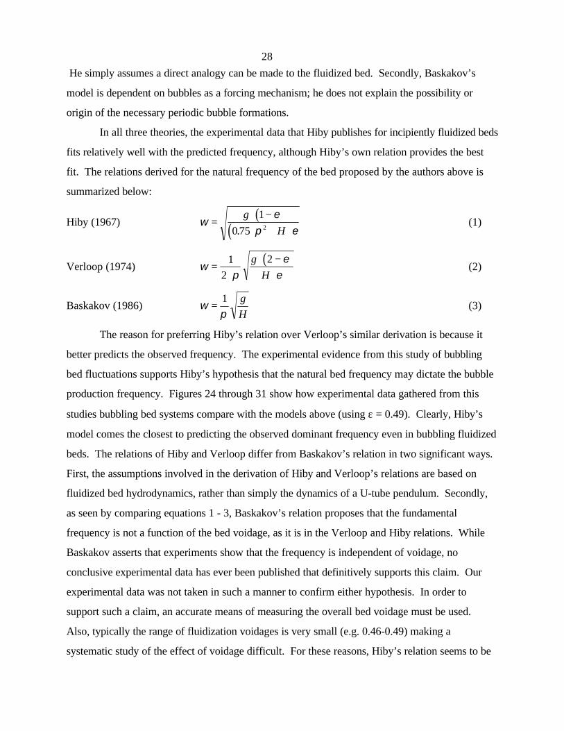
In all three theories, the experimental data that Hiby publishes for incipiently fluidized beds

fits relatively well with the predicted frequency, although Hiby’s own relation provides the best

fit. The relations derived for the natural frequency of the bed proposed by the authors above is

summarized below:

Hiby (1967)( )

( )ωε

π ε=

⋅ −⋅ ⋅ ⋅

g

H

1

0 75 2.(1)

Verloop (1974)( )ω

πε

ε=

⋅⋅ −

⋅1

2

2g

H(2)

Baskakov (1986) ωπ

=1 g

H(3)

The reason for preferring Hiby’s relation over Verloop’s similar derivation is because it

better predicts the observed frequency. The experimental evidence from this study of bubbling

bed fluctuations supports Hiby’s hypothesis that the natural bed frequency may dictate the bubble

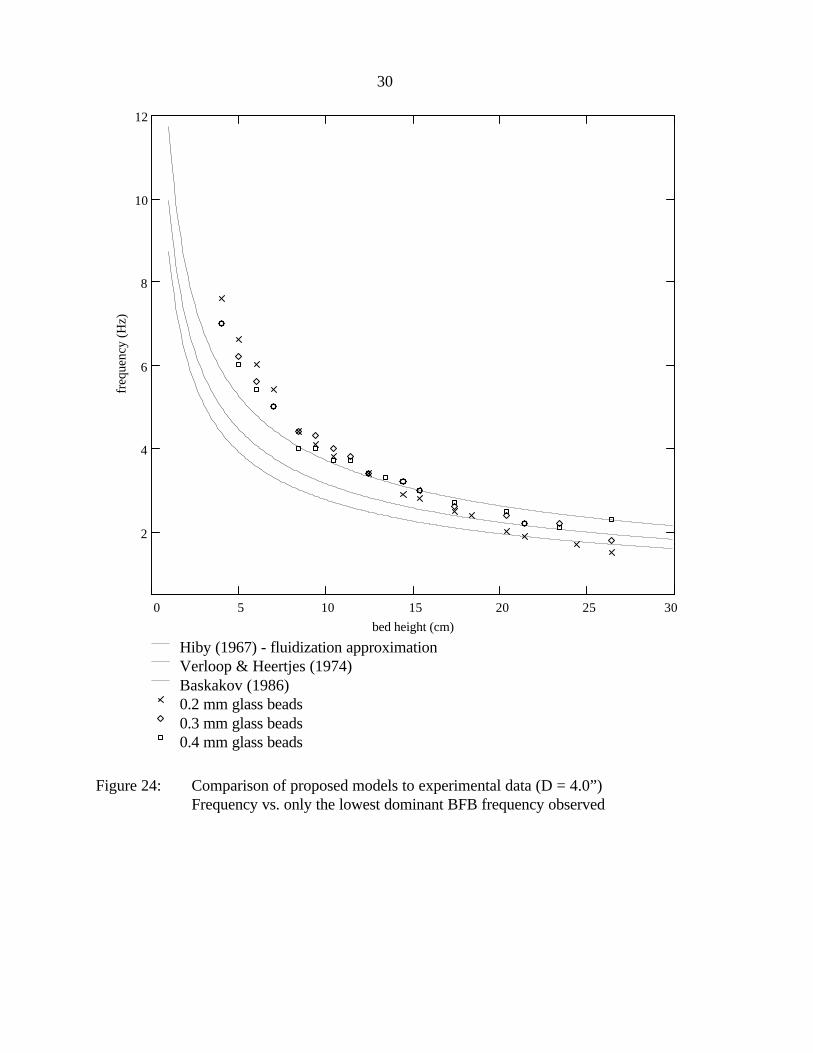
production frequency. Figures 24 through 31 show how experimental data gathered from this

studies bubbling bed systems compare with the models above (using ε = 0.49). Clearly, Hiby’s

model comes the closest to predicting the observed dominant frequency even in bubbling fluidized

beds. The relations of Hiby and Verloop differ from Baskakov’s relation in two significant ways.

First, the assumptions involved in the derivation of Hiby and Verloop’s relations are based on

fluidized bed hydrodynamics, rather than simply the dynamics of a U-tube pendulum. Secondly,

as seen by comparing equations 1 - 3, Baskakov’s relation proposes that the fundamental

frequency is not a function of the bed voidage, as it is in the Verloop and Hiby relations. While

Baskakov asserts that experiments show that the frequency is independent of voidage, no

conclusive experimental data has ever been published that definitively supports this claim. Our

experimental data was not taken in such a manner to confirm either hypothesis. In order to

support such a claim, an accurate means of measuring the overall bed voidage must be used.

Also, typically the range of fluidization voidages is very small (e.g. 0.46-0.49) making a

systematic study of the effect of voidage difficult. For these reasons, Hiby’s relation seems to be

29

the most plausible theory to explain the oscillatory behavior in bubbling fluidized bed systems, but

as will be shown in the following section, this theory has a fundamental error in its assumptions.

By correcting this assumption, a modified Hiby formulation is derived that better predicts the

observed frequency.

Since only Hiby’s data for incipient fluidization was used for comparison to these theories,

it was not observed that as the bed height increases to heights greater than 10 cm, multiple peaks

begin appearing in the spectrum, complicating the overall system (see Figures 25 and 26). As the

bed height increases the frequency tends to be at a lower frequency than predicted by theories for

natural bed oscillations. Increasing the height increases bubble coalescence, resulting in the upper

surface lifting or erupting from its equilibrium position. Throughout the bed, this subsequent

oscillation of the surface can be detected concurrently with natural bed oscillations. In very deep

beds significant coalescence occurs and the surface fluctuations will occur at a slightly lower

frequency than the natural bed frequency. This surface effect will begin to interfere with the

natural oscillation of the bed such that the observed frequency is less than the predicted value

inversely proportional to the square root of the bed height. This effect produced by excessive

bubble coalescence was not observed by other researchers since previous experimental data was

recorded in beds that were operated at incipient fluidization conditions only. The decrease in the

fluctuation frequency due to this surface phenomena is most pronounced as the particle size

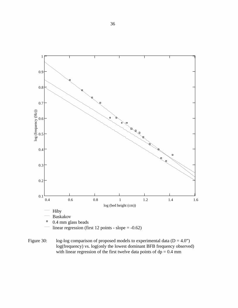
decreases. For large particle sizes, the slope observed on the log-log plot of frequency versus bed

height is close to the -0.5 predicted by theory (see Figure 30). For smaller particle sizes the slope

becomes steeper and seems to approach a slope closer to -1.0 as the bed height increases (see

Figures 28 and 29). Smaller particles will tend to produce smaller bubbles. These smaller bubbles

will rise faster, increasing the rate of bubble coalescence. As coalescence increases, the surface

eruption frequency decreases due to the fewer (but larger) bubbles at the bed surface. Figure 31

shows how the observed frequencies are complicated in small diameter beds, or more specifically,

beds with a high H/D ratio. Again, this is due to bubble coalescence, which will increase as the

height is increased, and to slugging behavior which increases as the diameter is reduced.

30

0 5 10 15 20 25 30

2

4

6

8

10

12

Hiby (1967) - fluidization approximationVerloop & Heertjes (1974)Baskakov (1986)0.2 mm glass beads0.3 mm glass beads0.4 mm glass beads

bed height (cm)

freq

uenc

y (H

z)

Figure 24: Comparison of proposed models to experimental data (D = 4.0”)Frequency vs. only the lowest dominant BFB frequency observed

31

0 5 10 15 20 25 30

2

4

6

8

10

12

Hiby (1967) - fluidization approximationVerloop & Heertjes (1974)Baskakov (1986)D = 4.0" - first peakD = 4.0" - second peakD = 2.0" - first peakD = 2.0" - second peakD = 2.0" - third peak

bed height (cm)

freq

uenc

y (H

z)

Figure 25: Comparison of proposed models to experimental data for 0.3 mm glass beadsFrequency vs. all dominant BFB frequencies

32

0 5 10 15 20 25 30

2

4

6

8

10

12

Hiby (1967) - fluidization approximationVerloop & Heertjes (1974)Baskakov (1986)0.2 mm glass beads0.3 mm glass beads0.4 mm glass beads

bed height (cm)

freq

uenc

y (H

z)

Figure 26: Comparison of proposed models to experimental data (D = 4.0”)Frequency vs. only the higher dominant BFB frequency observed

33

0.6 0.8 1 1.2 1.4 1.60.1

0.2

0.3

0.4

0.5

0.6

0.7

0.8

0.9

1

1.1

HibyBaskakov0.2 mm glass beads0.3 mm glass beads0.4 mm glass beads

log (bed height (cm))

log

(fre

quen

cy (

Hz)

)

Figure 27: log-log comparison of proposed models to experimental data (D = 4.0”)log(frequency) vs. log(only the lowest dominant BFB frequency observed)

34

0.4 0.6 0.8 1 1.2 1.4 1.60.1

0.2

0.3

0.4

0.5

0.6

0.7

0.8

0.9

1

HibyBaskakov0.2 mm glass beadslinear regression (first 4 points - slope = -0.60)


log

(fre

quen

cy (

Hz)

)

Figure 28: log-log comparison of proposed models to experimental data (D = 4.0”)log(frequency) vs. log(only the lowest dominant BFB frequency observed)with linear regression of the first four data points of dp = 0.2 mm

35

0.4 0.6 0.8 1 1.2 1.4 1.60.1

0.2

0.3

0.4

0.5

0.6

0.7

0.8

0.9

1



log

(fre

quen

cy (

Hz)

)

Figure 29: log-log comparison of proposed models to experimental data (D = 4.0”)log(frequency) vs. log(only the lowest dominant BFB frequency observed)with linear regression of the first eight data points of dp = 0.3 mm

36

0.4 0.6 0.8 1 1.2 1.4 1.60.1

0.2

0.3

0.4

0.5

0.6

0.7

0.8

0.9

1



log

(fre

quen

cy (

Hz)

)

Figure 30: log-log comparison of proposed models to experimental data (D = 4.0”)log(frequency) vs. log(only the lowest dominant BFB frequency observed)with linear regression of the first twelve data points of dp = 0.4 mm

37

0.4 0.6 0.8 1 1.2 1.4 1.60.2

0.3

0.4

0.5

0.6

0.7

0.8

0.9

1

HibyBaskakovD = 2.0"/dp = 0.3/second peakD = 2.0"/dp = 0.3/first peak


log

(fre

quen

cy (

Hz)

)

Figure 31: log-log comparison of proposed models to experimental data (D = 2.0”)log(frequency) vs. log(all dominant BFB frequencies observed)

38

Derivation of a Modified-Hiby Model for Bubbling Fluidized Bed Dynamics

While Hiby’s research provides the most plausible theory and rigorous derivation to date,

he makes a fundamental error in the assumptions used in his theoretical derivation. By correcting

this error, a more accurate relation can be developed to both predict the natural frequency and

explain the second order dynamics observed in the BFB pressure fluctuations. Hiby begins his

derivation by considering a single particle suspended in a fluidized bed [9]. If this particle is

displaced from its equilibrium position (either upwards or downwards), the forces on the particle

are altered in such a way to bring it back to its equilibrium position. The number of particles in a

fluidized bed can be defined as:

( )N

VV

V

d

s

pp

= =⋅ −

⋅

1

63

επ

(4)

The force acting on a single particle is the sum of its weight and the drag force exerted by the gas

flow (neglecting buoyancy forces which are typically very small in gas fluidization systems). The

average drag force on an individual particle can be estimated by dividing the total lifting force

acting on the bed (∆p⋅A) by the total number of particles.

( )F mg

p A d

Vp= − +

⋅ ⋅ ⋅⋅ ⋅ −

πε

∆ 3

6 1(5)

Substituting A/V = 1/H:

( )F mg

d pH

p= − +⋅

⋅ −

⋅

πε

3

6 1

∆(6)

Under fluidization conditions the pressure drop can be estimated using the Ergun equation at

minimum fluidization velocity (Umf). This is where Hiby makes an error in his derivation. He uses

the variable U rather than the constant Umf to estimate the pressure drop in an incipiently fluidized

bed. While at incipient conditions these will be equal by definition, his use of U rather than Umf

leads him to some faulty conclusions, as will be shown later. From the Ergun equation:

( ) ( )∆pH

U

d

U

dmf

p

g mf

p

= ⋅⋅

⋅−

+ ⋅⋅

⋅−

1501

1751

2

2

3

2

3

µ εε

ρ εε

. (7)

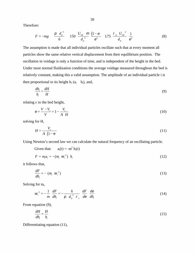
39

Therefore:

( )F mg

d U

d

U

dp mf

p

g mf

p

= − +⋅

⋅ ⋅

⋅⋅

−+ ⋅

⋅⋅

π µ εε

ρε

3

2 3

2

36150

1175

1. (8)

The assumption is made that all individual particles oscillate such that at every moment all

particles show the same relative vertical displacement from their equilibrium position. The

oscillation in voidage is only a function of time, and is independent of the height in the bed.

Under most normal fluidization conditions the average voidage measured throughout the bed is

relatively constant, making this a valid assumption. The amplitude of an individual particle i is

then proportional to its height hi (ai ∼ hi), and,

dhh

dHH

i

i

= (9)

relating ε to the bed height,

ε =−

= −⋅

V VV

VA H

s s1 (10)

solving for H,

( )H

VA

s=⋅ −1 ε

(11)

Using Newton’s second law we can calculate the natural frequency of an oscillating particle.

Given that: ai(t) = -ω2⋅hi(t)

F ma m hi i i i i= = − ⋅ ⋅( )ω 2 (12)

it follows that,

dFdhi

= − ( )mi i⋅ω 2 (13)

Solving for ωi,

ωπ ρ ε

εi

i p s imdFdh d

dFd

ddh

23

1 6= − ⋅ = −

⋅ ⋅⋅ ⋅ (14)

From equation (9),

dHdh

Hhi i

= (15)

Differentiating equation (11),

40

ddH

VA H

sε=

⋅ 2(16)

From equations (16), (15), and (11),

ddh

ddH

dHdh

VA H h hi i

s

i i

ε ε ε= ⋅ =

⋅ ⋅=

−1(17)

Differentiating equation (8),

dFd

d U

d

U

dp mf

p

g mf

pεπ µ ε

ερ

ε= −

⋅

⋅ ⋅

⋅⋅

− ⋅+ ⋅

⋅⋅

3

2 4

2

46150

3 2175

3. (18)

Substituting (17) and (18) into equation (14),

( ) ( )ωρ

µ ε εε

ρ εεi

s i

mf

p

g mf

ph

U

d

U

d2

2 4

2

4

3150

1 3 2

3175

1=

⋅⋅ ⋅

⋅⋅

− ⋅ − ⋅⋅

+ ⋅⋅

⋅−

. (19)

Therefore:

ω i iC h= ⋅ −1

0 5. (20)

where

( ) ( )C

U

d

U

ds

mf

p

g mf

p1 2 4

2

4

3150

1 3 2

3175

1= ⋅

⋅⋅

− ⋅ − ⋅⋅

+ ⋅⋅

⋅−

ρ

µ ε εε

ρ εε

. (21)

This shows that the natural frequency of a particle depends on its height in the bed. It is obvious

that the bed will tend to oscillate at an overall mean frequency as the bed is “pulled into tune”.

Hiby estimates this mean frequency by summing up a weighted average based on the amplitude of

oscillation of each layer of particles.

ω m

H

H

C h dh

hdhC H=

⋅= ⋅ ⋅

−

−∫∫1

0 5

0

0

10 54

3

.

. (22)

therefore,

( ) ( )ωρ

µ ε εε

ρ εεm

s

mf

p

g mf

pH

U

d

U

d=

⋅⋅ ⋅

⋅⋅

− ⋅ − ⋅⋅

+ ⋅⋅

⋅−

4

3

3150

1 3 2

3175

12 4

2

4. (23)

and converting to cycles per second (Hz),

( ) ( )νπ ρ

µ ε εε

ρ εεm

s

mf

p

g mf

pH

U

d

U

d=

⋅ ⋅⋅ ⋅

⋅⋅

− ⋅ − ⋅⋅

+ ⋅⋅

⋅−

2

3

3150

1 3 2

3175

12 4

2

4. (24)

41

Hiby develops an equation identical to equation 24 except that νm is a function of U rather than

Umf. Using some algebraic manipulation, and an approximation he arrives at a simplified equation

of the form shown in equation 28 below. By initially using the better assumption of Umf rather

than U in equation 7 the following relations can be used to simplify the equation 24. For Rep <

20 the first term within the bracket dominates and Umf can be estimated,

Ud g

mfp s mf

mf

=⋅ ⋅

⋅ −

2 3

150 1

ρµ

εε

(25)

Assuming εmf ≈ ε, the natural frequency from (24) would reduce to:

( )ν

πε

εm

gH

=⋅

⋅− ⋅

2

3

3 2(26)

For Rep > 20 the second term within the bracket dominates and Umf can be estimated,

Ud g

mfp s mf

g

=⋅ ⋅ ⋅

⋅ρ ε

ρ

3

175.(27)

Again, assuming εmf ≈ ε, the natural frequency from (24) would reduce to:

νπ

εεm

gH

=⋅

⋅⋅

−

2

3

3 1(28)

For this study Rep is significantly less than twenty and Equation (26) should predict the frequency

of oscillation for shallow fluidized beds. Figures 32 and 33 demonstrate that equation 26 more

accurately predicts the observed natural frequency than any previously proposed model. The

error in Hiby’s derivation is made evident as he tries to address his relations dependence on U and

dp [9]. According to his theory, the superficial velocity and the particle diameter would have a

significant effect on the observed frequency. Using his relation, for laminar conditions of flow, νm

∼ U -0.31 and νm ∼ dp-1. For turbulent conditions νm ∼ U -1 and νm ∼ dp

-0.5. These predictions are

contrary to experimental observations which show frequency to be independent of U and dp.

42

0 5 10 15 20 25 30

2

4

6

8

10

12

14

Modified Hiby derivation for laminar conditionsHiby (1967) - fluidization approximationVerloop & Heertjes (1974)Baskakov (1986)0.2 mm glass beads0.3 mm glass beads0.4 mm glass beads

bed height (cm)

freq

uenc

y (H

z)

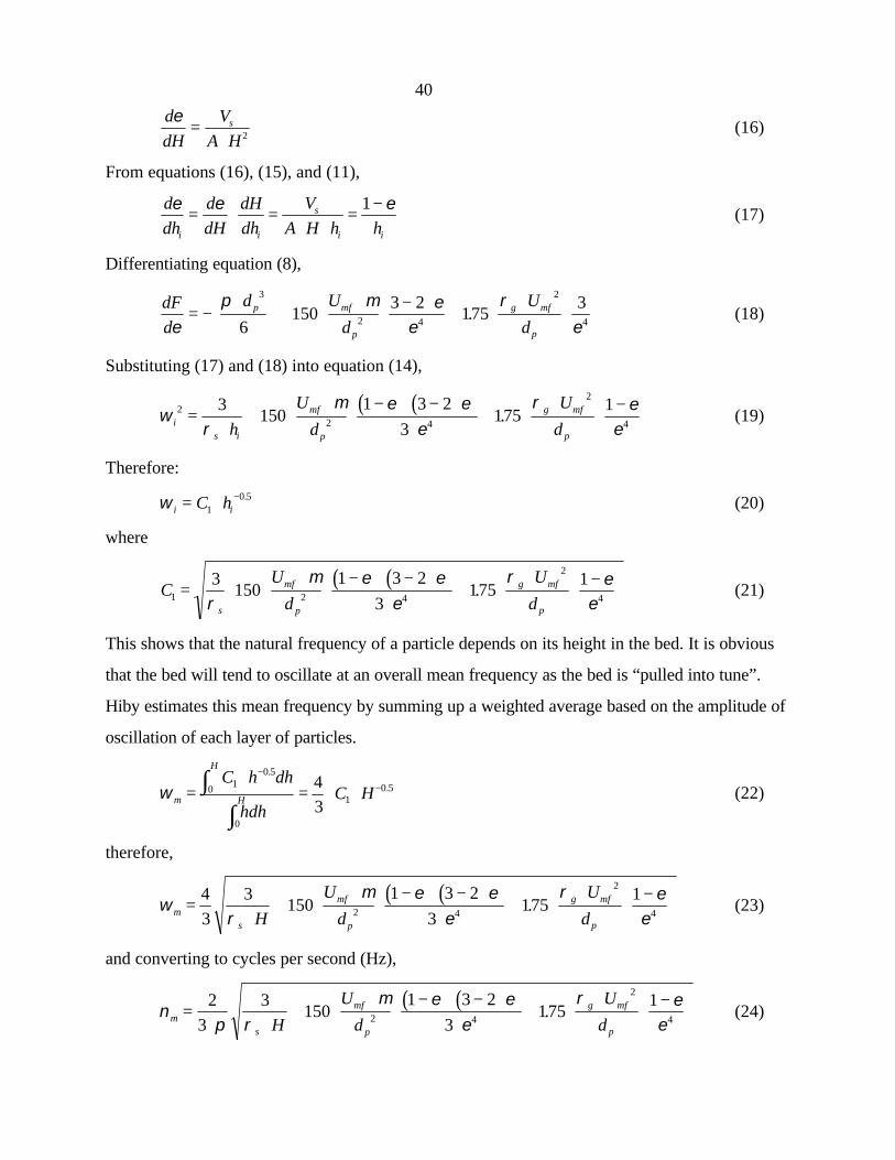
Figure 32: Comparison of modified Hiby model to experimental data (D = 4.0”)Frequency vs. only the lowest dominant BFB frequency observed

43

0.6 0.8 1 1.2 1.4 1.60.1

0.2

0.3

0.4

0.5

0.6

0.7

0.8

0.9

1

1.1

1.2

Modified HibyHiby (1967)Baskakov (1986)0.2 mm glass beads0.3 mm glass beads0.4 mm glass beads


log

(fre

quen

cy (

Hz)

)

Figure 33: log-log comparison of modified Hiby model to experimental data (D = 4.0”)log(frequency) vs. log(only the lowest dominant BFB frequency observed)

44

In addition to establishing that the modified Hiby relation better predicts the observed

natural frequency of the bed, it is evident from the derivation of this dynamic model that pressure

fluctuations will exhibit second order behavior. From Newton’s second law on a single particle

with u(t) as the white noise forcing function and neglecting damping mechanisms:

dh tdt

h t u ti

i

2

22( )

( ) ( )+ =ω (29)

Knowing that the change in position is proportional to the change in voidage, and the change in

voidage proportional to the change in pressure drop.

)()()( 2

2

2

tutpdt

tpd=∆+

∆ ω (30)

The modified Hiby relation satisfies the two important criteria for a global dynamic model

of shallow fluidized bed systems. It not only predicts well the dominant frequency, but also

provides an explanation for the second order pressure fluctuation response observed. The first

peak observed in the frequency spectrum is the result of this natural bed frequency.

The second dominant peak that appears in the spectrum of deep beds represents the

interference of the surface eruption frequency with the natural bed frequency. Due to the

increased coalescence of bubbles, the surface dynamics become more pronounced and nearly

equal in magnitude to the natural bed fluctuations. This surface phenomena will have two effects.

First, as seen in Figures 3 and 4, this frequency of surface eruption is propagated down

throughout the bed and can be observed simultaneously interfering with the pressure fluctuations

of the lower bed region. The higher frequency spikes in the spectrum are the result of

simultaneously measuring the natural and surface fluctuations which are not acting in phase.

Secondly, as this surface phenomena becomes more pronounced, and as bubble coalescence

produces surface eruptions at a frequency lower than the natural frequency, this effect begins to

pull the natural frequency “out of tune with the bed height” to a lower frequency. This is why the

experimental results begin to deviate from the proposed model in Figures 32 and 33 at heights of

around 10 cm. The observed frequency continues to deviate to a greater extent from its predicted

value as the bed height and corresponding coalescence continues to increase. In the case of very

tall and narrow beds, a third, even higher, frequency peak can be observed in the spectrum. This

45

high frequency is always observed at twice the frequency of the natural bed frequency. It is

possible that this is a harmonic overtone of this fundamental natural frequency.

Surface Waves in Fluidized Bed Systems

In addition to the voidage waves reported and discussed previously, another second order

phenomenon that may be responsible for pressure fluctuations in fluidized beds is surface waves

analogous to surface waves observed in water. As proposed by Sun et. al [12], since the

hydrodynamics of fluidized bed systems exhibit many of the characteristics of liquid, surface

waves are expected in a fluidized bed. Water waves are classified according to the ratio of water

depth (H) to wave length (λ) [13]. For H/λ < 1/20, the waves are termed shallow waves and the

frequency is dependent on both the water depth and wave length. For shallow waves, the

governing wave equation (presented by Sun [12]) reduces to a simplified relation that can be used

to estimate the wave frequency:

ωλ

=gH

(31)

For intermediate depth waves 1/20 > H/λ < 1/2, the wave equation cannot be reduced to a

simple expression for wave frequency, and must be estimated as:

ωπ λ π

πλ

=⋅ ⋅ ⋅

⋅⋅

⋅

1

2 2

2gHtanh (32)

For deep waves (H/λ > 1/2), the wave equation can be again be simplified and the

frequency is only dependent on the wavelength and can be estimated as:

ωπλ

=g

2(33)

For surface waves in a cylindrical container the wavelength is determined by the container

diameter:

Dn

=2

λ (34)

where n is an integer greater than zero. The fundamental frequency is represented by n = 1, with

overtones represented by higher integer values. Assuming that a half-wave is established in the

bed (λ/2 = D) the deep wave frequency in a fluidized bed could be estimated as:

46

ωπ

=gD4

(35)

This surface wave phenomenon provides additional insight into the pressure dynamics of both

turbulent (transition regime) and circulating beds.

The Use of Pressure Fluctuations to Validate Similitude Parameters

Glicksman [14, 15] has done the most extensive research on the subject of similitude in

fluidized bed systems. Using both the Buckingham Pi theorem and derivations based on

fundamental equations of motion, Glicksman proposes a set of similitude parameters that govern

fluidization. Glicksman assumes that if the PSDs or PDFs of pressure fluctuations match between

model and prototype, then the fluidized beds are in hydrodynamic similitude. However, he does

not distinguish the important characteristics of the PSD that must match in order for two beds to

be governed by similar dynamics. Particularly in CFBs, Glicksman’s data does not show the

important spectral characteristics in the PSD due to inadequate data sampling. Furthermore,

Glicksman never questioned whether pressure fluctuations were correlated to the hydrodynamic

state of a fluidized bed. In addition to relating Bode plot characteristics to physical phenomena in

fluidized beds, a secondary goal of this study is to reassess whether pressure fluctuations can be

used to validate proposed BFB and CFB similitude parameters.

BFB Similitude

The Buckingham Pi theorem will be used to develop the important non-dimensional

fluidized bed parameters. Using the frequency of pressure fluctuations as the dependent

parameter, all independent variables important for bubbling fluidization can be defined:

ω ρ ρ µ φ= f U g D H dp s g( , , , , , , , , )

The dimensions are as follows:

[ω] = 1/T [U] = L/T [g] = L/T2 [D] = L

[H] = L [dp] = L [ρs] = M/L3 [ρg] = M/L3

[µ] = M/LT [φ] = 1

If we choose U, dp, and ρg as the dimensionally independent parameters the remaining variables

can be non-dimensionalized based on these variables.

47

gg d

Up→

⋅2

HHdp

→ DDdp

→

ρ ρρs

s

g

→ µ µρ

→⋅ ⋅g pU d

ω ω→ ⋅d

Up

Recognizing the dimensionless g and µ as the inverse of the Froude number and Reynolds number

respectively the full set of dimensionless parameters as Glicksman defines them is:

FrU

g d p

=⋅

2 Hdp

Ddp

ρρ

g

s

Repg pU d

=⋅ ⋅ρµ

Also, it is more convenient to modify the dependent frequency spectrum parameter by multiplying

by other dimensionless groupings as shown below.

ω ω ω⋅ ⇒ ⋅ ×⋅

× ⇒ ⋅d

U

d

UU

g dHd

Hg

p p

p p

2

By matching the dimensionless parameters in a 10.2 cm BFB and a 5.1 cm pressurized BFB, the

corresponding non-dimensionalized Bode plots can be compared.

Another important dependent variable that should be compared in fluidized bed systems is

the pressure drop per unit length. Non-dimensionalizing this dependent variable via the same

Buckingham Pi approach used above yields:

( ) ( )∆PL

g gD

UFrs s

f

s

f

= ⋅ − ⋅ ⇒ ⋅ − ⋅ ⋅⋅

= − ⋅ ⇒ −ρ ε ρ ερ

ρρ

ε ε1 1 1 12

( ) ( )

In addition to the Bode plot profiles of pressure fluctuations being similar, the local voidage

measured in the fluidized bed should be equal.

Using the full set of dimensionless parameters should result in similitude; however, it

becomes difficult to scale very large fluidized beds to the laboratory scale. Considering that solids

in industrial fluidized beds are already very small, scaling with the D/dp parameter becomes very

difficult.

Glicksman et al. [16] propose that since the Ergun equation approximately represents the

drag forces and at low Reynolds number the Ergun equation reduces to its first set of terms,

matching U/Umf, voidage, and Froude number guarantees that the drag is identical. With this

assumption, the full set of dimensionless parameters reduces to:

48

FrUg D

=⋅

2

,ρρ

s

g

,U

U mf

,HD

, φ, PSD

Using this simplified set of parameters increases the flexibility in the design of a model to

simulate a prototype reactor. With the full set of parameters, after the model fluidizing gas

properties are chosen, there exists only one set of particle size and density, bed size, and gas

velocity which can be used in the model. Using the simplified set, fixing the fluidizing gas

properties only fixes the particle density in the model. The model size can be changed as long as

the velocity is adjusted to keep the Froude number constant. A particle size is then picked to

keep U/Umf constant.

Scaling large industrial units to small laboratory scale units can still be difficult with

Glicksman’s reduced set. Large changes in bed diameter will require reductions in the superficial

velocity to keep the Froude number constant. Velocity reductions require smaller particle sizes to

keep U/Umf constant. If the diameter change between prototype and model is great enough and

the particle size in the prototype is small enough, it will become difficult to find particles which

are small enough and which fluidize well.

Returning to the full set of similitude parameters (with hydraulic Reynolds number

substituted for D/dp):

FrU

g d p

=⋅

2

HD

ReHg U D

=⋅ ⋅ρµ

ρρ

g

s

Re p

g pU d=

⋅ ⋅ρµ

Based on the knowledge that at high hydraulic Reynolds numbers inertial forces in the gas flow

dominate frictional forces at the wall, an argument for dropping the hydraulic Reynolds number

can be made. The friction factor in a pipe becomes essentially independent of hydraulic Reynolds

number at sufficiently high values of hydraulic Reynolds number [17], thus changing the bed

diameter at high values of hydraulic Reynolds number will not affect the overall fluidized bed

hydrodynamics. With this simplification, the set of similitude parameters reduces to:

FrU

g d p

=⋅

2 HD

ρρ

g

s

Re p

g pU d=

⋅ ⋅ρµ

This simplified set relaxes the constraint on the ratio of particle diameter to bed diameter as long

as the hydraulic Reynolds number is high in both the model and prototype bed.

49

With this simplification, scaling the bed becomes a matter of matching the density ratios

and choosing appropriate velocities and particle diameters based on the fluidizing gas viscosities.

It can be shown based on the above similitude parameters, the following relations apply for

similitude:

ρρ

ρρ

s

s

g

g

1

2

1

2

=U

U1

2

1

2

1

3

=

νν

d

dp

p

1

2

1

2

2

3

=

νν

where ν is the kinematic viscosity of the fluidizing gas.

Transition Regime Fluctuations

Pressure fluctuations in the transition regime provide an important link between the nature

of fluctuations in bubbling and circulating beds. Depending on the diameter of the bed, this

regime can be described as a slugging or turbulent bed. The Bode plots throughout this regime

continue to represent the output of multiple second order systems (i.e. a -40 dB/decade

asymptotic slope). As previously shown, the frequency of voidage waves in BFB pressure

fluctuations stays relatively constant as the superficial velocity increases. This holds true in the

transition regime even as the bed approaches the fast fluidization regime (U/Umf > 20.0 for the

prototype BFB). This is shown in Figure 34 which plots the observed frequencies versus U/Umf

for the transition regime. The surface eruption frequency phenomena observed in bubbling

fluidized beds is also observed in the transition regime. This surface eruption frequency

approaches the voidage wave frequency as the superficial velocity increases. At high velocities

near fast fluidization, these two frequencies become nearly impossible to differentiate.

An interesting result observed in Figure 34, is that an additional frequency peak, that is

nearly non-existent in BFBs, begins to appear in the spectrum of transition regime beds at a

frequency of 0.9 Hz in the prototype. This frequency (although significantly damped) is seen first

in the pressure fluctuations recorded immediately above the bed surface as the bed moves from

bubbling to fast fluidization. At U/Umf > 18 this frequency is observed in the bed fluctuation

50

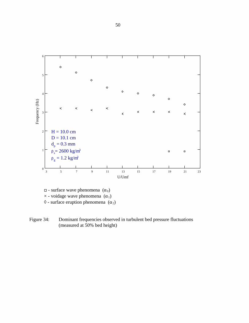
3 5 7 9 11 13 15 17 19 21 230

1

2

3

4

5

6

U/Umf

Freq

uenc

y (H

z)

H = 10.0 cm D = 10.1 cm dp = 0.3 mm

ρs= 2600 kg/m3

ρg = 1.2 kg/m3

o - surface wave phenomena (α0)× - voidage wave phenomena (α1)◊ - surface eruption phenomena (α2)

Figure 34: Dominant frequencies observed in turbulent bed pressure fluctuations(measured at 50% bed height)

51

measurements as well. This suggests that this phenomenon is not solely a characteristic of fast

fluidization. As the superficial velocity increases in the transition regime, a well defined bed

surface is no longer observed. While some bubbles are still observed propagating through the

system, the predominant motion of the bed is the sloshing motion at the surface. This sloshing

motion increases in magnitude until, near the fast fluidization regime, some particles are projected

1-3 m above the original surface of the bed. Visually it is easy to relate such a motion to the wave

behavior of a liquid.

According to surface wave theory, deep beds should exhibit a wave frequency inversely

proportional to D . For the prototype BFB, the predicted frequency for surface waves is 0.45

Hz for the fundamental, and 0.9 Hz for the first harmonic. For the model BFB, the predicted

frequency is 0.65 Hz for the fundamental, and 1.3 Hz for the first harmonic. These values

correspond closely to the frequency measured in fluidized systems approaching the fast

fluidization regime for both the model and the prototype.

In summary, the voidage fluctuation phenomena and the surface eruption frequency (seen

previously in BFB Bode plots) are observed throughout the transition from turbulent to fast

fluidization. A surface wave phenomenon with its corresponding harmonics can be observed near

the onset of fast fluidization.

Validation of BFB similitude parameters

Table 3 summarizes the results from a similitude study on the prototype and model

bubbling fluidized beds over a broad range of operating conditions. The table indicates which

experiments resulted in similar Bode plot profiles in the prototype and model. For hydrodynamics

to be considered similar, the voidage must be equal in the two beds. Also, the dimensionless

frequency and damping of the observed peaks in the fluctuation spectrum must match. The

damping coefficients and system frequencies were quantitatively estimated by fitting multiple

second order systems (acting in parallel) to the BFB Bode plots, as was done in previous work

[18]. Table 3 rates the degree of similarity between the important dependent parameters in the

prototype and model BFB under similitude. The rating for each observed frequency includes both

a comparison of the damping and a comparison of the dimensionless frequency. The table

includes the complete set of independent dimensionless parameters used in each run. The percent

52

Table 3. Summary of BFB similitude study

Exp. # U/Umf Rep Fr ρs/ρg H/D D/dp % H ε α1 α2 α0

1 1.1 4.1 5.9 2.2 1.06 254 100 N/A ** ** -2 1.1 4.0 5.9 2.2 1.06 254 100 N/A ** ** -3 1.4 5.4 10 2.2 1.06 254 100 N/A ** ** -4a 1.1 4.2 5.9 2.2 1.48 254 68 ** ** - -4b 1.1 4.2 5.9 2.2 1.48 254 100 ** * ** -5a 1.4 5.3 10 2.2 1.48 254 68 * ** * -5b 1.4 5.3 10 2.2 1.48 254 100 N/A * * -6a 1.8 6.9 16 2.2 1.48 254 68 ** ** - -6b 1.8 6.9 16 2.2 1.48 254 100 N/A * ** -7a 1.1 4.2 5.9 2.2 1.97 254 25 ** ** ** -7b 1.1 4.2 5.9 2.2 1.97 254 50 ** ** * -8a 1.4 5.3 10 2.2 1.97 254 25 ** ** ** -8b 1.4 5.3 10 2.2 1.97 254 50 ** ** - -9a 1.8 6.9 16 2.2 1.97 254 25 ** ** - -9b 1.8 6.9 16 2.2 1.97 254 50 ** ** - -10 1.1 2.0 3.3 2.2 1.06 339 100 N/A * ** -11 1.4 2.6 5.5 2.2 1.06 339 100 N/A ** ** -12 1.8 3.3 9 2.2 1.06 339 100 N/A * * -13 2.2 4.0 13 2.2 1.06 339 100 N/A * no -14a 1.1 2.0 3.3 2.2 1.48 339 68 ** ** * -14b 1.1 2.0 3.3 2.2 1.48 339 100 N/A * * -15a 1.4 2.6 5.6 2.2 1.48 339 68 ** ** * -15b 1.4 2.6 5.6 2.2 1.48 339 100 N/A * * -16a 1.8 3.3 9 2.2 1.48 339 68 ** ** * -16b 1.8 3.3 9 2.2 1.48 339 100 N/A no * no

Rating system:

** Dependent parameter identical in prototype and model* Dependent parameter is approximately the same in prototype and modelno Dependent parameter does not match in prototype and modelα0 - surface wave phenomenonα1 - voidage wave phenomenonα2 - surface eruption frequency

53

(Table 3 continued)

Exp. # U/Umf Rep Fr ρs/ρg H/D D/dp % H ε α1 α2 α0

17a 2.2 4.0 13 2.2 1.48 339 68 ** * ** *17b 2.2 4.0 13 2.2 1.48 339 100 N/A no * no18a 1.1 2.0 3.3 2.2 1.97 339 25 * ** ** -18b 1.1 2.0 3.3 2.2 1.97 339 50 ** * ** -19a 1.4 2.6 5.5 2.2 1.97 339 25 ** ** ** -19b 1.4 2.6 5.5 2.2 1.97 339 50 ** * ** -20a 1.8 3.3 9 2.2 1.97 339 25 ** ** ** -20b 1.8 3.3 9 2.2 1.97 339 50 ** * ** -21a 2.2 4.0 13 2.2 1.97 339 25 ** ** no no21b 2.2 4.0 13 2.2 1.97 339 50 ** * * no22a 1.1 0.6 1.0 2.2 1.48 508 68 ** * no -22b 1.1 0.6 1.0 2.2 1.48 508 100 N/A no * -23a 1.4 0.7 1.6 2.2 1.48 508 68 ** * * -23b 1.4 0.7 1.6 2.2 1.48 508 100 N/A * no -24a 1.8 1.0 2.7 2.2 1.48 508 68 ** * no -24b 1.8 1.0 2.7 2.2 1.48 508 100 N/A * no -25a 1.1 0.6 1.0 2.2 1.97 508 25 ** ** - -25b 1.1 0.6 1.0 2.2 1.97 508 50 ** ** - -26a 1.4 0.7 1.6 2.2 1.97 508 25 ** ** * -26b 1.4 0.7 1.6 2.2 1.97 508 50 ** ** * -27a 1.8 0.6 2.7 2.2 1.97 508 25 * ** * -27b 1.8 0.6 2.7 2.2 1.97 508 50 ** ** no -

54

height at which the pressure measurement is taken is also given. In general, matching

dimensionless parameters in two BFBs results in similar pressure dynamics. The average voidage

matches well in both beds under all conditions.

The only exception is that under conditions of relatively high superficial velocity, when

pressure fluctuations are measured in the upper regions of the bed, the peaks that result from

surface phenomena do not always show similar damping or dimensionless frequency. Evidently,

the nature of bubble coalescence in the model and prototype differ as the surface eruptions begins

to dominate the spectrum. Observation of the bubbling bed surface confirms the differences. The

surface of the small bed is noticeably lifted by large single bubble eruptions, while the prototype

surface exhibits multiple bubble eruptions across a more stationary surface.

BFB Combustor Similitude Verification

With a reliable set of scaling parameters, researchers can confidently design and build

fluidized bed pilot plants which will scale to large industrial units. To have confidence in

similitude, it is important to validate the previously given scaling parameters. Using a 20.32 cm

diameter bubbling fluidized bed combustor, a 10.16 cm diameter cold BFB, and a 5.08 cm cold

BFB, this study attempts to achieve similitude between a hot BFB combustor and cold BFB.

Only a few researchers have attempted to validate the scaling parameters between hot and

cold beds. Fitzgerald et al[19] and Nicastro and Glicksman[4] have applied the scaling rules to

small scale fluidized bed combustors. Fitzgerald et al [19], using a 2 m x 2 m BFB combustor

prototype and a 0.46 m x 0.46 m cold BFB model, concluded that agreement of the

autocorrelation plots was insufficient to prove similitude. They suggested that additional

unidentified parameters such as electrostatic forces, distributor plate scaling, and/or bed geometry

must be important. Nicastro and Glicksman [4] using a 0.61 m x 0.61 m BFB combustor as

prototype and a 0.15 m x 0.15 m cold model concluded that similitude was achieved when the full

set of dimensionless parameters were matched. Both researchers use pressure fluctuations to

confirm similitude. Fitzgerald used autocorrelation functions, whereas Nicastro and Glicksman

used the power spectral density functions.

Nicastro and Glicksman only collect data for 40 to 120 seconds thus missing much of the

low frequency phenomena that characterizes fluidized bed fluctuations. The PSD plots presented

55

by Nicastro and Glicksman for the combustor (prototype) and cold fluidized bed (model) have

neither the same power level nor exactly the same dimensionless frequency. As shown in the

methods of analysis section, inadequate data sampling and averaging can lead to misleading

results and conclusions. In addition, Nicastro and Glicksman did not specify what constituted a

“good match” between model and prototype power spectral plots.

To evaluate similitude between hot and cold fluidized beds, the BFB combustor was

fluidized with silica sand with a sphericity of 0.70. Tests were run with both natural gas and

Pittsburgh #9 coal to test for possible differences in pressure fluctuations resulting from

combustion. The conditions of the combustor and subsequent similitude trial are listed in Table 4.

As can be seen in Figures 35 and 36, there is no discernible difference in the structure of the Bode

plot for the combustor when fueled with natural gas or coal. The only difference is the slightly

larger fluctuations arising from the burning of natural gas.

After repeating the combustor run with different pressure transducers and computers

while achieving similar results, similitude was attempted in a 5.08 cm diameter cold BFB using the

full set of scaling parameters. Fluidizing parameters (see Table 4) were calculated to properly

scale the 5.08 cm BFB from the conditions in the combustor using Glicksman’s full set of

similitude parameters previously listed. From this full set, it was found that copper particles

provided a good density match when fluidized with air at ambient conditions. The resulting Bode

and PSD plot for the 5.08 cm diameter BFB as shown in Figure 37

Examining the results for the full set similitude trial as shown in Figure 38 a distinct shift

in peak frequency between the combustor and model is seen. On a nondimensional basis,

multiplying the frequencies by the square root of bed height divided by g (gravitational constant),

the peak frequency changes from 0.35 in the combustor to 0.27 in the model. In addition, a

second, but much lower magnitude frequency peak occurs in the cold model at approximately

0.48 that is not seen in the combustor. This second frequency peak, may be the result of flow

instabilities in this small bed.

This study’s proposed scaling parameter simplification and Glicksman’s simplified set of

scaling parameters are used to test similitude using a 10.16 cm bed. The operating conditions are

56

Table 4: Bed operating conditions

Combustor - Coal Combustor - CH4

dp = 0.725 mm dp = 0.725 mmD = 20.32 cm D = 20.32 cmL = 18.0 cm L = 18.0 cmU = 0.494 m/s U = 0.618 m/sρg = 0.355 kg/m3 ρg = 0.318 kg/m3

ρs = 2600 kg/m3 ρs = 2600 kg/m3

T = 805 deg C T = 782 deg CU/Umf = 1.91 U/Umf = 2.4

Rep = 2.9 Rep = 3.3Fr = 34.3 Fr = 53.8ρs/ρg = 7330 ρs/ρg = 8180L/D = 0.89 L/D = 0.89D/dp = 280 D/dp = 280

full set Glicksman’s reduced D/dp relaxation5.08 cm cold BFB 10.16 cm cold BFB 10.16 cm cold BFBdp = 0.200 mm dp = 0.238 mm dp = 0.200 mmD = 5.08 cm D = 10.16 cm D = 10.16 cmL = 4.5 cm L = 8.6 cm* L = 9.0 cmU = 0.247 m/s U = 0.298 m/s U = 0.247 m/sρg = 1.20 kg/m3 ρg = 1.20 kg/m3 ρg = 1.20 kg/m3

ρs = 8930 kg/m3 ρs = 8930 kg/m3 ρs = 8930 kg/m3

T = 20 deg C T = 20 deg C T = 20 deg CU/Umf = 1.3 U/Umf =1.9 U/Umf = 1.3

Rep = 3.2 Rep = 4.7 Rep = 3.2Fr = 31.7 Fr = 38.0 Fr = 31.7ρs/ρg = 7420 ρs/ρg = 7420 ρs/ρg = 7420L/D = 0.89 L/D = 0.85 L/D = 0.89D/dp = 260 D/dp = 426 D/dp =508

*Bed height was only 8.6 cm instead of 9.0 cm due to lack of available material.

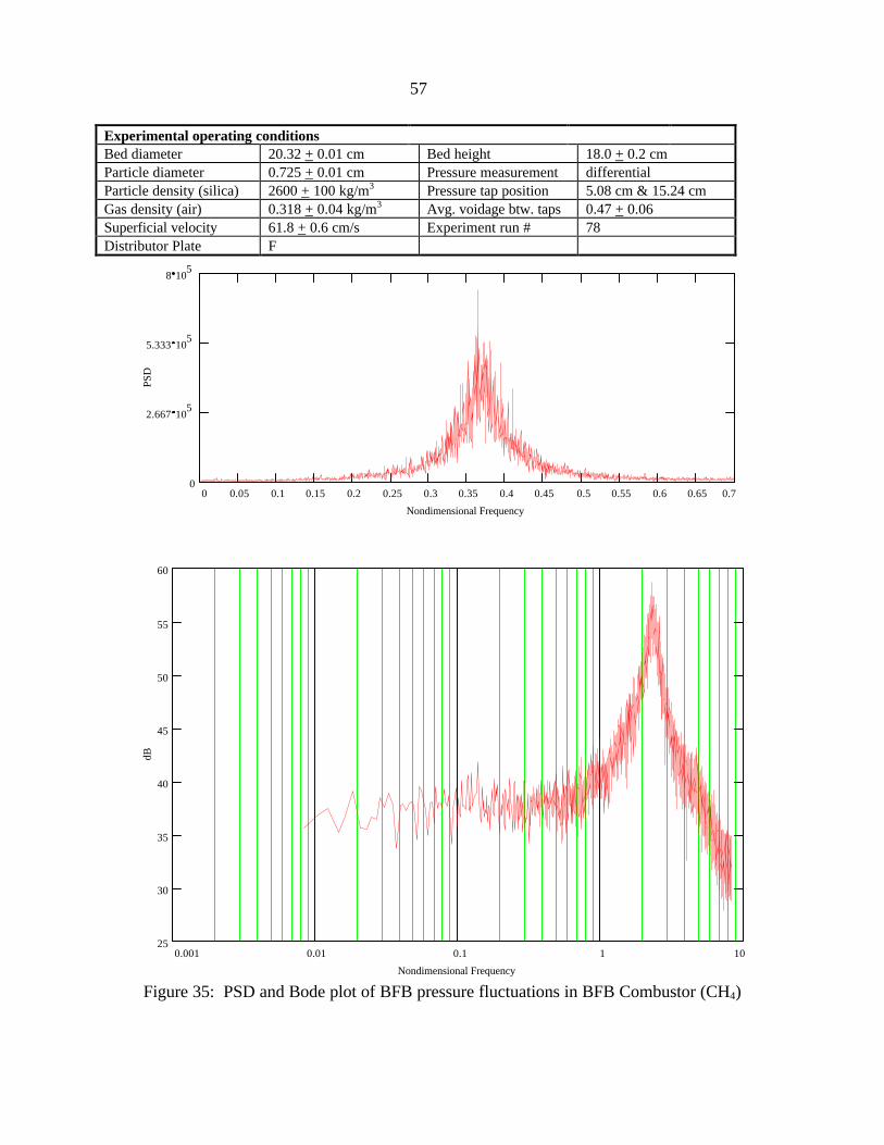
57

Experimental operating conditionsBed diameter 20.32 + 0.01 cm Bed height 18.0 + 0.2 cmParticle diameter 0.725 + 0.01 cm Pressure measurement differentialParticle density (silica) 2600 + 100 kg/m3 Pressure tap position 5.08 cm & 15.24 cmGas density (air) 0.318 + 0.04 kg/m3 Avg. voidage btw. taps 0.47 + 0.06Superficial velocity 61.8 + 0.6 cm/s Experiment run # 78Distributor Plate F

0 0.05 0.1 0.15 0.2 0.25 0.3 0.35 0.4 0.45 0.5 0.55 0.6 0.65 0.70

2.667 105

5.333 105

8 105

Nondimensional Frequency

PSD

0.001 0.01 0.1 1 1025

30

35

40

45

50

55

60


dB

Figure 35: PSD and Bode plot of BFB pressure fluctuations in BFB Combustor (CH4)

58

Experimental operating conditionsBed diameter 20.32 + 0.01 cm Bed height 18.0 + 0.2 cmParticle diameter 0.725 + 0.01 mm Pressure measurement differentialParticle density (silica) 2600 + 100 kg/m3 Pressure tap position 5.08 cm & 15.24 cmGas density (air) 0.355 + 0.04 kg/m3 Avg. voidage btw. taps 0.47 + 0.06Superficial velocity 49.4 + 0.6 cm/s Experiment run # 79Distributor Plate F

0 0.05 0.1 0.15 0.2 0.25 0.3 0.35 0.4 0.45 0.5 0.55 0.6 0.65 0.70

1.333 105

2.667 105

4 105


PSD

0.001 0.01 0.1 1 1025

30

35

40

45

50

55

60


dB

Figure 36: PSD and Bode plot of BFB pressure fluctuations in BFB combustor (coal)

59

Experimental operating conditionsBed diameter 5.08 + 0.01 cm Bed height 4.5 + 0.2 cmParticle diameter 0.196 + 0.01 cm Pressure measurement differentialParticle density (copper) 8930 + 100 kg/m3 Pressure tap position 1.27 cm & 3.81 cmGas density (air) 1.20 + 0.04 kg/m3 Avg. voidage btw. taps 0.50 + 0.06Superficial velocity 24.7 + 0.6 cm/s Experiment run # 80Distributor Plate A

0 0.05 0.1 0.15 0.2 0.25 0.3 0.35 0.4 0.45 0.5 0.55 0.6 0.65 0.70

5000

1 104

1.5 104


PSD

0.001 0.01 0.1 1 1015

20

25

30

35

40

45


dB

Figure 37: PSD and Bode plot of BFB pressure fluctuations in 5.08 cm diameter bedfull set of similitude parameters

60

0.01 0.1 1 1010

20

30

40

50

60

Dimensionless Frequency Hz(H/g)^.5

dB

0 0.1 0.2 0.3 0.4 0.5 0.6 0.70

6666.667

1.333 104

2 104

5.08 cm BFB - dist. plate A


PSD

0 0.1 0.2 0.3 0.4 0.5 0.6 0.70

1.333 105

2.667 105

4 105

20.32 cm BFB - dist plate F


PSD

Figure 38: Hot bed similitude with 5.08 cm cold BFB method: full set scalingparameters comparison of Figure 36 and Figure 37

5.08 cm cold BFB

20.32 cm Combustor

61

listed in Table 4 for both methods of scaling. Using the proposed simplification, the same

fluidization conditions exist in the 10.16 cm bed as exist in the 5.08 cm bed. This condition is

expected as long as the hydraulic Reynolds number is high enough that wall effects can be

ignored.

Using Glicksman’s reduced set, the 10.16 cm bed with fluidization air at ambient

conditions were selected. With these choices, an appropriate size of size of copper was selected

using the Ergun equation to find a particle size with the correct minimum fluidization velocity to

match the U/Umf ratio of the combustor. Operating under the fluidization conditions listed in

Table 4, the resulting Bode and PSD plot is shown as Figure 39. The comparison for this hot bed

similitude is given in Figure 40. The peak frequency for the 10.16 cm BFB occurs at the

nondimensional frequency of 0.27 as it did in the 5.08 cm BFB, however; a second lower

magnitude frequency peak does not occur. Thus the second frequency appears to arise from some

flow instability in the smaller bed. This result suggests that very small beds may not be able to

achieve similitude even if the full set of dimensionless parameters is used. The magnitude of the

fluctuations is much higher than the 5.08 cm bed which can be attributed to a higher superficial

velocity in the bed.

Using this study’s proposed relaxation of the D/dp scaling parameter results in Bode plots

with nearly the same peak frequency magnitude and fall off slope as the combustor run as shown

in Figure 41 and in the similitude comparison shown in Figure 42. As with Glicksman’s

simplification, the second low magnitude, high frequency peak seen in the 5.08 cm bed is not

present; however, a shift in peak frequency is seen. Assuming pressure fluctuations fully

characterize the hydrodynamics of the fluidized beds, one of two things can be concluded. Either

none of the cases are in similitude or the method for non-dimensionalizing is in error.

Bubbling Bed Sensitivity Study

In an attempt to better understand the phenomena seen in the scaling parameter validation

study, a parametric study was conducted to look for general trends in the effect of individual

parameters. In order to use spectral analysis of pressure fluctuations to confirm similitude, it is

important to know the sensitivity of the spectral analysis to individual parameters. Describing the

62

Experimental operating conditionsBed diameter 10.16 + 0.01 cm Bed height 8.6 + 0.2 cmParticle diameter 0.238 + 0.01 cm Pressure measurement differentialParticle density (copper) 8933 + 100 kg/m3 Pressure tap position 2.5 cm & 7.6 cmGas density (air) 1.20 + 0.04 kg/m3 Avg. voidage btw. taps 0.49 + 0.06Superficial velocity 29.8 + 0.6 cm/s Experiment run # 98Distributor Plate C

0 0.05 0.1 0.15 0.2 0.25 0.3 0.35 0.4 0.45 0.5 0.55 0.6 0.65 0.70

2.667 105

5.333 105

8 105


PSD

0.001 0.01 0.1 1 1010

20

30

40

50

60


dB

Figure 39: PSD and Bode plot of BFB pressure fluctuations in 10.16 cm diameter bedGlicksman’s reduced set of similitude parameters

63

0.01 0.1 1 1010

20

30

40

50

60


dB

0 0.1 0.2 0.3 0.4 0.5 0.6 0.70

3.333 105

6.667 105

1 106

10.16 cm BFB - dist. plate C


PSD

0 0.1 0.2 0.3 0.4 0.5 0.6 0.70

1.333 105

2.667 105

4 105



PSD

Figure 40: Hot bed similitude with 10.16 cm cold BFB method: Glicksman’sreduced set comparison of Figure 36 and Figure 39

10.16 cm BFB

20.32 cm BFB

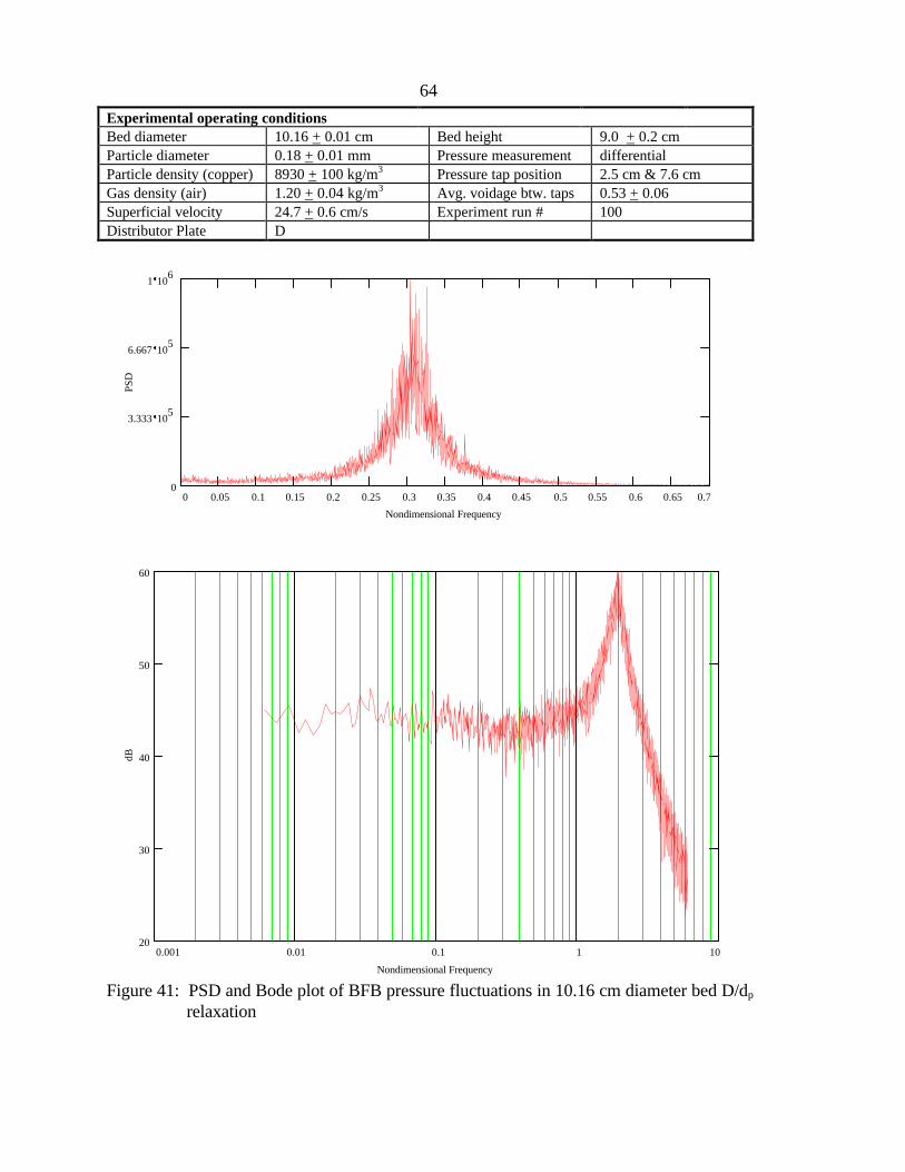
64

Experimental operating conditionsBed diameter 10.16 + 0.01 cm Bed height 9.0 + 0.2 cmParticle diameter 0.18 + 0.01 mm Pressure measurement differentialParticle density (copper) 8930 + 100 kg/m3 Pressure tap position 2.5 cm & 7.6 cmGas density (air) 1.20 + 0.04 kg/m3 Avg. voidage btw. taps 0.53 + 0.06Superficial velocity 24.7 + 0.6 cm/s Experiment run # 100Distributor Plate D

0 0.05 0.1 0.15 0.2 0.25 0.3 0.35 0.4 0.45 0.5 0.55 0.6 0.65 0.70

3.333 105

6.667 105

1 106


PSD

0.001 0.01 0.1 1 1020

30

40

50

60


dB

Figure 41: PSD and Bode plot of BFB pressure fluctuations in 10.16 cm diameter bed D/dp

relaxation

65

0.01 0.1 1 1020

30

40

50

60


dB

0 0.1 0.2 0.3 0.4 0.5 0.6 0.70

3.333 105

6.667 105

1 106



PSD

0 0.1 0.2 0.3 0.4 0.5 0.6 0.70

1.333 105

2.667 105

4 105



PSD

Figure 42: Hot bed similitude with 10.16 cm diameter bedmethod: D/dp relaxation comparison ofFigure 36 and Figure 41

10.16 cm BFB

20.32 cm BFB

66

hydrodynamics quantitatively is difficult to do with spectral analysis, as the frequency peaks are

typically made up of a broad band of frequencies. In this study, the location of the center of the

of the peak, the height of the peak, and the shape of the peak are considered most important, the

height and shape are hence forth referred to as the structure of the Bode plot. In addition, the

average bed voidage is measured for each experiment and should be equal under conditions of

similitude.

This study attempts to assess the effect particle diameter, bed diameter, particle density,

and distributor plate design have on the pressure fluctuations. As shown in Figures 43 and 44, the

superficial velocity has an effect on the peak frequency. There is a general upward trend in the

peak frequency as the superficial velocity increases in both the 10.16 and 20.32 cm diameter

BFBs. Studies by Brue [20] and de la Cruz Baez [21] examined this effect and drew different

conclusions. For instance, de la Cruz Baez reports that the peak frequency decreases as

superficial velocity increases, whereas Brue reports that peak frequency remains essentially

constant with an increase in superficial velocity above U/Umf = 1.5 as illustrated in Figure 43.

Comparing Figures 45 and 46, very little change in peak frequency is seen with a doubling

of the particle size. A very small change in the peak frequency may occur, but it is too small to

resolve accurately. Brue [20] addresses the issue of particle diameter and shows that changes in

particle diameter do not significantly affect the peak frequency. Further review of Figure 45, 200

micron steel, reveals a second frequency peak at approximately5 Hz that does not exist in the 100

micron steel under the same conditions. In addition, the PSD power level at low frequencies is

much higher fluidizing with 100 micron steel than with 200 micron steel.

Another important physical parameter of a fluidized bed is the distributor plate. Knowing

that it is important to scale a fluidized bed distributor plate, distributor plates with different hole

spacing and hole diameter were used under identical conditions with 300 micron glass beads in

two cold bubbling fluidized beds. In these tests, two plates of differing hole geometry were used

in the 5.08 cm BFB and again in the 10.16 cm BFB. The details of the hole geometry is provided

in Table 1. The dimensional results for the 10.16 bed are listed in Figures 47 and 48. A

nondimensional comparison for the 10.16 BFB is listed as Figure 49 and for the 5.08 cm BFB as

Figure 50. Note that in the 10.16 cm bed, a shift in peak frequency and magnitude is seen, but the

67

0

0.5

1

1.5

2

2.5

3

3.5

4

4.5

1 1.5 2 2.5 3 3.5

U/Umf

Pea

k F

req

uen

cy (

Hz)

Shroeder (300 micron glass)

Brue (300 micron glass)

de la Cruz Baez (400 micron glass)

Figure 43: Effect of Velocity on Peak Frequency

0

1

2

3

4

5

6

1 1.5 2 2.5 3

U/Umf

Pea

k F

req

uen

cy (

Hz)

Figure 44: Effect of velocity on peak frequency 20.32 cm BFB, 300 micron glass beads, 13.6 cmbed height

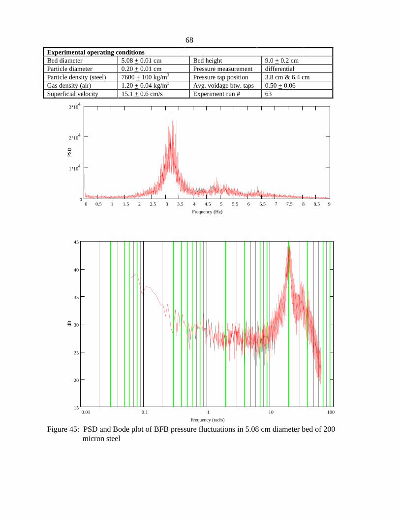
68

Experimental operating conditionsBed diameter 5.08 + 0.01 cm Bed height 9.0 + 0.2 cmParticle diameter 0.20 + 0.01 cm Pressure measurement differentialParticle density (steel) 7600 + 100 kg/m3 Pressure tap position 3.8 cm & 6.4 cmGas density (air) 1.20 + 0.04 kg/m3 Avg. voidage btw. taps 0.50 + 0.06Superficial velocity 15.1 + 0.6 cm/s Experiment run # 63

0 0.5 1 1.5 2 2.5 3 3.5 4 4.5 5 5.5 6 6.5 7 7.5 8 8.5 90

1 104

2 104

3 104

Frequency (Hz)

PSD

0.01 0.1 1 10 10015

20

25

30

35

40

45

Frequency (rad/s)

dB

Figure 45: PSD and Bode plot of BFB pressure fluctuations in 5.08 cm diameter bed of 200micron steel

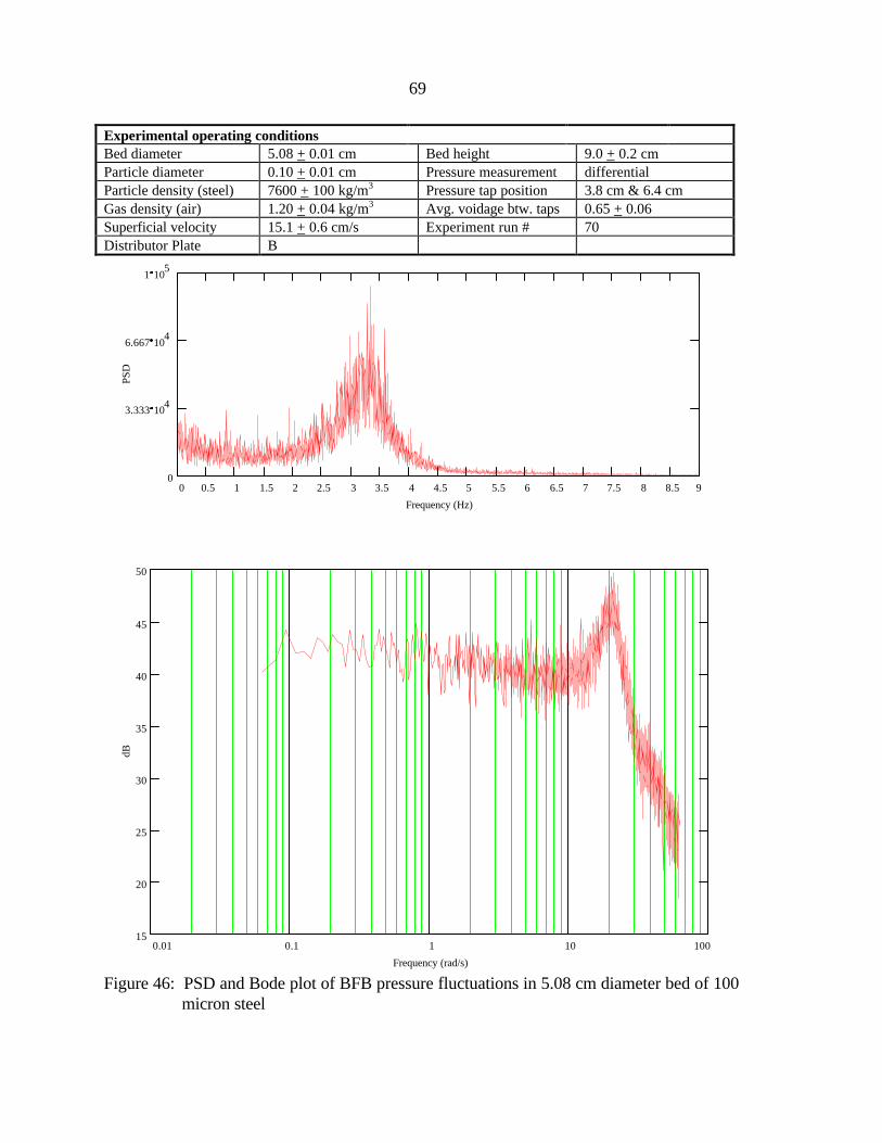
69

Experimental operating conditionsBed diameter 5.08 + 0.01 cm Bed height 9.0 + 0.2 cmParticle diameter 0.10 + 0.01 cm Pressure measurement differentialParticle density (steel) 7600 + 100 kg/m3 Pressure tap position 3.8 cm & 6.4 cmGas density (air) 1.20 + 0.04 kg/m3 Avg. voidage btw. taps 0.65 + 0.06Superficial velocity 15.1 + 0.6 cm/s Experiment run # 70Distributor Plate B

0 0.5 1 1.5 2 2.5 3 3.5 4 4.5 5 5.5 6 6.5 7 7.5 8 8.5 90

3.333 104

6.667 104

1 105

Frequency (Hz)

PSD

0.01 0.1 1 10 10015

20

25

30

35

40

45

50

Frequency (rad/s)

dB

Figure 46: PSD and Bode plot of BFB pressure fluctuations in 5.08 cm diameter bed of 100micron steel

70

Experimental operating conditionsBed diameter 10.16 + 0.01 cm Bed height 9.0 + 0.2 cmParticle diameter 0.30 + 0.01 cm Pressure measurement differentialParticle density (glass) 2600 + 100 kg/m3 Pressure tap position 3.8 cm & 6.4 cmGas density (air) 1.20 + 0.04 kg/m3 Avg. voidage btw. taps 0.47 + 0.06Superficial velocity 15.1 + 0.6 cm/s Experiment run # 82Distributor Plate C

0 0.5 1 1.5 2 2.5 3 3.5 4 4.5 5 5.5 6 6.5 7 7.5 8 8.5 90

100

200

300

Frequency (Hz)

PSD

0.01 0.1 1 10 1005

0

5

10

15

20

25

Frequency (rad/s)

dB

Figure 47: PSD and Bode plot of BFB pressure fluctuations in 10.16 cm diameter bed distributorplate C

71

Experimental operating conditionsBed diameter 10.16 + 0.01 cm Bed height 9.0 + 0.2 cmParticle diameter 0.30 + 0.01 cm Pressure measurement differentialParticle density (glass) 2600 + 100 kg/m3 Pressure tap position 3.8 cm & 6.4 cmGas density (air) 1.20 + 0.04 kg/m3 Avg. voidage btw. taps 0.51 + 0.06Superficial velocity 15.1 + 0.6 cm/s Experiment run # 84Distributor Plate D

0 0.5 1 1.5 2 2.5 3 3.5 4 4.5 5 5.5 6 6.5 7 7.5 8 8.5 90

200

400

600

800

Frequency (Hz)

PSD

0.01 0.1 1 10 1000

5

10

15

20

25

30

Frequency (rad/s)

dB

Figure 48: PSD and Bode plot of BFB pressure fluctuations in 10.16 cm diameter bed distributorplate D

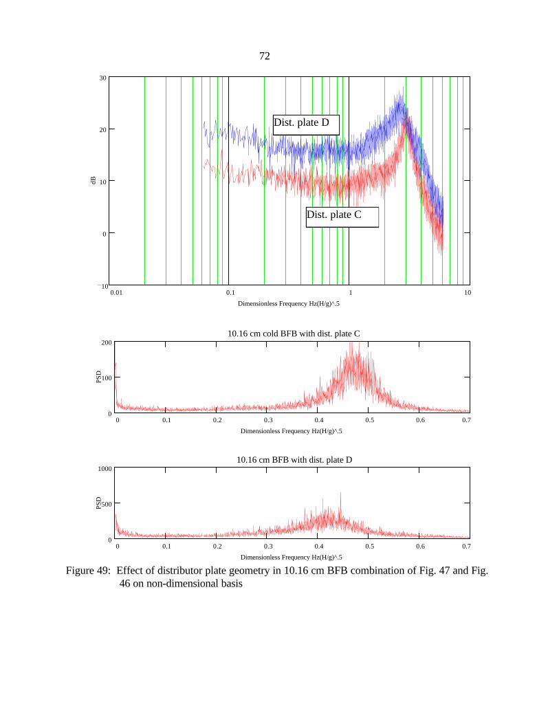
72

0.01 0.1 1 1010

0

10

20

30


dB

0 0.1 0.2 0.3 0.4 0.5 0.6 0.70

100

20010.16 cm cold BFB with dist. plate C


PSD

0 0.1 0.2 0.3 0.4 0.5 0.6 0.70

500

100010.16 cm BFB with dist. plate D


PSD

Figure 49: Effect of distributor plate geometry in 10.16 cm BFB combination of Fig. 47 and Fig.46 on non-dimensional basis

Dist. plate D

Dist. plate C

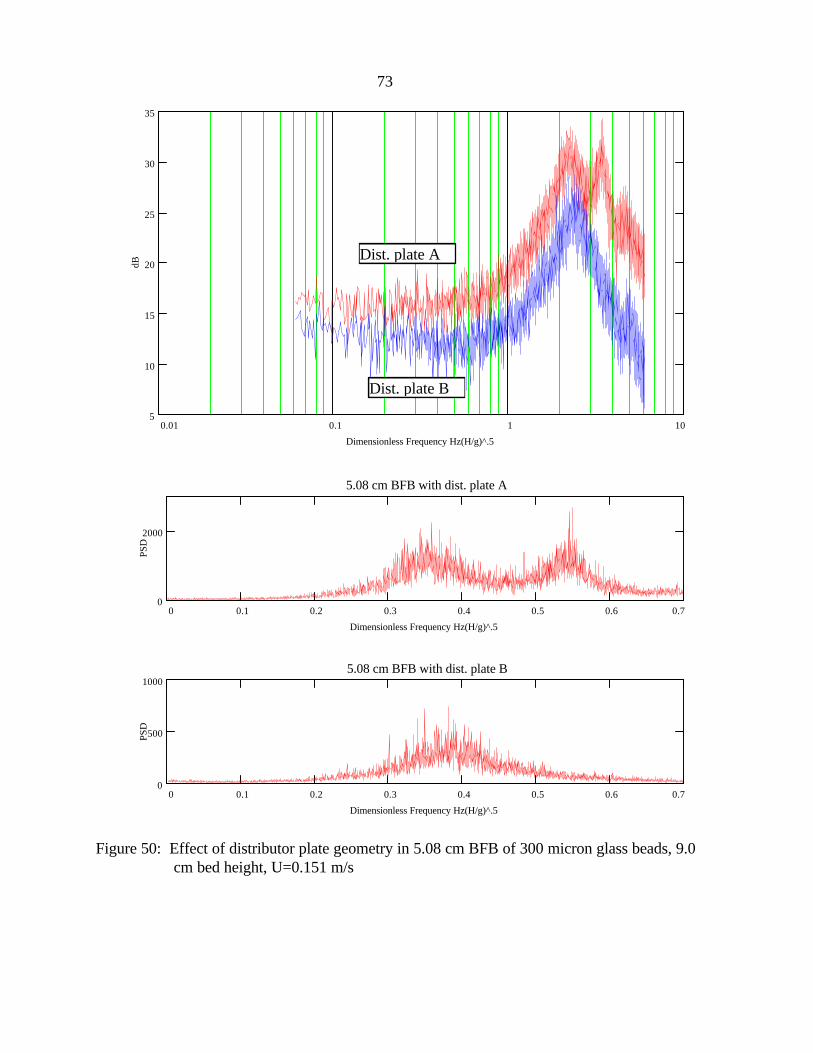
73

0.01 0.1 1 105

10

15

20

25

30

35


dB

0 0.1 0.2 0.3 0.4 0.5 0.6 0.70

2000

5.08 cm BFB with dist. plate A


PSD

0 0.1 0.2 0.3 0.4 0.5 0.6 0.70

500

10005.08 cm BFB with dist. plate B


PSD

Figure 50: Effect of distributor plate geometry in 5.08 cm BFB of 300 micron glass beads, 9.0cm bed height, U=0.151 m/s

Dist. plate A

Dist. plate B

74

general Bode plot structure is very similar with this change in distributor plate geometry. Once

again, a second peak frequency appears in the 5.08 cm BFB as illustrated in Figure 50 in the case

using plate A with 0.6 mm holes in the distributor plate. It seems that the small diameter of the

5.08 cm bed causes changes in the fluidization hydrodynamics that result in a second frequency

peak. De la Cruz Baez [21], investigated the effect of different distributor plates comparing two

plates with different number of 1 mm holes and a filter paper distributor plate. He compared three

distributor plates under identical operating conditions and always saw differing peak frequencies

in the pressure fluctuations regardless of superficial velocity when comparing distributor plate

geometries. Based on this study’s results and those of de la Cruz Baez, it can be concluded that

the distributor has an effect on BFB hydrodynamics and must be a consideration in all

similitude studies.

Important for simplifying the scaling parameters, it must be verified that the D/dp ratio can

be relaxed. Experimental runs in both the 20.32 cm and 10.16 cm BFBs were completed under

identical conditions to verify that the diameter ratio term may be relaxed. To avoid results being

changed by the distributor plates, tests were run in the 10.16 cm BFB using a ½ scale distributor

plate (plate C): hole size and spacing are reduced by ½. Another distributor was fabricated for

the ½ scale model that had identical geometry as the 20.32 cm bed (plate E): in this case hole size

and spacing are identical. The ½ scale plate is referred to as the “scaled plate” while the plates

with identical hole size and spacing is referred to as the “identical distributor plate” in this study.

Using 300 micron glass beads, tests were run at superficial velocities of 15.1 cm/s, U/Umf

= 1.7, and 29.1 cm/s, U/Umf = 3.2. The results of these runs are listed in Figures 51 - 54. Notice

that the peak frequencies do not coincide with one another in any case. In the 15.1 cm/s

comparison, Figure 51, the peaks are neither similar in frequency or magnitude when the scaled

distributor plate is used. Switching to the identical distributor plate in Figure 52, the peak

frequency is increased some and the magnitude of the peak is lowered to the level of the 20.32 cm

bed. Inspecting the 29.1 cm/s superficial velocity case, Figures 53 and 54, it is apparent that the

PSD and Bode plots are very similar, almost identical, except for a definite shift in peak frequency

in both the identical and scaled distributor plate cases.

With this evidence, it is not possible to conclude that the D/dp can be ignored as a scaling

parameter in these small beds. Many times the Bode and PSD plots would be similar and suggest

75

0.01 0.1 1 100

10

20

30

40


dB

0 0.1 0.2 0.3 0.4 0.5 0.6 0.70

3333.333

6666.667

1 104



PSD

0 0.1 0.2 0.3 0.4 0.5 0.6 0.70

666.667

1333.333



PSD

Figure 51: Bed diameter comparison of 20.32 BFB and 10.16 BFB at ambient 300 micron glassbeads, 13.7 cm bed height, U=0.151m/s scaled distributor plate geometry

10.12 cm BFB

20.32 cm BFB

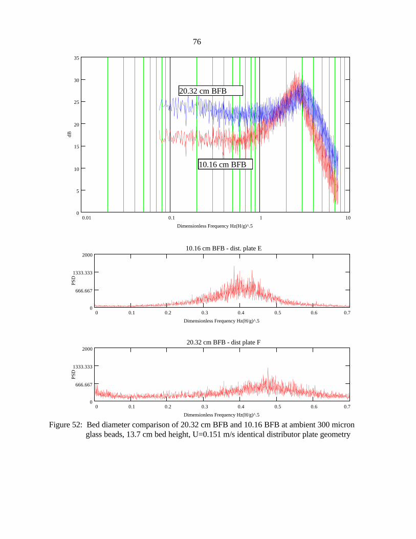
76

0.01 0.1 1 100

5

10

15

20

25

30

35


dB

0 0.1 0.2 0.3 0.4 0.5 0.6 0.70

666.667

1333.333

200010.16 cm BFB - dist. plate E


PSD

0 0.1 0.2 0.3 0.4 0.5 0.6 0.70

666.667

1333.333



PSD

Figure 52: Bed diameter comparison of 20.32 cm BFB and 10.16 BFB at ambient 300 micronglass beads, 13.7 cm bed height, U=0.151 m/s identical distributor plate geometry

10.16 cm BFB

20.32 cm BFB

77

0.01 0.1 1 1020

25

30

35

40

45

50


dB

0 0.1 0.2 0.3 0.4 0.5 0.6 0.70

2 104

4 104

6 104



PSD

0 0.1 0.2 0.3 0.4 0.5 0.6 0.70

2 104

4 104

6 104



PSD

Figure 53: Bed diameter comparison of 20.32 BFB and 10.16 BFB at ambient 300 micron glassbeads, 13.7 cm bed height, U=0.291m/s scaled distributor plate geometry

10.16 cm BFB

20.32 cm BFB

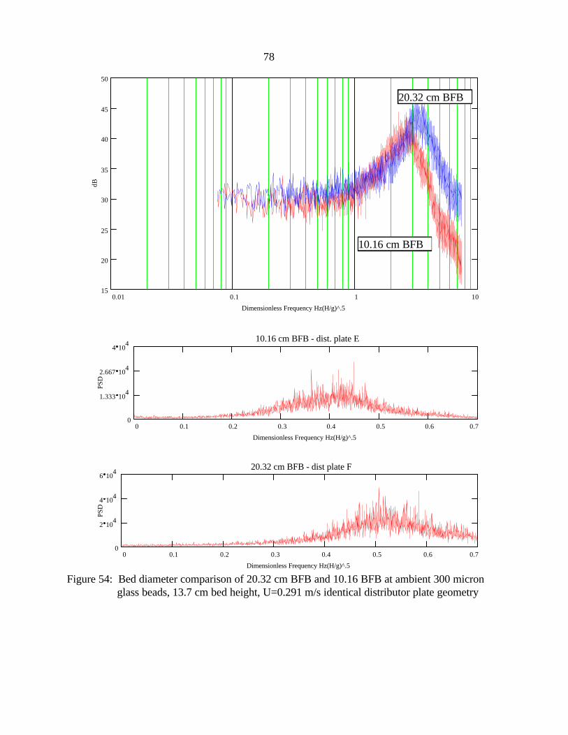
78

0.01 0.1 1 1015

20

25

30

35

40

45

50


dB

0 0.1 0.2 0.3 0.4 0.5 0.6 0.70

1.333 104

2.667 104

4 104

10.16 cm BFB - dist. plate E


PSD

0 0.1 0.2 0.3 0.4 0.5 0.6 0.70

2 104

4 104

6 104



PSD

Figure 54: Bed diameter comparison of 20.32 cm BFB and 10.16 BFB at ambient 300 micronglass beads, 13.7 cm bed height, U=0.291 m/s identical distributor plate geometry

10.16 cm BFB

20.32 cm BFB

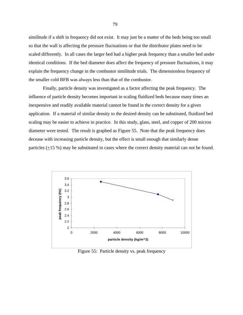
79

similitude if a shift in frequency did not exist. It may just be a matter of the beds being too small

so that the wall is affecting the pressure fluctuations or that the distributor plates need to be

scaled differently. In all cases the larger bed had a higher peak frequency than a smaller bed under

identical conditions. If the bed diameter does affect the frequency of pressure fluctuations, it may

explain the frequency change in the combustor similitude trials. The dimensionless frequency of

the smaller cold BFB was always less than that of the combustor.

Finally, particle density was investigated as a factor affecting the peak frequency. The

influence of particle density becomes important in scaling fluidized beds because many times an

inexpensive and readily available material cannot be found in the correct density for a given

application. If a material of similar density to the desired density can be substituted, fluidized bed

scaling may be easier to achieve in practice. In this study, glass, steel, and copper of 200 micron

diameter were tested. The result is graphed as Figure 55. Note that the peak frequency does

decease with increasing particle density, but the effect is small enough that similarly dense

particles (+15 %) may be substituted in cases where the correct density material can not be found.

2

2.2

2.4

2.6

2.8

3

3.2

3.4

3.6

0 2000 4000 6000 8000 10000

particle density (kg/m^3)

pea

k fr

equ

ency

(H

z)

Figure 55: Particle density vs. peak frequency

80

Experimental Apparatus and Procedures: Circulating Fluidized Bed

Circulating Fluidized Bed

This study was performed in two geometrically similar cold-flow CFBs, illustrated in

Figure 56. The riser of the larger unit (prototype) is 10.2 cm in diameter and 3.00 m tall. This

unit is fluidized with 0.2, 0.3, and 0.4 mm diameter glass beads. Pressure taps are located at 25.4

cm intervals along the riser, with two additional pressure taps spaced evenly between the first

25.4 cm interval. Each pressure tap is threaded into the CFB so that the tap is flush with the inner

wall. The riser, cyclone, and L-valve of both circulating fluidized beds are constructed of

aluminum to reduce electrostatic effects. The downcomer and solids flux meter are constructed

of Plexiglas to allow visual observation of bed operation. The 10.2 cm diameter CFB has two

small Plexiglas sections in the riser to observe solids circulation. This large CFB is designed to be

operated only at atmospheric pressure, using air as the fluidizing gas. The smaller unit is a one-

half scale model of the larger unit with an inside diameter of 5.08 cm and a height of 1.50 m. The

smaller CFB (model) is fluidized with 0.1, 0.15, and 0.2 mm diameter steel shot, for the purpose

of conducting hydrodynamic similitude studies between the two beds. Since the fluidizing gas

density must be greater in the small bed in order to achieve similitude, it is fluidized with

pressurized air (0-200 kPa gage).

Solids Flux Measurement

Since the accurate measurement of solids flux is very important for similitude studies, a

meter was constructed that, when activated, would capture particles as they exited the cyclone. A

schematic of this solids flux meter is shown in Figure 57. The time it takes for this meter to fill is

recorded and converted to a solids flux in kg/m2s. The design of this meter involved a trade-off.

If the meter was constructed too small, the time at which it filled would be to short for high

accuracy measurements. If it was built too large, the particles removed by the meter would

significantly reduce the height of the particles in the L-valve. This change in downcomer bed

height reduces the solids circulation rate of the system during measurement. Designing a valve to

release the particles from the meter after measurement proved to be difficult. In the end, a simple

rubber plug suspended by a nylon cord that extended down through the top of the cyclone was

used to control filling and emptying of the flux meter. The meter measured the solids flux with an

81

Figure

56:

Cold-

Figure 56: Circulating fluidized bed apparatus (dimensions shown for model)

B-2.0”ID x 1/4” Aluminum

D-Aluminum cyclone

59.0

4.42

14-pressure1\8” NPT

14.82

16.75

18.00

7.25

5.81

13.5 4.00

11.0

B

D

E

F

A

C

4.75

“DEAD-SPACE EXTENSION (used for top-plate effect experiments)

A-2.0”ID x 1/4”W Plexiglass

C-2.0” x 1.0” - 1/8”W Aluminum

E- Plexiglass solids flux meterF- 1.25”ID x 1/8”W Plexiglass

Notes: Dimensions are given for the CFB model in inches Prototype dimesions = 2 x modeldimensions

82

Figure 57: Solids flux meter detail

16.75

18.00

11.0

Plug control cord

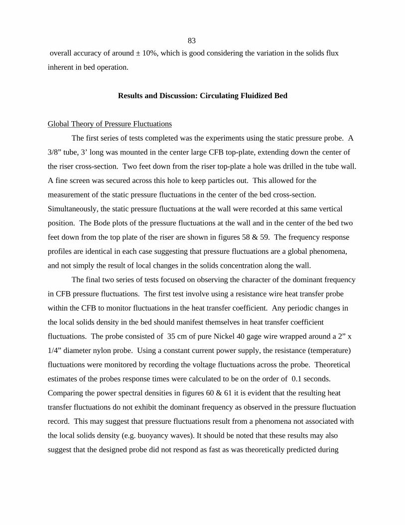
83

overall accuracy of around ± 10%, which is good considering the variation in the solids flux

inherent in bed operation.

Results and Discussion: Circulating Fluidized Bed

Global Theory of Pressure Fluctuations

The first series of tests completed was the experiments using the static pressure probe. A

3/8” tube, 3’ long was mounted in the center large CFB top-plate, extending down the center of

the riser cross-section. Two feet down from the riser top-plate a hole was drilled in the tube wall.

A fine screen was secured across this hole to keep particles out. This allowed for the

measurement of the static pressure fluctuations in the center of the bed cross-section.

Simultaneously, the static pressure fluctuations at the wall were recorded at this same vertical

position. The Bode plots of the pressure fluctuations at the wall and in the center of the bed two

feet down from the top plate of the riser are shown in figures 58 & 59. The frequency response

profiles are identical in each case suggesting that pressure fluctuations are a global phenomena,

and not simply the result of local changes in the solids concentration along the wall.

The final two series of tests focused on observing the character of the dominant frequency

in CFB pressure fluctuations. The first test involve using a resistance wire heat transfer probe

within the CFB to monitor fluctuations in the heat transfer coefficient. Any periodic changes in

the local solids density in the bed should manifest themselves in heat transfer coefficient

fluctuations. The probe consisted of 35 cm of pure Nickel 40 gage wire wrapped around a 2” x

1/4” diameter nylon probe. Using a constant current power supply, the resistance (temperature)

fluctuations were monitored by recording the voltage fluctuations across the probe. Theoretical

estimates of the probes response times were calculated to be on the order of 0.1 seconds.

Comparing the power spectral densities in figures 60 & 61 it is evident that the resulting heat

transfer fluctuations do not exhibit the dominant frequency as observed in the pressure fluctuation

record. This may suggest that pressure fluctuations result from a phenomena not associated with

the local solids density (e.g. buoyancy waves). It should be noted that these results may also

suggest that the designed probe did not respond as fast as was theoretically predicted during

84

0.1 1 10 10040

30

20

10

0

frequency (rad/s)

dB

Figure 58: Bode Plot of CFB pressure fluctuations (center probe configuration)

80 % bed height solids flux: 19 ± 3 kg/m s2Large model w/ 0.2 mm glass beads superficial velocity: 3.0 ± 0.3 m/s

0.1 1 10 10050

40

30

20

10

0

frequency (rad/s)

dB

Figure 59: Bode Plot of CFB pressure fluctuations at riser wall

80 % bed height solids flux: 19 ± 3 kg/m s2Large model w/ 0.2 mm glass beads superficial velocity: 3.0 ± 0.3 m/s

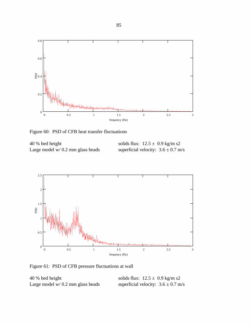
85

0 0.5 1 1.5 2 2.5 30

0.2

0.4

0.6

0.8

frequency (Hz)

PSD

Figure 60: PSD of CFB heat transfer fluctuations

40 % bed height solids flux: 12.5 ± 0.9 kg/m s2Large model w/ 0.2 mm glass beads superficial velocity: 3.6 ± 0.7 m/s

0 0.5 1 1.5 2 2.5 30

0.5

1

1.5

2

2.5

frequency (Hz)

PSD

Figure 61: PSD of CFB pressure fluctuations at wall

40 % bed height solids flux: 12.5 ± 0.9 kg/m s2Large model w/ 0.2 mm glass beads superficial velocity: 3.6 ± 0.7 m/s

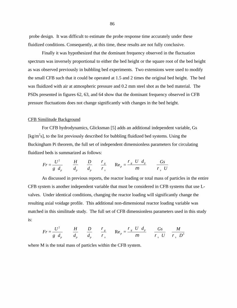
86

probe design. It was difficult to estimate the probe response time accurately under these

fluidized conditions. Consequently, at this time, these results are not fully conclusive.

Finally it was hypothesized that the dominant frequency observed in the fluctuation

spectrum was inversely proportional to either the bed height or the square root of the bed height

as was observed previously in bubbling bed experiments. Two extensions were used to modify

the small CFB such that it could be operated at 1.5 and 2 times the original bed height. The bed

was fluidized with air at atmospheric pressure and 0.2 mm steel shot as the bed material. The

PSDs presented in figures 62, 63, and 64 show that the dominant frequency observed in CFB

pressure fluctuations does not change significantly with changes in the bed height.

CFB Similitude Background

For CFB hydrodynamics, Glicksman [5] adds an additional independent variable, Gs

[kg/m2s], to the list previously described for bubbling fluidized bed systems. Using the

Buckingham Pi theorem, the full set of independent dimensionless parameters for circulating

fluidized beds is summarized as follows:

FrU

g dp

=⋅

2

Hdp

Ddp

ρρ

g

s

Repg pU d

=⋅ ⋅ρµ

Gs

Usρ ⋅

As discussed in previous reports, the reactor loading or total mass of particles in the entire

CFB system is another independent variable that must be considered in CFB systems that use L-

valves. Under identical conditions, changing the reactor loading will significantly change the

resulting axial voidage profile. This additional non-dimensional reactor loading variable was

matched in this similitude study. The full set of CFB dimensionless parameters used in this study

is:

FrU

g dp

=⋅

2

Hdp

Ddp

ρρ

g

s

Repg pU d

=⋅ ⋅ρµ

Gs

Usρ ⋅

MDsρ ⋅ 3

where M is the total mass of particles within the CFB system.

87

Fast Fluidization Fluctuations - General characteristics

Two predominant phenomena are observed in the frequency spectrum of fast fluidization

systems. Figures 65-67 show typical CFB Bode plots under different operating conditions.

Under relatively dilute conditions (and in the upper regions of the bed) the surface wave

phenomenon appears along with its first harmonic in the spectrum (see Figure 60). In the

transition from dilute to dense conditions, the Bode plot of fluctuations appears highly damped as

shown in Figure 66 (i.e. no distinct peaks are observed in the pressure dynamics). Under the

dense conditions shown in Figure 67, the voidage wave frequency is evident in the Bode plot.

This voidage wave phenomenon is most dominant when fluctuations are measured at low

elevations in the bed (5-10 % bed height). The CFB Bode plots under all conditions exhibit a

final asymptotic slope of -40 dB/decade.

Discussion of Voidage Wave Phenomenon in CFBs

By observing pressure fluctuations throughout the transition from bubbling to turbulent to

fast fluidization, it is evident that the voidage wave phenomenon is present in all three regimes.

This phenomenon originates from the lower dense regions of the CFB. It appears only when a

lower dense bed has been established (i.e. the axial voidage profile shows decreasing voidage at

low bed heights). It is also most dominantly sensed at the lower elevations of the CFB. Figure 68

shows how voidage waves are manifest in the CFB Bode plots of fluctuations measured at

different elevations. Secondly, in addition to the observation of this phenomena throughout

bubbling, turbulent, and fast fluidization regimes, the frequency of this phenomena can be

predicted from the modified-Hiby model proposed for bubbling fluidized beds. The height of the

lower dense bed can be estimated from the axial voidage profiles to be between 10-20 cm (in the

10.2 cm diameter CFB model). The theory for voidage oscillations under turbulent conditions

predicts that this frequency should appear between 2-3 Hz. All Bode plots of lower dense bed

pressure fluctuations confirm this.

As expected, this voidage wave also exhibits an inverse square root dependence on dense

bed height. When the two CFB models are operated such that similar axial voidage profiles are

88

0 0.5 1 1.5 2 2.5 30

1

2

3

frequency (Hz)

PSD

Figure 62: Bode Plot of CFB static pressure fluctuations

2 x standard bed height (48” extension) solids flux: 34 ± 4 kg/m s2Large model w/ 0.2 mm glass beads superficial velocity: 5.5 ± 0.4 m/s

0 0.5 1 1.5 2 2.5 30

1

2

3

frequency (Hz)

PSD

Figure 63: Bode Plot of CFB static pressure fluctuations

1.5 x standard bed height (24” extension) solids flux: 49 ± 5 kg/m s2Large model w/ 0.2 mm glass beads superficial velocity: 6.2 ± 0.4 m/s

89

0 0.5 1 1.5 2 2.5 30

0.5

1

1.5

2

frequency (Hz)

PSD

Figure 64: Bode Plot of CFB static pressure fluctuationsstandard bed height (no extension) solids flux: 38 ± 7 kg/m s2Large model w/ 0.2 mm glass beads superficial velocity: 5.6 ± 0.4 m/s

90

0.9 0.95 10

20

40

60

80

100(a) Axial Voidage Profile

Average voidage

% b

ed h

eigh

t

CFB Operating Conditions: Gs = 13 kg/m2s

U = 4.7 m/s (air @ 1.0 atm) D = 10.2 cm dp = 0.4 mm (glass beads)

Differential pressure measurement @ 13 % bed height - 25.4 cm tap spacing

0 2 4 60

0.1

0.2(b) Power Spectral Density

frequency (Hz)

PSD

0.1 1 10 10050

40

30

20

10

0(c) Bode Plot

frequency (rad/s)

dB

Figure 65: Dilute CFB operating conditions - a) axial voidage, b) PSD, c) Bode plot

91

0.9 0.95 10

20

40

60

80


Average voidage

% b

ed h

eigh

t




0 2 4 60

5

10(b) Power Spectral Density

frequency (Hz)

PSD

0.1 1 10 10030

20

10

0

10(c) Bode Plot

frequency (rad/s)

dB

Figure 66: Damped CFB operating conditions - a) axial voidage, b) PSD, c) Bode plot

92

0.9 0.95 10

20

40

60

80


Average voidage

% b

ed h

eigh

t




0 2 4 60

10

20(b) Power Spectral Density

frequency (Hz)

PSD

0.1 1 10 10020

10

0

10

20(c) Bode Plot

frequency (rad/s)

dB

Figure 67: Dense CFB operating conditions - a) axial voidage, b) PSD, c) Bode plot

93

CFB Operating conditions:

U = 4.1 ± 0.2 m/s (air @ 1.0 atm)Gs = 18 ± 4 kg/m2sD = 10.2 cmdp = 0.3 mm (glass beads)

0.1 1 10 1000

5

10

15

20

25

30

35

40

45

50

55

1.2 % CFB height30 % CFB height75 % CFB height

frequency (rad/s)

dB

Figure 68: Appearance of dense phase phenomena at various bed elevations

94

attained, the lower dense bed height in the large CFB will be twice the height of the small CFB

dense bed. Consequently, the lower dense bed frequency in the model CFB appears at a

frequency that is 1.4 (or 21/2) times the frequency that is observed in the prototype CFB. This is

shown conclusively in the results of the similitude study that follow. This result suggests that

pressure fluctuation measurements at one location could be used as an indicator of the height of

the lower dense region in a CFB

Discussion of surface wave frequency phenomena in CFBs

As seen in the transition regime, surface waves begin to appear in the high velocity

turbulent regime prior to fast fluidization. This suggests that this phenomena is associated with

the behavior of particles leaving and returning to the dense bed surface, rather than a phenomena

associated with the structural CFB height.

Visual observations in circulating fluidized beds and turbulent beds (as they approach fast

fluidization) show clusters of solids leaving the dense bed surface at approximately 1 Hz, which

corresponds to the frequency peaks observed in the Bode plots. Similar to the transition regime,

this frequency of sloshing/cluster propagation originating at the lower dense region of the CFB is

hypothesized to be governed by surface wave phenomena. It appears that this frequency is

inversely proportional to the square root of the bed diameter, which further supports the

hypothesis of pressure fluctuations governed by deep wave phenomena. This result suggests that

pressure fluctuation measurements at one location could be used as an indicator of the height of

the lower dense region in a CFB.

Summary of CFB pressure fluctuations

CFB pressure fluctuations are indicative of CFB hydrodynamics in two ways. First, the

frequency phenomenon that is observed in the lower regions of the CFB under conditions of high

solids loading is the result of lower dense bed voidage oscillations as observed in bubbling and

turbulent beds also. Our results suggest that a surface wave phenomena inversely proportional to

the square root of the bed diameter is also be observed in CFB pressure fluctuations under most

conditions. Knowing how pressure fluctuations reflect CFB hydrodynamics, it is possible to use

the analysis of pressure fluctuations to validate proposed similitude parameters.

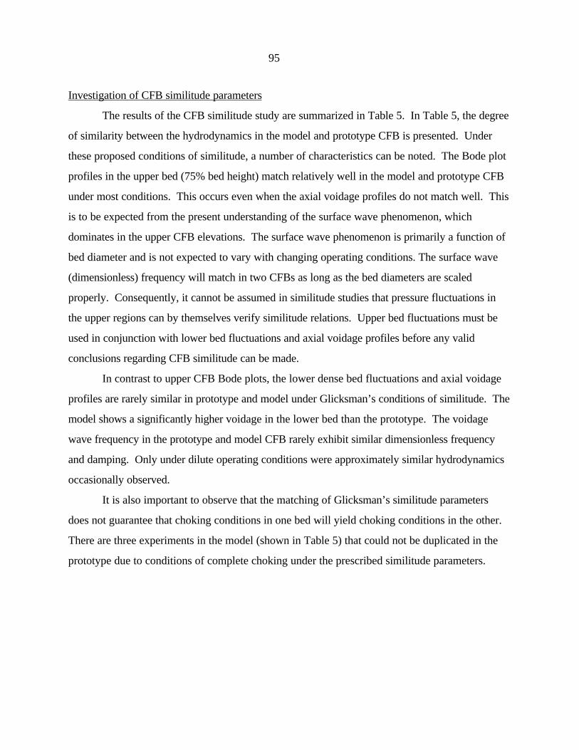
95

Investigation of CFB similitude parameters

The results of the CFB similitude study are summarized in Table 5. In Table 5, the degree

of similarity between the hydrodynamics in the model and prototype CFB is presented. Under

these proposed conditions of similitude, a number of characteristics can be noted. The Bode plot

profiles in the upper bed (75% bed height) match relatively well in the model and prototype CFB

under most conditions. This occurs even when the axial voidage profiles do not match well. This

is to be expected from the present understanding of the surface wave phenomenon, which

dominates in the upper CFB elevations. The surface wave phenomenon is primarily a function of

bed diameter and is not expected to vary with changing operating conditions. The surface wave

(dimensionless) frequency will match in two CFBs as long as the bed diameters are scaled

properly. Consequently, it cannot be assumed in similitude studies that pressure fluctuations in

the upper regions can by themselves verify similitude relations. Upper bed fluctuations must be

used in conjunction with lower bed fluctuations and axial voidage profiles before any valid

conclusions regarding CFB similitude can be made.

In contrast to upper CFB Bode plots, the lower dense bed fluctuations and axial voidage

profiles are rarely similar in prototype and model under Glicksman’s conditions of similitude. The

model shows a significantly higher voidage in the lower bed than the prototype. The voidage

wave frequency in the prototype and model CFB rarely exhibit similar dimensionless frequency

and damping. Only under dilute operating conditions were approximately similar hydrodynamics

occasionally observed.

It is also important to observe that the matching of Glicksman’s similitude parameters

does not guarantee that choking conditions in one bed will yield choking conditions in the other.

There are three experiments in the model (shown in Table 5) that could not be duplicated in the

prototype due to conditions of complete choking under the prescribed similitude parameters.

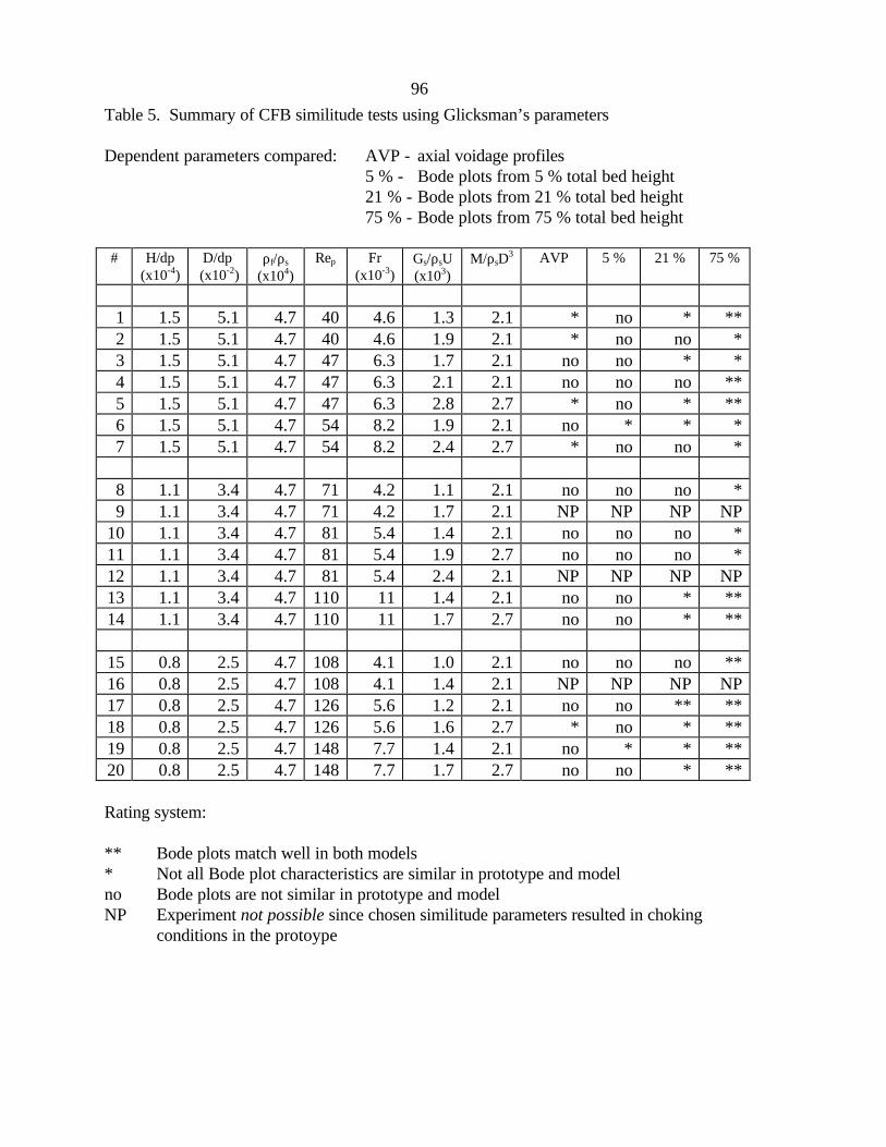
96

Table 5. Summary of CFB similitude tests using Glicksman’s parameters

Dependent parameters compared: AVP - axial voidage profiles5 % - Bode plots from 5 % total bed height21 % - Bode plots from 21 % total bed height75 % - Bode plots from 75 % total bed height

# H/dp(x10-4)

D/dp (x10-2)

ρf/ρs

(x104)Rep Fr

(x10-3)Gs/ρsU(x103)

M/ρsD3 AVP 5 % 21 % 75 %

1 1.5 5.1 4.7 40 4.6 1.3 2.1 * no * **2 1.5 5.1 4.7 40 4.6 1.9 2.1 * no no *3 1.5 5.1 4.7 47 6.3 1.7 2.1 no no * *4 1.5 5.1 4.7 47 6.3 2.1 2.1 no no no **5 1.5 5.1 4.7 47 6.3 2.8 2.7 * no * **6 1.5 5.1 4.7 54 8.2 1.9 2.1 no * * *7 1.5 5.1 4.7 54 8.2 2.4 2.7 * no no *

8 1.1 3.4 4.7 71 4.2 1.1 2.1 no no no *9 1.1 3.4 4.7 71 4.2 1.7 2.1 NP NP NP NP

10 1.1 3.4 4.7 81 5.4 1.4 2.1 no no no *11 1.1 3.4 4.7 81 5.4 1.9 2.7 no no no *12 1.1 3.4 4.7 81 5.4 2.4 2.1 NP NP NP NP13 1.1 3.4 4.7 110 11 1.4 2.1 no no * **14 1.1 3.4 4.7 110 11 1.7 2.7 no no * **

15 0.8 2.5 4.7 108 4.1 1.0 2.1 no no no **16 0.8 2.5 4.7 108 4.1 1.4 2.1 NP NP NP NP17 0.8 2.5 4.7 126 5.6 1.2 2.1 no no ** **18 0.8 2.5 4.7 126 5.6 1.6 2.7 * no * **19 0.8 2.5 4.7 148 7.7 1.4 2.1 no * * **20 0.8 2.5 4.7 148 7.7 1.7 2.7 no no * **

Rating system:

** Bode plots match well in both models* Not all Bode plot characteristics are similar in prototype and modelno Bode plots are not similar in prototype and modelNP Experiment not possible since chosen similitude parameters resulted in choking

conditions in the protoype

97

It is hypothesized from these experiments that solids flux is not an appropriate

independent variable for the establishing of similitude. Representing a measure of the rate of

particles leaving the riser, it is not fundamentally an indicator of the total amount of solids

suspended in the riser, which is more important for similitude studies.

An alternative to dimensionless solids flux is suggested by these results. Dimensionless

solids loading in the riser was substituted for dimensionless solids flux in the experiments

illustrated in Figures 69-78. This was done by maintaining the appropriate level of solids (Lv) in

the CFB downcomer. The full set of dimensionless similitude parameters used in this approach is:

FrU

g dp

=⋅

2

Hdp

Ddp

ρρ

g

s

Repg pU d

=⋅ ⋅ρµ

MDsρ ⋅ 3

LD

v

The pressure fluctuation Bode plots and the axial voidage profiles match very well when this full

set of parameters is matched. In spite of these hydrodynamic similarities, there is one obvious

difference between the conditions in the two cases. The dimensionless solids flux (now used as a

dependent parameter) is over 50% greater in the model than the prototype. It was hypothesized

that this may be the result of differences in the elasticity of the solids in the riser; changing the

dynamics of particle/particle or particle/bed collisions.

Since the predominant collisions in the riser occur between particles and the riser top-

plate, differences between the steel shot/aluminum top-plate (model) collisions and the glass

bead/Plexiglas top-plate (prototype) collisions were investigated. By measuring the rebound

height of steel and glass beads, the coefficients of restitution were estimated:

ehH

r

d

=

where Hd is the drop height and hr is the rebound height. The resulting coefficient of restitution of

glass/Plexiglas collision is over 50% higher than the coefficient of restitution of steel/aluminum

collision. This being the case, the glass particles in the large CFB model are more likely to

rebound off the top-plate and back down into the riser, rather than exiting the riser to the cyclone.

As a result, the internal recycle rate of steel shot will be much higher, yielding a higher solids flux

in the model reactor. The axial voidage profiles in Figures 69 and 74 support this hypothesis by

showing a slightly denser upper region in the prototype.

98

To definitively support this hypothesis that the top-plate collision strongly affects the

measured solids flux, 26” and 13” extensions were added to the large and small CFBs

respectively. These extensions allowed particles to progress beyond the riser exit, and change

direction, without contacting the riser top-plate. The results of this experiment presented in

Figures 79-83 confirms that the coefficient of restitution of particle/bed collisions is an important

consideration in similitude studies. In this experiment, the dimensionless solids flux matches

exactly in both beds, in addition to pressure fluctuations and axial voidage profiles. Complete

hydrodynamic similitude was achieved in this test.

A number of conclusions can be drawn from this CFB similitude study. First, spectral

analysis of pressure fluctuations, if properly applied, can be used to verify that similitude has been

achieved. To do this, not only must the Bode plot characteristics important for hydrodynamics be

identified, but the pressure fluctuation structure at all elevations of the CFB must be similar. The

set of similitude parameters defined by Glicksman is not sufficient to establish hydrodynamic

similitude. The solids flux as typically measured in the downcomer does not contain information

on the solids hold-up in the riser, or the amount of solids that progress downwards in the annulus

rather than exit the riser. It is better to use the total mass contained in the riser (using a

measurement such as Lv) as the important “solids” parameter for the establishment of similitude,

rather than the solids flux. This measurement of Lv can be made more accurately, monitored

continuously, and is a much simpler measurement to perform in most CFB systems. Even with

this new set of dimensionless parameters, the differences in the coefficient of restitution of

particle/bed collisions may make a significant difference in the CFB hydrodynamics.

L-valve Flow Characteristics

With the proposed set of similitude parameters including the L-valve height, the need for

understanding the effect L-valve height has on bed hydrodynamics becomes important. With the

scale setup to measure the solids mass out of the L-valve, a number of aeration rates and particle

diameters were run. A characteristic set of results is given in Figure 84

The data as shown in Figure 84 shows that L-valve flow rate is essentially constant at high

heights. As the standpipe height drops, a point is reached at which the flow rate begins to

decrease. The height at which the solids flow rate decreases is lowered with increasing aeration

99

Table 6. Operating conditions forsimilitude experiments (Figs. 7-11) Usingriser loading as the independent solidsparameter

SMALL CFB

Lv 23 ± 1 inchesReactor loading 750 ± 25 mLSuperficial velocity 2.9 ± 0.1 m/sSolids flux 30 ± 4 kg/m2s

Rep 85 ± 12Fr 5700 ± 800Gs/ρsU 0.0014 ± 0.0002H/dp 10200 ± 1400D/dp 340 ± 50ρg/ρs 2150 ± 30M/ρsD

3 3.15 ± 0.08

LARGE CFB



3 3.15 ± 0.05

0.6 0.7 0.8 0.9 10

0.1

0.2

0.3

0.4

0.5

0.6

0.7

0.8

LCFB - D = 4.0"SCFB - D = 2.0"

voidage

% C

FB h

eigh

t

Figure 69: CFB axial voidage profiles(Using revised similitude parameters)

100

0.1 1 10 10010

20

30

40

50

60

70

SCFBLCFB (shifted +10 dB for visualization)

dB

frequency x (L/g)1/2

Figure 70: Bode plots of CFB under similitude conditions (1-2 % bed height)Using revised similitude parameters

0.1 1 10 10010

20

30

40

50

60


dB


Figure 71: Bode plots of CFB under similitude conditions (5 % bed height)Using revised similitude parameters

101

0.1 1 10 1000

10

20

30

40

50


dB



0.1 1 10 10020

0

20

40

60


dB



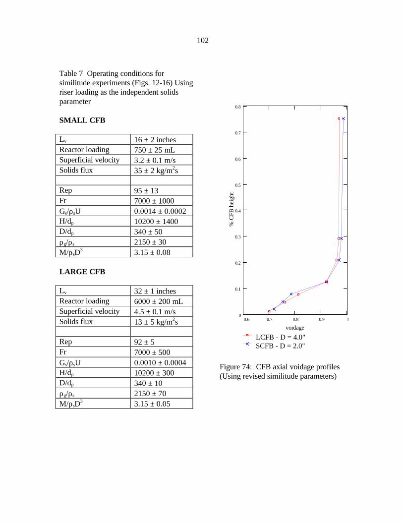
102

Table 7 Operating conditions forsimilitude experiments (Figs. 12-16) Usingriser loading as the independent solidsparameter

SMALL CFB



3 3.15 ± 0.08

LARGE CFB



3 3.15 ± 0.05

0.6 0.7 0.8 0.9 10

0.1

0.2

0.3

0.4

0.5

0.6

0.7

0.8

LCFB - D = 4.0"SCFB - D = 2.0"

voidage

% C

FB h

eigh

t

Figure 74: CFB axial voidage profiles(Using revised similitude parameters)

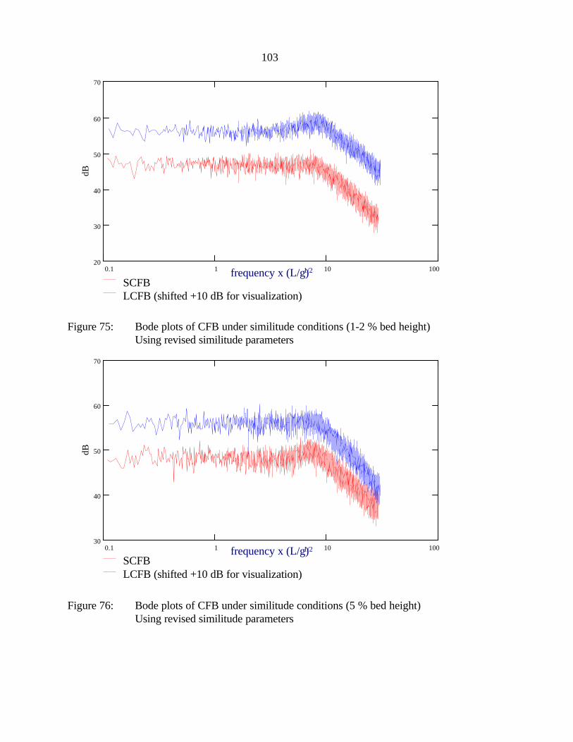
103

0.1 1 10 10020

30

40

50

60

70


dB


Figure 75: Bode plots of CFB under similitude conditions (1-2 % bed height)Using revised similitude parameters

0.1 1 10 10030

40

50

60

70


dB



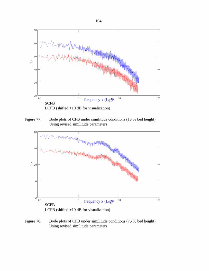
104

0.1 1 10 10020

30

40

50

60

70


dB



0.1 1 10 10020

0

20

40

60


dB



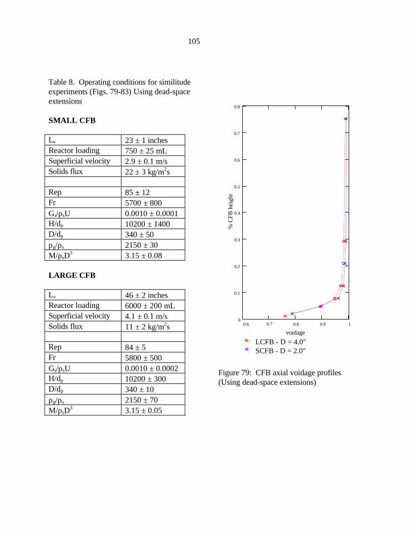
105

Table 8. Operating conditions for similitudeexperiments (Figs. 79-83) Using dead-spaceextensions

SMALL CFB



3 3.15 ± 0.08

LARGE CFB



3 3.15 ± 0.05

0.6 0.7 0.8 0.9 10

0.1

0.2

0.3

0.4

0.5

0.6

0.7

0.8

LCFB - D = 4.0"SCFB - D = 2.0"

voidage

% C

FB h

eigh

t

Figure 79: CFB axial voidage profiles(Using dead-space extensions)

106

0.1 1 10 10020

30

40

50

60


dB

Figure 80: Bode plots of CFB under similitude conditions (1-2 % bed height)Using dead-space extensions

0.1 1 10 10010

20

30

40

50

60


dB

Figure 81: Bode plots of CFB under similitude conditions (5 % bed height)Using dead-space extensions

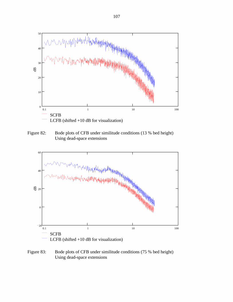
107

0.1 1 10 1000

10

20

30

40

50


dB


0.1 1 10 10020

0

20

40

60


dB


108

rates. If directly applicable to bed operation, this would demonstrate that there is a height at

which L-valves should be operated above in similitude studies to avoid changes in solids flux

related to L-valve operation instead of bed hydrodynamics.

These results are similar to what is expected of an L-valve operating in automatic solids

flow. With a constant aeration rate, the air flow is split between moving down around the

constricting bend and upward through the solids in the standpipe. With a large amount of solids

in the standpipe, a large resistance is present to flow through the standpipe so most of the air

moves downward through the constricting bend. The air moving downward provides the

necessary force to propel the solids out of the L-valve. As the L-valve height is decreased, a

larger portion of the aeration air moves upward through the solids in the standpipe. This upward

moving air does not provide any propulsion for the solids to move through the constricting bend

so the solids flow rate decreases.

This automatic mode of operation is directly observed in circulating fluidized bed

operation. The height of solids in an L-valve will adjust to match the mass flux leaving the

cyclone. Increasing the L-valve aeration rate will decrease the L-valve height but not necessarily

the solids flow rate. The L-valve height will decrease so that the standpipe pressure drop is

decreased, with this decreased pressure drop in the standpipe, the increased air flow will flow

through the standpipe and not downward through the L-valve constricting bend. Without

additional air flow through the constricting bed, the solids flow rate of the L-valve will remain

constant. Thus the solids flow rate is determined mostly by the bed operation. The effect of

increased solids loading resulting from a lower L-valve height needs to be studied to understand

how it affects the mass flux leaving the top of the riser. In addition, the operation of the L-valve

in the observed constant flow region needs to be further investigated to see if the L-valve cannot

operate in automatic mode above a certain solids level when run in conjunction with bed

operation.

109

Height in Isolated L-valve vs. Time 300 micron glass

0

10

20

30

40

50

60

0 50 100 150 200 250 300 350 400

time (sec)

L-v

alve

hei

gh

t (i

nch

es)

0.27 scfm aeration

0.34 scfm aeration0.41 scfm aeration

Figure 84: L-valve height vs. Time, 300 micron glass beads

110

ISU Power Plant CFB Boilers

A number of experiments were completed to determine the nature of industrial scale CFB

Boiler pressure fluctuations. These tests were developed to determine whether CFB pressure

fluctuations can be used as diagnostic indicators in industrial scale CFB boilers, and also whether

these signals can be related to similar pressure fluctuations observed in small-scale cold-model

CFBs. Two 170,000 lb/hr steam Pyropower CFB boilers are located on the campus of Iowa State

University. ISU’s CFB Boiler #1 and CFB Boiler #2 both had two transducers installed along the

CFB wall to monitor absolute pressure. All four transducers in the two boilers had an output of 1

to 4 volts. The transducers that measure what was referred to as the bed pressure record static

pressure fluctuations immediately above the gas distribution plate. These transducers have a

range of 0 to 60 inches of H20. The transducers in the combustion chamber measure the static

pressure fluctuations at an elevation of 60 feet above the distributor plate. These transducers

have a range of -3 to 17 inches of H20. The boilers have a square cross-section of 4.3 x 4.3

meters (14’x14’), and a height from distributor to top of CFB riser of around 20 meters (65 feet).

Under standard operating conditions, the boiler operates with 137,000 lb/hr fluidizing air and

74,000 lb/hr secondary air. The bed material (ash, limestone, and coal) consists of particles which

predominantly range between 100 and 1000 micrometers in diameter. The pressure measured at

the bottom of the bed under these conditions approximately ranges from 15-25 inches of H20, and

the bed temperature is maintained between 1400-1600 °F. The fluctuation data was sampled at

20, 50, 90, 200, 400, and 1000 Hz, with data set sizes ranging from 70,000 to 620,000 data

points to insure adequate Bode plot resolution. Using a portable computer with a 12 bit A/D (0-

5V) board, the output voltage from the boiler transducers was recorded and stored.

Fluctuations in lower regions of CFB boiler

Although there is some variation in the structure of the lower bed fluctuations, as seen in

time domain plots of Figures 85 and 86, they always exhibit a signal similar to a 0.25 - 0.3 Hz

square wave. It is evident that the lower bed signal has a dominant period, on the order of a cycle

every 3 to 4 seconds. This dominant frequency at 0.25 - 0.3 Hz is very pronounced in the power

spectral density of these signals shown in Figures 87 and 88. Examining the Bode plot of the bed

pressure fluctuations in Figure 87b, the low frequency region of the Bode plot seemingly exhibits

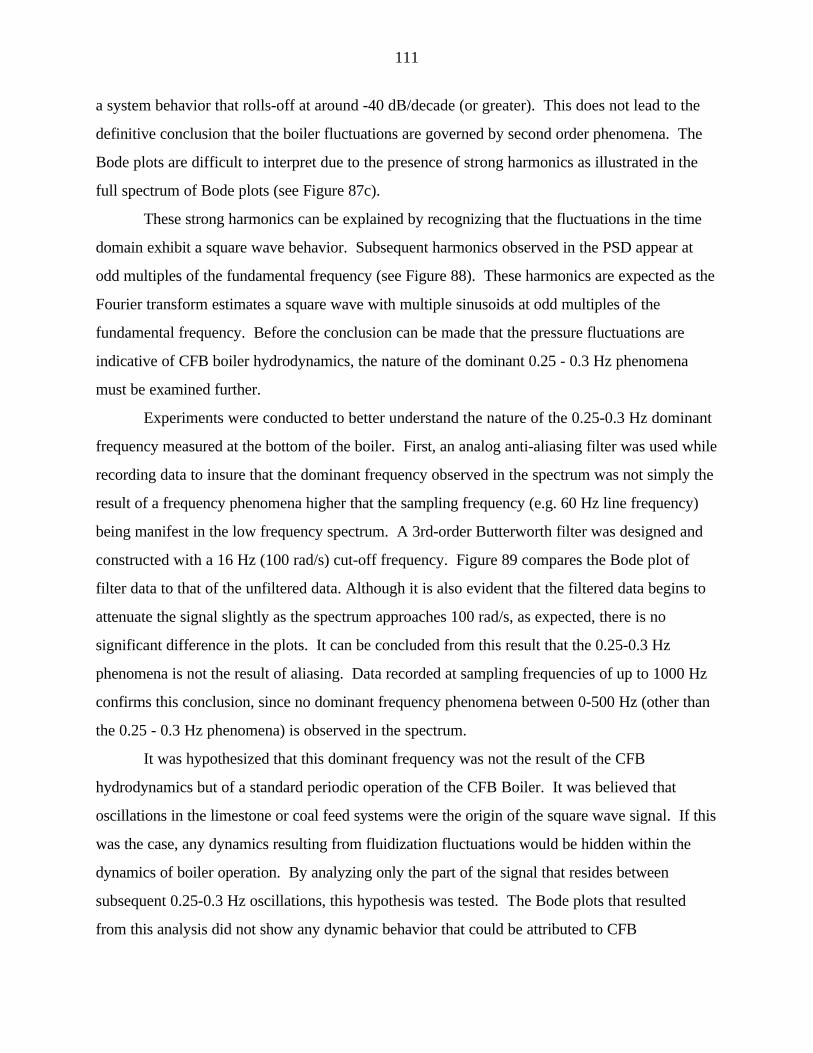
111

a system behavior that rolls-off at around -40 dB/decade (or greater). This does not lead to the

definitive conclusion that the boiler fluctuations are governed by second order phenomena. The

Bode plots are difficult to interpret due to the presence of strong harmonics as illustrated in the

full spectrum of Bode plots (see Figure 87c).

These strong harmonics can be explained by recognizing that the fluctuations in the time

domain exhibit a square wave behavior. Subsequent harmonics observed in the PSD appear at

odd multiples of the fundamental frequency (see Figure 88). These harmonics are expected as the

Fourier transform estimates a square wave with multiple sinusoids at odd multiples of the

fundamental frequency. Before the conclusion can be made that the pressure fluctuations are

indicative of CFB boiler hydrodynamics, the nature of the dominant 0.25 - 0.3 Hz phenomena

must be examined further.

Experiments were conducted to better understand the nature of the 0.25-0.3 Hz dominant

frequency measured at the bottom of the boiler. First, an analog anti-aliasing filter was used while

recording data to insure that the dominant frequency observed in the spectrum was not simply the

result of a frequency phenomena higher that the sampling frequency (e.g. 60 Hz line frequency)

being manifest in the low frequency spectrum. A 3rd-order Butterworth filter was designed and

constructed with a 16 Hz (100 rad/s) cut-off frequency. Figure 89 compares the Bode plot of

filter data to that of the unfiltered data. Although it is also evident that the filtered data begins to

attenuate the signal slightly as the spectrum approaches 100 rad/s, as expected, there is no

significant difference in the plots. It can be concluded from this result that the 0.25-0.3 Hz

phenomena is not the result of aliasing. Data recorded at sampling frequencies of up to 1000 Hz

confirms this conclusion, since no dominant frequency phenomena between 0-500 Hz (other than

the 0.25 - 0.3 Hz phenomena) is observed in the spectrum.

It was hypothesized that this dominant frequency was not the result of the CFB

hydrodynamics but of a standard periodic operation of the CFB Boiler. It was believed that

oscillations in the limestone or coal feed systems were the origin of the square wave signal. If this

was the case, any dynamics resulting from fluidization fluctuations would be hidden within the

dynamics of boiler operation. By analyzing only the part of the signal that resides between

subsequent 0.25-0.3 Hz oscillations, this hypothesis was tested. The Bode plots that resulted

from this analysis did not show any dynamic behavior that could be attributed to CFB

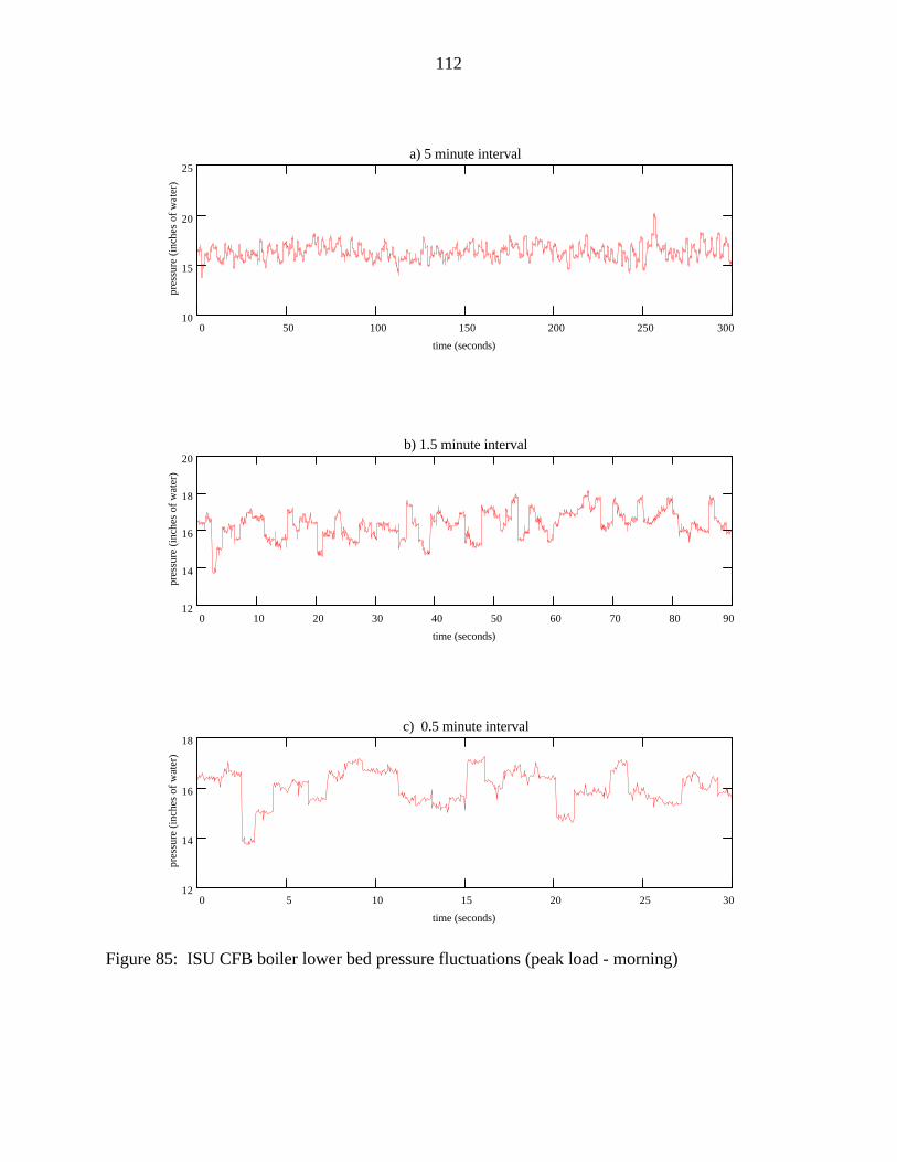
112

0 50 100 150 200 250 30010

15

20

25a) 5 minute interval

time (seconds)

pres

sure

(in

ches

of

wat

er)

0 10 20 30 40 50 60 70 80 9012

14

16

18

20b) 1.5 minute interval

time (seconds)

pres

sure

(in

ches

of

wat

er)

0 5 10 15 20 25 3012

14

16

18c) 0.5 minute interval

time (seconds)

pres

sure

(in

ches

of

wat

er)

Figure 85: ISU CFB boiler lower bed pressure fluctuations (peak load - morning)

113

0 50 100 150 200 250 30015

20

25


time (seconds)

pres

sure

(in

ches

of

wat

er)

0 10 20 30 40 50 60 70 80 9015

20

25


time (seconds)

pres

sure

(in

ches

of

wat

er)

0 5 10 15 20 25 3015

20

25


time (seconds)

pres

sure

(in

ches

of

wat

er)

Figure 86: ISU CFB boiler lower bed pressure fluctuations (afternoon load)

114

0 0.2 0.4 0.6 0.8 1 1.2 1.4 1.60

20

40a) Power Spectral Density

frequency (Hz)

PSD

0.1 1 1020

10

0

10

20b) Bode plot - partial spectrum

frequency (rad/s)

dB

0.1 1 10 10030

20

10

0

10

20c) Bode plot - full spectrum

frequency (rad/s)

dB

Figure 87: Peak load CFB boiler fluctuations a) PSD b) partial b) full Bode

115

0.2 0.4 0.6 0.8 1 1.2 1.4 1.60

5 104

1 105

1.5 105

frequency (Hz)

PSD

0.1 1 1020

0

20

40

60

frequency (rad/s)

dB

Figure 88: Bode plot & PSD of CFB boiler lower bed fluctuations (afternoon load)

116

hydrodynamics. The resulting plots were typical of the Bode plots of a white noise signal,

containing no important dynamic information. It is assumed that all observed dynamics contained

in the spectrum are related to the 0.25-0.3 Hz oscillation.

The most likely explanation for this periodic behavior is the coal feed system. Coal is fed

into the boiler at two locations; via the loop seal and directly into the bed on a cleated conveyor

belt. Due to the spacing of the cleats and the typical speed of the conveyor, a cleat reaches the

entrance of the boiler every 3 to 4 seconds. Assuming that the coal will have a tendency to pile

up near the cleat, the rate at which coal enters the boiler will not be continuous. Rather, the

feeder will input a batch of coal every 3 to 4 seconds.

By observing boiler fluctuations under high and low loading conditions, this hypothesis is

supported. Figure 86 shows bed fluctuations measured mid-afternoon while Figure 85 represents

the fluctuations measure during peak operation 8:00-9:00 a.m. During this period of high load,

the fluctuations appear less dominated by the “square wave” coal feed fluctuations. This is

expected since an increased circulation rate increases the solids suspended in the bed and

decreases the observed effect of the coal feed directly into the CFB. The more dilute the

operation of the CFB is, the more evident the periodic coal feed will be in the frequency spectrum.

Fluctuations in upper region of CFB boiler

The combustion chamber pressure fluctuations differ from the lower bed fluctuations because the

periodic nature of the coal feed no longer is sensed as strongly at the top of the bed (see Figure

90). At this elevation, the periodic batches of coal entering the combustor have been more evenly

dispersed in the upward moving gas flow. The Bode plot of the combustion chamber pressure

fluctuations shown in Figure 91 does seem to exhibit an initial roll-off of around -40

dB/decade.This characteristic frequency occurring at around 0.4-0.5 rad/s (0.06 - 0.08 Hz) may

be a wave phenomena similar to that previously observed in the CFB models.

The equivalent diameter of the CFB boilers is 4.85 meters. This is 47.5 times greater than

the 10.2 cm diameter CFB model. If a wave phenomena observed in the CFB models was

observed in the CFB boiler, it would appear at a frequency inversely proportional to the square

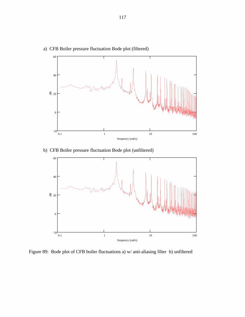
117

a) CFB Boiler pressure fluctuation Bode plot (filtered)

0.1 1 10 10020

0

20

40

60

frequency (rad/s)

dB

b) CFB Boiler pressure fluctuation Bode plot (unfiltered)

0.1 1 10 10020

0

20

40

60

frequency (rad/s)

dB

Figure 89: Bode plot of CFB boiler fluctuations a) w/ anti-aliasing filter b) unfiltered

118

0 50 100 150 200 250 3000.2

0.4

0.6

0.8


time (seconds)

pres

sure

(in

ches

of

wat

er)

0 10 20 30 40 50 60 70 80 900.2

0.4

0.6

0.8


time (seconds)

pres

sure

(in

ches

of

wat

er)

0 5 10 15 20 25 300.2

0.4

0.6

0.8


time (seconds)

pres

sure

(in

ches

of

wat

er)

Figure 90: ISU CFB boiler combustion chamber pressure fluctuations

119

0.2 0.4 0.6 0.8 1 1.2 1.4 1.60

50

100

frequency (Hz)

PSD

0.1 1 1010

0

10

20

30

frequency (rad/s)

dB

Figure 91: Bode plot & PSD of CFB boiler combustion chamber pressure fluctuations

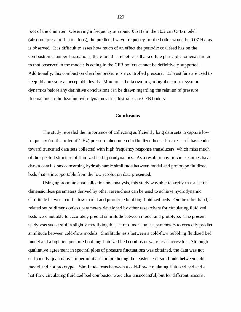
120

root of the diameter. Observing a frequency at around 0.5 Hz in the 10.2 cm CFB model

(absolute pressure fluctuations), the predicted wave frequency for the boiler would be 0.07 Hz, as

is observed. It is difficult to asses how much of an effect the periodic coal feed has on the

combustion chamber fluctuations, therefore this hypothesis that a dilute phase phenomena similar

to that observed in the models is acting in the CFB boilers cannot be definitively supported.

Additionally, this combustion chamber pressure is a controlled pressure. Exhaust fans are used to

keep this pressure at acceptable levels. More must be known regarding the control system

dynamics before any definitive conclusions can be drawn regarding the relation of pressure

fluctuations to fluidization hydrodynamics in industrial scale CFB boilers.

Conclusions

The study revealed the importance of collecting sufficiently long data sets to capture low

frequency (on the order of 1 Hz) pressure phenomena in fluidized beds. Past research has tended

toward truncated data sets collected with high frequency response transducers, which miss much

of the spectral structure of fluidized bed hydrodynamics. As a result, many previous studies have

drawn conclusions concerning hydrodynamic similitude between model and prototype fluidized

beds that is insupportable from the low resolution data presented.

Using appropriate data collection and analysis, this study was able to verify that a set of

dimensionless parameters derived by other researchers can be used to achieve hydrodynamic

similitude between cold –flow model and prototype bubbling fluidized beds. On the other hand, a

related set of dimensionless parameters developed by other researchers for circulating fluidized

beds were not able to accurately predict similitude between model and prototype. The present

study was successful in slightly modifying this set of dimensionless parameters to correctly predict

similitude between cold-flow models. Similitude tests between a cold-flow bubbling fluidized bed

model and a high temperature bubbling fluidized bed combustor were less successful. Although

qualitative agreement in spectral plots of pressure fluctuations was obtained, the data was not

sufficiently quantitative to permit its use in predicting the existence of similitude between cold

model and hot prototype. Similitude tests between a cold-flow circulating fluidized bed and a

hot-flow circulating fluidized bed combustor were also unsuccessful, but for different reasons.

121

The circulating fluidized bed combustor, an industrial-scale boiler, presented unique data filtering

problems that were never overcome. Modulated air dampers produced pressure fluctuations that

propagated into the fluidized bed where they overwhelmed pressure fluctuations associated with

the hydrodynamics of the particulate-gas mixture.

The study developed models of pressure fluctations in the circulating fluidized beds in an

attempt to understand the nature of the fluctuations. As dynamical systems, circulating fluidized

beds proved to be surprisingly complicated. Linear models were constructed from spectral plots

of pressure fluctuations, but they proved of limited use in deriving physical insight into

hydrodynamic behavior. A variety of acoustical and wave phenomena were used as the basis for

explaining pressure fluctuations in the fluidized bed but with little success.

122

References Cited

[1] Glicksman, L.R. "Scaling relationships for fluidized beds." Chem. Eng. Science 1984,30(9), 1373-1379.

[2] Glicksman, L.R., D. Westphalen, K. Woloshun, T. Ebert, K. Roth, and M. Lints."Experimental scale models of circulating fluidized bed combustors." Fluidized BedCombustion, ASME 1991; 1169-1174.

[3] Louge M, and H. Chang. "Fluid dynamic similarity of circulating fluidized beds" PowderTechnology 1992, 70, 259-270.

[4] Glicksman L.R., and M.T. Nicastro. "Experimental verification of scaling relationshipsfor fluidized bed." Chem. Eng. Science 1984, 39(9), 1381-1391.

[5] Glicksman, L.R., D. Westphalen, C. Bereton, and J. Grace. "Verification of the scalinglaws for circulating fluidized beds." In Circulating Fluidized Bed Technology III. P.Basu, M. Hasatan, and M. Horio, Eds.; Pergamon Press: Oxford, 1991; 199-124.

[6] Glicksman, L. R., M. R. Hyre, and K. Woloshun. “Scale models of circulating fluidizedbed combustors.” Report # DOE/MC/25049-3372, USDOE, Washington, D. C.

[7] Davidson, J. F. "The two-phase theory of fluidization: successes and opportunities."AIChE Symposium Series 1991, 87(281), 1-12.

[8] Roy, R., J.F. Davidson, and V.G. Tuponogov. "The velocity of sound in fluidized beds."Chem. Eng. Sci. 1990, 45(11), 3233-3245.

[9] Hiby, J.W. "Periodic phenomena connected with gas-solid fluidization." In Proceedingsof the International Symposium on Fluidization, Eindhoven; Netherlands UniversityPress: Amsterdam, 1967; 99.

[10] Verloop, J. and P.M. Heertjes. "Periodic pressure fluctuations in fluidized beds." Chem.Eng. Science 1974, 29, 1035-1042.

[11] Baskakov, A.P., V.G. Tuponogov, and N.F. Filippovsky. "A study of pressurefluctuations in a bubbling fluidised bed." Powder Technology 1986, 45, 113-117.

[12] Sun, J., M.M. Chen, and B.T. Chao. "On the fluctuation motions due to surface waves ingas fluidized beds." In Proceedings of the First World Conference on Experimental HeatTransfer, Fluid Mechanics and Thermodynamics, Dubrovnik. R.K. Shah, E.N. Ganic,and K.T. Yang, Eds.;Elsevier: New York, 1988; 1310.

123

[13] Rahman, M.. Water Waves: Relating Modern Theory to Advanced EngineeringApplications; Claredon Press: Oxford, 1995.

[14] Glicksman, L.R. "Scaling relationships for fluidized beds." Chem. Eng. Science 1984,30(9), 1373-1379.

[15] Glicksman L.R., M.R. Hyre, and P.A. Farrell. "Dynamic similarity in fluidization." Int. J.Multiphase Flow 1994, 20, 331-386.

[16] Glicksman, L.R., M. Hyre, and K. Woloshun. “Simplified scaling relationships forfluidized beds.” Powder Technology, 1993, 77, 177-199.

[17] Moody, L.F., “Friction factors for pipe flow.” Transactions of the ASME, Vol. 66, 1944.

[18] Schnitzlein, M.G. and H. Weinstein. "Flow characterization in high-velocity fluidized bedsusing pressure fluctuations." Chem. Eng. Science 1988, 43(10), 2605-2614.

[19] Fitzgerald, T., D. Bushnell, S. Crane, and Yeong-Cheng Shieh. "Testing of cold scaledbed modeling for fluidized bed combustors." Powder Technology 1984, 38, 107-120.

[20] Brue, E. "Pressure fluctuations as a diagnostic tool for fluidized beds." PhD.Dissertation, Iowa State University, Ames, 1996.

[21] de la Cruz Baez, R. G. “Frequency analysis of pressure fluctuations in bubbling fluidizedbeds and its application to similitude stuudies.” Master’s Thesis, Iowa State University,Ames, 1994.

pressure fluctuations as a diagnostic tool for fluidized beds/67531/metadc673151/m2/1/high... ·...

Documents