pressure loss modeling of non-symmetric gas turbine
TRANSCRIPT

Pressure Loss Modeling of Non-Symmetric Gas Turbine
Exhaust Ducts using CFD
Steven Farber
A Thesis
in
The Department
of
Mechanical and Industrial Engineering
Presented in Partial Fulfillment of the Requirements for the Degree of Master of Applied Science (Mechanical Engineering)at
Concordia University Montreal, Quebec, Canada
April 15, 2008
© Steven Farber, 2008

1*1 Library and Archives Canada
Published Heritage Branch
395 Wellington Street Ottawa ON K1A0N4 Canada
Bibliotheque et Archives Canada
Direction du Patrimoine de I'edition
395, rue Wellington Ottawa ON K1A0N4 Canada
Your file Votre reference ISBN: 978-0-494-40910-7 Our file Notre reference ISBN: 978-0-494-40910-7
NOTICE: The author has granted a nonexclusive license allowing Library and Archives Canada to reproduce, publish, archive, preserve, conserve, communicate to the public by telecommunication or on the Internet, loan, distribute and sell theses worldwide, for commercial or noncommercial purposes, in microform, paper, electronic and/or any other formats.
AVIS: L'auteur a accorde une licence non exclusive permettant a la Bibliotheque et Archives Canada de reproduire, publier, archiver, sauvegarder, conserver, transmettre au public par telecommunication ou par Plntemet, prefer, distribuer et vendre des theses partout dans le monde, a des fins commerciales ou autres, sur support microforme, papier, electronique et/ou autres formats.
The author retains copyright ownership and moral rights in this thesis. Neither the thesis nor substantial extracts from it may be printed or otherwise reproduced without the author's permission.
L'auteur conserve la propriete du droit d'auteur et des droits moraux qui protege cette these. Ni la these ni des extraits substantiels de celle-ci ne doivent etre imprimes ou autrement reproduits sans son autorisation.
In compliance with the Canadian Privacy Act some supporting forms may have been removed from this thesis.
Conformement a la loi canadienne sur la protection de la vie privee, quelques formulaires secondaires ont ete enleves de cette these.
While these forms may be included in the document page count, their removal does not represent any loss of content from the thesis.
Canada
Bien que ces formulaires aient inclus dans la pagination, il n'y aura aucun contenu manquant.

ABSTRACT
Pressure Loss Modeling of Non-Symmetric Gas Turbine Exhaust Ducts using CFD
Steven Farber
In typical gas turbine applications, combustion gases that are discharged from the turbine
are exhausted into the atmosphere in a direction that is sometimes different from that of the
inlet. In such cases, the design of efficient exhaust ducts is a challenging task particularly
when the exhaust gases are also swirling. Designers are in need for a tool today that can
guide them in assessing qualitatively and quantitatively the different flow physics in these
exhaust ducts so as to produce efficient designs.
In this thesis, a parametric Computational Fluid Dynamics (CFD) based study was
carried out on non-symmetric gas turbine exhaust ducts where the effects of geometry and
inlet aerodynamic conditions were examined. The results of the numerical analysis were
used to develop a total pressure loss model.
These exhaust ducts comprise an annular inlet, a flow splitter, an annular to rectangular
transition region, and an exhaust stub. The duct geometry, which is a three-dimensional
complex one, is approximated with a five-parameter model, which was coupled with a design
of experiment method to generate a relatively small number of exhaust ducts. The flow in
these ducts was simulated using CFD for different values of inlet swirl and aerodynamic
blockage and the numerical results were reviewed so as to assess the effects of the geometric
and aerodynamic parameters on the total pressure loss in the exhaust duct. These flow
simulations were used as a data base to generate a total pressure loss model that designers
can use as a tool to build more efficient non-symmetric gas turbine exhaust ducts. The
resulting correlation has demonstrated satisfactory agreement with the CFD-based data.
m

Acknowledgments
I would like to first thank my supervisor Prof. W.S. Ghaly and Co-supervisor Ed Vlasic
for their guidance and suggestions on this project.
Thanks also go to the following people and organizations without which this work would
not have been possibe:
To Pratt & Whitney Canada for their financial and technical support, especially Remo
Marini and Mark Cunningham.
To the Natural Sciences and Engineering Research Council of Canada (NSERC) for
financial support.
IV

Contents
1 Introduction 1
1.1 Background 1
1.2 Single Port Annular-to-Rectangular Exhaust Ducts 3
1.3 Contribution and Scope of the Present Study 4
2 Theory and Literature Review 6
2.1 Diffuser Performance 6
2.1.1 Static Pressure Recovery Coefficient 6
2.1.2 Diffuser Effectiveness 7
2.1.3 Total Pressure Loss Coefficient 7
2.2 Conical Diffusers 7
2.2.1 Geometry 7
2.2.2 Swirl 8
2.2.3 Aerodynamic Blockage 9
2.3 Annular Diffusers 11
2.3.1 Swirl 14
2.3.2 Aerodynamic Blockage 19
2.4 Past Research Contributions 21
2.4.1 Loka et al 21
2.4.2 Cunningham 24
3 Design of Experiment 30
3.1 Geometric Design Space 30
v

3.1.1 Equivalent Cone Diffusion Angle 31
3.1.2 Flow Splitter Wedge Angle 31
3.1.3 Gas Path Aspect Ratio 34
3.1.4 Annular to Rectangular Transition Region 35
3.1.5 Exhaust Stubs 36
3.2 Aerodynamic Design Space 38
3.2.1 Swirl 38
3.2.2 Inlet Boundary Layer Blockage 40
3.3 Full Factorial Design 40
3.4 Taguchi Design 43
3.4.1 Assumption 43
3.4.2 Interactions 43
3.4.3 Selecting an Orthogonal Array 44
4 Geometry Synthesis 47
4.1 Equivalent Cone Diffusion Angle 49
4.2 Gas Path 51
4.3 Gas Path Aspect Ratio 51
4.4 Flow Splitter Leading Edge 51
4.5 Flow Splitter Wedge Angle 54
4.6 Duct Exit Cross-Section 54
4.7 Annular to Rectangular Transition Region 57
4.8 Plenum 59
5 Computational Study 62
5.1 Data Reduction 62
5.2 Pressure-Velocity Coupling 63
5.3 Advection Scheme 63
5.4 Turbulence Modelling 64
5.4.1 k - e 64
5.4.2 SST 64
VI

5.5 Computational Domain 65
5.5.1 Boundary Conditions 66
5.5.2 Grid Structure 68
5.5.3 Grid Study 72
6 CFD-Based Parametric Study 78
6.1 Effect of Swirl 79
6.2 Effect of Stub Direction 85
6.3 Effect of ECDA 87
6.4 Effect of Wedge Angle 89
6.5 Effect of Aspect Ratio and Area Ratio in the Annular to Rectangular Tran
sition Region 92
6.6 Effect of Inlet Boundary Layer Blockage 96
7 Correlation of the Total to Total Pressure Loss 99
7.1 Japikse Correlation of Annular Diffusers 100
7.2 Correlation of the CFD Results 104
8 Conclusion and Recommendation 111
8.1 Conclusion I l l
8.2 Recommendation 112
Bibliography 114
vn

List of Figures
1-1 Pratt and Whitney PW200 engine 2
1-2 Pratt and Whitney PT6 engine 2
1-3 Exhaust duct geometric features 3
2-1 Conical diffuser presented with dimensional parameters 8
2-2 Conical diffuser performance chart based on data from Cockrell and Mark-
land (Bt « .20) 9
2-3 Conical diffuser performance chart from McDonald and Fox 10
2-4 Diffuser performance coefficient as a function of area ratio for (a) axial inlet
flow (b) swirling inlet flow 11
2-5 Radial distributions of total and static pressures at the inlet section . . . . 12
2-6 Variation of total pressure along stream surfaces of revolution 12
2-7 Maximum Pressure Recovery of Conical and Square Diffusers - Mth = 0.8 . 13
2-8 Variation of the total pressure loss coefficient with entrance length (X/D) for
a 5°; a) Reynolds number 1 x 10⁵, b) Reynolds number 4 x 10⁵ 13
2-9 Conical diffuser loss map using Sharan's data 14
2-10 Exit discharge area ratio for conical diffusers on Cp* (based on data from
Cockrell and Markland) 15
2-11 Annular diffusers (a) equiangular (b) straight core (c) double divergent . . . 16
2-12 Annular diffuser performance chart (B\ ~ .02) 16
2-13 Pressure recovery contours 17
2-14 Straight annular diffuser performance with swirl 17
2-15 Performance of equiangular diffusers 18
viii

2-16 Loss map using Stevens and Williams data 19
2-17 Variation of the total pressure loss coefficient with entry blockage (Figure
adapted from Klein) . . 20
2-18 Exit discharge area ratio for annular diffusers on Cp* 20
2-19 Experimental setup 22
2-20 2D Cross-sectional View of Exhaust 22
2-21 Schematic of experimental setup 25
2-22 Domain of CFD grid used for computations 26
3-1 Equivalent Cone Diffusion Angle Levels Studied 32
3-2 Duct Wedge Angle Levels Studied 33
3-3 Gas Path Aspect Ratio 34
3-4 Gas Path Aspect Ratio Levels Studied 35
3-5 Duct Locations where Area is Specified 36
3-6 Exhaust Stub Direction 37
3-7 Sample of exhaust duct inlet swirl gradients 39
3-8 Boundary layer axial velocity profiles 41
4-1 Sample P&WC Single Port Swept Exhaust Duct 48
4-2 Equivalent Cone Diffusion Angle 49
4-3 Gas Path Conic 50
4-4 Gas Path Spline and Aspect Ratio 52
4-5 Flow Splitter 53
4-6 Flow Splitter Construction Plane 55
4-7 Flow Splitter Construction Plain 56
4-8 Flow Splitter Wedge Angle 57
4-9 Duct Exit Profile 58
4-10 Duct Cross-Sections Downstream of Flow Splitter 59
4-11 Duct Surface Passing Through Cross-Sections 60
4-12 Plenum 61
5-1 Air solid model of the computational domain 65
IX

5-2 CFD boundary conditions 67
5-3 Exhaust Duct Inlet Showing Prism Layer Elements 69
5-4 Plenum surface grid 70
5-5 Cross-section of the plenum domain showing element sizes 71
5-6 ^ p 1 ploted versus total number of prism layers 73
5-7 Three grids constructed from tetrahedral sizes of h/3 (coarse), h/6 (interme
diate), and h/12 (fine) 74
APtt 91
5-9 Mach contours for the three grid densities . 76
5-8 ^P1 ploted versus total number of nodes 75
6-1 Cross-sections used for data reduction and flow visualization 78
6-2 Total pressure loss coefficient evaluated at each section defined in figure 6-1 79
6-3 Velocity contours normal to cross-section (nominal 0° swirl) 80
6-3 Velocity contours normal to cross-section (nominalO0 swirl)....con't 81
6-4 Velocity contours normal to cross-section (nominal 35° swirl) 82
6-4 Velocity contours normal to cross-section (nominal35° swirl)....con't . . . . 83
6-5 Mach contours at mid plane demonstrating the effect of stub direction (nom
inal 0° inlet swirl) 85
6-6 Normalized static pressure contours at mid plane demonstrating the effect of
stub direction (nominal 0° inlet swirl) 86
6-7 Total pressure losses calculated for C-shape, Straight, and S-shaped exhaust
stubs (low inlet blockage) 87
6-8 Mach number contours at mid-plane demonstrating the effect of ECDA (inlet
conditions: nominal 0° swirl with low blockage) 88
6-9 Total pressure losses as a function of ECDA calculated at exit of the annulus 89
6-10 Wall shear stress contours (nominal 25° swirl) 90
6-11 Wall shear stress contours (nominal 35° swirl) 91
6-12 Total pressure losses as a function of wedge angle calculated at section 3 . . 92
6-13 Mach number contour plot on a plane through the flow splitter 93
6-14 Normalized wall static pressure contours demonstrating the effect of aspect
ratio and area ratio in the annular to rectangular transition region 94
x

6-15 Mach number contours demonstrating the effect of aspect ratio and area ratio
in the annular to rectangular transition region 95
6-16 Mach number contours demonstrating the effect of inlet blockage on three
exhaust ducts with ECDA of 0°, 10°, and 20° 97
6-17 Total pressure loss coefficient vs. inlet swirl for low and medium inlet blockage 98
6-18 Total pressure loss coefficient vs. inlet swirl for medium and high inlet blockage 98
7-1 Diffuser effectiveness versus area ratio with low level inlet aerodynamic block
age and no inlet swirl 100
7-2 Diffuser effectiveness with principle geometric effects removed including data
at all levels of inlet aerodynamic blockage 101
7-3 Diffuser effectiveness with the principle effects of geometry and inlet swirl
removed according to preceding correlations 102
7-4 Diffuser effectiveness with the principle effects of geometry, inlet swirl, and
inlet blockage removed 103
7-5 Total pressure loss trend in the exhaust for low inlet blockage 104
7-6 Total pressure loss trend in the exhaust for medium inlet blockage 105
7-7 Total pressure loss trend in the exhaust for large inlet blockage 105
7-8 Surface passing through normalized losses for ECDA and aspect ratio (Solid
circles are points lying above the surface and hollow circles are points lying
below) 106
7-9 Normalized losses versus wedge angle with the effects of blockage, swirl,
ECDA, and aspect ratio removed 107
7-10 Normalized losses versus area ratio with the effects of blockage, swirl, ECDA,
aspect ratio, and wedge angle removed 108
7-11 Plot of CFD losses vs. predicted losses between inlet and section-12 . . . . 109
XI

List of Tables
2.1 Summary of performance of CFD analysis in the study of single port gas
turbine exhaust 28
3.1 Exhaust Duct Area Ratio (referenced to figure 3-5) 37
3.2 Geometric Parameters 42
3.3 Aerodynamic Parameters 42
3.4 Lg Orthogonal Array 45
3.5 Lg Orthogonal Array Expanded for Stub Direction 46
7.1 Break Down of Correlation Accuracy 108
xn

Nomenclature
Variables
A area (in2)
AB blockage area JA (l — |j) dA
AE effective area JA jjdA
AR area ratio
AS aspect ratio
Cp static pressure recovery coefficient P2Z_Pl
Cpi ideal pressure recovery coefficient 1 — - ^ j
D diameter (in)
Dh hydraulic diameter (in) = 4 — - £ % % £ £ "
E effective area ratio ^f-
g swirl parameter ° ;R/ _, ,
h annulus height (in) = r0 — r»
i? height (in)
A; turbulent kinetic energy
if total pressure loss coefficient t2Z- ll
L diffuser length (in)
M Mach number
P static pressure (psi)
Pt total pressure (psi)
q dynamic pressure (psi)
r radius (in)
T static temperature (R)
Tt total temperature (R)
u axial velocity (ft/s)
ug tangential velocity (ft/s)
U maximum axial velocity in cross section (ft/s)
xin

Variables
APts
Pa - Pa
Ptx - P*
Greek Symbols
a
5
e
V
9
P
UJ
average swirl angle
blockage ±f^ x 100
boundary layer thickness (in)
turbulence disipation rate
diffuser effectiveness -rr~ c, Pi
half cone angle
density (slug/in3)
turbulent frequency
Subscripts
1
2
duct inlet
duct outlet
inner
outer
Superscripts
mass averaged quantity
xiv

Chapter 1
Introduction
1.1 B ackground
Turboprop and Turboshaft gas turbine engines find their way in many aerospace and indus
trial applications. Figures 1-1 and 1-2 give a schematic layout of such gas turbines where
each engine component is labelled. Careful review of these two figures demonstrates that
the engine layout results in two very different exhaust ducts. In the first figure, Fig 1-1,
an annular exhaust duct is found, where the flow and losses are rather well understood. In
the second figure, Fig. 1-2, the engine layout does not allow for an annular exhaust duct
resulting in the exhaust gases being redirected in a direction which differs from the inlet
direction. A quick overview of the open literature shows that there is very little knowledge
about these single port annular-to-rectangular exhaust ducts, be it flow physics, shape, de
sign methods, performance, etc... Therefore, there is a need to study such exhaust ducts
which redirect the combustion gases in a direction that differs from the inlet direction.
Significant gains in gas turbine performance can be made by reducing the exhaust duct
loss. For example, consider a simple gas turbine cycle with a pressure ratio of 10 and at a
constant power output, a 1% drop in the absolute back pressure to the turbine will result
in a 1% improvement in the specific fuel consumption, therefore care should be taken to
design an exhaust duct that would minimize any pressure loss.
1

accessory compressor power gearbox compressor turbine turbine
reduction gearbox
combustion chamber
exhaust duct
Figure 1-1: Pratt and Whitney PW200 engine (source: www.pwc.ca)
exhaust duct
combustion chamber
centrifugal compressor
inlet screen
output shaft
power turbine compressor
turbine
axial compressor
accessory gearbox
Figure 1-2: Pratt and Whitney PT6 engine (source: www.pwc.ca)
2

Inlet Exit
Figure 1-3: Exhaust duct geometric features
1.2 Single Port Annular-to-Rectangular Exhaust Ducts
As was explained in the previous section, single port annular-to-rectangular exhaust ducts
find their use in gas turbine applications where the output shaft does not allow for an annular
exhaust duct application. In this situation, the exhaust gases are required to be redirected,
crossing over the output shaft, and diffused to ambient through a rectangular exhaust stub.
The distinct geometric characteristics of these exhaust ducts are an annular inlet followed by
a flow splitter, an annular to rectangular transition region, and a rectangular exhaust stub,
see Fig. 1-3. The annular diffuser function is to efficiently diffuse the flow to a low Mach
number before the gases enter the transitional region. Within the transitional region, the
gases are forced to make an aggressive 90° turn crossing over the power turbine shaft. It is in
this region that the lower inlet Mach numbers will result in a lower loss making it important
to obtain as much diffusion as possible in the upstream annular diffuser. A flow splitter is
located at the start of the transition region to provide guidance to the gases directing the
flow around the inner annulus surface. The exhaust gases enter a rectangular duct after
3

crossing the inner annulus surface where diffusion is continued and the exhaust gases are
directed to the ambient atmosphere. In aerospace applications, these exhaust ducts are
bound to be small in size, making efficient diffusion difficult and sometimes impossible.
One such application of this exhaust duct configuration is found in PT6 engines produced
by Pratt and Whitney Canada, Fig. 1-2. A PT6 engine has two spools, one for the gas
generator, and a mechanically independent power turbine output shaft. The exhaust duct
is mounted downstream of the last turbine stage. The flow into the exhaust duct is subsonic
and swirling with the magnitude of swirl varying over the engine operating range.
1.3 Contribution and Scope of the Present Study
In this work, a pressure loss model is produced for single port annular-to-rectangular exhaust
ducts. A parametric study was carried out using Computational Fluid Dynamics (CFD)
to simulate the flow numerically in exhaust ducts where key geometric and aerodynamic
parameters are varied and their effect on the total pressure loss is observed. Furthermore,
the duct geometry is approximated through a five parameter model, which was coupled
with a design of experiment method to generate a relatively small number of exhaust ducts
for numerical simulation. The resulting numerical data that was produced, has been used
as database to generate a total pressure loss model that designers can use as a tool to build
more efficient non-symmetric gas turbine exhaust ducts.
The scope of the present study has been divided into the following sections consisting
of:
1. Theory and Literature Review
• summary of past research on simple 2D conical and annular diffusers
• summary of past research on single port annular-to-rectangular exhaust ducts
2. Design of Experiment (DOE)
• n-dimension design space reduced to a five parameter model to approximate the
duct geometry
• definition of the key inlet aerodynamic parameters
4

• use methods of DOE to generate a relatively small number of exhaust ducts for
numerical simulation
3. Geometry Synthesis
• synthesis of a single port annular-to-rectangular exhaust duct based on the five
geometric parameters
4. Computational Study
• discussion on the use of a commercial CFD solver
• definition of the computational domain and grid structure
5. CFD-Based Parametric Study
• presentation and discussion of the results of the numerical study
6. Correlation of the Total to Total Pressure Loss
• review of a correlation produced by Japikse [7]
• correlation of the numerical data produced from the present work
7. Conclusion and Recommendation
5

Chapter 2
Theory and Literature Review
2.1 Diffuser Performance
2.1.1 Static Pressure Recovery Coefficient
The static pressure recovery coefficient is defined as the static pressure rise across the diffuser
divided by the inlet dynamic head:
Cp = 5^L (2.1)
For an incompressible and isentropic flow Bernoulli's equation can be used to define an ideal
pressure recovery coefficient in terms the Area Ratio:
C« = ! - ^ (2.2)
A useful expression for annular diffusers which relates the influence of inlet swirl a.\ to the
ideal pressure recovery is given by:
ri tan^ a\ + 1
6

2.1.2 Diffuser Effectiveness
A useful parameter for evaluating the performance of a diffuser is through the diffuser
effectiveness:
This relation relates the actual diffuser pressure recovery to the maximum potential pressure
recovery.
2.1.3 Total Pressure Loss Coefficient
The diffuser total pressure loss coefficient, which is the parameter focused on in this work,
is determined in the same manner as the static pressure recovery coefficient where the total
pressure difference between diffuser inlet and outlet is divided by the inlet dynamic head:
K^-J^ (2.5)
The total pressure loss coefficient for simple diffusers with uniform inlet and exit flow
conditions can be determined from Cp and Cpi through:
K = CPi - Cp (2.6)
2.2 Conical Diffusers
2.2.1 Geometry
Conical diffusers, Fig. 2-1 are commonly characterized by various dimensionless parameters.
Two of such dimensionless parameters are the dimensionless length, L/D\, and area ratio,
AR = A2/A1. The AR of a conical diffuser can further be described through the following
geometric relation:
A R = [ l + 2(L/£>i)tane]2 (2.7)
Various studies have been performed on conical diffusers that take account inlet condi
tions as well as non-dimensional length and area ratio. One such study was performed by
7

Y
Figure 2-1: Conical diffuser presented with dimensional parameters
Cockrell and Markland and was presented as a performance chart, see Fig. 2-2, in a paper
written by Sovran and Klomp [1]. This chart presents pressure recovery coefficient (Cp)
versus non-dimensional length and area ratio. Furthermore the locus of the maximum pres
sure recovery for both non-dimensional length (Cp*) and area ratio (Cp**) can be found.
Another study performed by McDonald and Fox [2] has produced a performance map with
similar results, Fig. 2-3.
2.2.2 Swirl
The performance of a conical diffuser can be affected significantly when a swirling component
is introduced to the flow field. The effects of swirl is different depending on the type of
swirl distribution (free vortex, forced vortex) effecting both the boundary layer and the core
of the flow. The importance of swirl on diffuser performance can be seen in the work of
McDonald et al. [9]. It is evident in Fig. 2-4 that the introduction of swirl can result in a
conical diffuser approaching the theoretical ideal performance.
Additional studies were performed by Senoo et al. [10], who studied conical diffuser
performance with swirling flow inlet conditions. The magnitude of swirl studied is quantified

1. I
.LLA
vC
_ — i
/ / rr
A *--/(*
*
£
_
Figure 2-2: Conical diffuser performance chart based on data from Cockrell and Markland (Bx « .20) [1]
through a swirl parameter defined as:
g = ^ ^ ^ ^ (2.8) R J0 (u2) rdr
These authors identified the development of a Rankin vortex type flow composed of a large
solid vortex core at the center of the conical diffuser where the axial velocity was very low.
The total and static pressure distribution for an inlet swirl parameter of g = 0.18 is shown
in Fig. 2-5. In Fig. 2-6, Senoo et al. have presented stream surfaces of revolution starting
from the axis to 100% at the wall. Total pressure is observed to rise in the core of the flow up
to a stream surface at 10% and again for 80% and 90%. This is due to the low momentum
flow at the core and the wall being dragged along by the main flow, and inversely, the low
momentum flow slows down the main flow producing a total pressure drop.
2.2.3 Aerodynamic Blockage
The effect of aerodynamic blockage in conical diffusers has been studied by many researchers.
One study by Livesey and Odukwe [13] looked at the length of the pipe preceding the conical
diffuser. Their results show that as the inlet pipe length is increased, the boundary layer
thickness increases resulting in a reduction in pressure recovery. A clear presentation of the
effect of aerodynamic blockage on pressure recovery was made by Dolan and Runstadler
9

Fi gure 2-3: Conical diffuser performance chart from McDonald and Fox [2]
[11] shown in Fig. 2-7. This study made a comparison between a conical diffuser and a
straight channel diffuser showing that the aerodynamic blockage is a significant aerodynamic
parameter. Sharan [12] carried out a study with careful measurements of pressure recovery
and total pressure loss on a 5° conical diffuser where he varied inlet pipe length, Reynolds
Number, and turbulence intensity. The results of his work, Fig. 2-8, demonstrate that
the total pressure losses increase with developing inlet blockage but following losses can
be seen to fall as a result the inlet flow field developing its own flow structure. Japikse
[14] has produced a loss map, see Fig. 2-9, using the data from Sharan where the data
loosely followed the trend of K = CPi - Cp demonstrating that inlet factors such as inlet
pipe length, Reynolds Number, and turbulence intensity must be considered. Kline [15] has
compared the results of numerous studies showing that approximately the same reduction
in pressure recovery for inlet aerodynamic blockage levels of approximately 14%. An early
correlation was produced by Sovran and Klomp [1] who have postulated that, for geometries
that are dominated by pressure forces (as oposed to viscous forces) the exit discharge can
be correlated with inlet blockage and area ratio. The results of their attempt to correlate
the data of Cockrell and Markland for conical diffuser geometries laying on the Cp* line is
presented in Fig. 2-10 demonstrating that the data collapse reasonable well.
10

-
" s
Symbcl
-o D
s
Divergence Angte. 29
4 .0 " 6 ,0 " i_
^ ^
a
,1 .1
-
-
-
6,03 8 - 0 « 1
0 12 .0 * , f M
0 15.8* ft 31.2"
Figure 2-4: Diffuser performance coefficient as a function of area ratio for (a) axial inlet flow (b) swirling inlet flow [9].
2.3 Annular Diffusers
Annular diffusers are geometrically represented similar to conical diffusers; however more
independent variables are present which require more complex relations. As in conical
diffusers, non-dimensional length is represented as, L/h, and area ratio, AR = A2/A1. The
AR of a three types of annular diffusers, shown in Fig. 2-11, can further be described
through the following geometric relation where:
1. Equiangular case
AR = l + 2(L//i)sin0 (2.9)
2. Straight Core is
AR = 1 + 2L sin 9 L2 sin2 0 / 1 - r ; / r0
h{\ + n/r0) + h2 1 + ri/r0
(2.10)
3. Double divergent
AR = 1+2 L\ s in0 1 + (rj/ro)sinG2 .(L\2 [l - n/ro] (sin2 ©i - sin2 0 2
h 1 + n/r0 -+lk 1 + n/ro (2.11)
11

100
40 0
K m,-0-I8
«-•? • • • *L
j * : Direct metnoii / ° : Present Tfth*)
K
0 10 40 60 16-75 r mm
Figure 2-5: Radial distributions of total and static pressures at the inlet section [10]
• Static fa^ssur* al.w$ th# cealfr • Stat* fswsAMt? sliwa ibe waU
3 ? ? / D ,
-A—A / / - • ,
| l l | < ' / T """—-Stal* irewc ilsnj ft* «n(er" — State pmswt ai»r.} the *8ll
(a )
2
0>}
3 z/D,
Figure 2-6: Variation of total pressure along stream surfaces of revolution [10]
12

*
8.3
Figure 2-7: Maximum Pressure Recovery of Conical and Square Diffusers - Mth = 0.8 [11]
0,4
0.3
o.2r. /
0.1
**\
o AR* 1.5 «4S = 2,5 „ 4ft* 3.5 n/W»S.O
0
SA-'-v<V * " ' tx_„.
^ ^•Y /
0 20 40 60 80 100 120 140 160
mo (a)
0.4 s < j 0.3[•
0.2!
0.1
0
o API- 1.5
<, 4fl«3.S n WJ«5.0
=:qr:i=^—-^
0 20 40 60 80 Too' 120 140 160 XID
(b)
Figure 2-8: Variation of the total pressure loss coefficient with entrance length (X/D) for a 5°; a) Reynolds number 1 x 10⁵, b) Reynolds number 4 x 10⁵ [12]
13

1
\
K° m 0
— ~ r —
*
» X
Symbol 0
E) f
m
r i -AR X/O Inlet 2.5
a.s
S.O
5.0
\
10-150
10-150
TO-150
10-150
—J
i Ha
1X10S
snias •
w o 5
6x10 B "
-
0.5 0.6 0,7 0.8 0.3 1.0
Figure 2-9: Conical diffuser loss map using Sharan's data [12]
Curved wall diffusers, which include axial to radial diffusers, are more complicated to
describe requiring their own derivation of L/h and AR specific to each shape.
Some of the first used annular diffuser maps produced by Sovran and Klomp [1] and
Howard et al. [3] were published in 1967, Figs. 2-12 and 2-13. Their research examined an
extensive selection of geometric diffuser types and produced detailed analysis of performance
measurements. The diffuser map presented in Fig. 2-12 shows the bulk of configurations
which gave the best performance. Same as with conical diffusers, the locus of the maximum
pressure recovery for both non-dimensional length (Cp*) and area ratio (Cp**) can be found.
The main difference between these studies is that the research of Howard et al. covered
fully developed inlet flow conditions while Sovran and Klomp covered low inlet blockage of
approximately .02.
2.3.1 Swirl
The effect of inlet swirl on pressure recovery has been studied by researchers and summarized
by Japikse and Baines [4] in Fig. 2-14. For each of the diffusers tested, a common trend has
been present. When inlet swirl is introduced the pressure recovery increases to a maximum
in range of 10° to 20° inlet swirl, and then pressure recovery decreases thereafter. The
effect of swirl on pressure recovery comes from two effects. The first is to press the flow
against the outer annulus surface due to the centrifugal force delaying separation on this
14

Bi-ora-- - 5**^-^
fis ** 2OQCO0
I^^C
J Cakoiati-cn
j
1
^o.?s
2 A 6 6 XJ
Figure 2-10: Exit discharge area ratio for conical diffusers on Cp* (based on data from
Cockrell and Markland)[l]
surface. The second comes from the centrifugal force destabilizing the inner hub boundary
layer resulting in the boundary layer approaching flow separation at the hub surface. From
the results shown in Fig. 2-14, it can be seen that the data of Coladipietro et al. shows that
equiangular diffusers are more efficient than the others. Elkersh et al. [5] studied equiangular
diffusers and confirmed the two effects that are produced are due to centrifugal forces acting
on the outer and inner annulus boundary layers. Their results show improvement in pressure
recovery up to inlet swirl values of 30°, and then decreasing performance with larger inlet
swirl values, Fig. 2-15. It is also demonstrated in Fig. 2-15 that the total pressure losses
tend to increase with increasing inlet swirl. A similar study to Elkersh et al. was performed
by Dovzhik and Kartavenko [16] on equiangular diffusers confirming that the total pressure
losses increase with increasing inlet swirl due to the intensity of flow separation at the outlet
along the inner hub. Klomp [17] has tested eight annular diffuser families where the inner
wall angles tested were both positive and negative. The results of this study demonstrated
that all diffusers tested were relatively insensitive to free-vortex type swirl ranging from 0°
to 25°. Greater inlet swirl levels lead to hub separation which was not found to result in
decreased performance in all diffusers tested. Swirl was found to have the largest impact
on the diffuser families with negative inner wall angles.
15

Figure 2-11: Annular diffusers (a) equiangular (b) straight core (c) double divergent
AR-1
as
\L^— £,,-02
0 4
'/ (J VA
• —
4^
1 2 5 10 20 Tfefl,
Figure 2-12: Annular diffuser performance chart {B\ ~ .02) [1]
16

Figure 2-13: Pressure recovery contours [3]
Sm."C&
0 ^ C A ' h ^ S1IM
<art$*o-,*n
n 'JVM'IX urn <d!'<m@&i<u
• J » t s t
4 i iSraaian sn3 Sr^sEaXa
X "6mlev ana *»j'4hes
_ i W a t ^ w M 61 ?
^ (Mwp-asro *>i 3.' •7 ujsi^p-eJra *fi,i ^ C* j {4<Jps«( t . ' ^< i '
^ . Gf~!3"A
>;
' , i
s
0
ft
t!
n /: >:• is
'<;
»iKJ5,
» £
§
* n
.>r! » .-.! SI
3 1
i. V
S41
8 5 .
" 1
•a
<<?«
•2 IB • J w
- :> ;f>
M
Aft
*>»SF
i I t
2 I"1
6 ?
4 =--7
, ,1
S i •5 t t j ,
' . • • 5
4JS
• ' t . ^ ,
l i cs
'• «6
{'•7
0 3 *
154
B S i
0»3
o«a ne? 0 7^
8
"*5ft
Hl£>>
S O D i
Uw*
t f j *
L, i . C M
SIC
E l f
t-T
r.
" t
» !,
e&WiiT%&i\im Maert ruirsji* ^ v~ s^>
Figure 2-14: Straight annular diffuser performance with swirl [4]
17

§ °3
o '•J>
•Si
© "Z 0.2
| -
"I 0-6
0.5
0,4
16° 20°
D
AR 1.65
'2.16 2.16
Predicted {!>
m 2:0 30 40 50
Swirl Made angle - j—i— " degrees
Figure 2-15: Performance of equiangular diffusers [5]
18

0 . 4 f
0.3
K 0.2
0 ,1
Q ^ _ __ __ ___ _^
Cp
Figure 2-16: Loss map using Stevens and Williams data [4]
2.3.2 Aerodynamic Blockage
The effect of thick ({3 — 0.10) and thin (/3 = 0.06) inlet boundary layer blockage with swirl
on annular diffuser performance was presented by Coladipietro et al. [18]. The authors
comment on the discovery of a forced vortex for the condition of a thick inlet boundary layer
partly due to the fact that the boundary layer penetrates deeply into the flow and meet near
the center of the annulus [18]. For the condition of a thin boundary layer, a forced vortex
is present near the wall but a free vortex is the predominant motion [18]. The authors
discovered that Cp was higher in diffusers with small non-dimensional length with thin
boundary layers and large non-dimensional length with thick boundary layers [18]. Japikse
[4] presented numerous data published by Stevens and Williams [19] in a study showing
the effect on inlet blockage, Fig. 2-16. From the data in this Fig. Japikse comments that
increasing inlet blockage results in reducing diffuser pressure recovery, however, when long
inlet lengths are present thus producing fully developed flow, the result is increasing pressure
~ N.
\ -.1 '\
\ — x \
V - Cp,
V
\ v-.a \
\*b*o \*9
\
„ l
Of0 a o , o 189 9x
0.101 \ J*
3
gNoraal I n l e t Boundary L»v«r Bloctcaq* Slew tttr&ilience)
• i n l e t Prid Used to fl«»«r#t« Higher I n l e t
Not*? ^ w ^F
28 \
o*ioV J*°-°«
\ \ !
S S
Turbulence Lab*lad nwnbers ~ indie*e« i n l e t feloekaew
**
1 X
19

W 2
0.10
OJ08
W*
&f:
f l / h , = SJ9J
Spoiler ^
Ni j
h I
W.I*
fi*9
fifW
w%
1 *
a-*"
i
ii/MUf
i** ^ **" v a
\
> ooa aioi cos oba aio o.i
Bf
Figure 2-17: Variation of the total pressure loss coefficient with entry blockage (figure adapted from Klein [6])
8 10
Figure 2-18: Exit discharge area ratio for annular diffusers on Cp* [1]
20

recovery. Klein [6] has taken the same data from Stevens and Williams and plotted it versus
inlet blockage, Fig. 2-17, showing dramatic improvement in the total pressure losses with
increasing inlet lengths. In the same manner as conical diffusers, Sovran and Klomp [1]
have added their test data on annular diffusers to the correlation presented in Fig. 2-10 for
conical diffusers, see Fig. 2-18, and found that for the inlet blockage tested the data are in
agreement for both geometric types.
2.4 Past Research Contributions
2.4.1 Loka et al.
A numerical and experimental study was carried out at Pratt and Whitney Canada to
achieve optimum integration of the PT6C-67A gas turbine engine on the Bell 609 aircraft
[20]. The authors conducted the numerical analysis using an in-house finite element, com
pressible, Navier-Stokes CFD solver with &k — ui turbulence model. The efforts consisted of
three phases; the first was to optimize the uninstalled engine; secondly the numerical sim
ulation was expanded to include the installation effects which included the exhaust ejector
system; lastly, experimental tests were conducted to validate the analysis.
Experimental Study
The experimental study was carried out on a full scale exhaust duct, Fig. 2-19. The
exhaust duct was mounted to a blower which could not attain the normalized flow levels
of an operating engine, therefore the authors had to extrapolate the data to represent
exhaust performance for an engine in flight. Inlet conditions were produced through a swirl
generator, which comprised of a series of adjustable vanes capable of producing swirl angles
in the range of 0° to 40°.
Computational Study
The computation domain consisted of a swept exhaust duct, an exhaust stub, and a plenum
chamber, Fig. 2-20. The plenum chamber was created to capture the sudden expansion
of the exhaust gases into the atmosphere. The computational boundary conditions at the
21

"SiCtis-;" •.
Figure 2-19: Experimental setup [20]
Farfield
FAfield Met, m as s flo w imp ose d (Air.p aft Flight) Farfield
Ps impo
v
Exit, ded
""""— 1 Exhaust Inlet, Enane mass flow imposed C enterline Engine Fl ow Pr cfil e
•
2;ure 2-20: 2D Cross-sectional View of Exhaust [20]
22

exhaust duct inlet were representative of engine profiles produced by the last stage turbine
rotor blades. Far-field boundary conditions in the plenum were modeled corresponding to
an aircraft in flight where, mass flow was imposed at the plenum inlet, and ambient static
pressure at the plenum exit.
Loss Mechanisms
Based on the CFD results, the authors [20] suggest that there are three pressure loss mech
anisms:
1. Incidence on the flow splitter: The authors have observed a stagnation zone on the
suction surface of the flow splitter where the flow has separated. This stagnation zone
results in narrow layer of separated flow along the hub surface which merges with hub
wake.
2. A wake being shed from the hub surface due to the cross flow effects: The effect of the
flow crossing over the hub toward the exit port leads to creating a wake downstream
of the hub surface. The authors suggest the existence of a Von-Karmen vortex sheet
and evidence of two counter rotating vortices.
3. Excessive diffusion along the inner curve resulting in flow separation: A peak in Mach
number is found at the duct inner curve. The excessive diffusion in this region results
in the flow separating producing a pressure loss
From the three loss mechanisms, two can be identified at the duct exit plane by regions of
low total pressure; Hub separation and separation due to the inner curvature. It is suggested
that the size of the low pressure regions dictate the magnitude of each loss mechanism.
The authors have concluded that when there is no swirl at the turbine exit, the main loss
mechanisms are due to the hub separation and the inner curvature which have been assessed
to be equal contributors to the pressure losses. At higher swirl conditions, the incidence
along the flow splitter will lead to larger losses which can not be identified at the duct exit
because the separation merges with the hub wake.
23

Results and Conclusions
A comparison was made between the CFD and experimental results where the total-to-total
pressure loss coefficient, total-to-static pressure loss coefficient, and discharge coefficient are
compared. The authors conclude that the trends predicted by the CFD are the same as
what was found from rig testing, however the absolute levels varied between the two.
2.4.2 Cunningham
A detailed experimental and computational study was carried out on a single port tractor
exhaust duct at Queens University in cooperation with P&WC [8]. In this study, the objec
tive was to determine the effect of inlet conditions and duct geometry on the flow structure
and the level of overall pressure losses. Conclusions were also made on the suitability of
boundary conditions for both experimental and computational work.
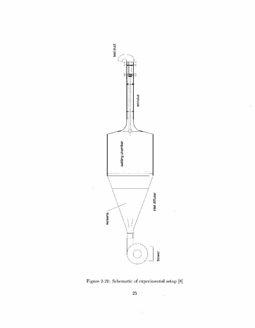
Experimental Study
The experimental study was carried out on a stereolithographic ^ scale model of the tractor
exhaust duct mounted to an annular cold flow wind tunnel, Fig. 2-21. A total of four
geometries were studied experimentally. The wind tunnel used was capable of producing
swirl, mass flow and inlet total pressure distributions similar to those seen in a gas turbine
engine. The range of swirl studied consisted of zero swirl and two radial profiles provided
by P&WC which are representative of what a sample PT6 engine exhaust duct would see at
the duct inlet plane. Total pressure profiling screens were used to produce circumferential
non-uniform total pressure profiles at inlet to the duct.
Computational Study
Five geometries were studied computationally. The computational domain consisted of an
inlet annulus, an exhaust duct, and a plenum chamber overlapping the exhaust duct exit,
Fig. 2-22. The plenum is a large conical domain with boundary conditions to allow the
exhaust jet to entrain flow freely into the plenum. The plenum also served to allow for
a non-uniform pressure distribution at the exhaust duct exit plane which results from the
large stream line curvature in the flow.
24
ffl n E ns
Figure 2-21: Schematic of experimental setup [8]
25

Plenum
7v \
*li\ . • • • • ' • . . . . ' . . . \
' • . . ' ; ; . . / . £'..••'„•-•' :'*.
• • ? * * . . " ' * ' • . * . - " . 4 . " *•
' * • . > ' * * J \
Inlet Annulus
• • - : : . . " • ' • • • i ^
••.•...-'•••-•• . " t r f c t i j
d u c t
Figure 2-22: Domain of CFD grid used for computations [8]
26

The computational grid was created using Gambit. Hexahedral elements were primarily
used to produce a structured mesh with only the annular to rectangular transitional region
requiring an unstructured grid composed of tetrahedral elements for ease of meshing. The
boundary layer was defined with prism elements in the first rows of mesh from the duct
surface. The flow solver used in this study was the commercial code Fluent 5.5. The most
suitable turbulence model which was available was the RNG k—e model; however the author
used the realizable k — e turbulence model through the majority of the study due to the
difficulty in obtaining a converged solution using the former.
Loss Mechanisms
Cunningham [8] has identified three geometric parameters affecting the total pressure losses
base on preliminary testing and literature:
1. Flow splitter.
2. Streamlining downstream of the center body.
3. Stub cross-sectional shape.
The three main pressure loss mechanisms were found and identified as:
1. Secondary flows: The secondary flows are generated through the duct bends as well
as the presence of the flow splitter redirecting the flow across the center-body.
2. Flow non-uniformity: Present at the stub exit representing undiffused kinetic energy
and therefore lower static pressure recovery. The exhaust stub cross-sectional shape
influenced the exit effective area-ratio.
3. Flow separation and recirculation: The total pressure losses are a function of the flow
separation and recirculation. Due to the complex shape of the exhaust duct, these
losses dominated over skin friction losses. Flow separation occurs along the inside
bend of the duct and in some cases, downstream of the center body.
27

Results and Conclusions
Cunningham [8] made a comparison of experimental and CFD results concluding that the
CFD consistently under-predicts the level of pressure losses in the exhaust ducts. CFD
has on the other hand shown that it is capable of capturing trends in losses by accurately
predicting changes in magnitude of pressure losses from one geometry to the next. When
comparing pressure losses due to inlet swirl, Cunningham found that the slope of the trend
line was under predicted when compared to measured results. This has been explained as
the inability of the turbulence models to handle the anisotropy of highly swirling flows.
Table 2.1 summarizes these findings.
Table 2.1: Summary of performance of CFD analysis in the study of single port gas turbine exhaust [8]
Parameter E
A P t t A Pts
geometry
flow structure
efficiency
inlet conditions
Suitability fair fair fair
good
fair
excellent
excellent
Comments Under-predicts distortion and secondary flow under-predicts losses under-predicts losses able to predict correct magnitude and trends with change in geometry easily gives details of internal flow structure, may not be reliable in identifying separation very efficient for studying inlet conditions, geometry limited by efficiency of mesher inlet conditions can be easily specified
If CFD is to be used to design optimum exhaust ducts, Cunningham has made the
following recommendations:
• In terms of predicting the total-to-static losses in the duct, the distribution of inlet
flow has a large effect on the distribution of the outlet flow. To be able to make a
realistic estimate of the total-to-static losses, a good estimate of the outlet flow is
required. To ensure this, velocity boundary conditions should be applied at the inlet
as this leads to a more realistic flow distribution at the exit.
28

• A large plenum is required at the exit of the duct to produce accurate flow distortions
in the duct near the exit.
• Turbulence models which account for swirl should be used if possible.
• Where possible, boundary conditions should be applied that account for the total
pressure non-uniformities at the duct inlet resulting from the presence of the engine.
29

Chapter 3
Design of Experiment
The work of Loka et al. [20], and Cunnigham [8] have identified many of the geometric and
aerodynamic parameters responsible for the overall duct loss. In this chapter, more param
eters are identified. Also discussed here are how the geometric parameters are quantified
and bounded within a specific design space, giving limits to the magnitude of each param
eter, for the purpose of creating a loss correlation. Next, combinations of each geometric
parameter are grouped together to create a set of exhaust duct models which, later, will be
simulated numerically along with the aerodynamic parameters to produce data for building
a loss correlation.
3.1 Geometric Design Space
A design space can be envisioned as being an n-dimensional box which is capable of contain
ing all practical exhaust duct shapes and sizes. The size of the box is chosen to allow each
geometric parameter to be varied from a minimum to a maximum value which is thought
to cover rather well the design space so that both good and bad performing exhaust ducts
are represented. For each parameter, a minimum of three changes are required to be able to
predict a non-linear trend with respect to exhaust duct losses. In this study, each geometric
parameter will be extended to the minimum and maximum limits of the design space with
one selection in the center.
30

3.1.1 Equivalent Cone Diffusion Angle
The exhaust duct region between the inlet and the flow splitter can be represented as an
annular duct. Quantifying an annulus using one parameter is done through an Equivalent
Cone DifFuser Angle (ECDA). Equation 3.1 combines inlet annulus area, Ain, exit annulus
area, Aout and duct length, L, into one convenient parameter.
ECDA = 2 arctan M I Aou±
(3-1)
The range of ECDA chosen for the axisymmetric annular duct is to provide for attached
and separated flow. McDonald et al. [9] have found that optimal pressure recovery can be
found for conical diffusers at cone angles between 6° and 8° with decreasing performance
at larger cone angles. The work of Sovran and Klomp [1] has demonstrated that the
optimum cone angle is 8° provided that the area ratio is large between exit and inlet. It
was therefore decided that an ECDA of 20° should be sufficient to create flow separation
given that downstream of the annular duct is the flow splitter and annular to rectangular
transition region which could influence the streamwise pressure gradient and ensure that
flow separation will occur. It is also of interest to see the effect of no diffusion before
the annular to rectangular transition region where higher Mach numbers are expected to
produce higher pressure losses in this region, therefore the minimum ECDA studied is 0°.
An ECDA of 10° is used as a middle value as it was found to closely approximate the
sample P&WC duct and is close to the optimal cone angles found by McDonald et al [9].
Figure 3-1 shows the annular ducts which were used in this study upstream of the annular
to rectangular transition region.
3.1.2 Flow Splitter Wedge Angle
A swirling flow will create an incidence angle with the flow splitter leading edge possibly
leading to form a separated region along the suction surface. It is expected that small wedge
angles will lead to more severely separated flow resulting from larger incident angles. Using
the sample duct provided by P&WC as a the reference for a mid point value of around 45°,
min and max values of 10° and 80° were chosen for this study, Fig. 3-2.
31

.q..
20' 10* 0'
Figure 3-1: Equivalent Cone Diffusion Angle Levels Studied
32

10° Wedge Angle 45° Wedge Angle
80 Wedge Angle
Figure 3-2: Duct Wedge Angle Levels Studied
33

Gas Path Spline
-4 Figure 3-3: Gas Path Aspect Ratio
3.1.3 Gas Path Aspect Ratio
The annular to rectangular region of the exhaust duct includes a 90° bend where the flow
will have a strong tendency to separate from the inner curve. While it is not possible
to avoid making the 90° bend, it is possible to adjust the length of duct over which the
transition will occur. It is expected that a short duct will lead to severe flow separation
along the inner curve as a result of an increased pressure gradient. Longer ducts will have
lower pressure gradients reducing or delaying flow separation. The length of the annular to
rectangular transition region can be quantified through Eq. 3.2 which adds the duct height
as an additional parameter. This aspect ratio is the ratio of axial length, L, over radial
height, H, of a spline curve representing the general flow direction. The length and height
are measured between the start and end points of the gas path spline as demonstrated in
Fig. 3-3.
34

L/H — 0.92 l_/l — -| ^5
L/H = 1.38
Figure 3-4: Gas Path Aspect Ratio Levels Studied
AS = | (3.2)
For this study, the height has been fixed while the length varied. The mean gas path
aspect ratio used is 1.15 which is representative of the sample P&WC duct. To ensure
that flow separation occurs, an aspect ratio of 0.92 was selected as the minimum because
of the aggressive turn along the inner curve. An aspect ratio of 1.38 was selected as the
maximum with the expectation that flow will remain attached along the inner curve. Figure
3-4 demonstrates these aspect ratios where each cross-section was created with an ECDA
of 10° and the same exit area.
3.1.4 Annular to Rectangular Transition Region
An additional factor affecting the pressure gradient along the annular to rectangular tran
sition is the remaining area ratio between the flow splitter and the duct exit, see Fig. 3-5
35

2 1
Figure 3-5: Duct Locations where Area is Specified
section 2 to 3. For a constant duct aspect ratio, any change in the area ratio will affect the
streamwise pressure gradient. Small area ratio ducts will have less diffusion and therefore
the smallest streamwise pressure gradient. Large area ratio ducts will have increased dif
fusion, a large streamwise pressure gradient, and increase the possibility of flow separation
due to the increased boundary layer growth. The area ratios of the annular to rectangular
transition region have been selected to give, once combined with the annular region, Fig.
3-5 section 1 to 2, overall area ratios that do not exceed more then 2 from duct inlet to duct
exit, Fig. 3-5 section 1 to 3. Table 3.1 lists the combined area ratios of the annular section
with the annular to rectangular section to give overall duct area ratios.
3.1.5 Exhaust Stubs
Swept exhaust ducts can be found in turboprop and turboshaft configurations that require
the engine to be mounted to the aircraft with the output shaft pointed in the fore or aft
direction. The end result is to have the exhaust gases leave the engine through an exhaust
36

Table 3.1: Exhaust Duct Area Ratio (referenced to figure 3-5)
ECDA ARi_2 AR2_3 ARi_3
0° 10° 20° 0° 10° 20° 0° 10° 20°
1.000 1.000 1.000 1.180 1.180 1.180 1.450 1.450 1.450
1.000 1.175 1.350 1.000 1.175 1.350 1.000 1.175 1.350
1.000 1.175 1.350 1.180 1.387 1.593 1.450 1.704 1.958
Pusher Intermediate Tractor Figure 3-6: Exhaust Stub Direction
37

stub in a direction which will be dictated by the airframe manufacturer. Three exhaust stub
configurations are modelled in this study to account for the possible change in the duct losses
with stub direction. Two of the configurations turn the flow to create a Pusher (S-Shape
Duct) and Tractor (C-Shape Duct) application while the third takes the exhaust gases
straight out (Intermediate-Shaped Duct) defining a transitional point, Fig. 3-6. For each
exhaust stub configuration, the cross-sectional area and length was maintained constant,
while for the turning exhaust stubs, the turning radius, was maintained constant.
3.2 Aerodynamic Design Space
3.2.1 Swirl
Moderate inlet swirl has been shown to be beneficial in achieving optimum diffusion in two
dimensional diffusers. Annular diffusers can be designed with a large ECDA (ie. short ducts
with large diffusion angles), resisting flow separation when swirl is present at the diffuser
inlet. For the current study, the effect of swirl on diffuser performance is not as apparent as
it is in two dimensional diffusers. While inlet swirl should still be beneficial in the annular
portion of the exhaust duct, the flow splitter performance, however, will not benefit from
large incidence angles and the annular to rectangular region of the exhaust duct will result
in an asymmetric flow field.
Some inlet swirl angle profiles of several similar exhaust ducts can be seen in Fig. 3-7.
These profiles are produced at P&WC using an in-house code which neglects the upstream
effect of the downstream diffuser and predicts a circumferentially uniform flow distribution.
While many profiles can be observed in Fig. 3-7, it was decided that the swirl gradient used
in the current study would be of a constant gradient which fits within the given sample,
identified in Fig. 3-7 as the dotted line. This swirl gradient varies by 8° from r, to r0 and
is identified by the swirl value found crossing mid way along the annulus height, Fig. 3-7
shows nominal 0°. The range of nominal swirl angles selected to be studied varies from
nominal 0° to 35°.
38

Inlet Swirl Angle at Design Point
-2 0 2 Swirl Angle (°)
Figure 3-7: Sample of exhaust duct inlet swirl gradients
39
3.2.2 Inlet Boundary Layer Blockage
It is fully evident from Chapter 2 that inlet boundary layer blockage defined by
f — dA Blockage = A
fV,. x 100 (3.3)
JAdA
has a significant effect on diffuser performance. With regards to the diffusers in this study,
it is expected that the duct pressure losses will increase with increasing inlet boundary layer
blockage. The presence of an adverse pressure gradient will result in further increasing the
boundary layer thickness as flow travels downstream from the exhaust duct inlet. As the
boundary layer thickness grows, the wall shear stress reduces due to a decreasing velocity
gradient in the direction normal to the wall. Flow separation will occur as the wall shear
stress approaches zero, contributing further to the exhaust duct losses. A turbulent inlet
boundary layer will either prevent or delay the onset of flow separation. In the current
work, three values of boundary layer blockage have been studied and are displayed in Fig.
3-8. The largest inlet blockage expected to exist in practice is 10%. The presence of the
turbine upstream of the exhaust duct inlet will likely produce a turbulent boundary layer,
therefore the minimum expected inlet blockage will be less then 1%. An inlet boundary layer
blockage between 4% and 8% will give a good mean value for correlating inlet boundary
layer blockage later on in this study. The 1/7*'1 power law given by
has been used to define the velocity gradient within the boundary layer.
3.3 Full Factorial Design
To find the sensitivity of each of the geometric and aerodynamic parameters on exhaust duct
performance requires the modelling of numerous exhaust duct cases covering every possible
combination of parameters. This approach to performing a sensitivity analysis is termed a
Full Factorial Design requiring tremendous resources to complete a timely analysis. To put
this into perspective, this study has identified five geometric parameters having a first order
40

Inlet Boundary Layer 0,4
0.35 H
0.3 H
0.25 • Annulus Height
fr-rt) Jf^ 0 .2-
0.15 4
o.H
0.05 A
0 0 0.1 0.2 0.3 0.4 0.5 0.6 0.7 0.8 0.9 1
u U
Figure 3-8: Boundary layer axial velocity profiles
41

Table 3.2: Geometric Parameters
Geometric Parameter Levels Number of Levels 1) ECDA 0°, 10°, 20° 2) Flow Splitter Wedge Angle 10°, 45°, 80° 3) AS 0.92, 1.15, 1.38 4) AR2_3 1.000 , 1.175, 1.350 5) Stub Direction S-Shape, C-Shape, Straight
Total Combinations =
3 3 3 3 3
243
Table 3.3: Aerodynamic Parameters
Aerodynamic Parameter Levels Number of Levels 1) Inlet Swirl Angle 0°, 10°, 25°, 35° 2) Inlet Boundary Layer Blockage Low, Med, High
Total Combinations —
4 3 12
effect on exhaust duct performance, where a minimum of three values are needed for each
parameter in order to find a non-linear effect on exhaust duct performance. Additionally,
each exhaust duct would need to be modelled using each combination of inlet swirl angle
and inlet boundary layer blockage. A full-factorial design with five parameters each having
three values will require 35 = 243 exhaust ducts to analyze as seen in Table 3.2. Each of
these exhaust ducts would then be modelled using each of the aerodynamic parameters in
Table 3.3 giving 12 aerodynamic boundary conditions. The total combination of geometric
and aerodynamic parameters which need to be modelled is 2916, which is an unpractical
task to perform. Consequently methods of selecting the minimum number of experiments
required to give the full information about each factor exist and are called partial-fraction
designs [21].
42

3.4 Taguchi Design
Dr. Genichi Taguchi [21] has created a set of guidelines for performing partial-fraction
designs using a special set of arrays called orthogonal arrays. In an orthogonal array all
levels of all factors are represented an equal number of times, and the combinations of any
two factors are also represented an equal number of times. In this respect, an orthogonal
array can be viewed as being well balanced, providing equal pairing between independent
parameters therefore reducing the total combination of parameters needed to determine
their effect on the dependent variable.
3.4.1 A s s u m p t i o n
Prior to choosing the orthogonal array, we must understand the assumption that is being
made in the Taguchi Design. The assumption is that the factors that are selected are
independent of each other and can be separated. Any interactions are assumed to have a
higher order effect on the dependent parameter and are confounded within the main effects.
The objective of this study is to catch the first order effects on exhaust duct losses. While
some interactions are expected to exist, they are assumed to have a smaller influence on
the exhaust duct losses then do the independent effects.
3.4.2 I n t e r a c t i o n s
Interactions that can be expected are upstream parameters affecting the downstream pa
rameters, such as flow separation in the annulus on the flow splitter and the annular to
rectangular transition region. It is not expected that a separated flow will interact with the
downstream parameters at the end-walls the same way as an attached flow does because of
changes in the boundary layer, however the stream-wise momentum is going to be an order
of magnitude larger and will continue to relate stronger to the first order duct losses. There
is one particular interaction that should not be neglected in this study, namely the inter
action between the exhaust duct and the exhaust stub direction because the same exhaust
duct can be used in both pusher and tractor configurations, Fig. 3-6.
43

3.4.3 Selecting an Orthogonal Array
An orthogonal array is selected by first considering the independent parameters one through
four in table 3.4. Each of the four parameters consist of three levels, therefore the minimum
number of geometries needed can be defined to be:
NV
NTaguchi = 1 + J2(L* ~ X) (3-5) i= l
Where:
NV = The number of parameters
and
Li = The number of levels for parameter i
For this study NV is equal to four and Li is equal to three for each of the parameters
giving nine geometries. An Lg orthogonal array shown in Table 3.4 is well suited for this
study. To include the interaction with exhaust stub direction, the L% orthogonal array
is expanded to allow each of the nine geometries to be combined with all stub directions
yielding 27 geometries to study. Table 3.5 presents the expanded Lg orthogonal array with
the physical variable to give exhaust duct families A through G. It can be well observed
that the Taguchi design has reduced the amount of geometries required for the sensitivity
analysis from 243 in the full factorial design to 27 in the partial factorial design.
44

Table 3.4: L9 Orthogonal Array
Independent Parameter Build Parameter 1 Parameter 2 Parameter 3 Parameter 4
1 2 3 4 5 6 6 8 9
1 1 1 2 2 2 3 3 3
1 2 3 1 2 3 1 2 3
1 2 3 2 3 1 3 1 2
1 2 3 3 1 2 2 3 1
45

Table 3.5: Lg Orthogonal Array Expanded for Stub Direction
Flow Sp: Duct ECDA Wedge I
~KA O5 io° A-2 0° 10° A-3 0° 10°^
T H O5 45° B-2 0° 45° B-3 0° 45°_
"CM 05 W C-2 0° 80° C-3 0° 80°_ D-l 10° 10° D-2 10° 10° D-3 10° HT E-l 10° 45° E-2 10° 45° E-3 10° 45°_ F- l 10° 80° F-2 10° 80° F-3 10° 80°
~~GA W 10° G-2 20° 10° G-3 20° 1(F H-l 20° 45° H-2 20° 45° H-3 20° 45°_
~ f l 20° 80° 1-2 20° 80° 1-3 20° 80°
ie AR2-3 AS Stub Direction
1.000 092 C-Shape 1.000 0.92 S-Shape 1.000 0.92 Straight 1.175 1.15 C-Shape 1.175 1.15 S-Shape 1.175 1.15 Straight 1.350 1.38 C-Shape 1.350 1.38 S-Shape 1.350 1.38 Straight 1.175 1.38 C-Shape 1.175 1.38 S-Shape 1.175 1.38 Straight 1.350 0.92 C-Shape 1.350 0.92 S-Shape 1.350 0.92 Straight 1.000 1.15 C-Shape 1.000 1.15 S-Shape 1.000 1.15 Straight 1.350 1.15 C-Shape 1.350 1.15 S-Shape 1.350 1.15 Straight 1.000 1.38 C-Shape 1.000 1.38 S-Shape 1.000 1.38 Straight 1.175 0.92 C-Shape 1.175 0.92 S-Shape 1.175 0.92 Straight
46

Chapter 4
Geometry Synthesis
The approach discussed here for geometry synthesis has been designed to produce exhaust
ducts which can be specified using only key geometric parameters thought to be responsible
for the total pressure losses in the exhaust duct. The 3D nature of the single port swept
exhaust duct makes its complete geometric representation impossible using only one dimen
sional geometric parameters. Therefore assumptions are made to complete the geometry.
The blanks in the steps discussed in this Chapter have been filled in based on the assump
tion of how a single port swept exhaust duct should be represented geometrically, and could
vary with each designer who uses this approach. It is the assumption of this author that the
steps not discussed here would only represent a second order effect on exhaust duct losses,
and therefore do not play a crucial role in the current study.
A sample of a single port swept exhaust duct taken from P&WC is shown in Fig. 4-1.
This exhaust duct has smooth flowing features which do not contain any sharp edges which
can disturb the flow. To describe the geometric features of this duct would require complex
splines and curves which do not suit the present study because of the numerous parameters
that would be needed. Steps have been taken to simplify the exhaust duct such that it can
be described by simple one dimensional parameters identified in Chapter 3.
47

Figure 4-1: Sample P&WC Single Port Swept Exhaust Duct
48

Figure 4-2: Equivalent Cone Diffusion Angle
4.1 Equivalent Cone Diffusion Angle
From examination of the annular region of the sample exhaust duct, the inner and outer
walls are not straight walled and are found to be represented by splines. The curved
profile has been made linear, and is now better suited to be described by Eq. 3.1. Further
examination of the sample exhaust duct shows tha t the hub surface is nearly straight walled
with a constant radius and has therefore been replicated this way in the current study. The
cross-sectional profile of the annular region is given in Fig. 4-2 which presents the sample
geometry with the simplified representation.
49

Figure 4-3: Gas Path Conic
50

4.2 Gas Pa th
The remaining portion of the gas path continues from the exit of the annular section to
the duct exit. The profile of the sample duct can be closely reproduced with the use of
conies as shown in Fig. 4-3. The conies used require five parameters; a start point, an
end point, a tangent direction at the start point, a tangent direction at the end point,
and a conic parameter. The start points and tangent directions are set from the preceding
section defined by the ECDA. The end points are defined by the exhaust duct exit area
and position. The tangent direction for the end points is always 90° from the duct inlet. A
conic parameter of 0.45 has been chosen based on a good fit with the sample duct and used
throughout this study. Once the inner and outer conies have been defined, equally spaced
points can be located along each curve and joined with straight lines. A gas path spline
can be constructed by locating the midpoints of each line and then connecting them with a
spline Fig. 4-4.
4.3 Gas Pa th Aspect Ratio
Once the inner and outer conies have been defined, equally spaced points can be located
along each curve and joined with straight lines. A gas path spline can be constructed by
locating the midpoints of each line and then connecting them with a spline, Fig. 4-4. The
gas path aspect ratio can now be measured according to Eq. 3.2.
4.4 Flow Splitter Leading Edge
The flow splitter is located downstream of the annular duct section at the bottom dead
center of the exhaust duct, Fig. 4-5). It can be described as being an axisymmetric vane
with an elliptical leading edge varying from hub to tip centered along a plane not fully
normal to the axial direction. Large fillets are used at hub and tip of the vane to merge
smoothly with rest of the domain. The flow splitter smoothly blends from the leading edge
outward to the exhaust duct through the annular to rectangular duct transition region.
To construct the flow splitter, a plane is located normal to the gas path spline slightly
51

Gas Path Spline
"ft Figure 4-4: Gas Path Spline and Aspect Ratio
52

Flow Splitter
Figure 4-5: Flow Splitter
53

downstream of the annular duct segment, Fig. 4-6. With the height of the flow splitter
located at the bottom dead center of the duct, it's center is located and a circle is drawn
of diameter D in a plain normal to the line defining the flow splitter height. The circle is
centered along the symmetry plane of the duct but not constrained to be centered on the
line defining the flow splitter height. Two lines are drawn at an angle a intersecting the
symmetry line of the flow splitter and tangent to the circle. The circle is allowed to move
along the center line with the tangent points falling on the plane positioned normal to the
gas path spline. The portion of the circle lying downstream of the plane positioned normal
to the gas path is removed leaving the upstream portion to be the leading edge of the flow
splitter, Fig. 4-7. The leading edge curve is then extruded to produce the flow splitter
which is then joined to the upstream annulus through fillets.
4.5 Flow Splitter Wedge Angle
The transition of the exhaust duct geometry from annular to rectangular continues from the
leading edge of the flow splitter through a wedge shaped inner passage directing the flow
around the hub toward the exhaust duct exit. The P&WC sample duct shown in Fig. 4-8
demonstrates that the varying leading edge diameter leads to a varying wedge angle from
hub angle a\ to shroud angle a^- The exhaust ducts created in this study contain a single
wedge angle as a result of using one leading edge profile from hub to shroud. To smoothly
merge the wedge angle into the duct transition section a limit was put on the flow splitter
length to allow a smooth transition to occur as seen in the P&WC sample exhaust duct in
Fig. 4-8. This limit was taken as being l/8 i fe the length, L, defined in the gas path aspect
ratio.
4.6 Duct Exit Cross-Section
The sample P&WC exhaust duct consists of an exit cross-section that is only symmetric
across one plane as shown in Fig. 4-9. The duct exit cross-section of the sample P&WC
exhaust has been developed through optimization for a given set of flow conditions which
are unknown to this author. For this reason, a fully symmetric exit cross-section, shown as
54

Gas Path Spline
Plane Normal To Gas Path Spline
Flow Splitter Height, L Center of Flow Splitter
Figure 4-6: Flow Splitter Construction Plane
55

Leading Edge
Tangents
Duct Symmetry Plane
Plane Normal to Gas Path Spline
Figure 4-7: Flow Splitter Construction Plane
56

P&WC Sample Duct Simplified Duct Wedge Angle
Figure 4-8: Flow Splitter Wedge Angle
the blue profile in Fig. 4-9, has been used throughout this study so not to introduce any
unknown influences produced by the sample P&WC exhaust duct.
4.7 Annular to Rectangular Transition Region
The shape of the exhaust duct from the flow splitter downstream to the exhaust duct
exit is defined by cross-section profiles built on planes passing through each of the lines
connecting the inner and outer conies shown in Figs. 4-3 and 4-4. The exhaust duct
transition from annular to rectangular produces complex cross-sections which cannot be
defined with straight lines and curves, resulting in the decision to use splines, Fig. 4-10.
Numerous control points are required to define each cross-section spline making it difficult
to develop a consistent approach to the design; however, some rules have been created and
followed throughout this study. The following rules that have been applied are:
1. The profile is bounded by the annulus hub radius.
2. The profile is bounded so as not to surpass the gas path inner conic.
57

Before
After
f ^
Symmetry Plane
(Before and After)
Symmetry Plane
(Only After)
Figure 4-9: Duct Exit Cross-Sectional Shape
58

Plane Downstream of Flow Splitter
Duct Exit
Figure 4-10: Duct Cross-Sections Downstream of Flow Splitter
3. The growth in cross-sectional area should be nearly linear.
4. The exhaust duct geometry should transition smoothly without any waviness or sharp
edges that may affect the flow of fluid.
To maintain the wedge angle defined in Sec. 2.2, a cross-section is placed passing through
a point marking the end of where the wedge angle is held to. Once the cross-sections are
completed, a surface is passed through them and then joined to the upstream flow splitter
and annulus, Fig. 4-11.
4.8 Plenum
A plenum domain, shown in Fig. 4-12, is created for each duct series as a function of the
exhaust s tub exit hydraulic diameter. The inlet surface parallel with the stub exit plane
has a diameter of 10Dhstubexit and the plenum length is \hDhstubexit- The half cone angle
of the plenum is 30°.
59
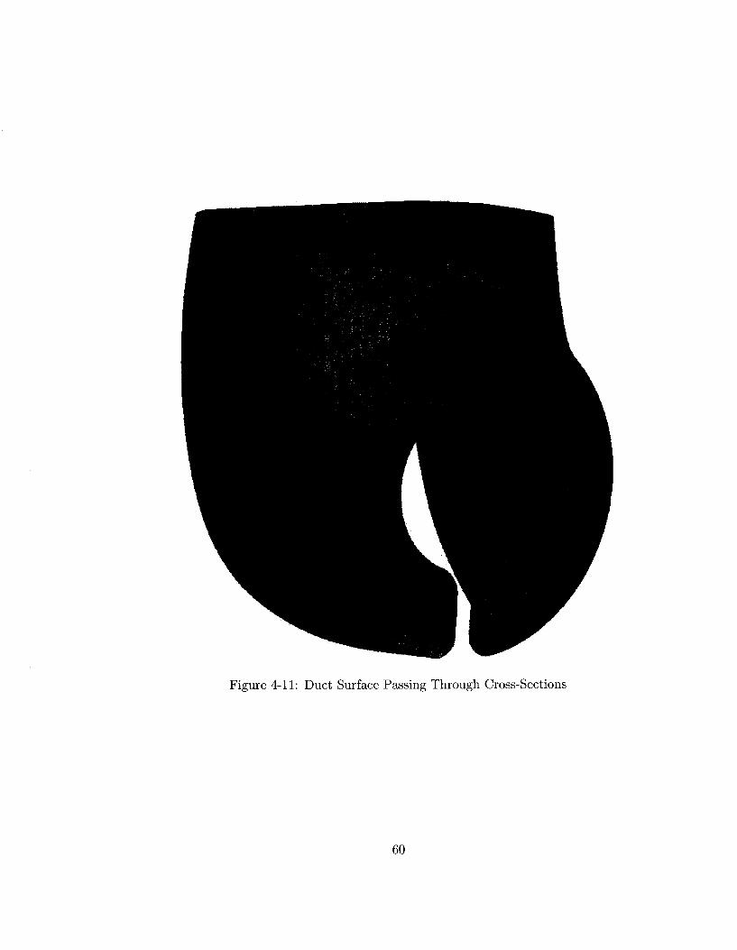
Figure 4-11: Duct Surface Passing Through Cross-Sections
60

30°
0 = 1OXDh stub exit
15 X D h s t u b e x i t
Figure 4-12: Plenum
61

Chapter 5
Computational Study
The computational analysis has been performed using CFX 5.7.1, which is a a commercial
Computational Fluids Dynamics (CFD) package developed by ANSYS. CFX 5.7.1, solves
the unsteady Navier-Stokes equations in their conservative form. The computational domain
is discretized into finite control volumes using a mesh. Each of the governing equations are
integrated over a control volume, such that the related quantity (mass, momentum, energy
etc.) is conserved in a discrete sense. The following sections cover the development of the
computational methodologies and mesh synthesis.
5.1 Data Reduction
Data reduction techniques for averaging flow properties must be carefully selected consid
ering the non-uniformity of the flow through the exhaust ducts considered in this study.
Errors can be introduced through averaging techniques which will affect the performance
parameters introduced in Sec. 2.1, where the total pressure loss coefficient is of prime
interest in the current analysis.
Perhaps the simplest form of averaging flow parameters (</>) is the area average given
by:
Parea = ^ I 5 - 1 )
A more apropriate averaging method for non-uniform flows is the mass average method
62

given by: J((f>pudA)
* = 7 O ^ A T (5'2)
Wyatt [22] has studied the errors generated using averaging methods that include Eqs. 5.1
and 5.2 in ducts with various velocity profiles. It was demonstrated that total pressure
losses in a duct for a Mach number of 0.3 resulted in an error of less then . 1 % and 1%
for the mass average and area average techniques respectively. Based on the above results
and to be consistent with the work of Cunningham [8], all flow parameters have been mass
averaged in the present study.
5.2 Pressure-Velocity Coupling
To overcome the decoupling of pressure and velocity, CFX 5.7.1 uses a single cell, un-
staggered, collocated grid. The continuity equation is a second order central difference
approximation to the first order derivative in velocity. A fourth derivative in pressure is
used to modify the equation to redistribute the influence of pressure and overcome the prob
lem of checker board oscillations found when variables are collocated. The method used is
similar to that from Rhie and Chow [23]. A number of extensions are implemented in CFX
which improve the robustness of the discretisation when pressure varies rapidly.
5.3 Advection Scheme
CFX 5.7.1 offers the first order upwind differencing scheme, the high resolution scheme,
or a specified blend factor to blend between first and second order advection schemes to
calculate the advection terms in the discrete finite volume equations. The high resolution
scheme, used in this study, has a blend factor which varies throughout the domain based
on the local flow field. In flow regions where there are low gradients, the blend factor will
take on a value close to one representing a second order advection scheme. Flow regions
with large gradients will have a blend factor near zero representing a first order advection
scheme to prevent overshoots and undershoots and maintain robustness.
63

5.4 Turbulence Modelling
A wide range of turbulence models are available in CFX 5.7.1 which include a standard
k-e, Large-Eddy-Simulation, and the Shear Stress Transport (SST) model. The two most
appropriate turbulence models for this analysis are the k-e and SST turbulence models.
5.4.1 k - e
The k-e model is robust and computationally inexpensive at solving turbulent flows. The
downfall of this turbulence model is that it predicts the onset of flow separation late and
tends to under-predict the magnitude of separation. Separated flow has been observed
in single port swept exhaust dust by Loka et al [20] and Cunningham [8]. Both authors
have observed flow separation along the exhaust duct hub and inner curve in the annular
to rectangular transitional region. It is important to note that diffusing flows produce
unstable boundary layers due to the flow traveling against an adverse pressure gradient.
The effect of predicting the onset of flow separation late results in over predicting exhaust
duct efficiencies, where flow separation leads to less pressure recovery and lower discharge
coefficients.
5.4.2 SST
A turbulence model developed to address the deficiencies of the k — e model is the SST
turbulence model developed by Menter [24]. This model works by solving the k—ui equations
at the near wall region and then the k — e in the free stream region with a blending function
for transition between the two models. The k — UJ based SST model takes into account the
transport of the turbulent shear stress to give highly accurate predictions of the onset and
the amount of flow separation under adverse pressure gradients. The key reason for the
deficiencies of the k — e model is that is does not account for the transport of the turbulent
shear stress resulting in an over prediction of the eddy-viscosity.
CFX guidelines for using this model requires an overall y+ of less then two and no less
then 10-15 grid points within the boundary layer. The SST model continues to be accurate
when these guidelines can not be achieved from the use of scalable wall functions. For fine
64

Figure 5-1: Air solid model of the computational domain
grids the k — to model is applied, but when a coarser grid is used, the model switches to a
wall function treatment making use of the logarithmic profile assumptions. For this reason,
a new near wall treatment was developed by CFX for the k — u> based models that allows
for a smooth shift from a low-Reynolds number form to a wall function formulation.
5.5 Computational Domain
The computational domains studied in this work are composed of an exhaust duct, exhaust
stub, and a plenum chamber as illustrated in Fig. 5-1. The plenum chamber has been
modeled to serve multiple functions which include providing a far-field boundary condition
and a domain for jet flow entrainment. The work of Loka et al, and Cunnigham have
made use of plenum chambers in their work, both demonstrating that non-uniform pressure
65

gradients exist at the exhaust stub exit. These pressure gradients are found to exist as
a result of the swirling flow and geometric influences causing streamline curvature. If no
plenum is modeled, the flow structure at the exhaust stub exit would be strongly influenced
by the imposed boundary conditions. A realistic exit flow structure can only then be
achieved if the pressure gradients at the exhaust stub exit are known in advance.
5.5.1 Boundary Condit ions
The CFD boundary conditions have been selected as being the most appropriate for deter
mining the aerodynamic and geometric parameters sensitivity on exhaust duct losses. The
boundary conditions are not consistent with what is experienced at flight conditions where
ambient conditions change according to aircraft speed, altitude, and engine installation.
The following boundary conditions can be seen in Fig. 5-2.
Duct Inlet
Ansys CFX contains a large variety of inlet boundary conditions to suit many situations.
The requirements of this study are to impose a swirl gradient and aerodynamic blockage
at the duct inlet plane. Total pressure and mass flow boundary condition do allow for an
imposed flow direction, however, the aerodynamic blockage is an implicit result of the flow
simulation making these boundary conditions a poor choice for the current study. The
most suitable inlet boundary condition for this study, that is offered in CFX, is to impose a
velocity gradient with magnitude and direction. Using this option both a swirl gradient and
blockage can be controled explicitly. Using the later choice of inlet boundary conditions,
the velocity magnitude and direction were specified as a function only of radius (constant
across the circumference). An inlet total temperature of 1530 R was used throughout this
study, being a common average total temperature for P&WC swept exhaust ducts. The final
parameters set at the inlet to the exhaust duct are turbulence intensity and eddy viscosity
ratio. A turbulence intensity of 10% and an eddy viscosity ratio of 300 were suggested by
P&WC experts and used throughout the study.
66

Plenum Inlet:
Mass Flow = 10% iniet mass flux
Tt = 519R
1 = 1%
e = 1
A
Openinq:
Ts
Ps
l =
e =
= 519R
= 14.7 psi
1%
1
Inlet:
Velocity
•Magnitude
•Direction
Tt=1530R
I = 10%
£ = 300
Walls:
No Slip
Adiabatic
Figure 5-2: CFD boundary conditions
67

Plenum
The conical plenum domain has an inlet and an outlet boundary condition. The inlet
boundary condition is mass flow with direction. The mass flow rate is implicitly defined
to be 10% of the duct inlet mass flux. The flow direction over the full surface is directed
normal to the exhaust stub exit plane. A uniform total temperature is imposed at 519
R. A low inlet turbulence intensity and eddy viscosity ratio of 1% and 1 respectively was
used. The plenum exit was modeled as an opening allowing both inflow and outflow from
the same location. The opening static pressure and temperature is set at 14.7psi and 519
R respectively. For the condition of inflow through the opening, a low turbulence intensity
and eddy viscosity ratio was selected to match the plenum inlet boundary condition.
Walls
The exhaust duct and stub wall have been modeled as no slip and adiabatic.
5.5.2 Grid Structure
The computational grid was created using ANSYS ICEM CFD. This meshing package offers
the capability to create grids in multi-block structured, unstructured hexahedral, tetrahe-
dral, hybrid grids consisting of hexahedral, tetrahedral, pyramidal and prismatic cells. For
this study, the computational domain was constructed using unstructured tetrahedral ele
ments with prismatic cells for near wall turbulence model requirements.
The three components of the computational domain (exhaust duct, stub, and plenum)
where meshed separately and later assembled in CFX making use of General Grid Interface
(GGI) which is used to create a fluid-to-fluid interface layer between two grid surfaces which
do not have matching node locations. The GGI theory involves a control surface treatment
of the numerical fluxes across the interface. The handling of the interface fluxes is fully
implicit and fully conservative in mass, momentum, and energy. The advantage of using
GGI capability of ANSYS CFX, is that a parametric study can be carried out with minimal
time spent creating computational grids. For one duct series in Chapter 3, only one exhaust
duct, one curved stub, one straight stub, and one plenum is needed to be meshed in ICEM
CFD. The C-Shaped domain is created by assembling the exhaust duct, curved stub, and
68

Figure 5-3: Exhaust Duct Inlet Showing Prism Layer Elements (20 layers shown)
plenum in ANSYS CFX and defining all the fluid-to-fluid interface surfaces. The S-Shaped
duct is created in ANSYS CFX by rotating the stub and plenum about an axis. To create
the Intermediate-Shaped duct, the curved stub is swapped with the straight stub, and the
plenum is rotated and translated in space to match interface surfaces.
Exhaust Duct and Stub Grid
The exhaust duct and stub grids are composed of prism elements to resolve the boundary
layer and tetrahedral elements to resolve the free-stream flow. These two computational
domains must respect the mesh requirements of the SST turbulence model discussed in
Sec. 5.4.2 since the walls in these domains are defined in CFX as no-slip surfaces where a
boundary layer is present. Prism elements are inflated from the walls of each domain up to
69

Figure 5-4: Plenum surface grid
a height which meets minimum requirement of putting 10-15 nodes in the boundary layer,
see Fig. 5-3. With the inlet area of the exhaust duct fixed in this study the prism layers
have been extended to a height of /i/6 measured normal from the wall surfaces. The prism
elements are formed by first growing one layer to the overall inflation layer height, xn, then
subdividing them using an exponential growth law with a height ratio of d, giving a smooth
transition of the last prism layer height, xn_i, to the tetrahedral elements resolving the free
stream flow. The height of a given prism layer, i, can be calculated from Eq. 5.3.
Xi = xix G P " 1 (5.3)
70

(jsissis^si e s is >s s» si s 5*3
& * * * * IS * * IS IS S IS a s !>QXlXIXIXlXlXlXlXIXIXlXIXP<f, e •:< s s s s si s s s s * s is s>s i$ e« si s g? m m s< si © m si si s e? is s< a s c © si s is is si si s is is si si s is is is s s S3i J S 3 © >S S •!< IS IS >S S >S S S S S S S 65 * S @ S S * S SfSe
@ si * is >s s >s s is K s >s £ <«* «•> >n s n< m n K< IS HOS IS (S IS IS S IS IS IS K£;?•
oxixixixixixixixixr ^ ^ S S ^ i S ^ ^ S ^ ^ ^ S ^ : ^ ; ^ . ^ ^ ^ . ^ : ^ ^ ^ : ^ : ^ : - : : - - ^ G l S S i S i S l S i S S i S ^ S ^ i ^ . * ^ - - ^ : ' ^ ©SS^Sf f lSSQff l iSOi©*; ; : :^ I e IS S S iS IS lS IS S IS lS IS 12^ :^ ;:*::: S;; ?* ::: :<*• ? £::: *::;: t::i::::^:-l&iS^S^diS^SlSlSiSl©&^: : - :^ :^-^:^: i ; -^- . ; -^ : : : - ; " -
^iSSIS^^^SIS^ISiSe^^iS.::.;:^^.^^:::'::-'::.^'ii1V^>i gi&oioioio^BiiojBBaK^:::;;.;:;.:::::;';',:;::;;-11
^ S d ^ S i S d d i S S d d S ^ ^ o ^ ^ ' l ^ ' i ^ ' V ^ ^ i i l S ^ S i 1 : SiSd^SiSddSiSdiS©^?J i:; :-^^'53.^fi! ie!dSlSlS^iS £< is >s si s is is si si s >s s s>* •; >-• a >n s s is is * s © * *
e f f iSS IS f f iBMSISSBSf f iSBBMWSlS lS lSEVV |& H K H S IS >S v IS S IS IS IS IS H IS IS IS IS S IS IS »3Q 6<iSSSSSiSiSiSSdiSKiSS>SiSiSSlSK?£^ e is is s s is ISIS <s s »is is si s is s s is vi
s is si s s >s is is sa s is si is si s Q g :i< m is x s is is is is s is is is & E S T
:;:;:;::;:; ';:v.: . iS & i S IS €
? ? ¥ h- S. *JSi IBs SI Si S IS S •!< g ^ v a Si S •!< IS SI SI S © ® * «
Figure 5-5: Cross-section of the plenum domain showing element sizes
71

Plenum Grid
The plenum domain is meshed with the inlet and opening surfaces as was explained in
Sec. 5.5.1. Only tetrahedral elements are used in this domain because there are no no-
slip surfaces requiring the grid resolution needed to resolve the boundary layer. One more
surface is included in this domain, shown in Fig. 5-4, having the same cross-sectional shape
as the exhaust stub exit plane. This surface is included for the GGI interface boundary
condition used to create the fluid-to-fluid interface which links the flow from the exhaust
stub to the plenum. The elements on this surface are sized to match the exhaust stub
tetrahedral size. The remaining surfaces do not require fine elements because high gradient
are not expected in these regions. The elements on these remaining surfaces are created
eight times larger then what is used in the exhaust duct and stub grid. Two ease the
transition from the small elements in the exhaust stub domains to the large elements in the
plenum, a volume of elements four times larger then the exhaust stub are produced in the
region where the jet flow first enters the plenum, Fig. 5-5.
5.5.3 Grid Study
Prior to fixing the mesh parameters for the current study, a sensitivity analysis has been
preformed to select the appropriate quantity of prism layers and tetrahedral grid density.
Selecting the Quantity of Prism Layers
Three sets of exhaust duct and stub meshes were created to test the sensitivity of the total
to total pressure losses versus the quantity of prism layers within an overall prism layer
height of h/6. For the three sets of meshes, total prism layer quantities of n = 20, 25,
and 30 were studied while the height, x\, of the first node from the wall was maintained
constant. Each of the meshes was created using the same density of tetrahedral elements
and same CFD boundary conditions so as to isolate the differences in numerical solution
with respect to the quantity of prism layers. The results of this analysis are plotted in Fig.
5-6. It is apparent that increasing the number of prism layers has only a small effect on the
total pressure losses within the exhaust duct and stub. Total pressure losses varied by only
2% when going from 20 to 30 prism layer. Considering the small differences in pressure
72

20 25
Total Prism Layers
Figure 5-6: ^-^ ploted versus of total number of prism layers
73

Coarse Intermediate Fine
Figure 5-7: Three grids constructed from tetrahedral sizes of h/3 (coarse), h/6 (intermediate), and h/12 (fine)
losses, 20 prism layers have been used thought this study resulting in a 25% reduction in
nodes versus the 30 prism layer runs.
Selecting the Grid Density
Grid dependence on grid density has been examined by constructing computational domains
using different tetrahedral element sizes. Three domains were created using tetrahedral sizes
of h/3, h/6, and h/12 while maintaining the same prism parameters as selected in Sec. 5.5.3.
Figure 5-7 demonstrates that the selected tetrahedral parameters lead to a coarse mesh of
135465 nodes, an intermediate mesh of 322371 nodes, and a fine mesh of 980284 nodes. The
three grids were solved numerically using the same boundary condition used in Sec. 5.5.3 and
74

200000 300000 400900 50O0OO SOOO09 700000 800000 900000 1000000
Total Number of Nodes
Figure 5-8: ^-^ ploted versus of total number nodes
75

Coarse Intermediate Fine
<$ A «*• <\ <,?> fr> nj) <& A% <£ <?• <y N* a r T v* «r V v
o- a- o- o- <s- is- o- cr o- s-
Mach Number
Figure 5-9: Mach contours for the three grid densities
76

the resulting total pressure losses are plotted in Fig. 5-8. It is apparent that grid dependence
is obtained with a difference in total pressure losses of 1.4% between the intermediate and
fine grids. Figure 5-9 further demonstrates that grid dependence is obtained by viewing the
Mach contours on the symmetry plane of the three grids. Examination of Fig. 5-9 shows
that the coarse grid fails to pick up the flow separation in the exhaust duct and stub along
the inner bend which is present in the other grids. Figure 5-9 also demonstrates that a lower
magnitude of flow separation along the exhaust duct center body is obtained in the coarse
grid where the intermediate and fine grids both demonstrate that flow is separating at the
same order of magnitude. Based on these results the remainding grids in the current study
have been created using a maximum tetrahedral size of h/Q with a computation savings of
nearly 70% less nodes than what was used in the fine grid.
77

Chapter 6
CFD-Based Parametric Study
The following sections present the findings of CFD analysis. Each geometric and aerody
namic parameter is presented and it is demonstrated, qualitatively and quantitative, how
they are related to the total pressure loss in the exhaust duct. Cross-sections are defined
throughout the study according to the method discussed in Chapter 4 to evaluate and
compare the losses between each duct studied. The sections presented in Fig. 6-1 will be
referenced throughout this Chapter, and distance is calculated along the gas path spline.
13 (Exit)
12 11 10 9 8 7 6 \ / / I
5 \ / /
3 2 1 (Inlet)
Figure 6-1: Cross-sections used for data reduction and flow visualization
Path Spline
78

Section # 1 (Inlet) 2 .3 4 5 6 7 8 9 10 11 12 13 (Exit)
0 1 2 3 4 5 6 7 8 9 10 11 12 13 14 15 16 17 18 19 20 21 22 23 24 25
Distance (in)
Figure 6-2: Total pressure loss coefficient evaluated at each section defined in figure 6-1
6.1 Effect of Swirl
Inlet swirl has been demonstrated to have a large influence on the internal flow structure
producing higher losses as inlet swirl is increased. As indicated in Fig. 6-2, the losses are
at a minimum for nominal 0° inlet swirl for a sample exhaust duct with a C-shaped stub.
In this figure, the total pressure loss coefficient is calculated at each section from Fig. 6-1
demonstrating how the total pressure losses can be seen to accumulate. To illustrate this,
contours of the normal component of velocity with vectors of the tangential component is
plotted on cross-sections for the sample exhaust duct in Figs. 6-3 and 6-4 for inlet boundary
conditions of nominal 0° and 35° inlet swirl with low inlet blockage.
The increasing loss between the inlet and section 2 can be attributed to the higher
velocity gradients. A symmetric flow field can be seen at section 2 for inlet swirl of nominal
0° where when inlet swirl is higher as in the case of nominal 35° the flow field is asymmetric.
This asymmetry in flow is caused as a result of an upstream influence of the flow splitter.
The resulting flow field has larger velocity gradients at higher inlet swirl conditions where
79

Normal Velocity [ftsA-l]
Inlet
Figure 6-3: Velocity contours normal to cross-section (nominal 0° swirl)
80

Figure 6-3: Velocity contours normal to cross-section (nominal 0° swirl)....con't
81

<£ <& v <P <ofo v c? <6fo v <$> «° v <r & v f t ? <v «° V> 1? nj> y t? tP Y & & y <£ <& <£> «P
Normal Velocity [ftsM]
Inlet
Figure 6-4: Velocity contours normal to cross-section (nominal 35° swirl)
82

Figure 6-4: Velocity contours normal to cross-section (nominal 35° swirl)....con't
83

viscous shear produces increasing pressure losses.
A large increase in losses is always found to occur between sections 2 and 3. It is at
these sections that the exhaust duct begins transitioning from annular to rectangular and
is where gradients in velocity are highest. Observing Figs. 6-3 and 6-4 at section 3 shows
that inlet swirl transforms the flow field and introduce regions of peak velocity and flow
separation due to incidence angles with the flow splitter. The losses rise at section 3 with
increasing swirl due to increasing asymmetry in the flow field and increasing flow separation.
Sections 3 through 12 finishes the exhaust duct transition from annular to rectangular,
and ends at section 12 bringing the flow out in a direction 90° from the inlet. The total
pressure losses through these sections are found to increase steadily for all inlet swirl con
ditions as indicated in Fig. 6-2. In Fig. 6-3 for an inlet swirl of nominal 0° high velocity
flow remains concentrated in the lower portion of section 3 near the hub and then separates
off the centerboby at section 5 in a manner similar to Von Karman Vortex shedding. This
low velocity flow can be seen to penetrate in to the core flow field, and is dissipated by
section 12. Counter rotating vortices are seen to form in the core flow by section 8 due to
the fluid turning while the low momentum fluid in the boundary layers at the outer sides of
the section is seen moving opposite to the vortices due to low pressure at the inner surface
of the bend. For the same sections with inlet swirl as in Fig. 6-4, the flow field is more
complex. At section 3 the flow is already seen to be separating at the hub and is joined
at section 4 with the separated flow off the flow splitter. High momentum flow is seen
concentrated along the left hand side of sections 3 through 9 until it becomes fairly more
uniform by section 10. The low velocity pocket of separated flow observed at section 4 is
seen to leave the centerbody at section 5 and can be seen to be almost fully dissipated by
section 12. The effect of turning the flow 90° is again shown by the presence of two counter
rotating vortices which are almost fully developed by section 9.
The remaining duct losses are occurring through the exhaust stub between section 12
through 13 where in both Figs. 6-3 and 6-4 display flow separation along the inner surface
due to the momentum of the fluid being pressed along the outer surface in the remaining
90° turn. The addition of inlet swirl produces a exhaust stub exit flow structure slightly
asymmetric to what is observed with nominal 0° inlet swirl.
84

Straight S-Shape
j $
^ i> <) t? ^ (J (? fl> (J d> «> <J eP «J iJ (? « ° o? Ob V V \ * "? T? 1,* f - ? V N1 (? If «?
Q- Q- Q- <&' ^- O" Q- ©• O- O' O' Cl (V O* Q- <V
Mach Number
Figure 6-5: Mach contours at mid plane demonstrating the effect of stub direction (nominal 0° inlet swirl)
6.2 Effect of Stub Direction
The exhaust stub direction has been shown to have an impact on the internal flow structure
in the exhaust duct. Figure 6-5 demonstrates through Mach contours the effect of stub
direction at nominal 0° inlet swirl on the internal flow structure. At the nominal inlet swirl
of 0° there is more flow separation in the case of the Straight stub and the S-shaped stub
then what is found in the C-shaped stub. The reason for this is seen in Fig. 6-6 where static
pressure contours are presented. In the case of the C-shaped stub, a high pressure region
is present along the outer curvature of the duct which prevents flow separation along the
inner curvature by forcing the flow to follow the surface. As for the case of the Straight and
S-shape stubs, this high pressure region is not present to prevent flow separation as seen in
Fig. 6-6.
85

C-Shape Straight S-Shape
<$ <\N &> \* «J> A & <§> AN t ? \* <& <^ >S> <S° $> 0 s s* V IT V & <r V <b V A* "S7 «T Sr
N<V NQ- 4>' N<V NQ' „$>' ,JV SQ- N 0 ' , $ ' .JV N 0 ' ^" .{V „ y
i««Hi
Q inlet
Figure 6-6: Normalized static pressure contours at mid plane demonstrating the effect of stub direction (nominal 0° inlet swirl)
86

1 (Inlet)
0.45 •
Section # 2 3 4 5 6 7 8 9 10 11 12 13 (Exit)
0.35
Stub Shape
( • ) C-Shape
( • ) S-Stiape
( A ) Straight
I
Distance (in)
Figure 6-7: Total pressure losses calculated for C-shape, Straight, and S-shaped exhaust stubs (low inlet blockage)
The exhaust duct total pressure losses at the exhaust stub exit plane are dependent on
the stub direction. However, the total pressure losses from exhaust duct inlet to the stub
inlet are nearly independent of the stub direction. The graph in Fig. 6-7 demonstrates the
general trend found in this study for a sample exhaust duct. For an inlet swirl angle of 0°
there is no discernable difference in the total pressure loss coefficient calculated from the
inlet up to the stub inlet at section 12. After the stub inlet, there is a clear difference in the
duct losses where the C-shaped stub demonstrates the lower losses with the next highest
being a Straight stub followed by the S-shaped stub being the worst. The same trend is
seen for higher inlet swirl conditions where variations in total pressure losses at a given
section can be less then 5% up to the stub inlet.
6.3 Effect of ECDA
As demonstrated in Figs. 6-3 and 6-4, the flow structure in the annular to rectangular
transition region can be quite complex. A two dimensional flow field becomes asymmetric
87

Mach Number
Figure 6-8: Mach number contours at mid-plane demonstrating the effect of ECDA (inlet conditions: nominal 0° swirl with low blockage)
by the exit of the annular region at section 2 with flow separation occurring in the down
stream sections. To produce lower losses downstream of the annulus, it is desirable to reduce
the fluid Mach number as much as possible.
The effect of the ECDA tested on the flow field can be seen in Fig. 6-8, where Mach
contours are plotted at mid plane of three exhaust ducts containing the different values of
ECDA tested. It is apparent in the figure that an ECDA of 10° led to the lowest mach
numbers at the exhaust duct exit, with the highest occurring when no diffusion is present.
The effect of too much diffusion in the annulus is seen in the figure, where flow separation
is observed along the outer annulus walls of the duct with an ECDA of 20°.
The total pressure losses are calculated at the exit of the annulus of the ducts tested
under inlet swirl conditions with low inlet blockage and presented in Fig. 6-9. The minimum
losses are found to occur in all ducts with an ECDA of 10°. A trend of pressure losses
increasing with increasing inlet swirl is also present in the figure with the exception of ducts
G and H which both have ECDA of 20°. For these two ducts flow the flow separation is
88

0 S 10 15 20 25 30 35 40
Inlet Swirl f°)
Figure 6-9: Total pressure losses as a function of ECDA calculated at exit of the annulus
seen to decrease from nominal 25° inlet swirl to 35° inlet swirl as shown by the contours of
wall shear stress in Figs. 6-10 and 6-11.
6.4 Effect of Wedge Angle
As it was explained in Sec. 6.1 the largest increase in losses is always found to occur between
section 2 and 3. It is between these two sections that we find the flow splitter. Figure 6-12
demonstrates the effect of increasing wedge angle on the pressure losses for three exhaust
ducts with the same ECDA upstream of section 2. At nominal 0° inlet swirl all three duct
produce similar losses however as inlet swirl is increased the exhaust duct with an 80° wedge
angle produces lower losses at 25° inlet swirl. To examine why the three exhaust duct are
not similar at an inlet swirl of 25°, Mach contours are presented in Fig. 6-13 at a given
cross-section cutting through the flow splitter. It is evident in the figure that the flow has
separated along the suction surface of the exhaust ducts with wedge angles of 10° and 45°
while the flow remains attached in the duct with the 80° wedge angle.
89

/ ? f f # /• / .* / .# ? <S> cS> # <? <f «F ^ f <*• «P *
<S' V N * N - •%•' " V " ? > ' ' V t . ' V V
' ,J l _J I Wal l Shear
Ipsa
Figure 6-10: Wall shear stress contours (nominal 25° swirl)
90

# cf>* ^ ^ <?* # ^ *?* ^ <$? ^
•3° o e* <r 0s *r <s> <r «* *?* <av
<v y \ - N- y y y v *• v y
Wall Shear Ipsi]
Figure 6-11: Wall shear stress contours (nominal 35° swirl)
91

ft* I
I
0 5 10 15 20 25 30 35 40
Inlet Swirl (°)
Figure 6-12: Total pressure losses as a function of wedge angle calculated at section 3
6.5 Effect of Aspect Ratio and Area Ratio in the Annular to
Rectangular Transition Region
The effect of aspect ratio and area ratio in the annular to rectangular transition region on
exhaust duct performance is difficult to quantify from the results of this analysis, because
they are under the influence of the geometric parameters that precede them (such as ECDA
and Wedge Angle). It can be seen from the test matrix in Table 3.5 that the influence
of the aspect ratio and area ratio can not be demonstrated independently from the other
geometric parameters. Some conclusions can be made when exhaust ducts are compared
under no inlet swirl and low inlet blockage where those preceding geometric influences are
at a minimum. Figures 6-14 and 6-15 present normalized static pressure and Mach number
of four exhaust ducts which represent the combinations of aspect ratio and area ratio which
are at the corners of the envelop tested. The normalized wall static pressure contours in
Fig. 6-14 demonstrate that gradients on the wall are largest when the aspect ratio and area
ratio are at the minimum. This is unfavorable since large pressure gradient will tend to
promote flow separation off the duct surface. The Mach number contour plots at mid plane
92
U.I4
0.12
0.08

Wedge Angle = 10c - >IRO Wedge Angle = 45
Wedge Angle = 80c
cP 4?i ^ of> ^ <? i ° -l1' 1^ «? -J?1 «J A (S i j (!) (? S> \ t t \» T,N f Y V tJ>" t?> V «?> «* <? V1 4?
<v «s- cr <v c»- Q- o- o cr <v o- Q ©• <v o- o '
Mach Number
Figure 6-13: Mach number contour plot on a plane through the flow splitter
93

AR = 1.000 AS = 0.920
AR= 1.350 AS = 0.920
AR = 1.350 AS = 1.380
AR= 1.000 AS = 1.380
# <f & # & ^ ^ <? ^ & & # # ^ #
•H9H
Q inlet
Figure 6-14: Normalized wall static pressure contours demonstrating the effect of aspect ratio and area ratio in the annular to rectangular transition region
94

AR= 1.000 AS = 0.920
AR = 1.350 AS = 1.380
D AR= 1.350 AS = 0.920
l ) AR= 1.000 AS = 1.380
o < £ " # <0» *<"> N** N> <VS C?5 & <£ <& \* t £ A^ C\Q
ti5 ^ <y <s° v N* *o -^ v" -v* T> v "r v t? <b' <y o- cr <a* <v <y O* Q* O O- <y <S- <y O-
I L.
Mach Number
Figure 6-15: Mach number contours demonstrating the effect of aspect ratio and area ratio in the annular to rectangular transition region
95

in Fig. 6-15 support this theory demonstrating that small aspect ratios do lead to flow
separation off the inner surface of the exhaust duct reducing the available flow area in the
streamwise direction. It can be concluded that it is favorable to have the largest available
aspect ratio to maintain an attached flow.
6.6 Effect of Inlet Boundary Layer Blockage
It has been found that the total pressure losses increase as a result of increasing inlet
boundary layer blockage. As seen in Fig. 6-16 a thick inlet boundary layer is more prone to
flow separation with the point of separation progressing closer to the inlet for thicker inlet
boundary layers. These results where expected when flowing against a positive pressure
gradient. The exhaust ducts with 20° ECDA demonstrated to have the most severe flow
separation over the other ECDA tested. The global effect of inlet blockage on all exhaust
ducts tested can be fully seen the Figs. 6-17 and 6-18. With low inlet blockage, there
no distinct relation to other tested geometric parameters, however increased blockage levels
have demonstrated higher levels of losses related to large inlet diffusion angles. It is apparent
in both figures that for medium and large inlet blockage, the exhaust ducts tested with 20°
ECDA have an overall higher trend of total pressure losses. When comparing medium to
high inlet blockage the same loss trends are found only at higher levels.
96

Inlet blockage
Low(3<1%)
I Medium (4% < B < 8%) High (8 2:10%)
ECDA = 0°
ECDA = 20°
en m (3
4l ECDA =10°
a ri Cm
C$ 1 ^ <?> 0$> «> t?> AN C? I 0 * «? o£> • > «?> V s C$ (? (i> ^ Q* V N5, <> f 'V' f f> V T V >°
c>- <v &• o- <a- o- Q- o- O' o- <y c>- cr o- <y J I ' ' '
Mach Number
Figure 6-16: Mach number contours demonstrating the effect of inlet blockage on three exhaust ducts with ECDA of 0°, 10°, and 20°
97

^
K vs. Inlet Swirl Low and Medium Inlet blockage (p)
0.400 :
0.350'
0.300'
0.260 • I
0.200 I
0.150 i I
0.100
1
0.050 •
0.000 :
• 1
1
0 > a
1 1
• •
0
5 t
a A
ECDA ECDA ECDA
= n° =10° =20°
B<1° o
D
• ! o
* • i D
A
4°<B<8° • 4 •
20 30 35 40
Inlet Swirl f)
jure 6-17: Total pressure loss coefficient vs. inlet swirl for low and medium inlet blockage
OH
I
3!
a,
J » 0.250
II
0.200 11
0.150
0.100
0.050
0.000
K vs. Inlet Swirl Medium and High Inlet blockage (p)
• I
• D
I
1
•! • " • " - " ' 1 ' ' | 1
•
• D
1 * o
ECDA ECDA ECDA
_
= 0° =10° =20°
,
£
zz
$m: 0
a D
• • D
i
£ A
B>10° • * •
Inlet Swirl (°)
jure 6-18: Total pressure loss coefficient vs. inlet swirl for medium and high inlet blockage

Chapter 7
Correlation of the Total to Total
Pressure Loss
A correlation is presented in the following sections where the total to total pressure loss
coefficient is related to the geometric and aerodynamic parameters based on the data pro
duced in the computational flow simulations. The resulting correlation serves as a suitable
tool for designers when involved in the preliminary design of annular to rectangular exhaust
ducts.
The results of the parametric study demonstrate that the geometry of the exhaust duct
produces a highly asymmetric flow field, under the influence of swirl, and flow separation is
almost unavoidable when the later is combined with inlet blockage. The favorable approach
to produce the loss correlation would be to build upon an exact solution of the Navier Stokes
equation which can be easily be interpreted by a designer. However, an exact solution to
the Navier Stokes equations does not exist for this complex geometry therefore a numerical
approach must be taken.
The development of a loss model can follow one of the following two approaches; 1)
a purely mathematical approach where a reduced order model or a surrogate model is
constructed from available data (eg. Artificial Neural Networks [25]), and 2) a physical
approach where a numerical correlation is composed of different terms each of which rep
resent the effect of one flow feature contributing to the loss. The first approach is a black
99
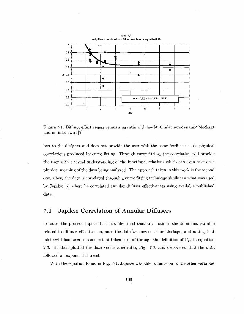
11 vs. AR only those points whose B1 is less than or equal to 0.06
• T1_
• I s If
#>
• '
•
t f •
eta = 0.72 + 3e*(-0.9 - 1.SAR)
1 1 1 1 0 1 2 3 4 5 6 7 8
AR
Figure 7-1: Diffuser effectiveness versus area ratio with low level inlet aerodynamic blockage and no inlet swirl [7]
box to the designer and does not provide the user with the same feedback as do physical
correlations produced by curve fitting. Through curve fitting, the correlation will provide
the user with a visual understanding of the functional relations which can even take on a
physical meaning of the data being analyzed. The approach taken in this work is the second
one, where the data is correlated through a curve fitting technique similar to what was used
by Japikse [7] where he correlated annular diffuser effectiveness using available published
data.
7.1 Japikse Correlation of Annular Diffusers
To start the process Japikse has first identified that area ratio is the dominant variable
related to diffuser effectiveness, once the data was screened for blockage, and noting that
inlet swirl has been to some extent taken care of through the definition of Cpi in equation
2.3. He then plotted the data versus area ratio, Fig. 7-1, and discovered that the data
followed an exponential trend.
With the equation found in Fig. 7-1, Japikse was able to move on to the other variables
100

r\ vs.«,
a. <
•
>
« 1 1
1
•
• b -
• • • • •
" ^ " — • - • J '
•
I I I
eta= 1.O5-O.M0W1.9
\t * <t
eta = 1.05-0. «)02«,*Z1
'•
i »
<>
25
«1
Figure 7-2: Diffuser effectiveness with principle geometric effects removed including data at all levels of inlet aerodynamic blockage [7]
by removing the effect of area ratio by dividing out the data by the new expression as
presented in Fig. 7-2. In this figure, the data has been plotted versus inlet swirl and has
revealed two trends. The upper trend represents diffusers experiencing mild stall while the
lower trend represents diffusers with substantial stall.
The data was again divided by the new equations defined in Fig. 7-2, and the with the
effects of area ratio and inlet swirl removed from the data Japikse then moved on to inlet
blockage as shown in Fig. 7-3. From this figure Japikse has determined that there are two
trends which have been defined. The lower trend (common blockage, "A"), which is seen
to passes through the square symbols, is data from Coladipietro et al. [18] where tests were
conducted at two different blockage levels. In these testes, inlet conditions consisted of a
clean uniform velocity profile where only the boundary layer thickness was varied. The upper
trend (classical profile blockage, "B") which shows that diffuser performance improves with
increasing inlet blockage comes from inlet conditions where the boundary layer becomes
fully developed and contains increase levels of turbulence and vorticity. Dividing the data
again by the new equations, Japikse represented the data versus inlet blockage in Fig. 7-3
101

il vs. Bi
Jt EC A or
ilJO
0.2
• ^ j
• ^ " • N I
ata- ' i . iK+ o.UB'in(b5l)
o
it
|y = 4.777364E+D1x i -1.217600E+01K +139214BE+Do|
r— „ B »
* " "A"
<>
o.oe
B1
Figure 7-3: Diffuser effectiveness with the principle effects of geometry and inlet swirl removed according to preceding correlations [7]
to reveal that the data has collapsed to a value of 1 ± .10.
The resulting set of equations produced by studying the data trends is the following:
Cp = CPi (ai , r 2 / r i , 62/61) V (AR) 77 ( « I ) r? (£1) (7.1)
rj {AR) = 0.72 + 3e(-o.9-i.5Jifl) ( 7 2 )
r] (ai) = 1.1 - O-OOOlaJ-9 delayed stall (7.3)
r)(ai) = 1.1 -0 .0002a? 1 ear/y staM (7.4)
77 (Bi) = 47.77364B? - 12.17600.Bi + 1.392146 curve 4 , common blockage (7.5)
77 (Si) = 1.22 + 0.08 x ln(Bi) curve B, classical profile blockage (7.6)
Now that the diffuser effectiveness can be predicted, Japikse suggest that a reasonable
first order estimate of the diffuser total pressure loss coefficient can be calculated using Eq.
2.6 (Cp is evaluated from Eq. 7.1 and Cpi from Eq. 2.3).
102

11 vs. Bt
1.2,
1.1
m
•Sf 0.9
"3 •c o.
0.7
•
i t • *
< •
<
•
•
•
•
p
< <
"
<
<
>
> ! *
•
<
•
r
•
0.02 0.04 O.OB 0.1 0.12 0.14
Figure 7-4: Diffuser effectiveness with the principle effects of geometry, inlet swirl, and inlet blockage removed [7]
103

K vs. Inlet Swirl Low Inlet blockage (P < 1%)
C-l
=8 Co
• • v .
a, i 1
i
1
4
0.450-
0.400 -
0.350'
0.300
0.250 •
0.200;
0.150
0.100
0.050 •
0.000 :
0 5 10 15 20 25 30 35 40
Inlet Swirl (°)
Figure 7-5: Total pressure loss trend in the exhaust for low inlet blockage
7.2 Correlation of the CFD Results
It was demonstrated in Sec. 6.2 that the total pressure losses in the exhaust duct are
independent of the stub direction. For this reason it was chosen to correlate the exhaust
duct losses independently of the stub losses. The following section presents a corelation to
predict the total pressure losses between the inlet and section-12 as shown in Fig. 6-1. The
correlations produced in this work have been found with the help of Windows Excel and
the statistical package LAB Fit [26].
The fist parameter that demonstrated to have the first order impact on losses in the
exhaust duct is inlet swirl. When inlet blockage was varied some distinct trends appeared
which demonstrated different behaviors in the losses depending on the magnitude of diffusion
taking place in the annular inlet of the exhaust duct. For low inlet blockage (j3 ^ 1%) it
is possible to find a single trend which can be used to normalize the data, Fig. 7-5. For
medium inlet blockage (4% < (3 ^ 8%) one trend has been defined for an ECDA of 20° and
one for the lower values tested, Fig. 7-6. When high inlet blockage (/3 > 10%) is present a
104

0.450
0.400 •
r v j
t '6
•O ft, |
*5 3
**** ft.
3 •5 53,
0.350
0.300
0.250
0.200
* 0.150
0.100
0.050
0.D00
K vs. Inlet Swirl Medium Inlet blockage (4% < p < 3%)
Y »O.112800C«Sff (0.047726-Jf) ECDA 0'
10' 201
20 25 30 35 40
Inlet Swirl f)
Figure 7-6: Total pressure loss trend in the exhaust for medium inlet blockage
8 ft, I
ft,
•5
II
0.400 •
0.350
0.300
0.250
0.200
0.150
0.100
0.050
0.000
K vs. Inlet Swirl High Inlet blockage (p > 10%)
Y - 0.214385COS/{0.033095-A'Xl+#)
J = 0.1 limCOSH (0.047726-XXI+ #)
5=0.1
ECDA • 0° * 10° • 20°
Met Swirl (°)
Figure 7-7: Total pressure loss trend in the exhaust for large inlet blockage
105

Figure 7-8: Surface passing through normalized losses for ECDA and aspect ratio (Solid circles are points lying above the surface and hollow circles are points lying below)
correction factor is used to increase the level of the trends used to describe medium inlet
blockage, Fig. 7-7. To calculate the loss due to intermediate ECDA and blockage levels, it is
recommended to interpolate between the trends in Fig. 7-6 and then interpolated with Fig.
7-5 for smaller inlet blockage or select a smaller correction factor for higher inlet blockages.
The equations derived above have considered the contribution to the losses due to the
effect of swirl with some consideration to the annular inlet section defined by ECDA. After
normalizing the data with those equations the effect of swirl with some consideration to
ECDA have effectively been removed and the other contributing parameters can now be
evaluated.
The next parameter considered is the aspect ratio of the exhaust duct. A good fit to
the data could not be found after trials at correlating the aspect ratio to the normalized
106

1.400
*4
1.200 H
1.000
4q DOT
S' 8 ft) S 0.600 •
* | 0.400 \
0.200 \
K vs. Wedge Angle
' * QJ0GO3JT1 -• 0.00338* +1.07369
- I
0.000 4 1 -i 1 1 1 1 1 1 1 1 1 1 1 1 r
0 5 10 15 20 25 30 35 40 45 50 55 BO 65 70 75 80 85 90
Wedge Angle {')
Figure 7-9: Normalized losses versus wedge angle with the effects of blockage, swirl, ECDA, and aspect ratio removed
data demonstrating that some other parameter is influencing the losses. It was discovered
that there may still remain some influence of the annular inlet effecting the data and when
correlating ECDA with the aspect ratio a surface could be passed through the data with
satisfactory results, Fig. 7-8. The surface plot in Fig. 7-8 supports the results presented
in Sec. 6.3 and 6.5 demonstrating that it is favorable to have a large aspect ratio and that
there is an optimum ECDA between 0° and 20°.
The data are again normalized with respect to the surface equation defined above and
plotted against the values of wedge angles tested, Fig. 7-9. A trend is visible and a
polynomial fit demonstrates that there is an optimum wedge angle near 60°. Once the data
are normalized again for this trend we see in Fig. 7-10 that there is only minimum influence
of the area ratio on the normalized pressure losses and a polynomial fit is made to the data.
The final result of the correlation can be seen in Fig. 7-11. It is demonstrated that 70%
of the data falls within ±10% error and 85% of the data falls within ±15% error. A more
detailed breakdown of the accuracy of the correlation is shown in Table 7.1. the resulting
107

K vs. Area Ratio
•§ 1.000 S
3 0.600 •
i i t
\r~-
• »
1 * •
= 1 84000-**-O.S330CMT3|
1
k
0.95 1.00 1.05 1.10 1.15 1.20 1.25 1.30 1.35 1.40
Ansa Ratio
Figure 7-10: Normalized losses versus area ratio with the effects of blockage, swirl, ECDA, aspect ratio, and wedge angle removed
Table 7.1: Break Down of Correlation Accuracy
Error (\(KCFD - KCorreiation\) Data Points(%) 0.00-0.02 0.02-0.04 0.04-0.06
72 22 6
108

CFD vs. Predicted
0.00 0.10 0.20 0.30 0.40 0.50
J V [Swtrl[[8CDA,AspectRatio][Wedge][AreaRatio]
Figure 7-11: Plot of CFD losses vs. predicted losses between inlet and section-12
109

set of equations are as follows:
K = K{Swirl, X blockage)K(ECDA, AspectRatio)K(WedgeAngle)K(AreaRatio) (7.7)
K(Swirl, low blockage) = 0.101720 cosh(0.047854a) all ECDA (7.8)
K(Swirl, medium blockage) = 0.112800 cosh(0.047726a) up to 10° ECDA (7.9)
K(Swirl, medium blockage) = 0.214385 cosh(0.033095a) 20° ECDA (7.10)
K(Swirl, high blockage) = K(Swirl, medium blockage)(l + £) £ = 0.1 (7.11)
( 0 78730 \
- — — 0.07885ECDA ) +0.0398OECZM AspectRatio )
(7.12)
K (WedgeAngle) = 0.00003(WedgeAngle)2 - 0.00338(Wedge Angle) + 1.07369 (7.13) K(AreaRatio) = 1.84000(Ar eaRatio) - 0.8Z300(AreaRatio)2 (7.14)
110

Chapter 8
Conclusion and Recommendation
8.1 Conclusion
A parametric CFD study has been carried out where key geometric and aerodynamic pa
rameters are varied and the effect on the total pressure loss is observed. The results of the
CFD data were then used to produce a correlation to predict the duct losses. Based on this
work the following conclusions are made:
1. Inlet Swirl
• Inlet swirl was demonstrated to have a high order effect on the pressure loss
in the exhaust duct. The minimum pressure losses occur when the swirl is at
a minimum. The introduction of inlet swirl causes an asymmetric flow field
yielding to flow separation with increased pressure losses.
2. Stub direction
• pressure loss at the exhaust duct exit was found to be independent of the stub
direction. The highest losses occur in the S-shaped stubs as a results unfavorable
flow separation due to pressure gradients.
3. ECDA
• The degree of ECDA demonstrated that too little and too large of an ECDA is
not favorable. The optimum value of ECDA resulting in the minimum velocity at
111

the inlet to the annular to rectangular transition region without flow separation
is between 7° and 10°.
4. Wedge Angle
• The three wedge angles tested perform similarly for inlet swirls up to 25°. At
this swirl angle flow separation on the suction surface of the flow splitter occurs
on the wedge angles of 10° and 45° and is delayed for the 80° flow splitter. At
35° inlet swirl the 80° wedge flow splitter would separate on the suction surface.
It is desirable to have a large wedge angle for reduced pressure loss.
5. Aspect Ratio and Area Ratio
• It was difficult to quantify the effect of these parameters since they proceed the
other geometric parameters. A small aspect ratio and area ratio lead to pressure
gradients that can result in flow separation.
6. Inlet Boundary Layer Blockage
• The total pressure losses increase with increasing inlet blockage. Exhaust ducts
with ECDA of 20° performed to worst of the geometries tested for medium and
high inlet blockage.
7. Correlation of the CFD Results
• The Taguchi Design provided a test matrix that provided the minimum amount
of exhaust duct models to successfully capture the resulting effects on the total
pressure loss coefficient. The CFD data has been correlated to the total pressure
loss coefficient with reasonable accuracy.
8.2 Recommendation
Examining the results of the current study, the following recommendations are made for
the loss modeling of non-symmetric gas turbine exhaust ducts using CFD:
112

1. As future work, it is desirable to include the exhaust stubs in the correlation. To
do this, first, a survey should be conducted to define common exhaust stubs used
in turbo-machinery applications which contain non-symmetric gas turbine exhaust
ducts. Secondly, model them numerically as in the current work and correlate the
pressure losses.
2. The correlation produced from the current work serves as a guide for designers to pro
duce more efficient non-symmetric gas turbine exhaust ducts. To be able to accurate
predict the total pressure loss will require that the current CFD work be calibrated
to experimental data.
113

Bibliography
[1] G. Sovran and E. Klomp, "Experimentally determined optimum geometries for recti
linear diffusers with rectangular, conical , or annular cross-section," Fluid Mechanics
of Internal Flows, pp. 270-319, 1967.
[2] A. McDonald and R. Fox, "An experimental investigation of incompressible flow in
conical diffusers," ASME Paper, no. 65-FE-25, 1965.
[3] J. H. G. Howard, A. B. Thornton-Trump, and H. J. Henseler, "Performance and flow
regimes for annular diffusers," ASME Paper, no. 67-WA/FE-21, 1967.
[4] D. Japikse and N. C. Baines, Diffuser Design Technology. Concepts ETI, Inc., 1998.
[5] A. Elkersh, A. Elgammal, and N. Maccallum, "An experimental investigation of the
performance of equiangular annular diffusers with swirled flow," Proceedings of the
Institution of Mechanical Engineers, vol. 199, no. C4, pp. 293-297, 1985.
[6] A. Klein, "Characteristics of combustor diffusers," Prog Aerospace Sci., vol. 31,
pp. 171-271, 1995.
[7] D. Japikse, "Correlation of annular diffuser performance with geometry, swirl, and
blockage," Proceedings of the 11th Thermal and Fluids Analysis Workshop, pp. 107-
118, 2000.
[8] M. Cunningham, Flow in Non-Symmetric Gas Turbine Exhaust Ducts. PhD thesis,
Queen's University, 2002.
114
[9] A. MacDonald, R. Fox, and R. Van Dewoestine, "Effects of swirling inlet flow on
pressure recovery in conical diffusers," AIAA Journal, vol. 9, no. 10, pp. 2014-2018,
1971.
[10] Y. Senoo, N. Kawaguchi, and T. Nagata, "Swirl flow in conical diffusers," Bulletin of
the JSME, vol. 21, no. 151, pp. 112-119, 1978.
[11] F. Dolan and P. J. Runstadler, "Pressure recovery performance of conical diffusers at
high subsonic mach numbers," NASA CR-2299, 1973.
[12] V. K. Sharan, "An exponential investigation of the behavior of conical diffusers in
turbulent flow," Journ Appl Math and Phys, vol. 27, 1976.
[13] J. Livesey and A. Odukwe, "Some effects of pipe flow generated entry conditions on
the performance of straight walled conical diffusers with high subsonic entry mach
number," Israel Journal of Technology, vol. 11, no. 4, pp. 217-222, 1973.
[14] D. Japikse, "A new diffuser mapping technique, part 1: Studies in component perfor
mance," Transactions of the ASME, vol. 108, pp. 148-156, 1986.
[15] A. Klein, "Review: Effects of inlet conditions on conical diffuser performance," ASME,
Transactions, Journal of Fluids Engineering, vol. 103, pp. 250-257, 1981.
[16] S. Dovzhik and V. Kartavenko, "Measurement of the effect of flow swirl on the efficiency
of annular ducts and exhaust nozzles of axial turbomachines," Fluid Mechanics - Soviet
Research, vol. 4, no. 4, pp. 156-172, 1975.
[17] E. Klomp, "Performance of straight-walled annular diffusers with swirling flow," Aero
nautical Journal, vol. 101, no. 1010, pp. 467-480, 1997.
[18] R. Coladipietro, J. Schneider, and K. Sridhar, "Effects of inlet flow conditions on the
performance of equiangular annular diffusers," Transactions of the CSME, vol. 3, no. 2,
pp. 75-82, 1975.
[19] S. Stevens and G. Williams, "The influence of inlet conditions on the performance
of annular diffusers," ASME, Transactions, Journal of Fluids Engineering, vol. 102,
pp. 357-363, 1980.
115

[20] M. Loka, M. Robichaud, W. Di Bartolomeo, D. Loe, and D. Sowers, "Aerodynamic op
timization of the exhaust-ejector system on the tiltrotor using navier-stokes analysis,"
paper AIAA 2000-0986, AIAA, 2000.
[21] R. K. Roy, Design of experiments using the Taguchi approach : 16 steps to product and
process improvement. Wiley, 2001.
[22] D. Wyatt, "Analysis of errors introduced by several methods of weighting nonuniform
duct flows," Tech. Rep. TN 3400, National Advisory Committee on Aeronautics, 1955.
[23] C. Rhie and W. Chow, "A numerical study of the turbulent flow past an isolated airfoil
with trailing edge separation," AIAA Paper 82-0998, 1982.
[24] F. Menter, "Zonal two equation k-u turbulence models for aerodynamic flows," AIAA
Paper 93-2906, 1993.
[25] R. J. Schalkoff, Artificial Neural Networks. McGraw-Hill, 1997.
[26] W. P. Silva and C. M. D. P. S. Silva, LAB Fit Curve Fitting Software (Nonlinear
Regression and Treatment of Data Program) V 7.2.42, 1999-2008.
116