Scholars' Mine Scholars' Mine

Doctoral Dissertations Student Theses and Dissertations

Spring 2019

Pressure versus impulse graph for blast-induced traumatic brain Pressure versus impulse graph for blast-induced traumatic brain

injury and correlation to observable blast injuries injury and correlation to observable blast injuries

Barbara Rutter

Follow this and additional works at: https://scholarsmine.mst.edu/doctoral_dissertations

Part of the Explosives Engineering Commons, and the Mathematics Commons

Department: Mining Engineering Department: Mining Engineering

Recommended Citation Recommended Citation Rutter, Barbara, "Pressure versus impulse graph for blast-induced traumatic brain injury and correlation to observable blast injuries" (2019). Doctoral Dissertations. 2791. https://scholarsmine.mst.edu/doctoral_dissertations/2791

This thesis is brought to you by Scholars' Mine, a service of the Missouri S&T Library and Learning Resources. This work is protected by U. S. Copyright Law. Unauthorized use including reproduction for redistribution requires the permission of the copyright holder. For more information, please contact scholarsmine@mst.edu.

PRESSURE VERSUS IMPULSE GRAPH FOR BLAST-INDUCED TRAUMATIC BRAIN

INJURY AND CORRELATION TO OBSERVABLE BLAST INJURIES

BY

BARBARA RUTTER

A DISSERTATION

Presented to the Faculty of the Graduate School of the

MISSOURI UNIVERSITY OF SCIENCE AND TECHNOLOGY

In Partial Fulfillment of the Requirements for the Degree

DOCTOR OF PHILOSOPHY

IN

EXPLOSIVES ENGINEERING

2019

Approved by:

Catherine E. Johnson, Advisor

Kyle Perry

Braden Lusk

Paul Worsey

Dimitri Feys

2019

Barbara Rutter

All Rights Reserved

iii

ABSTRACT

With the increased use of explosive devices in combat, blast induced traumatic

brain injury (bTBI) has become one of the signature wounds in current conflicts. Animal

studies have been conducted to understand the mechanisms in the brain and a pressure

versus time graph has been produced. However, the role of impulse in bTBIs has not been

thoroughly investigated for animals or human beings.

This research proposes a new method of presenting bTBI data by using a pressure

versus impulse (P-I) graph. P-I graphs have been found useful in presenting lung lethality

regions and building damage thresholds. To present the animal bTBI data on a P-I graph

for humans, the reported peak pressures needed to be scaled to humans, impulse values

calculated, and impulse values scaled. Peak pressures were scaled using Jean et al.’s

method, which accounts for all the structures of the head. Impulse values were estimated

in two methods: Friedlander’s impulse equation and a proposed modification to the

Friedlander’s impulse equation. The modification was needed as some animal testing was

not subjected to shock waves with a steady decay, such as outside the end of a shock tube.

Mass scaling was used to scale the reported time duration in the impulse calculation.

The scaled peak pressure and impulse values were plotted on a P-I graph with the

reported severity. The three severities did not overlap; thus, each severity had its own

region on the P-I graph. The severity regions were overlaid with lung damage and eardrum

rupture P-I curves. Seven correlations were found between the bTBI regions and the

observable injuries. bTBIs are not a new phenomenon, but in the past other serious injuries

were more prominent, due to body armor not attenuating the shock wave as effectively.

iv

ACKNOWLEDGMENTS

I want to thank the numerous people who have aided me in my pursuit of my

doctorate degree in Explosives Engineering. First, I would like to thank all the people who

invested their time in my research. I especially want to thank my advisor, Dr. Johnson, for

all her help and encouragement with this research. I want to thank Martin Langenderfer,

Jason Ho, Jacob Brinkman, Kelly Williams, Jacob Miller, Mingi Seo, James Seaman, and

David Doucet for all their assistance with testing and proofreading of this dissertation. I

especially want to thank Jeffery Heniff, Jay Schafler, and the Rock Mechanics staff for

building the shock tube for this research. I want to thank Dr. Mulligan for his helpful

discussions and insights into shock physics. I want to thank my committee members Dr.

Perry, Dr. Lusk, Dr. Worsey, and Dr. Feys for all their helpful discussions and constructive

criticisms they each provided throughout my pursuit of my degree. I want to thank Kayla

McBride for drawing Figure 2.3.

Second I would like to thank all those who provided me encouragement as I pursued

my doctorate. I especially want to thank my mother for telling me I can do this. I want to

thank everyone from church, school organizations, and friends. I sincerely thank the

Marines I served with around the world, who encouraged me and told me not to give up. I

would like to thank God for giving me the strength to finish.

Finally, I want to dedicate this dissertation to all who have sustained a blast-induced

traumatic brain injury in the wars against terrorism in Iraq, Afghanistan, and beyond.

v

TABLE OF CONTENTS

Page

ABSTRACT ....................................................................................................................... iii

ACKNOWLEDGMENTS ................................................................................................. iv

LIST OF FIGURES ......................................................................................................... viii

LIST OF TABLES .............................................................................................................. x

NOMENCLATURE .......................................................................................................... xi

SECTION

1. INTRODUCTION ..................................................................................................... 1

1.1. PROBLEM STATEMENT ................................................................................. 1

1.2. TRAUMATIC BRAIN INJURY ........................................................................ 3

1.3. RESEARCH APPROACH ................................................................................. 5

1.4. CONTRIBUTION TO SCIENCE ...................................................................... 8

2. LITERATURE REVIEW ........................................................................................ 10

2.1. IMPULSE CALCULATION ............................................................................ 10

2.1.1. Shock Waves .......................................................................................... 10

2.1.2. Impulse ................................................................................................... 19

2.1.3. Friedlander Equation .............................................................................. 21

2.1.4. Shock Tubes ........................................................................................... 24

2.1.5. TNT Equivalency ................................................................................... 30

2.1.6. Pressure-Impulse Graphs ........................................................................ 32

2.2. PRESENT bTBI DATA AND SCALING METHODS ................................... 34

2.2.1. bTBI Testing ........................................................................................... 34

2.2.2. bTBI Scaling ........................................................................................... 36

vi

2.2.2.1. Mass scaling .............................................................................. 36

2.2.2.2. Head scaling .............................................................................. 37

2.3. HUMAN BLAST INJURIES ........................................................................... 40

2.3.1. Lung Damage ......................................................................................... 40

2.3.2. Eardrum Rupture .................................................................................... 42

2.4. SUMMARY ...................................................................................................... 44

3. FORMULATION EQUATION TO CALCULATE IMPULSE AT THE EXIT

AND OUTSIDE OF A SHOCK TUBE (OBJECTIVE 1) ....................................... 45

3.1. EXPLOSIVE EQUIVALENTS METHODS NEEDED .................................. 46

3.1.1. Gas Produced Relationship to TNT ........................................................ 49

3.1.2. Density Relationship to TNT ................................................................. 50

3.1.3. Mass Relationship to TNT ..................................................................... 51

3.2. TEST SETUP ................................................................................................... 52

3.3. RESULTS ......................................................................................................... 57

3.3.1. Exit of the Shock Tube ........................................................................... 57

3.3.2. 3 Centimeters from Exit of the Shock Tube ........................................... 59

3.3.3. 6 Centimeters from Exit of the Shock Tube ........................................... 61

3.3.4. 9 Centimeters from Exit of the Shock Tube ........................................... 63

3.3.5. Observed Jet Wind Effect ....................................................................... 65

3.4. MODIFICATIONS TO THE FRIEDLANDER (OBJECTIVE 1) ................... 68

3.5. SUMMARY ...................................................................................................... 75

4. PROPOSED HUMAN BTBI SEVERITY REGIONS (OBJECTIVE 2) ................ 77

4.1. SCALING OF IMPULSE ................................................................................. 77

4.2. SCALING ANIMAL DATA TO HUMANS ................................................... 79

vii

4.3. HUMAN SEVERITY CURVES (OBJECTIVE 2) .......................................... 81

4.4. SUMMARY ...................................................................................................... 84

5. HUMAN bTBI RELATIONSHIP TO PHYSIOLOGICAL INJURIES

(OBJECTIVE 3)....................................................................................................... 85

5.1. LUNG INJURY ................................................................................................ 85

5.2. EARDRUM RUPTURE ................................................................................... 87

5.3. HUMAN bTBI SEVERITY REGIONS WITH PHYSIOLOGICAL INJURY

P-I CURVES OVERLAID (OBJECTIVE 3) ................................................... 88

5.4. SUMMARY ...................................................................................................... 90

6. CONCLUSIONS...................................................................................................... 91

6.1. IMPULSE EQUATION MODIFICATION ..................................................... 91

6.2. HUMAN bTBI SEVERITY REGIONS ........................................................... 92

6.3. CORRELATIONS BETWEEN bTBI SEVERITIES AND OBSERVABLE

INJURIES ......................................................................................................... 93

6.4. CONCLUSIONS .............................................................................................. 94

7. FUTURE WORK ..................................................................................................... 95

APPENDICES

A. DATA TO ACCOMPANY SECTION 3 ........................................................... 97

B. DATA TO ACCOMPANY SECTION 4 .......................................................... 101

C. DATA TO ACCOMPANY SECTION 5 .......................................................... 108

REFERENCES ............................................................................................................... 111

VITA ............................................................................................................................. 123

viii

LIST OF FIGURES

Page

Figure 2.1. Shock front moving through a material, adapted from Cooper ...................... 11

Figure 2.2. Characteristics of a shock wave ..................................................................... 12

Figure 2.3. Illustration of a left going pressure wave ....................................................... 13

Figure 2.4. Ten popsicle sticks, adapted from Cooper ..................................................... 15

Figure 2.5. Popsicle method to describe particle velocity and shock velocity, adapted

from Cooper .................................................................................................... 15

Figure 2.6. Pressure transducer orientation ....................................................................... 17

Figure 2.7. Overpressure to reflective pressure conversion chart with overpressure and

reflective columns outlined, adapted from Swisdak ....................................... 18

Figure 2.8. Example of experimental pressure trace taken 60 ft. from a 70 g C4

spherical charge .............................................................................................. 20

Figure 2.9. Example of Friedlander curve with 29 psi peak pressure and 0.3 ms

duration ........................................................................................................... 23

Figure 2.10. Comparison of open-air and explosively driven shock tube pressure trace . 25

Figure 2.11. Gas driven shock tube pressure trace ........................................................... 26

Figure 2.12. Vortices formed at shock tube exit after the passage of the shock wave ..... 27

Figure 2.13. Jet wind effect............................................................................................... 29

Figure 2.14. Typical P-I curves for structures with sensitivities labeled, adapted from Aa

a Krauthammer et al. ....................................................................................... 33

Figure 2.15. 70 kg man lung lethality curves adapted from Courtney and Courtney ...... 41

Figure 2.16. 50% lung survival pressure versus impulse curve from Baker et al............. 42

Figure 2.17. P-I curves for eardrum rupture from Baker et al. ......................................... 43

Figure 3.1. Explosively driven shock tube with charge location shown and sensor

locations denoted by numbers 1-4 .................................................................. 47

ix

Figure 3.2. Charge holder for shock tube testing .............................................................. 53

Figure 3.3. Pencil probe holder for shock tube testing ..................................................... 54

Figure 3.4. Setup of explosive charges a. Detonator b. Stinger c. C4. d. Charge inserted

into shock tube ................................................................................................ 55

Figure 3.5. Sensor at exit location .................................................................................... 56

Figure 3.6. Pentolite data recorded at the end of the shock tube for three iterations ........ 58

Figure 3.7. C4 data recorded at the end of the shock tube ................................................ 59

Figure 3.8. Pentolite data recorded 3 cm from the end of the shock tube ........................ 60

Figure 3.9. C4 data recorded 3 cm from the end of the shock tube .................................. 61

Figure 3.10. Pentolite data recorded 6 cm from the end of the shock tube ...................... 62

Figure 3.11. C4 data recorded 6 cm from the end of the shock tube ................................ 63

Figure 3.12. Pentolite data recorded 9 cm from the end of the shock tube ...................... 64

Figure 3.13. C4 data recorded 9 cm from the end of the shock tube ................................ 65

Figure 3.14. Sample pentolite pressure trace with stills from high speed video for

aiindicated areas .............................................................................................. 66

Figure 3.15. Overlay of all tested distances showing the separation of the shock wave

aiand vortex ring ............................................................................................. 67

Figure 3.16. Values of β and best-fit trend line greater than 1.0 for pentolite and C4 at

aitested distances ............................................................................................. 70

Figure 4.1. Human bTBI P-I graph with severities denoted ............................................. 82

Figure 4.2. Human bTBI P-I graph with severity region identified.................................. 84

Figure 5.1. P-I lung damage curve for 70 kg man, calculated from Courtney and

Courtney and Baker et al................................................................................ 86

Figure 5.2. P-I curve for eardrum rupture, adapted from Baker et al. .............................. 87

Figure 5.3. Human bTBI P-I graph with eardrum rupture and lung lethality curves

overlaid ........................................................................................................... 88

Figure 7.1. Pressure trace of cap measured at 6 cm outside the shock tube ..................... 96

x

LIST OF TABLES

Page

Table 1.1. TBI characteristics from Ling et al. and DVBIC ............................................... 4

Table 1.2. Objectives of Research and Sections where each is addressed ......................... 6

Table 2.1. Data considered for proposed P-I curve .......................................................... 35

Table 2.2. Parameters for Equation (17) for selected species ........................................... 39

Table 2.3. Data points in Figure 2.16, adapted from Baker et al. ..................................... 42

Table 3.1. Sensor and distances from explosive charge for sensors shown in Figure 3.1 47

Table 3.2. Parameters of test series used to gather data to develop impulse equations .... 48

Table 3.3. Moles of gas produced by TNT, C4, and pentolite and ratios ......................... 50

Table 3.4. Density of TNT, C4, and pentolite .................................................................. 51

Table 3.5. Mass and equivalent TNT mass of C4 and pentolite ....................................... 52

Table 3.6. Peak pressures, durations, and impulses at the exit of the shock tube ............. 59

Table 3.7. Peak pressures, durations, and impulse 3 cm from the exit of the shock tube 61

Table 3.8. Peak pressures, durations, and impulse 6 cm from the exit of the shock tube 63

Table 3.9. Peak pressures, durations, and impulse 9 cm from the exit of the shock tube 64

Table 3.10. Values of β, impulse modifier, at each tested distance for both explosives .. 69

Table 3.11. Values of a, h, and k from Equation (30) and percent error .......................... 75

Table 3.12. Comparison of error between Friedlander and proposed methods ................ 75

Table 4.1. Impulse equations used for data sets that did not include impulse .................. 79

Table 4.2. Scaling parameter for referenced animal models for use in equation (17) ...... 80

Table 4.3. Thresholds for each human bTBI severity region ........................................... 83

xi

NOMENCLATURE

Symbol Description

a Experiment-fitting constant

a Direction and width of parabola

A Fitting parameter

b Experiment-fitting constant

B Fitting parameter

bTBI Blast-induced traumatic brain injury

c Speed of sound

C1 Fitting constant for a

C2 Fitting constant for h

C3 Fitting constant for k

cbrain Speed of sound in brain

cflesh Speed of sound in flesh

cm Centimeter

cskull Speed of sound in skull

D Detonation velocity

DAS Data acquisition system

DDESB Department of Defense Explosives Safety Board

DVBIC Defense and Veterans Brain Injury Center

Eexp Available energy of an explosive to do work

EDR Eardrum rupture

FM Molecular weight

xii

g Grams

ge moles of gas produced by explosive

GCS Glasgow coma scale score

h x value of vertex of a parabola

HE High explosive

I Impulse

IED Improvised explosive device

k y value of vertex of a parabola

kg Kilogram

kJ Kilojoules

kPa Kilopascal

kPa*s Kilopascal seconds

LLNL Lawrence Livermore National Laboratory

m Meter

mbaseline Scaling mass

me Mass of explosive

Missouri S&T Missouri University of Science and Technology

modTBI Moderate traumatic brain injury

ms Milliseconds

msbrain Mass of brain in species

mscaled Mass being scaled

msflesh Mass of flesh in species

msskull Mass of skull in species

xiii

mTBI Mild traumatic brain injury

P Pressure

P(t) Pressure function with respect to time

P0 Fitting parameter

PETN Pentaerythritol tetranitrate

Pamb Ambient pressure

P-I Pressure versus impulse

Pincident Incident pressure

Pr Reflective pressure

Ps Peak overpressure

PP Peak pressure

psi Pounds per square inch

psi*s Pounds per square inch seconds

P-sT Pressure versus scaled duration

P-T Pressure versus duration

q Dynamic pressure

Ref Reference

s Seconds

sTBI Severe traumatic brain injury

t Time

T Time duration

t+ End of positive phase

t0 Time of arrival

xiv

TBI Traumatic brain injury

TNT Trinitrotoluene

TNT equ TNT equivalency

UN United Nations

V Volume of the shock tube between the explosive and exit

wt Weight of explosive

α Constant modifier

α Fitting parameter

β Impulse modifier

γ Ratio of specific heats of the air

ΔHR0 Molar heat of detonation

Δn Number of moles of gas produced per mole of high explosive

Δt Change in time

ηs Scaling parameter

1. INTRODUCTION

1.1. PROBLEM STATEMENT

Traumatic brain injury (TBI) has become one of the most prominent [1–4] and

difficult to diagnose injuries [5] of the modern warfighter. Though TBIs have occurred in

previous conflicts, modern warfighters are exposed to a greater risk of TBIs. The advent

and increased use of improvised explosive devices (IEDs) have led to modern warfighters

being more at risk to explosives detonating in close proximity that result in blast-induced

TBIs (bTBIs). The increased exposure to conditions that can generate bTBIs has

illuminated the need to understand further the bTBI pressure and impulse thresholds.

The survivability after an explosive blast has greatly improved from previous

conflicts due to advances in three areas. The first advancement is improved body armor,

which has reduced the number of individuals dying from lung injuries. Second,

advancements in transporting critically injured warfighters to field hospitals in a timely

manner have resulted in life-saving medical treatment. Third, advances in field medicine

and field hospitals have allowed medical professionals to stabilize the most critically

injured for transport to hospitals in allied countries to receive appropriate treatment [6–8].

Consequentially, the number of warfighters who survive an event resulting in a bTBI whom

may have otherwise succumbed to their injuries in previous conflicts have increased. An

unfortunate consequence of the increased survival rate is that bTBIs have become more

apparent than in prior conflicts. The warfighters who sustained bTBIs can have a wide

range of struggles and treatments. For the less severe cases, such as concussion, the

treatment has a short duration and has no major lifelong effects. However, for the more

2

severe cases, the treatment is lifelong and the warfighter may not be able to reenter the

workforce [9].

Numerous animal studies have been conducted to gain an understanding of the

mechanisms that result in a bTBI. The focus of bTBI studies is identifying the brain’s

response to dynamic loading from an explosive blast, to aid earlier detection and treatment

of bTBIs. A pressure versus scaled duration (P-sT) graph, which was used by Bowen et al.

[10] to display lung injury thresholds, is currently used to compare bTBI results across

different studies , for example Zhu et al., Jean et al., and Rafaels [11–13]. To allow various

animal studies to be viewed on one graph, the overall mass of the animal subject is used as

a scaling factor. P-sT graphs plot the peak pressure of the shock wave versus the scaled

positive phase.

The P-sT graph cannot be easily compared to other published building damage and

lung injury curves. One commonly used method to compare different damage and injury

curves from a detonation of an explosive is pressure versus impulse (P-I) graphs [14].

Impulse is defined as the area under the pressure curve in a pressure versus time (P-T)

graph, where pressure is the pressure of the shock wave and time is the duration of the

shock wave above ambient pressure. Unlike the P-sT graph, a P-I graph accounts for the

different impulse values. For example, an open air and shock tube test can have the same

peak pressure, but the impulse values can be vastly different. Due to the wide use of the P-

sT graph; majority of researchers do not publish the impulse and only publish peak pressure

and duration. By graphing both bTBI data and observable physical injury data together on

a single P-I graph would allow for any correlations to be identified. Identified correlations

3

could then be used as visual indicators of an otherwise invisible injury. Early identification

and prompt treatment result in improved outcomes for people exposed to bTBI.

1.2. TRAUMATIC BRAIN INJURY

A TBI is “a nondegenerative, noncongenital (not existing at birth) insult to the brain

from an external mechanical force, possibly leading to permanent or temporary impairment

of cognitive, physical, and psychosocial functions, with an associated diminished or altered

state of consciousness” [15]. Four methods of TBIs exist, which are blast-induced,

acceleration, thoracic, and penetrating, and are differentiated by the way in which the TBI

was acquired. These four methods are further separated into two types, primary and

secondary. Primary TBIs occur when an outside force directly interacts with the brain,

where bTBI and penetrating TBI are types of primary TBI. Examples include the shock

wave encountered in close proximity to a detonating explosive and shrapnel thrown from

a detonating explosive impaling the brain, respectively. A secondary TBI occurs when the

outside force interacts with the body and the brain is injured as a result of the body insult.

Acceleration and thoracic methods are secondary TBIs. Examples of secondary type TBIs

include falling, whiplash, and gunshot wounds to the chest. The focus of this research is

on primary bTBI and will not discuss the other methods of acquiring TBIs.

A bTBI is acquired when an explosively produced blast wave passes through the

skull and interacts with the brain; however, the exact mechanisms behind the injury are not

known [16, 17]. For bTBIs and other TBI methods, three severity levels exist: mild,

moderate, and severe. One tool found useful in classifying civilian TBIs, but not proven

useful in classifying bTBIs, is the Glasgow Coma Scale score (GCS) and is currently used

to help determine the severity of bTBIs [4, 18]. The Defense and Veterans Brain Injury

4

Center (DVBIC) has also published the characteristics of each bTBI severity and the

number of service members who have sustained a bTBI [19]. Mild TBI (mTBI) is the most

common diagnosis for bTBIs in warfighters [19]. Moderate TBI (modTBI) and severe TBI

(sTBI) are less common. The characteristics of mTBI, modTBI, and sTBI are summarized

in Table 1.1.

Table 1.1. TBI characteristics from Ling et al. [18] and DVBIC [19]

mTBI modTBI sTBI

GCS 15-13 13-9 8-3

Confusion < 24 hrs. > 24 hrs. > 24 hrs.

Unconsciousness < 30 min. 30 min. – 24 hrs. > 24 hrs.

Memory Loss < 24 hrs. 24 hrs. – 7 days > 7 days

CT scan normal normal/abnormal -

Brain Imagining normal normal/abnormal abnormal

Unlike other battlefield injuries such as gunshot wounds and traumatic

amputations, bTBIs are difficult to diagnose quickly and treatments are varied. Depending

on the severity of the bTBI, treatments range from rest to long term rehabilitation therapies

[20]. Other currently investigated therapies that have been shown to improve bTBIs include

hyperbaric oxygen therapy, noninvasive brain stimulation, and virtual reality [21]. These

and other methods in development may lead to alleviating and possibly reversing the

effects of TBIs [22]. The likelihood of TBI’s effects being reversed or reduced are greatly

improved when treatment is rendered shortly after the TBI was acquired [22].

5

1.3. RESEARCH APPROACH

The overall objective of this research is to use observable physiological injuries as

a visual guide in determining if an individual subjected to an explosive blast sustained an

invisible bTBI. The hypothesis of this research is a pressure versus impulse (P-I) graph can

be used to represent the regions for mild, moderate, and severe bTBIs in humans and relate

those regions to observable physiological injuries, which then can be used as an early

indicator of the bTBI. Five assumptions were made to produce a P-I graph from available

animal bTBI data, which included 16 Missouri blast model tests and 157 data points

resulting in a total of 258 data points.

1. bTBI is solely caused by a shock wave (Section 2.2.1)

2. severities of the bTBI are assumed the same whether determined based on

behavioral or histological studies (Section 2.2.1)

3. reported pressures and durations are assumed true and can be used for impulse

calculations (Section 2.2.1)

4. head scaling is assumed to be true and correct to scale different animal species on

the same graph (Section 2.2.2.2)

5. severity regions are independent of animal orientation with respect to shock wave

origin (Section 2.2.1)

Assumptions one and two were not addressed in this research, as the data collected

from the animals cannot be reanalyzed and this is beyond the scope of this research. Three

objectives, summarized in Table 1.2, were defined to address assumptions 3-5 and

6

determine the validity of the hypothesis. Each objective required a positive outcome to

validate the proposed hypothesis. This research has shown it is possible to present bTBI

data on a P-I graph with the severity regions related to observable physiological injuries.

Table 1.2. Objectives of Research and Sections where each is addressed

Objective Section

1 Accurately determine impulse for all experimental designs 3

2 Scale bTBI studies to humans and create a P-I graph with severity regions 4

3 Correlate human bTBI to observable injuries 5

Objective one required determining impulse equations that could represent all

experimental designs when impulse is not calculated and published in the literature. The

three experimental designs used to conduct animal bTBI testing are: open-air, shock tube

with the animal placed within the shock tube, and shock tube with the animal placed outside

the shock tube. For both open-air and shock tube with the animal placed within the tube

experimental designs, the integration of the Friedlander equation has been documented to

closely approximate the impulse of a shock wave [23]. The Friedlander equation

mathematically describes the exponential decay of an open-air blast and estimates the

impulse of the shock wave when integrated. Unlike the two previously mentioned

locations, animals placed outside the shock tube are exposed to the shock wave and a vortex

ring. The vortex ring forms as the shock wave exits the shock tube and follows the shock

wave at a slower velocity. The vortex ring influences the shape and duration of the shock

wave until the shock wave and vortex ring separate [24–27]. However, no impulse equation

7

has been published for shock tube experimental designs with the animal placed outside the

shock tube. The hypothesis of this objective is the impulse equation for experimental

design with the animal placed outside the shock tube is a piecewise function to account for

the vortex ring influencing the shape of the shock wave. To test this hypothesis,

experimental testing was conducted with a cylindrical shock tube with a pressure sensor

placed at set distances outside the tube. This objective is described in Section 3.

Objective two applied the Friedlander equation and the impulse equation

determined in objective one to the gathered published animal bTBI data that did not report

impulse. The Friedlander equation was used for open air test and interior shock tube

experiments. The derived equation was applied to data where the animal was placed outside

the shock tube. The impulse was calculated by inputting the needed published values: peak

pressure, time duration, mass of explosive, density of explosive, and distance outside the

shock tube plus the calculated values: volume of the shock tube and moles of gas produced

by the explosive. The reported peak pressures were then scaled to humans by using Jean et

al.’s scaling method [12] from assumption four. The published and calculated impulse

values were scaled using the mass scaling method proposed by Bowen et al. [10]. The

severity and orientation of the animal was applied to each datum point to determine the

validity of assumption five. The severity regions for humans were determined by the

location of each scaled severity point. The postulate of this objective is humans have a

lower pressure threshold, but higher impulse threshold than a majority of animals. The

produced P-I graph with severity threshold P-I curves was used to achieve objective two

and is discussed in Section 4.

8

Objective three required gathering known P-I impulse curves for eardrum rupture

thresholds, lung injury thresholds, and lung lethality thresholds after an explosive blast.

The human bTBI severity curves determined in objective two were then overlaid with these

observable injuries to determine if any correlations exist. The hypothesis of this objective

is eardrum rupture can be used as a visual sign for possibly sustained mTBI or modTBI

and lung injury is a visual sign for both modTBI and sTBI. The existence of correlations

between human bTBI P-I severity threshold curves and observable human physiological

injury curves would confirm or deny the proposed hypothesis. This objective is described

in Section 5. Note: However, in the modern battlefield our troops wear body armor which

raises the threshold levels for lung damage. Have sheep, pigs, and goats been tested with

body armor?

1.4. CONTRIBUTION TO SCIENCE

This research proposes presenting bTBI data on a pressure versus impulse graph

and defining severity regions. To the author’s knowledge, no such graph currently exists

and would greatly aid in finding the threshold for bTBI in humans. These severity regions

can then be compared to published injury thresholds, thus relating the probable severity of

an “invisible” injury to observable physical injuries. The visible indictors for unprotected

humans could be used by first responders to quickly assess the wounded to determine who

also needs to be evaluated for a possible bTBI. Overall, the generation of the bTBI P-I

graph can have far reaching effects in military combat situations, live fire training for the

military and police, industrial explosions, and acts of terrorism involving explosives.

A new impulse equation was developed to more accurately estimate the impulse of

a shock wave outside of a shock tube with the variables provided in published bTBI studies.

9

The equation accounts for the vortex ring interacting with different portions of the shock

wave, resulting in different decay rates and estimates the distance where the vortex ring

and shock wave separate. Based on the experiments conducted as part of this research, it is

philosophized that:

The vortex ring extends the positive phase duration of the shock wave

The vortex ring expands and weakens as it travels away from the shock tube

The separation distance was found to be dependent upon mass of the

explosive, density of the explosive, and gas production of the explosive

With the new impulse equation, a pressure versus impulse graph for human bTBIs

was produced from published animal bTBI data. From the pressure versus impulse graph,

regions were identified that had little to no bTBI data points. The severity regions were

defined and compared to published eardrum rupture and lung injury thresholds. bTBIs were

found to occur below the threshold of eardrum rupture, thus a bTBI is likely to have

occurred when the eardrum is ruptured or would have without appropriate personal

protective equipment.

10

2. LITERATURE REVIEW

The review of the published literature presented in this section is important to

understand the reasoning behind the five assumptions and accomplishment of the three

objectives. The literature review is divided into subsections for each of the three objectives

listed in Table 1.2. To formulate an impulse equation, knowledge of shock waves, shock

wave characteristics, tools used to simulate shock waves, and tools comparing different

explosive characteristics are needed (Section 2.1). The current methods used to document

bTBIs in animals and scaling methods used to compare between different animal species

need to be known in order to derive a P-I graph of human bTBI data from animal bTBI

studies (Section 2.2). In order to correlate human bTBI regions to observable injuries, the

thresholds and visual characteristics of common shock wave induced injuries need to be

known and understood (Section 2.3).

2.1. IMPULSE CALCULATION

This section discusses the properties of shock waves, explosives, and P-I graphs.

2.1.1. Shock Waves. A shock wave is a compressive wave traveling through a

media faster than the media’s speed of sound [28]. The shock wave can also be described

as a compression wave, which is a longitudinal wave propagated by the elastic compression

of the medium [29]. The near vertical front of the shock wave causes the material, through

which the wave is traveling, to “jump” from an unshocked state to shocked state, as

illustrated in Figure 2.1.

Shock waves have been studied by observing explosives detonating in various

environments, such as in open air and shock tubes. Though the mechanisms of shock wave

11

generation are different, the characteristics of the shock waves produced by these

mechanisms remains the same. The shock wave is a complex phenomenon composed of

numerous characteristics; however, only the pertinent characteristics to this research will

be discussed. These characteristics are jump conditions, attenuation wave, pressure wave,

shock velocity, and reflections. These characteristics were chosen, because they are needed

to understand how the shock wave interacts with the brain and the surrounding

environment. The jump condition characteristic describes how the shock wave causes a

discontinuity of the material as the shock wave moves through the material, as shown in

Figure 2.1. As the shock wave moves through the material, the material goes from an

unshocked state to a shocked state resulting in increased pressure, density, and other

internal material properties. These changes occur almost instantaneously as the shock front

moves through the material. This type of loading is known as dynamic loading, as the load

is applied rapidly over time.

Figure 2.1. Shock front moving through a material, adapted from Cooper [28]

As the shock wave moves through the material, a pressure wave is formed and

travels behind the shock front. A pressure wave is “a wave in which the propagated

12

disturbance is a variation of pressure in a material medium” [30]. The pressure wave is

measured to understand how the shock wave affected the material and has several

characteristics as well. A defining characteristic of a pressure wave is the occurrence of a

positive phase and a negative phase, as shown in Figure 2.2. The positive phase is relative

to the compression wave of the shock wave, as the pressure nearly instantaneously rises

from ambient pressure to peak pressure, shown in Figure 2.2b. The negative phase is the

region of negative pressure associated with the rarefaction wave, as shown in Figure 2.2c.

The rarefaction wave is “the progression of particles being accelerated away from the

compressed or shocked zone” [28]. The negative phase only occurs some distance away

from the point of origin. The negative phase is observed initially at minimum distance of

roughly one-tenth the scaled distance and exponentially increases to roughly one scaled

distance, where it plateaus [28, 31]. Scaled distance is a factor relating explosive blasts

with different charge weights of the same explosive at various distances and calculated by

Equation (1) [28, 32].

Figure 2.2. Characteristics of a shock wave a. ambient pressure b. positive phase c.

negative phase d. return to ambient pressure, adapted from Cooper [28]

13

An exaggerated illustrative representation of a shock wave on a house can be seen

in Figure 2.3. The ambient pressure before the shock wave passes through is represented

by 2.3a. The positive phase, the “push”, of the shock wave is represented by 2.3b. The

negative phase of the shock wave, the “pull” to fill the vacuum, is represented by 2.3c. The

return to ambient pressure after the passage of the shock wave is represented by 2.3d. It

must be noted that Figure 2.3 is an extremely exaggerated illustration of the effect of a

shock wave on a house. The air, however, does not experience damage when a shock wave

passes through. The air experiences changes in pressure from the shock wave and returns

to ambient pressure with little to no damage [31].

Figure 2.3. Illustration of a left going pressure wave a. ambient pressure b. positive phase

c. negative phase d. return to ambient pressure, adapted from Kinney and Graham [31]

𝑆𝑐𝑎𝑙𝑒𝑑 𝑑𝑖𝑠𝑡𝑎𝑛𝑐𝑒 = 𝑑𝑖𝑠𝑡𝑎𝑛𝑐𝑒/√𝑤𝑒𝑖𝑔ℎ𝑡 𝑜𝑓 𝑒𝑥𝑝𝑙𝑜𝑠𝑖𝑣𝑒𝑠3

(1)

14

Each material’s properties govern how the material responds to compression caused

by the shock wave. In many cases, the shock wave causes the material to compress beyond

its natural limits resulting in damaged regions. In some materials, the damaged regions can

appear as spalling, when the tensile wave magnitude is greater than the tensile strength of

the material [28]. The tensile wave increases the length of the material. The shock wave

causes the compression of the material until the shock wave impacts a free surface (air).

The shock wave reflects back into the material forcing the material into tension [33]. The

attenuation wave occurs after the passage of the shock wave, and slowly relieves the

material of the increased pressure and density.

As a shock wave moves through a medium, the particles in the medium are set into

motion. The shock wave and particle velocities can be described by using Cooper’s

popsicle stick analogy [28]. Ten popsicle sticks are lined up with the width of the popsicle

stick used as the distance between each of the popsicle sticks, as shown in Figure 2.4. For

this analogy, the popsicle sticks are assumed to be five centimeters wide, thus the distance

between the popsicle sticks is five centimeters. The left most popsicle stick is then given a

constant velocity towards the other popsicle sticks and contacts the tenth popsicle stick 15

seconds later. The first stick traveled 45 centimeters; therefore, the velocity was 3

centimeters per second. The sticks represent the particles in the medium, thus the particle

velocity was 3 centimeters per second. Likewise, the velocity of the front of the popsicle

can be calculated. The front of the stick traveled 90 centimeters in the same length of time

resulting in a velocity of 6 centimeters per second, as shown in Figure 2.5. This higher

velocity represents the velocity of a shock wave through a material. Thus, the shock wave

would arrive before the particles in which the shock wave is traveling [28].

15

Figure 2.4. Ten popsicle sticks, adapted from Cooper [28]

Figure 2.5. Popsicle method to describe particle velocity and shock velocity, adapted

from Cooper [28]

16

The attenuation wave slowly relieves the shocked material back to the ambient

state, as shown in Figure 2.1. Unlike the jump condition, the attenuation wave is an

exponential decay. The decay is the result of the attenuation wave traveling faster than the

shock front. The attenuation wave has a higher velocity than the shock wave because the

attenuation wave is traveling through material that is already in motion with a higher

density after the passage of the shock front.

Pressure transducers and data acquisition systems (DAS) are used to measure and

record the pressures produced by the passage of the pressure wave, respectively. The

pressure transducers produce a voltage, which is converted to pressure by a unique

calibration value. The pressure transducers are placed in either the reflective orientation or

incident orientation. In the reflective orientation, the pressure transducer is placed facing

the explosive, as shown in Figure 2.6a and measures the reflected pressure. Reflected

pressure occurs when a shock wave impacts an object and produces a higher pressure [34].

In the incident orientation, the pressure transducer is placed facing 90 degrees to the blast,

as shown in Figure 2.6b and measures the incident pressure. The pressures and time

durations of the pressure wave recorded by these two sensor orientations vary greatly. The

measured reflective peak pressures range from two to eight times higher than the incident

pressures (overpressure) [35] and shown in Figure 2.7. Swisdak mathematically

determined how reflective and incident pressures can be calculated from one another [35]

as well as shock and particle velocities, as shown in Figure 2.7 and Equation 2,

𝑃𝑟 = 2𝑃 + (𝛾 + 1)𝑞 (2)

17

where Pr is reflective pressure, P is incident pressure, γ is the ratio of specific heats of air

with average value of 1.4 below 1000 psi, and q is dynamic pressure. Equation (2) can be

rewritten to solve for P resulting in Equation (3).

𝑃 =𝑃𝑟 − (𝛾 + 1)𝑞

2 (3)

Due to the orientations recording drastically different values, the orientation of the pressure

transducer must be given in shock wave experiments.

Figure 2.6. Pressure transducer orientation a. Reflective b. Incident

18

Figure 2.7. Overpressure to reflective pressure conversion chart with overpressure and

reflective columns outlined, adapted from Swisdak [35]

There are two tools commonly used to estimate the incident and reflective pressures

and impulses from an open-air detonation. The first tool is the Kingerly-Bulmash blast

calculator from the United Nations (UN). The Kingerly-Bulmash calculator uses an

equation developed from numerous explosive tests, of which hemispherical charges of

TNT are the most common. The three parameters needed for the Kingerly-Bulmash

calculator equation are explosive type, charge weight, and distance from the explosive [36].

The second tool is the Department of Defense Explosives Safety Board (DDESB) Blast

19

Effects Computer [37]. This calculator accounts for all of the same parameters as the UN

calculator, and also if the explosive is in a building, and if the explosive is enclosed in

something that could produce fragments upon detonation. The DDESB Blast Effects

Computer also gives a probability of eardrum rupture and lung damage from the explosive

detonation at the given distance.

Swisdak also observed that the overpressure of an explosive blast can be related to

the velocity of both the shock wave and particles in the medium [35]. If the overpressure

(incident pressure) is known, the velocity of the shock wave can also be determined. The

velocity could be determined in two manners. The first manner interpolates the value

between two given pressures, shown in Figure 2.7. The second manner uses Equation (4)

to calculate velocity,

where U is shock velocity, C0 is ambient speed of sound, γ ratio of specific heats of the

medium with 1.4 average value below 1000 psi, P peak overpressure, and P0 is ambient

pressure.

2.1.2. Impulse. The area under the curve in a pressure versus time graph as

depicted in Figure 2.8, is impulse. The oscillating pressure after the negative phase in

Figure 2.8 is not considered for the calculation of impulse. The oscillations are the result

of the air returning to ambient pressure.

𝑈 = 𝐶0 (1 +𝛾 + 1

2𝛾∗

𝑃

𝑃0)

1/2

(4)

20

Figure 2.8. Example of experimental pressure trace taken 60 ft. from a 70 g C4 spherical

charge

Impulse can be calculated with two different techniques. The first technique is to

calculate the impulse between the time of arrival and the return to ambient pressure. This

technique results in higher impulse due to all the changes in pressure being accounted for;

however, this technique was not used in this research because this method is not used in

majority of bTBI research. The other technique calculates impulse between the time of

arrival of the shock wave and the end of the positive phase. For both impulse calculation

techniques, the midpoint approximation method is used, as shown in Equation (5);

𝐼 = ∫ 𝑃(𝑡) = ∑ (𝑃𝑖 + 𝑃𝑖+1

2) ∗ (𝑡𝑖+1 − 𝑡𝑖)

𝑡+

𝑖=𝑡0

𝑡+

𝑡0

(5)

21

where I is impulse, t0 is time of arrival, t+ is end of positive phase, P(t) is pressure as a

function of time, Pi is pressure at specified time, and ti is time at given i value. The midpoint

approximation method can also be simplified to Equation (6),

where A is the initial value, yi is change in pressure, and Δt is the change in time [38]. Both

Equations 3 and 4 take the average of the peak pressures at the specified time values,

multiply them by the change in time, and are summed over the duration of the positive

phase.

The data acquisition software can also calculate impulse using Equation (5). The

Hi-Techniques Synergy Data Acquisition System [39] can calculate impulse in two

different methods. The first method (integral) accounts for all changes in pressure over the

time interval under review [38]. The second method (ac-integral) is similar to the first, but

subtracts the mean value of the data before the summation to remove small variations in

the data. These small variations can greatly affect the calculated impulse, thus should be

used if no changes or offsets in the data are expected in the signal are expected [38].

2.1.3. Friedlander Equation. In 1946, Friedlander published a series of

calculations that resulted in an equation to describe how an incident sound wave travels

parallel to a wall [40], which was based off of Taylor’s previous work on blast waves [41].

𝐼 = ∑(𝑦𝑖) ∗ ∆𝑡

𝑗

𝑖=𝐴

(6)

22

This equation describes how the sound wave pressure exponentially decayed as it traveled

past the wall. Friedlander’s equation was found to be representative of an open-air surface

explosive detonation in the 1940s with the advent of piezo-electric transducers and

amplifiers [34, 42, 43]. However, the Friedlander does not account for reflections off the

ground or surrounding materials. The equation only requires the peak overpressure, Ps,

time of arrival, t, and the total positive phase time duration, t+, shown in Equation (7) and

Figure 2.9.

𝑃 = 𝑃𝑠𝑒(

−𝑡𝑡+)

(1 −𝑡

𝑡+)

(7)

The impulse of the pressure wave could be calculated by integrating Equation (7) with

respect to time, resulting in Equation (8).

𝐼 =𝑃𝑠𝑡+

𝑒= 0.368𝑃𝑠𝑡+ (8)

Many of the properties of the Friedlander equation were initially developed and described

by Thornhill [44]. Thornhill also introduced a constant modifier, α, to Equation (7)

23

resulting in the modified Friedlander equation given in Equation (9) and when integrated,

Equation (10), to describe different decay rates of various shock waves [34, 43, 44].

Dewey later clarified that the Friedlander equation was valid up to one atmosphere and the

modified Friedlander equation was valid up to seven atmospheres [42].

Figure 2.9. Example of Friedlander curve with 29 psi peak pressure and 0.3 ms duration

-5

0

5

10

15

20

25

30

35

0 0.5 1 1.5 2 2.5

Pre

ssu

re (

psi

)

Time (ms)

𝑃 = 𝑃𝑠𝑒

−𝛼𝑡

𝑡+ (1 −𝑡

𝑡+)

(9)

𝐼 =

𝑃𝑠

∝2 𝑡+(𝑒−∝𝑡+

− 1+∝ 𝑡+) (10)

24

2.1.4. Shock Tubes. A shock tube is an instrument used to simulated an open-air

explosive blast by focusing the shock wave’s energy down the length of the tube [45]. A

result of the focusing of shock wave energy, shock tubes can produce pressure traces that

are very repeatable and similar to the Friedlander waveform. As a result, researchers

studying how the brain responds to explosive loading use a shock tube to produce the shock

wave. However, the resulting shock wave’s duration is longer than in open-air testing.

Shock tubes can either be explosively driven or gas driven [46]. For explosively driven

shock tubes, explosives are used to generate the shock wave and uses less explosives than

open-air. Depending on the design of the experiment, the shock tube can be composed of

either one continuous tube or numerous sections [47]. The shock tube sections are used to

confine the explosive energy and can gradually increase in diameter to accommodate the

animal subject.

For gas driven shock tubes, a diaphragm separates the high-pressure section and the

low-pressure section. The high-pressure section is filled with gas to the desired pressure

for the experiment, whereas the low-pressure section is open to the ambient air. For a

majority of experiments, the diaphragm ruptures when the desired pressure is reached in

the high-pressure section. Few experiments use diaphragms that need to be manually

punctured [48]. Once the diaphragm ruptures, a shock wave is produced, travels down the

length of the tube, and exits the shock tube. The wide use of gas driven shock tubes to

produce the shock wave has resulted in inconsistencies with the results made in the

academic world [49–51]. Reneer et al. [52] tested compressed air, compressed helium,

oxyhydrogen, and RDX to determine if the compressed gasses produced a similar pressure

wave profile to the RDX. The compressed air did not fit the pressure profile of the RDX,

25

whereas compressed helium and oxyhydrogen did resemble the RDX pressure trace [52].

Gas driven shock tubes are accepted because the shock waves can be replicated quite well

and do not require the use of explosives.

The progression of the shock wave in an explosively driven shock tube is similar

to an open-air blast; however, the positive phase time duration and the rise time are longer

due to the shock wave being confined and reflecting off of the walls of the shock tube. Rise

time is the amount of time between the arrival of the shock wave and the time of peak

pressure. The shock tube confines the shock wave generated during the detonation process

resulting in reflected shock waves [53]. In an open-air blast, when the explosive is

detonated, the resulting shock wave expands spherically and unimpeded from the

explosive, as shown in Figure 2.10. When the same amount of explosive is placed in a

shock tube, the shock wave expands spherically and at the same velocity as open air, until

it encounters the walls of the shock tube [54, 55]. The shock wave then reflects off the

walls of the tube, resulting in the shock wave’s energy being confined and focused down

the length of the tunnel, as shown in Figure 2.10.

Figure 2.10. Comparison of open-air and explosively driven shock tube pressure trace

26

The passage of a gas driven shock wave is similar to the explosively driven shock

wave; however, the generation of the shock wave is much different. The shock wave is

generated by the rupturing of the diaphragm, which separates the high and low-pressure

sections. The shock wave then travels down the low-pressure section of the shock tube, as

shown in Figure 2.11. The resulting pressure trace can be similar to the explosively driven

shock tube or vastly different, as noted by Reneer et al. [52]. Due to the reduced cost and

the high repeatability, gas driven shock tubes have been widely used for blast induced TBI

research.

Figure 2.11. Gas driven shock tube pressure trace

Numerous studies have been conducted to understand the behavior of a shock wave

at the exit of shock tubes [24, 25, 27, 49, 56–60]. Through these studies, it has been found

that the pressures and durations exiting the end of the shock tube are greater than those

27

observed for open air explosive detonations represented by the Friedlander equation. These

sustained pressures and longer positive phase durations result in the jet wind [25], also

known as exit jet [49], effect. The jet wind is the result of vortices forming behind the

shock wave as it exits the shock tube, as shown in Figure 2.12. Henkes and Olivier observed

a nearly straight secondary shock wave caused by the expansion of hot gases exiting the

shock tube [57]. Duan et al. also observed a similar phenomenon and determined the

phenomenon was a Mach disk [59]. The surrounding energy and particles are redirected by

vortices resulting in sustained low pressure over an extended time duration. The vortices

are formed for simple geometry shock tubes, such as rectangular prisms and cylinders.

Figure 2.12. Vortices formed at shock tube exit after the passage of the shock wave [27]

When shock tubes are used to conduct bTBI research, a number of parameters must

be reported so that the results can be properly compared to other published studies. The

parameters that must reported are location of animal subject relative to the source of the

28

shock wave, diameter, and length of shock tube [61]. Each parameter is important because

the resulting shock wave and brain injury are affected by any minor change in these

parameters.

The initial parameter in animal bTBI research to be reported is the location of the

animal. The three commonly used locations are in the center of the shock tube, at the exit,

and a short distance from the exit [49, 61]. The Friedlander equation was found to be

representative of shock waves for centrally placed animal specimens [23, 62]. However,

the Friedlander equation does not describe the shape of shock waves measured outside the

shock tube [23, 25, 62]. Giannuzzi et al. found that the pressures exiting a shock tube do

not decay immediately, but remain “stagnant” for a distance similar to the diameter of the

shock tube [26]. For the locations outside the shock tube, the shock wave will not be

representative of an open-air test. Chandra et al.’s [25] experimental and simulation

research found two differences between open air testing and a rectangular gas driven shock

tube. The first difference observed was a secondary peak in the pressure trace, as shown in

Figure 2.13A. The researchers determined that this second peak was due to reflections off

the walls of the shock tube. The second peak was observed only by the sensors located

within the tube and the first sensor outside the tube [25]. The second difference observed

was the extended positive phase duration in the simulation and experimental results. This

discrepancy in time duration was the result of the confinement of the shock tube and termed

“jet wind”, as shown in in Figure 2.13B.

A jet wind is the result of the rarefaction wave and low-pressure vortices at the exit

of the shock tube. The vortices redirect some of the shock wave energy and surrounding

air resulting in extended low pressure and long duration across the end of the open shock

29

tube (Figure 2.13) [25, 27, 63, 64]. Due to the Bernoulli Effect, the distance between the

shock front and vortexes is shorter than the shock tube diameter. The particle velocities

were higher in the jet wind than the shock front resulting in shorter time duration for

pressures measured all distances (26, 103, 229, 391, and 596 mm) measured from the end

of the open shock tube [25]. The placement of the animal subject influences the loading on

the brain and affects the other two parameters. As a result, placement of the animal subject

is an important parameter.

Figure 2.13. Jet wind effect: A-Sample of Chandra et al.’s data with pressure peaks

denoted by dashed arrows B-Illustration of the jet wind with represent velocities with ‘X’

denoting location of pressure sensor, adapted from Chandra et al. [25]

The second parameter in animal bTBI research to be considered is the diameter of

the shock tube. For animals placed inside the shock tube, the diameter must be large enough

that the cross-sectional area of the animal’s body does not occupy more than 20% of the

cross-sectional area of the shock tube to reduce dynamic pressures that the animal is

subjected to [49, 65, 66]. For animals placed outside the shock tube, the 20% cross-

30

sectional area does not apply allowing for the smaller diameter tubes to be used. The

minimum diameter of the tube is the diameter of the animal subject’s head. Overall, the

diameter of the shock tube is a key parameter that must be considered if shock tube testing

is to be conducted.

The third parameter in animal bTBI research to be considered is the length of the

shock tube. The recommended minimum length for the shock tube is between three to ten

times the diameter of the shock tube, which allows the shock wave to become planar [61,

67, 68]. A planar shock wave is desired because uniform pressure will be applied across

the animal’s head. The diameter of the shock tube and the desired peak pressure of the

shock wave must be taken into account when determining the length of the shock tube.

Explosively and gas driven shock tubes are effective tools to produce repeatable

shock waves in animal bTBI testing. Three parameters that should be reported for both

types of shock tubes are location of animal subject, diameter, and length of the shock tube.

Overall, shock tubes are useful in animal bTBI testing and can simulate open air testing.

2.1.5. TNT Equivalency. An equivalency tool for explosives was developed to

compare the strengths between various different types of explosive. Trinitrotoluene (TNT)

was chosen as the standard, due to TNT being one of the oldest and most well studied

explosives [69]. Different equivalency equations have been developed to compare various

explosive properties. All of these TNT equivalency equations are used to determine the

equivalent weight of another explosive to the weight of TNT [28, 70].

Three equivalency equations are commonly used to determine the equivalent

weight of explosives. The first TNT equivalency relates the explosive’s available energy

to work to that of TNT, as shown in Equation (11) [28],

31

where wt is weight, HE is high explosive, and Eexp is the available energy of the explosive

to do work. The second equivalency equation relates the detonation velocities of the high

explosive to TNT, as shown in Equation (12) [28],

where D is the detonation velocity in km/s and 48.3 is this the detonation velocity of TNT

squared with a density of 1.64 g/cm3. This equation was used in this research to determine

the equivalent amount of explosives. The third equivalency relates the gas production of

the high explosive to TNT and was developed by Berthelot [28, 71, 72]. The Berthelot

method is shown in Equation (13),

where Δn is the number of moles of gas produced per mole of high explosive, ΔHR0 is the

molar heat of detonation (kJ/mole), and FM is the molecular weight of the explosive. The

values for the Berthelot method variables can be found in numerous reliable sources, such

wt(TNT equivalent) =

𝑤𝑡(𝐻𝐸) ∗ 𝐸𝑒𝑥𝑝(𝐻𝐸)

𝐸𝑒𝑥𝑝(𝑇𝑁𝑇) (11)

𝑇𝑁𝑇 𝑒𝑞𝑢𝑖𝑣𝑎𝑙𝑒𝑛𝑡 =

𝐷2(𝐻𝐸)

48.3 (12)

%(𝑇𝑁𝑇 𝑒𝑞𝑢𝑖𝑣) =

840 ∗ ∆𝑛 ∗ (−∆𝐻𝑅0)

(𝐹𝑀)2 (13)

32

as: Explosives Engineering [28], Lawrence Livermore National Laboratory (LLNL) [73],

and National Center for Biotechnology Information [74]. The Berthelot equation was used

to calculate the gas production of the pentolite explosive, because all other values were

known.

2.1.6. Pressure-Impulse Graphs. Another tool used to describe the destructive

power of an explosive is a pressure-impulse (P-I) graph. A P-I graph visually shows the

regions where damage is likely to occur to either a building [75–77] or a human [14] after

the detonation of an explosive. The P-I curve is a combination of two asymptotic lines

connected by a curve, which is the dynamic region. The dynamic region failure is

dependent upon both the peak pressure and impulse of the shock wave [78]. The line

separating the non-damaged region from the damaged region is the P-I curve, as shown in

Figure 2.14. The asymptotic lines and dynamic region are determined by the use of

experimental testing, simulations, or a combination of testing and simulations. Every

structure has its own unique P-I curve to denote the line between no damage to severe

damage. P-I curves have been developed for buildings with reinforced concrete columns

[79], human lungs [80], and human eardrums [81]. Some P-I graphs differentiate the

different severities of damage. One of the first published instances of a P-I graph was from

an analysis of an elastic single degree of freedom model by Mays and Smith [14].

P-I graphs can also be used to denote the areas more sensitive to pressure, impulse,

or both [82], as shown in Figure 2.14. In the pressure sensitive region, the structure is more

likely to be damaged when the minimum pressure is exceeded, with little regard to the

impulse. The same trend is observed for the impulse sensitive region, as long as the

pressure is above the minimum. For the dynamically sensitive region, both the pressure

33

and impulse must be above the minimum values. The dynamically sensitive region can also

be defined by an equation. These three regions have been termed “close in” for impulse

sensitive loading, “far-field” for pressure sensitive region, and “near-field” for the

dynamically sensitive region [83, 84]. Near field is any distance within ten times the charge

diameters length [85]. Close in is any distance below 20 times the charge diameter [86].

Human P-I graphs for lungs and eardrums have been developed and discussed in more

detail in Sections 2.3.1 and 2.3.2, respectively.

Figure 2.14. Typical P-I curves for structures with sensitivities labeled, adapted from

Krauthammer et al. [87]

34

2.2. PRESENT bTBI DATA AND SCALING METHODS

This section discusses the animal bTBI data used and two animal scaling methods.

2.2.1. bTBI Testing. Numerous studies have been conducted to understand how

bTBIs affect the brain. A majority of these studies expose small mammals, such as rats and

mice, to a shock wave of varying strengths, durations and evaluating the animals for bTBIs.

There are two main types of tests conducted to mimic an explosive blast experienced by a

service member or civilian after an improvised explosive device detonates. These types are

open air and shock tube, as discussed in Section 2.1.

Before a human bTBI P-I graph could be generated, several online search engines

were used to find animal bTBI studies. The primary search engines used were Google

Scholar, Scopus, and PubMed. For each of the search engines, the following terms were

used: “traumatic brain injury”, “open air”, “shock tube”, “blast”, “bTBI”, and “impulse”.

The results from the searches in Google Scholar, Scopus, and PubMed were approximately

5,000, 135, and 75 results, respectively. From those, all references that reported test type,

sensor orientation, peak pressure, time duration, model, and animal location were used and

given in Table 2.1. The first author column gives the last name of the first author of the

article and the reference. The test type column states if the tests were conducted in open-

air or with a shock tube. The model denotes the species of animal used: mouse, rat, goat,

or pig. The sensor orientation indicates whether incident or reflective pressure were

reported. The reported peak pressure, impulse, duration, and severity columns list the given

values in each article. As observed in Table 2.1, the reporting of bTBI results is varied and

can lead to incorrect assumptions, as noted by Needham et al [49], Panzer et al. [50], and

Beamer et al. [51].

35

Table 2.1. Data considered for proposed P-I curve

First Author Test

type Model

Sensor

Orientation

Reported

Peak

Pressure

(kPa)

Impulse

(kPa*ms)

Duration

(ms) Severity*

Song [88, 89] Open

Air Mice Incident 19.3 to 581 2.89 to 70.3

0.568 to

3.54 M

Pun [90] Open

Air Rats Incident 77.3 & 48.9 -

18.2 &

14.5 M

Chen 1 [91] Open

Air Goats Incident 41 to 703 -

0.442 to

5.90 -

Li [92] Open

Air Goats Incident 45 to 913 -

0.0663 to

2.7 -

Saljo 1 [93] Open

Air Pigs Incident 9 to 42 - 1.5 to 5 M

Chen 2 [94] Open

Air Pigs Incident 420 & 450 - 3.42 & 4.2 M

Beamer [51] Shock

Tube Mice Incident 202 to 456 41 to 160

0.61 &

0.108

M to

Mod

Wang [48] Shock

Tube Mice Reflective 64 to 918 - 3 to 4 -

Kabu [95] Shock

Tube Rats Incident 313 to 839 - 2 & 4 M to S

Turner [96] Shock

Tube Rats Reflective 216 to 621 - 2 -

Risling [97] Shock

Tube Rats Incident 136 & 236 - 1 & 2 M

Pham [98] Shock

Tube Rats Incident 100 to 214 - 7.5 -

Kochanek [99] Shock

Tube Rats Incident 241 - 4 M

Budde [100] Shock

Tube Rats Incident 39 & 110 -

0.34 &

0.46 -

Reneer [52] Shock

Tube Rats Incident 120 175 to 275 3.5 to 5.5 M

Kawoos [101] Shock

Tube Rats Incident 72 & 110 150 &320 5.1 &7.1 -

Sawyer [102] Shock

Tube Rats Incident 103 to 203 204 to 456 5.8 to 7.6 -

Skotak [103] Shock

Tube Rats Incident 127 to 288 184 to 452 - -

Long [104] Shock

Tube Rats Incident 114 to 147 - 3.5 -

Svetlov [105] Shock

Tube Rats Incident 110 to 358 - 1 to 10 -

Garman [106] Shock

Tube Rats Incident 241 - 4 M

Kuehn [107] Shock

Tube Rats Incident 262 to 1372 - 3 -

Saljo 2 [108] Shock

Tube Rats Incident 154 & 240 - 1.7 &2 -

Shridharani [109] Shock

Tube Pigs Incident 107 to 741 87 to 869 - M

Note: * M – mild, Mod – moderate, S – severe

36

2.2.2. bTBI Scaling. Different methods have been used to scale animal bTBI

injury and lethality curves to humans. Common methods are mass scaling and brain

scaling. Mass scaling scales the entire body from one animal to another. Brain scaling only

scales the mass of the brain. When scaling is conducted improperly from animals to

humans, the data can be off by orders of magnitude [49]. For example, when the blast is

not scaled down to the animal subject before experimentation, a mouse subjected to a 1

millisecond blast could equate to 13 milliseconds for a human [49].

2.2.2.1 Mass scaling. Bowen et al. [10] published a mass scaling equation based

on a large number of animal lung injury data. The mass scaling equation scales the duration

of the shock wave between different animal species, as shown in Equation (14),

where mscaled is the mass of humans, mbaseline is the mass of test subject, and t is positive

phase time duration. The one third power of mass comes from the one third power scaling

for shock waves in air [28], as discussed in Section 2.1.1 and Equation (1). The mass

scaling equation has been found to accurately predict lung damage [10, 110]. Rafaels et al.

[13] conducted bTBI testing on rabbits and developed a pressure scaling equation from the

data. Rafaels et al.’s proposed equation was a modification of the mass scaling equation

𝑡𝑠𝑐𝑎𝑙𝑒𝑑 = (𝑚𝑠𝑐𝑎𝑙𝑒𝑑

𝑚𝑏𝑎𝑠𝑒𝑙𝑖𝑛𝑒)

13⁄ 𝑡 (14)

37

and. hypothesized that the brain sustained injury in the same manner as the lungs resulting

in Equation (15),

where t is positive time duration and P0, a, and b are experiment-fitting constants. Zhu et

al. [11] conducted similar research on rats and found that the brain responded different to

shock loading than lungs. Zhu et al. modified the values of variables a and b so that the

bTBI P-T curve and lung injury P-T curve intersected. The bTBI P-T graph Zhu et al.

produced did not account for impulse, which can vary between different experimental

setups. Neither the Rafaels nor Zhu’s equation accounted for the properties of the head of

the animal.

2.2.2.2 Head scaling. Jean et al. [12], henceforward referred to as Jean,

published a paper that proposed a different scaling method. Unlike Rafaels et al. and Zhu

et al. equations, Jean’s proposed scaling method accounts for all the major structures of the

animal’s head: brain, skull, and surrounding soft tissue. Jean’s work was based on

advanced computational models of a mouse, pig, and human. Jean proposed the scaling

parameter that accounted for major characteristics of the head in Equation (16),

𝜂𝑠 =

𝑐𝑏𝑟𝑎𝑖𝑛𝑚𝑏𝑟𝑎𝑖𝑛𝑠

𝑐𝑠𝑘𝑢𝑙𝑙𝑚𝑠𝑘𝑢𝑙𝑙𝑠 + 𝑐𝑓𝑙𝑒𝑠ℎ𝑚𝑓𝑙𝑒𝑠ℎ

𝑠 (16)

𝑃𝑖𝑛𝑐𝑖𝑑𝑒𝑛𝑡 = 𝑃0(1 + 𝑎𝛥𝑡−𝑏) (15)

38

where c is speed of sound in the material, s is the species, and m is the mass of the material

[12]. This accounts for the changes in intracranial pressure when the head is subjected to

an incident shock wave. Jean assumed that the intracranial pressure threshold is normalized

and invariant across species. Jean also assumed that the speed of sound for the brain, skull,

and flesh were the same across all species. The resulting scaling factor was given as

Equation (17),

𝑝𝑖𝑛𝑐𝑖𝑑𝑒𝑛𝑡

ℎ = 𝑝𝑖𝑛𝑐𝑖𝑑𝑒𝑛𝑡𝑠 (

𝜂𝑠

𝜂ℎ)

𝛼

+𝐵

𝐴[1 − (

𝜂𝑠

𝜂ℎ)

𝛼

](𝑃𝑎𝑚𝑏) (17)

where α, A, and B are fitting parameters , ps is incident-normalized overpressure that results

in injury, ηs is the tested animal, and ηh is the human. Equation (16) is used to calculate the

values for both the tested animal and humans. The values of α, A, and B were 0.48, 15.3,

and 3.13, respectively. In Equation (17), ps can be replaced with Equation (15) resulting in

Equation (18). To illustrate the use of Equation (18), Jean inserted the parameters of the

50% survivability curve from Rafaels’ work into Equation (18). The mass scaling curve

was found to be 106% of the rabbit; whereas, Jean’s proposed method estimated human

survivability curve was 72% of the rabbit. By this comparison, Jean’s method is more

conservative than other scaling methods [111, 112].

Jean’s method will be used to scale the different animal species given in

Table 2.1, as it is the most conservative and accounts for the characteristics of the head.

The characteristics of mice, rats, goats, pigs, and humans required for Equation (16) are

39

given in Table 2.2 along with the reference in parenthesis. Wherever possible, the masses

of the brain, skull and flesh were found in the literature. The values not explicitly given

will be calculated in Section 4.

pincident

h = P0(1 + a∆t−b) (ηs

ηh)

α

+B

A[1 − (

ηs

ηh)

α

](Pamb) (18)

Table 2.2. Parameters for Equation (17) for selected species

Jean’s equation finds that humans are more susceptible to brain injuries than other

animals. As shown in Table 2.2, humans have less skull and less surrounding soft tissue

resulting in the shock wave not being attenuated. The snout and elongated skull of other

mammals attenuates the shock wave resulting in the animals being able to endure a larger

pressures before injury occurs. Jean’s equation will be used in scaling animal bTBI data to

humans, as the resulting values are more conservative than the mass scaling. For example,

mouse to human results in 0.168, thus lowering the threshold for brain injury in humans.

Species Brain, g Skull, g Flesh, g cbrain, m/s cskull, m/s cflesh, m/s ηs

Mouse 0.41 [12] 0.74 [12] 1.876 [12] 1,549 [12] 2,295 [12] 1,778 [12] 0.126 [12]

Rat 2 [90] 3.19 [113] - 1,549 [12] 2,295 [12] 1,778 [12] -

Goat 115 [114] 179.5 [115] 1455.5 [114] 1,549 [12] 2,295 [12] 1,778 [12] -

Pig 151.3 [12] 948.9 [12] 4186 [12] 1,549 [12] 2,295 [12] 1,778 [12] 0.024 [12]

Human 1573 [12] 705.6 [12] 918.1 [12] 1,549 [12] 2,295 [12] 1,778 [12] 0.75 [12]

40

2.3. HUMAN BLAST INJURIES

If precautions for safe distance and personal protective equipment are not available,

animals and people can be injured when an explosive detonates, where the most susceptible

organs to blast injury are the air containing organs: lungs, ears, and bowels [13, 116–118].

Eardrum rupture and lung damage can be physically observed unlike damage to the bowels.

Eardrum rupture is observed from discharge from the ear canal and hearing loss [119] Lung

injury observable symptoms are labored breathing, coughing, coughing up blood and chest

pain [120]. Due to the observability of eardrum rupture and lung damage, numerous studies

have been conducted to determine the peak pressures and durations that would result in

injury or death. These properties will be discussed in further detail in the subsequent

subsections.

2.3.1. Lung Damage. Numerous animal studies have been conducted to

determine the lethality range for lung damage as a result of a blast incident [10]. Bowen et

al. [10] concluded that lung injury was directly proportional to the mass of the specimen.

Thus, mass scaling equations (Equations (15 and (14) were developed to estimate a 70 kg

human’s tolerance to an explosive blast. The results were plotted on a P-T diagram with

threshold for injury, 99%, 90%, 50%, 10%, and 1% survivability curves plotted. For

example, a child has a lower lung injury threshold than an adult [81]. Since the orientation

of the specimen to the blast effects the lung injury curves, P-T graphs have been produced

for each of the various orientations. For example, Courtney and Courtney examined how a

70 kg person in the incident orientation was affected by the shock wave [110], as shown in

Figure 2.15 based upon Bowen et al.’s work [10]. These thresholds will increase for

animals and humans with some sort of lung protection, such as a protective vest [61].

41

Figure 2.15. 70 kg man lung lethality curves adapted from Courtney and Courtney [110]

Baker et al. [80] produced a P-I curve for 50% lung lethality, shown in Figure 2.16.

This P-I graph was produced from Bowen et al. and White et al.’s [10, 121] pressure and

impulse points, as shown in Table 2.3. The 50% lung lethality curve is applicable to all

people in an incident orientation to the blast as long as ambient pressure in Pascals and

mass of the subject in kilograms are known.

An individual can sustain both a bTBI and a lung injury from the same blast. As a

result, the bTBI can exacerbated due the reduced amount of oxygen in the blood [122, 123].

Therefore, lung injury curves should be plotted on a human bTBI P-I graph to determine if

the TBI is exclusively from the blast. The lung injury could be observed before the brain

injury; thus, the individual can receive appropriate treatment.

42

Figure 2.16. 50% lung survival pressure versus impulse curve from Baker et al. [80]

Table 2.3. Data points in Figure 2.16, adapted from Baker et al. [80]

Scaled Peak Pressure Scaled Impulse

Scaled Peak Pressure Scaled Impulse

2.35 100.66

4.95 0.953

4.8 1.4

2.9 2.53

2.8 28.23

2.8 5.79

4.1 0.97

2.85 64.02

2.9 2.5

2.65 55.88

2.75 2.27

32 0.378

2.55 3.21

7 0.749

2.5 7.92

2.75 21.87

2.49 57.58

2.3 10.86

2.3.2. Eardrum Rupture. Eardrums vibrate as sound enters the ear canals and

ruptures when vibration limits are exceeded [81]. For an explosive blast, eardrum rupture

occurs when the thresholds of minimum peak pressure and impulse are exceeded [81], as

shown in Figure 2.17. If the sound wave has a very fast rise time, such as a normal rise

43

time for an explosive shock wave, Hirsh determined that the threshold was 34.5 kPa (5 psi)

[124], which was also supported by White over a range of time durations [125]. Once the

pressure is reached, the eardrum will rupture at any time interval, which is the cause of the

horizontal lines in Figure 2.17. Hirsh also determined the 50% eardrum rupture occurs at

103 kPa (15 psi) [126].

Figure 2.17. P-I curves for eardrum rupture from Baker et al. [81]

Peters [117] conducted a review of published literature of eardrum rupture caused

by explosive loading, since eardrum rupture has been used as an indicator for other types

of explosive trauma. Peters found that the eardrums do not always rupture when an

individual sustains a bTBI. The bTBIs are theorized to occur below the threshold for

eardrum rupture. However, the severity of the bTBI at eardrum rupture is not known. Thus,

graphing the bTBI and eardrum rupture P-I curves will aid in determining the severity of

the bTBI.

44

2.4. SUMMARY

The theories and concepts reviewed in this section discussed the characteristics of

shock waves, P-I graphs, and shock waves’ effect on human bodies. Understanding of the

methods used to report bTBI animal data were required to conduct this research. This

research proposes using a P-I graph to display animal bTBI data, which has not been

previously done. This research opens significant opportunities to advance the

understanding of bTBI and shock wave behavior at the end of a shock tube for a number

of disciplines. Two significant opportunities are defining the jet wind region and a novel

method of presenting bTBI data from a large number of studies.

45

3. FORMULATION EQUATION TO CALCULATE IMPULSE AT THE EXIT

AND OUTSIDE OF A SHOCK TUBE (OBJECTIVE 1)

The current method to calculate impulse when only peak pressure and positive time

duration are given is the Friedlander equation. The Friedlander equation has been found to

represent the pressure trace produced from open-air and interior the shock tube testing [23,

25, 62]. However, the Friedlander equation does not account for sustained pressures

observed at and near the shock tube’s exit [53–55, 68, 105]. As a result, the loading on the

brain is either underestimated or overestimated. To produce a more representative P-I graph

of all animal bTBI data, the impulse of the shock wave must be more accurately calculated

for the externally placed animal specimens, which accounts for 31.58% of the data points

cited in Table 2.1. The equation needed to be calculated from the initial mass, moles of gas

produced, and density of the explosive.

Experimental testing was conducted to determine whether modifications to the

Friedlander equation or a new equation was needed for the commonly used external test

locations to more accurately calculate impulse (Objective 1). The commonly used external

test locations are the exit of the shock tube and a short distance away from the exit of the

shock tube. At both external locations, the animal specimens are subjected to sustained

pressures after the initial pressure decay [105]. The author hypothesizes that the vortex ring

formed from the passage of the shock wave needs to be accounted for in the proposed

equation, as the vortex ring would affect the pressure decay rate, thus affecting the shape

of the measured pressure wave. This new impulse equation would allow for the creation of

a human bTBI P-I graph scaled from small mammal bTBI testing when only peak pressure

and positive phase duration are provided.

46

3.1. EXPLOSIVE EQUIVALENTS METHODS NEEDED

To test the proposed hypothesis and determine the parameters of the impulse

equation to achieve Objective 1, a 15-foot-long, 6.125-inch-diameter pipe was used to

conduct explosive testing. The 15 ft. length was chosen because the average distance

between the shock source and sensor location was 14 ft. for the shock tubes referenced in

Table 2.1. The explosive charge was placed 1 ft. into the pipe to achieve the 14 ft. distance

between the explosive and the end of the pipe. The 6.125 in. diameter was chosen so that

the pressure sensor would not obstruct more than 20% of the cross-sectional area of the

pipe in accordance with Needham et al.’s findings [49]. The PCB pencil probe (model

137B23B) has a diameter of 0.87 in., and thus the probe obstructs approximately 2% of the

cross-sectional area of the pipe. Reflected measurements were also recorded but not

investigated further in this research.

The pencil probe was placed at four different locations outside of the shock tube so

that the center of the sensor was located at horizontal and vertical centerline at 0 cm (0 in.),

3 cm (1.18 in.), 6 cm (2.36 in.), and 9 cm (3.54 in.) from the exit, as shown in Figure 3.1

and Table 3.1. The chosen distances were representative of external shock tube animal

bTBI studies. These locations were chosen to determine the relationship of the shock wave

and vortex ring, the vortex ring effect on positive phase time duration, the vortex ring effect

on the measured impulse, and the decay rate of peak pressure. The data collected from

these four distances would allow for verification that the vortex ring is the main source of

the jet wind reported in numerous studies [25, 49, 62, 63] and the pressure does not decay

immediately upon exiting the shock tube [26].

47

Figure 3.1. Explosively driven shock tube with charge location shown and sensor

locations denoted by numbers 1-4

Table 3.1. Sensor and distances from explosive charge for sensors shown in Figure 3.1

Sensor # 1 2 3 4

Distance (ft.) 14 (14) + 0.098 (14) + 0.197 (14) + 0.295

Distance (in.) 168 (168)+ 1.18 (168)+ 2.36 (168)+ 3.54

Distance (cm) 426.72 (426.72) + 3 (426.72) + 6 (426.72) + 9

Two different types of explosives were used to generate the shock waves. The first

explosive, pentolite, was used to determine the impulse equation. The second explosive,

C4, was used to determine the applicability of the proposed impulse equation to different

types of explosives. A 10 g Dyno Nobel Trojan Stinger was used for the pentolite charge.

The pentolite charge produced pressures at the upper limit of the pencil probe pressure

transducers calibrated range of 50 psi and characteristics of transducers are given in

Appendix A. To ensure that the pressures did not exceed the calibrated range of the pencil

probes, the weight of the C4 had to be reduced, as C4 is documented to have a higher

brisance. An equivalence of 46% to pentolite was chosen resulting in 4.3 g C4 sphere. The

mass of the C4 was determined by: calculating the pentolite charge’s equivalent weight of

48

TNT using the detonation velocity method, multiplying 12.596 g by 0.46 to achieve 46%,

and dividing by C4’s equivalency resulting in approximately 4.3 g. The 46% TNT

equivalency was used to determine the applicability of the impulse equation to varying

TNT equivalencies. The detonation velocity method was used, because the detonation

velocities were well documented by the manufacturers. The testing was broken into two

test series: one for pentolite and one for C4. Each series was composed of 12 experiments

allowing for three test iterations for each distance and shown in Table 3.2. One distance

was tested at a time, due to space restrictions and interferences. Addition of another sensor

would cause changes in the pressure readings not observed in animal bTBI studies.

Table 3.2. Parameters of test series used to gather data to develop impulse equations

Test series Experiment # Location Explosive Sensor location

1

1-3 Exit

10 g

Pentolite

1

4-6 3 cm 2

7-9 6 cm 3

10-12 9 cm 4

2

1-3 Exit

4.3 g C4

1

4-6 3 cm 2

7-9 6 cm 3

10-12 9 cm 4

Before the equation could be developed, the relationships between the pentolite and

the C4 needed to be known. Three such relationships are amount of gas produced/released

to one mole of TNT, density of the explosive or gas to the average density of TNT, and the

mass of the explosive or gas to the equivalent TNT mass.

49

3.1.1. Gas Produced Relationship to TNT. The first relationship is the gas ratio

between the moles of gas produced or released from an explosive to the equivalent amount

of gas produced by one mole of TNT. Explosives produce gas when detonated and must

be considered in explosively driven shock tubes. The number of moles of gas produced per

mole of explosive has been well documented by Cooper [28]. Other methods exist to

calculate the number of moles produced by an explosive, such as Berthelot’s gas

equivalency method [28, 71, 72] and balancing the chemical reaction equation [28]. For

gas driven shock tubes, the moles of gas released can be calculated by solving for moles of

gas in the ideal gas law [28]. The volume of the driver section, rupture pressure, and

temperature of gas are normally given in shock tube testing. Some studies provide the

volume of gas from which moles can be calculated. The volume of gas is multiplied by

density and moles per gram to determine the number of moles released into the driven

section. The gas production relationship is the ratio between the moles of gas produced or

released in the shock tube and the total moles of gas produced by an equivalent amount of

TNT.

The moles of gas produced per mole of TNT and C4 were found in Cooper’s work

[28]. The moles of gas produced by pentolite were determined by solving for moles of gas

produced in the Berthelot equation (Equation(19)). The value of molecular mass of 50/50

pentolite was determined to be twice the molar mass of pentaerythritol tetranitrate (PETN),

as the 50/50 ratio is determined by weight and not moles, resulting in a mass of 0.454

kg/mol. The Berthelot’s TNT equivalency and molar heat of detonation were taken from

Explosives Engineering [28] (1.56% TNT equivalent) and a LLNL report [73] (6.4 MJ/kg

or 2907.29 kJ/mol), respectively. When all the values were inserted into the Berthelot

50

equation, one mole of pentolite was found to produce 13 mol of gas when detonated, as

shown in Equation (19). The moles of gas produced for each explosive and ratio to TNT

gas production are shown in Table 3.3.

∆𝑛 =%(𝑇𝑁𝑇 𝑒𝑞𝑢𝑖𝑣) ∗ (𝐹𝑀)2

840 ∗ (−∆𝐻𝑅0)

=156 ∗ 0. 4542642

840 ∗ 2907.29= 13.18 ≈ 13 (19)

Table 3.3. Moles of gas produced by TNT, C4, and pentolite and ratios

TNT C4 Pentolite

Gas (mole) 11 9 13

TNT ratio 1 9/11 (0.8182) 13/11 (1.182)

C4 Pentolite ratio - 9/13 (0.6923) 13/9 (1.444)

3.1.2. Density Relationship to TNT. The second relationship is the density of

the explosive or gas to the density of TNT. For explosively driven shock tubes, the density

is not always given; however, the characteristics of the explosive charge are given. The

density can be calculated from the mass of the charge divided by the volume of the charge.

For the gas-driven shock tube, the density of the air can be calculated from the number of

moles of gas found in the ideal gas relationship. The moles of gas need to be multiplied by

the grams per mole for the gas and then divided by the volume of the driver section of the

shock tube, as shown in Equation (20). The TNT density of 1.64 g/cm3 given by Cooper

[28] was used because the detonation velocity at this density will be used in the following

relationship. The density of the pentolite was given by the manufacturer as 1.6 g/cm3. The

51

density of C4 was determined by dividing the mass of the explosive by the volume of the

explosive. The density was found to be 1.41 g/cm3. The density of each explosive and ratio

to TNT density are given in Table 3.4.

𝑑𝑒𝑛𝑠𝑖𝑡𝑦 𝑜𝑓 𝑎𝑖𝑟 =𝑚𝑜𝑙𝑒𝑠 𝑜𝑓 𝑎𝑖𝑟 ∗ 𝑔/𝑚𝑜𝑙𝑒

𝑣𝑜𝑙𝑢𝑚𝑒 𝑜𝑓 𝑑𝑟𝑖𝑣𝑒𝑟 𝑠𝑒𝑐𝑡𝑖𝑜𝑛 (20)

Table 3.4. Density of TNT, C4, and pentolite

TNT C4 Pentolite

Density (g/cm3) 1.64 1.41 1.6

TNT ratio 1 1.41/1.64 (0.8598) 1.6/1.64 (0.9756)

3.1.3. Mass Relationship to TNT. The third relationship is the mass of the

explosive or gas to the equivalent TNT mass. The equivalent TNT mass can be calculated

by three different methods, as described in Section 2.1.5. However, to determine TNT

equivalency of a gas driven shock tube, the detonation velocity method (Equation (12))

needs to be used, as only one variable needs to be determined. For explosively driven shock

tubes, the detonation velocity of an explosive is usually given by the manufacturer and can

be found in books, such as Cooper’s book [28]. To determine the detonation velocity of a

gas driven shock tube, the equivalent velocity of the rupture pressure was assumed

equivalent to the detonation velocity of an explosive. The velocity at the rupture pressure

was determined by using Equation (4) and Figure 2.7 developed by Swisdak [35]. The

52

relationship between the mass of an explosive or gas to the equivalent mass of TNT is

needed to determine the equation to calculate impulse at the end of a shock tube.

The detonation velocity of the C4 and pentolite given by the manufacturer were

used in Equation (12) to calculate the TNT equivalency of each explosive and assumed

true for both explosives. C4 has a higher detonation velocity than pentolite resulting in a

greater TNT equivalency. The C4 mass was found to be 46.3% of the mass of the pentolite.

The equivalent masses for C4 and TNT are summarized in Table 3.5.

Table 3.5. Mass and equivalent TNT mass of C4 and pentolite

TNT C4 Pentolite

Mass (g) 0 4.3 10

TNT equivalency 1 1.3556 1.2596

Equivalent mass (g) 0 5.829 12.596

The three previously discussed relationships will be needed when the results of the

experiments are analyzed. These relationships will aid in the development of an equation

to more closely determine the impulse of a shock wave at and beyond the exit of a shock

tube. The following section will discuss the setup of the experimental testing. The

presented relationships will be further discussed in Sections 3.3 and 3.4.

3.2. TEST SETUP

The experimental testing took place at the Missouri S&T Experimental Mine’s blast

pad. The 15 ft. pipe (shock tube) described in Section 3.1 was placed on the blast pad on

two stands so that the pipe did not move or rotate during the experimentation. Once the

53

shock tube was in the desired location, the charge holder was placed at one end of the shock

tube, shown in Figure 3.2. The charge holder was a small section pipe with the same

diameter of the shock tube with a three-pronged rod holder at one end of the pipe. The rod

holder held a two-foot-long hollow conduit pipe. The conduit pipe ensured that the charge

was placed 1 ft. into the shock tube. To ensure that the charge was centrally placed within

the tube, two pieces of angle iron were welded to the sides of the charge holder.

Figure 3.2. Charge holder for shock tube testing

The pencil probe holder was placed at the opposite end of the shock tube to record

incident pressure. Incident pressure was used, because majority of the studies listed in

Table 2.1 reported incident pressures. The pencil probe holder had a similar design to the

charge holder except for the angle iron, as shown in Figure 3.3. The pencil probe holder

had this design so that the pencil probe was placed in the center of the shock tube. The

54

central location was chosen to replicate animal bTBI testing. To ensure that the pressures

measured by the pencil probe (PCB model: 137B23B) were only from the shock wave

exiting the shock tube, the distance between the pressure transducer and the pencil probe

holder was approximately 8.5 inches. If the pressure sensor was placed near the holder, the

sensor would record both the incident shock wave and reflections from the holder. The 8.5

inches distance allowed for the entire shock wave to pass over before any reflections could

reach the sensor and prolong the wave duration further.

Figure 3.3. Pencil probe holder for shock tube testing

The placement of the detonator was the same for both test series. However, the

procedure for attaching the explosive charge to the detonator and conduit pipe was different

between Test Series 1 and 2. The detonator was fed through the conduit pipe and then

placed into the charge holder, as shown in Figure 3.4.a. For Test Series 1, the detonator

55

was inserted into a coupler attached to the pentolite stinger insuring that the detonator was

in direct contact with the stinger. The detonator end of the pentolite stinger was placed end

to end with the conduit pipe and secured in place with electrical tape. A break wire was

placed on the other end of the pentolite stinger and secured with tape, as shown in Figure

3.4.b. For Test Series 2, the same procedure was used for the detonator and the conduit;

however, the break wire was placed over the detonator. The C4 sphere was placed inside

the finger portion of a latex glove and then the detonator was centrally placed within the

charge. The charge was taped to the detonator to hold the detonator in place, increase

confinement, and density of the C4. The charge was then measured to calculate the density

of the charge. The C4 was taped to the end of the conduit, as shown in Figure 3.4.c. After

the charge was attached to the end of the conduit pipe, a 1 ft. distance from the front of the

explosive charge was measured, marked on the conduit and then inserted into the shock

tube to the marked distance, as shown in Figure 3.4b. Once the charge and pencil probe

were in place, the detonator’s leg wires were connected to a lead line and then detonated

with a hand-held blasting box.

Figure 3.4. Setup of explosive charges a. Detonator b. Stinger c. C4. d. Charge inserted

into shock tube

56

As the charge was being placed, the pencil probe was positioned at the locations

given in Table 3.2. For the exit location, the sensor was bisected by the cross section of the

shock tube exit, being equally placed in the shock tube and in the open air, as shown in

Figure 3.5. The locations of 3, 6, and 9 cm were measured from the end of the shock tube.

The pencil probe holder was marked on the concrete pad at each distance; the marking was

used to determine if the pencil probe holder was moved as a result of the shock wave as

well as ensuring the probe was placed in the same location for each repeated test.

Figure 3.5. Sensor at exit location

A Synergy High Techniques Data Acquisition System (DAS) was used to record

the pressure of the shock wave and vortex ring after each initiation of an explosive charge.

The DAS was set to record 2 million samples per second and the pressure sensor has a

response rate of approximately 154 kilohertz, thus allowing for the peak of the shock wave

to be recorded and approximately 217 samples in the rise time. The DAS was connected to

the pencil probe by a 100 ft. coaxial cable. The DAS was triggered by the explosive

57

breaking the break wire that was either connected to the DAS via a trigger box or to a

phantom high-speed camera that was connected in series to the DAS. A pre-trigger of 25%

was used on the DAS to ensure that the entire explosive event was captured. The recorded

results were then exported and saved as an Excel file for data analysis.

Two different high-speed cameras were used to capture detonation, shock wave,

and vortex ring. A color MREL Blaster’s Ranger II high-speed camera was used to capture

the majority of the experiments at different angles. The frame rate for the MREL was 668

frames per second. For the other experiments, a monochromatic Phantom high-speed

camera was used to capture the progression of the shock wave and vortex ring. The frame

rate of the Phantom was 22,000 frames per second. Both cameras used a lens with a 200

mm focal length.

3.3. RESULTS

The results were analyzed for each iteration after each day of testing. For brevity,

the three iterations at each distance are presented on the same pressure versus time (P-T)

graph. The peak pressure and the impulse calculated by the midpoint approximation

method (Equation (5)) are given in tabular form for easier comparison and analysis. For

each of the results, only the initial positive pressure phases were considered.

3.3.1. Exit of the Shock Tube. The first distance tested for both types of

explosives was at the exit of the shock tube. The results for Pentolite and C4 (Figure 3.6

and Figure 3.7 respectively) are presented on different graphs so that the trends are easier

to observe. The peak pressure and calculated impulse are presented in the same table, as

shown in Table 3.6. The 95% confidence intervals for peak pressure and time duration for

both pentolite and C4 were calculated. The pentolite’s confidence intervals were (46.573

58

psi, 50.221 psi) for peak pressure and (2.188 ms, 2.351 ms) for time duration. The C4’s

confidence intervals were (26.856 psi, 28.974 psi) for peak pressure and (1.878 ms, 1.946

ms) for time duration. Based on these confidence intervals, the data collected indicated a

high level of precision and three test iterations were adequate. The P-T curves for the first

and second iterations had more noise than the third iteration.

The variation in recorded signal, or noise, was observed in the first pentolite data

set collected at the exit of the shock tube. The noise may be the result of a breeze passing

over the sensor during the recording of the pressure trace. Another possibility is the

interference of the coaxial cable exaggerated the minute pressure changes. This pressure

trace was compared to the other two iterations and the first pressure trace was found to be

in good agreement. Based on the close similarities, all three iteration at the exit of the shock

tube were used in the development of the impulse equation.

Figure 3.6. Pentolite data recorded at the end of the shock tube for three iterations

-20

-10

0

10

20

30

40

50

60

0 0.5 1 1.5 2 2.5 3

Pre

ssu

re (

psi

)

Time (ms)

0 cm 1 0 cm 2 0 cm 3

59

Figure 3.7. C4 data recorded at the end of the shock tube

Table 3.6. Peak pressures, durations, and impulses at the exit of the shock tube

Pentolite C4

Experiment 1 2 3 1 2 3

Peak Pressure (psi) 50.673 47.381 47.138 26.740 27.973 29.030

Duration (ms) 2.182 2.358 2.267 1.948 1.875 1.913

Impulse (psi*ms) 37.795 37.574 39.525 16.549 16.837 18.341

Peak Pressure (kPa) 349.376 326.680 325.006 184.367 192.870 200.158

Impulse (kPa*ms) 260.584 259.062 272.513 114.102 116.089 126.459

3.3.2. 3 Centimeters from Exit of the Shock Tube. The second distance tested

for both types of explosives was 3 cm (1.18 in.) from the exit of the shock tube. The results

for each explosive (Figure 3.8 and Figure 3.9) are presented on different graphs so that the

-10

0

10

20

30

40

50

60

0 0.5 1 1.5 2 2.5 3

Pre

ssu

re (

psi

)

Time (ms)

0 cm 1 0 cm 2 0 cm 3

60

trends are easier to observe. The third pressure trace in Figure 3.9 has a faster decay rate

due to different weather conditions. The first two iterations were conducted on sunny days

and no rainfall the day before. The third iteration was conducted on a cloudy day after a

night of rain. A similar trend was also observed in the third iteration of pentolite with the

sensor placed 6 cm from the end of the shock tube. The peak pressure and calculated

impulse are both presented in Table 3.7. The 95% confidence intervals for peak pressure

and time duration for both pentolite and C4 were calculated. The pentolite’s confidence

intervals were (45.007 psi, 51.417 psi) for peak pressure and (1.818 ms, 1.943 ms) for time

duration. The C4’s confidence intervals were (25.514 psi, 27.722 psi) for peak pressure

and (0.957 ms, 1.438 ms) for time duration. Based on these confidence intervals, the data

collected indicated a high level of precision and three test iterations were adequate.

Figure 3.8. Pentolite data recorded 3 cm from the end of the shock tube

-10

0

10

20

30

40

50

60

0 0.5 1 1.5 2 2.5 3

Pre

ssu

re (

psi

)

Time (ms)

3 cm 1 3 cm 2 3 cm 3

61

Figure 3.9. C4 data recorded 3 cm from the end of the shock tube

Table 3.7. Peak pressures, durations, and impulse 3 cm from the exit of the shock tube

Pentolite C4

Experiment 1 2 3 1 2 3

Peak Pressure (psi) 51.965 47.713 47.959 27.439 27.169 25.247

Duration (ms) 1.851 1.957 1.833 1.308 1.384 0.900

Impulse (psi*ms) 29.974 27.047 29.211 9.446 9.694 6.780

Peak Pressure (kPa) 358.283 328.968 330.664 189.182 187.322 174.07

Impulse (kPa*ms) 206.661 186.481 201.406 65.1264 66.8371 46.746

3.3.3. 6 Centimeters from Exit of the Shock Tube. The third distance tested for

both types of explosives was 6 cm (2.36 in.) from the exit of the shock tube. The results

for each explosive (Figure 3.10 and Figure 3.11) are presented on different graphs so that

the trends are easier to observe. The third iteration of the pentolite had a faster decay rate

-10

0

10

20

30

40

50

60

0 0.5 1 1.5 2 2.5 3

Pre

ssu

re (

psi

)

Time (ms)

3 cm 1 3 cm 2 3 cm 3

62

than the other two iterations because rainfall on the previous night. The peak pressure and

calculated impulse are both presented in Table 3.8. The 95% confidence intervals for peak

pressure and time duration for both pentolite and C4 were calculated. The pentolite’s

confidence intervals were (45.426 psi, 48.217 psi) for peak pressure and (0.753 ms, 0.888

ms) for time duration. The C4’s confidence intervals were (28.251 psi, 29.768 psi) for peak

pressure and (0.342 ms, 0.365 ms) for time duration. Based on these confidence intervals,

the data collected indicated a high level of precision and three test iterations were adequate.

Figure 3.10. Pentolite data recorded 6 cm from the end of the shock tube

-10

0

10

20

30

40

50

60

0 0.5 1 1.5 2 2.5 3

Pre

ssu

re (

psi

)

Time (ms)

6 cm 1 6 cm 2 6 cm 3

63

Figure 3.11. C4 data recorded 6 cm from the end of the shock tube

Table 3.8. Peak pressures, durations, and impulse 6 cm from the exit of the shock tube

Pentolite C4

Experiment 1 2 3 1 2 3

Peak Pressure (psi) 48.527 46.284 45.653 29.919 28.784 28.324

Duration (ms) 0.822 0.746 0.892 0.361 0.361 0.339

Impulse (psi*ms) 9.072 7.563 9.401 4.570 4.219 4.229

Peak Pressure (kPa) 334.581 319.119 314.764 206.286 198.462 195.288

Impulse (kPa*ms) 62.5507 52.1476 64.8157 31.5072 29.0919 29.1562

3.3.4. 9 Centimeters from Exit of the Shock Tube. The fourth distance tested

for both types of explosives was 9 cm (3.54 in.) from the exit of the shock tube. The results

for each explosive (Figure 3.12 and Figure 3.13) are presented on different graphs so that

the trends are easier to observe. The peak pressure and calculated impulse are both

-10

0

10

20

30

40

50

60

0 0.5 1 1.5 2 2.5 3

Pre

ssu

re (

psi

)

Time (ms)

6 cm 1 6 cm 2 6 cm 3

64

presented in Table 3.9. The 95% confidence intervals for peak pressure and time duration

for both pentolite and C4 were calculated. The pentolite’s confidence intervals were

(46.301 psi, 48.396 psi) for peak pressure and (0.261 ms, 0.284 ms) for time duration. The

C4’s confidence intervals were (26.466 psi, 28.107 psi) for peak pressure and (0.336 ms,

0.345 ms) for time duration. Based on these confidence intervals, the data collected

indicated a high level of precision and three test iterations were adequate.

Figure 3.12. Pentolite data recorded 9 cm from the end of the shock tube

Table 3.9. Peak pressures, durations, and impulse 9 cm from the exit of the shock tube

Pentolite C4

Experiment 1 2 3 1 2 3

Peak Pressure (psi) 46.918 48.197 43.788 28.265 27.062 26.532

Duration (ms) 0.269 0.263 0.287 0.336 0.341 0.345

Impulse (psi*ms) 5.076 5.311 4.628 3.412 3.348 3.338

Peak Pressure (kPa) 323.485 332.305 301.906 194.883 186.589 182.934

Impulse (kPa*ms) 34.9953 36.6184 31.9116 23.5218 23.0821 23.0145

-20-10

0102030405060

0 0.5 1 1.5 2 2.5 3

Pre

ssu

re (

psi

)

Time (ms)

9 cm 1 9 cm 2 9 cm 3

65

Figure 3.13. C4 data recorded 9 cm from the end of the shock tube

3.3.5. Observed Jet Wind Effect. The jet wind effect was observed in the

Phantom high-speed videos. Test Series 1 Experiment 8 (pentolite with sensor at 6 cm)

DAS data and Phantom video were used to illustrate the observed jet wind effect, as shown

in Figure 3.14. The majority of the shock wave passed the pressure sensor before the arrival

of the vortex ring. The arrival of the shock wave is denoted by “a.” in Figure 3.14. The

arrival of the vortex ring occurs approximately 0.45 ms after the shock wave and changes

the decay rate of the pressure trace, as shown in Figure 3.14.b. The vortex ring fully passes

over the pressure sensor approximately 0.8 ms after the arrival of the vortex ring, as shown

in Figure 3.14c. The observed jet wind effect is caused by the formation and travel of the

vortex ring with respect to the shock wave.

-10

0

10

20

30

40

50

60

0 0.5 1 1.5 2 2.5 3

Pre

ssu

re (

psi

)

Time (ms)

9 cm 1 9 cm 2 9 cm 3

66

Figure 3.14. Sample pentolite pressure trace with stills from high speed video for

indicated areas a. Arrival of the shock wave b. Arrival of vortex ring c. Departure of

shock wave and vortex ring

After the explosive is detonated, the shock wave travels down the length of the

shock tube and accelerates the air particles within the shock tube. After the shock wave

67

emerges from the end of the shock tube, the vortex ring is formed. The shock wave is

traveling at a higher velocity than the vortex ring, thus complete separation will occur when

the shock wave outruns the vortex ring. This separation can be clearly observed in Figure

3.15. The duration of the positive phase decreases as the distance from the end of the shock

tube increases. Complete separation occurred between 6 and 9 cm (38.57% and 57.85% of

the shock tube diameter) away from the shock tube exit. The 9 cm (orange) pressure trace

clearly shows the distinction between the shock wave and the vortex ring. Overall, the

observance of a Friedlander wave remains consistent only after separation of the shock

wave and vortex ring.

Figure 3.15. Overlay of all tested distances showing the separation of the shock wave and

vortex ring

68

3.4. MODIFICATIONS TO THE FRIEDLANDER (OBJECTIVE 1)

The development of the modifications to be applied to the integral of the traditional

Friedlander equation, Equation (8), began shortly after the first data sets were analyzed.

One of the first observations made was that the decay rates followed the same trend but at

different intervals for the two explosives. The decay rates of the C4 at 0 cm, 3 cm, and 6

cm distances appeared to have the same trend as the decay rates of the pentolite at 3 cm, 6

cm, and 9 cm, respectively, as shown in Table 3.10. This observance was initially assumed

to be based on the gas production of the explosive instead of the mass of the explosive, as

pentolite produces more gas than C4. To investigate the roles of gas production and

velocity of the vortex ring, Equation (8) was used as the base equation. Equation (8) was

used because peak pressure and positive phase time duration are required parameters. In

addition, the Friedlander equation and variations are documented to describe an ideal

decay. Equation (8) was modified by changing the exponent to the exponential from one

to a variable. The modified Equation (8) resulted in Equation (21), where β is the impulse

modifier.

𝐼 =

𝑃𝑠𝑡+

𝑒𝛽 (21)

To determine the value of β, Equation (21) was rearranged to solve for β. The

documented peak pressure, positive phase duration, and calculated impulse for each of the

24 experimental tests were inserted into Equation (21) and the β value calculated. The

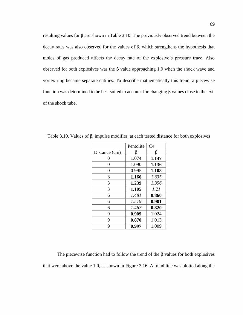
69

resulting values for β are shown in Table 3.10. The previously observed trend between the

decay rates was also observed for the values of β, which strengthens the hypothesis that

moles of gas produced affects the decay rate of the explosive’s pressure trace. Also

observed for both explosives was the β value approaching 1.0 when the shock wave and

vortex ring became separate entities. To describe mathematically this trend, a piecewise

function was determined to be best suited to account for changing β values close to the exit

of the shock tube.

Table 3.10. Values of β, impulse modifier, at each tested distance for both explosives

Pentolite C4

Distance (cm) β β

0 1.074 1.147

0 1.090 1.136

0 0.995 1.108

3 1.166 1.335

3 1.239 1.356

3 1.105 1.21

6 1.481 0.860

6 1.519 0.901

6 1.467 0.820

9 0.909 1.024

9 0.870 1.013

9 0.997 1.009

The piecewise function had to follow the trend of the β values for both explosives

that were above the value 1.0, as shown in Figure 3.16. A trend line was plotted along the

70

nine points for each explosive. Each trend line was a second-degree polynomial with an R2

value above 0.9. Another form a second-degree polynomial is shown in Equation (22),

𝑦 = 𝑎(𝑥 − ℎ)2 + 𝑘 (22)

where a defines the direction and width of the parabola, h is the x value of the vertex, and

k is the y value of the vertex. The vertex is the maximum value of the parabola when a is

negative and minimum value of the parabola when a is positive. To determine the values

of a, h, and k, the ratios of the pentolite were used. The calculated values for a, h, and k

were used to determine the equation for C4 as a confirmation of the values.

Figure 3.16. Values of β and best-fit trend line greater than 1.0 for pentolite and C4 at

tested distances

71

Before the values of a, h, and k could be determined, the trend line had to be

rewritten in the form of Equation (22). The values for pentolite from Figure 3.16 were used

to determine the maximum value and the location of the vertex, resulting in Equation (23).

𝑦 = −0.049(𝑥 − 5.5857)2 + 1.498 = −0.049(𝑥 − 5.59)2 + 1.5 (23)

The hypothesis that a related to gas production of the explosive was tested by equating the

value of a to the gas production ratio, volume of the shock tube, and a constant, as shown

in Equation (24),

−0.049 =𝑔𝑝𝑒𝑛𝑡𝑜𝑙𝑖𝑡𝑒

𝑔𝑇𝑁𝑇∗ 𝑉 ∗ 𝐶1 (24)

where g is moles of gas produced by one mole of explosive, V is volume of the shock tube

between the explosive and exit, and C1 is a constant. Equation (25) solves for C1,

𝐶1 =−0.049 ∗ 𝑔𝑇𝑁𝑇

𝑔𝑝𝑒𝑛𝑡𝑜𝑙𝑖𝑡𝑒 ∗ 𝑉= −5.11 ∗ 10−7 𝑐𝑚−3 (25)

72

which was found to have a small value due to the large volume of the shock tube. The mass

relationship and density relationship from Section 3.1 were used to determine the values of

h and k from Equation (23).

The mass of the explosive determines how much energy is imparted into the shock

wave and would have a greater influence than density. Thus, h was hypothesized to be the

mass relationship and k was the density relationship. As with a, h was equated to volume

of the shock tube and a constant with the mass relationship, as shown in Equation 26,

−5.59 = 𝑚𝑒 ∗ 𝑇𝑁𝑇 𝑒𝑞𝑢 ∗ 𝑉 ∗ 𝐶2 (26)

where me is the mass of the explosive, TNT equ is TNT equivalency, V is volume of the

shock tube, and C2 is the fitting constant. The value of C2 was solved for, as shown in

Equation (27),

𝐶2 =

−5.59

𝑚𝑒 ∗ 𝑇𝑁𝑇 𝑒𝑞𝑢 ∗ 𝑉= 5.47 ∗ 10−6 𝑐𝑚−3𝑔−1

(27)

The value for k was similar to a, but with a density ratio, as shown in Equation (28),

73

1.5 =𝜌𝑝𝑒𝑛𝑡𝑜𝑙𝑖𝑡𝑒

𝜌𝑇𝑁𝑇∗ 𝑉 ∗ 𝐶3

(28)

where ρ is density, V is volume of the shock tube, and C3 is the fitting constant. The value

of C3 was solved for, as shown in Equation (29),

The absolute values of the constants increase an order of magnitude with each successive

parameter. With the parameters a, h, and k known, the piecewise function to describe β can

be developed.

The proposed parabolic function accounts for the separation of the shock wave and

the vortex ring. The parabolic function takes the form of Equation 30, when all the

parameters are inserted into Equation (21), where x is the distance outside the shock tube.

When combined with the constant decay rate after separation, the piecewise function takes

the form of Equation (30),

𝑦 = 𝐶1 ∗ 𝑉 ∗𝑔𝑒

𝑔𝑇𝑁𝑇(𝑥 − (𝐶2 ∗ 𝑚𝑒 ∗ 𝑇𝑁𝑇 𝑒𝑞𝑢 ∗ 𝑉))

2+ 𝐶3 ∗ 𝑉 ∗

𝜌𝑒

𝜌𝑇𝑁𝑇 (30)

𝐶3 =

1.5 ∗ 𝜌𝑇𝑁𝑇

𝜌𝑝𝑒𝑛𝑡𝑜𝑙𝑖𝑡𝑒 ∗ 𝑉= 1.89 ∗ 10−5 𝑐𝑚−3

(29)

74

where β is the exponent to the exponential in Equation (21) and y is the parabolic function

given in Equation (31) or the Rutter-Johnson equation.

𝐼 =

𝑃𝑇

𝑒𝛽, 𝑤ℎ𝑒𝑟𝑒 𝛽 = {

1 𝑖𝑓 𝑦 < 1𝑦 𝑖𝑓 𝑦 ≥ 1

(31)

The Rutter-Johnson equation was then applied to the C4 to determine the

soundness. The resulting values and percent error with respect to the parabola values are

given in Table 3.11. The values for a and k are very close to parabola values. The h value

was 10% above the given value, which may be because the third iteration at 3 cm for the

C4 is an outlier. If the value in the equation is removed from the trend line calculation, the

percent error for h would be reduced; however, the percent error of a and k would increase.

Before the equation could be considered a replacement for the current method, the error

between the Rutter-Johnson equation and the Friedlander method would need to be

compared.

The midpoint approximation method was used to calculate the actual impulse value

for each of the experimental data sets. The error was calculated by comparing actual

impulse value to impulse values calculated from Equation (8) (Friedlander method) and

Equation (31) (Rutter-Johnson method). The percent error for the Friedlander and Rutter-

Johnson methods is presented in Table 3.12, where the listed error is representative of the

other iterations at each distance for both explosives. The reduction of the error from the

Friedlander impulse calculation is needed for the development of the P-I graph of animal

75

data to be scaled to humans. The entire error comparison table is given in Appendix A. The

Rutter-Johnson method reduced the error from the Friedlander method when the vortex

ring interacts with the shock wave. The error between the Friedlander method and the

Rutter-Johnson method is the same when the value of β is equal to one, which is when the

shock wave and vortex ring are separate entities. Overall, the Rutter-Johnson method

accounts for the vortex ring interacting with different portions of the shock wave.

Table 3.11. Values of a, h, and k from Equation (30) and percent error

Equation (30) Parabola Percent Error

a -0.0339 -0.0339 0.00%

h 2.5872 2.33 9.94%

k 1.3181 1.315 0.24%

Table 3.12. Comparison of error between Friedlander and proposed methods Pentolite C4

Distance (cm) Friedlander

error

Rutter-Johnson

error

Friedlander

error

Rutter-Johnson

error

0 9.41% 9.41% 15.79% 3.99%

3 10.71% 8.12% 23.36% 11.16%

6 59.45% 3.81% 16.47%* 16.47%*

9 12.20%* 12.20%* 2.41%* 2.41%*

*The value of β is one

3.5. SUMMARY

This section has proposed a new method for calculating impulse outside of a shock

tube (Section 3.4). Based on the four confidence intervals, the peak pressure remains steady

76

for both pentolite and C4 outside the shock tube, which is consistent with Giannuzzi et al.’s

work [26]. However, this is not true with the time duration, as the vortex ring extends the

positive phase. This proposed method accounts for the changes in decay rate as the shock

wave and vortex ring separate from one another. The proposed method reduces the error

found in Friedlander methods when the vortex ring directly influences the decay of the

shock wave. Thus, the Rutter-Johnson equation fulfills the requirements for Objective 1

which was to accurately determine impulse for all experimental designs.

Through analysis of the experimental data and the Rutter-Johnson equation, the

distance at which the shock wave and vortex ring separate was found to always occur

before or at 60% of the shock tube diameter. The 60% shock tube diameter should be used

in future animal bTBI to ensure the animal is exposed decay trends observed in open-air

testing. The Rutter-Johnson can be used on other shock tube diameters and sizes, since

volume is accounted for in the equation. The Rutter-Johnson equation was not tested with

reflected pressures and the relationship to related pressures needs to be studied.

The Rutter-Johnson method will be used in the following sections in the generation

of a human P-I graph of bTBI and its relationship with observable injuries. The Rutter-

Johnson method will be used on 31.58% of the gathered animal bTBI data, which will then

be scaled to humans. The Friedlander method will be applied to the other 68.42% from

open-air and interior shock tube experimental designs that did not include impulse. Overall,

the modification to the Friedlander method of calculating impulse with only peak pressure

and time duration allows for a better representation of the loading on an animal’s brain

outside a shock tube.

77

4. PROPOSED HUMAN BTBI SEVERITY REGIONS (OBJECTIVE 2)

The human bTBI severity regions were determined by plotting the scaled peak

pressure and scaled impulse presented in Table 2.1 (page 35) from the animal model to

humans. The peak pressure was scaled using Jean’s method (Equations (16) (page 37) and

(17) (page 38)). A scaling method has been developed for impulse, as no impulse scaling

method had been published.

This section is divided into four subsections. The impulse calculation for open air,

interior shock tube, and exterior shock tubes is discussed in Section 4.1. The scaling of

peak pressure and positive phase duration from the animal model to humans is discussed

in Section 4.2. The proposed human bTBI P-I graph and severity regions are presented and

discussed in Section 4.3. A summary of the methods used to determine human bTBI

severity regions is presented in Section 4.4.

4.1. SCALING OF IMPULSE

In Section 3, the Friedlander impulse equation (8) was used to calculate impulse for

open air and interior shock tube experiments. For both of these test methods, the shock

wave and resulting pressure trace resemble a Friedlander curve. However, exterior shock

tube experiments do not always resemble a Friedlander curve. To determine the impulse

for the exterior shock tube experiments, the Rutter-Johnson equations developed in Section

3.4 (Equation (30) and (31)) were used. The equations used for each cited study are

summarized in Table 4.1.

The open-air and exterior shock tube experiments that included impulse (Song,

Beamer, and Shridharani) had the β decay value calculated using Equation (32),

78

where P is the given peak pressure, T is the given positive phase time duration, and I is the

given impulse value. The calculated β value was assumed to describe the decay rate of the

pressure trace for each specific experimental design. The calculated β value will be used

for the scaled impulse in Section 4.2.

The other exterior shock tube experiment’s impulse values were calculated by using

the Rutter-Johnson equation developed in Section 3.4. 60% shock tube diameter exit

distance was confirmed by analyzing Kabu, Budde, and Svetlov works. The shock wave

and vortex ring were found to be separate entities at those distances. For the shock tube

experiments where the animals were placed at the end of the shock tube (Long and Kuehn),

the y value (Equation (23)) was found to be less than one for both experiments. Thus, the

traditional Friedlander equation was used to calculate impulse.

Two of the data sets in Table 2.1, Turner and Wang, reported reflective peak

pressures. To determine the impulse value for these studies, Equation (3) was used to

calculate the incident peak pressure. The dynamic pressures associated with the reported

reflective pressure were determined by interpolating the dynamic pressure delta value from

reflective pressures in reported in Figure 2.7 that were directly above and below the

reflective pressure reported by Turner and Wang. The calculated incident peak pressure

was used to determine the impulses for Turner and Wang by using the proposed modified

impulse calculation equation and the Friedlander equation, respectively. The impulse for

Turner was found to be the same as the Friedlander method.

𝛽 = ln (

𝑃𝑇

𝐼) (32)

79

Table 4.1. Impulse equations used for data sets that did not include impulse

First Author Test

type Model

Sensor

Orientation

Reported Data

points Equation Value

PP I T

Song [88, 89] Open

Air Mice Incident x x x 101 β

Beamer [51] Shock

Tube Mice Incident x x x 2 β

Shridharani

[109]

Shock

Tube Pigs Incident x x - 20 β

Pun [90] Open

Air Rats Incident x - x 2 Friedlander Impulse

Chen 1 [91] Open

Air Goats Incident x - x 4 Friedlander Impulse

Li [92] Open

Air Goats Incident x - x 7 Friedlander Impulse

Saljo 1 [93] Open

Air Pigs Incident x - x 8 Friedlander Impulse

Chen 2 [94] Open

Air Pigs Incident x - x 4 Friedlander Impulse

Wang [48] Shock

Tube Mice Reflective x - x 9

Friedlander

Swisdak Impulse

Risling [97] Shock

Tube Rats Incident x - x 4 Friedlander Impulse

Pham [98] Shock

Tube Rats Incident x - x 8 Friedlander Impulse

Kochanek

[99]

Shock

Tube Rats Incident x - x 1 Friedlander Impulse

Garman [106] Shock

Tube Rats Incident x - x 1 Friedlander Impulse

Saljo 2 [108] Shock

Tube Rats Incident x - x 2 Friedlander Impulse

Turner [96] Shock

Tube Rats Reflective x - x 4

Rutter-

Johnson

Swisdak

Impulse

Kabu [95] Shock

Tube Rats Incident x - x 20

Rutter-

Johnson Impulse

Budde [100] Shock

Tube Rats Incident x - x 2

Rutter-

Johnson Impulse

Long [104] Shock

Tube Rats Incident x - x 3

Rutter-

Johnson Impulse

Svetlov [105] Shock

Tube Rats Incident x - x 5

Rutter-

Johnson Impulse

Kuehn [107] Shock

Tube Rats Incident x - x 26

Rutter-

Johnson Impulse

4.2. SCALING ANIMAL DATA TO HUMANS

Four animal species were cited in this research and needed to be scaled to humans

individually. The peak pressure and impulse were scaled using two different methods. The

80

peak pressure was scaled by using Jean’s method discussed in Section 2.2.2.2. The three

values in Table 2.2 are calculated in order to scale the rat and goat animal models. The

mass of the flesh surrounding the skull of a rat could not be found, thus it was assumed that

the ratio of a mouse’s skull and flesh is the same for a rat. This value may change with new

research but goes beyond the scope of this research. The resulting value of the mass of a

rat’s flesh surrounding the skull was found to be approximately 8 grams. The η value, head

scaling formula, for the rat and goat were then calculated using Equation (16). The η values

for each of the animal models and humans are given in Table 4.2. The given peak pressure

and model specific η were then inserted into Equation (17) resulting in the equivalent

human peak pressure. The human peak pressures were found to be lower than the animal

models, due to humans having a higher η value (less soft tissue and skull).

Table 4.2. Scaling parameter for referenced animal models for use in equation (17)

Species ηs

Mouse 0.126

Rat 0.143

Goat 0.059

Pig 0.024

Human 0.75

The scaled impulse was calculated using Equation (33),

𝐼𝑠𝑐𝑎𝑙𝑒𝑑 =

𝑃𝑠𝑐𝑎𝑙𝑒𝑑𝑇𝑠𝑐𝑎𝑙𝑒𝑑

𝑒𝛽

(33)

81

where Pscaled is scaled peak pressure (Equation (17)), Tscaled is scaled duration (Equation

(14)), and β is the decay rate calculated by either Equation (21) or (32). Equation (21) was

used when the animal was outside the shock tube and impulse was not given; whereas,

Equation (32) was used when the impulse value was given. If the testing was conducted

inside a shock tube or in open air and impulse was not reported, the value for β was 1.0

based on Tasissa et al., Chandra et al., and Kleinschmit [23, 25, 62] discussed in Section

2.1.4.

4.3. HUMAN SEVERITY CURVES (OBJECTIVE 2)

The scaled peak pressures and impulse values were divided into four severity

groups: mild, moderate, severe, and not given. After the data sets were separated into

severity groups, the values were plotted on a P-I graph. The produced human bTBI P-I

graph, shown in Figure 4.1, has regions where numerous studies have been conducted and

other regions with little to no research. The severity group with the largest number of data

points was the mild group, because the focus of bTBI research has been on mild bTBI. The

second largest group was the severity not explicitly given group. This group was plotted to

show the areas were bTBI studies have been conducted and determine the likelihood of

bTBI based on the relationship produced in this research. The moderate and severe severity

groups had the least number of data, because lung protection is required to prevent lung

injury. Without lung protection, the brain will sustain secondary injuries from reduced

oxygen [61, 109, 116]. From Figure 4.1, the spread of the mild bTBI data points is diverse

allowing for a good understanding of the mild bTBI. Note: pressure will be on the x-axis

and impulse will be on the y axis for the rest of this dissertation, although both orientations

are acceptable and data published with axis titles switched. However, the moderate and

82

severe bTBI data points are linear, due to the use of shock tubes. Thus, more testing needs

to be conducted on moderate and severe bTBI to produce a more definitive ranges.

Figure 4.1. Human bTBI P-I graph with severities denoted

The three explicitly given severities had no overlapping data points on Figure 4.1,

thus each bTBI severity has a distinct region based on the relationship between pressure

and impulse. The region for each severity began at the lowest peak pressure and the lowest

impulse occurrence, as shown in Figure 4.2. A log-log graph was used to present the

severity regions, so the spread of the data could be visualized easier. The mTBI region

0

500

1000

1500

2000

2500

3000

3500

4000

4500

5000

0 100 200 300 400 500 600 700

imp

uls

e (k

Pa*m

s)

Pressure (kPa)

Not Given Mild Moderate Severe

83

began with the lowest occurrence of a bTBI in the unspecified group, since an injury was

documented. The author assumed the “not given” data points in this region were mild

bTBIs. The other “not given” data points were assigned the severity of the data points in

close proximity. Boxes were used to assign severity regions instead of curves discussed in

Section 2.1.6 because the dynamic region of the severities are not known and produces a

more conservative model. The beginning point of each severity region for humans is given

in Table 4.3. Unlike other P-sT bTBI graphs that give a finite range, the starting point is

only given, due to severity regions extending along both axes. These severity regions will

be referred to in the following section (Section 5). These severity regions are conservative,

since Jean’s pressure scaling is conservative. Upon further examination of Figure 4.2, six

regions of under researched areas were found, which were: greater than 100 kPa and lower

than 75 kPa*ms; greater than 20 kPa and 4,000 kPa*ms; greater than 300 kPa and 100

kPa*ms; boundaries between no bTBI and mild; boundaries between mild and moderate;

and boundaries between moderate and severe. Testing is not feasible, however, for low

pressure and high impulse or high pressure and low impulse regions, as these values are

difficult to achieve experimentally. These regions have not, to the author’s knowledge,

been previously identified.

Table 4.3. Thresholds for each human bTBI severity region

Threshold Pressure (kPa) Impulse (kPa*ms)

mild 17.7 7.2

moderate 190 935

severe 319 1467

84

Figure 4.2. Human bTBI P-I graph with severity region identified

4.4. SUMMARY

The human bTBI P-I graph with proposed severity regions defined was developed

in this section. The severities were determined from scaled animal bTBI studies that

explicitly stated the severity of the bTBI and grouped other that were unspecified. The

influence of impulse has been overlooked in the search of understanding the mechanisms

of bTBI. The peak pressures were scaled by using the method proposed by Jean et al. [12].

The impulse scaling was conducted by using mass scaling on the time duration. The

proposed bTBI regions will be used in the following section to determine the correlation

between observable blast injuries (eardrum rupture and lung damage) and the occurrence

of bTBIs, see Appendix B Table B.1 for all calculated values.

85

5. HUMAN bTBI RELATIONSHIP TO PHYSIOLOGICAL INJURIES

(OBJECTIVE 3)

Explosive blasts detonated in the vicinity of animals or people can cause injuries to

air-containing organs. The three most susceptible structures are bowels, lungs, and ears.

However, lung damage and eardrum rupture are more observable than the bowel injuries.

Observable lung injury symptoms are labored breathing, coughing, coughing up blood and

chest pain [120]. Eardrum rupture is observed from discharge from the ear canal and

hearing loss [119] As a result, numerous studies have been conducted to understand and

define injury regions, which were discussed in Section 2.2. This section is divided into four

subsections: lung damage, eardrum rupture, bTBI correlation to observable injuries, and

summary of the section. The lung damage subsection discusses the processes used to create

a P-I graph from the data presented in Section 2.3.1. The eardrum rupture subsection

presents a P-I graph with different eardrum rupture regions from literature. The correlation

subsection discusses correlations between the proposed bTBI P-I graph presented in

Section 4.3. The summary subsection briefly recaps the correlations observed in the

previous subsection. The overall goal of this section is to show that human bTBI regions

can be related to observable blast induced injuries as a diagnostic tool on the battlefield.

5.1. LUNG INJURY

The blast effects on lung tissue has been greatly studied [10, 80, 81, 110, 121, 125].

As a result, improved body armor has been developed and the prevalence of lung injury

has reduced in recent years. The same cannot yet be said for bTBI. Courtney and Courtney

[110] produced a P-T graph for lung lethality curves from Bowen et al.’s [10] work. Baker

et al. [80, 81] also used Bowen et al.’s [10] work to produce a 50% lung lethality P-I graph.

86

This researcher inferred data points from both graphs and were used to create a lung

damage P-I graph for the four lung damage and lethality curves: threshold for injury, 1%

lethality, 50% lethality, and 99% lethality. The impulse was calculated using Equation (8)

with the inferred peak pressure and time duration values. The produced P-I 50% lethality

curve was compared to the values given by Baker et al. [80, 81] in Figure 2.16 and Table

2.3. The inferred 50% lethality curve was found to have very similar values and further

explained in Appendix C. The resulting lung damage and lethality P-I is shown as a log-

log plot in Figure 5.1. The circle curve denotes the threshold for lung damage. The triangle

curve denotes the region of 1% chance of lethality. The square curve denotes the 50%

chance of lethality. The diamond curve denotes the area where 99% lethality occurs. Bass

et al. [61] reported that these curves would shift up and to the right if a protective vest is

worn. The curves presented in Figure 5.1 will be used for comparison with the proposed

bTBI severity P-I curves in Section 5.3.

Figure 5.1. P-I lung damage curve for 70 kg man, calculated from Courtney and Courtney

[110] and Baker et al. [80, 81]

1

10

100

1000

10000

100000

1 10 100 1000 10000

Imp

uls

e (k

Pa*

ms)

Pressure (kPa)

Threshold 1% 50% 99%

87

5.2. EARDRUM RUPTURE

As with lung damage, studies have been conducted on eardrum rupture after an

explosive blast [81, 124–126]. Unlike the lung damage P-I curves, the tympanic membrane

(eardrum) ruptures at a minimum pressure and over large range of impulse values. The

eardrum rupture from Section 2.3.2 (Figure 2.17) was redrawn to have the same axes as

the proposed human bTBI P-I graph (Figure 4.2) and is given in Figure 5.2, where EDR is

eardrum rupture. The triangle dotted line represents the threshold for eardrum rupture. The

circle dotted line represents the 50 percent threshold for eardrum rupture. These two

thresholds for eardrum rupture will be used in the comparison between human bTBIs and

observable injuries in the following section (Section 5.3).

Figure 5.2. P-I curve for eardrum rupture, adapted from Baker et al. [81]

1

10

100

1000

10000

0 20 40 60 80 100 120

Imp

uls

e (k

Pa*m

s)

Pressure (kPa)

EDR Thre EDR 50%

88

5.3. HUMAN bTBI SEVERITY REGIONS WITH PHYSIOLOGICAL INJURY P-I

CURVES OVERLAID (OBJECTIVE 3)

The proposed human bTBI P-I graph from Section 4.3 was combined with the lung

lethality curves from Section 5.1 and thresholds for eardrum rupture from Section 5.2. The

bTBI severity regions were overlaid on the graph of observable physical injuries resulting

in Figure 5.3.

Figure 5.3. Human bTBI P-I graph with eardrum rupture and lung lethality curves

overlaid

89

Several correlations can be from the produced graph.

1. mTBI occurs before eardrum rupture, which is consistent with White et al.’s

findings [125]. Thus, eardrum rupture implies that an individual has a bTBI

after a blast.

2. Lung injury is in the mTBI region. The mTBI region encompasses the

majority of the threshold for lung injury region.

3. modTBI region encompassed the pressure sensitive regions of the 1 and

50% lung lethality curves.

4. mTBI region included the impulse sensitive region of the 1 and 50% lung

lethality curves.

5. modTBI region contained the impulse sensitive region of the 99% lung

lethality curve.

6. sTBI region contained the dynamic region of the 50% lung lethality curve.

7. sTBI region contained the pressure sensitive and dynamic regions of the

99% lung lethality curve.

These observed correlations indicate that physical injuries can be used as a guide

in determining if a bTBI was acquired after an explosive blast.

By further examining the observed correlations, practical applications can be

applied to the battlefield and urban environments. The correlations with the bTBI regions

allow the individuals subjected to an explosive blast to quickly determine if they likely

sustained a bTBI and seek appropriate medical attention. The occurrence of individuals

90

with ruptured eardrums and lung injury after a blast could be used as an indicator that the

individuals in the area may have sustained a bTBI. However, if a few individuals perished,

the surviving individuals may have a modTBI. If a large number of individuals have

perished, the surviving individuals in close proximity would likely have lung injuries and

either modTBI or sTBI. The individuals at a further distance may have sustained an mTBI.

The ability to quickly associate a visible injury to a bTBI would allow for earlier treatment

of individuals with a suspected bTBI and possibly reduce the long-term effects of the bTBI.

5.4. SUMMARY

The proposed human bTBI P-I severity regions were found to have seven

correlations with known P-I curves for both lung damage and eardrum rupture. The ability

to correlate an “invisible” injury to an observable injury in the same individual would

further the understanding of the effects bTBIs after blast exposure. The correlations would

also allow for individuals subjected to an explosive blast to receive appropriate medical

treatment earlier and possibly reduce the long-term effects of the bTBI.

91

6. CONCLUSIONS

A signature wound of the current military conflicts is bTBI. Currently, the diagnosis

of bTBIs is difficult, due to few observable symptoms as described in Section 1.2. This

research was conducted to determine if correlations between the occurrence of bTBIs and

observable physical injuries exist after an explosive blast, thus allowing for affected

individuals to receive appropriate medical treatment. To achieve this goal, three objectives

were identified. Objective 1 was to identify and develop impulse calculation equations for

all animal bTBI testing methods. Objective two was to create a human bTBI P-I graph

based on published animal bTBI data. Objective three was to correlate the human bTBI

severity regions to observable blast injuries. Dr. Johnson’s research team has been studying

bTBI since 2015 publishing 85 [88, 89, 127, 128] of the 258 total data points on bTBI

studies published to date. Experimental testing was also conducted to determine an impulse

calculation equation for animals placed outside a shock tube. The equation allowed for the

accomplishment of the objective. The following sections summarize the significance and

conclusions identified for each of the three objectives.

6.1. IMPULSE EQUATION MODIFICATION

The Friedlander impulse equation (Equation (8)) was found not to estimate the

impulse of a shock wave outside a shock tube in the jet wind region. When the shock wave

exits the shock tube, a vortex ring forms thus increasing the duration of the shock wave.

Experimental testing was conducted to develop and validate an equation to calculate

impulse outside the shock tube and discussed in Section 3.2.

92

Upon analysis of the results, the vortex ring was found to extend the positive phase

of the shock wave up to 9 times the duration inside the shock tube or beyond the vortex

ring. The vortex ring had a slower velocity than the shock wave. The Rutter-Johnson

equation (Equation (31)) was developed to account for this distance, which was found to

be 60% of the shock tube diameter. Three equivalents were found to influence the

separation of the shock wave and vortex ring were:

ratio of gas production to TNT production

mass of the equivalent amount of explosives

density ratio to TNT

The Rutter-Johnson equation was found to reduce the error up to 66 % of the traditional

Friedlander impulse equation outside a shock tube when within 60% of the shock tube

diameter from the end of the shock tube.

6.2. HUMAN bTBI SEVERITY REGIONS

The data presented in Table 2.1 was converted from the animal models to humans

using two different scaling methods. The reported peak pressure of the animals studied was

scaled to humans using Jean et al.’s scaling method [12], which accounts for all the

structures of the head including mass of the skull, mass of the brain, and mass of the

surrounding soft tissue. An impulse scaling equation was developed to plot the impulse

data on a P-I graph. The impulse scaling equation consisted of multiplying the scaled peak

pressure (Jean et al.’s scaling method [12]) and scaled time duration (mass scaling method

Equation (14)) and diving by the exponential to the β value, which is the impulse modifier.

93

Upon examination of the human bTBI P-I graph, five under researched regions were

observed: greater than 100 kPa and lower than 75 kPa*ms, greater than 20 kPa and 4000

kPa*ms, greater than 300 kPa and 100 kPa*ms, boundary between mild and moderate, and

boundary between moderate and severe.

6.3. CORRELATIONS BETWEEN bTBI SEVERITIES AND OBSERVABLE

INJURIES

The human bTBI P-I graph with defined severity regions was overlaid with P-I

curves for lung damage and eardrum rupture. Severn correlations were observed between

the bTBI severity regions and observable physical injuries.

1. mTBI occurs before eardrums rupture

2. mTBI region encompasses majority of the threshold for lung injury region

3. mTBI region included the impulse sensitive region of the 1 and 50 percent

lung lethality curves

4. modTBI region encompassed the pressure sensitive regions of the 1 and 50

percent lung lethality curves

5. modTBI region contained the impulse sensitive region of the 99 percent

lung lethality curve

6. sTBI region contained the dynamic region of the 50 percent lung lethality

curve

7. sTBI region contained the pressure sensitive and dynamic regions of the 99

percent lung lethality curve

94

Based on these correlations, a bTBI is very likely to be sustained by an individual

subjected to an explosive event, whose unprotected eardrums ruptured. Moderate and

severe bTBIs are likely sustained by individuals in close vicinity of deceased individual

after an explosive event. Whilst survivability has increased due to improved body armor

and hearing protection, the occurrence of bTBIs have increased.

6.4. CONCLUSIONS

One of the signature wounds of the current military conflicts is bTBI. This research

has proposed using a P-I graph to identify the regions for each type of severity, never

previously published.

A P-I graph can be used to present bTBI data with 3 clear distinctions for

mild, moderate and severe TBIs.

Rutter-Johnson equation was developed to determine impulse outside of a

shock tube.

The minimum distance where the shock wave and vortex ring separate from

one another at 60% of the shock tube diameter.

The vortex ring was found to be influenced by the shock wave’s source gas

production, density, and mass in relation to TNT.

The jet wind region was quantified.

bTBIs can be correlated to observable blast injuries.

Mild bTBI can be sustained without any visible indicator.

95

7. FUTURE WORK

Future research is needed to refine the severity regions for bTBI proposed by this

dissertation. To achieve defining severity regions, testing needs to be conducted in the areas

with little data on the P-I graph. Higher impulses need to be studied as well to determine

the lethal limit. To achieve these higher impulses, shock tubes and shock tunnels need to

be constructed to sustain pressures over a long positive phase duration. Testing needs to be

conducted to determine the dynamic regions of the bTBI severities. An impulse scaling

factor is also needed to more accurately represent the loading that the brain experiences.

The produced P-I graph can be used by all researchers to add their bTBI data with

the goal of diagnosing and treating bTBIs. Also, the P-I graph can be used to determine if

correlations exist between bTBIs and building damage after an explosive blast, in addition

to the human observable injuries studied in this research.

Future research is needed to determine the effect that helmets have on the proposed

human bTBI P-I graph. Since helmets are worn by members of the military and police, the

P-I graph needs to account for this added layer of protection. The research will need to

determine if the helmet is added to Jean et al.’s scaling parameter or the pressure and

impulse thresholds modified.

The influence of the detonating cap on the explosives needs to be further

investigated. A single cap test was conducted in this research, as shown in Figure 7.1. This

pressure trace was the result of the cap and the pentolite stinger not being properly coupled.

As with the other pentolite tests conducted at 6 cm the duration is extended at a low

pressure.

96

Figure 7.1. Pressure trace of cap measured at 6 cm outside the shock tube

97

APPENDIX A.

A. DATA TO ACCOMPANY SECTION 3

98

This appendix provides the recorded weight, peak pressure, time durations and

impulses used for the calculations of β and the expanded Table 3.12. Pentolite stingers

were used in this research, because they were commercially available. Before testing

began, 30 pentolite stingers were weighed to ensure the mass of explosives was the same.

The pentolite stingers were encased in plastic. All the stingers used in this research were

12 g, where 10 g were the pentolite and 2 g were the plastic chasing to ensure that all the

stingers had the same weight. The C4 charges were weighed before each test to ensure each

charge was 4.3 g. The impulse was determined by the midpoint approximation method on

each of the recorded pressure traces. The peak pressure, positive phase time duration, and

impulse values for all experimental testing are shown in Table A.1. The peak pressures

remain relatively constant for the four distances measured, which is consistent with

Giannuzzi et al.’s work [26]. The characteristics of the sensors used in this research were

taken from the PCB website and published specification sheets [129–131].The time

duration steadily decayed until the shock wave and vortex ring separated from one another.

A similar trend to the time duration was observed with the calculated impulse at the

distance where the vortex ring was no longer influencing the shock wave.

The expanded Table 3.12, shown in Tables A.2 (pentolite) and A.3 (C4), displays

the values for impulse calculated using three different methods and the percent error

between them. The first method was the midpoint approximation method (Equation (5)),

which provides closest value to the actual impulse value. The midpoint approximation

method values were used as the baseline for comparison for the other two methods. The

second method was the integration of the traditional Friedlander pressure equation

(Equation (8)), which is the current method to calculate impulse when peak pressure and

99

positive phase time duration are only given. The third method used was the proposed

equation from Section 3.4 (Equations (30) and (31)), which estimates the decay rate of the

pressure trace with the given peak pressure, time duration, distance outside the shock tube,

rupture pressure, and the volume of air in the shock tube between the shock wave source

and the end of the shock tube. The proposed method reduces the error of the Friedlander

method greatly. The most drastic error reduction was found to occur when the vortex ring

was influencing the end of the shock wave.

Table A.1. Recorded peak pressures, time durations, and calculated impulses P T I

explosive distance experiment (psi) (ms) (psi*ms)

Pentolite

0

1 50.6727 2.1825 37.79453

2 47.381 2.3585 37.57377

3 47.1381 2.2675 39.52465

3

4 51.9646 1.851 29.97359

5 47.7127 1.9575 27.04682

6 47.9587 1.833 29.21142

6

7 48.5269 0.822 9.072208

8 46.2843 0.7465 7.563371

9 45.6526 0.8925 9.400715

9

10 46.9175 0.2685 5.075643

11 48.1968 0.263 5.311055

12 43.7877 0.2865 4.628384

C4

0

1 26.7402 1.948 16.54909

2 27.9734 1.875 16.83731

3 29.0304 1.9135 18.34129

3

4 27.4385 1.308 9.445778

5 27.1687 1.384 9.693903

6 25.2467 0.9005 6.779982

6

7 29.9192 0.361 4.569728

8 28.7844 0.361 4.219427

9 28.3241 0.339 4.228745

9

10 28.2654 0.336 3.411553

11 27.0624 0.3405 3.34777

12 26.5323 0.345 3.337972

100

Table A.2. Comparison between Pentolite Friedlander and Rutter-Johnson methods

percent error

Pentolite

Distance

(cm)

Midpoint Friedlander Percent

error

Rutter-

Johnson

Percent

error

0 37.795 40.685 7.65% 40.685 7.65%

0 37.574 41.110 9.41% 41.110 9.41%

0 39.525 39.321 0.52% 39.321 0.52%

3 29.974 35.385 18.05% 29.366 2.03%

3 27.047 34.359 27.04% 28.514 5.43%

3 29.211 32.340 10.71% 26.838 8.12%

6 9.072 14.674 61.75% 8.852 2.43%

6 7.563 12.711 68.06% 7.668 1.38%

6 9.401 14.989 59.45% 9.042 3.81%

9 5.076 4.634 8.70% 4.634 8.70%

9 5.311 4.663 12.20% 4.663 12.20%

9 4.628 4.615 0.29% 4.615 0.29%

Table A.3. Comparison between C4 Friedlander and Rutter-Johnson methods percent

error

C4

Distance

(cm)

Midpoint Friedlander Percent

error

Rutter-

Johnson

Percent error

0 16.549 19.163 15.79% 17.209 3.99%

0 16.837 19.295 14.60% 17.328 2.91%

0 18.341 20.436 11.42% 18.352 0.06%

3 9.446 13.203 39.78% 9.509 0.67%

3 9.694 13.833 42.70% 9.962 2.77%

3 6.780 8.364 23.36% 6.023 11.16%

6 4.570 3.973 13.05% 3.973 13.05%

6 4.219 3.823 9.40% 3.823 9.40%

6 4.229 3.532 16.47% 3.532 16.47%

9 3.412 3.494 2.41% 3.494 2.41%

9 3.348 3.390 1.26% 3.390 1.26%

9 3.338 3.367 0.88% 3.367 0.88%

101

APPENDIX B.

B. DATA TO ACCOMPANY SECTION 4

102

This appendix discusses the calculations used in Section 4. The calculations

discussed are converting reflective pressure to incident pressure, the calculation of β for

the external shock tube tests, and completion of Table 2.2 resulting in Table 4.1. One

example will be given for reflective to incident pressure calculation and β, since all

calculations were conducted in the same manner.

The reflective pressures reported by Turner et al. [96] and Wang et al. [48] were

converted to incident pressures using Equations (2) and (3) from Section 2.1.1. In order to

use Equation (3), the values for q, given in Figure 2.7, had to be estimated for the reported

peak reflective pressures. The estimated q values were determined by using the example

Swisdak [35] provided on page 100. The following calculations are representative of all

reflective to incident pressure conversions. Equation 1 is the estimation of the dynamic

pressure for the reported peak pressure.

𝑞 =(31.47 − 25.1) ∗ (4.77 − 2.21)

(41.45 − 25.31)+ 2.21 =

15.7

16.14+ 2.21 = 3.187 𝑝𝑠𝑖 (1)

The numerator of Equation (1) is the difference between the reported reflective pressure

and closest reflective pressure in Figure 2.7 multiplied by the difference in dynamic

pressures in the desired region. The denominator of Equation (1) is the difference in

reflective pressures in desired region of Figure 2.7. The resulting value is added to the

lower tabulated dynamic pressure. The resulting value from Equation (1) is inserted into

103

Equation (2) resulting in the estimated incident peak pressure. The resulting value was then

converted to kilopascals to be used in Figure 4.1 and Figure 4.2. The same calculations

were used for all the reported peak reflective pressure listed in Table 2.1

𝑃 =31.47 − (1.4 + 1) ∗ 3.187

2=

31.47 − 7.649

2= 11.91 𝑝𝑠𝑖 (2)

The following example paragraphs explain the methods used to determine the β

decay of Equation (31) for studies that placed the animal subject outside the shock tube.

The β value was determined in two different methods. The first method used Equation (32),

when peak pressure, positive phase time duration, and impulse were reported. The second

method used the proposed equation to determine the β value. The first method was used

for Shridharani et al. and Beamer et al.’s [51, 109] studies. The second method was used

for Kabu et al., Long et al., Budde et al., Svetlov et al., Kuehn et al., and Turner et al.’s

[95, 96, 100, 104, 105, 107] studies.

Numerous steps were required to determine the β value in the second method. First

the detonation velocity had to be determined. For the gas driven shock tubes, the rupture

pressure was converted to velocity using Equation (4), as the velocity at the rupture

pressure was assumed to be the detonation velocity. The method to determine the velocity

at pressures not listed in Figure 2.7 was calculated similar to the dynamic pressure seen in

Equation (1). The second step was to determine the volume in both the driver and driven

104

sections of the shock tube. The third step was determining the moles of gas in driver section

of the shock tube. The ideal gas equation, Equation (3), was used to determine the number

of moles in the driver section. The fourth step was to determine the mass of the gas, which

was calculated from the grams per mole ratio for the specific gas used in the study. The

fifth step was to determine the density of the gas, which was calculated by dividing the

mass by the volume of the driver section of the shock tube. The sixth step was to insert all

the values in Equation (30). These steps allowed for the calculation of β.

𝑛 =𝑃𝑉

𝑅𝑇 (3)

The missing rat and goat values in Table 2.2 were calculated in different manners.

For the rat, the ratio of the skull to surrounding soft tissue was assumed to be the same.

The ratio was used to estimate the mass the soft tissue surrounding the skull of a rat. The

ratio and resulting soft tissue mass for the rat are given in Equation (4). The resulting value

and other tabulated values were used to calculate η by using Equation (16). The goat η

value was determined by inputting the goat values given in Table 2.2 into Equation (16).

These calculations allowed for the values of η to be determined for use in Equation (17),

which are given in Table 4.1.

105

𝑀𝑟𝑎𝑡 𝑓𝑙𝑒𝑠ℎ =𝑀𝑟𝑎𝑡 𝑠𝑘𝑢𝑙𝑙 ∗ 𝑀𝑚𝑜𝑢𝑠𝑒 𝑓𝑙𝑒𝑠ℎ

𝑀𝑚𝑜𝑢𝑠𝑒 𝑠𝑘𝑢𝑙𝑙=

3.19 ∗ 1.876

0.74= 8.087 𝑔 (4)

Table B.1. Data points in Figure 4.1

Not Given Mild Moderate Severe

222.5898 47.63921 19.88978 409.087 222.4901 1021.85 324.4876 1490.303

58.4753 70.87128 19.88978 409.087 219.3805 1007.568 319.5121 1467.452

36.42167 57.01677 19.93735 431.6389 222.4901 2043.701 324.4876 2980.606

26.94898 76.96336 19.96025 411.2269 219.3805 2015.137 319.5121 2934.903

57.36629 988.0173 19.99358 390.5223 303.3418 1393.185 389.7908 1790.227

58.61016 1009.44 19.99358 394.2741 266.0256 1221.8 385.4372 1770.232

71.04887 1223.672 20.01658 397.3289 303.3418 2786.37

76.02435 1309.364 20.01658 398.9981 266.0256 2443.599

88.15209 1518.24 20.08599 412.9318 190.6946 935.8669

90.0179 1550.375 20.13653 416.0585

101.8347 1753.895 20.13653 416.0585

107.4321 1850.299 20.26139 445.4182

43.81654 513.1624 20.44781 404.9391

60.95532 993.8402 20.55456 420.0626

284.8136 91.43474 20.65976 459.1994

69.3097 66.3495 20.65999 440.5703

35.56321 21.4047 22.54756 480.5184

39.11547 47.91882 22.54756 480.5184

29.34675 28.88913 22.8954 497.5603

27.86664 36.4322 22.8954 497.5603

35.56321 40.76019 23.69606 538.5964

57.98822 800.3147 24.4779 555.9591

58.29919 817.9943 25.40533 534.1749

58.61016 835.8167 25.40533 533.9219

57.83274 770.2794 25.59167 527.911

57.98822 785.6667 25.59167 527.4724

58.14371 801.1254 25.95155 494.0776

71.35983 1132.344 26.1534 510.7892

73.22564 1178.766 26.20256 522.6792

75.09145 1226.046 26.43911 504.5283

73.22564 1160.269 29.15914 604.5496

73.84758 1187.082 29.61121 592.6676

74.46951 1214.181 29.61121 592.6676

89.39596 1529.399 29.73126 586.5671

90.0179 1571.046 29.96772 554.8263

102.7676 1732.203 30.29201 598.2252

101.8347 1707.124 30.53876 594.6462

24.40851 14.51518 30.53876 594.6462

22.3016 33.15561 30.59703 584.407

18.61451 11.06962 30.70375 562.9414

21.07257 9.398526 30.70375 559.0201

106

Table B.1. Data points in Figure 4.1 (Cont.)

21.95045 26.10685 30.77683 566.5532

20.54584 48.87254 30.86205 568.734

17.73663 15.82134 30.86205 568.6431

18.79008 7.263117 30.94111 541.1649

68.62267 620.4124 30.94111 540.6845

99.29207 1064.446 31.02736 578.5702

111.9206 1230.826 31.07418 552.3165

120.9411 1357.212 31.09597 563.9841

141.237 1383.226 31.13093 570.5446

120.1818 1103.939 31.27979 574.2387

119.588 549.2425 31.30342 584.5344

80.80023 315.4337 31.34959 537.5695

100.0817 74.78148 31.36523 574.5238

59.5237 54.91285 31.44562 563.9394

147.1361 141.1061 31.44737 555.2467

49.69145 17.84285 31.44826 575.1381

56.89006 26.94207 31.46531 578.5662

48.11127 21.49604 31.51878 559.016

62.68407 58.1547 31.53522 536.4274

48.11127 17.32517 31.58109 568.6249

60.92831 56.42301 31.59286 535.0473

35.82095 11.82809 31.59286 537.4424

57.94352 57.03216 31.67801 581.3054

65.84444 100.0092 31.74279 537.0657

64.26425 97.44605 31.75242 554.7412

64.79098 98.02578 31.93418 575.2939

58.99697 35.08697 32.0163 607.0374

104.9979 78.90914 32.06166 526.9995

109.2117 81.779 32.06166 525.568

65.14213 98.79873 32.06761 549.8534

104.9979 78.66873 32.06761 550.7897

58.11909 34.42906 32.09823 545.9045

60.95532 279.955 32.09823 546.0752

88.01656 808.4831 32.16197 573.9382

172.8084 396.8364 32.22143 595.463

88.9186 816.7688 32.28885 551.0075

172.8084 3968.364 32.3602 544.4826

272.484 1877.192 32.5425 540.6875

257.1493 1771.549 32.5508 574.1753

229.186 1578.905 32.60957 574.9443

198.0656 1364.51 33.11033 555.0941

148.0023 1019.615 33.21613 532.3914

201.2227 1386.26 33.21613 531.8511

175.9656 1212.259 33.58722 569.7098

154.3166 1063.115 34.13896 534.6852

148.0023 1019.615 34.20139 565.2763

142.139 979.2219 35.12596 572.5327

129.5104 892.2214 43.59877 376.6674

135.8247 935.7216 45.31711 586.5621

132.6676 913.9715 45.82251 560.2598

630.1433 4341.173 46.15815 593.5098

107

Table B.1. Data points in Figure 4.1 (Cont.)

486.7187 3353.095 46.16737 571.1136

403.2799 2778.27 46.42601 558.0325

306.7615 2113.337 46.91357 380.3048

229.186 1578.905 46.92784 610.6489

313.0758 2156.837 47.3387 549.8922

306.7615 2113.337 48.0076 374.1793

257.1493 1771.549 48.12057 560.3279

250.835 1728.048 48.27814 567.9029

244.5207 1684.548 50.47215 567.7485

219.7146 1513.654 46.20695 1931.191

213.4003 1470.154 33.39797 1112.076

203.9288 1404.903 72.68186 166.9062

28.93287 30.56299 72.68186 333.8125

60.95532 47.59235 117.7839 270.4784

62.75941 504.4213 117.7839 540.9567

68.17165 547.9216 65.46553 526.1715

77.64308 624.0471 65.46553 826.8409

48.381 222.2037 65.46553 601.3388

65.95694 302.9264 65.46553 601.3388

83.36675 382.8859 90.77622 92.31008

96.94041 445.2269 96.0435 97.66636

27.99646 70.86645 90.77622 113.3633

63.37341 160.4149 96.0435 119.9411

100.4862 254.3573 120.1818 1103.939

30.93468 78.30389 154.3882 709.0726

24.96655 63.19695 152.5224 700.5033

45.53245 115.2547 154.3882 1418.145

79.29417 200.7146 152.5224 1401.007

76.73963 194.2483 104.4576 307.5542

121.6005 307.803

108

APPENDIX C.

C. DATA TO ACCOMPANY SECTION 5

109

This appendix details the methods used to create the lung damage P-I curves in

Figure 5.1 and how the overlay was applied on Figure 5.3. The lung damage P-I curves

were created by estimating numerous points on the P-T graph shown in Figure 2.15. The

points were estimated by overlaying an Excel graph with the same dimensions and axes,

as shown in Figure C.1. Points were plotted on the Excel graph and compared to the lung

damage curves. This method was used for the four P-T curves. The Friedlander impulse

equation, Equation (8), was used to determine the impulse value. The created 50% P-I

curve was compared to the data points presented in Table 2.3 from Baker et al. [80, 81]

and found to be representative of the data. Thus, the lung P-I graph was determined to be

a good representation of lung damage.

Figure C.1. P-T lung damage graph [110] with Excel P-T graph overlaid with points on

the curves

110

The overlay was applied on Figure 5.3 by plotting the lung damage and eardrum

rupture P-I curves on an Excel graph. The threshold points for each bTBI severity, shown

in Table 4.3, were also plotted on the P-I graph, as shown in Figure C.2. The threshold

points served as the corners of the severity regions, as the dynamic regions have yet to be

defined. The mild and moderate severity regions were defined by an “L” shape beginning

at the threshold point and extended to the next threshold point. For the severe severity

region, a rectangular shape was used, as the lethality region has yet to be defined. Each

severity region extends indefinitely in both pressure and impulse between threshold points,

as this is the nature of a P-I curve.

Figure C.2. Human bTBI P-I graph with threshold for each severity shown overlaid with

observable injuries

111

REFERENCES

1. DePalma, R.G., Burris, D.G., Champion, H.R., Hodgson, M.J.: Blast Injuries. N.

Engl. J. Med. 352, 1335–1342 (2005). doi:10.1056/NEJMra042083

2. DePalma, R.G.: Combat TBI: History, Epidemiology, and Injury Modes. In:

Kobeissy, F.H. (ed.) Brain Neurotrauma: Molecular, Neuropsychological, and

Rehabilitation Aspects. CRC Press/Taylor & Francis, Boca Raton, FL (2015)

3. Benzinger, T., Brody, D., Cardin, S., Curley, K., Mintun, M., Mun, S., Wong, K.,

Wrathall, J.: Blast-related brain injury: Imaging for clinical and practical

applications: Report of the 2008 St. Louis workshop. J Neurotrauma. 26, 2127–2144

(2009). doi:10.1089/neu.2009.0885

4. Faul, M., Coronado, V.: Epidemiology of traumatic brain injury. In: Grafman, J. and

Salazar, A.M. (eds.) Handbook of Clinical Neurology. pp. 3–13. Elsevier (2015)

5. Rao, V., Koliatsos, V., Ahmed, F., Lyketsos, C., Kortte, K.: Neuropsychiatric

disturbances associated with traumatic brain injury: A practical approach to

evaluation and management. Semin. Neurol. 35, 64–82 (2015). doi:10.1055/s-0035-

1544241

6. Glassberg, E., Nadler, R., Erlich, T., Klien, Y., Kreiss, Y., Kluger, Y.: A decade of

advances in military trauma. Scand. J. Surg. 103, 126–131 (2014).

doi:10.1177/1457496914523413

7. Butler, F.K., Blackbourne, L.H.: Battlefield trauma care then and now: A decade of

Tactical Combat Casualty Care. J. Trauma Acute Care Surg. 73, S395–S402 (2012).

doi:10.1097/TA.0b013e3182754850

8. Butler, F.K.: Two Decades of Saving Lives on the Battlefield: Tactical Combat

Casualty Care Turns 20. Mil. Med. 182, e1563–e1568 (2017).

doi:10.7205/MILMED-D-16-00214

9. Centers for Disease Control and Prevention, National Institutes of Health,

Department of Defense, Department of Veterans Affairs: Report to Congress on

Traumatic Brain Injury in the United States : Understanding the Public Health

Problem among Current and Former Military Personnel. (2013)

10. Bowen, I.G., Fletcher, E.R., Richmond, D.R.: Estimate of man’s tolerance to the

direct effects of air blast. (1968)

11. Zhu, F., Chou, C.C., Yang, K.H., King, A.I.: Some considerations on the threshold

and inter-species scaling law for primary blast-induced traumatic brain injury: A

semi-analytical approach. J. Mech. Med. Biol. 13, 1350065 (2013).

doi:10.1142/S0219519413500656

112

12. Jean, A., Nyein, M.K., Zheng, J.Q., Moore, D.F., Joannopoulos, J.D., Radovitzky,

R.: An animal-to-human scaling law for blast-induced traumatic brain injury risk

assessment. Proc. Natl. Acad. Sci. U. S. A. 111, 15310–15315 (2014).

doi:10.1073/pnas.1415743111

13. Rafaels, K.A.: Blast Brain Injury Risk, (2010)

14. Mays, G.C., Smith, P.D. eds: Blast effects on buildings. Design of buildings to

optimize resistance to blast loading. Thomas Telford, London (1995)

15. Dawodu, S.T.: Traumatic Brain Injury (TBI) - Definition, Epidemiology,

Pathophysiology: Overview, Epidemiology, Primary Injury,

https://emedicine.medscape.com/article/326510-overview#a1

16. Mayo clinic staff: Traumatic brain injury - Symptoms and causes - Mayo Clinic,

https://www.mayoclinic.org/diseases-conditions/traumatic-brain-injury/symptoms-

causes/syc-20378557

17. Shively, S.B., Horkayne-Szakaly, I., Jones, R. V, Kelly, J.P., Armstrong, R.C., Perl,

D.P.: Characterisation of interface astroglial scarring in the human brain after blast

exposure: a post-mortem case series. Lancet Neurol. 15, 944–953 (2016).

doi:10.1016/S1474-4422(16)30057-6

18. Ling, G., Ecklund, J.M., Bandak, F.A.: Brain injury from explosive blast:

description and clinical management. In: Grafman, J. and Salazar, A.M. (eds.)

Handbook of Clinical Neurology. pp. 173–180. Elsevier (2015)

19. Defense and Veterans Brain Injury Center: DOD Worldwide Numbers for TBI.

(2017)

20. Centers for Disease Control and Prevention: What are the treatments for TBI?,

http://www.neurology.org/cgi/doi/10.1212/WNL.0b013e3182553c38

21. Dang, B., Chen, W., He, W., Chen, G.: Rehabilitation Treatment and Progress of

Traumatic Brain Injury Dysfunction,

https://www.hindawi.com/journals/np/2017/1582182/, (2017)

22. Chou, A., Krukowski, K., Jopson, T., Zhu, P.J., Costa-Mattioli, M., Walter, P., Rosi,

S.: Inhibition of the integrated stress response reverses cognitive deficits after

traumatic brain injury. Proc. Natl. Acad. Sci. 114, E6420–E6426 (2017).

doi:10.1073/pnas.1707661114

23. Tasissa, A.F., Hautefeuille, M., Fitek, J.H., Radovitzky, R.A.: On the formation of

Friedlander waves in a compressed-gas-driven shock tube. Proc. R. Soc. A Math.

Phys. Eng. Sci. 472, (2016). doi:10.1098/rspa.2015.0611

113

24. Phillips, M.: Numerical modeling and characterization of blast waves for application

in blast-induced mild traumatic brain injury research,

https://lib.dr.iastate.edu/etd/15789/, (2016)

25. Chandra, N., Ganpule, S., Kleinschmit, N.N., Feng, R., Holmberg, A.D.,

Sundaramurthy, A., Selvan, V., Alai, A.: Evolution of blast wave profiles in

simulated air blasts: Experiment and computational modeling. Shock Waves. 22,

403–415 (2012). doi:10.1007/s00193-012-0399-2

26. Giannuzzi, P.M., Hargather, M.J., Doig, G.C.: Explosive-driven shock wave and

vortex ring interaction with a propane flame. Shock Waves. 26, 851–857 (2016).

doi:10.1007/s00193-016-0627-2

27. Arakeri, J.H., Das, D., Krothapalli, A., Lourenco, L.: Vortex ring formation at the

open end of a shock tube: A particle image velocimetry study. Phys. Fluids. 16,

1008–1019 (2004). doi:10.1063/1.1649339

28. Cooper, P.W.: Explosives Engineering. Wiley-VCH, New York (1996)

29. Editors of Merriam-Webster Dictionary: Compressional Wave,

https://www.merriam-webster.com/dictionary/compressional wave

30. Merriam-Webster: Pressure Wave | Definition of Pressure Wave,

https://www.merriam-webster.com/dictionary/pressure wave

31. Kinney, G.F., Graham, K.J.: Explosive Shocks in Air. Springer Berlin Heidelberg,

Berlin, Heidelberg (1985)

32. Sochet, I. ed: Blast effects : physical properties of shock waves. Springer

International Publishing (2018)

33. Johnson, C.E.: Fragmentation Analysis in the Dynamic Stress Wave Collision

Regions in Bench Blasting, https://uknowledge.uky.edu/mng_etds/16, (2014)

34. Dewey, J.M.: Measurement of the physical properties of blast waves. In: Igra O.,

S.F. (ed.) Experimental Methods of Shock Wave Research. pp. 53–86. Springer

International Publishing, Cham (2016)

35. Swisdak Jr., M.M.: Explosion Effects and Properties Part I - Explosion in Air. ,

White Oak, Silver Spring, Maryland (1975)

36. Kingery, C.N., Bulmash, G.: UN - SaferGuard - Kingery Bulmash Blast Parameter

Calculator, https://www.un.org/disarmament/un-saferguard/kingery-bulmash/

37. Swisdak, M.M.: DDESB blast effects computer version 6, user’s manual and

documentation. DDESB Tech. Pap. (2005)

114

38. Hi-Techniques: Synergy Operator’s Manual, http://www.hi-techniques.com/,

(2013)

39. Hi-Techniques: Hi-Techniques - Synergy | High Speed Data Acquisition,

http://www.hi-techniques.com/products/synergy/

40. Friedlander, F.G.: The Diffraction of Sound Pulses. I. Diffraction by a Semi-Infinite

Plane. Proc. R. Soc. A Math. Phys. Eng. Sci. 186, 322–344 (1946).

doi:10.1098/rspa.1946.0046

41. Taylor, G.I.: The propagation of blast waves on the ground. In: Batchelor, G.K. (ed.)

The Scientific Papers of Sir Geoffrey Ingram Taylor volume 3. Cambridge

University Press, Cambridge (1941)

42. Dewey, J.M.: The Friedlander Equations. In: Sochet, I. (ed.) Blast Effects: physical

properties of shock waves. pp. 37–55. Springer International Publishing, Cham

(2018)

43. Dewey, J.M.: The shape of the blast wave: studies of the Friedlander equation. In:

Proceeding of the 21st International Symposium on Military Aspects of Blast and

Shock (MABS), Israel. pp. 1–9. , Israel (2010)

44. Thornhill, C.: The shape of a spherical blast wave, Armament Research and

Development Establishment (ARDE) Memo.(B) 41/59. , London (1959)

45. Ben-Dor, G., Igra, O., Elperin, T. eds: Handbook of shock waves. Academic Press

(2001)

46. Zhu, F.: Modeling of Blast Wave and Its Effect on the Human/Animal Body. In:

Basic Finite Element Method as Applied to Injury Biomechanics. pp. 689–701.

Elsevier (2018)

47. Needham, C.E.: Blast waves Propagation. In: Blast Waves. pp. 87–99. Springer

Berlin Heidelberg, Berlin, Heidelberg (2010)

48. Wang, H., Zhang, Y.P., Cai, J., Shields, L.B.E., Tuchek, C.A., Shi, R., Li, J., Shields,

C.B., Xu, X.-M.: A compact blast-induced traumatic brain injury model in mice. J.

Neuropathol. Exp. Neurol. 75, 183–196 (2016). doi:10.1093/jnen/nlv019

49. Needham, C.E., Ritzel, D., Rule, G.T., Wiri, S., Young, L.: Blast testing issues and

TBI: Experimental models that lead to wrong conclusions. Front. Neurol. 6, (2015).

doi:10.3389/fneur.2015.00072

50. Panzer, M.B., Wood, G.W., Bass, C.R.: Scaling in neurotrauma: How do we apply

animal experiments to people? Exp. Neurol. 261, 120–126 (2014).

doi:10.1016/j.expneurol.2014.07.002

115

51. Beamer, M., Tummala, S.R., Gullotti, D., Kopil, K., Gorka, S., Ted Abel, Bass,

C.R.D., Morrison, B., Cohen, A.S., Meaney, D.F.: Primary blast injury causes

cognitive impairments and hippocampal circuit alterations. Exp. Neurol. 283, 16–28

(2016). doi:10.1016/j.expneurol.2016.05.025

52. Reneer, D. V., Hisel, R.D., Hoffman, J.M., Kryscio, R.J., Lusk, B.T., Geddes, J.W.:

A multi-mode shock tube for investigation of blast-induced traumatic brain injury.

J. Neurotrauma. 28, 95–104 (2011). doi:10.1089/neu.2010.1513

53. Hoffman, J.M., Lusk, B.T., Perry, K.: Investigations of Shock Tunnel Dynamics and

Energy Realization. Blasting Fragm. 3, 207–226 (2009)

54. McLane, D.J., Rathbun, J.T., Hoffman, J.M., Lusk, B.T.: Shock-tunnel waveform

analysis. In: 37th Conference on Explosives and Blasting Technique. International

Society of Explosive Engineers, San Diego, CA (2011)

55. Rathbun, J.T., McLane, D.J., Hoffman, J.M., Lusk, B.T.: Examination and

Comparison of Shock Wave Characteristics in Open-Air Arena Test vs. Shock

Tunnel Confinement. Blasting Fragm. 7, 1–10 (2013)

56. Yu, Q., Grönig, H.: Shock waves from an open-ended shock tube with different

shapes. Shock Waves. 6, 249–258 (1996). doi:10.1007/BF02535738

57. Henkes, C., Olivier, H.: Flow characterization of a detonation gun facility and first

coating experiments. J. Therm. Spray Technol. 23, 795–808 (2014).

doi:10.1007/s11666-014-0083-4

58. Bazhenova, T. V., Bormotova, T.A., Golub, V. V., Kotel’nikov, A.L., Chizhikov,

A.S.: The total pressure losses in a flow behind a shock wave emerging from

channels of various geometries. Tech. Phys. Lett. 27, 669–670 (2001).

doi:10.1134/1.1398963

59. Duan, Q., Xiao, H., Gao, W., Shen, X., Wang, Q., Sun, J.: Experimental

investigation on shock waves generated by pressurized gas release through a tube.

J. Loss Prev. Process Ind. 36, 39–44 (2015). doi:10.1016/j.jlp.2015.05.007

60. Haselbacher, A.C., Balachandar, S., Kieffer, S.W.: Open-Ended Shock Tube Flows:

Influence of Pressure Ratio and Diaphragm Position. AIAA J. 45, 1917–1929

(2007). doi:10.2514/1.23081

61. Bass, C.R., Panzer, M.B., Rafaels, K.A., Wood, G., Shridharani, J., Capehart, B.:

Brain injuries from blast. Ann. Biomed. Eng. 40, 185–202 (2012).

doi:10.1007/s10439-011-0424-0

116

62. Kleinschmit, N.N.: A Shock Tube Technique for Blast Wave Simulation and Studies

of Flow Structure Interactions in Shock Tube Blast Experiments,

http://digitalcommons.unl.edu/engmechdisshttp://digitalcommons.unl.edu/engmec

hdiss/22, (2011)

63. Maeno, K., Kaneta, T., Morioka, T., Honma, H.: Pseudo-schlieren CT measurement

of three-dimensional flow phenomena on shock waves and vortices discharged from

open ends. Shock Waves. 14, 239–249 (2005). doi:10.1007/s00193-005-0256-7

64. Honma, H., Ishihara, M., Yoshimura, T., Maeno, K., Morioka, T.: Interferometric

CT measurement of three-dimensional flow phenomena on shock waves and

vortices. Shock Waves. 13, 179–190 (2003). doi:10.1007/s00193-003-0206-1

65. Ethridge, N.H., Lottero, R.E., Wortman, J.D., Bertrand, B.P.: Computational and

experimental studies of blockage effects in a blast simulator. , ABERDEEN

PROVING GROUND MD (1984)

66. Wortman, J.D., Lottero, R.E.: Comparison of Hull Hydrocode Computations of

Shock Tube Blockage Effects on Target Loading for Step Shocks and Rapidly-

Decaying Shocks. , Aberdeen Proving Ground MD (1982)

67. Celander, H., Clemedson, C.-J., Ericsson, U.A., Hultman, H.I.: The Use of a

Compressed Air Operated Shock Tube for Physiological Blast Research. Acta

Physiol. Scand. 33, 6–13 (1955). doi:10.1111/j.1748-1716.1955.tb01188.x

68. Rathbun, J.T., McLane, D.J., Hoffman, J.. M., Lusk, B.T.: Investigating Planer

Propagation of a Shock Wave in a Shock Tunnel. In: 38th Annual Conference on

Explosives and Blasting Technique. International Society of Explosive Engineers,

Nashville, TN (2012)

69. Slotnick, J.A.: Explosive Threats and Target Hardening Understanding Explosive

Forces, It’s Impact on Infrastructure and the Human Body. In: Lonnermark, A. and

Ingason, H. (eds.) Fourth International Symposium on Tunnel Safety and Security.

pp. 19–30. International Symposium on Tunnel Safety and Security, Frankfurt,

Germany (2010)

70. Jeremić, R., Bajić, Z.: An approach to determining the TNT equivalent of high

explosives. Sci. Rev. 56, 58–62 (2006)

71. Berthelot, M.: Explosives and their power. John Murrary, London (1892)

72. Berthelot, M.: Sur la force de la poudre et des matières explosives. Gauthier-Villars,

Imprimeur-Libraire, Paris (1872)

73. Dobratz, B.M.: Properties of Chemical Explosives and Explosive Simulants. ,

Livermore, CA (United States) (1972)

117

74. National Center for Biotechnology Information: Pentolite | C12H13N7O18 -

PubChem, https://pubchem.ncbi.nlm.nih.gov/compound/56841779

75. Marchand, K.A., Cox, P.A., Peterson, J.P.: Blast analysis manual, Part I–Level of

protection assessment guide–Key asset protection program construction option

(KAPPCO). (1991)

76. Merrifield, R.: Simplified calculations of blast induced injuries and damage. Health

and Safety Executive, Technology and Health Sciences Division (1993)

77. Oswald, C.J., Skerhut, D.: FACEDAP user’s manual. (1993)

78. Parisi, F., Balestrieri, C., Asprone, D.: Blast resistance of tuff stone masonry walls.

Eng. Struct. 113, 233–244 (2016). doi:10.1016/j.engstruct.2016.01.056

79. Parisi, F.: Blast fragility and performance-based pressure-impulse diagrams of

European reinforced concrete columns. Eng. Struct. 103, 285–297 (2015).

doi:10.1016/j.engstruct.2015.09.019

80. Baker, W.E., Kulesz, J.J., Ricker, R.E., Bessey, R.L., Westine, P.S., Parr, V.B.,

Oldham, G.A.: Workbook for predicting pressure wave and fragment effects of

exploding propellant tanks and gas storage vessels. , San Antonio, TX (1975)

81. Baker, W.E., Cox, P.A., Kulesz, J.J., Strehlow, R.A., Westine, P.S.: Explosion

hazards and evaluation. Elsevier, New York (1983)

82. Blasts / Explosions | MB Industries, http://wm.mbindustries.com/what-we-protect-

against/85-2/

83. Nalagotla, J.K.R.: Pressure-Impulse Diagrams using finite element analysis for

reinforced concrete slabs subjected to blast loading,

https://mospace.umsystem.edu/xmlui/bitstream/handle/10355/33223/NalagotlaPreI

mpDia.pdf?sequence=1&isAllowed=y, (2013)

84. Li, Q.M., Meng, H.: Pressure-impulse diagram for blast loads based on dimensional

analysis and single-degree-of-freedom model. J. Eng. Mech. 128, 87–92 (2002).

doi:10.1061/(ASCE)0733-9399(2002)128:1(87)

85. Piehler, T., Birk, A., Benjamin, R., Boyle, V., Summers, E., Aubert, S.: Near-Field

Impulse Loading Measurement Techniques for Evaluating Explosive Blast. (2009)

86. Rao, B., Chen, L., Fang, Q., Hong, J., Liu, Z. xian, Xiang, H. bo: Dynamic responses

of reinforced concrete beams under double-end-initiated close-in explosion. Def.

Technol. 14, 527–539 (2018). doi:10.1016/j.dt.2018.07.024

118

87. Krauthammer, T., Astarlioglu, S., Blasko, J., Soh, T.B., Ng, P.H.: Pressure–impulse

diagrams for the behavior assessment of structural components. Int. J. Impact Eng.

35, 771–783 (2008). doi:10.1016/J.IJIMPENG.2007.12.004

88. Song, H., Cui, J., Simonyi, A., Johnson, C.E., Hubler, G.K., DePalma, R.G., Gu, Z.:

Linking blast physics to biological outcomes in mild traumatic brain injury:

Narrative review and preliminary report of an open-field blast model. Behav. Brain

Res. 340, 147–158 (2018). doi:10.1016/J.BBR.2016.08.037

89. Song, H., Konan, L.M., Cui, J., Johnson, C.E., Langenderfer, M., Grant, D., Ndam,

T., Simonyi, A., White, T., Demirci, U., Mott, D.R., Schwer, D., Hubler, G.K.,

Cernak, I., DePalma, R.G., Gu, Z.: Ultrastructural brain abnormalities and

associated behavioral changes in mice after low-intensity blast exposure. Behav.

Brain Res. 347, 148–157 (2018). doi:10.1016/j.bbr.2018.03.007

90. Pun, P.B.L., Kan, E.M., Salim, A., Li, Z., Ng, K.C., Moochhala, S.M., Ling, E.-A.,

HongTan, M., Lu, J.: Low level primary blast injury in rodent brain. Front. Neurol.

APR, (2011). doi:10.3389/fneur.2011.00019

91. Chen, H.-J., Xu, C., Li, Y., Chen, Z.-Q., Li, G.-H., Duan, Z.-X., Li, X.-X., Zhang,

J.-Y., Wang, Z., Feng, H., Li, B.-C.: An open air research study of blast-induced

traumatic brain injury to goats. Chinese J. Traumatol. - English Ed. 18, 267–274

(2015). doi:10.1016/j.cjtee.2015.11.006

92. Li, B.C., Li, Y., Xu, C., Wang, J., Chen, Z., Li, G., Zhang, J., Hu, S., Wang, L.,

Feng, H.: Blast-induced traumatic brain injury of goats in confined space. Neurol.

Res. 36, 974–982 (2014). doi:10.1179/1743132813Y.0000000314

93. Säljö, A., Mayorga, M., Bolouri, H., Svensson, B., Hamberger, A.: Mechanisms and

pathophysiology of the low-level blast brain injury in animal models. Neuroimage.

54, (2011). doi:10.1016/j.neuroimage.2010.05.050

94. Chen, C., Zhou, C., Cavanaugh, J.M., Kallakuri, S., Desai, A., Zhang, L., King, A.I.:

Quantitative electroencephalography in a swine model of blast-induced brain injury.

Brain Inj. 31, 120–126 (2017). doi:10.1080/02699052.2016.1216603

95. Kabu, S., Jaffer, H., Petro, M., Dudzinski, D., Stewart, D., Courtney, A., Courtney,

M., Labhasetwar, V.: Blast-associated shock waves result in increased brain

vascular leakage and elevated ROS levels in a rat model of traumatic brain injury.

PLoS One. (2015). doi:10.1371/journal.pone.0127971

96. Turner, R.C., Naser, Z.J., Logsdon, A.F., DiPasquale, K.H., Jackson, G.J., Robson,

M.J., Gettens, R.T.T., Matsumoto, R.R., Huber, J.D., Rosen, C.L.: Modeling

clinically relevant blast parameters based on scaling principles produces functional

& histological deficits in rats. Exp. Neurol. 248, 520–529 (2013).

doi:10.1016/j.expneurol.2013.07.008

119

97. Risling, M., Plantman, S., Angeria, M., Rostami, E., Bellander, B.-M., Kirkegaard,

M., Arborelius, U., Davidsson, J.: Mechanisms of blast induced brain injuries,

experimental studies in rats. Neuroimage. 54, S89–S97 (2011).

doi:10.1016/j.neuroimage.2010.05.031

98. Pham, N., Sawyer, T.W., Wang, Y., Jazii, F.R., Vair, C., Taghibiglou, C.: Primary

blast-induced traumatic brain injury in rats leads to increased prion protein in

plasma: A potential biomarker for blast-induced traumatic brain injury. J.

Neurotrauma. 32, 58–65 (2015). doi:10.1089/neu.2014.3471

99. Kochanek, P.M., Dixon, C.E., Shellington, D.K., Shin, S.S., Bayir, H., Jackson,

E.K., Kagan, V.E., Yan, H.Q., Swauger, P.V., Parks, S.A., Ritzel, D.V., Bauman,

R., Clark, R.S.B., Garman, R.H., Bandak, F., Ling, G., Jenkins, L.W.: Screening of

biochemical and molecular mechanisms of secondary injury and repair in the brain

after experimental blast-induced traumatic brain injury in rats. J. Neurotrauma. 30,

920–937 (2013). doi:10.1089/neu.2013.2862

100. Budde, M., Shah, A., McCrea, M., Cullinan, W., Pintar, F., Stemper, B.: Primary

Blast Traumatic Brain Injury in the Rat: Relating Diffusion Tensor Imaging and

Behavior. Front. Neurol. 4, 154 (2013)

101. Kawoos, U., Gu, M., Lankasky, J., McCarron, R.M., Chavko, M.: Effects of

exposure to blast overpressure on intracranial pressure and blood-brain barrier

permeability in a rat model. PLoS One. 11, (2016).

doi:10.1371/journal.pone.0167510

102. Sawyer, T.W., Wang, Y., Ritzel, D.V., Josey, T., Villanueva, M., Shei, Y., Nelson,

P., Hennes, G., Weiss, T., Vair, C., Fan, C., Barnes, J.: High-Fidelity Simulation of

Primary Blast: Direct Effects on the Head. J. Neurotrauma. 33, 1181–1193 (2016).

doi:10.1089/neu.2015.3914

103. Skotak, M., Wang, F., Alai, A., Holmberg, A., Harris, S., Switzer, R.C., Chandra,

N.: Rat injury model under controlled field-relevant primary blast conditions: Acute

response to a wide range of peak overpressures. J. Neurotrauma. 30, 1147–1160

(2013). doi:10.1089/neu.2012.2652

104. Long, J.B., Bentley, T.L., Wessner, K.A., Cerone, C., Sweeney, S., Bauman, R.A.:

Blast Overpressure in Rats: Recreating a Battlefield Injury in the Laboratory. J.

Neurotrauma. 26, 827–840 (2009). doi:10.1089/neu.2008.0748

105. Svetlov, S.I., Prima, V., Kirk, D.R., Gutierrez, H., Curley, K.C., Hayes, R.L., Wang,

K.K.W.: Morphologic and biochemical characterization of brain injury in a model

of controlled blast overpressure exposure. J. Trauma - Inj. Infect. Crit. Care. 69,

795–804 (2010). doi:10.1097/TA.0b013e3181bbd885

120

106. Garman, R.H., Jenkins, L.W., Switzer, R.C., Bauman, R.A., Tong, L.C., Swauger,

P. V, Parks, S.A., Ritzel, D. V, Dixon, C.E., Clark, R.S.B., Bayir, H., Kagan, V.,

Jackson, E.K., Kochanek, P.M.: Blast exposure in rats with body shielding is

characterized primarily by diffuse axonal injury. J. Neurotrauma. 28, 947–959

(2011). doi:10.1089/neu.2010.1540

107. Kuehn, R., Simard, P.F., Driscoll, I., Keledjian, K., Ivanova, S., Tosun, C., Williams,

A., Bochicchio, G., Gerzanich, V., Simard, J.M.: Rodent Model of Direct Cranial

Blast Injury. J. Neurotrauma. 28, 2155–2169 (2011). doi:10.1089/neu.2010.1532

108. Säljö, A., Bao, F., Haglid, K.G., Hansson, H. a: Blast exposure causes redistribution

of phosphorylated neurofilament subunits in neurons of the adult rat brain. J.

Neurotrauma. 17, 719–26 (2000). doi:10.1089/089771500415454

109. Shridharani, J.K., Wood, G.W., Panzer, M.B., Capehart, B.P., Nyein, M.K.,

Radovitzky, R.A., Bass, C.R.D.: Porcine head response to blast. Front. Neurol.

MAY, (2012). doi:10.3389/fneur.2012.00070

110. Courtney, M.W., Courtney, A.C.: Working toward exposure thresholds for blast-

induced traumatic brain injury: Thoracic and acceleration mechanisms.

Neuroimage. 54, S55–S61 (2011). doi:10.1016/j.neuroimage.2010.05.025

111. Mishra, V., Skotak, M., Schuetz, H., Heller, A., Haorah, J., Chandra, N.: Primary

blast causes mild, moderate, severe and lethal TBI with increasing blast

overpressures: Experimental rat injury model. Sci. Rep. 6, 26992 (2016).

doi:10.1038/srep26992

112. Ouellet, S., Petel, O.E.: On the prospective contributions of the shock physics

community to outstanding issues concerning blast-induced traumatic brain injury.

Shock Waves. 27, 821–827 (2017). doi:10.1007/s00193-017-0773-1

113. Brown rat - Skull Base, http://skullbase.info/skulls/mammals/brown_rat.php

114. McGregor, B.: Meat, Carcass and Offal Yields of Goats,

http://agriculture.vic.gov.au/agriculture/livestock/goats/production/meat-and-offal-

yields-of-goats

115. Sarma, K.: Morphological and craniometrical studies on the skull of Kagani goat

(Capra hircus) of Jammu Region. Int. J. Morphol. 24, 449–455 (2006).

doi:10.4067/S0717-95022006000400025

116. Bass, C.R., Rafaels, K.A., Salzar, R.S.: Pulmonary injury risk assessment for short-

duration blasts. J. Trauma - Inj. Infect. Crit. Care. 65, 604–615 (2008).

doi:10.1097/TA.0b013e3181454ab4

121

117. Peters, P.: Primary blast injury: an intact tympanic membrane does not indicate the

lack of a pulmonary blast injury. Mil. Med. 176, 110–114 (2011).

doi:10.7205/MILMED-D-10-00300

118. Mrena, R., Pääkkönen, R., Bäck, L., Pirvola, U., Ylikoski, J.: Otologic consequences

of blast exposure: A finnish case study of a shopping mail bomb explosion. Acta

Otolaryngol. 124, 946–952 (2004). doi:10.1080/00016480310017045

119. Mayo clinic staff: Ruptured eardrum (perforated eardrum) - Symptoms and causes -

Mayo Clinic, https://www.mayoclinic.org/diseases-conditions/ruptured-

eardrum/symptoms-causes/syc-20351879

120. Madsen, J.: Explosives and Blast Injuries - Injuries; Poisoning - Merck Manuals

Professional Edition, https://www.merckmanuals.com/professional/injuries-

poisoning/mass-casualty-weapons/explosives-and-blast-injuries

121. White, C.S., Jones, R.K., Damon, E.G., Fletcher, E.R., Richmond, D.R.: The

Biodynamics of Airblast. , Albuquerque, NM (1971)

122. Butler, F.K., Giebner, S.D., McSwain, N., Pons, P. eds: Prehospital Trauma Life

Support Manual: Military Version. Jones and Bartlett Learning, Burlington, MA

(2014)

123. Butler, F.K., Bennett, B., Wedmore, C.I.: Tactical Combat Casualty Care and

Wilderness Medicine: Advancing Trauma Care in Austere Environments. Emerg.

Med. Clin. North Am. 35, 391–407 (2017). doi:10.1016/j.emc.2016.12.005

124. Hirsch, A.E.: The Tolerance of Man to Impact. Ann. N. Y. Acad. Sci. 152, 168–171

(1968). doi:10.1111/j.1749-6632.1968.tb11974.x

125. White, C.S.: The Scope of Blast and Shock Biology and Problem Areas in Relating

Physical and Biological Parameters. Ann. N. Y. Acad. Sci. 152, 89–102 (1968).

doi:10.1111/j.1749-6632.1968.tb11969.x

126. Hirsch, F.G.: Effects of Overpressure on the Ear-A Review. Ann. N. Y. Acad. Sci.

152, 147–162 (1968). doi:10.1111/j.1749-6632.1968.tb11972.x

127. Song, H., Konan, L., Cui, T. Ndam, A. Simonyi, J., Johnson, C.E., Cernak, I.,

Demirci, U., Hubler, G.K., DePalma, R.G., Gu, Z.: The Behaviours and

Neuropathology Linked with Biomechanics in a Murine Model of Open-Field Blast-

Induced Mild Traumatic Brain Injury. In: Society for Neuroscience Annual Meeting,

Neuroscience 2017. , Washington, DC (2017)

122

128. Song, H., Landry Konan, J., Cui, I., Ndam, T., Simonyi, A., Johnson, C.E., Cernak,

I., Demirci, U., G., G., Hubler, R., DePalma, G., Gu, Z.: The behaviors and

neuropathology linked with biophysics in a murine model of open-field blast-

induced mild traumatic brain injury. In: Military Health System Research

Symposium (MHSRS) (2017)

129. PCB Piezotronics: 137B23B Quartz, free-field, ICP® Blast Pressure Pencil Probe

Specifications, www.pcb.com, (2018)

130. Walter, P.L.: Measuring Static Overpressures in Air Blast Environments. PCB

Piezotronics, Depew, NY, Tech. Note No. PCB-TN-27-051009. (2010)

131. Walter, P.: Air-Blast and the Science of Dynamic Pressure Measurements.

Piezotronics, PCB, Sound Vib. 10–16 (2004)

123

VITA

Barbara Rutter was born in Germany. She attended school in the Vernon Parish

School District and graduated from Leesville High School in May 2008. She joined the

United States Marine Corps in May 2009 and deployed to Afghanistan in 2012. She

received her Bachelor of Science degree in Engineering Physics from Southern Arkansas

University in December 2013. She received her Master of Science degree in Explosives

Engineering from Missouri University of Science and Technology in December 2015. She

was discharged from the Marine Corps in 2017. She received her Doctor of Philosophy in

Explosives Engineering from Missouri S&T in May 2019.