preventing currency crises in emerging markets · episodes.2 the view that current account deficits...
TRANSCRIPT

This PDF is a selection from a published volume from theNational Bureau of Economic Research
Volume Title: Preventing Currency Crises in Emerging Markets
Volume Author/Editor: Sebastian Edwards and Jeffrey A.Frankel, editors
Volume Publisher: University of Chicago Press
Volume ISBN: 0-226-18494-3
Volume URL: http://www.nber.org/books/edwa02-2
Conference Date: January 2001
Publication Date: January 2002
Title: Does the Current Account Matter?
Author: Sebastian Edwards
URL: http://www.nber.org/chapters/c10633

21
1.1 Introduction
The currency crises of the 1990s shocked investors, academics, inter-national civil servants, and policy makers alike. Most analysts had missedthe financial weaknesses in Mexico and East Asia, and when the criseserupted almost every observer was surprised by their intensity.1 This in-ability to predict major financial collapses is viewed as an embarrassmentof sorts by the economics profession. As a result, during the last few yearsmacroeconomists in academia, in the multilateral institutions, and in in-vestment banks have been frantically developing crisis “early warning”models. These models have focused on a number of variables, includingthe level and currency composition of foreign debt, debt maturity, theweakness of the domestic financial sector, the country’s fiscal position, itslevel of international reserves, political instability, and real exchange rateovervaluation, among others. Interestingly, different authors do not seemto agree on the role played by current account deficits in recent financialcollapses. While some analysts have argued that large current accountdeficits have been behind major currency crashes, according to othersthe current account has not been overly important in many of these
Sebastian Edwards is the Henry Ford II Professor of International Business Economics atthe Anderson Graduate School of Management at the University of California, Los Angeles(UCLA) and a research associate of the National Bureau of Economic Research.
The author thanks Alejandro Jara and Igal Magendzo for excellent assistance and benefitedfrom discussions with Ed Leamer and James Boughton. The author is also grateful to Alejan-dro M. Werner and Jeffrey A. Frankel for helpful comments.
1. It should be noted that the crises in Russia (August 1998) and Brazil (January 1999) werewidely anticipated.
1Does the Current Account Matter?
Sebastian Edwards
episodes.2 The view that current account deficits have played a limitedrole in recent financial debacles in the emerging nations is clearly pre-sented by U.S. Treasury Secretary Larry Summers, who argued in hisRichard T. Ely lecture that “[t]raditional macroeconomic variables, in theform of overly inflationary monetary policies, large fiscal deficits, or evenlarge current account deficits, were present in several cases, but are notnecessary antecedents to crisis in all episodes” (Summers 2000, 7, empha-sis added).
The purpose of this paper is to investigate in detail the behavior of thecurrent account in emerging economies, and in particular its role—if any—in financial crises. Models of current account behavior are reviewed, and adynamic model of current account sustainability is developed. The empiri-cal analysis is based on a massive data set that covers over 120 countriesduring more than twenty-five years. Important controversies related to thecurrent account—including the extent to which current account deficitscrowd out domestic saving—are also analyzed. Throughout the paper I aminterested in whether there is evidence to support the idea that there arecosts involved in running “very large” deficits. Moreover, I investigate thenature of these potential costs, including whether they are particularly highin the presence of other types of imbalances.
The rest of the paper is organized as follows: In section 1.2 I review theway in which economists’ views on the current account have evolved in thelast twenty-five years or so. The discussion deals with academic as well aspolicy perspectives and includes a review of evolving theoretical models ofcurrent account behavior. The analysis presented in this section shows thatthere have been important changes in economists’ views on the subject,from “deficits matter” to “deficits are irrelevant if the public sector is inequilibrium,” back to “deficits matter,” to the current dominant view that“current deficits may matter.” In this section I argue that “equilibrium”models of frictionless economies are of little help in understanding actualcurrent account behavior or assessing a country’s degree of vulnerability. Insection 1.3 I focus on models of the current account sustainability that haverecently become popular in financial institutions, both private and official.More specifically, I argue that although these models provide some usefulinformation about the long-run sustainability of the external sector ac-counts, they are of limited use in determining if, at a particular moment intime, a country’s current account deficit is “too large.” In order to illustratethis point, I develop a simple model of current account behavior that em-phasizes the role of stock adjustments. In section 1.4 I use a massive data setto analyze some of the most important aspects of current account behavior
22 Sebastian Edwards
2. For discussions on the causes behind the crises see, for example, Corsetti, Pesenti, andRoubini (1998), Sachs, Tornell, and Velasco (1996), the essays in Dornbusch (2000), and Ed-wards (1999).

in the world economy during the last quarter century. The discussion dealswith the following issues: (a) the distribution of current account deficitsacross countries and regions; (b) the relationship between current accountdeficits, domestic saving, and investment; (c) the effects of capital accountliberalization on capital controls on the current account; and (d) the cir-cumstances surrounding major current account reversals. I investigate, inparticular, how frequent and how costly these reversals have been. In sec-tion 1.5 I deal with the relationship between current account deficits and fi-nancial crises. I review the existing evidence and present some new results.Finally, section 1.6 contains some concluding remarks.
1.2 Evolving Views on the Current Account: Models and Policy Implications
In this section I analyze the evolving view on current account deficits, fo-cusing on theoretical models as well as policy analyses. I show that econo-mists’ views have changed in important ways during the last twenty-fiveyears, and I argue that many of these changes have been the result of im-portant crisis situations in both the advanced and the emerging nations.
1.2.1 The Early Emphasis on Flows
In the immediate post–World War II period, most discussions on a coun-try’s external balance were based on the elasticities approach and focusedon flows behavior. Even authors who fully understood that the current ac-count is equal to income minus expenditure—including Meade (1951), Har-berger (1950), Laursen and Metzler (1950), Machlup (1943), and Johnson(1955)—tended to emphasize the relation between relative price changesand trade flows.3
This emphasis on elasticities and the balance of trade also affected policydiscussions in the developing nations. Indeed, until the mid-1970s, policydebates in the less developed countries were dominated by the so-called“elasticities pessimism” view, and most authors focused on whether a de-valuation would result in an improvement in the country’s external posi-tion, including its trade and current account balances. Cooper’s (1971a, b)influential work on devaluation crisis in the developing nations is a good ex-ample of this emphasis. In these papers Cooper analyzed the consequencesof twenty-one major devaluations in the developing world in the 1958–69period, focusing on the effect of these exchange rate adjustments on the realexchange rate and on the balance of trade. Cooper (1971a) argued that al-though the relevant elasticities were indeed small, devaluations had, over-all, been successful in helping to improve the trade and current account bal-ances in the countries in his sample. In an extension of Cooper’s work,
Does the Current Account Matter? 23
3. See, for example, Meade’s (1951) discussion on pages 35–36.

Kamin (1988) confirmed the results that, historically, (large) devaluationstended to improve developing countries’ trade balance.
Authors in the structuralist tradition argued that in the developing na-tions trade and current account imbalances were “structural” in nature andseverely constrained poorer countries’ ability to grow. According to thisview, however, the solution was not to adjust the country’s peg, but to en-courage industrialization through import substitution policies. In LatinAmerica this view was persuasively articulated by Raul Prebisch, the charis-matic executive secretary of the U.N. Economic Commission for LatinAmerica; in Asia it found its most respected defender in Professor Maha-lanobis, the father of planning and the architect of India’s Second Five YearPlan; and in Africa it was made the official policy stance with the LagosPlan of Action of 1980.
1.2.2 The Current Account as an Intertemporal Phenomenon: The Lawson Doctrine and the 1980s Debt Crisis
During the second part of the 1970s, and partially as a result of the oilprice shocks, most countries in the world experienced large swings in theircurrent account balances. These developments generated significant con-cern among policy makers and analysts and prompted a number of expertsto analyze carefully the determinants of the current account. Perhaps themost important analytical development during this period was a move awayfrom trade flows and a renewed and formal emphasis on the intertemporaldimensions of the current account. The departing point was, of course, verysimple and was based on the recognition of two interrelated facts. First,from a basic national accounting perspective, the current account is equalto saving minus investment. Second, since both saving and investment de-cisions are based on intertemporal factors—such as life cycle considera-tions and expected returns on investment projects—the current account isnecessarily an intertemporal phenomenon. Sachs (1981) forcefully empha-sized the intertemporal nature of the current account, arguing that, to theextent that higher current account deficits reflected new investment oppor-tunities, there was no reason to be concerned about them.
Theoretical Issues
Obstfeld and Rogoff (1996) have provided a comprehensive review ofmodern models of the current account that assume intertemporal opti-mization on behalf of consumers and firms. In this type of model, con-sumption smoothing across periods is one of the fundamental drivers of thecurrent account. The most powerful insight of the modern approach to thecurrent account can be expressed in a remarkably simple equation. Assum-ing a constant world interest rate, equality between the world discount fac-tor [1/(1 � r)] and the representative consumer’s subjective discount factor
24 Sebastian Edwards
�, and no borrowing constraints, the current account deficit (CAD) can bewritten as4
(1) CADt � (Y t∗ – Yt ) – (It
∗ – It ) – (Gt – Gt∗),
where Yt , It, and Gt are current output, consumption, and governmentspending, respectively. Yt
∗, It∗, and Gt
∗, on the other hand, are the “perma-nent” levels of these variables. The permanent value of Y (Yt
∗) is defined as
(2) Yt∗ � �
1 �
r
r� �
j�t��1 �
r
r�� j–t
Yj .
The sum runs from j � t to infinity. That is, equation (2) defines the perma-nent value of Y as the annuity value computed at the constant interest rater. The definitions of It
∗ and Gt∗ are exactly equivalent to that of Yt
∗ in equa-tion (2).
According to equation (1), if output falls below its permanent value, (Yt∗
– Yt ) � 0, there will be a higher current account deficit. Similarly, if invest-ment increases above its permanent value, there will be a higher current ac-count deficit. The reason for this is that new investment projects will be par-tially financed with an increase in foreign borrowing, thus generating ahigher current account deficit. Likewise, an increase in government con-sumption above Gt∗ will result in a higher current account deficit. Althoughequation (1) is very simple, it captures the fundamental insights of moderncurrent account analysis. Moreover, extensions of the model, including therelaxation of the assumption that the subjective discount factor is equal tothe world discount factor, do not alter its most important implications. If,however, the constant world interest rate assumption is relaxed, the analysisbecomes somewhat more complicated. In this case, the current accountdeficit will be fundamentally affected by the country’s net foreign assets po-sition and by the relationship between the world interest rate and its “per-manent” value, rt
∗. With a variable world interest rate, equation (1) becomes
(3) CADt � (Yt∗ – Yt ) – (It
∗ – It) – (Gt – Gt∗) – (rt
∗ – rt )Bt – ξt,
where Bt is the country’s net foreign asset position. If the residents of thiscountry are net holders of foreign assets, Bt � 0 (see Obstfeld and Rogoff1996). The consumption adjustment factor, ξt , arises from the fact that theworld discount factor is not any longer equal to the consumers’ subjective dis-count factor. Notice that under most plausible parameter values ξt is rathersmall (Obstfeld and Rogoff 1996). An important implication of equation (3)says that if the country is a net foreign debtor (Bt � 0) and the world interestrate exceeds its permanent level, the current account deficit will be higher.
Does the Current Account Matter? 25
4. Obstfeld and Rogoff (1996, 74). For models that generate similar expressions see, for ex-ample, Razin and Svensson (1983), Frenkel and Razin (1987), and Edwards (1989).

A number of versions of optimizing models of the current account haveappeared in the literature published since 1980. Razin and Svensson (1983),for example, built an optimizing framework to explore the validity of theLaursen-Metzler-Harberger condition developed in the 1950s and con-cluded that the insights from these early models were largely valid in a fullyoptimizing, two period, general equilibrium model. Edwards and van Wijn-bergen (1986) explored the current account implications of alternativespeeds of trade liberalization. They found out that in a framework in whichthe country in question faced a borrowing constraint, a gradual liberaliza-tion of trade was preferred to a cold-turkey approach. Frenkel and Razin(1987) analyzed the way in which alternative fiscal policies affected the cur-rent account balance through time. Edwards (1989) introduced nontrad-able goods in an effort to understand the connection between the real ex-change rate and the current account through time. Sheffrin and Woo (1990)used an annuity framework to develop a number of specific testable hy-potheses from the intertemporal framework. Ghosh and Ostry (1995)tested the intertemporal model using data for a group of developing coun-tries. They argue that, overall, their results adequately capture the most im-portant features of modern optimizing models of the current account.
Numerical simulations based on the intertemporal approach sketchedabove suggest that a country’s optimal response to negative exogenousshocks is to run very high current account deficits. These large deficits are,of course, the mechanism through which the country nationals smooth con-sumption. An important consequence of this models’ result is that a smallcountry can accumulate a very large external debt and will have to run asizeable trade surplus in the steady state in order to repay it. The problem,however, is that the external accounts and the external debt ratios impliedby these models are not observed in reality. Obstfeld and Rogoff (1996), forexample, develop a model of a small open economy with Ak technologyand a constant rate of productivity growth that exceeds world productivitygrowth.5 This economy faces a constant world interest rate r and no bor-rowing constraint. Under a set of plausible parameters, the steady-statetrade surplus is equal to 45 percent of gross domestic product (GDP), andthe steady-state ratio of debt to GDP is equal to 15.6 Needless to say, neitherof these figures has been observed in modern economies (on actual distri-butions of the current account see the discussion in section 1.4 of this pa-per). Fernandez de Cordoba and Kehoe (2000) developed an intertemporalmodel of a small economy to analyze the effects of lifting capital controlson the dynamics of the current account. The basic version of their model as-sumes both tradable and nontradable goods, physical capital, and interna-
26 Sebastian Edwards
5. “Small” means that the cost of borrowing does not rise with the quantity.6. Obstfeld and Rogoff (1996) do not claim that this model is particularly realistic. In fact,
they present its implications to highlight some of the shortcomings of simple intertemporalmodels of the current account.

tionally traded bonds, and no borrowing constraint. An important featureof the model—and one that sets it apart from that of Obstfeld and Rogoff(1996) discussed above—is that the rate of technological progress is equalto that of the rest of the world. The authors calibrate the model for the caseof Spain and find that the optimal response to a financial reform is to run acurrent account deficit that peaks at 60 percent of GDP.7 As the authorsthemselves acknowledge, this figure tends to contradict strongly what is ob-served in reality. Following the financial liberalization reform, Spain’s cur-rent account deficit peaked at 3.4 percent of GDP.
The fact that these models predict optimal levels of the current accountdeficit that are an order of magnitude higher than those observed in the realworld poses an important challenge for economists. A number of authorshave tried to deal with these disturbing results by introducing adjustmentcosts and other type of rigidities into the analysis. Blanchard (1983), for ex-ample, developed a current account model with investment installationcosts to investigate the dynamics of debt and the current account in a smalldeveloping economy, such as that of Brazil. A simulation of this model forfeasible parameter values indicated that a country with Brazil’s character-istics should accumulate foreign debt in excess of 300 percent of its gross na-tional product (GNP). Moreover, according to this model, in the steadystate the country in question should run a trade surplus equal to 10 percentof GDP. Although these numbers are not as extreme as those obtained fromsimple models without rigidities, they are quite implausible and are notusually observed in the real world. Fernandez de Cordoba and Kehoe(2000) introduced a series of extensions to their basic model in an effort togenerate more plausible simulation results. They showed that it was notpossible to improve the results by simply imposing a greater degree of cur-vature into the production possibility frontier. They also show that by as-suming costly and slow factor mobility across sectors they could generatecurrent account deficits in their simulation exercises that were more mod-est, although still very high from a historical perspective. More recently, anumber of authors have developed models with borrowing constraints in aneffort to generate current account paths that are closer to reality.
Policy Interpretations of the Intertemporal Approach
An important policy implication of the intertemporal perspective is thatpolicy actions that result in higher investment opportunities will necessar-ily generate a deterioration in the country’s current account. According tothis view, however, this type of worsening of the current account balanceshould not be a cause for concern or for policy action. This reasoning ledSachs (1981, 243) to argue that the rapid increase in the developing coun-
Does the Current Account Matter? 27
7. Their analysis is carried out in terms of the trade account balance. In this model there areno differences between the trade and current account balances.

tries’ foreign debt in the 1978–81 period was not a sign of increased vulner-ability. It is interesting to quote Sachs extensively:
The manageability of the LDC debt has been the subject of a large liter-ature in recent years. If my analysis is correct, much of the growth in LDCdebt reflects increased in investment and should not pose a problem of re-payment. The major borrowers have accumulated debt in the context of ris-ing or stable, but not falling, saving rates. This is particularly true forBrazil and Mexico. . . . (Sachs 1981, 243, emphasis added)
This view was also endorsed by Robischek (1981), one of the most senior andinfluential International Monetary Fund (IMF) officials during the 1970sand 1980s. Commenting on Chile’s situation in 1981—a time when the coun-try’s current account deficit surpassed 14 percent of GDP—he argued that,to the extent that the public sector accounts were under control and that do-mestic saving was increasing, there was absolutely no reason to worry aboutmajor current account deficits. As it turned out, however, shortly after Ro-bischek expressed his views, Chile entered into a deep financial crisis thatended with a major devaluation, the bankruptcy of the banking sector, anda GDP decline of 14 percent (see Edwards and Edwards 1991). The argu-ment that a large current account deficit is not a cause of concern if the fis-cal accounts are balanced has been associated with former Chancellor of theExchequer Nigel Lawson and has come to be known as Lawson’s Doctrine.
The respected Australian economist Max Corden has possibly been themost articulate exponent of the intertemporal policy view of the current ac-count. In the important article “Does the Current Account Matter?” Cor-den (1994) makes a distinction between the “old” and “new” views on thecurrent account. According to the former, “a country can run a current ac-count deficit for a limited period. But no positive deficit is sustainable in-definitely” (Corden 1994, 88). The “new” view, on the other hand, makes adistinction between deficits that are the result of fiscal imbalances and thosethat respond to private sector decisions. According to the new view, “an in-crease in the current account deficit that results from a shift in private sec-tor behavior—a rise in investment or a fall in savings—should not be a mat-ter of concern at all” (Corden 1994, 92, emphasis added).
The eruption of the debt crisis in 1982 suggested that some of the moreimportant policy implications of the new (intertemporal) view of the cur-rent account were subject to important flaws. Indeed, some of the countriesaffected by this crisis had run very large current account deficits in the pres-ence of increasing investment rates or balanced fiscal accounts. In that re-gard, the case of Latin America is quite interesting. With the exception ofoil producer Venezuela, current account deficits skyrocketed in 1981. Thiswas the case in countries with increasing investment, such as Brazil andMexico, as well as in countries with a balanced fiscal sector and rising in-vestment, such as Chile.
28 Sebastian Edwards

1.2.3 Views on the Current Account in the Post-1982 Debt Crisis Period
In light of the debt crisis of 1982, a number of authors explicitly movedaway from the implications of the Lawson Doctrine and argued that largecurrent account deficits were often a sign of trouble to come, even if do-mestic savings were high and increasing. Fischer (1988) made this pointforcefully in an article on real exchange rate overvaluation and currencycrises: “The primary indicator [of a looming crisis] is the current accountdeficit. Large actual or projected current account deficits—or, for countriesthat have to make heavy debt repayments, insufficiently large surpluses—are a call for devaluation” (115). An important point raised by Fischer wasthat what matters is not whether there is a large deficit, but whether thecountry in question is running an “unsustainable” deficit. In his words, “ifthe current account deficit is ‘unsustainable’ . . . or if reasonable forecastsshow that it will be unsustainable in the future, devaluation will be neces-sary sooner or later” (115). In the aftermath of the 1990s crises, (as will bediscussed in section 1.3 of this paper) the issue of current account sustain-ability moved decisively to the center of the policy debate. In the years im-mediately following the 1982 debt crisis, Cline (1988) also emphasized theimportance of current account deficits, as did Kamin (1988), whose exten-sive empirical work suggested that the trade and current accounts “deteri-orated steadily through the year immediately prior to devaluation” (14). Intheir analysis of the Chilean crisis of 1982, Edwards and Edwards (1991) ar-gued that Chile’s experience—in which a 14 percent current account deficitwas generated by private-sector–induced capital inflows—showed that theLawson Doctrine was seriously flawed.
1.2.4 The Surge of Capital Inflows in the 1990s, the Current Account, and the Mexican Crisis
During much of the 1980s the majority of the developing countries werecut off from the international capital markets, and either ran current ac-count surpluses or small deficits. This was even the case for the so-calledEast Asian Tigers, which had not been affected by the debt crisis. Indeed,between 1982 and 1990 Hong Kong, Korea, and Singapore posted currentaccount surpluses, while Indonesia, Malaysia, the Philippines, and Thai-land ran moderate deficits. Indonesia’s and Thailand’s deficits were thehighest in the group, averaging 3.2 percent of GDP.
Starting in 1990, however, a large number of emerging countries were ableonce again to attract private capital. This was particularly the case in LatinAmerica, where by 1992 the net volume of funds had become so large—ex-ceeding 35 percent of the region’s exports—that a number of analysts be-gan to talk about Latin America’s “capital inflows problem” (Calvo, Lei-derman, and Reinhart 1993; Edwards 1993). Naturally, the counterpart ofthese large capital inflows was a significant widening in capital account
Does the Current Account Matter? 29

deficits as well as a rapid accumulation of international reserves. During thefirst half of the 1990s, and in the midst of international capital abundance,there was a resurgence of Lawson’s Doctrine in some policy circles. This wasparticularly the case in analyses of the evolution of the Mexican economyduring the years preceding the peso crisis of 1994–95. In 1990 the interna-tional financial markets rediscovered Mexico, and large amounts of capitalbegan flowing into the country. As a result, Mexico could finance signifi-cant current account deficits—in 1992–94 they averaged almost 7 percentof GDP. When some analysts pointed out that these deficits were very large,the Mexican authorities responded by arguing that, since the fiscal ac-counts were under control, there was no reason to worry. In 1993 the Bankof Mexico maintained that “the current account deficit has been deter-mined exclusively by the private sector’s decisions. . . . Because of the aboveand the solid position of public finances, the current account deficit shouldclearly not be a cause for undue concern” (179–80, emphasis added). In hisrecently published memoirs, former President Carlos Salinas de Gortari(2000) argues that the very large current account deficit was not a cause ofthe December 1994 crisis. According to him, two of the most influentialcabinet members—Secretary of Commerce Jaime Serra and Secretary ofProgramming, and future president, Ernesto Zedillo—pointed out in theearly 1990s that, since the public sector was in equilibrium, Mexico’s largecurrent account deficit was harmless.8
Not everyone, however, agreed with this position. In the 1994 BrookingsPanel session on Mexico, Stanley Fischer argued that
[t]he Mexican current account deficit is huge, and it is being financedlargely by portfolio investment. Those investments can turn around veryquickly and leave Mexico with no choice but to devalue . . . [a]nd as theEuropean and especially the Swedish experiences show, there may be nointerest rate high enough to prevent an outflow and a forced devaluation.(1994, 306)
The World Bank staff expressed concern about the widening current ac-count deficit. In Trends in Developing Economies 1993, the Bank staff wrote:“In 1992 about two-thirds of the widening of the current account deficit canbe ascribed to lower private savings. . . . If this trend continues, it could re-new fears about Mexico’s inability to generate enough foreign exchange toservice debt” (World Bank 1993, 330).
1.2.5 Views on the Current Account in the Post-1990s Currency Crashes
In the aftermath of the Mexican crisis of 1994, a large number of analystsmaintained, once again, that Lawson’s Doctrine was seriously flawed. In anaddress to the Board of Governors of the Interamerican Development
30 Sebastian Edwards
8. See Salinas de Gortari (2000), pages 1091–94.

Bank, Lawrence Summers (1996), then the U.S. deputy secretary of thetreasury, was extremely explicit when he said, “current account deficits can-not be assumed to be benign because the private sector generated them”(46). This position was also taken by the IMF in postmortems of the Mex-ican debacle. In evaluating the role of the fund during the Mexican crisis,the director of the Western Hemisphere department and the chief of theMexico division wrote: “[L]arge current account deficits, regardless of thefactors underlying them[,] are likely to be unsustainable (Loser and Wil-liams 1997, 268). According to Secretary Summers, “close attention shouldbe paid to any current account deficit in excess of 5 percent of GDP, partic-ularly if it is financed in a way that could lead to rapid reversals.”
Whether “large” current account deficits were in fact a central cause ofthe East Asian debacle continues to be a somewhat controversial issue. Us-ing the available evidence, in a recent comprehensive study Corsetti, Pe-senti, and Roubini (1998) analyze the period leading to the East Asian cri-sis and argue that there is some support for the position that large currentaccount deficits were one of the principal factors behind the crisis. Accord-ing to them, “as a group, the countries that came under attack in 1997 appearto have been those with large current account deficits throughout the 1990s”(7, emphasis in the original). They then add in a rather guarded way, “primafacie evidence suggests that current account problems may have played arole in the dynamics of the Asian meltdown” (8). Radelet and Sachs (2000)have also argued that large current account deficits were an important fac-tor leading to the crisis. Additionally, commenting on the eruption of thecrisis in Thailand, the Chase Manhattan Bank (1997) argued that large cur-rent account deficits had been a basic cause of the crises. A close analysis ofthe data shows, however, that with the exceptions of Malaysia and Thailandthe current account deficits were not very large. Take, for instance, the1990–96 period: for the five East Asia crisis countries, the deficit exceededthe arbitrary 5 percent threshold only twelve out of thirty-five possibletimes. The frequency of occurrence is even lower for the two years preced-ing the crisis, at three out of ten possible times (Edwards 1999).
In view of the (perceived) limited importance of the current account,many authors have developed crisis models in which the current accountdeficit is not central. In Calvo (2000), for example, a currency crisis re-sponds to financial fragilities in the country in question and is independentof the current account. A particularly important fragility is the mismatchbetween the maturity of banks’ assets and obligations. Chang and Velasco(2000) have developed a series of models in which a crisis is the result ofself-fulfilling expectations. A somewhat different line of research has em-phasized the role of borrowing constraints. In this setting, the nationals ofthe country in question cannot borrow as much as they wish from the in-ternational financial market; an upward-sloping supply for foreign fundslimits their ability to smooth consumption. An appealing feature of this
Does the Current Account Matter? 31
type of model is that the optimal current account deficit does not take theimplausible values generated by the small country models discussed above.Moreover, in borrowing constraints models, changes in the level of the bor-rowing constraint—generated by changes in the lender’s expectations, forexample—can indeed result in currency crises. A good example is Atkesonand Rios-Rull’s (1996) model of a credit-constrained country. In this set-ting, current account problems may arise even if fiscal and monetary poli-cies are consistent; a change in investors’ perceptions is all that is neces-sary.
An important consequence of the 1990s currency crashes was that mar-ket participants, and in particular private investors, became concerned withthe evolution of emerging nations’ current account balances. This concernhas been translated into formal efforts to develop models of current ac-count “sustainability.” The issue at hand has been succinctly put by Milesi-Ferretti and Razin (1996): “What persistent level of current account deficitsshould be considered sustainable? Conventional wisdom is that current ac-count deficits above 5% of GDP flash a red light, in particular if the deficitis financed with short-term debt.”
1.3 How Useful are Models of Current Account Sustainability?
As mentioned in the preceding section, in the aftermath of the Mexicancrisis many analysts argued that the so-called “new” view of the current ac-count, based on Lawson’s Doctrine, was seriously flawed. While some, suchas Bruno (1995), argued that large deficits stemming from higher invest-ment (as in East Asia) were not particularly dangerous, others maintainedthat any deficit in excess of a certain threshold—say, 4 percent of GDP—was a cause for concern. Partially motivated by this debate, Milesi-Ferrettiand Razin (1996) developed a framework to analyze current account sus-tainability. Their main point was that the “sustainable” level of the currentaccount was that level consistent with solvency. This, in turn, means thelevel at which “the ratio of external debt to GDP is stabilized” (Milesi-Ferretti and Razin 1998). Analyses of current account sustainability havebecome particularly popular among investment banks. For instance, Gold-man Sachs’s GS-SCAD model developed in 1997 has become popularamong analysts interested in assessing emerging nations’ vulnerability.More recently, Deutsche Bank (2000) has developed a model of current ac-count sustainability both to analyze whether a particular country’s currentaccount is “out of line” and to evaluate the appropriateness of its real ex-change rate.
The basic idea behind sustainability exercises is captured by the follow-ing simple analysis. As pointed out, solvency requires that the ratio of the(net) international demand for the country’s liabilities (both debt and non-debt liabilities) stabilize at a level compatible with foreigners’ net demand
32 Sebastian Edwards

for these claims on future income flows. Under standard portfolio theory,the net international demand for country j’s liabilities can be written as
(4) δj � �j (W – Wj ) – (1 – �jj )Wj,
where �j is the percentage of world’s wealth (W ) that international investorsare willing to hold in the form of country j’s assets; Wj is country j’s wealth(broadly defined), and �jj is country j’s asset allocation on its own assets.The asset allocation shares �j and �jj depend, as in standard portfolio analy-ses, on expected returns and perceived risk. Assuming that country’s jwealth is a multiple λ of its (potential or full employment) GDP, and thatcountry’s j wealth is a fraction �j of world’s wealth W, it is possible to writethe (international) net demand for country’s j assets as9
(5) δj � [�j θj – (1 – �jj )]λjjYj ,
where Yj is (potential) GDP, and θj � (1 – �j )/�j . Denoting {[�j θj – (1 –�jj )]λjj} � γ j
∗, then,
(6) δj � γ j∗Yj .
Equation (6) simply states that, in long-run equilibrium, the net interna-tional demand for country j’s assets can be expressed as a proportion γ j
∗ ofthe country’s (potential or sustainable) GDP. The determinants of the fac-tor of proportionality are given by equation (3) and, as expressed, includerelative returns and perceived risk of country j and other countries.10
In this framework, and under the simplifying assumption that interna-tional reserves don’t change, the “sustainable” current account ratio isgiven by11
(7) (C/Y )j � (gj � �j∗) {[�j θj – (1 – �jj )] λjj},
where gj is the country’s sustainable rate of growth, and �j∗ is a valuation
factor (approximately) equal to international inflation.12 Notice that if [�j θj
– (1 – �jj )] � 0, domestic residents’ demand for foreign liabilities exceedsforeigners’ demand for the country’s liabilities. Under these circumstances,the country will have to run a current account surplus in order to maintaina stable (net external) liabilities-to-GDP ratio. Notice that according toequation (4) there is no reason for the “sustainable” current account deficitto be the same across countries. In fact, that would only happen by sheer co-incidence. The main message of equation (4) is that “sustainable” current
Does the Current Account Matter? 33
9. This expression will hold for every period t; I have omitted the subscript t in order to econ-omize on notation.
10. The assumptions of constant λ and θ are, of course, highly simplifying.11. As a result of this assumption, equation (6) overstates (slightly) the “sustainable” cur-
rent account ratio.12. Under the restrictive assumption that international inflation is equal to zero, this ex-
pression corresponds exactly to Goldman Sachs’s equation (8). See Ades and Kaune (1997, 6).

34 Sebastian Edwards
Table 1.1 External World’s Desired Holdings of a Country’s Liabilities (% of GDP)
Country Desired Holding
Argentina 48.4Brazil 38.3Bulgaria 42.8Chile 48.4China 129.2Colombia 38.3Czech Republic 31.3Ecuador 31.3Hungary 31.3India 47.2Indonesia 53.9Korea 55.4Malaysia 53.9Mexico 38.3Morocco 31.9Panama 38.3Peru 48.4The Philippines 57.1Poland 55.4Romania 38.3Russia 38.3South Africa 38.3Thailand 64.6Turkey 38.3Venezuela 38.3
Source: Goldman Sachs.
account balances vary across countries and depend on whatever variablesaffect portfolio decisions and economic growth. In other words, the notionthat no country can run a sustainable deficit in excess of 4 or 5 percent ofGDP, or any other arbitrary number, is nonsense.
Using a very similar framework to the one developed above, GoldmanSachs has made a serious effort to actually estimate long-run sustainablecurrent account deficits for a number of countries (Ades and Kaune 1997).Using a twenty-five-country data set, Goldman Sachs estimated the ratio ofexternal liabilities foreigners are willing to hold—γ j
∗ in the model sketchedabove—as well as each country’s potential rate of growth. Table 1.1 con-tains Goldman Sachs’s estimates of γ j
∗, while table 1.2 presents their es-timates of long-run sustainable current account deficits. In addition toestimating these steady-state imbalances, Goldman Sachs calculatedasymptotic convergence paths toward those long-run current accounts.These are presented in table 1.2 under short-run sustainable balances. Sev-eral interesting features emerge from these tables. First, there is a wide vari-

ety of estimated long-run “sustainable” deficits. Second, with the notable ex-ception of China—whose estimated “sustainable” deficit is an improbable11 percent of GDP—the estimated levels are very modest, ranging from 1.9to 4.5 percent of GDP. Third, although the range for the short-run sustain-able level is broader, in very few countries does it exceed 4 percent of GDP.Fourth, the estimates of the ratio of the external liabilities foreigners arewilling to hold for each country—γ j
∗ in the model sketched above—exhibitmore variability. Here the range (excluding China) goes from 31.5 to 64.6percent of GDP.
Although this type of analysis represents an improvement with respect toarbitrary current account thresholds, it is subject to a number of seriouslimitations, including the fact that it is exceedingly difficult to obtain reli-able estimates for the key variables. In particular, there is very little evidenceon equilibrium portfolio shares. Also, the underlying models used for cal-culating the long-run growth tend to be very simplistic.
The most serious limitation of this framework, however, is that it does nottake into account, in a satisfactory way, transitional issues arising from
Does the Current Account Matter? 35
Table 1.2 Sustainable Current Account Deficit (SCAD) (% of GDP)
Country 1997 CAD SCAD Steady-State SCAD
Argentina 2.7 3.9 2.9Brazil 4.5 2.9 1.9Bulgaria –2.6 0.4 2.4Chile 3.7 4.2 2.9China –1.4 12.9 11.1Colombia 4.8 2.6 1.9Czech Republic 8.6 2.1 1.3Ecuador 2.0 –0.5 1.3Hungary 4.0 0.8 1.3India 1.8 3.8 2.8Indonesia 3.0 4.0 3.4Korea 3.8 4.9 3.6Malaysia 4.1 4.9 3.4Mexico 1.7 2.1 1.9Morocco 1.8 0.3 1.3Panama 6.1 0.8 1.9Peru 5.1 3.3 2.9The Philippines 4.2 4.5 3.8Poland 3.8 4.7 3.6Romania 0.5 2.3 1.9Russia –2.8 2.5 1.9South Africa 1.8 3.0 1.9Thailand 5.4 6.0 4.5Turkey 1.2 2.1 1.9Venezuela –4.6 2.2 1.9
Source: Goldman Sachs.

changes in portfolio allocations. These can have a fundamental effect on theway in which the economy adjusts to changes in the external environment.For example, the speed at which a country absorbs surges in foreigners’ de-mand for its liabilities will have an effect on the sustainable path of the cur-rent account (Bacchetta and van Wincoop 2000).
The key point is that even small changes in foreigners’ net demand for thecountry’s liabilities may generate complex equilibrium adjustment paths forthe current account. These current account movements will be necessaryfor the new portfolio allocation to materialize and will not generate a dise-quilibrium, or unsustainable balance. However, when this equilibrium pathof the current account is contrasted with threshold levels obtained frommodels, such as the one sketched above, analysts could (incorrectly) con-clude that the country is facing a serious disequilibrium.
In order to illustrate this point, assume that equation (8) captures the wayin which the current account responds to change in portfolio allocations. Inthis equation, γ t
∗ is the new desired level (relative to GDP) of foreigners’(net) desired holdings of the country’s liabilities; γ∗
t–1, on the other hand, isthe old desired level.
(8) (C/Y )t � (g � �∗) γ t∗ � �(γ t
∗ – γ∗t–1 ) – η [(C/Y )t–1 – (g � �∗) γ t
∗],
where, as before, γ ∗ � {[�j θj – (1 – �jj)]λjj}. According to this equation,short-term deviations of the current account from its long-run level can re-sult from two forces. The first is a traditional stock adjustment term, (γ t
∗ –γ∗
t–1), that captures deviations between the demanded and the actual stock ofassets. If γ t
∗ � γ∗t–1, then the current account deficit will exceed its long-run
value. The speed of adjustment, �, will depend on a number of factors, in-cluding the degree of capital mobility in the country in question and the ma-turity of its foreign debt. The second force, which is captured by –η [(C/Y )t–1
– (g � �∗) γ t∗] in equation (7), is a self-correcting term. This term plays the
role of making sure that in this economy there is some form of “consump-tion smoothing.” The importance of this self-correcting term will depend onthe value of η. If η � 0, the self-correcting term will play no role, and the dy-namics of the current account will be given by a more traditional stock ad-justment equation. In the more general case, however, when both � and η aredifferent from zero, the dynamics of the current account will be richer, anddiscrepancies between γ t
∗ and γ∗t–1 will be resolved gradually through time.
As may be seen from equation (8), in the long-run steady state, when (γ t∗
� γ∗t–1) and (CY )t–1 � C/Y, the current account will be at its sustainable level,
(g � �∗) {[�j θj – (1 – �jj )] λjj}. The dynamic behavior for the net stock of thecountry’s assets in the hands of foreigners, as a percentage of GDP, will begiven by equation (9).
(9) γt ��γ1t–
�
1 �
g
(
�
C/
�
Y∗)t
�.
36 Sebastian Edwards

The implications of incorporating the adjustment process can be illus-trated with a simple example based on the Goldman Sachs computationspresented above. Notice that according to the figures in table 1.1, by the endof 1996 there was a significant gap between Goldman Sachs’s estimates offoreigners’ desired holdings of Mexican and Argentine liabilities: Althoughthe Mexican ratio stood at 38.3 percent of the country’s GDP, the corre-sponding figure for Argentina was 48.4 percent. Assume that for some rea-son—a reduction in perceived Mexican country risk, for example—thisgap is closed to one-half of its initial level and that the demand for Mexicanliabilities increases to 43 percent of Mexican GDP. Figure 1.1 presents theestimated evolution of the sustainable current account path under the as-sumptions that Mexican growth remains at 5 percent and that world infla-tion is zero—both assumptions made by Goldman Sachs. In addition, it isassumed that � � 0.65, η � 0.45, and that the increase in γ∗ is spread overthree years.
The results from this simple exercise are quite interesting: First, as maybe seen, the initial level of the sustainable current account level is equal to1.9 percent of GDP, exactly the level estimated by Goldman Sachs (see table1.2). Second, the current account converges to 2.15 percent of GDP, as sug-gested by equation (7). Third, and more important for the analysis in thissection, the dynamic of the current account is characterized by a sizableovershooting, with the “equilibrium path” deficit peaking at 3.5 percent ofGDP. If, on the other hand, it is assumed that the increase in γ∗ takes placein one period, the equilibrium deficit would peak at a level in excess of 5 per-cent, a figure twice as large as the new long-term sustainable level. Whatmakes this exercise particularly interesting is that these rather large over-shootings are the result of very small changes in portfolio preferences. Thisstrongly suggests that in a world where desired portfolio shares are con-stantly changing, the concept of a sustainable equilibrium current accountpath is very difficult to estimate. Moreover, this simple exercise indicatesthat relying on current account ratios—even ratios calculated using current“sustainability” frameworks—can be highly misleading. These dynamicfeatures of current account adjustment may explain why so many authorshave failed to find a direct connection between current account deficits andcrises.
The analysis presented above suggests two important dimensions of ad-justment and crisis prevention. First, current account dynamics will affectreal exchange rate behavior. More specifically, current account overshoot-ing will be associated with a temporary real exchange rate appreciation. Theactual magnitude of this appreciation will depend on a number of variables,including the income demand elasticity for nontradables and the labor in-tensity of the nontradable sector. In order for this dynamic adjustment tobe smooth, the country should have the ability to implement the requiredreal exchange rate depreciation in the second phase of the process. This is
Does the Current Account Matter? 37

A
B
Fig. 1.1 On the equilibrium path of the current account deficit: A simulation exercise;A, Assumed evolution of foreigners’ net demand for Mexico’s liabilities; B, Simulatedequilibrium path of Mexico’s current account deficit

likely to be easier under a flexible exchange rate regime than under a rigidone. Second, if foreigners’ (net) demand for the country’s liabilities de-clines—as is likely to be the case if there is some degree of contagion, for ex-ample—the required current account compression will also overshoot. Inthe immediate future the country will have to go through a very severe ad-justment. This can be illustrated by the following simple example. Assumethat as a result of external events—a crisis in Brazil, say—the demand forArgentine liabilities declines from the level estimated by Goldman Sachs,48.4 percent of GDP, to 40 percent of GDP. While the long-run equilibriumcurrent account, as calculated by Goldman Sachs, would experience a verymodest decline from 2.9 percent to 2.4 percent of GDP, in the short run theadjustment would be drastic. In fact, the simple model developed abovesuggests that after two years the deficit would have to be compressed to ap-proximately 0.5 percent of GDP.13
1.4 Current Account Behavior Since the 1970s
In this section I provide a broad analysis of current account behavior inboth emerging and advanced countries. The section deals with three spe-cific issues: (1) the distribution of the current account across regions, (2) thepersistence of high current account deficits, and (3), a detailed analysis ofcurrent account reversals and their costs. The discussion of the relationship,if any, between current account deficits and financial crises is the subject ofsection 1.5.
1.4.1 The Distribution of Current Account Deficits in the World Economy
In this subsection I use data for 149 countries during 1970–97 to analyzesome basic aspects of current account behavior. I am particularly interestedin understanding the magnitudes of deficits through time. This first look atthe data should help answer questions such as “From a historical point ofview, is 4 percent of GDP a large current account deficit?” and “Historically,for how long have countries been able to run ‘large’ current accountdeficits?” The data are from the World Bank comparative data set. However,when data taken from the IMF’s International Financial Statistics are used,the results obtained are very similar. Throughout the analysis I have con-centrated on the current account deficit as a percentage of GDP; that is, inwhat follows, a positive number means that the country in question, for thatparticular year, has run a current account deficit. In order to organize the dis-cussion I have divided the data into six regions: (1) industrialized countries,(2) Latin America and the Caribbean, (3) Asia, (4) Africa, (5) the Middle
Does the Current Account Matter? 39
13. This assumes that growth is not affected. If, as is likely, it declines, the required com-pression would be even larger.

East and Northern Africa, and (6) Eastern Europe. In table 1.3 I present thenumber of countries in each region and year for which data are available.This table summarizes the largest data set that can be used in empirical work.As will be specified later, in some of the empirical exercises I have restrictedthe data set to countries with populations above half a million people and in-come per capita above US$500 in 1985 purchasing power parity (PPP) terms.For a list of the countries included in the analysis, see the appendix.
Tables 1.4, 1.5, and 1.6 contain basic data on current account deficits byregion for the period 1970–97. In table 1.4 I present averages by region andyear. Table 1.5 contains medians, and in table 1.6 I present the 3rd quartileby year and region. I have used the data on the 3rd quartile presented in thistable as cutoff points to define “high deficit” countries. Later in this sectionI analyze the persistence of high deficits in each of the six regions.
40 Sebastian Edwards
Table 1.3 Number of Observations per Region Used in Current Account Analysis
Latin Middle EasternYear Industrialized America Asia Africa East Europe Total
1970 8 5 5 2 2 0 221971 9 6 5 2 3 0 251972 10 6 6 2 3 0 271973 10 6 6 2 3 0 271974 11 7 7 10 4 1 401975 18 10 9 18 5 1 611976 20 17 10 23 8 1 791977 22 25 11 32 9 1 1001978 22 27 11 36 9 1 1061979 21 29 12 37 9 1 1091980 21 32 13 40 10 3 1191981 22 32 15 41 10 3 1231982 22 32 15 42 10 4 1251983 22 32 15 42 10 4 1251984 22 33 17 42 10 5 1291985 22 33 17 44 10 5 1311986 22 31 17 45 10 5 1301987 22 32 17 47 10 6 1341988 22 32 17 47 10 6 1341989 22 32 17 47 10 6 1341990 22 32 17 46 11 6 1341991 23 32 17 45 10 7 1341992 23 33 18 44 10 13 1411993 23 33 18 44 10 18 1461994 23 33 18 44 11 20 1491995 23 31 18 36 11 20 1391996 23 26 18 28 7 21 1231997 20 17 18 22 7 19 103
Total 550 696 384 910 232 177 2,949
Source: Author’s calculations.

A number of interesting features of current account behavior emergefrom these tables. First, after the 1973 oil shock, there were importantchanges in current account balances in the industrial nations, the MiddleEast, and Africa. Interestingly, no discernible change can be detected inLatin America or Asia. Second, and in contrast to the previous point, the1979 oil shock seems to have affected current account balances in every re-gion in the world. The impact of this shock was particularly severe in LatinAmerica, where the deficit jumped from an average of 3.4 percent of GDPin 1978 to over 10 percent of GDP in 1981. Third, these tables capturevividly the magnitude of the external adjustment undertaken by the emerg-ing economies in the 1980s. What is particularly interesting is that, contrary
Does the Current Account Matter? 41
Table 1.4 Average Current Account to GDP Deficit Ratios, by Region, 1970–97
Latin Middle EasternYear Industrialized America Asia Africa East Europe Total
1970 –0.02 7.59 –0.52 0.92 7.86 n.a. 2.401971 –0.28 5.59 0.08 5.25 –0.13 n.a. 1.661972 –1.54 3.86 1.80 6.16 –4.39 n.a. 0.661973 –1.18 3.40 0.53 7.18 0.61 n.a. 1.041974 3.00 3.30 3.55 –3.22 –10.14 1.50 0.241975 1.49 2.44 2.02 4.72 –9.52 3.52 1.811976 2.20 1.42 0.81 5.70 –10.59 3.81 1.601977 1.86 4.09 0.90 3.77 –5.88 5.15 2.261978 0.52 3.39 2.82 8.62 0.77 1.88 4.281979 1.43 4.28 3.54 6.51 –8.18 1.54 3.351980 2.22 7.13 9.40 7.12 –9.02 2.06 5.021981 2.47 10.15 10.15 10.68 –8.00 3.17 7.301982 2.41 9.09 9.94 12.38 –1.67 1.46 8.021983 1.24 6.39 9.52 8.76 1.61 1.47 6.111984 0.99 4.16 5.83 6.19 1.32 0.40 4.141985 1.17 2.72 4.67 6.44 1.45 1.54 3.821986 0.98 5.44 3.60 6.60 1.30 2.80 4.431987 1.04 5.37 2.24 4.75 1.25 0.17 3.511988 0.91 4.28 1.65 5.80 0.54 –1.05 3.411989 1.20 5.28 2.85 4.64 –2.99 0.33 3.241990 1.18 4.59 2.31 4.51 –4.73 2.96 2.881991 0.68 7.19 2.56 4.79 n.a. 1.78 6.261992 0.44 5.47 2.33 6.31 7.90 –0.14 4.171993 –0.45 5.89 5.10 6.75 5.64 1.26 4.461994 –0.35 4.65 3.38 6.47 –0.31 0.91 3.391995 –0.32 4.43 5.07 8.00 –1.63 2.59 3.911996 –0.44 5.29 4.33 8.51 –2.60 6.45 4.561997 –0.66 3.87 3.79 4.57 –3.89 6.51 3.09
Total 0.87 5.28 4.12 6.56 –0.40 2.52 4.09
Source: Computed by the author using raw data obtained from the World Bank.Note: A positive number denotes a current account deficit. A negative number represents a surplus. n.a. = not available.

to popular folklore, this adjustment was not confined to the Latin Ameri-can region. Indeed, the nations of Asia and Africa also experienced severereductions in their deficits during this period. Fourth, the industrializedcountries regained sustained surpluses only after 1993. Finally, during themost recent period, current account deficits have been rather modest froma historical perspective. This has been the case in every region, with the im-portant exception of Eastern Europe.
The data on 3rd quartiles presented in table 1.6 show that 25 percent ofthe countries in our sample had, at one point or another, a current accountdeficit in excess of 7.22 percent of GDP. Naturally, as the table shows, the3rd quartile differs for each region and year, with the largest values corre-sponding to Africa and Latin America. I use the 3rd-quartile data in table
42 Sebastian Edwards
Table 1.5 Median Current Account to GDP Deficit Ratios, by Region, 1970–97
Latin Middle EasternYear Industrialized America Asia Africa East Europe Total
1970 –0.41 4.06 0.94 0.92 7.86 n.a. 0.861971 –0.51 4.83 1.10 5.25 5.74 n.a. 1.081972 –1.06 1.70 1.57 6.16 2.88 n.a. 0.441973 0.18 1.24 0.77 7.18 5.42 n.a. 0.951974 2.94 4.10 3.02 2.39 0.14 1.50 2.971975 1.34 4.52 3.23 6.56 –2.73 3.52 3.401976 2.71 1.41 0.62 5.00 –6.65 3.81 3.271977 2.11 3.80 –0.03 4.24 –3.71 5.15 2.841978 0.68 3.48 2.74 9.95 3.01 1.88 3.601979 0.66 4.68 3.73 6.52 –8.89 1.54 3.321980 2.35 5.59 5.03 8.36 –3.96 4.95 4.661981 2.73 9.06 5.92 10.09 1.46 2.72 6.581982 2.02 7.60 5.10 9.85 –1.53 1.88 6.411983 0.88 4.70 7.18 6.59 5.10 1.48 4.331984 0.22 3.66 2.12 3.76 4.89 1.43 2.511985 0.98 2.07 3.13 4.42 2.61 1.51 2.911986 –0.12 2.99 2.42 3.76 2.30 1.93 2.681987 0.42 4.15 1.34 5.22 3.04 0.76 2.611988 1.15 2.25 2.68 5.50 2.00 0.72 2.661989 1.54 4.41 3.35 3.76 –0.39 1.70 2.851990 1.60 3.00 3.41 3.78 –0.58 3.69 2.831991 0.91 4.83 3.17 3.64 9.74 0.70 3.021992 0.86 4.34 1.94 5.65 7.29 0.40 3.011993 0.55 4.60 4.18 6.81 4.20 1.58 3.181994 –0.37 3.19 4.63 5.65 –0.38 1.39 2.491995 –0.71 3.90 4.91 4.81 –2.14 1.99 2.701996 –0.56 3.97 4.76 4.15 –0.99 4.50 3.281997 –0.57 4.12 3.61 3.71 –2.39 6.29 2.94
Total 0.77 4.12 3.14 5.33 1.95 1.93 3.17
Source: Computed by the author using raw data obtained from the World Bank.Note: n.a. = not available

1.6 to define “large current account deficit” countries. In particular, if dur-ing a given year a particular country’s deficit exceeds its region’s 3rd quar-tile, I classify it as being a “high-deficit country.”14 An important policyquestion is how persistent high deficits are. I deal with this issue in table 1.7,where I have listed those countries that have had a “high current accountdeficit” for at least five years in a row. The results are quite interesting andindicate that a rather small number of countries experienced very long pe-riods of high deficits. In fact, I could detect only eleven countries with high
Does the Current Account Matter? 43
Table 1.6 Third Quartile of Current Account to GDP Deficit Ratios, by Region, 1970–97
Latin Middle EasternYear Industrialized America Asia Africa East Europe Total
1970 0.64 6.86 1.28 1.93 9.85 n.a. 4.061971 0.43 7.77 1.74 8.28 9.31 n.a. 4.551972 0.30 2.37 3.63 11.96 5.30 n.a. 2.591973 1.33 4.12 1.30 9.99 5.81 n.a. 4.121974 4.41 10.05 5.61 4.64 14.44 1.50 5.521975 4.46 6.78 5.06 8.44 13.98 3.52 7.751976 4.38 4.23 6.19 8.80 4.36 3.81 5.471977 3.62 7.37 4.49 7.86 2.47 5.15 6.351978 2.50 7.07 4.80 12.85 9.17 1.88 9.171979 2.76 6.60 6.57 12.30 5.17 1.54 7.621980 3.70 12.92 8.46 13.11 2.63 5.99 10.601981 4.32 15.06 10.04 12.85 5.85 7.38 11.761982 4.05 11.74 11.49 14.48 8.26 2.63 10.571983 2.41 8.33 9.01 12.39 7.73 2.61 8.331984 3.08 6.56 4.88 8.78 8.17 1.46 5.691985 3.75 6.05 4.82 9.68 7.45 1.85 6.421986 3.51 7.75 5.16 8.19 9.36 4.69 6.441987 3.24 8.79 4.07 9.69 6.35 2.53 6.351988 3.03 7.67 4.30 9.49 4.65 1.75 6.511989 3.60 7.61 5.91 7.02 5.43 2.02 5.691990 3.37 7.64 6.08 8.93 2.77 8.25 6.131991 2.78 11.57 6.61 9.05 17.96 3.51 7.571992 2.67 8.04 4.70 9.01 15.72 3.68 6.861993 1.65 8.81 6.42 8.80 11.45 4.45 7.861994 1.83 7.27 6.46 8.88 6.62 3.57 6.501995 1.64 5.42 8.06 10.42 4.24 5.54 6.611996 1.83 7.02 8.10 9.25 3.32 9.16 7.601997 1.91 5.93 6.89 7.05 2.94 11.07 6.291998
Total 3.06 8.16 6.37 10.09 7.14 4.84 7.22
Source: Computed by the author using raw data obtained from the World Bank.Note: n.a. = not available
14. Notice, however, that the actual cutoff points correspond to fairly large deficits even forthe Middle Eastern countries.

deficits for ten or more years. Of these, five are in Africa, three are in Asia,and, perhaps surprisingly, only two are in Latin America and the Carib-bean. Interestingly enough, Australia and New Zealand are among the verysmall group of countries with a streak of high current account deficits inexcess of ten years. In the subsection that follows I will analyze some of themost important characteristics of deficits reversals.
44 Sebastian Edwards
Table 1.7 Countries with Persistently High Current Account Deficits, by Region,1975–97
Region Period
Industrialized CountriesAustralia 1981–97Canada 1989–94Greece 1979–85Ireland 1976–85Malta 1993–97New Zealand 1975–88, 1993–97
Latin America and the CaribbeanGrenada 1986–96Guyana 1979–85Honduras 1975–79Nicaragua 1980–90
AsiaBhutan 1981–97Laos 1980–90Maldives 1980–85Nepal 1985–97Vietnam 1993–97
AfricaCongo 1990–97Côte D’Ivoire 1980–92Equatorial Guinea 1987–91Guinea-Bissau 1982–94Mali 1984–89Mauritania 1975–88Mozambique 1986–96São Tomé 1981–90Somalia 1982–87Sudan 1990–97Swaziland 1978–85Tanzania 1990–97
Middle EastCyprus 1977–81
Eastern EuropeNone
Source: Computed by the author.Note: The countries in this list have had a “high current account deficit” for at least five yearsin a row. See the text for the exact definition of “high current account deficit.”

1.4.2 Current Account Reversals: How Common, How Costly?
In this section I provide an analysis of current account reversals. In par-ticular I ask three questions: First, how common are large current accountdeficit reversals? Second, from a historical point of view, have these rever-sals been associated with currency or financial crashes? Third, how costly,in terms of economic performance indicators, have these reversals been?With respect to this third point, I argue that the most severe effect of cur-rent account reversals on economic performance takes place indirectly,through their impact on investment. The analysis presented in this subsec-tion complements the results in a recent important paper by Milesi-Ferrettiand Razin (2000).15
I use two alternative definitions of current account reversals: Reversal1 isdefined as a reduction in the deficit of at least three percent of GDP in oneyear, and Reversal2 is defined as a reduction of the deficit of at least 3 per-cent of GDP in a three-year period. Due to space considerations, the resultsreported here correspond to those obtained when the Reversal1 definitionwas used. However, the results obtained under the alternative—and lessstrict—definition, Reversal2, were very similar to those discussed in thissubsection.16
The first question I ask is how common reversals are. This issue is ad-dressed in table 1.8, where I present tabulations by region, as well as for thecomplete sample, for the Reversal1 variable. As may be seen, for the sampleas a whole the incidence of “reversals” was equal to 16.7 percent of theyearly episodes. This reversal occurrence varied across regions; not surpris-ingly, given the definition of reversals, the lowest incidence is in the indus-trialized countries (6 percent). The two highest regions are Africa and theMiddle East, with 27 and 26 percent of reversals respectively. Both from atheoretical and from a policy perspective, it is important to determinewhether these reversals are short lived or sustained. Short-term reversalsmay be the result of consumption smoothing, while more permanent onesare likely to be the consequence of policy-related external adjustments. I ad-dress this issue by asking in how many “reversal” cases the current accountdeficit was still lower three years after the reversal was detected. The answerlies in the two-way tabulation tables presented in table 1.9.17 These resultsindicate that, for the sample as a whole, 45 percent of the “reversals” weretranslated into a medium-term (three-year) improvement in the current ac-count balance. The degree of permanency of these reversals varied by re-
Does the Current Account Matter? 45
15. My data set, however, is larger than that of Milesi-Ferretti and Razin (2000).16. These definitions of reversal are somewhat different from those used by Milesi-Ferretti
and Razin (2000).17. This table includes only countries whose population is greater than half a million people
and whose GDP per capita is above $500. It also excludes countries whose current account wasin surplus.

gion, however. In the advanced countries, 75 percent of the reversals weresustained after three years; the smallest percentage corresponds to theLatin American nations, where only 37 percent of the reversals were sus-tained after three years.
In their influential paper, Milesi-Ferretti and Razin (2000) analyzed theeffects of current account reversals on economic performance and in par-ticular on GDP growth. They relied on two methods to address this issue.They first used a “before and after” approach and tentatively concludedthat “reversals in current account deficits are not necessarily associatedwith domestic output compression” (302). Since “before and after” analy-ses are subject to a number of serious shortcomings, Milesi-Ferretti andRazin also address the issue by estimating a number of multiple regressions
46 Sebastian Edwards
Table 1.8 Current Account Reversals: Tabulations by Region, 1970–97
Frequency Percent Cumulative
Industrialized0 451 93.96 93.961 29 6.04 100.00Total 480 100.00
Latin America0 359 81.04 81.041 84 18.96 100.00Total 443 100.00
Asia0 250 85.91 85.911 41 14.09 100.00Total 291 100.00
Africa0 230 72.56 72.561 87 27.44 100.00Total 317 100.00
Middle East0 156 74.29 74.291 54 25.71 100.00Total 210 100.00
Eastern Europe0 134 85.90 85.901 22 14.10 100.00Total 156 100.00
All countries0 1580 83.29 83.291 317 16.71 100.00Total 1897 100.00
Source: Author’s calculations.Note: Reversals are defined as a reduction in the deficit of at least 3 percent of GDP in one year.A number 1 captures reversals. The data set has been restricted to countries with populationsin excess of half a million people and GDP per capita over $500 at PPP value.

Does the Current Account Matter? 47
Table 1.9 Current Account Reversals and Medium-Term Improvement
Reversal in 1 year(Greater than 3%)
CAD Improvement 0 1 Total
Industrial0 128 5 1331 156 12 168Total 284 17 301
Latin America0 156 33 1891 174 19 193Total 330 52 382
Asia0 137 18 1551 116 13 129Total 253 31 284
Africa0 211 72 2831 231 61 292Total 442 133 575
Middle East0 45 11 561 62 8 70Total 107 19 126
Eastern Europe0 67 6 731 36 6 42Total 103 12 115
Source: Author’s calculations.Note: CAD improvement is in a three-year period, forward.
on different samples. Their dependent variable is the rate of per capita out-put growth, and the independent variables include a measure of exchangerate overvaluation, an index of openness, the level of indebtedness, initialGDP, and the investment-to-GDP ratio, among others. After analyzing theresults obtained from this regression analysis, the authors argue that “re-versals . . . are not systematically associated with a growth slowdown”(303).
Milesi-Ferretti and Razin (2000) reach this conclusion after estimatinggrowth equations that control for investment (among other variables). It ishighly probable, however, that current account reversals affect investment it-self, and that through this channel they affect real GDP growth. The reasonfor this potential effect of reversals is rather simple: investment is financedby the sum of national and foreign saving. The latter, of course, is exactlyequal to the current account deficit. Thus, any current account reversal willimply a reduction in foreign saving. What will happen to aggregate saving,

and thus to investment, will depend on the relationship between foreign andnational saving. The existing empirical evidence on this matter strongly sug-gests that foreign saving partially, and only partially, crowds out domesticsaving. Edwards (1996), for example, estimated a number of private savingequations for developing countries and found that the coefficient of the cur-rent account deficit was significant and in the neighborhood of –0.4.Loayza, Schmidt-Hebbel, and Servén (2000) used a new data set on privatesavings in emerging economies and estimated that the coefficient of the cur-rent account deficit was –0.33 and highly significant. These results, then,suggest that a decline in foreign saving—that is, a lower current accountdeficit—will reduce aggregate saving and, thus, aggregate investment. Sincethere is ample evidence supporting the idea that investment has a positiveeffect on growth, the previous argument would suggest that, in contrastwith Milesi-Ferretti and Razin’s (2000) claim, current account reversals willhave a negative, albeit indirect, effect on growth.
In order to investigate whether indeed current account reversals have af-fected aggregate investment negatively, I estimated a number of investmentequations using panel data for a large number of countries for the period1970–97. The recent empirical literature on investment, including Attana-sio, Picci, and Scorcu (2000), indicates that investment exhibits a strong de-gree of persistence through time. This suggests estimating equations of thefollowing type:18
(10) INVGDPtj � � INVGDPt–1, j � δ GOVCONStj
INVGDPtj � � TRADE_OPENNESStj � γ REVERSALtj � ωtj ,
where INVGDP is the investment-to-GDP ratio, GOVCONS is the ratio ofgovernment expenditure to GDP, and TRADE_OPENNESS is an indexthat captures the degree of openness of the economy. REVERSAL is a vari-able that takes the value of 1 if the country in question has been subject toa current account reversal, and 0 otherwise.19 Finally, ω is an error term,which takes the following form:
ωtj � εj � µtj ,
where εj is a country-specific error term and µtj is an independently andidentically distributed (i.i.d.) disturbance with the standard characteristics.
The estimation of equation (10) presents two problems. First, it is wellknown from early work on dynamic panel estimation by Nerlove (1971) thatif the error contains a country-specific term, the coefficient of the lagged de-
48 Sebastian Edwards
18. On recent attempts to estimate investment equations using a cross section of countriessee, for example, Barro and Sala-i-Martin (1995) and Attanasio, Picci, and Scorcu (2000).
19. In principle, the log of initial GDP may also be included. However, because of the panelnature of the data, and given the estimation procedures used, this is not possible.

pendent variable will be biased upward. There are several ways of handlingthis potential problem. Possibly the most basic approach is using a fixedeffect model, in which a country dummy (one hopes) picks up the effect ofthe country-specific disturbance. A second way is to estimate the instru-mental variables procedure recently proposed by Arellano and Bond (1991)for dynamic panel data. This method consists of differentiating the equa-tion in question, equation (10) in our case, in order to eliminate the coun-try-specific disturbance εj . The differenced equation is then estimated usinginstrumental variables, where the lagged dependent variable (in levels), thepredetermined variables (also in levels), and the first differences of the ex-ogenous variables are used as instruments. In this paper I report resultsfrom the estimation of equation (10) using both a fixed effect procedure andthe Arellano and Bond method.
A second problem in estimating equation (10) is that, since current ac-count reversals are not drawn from a random experiment, the REVERSALjt
dummy is possibly correlated with the error term. Under these circum-stances, the estimated coefficients in equation (10) will be biased and mis-leading. In order to deal with this problem I follow the procedure recentlysuggested by Heckman, Ichimura, and Todd (1997, 1998) for estimating“treatment interventions” models. This procedure consists of estimatingthe equation in question using observations that have a common supportfor both the treated and the nontreated. In the case at hand, countries thatexperience a reversal are considered to be subject to the “treatment inter-vention.” From a practical point of view, a two-step procedure is used. First,the conditional probability of countries facing a reversal, called the propen-sity score, is first estimated using a probit regression. Second, the equationof interest is estimated using only observations whose estimated probabil-ity of reversal falls within the interval of estimated probabilities for coun-tries with actual reversals. I follow the Heckman, Ichimura, and Todd(1997, 1998) sample correction both for the fixed effect and the Arellanoand Bond procedures. In estimating the propensity scores I used a paneldata probit procedure and included as regressors the level of the current ac-count deficit in the previous period, the level of the fiscal deficit, domesticcredit creation, and time-specific dummies. The results obtained from thisfirst step are not presented here due to space consideration but are availableon request. Table 1.10 contains the results of estimating investment equa-tion (10) on an unbalanced panel of 128 countries for the period 1971–97.In part A of table 1.10 I present the results obtained from the estimation ofthe Arellano-Bond instrumental variables procedure. In part B of table 1.10I present the results from the fixed effect estimation. In both cases I haveintroduced the REVERSALS indicator both contemporaneously andwith a one-period lag. In the Arellano-Bond estimates, the standard errorshave been computed using White’s robust procedure that corrects for
Does the Current Account Matter? 49
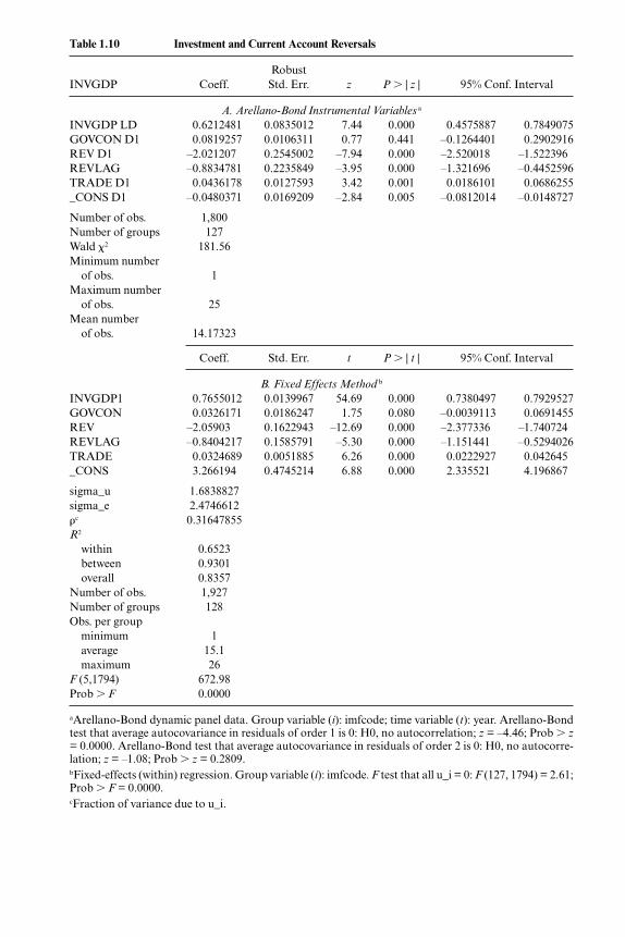
Table 1.10 Investment and Current Account Reversals
RobustINVGDP Coeff. Std. Err. z P � | z | 95% Conf. Interval
A. Arellano-Bond Instrumental Variables a
INVGDP LD 0.6212481 0.0835012 7.44 0.000 0.4575887 0.7849075GOVCON D1 0.0819257 0.0106311 0.77 0.441 –0.1264401 0.2902916REV D1 –2.021207 0.2545002 –7.94 0.000 –2.520018 –1.522396REVLAG –0.8834781 0.2235849 –3.95 0.000 –1.321696 –0.4452596TRADE D1 0.0436178 0.0127593 3.42 0.001 0.0186101 0.0686255_CONS D1 –0.0480371 0.0169209 –2.84 0.005 –0.0812014 –0.0148727
Number of obs. 1,800Number of groups 127Wald 2 181.56Minimum number
of obs. 1Maximum number
of obs. 25Mean number
of obs. 14.17323
Coeff. Std. Err. t P � | t | 95% Conf. Interval
B. Fixed Effects Method b
INVGDP1 0.7655012 0.0139967 54.69 0.000 0.7380497 0.7929527GOVCON 0.0326171 0.0186247 1.75 0.080 –0.0039113 0.0691455REV –2.05903 0.1622943 –12.69 0.000 –2.377336 –1.740724REVLAG –0.8404217 0.1585791 –5.30 0.000 –1.151441 –0.5294026TRADE 0.0324689 0.0051885 6.26 0.000 0.0222927 0.042645_CONS 3.266194 0.4745214 6.88 0.000 2.335521 4.196867
sigma_u 1.6838827sigma_e 2.4746612�c 0.31647855R2
within 0.6523between 0.9301overall 0.8357
Number of obs. 1,927Number of groups 128Obs. per group
minimum 1average 15.1maximum 26
F (5,1794) 672.98Prob � F 0.0000
aArellano-Bond dynamic panel data. Group variable (i): imfcode; time variable (t): year. Arellano-Bondtest that average autocovariance in residuals of order 1 is 0: H0, no autocorrelation; z = –4.46; Prob � z= 0.0000. Arellano-Bond test that average autocovariance in residuals of order 2 is 0: H0, no autocorre-lation; z = –1.08; Prob � z = 0.2809.bFixed-effects (within) regression. Group variable (i): imfcode. F test that all u_i = 0: F (127, 1794) = 2.61;Prob � F = 0.0000.cFraction of variance due to u_i.

heteroskedasticity. The results obtained are quite interesting. In both pan-els the coefficient of the lagged dependent variable is relatively high, cap-turing the presence of persistence. Notice, however, that the coefficient issignificantly smaller when the Arellano-Bond procedure is used. The co-efficient of GOVCON is positive and nonsignificant. The estimated coeffi-cient of trade openness is significant and positive, indicating that, after con-trolling for other factors, countries with a more open trade sector will tendto a higher investment-to-GDP ratio. More importantly for this paper, thecoefficients of the contemporaneous and lagged reversal indicator are sig-nificantly negative, with very similar point estimates. Interestingly, whenthe REVERSAL variable was added with a two-year lag, its estimated co-efficient was not significant at conventional levels.
In order to check for the robustness of these results, I also estimatedequation (10) using alternative samples and definitions of current accountreversals. The results obtained provide a strong support to those shownhere and indicate that, indeed, current account reversals have affected eco-nomic performance negatively through the investment channel. An impor-tant question is whether the compression in investment is a result of privateor public sector behavior. An analysis undertaken on a smaller sample(forty-four countries) suggests that, although both private- and public-sec-tor investment are negatively affected by current account reversals, the im-pact is significantly higher on private investment. According to these esti-mates, available from the author, a current account reversal results in adecline in private investment equal to 1.8 percent of GDP; the long-term re-duction of public-sector investment is estimated to be, on average, 0.5 per-cent of GDP.
An important question is whether current account reversals have affectedeconomic growth through other channels. I investigated this issue by usingthe large data set to estimate a number of basic growth equations of the fol-lowing type.
(11) GROWTHtj � � INVGDPtj � δ GOVCONStj
GROWTHtj � � TRADE_OPENNESStj � θ LOGGDPOj
� γ REVERSALtj � ξtj ,
where GROWTHtj is growth of GDP per capita in country j during year t,and LOGGDPOj is the initial level of GDP (1970) for country j. As Barroand Sala-i-Martin (1995) have pointed out, the coefficient of GOVCONS isexpected to be negative, while that of openness is expected to be positive. Ifthere is a catching-up in growth, we would expect that the estimated coeffi-cient of the logarithm of 1970 GDP per capita will be negative. The main in-terest of this analysis is the coefficient of REVERSAL. If sharp and largereductions in the current account deficit have a negative effect on invest-ment, we would expect the estimated γ to be significantly negative. The er-
Does the Current Account Matter? 51

ror ξtj is assumed to be heteroskedastic, with a different variance for eachcountry (panel). Thus, assuming k panels (countries):
E(ξξ�) �
�σ2
1I 0 . . . 0
�0 σ22I . . . 0
. . . .
. . . .
. . . .
0 0 . . . σ2kI
Equation (12) was estimated using the feasible generalized least squaresprocedure (FGLS) suggested by Beck and Katz (1995) for unbalanced pan-els. The samples in the different estimations were determined by the avail-ability of data on the different regressors. The data were obtained from theWorld Bank and from the Summer and Hestons data set. In the base esti-mates I used the definition of current account reversals given by Reversal1above. The basic results obtained from the estimation of equation (11) arepresented in table 1.11. In addition to the regressors in equation (11), I in-troduced time-specific dummy variables. As may be seen from the table, theresults obtained support the hypothesis that current account reversals havehad a negative effect on GDP per capita growth, even after controlling byinvestment. Moreover, the coefficients for the other variables in the regres-sion have the expected signs and are significant at conventional levels.When alternative estimation techniques were used, including fixed effects,the results obtained were very similar.20
1.5 Current Account Deficits and Financial Crises: How Strong Is the Link?
As we pointed out in section 1.2 of this paper, a large number of recentempirical studies have been unable to find a strong and significant connec-tion between large current account deficits and financial crises (Frankel andRose 1996). However, much of the policy literature—both from investmentbanks and from the multilateral institutions—insists that large deficits havebeen at the center of recent crises. In this section, I address this issue by an-alyzing in some detail the evidence on financial crises in a large cross sectionof countries. The section is organized as follows: In section 1.5.1, I deal withthe definition of crisis. In section 1.5.2, I provide some preliminary evidenceon the connection between current account reversals and crises, as wellas between high current account deficits and crises. In this analysis I use
52 Sebastian Edwards
20. Naturally, when fixed effects are used it is not possible to include (the log of) initial GDPas a regressor.
(12) E(ξξ�) �
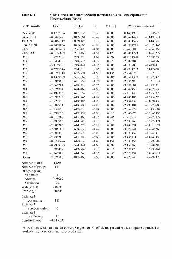
Table 1.11 GDP Growth and Current Account Reversals: Feasible Least Squares withHeteroskedastic Panels
GDP Growth Coeff. Std. Err. z P � | z | 95% Conf. Interval
INVGDP 0.1732786 0.0129535 13.38 0.000 0.1478901 0.198667GOVCON –0.044147 0.0129061 –3.42 0.001 –0.0694425 –0.0188514TRADE 0.0066118 0.0021185 3.12 0.002 0.0024595 0.010764LOGGPP0 –0.7458834 0.0754805 –9.88 0.000 –0.8938225 –0.5979443REV –0.8387433 0.2063497 –4.06 0.000 –1.243181 –0.4343053REVLAG –0.3106008 0.2014468 –1.54 0.123 –0.7054293 0.0842277D73 1.270318 0.759329 1.67 0.094 –0.2179398 2.758575D74 –1.342419 0.7482716 –1.79 0.073 –2.809004 0.1241666D75 –3.115973 0.7482444 –4.16 0.000 –4.582505 –1.649441D76 0.6267746 0.7248618 0.86 0.387 –0.7939283 2.047478D77 –0.9757318 0.6522791 –1.50 0.135 –2.254175 0.3027116D78 0.1379759 0.5050662 0.27 0.785 –0.8519357 1.127887D79 –1.096983 0.6317958 –1.74 0.083 –2.33528 0.1413142D80 –2.360201 0.6280218 –3.76 0.000 –3.591101 –1.129301D81 –2.826354 0.6242467 –4.53 0.000 –4.049855 –1.602853D82 –4.194326 0.6217559 –6.75 0.000 –5.412945 –2.975707D83 –2.990355 0.6199746 –4.82 0.000 –4.205483 –1.775227D84 –1.221758 0.6185186 –1.98 0.048 –2.434032 –0.0094836D85 –1.784731 0.6187208 –2.88 0.004 –2.997401 –0.5720605D86 –1.75282 0.617261 –2.84 0.005 –2.962629 –0.5430107D87 –1.596635 0.6173792 –2.59 0.010 –2.806676 –0.3865935D88 –0.7132081 0.6150168 –1.16 0.246 –1.918619 0.4922027D89 –1.492796 0.6147887 –2.43 0.015 –2.69776 –0.2878324D90 –2.005303 0.6140373 –3.27 0.001 –3.208794 –0.8018121D91 –2.686583 0.6082038 –4.42 0.000 –3.878641 –1.494526D92 –2.38132 0.6155925 –3.87 0.000 –3.587859 –1.17478D93 –2.23038 0.6150288 –3.63 0.000 –3.435814 –1.024945D94 –0.8790476 0.6164939 –1.43 0.154 –2.087353 0.3292582D95 –0.9938183 0.5940141 –1.67 0.094 –2.158065 0.170428D96 –1.480438 0.6129868 –2.42 0.016 –2.68187 –0.2790063D97 –1.263988 0.6449348 –1.96 0.050 –2.528037 0.0000611_Cons 7.826786 0.8179467 9.57 0.000 6.22364 9.429932
Number of obs. 1,856Number of groups 111Obs. per group
Minimum 1Average 19.28987Maximum 26
Wald 2 (31) 708.80Prob � 2 0.0000
Estimated covariances 111
Estimated autocorrelations 0
Estimated coefficients 32
Log-likelihood –4.913.651
Notes: Cross-sectional time-series FGLS regression. Coefficients: generalized least squares; panels: het-eroskedastic; correlation: no autocorrelation.

statistical methods borrowed from the epidemiology literature. Finally, insection 1.5.3, I provide some empirical results, obtained using econometrictechniques, on the relationship between large current account deficits andfinancial crises. I argue that whether one finds a connection depends largelyon three factors: (1) the definition of crisis, (2) the sample considered, and(3) the lag structure used in the analysis.
1.5.1 Defining a Crisis
Paul Krugman has recently said that “there is no generally accepted for-mal definition of a currency crisis, but we know them when we see them”(Krugman 2000, 1). While some authors, including myself in Edwards(1989) and Edwards and Santaella (1993), have defined a currency crisis asa very significant depreciation of the currency (see also Frankel and Rose1996 and Milesi-Ferretti and Razin 2000) others have defined a crisis as asituation in which a country’s currency is depreciated or its international re-serves are seriously depleted (Eichengreen, Rose, and Wyplosz 1996; Gold-stein, Kaminsky, and Reinhart 2000). In this paper, and in order to cast avery wide net in the empirical analysis, I have used two alternative criteriafor defining crises.
The first definition follows Frankel and Rose (1996) and defines a cur-rency crisis as a situation in which there is a currency depreciation of at least25 percent as well as a 10 percent increase in the rate of depreciation. I callthis variable aevent.21 The second definition is broader, and includes ascrises situations in which the country in question has experienced a large de-preciation or a significant loss in reserves. In constructing this variable,which I call acrisis, I followed a three-step procedure:
1. I created a weighted average index of monthly rate of change of the ex-change rate (∆e/e) and of reserves (∆R/R), such that both components ofthe index have equal sample volatility: It � ∆e /e – (σe /σR ) (∆R/R).
2. I define a crisis (Ct ) to have taken place when the index exceeds themean of the index plus three standard deviations:
Ct � �1 if It ≥ mean (It ) � 3σI
0 otherwise
3. I annualized the crisis index by considering each year as a June-Juneperiod. In other words, a year t is assigned a crisis (�1) if any month be-tween June of year t and June of year t � 1 is a crisis.
As Milesi-Ferretti and Razin (2000) have pointed out, results from crisisanalyses may be affected by the treatment of currency upheaval in consec-utive years. In order to address this issue, I defined two additional crisis
54 Sebastian Edwards
21. The index was constructed on monthly data. In order to annualize it, I consider June-to-June years.

indicators that exclude adjacent “crises.” These indicators consider a three-year window after each crisis: aevent2 is the three-year window correspon-ding to aevent, and acrisis2 is the corresponding indicator for acrisis.
How frequent have currency crises taken place, according to these indi-cators? This question is addressed in table 1.12, where I present tabulationsfor the four indexes for the complete sample. As may be seen, the frequencyof “crises” goes from 4 percent to 11 percent of the country-year observa-tions. In terms of the distribution across regions (the results are not pre-sented in detail due to space considerations) according to both aevent indi-cators, crises have had a higher frequency in Eastern Europe; the lowestfrequency is in the industrialized nations, with no crises recorded. The acri-sis index records a frequency at approximately 10 percent in Latin America,Asia, and Africa; the acrisis2 index shows that the highest frequency ofcrises has been in Africa, with a 13.7 percent frequency of occurrence.
1.5.2 Current Account Reversals and Crises: A Preliminary Analysis
An important finding from the preceding analysis is that current accountreversals are common and quite frequent. Countries in every region tend torun deficits that occasionally exceed their long-run sustainable level. Thismeans that, as documented above, at some point the country must gothrough an adjustment process in which the current account deficit is re-versed and moves closer to its long-run equilibrium. From a policy perspec-tive, it is important to understand whether current account reversals arerelated to currency crises. In order to address this issue, I followed a
Does the Current Account Matter? 55
Table 1.12 Frequency of Crises: Alternative Indicators
Frequency Percent Cumulative
aevent: (mean) event0 2818 94.09 94.091 177 5.91 100.00Total 2995 100.00
aevent20 2318 95.79 95.791 102 4.21 100.00Total 2420 100.00
acrisis: (mean) crisis0 2548 90.26 90.261 275 9.74 100.00Total 2823 100.00
acrisis20 1564 88.91 88.911 195 11.09 100.00Total 1759 100.00
Source: Author’s calculations.Note: See the text for the exact definition of these indicators.

case-control methodology.22 This approach consists of using a 2 statistic toformally test whether there is a significant relationship between a particularoutcome (the case) and another variable to which both case and control vari-ables have been exposed. The first step in applying this approach, then, is toseparate observations into a case group and a control group. A country thatfor a given year experienced a “crisis” is considered to be a case, and noncri-sis observations constitute the control group. The second step consists of cal-culating how many observations in both the case and control groups havebeen subject to a current account reversal. From this information an odds ra-tio is computed, and a 2 test is computed in order to determine whether theodds ratio is significantly different from 1. If the null hypothesis cannot be re-jected, then there is evidence supporting the hypothesis that countries thatare subject to a reversal have a significant probability of experiencing a crisis.
The computation of the 2 test statistic using contemporaneous values ofcrisis and reversals results in the rejection of the null hypothesis that reversalcountries are associated with a crisis. This result holds for all four definitionsof a crisis. The p-values of the 2 tests are on the order of 0.6, or higher. Thisresult is consistent with the conclusions reached through a less formal anal-ysis, and using a smaller data set, by Milesi-Ferretti and Razin (2000).
A possible limitation of a simple application of this 2 test, however, isthat from a theoretical point of view the relationship between reversals andcrises implies complex timing and causality issues. In fact, there are reasonsto believe that reversals may occur at the same time as a crisis, before a cri-sis, or even after a crisis. For instance, the reversal may be so pronouncedthat the country in question has no alternative but to devalue its currencyor deplete its international reserves. There is no reason, however, why thesephenomena would take place at exactly the same time. Also, the reversalmay be the result, rather than the cause, of a devaluation. For this reason, Ialso asked whether there is statistical evidence that there is a current ac-count reversal in the “neighborhood” of a crisis. In order to do this, I definea new variable, reversaln, that takes a value of one on the year a reversal wasdetected, as well as in the previous and next years. The results from this sec-ond test suggest that it is not possible to reject the null hypothesis that cur-rency crises occur “in the neighborhood of” current account reversals. Thisis the case for any of the four crisis definitions used in this study. In table 1.13I present the results obtained from the computation of these 2 statisticswhen the aevent definition of crisis was considered as the “case.” In order toillustrate the nature of the results I have presented the 2 corresponding totwo definitions of reversals. In part A I used the narrow one-year definitionof reversal, while in part B I use the broader three-year neighborhood defi-nition of reversal. As may be seen, although in part A the 2 test is not sig-
56 Sebastian Edwards
22. This approach is used frequently by epidemiologists. I became interested in the statisti-cal techniques used by epidemiologists while doing research on financial crisis contagion acrosscountries (see Edwards 2000). See Fleiss (1981) for details on the actual case-control method.

nificant, in part B it is highly significant—the p-value is 0.009.23 Results ob-tained for the other three definitions of a crisis are very similar and are avail-able from the author on request.
1.5.3 Current Account Deficits and Currency Crises: A Formal Analysis
In a recent and influential paper, Frankel and Rose (1996) empirically an-alyzed the determinants of currency crashes. Their data set included 105countries for the period 1970–91, and their definition of a crisis was con-fined to devaluations in excess of 25 percent.24 The results from their probit
Does the Current Account Matter? 57
Table 1.13 Case-Control �2 Test: Analysis of Crisis and Current Account Reversals(for Aevent definition of crisis)
ProportionExposed Unexposed Total Exposed
A. Exposed: Reversal1 definition of current account reversal a
Cases 28 124 152 0.1842Controls 410 1,793 2,203 0.1861Total 438 1,917 2,355 1.1860
Point Estimate 95% Conf. Interval
Odds ratio (Cornfield) 0.9874902 0.6481554 1.504718
Prev. frac. ex. (Cornfield) 0.0125098 –0.504718 0.3518446
Prev. frac. pop 0.0023282
ProportionExposed Unexposed Total Exposed
B. Exposed: Reversaln1 definition of current account reversal b
Cases 52 35 87 0.5977Controls 563 679 1,242 0.4533Total 615 714 1,329 0.4628
Point Estimate 95% Conf. Interval
Odds ratio (Cornfield) 1.791829 1.15408 2.718784
Attr. frac. ex. (Cornfield) 0.4419112 0.1335086 0.6405185
Attr. frac. pop. 0.2641308
Source: Computed by the author.Note: Prev. = previous; frac. = fraction; ex. = explained; pop. = population; attr. = attributed.a2 (1) = 0.00; Prob. � 2 = 0.9536.b2 (1) = 6.82; Prob. � 2 = 0.0090.
23. These results, however, should be interpreted with caution, as they are subject to all thelimitations of this type of case-control analysis, including the fact that no causality can be es-tablished. In this case, however, I am not particularly interested in causation.
24. See section 1.5.1 for a discussion of their definition.

regression analysis indicated that a number of variables were good predic-tors of a currency crash. These included the fraction of the debt obtained inconcessional terms, the ratio of foreign direct investment (FDI) to GDP, thereserves-to-imports ratio, the rate of growth of domestic credit, the coun-try’s rate of growth, and international interest rates. In terms of the presentpaper, what is particularly interesting is that in Frankel and Rose (1996) thecurrent account deficit was not significant, and in many of the regressionsit even had the wrong sign. This led the authors to conclude that, “curiously,neither current account nor government budget deficits appear to play animportant role in a typical crash” (365).25
My own initial analysis of the determinants of crises, using an almostidentical data set, supports the results reported by Frankel and Rose (1996).When a broad sample and their regressors are used, the current accountseems to play no role in major currency crashes.26 This is the case indepen-dently of the estimation technique used, and of whether the actual value ofthe current account deficit or a dummy for high deficits is included as a re-gressor. To my surprise, the incorporation of an independent variable thatinteracted the fiscal and current account deficits (the “twin” deficits) didnot change the result.
In order to investigate this issue further, and in an effort to determine therobustness of these results, I followed four avenues of analysis: First, I in-quired whether the results would hold under alternative data sets. In partic-ular, I investigated whether the exclusion of particular regions would alterthe finding of current account “irrelevance.” Second, I considered alternativesets of independent variables in the estimation of probit equations for crises.In particular I considered alternative lag structures, and I included somevariables that capture the economic structure of the countries in the sample.Third, I considered alternative definitions of crisis. More specifically, I esti-mated a number of probit equations for all four definitions of crisis describedin subsection 1.5.1 of this paper: aevent, aevent2, acrisis, and acrisis2. Fourth,I used different estimation techniques and considered assumptions regard-ing the nature of the error term, including the assumption that it takes a ran-dom effect form. Generally speaking, the results obtained were not affectedby the technique used, and for this reason I only report the basic results.
In the estimation of crisis models I used the following regressors:27
(1) percentage of debt in commercial terms; (2) percentage of debt in con-cessional terms; (3) percentage of debt at variable rate; (4) percentage ofshort-term debt; (5) FDI; (6) public-sector debt as percentage of GDP; (7)debt to the multilateral institutions; (8) the ratio of (gross) international re-serves to imports; (9) the ratio of foreign debt to GDP; (10) the rate of
58 Sebastian Edwards
25. This finding is not affected by any of the sensitivity tests undertaken by the authors.26. By “broad sample” I mean one that includes all regions in the world.27. Most, but not all, of these regressors were used by Frankel and Rose (1996). The results
reported here are not directly comparable to those of Frankel and Rose (1996), since the datasets are somewhat different.

growth of domestic credit; (11) deviations of the real exchange rate fromPPP (a measure of “overvaluation”); (12) the rate of growth of GDP; (13)the degree of openness of the economy, measured as imports plus exportsdivided by GDP; (14) the ratio of government expenditure to GDP; (15) in-terest rates in the advanced countries; and (16) the current account deficit.All the variables are from the World Bank and, as in the Frankel and Rose(1996) paper, cover the 1971–92 period. With the exception of the crisis in-dexes, trade openness, and government consumption, these variables cor-respond to those used by Frankel and Rose (1996).
In reporting the regressions, I follow the tradition of presenting theeffects of a unitary change in the independent variables on the probabilityof a crisis. In all of the regressions I report White’s robust standard errorsthat correct for heteroskedasticity.
The results obtained when all variables are entered contemporaneouslyand all regions are included are presented in table 1.14. The results are quiteinteresting and, to a large extent, in agreement with expectations. In termsof the current account—the variable of greatest interest in this paper—theresults show significant differences, depending on the definition of crisisused. For both the acrisis and acrisis2 indicators, the estimated coefficientof the current account deficit to GDP is positive and significant at the 10percent level. On the other hand, when the aevent and aevent2 currencycrash indicators are used as the dependent variable, the estimated coeffi-cients of the current account deficits are not significant, and in the case ofaevent2, the sign is incorrect (although it is not significantly different fromzero). Of course, the results for the events correspond to the Frankel andRose (1996) findings discussed above. In terms of the other regressors, theresults in table 1.14 suggest that higher reserves and higher growth reducethe probability of both types of crisis. Large FDI plays a particularly im-portant role in reducing the probability of an event type of crisis. A high per-centage of debt in commercial terms increases the probability of both typesof crisis. A greater degree of openness reduces the probability under all cri-sis definitions. Notice that in contrast with the Frankel and Rose (1996) re-sults, a higher public deficit ratio significantly increases the probability ofaevent-type crises.
The results presented in table 1.14 were obtained using a data set that cov-ers every region. There are, however, important reasons to believe that(most) African countries have behaved differently during the period understudy. This is the case for two reasons: First, during the complete period un-der analysis a large number of African nations belonged to the CFA cur-rency zone and were institutionally shielded from devaluations. Second, itis well known that during most of this period even non-CFA African na-tions had a great reluctance to adjust their parity. This was the case evenwhen the external imbalance was very large (World Bank 1994). An impor-tant question, then, is how these results will be affected if the African na-tions are excluded from the sample. This is done in table 1.15, where probit
Does the Current Account Matter? 59
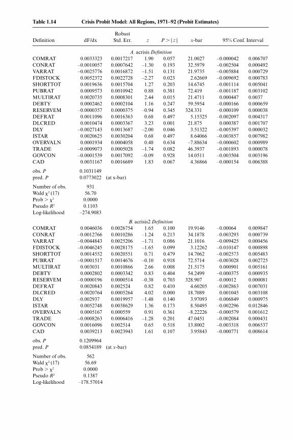
Table 1.14 Crisis Probit Model: All Regions, 1971–92 (Probit Estimates)
RobustDefinition dF/dx Std. Err. z P � | z | x-bar 95% Conf. Interval
A. acrisis DefinitionCOMRAT 0.0033323 0.0017217 1.90 0.057 21.0027 –0.000042 0.006707CONRAT –0.0010057 0.0007642 –1.30 0.193 32.5979 –0.002504 0.000492VARRAT –0.0025776 0.0016872 –1.51 0.131 21.9735 –0.005884 0.000729FDISTOCK 0.0052372 0.0022728 –2.27 0.023 2.62669 –0.009692 0.000783SHORTTOT 0.0019636 0.0015704 1.27 0.203 14.6745 –0.001114 0.005041PUBRAT 0.0009573 0.0010942 0.88 0.381 72.419 –0.001187 0.003102MULTIRAT 0.0020735 0.0008301 2.44 0.015 21.4711 0.000447 0.0037DEBTY 0.0002462 0.0002104 1.16 0.247 59.5954 –0.000166 0.000659RESERVEM –0.0000357 0.0000375 –0.94 0.345 324.331 –0.000109 0.000038DEFRAT 0.0011096 0.0016363 0.68 0.497 5.15325 –0.002097 0.004317DLCRED 0.0010474 0.0003367 3.23 0.001 21.875 0.000387 0.001707DLY –0.0027143 0.0013687 –2.00 0.046 3.51322 –0.005397 0.000032ISTAR 0.0020625 0.0030204 0.68 0.497 8.64066 –0.003857 0.007982OVERVALN 0.0001934 0.0004058 0.48 0.634 –7.88634 –0.000602 0.000989TRADE –0.0009073 0.0005028 –1.74 0.082 46.3937 –0.001893 0.000078GOVCON –0.0001539 0.0017092 –0.09 0.928 14.0511 –0.003504 0.003196CAD 0.0031167 0.0016689 1.83 0.067 4.36866 –0.000154 0.006388
obs. P 0.1031149pred. P 0.0773022 (at x-bar)
Number of obs. 931Wald 2 (17) 56.70Prob � 2 0.0000Pseudo R2 0.1103Log-likelihood –274.9083
B. acrisis2 DefinitionCOMRAT 0.0046036 0.0026754 1.65 0.100 19.9146 –0.00064 0.009847CONRAT –0.0012766 0.0010286 –1.24 0.213 34.1878 –0.003293 0.000739VARRAT –0.0044843 0.0025206 –1.71 0.086 21.1016 –0.009425 0.000456FDISTOCK –0.0046245 0.0028175 –1.65 0.099 3.12262 –0.010147 0.000898SHORTTOT 0.0014552 0.0020551 0.71 0.479 14.7062 –0.002573 0.005483PUBRAT –0.0001517 0.0014676 –0.10 0.918 72.5714 –0.003028 0.002725MULTIRAT 0.003031 0.0010866 2.66 0.008 21.5175 0.000901 0.005161DEBTY 0.0002802 0.0003342 0.83 0.404 54.2499 –0.000375 0.000935RESERVEM –0.0000196 0.0000514 –0.38 0.703 328.907 –0.00012 0.000081DEFRAT 0.0020843 0.002524 0.82 0.410 4.60205 –0.002863 0.007031DLCRED 0.0020764 0.0005264 4.02 0.000 18.7089 0.001045 0.003108DLY –0.002937 0.0019957 –1.48 0.140 3.97093 –0.006849 0.000975ISTAR 0.0052748 0.0038629 1.36 0.173 8.50495 –0.002296 0.012846OVERVALN 0.0005167 0.000559 0.91 0.361 –8.22226 –0.000579 0.001612TRADE –0.0008263 0.0006416 –1.28 0.201 47.0451 –0.002084 0.000431GOVCON 0.0016096 0.002514 0.65 0.518 13.8002 –0.003318 0.006537CAD 0.0039213 0.0023943 1.61 0.107 3.95843 –0.000771 0.008614
obs. P 0.1209964pred. P 0.0854189 (at x-bar)
Number of obs. 562Wald 2 (17) 56.69Prob � 2 0.0000Pseudo R2 0.1387Log-likelihood –178.57014

Table 1.14 (continued)
RobustDefinition dF/dx Std. Err. z P � | z | x-bar 95% Conf. Interval
C. aevent DefinitionCOMRAT 0.0003686 0.0008709 0.42 0.671 20.962 –0.001338 0.002075CONRAT –0.000823 0.0004234 –1.82 0.069 32.6715 –0.001653 6.9e–06VARRAT –0.0007301 0.0008421 –0.86 0.388 21.9302 –0.002381 0.000921FDISTOCK –0.0033417 0.0012196 –2.69 0.007 2.62084 –0.005732 –0.000951SHORTTOT –0.0000499 0.0008731 –0.06 0.955 14.6571 –0.001761 0.001661PUBRAT –0.0001298 0.0006229 –0.21 0.836 72.4703 –0.001351 0.001091MULTIRAT –0.0002948 0.0005312 –0.56 0.578 21.4961 –0.001336 0.000746DEBTY 0.0002863 0.0001209 2.49 0.013 59.7336 0.000049 0.000523RESERVEM –0.0000194 0.0000197 –1.01 0.315 325.061 –0.000058 0.000019DEFRAT 0.0016828 0.0009088 1.85 0.065 5.21531 –0.000098 0.003464DLCRED 0.0004128 0.0002005 2.53 0.012 21.8889 0.000026 0.000812DLY –0.001096 0.0008227 –1.34 0.179 3.51907 –0.002708 0.000516ISTAR –0.0000236 0.0017433 –0.01 0.989 8.63804 –0.00344 0.003393OVERVALN –0.0003881 0.0002363 –1.64 0.102 –7.82043 –0.000851 0.000075TRADE –0.001114 0.0003071 –3.06 0.002 46.3682 –0.001716 –0.000512GOVCON –0.0037107 0.0012011 –2.97 0.003 14.071 –0.006065 –0.001357CAD 0.0003098 0.0010221 0.30 0.764 4.37692 –0.001693 0.002313
obs. P 0.0706638pred. P 0.0296255 (at x-bar)
Number of obs. 934Wald 2 (17) 70.66Prob � 2 0.0000Pseudo R2 0.2072Log-likelihood –189.0942
D. aevent2 DefinitionCOMRAT –0.000135 0.0009079 –0.15 0.883 19.8866 –0.001914 0.001644CONRAT –0.0003336 0.000392 –0.85 0.395 35.0182 –0.001102 0.000435VARRAT 7.77e–06 0.0008146 0.01 0.992 20.4507 –0.001589 0.001604FDISTOCK –0.0015405 0.0009866 –1.62 0.104 3.08108 –0.003474 0.000393SHORTTOT 0.0005935 0.0007601 0.81 0.416 14.3259 –0.000896 0.002083PUBRAT 0.000125 0.0005304 0.24 0.810 72.7421 –0.000914 0.001164MULTIRAT –0.0004797 0.0005018 –0.94 0.349 22.8628 –0.001463 0.000504DEBTY 0.0002004 0.0001292 1.62 0.105 54.0278 –0.000053 0.000454RESERVEM –0.0000252 0.0000191 –1.38 0.166 328.073 –0.000063 0.000012DEFRAT 0.0022043 0.0010298 2.11 0.035 4.93033 0.000186 0.004223DLCRED 0.0005069 0.000229 2.74 0.006 18.4827 0.000058 0.000956DLY –0.0015771 0.0008004 –1.90 0.057 4.18559 –0.003146 –8.3e–06ISTAR 0.0000685 0.0014788 0.05 0.963 8.62569 –0.00283 0.002967OVERVALN –0.0001668 0.0002045 –0.84 0.402 –7.73555 –0.000568 0.000234TRADE –0.0007145 0.0002938 –2.41 0.016 48.7758 –0.00129 –0.000139GOVCON –0.0028422 0.001161 –2.20 0.028 14.5617 –0.005118 –0.000567CAD –0.0007552 0.0009831 –0.79 0.432 4.27947 –0.002682 0.001172
obs. P 0.0555556pred. P 0.0206342 (at x-bar)
Number of obs. 702Wald 2 (17) 48.97Prob � 2 0.0001Pseudo R2 0.2208Log-likelihood –117.36778
Notes: Probit estimates. The tests that the underlying coefficient is 0 are z and P � | z |.

Table 1.15 Probit Model of Currency Crises, Africa Excluded, 1971–92 (Probit Estimates)
RobustDefinition dF/dx Std. Err. z P � | z | x-bar 95% Conf. Interval
A. acrisis DefinitionCOMRAT 0.0029271 0.0020359 1.42 0.157 26.3123 –0.001063 0.006917CONRAT –0.0012155 0.0008973 –1.32 0.186 28.4099 –0.002974 0.000543VARRAT –0.0020405 0.0019753 –1.02 0.306 27.1534 –0.005912 0.001831FDISTOCK –0.005784 0.0024845 –2.24 0.025 3.17666 –0.010653 0.000915SHORTTOT 0.0016729 0.002148 0.81 0.418 15.9367 –0.002537 0.005883PUBRAT 0.0014678 0.0013265 1.13 0.258 69.9099 –0.001132 0.004068MULTIRAT 0.0026282 0.000894 2.77 0.006 19.8038 0.000876 0.00438DEBTY 3.91e–06 0.0003489 0.01 0.991 53.1143 –0.00068 0.000688RESERVEM –7.38e–06 0.0000403 –0.18 0.855 412.658 –0.000086 0.000072DEFRAT 0.0010166 0.0019793 0.52 0.606 4.5621 –0.002863 0.004896DLCRED 0.0008556 0.0003243 2.85 0.004 25.8435 0.00022 0.001491DLY –0.0021348 0.0017565 –1.24 0.215 3.8471 –0.005577 0.001308ISTAR 0.0026776 0.0036062 0.73 0.466 8.48895 –0.00439 0.009746OVERVALN –0.0000309 0.0005285 –0.06 0.953 –5.23607 –0.001067 0.001005TRADE –0.0010877 0.0006823 –1.48 0.140 47.171 –0.002425 0.00025GOVCON 0.0017909 0.0023691 0.76 0.448 13.3222 –0.002852 0.006434CAD 0.0048408 0.0021958 2.08 0.037 3.62618 0.000537 0.009145
obs. P 0.1075085pred. P 0.0718758 (at x-bar)
Number of obs. 586Wald 2 (17) 47.59Prob � 2 0.0001Pseudo R2 0.1381Log-likelihood –172.36345
B. acrisis2 DefinitionCOMRAT 0.004239 0.0031281 1.27 0.203 25.0805 –0.001892 0.01037CONRAT –0.0013723 0.0013069 –1.08 0.279 30.3854 –0.003934 0.001189VARRAT –0.0049427 0.0028411 –1.67 0.095 26.3258 –0.010511 0.000626FDISTOCK –0.0015863 0.0024665 –0.65 0.515 3.68785 –0.006421 0.003248SHORTTOT 0.001403 0.0024508 0.57 0.569 16.3144 –0.003401 0.006207PUBRAT –0.0001419 0.001806 –0.08 0.937 69.3619 –0.003682 0.003398MULTIRAT 0.003184 0.0011121 2.54 0.011 19.659 0.001004 0.005364DEBTY 0.0001755 0.0006922 0.25 0.800 47.3123 –0.001181 0.001532RESERVEM 0.0000193 0.0000523 0.37 0.709 418.177 –0.000083 0.000122DEFRAT 0.0015161 0.0030651 0.49 0.625 3.85896 –0.004491 0.007524DLCRED 0.0016191 0.0005431 3.02 0.003 22.0399 0.000555 0.002684DLY –0.0028787 0.0026685 –1.12 0.261 4.74403 –0.008109 0.002352ISTAR 0.0047575 0.0043004 1.12 0.264 8.25318 –0.003671 0.013186OVERVALN 0.004106 0.0006962 0.59 0.555 –3.96003 –0.000954 0.001775TRADE –0.0019974 0.0007404 –2.51 0.012 48.4653 –0.003448 –0.000546GOVCON 0.0074273 0.0029808 2.69 0.007 12.9495 0.001585 0.01327CAD 0.0066269 0.0030252 2.15 0.032 2.94552 0.000698 0.012556
obs. P 0.1232092pred. P 0.0684454 (at x-bar)
Number of obs. 349Wald 2 (17) 56.33Prob � 2 0.0000Pseudo R2 0.2104Log-likelihood –102.86684

Table 1.15 (continued)
RobustDefinition dF/dx Std. Err. z P � | z | x-bar 95% Conf. Interval
C. aevent DefinitionCOMRAT 0.0005594 0.0009588 0.58 0.561 26.2654 –0.00132 0.002439CONRAT –0.0004993 0.0005171 –0.89 0.373 28.4811 –0.001513 0.000514VARRAT –0.0002586 0.000949 –0.27 0.787 27.1044 –0.002119 0.001601FDISTOCK –0.0029753 0.0012766 –2.27 0.023 3.16641 –0.005477 0.000473SHORTTOT 0.0009613 0.0011325 0.91 0.363 15.9162 –0.001258 0.003181PUBRAT 0.0012306 0.0008209 1.71 0.086 69.9671 –0.000378 0.00284MULTIRAT –0.0006806 0.0006162 –1.21 0.227 19.7912 –0.001888 0.000527DEBTY 0.0000792 0.0001567 0.51 0.613 53.3316 –0.000228 0.000386RESERVEM –0.0000334 0.0000222 –1.57 0.115 412.677 –0.000077 0.00001DEFRAT 0.0011607 0.0009477 1.19 0.233 4.61603 –0.000697 0.003018DLCRED 0.0002325 0.0001554 1.85 0.064 25.8675 –0.000072 0.000537DLY –0.0015439 0.0009927 –1.73 0.084 3.85051 –0.003489 0.000402ISTAR 0.0001112 0.0019632 0.06 0.955 8.4883 –0.003737 0.003959OVERVALN –0.0003815 0.0002373 –1.49 0.137 –5.18871 –0.000847 0.000084TRADE –0.0010118 0.0003537 –2.52 0.012 47.1363 –0.001705 0.000318GOVCON –0.0021182 0.0012636 –1.57 0.116 13.35 –0.004595 0.000358CAD 0.0018845 0.0011319 1.62 0.105 3.64741 –0.000334 0.004103
obs. P 0.0748299pred. P 0.0253162 (at x-bar)
Number of obs. 588Wald 2 (17) 64.52Prob � 2 0.0000Pseudo R2 0.2262Log-likelihood –121.01338
D. aevent2 DefinitionCOMRAT –0.000477 0.0006752 –0.72 0.472 24.5388 –0.0018 0.000846CONRAT –0.0001558 0.0003666 –0.41 0.680 31.8778 –0.000874 0.000563VARRAT 0.0003588 0.0006383 0.57 0.569 24.764 –0.000892 0.00161FDISTOCK –0.0011275 0.0007419 –1.46 0.145 3.82585 –0.002582 0.000327SHORTTOT 0.0000871 0.0007133 0.12 0.901 15.8634 –0.001311 0.001485PUBRAT 0.0002927 0.0005123 0.63 0.529 69.6303 –0.000711 0.001297MULTIRAT –0.0011583 0.0005954 –2.48 0.013 21.8597 –0.002325 8.6e–06DEBTY 0.0001485 0.000146 1.05 0.295 45.5271 –0.000138 0.000435RESERVEM –0.000016 0.0000162 –1.10 0.271 427.66 –0.000048 0.000016DEFRAT 0.000573 0.0007951 0.71 0.476 4.27868 –0.000985 0.002131DLCRED 0.0000761 0.000141 0.61 0.541 21.1944 –0.0002 0.000353DLY –0.0013861 0.0008992 –1.99 0.046 4.62599 –0.003148 0.000376ISTAR –0.0002626 0.0011823 –0.22 0.823 8.3681 –0.00258 0.002055OVERVALN –0.0003454 0.0001643 –2.03 0.042 –4.5647 –0.000667 –0.000023TRADE –0.0008508 0.0003236 –3.50 0.000 50.8592 –0.001485 –0.000217GOVCON –0.0004142 0.0008319 –0.48 0.630 13.843 –0.002045 0.001216CAD 0.001496 0.0009603 1.62 0.105 3.12759 –0.000386 0.003378
obs. P 0.0636792pred. P 0.01217 (at x-bar)
Number of obs. 424Wald 2 (17) 44.63Prob � 2 0.0003Pseudo R2 0.2642Log-likelihood –73.926915
Notes: Probit estimates. The tests that the underlying coefficient is 0 are z and P � | z |.
regressions for our four crisis definitions are presented for a non-Africasample. As may be seen, when this is done, the estimated coefficient of thecurrent account deficit is positive and significant either at the 5 or 10 per-cent level. It is important to notice that what makes a difference here iswhether Africa is included in the sample. If instead of focusing on Africa Iuse GDP per capita as the key variable to split the sample, as Milesi-Ferrettiand Razin (2000) do, and I include only middle-income countries, the re-sults are not as distinct as those reported in table 1.15.
The results presented above follow Frankel and Rose (1996) and controlfor a number of variables, including the external debt ratio, capital flows inthe form of FDI, and international reserves. A problem with including thisgroup of controls, however, is that it becomes difficult to interpret the cur-rent account coefficient in the probit regressions. The reason for this is thatwe are not allowing the current account deficit to be financed through thetraditional channels: an increase in indebtness or a reduction in interna-tional reserves. In fact, in the results reported above, as well as in Frankeland Rose (1996), higher account deficits are being financed exclusively byan increase in non–debt-generating capital inflows. It is interesting to un-derstand, however, if an increase in the current account deficit that is fi-nanced by running up the debt or depleting international reserves increasesthe probability of a crisis. The results in table 1.16, which were obtainedwhen both reserves and debt are not included as controls, show that an in-crease in the current account deficit financed by traditional means indeedincreases the probability of an aevent type of crisis.28
As a final exercise, and in order to analyze the robustness of these results,I investigated whether they held under different lag structures for the re-gressors. In particular I considered the following structure: all debt vari-ables were entered contemporaneously, as were the structural variables, andthe country performance and policy variables were entered with a one-period lag. The results obtained indicate that when this alternative lag struc-ture is used, the coefficient of the current account deficit remains positiveand significant at conventional levels. When every regressor is entered withone lag, the coefficient of the current account deficit remains positive andsignificant. In that case, however, some of the debt variables became non-significant.
To sum up, the results presented in this section suggest that the effects oflarger current account deficits on crisis depend on both the definition of acrisis and on the regions of the world being covered. More specifically, theresults indicate that when the broader definitions acrisis and acrisis2 areused, a higher current account deficit increases the probability of crisis inthe larger sample. Higher current account deficits also increase the proba-
64 Sebastian Edwards
28. The results for an acrisis type of crisis are similar and are not reported here due to spaceconsiderations.

bility of aevent crises significantly when the African nations are excludedfrom the sample.
1.6 Concluding Remarks
The main question addressed in this paper is whether the current account“matters.” If this question is interpreted very narrowly, in the sense thatcountries with an arbitrarily defined large current account deficit almost in-evitably face a crisis, then the answer is no. If, however, it is interpreted morebroadly, as suggesting that there are costs involved in running very largedeficits, the research reported in this paper suggests that the answer is aqualified yes.29
Does the Current Account Matter? 65
Table 1.16 Crisis and the Current Account: Probit Estimates, Alternative Set of Controls(Africa Excluded, 1970–92)
RobustAevent dF/dx Std. Err. z P � | z | x-bar 95% Conf. Interval
COMRAT –0.0000411 0.0008099 –0.05 0.960 26.3022 –0.001629 0.001546CONRAT –0.0005226 0.000528 –0.93 0.354 28.4596 –0.001557 0.000512VARRAT 0.000294 0.000864 0.34 0.731 27.1331 –0.001399 0.001988FDISTOCK –0.0034274 0.0013471 –2.52 0.012 3.15382 –0.006068 –0.000787SHORTTOT 0.0009178 0.0011867 0.81 0.417 15.9153 –0.001408 0.003244PUBRAT 0.0012746 0.0008641 1.65 0.099 70.0393 –0.000419 0.002968MULTIRAT –0.0007383 0.0006296 –1.27 0.202 19.7436 –0.001972 0.000496DEFRAT 0.017021 0.000881 1.85 0.064 4.68826 –0.000025 0.003429DLCRED 0.0002103 0.0001511 1.66 0.096 26.0009 –0.000086 0.000506DLY –0.0018491 0.0010946 –1.87 0.062 3.83729 –0.003995 0.000296ISTAR 0.0003013 0.0020829 0.14 0.885 8.48095 –0.003781 0.004384OVERVALN –0.000391 0.0002352 –1.52 0.128 –5.48445 –0.000852 0.00007TRADE –0.0010849 0.0003564 –2.56 0.011 47.1491 –0.001783 –0.000386GOVCON –0.0019375 0.0012981 –1.43 0.153 13.455 –0.004482 0.000607CAD 0.0024955 0.001186 2.09 0.037 3.71074 0.000171 0.00482
obs. P 0.0761421pred. P 0.0279486 (at x-bar)
Number of obs. 591Wald 2 (17) 65.13Prob � 2 0.0000Pseudo R2 0.2198Log-likelihood –124.15434
Notes: Excludes reserves and debt. Probit estimates. The tests that the underlying coefficient is 0 are z andP � | z |.
29. Naturally, a major challenge in this work is defining what a “large” deficit means. In the-ory, “large” should mean “significantly larger than the sustainable level.” In practice, however,and as is shown in section 1.3 of this paper, existing sustainability models are not very useful,especially in a dynamic environment. For this reason, in this paper I have defined a “highdeficit” arbitrarily, as a deficit that for that year exceeds the 3rd quartile of the deficit distribu-tion for the region to which the country belongs.

The analysis presented in this paper has shown that large current accountdeficits tend not to be persistent. Very few countries run large deficits forfive years in a row, and only a handful have run large deficits for ten years ina row. As the analysis in section 1.4 of this paper suggests, the typical pat-tern of current account deficits is that countries that experience large im-balances do so for a limited time; after a while, these imbalances are re-duced, and a current account reversal is observed. In section 1.4 I analyzedin detail the consequences, in terms of economic performance, of currentaccount reversals using a large (unbalanced) panel of countries for 1970–97. Using recently developed econometric techniques, I found that, con-trary to what has been recently suggested, reversals do have a negative effecton economic performance. They negatively affect aggregate investment;moreover, even when I control for investment, the regression analysis sug-gests that reversals have a negative impact on GDP growth per capita.
In section 1.5 I addressed the narrower question of whether larger deficitsincrease the probability of a country experiencing a currency crisis. My re-sults suggest that the answer to this question depends on the definition of acrisis as well as on the sample used in the analysis. As the detailed explana-tion in that section indicates, my results show that when Africa is ex-cluded—and I argue that there are good reasons for doing so—an increasein the deficit raises the probability of a crisis, independently of how thisterm is defined. When the complete sample is used, higher deficits increasethe probability of broadly defined crises. They have no statistical effect onnarrowly defined crashes, however.
In sum, my conclusion is that, in spite of recent claims of the irrelevanceof current account deficits, the evidence provides rather strong support forthe view that, from a policy perspective, large deficits should be a cause forconcern. This does not mean, of course, that every large deficit leads to acrisis; nor does it mean that only when there is a large current accountdeficit can a crisis take place.
References
Ades, Alberto, and Federico Kaune. 1997. A new measure of current account sus-tainability for developing countries. New York: Goldman Sachs Emerging Mar-kets Economic Research.
Arellano, Manuel, and Stephen Bond. 1991. Estimation of dynamic models with er-ror components. Journal of the American Statistical Association 76:245–67.
Atkeson, Andrew, and Jose-Victor Rios-Rull. 1996. The balance of payments andborrowing constraints: An alternative view of the Mexican crisis. Federal ReserveBank of Minneapolis Staff Report no. 212.
Attanasio, Orazio P., Lucio Picci, and Antonello E. Scorcu. 2000. Saving, growth,and investment: A macroeconomic analysis using a panel of countries. Review ofEconomics and Statistics 82 (2): 182–211.
66 Sebastian Edwards

Bacchetta, Philippe, and Eric van Wincoop. 2000. Trade in nominal assets and net in-ternational capital flows. Journal of International Money and Finance 19 (1): 66–91.
Bank of Mexico. The Mexican Economy, various issues. Mexico City: Bank of Mex-ico.
Barro, Robert J., and Xavier Sala-i-Martin. 1995. Economic Growth. Cambridge:MIT Press.
Beck, Nathaniel, and Jonathan N. Katz. 1995. What to do (and not to do) with time-series cross-section data. American Political Science Review 89 (3): 124–47.
Blanchard, Olivier. 1983. Debt and the current account deficit in Brazil. In Finan-cial policies and the world capital market: The problem of Latin American countries,ed. Pedro Aspe-Armella, Rudiger Dornbusch, and Maurice Obstfeld, 95–109.Chicago: University of Chicago Press.
Bruno, Michael. 1995. Currency crises and collapses: Comment. Brookings Paperson Economic Activity, Issue no. 2:278–85.
Calvo, Guillermo A. 2000. Balance of payments crises in emerging markets: Largecapital inflows and sovereign governments. In Currency crises, ed. Paul Krugman,3–28. Chicago: University of Chicago Press.
Calvo, Guillermo A., Leonardo Leiderman, and Carmen Reinhart. 1993. Capitalinflows and real exchange rate appreciation in Latin America: The role of exter-nal factors. IMF Staff Papers 40 (March): 868–907.
Chang, Roberto, and Andres Velasco. 2000. Exchange-rate policy for developingcountries. American Economic Review 90 (2): 71–75.
Chase Manhattan Bank. 1997. Emerging markets after Thailand: Guilt by associa-tion or flattered by comparison? Unpublished report, October 1.
Cline, William R. 1988. International debt: Progress and strategy. Finance and De-velopment 25 (2): 9–11.
Cooper, Richard N. 1971a. Currency devaluation in developing countries. Prince-ton Studies in International Finance no. 86. Princeton University, Department ofEconomics, International Economics Section.
———. 1971b. Issues for trade policy in the seventies. Tübingen, Germany: Mohr.Corden, W. Max. 1994. Economic policy, exchange rates, and the international sys-
tem. Oxford: Oxford University Press.Corsetti, Giancarlo, Paolo Pesenti, and Nouriel Roubini. 1998. Paper tigers? A
model of the Asian crisis. Paper presented at the NBER-Bank of Portugal Inter-national Seminar on Macroeconomics. 14–15 June, Lisbon, Portugal.
Deutsche Bank. 2000. Global market research. New York: Deutsche Bank. March.Dornbusch, Rudiger. 2000. Keys to prosperity: Free markets, sound money, and a bit
of luck. Cambridge: MIT Press.Edwards, Sebastian. 1989. Structural adjustment policies in highly indebted coun-
tries. In Developing country debt and economic performance vol. 2, ed. Jeffrey D.Sachs, 234–67. Chicago: University of Chicago Press.
———. 1993. Exchange rates as nominal anchors. Weltwirtschaftliches Archiv 129:1–33.
———. 1996. Why are Latin America’s savings rates so low? An international com-parative analysis. Journal of Development Economics 51 (1): 5–44.
———. 1999. On crisis prevention: Lessons from Mexico and East Asia. In Finan-cial markets and development, ed. Alison Harwood, Robert E. Litan, and MichaelPomerleano, 269–334. Washington, D.C.: Brookings Institution.
———. 2000. Contagion. The World Economy 23 (7): 873–900.Edwards, Sebastian, and Alejandra Edwards. 1991. Monetarism and liberalization:
The Chilean experience. Chicago: University of Chicago Press.Edwards, Sebastian, and Julio Santaella. 1993. Devaluation controversies in the de-
veloping countries: Lessons from the Bretton Woods era. In A retrospective on the
Does the Current Account Matter? 67

Bretton Woods System: Lessons for international monetary reform, ed. Michael D.Bordo and Barry J. Eichengreen, 405–60. Chicago: University of Chicago Press.
Edwards, Sebastian, and Sweder van-Wijnbergen. 1986. The welfare effects of tradeand capital market liberalization. International Economic Review 27 (1): 325–41.
Eichengreen, Barry, Andrew K. Rose, and Charles Wyplosz. 1996. Contagious cur-rency crises. NBER Working Paper no. 5681. Cambridge, Mass.: National Bu-reau of Economic Research, April.
Fernandez de Cordoba, Gonzalo, and Timothy J. Kehoe. 2000. Capital flows andreal exchange rate fluctuations following Spain’s entry into the European Com-munity. Journal of International Economics 51 (1): 128–51.
Fischer, Stanley. 1988. Real balances, the exchange rate, and indexation: Real vari-ables in disinflation. Quarterly Journal of Economics 103 (1): 27–49.
———. 1994. Comments on Dornbusch and Werner. Brookings Papers on EconomicActivity, Issue no. 1:304–09.
Fleiss, J. L. 1981. Statistical methods for rates and proportions. New York: John Wi-ley and Sons.
Frankel, Jeffrey A., and Andrew Rose. 1996. Currency crashes in emerging markets:An empirical treatment. Journal of International Economics 41 (November): 351–66.
Frenkel, Jacob A., and Assaf Razin. 1987. Fiscal policies and the world economy: Anintertemporal approach. Cambridge: MIT Press.
Ghosh, Atish R., and Jonathan D. Ostry. 1995. The current account in developingcountries: A perspective from the consumption-smoothing approach. WorldBank Economic Review 9: 45–67.
Goldstein, Morris, Graciela L. Kaminsky, and Carmen R. Reinhart. 2000. Assess-ing financial vulnerability: An early warning system for emerging markets. Wash-ington, D.C.: Institute for International Economics.
Harberger, Arnold. 1950. Currency depreciation, income and the balance of trade.Journal of Political Economy 2 (February): 341–57.
Heckman, James J., Hidehiko Ichirmua, and Petra Todd. 1998. Matching as aneconometric evaluation estimator. Review of Economic Studies 65 (2).
Johnson, Harry G. 1955. Economic expansion and international trade. ManchesterSchool of Economic and Social Studies 23.
Kamin, Steven B. 1988. Devaluation, exchange controls, and black markets for for-eign exchange in developing countries. Board of Governors of the Federal Re-serve System, International Finance Discussion Paper no. 334. Washington,D.C.: Board of Governors of the Federal Reserve System.
Krugman, Paul. 2000. Currency crises. Chicago: University of Chicago Press.Laursen, Svend, and Lloyd Metzler. 1950. Flexible exchange rates and the theory of
employment. Review of Economics and Statistics 32.Loayza, Norman, Klaus Schmidt-Hebbel, and Luis Servén. 2000. What drives
private saving around the world? World Bank Development Research GroupWorking Paper no. 2309. Washington, D.C.: World Bank.
Loser, Claudio M., and Ewart S. Williams. 1997. The Mexican crisis and its after-math: An IMF perspective. In Mexico 1994, ed. Sebastian Edwards and MoisesNaim, 259–73. Washington, D.C.: Carnegie Endowment.
Machlup, Fritz. 1943. International trade and international income multiplier.Philadelphia: Blakiston.
Meade, James E. 1951. The balance of payments. London: Oxford University Press.Milesi-Ferretti, Gian Maria, and Assaf Razin. 1996. Sustainability of persistent
current account deficits. NBER Working Paper no. 5467. Cambridge, Mass.: Na-tional Bureau of Economic Research, September.
———. 1998. Sharp reduction in current account deficits: An empirical analysis.European Economic Review 42:127–45.
68 Sebastian Edwards

———. 2000. Current account reversals and currency crises: Empirical regularities. InCurrency crises, ed. Paul Krugman, 285–326. Chicago: University of Chicago Press.
Nerlove, Marc. 1971. Further evidence on the estimation of dynamic economic re-lations from a time series of cross-sections. Econometrica 39:359–82.
Obstfeld, Maurice, and Kenneth Rogoff. 1996. Foundations of international macro-economics. Cambridge: MIT Press.
Radelet, Steven, and Jeffrey Sachs. 2000. The onset of the East Asian financial cri-sis. In Currency crises, ed. Paul Krugman, 105–58. Chicago: University of Chi-cago Press.
Razin, Assaf, and Lars E. O. Svensson. 1983. The current account and the optimalgovernment debt. Journal of International Money and Finance 2 (2): 459–501.
Robichek, E. Walter. 1981. Some reflections about external public debt manage-ment. Estudios Monetarios VII: 139–49. Santiago, Chile: Banco Central de Chile.
Sachs, Jeffrey. 1981. The current account and macroeconomic adjustment in the1970s. Brookings Papers on Economic Activity, Issue no. 1:201–68. Washington,D.C.: Brookings Institution.
Sachs, Jeffrey, Aaron Tornell, and Andrés Velasco. 1996. Financial crises in emerg-ing markets: The lessons of 1995. Brookings Papers on Economic Activity, Issueno. 1:147–217. Washington, D.C.: Brookings Institution.
Salinas de Gortari, Carlos. 2000. Memorias. Madrid: Editorial Plaza y Janes.Sheffrin, Steven M., and Wing Thye Woo. 1990. Testing an optimizing model of the
current account via the consumption function. Journal of International Moneyand Finance 9 (2).
Summers, Lawrence H. 1996. Commentary. In Volatile capital flows, ed. RicardoHausmann and Liliana Rojas-Suarez, 17–25. Washington, D.C.: Inter-AmericanDevelopment Bank.
———. 2000. International financial crises: Causes, prevention, and cures. Ameri-can Economic Review 90 (2): 3–21.
World Bank. 1993. Trends in developing economies. World Bank.———. 1994. Trends in developing economies. World Bank.
Comment Alejandro M. Werner
This paper touches upon three issues. First, it comprehensively reviews theevolution of the academic and policy makers’ views on the role of the cur-rent account during the last twenty-five years. Second, it goes over modelsof current account sustainability used in financial institutions to argue that,although these models provide certain information regarding sustainability,they are useless to determine whether, at a particular point in time, a coun-try is running large current account deficits. Finally, the paper presents theresults from a huge data set on
1. The distribution of current account deficits across time and across re-gions.
2. The channels though which sudden stops affect growth.3. The relationship between current account deficits and financial crises.
Does the Current Account Matter? 69
Alejandro M. Werner is director of economic studies at Bank of Mexico.

Let me say that I am sympathetic to the idea that current accounts mat-ter, and that I think the evidence presented in this paper shows this to be thecase and goes deeper into the channels through which this takes place. Inmy comments, I will concentrate on two issues: first, the empirical relevanceof the sustainability model presented in the paper, and second, the relation-ship between current account reversals and crises.
Models of Current Account Sustainability
Given that the sustainable level of the current account should be deter-mined by the willingness of the rest of the world to finance it, Edwards be-gins from standard portfolio theory and derives the net demand for a coun-try’s liabilities. This is a perfectly reasonable way to explain the determinantsof the sustainable level for the current account deficit. However, to judgewhether this model provides a sensible order of magnitude for the sustain-able current account deficit in different countries, Edwards uses the resultsof a model developed by Goldman Sachs. He claims that,
Using a very similar framework to the one developed above, GoldmanSachs has made a serious effort to actually estimate long-run sustainablecurrent account deficits for a number of countries (Ades and Kaune1997). . . . [T]he estimated levels . . . [range] from 1.9 to 4.5 percent ofGDP. . . . [A]lthough the range for the “Short-Run Sustainable Level”is broader, in very few countries does it exceed 4 percent of GDP.
Although the Ades and Kaune model was also developed to calculate sus-tainable current account deficits, it is conceptually different from the modelpresented in Edwards’s paper. In the Ades and Kaune model, the net inter-national demand for a country’s liabilities is not derived from a portfoliomodel. When calculating this net demand, Ades and Kaune take into ac-count a country’s incentives for defaulting on its debt. Therefore, the inter-national net demand for a country’s liabilities is determined by the maximumamount international capital markets can safely lend without triggering adefault. Thus, the stock of a country’s liabilities held by foreigners and thesustainable current account deficit will be determined by the equality be-tween the benefit of defaulting (and suffering the penalty of losing access tothe international capital market) and the benefit of maintaining access to theinternational capital market.
The literature that is closest to Edwards’ derivation of the sustainable cur-rent account deficit and that should be used to test the relevance of thismodel is the one that tries to explain the equity home bias puzzle (seeFrench and Poterba 1991; Tesar and Werner 1998; Lewis 1999). In this lit-erature, the international investor chooses the proportion of his or herwealth that he or she wants to hold in domestic equity, and finds a demandfor domestic stocks equivalent to equation (4) in Edwards’s paper. Whenthese models are confronted with the evidence, the degree of diversificationimplied by them is much larger than that observed in the real world. Ac-
70 Sebastian Edwards
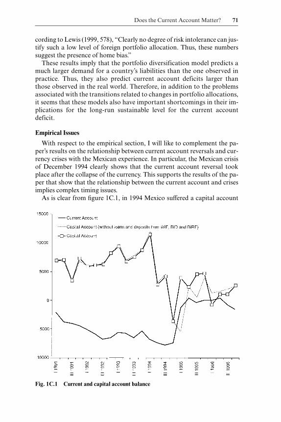
Does the Current Account Matter? 71
cording to Lewis (1999, 578), “Clearly no degree of risk intolerance can jus-tify such a low level of foreign portfolio allocation. Thus, these numberssuggest the presence of home bias.”
These results imply that the portfolio diversification model predicts amuch larger demand for a country’s liabilities than the one observed inpractice. Thus, they also predict current account deficits larger thanthose observed in the real world. Therefore, in addition to the problemsassociated with the transitions related to changes in portfolio allocations,it seems that these models also have important shortcomings in their im-plications for the long-run sustainable level for the current accountdeficit.
Empirical Issues
With respect to the empirical section, I will like to complement the pa-per’s results on the relationship between current account reversals and cur-rency crises with the Mexican experience. In particular, the Mexican crisisof December 1994 clearly shows that the current account reversal tookplace after the collapse of the currency. This supports the results of the pa-per that show that the relationship between the current account and crisesimplies complex timing issues.
As is clear from figure 1C.1, in 1994 Mexico suffered a capital account
Fig. 1C.1 Current and capital account balance

surplus reversal. In that year, the capital account balance went from a sur-plus of 11.4 billion dollars in the first quarter to –3.7 billion dollars in thefourth quarter. As shown in figure 1C.1, the current account deficit contin-ued its downward trend during 1994. Obviously, domestic absorption wascushioned from the correction in the capital account surplus by the foreignreserve loses incurred by the central bank (see fig. 1C.2). Once reserves weredepleted, the currency crisis ensued and the correction in the current ac-count took place.
In conclusion, I think the paper is an important contribution to the liter-ature and provides new and important evidence of the role that current ac-count deficits play in currency crises, and the channels through which largecurrent account reversals affect growth.
References
Ades, Alberto, and Federico Kaune. 1997. A new measure of current account sus-tainability for developing countries. Goldman Sachs Emerging Markets Eco-nomic Research. 29 September.
French, Kenneth R., and James M. Poterba. 1991. International diversification andinternational equity markets. American Economic Review 81 (2): 526–66.
Lewis, Karen. 1999. Trying to explain home bias in equities and consumption. Jour-nal of Economic Literature 37:571–608.
Tesar, Linda, and Ingrid Werner. 1998. The internationalization of securities mar-kets since the 1987 crash. In Brookings-Wharton papers on financial services, ed.Robert E. Litan and Anthony M. Santomero. Washington, D.C.: Brookings In-stitution.
72 Sebastian Edwards
Fig. 1C.2 Capital account and international reserves

Discussion Summary
A few people made remarks on whether and why current accounts matterfor predicting crises. According to Jeffrey A. Frankel, it is important to dis-tinguish whether the current account deficit matters for causing currencycrises or for other things, such as long-term growth. As far as crises are con-cerned, it is important to determine whether a current account deficit is anecessary or a sufficient condition, or, as the economic profession views it,whether there is a statistically significant relationship between current ac-count deficits and crises. Frankel commended the author for emphasizingthe difference between the isolated effect of the current account on crises (ina multivariate setting) and the effect in a univariate regression.
Frankel made a couple of additional comments, offering an insight on thehistory of thought regarding the Lawson fallacy. The statement attributedto Nigel Lawson is that the current account deficit is not a cause for concernif foreign borrowing goes to the private sector. Lawson later qualified thisstatement, pointing out that this is not to say that high current accountdeficits will never lead to a crisis. According to Frankel, this qualification isa weak “straw man.” Frankel went on to comment on the paper’s approachto identifying the impact of a sudden reversal of the current account on theoutput growth rate. He said that a sudden reversal is most likely to takethe form of a reduction in investment. The author showed that, indeed, thesudden reversal of the current account affects the growth rate through thischannel.
Anne O. Krueger discussed why and how the composition of a current ac-count deficit matters. She emphasized that the correct distinction is not be-tween public and private uses of foreign capital, but rather of how efficientlythe money is spent. The former distinction is useless for a category as fun-gible as the current account. She brought up the example of Brazil: WhenBrazil increased its interest rates, the private sector responded by borrow-ing from abroad while the public sector borrowed domestically. Kruegerquestioned whether this made any difference. As for the matter of sustain-ability, she stressed that the important difference is between rapidly grow-ing countries excess demand for investment, and countries that have veryhigh investment rates in order to sustain some degree of growth without anincrease of productivity. For example, Korea had 10 percent of current ac-count deficit during its ten years of most rapid growth. She suggested thatthe author find variables to capture productivity in the study of current ac-count. Later in the discussion, Jungho Yoo echoed Krueger’s comment onhow foreign savings (current account) are utilized.
Liliana Rojas-Suarez supported Krueger’s point. She said that a currentaccount should be understood as being on a sustainable path if the economyis generating trade balances that enable it to avoid an ever-increasing accu-
Does the Current Account Matter? 73

mulation of net foreign liabilities without the need either to devalue or toadjust economic activity severely. In this regard, the quality of investment isextremely relevant. A current account deficit that is basically the result ofhighly productive investment is likely to be more sustainable than a currentaccount deficit resulting from low saving. The reason is that highly produc-tive investment increases the economy’s production capacity. Higher futureoutput, in turn, enables the economy to pay back its foreign liabilities. Shesaid that, in general, funding the current account deficit with foreign directinvestment tends to help sustainability because FDI tends to go to produc-tive investment projects, especially on the tradable goods sector.
Relating to the discussion of how the quality of investments affects thesustainable debt level, Michael P. Dooley agreed that, historically, whatcountries do with the money seems to have been important. However, headded, the conclusion might be the opposite of that implicit in the previousparagraph: If defaulting on the external debt is a strategic decision, then thebetter a debtor uses the capital inflow, the more independent the debtor be-comes, and the more likely it will default.
That for which the current account deficit matters was also discussed.Jorge Braga de Macedo suggested that the paper could broaden the scope,rather than limiting the discussion to emerging markets or adjustable pegs.For example, he said that current accounts still matter within the euro zone.Even if there will no longer be currency crises, there could still be debt orbanking crises in the euro zone. Jaume Ventura pointed out that the ques-tion of how well current account deficits predict crises is different from theconventional approach to its welfare consequences. In (intertemporal)models of the current account, a large deficit has no welfare costs and doesnot ask for government intervention. Eduardo Borensztein commented onwhether current account deficits could predict crises. He said that an IMFstudy focusing on emerging markets (twenty-seven countries) found thatcurrent account deficits are very significant predictors of crises. The some-what weak result of the paper in this regard may suggest that the effects ofcurrent accounts differ across different groups of countries.
On the paper’s treatment (exclusion) of African countries, Braga deMacedo disagreed with the author. He said that the devaluation in someAfrican countries in 1994 showed that Africa is just like any other region,and that excluding these countries from the sample seemed unjustified.Frankel said that, in his paper with Andrew Rose, he and Rose found no sig-nificant relationship between current accounts and crises in univariate re-gressions. Edwards’ finding of a significant correlation could be the resultof excluding African countries from the sample. Dooley supported thispoint by citing his 1987 paper with Frankel and Don Mathieson, whichfound that non-market borrowers (those who depend primarily on officialfinancing) have much larger and more persistent current account imbal-ances. This, he said, could explain why the Edwards paper found different
74 Sebastian Edwards
results when dropping African countries. Krueger suggested the authorcould include African countries but exclude the official aid flows to the re-gion.
Martin Feldstein commended the paper’s emphasis on the transition be-tween different optimal stock levels of foreign capital. He said that this em-phasis was very important because countries easily confuse the temporaryincrease of capital flows as a result of a shift in the desired stock level with asustainable higher level of current account flow, as in the case of Mexico.
Ventura commented on the idea of sustainability, saying that transver-sality conditions were introduced in the early models where the currentaccount was assumed to equal domestic saving. In these models, checkingsustainability simply means to confirm empirically, the transversality con-dition, which is a theoretical artifact. The approach of this paper, however,is different from that of the earlier literature in that the current accounts area result of portfolio choices. Ventura questioned the meaning of sustain-ability in this new context.
Rudi Dornbusch said that the sudden-stop view would predict crises firstand large current account reversals second. He suggested that the authorlook into this relationship.
Krueger also expressed concerns about the data on different forms ofcapital flows, such as equity and foreign direct investment. She said that theuse of derivatives is most likely to blur the distinction among such cat-egories.
Kristin J. Forbes asked what the author’s view was on the (high) U.S. cur-rent account deficit.
Regarding that for which the current account matters, Edwards said thatin the newer version of the paper, he had made it explicit. That is, large cur-rent account deficits do not unavoidably lead to catastrophic crises, but theydo, with high degree of likelihood, result in large welfare losses. He said thatthe policy implication of the paper is very important. For example, there isa heated discussion on whether the Mexican current account deficit (about4 percent) is too large. Should Mexico allow the exchange rate to depreci-ate to handle that deficit, or should it be left to float and possibly lead to acrisis? The concern of the paper is whether a large current account warrantsa policy intervention.
A related question is when to “apply the break,” as some countries (suchas Chile) use large account deficits as targets for their monetary policies.
On the questions of the crowding out of foreign saving by domestic sav-ing and on the use of saving, he said that the quality of investment couldpossibly be proxied by interacting the deficit and the competitiveness indexfrom the World Economic Index.
Finally, on the current high level of the U.S. current account, Edwardssaid that no industrial country has had so high a level of current deficit inhis data set, and that he believes this level is unsustainable.
Does the Current Account Matter? 75
