Preventing Infectious Disease in Dynamic Populations Under Uncertainty

Bryan Wilder13, Sze-Chuan Suen23, Milind Tambe131Department of Computer Science 2Department of Industrial and Systems Engineering

3Center for Artificial Intelligence in SocietyUniversity of Southern California{bwilder, ssuen, tambe}@usc.edu

Abstract

Treatable infectious diseases are a critical challenge for pub-lic health. Outreach campaigns can encourage undiagnosedpatients to seek treatment but must be carefully targeted tomake the most efficient use of limited resources. We presentan algorithm to optimally allocate limited outreach resourcesamong demographic groups in the population. The algorithmuses a novel multiagent model of disease spread which bothcaptures the underlying population dynamics and is amenableto optimization. Our algorithm extends, with provable guar-antees, to a stochastic setting where we have only a distri-bution over parameters such as the contact pattern betweenagents. We evaluate our algorithm on two instances wherethis distribution is inferred from real world data: tuberculosisin India and gonorrhea in the United States. Our algorithmproduces a policy which is predicted to avert an average ofleast 8,000 person-years of tuberculosis and 20,000 person-years of gonorrhea annually compared to current policy.

IntroductionTreatable infectious diseases cause hundreds of thousandsof cases of disability and death worldwide. Often, this bur-den is caused by long-term diseases which are continuouslypresent in the population, as opposed to short-term epi-demics like influenza. For instance, tuberculosis (TB) deathsin India numbered over 480,000 in 2014 (WHO 2015b), andeven developed nations like the U.S. have observed over395,000 cases of gonorrhea in 2015 (CDC 2015). In bothcases, many individuals remain undiagnosed although treat-ment is available. Outreach efforts to increase screening canlower disease burden; e.g., the Indian government conductsadvertising campaigns for TB awareness. Limited resourcesrequire these campaigns to be carefully targeted at the mosteffective groups for reducing disease. Targeting is compli-cated by changing population dynamics, as individuals ageand migrate over time, as well as by uncertainty around dis-ease transmission rates. Officials currently make such deci-sions by hand as no algorithmic assistance is available.

To remedy this situation, we design an algorithm to dividea limited outreach budget between demographic groups inorder to minimize long term disease prevalence under un-certain population dynamics. Our approach contrasts with

Copyright c© 2018, Association for the Advancement of ArtificialIntelligence (www.aaai.org). All rights reserved.

existing algorithms for disease control, which often con-sider disease spread between nodes on a static graph (Sahaet al. 2015; Borgs et al. 2010). This is a sensible model ofshort term disease spread but is less suitable for long-termplanning in diseases such as TB or gonorrhea, where peopleare born, die, age, and move (Luke and Stamatakis 2012).Accounting for changes in the underlying agents is partic-ularly salient for a policymaker who must divide resourcesbetween demographic groups over many years to maximizesocietal long-term health. For instance, India produces 5year plans to combat TB (RNTCP 2016). Our approach alsocontrasts with previous work on agent-based disease models(Jindal and Rao 2017; Lee et al. 2010). Such models mayinclude realistic behaviors, but their complexity usually pre-cludes algorithmic approaches to finding the optimal policyin an entire feasible set.

An additional challenge, largely unexplored in previousalgorithmic work, is that of uncertainty. Data is always lim-ited; policymakers are never sure of exactly how many peo-ple are infected in each group, or of the contact patterns be-tween them. In order to impact real world policy, algorithmsfor resource allocation must account for such uncertainties.

We introduce a model which both captures underlyingagent dynamics and can be solved using an algorithmic ap-proach in a stochastic setting. We make four main contri-butions. First, we present the MCF-SIS model (MultiagentContinuous Flow-SIS) where disease spreads in a multiagentsystem with birth, death, and movement. The system evolvesaccording to SIS (susceptible-infected-susceptible) dynam-ics and is stratified across age groups. This introduces a newproblem in multiagent systems: computing the optimal re-source allocation under MFS-SIS, as in the case where anoutreach campaign must decide how to divide limited ad-vertising dollars (or rupees) between the groups.

MCF-SIS introduces a continuous, nonconvex, highlynonlinear optimization problem which cannot be solved byexisting methods. Many factors must be accounted for. E.g.,between-group disease transmission makes focusing on thegroups with the most infected agents suboptimal. Moreover,agents in a targeted group are not cured instantaneously, so,e.g., to reduce prevalence in age group 30, we may needto start targeting resources at age 27. Lastly, we consider astochastic setting where parts of the model (contact patternsbetween agents, the number of infected agents in each group,

𝑆𝑖𝑡

𝑆𝑖+1𝑡+1

𝐼𝑖𝑡

𝐼𝑖+1𝑡+1

𝜇𝑖 𝑑𝑖

(1 − 𝜇𝑖)(1 − 𝜌𝑖𝑡)𝑆𝑖

𝑡

…

1 − 𝜇𝑖 𝜌𝑖𝑡𝑆𝑖

𝑡

(1 − 𝜈𝑖)(1 − 𝑑𝑖)𝐼𝑖𝑡

𝜈𝑖 1 − 𝑑𝑖 𝐼𝑖𝑡

ሚ𝑆𝑖𝑡 ሚ𝐼𝑖

𝑡

a

𝑀 =0 10 0

𝛽 =0.4 0.10.1 0.3

𝑑 =0.20.2

𝜇 =0.051

𝐼0 =1010

𝑆0 =10,00010,000

𝑁0 =10,01010,010

(1) 𝑀T 𝑑𝑖𝑎𝑔 𝑆0 𝑑𝑖𝑎𝑔 1 − 𝜇 𝛽 𝑑𝑖𝑎𝑔1

𝑁0 + 𝑑𝑖𝑎𝑔 1 − 𝜈 𝑑𝑖𝑎𝑔 1 − 𝑑 =0 0

0.94 0.09

(2) I1 =0 0

0.94 0.09𝐼0 + ሚ𝐼0 =

512.3

𝜈 =0.30.4

ሚ𝐼0 =52

Figure 1: Top: Illustration of the MCF-SIS model. Bottom:a single step in the model with 2 age groups.

etc.) are not known exactly but are drawn from a distribution.Our second contribution shows that optimal allocation in

MCF-SIS is a continuous submodular problem. This opensup a novel set of optimization techniques which have notpreviously been used in disease prevention. Continuous sub-modularity generalizes submodular set functions to contin-uous domains. Intuitively, infections averted by spendingone unit of treatment resources can no longer be averted byadditional spending, creating diminishing returns. Contin-uous submodularity is deliberately enabled by our model-ing choices, in particular our shift from the discrete, graph-based setting common in previous work (Saha et al. 2015;Borgs et al. 2010) to a continuous, population-based model.

Our third contribution is a new algorithm called DOMO(Disease Outreach via Multiagent Optimization), which ob-tains an efficient (1 − 1/e)-approximation to the optimalallocation. Our algorithm builds on a recent theoreticalframework for submodular optimization (Bian et al. 2017).DOMO’s generalization of this framework to the stochasticsetting may be of independent interest.

Our fourth contribution is to instantiate MCF-SIS in twodomains using empirical data which takes into account be-havioral, demographic, and epidemic trends: first, TB spreadin India, and second, gonorrhea in the United States. DOMOaverts 8,000 annual person-years of TB and 20,000 person-years of gonorrhea compared to current policy.

MCF-SIS: a new modeling approachThe MCF-SIS model has two goals: to enable both realis-tic population dynamics and efficient optimization. In MCF-SIS, a finite population evolves in discrete time. Each agenthas two possible states. In the susceptible (S) state, an agenthas not contracted the disease. In the infected (I) state, anagent can transmit the disease to others. They can also becured and return to the susceptible state.

The population is segmented into n groups. Our runningexample is where each group is an age range because trans-mission patterns for infection vary with age (Suen et al.2015). Figure 1 shows this instantiation of the model. How-ever, our techniques generalize to any segmentation (e.g.,

geographic location or occupation). We denote the numberof susceptible agents in each group at time t as the vectorSt where Sti is the number of susceptible agents of group i.Likewise, It gives the number of infected agents. The totalpopulation is N t = St + It. At each time step, agents movebetween groups according to a movement matrix M , whereMij is the fraction of agents in group iwho move to group j.For instance, when the groups represent age, agents advancefrom age i to i+ 1. So, we have Mi,i+1 = 1, i = 1...n− 1,and all other entries of M are zero. Agents die of naturalcauses at rate µi. New agents enter the population throughbirth or migration, given by the vector St. We also allow foran exogenous inflow of infected agents It.

Disease spreads through contact with infected agents, de-scribed by the matrix β: agents in group i interact with group

j with frequency βij . A fraction ρti =∑nj=1 βij

ItjNt

jof group

i encounters an infected agent and becomes infected them-selves. At each time step, a fraction di of infected agents ingroup i die. Of those who do not die, a fraction νi are curedand become susceptible again. νi is referred to as the clear-ance rate, and captures the total rate at which infected agentsare diagnosed, enter treatment, and are successfully cured.

While compartmental models like ours do not simulatethe micro-level details of individual agents, they can be real-istic enough to capture long term trends. Similar models arecommonly used in health policy analyses (White et al. 2005;Chan, McCabe, and Fisman 2011; Dowdy et al. 2012).

Interventions: We consider optimal resource allocationmodeled through the clearance vector ν. Suppose a policy-maker can conduct outreach to selected groups. Since somepercentage of people who see an advertisement will entertreatment, we can model the policymaker’s decisions as in-creasing νi for the targeted groups. We suppose the algo-rithm has a budget K for new advertising to split amongthe groups. ν starts at a lower bound L, reflecting pre-campaign treatment rates. The algorithm may select anypost-campaign ν with ||ν−L||1 ≤ K and Li ≤ νi ≤ Ui ∀i,where U < 1 is an upper bound. Note that U is strictly lessthan 1 because we can never realistically treat 100% of anygiven group. Denote the set of ν satisfying these constraintsas the feasible polytope P . While we focus on the aboveP for concreteness, our approach works for any downward-closed polytope. The goal is to select a ν ∈ P which mini-mizes the total infected agents over a time horizon T .

Optimization formulation: We assume that the numberof infected agents (and hence deaths) is small compared tothe total population. For instance, less than 1% of the totalpopulation is infected with TB in India or gonorrhea in theU.S. (WHO 2015b; CDC 2015). Therefore, we consider thetotal population size (the vector N t) as fixed independentlyof ν. Thus, the state of the system is captured just by theinfected vector It. A single group i evolves as

It+1i =

n∑j=1

Mji

(Stj(1− µj)

n∑k=1

βjkItkN tk

+ (1− νj)(1− dj)Itj)

+ Iti .

The expression in parentheses is the number of infectedagents in group j. The first term is the number who are newlyinfected and the second is the number from previous stepswho are not cured and do not die. The outer summation ac-counts for the number of these infected agents who transitionfrom group j to group i. Lastly, we add the new arrivals Iti .

We can iterate the equation for each group forward fromt = 1...T in order to obtain the total number of infectedagents at time T . Instead though, we will work with anequivalent matrix formulation of the system for ease of nota-tion. For convenience, we will use the augmented state vec-tor xt = [It 1]. That is, xt is the number of infected peopleappended with a single one. The one is just for mathematicalconvenience. We formulate a time-varying linear operatorBt(ν) such that xt+1 = Bt(ν)xt via the block form

Bt(ν) =

[At(ν) It

~0 1

]where the block At(ν) is defined as

At(ν) = M>(diag(St)diag(1− µ) β diag

( 1

N t

)+diag(1− ν)diag(1− d)

).

where diag(v) is the matrix with the entries of v on thediagonal.At(ν)It gives the number of infected agents givenonly the internal dynamics of the population, resulting in atotal of At(ν)It + It infected agents. Figure 1 shows an ex-ample of a simple case of the model with two age groups.Example parameter values are given, along with the ini-tial prevalence I0. The first equation computes the matrixA0(ν). The second applies A0(ν) to the initial prevalenceI0 and then adds the exogenous inflow I0. The number ofinfected agents in group 1 increases because more agents areinfected than cured. These agents then transition to group 2.Because there are only two groups in our modeled popula-tion for this example, all agents in group 2 exit the modeledpopulation.

We aim to minimize the total infected agents over T steps:

min

T∑t=1

c>

1∏j=t

Bj(ν)

x0

1>ν ≤ 1>L+K (1)Li ≤ νi ≤ Ui ∀i = 1...n

c can be any nonnegative cost vector, e.g., c = [~1 0] (nones and a zero) sums over the number of infected agentsin each group. x0 is the initial state (number of infectedagents). We use the notation

∏1j=tB

t(ν) as shorthand forBt(ν)Bt−1(ν)...B1(ν).

Algorithmic approachWe now turn to computing a (near) optimal solution to Prob-lem 1. This is a continuous optimization problem since each

νi may take any value in [Li, Ui]. Unfortunately, the objec-tive function is nonconvex, which rules out standard meth-ods for efficiently obtaining good solutions. It is also highlynonlinear since the decision variables ν are raised to thepower T , which may be large (e.g., a time horizon of 10or 20 years). This suggests that many local optima could bepresent and renders optimization more complicated.

However, MCF-SIS’s definition contains useful structure.Intuitively, resources have diminishing returns: infectionsaverted by increasing one νi can no longer be treated by in-creasing some other νj . Diminishing returns suggests sub-modularity. However, since our optimization problem is notdiscrete, standard submodularity and the greedy algorithmdo not apply. Instead, we show that our objective is con-tinuous submodular, a generalization of submodularity tocontinuous domains (Bach 2015; Bian et al. 2017). Contin-uous submodularity enables efficient optimization and al-lows us to handle the stochastic case in a natural man-ner. This framework is crucially enabled by the modelingchoice to shift from the discrete, graph-based setting com-mon in previous work (Saha et al. 2015; Borgs et al. 2010;Chung, Horn, and Tsiatas 2009) to a continuous, population-based model. Not only does our model account for popula-tion dynamics, but it is also more amenable to optimization.

We now define continuous submodularity1. Let ∧ and∨ denote coordinatewise minimum and maximum respec-tively. A function F : Rn → R is continuous submodular ifF (x)+F (y) ≥ F (x∨y)+F (x∧y) for all feasible x, y. Thisis reminiscent of submodular set functions, but extended tothe continuous domain. F is called continuous supermodularif the inequality is reversed. If F is continuous submodular,−F is continuous supermodular. Note that continuous sub-modularity is not convexity or concavity; it is a distinct classof functions with distinct optimization techniques.

We will draw on these techniques to solve Problem 1.Bian et al. (2017) define a theoretical framework for opti-mizing continuous submodular functions. In order to makeuse of this framework, we need to first show that our prob-lem falls into it. Then, we need to fill in the algorithmic com-ponents required to instantiate the approach that the frame-work suggests (two oracles explained below). Lastly, weneed to prove that our objective is sufficiently smooth forthe resulting algorithm to converge in a reasonable numberof iterations. None of these pieces are covered by previouswork; they are algorithmic contributions specific to our do-main.

We start out by showing that the continuous submodu-larity framework applies. Denote the objective of Problem1 as F (ν). We will show that F is continuous supermodu-lar which in turn implies that −F is continuous submodu-lar. Since minimizing F is equivalent to maximizing −F ,this will allow us to design an efficient algorithm based oncontinuous submodularity. Our proof that F is supermod-ular has two steps. First, we show that F is a posynomialin the variables 1 − νi. A posynomial is a polynomial with

1Technically, we use the stronger condition of DR-submodularity. Details related to showing our objective isDR-submodular can be found in the supplement.

entirely nonnegative coefficients2. Then, we will show thatany function which is a posynomial in 1 − ν is continuoussupermodular in ν. We start by showing the following:Lemma 1. F is a posynomial in the variables 1− νi.Proof. First, note that F depends on ν only through the termdiag(1− ν). Note also that every term in the expression forthe block At(ν) is nonnegative. Since matrix multiplicationis just a series of multiplications and additions, it followsthat c>

∏1j=t

[B(ν)j

]x0 (and hence the sum over time t =

1...T ) is a polynomial in 1 − ν and all of the coefficientsof this polynomial are nonnegative. This can also be seenthrough the expression for the evolution of a single group,which contains only terms of the form (1 − νi) multipliedby nonnegative coefficients.

Note that this step hinged on MCF-SIS’s continuous,population-based nature. Since F is a posynomial in 1−νi, itcan be written in the form F (ν) =

∑`j=1 aj

∏ni=1(1−νi)pij

where aj is a nonnegative coefficient for term j and pij is anonnegative integer. This representation does not have to becomputed; its existence is just useful for the proofs.

We now turn to showing that any function that is a posyn-omial in 1 − ν is continuous supermodular in ν. Our resultbuilds on the following lemma:Lemma 2 (Staib and Jegelka (2017)). Let f1...fn : R →R+ be nonnegative, differentiable functions which are ei-ther all nonincreasing or all nondecreasing. Then, F (x) =∏ni=1 fi(x) is continuous supermodular.Using this, we show the following:

Lemma 3. Whenever F is a posynomial in 1− ν, it is alsocontinuous supermodular in ν.

Proof. First, note that continuous supermodularity is pre-served under nonnegative linear combinations. Hence, wefocus on an individual term

∏ni=1(1− νi)pij in the posyno-

mial representation of F . For each i = 1...n, define fi(ν) =(1 − νi)

pij . Note that each fi is nonincreasing in νi since0 ≤ νi < 1. Further, fi(νi) ≥ 0 always holds. The conclu-sion now follows from Lemma 2.

To sum up: we want to minimize F , which via Lemma 1is a posynomial in 1−ν. Via Lemma 3, this implies that F iscontinuous supermodular in ν. Hence, maximizing −F is acontinuous submodular optimization problem. We will actu-ally maximize the objective G(ν) = −F (ν) +M , where Mis any constant large enough to ensure thatG is nonnegative.Clearly, this is also equivalent to minimizing F .

The DOMO algorithmWe now introduce the DOMO algorithm (Disease Outreachvia Multiagent Optimization, Algorithm 1) to exploit con-tinuous submodularity. We start out with the determinis-tic setting where model parameters are fully known. Here,DOMO builds on the Frank-Wolfe approach (Bian et al.

2Under some circumstances, posynomials can be optimized viageometric programming. Unfortunately, this does not work for ourproblem since the feasible set is not convex in 1− ν.

2017) (though new techniques are needed in the stochas-tic setting). DOMO generates a series of feasible solutionsν0...νR, where R is the total number of iterations. Moreiterations imply greater accuracy (Theorem 1 bounds thenumber needed). The algorithm starts at ν0 = L, the lowerbound. Each iteration alternates between two steps (lines 4-5). First, it computes the gradient of the objective at the cur-rent point. Second, it takes a step in the direction of the pointwhich optimizes the gradient over the feasible set P . Essen-tially, at each iteration the algorithm spends a fraction 1

R ofthe budget according to the current gradient. Higher R al-lows finer control over the solution.

It is known that this strategy gives a (1 − 1/e)-approximation for continuous submodular functions (Bianet al. 2017). However, it is not an out-of-the-box approach(even in the deterministic setting). DOMO requires two ora-cles (specific to our problem) to instantiate the algorithm – agradient oracle which supplies the gradient ofG at any givenpoint, and a linear optimization oracle which maximizes agiven linear function over the feasible set P . Additionally,the number of iterations (and hence runtime) required is po-tentially unbounded. We prove (in Theorem 1) that our ob-jective is sufficiently smooth for the algorithm to convergeefficiently. We first supply appropriate oracles.

Gradient oracle: Instead of tediously computing theposynomial representation, we directly compute the gradi-ent using the block matrix representation of MCF-SIS. De-note Y t(ν) =

∏tj=1B(ν)j . We can concisely express the

gradient via matrix calculus (Petersen and Pedersen 2008):

∂G(ν)

νi= −

T∑t=1

Tr

[(∂c>Y t(ν)x0

Y t(ν)

)>∂Y t(ν)

νi

]=

−T∑t=1

Tr

[cx>0

t∑`=1

[`+1∏i=t

Bi(ν)

]∂B`(ν)

∂νi

[1∏

i=`−1

Bi(ν)

]]where the first step is the chain rule and the second fol-

lows from the product rule and induction on n. Tr denotesthe matrix trace. This reduces gradient evaluation to com-puting ∂

∂νiBj(ν) for each i and j. Bj depends on νi only

through the block Aj(ν), so we have ∂∂νi

Bj(ν) = (1 −di)M

>Ji,i, where Ji,i is the matrix with a one in entry (i, i)and zeros elsewhere. By appropriately ordering multiplica-tions, the entire procedure uses T matrix multiplications.

Linear optimization oracle: Since P is a polytope, lin-ear optimization could be performed by solving a linear pro-gram. However, exploiting the special structure of P lets usperform linear optimization in time O(n log n) via a simplegreedy algorithm (function GREEDYLINEAR in Algorithm1). This algorithm simply orders the group i = 1...n ac-cording to ∇iG(ν) (Line 10). It then proceeds through thegroups in this order, spending as much of the budget as pos-sible (Line 15) before moving on to the next.Lemma 4. GREEDYLINEAR finds an optimal solution to thelinear optimization problem over P .

Proof. We recognize the linear optimization problem as afractional knapsack problem where each item takes up the

Algorithm 1 DOMO

1: function DOMO(R,K)2: ν0← L3: for k = 1...R do4: ∇k ← GRADIENTORACLE(νk−1)5: yk ← LINEARORACLE(∇k,K)6: νk ← νk−1 + 1

Ryk

7: return νR8: function GREEDYLINEAR(∇, K)9: y← L

10: π← ordering of 1...n such that∇π(i) ≥ ∇π(i+1) ∀i11: i← 012: while ||y − L||1 < K do13: yπ(i) += min(Uπ(i) − Lπ(i),K − ||y − L||1)14: i += 115: return y

same amount of space. The value of each item is the cor-responding entry of the gradient. Hence, greedily taking asmuch as possible of the highest-value items is optimal.

Convergence analysis: The runtime of Algorithm 1 de-pends on the number of iterations R, which Bian et al.(2017) show must be proportional to the Lipschitz constantof the gradient of G. Essentially, functions with Lipschitzcontinuous gradients are smooth in a sense that allows thealgorithm to quickly converge. Let Umax = maxi Ui. Webound the Lipschitz constant for our model and show that

Theorem 1. For any ε > 0, using R = Kε

(T

1−Umax

)2

iterations, the ν output by Algorithm 1 satisfies G(ν) ≥(1− 1

e − ε)G(ν∗), where ν∗ is an optimal solution.

The proof is given in the supplement due to space con-straints. We remark that Umax is always bounded away from1 since we can never realistically treat 100% of any singlegroup. Thus, the number of iterations is O

(KT 2

ε

). Each it-

eration requires one linear optimization over P (which takestime O(n log n) using GREEDYLINEAR) and one gradientevaluation (which takes timeO(Tnω), where ω is the matrixmultiplication constant). The final runtime is O

(KT 3nω

ε

).

Stochastic optimizationIn reality, some parameters of the multiagent system willnot be known exactly. For instance, the contact matrix βis almost never precisely known in practice. Additionally,for many diseases, there is considerable uncertainty aboutthe initial prevalence I0 (Suen et al. 2015). We now extendDOMO to the stochastic case where model parameters aredrawn from a distribution instead of known exactly. Hence,we can infer an appropriate prior distribution from whateverdata is available and optimize the expected value over thisdistribution. Our formulation is very general, and will allowany of the parameters (M , β, I0, I , etc.) to be unknowns.Suppose that we have an uncertainty set Ξ for the joint val-ues of the unknowns and Ξ is equipped with a distribution

D. Let G(·, ξ), ξ ∈ Ξ denote the objective for any fixed setof parameters. We wish to solve the stochastic problem

maxν∈P

Eξ∼D

[G(ν, ξ)] (2)

Such stochastic problems are typically difficult compu-tationally. For instance, Zhang et al. (2014) study vaccina-tion on a graph when the initially infected nodes (I0 in ourmodel) are uncertain. To design a scalable algorithm, theymust assume thatD is an independent distribution. However,I0 for different groups will clearly be correlated because ofthe underlying multiagent dynamics. A common approach toaccounting for uncertainty without such strong assumptionsis robust optimization, which solves the worst case prob-lem maxν∈P minξ∈ΞG(ν, ξ). Han et al. (2015) take this ap-proach for a vaccination problem when the graph β is un-known. However, robust optimization introduces a compu-tationally challenging bilevel optimization problem whichrequires specialized techniques. This makes it difficult to in-corporate uncertainty in multiple parts of the model.

We resolve these difficulties through an alternate ap-proach which efficiently handles uncertainty over any of themodel parameters, expressed through an arbitrary distribu-tion D. Moreover, we obtain provable guarantees just as inthe deterministic case. We start out by noting that the ob-jective of Problem 2 is continuous submodular since it is anonnegative linear combination of continuous submodularfunctions. Also note that Algorithm 1 accesses the objectiveonly through GRADIENTORACLE. While we can no longeraccess the gradient in closed form, the key idea is to insteaduse a stochastic approximation. At each iteration, we drawr samples ξ1...ξr i.i.d. from D. Our estimate of the gradi-ent is ∇ = 1

r

∑ri=1∇G(ν, ξi). We then modify Line 5 of

Algorithm 1 to call LINEARORACLE(∇).To our knowledge, no previous work has analyzed

stochastic continuous submodular optimization. We give anew analysis which draws on tools for analyzing stochasticconcave problems (Hazan and Luo 2016). We extend thesetechniques to (nonconcave) continuous submodular func-tions and prove the following guarantee:

Theorem 2. Using r =(

4KT1−Umax

)2

samples, DOMO out-

puts a ν satisfying E [G(ν, ξ)] ≥(1− 1

e − ε)E [G(ν∗, ξ)]

where ν∗ is an optimal solution to Problem 2. The numberof iterations is the same as Theorem 1.

Note that the guarantee for E[G(ν, ξ)] exactly matchesthat for G(ν) in the deterministic case. Further, our analysisgeneralizes to any smooth continuous submodular functionand may be of interest in other domains.

ExperimentsWe now present experimental results on two real-worldproblem instances: TB prevention in India and gonorrheaprevention in the United States. In both, we produce a highlyrealistic evaluation by instantiating MCF-SIS using demo-graphic and epidemiological data drawn from a variety ofgovernmental and NGO sources. Since prevalence numbers

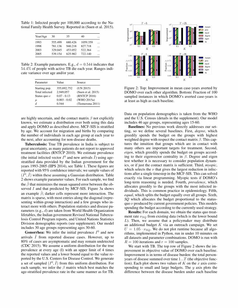
Table 1: Infected people per 100,000 according to the Na-tional Family Health Survey. Reported in (Suen et al. 2015).

Year/Age 30 35 40 ...

1993 555.499 680.426 1059.359 ...1998 781.136 940.218 827.718 ...2003 329.045 453.052 522.364 ...2005 539.154 625.982 722.140 ...

Table 2: Example parameters. E.g., d = 0.544 indicates that54.4% of people with active TB die each year. Ranges indi-cate variance over age and/or year.

Parameter Value Source

Starting pop. 355,692,752 (UN 2015)Total infected 2,949,057 (Suen et al. 2015)Status quo ν 0.07 - 0.13 (RNTCP 2016)µ 0.003 - 0.02 (WHO 2015a)d 0.544 (Tiemersma 2011)

are highly uncertain, and the contact matrix β not explicitlyknown, we estimate a distribution over both using this dataand apply DOMO as described above. MCF-SIS is stratifiedby age. We account for migration and births by comparingthe number of individuals in each age group at each year tothe next, after accounting for non-disease deaths.

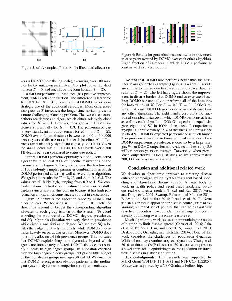
Tuberculosis: True TB prevalence in India is subject togreat uncertainty, as many patients do not report to approvedtreatment facilities (RNTCP 2010). We estimate prevalence(the initial infected vector I0 and new arrivals I) using age-stratified data provided by the Indian government for theyears 1993-2005 (IIPS 2014), see Table 1. These figures arereported with 95% confidence intervals; we sample values of(I0, I) within these assuming a Gaussian distribution. Table2 shows example parameter values. For each sample, we findthe β that minimizes the mean squared error between the ob-served I and that predicted by MCF-SIS. Figure 3a showsan example β; darker cells represent more interaction. Thematrix is sparse, with most entries along the diagonal (repre-senting within-group interaction) and a few groups who in-teract more with others. Population statistics and disease pa-rameters (e.g., d) are taken from World Health Organizationlifetables, the Indian government Revised National Tubercu-losis Control Program reports, and United Nations StatisticsDivision demographic reports (see supplement). Our modelincludes 30 age groups representing ages 30-60.

Gonorrhea: We infer the initial prevalence I0 and newarrivals I from reported disease cases. However, up to80% of cases are asymptomatic and may remain undetected(CDC 2015). We assume a uniform distribution for the trueprevalence at every age (I) with an upper limit of 4 timesthe reported values and a lower bound equal to the value re-ported by the U.S. Centers for Disease Control. We generatea set of sampled (I0, I) from this uniform distribution. Foreach sample, we infer the β matrix which best matches theage-stratified prevalence rate in the same manner as for TB.

0.1 0.3

K

100

102

104

106

Impr

ovem

ent

T =5

0.1 0.3

K

100

102

104

106

Impr

ovem

ent

T =25

myopic

prev

equal

degree

eigen

sq

0.1 0.3

K

0.00

0.25

0.50

0.75

1.00

Fra

ctio

n≥

T =5

0.1 0.3

K

0.00

0.25

0.50

0.75

1.00

Fra

ctio

n≥

T =25

myopic

prev

equal

degree

eigen

sq

Figure 2: Top: Improvement in mean case-years averted byDOMO over each other algorithm. Bottom: Fraction of 100sampled instances in which DOMO’s averted case-years isat least as high as each baseline.

Data on population demographics is taken from the WHOand the U.S. Census (details in the supplement). Our modelincludes 46 age groups, representing ages 15-60.

Baselines: No previous work directly addresses our set-ting, so we define several baselines. First, degree, whichgreedily spends the budget on the groups with highestweighted degree with respect the contact matrix β. This cap-tures the intuition that groups which are in contact withmany others are important targets for treatment. Second,eigen, which greedily spends the budget on groups accord-ing to their eigenvector centrality in β. Degree and eigentest whether it is necessary to consider population dynam-ics, or if just the contact matrix is sufficient. Third, myopic,which selects the ν that gives the largest reduction in infec-tions after a single timestep in the MCF-SIS. This can solvedexactly via linear programming. Myopic tests if DOMO’slong-term reasoning is needed. Fourth, prevalence, whichallocates greedily to the groups with the most infected in-dividuals. This is common practice in epidemiology. Fifth,equal, which splits the budget equally over all groups. Sixth,SQ which allocates the budget proportional to the status-quo ν produced by current government policies. This modelsspending the budget according to the currently used strategy.

Results: For each domain, we obtain the status quo treat-ment rate νSQ from existing data (which is the lower boundL). Then, we assume that a policymaker may distributean additional budget K via an outreach campaign. We setU = 1.05 · νSQ. We do not plot runtime because all algo-rithms, implemented in Python, run in under 10 minutes onall datasets and parameter combinations. DOMO is run withR = 100 iterations and r = 100 samples.

We start with TB. The top row of Figure 2 shows the im-provement in objective value of DOMO over each baseline.Improvement is in terms of disease burden: the total person-years of disease summed over time 1...T (the objective func-tion). Each plot shows two values of K on the x axis corre-sponding to small and large budgets. The y axis plots thedifference between the disease burden under each baseline

0.02

0.04

0.06

0.08

0.10

0.12

0.14

(a)

0.00

0.05

Bud

get

DOMO degree

30 40 50 60Age

0.00

0.05

Bud

get

prev

30 40 50 60Age

SQ

(b)

Figure 3: (a) A sampled β matrix. (b) Illustrated allocation

versus DOMO (note the log scale), averaging over 100 sam-ples for the unknown parameters. One plot shows the shorthorizon T = 5, and one shows the long horizon T = 25.

DOMO outperforms all baselines (has positive improve-ment) under each configuration. The difference is larger forK = 0.3 than K = 0.1, indicating that DOMO makes morestrategic use of the additional resources. Most differencesalso grow as T increases; the longer time horizon presentsa more challenging planning problem. The two closest com-petitors are degree and eigen, which obtain relatively closevalues for K = 0.1. However, their gap with DOMO in-creases substantially for K = 0.3. The performance gapis very significant in policy terms: for K = 0.3, T = 25,DOMO averts (approximately) between 64,000 to 300,000person-years of disease more than each baseline. All differ-ences are statistically significant (t-test, p < 0.001). Giventhe annual death rate d = 0.544, DOMO averts over 6,500TB deaths per year compared to status quo policy.

Further, DOMO performs optimally out of all consideredalgorithms in at least 90% of specific realizations of theparameters. In Figure 2, the y axis shows the fraction outof 100 randomly sampled parameter combinations in whichDOMO performed at least as well as every other algorithm.We again plot results for T = 5, 25, and K = 0.1, 0.3. Thevalues are all fairly high, ranging from 0.9 to 1. We con-clude that our stochastic optimization approach successfullycaptures uncertainty in this domain because it has high per-formance almost all circumstances, not just in expectation.

Figure 3b contrasts the allocation made by DOMO andother policies. We focus on K = 0.3, T = 10. Each lineshows the amount of budget the corresponding algorithmallocates to each group (shown on the x axis). To avoidcrowding the plot, we show DOMO, degree, prevalence,and SQ. Myopic’s allocation was very close to prevalencewhile eigen’s was similar to degree. We see that SQ allo-cates the budget relatively uniformly, while DOMO concen-trates heavily on particular groups. Moreover, DOMO doesnot simply allocate to high-prevalence groups. This indicatesthat DOMO exploits long term dynamics beyond whichagents are immediately infected. DOMO also does not sim-ply allocate to high degree groups. Its allocation overlapswith the high degree elderly groups, but places little budgeton the high degree groups near ages 30 and 40. We concludethat DOMO leverages non-obvious patterns in the multia-gent system’s dynamics to outperform simpler heuristics.

0.1 0.3

K

100

102

104

106

Impr

ovem

ent

T =25

0.1 0.3

K

0.00

0.25

0.50

0.75

1.00

Fra

ctio

n≥

T =25

myopic

prev

equal

degree

eigen

sq

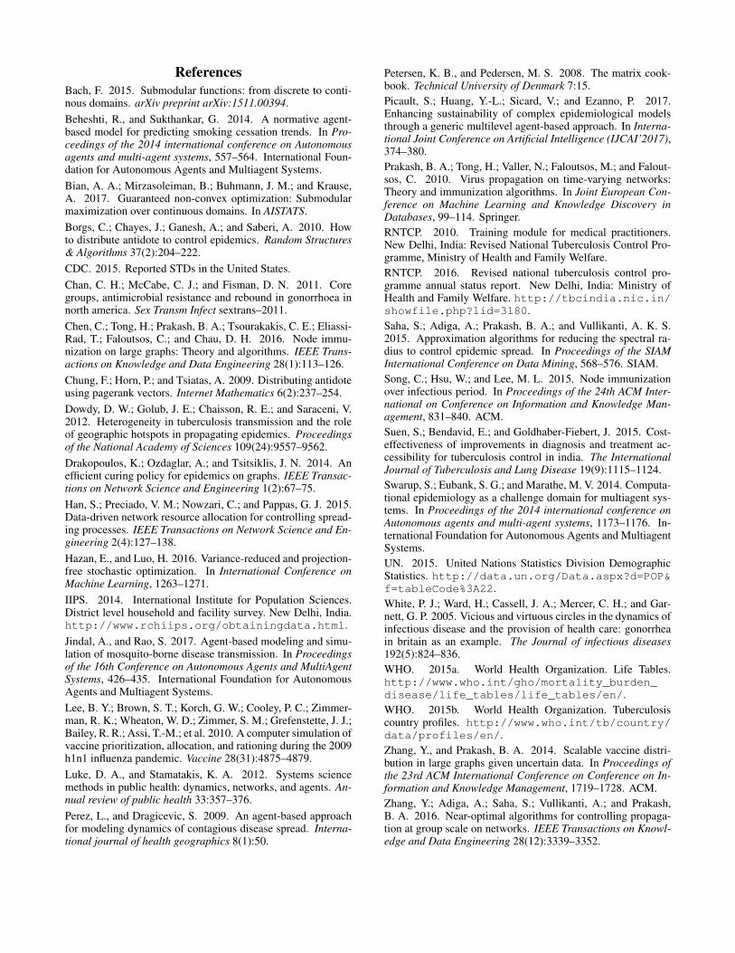
Figure 4: Results for gonorrhea instance. Left: improvementin case-years averted by DOMO over each other algorithm.Right: fraction of instances in which DOMO performs atleast as well as each baseline.

We find that DOMO also performs better than the base-lines in our gonorrhea example (Figure 4). Generally, resultsare similar to TB, so due to space limitations, we show re-sults for T = 25. The left hand figure shows the improve-ment in disease burden that DOMO makes over each base-line; DOMO substantially outperforms all of the baselinesfor both values of K. For K = 0.3, T = 25, DOMO re-sults in at least 500,000 fewer person-years of disease thanany other algorithm. The right hand figure plots the frac-tion of sampled instances in which DOMO performs at leastas well as each algorithm. DOMO outperforms equal, de-gree, eigen, and SQ in 100% of instances. It outperformsmyopic in approximately 75% of instances, and prevalencein 60-70%. DOMO’s expected performance is much higherthan prevalence because in those sampled instances whereDOMO outperforms prevalence, it does so by a large mar-gin. When DOMO outperforms prevalence, it does so by 3.9million person-years on average. Conversely, when preva-lence outperforms DOMO, it does so by approximately200,000 person-years on average.

Conclusion and additional related workWe develop an algorithmic approach to targeting diseaseoutreach campaigns which synthesizes agent-based mod-eling and algorithmic disease control. A large body ofwork in health policy and agent based modeling devel-ops realistic disease models (Jindal and Rao 2017; Perezand Dragicevic 2009; Swarup, Eubank, and Marathe 2014;Beheshti and Sukthankar 2014; Picault et al. 2017). Noneuse an algorithmic approach for disease control, instead ex-amining a limited set of policies that can be exhaustivelysearched. In contrast, we consider the challenge of algorith-mically optimizing over the entire feasible set.

Much algorithmic work focuses on immunizing the nodesof a graph to limit disease spread (Chen et al. 2016; Sahaet al. 2015; Song, Hsu, and Lee 2015; Borgs et al. 2010;Drakopoulos, Ozdaglar, and Tsitsiklis 2014). None of thiswork considers the challenges of population dynamics.While others may examine subgroup dynamics (Zhang et al.2016) or time trends (Prakash et al. 2010), our work presentsa novel approach to optimizing resource allocation for infec-tious diseases in a stochastic setting.

Acknowledgments: This research was supported byMURI Grant W911NF-11-1-0332 and NSF CCF-1522054.Wilder was supported by a NSF Graduate Fellowship.

ReferencesBach, F. 2015. Submodular functions: from discrete to conti-nous domains. arXiv preprint arXiv:1511.00394.Beheshti, R., and Sukthankar, G. 2014. A normative agent-based model for predicting smoking cessation trends. In Pro-ceedings of the 2014 international conference on Autonomousagents and multi-agent systems, 557–564. International Foun-dation for Autonomous Agents and Multiagent Systems.Bian, A. A.; Mirzasoleiman, B.; Buhmann, J. M.; and Krause,A. 2017. Guaranteed non-convex optimization: Submodularmaximization over continuous domains. In AISTATS.Borgs, C.; Chayes, J.; Ganesh, A.; and Saberi, A. 2010. Howto distribute antidote to control epidemics. Random Structures& Algorithms 37(2):204–222.CDC. 2015. Reported STDs in the United States.Chan, C. H.; McCabe, C. J.; and Fisman, D. N. 2011. Coregroups, antimicrobial resistance and rebound in gonorrhoea innorth america. Sex Transm Infect sextrans–2011.Chen, C.; Tong, H.; Prakash, B. A.; Tsourakakis, C. E.; Eliassi-Rad, T.; Faloutsos, C.; and Chau, D. H. 2016. Node immu-nization on large graphs: Theory and algorithms. IEEE Trans-actions on Knowledge and Data Engineering 28(1):113–126.Chung, F.; Horn, P.; and Tsiatas, A. 2009. Distributing antidoteusing pagerank vectors. Internet Mathematics 6(2):237–254.Dowdy, D. W.; Golub, J. E.; Chaisson, R. E.; and Saraceni, V.2012. Heterogeneity in tuberculosis transmission and the roleof geographic hotspots in propagating epidemics. Proceedingsof the National Academy of Sciences 109(24):9557–9562.Drakopoulos, K.; Ozdaglar, A.; and Tsitsiklis, J. N. 2014. Anefficient curing policy for epidemics on graphs. IEEE Transac-tions on Network Science and Engineering 1(2):67–75.Han, S.; Preciado, V. M.; Nowzari, C.; and Pappas, G. J. 2015.Data-driven network resource allocation for controlling spread-ing processes. IEEE Transactions on Network Science and En-gineering 2(4):127–138.Hazan, E., and Luo, H. 2016. Variance-reduced and projection-free stochastic optimization. In International Conference onMachine Learning, 1263–1271.IIPS. 2014. International Institute for Population Sciences.District level household and facility survey. New Delhi, India.http://www.rchiips.org/obtainingdata.html.Jindal, A., and Rao, S. 2017. Agent-based modeling and simu-lation of mosquito-borne disease transmission. In Proceedingsof the 16th Conference on Autonomous Agents and MultiAgentSystems, 426–435. International Foundation for AutonomousAgents and Multiagent Systems.Lee, B. Y.; Brown, S. T.; Korch, G. W.; Cooley, P. C.; Zimmer-man, R. K.; Wheaton, W. D.; Zimmer, S. M.; Grefenstette, J. J.;Bailey, R. R.; Assi, T.-M.; et al. 2010. A computer simulation ofvaccine prioritization, allocation, and rationing during the 2009h1n1 influenza pandemic. Vaccine 28(31):4875–4879.Luke, D. A., and Stamatakis, K. A. 2012. Systems sciencemethods in public health: dynamics, networks, and agents. An-nual review of public health 33:357–376.Perez, L., and Dragicevic, S. 2009. An agent-based approachfor modeling dynamics of contagious disease spread. Interna-tional journal of health geographics 8(1):50.

Petersen, K. B., and Pedersen, M. S. 2008. The matrix cook-book. Technical University of Denmark 7:15.Picault, S.; Huang, Y.-L.; Sicard, V.; and Ezanno, P. 2017.Enhancing sustainability of complex epidemiological modelsthrough a generic multilevel agent-based approach. In Interna-tional Joint Conference on Artificial Intelligence (IJCAI’2017),374–380.Prakash, B. A.; Tong, H.; Valler, N.; Faloutsos, M.; and Falout-sos, C. 2010. Virus propagation on time-varying networks:Theory and immunization algorithms. In Joint European Con-ference on Machine Learning and Knowledge Discovery inDatabases, 99–114. Springer.RNTCP. 2010. Training module for medical practitioners.New Delhi, India: Revised National Tuberculosis Control Pro-gramme, Ministry of Health and Family Welfare.RNTCP. 2016. Revised national tuberculosis control pro-gramme annual status report. New Delhi, India: Ministry ofHealth and Family Welfare. http://tbcindia.nic.in/showfile.php?lid=3180.Saha, S.; Adiga, A.; Prakash, B. A.; and Vullikanti, A. K. S.2015. Approximation algorithms for reducing the spectral ra-dius to control epidemic spread. In Proceedings of the SIAMInternational Conference on Data Mining, 568–576. SIAM.Song, C.; Hsu, W.; and Lee, M. L. 2015. Node immunizationover infectious period. In Proceedings of the 24th ACM Inter-national on Conference on Information and Knowledge Man-agement, 831–840. ACM.Suen, S.; Bendavid, E.; and Goldhaber-Fiebert, J. 2015. Cost-effectiveness of improvements in diagnosis and treatment ac-cessibility for tuberculosis control in india. The InternationalJournal of Tuberculosis and Lung Disease 19(9):1115–1124.Swarup, S.; Eubank, S. G.; and Marathe, M. V. 2014. Computa-tional epidemiology as a challenge domain for multiagent sys-tems. In Proceedings of the 2014 international conference onAutonomous agents and multi-agent systems, 1173–1176. In-ternational Foundation for Autonomous Agents and MultiagentSystems.UN. 2015. United Nations Statistics Division DemographicStatistics. http://data.un.org/Data.aspx?d=POP&f=tableCode%3A22.White, P. J.; Ward, H.; Cassell, J. A.; Mercer, C. H.; and Gar-nett, G. P. 2005. Vicious and virtuous circles in the dynamics ofinfectious disease and the provision of health care: gonorrheain britain as an example. The Journal of infectious diseases192(5):824–836.WHO. 2015a. World Health Organization. Life Tables.http://www.who.int/gho/mortality_burden_disease/life_tables/life_tables/en/.WHO. 2015b. World Health Organization. Tuberculosiscountry profiles. http://www.who.int/tb/country/data/profiles/en/.Zhang, Y., and Prakash, B. A. 2014. Scalable vaccine distri-bution in large graphs given uncertain data. In Proceedings ofthe 23rd ACM International Conference on Conference on In-formation and Knowledge Management, 1719–1728. ACM.Zhang, Y.; Adiga, A.; Saha, S.; Vullikanti, A.; and Prakash,B. A. 2016. Near-optimal algorithms for controlling propaga-tion at group scale on networks. IEEE Transactions on Knowl-edge and Data Engineering 28(12):3339–3352.