PRICE DETERMINATION FOR BUNDLED PRODUCTS: APPLICATION FOR

A HOUSEHOLD PRODUCT GROUP

A THESIS SUBMITTED TO

THE GRADUATE SCHOOL OF SOCIAL SCIENCES

OF

MIDDLE EAST TECHNICAL UNIVERSITY

BY

KERİMAN HANDE ERSÖZ

IN PARTIAL FULFILLMENT OF THE REQUIREMENTS

FOR

THE DEGREE OF MASTER OF BUSINESS ADMINISTRATION

IN

THE DEPARTMENT OF BUSINESS ADMINISTRATION

JULY 2012

ii

Approval of the Graduate School of Social Sciences

Prof. Dr. Meliha Altunışık

Director

I certify that this thesis satisfies all the requirements as a thesis for the degree of

Master of Business Administration.

Assoc. Prof. Dr. Engin Küçükkaya

Head of Department

This is to certify that we have read this thesis and that in our opinion it is fully

adequate, in scope and quality, as a thesis for the degree of Master of Business

Administration.

Prof. Dr. F.N. Can Şımga Muğan

Supervisor

Examining Committee Members

Prof. Dr. Cengiz Yılmaz (METU,BA)

Prof. Dr. F.N. Can Şımga Muğan (METU,BA)

Dr. Nazli Akman (BILKENT,BA)

iii

LAGIARISM

I hereby declare that all information in this document has been obtained and

presented in accordance with academic rules and ethical conduct. I also declare

that, as required by these rules and conduct, I have fully cited and referenced

all material and results that are not original to this work.

Name, Last Name: Keriman Hande Ersöz

Signature :

iv

ABSTRACT

PRICE DETERMINATION FOR BUNDLED PRODUCTS: APPLICATION FOR

A HOUSEHOLD PRODUCT GROUP

Ersöz, Keriman Hande

M.B.A., Department of Business Administration

Supervisor: Prof. Dr. F.N. Can Şımga Muğan

July 2012, 62 pages

The aim of this thesis is to search for the best way to allocate revenues gathered from

a group of products in a household supplies company. In so doing, it purports to

determine the price which brings customer perception and organizational benefit to

equilibrium. To compare alternatives of revenue allocation methods, data obtained

for a main product and its variants from a household company will be analyzed in an

organized manner. Three ways of product bundling (pure bundling, mixed bundling,

unbundling) is discussed as a framework for underlying different detailed aspects. In

the end, pricing and promotional policies of the company is critically evaluated and

simultaneous strategy changes are suggested.

Keywords: Bundling, Optimization, Pricing

v

ÖZ

DEMETLİ ÜRÜNLER İÇİN PAKET FİYAT BELİRLENMESİ: EV EŞYALARI

ÜRÜN GRUBU İÇİN UYGULAMA

Ersöz, Keriman Hande

Yüksek Lisans, İşletme Bölümü

Tez Yöneticisi : Prof. Dr. F.N. Can Şımga Muğan

Temmuz 2012, 62 sayfa

Bu tez, ev eşyaları grubu demetli ürünlerinden elde edilen gelirin dağıtılmasındaki en

iyi yöntemi bulmak amacıyla yazılmıştır. Bu şekilde, müşteri algısı ve şirket

menfaatlerini dengeye getirecek fiyatın belirlenmesi de amaçlanmaktadır. Gelir

dağılım alternatiflerini karşılaştırmak için söz konusu şirketten alınan çeşitli veri

örnekleri düzenli bir şekilde analiz edilecektir. Üç farklı ürün paketleme yöntemi; saf

paketleme, karma paketleme ve paketlememe diğer konulara çerçeve olacak şekilde

ele alınacaktır. Şirketin fiyatlandırma ve promosyonal politikaları değerlendirilirken,

stratejilerde eş zamanlı değişiklikler önerisi getirilmektedir.

Anahtar Kelimeler: Demetli Ürünler, Optimizasyon, Fiyat Belirleme

vi

DEDICATION

To My Grandfather

vii

ACKNOWLEDGMENTS

It took me one and a half years to complete my journey of master’s thesis. It was full

of distractions, dead ends and reworks. My advisor Can Şımga Muğan was the one

who enlightened my road with her load of knowledge and supported me with her

happy heart and trust in me.

Account manager of the FMCG Company and his marketing team supported me with

the exact data I needed and always clarified my questions patiently. The data and

trust they put in during the research are truly acknowledged.

I also want to express my gratitude to my parents. Their support is endless; within

my changing environment, I could not be able to see the very end of this thesis

without their patient help.

My officemates Uygar Yüzsüren, Onur Tekel, Umut Türeli and Ecenur Uğurlu put

their real support and ideas in whenever I felt stuck or drawing circles revising the

same issue over and over again. My friends Ersin Karcı and Güçlü Özcan were my

actual saviors; they literally rescued me whenever I lacked provision and perspective

especially in the presentation and publishing processes. My classmates, İpek Pınar

Renda, İlayda Başaran, Can Kütükçü, Onur Urunlu, Yılmaz Yıldız and my roommate

Arezoo Hosseini were always supportive along the way and their help is sincerely

acknowledged.

Writing thesis is a journey about aligning dominos, destructing and reconstructing

but never giving up. I want to thank all of the people that I couldn’t name but who

keeps my dominos up.

viii

TABLE OF CONTENTS

PLAGIARISM ............................................................................................................ iii

ABSTRACT ................................................................................................................ iv

ÖZ ............................................................................................................................. v

DEDICATION ............................................................................................................ vi

ACKNOWLEDGMENTS……………………………………………………….….vii

TABLE OF CONTENTS .......................................................................................... viii

LIST OF FIGURES ..................................................................................................... x

LIST OF TABLES ...................................................................................................... xi

CHAPTERS

1. INTRODUCTION ................................................................................................ 1

1.1. Outline of the Thesis ..................................................................................... 2

2. LITERATURE REVIEW ..................................................................................... 3

2.1. Pricing ........................................................................................................... 3

2.2. Pricing strategies ........................................................................................... 8

2.2.1. Product Line Pricing .............................................................................. 8

2.2.2. Optional-Product Pricing ....................................................................... 9

2.2.3. Captive-Product Pricing ......................................................................... 9

2.2.4. By-Product Pricing ............................................................................... 10

2.2.5. Bundle Pricing ...................................................................................... 10

2.2.5.1. Product Bundling .......................................................................... 12

2.2.5.2. Price Bundling .............................................................................. 13

2.2.5.3. Unbundling ................................................................................... 13

2.2.5.4. Pure Bundling ............................................................................... 14

2.2.5.5. Mixed Bundling ............................................................................ 15

2.2.5.6. Complementarity .......................................................................... 17

2.3. Price Adjustment Strategies ........................................................................ 17

2.3.1. Discount and Allowance Pricing .......................................................... 18

ix

2.3.2. Segmented Pricing ............................................................................... 19

2.3.3. Psychological Pricing ........................................................................... 20

2.3.4. Promotional Pricing ............................................................................. 21

2.3.5. Geographical Pricing ............................................................................ 22

2.3.6. International Pricing ............................................................................. 24

3. DATA AND METHODOLOGY........................................................................ 25

3.1. Introduction ................................................................................................. 25

3.2. Defining Products and Data ........................................................................ 25

3.3. Data Analysis .............................................................................................. 27

3.4. Problem Definition ...................................................................................... 35

3.4.1. Optimization Algorithm ....................................................................... 36

3.5. Results ......................................................................................................... 42

3.6. Conclusion ................................................................................................... 46

REFERENCES ........................................................................................................... 49

APPENDICES

A: Raw Demand Data ............................................................................................ 52

B: Screenshot of Codes ......................................................................................... 54

C: Demand Data Multiplied by Promotional Coefficients .................................... 55

D: Demand Data Multiplied by Pricing Coefficients ............................................ 57

E: Solution Sheet for 50% to 50% Weights .......................................................... 59

F: Tez Fotokopisi İzin Formu ……………………………………………….......62

x

LIST OF FIGURES

FIGURES

Figure 2.1: The effect of pricing on profitability ......................................................... 4

Figure 2.2: Diagram of Factors Effecting on Pricing Decisions .................................. 6

Figure 2.3: Graphical Illustration of Unbundling ...................................................... 14

Figure 2.4: Graphical Illustration of Pure Bundling .................................................. 15

Figure 2.5: Graphical Comparison of Mixed Bundling, Pure Bundling and

Unbundling ................................................................................................................. 16

Figure 2.6: A kinked demand curve ........................................................................... 21

Figure 2.7: Illustration of Zone Pricing...................................................................... 23

Figure 3.1: A Graphical Demonstration of Data Given In Appendix A .................... 26

Figure 3.2: Main Effects Plot for 1M2B .................................................................... 29

Figure 3.3: Main Effects Plot for 1M1B .................................................................... 29

Figure 3.4: Main Effects Plot for 3B .......................................................................... 30

Figure 3.5: Main Effects Plot for 1B .......................................................................... 30

Figure 3.6: Interaction Plot for 1M2B; Promotion and Season ................................. 31

Figure 3.7: Interaction Plot for 1M1B; Promotion and Season ................................. 32

Figure 3.8: Interaction Plot for 3B; Promotion and Season ....................................... 32

Figure 3.9: Interaction Plot for 1B; Promotion and Season ....................................... 33

Figure 3.10: Interaction Plot for 1M2B; Promotion, Season and Price Change ........ 33

Figure 3.11: Interaction Plot for 3B; Promotion, Season and Price Change ............. 34

Figure 3.12: Graphic of Profit and Demand Goals .................................................... 44

Figure 3.13: Comparison Chart .................................................................................. 45

xi

LIST OF TABLES

TABLES

Table 2.1: Profit Analysis Bundling vs. Unbundling ................................................. 11

Table 2.2: Comparison of Pricing Strategies ............................................................. 16

Table 3.1: Final Prices and Total Sales Table ............................................................ 27

Table 3.2: Promotional Pricing Effect ....................................................................... 28

Table 3.3: Correlation among Bundles ...................................................................... 35

Table 3.4: Demand Data ............................................................................................ 37

Table 3.5: Coefficients for Different Promotional Conditions .................................. 38

Table 3.6: Demand under different Price Levels ...................................................... 38

Table 3.7: Coefficients for Different Price Levels ..................................................... 38

Table 3.8: Monthly Data Prepared for Algorithm ...................................................... 39

Table 3.9: Studies of Market Share and Profitability Relationship ........................... 43

Table 3.10: Results for Different Weights of Profit and Demand Goals ................... 43

Table 3.11: Existing Conditions for Bundles ............................................................. 44

Table 3.12: Comparison of Results and Existing Conditions .................................... 45

Table 3.13: Comparison Table of Proposed vs. Existing Pricing Structures ............. 46

1

CHAPTER

1. INTRODUCTION

Looking through the producer’s side of view, price is the amount of money that

customers have to pay in order to consume or get the service or product in question.

But how much money those customers are willing to pay is a question that needs to

be answered. However, it is not quite possible to detect an accurate reservation price1

in a quick changing, highly dependent environment. Studies in this field primarily

focused on processes that extract reservation prices without manipulating what is

exactly on customer’s mind. However, this study focuses on raw demand data taken

from a multinational company to determine the optimum bundle and price for a given

product and its variants. Real demand data will be analyzed in terms of trends,

fluctuations, seasonality and other buying habits of consumers. In other words,

customers’ willingness to pay will be exposed to find an optimum strategy for the

company.

In literature, pricing is a very general concept and has many sub categories attached

to it. Another important sub-strategy that given data includes is bundling. Products

are not only sold separately but also together in different bundles. This type of

strategy is called mixed bundling. Selling goods that are only available in a bundle

form and cannot be bought separately is called pure bundling. Demands can fluctuate

in terms of different bundle combinations. Bundles can consist of either same type or

different types of products. Product types are more important when they are

complementary to each other. Bundles are generally sold with a discounted price to

attract more customers because it would not make any sense to buy a package of

products if there is no added value or a financial opportunity. An immediate follow

up challenge is to determine the optimum discount that attracts customers and

maximizes profit at the same time.

1 Maximum price a customer is willing to pay

2

To conclude, the aim of this study is to find an optimum and applicable price through

analyzing a demand data set taken from a multinational house goods company in

terms of pricing and price adjustment strategies. In the process, demand

maximization goal of preferably increasing market share or at least keeping the same

level is defined and included in the algorithm.

1.1. Outline of the Thesis

The marketing framework of the study will be represented in Chapter 2. Background

information about all types of pricing and price adjustment strategies will be

explained and important ones that are applicable into the data in question will be

underlined. In first half of the Chapter 3 data is be analyzed in detail and . the

relevant statistical tests are presented and interpreted. In the last part of Chapter 3,

the model is developed and the algorithm of the model is explained step by step.

Chapter 3 also reports the result of the algorithm with the appropriate data set and

the related interpretation. In the conclusion part, thesis results and suggestions are

provided.

3

2. LITERATURE REVIEW

2.1. Pricing

Pricing is an ongoing, complex problem for both service and manufacturing

industries. Although all companies face difficult and everlasting decision periods,

some companies make continuous mistakes, get beaten by rivals and lose market

share but some of them do not. What makes successful companies’ decisions

different than others? What it takes to stop being a price taker and turn into a price

maker? While businesses try to find out answers by trial and error, academicians

keep developing theories, rules, or paths.

Price of a product in general; is the economic value that is charged to customers in

return to the benefits they will get for owning or consuming that product or service.

(Kotler, 2004) Price is not the only term used for this type of valuating. For example;

price for education is called “tuition”, price for living in somebody’s house is called

“rent”. (Zikmund, 1996) Other than that price is not just a number indicating a value;

it also shows the quality class and defines the way of customer perception.

In marketing literature pricing is discussed under the marketing mix concept

framework which is first introduced in 1964 by Neil H. Borden in his article “The

Concept of the Marketing Mix”. The goal of marketing mix is defined as fulfilling

individual and organizational objectives by executing a strategic plan of pricing,

promotion, distributing and placement. Thus, it will not be appropriate to separate

pricing from marketing mix concept. All 4P elements; price, product, place and

promotion support each other in a well-structured marketing strategy. Product

determines value from which the price is derived from. Promotion affects the price

sensitivity which is directly related to price, and finally distribution channel choice

determines the image of the company which complements a product’s price.

(Indounas, 2006) Price is the most neglected, yet so important issue of the 4P

because in fact it involves complex decision variables and uncertainty and that

4

directly contributes to revenue and profits. Its effect on profitability is incredibly

high; even small increases end up with higher margins of improvement on operating

profits.

Figure 2.1: The effect of pricing on profitability (Hinterhuber, 2004, pg. 767)

As shown in Figure 2.1 (research among Fortune 500 companies), a 5% increase in

average price induces EBIT (earnings before interest and taxes) to increase by 22%.

The closest follower, revenue (increase by 5%) has only 12% effect on EBIT.

However, a common belief is that increasing in prices may lead to low market share

and will trigger low profits. It is recommended for companies to lower prices when

introducing a new product to the market for a rapid growth but after that stage price

can be increased to gather higher short term profit. (Hinterhuber, 2004)

Even if marketers and managers think that customers are very price conscience, tests

about prices state that many of the customers do not even remember the prices after

shopping and another considerable fact is that many of them buy products without

even noticing to the price. (Hinterhuber, 2004) It is also known that consumers’ price

sensitiveness change according to how much that product adds value to their life, the

quality risk they’re undertaking and whether the product is critical or not. In some

cases customers may prefer higher priced products, especially when health,

knowledge based services (e.g. teaching, IT problem solving) or personal taste issues

5

such as style is involved in factors of choosing that product. Customers are in hope

of getting the most value with the high price they pay. (Mandell, 1985)

Pricing as a complex issue of marketing mix; needs to be treated differently for

service or manufacturing industries. Service is not a tangible good that can be

touched, stored or consumed later. It is also instantly perishable which does not add

inventory costs to total costs but makes it harder to promote; no package and no eye-

catching design is applicable. Service marketers should find and use other types of

human senses in order to attract customers and be less forgettable. For example,

creating tangible indicators to prove that service has been taken like education

certificates, fancy checks, and memorial photos. Those kinds of tangible proofs make

service goods catchier. Also, providing tangible additions to their services give

organizations chance to price their service higher than the companies which do not.

Even if there is always room to improve prices, costs of service organizations are

higher due to government regulations, the need of highly trained personnel and the

necessity of being located close to the customer. (Montgomery, 1988)

Pricing is the easiest one to change among the marketing mix elements. But its

advantages are commonly lasts shorter than the others because it is easier for rivals

to imitate prices than the other marketing mix elements. However price is just a

number attached to a product or service and it is so very easy to change that number;

the most difficult thing in pricing is finding and establishing the “right” price. It is

not quite simple to be sure of the exact “right” price because there are too many

factors to be considered in making that decision and many of them are usually

unforeseeable. Unexpected weather conditions, rivals’ strategy shifts or instant

changes in raw material costs can be given as examples that can ruin a well-planned

long term pricing strategy. (Mandell, 1985)

6

PRICING DECISIONS

INTERNAL

CONSIDERATIONS

DEM

AN

D

ECONOMIC

CONDITIO

NS

GOVERNMENT

ETHICAL

CON

SIDERATIO

NS

SUPPLIERSBUYERS

EXTERNAL CONSIDERATIONS

OB

JEC

TIV

ES

ORGANIZATIONAL

FACTORS

MA

RKETING

MIX

PRODUCT

DIFFERENTIA

TION

COSTS

CO

MPE

TITI

ON

Figure 2.2: Diagram of Factors Effecting on Pricing Decisions (Mandell, 1985, pg. 276)

As shown in the figure above, price is effected by two layers of factors; internal and

external. Internal level of factors typically consists of decisions that are made inside

the organization. Organizational factors reflect company’s organizational decision

processes whether they are made by either marketing or finance departments

effecting directly on pricing decisions. Remaining other 3 elements of marketing mix

(product, place and promotion) directly affects pricing decisions by rising costs and

narrowing profit margins. (Mandell, 1985) Heavy advertising, packaging and

distribution costs are directly connected to unit costs leading to higher prices. But if

the product is highly differentiated from other products in the market, it raises the

chance of demanding premium prices for the product. Total costs of the product are

directly related to the price of the product and vice versa. Price objectives of a

company also drive costs by effecting choices of product features, organizational or

administrational costs, raw material preference and etc. Organizational objectives

and missions effect on pricing decisions with the choice of premium pricing or being

cost leader. It is almost impossible to think of an organization not affected by the

environment they are operating in, so does pricing. Since the operating profit of a

7

company is directly related to the market demand, it influences price levels in order

to increase or maintain profit margins. It is also highly recommended for companies

to observe their market and act according to the competition. Dragging into a price

war is not the only choice, differentiation or premium pricing may be the options of

surviving heavy competition conditions. Suppliers have the power of bargaining if

they are few or the product is highly differentiated which also increases costs and

revealing a need of reorganizing price issues. Like the supplier side of bargaining,

customers if there are a few of them, may have strong influences on pricing

decisions. Economic conditions determine power of buying, inflation, crisis, raw

material shortages which directly affects costs and prices. Economic conditions may

change from country to country except for the global crisis and international and

local companies should establish different pricing strategies in order to survive. It is

the government that applies anti-trust laws, defines price levels for some services or

products and also it is the largest buyer in some industries like defense sector.

Largest companies may even get in trouble with governmental regulations. Also,

companies cannot operate apart from the society, so ethical considerations like

adjusting prices for elderly or poor people should not be skipped. (Mandell, 1985)

Price objectives should be consistent with the mission and objectives of the whole

organization like the other elements of the marketing mix. Pricing generally has

financial or market based objectives. Financial based objectives include profit

maximization and target return. In profit maximization objective, it is expected for

the firm to set high prices in order to generate higher profits. But this should be

analyzed further whether higher prices can compensate the loss of demand or not. In

target return objective, firm sets a target profit goal by analyzing costs, future growth

needs etc. and tries to reach it by lowering costs and increasing revenues. In market

based price objectives, market share is centered and the long term aim is to dominate

the market. In practice, these two objectives i.e., financial based and market based

objectives conflict with each other. Setting high prices may satisfy the financial

based objectives but the lowering effect on market share conflicts with marketing

strategy. However, in some research it is suggested that gaining market share is the

key to success. (Lusch, 1987) Because while it rises demand with low prices and

good marketing mix, accumulating experience of both marketing and production will

8

lead to reduced costs. Hence, it is not very interesting for the market leaders to be the

most profitable firms at the same time.

2.2. Pricing strategies

It is almost impossible to find a strategy that fits with both organization and product

mix without knowing the product, its segment, demand and the degree of

competition between competitors of market. Some main strategies will be discussed

one by one under this topic.

2.2.1. Product Line Pricing

Companies generally create lines of products that are sold at different levels of prices

which are called “price points” rather than selling and pricing products individually.

This gives customer groups with strict reservation prices, a line of choice.

Considering an apparel shop; there may be an economic line of dresses sold at 49TL

and an expensive line 199TL

. These different price lines are surely attractive to

different groups of customers with different purchasing powers. It is important for

companies to know their customer segments and their distribution of reservation

prices before setting these price points. (Zikmund, 1996)

Products belonging to a product line usually have some common parts, which means

they are possessing joint costs differing in only direct costs. That is, manufacturer of

food processors line produces same body part for all processors but assembles

different containers with increasing level of capacity in the same line. Body part

costs are the same joint cost but container direct costs are different from one product

classified under a price point to another price point. (Lusch, 1987)

Another aspect of line pricing is the cross elasticity between products or product

lines. Cross elasticity is the relationship between Product X’s demand and Product

Y’s price. If cross-elasticity is negative, the products are complements which mean

an increase in Y’s price causes demand of X to fall. If cross-elasticity is positive, the

products are substitutes which mean an increase in Y’s price causes demand of X to

9

rise. (Zikmund, 1996) For example if a laundry machines manufacturer raises the

price of its deluxe washing machine line, customers may choose to buy more from

the economic line of washing machines. This shows positive cross-elasticity exists

between those deluxe and economy lines. But, if an increase in the price of washing

machine lowers the demand of dryers, it means this kind of relationship is an

indicator of negative cross-elasticity. (Mandell, 1985)

2.2.2. Optional-Product Pricing

Companies set prices low enough to attract customers, but they then charge them for

every add-on, accessory or additional service to reach a higher profit margin which

they could not make from the main bare product. It is a complex problem which

features to list as optional or not. During economic recessions almost every feature

becomes optional to make prices seem lower. (Kotler, 2004) Automotive industry is

the main user of this strategy but nowadays airline industry is making billions of

dollars by utilizing this strategy. They set prices low for seats but then they charge

for luggage, seat’s position (isle or window), snacks, headphones and more.

2.2.3. Captive-Product Pricing

Gathering higher profit margins not from the main product but from the

complementary products is called captive-product pricing. Complementary products’

variable cost is so low that even if they sell the main product below cost, firms still

continue to earn more profit margins. A common example for this type of strategy is

game consoles like PS3 or Xbox360. What makes Sony and Microsoft’s captive

product pricing strategy profitable in gaming market is that they make money from

the games sold, not from the game consoles. (Kotler, 2004) Also mobile application

providers like AppStore or Android Market, make profits from their downloadable

applications rather than their operating systems or smart phones. They get a

predefined percentage of shares from each application downloaded.

10

2.2.4. By-Product Pricing

By-products are secondary products that are arisen from the manufacturing process

or a chemical reaction of the main product and if it is not a complete waste and have

any other separate market; they are sold to make the main product cheaper which is

called by-product pricing. Zoos’ may sell manures to organic manure seller

companies which are practically useless for zoos but beneficial for gardeners.

Companies are free of disposal of these kinds of secondary products and even more

they make money of them. (Kotler, 2004) Cheese producers transform their

secondary product whey to whey powder (ingredient of most chocolates, biscuits and

etc) and sell them to make the main product cheaper and be the price leader.

2.2.5. Bundle Pricing

Packaging goods together and selling them at a discounted price has become a

common way of marketing practice in many service and manufacturing industries.

(Fürderer, 1999) Bundling is classified as an alternative technique for price

discrimination (Stigler, 1963) and has been analyzed as a tool for profit

maximization in goods or service providing industries after since. It has been an

effective catalyzer for boosting demand in different sectors and their separately

segmented or complementary goods/services. To reduce the confusing and differing

definitions in bundling literature Stremersch and Tellis (2002) redefined all the key

terms that are mostly used. Their definition for bundling is; the sale of two or more

separate products in one package. They also defined separate markets as products for

which separate markets exist, because at least some buyers buy or want to buy

products separately. A well-known, up to date example of bundling is Microsoft’s

Office Package. It contains several products for daily or professional usage. The

package ingredients are not available separately which is called “pure bundling

strategy”. Using bundling as a business strategy, Microsoft cleverly created demand

for its less wanted products like PowerPoint and Access by bundling these products

with more attractive products like Excel and Word. Microsoft also dominated web-

browser market by bundling its Internet Explorer with its market power beholder

operating system Windows. (Simon, 1999) However, with the development of

11

internet age and active players in the web browser market like Google Chrome,

Firefox; Microsoft’s Internet Explorer is facing a rapid loss of some of its market

share.

Another term bundling literature is constructed on is reservation price, first

introduced by Stigler (1963) is by definition the maximum price a consumer is

willing to pay for the product (Stremersch, 1992). Reservation price is directly

related to the value consumer gets from that product which will also determine how

much he/she will pay for that type of product. If the price of the product is smaller

than the reservation price which means there is a positive consumer plus, it is

expected for the consumer to buy that product. Otherwise, consumer will not buy the

product with a negative consumer surplus and buy nothing or worse switch to

another supplier. In literature, there are three ways used to capture the reservation

prices of different customer segments. First method is directly asking to customers

but it creates unrealistic reservation prices due to high price consciousness. Second

way is to make conjoint measurement by asking customers which feature of the

product value more to them. However, this way is too complex since each feature is

evaluated in dual feature combinations. Last way of measuring the reservation prices

is the expert judgment but it may not be realistic or reflect all customer groups’ taste

preferences. (Simon, 1999)

In the long run, the aim of bundling is to extract more of consumer surplus and

gaining more market share with increased profits. But how does bundling do it so?

Table 2.1: Profit Analysis Bundling vs. Unbundling

Customer R1 R2 P1 P2 C1 C2 Profit PB CB Profit

A 30 20 30 30 10 10

20 50 20

30

B 20 30 20 30

Total 40 60

Ri = Reservation price for product i

Pi= Price for product i PB= Price for bundle

Ci= Cost for product i CB= Cost for bundle, equals to C1+ C2

12

For the sake of simplicity, in the table above two different segments of customer and

two different product types are represented. Reservation prices are defined as

A(30,20), B(20,30) and costs are set to 10TL for each product. In the unbundled

case; there are only one customer buying each product but in the bundled case both

customers A and B are buying the bundled product. So when we compare the total

profits resulting from excluding cost from revenue, it is found that total profit is

higher in the bundled case (60) than the unbundled case (40).

Also another cost cutting issue in bundling strategy is that the total cost of the bundle

may be lower than the sum of the costs for the separate products which is called sub-

additivity. Hence, it allows suppliers to discriminate different customer groups with

different reservation prices.

The concept of bundling was first introduced by Stigler (1963). He brought the

examples of bundles with negatively correlated reservation prices where they were

used as a third degree price discrimination tool. At a later research Adams and

Yellen (1976) showed that the bundling can be profitable even if motivations like

cost savings in production, transactions and complementarity of bundle components

do not exist considering three different strategies: unbundling, pure bundling and

mixed bundling. These 3 concepts are going to be criticized at a later chapter in this

research. McAfee et al. (1989) widened Adams and Yellen’s model by finding under

what circumstances their strategies are optimal. Before them Schmalensee (1984)

proved that bundling can be optimal when the correlation between reservation values

among customers is nonnegative by using Gaussian demand function. Salinger

(1995) analyzed both cost and demand effect of bundling, found that it tends to be

more profitable when demands for the components are highly positively correlated

and component costs are high.

2.2.5.1. Product Bundling

Product bundling is often being confused with the terms bundling or price bundling.

To use a clear terminology thorough out the entire thesis; product bundling term will

represent the bundles consisting of products integrated to each other and creating

13

value together. Some basic examples in the literature for this concept are mostly in

computer and/or high technology products like internal hard disk, CD/DVDRom

drivers integrated inside of a computer instead of external hard disk or CD/DVDRom

player bundles. Supplier may or may not want a premium price for these kinds of

bundles because ingredients of the bundle create more value together than they are

sold separately. Product bundling as its natural design needs research, revised

manufacturing systems and also in service industry it needs redesign of the existing

interfaces, customer touch points or rebuilt delivery processes which ends up with a

lot of investment and struggle on companies’ shoulders. Thus, this makes product

bundling a long term differentiation strategy or a new product development process

rather than a short term pricing decision. (Stremersch, 1992)

2.2.5.2. Price Bundling

Price bundling mainly consists of several products, services or products and services

brought and sold together which are may or may not be complementary to each other

with a price discount to make sure that customers will not make their own bundles

themselves if those products are being sold separately simultaneously. If bundled

products are not sold separately a price discount will not be necessary, hence it will

not be meaningful to talk about a price contrast if there is not any negligible separate

prices. This kind of strategy will be named with the term “pure bundling”.

2.2.5.3. Unbundling

Unbundling as a pricing strategy means selling and pricing products separately. What

differs this from other strategies is any kind of bundle should not exist in each of the

product’s separate markets. Also this is a widely used common strategy not named

necessarily but in the bundling literature the term “unbundling” is used to differ it

from other strategies.

14

Figure 2.3: Graphical Illustration of Unbundling (Adams, 1976, pg. 478)

This figure above represents separate markets without any existing bundle. Area C

consists of customers with reservation prices lower than the actual prices of the

products. Under the fact that if the price of the product is higher than the reservation

price for the customer, customer does not buy the product; C type of customers buy

nothing. Customers in Area B buy only product 2, customers in Area D buy only

product 1 because their reservation price exceeds only one type of product’s price.

2.2.5.4. Pure Bundling

Pure bundling is selling products only within a bundle. To call a strategy pure

bundling none of the products must be sold separately. Considering a bundle with 2

products; if a customer wants to buy only one of the products in the bundle, there is

no way rather than buying the bundle. Hence, this is what makes this “pure price

bundling” strategy illegal for market power beholder companies. (Stremersch, 1992)

Windows and Internet Explorer or Windows Media Player pure bundling cases can

be given as examples for dealing with these kinds of anti-trust issues. (Simon, 1999)

Another aspect of pure bundling is depoliferation which is the reduction of

complexity. It lowers the product combinations and limits the decision variety not

just for the supplier but also for the customer. It reduces the product variety which is

not eligible for mixed bundling. (Eckalbar,2005)

15

Figure 2.4: Graphical Illustration of Pure Bundling (Eckalbar,2005, pg. 73)

In Figure 1.2 shaded area represents the bundle buyers. Since this is a pure bundling

strategy, if customers do not buy the bundle they do not have any other choice so

they do not buy anything.

2.2.5.5. Mixed Bundling

This strategy is to sell both bundle and at least one of the ingredients of the bundle

separately. Customer should make a decision whether to buy the bundle or just the

product alone.

16

Figure 2.5: Graphical Comparison of Mixed Bundling, Pure Bundling and Unbundling

(Fürderer, 1999, pg. 91)

To illustrate graphically, 4 types of customers are generated with negatively

correlated reservation prices; A (10, 95), B (40, 80), C (80, 40), D (95, 10) and costs

are set to 20 for each separate product and 40 for the bundle. According to the

Figure1.3 the following results are obtained.

Table 2.2: Comparison of Pricing Strategies (Fürderer, 1999)

Pricing Strategy P1 P2 PB Revenue Costs Profit

Unbundling 80 80 - 320 80 240

Pure Bundling - - 105 420 160 260

Mixed Bundling 95 95 120 430 120 310

Mixed bundling seems to be an optimal pricing strategy for the markets including

customers with both “balanced” and “extreme” preferences. (Simon, 1999)

Under different types of correlations between reservation prices results may vary but

it is argued that mixed bundling weakly gives better results than pure bundling

17

(Salinger, 1995). Also it is suggested by Bakos et al. (2000) that mixed bundling

dominates pure bundling with or without the existence of marginal costs.

2.2.5.6. Complementarity

Complementary products are by definition; products that can function together or

product groups that are dependent to each other. These products can be sold either in

bundle or separately. In unbundling or in mixed bundling case, complementary

products’ demands fluctuate attached to each other because customers need to buy

both products to get value from each product. (e.g., shaving cream and razor, printers

and ink cartridges) Once one of the complementary product’s price decreased and its

demand increased, demand of the other product increases even if its price doesn’t

change or increases.

Researchers have tried to understand the effect of complementarity on many issues

like customer perception, firm profitability or mental accounting. In a recent research

Leszczyc and Häubl (2010) argued that bundle auctions with (moderate or more)

complementarity is %50 more profitable than auctions with no complementarity as a

result of three different field studies. (Popkowski, 2010) Sheng and Parker (2007)

carried out a research to understand how customers value bundle components after a

price discount; they found that complementarity weakens the negative effect of price

cuts. (Sheng, 2007)

2.3. Price Adjustment Strategies

An accurate understanding of customer needs, perceptions and reservation prices is

crucial for establishing a price for a new or an existing product. Even if all factors are

analyzed accurately and an approximately “right” price is given, a need of

adjustment may exist. Thus, some adjustment strategies are analyzed below.

18

2.3.1. Discount and Allowance Pricing

Adjusting prices in order to attract more customers is a common method in different

industries. There are various ways of discount and allowance pricing supporting

early payment, high volume selling or off-season buying. It can be made by either a

price adjustment the list price of that product or paying a service (such as

maintaining, transporting) for that product on behalf of the customers. (Zikmund,

1996)

Cash discount is the most common type of discounting, used to reward buyers who

make their payments promptly. They are generally shown in bills like “2/10, net 30”

meaning payment is due to 30 days but if the customers pay in 10 days, they can pay

%2 of the price less. After 10th

day, the full amount of payment is expected. Cash

discounts help industries to improve their bad debts ratio and credit collection costs.

(Kotler, 2004) With the developing environment of marketing, it is also being

common for companies to offer cash discount coupons of other companies to their

subscribers. For example, if you are a customer of X Communication Company, you

get %25 cash discount from an apparel shop Y for a limited time. And also cash

discounts are legal if made equally to all customers.

Trade discounts are available for companies operating in the same trade channels.

They are generally given to wholesalers, retail dealers, transporter or storing

companies dealing in the same industry.

Quantity discount is to reduce the price of a product or service according to the

amount purchased by customers. This type of discount lowers the inventory costs

while increasing the advantages of economies of scale. Quantity discounts may be

cumulative or non-cumulative. Non-cumulative quantity discounts are valid for a

one-time purchase. Past purchases are not taken into consideration. Cumulative price

discounts are extended version of non-cumulative price discounts for a given amount

of time. (Zikmund, 1996) For example, if a small quantity but frequent purchaser

fulfills the total amount to be purchased in a year, it earns a discount for the next

purchase(s). Also this type of discount may be done due to an agreement covering a

large amount promised to be purchased until the end of a given period. (Mandell,

19

1985) Another way of doing cumulative quantity discount is to increase the amount

discounted incrementally for the upcoming purchases. The purpose of the cumulative

quantity discounts is to keep the consumer locked in. (Zikmund, 1996)

Seasonal discount is to support purchases out of season. Clothing (e.g. winter or

summer), ice cream, gardening products are examples of seasonal discounted

products. It helps companies to surrender out of season and keep producing at a low

level. (Kotler, 2004)

Allowances can be done in two ways trade-in or promotional. Trade-in allowance

exists generally in durable goods industry because discount is made in return of the

old product such as refrigerators or vehicles. Promotional allowance can be made if

the purchaser participates in and advertising or a supporting program. Thus it can be

said that allowances are always made in return of valuable contribution from the

customer. (Kotler, 2004)

2.3.2. Segmented Pricing

Segmenting customers in order to extract different levels of consumer surplus by

setting different prices for different segments is called segmented pricing. In

segmented pricing, the product itself or its cost does not change heavily but the price

each segment has to pay changes according to the features of each segment. (Kotler,

2004) To apply an effective segmented pricing strategy, market must be

segmentable, each segment should be paying according to their own demand curve,

price differences between segments should not be so high that any of the lower

priced segments have the will to resell the product to an upper segment member.

(Mandell, 1985)

In customer-segment pricing, product or service does not change from customer to

customer but price changes respectively. A common example for customer

segmentation is the price policies travelling companies establish. Students and elder

people pay less while middle-aged customers pay more while the service which is in

this case transportation from one place to another stays exactly the same. This

example can be widening to entertainment sector such as cinemas, theatres or

20

concerts whereas the ticket price differs according to the age of customers. (Kotler,

2004)

Product-form pricing occurs when a slightly different version of a product is sold

much higher than the original product even if the cost stays the same or increases

barely between the versions. (Mandell, 1985) Updated versions of lecture books

double their prices while the total pages and total costs stay the same

The location pricing can be defined as different prices for different places offered

whereas the cost of offering stays the same. Same hotel rooms’ prices may differ due

to the scene viewed from the windows such as sea or street. (Mandell, 1985)

Time pricing is used to benefit more from the less preferred hours of service by

setting low prices but gaining more customers. Generally, prices are lower for using

phones, flying during week days than the weekends. Theatre tickets are lower for

matinees than evening or weekend performances (Mandell, 1985)

2.3.3. Psychological Pricing

As mentioned before price is not just a number indicating costs and profits attached

to a product. Customer perception is far too different from this simple logic. Price is

also an indicator of quality. If the product is going to be bought for the first time, the

most eligible data customers have is the product’s price before deciding over a range

of products. Customers usually buy higher priced products in hope of higher quality.

If it is not the first time, then they can use their judgments accumulated from their

past usages. Companies also influence the price - quality matches in customers’

minds by arranging places of products offered to indicate higher priced product area

brings higher quality. (Kotler, 2004) Prestige pricing is also used for products whose

price is directly related to its percept quality, such as high priced perfumes, luxury

cars. (Lusch, 1987)

Odd/even pricing is a common method being used by marketers. Pricing a stereo

299TL

instead of 300TL

results with more psychological effect compared to the little

21

decrease in price. (Kotler, 2004) Researches show that approximately 60% of prices

end with”9”, 30% of prices end with digit “5” and totally 97% of prices end in three

digits which are “9,5,0”. (Holdershaw, 1997) Even if there is no strong evidence of

the clear effect on consumers, it is suggested that it creates a kink effect on demand

curve. (Gendall, 1997)

Figure 2.6: A kinked Demand Curve (Holdershaw, 1997, pg. 55)

The reasons of creating a kinked curve as represented in Figure 2.6. are suggested as

price illusions, convincing the customer that it is the lowest price among rivals’

products. (Holdershaw, 1997)

2.3.4. Promotional Pricing

In order to create additional demand and the physiological effect of urgency,

companies establish promotional prices which are below list prices for a particular

time period. Retailing sector promotions are often organized to attract customers into

the market and hope to sell more form the other normal mark-up priced products.

This is called leader pricing because the product in promotional discount is often the

most preferred product in that store or chain of stores. The cons of this strategy is

that customer may not buy any of the normally priced products, firm sacrifices some

22

of its profit and earns nothing and the worse is that the customer may resist to buy

that product from its normal price. (Mandell, 1985) Also seasonal discounts

mentioned before is another example of promotional pricing. They are made to create

additional demand and they are valid for limited time. (Kotler, 2004) But

promotional sales create both end addiction; each time a company gets in trouble

creates a promotional discount and also customers wait for the promotional discount

to buy a product of that company. Also price promotions are easy to copy by rivals;

once it is copied the advantage of promotion disappears. Another important risk of

promotional pricing is that if it is made too often, it creates “price wars” which

threatens the profitability of the market. (Kotler, 2004)

2.3.5. Geographical Pricing

Some organizations’ customers may have been distributed among the country or

maybe even farther, worldwide. In order to cope with transportation costs changing

from customer to customer and not get excluded from the competition among

rivalries because of the escalating prices, some different strategies and policies are

developed.

FOB Origin, meaning free on board is a strategy in which the buyer pays the

transportation cost from factory to the destination. The costs increase with distance

where the products are transported. Though it is a fair way of distributing

transportation costs since every buyer is charged with the same unit transportation

cost multiplied with their distance from the origin of the factory, it makes the good

provider a high cost company according to the farthest buyers. (Kotler, 2004) But if

all sellers in use FOB origin pricing strategy, then there will be no choice for the

buyers but to buy from the nearest provider. To help buyer reduce the total cost (unit

cost plus transportation cost), seller may reduce its product price to make it somehow

equal to the nearest providers offering in the perspective of the buyer. (Lusch, 1987)

Uniform delivered pricing is a strategy that every buyer pays the same price

regardless of the distance they are located from the factory. Under this strategy,

buyers located the farthest from the manufacturer gets the biggest price

23

discrimination. (Lusch, 1987) It is a better way to capture the customers that are

distant than the FOB origin pricing establisher companies. This strategy is also easier

to administer because all prices are the same, and it gives chance to companies

announce their prices nationally. (Kotler, 2004)

Zone pricing is a combination of both uniform delivered and FOB origin pricing

strategies. While it gives the same price to all customers in a given zone, that price

changes according to the distance of those predefined zones. Zone pricing reduces

the administrative paperwork of thousands of buyers to the number of regions

defined.

Figure 2.7: Illustration of Zone Pricing

Basing point pricing is to define base points regardless of the location of the factory

and charge every customer not from the distance from the origin of the factory but

from the base point. This strategy is a lot like the FOB origin strategy. Thus it gives

farther buyers to pay less and closer buyers to pay more, compared to what they will

pay when the reference point is set as the factory not the base point. Also, basing

points can be multiple so buyers choose the nearest reference point to pay less cost.

(Kotler, 2004)

And last, freight absorption pricing is to not bill all or part of the transportation cost

to the customer in order to compete with closely located rivals. For the seller it may

24

be financially better to pay the transportation cost itself and not to lose the customer

than to produce less and increase the average unit cost. This strategy is common in

markets with high competition levels and allows establishing market penetration

strategy. (Kotler, 2004)

2.3.6. International Pricing

In order to reflect and adapt to the market conditions of countries they are operating

in, companies mostly adjust their pricing policies accordingly. International

organizations decide upon economic conditions, transportation costs, competition

and rivalry, marketing intermediaries, laws and regulations and form their pricing

strategy considering each element. (Kotler, 2004) Local marketing objectives often

conflict with the global managers’ price decisions. International level management

may be seeking universal prices but tariffs and competitiveness in some countries’

markets may not let local managers to set higher prices and vice versa. The changing

environment also causes different variable costs to increase which directly adds up

on price in a cost-plus pricing strategy and does not let companies to compete with

local companies in a fair condition. (Montgomery, 1988) For example; while

exporting overseas; shipping, port and insurance charges adds up incrementally on

costs and cause a price escalation. In order to be effected less by those costs, it is

suggested for companies to build their facilities where lower freight and duty charges

exist and also closer to their existing or potential markets. With the help of low labor,

transportation and costs, market dominance can be gathered internationally.

25

3. DATA AND METHODOLOGY

3.1. Introduction

In this chapter, the data gathered from a multinational company will be analyzed in

detail using statistical and normalization approaches. Afterwards, the problem will be

defined and using an optimization approach optimum price will be gathered for

changing coefficients of pre-determined goals. In the last part of this chapter, results

will be interpreted and suggestions about product lines and prices will be provided.

3.2. Defining Products and Data

As a result of detailed investigation of several companies operating in different

industries, we decided to collaborate with a multinational fast moving consumer

goods company which produces household products among other things. Fast

changing environment and quick response to price fluctuations made FMCG the

most appropriate industry to observe and apply bundling strategies. After contacting

with the company, explaining our needs of bundle and willingness to analyze their

pricing strategies upon changing demands of customers, they decided to give us

demand data of 4 different bundles of 2 different complementary household

products. Because of privacy issues, we will hide name of the company and product.

First product will be mentioned as “Bottle” and second product will be mentioned as

“Machine”. In this type of complementarity the bottle cannot be used without a

machine integrated onto it. While machine is a lifetime good, bottle can be consumed

in a month or so. Machine is not sold alone while the bottle is sold solely or in

different types of bundles. As mentioned before, the firm’s strategy is a type of

mixed bundling where only one product of the bundle is sold alone but the only way

to get the other product is to buy it in a bundle.

26

Product and bundle types are as follows;

B1 consists of a machine and a bottle,

B12 consists of a machine and 2 bottles,

B222 consists of 3 bottles,

B2 consists of only 1 bottle

The raw demand data which will be analyzed in further sections is given in Appendix

A. This weekly time series data starts from 04.01.2010 and ends in week of

14.03.2011 consisting of 63 weeks for 4 different types of bundles and also shown

graphically in Figure 3.1.

Figure 3.1: A Graphical Demonstration of Data Given In Appendix A

As seen from the figure above there is a reverse relationship and a cannibalization

effect between bundles 1M2B and 1M1B while bundles that consist of different

number of bottles are fluctuating relatively steady. This is a result of company’s

promotional strategy. Company starts a promotional pricing period generally starting

at the end of January and ending at the end of April. In this period, company

packages 1M1B instead of packaging 1M2B and sells this promotional bundle with a

discounted price. While not being packaged as a 1M2B and having an inside the

brand rival, the demand of 1M2B starts to fall rapidly. Promotional effect continues

0

5.000

10.000

15.000

20.000

25.000

30.000

35.000

04.0

1.1

0

25.0

1.1

0

15.0

2.1

0

08.0

3.1

0

29.0

3.1

0

19.0

4.1

0

10.0

5.1

0

31.0

5.1

0

21.0

6.1

0

12.0

7.1

0

02.0

8.1

0

23.0

8.1

0

13.0

9.1

0

04.1

0.1

0

25.1

0.1

0

15.1

1.1

0

06.1

2.1

0

27.1

2.1

0

17.0

1.1

1

07.0

2.1

1

28.0

2.1

1

1M2B

1M1B

3B

1B

27

till the inventory stocks of distributers and/or markets vanished. This period is

repeated every year cyclically causing 1M1B demand to boom and 1M2B demand to

hit the bottom.

Lastly, in Table 3.1 prices and total sales for 63 weeks of each bundle are shown but

those prices are not valid throughout whole period. In other words, company made

price changes in two of the bundles; 1M2B and 3B. Those changes occurred on

05.07.2010 week as 9% price increase in both bundles. Also in 3B bundle one more

change occurred on 03.01.2011 as 16% price increase. The price of promotional

bundle (1M1B) and the separate product (1B) stayed constant during the whole time

period of the data. Effects of these changes are analyzed in following sections.

Table 3.1: Final Prices and Total Sales Table

Price (TL) Total Sales (63 weeks)

1Machine + 2Bottle 17,99 433335

1Machine + 1Bottle 9,99 500408

3Bottles 21 624036

1Bottle 8,99 336724

Prices presented in Table 3.1, can be classified as psychological and odd pricing

strategy. Main reason for the company to set odd prices is to make customers believe

that these are the lowest price for this type of consumer goods and expect a kinked

effect on their demand data.

3.3. Data Analysis

First thing that has done in this part is to find out factors that affect demand of the

products. Promotional effect is a known and obvious effect that is directly related to

1M2B and 1M1B bundle demands. Hence, first question we search an answer is

directly related to the effect of promotion on remaining bundle demands. The main

reason for the company to sell promotional bundle at a discounted price is to make

customers buy the machine and continue to consume other higher priced non-

28

machine bundles such as 3B or 1B which is also called captive pricing strategy in

literature. Once the customer buys the machine of a particular brand, they have to

continue using that brand’s complementary products. If not, machine will not

function and the money spent will be sunk cost. However, a benchmark among

company’s rivals shows that they are using an opposite strategy. During a visit to the

stores where both products are sold it is discovered that the rival companies’ bottled

products or bundles can be used with any machine, meaning that they are taking

advantage of customers who are willing to switch between different brands. The

effect of this strategy cannot be analyzed because of non-existing rival demand data.

Table 3.2: Promotional Pricing Effect

Promotional Period (14 weeks) Regular Period (38 weeks)

Sum Average Median S. Deviation Sum Average Median S. Deviation

1M2B 46360 3311,43 1955,5 3316,12 332910 8760,79 5973 5441,74

1M1B 245572 17540,86 27913 8490,74 148300 3902,63 3208 2437,87

3B 169311 12093,64 13212 2134,07 353761 9309,49 9388 3392,08

1B 78792 5628 5576 1288,36 198646 5227,53 5788 1241,38

The basic effects of promotion can be seen from Table 3.2. Promotional period has a

direct effect on bundles 1M2B and 1M1B, resulting with a peak on 1M1B and a

rapid fall on 1M2B. It also affects bundle 3B and product 1B causing 3B’s demand

to increase relatively less.

Another effect that is mostly observed in time series data is the seasonality factor. In

order to gather accurate results in further applications the effect of seasons is

analyzed. Main effects plot is used as a statistical tool for analyzing those 2 types of

effects for each bundle. Minitab 13.0 is used to draw main effects plots for existing

demand conditions covering 63 weeks. Minitab finds out each season’s and

promotion’s mean in data, season and promotion pairs. The resulting plots are shown

and interpreted below.

29

21

10000

9000

8000

7000

6000

5000

4000

3000

4321

Promotion

Me

an

Season

Main Effects Plot for 1M2BData Means

Figure 3.2: Main Effects Plot for 1M2B

21

18000

16000

14000

12000

10000

8000

6000

4000

2000

4321

Promotion

Me

an

Season

Main Effects Plot for 1M1BData Means

Figure 3.3: Main Effects Plot for 1M1B

30

21

14000

13000

12000

11000

10000

9000

8000

7000

4321

Promotion

Me

an

Season

Main Effects Plot for 3BData Means

Figure 3.4: Main Effects Plot for 3B

21

15000

12500

10000

7500

5000

4321

Promotion

Me

an

Season

Main Effects Plot for 1BData Means

Figure 3.5: Main Effects Plot for 1B

In the promotional side of plots given in figures above, number 2 refers to

promotional period and number 1 refers to its opposite; no-promotion. Promotional

effect has a significant increasing effect for all types of bundles except for the 1M2B

bundle. This is because of firm’s natural cycle of promotional and non promotional

periods. 1M1B is far less priced than 1M2B and while 1M1B is pushed to the stores,

1M2B is not packaged until the end of promotion. Other remarkable effect that can

be caught through the plots is that even there is no promotion or discount in non-

machine bundles, there is a significant positive effect on their demands. Consumers

tend to buy more bottles in order to use with the machine they bought since there is

31

only one bottle sold in the promotional package. Main effects plot is usually used for

comparing effects. In our plots none of the dots are close to the general mean line so

it is not possible to say which effect mainly drives the data. Both promotion and

season have close and significant effect on data.

In the seasonal side of plots given in figures above, numbers 1 to 4 refers to seasons;

winter to autumn respectively. Plots can be misleading due to the fact that promotion

is made only in 5 weeks from winter and 9 weeks from spring. Spring and winter

(partially) will not be included in the analysis due to this reason. When remaining

seasons are checked, it can be seen that summer is the season that customers are least

likely to buy the bundles or product. Autumn is the season that can partially recover

the negative effects of summer. Although, winter has promotional weeks in it, it can

be said that the reason of high levels of sales in this specific season is not only

promotion but also weather conditions. Overall, bundle demand is reversely

correlated with the temperature of weather.

Analysis part continues with interaction plots. Those types of plots help comparing

importance of main effects and analyzing interactions in concern. (Sematech, 2012)

The results are given in Figures 3.6 to 3.11.

4321

12000

10000

8000

6000

4000

2000

Season

Me

an

1

2

Promotion

Interaction Plot for 1M2BData Means

Figure 3.6: Interaction Plot for 1M2B; Promotion and Season

32

4321

20000

15000

10000

5000

0

Season

Me

an

1

2

Promotion

Interaction Plot for 1M1BData Means

Figure 3.7: Interaction Plot for 1M1B; Promotion and Season

4321

14000

13000

12000

11000

10000

9000

8000

7000

Season

Me

an

1

2

Promotion

Interaction Plot for 3BData Means

Figure 3.8: Interaction Plot for 3B; Promotion and Season

33

4321

20000

17500

15000

12500

10000

7500

5000

Season

Me

an

1

2

Promotion

Interaction Plot for 1BData Means

Figure 3.9: Interaction Plot for 1B; Promotion and Season

4321 21

12000

8000

4000

12000

8000

4000

Promotion

Season

Price

1

2

Promotion

1

2

3

4

Season

Interaction Plot for 1M2BData Means

Figure 3.10: Interaction Plot for 1M2B; Promotion, Season and Price Change

34

4321 321

20000

15000

10000

20000

15000

10000

Promotion

Season

Price

1

2

Promotion

1

2

3

4

Season

Interaction Plot for 3BData Means

Figure 3.11: Interaction Plot for 3B; Promotion, Season and Price Change

Parallelism between curves in interaction plots means there exists no or slight

relationship between main effects defined. Triple interaction plots can only be made

for bundles 1M2B and 3B because they are the only bundles that have price changes

during the time interval. In none of the plots a conflicting curve exists so it can be

said that there is no significant cross over effect between promotion, season and price

effects. So it can be said that the effects of promotion and price stay the same or

change slightly in whichever season the bundles are sold. Main reason for analyzing

interaction plots is that in the algorithm part the information of if promotion effect

change according to the season is needed. The promotion coefficient will be taken

constant in the algorithm during the seasons because of non-existing cross over

interaction between promotion, season and pricing issues. If it existed, the coefficient

of promotion would have been different for 4 seasons.

In the final part of analysis section, correlation table for all bundle demands is built

using MS Excel. Results are shown in Table 3.3.

35

Table 3.3: Correlation among Bundles

1M2B 1M1B 3B 1B

1M2B 1

1M1B -0,52 1

3B 0,17 0,47 1

1B 0,28 0,07 0,32 1

For the amount of data used 63 weeks, it is not that healthy to make a comment about

the relationship between bundles. But the correlation table gives us hints about the

nature of target segment consumers. The negative relationship between bundles

1M2B and 1M1B is expected due to the reasons that both of them are not being

produced at the same time period. But what is interesting on the table is relationship

between 1M1B and 3B bundles. Once customer buys the machine for a discounted

price, they buy simultaneously or afterwards bottle bundle. Hence, 1M1B is not only

a self-promoting product, it also makes other higher profit bundle demands to

increase working as a seed.

3.4. Problem Definition

Interpreting graphics drawn in section 3.2, it wouldn’t be accurate to ignore declining

trend in demand curves. This could be a result of actions that is made to boost profit,

rival brand initiatives, a general shrink in market demand, decreasing buying power

of target segment, increasing number of new entrants into the market. Firms should

be able to keep their market share while maximizing their profits. Profit

maximization is essential in both short and long term decisions. However, losing

market share in long term can be dangerous and may harm companies’ profitability

and even worse if the company runs on only one type of product, they may even face

bankruptcy.

In line with those effects of profitability and market share issues, the first issue to

wonder about the company in question is if the pricing structure of the company

harms market share or profitability. Prices of the bundles may not have been set

according to maximizing profit and keeping or increasing market share aims. The

previous part of the thesis shows that, nearly all bundle demands affect each other. A

36

correct re-pricing of even one bundle may create a bigger influence on both market

share and profitability. Within the limitations of the data given, it is appropriate to

investigate profit, market shares and pricing policies of the company.

Apart from those market share and profitability issues, company has issued

seeding/harvesting periods of bundles (machine including) which brings out new

questions such as if those periods are long enough, and if they are positioned in the

calendar accurately.

To sum up, the research questions that the algorithm structure will be built on are as

follows;

Is the pricing structure of the company right?

Is it possible to improve profit without harming market share?

What should the price of each product or bundle be?

Is promotional period necessary? If so, is it positioned right in the calendar?

How long should the promotional period last?

Answers of these questions will be given and interpreted in results section.

3.4.1. Optimization Algorithm

In order to solve problems and answer questions defined in Section 3.3, an

optimization algorithm is developed using Lingo 11.0 optimization software. In this

part, firstly data preparation process will be shown and then model developed will be

explained step by step. Besides, a screen shot of codes written can be found in

Appendix B.

Although pricing and promotional decisions cannot be made for short periods, data

supplied from the company is weekly. So in order to manage an applicable solution,

data will be purified to be a base data which does not include any existing pricing

and promotional policies. Afterwards, it will be converted from weekly into monthly

periods. All effects that are determined in data will be extracted except for the

37

seasonality. The basic reason for not extracting seasonality is that, it is not possible

to make any changes on it. Floating demand through seasons is in the nature of

products that are in question. Also, seasonality does not have any interaction with

pricing and promotion strategies according to the plots drawn in data analysis part

3.3. Promotional periods cannot be accurately placed without the seasonality effect

remaining in data. So it is not accurate to extract seasonal effect from data.

To derive a base data that has no pricing and promotional effects in it, method of

normalizing data means is used. First step for preparing data is to slightly shifting

usable time period 3 weeks from the start. This step was done to get rid of

inconsistent weeks at the beginning of the data. Instead of using first 3 weeks from

2010, first 3 weeks from 2011 will be used during preparation and also in the model.

Model developed will be using 52 week data starting from 25.01.10 and ending in

17.01.11. Next step will be neutralizing promotional weeks’ mean and non-

promotional week’s mean given in Table 3.4.

In addition to promotional and non-promotional effects, there is a significant

difference in means of 5 weeks after promotion so they will be neutralized

separately. It takes 5 weeks to pass until 1M1B reaches to its own non-promotional

mean (3339,18).

Table 3.4: Demand Data

Means of Periods

Bundles Promotional After Pro. Non-Pro. Full data

Mean

1M2B 3311,43 7525,20 8251,48 6851,63

1M1B 17540,86 9640,80 3339,18 7768,63

3B 12093,64 13222,60 8623,98 10000,29

1B 5628,00 6681,80 5044,94 5359,31

Neutralization is done by calculating coefficients to multiply each week to acquire

stabilized means in each period. Coefficients for each bundle in Table 3.5 is found by

dividing each period mean to total mean.

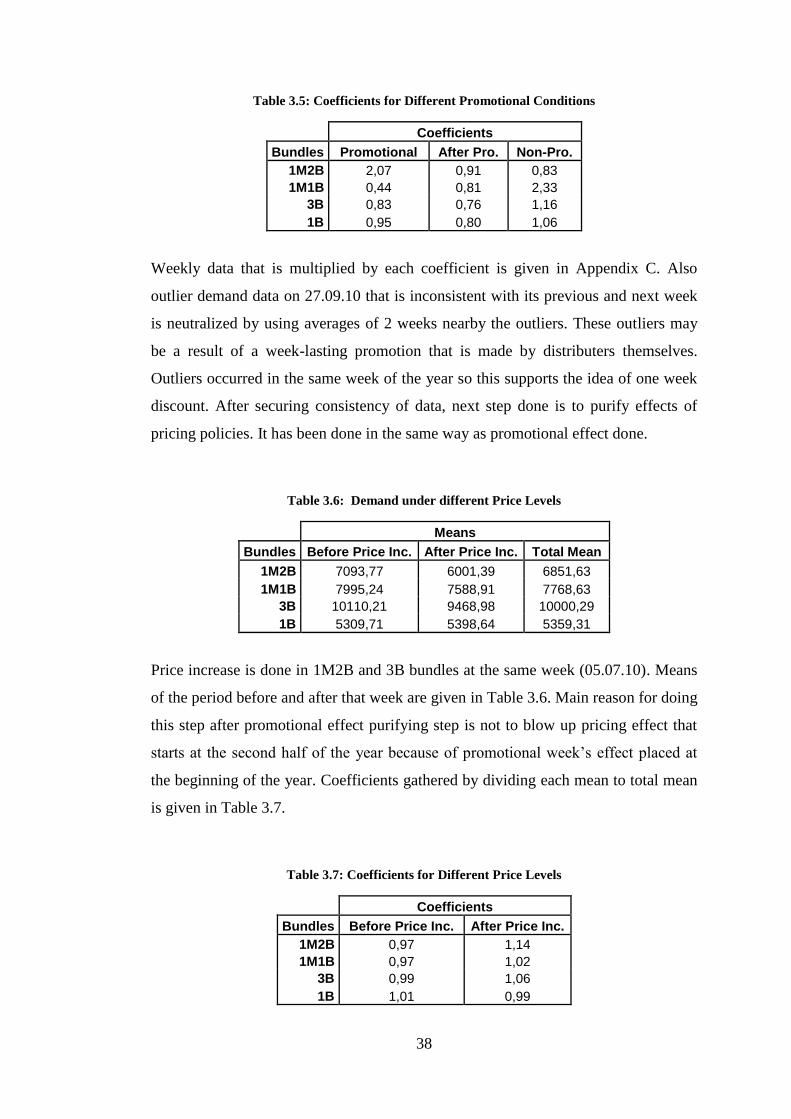
38

Table 3.5: Coefficients for Different Promotional Conditions

Coefficients

Bundles Promotional After Pro. Non-Pro.

1M2B 2,07 0,91 0,83

1M1B 0,44 0,81 2,33

3B 0,83 0,76 1,16

1B 0,95 0,80 1,06

Weekly data that is multiplied by each coefficient is given in Appendix C. Also

outlier demand data on 27.09.10 that is inconsistent with its previous and next week

is neutralized by using averages of 2 weeks nearby the outliers. These outliers may

be a result of a week-lasting promotion that is made by distributers themselves.

Outliers occurred in the same week of the year so this supports the idea of one week

discount. After securing consistency of data, next step done is to purify effects of

pricing policies. It has been done in the same way as promotional effect done.

Table 3.6: Demand under different Price Levels

Means

Bundles Before Price Inc. After Price Inc. Total Mean

1M2B 7093,77 6001,39 6851,63

1M1B 7995,24 7588,91 7768,63

3B 10110,21 9468,98 10000,29

1B 5309,71 5398,64 5359,31

Price increase is done in 1M2B and 3B bundles at the same week (05.07.10). Means

of the period before and after that week are given in Table 3.6. Main reason for doing

this step after promotional effect purifying step is not to blow up pricing effect that

starts at the second half of the year because of promotional week’s effect placed at

the beginning of the year. Coefficients gathered by dividing each mean to total mean

is given in Table 3.7.

Table 3.7: Coefficients for Different Price Levels

Coefficients

Bundles Before Price Inc. After Price Inc.

1M2B 0,97 1,14

1M1B 0,97 1,02

3B 0,99 1,06

1B 1,01 0,99

39

For the sake of simplicity, price change that is only made in 3B bundle is not taken

into calculation. New set of data calculated by multiplying each coefficient to its

affiliated week is given in Appendix D.

Last step is to bring each week together to create a monthly basis data. Set of

monthly data used in optimization algorithm is given in Table 3.8.

Table 3.8: Monthly Data Prepared for Algorithm

Months

Bundles 1 2 3 4 5 6

1M2B 42267 42419 18434 6519 33089 31850

1M1B 25130 21747 53915 29724 37742 35258

3B 35144 36008 50812 40475 49458 42067

1B 25401 26742 26063 16418 27047 20486

Months

7 8 9 10 11 12 Total

12963 19836 23042 32061 39476 54328 356285

30968 36858 32235 27941 41309 31142 403969

28986 41075 43445 48528 55726 48289 520015

19980 20702 21966 18263 32477 23139 278684

Since it is an optimization problem, first step is building the algorithm to define the

objective function. As mentioned in Section 3.3, there are two conflicting goals that

need to be maximized. To maximize more than one goal in one problem, it is

appropriate to use goal modeling. In order to show how goals change under different

levels of weights, model will be run several times with changing weights.

( )

((( ) ( ) ( ) ( ) ) ) ⁄

(( ) ) ⁄

(3.1)

Objective function for undefined weighted goals is given in Equation 3.1.

GOAL1P is the percentage profit change using the new price, demand and extracting

existing profit. Total theoretical profit gathered selling 4 different bundles in year

2010 is 18.901.174 TL.

40

GOAL2P is the percentage demand change from the existing total demand. While

maximizing profit by increasing price, the firm should be protecting its current

position in the market. This goal helps providing this type of aim.

(3.2)

Equation 3.2 is written to claim that price of any bundle cannot be less than its cost.

Costs used are not real because of privacy issues but they are approximately adapted

from real costs. Each unit in bundle is taken as 1TL and 1TL as packaging costs are

added afterwards. For example, price of 1M2B is a sum of 1TL machine cost, 2TL

bottle cost and 1TL packaging cost.

(3.3)

To protect company’s pricing policy at least partially, constraints for rational

relationship between bundle prices is included into the model. In existing price

structure, price of 1M1B is 60% of price of 1M2B and 1B price is 80% of 1M1B

price. To sum up, 1M1B price changes depends on the price of 1M2B and 1B price

changes depends on the price of 1M1B. Price of 3B is left alone to float itself.

In the optimization model, Equations from 3.4 to 3.7 is written in a loop to use set of

monthly data and assign promotional month(s) into binary variables. Loop format of

equations can be found in Appendix B.

41

∑( ) ((

) ( ) )

( ((

) ( ) ))

(3.4)

∑( ) ((

) ( ) )

( ((

) ( ) ))

(3.5)

∑( ) ((

) ( ) )

( ((

) ( ) ))

(3.6)

∑( ) ((

) ( ) )

( ((

) ( ) ))

(3.7)

In the equations above, PROi is a binary variable which gets 1 as a value when it is

optimum to make promotion on that month, gets 0 when it is not feasible to make

promotion. Data sets of 12 months calculated earlier in this section are used as set of

values for variables B12i, B1i, B222i and B2i in the algorithm of the model.

Equations from 3.4 to 3.7 are the main body of the algorithm written. They are built

to change demand for different promotional and pricing conditions. At first glance,

they consist of two parts; during promotion period price; and no promotion price. To

actualize the total demand equation depending on the price conditions, how much

demand changes for 1 unit of increase/decrease in price is found. Demand reflection

42

to the price change is found from the real data set by using basic ratios. The

normalized average difference between higher priced months and lower priced

months is 3566 for average price change of 1,63. So, 1 unit distinction in price

causes demand to decrease/increase 2188 units. In algorithm, the program

cumulatively sums demands of each month and ends up with total demand to use in

objective function.

3.5. Results

To gather results, percentage weights are used for W in Equation 3.1. In literature,

many studies have done to search for relationship between market share and

profitability. In years according to the Table 3.9, results change from strongly

positive to no or weakly positive relationship. Fraering and Minor (1994) also

resulted with a too weak relationship in their comparative study of company ROAs

(return on asset) and market shares. In order for an entity to sustain its existence, it

must be profitable; except for the charities and non-profit organizations. Thus,

weights are chosen in a scale that is closer to the profitability goal. Goals starts from

50% to 50%, additively 10% increases in each step and finally reaches to 100% to

%0.

Equations explained in the previous section are turned into language of Lingo

optimization program and run for different levels of goal weights. A screenshot of

codes and a sample solution sheet for 50% weights is given in Appendix E. Results

for different levels of weights are given in Table 3.10. In addition to that, existing

conditions are shown in Table 3.11 to compare before and after optimization.

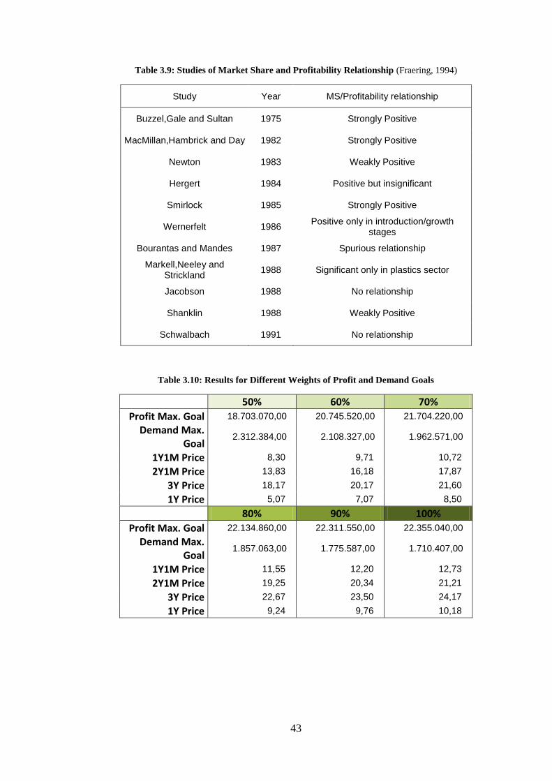
43

Table 3.9: Studies of Market Share and Profitability Relationship (Fraering, 1994)

Study Year MS/Profitability relationship

Buzzel,Gale and Sultan 1975 Strongly Positive

MacMillan,Hambrick and Day 1982 Strongly Positive

Newton 1983 Weakly Positive

Hergert 1984 Positive but insignificant

Smirlock 1985 Strongly Positive

Wernerfelt 1986 Positive only in introduction/growth

stages

Bourantas and Mandes 1987 Spurious relationship

Markell,Neeley and Strickland

1988 Significant only in plastics sector

Jacobson 1988 No relationship

Shanklin 1988 Weakly Positive

Schwalbach 1991 No relationship

Table 3.10: Results for Different Weights of Profit and Demand Goals

50% 60% 70%

Profit Max. Goal 18.703.070,00 20.745.520,00 21.704.220,00

Demand Max. Goal

2.312.384,00 2.108.327,00 1.962.571,00

1Y1M Price 8,30 9,71 10,72

2Y1M Price 13,83 16,18 17,87

3Y Price 18,17 20,17 21,60

1Y Price 5,07 7,07 8,50

80% 90% 100%

Profit Max. Goal 22.134.860,00 22.311.550,00 22.355.040,00

Demand Max. Goal

1.857.063,00 1.775.587,00 1.710.407,00

1Y1M Price 11,55 12,20 12,73

2Y1M Price 19,25 20,34 21,21

3Y Price 22,67 23,50 24,17

1Y Price 9,24 9,76 10,18

44

Table 3.11: Existing Conditions for Bundles

Existing C.

Profit Max. Goal 18.901.174,00

Demand Max. Goal 1.573.652,00

1Y1M Price 9,99

2Y1M Price 17,99

3Y Price 20,99

1Y Price 8,99

Results are given in Table 3.10 are graphically visualized in Figure 3.12. Profit

increases faster at the beginning of the model runs where the goal weights are closer

to each other. But closer to the last runs, profit stays relatively steady. This is

because of the negative effects of price increase. Consumers stop buying or buy less

frequent when the price of the product is higher than their reservation prices. As the

model increases prices, demand falls but it needs high demand and high price to

maximize the profit goal defined. Thus, it stabilizes the increase of profit.

Figure 3.12: Graphic of Profit and Demand Goals

Prices and demands are not the only results of the algorithm written. There was

another important variable to analyze carefully; promotional months. Promotional

month results for all goal weights are the same and equal to 1, meaning promotion

should be continuous and deployed into all year. Promotional month is not just a type

of discount period, it brings out a new bundle which is only available in that months.

When promotion is spread to whole year, it means bringing promotional 1M1B

bundle package as a normal product that is packaged continuously.

-

500.000,00

1.000.000,00

1.500.000,00

2.000.000,00

2.500.000,00

16.000.000,00

17.000.000,00

18.000.000,00

19.000.000,00

20.000.000,00

21.000.000,00

22.000.000,00

23.000.000,00

50% 60% 70% 80% 90% 100%

Profit Max. Goal (TL)

Demand Max. Goal

45

To show the effect of profit and market share changes, Table 3.12 is drawn.

Percentage increases got closer to each other around 80% - 20% weight distribution

model.

Table 3.12: Comparison of Results and Existing Conditions

Percentage Change

Weights 50% 60% 70% 80% 90% 100%

Profit -1% 10% 15% 17% 18% 18%

Demand 47% 34% 25% 18% 13% 9%

Total 23% 19% 18% 17% 18% 18%

Figure 3.13: Comparison Chart

According to the results of the algorithm utilized, the existing strategy of the firm is

not right and should be changed. In line with the research questions defined in

Problem Definition section, we suggest that the 80% weighted result is the most

appropriate price structure for the company. It improves both profit and market share

with more balanced change ratios (17% Profit Increase and 18% Market Share

Increase).

-1% 10%

15% 17% 18% 18%

47%

34% 25%

18% 13% 9%

50% 60% 70% 80% 90% 100%

Profit Change Demand Change

46

Table 3.13: Comparison Table of Proposed vs. Existing Pricing Structures

Existing C. Proposed Change %

Profit 18.901.174,00 22.134.860,00 17,1%

Demand 1.573.652,00 1.857.063,00 18,0%

1M1B Price 9,99 11,55 15,6%

1M2B Price 17,99 19,25 7,0%

3B Price 20,99 22,67 8,0%

1B Price 8,99 9,24 2,8%

Generally there exists a price increase between new and old prices. But, according to

Table 3.13, those changes do not exceed company’s price increase strategy that has

been done before as 9% and 16% price increases. While proposed pricing structure

does not exceed company’s framework of price increase, it improves both profit and

demand simultaneously.

Apart from pricing results of algorithm, promotional results show that there is no

need of any promotional period or promotional product. Instead the “promotional

product1M1B” bundle should be added to the product portfolio and sold all year

long based on the existing demand conditions. Thus, company should package 1M2B

and 1M1B simultaneously.

To sum up, results given in this section support that; it is possible to both increase

profit and demand by making promotional product available all year and making

small adjustments to the existing pricing strategies. While promotion boosts demand

for most of the bundles and increases profit accordingly, slightly higher prices will

not make big differences in company’s position in the market, instead they will help

increase profits.

3.6. Conclusion

Bundling, one of the common application of selling practices, has been analyzed for

over many years. Packaging products together and selling them as a bundle is done

for increasing sales volume and decreasing uncertainty, like many marketing

strategies are intended to do. But sales volume is not the only multiplier in sales

revenue; price is another strong player in both marketing and financial analysis. To

co-operate with those two difficult revenue drivers was what this thesis aimed to

47

achieve. It has always needed a hard work to maximize both profit and sales volume.

Profit generally depends on high prices while demand is in a reverse relationship

with price. As a matter of fact, an optimization model was developed to maximize

profits by using accurate price allocation constraints while taking advantage of

bundling as a volume increaser inhibitor. The aim of optimizing simultaneously to

conflicting goals is achieved. A new strategy of canceling promotional periods and

selling them as a regular product is achieved. New prices for existing bundles and

products are defined. With the help of new strategy and new prices demand is

improved 18% and profit increase by 17%.

Bundling was usually investigated by making assumptions, applying survey methods

about non-existing products. Results were usually dependent to theoretical

approaches, judgmental data that is likely to differ from research to research.

Considering bundles that do not even exist was not sufficient in order to develop

right strategies for right bundles in right prices. In that manner, the most important

role of this research was to work with real bundle demand data without getting lost in

approaches or assumptions. Optimization was the most appropriate method that is

likely to solve chaos of conflicting goals, price and demand constraints, and

maximization issues in the demand data that is given by the company. It is full of

surprises, unexpected errors to work with real demand data. Mixed bundling demand

data was laying untouched at the beginning of this research but after many attempts,

creating, disposing, recreating many models a solution was gathered. Initial models

were mainly focused on building a regression equation that consists of every impact,

making each demand curve float through time. Lingo 11.0 is used as a tool to find an

optimum solution for the models developed. Infinite loops, inapplicable too high

prices were the main problems of the initial models. Those problems were solved

with a lean model that accepts only two effects as main demand drivers and ignores

others because they are in the nature of the products/bundles. Results were

acceptable and we achieved our aim of maximizing two conflicting profit and

demand goals. In addition, a new promotional strategy is suggested.

Scarce amount of data was our limitations. With the help of longer data periods,

recursive promotional periods results can be improved. Also, some effects are

ignored because of absence of rival companies’, substitute product data. More

48

reflective results can be gathered by including more data and more effects into the

model developed. Working with a real company, observing real customer reactions

to changes in strategies gives encouraging and motivational aim to achieve but it also

brings some difficulties indeed.

49

REFERENCES

Adams, W. J. and Yellen, J.L., 1976 “Commodity Bundling and the Burden of

Monopoly”, Quarterly Journal of Economics, 90, pp. 475-498

Eckalbar, J.C., 2005 “Exploring Bundling Theory with Geometry”, Journal of

Economic Education Winter 2006, pp. 68-82

Fraering, J.M. and Minor, S.M., 1994,"The Industry-specific Basis of the Market

Share-Profitability Relationship”, Journal of Consumer Marketing, Vol. 11 Iss: 1 pp.

27 – 37

Fürderer, A. Hermann, amd G. Wübker (Eds.), 1999, Optimal Bundle Pricing:

Marketing Strategies for Improving Economic Performance, chapter “Introduction to

Price Bundling”. Berlin, Heidelberg: Springer Verlag

Gendall, P., Holdershaw, J., Garland, R., 1997, "The effect of odd pricing on

demand", European Journal of Marketing, Vol. 31, November-December, pp.799-

814

Hinterhuber, A., 2004, “Towards Value Based Pricing- An Integrative Framework

for Decision Making”, Industrial Marketing Management, 33, pp. 765-778

Holdershaw, J., Gendall, P. and Garland, R., 1997, “The Widespread use of odd

pricing in the retail sector”, Marketing Bulletin, Vol. 7, pp. 53-58

Indounas, K., 2006, “Making Effective Pricing Decisions”, Business Horizons, 49,

pp. 415-427

Kotler, P. and Armstrong, G., 2004, “Principles of Marketing”, 10th ed.,

Pearson/Prentice-Hall, Upper Saddle River, NJ

50

Lusch, R.F., Lusch, V., 1987, “Principles of Marketing”, Wadsworth, Inc., California

Simon, H. and Wuebker, G., 1999 “Bundling – A Powerful Method to Better Exploit

Profit Potential” Optimal Bundling, pp. 7-28

Mandell, Maurice I., 1985, “Marketing”, 3rd

ed., Prentice-Hall, Inc, Englewood

Cliffs, New Jersey

NIST/SEMATECH e-Handbook of Statistical Methods,

http://www.itl.nist.gov/div898/handbook/, April 2012

Popkowski L. and Haubl G., 2010, “To Bundle or Not to Bundle: Determinants of

the Profitability of Multi-Item Auctions”, Journal of Marketing, 74(4):110–124

Sheng, S., Parker, A.M. and Nakamoto, K., 2007, “The effects of price discount and

product complementarity on consumer evaluations of bundle components”, Journal

of Marketing Theory and Practice, Vol. 15 No. 1, pp. 53-64

Salinger, M.A., 1995, “A Graphical Analysis of Bundling”, The Journal of Business,

Vol. 68, No. 1, pp. 85-98

Stremersch S., Tellis, 2002, “Strategic bundling of products and prices: a new

synthesis for marketing”, Journal of marketing Vol. 66, 55-72

Zikmund, W., D’Amico M., 1996 “Marketing”, Fifth Edition, West Publishing,

Minneapolis, USA

Montgomery, S., 1988 “Profitable Pricing Strategies”, McGraw-Hill, Inc

51

APPENDICES

52

APPENDIX A: Raw Demand Data

Dates 04.01.10 11.01.10 18.01.10 25.01.10 01.02.10 08.02.10

Bun

dle

s 1M2B 9392 16171 15345 12648 6164 5339

1M1B 141 107 84 680 4614 8951

3B 6988 6909 8722 13677 9750 14902

1B 5463 6510 4696 6771 7754 7647

Dates 15.02.10 22.02.10 01.03.10 08.03.10 15.03.10 22.03.10

Bun

dle

s 1M2B 5426 4297 2980 2153 1758 1274

1M1B 16964 20006 27441 29039 26787 23553

3B 10231 9141 9645 14214 12210 14067

1B 6324 6098 6690 5773 5379 4541

Dates 29.03.10 05.04.10 12.04.10 19.04.10 26.04.10 03.05.10

Bun

dle

s 1M2B 1059 1016 885 729 632 1126

1M1B 18465 16263 13343 23200 16266 14507

3B 11988 10359 10811 12827 15489 14171

1B 4733 4749 4325 3878 4130 5042

Dates 10.05.10 17.05.10 24.05.10 31.05.10 07.06.10 14.06.10

Bun

dle

s 1M2B 2970 11118 13344 9068 6099 7430

1M1B 10220 7259 10610 5608 3942 3783

3B 10761 10567 19929 10685 7616 6896

1B 6162 5330 9753 7122 4296 4545

Dates 21.06.10 28.06.10 05.07.10 12.07.10 19.07.10 26.07.10

Bun

dle

s 1M2B 6812 19372 4051 3535 3257 2831

1M1B 3650 4222 3696 3487 3221 2599

3B 9325 12839 6559 5974 5976 5160

1B 4182 6083 4485 4475 5219 4767

Dates 02.08.10 09.08.10 16.08.10 23.08.10 30.08.10 06.09.10

Bun

dle

s 1M2B 3852 4036 3771 4291 4974 6704

1M1B 2901 3027 3121 3067 3360 3888

3B 6895 7226 5743 6001 7675 10779

1B 4132 4047 3720 3570 4162 4857

53

APPENDIX A: CONT’D

Dates 13.09.10 20.09.10 27.09.10 04.10.10 11.10.10 18.10.10

Bun

dle

s 1M2B 5973 5884 28733 5120 6004 7895

1M1B 3208 3158 3281 3200 3050 2824

3B 9388 6853 19563 8154 9427 8563

1B 5788 4200 5984 5091 4123 4304

Dates 25.10.10 01.11.10 08.11.10 15.11.10 22.11.10 29.11.10

Bun

dle

s 1M2B 14801 5381 9576 9665 8890 8130

1M1B 2658 2744 4179 3624 3480 3318

3B 13483 7563 12627 8431 7396 9487

1B 3800 4423 7335 6874 6309 5855

Dates 06.12.10 13.12.10 20.12.10 27.12.10 03.01.11 10.01.11

Bun

dle

s 1M2B 11731 16035 18371 11172 5854 6143

1M1B 3494 3421 3318 2843 3219 3747

3B 9567 11506 10117 8241 6372 6931

1B 6394 5271 5016 5261 5832 6862

Dates 17.01.11 24.01.11 31.01.11 07.02.11 14.02.11 21.02.11

Bun

dle

s 1M2B 5926 9.191 9.587 3.899 4.256 2.339

1M1B 3463 3.085 3.950 7.705 9.784 17.361

3B 6260 12276 13537 11604 14040 19700

1B 5221 4654 4552 5073 5486 4869

Dates 28.02.11 07.03.11 14.03.11 Avr. Sum

Profit / Unit

Total Profit

Bun

dle

s 1M2B 2.526 2.107 2.237 6851,6 356285 14 4987990

1M1B 21.451 17.368 15.403 7768,6 403969 7 2827783

3B 23977 19475 17640 10000,3 520015,3 17 8840261

1B 5300 5147 6290 5359,3 278684 7 1950788

Total

Demand 1558953

Total Profit

18606822

Notes:

Red colored area is not used in one year calculations. Instead, yellow colored area is

used.

Blue colored area represents promotional periods.

Green colored area shows after promotional period.

Red lines indicate the dates of price increases.

54

APPENDIX B: Screenshot of Codes

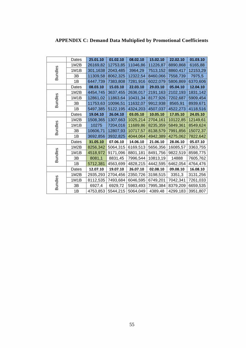
55

APPENDIX C: Demand Data Multiplied by Promotional Coefficients

Dates 25.01.10 01.02.10 08.02.10 15.02.10 22.02.10 01.03.10 B

un

dle

s 1M2B 26169,82 12753,85 11046,86 11226,87 8890,868 6165,88

1M1B 301,1638 2043,485 3964,29 7513,152 8860,417 12153,29

3B 11309,58 8062,325 12322,54 8460,066 7558,739 7975,5

1B 6447,739 7383,808 7281,916 6022,079 5806,869 6370,606

Dates 08.03.10 15.03.10 22.03.10 29.03.10 05.04.10 12.04.10

Bun

dle

s 1M2B 4454,745 3637,455 2636,017 2191,163 2102,193 1831,142

1M1B 12861,02 11863,64 10431,34 8177,926 7202,687 5909,454

3B 11753,63 10096,51 11632,07 9912,938 8565,91 8939,671

1B 5497,385 5122,195 4324,203 4507,037 4522,273 4118,516

Dates 19.04.10 26.04.10 03.05.10 10.05.10 17.05.10 24.05.10

Bun

dle

s 1M2B 1508,365 1307,663 1025,214 2704,161 10122,85 12149,61

1M1B 10275 7204,016 11689,86 8235,359 5849,361 8549,624

3B 10606,71 12807,93 10717,57 8138,579 7991,856 15072,37

1B 3692,856 3932,825 4044,064 4942,389 4275,062 7822,642

Dates 31.05.10 07.06.10 14.06.10 21.06.10 28.06.10 05.07.10

Bun

dle

s 1M2B 8256,342 5064,315 6169,513 5656,356 16085,57 3363,755

1M1B 4518,972 9171,096 8801,181 8491,756 9822,519 8598,775

3B 8081,1 8831,45 7996,544 10813,19 14888 7605,762

1B 5712,381 4563,699 4828,215 4442,595 6462,054 4764,476

Dates 12.07.10 19.07.10 26.07.10 02.08.10 09.08.10 16.08.10

Bun

dle

s 1M2B 2935,293 2704,456 2350,726 3198,515 3351,3 3131,256

1M1B 8112,535 7493,684 6046,595 6749,201 7042,341 7261,033

3B 6927,4 6929,72 5983,493 7995,384 8379,209 6659,535

1B 4753,853 5544,215 5064,049 4389,48 4299,183 3951,807

56

APPENDIX C CONT’D

Dates 23.08.10 30.08.10 06.09.10 13.09.10 20.09.10 27.09.10

Bun

dle

s 1M2B 3563,039 4130,169 5566,678 4959,691 4885,79 4770,578

1M1B 7135,401 7817,068 9045,465 7463,439 7347,114 7633,274

3B 6958,709 8899,866 12499,24 10886,25 7946,682 9804,83

1B 3792,46 4421,349 5159,657 6148,671 4461,717 6356,885

Dates 04.10.10 11.10.10 18.10.10 25.10.10 01.11.10 08.11.10

Bun

dle

s 1M2B 4251,401 4985,432 6555,627 12290,04 4468,123 7951,448

1M1B 7444,827 7095,851 6570,06 6183,859 6383,939 9722,479

3B 9455,31 10931,08 9929,197 15634,39 8769,605 14642,16

1B 5408,239 4379,919 4572,198 4036,792 4698,613 7792,07

Dates 15.11.10 22.11.10 29.11.10 06.12.10 13.12.10 20.12.10

Bun

dle

s 1M2B 8025,349 7381,827 6750,759 9740,856 13314,69 15254,39

1M1B 8431,267 8096,249 7719,355 8128,82 7958,985 7719,355

3B 9776,904 8576,34 11000,66 11094,2 13342,26 11731,59

1B 7302,344 6702,136 6219,846 6792,433 5599,455 5328,565

Dates 27.12.10 03.01.11 10.01.11 17.01.11 Avr. Sum

Bun

dle

s 1M2B 9276,689 4860,879 5100,851 4920,664 6484,559 337197,1

1M1B 6614,263 7489,031 8717,427 8056,699 7768,635 403969

3B 9555,808 7388,531 8036,743 7259,43 9752,598 507135,1

1B 5588,832 6195,413 7289,596 5546,339 5359,308 278684

Notes:

Blue colored area represents promotional periods.

Green colored area shows after promotional period.

Non-colored area shows the non-promotional area.

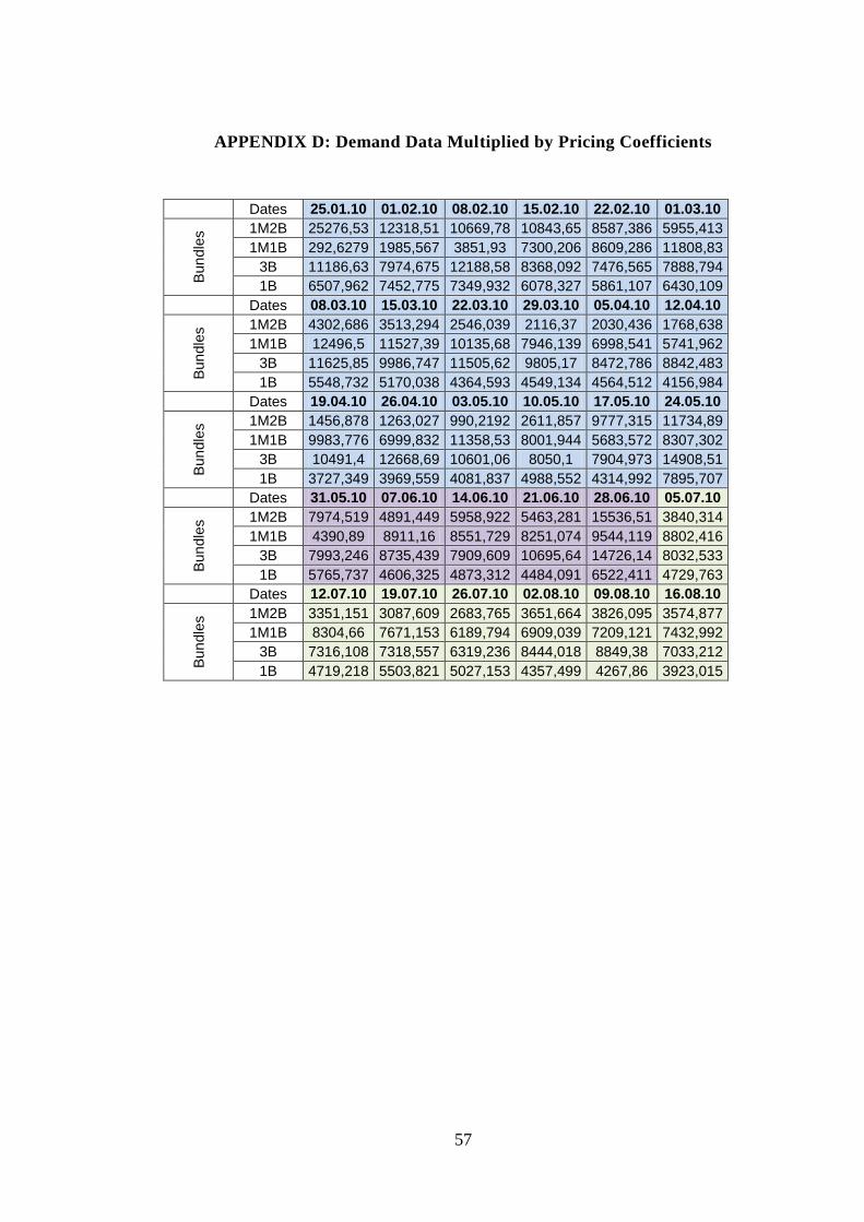
57

APPENDIX D: Demand Data Multiplied by Pricing Coefficients

Dates 25.01.10 01.02.10 08.02.10 15.02.10 22.02.10 01.03.10 B

un

dle

s 1M2B 25276,53 12318,51 10669,78 10843,65 8587,386 5955,413

1M1B 292,6279 1985,567 3851,93 7300,206 8609,286 11808,83

3B 11186,63 7974,675 12188,58 8368,092 7476,565 7888,794

1B 6507,962 7452,775 7349,932 6078,327 5861,107 6430,109

Dates 08.03.10 15.03.10 22.03.10 29.03.10 05.04.10 12.04.10

Bun

dle

s 1M2B 4302,686 3513,294 2546,039 2116,37 2030,436 1768,638

1M1B 12496,5 11527,39 10135,68 7946,139 6998,541 5741,962

3B 11625,85 9986,747 11505,62 9805,17 8472,786 8842,483

1B 5548,732 5170,038 4364,593 4549,134 4564,512 4156,984

Dates 19.04.10 26.04.10 03.05.10 10.05.10 17.05.10 24.05.10

Bun

dle

s 1M2B 1456,878 1263,027 990,2192 2611,857 9777,315 11734,89

1M1B 9983,776 6999,832 11358,53 8001,944 5683,572 8307,302

3B 10491,4 12668,69 10601,06 8050,1 7904,973 14908,51

1B 3727,349 3969,559 4081,837 4988,552 4314,992 7895,707

Dates 31.05.10 07.06.10 14.06.10 21.06.10 28.06.10 05.07.10

Bun

dle

s 1M2B 7974,519 4891,449 5958,922 5463,281 15536,51 3840,314

1M1B 4390,89 8911,16 8551,729 8251,074 9544,119 8802,416

3B 7993,246 8735,439 7909,609 10695,64 14726,14 8032,533

1B 5765,737 4606,325 4873,312 4484,091 6522,411 4729,763

Dates 12.07.10 19.07.10 26.07.10 02.08.10 09.08.10 16.08.10

Bun

dle

s 1M2B 3351,151 3087,609 2683,765 3651,664 3826,095 3574,877

1M1B 8304,66 7671,153 6189,794 6909,039 7209,121 7432,992

3B 7316,108 7318,557 6319,236 8444,018 8849,38 7033,212

1B 4719,218 5503,821 5027,153 4357,499 4267,86 3923,015

58

APPENDIX D CONT’D

Dates 23.08.10 30.08.10 06.09.10 13.09.10 20.09.10 27.09.10

Bun

dle

s 1M2B 4067,832 4715,311 6355,336 5662,354 5577,983 5446,449

1M1B 7304,386 8002,196 9259,684 7640,192 7521,112 7814,049

3B 7349,174 9399,252 13200,59 11497,09 8392,583 10355

1B 3764,828 4389,136 5122,065 6103,873 4429,21 6310,57

Dates 04.10.10 11.10.10 18.10.10 25.10.10 01.11.10 08.11.10

Bun

dle

s 1M2B 4853,718 5691,742 7484,395 14031,23 5101,143 9077,969

1M1B 7621,139 7263,898 6725,655 6330,309 6535,127 9952,732

3B 9985,863 11544,44 10486,34 16511,66 9261,682 15463,76

1B 5368,835 4348,008 4538,886 4007,38 4664,38 7735,299

Dates 15.11.10 22.11.10 29.11.10 06.12.10 13.12.10 20.12.10

Bun

dle

s 1M2B 9162,34 8427,646 7707,173 11120,89 15201,05 17415,56

1M1B 8630,94 8287,989 7902,169 8321,331 8147,474 7902,169

3B 10325,5 9057,572 11617,92 11716,71 14090,92 12389,87

1B 7249,14 6653,306 6174,53 6742,945 5558,659 5289,742

Dates 27.12.10 03.01.11 10.01.11 17.01.11 Avr. Sum

Bun

dle

s 1M2B 10590,96 5549,543 5823,513 5617,799 6851,635 356285

1M1B 6770,906 7666,39 8923,878 8247,502 7768,635 403969

3B 10092 7803,114 8487,698 7666,769 10000,29 520015,3

1B 5548,113 6150,274 7236,485 5505,93 5359,308 278684

Notes:

Framed cells are normalized using the two cells around them.

Each color shows a different price period.

59

APPENDIX E: Solution Sheet for 50% to 50% Weights

Local optimal solution found.

Objective value: 0.2442367

Objective bound: 0.2442367

Infeasibilities: 0.3725290E-08

Extended solver steps: 0

Total solver iterations: 96

Variable Value Reduced Cost

GOAL1P 0.7650910E-02 0.000000

GOAL2P 0.4808226 0.000000

P1 8.326821 0.000000

D1 956236.7 0.000000

P12 13.87804 0.000000

D12 270936.1 0.000000

P222 18.20742 0.000000

D222 686407.5 0.000000

P2 5.106906 0.000000

D2 394952.4 0.000000

GOAL1 0.1874918E+08 0.000000

GOAL2 2308533. 0.000000

MD12( JAN) 28636.11 0.000000

MD12( FEB) 29521.19 0.000000

MD12( MAR) 17928.38 0.000000

MD12( APR) 12169.65 0.000000

MD12( MAY) 25011.51 0.000000

MD12( JUN) 24412.85 0.000000

MD12( JUL) 14664.90 0.000000

MD12( AUG) 17658.44 0.000000

MD12( SEP) 19054.98 0.000000

MD12( OCT) 22983.24 0.000000

MD12( NOV) 26212.97 0.000000

MD12( DEC) 32681.92 0.000000

B12( JAN) 40588.09 0.000000

B12( FEB) 42419.33 0.000000

B12( MAR) 18433.80 0.000000

B12( APR) 6518.979 0.000000

B12( MAY) 33088.80 0.000000

B12( JUN) 31850.16 0.000000

B12( JUL) 11681.65 0.000000

B12( AUG) 17875.30 0.000000

B12( SEP) 20764.74 0.000000

B12( OCT) 28892.31 0.000000

B12( NOV) 35574.61 0.000000

B12( DEC) 48958.88 0.000000

MD1( JAN) 60414.30 0.000000

MD1( FEB) 52773.36 0.000000

MD1( MAR) 125419.1 0.000000

MD1( APR) 70788.53 0.000000

MD1( MAY) 88896.33 0.000000

MD1( JUN) 83286.21 0.000000

MD1( JUL) 73597.73 0.000000

MD1( AUG) 86898.79 0.000000

60

APPENDIX E CONT’D

MD1( SEP) 76459.11 0.000000

MD1( OCT) 66761.64 0.000000

MD1( NOV) 96951.25 0.000000

MD1( DEC) 73990.36 0.000000

B1( JAN) 25130.40 0.000000

B1( FEB) 21746.99 0.000000

B1( MAR) 53914.54 0.000000

B1( APR) 29724.11 0.000000

B1( MAY) 37742.24 0.000000

B1( JUN) 35258.08 0.000000

B1( JUL) 30968.02 0.000000

B1( AUG) 36857.73 0.000000

B1( SEP) 32235.04 0.000000

B1( OCT) 27941.00 0.000000

B1( NOV) 41308.96 0.000000

B1( DEC) 31141.88 0.000000

MD222( JAN) 47308.24 0.000000

MD222( FEB) 49650.56 0.000000

MD222( MAR) 67551.73 0.000000

MD222( APR) 55052.55 0.000000

MD222( MAY) 65914.13 0.000000

MD222( JUN) 56976.94 0.000000

MD222( JUL) 39589.88 0.000000

MD222( AUG) 53552.37 0.000000

MD222( SEP) 56290.01 0.000000

MD222( OCT) 62161.01 0.000000

MD222( NOV) 70474.94 0.000000

MD222( DEC) 61885.18 0.000000

B222( JAN) 34070.81 0.000000

B222( FEB) 36007.91 0.000000

B222( MAR) 50812.18 0.000000

B222( APR) 40475.36 0.000000

B222( MAY) 49457.88 0.000000

B222( JUN) 42066.83 0.000000

B222( JUL) 27687.73 0.000000

B222( AUG) 39234.71 0.000000

B222( SEP) 41498.74 0.000000

B222( OCT) 46354.05 0.000000

B222( NOV) 53229.67 0.000000

B222( DEC) 46125.94 0.000000

MD2( JAN) 35199.44 0.000000

MD2( FEB) 36608.57 0.000000

MD2( MAR) 35894.78 0.000000

MD2( APR) 25764.31 0.000000

MD2( MAY) 36928.63 0.000000

MD2( JUN) 30037.14 0.000000

MD2( JUL) 29505.44 0.000000

MD2( AUG) 30264.24 0.000000

MD2( SEP) 31591.32 0.000000

MD2( OCT) 27702.03 0.000000

MD2( NOV) 42632.22 0.000000

MD2( DEC) 32824.24 0.000000

B2( JAN) 25400.65 0.000000

B2( FEB) 26742.14 0.000000

B2( MAR) 26062.61 0.000000

61

APPENDIX E CONT’D

B2( APR) 16418.40 0.000000

B2( MAY) 27046.83 0.000000

B2( JUN) 20486.14 0.000000

B2( JUL) 19979.96 0.000000

B2( AUG) 20702.34 0.000000

B2( SEP) 21965.72 0.000000

B2( OCT) 18263.11 0.000000

B2( NOV) 32476.65 0.000000

B2( DEC) 23139.46 0.000000

PRO( JAN) 1.000000 -0.1355669E

PRO( FEB) 1.000000 -0.1044292E

PRO( MAR) 1.000000 -0.5144237E

A PRO( APR) 1.000000 -0.3302470E

PRO( MAY) 1.000000 -0.3124164E

PRO( JUN) 1.000000 -0.2757151E

PRO( JUL) 1.000000 -0.2894133E

PRO( AUG) 1.000000 -0.3415884E

PRO( SEP) 1.000000 -0.2962256E

PRO( OCT) 1.000000 -0.2356187E

PRO( NOV) 1.000000 -0.3437207E

PRO( DEC) 1.000000 -0.1794916E

62

APPENDIX F: Tez Fotokopi İzin Formu

ENSTİTÜ

Fen Bilimleri Enstitüsü

Sosyal Bilimler Enstitüsü

Uygulamalı Matematik Enstitüsü

Enformatik Enstitüsü

Deniz Bilimleri Enstitüsü

YAZARIN

Soyadı : Ersöz

Adı : Keriman Hande

Bölümü : İşletme Bölümü

TEZİN ADI (İngilizce) : Price Determination For Bundled Products:

Applicatıon For A Household Product Group

TEZİN TÜRÜ : Yüksek Lisans Doktora

1. Tezimin tamamı dünya çapında erişime açılsın ve kaynak gösterilmek

şartıyla tezimin bir kısmı veya tamamının fotokopisi alınsın.

2. Tezimin tamamı yalnızca Orta Doğu Teknik Üniversitesi kullancılarının

erişimine açılsın. (Bu seçenekle tezinizin fotokopisi ya da elektronik kopyası

Kütüphane aracılığı ile ODTÜ dışına dağıtılmayacaktır.)

3. Tezim bir (1) yıl süreyle erişime kapalı olsun. (Bu seçenekle tezinizin

fotokopisi ya da elektronik kopyası Kütüphane aracılığı ile ODTÜ dışına

dağıtılmayacaktır.)

Yazarın imzası ............................ Tarih ………………….