Work Package 2: Change of BehaviorSCCER CREST

WP2 - 2018/01

Price elasticities of electricity demand in Switzerland: Results from a household panel

Benjamin Volland Ivan Tilov

May 2018

Schweizerische EidgenossenschaftConfédération suisseConfederazione SvizzeraConfederaziun svizra

Swiss Confederation

Innosuisse – Swiss Innovation Agency

This research is part of the activities of SCCER CREST (Swiss Competence Center for Energy Research), which is financially supported by Innosuisse under Grant No. KTI. 1155000154.

1

Price elasticities of electricity demand in Switzerland:

Results from a household panel*

Benjamin Volland† and Ivan Tilov†

This version: 1 May 2018

Abstract

In this paper, we use data from a new household-level panel survey to estimate short- and long-run price

elasticities of residential electricity demand in Switzerland. We exploit Switzerland’s unique local

variation in topography-related grid maintenance costs and electricity taxation, to address endogeneity

of average prices in our models. Using first difference and gradual adjustment models, we find short-

run elasticities of -0.3 and long-run elasticities in excess of negative unity. Results thus suggest that a

tax on electricity, as initially foreseen as a part of Switzerland’s Energy Strategy 2050, is likely to have

a moderate effect in the short run, but an important one in the long run.

JEL classification: C23, D12, Q41, Q48,

Keywords: Residential electricity demand, price elasticity, panel data, Switzerland

* This research is part of the activities of SCCER CREST (Swiss Competence Center for Energy Research), which

is financially supported by the Swiss Commission for Technology and Innovation (CTI) under Grant No. KTI.

1155000154. We are also indebted to Mehdi Farsi for helpful comments on earlier versions of the paper.

Remaining errors are ours. † University of Neuchâtel, Institute of Economic Research, Corresponding author: benjamin.volland@unine.ch

2

1 Introduction

One of the basic principles of microeconomic theory is that as the price of a good increases, the quantity

demanded of this good will decrease. This “law of demand”, which has been found to be valid in many

situations and for almost all goods,1 plays a prominent role in most countries’ efforts to reduce

greenhouse gas emissions and combat climate change, as it provides the rationale for taxation schemes

raising the price of energy.

In Switzerland, for instance, the government’s long-term energy strategy plan, the Energy Strategy 2050,

includes the introduction of such an energy tax. Its primary purpose is to incentivize consumers to switch

to more energy efficient appliances and to adopt sufficiency behaviours, and thereby to contribute to

attaining the strategy’s objectives of reducing per-capita energy consumption by 35% over the period

between 2000 and 2035, and electricity demand by 18% until 2050 (BfE/OFEN, 2013). An important

target group of the energy tax are private households, who accounted for about 35% of total greenhouse

gas emissions in 2016 (BfS/OFS, 2017), and are responsible for almost 60% of the 5866 GWh increase

in Swiss electricity consumption since 2000 (BfE/OFEN, 2017). Understanding how sensitive Swiss

consumers react to changes in electricity prices is thus crucial in order to evaluate and predict the

efficacy of such a price-based policy instrument in the Swiss context.

While a number of previous studies have estimated electricity price-elasticities in the Swiss residential

sector (Carlevaro & Spierer 1983; Dennerlein and Flaig 1987; Zweifel et al. 1997; Filippini 1995; 1999;

2011; Boogen et al. 2014; 2017), none of these studies has had access to household level panel data.

Instead estimations were either based on household level cross-sectional data (e.g. Dennerlein and Flaig

1987; Zweifel et al. 1997, Boogen et al. 2014) or have relied on panels using data aggregated at the level

of (a limited number of) cities or utilities (e.g. Filippini 1999, 2011, Boogen et al. 2017). Both

approaches are problematic for the identification of structural coefficients and thus price elasticities.

Cross-sectional estimates reflect price-related differences in electricity consumption between

households, rather than changes in electricity consumption by households facing changing prices.

Aggregation, on the other hand, levels out variation across heterogeneous consumers, and thus produces

estimates that tend to differ substantially from micro-level findings (Bohi 1981, Bohi and Zimmerman

1984, Micklewright 1989, Miller and Alberini 2016).

In this contribution, we therefore draw on the Swiss Household Energy Demand Survey (SHEDS), a

new, two-wave panel data set on energy consumption and expenditures of Swiss households, to estimate

dynamic electricity demand models at the household level. The survey contains comprehensive

information on energy demand, appliance stock as well as socio-economic characteristics of the

household and the people living therein (cf. Weber et al., 2017). We augment this survey data with

1 For an empirical example of a good violating this pattern, see Jensen and Miller (2008).

3

information on electricity prices and pricing schemes of suppliers in Switzerland obtained from the

Federal Electricity Commission (ElCom). We deal with the endogeneity of electricity prices by making

use of the fact that electricity distributers are essentially monopolies in Switzerland, and that the price

for residential consumers depends to a non-negligible part on community taxes and fees as well as

topography-related differences in the costs of constructing and maintaining the local distribution grid.

Using first difference and gradual adjustment models, we identify short-run elasticities of about -0.3 and

long-run elasticities in excess of -1.0. Our results thus suggest that household electricity demand is

inelastic in electricity prices in the short run, but elastic in the long run. Short-run estimates are very

similar to recent findings based on utility-level panel data (Boogen et al., 2017), and thus corroborate

the conclusions drawn from this type of data. While long-run elasticities also match previous utility-

level findings (Filippini, 2011), results are too imprecise to derive empirically robust conclusions.

Nevertheless, our findings highlight that an environmental tax on electricity is likely to be an efficient

strategy to achieve the electricity-related goals of the Energy Strategy 2050.

The structure of the paper is as follows. The next section provides the background to Switzerland’s

energy transition, describes the Swiss electricity market, and provides a review of the preceding

literature with a focus on empirical work on Swiss residential electricity consumption. The ensuing

section 3 introduces the different data sets on which this analysis is based. Empirical strategies are

detailed in section 4, while section 5 gives their results. Robustness of these results is checked in section

6. The final section then summarizes results and gives concluding remarks.

2 Background

2.1 Energy Strategy 2050

In the wake of the major accident at the Japanese nuclear power plant at Fukushima on 11th March 2011,

the Swiss government decided to gradually phase out nuclear energy. While existing nuclear plants are

allowed to continue operating until the end of their service life, replacements are outlawed, such that the

last plant is predicted to be taken off the grid by 2034 (BfE/OFEN, 2013).

Since roughly one-third of Switzerland’s electricity is generated from nuclear fission today (BfE/OFEN,

2017), the implications of such a switch in the structure of electricity supply are substantial. In order to

counter potential electricity supply gaps, the government initiated a long-term energy policy plan, the

so-called Energy Strategy 2050. It aims to expand the production of electricity from renewable sources,

in particular hydropower, and seeks to reduce per-capita electricity consumption by 18% between the

years 2000 and 2050 (BfE/OFEN, 2013). Since the domestic sector is the one with the highest increase

in electricity consumption since the turn of the millennium and thus accounts for a growing share of

4

total electricity use in Switzerland (BfE/OFEN, 2017), it presents a key target group of the energy policy

plan. To reduce energy consumption in the domestic sector the strategy includes subsidies and tax

incentives for efficiency improvements in the building stock, and proposes the introduction of an

ecological tax to be levied on the consumption of fossil fuels and electricity (Ecoplan, 2012).2

Understanding household responses to changes in electricity prices is therefore crucial for evaluating

the efficacy of such a tax for reducing electricity consumption in the domestic sector.

2.2 The market for residential electricity

In Switzerland, the market for residential electricity is dominated by a large number of comparatively

small local or regional network operators. Of the 650 utilities – in their majority publicly owned and run

entities – that operated in Switzerland in 2015, less than 77 serviced more than 10’000 end consumers

(ElCom, 2017a). Each utility holds a monopoly for the operation of the local distribution network and

for the supply of electricity to final consumers who are connected to this network and use less than 100

MWh per year. Their activities are supervised by the Federal Electricity Commission (ElCom) who also

controls and regulates network and electricity tariffs for the consumer segment. Tariffs are fixed on an

annual basis and subject to an approval process that compares them to suppliers’ production,

procurement and distribution costs (ElCom, 2017a).3 As particularly the latter can differ substantially

across utilities, electricity prices for private households can vary considerably across Switzerland.

This is exemplified in Panel A of Figure 1, which plots a heat map of mean electricity price per kWh

for each municipality in Switzerland in 2015 based on data collected by the ElCom (see below). Darker

colours imply higher prices. The colour gradient highlights the substantial price disparities across the

country with prices ranging from just over 5 to about 25 cents per kWh. Moreover, the colour pattern

suggests that the spatial distribution of electricity prices can – at least partially – be traced to the dramatic

topographic differences across Switzerland. Households situated in the mountainous regions of the

central Alps and the Jura range tend to face higher prices than households in the flatter regions of

country. For instance, the mean price per kWh for small consumers living in the municipality of Berikon

(Aargau), a comparatively flat region in Northern Switzerland, amounted to 13.1 cents per kWh in 2015,

while households living in municipality of Vallorbe (Vaud), a community in the Jura mountain range

faced a mean price of 24.2 cents per kWh. Notable exceptions to this common pattern are municipalities

2 This tax has been partially introduced already in the form of a CO2 tax. However, it currently applies only to

fossil fuels (e.g. heating oil or gas) and exempts energy-intensive companies like electricity producers if they agree

on a self-administered emission reduction target or participate in an existing emission trading scheme

(Bundesversammlung der Schweizerischen Eidgenossenschaft, 2011). That is, it is does not apply to electricity.

Its extension to electricity within the framework of the Energy Strategy 2050 is currently a question of political

debate. 3 The sum of all other positions, including administration costs and profits, is legally capped at CHF 95 per

household and year (ElCom, 2015).

5

accommodating hydro-power plants. These can generally be found in the bottom of the price

distribution.

The link between topography and prices arises primarily from the substantial impact of the terrain on

the costs of building and maintaining the local distribution network. In particular for the construction

and repair of power lines, utilities in the mountainous regions often face substantially higher costs, than

their counterparts active in flatter regions of the country. The Association of Electricity Companies in

Switzerland (AES), for instance, calculates that the construction of medium voltage overhead lines, i.e.

those lines typically used for the regional distribution of electricity, costs about CHF 50 000 per

kilometre in the flat regions of the Mittelland, but CHF 125 000 per km in the Alps (Wiederkehr et al.,

2007, p. 15). Since local utilities can pass these costs on to final consumers, it is little surprising that

mean grid utilisation tariffs for private households also tend to reflect Swiss topography. This is shown

in Panel B of Figure 1, which maps average grid access fees per kWh for each municipality. While not

as evident, it again shows that compared to flatter parts of the country, higher grid access fees tend to

be charged along the central Alps and the Jura range.4 This is also reflected in the differences in grid

utilisation tariffs for private households in the two municipalities from the previous example. In Vallorbe

these fees amounted to 12.8 cents per kWh in 2015, while households in Berikon paid only 5.9 cents per

kWh for the same service. Notably, grid access fees are an important position of the total electricity

price. According to ElCom data, they accounted for almost half of the total per kWh price for the average

Swiss household in 2015.

Aside from differences in costs, variation in prices across suppliers arise because municipalities retain

the right to levy taxes on electricity supply in their jurisdiction. This is commonly done by either adding

fixed surcharges, thus directly increasing the price of electricity, or by mandating reduced tariffs for

public sector services such as schools, swimming pools or public lighting (ElCom, 2017b). Accruing

costs can be redistributed to other grid users. On average, about 5% of the electricity price of private

households arises from such taxation schemes. Panel C of Figure 1 shows the distribution of these taxes

in cents per kWh over Swiss municipalities.5

Both costs and taxes change across time within the same municipality. Cost positions, for instance,

decrease due to linear depreciation in the value of all technical equipment mandated by ElCom

regulations. On the other hand, they can increase because of maintenance or investments in the

distribution network. Moreover, due to annual variations in public sector consumption and adjustments

in political decisions, changes in local taxation regimes also take place. This is important, as decisions

4 More generally, among the 50 (20) communities with the highest grid access fees in 2015, 71% (76%) lie in the

Alps or Jura mountain range. Among the 50 (20) communities with the lowest grid access fees in 2015 only 46%

(50%) are found in these parts of Switzerland. 5 One striking feature of this graph is that it highlights the major difference in electricity taxation between the

canton Basel-Stadt and the rest of the country. In 1999 Basel-Stadt introduced an electricity levy of (up to) 5% on

the electricity price (Iten et al., 2003).

6

over the refurbishment or extension of the distribution network by the local utility as well as choices

over taxation and public sector consumption are unlikely to be determined by the electricity consumption

of an individual household. Information on (changes in) local network costs and electricity taxation

therefore provide a source of variation in prices which is exogenous to electricity consumption at the

household level. A fact that we will exploit for the identification of price elasticities.

INSERT FIGURE 1 ABOUT HERE

2.3 Literature review

An impressive body of empirical literature on the price responsiveness of electricity demand in the

residential sector has developed over the past half-century (for recent quantitative surveys of the

international literature, see Espey and Espey, 2004, and Labandeira et al., 2017). Applying a meta-

regression to the results from almost 300 studies produced between 1990 and 2016, Labandeira et al.

(2017) identify average short- and long-run price elasticities of electricity demand in the residential

sector of -0.191 and -0.365, respectively. That is, households in general seem to be insensitive to price

changes in electricity, even as responsiveness increases in the long-run.6 However, estimated elasticities

vary dramatically, ranging from -24.0 to 4.2 (Labandeira et al., 2017, p. 552), suggesting that the price

elasticity of residential electricity demand may depend on a number of very specific factors both within

and across different populations (Jessoe et al., 2014).

Interest in residential responsiveness to electricity prices has also been increasing in Switzerland over

the past decades, with two kinds of empirical approaches dominating the literature. For one, a number

of studies have aimed to elicit price elasticities by regressing electricity demand on prices in cross-

sectional household data. Early studies include Flaig and Dennerlein (1987) and Dennerlein (1990) who

use information from cross-sectional expenditure surveys covering the period 1974 to 1984. They

estimate own-price elasticities of -0.2 to -0.5 in the short run, and of -0.4 to -0.7 in the long run.

Similarly, Zweifel et al. (1997) combine data from two different cross-sectional household surveys for

the years 1989, 1991 and 1992, with electricity use information provided by the electricity suppliers of

6 Notably the elasticities identified by Labandeira et al. (2017) are substantially smaller than the ones reported in

the earlier meta-analysis by Espey and Espey (2004), who find short-run elasticities of -0.35 and corresponding

long-run elasticities of -0.85. As pointed out by Labandeira et al. (2017: p.554), this is likely to reflect different

time periods covered by the two meta-analyses (1947–1997 in Espey and Espey, 2004, compared to 1990–2016

for Labandeira et al., 2017). Differences in the time period are likely to be important as they echo differences in

disposable household income and energy efficiency, both of which have increased substantially since the midst of

the last century. More importantly, both are likely to affect consumer responsiveness to price changes, as they

reduce the need and the possibility of households to react to changes in prices. While higher incomes permit

consumers to maintain their accustomed levels of electricity consumption even in the face of rising prices, higher

levels of energy efficiency reduce the potential scope for further reductions in such a case.

7

participating households. Restricting the sample to households residing in cities with more than 10’000

inhabitants, they estimate price elasticities of electricity demand ranging from -0.08 to -0.66. They find

that responsiveness to price changes depends on the nature of the pricing scheme, with households facing

a time-of-use structure reacting significantly more sensitive than households which are billed based on

a single tariff.

More recently, Boogen et al. (2014) have used data from roughly 2000 households answering to two

telephone surveys conducted in 2005 and 2011 by the AES. The study population is the one served by

7 unnamed utility companies accounting for almost a quarter of residential electricity consumption. The

surveys collect a wide range of household-level information and are augmented by metered annual

electricity consumption and price data from the ElCom. They differentiate between long-run and short-

run elasticities by controlling for the appliance stock in the latter and the price of the appliance stock in

the former case. Using an instrumental variable approach to deal with the endogeneity of average prices

and appliance holdings, they estimate short-run elasticities in the range between -0.54 and -0.59, while

long-run elasticities are only marginally larger taking values between -0.56 and -0.68.

A disadvantage of relying on cross-sectional data for identification of price elasticities is that it permits

for a static analysis only. That is, it essentially relates the variation in electricity consumption across

households to the variation in price across these households. This is often not identical to the dynamic

effect of a change in electricity prices on a change in consumption within households, particularly if

households additionally differ in unobserved characteristics that are correlated to the price of electricity

(Miller and Alberini 2016, Labandeira et al. 2017).7 Moreover, differentiating short-run from long-run

elasticities in such a context is often based on fixing the households’ appliance stock and efficiency of

electricity-consuming durables (cf. Espey and Espey 2004), and thus crucially depends on how detailed

such differences can be observed.

The second strand of literature has, therefore, tried to address these issues using panel data which allow

to directly model dynamics and account for unobserved heterogeneity by following the same units of

observation over several time periods (cf. Baltagi, 2008). In the absence of household-level panel data

of energy demand for Switzerland, this literature has approached the problem by focusing on utilities or

municipalities and measuring electricity consumption of the residential sector at this aggregated level.

Relying on such a data set covering 40 municipalities over the period 1987 to 1990, Filippini (1999)

identified price elasticities of about -0.25. Similarly, Boogen et al. (2017) construct an unbalanced panel

for the period 2006 to 2012 by combining information from a survey of 30 utilities with official

7 For instance, because households with a higher pro-environmental norms are more inclined to buy more

expensive green electricity tariffs (Clark et al., 2003; Kotchen and Moore, 2007) and use electricity more frugally

(Sapci and Considine, 2014).

8

municipality statistics. Estimating dynamic electricity demand models they obtain short-run price

elasticities of -0.30 and corresponding long-run elasticities of -0.58.

In a refinement to this approach, Filippini (2011, 1995) exploits the fact that some utilities mandate

pricing schemes charging higher rates during the day than at night to estimate price elasticities by time-

of-use. In Filippini (1995) he estimates a linear Almost Ideal Demand System using data from 21 utilities

over the period 1987 to 1990. Price elasticities are estimated between -1.29 and -1.54 during the day,

and between -2.36 and -2.42 during the night. Results, thus, not only suggest that consumers react elastic

to price changes, but also that price changes in low-price settings trigger substantially larger reactions

than price changes in high-price environments. In a more recent contribution relying on city level data

from 22 municipalities over the period 2000 to 2006 and applying dynamic panel data estimators

(Filippini 2011), these earlier findings are only partially replicated. While estimated elasticities are large,

reaching -0.78 and -0.65 in the short run, and -2.27 and -1.65 in the long run for day and night demand,

respectively, responsiveness during the high-price period now exceeds responsiveness during the low-

price period. Note, however, that neither paper reports on the statistical significance of the time-related

difference in elasticities. It is, thus, impossible to evaluate whether these differences apply to the

population of interest.

While the use of panel data has allowed this strand of literature to explicitly model demand dynamics

and to control for unobserved heterogeneity,8 the use of municipality level data comes at a price. As

aggregation, by construction, levels out the variation across heterogeneous individual consumers,

obtaining reliable estimates of structural coefficients based on this kind of information has been shown

to be problematic (Blundell et al., 1993; Blundell and Stoker, 2005; Bohi and Zimmerman, 1984;

Halvorsen and Larsen, 2013; Micklewright, 1989; Miller and Alberini, 2016). Moreover, changes in

price elasticities across different levels of aggregation, have been found to be non-monotonic, with

estimates based on aggregate data being both larger and smaller than micro-level estimates (Bohi, 1981;

Miller and Alberini, 2016).

The current analysis, therefore, aims to combine the two approaches by estimating dynamic models of

electricity demand using household-level panel data. We therefore rely on a new panel survey,

containing comprehensive information of energy consumption and expenditures at the household level.

Moreover, to address the endogeneity of electricity prices in our demand models, we exploit

Switzerland’s unique local variation in grid maintenance costs and electricity taxation.

8 Since the unit of analysis in these studies are utilities or municipalities, the applied panel data estimators also

control for unobserved heterogeneity across these units, rather than across households.

9

3 Data and descriptives

3.1 Electricity demand data

The primary data set used in this analysis is the Swiss Household Energy Demand Survey (SHEDS), a

longitudinal survey of roughly 5000 individuals living in the French- and German-speaking parts of

Switzerland (for detailed information on the survey, see also Weber et al. (2017), on whom this

description relies). It is carried out by the Competence Center for Research in Energy, Society, and

Transition (CREST), which is part of the larger Swiss Competence Centers for Energy Research

(SCCER) network. The survey - currently hosted at the University of Neuchâtel - was explicitly designed

to trace and model household energy consumption and its change. As such it provides comprehensive

data on household level energy demand, expenditures and usage patterns, but also contains a wide array

of information on respondents’ socio-economic characteristics, psychological profiles and living

conditions. Data collection in form of an online survey is carried out annually since 2016 in collaboration

with the market research company Intervista. Respondents are paid for participation, and receive the

equivalent of CHF 6 for answering the survey.9 Up to now, two waves of data are available.

Information on electricity consumption (in kWh) and expenditures (in CHF) is obtained from survey

respondents who are asked to base their answers on their last annual bill. As reported elsewhere (Weber

et al. 2017), energy consumption as found in the SHEDS tend to match well with the amounts for typical

households reported in official statistics.

We restrict the sample to individuals who report electricity consumption and expenditures in both waves,

thereby substantially reducing the sample size to 808 households. This loss of observations is largely

due to the fact that less than a third of respondents provide information on electricity consumption in

the 2016 wave, and that attrition reaches almost 50% in this sample. Notably, when regressing response

status in 2017 on electricity consumption in 2016 wave, we find no evidence that attrition is related to

electricity consumption (p < 0.397). Similarly, a two-sample Kolmogorov-Smirnov test suggests that

there are no significant differences in the distribution of electricity consumption between respondents

who continued and respondents that were lost to follow-up (p < 0.569).

We exclude another 33 respondents who moved across municipal borders between waves. The rationale

for restricting the sample to non-movers is that changes in electricity price that arise from changes in

the place of living are generally accompanied by a number of other important changes in life-style and

living conditions that we may not be able to observe. To further limit the effect of extreme outliers on

the analysis we follow Boogen et al. (2014) and exclude 30 observations whose reported electricity

9 Reimbursement is based on points instead of real money. However, points can be traded against goods in a

number of online stores.

10

consumption was below 200 kWh or above 30 000 kWh in any year. Finally, three observations were

removed based on unlikely large changes in expenditures on electricity.10 This leaves us with a balanced

two-wave panel of 742 observations.

Average annual consumption per household in this sample reaches 4251 kWh in 2016 and 4232 kWh in

2017. These values are larger than the ones reported by Boogen et al. (2014, 2017) who use metered

household consumption as provided by utilities. At the same time, they are below the benchmark of

5167 kWh given by the Federal Office of Energy, which is likewise derived from aggregated utility

reports (BfE/OFEN, 2017). One plausible reason for the discrepancy between our values and official

statistics is that households from the canton of Ticino are not included in the SHEDS, and that

households from the cantons of Grisons and Valais are slightly underrepresented in our final sample. As

electrical resistance heaters are relatively common in all three of these cantons, residential electricity

consumption has been found to be particularly high there (Eymann et al., 2014, pp. 38–43).11

Corresponding expenditures on electricity are CHF 904 in 2016 and CHF 911 in 2017. More

comprehensive descriptive statistics can be found in Table 1.

INSERT FIGURE 2 ABOUT HERE

To obtain a first impression on changes in electricity demand, Figure 2 plots the distribution of electricity

consumption for the two waves. We observe that for most households, consumption as reported in the

2017 wave seems to follow respective values in the preceding year, although few households report the

exact same values (this is the case for 48 households). Moreover, the share of households reporting

demand expansions is roughly balanced by the share of households with shrinking demand. At the

aggregate level, we therefore observe very small changes, with average consumption falling by 19.1

kWh. This aggregate perspective, however, hides substantial variation at the household level. Among

the sub-sample of households with increasing demand, for instance, mean increase reaches 927.4 kWh.

This value corresponds to an increase of 22% with respect to initial levels. Demand decreases in the

remaining sample match these values almost perfectly with a mean decline of 962.8 kWh.

Aside from information on electricity demand, we retain a number of additional household

characteristics from the SHEDS data set. These include the number of people in the home, as well as

the share of women and the share of those employed at 50% or more. Further, the household’s monthly

10 We have experimented with a number of additional outlier definitions, generally obtaining results that were very

similar to the ones presented below. Basic robustness checks, including the results from estimations using all 821

observations reporting electricity consumption in both waves are given in Table A1 in the Appendix. 11 As reported by Eymann et al. (2014) 15% of households in Grisons rely on electrical resistance heating, while

26% do so in Ticino and Valais.

11

income,12 the size of the inhabited living space, whether the respondent owns or rents the place and

whether it can be found in an urban or rural area. Moreover, we measure if the household heats space or

water with electricity, and whether the household possesses a number of important electronic durables.

Finally, we use two dummy variables indicating whether the household purchases his provider’s

standard electricity mix, and whether the items on electricity consumption and expenditure were

answered using the last electricity bill or otherwise. Summary statistics on these variables are provided

in Table 1.

3.2 Price data

We obtain price information for each household by drawing on utility-level data provided by the Federal

Electricity Commission (ElCom).13 On an annual basis, the ElCom collects weighted average prices

faced by eight types of “typical” households from each electricity supplier in Switzerland. The weighting

scheme accounts for the fact that electricity prices can vary according to the time of day, the season, and

the chosen tariff. Typical households are defined in terms of their consumption profile, the type of

dwelling (single family house or apartment), the number of rooms in the dwelling and the ownership of

a set of electric appliances (oven, boiler, tumble dryer, electric resistance heater and heat pump). Since

this information is also available in the SHEDS, we are able to assign ElCom types to SHEDS

households. Households that cannot be matched to these types are assigned to one of two default

categories, depending on the number of rooms in the dwelling. More precisely, households residing in

flats with three rooms, are assigned the average price of flats with two and flats with four rooms, while

the remaining households are assigned the average price of all existing categories.

Given the monopoly structure of residential electricity supply, we can use the household’s location as

identified by its postcode to match each SHEDS household to its local monopolist, and then assign it

the (weighted average) electricity price paid by a typical household with similar characteristics serviced

by the same supplier in the same year.14

12 Information on household income is collected in brackets in the SHEDS. To obtain a continuous measure, we

use midpoints. To limit the number of missing observations, households that did not report their income are

assigned median values. They are additionally identified by a dummy variable. 13 SHEDS questionnaires are fielded in April of each year and ask respondents for electricity demand over the past

12 months, we assume that the relevant prices are those that were reported for the previous year. We therefore

match SHEDS respondents from the 2016 wave to Elcom prices collected for 2015, and prices collected for 2016

to demand information provided in April 2017. 14 Note that about 9% of the 2561 Swiss municipalities have more than one electricity supplier. While these

suppliers still hold monopolies over parts of these municipalities, we are no longer able to exactly identify the

provider servicing the SHEDS households living there. In the 2016 wave, this is the case for 65 of the 742

households in the final sample. In the 2017 wave, this affects 63 households. To obtain a proxy for the electricity

price paid by these households, we therefore average type-specific prices provided by each supplier in the

municipality. As can be seen in Table A1 in the Appendix, results are robust to excluding these households from

the analysis.

12

Doing so, we identify 182 providers that supply electricity to the 742 respondents from our SHEDS

sample throughout the two waves. Each provider services between 1 and 87 respondents, with the

median provider supplying 2 households from our sample. Descriptive statistics for electricity prices are

given in Table 1. They show that in each year electricity prices vary substantially across households,

ranging from 11 cents to 35 cents per kWh for the 2016 wave, and between 11 cents and 34 cents for

the 2017 wave. On average prices decrease by 0.22 cents between the two waves, with largest decreases

exceeding 9.5 cents and largest increases reaching 8.84 cents, corresponding to changes of -48% and

44% of the 2016 mean.

INSERT TABLE 1 ABOUT HERE

3.3 Descriptive analysis

As an initial step in investigating the relationship between these changes in price and adaptations in

demand, Figure 3 plots first differences in the log of electricity prices against first differences in log of

consumption. It additionally includes a plot of a linear prediction of changes in demand based on

changes in prices. At first inspection there appears to be no evident relationship between the change in

electricity prices and the change in consumption. While, linear predictions suggest a weak positive

relationship, the majority of observed changes in demand seems to be independent of the

contemporaneous changes in prices. These findings thus indicate that, at least in the short run,

household’s electricity consumption may be unresponsive to changes in price.

INSERT FIGURE 3 ABOUT HERE

A number of issues can, however, be taken with this simple graphic analysis. For one, ignoring potential

covariates like changes in household size, income or the possession of electronic durables may lead to

omitted variable bias in the estimated slope of the linear prediction if price changes happen to be related

to changes in these characteristics. Moreover, using imputed average prices as a proxy for the true

marginal (or average) price of electricity faced by the household affects identification through

measurement error and endogeneity bias.

Measurement error arises from the imputation process itself, as the utility-level average price paid by a

typical household with similar characteristics is clearly a noisy measure of the true average price any

specific household faces. This problem is exacerbated if - as economic theory in general holds -

13

households align their demand behaviour to the marginal rather than the average price (Alberini et al.,

2011; Hewitt and Hanemann, 1995; Reiss and White, 2005).15 In this case the presence of fixed service

charges and time-of-use tariffs, would lead to measurement error even if exact average prices were

observable.

Endogeneity bias arises from the fact that the electricity consumption of a SHEDS household is an

argument in its assignment to an ElCom type. This implies that this household is likely part of the group

from which weighted average prices have been calculated, such that household choices – for example

when deciding on a tariff option based on expected consumption – can affect the value the average price.

More importantly, due to application of a fixed service charge by all suppliers, average prices per kWh

in the ElCom data fall as household electricity consumption increases. As a consequence, households

with higher consumption are assigned lower electricity prices.

To address these issues we use an instrumental variable approach, exploiting the unique structure of the

supply side of the Swiss market for residential electricity. In particular, we make use of the fact that –

as discussed in section 2.2 – differences in prices across suppliers and years are partially driven by local

and temporal differences in grid maintenance costs and taxation. We therefore use median grid access

costs and communal taxes at the community level as instruments for the electricity price.

4 Empirical strategy

To identify the dynamics of household electricity demand in the two-wave SHEDS panel, we extend the

graphical analysis from the preceding section by estimating a multivariate electricity demand model in

first differences (FD). Aside from directly linking changes in electricity demand to changes in important

determinants, this modelling strategy entails the advantage of dealing with unobserved time-invariant

heterogeneity across households. To see that imagine that demand for electricity by household 𝑖 at time

𝑡 can be specified by:

ln 𝐸𝑖𝑡 = 𝛼 + 𝛽 ln𝑝𝑖𝑡 +∑𝛾𝑙𝑋𝑙𝑖𝑡

𝐿

𝑙=1

+ 𝑢𝑖 + 𝑣𝑡 + 𝜁𝑖𝑡 , (1)

where 𝐸𝑖𝑡 is electricity consumption in kWh, 𝑝𝑖𝑡 is the price per kWh, and 𝑋𝑖𝑡 is a set of 𝐿 additional

characteristics of the household and the dwelling in which it resides. The error term consists of three

15 There is considerable debate in the literature whether this assumption is justified. Shin (1985), Borenstein (2009)

and Ito (2014), for instance, argue that the complexity in tariff structures coupled with consumer limitations in

information, stakes and cognitive abilities often render the computation of marginal prices prohibitively costly and

compel consumers to rely on average prices as an efficient approximation. In accordance, all three demonstrate

empirically that observable consumer behaviour is overwhelmingly guided by average rather than marginal prices.

14

components: a household-specific time-invariant effect, 𝑢𝑖, a period fixed effect, 𝑣𝑡, and a random

element, 𝜁𝑖𝑡. As highlighted, amongst others by Wooldridge (2010), taking first differences eliminates

the unobserved household-specific heterogeneity, 𝑢𝑖, in electricity demand, such that:

Δ ln𝐸𝑖𝑡 = 𝜙 + 𝛽𝐹𝐷Δ ln 𝑝𝑖𝑡 +∑𝛾𝑙𝐹𝐷Δ𝑋𝑙𝑖𝑡

𝐿𝐹𝐷

𝑙=1

+ Δ𝜁𝑖𝑡, (2)

where Δ ln𝐸𝑖𝑡 = ln𝐸𝑖𝑡 − ln𝐸𝑖𝑡−1, Δ ln 𝑝𝑖𝑡 = ln 𝑝𝑖𝑡 − ln 𝑝𝑖𝑡−1, Δ𝑋𝑙𝑖𝑡 = 𝑋𝑙𝑖𝑡 − 𝑋𝑙𝑖𝑡−1, and Δ𝜁𝑖𝑡 = 𝜁𝑖𝑡 −

𝜁𝑖𝑡−1. 𝜙 is a constant arising from the first-differencing transformation of the time-fixed effect, 𝑣𝑡. It

captures changes in electricity demand between the two survey waves that are identical for all household

across Switzerland.

A disadvantage of this approach is that it likewise eliminates all variables that are either time-invariant,

such as the respondent’s sex, or change by the same increment for each respondent between the survey

waves, such as age in years. As a consequence 𝐿𝐹𝐷 < 𝐿. A similar difficulty arises for variables where

changes occur infrequently and thus variance within observations is small.16 For instance, change in

many socio-economic characteristics such as family size or the share of women in the household is, for

reasons related to the mainly gradually changing nature of the family life-cycle, rare. For a vast majority

of our sample we, consequently, observe little to no change in many of these variables. For example,

95% of respondents report the same household size and share of women across the two waves. Similarly,

only 20 out of the 742 sample respondents change the ownership status of their home between the two

waves. As evidenced in Table 1, the same holds for the ownership of many electric appliances, where

changes between the two years of observation are likewise rare, and thus within variance is small. While

addressing issues related to unobserved heterogeneity, FD estimations will be very inefficient in

identifying the effect of such slowly changing variables.

Another important caveat of using FD in estimating price effects is that it only identifies short-run

elasticities. That is, it relates changes in electricity consumption from one year to the next, to changes

in electricity prices over the same period, without considering that households may adapt more slowly

to such changes in the price environment. For instance, consumers can be expected to gradually rather

than instantaneously replace their electric appliances by more efficient ones. As a consequence, the

impact of changing prices is actually much greater in the long run than suggested by short-term

elasticities (cf. Espey and Espey 2004; Labandeira et al. 2017).

To understand, in how far our FD estimates suffer from inefficiency, and to obtain an idea of the

difference between short- and long-term effects of price changes, we adopt an additional estimation

strategy for identifying price elasticities. More precisely, we estimate simple dynamic gradual

16 For a more comprehensive discussion on the inefficiencies in identifying rarely changing variables in panel

setting with unit-fixed effects, see Beck and Katz (2001), and Plümper and Troeger (2007).

15

adjustment models (GA), which have frequently been used on aggregate data in the Swiss context (e.g.

by Boogen et al., 2017; Filippini, 2011) and abroad (Alberini et al., 2011). This type of model assumes

that the observable change in electricity consumption between two periods is only a fraction of the

adjustment necessary to reach the new long-run equilibrium demand. More formally:

ln 𝐸𝑖𝑡 − ln𝐸𝑖𝑡−1 = 𝜆(ln𝐸𝑖𝑡𝑒𝑞𝑢𝑖𝑙𝑖𝑏𝑟𝑖𝑢𝑚

− ln𝐸𝑖𝑡−1), (3)

where 𝐸𝑖𝑡𝑒𝑞𝑢𝑖𝑙𝑖𝑏𝑟𝑖𝑢𝑚

is the new but unobservable long-run equilibrium defined by the conditions in period

𝑡, including the new price level. 𝜆 ∈ [0,1] is an adjustment factor that describes the deviation of

instantaneous from long-term adaptations. The closer it is to one, the lower is the difference between

the two. Assuming that the long-term equilibrium can be expressed as a function of observables

including electricity price and socio-economic characteristics, 𝐸𝑖𝑡𝑒𝑞𝑢𝑖𝑙𝑖𝑏𝑟𝑖𝑢𝑚

= 𝛼 × 𝑝𝑖𝑡𝛽× exp(𝑋𝛾), with

𝛽 being the long-run price elasticity, and including a random error term, 𝜀𝑖𝑡, equation (3) can be

rearranged to a lagged dependent variable model of the form:

ln 𝐸𝑖𝑡 = 𝜆𝛼 + 𝜆𝛽 ln 𝑝𝑖𝑡 +∑𝜆𝛾𝑙𝑋𝑙𝑖𝑡

𝐿

𝑙=1

+ (1 − 𝜆) ln𝐸𝑖𝑡−1 + 𝜀𝑖𝑡 (4)

In this set-up, the short-run elasticities are given by the product 𝜆𝛽, which is the coefficient on the logged

price. The corresponding long-run elasticities can be obtained by standardizing these elasticities by the

estimate of 𝜆, which can be obtained by subtracting the coefficient of the lagged dependent variable

from 1. Since we only have two periods of observation in the data set, we are no longer able to account

for household-specific heterogeneity using this estimation strategy, forcing us to assume that its

distribution is independent from the distribution of observables. Yet, by deviating from the first

differencing strategy we are able to identify the impact of time-invariant and rarely changing variables.

We, thus, add them to the list of covariates in all estimations.17

For both types of models, we assume that prices are endogenous to consumption. To deal with this issue,

we instrument Δ ln 𝑝𝑖𝑡 in eq. (2) using the change in community level taxes and median grid access costs

between the two waves, and their values in levels to instrument ln 𝑝𝑖𝑡 in eq. (4).

17 In detail, these include the respondent’s sex, age and educational attainment, as well as the dwelling’s age, type

and position along the urban-rural continuum. Moreover, we substitute household and dwelling size by a set of

dummy variables, allowing for non-linear relationships between these characteristics and household electricity

use.

16

5 Findings

Results obtained by using 2SLS to estimate FD and GA models based on equations (2) and (4) are given

in Table 2. Standard errors are clustered at the level of the electricity provider. Results from a

specification containing no further control variables are given in columns (1) and (5), respectively.

Ensuing columns than track changes in estimated price responsiveness with an increasing number of

controls, characterizing the household, the household head and the type of electricity tariff that the

household obtains. All estimations using GA models include cantonal dummies. The implied long-term

elasticities from these models are given at the bottom of the table.

Across all specifications and models, we observe that overidentification restrictions are valid, with p-

values of the Sargan test (Sargan, 1958) exceeding 0.31 in all specifications. Moreover, first-stage F-

statistics of excluded instruments exceed a value of 80 in all cases, indicating that instruments are

relevant and strong. Interestingly, as indicated by the insignificant F-statistics from the Wooldridge’s

(1995) robust score test, we find no evidence that 2SLS estimates differ significantly from estimates

based on OLS. Considering that we observe price changes between two periods only, and thus have

limited variation in price changes, as well as the inherent inefficiency in IV estimation, this may not be

entirely surprising.18

Independent of the estimation strategy, and contrary to the descriptive findings from section 3.3, results

suggest that changes in prices have a small, but non-negligible dampening impact on electricity

consumption. Short-run elasticities across specification average at -0.32 in FD models and at -0.33 in

GA models, suggesting that even in the short run a price increase in electricity of about 10% reduces

residential electricity consumption by slightly more than 3%. These results correspond well to previous

short-run estimates for Switzerland obtained from utility-level panel data (Boogen et al., 2017; Filippini,

1999), but are substantially below recent cross-sectional findings (Boogen et al., 2014). Notably,

standard errors of price coefficients in FD estimations are about twice as large as the standard errors in

corresponding GA models, hinting at an efficiency problem in FD models. Consequently, we find no

statistically significant evidence for an impact of prices on consumption in FD models, while the

majority of coefficients in GA models are statistically significant at conventional levels of error.

18 Another potential explanation for the similarity between OLS and IV estimates in our estimations is that in the

current set-up, OLS estimates are plagued by two counter-acting sources of bias. On the one hand, measurement

error, which attenuates coefficients. On the other hand, endogeneity, which in our case leads to an over-estimation

(in absolute terms) of the price coefficient. Note, however, that OLS coefficients in FD models range between -

0.01 and 0.05 and thus differ considerably from IV estimates (in GA models point estimates of the two techniques

are closer). For OLS estimates, see Table A2. Hence, counteracting effects of different biases seems unlikely to

explain the missing significance of coefficients. Considering the substantial standard errors across all

specifications rather suggests that inefficiencies in identification are more likely to explain the statistical similarity

between OLS and IV.

17

This problem of efficiency in FD estimations is likewise reflected in the statistical significance of point

estimates for other control variables. Size and sign of most coefficients correspond well to results from

GA models, as well as findings from previous studies. For instance, we replicate the common finding

that electricity use increases in both the size of the home and the number of inhabitants, or that the

introduction of mandatory time-of-use pricing tends to reduce electricity consumption (cf. Boogen et al.

2014). However, for a majority of these estimates we find no evidence that effects differ significantly

from zero. We believe this primarily indicates that within variation for these characteristics in our two-

wave panel is too small to efficiently identify the effects of their change on the change in electricity

usage.

INSERT TABLE 2 ABOUT HERE

Significant effects are found in particular for characteristics that are associated with substantial changes

in the home and the home’s stock of electric appliances. For instance, we find an elasticity of electricity

use with respect the size of the dwelling of residence is about 0.18, indicating that for any change in

home size of 1%, one would expect an equal-directional change in electricity demand by 0.18%. At

2016 sample means, this implies about 76.5 kWh of additionally consumed electricity for an increase in

dwelling size of 1.3 m2. Similarly we observe that obtaining an air-conditioning unit drives up

consumption by up to 80%. While these results are in line with the previous literature on the

determinants of household electricity consumption (Alberini et al., 2011; Boogen et al., 2014), caution

is advised when interpreting these coefficients. Few observations actually change these characteristics

across the two survey waves, making point estimates (and standard errors) susceptible to misreporting

and misspecification.

The importance of differences in living conditions is also reflected in the results from the GA models

that draw on cross-sectional variation for their identification. For instance, we find that electricity

demand not only increases with the size of the home, but also with its age (albeit the effect appears to

be non-linear). This is likely to capture the effect of unobserved differences in efficiency levels of

electronic appliances. Similarly, these results underline the common finding that household appliance

holding matters for their electricity consumption (van den Bergh, 2008). For instance, households

owning a dishwasher report about 8% higher electricity use than comparable households without such

an appliance.

More importantly, GA results suggest that residential electricity consumption is highly stable across

time, with past demand being a strong and significant predictor of current consumption levels. The

coefficient of lagged consumption decreases from 0.84 to 0.68 as the number of controls increases,

18

suggesting that inter-temporal similarity in electricity use is at least partially driven by the fact that the

framework in which electricity use decisions are taken remains stable (Ajzen, 2002). That is, across both

waves, households reside in the same dwelling, are largely composed of the same individuals and hold

a similar set of appliances, all which contribute to a congruence of electricity consumption in ensuing

years. By the same token, it implies that long-run elasticities are substantially larger in specifications

omitting controls for dwelling characteristics and appliance holdings (columns (5) to (7)). This seems

reasonable, as it simply suggests that when choices over the place of living and the stock of appliances

are reversible (which they usually are in long run), changes in price lead to more pronounced responses

than when assuming that these household characteristics are fixed.

Nevertheless, the congruence of consumption is high across years independent of specification, yielding

highly elastic long-run elasticities. Estimates range between -2.4 to -0.99, which substantially exceeds

previous cross-sectional and utility-level panel estimates. One reason for this difference between our

results and the ones reported in the previous literature may be unobserved heterogeneity in demand. If

present, this heterogeneity will cause a correlation between the lagged dependent variable and the

regression error term and thus introduce endogeneity bias in our estimations. To understand the extent

of this bias in GA estimations, columns (9) and (10) give results from a set of GA estimations

additionally instrumenting lagged consumption by the lagged leave-out cantonal average of electricity

consumption. That is, we instrument household electricity consumption from the 2016 wave by the

average electricity consumption of all other households residing in the same canton throughout the same

year. The rationale for using this instrument is that households residing in the same canton are subject

to the same local conditions, such as regulation or weather patterns. Consequently, electricity use should

be correlated. On the other hand, there is little reason to assume that electricity consumption of a

household in one year influences the consumption of neighbouring households in the year before.19 As

shown by first stage F statistics, the instrument is reasonably strong. Results assuming that choices over

dwelling characteristics and appliance stock are reversible are given in column (9), while column (10)

presents coefficients for an estimation including these characteristics into the set of controls. Both find

little evidence for a major impact of endogeneity on the coefficient of the lagged dependent variable,

which again takes values around 0.8. Thus, results suggest that long-term elasticity demand in

Switzerland reacts highly elastic to changes in electricity prices, with elasticities substantially below

negative unity.

While these results correspond closely to earlier findings by Filippini (2011) on the long-run elasticities

of electricity demand by time-of-day, caution is nevertheless advised when interpreting the long-term

19 Results using lagged leave-out means of households being serviced by the same provider as instruments for

lagged household consumption are very similar to the ones presented in Table 2. However, in our data the average

number of households serviced by the same utility is only about 6. Moreover, 40% of utilities service a single

household. Hence, computed (leave-out) averages rest on a weak empirical basis. In comparison, we observe an

average of 66 households reporting electricity consumption per canton in the 2016 wave.

19

elasticities presented here. Since the currently used panel contains only two waves, results for the lag

dependent variable depend entirely on the change in behaviour between these two years. As a

consequence, estimated sampling variance for long-term elasticities is large and inference therefore

often problematic. This is, for instance, evident when considering 95% confidence intervals for long-

term elasticities, which include zero in all but one case. While our results, thus, indicate that in the long-

term household demand reacts elastic to changes in electricity prices, further studies using longer panels

will be important to obtain more precise results.

In summary, our results suggest that electricity demand in Switzerland is inelastic in the short run. Short-

run elasticity estimates indicate that an increase in electricity prices by 10%, or about 2 cents if measured

at the mean of the price distribution, will reduce electricity consumption by about 3% even without

considering long-term effects of such price changes on households’ decisions over living conditions and

appliance holding. When taking these adaptations into account, our estimates increase substantially

yielding long-term elasticities in excess of negative one.

6 Robustness checks

Point estimates for price elasticities from the preceding section corroborate previous panel estimates for

Switzerland, although our results are based on a disaggregated household panel, whereas previous

findings stem from data aggregated at the level of cities or utilities. However, confidence intervals of

our estimates are large, even in gradual adjustment models, such that inference based on our results is

often uncertain. This is problematic, as it also suggests that point estimates may be unreliable. A careful

evaluation of the robustness of our results, in particular concerning data reliability and self-selection, as

well as potential asymmetries in the effect of price changes therefore seems in order, before drawing

conclusions about the efficiency of price-based policy instruments as a means to reduce electricity

consumption.20

6.1 Validity of self-reported consumption

A first important issue that needs to be addressed in this context is the validity of self-reported electricity

consumption in the SHEDS. Summary statistics as reported in section 3.1, suggest that mean electricity

usage of households in our final sample is substantially below that of the average Swiss household as

identified from producer statistics. While, as discussed there, this is likely to be related to the

underrepresentation of the cantons with the highest residential electricity consumption, it could also be

20 Additional robustness estimations are given in Table A1 in the appendix to the paper.

20

indicative of, at least, two problems related to our sampling procedure. For one, households in our

sample may – due to a lack of factual knowledge or desirability bias – systematically under-report their

electricity consumption. While the few studies that have probed the relationship between self-reported

and actual electricity consumption have not found evidence for such systematic biases and show that

both measures tend to be closely correlated (Fuj et al., 1985; Warriner et al., 1984), we cannot exclude

the possibility that there is systematic reporting error in our sample.

We run several experiments, to evaluate in how far such forms of misreporting affect the point estimates

presented in section 5. In a first approach, we further restrict the sample to individuals who are likely to

hold more accurate information about their true electricity consumption. In particular, we exclude the

186 individuals who state in any year that their reported electricity consumption was based on an

estimate rather than their last available electricity bill. The assumption is that, individuals relying on

their bill will have (and report) more precise information than respondents who do not have access to

this memory aid. Results for this sub-sample is given in columns (1) and (6) of Table 3. Another sub-

sample with more precise information about their electricity consumption are households living in single

family houses. The reason is that for many residents of multi-family dwellings, parts of their electricity

consumption accrue in shared spaces such has the basement and through the use of shared appliances

such as jointly-owned washing machines or lifts. Since electricity consumption for these services is

often not recorded based on the user, arising expenses commonly do not appear on the individual

electricity bill, but form part of the dwelling’s general running costs. That is, contrary to households

residing in single family dwellings, those living in multi-family buildings may not have full information

about their electricity use, even if they rely on their bill for answering the SHEDS item. Columns (2)

and (7) of Table 3 therefore presents results for the sub-sample of individuals who have resided in a

single-family home in both survey waves. Although GA estimates for the bill-based sub-sample are

comparatively high, estimated price elasticities across sub-samples and estimators tend to be close to

the ones presented in the preceding section. Hence, we do not find much indication which would suggest

that any form of systematic measurement error is affecting our results.

INSERT TABLE 3 ABOUT HERE

6.2 Self-selection

Another issue that could lead to systematically lower electricity consumption in our sample is self-

selection, a phenomenon which is known to be a particularly pervasive problem in online surveys like

the SHEDS (Bethlehem, 2010; Couper, 2000). For instance, it is plausible to assume that households

that are interested in environmental issues have a higher intrinsic motivation to participate in an energy-

21

related survey. At the same time these households have been found to be more conscious about their

usage patterns and energy-related behaviours and more conservative on energy use (e.g., by Lange et

al., 2014; Sapci and Considine, 2014). That is, voluntary surveys like the SHEDS run the risk of

attracting and retaining households that are particularly frugal in their electricity use and especially

efficient in their stock of appliances. This is problematic as the potential scope for further electricity

savings may be substantially smaller among this sub-set of the population, leading to a up-ward bias in

estimated price elasticities.

In effort to understand the effect of self-selection on our results, we perform several robustness checks

adapting sampling and estimation strategy. In a first step, we apply a simple re-weighting scheme,

increasing the weight of households above average electricity consumption. The scheme is chosen such

that the weighted average matches the national average as reported in the Swiss Electricity Statistics

(BfE/OFEN, 2017). Estimations thus put more weight on consumers in the upper tail of the demand

distribution. Results from an estimation based on this sub-sample are given in columns (3) and (8) of

Table 3. They give point estimates that are highly similar to the ones presented in Table 2, suggesting

that the re-weighting exercise has not affected point estimates.

A different way to gauge the extent of selection bias in our main results is to model the selection process

directly using a Heckman type model (Heckman, 1979). As shown by Wooldridge (2010), adding the

inverse Mill’s ratio from the selection process to the set of independent variables yields consistent point

estimates in 2SLS regressions. We use information on the respondents’ value orientations and energy

literacy measured during the first interview round to predict their probability to be retained in our final

sample,21 and correct standard errors using the bootstrap based on 1000 replications (Wooldridge, 2010).

For both estimators, we find that the respondent’s value orientation and energy literacy have a significant

effect on the selection into the sample, with joint significance levels below 0.001. However, coefficients

from the main equations are indistinguishable from the ones ignoring the selection process, even with

the coefficients on the inverse Mill’s ratio being comparatively large (albeit statistically insignificant).

In summary, we do not find any evidence that self-selection is a reasonable explanation for the findings

from section 5.

21 We measure values using an adapted version of the questionnaire introduced by Steg et al. (2016; 2014), and

judge energy literacy by the share of correct answers to a number of questions aimed to measure respondents’

knowledge about the energy use of various consumption behaviours. All of these factors have been found to be

related to households’ energy use and appliance efficiency (Blasch et al., 2017; Brounen et al., 2013). A detailed

description of these factors is given in Appendix B.

22

6.3 Asymmetric price responses

A final issue of concern pertains to the fact that electricity prices are, on average, falling between the

two years of observation. This is problematic if, as indicated by prior empirical findings (Haas and

Schipper, 1998; Wadud, 2017),22 increasing and decreasing prices do not elicit symmetric reactions in

household demand behaviour. In this case, responses to price increases via taxation may differ

considerably from the price elasticities presented in this study, as the latter are estimated using a sample

where a majority of households experience declining electricity prices. More precisely, if households

react stronger to rising than to falling prices, price elasticities estimated from the current data, may

underestimate true effect of an electricity tax. In the reverse case, estimated elasticities will draw an

exaggerated picture of household reactions to a tax-induced price increase.

To investigate the extent to which such price asymmetries are likely to affect our main results, we repeat

estimations from section 5, using only information from the 296 households facing rising prices. Results

for this sub-sample are given in columns (5) and (11) of Table 3. Point estimates seem indeed larger

than in the entire sample, particularly in the FD estimation, indicating that findings from Table 2 may

in fact be conservative, at least in terms of short-run elasticities. This would also imply that price

elasticities of residential electricity demand are different for rising and falling prices. However, the

estimated sampling distribution is again very wide, such that we obtain no evidence that coefficients

from these exercises differ significantly from the ones presented in Table 2. Hence, if at all, results from

this exercise reinforce the basic insight from our analysis, namely that changes in the price of electricity

entail considerable changes in household electricity demand.

7 Conclusion

How sensitive households react to changes in the price of electricity is key to understanding the efficacy

of price-based policy instruments, such as environmental taxes, for the reduction of residential electricity

consumption. While a number of previous studies have evaluated the effect of prices on residential

electricity demand in Switzerland, we are the first to use a household level panel data set for this purpose.

More specifically, we draw on the Swiss Household Energy Demand Survey (SHEDS), a new, two-

wave panel data set on energy consumption and expenditures of Swiss households. Estimating dynamic

electricity demand models on a balanced sub-sample, we identify short-run elasticities of about -0.3 and

22 Evidence on asymmetries in price elasticities is, at best, mixed, with many studies finding no significant

differences in demand reactions to rising and falling prices (Griffin and Schulman, 2005; Kilian and Vigfusson,

2011; Ryan et al., 1996). Moreover, to the best of our knowledge no study has investigated this phenomenon at

the household level for the case of electricity demand. While we have no intention to enter this debate here, we

nevertheless believe that it is important to account for its potential existence when assessing the robustness of our

findings.

23

long-run elasticities below -1. Thus, electricity consumption by Swiss households clearly reacts inelastic

to changes in prices over the short term, but is likely to yield substantially greater effects in the long run

as households adapt fully to the new price environment.

From this perspective, our results suggest that changes in electricity prices are an important and efficient

tool for achieving the electricity-related goals of the Energy Strategy 2050 in the residential sector.

While alternative policy strategies, including subsidies for efficient devices, information provision and

nudging schemes (for a more detailed discussion, see e.g. Burger et al., 2015) certainly present viable

complementary approaches, our results indicate the introduction of an environmental tax on electricity

should figure prominently in policy efforts. Others have suggested that the introduction of alternative

pricing schemes such as time-of-use or dynamic pricing may also contribute to reducing overall

electricity consumption (Boogen et al., 2017). While we do not find evidence that households residing

in municipalities with mandatory participation in TOU pricing consume less electricity than households

in municipalities with voluntary participation, we do not observe which of the households in the latter

group opt into this pricing scheme.

Another important outcome from our results concerns methods. In particular, we observe that (short-

term) elasticities estimated from our household panel match almost one-to-one previous elasticity

estimates from utility panels, and thus corroborate these earlier findings. It thus suggests that, contrary

to previous findings for the US (Miller and Alberini, 2015), aggregation bias for residential electricity

demand in Switzerland may be negligible.

There are a number of limitations to the current research. First of all, it is clear that due to the limited

time dimension of our panel and the gradually changing nature of many variables, we are unable to

precisely identify the effect of many potentially important control variables. More importantly, this lack

of variation within units of observation also affects the precision of our price estimates such that

inference based on our results is often uncertain. As the SHEDS is an on-going survey, an important

extension to the current research would therefore consist in updating results as more information

becomes available. Moreover, households present only one sector of the economy, such that their

responsiveness to price changes gives only a partial picture of the effect of an energy tax on national

electricity demand. Estimating price elasticities for industry, services and transport, as well as the

primary sector would therefore be an important complement to the current findings.

24

References

Ajzen, I., 2002. Residual Effects of Past on Later Behavior: Habituation and Reasoned Action

Perspectives. Personal. Soc. Psychol. Rev. 6, 107–122. doi:10.1207/S15327957PSPR0602_02

Alberini, A., Gans, W., Velez-Lopez, D., 2011. Residential consumption of gas and electricity in the

U.S.: The role of prices and income. Energy Econ. 33, 870–881.

doi:10.1016/j.eneco.2011.01.015

Baltagi, B.H., 2008. Econometric Analysis of Panel Data, 4th ed. John Wiley & Sons, Chichester.

Beck, N., Katz, J.N., 2001. Throwing Out the Baby with the Bath Water: A Comment on Green, Kim,

and Yoon. Int. Organ. 55, 487–495. doi:10.1162/00208180151140658

Bethlehem, J., 2010. Selection bias in web surveys. Int. Stat. Rev. 78, 161–188. doi:10.1111/j.1751-

5823.2010.00112.x

BfE/OFEN, 2017. Schweizerische Elektrizitätsstatistik 2016/Statistique suisse de l’électricité 2016.

Bern.

BfE/OFEN, 2013. Message relatif au premier paquet de mesures de la Stratégie énergétique 2050

(Révision du droit de l’énergie) et à l’initiative populaire fédérale «Pour la sortie programmée de

l’énergie nucléaire (Initiative ‹Sortir du nucléaire›)» (No. No 40), Feuille fédérale. Bern.

BfS/OFS, 2017. Luftemissionskonten der Haushalte und der Wirtschaft. Neuchâtel.

Blasch, J., Boogen, N., Filippini, M., Kumar, N., 2017. The Role of Energy and Investment Literacy

for Residential Electricity Demand and End-use Efficiency (No. 17/269), Economics Working

Paper Series. Zürich.

Blundell, R., Pashardes, P., Weber, G., 1993. What Do We Learn About Consumer Demand Patterns

from Micro Data? Am. Econ. Rev. 83, 570–597.

Blundell, R., Stoker, T.M., 2005. Heterogeneity and Aggregation. J. Econ. Lit. 43, 347–391.

doi:10.1257/0022051054661486

Bohi, D.R., 1981. Analyzing Demand Behavior: A Study of Energy Elasticities. The Johns Hopkins

University Press, New York.

Bohi, D.R., Zimmerman, M.B., 1984. An Update on Econometric Studies of Energy Demand

Behavior. Annu. Rev. Energy 9, 105–154.

Boogen, N., Datta, S., Filippini, M., 2017. Dynamic models of residential electricity demand:

Evidence from Switzerland. Energy Strateg. Rev. 18, 85–92. doi:10.1016/j.esr.2017.09.010

Boogen, N., Datta, S., Filippini, M., 2014. Going beyond tradition: Estimating residential electricity

demand using an appliance index and energy services (No. 14/200), Economics Working Paper

Series. Zürich.

Borenstein, S., 2009. To what electricity price do consumers respond? Residential demand elasticity

under increasing-block pricing. Prelim. Draft April 1–37.

Brounen, D., Kok, N., Quigley, J.M., 2013. Energy literacy, awareness, and conservation behavior of

residential households. Energy Econ. 38, 42–50. doi:10.1016/j.eneco.2013.02.008

Bundesversammlung der Schweizerischen Eidgenossenschaft, 2011. Bundesgesetz über die Reduktion

der CO2-Emissionen (CO2-Gesetz). Bern.

Burger, P., Bezençon, V., Bornemann, B., Brosch, T., Carabias-Hütter, V., Farsi, M., Hille, S.L.,

Moser, C., Ramseier, C., Samuel, R., Sander, D., Schmidt, S., Sohre, A., Volland, B., 2015.

Advances in Understanding Energy Consumption Behavior and the Governance of Its Change -

Outline of an Integrated Framework. Front. Energy Res. 3. doi:10.3389/fenrg.2015.00029

Burri, S.P., Stephani, E., 2016. ggswissmaps: Offers Various Swiss Maps as Data Frames and

“ggplot2” Objects.

Clark, C.F., Kotchen, M.J., Moore, M.R., 2003. Internal and external influences on pro-environmental

behavior: Participation in a green electricity program. J. Environ. Psychol. 23, 237–246.

doi:10.1016/S0272-4944(02)00105-6

Couper, M.P., 2000. Web Surveys: A Review of Issues and Approaches. Public Opin. Q. 64, 464–494.

doi:10.1086/318641

Dennerlein, R.K.-H., 1990. Energieverbrauch privater Haushalte: Die Bedeutung von Technik und

Verhalten. MaroVerlag, Augsburg.

DeWaters, J., Powers, S., 2013. Establishing measurement criteria for an energy literacy questionnaire.

25

J. Environ. Educ. 44, 38–55. doi:10.1080/00958964.2012.711378

DeWaters, J.E., Powers, S.E., 2011. Energy literacy of secondary students in New York State (USA):

A measure of knowledge, affect, and behavior. Energy Policy 39, 1699–1710.

doi:10.1016/j.enpol.2010.12.049

Ecoplan, 2012. Volkswirtschaftliche Auswirkungen einer ökologischen Steuerreform: Analyse mit

einem berechenbaren Gleichgewichtsmodell für die Schweiz. Bern.

ElCom, 2017a. Report on the activities of ElCom 2016. Bern.

ElCom, 2017b. Wegleitung zum Erhebungsbogen: Kostenrechnung für die Tarife 2018. Bern.

ElCom, 2015. 95-Franken-Regel. Bern.

Espey, J.A., Espey, M., 2004. Turning on the Lights: A Meta-Analysis of Residential Electricity

Demand Elasticities. J. Agric. Appl. Econ. 36, 65–81.

Eymann, L., Rohrer, J., Stucki, M., 2014. Energieverbrauch der Schweizer Kantone:

Endenergieverbrauch und Mittelabfluss durch den Energie‐Import. Wädenswil.

Filippini, M., 2011. Short- and long-run time-of-use price elasticities in Swiss residential electricity

demand. Energy Policy 39, 5811–5817. doi:10.1016/j.enpol.2011.06.002

Filippini, M., 1999. Swiss residential demand for electricity. Appl. Econ. Lett. 6, 533–538.

doi:10.1080/135048599352880

Filippini, M., 1995. Swiss residential demand for electricity by time-of-use: An Application of the

Almost Ideal Demand System. Resour. Energy Econ. 17, 281–290. doi:10.1016/0928-

7655(95)00005-I

Fuj, E.T., Hennessy, M., Mak, J., 1985. An Evaluation of the Validity and Reliability of Survey

Response Data On Household Electricity Conservation. Eval. Rev. 9, 93–104.

doi:10.1177/0193841X8500900106

Griffin, J.M., Schulman, C.T., 2005. Price asymmetry in energy demand models: A proxy for energy-

saving technical change? Energy J. 26, 1–21. doi:10.5547/ISSN0195-6574-EJ-Vol26-No2-1

Haas, R., Schipper, L., 1998. Residential energy demand in OECD-countries and the role of

irreversible efficiency improvements. Energy Econ. 20, 421–442. doi:10.1016/S0140-

9883(98)00003-6

Halvorsen, B., Larsen, B.M., 2013. How serious is the aggregation problem? An empirical illustration.

Appl. Econ. 45, 3786–3794. doi:10.1080/00036846.2012.732690

Heckman, J.J., 1979. Sample Selection Bias as a Specification Error. Econometrica 47, 153–161.

doi:10.2307/1912352

Hewitt, J. a, Hanemann, W.M., 1995. A Discrete / Continuous Water Choice Approach to Residential

Demand under Block Rate Pricing. Land Econ. 71, 173–192. doi:10.2307/3146499

Hille, S.L., Weber, S., Brosch, T., 2017. Consumers’ preferences for electricity saving programs:

Evidence from a choice-based conjoint study (No. WP2-2017/05), SCCER CREST Working

Paper Series. Basel.

Iten, R., Vettori, A., Schmid, N., Vaterlaus, S., Wild, J., 2003. Evaluation des Stromsparfonds Basel.

Bern.

Ito, K., 2014. Do consumers respond to marginal or average price? Evidence from nonlinear electricity

pricing. Am. Econ. Rev. 104, 537–563. doi:10.1257/aer.104.2.537

Jensen, R.T., Miller, N.H., 2008. Giffen behavior and subsistence consumption. Am. Econ. Rev. 98,

1553–1577. doi:10.1257/aer.98.4.1553

Kilian, L., Vigfusson, R.J., 2011. Are the responses of the U.S. economy asymmetric in energy price

increases and decreases? Quant. Econom. 2, 419–453. doi:10.3982/QE99

Kotchen, M.J., Moore, M.R., 2007. Private provision of environmental public goods: Household

participation in green-electricity programs. J. Environ. Econ. Manage. 53, 1–16.

doi:10.1016/j.jeem.2006.06.003

Labandeira, X., Labeaga, J.M., López-Otero, X., 2017. A meta-analysis on the price elasticity of

energy demand. Energy Policy 102, 549–568. doi:10.1016/j.enpol.2017.01.002

Lange, I., Moro, M., Traynor, L., 2014. Green hypocrisy?: Environmental attitudes and residential

space heating expenditure. Ecol. Econ. 107, 76–83. doi:10.1016/j.ecolecon.2014.07.021

Micklewright, J., 1989. Towards a household model of UK domestic energy demand. Energy Policy

17, 264–276. doi:10.1016/0301-4215(89)90051-7

Miller, M., Alberini, A., 2016. Sensitivity of price elasticity of demand to aggregation, unobserved

26

heterogeneity, price trends, and price endogeneity: Evidence from U.S. Data. Energy Policy 97,

235–249. doi:10.1016/j.enpol.2016.07.031

Miller, M., Alberini, A., 2015. Sensitivity of price elasticity of demand to aggregation, unobserved

heterogeneity, price trends, and price endogeneity: Evidence from U.S. Data (No. Working Paper

15/223), Economics Working Paper Series. Zürich.

Plümper, T., Troeger, V.E., 2007. Efficient estimation of time-invariant and rarely changing variables

in finite sample panel analyses with unit fixed effects. Polit. Anal. 15, 124–139.

doi:10.1093/pan/mpm002

Reiss, P.C., White, M.W., 2005. Household Electricity Demand, Revisited. Rev. Econ. Stud. 72, 853–

883. doi:10.1111/0034-6527.00354

Ryan, D.L., Wang, Y., Plourde, A., 1996. Asymmetric price responses of residential energy demand in

Ontario. Can. J. Econ. … 29, S317–S323. doi:10.2307/136008

Sapci, O., Considine, T., 2014. The link between environmental attitudes and energy consumption

behavior. J. Behav. Exp. Econ. 52, 29–34. doi:10.1016/j.socec.2014.06.001

Sargan, J.D., 1958. The Estimation of Economic Relationships using Instrumental Variables.

Econometrica 26, 393. doi:10.2307/1907619

Schwartz, S.H., 1992. Universals in the content and structure of values: Theoretical advances and

empirical tests in 20 countries. Adv. Exp. Soc. Psychol. 25, 1–65. doi:10.1016/S0065-

2601(08)60281-6

Shin, J.-S., 1985. Perception of Price When Price Information Is Costly: Evidence from Residential

Electricity Demand. Rev. Econ. Stat. 67, 591. doi:10.2307/1924803

Steg, L., 2016. Values, Norms, and Intrinsic Motivation to Act Proenvironmentally. Annu. Rev.

Environ. Resour. 41, 277–292. doi:10.1146/annurev-environ-110615-085947

Steg, L., Perlaviciute, G., van der Werff, E., Lurvink, J., 2014. The Significance of Hedonic Values for

Environmentally Relevant Attitudes, Preferences, and Actions. Environ. Behav. 46, 163–192.

doi:10.1177/0013916512454730

U.S. Departement of Energy, 2014. Energy Literacy: Essential Principles and Fundamental Concepts

for Energy Education. Washington, DC.

van den Bergh, J.C.J.M., 2008. Environmental regulation of households: An empirical review of

economic and psychological factors. Ecol. Econ. 66, 559–574.

doi:10.1016/j.ecolecon.2008.04.007

Wadud, Z., 2017. Asymmetry in transport fuel demand: Evidence from household level data. Transp.

Res. Part D Transp. Environ. 57, 277–286. doi:10.1016/j.trd.2017.09.025

Warriner, G.K., McDougall, G.H.G., Claxton, J.D., 1984. Any Data or None at All? Living with

Inaccuracies in Self-Reports of Residential Energy Consumption. Environ. Behav. 16, 503–526.

doi:10.1177/0013916584164005

Weber, S., Burger, P., Farsi, M., Martinez-Cruz, A.L., Puntiroli, M., Schubert, I., Volland, B., 2017.

Swiss Household Energy Demand Survey (SHEDS): Objectives, Design, and Implementation

(No. WP2-2017/04), SCCER CREST Working Papers. Basel.

Wiederkehr, B., Läderach, S., Henn, N., Jendly, A., Brugger, R., Sutterlüti, K., Schroeder, C.,

Bachmann, P., Troxler, B., Betz, P., Kohl, J., 2007. Branchenempfehlung Strommarkt Schweiz:

Einheitskosten, Ausgabe 2007. Aarau.

Wooldridge, J.M., 2010. Econometric Analysis of Cross Section and Panel Data. MIT Press.

doi:10.1515/humr.2003.021

Wooldridge, J.M., 1995. Score diagnostics for linear models estimated by two stage least squares, in:

Maddala, G.S., Phillips, P.C.B., Srinivasan, T.N. (Eds.), Advances in Econometrics and

Quantitative Economics. Blackwell, Oxford, pp. 66–87.

Zweifel, P., Filippini, M., Bonomo, S., 1997. Elektrizitätstraife und Stromverbrauch im Haushalt.

Phyisca-Verlag, Heidelberg.

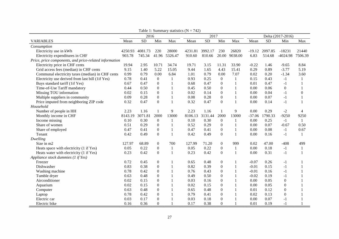
27

Table 1: Summary statistics (N = 742)

2016 2017 Delta (2017-2016)

VARIABLES Mean SD Min Max Mean SD Min Max Mean SD Min Max

Consumption

Electricity use in kWh 4250.93 4081.73 220 28000 4231.81 3992.17 230 26820 -19.12 2097.85 -18231 21440

Electricity expenditures in CHF 903.78 745.34 41.96 5326.47 910.60 810.66 20.00 9038.00 6.83 514.68 -4024.98 7506.39

Price, price components, and price-related information

Electricity price in CHF cents 19.94 2.95 10.71 34.74 19.71 3.15 11.31 33.90 -0.22 1.46 -9.65 8.84

Grid access fees (median) in CHF cents 9.15 1.40 5.22 15.05 9.44 1.65 4.43 15.41 0.29 0.89 -3.77 5.19

Communal electricity taxes (median) in CHF cents 0.99 0.79 0.00 6.84 1.01 0.79 0.00 7.07 0.02 0.20 -1.34 3.60

Electricity use derived from last bill (1if Yes) 0.78 0.41 0 1 0.93 0.25 0 1 0.15 0.43 -1 1

Buys standard tariff (1if Yes) 0.67 0.47 0 1 0.68 0.47 0 1 0.01 0.47 -1 1

Time-of-Use Tariff mandatory 0.44 0.50 0 1 0.45 0.50 0 1 0.00 0.06 0 1

Missing TOU information 0.02 0.15 0 1 0.02 0.14 0 1 0.00 0.04 -1 0

Multiple suppliers in community 0.09 0.28 0 1 0.08 0.28 0 1 0.00 0.07 -1 1

Price imputed from neighboring ZIP code 0.32 0.47 0 1 0.32 0.47 0 1 0.00 0.14 -1 1

Household

Number of people in HH 2.23 1.16 1 9 2.23 1.16 1 9 0.00 0.29 -2 4

Monthly income in CHF 8143.19 3071.81 2000 13000 8106.13 3131.44 2000 13000 -37.06 1790.33 -9250 9250

Income missing 0.10 0.30 0 1 0.10 0.30 0 1 0.00 0.25 -1 1

Share of women 0.51 0.29 0 1 0.52 0.29 0 1 0.00 0.07 -0.67 0.50

Share of employed 0.47 0.41 0 1 0.47 0.41 0 1 0.00 0.08 -1 0.67

Tenant 0.42 0.49 0 1 0.42 0.49 0 1 0.00 0.16 -1 1

Dwelling

Size in m2 127.97 68.89 0 700 127.99 71.20 0 999 0.02 47.00 -408 499

Heats space with electricity (1 if Yes) 0.05 0.22 0 1 0.05 0.22 0 1 0.00 0.18 -1 1

Heats water with electricity (1 if Yes) 0.23 0.42 0 1 0.23 0.42 0 1 0.00 0.31 -1 1

Appliance stock dummies (1 if Yes)

Freezer 0.72 0.45 0 1 0.65 0.48 0 1 -0.07 0.26 -1 1

Dishwasher 0.83 0.38 0 1 0.82 0.39 0 1 -0.01 0.15 -1 1

Washing machine 0.78 0.42 0 1 0.76 0.43 0 1 -0.01 0.16 -1 1

Tumble dryer 0.63 0.48 0 1 0.49 0.50 0 1 -0.02 0.19 -1 1

Airconditioner 0.02 0.15 0 1 0.03 0.16 0 1 0.00 0.05 0 1

Aquarium 0.02 0.15 0 1 0.02 0.15 0 1 0.00 0.05 0 1

Computer 0.63 0.48 0 1 0.65 0.48 0 1 0.01 0.12 0 1

Laptop 0.78 0.42 0 1 0.79 0.41 0 1 0.02 0.13 0 1

Electric car 0.03 0.17 0 1 0.03 0.18 0 1 0.00 0.07 -1 1

Electric bike 0.16 0.36 0 1 0.17 0.38 0 1 0.01 0.19 -1 1

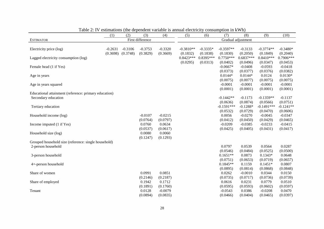
28

Table 2: IV estimations (the dependent variable is annual electricity consumption in kWh) (1) (2) (3) (4) (5) (6) (7) (8) (9) (10)

ESTIMATOR First difference Gradual adjustment

Electricity price (log) -0.2631 -0.3106 -0.3753 -0.3320 -0.3810** -0.3335* -0.3597** -0.3133 -0.3774** -0.3480*

(0.3698) (0.3748) (0.3829) (0.3669) (0.1832) (0.1838) (0.1830) (0.2050) (0.1849) (0.2040)

Lagged electricity consumption (log) 0.8423*** 0.8395*** 0.7750*** 0.6837*** 0.8410*** 0.7906***

(0.0295) (0.0313) (0.0402) (0.0496) (0.0347) (0.0453)

Female head (1 if Yes) -0.0667* -0.0408 -0.0593 -0.0418

(0.0373) (0.0377) (0.0376) (0.0382)

Age in years 0.0144* 0.0144* 0.0124 0.0130*

(0.0075) (0.0077) (0.0075) (0.0075)

Age in years squared -0.0001 -0.0001 -0.0001 -0.0001

(0.0001) (0.0001) (0.0001) (0.0001)

Educational attainment (reference: primary education)

Secondary education -0.1442** -0.1173 -0.1359** -0.1137

(0.0636) (0.0874) (0.0566) (0.0751)

Tertiary education -0.1591*** -0.1288* -0.1491*** -0.1241**

(0.0532) (0.0729) (0.0470) (0.0606)

Household income (log) -0.0107 -0.0215 0.0056 -0.0270 -0.0045 -0.0347

(0.0764) (0.0797) (0.0412) (0.0450) (0.0429) (0.0465)

Income imputed (1 if Yes) 0.0760 0.0634 -0.0209 -0.0385 -0.0233 -0.0415

(0.0537) (0.0617) (0.0425) (0.0405) (0.0431) (0.0417)

Household size (log) 0.0080 0.0060

(0.1247) (0.1293)

Grouped household size (reference: single household)

2-person household 0.0797 0.0539 0.0564 0.0287

(0.0546) (0.0484) (0.0525) (0.0500)

3-person household 0.1651** 0.0873 0.1343* 0.0648

(0.0751) (0.0653) (0.0719) (0.0657)

4+-person household 0.1845** 0.1159 0.1451* 0.0807

(0.0895) (0.0814) (0.0868) (0.0848)

Share of women 0.0991 0.0851 0.0262 -0.0010 0.0344 0.0150

(0.2146) (0.2187) (0.0735) (0.0717) (0.0736) (0.0739)

Share of employed 0.1942 0.1712 0.0616 0.0231 0.0779 0.0510

(0.1891) (0.1760) (0.0595) (0.0593) (0.0602) (0.0597)

Tenant 0.0128 -0.0079 -0.0543 0.0386 -0.0208 0.0470

(0.0894) (0.0835) (0.0466) (0.0404) (0.0465) (0.0397)

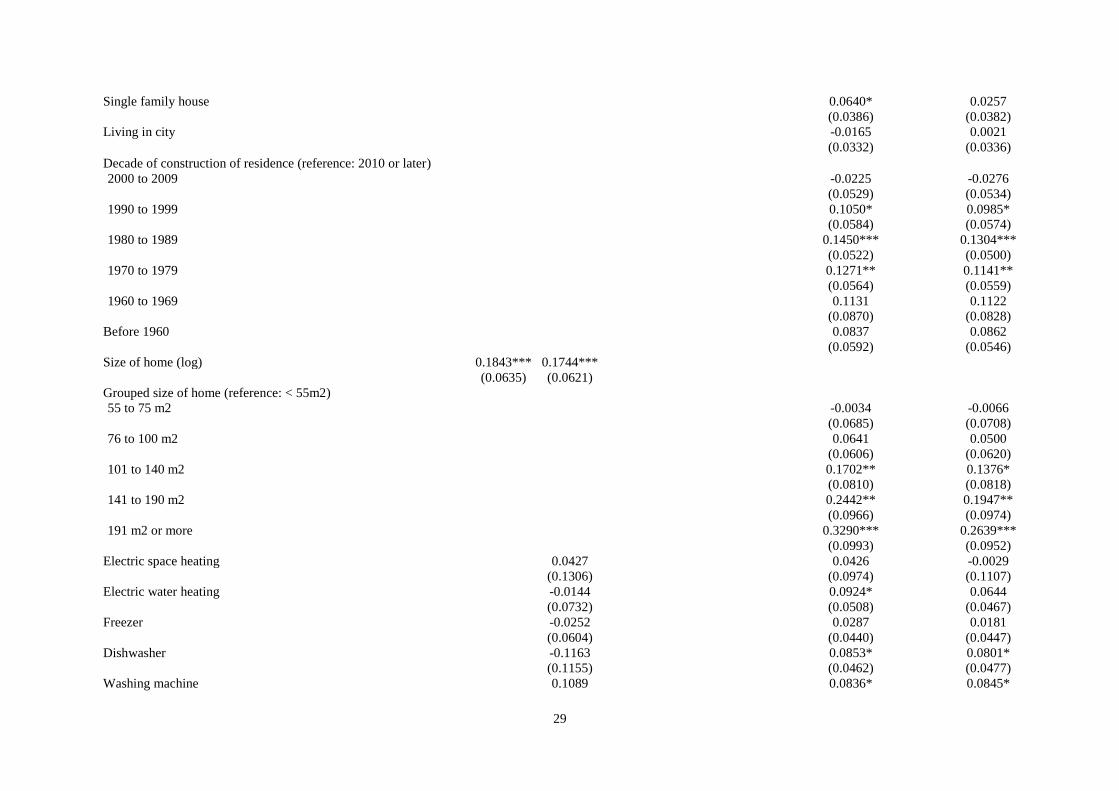
29

Single family house 0.0640* 0.0257

(0.0386) (0.0382)

Living in city -0.0165 0.0021

(0.0332) (0.0336)

Decade of construction of residence (reference: 2010 or later)

2000 to 2009 -0.0225 -0.0276

(0.0529) (0.0534)

1990 to 1999 0.1050* 0.0985*

(0.0584) (0.0574)

1980 to 1989 0.1450*** 0.1304***

(0.0522) (0.0500)

1970 to 1979 0.1271** 0.1141**

(0.0564) (0.0559)

1960 to 1969 0.1131 0.1122

(0.0870) (0.0828)

Before 1960 0.0837 0.0862

(0.0592) (0.0546)

Size of home (log) 0.1843*** 0.1744***

(0.0635) (0.0621)

Grouped size of home (reference: < 55m2)

55 to 75 m2 -0.0034 -0.0066

(0.0685) (0.0708)

76 to 100 m2 0.0641 0.0500

(0.0606) (0.0620)

101 to 140 m2 0.1702** 0.1376*

(0.0810) (0.0818)

141 to 190 m2 0.2442** 0.1947**

(0.0966) (0.0974)

191 m2 or more 0.3290*** 0.2639***

(0.0993) (0.0952)

Electric space heating 0.0427 0.0426 -0.0029

(0.1306) (0.0974) (0.1107)

Electric water heating -0.0144 0.0924* 0.0644

(0.0732) (0.0508) (0.0467)

Freezer -0.0252 0.0287 0.0181

(0.0604) (0.0440) (0.0447)

Dishwasher -0.1163 0.0853* 0.0801*

(0.1155) (0.0462) (0.0477)

Washing machine 0.1089 0.0836* 0.0845*

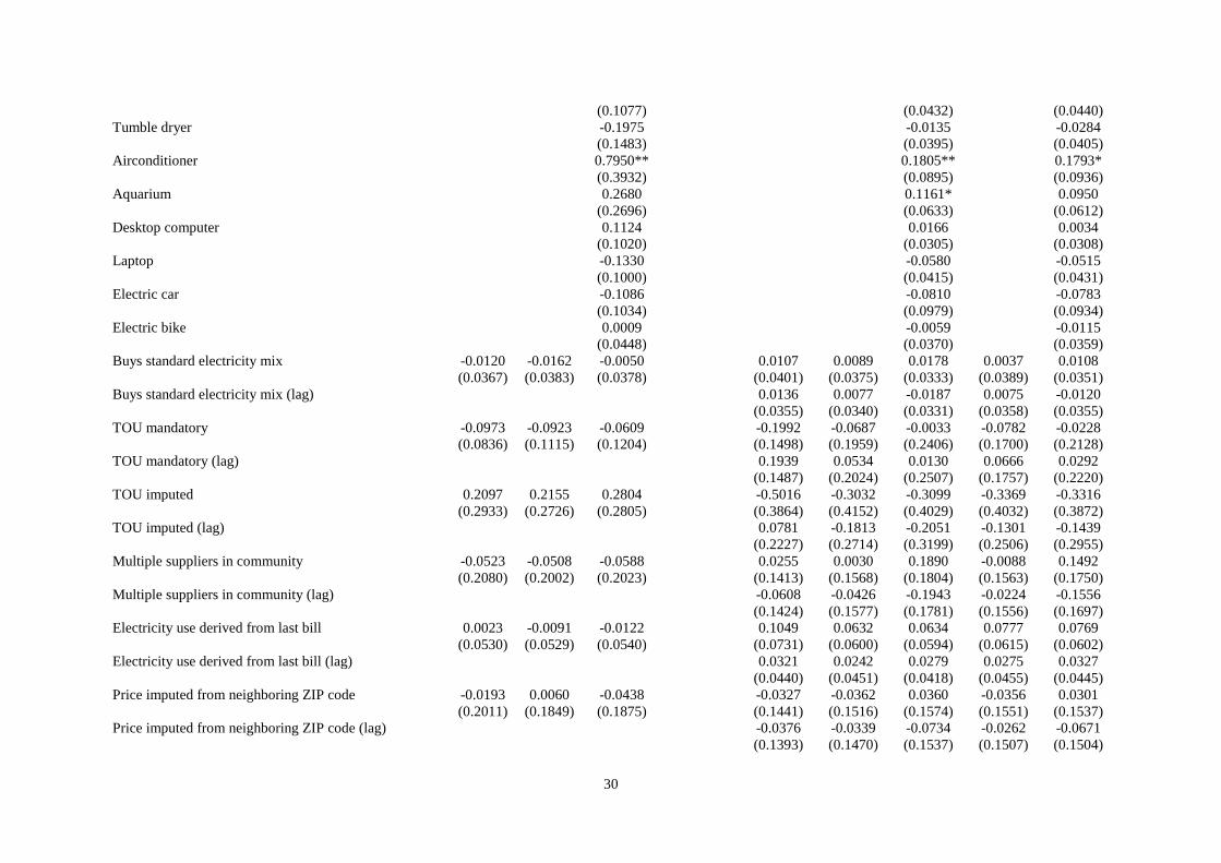
30

(0.1077) (0.0432) (0.0440)

Tumble dryer -0.1975 -0.0135 -0.0284

(0.1483) (0.0395) (0.0405)

Airconditioner 0.7950** 0.1805** 0.1793*

(0.3932) (0.0895) (0.0936)

Aquarium 0.2680 0.1161* 0.0950

(0.2696) (0.0633) (0.0612)

Desktop computer 0.1124 0.0166 0.0034

(0.1020) (0.0305) (0.0308)

Laptop -0.1330 -0.0580 -0.0515

(0.1000) (0.0415) (0.0431)

Electric car -0.1086 -0.0810 -0.0783

(0.1034) (0.0979) (0.0934)

Electric bike 0.0009 -0.0059 -0.0115

(0.0448) (0.0370) (0.0359)

Buys standard electricity mix -0.0120 -0.0162 -0.0050 0.0107 0.0089 0.0178 0.0037 0.0108

(0.0367) (0.0383) (0.0378) (0.0401) (0.0375) (0.0333) (0.0389) (0.0351)

Buys standard electricity mix (lag) 0.0136 0.0077 -0.0187 0.0075 -0.0120

(0.0355) (0.0340) (0.0331) (0.0358) (0.0355)

TOU mandatory -0.0973 -0.0923 -0.0609 -0.1992 -0.0687 -0.0033 -0.0782 -0.0228

(0.0836) (0.1115) (0.1204) (0.1498) (0.1959) (0.2406) (0.1700) (0.2128)

TOU mandatory (lag) 0.1939 0.0534 0.0130 0.0666 0.0292

(0.1487) (0.2024) (0.2507) (0.1757) (0.2220)

TOU imputed 0.2097 0.2155 0.2804 -0.5016 -0.3032 -0.3099 -0.3369 -0.3316

(0.2933) (0.2726) (0.2805) (0.3864) (0.4152) (0.4029) (0.4032) (0.3872)

TOU imputed (lag) 0.0781 -0.1813 -0.2051 -0.1301 -0.1439

(0.2227) (0.2714) (0.3199) (0.2506) (0.2955)

Multiple suppliers in community -0.0523 -0.0508 -0.0588 0.0255 0.0030 0.1890 -0.0088 0.1492

(0.2080) (0.2002) (0.2023) (0.1413) (0.1568) (0.1804) (0.1563) (0.1750)

Multiple suppliers in community (lag) -0.0608 -0.0426 -0.1943 -0.0224 -0.1556

(0.1424) (0.1577) (0.1781) (0.1556) (0.1697)

Electricity use derived from last bill 0.0023 -0.0091 -0.0122 0.1049 0.0632 0.0634 0.0777 0.0769

(0.0530) (0.0529) (0.0540) (0.0731) (0.0600) (0.0594) (0.0615) (0.0602)

Electricity use derived from last bill (lag) 0.0321 0.0242 0.0279 0.0275 0.0327

(0.0440) (0.0451) (0.0418) (0.0455) (0.0445)

Price imputed from neighboring ZIP code -0.0193 0.0060 -0.0438 -0.0327 -0.0362 0.0360 -0.0356 0.0301

(0.2011) (0.1849) (0.1875) (0.1441) (0.1516) (0.1574) (0.1551) (0.1537)

Price imputed from neighboring ZIP code (lag) -0.0376 -0.0339 -0.0734 -0.0262 -0.0671

(0.1393) (0.1470) (0.1537) (0.1507) (0.1504)

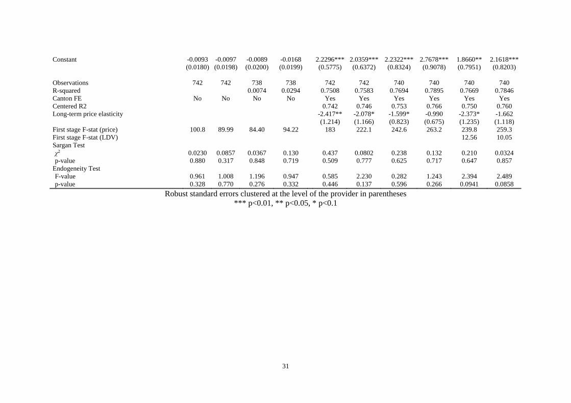
31

Constant -0.0093 -0.0097 -0.0089 -0.0168 2.2296*** 2.0359*** 2.2322*** 2.7678*** 1.8660** 2.1618***

(0.0180) (0.0198) (0.0200) (0.0199) (0.5775) (0.6372) (0.8324) (0.9078) (0.7951) (0.8203)

Observations 742 742 738 738 742 742 740 740 740 740

R-squared 0.0074 0.0294 0.7508 0.7583 0.7694 0.7895 0.7669 0.7846

Canton FE No No No No Yes Yes Yes Yes Yes Yes

Centered R2 0.742 0.746 0.753 0.766 0.750 0.760

Long-term price elasticity -2.417** -2.078* -1.599* -0.990 -2.373* -1.662

(1.214) (1.166) (0.823) (0.675) (1.235) (1.118)

First stage F-stat (price) 100.8 89.99 84.40 94.22 183 222.1 242.6 263.2 239.8 259.3

First stage F-stat (LDV) 12.56 10.05

Sargan Test

χ2 0.0230 0.0857 0.0367 0.130 0.437 0.0802 0.238 0.132 0.210 0.0324

p-value 0.880 0.317 0.848 0.719 0.509 0.777 0.625 0.717 0.647 0.857

Endogeneity Test

F-value 0.961 1.008 1.196 0.947 0.585 2.230 0.282 1.243 2.394 2.489

p-value 0.328 0.770 0.276 0.332 0.446 0.137 0.596 0.266 0.0941 0.0858

Robust standard errors clustered at the level of the provider in parentheses

*** p<0.01, ** p<0.05, * p<0.1

32

Table 3: IV estimations: Robustness I (the dependent variable is annual electricity consumption in kWh) (1) (2) (3) (4) (5) (6) (7) (8) (9) (10)

Estimator First difference Gradual adjustment

Change in

estimation/sample

Only

respondents

using

electricity bill

Only

respondents in

single family

houses

Re-

weighting

Heckman Increasing

prices

Only

respondents

using

electricity bill

Only

respondents in

single family

houses

Re-

weighting

Heckman Increasing prices

Electricity price (log) -0.2590 -0.4728 -0.3060 -0.2815 -1.3128 -0.6670*** -0.2479 -0.3648* -0.2720 -0.4490

(0.4827) (0.4884) (0.3507) (0.5724) (0.8160) (0.2408) (0.2897) (0.2162) (0.3668) (0.2835)

Lagged electricity 0.7165*** 0.7129*** 0.6993*** 0.6828*** 0.5860***

consumption (log) (0.0444) (0.0676) (0.0485) (0.0649) (0.0460)

Female head (1 if Yes) -0.0227 -0.0604 -0.0246 -0.0438 0.0188

(0.0385) (0.0504) (0.0362) (0.0681) (0.0508)

Age in years 0.0055 -0.0043 0.0151* 0.0140 0.0135

(0.0081) (0.0111) (0.0079) (0.0141) (0.0087)

Age in years squared -0.0000 0.0000 -0.0001 -0.0001 -0.0001

(0.0001) (0.0001) (0.0001) (0.0001) (0.0001)

Educational attainment (reference: primary education)

Secondary education -0.0796 -0.0452 -0.1183 -0.1250 -0.1551

(0.0791) (0.1807) (0.0838) (0.1695) (0.1694)

Tertiary education -0.0990 -0.0533 -0.1308* -0.1321 -0.1595

(0.0751) (0.1765) (0.0739) (0.1721) (0.1324)

Household income

(log)

-0.0624 -0.0837 -0.0875 -0.0329 0.0384 -0.0403 -0.0400 -0.0384 -0.0224 -0.0447

(0.1090) (0.1183) (0.1008) (0.1248) (0.1387) (0.0472) (0.0705) (0.0507) (0.0806) (0.0636)

Income imputed (1 if

Yes)

0.1247* 0.2225** 0.0827 0.0532 0.1380 -0.0221 0.0438 -0.0273 -0.0406 -0.0598

(0.0651) (0.1055) (0.0589) (0.1060) (0.0965) (0.0442) (0.0869) (0.0404) (0.0823) (0.0684)

Household size (log) -0.1064 -0.0363 0.0273 -0.0144 -0.3211

(0.1715) (0.2084) (0.1517) (0.2292) (0.3117)

Grouped household size (reference: single household)

2-person household 0.0405 -0.0347 0.0543 0.0419 0.1391*

(0.0436) (0.0945) (0.0511) (0.0752) (0.0839)

3-person household 0.0982 -0.0510 0.1091* 0.0764 0.2030**

(0.0626) (0.1119) (0.0657) (0.1123) (0.1011)

4+-person household 0.0730 0.0425 0.1217 0.0977 0.1214

(0.0665) (0.1331) (0.0792) (0.1183) (0.1221)

Share of women -0.0899 0.2512 0.2038 0.0539 -0.6108** 0.0228 0.2496** 0.0157 -0.0125 0.0339

(0.3378) (0.2567) (0.2267) (0.4067) (0.2769) (0.0805) (0.1132) (0.0725) (0.1085) (0.1129)

Share of employed -0.0516 -0.2374 0.0973 0.1564 -0.5116* 0.0540 0.0720 0.0684 0.0065 0.0586

(0.1587) (0.2310) (0.1777) (0.3037) (0.2931) (0.0586) (0.0979) (0.0603) (0.1018) (0.0794)

Tenant -0.0842 0.1156*** 0.0166 -0.0163 -0.0538 0.0390 0.0655 0.0572 0.0010 0.1382***

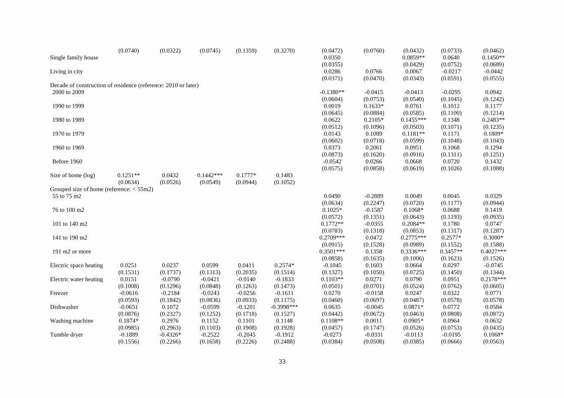
33

(0.0740) (0.0322) (0.0745) (0.1359) (0.3270) (0.0472) (0.0760) (0.0432) (0.0733) (0.0462)

Single family house 0.0350 0.0859** 0.0640 0.1450**

(0.0355) (0.0429) (0.0752) (0.0689)

Living in city 0.0286 0.0766 0.0067 -0.0217 -0.0442

(0.0371) (0.0470) (0.0343) (0.0591) (0.0555)

Decade of construction of residence (reference: 2010 or later)

2000 to 2009 -0.1380** -0.0415 -0.0413 -0.0295 0.0942

(0.0604) (0.0753) (0.0540) (0.1045) (0.1242)

1990 to 1999 0.0019 0.1633* 0.0761 0.1012 0.1177

(0.0645) (0.0884) (0.0585) (0.1100) (0.1214)

1980 to 1989 0.0622 0.2105* 0.1455*** 0.1348 0.2483**

(0.0512) (0.1096) (0.0503) (0.1071) (0.1235)

1970 to 1979 0.0143 0.1089 0.1181** 0.1171 0.1809*

(0.0602) (0.0718) (0.0599) (0.1048) (0.1043)

1960 to 1969 0.0373 0.2061 0.0951 0.1068 0.1294

(0.0873) (0.1620) (0.0916) (0.1311) (0.1251)

Before 1960 -0.0542 0.0266 0.0668 0.0720 0.1432

(0.0575) (0.0858) (0.0619) (0.1026) (0.1088)

Size of home (log) 0.1251** 0.0432 0.1442*** 0.1777* 0.1483

(0.0634) (0.0526) (0.0549) (0.0944) (0.1052)

Grouped size of home (reference: < 55m2)

55 to 75 m2 0.0490 -0.2889 0.0049 0.0045 0.0329

(0.0634) (0.2247) (0.0720) (0.1177) (0.0944)

76 to 100 m2 0.1025* -0.1587 0.1068* 0.0688 0.1419

(0.0572) (0.1351) (0.0643) (0.1193) (0.0935)

101 to 140 m2 0.1772** -0.0355 0.2084** 0.1780 0.0747

(0.0783) (0.1318) (0.0853) (0.1317) (0.1287)

141 to 190 m2 0.2709*** 0.0472 0.2775*** 0.2577* 0.3000*

(0.0915) (0.1528) (0.0989) (0.1552) (0.1588)

191 m2 or more 0.3501*** 0.1358 0.3336*** 0.3457** 0.4027***

(0.0858) (0.1635) (0.1006) (0.1623) (0.1526)

Electric space heating 0.0251 0.0237 0.0599 0.0411 0.2574* -0.1045 0.1603 0.0664 0.0297 -0.0745

(0.1531) (0.1737) (0.1313) (0.2035) (0.1514) (0.1327) (0.1050) (0.0725) (0.1450) (0.1344)

Electric water heating 0.0151 -0.0790 -0.0421 -0.0140 -0.1833 0.1103** 0.0271 0.0790 0.0951 0.2178***

(0.1008) (0.1296) (0.0848) (0.1263) (0.1473) (0.0501) (0.0701) (0.0524) (0.0762) (0.0605)

Freezer -0.0616 -0.2184 -0.0243 -0.0256 -0.1611 0.0270 -0.0158 0.0247 0.0322 0.0771

(0.0593) (0.1842) (0.0836) (0.0933) (0.1175) (0.0460) (0.0697) (0.0487) (0.0578) (0.0578)

Dishwasher -0.0651 0.1072 -0.0599 -0.1201 -0.3998*** 0.0635 -0.0045 0.0871* 0.0772 0.0584

(0.0876) (0.2327) (0.1252) (0.1718) (0.1527) (0.0442) (0.0672) (0.0463) (0.0808) (0.0872)

Washing machine 0.1874* 0.2976 0.1152 0.1101 0.1148 0.1108** 0.0011 0.0905* 0.0964 0.0632

(0.0985) (0.2963) (0.1103) (0.1908) (0.1928) (0.0457) (0.1747) (0.0526) (0.0753) (0.0435)

Tumble dryer -0.1889 -0.4326* -0.2522 -0.2045 -0.1912 -0.0273 -0.0331 -0.0113 -0.0195 0.1068*

(0.1556) (0.2266) (0.1658) (0.2226) (0.2488) (0.0384) (0.0508) (0.0385) (0.0666) (0.0563)

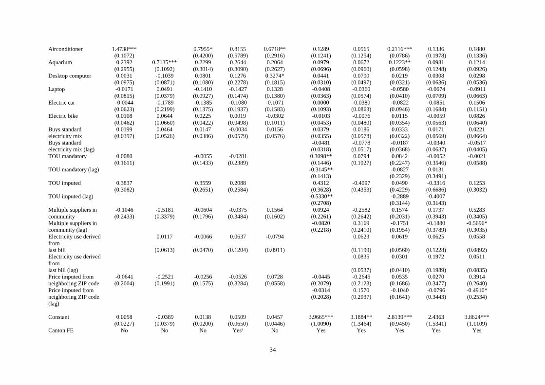
34

Airconditioner 1.4738*** 0.7955* 0.8155 0.6718** 0.1289 0.0565 0.2116*** 0.1336 0.1880

(0.1072) (0.4200) (0.5789) (0.2916) (0.1241) (0.1254) (0.0786) (0.1978) (0.1336)

Aquarium 0.2392 0.7135*** 0.2299 0.2644 0.2064 0.0979 0.0672 0.1223** 0.0981 0.1214

(0.2955) (0.1092) (0.3014) (0.3090) (0.2627) (0.0696) (0.0960) (0.0598) (0.1248) (0.0926)

Desktop computer 0.0031 -0.1039 0.0801 0.1276 0.3274* 0.0441 0.0700 0.0219 0.0308 0.0298

(0.0975) (0.0871) (0.1080) (0.2278) (0.1815) (0.0310) (0.0497) (0.0321) (0.0636) (0.0536)

Laptop -0.0171 0.0491 -0.1410 -0.1427 0.1328 -0.0408 -0.0360 -0.0580 -0.0674 -0.0911

(0.0815) (0.0379) (0.0927) (0.1474) (0.1380) (0.0363) (0.0574) (0.0410) (0.0709) (0.0663)

Electric car -0.0044 -0.1789 -0.1385 -0.1080 -0.1071 0.0000 -0.0380 -0.0822 -0.0851 0.1506

(0.0623) (0.2199) (0.1375) (0.1937) (0.1583) (0.1093) (0.0863) (0.0946) (0.1684) (0.1151)

Electric bike 0.0108 0.0644 0.0225 0.0019 -0.0302 -0.0103 -0.0076 0.0115 -0.0059 0.0826

(0.0462) (0.0660) (0.0422) (0.0498) (0.1011) (0.0453) (0.0480) (0.0354) (0.0563) (0.0640)

Buys standard 0.0199 0.0464 0.0147 -0.0034 0.0156 0.0379 0.0186 0.0333 0.0171 0.0221

electricity mix (0.0397) (0.0526) (0.0386) (0.0579) (0.0576) (0.0355) (0.0578) (0.0322) (0.0569) (0.0664)

Buys standard -0.0481 -0.0778 -0.0187 -0.0340 -0.0517

electricity mix (lag) (0.0318) (0.0517) (0.0368) (0.0637) (0.0405)

TOU mandatory 0.0080 -0.0055 -0.0281 0.3098** 0.0794 0.0842 -0.0052 -0.0021

(0.1611) (0.1433) (0.2389) (0.1446) (0.1027) (0.2247) (0.3546) (0.0588)

TOU mandatory (lag) -0.3145** -0.0827 0.0131

(0.1413) (0.2329) (0.3491)

TOU imputed 0.3837 0.3559 0.2088 0.4312 -0.4097 0.0490 -0.3316 0.1253

(0.3082) (0.2651) (0.2584) (0.3628) (0.4353) (0.4229) (0.6686) (0.3032)

TOU imputed (lag) -0.5330** -0.2889 -0.4007

(0.2708) (0.3144) (0.3143)

Multiple suppliers in -0.1046 -0.5181 -0.0604 -0.0375 0.1564 0.0924 -0.2582 0.1574 0.1737 0.5283

community (0.2433) (0.3379) (0.1796) (0.3484) (0.1602) (0.2261) (0.2642) (0.2031) (0.3943) (0.3405)

Multiple suppliers in -0.0820 0.3169 -0.1751 -0.1880 -0.5696*

community (lag) (0.2218) (0.2410) (0.1954) (0.3789) (0.3035)

Electricity use derived

from

0.0117 -0.0066 0.0637 -0.0794 0.0623 0.0619 0.0625 0.0558

last bill (0.0613) (0.0470) (0.1204) (0.0911) (0.1199) (0.0560) (0.1228) (0.0892)

Electricity use derived

from

0.0835 0.0301 0.1972 0.0511

last bill (lag) (0.0537) (0.0410) (0.1989) (0.0835)

Price imputed from -0.0641 -0.2521 -0.0256 -0.0526 0.0728 -0.0445 -0.2645 0.0535 0.0270 0.3914

neighboring ZIP code (0.2004) (0.1991) (0.1575) (0.3284) (0.0558) (0.2079) (0.2123) (0.1686) (0.3477) (0.2640)

Price imputed from -0.0314 0.1570 -0.1040 -0.0796 -0.4910*

neighboring ZIP code

(lag)

(0.2028) (0.2037) (0.1641) (0.3443) (0.2534)

Constant 0.0058 -0.0389 0.0138 0.0509 0.0457 3.9665*** 3.1884** 2.8139*** 2.4363 3.8624***

(0.0227) (0.0379) (0.0200) (0.0650) (0.0446) (1.0090) (1.3464) (0.9450) (1.5341) (1.1109)

Canton FE No No No Yesa No Yes Yes Yes Yes Yes

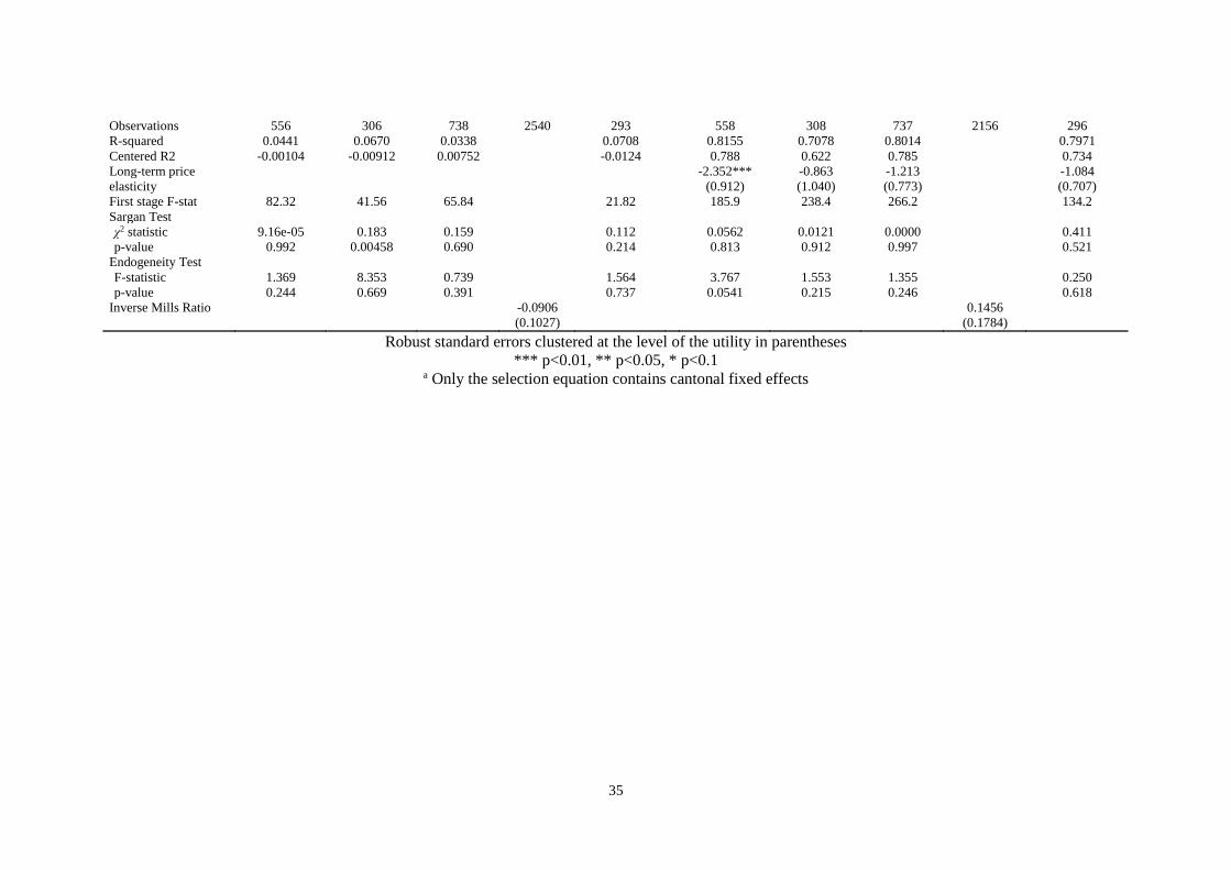
35

Observations 556 306 738 2540 293 558 308 737 2156 296

R-squared 0.0441 0.0670 0.0338 0.0708 0.8155 0.7078 0.8014 0.7971

Centered R2 -0.00104 -0.00912 0.00752 -0.0124 0.788 0.622 0.785 0.734

Long-term price -2.352*** -0.863 -1.213 -1.084

elasticity (0.912) (1.040) (0.773) (0.707)

First stage F-stat 82.32 41.56 65.84 21.82 185.9 238.4 266.2 134.2

Sargan Test

χ2 statistic 9.16e-05 0.183 0.159 0.112 0.0562 0.0121 0.0000 0.411

p-value 0.992 0.00458 0.690 0.214 0.813 0.912 0.997 0.521

Endogeneity Test

F-statistic 1.369 8.353 0.739 1.564 3.767 1.553 1.355 0.250

p-value 0.244 0.669 0.391 0.737 0.0541 0.215 0.246 0.618

Inverse Mills Ratio -0.0906 0.1456

(0.1027) (0.1784)

Robust standard errors clustered at the level of the utility in parentheses

*** p<0.01, ** p<0.05, * p<0.1 a Only the selection equation contains cantonal fixed effects

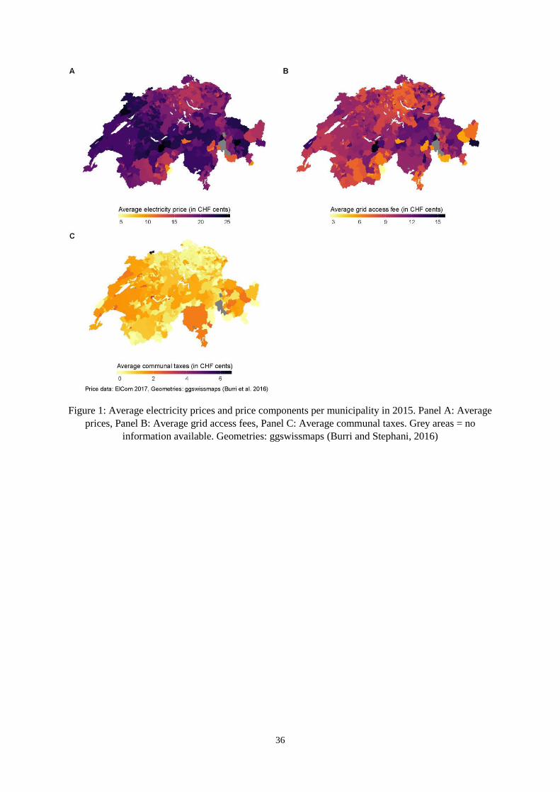
36

Figure 1: Average electricity prices and price components per municipality in 2015. Panel A: Average

prices, Panel B: Average grid access fees, Panel C: Average communal taxes. Grey areas = no

information available. Geometries: ggswissmaps (Burri and Stephani, 2016)

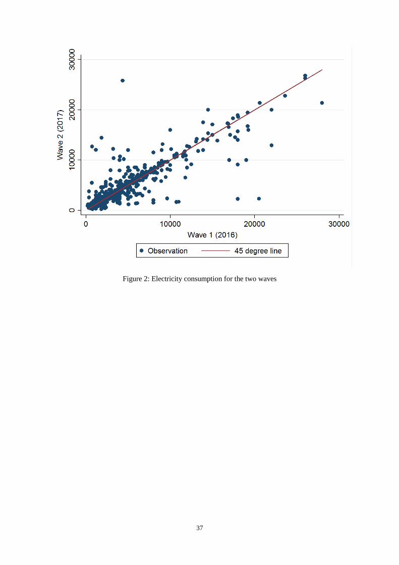
37

Figure 2: Electricity consumption for the two waves

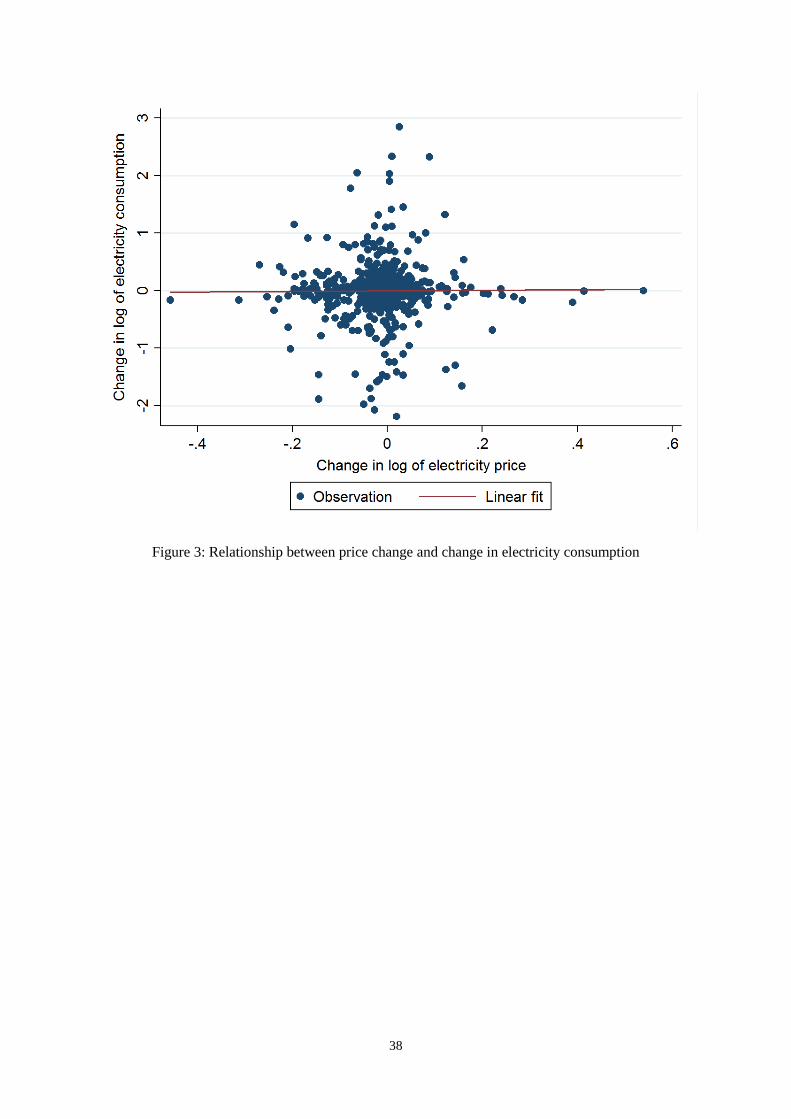
38

Figure 3: Relationship between price change and change in electricity consumption

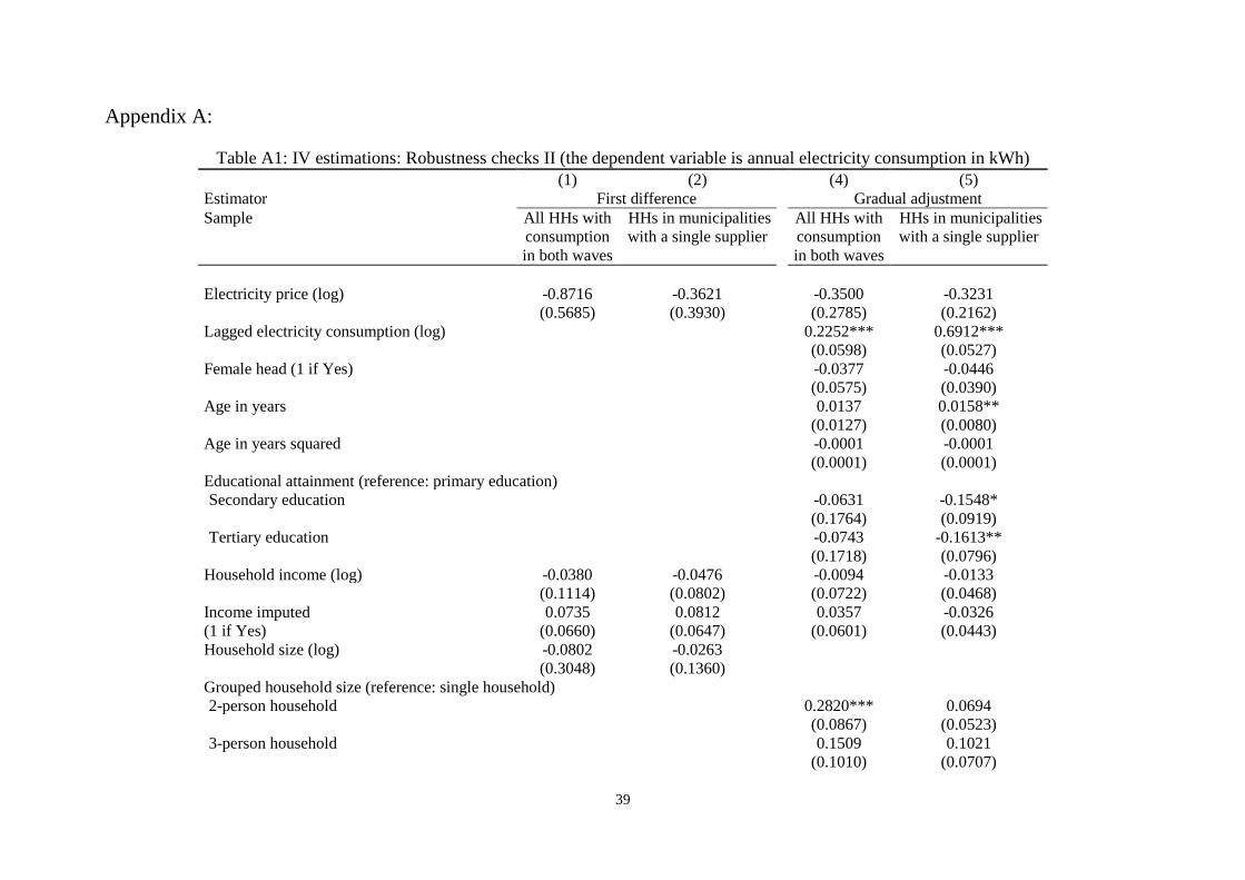
39

Appendix A:

Table A1: IV estimations: Robustness checks II (the dependent variable is annual electricity consumption in kWh)

(1) (2) (4) (5)

Estimator First difference Gradual adjustment

Sample All HHs with

consumption

in both waves

HHs in municipalities

with a single supplier

All HHs with

consumption

in both waves

HHs in municipalities

with a single supplier

Electricity price (log) -0.8716 -0.3621 -0.3500 -0.3231

(0.5685) (0.3930) (0.2785) (0.2162)

Lagged electricity consumption (log) 0.2252*** 0.6912***

(0.0598) (0.0527)

Female head (1 if Yes) -0.0377 -0.0446

(0.0575) (0.0390)

Age in years 0.0137 0.0158**

(0.0127) (0.0080)

Age in years squared -0.0001 -0.0001

(0.0001) (0.0001)

Educational attainment (reference: primary education)

Secondary education -0.0631 -0.1548*

(0.1764) (0.0919)

Tertiary education -0.0743 -0.1613**

(0.1718) (0.0796)

Household income (log) -0.0380 -0.0476 -0.0094 -0.0133

(0.1114) (0.0802) (0.0722) (0.0468)

Income imputed 0.0735 0.0812 0.0357 -0.0326

(1 if Yes) (0.0660) (0.0647) (0.0601) (0.0443)

Household size (log) -0.0802 -0.0263

(0.3048) (0.1360)

Grouped household size (reference: single household)

2-person household 0.2820*** 0.0694

(0.0867) (0.0523)

3-person household 0.1509 0.1021

(0.1010) (0.0707)

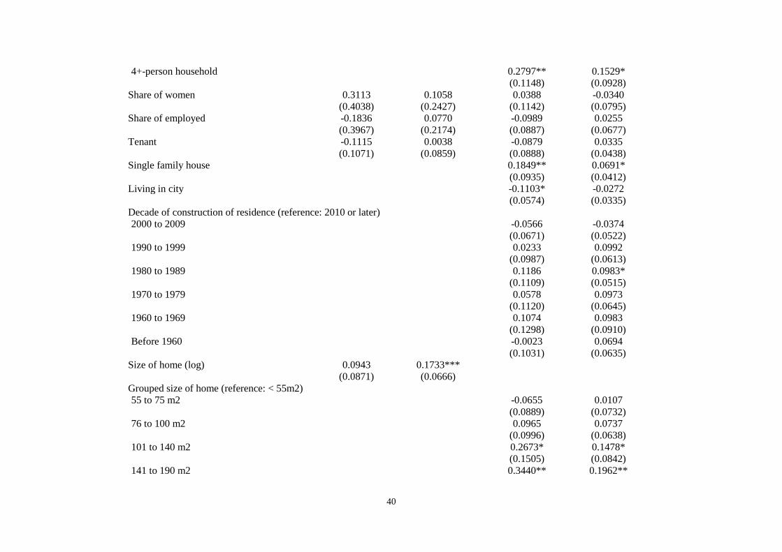
40

4+-person household 0.2797** 0.1529*

(0.1148) (0.0928)

Share of women 0.3113 0.1058 0.0388 -0.0340

(0.4038) (0.2427) (0.1142) (0.0795)

Share of employed -0.1836 0.0770 -0.0989 0.0255

(0.3967) (0.2174) (0.0887) (0.0677)

Tenant -0.1115 0.0038 -0.0879 0.0335

(0.1071) (0.0859) (0.0888) (0.0438)

Single family house 0.1849** 0.0691*

(0.0935) (0.0412)

Living in city -0.1103* -0.0272

(0.0574) (0.0335)

Decade of construction of residence (reference: 2010 or later)

2000 to 2009 -0.0566 -0.0374

(0.0671) (0.0522)

1990 to 1999 0.0233 0.0992

(0.0987) (0.0613)

1980 to 1989 0.1186 0.0983*

(0.1109) (0.0515)

1970 to 1979 0.0578 0.0973

(0.1120) (0.0645)

1960 to 1969 0.1074 0.0983

(0.1298) (0.0910)

Before 1960 -0.0023 0.0694

(0.1031) (0.0635)

Size of home (log) 0.0943 0.1733***

(0.0871) (0.0666)

Grouped size of home (reference: < 55m2)

55 to 75 m2 -0.0655 0.0107

(0.0889) (0.0732)

76 to 100 m2 0.0965 0.0737

(0.0996) (0.0638)

101 to 140 m2 0.2673* 0.1478*

(0.1505) (0.0842)

141 to 190 m2 0.3440** 0.1962**

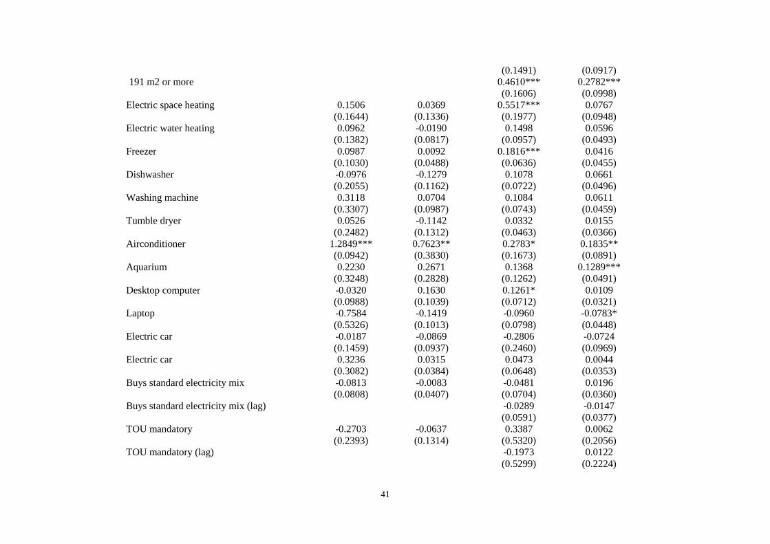
41

(0.1491) (0.0917)

191 m2 or more 0.4610*** 0.2782***

(0.1606) (0.0998)

Electric space heating 0.1506 0.0369 0.5517*** 0.0767

(0.1644) (0.1336) (0.1977) (0.0948)

Electric water heating 0.0962 -0.0190 0.1498 0.0596

(0.1382) (0.0817) (0.0957) (0.0493)

Freezer 0.0987 0.0092 0.1816*** 0.0416

(0.1030) (0.0488) (0.0636) (0.0455)

Dishwasher -0.0976 -0.1279 0.1078 0.0661

(0.2055) (0.1162) (0.0722) (0.0496)

Washing machine 0.3118 0.0704 0.1084 0.0611

(0.3307) (0.0987) (0.0743) (0.0459)

Tumble dryer 0.0526 -0.1142 0.0332 0.0155

(0.2482) (0.1312) (0.0463) (0.0366)

Airconditioner 1.2849*** 0.7623** 0.2783* 0.1835**

(0.0942) (0.3830) (0.1673) (0.0891)

Aquarium 0.2230 0.2671 0.1368 0.1289***

(0.3248) (0.2828) (0.1262) (0.0491)

Desktop computer -0.0320 0.1630 0.1261* 0.0109

(0.0988) (0.1039) (0.0712) (0.0321)

Laptop -0.7584 -0.1419 -0.0960 -0.0783*

(0.5326) (0.1013) (0.0798) (0.0448)

Electric car -0.0187 -0.0869 -0.2806 -0.0724

(0.1459) (0.0937) (0.2460) (0.0969)

Electric car 0.3236 0.0315 0.0473 0.0044

(0.3082) (0.0384) (0.0648) (0.0353)

Buys standard electricity mix -0.0813 -0.0083 -0.0481 0.0196

(0.0808) (0.0407) (0.0704) (0.0360)

Buys standard electricity mix (lag) -0.0289 -0.0147

(0.0591) (0.0377)

TOU mandatory -0.2703 -0.0637 0.3387 0.0062

(0.2393) (0.1314) (0.5320) (0.2056)

TOU mandatory (lag) -0.1973 0.0122

(0.5299) (0.2224)

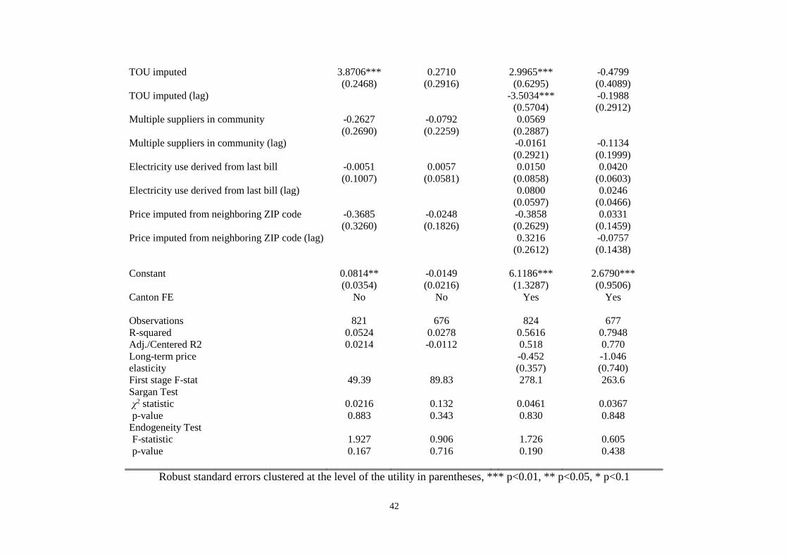
42

TOU imputed 3.8706*** 0.2710 2.9965*** -0.4799

(0.2468) (0.2916) (0.6295) (0.4089)

TOU imputed (lag) -3.5034*** -0.1988

(0.5704) (0.2912)

Multiple suppliers in community -0.2627 -0.0792 0.0569

(0.2690) (0.2259) (0.2887)

Multiple suppliers in community (lag) -0.0161 -0.1134

(0.2921) (0.1999)

Electricity use derived from last bill -0.0051 0.0057 0.0150 0.0420

(0.1007) (0.0581) (0.0858) (0.0603)

Electricity use derived from last bill (lag) 0.0800 0.0246

(0.0597) (0.0466)

Price imputed from neighboring ZIP code -0.3685 -0.0248 -0.3858 0.0331

(0.3260) (0.1826) (0.2629) (0.1459)

Price imputed from neighboring ZIP code (lag) 0.3216 -0.0757

(0.2612) (0.1438)

Constant 0.0814** -0.0149 6.1186*** 2.6790***

(0.0354) (0.0216) (1.3287) (0.9506)

Canton FE No No Yes Yes

Observations 821 676 824 677

R-squared 0.0524 0.0278 0.5616 0.7948

Adj./Centered R2 0.0214 -0.0112 0.518 0.770

Long-term price -0.452 -1.046

elasticity (0.357) (0.740)

First stage F-stat 49.39 89.83 278.1 263.6

Sargan Test

χ2 statistic 0.0216 0.132 0.0461 0.0367

p-value 0.883 0.343 0.830 0.848

Endogeneity Test

F-statistic 1.927 0.906 1.726 0.605

p-value 0.167 0.716 0.190 0.438

Robust standard errors clustered at the level of the utility in parentheses, *** p<0.01, ** p<0.05, * p<0.1

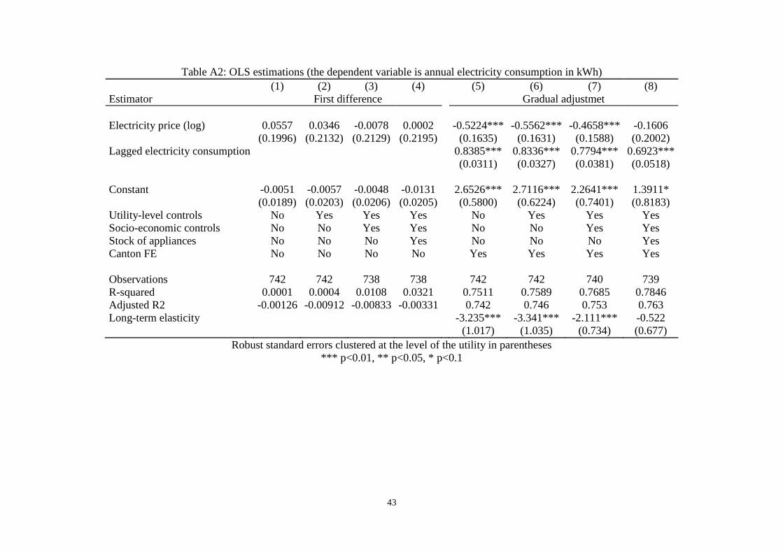
43

Table A2: OLS estimations (the dependent variable is annual electricity consumption in kWh)

(1) (2) (3) (4) (5) (6) (7) (8)

Estimator First difference Gradual adjustmet

Electricity price (log) 0.0557 0.0346 -0.0078 0.0002 -0.5224*** -0.5562*** -0.4658*** -0.1606

(0.1996) (0.2132) (0.2129) (0.2195) (0.1635) (0.1631) (0.1588) (0.2002)

Lagged electricity consumption 0.8385*** 0.8336*** 0.7794*** 0.6923***

(0.0311) (0.0327) (0.0381) (0.0518)

Constant -0.0051 -0.0057 -0.0048 -0.0131 2.6526*** 2.7116*** 2.2641*** 1.3911*

(0.0189) (0.0203) (0.0206) (0.0205) (0.5800) (0.6224) (0.7401) (0.8183)

Utility-level controls No Yes Yes Yes No Yes Yes Yes

Socio-economic controls No No Yes Yes No No Yes Yes

Stock of appliances No No No Yes No No No Yes

Canton FE No No No No Yes Yes Yes Yes

Observations 742 742 738 738 742 742 740 739

R-squared 0.0001 0.0004 0.0108 0.0321 0.7511 0.7589 0.7685 0.7846

Adjusted R2 -0.00126 -0.00912 -0.00833 -0.00331 0.742 0.746 0.753 0.763

Long-term elasticity -3.235*** -3.341*** -2.111*** -0.522

(1.017) (1.035) (0.734) (0.677)

Robust standard errors clustered at the level of the utility in parentheses

*** p<0.01, ** p<0.05, * p<0.1

44

Appendix B: Measuring values and energy literacy using SHEDS

The SHEDS survey contains a number of items aiming to elicit the respondents’ attitudes and energy

literacy.

Psychological literature defines values as “desirable transsituational goals varying in importance, which

serve as a guiding principle in the life of a person” (Schwartz, 1992, p. 21). These principles are assumed

to be comparatively stable over time, and to affect beliefs, preferences and behavior by defining the

valuation individuals attach to an outcome and to competing alternatives of achieving this outcome

(Steg, 2016; Steg et al., 2014). Four value dimensions have been identified as important for explaining

inter-individual differences in environmental attitudes, preferences, and behaviors: biospheric, altruistic,

egoistic and hedonistic (Hille et al., 2017; Steg, 2016; Steg et al., 2014). For measuring these

dimensions, the SHEDS uses a test battery of 16 items for which respondents rate the importance “as a

guiding principle for their life” on a scale from 1 (not important) to 5 (very important). The battery is

similar to the one developed by Steg et al. (2014). More precisely, we measure each of the four values

based on standardized sum of responses to the following items:

Biospheric: respecting the earth, unity with nature, protecting the environment, preventing

pollution (Cronbach’s 𝛼 = 0.86)

Altrusitic: equality, a world at peach, social justice, helpful (Cronbach’s 𝛼 = 0.76)

Egoistic: social power, wealth, authority, influential, ambitious (Cronbach’s 𝛼 = 0.75)

Hedonistic: pleasure, enjoying life, self-indulgent (Cronbach’s 𝛼 = 0.76)

Principal component analysis yielded four underlying items as judged by the number of principal

components with eigenvalues of one or larger. Element loadings are identical to the ones applied above.

The Kaiser-Meyer-Olkin measure of sampling adequacy reached 0.85, suggesting sufficient overlap

between these items to merit the construction of the four value measures.1

Energy literacy is understood as a goal of environmental education. It describes the individual’s

understanding of the role of energy in every-day life, and her ability to apply this understanding to make

informed decisions about energy use (DeWaters and Powers, 2013, 2011; U.S. Departement of Energy,

2014). This includes, but is not limited to, the individual’s knowledge how much energy she uses for

what purpose (U.S. Departement of Energy, 2014). The SHEDS comprises a set of 12 items aiming to

evaluate this form of knowledge among survey respondents. These items are structured as a set of

multiple-choice questions. From these questions, we construct an index measuring the share of correct

answers. Since multiple-choice questions differ in the number of pre-specified answers (from two to

six), we account for corresponding differences in getting the correct answer by chance by weighting

1 Moreover, results from the Heckman model are identical when replacing the standardized sums by factor scores

from the principle component analysis.

45

questions based on the number of answering options. On average respondents answer 52% of questions

correctly, which roughly corresponds to earlier findings from Switzerland (Blasch et al., 2017).