Seediscussions,stats,andauthorprofilesforthispublicationat:https://www.researchgate.net/publication/301757868

Priceelasticityofon-andoff-premisesdemandforalcoholicdrinks:ATobitanalysis

ArticleinDrugandalcoholdependence·April2016

DOI:10.1016/j.drugalcdep.2016.04.026

CITATION

1

READS

116

4authors:

HengJiang

LaTrobeUniversity

30PUBLICATIONS56CITATIONS

SEEPROFILE

MichaelJohnLivingston

LaTrobeUniversity

117PUBLICATIONS1,652CITATIONS

SEEPROFILE

RobinRoom

LaTrobeUniversity

516PUBLICATIONS20,581CITATIONS

SEEPROFILE

SarahCallinan

LaTrobeUniversity

28PUBLICATIONS86CITATIONS

SEEPROFILE

AllcontentfollowingthispagewasuploadedbyHengJiangon04May2016.

Theuserhasrequestedenhancementofthedownloadedfile.Allin-textreferencesunderlinedinblueareaddedtotheoriginaldocument

andarelinkedtopublicationsonResearchGate,lettingyouaccessandreadthemimmediately.

1

Price elasticity of on- and off-premises demand for alcoholic drinks: a

Tobit analysis

Heng Jiang1*, Michael Livingston1, Robin Room1,2, Sarah Callinan1

1 Centre for Alcohol Policy Research, School of Psychology and Public Health, La Trobe University,

Melbourne, Victoria, Australia, 2 Centre for Social Research on Alcohol and Drugs, Stockholm University, Stockholm, Sweden.

Running head: Price elasticity of alcohol demand

Total page count: 15

Word count for abstract: 248

Word count for body text: 3983

References: 37

Figures: 0

Tables: 4

Corresponding Author:

Dr.Heng Jiang

Centre for Alcohol Policy Research, School of Psychology and Public Health, La Trobe

University; 215 Franklin St, Melbourne, VIC, Australia, 3000

Tel: 03 9479 8795; Fax: 03 9479 8711; E-mail: jason.jiang@latrobe.edu.au

2

ABSTRACT

Background: Understanding how price policies will affect alcohol consumption requires estimates of

the impact of price on consumption among different types of drinkers and across different consumption

settings. This study aims to estimate how changes in price could affect alcohol demand across different

beverages, different settings (on-premise, e.g. bars, restaurants and off-premise, e.g. liquor stores,

supermarkets), and different levels of drinking and income.

Methods: Tobit analysis is employed to estimate own- and cross-price elasticities of alcohol demand

among 11 subcategories of beverage based on beverage type and on- or off-premise supply, using cross-

sectional data from the Australian arm of the International Alcohol Control survey 2013. Further

elasticity estimates were derived for sub-groups of drinkers based on their drinking and income levels.

Results: The results suggest that demand for nearly every subcategory of alcohol significantly responds

to its own price change, except for on-premise spirits and ready-to-drink spirits. The estimated demand

for off-premise beverages is more strongly affected by own price changes than the same beverages in

on-premise settings. Demand for off-premise regular beer and off-premise cask wine is more price

responsive than demand for other beverages. Harmful drinkers and lower income groups appear more

price responsive than moderate drinkers and higher income groups.

Conclusion: Our findings suggest that alcohol price policies, such as increasing alcohol taxes or

introducing a minimum unit price, can reduce alcohol demand. Price appears to be particularly effective

for reducing consumption and as well as alcohol-related harm among harmful drinkers and lower

income drinkers.

Key words: Alcohol demand, elasticities, price policy, Tobit model

3

Introduction

Excessive alcohol consumption is an important cause of social and health harms (Babor et al., 2010).

There is strong evidence that price-based interventions, such as increasing alcohol taxation, banning

alcohol promotions, or introducing a minimum unit price, would be effective approaches to reduce the

level of alcohol consumption and related health and social problems in a society (Anderson et al., 2009).

However, to determine the most effective approach to alcohol pricing interventions, good estimates of

price elasticity are needed.

The price elasticity of demand, a ratio of percentage changes in demand of a product given a price

change, has been widely discussed in many previous studies for a range of goods and services. Based

on the results of more than 100 studies in over 25 countries, three meta-analyses found that the mean

overall price elasticity of alcohol demand is about -0.5 (Gallet, 2007; Wagenaar et al., 2009; Fogarty,

2010). Importantly, this overall elasticity provides little information on how pricing policies will affect

particular drinkers or beverage categories. Recent studies have focused on the estimation of elasticities

for different beverage types and different trade sectors for alcohol price policy appraisal (Doran et al.,

2013; Holmes et al., 2014; Meng et al., 2014; Srivastava et al., 2014), highlighting the important

differences in price effects across the alcohol market. Elasticities vary across different categories

depending on consumers’ preferences, and are also affected by the different existing taxes and prices

for different beverage types.

A consumer’s response to price may also be expected to vary by whether the beverage is purchased for

on-premise or off-premise consumption, since an on-premise drink is considerably more costly than an

off-premise drink. This has important implications for the likely impact of price changes on both

consumption and on different types of business. However, previous studies have rarely differentiated

between on-premise and off-premise price-elasticities, as the present study does. The extent to which a

change in one beverage’s price or tax affects consumption of competing goods is measured as a cross-

elasticity. Estimating cross-price elasticities between different types of beverages and between on- and

off-premise purchases allows us to understand the substitutory or complementary relationships between

different beverage categories (Meng et al., 2014).

Understanding how changes in price could affect alcohol demand among different subpopulation groups

has become increasingly important as policy makers look for evidence that price policies will affect

heavy or problem drinkers and raise concerns that price policies may unduly affect moderate drinkers

(e.g. Australian Government, 2010). Research suggests that drinkers who are socioeconomically

disadvantaged and risky drinkers are more likely to purchase cheap alcohol and to experience more

alcohol-related harms than others in the population (Ally et al., 2014; Callinan et al., 2015; Morrison et

al., 2015). Using cross-sectional survey data, Holmes et al. (2014) and Meier et al. (2010) have

estimated alcohol price elasticities among different subpopulation groups in the U.K. and have found

that lower income and more hazardous drinkers are more price responsive than higher income and

moderate drinkers. However, the effect of price on heavy drinkers in particular remains controversial,

with different reviews coming to different conclusions (Wagenaar et al., 2009; Nelson, 2013),

suggesting a need for further empirical studies.

In measuring price elasticities of alcohol demand among different subpopulation groups, many previous

studies used population survey data (Purshouse et al., 2010; Meier et al., 2010; Meng et al., 2014;

Holmes et al., 2014; Sharma et al., 2014), as it provides price variations based on an individual’s

consumption and purchasing behaviour, unlike aggregate-data, time series and experimental data.

4

However, most of these previous studies have excluded zero observations in the analysis. This means

that, when estimating price elasticity of demand for a type of beverage, participants with zero

consumption of this particular beverage dropped out (for instance, consumers reporting that they only

consumed beer and cider in the survey were then excluded in the estimation of price elasticity of wine

demand). Similarly, abstainers were excluded from all estimation. This can lead to inconsistent results,

because the error term on such conditional equations is no longer symmetrically distributed (Greene,

2011). Collis et al. (2010) suggested that a Tobit model can overcome this issue by coping with zero

observations. Therefore, consumers who chose not to consume alcohol or a particular type of beverages

can be involved in the estimation.

The present study employs a Tobit model approach to estimate own- and cross-price elasticities of 11

categories of beverage [comprising on- and off-premise separately for regular beer (full strength), low-

mid strength beer, bottle wine, spirits and Ready to Drink spirits (RTDs), and off-premise cask wine],

using cross-sectional data from the 2013 Australian arm of the International Alcohol Control (IAC)

survey. Previous studies, including the influential modelling work that underpins the Sheffield Alcohol

Model, have used cross-sectional survey data to estimate price elasticities, based on the cross-sectional

variations in prices that respondents are exposed to [e.g. (Angulo et al., 2001; Purshouse et al., 2010)].

Price elasticities of alcohol demand were also estimated for different subgroups, particularly for

different types of drinkers and income levels, and compared with previous estimates from the literature.

Methods

Data

Data were collected from the IAC survey—a national telephone survey collecting data on the experience

of alcohol consumption and purchasing from 2020 English-speakers (age 16+) across Australia. A

computer-assisted telephone interview with a general population sample was reached by random digit

dialling to landlines (60%) or mobile phones. The sample was generally representative of the Australian

adult population (Jiang et al., 2014). The cooperation rate was 51.5% (the proportion of responders

among the eligible people actually contacted) and if including all cases of non-contact as part of the

denominator, the response rate was 37.2%, computed by the standards set by the American Association

for Public Opinion Research (AAPOR; 2008).

Risky drinkers were oversampled, using a preliminary screener question where potential respondents

were asked, “how often would you consume five or more standard drinks in a session?”. Respondents

who stated that they did this once a month or more often were considered risky drinkers for the purposes

of study sampling, and invited to participate. Of the respondents who did not drink five or more

Australian Standard Drinks (ASD, one ASD = 10 grams ethanol) in a session at least monthly (including

non-drinkers), a randomised one-third were asked to participate. Using this method, the 30.1% of

Australians who reported drinking five or more ASDs in a session once a month or more [as per the

2010 National Drug Strategy Household Survey (Australian Institute of Health and Welfare, 2011)]

made up 67% of the sample. Respondents were assigned weights reflecting the number of eligible

persons in the household (for landlines), and their access to landlines and/or mobile phones, as well as

whether they were in the heavier-drinking subsample. In a second stage of weighting, data were

weighted inversely by sample selection probability and to reproduce the age, sex and geographic

composition and drinking status of the Australian adult population in the 2011 census (ABS, 2011),

with the weighted total number set equal to the unweighted sample size (Livingston and Callinan, 2015).

The over-sampling of risky drinkers has thus been adjusted for in all results presented in this paper.

5

The Australian survey was adapted from the New Zealand version of the IAC survey (Casswell et al.,

2012). Questions about purchasing of alcohol were asked using detailed loops: respondents were asked

how often they consume and purchase alcohol from a range of types of on- and off-premise venues,

what they usually purchase at each venue type, and how much they consume. Information on the amount

and cost of alcohol purchased allowed calculation of a unit price per standard drink across different

beverage and outlet types (See Appendix for more details of computing alcohol prices, consumption

and purchasing using survey questions). Thus, the IAC survey data provide the opportunity to estimate

price elasticity by utilizing cross-sectional variation in alcohol consumption, purchasing and price to

determine price sensitivity across the population at a point in time. The survey questionnaire,

methodology and sample design are reported in detail in the Australian IAC technical report (Jiang et

al., 2014).

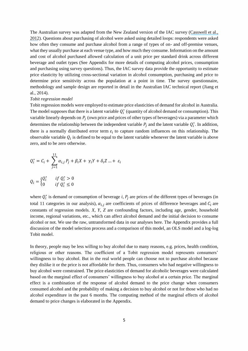
Tobit regression model

Tobit regression models were employed to estimate price elasticities of demand for alcohol in Australia.

The model supposes that there is a latent variable 𝑄𝑖∗ (quantity of alcohol demand or consumption). This

variable linearly depends on 𝑃𝑗 (own price and prices of other types of beverages) via a parameter which

determines the relationship between the independent variable 𝑃𝑗 and the latent variable 𝑄𝑖∗. In addition,

there is a normally distributed error term 휀𝑖 to capture random influences on this relationship. The

observable variable 𝑄𝑖 is defined to be equal to the latent variable whenever the latent variable is above

zero, and to be zero otherwise.

𝑄𝑖∗ = 𝐶𝑖 + ∑ 𝛼𝑖,𝑗

11

𝑗=1

𝑃𝑗 + 𝛽𝑖𝑋 + 𝛾𝑖𝑌 + 𝛿𝑖𝑍 … + 휀𝑖

𝑄𝑖 = {𝑄𝑖

∗ 𝑖𝑓 𝑄𝑖∗ > 0

0 𝑖𝑓 𝑄𝑖∗ ≤ 0

where 𝑄𝑖∗ is demand or consumption of beverage i, 𝑃𝑗 are prices of the different types of beverages (in

total 11 categories in our analysis), 𝛼𝑖,𝑗 are coefficients of prices of difference beverages and 𝐶𝑖 are

constants of regression models. X, Y, Z are confounding factors, including age, gender, household

income, regional variations, etc., which can affect alcohol demand and the initial decision to consume

alcohol or not. We use the raw, untransformed data in our analyses here. The Appendix provides a full

discussion of the model selection process and a comparison of this model, an OLS model and a log-log

Tobit model.

In theory, people may be less willing to buy alcohol due to many reasons, e.g. prices, health condition,

religious or other reasons. The coefficient of a Tobit regression model represents consumers’

willingness to buy alcohol. But in the real world people can choose not to purchase alcohol because

they dislike it or the price is not affordable for them. Thus, consumers who had negative willingness to

buy alcohol were constrained. The price elasticities of demand for alcoholic beverages were calculated

based on the marginal effect of consumers’ willingness to buy alcohol at a certain price. The marginal

effect is a combination of the response of alcohol demand to the price change when consumers

consumed alcohol and the probability of making a decision to buy alcohol or not for those who had no

alcohol expenditure in the past 6 months. The computing method of the marginal effects of alcohol

demand to price changes is elaborated in the Appendix.

6

Both alcohol consumption and purchasing data were used in the analysis. Of the 2020 respondents,

1789 reported they consumed alcohol in the last 6 months and 1823 reported they purchased alcohol

either from on- or off-premise, although 70 of them did not report purchasing expenditures.

Respondents who did not consume or purchase alcohol in the survey period (abstainers or no alcohol

consumption or purchasing; n=267) are censored as a consumption choice problem. Furthermore, when

estimating price elasticities for beverage type “A”, respondents who consumed other types of beverages

without consuming any “A” in the last 6 months were also censored as a corner solution in the regression

(A consumer may consume good “X” but not consume “Y” by saying that "I wouldn't buy Y at any

price" or "I will do X no matter the cost”, and this consumption choice is called a “corner solution” in

microeconomics). The volume and total costs of consumption and purchasing were doubled in the

analysis to give an annual amount, comparable to other Australian survey analyses. Since the six months

before the survey fieldwork included the seasons when more alcohol is consumed, annual consumption

is likely to be slightly overestimated.

Due to limited observations, on-premise cask wine and on- and off-premise cider purchases were

excluded in the price elasticity analysis. In subpopulation analyses, alcohol consumers were classified

into three groups: moderate drinkers (≤14 ASDs per week for men and women), hazardous drinkers

(>14-42 ASDs for men and >14-35 ASDs for women), and harmful drinkers (>42 ASDs for men and

>35 ASDs for women). The three drinking levels follow definitions in Australian Guidelines to Reduce

Health Risk from Drinking Alcohol (National Health and Medical Research Council, 2009). The total

population was also split into three income groups with fairly equal observations based on the annual

income in the respondent’s household: lower income (<$47k), middle income ($47-90k) and higher

income (>$90k). The price elasticities of demand among three different drinking levels and income

levels were evaluated in our models in order to understand how price changes could affect alcohol

demand among different subgroups of consumers.

When estimating price elasticities by level of drinking and income level, we combined cask wine and

bottle wine into one group, “wine”, while regular-beer and low-mid strength beer were combined as

“beer”, in order to increase price variations, thus enhancing estimation performance in subpopulation

groups. Additionally, control variables and instrumental variables that can affect demand and

consumption choice were included in estimating models (missing data were found in some control

variables and multiple imputation techniques were applied to impute missing data in our analyses, see

Appendix). For example, a consumer’s gender, age, household income, education levels, number of

household aged 18 and over, marital status and regional variations can affect drinking preferences,

affordability for alcohol products (Treno et al., 2006; Morrison et al., 2015). Due to data availability,

some confounding factors were not included in our estimation, such as respondent’s health conditions

and religious affiliation (the full list of variables used in the estimation and robustness checks and

discussion of alternative methods are detailed in the Appendix). Two sample t-tests were utilised to test

the differences in mean price per ASD between different beverages, and one-way ANOVA tests were

conducted to test for differences in the average amount of alcohol purchased and mean price per ASD

across different drinker and income groups. All analyses presented in this study are on data weighted

to benchmarks from the Australian Bureau of Statistics 2011 Census (ABS, 2011).

Results

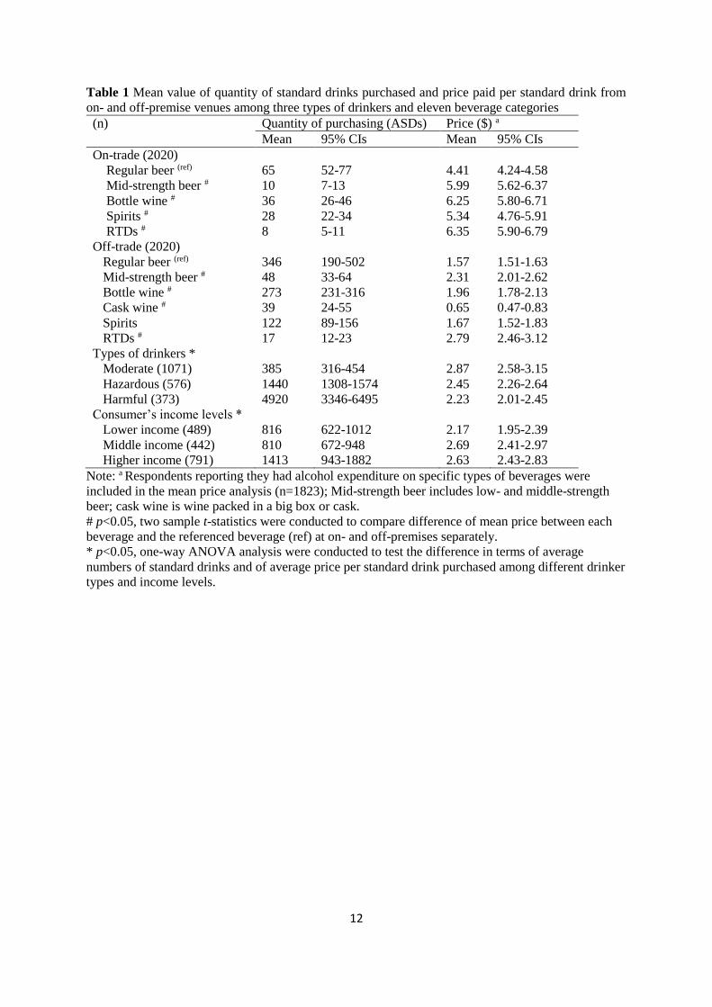
On average, Australians aged 16 and overconsumed a higher volume of off-premise bottle wine and

off-premise regular beer than the nine other categories of beverage (shown in Table 1), and consumed

higher volumes of regular beer and bottle wine than other types of beverages in both on- and off-

7

premises settings. The average price per ASD of all beverage types purchased off-premise is one-third

(0.34) of the average price of an on-premise drink, and off-premise cask wine is the cheapest beverage

($0.65AUD per ASD; t=12.36, p<0.001) among the 11 categories. Harmful drinkers purchased four

times the average number of ASDs in the form of cheaper alcohol than hazardous and moderate drinkers

(F(2)=652.18, p<0.001). Lower income consumers drank a lower average amount of alcohol annually

than a higher income group, also consuming cheaper beverages than middle and higher income

consumers (F(2)=11.64, p=0.003).

<Insert Table 1 here>

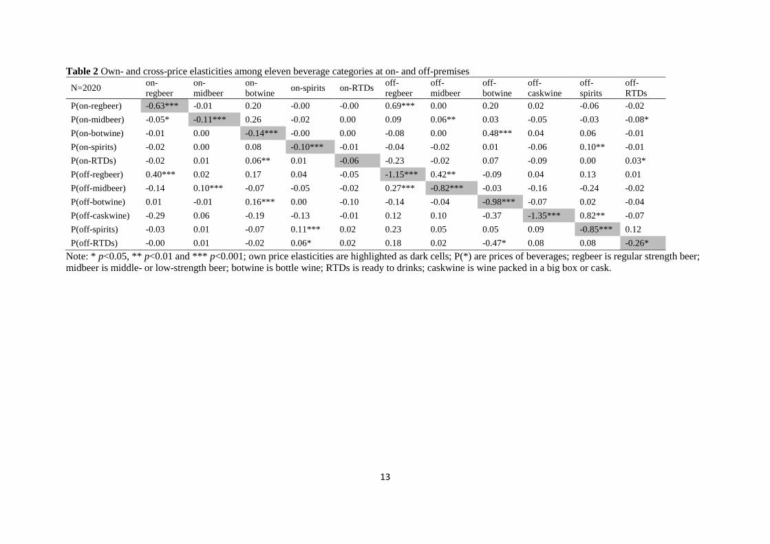
The Tobit regression outputs for the 11 beverage categories are presented in Appendix Table A.3. The

own- and cross-price elasticities of demand among 11 categories of on- and off-premise beverages are

calculated based on the mean of the marginal effects and then summarized in Table 2. The results

indicate that nearly all prices were negatively and significantly associated with the beverage’s own

demand (own price elasticities highlighted as dark cells), except for on-premise RTDs. Off-premise

cask wine has the highest own-price elasticity (coefficient=-1.35), followed by off-premise regular beer

with -1.15. The results for cross-price elasticities suggest that the prices of off-premise beverages were

significantly and positively associated with demand for the same beverage on-premise.

<Insert Table 2 here>

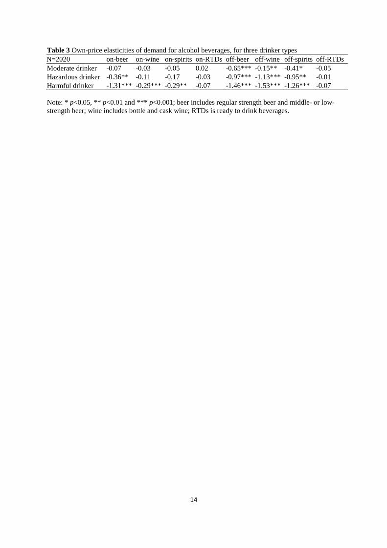
The own-price elasticities of alcohol demand among three types of drinkers and eight categories of

beverage are summarized in Table 3. The elasticity values suggest that harmful drinkers are more price

responsive than hazardous and moderate drinkers across nearly all on- and off-premise beverages

(except for on-and off-premise RTDs). The own-price elasticities of demand for on –premise beer, off-

premise beer, wine and spirits are over 1 in the harmful drinkers model, indicating that the harmful

drinkers’ demand for these four types of beverages are price elastic and more price responsive than for

other beverage categories.

<Insert Table 3 here>

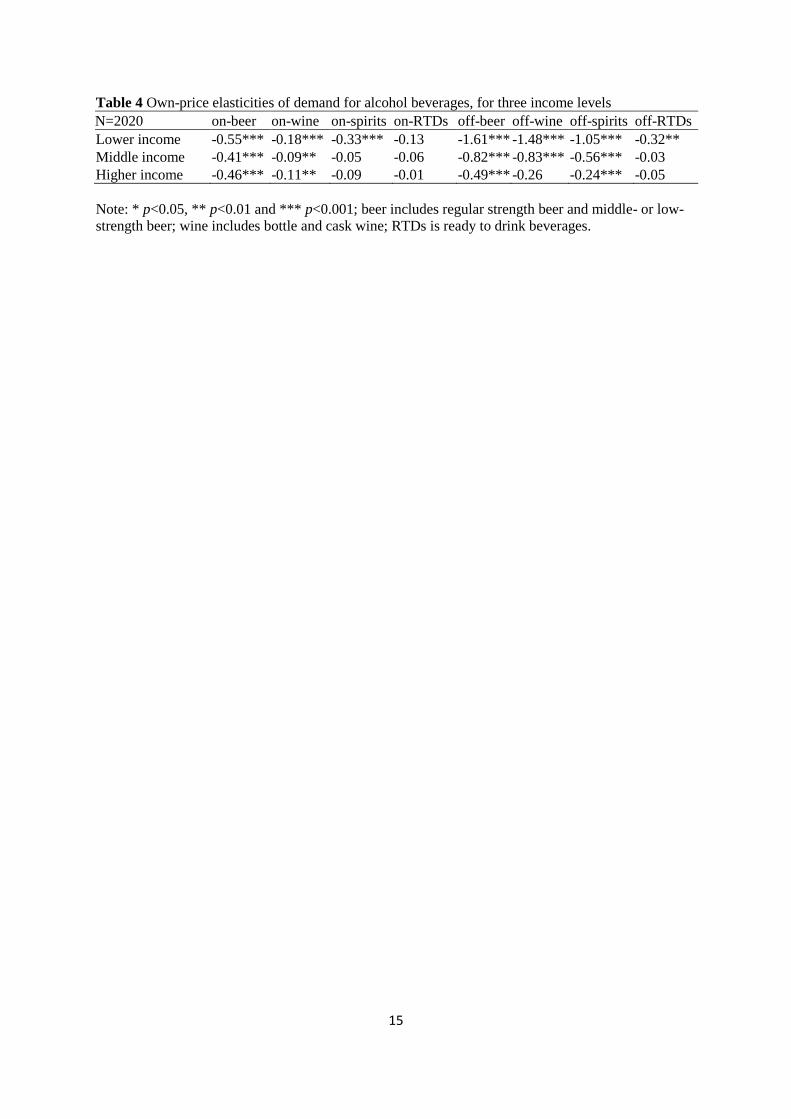
Table 4 shows the own-price elasticities of alcohol demand among three income groups and 8 categories

of beverage. The results suggest that absolute values of own-price elasticities of demand for nearly all

beverages are higher among lower income drinkers than among middle and higher income drinkers.

Price elasticities of demand for on-premise beer and wine are similar across three household income

groups.

<Insert Table 4 here>

Discussion

The own-price elasticities estimated in this study are similar to those reported in the previous meta-

analyses; 0.46 to -0.83 for beer, -0.69 to -1.11 for wine and -0.36 to -1.09 for spirits (Gallet, 2007;

Wagenaar et al., 2009; Fogarty, 2010). The estimated elasticities in our study are not directly

comparable with most previous estimates, because the beverage categories included are more detailed

than most previous studies. Another possible reason for the heterogeneity of the elasticity estimates in

the literature is due to the mix of tax elasticity and price elasticity; tax elasticity is different from price

elasticity, as tax is only a fraction of price (Xuan et al., 2015). Beverage-specific negative elasticities

8

estimated in the Australian study of Srivastava et al. (2014) are much higher than our estimations, but

this study did not differentiate on- and off-premise purchases. Conversely, our estimates are broadly in

line with some previous disaggregated studies [i.e. Doran et al. (2013) and Meng et al. (2014)], revealing

that off-premise beverages are generally more price responsive than beverages sold on-premise. Meng

et al. (2014) suggested that off-premise beer is more price responsive than off-premise wine, spirits,

and RTDs, and on-premise beer is more elastic than on-premise wine. A similar pattern is also observed

in our study, while our estimations further suggest that off-premise cask wine – the cheapest form of

alcohol in Australia, but never discussed in previous elasticity studies -- is the most price responsive

beverage in the current analysis.

The own- and cross-price elasticities estimated in this study can be utilised to estimate the effects of

price-based interventions on alcohol consumption and related harms in Australia -- allowing detailed

examination of change in beverage-specific demand in response to changes in price in the on- and off-

premise sectors. For example, the present study yields an estimate that if off-premise regular beer and

cask wine prices increased by 10%, demand for the two beverages will decrease by 14% and 12%

respectively, and demand for on-premise regular beer will increase by 7%.

The effectiveness of price-based intervention is further supported by our findings on own-price

elasticities, suggesting that an increase in alcohol price or tax will effectively reduce the demand for

alcohol, particularly for off-premise cask wine, bottle wine, spirits and regular beer. In contrast, demand

for on-premise low-to-mid strength beer, spirits and RTDs would not be significantly affected by own

price changes. The estimated cross-price elasticities show complex substitution and complementary

relationships among different categories of beverage, suggesting that alcohol price policies should not

be focused on particular types of beverage (the complexity of the Australian alcohol taxation system is

explained in the Appendix), but rather on a uniform price or tax policy, such as a minimum price per

standard drink or a volumetric taxation system based on alcohol content (Jiang and Livingston, 2015).

As absolute own-price elasticities of off-premise beverages are estimated to be greater than on-premise

beverages and off-premise venues sell cheaper priced alcohol than on-premise venues, it can be

expected that price policies will have a greater proportional reduction on off-premise alcohol

consumption than on on-premise alcohol consumption.

A recent policy debate in Australia has posed the question whether any increase in the alcohol price or

tax would disproportionately affect moderate drinkers (Australian Government, 2010; Sharma et al.,

2014). This study provides evidence that harmful drinkers are more price responsive than hazardous

and moderate drinkers, suggesting an increase in alcohol price or tax will achieve a greater reduction in

alcohol consumption for harmful drinkers and a considerably smaller reduction in hazardous and

moderate drinkers. This is consistent with findings in the U.K. (Holmes et al., 2014

) and a longitudinal study in the US (Farrell et al., 2003), though it differs from an earlier cross-sectional

quintile regression analysis involving the same group in the US (Manning et al., 1995).

Previous studies show that disadvantaged groups are generally less likely to report alcohol use, but

experience more severe health outcomes at all levels of consumption compared to those with a higher

socioeconomic status (Jefferis et al., 2007; Schmidt et al., 2010). Our research findings suggest that

lower income drinkers are generally more price responsive than middle and higher income drinkers,

particularly for on- and off-premise beer and wine, and off-premise spirits. Therefore, an increase in

alcohol price or tax, or the introduction of a minimum unit price, would have a greater effect on lower

income drinkers than on middle and higher income drinkers, especially since lower income drinkers are

9

more likely to consume cheaper alcohol than the other two income groups. These findings are

unsurprising, as alcohol price changes will more significantly affect the spending money of more

disadvantaged drinkers – one of the reasons that excise taxes are generally considered regressive.

However, the regressiveness of alcohol taxes needs to be considered against the potential reductions in

health inequalities (Jiang et al., 2015), which our findings suggest could be substantial.

Limitations

There are some limitations in this study. One limitation pertains to recall bias. Respondents were asked

to report their usual alcohol consumption and purchasing in the last 6 months, thus costs and volumes

of consumption and purchasing reported may not be completely accurate. However, this method of

questioning yields results closer to measured consumption than other methods (Livingston and Callinan,

2015). Furthermore, as noted in the method, close examination of the prices paid yielded a very small

number of implausible responses, lending support to the method. It is worth noting that the present

study’s low response rate is similar to the response rates for other population surveys in Australia,

including other alcohol surveys, such as the National Drug Strategy Household Survey (32.7%)

(Australian Institute of Health and Welfare, 2014), and the Alcohol’s Harm to Others Survey (35.2%)

(Laslett et al., 2011). There are no temporal variations in the cross-sectional data, which may affect the

magnitude of alcohol prices, consumption and purchasing. Doubling of 6-month data to calculate annual

rates without considering seasonality of alcohol purchasing and consumption may affect the price

elasticity estimation, but the impact of this will be small. The term elasticity generally implies a causal

relationship. However, since the price elasticities estimated in the study are based on cross-sectional

data, there needs to some caution about assuming that they accurately model how behaviour will change

in response to changes in price.

Conclusions

This study expands beyond the existing studies in the U.K. (Holmes et al., 2014), the U.S. (Farrell et

al., 2003) and Australia (Srivastava et al., 2014) by utilising a Tobit approach to estimate price

elasticities of demand for alcohol. Using national survey data on both reported alcohol consumption

and purchasing, the own- and cross-price elasticities of demand for 11 categories of beverage were

estimated. On the basis of its cross-sectional data, the study found demand for nearly all beverage

categories significantly and negatively correlated to their own price changes, except for on-premise

RTDs. Raising alcohol price or tax could help to reduce alcohol consumption, and is likely to be

particularly effective for reducing consumption among harmful drinkers and lower income drinkers.

Increases in alcohol prices are likely to particularly affect purchases from off-premise outlets, due to

the lower price of alcohol sold from these settings. However, separating price effects for the off-premise

and on-premise sectors has been relatively rare in the literature. The present survey, recording price,

consumption and purchasing data for a wide range of beverages at on- and off-premises, thus gives a

more nuanced picture of price elasticities in different segments of the populations.

10

References

ABS, 2011. The Census of Population and Housing. Australian Bureau of Statistics, Canberra.

Ally, A.K., Meng, Y., Chakraborty, R., Dobson, P.W., Seaton, J.S., Holmes, J., Angus, C., Guo, Y.,

Hill-McManus, D., Brennan, A., Meier, P.S., 2014. Alcohol tax pass-through across the product

and price range: do retailers treat cheap alcohol differently? Addiction. 109, 1994-2002.

AAPOR, 2008. Standard definitions: Final dispositions of cases, codes and outcome rates for surveys.

American Association for Public Opinion Research, Lenexa, Kansas.

Anderson, P., Chisholm, D., Fuhr, D.C., 2009. Effectiveness and cost-effectiveness of policies and

programmes to reduce the harm caused by alcohol. Lancet. 373, 2234-2246.

Angulo, A.M., Gil, J.M., Gracia, A., 2001. The demand for alcoholic beverages in Spain. Agricultural

Economics. 26, 71-83.

Australian Government, 2010. Australia's future tax system: Report to the Treasurer. Commonwealth

of Australia, Canberra.

Australian Institute of Health and Welfare, 2011. 2010 National Drug Strategy Household Survey

report. Drug Statistic Series. Australian Institute of Health and Welfare, Canberra.

Australian Institute of Health and Welfare, 2014. 2013 National Drug Strategy Household Survey

report. Drug Statistic Series. AIHW Canberra.

Babor, T., Caetano, R., Casswell, S., Edwards, G., Giesbrecht, N., Graham, K., Grube, J., Hill, L.,

Holder, H., Homel, R., Livingston, M., Österberg, E., Rehm, J., Room, R., Rossow, I., 2010.

Alcohol: No ordinary commodity - Research and public policy. 2nd ed. Oxford University

Press, Oxford.

Callinan, S., Room, R., Livingston, M., Jiang, H., 2015. Who Purchases Low-Cost Alcohol in

Australia? Alcohol Alcohol. 50, 647-653.

Casswell, S., Meier, P., MacKintosh, A.M., Brown, A., Hastings, G., Thamarangsi, T., Chaiyasong, S.,

Chun, S., Huckle, T., Wall, M., You, R.Q., 2012. The International Alcohol Control (IAC)

Study—Evaluating the Impact of Alcohol Policies. Alcohol Clin Exp Res. 36, 1462-1467.

Collis, J., Grayson, A., Johal, S., 2010. Econometric anslysis of alcohol consumption in the UK. In: Her

Majesty's Revenue and Customs (HMRC) (Ed.). HMRC, London.

Doran, C.M., Byrnes, J.M., Cobiac, L.J., Vandenberg, B., Vos, T., 2013. Estimated impacts of

alternative Australian alcohol taxation structures on consumption, public health and

government revenues. Med J Aust. 199, 619-622.

Farrell, S., Manning, W.G., Finch, M.D., 2003. Alcohol dependence and the price of alcoholic

beverages. J Health Econ. 22, 117-147.

Fogarty, J., 2010. The demand for beer, wine and spirits: A survey of the literature. J Econ Surv.. 24,

428-478.

Gallet, C.A., 2007. The demand for alcohol: a meta-analysis of elasticities. Aust J Agric Resour Econ..

51, 121-135.

Greene, W.H., 2011. Econometric Analysis. Prentice Hall, New York.

Holmes, J., Meng, Y., Meier, P.S., Brennan, A., Angus, C., Campbell-Burton, A., Guo, Y., Hill-

McManus, D., Purshouse, R.C., 2014. Effects of minimum unit pricing for alcohol on different

income and socioeconomic groups: a modelling study. Lancet. 383, 1655-1664.

Jefferis, B.J.M.H., Manor, O., Power, C., 2007. Social gradients in binge drinking and abstaining: trends

in a cohort of British adults. J Epidemiol Community Health. 61, 150-153.

Jiang, H., Callinan, S., Room, R., 2014. Alcohol Consumption and Purchasing (ACAP) Study: Survey

approach, data collection procedures and measurement of the first wave of the Australian arm

of the International Alcohol Control Study. Centre for Alcohol Policy Research, Melbourne.

11

Jiang, H., Livingston, M., 2015. The dynamic effects of changes in prices and affordability on alcohol

consumption: an impulse response analysis. Alcohol Alcohol. 50, 631-638.

Jiang, H., Livingston, M., Room, R., 2015. How financial difficulties interplay with expenditures on

alcohol: Australian experience. J Public Health. 23, 267-276.

Laslett, A., Room, R., Ferris, J., Wilkinson, C., Livingston, M., Mugavin, J., 2011. Surveying the range

and magnitude of alcohol’s harm to others in Australia. Addiction. 106, 1603-1611.

Livingston, M., Callinan, S., 2015. Underreporting in alcohol surveys: whose drinking is

underestimated? J Stud Alcohol Drugs. 76, 158-167.

Manning, W.G., Blumberg, L., Moulton, L.H., 1995. The demand for alcohol: the differential response

to price. J Health Econ. 14, 123-148.

Meier, P., Purshouse, R., Brennan, A., 2010. Policy options for alcohol price regulation: the importance

of modelling population heterogeneity. Addiction. 105, 383-393.

Meng, Y., Brennan, A., Purshouse, R., Hill-McManus, D., Angus, C., Holmes, J., Meier, P.S., 2014.

Estimation of own and cross price elasticities of alcohol demand in the UK—A pseudo-panel

approach using the Living Costs and Food Survey 2001–2009. J Health Econ. 34, 96-103.

Morrison, C., Ponicki, W.R., Smith, K., 2015. Social disadvantage and exposure to lower priced alcohol

in off-premise outlets. Drug Alcohol Rev. 34, 375-378.

National Health and Medical Research Council, 2009. Australian guidelines to reduce health risks from

drinking alcohol. NHMRC, Canberra.

Nelson, J.P., 2013. Does Heavy Drinking by Adults Respond to Higher Alcohol Prices and Taxes? A

Survey and Assessment. Economic Analysis and Policy. 43, 265-291.

Purshouse, R.C., Meier, P.S., Brennan, A., Taylor, K.B., Rafia, R., 2010. Estimated effect of alcohol

pricing policies on health and health economic outcomes in England: an epidemiological

model. Lancet. 375, 1355-1364.

Schmidt, L., Mäkelä, P., Rehm, J., Room, R., 2010. Alcohol: equity and social determinants. In: Blas,

E., Sivasankara Kurup, A. (Eds.), Equity, Social Determinants and Public Health Programmes.

World Health Organisation, Geneva. pp. 11-29.

Sharma, A., Vandenberg, B., Hollingsworth, B., 2014. Minimum pricing of alcohol versus volumetric

taxation: Which policy will reduce heavy consumption without adversely affecting light and

moderate consumers? PLoS ONE. 9, 1-13.

Srivastava, P., McLaren, K.R., Wohlgenant, M., Zhao, X., 2014. Disaggregated econometric estimation

of consumer demand response by alcoholic beverage types. Aust J Agric Resour Econ. 59, 1-

21.

Treno, A., Gruenewald, P.J., Wood, D.S., Ponicki, W.R., 2006. The price of alcohol: A consideration

of contextual factors. Alcohol Clin Exp Res. 30, 1-9.

Wagenaar, A.C., Salois, M.J., Komro, K.A., 2009. Effects of beverage alcohol price and tax levels on

drinking: a meta-analysis of 1003 estimates from 112 studies. Addiction. 104, 179-190.

Xuan, Z., Chaloupka, F.J., Blanchette, J.G., Nguyen, T.H., Heeren, T.C., Nelson, T.F., Naimi, T.S.,

2015. The relationship between alcohol taxes and binge drinking: evaluating new tax measures

incorporating multiple tax and beverage types. Addiction. 110, 441-450.

12

Table 1 Mean value of quantity of standard drinks purchased and price paid per standard drink from

on- and off-premise venues among three types of drinkers and eleven beverage categories

(n) Quantity of purchasing (ASDs) Price ($) a

Mean 95% CIs Mean 95% CIs

On-trade (2020)

Regular beer (ref) 65 52-77 4.41 4.24-4.58

Mid-strength beer # 10 7-13 5.99 5.62-6.37

Bottle wine # 36 26-46 6.25 5.80-6.71

Spirits # 28 22-34 5.34 4.76-5.91

RTDs # 8 5-11 6.35 5.90-6.79

Off-trade (2020)

Regular beer (ref) 346 190-502 1.57 1.51-1.63

Mid-strength beer # 48 33-64 2.31 2.01-2.62

Bottle wine # 273 231-316 1.96 1.78-2.13

Cask wine # 39 24-55 0.65 0.47-0.83

Spirits 122 89-156 1.67 1.52-1.83

RTDs # 17 12-23 2.79 2.46-3.12

Types of drinkers *

Moderate (1071) 385 316-454 2.87 2.58-3.15

Hazardous (576) 1440 1308-1574 2.45 2.26-2.64

Harmful (373) 4920 3346-6495 2.23 2.01-2.45

Consumer’s income levels *

Lower income (489) 816 622-1012 2.17 1.95-2.39

Middle income (442) 810 672-948 2.69 2.41-2.97

Higher income (791) 1413 943-1882 2.63 2.43-2.83

Note: a Respondents reporting they had alcohol expenditure on specific types of beverages were

included in the mean price analysis (n=1823); Mid-strength beer includes low- and middle-strength

beer; cask wine is wine packed in a big box or cask.

# p<0.05, two sample t-statistics were conducted to compare difference of mean price between each

beverage and the referenced beverage (ref) at on- and off-premises separately.

* p<0.05, one-way ANOVA analysis were conducted to test the difference in terms of average

numbers of standard drinks and of average price per standard drink purchased among different drinker

types and income levels.

13

Table 2 Own- and cross-price elasticities among eleven beverage categories at on- and off-premises

N=2020 on-

regbeer

on-

midbeer

on-

botwine on-spirits on-RTDs

off-

regbeer

off-

midbeer

off-

botwine

off-

caskwine

off-

spirits

off-

RTDs

P(on-regbeer) -0.63*** -0.01 0.20 -0.00 -0.00 0.69*** 0.00 0.20 0.02 -0.06 -0.02

P(on-midbeer) -0.05* -0.11*** 0.26 -0.02 0.00 0.09 0.06** 0.03 -0.05 -0.03 -0.08*

P(on-botwine) -0.01 0.00 -0.14*** -0.00 0.00 -0.08 0.00 0.48*** 0.04 0.06 -0.01

P(on-spirits) -0.02 0.00 0.08 -0.10*** -0.01 -0.04 -0.02 0.01 -0.06 0.10** -0.01

P(on-RTDs) -0.02 0.01 0.06** 0.01 -0.06 -0.23 -0.02 0.07 -0.09 0.00 0.03*

P(off-regbeer) 0.40*** 0.02 0.17 0.04 -0.05 -1.15*** 0.42** -0.09 0.04 0.13 0.01

P(off-midbeer) -0.14 0.10*** -0.07 -0.05 -0.02 0.27*** -0.82*** -0.03 -0.16 -0.24 -0.02

P(off-botwine) 0.01 -0.01 0.16*** 0.00 -0.10 -0.14 -0.04 -0.98*** -0.07 0.02 -0.04

P(off-caskwine) -0.29 0.06 -0.19 -0.13 -0.01 0.12 0.10 -0.37 -1.35*** 0.82** -0.07

P(off-spirits) -0.03 0.01 -0.07 0.11*** 0.02 0.23 0.05 0.05 0.09 -0.85*** 0.12

P(off-RTDs) -0.00 0.01 -0.02 0.06* 0.02 0.18 0.02 -0.47* 0.08 0.08 -0.26*

Note: * p<0.05, ** p<0.01 and *** p<0.001; own price elasticities are highlighted as dark cells; P(*) are prices of beverages; regbeer is regular strength beer;

midbeer is middle- or low-strength beer; botwine is bottle wine; RTDs is ready to drinks; caskwine is wine packed in a big box or cask.

14

Table 3 Own-price elasticities of demand for alcohol beverages, for three drinker types

N=2020 on-beer on-wine on-spirits on-RTDs off-beer off-wine off-spirits off-RTDs

Moderate drinker -0.07 -0.03 -0.05 0.02 -0.65*** -0.15** -0.41* -0.05

Hazardous drinker -0.36** -0.11 -0.17 -0.03 -0.97*** -1.13*** -0.95** -0.01

Harmful drinker -1.31*** -0.29*** -0.29** -0.07 -1.46*** -1.53*** -1.26*** -0.07

Note: * p<0.05, ** p<0.01 and *** p<0.001; beer includes regular strength beer and middle- or low-

strength beer; wine includes bottle and cask wine; RTDs is ready to drink beverages.

15

Table 4 Own-price elasticities of demand for alcohol beverages, for three income levels

N=2020 on-beer on-wine on-spirits on-RTDs off-beer off-wine off-spirits off-RTDs

Lower income -0.55*** -0.18*** -0.33*** -0.13 -1.61*** -1.48*** -1.05*** -0.32**

Middle income -0.41*** -0.09** -0.05 -0.06 -0.82*** -0.83*** -0.56*** -0.03

Higher income -0.46*** -0.11** -0.09 -0.01 -0.49*** -0.26 -0.24*** -0.05

Note: * p<0.05, ** p<0.01 and *** p<0.001; beer includes regular strength beer and middle- or low-

strength beer; wine includes bottle and cask wine; RTDs is ready to drink beverages.