price transmission in the unsecured money market · ifc bulletin no 39 1 price transmission in the...

IFC Bulletin No 39 1

Price Transmission in the Unsecured Money Market

Edoardo Rainone1

Abstract

The price of money in the interbank market is a fundamental indicator of the smooth transmission of signal rates by the central bank. Public information plays an important role in this context, as central banks announce their signal rate and market rates are published daily. Nevertheless, according to the theoretical literature on OTC markets, private information may have an important role in a decentralized market. The diffusion of private information can thus generate prices that depend on the interbank network structure. In this paper we use an ad hoc (network) version of the spatial autoregressive model for assessing the presence of this mechanism in the euro unsecured money market. A wide time span including sovereign debt crises in the euro area is considered. We find that private information played a greater role during periods dominated by strong uncertainty.

Keywords: Interbank markets, money, spatial autoregressive models, trading networks, payment systems

JEL classification Codes: E52, E40, C21, G21, D40

1 Banca d’Italia. I wish to thank Giovanni di Iasio, Marco Rocco and Francesco Vacirca for sharing data

and thoughts with me, Salvatore Alonzo and Fabrizio Palmisani for giving me the time and the opportunity to investigate this topic, for their comments, Vincent Ang, Paolo Angelini, Jacques Fournier, Simone Giansante, Lincoln H. Groves, Luigi Infante, Péter Kondor, Fabrizio Mattesini, also participants of the workshop “The interbank market and the crisis” at Banca d’Italia in Rome, participants of the 7th Irving Fisher Committee Conference at BIS in Basel, my colleagues at the Financial Stability Directorate and finally participants of the Macro-prudential Research Network (MaRS) workshop at the ECB in Frankfurt. A special thanks goes to Francesco Vacirca for his precious guidance through the unsecured money market dataset. I also thank colleagues of Banca d’Italia – Wholesale Payment Systems Division at the Payment System Directorate for their useful contribution to the discussions. All errors are my own responsibility. The author of this paper is member/alternate of one of the user groups with access to TARGET2 data in accordance with Article 1(2) of Decision ECB/2010/9 of 29 July 2010 on access to and use of certain TARGET2 data. Banca d’Italia and the PSSC have checked the paper against the rules for guaranteeing the confidentiality of transaction-level data imposed by the PSSC pursuant to Article 1(4) of the above mentioned issue. The views expressed in the paper are solely those of the author and do not necessarily represent the views of the Eurosystem.

2 IFC Bulletin No 39

1. Introduction

Average rates in the unsecured money market and their volatility are key indicators for a large set of phenomena: financial tensions, market expectations and the cost of mortgages and loans to the real economy (the pass-through mechanism from market to banking rates). Some relevant market rates, like EONIA and EURIBOR in the Euro area, have a direct impact on lending and deposit rates, as shown in Gambacorta (2008) and other papers, determining the amount of households and firms’ debts at variable rates. Furthermore banking rates are influenced by interest rate volatility, following the model by Ho and Saunders (1981). The mechanism investigated in this paper has relevant implications on both market rates and rates volatility, having thus indirect effects on micro and macro financial conditions of households and firms. Rates in money markets represent an important issue for central banks since uncontrolled market rates prevent a smooth rate transmission, which is one of its fundamental missions. Financial stability of the system may be threatened as well. In order to achieve this goal, central banks try to be fully conscious about all the factors impacting interbank market rates.

Prices are supposed to be mainly driven by public information in money markets. Central banks determine upper and lower bound for the cost of money and, collecting information from banks and publishing it, provide banks with market average rates in order to avoid information asymmetry and to smoothly transmit their signal rate.2 Nevertheless, given the decentralized nature of this market, private information may play a relevant role as argued by a growing theoretical literature on OTC markets.

The process of trade can transmit some relevant information in a decentralized market characterized by asymmetric information (Wolinsky; 1990). The idea that prices contain information appears in Hayek (1945) and was deeply investigated by the literature on information transmission in rational expectation equilibrium (Grossman; 1981; Grossman and Stiglitz; 1980). Recently, Babus and Kondor (2013) propose a model characterized by information diffusion in OTC markets. In their model dealers have private information and each bilateral price partially aggregates the private information of other dealers, depending on the market network structure. They theoretically show how it is implied by decentralization and heterogeneous dealers’ valuation on the exchanged asset. The authors also mention the fed funds market as an example. The econometric model proposed in this paper can be used to test for one of the empirical predictions of Babus and Kondor (2013) theoretical model, the latter can thus be taken as one of the possible microfoundations for our empirical specification.

This mechanism of diffusion implies that if a lender increases (decreases) her valuation about central bank money future value because of a random idiosyncratic shock, this will have an impact on prices of loans she agrees and, because of

2 Here we are simplifying this process. Market rates are not always published by the central bank.

They may be published by international non-profit making associations. In Europe, for instance, Euribor-EBF is in charge with this task, see http://www.euribor-ebf.eu/euribor-ebf-eu/about-us.html. A corridor is often used to place lower and upper bounds to market rates. Bounds are determined by marginal lending and overnight deposit rates, these are set by the central bank. Other instruments can be used in order to control market rates.

http://www.euribor-ebf.eu/euribor-ebf-eu/about-us.html

http://www.euribor-ebf.eu/euribor-ebf-eu/about-us.html


diffusion process, on prices of loans in which she is not involved. Observe that it generates a higher (lower) variation in the average price.3 Coming back to the pass-through mechanism, if a shock on single price has a stronger impact on price average and variance because of transmission mechanism, it will have a stronger impact on the households and firms’ debts as well. It implies that an increase in the price of an interbank loan will lead to a higher increase of the rate of loans to households and firms if a transmission mechanism is at work (ceteris paribus).

Moving to the empirical argument, the market rate and its variance, are the first and second moments of the rate distribution, which is composed by single rates. The rate of a loan has been usually modelled as a function of lender and borrower’s characteristics and aggregate conditions. Nevertheless, the unsecured money market is known to be a decentralized one, thus formed by bilateral relationships. This set of interbank relationships generates a network.

Given the relational nature of these loans and following the theoretical literature on OTC markets, we want to test for a cross-sectional dependence among rates implied by private information diffusion. The network nature of this market makes this task easier since, if micro-data is available, the structure of this dependence can be exactly traced. The spatial econometrics literature has developed a large set of models to formalize this dependence and it recently focused on networks (Lee; 2007; Lee et al.; 2010; Liu and Lee; 2010). Conceptually, this cross-sectional dependence can be seen as a consequence of the process of private information diffusion in the interbank network, according to Babus and Kondor (2013).4

This paper empirically explores the informational role of prices in the Euro unsecured money market. The nature of the exchanges’ network is used for exploiting the diffusion of private information. Suppose that bank i trades with bank j and bank j trades with bank k, then the prices of these two loans are connected. The diffusion of private information is measured by network-based spillover effects among connected prices. We rigorously test this hypothesis, estimate the magnitude of this effect in the Euro unsecured money market and its evolution over time. Network theory and a rearranged spatial econometric toolkit are, respectively,

3 Here, the behavioral mechanism can be synthesized as follows: when a bank has to evaluate the

expected price of a loan, it can be influenced by prices experienced in other loans (in addition to its own characteristics, counterpart’s characteristics and liquidity conditions of the system). Prices experienced represent the private signals coming from other banks and reflect a mixture of their expectations. Note that here we used the term ”expectation”. If we think about the bank’s production function in the money market, it is characterized by a ”lag” (the final outcome comes out at the end of a maintenance period). It naturally implies the presence of expectations about the future value of central bank money. Note also that the process of expectations’ formation about prices is typically conceived as based on time-lags (Muth; 1961; Nerlove; 1958). What we are hypothesizing here, is that it may be based on network-lags.

4 Rates reflect the expectation of market operators, thus a cross-sectional dependence of rates, after having controlled for counterparts characteristics and aggregate conditions, may indicate a diffusion of expectations. Single rates can be observed only by the respective counterparts, so that they represent a piece of private information about the cost of money, contrasting the public information provided by market rates, i.e. the average of rates. Each bank can see its experienced prices and the market average, thus they respectively play the role of private and public information. Other definitions of private information can be conceived. Given that price is the outcome of interest here, this specification seems to be the most appropriate.


used to formalize the local diffusion in prices and to identify and estimate the spillover effects.

The dataset used consists of loans detected with the Furfine algorithm (with maturities from one day up to one year) implemented on Target2 data (Arciero et al.; 2013). Loans are then matched with lender and borrower characteristics.5 This large set of information allows us to distinguish a price variation due to a change in bank’s economic outlook from one generated by an impulse coming from connected prices. We consider a wide time period, as it enables us to study also time series of spillover intensity.

Summing up, the main contribution of this paper is to examine a novel banks’ behavioral mechanism and to test for it. This suggests a different perspective from which money market dynamics can be studied and provides a new tool for measuring market tensions. It translates into an additional explicative variable when price is modeled. A consistent methodology for estimating this (endogenous) variable is proposed, using an ad hoc spatial autoregressive model.

The main empirical findings are the following: (i) information diffusion is relevant only when there are market tensions and high uncertainty, (ii) diffusion flows in multiple directions through the interbank network, lenders are influenced by the price they experience as borrowers and borrowers are influenced by the price they experience as lenders.

The rest of the paper is organized as follows. Section 2 outline the link between the conceptual framework and the econometric setup, Section 3 provides preliminary evidence and the basic ingredients of the analytical framework. Section 4 describes the econometric model and discusses the issues related to the consistent estimation of the spillover effects. Section 5 presents the results of the application of the econometric model on the Euro unsecured money market estimated by the application of Furfine algorithm on Target2 data. Section 6 discusses the transmission mechanism, Section 7 concludes.

2. Conceptual Framework and Econometric setup

Suppose that the market is composed by n banks that trade bilaterally an asset (central bank money) and they are uncertain about its market value.6 Assume that each bank receives a private signal about the value, it implies that the information on the price of a unit of money, I, can be split in two components for each bank i, IM and Ii, respectively public and private information. Note that this setting is the same of Babus and Kondor (2013), thus we can set bank i’s valuation as θi = θ + ηi, where

5 Furfine algorithm is used to detect loans from a set of payments. By definition a loan consists of

two payments, the first equal to l and the second equal to l(1 + i), where i is the interest rate. The algorithm matches those two legs, see Furfine (1999) for more details. The procedure is described in Arciero et al. (2013). See Armantier and Copeland (2012) for an assessment of the quality of Furfine-based algorithms. Target2 is the European RTGS Payment System. Banks characteristics come from Bankscope.

6 Note that, given that bank’s production function in the money market is characterized by a ”lag” (the final outcome realizes at the end of a maintenance period), it naturally implies the presence of valuations about the value of central bank money.


θ is the common component which represents public information while ηi is the individual one which reflects private information. It implicitly implies that there is heterogeneity in banks’ valuation. As an example, we can have that θ = n(p̄ k∈K ; ψ),

where K is a set of lags and ψ is a set of parameters, it implies that the public component is a function of market rates observed in the past. As an alternative, we can suppose that the term structure of interest rates is used for computing θθ = b(p̄m, m ∈ M ; ι), where M is a set of maturities and ι is a set of parameters (Alonzo et al.;

1994; Shiller and McCulloch; 1987). Observe that we can assume that both are considered in θ.7

Bilateral trading and heterogeneity in valuations imply price dispersion and transmission of information. According with Babus and Kondor (2013), each price thus partially incorporates private signals of market participants. It also implies that if agent j trades with agent k then pjk may affect pij. Indeed, the residual inverse demand function of dealer i in a transaction with dealer j in their model is a function of other prices.8

Suppose now that the price of a loan which has b as a borrower and l as a lender is also a function of lender and borrower characteristics. We thus have pbl = f (cbl(P), xb, xl, Ebl, χ), where χ is a set of parameters, Ebl is a random component, P is a vector containing all the prices in the market, cbl(•) is a loan-specific function which includes prices that are connected with pbl, xb and xl are borrower and lender characteristics respectively. If we assume linearity we thus have that pbl = α + βcbl(P) + γxb + µxl + Ebl, with χ = (α, β, γ, µ).

In other words, each price starts from a ”baseline” price, α, determined by market-wide expectations (which captures θ, the common component which represents public information), then spreads depending on counterparts’ characteristic (xb, xl) are added (for instance a risky borrower should be priced accordingly to its probability of default) and finally a set of other prices (cbl(P)) play a role in determining the agreed (observed) price, capturing the diffusion of private information via prices.

Observe that, according to this specification, if only public information matters, i.e. θi = θ, the price equation reduces to pbl = α + γxb + µxl + Ebl, thus a formal test for the presence and diffusion of private information consists in estimating the full model and checking whether we would reject the null β = 0. If private information matters, i.e. ηi ≠ 0, β will be significantly different from zero.

3. Preliminary Evidence

Price volatility in the Euro unsecured money market (hereafter UMM) estimated by Furfine algorithm shows significant time-variation. Panel (a) of Figure 1 depicts the variance of price across loans with maturities from overnight to three days agreed in

7 Note that we are assuming separability, thus each bank elaborates in the same way the common

information available. This assumption can be relaxed, but here is useful for the sake of simplicity. 8 They also show that pij can be represented as a function of posterior beliefs of i and j, which in turn

are shaped by prices privately observed by i and j.


each maintenance period. We can see that it remarkably increased after Lehman, first and second Sovereign Crises (hereafter FC and SC), and drastically decreased after ECB intervention by 2011 LTRO.9 During these crises the credit default swap of hit countries dramatically increased, the default risk of banks belonging those countries increased as well. It produced big uncertainty in the interbank money market. Furthermore, the expectations about the reaction of ECB dispersed until the LTRO took place, generating an additional source of uncertainty in the interbank money market. If we take two maintenance periods, the first from 2010-01-20 to 2010-02-09 (before FC) and the second from 2011-07-13 to 2011-08-09 (after SC), we can see from panel (b) of Figure 1 that the density changes dramatically. The price dispersion has notably increased in the second period.

Price Variance Figure 1

(a) Time Evolution (b) Density Change

Panel (a): violet vertical line traces first Sovereign crises, black vertical line traces second Sovereign crises, green lines trace LTROs and azure line traces signal rate change in July 2012. Maintenance periods are considered. Panel (b): kernel density of prices centered to zero. Bandwidth = 0.2, kernel = Normal. Red line: distribution of prices during the maintenance period from 2010-01-20 to 2010-02-09, blue line: distribution of prices during the maintenance period from 2011-07-13 to 2011-08-09.

The main reason behind this change is the generalized increase in perceived

risk by treasurers. An additional source of variation might be the propagation of changes in agents’ expectations. Agents show updated expectations by changing their reference prices, thus sending signals to other agents. If this mechanism is at work, we should see a higher variance for connected prices during hot periods since they are contracts characterized by agents which receive more signals.10 Panel (a) of Figure 2 shows the variance computed for connected and unconnected prices, the variance among connected prices is usually higher than the one computed for unconnected (it happens roughly 80 percent of total observations), apparently confirming the intuition. Connectedness can also act as a valid support for searching (and even finding) lower prices, panel (b) of Figure 2 depicts the average price for the two subsamples previously defined. It highlights that connected prices are on

9 The first Sovereign crises was in April 2010 and hit Ireland, Greece and Portugal, while the second

Sovereign crises was in August 2011 and hit Italy and Spain. 10 A price of a loan is connected whether it has its borrower or lender shared with other loans.


average lower than unconnected ones, the spread starts to be significant after the FC and approaches to zero after 2011 LTRO.11 The rest of the paper is based on the subsample of connected price.

Connected vs Unconnected Spreads Figure 2

(a) Volatility (b) Price Density Change

Violet vertical line traces first Sovereign crises, black vertical line traces second Sovereign crises, green lines trace LTROs and azure line traces signal rate change in July 2012.

The question does the prices’ volatility have a network nature? In other words:

is it likely that ”neighbors” prices are more similar? Or from a distributional perspective: If we draw two similar prices how likely is that they are neighbors? Here the main idea is that the prices’ positions in the money market network may be relevant in explaining the aggregate dispersion, consequently the experienced prices influence the bargained price of a contract. This price is couple-specific to the banks, and represents a deviation from the average market rate that is a common piece of information available to everyone because it is published daily in the European market. Suppose that an idiosyncratic shock strikes a bank, given the network nature of these exchanges – if this mechanism is found to take place – we should observe a propagation of this shock through the network. Testing for this mechanism may be quite important for understanding the money market dynamics and correctly interpreting its evolution over time.

3.1 Payment System Data and Furfine Algorithm

The data used in this paper come from Target2 (hereafter T2), the European RTGS (Real Time Gross Settlement) Payment System.12 T2 allows banks operating in European central bank money (hereafter ECBM) to settle large value payments on their accounts. The reserve requirement (hereafter RR) is managed on these accounts too, so participating banks have to exchange money in T2 for

11 From Figure 2 we can also observe a sharp decrease of interbank rates after 2011 LTRO. Bech and

Klee (2011) develop a model to explain this phenomenon. 12 For more information about Target2 see http://www.ecb.europa.eu/paym/t2/html/index.en.html.

http://www.ecb.europa.eu/paym/t2/html/index.en.html


accomplishing RR.13 The Market for ECBM is thus generated by RR and has T2 as a designed support. Several types of markets settle in T2, according to their nature. The main sources of liquidity for a bank are basically three: central bank, secured money market, and UMM.14 The focus of this paper is on the third source. The UMM transactions can be settled basically in two ways. First, through Ancillary Systems,15 which make easy to detect loans among banks. Second, the two legs (the loan and its pay back) can be freely sent through T2 without labeling. In the second scenario UMM is confounded with other types of payments, making more challenging to identify loans. Furfine (1999) argued that matching these two legs is a way for identifying them. Arciero et al. (2013) applied this criterion on payments settled in T2, augmenting the maturity spectrum up to one year.16 The starting point of this paper is consequently the Money Market Database generated by Arciero et al. (2013) where information about prices of unsecured ECBM loans are provided for maturities from overnight up to one year. The time span considered here is from June 2008 to the end of 2012.17 The very basic time unit considered here is the maintenance period (hereafter MP),18 it has at least two big advantages compared with other choices. Firstly an economical and statistical reason, banks are constrained to have an average amount of ECBM in their T2 account taking MP as time interval, thus it makes MP as a natural candidate for money market analysis. Statistically it makes comparable different MPs. Hamilton (1996) and Prati et al. (2003) showed that days are not comparable since the position of day in MP makes the market conditions completely different depending on its distance to the end of MP. The second, more operational, reason is its practicality when considering a large time interval.

3.2 Network of Prices

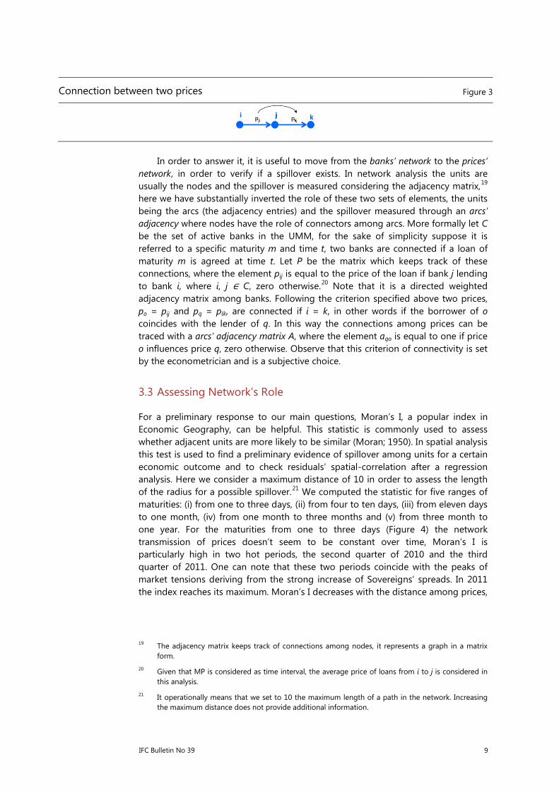
Suppose that bank i trades with bank j and bank j trades with bank k, we want to address the following question: to what extent does the price of the loan of bank i to bank j affect the price of the loan of bank j to bank k (Figure 3)?

13 Many types of payments are actually settled in T2, here a short list: Customer Payments, Securities

Systems Payments, Open Market Operations, Treasury Bonds issues. This should give an idea of the importance of this system and its centrality in a bank’s liquidity management perspective.

14 Of course the list can be largely expanded, intra-group transfers are an example. Here I will not deepen this argument since is out of the scope of this paper.

15 An Ancillary System is connected and send payments instructions to T2, operating upon banks’ accounts. Payments coming from an Ancillary System can be labelled and isolated. e-MID is an example of ancillary system.

16 Their paper contains detailed information about the algorithm and its practical implementation in T2. I will not deepen the algorithm’s details since is out of paper’s scope. In Arciero et al. (2013) the database is based on settler banks, since final agents information was not available at that time. The 3CB recently made this information available and then let the same authors run the algorithm with this new information and make it possible to have the database used in this analysis. 3CB are the three central banks, Banca d’Italia, Banque de France and Deutsche Bundesbank, which provide T2 as a service. I am grateful to both Arciero et al. (2013) and 3CB for providing this essential information, making this paper and a wider investigation possible.

17 T2 starting date was 19 November 2008. The analysis is limited to the end of 2012. The database is up to date so that the analysis can be updated.

18 See http://www.ecb.europa.eu/home/glossary/html/act4m.en.html#226 for details.

http://www.ecb.europa.eu/home/glossary/html/act4m.en.html


Connection between two prices Figure 3

In order to answer it, it is useful to move from the banks’ network to the prices’

network, in order to verify if a spillover exists. In network analysis the units are usually the nodes and the spillover is measured considering the adjacency matrix,19 here we have substantially inverted the role of these two sets of elements, the units being the arcs (the adjacency entries) and the spillover measured through an arcs’ adjacency where nodes have the role of connectors among arcs. More formally let C be the set of active banks in the UMM, for the sake of simplicity suppose it is referred to a specific maturity m and time t, two banks are connected if a loan of maturity m is agreed at time t. Let P be the matrix which keeps track of these connections, where the element pij is equal to the price of the loan if bank j lending to bank i, where i, j ∈ C, zero otherwise.20 Note that it is a directed weighted adjacency matrix among banks. Following the criterion specified above two prices, po = pij and pq = plk, are connected if i = k, in other words if the borrower of o coincides with the lender of q. In this way the connections among prices can be traced with a arcs’ adjacency matrix A, where the element aqo is equal to one if price o influences price q, zero otherwise. Observe that this criterion of connectivity is set by the econometrician and is a subjective choice.

3.3 Assessing Network’s Role

For a preliminary response to our main questions, Moran’s I, a popular index in Economic Geography, can be helpful. This statistic is commonly used to assess whether adjacent units are more likely to be similar (Moran; 1950). In spatial analysis this test is used to find a preliminary evidence of spillover among units for a certain economic outcome and to check residuals’ spatial-correlation after a regression analysis. Here we consider a maximum distance of 10 in order to assess the length of the radius for a possible spillover.21 We computed the statistic for five ranges of maturities: (i) from one to three days, (ii) from four to ten days, (iii) from eleven days to one month, (iv) from one month to three months and (v) from three month to one year. For the maturities from one to three days (Figure 4) the network transmission of prices doesn’t seem to be constant over time, Moran’s I is particularly high in two hot periods, the second quarter of 2010 and the third quarter of 2011. One can note that these two periods coincide with the peaks of market tensions deriving from the strong increase of Sovereigns’ spreads. In 2011 the index reaches its maximum. Moran’s I decreases with the distance among prices,

19 The adjacency matrix keeps track of connections among nodes, it represents a graph in a matrix

form. 20 Given that MP is considered as time interval, the average price of loans from i to j is considered in

this analysis. 21 It operationally means that we set to 10 the maximum length of a path in the network. Increasing

the maximum distance does not provide additional information.


it is typical in a process of diffusion, but for some periods it doesn’t converge to zero when the distance increases.22

Anselin (1996) interpreted Moran’s I as a regression coefficient in a regression of Ad

m,tPm,t on Pm,t, but it must be noted that Moran’s I is not a consistent estimator of spillover effects, consequently it can’t be stated that the transmission in prices network in the third quarter of 2011 is higher than the one in the second quarter of 2010, it simply tests the existence of spillover effects. In order to estimate the magnitude of the latter we need to employ a different approach. Note also that a price depends on lender and borrowers characteristics, if an assortative (dissortative) matching takes place in UMM the statistical significance of Moran’s I may be driven by banks covariates.23

Moran’s I Statistic for maturities from one to three days, computed for distances from 1 to 10 Figure 4

The focus has been on maturities from overnight to three days so far. Given the augmentation of maturities in Arciero et al. (2013) we can split loans in several maturities’ intervals. Another interesting point is that the Moran’s I is less likely to be significantly different from zero as the maturity increases (Figure 5). As we can see the index signals a high network-correlation up to one month maturities. The period between FC and SC seems to be the more interested by high price transmission for maturities from four days to one month. Maturities longer than one month seem to be less impacted by price transmission, even though maturities from one to three months seem to be impacted during the SC and maturities over three

22 This may indicate the presence of cycles in chains of loans. 23 If assortative matching is at work, banks which are similar to each other tend to connect;

dissortative means exactly the contrary. If banks connected with an assortative matching during FC and SC and the price was a function of the same characteristics that drive the link formation process, the higher Moran’s I would just reflect this change in matching process.


months during the FC. From this preliminary evidence it seems that short maturities’ prices are more sensitive to the network nature of the market while for long ones the bargained prices do not depend strongly on their neighbors. Standard errors are larger for maturities longer than three days, the reason why is that the relative networks are much sparser, highlighting a thin market. The low market thickness and consequently network density precludes a robust estimation of price transmission as well, paths longer than length 2 are few and, as we will see in the next section, sound instrumental variables are difficult to find. This is the reason why we will mainly focus on short maturities (up to three days) in this paper.24

Moran’s I Statistic for longer maturities, computed for distances 1 Figure 5

(a) from four to ten days (b) from eleven days to one month

(c) from one month to three months (d) from three month to one year

Violet vertical line traces first Sovereign crises, black vertical line traces second Sovereign crises, green lines trace LTROs and azure line traces signal rate change in July 2012.

4. Econometric Model

As stated before, Moran’s I offers evidence of spillover effects, but this index can’t account for the matching process and the omitted variables problem. Furthermore it is not a consistent estimator of spillover effects, and, for this reason, we have to deal with these issues using different tools.

In this framework the basic unit is the price of a contract, as explained in Section 3.2. Modeling outcomes of arcs instead of outcomes of nodes is not common in the network and spatial econometric literature. Here the switch is useful since we are not interested in a node specific characteristic, prices are bilateral by definition, so that they are couple-specific. This makes difficult to think about an outcome that is node-specific, the best way of measuring network transmission seems to take arcs (prices) as basic unit.

24 The network sparseness can be mitigated by enlarging the number of banks for which covariates

are available. Efforts along this way are still an object of our interest.


Martinez and Leon (2014) take the weighted average price (as a borrower) as outcome of a node and the row-normalized matrix of exchanged volumes as network which spillover passes through. This approach may be problematic because of an in-built correlation induced between the outcome and its spatial lag. Preventing this issue requires one to take prices (arcs) as the unit of analysis and consider their adjacency matrix.

4.1 Including Banks’ Characteristics

If banks’ characteristics should be the main driver of loan’s price deviation from the public signal (EONIA), as shown in Angelini et al. (2011) and Afonso et al. (2011), then it is important to include them when explaining the price variations among different loans. Furthermore, if the matching process between lender and borrower is driven by those characteristics, the interaction of these two factors may create an apparent network transmission of prices driven by omitted variables. Controlling for banks’ covariates is fundamental in assessing the presence and magnitude of spillover in prices. For instance we can find an high network correlation among prices, looking at Moran’s I statistic, simply because similar banks are used to lend each other, cleaning up this source of variation is necessary to understand whether a price’s deviation is purely influenced by adjacent prices’ deviations from the average market price. Suppose we want to estimate the effect of adjacent prices on price, in matrix form we have

P̄m,t = αm,tι + φm,tAm,tP̄m,t + E∗m,t,

where P̄m,t is the vector of connected prices, Am,t is the row-normalized prices’

adjacency matrix and E∗m,t is the error component, αm,t is a constant and ι is a Nm,t vector of ones, all evaluated for maturity m at time t.25 The term αm,t captures the general market conditions for maturity m at time t. If lender and borrower’s characteristics matter in price determination, suppose linearly, the OLS estimate of φm,t may be not consistent because of omitting variables problem, given the elements included in the error term. If [xb,m,t, xl,m,t] is correlated with ∑q aoq,m,t pq,m,t inconsistency occurs, note that in this framework it is may be true since two prices are neighbors if the borrower of one coincides with the lender of the other. The bias is evidently different from zero if corr(aoq,m,tpq,m,t, xb,m,t) ≠ 0 or corr(aoq,m,tpq,m,t, xl,m,t) ≠ 0, it occurs if aoq,m,t = f (xb,m,t, xl,m,t) and f(•) allows for such correlation. In other words, if the link formation process is driven by banks characteristics, then bias is non-zero, which demonstrates the necessity of including covariates in this framework. We include this information with data available from Bankscope, balance sheet variables and country dummies are considered here. The econometric model expressed in matrix form is thus the following

P̄m,t = αm,tι + φm,tAm,tP̄m,t + βB,m,tXB,m,t + βL,m,tXL,m,t + Em,t, (1)

25 Row normalizing Am,t means that we are looking at the effect of the average neighbor prices. It

evidently makes more sense than considering the non row-normalized adjacency matrix in this context, because the latter produces a sum (instead of an average) of neighbor prices and it is not a meaningful statistic for price setting.


where XB,m,t and XL,m,t are two Nm,t × K matrices collecting respectively the lenders and borrowers’ characteristics for each loan observed,26 Em,t is an error term i.i.d normally distributed with zero mean and variance σum,t. Observe that equation (1) is basically one of the possible empirical counterparts of the price equation outlined in Section 2.27

4.2 Accounting for Endogeneity

Another issue occurs when we want to estimate equation (1), the simultaneity. If each price depends on the others, simultaneity characterizes the set of individual

equations. In this context we have to account for possible endogeneity of Am,tP̄m,t, as usual in network models, see Lee et al. (2010), Kelejian and Prucha (2004) and Kelejian and Prucha (1998) for a detailed discussion. This step is a fundamental one, because we can be completely misled by OLS estimation if it is inconsistent. The simultaneity of equations in model (1) creates an intrinsic endogeneity likelihood if

E[(Am,tP̄m,t),Em,t] = E[(Am,t(I − φm,tAm,t)−1 (αm,tι + βB XB,m,t + βLXL,m,t +

Em,t)),Em,t] ≠ 0,

from the reduced form of equation (1) we have

P̄m,t = (I − φm,tAm,t)−1 (αm,tι + βB,m,tXB,m,t + βL,m,tXL,m,t + Em,t).

The last inequality holds if

E[(Am,t(I − φm,tAm,t)−1 Em,t)

,Em,t] = σ2

Em,t tr(Am,t(I − φm,tAm,t)−1) ≠ 0.

Note that endogeneity is basically determined by the structure of the observed network, represented by Am,t. The literature of network econometrics deeply investigated several methods to treat the endogeneity created by these simultaneous equations, Kelejian and Prucha (1999) and Liu and Lee (2010) propose a GMM approach, Lee (2004) used a Quasi-Maximum Likelihood Estimator. In this paper we use an instrumental variable approach, following Lee et al. (2010), Lee (2007) and Kelejian and Prucha (1998), the IVs are substantially ”network embedded”, in other words the network topology is used to create IVs which are correlated with the variables to be instrumented, being independent from the error

term.28 The expected value of the endogenous variable, E(Am,tP̄m,t), meets these two conditions. Taking advantage of the reduced form, the theoretical best IV is thus derived as

TIVm,t = E(Am,tP̄m,t) = E[Am,t(I − φm,tAm,t)−1 (αm,tι + βB XB,m,t + βLXL,m,t)],

(2) since E((I − φm,tAm,t)

−1 Em,t) = 0. Given that the parameters in equation (2) are unknown, TIVm,t is unfeasible. Assuming |φm,t| < 1,29 the term (I − φm,tAm,t)

−1 is an

26 Note that in this framework a bank can be represented many times in both these two matrices,

depending on its activity in the UMM. 27 Here we set ci(pt_l,l ∈L) = AoP 28 2SLS estimation is faster and, consequently, more convenient when a multiple repeated cross

section data is analysed. 29 This is a necessary condition for the invertibility of (I − φm,tAm,t), it also determines the parameter

space for spillover effects.


infinite sum of elements Σ𝑘𝑘=0∞ 𝜑𝜑 𝐴𝐴𝑚𝑚,𝑡𝑡𝑘𝑘 𝑘𝑘

𝑚𝑚,𝑡𝑡. A linear approximation of vectors appearing in equation (2) can thus be used for the empirical IV, in practice we use a second order approximation EIVm,t = [Am,t[XB,m,t, XL,m,t], A

2m,t[XB,m,t, XL,m,t]]

Identification is guaranteed if (Am,tP̄m,t, ι, XB,m,t, XL,m,t) has full column rank, it can be shown that if (ι, XB,m,t, XL,m,t) has full column rank and Im,t, Am,t and A2

m,t are linear independent this condition is met (Bramoulle’ et al.; 2009). In other words, the network must not be composed by transitive triads. A transitive triad is composed by three loans, say i, j and k, which are fully connected. Each loan is connected with the other two. If a network is composed only by transitive triads (Figure 6, panel (b)), then Im,t, Am,t and A2

m,t are linear dependent. The intuition is as follows, if we use the exogenous characteristics of loan k as an instrument for the price of loan j, when the price of loan i is the dependent variable, we have no exclusion restriction if loan k is connected with loan i. The interbank unsecured money market network meets this condition in almost every maintenance period considered in this analysis.

Network structure and identification Figure 6

(a) Intransitive triad (b) Transitive triad

In this context, which has arcs as units and nodes as connectors, we are constrained to use only a one side IV because of collinearity issues. Let us make a simple example, suppose we want to evaluate the effect of p1 on p2 in Figure 7. We can’t use [B0, L0], where L0 are the characteristics of lender and B0 are the characteristics of borrower of loan with price p0 as IV, because B0 = L1 and it implies a not full rank matrix of instruments. Consequently only L0, L1, ... can be used in the IV chain, which is thus extended only on the lender side, when the optimal IV is approximated.

Instrumental variables’ chain Figure 7

Consequently the applied IV in this context is the following AIVm,t = [Am,tXL,m,t, A

2m,t XL,m,t].

Note that this approach must be used in every application in which flows or interactions between nodes are modeled including spillover effects and nodes


characteristics. The estimation of parameters using this approach is consequently

θ̂ m,t,2SLS = (Z,PQZ)−1(Z,PQZ),

where Z = [ι, Am,tP̄m,t, XB,m,t, XL,m,t], PQ = Q(Q,Q)−1Q,, Q = [ι, AIVm,t, XB,m,t,

XL,m,t] and θ̂ m,t,2SLS = [α̂m,t,2SLS, φ̂ m,t,2SLS, β̂B m,t,2SLS, β̂ Lm,t,2SLS].

5. Empirical Analysis

Given the wide time span and the large volume of trades, we can estimate a regression for each time (maintenance period) and evaluate all the parameters for each time observation, being able to keep track of time patterns in spillover effects. In this section we will focus on overnight to three days maturities.30 In the empirical analysis both OLS and 2SLS are performed for each time observation (MP). The OLS estimate of φm,t in model (1) are reported in the first row panels of Figure 8, while 2SLS estimate are plotted in the second row. The baseline model is estimated in the first column-panels, model (1) is augmented with the lender network-lag (i.e. AXL,m,t) in the second column-panels.31

The characteristics included in the model are the balance sheet variables and country dummies. Total assets expressed in millions of Euros captures the dimension of each bank. Balance sheet items are included as percentages of total assets. On the asset side Loans, Fixed Assets and Non-Earning Assets are included.32 On the liabilities side Deposits and Short term funding, Other interest bearing liabilities, Other Reserves and Equity are included.33 Country dummies are included as well: Italy, France, Spain, Netherlands, Greece, Ireland, United Kingdom, Austria, Portugal, Luxembourg, Cyprus, Switzerland, Finland and Belgium have a specific dummy. Other European countries are grouped in one dummy as well as US, Japan and other non-European countries. Results of the empirical analysis are represented in Figure (8).

The first emerging evidence is that the price transmission is not constant through the time span considered, and estimates of φm,t are not significantly different from zero for each MP considered (panel (c) and (d) of Figure 8). Price transmission becomes relevant after the big crises that characterize the time interval, i.e. the FC and SC. The higher risk perceived by treasures after these macro shocks seemed to increase attention to market signals and price transmission as well.

The second interesting point is that the estimation results using a 2SLS estimation with AIVm,t as instrument do not change drastically qualitative

conclusions derived from the OLS estimation, in fact φ̂ m,t,OLS and φ̂

m,t,2SLS are quite

30 As mentioned before, we can potentially analyse several maturities. The reason behind this choice is

that the number of loans is very sparse for maturities higher than one week in time interval under analysis. The small sample size may lead to bad inference.

31 In this model the set of instrument is augmented as well AIVm,t = [Am,tXL,m,t,A2m,tXL,m,t,A

3m,tXL,m,t]

32 Other Earning Assets are dropped because of collinearity. 33 Loan Loss Reserves and Other (Non-Interest bearing) are dropped.


similar as can be noticed from panel (a)–(d) of Figure 8, even if point estimates are different and OLS shows a small bias. The closeness between OLS and 2SLS is due to the particular topology of the UMM network, as stated before the endogeneity problem is generated by the observed network’s topology. In particular it is generated by circularity, Figure 9 shows a simple example of it. More specifically, the higher is the number of cycles in the network the higher is the circularity, the more relevant is the endogeneity issue.

As we can see in the third row-panels of Figure 8, where the time series of

tr(Am,t(I − φ̂m,t,2SLS Am,t)−1 and σ̂m,t,2SLS tr(Am,t(I − φ̂m,t,2SLS Am,t)

−1) are plotted, the level of circularity is quite low in the Unsecured Money Market (see Figure 9), consequently the OLS bias is not huge in most of the cases.

Another interesting aspect is that the sparseness of UMM network after the LTROs generates a very large increase in estimated standard errors for both OLS and 2SLS, thus price transmission assessment after April 2012 is not reliable.

The last interesting fact is that including the lender’s characteristics of the influencing loan (i.e. AXL,m,t) is important in order to better fit the data, in fact the generalized R2 (plotted in the last row of Figure 8) is strictly preferable for the augmented model.34 In the fourth panel of Figure 8 Moran’s I is computed for the residuals of 2SLS estimators, excluding AXL,m,t brings to a strong network-correlation in residuals, while including it brings to an extremely frequent rejection of residual network-correlation.35 Note also that including AXL,m,t brings to a higher estimated price transmission.

6. Mechanism of Diffusion and Market Rate

The presence of price transmission in the unsecured money market has an impact on the market rate and its volatility, which in turn has an effect on banking rates. It seems worthy to provide an example of the implications that this mechanism has on the market rate. Suppose that there are four banks and three loans in the unsecured money market and they do not change over time (Figure 10). Let ∆p > 0 be an idiosyncratic exogenous shock, and pji = pkj = pgk = p∗ = EONIA are the prices before the shock.36 Suppose ∆p hits pji, without price transmission the new EONIA will be

p∗∗ = 3𝑝𝑝∗+∆𝑝𝑝3

,

with price transmission the new EONIA will be

p∗∗∗ = 3𝑝𝑝∗+(1+𝜑𝜑+𝜑𝜑2)∆𝑝𝑝3

> p∗∗, ifφ > 0.

34 Since we are evaluating the fitting quality of 2SLS a generalized R2 is used, see Pesaran and Smith

(1994) for more details. 35 Some MPs are characterized by network-correlation of residuals, this may be caused by the

omission of some unobservable bank characteristic. The small entity of the problem doesn’t erode the robustness of results. Inclusion of unobservable factors is an objective of future research.

36 Let us assume that all the banks are in the EONIA panel. Observe that a change in signal rate by the central bank would not imply this mechanism of diffusion because it has an impact on all the rates, the following holds only for the propagation of a shock hitting a single loan.


The difference between p∗∗∗ and p∗∗ ((𝜑𝜑+𝜑𝜑2)∆𝑝𝑝3

) is generated by the transmission mechanism, which brings the EONIA to a higher level after a positive shock received by a single loan. The propagation of this shock (∆p) depends on the structure of the interbank network and on a multiplier φ. This parameter, according to our econometric model, is constrained to be less than one in absolute value. It implies that the initial shock has a decaying effect on other loans when the distance in the network increases (φ > φ2 > φ3 > • • •). A similar argument can be made for the effect of the transmission mechanism on prices’ volatility. Observe also that, given that the final effect of a shock depends on where it hits the interbank network, if a shock hits a central loan, it would have a higher impact on market rates with respect of a peripheral loan. This example highlights the effect that the presence of this mechanism of diffusion has on market rates and the relevant role it may play when shocks occur.

2SLS and OLS estimation of φm,t, m = overnight to three days maturities Figure 8

(a) OLS (b) OLS – AXL

(c) 2SLS (d) 2SLS – AXL

(e) Endogenity (f) Endogenity – AXL

(g) Residuals Moran’s I (h) Residuals Moran’s I - AXL

(i) Representation Quality

Dashed lines represent 95 percent confidence intervals. Violet vertical line traces first Sovereign crises, black vertical line traces second Sovereign crises, green lines trace LTROs and azure line traces signal rate change in July 2012. Third-row panels represent the estimated tr(A(I − φA)−1) and σ2tr(A(I − φA)−1) which measure the endogeneity issue in observed network. Generalized R2 is used for evaluating representation quality.


An Example of Network Circularity Figure 9

In this example the level of circularity between i and j is high.

Chain of loans Figure 10

7. Concluding Remarks

The main contribution of this paper is to uncover a behavioral mechanism implemented by banks in the Euro unsecured money market. According to the relevant theoretical literature on OTC markets (Babus and Kondor; 2013), private information may have a relevant role in a decentralized market with heterogeneous valuations of the exchanged asset. A formal test for the presence and diffusion of private information is proposed using network econometrics. If it is at work, this mechanism has a direct role in defining the average market rates and their volatility, and an indirect one in determining debts at variable rates of households and firms, via the pass-through from market to banking rates. Along this way, the paper proposes also a new perspective from which studying the dynamics of money market and its turbulence.

The second contribution is empirical, we tested for private information diffusion in the Euro unsecured money market network detected by applying an augmented Furfine algorithm on Target2 payments data. Spatial econometrics techniques were adapted to a network framework in which arcs (loans) are considered as basic units instead of nodes (banks) and spillover effects in bargained prices are estimated. 2SLS estimation was proposed and computed for a wide time span from June 2008 to the end of 2012, estimates reveal that diffusion is not constantly at work during the period considered. It is relevant only during hot periods. This evidence indicates that market tensions and Sovereign crises let individual evaluations be dispersed and diffusion of private information take place, with banks paying a higher attention to signals coming from others. The estimated parameter, which captures private information diffusion, can be seen as a multiplier of price dispersion. Idiosyncratic shocks to bank’s valuation (about central bank money market value) trigger propagation of deviance (from the signal rate) through the interbank network, resulting in a higher aggregate price dispersion. A robust estimator of this multiplier is proposed. Diffusion has been found to flow in multiple directions through the interbank network, lenders are influenced by the price they experience as borrowers and borrowers are influenced by the price they experience as lenders. Transmission cannot be evaluated robustly after ECB 2011 LTRO intervention, highlighting it as a right decision if private information diffusion is not thought worthy in this market.


EONIA and, more widely, public information provided by monetary institutions are designed for preventing asymmetric information and strong (or clustered) deviance from the signal rate. We found that during periods characterized by strong uncertainty, even on future central bank decisions, the role of private information becomes relevant. Deviance form public signal seems to take place and have a network nature driven by private signals that market participants send to each other. In a similar scenario the intervention of ECB through Open Market Operations was effective in avoiding a similar pattern evolving. The practical implication of this intervention was to provide banks with a large amount of collateralized liquidity, with the ECB acting as an intermediary.

As a minor contribution, the paper may be seen as an application of spatial econometrics which is concerned about spillover effects among arcs instead of nodes.

References

Afonso, G., Kovner, A. and Schoar, A. (2011). Stressed, not frozen: The federal funds market in the financial crisis, The Journal of Finance 66(4): 1109–1139.

Alonzo, S., Masi, P. and Tresoldi, C. (1994). La riserva obbligatoria ei tassi di interesse: il comportamento delle banche, Bancaria.

Angelini, P., Nobili, A. and Picillo, C. (2011). The interbank market after august 2007: what has changed, and why?, Journal of Money, Credit and Banking 43(5): 923–958.

Anselin, L. (1996). The moran scatterplot as an esda tool to assess local instability in spatial association, Spatial analytical perspectives on GIS 4: 111–127.

Arciero, L., Heijmans, R., Heuver, R., Massarenti, M., Picillo, C. and Vacirca, F. (2013). How to measure the unsecured money market? the eurosystem’s implementation and validation using target2 data, DNB Working Papers 369.

Armantier, O. and Copeland, A. (2012). Assessing the quality of furfine-based algorithms, Federal Reserve Bank of New York staff report 575.

Babus, A. and Kondor, P. (2013). Trading and information diffusion in over-the-counter markets, Technical report, Working paper.

Bech, M. L. and Klee, E. (2011). The mechanics of a graceful exit: Interest on reserves and segmentation in the federal funds market, Journal of Monetary Economics 58(5): 415–431.

Bramoulle’, Y., Djebbari, H. and Fortin, B. (2009). Identification of peer effects through social networks, Journal of Econometrics 150: 41–55.

Calvó-Armengol, A., Patacchini, E. and Zenou, Y. (2009). Peer effects and social networks in education, The Review of Economic Studies 76(4): 1239–1267.

Furfine, C. (1999). The microstructure of the federal funds market, Financial Markets, Institutions & Instruments 8(5): 24–44.

Gambacorta, L. (2008). How do banks set interest rates?, European Economic Review 52(5): 792–819.


Graham, B. S. (2008). Identifying social interactions through conditional variance restrictions, Econometrica 76(3): 643–660.

Grossman, S. J. (1981). An introduction to the theory of rational expectations under asymmetric information, The Review of Economic Studies pp. 541–559.

Grossman, S. J. and Stiglitz, J. E. (1980). On the impossibility of informationally efficient markets, The American economic review pp. 393–408.

Hamilton, J. D. (1996). The daily market for federal funds, Journal of Political Economy 104(1): 26–56.

Hayek, F. A. (1945). The use of knowledge in society, The American economic review pp. 519– 530.

Ho, T. S. and Saunders, A. (1981). The determinants of bank interest margins: theory and empirical evidence, Journal of Financial and Quantitative Analysis 16(04): 581–600.

Kelejian, H. and Prucha, I. R. (1998). A generalized spatial two-stage least squares procedure for estimating a spatial autoregressive model with autoregressive disturbances, The Journal of Real Estate Finance and Economics 17(1): 99–121.

Kelejian, H. and Prucha, I. R. (1999). A generalized moments estimator for the autoregressive parameter in a spatial model, International economic review 40(2): 509–533.

Kelejian, H. and Prucha, I. R. (2004). Estimation of simultaneous systems of spatially interrelated cross sectional equations, Journal of Econometrics 118(1): 27–50.

Lee, L. F. (2004). Asymptotic distributions of quasi-maximum likelihood estimators for spatial autoregressive models, Econometrica 72(6): 1899–1925.

Lee, L. F. (2007). Identification and estimation of econometric models with group interactions, contextual factors and fixed effects, Journal of Econometrics 140: 333–374.

Lee, L. F., Liu, X. and Lin, X. (2010). Specification and estimation of social interaction models with network structures, The Econometrics Journal 13: 145–176.

Liu, X. and Lee, L. F. (2010). Gmm estimation of social interaction models with centrality, Journal of Econometrics 159: 99–115.

Martinez, C. and Leon, C. (2014). The Cost of Collateralized Borrowing in the Colombian Money Market: Does Connectedness Matter?, Borradores de Economia 803, Banco de la Republica de Colombia.

Moran, P. A. P. (1950). Notes on continuous stochastic phenomena, Biometrika 37(1/2): 17–23.

Muth, J. F. (1961). Rational expectations and the theory of price movements, Econometrica pp. 315–335.

Nerlove, M. (1958). Adaptive expectations and cobweb phenomena, The Quarterly Journal of Economics 72(2): 227–240.

Pesaran, M. H. and Smith, R. J. (1994). A generalized r2 criterion for regression models estimated by the instrumental variables method, Econometrica 62(3): 705–10.


Prati, A., Bartolini, L. and Bertola, G. (2003). The overnight interbank market: Evidence from the g-7 and the euro zone, Journal of banking & finance 27(10): 2045–2083.

Shiller, R. J. and McCulloch, J. H. (1987). The term structure of interest rates, National Bureau of Economic Research Cambridge, Mass., USA.

Wolinsky, A. (1990). Information revelation in a market with pairwise meetings, Econometrica 58(1): 1–23.

price transmission in the unsecured money market · ifc bulletin no 39 1 price transmission in the...

Documents