prices, spatial competition, and heterogeneous producers...

Prices, Spatial Competition, and Heterogeneous

Producers: An Empirical Test*

Chad Syverson University of Chicago and NBER

[email protected]

April 2006

* An early version of this paper was titled, “Price Dispersion: The Role of Product Substitutability and Productivity.” I thank John Haltiwanger, Saul Lach, Aviv Nevo, Julio Rotemberg, Ken Troske, Frank Verboven, three anonymous referees, and participants at various seminars for helpful comments. Mark Roberts and Lucia Foster offered generous help in identifying imputed quantity data in the Census of Manufactures. The research in this paper was conducted while the author was a research associate at the Center for Economic Studies, U.S. Bureau of the Census. Research results and conclusions expressed are those of the author and do not necessarily indicate concurrence by the Bureau of the Census or the Center for Economic Studies. This paper has been screened to ensure that no confidential information is released. Support for research at the Chicago RDC from NSF (awards no. SES-0004335 and ITR-0427889) is also gratefully acknowledged. Correspondence can be addressed to the author at the Department of Economics, University of Chicago, 1126 E. 59th Street, Chicago, IL 60637.

Abstract

In markets where spatial competition is important, many models predict that average prices are

lower in denser markets (i.e., those with more producers per unit area). Homogeneous-producer

models attribute this effect solely to lower optimal markups. However, when producers instead

differ in their production costs, a second mechanism also acts to lower equilibrium prices:

competition-driven selection on costs. Consumers’ greater substitution possibilities in denser

markets make it more difficult for high-cost firms to profitably operate, truncating the

equilibrium cost (and price) distributions from above. This selection process can be empirically

distinguished from the homogenous-producer case because it implies that not only do average

prices fall as density rises, but that upper-bound prices and price dispersion should also decline

as well. I find empirical support for this process using a rich set of price data from U.S. ready-

mixed concrete plants. Features of the industry offer an arguably exogenous source of producer

density variation with which to identify these effects. I also show that the findings do not simply

result from lower factor prices in dense markets, but rather because dense-market producers have

low costs because they are more efficient.

I. Introduction

When spatial product differentiation is important, theory typically associates higher

producer density—the number of producers per unit area—with more intense competition and

lower prices in a market. Closer producer spacing raises substitution possibilities for consumers,

raising the elasticities of producers’ residual demand curves and lowering optimal markups and

prices.1 This effect is manifested in, for example, Salop’s (1979) spatial competition model.

Exogenous increases in consumer density (the number of purchasers dispersed around the unit-

circumference circular market) yield equilibria with more and closer-spaced producers and a

lower equilibrium price. A similar mechanism is also appealed to in Bresnahan and Reiss

(1991), though the spatial element is implicit. They infer differences in the intensity of

competition from the response of the number of producers to increases in market size.

A typical assumption in such models is that producers have homogeneous production

costs. Thus the models only characterize the response of the (unique) average price in a market

to shifts in the intensity of competition. In the more realistic case where producers have different

costs, there are richer predictions regarding spatial competition’s effect on prices. Indeed,

heterogeneous-producer frameworks imply a new, selection-based channel through which

competition influences equilibrium prices (though the above effect on markups can remain as

well). This paper describes this new mechanism, tests for it in an industry where spatial

competition is significant, and finds support for its implications.

The basic intuition of the mechanism can be put rather simply. Increases in the toughness

of competition strengthen the selection process that eliminates relatively inefficient (high-cost)

producers from the market. This truncates the equilibrium production-cost distribution from

above, and this is in turn reflected in two ways in a truncated equilibrium price distribution.

First, high-cost producers that would optimally set high prices are eliminated from the market.

Second, the remaining firms face a more selected set of competitors, and this reduces their

optimal price. Therefore with heterogeneity, more competitive markets exhibit not only lower

average prices, as homogeneous-producer frameworks imply, but also lower upper-bound prices

and (given some additional regularity assumptions on the underlying cost distribution) less price

1 However, Ohta (1981) discusses a few exceptions to the conventional wisdom.

1

dispersion.2 In other words, competition among heterogeneous producers shapes the equilibrium

price distribution through its impact on the equilibrium cost distribution.

I present below empirical evidence regarding the interaction between spatial competition

and equilibrium prices. In a case study of the ready-mixed concrete industry (SIC 3273), I find

strong support for the conventional wisdom that average prices tend to be lower in markets

where spatial competition is expectedly more intense. (I describe the measurement of

competition intensity and argue its exogeneity below.) However, I also document nontrivial

within-market price dispersion, and find that this dispersion as well as the upper-bound market

price both fall with increases in competition. These results, which are robust across several

alternate empirical specifications, suggest that competition-driven selection among

heterogeneous producers is important to understanding pricing patterns in industries where

transport costs exist.

I go on to show that these price patterns are not a result of systematic differences in input

costs across markets. This further suggests that the selection mechanism is acting along the

efficiency margin, weeding out the less efficient in more competitive markets. This is consistent

with evidence I have found in previous work (Syverson 2004a, 2004b) that product

substitutability, spatial or otherwise, shapes equilibrium productivity distributions.

The paper intermeshes conceptually with the previous empirical literature along two

primary dimensions. Recent research such as Sorensen (2000); Clay, Krishnan, and Wolff

(2001); Goolsbee and Brown (2002); Chevalier and Goolsbee (2003); Baye, Morgan, and

Scholten (2004); and Goldberg and Verboven (2005) has inferred consumers’ substitution

possibilities (or lack thereof) from observed price dispersion.3 These papers rely on differences

in search incentives, technology, or regulatory structures (e.g., repeat purchases, access to the

internet, or reductions in trade barriers) to identify substitutability changes connected to

2 Given the spatial nature of the market, one could of course observe dispersion in delivered prices in the homogeneous-producers case because of differing transport costs across consumers. However, factory-door/free-on-board prices—those for which I have data in this study—would be equal. In the heterogeneous-producers case, however, free-on-board prices exhibit dispersion. Note also that a simple generalization of the homogenous-producers model to allow for noisy prices (say from mismeasurement) would not fit the implications of the selection-driven mechanism. Selection acts asymmetrically on the cost and price distributions, implying changes in the upper-bound and dispersion of the distributions that noise alone would not create. 3 Of course, these papers are only a small fraction of a vast empirical literature on the shape of price distributions for various products. Some of this literature focuses on price dispersion within a single firm (i.e., price discrimination), some on dispersion across firms. This paper concentrates on the latter, though the possibility of within-firm price variation existing in the data will be discussed further below.

2

increases in search intensity. In this paper, the analysis is explicitly spatial since transport costs

are the source of consumers’ limited substitution opportunities in ready-mixed concrete. The

focus on the transport-cost-intensive ready-mixed industry also offers, as I will explain below,

exogenous substitutability/competitiveness variation across many geographically independent

markets, allowing considerable empirical leverage for identifying equilibrium price effects. The

paper also departs from this other work in its particular focus on how substitutability influences

the price distribution through selection on producer costs.

The impact of cost-based selection accounts for the paper’s second point of contact with

the literature. Empirical work on selection mechanisms in heterogeneous-producer industries—

Baily, Hulten, and Campbell (1992); Olley and Pakes (1996); and Foster, Haltiwanger, and

Krizan (forthcoming) are just a few examples—has shown that competitive forces tend to drive

out less efficient producers in industry equilibrium. This paper extends this research, which has

focused primarily on producers’ observed costs, to investigate equilibrium price distributions.

Besides highlighting the distinct truncation impact of cost-based selection on the price

distribution that the standard homogeneous-producer model misses, looking at price patterns is

useful for other reasons. First, the relative magnitudes of cost and price truncation show the

extent to which equilibrium price distributions constrain (or magnify) the benefits of cost

truncation accruing to consumers. Selection of low-cost producers can improve total welfare,

but consumers see a greater portion of these benefits when equilibrium prices are more response

to those low costs. Second, while cost truncation necessarily implies price truncation if all

producers in a market face the same demand curve, in reality there will likely be demand

idiosyncrasies across producers in the same market. This opens the possibility that the

correspondence between cost and price truncation may not be ironclad. The paper’s empirical

work allows one to test this possibility. Third, the results inform recent empirical work (Foster,

Haltiwanger, and Syverson [2005]) connecting plants’ survival likelihoods to their price levels,

where prices are recognized to confound opposing cost- and demand-side influences on survival.

The results below are only for a single industry. However, given the empirical ubiquity

of price dispersion for what may at first glance be homogeneous goods, it seems likely that the

mechanisms discussed here could reach beyond the ready-mixed concrete industry alone.

3

II. Conceptual Framework

A. Competition-Driven Selection

Because of space considerations, I present an intuitive discussion of the theoretical

framework for selection-driven price distribution effects in lieu of a formal model. However,

models yielding such results can be found in Syverson (2004a and 2004b).4

Consider entry into a market as a two-stage, simultaneous move game. In the first stage,

ex-ante identical producers decide, upon observing the level of demand, whether to take an initial

entry step into the market. If they choose to do so, they incur a sunk cost and then learn their

own (constant) marginal cost of production. This marginal cost is drawn from a distribution

common to all entrants. Upon learning its cost level, the firm then decides whether or not to

commence production, which entails another fixed cost.5

Two conditions are imposed on the equilibrium: no producer operates at a loss (they can

always forgo production and earn nothing, though they must forfeit any sunk costs if so), and

entry occurs until ex-ante expected profits (i.e., before sunk entry costs are paid and cost draws

are learned) are zero. Because a producer’s operating profits decrease in its marginal cost, the

former condition implies there must be a critical marginal cost draw such that a producer with

this cost level earns zero operating profits.6 Those drawing costs higher than this level will

choose not to produce in equilibrium.

This cutoff (zero-operating-profit) marginal cost is critical because it determines the

extent of cost truncation in equilibrium. Changes in exogenous factors that shift this cutoff level

to lower cost levels further truncate the distribution. Clearly, then, to understand the truncation

4 The latter is explicitly spatial and is most directly applicable to the ready-mixed concrete industry, though both yield the same implications with regard to the shape of the equilibrium price distribution. Some additional models of selection among heterogeneous producers in an industry equilibrium (though not all are concerned with price effects) include Hopenhayn (1992), Melitz (2003), and Asplund and Nocke (2006). 5 Empirical evidence suggests that producers do sink resources into entry before learning their costs. Several papers, such as Dunne, Roberts, and Samuelson (1989); Baily, Hulten, and Campbell (1992); and Foster, Haltiwanger, and Krizan (forthcoming) have found that young plants have higher failure (exit) rates than incumbents. Thus it seems entering producers do not typically know very well their own position relative to their competition when it comes to profitability components like production costs. There are several possible sources of these cost differences in the ready-mixed industry. Plausible candidates include differences in managerial practices, logistical operations, capital vintages, or perhaps even factor prices. Pinning down the separate contribution of these or other underlying cost drivers is beyond the scope of this paper, but it is an active area of continuing research. I will explicitly control for factor price differences in some of the empirical specifications below. 6 It is assumed that the marginal cost distribution spans a sufficient domain so that not every draw is profitable (or every draw unprofitable) given the size of the sunk entry and fixed production costs.

4

effect of greater demand density and its concomitant increase in spatial substitutability, one

needs to understand how density affects this cutoff cost level. In equilibrium, the cutoff is

pinned down by the second, free-entry condition above: it is the value that sets expected profits

at entry equal to zero.

To see why, consider the cutoff cost’s role in the free-entry condition. The expected

gross benefit of entry averages operating profits over the cost distribution, but only for those cost

draws that yield positive operating profits. Free entry equates this expected benefit with the sunk

entry cost. Clearly, a higher cutoff cost level corresponds to a higher probability of successful

entry, since a greater proportion of draws from the cost distribution will imply positive profits.

Further, a higher cutoff also increases the expected profits conditional on commencing

production. This is because higher-cost producers are let into the market, raising the average

costs of any given producer’s rivals. The expected value of entry therefore increases

monotonically in the cutoff cost level, implying a unique equilibrium cutoff where the free entry

condition holds.

Now consider the comparative static of interest: the change in the cutoff marginal cost in

response to a rise in market demand (and since the market area is fixed, an increase in demand

density). For simplicity, let it be simply a multiplicative increase from the previous level. In the

absence of any other change in the market, this would clearly raise the expected value of entry,

since each producer would sell more output at the same price. Therefore there must be a

countervailing effect that lowers expected profits enough to ensure the free-entry condition

holds. An increase in the number producers paying to enter the market will induce greater

substitution opportunities for market consumers, lowering optimal markups and prices. If the

loss in profits from lower prices is greater than the gain due to higher sales for the formerly

marginal producer (and Syverson 2004a and 2004b show that this is the case), this will decrease

the cutoff cost value.7 This in turn leads to a smaller probability of successful entry and lower

expected profits from production, bringing the expected value of entry back to zero and yielding

a new equilibrium with a lower cutoff cost level. Therefore the initial increase in demand

density leads to more severe cost selection in the market.

7 Not all producers need suffer profit declines when substitutability rises; for instance, low-cost producers could benefit if their quantities sold become more responsive to their cost and price advantage when substitutability is higher. What is important is that the profits of relatively high-cost producers fall.

5

If all producers in a market face the same demand curve, prices monotonically increase in

costs, and producers’ rank ordering will be the same in both the cost and price distributions.

This implies that cost truncation will directly lead to price truncation, as high-cost producers are

eliminated and remaining firms face lower-cost competitors. (In reality, there will likely be

demand idiosyncrasies across producers in the same market. Thus empirical tests are necessary

to see if price truncation occurs on average.) The upper-bound price and dispersion impacts

discussed above reflect the progressive truncation of the marginal cost distribution when density

rises. Furthermore, this truncation combines with lower optimal markups (due to higher

substitutability and the heightened selection of lower-cost competitors) to result in lower average

prices in denser markets.

B. Ready-Mixed Concrete as a Case Study

The U.S. ready-mixed concrete industry offers several advantages as a test case to study

the equilibrium price effects of the intensity of spatial competition. I discuss these briefly here.

Ready-mixed concrete’s relative homogeneity minimizes price dispersion driven by

variation in vertical or horizontal product attributes (other than location, of course), sharpening

the focus on how cost differences, rather than quality disparities, affect the price distribution.8

The industry’s very high transport costs are also helpful. Besides creating the spatial

nature of industry competition, they imply that the national industry is actually comprised many

virtually independent markets. There is considerable variation producer density and spatial

substitutability across these markets. It is this disparity in producer spacing that results in

differences in the toughness of competition from market to market.

One problem with inferring the price effects of market competition by looking at markets

with different producer densities is that this spacing is itself an endogenous response to the 8 While concrete can be differentiated along some vertical dimensions (compressive strength, cure time, etc.), the impact of such differences on this study is mitigated for a few reasons. First, discussions with industry managers suggest that the mix of vertical concrete types produced varies mostly within, rather than between, plants. Delivery constraints more or less require that all plants make concrete batches along the entire vertical dimension, rather than the alternative of some plants specializing in high-end product and others in low-end concrete. Thus it is likely that across-plant variation in product quality mix is small. This is also suggested by my findings below that price levels and price dispersion are smaller in dense markets. If across-plant quality variations were substantial, one might expect the opposite. Presumably the willingness to pay for quality would be higher in more urbanized areas (perhaps due to income effects), tending to raise the expected average price. Moreover, larger markets could better support producers who specialized in a particular quality, which would tend to increase observed price dispersion. These patterns are not seen in the data. Finally, to the extent that quality variation is embodied in input prices, I control for their effects in some specifications below and find that the basic results do not change.

6

competitive environment in a market. However, the input-output patterns in the ready-mixed

industry allow a way to circumvent this endogeneity. I am able to measure the density of ready-

mixed demand using construction sector employment per square mile in the local market. This is

a virtually comprehensive demand measure; the sector (SICs 15-17) buys 97.2 percent of ready-

mixed output according to the 1987 Benchmark Input-Output Tables. Thus I observe a major

determinant of producer density in local markets (the empirical correlation between demand

density and producer density is roughly 0.7). Especially useful, though, is the fact that the

demand density in a market is arguably exogenous to the nature of competition among local

ready-mixed concrete plants. Because construction projects require output from a wide array of

industries, the cost share of ready-mixed alone is small (only 2.0 percent of the construction

sector’s total costs, looking again at the 1987 Input-Output Tables). Therefore a shock to the

competitiveness of the local ready-mixed industry—that would lower average concrete prices,

say—is unlikely to spur a construction boom. Causation travels from construction demand to

concrete competitiveness, not in the reverse direction.

Focusing on the ready-mixed industry also affords the use of data from the Census of

Manufactures (CM), a rich source of establishment-level production data. Unlike many

economic microdata sets, the CM has at the detailed product level information on both

establishments’ revenues and physical units. This allows me to, in a given year, compute

average unit prices for roughly 3100 ready-mixed plants spread across hundreds of local markets.

Moreover, the CM has available information on intermediate materials input prices for a subset

of these producers. This makes it possible to see if the key empirical findings are affected by

input price differences across markets.

III. Data

A. Output and Factor Prices

To test the theoretical implications outlined above, I use data collected from several

thousand ready-mixed concrete (SIC 3273) plants in the 1977, 1982, 1987, and 1992 Census of

Manufactures (CM) Product Files. These contain plant-level data on the value of shipments by

detailed (seven-digit SIC) product category. Furthermore, when feasible, annual production in

physical units is also collected. (The unit is thousands of cubic yards for ready-mixed concrete.)

7

This data allows unit prices to be computed at the plant level, offering an unusually rich set of

producer prices from many different local markets that I exploit here.9

There are two important notes regarding these calculated unit prices. First, the value-of-

shipments data is collected on a free-on-board basis, i.e., exclusive of any shipping costs. Prices

should reflect not the delivered cost of ready-mixed but rather what one could buy it for at the

plant gate. This price measure better reflects the prices described in the theoretical framework

and allows direct testing of the theory. The observation of lower prices in denser markets does

not simply reflect shorter average shipment distances in such markets.

Second, the unit prices are annual averages, which are equivalent to a quantity-weighted

average of all transaction prices charged by the plant during the year.10 Thus the prices reflect

pricing decisions sustained over the course of a year, as opposed to promotional or other

(uncharacteristic) temporary prices that might be captured in a single snapshot. While short-term

fluctuations are interesting in their own right (and have been explored in papers such as Kashyap

[1995]; Lach [2002]; and Bils, Klenow, and Kryvtsov [2003]), I am concerned here with

productivity-driven price differences that are supported in long-run equilibria. Removing high-

frequency price fluctuations allows clearer focus on the price dispersion source of interest.

Roughly 5200 ready-mixed plants operate in the United States. While the CM contains

information on each of these, the data required to compute unit prices is not available for all

plants.11 The largest excluded set, roughly one-third of plants, are Administrative Record (AR)

establishments. These are very small producers (typically with less than five employees, so their

9 Roberts and Supina (1996) and Beaulieu and Mattey (1999) use unit prices computed from the same dataset to study patterns of price dispersion across several industries. The former paper focuses on issues regarding the persistence of prices over time and their correlation with producer sizes, while the latter explores the links between industry-level inflation and price dispersion. 10 Prices are deflated to 1987 dollars using the ready-mixed concrete industry’s output deflator from the NBER Productivity Database. 11 Most ready-mixed concrete plants in the U.S. during my sample period were single-unit firms (3749 firms controlled the 5319 ready-mixed plants operating in 1987, for example), though the fraction of single-unit firms has been falling over time. The theoretical framework discussed above assumes each plant prices independently, and in most of the empirical work below I treat each plant’s price observation independently. This clearly abstracts from multiproduct pricing considerations that might arise if a firm owns two or more plants in the same market. Such considerations should have limited empirical impact due to the prominent role of single-unit firms in the industry: 61 percent of the sample plants are the only plant owned by their firm in their market, and another 12 percent are one of only two plants in the market owned by the same firm. Furthermore, in a robustness check below I compute local price distribution moments from firms’ average prices rather than plants’ prices. The results are not different in any noticeable way.

8

output and employment shares within the industry are much smaller than one-third) exempted

from most CM reporting requirements. As such, these plants are not useful for my sample.

Some further data cleaning is necessary. Plant-level data contains occasional reporting

and recording errors. I remove the small number of gross outliers having prices greater than five

times or less than one-fifth the median in a given year. I further limit the sample to those plants

with ready-mixed sales accounting for over one-half of yearly revenues. Producers who do not

specialize in concrete may be operating under different conditions than specialist producers in

the same market, and as such may price differently due to product bundling considerations, or

simply because setting optimal prices is costly and the losses from small deviations from their

profit-maximizing prices are smaller for these producers. This sample criterion is not very

restrictive in practice; most ready-mixed producers are specialists. The average fraction of plant

revenues from ready-mixed concrete sales is over 90 percent for plants in the sample.12

The final group of excluded establishments are those non-AR producers who happen to

have (mostly because of incomplete reporting) physical quantities imputed by the Census

Bureau. Unfortunately, these imputes are not flagged. To distinguish and remove imputed

product-level data from my sample, I use the techniques described in detail in Supina (1994),

Roberts and Supina (1996), and Foster, Haltiwanger, and Syverson (2005).13

After removing gross outliers, unspecialized producers, and those with imputed output

quantities, my final core sample includes 12,376 plant-year price observations.

In some specifications below, I also use plant-level information on three factor prices

computed using CM data. One of these, a plant’s average salary (the producer’s total yearly

wage bill, including supplements such as Social Security payments, divided by the number of

employees) is available for almost every producer in the sample. The other two are computed

from the CM materials supplement, which provides input price information for a subset of plants

12 Other products produced (usually in small amounts) by the plants typically include pre-formed concrete products such as blocks and pipe. 13 Complicating the detection of imputes is the fact that the Census Bureau uses different imputation methods. One involves calculating the average industry unit price (from establishments reporting both quantity and value data) and dividing the establishment’s reported value of production by this price. These imputes can be eliminated by simply removing plant-year observations that are at the modal price for the year. The second imputation algorithm is the “hot-deck” method. This uses ratios of both plants’ total value of shipments and intermediate materials expenditures to payroll in order to assign imputed quantities to similar plants. I identify hot-deck imputes by finding plants with modal values of these two ratios and remove from the sample. One should remain mindful, however, that these methods are imperfect for identifying imputed data given the absence of explicit identifiers.

9

(3,452 plant-year observations, or 28 percent of the sample). The materials supplement, like the

CM product files, collects detailed product-level data by plant, except it covers intermediate

material inputs rather than outputs. Total annual purchases by material input as well as their

physical quantities (when feasible) are collected. For ready-mixed concrete plants, unit prices

can be computed for two material inputs: cement and sand and gravel (sand and gravel are

treated as a composite good by the Census Bureau).14 Despite the sparser coverage, this data

allows me to isolate—at least in part—productivity selection’s effect on prices by controlling for

across-market factor price differences.

B. Local Markets and Demand Density in the Ready-Mixed Concrete Industry

The empirical work uses variations in demand density across geographic markets to

identify the effect of spatial competition on the equilibrium price distribution. This of course

raises the issue of how to suitably define markets within the industry. I use the Bureau of

Economic Analysis’s Component Economic Area (CEA). CEAs are collections of counties

usually—but not always—centered on Metropolitan Statistical Areas (MSAs). Counties are

selected for inclusion in a given CEA based upon their MSA status, worker commuting patterns,

and newspaper circulation patterns, subject to the condition that CEAs must contain only

contiguous counties. The selection criteria ensure that counties in a given CEA are economically

intertwined. This classification process groups the roughly 3200 U.S. counties into 348 markets

that are mutually exclusive and exhaustive of the land mass of the United States.15

The CEA-based market is a compromise between conflicting requirements. Markets

definitions should minimize interactions between producers in different markets. While there are

bound to be some cross-CEA concrete sales in reality, the high transport costs of the industry

make this unlikely. Detailed industry-level shipments data from the 1977 Commodity

Transportation Survey support this. Ready-mixed plants shipped 94.4 percent (by weight) of

14 Cement and sand and gravel account for approximately 30 and 15 percent, respectively, of total reported industry materials costs. (This likely understates their cost shares. The plant data report a substantial portion of materials costs as “not specified by kind,” which almost surely includes cement and aggregate purchases for some plants that are unable or unwilling to break down reported purchases by specific product.) Total intermediate materials costs average about 60 percent of industry revenue. The wage bill accounts for another 20 percent or so. Thus I am able to control for prices of inputs whose costs comprise about half of the industry’s total revenue. Note also that while often interchanged colloquially, cement is not synonymous with concrete. Instead, cement is a single albeit important input into concrete production. 15 See Johnson (1995) for more detailed information about CEA creation.

10

their total output less than 100 miles. Discussions with industry managers also offer anecdotal

evidence along these lines; stated maximum ideal delivery distances were between 30- and 45-

minute drives from the plant. (An additional factor minimizing cross-market shipments is that

most CEA boundaries are in outlying parts of urban areas and are thus less likely to be near areas

heavily populated with concrete plants.) CEAs are also not required to adhere to state

boundaries, which would sometimes place unwarranted market boundaries in economically

interconnected areas. Of course, markets should not be so large that the plants they contain do

not respond to the same market forces, either external or caused by the actions of industry

competitors. CEAs are a suitable compromise to resolve the tension between isolating markets

yet ensuring the producers within them are interconnected.

The key exogenous variable in the model is demand density. To measure this

empirically, I use the log of the number of construction-sector workers per square mile in the

CEA-year market. Construction sector employment is obtained from County Business Patterns

data aggregated at the CEA level.16 Land areas are from the City and County Data Book. As

discussed above, construction sector employment density is arguably an exogenous demand-

density shifter because, while the sector buys most of the ready-mixed concrete industry’s

output, concrete’s cost share in total construction costs is quite small.

IV. Empirical Specification

The theory implies higher demand density should decrease the maximum, central

tendency, and (given some regularity conditions on the distribution) dispersion of prices in the

local market. This suggests a simple empirical model:

itcitcitdit BXdensy εββ +++= ,0

where yit is a moment of the (log) price distribution for market i in year t, densit is the market’s

demand density, Xc,it is a vector of (possibly time-varying) local market conditions that might

16 County Business Patterns data occasionally have missing observations due to data disclosure regulations. This is a small matter in the case of the construction sector (SICs 15-17), however. The sector’s ubiquity and abundance of small firms allows full disclosure of total employment in nearly all counties (employment data is withheld in roughly 1.5 percent of the county-year observations in my sample). I impute employment when missing by multiplying the number of establishments in each of nine employment ranges (which are always reported) by the midpoint of their respective employment ranges, and summing the result. The impact of using imputes is likely to be even less than their proportion indicates, as the typically small nondisclosure counties are less likely to contain non-AR ready-mixed plants.

11

also influence price moments, and εit a disturbance term. The coefficient on demand density, βd,

is the estimate of interest.17

I use six empirical moments of logged price distributions as dependent variables: two

each to measure the upper bound, central tendency, and dispersion of the distribution. The

upper-bound price measures offer the most direct test of the hypothesized cost-selection

truncation and shaping of the price distribution. The maximum price is the obvious measure to

use, but it is also the moment most vulnerable to outliers. Therefore I also run specifications

using the 90th percentile price. This equals the maximum price in markets with fewer than 10

observable prices, but it does remove the influence of outliers in large markets. The two central

tendency moments are the median and the physical-output-weighted average prices. The former

is used for its robustness to outliers and the latter to better capture the average transaction price

in the market by giving more weight to producers who sell more output.18 The dispersion

measures are the interquartile and 90-10 percentile ranges (the latter equals the range in markets

with fewer than 10 prices). Note that because the moments are for logged price distributions,

these dispersion measures reflect relative price disparity—i.e., percentage differences—rather

than differences in absolute levels.

The local demand controls in Xc,it include an assortment of variables that plausibly shift

the demand structure of the local ready-mixed concrete market through channels other than the

spatial substitutability influence of demand density.19 These include demographics of the CEA:

17 A reasonable alternative specification would replace demand density with (endogenous) producer density and instrument for the latter with the former. This would offer estimates of producer density’s direct effect on price moments. I chose the specification here because while the price effects of producer density per se in the industry (effects whose magnitudes are almost surely industry-specific) are interesting, I am primarily concerned with testing the more general notion that density differences shape the equilibrium price distribution in certain ways. I posit that while the magnitudes of such effects may differ for other products, the directions of these effects are more likely to be robust. That is, the most important issue is the sign of density’s effects, rather than their size for this particular industry (conditional of course on the effects being economically nontrivial). As long as demand and producer density are correlated—and recall that the correlation of these two measures is 0.7 across markets—including the exogenous value directly in the regression will yield the same implications as the more structural estimate. 18 Note that homogeneous-producer models imply no distinction between weighted and unweighted price moments. Cost heterogeneity makes the distinction an interesting one. Weighted average prices can decline because all producers’ prices are declining, or through a reallocation of quantities sold to low-price producers, or a combination thereof. Comparing weighted to unweighted central tendency moments allows measurement of the relative size of the quantity-reallocation effect. 19 Of course, these other influences will not necessary bias the demand density results in the simpler specifications if they are orthogonal to my measure of demand density. It seems possible, however, that some of these control variables independently influence both local ready-mixed market structure and the overall level of construction activity (which is a key element of the demand density measure). Due to data limitations, some of these measures

12

the percentage of the population that is nonwhite, the fraction over 25 years old, the proportion

with at least a bachelor’s degree, and the number of marriages per 1000 population. Each of

these variables is aggregated from values in the 1988 City and County Data Book. The race and

the marriage variables constructed from 1984 data, while the others are from the 1980 population

census. I also include variables conceivably correlated with concrete demand specifically: the

fraction of households owning at least two automobiles, the fraction of housing units that are

owner-occupied, the median value of owner-occupied housing, and median personal income

(also from 1980 and 1984). The output-weighted average specialization ratio (that is, the

fraction of plant revenue from ready-mixed) in the market is included to control for any

systematic differences in specialization across markets. Finally, I also add the growth rate of

local construction employment over the previous five years to control for short-term effects (e.g.,

a transient construction boom that allows relatively high-priced producers to temporarily

operate). Because demand growth is included in the control vector, specifications where controls

are included use only market-level price moments from 1982, 1987, and 1992.

As estimated, the empirical tests identify density’s impact primarily from across-market

differences in price distribution moments and density levels. This strategy is used because the

theoretical framework focuses on longer-run equilibrium price distribution responses to density,

rather than short-term responses. Across-market variation better isolates these long-run effects

than would the within-market responses of prices to intertemporal density movements. The latter

may confound responses to temporary demand shocks that could (for a certain period) actually

reduce the intensity of cost-based selection.

V. Empirical Results—Price Distributions

A. Benchmark

Table 1 contains summary statistics for the key variables in my regressions. The price

moments reported in the table are calculated at the CEA-year market level. The main sample

uses only those markets in which I observe at least five producers’ prices, though I show below

that the basic results are robust to changes in this cutoff. As can be seen in the table, prices vary

both within and across markets in the industry. The average within-market interquartile range is

are CEA-specific but not CEA-year-specific. In these cases, I have attempted to use values gathered as close to the middle of the sample period as possible.

13

roughly 10 percent, and the variation across markets in this within-market dispersion measure is

8 percent. The 90-10 percentile range indicates that price variations on the order of 25 percent

are not unusual within markets. The central tendency moments indicate the average median

concrete price in a market is $45.56 per cubic yard (in 1987 dollars), and the output-weighted

average is roughly the same. These also vary across markets, with standard deviations of

roughly seven and ten percent for the median and output-weighted mean, respectively. The

measures of the upper-bound prices are mover volatile still, with the maximum price (whose

average is $54.71) having a standard deviation of around 20 percent.20

Table 2 presents the benchmark estimates. The table shows the local demand density

coefficient obtained when each of the six local price distribution moments is regressed on density

and, if applicable, the other covariates. (I report only the demand density coefficients here for

the sake of brevity, though I report the qualitative nature of the covariate estimates below.) Price

moments are listed by rows, and columns denote different sets of regressors in Xc,it.

Consider first the results from column 1, which come from specifications that regress the

price moments on demand density and a set of year dummies. The correlations between demand

density and price moments are in directions consistent with the theoretical framework. Increases

in demand density are associated with declines in each price moment. This negative effect is

significant in four of the six cases.

When the demand controls are added in column 2, the implied negative connection

between demand density and the price moments becomes even stronger. All six coefficients rise

in magnitude, particularly demand density’s downward influence on the maximum price in the

market, which is now significant. (The impact on the interquartile range remains insignificant

despite the larger coefficient.) The size of the effects implied by these coefficients seems, at

least for the upper bound and central tendency results, economically relevant. For example, a

one standard deviation increase in density (a change equivalent to an increase from 1.6

construction workers per square mile—the geometric mean density across markets in the

sample—to 6.7 workers per square mile) corresponds roughly to a 6 percent drop in the

maximum market price. This is one-third of its across-market standard deviation and implies a

drop in the maximum price of $3.15 when evaluated at its mean. The same density shift implies

20 Pooling all price observations together into a single distribution yields a (geometric) mean price level of $45.20 with a standard deviation of about 15 percent. Thus, not surprisingly, prices are more variable across producers than are the central tendencies of price distributions across markets.

14

a similarly sized 7 percent fall in the 90th percentile price. The median (output-weighted

average) price would expectedly drop 1.6 percent (3.2 percent), or about one-fourth (one-third)

of a standard deviation, in response to this density increase. In levels this means the 75th-

percentile density market should have a median (output-weighted average) price $0.63/yd3

($1.69/yd3) lower than the 25th percentile market (this assumes median and weighted average

prices are distributed symmetrically across markets, as seems reasonable given the skewness

values reported in Table 1). The implied effects on within-market price dispersion are weaker,

with a one standard deviation density increase implying decreases in the interquartile and 90-10

percentile ranges of 0.7 and 1.3 percent, respectively, or about one-twelfth of their standard

deviations.

Table 3 reports the qualitative features of the demand covariates estimates from the full-

model specifications in column 2. While the effects of many of the controls change across price

moments, perhaps the most consistent result is the positive correlation between price levels and

the median household income in the market (its coefficient is positive and significant for all the

upper bound and central tendency moments). This is not altogether surprising; many goods are

more expensive in higher-income areas, and building materials are unlikely to be an exception to

this. Prices seem to be lower in markets with high rates of owner-occupied housing. Price

dispersion is lower in 1992 than other years, and in markets with more specialized producers.

Demand growth is only significant for two of the price moments; it seems that short-run effects

of changing market sizes do not have great impacts on the shapes of equilibrium price

distributions.

The results from the benchmark specification are consistent with the theorized

mechanism above. Upper-bound prices are lower in denser markets. This truncation suggests

that cost-based selection in the presence of heterogeneous producers plays an important role in

determining equilibrium prices. Selection’s impact also carries over into average prices, which

are lower in high-density markets. There is some support for the implication that prices are less

disperse in denser markets as well, although this appears to be concentrated in the tails of the

distribution and the quantitative impact in economic terms is small. Note, however, that even in

the specifications that include demand covariates, most of the across-market variation in price

moments remains unexplained. Hence cost-based selection, while having non-negligible effects,

is hardly the complete story on price variation within an industry.

15

B. Robustness Checks

I conduct a number of checks on the robustness of the results. These checks are

described briefly below, and the estimated demand density coefficients from the various

specifications are reported in Table 4. In each case, the implied impact of demand density is

qualitatively and quantitatively similar to that found in the benchmark exercises above. (All

reported specifications include the full set of demand controls.)

The first robustness test investigates whether density specifically, rather than just market

size, drives cost-based selection and the resulting price distribution effects. I do so by estimating

a specification that includes both demand density and demand size (logged construction

employment in the local market) as explanatory variables. The results are reported in column 2

of the table. The demand density coefficients retain their negative signs in all cases as well as

the benchmark results’ patterns of significance.21 Thus spatial substitutability specifically, and

not just overall size, shapes the cost and price distributions of market establishments.

The next specification checks if demand density’s impact on the price distribution is

nonlinear by including the square of demand density as a covariate. The results, which exhibit

little difference from the benchmark estimation, are in column 3 of Table 4. The unreported

coefficients on the quadratic density term are positive for every price moment, though only

significant in the case of the 90th percentile price level and the two central tendency moments.

So demand density’s impact may fade somewhat at higher density levels, but this effect is

statistically weak.

For inclusion in my benchmark sample, I require that a market has at least five ready-

mixed producers with non-imputed price data. To check if changing this exclusion criterion

affects the results, I estimate the model using the samples obtained when the cutoff levels for the

minimum number of plants are instead two and ten. The sample size is of course larger in the

former case (927 markets) and smaller in the latter (318 markets). In both cases the results

largely coincide with the benchmark values, as is seen in columns 4 and 5.

21 The coefficients on market size (not shown) are somewhat erratic. While negative in four cases—the 90th percentile price, median price, and the two dispersion moments—they are significant only in the former two cases. Moreover, they are significant and positive in the maximum and output-weighted average price regressions. One must be mindful that these coefficients reflect only the effect of size variation that is orthogonal to density variation. Still, it is unusual that size would have an oppositely signed (and significant) impact on two moments meant to measure the same shape attributes of the price distribution.

16

The next robustness check tests whether multiproduct pricing considerations impact the

results. The theoretical framework assumes each production unit prices independently.

However, firms owning multiple plants in a market likely set prices recognizing that a low price

at one of their plants could cannibalize market share from their other plants. This consideration

might shape the price distribution in ways outside the theoretical framework. Such concerns are

tempered in this industry during the sample period because, as discussed previously, most of the

establishments are the only concrete plant owned by their firm. To make sure any empirical

impacts are small, I estimate a specification where, rather than looking at the price distribution

across plants in the market, I instead look at the price distribution across firms. This is done as

follows. If a firm owns two or more plants in a market, I compute the quantity-weighted average

price across all these plants. Any firm owning only a single plant in a market (the majority case)

simply has that plant’s price as its observation. I then compute the same six price distribution

moments as above, now from these firm averages rather than the plant-level price observations.

The sample is somewhat smaller because I again impose the restriction that only markets with at

least five price observations are included. This excludes some benchmark sample markets with

five or more plants but less than five firms. The results obtained with these moments, shown in

column 6, match the benchmark results quite closely. Multi-unit pricing apparently has little

impact on demand density’s effect on the price distribution.

Column 7 reports the results from a specification where a market’s demand density is

measured as the employment-weighted sum of the densities of the market’s component counties,

rather than the ratio of total market employment to land area. The qualitative patterns of the

benchmark results remain, with the exception of the maximum price regression, where the

density coefficient is positive and insignificant. Both density measures have roughly equal

standard deviations, so the smaller coefficients in this specification suggest that the implied

impact of the alternative demand density measure is smaller than that of the benchmark.

Column 8 presents the estimates from a random effects model with CEA as the

longitudinal unit. This specification allows for the presence of correlated error terms over time

within markets. If present and of sufficient size, these could affect inference in the earlier results

due to understated standard errors. However, the estimates in column 8 indicate the earlier

patterns remain in the random effects model. Some of the coefficients are insignificantly smaller

than their benchmark counterparts, though none lose their statistical significance.

17

C. Robustness—Input Price Effects

One possible concern regarding the results above is that they reflect variations in input

prices rather than differences in true technical efficiency levels. While selection among

heterogeneous producers does in fact depend on cost differences regardless of whether their

source is input prices or productivity levels, most models abstract from such distinctions. Thus it

is possible that the patterns observed above obtain because simply because input prices are lower

in dense markets rather than more stringent selection on productivity. However, I observe three

plant-specific input prices for a subset of my data: (the composite) sand and gravel, cement, and

labor (using the average salary). I use these to separate the influence of productivity selection

from factor price differences.

The broadest patterns seen in these input prices yield mixed implications about their

possible influence on the results above. Table 5 contains a host of descriptive statistics obtained

using the subsample of establishments for which I observe these input prices. Panel A shows

some basic moments of the plant-level prices, while Panel B contains their correlations. Not

surprisingly, producers that pay more for their intermediate inputs charge higher prices; higher

sand/gravel and cement prices are positively correlated with output price. However, average

salary is negatively correlated with the ready-mixed price of the producer.22 None of these

correlations say anything about the relationship between demand density in a market and the

relationship between input and output prices, however.

To see this market-level relationship more directly, consider the correlation coefficients

reported in Panel C of Table 5. The panel shows the covariance patterns between a market’s

demand density and the median of observed input and output prices in the market. The plant-

level comovement between output and input prices seen above is reflected in the patterns of

22 Some further discussion of these input prices is appropriate. Some ready-mixed concrete producers mine sand and gravel on the factory site. Producers who obtain all of such inputs on site will not be included in the input-price subsample, since plants report only materials purchases from other establishments (though these other plants could be owned by the same firm, in which case they are still to report the “full economic value” of the materials purchases as with purchases from arms-length suppliers). While I do not directly observe if producers have on-site mining operations, the vast majority of industry plants have materials’ revenue shares that are narrowly distributed around the industry average share. Given that gravel and stone are major intermediate inputs, materials costs at these levels suggest on-site mining is the exception rather than the rule. As for the average salary measure, I am of course abstracting from the possibility that wage variation reflects differences in the quality of labor inputs. It is possible, for example, that higher-wage workers work at more productive establishments who are still able to pass along the resulting cost advantage to their customers in lower prices.

18

market medians. However, notice the correlations between these prices and demand density.

While as with ready-mixed, cement tends to be less expensive in denser markets, sand and gravel

prices as well as average salaries are higher. Therefore at first glance it seems unlikely that the

lower ready-mixed prices observed in denser markets arise simply as the result of systematically

lower input costs.

To more rigorously test for this invariance of the key results to input price variation, I

rerun the benchmark models, now including the input price moments corresponding to the ready-

mixed price moment used as the dependent variable. That is, the interquartile ranges of cement,

sand and gravel, and average salary are included in the interquartile price dispersion regressions,

the median input prices in the median regressions, and so on. The results are presented in Table

6.23

Column 1 presents the results from the specification that excludes all demand controls

but year dummies, while column 2 contains the full-covariate model results. Notice first the

correspondence between input and output price moments. The results observed in the median

correlations above remain prevalent in this specification. In every case, a higher input price

moment in a market corresponds to an increase in the same moment of ready-mixed prices, and

this effect is statistically significant in virtually every instance as well. Even average salaries,

despite having raw correlations that suggest a negative comovement with ready-mixed price

levels, have a positive impact once I control for demand density and the other input price

moments. It appears that these input price controls do absorb ready-mixed price variation arising

from input cost differences.

The demand density coefficients now capture the density effects on the equilibrium price

distribution that are independent of major input price differences. The results in Table 6 indicate

that the relationships seen in the benchmark results remain. The demand density coefficients are

negative in all regressions but one. They are significant for the upper bound and central

tendency moments, while insignificant for the dispersion moments. Considerably larger impacts

are implied for median and output-weighted average prices here. This is probably because the

23 The results in this table and in the reported market-level correlations in Table 5 are obtained from a sample comprised of the 575 market-year observations for which I observe at least two plants with both output and input price data. I use this smaller minimum-producer cutoff here because of the sparser coverage of the input price data. Results using the five-producer cutoff of the benchmark specification (which cuts the sample down to just over 200 market-year observations rather than the 575 here) were roughly equivalent in magnitude to those reported below, but not surprisingly less precisely estimated and as such were less likely to be statistically distinguishable from zero.

19

input price moments control for the unconditional positive correlations between demand density,

average salary, and sand and gravel prices, that would otherwise tend to bias downward the

estimated impact of demand density on average ready-mixed prices.

Therefore it appears that demand density’s shaping of the equilibrium price distribution

arises from selection on more efficient producers, as theorized, and not merely through

coincidental relationships between density and input prices. Indeed, its impact on the central

tendency of the price distribution is larger once the influence of input prices is accounted for.

VI. Discussion and Conclusion

This paper has explored how differences in the intensity of spatial competition across

markets are manifested in equilibrium prices. Standard models predict that, ceteris paribus, price

should fall as producer density (the number of producers per unit area) increases, since this raises

substitution possibilities for consumers and lowers optimal markups. I find empirical support for

this in a case study of the ready-mixed concrete industry: average prices are lower in denser

markets.

However, I also find that there are considerable within-market price differences, and that

this dispersion as well as upper bound prices also fall with density. These observations cannot

be explained by homogeneous-producer models of competition (even if extended to cases with

noisy price measurement) that are commonly appealed to. On the other hand, heterogeneous-

producer models where production costs differ are able to account for the empirical patterns.

These models imply a competition-driven selection effect on equilibrium prices that is absent

from homogeneous-producer frameworks. As more intense competition drives out high-cost

producers, upper-bound prices, average prices, and price dispersion all decline. These effects are

all observed in the data.

An advantage of testing for these effects in the ready-mixed concrete industry is that the

measured price differences are in response to changes in concrete demand density, which is an

arguably exogenous shifter of the intensity of competition across local concrete markets. Thus

the price effects of competition seen here can be reasonably seen to be causal. The responses are

economically nontrivial and robust to several alternative empirical modeling assumptions.

Furthermore they do not simply result from across-market differences in input price

20

distributions, suggesting that selection on actual efficiency differences drives the connection

between the equilibrium cost and price distributions.

While these empirical results were derived using data from a single industry, they seem

likely to apply more generally. The spatial nature of competition that dominates the ready-mixed

concrete industry is also important in many other industries. Indeed, spatial competition is

probably weaker in manufacturing industries than in the service, retail, or wholesale trades,

where the mechanisms explored here could are likely to play an even larger role. Furthermore,

the body of evidence showing producer cost heterogeneity exists and is important to describing

plant and firm survival continues to grow. The presence of cost-based selection means the link

between competition and average market prices hides a more complex mechanism with

additional implications about the shape of the equilibrium price distribution.

Much is still left to be learned about the connection between the intensity of competition

and the shape of the equilibrium price distribution. While the theoretical framework outlined

above implies within-market price dispersion can exist in equilibrium, all across-market

differences in price distribution moments are completely explained by density variation. Yet this

is clearly not true in the empirical results. This could be in part from market-specific differences

in other parameters in the model, like transport costs. It may also result from the coarse nature of

the spatial measures—average market density measures rather than detailed, location-specific

interactions—and could be reconciled with more detailed data. Further, there are also likely

other ways (often not measurable) that product differentiation arises, such as variation in the

services that come bundled with manufactured outputs, that may explain some of remaining

variation. These areas seem ripe for future research.

21

References Asplund, Marcus and Volker Nocke, “Firm Turnover in Imperfectly Competitive Markets.”

Review of Economic Studies, 73(2), 2006, 295-327. Baily, Martin Neil, Charles Hulten, and David Campbell. “Productivity Dynamics in

Manufacturing Plants.” Brookings Papers on Economic Activity. Microeconomics, 1992, 187-249.

Baye, Michael R, John Morgan, and Patrick Scholten. “Price Dispersion in the Small and in the

Large: Evidence from an Internet Price Comparison Site.” Journal of Industrial Economics, 52(4), 2004, 463-496.

Beaulieu, Joe and Mattey, Joe. “The Effects of General Inflation and Idiosyncratic Cost Shocks

on Within-Commodity Price Dispersion: Evidence from Microdata.” Review of Economics and Statistics, 81(2), 1999, pp. 205-216.

Bils, Mark, Peter J. Klenow, and Oleksiy Kryvtsov. “Sticky Prices and Monetary Policy

Shocks.” Federal Reserve Bank of Minneapolis Quarterly Review, 27(1), 2003, 1-9. Bresnahan, Timothy F. and Peter C. Reiss. “Entry and Competition in Concentrated Markets.”

Journal of Political Economy, 99(5), 1991, 977-1009. Brown, Jeffery R. and Austan Goolsbee. “Does the Internet Make Markets More Competitive?

Evidence from the Life Insurance Industry.” Journal of Political Economy, 110(3), 2002 , 481-507.

Chevalier, Judith and Austan Goolsbee. “Price Competition Online: Amazon Versus Barnes and

Noble.” Quantitative Marketing and Economics, 1(2), 2003, 203-222. Clay, Karen, Ramayya Krishnan, and Eric Wolff. “Prices and Price Dispersion on the Web:

Evidence from the Online Book Industry.” Journal of Industrial Economics, 49(4), 2001, 521-539.

Dunne, Timothy, Mark J. Roberts, and Larry Samuelson. “The Growth and Failure of U.S.

Manufacturing Plants.” Quarterly Journal of Economics, 104(4), 1989, 671-698. Foster, Lucia, John Haltiwanger, and C. J. Krizan. “Market Selection, Reallocation and

Restructuring in the U.S. Retail Trade Sector in the 1990s.” Review of Economics and Statistics, forthcoming.

Foster, Lucia, John Haltiwanger, and Chad Syverson. “Reallocation, Firm Turnover and

Efficiency: Selection on Productivity or Profitability?” NBER Working Paper 11555, 2005.

Goldberg, Pinelopi K. and Frank Verboven. “Market Integration and Convergence to the Law of

http://web29.epnet.com/citation.asp?tb=1&_ug=sid+02B9E36C%2D72DE%2D428C%2DB355%2D155940A56176%40sessionmgr3+dbs+ecn+cp+1+FA0A&_us=frn+1+hd+False+hs+False+or+Date+fh+False+ss+SO+sm+ES+sl+%2D1+dstb+ES+mh+1+ri+KAAACBZC00054979+9CF1&_uso=hd+False+tg%5B2+%2D+tg%5B1+%2DAU+tg%5B0+%2DAU+st%5B2+%2Dscholten+st%5B1+%2Dmorgan+st%5B0+%2Dbaye+db%5B0+%2Decn+op%5B2+%2DAnd+op%5B1+%2DAnd+op%5B0+%2D+EF0E&fn=1&rn=1

http://web29.epnet.com/citation.asp?tb=1&_ug=sid+02B9E36C%2D72DE%2D428C%2DB355%2D155940A56176%40sessionmgr3+dbs+ecn+cp+1+FA0A&_us=frn+1+hd+False+hs+False+or+Date+fh+False+ss+SO+sm+ES+sl+%2D1+dstb+ES+mh+1+ri+KAAACBZC00054979+9CF1&_uso=hd+False+tg%5B2+%2D+tg%5B1+%2DAU+tg%5B0+%2DAU+st%5B2+%2Dscholten+st%5B1+%2Dmorgan+st%5B0+%2Dbaye+db%5B0+%2Decn+op%5B2+%2DAnd+op%5B1+%2DAnd+op%5B0+%2D+EF0E&fn=1&rn=1

http://web16.epnet.com/citation.asp?tb=1&_ug=sid+519E9DFF%2D1E13%2D4542%2DAF58%2DED9D4E820438%40sessionmgr5+dbs+ecn+cp+1+0686&_us=frn+1+hd+False+hs+False+or+Date+fh+False+ss+SO+sm+ES+sl+%2D1+dstb+ES+mh+1+ri+KAAACBYB00060795+DBCD&_uso=hd+False+tg%5B2+%2D+tg%5B1+%2DAU+tg%5B0+%2DAU+st%5B2+%2D+st%5B1+%2Dkrishnan+st%5B0+%2Dclay+db%5B0+%2Decn+op%5B2+%2DOr+op%5B1+%2DAnd+op%5B0+%2D+37B9&fn=1&rn=1

http://web16.epnet.com/citation.asp?tb=1&_ug=sid+519E9DFF%2D1E13%2D4542%2DAF58%2DED9D4E820438%40sessionmgr5+dbs+ecn+cp+1+0686&_us=frn+1+hd+False+hs+False+or+Date+fh+False+ss+SO+sm+ES+sl+%2D1+dstb+ES+mh+1+ri+KAAACBYB00060795+DBCD&_uso=hd+False+tg%5B2+%2D+tg%5B1+%2DAU+tg%5B0+%2DAU+st%5B2+%2D+st%5B1+%2Dkrishnan+st%5B0+%2Dclay+db%5B0+%2Decn+op%5B2+%2DOr+op%5B1+%2DAnd+op%5B0+%2D+37B9&fn=1&rn=1

http://web29.epnet.com/citation.asp?tb=1&_ug=sid+02B9E36C%2D72DE%2D428C%2DB355%2D155940A56176%40sessionmgr3+dbs+ecn+cp+1+FA0A&_us=frn+1+hd+False+hs+False+or+Date+fh+False+ss+SO+sm+ES+sl+%2D1+dstb+ES+mh+1+ri+KAAACBZC00055008+C9C5&_uso=hd+False+tg%5B2+%2D+tg%5B1+%2DAU+tg%5B0+%2DAU+st%5B2+%2D+st%5B1+%2Dgoldberg+st%5B0+%2Dverboven+db%5B0+%2Decn+op%5B2+%2DAnd+op%5B1+%2DAnd+op%5B0+%2D+CB49&fn=1&rn=1

One Price: Evidence from the European Car Market.” Journal of International Economics, 65(1), 2005, 49-73.

Hopenhayn, Hugo A., “Entry, Exit, and Firm Dynamics in Long Run Equilibrium,”

Econometrica, 60(5), 1992, 1127-1150. Johnson, Kenneth P. “Redefinition of the BEA Economic Areas.” Survey of Current Business,

75(2), 1995, 75-81. Kashyap, Anil K. “Sticky Prices: New Evidence from Retail Catalogs.” The Quarterly Journal

of Economics, 110(1), 1995, 245-274. Lach, Saul. “Existence and Persistence of Price Dispersion: An Empirical Analysis.” Review of

Economics and Statistics, 84(3), 2002, 433-444. Melitz, Marc J., “The Impact of Trade on Intra-Industry Reallocations and Aggregate Industry

Productivity,” Econometrica, 71(6), 2003, 1695-1725. Ohta, H. “The Price Effects of Spatial Competition.” Review of Economic Studies, 48(2), 1981,

317-325. Olley, Steven G. and Pakes, Ariel. “The Dynamics of Productivity in the Telecommunications

Equipment Industry.” Econometrica, 64(4), 1996, 1263-1297. Roberts, Mark J. and Dylan Supina. “Output Price, Markups, and Producer Size.” European

Economic Review, 40(3-5), 1996, 909-921. Salop, Steven C. “Monopolistic Competition with Outside Goods.” Bell Journal of Economics,

10(1), 1979, 141-156. Sorensen, Alan T. “Equilibrium Price Dispersion in Retail Markets for Prescription Drugs.”

Journal of Political Economy, 108(4), 2000, 833-850. Supina, Dylan. “Price and Markup Dispersion Among U.S. Manufacturing Plants.” Ph.D.

Dissertation, Pennsylvania State University, 1994.

Syverson, Chad. “Market Structure and Productivity: A Concrete Example.” Journal of Political Economy, 112(6), 2004a, 1181-1222.

Syverson, Chad. “Product Substitutability and Productivity Dispersion.” Review of Economics

and Statistics, 86(2), 2004b, 534-550. U.S. Bureau of Labor Statistics. Trends in Multifactor Productivity, 1948-81. Bulletin 2178,

Washington, DC: Government Printing Office, 1983.

http://web29.epnet.com/citation.asp?tb=1&_ug=sid+02B9E36C%2D72DE%2D428C%2DB355%2D155940A56176%40sessionmgr3+dbs+ecn+cp+1+FA0A&_us=frn+1+hd+False+hs+False+or+Date+fh+False+ss+SO+sm+ES+sl+%2D1+dstb+ES+mh+1+ri+KAAACBZC00055008+C9C5&_uso=hd+False+tg%5B2+%2D+tg%5B1+%2DAU+tg%5B0+%2DAU+st%5B2+%2D+st%5B1+%2Dgoldberg+st%5B0+%2Dverboven+db%5B0+%2Decn+op%5B2+%2DAnd+op%5B1+%2DAnd+op%5B0+%2D+CB49&fn=1&rn=1

Table 1: Descriptive Statistics

Variable Mean Std. Dev. Skewness IQ Range 90-10%ileMaximum Price 4.002 0.190 2.587 0.205 0.376

90th Percentile Price 3.942 0.149 3.378 0.154 0.299 Median Price 3.819 0.067 0.386 0.040 0.129

Output-Weighted Avg. Price 3.808 0.100 -1.790 0.095 0.210 Price Dispersion (IQ Range) 0.093 0.081 1.746 0.098 0.182

Price Dispersion (90-10 Range) 0.242 0.185 2.804 0.172 0.354 Demand Density 0.491 1.413 0.118 1.704 3.552

exp(Demand Density) 4.728 11.14 6.083 3.120 10.13 (Demand Density)2 2.235 3.434 2.682 2.812 6.331

Demand 9.233 1.041 0.353 1.563 2.712 Alt. Demand Density Measure 1.741 1.458 0.018 2.039 3.878

Ready-Mixed Price Level

(12,376 plants), $1987 45.68 7.045 4.815 3.134 12.66

Ready-Mixed Logged Price (12,376 plants), $1987 3.811 0.143 -0.452 0.069 0.277

Notes: This table reports descriptive statistics for the primary variables of interest in empirical tests below. Unless otherwise noted, statistics are computed across the 795 market-year observations in the core sample. Note that price moments are computed from local logged price distributions; for example, the average (across market-years) of within-market interquartile logged price ranges is 0.093. Demand density is measured as the log of the number of construction sector employees per square mile in a market-year (the alternative density measure is an employment-weighted average of county-level densities in the market-year). Demand is simply the logged number of construction sector employees.

Table 2. Benchmark Results—Price Distribution Moments and Demand Density Coefficients

Dependent Variable Statistic [1] [2] R2 0.014 0.107

Maximum Price Demand Density -0.004 (0.006)

-0.042* (0.010)

R2 0.049 0.144

90th Percentile Price Demand Density -0.018* (0.005)

-0.047* (0.009)

R2 0.096 0.122

Median Price Demand Density -0.006* (0.002)

-0.011* (0.003)

R2 0.059 0.089 Output-Weighted

Average Price Demand Density -0.009* (0.003)

-0.022* (0.005)

R2 0.000 0.121 Price Dispersion

(Interquartile Range) Demand Density -0.000 (0.003)

-0.005 (0.008)

R2 0.051 0.117 Price Dispersion

(90-10 Range) Demand Density -0.011* (0.005)

-0.026* (0.010)

Year Dummies Yes Yes

Demand Controls No Yes Notes: This table shows the estimated coefficients on demand density when various moments of the local price distributions are regressed on demand density and (when applicable) a set of demand controls. Specifications are by column and dependent variables by row. The sample consists of 795 region-year observations (609 in the specification that includes demand controls—see text for details) with at least five plants for which I have non-imputed output price data. Reported standard errors are robust to heteroskedasticity, and an asterisk denotes significance at the 5 percent level.

Table 3. Benchmark Results—Significance of Demand Controls

Dependent Variable Negative and Significant Positive and Significant Maximum Price Married, Autos2 MedIncome

90th Percentile Price Married, Occup, Autos2 MedIncome

Median Price 1992 Dummy, Occup, MedHouse

Over25, MedIncome, Demand Growth

Output-Weighted

Average Price Occup Over25, MedIncome

Price Dispersion

(Interquartile Range) 1992 Dummy, Spec, Demand

Growth 1987 Dummy

Price Dispersion (90-10 Range)

1992 Dummy, Nonwhite, Over25, Auto2, Spec 1987 Dummy, MedIncome

Notes: This table shows, by dependent variable, the significance of the demand controls included in the specification corresponding to column 2 of Table 2. All demand controls are included in each regression; those not reported were statistically insignificant. Key to Demand Controls: Married—Fraction of population that is married Nonwhite—Fraction of population that is non-white College—Fraction of population with college education Over25—Fraction of population over 25 years old MedIncome—Logged median household income Auto2—Fraction of households with at least two cars Occupied—Fraction of owner-occupied housing units MedHouse—Logged value of median home Demand Growth—Demand growth over past 5 years (log change in construction sector employees) Spec—Output-weighted average revenue share of ready-mixed concrete among concrete plants

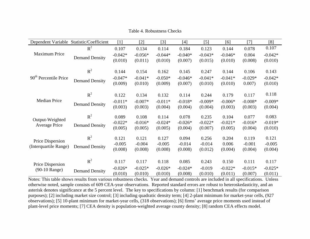
Table 4. Robustness Checks

Dependent Variable Statistic/Coefficient [1] [2] [3] [4] [5] [6] [7] [8] R2 0.107 0.134 0.114 0.184 0.123 0.144 0.078 0.107

Maximum Price Demand Density -0.042*

(0.010) -0.056* (0.011)

-0.044* (0.010)

-0.040* (0.007)

-0.043* (0.015)

-0.046* (0.010)

0.004 (0.008)

-0.042* (0.010)

R2 0.144 0.154 0.162 0.145 0.247 0.144 0.106 0.143

90th Percentile Price Demand Density -0.047* (0.009)

-0.041* (0.010)

-0.050* (0.009)

-0.046* (0.007)

-0.041* (0.010)

-0.041* (0.010)

-0.029* 0.007)

-0.042* (0.010)

R2 0.122 0.134 0.132 0.114 0.244 0.179 0.117 0.118

Median Price Demand Density -0.011*

(0.003) -0.007* (0.003)

-0.011* (0.004)

-0.018* (0.004)

-0.009* (0.004)

-0.006* (0.003)

-0.008* (0.003)

-0.009* (0.004)

R2 0.089 0.108 0.114 0.078 0.235 0.104 0.077 0.083 Output-Weighted

Average Price Demand Density -0.022* (0.005)

-0.016* (0.005)

-0.024* (0.005)

-0.026* (0.004)

-0.022* (0.007)

-0.021* (0.005)

-0.016* (0.004)

-0.019* (0.010)

R2 0.121 0.121 0.127 0.094 0.256 0.204 0.119 0.121 Price Dispersion

(Interquartile Range) Demand Density -0.005 (0.008)

-0.004 (0.008)

-0.005 (0.008)

-0.014 (0.008)

-0.014 (0.012)

0.006 (0.004)

-0.001 (0.004)

-0.005 (0.004)

R2 0.117 0.117 0.118 0.085 0.243 0.150 0.111 0.117 Price Dispersion

(90-10 Range) Demand Density -0.026* (0.010)

-0.025* (0.010)

-0.026* (0.010)

-0.024* (0.008)

-0.019 (0.010)

-0.022* (0.011)

-0.015* (0.007)

-0.025* (0.011)

Notes: This table shows results from various robustness checks. Year and demand controls are included in all specifications. Unless otherwise noted, sample consists of 609 CEA-year observations. Reported standard errors are robust to heteroskedasticity, and an asterisk denotes significance at the 5 percent level. The key to specifications by column: [1] benchmark results (for comparison purposes); [2] including market size control; [3] including quadratic density term; [4] 2-plant minimum for market-year cells, (927 observations); [5] 10-plant minimum for market-year cells, (318 observations); [6] firms’ average price moments used instead of plant-level price moments; [7] CEA density is population-weighted average county density; [8] random CEA effects model.

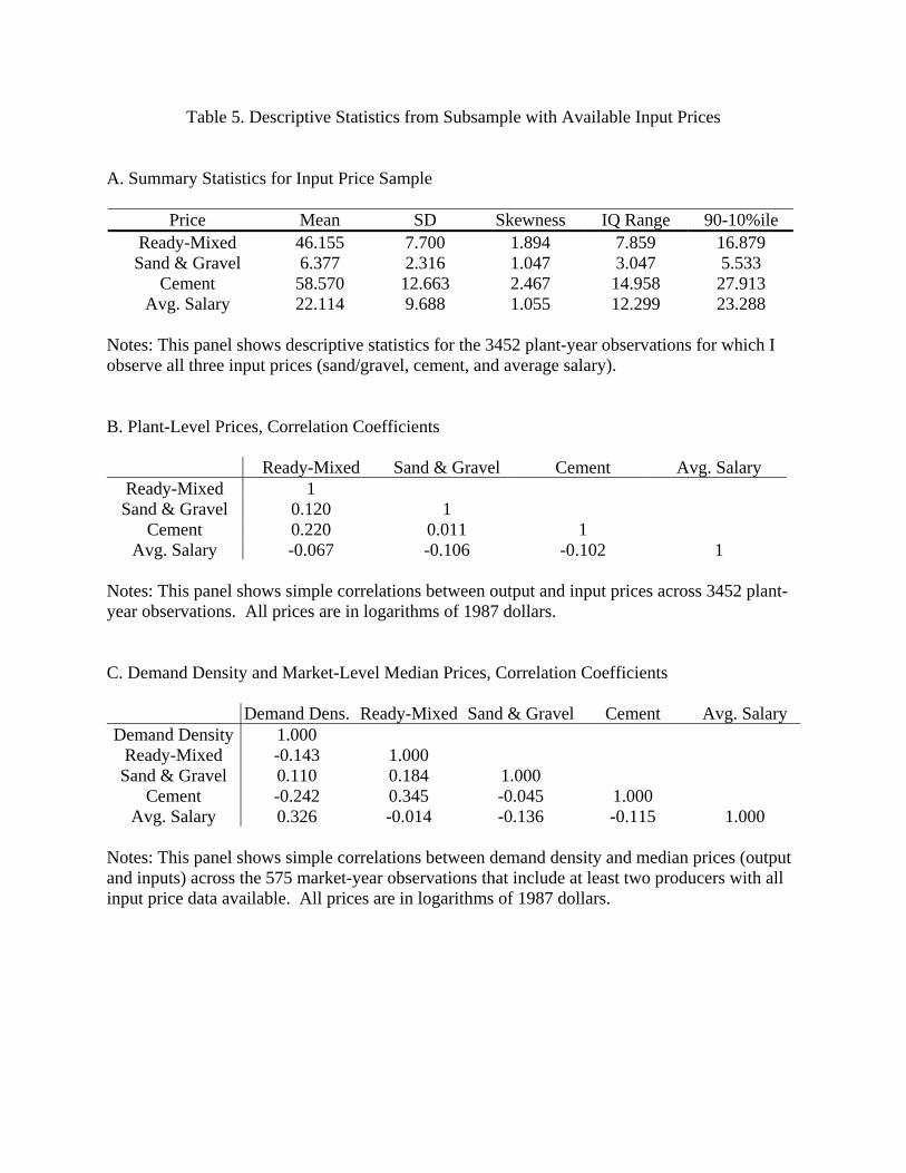
Table 5. Descriptive Statistics from Subsample with Available Input Prices A. Summary Statistics for Input Price Sample

Price Mean SD Skewness IQ Range 90-10%ile Ready-Mixed 46.155 7.700 1.894 7.859 16.879 Sand & Gravel 6.377 2.316 1.047 3.047 5.533

Cement 58.570 12.663 2.467 14.958 27.913 Avg. Salary 22.114 9.688 1.055 12.299 23.288

Notes: This panel shows descriptive statistics for the 3452 plant-year observations for which I observe all three input prices (sand/gravel, cement, and average salary). B. Plant-Level Prices, Correlation Coefficients

Ready-Mixed Sand & Gravel Cement Avg. Salary Ready-Mixed 1 Sand & Gravel 0.120 1

Cement 0.220 0.011 1 Avg. Salary -0.067 -0.106 -0.102 1

Notes: This panel shows simple correlations between output and input prices across 3452 plant-year observations. All prices are in logarithms of 1987 dollars. C. Demand Density and Market-Level Median Prices, Correlation Coefficients

Demand Dens. Ready-Mixed Sand & Gravel Cement Avg. Salary Demand Density 1.000

Ready-Mixed -0.143 1.000 Sand & Gravel 0.110 0.184 1.000

Cement -0.242 0.345 -0.045 1.000 Avg. Salary 0.326 -0.014 -0.136 -0.115 1.000

Notes: This panel shows simple correlations between demand density and median prices (output and inputs) across the 575 market-year observations that include at least two producers with all input price data available. All prices are in logarithms of 1987 dollars.

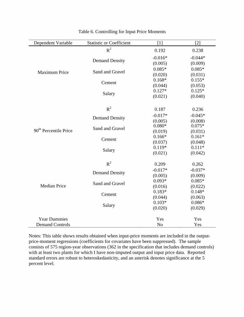
Table 6. Controlling for Input Price Moments

Dependent Variable Statistic or Coefficient [1] [2] R2 0.192 0.238

Demand Density -0.016* (0.005)

-0.044* (0.009)

Sand and Gravel 0.085* (0.020)

0.085* (0.031)

Cement 0.168* (0.044)

0.155* (0.053)

Maximum Price

Salary 0.127* (0.021)

0.125* (0.040)

R2 0.187 0.236


-0.045* (0.008)


0.075* (0.031)

Cement 0.166* (0.037)

0.161* (0.048)

90th Percentile Price

Salary 0.119* (0.021)

0.111* (0.042)

R2 0.209 0.262


-0.037* (0.009)


0.085* (0.022)

Cement 0.183* (0.044)

0.148* (0.063)

Median Price

Salary 0.103* (0.020)

0.086* (0.029)

Year Dummies Yes Yes

Demand Controls No Yes Notes: This table shows results obtained when input-price moments are included in the output-price-moment regressions (coefficients for covariates have been suppressed). The sample consists of 575 region-year observations (362 in the specification that includes demand controls) with at least two plants for which I have non-imputed output and input price data. Reported standard errors are robust to heteroskedasticity, and an asterisk denotes significance at the 5 percent level.

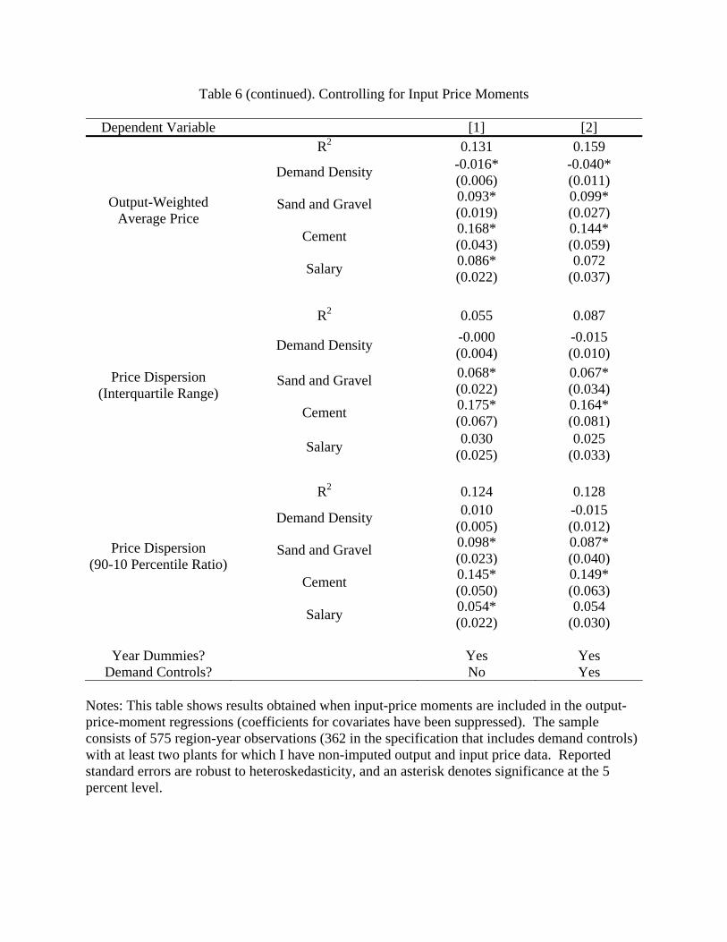
Table 6 (continued). Controlling for Input Price Moments

Dependent Variable [1] [2] R2 0.131 0.159


-0.040* (0.011)


0.099* (0.027)

Cement 0.168* (0.043)

0.144* (0.059)

Output-Weighted Average Price

Salary 0.086* (0.022)

0.072 (0.037)

R2 0.055 0.087

Demand Density -0.000 (0.004)

-0.015 (0.010)


0.067* (0.034)

Cement 0.175* (0.067)

0.164* (0.081)

Price Dispersion (Interquartile Range)

Salary 0.030 (0.025)

0.025 (0.033)

R2 0.124 0.128

Demand Density 0.010 (0.005)

-0.015 (0.012)


0.087* (0.040)

Cement 0.145* (0.050)

0.149* (0.063)

Price Dispersion (90-10 Percentile Ratio)

Salary 0.054* (0.022)

0.054 (0.030)

Year Dummies? Yes Yes

Demand Controls? No Yes Notes: This table shows results obtained when input-price moments are included in the output-price-moment regressions (coefficients for covariates have been suppressed). The sample consists of 575 region-year observations (362 in the specification that includes demand controls) with at least two plants for which I have non-imputed output and input price data. Reported standard errors are robust to heteroskedasticity, and an asterisk denotes significance at the 5 percent level.

prices, spatial competition, and heterogeneous producers...

Documents