pricing and hedging quanto options in energy markets · quanto option in terms of tradeable...

Pricing and Hedging Quanto Options in Energy Markets

Fred Espen Benth∗ Nina Lange† Tor Åge Myklebust‡

September 28, 2012

Abstract

In energy markets, the use of quanto options have increased significantly in the recent years.

The payoff from such options are typically triggered by an energy price and a measure of

temperature and are thus suited for managing both price and volume risk in energy markets.

Using an HJM approach we derive a closed form option pricing formula for energy quanto

options, under the assumption that the underlying assets are log-normally distributed. Our

approach encompasses several interesting cases, such as geometric Brownian motions and multi-

factor spot models. We also derive delta and cross-gamma hedging parameters. Furthermore,

we illustrate the use of our model by an empirical pricing exercise using NYMEX traded natural

gas futures and CME traded HDD temperature futures for New York and Chicago

∗Center of Mathematics for Applications, University of Oslo, PO Box 1053 Blindern, N-0316 Oslo, Norway. E-mail: [email protected], +47 2282 2559. Financial support from "Managing Weather Risk in Electricity Markets(MAWREM)" RENERGI/216096 funded by the Norwegian Research Council is gratefully acknowledged.†Department of Finance, Copenhagen Business School, Solbjerg Plads 3, DK-2000 Frederiksberg. E-mail:

[email protected], +45 3815 3615‡Department of Finance and Management Science, Norwegian School of Economics, Helleveien 30, N-5045 Bergen.

E-mail: [email protected].

1

1 Introduction

The market for standardized weather derivatives peaked in 2007 with a total volume of trades

at the Chicago Mercantile Exchange (CME) close to 930,000 and a corresponding notional value

of $17.9 billion1. Until recently these products have served as a tool for hedging volume risk

of energy commodities like gas or power. Warm winters and cold summers lead to a decline in

energy consumption as there is less need for heating respectively cooling. Cold winters and warm

summers lead to a higher demand for energy, e.g., gas or electricity. However, in the last couple

of years, this market has experienced severe retrenchment. In 2009, the total volume of trades

dipped below 500,000, amounting to a notional value of around $5.3 billion. A big part of this sharp

decline is attributed to the substantial increase in the market for tailor-made quantity-adjusting

weather contracts (quanto contracts). Quanto deals with a size of $100 million have been reported.

Market participants indicate that the demand for quanto-options are international with transactions

being executed in the US, Europe, Australia and South America. The Weather Risk Management

Association (WRMA) believes the developing market in India alone has a potential value of $2.35

billion in the next two or three years.

The label ’quanto options’ have traditionally been assigned to a class of derivatives in currency

markets used to hedge exposure to foreign currency risk. Although the same term is used for the

specific type of energy options that we study in this paper, these two types of derivatives contracts

are different. A typical currency quanto option have a regular call/put payoff structure, whereas

the energy quanto options we study have a payoff structure similar to a product of call/put options.

Pricing of currency quanto options have been extensively researched, and dates back to the original

work of ?. In comparison, research related to the pricing of quanto options in energy markets are

scarce. Pricing options in energy markets are generally different from pricing options in financial

markets since one has to take into account, e.g., different asset dynamics, non-tradeable underlyings

and less liquidity.

In energy markets, quanto options are mainly used to hedge exposure to both price and volume

risk. This is contrary to industries with fixed prices over the short term, where hedging volumetric

risks by using standardized weather derivatives is an appropriate hedging strategy. But when1The numbers reported in this paragraph are taken directly from the article "A new direction for weather deriva-

tives", published in the Energy Risk Magazine, June 2010.

2

earnings volatility is affected by more than one factor, the hedging problem quickly becomes more

complex. Take as an example a gas distribution company which operates in an open wholesale

market. Here it is possible to buy and sell within day or day ahead gas, and thus the company is

exposed to movements in the spot price of gas as well as to variable volumes of sales due to the

fluctuations in temperature. Their planned sales volumes per day and the price at which they are

able to sell to their customers form the axes about which their exposure revolves. If for example, one

of the winter months turn out to be warmer than usual, demand for gas would drop. This decline in

demand would probably also affect the market price for gas, leading to a drop in gas price. The firm

makes a loss against planned revenues equal to the short fall in demand multiplied by the difference

between the retail price at which they would have sold if their customers had bought the gas and the

market price where they must now sell their excess gas. The above example clearly illustrates that

the adverse movements in market price and demand due to higher temperatures represent a kind of

correlation risk which is difficult to properly hedge against. Using standard weather derivatives and,

e.g., futures contracts would most likely represent both an imperfect and rather expensive hedging

strategy.

In order for quanto contracts to provide a superior risk management tool compared to standard-

ized futures contracts, it is crucial that there is a significant correlation between the two underlying

assets. In energy markets, payoffs of a quanto option is triggered by movements in both energy

price and temperature (contracts). ? document that temperature is important to forecast electric-

ity prices and ? document at strong relationship between natural gas prices and heating degree

days (HDD).

The literature on energy quanto options is scarce. One exception is ? who propose a bivariate

time series model to capture the joint dynamics of energy prices and temperature. More specifically,

they model the energy price and the average temperature using a sophisticated parameter-intensive

econometric model. Since they aim to capture features like seasonality in means and variances, long

memory, auto-regressive patterns and dynamic correlations, the complexity of their model leaves no

other option than simulation based procedures to calculate prices. Moreover, they leave the issue

of how one should hedge such options unanswered.

We also study the pricing of energy quanto options, but unlike ? we derive analytical solutions

to the option pricing problem. Such closed form solutions are easy to implement, fast to calculate

3

and most importantly; they give a clear answer to how the energy quanto option should be properly

hedged. Our idea is to convert the pricing problem by using futures contracts as underlying assets,

rather than energy spot prices and temperature. We are able to do so since the typical energy

quanto options have a payoff which can be represented as an "Asian" structure on the energy spot

price and the temperature index. The markets for energy and weather organize futures with delivery

periods, which will coincide with the aggregate or average spot price and temperature index at the

end of the delivery period. Hence, any "Asian payoff" on the spot and temperature for a quanto

option can be viewed as a "European payoff" on the corresponding futures contracts. It is this

insight which is the key to our solution. This also gives the desirable feature that we can hedge the

quanto option in terms of tradeable instruments, namely the underlying futures contracts. Note

the contrast to viewing the energy quanto option as an "Asian-type" derivative on the energy spot

and temperature index (cf. ?). Temperature is not a tradeable asset, naturally, and in the case of

power the spot is not as well. Thus, the hedging problem seems challenging in this context.

Using an HJM approach, we derive options prices under the assumption that futures dynamics

are log-normally distributed with a possibly time-varying volatility. Furthermore, we explicitly

derive delta- and cross-gamma hedging parameters. Our approach encompasses several models

for the underlying futures prices, such as the standard bivariate geometric Brownian motion and

the two-factor model proposed by ?, and later extended by ? to include seasonality. The latter

model allows for time-varying volatility. We include an extensive empirical example to illustrate our

findings. Using futures contracts on natural gas and HDD temperature index, we estimate relevant

parameters in the seasonal two-factor model of ? based on data collected from the New York

Mercentile Exchange (NYMEX) and the Chicago Mercentile Exchange (CME). We compute prices

for various energy quanto options and benchmark these against products of plain-vanilla European

options on gas and HDD futures. The latter can be priced by the classical Black-76 formula (see

?), and corresponds to the case of the energy quanto option for independent gas and temperature

futures.

In section 2, we discuss the structure of energy quanto options as well as introduce the pricing

problem. In section 3, we derive the pricing and hedging formulas and show how the model of ?

related to the general pricing formula. In section 4, we present the empirical case study and section

5 concludes.

4

2 Energy Quanto Options

In this section we first present typical examples of energy quanto options. We then argue that the

pricing problem can be simplified using standardized futures contracts as the underlying assets.

2.1 Contract structure

Most energy quanto contracts have in common that payoffs are triggered by two underlying “assets”;

temperature and energy price. Since these contracts are tailormade rather than standardized, the

contract design varies. In its simplest form a quanto contract resembles a swap contract and has a

payoff function S that looks like

S = V olume× (TV ar − TFix)× (PV ar − PFix) (1)

Payoff is determined by the difference between some variable temperature measure (TV ar) and some

fixed temperature measure (TFix), multiplied by the difference between variable and fixed energy

price (PV ar and PFix). Note that the payoff might be negative, indicating that the buyer of the

contract pays the required amount to the seller.

Entering into a swap contract of this type might be risky since the downside may potentially

become large. For hedging purposes it seems more reasonable to buy a quanto structure with

optionality, i.e., so that you eliminate all downside risk. In Table 1 we show a typical example of

how a quanto option might be structured. The example contract has a payoff which is triggered by

an average gas price denoted E (defined as the average of daily prices for the last month), and it also

offers an exposure to temperature through the accumulated number of Heating Degree Days (HDD)

in the corresponding month (denoted H). The HDD index is commonly used as the underlying

variable in temperature derivatives and is defined as

τ2∑t=τ1

max(c− Tt, 0), (2)

where c is some prespecified temperature threshold (65◦F or 18◦C), and Tt is the mean temperature

on day t. If the number of HDDs H and the average gas price E is above the high strikes (KI

and KE respectively), the owner of the option would receive a payment equal to the prespecified

5

volume multiplied by the actual number of HDDs less the strike KI , multiplied by the difference

between the average energy price less the strike price KE (if E > KE). On the other hand, if it is

warmer than usual and the number of HDDs dips below the lower strike of KI and the energy price

at the same time is lower than KE , the owner receives a payout equal to the volume multiplied by

KI less the actual number of HDDs multiplied by the difference between the strike price KE and

the average energy price. Note that the volume adjustment is varying between months, reflecting

the fact that ’unusual’ temperature changes might have a stronger impact on the optionholder’s

revenue in the coldest months like December and January. Also note that the price strikes may vary

between months.

Nov Dec Jan Feb Mar

(a) High Strike (HDDs) K11I K

12I K

1I K

2I K

3I

(b) Low Strike (HDDs) K11I K12

I K1I K2

I K3I

(a) High Strike (Price/mmBtu) K11E K

12E K

1E K

2E K

3E

(b) Low Strike (Price/mmBtu) K11E K12

E K1E K2

E K3E

Volume (mmBtu) 200 300 500 400 250

Table 1: A specification of a typical energy quanto option. The underlying process triggering payouts tothe optionholder is accumulated number of heating-degree days H and monthly index gas price E.As an example the payoff for November will be: (a) In cold periods - max(H −KI , 0)×max(E −KE , 0)× Volume. (b) In warm periods - max(KI−H, 0)×max(KE−E, 0)× Volume. We see thatthe option pays out if both the underlying temperature and price variables exceed (dip below) thehigh strikes (low strikes).

This example illustrates why quanto options might be a good alternative to more standardized

derivatives. The structure in the contracts takes into account the fact that extreme temperature

variations might affect both demand and prices, and compensates the owner of the option by

making payouts contingent on both prices and temperatures. The great possibility of tailoring

these contracts provides the potential customers with a powerful and efficient hedging instrument.

2.2 Pricing Using Terminal Value of Futures

As described above energy quanto options have a payoff which is a function of two underlying assets;

temperature and price. We focus on a class of energy quanto options which has a payoff function

6

f(E, I), where E is an index of the energy price and I an index of temperature. To be more specific,

we assume that the energy index E is given as the average spot price over some measurement period

[τ1, τ2], τ1 < τ2,

E =1

τ2 − τ1

τ2∑u=τ1

Su ,

where Su denotes the spot price of the energy. Furthermore, we assume that the temperature index

is defined as

I =

τ2∑u=τ1

g(Tu) ,

for Tu being the temperature at time u and g some function. For example, if we want to consider

a quanto option involving the HDD index, we choose g(x) = max(x − 18, 0). The quanto option

is exercised at time τ2, and its arbitrage-free price Ct at time t ≤ τ2 is defined as by the following

expression:

Ct = e−r(τ2−t)EQt

[f

(1

τ2 − τ1

τ2∑u=τ1

Su,

τ2∑u=τ1

g(Tu)

)]. (3)

Here, r > 0 denotes the risk-free interest rate, which we for simplicity assumes constant. The

pricing measure is denoted Q, and EQt [·] is the expectation operator with respect to Q, conditioned

on the market information at time t given by the filtration Ft.

We now argue how to relate the price of the quanto option to futures contracts on the energy

and temperature indices E and I. Observe that the price at time t ≤ τ2 of a futures contract written

on some energy price, e.g, natural gas, with delivery period [τ1, τ2] is given by

FEt (τ1, τ2) = EQt

[1

τ2 − τ1

τ2∑u=τ1

Su

].

At time t = τ2, we find from the conditional expectation that

FEτ2 (τ1, τ2) =1

τ2 − τ1

τ2∑u=τ1

Su ,

i.e., the futures price is exactly equal to what is being delivered. Applying the same argument to a

futures written on the temperature index, with price dynamics denoted F It (τ1, τ2), we immediately

7

see that the following must be true for the quanto option price:


[f

(1

τ2 − τ1

τ2∑u=τ1

Su,

τ2∑u=τ1

g(Tu)

)]

= e−r(τ2−t)EQt

[f(FEτ2(τ1, τ2), F Iτ2(τ1, τ2)

)]. (4)

Equation (4) shows that the price of a quanto option with payoff being a function of the energy

index E and temperature index I must be the same as if the payoff was a function of the terminal

values of two futures contracts written on the energy and temperature indices, and with the delivery

period being equal to the contract period specified by the quanto option. Hence, we view the quanto

option as an option written on the two futures contracts rather than on the two indices. This is

advantageous from the point of view that the futures are traded financial assets. We note in passing

that we may extend the above argument to quanto options where the measurement periods of the

energy and the temperature indices are not the same.

To compute the price in (4) we must have a model for the futures price dynamics FEt (τ1, τ2)

and F It (τ1, τ2). The dynamics must account for the dependency between the two futures, as well as

their marginal behavior. The pricing of the energy quanto option has thus been transferred from

modeling the joint spot energy and temperature dynamics followed by computing the Q-expectation

of an index of these, to modeling the joint futures dynamics and pricing a European-type option on

these. The former approach is similar to pricing an Asian option, which for most relevant models

and cases is a highly difficult task. Remark also that by modeling and estimating the futures

dynamics to market data, we can easily obtain the market-implied pricing measure Q. We will see

this in practice in Section 4 where we analyze the case of gas and HDD futures. If one chooses to

model the underlying energy spot prices and temperature dynamics, one obtains a dynamics under

the market probability P, and not under the pricing measure Q. Additional hypotheses must be

made in the model to obtain this. Moreover, for most interesting cases the quanto option must be

priced by Monte Carlo or some other computationally demanding method (see ?). Finally, but not

less importantly, with the representation in (4) at hand one can discuss the issue of hedging energy

quanto options in terms of the underlying futures contracts.

In many energy markets, the futures contracts are not traded within their delivery period. That

means that we can only use the market for futures up to time τ1. This has a clear consequence

8

on the possibility to hedge these contracts, as a hedging strategy inevitably will be a continuously

rebalanced portfolio of the futures up to the exercise time τ2. As this is possible to perform only

up to time τ1 in many markets, we face an incomplete market situation where the quanto option

cannot be hedged perfectly. Moreover, it is to be expected that the dynamics of the futures price

have different characteristics within the delivery period than prior to start of delivery, if it can

be traded for times t ∈ (τ1, τ2]. The reason being that we have less uncertainty as the remaining

delivery period of the futures become shorter. The entry time of such a contract is most naturally

taking place prior to delivery period. However, for marking-to-market purposes, one is interested

in the price Ct also for t ∈ (τ1, τ2]. The issuer of the quanto option may be interested in hedging

the exposure, and therefore also be concerned of the behavior of prices within the delivery period.

Before we start looking into the details of pricing quanto options we investigate the option

contract of the type described in section 2.1 in more detail. This contract covers a period of 5 months,

from November through March. Since this contract essentially is a sum of one-period contracts we

focus our attention on such, i.e., an option covering only one month of delivery period [τ1, τ2]. Recall

that the payoff in the contract is a function of some average energy price and accumulated number

of HDDs. From the discussion in the previous section we know that rather than using spot price

and HDD as underlying assets, we can instead use the terminal value of futures contracts written

on price and HDD, respectively. The payoff function p(FEτ2(τ1, τ2), F Iτ2(τ1, τ2),KE ,KI ,KE ,KI) = p

of this quanto contract is defined as

p = γ ×[max

(FEτ2(τ1, τ2)−KE , 0

)×max

(F Iτ2(τ1, τ2)−KI , 0

)+ max

(KE − FEτ2(τ1, τ2), 0

)×max

(KI − F Iτ2(τ1, τ2), 0

)], (5)

where γ is the contractual volume adjustment factor. Note that the payoff function in this contract

consists of two parts, the first taking care of the situation where temperatures are colder than usual

(and prices higher than usual), and the second taking care of the situation where temperatures are

warmer than usual (and prices lower than usual). The first part is a product of two call options,

whereas the second part is a product of two put options. To illustrate our pricing approach in the

simplest possible way it suffices to look at the product call structure with the volume adjuster γ

9

normalized to 1, i.e., we want to price an option with the following payoff function:

p̂(FEτ2(τ1, τ2), F Iτ2(τ1, τ2),KE ,KI

)= max

(FEτ2(τ1, τ2)−KE , 0

)×max

(F Iτ2(τ1, τ2)−KI , 0

). (6)

In the remaining part of this paper we will focus on this particular choice of a payoff function for

the energy quanto option. It corresponds to choosing the function f as f(E, I) = max(E−KE , 0)×

max(I −KI , 0) in (4). Other combinations of put-call mixes as well as different delivery periods for

the energy and temperature futures can easily be studied by a simple modification of what comes.

3 Pricing and hedging an energy quanto option

Suppose that the two futures price dynamics under the pricing measure Q can be expressed as

FET (τ1, τ2) = FEt (τ1, τ2) exp(µE +X) (7)

F IT (τ1, τ2) = F It (τ1, τ2) exp(µI + Y ) (8)

where t ≤ T ≤ τ2, and X, Y are two random variables independent of Ft, but depending on t, T ,

τ1 and τ2. We suppose that (X,Y ) is a bivariate normally distributed random variable with mean

zero, with covariance structure depending on t, T and τ2. We denote σ2X = V ar(X), σ2

Y = V ar(Y )

and ρX,Y = corr(X,Y ). Obviously, σX , σY and ρX,Y are depending on t, T, τ1 and τ2. Moreover,

as the futures price naturally is a martingale under the pricing measure Q, we have µE = −σ2X/2

and µI = −σ2Y /2.

Our general representation of the futures price dynamics (7) and (8) encompasses many inter-

esting models. For example, a bivariate geometric Brownian motion looks like

FET (τ1, τ2) = FEt (τ1, τ2) exp

(−1

2σ2E(T − t) + σE(WT −Wt)

)F IT (τ1, τ2) = F It (τ1, τ2) exp

(−1

2σ2I (T − t) + σI(BT −Bt)

)

with two Brownian motions W and B being correlated. We can easily associate this GBM to

the general set-up above by setting µE = −σ2E(T − t)/2, µI = −σ2

I (T − t)/2, σX = σE√T − t,

σY = σI√T − t, and ρX,Y being the correlation between the two Brownian motions. In section 3.3

10

we show that also the two-factor model by ? and the later extension of ? fits this framework.

3.1 A General Solution

The price of the quanto option at time t is


[p̂(FEτ2(τ1, τ2), F Iτ2(τ1, τ2),KE ,KI

)], (9)

where the notation EQ states that the expectation is taken under the pricing measure Q. Given

these assumptions Proposition 1 below states the closed-form solution of the energy quanto option.

Proposition 1. For two assets following the dynamics given by (7) and (8), the time t market price

of an European energy quanto option with exercise at time τ2 and payoff described by (6) is given

by

Ct = e−r(τ2−t)(FEt (τ1, τ2)F It (τ1, τ2)eρX,Y σXσYM(y∗∗∗1 , y∗∗∗2 ; ρX,Y )− FEt (τ1, τ2)KIM (y∗∗1 , y

∗∗2 ; ρX,Y )

− F It (τ1, τ2)KEM (y∗1, y∗2; ρX,Y ) +KEKIM (y1, y2; ρX,Y )

)

where

y1 =log(FEt (τ1, τ2))− log(KE)− 1

2σ2X

σX, y2 =

log(F It (τ1, τ2))− log(KI)− 12σ

2Y

σY,

y∗1 = y1 + ρX,Y σY , y∗2 = y2 + σY ,

y∗∗1 = y1 + σX , y∗∗2 = y2 + ρX,Y σX ,

y∗∗∗1 = y1 + ρX,Y σY + σX , y∗∗∗2 = y2 + ρX,Y σX + σY .

Here M(x, y; ρ) denotes the standard bivariate normal cumulative distribution function with corre-

lation ρ.

11

Proof. Observe that the payoff function in (6) can be rewritten in the following way:

p̂(FE , F I ,KE ,KI) = max(FE −KE , 0) ·max(F I −KI , 0)

=(FE −KE

)·(F I −KI

)· 1{FE>KE} · 1{F I>KI}

= FEF I · 1{FE>KE} · 1{F I>KI} − FEKI · 1{FE>KE} · 1{F I>KI}

− F IKE · 1{FE>KE} · 1{F I>KI} +KEKI · 1{FE>KE} · 1{F I>KI}.

The problem of finding the market price of the European quanto option is thus equivalent to the

problem of calculating the expectations under the pricing measure Q of the four terms above. The

four expectations are derived in Appendix C in details.

3.2 Hedging

Based on the formula given in Proposition 1 we derive the delta and cross-gamma hedging pa-

rameters, which are straightforwardly calculated from partial differentiation of the price Ct with

respect to the futures prices. All hedging parameters are given by the current futures price of the

two underlying contracts and are therefore simple to implement in practice. The delta hedge with

respect to the energy futures is given by

∂Ct

∂FEt (τ1, τ2)= F It (τ1, τ2)e−r(τ2−t)+ρX,Y σXσY

(M (y∗∗∗1 , y∗∗∗2 ; ρX,Y ) +B(y∗∗∗1 )N(y∗∗∗2 − ρX,Y )

1

σX

)−KIe

−r(τ2−t)(M (y∗∗1 , y

∗∗2 ; ρX,Y ) +B(y∗∗1 )N(y∗∗2 − ρX,Y )

1

σX

)− F It (τ1, τ2)KE

FEt (τ1, τ2)σXe−r(τ2−t)B(y∗1)N(y∗2 − ρX,Y )

+KEKI

FEt (τ1, τ2)σXe−r(τ2−t)B(y1)N(y2 − ρX,Y ) , (10)

where N(·) denotes the standard normal cumulative distribution function, and

B(x) =e(x

2−ρ2X,Y )

4π2(

1− ρ2X,Y

) .The delta hedge with respect to the temperature index futures is of course analogous to the energy

delta hedge, only with the substitutions FEt (τ1, τ2) = F It (τ1, τ2), y∗∗∗1 = y∗∗∗2 , y∗∗1 = y∗∗2 , y∗1 = y∗2,

12

y1 = y2, σY = σX and σX = σY . The cross-gamma hedge is given by

∂C2t

∂FEt (τ1, τ2)∂F It (τ1, τ2)

= e−r(τ2−t)+ρX,Y σXσY(M (y∗∗∗1 , y∗∗∗2 ; ρX,Y ) +B(y∗∗∗2 )N(y∗∗∗1 − ρX,Y )

1

σY

)+ e−r(τ2−t)+ρX,Y σXσY B(y∗∗∗1 )

(N(y∗∗∗2 − ρX,Y )

1

σX+ n(y∗∗∗2 − ρX,Y )

1

σY

)− KI

F It (τ1, τ2)σYe−r(τ2−t)

(B(y∗∗2 )N(y∗∗1 − ρX,Y ) +B(y∗∗1 )n(y∗∗2 − ρX,Y )

1

σX

)− KE

FEt (τ1, τ2)σXe−r(τ2−t)B(y∗1)

(N(y∗2 − ρX,Y ) + n(y∗2 − ρX,Y )

1

σY

)+

KEKI

FEt (τ1, τ2)F It (τ1, τ2)(σX + σY )e−r(τ2−t)B(y1)n(y2 − ρX,Y ) , (11)

where n(·) denotes the standard normal probability density function. In our model it is possible to

hedge the quanto option perfectly, with positions described above by the three delta and gamma

parameters. In practice, however, this would be difficult due to low liquidity in for example the

temperature market. Furthermore, as discussed in Section 2.2, we cannot in all markets trade

futures within the delivery period, putting additional restrictions on the suitability of the hedge. In

such cases, the parameters above will guide in a partial hedging of the option.

3.3 Two-dimensional Schwartz-Smith Model with Seasonality

The popular commodity price model proposed by ? is a natural starting point for deriving dynamics

of energy futures. In this model the log-spot price is the sum of two processes, one representing

the long term dynamics of the commodity prices in form of an arithmetic Brownian motion and

one representing the short term deviations from the long run dynamics in the form of an Ornstein-

Uhlenbeck process with a mean reversion level of zero. As we have mentioned already, ? extends

the model of ? to include seasonality. The dynamics under P is given by

logSt = Λ(t) +Xt + Zt ,

dXt =

(µ− 1

2σ2

)dt+ σdW̃t ,

dZt = −κZtdt+ νdB̃t .

13

Here B̃ and W̃ are correlated Brownian motions and µ, σ, κ and η are constants. The deterministic

function Λ(t) describes the seasonality of the log-spot prices. In order to price a futures contract

written on an underlying asset with the above dynamics, a measure change from P to an equaivalent

probability Q is made:

dXt =

(α− 1

2σ2

)dt+ σdWt

dZt = − (λZ + κZt) dt+ νdBit.

Here, α = µ − λX , and λX and λZ are constant market prices of risk associated with Xt and Zt

for asset i, respectively. This correponds to a Girsanov transform of B̃ and W̃ by a constant drift

so that B and W become two correlated Q-Brownian motions. As is well-known for the Girsanov

transform, the correlation between B and W is the same under Q as the one for B̃ and W̃ under

P (see ?). As it follows from ?, the futures price Ft(τ) at time t ≥ 0 of a contract with delivery

at time τ ≥ t has the following form on log-scale (note that it is the Schwartz-Smith futures prices

scaled by a seasonality function):

logFt(τ) = Λ(τ) +A(τ − t) +Xt + Zte−κ(τ−t) , (12)

where A(τ) = ατ − λZ−ρσνκ (1− e−κτ ) + ν2

4κ

(1− e−2κτ

). The futures prices are affine in the two

factors X and Z driving the spot price and scaled by functions of time to delivery τ − t. ? chooses

to parametrize the seasonality function Λ by a linear combination of cosine and sine functions:

Λ(t) =

K∑k=1

(γk cos(2πkt) + γ∗k sin(2πkt)) (13)

However, other choices may of course be made to match price observations in the market in question.

In this paper we have promoted the fact that the payoff of energy quanto options can be expressed

in terms of the futures prices of energy and temperature index. One may use the above procedure

to derive futures price dynamics from a model of the spot. However, one may also state directly

a futures price dynamics in the fashion of Heath-Jarrow-Morton (HJM). The HJM approach has

been proposed to model energy futures by ?, and later investigated in detail by ? (see also ? and

?). We follow this approach here, proposing a joint model for the energy and temperature index

14

futures price based on the above seasonal Schwartz-Smith model.

In stating such a model, we must account for the fact that the futures in question are delivering

over a period [τ1, τ2], and not at a fixed delivery time τ . There are many ways to overcome this

obstacle. For example, as suggested by ?, one can model Ft(τ) and define the futures price Ft(τ1, τ2)

of a contract with delivery over [τ1, τ2] as

Ft(τ1, τ2) =

τ2∑u=τ1

Ft(u) .

If the futures price Ft(τ1, τ2) refers to the average of the spot, we naturally divide by the number of

times delivery takes place in the relation above. In the case of exponential models, as we consider,

this leads to expressions which are not analytically tractable. Another, more attractive alternative, is

to let Ft(τ1, τ2) itself follow a dynamics of the form (12) with some appropriately chosen dependency

on τ1 and τ2. For example, we may choose τ = τ1 in (12), or τ = (τ1+τ2)/2, or any other time within

the delivery period [τ1, τ2]. In this way, we will account for the delivery time-effect in the futures

price dynamics, sometimes referred to as the Samuelson effect. We remark that it is well-known

that for futures delivering over a period, the volatility will not converge to that of the underlying

spot as time to delivery goes to zero (see ?). By the above choices, we obtain namely that effect.

Note that the futures price dynamics will not be defined for times t after the "delivery" τ . Hence,

if we choose τ = τ1, we will only have a futures price lasting up to time t ≤ τ1, and left undefined

thereafter.

In order to jointly model the energy and temperature futures price, two futures dynamics of the

type in (12) are connected by allowing the Brownian motions to be correlated across assets. We

will have four Brownian motions WE , BE ,W I and BI in our two-asset two-factor model. These are

assumed correlated as follows: ρE = corr(WE1 , B

E1 ), ρI = corr(W I

1 , BI1), ρW = corr(WE

1 ,WI1 ) and

ρB = corr(BE1 , B

I1). Moreover, we have cross-correlations given by

ρW,BI,E = corr(W I1 , B

E1 ) ,

ρW,BE,I = corr(WE1 , B

I1) .

We refer to Appendix A for an explicit construction of four such correlated Brownian motions from

four independent ones. In a HJM-style, we assume that the joint dynamics of the futures price

15

processes FEt (τ1, τ2) and F It (τ1, τ2) under Q is given by

dF it (τ1, τ2)

F it (τ1, τ2)= σidW

it + ηi(t)dB

it , (14)

for i = E, I and with

ηi(t) = νie−κi(τ2−t) . (15)

Note that we suppose that the futures price is a martingale with respect to the pricing measure Q,

which is natural from the point of view that we want an arbitrage-free model. Moreover, we have

made the explicit choice here that τ = τ2 in (12) when modelling the delivery time effect.

Note that

d logF it (τ1, τ2) = −1

2

(σ2i + ηi(t)

2 + 2ρiσiηi(t))dt+ σidW̃

it + ηi(t)dB̃

it

for i = E, I. Hence, we can make the representation FET (τ1, τ2) = FEt (τ1, τ2) exp (−µE +X) by

choosing

X ∼ N

0,

∫ T

t

(σ2E + ηE(s)2 + 2ρEσEηE(s)

)ds︸︷︷︸

σ2X

, µE = −1

2σ2X

and similar for F IT (τ1, τ2). These integrals can be computed analytically in the above model, where

ηi(t) = νie−κi(τ2−t). We can also compute the correlation ρX,Y analytically, since ρX,Y = cov(X,Y )

σXσY

and

cov(X,Y ) = ρW

∫ T

tσEσIds+ ρW,BE,I

∫ T

tσEηI(s)ds+ ρW,BI,E

∫ T

tηE(s)σIds+ ρB

∫ T

tηE(s)ηI(s)ds .

A closed-form expression of this covariance can be computed. In the special case of zero cross-

correlations this simplifies to

cov(X,Y ) = ρW

∫ T

tσEσIds+ ρB

∫ T

tηE(s)ηI(s)ds

The exact expressions for σX , σY and cov(X,Y ) in the two-dimensional Schwartz-Smith model with

16

seasonality are presented in Appendix D.

This bivariate futures price model has a form that can be immediately used for pricing energy

quanto options by inferring the result in Proposition 1. We shall come back to this model in the

empirical case study in Section 4. We note that our pricing approach only looks at futures dynamics

up to the start of the delivery period τ1. As briefly discussed in Section 2.2 it is reasonable to expect

that the dynamics of a futures contract should be different within the delivery period [τ1, τ2]. For

times t within [τ1, τ2] we will in the case of the energy futures have

Ft(τ1, τ2) =1

τ2 − τ1

t∑u=τ1

Su + EQt

[1

τ2 − τ1

τ2∑u=t+1

Su

].

Thus, the futures price must consist of two parts, the first simply the tracked observed energy spot

up to time t, and next the current futures price of a contract with delivery period [t, τ2]. This latter

part will have a volatility that must go to zero as t tends to τ2.

4 Empirical Analysis

In this section, we present an empirical study of energy quanto options written on natural gas and

HDD temperature index. We present the futures price data which consitute the basis of our analysis,

and next estimate the parameters in the joint futures price model (14). We then discuss the impact

of correlation on the valuation of the option to be priced.

4.1 Data

A futures contract on Heating Degree Days are traded on CME for several cities for the months

October, November, December, January, February, March, and April a couple of years out. The

contract value is 20$ for each HDD throughout the month and it trades until the beginning of

the concurrent month. The underlying is one month of accumulated HDD’s for a specific location.

The futures price is denoted by F It (τ1, τ2) and settled on the index∑τ2

u=τ1HDDu. We observe the

futures prices for seven specific combinations of [τ1, τ2]’s per year. We let the futures price follow a

price process of the type (12) discussed in the previous Subsection.

For liquidity reasons, we do not include all data. Liquidity is limited after the first year, so for

every day we choose the first seven contracts, where the index period haven’t started yet. I.e., for

17

January 2nd, 2007, we use the February 2007, March 2007, April 2007, October 2007, November

2007, December 2007 and January 2008 contracts. The choice of the seasonality function Λ is copied

from ?, i.e., K = 1 in equation 13, that is, a sum of a sine and cosine function with yearly frequency.

The chosen locations are New York and Chicago, since these are located in an area with fairly

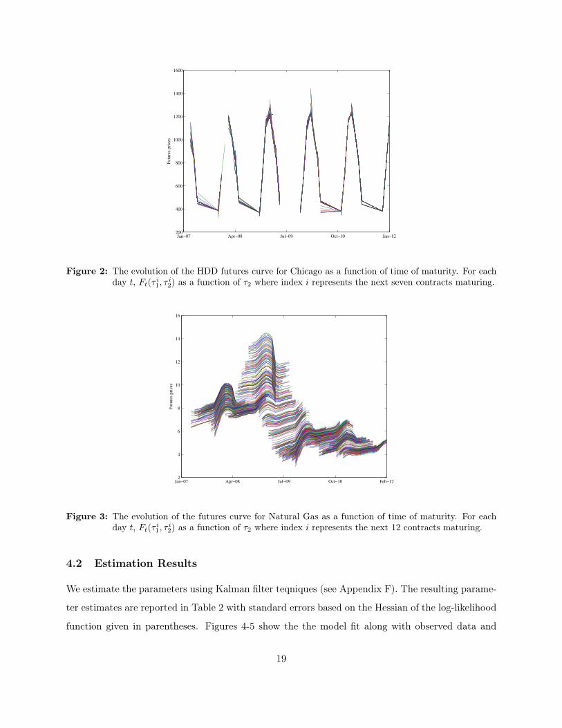
large gas consumption. The development in the futures curves are shown in Figures 1 and 2.

Futures contracts for delivery of gas is traded on NYMEX for each month ten years out. The

underlying is delivery of gas throughout a month and the price is per unit. The contract trades

until a couple of days before the delivery month. Many contracts are closed prior to the last trading

day, we choose the first 12 contracts for delivery at least one month later. I.e., for January 2nd,

we use March 2007 to February 2008 contracts. The choice of Λ is also in this case borrowed from

?, where we for this case choose K = 2 in equation 13. The evolution of the futures gas curves is

shown in Figure 3.

Jan−07 Apr−08 Jul−09 Oct−10 Jan−120

200

400

600

800

1000

1200

Futu

res

pri

ces

Figure 1: The evolution of the HDD futures curve for New York as a function of time of maturity. For eachday t, Ft(τ

i1, τ

i2) as a function of τ2 where index i represents the next seven contracts maturing.

18

Jan−07 Apr−08 Jul−09 Oct−10 Jan−12200

400

600

800

1000

1200

1400

1600

Futu

res

pri

ces

Figure 2: The evolution of the HDD futures curve for Chicago as a function of time of maturity. For eachday t, Ft(τ

i1, τ

i2) as a function of τ2 where index i represents the next seven contracts maturing.

Jan−07 Apr−08 Jul−09 Oct−10 Feb−122

4

6

8

10

12

14

16

Futu

res

pri

ces

Figure 3: The evolution of the futures curve for Natural Gas as a function of time of maturity. For eachday t, Ft(τ

i1, τ

i2) as a function of τ2 where index i represents the next 12 contracts maturing.

4.2 Estimation Results

We estimate the parameters using Kalman filter teqniques (see Appendix F). The resulting parame-

ter estimates are reported in Table 2 with standard errors based on the Hessian of the log-likelihood

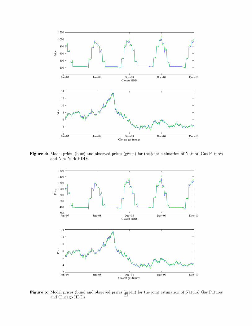
function given in parentheses. Figures 4-5 show the the model fit along with observed data and

19

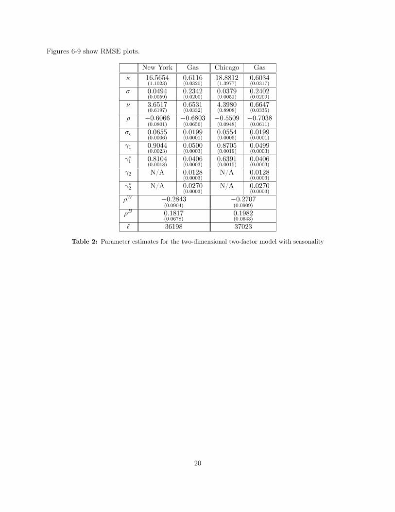
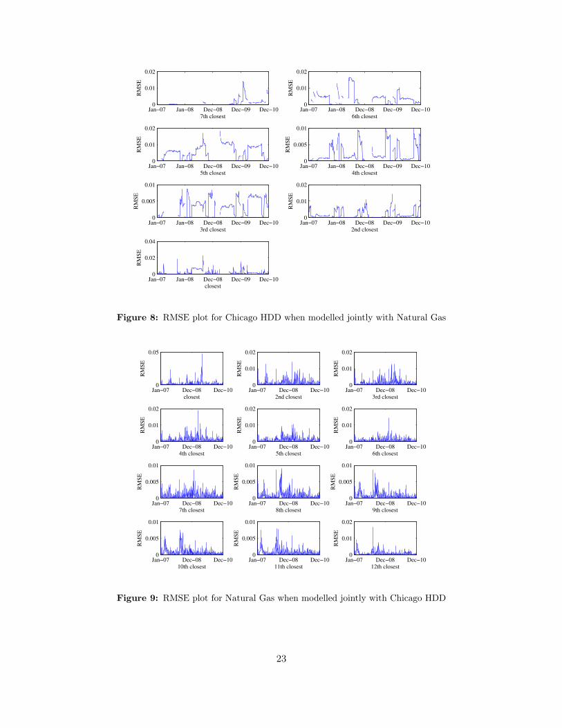
Figures 6-9 show RMSE plots.

New York Gas Chicago Gasκ 16.5654

(1.1023)0.6116(0.0320)

18.8812(1.3977)

0.6034(0.0317)

σ 0.0494(0.0059)

0.2342(0.0200)

0.0379(0.0051)

0.2402(0.0209)

ν 3.6517(0.6197)

0.6531(0.0332)

4.3980(0.8908)

0.6647(0.0335)

ρ −0.6066(0.0801)

−0.6803(0.0656)

−0.5509(0.0948)

−0.7038(0.0611)

σε 0.0655(0.0006)

0.0199(0.0001)

0.0554(0.0005)

0.0199(0.0001)

γ1 0.9044(0.0023)

0.0500(0.0003)

0.8705(0.0019)

0.0499(0.0003)

γ∗1 0.8104(0.0018)

0.0406(0.0003)

0.6391(0.0015)

0.0406(0.0003)

γ2 N/A 0.0128(0.0003)

N/A 0.0128(0.0003)

γ∗2 N/A 0.0270(0.0003)

N/A 0.0270(0.0003)

ρW −0.2843(0.0904)

−0.2707(0.0909)

ρB 0.1817(0.0678)

0.1982(0.0643)

` 36198 37023

Table 2: Parameter estimates for the two-dimensional two-factor model with seasonality

20

Jan−07 Jan−08 Dec−08 Dec−09 Dec−100

200

400

600

800

1000

1200

Closest HDD

Pri

ce


4

6

8

10

12

14

Closest gas futures

Pri

ce

Figure 4: Model prices (blue) and observed prices (green) for the joint estimation of Natural Gas Futuresand New York HDDs


400

600

800

1000

1200

1400

1600

Closest HDD

Pri

ce


4

6

8

10

12

14

Closest gas futures

Pri

ce

Figure 5: Model prices (blue) and observed prices (green) for the joint estimation of Natural Gas Futuresand Chicago HDDs 21


0.02

0.04

7th closest

RM

SE


0.05

6th closest

RM

SE


0.05

5th closest

RM

SE


0.02

0.04

4th closest

RM

SE


0.05

0.1

3rd closest

RM

SE


0.02

0.04

2nd closest

RM

SE


0.02

0.04

closest

RM

SE

Figure 6: RMSE plot for New York HDD when modelled jointly with Natural Gas

Jan−07 Dec−08 Dec−100

0.05

closest

RM

SE


0.01

0.02

2nd closest

RM

SE


0.01

0.02

3rd closest

RM

SE


0.01

0.02

4th closest

RM

SE


0.01

0.02

5th closest

RM

SE


0.01

0.02

6th closest

RM

SE


0.005

0.01

7th closest

RM

SE


0.005

0.01

8th closest

RM

SE


0.005

0.01

9th closest

RM

SE


0.005

0.01

10th closest

RM

SE


0.005

0.01

11th closest

RM

SE


0.01

0.02

12th closest

RM

SE

Figure 7: RMSE plot for Natural Gas when modelled jointly with New York HDD

22


0.01

0.02

7th closest

RM

SE


0.01

0.02

6th closest

RM

SE


0.01

0.02

5th closest

RM

SE


0.005

0.01

4th closest

RM

SE


0.005

0.01

3rd closest

RM

SE


0.01

0.02

2nd closest

RM

SE


0.02

0.04

closest

RM

SE

Figure 8: RMSE plot for Chicago HDD when modelled jointly with Natural Gas


0.05

closest

RM

SE


0.01

0.02

2nd closest

RM

SE


0.01

0.02

3rd closest

RM

SE


0.01

0.02

4th closest

RM

SE


0.01

0.02

5th closest

RM

SE


0.01

0.02

6th closest

RM

SE


0.005

0.01

7th closest

RM

SE


0.005

0.01

8th closest

RM

SE


0.005

0.01

9th closest

RM

SE


0.005

0.01

10th closest

RM

SE


0.005

0.01

11th closest

RM

SE


0.01

0.02

12th closest

RM

SE

Figure 9: RMSE plot for Natural Gas when modelled jointly with Chicago HDD

23

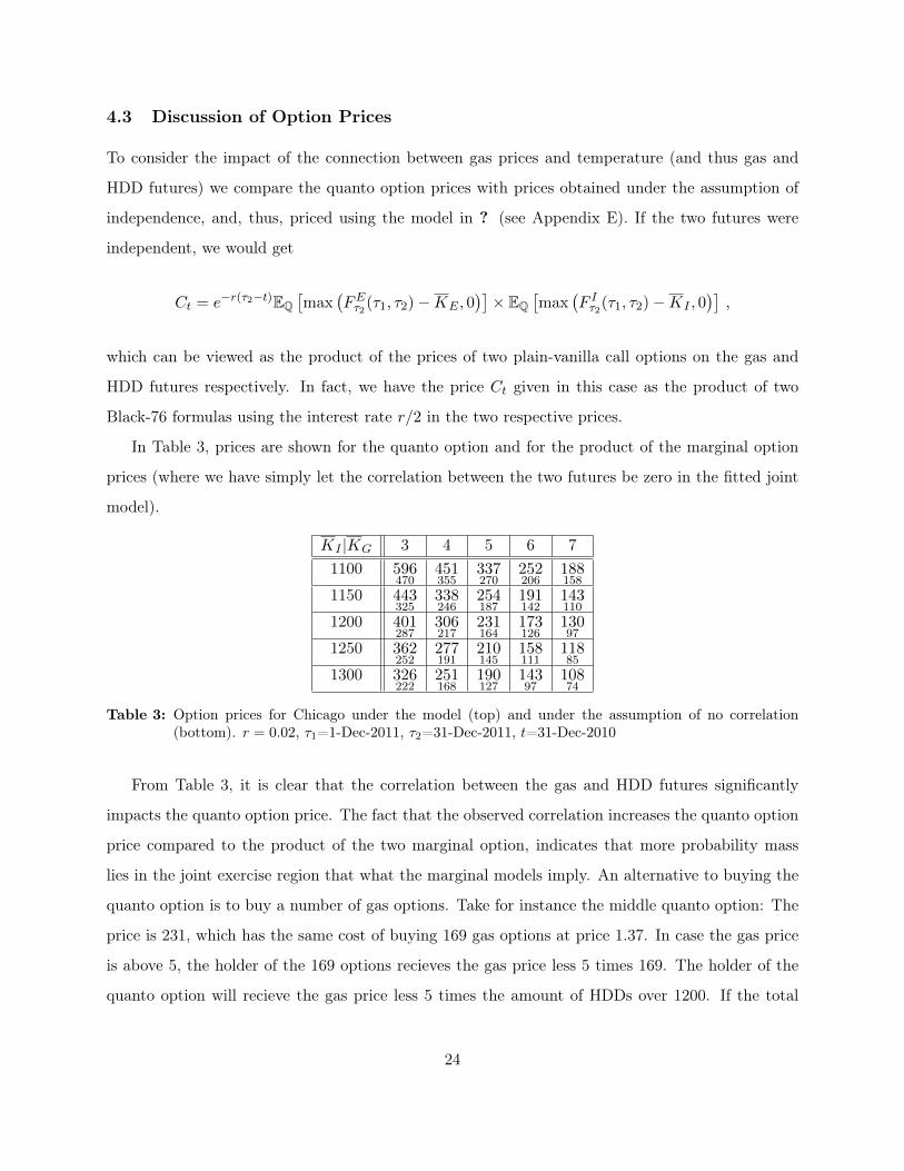
4.3 Discussion of Option Prices

To consider the impact of the connection between gas prices and temperature (and thus gas and

HDD futures) we compare the quanto option prices with prices obtained under the assumption of

independence, and, thus, priced using the model in ? (see Appendix E). If the two futures were

independent, we would get

Ct = e−r(τ2−t)EQ[max

(FEτ2(τ1, τ2)−KE , 0

)]× EQ

[max

(F Iτ2(τ1, τ2)−KI , 0

)],

which can be viewed as the product of the prices of two plain-vanilla call options on the gas and

HDD futures respectively. In fact, we have the price Ct given in this case as the product of two

Black-76 formulas using the interest rate r/2 in the two respective prices.

In Table 3, prices are shown for the quanto option and for the product of the marginal option

prices (where we have simply let the correlation between the two futures be zero in the fitted joint

model).

KI |KG 3 4 5 6 71100 596

470451355

337270

252206

188158

1150 443325

338246

254187

191142

143110

1200 401287

306217

231164

173126

13097

1250 362252

277191

210145

158111

11885

1300 326222

251168

190127

14397

10874

Table 3: Option prices for Chicago under the model (top) and under the assumption of no correlation(bottom). r = 0.02, τ1=1-Dec-2011, τ2=31-Dec-2011, t=31-Dec-2010

From Table 3, it is clear that the correlation between the gas and HDD futures significantly

impacts the quanto option price. The fact that the observed correlation increases the quanto option

price compared to the product of the two marginal option, indicates that more probability mass

lies in the joint exercise region that what the marginal models imply. An alternative to buying the

quanto option is to buy a number of gas options. Take for instance the middle quanto option: The

price is 231, which has the same cost of buying 169 gas options at price 1.37. In case the gas price

is above 5, the holder of the 169 options recieves the gas price less 5 times 169. The holder of the

quanto option will recieve the gas price less 5 times the amount of HDDs over 1200. If the total

24

number of HDDs is less that 1369, the holder of the marginal options will receive more, but if the

total number of HDDs is above 1369, the holder of the quanto options receives more. We thus see

that the quanto option emphasises the more extreme sitations.

5 Conclusion

In this paper we have presented a closed form pricing formula for an energy quanto option under

the assumption that the underlying assets are log-normal. Taking advantage of the fact that energy

and temperature futures are designed with a delivery period, we show how one can price quanto

options using futures contracts as underlying assets. Correspondingly, we adopt an HJM approach,

and model the dynamics of the futures contracts directly. We show that our approach encompasses

relevant cases, such as geometric Brownian motions and multi-factor spot models. Importantly, our

approach enable us to derive hedging strategies and perform hedges with traded assets. We illustrate

the use of our pricing model by estimating a two-dimensional two-factor model with seasonality using

NYMEX data on natural gas and CME data on temperature HDD futures. We calculate quanto

energy option prices and show how correlation between the two asset classes significantly impacts

the prices.

25

A A Comment on Four Correlated Brownian Motions

We have in our two-factor model four Brownian motionsWE , BE ,W I and BI . These are correlated

as follows: ρE = corr(WE1 , B

E1 ), ρI = corr(W I

1 , BI1), ρW = corr(WE

1 ,WI1 ) and ρB = corr(BE

1 , BI1).

Moreover, we have cross-correlations given by

ρW,BI,E = corr(W I1 , B

E1 )

ρW,BE,I = corr(WE1 , B

I1) .

We may represent these four correlated Brownian in terms of four independent standard Brownian

motions. To this end, introduce the four independent Brownian motions UxE , UyE , U

xI and UyI . First,

we define

dWE = dUxE (16)

Next, let

dBE = ρEdUxE + dUyE (17)

Then we see that corr(WE1 , B

E1 ) = ρE as desired. If we define

dWE = ρWdUxE + (ρW,BI,E − ρEρW )dUyE + dUxI (18)

we find easily that corr(WE1 ,W

I1 ) = ρW and corr(BE

1 ,WI1 ) = ρW,BI,E , as desired. Finally, we define

dBI = ρW,BE,I dUxE + (ρB − ρEρW,BE,I )dUyE + cdUxI + dUyI (19)

with

c = ρI − ρWρW,BE,I − (ρW,BI,E − ρEρW )(ρB − ρEρW,BE,I ) . (20)

With this definition, we find corr(WE1 , B

I1) = ρW,BE,I , corr(BE

1 , BI1) = ρB

and corr(W I1 , B

I1) = ρI , as desired.

26

Note the special case with ρW,BE,I = ρW,BI,E = 0. Then we have

dWE = dUxE

dBE = ρEdUxE + dUyE

dWI = ρWdUxE − ρEρWdU

yE + dUxI

dBI = ρBdUyE + (ρI + ρEρWρB)dUxI + dUyI

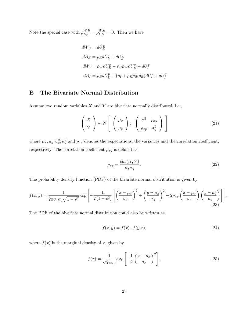
B The Bivariate Normal Distribution

Assume two random variables X and Y are bivariate normally distributed, i.e.,

X

Y

∼ N µx

µy

,

σ2x ρxy

ρxy σ2y

(21)

where µx, µy, σ2x, σ

2y and ρxy denotes the expectations, the variances and the correlation coefficient,

respectively. The correlation coefficient ρxy is defined as

ρxy =cov(X,Y )

σxσy. (22)

The probability density function (PDF) of the bivariate normal distribution is given by

f(x, y) =1

2πσxσy√

1− ρ2exp

[− 1

2 (1− ρ2)

[(x− µxσx

)2

+

(y − µyσy

)2

− 2ρxy

(x− µxσx

)(y − µyσy

)]].

(23)

The PDF of the bivariate normal distribution could also be written as

f(x, y) = f(x) · f(y|x), (24)

where f(x) is the marginal density of x, given by

f(x) =1√

2πσxexp

[−1

2

(x− µxσx

)2], (25)

27

and the density of y conditional on x, f(y|x), is given by

f(y|x) =1

σy√

2π√

1− ρ2xy

exp

[1

2σ2y (1− ρ2)

(y − µy −

ρxyσyσx

(x− µx)

)2]. (26)

C Proof of Pricing Formula

In Section 4.1 we showed that the payoff function in (6) could be rewritten in the following way:

p̂(FET , FIT ,KI ,KE) = max(F IT −KI , 0) ·max(FET −KE , 0)

=(FET −KE

)·(F IT −KI

)· 1{FET >KE} · 1{F IT>KI}

= FET FIT · 1{FET >KE} · 1{F IT>KI} − F

ET KI · 1{FET >KE} · 1{F IT>KI}

− F ITKE · 1{FET >KE} · 1{F IT>KI} +KEKI · 1{FET >KE} · 1{F IT>KI}.

Now let us calculate the expectation under Q of the payoff function, i.e., EQt

[p̂(FET , F

IT ,KI ,KE)

].

We have

EQt

[p̂(FET , F

IT ,KI ,KE)

]= EQ

t

[max(F IT −KI , 0) ·max(FET −KE , 0)

]= EQ

t

[FET F

IT 1{FET >KE}1{F IT>KI}

]− EQ

t

[FET KI1{FET >KE}1{F IT>KI}

]− EQ

t

[F ITKE1{FET >KE}1{F IT>KI}

]+ EQ

t

[KEKI1{FET >KE}1{>KI}

]. (27)

In order to calculate the four different expectation terms we will use the same trick as ?, namely to

rewrite the PDF of the bivariate normal distribution using the identity in (24). Remember that we

assume FET and F IT to be log-normally distrubuted under Q (i.e., (X,Y ) are bivariate normal):

FET = FEt eµE+X , (28)

F IT = F It eµI+Y , (29)

28

where σ2X denotes variance ofX, σ2

Y denotes variance of Y and they are correlated by ρX,Y . Consider

the fourth expectation term first,

EQt

[KEKI1{FET >KE}1{F IT>KI}

]= KEKIEQ

t

[1{FET >KE}1{F IT>KI}

]= KEKIQt

(FET > KE ∩ F IT > KI

)= KEKIQt

(FEt e

µE+X > KE ∩ F It eµI+Y > KI

)= KEKIQt

(X > log

(KE

FEt

)− µE ∩ Y > log

(KI

F It

)− µI

)= KEKIQt

(−X < log

(FEtKE

)+ µE ∩ −Y < log

(F ItKI

)+ µI

)= KEKI ·M (y1, y2; ρX,Y ) ,

where (ε1, ε2) are standard bivariate normal with correlation ρX,Y and

y1 =log(FEtKE

)+ µE

σXy2 =

log(F ItKI

)+ µI

σY.

Next, consider the third expectation term,

EQt


]= F It KEe

µIE[eY 1{FET >KE}1{F IT>KI}

]= F It KEe

µIE[eσY ε21{ε1<y1}1{ε2<y2}

]= F It KEe

µI

∫ y2

−∞

∫ y1

−∞eσY ε2f (ε1, ε2) dε1dε2

= F It KEeµI

∫ y2

−∞

∫ y1

−∞eσY ε2f (ε2) f (ε1|ε2) dε1dε2

= F It KEeµI

∫ y2

−∞

∫ y1

−∞eσY ε2

1√2π

exp

(−1

2ε22

)·

1√

2π√

1− ρ2X,Y

exp

[−1

2(1− ρ2X,Y )

(ε1 − ρX,Y ε2)2

]dε1dε2

(30)

29

Look at the exponent in the above expression

σY ε2 −1

2ε22 −

1

2(1− ρ2X,Y )

(ε21 + ρ2

X,Y ε22 − 2ρX,Y ε1ε2

)= − 1

2(1− ρ2X,Y )

(−2σY (1− ρ2

X,Y )ε2 + (1− ρ2X,Y )ε22 + ε21 + ρ2

X,Y ε22 − 2ρX,Y ε1ε2

)= − 1

2(1− ρ2X,Y )

(ε21 − 2σY (1− ρ2

X,Y )ε2 + ε22 − 2ρX,Y ε1ε2)

= − 1

2(1− ρ2X,Y )

(w2 + z2 − 2ρX,Y zw − (1− ρ2

X,Y )σ2Y

)= − 1

2(1− ρ2X,Y )

(w2 + z2 − 2ρX,Y zw

)+σ2Y

2

using the substitution w = −ε1 + ρε1,ε2σY and z = −ε2 + σY , (30) can be written as

EQt


]=

F It KEeµI+

σ2Y2

∫ y∗2

−∞

∫ y∗1

−∞

1

2π√

1− ρ2X,Y

exp

[− 1

2(1− ρ2X,Y )

(w2 + z2 − 2ρX,Y zw

)]dwdz

= F It KEeµI+

σ2Y2 M (y∗1, y

∗2; ρX,Y )

where

y∗1 = y1 + ρX,Y σY y∗2 = y2 + σY .

The second expectation term can be calculated in the same way as we calculated the third term.

The only difference is that we now use the substitution w̄ = −ε1 + σX and z̄ = −ε2 + ρX,Y σX , so

we can write

EQt

[FET KI1{FET >KE}1{F IT>KI}

]=

FEt KIeµE+

σ2X2

∫ y∗∗2

−∞

∫ y∗∗1

−∞

1

2π√

1− ρ2X,Y

exp

[− 1

2(1− ρ2X,Y )

(w2 + z2 − 2ρX,Y zw

)]dwdz

= FEt KIeµE+

σ2X2 M (y∗∗1 , y

∗∗2 ; ρX,Y )

where

y∗∗1 = y1 + σX y∗∗2 = y2 + ρX,Y σX .

30

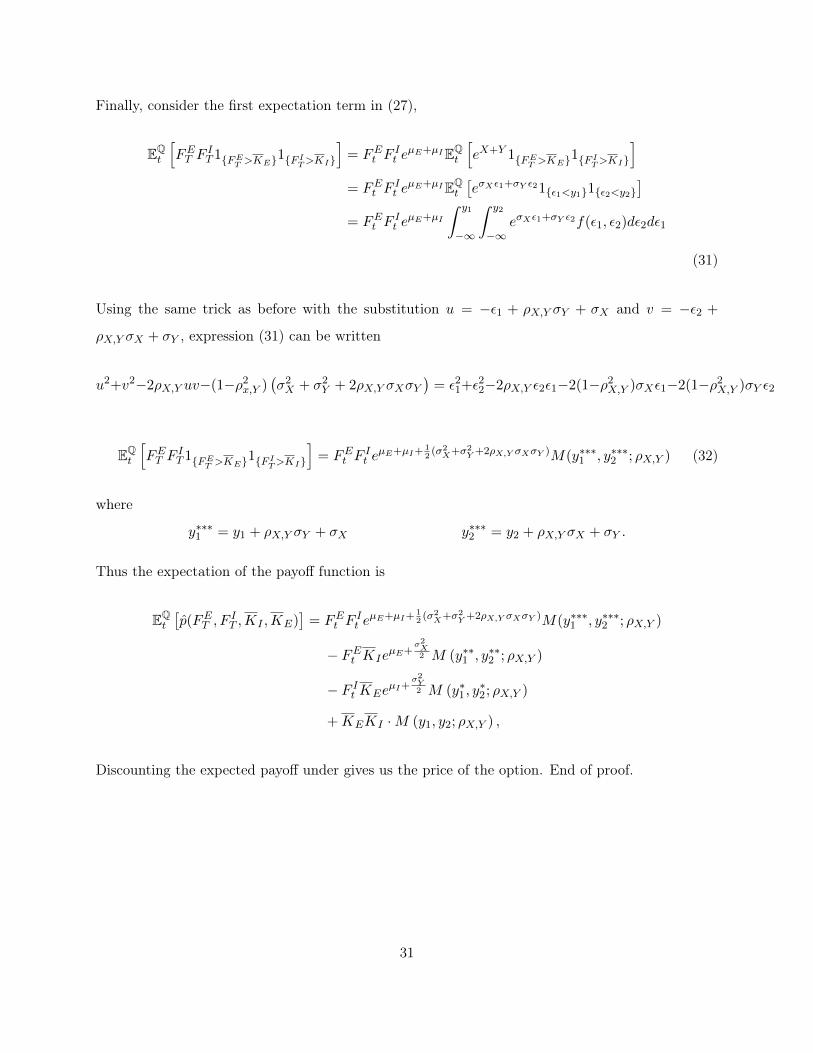
Finally, consider the first expectation term in (27),

EQt

[FET F


]= FEt F

It e

µE+µIEQt

[eX+Y 1{FET >KE}1{F IT>KI}

]= FEt F

It e

µE+µIEQt

[eσXε1+σY ε21{ε1<y1}1{ε2<y2}

]= FEt F

It e

µE+µI

∫ y1

−∞

∫ y2

−∞eσXε1+σY ε2f(ε1, ε2)dε2dε1

(31)

Using the same trick as before with the substitution u = −ε1 + ρX,Y σY + σX and v = −ε2 +

ρX,Y σX + σY , expression (31) can be written

u2+v2−2ρX,Y uv−(1−ρ2x,Y )

(σ2X + σ2

Y + 2ρX,Y σXσY)

= ε21+ε22−2ρX,Y ε2ε1−2(1−ρ2X,Y )σXε1−2(1−ρ2

X,Y )σY ε2

EQt

[FET F


]= FEt F

It e

µE+µI+ 12

(σ2X+σ2

Y +2ρX,Y σXσY )M(y∗∗∗1 , y∗∗∗2 ; ρX,Y ) (32)

where

y∗∗∗1 = y1 + ρX,Y σY + σX y∗∗∗2 = y2 + ρX,Y σX + σY .

Thus the expectation of the payoff function is

EQt

[p̂(FET , F

IT ,KI ,KE)

]= FEt F

It e

µE+µI+ 12

(σ2X+σ2

Y +2ρX,Y σXσY )M(y∗∗∗1 , y∗∗∗2 ; ρX,Y )

− FEt KIeµE+

σ2X2 M (y∗∗1 , y

∗∗2 ; ρX,Y )

− F It KEeµI+

σ2Y2 M (y∗1, y

∗2; ρX,Y )

+KEKI ·M (y1, y2; ρX,Y ) ,

Discounting the expected payoff under gives us the price of the option. End of proof.

31

D Closed Form Solutions for σ and ρ in the two-dimensional Schwartz-

Smith Model with Seasonality

σ2X =

∫ T

t

(σ2E +

(νEe

−κE(τ−s))2

+ 2ρEσE

(νEe

−κE(τ−s)))

ds

= σ2E(T − t) + νE

∫ T

te−2κE(τ−s)ds+ 2ρEσEνE

∫ T

te−κ

E(τ−s)ds

= σ2E(T − t) +

νE2κE

e−2κEτ(e2κET − e2κEt

)+ 2

ρEσEνEκE

e−κEτ(eκ

ET − eκEt)

cov(X,Y ) = ρW

∫ T

tσEσIds+ ρB

∫ T

t

(νEe

−κE(τ−s))(

νIe−κI(τ−s)

)ds

= ρWσEσI(T − t) + ρBνEνIe−(κE+κI)τ

∫ T

te(κE+κI)sds

= ρWσEσI(T − t) +ρBνEνIκE + κI

e−(κE+κI)τ(e(κE+κI)T − e(κE+κI)t

)ρX,Y =

cov(X,Y )

σXσY

When T = τ , this simplifies to

σX = σ2E(τ − t) +

νE2κE

(1− e−2κE(τ−t)

)+ 2

ρEσEνEκE

(1− eκE(τ−t)

)ρX,Y =

ρWσEσI(τ − t) + ρBνEνIκE+κI

(1− e−(κE+κI)(τ−t)

)σXσY

E One-dimensional Option Prices

As before, assume that the dynamics of a gas futures contract is given by:

FET (τ1, τ2) = FEt (τ1, τ2) exp(µE +X).

Consider now a call option written on gas futures only. The price ct of this option is then given by

the Black-76 formula, i.e.

ct = e−r(T−t) [FN(d1)−KN(d2)] ,

where

d1 =ln

FEtKE− µE

σXd2 =

lnFEtKE

+ µE

σX.

32

The same formula of course applies to an option written only on temperature futures.

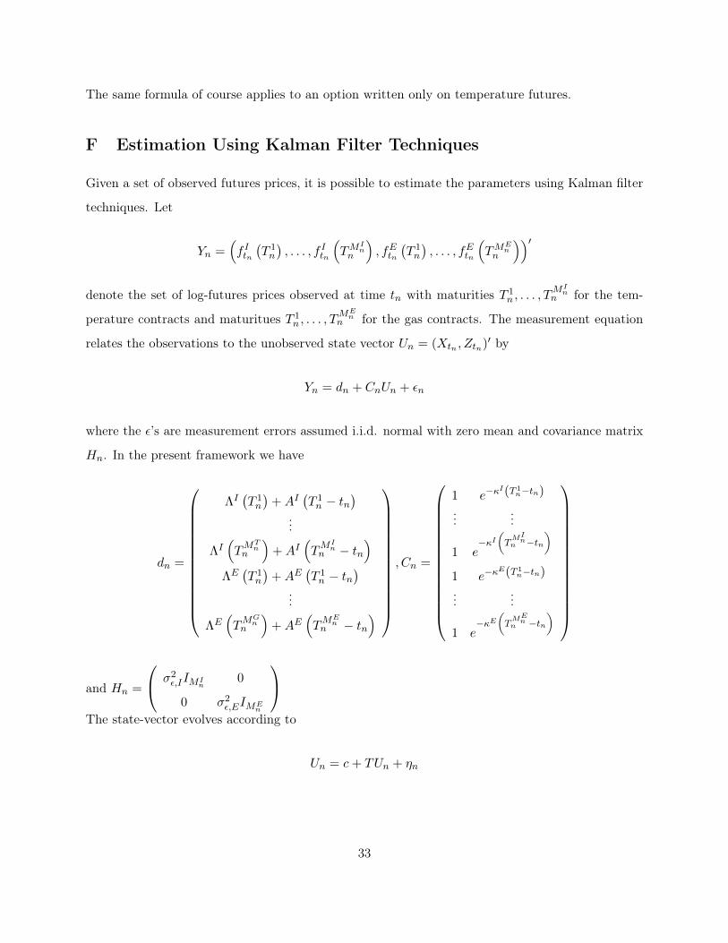
F Estimation Using Kalman Filter Techniques

Given a set of observed futures prices, it is possible to estimate the parameters using Kalman filter

techniques. Let

Yn =(f Itn(T 1n

), . . . , f Itn

(TM

In

n

), fEtn

(T 1n

), . . . , fEtn

(TM

En

n

))′denote the set of log-futures prices observed at time tn with maturities T 1

n , . . . , TMIn

n for the tem-

perature contracts and maturitues T 1n , . . . , T

MEn

n for the gas contracts. The measurement equation

relates the observations to the unobserved state vector Un = (Xtn , Ztn)′ by

Yn = dn + CnUn + εn

where the ε’s are measurement errors assumed i.i.d. normal with zero mean and covariance matrix

Hn. In the present framework we have

dn =

ΛI(T 1n

)+AI

(T 1n − tn

)...

ΛI(TMTn

n

)+AI

(TMIn

n − tn)

ΛE(T 1n

)+AE

(T 1n − tn

)...

ΛE(TMGn

n

)+AE

(TMEn

n − tn)

, Cn =

1 e−κI(T 1

n−tn)

......

1 e−κI

(TMIn

n −tn)

1 e−κE(T 1

n−tn)

......

1 e−κE

(TMEn

n −tn)

and Hn =

σ2ε,IIMI

n0

0 σ2ε,EIME

n

The state-vector evolves according to

Un = c+ TUn + ηn

33

where ηn are i.i.d. normal with zero-mean vector and covariance matrix Q and where

c =

µI − 1

2

(σI)2

0

µE − 12

(σE)2

0

∆n+1, T =

1 0 0 0

0 e−κI∆n+1 0 0

0 0 1 0

0 0 0 e−κE∆n+1

Q =

(σI)2

∆n+1 0 ρSσIσE∆n+1 0

0(νI)

2(

1−e−2κI∆n+1

)2κI

0 ρLνIνE

(1−e−(κI+κE)∆n+1

)(κI+κE)

ρSσIσE∆n+1 0(σE)2

∆n+1 0

0 ρLνIνE

(1−e−(κI+κE)∆n+1

)(κI+κE)

0(νE)

2(

1−e−2κE∆n+1

)2κE

34

pricing and hedging quanto options in energy markets · quanto option in terms of tradeable...

Documents