pricing death: frameworks for the valuation and ... · frameworks for the valuation and...
TRANSCRIPT

Pricing Death:Frameworks for the Valuation and Securitization of
Mortality Risk∗
Andrew J.G. Cairnsb, David Blake, and Kevin Dowd
First version: June 2004This version: December 16, 2005
Abstract
It is now widely accepted that stochastic mortality – the risk that aggregate mor-tality might differ from that anticipated – is an important risk factor in both lifeinsurance and pensions. As such it affects how fair values, premium rates, and riskreserves are calculated.
This paper makes use of the similarities between the force of mortality and interestrates to examine how we might model mortality risks and price mortality-relatedinstruments using adaptations of the arbitrage-free pricing frameworks that havebeen developed for interest-rate derivatives. In so doing, the paper pulls togethera range of arbitrage-free (or risk-neutral) frameworks for pricing and hedging mor-tality risk that allow for both interest and mortality factors to be stochastic. Thedifferent frameworks that we describe – short-rate models, forward-mortality models,positive-mortality models and mortality market models – are all based on positive-interest-rate modelling frameworks since the force of mortality can be treated in asimilar way to the short-term risk-free rate of interest. While much of this paper isa review of the possible frameworks, the key new development is the introduction ofmortality market models equivalent to the LIBOR and swap market models in theinterest-rate literature.
These frameworks can be applied to a great variety of mortality-related instruments,from vanilla longevity bonds to exotic mortality derivatives.
Keywords: stochastic mortality, term structure of mortality, survivor index, spotsurvival probabilities, spot force of mortality, forward mortality surface, short-ratemodels, forward mortality models, positive mortality framework, mortality marketmodels, annuity market model, SCOR market model.
∗First version presented at the 14th International AFIR Colloquium, Boston, 2004, un-der the title Pricing Frameworks for Securitization of Mortality Risk, available online athttp://afir2004.soa.org/afir papers.htm .
bCorresponding author: E-mail [email protected]

1 INTRODUCTION 2
1 Introduction
A large number of products in life insurance and pensions by their very naturehave mortality as a primary source of risk. By this we mean that products areexposed to unanticipated changes over time in the mortality rates of the appropriatereference population. For example, annuity providers are exposed to the risk thatthe mortality rates of pensioners will fall at a faster rate than accounted for intheir pricing and reserving calculations, and life insurers are exposed to the risk ofunexpected increases in mortality (a recent example being those due to HIV/AIDS).On the asset side of their balance sheets, insurance companies are also exposedto investment risks and, since their investment portfolios are predominantly fixedincome, this means that they are heavily exposed to interest-rate risk.
However, there is a huge gap in the tools available to model these two types of risk.On the one hand, the theory and practice of interest-rate modelling is very welldeveloped (see, for example, Vasicek, 1977, Cox, Ingersoll and Ross, 1985, Heath,Jarrow and Morton, 1992, Miltersen, Sandmann and Sondermann, 1997, Brace,Gatarek and Musiela, 1997, Jamshidian, 1997, Brigo and Mercurio, 2001, Jamesand Webber, 2002, Rebonato, 2002, and Cairns, 2004b). On the other hand, thestate and practice of mortality risk modelling is relatively primitive.
Previous authors (see, for example, Milevsky and Promislow, 2001, Dahl, 2004, andBiffis, 2005) have observed that there are important similarities between the forceof mortality and interest rates. In particular, both are positive processes, have termstructures, and are fundamentally stochastic in nature. Milevsky and Promislow(2001) and Dahl (2004) exploited these similarities to model mortality risk usingmethods developed in interest-rate modelling. In a similar fashion, Biffis (2005)exploited the similarities between mortality risk and credit risk. This paper seeks todevelop their insights further. In particular, it makes use of the similarities betweenmortality and interest rate risks to show how we can model mortality risks andprice mortality-related instruments using adaptations of the arbitrage-free pricingframeworks that have been developed for interest-rate derivatives. In so doing, itdevelops a range of arbitrage-free frameworks for pricing and hedging mortality riskthat allow for both interest and mortality factors to be stochastic.
1.1 Evidence that mortality is stochastic
To motivate our discussion, we will first summarise some evidence that confirms thatmortality improvements are indeed stochastic. We then briefly discuss the state ofthe art in mortality modelling, and go on to consider some financial instrumentswhose values depend on mortality and where it is therefore important to modelmortality risk factors in an appropriate way.
The idea that mortality is stochastic is not a new one, and it has been evident for

1 INTRODUCTION 3
many years that mortality rates have been evolving in an apparently stochastic fash-ion. The uncertainty of mortality forecasts is illustrated in recent work by Currie,Durban and Eilers (2004) (hereafter CDE) which analysed historical trends in mor-tality using P-splines. The fitted surface of values for the force of mortality1 µ(t, x)is plotted on a log scale in Figure 1.1 while the development of the force of mortalityfor specific ages over time relative to values in 1947 is plotted in Figure 1.2. Figure1.2 reveals some detail that we cannot easily see in Figure 1.1: specifically thatthe rate of improvement has varied significantly over time, and that the improve-ments have varied substantially between different age groups. CDE also constructedconfidence bounds for the future development of mortality rates. Inevitably, theseconfidence bounds get wider as the forecast horizon lengthens and CDE found thateven 15-20 years ahead the bounds are very wide. In general terms, the analysisof CDE, as well as other analyses using the stochastic mortality models discussedbelow, indicates that future mortality improvements cannot be forecast with anydegree of precision. Other studies (e.g., Forfar and Smith, 1987, Macdonald et al,1998, Willets, 1999, and Macdonald et al, 2003) have come to similar conclusions.
We focus in this paper on systematic mortality risk: the risk that aggregate mortal-ity rates differ from those anticipated. Mortality risk can manifest itself in differentways and to help differentiate between them we will employ the following taxonomy.The term mortality risk will be used to cover all forms of deviations in aggregatemortality rates from those anticipated at different ages and over different time hori-zons. Longevity risk will be used to refer to the risk that, in the long term, aggregatesurvival rates for identified cohorts are higher than anticipated. Short-term, catas-trophic mortality risk will refer to the risk that, over short periods of time, mortalityrates are very much higher than would normally be experienced.
1.2 Recent models of mortality
A number of recent studies have sought to model mortality as a stochastic process.We shall see presently that all these studies bar one (Lin and Cox, 2005a) can beseen as belonging to one of the more general frameworks that we will describe later inthis paper. We will describe these briefly here and in the Appendices. The majorityof work in this field has concentrated on what we describe as short-rate models formortality: that is, they are modelling the spot mortality rates2, q(t, x), or the spotforce of mortality, µ(t, x).
The most coherent group of papers that use the short-rate-modelling framework in
1For an individual aged x at time t and still alive at that time, the force of mortality µ(t, x)represents the instantaneous death rate: that is, for a small interval of time dt, the probability ofdeath between t and t + dt is µ(t, x)dt + o(dt) as dt → 0 (that is, approximately µ(t, x)dt for smalldt). The force of mortality µ(t, x) is described in more detail at the start of Section 2.
2The spot mortality rate q(t, x) is the probability at time t that an individual who is aged xand still alive at time t will die before time t + 1.

1 INTRODUCTION 4
Year, t1950
1960
1970
1980
1990
Age, x20
4060
80100
0.001
0.01
0.1
µ(t,
x)
Figure 1.1: Fitted values using P-splines for the force of mortality µ(t, x) for theyears t = 1947 to 1999 and for ages x = 11 to 100 from Currie, Durban and Eilers,2004. (Data: UK males, assured lives.)

1 INTRODUCTION 5
1950 1960 1970 1980 1990 2000
0.0
0.2
0.4
0.6
0.8
1.0
x = 21
x = 21
x = 31
x = 41
x = 51
x = 51
x = 61
x = 61
x = 71
x = 71
x = 81
x = 81
x = 91
x = 91
Year, t
µ(t,
x)µ(
1947
, x)
Figure 1.2: µ(t, x)/µ(1947, x): Fitted values using P-splines for the force of mortalityµ(t, x), relative to the 1947 value for the years t = 1947 to 1999 and for ages x =21, 31, 41, 51, 61, 71 and 81 from Currie, Durban and Eilers, 2004. Note that thepattern of improvements is different at different ages. (Data: UK males, assuredlives.)

1 INTRODUCTION 6
discrete time build on the original work of Lee and Carter (1992) (see, also, Lee,2000b). This study introduced a simple model for central mortality rates involvingboth age-dependent and time-dependent terms and applied it to US populationdata (see Appendix A for further details). The time-dependency is modelled usinga univariate ARIMA time-series model implying that changes in the mortality curveat all ages are perfectly correlated. Brouhns, Denuit and Vermunt (2002) appliedthe same model to Belgian data and also improved some of the statistical aspects ofLee and Carter’s work. The possibility of imperfect mortality correlation was theninvestigated by Renshaw and Haberman (2003) who extend the Lee and Carterapproach by adding a second time-dependent set of changes.
A second approach that also uses the short-rate-modelling framework in discretetime has been proposed by Lee (2000a) and Yang (2001). They take a deterministicprojection of the spot mortality rates, q(t, x), as given, and then apply an adjustmentthat evolves over time in a stochastic way. (For further, brief details, see AppendixB.) Lee and Yang’s approach has been continued in later work by Cairns, Blake andDowd (2005) and Lin and Cox (2005b).
Short-rate models for the development in continuous time of the force of mortal-ity have been proposed by Milevsky and Promislow (2001), Dahl (2004), and Biffis(2005). Milevsky and Promislow (2001) take a more theoretical approach in contin-uous time which assumes that the force of mortality µ(t, x) has a Gompertz formξ0(t) exp(ξ1x) where the ξ0(t) term is modelled using a simple mean-reverting diffu-sion process (see Appendix C). Dahl (2004) works initially in a much more generalsetting than Milevsky and Promislow. He starts by considering a general diffusionprocess for the force of mortality before focusing on the parsimonious, affine class ofprocesses and we discuss his approach further in Appendix D. Biffis (2005) extendsDahl’s approach to cover jump-diffusion affine processes.
In contrast to the papers mentioned above, Lin and Cox (2005a) do not propose aspecific model for stochastic mortality. Instead, they apply the Wang (1996, 2000,2002, 2003) transform to convert deterministic projected mortality rates into whatmight be described as risk-adjusted probabilities. The use of the Wang transformis gaining in popularity in non-life insurance applications where there is a lack ofliquidity in the instruments subject to the underlying risks. However, it is not clearfrom Lin and Cox (2005a) how different transforms for different cohorts and termsto maturity relate to one another to form a coherent whole.
Another approach to the pricing problem in incomplete financial markets has beenproposed by Froot and Stein (1998). They discuss how the capital structure ofa financial institution affects the price they are prepared to pay to take on or tooffload a non-hedgeable risk. Typically this takes the form of an over-the-counterdeal between two institutions. Amongst other results, they demonstrate that theprice at which an institution is willing to trade these instruments also depends onhow well capitalised it is.

1 INTRODUCTION 7
1.3 Applications of stochastic mortality models
There are many financial applications in which it is necessary to take account ofthe stochastic behaviour of mortality. One example is the calculation of quantile (orvalue-at-risk) reserves for life-office portfolios, where the uncertain future pattern ofliability payments will depend, amongst other things, on the future evolution of theforce of mortality µ(t, x). It is also important to take account of stochastic mortalitywhen reserving for policies that incorporate certain types of guarantee.
Taking account of stochastic mortality is also critical when pricing mortality deriva-tives. Below we provide some examples of mortality derivatives that have beenproposed in the literature, not all of which exist in practice at the time of writing:
• Longevity bonds (where coupon payments are linked to the number of sur-vivors in a given cohort). Long-dated longevity bonds (also referred to assurvivor bonds: Blake and Burrows, 2001) intended to manage longevity riskhave recently been revived by Cox, Fairchild and Pedersen (2000), Blake andBurrows (2001) and Lin and Cox (2005a). Their origin dates back to Ton-tine bonds issued by a number of European governments in the 17th and 18th
centuries. The first modern issue of a longevity bond, with a maturity of 25years, was announced in November 2004 by the European Investment Bankand BNP Paribas. However, Cox, Fairchild and Pedersen (2000) commentedthat a number of insurers were proposing to issue longevity bonds as early as1997. The fact that issues of such bonds were so long in coming suggests thatthere are substantial practical problems which need to be overcome or thatthe market is not yet ready to invest in such long-term bonds. (For furtherdetails of the EIB/BNP bond, see Cairns, Blake, and Dowd (2005), Cairns,Blake, Dawson and Dowd (2005) and Blake, Cairns and Dowd (2006).)
• Short-dated, mortality-linked securities (market-traded securities whose pay-ments are linked to a mortality index). The first, widely-marketed, bond ofthis type was issued by Swiss Re at the start of 2004, and it shares charac-teristics with traditional catastrophe bonds in the non-life insurance markets(see, for example, Schmock, 1999, Lane, 2000, Wang, 2002, and Muermann,2004). It involves a three-year contract (maturing on 1 January 2007) whichallows the issuer to reduce its exposure to short-term catastrophic mortalityrisk. The repayment of the principal is linked to a combined mortality indexof experienced mortality rates in five countries (France, Italy, Switzerland, theUK and the USA). Under the contract, the principal will be at risk “if, duringany single calendar year in the risk coverage period, the combined mortalityindex exceeds 130% of its baseline 2002 level”. The credit spread at issue of135 basis points (0.0135%) equates to a risk-neutral probability of about 0.04(that is, 1−(1−0.0135)3 ≈ 0.04) that the principal would not be repaid at all.This is equivalent to a catastrophic event that would happen, on average, once

1 INTRODUCTION 8
every 75 years (treating individual years as being independent). The types ofcatastrophic mortality events that are large enough to breach the thresholdinclude (but are not restricted to) an influenza pandemic, or a natural catas-trophe. However, the Swiss Re bond addresses a different type of mortalityrisk (short-term catastrophic mortality risk) from that considered in this paper(unanticipated long-term changes in population mortality). The catastropherisks being covered by the Swiss Re bond might be correlated with financialmarkets (past examples – albeit on a “smaller” scale – include 9/11 or the Kobeearthquake in 1995). In contrast, we assume for convenience that systematicmortality risks are independent of the financial markets: an assumption thatsimplifies the mathematical developments that follow. However, we do discussbriefly how this assumption might be relaxed.
• Survivor swaps (where counterparties swap a fixed series of payments for aseries of payments linked to the number of survivors in a given cohort). Asmall number of survivor swaps have been arranged on an over-the-counterbasis. They are not traded contracts and therefore only provide direct benefitto the counterparties in the transaction. The case for survivor swaps is madeby Dowd et al (2006).
• Annuity futures (where prices are linked to a specified future market annuityrate). As an example, suppose that a(t, x) represents the market price at timet of a level annuity of £1 per annum payable monthly in arrears to a maleaged x at time t. (This might, for example, be a weighted average of the top5 quotes in the market.) It has been suggested by AFPEN (the associationof French Pension Funds) that a traded futures market be set up with a(t, x)(or its reciprocal) as the underlying instrument for selected values of x andwith a selection of maturity dates stretching out many years into the future.For a given maturity date, the market could be closed out some months oreven a year before the maturity date itself, to reduce the impact, for example,of moral hazard, changes in expensing bases, or the movements of individualannuity providers in and out of the market. For further discussion of annuityfutures, see Blake, Cairns and Dowd (2006).
• Mortality options (a range of contracts with option characteristics whose payoffdepends on an underlying mortality table at the payment date). For example,a guaranteed annuity option is an investment-linked deferred-annuity contractthat gives a policyholder the option to convert his accumulated fund at re-tirement at a guaranteed rate rather than at market annuity rates. Marketannuity rates are set with reference to both interest rates at retirement and onthe mortality table in current use by the annuity provider, and this table, ofcourse, depends on mortality forecasts at that time. Contracts of this type arediscussed further in Section 4.2. Previous analyses of the role of systematicmortality risk in guaranteed annuity contracts include those of Yang (2001)

1 INTRODUCTION 9
and Biffis and Millossovich (2004). Milevsky and Promislow (2001) considerboth pricing and hedging of contracts involving annuity options. Dahl (2004)applies his model to problems involving insurance contracts with mortality-linked cashflows.
For a more detailed discussion of the types of security that might be issued and thepractical issues associated with these contracts, see Blake, Cairns and Dowd (2006).
The more general impact of systematic mortality risk on life insurance has been con-sidered at a theoretical level by Dahl and Møller (2005), while Marocco and Pitacco(1998) and Pitacco (2002) discuss the risk in more general terms. Cowley and Cum-mins (2005) consider securitisation of life insurance portfolios that incorporate amixture of risks including mortality.
A final application is the development of optimal asset-allocation strategies in thepresence of systematic mortality risk. This type of problem is considered by Dahland Møller (2005) (who examine optimal hedging) and Yang and Huang (2005) (whoexamine optimal strategies for defined contribution pension plans).
It is, of course, essential that the evolution of the prices of these derivative contractsshould accurately reflect the stochastic evolution of µ(t, x). The evolution of µ(t, x)can affect prices in several ways. Most obviously, stochastic mortality has an impacton the value of mortality options: the greater the volatility in mortality rates, thegreater is the value of a mortality option (as with financial options). However,the second effect is more subtle and relates to the fact that the ‘true’ values offinancial contracts are often non-linear functions of underlying factors. This pointoften manifests itself through Jensen’s inequality, and an example in the presentcontext would be that the price of a contract based on expected cash flow may notbe equal to the value of the contract assuming that mortality follows some centralprojection. Also (in line with the pricing of financial options) it might manifestitself in our calculating expectations using a different probability measure (denotedbelow by Q) from the real-world or true measure (denoted by P ) as, for example, isthe case in Dahl (2004). We do not discuss in this paper the many practical issuesrelated to the securitization of mortality risks. These issues are discussed elsewhere(see Cowley and Cummins, 2005, Dowd et al., 2006, Lin and Cox, 2005a, and Blake,Cairns and Dowd, 2006).
1.4 Choice of reference population
It is important to note that the reference population underlying the calculation ofthe mortality rates is critical to both the viability and liquidity of these contracts.Some investors (for example, life offices) will wish to use such contracts to help hedgetheir mortality risk, but if the reference population is inappropriate, they will beexposed to significant basis risk and the mortality derivative might not provide an

1 INTRODUCTION 10
adequate hedge. Other investors, such as hedge funds, will be attracted to mortality-linked securities because their lack of correlation with other assets helps with thediversification of risk on a general portfolio of investments (see, for example, Cox,Fairchild and Pedersen, 2000). These investors might be less interested in using thesederivatives for hedging mortality risk but will be interested in liquidity (liquiditybeing a key issue as well for speculators). Adequate liquidity will then require asmall number of reference populations, but these will need to be chosen carefullyto ensure that the level of basis risk is relatively small for those hoping to use thecontracts for hedging purposes. For more detail, see Section 2.1.
1.5 Requirements of a good stochastic mortality model
Given that mortality is best modelled as a stochastic process, it is reasonable tosuppose that any ‘plausible’ mortality model would meet the following criteria:
• The model should keep the force of mortality positive.
• The model should be consistent with historical data.
• The long-term future dynamics of the model should be biologically reason-able. For example, one might rule out the possibility of an ‘inverted’ mortalitycurve (that is, one in which mortality rates for the elderly fall with age). An‘inverted’ curve is not only unreasonable a priori, but also conflicts with thenormal upward-sloping curves that are always observed in historical data.
• Long-term deviations in mortality improvements from those anticipated shouldnot be mean-reverting to a pre-determined target level, even if this target istime dependent and incorporates mortality improvements. In contrast, short-term deviations from the trend due to local environmental fluctuations mightbe mean-reverting around the stochastic long-term trend. (We comment fur-ther on this below.)
• The model should be comprehensive enough to deal appropriately with thecurrent pricing, valuation or hedging problem.
• It should be possible to value the most common mortality-linked derivativesusing analytical methods or using fast numerical methods. However, we stressthat this criterion is one of convenience only, and should not be allowed tooverride the other criteria, which are more important because they are criteriaof principle. In other words, we should not drop one of the other criteriamerely to obtain an easy (for example, analytical) solution to the problem athand.

1 INTRODUCTION 11
It is worth commenting further on why, specifically, we take the view that long-run stochastic improvements in mortality, µ(t, y), should not be strongly mean-reverting to some deterministic projection, µ(t, y). The inclusion of mean reversionwould mean that if mortality improvements have been faster than anticipated inthe past then the potential for further mortality improvements will be significantlyreduced in the future. In extreme cases, significant past mortality improvementsmight be reversed if the degree of mean reversion is too strong. Such extreme meanreversion is difficult to justify on the basis of previous observed mortality changesand with reference to our perception of the timing and impact of, for example, futuremedical advances. Short-term trends might be detected by analysing carefully recentdevelopments in healthcare and in the pharamaceutical industry, but even then theprecise, long-term effects of such advances are difficult to judge. As we peer furtherinto the future, it becomes even more difficult to predict what medical advances theremight be, when they will happen, and what impacts they will have on survival rates.All of these uncertainties rule out strong mean reversion in a model for stochasticmortality.
Given this list of criteria, it is readily apparent that no one framework dominatesthe rest: some frameworks fare better by some criteria, and worse by others. Thereis therefore no strong reason why we should prefer models within any one modellingframework over models in another.
We described above a number of studies that propose specific stochastic modelsfor the future evolution of mortality rates. With the exception of Section 4, thispaper does not offer a new model type. Instead, we seek to set down the generalformulation of the problem in continuous time and suggest a range of frameworksfor the pricing and valuation of mortality-linked derivatives. Our aim in doingso is to provide, in one place, extensive foundations for the development in thefuture of further stochastic models for mortality and to ensure that they are usedin appropriate ways in pricing problems. To make the exposition easier to follow,we focus our discussion on the problem of pricing new securities. However, weemphasize that the same basic approaches apply to related problems. For example,they apply to the valuation of insurance liabilities that incorporate mortality-linkedderivatives, and they also apply (with appropriate changes from risk-neutral to real-world probabilities) to the estimation of risk measures (for example, value at risk)for mortality-related positions.
1.6 Layout of the paper
The layout of the paper is as follows. In Section 2, we introduce the fundamentalprocesses for mortality (the force of mortality process µ(t, x)) and for the risk-freerate of interest (r(t)). These processes feed into survivor indices S(u, y) and a risk-free cash account C(t) that play central roles in our analysis. We work with two

1 INTRODUCTION 12
fundamental types of financial contract:
• pure endowment contracts (zero-coupon longevity bonds) for a full range ofages and terms to maturity; and
• default-free zero-coupon bonds for a full range of terms to maturity.
By noting parallels with interest-rate and credit-risk theory, we then describe howpure endowment contracts should be priced if they trade in a perfectly liquid, fric-tionless and arbitrage-free market.3
In this paper we use the terms framework and model in a precise way. Frameworksprovide us with general approaches to modelling, and it is frameworks that are themain focus of this paper. We use the word model to mean a particular formulationdeveloped within a given framework. For example, we have the Vasicek (1977),Cox, Ingersoll and Ross (1985), and Black and Karasinski (1991) models within theshort-rate modelling framework. The framework normally defines what we can useas the basic building blocks in the modelling process.
In Section 3 we go on to describe briefly different frameworks that could be employedto build up models for stochastic mortality with further detail given in the Appen-dices. Subsection 3.1 pulls together all of the short-rate models described aboveunder the one short-rate-modelling framework and discusses how these models canbe used to build an arbitrage-free market in mortality derivatives. Subsections 3.2to 3.4 then discuss various other modelling frameworks that have received much lessattention. From these, the most novel contribution in this paper is contained inthe separate Section 4 where we propose a number of different market models formortality. Section 5 concludes.
Each of these frameworks is drawn from the field of interest-rate modelling but withthe risk-free rate of interest replaced by the force of mortality. These are all describedin theoretical terms: and, with the exception of Section 4, no specific models areproposed or analysed. Rather, the aim is to give readers a choice of frameworkswithin which they can build their own continuous-time stochastic mortality models.Most models built up within one framework can be reformulated within any of theother frameworks (in the same way, for example, that the Vasicek, 1977, short-ratemodel for r(t) can be re-expressed as a forward-rate model). This said, it is alsothe case that most models rest naturally within one particular framework, and areawkward to express within the others.
3Naturally, we do not claim that real-world markets are perfectly liquid or frictionless. However,we can state that if prices are calculated in the way proposed then even an illiquid market withfrictions will be arbitrage-free. Conversely, if we were to propose a pricing framework that violatesthe conditions in Section 2, then the possibility of arbitrage would emerge over time as the marketbecomes more liquid or trading costs begin to fall.

2 THE TERM STRUCTURE OF MORTALITY 13
2 The term structure of mortality
In this section, we will define the basic components of a model for stochastic mor-tality. We start by considering the force of mortality, µ(t, x), at time t for individ-uals aged x at time t. Traditional static mortality models implicitly assume thatµ(t, x) ≡ µ(x) for all t and x, while deterministic mortality projections imply thatµ(t, x) is a deterministic function of t and x. By contrast, the models we will considerhere will treat µ(t, x) as a stochastic process.
There are two types of stochastic mortality (see, for example, Dahl, 2004):
• The first is specific (or unsystematic) mortality risk – the risk that the actualnumber of deaths deviates from the anticipated number because of the finitenumber of lives in a given cohort. This type of risk can largely be diversifiedby investors under the usual assumption that future lifetimes for differentindividuals are independent random variables. Specific mortality risk does notlead to a risk premium in the price of mortality derivatives.
• Systematic mortality risk – the risk that the force of mortality evolves in adifferent way from that anticipated. This type of risk cannot be diversifiedaway and therefore leads to the incorporation of a risk premium.
By drawing parallels with the pricing of financial contracts, we might expect thatwith mortality derivatives systematic mortality risk should be priced using a risk-neutral probability measure, Q, which is different from the real-world probabilitymeasure, P (sometimes also called the objective or physical measure). This intuitionturns out to be correct: we will argue below that mortality derivatives need to bepriced with reference to such a measure in order for the market to be arbitragefree. We stress at this point, though, that the risk-neutral measure Q might notbe uniquely determined due to market incompleteness. Instead the choice of Qbecomes part of the modelling process. An important additional observation is thatthe explicit use of a risk-neutral measure, Q, for pricing – even if the market ishighly illiquid or has high transaction costs – ensures that the market the marketwill be free from riskless arbitrage (Fundamental Theorem of Asset Pricing). Asmortality-linked securities begin to emerge and as we gather market price data wecan then test for the validity of our assumptions about Q. For further discussionof the relationship between P and Q, the reader is referred to Dahl (2004), Cairns,Blake and Dowd (2005) and Biffis (2005).
One example where prices might be calculated with reference to a risk-neutral mea-sure is the Swiss Re mortality bond. The 135 basis point spread equates to a risk-neutral probability, approximately, of 0.0135 per annum of default: that is, that theprincipal will not be paid out. However, the real-world probability is thought to berather less than this (see, for example, Beelders and Colarossi, 2004).
2 THE TERM STRUCTURE OF MORTALITY 14
2.1 Basic building blocks
We have previously indicated that our aim is to develop a set of theoretical frame-works to price mortality derivatives. In order to do so, we will make the convenientbut over-simplifying assumption that the force of mortality at time t, µ(t, y), is ob-servable at time t for all y. In reality, we can only estimate µ(t, y) from a finiteamount of data, and this estimate is only calculated and published some monthsor years after the event. The length of this delay also depends considerably onthe reference population: for example, the UK industry-wide Continuous MortalityInvestigation tables take longer to compile than tables relating to one specific lifeoffice. We recognise that these are important practical issues but we will leave themfor future work.
2.1.1 The survivor index
We will use as our basic building block a family of index-linked zero-coupon longevitybonds. The indices we will employ are related to survival probabilities for differentages. Thus we define the survivor index
S(u, y) = exp
(−
∫ u
0
µ(t, y + t)dt
). (2.1)
If µ(t, x) is deterministic then S(u, y) is equal to the probability that an individualaged y at time 0 will survive to age y+u. Similarly, the probability that an individualaged x at time t1 will survive until a later time t2 is S(t2, x− t1)/S(t1, x− t1).
In this paper, we are mainly concerned with models in which µ(t, x) is stochastic.Looking forward from time 0, this means that S(u, y) is now a random variable. Inthis case, S(u, y) can still be regarded as a survival probability, albeit one that canonly be observed at time u rather than at time 0. However, it is straightforwardto extract a survival probability by taking the expectation of the random variableS(t, x) (equation (2.2) below). We prove this by using a combination of indicatorrandom variables and conditional expectation. Thus, consider an individual agedx at time 0. Let Yx(u) be a Markov chain which is equal to 1 if the individual isstill alive at time u. Also let Mt be the filtration (or information) generated by theevolution of the term-structure of mortality, µ(u, x), up to time t (that is, Mt givesus full information about changes in mortality up to and including time t, but noinformation about how mortality rates will develop after time t). The real-world ortrue survival probability measured at time 0, that an individual aged x at time 0survives until time u is
pP (0, u, x) = EP [Yx(u)] = EP [EP{Yx(u)|Mu}] = EP [S(u, x)]. (2.2)
Remark 2.1.1 Note that EP [S(u, x)] > exp[− ∫ u
0EP (µ(t, y + t))dt
]by Jensen’s
inequality. Also, if µ(t, y + t) is a deterministic best estimate at time 0 of future

2 THE TERM STRUCTURE OF MORTALITY 15
mortality (for example, the median) then we will still usually have EP [S(u, x)] 6=exp
[− ∫ u
0µ(t, y + t)dt
].
More generally, we can define the survival probabilities at time t as follows. LetpP (t, u, x) be the probability under P that an individual aged x at time 0 and stillalive at the current time t survives until time u:
pP (t, u, x) = EP [Yx(u)|Yx(t) = 1,Mt] = EP
[S(u, x)
S(t, x)
∣∣∣∣ Mt
].
For the alternative risk-neutral probability measure Q, we can define the correspond-ing survival probabilities:
pQ(t, u, x) = EQ[Yx(u)|Yx(t) = 1,Mt] = EQ
[S(u, x)
S(t, x)
∣∣∣∣ Mt
].
Remark 2.1.2 In deriving this last expression, we have relied on the conventionalassumption that non-systematic mortality risk does not attract a risk premium. Evenwhen S(u, x)/S(t, x) is known, there is a range of equivalent probability measures forthe Bernoulli random variable (Yx(u)|Yx(t) = 1,Mu). However, only one of these isconsistent with the absence of a risk premium for the non-systematic mortality risk:specifically PrQ[Yx(u) = 1|Yx(t) = 1,Mu] = S(u, x)/S(t, x).
2.1.2 Zero-coupon longevity bonds
We are now in a position to consider the pricing of index-linked zero-coupon longevitybonds. There is (potentially) a different bond for each maturity date T and for eachage x at time 0. We refer to a specific bond as the (T, x)-bond for compactness.
The (T, x)-bond pays the amount S(T, x) at time T . This payment is well definedin the sense that S(T, x) is an observable quantity at time T . The (T, x)-bond isan example of what financial mathematicians call a tradeable asset (also known asa pure-discount asset to some financial economists): that is, an asset that pays nocoupons or dividends and whose price, relative to the issue price, at any time t < Trepresents the total return on an investment in that asset. For an asset that does paydividends or coupons a tradeable asset can be created by reinvesting the dividendsin the underlying asset itself.
To price such bonds, we need to use the term-structure of interest rates. Let P (t, T )represent the price at time t of a zero-coupon bond that pays 1 at time T . Theinstantaneous forward rate curve at time t is given by
f(t, T ) = − ∂
∂Tlog P (t, T )

2 THE TERM STRUCTURE OF MORTALITY 16
and the instantaneous risk-free rate of interest is
r(t) = limT→t
f(t, T )
(see, for example, Cairns, 2004b).
A cash (or money-market) account accrues at the risk-free rate of interest. Its valueat time t is denoted by C(t) with
dC(t) = r(t)C(t)dt
⇒ C(t) = C(0) exp
(∫ t
0
r(u)du
). (2.3)
Let Ft be the filtration generated by the term-structure of interest rates up to timet, and Ht be the combined filtration for both the term-structure of interest ratesand mortality.
Now let B(t, T, x) represent the price at time t of the (T, x)-bond that pays S(T, x)at time T . If there exists a measure Q (the risk-neutral measure) equivalent to thereal-world measure P with
P (t, T ) = EQ
[C(t)
C(T )
∣∣∣∣ Ft
](2.4)
and B(t, T, x) = EQ
[C(t)
C(T )S(T, x)
∣∣∣∣ Ht
](2.5)
for all t, T and x (which implies that P (t, T )/C(t) and B(t, T, x) are Q-martingales)then the dynamics of the combined financial market are arbitrage free. Equation 2.5matches those of Milevsky and Promislow (2001) and Dahl (2004) and encompassesthe full range of models including those with more than one source of randomness.
Assumption 1
We now make the convenient assumption that, under the risk-neutral measure Q,the dynamics of the term structure of mortality are independent of the dynamicsof the term-structure of interest rates. This assumption simplifies the discussionand allows us to present the modelling analogies with the maximum possible clarity.However, it is not essential that we make this assumption and it can be relaxed.
Whether interest rates and mortality rates are related is a topic for debate: manyeconomists are sceptical, but others point to anecdotal evidence that suggests someform of relationship. Should one believe that interest and mortality rates are de-pendent, one might model it along lines such as those pursued by Miltersen andPersson (2005), who present a forward-mortality framework that explicitly allowsfor interest and mortality to be related.
A key consequence of this independence assumption is that it allows us to separate

2 THE TERM STRUCTURE OF MORTALITY 17
the pricing of mortality risk from the pricing of interest-rate risk. It follows that
B(t, T, x) = EQ
[C(t)
C(T )
∣∣∣∣ Ft
]EQ [S(T, x) | Mt]
= P (t, T )B(t, T, x)
where B(t, T, x) = EQ [S(T, x) | Mt] .
Thus B(t, T, x) is a martingale under Q. We can also assume that the B(t, T, x)processes are strictly positive (which is equivalent to ruling out the possibility ofcatastrophic events that wipe out the entire population).
This allows us to make three further observations:
• B(t, T, x)/B(t, t, x) = pQ(t, T, x). Since we can regard the B(t, T, x) as spotestimates, we will refer to the pQ(t, T, x) as spot survival probabilities.
• We can use the B(t, T, x) to define the forward force of mortality surface(see, for example, Milevsky and Promislow, 2001, and Dahl, 2004) (we willsometimes shorten this to forward mortality surface):
µ(t, T, x + T ) = − ∂
∂Tlog B(t, T, x). (2.6)
Conversely, knowledge of the forward mortality surface allows us to price thebonds:
B(t, T, x)
B(t, t, x)= exp
[−
∫ T
t
µ(t, u, x + u)du
].
If we take T = t, we get the spot force of mortality:
µ(t, x + t) = µ(t, t, x + t).
(A more general form for the forward force of mortality surface has beendefined in the parallel work of Miltersen and Persson (2005). In their for-mulation, interest and mortality rates are allowed to be dependent, so thatseparation of B(t, T, x) into P (t, T )×B(t, T, x) is not possible without resort-ing to the use of forward measures equivalent to Q. They define µ(t, T, x +T ) = − ∂
∂Tlog B(t, T, x) − f(t, T ), where f(t, T ) is the forward interest rate
− ∂∂T
log P (t, T ). If Assumption 1 holds then Mitersen and Persson’s definitionis equivalent to that in equation (2.6).)
It is also convenient at this point to define the forward survival probability:pQ(t, T0, T1, x) = the probability, based on the information about mortalityrates available at time t, Mt, that an individual alive and aged x + T0 at timeT0 will survive until time T1. This definition implies that
pQ(t, T0, T1, x) = exp
[−
∫ T1
T0
µ(t, u, x + u)du
]=
B(t, T1, x)
B(t, T0, x). (2.7)

2 THE TERM STRUCTURE OF MORTALITY 18
• Let us assume that the dynamics of the term structure of mortality are gov-erned by an n-dimensional Brownian motion W (t) under Q. The martingaleproperty of B(t, T, x) together with its positivity now allows us to write downthe stochastic differential equation for B(t, T, x) in the following form
dB(t, T, x) = B(t, T, x)V (t, T, x)′dW (t)
where V (t, T, x) is a family of previsible4 vector processes that specify thevolatility term structure of the B(t, T, x).
We will now consider the possible frameworks which we can use to model the dy-namics of the B(t, T, x) processes. These correspond to a variety of frameworks usedin modelling interest rates (see, for example, Cairns, 2004b):
• short-rate modelling framework for the dynamics of µ(t, y) (which correspondto short-rate models for the risk-free rate of interest, r(t), including those ofVasicek, 1977, Cox, Ingersoll and Ross, 1985, and Black and Karasinski, 1991);
• forward-mortality modelling framework for the dynamics of the forward mor-tality surface, µ(t, T, x+T ) (corresponding to the framework of Heath, Jarrowand Morton, 1992);
• positive-mortality modelling framework for the spot survival probabilities,pQ(t, T, x) (corresponding to the positive-interest framework developed by Fle-saker and Hughston, 1996, Rogers, 1997, and Rutkowski, 1997);
• market modelling framework for forward survival probabilities or forward an-nuity prices (corresponding to the LIBOR and swap market models of Brace,Gatarek and Musiela, 1997, and Jamshidian, 1997).
We also include a short section that discusses the parallels between pricing mortalityand credit derivatives. In doing so, we also review the similarities that allow us toapply some of the intensity-based models that have been developed in the credit-pricing literature to mortality problems.
We stress that the purpose of the following sections is to pull together the theoreticalfoundations of this relatively new field. We leave for further work the developmentof specific new models within the different frameworks considered here. We alsoleave for others the process of fitting these models to historical and market data:such a task requires the use of estimation techniques that are tailored to individualmodels and goes well beyond the scope of the present paper.
4To describe a process, X(t), as previsible means that the value of X(t) is known or observableby time t.

3 REVIEW OF EXISTING MODELLING FRAMEWORKS 19
3 Review of existing modelling frameworks
3.1 Short-rate modelling framework
Models built up within this framework specify directly the dynamics of µ(t, y).Existing models for the term-structure of mortality within this framework includeLee and Carter (1992), Lee (2000a), Yang (2001), Brouhns, Denuit and Vermunt(2002), Renshaw and Haberman (2003), and Cairns, Blake and Dowd (2005) indiscrete time, and Milevsky and Promislow (2001) and Luciano and Vigna (2005)in continuous time. Milevsky and Promislow (2001) exploit the completeness of themarket in their model to calculate both prices and hedging strategies for an annuityoption. Dahl (2004) develops the general one-factor version of equation (3.1) belowand then focuses on the affine class of processes as one that gives an analyticalsolution for pQ(t, T, x). In continuous time, we model the force of interest which willhave the general stochastic differential equation
dµ(t, y) = a(t, y)dt + b(t, y)′dW (t) (3.1)
where a(t, y) and b(t, y) (an n × 1 vector) are previsible processes and W (t) is astandard n-dimensional Brownian motion under the risk-neutral measure Q.5 Wethen have (see, for example, Milevsky and Promislow, 2001, or Dahl, 2004)6
B(t, T, x)
B(t, t, x)= pQ(t, T, x)
= EQ
[exp
(−
∫ T
t
µ(u, x + u)du
) ∣∣∣∣ Mt
]. (3.2)
We can make the following observations about this framework:
• We have specified that W (t) and b(t, y) are n × 1 vectors. This means thatwe can allow for the possibility that short-term changes in the term-structureof mortality can be different at different ages: that is, mortality changes atdifferent ages are not perfectly correlated. Different rates of change at differentages can also be achieved through the a(t, y) drift function.
• a(t, y) and b(t, y) might depend on other diffusion processes which are them-selves adapted to Mt. Note that this dependence allows b(t, y) ≡ 0, in whichcase the force of mortality curve evolves in a smooth fashion over time. How-ever, the evolution of the force of mortality curve is still stochastic because of
5The dynamics expressed in (3.1) have been extended by Biffis (2005) to include jumps as wellas a diffusion.
6If we are modelling the spot survival probabilities, pQ(t, t + 1, x), or the spot mortality rates,qQ(t, t+1, x) = 1− pQ(t, t+1, x) in discrete time, then the equivalent of equation (3.2) in discretetime is pQ(t, T, x) = EQ [pQ(t, t + 1, x)× . . .× pQ(T − 1, T, x + (T − 1− t))|Mt].

3 REVIEW OF EXISTING MODELLING FRAMEWORKS 20
its dependence on the stochastic drift rate a(t, y). Other models might assumethat b(t, y) 6= 0, in which case the force of mortality curve exhibits a degree oflocal volatility.
• The assumption that b(t, y) ≡ 0 is equivalent to the assumption that thevolatility function V (t, T, x) for the B(t, T, x) processes, and their first deriva-tives with respect to T , tend to zero as T → t. Thus, the shortest-dated bondswill have a very low volatility.
• This framework also includes models that assume that µ(t, y) takes some para-metric form (for example, the Gompertz-Makeham model µ(t, x) = ξ0(t) +ξ1(t)e
ξ2(t)x). We can model the parameters in this curve as diffusion processes.This class is a specific example of the type noted above where a(t, y) and b(t, y)themselves depend on other diffusion processes.
The framework includes the affine class of models for µ(t, x) considered by Dahl(2004) (with mean reversion around a deterministic projection) under which thespot survival probabilities have the closed form
pQ(t, T, x) = exp [A0(t, T, x)− A1(t, T, x)µ(t, x + t)]
with n = 1 dimension. Dahl provides sufficient conditions on a(t, y) and b(t, y)(equation (3.1)) that result in this affine representation for pQ(t, T, x). These con-ditions mimic those of Duffie and Kan (1996) for interest-rate models.
An approach that generalises equation (3.1) to what is more truly a bidimensionalprocess has been proposed by Biffis and Millosovich (2005). Their model for µ(t, y)is driven by a Markov random field (within which our finite-dimensional Brownianmotion is a special case). A specific example for µ(t, y) suggested by Biffis and Mil-lossovich is linked to a Markov-random-field version of the autoregressive quadraticterm structure model investigated by Ahn, Dittmar and Gallant (2002) and Rogers(1997) (see also Cairns, 2004b).
3.2 Forward mortality modelling framework
The next set of models are forward mortality models.
3.2.1 Risk-neutral dynamics
Suppose that we have the two stochastic differential equations:
dB(t, T, x) = B(t, T, x)V (t, T, x)′dW (t) (3.3)
and dµ(t, T, x + T ) = α(t, T, x + T )dt + β(t, T, x + T )′dW (t) (3.4)

3 REVIEW OF EXISTING MODELLING FRAMEWORKS 21
where V (t, T, x), α(t, T, x + T ) and β(t, T, x + T ) are previsible processes. Nowwe might ask if we can specify V (t, T, x), α(t, T, x + T ) and β(t, T, x + T ) freely.However, by drawing parallels with the forward-interest-modelling framework ofHeath, Jarrow and Morton (1992) (HJM), we can see that there will need to be someform of relationship between V (t, T, x), α(t, T, x + T ) and β(t, T, x + T ) to be surethat we have an arbitrage-free framework for pricing mortality-linked derivatives.Before we develop the mathematical form of this relationship we can remark thatthe presence of age as an additional dimension means that our framework providesa richer and more complex modelling environment than does the classical HJMframework.
One can use a similar argument to Heath, Jarrow and Morton (1992) to show thatfor the model dynamics to be arbitrage free we require
α(t, T, x + T ) = −V (t, T, x)′β(t, T, x + T ). (3.5)
The mathematical argument that leads to this identity focuses on a single age x attime 0. However, since the mortality dynamics of all cohorts are driven by the samen-dimensional Brownian motion dW (t), we can see that (3.5) must apply to all agesx, otherwise there would be arbitrage between cohorts.
As already noted, a more general approach to modelling of the forward mortalitysurface has been taken by Miltersen and Persson (2005) which includes dependencebetween interest and mortality rates. This results in a more complex expression forthe drift α(t, T, x + T ) than that in (3.5).
As with the other frameworks, the challenge is to specify an appropriate form forβ(t, T, x+T ) or V (t, T, x). The chosen formulation needs to ensure that the forwardmortality surface remains strictly positive. This requirement is most easily achievedby making β(t, T, x + T ) explicitly dependent on the current forward mortality sur-face. In addition, the chosen form needs to ensure that the spot force of mortalitycurve, µ(t, y), retains an appropriate shape (for example, that it is increasing withage).
An alternative approach to modelling forward mortality rates has been developedby Olivier and Smith (see Olivier and Jeffery, 2004, and Smith, 2005). They workwith the one-year forward survival probabilities pQ(t, T − 1, T, x) and exploit themartingale property of EQ[S(T, x)|Mt] and the analytical properties of the Gammadistribution to derive arbitrage-free dynamics.
3.2.2 Real-world dynamics
In Sections 3.1 and 3.2.1, we considered dynamics under the risk-neutral measure.This is appropriate for pricing but it is not appropriate for risk measurement pur-poses where we require true or real-world probabilities. This can be achieved byincorporating a market price of risk γW (t), a previsible process. In the forward

3 REVIEW OF EXISTING MODELLING FRAMEWORKS 22
modelling context this means we replace dW (t) in equations (3.3) and (3.4) by
dW (t) + γW (t)dt to get, for example, dB(t, T, x) = B(t, T, x)V (t, T, x)′(dW (t) +
γW (t)dt). Besides allowing us to measure risk using real-world probabilities, it also
allows us to separate the risk premium on a mortality-linked security into risk pre-miums linked to interest-rate risk and mortality risk. Where there is dependencebetween interest and mortality rates (Miltesen and Persson, 2005) this risk premiummight even be decomposed into three parts: the pure interest-rate risk premium asa result of the discount factor, a risk premium resulting from correlation betweenthe underlying and interest rates, and a risk premium resulting from independent(specific) mortality risk.
3.3 The positive-mortality framework
We now turn to our third class of models, the positive mortality framework (see, forexample, Rogers, 1997, and Rutkowski, 1997).
Let P be some measure equivalent to Q, and let A(t, x) be some family of Mt
adapted, strictly-positive supermartingales.
Define
pQ(t, T, x) =B(t, T, x)
B(t, t, x)=
EP [A(T, x)|Mt]
A(t, x). (3.6)
The strict positivity of A(t, x) means that pQ(t, T, x) is positive. The supermartin-gale property of A(t, x) ensures that the pQ(t, T, x) are less than or equal to 1 anddecreasing in T > t (so the force of mortality is always positive). It is straightfor-ward to demonstrate (for example, through the application of the Radon-Nikodymderivative dQ/dP ) that the resulting dynamics of B(t, T, x) are appropriate for anarbitrage-free pricing model (see, also, Rogers, 1997, and Rutkowski, 1997). Withinthis pricing framework, the drift of A(t, x) under P is equal to −µ(t, x+ t)×A(t, x).(In the corresponding positive-interest model the drift of A(t) is equal to −r(t)×A(t)– see, for example, Cairns, 2004b.)
Equation (3.6) appears deceptively simple as a pricing formula. However, the ef-fort comes in specifying a model for the processes A(t, x) and in calculating theexpectations. In particular, besides the requirement that, for each x, A(t, x) be asupermartingale, all of the A(t, x) must evolve in a way that results in a biologicallyreasonable form for µ(t, x+t) at each t. (For examples in interest-rate modelling, seeFlesaker and Hughston, 1996, Rogers, 1997, Cairns, 2004a, and Cairns and GarciaRosas, 2004.)
A special case of this framework is an adaptation of Flesaker and Hughston (1996)(FH). Let N(t, s, x), for 0 < t < s, be a family of strictly-positive martingales under

3 REVIEW OF EXISTING MODELLING FRAMEWORKS 23
P . Define
A(t, x) =
∫ ∞
t
N(t, s, x)ds.
The martingale property of N(t, s, x) means that
EP [A(T, x)|Mt] =
∫ ∞
T
N(t, s, x)ds (3.7)
< A(t, x). (3.8)
It follows from (3.8) that A(t, x) satisfies the Rogers/Rutkowski requirements for astrictly-positive supermartingale.
Combining equations (3.7) and (3.6) we now get
pQ(t, T, x) =
∫∞T
N(t, s, x)ds∫∞t
N(t, s, x)ds.
From a computational point of view this involves, at worst, the numerical evaluationof a one-dimensional integral, no matter what the model for N(t, s, x) or the numberof factors involved. Our problem is now one of devising an appropriate model forthe family of martingales N(t, s, x).
It is common in interest-rate-derivatives markets to calibrate the initial term struc-ture of the model to the observed interest-rate term structure, and we can applythis approach to the mortality term structure too. Suppose then that we take asgiven at time 0 the market prices of the zero-coupon bonds, P (0, T ), and the (T, x)-bonds, B(0, T, x), for all x and T > 0. From this, we can derive the implied spotsurvival probabilities pQ(0, T, x) = B(0, T, x)/P (0, T ). The initial values for thefamily N(t, T, s) can then be calibrated as follows:
N(0, T, x) = − ∂
∂TpQ(0, T, x) = µ(0, T, x + T )pQ(0, T, x).
This initial calibration is unique up to a strictly-positive, constant scaling factor.
By analogy with interest-rate modelling, this framework might contain naturalmodel formulations that are difficult to identify in other frameworks. For exam-ple, the Cairns (2004a) interest-rate model can be reformulated as a short-ratemodel. However, the short-rate formulation is rather clumsy compared with thepositive-interest formulation.
3.4 Credit-risk modelling framework
In this review section we consider, finally, credit-risk models.
Artzner and Delbaen (1995), Milevsky and Promislow (2001) and Biffis (2005) notedthat the zero-coupon longevity bond with price B(t, T, x) at time t is similar to a

3 REVIEW OF EXISTING MODELLING FRAMEWORKS 24
zero-coupon corporate bond that pays 1 at T if there has been no default and 0 ifthe bond has defaulted. There are many models that address the problem of how toprice such bonds (see, for example, the textbooks by Schonbucher, 2003, or Lando,2004). In the present context, the most useful models for default risk that couldbe translated into a stochastic mortality model are intensity-based models (see, forexample, Schonbucher, 2003, Chapter 7). In these models the default intensity, λ(t)corresponds to the force of mortality µ(t, x+ t). This similarity between the force ofmortality and the default intensity allows us to apply intensity-based models fromthe credit-risk literature to the pricing of mortality instruments.
However, there are some differences between mortality risk and credit risk that willbe reflected in the type of model used:
• In a credit risk context different companies are equivalent to different cohortsin the mortality model. In mortality modelling there is a natural ordering ofthe different cohorts (that is, by current age) with strong correlations betweenadjacent cohorts. In contrast, there is no natural ordering of individual compa-nies and consequently, although defaults may be correlated, there is no naturalcounterpart to the additional age-related structure in a mortality model.
• The default intensity in a credit model is likely to be modelled as a mean-reverting process that is also possibly time-homogeneous. In contrast, mor-tality models are certainly time inhomogeneous and need to incorporate non-mean-reverting elements. This has the important implication that Cox, Inger-soll and Ross (1985)-type models can be used for credit-risk models, but notfor mortality-based models.
• The default intensity is likely to be correlated with the interest-rate termstructure, whereas the force of mortality is unlikely to be.
We can conclude that credit-risk modelling does have something to offer us in themortality context. However, we need to use models that reflect the differences de-scribed above, or else we must adapt suitable credit-risk models to handle mortalityrisk.
Remark 3.4.1 In Remark 2.1.2, we noted that once the development of µ(t, x + t)is known, the date of death of an individual does not attract a further risk premiumsince this risk is diversifiable. In considering credit risk, we cannot assume thatdefault timings are independent and that this risk (once the default intensities havebeen established) is diversifiable. Credit risk is, therefore, more general than stochas-tic mortality modelling in that the modelling of the default event can be subject to arisk premium, even when the default intensity is known.

4 MORTALITY MARKET MODELLING FRAMEWORK 25
4 Mortality market modelling framework
We turn now to the mortality market models. This section describes the first devel-opment of a stochastic mortality mortality model in the same spirit as the marketmodels used in interest-rate modelling. We begin with some preliminaries about thetypes of model covered by this framework.
As with the previous frameworks, market models are formulated in continuous time.However, in contrast to the previous frameworks, market models give us the dynam-ics for a restricted set of assets or forward rates (for example, the prices B(t, T, x) forT ∈ {1, 2, 3, . . .}). The prices of other assets not modelled might be inferred by in-terpolation. However, these inferences are not exact, since the market is incompleteoutside of the market variables that are modelled explicitly.
Within an interest-rate context, one of the key steps in the development of a mar-ket model (see, for example, Miltersen, Sandmann and Sondermann, 1997, Brace,Gatarek and Musiela, 1997, and Jamshidian, 1997) is making a change from the tra-ditional risk-neutral probability measure Q to a different and more-suitable pricingmeasure. This is done by changing the numeraire from cash to a different tradeableasset. For example, with the LIBOR market model, we use a zero-coupon bond,P (t, T ) as the numeraire. In this section we will discuss first a possible change ofnumeraire in the mortality-modelling context and then show how this change ofnumeraire can be used to develop mortality market models.
4.1 Change of numeraire
To begin our discussion, we simplify matters by placing ourselves in a zero-interestenvironment. In this case, the B(t, T, x) represent the price processes for a set oftradeable assets, since B(t, T, x) = B(t, T, x). Recall that the processes B(t, T, x)are martingales under Q with SDE’s
dB(t, T, x) = B(t, T, x)V (t, T, x)′dW (t)
for appropriate previsible volatility functions V (t, T, x).7
Now consider some, strictly-positive, tradeable assets as numeraires. As a specificfirst example, consider B(t, τ, y) as the numeraire. We then consider processes ofthe type
Z(t, T, x) =B(t, T, x)
B(t, τ, y).
7Readers who are familiar with interest-rate market models can consider the cash (or money-market) account (equation 2.3) as being the numeraire when pricing under Q. In this zero-interest-rate environment, the cash account is equal to 1 for all time.

4 MORTALITY MARKET MODELLING FRAMEWORK 26
For most problems, it is likely that the most productive choice of y will be x itself(since then Z(τ, τ, x) = pQ(τ, T, x)). If we then apply Ito’s formula and the productrule, we find that
dZ(t, T, x) = Z(t, T, x)(V (t, T, x)− V (t, τ, x)
)′(dW (t)− V (t, τ, x)dt
).
Now define a new process W τ,x(t) = W (t)− ∫ t
0V (s, τ, x)ds. Provided that V (t, τ, x)
satisfies the Novikov condition we can use the Girsanov theorem (see, for example,Karatzas and Shreve, 1998) to infer that there exists a measure Pτ,x equivalent toQ under which W τ,x(t) is a standard Brownian motion. In this case
dZ(t, T, x) = Z(t, T, x)(V (t, T, x)− V (t, τ, x)
)′dW τ,x(t),
so that Z(t, T, x) is a martingale under Pτ,x.
In what follows, we will make more sophisticated choices for the numeraire, but thebasic techniques described above will remain the same.
4.2 The annuity market model
In this section we will consider how to model the price processes underpinning aspecific type of insurance contract, the deferred annuity. In its simplest form adeferred annuity contract promises to pay a fixed annuity for life from some futuredate in return for the payment of a single premium at the commencement of thepolicy.
Variations on this basic contract are better described as savings contracts that areused at a future date to purchase an annuity at the prevailing rates at that time.The simplest form of this contract promises to deliver a lump sum of, say, £1000at time T which is then converted at market rates into an annuity. In the UK andmany other countries, contracts of this type were often accompanied in the late20th century by a guarantee that the resulting annuity would be no less than someguaranteed minimum. We will consider in this section how to value this contract.The approach that we take here is also in the spirit of the Pelsser (2003) analysisof the pricing of guaranteed annuity options. However, Pelsser concentrates on theinherent interest-rate and equity risks, whereas we concentrate here on mortalityand interest-rate risks.
To begin, we consider the following linear (that is, option-free) forward annuitycontract:
• The contract is issued at time t to N(t) identical individuals (the policyholders)who are all age x + t at time t.
• No money is exchanged at time t.

4 MORTALITY MARKET MODELLING FRAMEWORK 27
• At time T > t, there are N(T ) survivors out of the original N(t).
• Each surviving policyholder at T must pay £1 and in return each will receive alevel annuity of £F per annum payable at times T +1, T +2, . . . for as long asthe policyholder is still alive (that is payments cease immediately on death).
• If a policyholder dies before time T , then the contract immediately expiresworthless.
When t = T the forward annuity rate F (T, T, x) is equal to the immediate annuityrate: that is, each £1 of premium at T buys an annuity of F (T, T, x) per annum.
The forward annuity rate is set at time t and is denoted by F (t, T, x). The fair valueof F is
F (t, T, x) =P (t, T )B(t, T, x)∑∞
s=T+1 P (t, s)B(t, s, x)=
B(t, T, x)
X(t)
where X(t) =∞∑
s=T+1
B(t, s, x).
Note that B(t, T, x) = P (t, T )B(t, s, x) and X(t) are tradeable assets, and thatX(t) > 0 for all t.
Now there exists a measure PX equivalent to the real-world measure P under whichV (t)/X(t) is a martingale for any tradeable asset with price process V (t). It followsthat F (t, T, x) is such a martingale with stochastic differential equation
dF (t, T, x) = F (t, T, x)[γP (t, T, x)′dZ(X)(t) + γB(t, T, x)′dW (X)(t)
]. (4.1)
In this SDE:
• Z(X)(t) is a standard nZ-dimensional Brownian motion under PX which drivesthe interest-rate process.
• W (X)(t) is a standard nW -dimensional Brownian motion under PX , indepen-dent of Z(X)(t), which drives developments in the mortality rates.
• γP (t, T, x) and γB(t, T, x) are Ht-previsible volatility processes which indicatehow the process F (t, T, x) reacts to changes in the term structures of interestrates and mortality.
If we assume that γP (t, T, x) and γB(t, T, x) are deterministic processes then F (s, T, x)for t < s ≤ T is log-normal under PX with
EPX[F (s, T, x)|Ht] = F (t, T, x)
V arPX[log F (s, T, x)|Ht] = σF (t, s, x)2
=
∫ s
t
(|γP (u, T, x)|2 + |γB(u, T, x)|2) du.
4 MORTALITY MARKET MODELLING FRAMEWORK 28
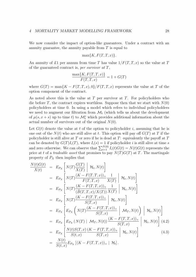
We now consider the impact of option-like guarantees. Under a contract with anannuity guarantee, the annuity payable from T is equal to
max{K, F (T, T, x)}.An annuity of £1 per annum from time T has value 1/F (T, T, x) so the value at Tof the guaranteed contract is, per survivor at T ,
max{K, F (T, T, x)}F (T, T, x)
= 1 + G(T )
where G(T ) = max{K − F (T, T, x), 0}/F (T, T, x) represents the value at T of theoption component of the contract.
As noted above this is the value at T per survivor at T . For policyholders whodie before T , the contract expires worthless. Suppose then that we start with N(0)policyholders at time 0. In using a model which refers to individual policyholderswe need to augment our filtration from Mt (which tells us about the developmentof µ(s, x + s) up to time t) to M∗
t which provides additional information about theactual number of survivors out of the original N(0).
Let G(t) denote the value at t of the option to policyholder i, assuming that he isone out of the N(t) who are still alive at t. This option will pay off G(T ) at T if thepolicyholder is still alive at T or zero if he is dead at T : equivalently the payoff at Tcan be denoted by G(T )Ii(T ), where Ii(s) = 1 if policyholder i is still alive at time s
and zero otherwise. We can observe that∑N(0)
i=1 Ii(t)G(t) = N(t)G(t) represents theprice at t of a tradeable asset that promises to pay N(T )G(T ) at T . The martingaleproperty of PX then implies that
N(t)G(t)
X(t)= EPX
[N(T )
G(T )
X(T )
∣∣∣∣ Ht, N(t)
]
= EPX
[N(T )
(K − F (T, T, x))+
F (T, T, x)
1
X(T )
∣∣∣∣ Ht, N(t)
]
= EPX
[N(T )
(K − F (T, T, x))+
(B(T, T, x)/X(T ))
1
X(T )
∣∣∣∣ Ht, N(t)
]
= EPX
[N(T )
(K − F (T, T, x))+
S(T, x)
∣∣∣∣ Ht, N(t)
]
= EPX
[EPX
(N(T )
(K − F (T, T, x))+
S(T, x)
∣∣∣∣ MT , N(t)
) ∣∣∣∣ Ht, N(t)
]
= EPX
[EPX
(N(T ) | MT , N(t))(K − F (T, T, x))+
S(T, x)
∣∣∣∣ Ht, N(t)
](4.2)
= EPX
[N(t)S(T, x)
S(t, x)
(K − F (T, T, x))+
S(T, x)
∣∣∣∣ Ht, N(t)
](4.3)
=N(t)
S(t, x)EPX
[ (K − F (T, T, x))+ | Ht] .
4 MORTALITY MARKET MODELLING FRAMEWORK 29
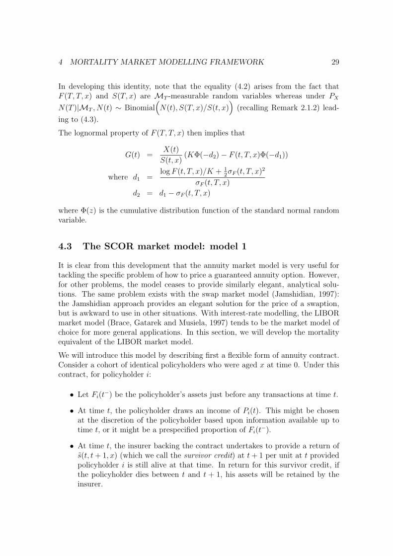
In developing this identity, note that the equality (4.2) arises from the fact thatF (T, T, x) and S(T, x) are MT -measurable random variables whereas under PX
N(T )|MT , N(t) ∼ Binomial(N(t), S(T, x)/S(t, x)
)(recalling Remark 2.1.2) lead-
ing to (4.3).
The lognormal property of F (T, T, x) then implies that
G(t) =X(t)
S(t, x)(KΦ(−d2)− F (t, T, x)Φ(−d1))
where d1 =log F (t, T, x)/K + 1
2σF (t, T, x)2
σF (t, T, x)
d2 = d1 − σF (t, T, x)
where Φ(z) is the cumulative distribution function of the standard normal randomvariable.
4.3 The SCOR market model: model 1
It is clear from this development that the annuity market model is very useful fortackling the specific problem of how to price a guaranteed annuity option. However,for other problems, the model ceases to provide similarly elegant, analytical solu-tions. The same problem exists with the swap market model (Jamshidian, 1997):the Jamshidian approach provides an elegant solution for the price of a swaption,but is awkward to use in other situations. With interest-rate modelling, the LIBORmarket model (Brace, Gatarek and Musiela, 1997) tends to be the market model ofchoice for more general applications. In this section, we will develop the mortalityequivalent of the LIBOR market model.
We will introduce this model by describing first a flexible form of annuity contract.Consider a cohort of identical policyholders who were aged x at time 0. Under thiscontract, for policyholder i:
• Let Fi(t−) be the policyholder’s assets just before any transactions at time t.
• At time t, the policyholder draws an income of Pi(t). This might be chosenat the discretion of the policyholder based upon information available up totime t, or it might be a prespecified proportion of Fi(t
−).
• At time t, the insurer backing the contract undertakes to provide a return ofs(t, t + 1, x) (which we call the survivor credit) at t + 1 per unit at t providedpolicyholder i is still alive at that time. In return for this survivor credit, ifthe policyholder dies between t and t + 1, his assets will be retained by theinsurer.

4 MORTALITY MARKET MODELLING FRAMEWORK 30
From the above description, the policyholder has no discretion over the choice ofinvestment strategy. The funds that a surviving policyholder will have at time(t + 1)− are then
Fi((t + 1)−) = (Fi(t−)− Pi(t))
(1 + s(t, t + 1, x)
).
The fair value for s(t, t + 1, x) requires that the value at t of the payoff at (t + 1)−
to the policyholder is equal to Fi(t−)− Pi(t). Thus
EQ
[C(t)
C(t + 1)Ii(t + 1)(1 + s(t, t + 1, x))
∣∣∣∣ Ht, Ii(t) = 1
]= 1
where Ii(t + 1) = 1 if policyholder i is still alive at t + 1 and zero otherwise.
Now we can follow a similar argument to that used with the annuity market modelto replace Ii(t + 1) in this expression with S(t + 1, x)/S(t, x). Noting also thats(t, t + 1, x) is set at time t, this implies that
B(t, t + 1, x)
B(t, t, x)(1 + s(t, t + 1, x)) = 1
⇒ s(t, t + 1, x) =B(t, t, x)− B(t, t + 1, x)
B(t, t + 1, x).
Now the construction of the survivor credit, s(t, t + 1, x), is reminiscent of howLIBOR rates are calculated. Indeed, if we set mortality rates to zero then s(t, t+1, x)is equal to the 12-month LIBOR rate
L(t, t, t + 1) =1− P (t, t + 1)
P (t, t + 1)
(using the forward LIBOR notation L(t, T0, T1) = (P (t, T0) − P (t, T1))/P (t, T1)).For this reason we choose to refer to s(t, t + 1, x) as the Survivor Credit Offer Rate,or SCOR.
Now let us define the forward SCOR. At time t, a contract is entered into betweenpolicyholder i (age x + t at time t) and the insurer that specifies that the survivorcredit payable between the future dates T and T + 1 will be s(t, T, T + 1, x). Underthis contract:
• No payment is made at t.
• If policyholder i is still alive at time T , he will pay £1 to the insurer at T .
• If policyholder i is still alive at time T +1, he will receive £1+ s(t, T, T +1, x)from the insurer at T + 1.

4 MORTALITY MARKET MODELLING FRAMEWORK 31
The value at t to the policyholder of this transaction is
(1 + s(t, T, T + 1, x)
)B(t, T + 1, x)
B(t, t, x)− B(t, T, x)
B(t, t, x).
The fair forward SCOR is thus
s(t, T, T + 1, x) =B(t, T, x)− B(t, T + 1, x)
B(t, T + 1, x).
Following the development of the LIBOR market model, we note that B(t, T, x) −B(t, T + 1, x) and B(t, T + 1, x) for t ≤ T are both tradeable assets. Since B(t, T +1, x) is also strictly positive we can use it as a numeraire. Thus there exists ameasure, PT+1,x under which U(t)/B(t, T + 1, x) is a martingale for any tradeableasset with price process U(t). Specifically s(t, T, T + 1, x) is a martingale underPT+1,x.
Now positive interest and positive mortality imply that 0 < B(t, T+1, x)/B(t, T, x) <1. It follows therefore that 0 < s(t, T, T + 1, x) < ∞, so we have the possibility tomodel s(t, T, T + 1, x) as a lognormal process. Thus we can write
ds(t, T, T+1, x) = s(t, T, T+1, x)(φP (t, T, T + 1, x)′dZ(T+1,x) + φB(t, T, T + 1, x)′dW (T+1,x)
)
for suitable previsible volatility vectors φP and φB and where Z(T+1,x)(t) and W (T+1,x)(t)are Brownian motions under PT+1,x.
Remark 4.3.1 It should be noted that while 0 < s(t, T, T + 1, x) < ∞ does guar-antee that 0 < B(t, T + 1, x)/B(t, T, x) < 1, it does not guarantee that pQ(t, T +1, x)/pQ(t, T, x) < 1: that is, there is a possibility that forward survival probabilitiesmight exceed 1.
We will address this drawback in model 2 below. However, the particular parametri-sation of the model may mean that the risk that this ratio exceeds 1 is very small.However, whatever the risk is, its consequences need to be carefully investigated.
Remark 4.3.2 If the volatility functions φP and φB are deterministic, s(u, T, T +1, x) for t < u ≤ T has a log-normal distribution under PT+1,x with
EPT+1,x[s(u, T, T + 1, x)|Ht] = s(t, T, T + 1, x)
and
V arPT+1,x[log s(u, T, T + 1, x)|Ht] =
∫ u
t
(|φP (v, T, T + 1, x)|2 + |φB(v, T, T + 1, x)|2) dv.

4 MORTALITY MARKET MODELLING FRAMEWORK 32
4.4 The SCOR market model: model 2
The SCOR market model 1 has several drawbacks including a restriction on theinvestment at T to a fixed quantity and the possibility that forward survival proba-bilities exceed 1 (as in Remark 4.3.1). We now adapt this basic model to circumventthese problems. Consider, therefore, the following forward contract struck at timet:
• At time t, no money exchanges hands.
• At time T , if the policyholder is still alive, he will pay £X(T ) to the insurer.We allow X(T ) to be random but restrict it to be FT -measurable (that is,adapted to the interest-rate model dynamics).
• At time T , the policyholder can choose how his fund of £X(T ) will be invested.
• At time T + 1, if the policyholder is still alive, he will receive £X(T )R(T +1)/R(T )(1 + s(t, T, T + 1, x)) where R(u) represents the price at u of a non-mortality-linked tradeable asset (that is, Ft-measurable) that reflects the pol-icyholder’s chosen previsible investment strategy. If the policyholder is notalive at T + 1, then the funds are retained by the insurer.
Remark 4.4.1 For convenience, we will continue to refer to s(t, T, T + 1, x) as theforward Survivor Credit Offer Rate, although it should be stressed that the definitionof this term is different from that under model 1.
Remark 4.4.2 The use of the SCOR in our modelling does not constrain us intolooking only at contracts whose benefits are defined in terms of the SCOR. Rather,the model provides us with a means of modelling the development of mortality ratesover time, since these can be easily backed out from the s(t, T, T + 1).
We now ask the question: what value of the forward SCOR, s(t, T, T +1, x), ensuresthat this contract has zero value at time t? Let I(u) be the indicator randomvariable that is equal to 1 if the policyholder is still alive at time u. Thus, for u > t,PrQ[I(u) = 1|I(t) = 1,Mu] = S(u, x)/S(t, x). For general S = 1 + s(t, T, T + 1, x)

4 MORTALITY MARKET MODELLING FRAMEWORK 33
the value at t is
EQ
[C(t)
C(T )X(T )
(C(T )
C(T + 1)
R(T + 1)
R(T )S I(T + 1)− I(T )
) ∣∣∣∣ Ht, I(t) = 1
]
= SEQ
[C(t)
C(T + 1)X(T )
R(T + 1)
R(T )
∣∣∣∣ Ft
]EQ[I(T + 1)|Mt, I(t) = 1]
−EQ
[C(t)
C(T )X(T )
∣∣∣∣ Ft
]EQ[I(T )|Mt, I(t) = 1]
= SEQ
[C(t)
C(T )X(T )
∣∣∣∣ Ft
]pQ(t, T + 1, x)
−EQ
[C(t)
C(T )X(T )
∣∣∣∣ Ft
]pQ(t, T, x) (recalling Remark 2.1.2)
which we require to be equal to zero to obtain the fair forward SCOR, s(t, T, T+1, x).This implies that
(1 + s(t, T, T + 1, x))pQ(t, T + 1, x)− pQ(t, T, x) = 0
⇒ s(t, T, T + 1, x) =pQ(t, T, x)− pQ(t, T + 1, x)
pQ(t, T + 1, x)
=B(t, T, x)−B(t, T + 1, x)
B(t, T + 1, x).
It follows that this revised SCOR market model has considerably wider applicabilitythan the SCOR model 1. Specifically, the policyholder can adopt any Ft-measurableinvestment strategy (but not strategies that depend, in addition, on changes in mor-tality). Furthermore, the amount of income that can be drawn from a policyholder’saccount can also be stochastic, provided it is an Ft-measurable process.
Now we need to investigate whether or not the forward SCOR can be constructedout of tradeable assets and this indeed turns out to be the case. Specifically, letR(t) be an Ft-adapted process that represents the price at t of a tradeable asset.Let D(t, T, x) represent the price at t for the investment and mortality-linked zero-coupon bond that pays R(T )S(T, x) at T . Clearly D(t, T, x) represents the price ofa tradeable asset (one that could be replicated using the P (t, T ) and the B(t, T, x)).Furthermore, since S(T, x) is independent of {Z(u) : 0 < u ≤ T}, we have
D(t, T, x) = EQ
[C(t)
C(T )R(T )S(T, x)|Ht
]
= EQ
[C(t)
C(T )R(T )|Ft
]EQ [S(T, x)|Mt]
= R(t)B(t, T, x).

4 MORTALITY MARKET MODELLING FRAMEWORK 34
Hence
s(t, T, T + 1, x) =B(t, T, x)−B(t, T + 1, x)
B(t, T + 1, x)(4.4)
=R(t)B(t, T, x)−R(t)B(t, T + 1, x)
R(t)B(t, T + 1, x)
=D(t, T, x)− D(t, T + 1, x)
D(t, T + 1, x).
As before there exists a measure PDT+1,x under which the process U(t)/D(t, T +1, x)
is a martingale for all tradeable-asset price processes U(t). Hence s(t, T, T + 1, x)is a martingale under PD
T+1,x. Since we are constraining ourselves to models underwhich B(t, T, x) is a decreasing function of T , we have s(t, T, T + 1, x) > 0. Hencethe SDE for s(t, T, T + 1, x) can be written in the form
ds(t, T, T + 1, x) = s(t, T, T + 1, x)ψB(t, T, T + 1, x)′dW (T+1,x) (4.5)
for a suitable previsible volatility vector ψB and W (T+1,x)(t) is a standard nW -dimensional Brownian motion under PD
T+1,x.
Remark 4.4.3 In contrast to model 1, model 2 does constrain the pQ(t, T, T +1, x)to lie between 0 and 1.
Remark 4.4.4 If the volatility function ψB(t, T, T+1, x) is deterministic, s(u, T, T+1, x) for t < u ≤ T has a log-normal distribution under PD
T+1,x with
EP DT+1,x
[s(u, T, T + 1, x)|Ht] = s(t, T, T + 1, x)
and V arP DT+1,x
[log s(u, T, T + 1, x)|Ht] =
∫ u
t
|ψB(v, T, T + 1, x)|2dv.
4.4.1 Simulation
Naturally we are interested in using the model to determine spot survival probabil-ities over a range of future dates T . So far equation (4.5) only tells us somethingabout the dynamics of a single forward SCOR, s(t, T, T +1, x). How do the dynamicsof the s(t, T, T + 1, x) interact for different T and how can they be simulated?
Application of the quotient rule for SDE’s to equation (4.4) gives us
ψB(t, T, T + 1, x) = (V (t, T, x)− V (t, T + 1, x))(1 + s(t, T, T + 1, x))
s(t, T, T + 1, x). (4.6)
Now define a series of future dates Tk = T0 + k for some T0 > 0 and k = 1, 2, . . ..Equation (4.6) can be rearranged to give
V (t, Tk, x)− V (t, Tk+1, x) =s(t, Tk, Tk+1, x)
(1 + s(t, Tk, Tk+1, x))ψB(t, Tk, Tk+1, x). (4.7)
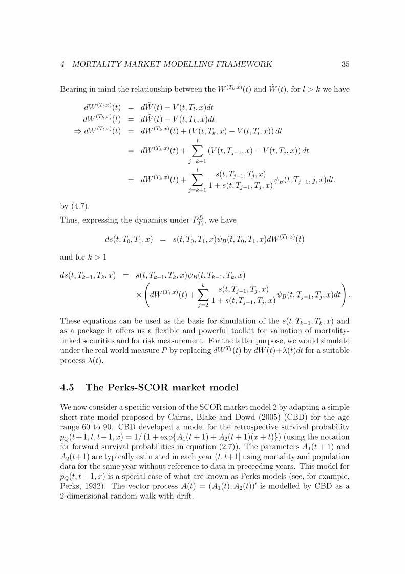
4 MORTALITY MARKET MODELLING FRAMEWORK 35
Bearing in mind the relationship between the W (Tk,x)(t) and W (t), for l > k we have
dW (Tl,x)(t) = dW (t)− V (t, Tl, x)dt
dW (Tk,x)(t) = dW (t)− V (t, Tk, x)dt
⇒ dW (Tl,x)(t) = dW (Tk,x)(t) + (V (t, Tk, x)− V (t, Tl, x)) dt
= dW (Tk,x)(t) +l∑
j=k+1
(V (t, Tj−1, x)− V (t, Tj, x)) dt
= dW (Tk,x)(t) +l∑
j=k+1
s(t, Tj−1, Tj, x)
1 + s(t, Tj−1, Tj, x)ψB(t, Tj−1, j, x)dt.
by (4.7).
Thus, expressing the dynamics under PDT1
, we have
ds(t, T0, T1, x) = s(t, T0, T1, x)ψB(t, T0, T1, x)dW (T1,x)(t)
and for k > 1
ds(t, Tk−1, Tk, x) = s(t, Tk−1, Tk, x)ψB(t, Tk−1, Tk, x)
×(
dW (T1,x)(t) +k∑
j=2
s(t, Tj−1, Tj, x)
1 + s(t, Tj−1, Tj, x)ψB(t, Tj−1, Tj, x)dt
).
These equations can be used as the basis for simulation of the s(t, Tk−1, Tk, x) andas a package it offers us a flexible and powerful toolkit for valuation of mortality-linked securities and for risk measurement. For the latter purpose, we would simulateunder the real world measure P by replacing dW T1(t) by dW (t)+λ(t)dt for a suitableprocess λ(t).
4.5 The Perks-SCOR market model
We now consider a specific version of the SCOR market model 2 by adapting a simpleshort-rate model proposed by Cairns, Blake and Dowd (2005) (CBD) for the agerange 60 to 90. CBD developed a model for the retrospective survival probabilitypQ(t+1, t, t+1, x) = 1/ (1 + exp{A1(t + 1) + A2(t + 1)(x + t)}) (using the notationfor forward survival probabilities in equation (2.7)). The parameters A1(t + 1) andA2(t+1) are typically estimated in each year (t, t+1] using mortality and populationdata for the same year without reference to data in preceeding years. This model forpQ(t, t + 1, x) is a special case of what are known as Perks models (see, for example,Perks, 1932). The vector process A(t) = (A1(t), A2(t))
′ is modelled by CBD as a2-dimensional random walk with drift.
4 MORTALITY MARKET MODELLING FRAMEWORK 36
In the model we adopt here, we apply the same process, A(t), to model one-yearspot survival probabilities rather than retrospective probabilities: that is,
pQ(t, t + 1, x) ≡ pQ(t, t, t + 1, x) =1
1 + eA1(t)+A2(t)(x+t). (4.8)
In the normal course of events, pQ(t, t + 1, x) will be a very accurate predictor ofpQ(t + 1, t, t + 1, x), so the change in concept used here does not undermine thesimple model proposed by CBD.
As commented above, analysis of historical data suggest that a reasonable model forthe discrete-time process A(t) = (A1(t), A2(t))
′ is a random walk with drift: that is,
A(t + 1) = A(t) + µ + C∆W (t + 1)
where µ is a 2×1, constant vector, C = (cij) is a 2×2 constant matrix and ∆W (t+1)is a 2× 1 vector of independent standard normal random variables.
Now we can easily write A(t) as a continuous process:
A(t) = A(0) + µt + CW (t)
where W (t) is a standard 2-dimensional Brownian motion. Thus dA(t) = µdt +CdW (t).
Returning to the SCOR market model, we are interested in modelling the futuredistribution of
s(T, T, T + 1, x) =1− pQ(T, T + 1, x)
pQ(T, T + 1, x)=
qQ(T, T + 1, x)
pQ(T, T + 1, x)
Now the Perks model above implies that
s(T, T, T + 1, x) = eA1(T )+A2(T )(x+T ).
Now we require the forward SCOR s(t, T, T +1, x) to be a martingale under PDT+1,x:
that is,
s(t, T, T + 1, x) = exp
[θ′ (A(t) + µ(T − t)) +
1
2θ′CC ′θ(T − t)
]
where θ =(1, (x + T )
)′. This implies that the volatility process for what we will
now call the Perks-SCOR market model should be
ψB(t, T, T + 1, x) = ν1 + ν2(x + T )
where ν1 =
(c11
c12
)
and ν2 =
(c21
c22
).

5 CONCLUSIONS 37
We then have the simple result that under PDT+1,x, s(T, T, T + 1, x) given s(t, T, T +
1, x) is log-normally distributed with
EP DT+1,x
[s(T, T, T + 1, x)|Mt] = s(t, T, T + 1, x)
and
V arP DT+1,x
[log s(T, T, T + 1, x)|Mt] =[(c11 + c21(x + T ))2 + (c12 + c22(x + T ))2
](T − t).
Remark 4.5.1 As we have noted before, the differences between the Perks-SCORmarket model and that of Cairns, Blake and Dowd (2005) are not great. The mech-anisms underlying a market model will, however, mean that the drift processes forthe two models are different.
5 Conclusions
We have presented here a number of theoretical frameworks that could be used forpricing many different types of mortality derivatives. More specifically, these frame-works demonstrate how an arbitrage-free (or risk-neutral) valuation methodologycan be used to price a great variety of mortality-related instruments, from vanillalongevity bonds to exotic mortality derivatives. These frameworks build on thosealready established for conventional interest-rate derivatives, and therefore help toshow how the existing literature on the valuation of interest-rate derivatives can beadapted to the valuation of derivatives involving mortality risk factors. They alsoprovide a basis for the future development of specific stochastic mortality models,which can be developed within the frameworks offered here.
Our valuation methodology is of course the same, in principle, as that used to pricederivatives based on other underlyings. As such, it is also open to exactly the samearguments over its merits. In particular, the use of arbitrage-free methods is al-ways problematic if markets are incomplete, as is certainly the case with mortalityderivatives markets. However, risk-free approaches provide natural benchmark val-uations, and one can also argue heuristically that they will become easier to justifyin any given context as markets become less incomplete over time. Naturally, wealso recognize that many of the assumptions underpinning these frameworks (suchas liquid, frictionless markets) do not hold in practice. Nevertheless, it is still thecase that, in such imperfect markets, if prices evolve in the way suggested by thesepricing frameworks, then the model will be arbitrage free. We are not assuming thatthe market must be complete, or that transactions costs must be zero or that assetsare infinitely divisible, and so on.
Needless to say, many challenges remain for future work. These challenges centrearound five main issues:

5 CONCLUSIONS 38
• Models: We need to investigate which models give adequate statistical de-scriptions of historical mortality data, and which models generate ‘reasonable’mortality dynamics.
• The number of risk factors: We need to determine how many risk factors areneeded to provide a satisfactory model of the mortality term structure. Is onerisk factor adequate, or do we need to have two or more factors to accommodateimperfectly correlated mortality improvements at different ages? One caneasily argue that multiple factors might be desirable because the factors thataffect mortality (medical advances, outbreaks of disease, etc.) are likely tohave different impacts on people of different ages.
• Basis risk vs. liquidity: As with other derivatives, there is the usual tradeoffbetween basis risk and liquidity. If we want to encourage the development ofmarket liquidity, then we would encourage standardized mortality instrumentstrading on organized exchanges; however, such instruments will embody con-siderable basis risk, which will reduce their usefulness as hedge instruments.Conversely, the basis risk for the primary client associated with tailor-made(or OTC) instruments will be low, but at the cost of poor liquidity. However,there are also other factors to consider. For example, the trading of mortalityderivatives can be encouraged by choosing ‘good’ reference populations for themortality indices (e.g., a good reference population might one be typical of thepopulation as a whole, or typical of the annuitant population). Furthermore,the market for mortality derivatives might be helped by the fact that mortal-ity risks have low market beta, and the willingness of investors to buy up theSwiss Re mortality-related bond is certainly encouraging.
• Index specification and moral hazard: The choice of index also needs to takeaccount of possible moral hazard. For example, can the index be manipulatedby the issuer of a security or by investors? Issuers of mortality-linked securitiescan learn from past experience of cat bond issuance, where moral hazard isalways present to some degree.8 A carefully-chosen index will not only increaseliquidity, as discussed above, but it will also reduce moral hazard. A conse-quence, though, is that this reduction is typically accompanied by increasedbasis risk for those wishing to use the security for hedging. With cat bonds,one of the principal ways to reduce moral hazard is to link the payments to anon-company-specific index rather than to the ceding company’s experience.The same arguments apply to mortality-related securities, although, perhaps,to a lesser degree: in other words, it is advisable that the survivor index definedin equation (2.1) is not calculated using the hedgers’ own mortality experience.
• The measurement-publication lag: How do we allow for the time lag between
8For a discussion of moral hazard as it relates to the issue of cat bonds, see, for example, thepapers by Doherty (1997) and Doherty and Richter (2002).

5 CONCLUSIONS 39
the measurement date and the date when mortality rates for that date havebeen graduated and made public? For example, is there something that canbe learned here from catastrophe derivatives, where information graduallyemerges after a catastrophic event? Connected to this issue is the need tospecify the contract in a way that minimises insider-trading moral hazard as-sociated with time lags in the release of information. This is a critical issue,not least because some early attempts to introduce non-life-insurance-linkedcatastrophe derivatives failed on precisely this point. We note though, thatthe Swiss Re mortality-related bond was issued successfully, implying thatinvestors must have been reassured on the issue of moral hazard.
In summary, mortality risks are an important new frontier in quantitative financialrisk. They offer intellectual challenges to those who study them and serious financialbenefits to those who trade them – and one would hope that they might also bringsignificant benefits to customers down the line.
Acknowledgements
The authors would like to thank both referees for their helpful comments on an earlierversion of this paper. AC would like to thank David Wilkie for some invaluablediscussions on the topic of mortality improvements and Vincent Vandier and JeanBerthon at AFPEN, Sam Cox, Kristian Miltersen and Svein-Arne Persson for someuseful insights. We are also grateful to Iain Currie for providing the data for Figures1.1 and 1.2 and to Owen Beelders for providing further details on the Swiss Remortality bond.
Part of this work was carried out while AC was a visitor at the Isaac NewtonInstitute, Cambridge during the Developments in Quantitative Finance Programme,and also when AC, DB and KD were in receipt of the ESRC research grant RES-000-23-1036: Survivor Derivatives.
References
Ahn, A.-H., Dittmar, R. F. and Gallant, A. R. (2002) Quadratic term structuremodels: theory and evidence. Review of Financial Studies, 15, 243288.
Artzner, P., and Delbaen, F. (1995) Default risk insurance and incomplete markets.Mathematical Finance, 5, 187-195.
Beelders, O., and Colarossi, D. (2004) Modelling mortality risk with extreme valuetheory: The case of Swiss Re’s mortality-indexed bond. Global Association ofRisk Professionals, 4 (July/August), 26-30.

5 CONCLUSIONS 40
Biffis, E. (2005) Affine processes for dynamic mortality and actuarial valuations.To appear in Insurance: Mathematics and Economics.
Biffis, E., and Millossovich, P. (2004) The fair value of guaranteed annuity options.Working paper, Bocconi University, Milan.
Biffis, E., and Millossovich, P. (2005) A bidimensional approach to mortality risk.Working paper, Bocconi University, Milan.
Black, F., and Karasinski, P. (1991) Bond and option pricing when short rates arelog-normal. Financial Analysts Journal, July-Aug, 52-59.
Blake, D., and Burrows, W. (2001) Survivor bonds: Helping to hedge mortalityrisk. Journal of Risk and Insurance, 68, 339-348.
Blake, D., Cairns, A.J.G., and Dowd, K. (2003) Pensionmetrics II: Stochasticpension plan design during the distribution phase. Insurance: Mathematics andEconomics, 33, 29-47.
Blake, D., Cairns, A.J.G., and Dowd, K. (2006) Living with mortality: longevitybonds and other mortality-linked securities. To appear in British Actuarial Jour-nal.
Brace, A., Gatarek, D., and Musiela, M. (1997) The market model of interest-ratedynamics. Mathematical Finance, 7, 127-155.
Brigo, D., and Mercurio, F. (2001) Interest Rate Models: Theory and Practice.Springer: Berlin.
Brouhns, N., Denuit, M., and Vermunt J.K. (2002) A Poisson log-bilinear regressionapproach to the construction of projected life tables. Insurance: Mathematics andEconomics, 31, 373-393.
Cairns, A.J.G. (2004a) A family of term-structure models for long-term risk man-agement and derivative pricing. Mathematical Finance, 14, 415-444.
Cairns, A.J.G. (2004b) Interest-Rate Models: An Introduction. PrincetonUniversity Press: Princeton.
Cairns, A.J.G., Blake, D., and Dowd, K. (2005) A two-factor model for stochasticmortality with parameter uncertainty. To appear in the Journal of Risk andInsurance.
Cairns, A.J.G., Blake, D., Dawson, P., and Dowd, K. (2005) Pricing the risk onlongevity bonds. Life and Pensions, October, 41-44.
Cairns, A.J.G., and Garcia Rosas, S.A. (2004) A family of term-structure modelswith stochastic volatility. In Proceedings of the 3rd World Congress of the BachelierSociety, Chicago, and Proceedings of the 35th International ASTIN Colloquium,Bergen.
CMI (1978) Proposed standard tables for life office pensioners and annuitants.

5 CONCLUSIONS 41
Continuous Mortality Investigation Reports, 3, 1-30.
CMI (1999) Projection factors for mortality improvement. Continuous MortalityInvestigation Reports, 17, 89-108.
Cox, S.H., Fairchild, J.R., and Pedersen, H.W. (2000) Economic aspects of securi-tization of risk. ASTIN Bulletin, 30, 157-193.
Cox, J., Ingersoll, J., and Ross, S. (1985) A theory of the term-structure of interestrates. Econometrica, 53, 385-408.
Cowley, A., and Cummins, J.D. (2005) Securitization of life insurance assets andliabilities. Journal of Risk and Insurance, 72, 193-226.
Currie I.D., Durban, M. and Eilers, P.H.C. (2004) Smoothing and forecastingmortality rates. Statistical Modelling, 4, 279-298.
Dahl, M. (2004) Stochastic mortality in life insurance: Market reserves andmortality-linked insurance contracts. Insurance: Mathematics and Economics,35, 113-136.
Dahl, M., and Møller, T. (2005) Valuation and hedging of life insurance liabilitieswith systematic mortality risk. In Proceedings of the 15th International AFIRColloquium, Zurich. (Available online at http://www.afir2005.ch)
Doherty, N.A. (1997) Innovations in managing catastrophe risk. Journal of Riskand Insurance, 64, 713-718.
Doherty, N.A., and Richter, A. (2002) Moral hazard, basis risk, and gap insurance.Journal of Risk and Insurance, 69, 9-24.
Dowd, K., Blake, D., Cairns, A.J.G., and Dawson, P. (2006) Survivor swaps. Toappear in Journal of Risk and Insurance.
Duffie, D., and Kan, R. (1996) A yield-factor model of interest rates. Mathe-matical Finance, 6, 379-406.
Flesaker, B., and Hughston, L.P. (1996) Positive interest. Risk, 9(1), 46-49.
Forfar, D.O., and Smith, D.M. (1987) The changing shape of English life Tables.Transactions of the Faculty of Actuaries, 40, 98-134.
Froot, K.A., and Stein, J.C. (1998) Risk management, capital budgeting, andcapital structure policy for financial institutions: an integrated approach. Journalof Financial Economics, 47, 55-82.
Heath, D., Jarrow, R. and Morton, A. (1992) Bond pricing and the term structure ofinterest rates: A new methodology for contingent claims valuation. Econometrica,60, 77-105.
James, J., and Webber, N. (2000) Interest Rate Modelling. Wiley: Chichester.
Jamshidian, F. (1997) LIBOR and swap market models and measures. Finance

5 CONCLUSIONS 42
and Stochastics, 1, 293-330.
Joint Mortality Investigation Committee (JMIC) (1974) Considerations affectingthe preparation of standard tables of mortality. Journal of the Institute ofActuaries, 101, 135-201.
Karatzas, I., and Shreve, S.E. (1998) Methods of Mathematical Finance. Springer-Verlag: New York.
Lando, D. (2004) Credit Risk Modeling: Theory and Applications. PrincetonUniversity Press: Princeton.
Lane, M.N. (2000) Pricing risk transfer transactions. ASTIN Bulletin, 30,259-293.
Lee, P.J. (2000a) A general framework for stochastic investigations of mortalityand investment risks. Presented at the Wilkiefest, Heriot-Watt University, March2000.
Lee, R. (2000b) The Lee-Carter method for forecasting mortality, with variousextensions and applications. North American Actuarial Journal, 4, 80-93.
Lee, R.D., and Carter, L.R. (1992) Modeling and forecasting U.S. mortality.Journal of the American Statistical Association, 87, 659-675.
Lin, Y., and Cox, S.H. (2005a) Securitization of mortality risks in life annuities.Journal of Risk and Insurance, 72, 227-252.
Lin, Y., and Cox, S.H. (2005b) A mortality securitization model. Working paper,Georgia State University.
Luciano, E., and Vigna, E. (2005) Non mean reverting affine processes for stochasticmortality. In Proceedings of the 15th International AFIR Colloquium, Zurich.(Available online at http://www.afir2005.ch)
Macdonald, A.S., Cairns, A.J.G., Gwilt, P.L., and Miller, K.A. (1998) An inter-national comparison of recent trends in population mortality. British ActuarialJournal, 4, 3-141.
Macdonald, A.S., Bartlett, D., Berman, C., Daykin, C., Grimshaw, D., Savill, P.(2003) Mortality improvements and the cohort effect. CMI Working Papers 1and 2; Presented to the Staple Inn Actuarial Society on 11 March 2003; 46 pages.(Available online at http://www.sias.org.uk)
Marocco, P., and Pitacco, E. (1998) Longevity risk and life annuity reinsurance.In Transactions of the 26th International Congress of Actuaries, Birmingham, 6:453-479.
Milevsky, M.A., and Promislow, S.D. (2001) Mortality derivatives and the optionto annuitise. Insurance: Mathematics and Economics, 29, 299-318.
Miltersen, K.R., and Persson, S.-A. (2005) Is mortality dead? Stochastic forward

5 CONCLUSIONS 43
force of mortality determined by no arbitrage. Working paper, University ofBergen.
Miltersen, K., Sandmann, K. and Sondermann, D. (1997) Closed-form solutionsfor term structure derivatives with log-normal interest rates. Journal of Finance,52, 409430.
Muermann, A. (2004) Catastrophe derivatives. In The Encyclopaedia of ActuarialScience, Volume 1, pages 231-236, Wiley, Chichester.
Olivier, P., and Jeffery, T. (2004) Stochastic mortality models. Presentation tothe Society of Actuaries of Ireland.(Available online at http://www.actuaries.ie/Resources/events papers/PastCalendarListing.htm)
Pelsser, A. (2003) Pricing and hedging guaranteed annuity options via static optionreplication. Insurance: Mathematics and Economics, 33, 283-296.
Perks, W. (1932) On some experiments in the graduation of mortality statistics.Journal of the Institute of Actuaries, 63, 12-57.
Pitacco, E. (2002) Longevity risk in living benefits. Presented at the third annualCeRP conference “Developing an Annuity Market in Europe”, Turin.
Rebonato, R. (2002) Modern Pricing of Interest-Rate Derivatives. PrincetonUniversity Press: Princeton.
Renshaw, A.E., and Haberman, S. (2003) Lee-Carter mortality forecasting withage-specific enhancement. Insurance: Mathematics and Economics, 33, 255-272.
Rogers, L.C.G. (1997) The potential approach to the term-structure of interestrates and foreign exchange rates. Mathematical Finance, 7, 157-164.
Rutkowski, M. (1997) A note on the Flesaker & Hughston model of the termstructure of interest rates. Applied Mathematical Finance, 4, 151-163.
Schmock, U. (1999) Estimating the value of the WINCAT coupons of the WintherthurInsurance Convertible Bond: A study of the model risk. ASTIN Bulletin, 29,101-163.
Schonbucher, P. (2003) Credit Derivatives Pricing Models: Models Pricing andImplementation. Wiley: Chichester.
Smith, A.D. (2005) Stochastic mortality modelling. Presentation at the Workshopon the Interface between Quantitative Finance and Insurance, Edinburgh, April2005.(Available online at www.icms.org.uk/meetings/2005/quantfinance/sci prog.html)
Vasicek, O. (1977) An equilibrium characterisation of the term structure. Journalof Financial Economics, 5, 177-188.
Wang, S.S. (1996) Premium calculation by transforming the layer premium density.ASTIN Bulletin, 26, 71-92.

5 CONCLUSIONS 44
Wang, S.S. (2000) A class of distortion operations for pricing financial and insurancerisks. Journal of Risk and Insurance, 67, 15-36.
Wang, S.S. (2002) A universal framework for pricing financial and insurance risks.ASTIN Bulletin, 32, 213-234.
Wang, S.S. (2003) Equilibrium pricing transforms: new results using Buhlmann’s1980 economic model. ASTIN Bulletin, 33, 57-73.
Willets, R.C. (1999) Mortality in the next millenium. Presented to the StapleInn Actuarial Society on 7 December 1999. (Available online at www.sias.org.uk.)
Yang, S. (2001) Reserving, pricing and hedging for guaranteed annuity options.PhD Thesis, Heriot-Watt University, Edinburgh.
Yang, S., and Huang, H.C. (2005) Optimal contribution rate and asset allocationfor defined contribution pension plan incorporating longevity risk. Working paper,Soochow University, Taiwan.

A THE LEE AND CARTER MODEL FOR STOCHASTIC MORTALITY 45
Appendices
A The Lee and Carter model for stochastic mor-
tality
Lee and Carter (1992) investigate the dynamics of the observed central mortalityrates m(t, x) for integer t and x. Their model breaks m(t, x) down into a log-bilinearmodel
log m(t, x) = a(x) + b(x)k(t)
with the translation and scaling constraints that∑
x b(x) = 1 and∑T1
t=T0k(t) =
0. a(x) and b(x) are non-parametric functions without any smoothing applied orfunctional form. Stage 1 of the modelling process estimates the functions a(x), b(x)and k(t) without reference to a dynamic model for k(t). For a given functional formfor a(x) and b(x), k(t) is estimated directly using the data for date t in isolation andwithout any assumption about its dynamic form. This is repeated until we optimisethe fit over a(x) and b(x) subject to the scaling constraints above. Stage 2 of themodelling process then fits an ARIMA process to the k(t).
B The Lee and Yang model for stochastic mor-
tality
Lee (2000a) and Yang (2001) proposed the following model for stochastic mortality.
Suppose that a deterministic forecast of annual mortality rates is made at time 0.Thus q(x, t) represents the probability (as estimated at time 0) that an individualaged x at time t will die before time t + 1 for each integer x and t. The actualmortality experience is modelled as
q(x, t) = q(x, t) exp
[X(t)− 1
2σ2
Y + σY ZY (t)
]
where X(t) = X(t− 1)− 1
2σ2
X + σXZX(t)
and ZX(t) and ZY (t) are mutually independent sequences of i.i.d. standard normalrandom variables.
It follows that the X(t) models the stochastic trend in the development of themortality curve while the −1
2σ2
Y + σY ZY (t) models one-off environmental variationsin mortality (such as a major flu epidemic). From the limited data available, Yangfound that σY was not significantly different from 0. In contrast, however, Linand Cox (2005b), using a longer run of US population data and a slightly different
C THE MILEVSKY AND PROMISLOW MODEL FOR STOCHASTIC MORTALITY46
model, found that mortality jumps of the type represented by σY ZY (t) above doform a significant part of the development of mortality over time.
Note that while q(x, t) is an unbiased estimate for q(x, t), the use of q(x, t) willnot produce, in general, unbiased estimates for other quantities: for example, thesurvivor index, S(t, x).
C The Milevsky and Promislow model for stochas-
tic mortality
Milevsky and Promislow (2001) model the force of mortality in the form µ(t, x) =ξ0 exp(ξ1x+Yt) where Yt is an Ornstein-Uhlenbeck process with SDE dYt = −αYtdt+σdWt. Essentially this is equivalent to a Gompertz model with a time-varying scalingfactor.
D The Dahl model for stochastic mortality
Dahl (2004) models the process for µ(t, x + t) as follows
dµ(t, x + t) = αµ(t, x, µ(t, x + t))dt + σµ(t, x, µ(t, x + t))dW (t). (D.1)
He finds that if the drift and volatility are of the form
αµ(t, x, µ(t, x + t)) = δα(t, x)µ(t, x + t) + ζα(t, x)
and σµ(t, x, µ(t, x + t)) =√
δσ(t, x)µ(t, x + t) + ζσ(t, x)
for some deterministic functions δα(t, x), δσ(t, x), ζα(t, x) and ζσ(t, x) then
pQ(t, T, x) = eA(t,T,x)−B(t,T,x)µ(t,x+t)
where the deterministic functions A(t, T, x) and B(t, T, x) are derived from differ-ential equations involving δα(t, x), δσ(t, x), ζα(t, x) and ζσ(t, x).
Dahl’s affine model has been extended by Biffis (2005) who added a jump processinto the SDE (D.1).

D THE DAHL MODEL FOR STOCHASTIC MORTALITY 47
Andrew J.G. CairnsDepartment of Actuarial Mathematics and StatisticsSchool of Mathematical and Computer SciencesHeriot-Watt UniversityEdinburgh, EH14 4ASUnited Kingdom
David BlakePensions InstituteCass Business School106 Bunhill RowLondon, EC1Y 8TZUnited Kingdom
Kevin DowdCentre for Risk & Insurance StudiesNottingham University Business SchoolJubilee CampusNottingham, NG8 1BBUnited Kingdom