pricing distressed cdos with base correlation and...

Working Paper Series

n. 01 ■ May 2010

Pricing distressed CDOs with Base Correlation and Stochastic Recovery

Martin Krekel

1 WORKING PAPER SERIES N. 01 - MAY 2010 ■

Statement of Purpose

The Working Paper series of the UniCredit & Universities Foundation is designed to disseminate and

to provide a platform for discussion of either work of the UniCredit Group economists and researchers

or outside contributors (such as the UniCredit & Universities scholars and fellows) on topics which are

of special interest to the UniCredit Group. To ensure the high quality of their content, the contributions

are subjected to an international refereeing process conducted by the Scientific Committee members

of the Foundation.

The opinions are strictly those of the authors and do in no way commit the Foundation and UniCredit

Group.

Scientific Committee

Franco Bruni (Chairman), Silvia Giannini, Tullio Jappelli, Catherine Lubochinsky, Giovanna Nicodano,

Reinhard H. Schmidt, Josef Zechner

Editorial Board

Annalisa Aleati

Giannantonio de Roni

The Working Papers are also available on our website (http://www.unicreditanduniversities.eu)

Pricing distressed CDOs with Base Correlation andStochastic Recovery

Dr. Martin Krekel

UniCredit Group

Corporate & Investment Banking

Quantitative Product Group - Credit Markets

Abstract

In February and March 2008 it was temporarily not possible to calibrate the standard Gaussian

Base correlation model to the complete set of CDX.IG and ITRAXX.IG CDO tranche quotes.

For instance, in CDX.IG it failed for the 15% - 30% senior tranche and hence the sucessive

30% - 100% tranche. The reason is that the Gaussian Base correlation model was not able to

generate enough probability for high portfolio losses, while preserving the calibration to mez-

zanine and equity tranches. We introduce a Gaussian Base correlation model with correlated

stochastic recovery rates to overcome this problem. Moreover, our model can be used to price

super senior tranches (e.g. 60% - 100%), which have a fair spread of zero in a standard copula

model with fixed recovery.

Keywords:

CDO, Base Correlation, Stochastic Recovery, Gaussian Copula

JEL Codes:

G13

WORKING PAPER SERIES N.01 - May 2010 • 2

1 Introduction

In February and March 2008 it was temporarily not possible to calibrate the Gaussian Base

correlation model to CDX.IG and ITRAXX.IG CDO market quotes of senior tranches (.e.g 15%

- 30% in CDX). The reason is that the Gaussian Base correlation was not able to generate

enough probability for high portfolio losses while preserving the calibration to mezzanine and

equity tranches. We introduce a Gaussian Base Correlation model with correlated stochastic

recovery rates to overcome this calibration problem. We this extension the calibration range of

the Base correlation model is significantly widen and in addition it will enable us to price super

senior tranches with attachment points outside the range of fixed recoveries. Random recovery

was already introduced by [1, Andersen, Sidenius (2004)]. They modelled the recovery rate as

a function of the common market factor and additional idiosyncratic risk factors. In contradiction

to this approach, in our model the recovery rate is driven by the default triggering factor which

circumvents some technical issues. The discrete recovery rate distribution is user input and

can arbitrarily be chosen.

The rest of the paper is organized as follows. In section 2 we shortly recapitulate the well-

known Gaussian copula model and in section 3 we present our stochastic recovery extension.

Section 4 contains the calibration results in distressed CDO markets and a derivation of the

recovery correlation. Finally, we present our conclusion in section 5.

2 Standard Gaussian Copula Model

Let’s assume the CDO index contains M obligors and the default probability of issuer m at time

Ti is labeled with qmi , where Ti (i = 1, . . . , I) are the coupon payment dates (These probabilities

are usually bootstrapped from the CDS quotes). The default triggering variable for Xmi at time

Ti for debtor m is modelled by

Xmi =

√ρZ0

i +√

1− ρZmi ,

Xmi ≤ cm

i ≡ τm ≤ Ti,

where Z0i is the systematic factor and Zm

i (m = 1, . . . ,M) are the idiosyncratic factors. These

random variables are independent and identically Gaussian distributed. Hence, Xmi is also

standard Gaussian distributed (denoted by N ) and the correlation between two factors Xmi

and Xni is ρ. We call this correlation the factor correlation, not to shuffle with the real default

correlation defined by COR[1{τm≤Ti, 1{τn≤Ti

], which is usually different. With

cmi := N−1(qm

i )


we achieve

P (Xmi ≤ cm

i ) = qmi

and

P (τm ≤ Ti|Z0i = z) ≡ P

(Xm

i ≤ cmi

∣∣Z0i = z

)= P

(√ρz +

√1− ρZm

i ≤ cmi

∣∣Z0i = z

)= P

(Zm

i ≤cmi −√ρz√

1− ρ

∣∣∣∣∣Z0i = z

)

= N(

cmi −√ρz√

1− ρ

).

If issuer m defaults, the portfolio notional is reduced by the nominal Nm times one minus the

quoted recovery rate, namely Nm(1− RECm). The cumulative loss Li until Ti is thus given by

Li =M∑

m=1

Nm(1− RECm)11{τm≤Ti}.

Conditioned on Z0i = z the loss distribution is a convolution of independent Bernoulli variables.

Methods to calculate respectively approximate this loss distribution can be found amongst oth-

ers in [1, Andersen & Sidenius (2004)], [2, Hull & White (2004)] or [3, Laurent & Gregory

(2004)]

For a tranche [A,D] with attachment point A and detachment point D in monetary units the

normalized cumulative loss of the tranche is defined as

LA,Di =

min((Lt −A)+ , (D −A)

)D −A

.

Let s be the annualized premium, Dfi the (riskless) discount factors and αi the year fractions.

The present values of the premium leg and credit leg are calculated as 1

PVPremLeg = E

[s

I∑i=1

Dfi αi

(1− LA,D

i

)]

= s

I∑i=1

Dfi αi

(1−

∫IR

E

[LA,D

i

∣∣∣∣Z0i = z

]fN (z)dz

),

PVCreditLeg = E

[I∑

i=1

(Dfi

(LA,D

i − LA,Di−1

)]

=I∑

i=1

Dfi

(∫IR

E

[LA,D

i

∣∣∣∣Z0i = z

]fN (z)dz

−∫

IRE

[LA,D

i−1

∣∣∣∣Z0i = z

]fN (z)dz

),

1We neglect the accrued for the ease of notation.


where fN is density of the standard normal distribution. That means we need to calculate the

expected tranche losses at each payment date. The remaining computations are trivial.

In the base correlation framework, introduced by [5, Lee McGinty et all (2004)], the tranche

losses are calculated by

E[LA,Di ] :=

D E[L0,Di ]−A E[L0,A

i ]D −A

where for the equity tranches different correlation are used. Additional constraints maybe added

to prevent from arbitrage.

3 Gaussian Copula Model with Stochastic Recovery

To induce stochastic recovery in the Gaussian copula framework we firstly choose for each

obligor m a discrete (marginal) recovery distribution Rmi conditioned on default (i.e. τm < Ti)

Rmi,τm≤Ti

=

rm1 with probability pm

1


2...

......

rmJ with probability pm

J

(1)

with

J∑j=1

pmj = 1,

J∑j=1

pmj rm

j = RECm,

and rmj (j = 1, . . . , J) the attainable recovery rates, pm

j (j = 1, . . . , J) the corresponding proba-

bilities.

While choosing the recovery rate distribution we have to make sure, that the average recovery

rate equals the quoted recovery rate RECm, used for bootstrapping the survival probabilities. It

is important to stress the fact, that the probabilities conditioned on default have that property,

otherwise our model would not be consistent with the single name CDS market and thereby

would not price the corresponding portfolio CDS correctly. A feasible distribution is for instance

Rmi,τm≤Ti

=

60% with probability 40%




. (2)

Of course a finer distribution can be used, which could make sense for bespoke super senior

tranches. But for standard tranches this distribution works very well.


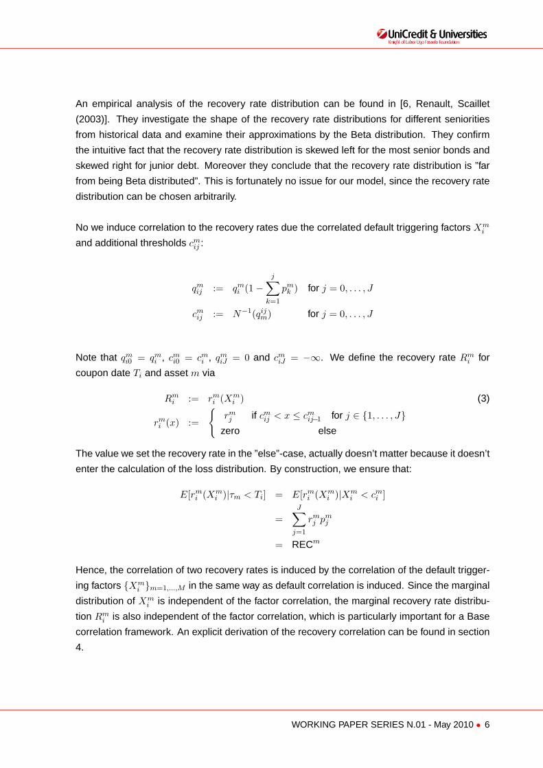
An empirical analysis of the recovery rate distribution can be found in [6, Renault, Scaillet

(2003)]. They investigate the shape of the recovery rate distributions for different seniorities

from historical data and examine their approximations by the Beta distribution. They confirm

the intuitive fact that the recovery rate distribution is skewed left for the most senior bonds and

skewed right for junior debt. Moreover they conclude that the recovery rate distribution is ”far

from being Beta distributed”. This is fortunately no issue for our model, since the recovery rate

distribution can be chosen arbitrarily.

No we induce correlation to the recovery rates due the correlated default triggering factors Xmi

and additional thresholds cmij :

qmij := qm

i (1−j∑

k=1

pmk ) for j = 0, . . . , J

cmij := N−1(qij

m) for j = 0, . . . , J

Note that qmi0 = qm

i , cmi0 = cm

i , qmiJ = 0 and cm

iJ = −∞. We define the recovery rate Rmi for

coupon date Ti and asset m via

Rmi := rm

i (Xmi ) (3)

rmi (x) :=

{rmj if cm

ij < x ≤ cmij−1 for j ∈ {1, . . . , J}

zero else

The value we set the recovery rate in the ”else”-case, actually doesn’t matter because it doesn’t

enter the calculation of the loss distribution. By construction, we ensure that:

E[rmi (Xm

i )|τm < Ti] = E[rmi (Xm

i )|Xmi < cm

i ]

=J∑

j=1

rmj pm

j

= RECm

Hence, the correlation of two recovery rates is induced by the correlation of the default trigger-

ing factors {Xmi }m=1,...,M in the same way as default correlation is induced. Since the marginal

distribution of Xmi is independent of the factor correlation, the marginal recovery rate distribu-

tion Rmi is also independent of the factor correlation, which is particularly important for a Base

correlation framework. An explicit derivation of the recovery correlation can be found in section

4.


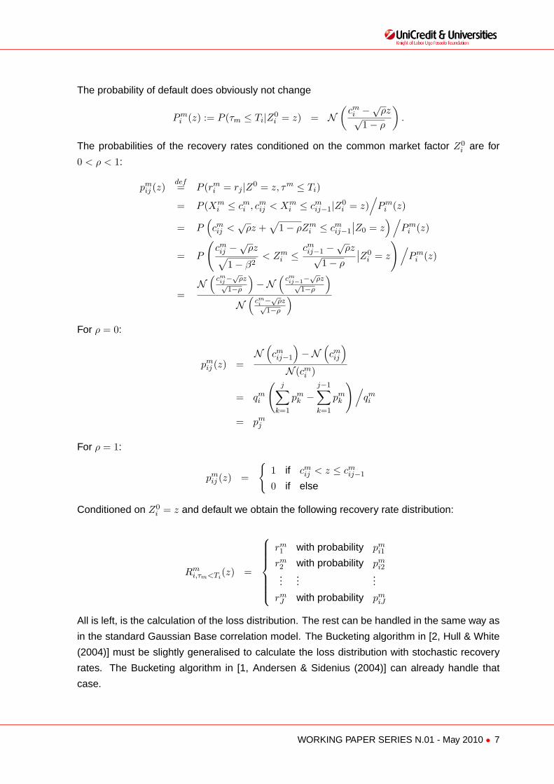
The probability of default does obviously not change

Pmi (z) := P (τm ≤ Ti|Z0

i = z) = N(

cmi −√ρz√

1− ρ

).

The probabilities of the recovery rates conditioned on the common market factor Z0i are for

0 < ρ < 1:

pmij (z)

def= P (rm

i = rj |Z0 = z, τm ≤ Ti)

= P (Xmi ≤ cm

i , cmij < Xm

i ≤ cmij−1|Z0

i = z)/

Pmi (z)

= P(cmij <

√ρz +

√1− ρZm

i ≤ cmij−1

∣∣Z0 = z)/

Pmi (z)

= P

(cmij −

√ρz√

1− β2< Zm

i ≤cmij−1 −

√ρz

√1− ρ

∣∣Z0i = z

)/Pm

i (z)

=N(

cmij−

√ρz

√1−ρ

)−N

(cmij−1−

√ρz

√1−ρ

)N(

cmi −

√ρz√

1−ρ

)For ρ = 0:

pmij (z) =

N(cmij−1

)−N

(cmij

)N (cm

i )

= qmi

(j∑

k=1

pmk −

j−1∑k=1

pmk

)/qmi

= pmj

For ρ = 1:

pmij (z) =

{1 if cm

ij < z ≤ cmij−1

0 if else

Conditioned on Z0i = z and default we obtain the following recovery rate distribution:

Rmi,τm<Ti

(z) =


i1


i2...

......

rmJ with probability pm

iJ

All is left, is the calculation of the loss distribution. The rest can be handled in the same way as

in the standard Gaussian Base correlation model. The Bucketing algorithm in [2, Hull & White

(2004)] must be slightly generalised to calculate the loss distribution with stochastic recovery

rates. The Bucketing algorithm in [1, Andersen & Sidenius (2004)] can already handle that

case.


4 Numerical Results

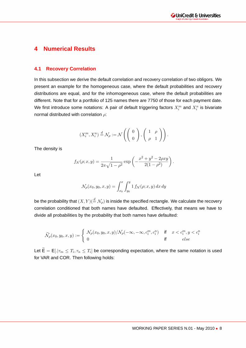
4.1 Recovery Correlation

In this subsection we derive the default correlation and recovery correlation of two obligors. We

present an example for the homogeneous case, where the default probabilities and recovery

distributions are equal, and for the inhomogeneous case, where the default probabilities are

different. Note that for a portfolio of 125 names there are 7750 of those for each payment date.

We first introduce some notations: A pair of default triggering factors Xmi and Xn

i is bivariate

normal distributed with correlation ρ:

(Xmi , Xn

i ) d= Nρ := N

((0

0

),

(1 ρ

ρ 1

)).

The density is

fN (ρ;x, y) =1

2π√

1− ρ2exp

(−x2 + y2 − 2ρxy

2(1− ρ2)

).

Let

Nρ(x0, y0, x, y) =∫ x

x0

∫ y

y0

1 fN (ρ;x, y) dx dy

be the probability that (X, Y )( d= Nρ) is inside the specified rectangle. We calculate the recovery

correlation conditioned that both names have defaulted. Effectively, that means we have to

divide all probabilities by the probability that both names have defaulted:

Nρ(x0, y0, x, y) :=

{Nρ(x0, y0, x, y)/Nρ(−∞,−∞, cm

i , cni ) if x < cm

i , y < cni

0 if else

Let E = E[.|τm ≤ Ti, τn ≤ Ti] be corresponding expectation, where the same notation is used

for VAR and COR. Then following holds:


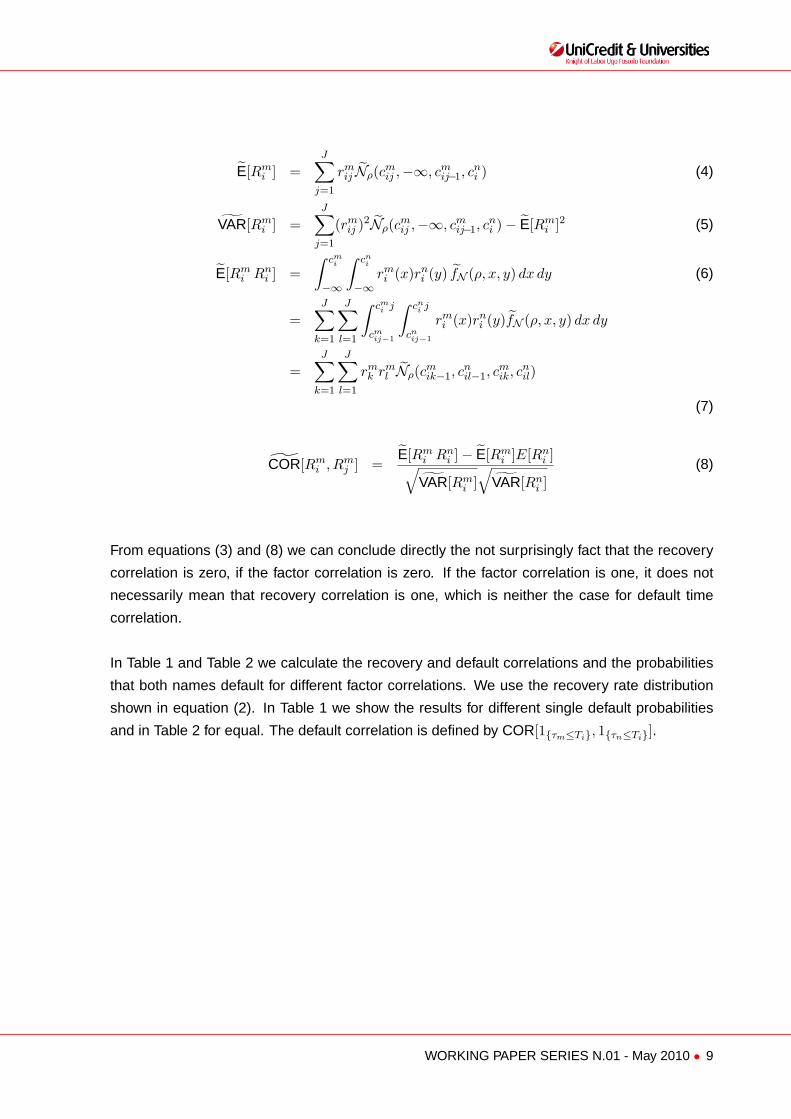
E[Rmi ] =

J∑j=1

rmij Nρ(cm

ij ,−∞, cmij−1, c

ni ) (4)

VAR[Rmi ] =

J∑j=1

(rmij )2Nρ(cm

ij ,−∞, cmij−1, c

ni )− E[Rm

i ]2 (5)

E[Rmi Rn

i ] =∫ cm

i

−∞

∫ cni

−∞rmi (x)rn

i (y) fN (ρ, x, y) dx dy (6)

=J∑

k=1

J∑l=1

∫ cmi j

cmij−1

∫ cni j

cnij−1

rmi (x)rn

i (y)fN (ρ, x, y) dx dy

=J∑

k=1

J∑l=1

rmk rm

l Nρ(cmik−1, c

nil−1, c

mik, c

nil)

(7)

COR[Rmi , Rm

j ] =E[Rm

i Rni ]− E[Rm

i ]E[Rni ]√

VAR[Rmi ]√

VAR[Rni ]

(8)

From equations (3) and (8) we can conclude directly the not surprisingly fact that the recovery

correlation is zero, if the factor correlation is zero. If the factor correlation is one, it does not

necessarily mean that recovery correlation is one, which is neither the case for default time

correlation.

In Table 1 and Table 2 we calculate the recovery and default correlations and the probabilities

that both names default for different factor correlations. We use the recovery rate distribution

shown in equation (2). In Table 1 we show the results for different single default probabilities

and in Table 2 for equal. The default correlation is defined by COR[1{τm≤Ti}, 1{τn≤Ti}].


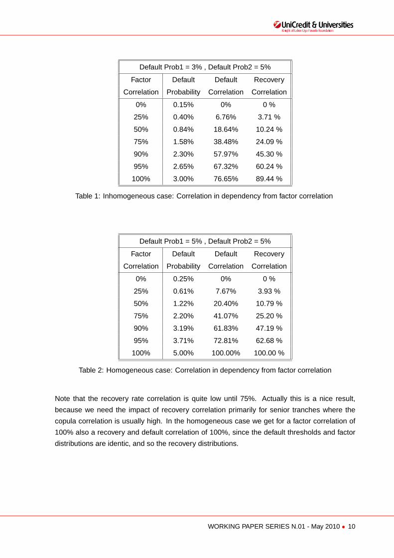
Default Prob1 = 3% , Default Prob2 = 5%

Factor Default Default Recovery

Correlation Probability Correlation Correlation

0% 0.15% 0% 0 %

25% 0.40% 6.76% 3.71 %

50% 0.84% 18.64% 10.24 %

75% 1.58% 38.48% 24.09 %

90% 2.30% 57.97% 45.30 %

95% 2.65% 67.32% 60.24 %

100% 3.00% 76.65% 89.44 %

Table 1: Inhomogeneous case: Correlation in dependency from factor correlation

Default Prob1 = 5% , Default Prob2 = 5%

Factor Default Default Recovery

Correlation Probability Correlation Correlation

0% 0.25% 0% 0 %

25% 0.61% 7.67% 3.93 %

50% 1.22% 20.40% 10.79 %

75% 2.20% 41.07% 25.20 %

90% 3.19% 61.83% 47.19 %

95% 3.71% 72.81% 62.68 %

100% 5.00% 100.00% 100.00 %

Table 2: Homogeneous case: Correlation in dependency from factor correlation

Note that the recovery rate correlation is quite low until 75%. Actually this is a nice result,

because we need the impact of recovery correlation primarily for senior tranches where the

copula correlation is usually high. In the homogeneous case we get for a factor correlation of

100% also a recovery and default correlation of 100%, since the default thresholds and factor

distributions are identic, and so the recovery distributions.


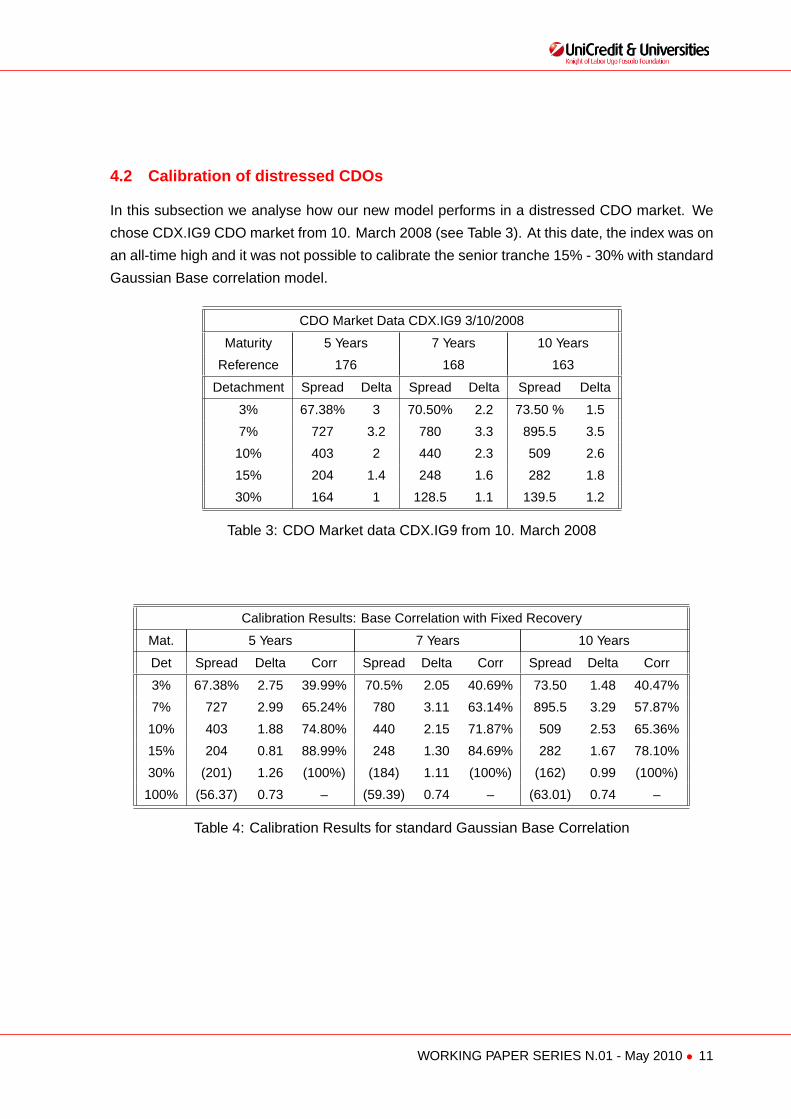
4.2 Calibration of distressed CDOs

In this subsection we analyse how our new model performs in a distressed CDO market. We

chose CDX.IG9 CDO market from 10. March 2008 (see Table 3). At this date, the index was on

an all-time high and it was not possible to calibrate the senior tranche 15% - 30% with standard

Gaussian Base correlation model.

CDO Market Data CDX.IG9 3/10/2008

Maturity 5 Years 7 Years 10 Years

Reference 176 168 163

Detachment Spread Delta Spread Delta Spread Delta

3% 67.38% 3 70.50% 2.2 73.50 % 1.5

7% 727 3.2 780 3.3 895.5 3.5

10% 403 2 440 2.3 509 2.6

15% 204 1.4 248 1.6 282 1.8

30% 164 1 128.5 1.1 139.5 1.2

Table 3: CDO Market data CDX.IG9 from 10. March 2008

Calibration Results: Base Correlation with Fixed Recovery

Mat. 5 Years 7 Years 10 Years

Det Spread Delta Corr Spread Delta Corr Spread Delta Corr

3% 67.38% 2.75 39.99% 70.5% 2.05 40.69% 73.50 1.48 40.47%

7% 727 2.99 65.24% 780 3.11 63.14% 895.5 3.29 57.87%

10% 403 1.88 74.80% 440 2.15 71.87% 509 2.53 65.36%

15% 204 0.81 88.99% 248 1.30 84.69% 282 1.67 78.10%

30% (201) 1.26 (100%) (184) 1.11 (100%) (162) 0.99 (100%)

100% (56.37) 0.73 – (59.39) 0.74 – (63.01) 0.74 –

Table 4: Calibration Results for standard Gaussian Base Correlation


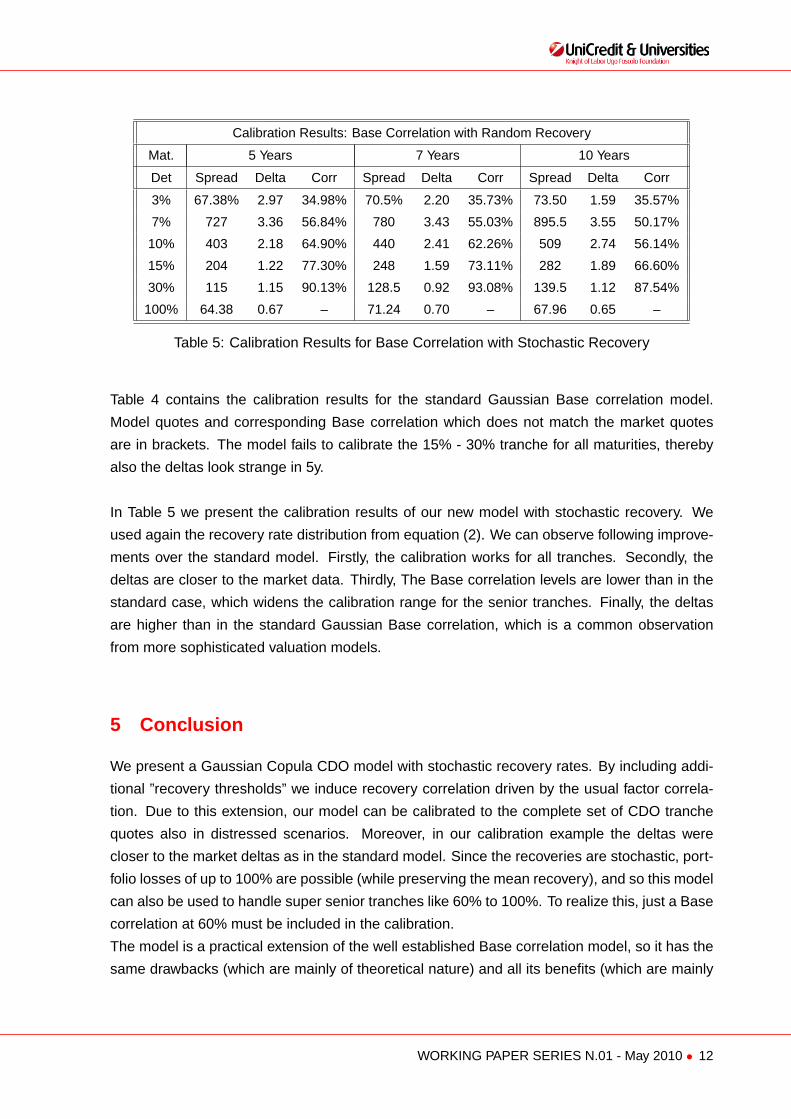
Calibration Results: Base Correlation with Random Recovery

Mat. 5 Years 7 Years 10 Years

Det Spread Delta Corr Spread Delta Corr Spread Delta Corr

3% 67.38% 2.97 34.98% 70.5% 2.20 35.73% 73.50 1.59 35.57%

7% 727 3.36 56.84% 780 3.43 55.03% 895.5 3.55 50.17%

10% 403 2.18 64.90% 440 2.41 62.26% 509 2.74 56.14%

15% 204 1.22 77.30% 248 1.59 73.11% 282 1.89 66.60%

30% 115 1.15 90.13% 128.5 0.92 93.08% 139.5 1.12 87.54%

100% 64.38 0.67 – 71.24 0.70 – 67.96 0.65 –

Table 5: Calibration Results for Base Correlation with Stochastic Recovery

Table 4 contains the calibration results for the standard Gaussian Base correlation model.

Model quotes and corresponding Base correlation which does not match the market quotes

are in brackets. The model fails to calibrate the 15% - 30% tranche for all maturities, thereby

also the deltas look strange in 5y.

In Table 5 we present the calibration results of our new model with stochastic recovery. We

used again the recovery rate distribution from equation (2). We can observe following improve-

ments over the standard model. Firstly, the calibration works for all tranches. Secondly, the

deltas are closer to the market data. Thirdly, The Base correlation levels are lower than in the

standard case, which widens the calibration range for the senior tranches. Finally, the deltas

are higher than in the standard Gaussian Base correlation, which is a common observation

from more sophisticated valuation models.

5 Conclusion

We present a Gaussian Copula CDO model with stochastic recovery rates. By including addi-

tional ”recovery thresholds” we induce recovery correlation driven by the usual factor correla-

tion. Due to this extension, our model can be calibrated to the complete set of CDO tranche

quotes also in distressed scenarios. Moreover, in our calibration example the deltas were

closer to the market deltas as in the standard model. Since the recoveries are stochastic, port-

folio losses of up to 100% are possible (while preserving the mean recovery), and so this model

can also be used to handle super senior tranches like 60% to 100%. To realize this, just a Base

correlation at 60% must be included in the calibration.

The model is a practical extension of the well established Base correlation model, so it has the

same drawbacks (which are mainly of theoretical nature) and all its benefits (which are mainly


of practical nature). The calculation time of our model is not more than doubled in comparison

to the standard model. The extension is obviously not restricted to Gaussian copulas and can

also be used within other copulas models like Levy as well as Random Factor Loading models.

References

[1] Leif Andersen, Jakob Sidenius (2004): Extension to the Gaussian Copula: Random Re-

covery and Random Factor Loadings, Journal of Credit Risk, Vol. 1, No. 1, Winter 2004,

29 - 70.

[2] J. Hull, A. White, Valuation of a CDO and an nth to Default CDS Without Monte Carlo

Simulation, Working Paper (2004).

[3] J.P.Laurent, J.Gregory (2003), Basket Default Swaps, CDO’s and Factor Copulas, working

paper.

[4] David X. Li (2000): On Default Correlation: A Copula Function Approach, Working Paper,

Nr. 99-07, RiskMetrics.

[5] Lee McGinty et all (2004): Introducing Base Correlations, Credit Derivatives Strategy Re-

search Paper, JPMorgan, 2004.

[6] O. Renault, O. Scaillet (2003): On the Way to Recovery: A Nonparametric Bias Free Esti-

mation of Recovery Rate Densities, FAME Research Paper Nr. 83, May 2003, University

of Geneva.


14WORKING PAPER SERIES N. 01 - MAY 2010 ■

Giannantonio De Roni – Secretary General

[email protected]

Annalisa Aleati - Scientific Responsible

[email protected]

Info at:

[email protected]

www.unicreditanduniversities.eu

mailto:[email protected]



http://www.unicreditanduniversities.eu

pricing distressed cdos with base correlation and...

Documents