pricing energy derivatives by linear programming: tolling

PRICING ENERGY DERIVATIVES BY LINEAR PROGRAMMING:TOLLING AGREEMENT CONTRACTS

Valeriy Ryabchenko and Stan Uryasev

Risk Management and Financial Engineering LabDepartment of Industrial and Systems Engineering

University of Florida303 Weil Hall, P.O. Box 116595, Gainesville, FL 32611-6595

Tel: (352) 392-1464 x2023Email: [email protected] and [email protected]

1

Abstract

We introduce a new approach for pricing energy derivatives known as tolling agreement contracts.The pricing problem is reduced to a linear program. We prove that the optimal operating strategyfor a power plant can be expressed through optimal exercise boundaries (similar to the exerciseboundaries for American options). We find the boundaries as a byproduct of the pricing algorithm.The suggested approach can incorporate various real world power plant operational constraints. Wedemonstrate computational efficiency of the algorithm by pricing 1- and 10-year tolling agreementcontracts.

Key words: energy derivatives, tolling agreement, dispatch policy, optimization, exercise bound-aries, multiple stopping.

2

1 Introduction

Recently, the problem of pricing tolling agreement contracts (also known as pricing scheduling flex-ibility of electricity generating facilities) has been extensively researched in the academic literature.Under a tolling agreement contract a renter receives a right to operate a power plant for a fixedtime horizon in exchange for a fixed payment. During the life of the contract the renter receivesall cash inflows and outflows associated with the power plant. We analyze the optimal operatingpolicies of the renter and estimate the value of the underlying tolling agreement contract. Tollingagreement contracts are popular exotic energy derivatives. The problem of pricing such contractsfalls into the class of multiple optimal stopping problems and is extremely hard from the compu-tational prospective.

Tolling agreement contracts have become popular since de-regulation of energy markets in the1970s. To price the contracts practitioners used standard at the time discounted cash flow meth-ods. Later, it was recognized in the literature (see, for example, Dixit and Pindyck (1994)) thatthe discounted cash flow approach is not suitable in a highly volatile price environment since ittends to underestimate the value of a contract. When researchers first became interested in thisproblem they tried to use well-developed approaches of option pricing. More specifically, they triedto represent scheduling flexibility of energy generating facilities as a sequence of so called sparkspread options owned by a renter. A spark spread option gives its holder at a specified time in thefuture the right to exercise a profit equal to the non-negative part of the difference between theprice of energy and the price of fuel multiplied by a coefficient called a heat rate, see Deng, Johnsonand Sogomonian (1998), and Eydeland and Wolyniec (2003). An overview of methods based onspread options pricing can be found in Carmona and Durrleman (2003). The option based methodsare extremely efficient in terms of computational time and provide much more accurate contractprice estimates then the discounted cash flow methods (see, for example, Deng, Jonhnson and So-gomonian (1998) for comparison).

Further development of pricing algorithms led to creation of methods based on the stochasticdynamic programming framework. Contrary to the option based methods, the stochastic dynamicprogramming methods are flexible in incorporating real world power plant operational constraints.In addition to flexibility these methods also remain computationally feasible for contracts withrelatively large horizons. One of the first attempts to use dynamic programming for pricing tollingagreement contracts was done by Deng and Oren (2003). In this paper the authors introduced anefficient dynamic programming algorithm that works with price processes defined on a lattice. Amore general case and more rigorous theoretical treatment of the problem was done in the recentpaper by Carmona and Ludkovski (2008). The paper builds a continuous-time stochastic controlframework with general assumptions regarding underlying energy and fuel price dynamics. Theapproach is capable of dealing with most of the real world operational constraints. The authorsalso provide a rigorous convergence and efficiency analysis of the algorithm.

Although usually not easy to implement and having its own limitations, when there are nostrict requirements on computational time and contract horizons are not too large, the dynamicprogramming framework seem to be a good alternative for pricing tolling agreement contracts.

Similarly to Carmona and Ludkovski (2008), a number of other authors tried to apply a dy-namic optimal control (also called an optimal switching) setting to solve the optimal schedulingflexibility problem. They attempted to derive a closed-form solution of the problem. Interestingdevelopments of this approach can be found in Dixit (1989), Brekke and Oksendal (1994), Bayrak-

3

tar and Egami (2007), Pham and Ly Vath (2007), and references therein. A more general setup isconsidered in Hamadene and Jeanblanc (2007).

We finish the literature survey by referencing an interesting approach capable of incorporatingvarious operational constraints found in Thompson (2004). In this work the authors consider a con-tinuous optimal control space. They derive nonlinear partial-integro-differential equations (PIDEs)for the valuation and optimal operating strategies of energy generation facilities. Sophisticatednumerical methods are available to solve the derived PIDEs.

In this paper we tried to look at the scheduling flexibility problem from a different optimizationperspective and apply a different set of optimization tools. Although, like in any other framework,in order to model a working behavior of a real world power plant we had to make a number ofsimplifying assumptions, we believe that the developed framework may be a viable alternative forpractitioners, especially in cases when computational time is critical or contract horizon is large.Also, the suggested framework is capable of working with price processes defined by a set of histori-cal sample paths. This property may be useful in practical applications. Next, we outline some keyfeatures of the developed optimization framework. The suggested framework is robust, computa-tionally efficient and produces contract price estimates with reasonable accuracy. The optimizationprocedure also provides a practical optimal dispatch strategy defined by a set of optimal exerciseboundaries. Optimization problem is reduced to solving a linear programming (LP) problem witha number of variables and constraints independent of the number of sample paths or the timehorizon used in the model. Computational speed of LP is the key factor of the efficiency of ourframework. The suggested approach can price contracts with horizons as large as 10 years andlonger. The robustness of the framework (resulting from explicit incorporation of shape propertiesof optimal exercise boundaries) allows us to obtain stable results with a small number of samplepaths. Because of this property it is possible to use historical sample paths within the framework.The framework is flexible enough to incorporate various power plant operational constraints, suchas start-up and shutdown costs, fixed renting costs, ramp up period time delay and ramp up periodoperational costs, as well as variable output capacity levels.

Section 2 provides a description of the problem and introduces notations. Section 3 derives astochastic optimal control optimization problem that a renter of the power plant has to solve inorder to find the optimal operating policy and, consequently, to find the price of the correspondingtolling agreement contract. Section 4 examines the properties of optimal operating strategies andproves theoretical results. The results of this section underly and justify the optimization frameworkdeveloped in the following sections. Section 5 introduces a notion of optimal exercise boundaries andformulates an optimal operating policy in terms of optimal exercise boundaries. Section 6 describesan algorithm for finding time independent optimal exercise boundaries and a corresponding priceof the tolling agreement contract. Section 7 generalizes the suggested approach to a case withtime dependent optimal exercise boundaries. Section 8 provides results of numerical experiments.We investigate various computational aspects of the algorithm and compare the results with thecorresponding results of dynamic programming algorithms. Section 9 summarizes the results.

2 Problem Description and Notation

Although the proposed methodology is quite general and may be applied to a wide class of tollingagreement contracts, this research considers an optimal policy of a renter leasing a two regime

4

turbine power plant. We consider a combined cycle gas turbine (CCGT) power plant which canwork in one of the two regimes: a high capacity mode and in a low capacity mode. Usually, theoutput capacity is measured in MWh (megawatt hours), i.e., megawatts (MW) of energy producedin one hour. To simplify the notation, we express the output capacity in megawatt hours per timeperiod:

MWh per period = MW · Number of hours in a period.

We assume that in the high capacity mode the power plant’s generating capacity is

Q MWh per period.

Consequently, we assume that in the low capacity mode the power plant’s generation capacity is

Q MWh per period, (Q > Q > 0).

We consider a discrete time operating environment for a renter of the power plant. At each timepoint the renter has two options. She can either turn down the plant when its operation is notprofitable (or keep the current state if the plant is already offline), or bring the plant online when itsoperation becomes profitable (or keep the current state if the plant is already online). The typicaloperation cycle: 1) a renter buys natural gas on the market, 2) converts it into electricity, and 3)sells the output energy on the market. The conversion rate is termed a heat rate. It is specified inBritish thermal units (MMBtu) of gas needed to produce one MWh of energy. In our model weassume an output dependent heat rate. Hence, in the high capacity mode the power plant has aheat rate

H MMBtu/MWh,

and in the low capacity mode the plant has a heat rate

H MMBtu/MWh.

For technical reasons we assume that

Q ·H ≥ Q ·H.

The last constraint is non-restrictive for the real world power generation facilities, because usuallythe ratio Q

Q is no less than 10060 = 5

3 , and the ratio HH is usually no less than 10

14 > 35 (a common case

is HH > 1). To bring the plant online the renter has to run it for a fixed period of time without

energy output: ramp up period. Depending on the power plant the typical range for the ramp upperiod is from 2 to 12 hours. We make the length of one ramp up period as the smallest time unitin the model. With this assumption, we always have that the length of the ramp up period equalsone. We also assume that during the ramp up period the power plant is in the low capacity mode.Thus, the total amount of gas consumed during the ramp up is

L = Q ·H MMBtu.

Finally, we assume that to bring the plant online in addition to the ramp up costs, the renter alsoincurs fixed startup costs

Cs (Cs ≥ 0).

To bring the plant down, she faces fixed shutdown costs equal to

Cd (Cd ≥ 0).

5

There are also fixed renting costsK and K (K, K ≥ 0)

when the plant is operating in the high and low capacity modes correspondingly. For technicalreasons we need to impose the constraint:

K ≤ Cs + Cd.

For practical applications the last constraint is not restrictive at all. We assume that switchingbetween the high and low capacity regimes is costless and instantaneous. Finally, we denote thetotal number of time periods specified by the tolling contract as

N (N > 0),

price processes for energy and gas as(Pi) and (Gi)

respectively, and a one period risk free interest rate as r. We model fuel and energy price dynamicsby continuous Markovian processes.

3 Stochastic Optimal Control Problem

Here we define renter’s cash flows associated with the operation of the energy generation facility.When the plant is online, at any period i the renter has an option to exercise the profit:

max(Q

(Pi −H ·Gi

)−K, Q (Pi −H ·Gi)−K),

called the spark spread. For simplicity let us denote the spark spread at time i as Mi. Therefore:

Mi = max(Q

(Pi −H ·Gi

)−K, Q (Pi −H ·Gi)−K).

At any time the renter also has the right to turn down the plant. In this case he incurs fixedshutdown costs Cd. When bringing the plant online he faces fixed startup costs and ramp upperiod costs (cost of gas burnt during ramp up), so the total cash outflow is (Cs + L ·Gi). Tosimplify reading we adopt the notation:

Cis = (Cs + L ·Gi) .

Therefore, at any time period i the renter has to make a decision either to turn on or turn offthe power plant. In order to efficiently operate the plant, at each time period she has to solve astochastic optimization problem of optimal switching (whether it is optimal to turn on or turn offthe generation facility). We construct the renter’s stochastic optimization problem below.

We start from introducing the stochastic framework. Let (Ω,F ,F = (Fi), P) be a stochasticbasis, where F is a filtration (F1 ⊆ F2... ⊆ Fi... ⊆ FN ⊆ F ). We assume that P is a risk-neutralprobability measure. We also assume that (Pi) and (Gi) are Markovian processes defined on theprobability space above and are adapted to the filtration F. Assume that the current time periodis 1. Let the vector (ξ1, ..., ξN ) be the vector representing the renter’s current switching decision,ξ1, and his future switching decisions, ξ2, ..., ξN . Let ξ0 denote the initial state of the power plant.Any of the ξis can take one of two values, 0 or 1, meaning that the plant is on when ξi = 1 and isoff when ξi = 0. Because we consider Markovian price processes only, the renter’s decision at time

6

i depends only on the current state of the plant, ξi−1, and the vector of current gas and energyprices, (Gi, Pi). Therefore, we can represent ξi as the following function: ξi(ξi−1, Gi, Pi). Lookingfrom the time period 1, the switching decisions at time periods 2, 3, ..., N are random stochasticcontrols taking values 0 or 1, and only ξ1 is a deterministic 0− 1 control variable.

The power plant is online (producing energy) at the beginning of a time period i only if it hasbeen in the ”on” state during the preceding time period. Therefore, the plant is online during thetime period i if and only if ξiξi−1 = 1. The total profit function for the period i is

φi = ξiξi−1Mi − [ξi − ξi−1]+Cis − [ξi−1 − ξi]+Cd. (1)

In the subsequent sections we also make use of the notation:

fi(ξi−1, ξi) = [ξi − ξi−1]+Cis + [ξi−1 − ξi]+Cd.

Hence, we haveφi = ξiξi−1Mi − fi(ξi−1, ξi).

Using the introduced notation, the cumulative profit for periods from j to N is

S(j, N) =N∑

i=j

φie−r(i−j). (2)

To find the value of the tolling contract and the optimal switching decision ξ1 at time 1, the renterhas to maximize the expected cumulative profit S(1, N) over the set of all admissible Fi-measurablestochastic controls ξi(w). In other words, she needs to solve the stochastic optimization problem:

P 1N : J1

N = supξ1,...,ξN

E[S(1, N)|F1] = supξ1,...,ξN

E[S(1, N)|G1, P1, ξ0]. (3)

Let (ξ∗1 , ξ∗2(w), ..., ξ∗N (w)) be an optimal solution of the above problem. The value of the contract is

the optimal objective value J1N , and the optimal switching decision at time 1 is the optimal solution

ξ∗1 . Similarly to the problem above, we can write an optimization problem for time j:

P jN−j+1 : J j

N−j+1 = supξj ,...,ξN

E[S(j,N)|Fj ] = supξj ,...,ξN

E[S(j, N)|Gj , Pj , ξj−1]. (4)

The upper index in J jN−j+1 and P j

N−j+1 denotes the starting time period, and the lower indexdenotes the total number of periods in the optimization problem. To find an optimal operatingdecision at time j the renter has to solve the problem P j

N−j+1 and take the optimal solution ξ∗jas his operating decision. Sometimes throughout this paper we indicate the conditioning on ξj−1

through the notation:J j

N−j+1(ξj−1) and P jN−j+1(ξj−1). (5)

4 Optimal Operating Strategy

For the reader’s convenience we derive all the theoretical results considering the optimization prob-lem P 1

N (ξ0). Nevertheless, all the results hold without changes if we consider the generalizedproblem P j

N−j+1(ξj−1) (only the variable indices have to be adjusted appropriately).

7

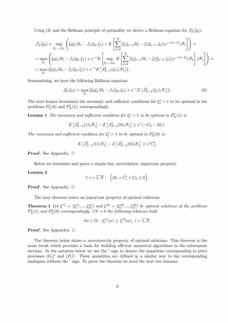
Using (3) and the Bellman principle of optimality we derive a Bellman equation for J1N (ξ0):

J1N (ξ0) = sup

ξ1,...,ξN

(ξ0ξ1M1 − f1(ξ0, ξ1) + E

[N∑

i=2

(ξiξi−1Mi − fi(ξi−1, ξi)) e−r(i−1)|F1

])=

= maxξ1

(ξ0ξ1M1 − f1(ξ0, ξ1) + e−rE

[sup

ξ2,...,ξN

E

[N∑

i=2

(ξiξi−1Mi − fi(ξi−1, ξi)) e−r(i−2)|F2

]|F1

])=

= maxξ1

(ξ0ξ1M1 − f1(ξ0, ξ1) + e−rE

[J2

N−1(ξ1)|F1

]).

Summarizing, we have the following Bellman equation:

J1N (ξ0) = max

ξ1

(ξ0ξ1M1 − f1(ξ0, ξ1) + e−rE

[J2

N−1(ξ1)|F1

]). (6)

The next lemma formulates the necessary and sufficient conditions for ξ∗1 = 1 to be optimal in theproblems P 1

N (0) and P 1N (1), correspondingly.

Lemma 1 The necessary and sufficient condition for ξ∗1 = 1 to be optimal in P 1N (1) is

E[J2

N−1(1)|F1

]−E[J2

N−1(0)|F1

] ≥ er (−Cd −M1) .

The necessary and sufficient condition for ξ∗1 = 1 to be optimal in P 1N (0) is

E[J2

N−1(1)|F1

]− E[J2

N−1(0)|F1

] ≥ erC1s .

Proof . See Appendix. 2

Below we formulate and prove a simple but, nevertheless, important property.

Lemma 2∀ i = 1, N :

(Mi + Ci

s + Cd ≥ 0)

.


The next theorem states an important property of optimal solutions.

Theorem 1 Let ξ∗1 = (ξ∗11 , ..., ξ∗1N ) and ξ∗0 = (ξ∗01 , ..., ξ∗0N ) be optimal solutions of the problemsP 1

N (1) and P 1N (0) correspondingly. ∀N > 0 the following relations hold

∀w ∈ Ω : ξ∗1i (w) ≥ ξ∗0i (w), i = 1, N.

Proof . See Appendex. 2

The theorem below shows a monotonicity property of optimal solutions. This theorem is themain result which provides a basis for building efficient numerical algorithms in the subsequentsections. In the notation below we use the ′ sign to denote the quantities corresponding to priceprocesses (Gi)′ and (Pi)′. These quantities are defined in a similar way to the correspondinganalogues without the ′ sign. To prove the theorem we need the next two lemmas.

8

Lemma 3 Consider two pairs of gas and energy price processes (Gi), (Pi) and (G′i), (P

′i ),

satisfying the condition:

∀ w ∈ Ω : P ′i (w) ≥ Pi(w), G′

i(w) ≤ Gi(w), i = 1, N.

The following inequalities hold

∀ i = 1, N : M ′i + Ci′

s ≥ Mi + Cis.


Lemma 4 ∀ N > 0 the following inequalities hold

1) J1N (1)− J1

N (0) ≤ M1 + C1s ,

2) J1N (1)− J1

N (0) ≥ −Cd.


Theorem 2 Consider two pairs of gas and energy price processes (Gi), (Pi) and (G′i), (P

′i ),

satisfying the condition of Lemma 3. Let ξ∗1, ξ∗0, ξ∗1′ and ξ∗0′ be optimal solutions of the problemsP 1

N (1), P 1N (0), P 1′

N (1), and P 1′N (0), correspondingly. ∀ N > 0 the following statements are true:

1) J1′N (1)− J1′

N (0) ≥ J1N (1)− J1

N (0),2) ξ∗01 ≤ ξ∗0′1 , and ξ∗11 ≤ ξ∗1′1 .


Corollary 2. 1 Consider two pairs of gas and energy price processes (Gi), (Pi) and (G′i), (P

′i )

with (Gi) and (G′i), (Pi) and (P ′

i ) following the same dynamics equations correspondingly. Let(G0, P0) and (G′

0, P′0) be the corresponding initial points satisfying the property:

P0 ≤ P ′0, G0 ≥ G′

0.

If energy and fuel price processes follow one of the following dynamics (equations for energy andfuel prices may be different):

1) Geometric Ornstein-Uhlenbeck process,2) Geometric Brownian Motion process;

then the optimal solutions of P 1N and P 1′

N have the following properties:

1) ξ∗01 ≤ ξ∗0′1 ,

2) ξ∗11 ≤ ξ∗1′1 .

The assertion remains valid if we add a possibility of non-negative jumps to the price dynamics withi.i.d. intensities and magnitudes. We assume that jump intensities and magnitudes are independentof the price level as well.


9

(a) (b)

Figure 1. a) Optimal exercise boundaries. b) Optimal operating policy when current state of theplant is “off”.

5 Optimal Exercise Boundary

As before, let ξ∗0 and ξ∗1 be optimal solutions of the problems P 1N (0) and P 1

N (1), respectively. By(XG, XP ), we denote the initial values P1 = XP and G1 = XG of energy and gas prices in theoptimization problems P 1

N (0) and P 1N (1). For i = 0, 1 consider the sets below:

RN,i0 = (XG, XP )|ξ∗i1 = 0,

RN,i1 = (XG, XP )|ξ∗i1 = 1.

We refer to RN,00 and RN,1

0 as an “off” and an “on” state 0-optimal exercise set, correspondingly.Consistently, we call RN,0

1 and RN,11 as an “off” and an “on” state 1-optimal exercise sets, re-

spectively. If we plot points (XG, XP ) on a plane where the y-coordinate represents XP and thex-coordinate represents XG, the boundary separating 0 and 1-optimal exercise sets on this planeis called an optimal exercise boundary. Clearly, there are two optimal exercise boundaries, oneis for the “off” state (problem P 1

N (0)) and the other one is for the “on” state (problem P 1N (1))

of the plant. From now on we concentrate on geometric Ornstein-Uhlenbeck (with and withoutjumps) price dynamics only. Although all the derived results are valid for other classes of stochas-tic processes (geometric Brownian Motion in particular), it is widely accepted in the literaturethat geometric Ornstein-Uhlenbeck processes are the most adequate to approximate energy andgas price dynamics. For the considered class of price dynamics the corollary of Theorem 2 impliesmonotonicity of the optimal exercise boundaries. Monotonicity of a boundary has to be understoodin the following sense. If a point (X1

G, X1P ) belongs to the 0-optimal exercise set for some state

of the plant, then any point (X2G, X2

P ), such that X1P ≥ X2

P and X1G ≤ X2

G, has to belong to the0-optimal exercise set for the same state of the plant as well. The monotonicity of the boundaryalso implies connectivity of the 0 and 1-optimal exercise sets. We denote the optimal exerciseboundaries for the “off” and the “on” states of the plant as OB0 and OB1, correspondingly. The-orem 1 implies that the boundary OB0 has to be always no lower than the boundary OB1. Figure1(a) summarizes properties of the optimal exercise boundaries. For any period of time the problemof finding the optimal exercise boundaries is equivalent to the renter’s optimal switching problem.With the help of optimal exercise boundaries it is easy to formulate the renter’s optimal switchingpolicy. If the current point (XG, XP ), representing current energy and gas prices, lies above theoptimal exercise boundary for the current state of the plant, then the optimal renter’s decision isto turn on the power plant (or leave it working if its current state is “on”). If the price point is

10

below the optimal exercise boundary, then it is optimal to turn down the power plant (or leaveit not working if its current state is “off”). If the optimal operating decision is to set the plantin the “on” state, then the optimal capacity regime is determined by instantaneous gains of theregime because switching between different capacity regimes is costless. Figure 1(b) explains theoptimal operating behavior of the renter if the current state of the plant is “off”(she needs to usethe boundary OB0 in this case). Finding the optimal exercise boundaries for every time period isa timely and resource consuming process. To overcome this difficulty, we suggest to make use ofthe heuristic argument below. If a tolling agreement contract has a relatively large time horizon(one year is long enough), then it is not necessary to build the optimal exercise boundaries forevery time period. A heuristic approach is to find a single pair of optimal exercise boundariesthat can be used for all time periods. We refer to these optimal time independent boundaries asoptimal stationary exercise boundaries. The proposed heuristic relies on a hypothesis that for mostof the time periods except for a small fraction of the very last periods, stationary optimal exerciseboundaries can be good approximations of the time dependent optimal exercise boundaries. Therationale for this is that for the time periods close to contract’s expiration, infinite horizon may bea bad assumption. However, according to the hypothesis this should have little influence on theresults since the fraction of such periods should be small relative to the total number of periodsunder the contract. Computational results reported later in the paper provide justification of thehypothesis for the considered setups. If needed, it is possible to extend the suggested approachon the case with time dependent boundaries. In the rest of the paper we concentrate on develop-ing efficient optimization procedures for finding optimal stationary exercise boundaries. In one ofthe final sections we provide a short outline of how to generalize the developed approach for thetime dependent case. We refer to the optimal stationary exercise boundary for the “off” state asSOB0 and to the optimal stationary exercise boundary for the “on” state as SOB1. It is naturalto assume that the optimal stationary exercise boundaries inherit all the properties from the timeperiod specific optimal exercise boundaries. Therefore, we restrict ourselves to the class of optimalstationary exercise boundaries having the monotonicity property discussed above and having theproperty that SOB0 lies above SOB1.

6 Finding Optimal Stationary Exercise Boundaries

6.1 Optimization on a Grid

In the preceding section we considered optimal exercise boundaries in a (XG, XP )-space. Here andthroughout the rest of the paper we switch to a different (lnXG, lnXP ) space. Since the logarithmtransformation is monotonic (in the sense that if P1(x1, y1), P2(x2, y2) are some points in the oldcoordinates, and P ′

1(x′1, y

′1), P

′2(x

′2, y

′2) their respective mappings in the new coordinates, then the

following property holds (x1 ≤ x2)&(y1 ≥ y2) ⇔ (x′1 ≤ x′2)&(y′1 ≥ y′2)), all the derived propertiesof optimal exercise boundaries hold in the new coordinates. The reason for switching to the loga-rithmic coordinates is that below in this section we work with uniform grids on the plane. Since weconcentrate on geometric price process dynamics, to make the choice of uniform grids justified weneed to convert geometric price processes into arithmetic ones, and, therefore, we use the logarithmtransformation.

Let (Gji , P

ji )j=1,...,NS

i=1,...,N be a set of sample paths generated using geometric Ornstein-Uhlenbeckdynamics, where as before N is the total number of time periods in the contract, and NS is the totalnumber of sample paths. Also let Pmax = max(i,j) lnP j

i , Gmax = max(i,j) ln Gji , Pmin = min(i,j) lnP j

i

and Gmin = min(i,j) ln Gji . On the (lnXG, lnXP )-plane consider a rectangle with the top left vertex

11

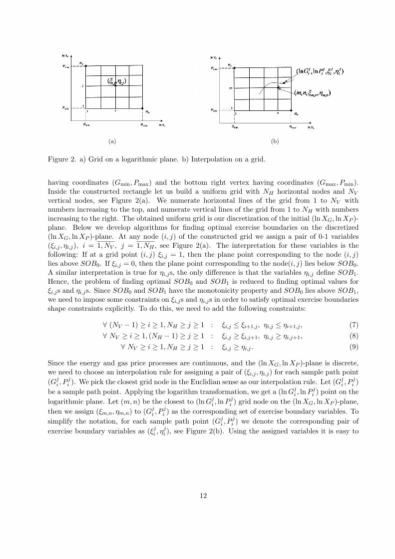
(a) (b)

Figure 2. a) Grid on a logarithmic plane. b) Interpolation on a grid.

having coordinates (Gmin, Pmax) and the bottom right vertex having coordinates (Gmax, Pmin).Inside the constructed rectangle let us build a uniform grid with NH horizontal nodes and NV

vertical nodes, see Figure 2(a). We numerate horizontal lines of the grid from 1 to NV withnumbers increasing to the top, and numerate vertical lines of the grid from 1 to NH with numbersincreasing to the right. The obtained uniform grid is our discretization of the initial (lnXG, ln XP )-plane. Below we develop algorithms for finding optimal exercise boundaries on the discretized(lnXG, ln XP )-plane. At any node (i, j) of the constructed grid we assign a pair of 0-1 variables(ξi,j , ηi,j), i = 1, NV , j = 1, NH , see Figure 2(a). The interpretation for these variables is thefollowing: If at a grid point (i, j) ξi,j = 1, then the plane point corresponding to the node (i, j)lies above SOB0. If ξi,j = 0, then the plane point corresponding to the node(i, j) lies below SOB0.A similar interpretation is true for ηi,js, the only difference is that the variables ηi,j define SOB1.Hence, the problem of finding optimal SOB0 and SOB1 is reduced to finding optimal values forξi,js and ηi,js. Since SOB0 and SOB1 have the monotonicity property and SOB0 lies above SOB1,we need to impose some constraints on ξi,js and ηi,js in order to satisfy optimal exercise boundariesshape constraints explicitly. To do this, we need to add the following constraints:

∀ (NV − 1) ≥ i ≥ 1, NH ≥ j ≥ 1 : ξi,j ≤ ξi+1,j , ηi,j ≤ ηi+1,j , (7)∀ NV ≥ i ≥ 1, (NH − 1) ≥ j ≥ 1 : ξi,j ≥ ξi,j+1, ηi,j ≥ ηi,j+1, (8)

∀ NV ≥ i ≥ 1, NH ≥ j ≥ 1 : ξi,j ≥ ηi,j . (9)

Since the energy and gas price processes are continuous, and the (lnXG, lnXP )-plane is discrete,we need to choose an interpolation rule for assigning a pair of (ξi,j , ηi,j) for each sample path point(Gj

i , Pji ). We pick the closest grid node in the Euclidian sense as our interpolation rule. Let (Gj

i , Pji )

be a sample path point. Applying the logarithm transformation, we get a (lnGji , lnP j

i ) point on thelogarithmic plane. Let (m,n) be the closest to (lnGj

i , ln P ji ) grid node on the (lnXG, ln XP )-plane,

then we assign (ξm,n, ηm,n) to (Gji , P

ji ) as the corresponding set of exercise boundary variables. To

simplify the notation, for each sample path point (Gji , P

ji ) we denote the corresponding pair of

exercise boundary variables as (ξji , η

ji ), see Figure 2(b). Using the assigned variables it is easy to

12

formulate the optimal operating policy on the sample paths:

1) If at a point (Gji , P

ji ) the current state of the plant is “off”, (10)

then it is optimal to turn on the plant ⇔ ξji = 1.

2) If at a point (Gji , P

ji ) the current state of the plant is “on”, (11)

then it is optimal to turn off the plant ⇔ ηji = 0.

6.2 Optimization with Two Optimal Stationary Exercise Boundaries

Here we construct an optimization problem to find optimal values of ξi,js and ηi,js. From (10)-(11) we see that depending on the current state of the plant, at any point (Gj

i , Pji ) the optimal

switching rule is either ξji or ηj

i . For the sake of simplicity, we introduce an auxiliary set of variablesχj

ij=1,...,NSi=1,...,N . With the new variables, the optimal decision rule at any point (Gj

i , Pji ) is χj

i . Tofollow the logic introduced by (10)-(11) the variables χj

i s have to satisfy the constraints below:

χji = (1− χj

i−1)ξji + χj

i−1ηji , i = 1, ..., N, j = 1, ..., NS ; (12)

χj0 = 0, j = 1, ..., NS , assuming the initial state of the plant is “off”. (13)

The logic behind these constraints is straightforward. At any point (Gji , P

ji ) the current state of

the plant is determined by a variable χji−1. Whenever χj

i−1 = 0, meaning that the plant is currently“off”, the optimal switching rule at (Gj

i , Pji ) is ξj

i . Whenever χji−1 = 1, meaning that the plant is

currently “on”, the optimal switching rule at (Gji , P

ji ) is ηj

i . Similarly to (1), we can construct aprofit function for each sample path j (j = 1, ..., NS) and each period i (i = 1, ..., N):

φji = e−r(i−1)

(χj

iχji−1M

ji − [χj

i − χji−1]

+Cjs,i − [χj

i−1 − χji ]

+Cd

),

where

M ji = max

(Q

(P j

i −H ·Gji

)−K, Q

(P j

i −H ·Gji

)−K

)is the spark spread,

Cjs,i = Cs + L ·Gj

i is the startup cost.

Parameters Cd, Cs, L,Q,H,Q, H, K, and K have been introduced earlier in the paper. Below weformulate an optimization problem maximizing the expected profit of operating the power plant:

(P2B) : maxξi,j ,ηi,j

1NS

NS∑

j=1

N∑

i=1

φji

s.t.

auxiliary variable constraints (12)-(13),optimal exercise boundaries shape constraints (7)-(9),ξi,j , ηi,j ∈ 0, 1 , i = 1, ..., NV , j = 1, ..., NH .

Although the optimization problem above solves the problem of finding optimal stationary exerciseboundaries, the obtained formulation is computationally hard in general case, since it is a non-linear 0-1 optimization problem. A standard remedy in this case is to linearize the problem. Theonly obstacle for this remedy is that linearization would require introducing a large number of

13

auxiliary variables and constraints making the resultant formulation computationally inefficient.The number of auxiliary variables and constraints in (P2B) is of O(NS · N) order. When thehorizon of the contract is large enough (that is the most interesting case for us) and the number ofsample paths is measured by at least hundreds, the linearized problem becomes computationallyintractable because it requires introducing even more additional variables and constraints. Hence,we conclude that the optimization problem for the case with two stationary exercise boundariesis computationally inefficient in the form introduced here. The following subsection suggests asimplification of the formulated problem considering only one exercise boundary. Later, we returnto the case with two boundaries suggesting an efficient heuristic.

6.3 Optimization with One Optimal Stationary Exercise Boundary

This subsection considers a simplification of the optimization problem formulated above. Since itturned out to be hard to construct a computationally efficient optimization problem for the casewith two stationary exercise boundaries, here we build an optimization problem assuming thatthe renter uses only one stationary boundary. Using the introduced notation, we assume thatindependently of the current state of the plant the renter always uses the stationary boundarydefined by ξi,js. In this case we do not need to introduce the auxiliary variables, χj

i s, and we canconstruct an optimization problem using only ξi,j grid variables. The objective of the new problemis obtained from the objective of (P2B) by replacing χj

i s with ξji s, and the feasible region of the new

problem is defined by the optimal exercise boundary shape constraints. Therefore, the optimizationproblem for finding a single optimal stationary exercise boundary is

(P1B) : maxξi,j

1NS

NS∑

j=1

N∑

i=1

e−r(i−1)(ξji ξ

ji−1M

ji − [ξj

i − ξji−1]

+Cjs,i − [ξj

i−1 − ξji ]

+Cd

)

s.t.

ξi,j ≤ ξi+1,j , i = 1, ..., (NV − 1) , j = 1, ..., NH ,

ξi,j ≥ ξi,j+1, i = 1, ..., NV , j = 1, ..., (NH − 1) ,

ξi,j ∈ 0, 1 , i = 1, ..., NV , j = 1, ..., NH .

Using the identity:∀ x, y ∈ 0, 1 : xy = x− [x− y]+, (14)

we rewrite (P1B) in the following equivalent form:

(P1B′) : maxξi,j

1NS

NS∑

j=1

N∑

i=1

e−r(i−1)(ξji M

ji − [ξj

i − ξji−1]

+(Cj

s,i + M ji

)− [ξj

i−1 − ξji ]

+Cd

)

s.t.

ξi,j ≤ ξi+1,j , i = 1, ..., (NV − 1) , j = 1, ..., NH ,

ξi,j ≥ ξi,j+1, i = 1, ..., NV , j = 1, ..., (NH − 1) ,

ξi,j ∈ 0, 1 , i = 1, ..., NV , j = 1, ..., NH .

14

The problem (P1B′) is not linear, but it can be easily linearized. In order to do this, we need tointroduce auxiliary variables, νj

i s and µji s. (P1B′) transforms into the following equivalent problem:

(P1BL) : maxξi,j

1NS

NS∑

j=1

N∑

i=1

e−r(i−1)(ξji M

ji − νj

i

(Cj

s,i + M ji

)− µj

iCd

)(15)

s.t.

νji ≥ ξj

i − ξji−1, νj

i ≥ 0, i = 1, ..., N, j = 1, ..., NS , (16)

νji ≤ 1− ξj

i−1, νji ≤ ξj

i , i = 1, ..., N, j = 1, ..., NS , (17)

µji ≥ ξj

i−1 − ξji , µj

i ≥ 0, i = 1, ..., N, j = 1, ..., NS , (18)

µji ≤ 1− ξj

i , µji ≤ ξj

i−1, i = 1, ..., N, j = 1, ..., NS , (19)ξi,j ≤ ξi+1,j , i = 1, ..., (NV − 1) , j = 1, ..., NH , (20)ξi,j ≥ ξi,j+1, i = 1, ..., NV , j = 1, ..., (NH − 1) , (21)

νji , µ

ji ∈ R, ξi,j ∈ 0, 1 , i = 1, ..., NV , j = 1, ..., NH , (22)

where constraints (16)-(19) ensure that νji = [ξj

i − ξji−1]

+ and νji = [ξj

i−1− ξji ]

+. There is one majorproblem with writing (P1BL) in the form given above. Although we obtained a linear problem,the notation states that we need to introduce N · NS auxiliary variables. It can be shown thatthere is a linearization of (P1B) that requires introducing no more than (N2

V ·N2H) new variables.

In this case, the total number of variables in the problem depends only on the number of nodes inthe grid and not on the number of sample paths or time periods. To make (P1B) linear we needto introduce an auxiliary variable for each of the pairs (ξj

i , ξji−1) and (ξj

i−1, ξji ). Hence, the total

number of auxiliary variables needed equals to the total number of different ordered pairs (ξji , ξ

ji−1)

and (ξji−1, ξ

ji ). Remembering the notation introduced earlier, by writing variables ξj

i we assume thefollowing mapping for the indexes (ji ) (we denote it by (ji )

ξ because it corresponds to variables ξ):

(ji )

ξ : 1, ..., N × 1, ..., NS → 1, ..., NH × 1, ..., NV .

From the last mapping, it follows that the total number of different pairs considered above is nogreater than N2

V · N2H . The alternative linear equivalent of (P1B) can be obtained from (P1BL)

by eliminating redundant νji s and µj

i s. From the above, each νji is associated with a pair of pairs(

(ji )

ξ, (ji−1)

ξ)

and each µji is associated with a pair of pairs

((ji−1)

ξ, (ji )

ξ). To eliminate the re-

dundancy we need to assume that any νji s or µj

i s that are associated with the same pair of pairsare synonyms of the same auxiliary variable. With this assumption, we should think of (P1BL)as a linear version of (P1B) that is free of sample path dependent variables. This step of leavingthe notation of (P1BL) unchanged should ease the reader’s understanding of the material below.Otherwise, the reader would have to spend a considerable amount of time to get through a muchmore complicated indexing system. Summarizing, from here and below the reader should think of(P1BL) and its consequent transformations as free of sample path dependent variables bearing inmind the trick with variable synonyms discussed above.

(P1BL) allows us to find a single optimal stationary exercise boundary. In general, (P1BL)may not be easy to solve because it is a mixed integer programming problem. Thus, we have to

15

work on finding a better formulation. Let us write the following chain of derivations:

∀ i = 1, ..., N, j = 1, ..., NS :

M ji + Cj

s,i = max(Q

(P j

i −H ·Gji

)−K + Cj

s,i, Q(P j

i −H ·Gji

)−K + Cj

s,i

)≥

≥ Q(P j

i −H ·Gji

)−K +

(Cs + L ·Gj

i

)=

= Q(P j

i −H ·Gji

)−K +

(Cs + Q ·H ·Gj

i

)= Q · P j

i −K + Cs ≥ Cs −K.

¿From the above, we have

∀ i = 1, ..., N, j = 1, ..., NS : Cs ≥ K ⇒ M ji + Cj

s,i ≥ 0. (23)

The condition Cs ≥ K is usually satisfied for all real life setups. It is almost always the case thatthe fixed costs incurred during the startup period are much bigger than the fixed renting costswhen the plant is in an energy generating mode. If the condition Cs ≥ K is satisfied, then we canwrite down a problem equivalent to (P1BL) that has a smaller number of constraints:

(P1BL′) : maxξi,j

1NS

NS∑

j=1

N∑

i=1

e−r(i−1)(ξji M

ji − νj

i

(Cj

s,i + M ji

)− µj

iCd

)

s.t.

νji ≥ ξj

i − ξji−1, νj

i ≥ 0, i = 1, ..., N, j = 1, ..., NS ,

µji ≥ ξj


i ≥ 0, i = 1, ..., N, j = 1, ..., NS ,

ξi,j ≤ ξi+1,j , i = 1, ..., (NV − 1) , j = 1, ..., NH ,

ξi,j ≥ ξi,j+1, i = 1, ..., NV , j = 1, ..., (NH − 1) ,

ξi,j ∈ 0, 1 , i = 1, ..., NV , j = 1, ..., NH .

(P1BL′) is obtained from (P1BL) by removing from its formulation the upper bound constraintsfor νj

i s and µji s. These two problems are equivalent because of the fact that it is never optimal for

νji s and µj

i s to be on their upper bounds because we are solving a maximization problem and havethe condition that M j

i +Cjs,i ≥ 0 (from (23)) and Cd ≥ 0. Now we have everything set to formulate

the main result of this section.

Theorem 3 Consider the linear programming problem below:

(L1) : maxξi,j

1NS

NS∑

j=1

N∑

i=1

e−r(i−1)(ξji M

ji − νj

i

(Cj

s,i + M ji

)− µj

iCd

)

s.t.

νji ≥ ξj

i − ξji−1, νj

i ≥ 0, i = 1, ..., N, j = 1, ..., NS ,

µji ≥ ξj


i ≥ 0, i = 1, ..., N, j = 1, ..., NS ,

ξi,j ≤ ξi+1,j , i = 1, ..., (NV − 1) , j = 1, ..., NH ,

ξi,j ≥ ξi,j+1, i = 1, ..., NV , j = 1, ..., (NH − 1) ,

0 ≤ ξi,j ≤ 1, i = 1, ..., NV , j = 1, ..., NH .

If the condition Cs ≥ K is satisfied, then (L1) has an optimal solution if and only if (P1BL′) hasan optimal solution, and at least one optimal solution of (L1) is optimal in (P1BL′).

16

This is an important theorem that reduces the problem of finding a single optimal stationaryexercise boundary to solving a linear programming problem. Although not any optimal solution of(L1) is optimal in (P1BL′), in the proof of the theorem we show that any optimal solution of (L1)that is attained at a vertex of the feasible region is optimal in (P1BL′). The last conclusion hasan important practical meaning. It says that if for solving (L1) we use any linear programmingsolver that searches for optimal points only among vertices of the feasible region (as is the case withthe simplex method based solvers), the optimal solution found is always a solution of (P1BL′).An important property of the derived linear program is that the maximal number of variables andconstraints in it does not depend on the number of time periods or sample paths. This maximalnumber is always determined by the size of the grid. The number of variables and constraints in(L1) is the same as the number of variables and constraints in (P1BL′) (the only difference is that(L1) has box constraints for ξi,js and (P1BL′) has integrality constraints instead). The proof ofthe theorem (see Appendix for the proof) relies on the result of the lemma below.

Lemma 5 Consider a system of equations with n variables and n equations. Let x1, ..., xn be thevariables of the system. Assume that each equation of the system is one of the following types:

1) xi1 = xi2 , for some i1, i2 ∈ 1, ..., n,2) xi1 = ci1 , for some i1 ∈ 1, ..., n, and some constant ci1 ∈ C ⊆ R.

If the system has a unique solution (x∗1, ..., x∗n), then the solution can be only of the following form:

∀ i ∈ 1, ..., n : x∗i = ci, where ci ∈ C.


We finish this subsection by pointing out some key features of the introduced approach. Thefirst point is that the suggested algorithm does not have an issue known in stochastic programmingas anticipativity. Since there are no sample path dependent variables involved and the algorithm isbased on variables defined on a grid with a rigid structure (imposed by monotonicity constraints),the algorithm is non-anticipative by construction. As it was mentioned earlier, the theoreticalmaximum number of variables and constraints in the constructed linear optimization problem hasan order of O(N2

H ·N2V ). O(N2

H ·N2V ) is just a theoretical upper bound. For the real world problems

the number of variables and constraints in the linear problem usually has an order of O(NH ·NV ).We can derive this estimate using simple arguments. For most of the real world price dynamics ofenergy and gas it is reasonable to assume that if (i, j) is the current price point on the grid, thena price point at the next time period will be in the vicinity of (i, j). In other words, if (i, j) is thecurrent price point on the grid and (m, n) is a price point at the next period of time, then with aprobability close to 1 we can claim that there holds

|i−m| ≤ R, |j − n| ≤ R,

for some fixed constant R. If this is the case, then the total number of auxiliary variables neededin the model has an order of O(R ·NH ·NV ) = O(NH ·NV ) (it is a linear function of the numberof nodes in the grid). Therefore, there are O(NH · NV ) grid variables and O(NH · NV ) auxiliaryvariables in the model. From the last statement, we get that the total number of variables in themodel should have an order of O(NH · NV ). The time of constructing the linear program has anorder of O(N ·NS) since we have to go through each time period of every sample path.

17

Figure 3. Heuristic for finding two optimal exercise boundaries.

6.4 Heuristic with Two Stationary Exercise Boundaries

The previous subsection suggested an algorithm for finding a single optimal stationary exerciseboundary. Here and further throughout the paper we refer to this boundary as an optimal “average”boundary (this boundary is used for all states of the plant, that is why the boundary is “average”in some sense). Above, we also suggested an optimization problem (P2B) for finding optimal “off”and “on” state exercise boundaries, but it turned out that the suggested formulation is hard tosolve. This subsection develops a heuristic for finding a suboptimal solution of (P2B) that we claimto be a good substitute for an optimal solution of (P2B). In the section presenting numerical resultsbelow, we examine the benefits of using suboptimal exercise boundaries given by the heuristic ascompared to using an optimal “average” boundary given by (L1). The idea of the heuristic is tolook for optimal “on” and “off” exercise boundaries in the class of exercise boundaries parallel tothe “average” optimal exercise boundary given by (L1). By “parallel” we mean boundaries thatcan be obtained from the “average” boundary by a parallel shift (an up shift for the “off” boundaryand a down shift for the “on” boundary). The heuristic works in two stages (see also Figure 3):

1) Assume that the “average” boundary found by solving (L1) is an optimal “off” boundaryand find an optimal “on” boundary that is parallel to it (find an optimal size δdown of thedown shift).

2)Assume that the boundary found on the previous stage is an optimal “on” boundary andfind an optimal “off” boundary that is parallel to it (find an optimal size δup of the up shift).

Using the notation introduced earlier in this section:

χpi =

ξpi , if the current state of the plant is “off” and i 6= 0,

ηpi , if the current state of the plant is “on” and i 6= 0,

0, if i = 0, assuming the initial state of the plant is “off”.

Below, we make use of the following lemma.

Lemma 6

∀ i = 1, N, p = 1, NS : χpi =

i∑

k=1

ξpk

i∏

l=k+1

(ηpl − ξp

l ).

18

(a) (b)

Figure 4. a) Distance between a point and the “off” boundary. b) Distance between a point andthe “on” boundary.


Now assume that an optimal “off” boundary is known and equal to the “average” boundaryfound by solving (L1). Using the notation introduced earlier, the last assumption means that thegrid variables ξi,j i = 1, NV and j = 1, NH are known. The heuristic approach suggests to find an“on” boundary as an optimal boundary that can be obtained by shifting the found “off” boundarydownwards. Therefore, the task is to find an optimal size of the shift δ ≥ 0. Let δ ≥ 0 be anarbitrary shift size. For each point (Gj

i , Pji ) let us also define δj

i , a vertical distance from a point(lnGj

i , ln P ji ) to the “off” boundary. Let (m, n) be the closest grid node to the point (lnGj

i , lnP ji )

on the logarithmic plane. Since we use the closest grid node as an interpolation rule on the grid,we approximate δj

i with a value equal to the distance between the “off” boundary and the node(m,n). Let in0 be the smallest index in the nth column, such that ξin0 ,n = 1, and 4v be the distancebetween two adjacent vertical nodes. Then,

δji = y(in0 )− 4v

2− y(m),

where y(i) denotes the y-coordinate of points in the ith row of the grid, see Figure 4(a). Because weconsider only δ ≥ 0, to make the algorithm computationally more efficient we make the followingadjustment to the computation of δj

i . We compute δji as defined above, and if we obtain δj

i < 0then we set δj

i = −ε (ε > 0). Any positive value can be taken as the value of ε. In cases whenξNV ,n = 0, meaning that there are no 1s in the nth column, we set δj

i = +∞. Since the “on”boundary is obtained from the “off” boundary by a shift of size δ, the following is true:

∀ i, j : ηji = sgn

([δ − δj

i ]+)

, (24)

where sgn(·) is a sign function. It is easy to notice, that for δ = 0 we get ηji = ξj

i . For ∀ i, j wealso define a set of indexes Sj

i and the maximal element kji of the set Sj

i :

Sji = k : ξj

k = 1, k ≤ i, ξjl = 0, l = k + 1, i,

kji =

max

k∈Sji, if Sj

i 6= ∅,

N + 1, if Sji = ∅.

It can be shown that|Sj

i | ≤ 1,

19

and the following formula is true:

∀ j, ∀ i > 1 : kji =

i, if ξj

i = 1,

kji−1, otherwise.

From Lemma 6, we have

∀ i = 1, N, j = 1, NS : χji =

∏il=kj

i +1ηj

l , if kji < i,

1, if kji = i,

0, if kji > i.

(25)

Applying (24) to (25):

∀ i = 1, N, j = 1, NS : χji =

∏il=kj

i +1sgn

([δ − δj

l ]+)

= sgn([δ − δ∗i,j ]

+)

, if kji < i,

1, if kji = i,

0, if kji > i,

(26)

where δ∗i,j = maxl=kj

i +1,iδj

l . If we extend the definition of δ∗i,j :

∀ i = 1, N, j = 1, NS : δ∗i,j =

maxl=kj

i +1,iδj

l = maxδ∗i−1,j , δji , if kj

i < i,

−ε, if kji = i,

+∞, if kji > i,

then (26) can be rewritten:

∀ i = 1, N, j = 1, NS : χji = sgn

([δ − δ∗i,j ]

+). (27)

To find an optimal δ we need to solve a version of (P2B) without the boundary shape constraints.We do not need the shape constraints because the “off” boundary is already known, and the shapeof the “on” boundary is completely determined by the shape of the “off” boundary (since we arelooking for a parallel boundary). Summarizing, we need to solve the problem:

maxδ1

NS

NS∑

j=1

N∑

i=1

e−r(i−1)(χj

iχji−1M

ji − [χj

i − χji−1]

+Cjs,i − [χj

i−1 − χji ]

+Cd

)

s.t.

δ ≥ 0, (27) constraints.

With (14) the last problem transforms into an equivalent problem:

(H1) : maxδ1

NS

NS∑

j=1

N∑

i=1

e−r(i−1)(χj

iMji − [χj

i − χji−1]

+(Cj

s,i + M ji

)− [χj

i−1 − χji ]

+Cd

)

s.t.

δ ≥ 0, (27) constraints.

(27) implies

[χji − χj

i−1]+ =

0, if δ∗i,j ≥ δ∗i−1,j ,

sgn([δ − δ∗i,j ]

+)− sgn

([δ − δ∗i−1,j ]

+)

, otherwise.(28)

20

[χji−1 − χj

i ]+ =

0, if δ∗i−1,j ≥ δ∗i,j ,

sgn([δ − δ∗i−1,j ]

+)− sgn

([δ − δ∗i,j ]

+)

, otherwise.(29)

From (27), (28), and (29) it follows that (H1) reduces to a problem of the type:

maxδ≥0

M∑

i=1

ai · sgn([δ − βi]+

), (30)

for some constants ai ∈ R, βi ≥ 0, and integer M > 0. The last problem is easily solvable. Withoutloss of generality we assume 0 ≤ β1 ≤ β2 ≤ ... ≤ βM (change variables if needed). We calculate

S0 = 0, Si =i∑

j=1

aj , i = 1,M,

i∗ = argmaxi=0,MSi.

Now we write down an optimal solution of the optimization problem above:

δ∗ =

βi∗+1, if i∗ < M,

βM (1 + ε), ∀ε > 0, if i∗ = M.

At the second stage of the heuristic we assume that an optimal “on” boundary is known and equalto the boundary found at the first stage. Using our notation, the last assumption means thatthe grid variables ηi,j i = 1, NV , j = 1, NH are known. The heuristic suggests finding an “off”boundary as an optimal boundary that can be obtained by shifting the “on” boundary upwards.Thus, the task is to find an optimal size of the shift δ ≥ 0. To do this we need to follow steps similarto the steps we performed at the first stage. Again, we need to define a distance between a pointon the logarithmic plane and the “on” boundary. Consider an arbitrary sample point (Gj

i , Pji ). Let

(m,n) be the closest grid node to the point (lnGji , ln P j

i ) on the logarithmic plane, in0 be the largestindex in the nth column, such that ηin0 ,n = 0, and 4v be the distance between two adjacent verticalnodes. Then, a distance between (lnGj

i , lnP ji ) and the “on” boundary is approximated as follows:

δji = y(m)− y(in0 )− 4v

2,

where y(i) denotes the y-coordinate of points in the ith row of the grid, see Figure 4(b). As atthe fist state, we make a similar adjustment of the formula above. If we have δj

i < 0 then we setδji = −ε, where ε can be any positive constant. In cases when there are no 0s in the nth column,

we set δji = +∞. Let δ ≥ 0 be an arbitrary shift size. Then, ∀i = 1, N, j = 1, NS it is true that:

ξji = sgn

([δj

i − δ]+)

. (31)

Below, we make use of the following lemma.

Lemma 7∀δ ≥ 0, ∀i = 1, N, j = 1, NS : χj

i = sgn([γi,j − δ]+

),

where γi,js are some constants that do not depend on δ.

21


Lemma 7 establishes a result similar to (27). From the proof of the lemma we deduce an explicitformula for computing γi,j :

∀i > 1, ∀j : γi,j =

−ε, if ηj

i = 0,

maxγi−1,j , δji , otherwise.

For i = 1 we have∀j : γ1,j = δj

1.

Similarly to the first stage, we come to a problem analogous to (30):

maxδ≥0

M∑

i=1

ai · sgn([βi − δ]+

), (32)

for some constants ai ∈ R, βi ≥ 0, and some integer M > 0. Without loss of generality we assumeβ1 ≥ β2 ≥ ... ≥ βM ≥ 0 (change variables if needed). We calculate

S0 = 0, Si =i∑

j=1

aj , i = 1,M,

i∗ = argmaxi=0,MSi.

Now we write down an optimal solution of the optimization problem above:

δ∗ =

βi∗+1, if i∗ < M,

βM (1− ε), ∀1 ≥ ε > 0, if i∗ = M.

Therefore, we showed both stages of the heuristic. As one can see, at each stage of the heuristicthe optimization problem that has to be solved is easily solvable. Moreover, we derived explicitsolutions of those formulations. The most time consuming operation when computing solutions issorting of the coefficients. Since the maximal number of coefficients is bounded from above by aconstant of an order O(NH ·NV ), the sorting time is bounded by O(NH ·NV · ln (NH ·NV )). Thetime of problem construction at each stage is O(N ·NS). Hence, the total time of the heuristic isO(NH ·NV · ln (NH ·NV )) + O(N ·NS), and usually it is of the same order as O(N ·NS).

7 Time Dependent Optimal Exercise Boundaries

In the previous section we developed algorithms for finding optimal stationary (time-independent)exercise boundaries. In this section we want to extend our approach for the case of time-dependentexercise boundaries. The underlying idea is simple. In the case with stationary exercise boundarieswe projected all sample paths on the (lnXG, ln XP ) plane and built optimal exercise boundarieson that plane. Instead of considering just one (lnXG, lnXP ) plane we can consider as manyplanes as we want, each plane corresponding to a different time point. In this case, we considera three-dimensional space (lnXG, ln XP , t), and time cuts in this space. A time cut is a planeperpendicular to the time axes (t) and intersecting it at some point ti. To define a time cut we onlyneed to define ti, a point of intersection with the time axes. Furthermore, we refer to a time cut,intersecting the time axes at some point ti, as (ti). Let us assume that we have n such time cuts:

22

Figure 5. A sequence of time cuts for points 0 ≤ t1 < t2 < ... < tn ≤ T .

Figure 6. “Average boundary” in a cut (tk).

0 ≤ t1 < t2 < ... < tn ≤ T , where T is the length of the contract, see Figure 5. Now we can usealgorithms from the previous section to build separate exercise boundaries for each time cut, (tk).We need to follow the same steps as before. The main difference in this case is that different samplepath points may be projected onto different planes (cuts). We apply the closest distance criteriumin mapping sample path points onto the cuts. Consider an arbitrary sample path point, (Gj

i , Pji ).

Let an index i correspond to a time moment, Ti. Hence, in our three dimensional space the samplepath point, (Gj

i , Pji ), has coordinates, (lnGj

i , ln P ji , Ti). In this case, we project (perpendicularly)

the point (lnGji , lnP j

i , Ti) onto a cut (tk), such that k = argminl=1,n|Ti − tl|. Now let us considera case when we want to build a separate “average” exercise boundary in each (tk). As before, atthe first step, in each plane (tk) we need to build a uniform grid in a similar way as we did before.Then, on each grid we need to introduce variables ξk

i,js defining an “average” exercise boundary.Finally, using a given set of sample paths (Gj

i , Pji ), i = 1, N, j = 1, NS we can build and solve an

optimization problem similar to (L1). As a result, we obtain n different exercise boundaries, onefor each (tk), see Figure 6. The points t1, ..., tn do not have necessarily to be uniformly distributed

23

Table 1. Parameters of geometric Ornstein-Uhlenbeck processes.

ae 3.0 ag 2.25be 3.2553 bg 0.87σe 0.79 σg 0.6ρ 0.3

Initial price of gas=$3.16, initial price of energy=$21.7.

on the time axes. A good strategy may be to use less points further from T , and more points closerto T , since time-dependence is more significant when there are relatively few periods remaininguntil the expiration of the contract.

Although we leave a detailed consideration of the subject beyond the scope of this paper, wewould like to mention that it is also possible to extend the algorithms for building independent“on” and “off” boundaries by shifting an “average” boundary to the case with multiple time cuts.

8 Numerical Case Studies

In this section we consider case studies for two different power plant setups. The first setup issimilar to the one considered in Deng and Oren (2003). We price a 10-year tolling agreementcontract and compare the obtained results with the results reported in Deng and Oren (2003). Thesecond setup is similar to the setup considered in Deng and Xia (2005). We price a 1-year tollingagreement contract and compare our results with the results reported in Deng and Xia (2005). Wealso investigate various characteristics of the introduced algorithms such as robustness with respectto the grid size, computational effects of the infinite horizon assumption, etc. At the end of thesection we briefly discuss a procedure used for sample paths generation and provide final remarksregarding the computational results. We conducted all our experiments on a desktop PC equippedwith Pentium(R) 4 CPU 3.80 GHz and 2.00 GB of RAM. We used CPLEX (R) 9.1 solver for solvinglinear programs.

8.1 Long Horizon Case Study

In this subsection we price a 10-year tolling agreement contract. We consider a power plant setupsimilar to the one used in Deng and Oren (2003). In this setup, the power plant has a ramp upperiod equal to 1 day. Hence, the length of one period in our model is set to 1 day. The powerplant operating profit is computed on a 16 hours a day basis. We consider operation of the powerplant during peak hours only (06:00 to 22:00). We use this modelling constraint in order to matchthe setup from Deng and Oren (2003). Keeping the notation introduced earlier, the remaining

24

Table 2. Prices (in million dollars) of 10-year tolling agreement contracts: calculated using thealgorithm with an “average” exercise boundary versus the values reported in Deng andOren (2003).

H Average Std. Dev. Deng Difference (%)

7.5 40.02 0.30 40.8 1.98.5 30.71 0.33 32.12 4.49.5 23.00 0.25 24.82 7.3

10.5 16.81 0.21 18.88 10.9

H=heat rate in the high capacity mode, Average=average contract price given by 20 runs of thealgorithm with an “average” exercise boundary and using 1000 sample paths, Std. Dev.=standarddeviation of the contract price estimates, Deng=contract price reported in Deng and Oren (2003),Difference (%)=(Deng-Average)/Deng.

parameters of the setup are given below:

N = 3650,Q = 100 ∗ 16 = 1600 MWh per period,

Q = 60 ∗ 16 = 960 MWh per period,

Cs = $8000,r = 4.5%,

Cd = K = K = 0.

We conduct case studies for various levels of H and H, but we keep the following ratio constant:

H : H = 1 : 1.38.

In Deng and Oren (2003), the ramp up costs function has an additional term that we do not havein our model. Although this term is non-significant, it can be modelled within our framework byadding the length of one period 4t to the fixed startup costs. Finalizing the setup description, weassume that the risk-neutral dynamics of the energy and the gas price processes are given by thefollowing geometric Ornstein-Uhlenbeck processes:

d lnPt = ae (be − lnPt) dt + σedW 1t ,

d ln Gt = ag (bg − ln Gt) dt + σgdW 2t ,

dW 1t dW 2

t = ρdt.

The parameters for the Ornstein-Uhlenbeck processes are given in Table 1. Having defined all themodel parameters, we proceed with pricing a 10-year tolling agreement contract. Below we providenumerical results for setups with four different pairs of heat rate levels H and H. For each setup,we find the contract’s price estimate using the developed algorithm with an optimal “average”stationary exercise boundary. We apply the suggested heuristic algorithm to find the suboptimal“off” and “on” stationary exercise boundaries. Then, we compare the price estimates given byboth algorithms with the prices reported in Deng and Oren (2003). To generate one price estimatewe make 20 independent runs of the algorithms using 1000 paths. Table 2 summarizes the results

25

Table 3. Prices (in million dollars) of 10-year tolling agreement contracts: calculated using theheuristic algorithm with two exercise boundaries versus the values reported in Deng andOren (2003) and versus the prices given by the algorithm with an “average” exerciseboundary.

H Average Std. Dev. Deng Diff. (%) 1 Boundary Diff. (%)

7.5 40.63 0.29 0.4 1.58.5 31.70 0.33 1.3 3.29.5 24.30 0.24 2.1 5.7

10.5 18.39 0.20 2.6 9.4

H=heat rate in the high capacity mode, Average=average contract price given by 20 runs of theheuristic algorithm with two exercise boundaries and using 1000 sample paths, Std.Dev.=standard deviation of the contract price estimates, Deng Diff. (%)=(Deng from Table 2-Average)/Deng from Table 2, 1 Boundary Diff. (%)=(Average-Average from Table 2 )/Averagefrom Table 2.

of the algorithm with one “average” exercise boundary and corresponding results of the algorithmpresented in Deng and Oren (2003). Table 3 summarizes the results obtained by applying theheuristic algorithm using the “average” boundary found by the initial algorithm. This table alsocompares the obtained prices with the prices from Deng and Oren (2003). In addition, we showthe advantage of using the heuristic algorithm by comparing the heuristic results with the resultsof the initial algorithm.

Table 2 shows that the initial algorithm with one “average” exercise boundary provides goodestimates for contract prices in setups with the most efficient power plants (H = 7.5 and H = 8.5).In setups with less efficient power plants the error exceeds the 5% level but, nevertheless, the largesterror is only slightly bigger than the 10% level. Overall, the algorithm generates reasonable lowerbounds for contract prices in all considered scenarios. Table 3 presents computational results forthe heuristic with two exercise boundaries. The heuristic turned out to be effective in reducingthe computational error of the initial ”average” boundary algorithm. The largest error has beenreduced from the 10.9% level to the mere 2.6% level. As reported in the table, the strategy withtwo exercise boundaries increases the operating profit on average from 1.5% to 9.4% dependingon the efficiency of the power plant. Remarkably, all the computational benefits of the heuristiccome almost at no additional computational costs. The heuristic does not require generating anyadditional sample paths, and the algorithms determining the optimal up and down shifts of the“average” boundary are time efficient.

The results show that with only 1000 sample paths and 20 independent runs we are able toachieve low levels of the standard deviation. The largest standard deviation reported in the ta-bles reaches only 1.3% (when H = 10.5) of the corresponding average estimate for the algorithmwith one exercise boundary and only 1.1% (when H = 10.5) for the algorithm with two exerciseboundaries. When we increased the number of sample paths to 2000 the largest standard deviationsharply dropped to 0.6%. We do not report here the results of the experiments with 2000 samplepaths because standard deviation is the only significantly changed quantity.

26

Table 4. Prices (in million dollars) of 10-year tolling agreement contracts: calculated on an 80x80grid versus calculated on a 50x50 grid.

H 50x50 Average 50x50 Std. Dev. 80x80 Average 80x80 Std. Dev.

7.5 40.63 0.29 40.66 0.308.5 31.70 0.33 31.74 0.359.5 24.30 0.24 24.31 0.23

10.5 18.39 0.20 18.40 0.26

H=heat rate in the high capacity mode, 50x50 Average=average contract price given by 20 runsof the heuristic algorithm using 1000 sample paths and calculated on a 50x50 grid, 50x50 Std.Dev.=standard deviation of the contract price estimates calculated on a 50x50 grid, 80x80Average= average contract price given by 20 runs of the heuristic algorithm using 1000 samplepaths and calculated on an 80x80 grid, 80x80 Std. Dev.=standard deviation of the contract priceestimates calculated on an 80x80 grid.

We have not discussed yet the granularity of the grid in the experiments. Robustness withrespect to the grid granularity is one of the most important properties of any algorithm defined ona grid. Lack of this type of robustness makes the algorithm too sensitive to the particular choiceof the grid, and the obtained experimental results cannot be considered reliable. The results abovewere obtained from running the algorithms on a grid with 50 vertical and 50 horizontal nodes. Totest the robustness of the reported results we conducted analogous case studies with a grid having80 vertical and 80 horizontal nodes. The results of the experiments with two exercise boundariesare presented in Table 4. The table shows that increasing the granularity of the grid has littleinfluence on the results. Numerical experiments show that the suggested algorithm is robust withrespect to the granularity of the grid. The algorithm is robust because of explicit incorporation ofthe exercise boundary shape constraints into the optimization model.

To estimate the time efficiency of the algorithm, Table 5 reports computational time of onerun of the optimization algorithm finding an “average” boundary for the setup with 1000 samplepaths and a 50x50 grid. The choice of H has no influence on computational time, but for the sakeof determination we took H = 7.5 . For the same setup we also provide computational time ofrunning the heuristic that determines the suboptimal “off” and “on” boundaries. The table showsthat the algorithm needs 13 seconds to find an optimal “average” boundary, and then it takes 4seconds for the heuristic to determine the suboptimal “on” and “off” boundaries. Summarizing,using the introduced computational scheme it takes only 17 seconds to generate one estimate of a10-year horizon tolling agreement contract price, and 20 runs of the algorithm provides an accurateestimate with a standard deviation as low as 1%.

Concluding the subsection, we would like to stress that the results generated by our algorithmclosely match the results reported in Deng and Oren (2003). Unfortunately, it is not possible to doa true comparison of our results with the results in Deng and Oren (2003) because the theoreticalcontract prices are not known. In favor of the approach suggested in Deng and Oren (2003) is thefact that the authors found time-dependent optimal exercise boundaries. The authors discretizedthe underlying energy and gas price processes on a lattice and then applied a dynamic programmingalgorithm. From our view, the main difficulty in this approach is to estimate the error coming from

27

Table 5. Computational times (in seconds) of pricing a 10-year tolling agreement contract using1000 sample paths and a 50x50 grid.

“Average” Boundary “On” Boundary “Off” Boundary

Forming Problem Solving Problem7 6 2 2

“Average” Boundary=time of finding the optimal “average” boundary, Forming Problem=time ofconstructing an optimization problem for finding the optimal “average” boundary, SolvingProblem=time of solving a linear programming problem determining the optimal “average”boundary, “On” Boundary=time of the heuristic finding the optimal down shift determining thesuboptimal “on” boundary, “Off” Boundary=time of the heuristic finding the optimal up shiftdetermining the suboptimal “off” boundary.

the convergence speed of a lattice process to the corresponding continuous process. The authors inDeng and Oren (2003) do not provide such estimates, but since in the considered setup the size ofa time period in the lattice used is small relative to the contract’s horizon, we expect the resultsto be in the vicinity of the corresponding theoretical values.

For the setups where it is possible to represent price processes on a lattice and the error of sucha representation is small, the dynamic programming based methods are the preferable alternativeswhen time-dependent boundaries are needed and there are no strict constraints in time efficiency.When time efficiency is needed or when it is hard represent price processes on a lattice (in thecase of price dynamics exhibiting jumps or defined by a set of historical sample paths) we see ourmethod as a valuable alternative. The reported results show that when contract horizon is largethe error coming from the approximation of time-dependent boundaries with a time-independentone is small.

8.2 Short Horizon Case Study

This subsection considers pricing of a 1-year tolling agreement contract under the setup similar tothe one described in Deng and Xia (2005). We assume the power plant operates 24 hours a day.In our model one time period equals 12 hours. Keeping our usual notation, the other parametersof the power plant are:

N = 730,Q = 150 ∗ 12 = 1800 MWh per period,

Q : Q = 0.2 : 1,

Cs = $2000,r = 5%,

Cd = $1000,K = K = 0.

We consider various levels of H and H, but we keep the following ratio constant:

H : H = 1 : 1.38.

28

Table 6. Parameters of geometric Ornstein-Uhlenbeck processes for the short horizon case study.

ae 0.0651 ag 0.0087be 3.5527 bg 1.3638σe 0.1507 σg 0.0468ρ 0.177

Note: Initial price of gas=$3, initial price of energy=$34.7.

Table 7. Prices (in million dollars) of 1-year tolling agreement contracts calculated using an“average” exercise boundary.

H Average Std. Dev.

7.5 15.83 0.158.0 13.92 0.13

10.5 4.59 0.1213.5 0.09 0.03

Note: H=heat rate in the high capacity mode, Average=average contract price given by 30 runsof the algorithm with an “average” exercise boundary and using 500 sample paths, Std.Dev.=standard deviation of the contract price estimates.

As in the previous case study, in Deng and Xia (2005) the ramp-up costs function has an additionalterm that is not present in our model. Although this term is non-significant, it can be easilymodelled within our framework by adding the length of one period 4t to the fixed startup costs.Finalizing the setup description we assume that the risk-neutral dynamics of the energy and gasprice processes are given by the following geometric Ornstein-Uhlenbeck processes:

d lnPt = ae (be − lnPt) dt + σedW 1t ,

d ln Gt = ag (bg − ln Gt) dt + σgdW 2t ,

dW 1t dW 2

t = ρdt.

The parameters for the Ornstein-Uhlenbeck processes are given in Table 6. Below we providenumerical results of pricing a 1-year tolling agreement contract with four different pairs of heatrate levels, H and H. For each setup we find the contract’s price estimate for the case with anoptimal “average” stationary exercise boundary. Then, we apply the heuristic algorithm to findthe suboptimal “off” and “on” stationary exercise boundaries. To generate one price estimate wemake 30 independent runs of the algorithms using 500 paths.

Tables 7 and 8 contain the estimates of 1-year contract prices calculated using the algorithm withone “average” exercise boundary and the heuristic with two exercise boundaries, correspondingly.The results reported in the tables are almost identical and the heuristic algorithm provides almostno advantage compared to the base algorithm with one boundary. This can be explained by lowswitching costs in the model and a small number of switches between different regimes required bythe optimal operating strategy.

Table 9 reports the computational time of one run of the algorithm for finding an “average”boundary for the setup with 500 sample paths and a 50x50 grid. The choice of H has no influence

29

Table 8. Prices (in million dollars) of 1-year tolling agreement contracts.

H 2b. Avg. 2b. Std. Deng Avg. Deng Std. No Costs Avg. No Costs Std.

7.5 15.83 0.15 16.29 0.32 15.86 0.0058.0 13.92 0.13 15.08 0.32 13.93 0.004

10.5 4.61 0.12 8.91 0.29 4.64 0.00513.5 0.11 0.03 4.87 0.2 0.18 0.001

Note: H=heat rate in the high capacity mode, Avg.=average contract price given by 30 runs ofthe heuristic algorithm with two exercise boundaries and using 500 sample paths, Std.=standarddeviation of the contract price estimates given in Avg., Deng Avg.=average contract pricereported in Deng and Xia (2005), Deng Std.=standard deviation of the contract price estimatesgiven in Deng Std., No Costs Avg.=average contract prices for the idealized no-costs power plantsetup calculated using Monte Carlo simulation with 1000 sample paths and 50 independent runs,No Costs Std.=standard deviation of the contract price estimates given in No Costs Std..

Table 9. Computational times (in milliseconds) of pricing a 1-year tolling agreement contractusing 500 sample paths and a 50x50 grid.

“Average” Boundary “On” Boundary “Off” Boundary

Forming Problem Solving Problem547 625 280 280

Note: “Average” Boundary=time of finding the optimal “average” boundary, “FormingProblem”=time of constructing an optimization problem for finding the optimal “average”boundary, “Solving Problem”=time of solving a linear programming problem determining theoptimal “average” boundary, “On” Boundary=time of the heuristic finding the optimal downshift determining the suboptimal “on” boundary, “Off” Boundary=time of the heuristic findingthe optimal up shift determining the suboptimal “off” boundary.

on computational time, but for the sake of determination we took H = 13.5. For the same setup wealso provide computational time for the heuristic determining suboptimal “off” and “on” bound-aries. The table shows that it takes 1.172 seconds to find an optimal “average” boundary, and thenit takes 0.56 seconds for the heuristic to determine the suboptimal “on” and “off” boundaries.

Our initial reason for choosing the particular power plant setup was to compare the resultsobtained by our algorithms with results reported in Deng and Xia (2005) (see Table 8). Case studyshowed that the prices from Deng and Xia (2005) are significantly higher than the prices producedby our algorithms. The difference in the prices takes an extreme value in the setups with H = 10.5and H = 13.5. To investigate this disparity, we ran another case study. We considered an idealizedversion of the previous power plant setting. We eliminated the ramp-up period constraint and allthe costs from the setup. In this idealized setting the optimal operating policy is trivial: run theplant in the high capacity mode whenever the spark spread is positive and shut down the plantin all other cases. In order to get an estimate of the contract price in this setting it is enough toconduct a simple Monte Carlo simulation.

30

Table 10. Prices (in million dollars) of 1-year tolling agreement contracts calculated using theheuristic algorithm with two exercise boundaries versus the prices computed for theidealized power plant setup without costs.

H Price with Costs Price without Costs Error Upper Bound (%)

7.5 15.83 15.86 0.198.5 13.92 13.93 0.079.5 4.61 4.64 0.65

10.5 0.11 0.18 63.6

Note: H=heat rate in the high capacity mode, Price with Costs=2b. Avg. from Table 8, Pricewithout Costs =No Costs Avg. from Table 8, Error Upper Bound (%)=upper bound for thepricing error produced by the heuristic with two boundaries ((Price without Costs-Price withCosts)/Price with Costs).

Table 8 reports the results of the conducted Monte Carlo simulations. To generate one estimatewe used 1000 sample paths and 50 independent runs. Analyzing the results, one should expect thecontract prices for the idealized power plant setup to be the upper bounds for the contract pricesfor the power plant setup with operational costs. We found that the results reported in Deng andXia (2005) significantly exceed the results computed for the setup without costs. There may be anumber of potential explanations for this finding. The simplest explanation could be that we arecomparing mismatched setups due to our misinterpretation of some parts of the setup describedin Deng and Xia (2005). Other potential explanations include typos in the specification of thepower plant setup parameters or typos in the documentation of the numerical results in Deng andXia (2005). It is also likely that potential problems with computational results in Deng and Xia(2005) come from the modelling approach. Deng and Xia use a simple Euler scheme to gener-ate sample paths given by the geometric Ornstein-Uhlenbeck dynamics. A number of researcherswarned about potential problems with the Euler scheme. Discretization errors associated with thisscheme may lead to various kinds of computational instabilities. One can find discussions of thistopic in Glasserman (2004). Deng and Xia also use the Tsitsiklis and Van Roy form (Tsitsiklis andVan Roy (2001)) of the regression algorithm for the dynamic programming equations. Carmonaand Ludkovski (2008) mention that empirical evidence shows poor convergence properties of theTsitsiklis and Var Roy form of the regression.

Contrary to the results from Deng and Xia (2005), the price estimates computed using ouralgorithms never exceed the contract price estimates for the idealized setup. Analyzing the resultsfrom Table 10, we can conclude that for all the heat rates but one (H = 13.5) our heuristic producesaccurate contract prices, since the pricing errors are bounded from above by 0.65% (such proximityto the prices from the idealized setup is explained by small number of switches needed). In thecase of H = 13.5, the operating costs are significant compared to the expected profit and the pricefor the idealized setup can no longer serve as a good upper bound.

We finish this subsection by investigating the effect of using time-dependent exercise bound-aries. For these purposes we conduct a case study using the algorithm with four time-dependentexercise boundaries. This algorithm is a generalization of the algorithm with one stationary exerciseboundary and was described in the preceding section.

31

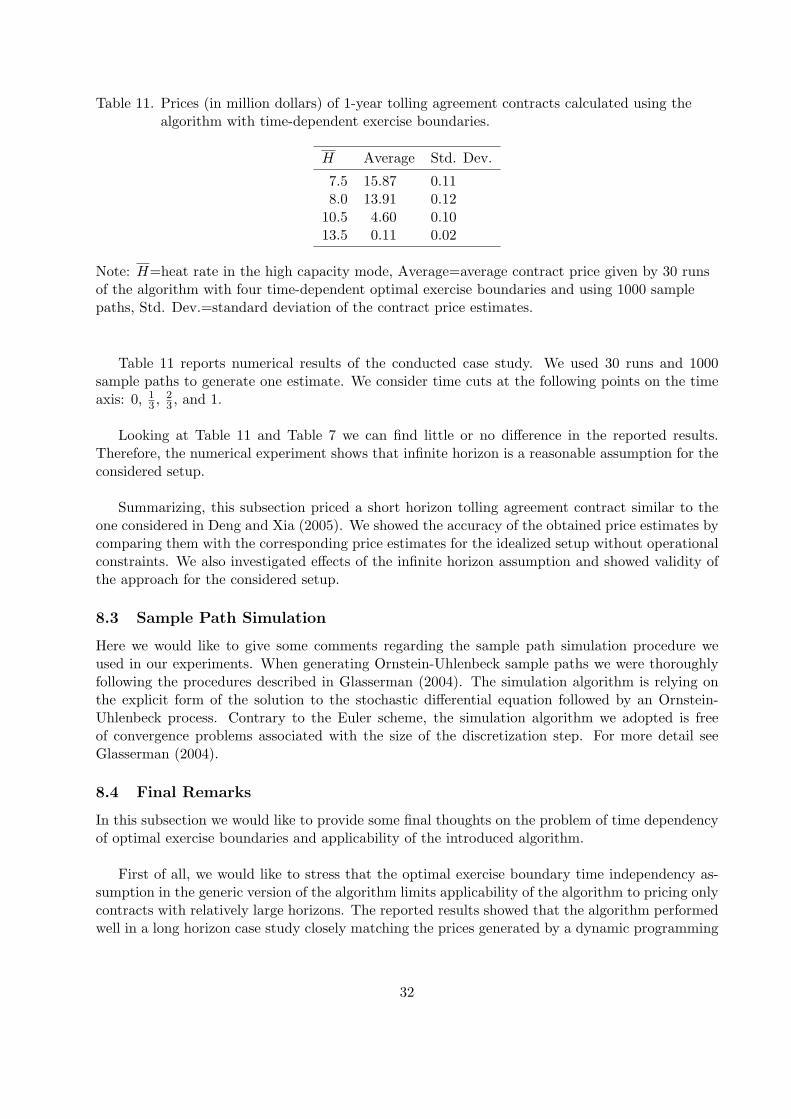
Table 11. Prices (in million dollars) of 1-year tolling agreement contracts calculated using thealgorithm with time-dependent exercise boundaries.

H Average Std. Dev.

7.5 15.87 0.118.0 13.91 0.12

10.5 4.60 0.1013.5 0.11 0.02

Note: H=heat rate in the high capacity mode, Average=average contract price given by 30 runsof the algorithm with four time-dependent optimal exercise boundaries and using 1000 samplepaths, Std. Dev.=standard deviation of the contract price estimates.

Table 11 reports numerical results of the conducted case study. We used 30 runs and 1000sample paths to generate one estimate. We consider time cuts at the following points on the timeaxis: 0, 1

3 , 23 , and 1.

Looking at Table 11 and Table 7 we can find little or no difference in the reported results.Therefore, the numerical experiment shows that infinite horizon is a reasonable assumption for theconsidered setup.

Summarizing, this subsection priced a short horizon tolling agreement contract similar to theone considered in Deng and Xia (2005). We showed the accuracy of the obtained price estimates bycomparing them with the corresponding price estimates for the idealized setup without operationalconstraints. We also investigated effects of the infinite horizon assumption and showed validity ofthe approach for the considered setup.

8.3 Sample Path Simulation

Here we would like to give some comments regarding the sample path simulation procedure weused in our experiments. When generating Ornstein-Uhlenbeck sample paths we were thoroughlyfollowing the procedures described in Glasserman (2004). The simulation algorithm is relying onthe explicit form of the solution to the stochastic differential equation followed by an Ornstein-Uhlenbeck process. Contrary to the Euler scheme, the simulation algorithm we adopted is freeof convergence problems associated with the size of the discretization step. For more detail seeGlasserman (2004).

8.4 Final Remarks

In this subsection we would like to provide some final thoughts on the problem of time dependencyof optimal exercise boundaries and applicability of the introduced algorithm.

First of all, we would like to stress that the optimal exercise boundary time independency as-sumption in the generic version of the algorithm limits applicability of the algorithm to pricing onlycontracts with relatively large horizons. The reported results showed that the algorithm performedwell in a long horizon case study closely matching the prices generated by a dynamic programming

32

algorithm with time dependent boundaries. Although we confirmed no evidence of algorithm in-stabilities in the conducted short horizon case study, in general we expect the algorithm to be moresuccessful in pricing contracts with longer horizons. Our intuition suggests that contract horizonsof 2 years and more should be long enough to justify the use of time-independent boundaries. Weexpect that when horizon is long enough, time-independent boundaries can potentially lead to sub-optimal operating decisions only at a small fraction of time points that are close to the expirationand this should have only a small impact on the profit objective function.

Section 7 presents the first step toward building an efficient algorithm with time dependentoptimal exercise boundaries. In the short horizon case study we applied the discussed version ofthe time-dependent algorithm to test sensitivity of the results to the number of optimal exerciseboundaries used. Although it remained outside the scope of the paper, it is also possible to gener-alize the heuristic that builds separate “on” and “off” exercise boundaries from a single “average”exercise boundary on the time dependent case.

Despite the conducted case study, the discussed version of the time-dependent algorithm remainsrather theoretical than practical in its current form. In order to make the time-dependent versionpractical more research is needed in identifying time-dependent shape properties of optimal exerciseboundaries. An important step would be to find at what time cut planes it is optimal to buildoptimal exercise boundaries and what is the minimal number of time cut planes needed to efficientlyprice a contract. With this regard, we would like to reference an interesting paper on a closelyrelated problem of pricing American put options. In AitSahlia (1999) the authors show that theoptimal exercise boundary in the American put option problem can be efficiently approximatedwith piecewise linear functions (in a transformed space) using a small number of knots. Ideas fromAitSahlia (1999) could potentially lead to a development of an efficient extension of our algorithmto the time dependent case.

9 Summary

We introduced a new approach for pricing tolling agreement contracts. The suggested approachcan incorporate various power plant operational constraints such as startup and shutdown costs,fixed renting costs, variable output capacity levels, output capacity dependent heat rates, ramp upperiod delay, and ramp up period costs. The developed framework does not rely on any particularenergy or fuel price process dynamics. The approach can deal with a general class of underlyingprice dynamics that includes Ornstein-Uhlenbeck processes with and without jumps and dynamicsdefined by historical sample paths.

The introduced algorithm reduces the problem of pricing tolling agreement contracts to a sin-gle linear programming problem. The existence of computationally efficient techniques for solvinglinear programming problems is the primary reason for computational efficiency of the algorithm.The developed algorithm remains efficient for contract horizons of 10 years and larger. An impor-tant property is that the maximum number of variables and constraints in the linear programmingproblem does not depend on the length of the contract or the number of sample paths in the model.The algorithm also provides an easy to use power plant operating strategy described by exerciseboundaries.

33

The algorithm is computationally stable and produces low variance contract price estimates evenwith a relatively small number of sample paths. It is also robust with respect to the granularity ofthe grid on which the optimal exercise boundaries are defined. In the conducted case studies we alsoinvestigated computational effects of optimal exercise boundaries time independence assumption.One of the important factors of the numerical stability of the algorithm is an implicit incorporationof shape properties of optimal exercise boundaries into the linear optimization problem via a set ofmonotonicity constraints on grid variables.

Of course, the suggested approach has its own limitations and simplifying assumptions. Oneof the most important issues that remains open is theoretical investigation of the infinite horizonassumption for the optimal exercise boundaries. Although the assumption proved to be reasonablein the conducted cases studies, it would be important to understand under what conditions theassumption fails to be justified. It is also important to theoretically estimate the error comingfrom the heuristic that builds “on” and “off” exercise boundaries from a single “average” exerciseboundary using a parallel shift.

In cases when time dependent boundaries are needed it is possible to use a time-depended versionof the introduced algorithm. In this paper we briefly outlined how to generalize the algorithm forfinding a single “average” exercise boundary on the time-dependent case but further research isneeded in order to build a more efficient algorithm for the case of time dependent optimal exerciseboundaries. We provided a brief outline of research in this direction.

34

Appendix

Proof of Lemma 1 . From (6) it flows that ξ∗1 = 1 is optimal in P 1N (1) if and only if:

M1 − f1(1, 1) + e−rE[J2

N−1(1)|F1

] ≥ −f1(1, 0) + e−rE[J2

N−1(0)|F1

] ⇔⇔ E

[J2

N−1(1)|F1

]−E[J2

N−1(0)|F1

] ≥ er (−Cd −M1) .

Similarly, from (6) it flows that ξ∗1 = 1 is optimal in P 1N (0) if and only if:

−f1(0, 1) + e−rE[J2

N−1(1)|F1

] ≥ −f1(0, 0) + e−rE[J2

N−1(0)|F1

] ⇔⇔ E

[J2

N−1(1)|F1

]−E[J2

N−1(0)|F1

] ≥ erC1s .

The lemma is proved. 2

Proof of Lemma 2 . The proof is straightforward:

Mi + Cis + Cd = max

(Q

(Pi −H ·Gi

)−K + Cis + Cd, Q (Pi −H ·Gi)−K + Ci

s + Cd

).

It is also true that:

Q (Pi −H ·Gi)−K + Cis + Cd = Q · Pi −Q ·H ·Gi −K + (Cs + L ·Gi) + Cd =

= Q · Pi +(L−Q ·H)

Gi + (Cs + Cd −K) ≥ Q · Pi ≥ 0.

Here we used the facts that L = Q ·H and Cs+Cd ≥ K (see Section 2). Since the second expressionunder the max sign is always nonnegative, the whole max expression is always nonnegative. Hence,the lemma is proved. 2

Proof of Theorem 1 . We work the proof using the method of mathematical induction by N .1). First, we verify the statement for N = 1. In this case the problem P 1

N (0) takes the form:

maxξ1

(−C1

s ξ1

).

Since C1s ≥ 0, the optimal solution of the problem above is ξ∗01 = 0. Hence, whatever the optimal

solution of P 1N (1) is, it is always true: ξ∗01 ≤ ξ∗11 .

2). Assume the statement is true for N = K − 1 (K > 1). Let us prove the theorem’s result forN = K. Using (6):

P 1K(0) : max

ξ1

(−f1(0, ξ1) + e−rE[J2

K−1(ξ1)])

P 1K(1) : max

ξ1

(M1ξ1 − f1(1, ξ1) + e−rE

[J2

K−1(ξ1)])

Let ξ∗01 = 1 be optimal in P 1K(0), then from Lemma 1 it has to be satisfied:

E[J2

K−1(1)]− E

[J2

K−1(0)] ≥ erC1

s . (33)

Using the same lemma, the necessary and sufficient condition for ξ∗11 = 1 to be optimal in P 1K(1) is

E[J2

K−1(1)]−E

[J2

K−1(0)] ≥ er (−Cd −M1) . (34)

35

From Lemma 2:C1

s ≥ −Cd −M1. (35)

Applying (35) to (33) we get (34), hence it is true that ξ∗11 = 1 is optimal in P 1K(1). Thus, we claim

ξ∗11 ≥ ξ∗01 . (36)

For any realized values of G2 and P2 let us consider the problem:

P 2K−1 : sup

ξ2,...,ξK

E[S(2,K)|F2].

Denote by ξ∗(K−1)(w, 1) and ξ∗(K−1)(w, 0) optimal solutions of the problems P 2K−1(1) and P 2

K−1(0),respectively. Since P 2

K−1 has (K − 1) time periods, applying the induction’s hypothesis we have

∀ w ∈ Ω, ∀ i = 2,K : ξ∗(K−1)i (w, 1) ≥ ξ

∗(K−1)i (w, 0). (37)

From (36) and (37):

∀ w ∈ Ω, ∀ i = 2,K : ξ∗(K−1)i (w, ξ∗11 ) ≥ ξ

∗(K−1)i (w, ξ∗01 ). (38)

Applying the principle of optimality:

ξ∗(K−1)i (w, ξ∗11 ) = ξ∗1i (w), (39)

ξ∗(K−1)i (w, ξ∗01 ) = ξ∗0i (w). (40)

Finally, from (38), (39) and (40):

∀ w ∈ Ω, ∀ i = 2,K : ξ∗1i (w) ≥ ξ∗0i (w) (41)

Combining (41) with (36), we get the theorem’s statement. Therefore, the induction step is shownand this completes the proof of the theorem. 2

Proof of Lemma 3 . For ∀ i = 1, N consider the derivations below.

If Q (Pi −H ·Gi)−K > Q(Pi −H ·Gi

)−K, then it is true:

Mi = Q (Pi −H ·Gi)−K ⇒M ′

i −Mi ≥ (Q

(P ′

i −H ·G′i

)−K)− (

Q (Pi −H ·Gi)−K)

=

= Q(P ′

i − Pi

)+ Q ·H (

Gi −G′i

) ⇒M ′

i −Mi ≥ Q ·H (Gi −G′

i

)= L

(Gi −G′

i

).

Analogously, if Q (Pi −H ·Gi)−K ≤ Q(Pi −H ·Gi

)−K we get:

M ′i −Mi ≥ Q ·H (

Gi −G′i

) ⇒M ′

i −Mi ≥ Q ·H (Gi −G′

i

)= L

(Gi −G′

i

).

Above we used a model constraint: Q ·H ≥ Q ·H. Hence, we proved

M ′i −Mi ≥ L

(Gi −G′

i

). (42)

36

Finally, because Cis − Ci′

s = L (Gi −G′i), and using (42) we come to

M ′i + Ci′

s ≥ Mi + Cis.

Hence, the lemma is proved. 2

Proof of Lemma 4 . Let ξ∗1 and ξ∗0 be optimal solutions of the problems P 1N (1) and P 1

N (0),respectively.

1) If ξ∗11 = 0 then from Theorem 1 ξ∗01 = 0. Using (6):

J1N (1)− J1

N (0) = −Cd.

Then, applying Lemma 2:M1 + C1

s ≥ J1N (1)− J1

N (0).

Summarizing, it is true:M1 + C1

s ≥ J1N (1)− J1

N (0) ≥ −Cd.

2) Now we consider the case when ξ∗11 = 1. If ξ∗01 = 1 then applying (6) we have

J1N (1)− J1

N (0) = M1 + C1s .

Then, from Lemma 2:J1

N (1)− J1N (0) ≥ −Cd.

Summarizing, it is true:M1 + C1

s ≥ J1N (1)− J1

N (0) ≥ −Cd. (43)

In the case ξ∗01 = 0 we apply the following arguments. Since ξ∗01 = 1 is suboptimal in P 1N (0), then

it is true:

J1N (1)− J1

N (0) ≤ M1 + C1s . (44)

Because ξ∗11 = 0 is suboptimal in P 1N (1), we get the inequality:

J1N (1)− J1

N (0) ≥ −Cd. (45)

From (43),(44), and (45) we get the assertion of the lemma for case 2). Hence, the lemma is proved.2

Proof of Theorem 2 . We work the proof using the method of mathematical induction by N .1). First, we verify the statements for N = 1.

J11 (1)− J1

1 (0) =

(supξ1

ξ1M1 − [1− ξ1]+Cd

)−

(supξ1

−ξ1C1s

)= sup

ξ1

ξ1M1 − [1− ξ1]+Cd.

Similarly:J1′

1 (1)− J1′1 (0) = sup

ξ′1ξ′1M

′1 − [1− ξ′1]

+C ′d.

It is obvious that ξ∗01 = ξ∗0′1 = 0 are optimal solutions in J11 (0) and J1′

1 (0) respectively. There aretwo possible cases for J1

1 (1):

a) If M1 ≥ −Cd ⇒ ξ∗11 = 1 is optimal in J11 (1) ⇒ J1

1 (1)− J11 (0) = M1.

b) If M1 < −Cd ⇒ ξ∗11 = 0 is optimal in J11 (1) ⇒ J1

1 (1)− J11 (0) = −Cd.

37

In case a) we also have

M ′1 ≥ M1 ≥ −Cd = −Cd′ ⇒ ξ∗1′1 = 1 is optimal in J1′

1 (1) and:J1′

1 (1)− J1′1 (0) = M ′

1 ≥ M1 = J11 (1)− J1

1 (0).

In case b):J1′

1 (1)− J1′1 (0) = max

(M ′

1,−C ′d

) ≥ −C ′d = −Cd = J1

1 (1)− J11 (0).

Summarizing a) and b):

J1′1 (1)− J1′

1 (0) ≥ J11 (1)− J1

1 (0),ξ∗1′1 ≥ ξ∗11 ,

ξ∗0′1 ≥ ξ∗01 .

2). Assume the statements are true for N = K − 1 (K > 1). Let us prove the theorem’s result forN = K. For any realizations of G2, P2, G′

2 and P ′2 we can consider the problems P 2

K−1 and P 2′K−1.

Applying the induction’s assumptions to these problems we have

J2′K−1(1)− J2′

K−1(0) ≥ J2K−1(1)− J2

K−1(0). (46)

Since G2, P2, G′2 and P ′

2 are random at time 1, by taking the expectations of both sides in (46),we derive

E[J2′

K−1(1)|F1

]− E[J2′

K−1(0)|F1

] ≥ E[J2

K−1(1)|F1

]−E[J2

K−1(0)|F1

]. (47)

We continue the proof conditioning on the optimal solution of J1K .

a) Assume ξ∗01 = 1 is optimal, then from Theorem 1 we get ξ∗11 = 1. Using (6):

J1K(1)− J1

K(0) = M1 + C1s . (48)

From Lemma 1, ξ∗01 = 1 implies:

E[J2

K−1(1)|F1

]− E[J2

K−1(0)|F1

] ≥ erC1s . (49)

Combining (47) with (49) and using G′1 ≤ G1:

E[J2′

K−1(1)|F1

]− E[J2′

K−1(0)|F1

] ≥ erC1s ≥ erC1′

s .

According to Lemma 1, the last inequality is equivalent to optimality of ξ∗0′1 = 1 in P 1′K (0). Using

Theorem 1 we also get ξ∗1′1 = 1 optimal in P 1′K (1). With the help of (6) we compute the difference:

J1′K(1)− J1′

K(0) = M ′1 + C1′

s . (50)

Since the condition of Lemma 3 is satisfied, then using the lemma and taking into account (48)and (50):

J1′K(1)− J1′

K(0) ≥ J1K(1)− J1

K(0).

The last relation completes the proof of the induction step for case a).b) Assume ξ∗11 = 0 is optimal in P 1

K(1). Automatically, from Theorem 1 we have that ξ∗01 = 0 isoptimal in P 1

K(0). Using (6):J1

K(1)− J1K(0) = −Cd. (51)

38

From Lemma 4 and (51):

J1′K(1)− J1′

K(0) ≥ −C ′d = −Cd = J1

K(1)− J1K(0).

Since for any optimal solutions, ξ∗1′1 and ξ∗0′1 , it is always true that ξ∗1′1 ≥ ξ∗11 and ξ∗0′1 ≥ ξ∗01 ,therefore, the induction step for case b) is shown.c) The last case left is when ξ∗11 = 1 and ξ∗01 = 0. Using (6) we compute

J1K(1)− J1

K(0) = M1 + e−r(E

[J2

K−1(1)|F1

]−E[J2

K−1(0)|F1

]). (52)

From the optimality of ξ∗11 = 1 and Lemma 1:

E[J2

K−1(1)|F1

]−E[J2

K−1(0)|F1

] ≥ er (−Cd −M1) . (53)

Combining (47), (53), and the condition that M ′1 ≥ M1:

E[J2′

K−1(1)|F1

]− E[J2′

K−1(0)|F1

] ≥ E[J2

K−1(1)|F1

]− E[J2

K−1(0)|F1

] ≥≥ er (−Cd −M1) ≥ er

(−Cd −M ′1

)= er

(−C ′d −M ′

1

). (54)

Using (54) and Lemma 1 again, we find that ξ∗1′1 = 1 is optimal in P 1′K (1). Therefore, the monotonic-

ity of optimal solutions is shown. It is left to show the inequality part of the induction hypothesis.If ξ∗0′1 = 0 is optimal, then using (6), (47), M ′

1 ≥ M1 and (52):

J1′K(1)− J1′

K(0) = M ′1 + e−r

(E

[J2′

K−1(1)|F1

]− E[J2′

K−1(0)|F1

]) ≥≥ M1 + e−r

(E

[J2

K−1(1)|F1

]− E[J2

K−1(0)|F1

])= J1

K(1)− J1K(0).

If ξ∗0′1 = 1 is optimal, then using (6):

J1′K(1)− J1′

K(0) = M ′1 + C1′

s . (55)

Applying Lemma 3 and Lemma 4 to (55), we get:

J1′K(1)− J1′

K(0) ≥ M1 + C1s ≥ J1

K(1)− J1K(0).

Hence the induction step for case c) is completed and this finishes the proof of the theorem. 2

Proof of Corollary 2.1 . First, consider the case of a geometric Ornstein-Uhlenbeck process. Theprocess is defined by the equation:

dXt = Xt (a (b− ln Xt) dt + σdWt) . (56)

Applying Ito’s Lemma:

d ln Xt =dXt

Xt− 1

2σ2dt,

dXt

Xt= d ln Xt +

12σ2dt.

Substituting the latter equation into (56), and setting St = ln Xt and θ = b− σ2

2a :

dSt = a (θ − St) + σdWt. (57)

39

Therefore, S(t) is a standard arithmetic Ornstein-Uhlenbeck process. The solution to (57) is

S(t) = e−atS(0) + a

∫ t

0e−a(t−s)θ(s)ds + σ

∫ t

0e−a(t−s)dWs. (58)

If (Pt) and (P ′t) follow the same geometric Ornstein-Uhlenbeck dynamics, then from the condition

P0 ≤ P ′0 and (58) we have

∀ t > 0, ∀ w ∈ Ω : lnPt(w) ≤ lnP ′t(w) ⇒ (59)

∀ t > 0, ∀ w ∈ Ω : Pt(w) ≤ P ′t(w). (60)

Analogously, if (Gt) and (G′t) have the same geometric Ornstein-Uhlenbeck dynamics then from

G0 ≥ G′0:

∀ t > 0, ∀ w ∈ Ω : Gt(w) ≥ G′t(w). (61)

For a process Xt following the geometric Brownian Motion we have

X(t) = X(0)e∫ t0 (µ(s)− 1

2σ2(s))ds+

∫ t0 σ(s)dWs . (62)

Using (62) and the corollary’s assumptions we derive (60) and (61).

We can also allow jumps with independent intensities and magnitudes in the price dynamics.Indeed, if we add a jump component ξdJ to the dynamics equation of the price process X(t), thenthe solution of the equation changes to:

X ′(t) = X(t) ·N(t)∏

i=1

(1 + ξi), for geometric price dynamics,

where N(t) is the total number of jumps before time t, ξis are realizations of jump magnitudes,and X(t) is a solution of the same dynamics equation but without jumps. It can be shown that if(60)- (61) like relations are satisfied for X(t) then they are also satisfied for the process X ′(t).

Using (60), (61) and applying Theorem 2 we get the assertion of the corollary. 2

Proof of Lemma 5 . Let k be the number of equations of type 2) in the system. Then for somei1, ..., ik ⊆ 1, .., n and some ci1 , ..., cik ⊆ C, the following equations are in the system:

xi1 = ci1 ,

...,

xik = cik .

Without loss of generality, we assume ij = j, j = 1, ..., k (change variables if needed). Therefore,in the solution we always have x∗i = ci, i = 1, ...k. Let the rest (n− k) equations of the system be

xi1 = xj1 ,

...,

xin−k= xjn−k

,

40

where i1, ..., in−k ⊆ 1, .., n and j1, ..., jn−k ⊆ 1, .., n. These (n − k) equations can berewritten as a number of chains of equalities of the form:

x11 = ... = x1

l1,

...,

xm1 = ... = xm

lm,

where 2 ≤ li ≤ (n− k), i = 1, ..., m (since (n− k) is the maximal possible length of a chain), andthe following conditions apply

∀ i, j = 1,m, i 6= j :xi

1, ..., xili

∩

xj1, ..., x

jlj

= ∅,

m⋃

i=1

xi

1, ..., xili

=

n−k⋃

p=1

xip , xjp.

The initial system has a unique solution if and only if the next condition is satisfied:

∀ i = 1,m ∃p : 1 ≤ p ≤ li, ∃j : 1 ≤ j ≤ k such that : xip = xj .

Hence, the solution of the system is

x∗1 = c1, ..., x∗k = ck,

x1∗1 = ... = x1∗

l1= cp1 ,

...,

xm∗1 = ... = xm∗

lm= cpm ,

where p1, ..., pm ⊆ 1, .., k and x∗k+1, ..., x∗n ⊆

⋃mi=1xi∗

1 , ..., xi∗li. From the last result, if the

system has a unique solution it has to be of the form specified in the statement of the lemma.Therefore, the lemma is proved. 2

Proof of Theorem 3 . Since the problems (P1BL′) and (L1) have box constraints for ξi,j variables,lower bounds on νj

i and µji variables, and it is always optimal for νj

i s and µji s to be on their

lower bounds (because we solve maximization problems and always have Cd ≥ 0 and Cs ≥ K ⇒(Cj

s,i + M ji ) ≥ 0), (P1BL′) and (L1) always have optimal solutions (the problems are bounded).

As (L1) is a continuous relaxation of (P1BL′), to prove the theorem it is enough to show that (L1)always has an integer optimal solution. Utilizing the fact that if a linear problem has an optimalsolution, at least one of the solutions is attained at a vertex of the feasible region (the optimalsolution set may consist of more than one point). Below we prove that all vertexes of the feasibleregion of (L1) may have only 0-1 coordinates. Let P be the total number of variables in (L1).Since we have a P -dimensional space of variables, in this space any vertex of the feasible regionhas to be a unique solution of a system of P equations (an intersection of P hyperplanes) and hasto satisfy all the feasibility constraints of the problem. Analyzing the constraints constituting thefeasible region of (L1), we find that the feasible region is constrained by hyperplanes defined byequations of one of the following types:

νji = ξj

i − ξji−1, νj

i = 0, µji = ξj

i − ξji−1, µj

i = 0, ξi,j = ξm,l, ξi,j = 0, ξi,j = 1.

Therefore, any vertex has to be a unique solution of a system of P equations, and each of theequations has to be of one of the types specified above. Let us consider such a system. For each

41

variable νji there are only two possible equations that can be present in the system and have νj

i inthem. These equations are

νji = ξj

i − ξji−1 and νj

i = 0.

For each νji there are three possible cases written below.

1) Only νji = 0 is present in the system.

2) Only νji = ξj

i − ξji−1 is present in the system.

3) Both νji = 0 and νj

i = ξji − ξj

i−1are present in the system.

In case 1) we eliminate the variable vji from the system and the newly obtained system still has to

have a unique solution. To get the solution of the initial system we just need to add νji = 0 to the

solution of the obtained system.

In case 2) we also eliminate the variable νji and the corresponding equation from the system.

The resultant system has one less variable and one less equation than the initial system. As theinitial system has a unique solution, the new system has to inherit this property. Let ξj

i = ξj∗i and

ξji−1 = ξj∗

i−1 be a part of the solution of the new system. We can get the solution of the initialsystem by adding νj

i = ξj∗i − ξj∗

i−1 to the solution of the obtained smaller system.

In case 3) we perform similar steps. We eliminate the variable νji and the two corresponding

equations. The only difference in this case is that we also add a new constraint ξji = ξj

i−1 (thisequation can be easily derived from the two equations with νj

i ) to the system. As in the previouscase the obtained system has one less variable, one less constraint, and it inherits the propertythat it has to have a unique solution. The solution of the initial system can be obtained by addingνj

i = 0 to the solution of the newly constructed system.

Applying the described steps we can reduce the original system with P equations to a smallersystem that does not have variables νj

i in it. From the above, we have that the constructed systemhas to have a unique solution. We can also apply a similar logic to eliminate variables µj

i from thesystem. Ultimately, we can get a system that has only variables ξi,j in it. This system has to havea unique solution, and can consist only of equations of the types:

ξi,j = ξm,l, ξi,j = 0, ξi,j = 1.

The variable elimination procedure guarantees that the number of variables in the obtained sys-tem equals to the number of equations. Applying Lemma 5 with C = 0, 1 to the system withξi,js only, we find that its unique solution has a 0-1 representation. From the variable eliminationprocedure we also get that νj

i , µji ∈ −1, 0, 1, but since νj

i = −1 and µji = −1 are not feasible in

(L1) we get the result that the vertexes of the feasible region can only have 0-1 coordinates. Thetheorem is proved. 2

Proof of Lemma 6 . We use the method of mathematical induction to prove the formula.1) For i = 1 the formula simplifies to the following: χp

1 = ξp1 . The last identity is true by the

definition of χpi since the initial state of the plant is “off”.

2)Assume the formula is true for ∀ i ≤ (K − 1) and let us prove it for i = K. From the definitionof χp

i we haveχp

K = (1− χpK−1)ξ

pK + χp

K−1ηpK = ξp

K + χpK−1(η

pK − ξp

K).

42

Using the induction assumption we expand the last equality as follows:

χpK = ξp

K +

(K−1∑

k=1

ξpk

K−1∏

l=k+1

(ηpl − ξp

l )

)(ηp

K − ξpK) = ξp

K +K−1∑

k=1

ξpk

K∏

l=k+1

(ηpl − ξp

l ) =

=K∑

k=1

ξpk

K∏

l=k+1

(ηpl − ξp

l ).

From the last equality, the formula is true for i = K. Therefore, the induction step is shown andthis finishes the proof of the lemma. 2

Proof of Lemma 7 . Consider an arbitrary j = 1, NS . We prove the lemma using an inductionby i.1) If i = 1 then using (31):

χj1 = ξj

1 = sgn([δj

1 − δ]+)

.

In this case γ1,j = δj1.

2) Suppose that the statement of the lemma is true for ∀i ≤ K − 1, for some K ≤ N . From thedefinition of χj

K we haveχj

K = (1− χjK−1)ξ

jK + χj

K−1ηjK .

If ηjK = 0, then we also have ξj

K = 0 (since the “off” boundary always lies no lower than the “on”boundary). Therefore:

χjK = 0 = sgn

([0− δ]+

).

In this case we have γK,j = 0. If ηjK = 1, then:

χjK = (1− χj

K−1)ξjK + χj

K−1 = maxχjK−1, ξ

jK.

Using the induction hypothesis we derive

χjK = max

sgn

([γK−1,j − δ]+

), ξj

K

= max

sgn

([γK−1,j − δ]+

), sgn

([δj

K − δ]+)

=

= sgn([γK,j − δ]+

),

where γK,j = maxγK−1,j , δjK. Therefore, the induction step is shown and the lemma is proved.

2

43

References

[1] AitSahlia, F. and Lai, T. L. (1999) A Canonical Optimal Stopping Problem for AmericanOptions and its Numerical Solution. J. Computational Finance3(2), 33-52.

[2] Bayraktar, E. and Egami, M. (2007) On the One-Dimensional Optimal Switching Problem.Working paper.

[3] Brekke, K. and Oksendal, B. (1994) Optimal Switching in an Economic Activity under Uncer-tainty. SIAM J. Control Optim. 32(4), 1021-1036. ISSN 0363-0129.

[4] Carmona, R. and Durrleman, V. (2003) Pricing and Hedging Spread Options. SIAM Rev. 45(4),627-685. ISSN 1095-7200.

[5] Carmona, R. and Ludkovski, M. (2008) Pricing Asset Scheduling Flexibility Using OptimalSwitching Agreements. Applied Mathematical Finance, Special Issue on Commodities, To Ap-pear 2008.

[6] Carmona, R. and Touzi, N. (2008) Optimal Multiple Stopping and Valuation of Swing Options.Mathematical Finance 18(2), 239-268.

[7] Deng, S.J., Johnson, B. and Sogomonian, A. (2001) Exotic Electricity Options and the Valuationof Electricity Generation and Transmission Assets, Decision Support Systems 30(3), 383-392.

[8] Deng, S.J. and Oren, S.S. (2003) Incorporating Operational Characteristics and Startup Costsin Option-Based Valuation of Power Generation Capacity, Probability in the Engineering andInformational Sciences (PEIS) 17, 155-181.

[9] Deng, S.J. and Xia, Z. (2006) A Real Options Approach for Pricing Electricity Tolling Agree-ments, International Journal of Information Technology&Decision Making 5(3), 421-436.

[10] Dixit, A. (1989) Entry and Exit Decisions under Uncertainty. J. Polit. Economy 97(3), 620-638.

[11] Dixit, A. and Pindyck, R. (1994) Investment under Uncertainty, Princeton University Press,Princeton, NJ.

[12] Eydeland, A. and Wolynec, K. (2003), Energy and Power Risk Management: New Develop-ments in Modeling, Pricing and Hedging, 421-436. John Wiley&Sons, Hoboken, NJ.

[13] Glasserman, P. (2004) Monte Carlo Method in Financial Engineering, Springer-Verlag, New-York.

[14] Hamadene, S. and Jeanblanc, M. (2007) On the Starting and Stopping Problem: Applicationin Reversible Investments. Mathematics of Operations Research 32(1), 182-192.

[15] Pham, H. and Ly Vath, V. (2007) Explicit Solution to an Optimal Switching Problem in theTwo Regime Case. SIAM J. Control Optim. 46(2), 395-426.

[16] Longstaff, F., Schwartz, E. (2001) Valuing American Options by Simulation: A Simple Least-Squares Approach, A Review of Financial Studies 14(1), 113-147.

[17] Thompson, M., Davison, M., Rasmussen, H. (2004) Valuation and Optimal Operation ofElectric Power Plants in Competetive Markets, Operations Research 52(4), 546-562.

44

[18] Tsitsiklis, J., Van Roy, B. (2001) Regression Methods for Pricing Complex American-StyleOptions, IEEE Trans. Neural Networks 12(4) (Special Issue on computational finance), 694-703.

45

pricing energy derivatives by linear programming: tolling

Documents