Radni materijali EIZ-a

EIZ Working Papers

.

ekonomskiinstitut,zagreb

Prosinac December. 2010

Pricing Options on

Commodity Futures: The

Role of Weather and Storage

Marin Božić

Br No. EIZ-WP-1003

Radni materijali EIZ-a EIZ Working Papers

EIZ-WP-1003

Pricing Options on Commodity Futures: The Role of Weather and Storage

Marin Bo�iæ Research Assistant

The Institute of Economics, Zagreb Trg J. F. Kennedyja 7

10000 Zagreb, Croatia

Research Assistant Department of Agricultural and Applied Economics

University of Wisconsin-Madison 311 Taylor Hall, 427 Lorch Street, Madison, WI 53706, U.S.

T. 1 608 239-6079 E. bozic@wisc.edu

www.eizg.hr

Zagreb, December 2010

IZDAVAÈ / PUBLISHER: Ekonomski institut, Zagreb / The Institute of Economics, Zagreb Trg J. F. Kennedyja 7 10000 Zagreb Croatia T. 385 1 2362 200 F. 385 1 2335 165 E. eizagreb@eizg.hr www.eizg.hr ZA IZDAVAÈA / FOR THE PUBLISHER: Sandra Švaljek, ravnateljica / director GLAVNA UREDNICA / EDITOR: �eljka Kordej-De Villa UREDNIŠTVO / EDITORIAL BOARD: Ivan-Damir Aniæ Valerija Botriæ Edo Rajh Paul Stubbs IZVRŠNI UREDNIK / EXECUTIVE EDITOR: Josip Šipiæ TEHNIÈKI UREDNIK / TECHNICAL EDITOR: Vladimir Sukser Tiskano u 80 primjeraka Printed in 80 copies ISSN 1846-4238 e-ISSN 1847-7844 Stavovi izra�eni u radovima u ovoj seriji publikacija stavovi su autora i nu�no ne odra�avaju stavove Ekonomskog instituta, Zagreb. Radovi se objavljuju s ciljem poticanja rasprave i kritièkih komentara kojima æe se unaprijediti buduæe verzije rada. Autor(i) u potpunosti zadr�avaju autorska prava nad èlancima objavljenim u ovoj seriji publikacija. Views expressed in this Series are those of the author(s) and do not necessarily represent those of the Institute of Economics, Zagreb. Working Papers describe research in progress by the author(s) and are published in order to induce discussion and critical comments. Copyrights retained by the author(s).

Contents

Abstract 5

1 Introduction 7

2 Theory 8

2.1 Foundations of Arbitrage Pricing Theory for Options on Futures 8

2.2 Theory of Storage and Time-Series Properties of Commodity Spot and Futures Prices 11

2.3 The Role of Weather for Intra-year Resolution of Price Uncertainty 13

2.4 Option Pricing Formula Using Generalized Lambda Distribution 13

3 Econometric Model 16

4 Data 17

5 Estimation Procedure and Results 18

6 Conclusions and Further Research 19

Appendix 21

References

31

5

Pricing Options on Commodity Futures: The Role of Weather and Storage Abstract: Options on agricultural futures are popular financial instruments used for agricultural price risk management and to speculate on future price movements. Poor performance of Black’s classical option pricing model has stimulated many researchers to introduce pricing models that are more consistent with observed option premiums. However, most models are motivated solely from the standpoint of the time series properties of futures prices and need for improvements in forecasting and hedging performance. In this paper I propose a novel arbitrage pricing model motivated from the economic theory of optimal storage and consistent with implications of plant physiology on the importance of weather stress. I introduce a pricing model for options on futures based on a generalized lambda distribution (GLD) that allows greater flexibility in higher moments of the expected terminal distribution of futures price. I use times and sales data for corn futures and options for the period 1995-2009 to estimate the implied skewness parameter separately for each trading day. An economic explanation is then presented for inter-year variations in implied skewness based on the theory of storage. After controlling for changes in planned acreage, I find a statistically significant negative relationship between ending stocks-to-use and implied skewness, as predicted by the theory of storage. Furthermore, intra-year dynamics of implied skewness reflect the fact that uncertainty in corn supply is resolved between late June and early October, i.e., during corn growth phases that encompass corn silking and grain maturity. Impacts of storage and weather on the distribution of terminal futures price jointly explain upward-sloping implied volatility curves. Keywords: arbitrage pricing model, options on futures, generalized lambda distribution, theory of storage, skewness JEL classification: G13, Q11, Q14 Odreðivanje cijena opcija na futures ugovore za poljoprivredne proizvode: utjecaj vremenskih uvjeta i zaliha Sa�etak: Opcije na futures ugovore za poljoprivredne proizvode su èesto korišteni financijski instrumenti u upravljanju cjenovnim rizikom u poljoprivredi i pri špekuliranju o smjeru kretanja futures cijena. Slabosti klasiènog Blackovog modela potakle su mnoge istra�ivaèe da predlo�e nove modele za odreðivanje cijena opcijskih ugovora koji su više u skladu s opa�enim premijama opcijskih ugovora. Meðutim, takvi modeli su gotovo bez iznimke osmišljeni iskljuèivo na temelju znaèajki vremenskih nizova cijena terminskih ugovora i potrebe za poboljšanjem predviðanja i hedginga. Ovaj rad predla�e novi arbitra�ni model za odreðivanje cijena opcija polazeæi od ekonomske teorije o optimalnom upravljanju zalihama i vodeæi raèuna o implikacijama fiziologije bilja na va�nost vremenskih uvjeta pri rastu. Predstavljen je model za odreðivanje cijena opcija na terminske ugovore zasnovan na generaliziranoj lambda distribuciji (GLD) koja omoguæava veæu fleksibilnost u višim momentima oèekivane krajnje distribucije cijena terminskih ugovora. Podaci o svim zabilje�enim transakcijama opcijskim i terminskim ugovorima za kukuruz u razdoblju 1995.-2009. korišteni su pri procjeni impliciranih parametara asimetrije, posebno za svaki radni dan. Kontrolirajuæi za utjecaj promjena u planiranoj površini za sadnju, nalazim statistièki znaèajan negativan utjecaj odnosa zaliha i potra�nje na implicirani parametar asimetrije, u skladu s hipotezom koja slijedi iz teorije o zalihama. Nadalje, dinamika promjena parametra asimetrije unutar iste godine reflektira èinjenicu da se neizvjesnost o konaènoj velièini �etve razrješava od lipnja do listopada, tj. u vremenskom razdoblju koje obuhvaæa reproduktivnu fazu rasta kukuruza i fazu dozrijevanja zrna. Utjecaj zaliha i vremenskih uvjeta objašnjava pojavu pozitivnog nagiba krivulja implicirane volatilnosti. Kljuène rijeèi: arbitra�ni model cijena, opcije na futures ugovore, generalizirana lambda distribucija, teorija zaliha, asimetrija JEL klasifikacija: G13, Q11, Q14

7

1 Introduction*

Options written on commodity futures have been investigated from several aspects in the

commodity economics literature. For example, Lence, Sakong and Hayes (1994),

Vercammen (1995), Lien and Wong (2002), and Adam-Müller and Panaretou (2009)

considered the role of options in optimal hedging. Use of options in agricultural policy

was examined by Gardner (1977), Glauber and Miranda (1989), and Buschena and

McNew (2008). The effects of news on options prices have been investigated by

Fortenbery and Sumner (1993), Isengildina-Massa et al. (2008), and Thomsen, McKenzie

and Power (2009). The informational content of options prices has been looked into by

Fackler and King (1990), Sherrick, Garcia and Tirupattur (1996), and Egelkraut, Garcia

and Sherrick (2007). Some of the most interesting work done in this area considers

modifications to the standard Black-Scholes formula that accounts for non-normality

(skewness, leptokurtosis) of price innovations, heteroskedasticity, and specifics of

commodity spot prices (i.e., mean-reversion). Examples include Kang and Brorsen (1995)

and Ji and Brorsen (2009).

In this article I revisit the well-known fact that the classical Black’s (1976a) model is

inconsistent with observed option premiums. Previous studies like Fackler and King

(1990) and Sherrick, Garcia and Tirupattur (1996) address this puzzle by identifying

properties of futures prices that deviate from the assumptions of Black’s model, i.e.,

leptokurtic and skewed distributions of the logarithm of terminal futures prices and

stochastic volatility. A common feature of past studies is the grounding of their

arguments in the time-series properties of stochastic processes for futures prices and the

distributional properties of terminal futures prices. In other words, their arguments are

primarily statistical. In contrast to previous studies, I offer an economic explanation for

the observed statistical characteristics. In this paper I analyze in detail options on corn

futures. The focus is on presenting an alternative pricing model that is not motivated by

improving the forecasts of options premiums compared to Black’s or other models, but

by linking option pricing models with the economics of supply for annually harvested

storable agricultural commodities. In particular, I demonstrate the effect of storability

and crop physiology (i.e., susceptibility to weather stress) on higher moments of the

futures price distribution. Only by understanding these fundamental economic forces

can we truly explain why classical option pricing models work so poorly for commodity

futures.

The article is organized as follows. In the second section I examine in detail the

implications of Black’s classical option pricing model on the shape and dynamics of the

futures price distribution. I follow by presenting the rational expectations competitive

equilibrium model with storage, and testable hypothesis on conditional new crop price

distributions that follow from it. In addition to storage, I present the agronomical

* This paper has benefited from helpful discussions with Jennifer Alix-Garcia, Jean-Paul Chavas, Bjorn Eraker, Jeremy

D. Foltz, T. Randall Fortenbery, Bruce E. Hansen, James E. Hodder, Paul D. Mitchell, as well as participants at UW-

Madison and The Institute of Economics, Zagreb seminars and NCCC-134 meetings. The usual disclaimer applies.

8

research on the impact of weather on corn yields. I then develop a novel arbitrage pricing

model for options on commodity futures based on the generalized lambda distribution

(GLD) which I propose to use in calibrating skewness of new crop futures price to match

observed option premiums. The third section describes the econometric model. In the

fourth section I summarize the data used in the econometric analysis. Finally, I describe

the estimation procedure and present results of statistical inference, followed by a set of

conclusions and directions for further research.

2 Theory

2.1 Foundations of Arbitrage Pricing Theory for Options on Futures

Black (1976) was the first to offer an arbitrage pricing model for options on futures

contracts. Despite numerous extensions and modifications proposed in the literature, and

the inability of the model to explain observed option premiums, traders still use this

model in practice, and widely used information systems for traders (e.g., Bloomberg) use

this as their workhorse model for commodity options. This is likely due to its simplicity

and ability to forecast option premiums after appropriate “tweaks” are put in place. Black

proposes that futures prices follow a stochastic process as described below:

dF Fdzσ= (1)

where F stands for futures price, σ for volatility, and dz is an increment of Brownian

motion.

The implication is that futures prices are unbiased expectations of terminal futures prices

(ideally equal to the spot price at expiration), and the stochastic process followed by

futures prices is a geometric Brownian motion.

The option premium V is equal to the present value of the expected option payoff

under a risk-neutral distribution for terminal prices. For example, for a call option with

strike K , volatility σ , risk-free interest rate r , and time left to maturity T :

( ) ( ) ( )0 00, , , , ,0 ; , , ,rT

T T TV K F T r e Max F K f F F r T dFσ σ∞−= −∫ . (2)

Because delta hedging options on futures do not require a hedger to pay the full value of

the futures contract due to margin trading, a risk-neutral terminal distribution for

futures prices is equivalent to a risk-neutral terminal distribution for a stock that pays a

dividend yield equal to the risk-free interest rate:

2 20

1ln ~ ln ,2TF N F Tσ σ⎛ ⎞−⎜ ⎟

⎝ ⎠. (3)

9

Thus, Black’s model postulates that the distribution of terminal futures prices,

conditional on information known at time zero, is lognormal with the first four

moments fully determined by the current futures price and volatility parameter σ . In

particular, the first four moments of the risk-neutral terminal distribution are equal to:

( ) 2 22 2 2 220

4 320

2( 2) 31 1 2t t t t t tF F e SKEW KUe e e eRT eσ σ σ σσ σμ σ += = + +− = − =% % . (4)

For example, if a futures price is $2.50, volatility is 30 percent, and there are 160 days left

to maturity, the standard deviation of the terminal distribution would be $0.50, skewness

would be 0.60, and kurtosis would be 3.64. Therefore, the standard Black’s model implies

that the expected distribution of terminal prices would be positively skewed and

leptokurtic. When complaints are raised that Black’s model imposes normality

restrictions, it is the logarithm of the terminal price that the critique refers to.

The standard way to check if Black’s model is an appropriate pricing strategy is to exploit

the fact that for a given futures price, strike price, risk-free interest rate, and time to

maturity, the model postulates a one-to-one relationship between the volatility coefficient

and the option premium. Thus, the pricing function can be inverted to infer the

volatility coefficient from an observed option premium. Such coefficients are referred to

as implied volatility (IV) and the principal testable implication of Black’s model is that

implied volatility does not depend on how deep in-the-money or out-of-money an option

is. If the logarithm of the terminal price is not normally distributed, then Black’s model

is not appropriate, and implied volatility will vary with option moneyness – a flagrant

violation of the model’s assumptions. Black’s model gives us a pricing formula for

European options on futures. Prices of American options on futures that are assumed to

follow the same stochastic process as in Black’s model must also account for the

possibility of early exercise. For that reason, their prices cannot be obtained through a

closed-form formula, but must be estimated through numerical methods such as the Cox,

Ross and Rubinstein (CRR) (1979) binomial trees.

Implied volatility curves for storable commodity products are almost always upward

sloping. As an example consider the December 2006 corn contract. The futures price on

June 26, 2006 was $2.49/bu. As seen in Figure 1, the implied volatility curve associated

with calculating IV using various December option strikes is strongly upward sloping,

with the implied volatility coefficients for the highest strike options close to 15

percentage points higher than the implied volatility for options with lower strikes.

Geman (2005) calls this phenomenon an “inverse leverage effect,” after the “leverage

effect” proposed to explain downward-sloping implied volatility curves for individual

company stocks. However, this is a complete misnomer. As Black (1976b) explains, the

leverage effect arises from the fact that as stock price declines, the ratio of a company’s

debts to equity value, its leverage, increases. If the volatility of company assets is constant,

then as the equity share of assets declines, volatility in equity will increase. While the

10

leverage effect has the coherent causal model to justify the term, nothing similar exists

for “inverse leverage effect.”

We can gain further insight as to how Black’s model performs if we plot the implied

volatility curve for a single contract at different time-to-maturity horizons. As an

example, consider December corn contracts in the years 2004 and 2006. As Figure 2

shows, three distinct patterns are noticeable. First, except when options are very near

maturity, we always see an upward-sloping implied volatility curve. Second, implied

volatility of at-the-money options, i.e., options that have the strike price equal to the

current futures price, rises almost linearly until the end of June, declines throughout the

summer months, and then starts rising again. Finally, near maturity, volatility skews give

way to symmetric volatility smiles. The implied volatility coefficient measures volatility

on an annual basis, and the variance of the terminal price, conditional on time

remaining to maturity, is ( )2 T tσ − . So if uncertainty about the terminal price is

uniformly resolved as time passes, implied volatility will not decrease, but will stay the

same. Likewise, when the same amount of uncertainty needs to be resolved in a shorter

time interval, implied volatility will increase. Therefore, linear increases in implied

volatility from distant horizons up until June are best interpreted not as increases in day

to day volatility of futures price changes, but as a market consensus that the conditional

variance of terminal prices is not much reduced before June.

While CRR binomial trees preserve the basic restrictions of Black’s model, i.e., normality

of log-prices terminal distribution, Rubinstein (1994; 1998) shows how that can be

relaxed to allow for non-normal skewness and kurtosis. To illustrate the effect of

skewness and kurtosis on Black’s implied volatility I used Edgeworth binomial trees

(Rubinstein, 1998). This allows for pricing options that exhibit skewed and leptokurtic

distributions of terminal log-prices. As can be seen in Figure 3, zero skewness and no

excess kurtosis (S=0, K=3) corresponds to a flat IV curve, i.e., CRR implied volatility

estimated from options premiums is the same no matter what strike is used to infer it,

just like Black’s model would have it. A leptokurtic distribution will cause so-called

“smiles”, i.e., options with strikes further away from the current futures price will

produce higher implied volatility coefficients. Positive skewness creates an upward-

sloping curve, and negative skewness a downward-sloping IV curve.

Faced with the inability of Black’s model to explain observed option premiums,

researchers and traders have pursued three different approaches to address this issue:

1) Start from the end: relax the assumptions concerning risk-neutral terminal

distributions of underlying futures prices, i.e., allow for non-lognormal skewness

and kurtosis. As long as delta hedging is possible at all times (i.e., markets are

complete), it is still possible to calculate option premiums as the present value of

expected option payoffs. Examples of this approach include Jarrow and Rudd

(1982), Sherrick et al. (1996), and Rubinstein (1998). While the formulas that

derive option premiums as discounted expected payoffs assume that options are

11

European, one can still price American options using implied binomial trees

calibrated to the terminal distribution of choice (Rubinstein, 1994).

2) Start from the beginning: start by asking what kind of stochastic process is

consistent with a non-normal terminal distribution. By introducing appropriate

stochastic volatility and/or jumps, one might be able to fit the data just as well as

by the approach above. Examples of this approach are Kang and Brorsen (1995),

Hilliard and Reis (1998), and Ji and Brorsen (2009).

3) “Tweak it so it works good enough” approach: if one is willing to sacrifice

mathematical elegance, the coherence of the second approach, and insights that

might emerge from the first approach, and if the only objective is the ability to

forecast day-ahead option premiums, one can simply tweak Black’s model. An

example of such an approach would be to model the volatility coefficient as a

quadratic function of the strike. Even though it makes no theoretical sense (this

is like saying that options with different strikes live in different universes), this

approach will work good enough for many traders. A seminal article that

evaluates the hedging effectiveness of such an approach is Dumas, Fleming and

Whaley (1998).

In this article I take the first approach, and modify Black’s model by modifying the

terminal distribution of the futures price. Instead of a lognormal, I propose a generalized

lambda distribution developed by Ramberg and Schmeiser (1974) and introduced to

options pricing by Corrado (2001). An alternative would be to use Edgeworth binomial

trees, but preliminary analysis showed that such an approach may not be adequate for

situations where skewness and kurtosis are rather high. In addition, Edgeworth trees work

with the skewness of terminal log-prices, while I prefer to have implied parameters for the

skewness of terminal futures prices directly, not their logarithms. In addition, the GLD

pricing model allows for a higher degree of flexibility in terms of skewness and kurtosis,

i.e., its parameters are easy to imply from observed options prices and it is

straightforward to develop a closed-form solution for pricing options. While these are all

favorable characteristics, it is in fact the ability to gain additional economic insight that

truly justifies yet another option pricing model. GLD allows us to get an explicit estimate

of skewness and kurtosis of the terminal distributions, and that knowledge can be used to

make a strong connection between the economics of supply and financial models for

pricing options on commodity futures.

2.2 Theory of Storage and Time-Series Properties of Commodity Spot and Futures Prices

Deaton and Laroque (1992) used a rational expectations competitive storage model to

explain nonlinearities in the time series of commodity prices: skewness, rare but dramatic

substantial increases in prices, and a high degree of autocorrelation in prices from one

12

harvest season to the next. The basic conclusion of their work was that inability to carry

negative inventories introduces a non-linearity in prices that manifests itself in the above

characteristics.

This is an example of theory being employed in an attempt to replicate patterns of

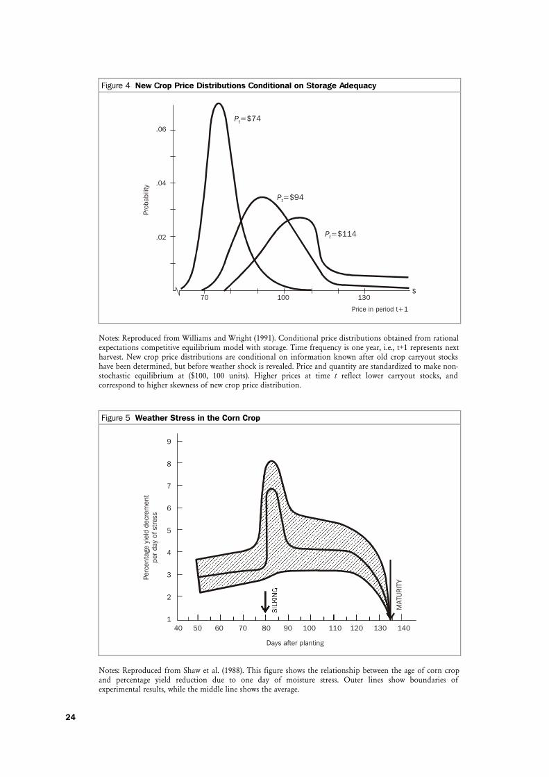
observed price data. In a similar fashion, but subtly different, Williams and Wright

(1991) postulate that the moments of expected price distributions at harvest time vary

with the current (pre-harvest) price and available carryout stocks, as shown in Figure 4.

According to them, when observed at annual or quarterly frequency, spot prices exhibit

positive autocorrelation which emerges because storage allows unusually high or low

excess demand to be spread out over several years. Furthermore, the variance of price

changes depends on the level of inventory. When stocks are high, and the spot price is

low, the abundance of stored stocks serves as a buffer to price changes, and variance is

low. When stocks are low, and thus spot price is high, stocks are nearly empty and unable

to buffer price changes. Finally, the third moment of the price change distribution also

varies with inventories. Since storage can always reduce the downward price pressure of a

windfall harvest, but cannot do as much for a really bad harvest, large price increases are

more common than large decreases. The magnitude of this cushioning effect of storage

depends on the size of the stocks. In conclusion, one should expect commodity prices to

be mean-stationary, heteroskedastic and with conditional skewness, where both the

second and third moments depend on the size of the inventories.

Testing the theory proceeds with this argument: if we can replicate the price pattern using

a particular set of rationality assumptions, then we cannot refute the claim that people

indeed behave in such manner. That is the road taken by Deaton and Laroque (1992) and

Rui and Miranda (1995). However, since in the spot price series we only see the

realizations of prices, not the conditional expectations of them, we cannot use spot price

data to directly test what the market expected to happen. As such, predictions from storage

theory focused on the scale and shape of expected distributions of new harvest spot

prices have remained untested. In this paper I use options data to infer the conditional

expectations of terminal futures prices, and therefore test the following prediction of the

theory of storage:

• The lower inventories are, the more positive the skewness of the conditional harvest

futures price distribution will be.

This is tested using an options pricing formula based on the generalized lambda

distribution to calibrate the skewness and kurtosis of expected (conditional) harvest

futures price distributions. Implied parameters from the model are then used to test the

hypotheses above, as described in detail in section 4.

13

2.3 The Role of Weather for Intra-year Resolution of Price Uncertainty

As demonstrated in section 2.1, a very small share of uncertainty concerning the terminal

price of a new crop futures contract is resolved before June. A large part of uncertainty is

resolved between late June and early October. The reason lies in corn physiology and the

way weather stress impacts corn throughout the growing season. In the major corn

producing areas of the U.S., corn is planted starting the last week of April. It takes about

80 days after planting for a plant to reach its reproduction stage, also known as corn

silking. At this juncture, the need for nutrients is highest, and moisture stress has a large

impact on final yield. Weather continues to play an important role through the rest of

the growing cycle, as summarized by Figure 5, taken from Shaw et al. (1988).

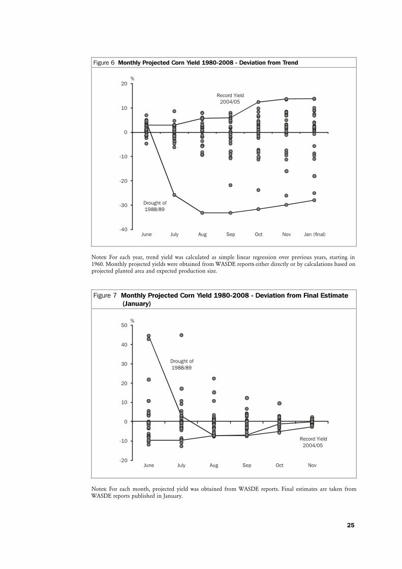
Every month during the growing, the United States Department of Agriculture (USDA)

publishes updated forecasts of corn yield per acre. At the beginning of the growing

season, before corn starts silking, these forecasts are dominated by the long-run trend that

reflects improvements in plant genetics. As can be seen in Figure 6, June forecasts of final

yield deviated from trend value essentially the same in both the record yield year

2004/2005, when final yield was 15 bushels above the trend, and the major draught year

of 1988/89, when final yields were 32 bushels below the trend. However, uncertainty is

quickly resolved in July and August. As shown in Figure 7, whereas June forecasts

deviated from final estimates from the low of -11 percent in 1994/95 to the high of 45

percent in 1988/89, the September estimate deviations ranged only from -7 percent to 12

percent.

A testable hypothesis that emerges from these stylized facts concerns the fundamental

role of seasonality in uncertainty resolution, as well as pronounced negative skewness in

deviations of final yields from trend values. In other words, do seasonal yield deviations

contribute to a positive skewness of terminal price distribution and the dynamics of

skewness throughout the marketing year? In particular, we might expect implied skewness

to decrease throughout the growing season.

2.4 Option Pricing Formula Using Generalized Lambda Distribution

The generalized lambda distribution was developed by Ramberg and Schmeiser (1974),

and its properties were described further by Ramberg et al. (1979). It was introduced to

options pricing by Corrado (2001) who derived a formula for pricing options on non-

dividend paying stocks. Here I review the properties of GLD and adopt Corrado’s

formula to options on futures.

GLD is most easily described by a percentile function1 (i.e., inverse cumulative density

function):

1 F here stands for futures price, not for cumulative density function.

14

( ) ( ) 43

12

1p pF p

λλ

λλ

− −= + . (5)

For example, to say that for ( )0.90, 4.5p F p= = means that the market expects with a

90 percent probability that the terminal futures price will be lower than or equal to

$4.50/bu.

GLD has four parameters: 1λ controls location, 2λ determines variance, and 3λ and 4λ jointly determine skewness and kurtosis. In particular, the mean and variance are

calculated as follows:

( )1 2

2 2 22

/

/

A

B A

μ λ λ

σ λ

= +

= − (6)

with

3 4

1 11 1

Aλ λ

= −+ +

and ( )3 43 4

1 1 2 1 ,1 21 2 1 2

B β λ λλ λ

= + − + ++ +

, where ( )β stands

for complete beta function. We see that the 3λ and 4λ parameters influence both

location and variance, however, 1λ influences only the first moment, and 2λ influences

only the first two moments, i.e., skewness and kurtosis do not depend on 1λ and 2λ .

The skewness and kurtosis formulas are:

3

33 3 2 3

22 4

44 4 4

2

3 2

4 6 3

C AB A

D AC A B A

μασ λ σ

μασ λ

− += =

− + −= =

(7)

with ( ) ( )3 4 3 43 3

1 1 3 1 2 ,1 3 1 ,1 21 3 1 3

C β λ λ β λ λλ λ

= − − + + + + ++ +

and ( ) ( ) ( )3 4 3 4 3 43 3

1 1 4 1 3 ,1 4 1 ,1 3 6 1 2 ,1 21 4 1 4

D β λ λ β λ λ β λ λλ λ

= + − + + − + + + + ++ +

.

A standardized GLD has a zero mean and unit variance, and has a percentile function of

the form:

( ) ( ) ( ) 43

2 3 4 4 3

1 1 11, 1 1

F p p p λλ

λ λ λ λ λ⎛ ⎞

= − − + −⎜ ⎟+ +⎝ ⎠ (8)

where ( ) ( ) 22 3 4 3, sign B Aλ λ λ λ= × − .

From here, we can move more easily to an options pricing environment. We wish to

make GLD an approximate generalization of the log-normal distribution so we keep the

mean and the variance the same as in (4), while allowing skewness and kurtosis to be

15

separately determined by the 3λ and 4λ parameters. Therefore, the percentile function

relevant for option pricing will be

( ) ( ) ( )2

430

2 3 4 4 3

1 1 11 1, 1 1

teF p F p pσ

λλ

λ λ λ λ λ

⎛ ⎞⎛ ⎞−⎜ ⎟= + − − + −⎜ ⎟⎜ ⎟+ +⎝ ⎠⎝ ⎠. (9)

Note that this is equivalent to (5) with ( )

2

1 02 3 4 4 3

1 1 1, 1 1

teFσ

λλ λ λ λ λ

⎛ ⎞−= + −⎜ ⎟+ +⎝ ⎠

and ( )

2

2 3 42

,

1teσλ λ λ

λ =−

. This will guarantee that the first two moments of the terminal

distribution will be ( )22 20 0 1tF F eσμ σ= = −% % , just like in Black’s model.

The pricing formula for European calls is

( ) ( ) ( )0 3 4 0, , , , , , , 0rT

TV K F T r e Max F K dp Fσ λ λ∞−= −∫ . (10)

As shown by Corrado (2001), we can simplify this through a change-of-variable approach

where ( ) TF p F= :

( ) ( ) ( ) ( ) ( )( )( )

1

0,0T TK p K

Max F K dp F F K dp F F p K dp∞ ∞

− = − = −∫ ∫ ∫ . (11)

Here ( )p K stands for the cumulative density function, evaluated at K. While there is no

closed-form formula for the function, values can be easily found with numerical

approaches by using the percentile function.

Integrating ( )F p we get

( )( ) ( )

( )

( )

( ) ( )( ) ( ) ( ) ( )( )

2 4

3

2 43

11

1 11 0

2 3 4 3 4 4 3

11

02 3 4 3 4

11 1 1 1, 1 1 1 1

1 111, 1 1

t

p K

p K

t

peG F p dp F p p p p

p K p Kp K p KeF p K

λσλ

λλσ

λ λ λ λ λ λ λ

λ λ λ λ λ

++

++

⎛ ⎞⎛ ⎞−−⎜ ⎟= = + + + −⎜ ⎟⎜ ⎟⎜ ⎟+ + + +⎝ ⎠⎝ ⎠

⎛ ⎞⎛ ⎞− − −−−⎜ ⎟⎜ ⎟= − + +⎜ ⎟⎜ ⎟+ +

⎝ ⎠⎝ ⎠

∫

with the final European call pricing formula being:

( )0 3 4 0 1 2, , , , , , rt rtV K F T r F e G e KGσ λ λ − −= − (12)

where 1G is defined above and ( )2 1G p K= − .

In a similar way it can be shown that the price for a put is

( ) ( ) ( )0 3 4 2 0 1, , , , , , 1 1rt rtPV K F T r e K G F e Gσ λ λ − −= − − − . (13)

16

3 Econometric Model

The first thing I seek to explain is inter-year variation in implied skewness. As argued in

the second section, skewness will likely be impacted by weather once corn silking starts.

Therefore, if we are to infer an impact of storage on skewness across many years, each

with its own weather peculiarities, we should choose the time before the reproductive

growth phase starts, i.e., no later than the third week of June. If we were to choose

skewness observed much earlier than that, we would risk falling in the endogeneity trap.

Before a marketing year is close to an end, consumption can react to changes in futures

price, possibly even in options premiums, thus increasing or decreasing carryout stocks.

It would make little sense then to use expected ending stocks-to-use as a predetermined

explanatory variable and implied skewness as a dependent variable. To avoid this

problem, expected ending stocks-to-use ratio, as reported in the June edition of the World

Agricultural Supply and Demand Estimates (WASDE) report,2 is employed as the

explanatory variable for storage adequacy.

If the supply of corn is not completely inelastic to prices, we would expect rational

producers to react to tighter expected storage stocks and higher new crop prices with an

increase in planted acreage, so acreage response is the second variable we need to include

in the model. To control for elastic supply, I use the measure of change between intended

plantings, as reported in the Prospective Plantings report3 published at the end of March,

and the actual acreage planted in the previous marketing year.

In addition to supply side covariates, we need to address possible asymmetries in

uncertainty of demand. Corn is used as livestock feed, an industrial sweetener and as an

input in ethanol production. All three of these derived demand categories are likely

impacted by macroeconomic shocks. Therefore, as a measure of demand uncertainty I use

the June-to-June change in the national unemployment rate as published by the Bureau

of Labor Statistics.

The final econometric model has the following form:

where ,t TIS stands for implied skewness at time t for a contract expiring at time T. The

change in acreage planted is Th . Since in June we only observe intended plantings,

expected change in acreage is used in the model. Expected ending stocks-to-use is

[ ]/t T tE S D and tUΔ is the June-to-June change in unemployment rate. Theory predicts

that all coefficients except the constant should be negative. A stronger acreage response

2 The WASDE report is published by the World Agricultural Outlook Board, an inter-agency body at the United States

Department of Agriculture. Historical WASDE reports can be accessed at

http://usda.mannlib.cornell.edu/MannUsda/viewDocumentInfo.do?documentID=1194. 3 Prospective Plantings is a government report produced annually by the National Agricultural Statistics Service, an

agency of the United States Department of Agriculture. Historical Prospective Plantings reports can be accessed at

http://usda.mannlib.cornell.edu/MannUsda/viewDocumentInfo.do?documentID=1136.

[ ], 1 2 3/t T t T t T t tIS E h E S D Uα β β β= + Δ + + Δ

17

and higher carryout stocks relative to demand imply more ability to buffer adverse

weather shocks, and will thus reduce skewness. Likewise, a more unstable macroeconomic

environment will decrease demand for fuel and possibly even meat, thus reducing

upward pressure on corn prices.

I did not perform an explicit econometric analysis of intra-year dynamics of skewness,

but I do present detailed visualizations in section 5 that support the argument that

implied skewness will decline during the reproductive and grain filling growth phases for

corn.

4 Data

Commodity futures for corn as well as options on futures are traded on the Chicago

Mercantile Exchange (formerly the Chicago Board of Trade). A dataset comprising all

recorded transactions, i.e., times and sales data for both futures and options on futures,

for the period 1995 through 2009, was obtained. It includes data for both the regular and

electronic trading sessions. The total number of transactions exceeds 30 million. Options

data were matched with the last preceding futures transaction. LIBOR interest rates were

obtained from the British Bankers’ Association and represent the risk-free rate of return.

Overnight, 1 and 2 weeks, and 1 through 12 months of maturity LIBOR rates for the

period 1995 through 2009 were used to obtain the arbitrage-free option pricing formulas.

In particular, each options transaction was assigned the weighted average of interest rates

with maturities closest to the contract traded. To avoid serial correlation in residuals

from estimating implied coefficients in subsequent steps, the data frequency was reduced

to not less than 15 minutes between transactions for the same options contract. This

resulted in 11,139 data files, each containing between 200 and 500 recorded transactions

for a particular trading day for a given commodity. For each data point I separately

estimate implied volatility using CRR binomial trees with 500 steps. Then, for each data

point, the price of a European option using Black’s formula is calculated using the same

parameters (futures price, interest rate, time to maturity) as that recorded for the

American option. In addition, volatility is set equal to the one implied for American

options. These “artificial” European options are then used in calibration and

econometric analysis.

The implied skewness used in the econometric analysis is calculated as a simple average

over 10 business days following the June WASDE report. Due to high incidence of limit-

move days and days with high intraday price changes, year 2008 is excluded from the

sample. Including 2008 would render the calculation of higher moments unreliable.

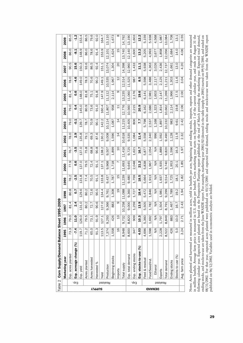
Descriptive statistics of variables used in the econometric analysis are given in Table 1,

and corn supply/demand balance sheets are in Table 2.

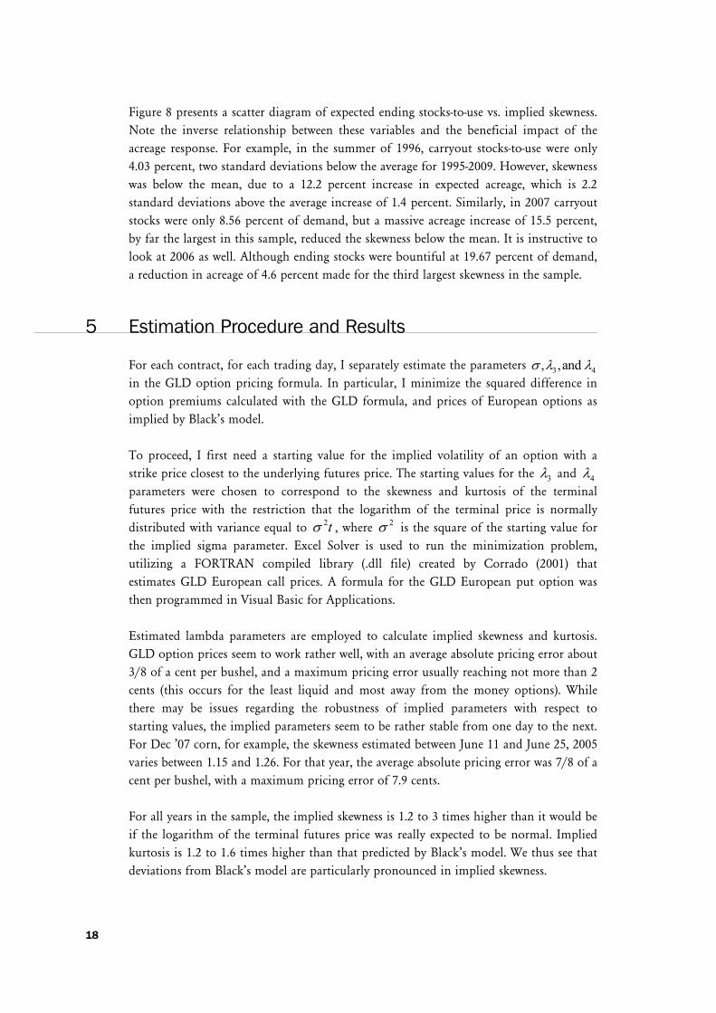
18

Figure 8 presents a scatter diagram of expected ending stocks-to-use vs. implied skewness.

Note the inverse relationship between these variables and the beneficial impact of the

acreage response. For example, in the summer of 1996, carryout stocks-to-use were only

4.03 percent, two standard deviations below the average for 1995-2009. However, skewness

was below the mean, due to a 12.2 percent increase in expected acreage, which is 2.2

standard deviations above the average increase of 1.4 percent. Similarly, in 2007 carryout

stocks were only 8.56 percent of demand, but a massive acreage increase of 15.5 percent,

by far the largest in this sample, reduced the skewness below the mean. It is instructive to

look at 2006 as well. Although ending stocks were bountiful at 19.67 percent of demand,

a reduction in acreage of 4.6 percent made for the third largest skewness in the sample.

5 Estimation Procedure and Results

For each contract, for each trading day, I separately estimate the parameters 3 4, ,and σ λ λ

in the GLD option pricing formula. In particular, I minimize the squared difference in

option premiums calculated with the GLD formula, and prices of European options as

implied by Black’s model.

To proceed, I first need a starting value for the implied volatility of an option with a

strike price closest to the underlying futures price. The starting values for the 3λ and 4λ

parameters were chosen to correspond to the skewness and kurtosis of the terminal

futures price with the restriction that the logarithm of the terminal price is normally

distributed with variance equal to 2tσ , where

2σ is the square of the starting value for

the implied sigma parameter. Excel Solver is used to run the minimization problem,

utilizing a FORTRAN compiled library (.dll file) created by Corrado (2001) that

estimates GLD European call prices. A formula for the GLD European put option was

then programmed in Visual Basic for Applications.

Estimated lambda parameters are employed to calculate implied skewness and kurtosis.

GLD option prices seem to work rather well, with an average absolute pricing error about

3/8 of a cent per bushel, and a maximum pricing error usually reaching not more than 2

cents (this occurs for the least liquid and most away from the money options). While

there may be issues regarding the robustness of implied parameters with respect to

starting values, the implied parameters seem to be rather stable from one day to the next.

For Dec ’07 corn, for example, the skewness estimated between June 11 and June 25, 2005

varies between 1.15 and 1.26. For that year, the average absolute pricing error was 7/8 of a

cent per bushel, with a maximum pricing error of 7.9 cents.

For all years in the sample, the implied skewness is 1.2 to 3 times higher than it would be

if the logarithm of the terminal futures price was really expected to be normal. Implied

kurtosis is 1.2 to 1.6 times higher than that predicted by Black’s model. We thus see that

deviations from Black’s model are particularly pronounced in implied skewness.

19

The effects of a “weather scare” on implied skewness is demonstrated in Figure 9. For

each contract month, skewness was averaged over 15 years (1995-2009) for the matching

time to maturity horizons. Here we clearly see that skewness does not decrease nearly

linearly as is the implication of Black’s model. Instead, we see three distinct phases. First,

before the growing season, skewness is very stable and rather high. Next, during the

growing season, skewness decreases from late June through October. Finally, over the last

90 days to option maturity, skewness declines concavely. It is fascinating to see exactly

the same pattern in all five contract months. This illustrates the rationale for using

skewness in June to search for the effect of storage – this is the time just before the

skewness starts declining.

Simple linear regression is estimated for the period 1995-2009 using implied skewness as

the dependent variable, with constant, expected ending stocks-to-use, expected planned

change in planted acreage, and changes in the unemployment rate as predetermined

explanatory variables. Regression statistics are reported in Table 3. Due to very low

degrees of freedom (10), we have to rely on t-table for critical values, and use a one-tail

test for the stocks-to-use coefficient.

An increase in stocks-to-use by 1 percentage point reduces skewness by 0.015, and this

coefficient estimate is statistically significant at the 95 percent confidence level. To put

this number in perspective, the difference between the lowest and the highest ending

stocks-to-use recorded in the sample reduces skewness from 1.47 to 1.24, which is 47

percent of the difference between the highest and the lowest recorded skewness in the

sample. Coefficients for demand uncertainty and acreage response are also statistically

significant, have the expected sign, and exhibit much less noise than storage variable.

6 Conclusions and Further Research

An options pricing model based on a generalized lambda distribution provides a useful

heuristic in thinking about determinants of the shape of terminal futures price

conditional distributions. Results indicate that crop inventories and plant physiology

play a significant role in determining the expected asymmetry of the terminal

distribution. In particular, results reveal that implied skewness is much more persistent

than implied by Black’s model. In years with low implied volatility, implied skewness

remains much higher than would be the case under the lognormality restriction, and

dynamics are dominated not by time to maturity, but by temporal patterns in resolution

of uncertainty regarding crop yields.

Further research will focus on extending this analysis to soybeans and wheat for which

times and sales data are also available. The U.S. is a major world player in corn, with 55.6

percent of world exports. That is higher than 45.3 percent of world exports of soybeans,

and especially than 17.7 percent in wheat. Extending the analysis to other crops will

identify the effect of trade and non-overlapping growing seasons in different countries on

20

the magnitude, inter-year differences, and intra-year dynamics on implied higher

moments of the terminal price distribution.

Thus far, the literature has focused on evaluating the impacts of government reports on

implied volatility coefficients. The model presented here allows us to extend this to

higher moments and examine how reports (i.e., information) influence the entire

distribution of prices, not just the second moment. For example, we could use weekly

crop progress reports to explain inter-year differences in the evolution of skewness

through the summer months.

In the absence of high frequency data, many researchers use end-of-day reported prices

for futures and options to evaluate implied higher moments. By re-estimating this model

using only end-of-day data it is possible to examine the amount of noise and possible

direction of bias such an approach brings to estimates of implied higher moments.

What happens when storage is not available to partially absorb the shocks to supply? It

would be interesting to use the GLD option pricing model to examine the evolution and

determinants of higher moments of non-storable commodities. Further research is needed

to examine the impact of durability of production factors for commodities that are

themselves not storable.

Finally, impacts of market liquidity and trader composition on the levels and stability of

implied higher moments is a promising new area for research. With careful design of the

analysis, we may be able to find a way to separate the part of the option price that is due

to implied terminal price distributions from additional premium influences incurred due

to hedging pressure or lack of market liquidity.

21

Appendix

Figure 1 Typical Pattern for Implied Volatility Coefficients for Options on Agricultural Futures

0.15

0.20

0.25

0.30

0.35

0.40

-0.3 -0.2 -0.1 0 0.1 0.2 0.3

Log(Strike/Underlying Futures Price)

Implied Volatility

Notes: Implied volatility coefficients are estimated for options on Corn December 2006 futures contract, on

6/26/2006 using Cox, Ross and Rubinstein’s binomial tree with 500 steps. Underlying futures price was

$2.49/bu. Dots represent implied volatility coefficients for each strike, and smooth line is fitted quadratic

trend.

22

Figure 2 Evolution of Implied Volatility Curve for Options on Dec’ 04 and Dec ’06 Corn Futures

ImpliedVolatility

0.42

0.38

0.34

0.30

0.26

0.22

0.18

TimeLn(K/F )t

-0.3

-0

.2

-

0.1

0

0.

1

0.2

Nov, ‘03 Jan, ‘04 Mar, ‘04 May, ‘04 Jul, ‘04 Sep, ‘04

ImpliedVolatility

0.42

0.38

0.34

0.30

0.26

0.22

0.18

TimeLn(K/F )t

-0.3

1

-0

.21

-

0.11

-0.0

1

0.0

9

0

.19

Nov, ‘05 Jan, ‘06 Mar, ‘06 May, ‘06 Jul, ‘06 Sep, ‘06

Notes: For each day, implied volatility is estimated for each traded option using 15-minute interval data.

Quadratic trend curve is fitted to produce implied volatility curve. 30-day moving average is calculated to

increase smoothness of the volatility surface and make it easier to see principal characteristic of the IV curve

evolution. Z-axis shows option moneyness calculated as logarithm of the ratio between option strike (K) and

underlying futures price Ft. When option strike price is equal to current futures price moneyness is zero.

23

Figure 3 Effects of Excess Kurtosis and Positive Skewness on Implied Volatility

2.80 3.30 3.80 4.30

Strike Price

Impl

ied

Vola

tility

0.40

0.39

0.38

0.37

0.36

0.35

0.34

0.33

0.32

0.31

0.30

S=0, K=3 S=0, K=3.5 S=0, K=4.5 S=0, K=5.4

$

3.00 3.50 4.00

BS:

Impl

ied

Vola

tility

0.43

0.42

0.41

0.40

0.39

0.38

0.37

0.36

0.35

0.34

0.33

0.32

0.31

0.30

S=0.3, K=3.5

Strike Price

S=0.6, K=4.5

$

Notes: S stands for skewness, K for kurtosis of terminal futures log-prices. Option premiums are calculated

via Rubinstein’s Edgeworth binomial trees that allow for non-normal skewness and kurtosis, and implied

volatility is inferred using Cox, Ross and Rubinstein’s binomial tree which assumes normality in terminal

futures prices. The black line in the above diagram with S=0 and K=3 corresponds to assumptions of Black’s

model, and in such a scenario implied volatility curve is flat across all strikes. Excess kurtosis (K>3) creates

convex and nearly symmetric “smiles”, and positive skewness produces an upward-sloping implied volatility

curve.

24

Figure 4 New Crop Price Distributions Conditional on Storage Adequacy

.06

.04

.02

70 100 130

Pt=$74

Pt=$94

Pt=$114

Price in period t+1

Prob

abili

ty

$

Notes: Reproduced from Williams and Wright (1991). Conditional price distributions obtained from rational

expectations competitive equilibrium model with storage. Time frequency is one year, i.e., t+1 represents next

harvest. New crop price distributions are conditional on information known after old crop carryout stocks

have been determined, but before weather shock is revealed. Price and quantity are standardized to make non-

stochastic equilibrium at ($100, 100 units). Higher prices at time t reflect lower carryout stocks, and

correspond to higher skewness of new crop price distribution.

Figure 5 Weather Stress in the Corn Crop

9

8

7

6

5

4

3

2

140 50 60 70 80 90 100 110 120 130 140

Days after planting

Perc

enta

ge y

ield

dec

rem

ent

per

day

of s

tres

s

SIL

KIN

G

MAT

UR

ITY

Notes: Reproduced from Shaw et al. (1988). This figure shows the relationship between the age of corn crop

and percentage yield reduction due to one day of moisture stress. Outer lines show boundaries of

experimental results, while the middle line shows the average.

25

Figure 6 Monthly Projected Corn Yield 1980-2008 - Deviation from Trend

Drought of 1988/89

Record Yield 2004/05

-40

-30

-20

-10

0

10

20

June July Aug Sep Oct Nov Jan (final)

%

Notes: For each year, trend yield was calculated as simple linear regression over previous years, starting in

1960. Monthly projected yields were obtained from WASDE reports either directly or by calculations based on

projected planted area and expected production size.

Figure 7 Monthly Projected Corn Yield 1980-2008 - Deviation from Final Estimate (January)

Drought of 1988/89

Record Yield 2004/05

-20

-10

0

10

20

30

40

50

June July Aug Sep Oct Nov

%

Notes: For each month, projected yield was obtained from WASDE reports. Final estimates are taken from

WASDE reports published in January.

26

Figure 8 Relationship between Implied Skewness and Expected Ending Stocks-to-Use

1995

1996

1997

1998

1999

2000

20012002

2003

2004

2005

2006

2007

20091.05

1.15

1.25

1.35

1.45

1.55

4 6 8 10 12 14 16 18 20 22

Ending Stocks-To-Use

Impl

ied

Skew

ness

%

Notes: Years with increase in intended cultivated acreage of 5 or more percent are marked with green rhombs.

Years with June-to-June increase in unemployment rate of 1 percent or more are marked with blue triangles.

Figure 9 Options on Corn Futures: Dynamics of Implied Skewness

Delivery Month: December

0

0.2

0.4

0.6

0.8

1

1.2

1.4

1.6

Dec Jan

Feb

Mar Apr

May Jun

Jul

Aug

Sep Oct

Nov

Impl

ied

Ske

wne

ss

Silking Starts

Harvest Starts

27

Figure 9 Continued

Delivery Month: March

Delivery Month: May

0

0.2

0.4

0.6

0.8

1

1.2

1.4

1.6

Jun

Jul

Aug

Sep Oct

Nov

Dec Jan

Feb

Mar Apr

Impl

ied

Ske

wne

ss

Harvest Starts

Silking Starts

Delivery Month: July

0

0.2

0.4

0.6

0.8

1

1.2

1.4

1.6

Jun

Jul

Aug

Sep O

t

I mpl

ied

Ske

wne

ss

c

Nov

Dec Jan

Feb

Mar Apr

May Jun

Harvest Starts

28

Figure 9 Continued

Delivery Month: September

0

0.2

0.4

0.6

0.8

1

1.2

1.4

1.6

Sep Oct Nov Dec

Impl

ied

Ske

wne

ss

Jan Feb Mar Apr May Jun Jul Aug

Silking Starts

Notes: Implied skewness is estimated for each contract and for each trading day separately using generalized

lambda distribution pricing model for options on commodity futures. Graphs show averages taken over

1995-2009 for each contract and each time to maturity. Corn silking is the reproductive stage of corn growth

where weather starts having major impact on final grain yield. In the major U.S. corn growing area corn

usually starts silking in the last days of June, and corn harvest normally begins in late September.

Table 1 Determinants of Implied Skewness: Descriptive Statistics

Variable Mean Standard deviation Min Max

Implied skewness 1.33 0.14 1.07 1.54

Ending stocks-to-use (%) WASDE June projection

14.4 5.36 4.03 21.23

Intended acreage planted – percentage change 1.37 5.89 -4.84 15.48

Unemployment rate change 0.17 0.23 -0.7 4.00

Notes: Implied skewness was calculated for December corn contracts as average for implied parameters over

10 trading days following June WASDE report. On average, 100-150 data points were used in estimating

implied parameters for each trading day in the stated periods.

Tabl

e 2

Cor

n S

uppl

y/D

eman

d B

alan

ce S

heet

19

95-2

009

Mar

keti

ng y

ear

19

95

19

96

199

7

199

8

19

99

200

0

200

1

20

02

2

00

3 2

004

2

005

20

06

2

00

7

20

08

20

09

Exp.

acr

es p

lant

ed

73.3

79

.0

81.4

80

.8

78.2

77

.9

76.7

78

.0

79.0

79

.0

81.4

78

.0

90.5

86

.0

85.0

Exp.

acr

eage

cha

nge

(%)

-7.4

11

.0

2.4

0

.7

-2.5

0

.6

-3.5

2

.9

-0.1

0.

4

0.6

-4

.6

15

.6

-8.1

-1

.2

Exp.

Exp.

yie

ld

119.

7 12

6.0

131.

0 12

9.6

131.

8 13

7.0

137.

0 13

5.8

139.

7 14

5.0

148.

0 14

9.0

150.

3 14

8.9

153.

4

Acre

s pl

ante

d 71

.2

79.5

80

.2

80.2

77

.4

79.5

75

.8

79.1

78

.7

80.9

81

.8

78.3

93

.6

86.0

86

.5

Acre

s ha

rves

ted

65.0

73

.1

72.7

72

.6

70.5

72

.4

68.8

69

.3

70.9

73

.6

75.1

70

.6

86.5

78

.6

79.6

Har

vest

ed %

91

.3

91.9

90

.6

90.5

91

.1

91.1

90

.8

87.6

90

.1

91.0

91

.8

90.2

92

.4

91.4

92

.0

Yiel

d 11

3.5

127.

1 12

7.0

134.

4 13

3.8

137.

1 13

8.2

130.

2 14

2.2

160.

4 14

7.9

149.

1 15

1.1

153.

9 16

4.7

Prod

uctio

n 7,

374

9,

293

9,

366

9,7

61

9,43

7 9,

968

9,

507

9,

008

10

,114

11

,80

7 11

,11

2 10

,53

5 13

,07

4 12

,101

13

,11

0

Beg

inni

ng s

tock

s 1,

558

42

6 88

3 1,

308

1,

787

1,7

18

1,8

99

1,5

96

1,0

87

958

2,1

14

1,9

67

1,3

04

1,6

24

1,67

3

Impo

rts

16

13

9 19

15

7

10

14

14

11

9 12

20

15

8

SUPPLY

Realized

Tota

l sup

ply

8,9

48

9,7

32

10,2

58

11,0

88

11,2

39

11,6

93

11,4

16

10,6

18

11,2

15

12,7

76

13,2

35

12,5

14

14,3

98

13,7

40

14,7

92

Exp.

tot

al d

eman

d 8,

600

8,

820

9,

000

9,3

60

9,48

0 9,

645

9,

725

9,

535

10

,405

10

,56

0 11

,06

0 11

,52

5 12

,96

0 12

,140

13

,19

0

Exp.

end

ing

stoc

ks

347

909

1,25

9 1,

727

1,

759

2,0

48

1,6

21

1,0

84

806

2,21

5 2,

176

98

7 1,

433

1,

600

1,

603

Exp.

Exp.

sto

cks-

to-u

se (

%)

4.0

3

10.3

1

3.9

1

8.4

1

8.5

21

.2

16

.7

11

.4

7.7

2

0.9

19

.6

8.5

1

1.1

1

3.2

1

2.2

Feed

& r

esid

ual

4,69

6 5,

360

5,

505

5,4

72

5,66

4 5,

838

5,

877

5,

558

5,

798

6,

162

6,1

41

5,5

98

5,9

38

5,2

05

5,15

9

Food

/See

d/In

d.

1,5

98

1,6

92

1,78

2 1,

846

1,

913

1,9

67

2,0

54

2,3

40

2,5

37

2,68

6 2,

981

3,

488

4,

363

4,

993

5.

938

E

than

ol

N/A

N

/A

N/A

N

/A

N/A

N

/A

N/A

99

6 1,

168

1,

323

1,6

03

2,1

17

3,0

26

3,6

77

4,56

8

Expo

rts

2,2

28

1,7

97

1,50

4 1,

981

1,

937

1,9

35

1,8

89

1,5

92

1,8

97

1,81

4 2,

147

2,

125

2,

436

1,

858

1,

987

Tota

l dem

and

8,5

22

8,8

49

8,79

1 9,

299

9,

514

9,7

40

9,8

20

9,4

90

10,2

32

10,6

62

11,2

69

11,2

11

12,7

37

12,0

56

13,0

84

Endi

ng s

tock

s 42

6 88

3 1,

467

1,7

89

1,72

5 1,

953

1,

596

1,

128

98

3 2,

114

1,9

66

1,3

03

1,6

61

1,6

84

1,70

8

DEMAND

Realized

Sto

cks-

to-u

se (

%)

5.0

10.0

16

.7

19.2

18

.1

20.1

16

.3

11.9

9.

61

19.8

17

.5

11.6

13

.0

14.0

13

.1

Avg.

farm

pric

e 3.

24

2.7

1 2.

43

1.94

1.

82

1.8

5 1.

97

2.3

2 2.

42

2.0

6 2.

00

3.0

4 4.

20

4.06

3.

55

Note

s: A

cres

pla

nte

d a

nd h

arve

sted

are

mea

sure

d i

n m

illion a

cres

, yi

eld i

n b

ush

els

per

acr

e, b

egin

nin

g an

d e

ndin

g s

tock

s, i

mport

s, e

xport

s an

d o

ther

dem

and c

ateg

ori

es a

re m

easu

red

in m

illion b

ush

els. A

vera

ge

farm

pri

ce i

s m

easu

red i

n U

.S.

dollar

s per

bush

el.

Corn

mar

ket

ing

year

sta

rts

on S

epte

mber

1 o

f th

e cu

rren

t ca

lendar

yea

r, a

nd e

nds

on A

ugust

31 t

he

follow

ing

cale

ndar

yea

r. E

xpec

ted a

cres

pla

nte

d a

re b

ased

on t

he

Pro

spec

tive

Pla

nti

ngs

rep

ort

publish

ed a

t th

e en

d o

f M

arch

pre

cedin

g t

he

mar

ket

ing

year

. E

xpec

ted t

ota

l dem

and,

endin

g st

ock

s, a

nd s

tock

s-to

-use

are

tak

en fro

m the

June

WA

SD

E r

eport

. For

exam

ple

, m

arket

ing

year

2001/0

2 (den

ote

d in th

e ta

ble

sim

ply

as

2001) st

arte

d o

n 0

9/0

1/2

001, a

nd e

nded

on

08/3

1/2

002.

For

that

yea

r, e

xpec

ted a

cres

pla

nte

d w

ere

publish

ed o

n 0

3/3

1/2

001 a

nd e

xpec

ted t

ota

l dem

and,

endin

g st

ock

s an

d s

tock

s-to

-use

wer

e ta

ken

fro

m t

he

WA

SD

E r

eport

publish

ed o

n 0

6/1

2/2

002. V

aria

ble

s use

d in e

conom

etri

c an

alys

is a

re b

old

ed.

29

30

Table 3 Determinants of Implied Sskewness: Regression Rresults

Explanatory variables Dependent variable: GLD implied skewness

Constant 1.55 (0.10)

Ending stocks-to-use (%) -1.28 (0.64)

Intended acreage planted percentage change

-1.52 (0.58)

Unemployment percentage change

-0.07 0.02

Degrees of freedom 10

Mean root square error 0.075

2R 0.66

Notes: Critical t-statistic for 10 d.f. for 95 percent is 1.81 for one-tail tests and 2.22 for two-tail tests. All

coefficients are statistically significant at a 95 percent confidence level (ending stocks-to-use coefficient is

significant at 95 percent using one-tail test or 90 percent using two-tail test).

31

References

Adam-Müller, A.F.A. and A. Panaretou, 2009, “Risk management with options and

futures under liquidity risk”, Journal of Futures Markets, 29(4), pp. 297-318.

Black, F., 1976a, “The pricing of commodity contracts”, Journal of Financial Economics,

3(1-2), pp. 167-179.

Black, F., 1976b, “Studies of Stock Price Volatility Changes”, in Proceedings of the 1976

Meetings of the Business and Economic Statistics Section, pp. 177-181, Alexandria, VA:

American Statistical Association.

Buschena, D. and K. McNew, 2008, “Subsidized Options in a Thin Market: A Case Study

of the Dairy Options Pilot Program Introduction”, Review of Agricultural Economics, 30(1),

pp. 103-119.

Corrado, C.J., 2001, “Option pricing based on the generalized lambda distribution”,

Journal of Futures Markets, 21(3), pp. 213-236.

Cox, J.C., S.A. Ross and M. Rubinstein, 1979, “Option pricing: A simplified approach”,

Journal of Financial Economics, 7(3), pp. 229-263.

Deaton, A. and G. Laroque, 1992, “On the Behaviour of Commodity Prices”, Review of

Economic Studies, 59(1), pp. 1-23.

Dumas, B., J. Fleming and R.E. Whaley, 1998, “Implied Volatility Functions: Empirical

Tests”, The Journal of Finance, 53(6), pp. 2059-2106.

Egelkraut, T.M., P. Garcia and B.J. Sherrick, 2007, “The Term Structure of Implied

Forward Volatility: Recovery and Informational Content in the Corn Options Market”,

American Journal of Agricultural Economics, 89(1), pp.1-11.

Fackler, P.L. and R.P. King, 1990, “Calibration of Option-Based Probability Assessments

in Agricultural Commodity Markets”, American Journal of Agricultural Economics, 72(1), pp.

73-83.

Fortenbery, T.R. and D.A. Sumner, 1993, “The effects of USDA reports in futures and

options markets”, Journal of Futures Markets, 13(2), pp. 157-173.

Gardner, B.L., 1977, “Commodity Options for Agriculture”, American Journal of

Agricultural Economics, 59, pp. 986-992.

Geman, H., 2005, Commodities and commodity derivatives, West Sussex: John Wiley & Sons

Ltd.

32

Glauber, J.W. and M.J. Miranda, 1989, “Subsidized Put Options as Alternatives to Price

Supports”, in Proceedings of the NCR-134 Conference on Applied Commodity Price Analysis,

Forecasting, and Market Risk Management, pp. 331-353, Chicago, IL: NCR-134,

http://www.farmdoc.uiuc.edu/nccc134 (accessed October 4, 2010).

Hilliard, J.E. and J. Reis, 1998, “Valuation of Commodity Futures and Options Under

Stochastic Convenience Yields, Interest Rates, and Jump Diffusions in the Spot”, The

Journal of Financial and Quantitative Analysis, 33(1), pp. 61-86.

Isengildina-Massa, O., S.H. Irwin, D.L. Good, and J.K. Gomez, 2008, “Impact of WASDE

reports on implied volatility in corn and soybean markets”, Agribusiness, 24(4), pp. 473-

490.

Jarrow, R. and A. Rudd, 1982, “Approximate option valuation for arbitrary stochastic

processes”, Journal of Financial Economics, 10(3), pp. 347-369.

Ji, D. and W. Brorsen, 2009, “A relaxed lattice option pricing model: implied skewness

and kurtosis”, Agricultural Finance Review, 69(3), pp. 268-283.

Kang, T. and B.W. Brorsen, 1995, “Conditional heteroskedasticity, asymmetry, and

option pricing”, Journal of Futures Markets, 15(8), pp. 901-928.

Lence, S.H., Y. Sakong and D.J. Hayes, 1994, “Multiperiod Production with Forward and

Option Markets”, American Journal of Agricultural Economics, 76(2), pp. 286-295.

Lien, D. and K.P. Wong, 2002, “Delivery risk and the hedging role of options”, Journal of

Futures Markets, 22(4), pp. 339-354.

National Agricultural Statistics Service, 2010, Prospective Plantings, Washington, DC:

National Agricultural Statistics Service, United States Department of Agriculture,

http://usda.mannlib.cornell.edu/MannUsda/viewDocumentInfo.do?documentID=1136

(accessed October 4, 2010).

Ramberg, J.S. and B.W. Schmeiser, 1974, “An approximate method for generating

asymmetric random variables”, Communications of the ACM, 17(2), pp. 78-82.

Ramberg, J.S., P.R. Tadikamalla, E.J. Dudewicz and E.F. Mykytka, 1979, “A Probability

Distribution and Its Uses in Fitting Data”, Technometrics, 21(2), pp. 201-214.

Rubinstein, M., 1994, “Implied Binomial Trees”, The Journal of Finance, 49(3), pp. 771-818.

Rubinstein, M., 1998, “Edgeworth Binomial Trees”, The Journal of Derivatives, 5(3), pp. 20-

27.

33

Rui, X. and M.J. Miranda, 1995, “Commodity Storage and Interseasonal Price

Dynamics”, in Proceedings of the NCR-134 Conference on Applied Commodity Price Analysis,

Forecasting, and Market Risk Management, pp. 44-53, Chicago, IL: NCR-134,

http://www.farmdoc.uiuc.edu/nccc134 (accessed October 4, 2010).

Shaw, R.H., J.E. Newman, D.G. Baker, R.V. Crow, R.F. Dale, R. Feltes, D.G. Hanway, P.R.

Henderlong and J.D. McQuigg, 1988, “Weather Stress in the Corn Crop”, OSU Current

Report, CR-2099, Stillwater, OK: Oklahoma State University, Cooperative Extension

Service.

Sherrick, B.J., P. Garcia and V. Tirupattur, 1996, “Recovering probabilistic information

from option markets: Tests of distributional assumptions”, Journal of Futures Markets,

16(5), pp. 545-560.

Thomsen, M.R., A. McKenzie and G.J. Power, 2009, “Volatility Surface and Skewness in

Live Cattle Futures Price Distributions with Application to North American BSE

Announcements”, paper presented at 2009 AAEA & ACCI Joint Annual Meeting,

Milwaukee, WI, July 26-28.

Vercammen, J., 1995, “Hedging with Commodity Options When Price Distributions Are

Skewed”, American Journal of Agricultural Economics, 77(4), pp. 935-945.

Williams, J.C. and B. Wright, 1991, Storage and commodity markets, Cambridge: Cambridge

University Press.

World Agricultural Outlook Board, 2010, World Agricultural Supply and Demand Estimates,

Washington, DC: World Agricultural Outlook Board, United States Department of

Agriculture,

http://usda.mannlib.cornell.edu/MannUsda/viewDocumentInfo.do?documentID=1194

(accessed October 4, 2010).

34

Popis objavljenih Radnih materijala EIZ-a / Previous issues in this series 2010 EIZ-WP-1002 Dubravka Jurlina Alibegoviæ i Sunèana Slijepèeviæ: Performance Measurement at

the Sub-national Government Level in Croatia

EIZ-WP-1001 Petra Posedel and Maruška Vizek: The Nonlinear House Price Adjustment Process in Developed and Transition Countries

2009 EIZ-WP-0902 Marin Bo�iæ and Brian W. Gould: Has Price Responsiveness of U.S. Milk Supply

Decreased?

EIZ-WP-0901 Sandra Švaljek, Maruška Vizek i Andrea Mervar: Ciklièki prilagoðeni proraèunski saldo: primjer Hrvatske

2008 EIZ-WP-0802 Janez Prašnikar, Tanja Rajkoviè and Maja Vehovec: Competencies Driving

Innovative Performance of Slovenian and Croatian Manufacturing Firms

EIZ-WP-0801 Tanja Broz: The Introduction of the Euro in Central and Eastern European Countries – Is It Economically Justifiable?

2007 EIZ-WP-0705 Arjan Lejour, Andrea Mervar and Gerard Verweij: The Economic Effects of Croatia's

Accession to the EU

EIZ-WP-0704 Danijel Nestiæ: Differing Characteristics or Differing Rewards: What is Behind the Gender Wage Gap in Croatia?

EIZ-WP-0703 Maruška Vizek and Tanja Broz: Modelling Inflation in Croatia

EIZ-WP-0702 Sonja Radas and Mario Teisl: An Open Mind Wants More: Opinion Strength and the Desire for Genetically Modified Food Labeling Policy

EIZ-WP-0701 Andrea Mervar and James E. Payne: An Analysis of Foreign Tourism Demand for Croatian Destinations: Long-Run Elasticity Estimates

9 771846 423001

I S S N 1 8 4 6 - 4 2 3 8