primal-dual heuristic for path flow estimation in medium ...docs.trb.org/prp/13-3451.pdf · travel...

Primal‐Dual Heuristic for Path Flow Estimation in Medium to Large Networks

Shikai Tang Graduate Student Researcher Institute of Transportation Studies University of California at Davis Davis, CA 95616 H. Michael Zhang Professor of Civil and Environmental Engineering University of California at Davis Davis, CA 95616 Email: [email protected] And Distinguished Professor of Transportation Engineering School of Transportation Engineering Tongji University, Shanghai, China 201804

Submission Date: 08/01/2012

Number of words: 4962

Number of figures and tables: 7

Total: 5354+8*250 = 7354

Submitted for presentation at the 92th Transportation Research Board Annual Meeting, January 13-17, 201

TRB 2013 Annual Meeting Paper revised from original submittal.

Tang and Zhang

Abstract The Path Flow Estimator (PFE), an Origin‐Destination (OD) demand estimation algorithm

that relies on the computation of path flows, can be slow when applied to medium to large networks. We develop a primal‐dual heuristic that can significantly improve the computational efficiency of the algorithm when it is applied to large networks. Numerical examples are provided to show the performance improvement of this primal‐dual heuristic over the original PFE algorithm.

Key words: Path Flow Estimator (PFE), primal‐dual heuristic, OD estimation for large networks

1


Tang and Zhang

Introduction The Origin‐Destination (OD) trip table is an essential input to many transportation

applications and numerous efforts have been devoted to develop models that estimate OD travel demand from traffic counts (see [1‐3] for a review on modeling, algorithm development and application on this topic). The earlier contributions along this direction are credited to Willumsen [4] for introducing entropy maximization, Van Zuylen [5] for the concept of information minimization, and Cascetta [6] for casting the problem in a generalized least square framework. After decades of research, various OD demand estimators have been proposed. In general, these estimators could be classified into two categories, equilibrium‐based or non equilibrium‐based. If the network concerned has no or minor congestion, i.e., travel time is almost independent of link traffic flow, its demand pattern is assumed to be exogenously determined and obtained by means of proportional loading procedures, which can for example be a simple all‐or‐nothing (AON) assignment. We call this type of models proportional‐assignment OD estimation (ODE) models. Many researchers, such as Willumsen [4] , Van Zuylen [5], Cascetta [6], Bell [7‐8], McNeil and Hendrickson [9] and Lo et al. [10] have proposed proportional‐assignment ODE models. However, as congestion prevails in a network, the proportional‐assignment assumption no longer holds. To take into account network congestion, equilibrium assignment models are incorporated into OD demand estimation. We call this type of models the equilibrium‐assignment OD estimation (E/ODE) models. The first E/ODE model, due to Nguyen [11] [12], is to find an OD matrix that reproduces the observed travel cost when assigned onto the network in a user‐equilibrium fashion. However, the solution of Nugyen’s estimation model may not be unique since the optimization problem is not strictly convex with respect to OD demands. That means there are multiple OD trip matrices that can produce the same link flows. Consequently, a great deal of work has been focused on introducing a secondary optimization problem that leads to a unique solution by minimizing the squared difference between the estimated OD table with a target/historical OD table (Turnquist & Gur [13] , LeBlanc & Farhangian [14]; Sheffi [15]; Yang et al. [16], Yang [17]), maximizing the likelihood of the estimated OD table (Spiess [18]; Maher [19]), or maximizing an entropy function that leads to the most likely OD table (Fisk & Boyce [20]; Fisk [21]).

Because of the second requirement of E/ODE models, they are widely cast into bi‐level form. Models of Yang et al. [16], Yang [17], and Maher et al. [22]’s are examples of this formulation. Although bi‐level formulations could capture equilibrium traffic distribution more accurately, they are very challenging to solve and there is no guarantee that the solution found numerically is the global solution. In order to avoid those challenges, path flow estimators (PFE) based on single‐level optimization, in which path flows instead of OD demands are treated as solution variables, are proposed. Sherali et al. [23] develop the first path flow estimator as a linear programming problem. The path decomposition of OD flows that reproduce the observed link flows is determined by a column generation procedure such that the resulting OD table is the closest to a target (historical) one, while link traffic flows are loaded to approximate user equilibrium assignment. Nie and Lee [24] suggest replacing the column generation procedure by

2


Tang and Zhang

a K‐shortest path ranking algorithm that determines those quasi‐UE paths (columns) exogenously. Nie, Zhang and Recker [25] incorporate this decoupled structure into a generalized least squares (GLS) framework to develop a GLS path flow estimator. In this paper, we study another path flow estimator proposed by Bell [26]‐‐‐the logit path flow estimator (LPFE), the core of which is a logit‐based path choice model. As the result of its convex programming formulation, LPFE gives unique path flows and does not require traffic volumes to be measured on all network links (constraints of linear PFE [23‐25]) but assuming that each unmeasured link has an explicit capacity. This simple mathematical structure of LPFE ensures a global convergence to a unique solution but has the drawback of enumeration of all possible paths between any OD pair, which makes the convergence slow when it is used in medium to large networks.

In this paper, we develop a primal‐dual heuristic that can significantly speed up the convergence of LPFE and enable its application in medium to large networks with considerably less computational time. In the following sections, we present the original LPFE model and its solution algorithm. We describe our primal‐dual heuristic to improve the original solution algorithm. We demonstrate the effectiveness of our primal‐dual heuristic with some numerical results and summarize them in the conclusion.

The Mathematical Formulation of LPFE and its Solution Algorithm

As given in Bell [26] and Chootinan et al. [27], the LPFE model is formulated as follows (See

Appendix for an explanation of the notations):

min Z f1θ

f K

log f 1D

tA

ω dω

(1)

s.t.

x 1 ε · v a M; λ

1 ·

(2)

ε v x ; a M λ

x C U; µ

(3)

a (4)

x fRS

K

fK

D · ε rs D; φ

D · 1 ε

1 (5)

fK

rs D; φ (6)

Where θ is called the dispersion parameter which represents travelers’ sensitivity to path costs. If θ ∞, the estimated path flows are close to user equilibrium. If θ 0, the estimated path flows are close to entropy maximization.

3


Tang and Zhang

In order to describe the solution algorithm of LPFE, we need to form the Lagrangian with dual variables (λ , λ , µ, φ , φ ):

L f, λ , λ , µ, φ , φ1θ

f log K

f 1D

tA

ω dω

f δ 1 ε · v · λ M

1 ε · v f δ · λ f δ C . µ M U

fK

D · 1 ε ε· φ D · 1 fK

· φ

(7)

λ , λ , µ , φ R , φThe d ivati e of function L with respect to f is:

(8)

er v

∂L∂f

1θ

logf t xA

δ δ ·M

λ δ ·M

λ

δ ·U

µ φ φ k K , rs RS (9)

The KKT optimality condition is then given by :

∂L∂f

0 f exp θ t xA

δ θ δ ·M

λ

θ δ ·M

λ θ δ · µ θφU

θφ

(10)

0 λ f δ 1 ε · v 0

0

(11)

λ 1 ε · v f 0 δ

µ

(12)

0 f δ C 0 (13)

0 φ fK

D · 1 ε 0

0 φ D · 1 ε

(14)

fK

0 (15)

4


Tang and Zhang

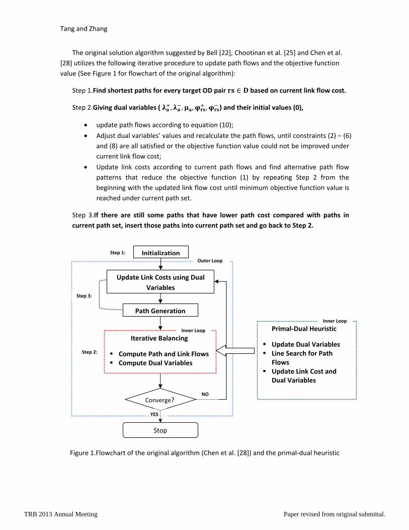
The original solution algorithm suggested by Bell [22], Chootinan et al. [25] and Chen et al. [28] utilizes the following iterative procedure to update path flows and the objective function value (See Figure 1 for flowchart of the original algorithm):

Step 1.Find shortest paths fo v O air based on current link flow cost. r e ery target D p

Step 2.Giving dual variables ( , , , , ) and their initial values (0),

• update path flows according to equation (10);

• Adjust dual variables’ values and recalculate the path flows, until constraints (2) – (6) and (8) are all satisfied or the objective function value could not be improved under current link flow cost;

• Update link costs according to current path flows and find alternative path flow patterns that reduce the objective function (1) by repeating Step 2 from the beginning with the updated link flow cost until minimum objective function value is reached under current path set.

Step 3.If there are still some paths that have lower path cost compared with paths in current path set, insert those paths into current path set and go back to Step 2.

InitializationStep 1:

Figure 1.Flowchart of the original algorithm (Chen et al. [28]) and the primal‐dual heuristic

Update Link Costs using Dual Variables

Path Generation

Iterative Balancing

Compute Path and Link Flows Compute Dual Variables

Converge?

Outer Loop

Inner Loop

Step 3:

Stop

NO

YES

Step 2:

Primal‐Dual Heuristic Inner Loop

Update Dual Variables Line Search for Path Flows

Update Link Cost and Dual Variables

5


Tang and Zhang

In above algorithm, Step 2 is most computationally intensive, in which the procedure of updating dual variables, path flows and link costs repeats multiple times. When combined with a line search procedure, this step becomes extremely slow especially applied to large networks. Hence, the key to improve the overall efficiency of the algorithm is to speed up Step 2 by improving its dual variables updating process. Chootinan et al. [24] notice this possibility of efficiency improvement and suggest a simple heuristic to update the dual variables more efficiently. That heuristic, however, does not take full advantage of the complementary relationship between link costs (t x ) and dual variables (λ , λ , µ, φ , φ ) in equation (10), i.e., increasing link costs to some extent would be equivalent to decreasing λ , µ or increasing λ by a certain amount when calculating path flows according to (10). Instead of updating dual variables from previous results, the practice of re‐initializing dual variables in Step 2 of the original algorithm takes default values (0) for all dual variables in every loop. Hence, we suggest a new primal‐dual heuristic, which adopts information obtained from previous iteration to update dual variables, to speed up the convergence of the whole algorithm. Through the proposed primal‐dual heuristic, the algorithm would avoid redundant computation on dual variables to retain a sub‐optimal path flow pattern (See definition 2) obtained by previous computation.

We use the following example as shown in Figure 2 (Red color stands for sub‐optimal path flows) to explain this process in more detail:

Definition 1.If path flows (f , f , … . f , rs D, k K ) satisfy the following conditions:

1) (Feasible Path Flows) Satisfy e link and historical OD demand constraints (2)‐(6). thti n with link costs fixed: 1θ

2) Minimize the objective func o

f K

log f 1D

CA

x

Here, C a A stands for the fixed link cost after some feasible path flow loading.

Then, these path flows are t l (Local Optimal) Path Flows. called Fixed Link Cost Op ima

Definition 2.If path flows (f , f , … . f , rs D, k K ) satisfy the following conditions:

1) (Feasible Path Flows) Satisfy the link and h to ic d is r al OD emand constraints (2) ‐ (6).

2) Within them, some subset of path flows (f ′ ′, f ′ ′, … . f′

′ ′, k′ K ′ ′ , K ′ ′

K ′ ′ , r′s′ D , D pathD ) minimize the partial flow objective function: 1θ

f′

′ ′

′ K ′ ′

log′

′ ′ 1′ ′ D

tAD

ω dω f

Here, D could be any non empty subset of D; AD stands for links crossed by the path subset.

Then, this subset of path flows (f ′ ′, f ′ ′, … . f′

′ ′, k′ K ′ ′ , K ′ ′ K ′ ′ , r′s′

D , D D ) is called Partial Optimal (Sub‐Optimal) Path Flows.

6


Tang and Zhang

Figure 2.Original Algorithm’s Dual Value Updating vs. The Primal‐Dual Heuristic

After New Path Generation

Path Measured Link Flow

Newly Generated Path Regular Short Two‐Way Link Origin Node

Destination Node

Extreme Long Two‐Way Link

Regular Node

f

f

After a new path (f in this case) is generated, the original algorithm starts with default dual values: λ , λ , λ , λ , λ , λ 0 . The original algorithm will repeat some computation to obtain sub‐optimal path flows , .

With our primal‐dual heuristics, the algorithm will adopt dual variable ( , ) from previous computation and retains the sub‐optimal path flows ( , ) according to equation (10) without further computation. The path flow optimization process will then focus only on the calculation of f and f .

Initial Problem

After Link Cost Update

λ

λ

λ

λ

Default Dual Value: λ , λ , λ , λ , λ , λ 0

After Link Cost Update, the original algorithm starts with default dual value: λ , λ , λ , λ , λ , λ 0 . Then, the original algorithm will have to repeat some computation on dual variables to re‐obtain sub‐optimal path flow and .

λ

f

λ f

After first loop of step 2, some dual variables become active, i.e., their values are not equal to 0. In this case, λ 0, λ0, λ 0. Local optimal path flows (f , f , f ) and sub‐optimal path flow and are found.

λ

With our primal‐dual heuristics, the algorithm will approximately retain sub‐optimal path flows after link cost update. In this case, the algorithm adjusts λ and retain sub‐optimal path flow for OD pair

, while it also adjusts λ and λ and make path flows f and f as optimal as possible after link cost update.

λ

λ

f

7


Tang and Zhang

As seen from Fig. 2, the LPFE solution algorithm starts with free flow traveling cost. After completing the first loop in Step 2, active dual variables (λ , λ , λ ) with local optimal path flows (f , f , f ) and sub‐optimal path flow , (See definition 1 & 2) are found. The original algorithm will update link costs with flow pattern (f , f , f ) and re‐initialize all dual variables with default values (0) to repeat the loop in Step 2. It needs to recalculate (λ , λ ) to obtain sub‐optimal path flows , again. But by using the complementary relationship between dual variables (λ , λ ) and their link cost (C , C ), our primal‐dual heuristic, to be presented in more detail later, will simply adjust active dual variable λ for the initialization process in Step 2 to retain sub‐optimal path flow without further computation. The primal‐dual heuristic also adjusts dual variables (λ , λ ) to make path flows (f , f )’s initial value obtained by (10) as optimal as possible.

The Primal-Dual Heuristic Based on earlier discussions, we propose the following primal‐dual heuristic for updating

the dual variables:

1) Initializing with default values 0 for all dual variables only for the first time Step 2 is implemented.

2) When link costs are fixed, find new path flows according to equation (10); If any constraint (2)‐(6) is not satisfied, update dual va s according to the following heuristics: riable

Set maximum adjus of all dual tment variables ξ 0.

• Fo ink , ute e lnx r each l a A comp l CIf e 0 set µ e; otherwise, if µ , set max µ e, 0 .

n,

Update ξ acco the valu µ 0 µ

rding to e change on µ .

• Fo te e lnx l 1r each link a A , compu v ε If e 0 et λ e; otherwise, if , set max λ e, 0 .

n, s

Update ξ acco the valuλ λ 0 λ

rding to e change on λ .

• Fo ute e lnv lr each link a A , comp 1 ε nx If e 0 et λ λ e; otherwise, if λ , set λ max λ e, 0 . , s 0Update ξ according to the value change on λ .

• For each O‐D pair rs for the r rmation exists, compute which target uppe bound info

n fK

l ε e l nD · 1

If e 0 et φ φ e ; otherwise, if φ 0, set φ max φ e, 0 . , sUpdate ξ according to the value change on φ .

• For each O‐D pair rs for e i rmation exists, compute which th target lower bound nfo

nD · 1 ε e l ln fK

If e 0 et φ φ e ; otherwise, if φ 0, φ max φ e, 0 . , sUpdate ξ according to the value change on φ .

8


Tang and Zhang

If ξ , update link costs, dual variables and objective function values according to procedure 3); otherwise, go back to the beginning of 2).

3) Apply the line search procedure to find path flow patterns that reduce the objective function value most, using the old path flow pattern in the previous loop and the new path flow pattern obtained in 2). Then, update link costs according to the line search path flow results. When link costs are updated link by link, use the following heuristics ( ) to update dual variables:

• Fo linkr each a A , compute e t̃ t

If set axe 0, µ m µ e, lnx e lnC , 0 ; If e 0, keep µ unchanged;

If e 0 and µ , 0 . 0, set µ max µ e• For each link a A , compute e t̃ t

If e 0, λ x λ e,ma lnx e lnv 1 ε , 0 , λ max λ e, 0 ;

O ctherwise, If e 0, keep λ and λ un hanged.

If e 0, λ x λ e, 0 λ max λ e,ma , lnv 1 ε e lnx , 0 ;

Other e 0, keep λ and λ unchanged. wis , if e• Keep φ , φ unchanged during the link cost update process.

• Calculate the comparative gap between the new objective function value obtained from the line search procedure and the old objective function value obtained in the previous

loop. If the comparative gap is lower than η , terminate; otherwise, go back to 2) with

current link costs and dual variable values.

Proposition 1.The above primal‐dual heuristic retains some sub‐optimal path flows and their corresponding link flows once found during the updating process for dual variables.

Proof.

Without loss of generality, we assume the procedure finds the following sub‐optimal path

flow pattern: f , f , … . f , k K , K K , r s D , D D at certain iteration before termination with stable link cost pattern C , a AD (Here, stable link cost pattern means C becomes constant or almost constant after a certain number of iterations).

According to the definition of sub‐optimal path flows, there must be some dual variables

( λ , λ , µ , φ , φ , a AD , r s D ) satisfying the following equation:

9


Tang and Zhang

f exp θ CAD

δ θ δ ·MD

λ

θ δ ·MD

λ θ δ ·UD

µ

θφ θφ

(16)

Follow the above primal‐dual heuristic, we would know that λ , λ , µ , φ , φ , aAD , rs D will be updated to compensate the link cost change as much as possible to maintain the equality between both sides of equation (16). If sub‐optimal path flows with stable link costs were found, the above primal‐dual heuristic will keep the equality exactly between both sides of equation (16) after the link cost updating procedure ( ). With any sub‐optimal path flow

pattern ( f , f , … . f , k K , K K , r s D , D D ) found, so is their

corresponding link flow pattern (x ∑ ∑ fKD , a AD ). The line search procedure

for global convergence won’t change those links’ flow pattern, which then brings no change to those links’ costs and further no effect on their corresponding dual variables according to the primal‐dual heuristic. So, the equality between both sides of Equation (16) is retained with no additional computation cost after performing the line search procedure. Also, the new path generation procedure doesn’t change link costs. If any sub‐optimal path flow pattern was found, those sub‐optimal path flows are intact after performing the new path generation procedure

according to Equation (16) and the primal‐dual heuristic.

Remark 1:

The above primal‐dual heuristic is like a warm‐start technique in regular optimization. It aims at providing a good starting point for updating dual variables after link costs change.

Without loss of generality, we assume the algorithm finds a set of paths whose estimated volumes are very close to their corresponding sub‐optimal values at a certain iteration before termination. We define link set AD as those links that are crossed by these paths. A subset of them AD AD have minor link cost changes in the following link cost updating, while others a AD but a AD have no link cost change in the following link cost updating. Among the links belonging to AD , AM denotes the measured link set, AU denotes the unmeasured link set.

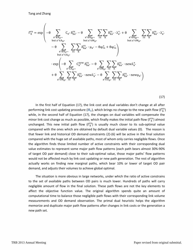
After the link cost updating procedure ( ), the new flow volumes for those paths are obtained by the following equation according to (10):

10


Tang and Zhang

f exp θ CAD

AD

δ θ δ ·AM

MD

λ θ δ ·AM

MD

λ

θ δ ·AU

AU

µ θφ θφ

· exp θ CAD

δ θ δ ·MD

newλ

θ δ ·MD

newλ θ δ ·UD

newµ

(17)

In the first half of Equation (17), the link cost and dual variables don’t change at all after performing link cost updating procedure ( ), which brings no change to the new path flow (f ) while, in the second half of Equation (17), the changes on dual variables will compensate the minor link cost change as much as possible, which finally makes the initial path flow (f ) almost unchanged. This new initial path flow (f ) is usually much closer to its sub‐optimal value compared with the ones which are obtained by default dual variable values (0). The reason is that fewer link and historical OD demand constraints (2)‐(6) will be active in the final solution compared with the huge set of available paths, most of whom only carries negligible flows. Once the algorithm finds those limited number of active constraints with their corresponding dual value estimates to represent some major path flow patterns (each path bears almost 30%‐90% of target OD pair demand) close to their sub‐optimal value, those major paths’ flow patterns would not be affected much by link cost updating or new path generation. The rest of algorithm actually works on finding new marginal paths, which bear 10% or lower of target OD pair demand, and adjusts their volumes to achieve global optimal.

The situation is more obvious in large networks, under which the ratio of active constrains to the set of available paths between OD pairs is much lower. Hundreds of paths will carry negligible amount of flow in the final solution. These path flows are not the key elements to affect the objective function value. The original algorithm spends quite an amount of computational time to balance those negligible path flows with their corresponding link volume measurements and OD demand observation. The primal dual heuristic helps the algorithm memorize and duplicate major path flow patterns after changes in link costs or the generation a new path set.

11


Tang and Zhang

Remark 2:

In practice, it’s impossible to obtain link flow counts and historical OD demand with a hundred percent accuracy. Many researchers (such as Lam and Lo [29], Chootinan et al. [24]) suggest using user‐specific measurement error bounds to handle the data inconsistency caused by inaccurate data. But there is no uniform way to set up user‐specific error bounds. It’s common to follow the so called “try and go” procedure to set up those error bounds. But the original algorithm, which could only re‐estimate new path flows from default dual variable values (0) after any link flow count or historical OD demand error bound change, causes tremendous computation burden for this “try and go” procedure. Now through the primal‐dual heuristic, the algorithm could establish some connections between new solutions that comply with new error bounds with old solutions that are optimized with old error bounds. The algorithm could treat the old path flow pattern as some intermediate result, which holds some sub‐optimal path flow patterns. The reason is that changes in some link flow counts’ error bounds would not affect sub‐optimal paths that do not go through these links. So the algorithm could start with the old path flow pattern and its corresponding dual variable values to find the new path flow patterns, within which some of original sub‐optimal path flows will be kept intact through the primal‐dual heuristic. The new algorithm only makes necessary flow adjustments on paths that hold different flow patterns to represent the new observation information.

Numerical Examples Two example networks (Figure 2) are used to evaluate the primal‐dual heuristic. In the first

example, the highway network of St. Helena, a small town located in the center of Napa Valley, California, is used to represent small‐size networks. It consists of 226 one‐way links, 88 of which have link traffic counts (Details shown in Table 1). In the second example, the highway network of Sacramento, the capital city of California, is used to represent large‐size networks. The Sacramento network consists of 8510 one‐way links, 70 of which have link traffic counts (Details shown in Table 1). The link traffic counts in cities of St. Helena and Sacramento are derived from tube and loop counts in the morning peak hour. We collected average morning peak hour tube and loop counts during different weekdays of a week. Then, we made some random adjustment on several observed link counts to generate the link count observation data.

12


Tang and Zhang

Figure 2.St.Helena (Left) and Sacramento (Right) Transportation Network

Table 1.Network Information

Network Name Number of Nodes

Number of Links (One‐way Per Link)

Number of Measured Links

Number of Target OD Pairs

St.Helena 86 226 88 756 Sacramento 2554 8510 70 14042

13


Tang and Zhang

Figure 3. Algorithmic convergence in the St Helena network

We applied our primal‐dual heuristic LPFE solution algorithm to the St. Helena network

with the given traffic counts and some arbitrarily added error bounds. The computational results are summarized in Figure 3, which depicts the decrease of comparative gap of the objective function value in each major and sub‐ iteration (indicated by a dot or square) and the amount of time taken in each iteration (which is measured by the horizontal spacing between each pair of dots/squares). Here the major iterations are those concerning path generation and line search, and sub‐iterations are those concerning the updating of the dual variables. The reason we use the comparative gap (See Appendix for the definition) rather than the actual objective function values is that for different sizes of networks their objective function values range widely and can be hard to compare. The comparative gap normalizes their values and makes it easy to compare algorithm performance for different sizes of networks.

As one can see from Fig. 3, during the first several iterations, the primal‐dual heuristic algorithm performs similarly as the original algorithm in terms of reducing the comparative gap. But each of the primal‐dual heuristic algorithm’s major iteration takes less computational time. The reason for this is obvious. At first several major iterations, the number of sub‐optimal paths are fewer. Due to the lack of necessary paths, the heuristic, which makes use of previous dual variables, does not have a clear advantage in reducing objective function values, but it does speed up the path generation process. Once enough paths are generated, the algorithm converges much more quickly than the original algorithm, due to its reuse of sub‐optimal paths and dual values from previous iterations. In contrast, the original algorithm stalls after more paths are generated, because without using the values of dual variables from previous iterations it does many redundant computations.

14


Tang and Zhang

Figure 4. Algorithmic convergence in the Sacramento network

The convergence patterns (Fig. 4) from the Sacramento network is similar with that from

the St. Helena network (Fig. 3) but showing greater computational advantage of the primal‐dual heuristic. The new algorithm enables quicker drops in the objective function value even at the first several major iterations than the original algorithm. The reason is that when the network size increases, the number of potential paths increases dramatically, but the number of active constraints are not expanding as quickly; the primal‐dual heuristic helps the algorithm retain those dual variables associated with the few active constraints and find their corresponding sub optimal path flows more quickly; Thus for each new path generated, its contribution to the reduction of the objective function value is substantial before reaching a small neighborhood of the optimal solution. In contrast, the original algorithm searches for a larger set of paths, some of which contain negligible flow that contribute little to the reduction of the objective function value. It repeatedly adds and drops such paths, which consumes a large share of computational time in the algorithm hence considerably slows the convergence of the algorithm.

15


Tang and Zhang

Conclusions In this paper, we introduce a primal‐dual heuristic for path flow estimation using traffic

counts and historical OD demands. The key element of this heuristic is to use the complementary relation between link flow and dual variables to “warm” start the updating of the dual variables. Two examples, one small network and one large network, are used to demonstrate the effectiveness of the proposed heuristic and it was found that the proposed algorithm converges much more quickly than the original solution algorithm, particularly in the case of the large network.

Reference 1. Bell, M.G.H. and Y. Iida, Transportation network analysis. 1997. 2. Cascetta, E., Transportation systems engineering: theory and methods. Vol. 49. 2001:

Springer. 3. Ortuzar, J. and L.G. Willumsen, Modelling transport. 1994. 4. Willumsen, L., Simplified transport models based on traffic counts. Transportation, 1981.

10(3): p. 257‐278. 5. Van Zuylen, H.J. and L.G. Willumsen, The most likely trip matrix estimated from traffic

counts. Transportation Research Part B: Methodological, 1980. 14(3): p. 281‐293. 6. Cascetta, E., Estimation of trip matrices from traffic counts and survey data: A

generalized least squares estimator. Transportation Research Part B: Methodological, 1984. 18(4): p. 289‐299.

7. Bell, M.G.H., The estimation of origin‐destination matrices by constrained generalised least squares. Transportation Research Part B: Methodological, 1991. 25(1): p. 13‐22.

8. Bell, M.G.H., The estimation of an origin‐destination matrix from traffic counts. Transportation Science, 1983. 17(2): p. 198‐217.

9. McNeil, S. and C. Hendrickson, A regression formulation of the matrix estimation problem. Transportation Science, 1985. 19(3): p. 278‐292.

10. Lo, H., N. Zhang, and W. Lam, Estimation of an origin‐destination matrix with random link choice proportions: a statistical approach. Transportation Research Part B: Methodological, 1996. 30(4): p. 309‐324.

11. Nguyen, S., ESTIMATING ORIGIN DESTINATION MATRICES FROM OBSERVED FLOWS. Publication of: Elsevier Science Publishers BV, 1984.

12. Nguyen, S., Estimating an OD matrix from network data: a network equilibrium approach, in Technical Report 60. 1977, University of Montreal.

13. Turnquist, M. and Y. Gur, Estimation of trip tables from observed link volumes. Transportation Research Record, 1979(730).

14. LeBlanc, L.J. and K. Farhangian, Selection of a trip table which reproduces observed link flows. Transportation Research Part B: Methodological, 1982. 16(2): p. 83‐88.

15. Sheffi, Y., Urban Transportation Networks: Equilibrium Analysis with Mathematical Programming Methods 1985, Englewood Cliffs, NJ Prentice‐Hall, Inc.

16. Yang, H., et al., Estimation of origin‐destination matrices from link traffic counts on congested networks. Transportation Research Part B: Methodological, 1992. 26(6): p. 417‐434.

16


Tang and Zhang

17. Yang, H., Heuristic algorithms for the bilevel origin‐destination matrix estimation problem. Transportation Research Part B: Methodological, 1995. 29(4): p. 231‐242.

18. Spiess, H., A maximum likelihood model for estimating origin‐destination matrices. Transportation Research Part B: Methodological, 1987. 21(5): p. 395‐412.

19. Maher, M., Inferences on trip matrices from observations on link volumes: a Bayesian statistical approach. Transportation Research Part B: Methodological, 1983. 17(6): p. 435‐447.

20. Fisk, C. and D. Boyce, A note on trip matrix estimation from link traffic count data. Transportation Research Part B: Methodological, 1983. 17(3): p. 245‐250.

21. Fisk, C., On combining maximum entropy trip matrix estimation with user optimal assignment. Transportation Research Part B: Methodological, 1988. 22(1): p. 69‐73.

22. Maher, M.J., X. Zhang, and D.V. Vliet, A bi‐level programming approach for trip matrix estimation and traffic control problems with stochastic user equilibrium link flows. Transportation Research Part B: Methodological, 2001. 35(1): p. 23‐40.

23. Sherali, H.D., R. Sivanandan, and A.G. Hobeika, A linear programming approach for synthesizing origin‐destination trip tables from link traffic volumes. Transportation Research Part B: Methodological, 1994. 28(3): p. 213‐233.

24. Nie, Y. and D.H. Lee, Uncoupled method for equilibrium‐based linear path flow estimator for origin‐destination trip matrices. Transportation Research Record: Journal of the Transportation Research Board, 2002. 1783(‐1): p. 72‐79.

25. Nie, Y., H. Zhang, and W. Recker, Inferring origin‐destination trip matrices with a decoupled GLS path flow estimator. Transportation Research Part B: Methodological, 2005. 39(6): p. 497‐518.

26. Bell, M.G.H., et al., A stochastic user equilibrium path flow estimator. Transportation Research Part C: Emerging Technologies, 1997. 5(3‐4): p. 197‐210.

27. Chootinan, P., A. Chen, and W. Recker, Improved path flow estimator for origin‐destination trip tables. Transportation Research Record: Journal of the Transportation Research Board, 2005. 1923(‐1): p. 9‐17.

28. Chen, A., S. Ryu, and P. Chootinan, l∞‐norm path flow estimator for handling traffic count inconsistencies: Formulation and solution algorithm. Journal of transportation engineering, 2010. 136(6): p. 565‐575.

29. Lam, W. and H. Lo, Accuracy of OD estimates from traffic counts. Traffic engineering & control, 1990. 31(6): p. 358‐367.

17


Tang and Zhang

A

: Estimated path k’s flow between origin r and destination s

ppendix, Notations:

f

Dispersion parameter θ:

t of all links A: Se

D : Target OD pairs and histor cal demand of OD pair rs D, i

: ny subset of Target OD pairs D A

, U: Set of measured links (with raffic counts) an unmeasured links (without traffic counts) M t d

Set of paths between origin r an tination s K : d des

ε , ε : Relative measurement errors 0,1 for traffic count on link a M and historical travel e nd of OD pair rs D d ma

Observed flow and estimated flow o link a v , x : n

t . : Capacity and cost functio of link a C , n

δ : Path link incidence indicator: 1 if link a is on path k between origin r and destination s, and rwise 0 othe

λ , λ : Dual variables associated with upper and lower bounds of the link flow observation nstraint on link a M; co

: l variables associated with link capacity constraint on link a U µ Dua

φ , φ : Dual variables associated with upper and lower bounds of the historical travel demand nstraint on OD pair rs D; co

: t of links consisted by paths k K , rs D AD Se

D , UD : Set of measured and unmeasured links by paths k K , rs D M

link cost updating procedure H : Primal‐Dual Heuristic during

Z f : Objective function value

: Maximum allowable dual value change

: Minimum comparative objective function value change

z : Objective function value obtained at the end of iteration t. The algorithm updates objective function value at the end of Step 2 minor iteration or Step 3 major iteration .

18


Tang and Zhang

19

z : Min

Gap z : Comparative gap of e

imum objective function value obtained from the algorithm

objectiv function value

Gap zz z

z100%


primal-dual heuristic for path flow estimation in medium ...docs.trb.org/prp/13-3451.pdf · travel...

Documents