primary and secondary frequency control techniques for

Primary and Secondary Frequency ControlTechniques for Isolated Microgrids

by

Mostafa Farrokhabadi

A thesispresented to the University of Waterloo

in fulfillment of thethesis requirement for the degree of

Doctor of Philosophyin

Electrical and Computer Engineering

Waterloo, Ontario, Canada, 2017c© Mostafa Farrokhabadi 2017

I hereby declare that I am the sole author of this thesis. This is a true copy of the thesis,including any required final revisions, as accepted by my examiners.

I understand that my thesis may be made electronically available to the public.

ii

Abstract

Isolated microgrids have been shown to be a reliable and efficient solution to provideenergy to remote communities. From the primary control perspective, due to the low sys-tem inertia and fast changes in the output power of wind and solar power sources, isolatedmicrogrids’ frequency can experience large excursions and thus easily deviate from nominaloperating conditions, even when there is sufficient frequency control reserves; hence, it ischallenging to maintain frequency around its nominal value. From the secondary controlperspective, the generation scheduling of dispatchable units obtained from a conventionalUnit Commitment (UC) are considered fixed between two dispatch time intervals, yield-ing a staircase generation profile over the UC time horizon; given the high variability ofrenewable generation output power, committed units participating in frequency regulationwould not remain fixed between two time intervals. The present work proposes techniquesto address these issues in primary and secondary frequency control in isolated microgridswith high penetration of renewable generation.

In this thesis, first, a new frequency control mechanism is developed which makes useof the load sensitivity to operating voltage and can be easily adopted for various types ofisolated microgrids. The proposed controller offers various advantages, such as allowingthe integration of significant levels of intermittent renewable resources in isolated/islandedmicrogrids without the need for large energy storage systems, providing fast and smoothfrequency regulation with no steady-state error, regardless of the generator control mecha-nism. The controller requires no extra communication infrastructure and only local voltageand frequency is used as feedback. The performance of the controller is evaluated andvalidated using PSCAD/EMTDC on a modified version of the CIGRE benchmark; also,small-perturbation stability analysis is carried out to demonstrate the contribution of theproposed controller to system damping.

In the second stage of the thesis, a mathematical model of frequency control in isolatedmicrogrids is proposed and integrated into the UC problem. The proposed formulationconsiders the impact of the frequency control mechanism on the changes in the generationoutput using a linear model. Based on this model, a novel UC model is developed whichyields a more cost efficient solution for isolated microgrids. The proposed UC is formulatedbased on a day-ahead scheduling horizon with Model Predictive Control (MPC) approach.To test and validate the proposed UC, the realistic test system used in the first part ofthe thesis is utilized. The results demonstrate that the proposed UC would reduce theoperational costs of isolated microgrids compared to conventional UC methods, at similarcomplexity levels and computational costs.

iii

Acknowledgement

First and foremost, I would like to express my sincere gratitude to my supervisors,Professor Claudio A. Canizares and Professor Kankar Bhattacharya for their guidance,patience, and support throughout my PhD studies. Under their supervision, I have learntbeyond the boundaries of power and energy systems. It has been my privilege to havecompleted my studies under their supervisions, and they continue to be my role model inprofessionalism and class throughout my life.

I would like to acknowledge the following members of my committees for their valuablesupport: Professor Mehrdad Kazerani, Professor Christopher Nielsen, and Prof. TarekEl-Fouly from the Department of Electrical and Computer Engineering, University of Wa-terloo; Professor Jatin Nathwani from the Department of Civil and Environmental En-gineering and Management Sciences, University of Waterloo; and Professor Reza Iravanifrom the Department of Electrical and Computer Engineering, University of Toronto.

I wish to acknowledge the University of Waterloo, Natural Sciences and Engineering Re-search Council (NSERC) Strategic Grants and NSERC Smart Microgrid Research Network(NSMG-Net) for providing the funding necessary to carry out this research.

I am always grateful for the support of my friends through the up and downs of thesepast few years. Special thanks to Aref, Bahare, Ehsan, Hootan, Mehrdad, and Mauriciofor being great friends throughout the years. I also acknowledge my officemates for theirfriendship in the EMSOL lab: Summit, Behnam, Daniel, Mariano, Isha, Nafeesa, Indrajit,Amir, Bharat, Fabian, Ivan, Juan Carlos, Edris, Victor, Edson, David, Sofia, Chioma,Alfredo, Akash, Dario, Fabricio, Felipe, Jose, Rajib, Rupali, and Shubha for all technicaldiscussions, and for all the fun we have had during the last few years. Thank you all forcreating a pleasant and friendly working environment in the lab.

Finally, I would like to thank my family and dedicate this thesis to my mom Zari, mydad Mohammad, my sister Maryam, and my brother-in-law Saeed for their unconditionallove and support through all these years. Thank you for all the sacrifices you made, thelife principles you taught me and the comfort you provided me.

iv

You can know the name of a bird in all the languages of the world, but when you’re finished,you’ll know absolutely nothing whatever about the bird... So let’s look at the bird and seewhat it’s doing, that’s what counts. I learned very early, the difference between knowingthe name of something and knowing something.

- R. P. Feynman

v

Table of Contents

List of Tables x

List of Figures xi

Nomenclature xiv

List of Acronyms xxii

1 Introduction 1

1.1 Motivation . . . . . . . . . . . . . . . . . . . . . . . . . . . . . . . . . . . . 1

1.1.1 Primary Frequency Control . . . . . . . . . . . . . . . . . . . . . . 2

1.1.2 Secondary Frequency Control . . . . . . . . . . . . . . . . . . . . . 3

1.2 Literature Review . . . . . . . . . . . . . . . . . . . . . . . . . . . . . . . . 3

1.2.1 Operation and Primary Control of Microgrids . . . . . . . . . . . . 4

1.2.2 Unit Commitment in Isolated Microgrids . . . . . . . . . . . . . . . 8

1.3 Research Objectives . . . . . . . . . . . . . . . . . . . . . . . . . . . . . . . 10

1.4 Outline of the Thesis . . . . . . . . . . . . . . . . . . . . . . . . . . . . . . 11

2 Background Review 13

2.1 Introduction . . . . . . . . . . . . . . . . . . . . . . . . . . . . . . . . . . . 13

2.2 Microgrids . . . . . . . . . . . . . . . . . . . . . . . . . . . . . . . . . . . . 13

2.3 Frequency and Voltage Control in Isolated Microgrids . . . . . . . . . . . . 18

vi

2.3.1 Load Sharing Techniques in Isolated Microgrids . . . . . . . . . . . 19

2.3.2 Frequency Control in Synchronous Machines . . . . . . . . . . . . . 21

2.3.3 Voltage Control in Synchronous Machines . . . . . . . . . . . . . . 25

2.3.4 Frequency and Voltage Controls in Inverters . . . . . . . . . . . . . 27

2.4 Unit Commitment . . . . . . . . . . . . . . . . . . . . . . . . . . . . . . . 31

2.5 Summary . . . . . . . . . . . . . . . . . . . . . . . . . . . . . . . . . . . . 32

3 Hybrid Droop-based Frequency Control in Inverter-based Isolated Mi-crogrids 33

3.1 Transient Decentralized Droop Control . . . . . . . . . . . . . . . . . . . . 33

3.2 Angle Droop Control . . . . . . . . . . . . . . . . . . . . . . . . . . . . . . 34

3.3 Hybrid Droop Control . . . . . . . . . . . . . . . . . . . . . . . . . . . . . 35

3.4 Results and Comparison . . . . . . . . . . . . . . . . . . . . . . . . . . . . 35

3.4.1 Existing Controllers . . . . . . . . . . . . . . . . . . . . . . . . . . . 36

3.4.2 Hybrid Droop Technique . . . . . . . . . . . . . . . . . . . . . . . . 37

3.4.3 Comparison . . . . . . . . . . . . . . . . . . . . . . . . . . . . . . . 38

3.5 Summary . . . . . . . . . . . . . . . . . . . . . . . . . . . . . . . . . . . . 40

4 Voltage-based Frequency Controller 41

4.1 Load Voltage Dependency . . . . . . . . . . . . . . . . . . . . . . . . . . . 41

4.2 Proposed Voltage-Based Frequency Controller . . . . . . . . . . . . . . . . 43

4.3 Impact of VFC on Small-Perturbation Stability . . . . . . . . . . . . . . . 46

4.4 Results for Diesel-based Test System . . . . . . . . . . . . . . . . . . . . . 47

4.4.1 Critical Eigenvalues vs. KV FC . . . . . . . . . . . . . . . . . . . . . 50

4.4.2 Scenario 1: VFC vs. Fast-Acting ESS . . . . . . . . . . . . . . . . . 51

4.4.3 Scenario 2: Disconnection of DER Units . . . . . . . . . . . . . . . 52

4.4.4 Scenario 3: Effect of Operating Voltage Limit . . . . . . . . . . . . 54

4.4.5 Scenario 4: Effect of Load Modelling . . . . . . . . . . . . . . . . . 55

vii

4.4.6 Scenario 5: Diesel Units at Different Buses . . . . . . . . . . . . . . 57

4.5 Results for Inverter-based Test System . . . . . . . . . . . . . . . . . . . . 58

4.5.1 Scenario 6: Disconnection of DER 2 . . . . . . . . . . . . . . . . . . 60

4.5.2 Scenario 7: Fast Active Power Output Variation . . . . . . . . . . . 63

4.6 Discussion . . . . . . . . . . . . . . . . . . . . . . . . . . . . . . . . . . . . 66

4.7 Summary . . . . . . . . . . . . . . . . . . . . . . . . . . . . . . . . . . . . 67

5 Unit Commitment in Isolated Microgrids Considering Frequency Con-trol 69

5.1 UC Model . . . . . . . . . . . . . . . . . . . . . . . . . . . . . . . . . . . . 69

5.1.1 Objective Function . . . . . . . . . . . . . . . . . . . . . . . . . . . 69

5.1.2 Operating Constraints . . . . . . . . . . . . . . . . . . . . . . . . . 74

5.1.3 Reserve Constraints . . . . . . . . . . . . . . . . . . . . . . . . . . . 76

5.2 Results and Discussions . . . . . . . . . . . . . . . . . . . . . . . . . . . . 77

5.2.1 Scenario 1: Proof of Concept . . . . . . . . . . . . . . . . . . . . . . 79

5.2.2 Scenario 2: ILS Control, Deterministic Forecast . . . . . . . . . . . 80

5.2.3 Scenario 3: ILS Control with MPC . . . . . . . . . . . . . . . . . . 82

5.2.4 Scenario 4: Droop Control with MPC . . . . . . . . . . . . . . . . . 84

5.3 Discussions . . . . . . . . . . . . . . . . . . . . . . . . . . . . . . . . . . . 84

5.3.1 Performance of Droop Control and ILS Control . . . . . . . . . . . 84

5.3.2 Control Hierarchies . . . . . . . . . . . . . . . . . . . . . . . . . . . 85

5.3.3 Primary Control Performance of Droop vs. ILS . . . . . . . . . . . 86

5.4 Summary . . . . . . . . . . . . . . . . . . . . . . . . . . . . . . . . . . . . 86

6 Conclusions, Contributions and Future Work 88

6.1 Summary . . . . . . . . . . . . . . . . . . . . . . . . . . . . . . . . . . . . 88

6.2 Contributions . . . . . . . . . . . . . . . . . . . . . . . . . . . . . . . . . . 90

6.3 Future Work . . . . . . . . . . . . . . . . . . . . . . . . . . . . . . . . . . . 91

viii

Bibliography 93

APPENDIX 104

ix

List of Tables

3.1 DERs power Rating and Network Parameters . . . . . . . . . . . . . . . . 37

3.2 Advantages and Disadvantages of Control Techniques . . . . . . . . . . . . 40

4.1 VFC Parameters . . . . . . . . . . . . . . . . . . . . . . . . . . . . . . . . 49

4.2 Critical Eigenvalue Damping . . . . . . . . . . . . . . . . . . . . . . . . . . 50

4.3 DER Parameters. . . . . . . . . . . . . . . . . . . . . . . . . . . . . . . . . 61

4.4 VFC Parameters . . . . . . . . . . . . . . . . . . . . . . . . . . . . . . . . 61

5.1 Diesel Generators Parameters . . . . . . . . . . . . . . . . . . . . . . . . . 79

5.2 Proposed UC vs. Conventional UC for Scenario 1 . . . . . . . . . . . . . . 80



5.5 Proposed UC vs. Conventional UC for Scneario 4 . . . . . . . . . . . . . . 84

1 Governor and AGC . . . . . . . . . . . . . . . . . . . . . . . . . . . . . . . 104

2 Synchronous Machine and AVR . . . . . . . . . . . . . . . . . . . . . . . . 105

3 Line Parameters for the CIGRE Test System . . . . . . . . . . . . . . . . . 106

4 Loads Apparent Power for the CIGRE Test System . . . . . . . . . . . . . 107

x

List of Figures

2.1 Different sizes and configurations of microgrids. . . . . . . . . . . . . . . . 14

2.2 Classification of bulk power system stability . . . . . . . . . . . . . . . . . 16

2.3 Frame for hierarchical control of a microgrid. . . . . . . . . . . . . . . . . . 18

2.4 Governor droop characteristics. . . . . . . . . . . . . . . . . . . . . . . . . 20

2.5 Load sharing by drooping governors. . . . . . . . . . . . . . . . . . . . . . 20

2.6 Block diagram of generator model (2.8). . . . . . . . . . . . . . . . . . . . 22

2.7 Block diagram of a generator-load model. . . . . . . . . . . . . . . . . . . . 22

2.8 Block diagram of a non-reheat steam turbine. . . . . . . . . . . . . . . . . 23

2.9 Block diagram of a speed governing system. . . . . . . . . . . . . . . . . . 24

2.10 Block diagram of synchronous machine frequency control system. . . . . . 24

2.11 Block diagram of synchronous machine frequency control system with ∆PLas input. . . . . . . . . . . . . . . . . . . . . . . . . . . . . . . . . . . . . . 24

2.12 Block diagram of an AVR. . . . . . . . . . . . . . . . . . . . . . . . . . . . 26

2.13 Typical inverter control scheme. . . . . . . . . . . . . . . . . . . . . . . . . 27

2.14 Droop-based reference set-points. . . . . . . . . . . . . . . . . . . . . . . . 29

2.15 Inverter control blocks. . . . . . . . . . . . . . . . . . . . . . . . . . . . . . 30

2.16 Centralized Unit Commitment (UC) for isolated microgrids. . . . . . . . . 31

3.1 Active power droop structure of the hybrid controller. . . . . . . . . . . . . 35

3.2 Test System. . . . . . . . . . . . . . . . . . . . . . . . . . . . . . . . . . . . 36

xi

3.3 Active and reactive power output of DERs with three control techniques:(a) frequency droop, (b) angle droop, and (c) transient droop. . . . . . . . 38

3.4 Frequency response of the system with the three control techniques. . . . . 39

3.5 Active and reactive power output of DERs with the proposed hybrid controller. 39

3.6 Frequency response with the angle droop and the proposed hybrid controltechniques. . . . . . . . . . . . . . . . . . . . . . . . . . . . . . . . . . . . . 40

4.1 The proposed VFC for a system voltage regulator, such as the one for asynchronous machine. . . . . . . . . . . . . . . . . . . . . . . . . . . . . . . 44

4.2 Block diagram of the proposed VFC and its integration with a synchronousmachine. . . . . . . . . . . . . . . . . . . . . . . . . . . . . . . . . . . . . . 44

4.3 Block diagram of the proposed VFC and its integration with a VSC. . . . . 45

4.4 Test microgrid based on a medium voltage distribution network benchmark. 48

4.5 Low-voltage 300 kW wind turbine measured output power. . . . . . . . . . 49

4.6 Dominant eigenvalue for different values of KV FC . . . . . . . . . . . . . . . 50

4.7 Voltage and frequency response of the system due to wind fluctuations forScenario 1. . . . . . . . . . . . . . . . . . . . . . . . . . . . . . . . . . . . . 52

4.8 Active and reactive power injection of diesel Unit 1 with and without theVFC for Scenario 1. . . . . . . . . . . . . . . . . . . . . . . . . . . . . . . . 53

4.9 Active power output of the ESS due to wind fluctuations (Scenario 1). . . . 53

4.10 Voltage and frequency response of the system before, during, and after thedisconnection of DER units for Scenario 2. . . . . . . . . . . . . . . . . . . 54

4.11 Active and reactive power injection of diesel Unit 1 with and without theVFC for Scenario 2. . . . . . . . . . . . . . . . . . . . . . . . . . . . . . . . 55

4.12 Voltages at different buses of the system for Scenario 2. . . . . . . . . . . . 56

4.13 Voltage and frequency response of the system with different voltage limitsfor Scenario 3. . . . . . . . . . . . . . . . . . . . . . . . . . . . . . . . . . . 57

4.14 Voltage and frequency response of the system with different nP for Scenario 4. 58

4.15 Frequency response of the system with and without the VFC for scenario 5. 59

4.16 Voltage response of the system with with and without the VFC for scenario 5. 59

xii

4.17 Active power injection of diesel Unit 1 with and without the VFC for scenario 5. 60

4.18 Reactive power injection of diesel Unit 1 and Unit 2 without the VFC forscenario 5. . . . . . . . . . . . . . . . . . . . . . . . . . . . . . . . . . . . . 60

4.19 Reactive power injection of diesel Unit 1 and Unit 2 with the VFC forscenario 5. . . . . . . . . . . . . . . . . . . . . . . . . . . . . . . . . . . . . 61

4.20 DERs-based Test microgrid based on a medium voltage distribution systembenchmark. . . . . . . . . . . . . . . . . . . . . . . . . . . . . . . . . . . . 62

4.21 Response of the system without VFC for scenario 6. . . . . . . . . . . . . . 63

4.22 Response of the system with VFC for scenario 6. . . . . . . . . . . . . . . . 64

4.23 Response of the system without the VFC for scenario 7. . . . . . . . . . . . 65

4.24 Response of the system with the VFC for scenario 7. . . . . . . . . . . . . 66

5.1 Energy provision in the conventional UC. . . . . . . . . . . . . . . . . . . . 70

5.2 Energy provision in the proposed UC. . . . . . . . . . . . . . . . . . . . . . 70

5.3 Cigre benchmark system for medium voltage netwrok. . . . . . . . . . . . . 78

5.4 Data used in Scenario 1 from scaled measurements of net demand in anactual remote microgrid. . . . . . . . . . . . . . . . . . . . . . . . . . . . . 80

5.5 Wind, PV, and load forecasted values based on scaled measurements in anactual remote microgrid for Scenarios 2, 3, and 4. . . . . . . . . . . . . . . 81

5.6 Dispatch results with the proposed and conventional UC for scenario 2. . . 82

5.7 Dispatch differences with the proposed and the conventional UC for scenario2. . . . . . . . . . . . . . . . . . . . . . . . . . . . . . . . . . . . . . . . . . 82

5.8 Dispatch results with the proposed and conventional UC for Scenario 3. . . 83

5.9 Dispatch differences with the proposed and the conventional UC for Scenario3. . . . . . . . . . . . . . . . . . . . . . . . . . . . . . . . . . . . . . . . . . 83

5.10 Dispatch results with the proposed and conventional UC for Scenario 4. . . 85

5.11 Dispatch differences with the proposed and the conventional UC for Scenario4. . . . . . . . . . . . . . . . . . . . . . . . . . . . . . . . . . . . . . . . . . 85

xiii

Nomenclature

Chapter 2, Chapter 3, and Chapter 4Cf Inverter output filter capacitor (F)

Cmax Maximum servo Position (gorvernor) (pu)

Cmin Minimum servo position (gorvernor) (pu)

D Damping coefficient (pu)

∆f System frequency deviation (pu)

∆PD Net electrical power demand (pu)

∆Pg Governor input power changes (pu)

∆Pin System electrical generation (pu)

∆PL Changes in the system electrical load (pu)

∆Pref Synchronous machine reference power (pu)

∆Pv Changes in the turbine valve position (pu)

δ Power angle (rad)

δn Nominal voltage angle (rad)

δo Operating voltage angle (rad)

H Inertia constant (s)

Ip Constant current load coefficient

xiv

io Inverter line current

KA Amplifier gain

KE Exciter gain

KG Synchronous machine gain

Kg Inverse of droop (governor) (pu)

KI VFC integrator gain

KIc Inverter current controller integrator gain

KIv Inverter voltage controller integrator gain

KP VFC proportional gain

KPc Inverter current controller proportional gain

KPv Inverter voltage controller proportional gain

KR Sensor gain

KV FC VFC gain

Lf Inverter output filter inductor (H)

mp Transient active power droop coefficient in inverter control (pu)

mδ Angle droop coefficient in inverter control (pu)

mp Active power droop coefficient in inverter control (pu)

nq Transient reactive power droop coefficient in inverter control (pu)

nP Load voltage index for active power

nQ Load voltage index for reactive power

nq Reactive power droop coefficient in inverter control (pu)

P Inverter fundamental frequency active output power (pu)

p Inverter instantaneous active output power (pu)

xv

Pe Synchronous Machine output electrical power (pu)

PL Load active power demand (pu)

PL0 Load rated active power demand (pu)

Pm Synchronous Machine driving mechanical power (pu)

Pp Constant power load coefficient

Pup Maximum opening rate (governor) (pu)

Pdown Maximum closing rate (gorvernor) (pu)

Q Inverter fundamental frequency reactive ourpur power (pu)

q Inverter instantaneous reactive output power (pu)

QL Load reactive power demand (pu)

QL0 Load rated reactive power demand (pu)

R Speed droop regulation (pu)

Ra Stator resistance (synchronous machine) (pu)

Ri Output residue of mode i

Rf Inverter output filter resistor (Ω)

Ve Amplifier input voltage (pu)

VF Synchronous machine field voltage (pu)

VL Load operating voltage (pu)

VL0 Load nominal operating voltage (pu)

Vn Nominal voltage magnitude (pu)

vo Inverter output voltage (pu)

VR Exciter input voltage (pu)

VS Sensor measured voltage (pu)

xvi

Vt Synchronous machine terminal voltage (pu)

X Synchronous reactance (synchronous machine) (pu)

Xl Stator leakage inductance (synchronous machine) (pu)

X ′ Transient reactance (synchronous machine) (pu)

X ′′ Sub-transient reactance (synchronous machine) (pu)

T ′0 Transient time constant (synchronous machine) (pu)

T ′′0 Sub-transient time constant (synchronous machine) (pu)

Zp Constant impedance load coefficient

αi Real part of eigenvalue i

βi Imaginary part of eigenvalue i

ω System electrical angular velocity (Rad/s)

ωFL Full-load steady-state speed (Rad/s)

ωn Reference angular velocity (Rad/s)

ωNL No-load steady-state speed (Rad/s)

ωo Inverter output angular velocity (Rad/s)

ωs Synchronous machine electrical angular velocity (Rad/s)

λi Eigenvalue i

τ1 VFC lead time constant (s)

τ2 VFC lag time constant (s)

τA Amplifier time constant (s)

τE Exciter time constant (s)

τT Turbine mechanical delay time constant (s)

τG synchronous machine time constant

xvii

τg Governor time constant (s)

τR Sensor time constant (s)

τSR Speed relay time constant (governor) (s)

τSM Gate servo time constant (governor) (s)

Chapter 5Indices and Superscripts

g Generation units

i, j Microgrid asset

k Time step

r Renewable generation units

s ESS units

Sets

F Dispatchable units that participate in frequency control

G Generation units

P Dispatchable units that do not participate in frequency control

R Renewable generation units

S ESS units

T Time steps

T1, T2 Subsets of T

T ∗ Time steps excluding the first step

xviii

Parameters

ai Quadratic term of cost function of diesel engine i ($/kW2h)

bi Linear term of cost function of diesel engine i ($/kWh)

ci Constant term of cost function of diesel engine i ($/h)

Cshgi Shut-down cost of diesel engine i ($)

Cstgi Start-up cost of diesel engine i ($)

Dk Net demand at time step k (kW)

Ek Required energy for dispatch time interval k (kWh)

IDi Inverse of droop of dispatchable unit i (kW/Hz)

MDgi Minimum down-time of dispatchable unit i (h)

MU gi Minimum up-time of dispatchable unit i (h)

P ri,k Forecasted power output of renewable unit i at time step k (kW)

PL,k Loading at time step k (kW)

P gi Maximum output power of generation unit i (kW)

¯P gi Minimum output power of generation unit i (kW)

P si Maximum charging/discharging power of storage unit i (kW)

Rgi Maximum ramp-rate of dispatchable unit i (kW/5-min)

¯Rgi Minimum ramp-rate of dispatchable unit i (kW/5-min)

Ri Droop of dispatchable unit i (Hz/kW)

RESk Spinning-up reserve limit at time step time k (kW)

SoCi Maximum state of charge of ESS i (kWh)

SoC i Minimum state of charge of ESS i (kWh)

∆τ Dispatch interval (5 min.)

xix

∆PL Load change (kW)

∆P ri Power output change of renewable generation unit i (kW)

∆Pref Reference power change of the dispatchable unit i

ηi Charging/discharging efficiency of ESS i

Variables

αgi,j,k Auxiliary variable for diesel engines i and j at time step k (kW)

ωgi,k Binary variable for unit commitment decision of dispatchable unit i at time step k

dsi,k Binary variable for ESS i representing the discharging(1)/charging(0) status at timestep k

ugi,k Start-up decision binary variable for diesel engine i at time step k

vgi,k Shut-down decision binary variable for diesel engine i at time step k

Cgi Cost function of dispatchable unit i ($/h)

Cτ gi Cost of energy delivered by dispatchable unit i during dispatch time interval k ($)

P gi,k Power output of diesel engine i at the beginning of time step k (kW)

P s,chgi,k Charging power of ESS i at time step k (kW)

P s,dchi,k Discharging power of ESS i at time step k (kW)

P gi (t) Time-domain function of power output of diesel engine i over a certain dispatch

interval (kW)

Pagi,k Auxiliary variable for power output of diesel engine i at the end of the time step k(kW)

PEgi,k Power output of diesel engine i at the end of the time step k (kW)

OCgi,k Total operating cost of dispatchable unit i during dispatch time interval k ($)

SoCi,k SoC of ESS i at time step k (kWh)

xx

∆fk Frequency change during during dispatch time interval k (Hz)

∆P gi,k Power output change of diesel engine i at the end of dispatch time interval k due to

changes in Dk (kW)

xxi

List of AcronymsAVR Automatic Voltage Regulator

CCM Current Control Mode

CERTS Consortium for Electric Reliability Technology Solutions

DDC Dynamic Demand Control

DERs Distributed Energy Resources

DG Distributed Generation

EMS Energy Management Systems

ESS Energy Storage Systems

FC Fuel Cell

GPS Global Positioning System

ILS Isochronous Load Sharing

MGCC MicroGrid Central Controller

MILP Mixed Integer Linear Programming

MIQP Mixed Integer Quadratic Programming

MINLP Mixed Integer Non-Linear Programming

MPC Model Predictive Control

MPPT Maximum Power Point Tracking

OPF Optimal Power Flow

PCC Point of Common Coupling

PSS Power System Stabilizer

PV Photovoltaic

xxii

RES Renewable Energy Resources

SCADA Supervisory Control and Data Acquisition

SoC State-of-Charge

SPWM Sinusoidal Pulse Width Modulation

UC Unit Commitment

VCM Voltage Control Mode

VSC Voltage-Sourced Converter

VFC Voltage-based Frequency Controller

xxiii

Chapter 1

Introduction

1.1 Motivation

Traditionally, electricity is produced in a few central generation plants of significant ca-pacity of a few gigawatts, and transmitted and distributed to local consumers. With thearrival of renewable energy technologies, this generation paradigm is gradually changing,and the focus is shifting toward small generators at the distribution system level, closerto the loads. In this context, the concept of microgrids was initially introduced by theConsortium for Electric Reliability Technology Solutions (CERTS) in 1998 in [1] and [2],where, a microgrid is defined as a cluster of distributed generation (Distributed Genera-tion (DG)) units such as diesel generators, solar panels, wind turbines, and Fuel Cell (FC)units, which can operate in grid-connected and/or in isolated/islanded mode.

Isolated/islanded microgrids play two important roles in shaping the present and futureof power and energy systems. First, they have been shown to be a reliable and efficientsolution to provide energy to remote communities or those with no access to electricity [3].Currently, 17% of global population lack access to electricity, and 38% lack clean cookingfacilities [4]; isolated microgrids have been shown to be a feasible solution to the problemof energy poverty. Aboriginal Affairs and Northern Development Canada reports thatthere are approx. 200 thousands Canadians live in 280 distant off-grid communities, whoseenergy needs are currently satisfied by local isolated microgrids [5].

The second significant role of isolated microgrids is their potential to integrate dis-tributed Renewable Energy Resources (RES) that contribute to the reduction of greenhousegas emission, hence mitigating the adverse impacts of climate change. In this context, in

1

the last decade, driven by the need for clean energy and cheaper wind and solar technolo-gies, RES such as wind and solar have proliferated all over the world. Thus, DistributedGeneration (DG) is growing rapidly, with attractive feed-in tariffs and carbon-emission taxpolicies, thereby increasing the penetration of RES. Most recently, with the IEEE 1547Standard permitting the islanded operation of distribution networks [6], isolated/islandedmicrogrids are becoming more prevalent, potentially improving the reliability of electricitysupply and allowing better integration of RES [7].

In comparison to the large interconnected systems, an isolated micorgid has a smallersize but could have a significantly higher share of RES. However, similar to traditionalsystems, an isolated microgrid should also meet reliability and adequacy standards, whichrequire all the controllable units to be actively involved in maintaining the system voltageand frequency within acceptable ranges. Hence, the power system controls may need tobe modified in different control hierarchies to account for the intrinsic microgrid charac-teristics, in particular the impact of significant levels of non-dispatchable variable RESon system voltage and frequency. Therefore, the focus in this thesis is on primary andsecondary control of frequency.

1.1.1 Primary Frequency Control

From the primary control perspective, the system frequency is traditionally controlledusing frequency droop characteristics [8], [9]. However, the system inertia in an isolatedmicrogrid is considerably lower compared to that of a large interconnected system, andthus the power generation may experience fast changes due to the high penetration ofRES. Consequently, in such a situation, conventional control mechanisms may not be fastenough to overcome the rapid changes in the output power of RES, resulting in the systemfrequency experiencing large excursions and easily deviating from its nominal operatingpoint [10]. In fact, in the case of a disturbance such as a generator outage, the rate ofchange of frequency can be as high as 1 Hz/s because of the negligible inertial response ofRES, that can be attributed to the presence of electronically coupled Photovoltaic (PV)panels and wind turbines [10], [11]. Therefore, it is a challenging task to maintain thesystem frequency around the nominal operating point in isolated microgrids with significantpenetration of RES [12].

In this thesis, first, a new frequency control mechanism is developed which makes useof the load sensitivity to operating voltage and can be easily adopted for various types ofisolated microgrids. The proposed controller offers various advantages, such as allowing theintegration of significant levels of intermittent RES in isolated/islanded microgrids without

2

the need for large energy storage systems, providing fast and smooth frequency regulationwith no steady-state error, regardless of the generator control mechanism. The controllerrequires no extra communication infrastructure and only local voltage and frequency areused as feedback. The performance of the controller is evaluated and validated throughvarious simulation studies in the PSCAD/EMTDC based on a a modified version of aCIGRE benchmark test system [13]. Small-perturbation stability analysis is carried out todemonstrate the positive impact of the proposed controller on system damping.

1.1.2 Secondary Frequency Control

In isolated microgrids, the Unit Commitment (UC) problem ensures reliable and eco-nomical operation [14]. The generation scheduling of dispatchable units obtained from aconventional UC are considered fixed within a dispatch time interval, yielding a staircasegeneration profile over the UC time horizon. This approach is reasonable in large inter-connected systems, where UC and frequency regulation are treated separately; however,the staircase schedule of generation outputs is shown in [15] to create large frequency de-viations at the beginning and end of each dispatch interval. Since, in isolated microgridsall DG units participate in frequency regulation, especially if RES are present, given theirhigh output-power variability, the DG units would not remain at fixed operating pointswithin one dispatch time interval. Hence, a UC model should be developed to consider theimpact of frequency control mechanism on the DGs power output.

In the second stage of this thesis, a mathematical model of frequency control in isolatedmicrogrids is proposed and integrated into the microgrid UC problem. The proposedformulation considers the impact of the frequency control mechanism on the changes in thegeneration output, resulting in a novel UC model that yields a more cost efficient solutionfor isolated microgrids. The proposed UC is formulated based on a day-ahead horizonwith a Model Predictive Control (MPC) approach, and is tested and validated using amodified CIGRE benchmark test system. The results demonstrate that the proposed UCwould reduce the operational costs of isolated microgrids compared to conventional UC,at similar complexity levels and computational costs.

1.2 Literature Review

This section presents a summary of some relevant works, pertaining to the issues addressedin this thesis.

3

1.2.1 Operation and Primary Control of Microgrids

Recently, the IEEE 1547 Standard [6] has defined a microgrid as an electric power systemthat has distributed resources and loads, has the ability to work in connected and isolatedmodes, and is intentionally planned to serve nearby loads. From the grid point of view, fourmodes of operation are defined for microgrids [3]: grid connected, transition-to-islanding,isolated, and reconnection mode. Each mode of operation has its own rules and challenges.

Compared to large interconnected power systems, isolated microgrids have lower systeminertia, and they may have a high penetration of RES. Hence, they have a lower abilityto deal with disturbances in the system, with frequency instability being a significantconcern in isolated microgrids. In traditional power systems, power mismatch betweengeneration and load is compensated by adjustment of generation; this is called primaryfrequency regulation, i.e. the adjustment of the mechanical input power of the conventionalgenerators using their governors [16], with an extensive number of strategies proposed andimplemented for traditional primary frequency control as discussed in [17].

In the context of microgrids, the deficiency of traditional control functions in the systemwas highlighted during an event in the Danish Bornholm Island [18], where, on December22, 2005, the island distribution system was isolated due to a failure in the high voltagecables that connect the system to the main transmission grid. During that period, lo-cal regulators were not able to keep up with the fast fluctuations of output power of thewind generators, and as a result the whole distribution system was forced to shut down.An extensive number of control methodologies have been proposed for the operation ofmicrogrids to mitigate some of the aforementioned problems [19–22]. These can be catego-rized in two groups, namely, decentralized and centralized controls [14]. For each category,many different control strategies have been proposed [23]. The focus of this section is ondecentralized control techniques, with centralized controls briefly discussed.

In [24], three levels of centralized control are proposed as follows: local DG and loadcontrols (decentralized), MicroGrid Central Controller (MGCC), and energy managementsystem; thereafter, it introduces a demand side and production side bidding scheme inthe context of MGCC. The aim is to optimize the production from the local DG unitsand power exchanges with the main grid. In [25], a secondary (as well as tertiary) controlscheme is proposed based on minimization of a “potential function” that corresponds to thecontrol goal. Both strategies in [24] and [25] require different components of the system tobe able to communicate and share data, which is an essential part of centralized hierarchicalcontrol techniques. The need for a communication infrastructure may expose the systemoperation to several drawbacks and risks such as communication delay and data reliability.Additionally, in the presence of a communication infrastructure, reconfiguration of the

4

network and adding/removing a component, which could be relatively frequent event inmicrogrids, is challenging.

Substantial efforts have been made on the development of local decentralized controllers,which is specifically possible in microgrids because of the presence of an abundant amountof modern power electronic devices [26]. In a microgrid, DERs are interfaced via powerelectronic inverters that can be controlled locally without requiring data from other invert-ers or locations [27]. Such DERs should be dispatchable, i.e. they should be able to adjusttheir injected active and reactive power. In this context, Energy Storage Systems (ESS)are a practical and viable option for isolated/islanded microgrids with high penetration ofRES, allowing for proper frequency and voltage control. Thus, in [10], it is demonstratedthat fast acting ESS considerably reduces the impact of wind and solar generation on iso-lated microgrid inertia. In [28], ESS performs the primary voltage and frequency controlin an inverter-based isolated microgrid, and is shown to be effective in maintaining thevoltage and frequency within acceptable ranges.

Control strategies based on droop controllers are the most common for dispatchableDERs [29]. These controllers allow generators to properly share active and reactive powersamong themselves by controlling frequency and voltage magnitude with no need for inter-communication between the units, as discussed in [30], where a control strategy is proposedto emulate the conventional droop control mechanism, providing the ability to distributethe total demand amongst DG units using local feedback signals, without the need forcommunications. This makes the droop mechanism one of the most appropriate primarycontrols for isolated microgrids, where access to communication infrastructure is limited,with many papers discussing and demonstrating the application of droop controllers; hence,droop controls are extensively discussed next.

There are some drawbacks associated with conventional droop controllers. First, in asystem with a frequency droop controller, a load perturbation results in the steady-statefrequency change; hence, secondary frequency regulation is required as proposed in [31].Second, the load sharing control affects the stability of the system because it requiresa change in the demand power of each inverter. Although increasing the droop gainsimproves the power sharing, the trajectories of the low-frequency modes will be shifted,which adversely affects the overall system stability; this issue has been fully exploredin [32] and [33]. In addition, there are limitations in the use of frequency deviation as acontrol signal, as measuring the instantaneous frequency accurately is not a straightforwardtask [34]. Furthermore, droop controllers may exhibit poor frequency regulation due torapid changes in the output power of the DG units [11]. Thus, there is a need for additionalfrequency control, especially in islanded microgrids with high penetration of RES.

5

In view of the limitations of droop control, numerous strategies have been proposedfor frequency control and power sharing in isolated/islanded microgrids. In [35, 36], theconventional drooping mechanisms are revised and supplemental transient droop character-istics are added via PID controllers. While this mechanism improves the transient responseof the system, it has a few drawbacks: first, the output impedance of the converter is ne-glected and is emulated by a high-pass filter; second, the PID controller needs carefultuning and is very sensitive to the X/R ratio of the system, a fact which is problematicin microgrids with frequent reconfiguration. In [37, 38], a simple PI controller is proposedthat works based on transient drooping of active and reactive power; while this imple-mentation improves the transient response and stability of the system, it has the samedrawbacks of [35], with inferior performance, and presents the problem that calculationof adaptive droop coefficients are sensitive to measurement noises and inaccuracies, whichmay jeopardize the system stability.

All the methods proposed in [35–38] are built on top of the conventional droopingmechanism, which results in steady-state frequency error. To overcome this drawback, aload-angle droop is introduced to replace the traditional frequency droop in [39,40]. In thismethodology, the active power sharing is done by drooping the converter output voltageangle instead of frequency, which is referred to as “angle droop”. In [39], it is shown thatthe standard deviation of the frequency in a system with angle droop controllers is less thanthe one in a system with conventional frequency droop controllers. Also, the steady-statefrequency deviation is improved, which decreases the dependency on secondary frequencyregulation. However, the major drawback of this methodology is that it requires signalsfrom a Global Positioning System (GPS) for angle referencing, which is an issue for thereliability of the system, since the GPS signal might not be always available. In addition, toensure proper load sharing, high values of angle droop gains are required, which negativelyaffect system stability, as illustrated in [40]. Also, it is important to mention that allthe methods in [35–40] rely on microgrids with dispatchable, electronically interfacedDistributed Energy Resources (DERs), while the majority of isolated micorgrids, speciallyin remote communities, rely on synchronous machines with diesel engines [5].

In low-voltage microgirds, lines are mainly resistive, which expose the droop controllersto poor and slow transient response due to real and reactive power coupling. To overcomethis problem, a virtual real and reactive power frame transformation is proposed in [41].However, the proposed method cannot directly control actual real and reactive powers andinstead relies on controlling the active and reactive currents. In addition, the efficiencyof the proposed methodology highly depends on the accuracy of the estimation of theX/R ratio of the system. In [42], power droop controllers with virtual impedances areproposed to improve the active and reactive power decoupling; however, this methodology

6

increases the impedance voltage drops and consequently affects the reactive power controland sharing error.

Generally, and in addition to previously highlighted shortcomings, droop controllersmay exhibit poor frequency regulation due to rapid changes in the output power of theDGs [11]. Thus, there is a need for additional frequency controls, especially in islandedmicrogrids with high penetration of RES. For example, in view of the need for additionalfrequency controls in isolated microgrids, in [43,44], a supplementary loop is introduced inthe control system of variable-speed wind turbines to extract power from the rotating massof the turbines in islanded systems. This strategy emulates the response of a conventionalsynchronous generator, and adds virtual inertia to the system, but this is limited by thespeed and power rating of the turbines and introduces delays into the recovery period ofthe turbine.

A long-established strategy in conventional systems to help with frequency regulationis Dynamic Demand Control (DDC), i.e. reducing the consumption of the loads by di-rectly turning them off or switching their operating voltage [45]. For example, the PacificNorthwest National Laboratory (PNNL) has developed a load controller that detects majordeviations in the grid frequency and turns off appliances accordingly [46]. Various othercentralized and decentralized DDC approaches have been reported in the literature [47–49].However, these techniques are not viable for isolated microgrids, especially those in remotecommunities, as DDC requires significant communication infrastructure and controllers tobe installed at each individual appliance.

The idea of reducing the system load during major under-frequency events by manip-ulating the grid voltage is introduced in [50,51], with operating voltages remaining withinacceptable limits to not affect customers. Since the load response in this case would bealmost instantaneous, this approach would improves the overall system frequency response,and in the case of droop controllers, there is no need for any inter-communication betweenthe controllers thereby improving the reliability of the system. However, the idea presentedin this paper is not of a dynamic controller, but it is a simple constant step-change in thesystem operating voltage activated by a certain threshold in the rate of change of frequency,imposed by changing the excitation reference set point; moreover, the issues pertaining tomeasuring the rate of change of frequency in the system is not discussed.

The review of the major works in the area of frequency control in isolated microgridsdiscussed in this section reveals the need for further improvements to ensure a reliableand stable operation of the system. Hence, a state-of-the-art Voltage-based FrequencyController (VFC) is proposed in this thesis for both diesel-based and inverter-based isolatedmicrogrids that acts as a primary controller providing frequency regulation support through

7

voltage regulators in parallel with the system conventional primary controls. In particular,the proposed VFC is based on the principle that, in microgrids, load powers are sensitive tovoltage variations and, given the network size, voltage changes at diesel generator excitersystems and DERs inverters directly affect load voltages.

1.2.2 Unit Commitment in Isolated Microgrids

The Unit Commitment (UC) problem determines the optimal generation schedule to supplydemand, while ensuring that the system operates within certain technical constraints [52].In isolated microgrids, the UC problem functions as a secondary control to ensure itsreliable and economical operation [14]. For microgrids with high penetration of RES, UCand its corresponding controls should be properly designed to take into account variouschallenges such as high supply and demand variability in the system, thus ensuring areliable and economical operation of microgrids.

Several researchers have proposed UC models for microgrids with different configura-tions and constraints. In [53], an off-line UC technique is proposed for small-scale isolatedmicrogrids with a low penetration of DERs. The optimal dispatch is pre-calculated fora range of different loading levels in the system; the obtained solutions are stored in alook-up table to be used in real-time based on the system loading condition. However,the proposed method is not appropriate for isolated microgrids with a significant numberof dispatchable DERs, because, as the number of units increases, the number of possibleoperating scenarios grows exponentially. In addition, this approach presents a problem insystems with ESS, because the State-of-Charge (SoC) of a battery is a time-dependentvariable that depends on the time-steps and the dispatch horizon. Finally, this model ne-glects some important operational constraints such as ramp up/down limits and minimumup/down times.

In view of the limitation of the aforementioned approach and other similar off-line UCtechniques, the focus here is on on-line methodologies where the optimal dispatch is cal-culated based on the system conditions and forecasts over a given time horizon. Thus,in [54], a UC model that includes operational constraints pertaining to DERs and ESSsuch as ramp-up, ramp-down, and minimum up/down-time constraints is proposed. How-ever, the accuracy of the solution obtained by deterministic methods such as the one in [54]directly depends on the accuracy of the forecast of RES and demand. To mitigate the neg-ative impacts of forecast inaccuracy, Model Predictive Control (MPC) theory [55] has beenapplied to UC. In MPC-based approaches, the optimal dispatch solutions are obtained ineach time step for a pre-defined horizon and is only applied to the next time interval; then

8

the problem is re-solved in the next time step with the updated forecast, repeating the pro-cess untill the end of the time horizon. For example, in [56], the dispatch is re-calculatedhourly for the next 48 hours, updating the forecast of RES and demand. However, MPC-based approaches might not be sufficient to ensure the reliability of the isolated microgridsdue to critical demand-supply balance [57]. Therefore, more detailed modelling techniquesfor uncertainties in the system can be combined with conventional MPC-based UC prob-lems to obtain a more reliable dispatch solution. Examples of these techniques are robustoptimization, stochastic optimization, and chance constrained optimization [57–60]

Generally, UC models for isolated microgrids are formulated as Mixed Integer Lin-ear Programming (MILP) problems. However, Mixed Integer Non-Linear Programming(MINLP) formulations are also proposed where conventional UC is combined with morecomplex network load flow constraints. In [58], the problem of optimal energy managementin microgrids is decomposed into UC and Optimal Power Flow (OPF) problems, incorpo-rating the distribution system constraints such as acceptable voltage ranges within the UCproblem while keeping the problem linear. In [61], a combined UC and OPF problem withsmart loads in microgrids is proposed to obtain the optimal dispatch decisions of genera-tion units. While such methods increase the accuracy of the optimal dispatch, the problemshould be carefully formulated to ensure reasonable computation performance.

So far, none of the above mentioned works account for the impact of frequency regu-lation on DG units output, assuming that the generation outputs are fixed between twodispatch intervals. There are some works that consider constraints related to frequencycontrol within the framework of UC for microgrids, with the majority focusing on reserve-related constraints. For example, in [62], the reserve required for frequency regulation ismodelled as a decrease in the minimum limit and an increase in the maximum limit of thelargest generator involved in the control process. In [63], a new constraint is introducedto control the frequency levels, which determines the minimum frequency reached if thesystem loses the largest generator; reserve levels are then adjusted through an iterativeprocess until the frequency constraint is satisfied. In [64], a frequency-regulating reserveconstraint and a load-frequency sensitivity index are introduced to calculate the properamount of reserves required to keep the system frequency higher than the minimum ac-ceptable value. In [65], the isochronous mode of generation is modelled and integrated intothe UC problem, with particular emphasis on the microgrid reserve requirements. Noneof these references model or consider the impact of the frequency control mechanism onthe generation output, and hence on the UC objective function; the primary assumptionof these works remains that the generation power outputs are fixed between two dispatchtime intervals.

The idea that dispatchable units’ power outputs would not be fixed between two dis-

9

patch intervals has been investigated in [66–68] for bulk power systems. In [66], it isdemonstrated that considering generation levels in UC problems as hourly energy blocksmay not be realizable in practice. To address this problem, the UC problem is reformulatedin [67] to incorporate energy delivery constraints based on a sub-hourly energy demandprofile. In [68], a UC-based market clearing model is proposed, considering the differencebetween power and energy, and accounting for start-up and shut-down power trajectoriesand ramping constraints; in this case, demand and energy are modelled as piecewise-linearfunctions representing their power trajectories. The methods proposed in these workshave not been applied to microgrids with various DERs; in addition, none of these worksinvestigate the impact of frequency control on power trajectories of dispatchable units.

Based on the aforementioned literature review, there is a need for state-of-the-art UCmodels for isolated microgrids that considers the impact of frequency control on generationoutputs, and hence integrates the corresponding frequency control model into the UCproblem formulation. Hence, in this thesis, a novel UC is proposed that integrates themathematical formulation of various frequency control techniques, thus considering for theimpact of these techniques on dispatchable DERs output.

1.3 Research Objectives

The review of the current technical literature reveals the need to improve the primary andsecondary frequency control techniques for isolated microgrids. In this context, the mainobjectives and contributions of this thesis are as follows:

1. Develop a state-of-the-art VFC for both diesel-based and inverter-based units inisolated micorgirds. The controller utilizes a load voltage regulation mechanism tomanipulate the system demand, and consequently balance the power mismatch. Theload voltage regulation will be performed via diesel generator exciter systems andDERs inverters, without the need for communication between different componentsof the system.

2. Investigate the impact of various frequency control mechanisms such as single unitcontrol, droop control, or isochronous load sharing (ILS) control mode on optimaldispatch solution, using the developed UC model.

3. Develop a hybrid droop-based frequency controller for inverter-based isolated micro-grids and investigate the impact of various droop-based frequency control mechanismson the transient response and stability of such systems.

10

4. Develop a novel mathematical formulation of the frequency control mechanism inte-grated within a UC framework for isolated microgrids, yielding a more economicaldispatch solution, and introducing a new reserve power constraint in the UC model torepresent the corresponding frequency control mechanism that yields a more realisticdispatch solution.

5. Develop a comprehensive dynamic and static simulation model of the CIGRE bench-mark system [13] for medium voltage distribution networks to carry out time-domainand steady-state simulations to test and demonstrate the proposed frequency con-trol paradigms. Detailed Models voltage and frequency control systems, both forsynchronous machines and inverters, will be developed.

1.4 Outline of the Thesis

The rest of the thesis is structured as follows: Chapter 2 provides a background review onthe main concepts, models and tools used in this thesis. It discusses microgrids in detail,with a focus on voltage and frequency control and Energy Management Systems (EMS)in isolated microgrids. Different types of DERs are also presented, and their benefits andshortcomings are briefly discussed.

Chapter 3 compares the performance of different droop-based control techniques in aninverter based isolated microgrid. Specifically, the following techniques are compared: con-ventional droop-based control including a Sinusoidal Pulse Width Modulation (SPWM)-based Voltage-Sourced Converter (VSC) with power, voltage and current controls, transientdecentralized droop controls, and angle droop controls. Finally, it proposes a hybrid con-troller that merges the advantages of both the transient decentralized droop controller andthe angle droop controller. The performance of these control techniques in an isolatedmicrogrid is evaluated through time domain simulations on a simple test system.

Chapter 4 describes the proposed VFC controller in detail. The microgrid test system,based on a CIGRE bench-mark system, and its components used to study and validatethe presented controller are also discussed, including the models of DERs and their cor-responding controls. Finally, simulation results are presented both for diesel-based andinverter-based test systems, and analyses are carried out to demonstrate the positive im-pact of the proposed controller.

Chapter 5 proposes a novel UC that integrates the mathematical model of frequencycontrol in isolated microgrids. A MILP problem is formulated to model the changes in theDERs output according to the system frequency control mechanism. A modified version

11

of the CIGRE benchmark test system is used to demonstrate and validate the proposedUC for isolated microgrids.

Finally, Chapter 6 summarizes the main conclusions and contributions of this thesis,and suggests possible future research work. Appendix A presents detailed data of the testsystem components and their corresponding controls used for simulations.

12

Chapter 2

Background Review

2.1 Introduction

This chapter presents a background review of the concepts, models and tools that areused in this thesis. First, microgrids are discussed in detail, with a general discussion onthe stability these systems, concentrating on frequency stability and the frequency controlproblem formulation. Then, voltage/frequency control and EMS in isolated microgrids arereviewed in detail.

2.2 Microgrids

Generally, a microgrid is defined as a cluster of DG units and loads such as diesel generators,solar panels, wind turbines, etc., connected to the main grid at the Point of CommonCoupling (PCC) [1,3]. Depending on the size and configuration, microgrids can be as largeand complex as a full substation, or as small and simple as a single customer microgrid,as shown in Figure 2.1.

Microgrids can operate both in grid-connected and islanded modes and are also ableto transit between these two modes of operation [69, 70]. Some microgrids may have noconnection available to the main grid, such as those built for remote communities [5]or industrial sites; these microgrids always operate in islanded mode, and are referredto as isolated microgrids1. In the grid-connected mode of operation, the voltage and

1In this thesis, the terms islanded and isolated microgrids are used interchangably.

13

DERDER

DER

DER

Main Grid

Full Substation

Microgrid

Full Feeder

Microgrid

Partial Feeder

Microgrid

Single Customer

Microgrid

PCC

Figure 2.1: Different sizes and configurations of microgrids.

frequency are imposed by the main grid, and the microgrid only performs pre-definedancillary services. On the other hand, in islanded operation, various DERs are in chargeof controlling the voltage and frequency.

Controlling microgrids in islanded mode of operation is challenging due to the criticaldemand-supply balance that should be locally satisfied. Furthermore, the system inertiais lower compared to traditional power systems, especially in the case of high penetrationof intermittent RES with the majority of DERs being electronically interfaced with thesystem, in which case the uncertainty of generation is significant, requiring accurate andfast control mechanisms to ensure stable and reliable operation.

Stable operation in microgrids refers to the formally accepted definition of power systemstability, which is “the ability of an electric power system, at a given initial operatingcondition, to regain a state of operating equilibrium after being subjected to a physicaldisturbance, with most system variables bounded so that practically the entire system

14

remains intact” [71]. Disturbances in isolated microgrids occur in many different forms,and are generally categorized into large and small disturbances. For example, continuouslychanging loads represents small disturbances, while the loss of generators or loads or shortcircuits on feeders can be categorized as large disturbances. In both cases, the isolatedmicrogrid should be able to remain stable, i.e. to damp the fluctuations in the systemoperating state and return to a new satisfactory equilibrium point.

Instability may be manifested in different ways and/or affect different states of thesystem. By states of the system one refers to those variables that define the systemoperating point, in particular voltages and system frequency. Hence, there is a need toidentify different types of instability that may occur in an isolated microgrid; however, thisis work currently underway and being lead by an IEEE Power & Energy Society (PES)Task Force, and thus there is not yet relevant literature in this topic. Therefore, in thisthesis, the definitions and concepts introduced in [71] are used as a starting point. In thispaper, power system instabilities are categorized based on the following factors:

• The physical origin of the instability

• The relative size of the disturbance

• The components that are involved in the process, and the time span that determinesthe instability

• The numerical methodology to calculate or predict the instability

Accordingly, instabilities can be classified into different categories as shown in Figure 2.2.In an event of instability, more than one type of instability may be triggered. In fact,in many cases one form of instability may result in another form. Hence, careful studiesshould be carried out to understand all types of instabilities in isolated microgrids in orderto develop proper controls.

The focus of this thesis is on frequency stability of isolated microgrids. Frequency in-stability is a major concern in isolated/islanded systems, where there might not be enoughinertia of rotating mass required to reduce the rate of change of frequency. Additionally, insuch systems, the number of generation units are relatively low, resulting in severe powermismatches in the event of a generator outage. In [71], frequency stability is defined as“the ability of a power system to maintain steady frequency following a severe systemupset resulting in a significant imbalance between generation and load”. Frequency in-stability is usually manifested in the form of sustained frequency swings that result intripping of generators. In the case of a sudden outage of a generator or load variations, the

15

Power System Stability

- Ability to maintain normal operating equilibrium

Rotor Angle Stability

- Ability to maintain Synchronism

- Torque balance of synchronous

machines

Frequency Stability

- Ability to maintain frequency within

acceptable ranges

- Active power balance

Voltage Stability

- Ability maintain voltage within

acceptable ranges

- Reactive power balance

Transient Stability

- Large disturbance

- Time span up to 10 s

Short-term Stability

- Large disturbance

- Time span up to

couple of seconds

Long-term Stability

- Slow dynamics

- Time span from tens

of seconds to several

mins

Large-Disturbance

- Coordination of

protection and

controls

Small-Signal Stability

- Insufficient damping/

synchronizing torque

- Unstable control

action

Small-Disturbance

- P/Q – V relations

Short-term

Stability

Long-term

StabilityShort-term

Stability

Figure 2.2: Classification of bulk power system stability [71].

system should be able to restore the balance between generation and load, with minimalunintentional loss of load. As shown in Figure 2.2, frequency stability can be either ashort-term or long-term phenomenon depending on the duration of the process and acti-vation time of the control and protection devices. A short-term frequency instability hasa time frame from a fraction of a second to a few seconds; it occurs when the equilibriumbetween the generation and the load is severely disturbed, resulting in a high rate of changeof frequency. Such a disturbance may result in a system blackout within a few seconds iftimely corrective actions are not taken (e.g., under-frequency load shedding). On the otherhand, long-term frequency instability is the result of situations in which the dynamics ofthe turbine overspeed controls and/or governor protection and controls are involved [72].Long-term frequency instability has a time frame from tens of seconds to several minutes.

The frequency response of an isolated microgrid, and more specifically the rate of changeof frequency, is a function of its frequency control mechanisms. Any change in the generatorand DERs output power and/or loads in the system will affect the frequency. However,even if the load changes instantaneously, the frequency will change smoothly due to thecontrols in the system. This behaviour is modelled with a damping coefficient D relatingthe changes in the electric power to the changes in the system frequency. Thus, any changein the generation input power ∆Pin and/or net electrical power demand ∆PD will resultin a frequency change ∆f , which can be modelled linearly as follows [52]:

G(s) =∆f

∆Pin −∆PD=

KS

1 + sTS(2.1)

16

where KS is a gain in reverse proportion to the amount of frequency sensitive loads, andTS is a time delay in the order of fractions of a second. The notation used in this equationand others throughout this thesis are defined in the nomenclature section found in page xi.Equation (2.1) models the rate of change of frequency with respect to a power imbalancein the system under the assumption that the frequency variation propagates through thesystem uniformly.

In an isolated microgrid, there are several controllers with different time constants andhierarchies to keep the system in a steady-state operating point, maintaining the systemvoltage and frequency within acceptable limits during disturbances, and ensuring a reliableand economic operation. Such control functions range from automatic localized actionswith fast dynamics to slower dynamic controls such as optimal dispatch. Large isolatedmicrogrids may be equipped with Supervisory Control and Data Acquisition (SCADA)systems that gather and monitor different signals from all over the system and performsignal processing tasks to take proper actions.

Based on the implementation (centralized or decentralized), time frame, and requiredinfrastructure, the controller can be categorized into three hierarchies: primary, secondary,tertiary, as shown in Figure 2.3 [14,73]. Primary level controls are usually autonomous anddesigned to react instantaneously to local feedback signals; examples of primary controlare voltage and frequency regulation in the system. Secondary controls are designed tosupervise and coordinate primary controls; they function within a time frame of severalminutes, with EMS falling under the secondary control category. Tertiary controls are usedto coordinate a cluster of interconnected microgrids or supervise the microgrid interactionwith the main grid. Hierarchical controls are essentially an extended version of autonomouscontrols, in which the control functions are shared among different levels of hierarchy thathave different time frames and functions, as illustrated in Figure 2.3 [74] [75].

Apart from certain pre-dispatch tasks and urgent intentional corrective actions, a bulkpower system is mostly controlled by changing the active and reactive power flows viaautomatic localized controllers. Active power changes mainly affect the system frequency,while reactive power changes dominantly affect the system voltage; hence, two separate con-trollers are responsible for controlling real and reactive powers. In this context, frequencycontrol takes care of the real power generation and frequency, while voltage control regu-lates the reactive power and the bus voltage magnitude. However, in the case of isolatedmicrogrids, especially those operating at low-voltage levels, the feeder is dominantly resis-tive, and thus relying on conventional controls may deteriorate system transient-responseand steady-state performance [76]. Hence, for these systems, there is a need to also considerthe impact of voltage magnitude on active power and voltage angle on reactive power.

17

Microgrid Physical Network

Primary Control

Voltage Stability Provision

Frequency Stability Provision

Secondary Control

Optimal Operation

Tertiary Control

Coordination a cluster of microgrids

Supervise interaction with main grid

Meas.

Figure 2.3: Frame for hierarchical control of a microgrid.

2.3 Frequency and Voltage Control in Isolated Micro-

grids

The objective of frequency control is to maintain the frequency within an acceptable limitby properly sharing the loads among the generation units. This is done by measuring theerror signal ∆f , and controlling the output power of DERs that participate in frequencycontrol. In this section, General load sharing techniques in isolated microgrids are describedand then technical details of frequency control in synchronous machines and inverter-basedDERs are discussed.

The purpose of voltage control is to maintain the system operating voltage and conse-quently to manage the reactive power generation. As reactive power plays a considerablerole in determining the overall system stability, voltage control is of paramount importancein power systems.

Different components produce or absorb reactive power in a power system. For example,synchronous generators can either generate or absorb reactive power depending on theirexcitation level. Inverter based ESS can also produce or absorb reactive power dependingon the system condition and controls. In isolated microgrids, transformers and feeders aresinks of reactive power, and loads also consume reactive power in the system.

There are different methods for voltage control in isolated microgrids that involve var-ious devices and mechanisms. A combination of these methods ensures a properly func-tioning voltage control. Technical details of voltage control in synchronous machines andinverter-based DERs are also discussed in this section.

18

2.3.1 Load Sharing Techniques in Isolated Microgrids

Load sharing between DERs can be done autonomously or via proper communicationchannels. The focus here is on autonomous load sharing controls.

Isochronous Control

In this control mode, a single generation unit is in charge of restoring the active powerbalance in the system, while the rest of the generation units’ outputs remain fixed; hence,the system steady-state frequency error is zero. This type of frequency control is usuallysuitable for small isolated microgrids with low penetration of RES, where a single DGunit provides a significant share of the active power demand of the system and changesin active power mismatch are not significant. For larger isolated microgrids with higherpenetration of RES, the active power mismatch can be substantial, and hence one singlecontrollable unit may not be able to properly regulate the system frequency; this mayresult in the system frequency deviating from its acceptable range of operation. In such acase, frequency control tasks should be divided amongst multiple generators.

Droop Load Sharing Control

Isochronous control is not practical in a large isolated microgrid with more than one gen-erator participating in the frequency control, because each generator will oppose the other,trying to compensate any changes in the power mismatch alone2. Hence, in such a sys-tem, frequency controllers are designed to allow the steady-state frequency to drop as theload increases, as shown in Figure 2.4. The slope of the curve in this figure is a uniquecharacteristic of each controller and is referred to as “speed regulation” or “droop” (R).Typically, a generator has a speed droop of 5 to 6 percent, which is calculated as follows:

R% =ωNL − ωFL

∆P× 100 (2.2)

where ωNL is the no-load steady-state speed, ωFL is the full-load steady-state speed, andω0 is rated speed.

Droop control allows for smooth load sharing between the generators in the systemwith no intercommunication required; the system frequency deviation is used as the local

2In special situations, multiple adjacent generators can operate under the isochronous paradigm.

19

f

NL

FLP

P

0

FL

( )f Hz

( )P MW

Figure 2.4: Governor droop characteristics.

feedback. Thus, suppose that two generators, generating P1 and P2 respectively, are oper-ating at the initial frequency f0. A load perturbation of ∆PL then occurs in the system,resulting in a drop in the system frequency, to which the droop-based controls react byincreasing the generation output until the system reaches the new equilibrium frequencyf ’. The amount of load picked up by each generator is in reverse relation to its droop R,as shown in Figure 2.5. Hence:

f

1P

0f

( )f Hz

( )P MW

( )f Hz

( )P MW

'f

0f

'f

2P

Figure 2.5: Load sharing by drooping governors.

∆P1

∆P2

=R2

R1

(2.3)

According to this equation, the generator with higher R participates less in compensatingfor load perturbations in the system.

20

Isochronous Load Sharing

Under the Isochronous Load Sharing (ILS) control paradigm, each unit operates based onthe isochronous control principle described previously; however, the units communicatetheir loading level to each other through load sharing communication lines to guaranteethat each unit is operating at the same percentage of its full-load rating. Hence, the steady-state frequency of the isolated microgrid is maintained at its nominal point. The changesin the generation units’ outputs can be mathematically modelled as follows [65]:

∆PiPi

=∆PjPj

(2.4)

where ∆Pi and Pi are the change in the power output and the rated power of DG unit i,respectively. It is crucial for the generation units participating in ILS control to establishand maintain reliable communication among themselves, otherwise the units would opposeeach other when regulating frequency. Thus, to ensure reliable operation, the units shouldbe physically close to one another.

2.3.2 Frequency Control in Synchronous Machines [77]

In a synchronous machine, the angle between the position of the rotor axis and the resultantmagnetic field axis is known as the “power or load angle” δ. When the system is subjectto a disturbance, an oscillatory motion occurs in which the rotor accelerates or decelerateswith respect to the rotating air gap mmf; if the system remains stable, the rotor will returnto synchronism. The equation which describes this oscillatory behaviour is known as the“swing equation” and is of paramount importance in power system stability analysis:

2H

ωs

d2δ

dt2= Pm(pu) − Pe(pu) (2.5)

where ωs is the electrical angular velocity, Pm is the driving mechanical power, Pe is thedeveloped electrical power by the generator, and H is “per unit inertia constant”, whichcan be defined as follows:

H =Kinetic Energy

Machine Rating(2.6)

During small-perturbations, (2.5) can be re-written as:

2H

ωs

d∆ ωωs

dt= ∆Pm(pu) −∆Pe(pu) (2.7)

21

The Laplace transform of (2.7) yields:

∆ω(s) =1

2Hs[∆Pm(s)−∆Pe(s)] (2.8)

which shows how a synchronous generator reacts to changes in the mechanical and electricalpowers, and can be depicted as shown in Figure 2.6:

12Hs

( )mP s

( )eP s

( )s

Figure 2.6: Block diagram of generator model (2.8).

Load Model

Generally, loads may or may not be sensitive to frequency. For example, for pure resistiveloads, the electrical power is entirely a function of the operating voltage and is not sensitiveto frequency. On the other hand, loads such as induction motors are sensitive to changesin frequency. Hence, a general model of any electrical load can be represented as follows:

∆Pe = ∆PL +D∆ω (2.9)

where ∆PL is the portion of the load that is not sensitive to changes in frequency, and D∆ωis the frequency-sensitive part of the load. D is a constant that indicates the percentage ofthe change in the load over the percentage of the change in the system frequency. Hence,the block diagram of a generator in Figure 2.6 can be integrated with (2.9), resulting inthe block diagram illustrated in Figure 2.7.

12Hs D

( )mP s

( )LP s

( )s

Figure 2.7: Block diagram of a generator-load model.

22

Turbine

The purpose of a turbine (e.g., hydraulic, steam, and gas) is to provide mechanical powerto the rotating generator shaft. Turbines have many different models with a variety of me-chanical and dynamic characteristics; however, they all work based on the same principle,i.e. the kinetic energy of a flowing fluid (e.g., steam, water, and hot gas) is used to rotatethe turbine shaft, where the output power of the turbine is a function of its mechanicalvalve position that defines the flow of the fluid into the turbine. In Figure 2.8, the blockdiagram of a simple non-reheat steam turbine is presented, where ∆PV shows the changesin the valve position, and τT is a time constant that models the mechanical delay in theturbine response to changes in the valve position.

11 T sW

( )mP s'( )VP s'

Figure 2.8: Block diagram of a non-reheat steam turbine.

Governor Model

The objective of a governor in the system is to re-adjust the turbine valve position, andconsequently the mechanical input power of the generator (output power of the turbine)according to changes in the system frequency. Changing the mechanical input power ofthe generator will change its output electrical power, which directly affects the systemfrequency.

From the governor speed characteristics, the following equation can be derived:

∆Pg = ∆Pref −1

R∆ω (2.10)

The Laplace transform of (2.10) yields:

∆Pg(s) = ∆Pref (s)− 1

R∆ω(s) (2.11)

The governor then changes the turbine valve position ∆PV with a specific time delay τg,resulting in the block diagram of Figure 2.9 for the speed governor system.

From the block diagrams of the governor, turbine, and generator-load system, it ispossible to derive the block diagram of a full synchronous machine frequency control system,

23

11 g sW

( )VP s'( )gP s'

( )refP s'

1R ( )sZ'

Figure 2.9: Block diagram of a speed governing system.

shown in Figure 2.10. To better understand the behaviour of the this system subject toa load perturbation of −∆PL(s), Figure 2.10 can be redrawn with −∆PL(s) as the inputand frequency deviation ∆ω(s) as the output as shown in Figure 2.11.

LP

11 g s

VPgP( )refP s

1R

11 T s

mP 1

2Hs D

Figure 2.10: Block diagram of synchronous machine frequency control system.

( )LP s

1

1 1g TR s s

12Hs D

Figure 2.11: Block diagram of synchronous machine frequency control system with ∆PL as input.

Utilizing the Laplace final value theorem, and assuming the load change is a step input,i.e. ∆PL(s) = ∆PL

s, the steady-state deviation in frequency can be derived as follows:

∆ωss = (−∆PL)1

D + 1/R1 + 1/R2 + · · ·+ 1/Rn

=−∆PLβ

(2.12)

Observe in (2.12) that a steady-state deviation of the frequency is dominantly defined by

24

the governor droops in the system, where β = D + 1/R1 + 1/R2 + · · · + 1/Rn is the systemfrequency response characteristic.

2.3.3 Voltage Control in Synchronous Machines [77]

The primary voltage controller of a synchronous generator is referred to as AutomaticVoltage Regulator (AVR). An AVR manipulates the generator excitation level in orderto keep the output terminal voltage within specific limits. A typical AVR consists of anamplifier, excitation controller, and a sensor. To better understand the operating principlesof a typical AVR, simple models of its different components along with the generator modelare presented.

Generator Model

A simple model of a synchronous generator can be provided by a linear relationship betweenthe generator terminal voltage and its field voltage, with a gain KG and a time constantτG, which can be represented with the following transfer function:

Vt(s)

VF (s)=

KG

1 + τGs(2.13)

where KG is around 1 and τG is in order of a few seconds.

Sensor Model

A sensor will measure the terminal voltage via a transformer and send the measured signalto the AVR through an amplifier. The sensor can be modelled by a simple first ordertransfer function as follows:

VS(s)

Vt(s)=

KR

1 + τRs(2.14)

where τR has a very small value, in the range of a few milliseconds. The amplifier can alsobe modelled in a similar way as follows:

VR(s)

Ve(s)=

KA

1 + τAs(2.15)

where KA is in the range of hundreds, while τA can be in the order of tens of milliseconds.

25

Exciter Model

There are several different excitation system model types for a synchronous generator[78]. Modelling a realistic excitation system in detail is a complicated task and requiresvarious aspects, such as the magnetic circuit saturation, to be taken into consideration [79].However, the following adequate linear model of the excitation system presented by a firstorder transfer function can be used for small generators of the kind found in isolatedmicrogrids:

VF (s)

VR(s)=

KE

1 + τEs(2.16)

Modern exciters have a very low τE, typically in the range of hundreds of milliseconds.

AVR Model

Considering the models provided for various components of the system, it is possible toobtain the simplified block diagram of an AVR shown in Figure 2.12. From the figure, it ispossible to calculate the closed-loop transfer function of the terminal voltage Vt(s) to thereference voltage Vref (s), as follows:

1

R

R

K

s

1

A

A

K

s( )refV s

1

E

E

K

s 1

G

G

K

s

( )SV s

( )eV s ( )RV s ( )FV s ( )tV s

Sensor

Amplifier Exciter Generator

Figure 2.12: Block diagram of an AVR.

Vt(s)

Vref (s)=

KAKEKGKR(1 + τRs)

(1 + τAs)(1 + τEs)(1 + τGs)(1 + τRs) +KAKEKGKR

(2.17)

This equation can be used to model the response of the AVR with respect to a referencevoltage such as the steady-state terminal voltage.

26

2.3.4 Frequency and Voltage Controls in Inverters

DC/AC inverters such as the ones used in PV, FC, and ESS are able to mimic the behaviourof the governor and exciter systems of a synchronous machine through voltage and currentcontrols. These controllers are based on feedback signals transformed into the d-q referenceframe [27], yielding the typical converter controls shown in Figure 2.13, where it is shownthat an inverter can be operated in Current Control Mode (CCM) or Voltage Control Mode(VCM) based on the microgrid control mechanism. Generally, inverters can be controlledunder three different paradigms: grid forming, grid supporting, and grid feeding [80].

Power

Calculation

Voltage

Controller

Current

Controller

dqoi

*

dov

*

dqlifL

fC

dqoi

cL

dqi

Three

Phase

VSC

AC Bus

abcdq

PLL

PLL

abcdq

P

QV-F Reference

Calculator

Current

Reference

Calculator

*

qov

nQ

PWMabc

dq

ref

PLL

ref

nVCCMVCM

dqov

*

idqv

dqov

nP

Figure 2.13: Typical inverter control scheme.

Grid forming inverters are in charge of controlling the voltage amplitude and frequencyin the system; hence, they are controlled in the VCM mode of operation [81], which canbe represented as an ideal AC voltage source with a low-output impedance. Grid form-ing inverters are usually used in inverter-based microgrids when there is no dominantsynchronous machine in the system. Because of the low-output impedance, grid forminginverters require an accurate synchronization system to be able to operate in parallel withother grid forming inverters in the system, which makes grid forming inverters prone tosystem instabilities.

Grid supporting inverters can be operated both in VCM or CCM modes, and partici-pate in the voltage and frequency regulation by controlling its active and reactive powerexchange with the grid [82]. Droop-based regulation techniques are used in grid supportinginverters to regulate the injection/absorption of active/reactive power based on the changes

27

in the system frequency/voltage [83]; hence, the inverter emulates the self-regulation be-haviour of a synchronous machine.

Finally, grid feeding inverters are controlled in CCM mode and are designed to inject theactive and reactive power defined by the control reference set-point; they do not participatein voltage and frequency regulation in the system. Grid feeding inverters are the mostcommon type of inverters used in RES, such as PV or wind [84]. Usually the active andreactive power set-points are calculated using a Maximum Power Point Tracking (MPPT)algorithm to maximize the energy yield [85].

Droop-based Grid Supporting Inverter in VCM Mode

Droop-based grid supporting inverters in VCM mode consist of controllers that include allparts necessary for other types of inverter controls, i.e. a droop-based reference calculatorblock, a voltage control block, and a current control block. As shown in Figure 2.13,the inverter is connected to the rest of the system via an LC filter along with a couplinginductor Lc. The purpose of a droop-based grid supporting inverter is to provide the voltagemagnitude and phase set-points based on a droop strategy, mimicing the behaviour of asynchronous machine. The back-to-back voltage and current control loops are designedto provide the control signal for the PWM module of the VSC, and to ensure that theoutput voltage follows the reference set-points provided by the power controller block. Atthe same time, these two control loops provide enough damping for the LC filter and theLc.

The calculations in the Power Calculation block are performed according to Park’s dq–axes theory as follows, and depicted in Figure 2.14, based on the notation in Figure 2.13:

p = vdoido − vqoiqoq = vdoiqo − vqoido

(2.18)

where vo and io are voltage and current of the line after the low pas filter, as shown inFigure 2.13. These instantaneous powers are then passed through low-pass filters to obtainthe fundamental frequency real and reactive powers P and Q as follows:

P =ωc

s+ ωcp

Q =ωc

s+ ωcq

(2.19)

where ωc is the cut-off frequency of the low-pass filters.

28

dov

*

qoV

qov

doi

qoi

do do qo qov i v i

do qo qo dov i v i

c

cs

c

cs

pm

qn *

doVQ

1

s

0

Pn

nV

Figure 2.14: Droop-based reference set-points.

Artificial droops are introduced to allow for the frequency and voltage magnitude todecrease as active and reactive power injections increase, respectively; thus, a behavioursimilar to that of a synchronous machine is synthesized to allow for proper power sharingbetween different generation units. The following calculations are then performed:

ωo = ωn −mpP (2.20)

V ∗do = Vn − nqQ V ∗qo = 0 (2.21)

where Vn and ωn are the nominal voltage magnitude and frequency. The output voltagemagnitude reference is aligned with the d- axis of the reference frame, while the q- axisreference is set to zero. In addition, mp and nq are the frequency and voltage droop gainsrespectively, and determine the proper power sharing amongst the DERs to maintain theactive and reactive power balance in the system. These droop coefficients are obtained asfollows:

mp =ωmax − ωmin

Pmax

(2.22)

nq =Vdomax − Vdomin

Qmax

(2.23)

Voltage and Current Control Blocks

The d- and q-axis voltage references obtained in the power calculation block are passedthrough the voltage controller to obtain the d- and q-axis current references, as shownin Figure 2.15(a). Observe that the voltage controller block consists of two identical PIcontrollers and feed-forward terms to decouple the two axes.

From Figure 2.15, the following voltage controller equations can be obtained:

dΦd

dt= V ∗do − Vdo

dΦq

dt= V ∗qo − Vqo (2.24)

29

*

doV

*

qoV

doV

qoV

Pv IvK K s

Pv IvK K s

fC

fC

F

F

doI

qoI

*

dlI

*

qlI

+-

+

-

+-

+

+

+

+

++

(a) Voltage Controller.

*

dlI

*

qlI

dlI

qlI

Pc IcK K s

Pc IcK K s

fL

fL

*

diV

*

qiV

+-

+

-

+-

+

+

(b) Current Controller.

Figure 2.15: Inverter control blocks.

I∗dl = FIdo − ωnCfVqo +KPv (V ∗do − Vdo) +KIvΦd (2.25)

I∗ql = FIqo + ωnCfVdo +KPv

(V ∗qo − Vqo

)+KIvΦq (2.26)

where KPv and KIv are the proportional and integral gains of the voltage PI controller,Cf is the output filter capacitor, and I∗dl and I∗ql are the current references that are passedthrough the current controller block. These current references are then passed through thecurrent controller to obtain the final PWM reference signals in d- and q- axis, as shown inFigure 2.15(b), resulting in the following equations:

dγddt

= I∗dl − Idldγqdt

= I∗ql − Iql (2.27)

V ∗di = −ωnLfIql +KPc (I∗dl − Idl) +KIcγd (2.28)

V ∗qi = ωnLfIdl +KPc

(I∗ql − Iql

)+KIcγq (2.29)

where KPc and KIc are the proportional and integral gains of the current PI controller,Lf is the output filter inductor, and V ∗di and V ∗qi are the voltage references, which aretransformed back to abc-reference frame to obtain the sinusoidal control signals for thePWM scheme of the VSC.

30

2.4 Unit Commitment

Generally, UC and EMS for isolated microgrids can be categorized into two main structures:centralized and decentralized [14]. The focus here is on centralized UC techniques, withthe general architecture shown in Figure 2.16 [57]. Observe that the UC problem is solvedbased on inputs that include forecasted power output of the non-dispatchable generatorsfor a pre-defined look-ahead window, forecasted local load for a pre-defined look-aheadwindow, State-of-charge (SoC) of the ESSs, operational limits of dispatchable generatorsand ESSs, and security and reliability constraints of the microgrid. The outputs are thecommitment decision variables and the DERs output power reference set-points, which aresent via a proper communication infrustructure.

Forecast of

RES

Forecast of

Local Loads

State-of-

Charge of

ESSs

Operational

Limits and

Constraints

Microgrid UC

Engine

Set-points and/or

commands for

dispatchable units

Figure 2.16: Centralized UC for isolated microgrids.

The UC model can be formulated as a mixed-integer optimization problem for a pre-defined time horizon, as follows [57]:

31

minT∑t=1

JUC(xt, ut, pt) +G(ωt)

s.t. g(xt, ut, ωt, pt) = 0 ∀th(xt, ut, ωt, pt) ≤ 0 ∀t

(2.30)

where pt is the vector representing the system parameters, demand, and operational con-straints such minimum up/down times and ramping limits; ut is the vector representing thecontinuous control variables such as optimal dispatch; xt is the vector of state variables;and finally ω ∈ 0, 1 represents the binary decision variables associated with the gener-ators commitment status. The objective function to be minimized consists of two parts:JUC(.), which represents the generators fuel cost, and G(.), which represents the costsassociated with the units start-up/shut-down operation and the fixed operational costsof a committed generator3. The function g(.) represents the set of equality constraints,including the power-balance of the system, and the logic constraints associated with thebinary variables; h(.) represents the inequality constraints including the generation limits,ramping limits, minimum up/down times, etc.

In isolated microgrids, the system size is usually small with short feeders comparedto conventional power systems; hence, the UC can yield an optimal dispatch, since itis feasible to approximate the classical power flow constraints with the the active powerdemand-supply balance equations. Thus, under such an assumption, the UC model wouldform a MILP problem that can be solved using highly efficient commercial grade softwarepackages, such as CPLEX [87]. There are numerous solution techniques that are exploredand reported in literature to solve the UC within a reasonable computation time [88–91].

2.5 Summary

This chapter provided a basic background review of microgrids and associated stabilityissues, and voltage and frequency control in isolated microgrids, as well as the formulationof UC in microgrids. Thus, the definition of microgrids and basic related concepts of voltageand frequency stability were first introduced and discussed. Then, voltage and frequencycontrol techniques were described in the context of isolated microgrids, including models ofdifferent components such as generator, governor, exciter, and inverters. Finally, a generalformulation of UC models in microgrids were provided, discussing the objective function,equality and inequality constraints, and solution techniques.

3In some works, JUC(.) is a dual function of generators fuel cost and emission [86].

32

Chapter 3

Hybrid Droop-based FrequencyControl in Inverter-based IsolatedMicrogrids

This section compares the performance of different droop-based control techniques in anislanded microgrid that operates solely on electronically interfaced DERs. Specifically, thefollowing techniques are compared: the conventional droop-based control including a fullSPWM-based VSC with power, voltage and current controls explained in Section 2.3.4 [27];transient decentralized droop controls that are built upon conventional droop controlswith extra feedback loops [37]; angle droop controls that operate based on drooping thepower angle instead of the frequency [92]; and herein a proposed hybrid controller thatmerges the advantages of both the transient decentralized droop controller and the angledroop controller. A simple test system is used for these comparisons, demonstrating theadvantages and disadvantages of the various droop controls studied, particularly of theproposed hybrid controller.

3.1 Transient Decentralized Droop Control

Transient droops are proposed in [37] to address the problem of poor transient response ofdroop controllers, providing transient active damping of the low frequency power sharingmodes of the system. Thus, additional derivative terms are incorporated into the droop

33

equations (2.20) and (2.21), as follows:

ωo = ωn −mpP − mpdP

dt(3.1)

V ∗do = Vn − nqQ− nqdQ

dt(3.2)

where mp and nq are the transient droop gains. The rest of the control mechanism, in-cluding the voltage and current controllers remains the same as described in Section 2.3.4.This configuration enables the controllers to obtain the voltage and frequency regulationvia original droop gains, whereas the transient gains can be tuned to damp the oscillatorybehaviour of the output active and reactive power. Small-signal analysis is carried outin [37] to demonstrate that the desired dynamic performance can be achieved by varyingmp and nq, without affecting the steady-state performance set by mp and nq. In addition,the damping of the active and reactive power sharing controls can be adjusted by meansof ole placement technique.

3.2 Angle Droop Control

To alleviate large variations of the frequency for normal load changes, angle droop isproposed as an alternative to frequency droop, fascilitating power sharing by controllingthe output voltage angle of each VSC [92]. Under such a control paradigm, the frequencydroop equation in Figure 2.14 is changed from frequency to voltage angle, as follows:

δo = δn −mδP (3.3)

where δn is the rated voltage angle when it is supplying the load at its rated power, and mδ

is the angle droop coefficient. This droop coefficient is determined so that, when the DERoutput power P is nominal, the operating voltage angle δo is zero; thus, δn = mδPrated.This approach is utilizing a DC load flow analysis of a system with two DERs in [92],where it is shown that the DER output active powers are in inverse proportion to theirangle droop coefficients, as follows:

P1

P2≈ mδ2

mδ1

(3.4)

The rest of the control strategy, including the voltage versus reactive power droop, andthe voltage and current control loops remains the same as described in Section 2.3.4.

34

3.3 Hybrid Droop Control

To simultaneously address the problem of poor transient and frequency response, a newhybrid controller is proposed in this section that provides transient active damping of thelow frequency modes of the system, and achieves the proper power sharing by controllingthe output voltage angle of each VSC. The active power droop block diagram of the newhybrid controller is shown in Figure 3.1, where the droop equations are modified as follows:

do do qo qov i v i c

cs

ˆ( )n Pm P s

1

s

nPn m P 0

Figure 3.1: Active power droop structure of the hybrid controller.

ωo = ωn − mpdP

dt(3.5)

δn =

∫ 2π

0

ωo dt (3.6)

δo = δn −mδP (3.7)

V ∗od = Vn − nqQ− nqdQ

dt(3.8)

Here, ωn is the nominal angular frequency, mP and nq are the transient droops, Vn is thenominal voltage, and mδ is the angle droop coefficient.

Under the hybrid droop control paradigm, the transient droop gains are tuned to ensurean enhanced transient response, while the angle droop coefficient is tuned to achieve theproper power sharing among the converters, based on (3.4), where the DERs output activepower is in inverse proportion to their angle droop coefficients.

3.4 Results and Comparison

The test system shown in Figure 3.2 is used to evaluate and compare the performancesof the aforementioned control techniques, modeling it in detail in PSCAD/EMTDC [93]as a three-phase system with two DERs represented as ideal DC sources. The DERs areinterfaced via PWM-based VSCs with power, voltage, and current controllers, as discussedin the previous chapter. The test system is based on the systems used in [27], [37], and [92].

35

Table 3.1 summarizes the systems parameters and the parameters corresponding to eachcontrol strategy, with all the parameters that the three control strategies have in commonbeing the same. The LC filter parameters are chosen from [37]; note that these parametersmay not be realistic due to inverter loss and voltage drop. However, from a theoreticalperspective, the droop control techniques performances discussed in this chapter does notdepend on the filter parameters; thus, it is expected that these control techniques woulddemonstrate similar performance in more realistic test systems. The controllers are tunedbased on trial-and-error to achieve an acceptable transient response and load sharing. Thedroop gains are adjusted so that the active and reactive power outputs of DER2 are doubleof those for DER1.

=˷

=˷ 5

2 3 4

1

DER2DER1

Figure 3.2: Test System.

3.4.1 Existing Controllers

The controls are tested by connecting an additional 30 kW load at Bus 3 at t = 0.5s.Figures 3.3(a)-3.3(c) show the active and reactive power output for all three existing con-trollers; note that all three different strategies are able to achieve an acceptable powersharing among the parallel DERs. However, the transient performance of the system withthe transient droop strategy is considerably improved compared to the other two strategies,as the system has a smoother active and reactive power output. Observe that the angledroop shows similar transient response as the conventional droop control.

Figure 3.4 shows the plot of system frequency before and after connection of the ad-ditional load. Observe that angle droop control improves the system frequency response,with near-to-zero steady state deviation from the nominal set-point. The transient droopcontrol has a slightly slower response compared to the conventional droop-based controltechnique, and has the same steady state deviation as the conventional control, and neitheris suitable for situations where frequency recovery to its nominal value is required.

36

Table 3.1: DERs power Rating and Network Parameters

DERs Nominal Ratings (kVA)

DER1 40

DER2 80

Network Parameters

Nominal frequency 60 Hz

Three phase RMS L-L Voltage 208 V

Total Load at nominal voltage 80 kVA

Feeder1-2 0.05+0.1j Ω

Feeder2-3 0.03+0.1j Ω

Feeder3-4 0.01+0.02j Ω

Feeder4-5 0.02+0.1j Ω

DER1 Parameters

Lf Rf Cf mp nq mp

1.5 mH 0.15 Ω 50 µF 8e−5 3e−3 4e−6

mδ KPv KIv KPc KIc nq

0.001 0.045 200 10 20000 15e−5

DER2 Parameters

Lf Rf Cf mp nq mp

1.5 mH 0.15 Ω 50 µF 4e−5 15e−4 2e−6

mδ KPv KIv KPc KIc nq

0.0005 0.045 200 10 20000 75e−6

3.4.2 Hybrid Droop Technique

The DERs active and reactive powers for the hybrid droop controller are shown in Fig-ure 3.5, while the frequency response of the system is compared with the one for the angledroop controller in Figure 3.6. Note that under the hybrid droop control paradigm, thepower is properly shared between the DERs. In addition, the system transient response

37

0 0.5 1 1.5

30

40

50

60

70

time(s)

P(kW

)

DER1 DER2

0 0.5 1 1.52

4

6

8

10

12

14

t(s)

Q(kVAR)

DER1 DER2

(a)

0 0.5 1 1.5

30

40

50

60

70

time(s)

P(kW

)

DER1 DER2

0 0.5 1 1.52

4

6

8

10

12

14

t(s)

Q(kVAR)

DER1 DER2

(b)

0 0.5 1 1.5

30

40

50

60

70

time(s)

P(kW

)

DER1 DER2

0 0.5 1 1.5

4

6

8

10

12

t(s)

Q(kVAR)

DER1 DER2

(c)

Figure 3.3: Active and reactive power output of DERs with three control techniques: (a) frequencydroop, (b) angle droop, and (c) transient droop.

is enhanced, and is the same as the transient response of the transient droop mechanism.Moreover, the frequency response of the system has zero steady-state error and is almostthe same as the frequency response under the the angle droop control paradigm.

3.4.3 Comparison

Both transient and angle droop controls suffer from drawbacks that should be taken intoconsideration in practice. The first increases the complexity of the system in terms of tuning

38

0 0.5 1 1.559.7

59.8

59.9

60

60.1

t(s)

f(Hz)

Frequency droop Angle droop Transient droop

Figure 3.4: Frequency response of the system with the three control techniques.

0 0.5 1 1.5

30

40

50

60

70

time(s)

P(kW

)

DER1 DER2

0 0.5 1 1.5

4

6

8

10

12

t(s)

Q(kVAR)

DER1 DER2

Figure 3.5: Active and reactive power output of DERs with the proposed hybrid controller.

and implementation, since obtaining droop gains that are based on the derivate of theoutput power can be problematic in practice. The latter control needs Phasor MeasurementUnits (PMUs) to ensure proper angle referencing in the system, thus undermining theadvantage of decentralized, communication independent, droop controls. A brief summaryof the advantages and disadvantages of each control technique is presented in Table 3.2.

39

0 0.5 1 1.559.7

59.8

59.9

60

60.1

t(s)

f(Hz)

Hybrid Angle droop

Figure 3.6: Frequency response with the angle droop and the proposed hybrid control techniques.

Table 3.2: Advantages and Disadvantages of Control Techniques

Technique Advantages Disadvantages

Frequencydroop

Simpler tuningand implementation

Poor transient responseand steady-state deviation

Angledroop

Improved frequencyresponse

Need for PMUs andpoor transient response

Transienttransientdroop

Improved transientresponse andsmall-perturbation stability

Complicated implementationand tuning

Hybriddroop

Improved transient andfrequency response

Increased implementation andtuning complexity andthe need for PMUs

3.5 Summary

In this chapter, conventional, transient, and angle droop controls were discussed. Theperformance of each control technique was evaluated through time domain simulationson a simple test system, and it was shown through simulation results that the transientdroop control demonstrated better transient response, while angle droop control exhibitedno steady-state deviation in the frequency response of the system. Following that, a newhybrid droop control was proposed based on the transient and angle droop control, showingthat it has better transient and improved frequency response. In spite of the increasedcomplexity in the tuning and implementation of the proposed controller, it demonstrates anoverall superior performance that would justify its adoption instead of the other discussedcontrols. The main content of this chapter is published in [94].

40

Chapter 4

Voltage-based Frequency Controller

This chapter presents a frequency control mechanism for an isolated/islanded microgridthrough voltage regulation. The proposed scheme makes use of the voltage sensitivity ofloads in isolated microgrids. The performance of the proposed controller is evaluated andvalidated through various simulation studies in the PSCAD/EMTDC software environmentbased on a realistic microgrid test system, using small-perturbation stability analysis todemonstrate the positive effect of the proposed controller in system damping.

4.1 Load Voltage Dependency

Loads in power systems, particularly microgrids, can be typically modelled by the followingequation [16]:

PL = PL0

(VLVL0

)nP

(4.1)

which is equivalent to a ZIP load model:

PL = PL0

[Zp

(VLVL0

)2

+ Ip

(VLVL0

)+ Pp

](4.2)

nP ≈2× Zp + 1× Ip + 0× Pp

ZP + Ip + Pp(4.3)

41

Similarly:

QL = QL0

(VLVL0

)nQ

(4.4)

QL = QL0

[Zq

(VLVL0

)2

+ Iq

(VLVL0

)+ Pq

](4.5)

nQ ≈2× Zq + 1× Iq + 0× Pq

Zq + Iq + Pq(4.6)

where PL is the active power demand; QL is the reactive power demand; PL0 is the ratedactive power, and QL0 is the rated reactive power at nominal operating voltage VL0; andnP and nQ are voltage indexes for the active power and reactive power, respectively; Zp,Ip, and Pp, and Zq, Iq, and Pq are the constant impedance, constant current, and constantpower coefficients for active and reactive power respectively. As it can be seen from (4.1),the active power demand sensitivity to the operating voltage (∂P/∂V ) is determined bynP ; thus as nP increases, the sensitivity of power consumption with respect to operatingvoltage also increases. In [95], a comprehensive study is carried out to model residentialloads that shows an average nP for existing residential load models in the range of 1.1 to1.7, which are the values expected in isolated microgrids, where the majority of the poweris consumed by households for heating and lightning purposes (resistive loads).

Throughout this thesis, two different values of nP are assumed, nP = 1.5 (Zp = 0.6,Ip = 0.3, Pp = 0.1) and nP = 1.2 (Zp = 0.3, Ip = 0.6, Pp = 0.1), which are in accordancewith practical measurements in [51]. For a system with nP = 1.5, a change in the operatingload voltage ∆V , will result in an active power demand change ∆PL, as follows:

∆PL =((VL + ∆VL)1.5 − V 1.5

L

) PL0

V 1.5L0

(4.7)

Assuming that VL and VL0 are both 1 pu, i.e. the loads were operating at their nominaloperating voltage prior to change, (4.7) can be re-written as follows:

∆PL =((1 + ∆VL)1.5 − 1

)PL0 (4.8)

From this equation, in a system with nP = 1.5, a 5% decrease in the operating voltage willreduce the active power demand by around 7.4%. In other words, a relatively slight dropin the operating voltage results in a comparable demand reduction. Furthermore, if duringa change in voltage, and subsequently demand, the input mechanical power remains fixed,

42

i.e. ∆PM = 0 (2.8), the latter can be written as:

∆ω(s) =0.076PL0

2Hs(4.9)

where H is typically in the range of 1 to 10 seconds. Thus, if H = 1 s, then for a 0.05 perunit change in the voltage, the frequency deviation of the system would be:

∆ω(s) =0.076PL0

2 s(4.10)

Hence, using the final value theorem, the steady-state deviation of the frequency withrespect to changes in the load voltage would be:

∆ω(s)ss = lims→0

S

(0.076PL0

2 s

)= 0.038 PL0 (4.11)

Observe that this leads to a 3.8% change in system frequency for a 1 pu nominal load.Therefore, it is possible to adequately manipulate the system frequency by modifying theoperating load voltage.

Even though the presented analysis is somewhat simple, and the roles of other microgridcomponents involved in the process are neglected, it gives a reasonable idea of the impactof load voltage variations on system frequency. Hence, this strategy is utilized in thischapter to provide a virtual reserve capacity for the system, which is provisioned from theproposed VFC. It would have an instantaneous effect on the system demand and thusalleviate the need for investing in ESS. In the coming sections, the VFC is discussed indetail and time-domain simulation results are presented, to demonstrate the potential ofusing load voltages for system frequency control.

4.2 Proposed Voltage-Based Frequency Controller

Figure 4.1 shows the proposed VFC for an isolated microgrid. The input signal to thecontroller is the system frequency deviation from the nominal set-point ∆f . The frequencyerror is passed through a Proportional-Integral (PI) controller to ensure that the steady-state error is zero, and the gain KV FC determines the damping factor provided by theVFC. The signal is passed through a lead-lag block to compensate for the phase differencebetween the voltage regulator input and output; to obtain the best response, more thanone lead-lag block may be used in practice. The limits V FCmax and V FCmin constrain

43

the output signal to ensure that the voltage remains within a desired range. The outputsignal of the VFC is then added to the reference set-point signal of the voltage regulatorVref . In a diesel-based system, the voltage regulator is the synchronous machine excitationsystem, as shown in Figure 4.2; in an inverter-based system, the voltage regulator wouldbe the voltage control block, hence the VFC would be integrated in the inverter controlsystem as shown in Figure 4.3.

1

2

1

1

s

s

VFCKPK

IK s

VFCMAX

VFCMIN

f Voltage

Regulator

refV

Figure 4.1: The proposed VFC for a system voltage regulator, such as the one for a synchronousmachine.

1

R

R

K

s

1

A

A

K

s( )refV s

1

E

E

K

s

( )SV s

( )eV s ( )RV s ( )FV s ( )tV s

outVFC

1

G

G

K

s

Figure 4.2: Block diagram of the proposed VFC and its integration with a synchronous machine.

It can be observed in Figure 4.1 that the VFC control structure is similar to thatof a Power System Stabilizer (PSS). However, there are fundamental differences in theapplication domain and performance of VFC and PSS. First, PSS acts on the derivativeof rotor speed of a synchronous machine, and is designed to damp the low frequencyelectromechanical oscillations in power systems in the range of 1-2 Hz, such as inter-area oscillations. Such phenomena may occur in traditional power systems with largetransmission networks. However, low frequency electromechanical oscillations are not amajor concern in isolated microgrids due to relatively short feeders. Second, PSS is notdesigned to address large frequency deviations and/or eliminate steady-state frequencyerror. On the other hand, since VFC reacts to large frequency changes, it provides virtualreserves for the system that compensates for the active power mismatch and can potentiallyprevent frequency instabilities in isolated microgrids.

44

*

doV

*

qoV

odV

oqV

Pv IvK K s

Pv IvK K s

fC

fC

F

F

doI

qoI

*

dlI

*

qlI

outVFC

+-

+

+

-

+-

+

+

+

+

++

Figure 4.3: Block diagram of the proposed VFC and its integration with a VSC.

The general transfer function of the VFC is given as follows:

GV FC(s) = KV FC1 + αs+ βs2

τis+ γs2(4.12)

α = (KP + 1)τi + τ2 β = KP τi τ2 + τi τ1 γ = τi τ2 (4.13)

and τi = 1KI

, τ1, and τ2 are the integrator and lead-lag block time constants, respectivelyan KP is the proportional gain. Care should be taken to tune the controller so as to ensurethe overall system stability. In addition, the controller gain KV FC should properly addressthe relation between the system operating frequency and the voltage.

In general, the VFC parameters would be very much dependent on the system charac-teristics. In a diesel-based isolated microgrid, the relation between changes in the operatingvoltage and hence frequency can be derived from (2.8) as follows:

∆f ′ = −f0PL0((VL + ∆VL)nP − V nP

L )

2HV nPL0

(4.14)

Assuming that VL0 = 1 pu and the system is operating at its nominal voltage prior to anychange, (4.14) can be re-written as:

∆VL = (∆f ′µ+ 1)1/nP − 1 (4.15)

45

where µ = −2Hf0PL0

reflects the system characteristics, since the inertia constant H, nominalfrequency f0, load power PL0, and voltage index nP determine the voltage frequency de-pendency. For an inverter-based system, the relation between the changes in the operatingvoltage and hence frequency can be derived from (4.15) as follows:

∆f = fn −mpPL0((VL + ∆VL)nP − V nP

L )

V nPL0

(4.16)

Assuming that V0 = 1 pu and the system is operating at its nominal voltage prior to anychange, (4.16) can be re-written as:

∆VL =

(fn −∆f

mpPL0

+ 1

)1/nP

− 1 (4.17)

4.3 Impact of VFC on Small-Perturbation Stability

Small-perturbation analysis is carried out using eigenvalue studies with the system lin-earized around a nominal operating point [16]. However, this approach is useful for systemsin balanced conditions, which is not the case in general for microgrids given the systemmodel complexities [96]. Hence, in this thesis a modal estimation approach is utilized, inparticular the Prony technique, to estimate the system eigenvalues [97]. Thus, the gener-ator speed signal ω(t) is extracted in continuous form and sampled in discrete form ω(k),and is represented as a sum of n damped complex sinusoids, as follows:

ω(t) =n∑i=1

Rieλit =

n/2∑i=1

Aieαit cos (βit+ Φi) (4.18)

ω(k) =n∑i=1

RiZi =n∑i=1

RieλiTs (4.19)

where Ri is an output residue corresponding to the mode λi = αi + jβi, Ts is the samplingtime, Ai = 2|Ri|, and k is the discrete time. According to the Prony method, λi and |Ri|can be calculated considering that (4.19) is the solution to a difference equation with ordern as follows:

ω(k) = −a1ω(k − 1)− a2ω(k − 2)− · · · − anω(k − n) (4.20)

This model is often referred to as an auto-regressive model [98], where the output is de-pendent on the past outputs.

46

Re-writing (4.20) in a matrix form results in the following:

Ω = Dθ (4.21)

Ω = [ωk+n ωk+n+1 ωk+n+2 . . . ωk+N ]TN−n+1 (4.22)

θ = [−a1 − a2 . . . − an]T (4.23)

D =

ωk+n−1 ωk+n−2 . . . ωkωk+n ωk+n−1 . . . ωK+1

...ωk+N−1 ωk+N−2 ... ωk+N−n

(4.24)

where N is the number of samples. A least square method can be utilized to compute θ,and the system characteristic equation can be formed using the vector θ as follows:

Zn + a1Zn−1 + a2Z

n−2 + · · ·+ an = 0 (4.25)

The eigenvalues of the system are the roots of (4.25). In this Chapter, the number ofcomplex sinusoids, i.e. the number of the complex poles of the system is considered to be8; This number was chosen by trial and error, with 8 modes giving the closest estimationof the input signal. The calculations are carried out using the MATLAB built-in Pronyfunction, as discussed next.

4.4 Results for Diesel-based Test System

To demonstrate the effectiveness of the proposed VFC, a test system, based on the CIGREbenchmark for medium voltage distribution network [13], is implemented in PSCAD/EMTDC[93], with two diesel-based synchronous machines along with three DERs. The generalschematic of the test system is shown in Figure 4.4, and the corresponding data is pro-vided in the Appendix. The total load of the system is about 7 MVA, distributed amongthe buses so as to have an unbalanced load. Feeders are modelled as coupled π sections.Observe that the CIGRE benchmark test system used in this thesis has a loop configura-tion that adds to the complexity of controls. The results obtained from the test scenariospresented in this chapter are expected to be similar for a radial configuration of the CIGREbenchmark test system, since the performance of the VFC dominantly depends on the loadvoltage sensitivity and voltage regulators’ time constant.

The DERs are connected through bi-directional VSCs that are fully modelled as shown

47

12

3

4

5

11

10

9

8

7

6

13

14

1.2 km

0.6 km

4.9 km

2.0 km

3.0 km

0.2 km

0.5 km0.6 km

D2D1

600 kW

1200 kW

1000 kW

1500 kW

1.7 km

0.3 km

1.3 km

1 km

1.5 km

BusLoad

WindESS

Gen. Bus

0.8 km

0.35 km

Notation:

12

1phase

subnetwork

1phase

subnetwork

1phase

subnetwork

1phase

subnetwork

1phase

subnetwork

Figure 4.4: Test microgrid based on a medium voltage distribution network benchmark.

in Figure 2.13, including PWM, abd ↔ dq transformations, PLLs, and control blocks.These are modelled as ideal dc sources, and their active power output is modelled usingactual measurements from an actual low-voltage 300 kW wind turbine, measured over 185swith a resolution of 0.1s, as shown in Figure 4.5. For the purpose of this study, DER#1comprises five sub-units, DER#2 two sub-units, and DER#3 four sub-units, with eachsub-unit output being the same as the power depicted in Figure 4.5; hence, the nominalratings of the DERs are 1.5 MW, 600 kW and 1.2 MW, respectively.

48

The synchronous machines nominal rating is a combined 5.4 MVA. In most of thecases discussed here, the two synchronous machines are in charge of regulating the voltage,and the DERs are operating under the CCM, paradigm with unity power factor and nocontribution to voltage regulation. Since in isolated microgrids, the voltage is dominantlycontrolled by the synchronous machine voltage regulation systems, the VFC is implantedon the exciters of these machines; The standard IEEE AC1A excitation systems are used inthis work [99]. Thus, the synchronous machines correspond to master controls regulatingthe voltage and frequency, and the DERs are the slave controls supplying active power tothe system. The parameters of the VFC are given in Table 4.1 and are obtained using theZiegler-Nichols Tuning technique [100]. It should be mentioned that two lead-lag filtershave been used to obtain the best performance of the controller; hence, in Table 4.1, τ1

and τ2 are the parameters of the first filter and τ ′1 and τ ′2 are the parameters of the secondfilter.

0 20 40 60 80 100 120 140 160 18080

100

120

140

160

180

200

220

t(s)

P(k

W)

Figure 4.5: Low-voltage 300 kW wind turbine measured output power.

Table 4.1: VFC Parameters

Parameter Value Parameter Value Parameter Value

KP 0.2 τi(s) 2.65 τ1(s) 0.01

τ2(s) 0.9 τ ′1(s) 0.01 τ ′2(s) 0.25

49

4.4.1 Critical Eigenvalues vs. KV FC

Critical eigenvalues are monitored to evaluate the impact of the VFC on the system small-perturbation stability. Figure 4.6 shows the trajectory of the most critical eigenvalue withrespect to changes in KV FC , from 0 (VFC not in effect) to 3.5; this eigenvalue correspondsto the low-frequency dominant mode of the system, and is largely sensitive to the controllingparameters. Observe that as KV FC increases, the damping increases untill reaching a pointwhere for further increase of the gain the system overall damping deteriorates. Table 4.2summarizes the critical eigenvalue damping with respect to changes in KV FC . Note thatKV FC = 1 yields the best result, and hence is adopted here as the VFC gain for the testmicrogrid.

-1-2-3-4-5-6-7

7

8

9

10

11

12

13

0VFCK

0.5VFCK

1VFCK

1.5VFCK

2VFCK

2.5VFCK

3VFCK

3.5VFCK

Real

Imag

inar

y

Figure 4.6: Dominant eigenvalue for different values of KV FC .

Table 4.2: Critical Eigenvalue Damping

KV FC ζ KV FC ζ

0 0.422 0.5 0.432

1 0.539 1.5 0.532

2 0.307 2.5 0.229

3 0.148 3.5 0.076

50

4.4.2 Scenario 1: VFC vs. Fast-Acting ESS

The effectiveness of the VFC during wind fluctuations is demonstrated by comparing theresponse of the system with and without the VFC. The initial wind generation powerpenetration level of the system is around 20%, and increases up to 40% following theprofile in Figure 4.5.

Figure 4.7 presents the frequency response of the base system without (solid line) andwith the proposed VFC (dotted line), and the RMS three-phase line-to-line voltages forthe generator bus and Bus 8. The active and reactive power generation of diesel Unit 1 isshown in Figure 4.8, with diesel Unit 2 exhibiting the same power injections. Note thatthe VFC is capable of providing a smooth frequency response as wind output fluctuates,even for a significant penetration of up to 40% of the total power in the system. This isespecially significant, since the system with the VFC has no storage. Observe that thevoltage variations are kept within the operating voltage range of 0.88-1.1 pu, which isacceptable in isolated microgrids [101]. Also, observe that the active power output of thediesel generators with the VFC has no significant change since the VFC compensates forthe wind variations.

To better evaluate the effectiveness of the VFC, the frequency response of the systemwith a fast-acting ESS and no VFC is also shown in Figure 4.7. The fast-acting ESScontrol strategy is similar to the one discussed in [10], and its battery is modelled basedon the battery model proposed in [102]. This ESS is connected to Bus 9, and operatesat unity power factor under the CCM paradigm; it is charged or discharged according tothe power imbalance in the system and has a regulating capacity of 30 MW/Hz, whichis a high power-frequency droop, considering that normal ESS droops are in the rangeof 1 MW/Hz. Such a high droop is chosen for the ESS to achieve a frequency responsesimilar to that of the VFC. Observe from the plot of the output active power of the ESS inFigure 4.9, that the ESS absorbs up to 1 MW of active power and about 20 kWh of energyis exchanged with the microgrid. Assuming that the initial SoC of the battery is 20%, theminimum capacity of storage required for this scenario over the course of 180 seconds isalmost 25 kWh, and if the wind fluctuations follows the same pattern for an hour, the ESSshould be as large as 0.5 MWh. Hence, since valve regulated lead-acid (VRLA) batteriesare among the most common batteries used in isolated microgrids, such an ESS would bequite expensive, since the procurement price for the VRLA ranges from $5 million to up to$12 million per MWh [103], without considering the price of operation and maintenance.Thus, the implementation of the proposed VFC can bring significant savings by reducingthe need for ESS.

51

0 20 40 60 80 100 120 140 160 18059.95

60

60.05

60.1

60.15

60.2

t(s)

f(H

z)

Base Storage VFC

0 20 40 60 80 100 120 140 160 1800.95

1

1.05

1.1

t(s)

V L

-L

RM

S (

pu)

Bus8 base Gen. base Gen. VFC Bus8 VFC

Figure 4.7: Voltage and frequency response of the system due to wind fluctuations for Scenario1.

4.4.3 Scenario 2: Disconnection of DER Units

To demonstrate the effectiveness of the proposed VFC during large disturbances, all theDERs are disconnected at t = 1s. Prior to disconnection, the microgrid is assumed to be insteady-state, and the instantaneous wind power penetration is about 30%, i.e. the DERsare generating more than 2 MW of active power.

Figure 4.10 demonstrates the frequency response and the RMS three-phase line-to-linevoltage of the generator bus for the base system (solid line) and for the proposed VFC(dashed line). Also, the active and reactive power injection of diesel Unit 1 is illustratedin Figure 4.11, with diesel Unit 2 exhibiting the same power injection. Observe thatfor the base system, the frequency drops below 59.8 Hz after the disturbance, which isconsidered as the minimum acceptable operating frequency of microgrids by some utilities[101]; therefore, the base system would require load shedding for secure operation. On theother hand, the frequency response of the system with the VFC is significantly improvedwith a steady-state frequency around 59.9 Hz, while the voltage remains within acceptable

52

0 20 40 60 80 100 120 140 160 1802

2.2

2.4

2.6

2.8

t(s)

P(MW)

Base VFC

0 20 40 60 80 100 120 140 160 1801.5

1.6

1.7

1.8

1.9

t(s)

Q(M

Var)

Base VFC

Figure 4.8: Active and reactive power injection of diesel Unit 1 with and without the VFC forScenario 1.

0 20 40 60 80 100 120 140 160 180-1

-0.5

0

0.5

t(s)

P(M

W)

Figure 4.9: Active power output of the ESS due to wind fluctuations (Scenario 1).

53

limits according to [101]; hence, the system does not require load curtailment in this case.

0 2 4 6 8 10

59.7

59.8

59.9

60

t(s)

f(H

z)

Base VFC

0 2 4 6 8 100.9

0.95

1

t(s)

V L

-L

RM

S (

pu)

Base VFC

Figure 4.10: Voltage and frequency response of the system before, during, and after the discon-nection of DER units for Scenario 2.

Note that the lower voltage limit for the VFC operation is set to 0.92 pu, which is0.04 pu higher than the minimum permitted operating voltage, so that the voltage dropsthrough the feeders as the distance increases from the generator bus do not exceed themaximum allowed values in steady-state. For a typical-size isolated microgrid, voltagedrops through the feeders would be around 1-2 percent, as shown by the voltages at Bus5, Bus 8, Bus 7, and Bus 14 depicted in Figure 4.12; observe that all these voltages remainwithin the acceptable range of operation, with a voltage drop of no more than 0.02 pu withrespect to the Gen. Bus.

4.4.4 Scenario 3: Effect of Operating Voltage Limit

In all previous cases, the voltage limit is considered to be in the range of 0.92-1.1 pu atthe generation bus. To examine the impact of these limits on the VFC performance, newvoltage limits of 0.95-1.05 pu are used here.

54

0 2 4 6 8 102

2.2

2.4

2.6

2.8

3

t(s)

P(M

W)

Base VFC

0 2 4 6 8 101.4

1.5

1.6

1.7

1.8

1.9

t(s)

Q(M

Var

)

Base VFC

Figure 4.11: Active and reactive power injection of diesel Unit 1 with and without the VFC forScenario 2.

Figure 4.13 shows a comparison of the frequency responses and the RMS line-to-linevoltage of the generation bus for the different voltage limits. Note that the frequencyresponse is the same when the voltage is within ±0.05 pu of the nominal voltage, i.e.before t = 110 s. However, once the voltage reaches a 1.05 pu limit, the VFC is notcapable of regulating the frequency anymore, since decreasing the operating voltage limitdecreases the virtual reserve that the VFC can provide to the system, thus reducing itsfrequency regulation capability.

4.4.5 Scenario 4: Effect of Load Modelling

As discussed in Section 4.1, the performance of the VFC directly depends on nP ; thus, toexamine its impact on the proposed VFC mechanism, nP is set to 1.2 here. Figure 4.14shows a comparison of the frequency responses for both values of nP . Observe that asthe voltage-dependency of the loads decreases, i.e. as nP decreases, the voltage variations

55

0 2 4 6 8 10

0.9

0.95

1

t(s)

V L

-L

RM

S (

pu)

Bus140 2 4 6 8 10

0.9

0.95

1

t(s)

V L

-L

RM

S (

pu)

Bus80 2 4 6 8 10

0.9

0.95

1

t(s)

V L

-L

RM

S (

pu)

0 2 4 6 8

0.9

0.95

1

t(s)

V L

-L

RM

S (

pu)

Bus5

Bus7

Figure 4.12: Voltages at different buses of the system for Scenario 2.

56

0 20 40 60 80 100 120 140 160 180

59.95

60

60.05

60.1

t(s)

f(H

z)

0.95 < V < 1.05 0.9 < V < 1.1

0 20 40 60 80 100 120 140 160 180

1

1.05

1.1

t(s)

V L

-L

RM

S (

pu)

0.95 < V <1.05 0.9 <V < 1.1

Figure 4.13: Voltage and frequency response of the system with different voltage limits for Sce-nario 3.

increase and reach a limit between t = 120 s to t = 160 s, as expected. However, theVFC still manages to properly regulate the effect of the wind fluctuations on the systemfrequency.

4.4.6 Scenario 5: Diesel Units at Different Buses

In all previous cases, both diesel generators are connected at the Gen. Bus. Hence, inthe test scenario here, the diesel Unit 2 is connected at Bus 5, while the diesel Unit 1remains connected at the Gen. Bus; both generator ratings and parameters are the sameas before. The same test scenario as the one in Section 4.4.2 is then carried out, wherethe effectiveness of the VFC during wind fluctuations is demonstrated by comparing theresponse of the system with and without the VFC.

Figure 4.15 demonstrates the frequency response of the system with and without theVFC. Voltages at the Gen. Bus and Bus 8 are shown in Figure 4.16; the active power output

57

0 20 40 60 80 100 120 140 160 180

1

1.05

1.1

t(s)

V L

-L

RM

S (

pu)

n

p=1.2 n

p=1.50 20 40 60 80 100 120 140 160 180

59.94

59.96

59.98

60

60.02

60.04

t(s)

f(H

z)

n

p=1.2 n

p=1.5

Figure 4.14: Voltage and frequency response of the system with different nP for Scenario 4.

of Unit 1 is shown in Figure 4.17 with Unit 2 exhibiting the same active power response.The reactive output of both units are shown in Figure 4.18 and Figure 4.19, respectively.Observe in Figures 4.15-4.19 that the system shows similar satisfactory performance as inthe previous cases, with the frequency close to 60 Hz and the voltages within acceptableoperating limits.

4.5 Results for Inverter-based Test System

A DER-based version of the CIGRE benchmark for medium voltage distribution networksas shown in Figure 4.20 is used in this section. The total unbalanced load in the system is7.14 MVA, which is modelled in detail for each bus and consists of 60% constant impedance,30% constant current, and 10% constant power loads, i.e. nP = 1.5.

The DERs ratings are 3.5 MVA for DER 1 and DER 2, and 1.3 MVA for DER 2. TheDERs are modelled as ideal DC sources, and are controlled based on the VSC principles

58

0 20 40 60 80 100 120 140 160 18059.95

60

60.05

60.1

60.15

60.2

t(s)

f(Hz)

Base VFC

Figure 4.15: Frequency response of the system with and without the VFC for scenario 5.

0 20 40 60 80 100 120 140 160 1800.95

1

1.05

1.1

t(s)

V L

-L

RM

S (

pu)

Bus8 base Gen. base Bus8 VFC Gen. VFC

Figure 4.16: Voltage response of the system with with and without the VFC for scenario 5.

explained in Chapter 2; the DERs parameters are given in Table 4.3. Similar to the previoussection, the VFC parameters are tuned based on a Ziegler-Nichols method to obtain anacceptable performance; these parameters are given in Table 4.4. Two lead-lag filters areused to obtain the best performance of the controller; hence, in Table 4.4, τ1 and τ2 arethe parameters of the first filter, and τ ′1 and τ ′2 are the parameters of the second filter.

59

0 20 40 60 80 100 120 140 160 1802

2.2

2.4

2.6

2.8

t(s)

P(MW)

Base VFC

Figure 4.17: Active power injection of diesel Unit 1 with and without the VFC for scenario 5.

0 20 40 60 80 100 120 140 160 180

1.4

1.6

1.8

2

t(s)

Q(MVar)

Unit1 Unit2

Figure 4.18: Reactive power injection of diesel Unit 1 and Unit 2 without the VFC for scenario5.

4.5.1 Scenario 6: Disconnection of DER 2

In this case, DER 1 and DER 2 are operating in the VCM mode and participate in thefrequency droop control, and DER 3 is operating in the CCM mode. The performance ofthe system with and without the VFC is compared when DER 3 is suddenly disconnected.The VFC is integrated with DER 1 and DER 2, and is tuned to keep the voltage withinthe operating voltage range of 0.91 - 1.1 pu, which is acceptable in low and medium voltageislanded microgrids [101]. Prior to the disconnection of DER 3, the network is in steadystate, with DER 3 being disconnected at t = 0.5s.

The performance of the system without the VFC is shown in Figure 4.21, and with

60

0 20 40 60 80 100 120 140 160 1801.2

1.4

1.6

1.8

2

2.2

t(s)

Q(MVar)

Unit1 Unit2

Figure 4.19: Reactive power injection of diesel Unit 1 and Unit 2 with the VFC for scenario 5.

Table 4.3: DER Parameters.

Parameters DER 3 DER 1 & DER 2

Switching frequency 5 kHz 5 kHz

Lf 38 µH 0.16 mH

Rf 1.2 mΩ 4.2 mΩ

Cf 2.2 mF 0.62 mF

ωc 30 rad/s 30 rad/s

m 5.4 (rad/s)/MW 2.7 (rad/s)/MW

n 0.057 kV/MVAr 0.027 kV/MVAr

Kpv 0.1 0.1

Kiv 200 200

Kpc 0.1 0.1

Kic 200 200

Table 4.4: VFC Parameters

Par. Value Par. Value Par. Value Par. Value

KP 0.2 τi(s) 2.65 τ1(s) 0.01 τ2(s) 0.9

τ ′1(s) 0.01 τ ′2(s) 0.25 KV FC 2.5

61

12

3

4

5

11

10

9

8

7

6

13

14

1.2 km

0.6 km

4.9 km

2.0 km

3.0 km

0.2 km

0.5 km0.6 km

1750 kW

3500 kW

3500 kW

1.7 km

0.3 km

1.3 km

1 km

1.5 km

BusLoad

Wind

0.8 km

0.35 km

Notation:

12

1phase

subnetwork

1phase

subnetwork

1phase

subnetwork

1phase

subnetwork

1phase

subnetwork

Ideal DC

Figure 4.20: DERs-based Test microgrid based on a medium voltage distribution system bench-mark.

the VFC in Figure 4.22. Before the disturbance, DER 1 and DER 2 are injecting around2.5 MW, while DER 3 is injecting 1.25 MW. After the disturbance, the frequency ofthe system without VFC drops to 59.7 Hz, which is not acceptable [101]. Hence, torecover from such a disturbance, the system needs ESS to compensate for the suddenloss of generation. However, for the system with the VFC, the frequency is stabilized ataround 59.9 Hz, allowing the system to continue operating. Observe that the voltages arewithin the acceptable range of operation; however, since the disturbance is relatively large,minimum voltage limits are reached, which is the reason why frequency does not return toits nominal value.

62

0.5 1 1.5 2 2.5 3

59.7

59.8

59.9

60

f(Hz)

0.5 1 1.5 2 2.5 32.5

3.2

PDER1

(MW)

0.5 1 1.5 2 2.5 32.5

3.2

PDER2

(MW)

0.5 1 1.5 2 2.5 3

0

1.25

PDER3

(MW)

0.5 1 1.5 2 2.5 3

0.95

1

1.05

VBus1&12

(pu)

0.5 1 1.5 2 2.5 3

0.95

1

1.05

VBus5

(pu)

0 0.5 1 1.5 2 2.5 3 3.5

0.95

1

1.05

VBus8

(pu)

t(s)

Figure 4.21: Response of the system without VFC for scenario 6.

4.5.2 Scenario 7: Fast Active Power Output Variation

In this case, DER 1 and DER 2 are operating in the VCM mode and participate in thefrequency droop mechanism, while DER 3 is operating in the CCM mode with constantpower factor to simulate a wind power generator. The performance of the system withand without the VFC is compared during a fast active power output variation for DER 3;these variations correspond to the wind profile in Figure 4.5. The VFC is integrated into

63

0.5 1 1.5 2 2.5 3

59.75

59.9

60f(Hz)

0.5 1 1.5 2 2.5 3

2.5

2.7

3.1

PDER1

(MW)

0.5 1 1.5 2 2.5 3

2.5

2.7

3.1

PDER2

(MW)

0.5 1 1.5 2 2.5 3

0

1.25

PDER3

(MW)

0.5 1 1.5 2 2.5 3

0.9

0.95

1

VBus1&12

(pu)

0.5 1 1.5 2 2.5 3

0.9

0.95

1

VBus5

(pu)

0 0.5 1 1.5 2 2.5 3 3.5

0.9

0.95

1

VBus8

(pu)

t(s)

Figure 4.22: Response of the system with VFC for scenario 6.

DER 1 and DER 2.

The performance of the system without the VFC is shown in Figure 4.23, and theperformance of the system with the VFC is shown in Figsure 4.24. Observe that for thesystem without the VFC, the frequency variation is between 60 Hz to 59.83 Hz, while forthe system with VFC, the frequency variation is negligible. Note also that the active powerinjection of DER 1 and DER 2 has no significant variation for the system with VFC, since

64

this controller compensates for the DER 3 output fluctuations. Finally, observe that thebus voltages are within the acceptable range of operation.

5 10 15 20 25

59.85

59.9

59.95

60

f(Hz)

5 10 15 20 25 30

2.6

3

PDER1

(MW)

5 10 15 20 25

2.6

3

PDER2

(MW)

0 5 10 15 20 25 30

0.4

1

PDER3

(MW)

5 10 15 20 250.95

1

1.05

VBus1&12

(pu)

5 10 15 20 250.95

1

1.05

VBus5

(pu)

0 5 10 15 20 25 300.95

1

1.05

t(s)

VBus8

(pu)

Figure 4.23: Response of the system without the VFC for scenario 7.

65

5 10 15 20 25 30

59.95

60

60.05f(Hz)

5 10 15 20 25

2.4

2.6

2.8

PDER1

(MW)

5 10 15 20 25

2.4

2.6

2.8

PDER2

(MW)

0 5 10 15 20 25 30

0.4

1

PDER3

(MW)

5 10 15 20 25

0.92

1

VBus1&12

(pu)

0 5 10 15 20 25 30

0.92

1

VBus5

(pu)

0 5 10 15 20 25 30

0.92

1

t(s)

VBus8

(pu)

Figure 4.24: Response of the system with the VFC for scenario 7.

4.6 Discussion

There are some aspects of the VFC that should be carefully taken into consideration. First,as shown in (4.16), the performance of the VFC depends on the system load composition,as demonstarted in Sections 4.4.2 and 4.4.5. Hence, in systems with very low voltage indexnP , the VFC would not be able to regulate the frequency. However, the focus of this work

66

is on isolated microgrids, such as those that exist in remote communities, where loadsare dominantly residential, with nP often higher than 1.1% [104–107]. For these typesof microgrids, experimental results are provided in [51] where the viability of frequencyregulation through load voltage control is discussed, showing that for the archipelago ofGuadeloupe in France, a 2.4% change in the voltage results in 3.5% change in the actualpower consumption. According to (4.8), this implies that the voltage index for such asystem would be nP = 1.47, which is in the range used in this work. The authors alsoshow that a 5% change in the voltage reference set-point of the generators will significantlyimprove the system transient frequency response for an 8% generation loss disturbance.

Second, the grid size will affect the VFC performance as well. Thus, for very largesystems, changing the generators output voltage will not necessarily decrease remote busvoltages. Additionally, for systems with long inductive feeders, the voltage drop for end-feeders may be significant, thus limiting the operating range of the VFC. However, bothscenarios are unlikely to be an issue for isolated microgrids, where the size of the grid istypically in the order of a few km. Observe that the test system used in this chapter isrelatively large, with feeders as long as 5 km and buses as far as 10 km from the Gen. Bus.However, the results show that the VFC is capable of regulating the frequency, while allthe voltages in the system remain within acceptable operating ranges.

Third, the VFC response time is determined by the time constant of the voltage regu-lators in the system. In diesel-based isolated microgrids, the time constant correspondingto the field excitation of synchronous machines determines the VFC speed; this value istypically around 500 ms for typical sized synchronous machines used in isolated micro-grids, and is sufficient to address the variations of RES output, which are in the range of 1second, as shown in Figure 4.7. For inverter-based isolated microgrids, the VFC responsetime is much faster and depends on the voltage control block of the inverter, which makesit comparable to the response time of fast ESS.

4.7 Summary

A fast voltage-based frequency controller was proposed in this chapter for isolated/islandedmicrogrids, acting as an additional control to conventional frequency controllers to improvefrequency response of the system. Based on the realistic analysis and results presented inthis chapter, the proposed controller is simple, has a straightforward implementation, andis easily applicable to a variety of different systems and voltage regulation devices (e.g.,synchronous machines, DERs with voltage regulation capacity).

67

The proposed controller offers several advantages, reducing the dependency of a micro-grid with high renewable energy sources penetration on ESS, which makes these types ofmicrogrids more viable. Hence, the VFC can play the role of a virtual storage, with capac-ity depending on the operating voltage levels and type of loads. In addition, the controllercan be very effective in minimizing the impact of large disturbances on the system suchas loss of a generation, enhancing small-perturbation stability by providing more dampingfor the system. The controller also provides zero steady-state error with respect to exist-ing frequency control techniques, and requires no additional investment or communicationinfrastructure. Finally, its response is almost instantaneous, and since the voltage can bekept within acceptable limits, it has no significant impact on customer quality of service;however, its performance is dependent on the load mix and overall voltage ranges.

The main content of this chapter was published in [108], [109], and [110].

68

Chapter 5

Unit Commitment in IsolatedMicrogrids Considering FrequencyControl

This chapter proposes a mathematical model of frequency control impact on generatoroutput in isolated microgrids, for integration into the UC problem. The proposed approachconsiders changes in the generation output due to frequecny control using a linear model,and based on that, a novel UC is developed to yield a more realistic solution for isolatedmicrogrids. The proposed UC is formulated based on a day-ahead with MPC approach.To test, validate, and demonstrate the advantages of the proposed UC, a modified versionof a CIGRE benchmark test system is used.

5.1 UC Model

5.1.1 Objective Function

Generally in UC problems, the objective function is formulated based on the cost of pro-viding a certain amount of energy between two dispatch time intervals; this energy isdetermined by the net demand of the system D, which is defined as follows:

Dk = PL,k −∑i∈R

P ri,k (5.1)

69

Dk+1

Dk

τk+1τk

time

Net demand forecast

τk+2 τk+3

Dk+3

Dk+2

Figure 5.1: Energy provision in the conventional UC.

time

Net demand forecast

τk+1τk τk+2 τk+3

Dk+1

Dk

Dk+3

Dk+2

Figure 5.2: Energy provision in the proposed UC.

where PL,k is the loading level at dispatch time k, and P ri,k is the renewable unit i active

power output at dispatch time k. In conventional UC, the basic assumption is that outputpower levels are fixed over a dispatch interval and jump to another value at the nextinterval, forming a staircase profile, as seen in Figure 5.1. Hence, the amount of energyprovided by the generation units during each interval, is calculated as follows:

70

Ek = Dk ∆τ (5.2)

However, in practice, the net demand does not jump from one value to another everydispatch interval, but it gradually changes until it reaches another value. Given thatdispatch intervals are short, these changes can be modelled linearly, as shown in Figure 5.2;this assumption is shown in Section 5.2.1 to be valid based on realistic measurements. InFigure 5.2, the forecasted net demand for each dispatch time is the same as in Figure 5.1;however, in this case, the power output levels are not fixed during the each dispatch timeinterval, yielding a different energy profile. Thus, the energy required during each dispatchtime interval can be calculated as follows:

Ek =Dk +Dk+1

2∆τ (5.3)

which is a generalized form of (5.2), and is equal to it only when Dk is equal to Dk+1, i.e.when the net demand does not change for two consecutive dispatch times.

Generation units react to changes in the net demand D according to the frequencycontrol mechanism used. Those units that do not participate in frequency control have aconstant power output during each dispatch time interval. However, assuming that changesin D are linear, the output of units participating in frequency control would change linearlydepending on their droop coefficient R in droop mode, or their nominal rating P g

rated inILS mode. For droop-based frequency regulation, the following equations can be used todetermine the output of a generation unit:∑

i∈F

∆P gi,k = Dk+1 −Dk (5.4)

∆P gi,k

IDi

= ∆fk ωi,k ∀i ∈ F (5.5)

where ∆P gi,k is the difference between the active power output of DG unit i at the beginning

and the end of dispatch time interval k1; IDi is the inverse of droop of dispatchable unit i;ωi,k is the commitment binary variable for DG unit i; ∆fk is the frequency change duringthe dispatch time interval k, and F is the set of units that participate in frequency control.

Equation (5.5) is nonlinear; hence, to keep the problem within the UC linear framework,

1Note that due to the frequency regulation, the output of the generators at the end of dispatch timeinterval k is equal to the net demand at the beginning of dispatch time interval k + 1.

71

this equation can be decomposed into four linear constraints, as follows [111]:

∆P gi,k

IDi

− (1− ωi,k)(Dk −Dk+1)2

IDi

≤ ∆fk ∀i ∈ F (5.6)

∆P gi,k

IDi

+ (1− ωi,k)(Dk −Dk+1)2

IDi

≥ ∆fk ∀i ∈ F (5.7)

ωi,k− (Dk −Dk+1)2

IDi

≤ ∆P gi,k ∀i ∈ F (5.8)

ωi,k(Dk −Dk+1)2

IDi

≥ ∆P gi,k ∀i ∈ F (5.9)

Observe in (5.6)-(5.9) that depending on whether ωi,k is 0 or 1,∆P g

i,k

IDiwould be equal to

0 or ∆fk, as per (5.5); therefore, under the proposed UC paradigm, each dispatchablegeneration unit is dispatched at a certain level P g

i,k at dispatch time k. However, theoutputs of units that participate in frequency control are expected to change by ∆P g

i,k atthe end of dispatch time interval k; hence, the power output of each dispatchable unitduring the dispatch time interval k can be modelled as follows:

P gi (t) = P g

i,k +∆P g

i,k

∆τt ∀i ∈ F ∧ τk ≤ t < τk+1 (5.10)

The operating cost of dispatchable generation unit i is usually given by the quadraticcost function as follows:

Cgi = ai (P

gi )2 + bi P

gi + ci (5.11)

In conventional UC, where P gi is assumed fixed over the dispatch time interval, (5.11)

can be multiplied by the duration of the time interval to calculate to total cost of energydelivery by unit i; however, in the proposed UC, P g

i (t) is a function of time, as per (5.10).

72

Hence, cost of delivering energy can be derived as follows:

Cτ gi,k =

∫ ∆τ

0

(aiP

gi (t)2 + biP

gi (t) + ci

)dt

=

[ai

((P g

i,k)2 +

(∆P gi,k)

2

3+ P g

i,k∆Pgi,k

)

+bi

(P gi,k +

∆P gi,k

2

)+ ci

]∆τ

∀i ∈ F ∧ τk ≤ t < τk+1

(5.12)

Defining Pagi,k = P gi,k + ∆P g

i,k/2, (5.12) can be re-written as follows:

Cτ gi,k =

[ai

((Pagi,k)

2 +(∆P g

i,k)2

12

)+

biPagi,k + ci

]∆τ ∀i ∈ F

(5.13)

Therefore, considering the generation units start-up and shut-down costs, the final costfunction for generation units that participate in frequency control can be stated as follows:

OCgi,k = Cτ gi,k + Cstgi .u

gi,k + Cshgi .v

gi,k ∀i ∈ F (5.14)

where Cstgi and ugi,k are the cost parameter of binary variable representing start-up oper-ation; similarly, Cshgi and vgi,k represent the shut-down operation.

The cost function for units that are not participating in frequency control can be derivedby multiplying (5.11) by ∆τ , as follows:

Cτ gj,k =(aj(P

gj,k)

2 + bjPgj,k + cj

)∆τ ∀j ∈ P (5.15)

where P is the set of units that does not participate in frequency control. Thus, similar to(5.14), the final cost function for these units is:

OCgj,k = Cτ gj,k + Cstgj .u

gj,k + Cshgj .v

gj,k ∀j ∈ P (5.16)

73

Therefore, the final objective function to be minimized can be defined as follows:

Z =∑k∈T

(∑i∈F

OCgi,k +

∑j∈P

OCgj,k

)(5.17)

Note that (5.17) guarantees that the generation units dispatch level P gi,k ∀i are optimized

based on the more realistic energy requirement (5.3) rather than (5.2). It is importantto consider that (5.3) is not an actual constraint included in the UC problem; instead,the conventional power balance constraint is sufficient, since it is the frequency controlresponsibility to satisfy the power balance during the rest of the time interval, thus ensuringthat the energy required is supplied by the generation units. Since the changes in thegeneration unit output due to frequency control is properly modelled in (5.17), the overallUC is guaranteed to consider and optimize for these changes.

The procedure used here to obtain the final objective function can be applied to anyother linear or nonlinear heat-rate function. Furthermore, even though (5.6) is developedbased on droop-based control, it can be modified to account for either single-unit or ILScontrols. For the former, the set F only contains a single generation unit index, and thereis no need for (5.5)-(5.9); for the latter, to model the ILS control mode, IDi should bereplaced by P g

rated,i in (5.5)-(5.9).

5.1.2 Operating Constraints

Power Balance

Similar to conventional UC, the proposed UC requires that the generated power and de-mand be equal at each dispatch time, yielding the following constraints:∑

i∈G

P gi,k +

∑i∈R

P ri,k +

∑i∈S

(P s,dchi,k − P s,chg

i,k

)− PL,k = 0

∀k ∈ T (5.18)

where P s,dchi,k and P s,chg

i,k are the discharging and charging power of the ESS in the system;G, R, and S are the set of diesel generation units, renewable generation units, and ESSunits, respectively.

74

Dispatchable Units

The following constraints are required to model all relevant generator limits:

¯P gi ωi,k ≤ P g

i,k ≤ P gi ωi,k ∀i ∈ G ∧ k ∈ T (5.19)

P gi,k+1 − P

gi,k ≤ Rg

i∆τ + ugi,k¯P gi ∀i ∈ P ∧ k ∈ T (5.20)

P gi,k − P

gi,k+1 ≤ ¯

Rgi∆τ + vgi,k¯

P gi ∀i ∈ P ∧ k ∈ T (5.21)

ugi,k − ugi,k−1 − u

gi,t ≤ 0 ∀i ∈ G ∧ k ∈ T ∗ ∧ t ∈ T1 (5.22)

ugi,k−1 − ugi,k + ugi,t ≤ 1 ∀i ∈ G ∧ k ∈ T ∗ ∧ t ∈ T2 (5.23)

ugi,k − vgi,k = ωgi,k − ω

gi,k−1 ∀i ∈ G ∧ k ∈ T (5.24)

ugi,k + vgi,k ≤ 1 ∀i ∈ G ∧ k ∈ T (5.25)

and,

T1 = t+ 1, . . . ,mint+MU gi − 1, length(τ)

T2 = t+ 1, . . . ,mint+MDgi − 1, length(τ)

(5.26)

where¯P gi and P g

i are the minimum and maximum output power generation of unit i,respectively;

¯Rgi and Rg

i are the minimum and maximum ramp-rate of dispatchable uniti respectively; ugi,k and vgi,k are the start-up and shut-down decision binary variables fordiesel engine i at time step k.

For ILS control, another constraint is included to ensure that each unit is operating atthe same percentage of its full-load rating, as follows [65]:

P gj,k

∑i∈F

ωgi,kPgi − P

gj ω

gj,k

∑i∈F

P gi,k = 0 ∀j ∈ F (5.27)

Since this constraint is nonlinear, it has been decomposed into its linear equivalent con-straints; hence, a new auxiliary variable αgi,j,k = ωgi,kP

gj,k is defined, resulting in the following

set of constraints: ∑i∈F

αgi,j,kPgi − P

gj

∑i∈F

αgj,i,k = 0 ∀j ∈ F (5.28)

0 ≤ αgi,j,k ≤ ωgi,kPgj,k ∀i, j ∈ F (5.29)

75

P gj,k −

(1− ωgi,k

)P gj ≤ αgi,j,k ≤ P g

j,k +(1− ωgi,k

)P gj

∀i, j ∈ F (5.30)

ESS

The following set of constraints are included to properly model the ESS behaviour:

SoC i ≤ SoCi,k ≤ SoCi ∀i ∈ S ∧ k ∈ T (5.31)

SoCi,k+1 − SoCi,k =

(P s,chgi,k ηi −

P s,dchi,k

ηi

)∆τ

∀i ∈ S ∧ k ∈ T(5.32)

0 ≤ P s,chgi,k ≤ P s

i

(1− dsi,k

)∀i ∈ P ∧ k ∈ T (5.33)

0 ≤ P s,dchi,k ≤ P s

i dsi,k ∀i ∈ P ∧ k ∈ T (5.34)

where SoC i and SoCi are the minimum and maximum SoC of ESS unit i, respectively;SoCi,k is the the SoC of ESS unit i at time step k; P s,chg

i,k and P s,dchi,k are the charging and

discharging powers of ESS unit i at time step k; ηi is the charging/discharging efficiencyof ESS unit i, and dsi,k is the binary variable for ESS unit i representing the discharg-ing/charging status at time step k. Note that the charging and discharging efficiencies areconsidered the same here, for the sake of simplicity, but in practice they may be slightlydifferent.

The SoC maximum and minimum limit constraints and the SoC evolution model overtime are modelled in (5.31) and (5.32). Also, (5.33) and (5.34) make sure that the ESScharge and discharge powers are within a certain range and would not take place simulta-neously.

5.1.3 Reserve Constraints

Spinning reserves play a key role in frequency control, and hence it should be carefullymodelled in the UC problem. Traditional UC models consider these constraints withoutconsidering the intra-interval generation changes. However, in the control of isolated mi-crogrids, this approach is not adequate for either droop control or ILS control, because mul-tiple generators participate in regulating the system frequency and the reserve constraint

76

should be applied to all participants as an aggregate. Therefore, the reserve constraint isrepresented here as follows:∑

i∈F

(ωgi,kP

gi − P

gi,k

)≥ RESk ∀k ∈ T (5.35)

where RESk is the amount of reserve required and is considered to be 10% of PL,k in thisthesis. Furthermore, at least one of the units that participate in frequency control shouldbe committed at every dispatch time step, which can be enforced as follows:∑

i∈F

ωgi,k ≥ 1 ∀k ∈ τ (5.36)

Finally, it should be ensured that the output of dispatchable units that participate infrequency control will remain within acceptable generation limits during the dispatch timeinterval; this can be enforced as follows:

¯P gi ≤ PEg

i,k ≤ P gi ∀i ∈ F ∧ k ∈ T (5.37)

where PEgi,k can be obtained from (5.10) as follows: PEg

i,k = P gi (τk+1). Note that (5.37)

is different from the conventional UC constraint that requires the dispatch values to bewithin an acceptable range, only at the beginning of the dispatch interval.

5.2 Results and Discussions

To test and validate the efficiency of the proposed UC for isolated microgrids, a modifiedversion of the CIGRE benchmark system for medium voltage networks is used [13], asshown in Figure 5.3. The test system has a total installed capacity of 27 MW, with5 diesel engines, ESS, and wind and PV based renewable energy resources. The peakload in the system is around 15 MW. Nominal ratings of the diesel engines are given inTable 5.1; the nominal rating of the wind turbine is 8000 kW and of the PV unit is 1000kW. Units D1, D3, and D4 participate in frequency control. Typical values are assumedfor parameters and heat-rates corresponding to the diesel engines [58]. For the ESS, ESS1has a maximum power rating of 1500 kW, a maximum energy rating of 5000 kWh, and aminimum allowable SoC of 300 kWh; and ESS2 has a maximum power rating of 500 kW,a maximum energy rating of 1000 kWh, and a minimum allowable SoC of 150 kWh. Inall test cases, the wind, PV, and load profiles are based on high resolution (1 s) realisticmeasurements from an actual isolated/remote microgrid.

77

D2

12

3

4

5

11

10

9

8

7

6

13

14

1.2 km

0.6 km

4.9 km

2.0 km

3.0 km

0.2 km

0.5 km0.6 km

D4D1

D5

120 kW

80 kW

120 kW 200 kW

160 kW 120 kW

120 kW

80 kW

1500

kW

3000

kW

2000

kW

500

kW3000

kW

1.7 km

0.3 km

1.3 km

1 km

1.5 km

600 kW

2250 kW

1500 kW

1200 kW

1500 kW

600 kW

1800 kW

1800 kW

1000 kW

1000 kW 1000 kW

750 KW

BusLoad

PV WindESS

Gen. Bus

0.8 km

0.35 km

Notation:

12

D3

Figure 5.3: Cigre benchmark system for medium voltage netwrok.

The performance of the proposed UC is tested over 24 h of operation, and a dispatchtime interval of 5 min. The Mixed Integer Quadratic Programming (MIQP) model is codedin GAMS [112], and is solved using the CPLEX solver [87]. The benefits of the proposedUC are demonstrated through several test case studies described next.

78

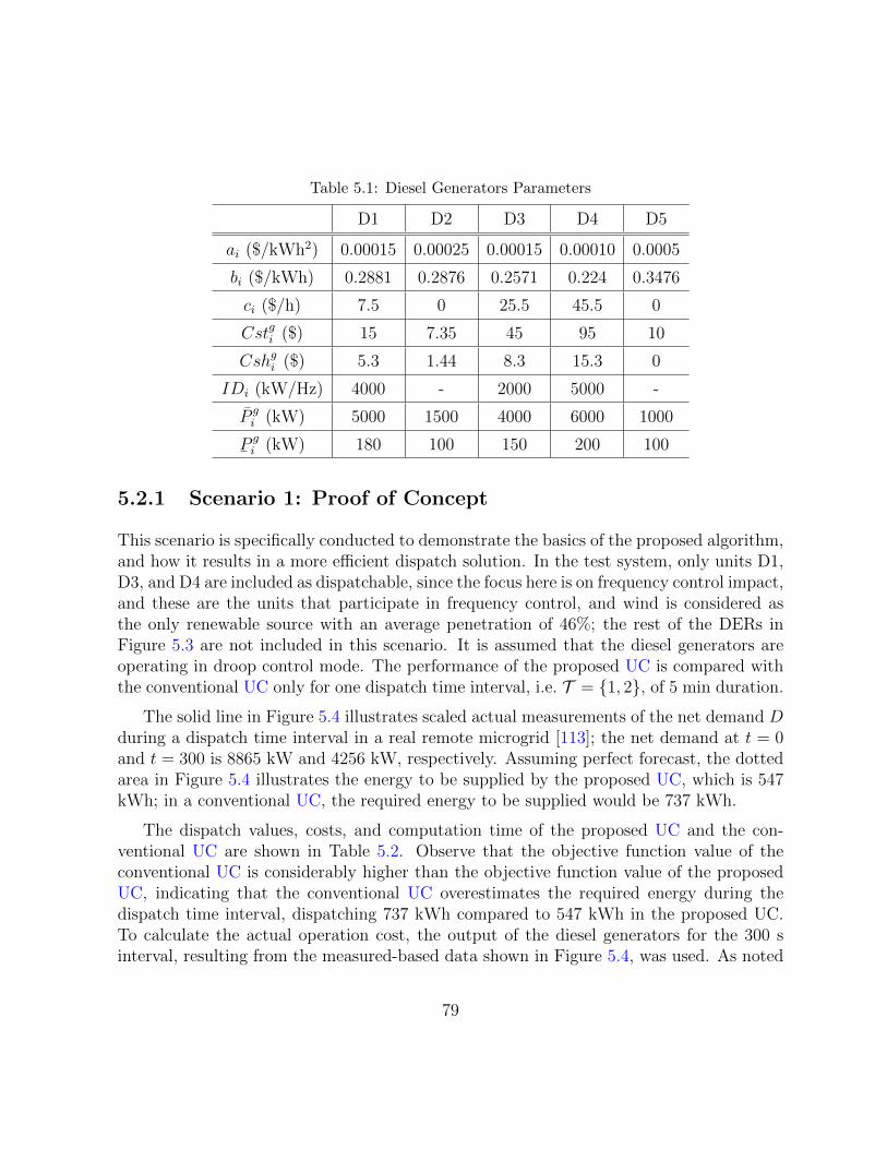
Table 5.1: Diesel Generators Parameters

D1 D2 D3 D4 D5

ai ($/kWh2) 0.00015 0.00025 0.00015 0.00010 0.0005

bi ($/kWh) 0.2881 0.2876 0.2571 0.224 0.3476

ci ($/h) 7.5 0 25.5 45.5 0

Cstgi ($) 15 7.35 45 95 10

Cshgi ($) 5.3 1.44 8.3 15.3 0

IDi (kW/Hz) 4000 - 2000 5000 -

P gi (kW) 5000 1500 4000 6000 1000

¯P gi (kW) 180 100 150 200 100

5.2.1 Scenario 1: Proof of Concept

This scenario is specifically conducted to demonstrate the basics of the proposed algorithm,and how it results in a more efficient dispatch solution. In the test system, only units D1,D3, and D4 are included as dispatchable, since the focus here is on frequency control impact,and these are the units that participate in frequency control, and wind is considered asthe only renewable source with an average penetration of 46%; the rest of the DERs inFigure 5.3 are not included in this scenario. It is assumed that the diesel generators areoperating in droop control mode. The performance of the proposed UC is compared withthe conventional UC only for one dispatch time interval, i.e. T = 1, 2, of 5 min duration.

The solid line in Figure 5.4 illustrates scaled actual measurements of the net demand Dduring a dispatch time interval in a real remote microgrid [113]; the net demand at t = 0and t = 300 is 8865 kW and 4256 kW, respectively. Assuming perfect forecast, the dottedarea in Figure 5.4 illustrates the energy to be supplied by the proposed UC, which is 547kWh; in a conventional UC, the required energy to be supplied would be 737 kWh.

The dispatch values, costs, and computation time of the proposed UC and the con-ventional UC are shown in Table 5.2. Observe that the objective function value of theconventional UC is considerably higher than the objective function value of the proposedUC, indicating that the conventional UC overestimates the required energy during thedispatch time interval, dispatching 737 kWh compared to 547 kWh in the proposed UC.To calculate the actual operation cost, the output of the diesel generators for the 300 sinterval, resulting from the measured-based data shown in Figure 5.4, was used. As noted

79

0

2000

4000

6000

8000

0 50 100 150 200 250 300

Net

dem

and

(k

W)

t (s)

Proposed UC

Actual Measurement

Figure 5.4: Data used in Scenario 1 from scaled measurements of net demand in an actual remotemicrogrid.

from Table 5.2, compared to the conventional UC, the proposed UC yields around 1% costsavings. Note that the simulated cost is very close to the solution obtained by the proposedUC, since the proposed UC obtained the solution by optimizing an amount of energy closeto the actual required energy during the 300 s interval. Observe also that the computationtime for both UC approaches are similar in an Intel(R) Xeon(R) CPU L7555 1.87GHz (4processors) server.

Table 5.2: Proposed UC vs. Conventional UC for Scenario 1

UC P g1 P g

3 P g4 Objective Simulated CPU

(kW) (kW) (kW) Function ($) Cost ($) Time (s)

Conv. 2777 1857 4231 471 299 1.45

Prop. 2591 2276 3998 303 296 1.45

5.2.2 Scenario 2: ILS Control, Deterministic Forecast

This scenario considers the full test system, with all diesel and renewable generation units.To validate the advantage of the proposed UC compared to the conventional UC, a perfectforecast is assumed for the load and renewable outputs; the wind, PV, and demand fore-casted values used are shown in Figure 5.5. Also, an extra constraint is added to ensurethat the SoC of the batteries are equal at the beginning and end of the day to avoid ESSdepletion. The test is conducted for 24 h of operation, with dispatch interval of 5 min.

80

0

4000

8000

12000

16000

0 250 500 750 1000 1250

Pow

er (

kW

)

t (min)

Wind PV Load

Figure 5.5: Wind, PV, and load forecasted values based on scaled measurements in an actualremote microgrid for Scenarios 2, 3, and 4.

Figure 5.6 shows the dispatch results obtained with the proposed and the conventionalUC. Observe the differences in the UC and charging/discharging patterns of the ESS, whichare magnified for two different dispatch windows; in addition, the dispatch difference ofthe diesel engines are shown in Figure 5.7. Note that these differences are significant whenthe net demand fluctuation is high, and low when the net demand fluctuation is also low.

The computation time and operation costs are reported in Table 5.3; the actual costis calculated using the same method described in Scenario 1. Observe in Table 5.3 thatthe simulated cost of operating the system for 24 h in 5 min dispatch intervals for theproposed UC is $168,148, whereas it is $172,410 for the conventional UC; hence, underperfect forecast assumption and given that the system is operating in ILS control mode,dispatching the units using the proposed UC will reduce the operation cost by 2.47%,yielding a saving of $4261 for the day. Also, note that the total computation time for thesimulated 24 h of the proposed UC is similar to the conventional one.


UC Obj. Function ($) Simulated Cost ($) Time (s)

Conv. 172,445 172,410 21

Prop. 168,148 168,148 65

81

-5000

0

5000

10000

15000

0 250 500 750 1000 1250

Po

wer

(k

W)

t (min)

Dispatch with the proposed objective function

ESS-CHG ESS-DCH WT+PV D1 D2 D3 D4 D5 Load

-5000

0

5000

10000

15000

0 250 500 750 1000 1250

Po

wer

(k

W)

t (min)



-5000

0

5000

10000

15000

0 250 500 750 1000 1250

Po

wer

(k

W)

t (min)

Dispatch with the conventional objective function


-5000

0

5000

10000

15000

1255 1280 1305 1330 1355 1380 1405 1430

Po

wer

(k

W)

t (5-min)

Dispatch with the proposed objective function (1255-1435)

Series1 Series2 Series3 Series4 Series5 Series6 Series7 Series8 Series9

-5000

0

5000

10000

15000

1255 1280 1305 1330 1355 1380 1405 1430

Po

wer

(k

W)

t (min)

Dispatch with the conventional objective function (1255-1435)


-5000

-5000 -5000-5000

0

5000

10000

15000

60 85 110 135 160 185 210 235

Po

wer

(k

W)

t (5-min)

Dispatch with the proposed objective function (60-240)


-5000

0

5000

10000

15000

60 85 110 135 160 185 210 235

Po

wer

(k

W)

t (min)

Dispatch with the conventional objective function (60-240)


-5000

0

5000

10000

15000

0 250 500 750 1000 1250

Po

wer

(k

W)

t (min)



Dispatch with the conventional UC

Dispatch with the proposed UC

Dispatch with the proposed UC (60-240)

Dispatch with the conventional UC (60-240)



Figure 5.6: Dispatch results with the proposed and conventional UC for scenario 2.

-3000

-2500

-2000

-1500

-1000

-500

0

500

1000

1500

0 50 100 150 200 250 300 350 400 450 500 550 600 650 700 750 800 850 900 950 1000 1050 1100 1150 1200 1250 1300 1350 1400

Pow

er (

kW

)

t (min)

Dispatch difference between the proposed and the conventional UC

D1 D2 D3 D4 D5

Figure 5.7: Dispatch differences with the proposed and the conventional UC for scenario 2.

5.2.3 Scenario 3: ILS Control with MPC

In this scenario, the same model as in Scenario 2 is used, but considering errors in theforecasted values of renewable energy and demand; these errors are computed assuminga cumulative density function (CDF) with a standard deviation obtained from a linearapproximation of the difference between the current time step and the forecasted time step,as per [61]. To mitigate the impact of forecast inaccuracy, the optimal dispatch solutionsobtained in each time step is only applied to the next time interval, and the problem isre-solved for the next time step with the updated forecast, repeating the process until theend of the 24 h, with a shrinking time horizon. This solution methodology is referred to

82

as a receding horizon approach [58].

The dispatch results obtained are shown in Figure 5.8, and the dispatch differencesare shown in Figure 5.9. The solution and actual costs, and the computation times arereported in Table 5.4. Observe that using the proposed UC, the actual costs for operatingthe system would decrease by 0.6%, saving around $1000 for the day. Note also that thetotal computation time for the simulated 24h of the proposed method is reduced by around50% compared to the conventional method.

-5000

0

5000

10000

15000

0 250 500 750 1000 1250

Po

wer

(k

W)

t (min)



-5000

0

5000

10000

15000

1255 1280 1305 1330 1355 1380 1405 1430

Po

wer

(k

W)

t (5-min)



-5000

0

5000

10000

15000

1255 1280 1305 1330 1355 1380 1405 1430

Po

wer

(k

W)

t (5-min)



-5000

0

5000

10000

15000

0 250 500 750 1000 1250

Po

wer

(k

W)

t (min)

Dispatch with th


-5000

0

5000

10000

15000

0 250 500 750 1000 1250

Po

wer

(k

W)



-5000

0

5000

10000

15000

60 85 110 135 160 185 210 235

Po

wer

(k

W)

t (5-min)



-5000

0

5000

10000

15000

60 85 110 135 160 185 210 235

Po

wer

(k

W)

t (5-min)



-5000

-5000

-5000

0

5000

10000

15000

0 250 500 750 1000 1250

Po

wer

(k

W)

t (min)



-5000

Figure 5.8: Dispatch results with the proposed and conventional UC for Scenario 3.

-3000

-2000

-1000

0

1000

2000

3000

4000

0 50 100 150 200 250 300 350 400 450 500 550 600 650 700 750 800 850 900 950 1000 1050 1100 1150 1200 1250 1300 1350 1400Po

wer

(k

W)

t (min)

Dispatch difference between the proposed and the conventional objective function

D1 D2 D3 D4 D5

Figure 5.9: Dispatch differences with the proposed and the conventional UC for Scenario 3.

83



Conv. 169,852 169,843 5951

Prop. 168,855 168,855 2781

5.2.4 Scenario 4: Droop Control with MPC

In this Scenario, the same model as in Scenarios 2 and 3 is used, except that the dieselunits are assumed to operate in droop control mode. Note that the errors for the forecastedvalues of renewable energy and demand are computed using the same CDF as in Scenario3, yielding different error values compared to the previous case.

The dispatch results obtained are shown in Figure 5.10, and the dispatch differencesare shown in Figure 5.11. The solution and actual costs and the computation times arereported in Table 5.5. Observe that using the proposed UC, the actual costs of operatingthe system would decrease by 1.15%, saving $1941 for the day. However, in this case thetotal computation time for the simulated 24 h is higher for the proposed UC, but stillwithin online dispatch requirements.

Table 5.5: Proposed UC vs. Conventional UC for Scneario 4


Conv. 169,149 169,134 656

Prop. 167,193 167,193 1001

5.3 Discussions

5.3.1 Performance of Droop Control and ILS Control

From the results presented in Scenarios 3 and 4, in Section 5.2, it may seem that the UCformulation with droop control outperforms the UC formulation with ILS control, sincethe UC in the former case yields a smaller objective function and takes less computationaltime. However, this cannot be generalized, as the performance of the UC in droop controlmode and ILS control mode depends on several factors such as the droop coefficients, the

84

-5000

0

5000

10000

15000

0 250 500 750 1000 1250

Po

wer

(k

W)

t (min)



-5000

0

5000

10000

15000

0 250 500 750 1000 1250

Po

wer

(k

W)

t (min)



-5000

0

5000

10000

15000

0 250 500 750 1000 1250

Po

wer

(k

W)

t (min)



-5000

-5000

0

5000

10000

15000

1255 1280 1305 1330 1355 1380 1405 1430

Po

wer

(k

W)

t (5-min)



-5000

0

5000

10000

15000

60 85 110 135 160 185 210 235

Po

wer

(k

W)

t (5-min)



-5000

0

5000

10000

15000

60 85 110 135 160 185 210 235

Po

wer

(k

W)

t (5-min)



-5000

-5000

0

5000

10000

15000

1255 1280 1305 1330 1355 1380 1405 1430

Po

wer

(k

W)

t (5-min)



-5000

-5000

0

5000

10000

15000

0 250 500 750 1000 1250

Po

wer

(k

W)

t (min)



Figure 5.10: Dispatch results with the proposed and conventional UC for Scenario 4.

-3000

-2000

-1000

0

1000

2000

3000

0 50 100 150 200 250 300 350 400 450 500 550 600 650 700 750 800 850 900 950 1000 1050 1100 1150 1200 1250 1300 1350 1400

Po

wer

(k

W)

t (min)

Dispatch difference between the proposed and the conventional objective function

D1 D2 D3 D4 D5

Figure 5.11: Dispatch differences with the proposed and the conventional UC for Scenario 4.

generators nominal rating, the forecasted values of renewable energy and demand, andother parameters.

5.3.2 Control Hierarchies

It is important to properly classify the proposed UC in the hierarchy of active powercontrol. The active power control in isolated microgrids usually consists of two controllevels [14]. The first level, or primary control, consists of local turbine governors andinverter controls that respond immediately to changes in the system, bringing the rate

85

of change of frequency to zero in a few seconds. Thus, primary controls are in charge ofmaintaining the system frequency stability.

In bulk power systems, Automatic General Control (AGC), or secondary control, takescare of frequency deviation, considering the power exchange among control areas. Inisolated/islanded microgrids, AGC is not necessary in ILS mode, since the primary controldoes not cause frequency deviations in steady state. For droop control, the dispatch ofunits is used to recover the steady-state frequency; hence, the UC plays the role of AGCor secondary control in isolated/islanded microgrids, as discussed in [14].

5.3.3 Primary Control Performance of Droop vs. ILS

As mentioned in Section 5.1.1, primary control regulates the frequency, ensuring frequencystability in real-time. The proposed UC mathematically models and considers the impactof primary frequency control, so that it more accurately optimizes each DER output. Fromthe primary control perspective, ILS control, in principle, exhibits a superior performancecompared to droop control, since there is no steady state frequency deviation; however,in this case, DERs need to communicate their power output, which imposes additionalcommunication requirements not needed in droop control. Note that in droop controloperation, if the droop coefficients are chosen in reverse proportion to the generation unitsnominal rating, the load sharing would be exactly the same as in the ILS control mode;hence, there would be little difference in the immediate response of the two techniques.

5.4 Summary

In this chapter, a mathematical model that represented changes in the dispatchable unitoutputs was proposed for isolated microgrids, for various frequency control techniques.The developed mathematical model was integrated into a UC model considering variousoperational constraints for a system with multiple DERs. In addition, typical reserveconstraints were modified to ensure the feasibility of frequency regulation in the system.The mathematical model was kept linear to allow its integration into current utility EMS.

It was shown through several case studies in a complex isolated test microgrid thatthe conventional UC either over-estimated or under-estimated the energy required duringeach time interval, yielding dispatch levels that were not necessarily optimized for the ac-tual required energy. By properly modelling the changes in the dispatchable unit outputs

86

considering their frequency regulation characteristics, it was demonstrated that the pro-posed method results in dispatch settings that were better optimized, yielding savings inoperational costs. Finally, it was shown that adopting the proposed UC had no significantimpact on computation times with respect to current utility practices.

The main content of this chapter has been published in [114].

87

Chapter 6

Conclusions, Contributions andFuture Work

6.1 Summary

This thesis concentrated on the problem of frequency control in isolated microgrids. Specifi-cally, the problem was investigated for two different system time-frames: transient dynamictime scale of 100 ms to a few seconds, and static dispatch time frame of 5 minutes. A com-prehensive investigation of the effects of various frequency control techniques on transientand frequency stability of isolated microgrids under balanced and unbalanced conditionshas been presented in this paper; based on these investigation, a practical voltage-basedfrequency controller has been proposed that offers several advantages and is easy to im-plement. In addition, the impact of frequency control techniques on the optimal dispatchof isolated microgrids had been investigated, and the problem of UC in these systems hasbeen reformulated to account for the impact of frequency control.

In Chapter 2, a basic background review of microgrids and associated stability issueswas provided; voltage and frequency control in isolated microgrids, as well as the formu-lation of UC in microgrids were also discussed. Thus, the definition of microgrids andbasic related concepts of voltage and frequency stability were first introduced and dis-cussed. Then, voltage and frequency control techniques were described in the context ofisolated microgrids, including models of different components such as generator, governor,exciter, and inverters. Finally, a general formulation of UC models in microgrids was pro-vided, discussing the objective function, equality and inequality constraints, and solutiontechniques.

88

In Chapter 3, conventional, transient, and angle droop controls were discussed. Theperformance of each control technique was evaluated through time domain simulationson a simple test system, and it was shown through simulation results that the transientdroop control demonstrated better transient response, while angle droop control exhibitedno steady-state deviation in the frequency response of the system. Following that, a newhybrid droop control was proposed based on the transient and angle droop control, showingthat it has better transient and improved frequency response. In spite of the increasedcomplexity in the tuning and implementation of the proposed controller, it has shown tohave an overall superior performance that would justify its adoption instead of the otherdiscussed controls.

In Chapter 4, a voltage-based frequency controller was proposed for isolated micro-grids that makes use of the load voltage sensitivity to manipulate their consumption andthus compensate for power mismatches in the system. The performance of the proposedcontroller was evaluated using diesel-based and inverter-based isolated microgrids test sys-tems. The simulation results showed that the VFC is efficient in controlling frequency andenhance the system damping, thus decreasing the system dependency on ESS.

In Chapter 5, a UC formulation was proposed for isolated microgrids that integrates inthe mathematical formulation of different frequency controls, namely single unit, isochronousload sharing, and droop-based controls. The performance of the proposed UC was eval-uated through various test scenarios. The simulation results showed that while the UCcomputation time is similar to the conventional UC, system dispatch is closer to realityresulting in more accurate and reduced operating costs.

The main conclusions of the presented work are:

• Manipulating loads consumption in an isolated microgrids through DERs voltagecontrol is a viable solution for addressing the problem of frequency stability. Com-pared to large conventional systems, isolated microgrids are smaller, and hence it ispossible to readily control DERs voltages throughout the system, given the relativelysmall voltage drops in the feeders.

• Eigenvalue studies show that the proposed VFC can improve system damping withproper controller tuning, as the dominant-poles of the system can be significantlyaffected by the controller.

• Time-domain simulations in PSCAD/EMTDC platform demonstrate the robust per-formance of the proposed VFC subject to various system disturbances. However, theVFC performance depends on the allowed voltage range and the loads voltage index.

89

• It is viable to have a 15% decrease in a residential load consumption by changing itsoperating voltage by 10%. Thus, the VFC can be seen as a virtual flywheel, with acapacity of up to 15% of the nominal load in the system. Hence, the VFC allows fora higher instantaneous penetration of renewable energies, thus saving fuel costs; theexact amount of fuel saved depends on the penetration of renewables, loading levels,and diesel engine efficiency.

• For isolated microgrids with a significant penetration of renewable energy, conven-tional UC either overestimates or underestimates the amount of energy for whichDERs need to be optimized.

• The proposed UC, which accounts for the changes in the RES in the system in theUC problem, yields more accurate DERs dispatches, and alleviates the under/overestimation problem, for various frequency control techniques.

• The proposed UC reduces the operating cost of the system compared to a conven-tional UC; the exact savings depend on the system renewable penetration, systemconfiguration, and renewable fluctuation.

6.2 Contributions

The main contributions of this thesis are the following:

• A state-of-the-art VFC has been developed for both diesel-based and inverter-basedunits in isolated micorgirds. The controller utilizes a load voltage regulation mech-anism to manipulate the system demand, and consequently balance the power mis-match. The load voltage regulation is performed via diesel generator exciter systemsand DER-based inverters, without the need for communication between differentcomponents of the system.

• A hybrid droop-based frequency controller has been designed for inverter-based iso-lated microgrids and the impact of various droop-based frequency control mechanismson the transient response and stability of such systems has been studied and com-pared in detail.

• The impact of various frequency control mechanisms such as single unit control,droop control, or isochronous load sharing (ILS) control mode on optimal dispatchhas been analyzed, using a novel UC model.

90

• A novel mathematical formulation of the frequency control mechanism integratedwithin a UC framework has been devised for isolated microgrids, yielding a moreeconomical dispatch solution. The proposed formulation also allows to introduce anew reserve constraint in the UC model to represent the corresponding frequencycontrol mechanism, considering intra-interval generation changes.

• A comprehensive dynamic and static simulation model of a CIGRE benchmark sys-tem for medium voltage distribution networks has been built to carry out time-domain and steady-state simulations to test and demonstrate the proposed frequencycontrol techniques. Models of detailed voltage and frequency control systems, bothfor synchronous machines and inverters, have been developed.

The main contents of this thesis have been published in [94], [108], [109], [110], and [114].

6.3 Future Work

Future research may be carried out to address the following issues:

• The problem of voltage flickers during the VFC operation is not considered in thestudies reported in this thesis; therefore, flickers during the VFC operation for atypical renewable energies output profile should be analyzed.

• The VFC proposed in this thesis compensates for steady-state frequency errors, es-sentially acting like an isochronous frequency controller; as a result, it cannot be usedin parallel with another isochronous frequency controller. The use of a negative feed-back loop added to the VFC control schematic, thus enabling it to work in parallelwith another isochronous control unit, should be evaluated.

• A comprehensive study on the impact of the VFC on fuel saving in the system dueto the higher renewable energies penetration should be carried out. Economic toolssuch as Homer or other developed codes would be suitable to perform such studies.

• Since the VFC is developed to avoid frequency instability in the system throughvoltage regulation, studies should be carried out to investigate the impact of differenttypes of loads on the performance of the VFC, and the impact of the VFC on theprotection scheme of the isolated microgrid.

91

• The proposed UC in this thesis does not include non-linear power flow constraints;thus, such constraints should be included to guarantee the feasibility of the optimaldispatch of DERs.

92

Bibliography

[1] R. H. Lasseter, C. M. A. Akhil, J. D. J. Stephens, R. Guttromson, A. Meliopoulous,and R. J. Yinger, “The CERTS microgrid concept,” Transmission Reliability Pro-gram, Office of Power Technologies, US Department of Energy, Tech. Rep., 2002.

[2] R. H. Lasseter, J. H. Eto, B. Schenkman, J. Stevens, H. Vollkommer, D. Klapp,E. Linton, H. Hurtado, and J. Roy, “CERTS microgrid laboratory test bed,” IEEETrans. Power Del., vol. 26, pp. 325–332, Jan. 2011.

[3] N. Hatziargyriou, H. Asano, R. Iravani, and C. Marnay, “Microgrids,” IEEE PowerEnergy Mag., vol. 5, no. 4, pp. 78–94, July 2007.

[4] World Energy Outlook. (2015) Electricity access database. [Online].Available: http://www.worldenergyoutlook.org/resources/energydevelopment/energyaccessdatabase/

[5] M. Arriaga, C. Canizares, and M. Kazerani, “Northern Lights: Access to Electricityin Canada’s Northern and Remote Communities,” IEEE Power Energy Mag., vol. 12,no. 4, pp. 50–59, Aug. 2014.

[6] IEEE Guide for Design, Operation, and Integration of Distributed Resource IslandSystems with Electric Power Systems, IEEE Std. 1547.4, 2011.

[7] J. M. Guerrero, F. Blaabjerg, T. Zhelev, K. Hemmes, E. Monmasson, S. Jemei, M. P.Comech, R. Granadino, and J. I. Frau, “Distributed generation: toward a new energyparadigm,” IEEE Ind. Electron. Mag., pp. 52–64, Mar. 2010.

[8] E. Barklund, N. Pogaku, M. Prodanovic, C. Hernandez-Aramburo, and T. C. Green,“Energy management in autonomous microgird using stability-constrained droopcontrol of inverters,” IEEE Trans. Power Electron., vol. 23, no. 5, pp. 2346–2353,Sep. 2008.

93

http://www.worldenergyoutlook.org/resources/energydevelopment/energyaccessdatabase/

http://www.worldenergyoutlook.org/resources/energydevelopment/energyaccessdatabase/

[9] C. K. Sao and P. W. Lehn, “Control and power management of converter fed micro-grids,” IEEE Trans. Power Syst., vol. 23, no. 3, pp. 1088–1098, Aug. 2008.

[10] G. Delille, B. Francois, and G. Malarange, “Dynamic Frequency Control Supportby Energy Storage to Reduce the Impact of Wind and Solar Generation on IsolatedPower System’s Inertia,” IEEE Trans. Sustain. Energy, vol. 3, no. 4, pp. 931–939,Oct. 2012.

[11] G. Lalor, A. Mullane, and M. O’Malley, “Frequency control and wind turbine tech-nologies,” IEEE Trans. Power Syst., vol. 20, no. 4, pp. 1905–1913, Nov. 2005.

[12] C. Yuen, A. Oudalov, and A. Timbus, “The Provision of Frequency Control ReservesFrom Multiple Microgrids,” IEEE Trans. Ind. Electron., vol. 58, no. 1, pp. 173–183,Jan. 2011.

[13] K. Strunz, “Developing benchmark models for studying the integration of distributedenergy resources,” in Proc. IEEE Power Eng. Soc. Gen. Meeting, Montreal, QC, Jul.2006.

[14] D. E. Olivares, A. Mehrizi-Sani, A. H. Etemadi, C. A. Canizares, R. Iravani, M. Kaz-erani, A. H. Hajimiragha, O. Gomis-Bellmunt, M. Saeedifard, R. Palma-Behnkeet al., “Trends in Microgrid Control,” IEEE Trans. Smart Grid, vol. 5, no. 4, pp.1905–1919, May 2014.

[15] UCTE ad-hoc Group, “Frequency Quality Investigation,” ENTSO-e,Brussels, Belgium, Tech. Rep., Aug. 2008, [Online]. Available: https://www.entsoe.eu/fileadmin/user upload/ library/publications/ce/otherreports/090330 UCTE FrequencyInvestigationReport Abstract.pdf.

[16] P. Kundur, Power System Stability and Control. New York: McGraw Hill, 1994.

[17] Y. G. Rebours, D. S. Kirschen, M. Trotignon, and S. Rossignol, “A survey of fre-quency and voltage control ancillary services part I: Technical features,” IEEE Trans.Power Syst., vol. 22, no. 1, pp. 350–357.

[18] Z. Xu, M. Togeby, and J. Østergaard, “Demand as frequency controlled reserve: Finalreport of the PSO project,” Technical University of Denmark, Tech. Rep., 2008.

[19] J. M. Guerrero, M. Chandorka, T. Lee, and P. C. Loh, “Advanced Control Archi-tectures for Intelligent Microgrids–Part I: Decentralized and Hierarchical Control,”IEEE Trans. Ind. Electron., vol. 60, no. 4, pp. 1254–1262, Apr. 2012.

94

https://www.entsoe.eu/fileadmin/user_upload/_library/publications/ce/otherreports/090330_UCTE_FrequencyInvestigationReport_Abstract.pdf



[20] J. M. Guerrero, P. C. Loh, T. Lee, and M. Chandorkar, “Advanced Control Architec-tures for Intelligent Microgrids–Part II: Power Quality, Energy Storage, and AC/DCMicrogrids,” IEEE Trans. Ind. Electron., vol. 60, no. 4, pp. 1263–1270, Apr. 2012.

[21] F. A. Bhuiyan and A. Yazdani, “Multimode control of DFIG-based wind power unitfor remote applications,” IEEE Trans. Power Del., vol. 24, no. 4, pp. 2079–2089,Sep. 2009.

[22] A. L. Dimeas and N. D. Hatziargyriou, “Operation of a multi-agent system for mi-crogrid control,” IEEE Trans. Power Syst., vol. 20, no. 3, pp. 1447–1455, Aug. 2005.

[23] J. A. P. Lopes, C. L. Moreira, and A. G. Madureira, “Defining control strategies formicrogrids islanded operation,” IEEE Trans. Power Syst., vol. 21, no. 2, pp. 916–924,May 2006.

[24] A. G. Tsikalakis and N. D. Hatziargyriou, “Centralized control for optimizing mi-crogrids operation,” IEEE Trans. Energy Convers., vol. 23, no. 1, pp. 243–248, Feb.2008.

[25] A. Mehrizi-Sani and R. Iravani, “Potential-Function based control of a microgrid inislanded and grid-connected modes,” IEEE Trans. Power Syst., vol. 25, no. 4, pp.1883–1891, Oct. 2010.

[26] J. M. Carrasco, L. G. Franquelo, J. T. Bialasiewicz, E. Galvan, R. C. P. Guisado,M. A. M. Prats, J. I. Leon, and N. Moreno-Alfonso, “Power-electronic systems for thegrid integration of renewable energy sources: A survey,” IEEE Trans. Ind. Electron.,vol. 53, no. 4, pp. 1002–1016, Aug. 2006.

[27] N. Pogaku, M. Prodanovic, and T. C. Green, “Modeling, analysis and testing ofautonomous operation of an inverter-based microgrid,” IEEE Trans. Power Electron.,vol. 22, no. 2, pp. 613–625, March 2007.

[28] J. G. de Matos, F. S. F. e Silva, and L. A. de S. Ribeiro, “Power control in AC isolatedmicrogrids with renewable energy sources and energy storage systems,” IEEE Trans.Ind. Electron., vol. 62, no. 6, pp. 3490–3498, June 2015.

[29] F. Katiraei and M. R. Iravani, “Power management strategies for a microgrid withmultiple distributed generation units,” IEEE Trans. Power Syst., vol. 21, no. 4, pp.1821–1831, Oct. 2006.

95

[30] M. . Marwali, J. W. Jung, and A. Keyhani, “Control of distributed generation systems- Part II: Load sharing control,” IEEE Trans. Power Electron., vol. 19, no. 6, pp.1551–1561, Nov. 2004.

[31] M. C. Chandorkar, D. M. Divan, and R. Adapa, “Control of parallel connectedinverters in standalone ac supply systems,” IEEE Trans. Ind. Appl., vol. 29, no. 1,pp. 136–143, Jan. 1993.

[32] M. N. Marwali, M. Dai, and A. Keyhani, “Robust stability analysis of voltage andcurrent control for distributed generation systems,” IEEE Trans. Energy Convers.,vol. 21, no. 2, pp. 516–526, Jun. 2006.

[33] ——, “Stability analysis of load sharing control for distributed generation systems,”IEEE Trans. Energy Convers., vol. 22, no. 3, pp. 737–745, Sep. 2007.

[34] G. F. Franklin, M. L. Workman, and D. Powell, Digital control of dynamic systems.Addison-Wesley Longman Publishing Inc., 1997.

[35] J. M. Guerrero, L. G. de Vecuna, J. Matas, M. Castilla, and J. Miret, “A wirelesscontroller to enhance dynamic performance of parallel inverters in distributed gen-eration systems,” IEEE Trans. Power Electron., vol. 19, no. 5, pp. 1205–1213, Sep.2004.

[36] R. Majumder, B. Chaudhuri, A. Ghosh, R. Majumder, G. Ledwich, and F. Zare,“Improvement of stability and load sharing in an autonomous microgrid using sup-plementary droop control loop,” IEEE Trans. Power Syst., vol. 25, no. 2, pp. 796–808,Apr. 2010.

[37] Y. A.-R. I. Mohamed and E. F. El-Saadany, “Adaptive decentralized droop controllerto preserve power sharing stability of paralleled inverters in distributed generationmicrogrids,” IEEE Trans. Power Electron., vol. 23, no. 6, pp. 2806–2816, Nov. 2008.

[38] J. Kim, J. M. Guerrero, P. Rodriguez, R. Teodorescu, and K. Nam, “Mode AdaptiveDroop Control With Virtual Output Impedances for an Inverter-Based Flexible ACMicrogrid,” IEEE Trans. Power Electron., vol. 26, no. 3, pp. 689–701, Nov. 2010.

[39] R. Majumder, G. Ledwich, A. Ghosh, S. Chakrabarti, and F. Zare, “Droop Controlof Converter-Interfaced Microsources in Rural Distributed Generation,” IEEE Trans.Power Del., vol. 25, no. 4, pp. 2768–2778, March 2010.

96

[40] R. Majumder, A. Ghosh, G. Ledwich, and F. Zare, “Load sharing and power qualityenhanced operation of a distributed microgrid,” IET Renew. Power Gener., vol. 3,no. 2, pp. 109–119, June 2009.

[41] K. D. Brabandere, B. Bolsens, J. V. den Keybus, A. Woyte, J. Driesen, andR.Belmans, “A voltage and frequency droop control method for parallel inverters,”IEEE Trans. Power Syst., vol. 22, no. 4, pp. 1107–1115, Jul. 2007.

[42] S. Chiang, C. Yen, and K. Chang, “A multimodule parallelable series-connectedPWM voltage regulator,” IEEE Trans. Ind. Electron., vol. 48, no. 3, pp. 506–516,Aug. 2002.

[43] J. Zhao, X. Lyu, Y. Fu, X. Hu, and F. Li, “Coordinated microgrid frequency regula-tion based on DFIG variable coefficient using virtual inertia and primary frequencycontrol,” IEEE Trans. Energy Convers., vol. 31, no. 3, pp. 833–845, Sep. 2016.

[44] M. F. M. Arani and E. F. El-Saadany, “Implementing virtual inertia in DFIG-basedwind power generation,” IEEE Trans. Power Syst., vol. 28, no. 2, pp. 1373–1384,May 2013.

[45] F. C. Schweppe, R. D. Tabors, J. L. Kirtley, H. R. Outhred, F. H. Pickel, and A. J.Cox, “Homeostatic utility control,” IEEE Trans. Power App. Syst., vol. 99, no. 3,pp. 1151–1163, May 1980.

[46] D. J. Hammerstrom, J. Brous, D. P. Chassin, G. R. Horst, R. Kajfasz, P. Michie,T. Oliver, T. A. Carlon, C. Eustis, O. M. Jervegren et al., “Part II. Grid FriendlyTM

appliance Project,” Pacific Northwest National Laboratory, Richland, Washington,Tech. Rep. PNNL-17079, Oct. 2007.

[47] A. Molina-Garcia, F. Bouffard, and D. Kirschen, “Decentralized Demand-Side Con-tribution to Primary Frequency Control,” IEEE Trans. Power Syst., vol. 26, no. 1,pp. 411–419, Feb. 2011.

[48] K. Pamdiaraj, P. Taylor, N. Jenkins, and C. Robb, “Distributed load control ofautonomous renewable energy systems,” IEEE Trans. Energy Convers., vol. 16, no. 1,pp. 14–19, Mar. 2001.

[49] J. A. Short, D. G. Infield, and L. L. Ferris, “Stabilization of grid frequency throughdynamic demand control,” IEEE Trans. Power Syst., vol. 23, no. 3, pp. 1284–1293,Aug. 2007.

97

[50] G. Delille, J. Yuan, and L. Capely, “Taking advantage of load voltage sensitivity tostabilize power system frequency,” in Proc. IEEE PowerTech Conf., June 2013, pp.1–6.

[51] G. Delille, L. Capely, D. Souque, and C. Ferrouillat, “Experimental validation ofa novel approach to stabilize power system frequency by taking advantage of loadvoltage sensitivity,” in Proc. IEEE PowerTech Conf., June 2015, pp. 1–6.

[52] A. G. Exposito, A. J. Conejo, and C. A. Canizares, Electric Energy Systems: Analysisand Operation. New York, US: CRC Press, 2008.

[53] C. A. H. Aramburo, T. C. Green, and N. Mugniot, “Fuel consumption minimizationof a microgrid,” IEEE Trans. Ind. Appl., vol. 41, no. 3, pp. 673–681, June 2005.

[54] C. Chen, S. Duan, T. Cai, B. Liu, and G. Hu, “Smart energy management systemfor optimal microgrid economic operation,” IET Renew. Power Gener., vol. 5, no. 3,pp. 258–267, May 2011.

[55] E. F. Camacho and C. B. Alba, Model Predictive Control. London, UK: Springer-Verlag, 2013.

[56] R. Palma-Behnke, C. Benavides, F. Lanas, B. Severino, L. Reyes, J. Llanos, andD. Saez, “A microgrid energy management system based on the rolling horizon strat-egy,” IEEE Trans. Smart Grid, vol. 4, no. 2, pp. 994–1006, Jan. 2013.

[57] D. E. Olivares, “Robust Energy Management Systems for Isolated Microgrids UnderUncertainty,” Ph.D. dissertation, University of Waterloo, Waterloo, ON, 2014.

[58] D. E. Olivares, C. A. Canizares, and M. Kazerani, “A centralized energy managementsystem for isolated microgrids,” IEEE Trans. Smart Grid, vol. 5, no. 4, pp. 1864–1875, April 2014.

[59] D. E. Olivares, J. D. Lara, C. A. Canizares, and M. Kazerani, “Stochastic-predictiveenergy management system for isolated microgrids,” IEEE Trans. Smart Grid, vol. 6,no. 6, pp. 2681–2693, Nov. 2015.

[60] J. D. Lara, “An Energy Management System for Isolated Microgrids ConsideringUncertainty,” Master’s thesis, University of Waterloo, Waterloo, ON, 2014.

[61] B. V. Solanki, A. Raghurajan, K. Bhattacharya, and C. A. Canizares, “Includingsmart loads for optimal demand response in integrated energy management systemsfor isolated microgrids,” IEEE Trans. Smart Grid, no. pre-print, pp. 1–10, Dec. 2015.

98

[62] Y. C. Wu, M. J. Chen, J. Y. Lin, W. S. Chen, and W. L. Huang, “Correctiveeconomic dispatch in a microgrid,” Int. J. Numer. Model. Electron. Netw. DevicesFields, vol. 26, no. 2, pp. 140–150, June 2012.

[63] J. W. O’Sullivan and M. J. O’Malley, “A new methodology for the provision of reservein an isolated power system,” IEEE Trans. Power Syst., vol. 14, no. 2, pp. 519–524,May 1999.

[64] G. W. Chang, C. Ching-Sheng, L. Tai-Ken, and W. Ching-Chung, “Frequency-regulating reserve constrained unit commitment for an isolated power system,” IEEETrans. Power Syst., vol. 28, no. 2, pp. 578–586, Aug. 2012.

[65] A. H. Hajimiragha, M. R. D. Zadeh, and S. Moazeni, “Microgrids frequency controlconsiderations within the framework of the optimal generation scheduling problem,”IEEE Trans. Smart Grid, vol. 6, no. 2, pp. 534–547, March 2013.

[66] G. X. Guan, F. Gao, and A. J. Svoboda, “Energy delivery capacity and generationscheduling in the deregulated electric power market,” IEEE Trans. Power Syst.,vol. 15, no. 4, pp. 1275–1280, Nov. 2000.

[67] Y. Yang, J. Wang, X. Guan, and Q. Zhai, “Subhourly unit commitment with feasibleenergy delivery constraints,” Appl. Energy, vol. 96, pp. 245–252, Aug. 2012.

[68] G. Morales-Espana, A. Ramos, and J. Garcia-Gonzalez, “An MIP formulation forjoint market-clearing of energy and reserves based on ramp scheduling,” IEEE Trans.Power Syst., vol. 29, no. 1, pp. 476–488, May 2013.

[69] H. Karimi, H. Nikkhajoei, and M. R. Iravani, “Control of an electronically-coupleddistributed resource unit subsequent to an islanding event,” IEEE Trans. Power Del.,vol. 23, no. 1, pp. 493–501, Jan. 2008.

[70] F. Katiraei, M. R. Iravani, and P. W. Lehn, “Micro-grid autonomous operation duringand subsequent to islanding process,” IEEE Trans. Power Del., vol. 20, no. 1, pp.248–257, Jan. 2005.

[71] P. Kundur, J. Paserba, V. Ajjarapu, G. Andersson, A. Bose, C. Canizares et al.,“Definition and classification of power system stability IEEE/CIGRE joint task forceon stability terms and definitions,” IEEE Trans. Power Syst., vol. 19, no. 3, pp. 1387–1401, Aug. 2004.

99

[72] P. Kundur, D. C. Lee, J. P. Bayne, and P. L. Dandeno, “Impact of turbine generatorcontrols on unit performance under system disturbance conditions,” IEEE Trans.Power App. Syst., vol. 5, no. 6, pp. 28–29, July 2010.

[73] Y. A.-R. I. Mohamed and A. A. Radwan, “Hierarchical control system for robustmicrogrid operation and seamless mode transfer in active distribution systems,” IEEETrans. Smart Grid, vol. 2, no. 2, pp. 352–362, Jan. 2011.

[74] M. D. Ilic and S. X. Liu, Hierarchical Power Systems Control: its value in a changingindustry. Springer Science & Business Media, 2012.

[75] J. M. Guerrero, J. C. Vasquez, J. Matas, L. G. de Vicuna, and M. Castilla, “Hierar-chical control of droop-controlled AC and DC microgrids A general approach towardstandardization,” IEEE Trans. Ind. Electron., vol. 58, no. 1, pp. 158–172, Dec. 2010.

[76] Y. Li and C. N. Kao, “An accurate power control strategy for power electronics-interfaced distributed generation units operating in a low-voltage multibus micro-grid,” IEEE Trans. Power Electron., vol. 24, no. 12, pp. 2977–2988, Dec. 2009.

[77] H. Saadat, Power System Analysis: Third Edition. PSA Publishing, 2010.

[78] IEEE Committee Report, “Proposed excitation systems definitions for synchronousmachines,” IEEE Trans. Power App. Syst., vol. 88, no. 8, pp. 1248–1258, Jan. 2007.

[79] ——, “Excitation system model for power system stability studies,” IEEE Trans.Power App. Syst., vol. 100, no. 2, pp. 494–509, Feb. 2007.

[80] J. Rocabert, A. Luna, F. Blaabjerg, and P. Rodriguez, “Control of power convertersin AC microgrids,” IEEE Trans. Power Electron., vol. 27, no. 11, pp. 4734–4749,Nov. 2012.

[81] S. M. Ashabani and Y. A.-R. I. Mohamed, “New family of microgrid control andmanagement strategies in smart distribution gridsanalysis, comparison and testing,”IEEE Trans. Power Syst., vol. 29, no. 5, pp. 2257–2269, Sep. 2014.

[82] J. C. Vasquez, J. M. Guerrero, A. Luna, P. Rodriguez, and R. Teodorescu, “Adaptivedroop control applied to voltage-source inverters operating in grid-connected andislanded modes,” IEEE Trans. Ind. Electron., vol. 56, no. 10, pp. 4088–4096, Oct.2009.

100

[83] J. M. Guerrero, J. Matas, L. G. de Vicuna, M. Castilla, and J. Miret, “Wireless-control strategy for parallel operation of distributed-generation inverters,” IEEETrans. Ind. Electron., vol. 53, no. 5, pp. 1461–1470, Oct. 2006.

[84] J. T. Bialasiewicz, “Renewable energy systems with photovoltaic power generators:Operation and modeling,” IEEE Trans. Ind. Electron., vol. 55, no. 7, pp. 2752–2758,July 2008.

[85] A. K. Abdelsalam, A. M. Massoud, S. Ahmed, and P. N. Enjeti, “High-performanceadaptive perturb and observe MPPT technique for photovoltaic-based microgrids,”IEEE Trans. Power Electron., vol. 26, no. 4, pp. 1010–1021, Apr. 2011.

[86] H. Kanchev, F. Colas, V. Lazarov, and B. Francois, “Emission reduction and eco-nomical optimization of an urban microgrid operation including dispatched pv-basedactive generators,” IEEE Trans. Sustain. Energy, vol. 5, no. 4, pp. 1397–1405, July2014.

[87] “IBM ILOG CPLEX V12.1 User’s Manual for CPLEX,” International Business Ma-chines Corporation, Tech. Rep., 2009, [Online]. Available: ftp://public.dhe.ibm.com/software/websphere/ilog/docs/optimization/cplex/ps usrmancplex.pdf.

[88] N. Padhy, “Unit commitment a bibliographical survey,” IEEE Trans. Power Syst.,vol. 19, no. 2, pp. 1196–1205, May 2004.

[89] P. G. Lowery, “Generating unit commitment by dynamic programming,” IEEETrans. Power App. Syst., vol. 85, no. 5, pp. 422–426, Jan. 2007.

[90] S. Virmani, E. C. Adrian, K. Imhof, and S. Mukherjee, “Implementation of a la-grangian relaxation based unit commitment problem,” IEEE Trans. Power Syst.,vol. 4, no. 4, pp. 1373–1380, Aug. 2002.

[91] Z. Ouyang and S. M. Shahidehpour, “A hybrid artificial neural network-dynamicprogramming approach to unit commitment,” IEEE Trans. Power Syst., vol. 7, no. 1,pp. 236–242, Aug. 2002.

[92] R. Majumder, A. Ghosh, G. Ledwich, and F. Zare, “Angle droop versus frequencydroop in a voltage source converter based autonomous microgrid,” in Proc. of IEEEPower Eng. Soc. gen. Meeting, July 2009, pp. 1–8.

[93] User’s Guide on the use of PSCAD. Winnipeg, MB, Canada: Manitoba HVDCResearch Centre, 2010.

101

ftp://public.dhe.ibm.com/software/websphere/ilog/docs/optimization/cplex/ps_usrmancplex.pdf

ftp://public.dhe.ibm.com/software/websphere/ilog/docs/optimization/cplex/ps_usrmancplex.pdf

[94] M. Farrokhabadi, C. A. Canizares, and K. Bhattacharya, “Evaluation of droop-basedcontrols in an islanded microgrid with electronically interfaced distributed energyresources,” in Proc. IEEE PowerTech Conf., Eindhoven, Netherlands, June 2015,pp. 1–6.

[95] A. J. Collin, G. Tsagarakis, A. E. Kiprakis, and S. McLaughlin, “Development ofLow-Voltage Load Models for the Residential Load Sector,” IEEE Trans. PowerSyst., vol. 29, no. 5, pp. 2180–2188, Feb. 2014.

[96] E. Nasr-Azadani, C. A. Canizares, D. E. Olivares, and K. Bhattacharya, “StabilityAnalysis of Unbalanced Distribution Systems With Synchronous Machine and DFIGBased Distributed Generators,” IEEE Trans. Smart Grid, vol. 5, no. 5, pp. 2326–2338, Sep. 2014.

[97] H. Ghasemi, “On-Line Monitoring and Oscillatory Stability Margin Prediction inPower Systems Based on System Identification,” Ph.D. dissertation, Univ. of Water-loo, Waterloo, ON, Aug. 2006.

[98] J. R. Smith, F. Fatehi, C. S. Woods, J. F. Hauer, and D. J. Trudnowski, “Trans-fer function identification in power system applications,” IEEE Trans. Power Syst.,vol. 8, no. 3, pp. 1282–1290, Aug. 1993.

[99] IEEE Recommended Practice for Excitation System Models for Power System Sta-bility Studies, IEEE Std. 421.5, 1992.

[100] J. Graf, PID Control: Ziegler-Nichols Tuning. CreateSpace Independent PublishingPlatform, 2013.

[101] “Distributed Generation Technical Interconnection Requirements: Interconnectionsat Voltages 50kV and Below,” Hydro One Networks INC., Toronto, Ontario, Tech.Rep. DT-10-015 R3, Mar. 2013.

[102] O. Tramblay, L. A. Dessaint, and A. I. Dekkiche, “A Generic Battery Model for theDynamic Simulation of Hybrid Electric Vehicles,” in Proc. IEEE Vehicle Power andPropulsion Conf., Arlington, TX, Sep. 2007.

[103] A. A. Akhil, G. Huff, A. B. Currier, B. C. Kaun, D. M. Rastler, S. B. Chen, A. L.Cotter, D. T. Bradshaw, and W. D. Gauntlett, “DOE/EPRI 2013 Electricity StorageHandbook in Collaboration with NRECA,” Sandia National Laboratories, Livermore,California, Tech. Rep. SAND2013-5131, July 2013.

102

[104] Z. Wang and J. Wang, “Review on implementation and assessment of conservationvoltage reduction,” IEEE Trans. Power Syst., vol. 29, no. 3, pp. 1306–1315, May2014.

[105] J. C. Erickson and S. R. Gilligan, “The effects of voltage reduction on distributioncircuit loads,” IEEE Trans. Power App. Syst., vol. 101, no. 7, pp. 2014–2018, July1982.

[106] V. J. Warnock and T. L. Kirkpatrick, “Impact of voltage reduction on energy anddemand: Phase ii,” IEEE Trans. Power Syst., vol. 1, no. 2, pp. 92–95, May 1986.

[107] Z. Wang, M. Begovic, and J. Wang, “Analysis of conservation voltage reductioneffects based on multistage svr and stochastic process,” IEEE Trans. Smart Grid,vol. 5, no. 1, pp. 431–439, Jan. 2014.

[108] M. Farrokhabadi, C. A. Canizares, and K. Bhattacharya, “Frequency control in iso-lated/islanded microgrids through voltage regulation,” IEEE Trans. Smart Grid, no.pre-print, pp. 1–10, Oct. 2015.

[109] ——, “A voltage-based frequency controller for inverter-based systems in micro-grids,” in Proc. IEEE Power Eng. Soc. Gen. Meeting, Boston, MA, July 2016, pp.1–5.

[110] ——, “Voltage-based Frequency Controller (VFC),” Invention Disclosure Form, Mar.2016, Hatch Ltd., Canada.

[111] C. A. Floudas, Nonlinear and Mixed-Integer Optimization: Fundamentals and Ap-plications. Oxford, UK: Oxford University Press, 1999.

[112] R. E. Rosenthal, GAMS – A User’s Guide. Washington, DC, USA: GAMS Devel-opment Corporation, 2016.

[113] M. Arriaga and C. A. Canizares, “Overview and analysis of data for microgrid atkasabonika lake first nation (KLFN),” Hatch Project Confidential Report, Universityof Waterloo, Tech. Rep., Sep. 2015.

[114] M. Farrokhabadi, C. A. Canizares, and K. Bhattacharya, “Unit commitment forisolated microgrids considering frequency control,” IEEE Trans. Smart Grid, no.pre-print, pp. 1–11, Oct. 2016.

103

APPENDIX

Test System Parameters

Table 1: Governor and AGC

Parameters Value

Dead Band 0 pu

Kg 20 1/pu

τSR 0.1 s

τSM 0.2 s

Pup 0.40 pu/s

Pdown -0.5 pu/s

Cmax 1.0 s

Cmin 0 pu

KAGC 1 pu

τAGC 1 s

104

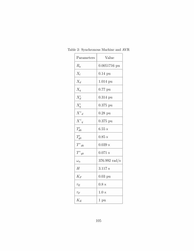
Table 2: Synchronous Machine and AVR

Parameters Value

Ra 0.0051716 pu

Xl 0.14 pu

Xd 1.014 pu

Xq 0.77 pu

X ′d 0.314 pu

X ′q 0.375 pu

X”d 0.28 pu

X”q 0.375 pu

T ′d0 6.55 s

T ′q0 0.85 s

T”d0 0.039 s

T”q0 0.071 s

ωn 376.992 rad/s

H 3.117 s

KF 0.03 pu

τE 0.8 s

τF 1.0 s

KE 1 pu

105

Table 3: Line Parameters for the CIGRE Test System

Node Node R′ph X ′ph B′ph R′0 X ′0 B′ph lFrom To Ω/km Ω/km µS/km Ω/km Ω/km µS/km km1 2 0.173 0.432 3.83 0.351 1.8 1.57 1.22 3 0.173 0.432 3.83 0.351 1.8 1.57 13 4 0.173 0.432 3.83 0.351 1.8 1.57 0.614 5 0.173 0.432 3.83 0.351 1.8 1.57 0.565 6 0.173 0.432 3.83 0.351 1.8 1.57 1.546 7 0.173 0.432 3.83 0.351 1.8 1.57 0.247 8 0.173 0.432 3.83 0.351 1.8 1.57 1.678 9 0.173 0.432 3.83 0.351 1.8 1.57 0.329 10 0.173 0.432 3.83 0.351 1.8 1.57 0.7710 11 0.173 0.432 3.83 0.351 1.8 1.57 0.3311 4 0.173 0.432 3.83 0.351 1.8 1.57 0.493 8 0.173 0.432 3.83 0.351 1.8 1.57 1.312 13 0.173 0.432 3.83 0.351 1.8 1.57 4.8913 14 0.173 0.432 3.83 0.351 1.8 1.57 2.9914 8 0.173 0.432 3.83 0.351 1.8 1.57 2

106

Table 4: Loads Apparent Power for the CIGRE Test System

(a) Phase a

Node Residential Commercial/Ind.1 subnetwork* —2 100 2003 — 804 200 —5 200 506 50 —7 — 1008 100 —9 100 —10 150 —11 50 15012 subnetwork* 8013 — 14514 — 90

(b) Phase b

Node Residential Commercial/Ind.1 — 1002 500 2003 200 804 100 —5 subnetwork* 2006 100 —7 100 1008 150 —9 150 —10 100 —11 50 15012 subnetwork* 8013 — 14514 — 90

(c) Phase c

Node Residential Commercial/Ind.1 200 1002 — 2003 50 804 100 —5 — 506 subnetwork* —7 — 1008 — 2009 100 —10 250 —11 — 15012 — 8013 — 14514 subnetwork* 90

(d) Power Factor

Node Residential Commercial/Ind.1 0.90 0.802 0.95 0.853 0.90 0.804 0.90 —5 0.95 0.856 0.95 —7 0.95 0.958 0.90 0.909 0.95 —10 0.90 —11 0.95 0.8512 0.90 0.8013 0.95 0.8514 0.90 0.90

* Subnetwork demand is 172 kVA with a power factor of 0.95.

107

primary and secondary frequency control techniques for

Documents