MARINE ECOLOGY PROGRESS SERIESMar Ecol Prog Ser

Vol. 303: 91–103, 2005 Published November 21

INTRODUCTION

Coastal waters play an important role as an origin ofglobal food resources. Although the coastal oceanoccupies only 8% of the ocean surface, about 90% ofthe world’s commercial fishes are caught in coastalwaters (Pernetta & Milliman 1995). Primary productioncomprises the basis of marine food webs and is animportant mediator of carbon flux in the ocean. Coastalprimary production has been estimated to contribute14 to 25% of the global oceanic primary production(Longhurst et al. 1995, Pernetta & Milliman 1995).

The Yellow Sea is a shelf sea surrounded by the Ko-rean peninsula and the eastern coast of China, with amean depth of 44 m and maximum depth of 103 m. It isaffected by strong tidal currents and freshwater dis-charges from the Changjiang (Yangtze) River, thelargest river in Asia. The Kuroshio Current, character-

ized by comparatively high-temperature and saline wa-ters, also influences the southeast area of the Yellow Sea.

There have been many studies of phytoplanktonprimary production based on field measurements inthe Yellow Sea (Choi & Shim 1986, Choi 1991, Kanget al. 1992, Choi et al. 1995, Wu et al. 1995, Yoo &Shin 1995). However, as these studies were temporallyand spatially restricted, it is not possible to estimateprimary production for the entire Yellow Sea basedon these measurements alone. Ocean-color data arepresently the only means of determining phytoplank-ton chlorophyll concentration on a basin or globalscale; however, some problems still remain to besolved (Balch et al. 1992, Sathyendranath & Platt 1993).Models based on remotely sensed chlorophyll a (chl a)concentration allow the estimation of ocean primaryproduction on both basin and global scales (Platt etal. 1991, Balch et al. 1992, Antoine et al. 1995, Long-

© Inter-Research 2005 · www.int-res.com*Email: seunghyun_son@umit.maine.edu

Primary production in the Yellow Sea determinedby ocean color remote sensing

SeungHyun Son1, 4,*, Janet Campbell1, Mark Dowell2, Sinjae Yoo3, Jaehoon Noh3

1Ocean Process Analysis Laboratory, University of New Hampshire, Durham, New Hampshire 03824, USA2Inland and Marine Waters Unit, Joint Research Centre, TP 272, I21020 Ispra, Italy

3Korea Ocean Research and Development Institute, PO Box 29, Ansan 425-600, South Korea

4Present address: School of Marine Sciences, University of Maine, Orono, Maine 04469-5741, USA

ABSTRACT: The Yellow Sea is a shelf sea surrounded by the Korean peninsula and the eastern coastof China. The bordering countries derive a substantial share of their food from fishing in these coastalwaters. Synoptic maps of water-column integrated primary production in May and September werederived using a primary production algorithm applied to ocean color satellite data from the YellowSea from 1998 to 2003. The middle of the Yellow Sea (MYS) had higher levels of primary productionin May and September than the shallower (<50 m) areas off the coasts of Korea and China. Althoughthe coastal areas had high phytoplankton biomass, lower levels of primary production were causedby high turbidity arising from strong tides and shallow depths. Lower turbidity in the central part ofthe Yellow Sea allows light necessary for primary production to penetrate deeper into the watercolumn. The mean daily integrated primary production in the MYS was 947 mg C m–2 d–1 in Mayand 723 mg C m–2 d–1 in September. The mean values in Chinese and Korean coastal waters were590 and 589 mg C m–2 d–1 in May, and 734 and 553 mg C m–2 d–1 in September, respectively. Ourcomputation of daily total primary production for the entire Yellow Sea was 19.7 × 104 t C d–1 in May,and 15.8 × 104 t C d–1 in September.

KEY WORDS: Primary production · Phytoplankton · Ocean color · SeaWiFS · Yellow Sea

Resale or republication not permitted without written consent of the publisher

Mar Ecol Prog Ser 303: 91–103, 2005

hurst et al. 1995, Antoine & Morel 1996, Behrenfeld &Falkowski 1997, Hoepffner et al. 1999).

Standard algorithms for primary production rely onremotely sensed chl a concentration, light attenuation,surface irradiance, and/or sea-surface temperature.Algorithms also require information not accessible byremote sensing, such as the vertical distribution ofphytoplankton biomass and photosynthetic parameters.To handle non-uniformity of phytoplankton biomass inthermally stratified waters, it has been customary torelate the remotely sensed chlorophyll concentration atthe surface to the vertical profile of phytoplankton bio-mass (Lewis et al. 1983, Platt et al. 1988, Morel &Berthon 1989). A shifted Gaussian distribution has beenproposed to derive biomass profiles (Platt et al. 1988b).

There are 2 main approaches to estimating photosyn-thetic parameters, but both methods have weaknesses(Platt et al. 1995). One is to derive the required para-meters as a function of environmental variables such assea-surface temperature (Behrenfeld & Falkowski 1997,Gong & Liu 2003). The other is to assign the parametersbased on their location and season from an existing data-base for biogeochemical provinces (Platt & Sathyen-dranath 1988, Longhurst et al. 1995, Sathyendranath etal. 1995, Hoepffner et al. 1999). The latter approach wasapplied to data from the Yellow Sea in the present study.

We used the primary production algorithm of Platt &Sathyendranath (1988) to estimate primary productionin the Yellow Sea. We first partitioned the Yellow Seainto 3 subregions based on bathymetry and physicalfeatures, and used in situ measurements taken in thesesubregions in May and September between 1992 and1998 to parameterize the algorithm. We explored sev-

eral ways of estimating the diffuse attenuation coeffi-cient, kd, and investigated whether it was necessary tomodel the vertical biomass profile. The resulting mapsof primary production calculated from the remotelysensed data provide the first synoptic views of primaryproduction in the Yellow Sea.

MATERIALS AND METHODS

In situ data. Cruise data on phytoplankton biomassand primary production in the Yellow Sea (from 32 to37° N and 122 to 127° E) were available from only 2months from 6 cruises conducted between 1992 and1998, namely May and September (Table 1). Parametersfrom 141 photosynthesis-light (P versus E; P-E) curveswere available from 6 different cruises between 1992and 1998. Of these, 93 P-E parameters were obtained atthe surface, 37 between 10 and 30 m, and 11 between 40and 75 m. All P-E measurements were based on 14Cmethods (Steemann Nielsen 1952). Water samples wereincubated for 2 h on deck under screens simulating 9 to10 light levels between 0 and 100% surface photosyn-thetically available radiation (PAR). The P-E data werethen fitted as described by Platt et al. (1980). For furtherdetails, see Choi et al. (1995) and Park (2000). Therewere 86 chl a fluorescence profiles available from the 6cruises between 1992 and 1998. These were measuredwith a CTD-SBE 25, and calibrated with discrete chl ameasured fluorometrically (Turner Design).

Estimates of daily water-column primary productionwere made only at 37 stations on the September 1992cruise of Choi et al. (1995) (Fig. 1b). Water-column

92

Fig. 1. Geography of the study area. The Yellow Sea was divided into 3 sub-regions using bathymetry and physical features.CCW: Chinese Coastal Waters, MYS: Mid-Yellow Sea, and KCW: Korean Coastal Waters. The serial oceanographic stations ofKODC (Korea Oceanographic Data Center) for Secchi depth data are shown in (a) and the observatory stations for primary

production of the Yellow Sea cruise in September 1992 (Choi et al. 1995) are shown in (b)

a b

Son et al.: Primary production in the Yellow Sea

integrated primary production could not be estimatedfor the other stations because of a lack of light profileor diffuse attenuation data. The daily water-columnprimary production at these 37 stations was comparedwith satellite-derived primary production, even thoughthe 2 data sets did not coincide temporally.

Cruise data on temperature, salinity, and trans-parency (Secchi depth) at 71 stations in the southeastYellow Sea were obtained from the Korea Oceano-graphic Data Center (KODC) (Fig. 1a). These datawere from oceanographic surveys carried out at 2 mointervals (February, April, June, August, October, andDecember) by the National Fisheries Research andDevelopment Institute (NFRDI). The Secchi depth (SD)data from 1998 to 2002 (coinciding with the time periodof the satellite data) were used to estimate the diffuseattenuation coefficient for PAR as explained below.

Satellite data. SeaWiFS Level 1a Version 4 data from1998 to 2003 for the Yellow Sea were obtained from theNASA Goddard Space Flight Center (GSFC). The dailySeaWiFS data, with a spatial resolution of 1 × 1 km2,were processed from Level 0 to 2 and remapped usingthe SeaWiFS Data Analysis System (SeaDAS) Version4.4 software (NASA GSFC). The standard algorithmsof SeaDAS were used for the atmospheric correction.After eliminating images acquired on cloudy days,there remained 1358 images of the Yellow Sea from1998 to 2003, including 236 images in the months ofMay and September.

The standard algorithm for the SeaWiFS chl a con-centration is based on Case 1 waters, defined as thosewaters where phytoplankton pigments are the sole fac-tor determining the color of the water (Morel & Prieur1977). Although the middle of the Yellow Sea may becharacterized as Case 1 waters in warm months of theyear (spring to fall), large areas of the Yellow Sea are

Case 2 waters. In particular, colored dissolvedorganic matter and suspended sediments alsoaffect the water color in shallow areas influ-enced by strong tidal mixing and river dis-charge. We used a local empirical algorithmof chl a concentration for the Yellow Seadeveloped by Ahn (2004):

(1)

where Rrs490 and Rrs555 are remote-sensingreflectance at 490 and 555 nm, respectively. Thealgorithm was developed using (1) measuredremote-sensing reflectance from the DualUV/VNIR spectroradiometer in the Korean Seasand (2) measured chlorophyll concentrations.Although it does not explicitly account for otherconstituents affecting water color, it was tailoredfor the optical properties of the Yellow Sea.

Primary production model. Since there were nospectral light or phytoplankton absorption measure-ments available from the cruises, we used a spectrally-integrated primary production model (Platt & Sathyen-dranath 1988). Daily depth-integrated primary pro-duction (IPP) was derived using the equation:

(2)

where B(z) is the chl a biomass at depth z; αB is theinitial slope of the P B versus E curve; E(z,t) is PAR atdepth z and time t; Pm

B is the assimilation number;t1 and t2 are the times of sunrise and sunset; and Zeu isthe euphotic depth. The vertical PAR profile is givenby E(z,t) = E(0,t) × exp(–kd × z) were E (0) is PAR inci-dent on the surface, and kd is the diffuse attenuationcoefficient for PAR. The input parameters used in theprimary production model (Eq. 2) are described in thefollowing sections.

Biomass profile (deep chlorophyll maximum [DCM]model). The Yellow Sea was partitioned into well-mixed and stratified waters using a relationshipbetween water-leaving radiance at 670 nm from Sea-WiFS and model-based temperature profiles (S. Sonet al. unpubl. data). We assumed that the biomass pro-file B(z) was uniform in well-mixed waters and non-uniform in stratified waters.

The shifted Gaussian distribution model (Platt etal. 1988, Sathyendranath & Platt 1989) was used todescribe the biomass profile:

(3)

where B0 is a background biomass (mg m–3); zm is thedepth of the chlorophyll maximum (m); σ is a measureof the thickness or vertical spread of the peak (m); h is

B z Bh z z

( ) exp( )= + − −⎡

⎣⎢⎤⎦⎥0

2

22 2σ π σm

IPPB

BmB

eu ( )· · ( , )

( · ( , ) / )=

+

B z E z t

E z t P

zα

α1 20∫∫∫

t

t

z t1

2

d d·

Chl aRrsRrs

..

= × ( )−1 05

490555

1 70

93

Cruise Source Period No. of No. of name P-E chl a

parameters profiles

YS-9210 Choi et al. 17 Sep– 38 38(1995) 2 Oct, 1992

COPEX KORDI 29 Aug– 11 105 Sep, 1994

COPEX KORDI 26 Apr– 24 96 May, 1995

LME KORDI 20–24 May, 1996 12 11

LME KORDI 20–31 May, 1997 36 14

LME KORDI 15–19 May, 1998 20 4

Total 1410 86

Table 1. Sources of data for the chlorophyll profiles and P-E parameters inthe Yellow Sea (32 to 37° N and 122 to 127° E). Total number is 141 stations.COPEX: Coastal Ocean Process Experiment cruise; LME: Yellow SeaLarge Marine Ecosystem cruise; KORDI: Korea Ocean Research and

Development Institut, South Korea

Mar Ecol Prog Ser 303: 91–103, 2005

the total biomass above the background (mg m–2); andpeak height above the baseline is given by H =h�(σ1232π). Parameters were estimated by fitting thismodel to the 86 chlorophyll profiles (Table 1).

PAR profile. The PAR product of SeaWiFS was usedfor the incident surface irradiance. Unfortunately,there were very few light measurements in the YellowSea available for this study. Since large areas of theYellow Sea are affected by colored dissolved organicmatter and suspended sediments, the diffuse attenua-tion model of Sathyendranath & Platt (1988), which isfor Case 1 waters (i.e. based on chlorophyll), was notapplicable to the Yellow Sea.

The SD data obtained from the NFRDI provided thebest source of information about light extinction inthese coastal Korean waters. In addition, there were 17stations from the primary productivity cruises (Table 1)where both Kd and SD had been measured. The kd val-ues were derived from measurements by a PAR sensorattached to the CTD-SBE 25. The relationship betweenSD and kd for these stations is shown in Fig. 2. Alsoshown is the relationship kd = 1.44/SD (Kirk 1994),which appears to be in reasonable agreement with thedata. Therefore, we used this relationship to derive kd

from the NRFDI SD data.The primary production algorithm requires kd at

every pixel in the image. Therefore, we explored therelationship between the SD and SeaWiFS K490 andnLw555 products. The SD data in the period between1998 and 2002 were matched with SeaWiFS data ob-tained within 1 d of the in situ measurement. Therewere 300 match-up pairs, including 149 made on thesame day.

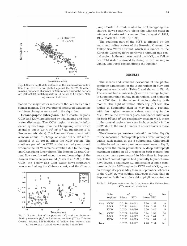
The match-up SD measurements were regressedagainst SeaWiFS K490 and nLw555 products (Figs. 3& 4). The SD data did not correlate as well to the K490data (r2 = 0.5, Fig. 3) as they did to the nLw555 data(r2 = 0.78, Fig. 4). Therefore, we used the derivedpower-law relationship SD = 6.4023 × (nLw555)–0.7269

to estimate SD, which was then converted to diffuseattenuation coefficient by the relationship kd = 1.44 SD(Kirk 1994).

The euphotic depth (Zeu) was defined as the depth atwhich PAR is 1% of the surface PAR. Accordingly,the euphotic depth is given by 4.6/kd with the assump-tion that kd is approximately constant with depth (Kirk1994). Given the relationship with SD, the euphoticdepth was then given by Zeu = 3.2 × SD.

Photosynthetic parameters. Two approaches to esti-mate the photosynthetic parameters for primary pro-duction were mentioned above. To consider the firstapproach, we investigated the relationship betweensea surface temperature and the photosynthetic para-meter (Pm

B) (Behrenfeld & Falkowski 1997), but foundno apparent relationship in our data set (Fig. 5). Thus,we chose the second approach whereby parametersare based on average properties measured within bio-geochemical provinces (Longhurst et al. 1995, Platt etal. 1995, Sathyendranath et al. 1995).

Accordingly, the Yellow Sea (between 32 and 37° N,122 and 127° E) was divided into 3 subregions based onbathymetry (Fig. 1b): (1) the Chinese Coastal Waters(CCW) and (2) the Korean Coastal Waters (KCW) shal-lower than 50 m, and (3) the central part of the YellowSea (MYS) deeper than 50 m. Ning et al. (1998) parti-

94

0.0

0.1

0.2

0.3

0.4

0.5

0.6

0 5 10 15 20 25

Secchi depth (m)

k d (1

/m)

kd = 1.44/SD

y = 0.5943x -1.2143

R2 = 0.4984

1.0

10.0

100.0

0.01 0.10 1.00

SeaWiFS K490

Sec

chi d

epth

(m)

Fig. 2. Scatter plots of measured diffuse attenuation derivedfrom PAR in the water column versus measured Secchi depth(SD) at 17 stations in the Yellow Sea. The line of kd = 1.44/SD

is also drawn on the scatter plots

Fig. 3. Secchi depth data obtained in the southeastern YellowSea from KODC were plotted against the SeaWiFS K490product (note log scale on both axes) in 286 stations duringthe periods of 1998 to 2002 (match up data is 1 d before to

1 d after)

Son et al.: Primary production in the Yellow Sea

tioned the major water masses in the Yellow Sea in asimilar manner. The averages of measured parameterswithin each region were used in the algorithm.

Oceanographic subregions. The 2 coastal regions,CCW and KCW, are affected by tidal mixing and fresh-water discharge. The CCW region is strongly influ-enced by discharge from the Changjiang River whichaverages about 2.9 × 104 m3 s–1 (S. Riedlinger & R.Preller unpubl. data). The Han and Keum rivers, witha mean annual discharge of about 1.0 × 103 m3 s–1

(Schubel et al. 1984), affect the KCW region. Thesouthern part of the KCW is tidally mixed year round,whereas the CCW remains stratified due to the buoy-ant Changjiang River plume. The Korean Coastal Cur-rent flows southward along the southern edge of theKorean Peninsula year round (Mask et al. 1998). In theCCW, the Yellow Sea Cold Water flows southwardyear round along the Chinese coast, and the Chang-

jiang Coastal Current, related to the Changjiang dis-charge, flows southward along the Chinese coast inwinter and eastward in summer (Beardsley et al. 1983,1985, Mask et al. 1998, Su 1998).

The southern part of the MYS is affected by thewarm and saline waters of the Kuroshio Current; theYellow Sea Warm Current, which is a branch of theKuroshio Current, flows northward through this cen-tral region. In the northern part of the MYS, the YellowSea Cold Water is formed by strong vertical mixing inwinter, and traces remain during the summer.

RESULTS

The means and standard deviations of the photo-synthetic parameters for the 3 subregions in May andSeptember are listed in Table 2 and shown in Fig. 6.The assimilation numbers (Pm

B) were on average higherin September than in May in all regions, and higher inthe KCW than in the other 2 regions during bothmonths. The light utilization efficiency (α B) was alsohigher in September than in May in all 3 regions,with the highest average values occurring in theMYS. While the error bars (95% confidence intervals)for both Pm

B and α B are reasonably small in MYS, thosein the coastal regions are very high, especially in theKCW, due to the small number of observations in thoselocations.

The Gaussian parameters derived from fitting Eq. (3)to the measured chlorophyll profiles were averagedwithin each month in the 3 subregions. Chlorophyllprofiles based on mean parameters are shown in Fig. 7,along with the mean parameters. A deep chlorophyllmaximum existed in all 3 regions in both months, butwas much more pronounced in May than in Septem-ber. The 2 coastal regions had generally higher chloro-phyll levels, a shallower zm, and smaller h and σ com-pared with the MYS region. In KCW and MYS, zm wason average deeper in May than in September, whereasin the CCW, zm was slightly shallower in May than inSeptember. Both the surface chlorophyll concentration

95

y = 6.4023x-0.7269

R2 = 0.7845

1.0

10.0

100.0

0.1 1.0 10.0

SeaWiFS nLw555

Sec

chi d

epth

(m)

0.0

2.0

4.0

6.0

8.0

10.0

12.0

14.0

10 15 20 25 30Temperature

P mB

CCWMYSKCW

Fig. 4. Secchi depth data obtained in the southeastern YellowSea from KODC were plotted against the SeaWiFS water-leaving radiances at 555 nm in 286 stations during the periodsof 1998 to 2002 (match up data is 1 d before to 1 d after). Note

log scale on both axes

Sub- αB PmB No.

regions Mean STD Mean STD

May CCW 0.0176 0.0062 3.90 1.52 8MYS 0.0221 0.0141 3.99 2.52 75KCW 0.0204 0.0096 6.50 3.46 9

Sep CCW 0.0268 0.0068 6.24 1.99 14MYS 0.0293 0.0097 5.49 2.01 31KCW 0.0233 0.0079 6.69 1.87 4

Total 0.0239 0.0122 4.78 2.54 1410

Table 2. P-E parameters for the 3 regions of the Yellow Sea. STD: standard deviation

Fig. 5. Scatter plots of temperature (°C) and the photosyn-thetic parameter (Pm

B) in 3 different regions (CCW: ChineseCoastal Waters, MYS: Middle of Yellow Sea waters, and

KCW: Korean Coastal Waters) in the Yellow Sea

Mar Ecol Prog Ser 303: 91–103, 2005

and the integrated chlorophyll (to 50 m in KCW andCCW, and to 80 m in MYS) were higher in May than inSeptember.

To test the effect of the non-uniform biomass profileon primary production, we compared primary produc-tion calculated using a uniform biomass profile (equalto the surface chlorophyll) with the integrated primaryproduction measured at the 37 stations in September1992 (Choi et al. 1995). The latter took into account thenon-uniform chlorophyll profiles at each station. Withthe exception of the biomass profile B (z), the samemeasured variables were used in both calculations.The scatter plot of non-uniform-biomass primary pro-duction (PP2) versus uniform-biomass primary produc-tion (PP1) is shown in Fig. 8. Assuming uniform bio-mass profiles, primary production was underestimatedby an average of 15.6% (and as much as 39%) atstations deeper than 50 m. In the shallower stations(<50 m), the error was on average only 7%.

Since the input parameters (PmB, αB and DCM) were

based on measurements made only in May and Sep-tember (Table 1), we applied the algorithm only to Mayand September SeaWiFS data. Monthly composites of

96

0.00

0.01

0.02

0.03

0.04

0.05

CCW_5 MYS_5 KCW_5 CCW_9 MYS_9 KCW_9

α B

0.00

2.00

4.00

6.00

8.00

10.00

12.00Pm

B

mg

C (m

g ch

l a)-1

h-1

(mE

ins

m-2

s-1

)-1m

gC

(mg

chl a

)-1 h

-1

0 1 2 3 4 0 1 2 3 4 0 1 2 3 4

0 1 2 3 40 1 2 3 40 1 2 3 4

0

20

40

60

80

0

20

40

60

80

0

20

40

60

80

0

20

40

60

80

0

20

40

60

80

0

20

40

60

80

CCW MYS KCW

Chlorophyll

Dep

th (m

)D

epth

(m)

Chlorophyll Chlorophyll

a

b

n = 5zm: 13.01B0: 1.43h: 19.05

sigma: 6.06

n = 30zm: 30.66B0: 0.79h: 23.45

sigma: 7.55

n = 3zm: 17.10B0: 1.76h: 21.22

sigma: 5.32

n = 14zm: 14.69B0: 0.96h: 5.54

sigma: 6.91

n = 30zm: 23.75B0: 0.44h: 12.35

sigma: 7.36

n = 4zm: 7.80B0: 0.66h: 4.44

sigma: 5.45

Fig. 6. Mean values of the light utilization efficiency (α B) andthe photosynthetic parameter (Pm

B) in 3 different regions(CCW, MYS, and KCW) in May (first 3 points from the left)and December (first 3 points from the right) with 95% confi-

dence intervals

Fig. 7. Mean fitted biomass(chlorophyll) profiles for the 3sub-regions of the Yellow Seain (a) May and (b) September.Number of data used (n) and4 parameters of DCM (deepchlorophyll maximum) modelare shown in each graph.B0: background biomass (mgm–3); zm: depth of chorophyllmaximum (m); h: total bio-mass above the background(mg m–2); σ: measure of thethickness or vertical spreadof the chlorophyll peak (m)

Son et al.: Primary production in the Yellow Sea

the input data PAR, kd and chl a, from 1998 to 2003,and their 6 year averages, are shown in Fig. 9, andthe monthly composite primary production imagesfor these years are shown in Fig. 10. Year-to-year vari-ations of the means in each subregion are shown inFig. 11.

The overall spatial distribution of PAR was uniform inMay, but increased from south to north in September.On average, PAR was 26% higher in May (6 year meanof 58.3 to 58.6 Ein m–2 d–1) than in September (6 yrmean of 45.9 to 46.6 Ein m–2 d–1). PAR was lower in 1999and 2003 in both months compared with other years.

The kd images were derived from the SeaWiFSnLw555 data using methods described above. Thespatial distribution of the 6 year average of kd in Mayand September were similar. In both months, high val-ues of kd were found near the Kyunggi Bay, the south-western coastal regions of Korea, the Shandong penin-sula, and the Changjiang River, while kd was lower inthe middle of the Yellow Sea. However, a compara-tively high kd patch appeared in the middle of theYellow Sea in May. The mean value of kd based on the6 year composites for May ranged from 0.33 to 0.38 m–1

in the coastal regions (CCW and KCW), to 0.13 m–1 inthe central regions of the Yellow Sea (MYS). The meanvalue of kd in September in the central Yellow Sea wassimilar to that in May (0.12 m–1), but September valueswere slightly lower in the coastal regions (0.30 m–1)compared to May. The interannual variability of kd wasmore pronounced in the coastal regions compared withthe MYS.

Spatial patterns of chl a were similar in both months,with higher chl a in coastal areas and near the Chang-jiang River, and relatively low values in the centralYellow Sea. The 6 year mean chl a was slightly higherin May (0.95 mg m–3) than in September (0.93 mg m–3),and chl a was slightly higher in the KCW (1.74 and1.81 mg m–3 in May and September, respectively) thanin the CCW (1.61 and 1.46 mg m–3 in May and Septem-ber, respectively). In the MYS, chl a was slightly lowerin May (0.70 mg m–3) than in September (0.77 mg m–3).A patch of significantly higher chl a appeared in thecentral Yellow Sea in each May image. This patch,located in the vicinity of a Korean dump site used since1992, varied in size and concentration from year toyear. The patch spread widely in 1999 and had thehighest chl a levels in 2001.

The depth-integrated daily primary production forMay and September are shown in Fig. 10, and themeans calculated for each subregion are listed inTable 3. Primary productivity throughout the YellowSea was higher in May than in September, and higherin the MYS than in the coastal regions. In the MYS, the6 year mean primary production was 947 mg C m–2 d–1

in May and 723 mg C m–2 d–1 in September; in theKCW, the mean was 734 mg C m–2 d–1 in May and554 mg C m–2 d–1 in September. There was almost nodifference between May and September in the CCW,with averages of 590 and 589 mg C m–2 d–1, respec-tively. Interannual variability can be clearly seen inFigs. 10 & 11. The daily primary production estimatedfor the entire Yellow Sea was 19.7 × 104 t C d–1 in Mayand 15.8 × 104 t C d–1 in September.

The measured IPP at 37 stations in September 1992were compared (1) to the range of values at the samelocations in the monthly composite satellite data ofeach year, and (2) to the 6 year averages (Fig. 12).At about two-thirds of the stations, the measuredIPP fell within the range of the satellite-derived values.Exceptions occurred along the C-line (Fig. 1b) wherethe satellite values were much higher than the mea-sured IPP, and at Stn F07, where the satellite valueswere much lower than the measured value.

DISCUSSION AND CONCLUSION

We estimated that an assumption of a uniform bio-mass profile would have resulted in an underestima-tion of primary production by 15% in the deep regions(>50 m) and 7% in the 2 shallower coastal regions.These results are consistent with results reported byothers. Platt et al. (1991) determined that a uniformbiomass profile would underestimate integral produc-tion by about 20% in the North Atlantic. Siswanto et al.(2004) found that primary production derived from a

97

1500

1200

900

600

300

00 300 600 900 1200 1500

PP1

PP

2

Fig. 8. Scatter plots of primary production calculated using auniform biomass profile (PP1) versus primary productionusing non-uniform biomass profile (PP2) at 37 stations ofthe Yellow Sea cruise in September, 1992 (Choi et al. 1995).Squares indicate primary production in deeper area (>50 m)

and circles in the shallower areas (<50 m)

Mar Ecol Prog Ser 303: 91–103, 200598

Fig. 9. Monthly composite SeaWiFS images from 1998 to 2003 in May and September as well as 6-year composite images (98-03 panels) of (a) PAR, (b) diffuse attenuation (kd) derived from nLw555, (c) chlorophyll derived from Ahn’s algorithm

1998 1999 2000 2001 2002 2003 98-03

1998 1999 2000 2001 2002 2003 98-03

Ein m–2 d–1

1/m

mg m–3

0.01 0.1 1.0 10.0

0 0.1 0.2 0.3 0.4 0.5 0.6 0.7

36 40 44 48 52 56 60 64

Sep

tem

ber

May

Sep

tem

ber

May

Sep

tem

ber

May

a

b

c 1998 1999 2000 2001 2002 2003 98-03

Son et al.: Primary production in the Yellow Sea

uniform profile model was underestimated by 20 to35% in the Kuroshio Current and frontal regions of theEast China Sea.

Primary production estimates would certainly bene-fit from more accurate information about photosynthe-sis-irradiance relationships (Morel et al. 1996). Studieshave shown that primary production is more sensitiveto changes in the P-E parameters than to the chloro-phyll–profile parameterization (Sathyendranath et al.1995). An error in our approach results from the aggre-gation of the parameters within provinces (Platt et al.1995). The natural variability within each province isreflected in the 95% confidence intervals for the mean,which were in the range from ±12% (MYS) to ±54%(KCW) for αB, and in the range from ±13% (MYS) to±44% (KCW) for Pm

B. The main reason for uncertaintyin the coastal regions is that only a small number ofdata points were available. According to Platt et al.(1988), measurement techniques cannot do better than±5% for Pm

B and ±20% for αB. Spectrally- and depth-resolved primary production

algorithms have been considered as benchmarks inestimating primary production (Platt et al. 1991, Kye-walyanga et al. 1992). Most studies have been con-ducted in open ocean waters and used a spectral modelfor the light field in the water column based on Case 1waters. The Case 1 spectral model is not applicable inthe Yellow Sea because large areas of the Yellow Seaare Case 2 waters. S. Son et al. (unpubl. data) showedthat diffuse attenuation based on a Case 1 (chloro-phyll-dependent) model underestimated kd in Case 2waters by a factor of 2 to 4. Unfortunately, we had veryfew light measurements in the database used for thisstudy. From 17 coincident measurements of SD and kd,

we found that kd = 1.44/SD (Kirk 1994) was a reason-able relationship to use. By applying this relationshipand an empirical relationship between measured SDand satellite water-leaving radiances at 555 nm, wederived an algorithm for estimating kd. A reasonablerelationship (r2 = 0.78) was found between SD and Sea-WiFS nLw555 at 300 stations measured within 1 d ofthe satellite overpass. We considered using the Sea-WiFS K490 product, but its relationship with SD did notprove to be as good as that of the 555 nm water-leavingradiance. The standard algorithm for the SeaWiFSK490 is known to have large uncertainties in turbidwater, especially where K490 is greater than 0.25 m–1

(O’Reilly et al. 2000). The mean kd derived from nLw555 was 0.12 m–1 in

the central Yellow Sea, and varied from 0.3 to 0.38 m–1

with a maximum value of 0.76 m–1 in the coastal re-gions. These values were similar to results reported byS. Son et al. (unpubl. data), in which kd in the YellowSea ranged from 0.09 m–1 to 0.74 m–1 with a mean of0.20 m–1.

Errors associated with ocean color chlorophyll algo-rithms range from 50 to 100% in turbid waters foundin near-shore areas of the Northeastern Atlantic(Hoepffner et al. 1999). Since a large part of the Yel-low Sea is characterized as Case 2 waters, the currentstandard chlorophyll algorithm overestimates thechlorophyll concentration and consequently primaryproduction. Therefore, we chose a local empiricalalgorithm for chl a concentration developed by Ahn(2004) for the Yellow Sea. Comparisons of SeaWiFSstandard algorithms (OC2 and OC4) with in situ mea-surements in Korean waters (Moon et al. 2002, Ahn2004) showed that the standard algorithms are suit-

99

Fig. 10. Monthly composite images of primary production based on SeaWiFS from 1998 to 2003 in May and September as well as 6-year composite images (98-03 panels)

mg C m–2 d–1

May

Sep

tem

ber

0 400 800 1200 1600 2000

1998 1999 2000 2001 2002 2003 98-03

Mar Ecol Prog Ser 303: 91–103, 2005

able in the Sea of Japan and the Kuroshio Current,which are characterized as Case 1 waters, but are notapplicable for Case 2 waters such as the Yellow andEast China Seas (root mean square [RMS] errors were0.618 mg m–3 for OC2 version 3 and 0.663 mg m–3 forOC4). The empirical chlorophyll algorithm developed

by Ahn (2004) for the Yellow Sea had a reduced RMSof 0.34 mg m–3; it is still a Case 1 algorithm as it doesnot account for variability in other optically activeconstituents.

In this study, we presented monthly primary produc-tion for only 2 months, May and September, because

100

Fig. 11. Year-to-year variations of the mean values of the SeaWiFS input values in the 3 sub-regions in May and September.(a) PAR, (b) diffuse attenuation (kd) derived from nLw555, (c) chlorophyll derived from Ahn’s algorithm, and (d) daily integrated

primary production (PP). j: CCW; D: MYS; f: KCW

Son et al.: Primary production in the Yellow Sea

in situ data on primary production and vertical biomassdistribution were available only for these months. IPPvaried from 590 to 947 mg C m–2 d–1 (with the overallmean of 836 mg C m–2 d–1) in May, and from 554 to723 mg C m–2 d–1 (with the overall mean of 672 mg Cm–2 d–1) in September. In both months, the primaryproduction was lower in the coastal waters and higherin the middle of the Yellow Sea. Despite higher chlo-rophyll concentrations, lower production resulted incoastal waters due to higher turbidity and shallowdepths. The overall mean primary production was 24%higher in May than in September, largely due to thefact that PAR was 26% higher in May than Septem-ber. Thus the seasonal variation of light may be animportant factor in determining variations in primaryproduction.

We calculated IPP using daily satellite images andthen averaged the IPP images to form monthly com-posites. By applying the IPP algorithm to daily data,

we avoided the problem of using averaged values innonlinear equations (Eqs. 2 & 3), a practice that canintroduce artifacts as described in Campbell (2004).However, the use of daily satellite data has an asso-ciated clear-sky bias since all input data are fromcloud-free pixels. This has a large effect on the PARvalues used as input, but its effect on the derived IPPcan be minimal depending on the algorithm (Camp-bell 2004).

There are only 2 studies that describe the distribu-tion of chlorophyll and primary productivity over theentire Yellow Sea (Choi et al. 1995, Wu et al. 1995).Both were based on cruises made in September 1992.Choi et al. (1995) reported mean primary production tobe 740 mg C m–2 d–1, which is similar to our result. Wuet al. (1995) reported a much lower mean primaryproduction (331 mg C m–2 d–1) for the same monthand year and similar stations. The large differencesbetween these primary production estimates may bethe result of different methods used to derive thedepth-integrated primary production. Choi et al. (1995)measured primary productivity using 14C methods andestimated depth-integrated primary production withthe formula of Platt et al. (1980). Wu et al. (1995) alsomeasured primary production using 14C, but appliedCadee & Hegeman’s (1974) formula to estimate depth-integrated primary production. In addition, bothstudies found very different chlorophyll levels (0.16 to3.20 mg m–3 with mean 0.69 mg m–3, Choi et al. [1995];0.43 to 17.43 mg m–3 with mean 1.362 mg m–3, Wu etal. [1995]), which were curiously opposite in magni-

101

0

500

1000

1500

2000

A05 A06 C01C02 C03 C04 C05 C06 C07 C09 C10 D01 D02 D06 D08 E01 E02 E03 E04 E05 E06 E09 F0

3F0

4F0

5F06 F07 F0

8F1

0G01

G02 G03 G04 G05G06 G07 G08

Stations

Prim

ary

pro

du

ctio

n

PP_meas.

1998

1999

2000

2001

2002

2003

comp(98-03)

Fig. 12. The values extracted from the monthly primary production images in 1998 to 2003 compared with the measured primary production (PP) at 37 stations of the Yellow Sea cruise in September, 1992 (Choi et al. 1995)

Sub- Area Mean primary production rateregion × 103 mg C m–2 d–1 ×104 ton C d–1

km2 May Sep May Sep

CCW 58.9 590.3 589.3 3.5 3.5 MYS 147.4 946.5 722.6 13.9 10.6 KCW 28.9 734.2 553.7 2.1 1.6

Mean 835.6 672.4

Total 235.2 19.7 15.8

Table 3. Primary production in the 3 regions of the Yellow Sea

Mar Ecol Prog Ser 303: 91–103, 2005

tude to different primary production estimates. In thisstudy, our primary production model was based onPlatt et al. (1988), and we used the data measured byChoi et al. (1995) as input data for our algorithm. Thus,our result should be comparable with that of Choi et al.(1995). In their results, the average primary productionwas 702 mg C m–2 d–1 in offshore stratified waters and620 mg C m–2 d–1 in the Korean coastal waters. Othersreported that primary production in the Kyunggi Baywas about 647 mg C m–2 d–1 in September 1986 (Chung& Park 1988). These mean values are similar to ourestimates: 740 mg C m–2 d–1 in the middle of the YellowSea, and 684 mg C m–2 d–1 in the Korean coastalwaters.

Choi et al. (2003) measured primary production inthe southeast Yellow Sea during 5 months in 1997(February, April, August, October and December).Although it was not possible to compare their resultswith our estimates, which were for different monthsbeginning in 1998, the spatial distributions of primaryproduction were similar; both studies found lower pri-mary production in the Kyunngi Bay and the south-western coastal waters of Korea, and higher levels inthe central waters of the Yellow Sea.

We do not have any measured primary productiondata to validate the satellite-derived primary produc-tion for the months of the SeaWiFS data. However, wecompared primary production measured at 37 stationsin September 1992 with monthly composite primaryproduction estimates at the same stations from Sep-tember 1998 to September 2003. Although the mea-sured IPP generally fell in the range of the satellite-derived IPP, about one-third of the measured IPP werebelow the range of the satellite estimates.

When we used the input parameters for May andSeptember to derive primary production for othermonths, we estimated the annual total primary pro-duction in the Yellow Sea to have varied from 47.8 to53.3 × 106 t C yr–1 between 1998 and 2003, with a meanof 50.1 3 × 106 t C yr–1. Clearly, we require models withbetter seasonal resolution before the annual produc-tion can be reliably estimated. However crude, ourresults provide the first synoptic maps of primary pro-duction in the Yellow Sea.

Acknowledgements. This work was supported by a NASAMODIS Instrument Team investigation contract (NAS5-96063) and the International Ocean Color CoordinatingGroup (IOCCG) Visiting Fellowship. We thank NASA Sea-WiFS Project, NASA Distributed Active Archieve Center, andthe OrbImage for production and distribution of the SeaWiFSdata. We thank Drs. Shubha Sathyendranath, Trevor Platt,and 3 anonymous reviewers for valuable comments. We alsothank Dr. YuHwan Ahn for kindly providing the chlorophyllalgorithm and Jisoo Park for contribution to collecting in situmeasurements on the cruises.

LITERATURE CITED

Ahn YH (2004) Study on prediction of oceanographic varia-bility of the Yellow Sea (the second phase). The KoreaOcean Research & Development Institute Report, BSPN50900–1627–1

Antoine D, Morel A (1996) Ocean primary production 2.Estimation at global scale from satellite (coastal zonecolor scanner) chlorophyll. Global Biogeochem Cycles10:57–69

Antoine D, Morel A, Andre J (1995) Algal pigment distribu-tion and primary production in the eastern Mediterraneanas derived from coastal zone color scanner observations.J Geophys Res 100:16193–16209

Balch W, Evans R, Brown J, Feldman G, McClain C, Esaias W(1992) The remote sensing of ocean primary productivity:use of a new data compilation to test satellite algorithms.J Geophys Res 97:2279–2293

Beardsley RC, Limeburner R, Le K, Hu D, Cannon GA,Pashinski DJ (1983) Structure of the Changjiang plume inthe East China Sea during June 1980. Proc Int SympSedimentation on the Continental Shelf, Spec Ref EastChina Sea, China Ocean Press, Beijing, p 265–284

Beardsley RC, Limeburner R, Yu H, Cannon GA (1985) Dis-charge of the Changjiang (Yangtze River) into the EastChina Sea. Cont Shelf Res 4:57–76

Behrenfeld M, Falkowski P (1997) Photosynthetic ratesderived from satellite-based chlorophyll concentration.Limnol Oceanogr 42:1–20

Cadee GC, Hegeman J (1974) Primary production of phyto-plankton in the dutch Wadden sea. Neth J Sea Res 8:240–259

Campbell J (2004) Issues linked to the use of binned data inmodels: an example using primary production. Antoine D(ed) Guide to the Creation and Use of Ocean-Colour,Level-3, Binned Data Products. Rep No. 4, IOCCG, Dart-mouth, p 23–37

Choi JK (1991) The influence of the tidal front on primaryproductivity and distribution of phytoplankton in themid-eastern coast of Yellow Sea. J Oceanogr Soc Korea26:223–241

Choi JK, Shim JH (1986) The ecological study of phytoplank-ton in Kyeonggi Bay, Yellow Sea: II. Light intensity, trans-parency, suspended substances. J Oceanogr Soc Korea 21:101–109

Choi JK, Noh JH, Shin KS, Hong KH (1995) The early autumndistribution of chlorophyll-a and primary productivity inthe Yellow Sea, 1992. Yellow Sea 1:68–80

Choi JK, Noh JH, Cho SH (2003) Temporal and spatial varia-tion of primary production in the Yellow Sea. Proc YellowSea Int Symp, Ansan, South Korea, p 103–115

Chung KH, Park YC (1988) Primary production and nitrogenregeneration by macrozooplanton in the Kyunggi Bay,Yellow Sea. J Oceanogr Soc Korea 23:194–206

Gong GC, Liu GJ (2003) An empirical primary productionmodel for the East China Sea. Cont Shelf Res 23:213–224

Hoepffner N, Sturm B, Finenko Z, Larkin D (1999) Depth-integrated primary production in the eastern tropicaland subtropical North Atlantic basin from ocean colourimagery. Int J Remote Sens 20:1435–1456

Kang YS (1992) Primary productivity and assimilation numberin the Kyonggi bay and the mid-eastern coast of YellowSea. J Oceanogr Soc Korea 27:237–246

Kirk JTO (1994) Light and photosynthesis in aquatic eco-systems, 2nd edn. Cambridge University Press, Cambridge,p119–120

Kyewalyanga M, Platt T, Sathyendranath S (1992) Ocean pri-

102

Son et al.: Primary production in the Yellow Sea

mary production calculated by spectral and broad-bandmodels. Mar Ecol Prog Ser 85:171–185

Lewis M, Cullen J, Platt T (1983) Phytoplankton and thermalsturucture in the upper ocean: consequences of nonunifor-mity in chlorophyll profile. J Geophys Res 88:2565–2570

Longhurst A, Sathyendranath S, Platt T, Caverhill C (1995)An estimate of global primary production in the oceanfrom satellite radiometer data. J Plankton Res 17:1245–1271

Mask AC, O’Brien JJ, Preller R (1998) Wind-driven effectson the Yellow Sea warm current. J Geophys Res 103:30713–30729

Moon JE, Ahn YH, Choi JK (2002) Compatible study on theSeaWiFS chlorophyll standard algorithm in Korean waters.Proceedings of the autumn meeting, Korean Society ofOceanography, Nov 14–15, 2002, Seoul, p 103–107

Morel A, Berthon JF (1989) Surface pigments, algal biomassprofiles, and potential production of the euphotic layer:relationships reinvestigated in view of remote-sensingapplications. Limnol Oceanogr 34:1545–1562

Morel A, Prieur L (1977) Analysis of variations in ocean color.Limnol Oceanogr 22:709–722

Morel A, Antoine D, Babin M, Dandonneau Y (1996) Mea-sured and modeled primary production in the northeastAtlantic (EUMELI JGOFS program): the impact of naturalvariations in photosynthetic parameters on model predic-tive skill. Deep-Sea Res I 43:1273–1304

Ning X, Liu Z, Cai Y, Fang M, Chai F (1998) Physicobiologicaloceanographic remote sensing of the East China Sea:satellite and in situ observations. J Geophys Res 103:21623–21635

O’Reilly JE, Maritorena S, O’Brien MC, Siegel DA and 21others (2000) SeaWiFS postlaunch calibration and valida-tion analyses, Part 3. In: Hooker SB, Firestone ER (eds)NASA technical memorandum 2000–206892, Vol 11.NASA Goddard Space Flight Center, Greenbelt, MD

Park J (2000) Vertical distribution and primary productivityof phytoplankton in the Yellow Sea in spring time.MSc thesis, Inha University, Incheon

Pernetta JC, Milliman JD (1995) Land-ocean interactions inthe coastal zone implementation plan. International Geo-sphere-Biosphere Program Report No. 33, Stockholm

Platt T, Sathyendranath S (1988) Oceanic primary production:estimation by remote sensing at local and regional scales.Science 241:1613–1620

Platt T, Gallegos C, Harrison WG (1980) Photoinhibition of

photosynthesis in natural assemblages of marine phyto-plankton. J Mar Res 38:687–701

Platt T, Sathyendranath S, Caverhill C, Lewis M (1988) Oceanprimary production and available light: further algorithmsfor remote sensing. Deep-Sea Res 35:855–879

Platt T, Caverhill C, Sathyendranath S (1991) Basin-scale esti-mates of oceanic primary production by remote sensing:the North Atlantic. J Geophys Res 96:15147–15159

Platt T, Sathyendranath S, Longhurst A (1995) Remote sens-ing of primary production in the ocean: promise and ful-fillment. Phil Trans R Soc Lond B 348:191–202

Sathyendranath S, Platt T (1988) The spectral irradiance fieldat the surface and in the interior of the ocean: a model forapplications in oceanography and remote sensing. J Geo-phys Res 93:9270–9280

Sathyendranath S, Platt T (1989) Remote sensing of oceanchlorophyll: consequence of nonuniform pigment profile.Appl Opt 28:490–495

Sathyendranath S, Platt T (1993) Underwater light field andprimary production: application to remote sensing. In:Barale V, Schlittenhardt PM (eds) Ocean colour: theoryand applications in a decade of CZCS experience. KluwerAcademic, Brussels, p 79–93

Sathyendranath S, Longhurst A, Caverhill C, Platt T (1995)Regionally and seasonally differentiated primary pro-duction in the North Atlantic. Deep-Sea Res 42:1773–1802

Schubel JR, Shen HT, Park MJ (1984) A comparison of somecharacteristic sedimentation processes of estuaries enter-ing the Yellow Sea. In: Marine geology and physical pro-cesses of the Yellow Sea. Proc Korea-USA Seminar &Workshop, Seoul, p 286–308

Siswanto E, Ishizaka J, Yokouchi K (2004) Estimating chloro-phyll vertical profiles from satellite data and the implica-tion to primary production in Kuroshio front of the EastChina Sea. J Oceanogr 61:575–589

Steeman Nielsen E (1952) The use of radioactive carbon (C14)for measuring organic production in the sea. J Cons IntExplor Mer 18:117–140

Su J (1998) Circulation dynamics of the China Seas North of18° N. In: Robinson AR, Brink KH (eds) The sea, Vol 11.Wiley, New York, p 483–505

Wu Y, Guo Y, Zhang Y (1995) Distributional characteristics ofchlorophyll-a and primary productivity in the Yellow Sea.Yellow Sea 1:81–92

Yoo S, Shin K (1995) Primary productivity properties in thenearshore region of Taean Peninsula. Ocean Res 17:91–99

103

Editorial responsibility: Otto Kinne (Editor-in-Chief),Oldendorf/Luhe, Germany

Submitted: December 21, 2004; Accepted: May 26, 2005Proofs received from author(s): October 18, 2005