PRIMARY TRANSIT OF THE PLANET HD 189733b AT 3.6 AND 5.8 �m

J. P. Beaulieu,1,2

S. Carey,3I. Ribas,

2,4and G. Tinetti

2,5

Received 2007 August 21; accepted 2007 November 21

ABSTRACT

The hot Jupiter HD 189733bwas observed during its primary transit using the InfraredArray Camera on the SpitzerSpace Telescope. The transit depths were measured simultaneously at 3.6 and 5.8 �m. Our analysis yields valuesof 2:356% � 0:019% and 2:436% � 0:020% at 3.6 and 5.8 �m, respectively, for a uniform source. We estimatedthe contribution of the limb-darkening and starspot effects on the final results. We concluded that although the limbdarkening increases by�0.02%Y0.03% the transit depths, the differential effects between the two IRAC bands is evensmaller, 0.01%. Furthermore, the host star is known to be an active spotted K star with observed photometric mod-ulation. If we adopt an extreme model of 20% coverage with spots 1000 K cooler of the star surface, it will makethe observed transits shallower by 0.19% and 0.18%. The difference between the two bands will be only of 0.01%, inthe opposite direction to the limb-darkening correction. If the transit depth is affected by limb darkening and spots, thedifferential effects between the 3.6 and 5.8 �m bands are very small. The differential transit depths at 3.6 and 5.8 �mand the recent one published by Knutson and coworkers) at 8�mare in agreement with the presence of water vapor inthe upper atmosphere of the planet. This is the companion paper to Tinetti et al., where the detailed atmosphere mod-els are presented.

Subject headinggs: planetary systems — planetary systems: formation

Online material: color figure

1. INTRODUCTION

Over 240 planets are now known to orbit stars different fromour Sun.6 This number is due to increase exponentially in thenear future thanks to space missions devoted to the detection ofexoplanets and the improved capabilities of the ground-basedtelescopes. Among the exoplanets discovered so far, the best-known class of planetary bodies are giant planets (EGPs) or-biting very close-in (hot Jupiters). In particular, hot Jupiters thattransit their parent stars offer a unique opportunity to estimatedirectly key physical properties of their atmospheres (Brown2001). The use of the primary transit (when the planet passes infront of its parent star) and transmission spectroscopy to probethe upper layers of the transiting EGPs has been particularly suc-cessful in the UV and visible ranges (Charbonneau et al. 2002;Richardson et al. 2003a, 2003b; Deming et al. 2005; Vidal-Madjar et al. 2003, 2004; Knutson et al. 2007; Ballester et al.2007; Ben-Jaffel 2007) and in the thermal IR (Richardson et al.2006; Knutson et al. 2007).

The hot Jupiter HD 189733b (Bouchy et al. 2005) has a massof Mp ¼ 1:15 � 0:04 MJup, a radius of Rp ¼ 1:26 � 0:03 RJup,and orbits amain-sequenceK-type star at a distance of 0.0312AU.This exoplanet is orbiting the brightest and closest star discov-ered so far, making it one of the prime targets for observations(Bakos et al. 2006a, 2006b; Winn et al. 2007; Deming et al.2006; Grillmair et al. 2007; Knutson et al. 2007).

Tinetti et al. (2007a) have modeled the infrared transmissionspectrum of the planet HD 189733b during the primary transitand have shown that Spitzer observations are well suited toprobe the atmospheric composition and, in particular, constrainthe abundances of water vapor and CO. Here we analyze theobservations of HD 189733b with the Infrared Array Camera(IRAC; Fazio et al. 2004) on board the Spitzer Space Telescopein two bands centered at 3.6 and 5.8 �m. We report the datareduction, and discuss our results in light of the theoretical pre-dictions and the recent observation at 8 �m (Knutson et al.2007).

2. METHODS

2.1. The Observations

HD 189733 was observed on 2006 October 31 (program ID30590) during the primary transit of its planet with the IRACinstrument. During the 4.5 hr of observations, 1.8 hr were spenton the planetary transit, and 2.7 hr outside the transit. High ac-curacy in the relative photometry was obtained so that the transitdata in the two bands could be compared. During the observa-tions, the pointing was held constant to keep the source centeredon a given pixel of the detector. Two reasons prompted us toadopt this approach:

1. The amount of light detected in channel 1 shows vari-ability that depends on the relative position of the source withrespect to a pixel center (called the pixel-phase effect). This effectcould be up to 4% peak-to-peak at 3.6 �m. Corrective terms havebeen determined for channel 1 and are reported in the IRACManual, but also by Morales-Calderon et al. (2006, hereafterMC06). These systematic effects are known to be variable acrossthe field. At first order we can correct them using the prescrip-tions of MC06 or of the manual, and then check for the need ofhigher order corrections.

2. Flat-fielding errors are another important issue. Observa-tions at different positions on the array will cause a systematic

1 Institut d’astrophysique de Paris, CNRS (UMR 7095), Universite Pierre &Marie Curie, Paris, France.

2 HOLMES collaboration.3 IPACYSpitzer Science Center, California Institute of Technology, Pasadena,

CA 91125.4 Institut deCiencies de l’Espai (CSIC-IEEC), CampusUAB, 08193Bellaterra,

Spain.5 European Space Agency; and University College London, Gower Street,

London WC1E 6BT, UK.6 See P. Bulter et al. (2207) at http://exoplanet.eu /index.php and J. Schneider

et al. (2007) at http://exoplanet.eu /index.php.

A

1343

The Astrophysical Journal, 677:1343Y1347, 2008 April 20

# 2008. The American Astronomical Society. All rights reserved. Printed in U.S.A.

scatter in the photometric data which may swamp the weak sig-nal we are aiming to detect.

Therefore, to achieve high-precision photometry at 3.6 �m, itis important to keep the source fixed at a particular position inthe array. Staring mode observations can keep a source fixedwithin 0.1500. It is crucial to have pretransit and posttransit datato estimate the systematic effects and to understand how to cor-rect for them.

There is no significant pixel-phase effect for channel 3 ofIRAC. However, the constraint on the flat-fielding error requiresthat the source is centered on the same pixel of the detector dur-ing the observations. A latent buildup may affect the responseof the detector as a function of time. To avoid the saturation ofthe detector for this K ¼ 5:5 mag target, a short exposure timewas used. The observations were split in consecutive subex-posures each integrated over 0.4 and 2 s for channels 1 and 3,respectively.

2.2. Data Reduction

We used the flat-fielded, cosmic-ray-corrected, and flux-calibrated data files provided by the Spitzer pipeline. We treatedthe data of the two channels separately. We used the BLUEsoftware (C. Alard 2008, in preparation), which performs point-spread function (PSF) photometry. Below we describe the de-tails of this approach.

The PSF was reconstructed from a compilation of the bright-est, unsaturated stars in the image. Once the local backgroundhad been subtracted and the flux normalized, we obtained a dataset representing the PSF at different locations on the image. Ananalytical model was fitted to this data set by using an expansionof Gaussian polynomial functions. To fit the PSF spatial varia-tions, the coefficients of the local expansion are polynomial func-tions of the position in the image. Note that the functions used for

the expansion of the PSF are similar to those used for the kernelexpansion in the image subtraction process. A full description ofthis analytical scheme is given in Alard (2000).The position of the centroid was quantified by an iterative

process. Starting from an estimate, based on the position of thelocal maximum of the object, we performed a linear fit of theamplitude and the PSF offsets (dx; dy) to correct the position.The basic functions for this fit were the PSF and its first twoderivatives. Note that in general the calculation of the PSF de-rivatives from its analytical model is numerically sensitive. Werecall also that the first moments are exactly the PSF deriva-tives in the case of a Gaussian PSF. This procedure convergesquickly: only few iterations are necessary for an accuracy ofless than 1/100 of a pixel.We performed photometry on all the frames of channels 1

and 3. We tried two different approaches: we used a Poissonweighting of the PSF fits and then the weight maps provided bythe Spitzer pipeline. Thesemaps contain for each pixel the prop-agated errors of the different steps through the Spitzer pipeline.The results of these two processing runs are almost indistinguish-able. Systematic trends were present in both channels. Here wediscuss each channel separately.

3. RESULTS

3.1. Channel 1

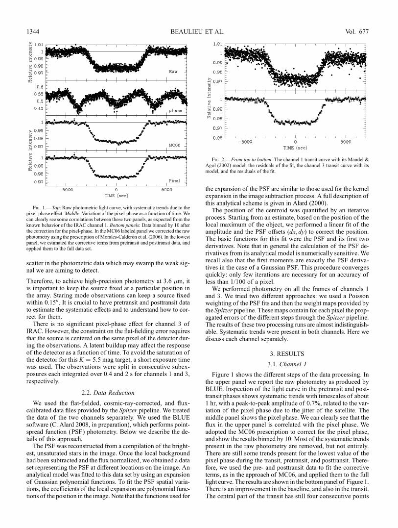
Figure 1 shows the different steps of the data processing. Inthe upper panel we report the raw photometry as produced byBLUE. Inspection of the light curve in the pretransit and post-transit phases shows systematic trends with timescales of about1 hr, with a peak-to-peak amplitude of 0.7%, related to the var-iation of the pixel phase due to the jitter of the satellite. Themiddle panel shows the pixel phase. We can clearly see that theflux in the upper panel is correlated with the pixel phase. Weadopted the MC06 prescription to correct for the pixel phase,and show the results binned by 10. Most of the systematic trendspresent in the raw photometry are removed, but not entirely.There are still some trends present for the lowest value of thepixel phase during the transit, pretransit, and posttransit. There-fore, we used the pre- and posttransit data to fit the correctiveterms, as in the approach of MC06, and applied them to the fulllight curve. The results are shown in the bottom panel of Figure 1.There is an improvement in the baseline, and also in the transit.The central part of the transit has still four consecutive points

Fig. 1.—Top: Raw photometric light curve, with systematic trends due to thepixel-phase effect.Middle: Variation of the pixel-phase as a function of time. Wecan clearly see some correlations between these two panels, as expected from theknown behavior of the IRAC channel 1. Bottom panels: Data binned by 10 afterthe correction for the pixel-phase. In theMC06 labeled panel we corrected the rawphotometry using the prescription ofMorales-Calderon et al. (2006). In the lowestpanel, we estimated the corrective terms from pretransit and posttransit data, andapplied them to the full data set.

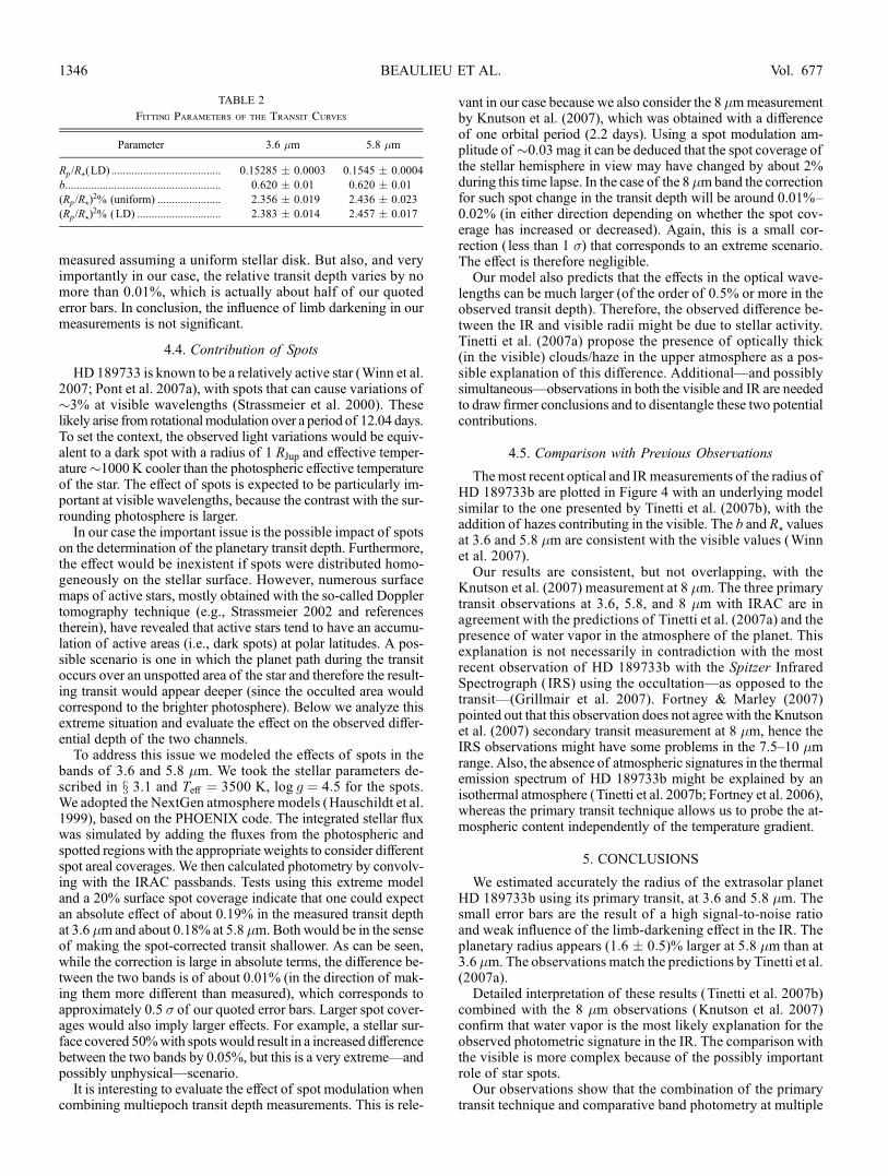
Fig. 2.—From top to bottom: The channel 1 transit curve with its Mandel &Agol (2002) model, the residuals of the fit, the channel 3 transit curve with itsmodel, and the residuals of the fit.

BEAULIEU ET AL.1344 Vol. 677

deviating by 1Y2 � around t � 200 s, corresponding to the low-est phase value. They are shown on Figure 1 but we will excludethem from further analysis (Fig. 2). These remaining systematiceffects are due to the phase. We ran calculations both by includ-ing these points and by excluding them, and then compared theresults. Also, we adopted different binning: by 5, 10, 20, or 50points. The results are compatible within the error bars. As wediscuss in more detail below, limb darkening effects are verysmall at 3.6 �m so the shape of the transit light curve is boxlike.

3.2. Channel 3

In Figure 3 we report the raw (top panel ) and the final(bottom panel ) photometric data. There is no correlation withthe pixel phase, but a long-term systematic trend can be seenboth out of and in the transit. This trend does not appear to becaused by a latent buildup, but it is probably linked to the var-iation of response of the pixels due to a long period of illu-mination. We used the pretransit and the posttransit data to fit alinear corrective term that we applied to all the data. The results,binned by 10, are shown in the bottom panel of Figure 3.

4. DISCUSSION

4.1. Comments about the Data Reduction

Using the BLUE software we carried out a full modeling ofthe PSF and obtained an optimal centroid determination. Withan undersampled PSF, in data sets with strong pixel-phase effects(channels 1 and 2 from Spitzer), accurate centroid determinationis a key issue for achieving high precision photometry.

In order to tackle the systematic trends that are present inIRAC observations, it is important to have sufficient baselineobservations to analyze transit data. Here, it has been vital tohave sufficient pretransit and posttransit data in order to be ableto check the nature of the systematics and correct for them. The4.5 hr of observations were centered on 1.8 hr transit. Giventhe�1 hr timescale of the pixel-phase variations, this was welladapted, but it is clearly a lower limit on the necessary observingtimescale to achieve such observations.

4.2. Calculation of the Transit Depth

Wedecide to do a direct comparison between the out-of-transitflux (Figs. 1 and 3) and the in-transit flux (the central 3500 s)averaged over its flat part for each channel. We estimate the

weighted mean and its error both in the out-of-transit flux andthe in-transit flux. For channel 1, we have excluded the mea-surements obtained at the lowest pixel phase values as discussedin 3.1. It yields values of 2:356% � 0:019% and 2:436% �0:020% in the 3.6 and 5.8 �m bands, respectively (Fig. 4). Thisis the same approach as adopted by Knutson et al. (2007).

4.3. Contribution of Limb-Darkening

As a further refinement in our analysis we considered the ef-fects of limb darkening. By inspection, the transit is clearly flatbottomed, and limb darkening was expected to be negligible.However, it was deemed worth calculating its contribution be-cause of the high accuracy claimed in the transit depth measure-ment given above. We adopted a nonlinear limb-darkening-lawmodel as described inMandel &Agol (2002) to calculate a limb-darkened light curve. We considered the more sophisticatedform using four coefficients (C1, C2, C3, and C4), These werecalculated using a Kurucz (2006) stellar model (TeA ¼ 5000 K,log g ¼ 4:5, solar abundance), which matches closely the ob-served parameters of HD 189733, convolved with the IRACpassbands. Parameters are given in Tables 1 and 2.

Amultiparameter fit of the two light curves using the adoptednonlinear limb-darkening model yielded depths of 2:387% �0:014% and 2:456% � 0:017% in the 3.6 and 5.8 �m bands,respectively. Two small effects can be identified. First, the limb-darkened transits become some 0.02%Y0.03% deeper than those

Fig. 3.—Top: Raw photometric light curve with a long-term systematic trend.Bottom: We estimated the corrective terms from pretransit and posttransit data,and applied them to the full data set. We then binned the data by 10 and estimatedthe associated error bar for each measurement.

Fig. 4.—Transit depths as a function of wavelength: our twomeasurements at3.6 and 5.8 �m are indicated with their error-bars. For comparison we showprevious measurements at 8 �m (Knutson et al. 2007) and in the visible (Winnet al. 2007). Horizontal bars illustrate the instrument bandpasses. The solid lineshows the simulated absorption spectrum of the planet between 0.5 and 10 �m.The atmospheric model includes water with a mixing ratio of 5 ; 10�4, sodiumand potassium absorptions, and hazes at the millibar level in the visible. The un-derlying continuum is given byH2�H2 contribution, which is sensitive to the tem-perature of the atmosphere at pressure higher than the� bar level. Details of thehaze free model are given in Tinetti et al. (2007b). Here, hazes are simulated witha distribution of particles peaked at 0.5 �m size. In this example haze opacitymask the atomic andmolecular features at wavelength bluer than 1.2�m. See alsoBrown (2001) and Pont et al. (2007b). [See the electronic edition of the Journalfor a color version of this figure.]

TABLE 1

Limb-darkening Coefficients

IRAC C1 C2 C3 C4

3.6 �m........................ 0.6023 �0.5110 0.4655 �0.1752

5.8 �m........................ 0.7137 �1.0720 1.0515 �0.3825

PRIMARY TRANSIT OF PLANET HD 189733b 1345No. 2, 2008

measured assuming a uniform stellar disk. But also, and veryimportantly in our case, the relative transit depth varies by nomore than 0.01%, which is actually about half of our quotederror bars. In conclusion, the influence of limb darkening in ourmeasurements is not significant.

4.4. Contribution of Spots

HD189733 is known to be a relatively active star (Winn et al.2007; Pont et al. 2007a), with spots that can cause variations of�3% at visible wavelengths (Strassmeier et al. 2000). Theselikely arise from rotationalmodulation over a period of 12.04 days.To set the context, the observed light variations would be equiv-alent to a dark spot with a radius of 1 RJup and effective temper-ature�1000 K cooler than the photospheric effective temperatureof the star. The effect of spots is expected to be particularly im-portant at visible wavelengths, because the contrast with the sur-rounding photosphere is larger.

In our case the important issue is the possible impact of spotson the determination of the planetary transit depth. Furthermore,the effect would be inexistent if spots were distributed homo-geneously on the stellar surface. However, numerous surfacemaps of active stars, mostly obtained with the so-called Dopplertomography technique (e.g., Strassmeier 2002 and referencestherein), have revealed that active stars tend to have an accumu-lation of active areas (i.e., dark spots) at polar latitudes. A pos-sible scenario is one in which the planet path during the transitoccurs over an unspotted area of the star and therefore the result-ing transit would appear deeper (since the occulted area wouldcorrespond to the brighter photosphere). Below we analyze thisextreme situation and evaluate the effect on the observed differ-ential depth of the two channels.

To address this issue we modeled the effects of spots in thebands of 3.6 and 5.8 �m. We took the stellar parameters de-scribed in x 3.1 and TeA ¼ 3500 K, log g ¼ 4:5 for the spots.We adopted the NextGen atmosphere models (Hauschildt et al.1999), based on the PHOENIX code. The integrated stellar fluxwas simulated by adding the fluxes from the photospheric andspotted regions with the appropriate weights to consider differentspot areal coverages. We then calculated photometry by convolv-ing with the IRAC passbands. Tests using this extreme modeland a 20% surface spot coverage indicate that one could expectan absolute effect of about 0.19% in the measured transit depthat 3.6 �m and about 0.18% at 5.8 �m. Both would be in the senseof making the spot-corrected transit shallower. As can be seen,while the correction is large in absolute terms, the difference be-tween the two bands is of about 0.01% (in the direction of mak-ing them more different than measured), which corresponds toapproximately 0.5 � of our quoted error bars. Larger spot cover-ages would also imply larger effects. For example, a stellar sur-face covered 50%with spots would result in a increased differencebetween the two bands by 0.05%, but this is a very extreme—andpossibly unphysical—scenario.

It is interesting to evaluate the effect of spot modulation whencombining multiepoch transit depth measurements. This is rele-

vant in our case because we also consider the 8 �mmeasurementby Knutson et al. (2007), which was obtained with a differenceof one orbital period (2.2 days). Using a spot modulation am-plitude of �0.03 mag it can be deduced that the spot coverage ofthe stellar hemisphere in view may have changed by about 2%during this time lapse. In the case of the 8�mband the correctionfor such spot change in the transit depth will be around 0.01%Y0.02% (in either direction depending on whether the spot cov-erage has increased or decreased). Again, this is a small cor-rection ( less than 1 �) that corresponds to an extreme scenario.The effect is therefore negligible.Our model also predicts that the effects in the optical wave-

lengths can be much larger (of the order of 0.5% or more in theobserved transit depth). Therefore, the observed difference be-tween the IR and visible radii might be due to stellar activity.Tinetti et al. (2007a) propose the presence of optically thick(in the visible) clouds/haze in the upper atmosphere as a pos-sible explanation of this difference. Additional—and possiblysimultaneous—observations in both the visible and IR are neededto draw firmer conclusions and to disentangle these two potentialcontributions.

4.5. Comparison with Previous Observations

Themost recent optical and IRmeasurements of the radius ofHD 189733b are plotted in Figure 4 with an underlying modelsimilar to the one presented by Tinetti et al. (2007b), with theaddition of hazes contributing in the visible. The b and R? valuesat 3.6 and 5.8 �m are consistent with the visible values (Winnet al. 2007).Our results are consistent, but not overlapping, with the

Knutson et al. (2007) measurement at 8 �m. The three primarytransit observations at 3.6, 5.8, and 8 �m with IRAC are inagreement with the predictions of Tinetti et al. (2007a) and thepresence of water vapor in the atmosphere of the planet. Thisexplanation is not necessarily in contradiction with the mostrecent observation of HD 189733b with the Spitzer InfraredSpectrograph ( IRS) using the occultation—as opposed to thetransit—(Grillmair et al. 2007). Fortney & Marley (2007)pointed out that this observation does not agree with the Knutsonet al. (2007) secondary transit measurement at 8 �m, hence theIRS observations might have some problems in the 7.5Y10 �mrange. Also, the absence of atmospheric signatures in the thermalemission spectrum of HD 189733b might be explained by anisothermal atmosphere (Tinetti et al. 2007b; Fortney et al. 2006),whereas the primary transit technique allows us to probe the at-mospheric content independently of the temperature gradient.

5. CONCLUSIONS

We estimated accurately the radius of the extrasolar planetHD 189733b using its primary transit, at 3.6 and 5.8 �m. Thesmall error bars are the result of a high signal-to-noise ratioand weak influence of the limb-darkening effect in the IR. Theplanetary radius appears (1:6 � 0:5)% larger at 5.8 �m than at3.6 �m. The observations match the predictions by Tinetti et al.(2007a).Detailed interpretation of these results (Tinetti et al. 2007b)

combined with the 8 �m observations (Knutson et al. 2007)confirm that water vapor is the most likely explanation for theobserved photometric signature in the IR. The comparison withthe visible is more complex because of the possibly importantrole of star spots.Our observations show that the combination of the primary

transit technique and comparative band photometry at multiple

TABLE 2

Fitting Parameters of the Transit Curves

Parameter 3.6 �m 5.8 �m

Rp/R?(LD) ...................................... 0.15285 � 0.0003 0.1545 � 0.0004

b...................................................... 0.620 � 0.01 0.620 � 0.01

(Rp/R?)2% (uniform) ...................... 2.356 � 0.019 2.436 � 0.023

(Rp/R?)2% (LD) ............................. 2.383 � 0.014 2.457 � 0.017

BEAULIEU ET AL.1346 Vol. 677

wavelengths is an excellent tool to probe the atmospheric con-stituents of transiting extrasolar planets. Similar studies and ob-servations should be considered for other targets, especially withthe foreseen James Webb Space Telescope, which could observemore distant and smaller transiting planets.

We thank the staff at the Spitzer Science Center for their help.We are very grateful to Christophe Alard for having helped us inthe data reduction phases of Spitzer data. His optimal centroiddetermination has been an important contribution to this analysis.

We thank David Kipping for careful reading of the manuscript,and David Sing for providing the limb-darkening coefficients.This work is based on observations made with the Spitzer SpaceTelescope, which is operated by the Jet Propulsion Laboratory,California Institute of Technology, under a contract with NASA.G. Tinetti acknowledge the support of the European SpaceAgency. I. R. acknowledges support from the SpanishMinisteriode Educacion y Ciencia via grant AYA2006-15623-C02-02.J. P. B., I. R., and G. T. acknowledge the financial support ofthe ANR HOLMES.

Facilities: Spitzer

REFERENCES

Alard, C. 2000, A&AS, 144, 363Bakos, G. A., Pal, A., Latham, D. W., Noyes, R. W., & Stefanik, R. P. 2006a,ApJ, 641, L57

Bakos, G. A., et al. 2006b, ApJ, 650, 1160Ballester, G. E., Sing, D. K., & Herbert, F. 2007, Nature, 445, 511Ben-Jaffel, L. 2007, ApJ, 671, L1Bouchy, F., et al. 2005, A&A, 444, L15Brown, T. M. 2001, ApJ, 553, 1006Charbonneau, D., Brown, T. M., Noyes, R. W., & Gilliland, R. L. 2002, ApJ,568, 377

Deming, D., Harrington, J., Seager, S., & Richardson, L. J. 2006, ApJ, 644, 560Deming, D., Seager, S., Richardson, L. J., & Harrington, J. 2005, Nature, 434,740

Fazio, G. G., et al. 2004, ApJS, 154, 10Fortney, J. J., Cooper, C. S., Showan, A. P., Marley, M. S. and Friedman, R. S.2006, ApJ, 652, 746

Fortney, J. J., & Marley, M. S. 2007, ApJ, 666, L45Grillmair, C. J., et al. 2007, ApJ, 658, L115Hauschildt, P. H., Allard, F., & Baron, E. 1999, ApJ, 512, 377

Knutson, H. A., et al. 2007, 447, 183Kurucz, R. 2006, Stellar Model and Associated Spectra (Cambridge: HarvardUniv.), http://kurucz.harvard.edu/grids.html

Mandel, K., & Agol, E. 2002, ApJ, 580, L171Morales-Calderon, et al. 2006, ApJ, 653, 1454 (MC06)Pont, F., et al., 2007, A&A, 476, 1347———. 2007b, MNRAS, submittedRichardson, L. J., Harrington, J., Seager, S., & Deming, D. 2006, ApJ, 649,1043

Richardson, L. J., Deming, D., & Seeger, S. 2003a, ApJ, 597, 581Richardson, L. J., et al. 2003b, 584, 1053Strassmeier, K. G. 2002, Astron. Nachr., 323, 309Strassmeier, K., Washuettl, A., Granzer, T., Scheck, M., & Weber, M. 2000,A&AS, 142, 275

Tinetti, G., et al. 2007a, ApJ, 654, L99———. 2007b, Nature, 448, 169Vidal-Madjar, A., et al. 2003, Nature, 422, 143———. 2004, ApJ, 604, L69Winn, J. N., Holman, M. J., Henry, G. W., et al. 2007, AJ, 133, 1828

PRIMARY TRANSIT OF PLANET HD 189733b 1347No. 2, 2008