~primer on the craig-bampton method - · pdf file~primer on the craig-bampton method an...
TRANSCRIPT
~PRIMER ON THE CRAIG-BAMPTON METHOD
AN INTRODUCTION TO BOUNDARY NODE FUNCTIONS BASE SHAKE ANALYSES
LOAD TRANSFORMATION MATRICES MODAL SYNTHESIS AND MUCH MORE
Edited by John T Young
Based on input from William B Haile
October 4 2000
1 of 54
TABLE OF CONTENTS
1 Introduction
2 Deve1opment of Craig-Bampton Methodology
21 The Primitive Equation of Motion for a Structu~e
22 The Craig-Bampton Transformation 23 Boundary Node Functions B 24 Fixed Base Mode Shapes (Constraint Modes) ltp 25 The Craig-Bampton Formulation 26 Checks on the Craig-Bampton Model
3 Common Applications of Craig-Bampton Methodology
31 Quasi-Static Analysis 32 Base-Shake Analyses 33 Modal Participation Factors and Modal Masses for
Base-Shake Analyses 34 The Load Transformation Matrix (LTM) 35 Application of the Craig-Bampton Method to Modal
Synthesis 36 Reduction of a Redundant Interface to a Single Point
4 References
100600 i Craig Bampton_1doc
2 of 54
APPENDICES
A Guyan Reduction
B NASTRAN DMAP for Generating a Craig-Barnpton Model
C NASTRAN DMAP for Computing an Equilibrium Check on the Free-Free Stiffness Matrix
D NASTRAN DMAP for Computing Modal participation Factors and Modal Weights
E NASTRAN DMAP for Generating an LTM
100600 1 1 Craig Bampton_ldoc
3 of 54
1 Introduction The Craig-Bampton methodology is used extensively in the
aerospace industry to re-characterize large finite element models into a set of relatively small matrices containing mass stiffness and mode shape information that capture the fundamental low frequency ~esponse modes of the structure The mode shape information consists of all boundary modes expressed in physical coordinates and a truncat-ed set of ela-stic modes expressed in modal coordinates These matrices are easily manipulated for a wide range of dynamic analyses The method was first developed by Walter Hurty in 1964 (Ref 1) and later expanded by Roy Craig and MerVYn Bampton in 1968 (Ref 2)
The Craig-Bampton formulation is most often used for
1 Efficient transmittal of spacecraft models to other organizations for a Coupled Loads Analysis (CLA) CraigshyBampton matrices are coupled with launch vehicle models and responses are determined for various flight events
2 Base-shake analyses in which motion of the boundary degrees of freedom is specified for a model from a Coupled Loads Analysis and responses for various perturbations to the model may be determined without repeating the entire CLA
3 Modal synthesis in which the models of two or more structures that have a common interface (each called a sub-structure) may be coupled together for an efficient analysis of the combined structure
The purpose of this paper is to present a summary of the Craig-Bampton assumptions and methodology Solutions to a few practical problems are outlined Some familiarity with NASTRAN is assumed
A secondary purpose is to present a standard set of notation that is based on NASTRAN DMAP terminology
100600 11 Craig Bampton_1doc
4 of 54
2 Development of Craig-Bampton Methodology
21 The Primitive Equation of Motion for a Structure
Complex linear elastic structures are universally analyzed today using finite element programs such as NASTRAN to generate mass and stiffness matrices that characterize the structure The models are generally developed for static analyses and are thus very large perhaps having several thousand degrees of freedom since static analyses require a detailed set of grid points to map internal stresses and strains However dynamic analyses which are based upon knowledge of f undamen t a L frequencies and their associated mode shapes are better performed with far fewer degrees of freedom in the formulation Indeed the number of nodes needed to characterize the fundamental modes is relatively small Furthermore modes above 100 Hz are typically truncated since they contain too little energy to be physically significant
When determining modes and mode shapes NASTRAN generates a set of critical degrees of freedom called the A-set (analysis set) and uses Guyan reduction (see Appendix A) to generate equivalent mass [M AA] and stiffness [K AA ] matrices that are associated with these freedoms The analysis set typically contains a few hundred freedoms for a large finite element model that has several thousand degrees of freedom specified on GRID cards
The corresponding displacements and accelerations for these 00
degrees of freedom are contained in the matrices [VA] and [VA] The applied forces are contained in the matrix [FA] The resulting undamped equation of motion for the free unconstrained structure is
Eq 211
Since the Craig-Bampton method will require the use of boundary and interior points it is convenient to partition these matrices into fixed interfaced or supported boundary nodes R and the independent elastic nodes L as follows
uJ ~ Eq 212
100600 211 Craig Bampton_1doc
5 of 54
and Eq 211 becomes
Eq 213~J~] +
Theb-oundary set includes not only the base degrees of freedom that might later be constrained but also the interface degrees of freedom that might later be coupled to another structure (modal synthesis) The boundary points can be released in later solutions
The choice of notation Rand L follows NASTRAN The R-set are those degrees of freedom specified on a SUPORT card that ~emove rigid body motion from the structure and the L-set are those degrees of freedom that are left after removing the R-set from the A-set
As a practical matter the effects of damping are considered when solving many dynamics problems Damping is assumed to be proportional to the velocity of each point in the displacement set and the equation of motion becomes
Eq 214
where eLL is typically the only non-zero term in the damping matrix
100600 212 Craig Bampton_1doc
6 of 54
22 The Craig-Bampton Transformation
There are two steps in performing the Craig-Bampton transformation First and foremost the set of elastic physical coordinates U
L for each mode is transformed to a set of modal
coordinates QL Thus the reduced finite element model discussed in Section 21 is transformed from a set of physical coordinates UA to a hybrid set of physical coordinates at the boundary UR and modal coordinates at the interior QL Identical solutions
result from either formulation The magic of the matrix QL is that each column representing one mode shape contains only one non-zero term
Secondly the set of modal solutions QL is truncated to
some smaller set say qm This is practical because in problems with multiple degrees of freedom the contribution of the higher frequency modes to the total response of a low frequency excitation is small and may be neglected As a rule of thumb the modal content of a given sub-structure should retain mode shapes with frequencies at least 15 times higher than that required in the composite structure in modal synthesis or 15 times higher than the excitation frequency
The Craig-Bampton hybrid coordinates UR ~ are related to the physical coordinates UR U
L as follows
mltL Eq 221
where B has A rows and R columns and $ has A rows and m
columns The vectors in B are usually referred to as the
Boundary Node Functions and the vectors in $ are usually referred to as the Fixed Base Mode Shapes
The Craig-Bampton transformation matrices B and $ may in turn be partitioned as
B Eq 222~ where [centR] and [~] are to be determined The identity matrix [I]
100600 221 Craig Bampton_1doc
7 of 54
has R rows and columns while matrix [centR] has L rows and R columns the null matrix [OJ has R rows and m columns while the matrix [centL] has L rows and m columns Thus
Eq 223uJ = ~ = ~~
Note that the physical displacements of the interior points are computed by
Eq 224
where [centR][U R] are the rigid body displacements of the L degrees
of freedom due to the R degrees of freedom and [centL][qm] are the displacements of the L degrees of freedom relative to the displaced base
Understanding the physical significance of the matrices [centR] and [centL] (or alternatively B and ~) and learning how to compute and manipulate them readily is the essence of learning the Craig-Bampton method
100600 222 Craig Bampton_1doc
8 of 54
23 Boundary Node Functions (Constraint Modes) B
The Boundary Node Functions B are also known as Constraint Modes Boundary Modes or Point Boundary Functions The full set is composed of two sub-matrices [I] and [centR] [I] with R rows and columns is the identity matrix and is a mathematical statement of the obvious in Eq 223 viz the physical boundary points displace rigidly during rigid body motion [centR] with L rows and R columns is a transformation matrix that relates rigid body physical displacements at the interface U
R to physical displacements of the elastic degrees
of freedom UL
bull
Allowing motion at the boundary produces the set of Boundary Node Functions To determine [centR] fix all boundary degrees of freedom and limiting consideration to the static problem
00 00
(U L =U R =0) Eq 213 the governing equation for this case reduces to
o Eq 231
Then release the first degree of freedom in the boundary set UR and solve for the vector of structural displacements due to unit displacement of this point Next re-fix the first degree of freedom release the second to unit motion and solve for its vector of structural displacements Continue the process in sequence for each degree of freedom in the boundary set Thus the set of boundary displacements UR becomes
1 0
o 1 = [I] Eq 232
which is a column matrix indicating the ordered sequence of unit displacements
By combining Eqs 224 (with qm = 0 because there is no elastic deformation of non-boundary points) 231 and 232 the set of internal displacements U
L may be solved as
Eq 233
100600 231 Craig Bampton_1doc
9 of 54
where Eq 234
Note the matrix inversion This requires a non-singular stiffness sub-matrix and is often the source of computer roundshyoff error
The full set of displacements is now formed as
Eq 235
where B is the matrix of Boundary Node Functions The subshymatrix [IJ has R rows and columns and the sub-matrix [centR] has L rows and R columns
NASTRAN NOTE As a practical matter [centR]is routinely computed in NASTRAN and is data block DM generated by module RBMG3 whenever SUPORT bulk data cards are present In Craig-Bampton analyses SUPORT cards are often used to define the R-set degrees of freedom because the free-free problem is still solved in dynamics The SUPORT card gives a rigid body eigen-vector at 0 Hz in the direction of specified support code It replaces the lowest frequency in the free-free run with this value If more than 6 degrees of freedom are supported real flexible eigen-vectors are over-written by the generated SUPORTd eigen-vectors The SUPORT card is used to find eigen-vectors along the coordinate axes for rigid body modes that already exist
The rigid body modes are embedded in these functions for both statically determinant and statically indeterminant structures The columns of [centR] are rigid body displacements at the L degrees of freedom due to a unit motion at one of the R degrees of freedom Note however that for a structure with a statically determinant boundary (exactly 6 degrees of freedom) [B] is just the matrix of 6 rigid body modes at the boundary points For this simple case rigid body modes can be computed from just the locations and orientations of the degrees of freedom
100600 232 Craig Bampton_1doc
10 of 54
24 Fixed Base Mode Shapes (Constraint Modes) ~
The matrix of Fixed Base Mode Shapes ~ is composed of two sub-matrices [0] and [centL] The matrix [0] with R rows and m columns is the null matrix and is a mathematical statement of the obvious in Eq 223 viz rigid body displacements are indeed rigid and not a function of the elastic mode shapes ~
The matrix [centL] with L rows and m columns is a transformation matrix that relates modal responses qm to physical displacements of the elastic degrees of freedom UL bull It is determined from the equations of motion with the interface
00
degrees of freedom constrained [U R =U R =0] and with no forces
acting on the interior points [FL=O] The equation of motion for this case is
00
Eq 241
iaJot Assume harmonic response (UL =centL qm e ) Then
o Eq 242
[ ltP
Eq 242 represents unforced harmonic motion of the grounded structure It may be solved using NASTRAN or some other computer program for the eigen-values [00
0
2] and mode shapes
L ] bull
The generalized (modal) mass [~] 1S defined to be
Eq 243
where [ltPL
] is diagonal since the mode shapes [ltPL
] are normal The matrix [~] is almost always normalized to unity that is the mode shapes are scaled so that [~] = [IJ
The generalized stiffness is defined to be
Eq 244
where Lu] llV0
2 J is also diagonal
101000 241 Craig Bampton_ldoc
11 of 54
NASTRAN NOTE In NASTRAN the eigen-vectors [~J are a non-standard output but may readily be computed in the READ module using appropriate DMAP The data block is typically named PHIL It is also common to mass normalize [~LJ such that [IlJ= [1J the identitymatrix Note that the units of the mode shapes are the same as the physical degrees of
freedom (inches meters radians) and the uni ts on the eigen-values are (radianssec)2
Having solved for (00 2 and ~LI the transformation back to
physical displacements UL
is accomplished by
Eq 245
where
[~L] is the matrix of eigen-vectors called normal mode shapes normal because each mode shape is orthogonal to all others it has L rows and m columns
2][(00 is the matrix of eigen-values and is diagonal The eigenshyvalues have units of radians per second squared The natural frequencies of the fixed base structure in Hertz are
computed as ~(Oo2 2tr
[~] is the column vector of generalized (modal) displacements The generalized displacements are dimensionless so all units (inches meters radians etc) are contained in ~L
100600 242 Craig Bampton_1doc
12 of 54
25 The Craig-Bampton Method
The Craig-Bampton method is based on a re-formulation of the equations of motion for a structure from the set of physical coordinates to a set of coordinates consisting of physical coordinates at some subset of boundary points and modal or generalized coordinates at the non-boundary points Once trarrsEormed to modal coordinat-esmode shapes represen-ting h-igher frequency responses may be truncated without loss of information
To apply the method transform the coordinate system for the equation of motion for a linear damped elastic structure
using the Craig-Bampton transformation
Eq 221
where B ~ are given in Eq 222 This yields equations of motion in terms of truncated modal coordinates
PpR
Eq 251 L
Multiply Eq 251 by the transpose of the Craig-Bampton transformation matrix B ~T to yield
Eq 252
1011000 251 Craig Bampton_1doc
13 of 54
Equation 252 is the Craig-Bampton equation of motion These equations may be readily solved for a large number of practical problems The transformation is successful because the modes become uncoupled from each other greatly reducing the manipulation required to solve the equations Typically modal displacements and accelerations are computed by numerical integration for a given set of initial conditions and forcing function time histories Physical accelerations and displacements follow from the Craig-Bampton transformation matrix
Eq 252 may be re-written as
M BB
MmB
Eq 253
where
M BB
- BTMB
= + + Eq 254aM RR
[M BB is the structural mass matrix reduced to the boundary nodes in the same way a Guyan reduction would be done]
MBm B T MltIgt
Eq 254b
ltIgtT MBMmB =
T centJL [M LR + M LL centJR ] Eq 2 5 4c
101000 252 Craig Bampton_1doc
14 of 54
M mm
Eq 254d
[M mm is the generalized mass and is almost always set equal to the identity matrix]
Eq 254e
[KM is the Guyan reduced stiffness matrix and is zero if the boundary is statically determinant]
= [KRL + 9RT
] 9L = a Eq 254fK LL
K IltIgtTKBK mB - = ~ K u 9R
= 9LT
[K LR + K U 9R ] = a Eq 25 4g
ltIgtTKltIgtlaquo - = ~r ~ ~~ T 2 = 9L K LL 9L = [u][illo ] Eq 25 4h
101000 253 Craig Bampton_ldoc
15 of 54
[Note that Wo is the natural frequency (radianssecond) of the fixed base modes]
Eq 254i
TNotetnat ( i5the equivaTent viscolis damping defined as the
ratio of damping c to critical damping co typically ( is 001 but can vary for each mode The amplitude of the response of a structure to a steady state excitation is inversely proportional to the damping Thus if the damping is doubled the response is halved The amplitude of the response of a structure to a transient excitation is far less dependent on damping and quite often the difference in response between 1 and 2 damping is negligible ]
As a practical matter BTCB BTCep and epTCB are nearly always chosen equal to [0] Damping of the boundary modes is non-standard and cannot be verified by test only the sub-matrix [2~uwo ] has significance
Note from Eqs 25 4b and 25 4c that [M Bm] = [M mB]T Eq 254e utilizes the relation found in Eq 234 The fact that Eqs 254f and 254g are null follows from Eq 234 Finally Eqs 254d and 254h follow from Eqs 243 and 244 Recall that the matrix centL is often mass normalized such that [u]=[I] the identity matrix
The generalized mass and stiffness matrices are defined to be [M mm] and [Kmm ] respectively
Typically in the analysis of spacecraft payloads all forces applied to the structure come through the boundary points and there are no applied loads to the non-boundary points i e only FR is of concern and FL is null However in the fullshycoupled loads analysis of payload and booster applied loads do act at non-boundary points in the booster and they must be considered
In summary for most practical problems the generalized mass matrix is normalized damping is ignored and only boundary forces are considered For these conditions the dynamic equation of motion for the Craig-Bampton method given in Eq 251 and reshystated in Eq 253 can be stated simply as
1011000 254 Craig Bampton_1doc
16 of 54
Eq 255
where is zero for a statically determinant interfaceKBB
NASTRAN Note A typical NASTRAN DMAP sequence that would be required to generate a Craig-Bampton model is shown in Appendix B
100600 255 Craig BamptoTI_1doc
17 of 54
26 Checks on the Craig-Bampton Model
There are several simple checks that should always be applied to Craig-Bampton models to guard against errors
261 Rigid Body Check
Test the equations opound motion by enforcing rigid body displacements at the boundary degrees of freedom UR and observing that the non-boundary or elastic freedoms displace appropriately Either by hand for models with a simple boundary or by computer for a more complex geometry construct the matrix of six rigid body modes [R] for the boundary degrees of freedom that satisfy the equation
Eg 261
where
lqrt~b~j is the (61) vector of pure rigid body displacements and
rotations for x y z Rx Ry and Rz motion at some convenient point and in global coordinates
As a common example the matrix of rigid body modes for a simple 6-degree of freedom interface at point A relative to some arbitrary point B is
1 0 0 0 sz -6Y
0 1 0 -fJ Omiddot M
[R] = 0
0
0
0
1
0
6Y
1
-M
0
0
0 Eg 262
0 0 0 0 1 0
0 0 0 0 0 1
where 6x = XB
- XA 6Y = YB - YA and 6Z = ZB - ZA Assuming no
elastic motion [qJ=[~m]=O and applying unit rigid body
displacement (one inch and one radian) or acceleration (one inchsecsec or one radiansecsec) the resulting boundary motion is
and [R][I] Eg 263
100600 261 Craig Bampton_1doc
18 of 54
A sample DMAP for an equilibrium check is shown in Appendix C
262 Rigid Body Mass Matrix
The Craig-Bampton equation of motion (Eq 252) provides the (66) rigid body mass matrix
m 0 0 0 mz -my
0 m 0 -mz 0 mx
[RY [Btrade B][R] = 0
0
0
-mz
m
my
my
In
-mx
Iry
0
I rz
Eq 264
mz 0 -mx I yx I yy I yz
-my mx 0 Iu middot1 zy I zz
where m is the total mass of the finite element model x y and z are the distances from the rigid body point to the center of mass and the I terms are the mass moments of inertia and products of inertia at the rigid body point
263 Free Eigen-Value Problem
Since the Craig-Bampton equation of motion (Eq 252) represents a free unconstrained structure it should yield natural frequencies and mode shapes for this condition To check this solve for the first few modes from the eigen-problem
Eq 265
The results should check the free modes from the original finite element model If the boundary is statically determinate BTKB = 0 and the rigid body modes are zero by definition However for indeterminate boundaries the eigen-value problem solution can give insight into the boundary modes
To note the frequency range represented by the boundary functions it is instructive to remove all fixed base modes and solve the eigen-problem
Eq 266
Print the eigen-values l to see the range 100600 262 Craig Barnpton_1doc
19 of 54
3 Common Applications of Craig-Bampton Methodology
31 Quasi-Static Analysis
It is often desirable to compute the boundary forces and internal displacements of a strue tur-e under a quas i st-atic gshye
field to check design load cases set up initial conditions or look for potential errors in the analysis The Craig-Bampton method is well suited for this computation
Set up the boundary acceleration [UR] equal to the
desired steady static acceleration [G] as though the structure were riding on a multi-degree of freedom elevator Then
= [G] is specified [~m] = 0 because the load is static
is ignored = 0 because [~m] = 0 and U R does not
need to be known since [B T KB]U R = [KBB][U R ] = 0 for this case
Consider the Craig-Bampton equation of motion Eq 252 The upper portion yields for boundary forces
Eq 311M BB G
and the lower portion yields for displacements
Eq 312
101000 311
Craig Barnpton_2doc
20 of 54
32 Base-Shake Analyses
Base shake analyses are very common in structural dynamics and are ideally suited to the Craig-Bampton formulation The input driving function in a base shake may be sinusoidal constant random or transient Steady state sinusoidal inputs are used to simulate a base shake test that is a standard method
middotof testing hardware Transient inputs are often derived from a large coupled loads analysis involving the Shuttle and one or more payloads and then as payload models are refined the interface transients are applied to the component models rather than repeating the long and costly coupled loads analysis The base shake analysis has proven to be a very efficient method for the iterative analysis of components without re-analyzing the entire structure
The base-drive problem is characterized by applying known accelerations to the boundary and solving for the response of the complete structure The Craig-Bampton formulation is particularly well suited for this analysis because the boundary is explicitly defined [F
R ] is the set of forces that are
exerted on the boundary and result in the base motions [DR] It should be emphasized that the forces [F R ] are usually not known initially only the accelerations at the R degrees of freedom are known The forces [F R ] are really the forces of constraint that are required to produce the desired base motion
00
Assume that U R(t) is known either as a transient or as steady state input Then the Craig-Bampton equation of motion (Eq 253) reduces to the equation for generalized response
00 0
j1 q m (t) + 2(j1mo q m (t) + j1m qm (t) Eq 321
which is the standard form for dynamics equations and can readily o 00
be solved for qm qm and qm For the typical base shake
analysis FL (t) =0 and the forcing function is just from the base 00
acceleration -MmB UR(t)
The reactions at the boundary can also be found from Eq 252 as functions of time
101000 321 Craig Bampton_2doc
21 of 54
32 Base-Shake Analyses
Base shake analyses are verycornmon in structural dynamics and are ideally suited to the Craig-Bampton formulation The input driving function in a base shake may be sinusoidal constant random or transient Steady state sinusoidal inputs are used to simulate a base shake test that is a standard method of testing hardware Transient inputs are often derived from a
- -largeconpled loads analysis involvin-g the Shuctle and one or more payloads and then as payload models are refined the interface transients are applied to the component models rather than repeating the long and costly coupled loads analysis The base shake analysis has proven to be a very efficient method for the iterative analysis of components without re-analyzing the entire structure
The base-drive problem is characterized by applying known accelerations to the boundary and solving for the response of the complete structure The Craig-Bampton formulation is particularly well suited for this analysis because the boundary is explicitly defined [F
R] is the set of forces that are
exerted on the boundary and result in the base motions [UR ] It should be emphasized that the forces [FR ] are usually not known initially only the accelerations at the R degrees of freedom are known The forces [F R ] are really the forces of constraint that are required to produce the desired base motion
Assume that [UR(t)] is known either as a transient or as
steady state input Then the Craig-Bampton equation of motion (Eq 253) reduces to the equation for generalized response
00 0 00
Ji q m (t) + 2(Jiwo q m (t) + JiW qm(t) = - M mB U R (t) + Eq 321
which is the standard form for dynamics equations and can readily o 00
be solved for qm qm and qm For the typical base shake
analysis FL (t) =0 and the forcing function is just from the base 00
acceleration -MmB U R(t)
The reactions at the boundary can also be found from Eq 252 as functions of time
100600 321 Craig Bampton_2doc
22 of 54
Eq 322
where as explained in Section 6 eBB is almost always null and
is zero for statically determinant boundaries Thus forK BB
many problems Eq 322 becomes
Eq 323
NASTRAN Note The matrix AlBB is data block MR generated by NASTRAN module RBMG4 when SUPORT cards are used
The matrix FL(t) is typically null since forces are applied only at the boundary Also for ease of manipulation Eq 252 the equation of motion is re-written to include the boundary acceleration as an output as well an input quantity This results in the uncoupled linear equation
Eq 324
The physical acceleration response is computed from
Eq 325
Eq 321 is readily solved using numerical integration routines (such as NASINT for transient response and SSR for steady state response in FLAME) for the modal displacements qm
00
and modal accelerations qm
100600 322 Craig Bampton_2doc
23 of 54
33 Modal Participation Factors and Modal Masses for Base-Shake Analyses
It is very common in the aerospace industry to test structures on a shake table In this test known accelerations are applied to the base of a structure These displacements may be sinusoidal (typically a controlled sweep over a given frequency range or a sine burst at a given frequency) or random CFypiEally with a controlled- energy con t en t ) Ba-se snakes are performed for a variety of reasons Quite often one goal is to measure response levels and frequencies with accelerometers at several critical locations and then to use this data as a test basis for verifying the finite element model
Finite element models can predict eigen-values and eigenshyvectors for a structure that correlate very closely with measured test data However they do not give a clear indication of which eigen-vectors will be important contributors in subsequent frequency response analysis Knowing the relative importance of each mode in terms of how much mass is moving and in what direction is crucial for good design of structures
Modal participation factors which are a property of the structure just as generalized mass and stiffness are can be calculated from the mode shapes of the structure Consider a slightly more general form of the Craig-Bampton equation of motion for a damped structure on a shaker table Eq 3310 where the mode shapes are not necessarily mass normalized
00 0 002[u][qm] + 2[u][][wo ][ q m] + [u][W
0 ][ qm] = -[MmB][UR] Eq 331
Note that the coefficients of the generalized motions are all diagonal matrices and that [u] = [centL f [M LL ][centL] from Eq
233 and M mB = centLT
(MLR+MLLcentR) from Eq 227
Each individualized modal equation i is
00 0 T 00
q i + 2j to q j + to2 qj = - (11 m ) centiL (M LR + M LL centR ) U R Eq 332
where ~L is the row of centL associated with the mode i and where
mil the generalized mass for mode i equals [centiL f [M LL ][centu]
Define an L x R matrix of factors [p] with rows
100600 331 Craig Bampton_2doc
24 of 54
Eq 333
Each row of [p] contains as many terms as there are motions for the shaker or equivalently as many degrees of freedom as are defined in the R-set In a base shake motions are applied either at only one point or at a number of points which are rigidly connected to a single point so the maximum number of freeuDIDs in the R~set shou-ld not exceed 6 ie the p-rob lern is statically determinant Each column of [p] contains the factors for all the modes associated each degree of freedom in the R-set Each term in [p] is interpreted as a modal participation factor since the solution to Eq 332 for some specified base motion at one degree of freedom will be proportional to the corresponding term in [p]
An important observation from Eq 333 is that for a determinant system that has been mass normalized the matrix MmB
is in reality the matrix of modal participation factors
Modal participation factors are useful in predicting the modal amplification of a sinusoidal input at resonance Assume a shaker motion that is a steady state sinusoidal input at some
frequency wj and ampli tude U R such that
00 2 - iliJt
and UR =-WmiddotJ
U R e Eq 334
The equation of motion for each mode becomes
00 0 00
q i + 2~i Wi q i + Wi 2 q i - PiR U R
Eq 335
Use the method of undetermined coefficients to solve for the iWjl generali zed motions Assume qi =C e and
00 iWjl
q i =- W C e bull Substituting these values into Eq 334
and noting that at resonance OJ =OJj C ~ [i p U 12) and
00
Eq 336
100600 332 Craig Bampton_2doc
25 of 54
where Qi==(l2~J is the modal amplification of mode i Eq 336 indicates that at resonance the modal acceleration is lagging the base acceleration by 90 and that modal acceleration is proportional to the product of the modal participation factor modal amplification and the magnitude of the shaker input
Modal mass is an analytical measure of how much mass is moving in each translational and rotational direction for each mode The total translational mass in each direction equals the total analytical mass in that direction The total rotational inertia about each axis equals the total rotational inertia about the support point By scanning the modal mass values in each direction the analyst may accurately decide at what frequency the mode shapes may be truncated without losing appreciable model accuracy
Modal masses are related to the constraint forces Consider the constraint forces previously derived for a base shake analysis (Eq 322) and note that for a determinant boundary [K BB ] == [0] Then
[FR] [M BB] [if R] + [M BJ [q]
Eq 337= [M BB] [if R] + [CM RL + - M u) centJ [~m ] Neglect the component due to shaker motion and consider only
the elastic component of [FR ] The constraint force for each mode i becomes
Eq 338
The complex amplitude of this force using Eq 335 is
= - i M RR Qi U R Eq 339
100600 333 Craig Bampton_2doc
26 of 54
where
Eq3310bull is the modal mass matrix for mode l
In practice [M RR ] may be readily computed from the modal participation factor [p~] defined by Eq 333 The modal mass for mode i is
Eq 3311
It is interesting to note that summing for all the modes
(m=L) yields M RR a square matrix of size R where
MRR = (MUcentR +MLRY M u (MUcentR +M LR)
(M RL + cent M U ) (centR + MuM LR )
Eq 3312
If there are no masses at the R-set degrees of freedom
then M RR =M BB the rigid body mass matrix wi th respec t to the boundary
It should be noted that modal participation factors and modal masses could be readily computed from the physical model using NASTRAN rigid solution 3 with just a few lines of DMAP This is presented in Appendix D
As a final note base shake problems are easily solved using matrix manipulation programs such as FLAME However if the problem is to be solved in NASTRAN base accelerations are typically applied by adding a fictitious seismic mass to the R-set degrees of freedom and then applying the appropriate force to the base such that the desired accelerations result
100600 334
Craig Bampton_2doc
27 of 54
34 The Load Transformation Matrix (LTM)
The Load Transformation Matrix (LTM) is used to recover physical parameters such as accelerations displacements forces and stresses from the original finite element model using the generalized accelerations and for redundant interfaces the physical displacements of the boundaries Although the use of the kT~ is standard practice in the aerospace industry several definitions of the LTM exist depending on company practice and the nature of the problem being solved Swales Aerospace uses an LTM based on recovering A-set displacements from the physical model this approach is well-suited forNASTRAN since all element forces and stresses are derived from the displacement field
341 Displacement LTMs
The functional relationship between A-set displacements and generalized motions (including boundary displacements) can be established as follows Recall that the primitive equation of motion for a structure in finite element analysis is
MRLSR + KRR KRLU R _ FR Eq 212M UL K K UL FLLL LR LL
where it will be assumed that no interior forces act (FL =0)
Thus
00 00
[M LR ][UR]+ [M LL ][Ud + [K LR ][UR]+ [K LL ][UL] [0] Eq 341
and
Eq 342
1010600 341 Craig Barnpton_2doc
28 of 54
Using the Craig-Bampton transformation (Eqs 221 and 222)
~L ~OqOO + [1fgtR] [U R][UJ = [Kzi MLR ] [-Kzi MuJ R I I
Eq 343
Merge UR and UL to form theA-set displacements
00
Eq 344
Eq 344 forms the basis for the LTM development Appendix E presents a NASTRAN DMAP sequence for solving this equation Element forces and stresses follow from knowledge of the displacement field The desired components of the LTM are requested in the NASTRAN output file A post-processor then reads this data and reformats it appropriately The LTM has units element forces (or stresses) per modal acceleration (or unit interface displacement) Typically stress equations are also coded in matrix form with units stress per element force (or interface displacement) The analytical flow is as follows
[Stress(time)] = [Stresselement force] x [Element forcemodal acceleration (or IF disp)] x [Modal acceleration(time) or IF disp(time)]
Note that quite often only acceleration histories are of concern and interface displacements due to redundancy are ignored Stresses induced by these displacements are often small enough to be ignored
100600 342 Craig Bampton_2doc
29 of 54
342 Interface Force LTM
Sometimes only the interface forces and net center of gravity forces are of interest Using the upper part of Eq 255 the boundary (interface) forces can be written in terms of the Craig-Bampton acceleration and boundary displacements as
Eq 345
Eq 345 can be re-arranged to form a single matrix that relates the boundary forces to the Craig-Bampton coordinates as
Eq 346[M BB M Bm
The matrix [M BB is the Interface Force LTM thatM Bm K BB ]
relates Craig-Bampton accelerations and boundary displacements to the interface forces
The Net CG Acceleration LTM can be created from Eq 346 by transforming the interface forces to the spacecraft CG (using the transformation matrix TB- CG ) and then dividing through by the 6x6 generalized mass matrix This can be written as follows
Eq 347
Since T[G_B = T CG-B
[Net CG Aeee]
Eq 348
where the transformation matrix TB - ffi may be computed in NASTRAN or by hand as shown in Section 36 Note that the forces due to
101000 343 Craig Bampton_2doc
30 of 54
the boundary displacements do not contribute to the Net CG Acceleration and thus the boundary displacements are not included in the formulation even for a redundant interface
The Interface Force LTM and the Net CG Accel LTM can be combined into a single LTM as follows
[Net CG Accelerations J] Eq 349
[ [InterfaceForcesJ
100600 344 Craig Bampton_2doc
31 of 54
35 Application of the Craig-Bampton Method to Modal Synthesis
The Craig-Bampton method was developed expressly to provide a way to couple (synthesize) two or more structures that are defined in terms of their modal properties The two-structure case defined here is easily extended to the multi-body case experience has shown however that the synthesis of many ~txuctures should be broken down into a sequence of two-structure steps
Let the superscripts A and B distinguish the two structures that will be coupled By simple overlay of Eq 214 the equation of motion for the system is
Eq 351
The structures are connected by equating the boundary displacements of B to those of A by
Eq 352
Matrix [e] is the necessary transformation made by the analyst to correct for differently ordered boundary points or for different coordinate locations It may be as simple as amiddotmatrix of direction cosines or even just the identity matrix If the boundary points are not exactly at the same location [e] must also contain rigid links to put the points together Usually the matrix for just re-ordering the boundary points looks like
0 1 0 0
1 0 0 0
[e] = 0 0 0 1 Eq 353
0 0 1 0
100600 351 Craig Bampton_2doc
32 of 54
If there are boundary points in A that do not connect to B just leave a zero column in [e) The matrix [e] will not be square for this case
The system displacement vector lU s J is
Eq 354
To transform from the subsystem displacements to this system displacement set we must use
I 0 0 0
0 0centJ centJt[Us] = [~] 0
0
I 0 0 0
centJ centJt 0 0 =
0 0 I 0
0 0 centJ centJ~
0 I 0
0 centJ centJ~
100
010
e 0 0
001
UR A
A qm
Eq 355UR
B
q~
Eq 356
Eq 357
The big transformation matrix E is defined by comparing the last two equations In practice however the matrix E never has to be formed because when it is used the results fallout in terms of data that has already been computed
100600 352
Craig Barnpton_2doc
33 of 54
Transforming from the component sets for the various subshystructures to the system set of coordinates results in the following system equation of motion
Eq 358
where the synthesized mass is
Eq 359
which expands to
and where the synthesized damping is
Eq 3510
and where the synthesized system stiffness is
Eq 3511
Eq 3512
which expands to
100600 Craig Bampton_2doc
353
34 of 54
o (fi (j)~ y Eq 3513
o
and finally the synthesized system forcing functions are
Eq 3514
which will not be expanded because it is typically more efficient to include the forced degrees of freedom in the LTM
1010600 354 Craig Bampton_2doc
35 of 54
36 Reduction of a Redundant Interface to a Single Point
The Craig-Bampton equation of motion for a structure (or sub-structure) on a 6 degree of freedom boundary and unity generalized mass with no internal loads is given by
00
Eq 321
00
where CUR] represents motion of the interface degrees of freedom If this set of interface DOFs is indeterminant it may be advantageous under certain circumstances to tie these points together for application of a single or average set of interface motions For example when solving for the steady state response of a structure with an indeterminant boundary it is easier to apply the motions to a single point and it may be even more appropriate since the mounting of a structure to a shaker table rigidizes the interface As another example it may be easier to visualize the excitation of several redundant degrees of freedom by first averaging the excitation in each djrectiort and then applying them to one point that is rigidly connected to the others The single point need not be (and typically isnt) one of the original boundary points Obviously any elasticity in the interface (such as ovalling of a ring) is lost as the interface points are all rigidly connected to the new point Therefore this technique should be used only when the interface is stiff relative to the rest of the structure or when stiffness is to be added to the interface
Consider a structure with three boundary points B1 B2 and B3 each with 6 DOFs for a total of 18 interface DOFs These points are to be replaced by the single point A The coordinates of point Bi are Xbi Ybi Zbi RXBi RYBi RZBi and the coordinates of point A are XA YA ZA RXA RYA RZA Let the displacements of points Bi be Uix Uiy Uiz Uijx Uijy Uijz and the displacements of point A be ux uy uz ujx ujy ujz Further let the set of all displacements at the boundary be [U] where [U] is an 18 x n matrix (n is the number of time steps) and let the set of displacements at point A be [u] where [u] is a 6 x n matrix The displacement vectors [U] and [u] are related by the transformation matrix [C] that may be determined from simple geometric considerations This relation is given as
[U] = [C][u] Eq 361a
or in expanded notation for any given point in time
100600 361 Craig Bampton_2doc
36 of 54
Utt 1 0 0 0 1121 - DoYl
Ul y 0 1 0 -1121 0 ~l Ul z Ul ex
0
0
0
0
1
0
DoYl
1
-~l
0
0
0 Ulry
0 0 0 0 1 0 -Ul
fk 0 0 0 0 0 1 U2 x 1 0 0 0 1122 -DoY2 U x
U2 y 0 1 0 - 1122 0 ~2 U y
U2 Z 0 0 1 DoY2 -~2 0 U z = in 0 0 0 1 0 0 Uex
in 0 0 0 0 1 0 ury
in 0 0 0 0 0 1 Ufk
U3 x 1 0 0 0 DZ3 -DoY3
U3 y 0 1 0 -DZ3 0 ~3
U3 0 0 1 DoY3 -~3 0
U3fJx 0 0 0 1 0 0
us 0 0 0 0 1 0 Eq 361b
us 0 0 0 0 0 1
where
~i = X Bi - X A
Do~ = YBi - YA
L1Z i = ZBi - ZA Eq 362
The pattern of Eq 361b may be repeated for any arbitrary number of redundant interface points
To reduce the number of interface DOFs in Eq 321 replace 00 00
[UR] with [C][u]and solve as usual for modal responses Note however that when transforming modal responses back to physical responses using the Craig-Bampton transformation (Eq 221) the matrix of Boundary Mode Functions [B] must be replaced with the matrix lBJ where lBJ=[B][C]
100600 362
Craig BarnptoTI_2doc
37 of 54
It is also interesting to note that the 6x6 rigid body mass matrix of the structure about point A may be computed from the
product [eY [MBB][e]
To obtain the average H motion [u] of a single point in each direction when motions [U] act at several boundary points one cannot simply average the motions of all the boundary points in each direction Continuing with the example above the correct approach is to determine the transformation matrix [T] such that
[u] = [THu] Eq 363
where [T] a 6 x 18 array is the inverse of [C] Begin by
multiplying Eq 361a by [e]T the transpose of [C] ThenI
[eY [u] = [eY [eHu] Eq 364
where [C]T [C] is a square matrix with a defined inverse It follows that
[u] = reV [en-I [eF [u] = [THu] Eq 365
so that the desired inverse transformation is
Eq 366
100600 363 Craig Barnpton_2doc
38 of 54
4 REFERENCES
1 Hurty Walter C On the Dynamic Analysis of Structural Systems Using Component Modes AIAA Paper No 64-487 First AIAA Annual Meeting Washington DC June 29-July 2 1964
2 Craig Roy and Bampton Mervyn Coupling of Substructures for Dynamic Analyses AIAA Journal Vol 6 No7 July 1968 pp 1313-1319
3 Haile William B Modal Synthesis Boundary Reaction Convergence Test Engineering Memorandum SampM 354 Space Telescope Program Lockheed Missiles and Space Co Inc Sunnyvale California December I 1982
4 Wilson Thomas A NASTRAN DMAP Alter for the Coupling of Modal and Physical Coordinate Substructures
100600 41 Craig Bampton_2doc
39 of 54
APPENDIX A
GUYAN REDUCTION
Guyan Reduction is a methodology used to reduce the number of degnes of freedom in a large finite element model typically generated for static analyses to some much smaller number of freedoms that can be much more readily solved for dynamic analyses In NASTRAN this reduced set of freedoms is called the ASET or analysis set
Consider the following equation in which the 1 space represents the omitted dofs that are assumed to carry no force and the 2 space represents the ASET dofs
Eq AI
Note that the ASET contains both boundary and interior freedoms Then
Eq A2
Eq A3
Eq A4
Eq AS
where is the ASET stiffness
Note that Eq A3 relates the omitted freedoms to the ASET freedoms and gives rise to the following transformation
Eq A6
where
100600 A1
Craig Bampton_2doc
40 of 54
This is equivalent to modal reduction Consider the eigenshyvalue problem for the overall structure and transform the displacements as above
Klttgt = M lttgt A Eq A7
TT K T lttgt = TT M T lttgt A Eq A8
Klttgt = MlttgtA Eq A9
[T1 = [T1 = X 2 =If k fJx IJ[~ J]x K 22 12Ik 21 k 22
Eq AI0
The corresponding mass matrix may be derived from the laws of motion
1 = M 12][~l] Eq AII
M 22 x2
Applying the transformation in Eq A6 and noting that the matrix T is not a function of time the acceleration matrix may be transformed as follows
[] [x ] middotEq A12
Eq A13
where 1 has forces both in 1 and 2 space
Finally transform the forces as follows
100600 A2
Craig Bampton_2doc
41 of 54
--
12 = [~ I] 1 = [Tj I][M M fJ x = M 22 x2 Eq A14 M 21 M22 I
where
M 22 = [Tj I][M U Eq A15MlnIM 21 M 22
100600 A3
Craig Bampton_2doc
42 of 54
APPENDIX B
NASTRAN DMAP for Generating a Craig-Bampton Model (This DMAP is for MSC Version 64 It assumes that the mode shapes are mass normalized and that the boundary degrees of freedom are specified on SUPORT cards)
SOL 30 ALTER 416417 $ Fixed Interface Modal Model
1 READ KLLMLL EEDUSETCASECCLAMAPHILMIOEIGS MODESSNNEIGV $
2 OFP LAMAOEIGS $ 3 UMERGE USETPHILPHILAALR $ 4 PARAM NOPVNMRP=-l $ 5 MATGEN AMR1REACT $ 6 DIAGONAL MIMIDIAGSQUARE $ 7 EQUIV MIDIAGMIMRP $ 8 UMERGE USETDMAMRPHIRBALR $ 9 PARAM CNADDVNNORPNVNREACTVNNEIGV $
10 MATGEN MP6NORPNREACTNEIGV $ 11 MERGE PHIRBPHILA MPPHIX1 $ 12 MPYAD MLLDMMLRMTP12 $ 13 MPYAD PHILMTP1MHB12 $ 14 TRNSP MHBMBH $ 15 MERGE MRMHBMBHMIMPMRRGN $ 16 MATPRN MIMRRGN $ 17 SPMYAD PHILKLLPHIL KW31 $ 18 MATPRN KW 19 DIAGONAL KWKWWSQUARE $ 20 MATPRN KWW $ 21 MPYAD KLRDMKRRKBB12 $ 22 MATPRN KBB $ 23 MERGE KBB KWWMPKRRGN $ 24 MATPRN KRRGN $ 25 OUTPUT4 KRRGNMRRGNPHIX -121 $
ENDALTER
middotNOTES
1 READ (Extract eigen-values from a real symmetric matrix) solves Eq 242 It takes the constrained mass (MLL) and stiffness arrays (KLL) and calculates the cantilevered modes (PHIL) and eigen-values (LAMA) It also computes the modal mass matrix MI which is given as [] in Eq 243 NEIGV is the number of eigen-vectors found
2 OFP (Output file processor) prints LAMA the real eigenvalue table and OEIGS the real eigen-value summary table
100600 B1 Craig Bampton_2doc
43 of 54
3 UMERGE (Merge two matrices based on USET) forms PHILA the fixed base mode shape matrix ~ defined by Eq 222 The mode shapes are brought to A-set size by merging zeros into the boundary coordinates
4 PARAM (Parameter processor) defines the parameter MRP used by EQUIV in step 7
5 MATGEN (Matrix generator) generates AMR an RxR identity matrix
6 DIAGONAL (Strip diagonal from matrix) forms MIDIAG a square matrix whose diagonal terms are taken from the matrix MI (MIDIAG and MI are equivalent MIDIAG has small offshydiagonal terms that are set to zero in MI)
7 EQUIV (Data block name equivalence) makes MIDIAG and MI equivalent
8 UMERGE forms PHIRB the Boundary Mode Function matrix [B] defined by Eq 222 It merges the identity matrix AMR with the rigid body transformation matrix DM that is defined as centR in Eq 2 3 4
9 PARAM defines the parameter NORPN to be the sum of REACT (the number of SUPORT degrees of freedom) and NEIGV (the number of eigen-vectors retained in the Craig-Bampton analysis)
10 MATGEN forms a column matrix MP with (R+m) rows The first R rows contain zeros and the remaining m rows contain ones
11 MERGE forms PHIX the [AxR+m)] Craig-Bampton transformation matrix [B ~] defined by Eq 221 Note that the order of the A rows is in the NASTRAN sequencing order with the L and R freedoms inter-dispersed
12 MPYAD (Matrix multiply and add) forms [M LR + M LL centR] part of Eq 254c
13 MPYAD forms [M rnB] (Eq 25 4c)
14 TRNSP (Matrix transpose) forms MBm the transpose of MmE
15 MERGE forms MRRGN the full Craig-Bampton mass matrix defined in Eq 253
16 MATPRN prints MI and MRRGN
100600 B2 Craig Bampton_2doc
44 of 54
17 SMPYAD (Matrix series multiply and add) computed Wo 2 from
Eq 244 and calls it KW
18 MATPRN prints the matrix of eigen-values KW
19 DIAGONAL forms KWW a square matrix whose diagonal terms are taken from matrix KW (KW and KWW are equivalent KW has small off-diagonal terms that are set to zero in KWW)
20 MATPRN prints matrix KWW
21 MPYAD computes KBB as given by Eq 254e
22 MATPRN prints matrix KBB
23 MERGE forms KRRGN the full Craig-Bampton stiffness matrix defined by Eq 253
24 MATPRN prints matrix KRRGN
25 OUTPUT4 writes matrices KRRGN MRRGN and PRIX onto Fortran unit 21
100600 B3
Craig Barnpton_2doc
45 of 54
APPENDIX C
NASTRAN DMAP for Computing an Equilibrium Check on the Free-Free Stiffness Matrix
(This DMAP is for MSC Version 64)
Appendix C presents the NASTRAN DMAP sequence for performing an equlTnJ-rium check on tne stiffness m~ftrices cfa physical shymodel The purpose of this check is to test for grounding in a structure that will generate erroneous internal forces The check shown is for the free-free stiffness (F-set) matrix but the approach is applicable to the other sets as well The rigid body transformation matrix KRBF multiplies the stiffness matrix KFF This product is then normalized to its maximum value to yield the array KRBFN Large terms in KRB indicate grounding the location of the ground is shown by KRBFN
SOL 30 ALTER 125
1 VECPLOTBGPDTEQEXINCSTM RBGLOBALVYMPFPNT=04 $ 2 VEC USETVRBGFCOMP $ 3 PARTN RBGLOBALVRBRBFSET +1 $ 4 TRNSP RBFSETRBTF $ 5 MPYAD KFFRBTFKRB $ 6 MPYAD RBFSETKRBKRBF $ 7 NORM KRBKRBFN $ 8 MATPRN KRBF $ 9 MATGPR GPLUSETSILKRBFNF1-2 $
ENDALTER
NOTES
1 VECPLOT generates RBGLOBAL the global rigid body matrix with 6 rows and g columns where each row represents the rigid body motion of all grid points about point MPFPNT The default value for MPFPNT is grid point 0 that is interpreted in NASTRAN as the origin of the basic coordinate system Another point about which rigid body motion is to be taken may be specified on a PARAM card in the Bulk Data deck The format of this card is PARAM MPFPNT Grid ID Note that VECPLOT is commonly used in other DMAP routines and is therefore shown above apart from the rest of the modal mass DMAP
100600 C1 Craig SamptoTI_2doc
46 of 54
-shy
2 VEC partitions USET into VRB to reduce the g-set into the f-set
3 PARTN partitions RBGLOBAL (6 x g) into RBFSET (6 x f) based on VRB
4 TRNSP transposes RBFSET into RBTF
5 MPYAD multiplies KFF the free~free stiffness matrix by RBTF the f x 6 rigid body matrix to form KRB an f x 6 matrix
6 MPYAD multiplies RBFSET the 6 x f rigid body matrix by KRB f x 6 to yield a 6 x 6 matrix KRBF This matrix is key to understanding if a structure is grounded A large term in this array indicates grounding
7 NORM normalizes KRB by the maximum value of the array to yield KRBFN
8 MATPRN prints KRBF the 6 x 6 matrix
9 MATGPR prints KRBFN (f x 6) with associated grid point ID number Only those values larger than 001 are printed This matrix identifies the location of the ground
NOTE
An equilibrium check of the F-set stiffness matrix has been described It is highly recommended that equilibrium checks also be performed on the G-set (global DOFs) the N-set (those DOFs Not taken out by MPCs) and the T-set (equivalent to the A-set when dynamic reduction is not involved) An example of this DMAP package for MSC Version 64 is as shown
ALTER 115 $$ G-SET CHECK VECPLOT BGPDTEQEXINCSTM RBGLVYMPFPNT=04 $ TRNSP RBGLRBGLT $ MPYAD KGGRBGLTKPHIG $ MATGPR GPLUSETSILKPHIGG1-S $ ALTER 121 $$ N-SET CHECK - CHECKS FOR PROBLEMS WITH MPCs VEC USETVGMGMCOMP $ PARTN RBGLVGM RBNNl $ TRNSP RBNNRBNNT $ MPYAD KNNRBNNTKPHIN $ MATGPR GPLUSETSILKPHINN1-S $ ALTER 126
100600 C2 Craig Bampton_2doc
47 of 54
$$ F-SET CHECK VEC USETVGFGFCOMP $ PARTN RBGLVGFRBFF 1 $ TRNSP RBFFRBFFT $ MPYAD KFFRBFFTKPHIF $ DIAGONAL KFFKFFDSQUARE-1 $ MPYAD KFFDKPHIFKPHIFN $ MATGPR GPLUS~TSILKPHIFNF1-5 $ $$ A-SET (T-SET) CHECK ALTER 174 VEC USETVGTGTCOMP $ PARTN RBGLVGTRBTT 1 $ TRNSP RBTTRBTTT $ MPYAD KTTRBTTTKPHIT $ DIAGONAL KTTKTTDSQUARE-1 $ MPYAD KTTDKPHITKPHITN $ MATGPR GPLUSETSILKPHITNT1-5 $ ENDALTER
100600 C3 Craig Bampton_2doc
48 of 54
APPENDIX D
NASTRAN DMAP for Computing Modal Participation Factors and Modal Weights
(This DMAP is for MSC Version 64)
SOL 30 ALTER 125
1 VECPLOT BGPDTEQEXINCSTM RBGLVYMPFPNT=04 $
$$$ COMPUTE MODAL PARTICIPATION AND MODAL WEIGHT 2 VEC USETVGTGTCOMP $ 3 PARTN RBGLVGTRBASET 1 $ 4 MPYAD RBASETMAARBMAA $ 5 MPYAD RBMAAPHILARBMPHI $ 6 DIAGONAL RBMPHIMPHI2WHOLE2 $ 7 ADD MPHI2EFWGHT(3864 0) $ 8 MATGEN IDP1NEIGV $ 9 DIAGONAL IDPCIDPCOLUMN1 $
10 MPYAD EFWGHTCIDPWTSUM $ 11 MATPRT EFWGHT $ 12 MATPRT WTSUM $
ENDALTER
NOTES
1 VECPLOT generates RBGL the global rigid body matrix with 6 rows and g columns where each row represents the rigid body motion of all grid points about point MPFPNT The default value for MPFPNT is grid point 0 that is interpreted in NASTRAN as the origin of the basic coordinate system Another point about which rigid body motion is to be takenmiddot may be specified on a PARAM card in the Bulk Data deck The format of this card is PARAM MPFPNT Grid ID Note that VECPLOT is commonly used in other DMAP routines and is therefore shown apart from the rest of the modal mass DMAP
2 VEC partitions USET into VGT to reduce the g-set into the t-set For practical purposes the t-set is equivalent to the a-set
3 PARTN partitions RBGL (6 x g) into RBASET (6 x a) based on VGT
4 MPYAD multiplies the rigid body a-set matrix RBASET by the a-set mass matrix MAA (a x a) to produce RBMAA (6 x a)
100600 D1 Craig Bampton_2doc
49 of 54
5 MPYAD multiplies RBMAA (6 x a) by elastic modes PHILA (a x modes) to produce RBMPHI 6 x modes the matrix of Modal Participation Factors
6 DIAGONAL squares all the terms in RMBPHI to produce MPHI2
7 ADD scales MPHI2 by 3864 to produce EFWGHT the matrix of modal weights (6 x modes)
8 MATGEN produces IDP an n x n identity matrix where n is NEIGV the number of modes specified on the EIGR card in Bulk Data
9 DIAGONAL strips the diagonal from IDP (n x n) to produce CIDP (n x 1)
10 MPYAD multiplies EFWGHT (6 x n) by CIDP (n x 1) to produce WTSUM (6 x 1) the sum of the modal weights for all modes in each direction
11 MATPRT prints EFWGHT
12 MATPRT prints WTSUM
100600 D2 Craig Bampton_2doc
50 of 54
APPENDIX E
NASTRAN DMAP for Generating an LTM (This DMAP is for MSC Version 64)
SOL 30 ALTER 416417
$$ This DMAP outputs data blocks OEF2 and OEF4 from $$ which a post-processor (such as the Fortran program $$ LTMGEN) can generate an LTM $$ $$ The DMAP from APPENDIX B for generating a Craigshy$$ Bampton model should be inserted here since data $$ blocks PHIL MP and PHIRB which were generated there $$ are also of required here $$ $$ LTM DMAP $$ $$ ACCELERATION DATA RECOVERY $$
1 MPYAD MLLDMMLRMIF $ 2 ADD MIFAMIF(-lO) $ 3 MPYAD MLLPHILLFOR-1 $ 4 MERGE AMIF LFOR MPLFORA1 $ 5 FBS LLL LFORALDISPA11 $ 6 UMERGE USETLDISPAADISPALR $ 7 SDR1 USETADISP GOGM PHIZ2 lREIG $ 8 OUTPUT4 PHIZ2 -124 $ 9 SDR2 CASECCCSTMMPTDITEQEXINSILETT BGPDTLAMA
PHIZ2ESTOPG2OQG2OPHIZ2OES2OEF2PUGV2REIG 10 OFP OEF2 $
$$ OUTPUT TABLES LISTED BELOW $$ $$ OQG2 SPC FORCES DUE TO ACCELERATIONS $$ OPHIZ - DISPLACEMENTS DUE TO ACCELERATIONS $$ OEF2 ELEMENT FORCES DUE TO ACCELERATIONS $$ $$ REDUNDANT FORCES $$
11 SDR1 USET PHIRB GOGM KFS PHIZ4 lREIG $ 12 SDR2 CASECCCSTMMPTDITEQEXINSILETT BGPDT LAMA
PHIZ4ESTOPG4OQG4OPHIZ4OES4OEF4PUGV4REIG $ 13 OFP OEF4 $
$$ $$ OUTPUT TABLES LISTED BELOW $$ $$ OEF4 - ELEMENT FORCES DUE TO IF DISPLACEMENTS $$ OQG4 - SPC FORCES DUE TO IF DISPLACEMENTS $$ OPHIZ4 - DISPLACEMENTS DUE TO IF DISPLACEMENTS ENDALTER
100600 E1 Craig Barnpton_2doc
51 of 54
NOTES
1 MPYAD generates data block MIF that equals [M LR +M LL centJR] in Eq 254c The terms in MIF are related to InterFace Mass Its size is LxR
2 ADD generates data block AMIF the negative of MIF
3 MPYAD generates data block LFOR that equals [M LL centJL] in Eq 243 Its size is Lxm The terms in LFOR are related to the L-set forces
4 MERGE generates data block LFORA the matrix [AMIF LFOR] Its size is Lx(R+m)
5 FBS (Matrix ForwardBackward Substitution) generates data block LDISPA that equals ~- K~ (M LR + M U centJR)J - K~ M u centJJ which are two of the sub-matrices in Eq 344 The terms in LDISPA are related to the L-set displacements
6 UMERGE takes the 1x2 matrix LDISPA and generates the 2x2 matrix ADISP by placing zeros in row 1 The terms in ADISP are related to the A-set displacements
7 SDR1 is a module that generates data block PHIZ2 which is the displacement matrix ADISP blown-up to G-set size
8 OUTPUT4 writes the matrix PHIZ2 onto Fortran unit 24
9 SDR2 is a module which outputs several data blocks (G-set size) related to forces stresses and displacements that result from unit modal accelerations
10 OFP outputs data block OEF2 the element forces due to modal accelerations
11 SDR1 is a module that generates data block PHIZ4 which 1S
the support vector matrix PHIRB blown-up to G-set size It contains the rigid body constraint modes
12SDR2 is a module which outputs several data blocks (G-set size) related to forces stresses and displacements that result from redundant interface forces
13 OFP outputs data block OEF4 the element forces due to the redundant interface forces
100600 E2 Craig Bampton_2doc
52 of 54
Note that the following symbolic relationships apply to this DMAP sequence
where
[~K [M ult + MU
0
~JcentRJ -KlMufJL
= [~K (AMIF) 0
-laquo (LFOR) ~M]
= [- K (~FORA) D~]
= [LD~SPA D~]
= [ADISP PHIRB]
Note also for this DMAP sequence the G-set displacement matrix [U G ] may be expressed symbolically as
00
00
[PHIZ2 PHIZ 4] q m
UR
Finally note that the data blocks OEF2 and OEF4 the LTM and are written into the NASTRAN output data
constitute file
100600 Craig Barnpton_2doc
E3
53 of 54
Typically a post-processor (such as the Fortran program LTMGEN) reads this file and re-formats it appropriately
100600 E4 Craig Bampton_2doc
54 of 54
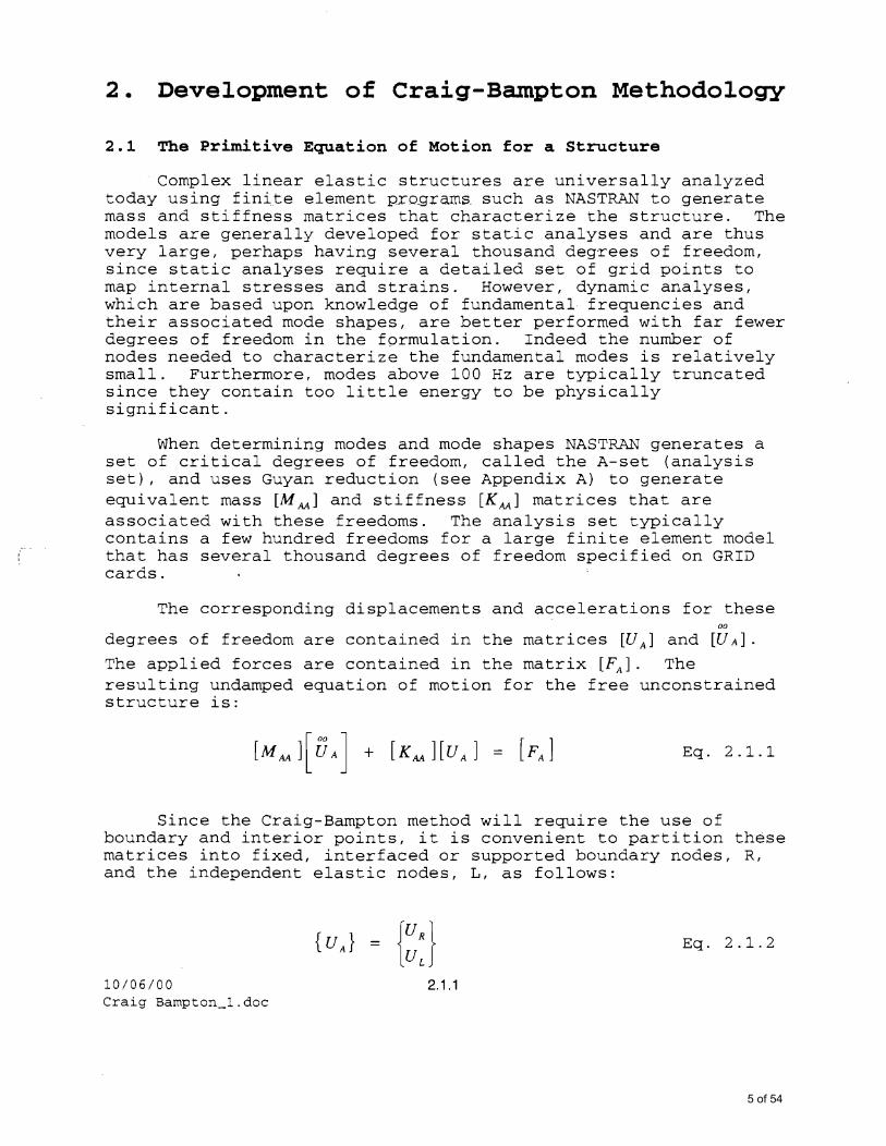
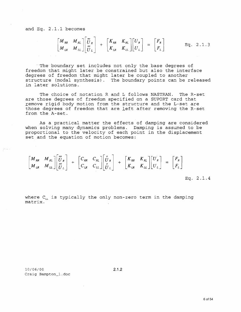
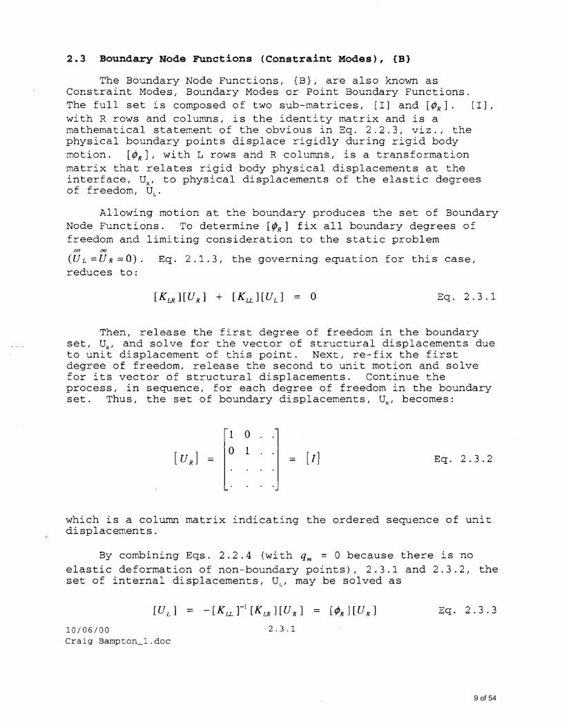
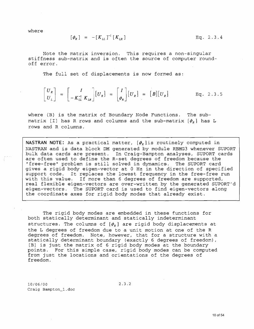
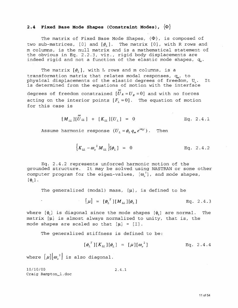
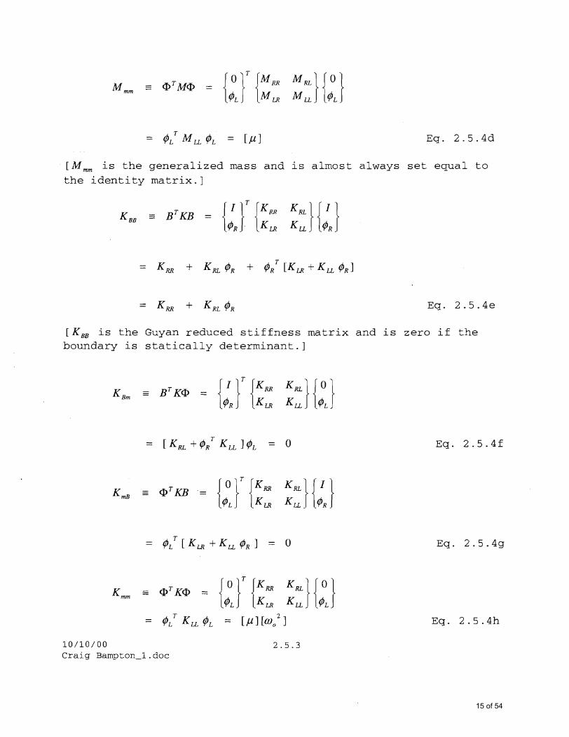
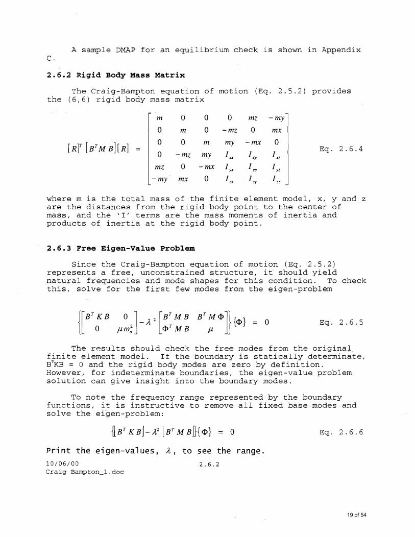
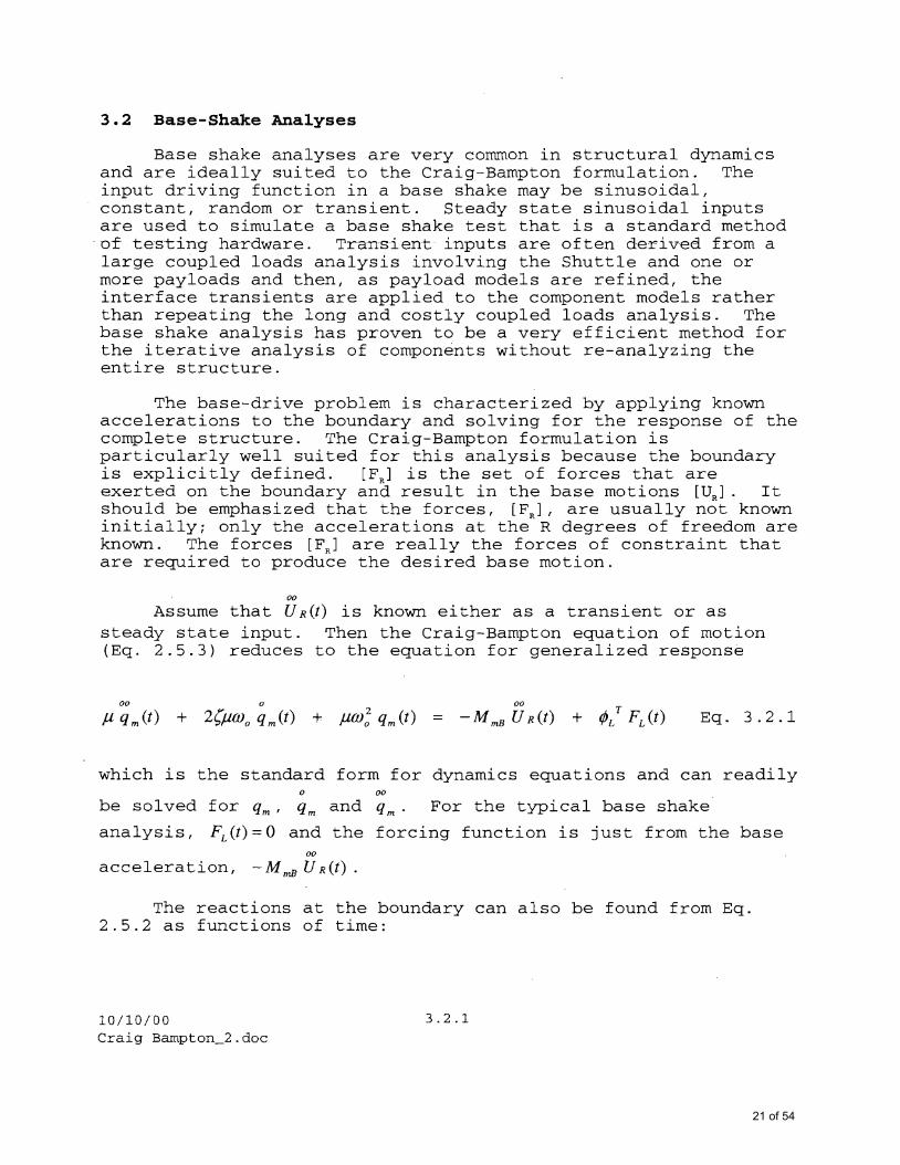
32 Base-Shake Analyses
Base shake analyses are verycornmon in structural dynamics and are ideally suited to the Craig-Bampton formulation The input driving function in a base shake may be sinusoidal constant random or transient Steady state sinusoidal inputs are used to simulate a base shake test that is a standard method of testing hardware Transient inputs are often derived from a
- -largeconpled loads analysis involvin-g the Shuctle and one or more payloads and then as payload models are refined the interface transients are applied to the component models rather than repeating the long and costly coupled loads analysis The base shake analysis has proven to be a very efficient method for the iterative analysis of components without re-analyzing the entire structure
The base-drive problem is characterized by applying known accelerations to the boundary and solving for the response of the complete structure The Craig-Bampton formulation is particularly well suited for this analysis because the boundary is explicitly defined [F
R] is the set of forces that are
exerted on the boundary and result in the base motions [UR ] It should be emphasized that the forces [FR ] are usually not known initially only the accelerations at the R degrees of freedom are known The forces [F R ] are really the forces of constraint that are required to produce the desired base motion
Assume that [UR(t)] is known either as a transient or as
steady state input Then the Craig-Bampton equation of motion (Eq 253) reduces to the equation for generalized response
00 0 00
Ji q m (t) + 2(Jiwo q m (t) + JiW qm(t) = - M mB U R (t) + Eq 321
which is the standard form for dynamics equations and can readily o 00
be solved for qm qm and qm For the typical base shake
analysis FL (t) =0 and the forcing function is just from the base 00
acceleration -MmB U R(t)
The reactions at the boundary can also be found from Eq 252 as functions of time
100600 321 Craig Bampton_2doc
22 of 54
Eq 322
where as explained in Section 6 eBB is almost always null and
is zero for statically determinant boundaries Thus forK BB
many problems Eq 322 becomes
Eq 323
NASTRAN Note The matrix AlBB is data block MR generated by NASTRAN module RBMG4 when SUPORT cards are used
The matrix FL(t) is typically null since forces are applied only at the boundary Also for ease of manipulation Eq 252 the equation of motion is re-written to include the boundary acceleration as an output as well an input quantity This results in the uncoupled linear equation
Eq 324
The physical acceleration response is computed from
Eq 325
Eq 321 is readily solved using numerical integration routines (such as NASINT for transient response and SSR for steady state response in FLAME) for the modal displacements qm
00
and modal accelerations qm
100600 322 Craig Bampton_2doc
23 of 54
33 Modal Participation Factors and Modal Masses for Base-Shake Analyses
It is very common in the aerospace industry to test structures on a shake table In this test known accelerations are applied to the base of a structure These displacements may be sinusoidal (typically a controlled sweep over a given frequency range or a sine burst at a given frequency) or random CFypiEally with a controlled- energy con t en t ) Ba-se snakes are performed for a variety of reasons Quite often one goal is to measure response levels and frequencies with accelerometers at several critical locations and then to use this data as a test basis for verifying the finite element model
Finite element models can predict eigen-values and eigenshyvectors for a structure that correlate very closely with measured test data However they do not give a clear indication of which eigen-vectors will be important contributors in subsequent frequency response analysis Knowing the relative importance of each mode in terms of how much mass is moving and in what direction is crucial for good design of structures
Modal participation factors which are a property of the structure just as generalized mass and stiffness are can be calculated from the mode shapes of the structure Consider a slightly more general form of the Craig-Bampton equation of motion for a damped structure on a shaker table Eq 3310 where the mode shapes are not necessarily mass normalized
00 0 002[u][qm] + 2[u][][wo ][ q m] + [u][W
0 ][ qm] = -[MmB][UR] Eq 331
Note that the coefficients of the generalized motions are all diagonal matrices and that [u] = [centL f [M LL ][centL] from Eq
233 and M mB = centLT
(MLR+MLLcentR) from Eq 227
Each individualized modal equation i is
00 0 T 00
q i + 2j to q j + to2 qj = - (11 m ) centiL (M LR + M LL centR ) U R Eq 332
where ~L is the row of centL associated with the mode i and where
mil the generalized mass for mode i equals [centiL f [M LL ][centu]
Define an L x R matrix of factors [p] with rows
100600 331 Craig Bampton_2doc
24 of 54
Eq 333
Each row of [p] contains as many terms as there are motions for the shaker or equivalently as many degrees of freedom as are defined in the R-set In a base shake motions are applied either at only one point or at a number of points which are rigidly connected to a single point so the maximum number of freeuDIDs in the R~set shou-ld not exceed 6 ie the p-rob lern is statically determinant Each column of [p] contains the factors for all the modes associated each degree of freedom in the R-set Each term in [p] is interpreted as a modal participation factor since the solution to Eq 332 for some specified base motion at one degree of freedom will be proportional to the corresponding term in [p]
An important observation from Eq 333 is that for a determinant system that has been mass normalized the matrix MmB
is in reality the matrix of modal participation factors
Modal participation factors are useful in predicting the modal amplification of a sinusoidal input at resonance Assume a shaker motion that is a steady state sinusoidal input at some
frequency wj and ampli tude U R such that
00 2 - iliJt
and UR =-WmiddotJ
U R e Eq 334
The equation of motion for each mode becomes
00 0 00
q i + 2~i Wi q i + Wi 2 q i - PiR U R
Eq 335
Use the method of undetermined coefficients to solve for the iWjl generali zed motions Assume qi =C e and
00 iWjl
q i =- W C e bull Substituting these values into Eq 334
and noting that at resonance OJ =OJj C ~ [i p U 12) and
00
Eq 336
100600 332 Craig Bampton_2doc
25 of 54
where Qi==(l2~J is the modal amplification of mode i Eq 336 indicates that at resonance the modal acceleration is lagging the base acceleration by 90 and that modal acceleration is proportional to the product of the modal participation factor modal amplification and the magnitude of the shaker input
Modal mass is an analytical measure of how much mass is moving in each translational and rotational direction for each mode The total translational mass in each direction equals the total analytical mass in that direction The total rotational inertia about each axis equals the total rotational inertia about the support point By scanning the modal mass values in each direction the analyst may accurately decide at what frequency the mode shapes may be truncated without losing appreciable model accuracy
Modal masses are related to the constraint forces Consider the constraint forces previously derived for a base shake analysis (Eq 322) and note that for a determinant boundary [K BB ] == [0] Then
[FR] [M BB] [if R] + [M BJ [q]
Eq 337= [M BB] [if R] + [CM RL + - M u) centJ [~m ] Neglect the component due to shaker motion and consider only
the elastic component of [FR ] The constraint force for each mode i becomes
Eq 338
The complex amplitude of this force using Eq 335 is
= - i M RR Qi U R Eq 339
100600 333 Craig Bampton_2doc
26 of 54
where
Eq3310bull is the modal mass matrix for mode l
In practice [M RR ] may be readily computed from the modal participation factor [p~] defined by Eq 333 The modal mass for mode i is
Eq 3311
It is interesting to note that summing for all the modes
(m=L) yields M RR a square matrix of size R where
MRR = (MUcentR +MLRY M u (MUcentR +M LR)
(M RL + cent M U ) (centR + MuM LR )
Eq 3312
If there are no masses at the R-set degrees of freedom
then M RR =M BB the rigid body mass matrix wi th respec t to the boundary
It should be noted that modal participation factors and modal masses could be readily computed from the physical model using NASTRAN rigid solution 3 with just a few lines of DMAP This is presented in Appendix D
As a final note base shake problems are easily solved using matrix manipulation programs such as FLAME However if the problem is to be solved in NASTRAN base accelerations are typically applied by adding a fictitious seismic mass to the R-set degrees of freedom and then applying the appropriate force to the base such that the desired accelerations result
100600 334
Craig Bampton_2doc
27 of 54
34 The Load Transformation Matrix (LTM)
The Load Transformation Matrix (LTM) is used to recover physical parameters such as accelerations displacements forces and stresses from the original finite element model using the generalized accelerations and for redundant interfaces the physical displacements of the boundaries Although the use of the kT~ is standard practice in the aerospace industry several definitions of the LTM exist depending on company practice and the nature of the problem being solved Swales Aerospace uses an LTM based on recovering A-set displacements from the physical model this approach is well-suited forNASTRAN since all element forces and stresses are derived from the displacement field
341 Displacement LTMs
The functional relationship between A-set displacements and generalized motions (including boundary displacements) can be established as follows Recall that the primitive equation of motion for a structure in finite element analysis is
MRLSR + KRR KRLU R _ FR Eq 212M UL K K UL FLLL LR LL
where it will be assumed that no interior forces act (FL =0)
Thus
00 00
[M LR ][UR]+ [M LL ][Ud + [K LR ][UR]+ [K LL ][UL] [0] Eq 341
and
Eq 342
1010600 341 Craig Barnpton_2doc
28 of 54
Using the Craig-Bampton transformation (Eqs 221 and 222)
~L ~OqOO + [1fgtR] [U R][UJ = [Kzi MLR ] [-Kzi MuJ R I I
Eq 343
Merge UR and UL to form theA-set displacements
00
Eq 344
Eq 344 forms the basis for the LTM development Appendix E presents a NASTRAN DMAP sequence for solving this equation Element forces and stresses follow from knowledge of the displacement field The desired components of the LTM are requested in the NASTRAN output file A post-processor then reads this data and reformats it appropriately The LTM has units element forces (or stresses) per modal acceleration (or unit interface displacement) Typically stress equations are also coded in matrix form with units stress per element force (or interface displacement) The analytical flow is as follows
[Stress(time)] = [Stresselement force] x [Element forcemodal acceleration (or IF disp)] x [Modal acceleration(time) or IF disp(time)]
Note that quite often only acceleration histories are of concern and interface displacements due to redundancy are ignored Stresses induced by these displacements are often small enough to be ignored
100600 342 Craig Bampton_2doc
29 of 54
342 Interface Force LTM
Sometimes only the interface forces and net center of gravity forces are of interest Using the upper part of Eq 255 the boundary (interface) forces can be written in terms of the Craig-Bampton acceleration and boundary displacements as
Eq 345
Eq 345 can be re-arranged to form a single matrix that relates the boundary forces to the Craig-Bampton coordinates as
Eq 346[M BB M Bm
The matrix [M BB is the Interface Force LTM thatM Bm K BB ]
relates Craig-Bampton accelerations and boundary displacements to the interface forces
The Net CG Acceleration LTM can be created from Eq 346 by transforming the interface forces to the spacecraft CG (using the transformation matrix TB- CG ) and then dividing through by the 6x6 generalized mass matrix This can be written as follows
Eq 347
Since T[G_B = T CG-B
[Net CG Aeee]
Eq 348
where the transformation matrix TB - ffi may be computed in NASTRAN or by hand as shown in Section 36 Note that the forces due to
101000 343 Craig Bampton_2doc
30 of 54
the boundary displacements do not contribute to the Net CG Acceleration and thus the boundary displacements are not included in the formulation even for a redundant interface
The Interface Force LTM and the Net CG Accel LTM can be combined into a single LTM as follows
[Net CG Accelerations J] Eq 349
[ [InterfaceForcesJ
100600 344 Craig Bampton_2doc
31 of 54
35 Application of the Craig-Bampton Method to Modal Synthesis
The Craig-Bampton method was developed expressly to provide a way to couple (synthesize) two or more structures that are defined in terms of their modal properties The two-structure case defined here is easily extended to the multi-body case experience has shown however that the synthesis of many ~txuctures should be broken down into a sequence of two-structure steps
Let the superscripts A and B distinguish the two structures that will be coupled By simple overlay of Eq 214 the equation of motion for the system is
Eq 351
The structures are connected by equating the boundary displacements of B to those of A by
Eq 352
Matrix [e] is the necessary transformation made by the analyst to correct for differently ordered boundary points or for different coordinate locations It may be as simple as amiddotmatrix of direction cosines or even just the identity matrix If the boundary points are not exactly at the same location [e] must also contain rigid links to put the points together Usually the matrix for just re-ordering the boundary points looks like
0 1 0 0
1 0 0 0
[e] = 0 0 0 1 Eq 353
0 0 1 0
100600 351 Craig Bampton_2doc
32 of 54
If there are boundary points in A that do not connect to B just leave a zero column in [e) The matrix [e] will not be square for this case
The system displacement vector lU s J is
Eq 354
To transform from the subsystem displacements to this system displacement set we must use
I 0 0 0
0 0centJ centJt[Us] = [~] 0
0
I 0 0 0
centJ centJt 0 0 =
0 0 I 0
0 0 centJ centJ~
0 I 0
0 centJ centJ~
100
010
e 0 0
001
UR A
A qm
Eq 355UR
B
q~
Eq 356
Eq 357
The big transformation matrix E is defined by comparing the last two equations In practice however the matrix E never has to be formed because when it is used the results fallout in terms of data that has already been computed
100600 352
Craig Barnpton_2doc
33 of 54
Transforming from the component sets for the various subshystructures to the system set of coordinates results in the following system equation of motion
Eq 358
where the synthesized mass is
Eq 359
which expands to
and where the synthesized damping is
Eq 3510
and where the synthesized system stiffness is
Eq 3511
Eq 3512
which expands to
100600 Craig Bampton_2doc
353
34 of 54
o (fi (j)~ y Eq 3513
o
and finally the synthesized system forcing functions are
Eq 3514
which will not be expanded because it is typically more efficient to include the forced degrees of freedom in the LTM
1010600 354 Craig Bampton_2doc
35 of 54
36 Reduction of a Redundant Interface to a Single Point
The Craig-Bampton equation of motion for a structure (or sub-structure) on a 6 degree of freedom boundary and unity generalized mass with no internal loads is given by
00
Eq 321
00
where CUR] represents motion of the interface degrees of freedom If this set of interface DOFs is indeterminant it may be advantageous under certain circumstances to tie these points together for application of a single or average set of interface motions For example when solving for the steady state response of a structure with an indeterminant boundary it is easier to apply the motions to a single point and it may be even more appropriate since the mounting of a structure to a shaker table rigidizes the interface As another example it may be easier to visualize the excitation of several redundant degrees of freedom by first averaging the excitation in each djrectiort and then applying them to one point that is rigidly connected to the others The single point need not be (and typically isnt) one of the original boundary points Obviously any elasticity in the interface (such as ovalling of a ring) is lost as the interface points are all rigidly connected to the new point Therefore this technique should be used only when the interface is stiff relative to the rest of the structure or when stiffness is to be added to the interface
Consider a structure with three boundary points B1 B2 and B3 each with 6 DOFs for a total of 18 interface DOFs These points are to be replaced by the single point A The coordinates of point Bi are Xbi Ybi Zbi RXBi RYBi RZBi and the coordinates of point A are XA YA ZA RXA RYA RZA Let the displacements of points Bi be Uix Uiy Uiz Uijx Uijy Uijz and the displacements of point A be ux uy uz ujx ujy ujz Further let the set of all displacements at the boundary be [U] where [U] is an 18 x n matrix (n is the number of time steps) and let the set of displacements at point A be [u] where [u] is a 6 x n matrix The displacement vectors [U] and [u] are related by the transformation matrix [C] that may be determined from simple geometric considerations This relation is given as
[U] = [C][u] Eq 361a
or in expanded notation for any given point in time
100600 361 Craig Bampton_2doc
36 of 54
Utt 1 0 0 0 1121 - DoYl
Ul y 0 1 0 -1121 0 ~l Ul z Ul ex
0
0
0
0
1
0
DoYl
1
-~l
0
0
0 Ulry
0 0 0 0 1 0 -Ul
fk 0 0 0 0 0 1 U2 x 1 0 0 0 1122 -DoY2 U x
U2 y 0 1 0 - 1122 0 ~2 U y
U2 Z 0 0 1 DoY2 -~2 0 U z = in 0 0 0 1 0 0 Uex
in 0 0 0 0 1 0 ury
in 0 0 0 0 0 1 Ufk
U3 x 1 0 0 0 DZ3 -DoY3
U3 y 0 1 0 -DZ3 0 ~3
U3 0 0 1 DoY3 -~3 0
U3fJx 0 0 0 1 0 0
us 0 0 0 0 1 0 Eq 361b
us 0 0 0 0 0 1
where
~i = X Bi - X A
Do~ = YBi - YA
L1Z i = ZBi - ZA Eq 362
The pattern of Eq 361b may be repeated for any arbitrary number of redundant interface points
To reduce the number of interface DOFs in Eq 321 replace 00 00
[UR] with [C][u]and solve as usual for modal responses Note however that when transforming modal responses back to physical responses using the Craig-Bampton transformation (Eq 221) the matrix of Boundary Mode Functions [B] must be replaced with the matrix lBJ where lBJ=[B][C]
100600 362
Craig BarnptoTI_2doc
37 of 54
It is also interesting to note that the 6x6 rigid body mass matrix of the structure about point A may be computed from the
product [eY [MBB][e]
To obtain the average H motion [u] of a single point in each direction when motions [U] act at several boundary points one cannot simply average the motions of all the boundary points in each direction Continuing with the example above the correct approach is to determine the transformation matrix [T] such that
[u] = [THu] Eq 363
where [T] a 6 x 18 array is the inverse of [C] Begin by
multiplying Eq 361a by [e]T the transpose of [C] ThenI
[eY [u] = [eY [eHu] Eq 364
where [C]T [C] is a square matrix with a defined inverse It follows that
[u] = reV [en-I [eF [u] = [THu] Eq 365
so that the desired inverse transformation is
Eq 366
100600 363 Craig Barnpton_2doc
38 of 54
4 REFERENCES
1 Hurty Walter C On the Dynamic Analysis of Structural Systems Using Component Modes AIAA Paper No 64-487 First AIAA Annual Meeting Washington DC June 29-July 2 1964
2 Craig Roy and Bampton Mervyn Coupling of Substructures for Dynamic Analyses AIAA Journal Vol 6 No7 July 1968 pp 1313-1319
3 Haile William B Modal Synthesis Boundary Reaction Convergence Test Engineering Memorandum SampM 354 Space Telescope Program Lockheed Missiles and Space Co Inc Sunnyvale California December I 1982
4 Wilson Thomas A NASTRAN DMAP Alter for the Coupling of Modal and Physical Coordinate Substructures
100600 41 Craig Bampton_2doc
39 of 54
APPENDIX A
GUYAN REDUCTION
Guyan Reduction is a methodology used to reduce the number of degnes of freedom in a large finite element model typically generated for static analyses to some much smaller number of freedoms that can be much more readily solved for dynamic analyses In NASTRAN this reduced set of freedoms is called the ASET or analysis set
Consider the following equation in which the 1 space represents the omitted dofs that are assumed to carry no force and the 2 space represents the ASET dofs
Eq AI
Note that the ASET contains both boundary and interior freedoms Then
Eq A2
Eq A3
Eq A4
Eq AS
where is the ASET stiffness
Note that Eq A3 relates the omitted freedoms to the ASET freedoms and gives rise to the following transformation
Eq A6
where
100600 A1
Craig Bampton_2doc
40 of 54
This is equivalent to modal reduction Consider the eigenshyvalue problem for the overall structure and transform the displacements as above
Klttgt = M lttgt A Eq A7
TT K T lttgt = TT M T lttgt A Eq A8
Klttgt = MlttgtA Eq A9
[T1 = [T1 = X 2 =If k fJx IJ[~ J]x K 22 12Ik 21 k 22
Eq AI0
The corresponding mass matrix may be derived from the laws of motion
1 = M 12][~l] Eq AII
M 22 x2
Applying the transformation in Eq A6 and noting that the matrix T is not a function of time the acceleration matrix may be transformed as follows
[] [x ] middotEq A12
Eq A13
where 1 has forces both in 1 and 2 space
Finally transform the forces as follows
100600 A2
Craig Bampton_2doc
41 of 54
--
12 = [~ I] 1 = [Tj I][M M fJ x = M 22 x2 Eq A14 M 21 M22 I
where
M 22 = [Tj I][M U Eq A15MlnIM 21 M 22
100600 A3
Craig Bampton_2doc
42 of 54
APPENDIX B
NASTRAN DMAP for Generating a Craig-Bampton Model (This DMAP is for MSC Version 64 It assumes that the mode shapes are mass normalized and that the boundary degrees of freedom are specified on SUPORT cards)
SOL 30 ALTER 416417 $ Fixed Interface Modal Model
1 READ KLLMLL EEDUSETCASECCLAMAPHILMIOEIGS MODESSNNEIGV $
2 OFP LAMAOEIGS $ 3 UMERGE USETPHILPHILAALR $ 4 PARAM NOPVNMRP=-l $ 5 MATGEN AMR1REACT $ 6 DIAGONAL MIMIDIAGSQUARE $ 7 EQUIV MIDIAGMIMRP $ 8 UMERGE USETDMAMRPHIRBALR $ 9 PARAM CNADDVNNORPNVNREACTVNNEIGV $
10 MATGEN MP6NORPNREACTNEIGV $ 11 MERGE PHIRBPHILA MPPHIX1 $ 12 MPYAD MLLDMMLRMTP12 $ 13 MPYAD PHILMTP1MHB12 $ 14 TRNSP MHBMBH $ 15 MERGE MRMHBMBHMIMPMRRGN $ 16 MATPRN MIMRRGN $ 17 SPMYAD PHILKLLPHIL KW31 $ 18 MATPRN KW 19 DIAGONAL KWKWWSQUARE $ 20 MATPRN KWW $ 21 MPYAD KLRDMKRRKBB12 $ 22 MATPRN KBB $ 23 MERGE KBB KWWMPKRRGN $ 24 MATPRN KRRGN $ 25 OUTPUT4 KRRGNMRRGNPHIX -121 $
ENDALTER
middotNOTES
1 READ (Extract eigen-values from a real symmetric matrix) solves Eq 242 It takes the constrained mass (MLL) and stiffness arrays (KLL) and calculates the cantilevered modes (PHIL) and eigen-values (LAMA) It also computes the modal mass matrix MI which is given as [] in Eq 243 NEIGV is the number of eigen-vectors found
2 OFP (Output file processor) prints LAMA the real eigenvalue table and OEIGS the real eigen-value summary table
100600 B1 Craig Bampton_2doc
43 of 54
3 UMERGE (Merge two matrices based on USET) forms PHILA the fixed base mode shape matrix ~ defined by Eq 222 The mode shapes are brought to A-set size by merging zeros into the boundary coordinates
4 PARAM (Parameter processor) defines the parameter MRP used by EQUIV in step 7
5 MATGEN (Matrix generator) generates AMR an RxR identity matrix
6 DIAGONAL (Strip diagonal from matrix) forms MIDIAG a square matrix whose diagonal terms are taken from the matrix MI (MIDIAG and MI are equivalent MIDIAG has small offshydiagonal terms that are set to zero in MI)
7 EQUIV (Data block name equivalence) makes MIDIAG and MI equivalent
8 UMERGE forms PHIRB the Boundary Mode Function matrix [B] defined by Eq 222 It merges the identity matrix AMR with the rigid body transformation matrix DM that is defined as centR in Eq 2 3 4
9 PARAM defines the parameter NORPN to be the sum of REACT (the number of SUPORT degrees of freedom) and NEIGV (the number of eigen-vectors retained in the Craig-Bampton analysis)
10 MATGEN forms a column matrix MP with (R+m) rows The first R rows contain zeros and the remaining m rows contain ones
11 MERGE forms PHIX the [AxR+m)] Craig-Bampton transformation matrix [B ~] defined by Eq 221 Note that the order of the A rows is in the NASTRAN sequencing order with the L and R freedoms inter-dispersed
12 MPYAD (Matrix multiply and add) forms [M LR + M LL centR] part of Eq 254c
13 MPYAD forms [M rnB] (Eq 25 4c)
14 TRNSP (Matrix transpose) forms MBm the transpose of MmE
15 MERGE forms MRRGN the full Craig-Bampton mass matrix defined in Eq 253
16 MATPRN prints MI and MRRGN
100600 B2 Craig Bampton_2doc
44 of 54
17 SMPYAD (Matrix series multiply and add) computed Wo 2 from
Eq 244 and calls it KW
18 MATPRN prints the matrix of eigen-values KW
19 DIAGONAL forms KWW a square matrix whose diagonal terms are taken from matrix KW (KW and KWW are equivalent KW has small off-diagonal terms that are set to zero in KWW)
20 MATPRN prints matrix KWW
21 MPYAD computes KBB as given by Eq 254e
22 MATPRN prints matrix KBB
23 MERGE forms KRRGN the full Craig-Bampton stiffness matrix defined by Eq 253
24 MATPRN prints matrix KRRGN
25 OUTPUT4 writes matrices KRRGN MRRGN and PRIX onto Fortran unit 21
100600 B3
Craig Barnpton_2doc
45 of 54
APPENDIX C
NASTRAN DMAP for Computing an Equilibrium Check on the Free-Free Stiffness Matrix
(This DMAP is for MSC Version 64)
Appendix C presents the NASTRAN DMAP sequence for performing an equlTnJ-rium check on tne stiffness m~ftrices cfa physical shymodel The purpose of this check is to test for grounding in a structure that will generate erroneous internal forces The check shown is for the free-free stiffness (F-set) matrix but the approach is applicable to the other sets as well The rigid body transformation matrix KRBF multiplies the stiffness matrix KFF This product is then normalized to its maximum value to yield the array KRBFN Large terms in KRB indicate grounding the location of the ground is shown by KRBFN
SOL 30 ALTER 125
1 VECPLOTBGPDTEQEXINCSTM RBGLOBALVYMPFPNT=04 $ 2 VEC USETVRBGFCOMP $ 3 PARTN RBGLOBALVRBRBFSET +1 $ 4 TRNSP RBFSETRBTF $ 5 MPYAD KFFRBTFKRB $ 6 MPYAD RBFSETKRBKRBF $ 7 NORM KRBKRBFN $ 8 MATPRN KRBF $ 9 MATGPR GPLUSETSILKRBFNF1-2 $
ENDALTER
NOTES
1 VECPLOT generates RBGLOBAL the global rigid body matrix with 6 rows and g columns where each row represents the rigid body motion of all grid points about point MPFPNT The default value for MPFPNT is grid point 0 that is interpreted in NASTRAN as the origin of the basic coordinate system Another point about which rigid body motion is to be taken may be specified on a PARAM card in the Bulk Data deck The format of this card is PARAM MPFPNT Grid ID Note that VECPLOT is commonly used in other DMAP routines and is therefore shown above apart from the rest of the modal mass DMAP
100600 C1 Craig SamptoTI_2doc
46 of 54
-shy
2 VEC partitions USET into VRB to reduce the g-set into the f-set
3 PARTN partitions RBGLOBAL (6 x g) into RBFSET (6 x f) based on VRB
4 TRNSP transposes RBFSET into RBTF
5 MPYAD multiplies KFF the free~free stiffness matrix by RBTF the f x 6 rigid body matrix to form KRB an f x 6 matrix
6 MPYAD multiplies RBFSET the 6 x f rigid body matrix by KRB f x 6 to yield a 6 x 6 matrix KRBF This matrix is key to understanding if a structure is grounded A large term in this array indicates grounding
7 NORM normalizes KRB by the maximum value of the array to yield KRBFN
8 MATPRN prints KRBF the 6 x 6 matrix
9 MATGPR prints KRBFN (f x 6) with associated grid point ID number Only those values larger than 001 are printed This matrix identifies the location of the ground
NOTE
An equilibrium check of the F-set stiffness matrix has been described It is highly recommended that equilibrium checks also be performed on the G-set (global DOFs) the N-set (those DOFs Not taken out by MPCs) and the T-set (equivalent to the A-set when dynamic reduction is not involved) An example of this DMAP package for MSC Version 64 is as shown
ALTER 115 $$ G-SET CHECK VECPLOT BGPDTEQEXINCSTM RBGLVYMPFPNT=04 $ TRNSP RBGLRBGLT $ MPYAD KGGRBGLTKPHIG $ MATGPR GPLUSETSILKPHIGG1-S $ ALTER 121 $$ N-SET CHECK - CHECKS FOR PROBLEMS WITH MPCs VEC USETVGMGMCOMP $ PARTN RBGLVGM RBNNl $ TRNSP RBNNRBNNT $ MPYAD KNNRBNNTKPHIN $ MATGPR GPLUSETSILKPHINN1-S $ ALTER 126
100600 C2 Craig Bampton_2doc
47 of 54
$$ F-SET CHECK VEC USETVGFGFCOMP $ PARTN RBGLVGFRBFF 1 $ TRNSP RBFFRBFFT $ MPYAD KFFRBFFTKPHIF $ DIAGONAL KFFKFFDSQUARE-1 $ MPYAD KFFDKPHIFKPHIFN $ MATGPR GPLUS~TSILKPHIFNF1-5 $ $$ A-SET (T-SET) CHECK ALTER 174 VEC USETVGTGTCOMP $ PARTN RBGLVGTRBTT 1 $ TRNSP RBTTRBTTT $ MPYAD KTTRBTTTKPHIT $ DIAGONAL KTTKTTDSQUARE-1 $ MPYAD KTTDKPHITKPHITN $ MATGPR GPLUSETSILKPHITNT1-5 $ ENDALTER
100600 C3 Craig Bampton_2doc
48 of 54
APPENDIX D
NASTRAN DMAP for Computing Modal Participation Factors and Modal Weights
(This DMAP is for MSC Version 64)
SOL 30 ALTER 125
1 VECPLOT BGPDTEQEXINCSTM RBGLVYMPFPNT=04 $
$$$ COMPUTE MODAL PARTICIPATION AND MODAL WEIGHT 2 VEC USETVGTGTCOMP $ 3 PARTN RBGLVGTRBASET 1 $ 4 MPYAD RBASETMAARBMAA $ 5 MPYAD RBMAAPHILARBMPHI $ 6 DIAGONAL RBMPHIMPHI2WHOLE2 $ 7 ADD MPHI2EFWGHT(3864 0) $ 8 MATGEN IDP1NEIGV $ 9 DIAGONAL IDPCIDPCOLUMN1 $
10 MPYAD EFWGHTCIDPWTSUM $ 11 MATPRT EFWGHT $ 12 MATPRT WTSUM $
ENDALTER
NOTES
1 VECPLOT generates RBGL the global rigid body matrix with 6 rows and g columns where each row represents the rigid body motion of all grid points about point MPFPNT The default value for MPFPNT is grid point 0 that is interpreted in NASTRAN as the origin of the basic coordinate system Another point about which rigid body motion is to be takenmiddot may be specified on a PARAM card in the Bulk Data deck The format of this card is PARAM MPFPNT Grid ID Note that VECPLOT is commonly used in other DMAP routines and is therefore shown apart from the rest of the modal mass DMAP
2 VEC partitions USET into VGT to reduce the g-set into the t-set For practical purposes the t-set is equivalent to the a-set
3 PARTN partitions RBGL (6 x g) into RBASET (6 x a) based on VGT
4 MPYAD multiplies the rigid body a-set matrix RBASET by the a-set mass matrix MAA (a x a) to produce RBMAA (6 x a)
100600 D1 Craig Bampton_2doc
49 of 54
5 MPYAD multiplies RBMAA (6 x a) by elastic modes PHILA (a x modes) to produce RBMPHI 6 x modes the matrix of Modal Participation Factors
6 DIAGONAL squares all the terms in RMBPHI to produce MPHI2
7 ADD scales MPHI2 by 3864 to produce EFWGHT the matrix of modal weights (6 x modes)
8 MATGEN produces IDP an n x n identity matrix where n is NEIGV the number of modes specified on the EIGR card in Bulk Data
9 DIAGONAL strips the diagonal from IDP (n x n) to produce CIDP (n x 1)
10 MPYAD multiplies EFWGHT (6 x n) by CIDP (n x 1) to produce WTSUM (6 x 1) the sum of the modal weights for all modes in each direction
11 MATPRT prints EFWGHT
12 MATPRT prints WTSUM
100600 D2 Craig Bampton_2doc
50 of 54
APPENDIX E
NASTRAN DMAP for Generating an LTM (This DMAP is for MSC Version 64)
SOL 30 ALTER 416417
$$ This DMAP outputs data blocks OEF2 and OEF4 from $$ which a post-processor (such as the Fortran program $$ LTMGEN) can generate an LTM $$ $$ The DMAP from APPENDIX B for generating a Craigshy$$ Bampton model should be inserted here since data $$ blocks PHIL MP and PHIRB which were generated there $$ are also of required here $$ $$ LTM DMAP $$ $$ ACCELERATION DATA RECOVERY $$
1 MPYAD MLLDMMLRMIF $ 2 ADD MIFAMIF(-lO) $ 3 MPYAD MLLPHILLFOR-1 $ 4 MERGE AMIF LFOR MPLFORA1 $ 5 FBS LLL LFORALDISPA11 $ 6 UMERGE USETLDISPAADISPALR $ 7 SDR1 USETADISP GOGM PHIZ2 lREIG $ 8 OUTPUT4 PHIZ2 -124 $ 9 SDR2 CASECCCSTMMPTDITEQEXINSILETT BGPDTLAMA
PHIZ2ESTOPG2OQG2OPHIZ2OES2OEF2PUGV2REIG 10 OFP OEF2 $
$$ OUTPUT TABLES LISTED BELOW $$ $$ OQG2 SPC FORCES DUE TO ACCELERATIONS $$ OPHIZ - DISPLACEMENTS DUE TO ACCELERATIONS $$ OEF2 ELEMENT FORCES DUE TO ACCELERATIONS $$ $$ REDUNDANT FORCES $$
11 SDR1 USET PHIRB GOGM KFS PHIZ4 lREIG $ 12 SDR2 CASECCCSTMMPTDITEQEXINSILETT BGPDT LAMA
PHIZ4ESTOPG4OQG4OPHIZ4OES4OEF4PUGV4REIG $ 13 OFP OEF4 $
$$ $$ OUTPUT TABLES LISTED BELOW $$ $$ OEF4 - ELEMENT FORCES DUE TO IF DISPLACEMENTS $$ OQG4 - SPC FORCES DUE TO IF DISPLACEMENTS $$ OPHIZ4 - DISPLACEMENTS DUE TO IF DISPLACEMENTS ENDALTER
100600 E1 Craig Barnpton_2doc
51 of 54
NOTES
1 MPYAD generates data block MIF that equals [M LR +M LL centJR] in Eq 254c The terms in MIF are related to InterFace Mass Its size is LxR
2 ADD generates data block AMIF the negative of MIF
3 MPYAD generates data block LFOR that equals [M LL centJL] in Eq 243 Its size is Lxm The terms in LFOR are related to the L-set forces
4 MERGE generates data block LFORA the matrix [AMIF LFOR] Its size is Lx(R+m)
5 FBS (Matrix ForwardBackward Substitution) generates data block LDISPA that equals ~- K~ (M LR + M U centJR)J - K~ M u centJJ which are two of the sub-matrices in Eq 344 The terms in LDISPA are related to the L-set displacements
6 UMERGE takes the 1x2 matrix LDISPA and generates the 2x2 matrix ADISP by placing zeros in row 1 The terms in ADISP are related to the A-set displacements
7 SDR1 is a module that generates data block PHIZ2 which is the displacement matrix ADISP blown-up to G-set size
8 OUTPUT4 writes the matrix PHIZ2 onto Fortran unit 24
9 SDR2 is a module which outputs several data blocks (G-set size) related to forces stresses and displacements that result from unit modal accelerations
10 OFP outputs data block OEF2 the element forces due to modal accelerations
11 SDR1 is a module that generates data block PHIZ4 which 1S
the support vector matrix PHIRB blown-up to G-set size It contains the rigid body constraint modes
12SDR2 is a module which outputs several data blocks (G-set size) related to forces stresses and displacements that result from redundant interface forces
13 OFP outputs data block OEF4 the element forces due to the redundant interface forces
100600 E2 Craig Bampton_2doc
52 of 54
Note that the following symbolic relationships apply to this DMAP sequence
where
[~K [M ult + MU
0
~JcentRJ -KlMufJL
= [~K (AMIF) 0
-laquo (LFOR) ~M]
= [- K (~FORA) D~]
= [LD~SPA D~]
= [ADISP PHIRB]
Note also for this DMAP sequence the G-set displacement matrix [U G ] may be expressed symbolically as
00
00
[PHIZ2 PHIZ 4] q m
UR
Finally note that the data blocks OEF2 and OEF4 the LTM and are written into the NASTRAN output data
constitute file
100600 Craig Barnpton_2doc
E3
53 of 54
Typically a post-processor (such as the Fortran program LTMGEN) reads this file and re-formats it appropriately
100600 E4 Craig Bampton_2doc
54 of 54
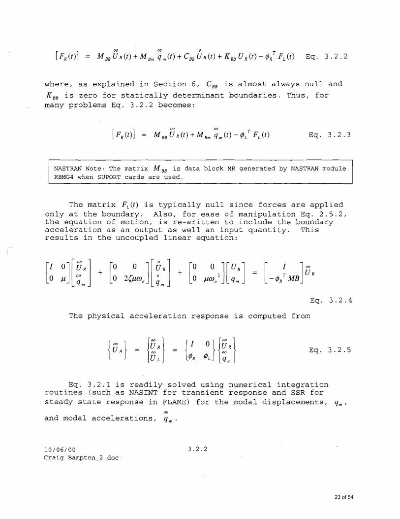
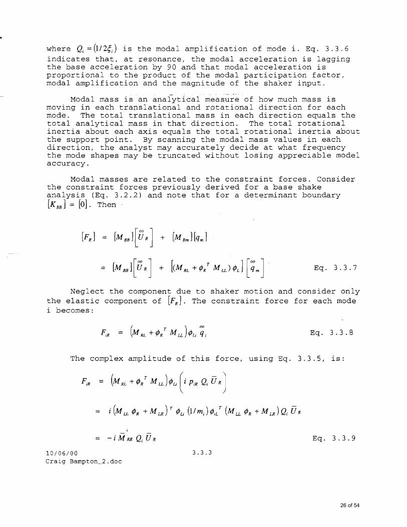
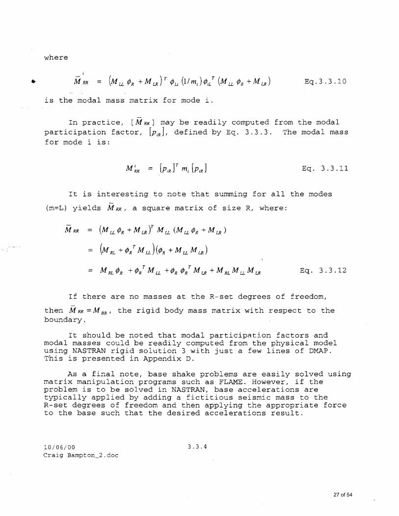
where
Eq3310bull is the modal mass matrix for mode l
In practice [M RR ] may be readily computed from the modal participation factor [p~] defined by Eq 333 The modal mass for mode i is
Eq 3311
It is interesting to note that summing for all the modes
(m=L) yields M RR a square matrix of size R where
MRR = (MUcentR +MLRY M u (MUcentR +M LR)
(M RL + cent M U ) (centR + MuM LR )
Eq 3312
If there are no masses at the R-set degrees of freedom
then M RR =M BB the rigid body mass matrix wi th respec t to the boundary
It should be noted that modal participation factors and modal masses could be readily computed from the physical model using NASTRAN rigid solution 3 with just a few lines of DMAP This is presented in Appendix D
As a final note base shake problems are easily solved using matrix manipulation programs such as FLAME However if the problem is to be solved in NASTRAN base accelerations are typically applied by adding a fictitious seismic mass to the R-set degrees of freedom and then applying the appropriate force to the base such that the desired accelerations result
100600 334
Craig Bampton_2doc
27 of 54
34 The Load Transformation Matrix (LTM)
The Load Transformation Matrix (LTM) is used to recover physical parameters such as accelerations displacements forces and stresses from the original finite element model using the generalized accelerations and for redundant interfaces the physical displacements of the boundaries Although the use of the kT~ is standard practice in the aerospace industry several definitions of the LTM exist depending on company practice and the nature of the problem being solved Swales Aerospace uses an LTM based on recovering A-set displacements from the physical model this approach is well-suited forNASTRAN since all element forces and stresses are derived from the displacement field
341 Displacement LTMs
The functional relationship between A-set displacements and generalized motions (including boundary displacements) can be established as follows Recall that the primitive equation of motion for a structure in finite element analysis is
MRLSR + KRR KRLU R _ FR Eq 212M UL K K UL FLLL LR LL
where it will be assumed that no interior forces act (FL =0)
Thus
00 00
[M LR ][UR]+ [M LL ][Ud + [K LR ][UR]+ [K LL ][UL] [0] Eq 341
and
Eq 342
1010600 341 Craig Barnpton_2doc
28 of 54
Using the Craig-Bampton transformation (Eqs 221 and 222)
~L ~OqOO + [1fgtR] [U R][UJ = [Kzi MLR ] [-Kzi MuJ R I I
Eq 343
Merge UR and UL to form theA-set displacements
00
Eq 344
Eq 344 forms the basis for the LTM development Appendix E presents a NASTRAN DMAP sequence for solving this equation Element forces and stresses follow from knowledge of the displacement field The desired components of the LTM are requested in the NASTRAN output file A post-processor then reads this data and reformats it appropriately The LTM has units element forces (or stresses) per modal acceleration (or unit interface displacement) Typically stress equations are also coded in matrix form with units stress per element force (or interface displacement) The analytical flow is as follows
[Stress(time)] = [Stresselement force] x [Element forcemodal acceleration (or IF disp)] x [Modal acceleration(time) or IF disp(time)]
Note that quite often only acceleration histories are of concern and interface displacements due to redundancy are ignored Stresses induced by these displacements are often small enough to be ignored
100600 342 Craig Bampton_2doc
29 of 54
342 Interface Force LTM
Sometimes only the interface forces and net center of gravity forces are of interest Using the upper part of Eq 255 the boundary (interface) forces can be written in terms of the Craig-Bampton acceleration and boundary displacements as
Eq 345
Eq 345 can be re-arranged to form a single matrix that relates the boundary forces to the Craig-Bampton coordinates as
Eq 346[M BB M Bm
The matrix [M BB is the Interface Force LTM thatM Bm K BB ]
relates Craig-Bampton accelerations and boundary displacements to the interface forces
The Net CG Acceleration LTM can be created from Eq 346 by transforming the interface forces to the spacecraft CG (using the transformation matrix TB- CG ) and then dividing through by the 6x6 generalized mass matrix This can be written as follows
Eq 347
Since T[G_B = T CG-B
[Net CG Aeee]
Eq 348
where the transformation matrix TB - ffi may be computed in NASTRAN or by hand as shown in Section 36 Note that the forces due to
101000 343 Craig Bampton_2doc
30 of 54
the boundary displacements do not contribute to the Net CG Acceleration and thus the boundary displacements are not included in the formulation even for a redundant interface
The Interface Force LTM and the Net CG Accel LTM can be combined into a single LTM as follows
[Net CG Accelerations J] Eq 349
[ [InterfaceForcesJ
100600 344 Craig Bampton_2doc
31 of 54
35 Application of the Craig-Bampton Method to Modal Synthesis
The Craig-Bampton method was developed expressly to provide a way to couple (synthesize) two or more structures that are defined in terms of their modal properties The two-structure case defined here is easily extended to the multi-body case experience has shown however that the synthesis of many ~txuctures should be broken down into a sequence of two-structure steps
Let the superscripts A and B distinguish the two structures that will be coupled By simple overlay of Eq 214 the equation of motion for the system is
Eq 351
The structures are connected by equating the boundary displacements of B to those of A by
Eq 352
Matrix [e] is the necessary transformation made by the analyst to correct for differently ordered boundary points or for different coordinate locations It may be as simple as amiddotmatrix of direction cosines or even just the identity matrix If the boundary points are not exactly at the same location [e] must also contain rigid links to put the points together Usually the matrix for just re-ordering the boundary points looks like
0 1 0 0
1 0 0 0
[e] = 0 0 0 1 Eq 353
0 0 1 0
100600 351 Craig Bampton_2doc
32 of 54
If there are boundary points in A that do not connect to B just leave a zero column in [e) The matrix [e] will not be square for this case
The system displacement vector lU s J is
Eq 354
To transform from the subsystem displacements to this system displacement set we must use
I 0 0 0
0 0centJ centJt[Us] = [~] 0
0
I 0 0 0
centJ centJt 0 0 =
0 0 I 0
0 0 centJ centJ~
0 I 0
0 centJ centJ~
100
010
e 0 0
001
UR A
A qm
Eq 355UR
B
q~
Eq 356
Eq 357
The big transformation matrix E is defined by comparing the last two equations In practice however the matrix E never has to be formed because when it is used the results fallout in terms of data that has already been computed
100600 352
Craig Barnpton_2doc
33 of 54
Transforming from the component sets for the various subshystructures to the system set of coordinates results in the following system equation of motion
Eq 358
where the synthesized mass is
Eq 359
which expands to
and where the synthesized damping is
Eq 3510
and where the synthesized system stiffness is
Eq 3511
Eq 3512
which expands to
100600 Craig Bampton_2doc
353
34 of 54
o (fi (j)~ y Eq 3513
o
and finally the synthesized system forcing functions are
Eq 3514
which will not be expanded because it is typically more efficient to include the forced degrees of freedom in the LTM
1010600 354 Craig Bampton_2doc
35 of 54
36 Reduction of a Redundant Interface to a Single Point
The Craig-Bampton equation of motion for a structure (or sub-structure) on a 6 degree of freedom boundary and unity generalized mass with no internal loads is given by
00
Eq 321
00
where CUR] represents motion of the interface degrees of freedom If this set of interface DOFs is indeterminant it may be advantageous under certain circumstances to tie these points together for application of a single or average set of interface motions For example when solving for the steady state response of a structure with an indeterminant boundary it is easier to apply the motions to a single point and it may be even more appropriate since the mounting of a structure to a shaker table rigidizes the interface As another example it may be easier to visualize the excitation of several redundant degrees of freedom by first averaging the excitation in each djrectiort and then applying them to one point that is rigidly connected to the others The single point need not be (and typically isnt) one of the original boundary points Obviously any elasticity in the interface (such as ovalling of a ring) is lost as the interface points are all rigidly connected to the new point Therefore this technique should be used only when the interface is stiff relative to the rest of the structure or when stiffness is to be added to the interface
Consider a structure with three boundary points B1 B2 and B3 each with 6 DOFs for a total of 18 interface DOFs These points are to be replaced by the single point A The coordinates of point Bi are Xbi Ybi Zbi RXBi RYBi RZBi and the coordinates of point A are XA YA ZA RXA RYA RZA Let the displacements of points Bi be Uix Uiy Uiz Uijx Uijy Uijz and the displacements of point A be ux uy uz ujx ujy ujz Further let the set of all displacements at the boundary be [U] where [U] is an 18 x n matrix (n is the number of time steps) and let the set of displacements at point A be [u] where [u] is a 6 x n matrix The displacement vectors [U] and [u] are related by the transformation matrix [C] that may be determined from simple geometric considerations This relation is given as
[U] = [C][u] Eq 361a
or in expanded notation for any given point in time
100600 361 Craig Bampton_2doc
36 of 54
Utt 1 0 0 0 1121 - DoYl
Ul y 0 1 0 -1121 0 ~l Ul z Ul ex
0
0
0
0
1
0
DoYl
1
-~l
0
0
0 Ulry
0 0 0 0 1 0 -Ul
fk 0 0 0 0 0 1 U2 x 1 0 0 0 1122 -DoY2 U x
U2 y 0 1 0 - 1122 0 ~2 U y
U2 Z 0 0 1 DoY2 -~2 0 U z = in 0 0 0 1 0 0 Uex
in 0 0 0 0 1 0 ury
in 0 0 0 0 0 1 Ufk
U3 x 1 0 0 0 DZ3 -DoY3
U3 y 0 1 0 -DZ3 0 ~3
U3 0 0 1 DoY3 -~3 0
U3fJx 0 0 0 1 0 0
us 0 0 0 0 1 0 Eq 361b
us 0 0 0 0 0 1
where
~i = X Bi - X A
Do~ = YBi - YA
L1Z i = ZBi - ZA Eq 362
The pattern of Eq 361b may be repeated for any arbitrary number of redundant interface points
To reduce the number of interface DOFs in Eq 321 replace 00 00
[UR] with [C][u]and solve as usual for modal responses Note however that when transforming modal responses back to physical responses using the Craig-Bampton transformation (Eq 221) the matrix of Boundary Mode Functions [B] must be replaced with the matrix lBJ where lBJ=[B][C]
100600 362
Craig BarnptoTI_2doc
37 of 54
It is also interesting to note that the 6x6 rigid body mass matrix of the structure about point A may be computed from the
product [eY [MBB][e]
To obtain the average H motion [u] of a single point in each direction when motions [U] act at several boundary points one cannot simply average the motions of all the boundary points in each direction Continuing with the example above the correct approach is to determine the transformation matrix [T] such that
[u] = [THu] Eq 363
where [T] a 6 x 18 array is the inverse of [C] Begin by
multiplying Eq 361a by [e]T the transpose of [C] ThenI
[eY [u] = [eY [eHu] Eq 364
where [C]T [C] is a square matrix with a defined inverse It follows that
[u] = reV [en-I [eF [u] = [THu] Eq 365
so that the desired inverse transformation is
Eq 366
100600 363 Craig Barnpton_2doc
38 of 54
4 REFERENCES
1 Hurty Walter C On the Dynamic Analysis of Structural Systems Using Component Modes AIAA Paper No 64-487 First AIAA Annual Meeting Washington DC June 29-July 2 1964
2 Craig Roy and Bampton Mervyn Coupling of Substructures for Dynamic Analyses AIAA Journal Vol 6 No7 July 1968 pp 1313-1319
3 Haile William B Modal Synthesis Boundary Reaction Convergence Test Engineering Memorandum SampM 354 Space Telescope Program Lockheed Missiles and Space Co Inc Sunnyvale California December I 1982
4 Wilson Thomas A NASTRAN DMAP Alter for the Coupling of Modal and Physical Coordinate Substructures
100600 41 Craig Bampton_2doc
39 of 54
APPENDIX A
GUYAN REDUCTION
Guyan Reduction is a methodology used to reduce the number of degnes of freedom in a large finite element model typically generated for static analyses to some much smaller number of freedoms that can be much more readily solved for dynamic analyses In NASTRAN this reduced set of freedoms is called the ASET or analysis set
Consider the following equation in which the 1 space represents the omitted dofs that are assumed to carry no force and the 2 space represents the ASET dofs
Eq AI
Note that the ASET contains both boundary and interior freedoms Then
Eq A2
Eq A3
Eq A4
Eq AS
where is the ASET stiffness
Note that Eq A3 relates the omitted freedoms to the ASET freedoms and gives rise to the following transformation
Eq A6
where
100600 A1
Craig Bampton_2doc
40 of 54
This is equivalent to modal reduction Consider the eigenshyvalue problem for the overall structure and transform the displacements as above
Klttgt = M lttgt A Eq A7
TT K T lttgt = TT M T lttgt A Eq A8
Klttgt = MlttgtA Eq A9
[T1 = [T1 = X 2 =If k fJx IJ[~ J]x K 22 12Ik 21 k 22
Eq AI0
The corresponding mass matrix may be derived from the laws of motion
1 = M 12][~l] Eq AII
M 22 x2
Applying the transformation in Eq A6 and noting that the matrix T is not a function of time the acceleration matrix may be transformed as follows
[] [x ] middotEq A12
Eq A13
where 1 has forces both in 1 and 2 space
Finally transform the forces as follows
100600 A2
Craig Bampton_2doc
41 of 54
--
12 = [~ I] 1 = [Tj I][M M fJ x = M 22 x2 Eq A14 M 21 M22 I
where
M 22 = [Tj I][M U Eq A15MlnIM 21 M 22
100600 A3
Craig Bampton_2doc
42 of 54
APPENDIX B
NASTRAN DMAP for Generating a Craig-Bampton Model (This DMAP is for MSC Version 64 It assumes that the mode shapes are mass normalized and that the boundary degrees of freedom are specified on SUPORT cards)
SOL 30 ALTER 416417 $ Fixed Interface Modal Model
1 READ KLLMLL EEDUSETCASECCLAMAPHILMIOEIGS MODESSNNEIGV $
2 OFP LAMAOEIGS $ 3 UMERGE USETPHILPHILAALR $ 4 PARAM NOPVNMRP=-l $ 5 MATGEN AMR1REACT $ 6 DIAGONAL MIMIDIAGSQUARE $ 7 EQUIV MIDIAGMIMRP $ 8 UMERGE USETDMAMRPHIRBALR $ 9 PARAM CNADDVNNORPNVNREACTVNNEIGV $
10 MATGEN MP6NORPNREACTNEIGV $ 11 MERGE PHIRBPHILA MPPHIX1 $ 12 MPYAD MLLDMMLRMTP12 $ 13 MPYAD PHILMTP1MHB12 $ 14 TRNSP MHBMBH $ 15 MERGE MRMHBMBHMIMPMRRGN $ 16 MATPRN MIMRRGN $ 17 SPMYAD PHILKLLPHIL KW31 $ 18 MATPRN KW 19 DIAGONAL KWKWWSQUARE $ 20 MATPRN KWW $ 21 MPYAD KLRDMKRRKBB12 $ 22 MATPRN KBB $ 23 MERGE KBB KWWMPKRRGN $ 24 MATPRN KRRGN $ 25 OUTPUT4 KRRGNMRRGNPHIX -121 $
ENDALTER
middotNOTES
1 READ (Extract eigen-values from a real symmetric matrix) solves Eq 242 It takes the constrained mass (MLL) and stiffness arrays (KLL) and calculates the cantilevered modes (PHIL) and eigen-values (LAMA) It also computes the modal mass matrix MI which is given as [] in Eq 243 NEIGV is the number of eigen-vectors found
2 OFP (Output file processor) prints LAMA the real eigenvalue table and OEIGS the real eigen-value summary table
100600 B1 Craig Bampton_2doc
43 of 54
3 UMERGE (Merge two matrices based on USET) forms PHILA the fixed base mode shape matrix ~ defined by Eq 222 The mode shapes are brought to A-set size by merging zeros into the boundary coordinates
4 PARAM (Parameter processor) defines the parameter MRP used by EQUIV in step 7
5 MATGEN (Matrix generator) generates AMR an RxR identity matrix
6 DIAGONAL (Strip diagonal from matrix) forms MIDIAG a square matrix whose diagonal terms are taken from the matrix MI (MIDIAG and MI are equivalent MIDIAG has small offshydiagonal terms that are set to zero in MI)
7 EQUIV (Data block name equivalence) makes MIDIAG and MI equivalent
8 UMERGE forms PHIRB the Boundary Mode Function matrix [B] defined by Eq 222 It merges the identity matrix AMR with the rigid body transformation matrix DM that is defined as centR in Eq 2 3 4
9 PARAM defines the parameter NORPN to be the sum of REACT (the number of SUPORT degrees of freedom) and NEIGV (the number of eigen-vectors retained in the Craig-Bampton analysis)
10 MATGEN forms a column matrix MP with (R+m) rows The first R rows contain zeros and the remaining m rows contain ones
11 MERGE forms PHIX the [AxR+m)] Craig-Bampton transformation matrix [B ~] defined by Eq 221 Note that the order of the A rows is in the NASTRAN sequencing order with the L and R freedoms inter-dispersed
12 MPYAD (Matrix multiply and add) forms [M LR + M LL centR] part of Eq 254c
13 MPYAD forms [M rnB] (Eq 25 4c)
14 TRNSP (Matrix transpose) forms MBm the transpose of MmE
15 MERGE forms MRRGN the full Craig-Bampton mass matrix defined in Eq 253
16 MATPRN prints MI and MRRGN
100600 B2 Craig Bampton_2doc
44 of 54
17 SMPYAD (Matrix series multiply and add) computed Wo 2 from
Eq 244 and calls it KW
18 MATPRN prints the matrix of eigen-values KW
19 DIAGONAL forms KWW a square matrix whose diagonal terms are taken from matrix KW (KW and KWW are equivalent KW has small off-diagonal terms that are set to zero in KWW)
20 MATPRN prints matrix KWW
21 MPYAD computes KBB as given by Eq 254e
22 MATPRN prints matrix KBB
23 MERGE forms KRRGN the full Craig-Bampton stiffness matrix defined by Eq 253
24 MATPRN prints matrix KRRGN
25 OUTPUT4 writes matrices KRRGN MRRGN and PRIX onto Fortran unit 21
100600 B3
Craig Barnpton_2doc
45 of 54
APPENDIX C
NASTRAN DMAP for Computing an Equilibrium Check on the Free-Free Stiffness Matrix
(This DMAP is for MSC Version 64)
Appendix C presents the NASTRAN DMAP sequence for performing an equlTnJ-rium check on tne stiffness m~ftrices cfa physical shymodel The purpose of this check is to test for grounding in a structure that will generate erroneous internal forces The check shown is for the free-free stiffness (F-set) matrix but the approach is applicable to the other sets as well The rigid body transformation matrix KRBF multiplies the stiffness matrix KFF This product is then normalized to its maximum value to yield the array KRBFN Large terms in KRB indicate grounding the location of the ground is shown by KRBFN
SOL 30 ALTER 125
1 VECPLOTBGPDTEQEXINCSTM RBGLOBALVYMPFPNT=04 $ 2 VEC USETVRBGFCOMP $ 3 PARTN RBGLOBALVRBRBFSET +1 $ 4 TRNSP RBFSETRBTF $ 5 MPYAD KFFRBTFKRB $ 6 MPYAD RBFSETKRBKRBF $ 7 NORM KRBKRBFN $ 8 MATPRN KRBF $ 9 MATGPR GPLUSETSILKRBFNF1-2 $
ENDALTER
NOTES
1 VECPLOT generates RBGLOBAL the global rigid body matrix with 6 rows and g columns where each row represents the rigid body motion of all grid points about point MPFPNT The default value for MPFPNT is grid point 0 that is interpreted in NASTRAN as the origin of the basic coordinate system Another point about which rigid body motion is to be taken may be specified on a PARAM card in the Bulk Data deck The format of this card is PARAM MPFPNT Grid ID Note that VECPLOT is commonly used in other DMAP routines and is therefore shown above apart from the rest of the modal mass DMAP
100600 C1 Craig SamptoTI_2doc
46 of 54
-shy
2 VEC partitions USET into VRB to reduce the g-set into the f-set
3 PARTN partitions RBGLOBAL (6 x g) into RBFSET (6 x f) based on VRB
4 TRNSP transposes RBFSET into RBTF
5 MPYAD multiplies KFF the free~free stiffness matrix by RBTF the f x 6 rigid body matrix to form KRB an f x 6 matrix
6 MPYAD multiplies RBFSET the 6 x f rigid body matrix by KRB f x 6 to yield a 6 x 6 matrix KRBF This matrix is key to understanding if a structure is grounded A large term in this array indicates grounding
7 NORM normalizes KRB by the maximum value of the array to yield KRBFN
8 MATPRN prints KRBF the 6 x 6 matrix
9 MATGPR prints KRBFN (f x 6) with associated grid point ID number Only those values larger than 001 are printed This matrix identifies the location of the ground
NOTE
An equilibrium check of the F-set stiffness matrix has been described It is highly recommended that equilibrium checks also be performed on the G-set (global DOFs) the N-set (those DOFs Not taken out by MPCs) and the T-set (equivalent to the A-set when dynamic reduction is not involved) An example of this DMAP package for MSC Version 64 is as shown
ALTER 115 $$ G-SET CHECK VECPLOT BGPDTEQEXINCSTM RBGLVYMPFPNT=04 $ TRNSP RBGLRBGLT $ MPYAD KGGRBGLTKPHIG $ MATGPR GPLUSETSILKPHIGG1-S $ ALTER 121 $$ N-SET CHECK - CHECKS FOR PROBLEMS WITH MPCs VEC USETVGMGMCOMP $ PARTN RBGLVGM RBNNl $ TRNSP RBNNRBNNT $ MPYAD KNNRBNNTKPHIN $ MATGPR GPLUSETSILKPHINN1-S $ ALTER 126
100600 C2 Craig Bampton_2doc
47 of 54
$$ F-SET CHECK VEC USETVGFGFCOMP $ PARTN RBGLVGFRBFF 1 $ TRNSP RBFFRBFFT $ MPYAD KFFRBFFTKPHIF $ DIAGONAL KFFKFFDSQUARE-1 $ MPYAD KFFDKPHIFKPHIFN $ MATGPR GPLUS~TSILKPHIFNF1-5 $ $$ A-SET (T-SET) CHECK ALTER 174 VEC USETVGTGTCOMP $ PARTN RBGLVGTRBTT 1 $ TRNSP RBTTRBTTT $ MPYAD KTTRBTTTKPHIT $ DIAGONAL KTTKTTDSQUARE-1 $ MPYAD KTTDKPHITKPHITN $ MATGPR GPLUSETSILKPHITNT1-5 $ ENDALTER
100600 C3 Craig Bampton_2doc
48 of 54
APPENDIX D
NASTRAN DMAP for Computing Modal Participation Factors and Modal Weights
(This DMAP is for MSC Version 64)
SOL 30 ALTER 125
1 VECPLOT BGPDTEQEXINCSTM RBGLVYMPFPNT=04 $
$$$ COMPUTE MODAL PARTICIPATION AND MODAL WEIGHT 2 VEC USETVGTGTCOMP $ 3 PARTN RBGLVGTRBASET 1 $ 4 MPYAD RBASETMAARBMAA $ 5 MPYAD RBMAAPHILARBMPHI $ 6 DIAGONAL RBMPHIMPHI2WHOLE2 $ 7 ADD MPHI2EFWGHT(3864 0) $ 8 MATGEN IDP1NEIGV $ 9 DIAGONAL IDPCIDPCOLUMN1 $
10 MPYAD EFWGHTCIDPWTSUM $ 11 MATPRT EFWGHT $ 12 MATPRT WTSUM $
ENDALTER
NOTES
1 VECPLOT generates RBGL the global rigid body matrix with 6 rows and g columns where each row represents the rigid body motion of all grid points about point MPFPNT The default value for MPFPNT is grid point 0 that is interpreted in NASTRAN as the origin of the basic coordinate system Another point about which rigid body motion is to be takenmiddot may be specified on a PARAM card in the Bulk Data deck The format of this card is PARAM MPFPNT Grid ID Note that VECPLOT is commonly used in other DMAP routines and is therefore shown apart from the rest of the modal mass DMAP
2 VEC partitions USET into VGT to reduce the g-set into the t-set For practical purposes the t-set is equivalent to the a-set
3 PARTN partitions RBGL (6 x g) into RBASET (6 x a) based on VGT
4 MPYAD multiplies the rigid body a-set matrix RBASET by the a-set mass matrix MAA (a x a) to produce RBMAA (6 x a)
100600 D1 Craig Bampton_2doc
49 of 54
5 MPYAD multiplies RBMAA (6 x a) by elastic modes PHILA (a x modes) to produce RBMPHI 6 x modes the matrix of Modal Participation Factors
6 DIAGONAL squares all the terms in RMBPHI to produce MPHI2
7 ADD scales MPHI2 by 3864 to produce EFWGHT the matrix of modal weights (6 x modes)
8 MATGEN produces IDP an n x n identity matrix where n is NEIGV the number of modes specified on the EIGR card in Bulk Data
9 DIAGONAL strips the diagonal from IDP (n x n) to produce CIDP (n x 1)
10 MPYAD multiplies EFWGHT (6 x n) by CIDP (n x 1) to produce WTSUM (6 x 1) the sum of the modal weights for all modes in each direction
11 MATPRT prints EFWGHT
12 MATPRT prints WTSUM
100600 D2 Craig Bampton_2doc
50 of 54
APPENDIX E
NASTRAN DMAP for Generating an LTM (This DMAP is for MSC Version 64)
SOL 30 ALTER 416417
$$ This DMAP outputs data blocks OEF2 and OEF4 from $$ which a post-processor (such as the Fortran program $$ LTMGEN) can generate an LTM $$ $$ The DMAP from APPENDIX B for generating a Craigshy$$ Bampton model should be inserted here since data $$ blocks PHIL MP and PHIRB which were generated there $$ are also of required here $$ $$ LTM DMAP $$ $$ ACCELERATION DATA RECOVERY $$
1 MPYAD MLLDMMLRMIF $ 2 ADD MIFAMIF(-lO) $ 3 MPYAD MLLPHILLFOR-1 $ 4 MERGE AMIF LFOR MPLFORA1 $ 5 FBS LLL LFORALDISPA11 $ 6 UMERGE USETLDISPAADISPALR $ 7 SDR1 USETADISP GOGM PHIZ2 lREIG $ 8 OUTPUT4 PHIZ2 -124 $ 9 SDR2 CASECCCSTMMPTDITEQEXINSILETT BGPDTLAMA
PHIZ2ESTOPG2OQG2OPHIZ2OES2OEF2PUGV2REIG 10 OFP OEF2 $
$$ OUTPUT TABLES LISTED BELOW $$ $$ OQG2 SPC FORCES DUE TO ACCELERATIONS $$ OPHIZ - DISPLACEMENTS DUE TO ACCELERATIONS $$ OEF2 ELEMENT FORCES DUE TO ACCELERATIONS $$ $$ REDUNDANT FORCES $$
11 SDR1 USET PHIRB GOGM KFS PHIZ4 lREIG $ 12 SDR2 CASECCCSTMMPTDITEQEXINSILETT BGPDT LAMA
PHIZ4ESTOPG4OQG4OPHIZ4OES4OEF4PUGV4REIG $ 13 OFP OEF4 $
$$ $$ OUTPUT TABLES LISTED BELOW $$ $$ OEF4 - ELEMENT FORCES DUE TO IF DISPLACEMENTS $$ OQG4 - SPC FORCES DUE TO IF DISPLACEMENTS $$ OPHIZ4 - DISPLACEMENTS DUE TO IF DISPLACEMENTS ENDALTER
100600 E1 Craig Barnpton_2doc
51 of 54
NOTES
1 MPYAD generates data block MIF that equals [M LR +M LL centJR] in Eq 254c The terms in MIF are related to InterFace Mass Its size is LxR
2 ADD generates data block AMIF the negative of MIF
3 MPYAD generates data block LFOR that equals [M LL centJL] in Eq 243 Its size is Lxm The terms in LFOR are related to the L-set forces
4 MERGE generates data block LFORA the matrix [AMIF LFOR] Its size is Lx(R+m)
5 FBS (Matrix ForwardBackward Substitution) generates data block LDISPA that equals ~- K~ (M LR + M U centJR)J - K~ M u centJJ which are two of the sub-matrices in Eq 344 The terms in LDISPA are related to the L-set displacements
6 UMERGE takes the 1x2 matrix LDISPA and generates the 2x2 matrix ADISP by placing zeros in row 1 The terms in ADISP are related to the A-set displacements
7 SDR1 is a module that generates data block PHIZ2 which is the displacement matrix ADISP blown-up to G-set size
8 OUTPUT4 writes the matrix PHIZ2 onto Fortran unit 24
9 SDR2 is a module which outputs several data blocks (G-set size) related to forces stresses and displacements that result from unit modal accelerations
10 OFP outputs data block OEF2 the element forces due to modal accelerations
11 SDR1 is a module that generates data block PHIZ4 which 1S
the support vector matrix PHIRB blown-up to G-set size It contains the rigid body constraint modes
12SDR2 is a module which outputs several data blocks (G-set size) related to forces stresses and displacements that result from redundant interface forces
13 OFP outputs data block OEF4 the element forces due to the redundant interface forces
100600 E2 Craig Bampton_2doc
52 of 54
Note that the following symbolic relationships apply to this DMAP sequence
where
[~K [M ult + MU
0
~JcentRJ -KlMufJL
= [~K (AMIF) 0
-laquo (LFOR) ~M]
= [- K (~FORA) D~]
= [LD~SPA D~]
= [ADISP PHIRB]
Note also for this DMAP sequence the G-set displacement matrix [U G ] may be expressed symbolically as
00
00
[PHIZ2 PHIZ 4] q m
UR
Finally note that the data blocks OEF2 and OEF4 the LTM and are written into the NASTRAN output data
constitute file
100600 Craig Barnpton_2doc
E3
53 of 54
Typically a post-processor (such as the Fortran program LTMGEN) reads this file and re-formats it appropriately
100600 E4 Craig Bampton_2doc
54 of 54
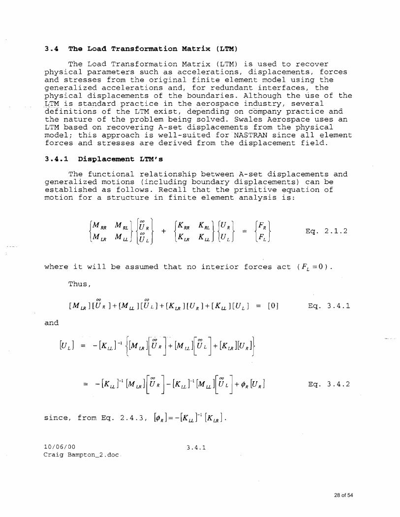
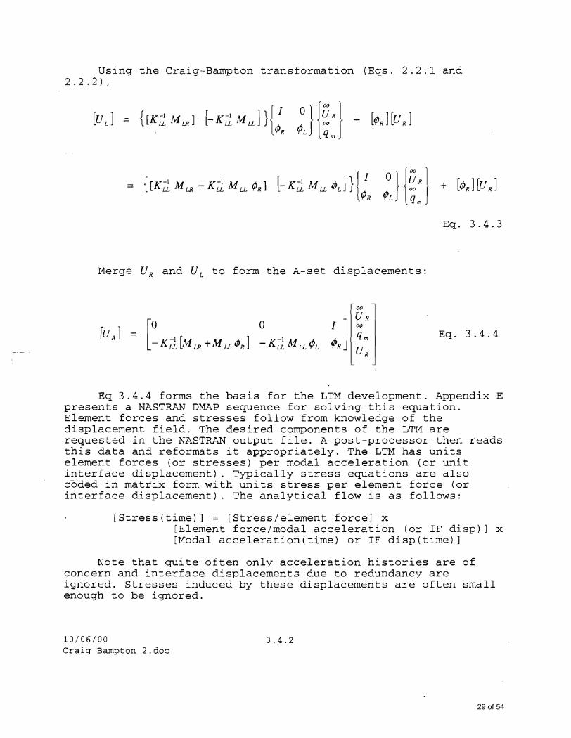
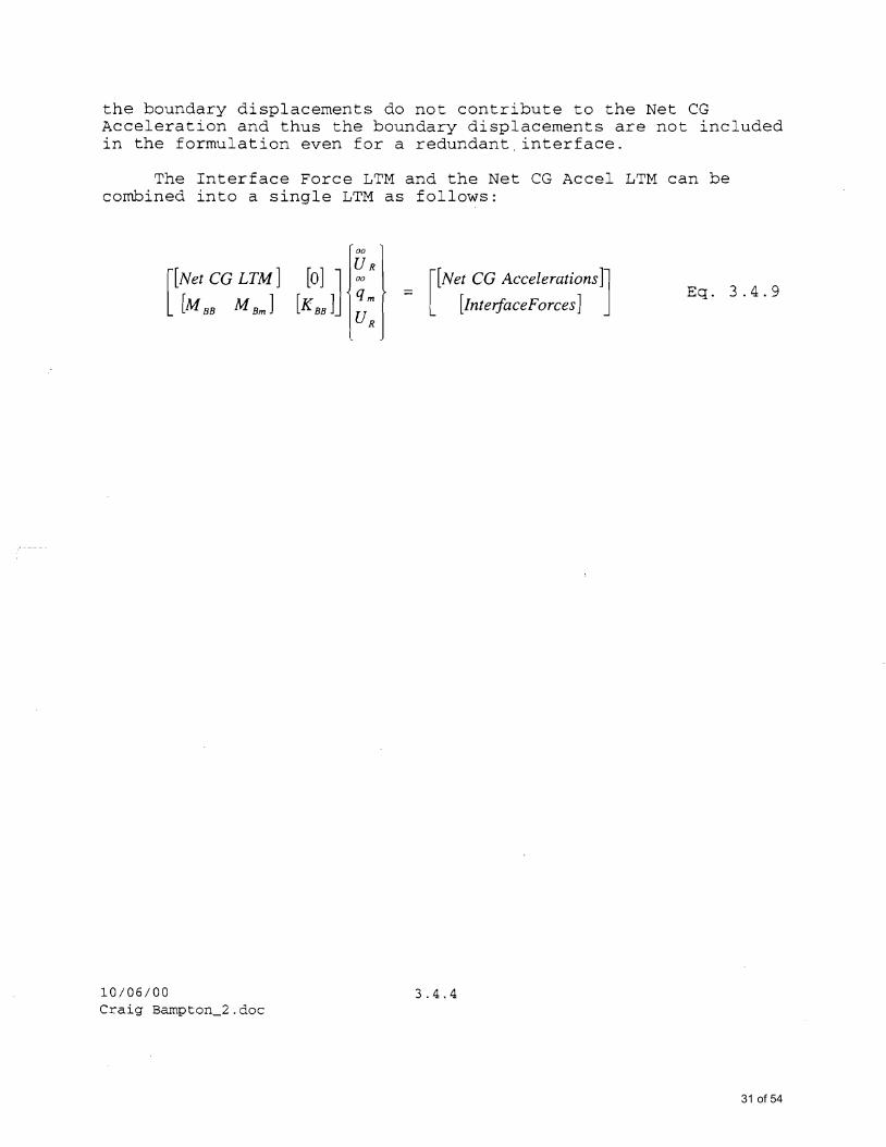
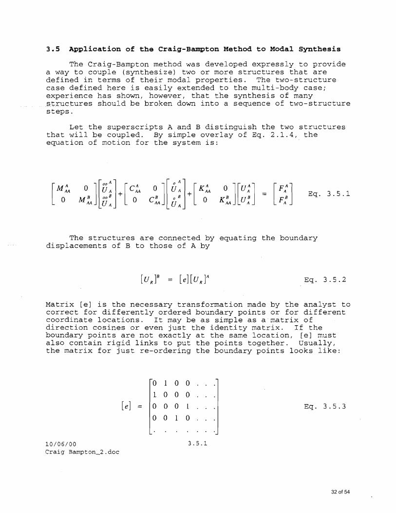
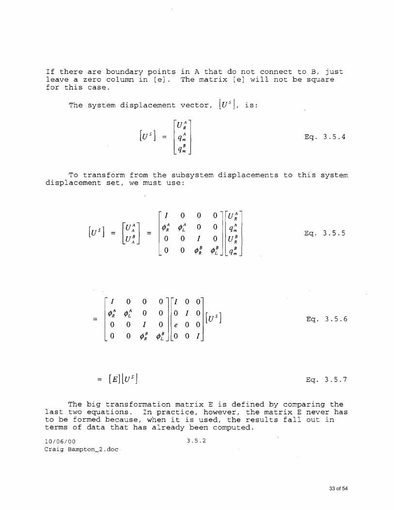
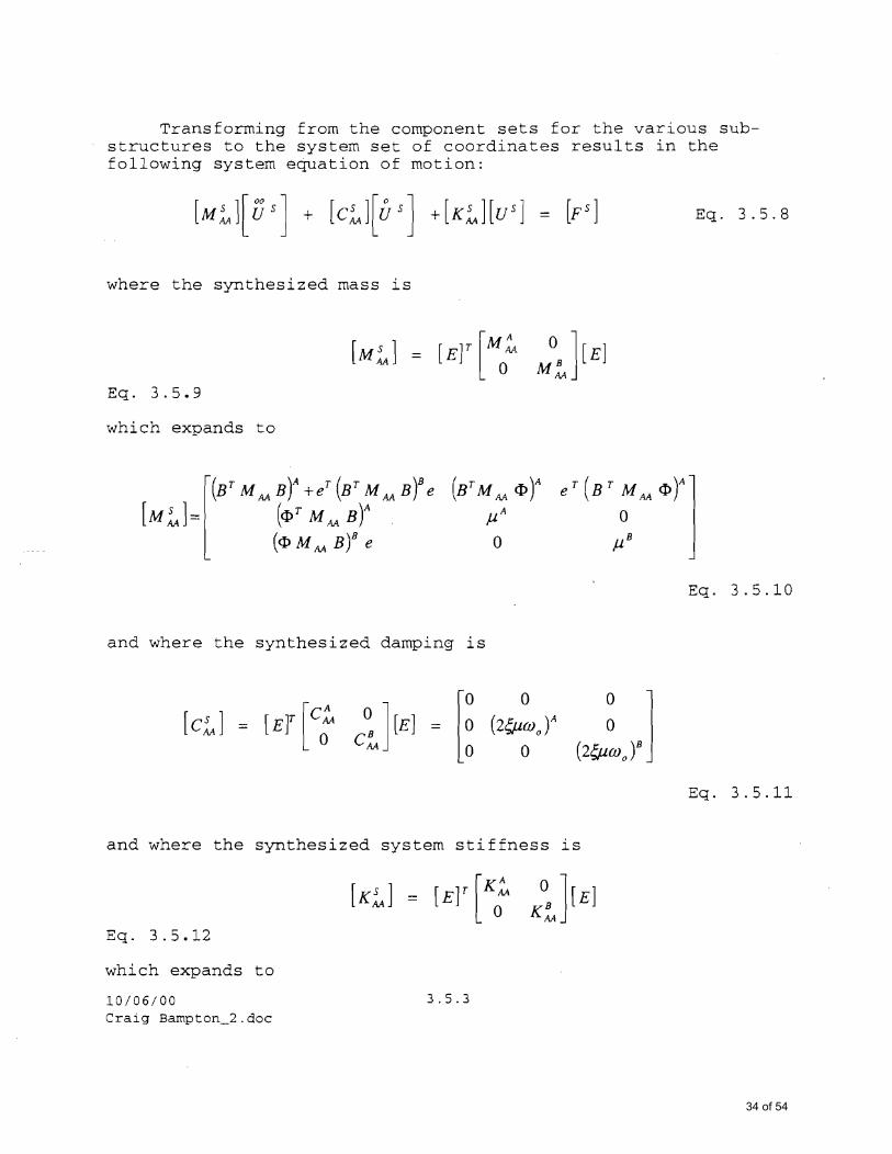
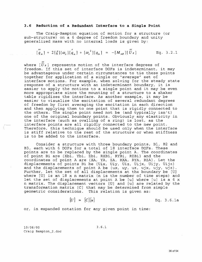
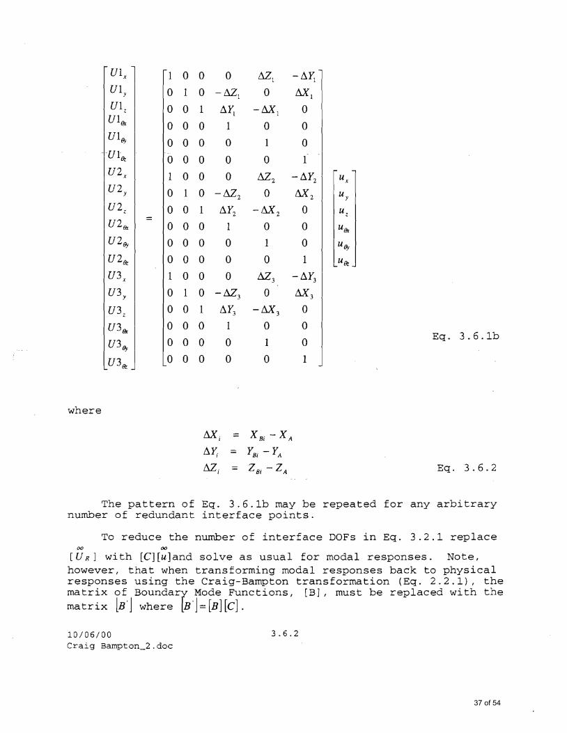
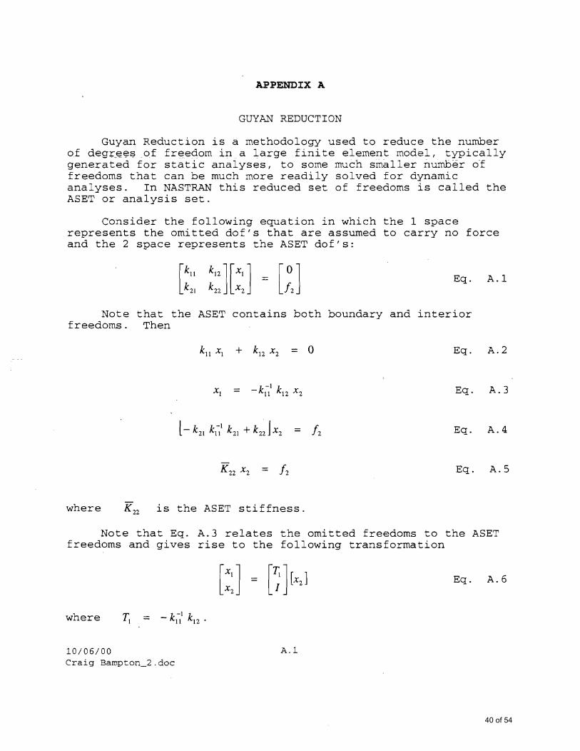
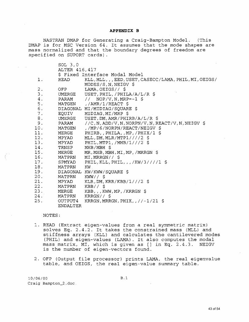
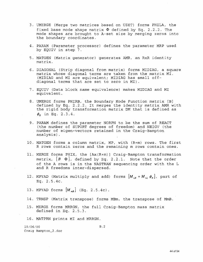
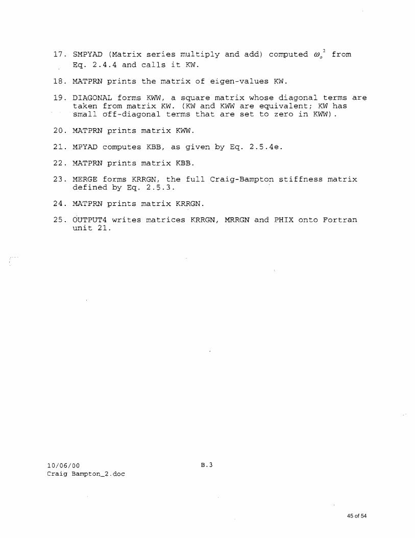
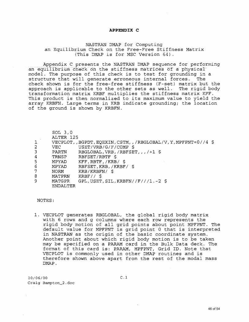
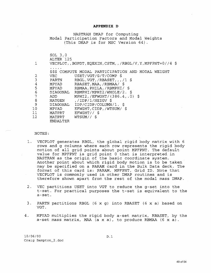
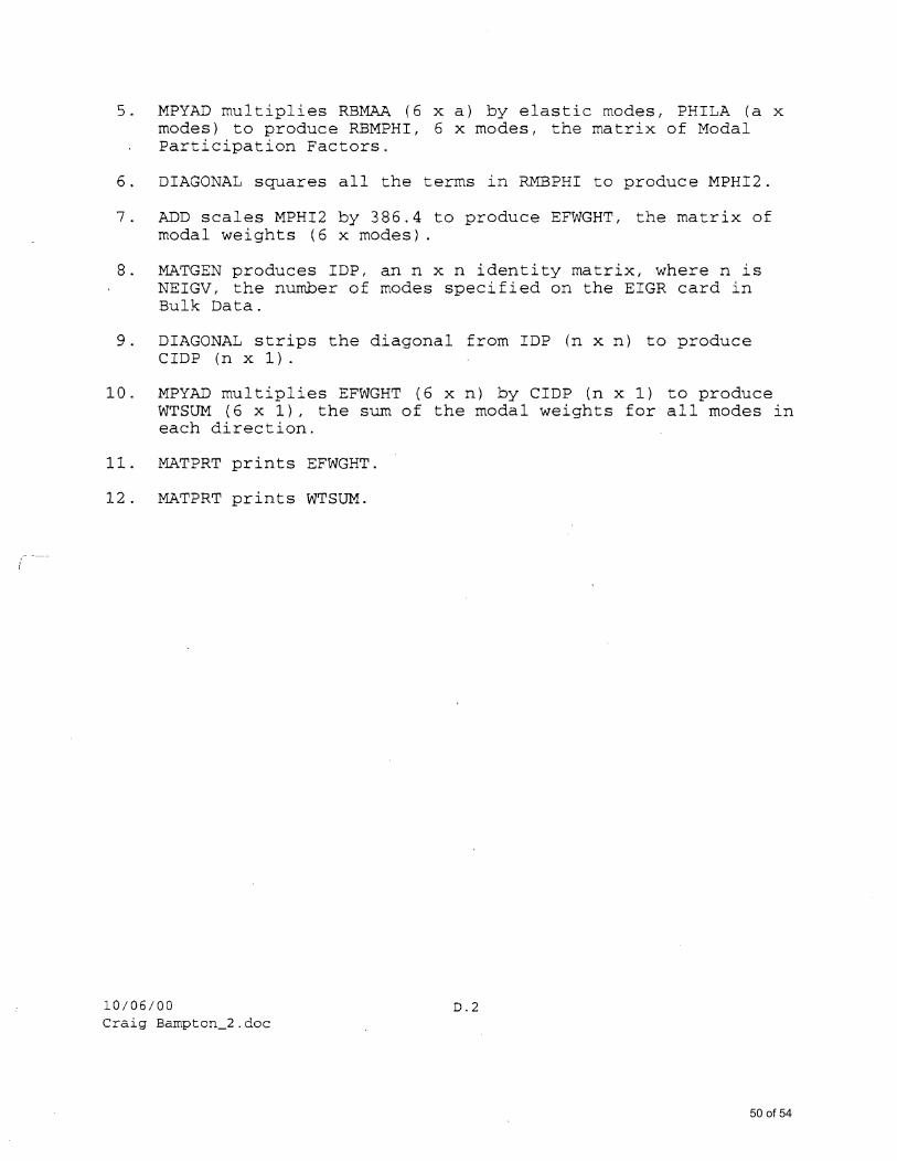
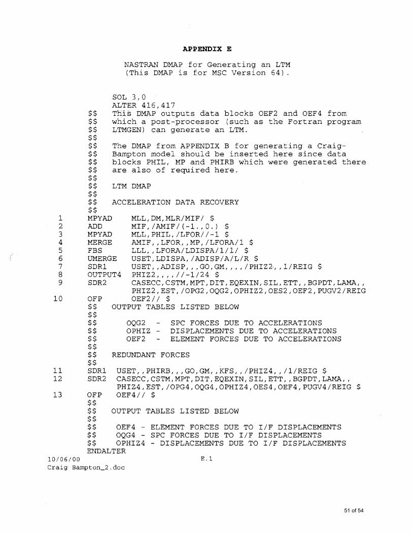

Typically a post-processor (such as the Fortran program LTMGEN) reads this file and re-formats it appropriately
100600 E4 Craig Bampton_2doc
54 of 54