i

A Cost-Benefit Assessment of Gasification-Based Biorefining in the Kraft Pulp and Paper Industry

Volume 1

Main Report

FINAL REPORT Under contract DE-FC26-04NT42260 with the U.S. Department of Energy

and with cost-sharing by the American Forest and Paper Association

21 December 2006

Eric D. Larson Princeton Environmental Institute Princeton University Princeton, NJ elarson@princeton.edu Stefano Consonni Department of Energy Engineering Politecnico di Milano Milan, Italy stefano.consonni@polimi.it Ryan E. Katofsky Navigant Consulting, Inc. Burlington, MA rkatofsky@navigantconsulting.com Kristiina Iisa and W. James Frederick, Jr. Institute of Paper Science and Technology School of Chemical and Biomolecular Engineering Georgia Institute of Technology Atlanta, GA Kristiina.Iisa@ipst.gatech.edu Jim.Frederick@ipst.gatech.edu

ii

This report consists of four volumes: Volume 1: Main Report. Volume 2: Detailed Biorefinery Design and Performance Simulation. Volume 3: Fuel Chain and National Cost-Benefit Analysis. Volume 4: Preliminary Biorefinery Analysis with Low-Temperature Black Liquor

Gasification. Note: “Navigant is a service mark of Navigant International, Inc. Navigant Consulting, Inc. (NCI) is not affiliated, associated, or in any way connected with Navigant International, Inc., and NCI’s use of “Navigant” is made under license from Navigant International, Inc.

iii

Abstract Production of liquid fuels and chemicals via gasification of kraft black liquor and woody residues (“biorefining”) has the potential to provide significant economic returns for kraft pulp and paper mills replacing Tomlinson boilers beginning in the 2010-2015 timeframe. Commercialization of gasification technologies is anticipated in this period, and synthesis gas from gasifiers can be converted into liquid fuels using catalytic synthesis technologies that are in most cases already commercially established today in the “gas-to-liquids” industry. These conclusions are supported by detailed analysis carried out in a two-year project co-funded by the American Forest and Paper Association and the Biomass Program of the U.S. Department of Energy. This work assessed the energy, environment, and economic costs and benefits of biorefineries at kraft pulp and paper mills in the United States. Seven detailed biorefinery process designs were developed for a reference freesheet pulp/paper mill in the Southeastern U.S., together with the associated mass/energy balances, air emissions estimates, and capital investment requirements. Commercial (“Nth”) plant levels of technology performance and cost were assumed. The biorefineries provide chemical recovery services and co-produce process steam for the mill, some electricity, and one of three liquid fuels: a Fischer-Tropsch synthetic crude oil (which would be refined to vehicle fuels at existing petroleum refineries), dimethyl ether (a diesel engine fuel or LPG substitute), or an ethanol-rich mixed-alcohol product. Compared to installing a new Tomlinson power/recovery system, a biorefinery would require larger capital investment. However, because the biorefinery would have higher energy efficiencies, lower air emissions, and a more diverse product slate (including transportation fuel), the internal rates of return (IRR) on the incremental capital investments would be attractive under many circumstances. For nearly all of the cases examined in the study, the IRR lies between 14% and 18%, assuming a 25-year levelized world oil price of $50/bbl – the US Department of Energy’s 2006 reference oil price projection. The IRRs would rise to as high as 35% if positive incremental environmental benefits associated with biorefinery products are monetized (e.g., if an excise tax credit for the liquid fuel is available comparable to the one that exists for ethanol in the United States today). Moreover, if future crude oil prices are higher ($78/bbl levelized price, the US Department of Energy’s 2006 high oil price scenario projection, representing an extrapolation of mid-2006 price levels), the calculated IRR exceeds 45% in some cases when environmental attributes are also monetized. In addition to the economic benefits to kraft pulp/paper producers, biorefineries widely implemented at pulp mills in the U.S. would result in nationally-significant liquid fuel production levels, petroleum savings, greenhouse gas emissions reductions, and criteria-pollutant reductions. These are quantified in this study. A fully-developed pulpmill biorefinery industry could be double or more the size of the current corn-ethanol industry in the United States in terms of annual liquid fuel production. Forest biomass resources are sufficient in the United States to sustainably support such a scale of forest biorefining in addition to the projected growth in pulp and paper production.

iv

TABLE OF CONTENTS FOR VOLUME 1 ABSTRACT .............................................................................................................................................................. III TABLE OF CONTENTS FOR VOLUME 1 .......................................................................................................... IV LIST OF TABLES IN VOLUME 1......................................................................................................................... VI LIST OF FIGURES IN VOLUME 1.................................................................................................................... VIII ACKNOWLEDGMENTS.......................................................................................................................................XII 1. INTRODUCTION ...................................................................................................................................................1

1.1 CONTEXT.....................................................................................................................................................1 1.2 SCOPE AND OBJECTIVES OF THIS STUDY .....................................................................................................3

2 SYNTHETIC FUELS CHOSEN FOR DETAILED ANALYSIS ..................................................................6 2.1 FISCHER-TROPSCH FUELS ...........................................................................................................................7 2.2 DIMETHYL ETHER .......................................................................................................................................9 2.3 ALCOHOL FUELS .......................................................................................................................................10

3 CHEMICAL RECOVERY AND POWER/STEAM COGENERATION AT PULP AND PAPER MILLS ........................................................................................................................................................................12

3.1 THE KRAFT PROCESS ................................................................................................................................12 3.2 REFERENCE KRAFT PULP/PAPER MILL FOR CASE STUDY COMPARISONS..................................................13 3.3 PREVIOUS RESULTS FOR PULP MILL POWER GENERATION .......................................................................14

3.3.1 Tomlinson Power/Recovery at the Reference Mill...............................................................................14 3.3.2 BLGCC Power/Recovery at the Reference Mill...................................................................................16

4 OVERVIEW OF BIOREFINERY DESIGNS...............................................................................................21 5 BIOREFINERY DESIGN AND PERFORMANCE SIMULATION ..........................................................26

5.1 APPROACH AND DESIGN/SIMULATION TOOLS...........................................................................................27 5.2 DESIGN AND SIMULATION OF KEY SUBSYSTEMS.......................................................................................28

5.2.1 Black Liquor Gasification Island.........................................................................................................28 5.2.2 Acid Gas Removal/Sulfur Recovery System .........................................................................................30 5.2.3 Biomass Gasification Island ................................................................................................................31 5.2.4 Gas Turbine Combined Cycle Island...................................................................................................35 5.2.5 Liquid Fuels Synthesis Island ..............................................................................................................37

5.3 TECHNOLOGY SUMMARY ..........................................................................................................................42 5.4 DETAILED BIOREFINERY MASS/ENERGY BALANCE RESULTS ...................................................................42

5.4.1 Process Flow Sheets and Performance Analysis .................................................................................42 5.4.2 Liquid fuel produced per unit of biomass input ...................................................................................56

6 “WELL-TO-WHEELS” ENVIRONMENTAL ANALYSIS........................................................................59 6.1 OVERVIEW AND APPROACH ......................................................................................................................59 6.2 WATER AND SOLID WASTE .......................................................................................................................60 6.3 MILL-RELATED AIR EMISSIONS ................................................................................................................61

6.3.1 Tomlinson Boiler Air Emissions ..........................................................................................................64 6.3.2 Gas Turbine Air Emissions ..................................................................................................................65

6.4 GRID POWER AIR EMISSIONS AND OFFSETS ..............................................................................................67 6.5 EMISSIONS FROM THE BIOREFINERY FUEL CHAIN .....................................................................................68

6.5.1 Biomass Collection and Transportation ..............................................................................................68 6.5.2 Biorefinery ...........................................................................................................................................69 6.5.3 Fuel Transportation and Distribution .................................................................................................69 6.5.4 Vehicles End Use .................................................................................................................................70 6.5.5 Fuel Blends versus Neat Fuels.............................................................................................................70

6.6 ENERGY USE AND EMISSIONS FROM CONVENTIONAL FUEL CHAINS .........................................................71 6.7 NET EMISSIONS ESTIMATES FOR THE CASE STUDY BIOREFINERY SYSTEMS .............................................71

v

6.7.1 Carbon Dioxide ...................................................................................................................................72 6.7.2 Sulfur Dioxide......................................................................................................................................73 6.7.3 Nitrogen Oxides ...................................................................................................................................74 6.7.4 Volatile Organic Compounds ..............................................................................................................74 6.7.5 Carbon Monoxide ................................................................................................................................75 6.7.6 Particulate Matter ...............................................................................................................................76 6.7.7 Total Reduced Sulfur ...........................................................................................................................76

7 BIOREFINERY CAPITAL COST ESTIMATES.........................................................................................78 7.1 APPROACH AND ASSUMPTIONS .................................................................................................................78 7.2 CAPITAL COSTS.........................................................................................................................................79

7.2.1 Specific Capital Investments per Unit of Biofuel Production ..............................................................82 7.3 EFFECTIVE LEVELIZED COST OF LIQUID FUEL PRODUCTION.....................................................................84

8 MILL-LEVEL FINANCIAL ANALYSIS......................................................................................................85 8.1 ASSUMPTIONS ...........................................................................................................................................86

8.1.1 General ................................................................................................................................................86 8.1.2 Energy Price Forecasts .......................................................................................................................87 8.1.3 Incentives and the Monetary Value of Environmental Attributes ........................................................92

8.2 RESULTS OF FINANCIAL ANALYSIS ...........................................................................................................94 8.2.1 BLGCC ................................................................................................................................................94 8.2.2 DME Results ........................................................................................................................................98 8.2.3 FT Results ..........................................................................................................................................107 8.2.4 MA (Mixed Alcohol) Results ..............................................................................................................114

8.3 SUMMARY DISCUSSION OF FINANCIAL RESULTS.....................................................................................120 9 NATIONAL IMPACTS OF A PULP MILL BIOREFINERY INDUSTRY.............................................121

9.1 MARKET PENETRATION SCENARIOS........................................................................................................121 9.2 ENERGY AND ENVIRONMENTAL IMPACTS ...............................................................................................124

9.2.1 Fossil Fuel Energy Savings ...............................................................................................................124 9.2.2 Renewable Energy Markets ...............................................................................................................127 9.2.3 National Emissions Reductions..........................................................................................................130 9.2.4 Energy Security and Fuel Diversity ...................................................................................................137 9.2.5 Economic Development .....................................................................................................................138 9.2.6 Reaping the Benefits of Government RD&D .....................................................................................139

10 CONCLUSIONS AND NEXT STEPS..........................................................................................................140 11 REFERENCES...............................................................................................................................................145

vi

List of Tables in Volume 1 Table 1. Markets and values for potential biorefinery products. ...................................................................................7 Table 2. Properties of DME, petroleum diesel, propane, and butane []. The latter two are the main constituents of

liquefied petroleum gas (LPG).................................................................................................................................9 Table 3. LPG consumption in the United States in 2004 []. ........................................................................................10 Table 4. Authors’ estimates of the number of centrally refueled urban fleet vehicles in the United States and

associated diesel fuel use, as of the mid-1990s......................................................................................................11 Table 5. Reference mill characteristics........................................................................................................................15 Table 6. Summary of key design parameter values for biorefinery simulations and, for comparison, BLGCC and

Tomlinson cases.....................................................................................................................................................22 Table 7. Assumed operating parameters for black liquor gasifier simulations ............................................................29 Table 8. Predicted raw syngas composition leaving the black liquor gasifier quench vessel. .....................................30 Table 9. Composition and heating value of hog fuel and wood waste.........................................................................33 Table 10. Key simulation assumptions for biomass gasifier/tar cracker unit. .............................................................34 Table 11. Summary of technologies included in our biorefinery designs including commercial status of each

technology..............................................................................................................................................................42 Table 12. Biorefinery performance estimates, with comparisons to Tomlinson and BLGCC. Units are megawatts

unless otherwise indicated. Fuel values are given on a lower heating value basis................................................44 Table 13. Energy efficiencies (LHV basis) for biorefineries and Tomlinson. See text for definitions.......................55 Table 14. Incremental efficiencies for biorefineries relative to Tomlinson.a...............................................................56 Table 15: Qualitative indication of relative environmental impact of different mill-level emissions, together with

relative emission rates for controlled and uncontrolled Tomlinson furnaces and with Biorefinery technology (VL = very low, L = low, M = moderate, H = high)......................................................................................................64

Table 16: Study assumptions for emissions characteristics of modern Tomlinson furnaces.a .....................................65 Table 17: Study assumptions for emissions characteristics of gas turbines burning syngas at biorefineries...............66 Table 18: Total average U.S. grid emissions (including non-fossil fuel sources) assumed in estimating grid offsets.a

...............................................................................................................................................................................68 Table 19: Correspondence between the biorefinery fuel and the fuel chain available in GREET – fuel transportation

and distribution ......................................................................................................................................................69 Table 20: Correspondence between the biorefinery fuel and the fuel chain available in GREET – vehicle end use ..70 Table 21: Biorefinery fuel and the corresponding conventional fuel chain used to estimate net emissions impacts...71 Table 22. Estimated overnight installed capital costs (thousand 2005$) and non-fuel operating and maintenance costs

(thousand 2005$ per year). Installed capital costs include engineering, equipment, installation, owner’s costs (including initial catalyst), contingencies, and spare parts.....................................................................................80

Table 23. Effective capital investment required per barrel of annual production capacity..........................................84 Table 24. Effective levelized cost of liquid fuels production at pulp mill biorefineries. .............................................85 Table 25: Summary of key input assumptions for the financial analysis.....................................................................87 Table 26: Levelized costs (in constant 2005$) for energy commodities (plant gate, no incentives). Fuel prices are on

a higher heating value basis.a .................................................................................................................................90 Table 27. Values assumed for financial incentives and monetized environmental benefits. .......................................93 Table 28. Renewable energy programs and incentives not included in the financial analysis. ...................................94 Table 29. Annual material and energy flows for the alternative power/recovery/biorefinery systems........................96 Table 30. Composition of mixed alcohol product. ....................................................................................................114 Table 31: Summary of IRR and NPV results for all cases, assuming no incentives..................................................120 Table 32: Summary of IRR and NPV results for all cases, assuming bundled incentives, including ETC, ITC, PTC,

and RECs.b ...........................................................................................................................................................121 Table 33: Summary of biorefinery market penetration scenarios developed in this study. .......................................123

vii

Table 34. Biofuel production potential (billion gal/year) for different biorefinery configurations.a These are actual volumes, not corrected for energy content, and are for the total industry. The estimates are total technical potential and do not consider any market penetration scenario. The current RFS target is 7.5 billion gallons by 2012. ....................................................................................................................................................................129

Table 35. Power production potential (MW) for different biorefinery configurations – incremental power production relative to continued use of Tomlinson technology.a ...........................................................................................131

Table 36. Cumulative market value (25 year) of certain emissions reductions relative to Tomlinson systems under the three market penetration scenarios in this study ............................................................................................140

viii

List of Figures in Volume 1 Figure 1. Primary energy use in the United States in 2004............................................................................................1 Figure 2. Future “biorefinery” concept based at a pulp and paper manufacturing facility. ...........................................2 Figure 3. Age distribution of Tomlinson recovery boilers in the United States. ...........................................................3 Figure 4. Organizational structure and principal participants in this project. ................................................................5 Figure 5. Simplified representation of kraft pulping and the associated chemical recovery cycle. Indicated mass

flows are on a dry-matter basis and intended only to be illustrative. .....................................................................13 Figure 6. Energy/mass balance for a new Tomlinson power/recovery system. ...........................................................16 Figure 7. Pressurized, oxygen-blown, high-temperature black liquor gasifier technology under development by

Chemrec. ................................................................................................................................................................17 Figure 8. Simplified schematic representation of “mill-scale” BLGCC system..........................................................19 Figure 9. Energy/mass balance for BLGCC with high-temperature gasifier and mill-scale gas turbine. ....................20 Figure 10. Schematic of biorefinery DMEa. Key features include recycling of unconverted syngas to increase DME

production and use of steam Rankine power island. ..............................................................................................23 Figure 11. Schematic of biorefinery DMEb. Key differences from DMEa (Figure 10), represented by darker shading,

include biomass gasifier and gas turbine combined cycle power island. ...............................................................24 Figure 12. Schematic of biorefinery DMEc. Key difference from DMEb (Figure 11), represented by darker shading,

include synthesis reactor operating in single-pass (rather than recycle) mode. .....................................................24 Figure 13. Schematic of biorefinery FTa. Key features of all FT designs are single-pass synthesis and gasification of

woody biomass. In FTa, the gasified biomass and unconverted syngas fuel the gas turbine combined cycle power island...........................................................................................................................................................25

Figure 14. Schematic of biorefinery FTb. The key difference compared to FTa is highlighted by the darker shading: a larger gas turbine, requiring greater woody biomass consumption.....................................................................25

Figure 15. Schematic of biorefinery FTc. Similar to FTa, except that gasified woody biomass supplements gasified black liquor flowing to the synthesis island. ..........................................................................................................26

Figure 16. Schematic of biorefinery MA. The design is similar to FTc in that syngas from both the black liquor gasifier and the biomass gasifier are processed through the synthesis reactor. MA differs from FTc in that a significant fraction of the unconverted synthesis gas is recycled for further conversion, as indicated by the more darkly-shaded blocks. ............................................................................................................................................26

Figure 17. Interactions between GS and Aspen Plus during process simulations. The black liquor gasification island is calculated first with GS. Aspen is then run twice to simulate the acid gas recovery (Rectisol) system and the fuel synthesis island. Finally, GS is re-run, taking into account the results generated by the Aspen runs. See Volume 2 for additional details..............................................................................................................................28

Figure 18. Equipment configuration for black liquor gasification...............................................................................29 Figure 19. Biomass gasification island for biorefinery designs utilizing the biomass-derived syngas as gas turbine

fuel. ........................................................................................................................................................................34 Figure 20. Biomass gasification island for biorefinery designs utilizing the biomass-derived syngas for liquid fuels

synthesis.................................................................................................................................................................35 Figure 21. General layout for the gas turbine combined cycle power island...............................................................35 Figure 22. Simplified schematic of liquid phase synthesis reactor. .............................................................................38 Figure 23. Mass and energy balance for DMEa. Key distinguishing features are the recycle synthesis loop and the

hog fuel/purchased residues boiler/steam cycle power island................................................................................45 Figure 24. Mass and energy balance for DMEb. Key distinguishing features are the recycle synthesis loop and the

hog fuel/residues gasifier gas turbine combined cycle power island. ....................................................................46 Figure 25. Mass and energy balance for DMEc. Key distinguishing features are the once-through synthesis reactor

and the hog fuel/residues gasifier gas turbine combined cycle power island.........................................................47 Figure 26. Mass and energy balance for FTa. Key distinguishing features are the once-through synthesis reactor and

the hog fuel/residues gasifier gas turbine combined cycle power island. ..............................................................48

ix

Figure 27. Mass and energy balance for FTb. Key distinguishing features are the once-through synthesis reactor and the hog fuel/residues gasifier gas turbine combined cycle power island with larger (7FA) gas turbine. ...............49

Figure 28. Mass and energy balance for FTc. Key distinguishing features are the once-through synthesis reactor fed with syngas from both black liquor and hog fuel/residues gasifiers. Unconverted syngas fuels the gas turbine combined cycle power island.................................................................................................................................50

Figure 29. Mass and energy balance for MA. Key distinguishing features are the recycle synthesis island fed with syngas from both black liquor and hog fuel/residues gasifiers. Unconverted syngas fuels the gas turbine combined cycle power island.................................................................................................................................51

Figure 30. Energy efficiencies and contribution of each output (steam, electricity, and liquid fuel) to ηfirst and to ηel

equiv..........................................................................................................................................................................55 Figure 31. Incremental biorefinery energy inputs and outputs relative to the Tomlinson case. ..................................56 Figure 32. Comparison of adjusted liquid fuel yields (gallon of gasoline equivalent or gallon of ethanol equivalent)

per metric tonne of dry biomass input. See text for discussion.............................................................................58 Figure 33. Accounting used to calculate the adjusted liquid fuel yields per unit of biomass input. ............................58 Figure 34: Well-to-Wheels Analysis Framework for Pulp and Paper Biorefineries....................................................60 Figure 35: Change in annual full fuel chain net CO2 emissions at the reference mill in 2010. ...................................73 Figure 36: Changes in annual full fuel-chain CO2 emissions and offsets at the reference mill in 2010 (million tons

per year). ................................................................................................................................................................73 Figure 37: Change in annual full fuel-chain net SO2 emissions at reference mill in 2010. .........................................74 Figure 38: Change in annual full fuel-chain net NOx emissions at the reference mill in 2010....................................75 Figure 39: Change in annual full fuel-chain net VOC emissions at the reference mill in 2010...................................75 Figure 40: Change in annual full fuel-chain net CO emissions at the reference mill in 2010. ....................................76 Figure 41: Change in annual full fuel-chain net PM10 emissions at the reference mill in 2010...................................77 Figure 42: Change in annual full fuel-chain net TRS emissions at the reference mill in 2010....................................77 Figure 43. Percentage breakdown of biorefinery investment costs. ............................................................................81 Figure 44. Effective capital investment intensity (2005$ per barrel diesel-equivalent per day) for liquid fuels

production as a function of liquids production capacity. See text for assumptions. .............................................82 Figure 45. Accounting used to calculate the capital intensity of liquid biofuel production.........................................83 Figure 46: Basic logic for the ethanol/mixed alcohol price forecast............................................................................89 Figure 47: Basic logic for the DME and FT crude price forecasts ..............................................................................89 Figure 48: Study assumptions for electricity prices.....................................................................................................91 Figure 49: Study assumptions for purchased wood, #6 oil and natural gas prices ($/MMBtu, HHV). .......................91 Figure 50: Biorefinery product prices forecasts – no incentives ($/MMBtu, HHV). ..................................................92 Figure 51: Allowable incremental capital cost for BLGCC relative to new Tomlinson to achieve different target IRR

values under the REP and TSEP scenarios. ...........................................................................................................95 Figure 52: Allowable incremental capital cost for BLGCC relative to new Tomlinson to achieve different target IRR

values with indicated biomass and power prices under our Reference Energy Price scenario and for baseline incremental capital cost estimate. ..........................................................................................................................97

Figure 53: IRR of incremental capital invested for BLGCC relative to new Tomlinson, with different environmental benefits monetized and for our Reference Energy Price (REP) scenario...............................................................98

Figure 54: Allowable incremental capital cost for DMEa biorefinery (with DME sold as vehicle fuel) relative to new Tomlinson investment for different target IRR values under our two energy price scenarios...............................99

Figure 55: IRR on incremental capital cost for DMEa biorefinery (with DME sold as vehicle fuel) relative to new Tomlinson system with indicated biomass and power prices and other energy prices as in the REP scenario......99

Figure 56: IRR on incremental capital investment in DMEa biorefinery (with DME sold as vehicle fuel) relative to a new Tomlinson system with different environmental benefits monetized under REP scenario. .........................100

Figure 57: IRR on incremental capital investment in DMEa biorefinery (with DME sold as vehicle fuel) relative to a new Tomlinson system with different environmental benefits monetized and for our TSEP scenario................100

Figure 58: Allowable incremental capital cost for DMEa biorefinery (with DME sold as LPG substitute) relative to new Tomlinson investment for different target IRR values under our two energy price scenarios. ....................101

x

Figure 59: IRR on incremental capital cost for DMEa biorefinery (with DME sold as LPG substitute) relative to new Tomlinson system with indicated biomass and power prices and other energy prices as in the REP scenario....101

Figure 60: IRR on incremental capital invested in DMEa biorefinery (with DME sold as LPG substitute) relative to new Tomlinson with environmental benefits monetized under REP scenario. ....................................................102

Figure 61: IRR on incremental capital invested in DMEa biorefinery (with DME sold as LPG substitute) relative to new Tomlinson, with environmental benefits monetized in TSEP scenario........................................................102

Figure 62: Allowable incremental capital cost for DMEb biorefinery (with DME sold as vehicle fuel) relative to new Tomlinson investment for different target IRR values under our two energy price scenarios.............................103

Figure 63: IRR on incremental capital cost for DMEb biorefinery (with DME sold as vehicle fuel) relative to new Tomlinson system with indicated biomass and power prices and other energy prices as in the REP scenario....104

Figure 64: IRR on incremental capital investment in DMEb biorefinery (with DME sold as vehicle fuel) relative to a new Tomlinson system with different environmental benefits monetized under REP scenario. .........................104

Figure 65: IRR on incremental capital investment in DMEb biorefinery (with DME sold as vehicle fuel) relative to a new Tomlinson system with different environmental benefits monetized and for our TSEP scenario................105

Figure 66: Allowable incremental capital cost for DMEc biorefinery (with DME sold as vehicle fuel) relative to new Tomlinson investment for different target IRR values under our two energy price scenarios.............................105

Figure 67: IRR on incremental capital cost for DMEc biorefinery (with DME sold as vehicle fuel) relative to new Tomlinson system with indicated biomass and power prices and other energy prices as in the REP scenario....106

Figure 68: IRR on incremental capital in DMEc biorefinery (with DME sold as vehicle fuel) relative to a new Tomlinson with different environmental benefits monetized under REP scenario..............................................106

Figure 69: IRR on incremental capital investment in DMEc biorefinery (with DME sold as vehicle fuel) relative to a new Tomlinson system with different environmental benefits monetized and for our TSEP scenario................107

Figure 70: Allowable incremental capital cost for FTa biorefinery relative to new Tomlinson investment for different target IRR values under our two energy price scenarios......................................................................................108

Figure 71: IRR on incremental capital cost for FTa biorefinery relative to new Tomlinson system with indicated biomass and power prices and other energy prices as in the REP scenario. ........................................................108

Figure 72: IRR on incremental capital investment in FTa biorefinery relative to a new Tomlinson system with different environmental benefits monetized under our REP scenario..................................................................109

Figure 73: IRR on incremental capital investment in FTa biorefinery relative to a new Tomlinson system with different environmental benefits monetized under our TSEP scenario................................................................109

Figure 74: Allowable incremental capital cost for FTb biorefinery relative to new Tomlinson investment for different target IRR values under our two energy price scenarios. ......................................................................110

Figure 75: IRR on incremental capital cost for FTb biorefinery relative to new Tomlinson system with indicated biomass and power prices and other energy prices as in the REP scenario. ........................................................110

Figure 76: IRR on incremental capital investment in FTb biorefinery relative to a new Tomlinson system with different environmental benefits monetized under our REP scenario..................................................................111

Figure 77: IRR on incremental capital investment in FTb biorefinery relative to a new Tomlinson system with different environmental benefits monetized under our TSEP scenario................................................................111

Figure 78: Allowable incremental capital cost for FTc biorefinery relative to new Tomlinson investment for different target IRR values under our two energy price scenarios......................................................................................112

Figure 79: IRR on incremental capital cost for FTc biorefinery relative to new Tomlinson system with indicated biomass and power prices and other energy prices as in the REP scenario. ........................................................112

Figure 80: IRR on incremental capital investment in FTc biorefinery relative to a new Tomlinson system with different environmental benefits monetized under our REP scenario..................................................................113

Figure 81: IRR on incremental capital investment in FTc biorefinery relative to a new Tomlinson system with different environmental benefits monetized under our TSEP scenario................................................................113

Figure 82: Allowable incremental capital cost for MA biorefinery (with MA sold as a fuel) relative to new Tomlinson investment for different target IRR values under our two energy price scenarios.............................115

Figure 83: IRR on incremental capital cost for MA biorefinery (with MA sold as fuel) with indicated biomass and power prices and other energy prices as in the REP scenario. .............................................................................116

xi

Figure 84: IRR on incremental capital investment in MA biorefinery (with MA sold as a fuel mixture) relative to a new Tomlinson system with different environmental benefits monetized under our REP scenario. ...................116

Figure 85: IRR on incremental capital investment in MA biorefinery (with MA sold as a fuel mixture) relative to a new Tomlinson system with different environmental benefits monetized under our TSEP scenario. .................117

Figure 86: Allowable incremental capital cost for MA biorefinery (with MA sold as components) relative to new Tomlinson investment for different target IRR values under our two energy price scenarios.52 .........................118

Figure 87: IRR on incremental capital cost for MA biorefinery (with MA sold as components) relative to new Tomlinson system with indicated biomass and power prices and other energy prices as in the REP scenario....118

Figure 88: IRR on incremental capital investment in MA biorefinery (with MA sold as components) relative to a new Tomlinson system with different environmental benefits monetized under our REP scenario. ...................119

Figure 89: IRR on incremental capital investment in MA biorefinery (with MA sold as components) relative to a new Tomlinson system with different environmental benefits monetized under our TSEP scenario. .................119

Figure 90: Market penetration estimates used to assess energy and environmental impacts of biorefinery implementation in the United States. ...................................................................................................................125

Figure 91: Net national fossil fuel savings relative to continued use of Tomlinson systems for the Aggressive biorefinery market penetration scenario...............................................................................................................126

Figure 92: Cumulative (25-year) national net fossil fuel savings relative to continued use of Tomlinson systems under different biorefinery market penetration scenarios. ...................................................................................127

Figure 93. Net annual national CO2 emissions reductions relative to continued use of Tomlinson systems under the Aggressive biorefinery market penetration scenario. ...........................................................................................132

Figure 94. Net annual national SO2 emissions reductions relative to continued use of Tomlinson systems under the Aggressive biorefinery market penetration scenario. ...........................................................................................133

Figure 95. Net annual national NOx emissions reductions relative to continued use of Tomlinson technology under the Aggressive biorefinery market penetration scenario. .....................................................................................134

Figure 96. Net annual national VOC emissions reductions relative to continued use of Tomlinson technology under the Aggressive biorefinery market penetration scenario. .....................................................................................134

Figure 97. Net annual national CO emissions reductions relative to continued use of Tomlinson technology under the Aggressive biorefinery market penetration scenario. .....................................................................................135

Figure 98. Net annual national PM10 emissions reductions relative to continued use of Tomlinson technology under the Aggressive biorefinery market penetration scenario. .....................................................................................136

Figure 99: Cumulative (25-year) national net fossil fuel and petroleum savings relative to continued use of Tomlinson systems under the Aggressive biorefinery market penetration scenario.............................................137

xii

Acknowledgments The authors thank Matthew Campbell and Etienne Parent (Navigant Consulting), Charles E. Courchene (Institute of Paper Science and Technology, Georgia Institute of Technology), Farminder Anand and Matthew Realff (School of Chemical and Biomolecular Engineering, Georgia Institute of Technology), Silvia Napoletano and Wang Xun (Department of Energy Engineering, School of Industrial Engineering, Politecnico di Milano), and Sheldon Kramer (Nexant Engineering) for their contributions to the analysis reported here. We also thank the Steering Committee and Resource Persons (see Figure 4 in this volume) for their suggestions and guidance throughout the project. We also thank the many other individuals who provided inputs to us in the course of this work. For primary financial support, we thank the U.S. Department of Energy Biomass Program and the American Forest and Paper Association. Additionally, support is gratefully acknowledged from the Princeton University Carbon Mitigation Initiative, the William and Flora Hewlett Foundation, and the member companies of the Institute of Paper Science and Technology (at the Georgia Institute of Technology) who have sponsored IPST's research project "Gasification and Biorefinery Development."

1

1. Introduction

1.1 Context The U.S. pulp and paper industry is the largest producer and user of biomass energy in the United States today, nearly all derived from sustainably-grown trees. Renewable resources used at pulp mills include bark, wood wastes, and black liquor, the lignin-rich by-product of cellulose-fiber extraction. The total of these biomass energy sources consumed at pulp mills in 2004 in the United States was an estimated 1.3 quads (one quad is 1015 BTU).1 Additionally, there are substantial residues that remain behind after harvesting of trees for pulpwood. A recent major study of U.S. biomass resources [1] estimates there are some 2 quads of unused wood resources (logging residues, fire-prevention thinnings, mill residues, and urban wood waste) that are recoverable on a sustainable basis at present, increasing to nearly 3 quads in the future. Additionally, the sustainable agricultural biomass resource potential (crop residues, crop processing residues, and future perennial energy crops) is estimated to be 10 to 17 quads by 2025. The sum of existing and potential biomass energy resources in the United States comes to 14 to 21 quads. For comparison, 100 quads of primary energy (all forms) were consumed in 2004 in the United States (Figure 1), about 3% of which was biomass in various forms.

Figure 1. Primary energy use in the United States in 2004.

With substantial renewable energy resources at its immediate disposal and with potentially much more extensive resources available in the long-term, the U.S. pulp and paper industry has the potential to contribute significantly to addressing climate change and U.S. energy security concerns, while also improving its global competitiveness. A key requirement for achieving these goals is the commercialization of breakthrough technologies, especially gasification, to 1 Approximately 1.0 quad of black liquor and 0.3 quads of woody residues (hog fuel) were generated and consumed in the U.S. paper industry in 2004 (based on estimates from the American Forest and Paper Association).

Natural Gas22.9%

Petroleum39.8%

Other6.1%

Biomass2.8%

Hydropower2.7%

Geothermal Energy0.3%

Nuclear8.2%

Coal and Coke23.0%

Wind Energy0.1%

Solar Energy0.1%

1. Included in biomass are the following: black liquor, wood/wood waste liquids, wood/wood waste solids, municipal solid waste (MSW), landfill gas, agriculture byproducts/crops, sludge waste, tires, alcohol fuels (primarily ethanol derived from corn and blended into motor gasoline) and other biomass solids, liquids and gases.

Source: DOE/EIA Renewable Energy Trends 2004, August 2005.Note: 1 Quad = 1015 Btu (1 quadrillion Btu) or about 1.055 Exajoules (1018 Joules), the amount of energy contained in about 172 million barrels of oil.

Total = 100.3 Quads Total = 6.1 Quads(Biomass1 = 2.8 Quads)

2

enable the clean and efficient conversion of biomass to useful energy forms, including electricity and transportation fuels. Gasification technology enables low-quality solid fuels like biomass to be converted with low pollution into a fuel gas (synthesis gas or “syngas”) consisting largely of hydrogen (H2) and carbon monoxide (CO). Syngas can be burned cleanly and efficiently in a gas turbine to generate electricity. It can be passed over appropriate catalysts to synthesize clean liquid transportation fuels or chemicals. It can also be converted efficiently into pure H2 fuel. While most pulp and paper manufacturing facilities in the United States today do not export electricity and none export transportation fuels, their established infrastructure for collecting and processing biomass resources provides a strong foundation for future gasification-based “biorefineries” that might produce a variety of renewable fuels, electricity, and chemicals in conjunction with pulp and paper products (Figure 2).

Wood ProductsPulpPaper

Steam,Power &Chemicals

Black liquor, wood residuals

Manufacturing

ExportSynthetic gasLiquid FuelsChemicalsComposites

Future Biorefinery

CO2

O2

CO2

Black liquor gasifierWood residuals gasifierGas turbine combined cycleFuel cell power plantFuels, chemicals synthesis

Wood ProductsPulpPaper

Steam,Power &Chemicals

Black liquor, wood residuals

Manufacturing

ExportSynthetic gasLiquid FuelsChemicalsComposites

Future Biorefinery

CO2

O2O2

CO2

Black liquor gasifierWood residuals gasifierGas turbine combined cycleFuel cell power plantFuels, chemicals synthesis

Figure 2. Future “biorefinery” concept based at a pulp and paper manufacturing facility.

If the biomass resources from which energy carriers are produced at such biorefineries are sustainably grown and harvested, there would be few net lifecycle emissions of CO2 associated with biorefineries and their products. To the extent that the biorefinery products replace fuels or chemicals that would otherwise have come from fossil fuels, there would be net reductions in CO2 emissions from the energy system as a whole. The reductions would be even more significant if by-product CO2 generated at biorefineries were to be captured and sent for long-term underground storage [2]. Carbon capture and storage with fossil fuels is of wide interest today [3]. Several large-scale CO2 storage projects (storing >1 million tonnes/year of CO2) are operating and more are under development worldwide to demonstrate feasibility.

3

Coupled with the potential to address national energy security and global warming concerns is the looming need in the U.S. pulp and paper industry for major capital investments to replace the aging fleet of Tomlinson recovery boilers used today to recover energy and pulping chemicals from black liquor. The majority of Tomlinson boilers operating in the United States were built beginning in the late 1960s through the 1970s (Figure 3). With serviceable lifetimes of 30 to 40 years, the Tomlinson fleet began undergoing a wave of life-extension rebuilds in the mid-1980s (Figure 3). Within the next 10 to 20 years, rebuilt boilers will be approaching the age at which they will need to be replaced, the capital investment for which at a typical mill is between $100 and $200 million. A similar situation exists in the European pulp industry [4]. This situation provides an unusual window of economic opportunity for introducing black liquor gasifiers as replacements for Tomlinson boilers. Concerted efforts are ongoing in the United States and Sweden to develop commercial black liquor gasification technologies.

Year Built / Rebuilt

0

2

4

6

8

10

12

14

16

18

20

1938

1947

1949

1951

1953

1955

1957

1959

1961

1963

1965

1967

1969

1971

1973

1975

1977

1979

1981

1983

1985

1987

1989

1991

1993

1995

1997

START-UPS RE-BUILDS

Figure 3. Age distribution of Tomlinson recovery boilers in the United States.

1.2 Scope and Objectives of this Study This report describes the results of a two-year effort to examine the prospective technical viability, commercial viability, and environmental and energy impacts locally and nationally of gasification-based biorefineries for liquid fuels production at kraft pulp and paper mills. One key objective of this study is to assess the prospective commercial viability of gasification technology in the long term. For this reason, the analysis in this study assumes that black liquor

4

gasification systems are at a comparable level of technological maturity as Tomlinson black liquor boiler systems. In particular, the commercial risk of installing a black liquor gasification system is assumed to be comparable to that of installing a Tomlinson system in the post-2010 time frame. The implicit assumption is that in the years between the present and the post-2010 time period, research, development, and demonstration work with black liquor gasification technology will bring it to the point where its commercial reliability approaches that of Tomlinson technology. Our biorefinery analysis began by identifying three biorefinery liquid products for detailed analysis. Detailed process design and simulation were then pursued for alternative configurations for the manufacture of these products assuming projected commercial (Nth plant) performance. Detailed mass and energy balances for each configuration were then reviewed with engineers at Nexant, the A&E firm that subsequently developed “Nth plant” capital cost estimates for each process design. A detailed internal rate of return analysis was carried out for each process design, both without and with the assumption that some renewable-energy financial incentives are available. The mill-level energy and environmental performance results were used as a basis for estimating potential national energy/environment impacts under alternative assumptions about the rate at which existing Tomlinson systems would be retired and replaced with biorefineries. The study described in this report has been built on the foundation of an earlier major study examining the potential for black liquor gasification combined cycle (BLGCC) electricity generation at U.S. kraft pulp and paper mills [5]. To facilitate comparisons with the BLGCC results, we have taken care to maintain as much consistency as possible between the two studies: • The reference pulp and paper mill used as the basis for the BLGCC analysis has been

adopted directly for this biorefinery study. The reference pulp and paper mill represents the expected state-of-the-art mill in the 2010 time frame in the Southeastern United States, where 2/3 of kraft pulp mill capacity is located. The reference mill produces uncoated freesheet paper, generating a nominal 6 million lbs/day of black liquor solids (BLS). Pulp mills at this scale or larger account for about 1/3 of all U.S. capacity today, and this fraction is expected to grow over time as mill consolidations continue.

• The core process design/simulation tool and, where appropriate, the equipment performance assumptions used for the biorefinery analysis are the same as used for the BLGCC analysis.

• The same engineering firm that was engaged to develop capital cost estimates for the BLGCC analysis was engaged to provide biorefinery capital cost estimates.

• The biorefinery cost-benefit analysis adopts, to the extent possible, the same financial and emissions model and parameter values as for the BLGCC analysis. However, in making comparisons of energy and environmental costs/benefits between the Tomlinson, BLGCC and biorefinery cases, we use the most recently available DOE forecasts for energy prices, fuel mix assumptions for power generation, and emissions factors for power generation, as detailed later in this report and in Volume 3. The forecast prices, fuel mixes, and emissions factors are different from those used in the BLGCC study [5], but the results from the BLGCC study shown later in this report are updated results using the same forecasts as used for the biorefinery cases.

5

• Finally, The biorefinery analysis has been carried out with guidance from an industry-government Steering Group (Figure 4), several members of which were also part of the BLGCC Steering Committee.

Analytical TeamEric Larson – Princeton UniversityRyan Katofsky, Matthew Campbell – Navigant ConsultingStefano Consonni, Silvia Napoletano – Politecnico di MilanoKristiina Iisa – IPST/Georgia TechJim Frederick – IPST/Georgia Tech

Additional Resource PersonsRon Reinsfelder – Shell Global SolutionsGord Homer – Air Liquide

Steering CommitteeCraig Brown/Del Raymond – WeyerhaeuserTheo Fleisch/Mike Gradassi – BP Paul Grabowski – U.S. Department of EnergyJennifer Holmgren – UOPTom Johnson – Southern Company Mike Pacheco - NRELSteve Kelley – North Carolina State UniversityLori Perine – American Forest & Paper Assoc.David Turpin – MeadWestvaco

Analytical TeamEric Larson – Princeton UniversityRyan Katofsky, Matthew Campbell – Navigant ConsultingStefano Consonni, Silvia Napoletano – Politecnico di MilanoKristiina Iisa – IPST/Georgia TechJim Frederick – IPST/Georgia Tech

Additional Resource PersonsRon Reinsfelder – Shell Global SolutionsGord Homer – Air Liquide

Steering CommitteeCraig Brown/Del Raymond – WeyerhaeuserTheo Fleisch/Mike Gradassi – BP Paul Grabowski – U.S. Department of EnergyJennifer Holmgren – UOPTom Johnson – Southern Company Mike Pacheco - NRELSteve Kelley – North Carolina State UniversityLori Perine – American Forest & Paper Assoc.David Turpin – MeadWestvaco

Figure 4. Organizational structure and principal participants in this project.

While consistency has been maintained to the extent possible between the BLGCC and biorefinery analyses, there are also key differences in the fundamental design approaches: • In the BLGCC analysis a key design criterion for the energy/chemical recovery area was

maximizing electricity production while providing all of the mill’s process steam needs. The biorefinery study recognizes the broader “breakthrough” nature of the gasification technology platform insofar as it can enable the production of high-value chemicals and/or transportation fuels in addition to or instead of electricity. The biorefinery designs maintain the constraint that pulp mill process steam demands are met, but focus on maximizing liquid fuels production or optimizing fuels and electricity co-production. In some cases, this results in the need for imports of electricity to satisfy mill process needs.

• The BLGCC analysis considered some use of natural gas (a non-renewable resource) as a supplemental fuel. The biorefinery analysis considers that only renewable biomass fuels (black liquor and woody residues) are used as feedstock, making the biorefinery products essentially fully renewable.

• The BLGCC analysis assumed that only a relatively modest level of woody residue is available as energy feedstock at the mill – a level much lower than potentially available at

6

many existing mills, as suggested by the recent “billion ton study” [1]. The biorefinery analysis assumes that larger quantities of forest-based residues are available in some cases. In the longer term, non-forest biomass (e.g., short rotation woody crops or perennial grasses) might augment forest-based biomass as feedstock for still larger-scale pulpmill biorefineries.

• The BLGCC analysis assumed that woody biomass residues would be burned in boilers to augment steam generation. The biorefinery analysis aims to maximize the capability to produce liquid fuels. Toward this end, the biomass residues used in all of the biorefinery designs except one are gasified to produce additional syngas rather than being burned to make steam. The potential exists in these cases to convert this syngas into liquid fuel.

• Finally, the BLGCC designs included ones using a high-temperature black liquor gasifier and one using a low-temperature black liquor gasifier in order to help assess the relative costs and benefits between the two gasifier designs. Because the high-temperature design showed more favorable performance and cost results in the BLGCC application, this gasifier design was selected for use in all of the detailed biorefinery analysis here. (A scoping study for low-temperature black liquor gasification, as reported in Volume 4 of this study, suggests that the low-temperature technology might be best suited for applications other than the biorefinery concepts examined in detail in this volume.) The focus on high-temperature black liquor gasification for detailed analysis enabled a broader set of process configurations and biorefinery products to be examined using the limited resources available for the project.

2 Synthetic Fuels Chosen for Detailed Analysis A wide variety of liquid fuels or chemicals can be made from synthesis gas [6,7]. A screening analysis was undertaken to help identify the products to be included for detailed analysis in this study. Potential domestic market size in the near-to-medium term and potential for enhancing domestic energy security were key screening criteria. Table 1 lists consumption and price levels of various fuels and bulk chemicals in the United States today. Among those listed, only ethanol and natural gas are not derived primarily from petroleum today in the United States. While the natural gas market today is large, with relatively high gas prices, a decision was made early in the project to limit the analysis to products with the potential for displacing petroleum directly. Among the other products in the table, fuels markets are substantially larger than chemicals markets, both in physical and monetary terms. Given the large potential size of a pulp mill-based biorefining industry, a further decision was made to focus the biorefinery analysis on liquid fuel products rather than on chemicals. In future actual biorefinery implementations where markets for higher-value products (e.g., chemicals) are accessible to a particular biorefiner, financial performance may be better than the results found in this work focusing on fuel products. The focus here on petroleum and transportation is also consistent with the DOE’s strategic objective of reducing dependence on imported oil. We chose not to examine hydrogen as a fuel product, because in the near-to-medium term, hydrogen is unlikely to play any significant commercial role as a transportation fuel. Three liquid fuel products were chosen for detailed analysis: Fischer-Tropsch liquids (FTL), dimethyl ether (DME), and mixed alcohols (MA). Each of these products and the current status of their production globally are discussed next.

7

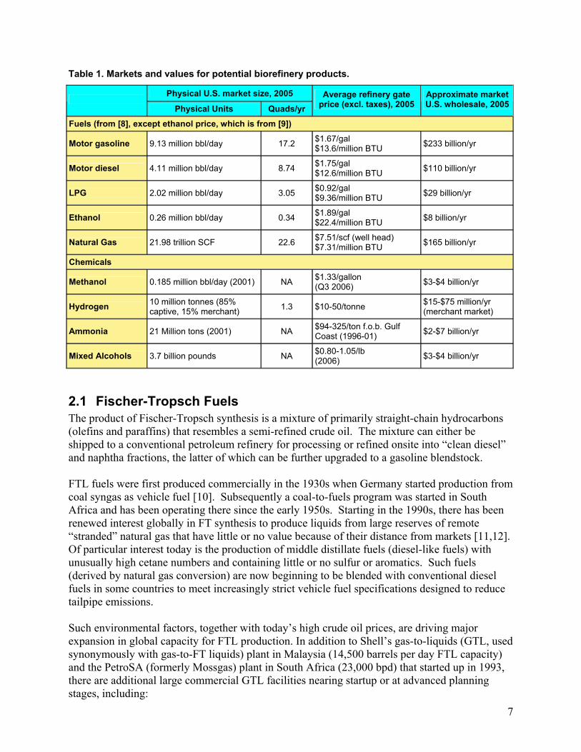
Table 1. Markets and values for potential biorefinery products.

Physical U.S. market size, 2005

Physical Units Quads/yr Average refinery gate

price (excl. taxes), 2005 Approximate market U.S. wholesale, 2005

Fuels (from [8], except ethanol price, which is from [9])

Motor gasoline 9.13 million bbl/day 17.2 $1.67/gal $13.6/million BTU $233 billion/yr

Motor diesel 4.11 million bbl/day 8.74 $1.75/gal $12.6/million BTU $110 billion/yr

LPG 2.02 million bbl/day 3.05 $0.92/gal $9.36/million BTU $29 billion/yr

Ethanol 0.26 million bbl/day 0.34 $1.89/gal $22.4/million BTU $8 billion/yr

Natural Gas 21.98 trillion SCF 22.6 $7.51/scf (well head) $7.31/million BTU $165 billion/yr

Chemicals

Methanol 0.185 million bbl/day (2001) NA $1.33/gallon (Q3 2006) $3-$4 billion/yr

Hydrogen 10 million tonnes (85% captive, 15% merchant) 1.3 $10-50/tonne $15-$75 million/yr

(merchant market)

Ammonia 21 Million tons (2001) NA $94-325/ton f.o.b. Gulf Coast (1996-01) $2-$7 billion/yr

Mixed Alcohols 3.7 billion pounds NA $0.80-1.05/lb (2006) $3-$4 billion/yr

2.1 Fischer-Tropsch Fuels The product of Fischer-Tropsch synthesis is a mixture of primarily straight-chain hydrocarbons (olefins and paraffins) that resembles a semi-refined crude oil. The mixture can either be shipped to a conventional petroleum refinery for processing or refined onsite into “clean diesel” and naphtha fractions, the latter of which can be further upgraded to a gasoline blendstock. FTL fuels were first produced commercially in the 1930s when Germany started production from coal syngas as vehicle fuel [10]. Subsequently a coal-to-fuels program was started in South Africa and has been operating there since the early 1950s. Starting in the 1990s, there has been renewed interest globally in FT synthesis to produce liquids from large reserves of remote “stranded” natural gas that have little or no value because of their distance from markets [11,12]. Of particular interest today is the production of middle distillate fuels (diesel-like fuels) with unusually high cetane numbers and containing little or no sulfur or aromatics. Such fuels (derived by natural gas conversion) are now beginning to be blended with conventional diesel fuels in some countries to meet increasingly strict vehicle fuel specifications designed to reduce tailpipe emissions. Such environmental factors, together with today’s high crude oil prices, are driving major expansion in global capacity for FTL production. In addition to Shell’s gas-to-liquids (GTL, used synonymously with gas-to-FT liquids) plant in Malaysia (14,500 barrels per day FTL capacity) and the PetroSA (formerly Mossgas) plant in South Africa (23,000 bpd) that started up in 1993, there are additional large commercial GTL facilities nearing startup or at advanced planning stages, including:

8

• 34,000 barrels per day (bpd) project of Qatar Petroleum that will use Sasol FT synthesis

technology and is slated to come on line in 2006. • 66,000 bpd expansion of the Qatar Petroleum project to startup in 2009. • 34,000 bpd Chevron project in Nigeria, also using Sasol FT technology, expected on line in

2009. • 30,000 bpd BP project in Colombia using BP’s FT synthesis technology to come on line in

2011. • 36,000 bpd project in Algeria to come on line in 2011. • 140,000 bpd Shell project in Qatar using Shell’s FT technology; to come on line in two

phases in 2009 and 2011. • 154,000 bpd ExxonMobil project in Qatar using ExxonMobil FT technology; to come on line

in 2011 There is also a growing resurgence of interest in FT fuels from gasified coal. Coal-based FT fuel production was commercialized beginning with the Sasol I, II, and III plants (175,000 b/d total capacity) built between 1956 and 1982 in South Africa. (Sasol I is now retired). China’s first commercial coal-FT project is under construction in Inner Mongolia. The plant is slated to produce 20,000 bpd when it comes on line in 2007. China has also signed a letter of intent with Sasol for two coal-FT plants that will produce together 120,000 bpd. The U.S. Department of Energy is cost-sharing a $0.6 billion demonstration project in Gilberton, Pennsylvania, that will make 5,000 bpd of FT liquids and 41 MWe of electricity from coal wastes. Also, there are proposals for 33,000 bpd and 57,000 bpd facilities for FT fuels production from coal in the state of Wyoming and for a comparable project in Southeastern Montana. The process for converting biomass into FT liquids is similar in many respects to that for converting coal. Preliminary technical/economic analyses on biomass conversion were published by Larson and Jin [13,14]. More recently, there have been several detailed technical and economic assessments published [15,16,17,18,19,20]. A preliminary study of FT fuels from black liquor has also recently been completed [4]. There is considerable current interest in Europe in production of FT fuels from biomass, motivated in part by large financial incentives. For example, in the UK a 20 pence per liter ($1.40/gal) incentive for biomass-derived diesel fuel has been in place since July 2002. Incentives are also in place in Germany, Spain, and Sweden. Such incentives have been introduced in part as a result of European Union Directive 2003/30/EC, which recommends that all member states have 2% of all petrol and diesel consumption (on an energy basis) be from biofuels or other renewable fuels by the end of 2005, reaching 5.75% by the end of 2010. The Shell Oil Company, which offers one of the leading commercial entrained-flow coal gasifiers and also has long commercial experience with FT synthesis, recently announced a partnership with Choren, a German company with a biomass gasification system, with plans for constructing a commercial biomass to FT liquids facility in Germany [21,22,23]. A “beta” plant, with a production capacity of 15,000 tonnes per year of FT diesel is currently under construction in Freiberg/Saxonia. The scale of most coal and natural gas FT projects today is far larger than could be supported by syngas from biomass feedstocks potentially available at a typical pulp mill biorefinery. Most prior biomass FTL analyses have used cost estimates scaled from such large-scale systems. However, smaller, modular, FTL reactors have been under development by several companies (Rentech, Syntroleum, BP) and are now commercially available [24]. This development has

9

been driven by an interest in monetizing the hundreds of smaller pockets of stranded gas, as well as by an interest in increasing factory production of components over field fabrication to reduce costs of even large installations. Such technology development is of direct interest for pulp mill biorefinery applications.

2.2 Dimethyl Ether Dimethyl ether (DME) is a colorless gas at ambient temperature and pressure, with a slight ethereal odor. It liquefies under slight pressure, much like propane. It is relatively inert, non-corrosive, non-carcinogenic, almost non-toxic, and does not form peroxides by prolonged exposure to air [25]. Today, DME is used primarily as an aerosol propellant in hair sprays and other personal care products, but its physical properties (Table 2) make it a suitable substitute (or blending agent) for liquefied petroleum gas (LPG, a mixture of propane and butane). It is also an excellent diesel engine fuel due to its high cetane number and absence of soot production during combustion. Table 2. Properties of DME, petroleum diesel, propane, and butane [26]. The latter two are the main constituents of liquefied petroleum gas (LPG).

Property DME Diesel Propane Butane Cetane number 55-60 40-55 na na Vapor Pressure @ 20 deg C [bar] 5.1 < 1 8.4 2.1 Liquid density @ 20 deg C [kg/m3] 668 840 501 610 Lower Heating Value [MJ/kg] 28.4 43.0 46.4 45.7

Until recently, DME was being produced globally at a rate of only about 150,000 tons per year [27]. This level is now increasing dramatically [28,29]. From 2003 through 2006, a total of 265,000 t/yr of DME production capacity (110,000 of which is from natural gas and the rest from coal) came on line in China. An additional 2.6 million t/yr of capacity (from coal) is expected to come on line there by 2009, and plans are being developed for a further one million t/yr of capacity. In Iran, a gas to DME facility producing 800,000 tons per year will come on line in 2008. There is also discussion of a facility to be built in Australia (with Japanese investment) to produce between one and two million tonnes per year of DME from natural gas. Thus by the end of this decade, DME production capacity globally may reach between 3.8 and 6.8 million t/yr, which would represent a 25 to 45 fold increase compared to the beginning of the decade. Essentially all new DME produced this decade will be used as an LPG substitute for domestic (household) fuel. In China, however, some DME will also be used in buses, initially in Shanghai and subsequently elsewhere. Commercial development of DME buses is underway in China, and volume production is anticipated before the end of this decade [29]. Development of heavy-duty vehicles (trucks and buses) fueled with DME is also underway in Sweden by Volvo, who expects to have 30 vehicles in field tests starting no later than 2009 [30] and commercial vehicles available by 2011 [31]. Major efforts in Japan are also ongoing to commercialize heavy duty DME road vehicles [32]. Volvo anticipates that biomass-derived DME will be available in the 2010 time frame from a commercial project to be established in Sweden, building on experiences at the Värnamo [33] and Piteå [34] pilot plant facilities. Two potential near-term markets for DME in the United States are as a blending agent in LPG and as a dedicated fuel for centrally refueled urban fleet vehicles. DME can be used as a substitute for LPG in stationary combustion applications, e.g., home heating, but the difference in calorific values between LPG and DME would necessitate changes to the burners and related

10

equipment if DME were to be used as a complete replacement for LPG. However, mixtures of DME and LPG can be used with combustion equipment designed for LPG without changes to the equipment, if the DME blending level is limited to 15-25% by volume [35,36]. Thus, DME as a blendstock for LPG provides an immediate market opportunity – one recognized by the World LP Gas Association [37]. Considering that the total market for LPG fuel in the United States is approximately one quad today (Table 3), the blending market for DME is about 0.2 quads, which is large enough to absorb the DME that could be produced by tens of pulp mill biorefineries. Table 3. LPG consumption in the United States in 2004 [38]. Thousand Metric Tonnes [quads] Fuel Feedstock Total Residential 14,843 [0.705] 0 14,843 [0.705] Agricultural 2,425 [0.115] 0 2,425 [0.115] Industrial 3,929 [0.187] 31,180 [1.482] 35,109 [1.669] Transport 740 [0.035] 0 740 [0.035] Total 21,937 [1.042] 31,180 [1.482] 53,117 [2.524] Note: Conversion from tonnes to quads assumes 47.5 MBTU/metric tonne lower heating value (for 60/40 butane/propane mix).] A second promising market for DME in the United States is as a fuel for compression ignition engine vehicles, an application being pursued in China, Sweden, and Japan, among other countries. It is not feasible to blend DME with conventional diesel fuel in existing engines, because DME must be stored under mild pressure to maintain a liquid state. However, because DME burns extremely cleanly in an appropriately designed compression ignition engine, an attractive application is in compression ignition vehicles operating in urban areas, where vehicle air pollution is most severe. Because vehicle refueling station equipment differs from that at conventional refueling stations dispensing petroleum-derived fuels, and modified on-board fueling systems are required, fleet vehicles that are centrally-maintained and centrally fueled (buses, delivery trucks, etc.) are a logical initial target market. Since many such vehicles operate in urban areas with petroleum diesel fuel today, the dramatically lower exhaust emissions with DME engines compared to diesel engines (especially of health-damaging small particles) [32,39] provides strong public motivation for adopting DME fleets. The estimated number of centrally fueled fleet vehicles in the United States provides a significant potential market for pulp mill biorefiners producing DME (Table 4).

2.3 Alcohol Fuels Two alcohol fuels are drawing attention in the United States at present. One is ethanol, the qualities of which as a vehicle fuel are relatively well known. A second potential fuel is a mixture of alcohols that includes a significant fraction of ethanol plus smaller fractions of several higher alcohols. Mixed-alcohol fuels have the potential to be used much the way ethanol is today for blending with gasoline, or higher alcohols can be separated from the ethanol fraction and sold for chemical use. The United States ranks as the largest producer of fuel ethanol in the world today (4 billion gallons in 2005 [40]). In the United States ethanol is used primarily for blending in gasoline as an oxygenate and an octane booster (at a blending rate of up to 10% by volume), and such blends can be used in gasoline engine vehicles without modification. Higher blends (up to about 25% ethanol, as found in Brazil) are feasible with only minor engine modifications. Flexible-fuel vehicles (FFVs), which are designed to use fuel with anywhere from zero to 85% ethanol (E85),

11

require some additional minor modifications, and are growing in number in the United States. The number of retail service stations in the United States offering E85 fuel tripled between 2004 to 2005 to a total of 650 [40]. Table 4. Authors’ estimates of the number of centrally refueled urban fleet vehicles in the United States and associated diesel fuel use, as of the mid-1990s.

Vehicle type Total number (thousands)

Centrally refueled (thousands)

Annual diesel use* million gal/y [quads/yr]

DME Million t/yr

Total of below 3 types 4,718 3,845 6,329 [0.922] 35 Urban transit buses 76 74 656 [0.096] 4 School buses 458 426 913 [0.133] 5 Light/delivery trucks 4,184 3,345 4,760 [0.693] 26 * Assuming 3.6 miles per gallon and 31,932 miles/yr for urban transit buses; 7.0 mpg and 15,000 mi/yr for school buses; and 17.6 mpg and 24,960 mi/yr for light/delivery trucks. Mixtures of alcohols have not been used commercially as a fuel in the United States or other countries. Higher alcohols are characterized by higher volumetric energy densities and lower vapor pressures than ethanol and these features make them more attractive as fuels or blending agents. A major private sector effort was recently announced to commercialize biomass-derived butanol as a gasoline blending agent [41]. All ethanol (and the proposed commercial butanol fuel) in the United States is produced by biological processing of primarily corn and also some sweet sorghum, both relatively expensive feedstocks. Development efforts to enable effective conversion of lower-cost feedstocks are ongoing. Most such efforts are focusing on biological routes for converting lignocellulosic feedstocks such as corn stover, wood residues, and energy crops like switchgrass. Such biological routes typically involve parallel or sequential processes to extract carbohydrate sugars from the cellulose and hemicelluose components of the feedstock and to ferment these sugars to ethanol. The lignin portion of the biomass is not amenable to fermentation. Advances in engineering of biological organisms and processes, and in low-cost production of lignocellulosic feedstocks like switchgrass, are projected to lead to commercial competitiveness of biological fuel ethanol (at crude oil prices well below mid-2006 levels) in the next 10 to 20 years [42]. Meanwhile there are also development efforts ongoing on technologies and processes for converting synthesis gas into ethanol by fermentation [7]. This combined thermo/bio-chemical route to ethanol, if it can be made commercially viable, would enable the lignin in the biomass feedstock, as well as the hemicellulose and cellulose, to be converted to ethanol. At least one private company (BRI Energy, Inc.) is actively seeking to commercialize technology for fermentation of syngas. BRI claims to have a viable process for cost-competitive production of ethanol [43], but little detailed documentation is available to enable an independent evaluation of this claim. BRI recently announced their intention to build two commercial facilities near Oak Ridge, Tennessee. One facility would convert coal-derived syngas to ethanol, and the other would convert municipal solid waste via gasification to ethanol [44]. Other than BRI’s commercially oriented activities, most other syngas fermentation technology development efforts are limited to small-scale research efforts [7]. Syngas can also be converted into a mixture of alcohols by catalytic synthesis. The process steps for making mixed alcohols this way from biomass resemble those for making FT liquids. Gasification is used to produce a synthesis gas that is cleaned and then passed over a catalyst, forming a mixture of alcohol molecules with from one to six carbons each. One company developing a mixed alcohol catalyst indicates an expected composition of 25-30% methanol (by

12

weight); 45-50% ethanol; 15% propanol; 5% butanol; 3% pentanol; and 2% hexanol and higher. The methanol fraction may be recycled to the reactor to increase the conversion to ethanol and higher alcohols. A number of different catalysts for mixed alcohol production from syngas were patented in the late 1970s and early 1980s [45], but most development efforts were abandoned after oil prices fell in the mid-1980s. Steep increases in oil prices in recent years have reignited interest. There are as yet no commercially-demonstrated technologies for synthesis of mixed alcohols, but several startup companies claim to be on the path to developing such technologies [46]. A commercial project is at an early stage of development in Hawaii by Clear Fuels Inc. to convert sugarcane bagasse via gasification and synthesis to ethanol [45]. BCT Inc. is developing a commercial system for gasification of any solid carbonaceous feedstock, followed by conversion of the syngas to a mixed-alcohol product [47]. Power Energy Fuels, Inc. [48], Nova Fuels [49], and Syntec Biofuel [50], are additional companies pursing similar technologies. Aside from patents and patent applications, relatively little published information is available concerning these private-sector activities.

3 Chemical Recovery and Power/Steam Cogeneration at Pulp and Paper Mills

3.1 The Kraft Process The pulp and paper industry represents one of the most energy-intensive industries in the United States in terms of energy use per dollar of value-added output. Unlike other energy-intensive industries, however, a majority of the energy consumed by the industry is generated from renewable biomass by-products of pulp production. The kraft pulping process, by which most pulp is produced from wood in the United States, is illustrated generically in Figure 5. At a typical kraft mill, logs are debarked and chipped, with the clean chips sent to the digester for cellulose separation. The bark and waste wood (called “hog fuel”) are used as a boiler fuel. The wood chips undergo cellulose separation in the digester in a solution of sodium sulfide (Na2S) and sodium hydroxide (NaOH) called “white liquor.” A subsequent washing step separates the cellulose fibers from the remaining solution (“black liquor”) containing the spent pulping chemicals and the lignin and hemicellulose fractions of the original wood chips. The cellulose fibers are processed into a final pulp product (at a stand-alone pulp mill) or into paper (at an integrated pulp and paper mill). The black liquor solids (BLS) contain about half the energy in the original wood chips sent into the digester, and thus represent a considerable energy resource. To make effective use of this energy, the black liquor is concentrated from a dilute solution (15-20% solids fraction) to one with a solids content of 75 to 80% in multiple-effect evaporators, with steam providing the heating in the evaporators. The concentrated black liquor is then burned in a Tomlinson recovery boiler. Steam from the Tomlinson boiler, together with steam from the hog fuel boilers (or in some cases from auxiliary fossil fuel boilers), provides the steam needed to run the pulp (or integrated pulp and paper) mill. The steam is raised at an elevated pressure and, before being used in the process, it is expanded to lower pressure through a steam turbine that generates electricity to provide a fraction of the mill’s electricity demand. Most U.S. mills must also purchase some electricity, since the amount generated from black liquor and hog fuel is not

13

sufficient to meet all of the mill’s electricity needs with the power generating technology in use today. In a Tomlinson boiler, the organic fraction of the black liquor burns to produce heat and the inorganic fraction leaves as a molten smelt containing largely Na2S and Na2CO3. Unlike in a conventional fuel or solid biomass boiler, boiler tube leaks are a considerable safety concern with Tomlinson systems, since water from the leak contacting molten smelt can result in a steam explosion, which can have deadly consequences. The smelt is dissolved in water to form “green liquor” that is sent to a causticizer, where lime (CaO) is added to convert the Na2CO3 in the green liquor back to the desired NaOH pulping chemical. The lime is converted to calcium carbonate (CaCO3) in the causticizer, and must be converted back to CaO by heating in the lime kiln. Typically, fuel oil or natural gas is burned in the kiln to generate the needed heat.

WOOD DIGESTORS

BLACK LIQUOR EVAPORATORS

BLACK LIQUOR RECOVERY BOILER

LIME KILN

PULP WASHING

CAUSTICIZER

WOOD DEBARKING, CHIPPING

HOG FUEL BOILER

STEAM TURBINE

CaCO3 + heat CaO + CO2

Na2CO3 + CaO +H2O 2NaOH + CaCO3

white liquor (Na2S, NaOH,

CaCO3 [dead load])

smelt (Na2S, Na2CO3)

1 t wood logs

0.42 t pulp to paper

0.91 tons wood chips

0.09 t hog fuel

Steam extracted for process use

steam

steam

electricity for process use

black liquor

makeup CaO

Figure 5. Simplified representation of kraft pulping and the associated chemical recovery cycle. Indicated mass flows are on a dry-matter basis and intended only to be illustrative.

3.2 Reference Kraft Pulp/Paper Mill for Case Study Comparisons To assess the prospective commercial competitiveness of biorefineries relative to existing Tomlinson-based systems, we developed detailed biorefinery process designs assuming these would be built as complete replacements of existing Tomlinson power/recovery systems at the reference mill used in the earlier BLGCC analysis [5]. The reference mill is an integrated pulp and paper mill producing uncoated freesheet paper from a 65/35 mix of hardwood and softwood. Consistent with the forward-looking nature of this study

14

and the continual improvements in process energy efficiency historically achieved by U.S. pulp and paper makers, the process steam demands at the mill are taken to be about 10% below current “best-practice” levels. The nominal scale of the reference mill is 6 million lbs/day of black liquor solids (BLS). Key reference mill parameter assumptions are shown in Table 5 for both conventional pulping and polysulfide pulping. The latter pulping chemistry is enabled by the use of black liquor gasification in the recovery area, and we assume this chemistry is implemented where biorefineries are installed.251Polysulfide pulping raises the digester yield, enabling a reduction in wood feed to the mill compared to conventional pulping (for the same paper production3). Pulpwood cost savings amount to over $4 million per year for the assumptions of this study, as will be detailed later. The higher digester yield also reduces the amount of black liquor solids sent to the recovery area. Consistent with industry trends toward higher solids concentration in black liquor sent to recovery, we have assumed a solids concentration of 80%.

3.3 Previous Results for Pulp Mill Power Generation For later comparisons against our biorefinery results, we reproduce here results for two options for steam and power generation at the reference mill examined in our earlier study [5]. One of these options is a new conventional Tomlinson power/recovery system – the “Base” Tomlinson design in our previous study. The second is a black liquor gasifier combined cycle (BLGCC) system. Three BLGCC desing were developed in our previous study incorporating different gasification technologies, gas turbines, and design philosophies: two “mill-scale” cases (each with a different gasifier design), wherein the gas turbine is sized to the flow of black liquor syngas available, and one “utility-scale” case employing a larger gas turbine co-fired with natural gas to achieve higher electricity output. As discussed later, we have selected the most appropriate of these three designs to include for comparison purposes here. Both of the Tomlinson and BLGCC systems used for comparison here provide all process steam needed by the mill. The BLGCC system produces more electricity than is needed by the mill, while the mill with the Tomlinson system must purchase some electricity to augment that generated in the power/recovery area.

3.3.1 Tomlinson Power/Recovery at the Reference Mill The Tomlinson case represents a state-of-the art power/recovery system assumed as the “business-as-usual” choice of technology when considering replacement of the existing power/recovery system at the reference mill. The process configuration for the Tomlinson system (Figure 6) features steam conditions of 1,250 psig (87.2 bar abs.) and temperature of 480°C (896°F), and a common high-pressure (HP) steam header for the Tomlinson and hog fuel

2 Elemental sulfur can be generated from H2S recovered from the product gas of a black liquor gasifier. When the elemental sulfur is mixed with a solution containing Na2S at moderate temperature (<100oF), polysulfide forms, for example, 3S + Na2S Na2-S3-S. Polysulfide pulping increases digester yield compared to conventional white liquor pulping [51], which enables a mill to decrease wood input compared to conventional pulping (for a fixed pulp production) or increase pulp production (for a fixed wood input). The cost impacts of integrating polysulfide pulping with black liquor gasification are considered in this study. 3 The implicit assumption here is that the mill is already operating at capacity (outside of the power/recovery area) when using conventional pulping, so that an increase in digester yield can be accommodated only by decreasing wood input, not by increasing pulp production.

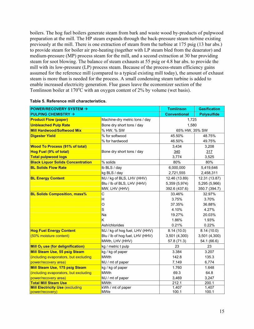
15

boilers. The hog fuel boilers generate steam from bark and waste wood by-products of pulpwood preparation at the mill. The HP steam expands through the back-pressure steam turbine existing previously at the mill. There is one extraction of steam from the turbine at 175 psig (13 bar abs.) to provide steam for boiler air pre-heating (together with LP steam bled from the deaerator) and medium-pressure (MP) process steam for the mill, and a second extraction at 30 bar providing steam for soot blowing. The balance of steam exhausts at 55 psig or 4.8 bar abs. to provide the mill with its low-pressure (LP) process steam. Because of the process-steam efficiency gains assumed for the reference mill (compared to a typical existing mill today), the amount of exhaust steam is more than is needed for the process. A small condensing steam turbine is added to enable increased electricity generation. Flue gases leave the economizer section of the Tomlinson boiler at 170oC with an oxygen content of 2% by volume (wet basis). Table 5. Reference mill characteristics.

POWER/RECOVERY SYSTEM Tomlinson Gasification PULPING CHEMISTRY Conventional Polysulfide Product Flow (paper) Machine-dry metric tons / day 1,725 Unbleached Pulp Rate Bone dry short tons / day 1,580 Mill Hardwood/Softwood Mix % HW, % SW 65% HW, 35% SW Digester Yield % for softwood 45.50% 48.75% % for hardwood 46.50% 49.75% Wood To Process (91% of total) 3,434 3,208 Hog Fuel (9% of total) 340 317 Total pulpwood logs

Bone dry short tons / day 3,774 3,525

Black Liquor Solids Concentration % solids 80% 80% BL Solids Flow Rate lb BLS / day 6,000,000 5,419,646 kg BLS / day 2,721,555 2,458,311 BL Energy Content MJ / kg of BLS, LHV (HHV) 12.46 (13.89) 12.31 (13.87) Btu / lb of BLS, LHV (HHV) 5,359 (5,974) 5,295 (5,966) MW, LHV (HHV) 392.6 (437.6) 350.7 (394.7) BL Solids Composition, mass% C 33.46% 32.97% H 3.75% 3.70% O 37.35% 36.88% S 4.10% 4.27% Na 19.27% 20.03% K 1.86% 1.93% Ash/chlorides 0.21% 0.22% Hog Fuel Energy Content MJ / kg of hog fuel, LHV (HHV) 8.14 (10.0) 8.14 (10.0) (50% moisture content) Btu / lb of hog fuel, LHV (HHV) 3,501 (4,300) 3,501 (4,300) MWth, LHV (HHV) 57.8 (71.3) 54.1 (66.6) Mill O2 use (for delignification) kg / metric t pulp 23 23 Mill Steam Use, 55 psig Steam kg / kg of paper 3.384 3.207 (including evaporators, but excluding MWth 142.8 135.3 power/recovery area) MJ / mt of paper 7,149 6,774 Mill Steam Use, 175 psig Steam kg / kg of paper 1.760 1.648 (including evaporators, but excluding MWth 69.3 64.8 power/recovery area) MJ / mt of paper 3,469 3,247 Total Mill Steam Use MWth 212.1 200.1

kWh / mt of paper 1,407 1,407 Mill Electricity Use (excluding power/recovery) MWe 100.1 100.1

16

The Tomlinson power/recovery system shown in Figure 6 has a gross electricity generation of 72MWe, with a parasitic load of 7.8 MWe. Considering both the black liquor and hog fuel inputs(393 and 58 MWLHV, respectively), the net electricity generating efficiency of the system is13.3% on a LHV basis). Since the mill requires 100 MWe of electricity for the process (Table 5),the mill must purchase 36 MWe to meet its needs.

Temp., °CPres., barFlow, kg/s

Gross electricity out = 71.99 MWe

Net electriciy out = 64.25 MWeMill steam = 212.06 MWth

Power boiler bark (HHV) = 71.2 MWth

Nat. gas (HHV) = 0Black liquor (HHV) = 437.59 MWth

return from mill+ makeup(110°C)

ash

Biomassboiler

Gascleanup

air

to stack

47578.522.30

Air

hea

ter

1471.0028.78

201.017.12

201.0128.78

1451.0135.91

black liquor(80% ds)

return frommill + makeup(110°C)

Tomlinsonboiler

smelt

air

LP Air Heater

soot-blowing steam

71.99 MWe

1651.00134.38

201.01

134.38

34330.05.25

HP steam from power boiler

1504.80

67.03

24613.0

33.23

1504.86.38

Flue gasclean-up

To stack

Drum(87.2 bar)

blowdown

1154.00

39.37

30187.21.73

1700.97

164.74

47578.5103.26

MP AirHeater

hog fuel(50% moisture)

Deaerator (4.8 bar)

Deaerator(4.8 bar)

24613.02.68

8501.01

14.26

1201.01

134.38

480°C

blwdwn flash

LP fw heater1081.333.16

480°C

4.8-barsteamto mill

1504.80

67.60

13-barsteamto mill

19213.0

35.15

Condenser(30.88 MWth)

400.07414.21

HP-MPST

LPST

feedwater to power boi ler

de-SH1504.80

16.13

leakage

~

Figure 6. Energy/mass balance for a new Tomlinson power/recovery system.

3.2.2. BLGCC Power/Recovery at the Reference MillGasifying black liquor enables it to be used as fuel in a gas turbine combined cycle, a much moreefficient electricity generating option than the Tomlinson boiler steam turbine technology.

3.2.2.1 Choice of Black Liquor Gasification TechnologyA number of concepts for black liquor gasification have been proposed in the past [52]. Ourearlier assessment of black liquor gasification combined cycle (BLGCC) systems includeddetailed analysis of two black liquor gasifiers that have been the focus of sustainedcommercialization efforts.

A pressurized, oxygen-blown, high-temperature black liquor gasification technology (Figure 7)is being developed by Chemrec, a Swedish company [53,54]. The Chemrec design isdistinguished by the majority of the inorganic material in the black liquor leaving the reactor as amolten liquid (smelt) due to the high reactor temperature (950-1000oC). The Chemrec processresembles an entrained-flow coal gasifier in this respect. Chemrec tested an initial pilot unitstarting in 1994 at a pulp mill near Karlstad, Sweden. This unit was designed to use air as theoxidant and to run at 15 bar pressure and 975oC temperature. The pilot plant was modified in

17

1997 to use oxygen instead of air, resulting in an increase in capacity to 10 t/day of black liquor solids (BLS). The unit was shut down in 2000, having provided significant data for further development of the technology. Meanwhile, the Weyerhaeuser company installed an atmospheric-pressure, air-blown Chemrec reactor (365 t/d BLS) at a mill in North Carolina in the late 1990s to augment the chemical recovery capacity provided by the existing Tomlinson boiler. The Weyerhaueser unit operated for three years before being shut down for repairs of an unanticipated problem. The unit was restarted in June 2003, after redesign based on the learnings from the original unit. Meanwhile, construction of a new Chemrec pilot plant was completed in the second half of 2005 at a pulp mill in Piteå, Sweden. The unit, which is designed to operate at 30 bar pressure on oxygen and process up to 20 tpd BLS, will provide data for scale-up [34] to full-scale Tomlinson boiler replacement applications.

Figure 7. Pressurized, oxygen-blown, high-temperature black liquor gasifier technology under development by Chemrec.

The second black liquor gasification process, being commercialized by Thermochem Recovery International (TRI), an American company, utilizes indirectly-delivered heat via a bank of pulse-combustor heat exchange tubes immersed in a fluidized bed [55,56]. Steam is used to fluidize the bed in which the black liquor is gasified. With a moderate temperature maintained in the reactor (~600oC), the condensed-phase material leaves as a dry solid. TRI carried out gasification studies of spent pulping liquor in a 0.5 tpd BLS pilot unit starting in the early 1990s. A nominal 50-ton per day pilot plant completed a 500-hour continuous test at a Weyerhaeuser kraft pulp mill in North Carolina in 1994/1995. Two commercial-scale (~200 tpd BLS) units are installed, one at a pulp mill in Trenton, Ontario (Canada) and one at a mill in Big Island, Virginia. Both of these mills use a non-sulfur pulping process. A decision to shut down the Big Island unit was made in mid-2006. The Trenton unit continues to operate, with some 18,000 hours of operation completed to date.

18

A key objective in the present biorefinery assessment is to understand the relative costs/benefits of liquid fuels production vis-à-vis electricity, so an early decision was made to focus the biorefinery analysis around a single black liquor gasifier design rather than carrying out parallel designs with two gasifiers as we did in our BLGCC work. The BLGCC work showed more favorable performance and economics for BLGCC systems designed around the high-temperature gasifier, so this gasifier design was selected for the detailed kraft pulp mill biorefinery designs we have developed in this work. This decision is supported by some less-detailed comparative analysis we have carried out for low-temperature BLG in a kraft pulpmill biorefinery application. Volume 4 describes this analysis.

3.3.2.2 Choice of Gas Turbine Technology From our prior study [5], we reproduce results here for the BLGCC design incorporating a high-temperature black liquor gasifier and a “mill-scale” gas turbine. Commercial gas turbines are available in only a relatively few specific sizes, unlike steam turbines which can be built to any desired size. Thus, the design of the BLGCC system is largely fixed by the specific choice of gas turbine. In our BLGCC design, we selected a gas turbine based on General Electric’s 6FA model, which is in the class of the most advanced machines now widely deployed in the market (“F” technology) and which has fuel requirements very close to the amount of synthesis gas available from the black liquor gasifier at our reference mill. As discussed earlier, another of the BLGCC designs included a “utility-scale” gas turbine, which required a considerable amount of natural gas to supplement the available synthesis gas. Since we do not consider the use of natural gas in our biorefinery analysis, the “mill-scale” BLGCC is the appropriate one for comparisons to be made later in this report. In our “mill scale” BLGCC (Figure 8), the black liquor is gasified, and the syngas product is cooled, cleaned, stripped of H2S (using a Selexol® unit), and then burned in the gas turbine. The turbine exhaust passes through a “duct burner” to the heat recovery steam generator (HRSG), where steam is raised to drive a steam turbine. A small amount of natural gas is burned in the duct burner4 to enable production of the requisite process steam needed to run the mill. Steam is extracted at two different pressures from the steam turbine. The HRSG steam production is augmented by steam delivered from hog fuel boilers assumed to be pre-existing at the reference mill. One design constraint in the BLGCC analysis was the size of the existing hog fuel boilers, which limited the available steam delivered from these boilers. (This limitation is the reason a small quantity of natural gas is used in the duct burner.)

3.3.2.3 Sulfur Cycle and Lime Cycle Issues with Kraft Black Liquor Gasification Unlike in a Tomlinson boiler, where essentially all of the sodium and sulfur leave in the smelt, there is a natural partitioning of sulfur (mainly as hydrogen sulfide, H2S) to the gas phase and sodium to the condensed phase during gasification of kraft black liquor. This split represents an important potential benefit to a pulp mill, since it can facilitate alternative pulping chemistries that can lead to increased pulp yields per unit of wood consumed [57]. Based on thermodynamic considerations, the lower the gasification temperature, the more complete will be the partitioning of sulfur and sodium.5 With the low-temperature black liquor gasification process described in

4 Because of the high air-fuel ratio that characterizes gas turbine combustion, there is sufficient oxygen in the gas turbine exhaust to burn additional fuel in the duct burner. 5 Higher pressure also favors greater conversion of sulfur to the gas phase.

19

Section 3.3.2.1, over 90% of the sulfur in the black liquor will leave the gasifier as H2S in the product gas. With the high-temperature process, slightly more than half of the sulfur goes to the gas phase.

Pressurized, high‐temp gasifier

Syngas cooling& cleaning

Remove H2S, recover sulfur

Gas turbine (6FA)

blackliquor

condensed phaseto causticizing 

sulfur to pulping liquor preparation

ELECTRICITY

process steam to mill

SteamTurbine

Heat Recovery Steam Generator

Air separation unit

oxygen

natural gas boostair

Steam from hog fuel boilers

~

Pressurized, high‐temp gasifier

Syngas cooling& cleaning

Remove H2S, recover sulfur

Gas turbine (6FA)

blackliquor

condensed phaseto causticizing 

sulfur to pulping liquor preparation

ELECTRICITY

process steam to mill

SteamTurbine

Heat Recovery Steam Generator

Air separation unit

oxygen

natural gas boostair

Steam from hog fuel boilers

~

Figure 8. Simplified schematic representation of “mill-scale” BLGCC system.

To take advantage of the natural separation of sulfur and sodium, it is necessary to recover H2S from the gas in a form suitable for preparing modified pulping liquors. Capture of acid gases like H2S is routinely practiced in other industries (e.g., petroleum refining) using patented physical or chemical absorption processes such as Selexol® or Rectisol®. It is also possible to capture H2S using green liquor or white liquor as a scrubbing medium, though this has ot been done in any commercial application. A negative consequence of the natural split of sulfur and sodium during gasification is a higher causticizing load, i.e., larger required lime kiln capacity and lime kiln fuel consumption per unit of black liquor solids processed compared to processing in a Tomlinson boiler. One cause of this increase is that more of the sodium (Na) in the condensed phase forms carbonate (Na2CO3) in the green liquor because less sulfur is available in the condensed phase to form sodium sulfide (Na2S). In effect, for each unit of sulfur that goes to the gas phase, one additional unit of carbonate forms in the condensed phase. Since the carbonate must be converted to hydroxide (NaOH) through the causticizing cycle (Figure 5), one additional unit of lime must be generated at the lime kiln. A second source of added causticizing load will appear if green or white liquor scrubbing is used to capture H2S, since some CO2 in the gas will be co-absorbed and form NaHCO3 in the liquor, which must eventually be converted back to NaOH. Alternatively, the problem associated with CO2 co-absorption can be eliminated entirely if H2S is captured using a commercial process (e.g., Selexol®) and then converted to elemental sulfur using a commercially available process (Claus/SCOT technology). This is the approach we have assumed in our BLGCC design.

3.3.2.4 Detailed BLGCC Performance Simulation Figure 9 gives the detailed mass/energy balance for our BLGCC design. The raw syngas undergoes an integral quench in the lower section of the black liquor gasifier, leaving the reactor

20

at 217°C, 35 bar. The gas is then cooled through a medium pressure boiler and a water heater.Most of the water in the syngas condenses, thereby releasing most of the energy picked-up in thequench. The syngas passes from the water heater at about 120°C to a trim cooler, which it leavesat 40°C before entering the sulfur recovery unit (SRU).

19513.02.25

Temp., °CPres., barFlow, kg/s

Gross electricity out = 135.14 MW e

Net electricity out = 114.7 MW eMill steam = 200.17 MW th

Power boiler bark (HHV) = 100.0 MW th

Nat. gas (HHV) = 14.32 MW th

Black liquor (HHV) = 391.05 MW th

535117

48.97

19513.00.36

13214.00.36

47578.5

31.27

18538.0149.23

13234.3

19.44

1524.80

64.05

25113.0

10.50

1431.01

217.92

18232.0

31.30

4032.4

21.80

11535.0

35.57

~Steam turbin e

Gasifier

green liquo r

waterheater

Black l iquor(80% ds)

Selexol system

clean syngas

Qu enchcooler

from mill +from saturator

+make -up

MP steam

LP steam

to stack

12233.6

25.59

rawgas

1000°C35 bar

condensate

48.16M We

11240.0

149.23

13832.0120.72

steam from power boiler(Pev=87.22 bar, Tsh=

480°C,h og fuel = 10.00 kg/s)

4032.9

24.24

trimcooler

M P steam to mill

19213.0

32.90

humidif ied syngas

201.01

40.53

14535.09.46

Oxygenplant

vent

a ir

251.05

30.65

- 14.30MWe

fromsaturator

18538.0130.20

19513.019.37

12242.0

33.74

13814.00.79

21735.0

59.32

ST leak age150

4.800.64

20034.3

59.32boiler

6261.05216.13

135816.1183.06

43116.6

153.33

201.01

186.37

~Gas turbine

air

86.98M We

95% O 2

Saturator

H 2S + CO 2

Claus + SCOTplant

to m

ill

1534.80

62.28

1406.0

6.83

to dea erator

1514.800.48

from b lowdownflash tank

condensate

105*1.2*

2.45*

19513.0

19.37

HRSGPev= 130 bar, Tsh= 540°C

(blow-dow n 1.14 kg/ s from HP drum not show n)

reboiler

stri

pperab

sorb

er

18232.01.55

18232.0

29.73

IP steam to sulfur recovery

1816.506.83

1524.801.23

13814.00.06

de -SH

natural gas

2030.00.26

Du ctbur ner

7121.05

217.92

1125.042.65

to gasif. islandand power boiler

mak e-up

make-uptank

to lime k iln25

1.050.42

95% O 2

Figure 9. Energy/mass balance for BLGCC with high-temperature gasifier and mill-scale gasturbine.

All of the H2S and some of the CO2 in the syngas are absorbed in the sulfur recovery unit (SRU)based on commercial Selexol technology. All of the absorbed H2S is converted into elementalsulfur via a standard, commercial Claus/SCOT system. About half of the sulfur in the blackliquor is contained in the H2S. The rest is contained in the gasifier smelt, where it forms theNa2S that provides the needed base for polysulfide formation when the recovered elementalsulfur is dissolved in it. The estimated additional lime-kiln load for this BLGCC design (relativeto the Tomlinson system) is a relatively modest 16%, and is accommodated by using oxygen-enriched air to increase the throughput capacity of the existing kiln, with oxygen provided fromthe air separation unit [5].

The sulfur-free syngas leaves the SRU and travels to a saturator, wherein the gas is humidifiedby mixing with water pre-heated to 185°C. By humidifying the syngas, a significant increase inpower production from the gas turbine can be achieved (due to increased syngas mass flow). Thehumidified gas also results in a lower flame temperature in the gas turbine combustor, therebyreducing thermal NOx emissions.

The available black liquor enables slightly more syngas to be generated than is required to fuelthe gas turbine. Excess syngas is burned in the duct burner. Hog fuel boilers (not shown inFigure 9) consume 54 MWLHV of hog fuel and 27 MWLHV of purchased wood residues, for a

21

total of 81 MWthLHV. A small amount of natural gas supplements the syngas burned in the duct burner to meet the mill’s steam demand, since it was assumed that the existing hog fuel boilers would be fully loaded at 81MWth (LHV) input, and adding a small amount of natural gas via the duct burner was more economical than adding hog fuel boiler capacity. This BLGCC power/recovery configuration has a gross electricity generation of 135 MWe, 64% of which is produced by the gas turbine. The parasitic load is 20.5 MWe, mostly due to the cryogenic air separation unit that produces the oxygen needed for the gasifier. Since the mill requires 100 MWe for the process, 14.5 MWe are available for export to the grid.

4 Overview of Biorefinery Designs We developed seven biorefinery designs taking into consideration the objective of being able to make meaningful performance and cost comparisons against our prior results for a conventional Tomlinson system and a BLGCC system. Beyond these comparisons, we wished to explore the potential impacts of supplementing to a substantial degree the relatively modest quantities of woody residues that are used for energy at typical pulp mills today. To maximize the effectiveness of woody residue utilization, all but one of our process designs incorporate gasification of biomass in tandem with gasification of black liquor. In this section we provide a schematic overview of our biorefinery designs – three variants for DME production, three variants for FTL production, and one design for mixed-alcohols production. (Design and simulation details are provided in Section 5.) The process designs all include five basic equipment “islands”: (i) black liquor gasification island, (ii) biomass gasification island (or, in one case, a hog fuel boiler island), (iii) syngas heat recovery and syngas clean-up island, (iv) fuel synthesis island, and (v) power island. The gasification island includes a cryogenic air separation unit for the production of oxygen. The black liquor and biomass gasification islands are essentially the same for all the cases considered (except for the size of the biomass gasification island). The syngas clean-up island is centered around commercial Rectisol® technology, except for the mixed alcohol case in which commercial Selexol® technology is adopted. For the fuel synthesis island, we consider one of two basic arrangements: single-pass or recycle. In the single-pass arrangement, the syngas passes once through the synthesis reactor and any syngas unconverted to liquid product is sent for use in the power island. In the recycle arrangement, some significant fraction of the unconverted syngas is recycled to the synthesis reactor to increase liquid fuel production. For the power island, in one case a boiler back-pressure steam turbine cycle is adopted. In the other six cases, a combined gas turbine/steam turbine cycle is employed. The gas turbine is modelled in five of the six cases on the medium-scale, heavy-duty 6FA gas turbine offered by General Electric. In the sixth case, we consider a larger GE gas turbine, the 7FA. Table 6 summarizes key design characteristics for each of the biorefineries, along with corresponding values for the Tomlinson and BLGCC designs developed in our prior work. As indicated in this table, the black liquor flow is the same in all cases, except for the Tomlinson case where more black liquor is available (at a mill with the same level of pulp/paper output) due to lower pulp yield compared to the mills where gasification is used (as discussed in Section 3.2). The woody biomass input as energy (including hog fuel and purchased residues) is also shown. The amount of biomass energy use is set by the constraint that the biorefinery provide all of the pulp/paper mill’s process steam demand, subject to other constraints placed on the biorefinery

22

design, as discussed later in this section. Table 6 also shows the net increase in total wood (pulpwood and purchased residues) that must be handled in the wood yard at the pulp/paper mill compared to the Tomlinson case. There is some reduction in pulpwood input to the mill (compared with Tomlinson case) with biorefining (due to higher-yield pulping process assumed), but this reduction is more than compensated for by the additional purchased residues needed so that wood handling capacity increases in all cases. For all but two of the biorefinery designs, the net increase in total wood flow that must be handled in the wood yard is 25% or less. The highest percentage increase in net wood flow is for the FTc design (69%). Table 6. Summary of key design parameter values for biorefinery simulations and, for comparison, BLGCC and Tomlinson cases.

Biomass used for energyb

Black Liquor

Metric t/d BLSa (MWLHV) Metric

dry t/d MWth LHV

Net incremental biomass to mill,

metric dry t/d (%)c

Gas turbine modeld

Syngas from wood gasifier

goes to

Synthesis loop

design

Biorefineries

DMEa 2,458 (351) 700 132 186 (5.4%) no GT no wood gasif. 97% recycle

DMEb 2,458 (351) 1,326 250 813 (24%) 6FA gas turbine 97% recycle

DMEc 2,458 (351) 678 128 165 (4.8%) 6FA gas turbine one pass

FTa 2,458 (351) 829 156 316 (9.2%) 6FA gas turbine one pass

FTb 2,458 (351) 2,246 423 1,733 (51%) 7FA gas turbine one pass

FTc 2,458 (351) 2,704 505 2,191 (64%) 6FA synthesis one pass

MA 2,458 (351) 760 143 247 (7.2%) 6FA synthesis 76% recycle

From 2003 BLGCC study [5]

Tomlinson 2,722 (393) 308 58 0 (0) no GT no wood gasif. no synth.

BLGCC 2,458 (351) 432 81 -82 (-2.4%) 6FA no wood gasif. no synth. (a) For mills with black liquor gasifiers, less black liquor is generated than with the Tomlinson system (for the same level of pulp output) due to the higher-yield polysulfide pulping process used. (b) This is biomass used directly for energy. The totals shown are the sum of hog fuel (9% of incoming pulpwood logs is converted to hog fuel) and purchased woody residues. (c) This is the net additional biomass that must be handled in the woodyard at the mill. It is the sum of pulpwood logs and purchased wood residues less the pulpwood-log flow in the reference (Tomlinson) case. The total incoming pulpwood logs is 3,421 metric dry t/day in the Tomlinson case and 3,197 metric dry t/d for gasification-based cases. (d) The rated output in simple-cycle mode when operating on natural gas is 75MW for the 6FA and 170MW for the 7FA. The right three columns in Table 6 show, respectively, the gas turbine selected in each case, whether syngas from a biomass gasifier (if present in the design) is used entirely as a gas turbine fuel or sent first to the liquids synthesis reactor, and whether a recycle or one-pass synthesis reactor design is used. The rationale for the parameter choices shown in Table 6 are described below for each biorefinery design. In the design identified as DMEa (Figure 10), the black liquor gasifier, supplied with oxygen from an air separation unit, provides all of the synthesis gas to a liquid-phase DME reactor. Unconverted synthesis gas is separated from product DME and 97% of it is recycled to the synthesis reactor to increase DME production. The 3% purge stream taken from the recycle loop prevents excessive buildup of inert gases. The purge gas is sent to the hog fuel boiler, where it

23

burns with an amount of wood residues selected such that the amount of steam generated is sufficient to meet all of the mill’s process steam needs. Heat recovered from the black liquor and syngas processing areas are integrated into the boiler to increase steam production and minimize the amount of woody residues needed. The steam is expanded through a back-pressure turbine to generate some electricity which goes toward meeting the mill’s process electricity needs. To fully meet the mill’s electricity need, some electricity must be imported from the grid. Because black liquor is being converted primarily into liquid fuel and not electricity, the amount of electricity imported is larger than with a conventional Tomlinson system.

Pressurized, high‐temp gasifier

Syngas cooling& cleaning

Remove H2S & some CO2

LP DME synthesis

Steam Turbine

blackliquor

condensed phaseto causticizing  sulfur   to polysulfide   

liquor   preparation

ELECTRICITY

process steam to mill

Existing hog fuelboiler

biomass (50% mc)

Air separation unit

oxygen

air

recovered heatpurgegas

DME

Separation, distillation

unconverted syngas

raw product

Pressurized, high‐temp gasifier

Syngas cooling& cleaning

Remove H2S & some CO2

LP DME synthesis

Steam Turbine

blackliquor

condensed phaseto causticizing  sulfur   to polysulfide   

liquor   preparation

ELECTRICITY

process steam to mill

Existing hog fuelboiler

biomass (50% mc)

Air separation unit

oxygen

air

recovered heatpurgegas

DME

Separation, distillation

unconverted syngas

raw product

Figure 10. Schematic of biorefinery DMEa. Key features include recycling of unconverted syngas to increase DME production and use of steam Rankine power island.

One approach to increasing net electricity production is to increase the consumption of wood residues and/or increase the efficiency with which electricity is being generated. Biorefinery DMEb adopts both of these approaches. In this design (Figure 11), the black liquor and synthesis gas processing areas are unchanged from DMEa, and DME production is identical to that in DMEa. However, woody biomass is gasified and used to fuel a gas turbine-steam turbine combined cycle (GTCC). In this design, the amount of biomass consumed is again set by the amount of process steam that must be raised to meet the pulp and paper mill demand. Because the GTCC is characterized by a higher electricity to steam production ratio than the boiler/steam turbine system in DMEa, more biomass must be used in the DMEb design than in the DMEa design to deliver the same amount of process steam, but electricity production with DMEb is considerably greater than with DMEa. Another approach to increasing electricity production compared to DMEa that involves woody biomass consumption not much greater than DMEa, is to use a lower level of syngas recycle to the synthesis reactor, such that more unconverted gas is available for power generation. In DMEc (Figure 12), we eliminate the syngas recycle loop entirely such that the synthesis gas passes only once through the reactor, leading to much lower DME production than in DMEb but requiring relativel little purchased biomass. The design is otherwise very similar to DMEb. Larson and Ren [58] indicate that high single-pass syngas conversion rates that characterize liquid-phase reactors (of the type assumed in our design) can make such “one-pass” synthesis designs especially attractive from an overall cost perspective when co-producing electricity with fuels. DMEc tests whether this might hold true for a pulp mill biorefinery.

24

Pressurized, high‐temp gasifier

Syngas cooling& cleaning

Remove H2S & some CO2

LP DME synthesis

Gas Turbine CC(Frame 6FA GT)

blackliquor

condensed phaseto causticizing 

sulfur   to polysulfide   liquor   preparation

ELECTRICITY

process steam to mill

Fluidized‐bedgasifier

biomass (50% mc)

Syngas cooling& cleaning

Air separation unit

oxygen

oxygen

air

recovered process heat

Dryer

DME

Separation, distillation

rawproduct

purge gas

unconverted syngas

Pressurized, high‐temp gasifier

Syngas cooling& cleaning

Remove H2S & some CO2

LP DME synthesis

Gas Turbine CC(Frame 6FA GT)

blackliquor

condensed phaseto causticizing 

sulfur   to polysulfide   liquor   preparation

ELECTRICITY

process steam to mill

Fluidized‐bedgasifier

biomass (50% mc)

Syngas cooling& cleaning

Air separation unit

oxygen

oxygen

air

recovered process heat

Dryer

DME

Separation, distillation

rawproduct

purge gas

unconverted syngas

Figure 11. Schematic of biorefinery DMEb. Key differences from DMEa (Figure 10), represented by darker shading, include biomass gasifier and gas turbine combined cycle power island.

Pressurized, high‐temp gasifier

Syngas cooling& cleaning

Remove H2S & some CO2

Once‐thru LP DME synthesis

Gas Turbine CC(Frame 6FA GT)

blackliquor

condensed phaseto causticizing 

sulfur   to polysulfide   liquor   preparation

ELECTRICITY

process steam to mill

Fluidized‐bedgasifier

biomass (50% mc)

Syngas cooling& cleaning

Air separation unit

oxygen

oxygen

air

recovered process heat

Dryer

DME

Separation, distillationunconverted syngas

raw  product

Pressurized, high‐temp gasifier

Syngas cooling& cleaning

Remove H2S & some CO2

Once‐thru LP DME synthesis

Gas Turbine CC(Frame 6FA GT)

blackliquor

condensed phaseto causticizing 

sulfur   to polysulfide   liquor   preparation

ELECTRICITY

process steam to mill

Fluidized‐bedgasifier

biomass (50% mc)

Syngas cooling& cleaning

Air separation unit

oxygen

oxygen

air

recovered process heat

Dryer

DME

Separation, distillationunconverted syngas

raw  product

Figure 12. Schematic of biorefinery DMEc. Key difference from DMEb (Figure 11), represented by darker shading, include synthesis reactor operating in single-pass (rather than recycle) mode.

For our FT biorefinery designs, which we developed after completing the detailed designs for our DME biorefineries, we chose to consider only single-pass synthesis due to the much higher single-pass conversion of syngas that can be achieved with FT synthesis compared to DME synthesis. Our FTa configuration is conceptually identical to the DMEc design, allowing for a meaningful comparison between FTL and DME. In this FT design, syngas from black liquor that is not converted to FTL in a single pass through the synthesis reactor is used, together with syngas from gasified biomass, to fuel a GTCC (Figure 13). The input of woody biomass residues for the FTa design is slightly higher than for DMEc (Table 6), as required to be able to meet the pulp and paper mill’s process steam needs.

25

The FTb and FTc configurations involve modifications to the FTa design to examine the impact of a lower fuels-to-electricity production ratio (FTb) and a higher fuels-to-electricity production ratio (FTc). Both involve an increase over FTa in consumption of woody residues. The design for FTb (Figure 14) utilizes a larger gas turbine (Frame 7FA), which requires more woody residues to be gasified to provide gas turbine fuel.

Pressurized, high‐temp gasifier

Syngas cooling& cleaning

Remove H2S & some CO2

Once‐thru LP FT synthesis

Gas Turbine CC(Frame 6FA GT)

Black liquor(80% ds)

condensed phaseto causticizing 

sulfur to polysulfide liquor preparation

ELECTRICITY

process steam to mill

CRUDE F-T LIQUIDS (to existing refinery)

Fluidized‐bedgasifier

Biomass chips(50% mc)

Syngas cooling& cleaning

Air separation unit

oxygen

oxygen

air

recovered process heat

Dryer

unconverted synthesis gas

Pressurized, high‐temp gasifier

Syngas cooling& cleaning

Remove H2S & some CO2

Once‐thru LP FT synthesis

Gas Turbine CC(Frame 6FA GT)

Black liquor(80% ds)

condensed phaseto causticizing 

sulfur to polysulfide liquor preparation

ELECTRICITY

process steam to mill

CRUDE F-T LIQUIDS (to existing refinery)

Fluidized‐bedgasifier

Biomass chips(50% mc)

Syngas cooling& cleaning

Air separation unit

oxygen

oxygen

air

recovered process heat

Dryer

unconverted synthesis gas

Figure 13. Schematic of biorefinery FTa. Key features of all FT designs are single-pass synthesis and gasification of woody biomass. In FTa, the gasified biomass and unconverted syngas fuel the gas turbine combined cycle power island.

Pressurized, high‐temp gasifier

Syngas cooling& cleaning

Remove H2S & some CO2

Once‐thru LP FT synthesis

Gas Turbine CC(Frame 7FA GT)

blackliquor

condensed phaseto causticizing 

sulfur to polysulfide liquor preparation

ELECTRICITY

process steam to mill

CRUDE F-T LIQUIDS (to existing refinery)

Fluidized‐bedgasifier

biomass (50% mc)

Syngas cooling& cleaning

Air separation unit

oxygen

oxygen

air

recovered process heat

Dryer

unconverted synthesis gas

Pressurized, high‐temp gasifier

Syngas cooling& cleaning

Remove H2S & some CO2

Once‐thru LP FT synthesis

Gas Turbine CC(Frame 7FA GT)

blackliquor

condensed phaseto causticizing 

sulfur to polysulfide liquor preparation

ELECTRICITY

process steam to mill

CRUDE F-T LIQUIDS (to existing refinery)

Fluidized‐bedgasifier

biomass (50% mc)

Syngas cooling& cleaning

Air separation unit

oxygen

oxygen

air

recovered process heat

Dryer

unconverted synthesis gas

Figure 14. Schematic of biorefinery FTb. The key difference compared to FTa is highlighted by the darker shading: a larger gas turbine, requiring greater woody biomass consumption.

The design for FTc involves passing all syngas (from both black liquor and biomass gasification) through the FT synthesis reactor and using only unconverted syngas to fuel the (6FA) gas turbine (Figure 15). In this case, the amount of woody biomass gasified is set such that the amount of unconverted syngas from the FT reactor is just sufficient to meet the gas turbine’s fuel needs. For the production of mixed-alcohols (Figure 16) we adopt a design similar to FTc in that syngas from black liquor and woody residue gasification are combined for processing through the

26

synthesis reactor. In the MA design, however, because the single-pass syngas conversion is much lower than for synthesis of FTL we recycle 76% of the unconverted syngas. The unrecycled portion of the syngas fuels the gas turbine combined cycle power island.

Pressurized, high‐temp gasifier

Syngas cooling& cleaning

Remove H2S & some CO2

Once‐thru LP FT synthesis 

Gas Turbine CC(Frame 6FA GT)

blackliquor

condensed phaseto causticizing 

sulfur to polysulfide liquor preparation

ELECTRICITY

process steam to mill

clean biomass syngas

Fluidized‐bedgasifier

biomass (50% mc)

Syngas quench w/ heat recovery

Air separation unit

oxygen

oxygen

air

recovered process heat

Dryer

CRUDE F-T LIQUIDS (to existing refinery)

unconverted syngas

Pressurized, high‐temp gasifier

Syngas cooling& cleaning

Remove H2S & some CO2

Once‐thru LP FT synthesis 

Gas Turbine CC(Frame 6FA GT)

blackliquor

condensed phaseto causticizing 

sulfur to polysulfide liquor preparation

ELECTRICITY

process steam to mill

clean biomass syngas

Fluidized‐bedgasifier

biomass (50% mc)

Syngas quench w/ heat recovery

Air separation unit

oxygen

oxygen

air

recovered process heat

Dryer

CRUDE F-T LIQUIDS (to existing refinery)

unconverted syngas

Figure 15. Schematic of biorefinery FTc. Similar to FTa, except that gasified woody biomass supplements gasified black liquor flowing to the synthesis island.

Pressurized, high‐temp gasifier

Syngas cooling& cleaning

Remove H2S & some CO2

Fixed Bed MoS2Synthesis)

Gas Turbine CC(Frame 6FA GT)

blackliquor

condensed phaseto causticizing 

sulfur to polysulfide liquor preparation

ELECTRICITY

process steam to mill

clean biomass syngas

Fluidized‐bedgasifier

biomass (50% mc)

Syngas quench w/ heat recovery

Air separation unit

oxygen

oxygen

air

recovered process heat

Dryerunconverted syngas + purgegases MIXED

ALCOHOLS

Separation, distillation

unconverted   syngas +methanol

rawproduct

Pressurized, high‐temp gasifier

Syngas cooling& cleaning

Remove H2S & some CO2

Fixed Bed MoS2Synthesis)

Gas Turbine CC(Frame 6FA GT)

blackliquor

condensed phaseto causticizing 

sulfur to polysulfide liquor preparation

ELECTRICITY

process steam to mill

clean biomass syngas

Fluidized‐bedgasifier

biomass (50% mc)

Syngas quench w/ heat recovery

Air separation unit

oxygen

oxygen

air

recovered process heat

Dryerunconverted syngas + purgegases MIXED

ALCOHOLS

Separation, distillation

unconverted   syngas +methanol

rawproduct

Figure 16. Schematic of biorefinery MA. The design is similar to FTc in that syngas from both the black liquor gasifier and the biomass gasifier are processed through the synthesis reactor. MA differs from FTc in that a significant fraction of the unconverted synthesis gas is recycled for further conversion, as indicated by the more darkly-shaded blocks.

5 Biorefinery Design and Performance Simulation We have developed detailed designs and calculated detailed mass and energy balances for each of the biorefinery designs described in the previous section. In this section we describe our design and simulation approach, tools, assumptions, and results, as well as comparisons with other results in the literature. See Volume 2 for full details of the design and simulation work.

27

5.1 Approach and Design/Simulation Tools A key objective of our process design work was to develop detailed equipment configurations and operating parameter values to maximize system efficiency within practical thermodynamic and capital cost constraints, so as to optimize overall financial performance. The final, detailed equipment arrangements and operating conditions are the outcome of significant screening work, which included testing a considerable number of alternatives and doing sensitivity analyses. This does not mean that the final configurations and operating parameters presented in this report are necessarily optimal, although we believe that performance improvements achievable by a more thorough optimization would be marginal. Significant improvements of efficiencies, power output or fuel output are likely to be achieved only by significant changes in the characteristics of the basic technologies, e.g. more effective catalysts, more efficient gas turbine, different gasification technologies, etc. Finally, the process configurations described below were arrived at only after reviewing detailed mass/energy balance simulation results from initial designs with Nexant engineers and revising the initial designs accordingly to improve performance and/or reduce capital costs and parasitic power consumption. A further objective in our work was to develop a set of biorefinery designs and performance results that would facilitate meaningful comparisons with the earlier designs we developed for a Tomlinson boiler power/recovery system and for a BLGCC power/recovery system. Toward this end, our process energy and mass balance calculations utilized the same computer code (called “GS” – see Volume 2) as in our BLGCC work. GS was originally developed at Politecnico di Milano and Princeton University beginning in the mid-1980s to predict the performance of complex electric power cycles involving both gas and steam turbines. The code has been built into a powerful and flexible tool that can accurately predict the performance of a wide variety of systems for electricity production or cogeneration, including systems where the feedstock is gasified to generate a syngas that undergoes a sequence of physical and chemical processes. In our biorefinery calculations, we applied GS to predict energy and mass balances around the types of equipment that were also found in our BLGCC designs. Most significantly, these included the black liquor gasification island, the gas turbine combined cycle power island, hog fuel boilers, and steam-rankine cycle power island. We also used GS to simulate woody biomass gasification in our biorefinery configurations, an application for which GS has previously been applied [59]. (Our BLGCC designs did not include woody biomass gasification.) Because GS is not well designed to handle calculations involving chemical synthesis and refining, we utilized an additional software tool, Aspen Plus, to simulate the performance of these aspects of our biorefineries. Aspen Plus is a widely used commercial chemical process simulation package originally developed for petrochemical refining applications. It includes a wide range of standard equipment modules (distillation columns, flash tanks, fixed-bed reactors, slurry reactors, and many others) that can be combined by the user to simulate specific configurations of interest. It is also possible to embed in an Aspen Plus flowsheet Fortran subroutines to simulate compounds or chemical kinetics that are not already part of standard modules found in the Aspen Plus code. We used this “user-subroutine” function to embed into our process flowsheets the kinetic fuel synthesis models for DME, Fischer-Tropsch liquids, and mixed-alcohols that we developed from empirical kinetic data in the literature. We also used Aspen Plus to simulate the acid gas removal island where H2S and CO2 are captured from syngas.

28

Because we used two different pieces of software to simulate different elements of our biorefineries, it was necessary to follow a somewhat cumbersome iterative sequence of GS and Aspen runs to ensure a wholly consistent set of final results in each case (Figure 17). Volume 2 describes the details of this procedure. While it is complex, the calculation procedure we adopted has the feature that it takes advantage of the strongest elements of each computer code to produce results with accuracy similar to (or better than) the most detailed engineering studies that can be found in the literature.

BL Gasificationand syngas

Cooling

Rectisol process

Power Island (with boiler or biomass

gasifier)

Fuel synthesisIsland

BL raw syngas

clean syngasheat

heat

steamto mill use

electricity

Fuel

unconvertedsyngas

Black Liquor

Biomass

electricityto mill or from grid

GS model

Aspen model

heatelectricityfor refrigerationand compressors

biomass raw syngas

Figure 17. Interactions between GS and Aspen Plus during process simulations. The black liquor gasification island is calculated first with GS. Aspen is then run twice to simulate the acid gas recovery (Rectisol) system and the fuel synthesis island. Finally, GS is re-run, taking into account the results generated by the Aspen runs. See Volume 2 for additional details.

5.2 Design and Simulation of Key Subsystems Before describing the detailed mass/energy balance results for each of the seven biorefineries, we describe details of the simulation of the black liquor gasification island and acid gas removal islands (which are common to all of the biorefineries), the biomass gasification island and gas turbine combined cycle island (which are found in all but one of the biorefineries), and the fuel synthesis islands for DME, FTL, and MA. Additional details for these subsystems are available in Volume 2, as are details for other components not discussed extensively here.

5.2.1 Black Liquor Gasification Island The black liquor gasification (BLG) island is identical in all respects in the seven biorefineries and also identical to the BLG island in our previous BLGCC study [5].6 The gasifier is simulated as a pressurized, oxygen-blown entrained-flow reactor. The input black liquor composition is given in Table 5. The basic operating conditions for the gasifier (Table 7) have been chosen in accordance with data published in the literature and information provided by Chemrec, the leading developer of this design of gasifier. The reactor is comprised of two main sections. In the upper section black liquor (80% dry solids) is gasified in oxygen (95% O2, 3.65% Ar, 1.35% N2) to produce syngas (the main components of which are CO, H2, CO2, and

6 In the course of the current work, we discovered a minor calculation error in the BLG simulation (relating to heat losses from the BLG) in our BLGCC study. We corrected this error in the BLG simultions in our biorefinery calculations, but we chose not to recalculate our earlier BLGCC simulations since the error was minor.

29

also some H2S) and a molten inorganic stream (smelt, containing primarily sodium and sulfurcompounds). In the lower section, the raw gas and smelt droplets are cooled by injection ofcondensate collected in the downstream syngas cooler. The smelt dissolves in the quench liquidto form green liquor, which is sent to chemical recovery after being cooled by heating thecondensate used for the quench (Figure 18).

Table 7. Assumed operating parameters for black liquor gasifier simulations

Reactor pressure 35 bar (483 psig)Pre-quench reaction temperature 1000°C (1832°F)Heat loss to environment 0.5% of black liquor higher heating valueHeat to cooling flows 2.0% of black liquor higher heating valueCarbon conversion 99.9%Methane in raw syngas 1.5% by mass on a dry gas basis

Quenchcooler

1000°C35 bar

BLGasifier

Black liquor(80% BLS)

115°C35.0 bar

35.57 kg/s

hot raw gas

condensate

water fromdeaerator

air

Oxygenplant

vent

to lime kiln

95%O2

water fromdeaerator

warm BL raw gas tofurther cooling and

cleaningMP steam

to mill (13 bar)

LP steamto mill (4.8 bar)

Syngascooler

water

preheatedwaterto deaerator

122°C

green liquor

0.42 kg/stobiomassgasifier

tobiomass

lockhoppers

N2

Figure 18. Equipment configuration for black liquor gasification.

The composition of the syngas leaving the gasifier (Table 8) is calculated assuming that (i) thecarbon conversion and methane concentration in the raw syngas are as specified in (Table 7); (ii)the small amount of unconverted carbon leaves the gasifier in the green liquor; (iii) ash andchlorides are inert; and (iv) all remaining material constitutes a mixture of gases and condensedphases at equilibrium, including the possibility for any sodium or potassium containingcompound to be in either the liquid or solid state or both, depending on temperature andpressure.7 This calculation scheme, which predicts that 57.5% of the sulfur in the black liquorgoes into the gas phase, gives satisfactory agreement with specific information provided byChemrec, as well as with qualitative indications found in the literature.

7 Compounds which are considered in the equilibrium calculation are: Ar, CO, CO2, COS, H2, H2O, H2S, NH3, N2,Na2CO3, Na2SO4, Na2S, NaOH, K2CO3, and K2SO4. The molten compounds are assumed to form an ideal mixture.

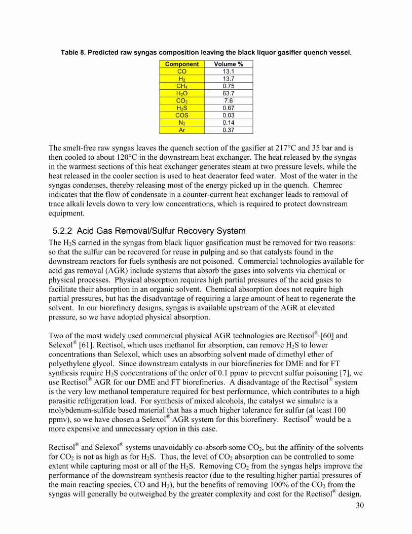
30

Table 8. Predicted raw syngas composition leaving the black liquor gasifier quench vessel. Component Volume %

CO 13.1 H2 13.7

CH4 0.75 H2O 63.7 CO2 7.6 H2S 0.67 COS 0.03 N2 0.14 Ar 0.37

The smelt-free raw syngas leaves the quench section of the gasifier at 217°C and 35 bar and is then cooled to about 120°C in the downstream heat exchanger. The heat released by the syngas in the warmest sections of this heat exchanger generates steam at two pressure levels, while the heat released in the cooler section is used to heat deaerator feed water. Most of the water in the syngas condenses, thereby releasing most of the energy picked up in the quench. Chemrec indicates that the flow of condensate in a counter-current heat exchanger leads to removal of trace alkali levels down to very low concentrations, which is required to protect downstream equipment.

5.2.2 Acid Gas Removal/Sulfur Recovery System The H2S carried in the syngas from black liquor gasification must be removed for two reasons: so that the sulfur can be recovered for reuse in pulping and so that catalysts found in the downstream reactors for fuels synthesis are not poisoned. Commercial technologies available for acid gas removal (AGR) include systems that absorb the gases into solvents via chemical or physical processes. Physical absorption requires high partial pressures of the acid gases to facilitate their absorption in an organic solvent. Chemical absorption does not require high partial pressures, but has the disadvantage of requiring a large amount of heat to regenerate the solvent. In our biorefinery designs, syngas is available upstream of the AGR at elevated pressure, so we have adopted physical absorption. Two of the most widely used commercial physical AGR technologies are Rectisol® [60] and Selexol® [61]. Rectisol, which uses methanol for absorption, can remove H2S to lower concentrations than Selexol, which uses an absorbing solvent made of dimethyl ether of polyethylene glycol. Since downstream catalysts in our biorefineries for DME and for FT synthesis require H2S concentrations of the order of 0.1 ppmv to prevent sulfur poisoning [7], we use Rectisol® AGR for our DME and FT biorefineries. A disadvantage of the Rectisol® system is the very low methanol temperature required for best performance, which contributes to a high parasitic refrigeration load. For synthesis of mixed alcohols, the catalyst we simulate is a molybdenum-sulfide based material that has a much higher tolerance for sulfur (at least 100 ppmv), so we have chosen a Selexol® AGR system for this biorefinery. Rectisol® would be a more expensive and unnecessary option in this case. Rectisol® and Selexol® systems unavoidably co-absorb some CO2, but the affinity of the solvents for CO2 is not as high as for H2S. Thus, the level of CO2 absorption can be controlled to some extent while capturing most or all of the H2S. Removing CO2 from the syngas helps improve the performance of the downstream synthesis reactor (due to the resulting higher partial pressures of the main reacting species, CO and H2), but the benefits of removing 100% of the CO2 from the syngas will generally be outweighed by the greater complexity and cost for the Rectisol® design.

31

Also, DME synthesis requires a certain (relatively low) level of CO2 in the syngas entering the reactor in order to maintain catalyst activity [58]. In the four DME and FT biorefinery designs utilizing once-through synthesis reactors (Table 6), about 80% of the CO2 is removed by the AGR system. The more complex AGR configuration required to remove 100% of CO2 is adopted in the two DME biorefinery designs where there is recycling of unconverted syngas back to the synthesis reactor. This is done to avoid excessive CO2 build-up in the recycle loop. In the case of the mixed-alcohols biorefinery, the Selexol AGR captures 18.4% of the CO2 along with H2S. It should be mentioned that removing such a low fraction of CO2 (leaving a relatively high concentration entering the synthesis reactor) may be detrimental to alcohol synthesis yield and increase costs. We were unable to evaluate the optimum degree of CO2 removal in the production of mixed alcohols from syngas because more kinetic data than are currently available in the literature are needed, along with more detailed cost estimates. Once the acid gases have been captured by the AGR unit, they are delivered to a standard Claus/SCOT plant that converts the H2S to elemental sulfur. This sulfur is then dissolved in a low-sulfidity white liquor (containing Na2S formed in the gasifier smelt) to reconstitute the polysulfide pulping liquor. In our simulations, we have not modeled the Claus/SCOT unit in detail. Rather we have used estimates of steam and power consumption for the Claus/SCOT system as a whole and used these in the calculation of the parasitic energy demands of the biorefineries. The Claus plant generates steam at medium pressure (MP, 13 bar) and at low pressure (LP, 4.8 bar), which are exported to the MP and LP headers serving the mill. The amount of steam produced is proportional to the amount of H2S converted to elemental sulfur. The tail gas exiting the Claus plant is further treated in the SCOT unit, which requires steam at 6.5 bar to regenerate the solvent used to absorb the residual SO2 in the tail gas.

5.2.3 Biomass Gasification Island In the six biorefinery designs that include a gas turbine in the power island (Table 6), a mixture of hog fuel and purchased wood wastes are processed through the biomass gasification island, which includes a biomass dryer, a pressurized oxygen/steam-blown fluidized-bed gasifier, and gas cleanup. The resulting syngas is fed either directly to the gas turbine as fuel or it is mixed with the syngas from black liquor gasification prior to feeding to the fuel synthesis island, depending on the biorefinery design. We have selected a pressurized, oxygen-blown circulating fluidized-bed design for biomass gasification, but there are a number of different biomass gasifier designs under commercial development [62,63]. For synthesis of fuels, a pressurized syngas undiluted by nitrogen is preferred for feeding to the synthesis reactor, since synthesis conversion rates generally increase with pressure and decrease with increasing fraction of inert components in the syngas (such as nitrogen). Also, reactor sizes (and capital cost) increase with content of inert components. If syngas can be produced directly from a gasifier without nitrogen dilution, the cost and complication of post-gasification removal of nitrogen can be avoided. Also, if gasification can be carried out at elevated pressure, the need for syngas compression prior to synthesis can be reduced or eliminated. Two alternatives for producing nitrogen-free syngas are oxygen/steam-blown gasification or indirectly-heated (pyrolytic) gasification. Indirectly-heated gasifiers designed to date are not easily amenable to pressurization. Thus, pressurized oxygen/steam-blown gasification appears to be the most suitable near-term biomass gasification technology for our biorefinery designs.

32

Since an air separation unit is needed onsite to provide oxygen to the black liquor gasifier, the incremental cost to also provide oxygen for biomass gasification is relatively modest. Development and pilot-plant demonstration efforts with pressurized oxygen/steam-blown fluidized bed gasification date to the early-1980s in Sweden [64,65] and the mid-1980s in the USA [66,67]. Most such efforts were curtailed when world oil prices fell in the late 1980s. With growing interest in hydrogen as an energy carrier in the United States, there has been some recent re-assessment of pressurized oxygen-blown gasification there [68]. As well, a major Finnish technology development effort for production of FT fuels from woody biomass is focusing on pressurized oxygen-blown fluidized bed gasification, including plans for a demonstration of the technology before 2010 at a scale of 100 to 200 dry tonnes per day of biomass feed [69]. Operating experiences have shown that the moisture content of the biomass fed to a gasifier should be in the range 10-20% by weight [68]. For our analysis, we assume hog fuel and wood residues (Table 9) are available with 50% moisture content, and we simulate drying to 20% moisture content using direct contact with the flue gases leaving the heat recovery steam generator (HRSG). The dryer exhaust temperature is set at a design value of 90°C. Some dryer exhaust gas is recycled back to the dryer inlet, where it mixes with the HRSG exhaust gases to maintain a dryer inlet temperature no greater than 250oC, which Brammer and Bridgwater [70] suggest as a maximum value to avoid onset of pyrolysis and to minimize risk of ignition during drying. We assume that a regenerative thermal oxidation (RTO) unit converts volatile organic compounds (VOCs) in the dryer exhaust gases before they are vented to the atmosphere. With the relatively low temperature of the gases used for drying, it may not be necessary to use a RTO system for VOC control, but we have chosen to include the RTO to be on the conservative side with our capital cost estimate.8 The parasitic electricity consumption for biomass handling and drying is assumed to be 5.6 kWh per metric tonne of wet biomass (50% moisture content) [59]. The dried biomass is delivered to lockhoppers pressurized using nitrogen from the air separation unit to feed to the gasifier, which operates at a pressure of 36 bar, a level that has been demonstrated, but only at pilot scales to date [71,72]. A more detailed engineering analysis (than is included in the scope of this work) is required to fully assess the relative benefits of biomass gasification at pressures higher or lower than 36 bar. We assume that the benefits of operating the gasifier at 36 bar (e.g., smaller reactor volume and reduced downstream syngas compression costs) will out-weigh the added complexity and operating costs associated with this pressure of operation. We have simulated the performance of biomass gasification, together with an external tar cracking unit, as described in detail in Volume 2. Oxygen from the air separation unit and steam (produced in most cases from heat released in the fuel synthesis reactor) are injected as gasifier reactants and for fluidization. The mass flow of steam is 28% of the dry biomass feed rate, based on [71,73], and the oxygen feed rate is set to achieve a specified temperature (950oC) at the exit of the gasifier/cracker system. A cyclone separator at the exit of the gasifier captures unconverted char and ash and recycles these to the bed. With the recycling, we assume 100% carbon conversion to syngas. Exiting the cyclone, the raw syngas passes to a catalytic tar cracker designed to decompose large tar molecules into light gases. Use of dolomite as an insitu gasifier

8 We have neglected the RTO fuel consumption in our calculations. Including it would not change our results significantly.

33

bed material for partial tar cracking in a pressurized (air-blown) fluidized-bed gasifier has been demonstrated [74], but additional cracking is likely to be needed for synthesis applications. Nickel-based catalysts are promising for tar cracking in a separate vessel [75], as we have simulated here.

Table 9. Composition and heating value of hog fuel and wood waste.

Bone Dry Hog Fuel and Wood Residues C (mass%) 49.98 H (mass%) 6.12 O (mass%) 42.49 N (mass%) 0.55 S (mass%) 0.06

Ash (mass%) 0.80 LHV 18.7 MJ/kg HHV 20.0 MJ/kg

As-Received Hog Fuel and Wood Residues Moisture (wt%) 50%

HHV 10.0 MJ/kg LHV 8.12 MJ/kg

Hog Fuel and Wood Residues After Dryer Moisture 20%

HHV 16.0 MJ/kg LHV 14.5 MJ/kg

For calculation purposes, we consider the gasifier and tar cracker reactions together. We assume that the syngas leaves the cracker at 950°C, with all species at chemical equilibrium except for methane and tar, which we model as phenol (C6H6O). We specify the concentration of these latter two compounds at the cracker exit (Table 10), as discussed in Volume 2. Because of the presence of a cracking catalyst and the relatively high reaction temperature, assuming that all species but methane and tar are at chemical equilibrium at the cracker outlet appears reasonable. Experimental data [75] show that equilibrium is nearly reached even at the more moderate conditions of 5 bar and 900°C. Following the tar cracker, the further processing of the biomass syngas follows one of two pathways. In five of the biorefinery designs, this syngas is used exclusively as fuel for the gas turbine combined cycle (Table 6). In these cases, the syngas temperature is maintained at 375oC or higher through the entire flow path from the exit of the tar cracker to the inlet of the gas turbine combustor to ensure that any residual tar in the gas does not condense. Because the syngas temperature is maintained above the condensation temperature of any tars, it may not be strictly necessary to employ a tar cracker, but given the operating problems (fouled heat transfer surfaces, clogged pipes and valves, etc.) that can be caused by inadvertent tar formation, including the cracker is prudent.

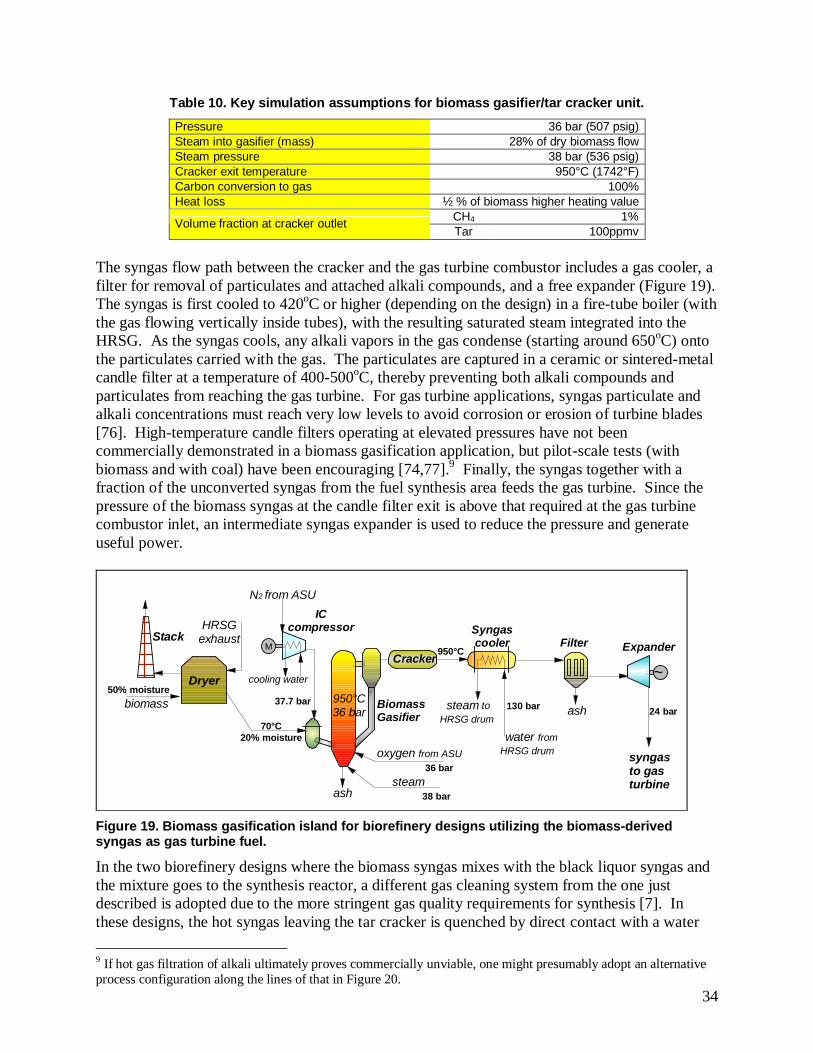
34

Table 10. Key simulation assumptions for biomass gasifier/tar cracker unit.

Pressure 36 bar (507 psig)Steam into gasifier (mass) 28% of dry biomass flowSteam pressure 38 bar (536 psig)Cracker exit temperature 950°C (1742°F)Carbon conversion to gas 100%Heat loss ½ % of biomass higher heating value

CH4 1%Volume fraction at cracker outlet Tar 100ppmv

The syngas flow path between the cracker and the gas turbine combustor includes a gas cooler, afilter for removal of particulates and attached alkali compounds, and a free expander (Figure 19).The syngas is first cooled to 420oC or higher (depending on the design) in a fire-tube boiler (withthe gas flowing vertically inside tubes), with the resulting saturated steam integrated into theHRSG. As the syngas cools, any alkali vapors in the gas condense (starting around 650oC) ontothe particulates carried with the gas. The particulates are captured in a ceramic or sintered-metalcandle filter at a temperature of 400-500oC, thereby preventing both alkali compounds andparticulates from reaching the gas turbine. For gas turbine applications, syngas particulate andalkali concentrations must reach very low levels to avoid corrosion or erosion of turbine blades[76]. High-temperature candle filters operating at elevated pressures have not beencommercially demonstrated in a biomass gasification application, but pilot-scale tests (withbiomass and with coal) have been encouraging [74,77].9 Finally, the syngas together with afraction of the unconverted syngas from the fuel synthesis area feeds the gas turbine. Since thepressure of the biomass syngas at the candle filter exit is above that required at the gas turbinecombustor inlet, an intermediate syngas expander is used to reduce the pressure and generateuseful power.

Syngascooler

Dryer

ash

N2 from ASU

BiomassGasifier

FilterStack

biomass

syngasto gasturbine

70°C20% moisture

HRSGexhaust

950°C

37.7 bar

oxygen from ASU

steam36 bar

38 bar

50% moisturesteam to

HRSG drum

water fromHRSG drum

130 bar

ash

CrackerM

cooling water

950°C36 bar

~

Expander

24 bar

ICcompressor

Figure 19. Biomass gasification island for biorefinery designs utilizing the biomass-derivedsyngas as gas turbine fuel.

In the two biorefinery designs where the biomass syngas mixes with the black liquor syngas andthe mixture goes to the synthesis reactor, a different gas cleaning system from the one justdescribed is adopted due to the more stringent gas quality requirements for synthesis [7]. Inthese designs, the hot syngas leaving the tar cracker is quenched by direct contact with a water

9 If hot gas filtration of alkali ultimately proves commercially unviable, one might presumably adopt an alternativeprocess configuration along the lines of that in Figure 20.

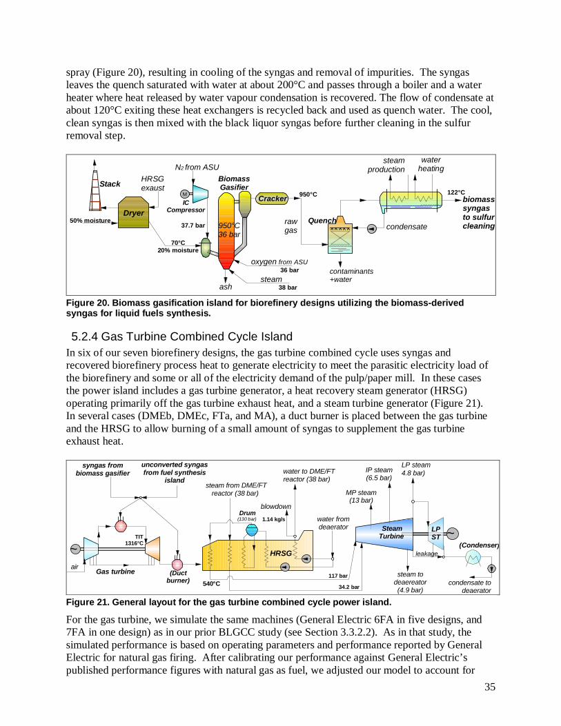
35

spray (Figure 20), resulting in cooling of the syngas and removal of impurities. The syngasleaves the quench saturated with water at about 200°C and passes through a boiler and a waterheater where heat released by water vapour condensation is recovered. The flow of condensate atabout 120°C exiting these heat exchangers is recycled back and used as quench water. The cool,clean syngas is then mixed with the black liquor syngas before further cleaning in the sulfurremoval step.

contaminants+water

Dryer

BiomassGasifierStack

M

70°C20% moisture

HRSGexaust

950°C

steam38 barash

950°C36 bar

Cracker

N2 from ASU

oxygen from ASU36 bar

condensate

steamproduction

waterheating

biomasssyngasto sulfurcleaning

122°C

rawgas

50% moisture

ICCompressor

Quench37.7 bar

Figure 20. Biomass gasification island for biorefinery designs utilizing the biomass-derivedsyngas for liquid fuels synthesis.

5.2.4 Gas Turbine Combined Cycle IslandIn six of our seven biorefinery designs, the gas turbine combined cycle uses syngas andrecovered biorefinery process heat to generate electricity to meet the parasitic electricity load ofthe biorefinery and some or all of the electricity demand of the pulp/paper mill. In these casesthe power island includes a gas turbine generator, a heat recovery steam generator (HRSG)operating primarily off the gas turbine exhaust heat, and a steam turbine generator (Figure 21).In several cases (DMEb, DMEc, FTa, and MA), a duct burner is placed between the gas turbineand the HRSG to allow burning of a small amount of syngas to supplement the gas turbineexhaust heat.

~LPST

~

Gas turbineair

Drum(130 bar)

(Ductburner)

blowdown

syngas frombiomass gasifier

unconverted syngasfrom fuel synthesis

island

TIT1316°C

water fromdeaerator Steam

Turbine

HRSG

540°C

water to DME/FTreactor (38 bar)

steam from DME/FTreactor (38 bar)

1.14 kg/s

117 bar

34.2 bar

MP steam(13 bar)

LP steam4.8 bar)IP steam

(6.5 bar)

steam todeaereator(4.9 bar)

(Condenser)leakage

condensate todeaerator

Figure 21. General layout for the gas turbine combined cycle power island.

For the gas turbine, we simulate the same machines (General Electric 6FA in five designs, and7FA in one design) as in our prior BLGCC study (see Section 3.3.2.2). As in that study, thesimulated performance is based on operating parameters and performance reported by GeneralElectric for natural gas firing. After calibrating our performance against General Electric’spublished performance figures with natural gas as fuel, we adjusted our model to account for

36

syngas as the fuel rather than natural gas. A key adjustment arises from the lower unit energy content of syngas compared to natural gas, which requires a larger mass flow of syngas to achieve the same turbine inlet temperature. This leads to higher mass flow through the expansion section of the gas turbine, which affects the match between compressor and expander operating conditions. Volume 2 describes details of the gas turbine model calibration and adjustments. While commercial applications of the 6FA and 7FA today are with natural gas or distillate fuel, a great deal of development work has been done and operating experience acquired in using these machines with synthesis gas in coal-integrated gasification combined cycle applications. General Electric now offers eight different gas turbine models for firing with syngas, ranging in outputs from 10 MW to 300 MW and including the 6FA and 7FA [78]. The gas turbine exhausts to a heat recovery steam generator (HRSG). The HRSG evaporation pressure and superheater exit temperature (130 bar/540oC with 6FA and 130 bar/565°C with 7FA) represent state-of-the-art levels for combined cycles. Because only clean combustion products pass over the boiler tubes in the HRSG, these conditions are higher than can be used with a recovery boiler or a wood-residue boiler. Steam generation in the HRSG is integrated with steam raised elsewhere in the biorefinery (syngas coolers and synthesis reactor) to maximize overall efficiency. In the mixed-alcohol case, the synthesis reactor operates at 350°C, enabling the heat released by the synthesis reactions to be used to raise steam at 130 bar. In the DME and FT reactors, which operate at 260°C, steam is raised at 38 bar. In all cases, the steam from the synthesis reactors is superheated in the HRSG. Medium-to-low temperature heat extracted from syngas at various points in the biorefinery are used to pre-heat the HRSG make-up water when possible.10 This is worthwhile in most cases because of the relatively high temperature of flue gas exiting the HRSG (necessitated by the inlet-gas temperature required at the biomass dryer). Leaving the HRSG, the steam expands in a turbine from which process steam is extracted at 13 bar and at 4.8 bar for supply to the pulp/paper mill. (Because of the relatively large steam extraction at 13 bar, only a single HRSG evaporation pressure level is used; additional pressures would give negligible benefits.) The steam turbine is a back-pressure design in some cases and includes a condensing section in other cases. Because of the steam conditions leaving the HRSG, the previously-existing steam turbine at the power/recovery plant of the reference pulp/paper mill must be replaced by a new machine capable of handling the higher conditions. We have not considered any steam reheating because given the relatively small scale of plants considered in our biorefineries and the large amount of steam extracted at 13 bar, the economic attractiveness of reheating would be questionable. In the one biorefinery configuration not utilizing a gas turbine in the power island (DMEa), we are able to adapt the back-pressure steam turbine previously existing at the reference pulp/paper mill for use in the power island, thereby avoiding the capital investment for a new steam turbine.

10 For each biorefinery, the integration of heat exchange among components is optimized, within practical limits, to increase overall efficiency. Heat is transferred across relatively small temperature differences with a minimum temperature difference of 10°C for gas-liquid heat exchange and around 15°C for gas-gas heat exchange. There is considerable process heat recovery, but there is also low-temperature heat rejection to the environment in all cases.

37

5.2.5 Liquid Fuels Synthesis Island The conversion of clean synthesis gas into a liquid fuel involves passing the syngas over a catalyst that promotes the desired synthesis reactions and then refining the raw product to obtain the final desired liquid fuel. Two basic designs for commercial synthesis reactors have been developed: gas-phase (or fixed-bed) and liquid-phase (or slurry-bed). Fixed-bed reactors have a long commercial history, but liquid phase reactors have been gaining popularity in commercial applications because of attractive performance attributes and lower cost. Liquid phase reactors are now commercially offered for FTL, methanol, and DME synthesis. Liquid phase reactors for mixed-alcohol synthesis are still under development. Fixed-bed and liquid-phase reactor designs differ primarily in their handling of reactor temperature control. Synthesis reactions are exothermic, such that the reactor temperature increases as the reactions proceed if no heat is removed. Higher temperatures promote faster reactions, but maximum (equilibrium) conversion is favored by lower temperatures. Also, catalysts are deactivated when overheated. Thus, the temperature rise in a synthesis reactor must be controlled. In commercial practice, a reactor operating temperature of 250-280oC for methanol, DME or FTL synthesis balances kinetic, equilibrium, and catalyst activity considerations. For mixed-alcohols synthesis, which is not yet a commercially established technology, higher reaction temperatures (300-400oC) have been indicated with catalysts identified to date. A gas-phase reactor incorporates the flow of syngas over a fixed-bed of catalyst pellets. With this design it is difficult to maintain isothermal conditions by direct heat exchange (due to low gas-phase heat transfer coefficients). To limit temperature rise, the synthesis reactions are typically staged, with cooling between reactor stages. Also, by limiting the initial concentration of CO entering the reactor (to 10-15 vol%) the extent of the exothermic reactions can be controlled. Control of the CO fraction is achieved in practice by maintaining a sufficiently high recycle of unconverted H2-rich syngas back to the reactor. In a liquid-phase reactor syngas is bubbled through an inert mineral oil containing powdered catalyst in suspension (Figure 22). Much higher heat release rates (i.e., extents of reaction) can be accommodated without excessive temperature rise as compared to a gas-phase reactor because of more effective reactor cooling by boiler tubes immersed in the fluid. The vigorous mixing, intimate gas-catalyst contact, and uniform temperature distribution enable a high conversion of feed gas to liquids in a relatively small reactor volume. Conversion by liquid-phase FT synthesis is especially high. A single-pass fractional conversion of CO of about 80% can be achieved [79], compared to less than 40% for conversion with traditional fixed-bed FT reactors. For the FT reactor conditions we assume in our simulations, the single-pass CO conversion is about 65%.

5.2.5.1 Dimethyl Ether Single-step DME synthesis reactors typically utilize a mix of two catalysts, one promoting the synthesis of methanol from syngas (CO + 2H2 CH3OH) and one promoting the dehydration of the methanol to DME (2CH3OH CH3OCH3 + H2O). Both liquid-phase and fixed-bed reactors are offered commercially.

38

LIQUID-PHASE SYNTHESISP = 50-100 atm.T = 200-300oC

Synthesis gas(CO + H2)

Cooling water

SteamCatalystpowderslurriedin oil

Disengagementzone

Fuel product (vapor)+ unreacted syngas

Synthesis gas(CO + H2)

Cooling water

SteamCatalystpowderslurriedin oil

Disengagementzone

Fuel product (vapor)+ unreacted syngas

catalystCO

H2

CH3OCH3CH3OHCnH2n+2(depending on catalyst)

catalystCO

H2

CH3OCH3CH3OHCnH2n+2(depending on catalyst)

LIQUID-PHASE SYNTHESISP = 50-100 atm.T = 200-300oC

Synthesis gas(CO + H2)

Cooling water

SteamCatalystpowderslurriedin oil

Disengagementzone

Fuel product (vapor)+ unreacted syngas

Synthesis gas(CO + H2)

Cooling water

SteamCatalystpowderslurriedin oil

Disengagementzone

Fuel product (vapor)+ unreacted syngas

catalystCO

H2

CH3OCH3CH3OHCnH2n+2(depending on catalyst)

catalystCO

H2

CH3OCH3CH3OHCnH2n+2(depending on catalyst)

Figure 22. Simplified schematic of liquid phase synthesis reactor.

Leading developers of liquid-phase DME synthesis reactors are DME Development, Inc., a Japanese consortium of nine companies led by NKK and Nippon Sanso [32,80,81], and Air Products and Chemicals [82,83,84,85,86,87]. The Institute of Coal Chemistry of the Chinese Academy of Sciences [88] has also been developing slurry-phase DME synthesis technology. DME Development, Inc. recently completed nearly two years of testing of a 100 tpd DME slurry-phase reactor in Kushiro, Hokkaido (Japan), and is offering the technology for commercial applications [32]. The Kushiro demonstration was preceded by testing of a five ton per day capacity reactor completed in 1999 by NKK [89], who prior to that (with support from the Japanese Ministry of International Trade and Industry) worked with the Taiheiyo Coal Mining Co., Sumitomo Metal Industries, and Japan’s Center for Coal Utilization to develop the DME slurry reactor technology with coal applications in mind. The DME reactor design of Air Products is derived from its liquid-phase methanol (LPMEOH) synthesis process developed in the 1980s. A commercial-scale LPMEOH demonstration plant (250 tonnes per day methanol capacity) has been operating since 1997 with gas produced by the Eastman Chemical Company’s coal gasification facility in Kingsport, Tennessee [90]. The construction of this facility was preceded by extensive testing in a 10 tpd process development unit (PDU) in LaPorte, Texas. The PDU was operated in 1999 to generate test data on direct DME synthesis [91,92]. Fixed-bed DME synthesis reactor designs are also commercially available. The leading supplier of this design is Halder-Topsoe.1193Mobil and Snamprogetti S.p.A. hold patents for DME synthesis processes [94,95], but at present are not pursuing commercial development of the technology. The Institute of Chemical Physics of the Chinese Academy of Sciences (Dalian) has done some work on fixed-bed DME synthesis technology [96]. 11 The fixed-bed design of Halder-Topsoe includes three stages of synthesis reactors with cooling between each stage and recycle of unconverted syngas [25]. The patent for this process specifies a feed gas CO concentration of less than 10% and a recycle volume of unconverted syngas ranging from 93% to 98% of the total unconverted syngas [93]. The fraction of CO converted on a single pass through each reactor stage (assuming a three-stage intercooled set of reactors) ranges from 16% to 34%, depending on the H2/CO ratio.

39

For our DME simulations, we adopt a liquid-phase synthesis reactor design, and we utilize a kinetic model developed in prior work [73] using kinetic rate data available in the published literature for the key reactions involved in DME synthesis. Volume 2 discusses our model. In all three of our DME configurations, only syngas from black liquor is used for synthesis of liquids (Table 6). Leaving the Rectisol® area, the clean syngas is compressed to 68 bar and then pre-heated to 100oC before it arrives to the synthesis island. Just ahead of the synthesis reactor, the syngas (now at 66 bar) is heated to 240ºC using the product stream from the synthesis reactor. The gas then enters the liquid-phase DME reactor in which isothermal synthesis conditions are maintained at 260ºC by immersed steam generation tubes. In a single pass of syngas only a portion of the CO and H2 are converted to DME. The product gas mixture passes to the product separation area, where a series of flash tanks separates most of the unconverted synthesis gas from DME, methanol and water. Further separation of the liquid products is achieved by cryogenic distillation. The distillation area includes three columns: the first separates DME/methanol/water and CO2 from residual light gases (CO, H2, etc.); the second separates DME from methanol/water; and the third separates water from methanol. The small amount of methanol is heated to 250°C and sent to an adiabatic dehydration reactor producing DME and water. A downstream flash tank separates the most volatile part of the product, including all DME, which is returned to the second distillation column for purification. The liquid fraction is recycled to the third distillation column. The final DME product has a purity of 99.8%. Process heat exchange in the separation area is optimized to minimize heating and refrigeration requirements. External heat requirements are met using steam from the power island. In the DMEa and DMEb configurations, 97% of the syngas that is unconverted in one pass through the synthesis reactor is compressed and recycled to the reactor to increase overall conversion to DME. The purge stream (3%) is sent as fuel to the power island. In the DMEc configuration, the recycle loop is eliminated and all syngas not converted to liquids on a single pass is sent as fuel to the power island.

5.2.5.2 Fischer-Tropsch Liquids Commercial Fischer-Tropsch catalysts include iron and cobalt based materials. Cobalt catalysts produce a large heavy-wax fraction that can be easily and with high selectivity refined into desired lighter products by subsequent hydrocracking (breaking up of the large hydrocarbon molecules into desired final products in a hydrogen-rich environment). Hydrocracking of the large straight-chain hydrocarbons formed by FT synthesis can be done under much less severe temperature conditions (350-400oC for cracking to C5-C18 range hydrocarbons) than is required for hydrocracking of aromatic molecules found in conventional petrochemical refining. Iron-based catalysts produce a broader product mix that requires a greater level of refining than with cobalt catalysts. Also, unlike cobalt catalysts, iron catalysts promote water-gas shift activity (CO + H2O H2 + CO2), making them well suited for use with syngas characterized by H2/CO ratios below the stoichiometic value of 2.2 for FT synthesis. In our analysis, we simulate a liquid-phase design for the FTL synthesis reactor. Liquid-phase FTL reactors are commercially available today from several vendors [12,97]. We utilize a kinetic model developed in prior work by Larson et al. [73] based on a model proposed by Fox and Tam [98] and drawing on published kinetic rate information, as described in Volume 2 of this study. Consistent with the preceding discussion, our model is for an iron-based catalyst

40

because of the low H2/CO ratio of the syngas feed in our biorefinery designs (1.04 to 1.11) . The powdered iron-based catalyst is suspended in a liquid bed made up of the heavy hydrocarbon fraction (wax) produced by the FT reactions. Because of the high single-pass conversion that can be achieved with slurry-phase FT synthesis, our three FTL biorefineries all utilize “once-through” synthesis, with unconverted syngas going to the power island as fuel. In FTa and FTb, the syngas entering the synthesis reactor is derived only from black liquor. In FTc, the syngas from black liquor and from biomass are combined to feed the synthesis reactor. The operating pressure of the synthesis reactor is set to 30.7 bar, which requires no upstream syngas compression. The incoming syngas stream to the synthesis reactor is preheated to 245oC and boiler tubes immersed in the slurry generate steam at 38 bar, limiting the reactor temperature to 260°C. The synthesis reactions produce a raw mix of products that must be refined to finished products. A flash step is used to separate light gases (including unconverted syngas and light gases produced in the FT reaction) from the heavier compounds that constitute the raw FTL product (a mixture of distillate, naphtha, and wax fractions). The light gases are sent to the power island as fuel. The raw FTL product – “FT crude” – could be refined onsite to finished products like diesel or gasoline blendstocks. However, because of the complexity and cost of refining at the relatively small scales of our biorefineries (compared to typical sizes for petroleum refineries), Nexant engineers with whom we reviewed our preliminary designs recommended the FT crude be transported by trucks (with heated tanks to maintain the wax fraction as a liquid) to existing petroleum refineries for processing to finished products. Accordingly, we assume the FT crude is exported from the biorefinery as a petroleum crude substitute.12

5.2.5.3 Mixed Alcohols Compared with FTL or DME synthesis, the technology for synthesis of mixed alcohols is considerably less commercially advanced, and there is sparse published literature on which to base detailed reactor performance estimates. Catalysts that have been examined in the past can be divided into four categories [99]: ruthenium-based catalysts, modified methanol catalysts, modified Fischer-Tropsch catalysts, and molybdenum-sulfide based catalysts. Among these, the MoS2 based catalysts (originally discovered by researchers at Dow and Union Carbide in the 1980s) have received considerable recent attention due to their high tolerance for sulfur-contaminated syngas, their water-gas shift activity, and their high activity and selectivity for linear alcohols. Selectivity is an especially important characteristic because if all possible chemical reactions between CO and H2 are allowed to compete without constraints, reactions other than those for synthesis of higher alcohols will thermodynamically out-compete reactions for synthesis of higher alcohols. In particular, the formation of Fischer-Tropsch hydrocarbons (α-olefins and n-paraffins) from CO and H2 is thermodynamically favored over the formation of higher alcohols.13 For this reason, to maximize performance of alcohol synthesis catalysts, high selectivity is an essential feature.

12 Our financial analysis (described later) assumes sale of the FT crude at the value of crude petroleum (on an equivalent energy basis). We do not model refining of the raw product to finished products. 13 The equilibrium constant, Keq, is higher for hydrocarbons than for alcohols.

41

For catalysts that have been identified to date, required reaction temperatures have been in the range of 300-400oC. Because of the difficulty of maintaining an inert liquid in the liquid state at these temperatures, most development efforts on synthesis reactors are focusing on gas-phase reactors, although at least one company claims to be developing a liquid-phase technology for mixed alcohol synthesis [48]. We have assumed a gas-phase reactor in our biorefinery design for synthesis of mixed alcohols, and we engaged the catalyst research group headed by Prof. Forzatti at Politecnico di Milano to develop a kinetic model of the synthesis reactor. The kinetic model was developed by Prof. Lietti and Prof. Tronconi in Forzatti’s group. As discussed in Section 2.3, the model is based on the most recent (mid-1990s) publicly-available empirical data for the performance of a particular MoS2 catalyst [100]. Volume 2 of our study provides details of the modeling effort. Our mixed alcohol biorefinery utilizes the combined black liquor and biomass syngas flows as the fresh feed gas for the synthesis reactor. Because the performance of both the acid gas removal system (Selexol®) and the mixed-alcohol synthesis reactor improve with pressure, we utilize an intercooled compressor to raise the syngas pressure to 106 bar as it approaches the Selexol® area. Following the Selexol® system the syngas is mixed with a recycle flow of unconverted syngas and a recycle flow of methanol, both coming from downstream of the synthesis reactor. This mixture is heated to 330°C before it enters the synthesis reactor. Heat generated by the reactions is recovered as 130 bar steam to maintain the reactor temperature at 350°C. The hot effluent from the reactor is cooled to 36oC by a sequence of heat exchange with the reactor inlet flow and then cooling water. At 36oC most of the alcohols condense, enabling separation of unconverted gas from the liquids. Of the unconverted gas, 76% is compressed and recycled back to the synthesis reactor. The remaining gas is preheated and expanded to about 25 bar (to recover useful power), humidified using a saturator and then used as fuel for the gas turbine. The recovered liquids are sent to a distillation column where methanol and lighter compounds are separated from the alcohols, recompressed and recycled to the synthesis reactor. The bottoms from the distillation column contain ethanol and higher alcohols along with water. A molecular sieve is used to separate the alcohols from water. The purge gas from the molecular sieve, composed of water vapor with a small percentage of alcohols, is compressed and sent to the gas turbine to recover the energy content and to increase the mass flow through the turbine so as to increase power production. The final mixture of C2+ alcohols can be used directly as a gasoline blendstock or separated into component alcohols for chemicals use. We have not simulated the separation of alcohols, but we have examined the potential impact on overall economics that might result from doing so (Section 8). Finally, it is important to note that our kinetic model predicts a considerably lower overall yield and significantly different composition of alcohols from values reported in the literature, e.g. by Aden et al. [46]. Because literature results are not based on kinetic models, however, it is difficult to make detailed comparisons between our kinetic-model results and others’ reported results. The catalyst we have modeled is the only one for which there is sufficient empirical data published for building a kinetic model. In general, others’ results (including claims of technology developers) show much higher yields and much greater selectivity for C2+ alcohols than we predict. More complete sets of empirical data for other catalysts are needed to better

42

understand and document the potential for synthesis of mixed alcohols. There may also be arrangements for recycle of unconverted syngas different from the design we have used that would improve overall system performance [101]. This is another area where further work might prove fruitful.

5.3 Technology Summary Table 11 summarizes the key technologies incorporated into each of our seven biorefinery designs. The column labeled “status” indicates the proximity to commercial offering for each technology. The majority of components are already in wide commercial use (in non-biorefinery applications). All but one of the technologies not in the commercial category fall into the category of technologies that have been or are currently being demonstrated at pilot scale, such that relatively near term (2010 time frame) commercial deployment is feasible. Only one technology (mixed-alcohols synthesis) appears to be at a relatively under-developed stage, though as noted in Section 2.3, several companies claim they will offer mixed-alcohol synthesis technology commercially in the near term. Table 11. Summary of technologies included in our biorefinery designs including commercial status of each technology.

Statusa FTa FTb FTc DMEa DMEb DMEc MA High-temp gasifier pilot ♦ ♦ ♦ ♦ ♦ ♦ ♦ Quench pilot ♦ ♦ ♦ ♦ ♦ ♦ ♦ Black Liquor

Gasification O2 feed com ♦ ♦ ♦ ♦ ♦ ♦ ♦ Fluid-bed gasifier pilot ♦ ♦ ♦ ♦ ♦ ♦ Syngas cooler pilot ♦ ♦ ♦ ♦ ♦ Hot gas filter pilot ♦ ♦ ♦ ♦ Quench cleanup com ♦ ♦ O2 feed com ♦ ♦ ♦ ♦ ♦ ♦

Woody Biomass Conversion

Boiler com ♦ Rectisol® com ♦ ♦ ♦ ♦ ♦ ♦ Selexol® com ♦ H2S Capture

and Recovery Claus/SCOT com ♦ ♦ ♦ ♦ ♦ ♦ ♦ Slurry bed reactor com ♦ ♦ ♦ ♦ ♦ ♦ Fixed-bed reactor lab ♦ Fuel Synthesis Syngas recycle com ♦ ♦ ♦ Gas turbine com ♦ ♦ ♦ ♦ ♦ ♦ Back pressure ST com ♦ ♦ ♦ ♦ ♦ Power Island Condensing ST com ♦ ♦

(a) Commercial status. com = commercially-offered; pilot = demonstrated at pilot scale; lab = demonstrated in laboratory.

5.4 Detailed Biorefinery Mass/Energy Balance Results

5.4.1 Process Flow Sheets and Performance Analysis Figure 23 through Figure 29 show the results of our detailed biorefinery process designs and mass/energy balance simulations. The following sections discuss each of these, and more detailed discussions are available in Volume 2. Table 12 summarizes performance results for all of the biorefineries and also includes, for comparison, results from our prior BLGCC study for the Tomlinson and BLGCC systems. Recall that in all cases all of the pulp/paper mill’s process steam demands are being met by the power/recovery/fuel system. Other key features of the biorefinery designs are as summarized in Table 6.

43

5.4.1.1 DME Flowsheets The liquid fuel produced by all the DME biorefineries comes only from the conversion of syngas from black liquor. The DME production train in DMEa (Figure 23) is identical to that in DMEb (Figure 24). Each has a production capacity of 511 metric tonnes per day of DME (168 MW lower heating value, LHV) and converts 48% of the LHV of the black liquor into DME. In DMEc (Figure 25), DME is also made only from gasified black liquor, but because a once-through synthesis configuration is used rather than recycle, the DME output is lower: 226 t/d, or 21% of the black liquor LHV. For the power island, DMEa utilizes woody biomass as the main fuel for a steam-Rankine cycle, DMEb uses a gasifier-GTCC with gasified woody biomass as the main fuel, and DMEc uses a gasifier-GTCC with gasified woody biomass and unconverted syngas for fuel. In all three cases, the amount of biomass consumed is set so that the power island can meet the process steam needs of the pulp/paper mill. With this constraint, the gross power outputs of DMEb and DMEc are about 3.5 times that of DMEa, and the net power output (after meeting biorefinery parasitic demands) is close to zero for DMEa and about 90 MW for DMEb and DMEc. In the latter two cases this power output is sufficient to meet about 90% of the pulp/paper mill’s process electricity needs. The bottom three rows of Table 12 show summary energy output-input ratios. The ratio of useful outputs from the biorefinery (mill process steam, net electricity, and DME) to total primary energy used to generate these outputs is close to 0.71 in all three cases. The ratio of exportable biorefinery products (net electricity and DME) to total fuel input ranges from 0.32 to 0.40. The value of this parameter for DMEb is higher than for DMEa because the only major difference between DMEa and DMEb is the replacement of the biomass boiler/steam cycle in DMEa with a more efficient biomass gasifier/GTCC in DMEb. The value for DMEc is lower than for DMEb primarily because the fuel to electricity output ratio for DMEb is higher than for DMEc, and since the “thermodynamic value” of fuel is lower than that of electricity, shifting the conversion toward more electricity decreases the ratio of (electricity+fuel) to total fuel input. This circumstance points out that the ratio between the sum (electricity+fuel) and total fuel input is not necessarily a good indicator of plant performance. It provides some information, but can be misleading. The final row of Table 12 shows the effectiveness with which the gasification-based facilities utilize additional purchased energy inputs (primarily woody residues, but also some additional lime kiln fuel). This “effectiveness of purchased fuels use” exceeds 100%, or nearly so, in all DME cases.14 This indicates that all of these designs are making very effective use of the additional energy inputs that characterize gasification compared to Tomlinson systems.

14 We use the term effectiveness, rather than efficiency, since efficiency greater than 100% is strictly not possible. Values of effectiveness greater than 100% are possible because the denominator includes only biomass that is purchased for energy (and excludes black liquor and hog fuel).

44

Table 12. Biorefinery performance estimates, with comparisons to Tomlinson and BLGCC. Units are megawatts unless otherwise indicated. Fuel values are given on a lower heating value basis.

Power Only Biorefineries Tomlin. BLGCC DMEa DMEb DMEc FTa FTb FTc MA FUEL INPUTS Black liquor 392.6 350.7 350.7 350.7 350.7 350.7 350.7 350.7 350.7 Hog fuel 57.8 54.1 54.1 54.1 54.1 54.1 54.1 54.1 54.1 Total mill by-product fuels 450.4 404.8 404.8 404.8 404.8 404.8 404.8 404.8 404.8 Purchased wood residues 0 27.1 77.4 195.5 73.4 101.6 368.5 451.3 89.2 Natural gas to duct burner -- 12.9 -- -- -- -- -- -- -- Lime kiln #6 fuel oil 31.1 35.9 35.9 35.9 35.9 35.9 35.9 35.9 35.9 Total purchased fuels 31.1 75.9 113.3 231.4 109.3 137.5 404.4 487.2 125.1 Total fuel inputs 481.5 480.7 518.1 636.2 514.1 542.3 809.2 892.0 529.9 STEAM TO PULP/PAPER MILL LP (55 psig) steam to process 142.8 135.3 135.3 135.3 135.3 135.3 135.3 135.3 135.3 MP (175 psig) steam to process 69.3 64.9 64.9 64.9 64.9 64.9 64.9 64.9 64.9 Total process steam production 212.1 200.2 200.2 200.2 200.2 200.2 200.2 200.2 200.2 LIQUID FUEL PRODUCTION -- -- 168.0 168.0 74.2 111.6 111.6 342.7 59.6 Barrels per day petroleum equiv.a -- -- 2362 2362 1043 1549 1549 4757 948 ELECTRICITY BALANCE Gas turbine gross output -- 87.0 -- 89.5 82.9 83.9 186.5 89.7 89.7 Steam turbine gross output 72.0 48.2 32.9 42.0 38.7 34.0 87.9 48.6 40.8 Syngas expander output -- -- 2.58 5.01 1.96 1.65 4.26 -- 2.99 Total gross production 72.0 135.1 35.5 136.5 123.6 119.5 278.7 138.3 133.5 Air separation unit power useb -- 14.9c 15.8 27.0 21.5 22.8 35.7 38.4 22.1 Syngas compressor power use -- -- 1.95 1.95 2.17 -- -- -- 7.37 Gas compressors (mainly recycle) -- -- 7.26 7.26 -- -- -- -- 1.77 Steam cycle auxiliaries 6.7 1.2 1.38 2.30 1.52 1.31 3.76 5.40 2.75 Black liquor gasification island aux. -- 2.7 2.67 2.67 2.67 2.67 2.67 2.67 2.67 Biomass gasification island aux. -- -- -- 3.37 1.74 2.11 5.66 6.75 1.95 Biomass boiler auxiliaries 1.00 1.2 1.75 -- -- -- -- -- -- Acid gas removal & S recovery aux. -- 1.1 0.97 0.97 0.96 0.96 0.96 2.59 1.81 Refrigeration for AGR -- -- 2.15 2.15 2.07 2.01 2.01 5.11 1.21 Synthesis island auxiliaries -- -- 1.00 1.00 0.40 -- -- -- -- Total recovery area use 7.7 21.1 34.9 48.7 33.0 31.8 49.8 60.9 41.6 Net Electricity Production 64.3 114.1 0.56 87.8 90.5 87.7 228.9 77.3 91.9 Power in excess of Tomlinson -- 50.4 - 63.2 24.1 26.8 24.0 165.2 13.6 28.2 Process use (excl. recovery area) 100.1 100.1 100.1 100.1 100.1 100.1 100.1 100.1 100.1 Mill electricity purchases 35.8 -15.2 99.6 12.3 9.58 12.4 -128.8 22.8 8.21 Energy Ratios Useful outputs/total inputsd 0.574 0.654 0.712 0.717 0.710 0.737 0.668 0.695 0.664 Exportable outputs/total inputse 0.133 0.237 0.325 0.402 0.320 0.368 0.421 0.471 0.286 Effectiveness of purchased fuel usef -- 1.11 1.27 0.956 1.28 1.27 0.740 0.780 0.928 (a) Barrels (bbl) per day of equivalent petroleum-derived fuel potentially displaced by the biorefinery fuel. The potentially-displaced

fuels are: diesel (6.15 GJ/bbl, LHV) for DME, crude oil (6.22 GJ/bbl, LHV) for FTL, and gasoline (5.43 GJ/bbl, LHV) for MA. (b) The parasitic ASU electricity load shown here includes 0.58 MW more than the ASU load shown in the detailed mass/energy

balance flowsheets. The additional 0.58 MW is from upsizing of the ASU to provide O2 for delignification (see text discussion). (c) In developing the biorefinery mass/energy balance simulations, a minor error was discovered in the previously-completed BLGCC

simulation, resulting in a slightly lower O2 flow to the black liquor gasifier in the BLGCC case than in the biorefinery cases. We have not revised the BLGCC results, because the error was minor. The error accounts for the slight difference in electricity needed for the ASU between the BLGCC and DMEa cases, which should otherwise have identical parastic power demands.

(d) Defined as the sum of process steam, net electricity, and liquid fuel outputs divided by the sum of all fuel inputs. (e) Defined as the sum of net electricity and liquid fuel production divided by the sum of all fuel inputs. (f) Defined as the sum of net electricity and liquid fuel production for the gasification-based facility minus this quantity for the

Tomlinson facility divided by the difference in total purchased fuel between the gasification and Tomlinson facilities.

45

Quenchcooler

1000°C35 bar

Gasifier

19213.03.7

green liquor

Black liquor(80% BLS)

15214.03.7

11535.035.6

raw gas

condensate

fromdeaerator

12242.034.3

21835.060.1

~SteamTurbine

ash

powerboiler

Gascleanup

airto stack

1451.0179.3

201.0116.2

201.0179.3

1451.01102.5

biomass

Air

heat

er

Claus +SCOT plant

201.0143.1

-15.2MWe

14535.010.1

251.050.4

air

Oxygenplant

vent

to lime kiln

95%O2

251.0532.6

LPsteamto mill

1524.8

64.1

MPsteamto mill

19213.032.9

unconvertedsyngas

DME island(0.97 recycle)

Deaerator (4.8 bar)

19513.02.4

152 4.81.3

1744.853.5

19213.020.2

1524.813.7

1116.0

95.0

2016.51.8

47578.547.7

47534.216.8

27713.07.7

2327.77.0

24738.016.8

1455.995.0

to deaerator

1754.91.2

13234.319.9

12233.625.8

to gasifierand de-SH

de-SHfrom

deaerator

15214.01.3

15214.00.7

Drum(87.2 bar) 248

38.016.8

leakage

DME5.92 kg/s

32.9MWe

steamfrom

ST

T [°C]

m [kg/s]p [bar]

480°C

350.7MWtLHV

131.5 MWtLHV

33.5 MWtLHV

168.0 MWtLHV

Rectisolsystem

BLcleansyngas

returnfrom mill

1341.0

61.5

155.033.5

makeup

-5732.013.3

235.4MWtLHV

1767.813.3104

33.225.2

3532.91.4

3532.625.5

-3532.325.5

condensatereturn

condensate

M-2.0

MWe

671.020.5

10066.413.3

steam to DMEisland

(reboilers)19213.01.9

1524.83.9

heat

2.8MWt

acid gas

gasrecycle

1524.81.9

14733.21.1

Rectisolregeneration

421.21.9

2.5MWref

145.8MWt

Figure 23. Mass and energy balance for DMEa. Key distinguishing features are the recycle synthesis loop and the hog fuel/purchasedresidues boiler/steam cycle power island.

46

19213.0

3.7

greenliquor

Black liquor(80% BLS)

15114.03.7

11535.035.6

raw gasQuenchcooler

1000°C35 bar

BLGasifier

condensate

fromdeaerator

12242.034.3

21835.060.1

201.0174.6

-26.4MWe

14536.010.1

251.05

0.4

air

Oxygenplant

vent

to lime kiln

95%O2

241.0554.9

Deaerator (4.8 bar)

19213.020.2

1524.813.6

11210.0

100.2

1456.0

100.2

12233.625.8

de-SH

steamfromST

37524.032.6

43116.6

151.86351.05210.0

89.5MWe~ 751

1.04217.4

135716.1

184.0

201.01177.8

Gas turbine (6FA)air

Syngas cooler31.8 MWt

Drum(130 bar)

~SteamTurbine

25813.0

7.9

42.0MWe

201.0130.7

701.0119.2

DryerLP

steamto mill

1524.864.1

MPsteamto mill

19213.032.9

Claus +SCOT plant

BL cleansyngas

13234.319.9

901.0228.9

unconvertedsyngas

2291.0217.4

95036.032.6

42134.232.6

331130.027.5

330130.0

27.5

14636.07.7

24838.04.3

oxygen

steam

37034.212.6

535117.0

63.0

1594.854.3

1886.51.8

16537.7

1.5

BiomassGasifier

19513.0

2.4

1524.81.3

15114.00.6

15114.00.4

HRSG

Duct burner

1504.80.2

fromblowdownflash

blowdown24738.01.14

540°C

Cracker

return frommill

1341.0

61.5

155.038.7

makeup

heat

ash

950°C36 bar DME island

(0.97 recycle)

5.7MWt

24738.016.8248

38.012.6

350.7MWtLHV

Filter

223.8MWtLHV

ash

biomass249.6 MWtLHV

36.3MWtLHV

T [°C]

m [kg/s]p [bar]

10.0 kg/s

bleeds

to deaerator 1594.81.6

~2.4

MWe

Expander

37524.032.2

10433.225.2

3532.91.4

23.5 MWt

134.0MWt

nitrogen

-0.9MWe

241.051.5

11324.07.4

37524.00.4

226.5MWtLHV

condensate

condensateto deaeratorM

coolingwater

0.6 MWt

M

2.5MWref

leakage

781.017.3

de-SH

19213.0

1.9

steam

to DMEisland

1524.83.9

Rectisolsystem

acid gas

gasrecycle

Rectisolrigeneration

14733.21.1

-5732.013.3

1767.813.3

3532.925.5

-3532.625.5

10066.413.3

1524.81.9

421.21.9

-2.0 MWe

235.4MWtLHV

DME5.92 kg/s

168.0 MWtLHV

33.5 MWtLHV

Figure 24. Mass and energy balance for DMEb. Key distinguishing features are the recycle synthesis loop and the hog fuel/residuesgasifier gas turbine combined cycle power island.

47

19213.03.7

greenliquor

Black liquor(80% BLS)

15114.03.7

11535.035.6

raw gasQuenchcooler

1000°C35 bar

BLGasifier

condensate

fromdeaerator

12242.034.3

21835.060.1

201.0159.2

-20.9MWe

14536.010.1

251.050.4

air

Oxygenplant

vent

to lime kiln

95%O2

241.0544.0

19213.020.2

1524.813.6

11210.098.0

1456.098.0

12233.625.8

44624.016.6

43116.6159.5

6201.05

217.9

82.9MWe~ 767

1.04221.6

135816.1

185.1

201.01192.4 Gas turbine (6FA)air

Syngas cooler14.1 MWt

201.0115.7

701.019.8

13234.319.9

901.0227.5

unconvertedsyngas

1631.0221.6

95036.016.6

49634.216.6

331130.012.2

330130.012.2

14636.03.9

24838.02.2

oxygen

steam

17137.70.8

BiomassGasifier

Duct burner

Cracker

ash

950°C36 bar

350.7MWtLHV

Filter

219.6MWtLHV

ash

biomass127.5 MWtLHV

42.9MWtLHV

T [°C]

m [kg/s]p [bar]

146.7 MWtLHV

~1.4

MWe

Expander

37524.025.5

nitrogen

-0.5MWe

241.050.8

9027.43.7

23527.18.9

115.7MWtLHV

M

coolingwater

0.3 MWt

2.0MWt

Deaerator (4.8 bar)

de-SH

steamfromST

~SteamTurbine

25813.06.8

38.7MWe

LPsteamto mill1524.864.1

MPsteamto mill

19213.032.9

Claus +SCOT plant

BL cleansyngas

10066.415.5

37034.24.5

535117.059.3

1594.852.4

1886.51.8

19513.02.4

1524.81.3

15114.00.5

15114.00.4

1504.80.2

fromblowdownflash

540°C

return frommill

1341.0

61.5

155.036.6

makeup

heat

-4432.015.5

DME island(once-through)

DME 2.61 kg/s

4.3MWt

24738.06.7

236.0MWtLHV

74.2 MWtLHV

1524.81.9

1.1 kg/s

bleeds

to deaerator1594.81.8

3367.815.5

10733.225.2

3532.91.4

3532.925.4

-3532.625.4

2.5 MWt

condensate

condensateto deaerator

M -2.2 MWe

2.5MWref

leakage

901.015.1

de-SH

19213.00.6

steam

to DMEisland

1524.82.0

Rectisolsystem

acid gas

gasrecycle

14433.21.0

Rectisolrigeneration

421.22.0

631.021.5

Drum(130 bar)

HRSG

blowdown24738.01.14

154.3MWt

24838.04.5

Dryer

Figure 25. Mass and energy balance for DMEc. Key distinguishing features are the once-through synthesis reactor and the hogfuel/residues gasifier gas turbine combined cycle power island.

48

greenliquor

Black liquor(80% BLS)

11535.035.6

raw gasQuenchcooler

1000°C35 bar

BLGasifier

condensate

fromdeaerator

201.0162.8

-22.2MWe

14636.010.1

251.050.4

air

Oxygenplant

vent

to lime kiln

95%O2

241.0546.5

cleansyngas

Deaerator (4.8 bar)

10710.085.8

1466.0

85.8

de-SH

steamfromST

43624.020.3

43116.6156.5

6241.05218.0

83.9MWe~ 657

1.04219.1

135816.1

185.5

201.01189.0 Gas turbine (6FA)air

Syngas cooler17.6 MWt

Drum(130 bar)

~SteamTurbine

25813.06.2

leakage

34.0MWe

201.0119.2

701.0112.0

Dryer

LPsteamto mill

1524.8

64.1

MPsteamto mill

19213.032.9

Claus +SCOT plant

BL cleansyngas

10031.015.5

911.0226.2

unconvertedsyngas

1811.0219.1

95036.020.3

48534.220.3

331130.015.2

330130.015.2

14636.04.8

24838.02.7

oxygen

steam

37234.217.3

535117.045.7

1604.850.4

1886.51.8

16737.71.0

BiomassGasifier

19513.02.4

1524.81.3

15114.00.5 151

14.00.4

HRSG

Duct burner

1504.80.2

fromblowdownflash

blowdown24738.01.1

540°C

Cracker

returnfrom mill

1341.061.5

157.036.6

makeup

heat

ash

950°C36 bar FT island

(once-through)

FT liquids 2.7 kg/s

6.7MWt

24738.020.0248

38.017.3

350.7MWtLHV

113.0MWtLHV

Filter

220.8MWtLHV

ash

biomass155.7 MWtLHV

9.3MWtLHV

T [°C]

m [kg/s]p [bar]

88.9 MWtLHV

3.0 kg/s

bleeds

to deaerator 1604.81.6

18028.29.7

~1.6

MWe

Expander

37524.029.0

1531.515.5

7.1 MWt

118.4MWt

nitrogen

-0.6MWe

coolingwater

241.051.0

18028.21.0

18028.28.7

1456.0

12.3

141.4MWtLHV

condensate

2 MWt

condensateto deaeratorM

coolingwater

0.4 MWt

Rectisolsystem

acid gas

gasrecycle

Rectisolregeneration

19213.03.7

15114.03.7

12242.034.3

21835.060.1

19213.020.2

1524.813.6

12233.625.8

13234.319.9

10433.225.2

3532.91.4

-4432.015.5

3532.925.4

-3532.625.4

0.9MWref

-1032.725.4

236.0MWtLHV

1524.81.9

14433.21.0

421.22.0

Figure 26. Mass and energy balance for FTa. Key distinguishing features are the once-through synthesis reactor and the hogfuel/residues gasifier gas turbine combined cycle power island.

49

greenliquor

Black liquor(80% BLS)11535.035.6

raw gasQuenchcooler

1000°C35 bar

BLGasifier

condensate

fromdeaerator

201.0196.5

-34.1 MWe

251.050.4

air

Oxygenplant

vent

to lime kiln

95%O2

241.0570.4

Deaerator (4.8 bar)

de-SH

steamfromST

40024.055.2

6251.05452.8

Gas turbine (7FA)

Drum(130 bar)

26613.06.2

201.0152.0

701.0132.5

Dryer

LPsteamto mill

1524.8

64.1

MPsteamto mill192

13.032.9

Claus +SCOT plant

901.0472.3

2051.0452.8

95036.055.2

14636.013.0

24838.0

7.2

oxygen

steam

38334.212.8

560117.095.1

1644.8

32.3

1936.51.8

16137.7

2.6

BiomassGasifier

15114.00.5 151

14.00.6

HRSG

blowdown

565°C

Cracker

ash

950°C36 bar FT island

(once-through)

350.7MWtLHV

Filter

472.4MWtLHV

ashbiomass

422.6 MWtLHV

T [°C]

m [kg/s]p [bar]

~4.3

MWe

Expander

37524.064.9

~

42016.1322.8

186.5MWe

135815.6

387.7

201.01387.9

air

~ HP-MP SteamTurbine

bleeds

87.9 MWe

1644.8

50.2

Condenser (70.6 MWt)

LPST

8.1 kg/s

leakage

todeaerator

400.07433.3

todeaerator

1644.81.0

10810.090.4

1436.0

91.0

24738.01.1

water fromcondenser

19.1 MWt

17.8 MWt

217.8MWt

cleansyngas

cleansyngas

156.0

41.3makeup

heat

unconvertedsyngas

383.6MWtLHV

nitrogen

241.052.6

returnfrom mill

1341.061.5

bleedscondensateto deaerator

7.5 kg/s

condensate

-1.4MWe

M

coolingwater

1.0 MWt

acid gas

gasrecycle

Rectisolregeneration

14033.21.1

1524.81.9

1504.80.2

fromblowdownflash

19213.0

3.7

15114.03.7

12242.034.3

21835.060.1

19213.020.2

1524.813.6

13234.319.9

10031.015.5

19513.02.4

1524.81.3

FT liquids 2.7 kg/s

24738.020.0248

38.012.8

113.0MWtLHV

1531.515.5122

33.625.8

10433.225.2

3532.91.4

-4432.015.535

32.925.4

-3532.625.4

0.9MWref

-1032.725.4

236.0MWtLHV

1456.012.3

88.9MWtLHV

18028.29.7

14636.010.1

Rectisolsystem

421.22.0

331130.044.3

44834.255.2

Syngas cooler51.3 MWt 6.7

MWt330

130.044.3

Figure 27. Mass and energy balance for FTb. Key distinguishing features are the once-through synthesis reactor and the hogfuel/residues gasifier gas turbine combined cycle power island with larger (7FA) gas turbine.

50

greenliquor

Black liquor(80% BLS)

11535.035.6

raw gasQuenchcooler

1000°C35 bar

BLGasifier

condensate

fromdeaerator

12243.348.2

201.01107.0

-37.8MWe

251.050.4

air

Oxygenplant

vent

to lime kiln

95%O2

241.0577.8

20713.019.8

1456.0

99.4

de-SH

steamfromST

18428.439.9

89.7MWe~ 635

1.05216.3

135716.1

184.9

201.01176.4

air

Drum(130 bar)

20713.010.4

LPsteamto mill

1524.864.1

MPsteamto mill192

13.032.9

Claus +SCOT plant

unconvertedsyngas

43116.6145.0

14636.015.6

3828.629.1

oxygen steam

40023.252.6

535117.022.3

1654.837.4

1946.51.8

19513.02.4

1524.81.3

15114.00.2151

14.00.6

HRSG

1504.80.2

fromblowdown

blowdown22525.81.1

540°C

FT island(once-through)

FT liquids 8.2 kg/s

24738.061.1

24838.052.6

350.7MWtLHV

346.7 MWtLHV

237.5MWtLHV

Dryer

901.0239.6

N2

Cracker

ash

950°C36 bar

Biomass

16037.73.1

BiomassGasifier

fromdeaerator

condensate

Quench

contaminants+water

1524.8

15.5

Saturator

15090.0

196.1

18532.0

189.3

24838.08.6

201.0162.2

505.4 MWtLHV

3581.0

216.370

1.0138.9

95036.066.0

21034.9100.7

-1.7MWe

~ HP-MP SteamTurbine

bleeds48.6 MWe

13.5kg/s

Condenser (66.0 MWt)

LPST

leakage

to BLsyngascoolers

400.07431.6

to deaerator

cleansyngas

10031.047.1

returnfrom mill

1341.061.5

1510

46.4makeup

692.8MWtLHV

1531.547.1102

33.276.2

3532.94.2

-1132.777.6

-3532.677.6

todeaerator

3532.977.6

water fromcondenser+makeup

356.037.9

preheatedmakeup

1456.0

46.4

241.13.1

1654.81.2

12233.652.5

19213.017.3

32.4 MWt

79.4MWt

condensateto deaerator

Gas turbine (6FA)

1654.8

31.0

coolingwater

condensate7.4MWt

M

cooling water1.2 MWt

11210.099.4

1456.0

145.7

Deaerator (4.8 bar)

acid gas

gasrecycle

Rectisolregeneration

12833.23.5

1524.84.7

-4532.047.1

Rectisolsystem

341.06.7

BL+biomassclean syngas

19213.03.7

15114.03.7

12242.034.3

21835.060.1

1524.813.6

13234.319.9

12233.625.8

14636.010.1

5.0MWref

T [°C]

m [kg/s]p [bar]

Figure 28. Mass and energy balance for FTc. Key distinguishing features are the once-through synthesis reactor fed with syngas fromboth black liquor and hog fuel/residues gasifiers. Unconverted syngas fuels the gas turbine combined cycle power island.

51

19213.0

3.7

greenliquor

Black liquor(80% BLS)

15114.03.7

11535.035.6

raw gasQuenchcooler

1000°C35 bar

BLGasifier

condensate

fromdeaerator

12243.313.6

21735.060.1

201.0160.8

-21.5MWe

14535.010.1

251.05

0.4

air

Oxygenplant

vent

to lime kiln

95%O2

241.0545.1

19213.020.2

1524.8

13.612233.625.8

de-SHsteamfromST

16824.037.1

89.7MWe~ 633

1.05218.4

135416.1

184.8

201.01180.0

air

Drum(130 bar)

25613.03.7

LPsteamto mill

1524.864.1

MPsteamto mill

19213.0

2.4

13234.319.9

unconvertedsyngas

43116.6146.4

14636.04.3

oxygen steam from ST

535117.065.3

1584.855.2

19213.03.2

19213.032.9

1524.81.3

15214.00.3

1504.80.5

HRSG

steam fromblowdown

blow down

22525.81.14

540°C

Selexol +mixOH island

(76% recycle)

mixOH liquids 2.1 kg/s

330130.0

35.8

331130.035.8

350.7MWtLHV

59.6 MWtLHV

T [°C]

m [kg/s]p [bar]

239.5MWtLHV

Dryer

911.0227.8

N2

Cracker

ash

950°C36 bar

Biomass16937.70.9

BiomassGasifier

fromdeaerator

condensate

Quench

contaminants+water

10890.063.6

18532.071.8

38138.02.5

201.0117.6

143.3MWtLHV

1661.0

221.2

701.0111.0

95036.018.6

21034.928.5

-0.5MWe

~Steam Turbine 40.8MWe

leakageto

deaerator

Claus +SCOT plant

BL+biomassraw syngas

returnfrom mill

1346.061.5

3532.935.9

makeupwater

241.050.9

1524.87.0

12233.612.1

19213.06.0

142.0MWt

Gas turbine (6FA)

1584.81.3

M

0.4 MWt

11310.0104.2

Deaerator (4.8 bar)

1006.027.5

biomass syngas

81105.735.9

4524.728.8

32224.01.3

tobiomassgasifier

purgegas

preheatedmakeup

1456.0

104.2586.015.2

Ductburner 713

1.04221.2

12233.6

2.8

de-SH

to Selexol

15214.00.3

3532.92.0

condensate

M

-7.4 MWe

157.0

27.5

12233.637.9

1846.51.8

tomixOH

distillation

4.8MWt

24.3MWtLHV

Saturator

Figure 29. Mass and energy balance for MA. Key distinguishing features are the recycle synthesis island fed with syngas from bothblack liquor and hog fuel/residues gasifiers. Unconverted syngas fuels the gas turbine combined cycle power island.

52

5.4.1.2 FTL Flowsheets The three FTL flowsheets (Figure 26 to Figure 28) share the common feature of a once-through configuration for the synthesis island. FTa and FTb utilize only syngas from black liquor in the synthesis reactor. FTc combines syngas from biomass with that from black liquor, resulting in approximately three times as much FTL output as compared to the other two designs. FTa and FTb each produce the same amount of liquid fuel, but gross and net electricity outputs for FTb are more than double those for FTa because of the larger gas turbine selected for the power island of FTb. FTb is the only biorefinery that is able to meet all of the pulp/paper mill’s electricity demand and also export some to the grid. The use of purchased biomass is higher for FTb than for FTa in order to produce the syngas needed by the larger gas turbine. The FTc design uses the same gas turbine as in FTa, but the gross output of the power island in FTc is higher than in FTa primarily because of the larger output from the steam turbine. The larger steam turbine output is due primarily to the larger amount of steam produced from heat generated in the much larger synthesis reactor. Gross electricity production is higher for FTc than for FTa, but net electricity production is lower due to higher parasitic electricity use in FTc arising primarily from the larger air separation unit. The liquids production in all of the FTc cases could be increased by recycling unconverted syngas to the synthesis reactor. However, the additional production of liquids would be relatively modest because a large fraction (65%) of the CO in the syngas is converted in a single pass.

5.4.1.3 MA Flowsheet In the mixed alcohol (MA) case, as in the FTc design, syngas from black liquor and biomass gasification are combined for feeding to the synthesis reactor. Because the single-pass conversion of syngas predicted by our mixed-alcohol synthesis model is very low, a portion of the unconverted syngas is recycled to increase liquid fuel output. The recycle fraction is set at a level of 76% in order that the remaining unconverted syngas is sufficient to fuel the gas turbine power island. Even with recycle of unconverted syngas, the overall conversion of syngas to liquids is still low: 17% of the LHV of the syngas input to the synthesis island appears in the mixed alcohol product. This results in a relatively modest level of liquid output from the MA biorefinery, and two of the three “energy ratio” indicators are also relatively low (Table 12). As noted in Section 5.2.5.3, our synthesis model is based on the most recently published and complete set of empirical data on the kinetic behavior of a particular MoS2-based catalyst [100]. Because catalysts for mixed alcohol production are not yet commercially established (in contrast to DME and FTL catalysts), the performance that can be expected from mature MA catalysts is not well established. It is likely to be better than we have predicted, but it is difficult to say how much better without additional empirical data being published. Some commercial developers of MA synthesis processes (see Section 2.3) claim much better catalyst performance than we predict in our simulation, but complete kinetic data in the peer-reviewed literature are not available to substantiate most of these claims. Nevertheless, because catalyst performance is highly sensitive to geometry and surface preparation method, even the same basic catalyst material (e.g., MoS2) can give very different performance results depending on preparation method. More published data are needed to improve the understanding of the extent to which

53

our simulation results here under-predict performance that can be expected with future commercial MA catalyst systems. For the time being, our analysis of MA production may be considered conservative.

5.4.1.4 Some comparisons among our designs Several comparisons among the performance predictions for our seven biorefinery designs and with the BLGCC and Tomlinson systems are informative. The ratio of useful energy outputs to total energy inputs (third row from bottom in Table 12) is higher for the biorefineries than it is for the BLGCC case and substantially higher than the Tomlinson case. Similarly, the ratio of exportable energy to total energy inputs for the DME and FTL cases compare favorably against the Tomlinson and BLGCC systems. The high value of these ratios for the biorefineries reflect the more effective use of the biomass resource that comes with gasification-based conversion and with co-producing a larger number of energy carriers. Also, the very high values for “effectiveness of purchased energy use” for all of the gasification-based systems indicate the very effective use of the additional energy inputs (relative to the Tomlinson case) that are part of these configurations. A comparison between the BLGCC and DMEa cases is of interest because the former exports electricity only and the latter exports liquid fuels only, while both utilize a black liquor gasifier and both meet the pulp/paper mill’s steam needs using hog fuel boilers. The DMEa case shows a higher useful energy output ratio, although this does not necessarily translate to better financial performance since considerable purchases of electricity by the pulp/paper mill would be required with the DMEa system. One may also compare DMEc and FTa, which have nearly identical equipment configurations – both utilize a once-through synthesis island and the same gas turbine in the power island. The FTa facility produces about 50% more liquid fuel (in LHV terms) due to a higher one-pass syngas conversion. However, purchased biomass use is higher in the FTa case because more of the fuel for the gas turbine must be provided from gasified biomass, since the amount of unconverted syngas from the synthesis reactor is lower. The FTc and MA designs both utilize a feed of combined syngas from black liquor and from biomass gasification to the synthesis reactor. Because of the low MA synthesis rates, the purchased biomass that must be used to ensure sufficient fuel gas for the gas turbine is much more modest than in the FTc case. This is true even though the FTc case uses a once-through synthesis design and the MA case uses recycle, because the overall conversion of syngas to liquids (in LHV terms) is much higher for once-through FTL (49%) than for recycle MA (17%). The MA and DMEb systems are similar insofar as they both utilize a recycle synthesis loop and the same gas turbine. The higher overall conversion of syngas to liquids in the DMEb case means that a larger amount of biomass must be purchased since there is less unconverted syngas available to fuel the gas turbine. The much higher value of the “exportable outputs” ratio for DMEb reflects the low efficiency of syngas conversion to liquids in the MA case.

5.4.1.5 Quantitative energy-efficiency comparisons The comparative conclusions in the preceding section are supported by quantification of various efficiency parameters. Table 13 shows the values of several such parameters for our biorefinery

54

designs and, for comparison, our Tomlinson system.15 We define these efficiency parameters (with all quantities expressed on a lower heating value basis) as follows: ηelec = net electricity produced divided by sum of all energy inputs, including black liquor,

woody biomass, and lime kiln fuel oil. ηfuel = exportable liquid fuel produced divided by sum of all energy inputs ηheat = energy carried in the process steam divided by the sum of all energy inputs ηfirst = ηelec + ηfuel + ηheat (efficiency by first law of thermodynamics). (This is the same

efficiency as reported in the third-from-last row in Table 12.) The values of ηfirst are helpful in appreciating the simple energy balances of each biorefinery system, but because each of the components of ηfirst (electricity, liquid fuel, steam) have quite different thermodynamic (and economic) values, ηfirst, is not necessarily the most appropriate indicator of the “best” system. The last row in Table 13 shows an electricity-equivalent efficiency that is a better indicator of the real thermodynamic quality of the multiple outputs from a biorefinery. The numerator of the electricity-equivalent efficiency for each case, ηel equiv, is the sum of the equivalent amounts of electricity that could be produced from each biorefinery. For example, clean liquid fuels like DME or mixed alcohols could be used directly in a combined cycle (the most efficient technology now available) to produce electricity. Similarly, steam produced at the biorefinery could be expanded through a steam turbine to generate power. The denominator of ηel equiv is the sum of all energy inputs. Volume 2 describes the quantitative assumptions used to calculate the equivalent electricity production potential for each biorefinery. A ranking of the biorefineries by values of ηfirst is different from a ranking by values of ηel equiv, reflecting the potentially misleading evaluation of efficiency using the first law efficiency. Calculating ηel equiv enables a thermodynamic “apples-to-apples” comparison among systems that produce different products. Figure 30 summarizes both the ηfirst and to ηel equiv results. On the basis of ηfirst or ηel equiv, all of the biorefinery cases show considerably higher values than the Tomlinson case, reflecting the intrinsically higher efficiency of gasification-based versus combustion-based conversion processes. Even the least-efficient biorefinery, DMEa (which co-produces only steam and liquid fuel) has a higher ηel equiv than for the Tomlinson system. On the other hand, the higher values of ηel equiv for the biorefineries other than DMEa show that co-producing some electricity with steam and liquid fuel enables better thermodynamic use of the black liquor and biomass resources. The best thermodynamic option is FTb, with a ηel equiv close to 42%. This is due to the high electric generating efficiency achievable with the large scale combined cycle in FTb. One may conclude from a comparison of ηel equiv for the biorefineries that gasification-based electricity generation from black liquor and biomass is thermodynamically more efficient than gasification-based liquid fuel production. Alternatively, one may conclude that there appears to be the potential for improving the thermodynamic efficiency of gasification-based liquid fuels production.

15 We have chosen not to include the BLGCC system in these comparisons because the use of some natural gas as input energy with that design complicates the comparisons.

55

Table 13. Energy efficiencies (LHV basis) for biorefineries and Tomlinson. See text for definitions. Biorefineries Tomlinson DMEa DMEb DMEc FTa FTb FTc MA ηelec (%) 13.4 0.2 13.9 17.7 16.3 28.4 8.7 17.4 ηfuel (%) 0 32.4 26.4 14.4 20.6 13.8 38.4 11.2 ηheat (%) 44.0 38.6 31.4 38.9 36.9 24.7 22.4 37.8 ηfirst (%) 57.4 71.3 71.8 71.1 73.7 66.9 69.6 66.4

ηel equiv (%) 25.0 28.2 36.7 35.9 36.3 41.8 33.9 33.6

Effic

ienc

ies

, %

Tomlinson DMEa DMEb DMEc FTa FTb FTc MixOH

ETA 1st

ETA eq. electr.

ETA 1st

ETA eq. electr.

ETA 1st

ETA eq. electr.

ETA 1st

ETA eq. electr.

ETA 1st

ETA eq. electr.

ETA 1st

ETA eq. electr..

ETA 1st

ETA eq. electr.

ETA 1st

ETA eq. electr.

0

10

20

30

40

50

60

70

80

90

100

ETA fuel ETA el.equiv. fuel ETA electricity

ETA heat ETA el.equiv. heat

57.4

71.3 71.8 71.173.7

66.969.6

66.4

25.028.2

36.7 35.9 36.3

41.8

33.9 33.6

Effic

ienc

ies

, %

Tomlinson DMEa DMEb DMEc FTa FTb FTc MixOH

ETA 1st

ETA eq. electr.

ETA 1st

ETA eq. electr.

ETA 1st

ETA eq. electr.

ETA 1st

ETA eq. electr.

ETA 1st

ETA eq. electr.

ETA 1st

ETA eq. electr.

ETA 1st

ETA eq. electr.

ETA 1st

ETA eq. electr.

ETA 1st

ETA eq. electr.

ETA 1st

ETA eq. electr.

ETA 1st

ETA eq. electr..

ETA 1st

ETA eq. electr..

ETA 1st

ETA eq. electr.

ETA 1st

ETA eq. electr.

ETA 1st

ETA eq. electr.

ETA 1st

ETA eq. electr.

0

10

20

30

40

50

60

70

80

90

100

ETA fuel ETA el.equiv. fuel ETA electricity

ETA heat ETA el.equiv. heat

57.4

71.3 71.8 71.173.7

66.969.6

66.4

25.028.2

36.7 35.9 36.3

41.8

33.9 33.6

Figure 30. Energy efficiencies and contribution of each output (steam, electricity, and liquid fuel) to ηfirst and to ηel equiv.

One additional efficiency comparison is informative. All of the biorefineries require more fuel inputs than the Tomlinson case. The added inputs are in the form of purchased residues and some lime kiln fuel. How well are these incremental energy inputs being used at the biorefineries? We addressed this question to some extent in the preceding section, but using the equivalent-electricity concept enables a more precise answer. Figure 31 shows the biorefinery incremental energy inputs, along with the incremental energy outputs. Note that the liquid fuel is always an incremental output with respect to the Tomlinson system. Using these inputs and outputs, we can calculate the effectiveness with which biorefinery utilizes the extra fuel (compared to the Tomlinson case) to generate extra electricity or to produce liquid fuels. The results are shown in the first two columns of Table 14. The third column in the table is the marginal equivalent-electricity efficiency, i.e the ratio between the extra equivalent-electricity for the biorefinery (numerator of ηel equiv minus electricity generated in Tomlinson case) divided

56

by the extra energy inputs. This marginal equivalent-electricity efficiency spans a wide range of values depending on the biorefinery design, but in general the values are quite high, indicating that the added energy inputs are being used very efficiently.

Extra

Con

sum

ptio

nor

Gen

erat

ion,

MW

LH

V

-100

-50

0

50

100

150

200

250

300

350

400

450

500 Wood Residuals Purcheased

Extra Kiln Fuel

Extra electricity generated

Fuel production

Case DMEa

CaseDMEb

CaseDMEc

CaseFTa

CaseFTb

CaseFTc

CaseMixOH

168

DME

- 63

82

168

74

26

78

200

2477 73

196DME

DMEFT

FT

FT

MA

112

24

107

102

369

373

165

112

456

14

343

94

2860

451

89

Extra

Con

sum

ptio

nor

Gen

erat

ion,

MW

LH

V

-100

-50

0

50

100

150

200

250

300

350

400

450

500 Wood Residuals Purcheased

Extra Kiln Fuel

Extra electricity generated

Fuel production

Case DMEa

CaseDMEb

CaseDMEc

CaseFTa

CaseFTb

CaseFTc

CaseMixOH

168

DME

- 63

82

168

74

26

78

200

2477 73

196DME

DMEFT

FT

FT

MA

112

24

107

102

369

373

165

112

456

14

343

94

2860

451

89

-100

-50

0

50

100

150

200

250

300

350

400

450

500 Wood Residuals Purcheased

Extra Kiln Fuel

Extra electricity generated

Fuel production

Case DMEa

CaseDMEb

CaseDMEc

CaseFTa

CaseFTb

CaseFTc

CaseMixOH

168

DME

- 63

82

168

74

26

78

200

2477 73

196DME

DMEFT

FT

FT

MA

112

24

107

102

369

373

165

112

456

14

343

94

2860

451

89

Figure 31. Incremental biorefinery energy inputs and outputs relative to the Tomlinson case.

Table 14. Incremental efficiencies for biorefineries relative to Tomlinson.a Marginal Efficiencies (% LHV basis) Electricity Liquid Fuel Equivalent Electricity DMEa -76.1 204.4 36.3 DMEb 12.3 83.9 58.5 DMEc 35.0 94.8 87.2 FTa 23.1 104.8 75.4 FTb 44.4 29.9 59.3 FTc 3.1 75.1 40.7 MA 30.6 63.4 65.4 (a) The electricity and liquid fuel marginal efficiencies are calculated as incremental electricity or liquid fuel output divided by incremental energy inputs. See text for discussion of marginal equivalent electricity efficiency.

5.4.2 Liquid fuel produced per unit of biomass input A commonly cited metric for liquid biofuels is the liquid yield per unit of biomass input, typically expressed in terms of gallons per dry ton. Figure 32 shows results for biofuel yields expressed in terms of gallons of gasoline energy equivalent per metric tonne of dry biomass feedstock (lower x-axis) and also in terms of gallons of ethanol equivalent per dry metric tonne of biomass (upper x-axi). Included in this figure are results from several studies in addition to ours: results for two stand-alone biorefinery designs developed by engineers at the National Renewable Energy Laboratory (NREL) for corn-stover conversion to ethanol via enzymatic hydrolysis routes, one based on vintage-2000 technology [102] and one based on advanced technology [103]; three results published by NREL for stand-alone production of alcohols via thermochemical routes, including one set of results derived from experimental data collected in a pilot-scale test in Gridley, California, where rice husks were converted to ethanol [104] and two sets of results from analyses by NREL engineers [46]; and three results for stand-alone

57

switchgrass conversion to DME (two different plant designs) and to Fischer-Tropsch fuels, developed in in the Renewable Biomass for America’s Energy Future (RBAEF) project [105]. The remaining ten results correspond to biorefineries integrated with pulp mills, including three results from a 2005 European Union study [4] and the seven designs described in this report. The biomass input in the case of the pulp mill biorefineries includes black liquor, hog fuel, and purchased residues. All of the designs included in Figure 32 generate one or more co-products with the biofuel. This necessitates some adjustments to arrive at the results shown in the figure. All results above the horizontal dashed line in Figure 32 are for plant designs that include some level of electricity co-production. To obtain a measure of the effective liquid fuel yield per unit of biomass feedstock for these cases, we have charged a portion of the input biomass to the electricity co-product. We have assumed that the amount of biomass charged to electricity is the amount that would be required to generate the same amount of electricity at a stand-alone biomass IGCC plant. We assume that such an IGCC plant would have a lower-heating value generating efficiency of 49.5% [106]. Figure 33(a) illustrates the accounting we have used in these cases. For the pulp mill biorefinery cases (below the dashed line in the figure), it is appropriate to make some additional adjustments to the biomass charged against liquid fuel production since these biorefineries serve to provide, in addition to liquid fuel, not only some electricity but also process steam to the pulp/paper mill and chemical recovery services. Accordingly, for the process designs below the dashed line, we charge only the purchased woody biomass residues against liquid fuels production. Black liquor and residues generated on site (hog fuel) are charged against the pulp mill’s steam, power, and chemical recovery needs, since this is the way these inputs are used with Tomlinson systems that exist at all pulp mills in the United States today. Additionally, several of the pulpmill biorefineries generate more electricity than the Tomlinson systems they would replace. In these cases, some of the purchased residues are charged to the added electricity production – see Figure 33(b). In several other cases, the pulp mill biorefinery produces less electricity than the Tomlinson systems they would replace. In these cases, some additional biomass purchases would be required to reach the same level of electricity production as with the Tomlinson. In these cases, this added biomass requirement is charged against liquid fuels production – see Figure 33(c). The most striking feature of Figure 32 is that the adjusted liquid fuel yields are higher or substantially higher for all pulp mill biorefineries than for the “stand-alone” biorefineries that co-produce liquid fuels and electricity. The high adjusted yields for the pulp mill biorefineries arise primarily because of the “credits” allocated for the services they provide in addition to delivery of liquids.16 As noted above, the additional services include process steam and electricity to the pulp/paper mill and pulping-chemicals recovery. In effect, the biomass resource is utilized more efficiently by integrating the biorefinery with a pulp mill than by using biomass in a stand-alone biorefinery. The value of integration will also be apparent in cost analysis reported later.

16 A liquid fuel yield of 126 gallons of gasoline equivalent per dry metric tonne of biomass (or 202 gallons of ethanol per dry metric tonne of biomass) would correspond to an energy conversion efficiency of biomass to liquid fuel of 100% (LHV basis). Because of co-product credits, the adjusted liquid fuel yields shown in Figure 32 exceed this level in some cases and sometimes by a considerable amount.

58

0 100 200 300 400 500

DMEa

DMEb

DMEc

FTa

FTb

FTc

MA

EU-MeOH

EU-DME

EU-FTD

Swg-FT

Swg-DME-OT

Swg-DME-RC

NREL Cur MA

NREL Goal MA

Gridley EtOH

Stover Eth, 2000

Stover EtOH, Adv

Gallons of gasoline equivalent per dry tonne of biomass

NREL

RBAEF

Pulp Mill Biorefineries

Biological Conversion

Gallons of ethanol equivalent per dry tonne of biomass

0 160 320 480 640 800

0 100 200 300 400 500

DMEa

DMEb

DMEc

FTa

FTb

FTc

MA

EU-MeOH

EU-DME

EU-FTD

Swg-FT

Swg-DME-OT

Swg-DME-RC

NREL Cur MA

NREL Goal MA

Gridley EtOH

Stover Eth, 2000

Stover EtOH, Adv

Gallons of gasoline equivalent per dry tonne of biomass

NREL

RBAEF

Pulp Mill Biorefineries

Biological Conversion

Gallons of ethanol equivalent per dry tonne of biomass

0 160 320 480 640 800

Figure 32. Comparison of adjusted liquid fuel yields (gallon of gasoline equivalent or gallon of ethanol equivalent) per metric tonne of dry biomass input. See text for discussion.

NREL and RBAEF SystemsDMEb, DMEc, FTa, FTb, FTc, MAPulp/Paper Mill Biorefineries

DMEa, EU-FTD, EU-DME, EU-MeOHPulp/Paper Mill Biorefineries

Hog fuel

Purchasedresidues

charged toliquid fuels

+

Liquidfuel

Most servicesof current

Tomlinson (allchem. recov.,all process

steam, someelectricity)

Black liquor

INPUTS

OUTPUTSMore purchasedresidues charged

to liquid fuels(to reach electricoutput of Tomlin-son, assumingbio-IGCC rate)

Hog fuel

Purchasedresidues

charged toliquid fuels

+

Liquidfuel

Most servicesof current

Tomlinson (allchem. recov.,all process

steam, someelectricity)

Black liquor

INPUTS

OUTPUTSMore purchasedresidues charged

to liquid fuels(to reach electricoutput of Tomlin-son, assumingbio-IGCC rate)

INPUTS

Hog fuel

Purchasedresidues

charged toliquid fuels

Liquidfuel

Servicesequivalent to

currentTomlinson

(chem. recov.,process steamand electricity)

Black liquor

OUTPUTS

Purchasedresidues

charged to electricity @

bio-IGCC rateElectricity in

excess of Tom.

INPUTS

Hog fuel

Purchasedresidues

charged toliquid fuels

Liquidfuel

Servicesequivalent to

currentTomlinson

(chem. recov.,process steamand electricity)

Black liquor

OUTPUTS

Purchasedresidues

charged to electricity @

bio-IGCC rateElectricity in

excess of Tom.Hog fuel

Purchasedresidues

charged toliquid fuels

Liquidfuel

Servicesequivalent to

currentTomlinson

(chem. recov.,process steamand electricity)

Black liquor

OUTPUTS

Purchasedresidues

charged to electricity @

bio-IGCC rateElectricity in

excess of Tom.

Purchasedbiomass

charged toliquid fuels

INPUTS

OUTPUTS

Liquidfuel

Electricity

Purchasedbiomass

charged toelectricity @stand-alone

bio-IGCC rate

Purchasedbiomass

charged toliquid fuels

INPUTS

OUTPUTS

Liquidfuel

Electricity

Purchasedbiomass

charged toelectricity @stand-alone

bio-IGCC rate

(a) (b) (c)NREL and RBAEF Systems

DMEb, DMEc, FTa, FTb, FTc, MAPulp/Paper Mill Biorefineries

DMEa, EU-FTD, EU-DME, EU-MeOHPulp/Paper Mill Biorefineries

Hog fuel

Purchasedresidues

charged toliquid fuels

+

Liquidfuel

Most servicesof current

Tomlinson (allchem. recov.,all process

steam, someelectricity)

Black liquor

INPUTS

OUTPUTSMore purchasedresidues charged

to liquid fuels(to reach electricoutput of Tomlin-son, assumingbio-IGCC rate)

Hog fuel

Purchasedresidues

charged toliquid fuels

+

Liquidfuel

Most servicesof current

Tomlinson (allchem. recov.,all process

steam, someelectricity)

Black liquor

INPUTS

OUTPUTSMore purchasedresidues charged

to liquid fuels(to reach electricoutput of Tomlin-son, assumingbio-IGCC rate)

INPUTS

Hog fuel

Purchasedresidues

charged toliquid fuels

Liquidfuel

Servicesequivalent to

currentTomlinson

(chem. recov.,process steamand electricity)

Black liquor

OUTPUTS

Purchasedresidues

charged to electricity @

bio-IGCC rateElectricity in

excess of Tom.

INPUTS

Hog fuel

Purchasedresidues

charged toliquid fuels

Liquidfuel

Servicesequivalent to

currentTomlinson

(chem. recov.,process steamand electricity)

Black liquor

OUTPUTS

Purchasedresidues

charged to electricity @

bio-IGCC rateElectricity in

excess of Tom.Hog fuel

Purchasedresidues

charged toliquid fuels

Liquidfuel

Servicesequivalent to

currentTomlinson

(chem. recov.,process steamand electricity)

Black liquor

OUTPUTS

Purchasedresidues

charged to electricity @

bio-IGCC rateElectricity in

excess of Tom.

Purchasedbiomass

charged toliquid fuels

INPUTS

OUTPUTS

Liquidfuel

Electricity

Purchasedbiomass

charged toelectricity @stand-alone

bio-IGCC rate

Purchasedbiomass

charged toliquid fuels

INPUTS

OUTPUTS

Liquidfuel

Electricity

Purchasedbiomass

charged toelectricity @stand-alone

bio-IGCC rate

(a) (b) (c)

Figure 33. Accounting used to calculate the adjusted liquid fuel yields per unit of biomass input.

59

6 “Well-to-Wheels” Environmental Analysis

6.1 Overview and Approach In addition to energy aspects of the biorefinery systems discussed in Section 5.3, we have also examined environmental attributes. Water, air, and solid effluents are all of potential concern. In assessing the impact that biorefinery systems would have on these effluents relative to levels found with Tomlinson power/recovery systems, one may consider changes both in direct effluents and in effluents associated with the displacement of grid electricity generation and conventional petroleum-based motor fuels. In particular, to effectively estimate the full environmental impacts of biorefineries, the current analysis involves estimating the emissions impacts from resource extraction to end use. This so-called “well-to-wheels” (WTW) analysis is a common approach for making meaningful comparisons between different alternative and conventional fuels. This approach is necessary because of the different upstream production and conversion processes, different downstream vehicle/engine types for different fuels and significant differences in fuel properties and combustion characteristics. Figure 34 illustrates the general approach to the WTW analysis conducted here. For the most part, this study has relied upon the detailed mass/energy balances described in Section 05.3, together with the sizable body of work that has been developed on WTW analysis for upstream (biomass collection and delivery) and downstream (fuel distribution and vehicle use) processes. For the upstream and downstream air emissions analysis, we rely in particular on the GREET (Greenhouse gases, Regulated Emissions, and Energy use in Transportation) model, developed by Argonne National Laboratory [107]. The GREET model was chosen for several reasons: • It is publicly available • It is spreadsheet based, which facilitated its integration into the current analysis • It is well documented • It includes all the fuels of interest (except mixed alcohols)17 • It has been developed and refined over a period of nearly ten years with sustained support

from DOE • Recent analysis using GREET for the Role of Biomass in America’s Energy Future project

has also added FT and DME from biomass to the list of fuel chains • It offers the flexibility to modify assumptions as needed18 • The current version of GREET (1.7 Beta) reflects the latest in tailpipe emissions

requirements for vehicles (TIER II), including the reduced sulfur content of gasoline and the use of low-sulfur diesel in light-duty vehicles.

17 For the relevant fuel chain steps we used estimates for ethanol, correcting for the relative energy content and density of mixed alcohols. 18 For example, the GREET model assumes woody biomass is derived from energy plantations, and so includes the energy use and emissions associated with pesticide and fertilizer use. However, it separates this from the emissions associated with the collection and transportation of biomass from farm to plant, such that we could take only those parts that were applicable to forest biomass (i.e., using collection and transportation only as a reasonable estimate for forest biomass).

60

In general, the default values within the GREET model were used, but in some cases, adjustments were made, mainly to tailpipe emissions for some of the alternative fuels. For tailpipe emissions with alternative fuels, GREET generally defaults to the same value as for the conventional vehicle. Since GREET 1.7 reflects the latest emissions standards for vehicles, as a starting point this is a reasonable assumption. However, for certain pollutants, the alternative fuel should still produce lower emissions. For example, DME should produce lower PM and NOx emissions than a diesel vehicle using low-sulfur diesel. Other key considerations include accounting for the impacts of net electricity purchases/exports and accounting for potential differences in the biorefinery fuel chain relative to what is in established models (e.g., transportation distances). Volume 3 provides complete details on assumptions and data sources.

6.2 Water and Solid Waste Water quality, temperature, and consumption are all potential concerns with biorefineries. Over time, as demand rises for limited fresh water supplies, these issues are likely to only become more important. Briefly, the issues are as follows: • Water quantity: any water savings results in a direct financial benefit to a mill and also

addresses growing concerns over the availability of fresh water for other purposes (e.g., agriculture, human consumption).19

• Water quality is of major concern for rare and endangered species, recreation, and for its effects on other users downstream (e.g., municipalities).

• Thermal discharge: The temperature of the cooling water discharge is also of concern for its effect on flora and fauna.

Developed in this study

Derived primarily from existing fuel chain models

The Forest Biorefinery Fuel Chain

• Net electricity purchases/ exports

• Other fuel consumption

Figure 34: Well-to-Wheels Analysis Framework for Pulp and Paper Biorefineries

19 Potential water savings, which were only assessed at a high level here, were not included in the financial analysis.

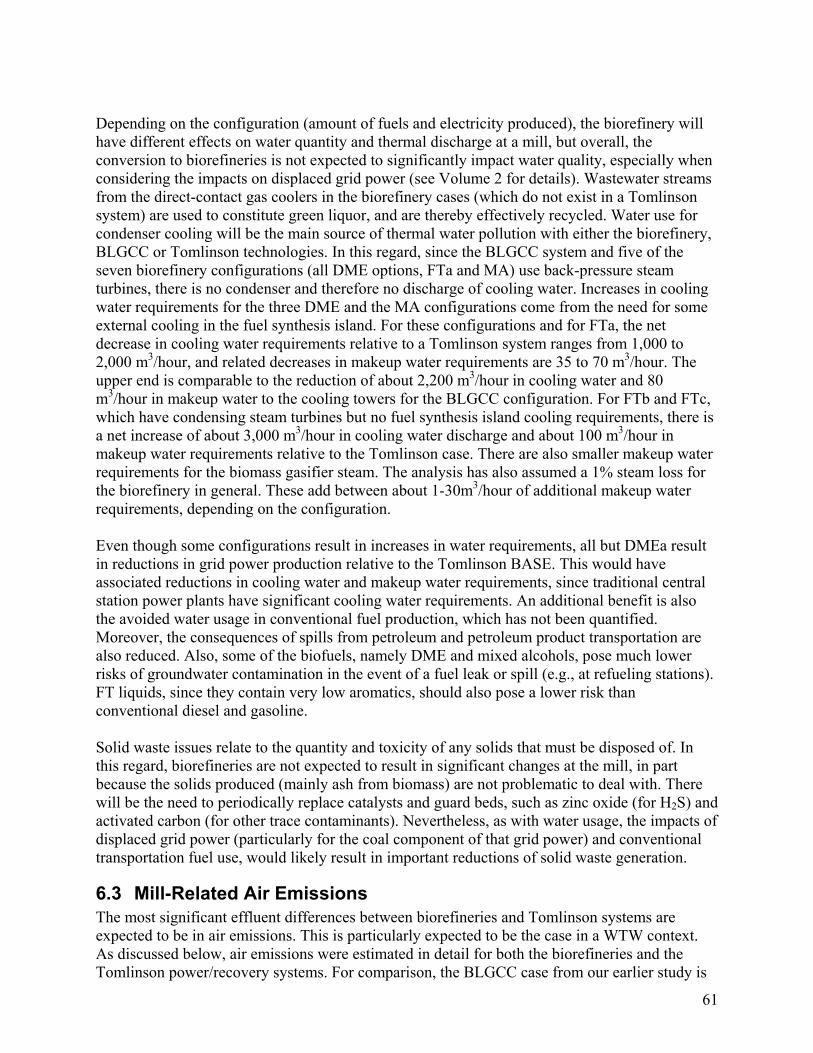
61

Depending on the configuration (amount of fuels and electricity produced), the biorefinery will have different effects on water quantity and thermal discharge at a mill, but overall, the conversion to biorefineries is not expected to significantly impact water quality, especially when considering the impacts on displaced grid power (see Volume 2 for details). Wastewater streams from the direct-contact gas coolers in the biorefinery cases (which do not exist in a Tomlinson system) are used to constitute green liquor, and are thereby effectively recycled. Water use for condenser cooling will be the main source of thermal water pollution with either the biorefinery, BLGCC or Tomlinson technologies. In this regard, since the BLGCC system and five of the seven biorefinery configurations (all DME options, FTa and MA) use back-pressure steam turbines, there is no condenser and therefore no discharge of cooling water. Increases in cooling water requirements for the three DME and the MA configurations come from the need for some external cooling in the fuel synthesis island. For these configurations and for FTa, the net decrease in cooling water requirements relative to a Tomlinson system ranges from 1,000 to 2,000 m3/hour, and related decreases in makeup water requirements are 35 to 70 m3/hour. The upper end is comparable to the reduction of about 2,200 m3/hour in cooling water and 80 m3/hour in makeup water to the cooling towers for the BLGCC configuration. For FTb and FTc, which have condensing steam turbines but no fuel synthesis island cooling requirements, there is a net increase of about 3,000 m3/hour in cooling water discharge and about 100 m3/hour in makeup water requirements relative to the Tomlinson case. There are also smaller makeup water requirements for the biomass gasifier steam. The analysis has also assumed a 1% steam loss for the biorefinery in general. These add between about 1-30m3/hour of additional makeup water requirements, depending on the configuration. Even though some configurations result in increases in water requirements, all but DMEa result in reductions in grid power production relative to the Tomlinson BASE. This would have associated reductions in cooling water and makeup water requirements, since traditional central station power plants have significant cooling water requirements. An additional benefit is also the avoided water usage in conventional fuel production, which has not been quantified. Moreover, the consequences of spills from petroleum and petroleum product transportation are also reduced. Also, some of the biofuels, namely DME and mixed alcohols, pose much lower risks of groundwater contamination in the event of a fuel leak or spill (e.g., at refueling stations). FT liquids, since they contain very low aromatics, should also pose a lower risk than conventional diesel and gasoline. Solid waste issues relate to the quantity and toxicity of any solids that must be disposed of. In this regard, biorefineries are not expected to result in significant changes at the mill, in part because the solids produced (mainly ash from biomass) are not problematic to deal with. There will be the need to periodically replace catalysts and guard beds, such as zinc oxide (for H2S) and activated carbon (for other trace contaminants). Nevertheless, as with water usage, the impacts of displaced grid power (particularly for the coal component of that grid power) and conventional transportation fuel use, would likely result in important reductions of solid waste generation.

6.3 Mill-Related Air Emissions The most significant effluent differences between biorefineries and Tomlinson systems are expected to be in air emissions. This is particularly expected to be the case in a WTW context. As discussed below, air emissions were estimated in detail for both the biorefineries and the Tomlinson power/recovery systems. For comparison, the BLGCC case from our earlier study is

62

also shown, with the updated assumptions consistent with the current analysis (e.g., grid power emissions). Actual air emissions data are available for modern Tomlinson systems. Since emissions data do not exist for BLGCC or biorefinery systems, estimates were made starting with data for coal IGCC and natural-gas combined cycle power systems and adjusting appropriately. Note that relative to the BLGCC configuration, sources of air emissions in a biorefinery are expected to be similar, namely the power island. The production of the biofuel itself does not lead to significant additional sources of air emissions at the biorefinery. For the portions of the fuel chain beyond the biorefinery, the GREET model was used, as described above. This covers biomass collection and transportation and biofuel transportation and vehicle use. Estimates for all systems also include emissions from the lime kiln and hog fuel boilers. Where it is part of the configuration, emissions from the duct burner of the gas turbine combined cycle are also included to provide complete comparisons between all options. Estimates for grid power offsets (for both avoided purchases and exported power relative to the Tomlinson) were also made. The air emissions analysis presented below is not intended to serve as a complete lifecycle analysis of biorefinery emissions. Rather the estimates provide indicative results of the potential impacts of biorefinery options relative to “business as usual” in the pulp and paper industry. For example, upstream emissions for grid power (i.e., fuel production and transportation to the power plant) are not included, but these are relatively small compared to the power plant emissions themselves and to the total emissions from conventional motor fuel chains. To the extent that most of the biorefinery configurations result in more displaced grid power than the Tomlinson case, the emissions benefits estimated in this study can be considered conservative because they do not also factor in emissions reductions related to fuel supply for power plants. Air emissions fall into three basic categories: criteria pollutants, hazardous air pollutants (HAPs), and greenhouse gases (GHGs). This study includes quantitative estimates for the criteria pollutants: sulfur dioxide (SO2), nitrogen oxides (NOx), carbon monoxide (CO), volatile organic compounds (VOCs), particulate matter (PM),20 and total reduced sulfur (TRS). Estimates are also made for carbon dioxide (CO2), the major greenhouse gas. HAPs and other emissions issues are discussed qualitatively.21 108109

20 For PM, the main concern is with the health impacts of fine particulates smaller than 10 and 2.5 microns in

diameter (PM10 and PM2.5, respectively). However, data for PM10 and PM2.5 are not always reported with data for total PM emissions. For this reason, estimates here are for total PM. To estimate PM10 and PM2.5 emissions, the reader may assume the following: For solid fuel combustion, if there is a PM control step, such as an electrostatic precipitator, the PM10 emissions are 50-80% of total PM emissions and PM2.5 emissions are 25-70% [108,114]. For natural gas combustion, the U.S. EPA assumes that all PM emissions are smaller than 2.5 microns so that PM, PM10 and PM2.5 emissions are equal [109].

21 According to Miner [110] EPA’s HAP rules focus on HAP metal emissions from recovery furnaces, using total particulate matter as a surrogate for metals emissions. For existing furnaces, they require reductions in emissions of organic HAPs, e.g. methanol, that arise from direct contact evaporators, associated black liquor oxidation systems, or wet bottom ESPs. EPA also decided that recovery furnace HCl emissions do not merit reductions, since the risks posed by the HCl emissions were determined to be minimal. Further EPA has opted not to address dioxin/furan emissions since there is no known control technology that could be applied to reduce them. Also, the industry believes dioxin/furan emissions from recovery furnaces are inconsequential. EPA did decide to impose a methanol (VOC surrogate) emission limit on new kraft recovery furnaces.

63

A distinctive feature of biorefinery technologies is the expected low relative emissions for most of the criteria pollutants compared to a modern Tomlinson system employing sophisticated pollution controls (Table 15). Low emissions are an intrinsic characteristic of gas turbine technology and of syngas conversion to fuels in part because considerable upstream removal of contaminants in the raw syngas is required to protect the gas turbine and various catalyst beds from damage, as well as to recover pulping chemicals from the syngas. Also, gas turbine combustion is inherently efficient and low in emissions, as is the combustion of purge gases in duct burners or existing boilers.22 It is worth noting that there could be emissions benefits from burning purge gases in existing power boilers (as in the DMEa case), for example as a reburn fuel to reduce NOx. Also, if excess purge gas could replace fuel oil in lime kilns, there may be further emissions benefits. These benefits have not been estimated here. Biomass is a renewable fuel from a GHG perspective if the CO2 emitted in its use is photosynthetically removed from the atmosphere by replacement biomass growth. There are some fossil fuel GHG emissions associated with the biomass-to-biofuel chain, which have been included in this analysis. However, no attempt has been made to estimate emissions resulting from land use changes or from the growing of the biomass itself, which is assumed to be from existing commercial timberland. Thus, the estimates here of total net emissions of CO2 and other pollutants described below for each configuration do account for the harvesting and transportation of the incremental biomass used compared to the Tomlinson case, as well as the downstream steps of transporting and distributing the biofuels, but with the assumption that wood-derived energy (for power or fuels) produces no net CO2 emissions, other than from the fossil fuels used in the process. For completeness, Volume 3 shows actual emissions of CO2 associated with the wood-derived power and fuels (in addition to the net emissions). Biomass combustion also generates small amounts of non-CO2 greenhouse gases - specifically, methane and nitrous oxide (N2O). However, even after considering the potency of methane and nitrous oxide as greenhouse gases, these emissions are expected to be small, and therefore, they have not been included in the analysis.23 However, the exploration and production of petroleum and natural gas does result in relatively large methane emissions, so that it is reasonable to expect that biorefineries would achieve net CH4 reductions on a WTW basis when they replace Tomlinson systems. An additional feature of biorefineries not evaluated here, but that could be important to overall mill operations as it relates to environmental discharges, is the potential to more tightly integrate and eliminate various waste steams.24 In “next generation” mills, the desire is to “close up” various emissions sources as much as possible. For example, the pulp & paper industry has been trying to develop a cost-effective way to eliminate the effluent from bleached kraft pulp mills. The most likely approach for eliminating these effluents (primarily bleach plant filtrates) involves sending them to the recovery furnace, yet few mills currently recycle bleach plant filtrates to the recovery furnace because these furnaces are sensitive to a number of elements contained in the filtrates (chlorides and potassium being of special note) and the costs of removing these substances are high. If gasification turns out to be more amenable to this type of

22 All syngas-to-fuel conversion processes result in some unconverted syngas, sometimes called “purge gas”. These

gases are low in contaminants and burn cleanly in gas turbines, duct burners or in existing boilers or unit operations.

23 For example, see [112]. 24 Personal communication with Reid Miner and Dr. John Pinkerton of NCASI, 3 December, 2002.

64

overall mill integration, this would be a significant advantage over conventional recovery systems.

6.3.1 Tomlinson Boiler Air Emissions Modern Tomlinson boilers are characterized by emissions of criteria pollutants that are similar overall to grid power (some are higher, like CO and PM, while others are lower, like SO2 and NOx). The most significant pollutants, in terms of both environmental impacts and relative emissions rates from Tomlinson boilers, are NOx and particulates (Table 15). While many furnaces already have particulate controls in place, there is no effective form of NOx after-treatment (see below). Furnace rebuilds and replacements trigger the New Source Review (NSR) process, which generally results in process modifications being made to reduce TRS emissions.25 Installation of more efficient particulate control is also common following a NSR, and generally, modern furnaces have better design and controls than older ones, which results in lower overall emissions. Table 15: Qualitative indication of relative environmental impact of different mill-level emissions, together with relative emission rates for controlled and uncontrolled Tomlinson furnaces and with Biorefinery technology (VL = very low, L = low, M = moderate, H = high).

VLLdLLTRSe

VL-LLLM-HWaste Waterf

VLLcLcM-HHAPs

L

L

Hc

L

M (can be highly variable)

M

L

Relative Emissions Rates from

Tomlinson Furnaces (uncontrolled)

VLLdL-MCH4

L

L-M

Ld

Md

Md

L (not required)

Relative Emissions Rates with Controls on

Tomlinson

VLHVOCs

LLSolids

VLHPMb

VLLCO

VLHNOx

VLHSO2

Relative Emissions Rates

Expected with Biorefineries

Relative Environmental

Impact of Pollutanta

Pollutant/Discharge

a) General importance, not specifically for the P&P industry.b) PM = particulate matter. Of greatest concern with PM emissions are fine particulates smaller than 10 and 2.5 microns in diameter

(PM10 and PM2.5 respectively).c) Current MACTII rules are expected to result in about a 10% reduction of HAPs and a modest reduction in PM.d) Not generally practiced other than by maintaining good combustion efficiency.e) Total reduced sulfur.f) For power systems, the issue is mainly one of the cooling water (quantity and discharge temperature).

The only regulatory trend regarding add-on controls to a Tomlinson system is to require installation of dry-bottom electrostatic precipitators (ESPs) on new kraft recovery furnaces. This is being driven by the current EPA MACT II26 regulations designed to reduce HAP emissions

25 Typically direct-contact evaporators and black liquor oxidation units are eliminated to reduce TRS emissions. 26 MACT stands for “maximum achievable control technology” and was put in place to reduce HAPs.

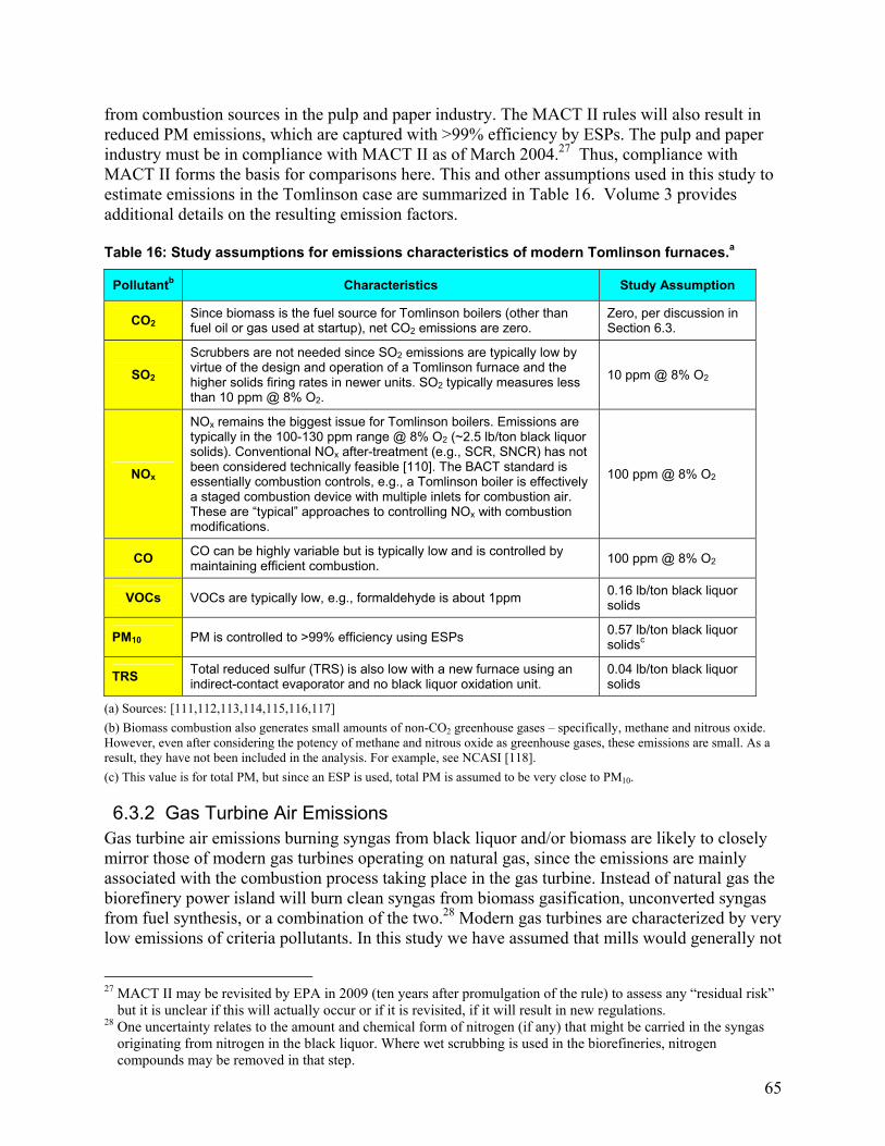
65

from combustion sources in the pulp and paper industry. The MACT II rules will also result in reduced PM emissions, which are captured with >99% efficiency by ESPs. The pulp and paper industry must be in compliance with MACT II as of March 2004.27 Thus, compliance with MACT II forms the basis for comparisons here. This and other assumptions used in this study to estimate emissions in the Tomlinson case are summarized in Table 16. Volume 3 provides additional details on the resulting emission factors. Table 16: Study assumptions for emissions characteristics of modern Tomlinson furnaces.a

Pollutantb Characteristics Study Assumption

CO2 Since biomass is the fuel source for Tomlinson boilers (other than fuel oil or gas used at startup), net CO2 emissions are zero.

Zero, per discussion in Section 6.3.

SO2 Scrubbers are not needed since SO2 emissions are typically low by virtue of the design and operation of a Tomlinson furnace and the higher solids firing rates in newer units. SO2 typically measures less than 10 ppm @ 8% O2.

10 ppm @ 8% O2

NOx

NOx remains the biggest issue for Tomlinson boilers. Emissions are typically in the 100-130 ppm range @ 8% O2 (~2.5 lb/ton black liquor solids). Conventional NOx after-treatment (e.g., SCR, SNCR) has not been considered technically feasible [110]. The BACT standard is essentially combustion controls, e.g., a Tomlinson boiler is effectively a staged combustion device with multiple inlets for combustion air. These are “typical” approaches to controlling NOx with combustion modifications.

100 ppm @ 8% O2

CO CO can be highly variable but is typically low and is controlled by maintaining efficient combustion. 100 ppm @ 8% O2

VOCs VOCs are typically low, e.g., formaldehyde is about 1ppm 0.16 lb/ton black liquor solids

PM10 PM is controlled to >99% efficiency using ESPs 0.57 lb/ton black liquor solidsc

TRS Total reduced sulfur (TRS) is also low with a new furnace using an indirect-contact evaporator and no black liquor oxidation unit.

0.04 lb/ton black liquor solids

(a) Sources: [111,112,113,114,115,116,117] (b) Biomass combustion also generates small amounts of non-CO2 greenhouse gases – specifically, methane and nitrous oxide. However, even after considering the potency of methane and nitrous oxide as greenhouse gases, these emissions are small. As a result, they have not been included in the analysis. For example, see NCASI [118]. (c) This value is for total PM, but since an ESP is used, total PM is assumed to be very close to PM10.

6.3.2 Gas Turbine Air Emissions Gas turbine air emissions burning syngas from black liquor and/or biomass are likely to closely mirror those of modern gas turbines operating on natural gas, since the emissions are mainly associated with the combustion process taking place in the gas turbine. Instead of natural gas the biorefinery power island will burn clean syngas from biomass gasification, unconverted syngas from fuel synthesis, or a combination of the two.28 Modern gas turbines are characterized by very low emissions of criteria pollutants. In this study we have assumed that mills would generally not

27 MACT II may be revisited by EPA in 2009 (ten years after promulgation of the rule) to assess any “residual risk”

but it is unclear if this will actually occur or if it is revisited, if it will result in new regulations. 28 One uncertainty relates to the amount and chemical form of nitrogen (if any) that might be carried in the syngas

originating from nitrogen in the black liquor. Where wet scrubbing is used in the biorefineries, nitrogen compounds may be removed in that step.

66

be located in ozone non-attainment areas and therefore would not be required to install NOx after-treatment such as SCR. Thus NOx emissions are assumed to be consistent with dry low-NOx gas turbine combustion, in the range of 25 ppm at 15% O2.29 Emissions of CO and VOCs are inherently low with gas turbines due to efficient combustion. PM in the syngas must be removed to very low levels in order to protect the gas turbine from damage, so PM emissions will also be low. There is considerable experience with successful use of inexpensive carbon bed filters for removal of mercury and other trace elements from fuel gas in coal gasification systems.30 A similar approach is assumed to be viable for the biorefinery power island. Operating experience with coal IGCC systems also provides a basis for estimating likely biorefinery power island air emissions, taking account of some important differences between black liquor/biomass and coal gasification. First, coal is much higher in ash and metals (other than alkali). Second, sulfur recovery efficiencies will be higher with black liquor (near 100%) because the goal is to capture sulfur for reuse in the pulping process, and in most cases, catalysts are easily poisoned by even trace amounts of sulfur.31 In comparison, coal IGCC plants are typically designed for sufficient sulfur removal (e.g., 98%) to meet permitting requirements. In the case of biomass syngas used directly in power generation (i.e., not used in fuel synthesis first), no sulfur removal is necessary. Table 17 summarizes emissions characteristics for gas turbines assumed in this study. Volume 3 provides additional details on the resulting emissions factors.

Table 17: Study assumptions for emissions characteristics of gas turbines burning syngas at biorefineries

Pollutant Characteristics Study Assumption

CO2 For any biomass-derived fuels used, net CO2 emissions are assumed to be zero (see discussion in Section 6.3)

Varies, depending on fuel mix

SO2 SO2 emissions are expected to be very low. In the case of the use of unconverted syngas, the fuel gas is scrubbed of nearly all H2S. In the case of the use of biomass syngas, the gas is not scrubbed of H2S, but biomass is low in sulfur (0.06% by weight, dry basis).

Varies, depending on the fuel used

NOx Dry low-NOx combustion can reduce emissions with natural gas to as low as 9 ppm @ 15% O2. For BLGCC operation we have assumed a more conservative value.

25 ppm @ 15% O2

CO CO is generally low from gas turbine combustors due to efficient combustion.

0.033 lb/MMBtu fuel input

VOCs VOCs are generally low with gas turbines due to efficient combustion – uncontrolled values are assumed.

0.0021 lb/MMBtu fuel input

PM PM are generally very low for gas turbine operation. Upstream syngas cleanup is assumed to control PM to very low levels.

0.0066 lb/MMBtu fuel input

TRS Total reduced sulfur (TRS) is essentially zero, since the fuel gas is scrubbed of H2S to return the sulfur to the pulping process. Zero

References: [119, 120, 121, 122,123,124,125,126]

29 Current BACT (best available control technology) for coal IGCC power plants is 15 ppm NOx @ 15% O2

(www.gepower.com, accessed 6/16/2003). 30 For example, such filters have been in use for many years at the Eastman Chemicals coal gasification facility in

Kingsport, Tennessee, where methanol is made from gasified coal. 31 Mixed alcohol catalysts are sulfur tolerant, but for FT and DME, essentially complete sulfur removal is required.

67

Other sources of emissions in the BLGCC and four of the biorefineries in this study are the gas turbine exhaust duct burners using unconverted syngas (or in the BLGCC case, a mixture of syngas and natural gas). Emissions from duct burners are assumed to be similar to state-of-the art natural gas combustion. Additional details are provided in Volume 3.

6.4 Grid Power Air Emissions and Offsets Varying amounts of power are generated in the different biorefinery cases. All except DMEa produce more net electricity than the Tomlinson case. Only the FTb case produces enough electricity to export power to the grid, however, after meeting mill process needs. The increase in power generation between the biorefinery cases and the Tomlinson case would therefore result in an equal amount of power generation offsets from the grid (again, with the DMEa case as the exception).32 The environmental value of these grid power offsets is an important consideration and will vary depending on what type of power is being displaced.33 Determining what type of grid power would be displaced is difficult, particularly in the context of a national impacts analysis. Even though the biorefinery would produce baseload power, the operation of existing baseload power plants (typically large coal, nuclear and hydropower plants, as well as gas-fired combined cycle plants) is not likely to change significantly by the addition of biorefineries at pulp/paper mills. Similarly, peaking and intermediate-load power plants, which would typically be smaller, older coal- or oil-fired plants, gas turbines and dispatchable hydropower, run intermittently and thus do not provide a good direct point of comparison, since their operation is dictated by the real-time needs of balancing supply and demand. Other renewable energy sources, like wind, solar and small hydro are also not likely to be directly displaced by biorefineries (or any other dispatchable power plant). These plants typically run whenever the resource is available and the grid can accept the power, with the load-following plants adjusting their output accordingly. Furthermore, these plants typically have very low marginal operating costs and would therefore be cost-effective to run whenever the resource is available. A more complicated analysis would be to estimate the marginal mix of power, as this is what would be displaced by the “next kWh” of generation added to the grid. Even if this were done, the concept of the marginal mix has limited meaning in a national context, since the marginal mix is mainly relevant for a specific regional power pool. A simpler analysis would use the grid average, since data are readily available. Given the scope and level of effort for this project, the grid-average approach was chosen, consistent with the recommendation of the Steering Committee in our prior BLGCC study [5]. The projected average fuel mix for electricity generation used to estimate the grid emissions offsets is shown in Table 18, based on the DOE’s most recent Reference Case forecast (for CO2,

32 As with our previous BLGCC study, we ignore any transmission and distribution energy losses associated with

grid power, even though for displaced purchases, there would be some additional benefits in this regard. 33 The impacts of biorefineries on HAP emissions were not quantified in the analysis. Given increasing concerns

over HAPs emissions, a useful follow-on activity would be to quantify the benefits of biorefineries vis-à-vis HAP emissions. Of particular significance would be the hydrochloric acid and mercury emissions that would be reduced if coal-generated power on the grid were displaced by biorefinery electricity.

68

SO2, and NOx) [134] and from EPA estimates of recent historical emissions (for CO, VOC, and PM10). Table 18: Total average U.S. grid emissions (including non-fossil fuel sources) assumed in estimating grid offsets.a

lb/MWh

2010 2020 2035b

CO2 1,340 1,303 1,316 SO2 2.836 1.684 0.851 NOx 1.125 0.886 0.584 CO 0.234 0.172 0.108

VOC 0.024 0.018 0.011 PM10 0.326 0.239 0.150

(a) Sources: [134,127,128,129, Navigant Consulting, Inc. analysis]. (b) Extrapolated from the EIA forecast [134], which only goes to 2030. The grid power emission assumptions here are similar to those used in our prior BLGCC study [5], with two important changes: 1. PM10 emissions: The EPA, in its National Emissions Inventory (NEI) Air Pollutant

Emissions Trends Data (formerly called the Air Pollutant Emissions Trends Data), has changed the way it reports PM10 data. Specifically, beginning with 1999 data, EPA now reports “primary PM10” which includes both filterable and condensable PM10. Prior to this change EPA only reported filterable PM10 for electric utilities. This is the main reason for the higher PM10 emissions in Table 18 compared to the values used in our earlier BLGCC study.

2. EPA’s new Clean Air Interstate Rule (CAIR): Promulgated in March 2005, the CAIR is intended to significantly reduce emissions of fine particulates (PM2.5), NOx, and SO2. As a result, the grid power emissions factors for NOx and SO2 – this study does not estimate PM2.5 – are substantially lower than in the earlier study, particularly in the out-years (2020 and beyond). This has a significant impact on the net emissions benefits of power generation at biorefineries, as far as SO2 and NOx are concerned.

6.5 Emissions from the Biorefinery Fuel Chain As depicted in Figure 34, the biorefinery itself is only one source of emissions along the full fuel chain. In this section we summarize the approach for estimating emissions from the various parts of the biofuels fuel chain. The detailed emissions and energy use figures for each stage of the fuel chain can be found in Volume 3.

6.5.1 Biomass Collection and Transportation For purchased biomass residues, we estimate the energy use and emissions associated with harvesting and transporting the wood to the mill. We ignore the energy use and emissions associated with pulpwood logs, since this is a pre-existing use of biomass not primarily related to the production of energy. We do, however take credit for any reductions in pulpwood log requirements resulting from higher pulping yields, and compute the collection and transportation

69

energy use and emissions on the net increase in biomass use at the mill, as a result of the conversion to a biorefinery.34 We used the GREET defaults for energy use and emissions associated with the collection and transportation of woody biomass from woody biomass energy plantations (i.e., excluding the energy and emissions associated with fertilizers, pesticides and farm equipment used for growing the biomass). We also increased GREET’s default 1-way transport distance from 40 to 75 miles.

6.5.2 Biorefinery Biorefinery emissions are estimated for the lime kiln and gas turbine, except in the DMEa case, where there is no gas turbine and the hog fuel and purchased residues (and some unconverted syngas) are burned in boilers. Although the use of syngas could help reduce emissions from the hog fuel boiler (e.g., as a “reburn” fuel to reduce NOx), we have only made adjustments to the SO2 emissions, since the unconverted syngas is scrubbed of sulfur. The DMEb, DMEc, FTa, and MA cases (like the BLGCC case) also make use of a duct burner to augment steam production in the heat recovery steam generator. Duct burner emissions are included in those cases. In the FTa, FTb and FTc cases, we also included an estimate of the energy use and emissions for refining the crude FT product into a finished product (32% FT gasoline and 68% FT diesel split, based on energy35). For FT gasoline we used the default GREET estimates for conventional gasoline refining, and for FT diesel we used GREET’s conventional diesel refining estimates. We chose not to use reformulated gasoline (RFG) or low-sulfur diesel (LSD) because crude FT is free of sulfur and aromatics, and therefore relatively easy to refine. Thus, the refining efficiencies are slightly higher than for RFG or LSD.

6.5.3 Fuel Transportation and Distribution The GREET model includes emissions estimates for the transportation and distribution of a wide range of biofuels and conventional fuels (and intermediates, such as crude oil). We have used these estimates for the biorefinery cases as given in Table 19. Table 19: Correspondence between the biorefinery fuel and the fuel chain available in GREET – fuel transportation and distribution

Biorefinery Fuel GREET Fuel Adjustments DME DME Assumed only rail and truck transport (i.e., used locally)

Crude FT Crude Oil Assumed only rail transport from biorefinery to petroleum refinery

FT Gasoline Conventional Gasoline None (assumes FT gasoline blended with regular gasoline for transport)

FT Diesel FT Diesel None Mixed Alcohols Ethanol Assumed only rail and truck transport (i.e., used locally)

34 For example, if the conversion to a biorefinery results in increased pulping yields, resulting in the reduction 5 units of wood to process for the same amount of finished product, but the purchased biomass requirements (for energy) are 75 additional units, the impacts of biomass collection are estimated on just 70 units of biomass, the net increase. 35 Our FT plants are designed to produce a synthetic crude product that is shipped to an existing petroleum refinery for upgrading to finished products. Larson et al. [105], using the same kinetic model as we have used, but including onsite upgrading to finished product, indicate that the finished product is produced as a split of 68% diesel and 32% motor gasoline (on an energy basis).

70

6.5.4 Vehicles End Use A number of vehicle options are possible, depending on the fuel. Table 20 shows the combinations assessed here. The analysis is limited to light-duty vehicles. In the case of DME, this fuel is most likely in the near term to be used in centrally-refueled heavy duty vehicles (buses, delivery trucks, etc.), as discussed in Section 2.2. However, we have chosen to focus on light-duty vehicles to provide a conservative estimate of WTW air emissions impacts. Reductions in air emissions are likely to be larger with heavy duty vehicles than what we have estimated here. (In our financial analyses presented in Section 8, we also consider the use of DME as an LPG replacement, but we have not carried out a full environmental impact assessment of this scenario. Similarly, our financial analysis for mixed alcohols included a scenario where higher alcohols are separated out and used to replace petroleum-derived chemicals, but we have not assessed the air emissions impacts of this scenario.) Table 20: Correspondence between the biorefinery fuel and the fuel chain available in GREET – vehicle end use

Biorefinery Fuel Vehicle Options Analyzed

DME Compression ignition direct injection (CIDI) engine • 100% DME (dedicated vehicle converted/optimized for DME use)

FT Gasoline Spark ignition (SI) engine • Low-level (10%) blend of FT gasoline with conventional gasoline • 100% FT gasoline

FT Diesel CIDI • Low-level (10%) blend of FT diesel with low-sulfur diesel • 100% FT diesel

Mixed Alcohols

SI engine • Low-level (10%) blend of mixed alcohols with conventional gasoline (similar to E10) • High level (85%) blend of mixed alcohol with conventional gasoline in flex-fuel vehicle

(similar to E85 FFV) In developing the biofuels tailpipe emissions factors, some adjustments were made to the GREET model default values, since they typically assume that the alternative fuel vehicle emissions are the same (in g/mile) as conventional petroleum fuels. For example, the GREET defaults for DME use in compression-ignition, direct-injection (CIDI) engines make no adjustment for PM10 or NOx, even though an engine optimized for DME is expected to produce virtually no tailpipe PM10 emissions and substantially reduced NOx. Nevertheless, because v1.7 of GREET includes the latest in tailpipe emissions requirements and the use of low-sulfur diesel, the baseline emissions are already relatively low. Thus, additional improvements from biofuel use are expected to be modest. The adjustments made to DME tailpipe emissions are based on Oguma and Shinichi [130]. Adjustments to FT gasoline and FT diesel as neat fuels are based on Delucchi [131]. Adjustments were also made to CO2 emissions based on the carbon content of the different fuels. For example, GREET has no CO2 factors for mixed alcohols, so the GREET CO2 emissions for ethanol were adjusted based on the relative carbon content of the two fuels. The specific assumptions made are included in Volume 3.

6.5.5 Fuel Blends versus Neat Fuels Although DME requires engine modifications for a diesel-engine vehicle to run on pure DME, FT fuels and mixed alcohols can be used in low-level (like E10) or high-level (like E85) blends with conventional fuels or as neat fuels (100% biofuels) with little or no engine modifications. Our baseline cases assume low-level blends, consistent with how most biofuels are used today.

71

Under these circumstances, tailpipe emissions of criteria pollutants are not expected to be substantially different than with conventional fuels. However, with high-level blends or neat fuels, engines can be optimized to take advantage of the desirable characteristics of the biofuels, resulting in lower tailpipe emissions. For the most part, the impact of this is modest, but for a selected set of pollutants and biorefinery cases, the differences are more pronounced. This analysis, presented in Volume 3, provides indicative results of the incremental benefits of neat biofuels over low-level blends. In this comparison, we have not assumed any differences in vehicle efficiencies, and as such the impacts of blends vs. neat fuels is limited to selected tailpipe emissions. Net CO2 emissions per unit of biofuel are essentially unchanged because vehicle efficiencies are assumed to be the same in both the low-level and high-level blend/neat fuel cases.

6.6 Energy Use and Emissions from Conventional Fuel Chains The default GREET assumptions form the basis for comparing the biofuel fuel chain options to conventional fuel chain options. These assumptions are for a 2010 timeframe. As discussed above, in that timeframe conventional vehicles in the United States are expected to have relatively low tailpipe emissions because of the implementation of TIER II standards and the use of low-sulfur diesel. Table 21 shows which of GREET’s conventional fuel chains have been used for comparisons to the biorefinery fuels. The specific assumptions that are used are summarized in Volume 3. Table 21: Biorefinery fuel and the corresponding conventional fuel chain used to estimate net emissions impacts

Biorefinery Fuel Conventional Fuel Chain Benchmark DME Low-sulfur diesel in a CIDI engine FT Gasoline 50:50 mix (fleet average) of conventional gasoline and RFG in an SI engine FT Diesel Low-sulfur diesel in a CIDI engine Mixed Alcohols 50:50 mix (fleet average) of conventional gasoline and RFG in an SI engine

6.7 Net Emissions Estimates for the Case Study Biorefinery Systems Total fuel cycle emissions for each biorefinery are shown here based on the above discussions and the detailed emission factors described in Volume 3. Included in the figures below are the following: Emissions Sources • Emissions associated with biomass collection and transport for the incremental biomass used

(as discussed above) in the biorefinery cases relative to the Tomlinson case. • All major emissions sources affected by the conversion of the mill to a biorefinery (lime kiln,

biomass boiler, Tomlinson boiler, gas turbine, duct burner). • Transportation and distribution of the biofuel (including, in the FT cases, an estimate of the

emissions due to crude FT transportation and upgrading) • Biofuel end-use (for simplicity, this is shown with transportation and distribution, although

end-use is the largest portion) Emissions Offsets • Displaced grid power emissions

72

• Conventional fuel chain emissions (well-to-wheel – shown as a single figure) • Biomass CO2 – consistent with the analysis by Larson, et al. [5], CO2 emissions associated

with biomass usage are included in the analysis but then are netted out, since they are assumed to be re-absorbed photosynthetically by subsequent biomass growth. Note that this does not net out the emissions associated with biomass collection and transportation described above.36

Note that the analysis assumes constant emission factors over time with the exception of grid power. Therefore, the values shown here for the year 2010 will change over time as grid emissions change. In particular, as shown earlier in Table 18, SO2 and NOx emissions from the grid are expected to decrease significantly over the forecast period. The temporal impacts on annual emissions reductions are given later in this report.

6.7.1 Carbon Dioxide Figure 35 shows the resulting impacts for CO2, for the case study mill in the year 2010. Note that in each case, the net CO2 emissions reductions are greater than for the Tomlinson case. Not surprisingly, the main driver for this is the amount of additional biomass used, although from a CO2 standpoint it is also more advantageous to displace electricity than fuels. For example, the FTb configuration consumes moderately less additional biomass than FTc yet produces the greatest net CO2 reductions. Also, the DMEa and DMEc configurations use almost the same quantity of additional biomass but the latter produces much more power, resulting in greater CO2 reduction for DMEc. Finally, the MA case uses only slightly more biomass than DMEa and DMEc, but produces mostly power, and so still has a greater net CO2 benefit than DMEa, which produces mostly fuels. This is driven by the fact that coal accounts for about 50% of the grid power that would be displaced, and coal is more carbon intensive per unit of contained energy than petroleum fuels. Figure 36 provides the details of the net CO2 calculation, showing the different emissions sources and offsets and the resulting net emissions that are shown in Figure 35. The remaining similar detailed-accounting figures for the other pollutants are given in Volume 3.

36 In this study, we make no attempt to account for other changes in greenhouse gas emissions associated with land use changes and biomass growth that are not directly related to collection and transportation (e.g., changes in soil carbon content or in methane emissions from decomposition of forest slash).

73

Figure 35: Change in annual full fuel chain net CO2 emissions at the reference mill in 2010.

‐1,600,000

‐1,400,000

‐1,200,000

‐1,000,000

‐800,000

‐600,000

‐400,000

‐200,000

0

NewTomlinson BLGCC DMEa DMEb DMEc FTa FTb FTc MA

Net CO2 Emissions Reductions 

(short tons per mill per year)

Relative to Conventional Fuel Chain

Relative to New  Tomlinson

Notes:Transportation of the crude FT product to the oil refinery included in FT cases.Excludes any emissions from land use changes and biomass growth that are not related to harvesting and transportation.FT cases assume FT gasoline blend in gasoline engines and FT diesel blend in CIDI engines.  MA case assumes low‐level blend with gasoline.

‐1,600,000

‐1,400,000

‐1,200,000

‐1,000,000

‐800,000

‐600,000

‐400,000

‐200,000

0

NewTomlinson BLGCC DMEa DMEb DMEc FTa FTb FTc MA

Net CO2 Emissions Reductions 

(short tons per mill per year)

Relative to Conventional Fuel Chain

Relative to New  Tomlinson

Notes:Transportation of the crude FT product to the oil refinery included in FT cases.Excludes any emissions from land use changes and biomass growth that are not related to harvesting and transportation.FT cases assume FT gasoline blend in gasoline engines and FT diesel blend in CIDI engines.  MA case assumes low‐level blend with gasoline.

Figure 36: Changes in annual full fuel-chain CO2 emissions and offsets at the reference mill in 2010 (million tons per year).

* Transportation of the crude FT product to the oil refinery included in FT cases.Note: excludes any emissions from land use changes and biomass growth that are not related to harvesting and transportation.Note on vehicle end use: FT cases assume FT gasoline blend in gasoline engines and FT diesel blend in CIDI engines.  MA case assumes low‐level blend with gasoline.

(5)

(4)

(3)

(2)

(1)

-

1

2

3

4

Em

issi

ons

Offs

ets

Net

Em

issi

ons

Offs

ets

Net

Em

issi

ons

Offs

ets

Net

Em

issi

ons

Offs

ets

Net

Em

issi

ons

Offs

ets

Net

Em

issi

ons

Offs

ets

Net

Em

issi

ons

Offs

ets

Net

Em

issi

ons

Offs

ets

Net

Em

issi

ons

Offs

ets

Net

Tomlinson BLGCC DMEa DMEb DMEc FTa FTb FTc MA

Mill

ions

Net EmissionsBiomass CO2Displaced conventional fuel chainDisplaced Grid PowerBiofuel transport, distribution & end use*MillBiomass Collection & Transport

* Transportation of the crude FT product to the oil refinery included in FT cases.Note: excludes any emissions from land use changes and biomass growth that are not related to harvesting and transportation.Note on vehicle end use: FT cases assume FT gasoline blend in gasoline engines and FT diesel blend in CIDI engines.  MA case assumes low‐level blend with gasoline.

(5)

(4)

(3)

(2)

(1)

-

1

2

3

4

Em

issi

ons

Offs

ets

Net

Em

issi

ons

Offs

ets

Net

Em

issi

ons

Offs

ets

Net

Em

issi

ons

Offs

ets

Net

Em

issi

ons

Offs

ets

Net

Em

issi

ons

Offs

ets

Net

Em

issi

ons

Offs

ets

Net

Em

issi

ons

Offs

ets

Net

Em

issi

ons

Offs

ets

Net

Tomlinson BLGCC DMEa DMEb DMEc FTa FTb FTc MA

Mill

ions

Net EmissionsBiomass CO2Displaced conventional fuel chainDisplaced Grid PowerBiofuel transport, distribution & end use*MillBiomass Collection & Transport

6.7.2 Sulfur Dioxide Figure 37 shows the resulting impacts for SO2. The main driver is the amount of grid power displaced, since the grid is the main source of SO2 emissions, and the use of conventional transportation fuels generates relatively little SO2, especially with the transition to low-sulfur

74

diesel. As such, the configuration with the greatest SO2 benefits are the BLGCC and FTb cases. The DMEa case, which only produces enough power to meet the biorefinery internal requirements, actually results in a net increase in SO2 emissions, since greater grid electricity purchases are required than with the Tomlinson case. Figure 37: Change in annual full fuel-chain net SO2 emissions at reference mill in 2010.

‐2,000

‐1,750

‐1,500

‐1,250

‐1,000

‐750

‐500

‐250

0

250

500

750

1,000

NewTomlinson BLGCC DMEa DMEb DMEc FTa FTb FTc MA

Net SO2 Em

issions Reductions 

(short tons per mill per year)

Relative to Conventional Fuel Chain

Relative to New  Tomlinson

Notes:Transportation of the crude FT product to the oil refinery included in FT cases.Excludes any emissions from land use changes and biomass growth that are not related to harvesting and transportation.FT cases assume FT gasoline blend in gasoline engines and FT diesel blend in CIDI engines.  MA case assumes low‐level blend with gasoline.

‐2,000

‐1,750

‐1,500

‐1,250

‐1,000

‐750

‐500

‐250

0

250

500

750

1,000

NewTomlinson BLGCC DMEa DMEb DMEc FTa FTb FTc MA

Net SO2 Em

issions Reductions 

(short tons per mill per year)

Relative to Conventional Fuel Chain

Relative to New  Tomlinson

Notes:Transportation of the crude FT product to the oil refinery included in FT cases.Excludes any emissions from land use changes and biomass growth that are not related to harvesting and transportation.FT cases assume FT gasoline blend in gasoline engines and FT diesel blend in CIDI engines.  MA case assumes low‐level blend with gasoline.

6.7.3 Nitrogen Oxides Figure 38 shows the resulting impacts for NOx. It is important to note that NOx emissions are in several cases higher than from conventional energy sources (the grid and conventional transportation fuels), but still, in all cases the biorefinery emissions are lower than the Tomlinson case. The relatively favorable grid and conventional fuel chain NOx emissions are driven by the lower expected grid power emissions from implementation of the EPA’s Clean Air Interstate Rule, as well as the use of low-sulfur diesel, which will permit the use of tailpipe NOx emissions controls on diesel cars. It is also worth noting that in the cases that use large amounts of additional biomass (DMEb, FTb, and FTc), this stage in the fuel chain is an important source of NOx emissions, because of the use of heavy duty diesel vehicles for biomass collection and transport (see Volume 3 for details).

6.7.4 Volatile Organic Compounds Figure 39 shows the resulting impacts for VOCs. The main emissions source is the vehicle tailpipe, but other important sources are the upstream processing of petroleum based fuels and the hog fuel and black liquor boilers.37 The other emission sources –syngas combustion and grid power, have comparatively low VOC emissions. As a result, all of the biorefinery cases, as well as the BLGCC case, result in significant VOC reductions relative to the Tomlinson case.

37 VOC emissions from biomass dryers (used in six of the biorefinery designs) are assumed to be zero, since a regenerative thermal oxidizer unit is included as part of the dryer.

75

Figure 38: Change in annual full fuel-chain net NOx emissions at the reference mill in 2010.

‐1,200

‐900

‐600

‐300

0

300

600

900

1,200

NewTomlinson BLGCC DMEa DMEb DMEc FTa FTb FTc MA

Net NOx Emissions Reductions 

(short tons per mill per year)

Relative to Conventional Fuel Chain

Relative to New  Tomlinson

Notes:Transportation of the crude FT product to the oil refinery included in FT cases.Excludes any emissions from land use changes and biomass growth that are not related to harvesting and transportation.FT cases assume FT gasoline blend in gasoline engines and FT diesel blend in CIDI engines.  MA case assumes low‐level blend with gasoline.

‐1,200

‐900

‐600

‐300

0

300

600

900

1,200

NewTomlinson BLGCC DMEa DMEb DMEc FTa FTb FTc MA

Net NOx Emissions Reductions 

(short tons per mill per year)

Relative to Conventional Fuel Chain

Relative to New  Tomlinson

Notes:Transportation of the crude FT product to the oil refinery included in FT cases.Excludes any emissions from land use changes and biomass growth that are not related to harvesting and transportation.FT cases assume FT gasoline blend in gasoline engines and FT diesel blend in CIDI engines.  MA case assumes low‐level blend with gasoline.

Figure 39: Change in annual full fuel-chain net VOC emissions at the reference mill in 2010.

‐250

‐225

‐200

‐175

‐150

‐125

‐100

‐75

‐50

‐25

0

25

50

75

100

NewTomlinson BLGCC DMEa DMEb DMEc FTa FTb FTc MA

Net VOC Emissions Reductions 

(short tons per mill per year)

Relative to Conventional Fuel Chain

Relative to New  Tomlinson

Notes:Transportation of the crude FT product to the oil refinery included in FT cases.Excludes any emissions from land use changes and biomass growth that are not related to harvesting and transportation.FT cases assume FT gasoline blend in gasoline engines and FT diesel blend in CIDI engines.  MA case assumes low‐level blend with gasoline.

‐250

‐225

‐200

‐175

‐150

‐125

‐100

‐75

‐50

‐25

0

25

50

75

100

NewTomlinson BLGCC DMEa DMEb DMEc FTa FTb FTc MA

Net VOC Emissions Reductions 

(short tons per mill per year)

Relative to Conventional Fuel Chain

Relative to New  Tomlinson

Notes:Transportation of the crude FT product to the oil refinery included in FT cases.Excludes any emissions from land use changes and biomass growth that are not related to harvesting and transportation.FT cases assume FT gasoline blend in gasoline engines and FT diesel blend in CIDI engines.  MA case assumes low‐level blend with gasoline.

6.7.5 Carbon Monoxide Figure 40 shows the resulting impacts for CO. The situation is similar to VOCs – that is, the main emissions source is the vehicle tailpipe. The hog fuel boiler is the next most important source so that the DMEa case, which involves burning substantially more biomass in a boiler, results in a net increase in CO emissions. The BLGCC case (which also retains a hog fuel boiler)

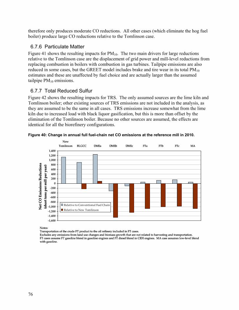
76

therefore only produces moderate CO reductions. All other cases (which eliminate the hog fuel boiler) produce large CO reductions relative to the Tomlinson case.

6.7.6 Particulate Matter Figure 41 shows the resulting impacts for PM10. The two main drivers for large reductions relative to the Tomlinson case are the displacement of grid power and mill-level reductions from replacing combustion in boilers with combustion in gas turbines. Tailpipe emissions are also reduced in some cases, but the GREET model includes brake and tire wear in its total PM10 estimates and these are unaffected by fuel choice and are actually larger than the assumed tailpipe PM10 emissions.

6.7.7 Total Reduced Sulfur Figure 42 shows the resulting impacts for TRS. The only assumed sources are the lime kiln and Tomlinson boiler; other existing sources of TRS emissions are not included in the analysis, as they are assumed to be the same in all cases. TRS emissions increase somewhat from the lime kiln due to increased load with black liquor gasification, but this is more than offset by the elimination of the Tomlinson boiler. Because no other sources are assumed, the effects are identical for all the biorefinery configurations. Figure 40: Change in annual full fuel-chain net CO emissions at the reference mill in 2010.

‐1,600

‐1,400‐1,200

‐1,000

‐800

‐600‐400

‐200

0

200400

600

800

1,0001,200

1,400

NewTomlinson BLGCC DMEa DMEb DMEc FTa FTb FTc MA

Net CO Emissions Reductions 

(short tons per mill per year)

Relative to Conventional Fuel Chain

Relative to New  Tomlinson

Notes:Transportation of the crude FT product to the oil refinery included in FT cases.Excludes any emissions from land use changes and biomass growth that are not related to harvesting and transportation.FT cases assume FT gasoline blend in gasoline engines and FT diesel blend in CIDI engines.  MA case assumes low‐level blend with gasoline.

‐1,600

‐1,400‐1,200

‐1,000

‐800

‐600‐400

‐200

0

200400

600

800

1,0001,200

1,400

NewTomlinson BLGCC DMEa DMEb DMEc FTa FTb FTc MA

Net CO Emissions Reductions 

(short tons per mill per year)

Relative to Conventional Fuel Chain

Relative to New  Tomlinson

Notes:Transportation of the crude FT product to the oil refinery included in FT cases.Excludes any emissions from land use changes and biomass growth that are not related to harvesting and transportation.FT cases assume FT gasoline blend in gasoline engines and FT diesel blend in CIDI engines.  MA case assumes low‐level blend with gasoline.

77

Figure 41: Change in annual full fuel-chain net PM10 emissions at the reference mill in 2010.

‐550‐500‐450‐400‐350‐300‐250‐200‐150‐100‐500

50100150200250300350

NewTomlinson BLGCC DMEa DMEb DMEc FTa FTb FTc MA

Net PM10 Emissions Reductions 

(short tons per mill per year)

Relative to Conventional Fuel Chain

Relative to New  Tomlinson

Notes:Transportation of the crude FT product to the oil refinery included in FT cases.Excludes any emissions from land use changes and biomass growth that are not related to harvesting and transportation.FT cases assume FT gasoline blend in gasoline engines and FT diesel blend in CIDI engines.  MA case assumes low‐level blend with gasoline.

‐550‐500‐450‐400‐350‐300‐250‐200‐150‐100‐500

50100150200250300350

NewTomlinson BLGCC DMEa DMEb DMEc FTa FTb FTc MA

Net PM10 Emissions Reductions 

(short tons per mill per year)

Relative to Conventional Fuel Chain

Relative to New  Tomlinson

Notes:Transportation of the crude FT product to the oil refinery included in FT cases.Excludes any emissions from land use changes and biomass growth that are not related to harvesting and transportation.FT cases assume FT gasoline blend in gasoline engines and FT diesel blend in CIDI engines.  MA case assumes low‐level blend with gasoline.

Figure 42: Change in annual full fuel-chain net TRS emissions at the reference mill in 2010.

‐30

‐25

‐20

‐15

‐10

‐5

0

5

10

15

20

25

30

NewTomlinson BLGCC DMEa DMEb DMEc FTa FTb FTc MA

Net TRS Emissions Reductions 

(short tons per mill per year)

Relative to Conventional Fuel Chain

Relative to New  Tomlinson

Notes:Transportation of the crude FT product to the oil refinery included in FT cases.Excludes any emissions from land use changes and biomass growth that are not related to harvesting and transportation.FT cases assume FT gasoline blend in gasoline engines and FT diesel blend in CIDI engines.  MA case assumes low‐level blend with gasoline.TRS emissions are for combustion sources only.

‐30

‐25

‐20

‐15

‐10

‐5

0

5

10

15

20

25

30

NewTomlinson BLGCC DMEa DMEb DMEc FTa FTb FTc MA

Net TRS Emissions Reductions 

(short tons per mill per year)

Relative to Conventional Fuel Chain

Relative to New  Tomlinson

Notes:Transportation of the crude FT product to the oil refinery included in FT cases.Excludes any emissions from land use changes and biomass growth that are not related to harvesting and transportation.FT cases assume FT gasoline blend in gasoline engines and FT diesel blend in CIDI engines.  MA case assumes low‐level blend with gasoline.TRS emissions are for combustion sources only.

78

7 Biorefinery Capital Cost Estimates

7.1 Approach and Assumptions As a basis for estimating prospective returns on investments in pulp mill biorefineries, engineers at Nexant, LLC, an independent engineering consulting firm originally created as a subsidiary of the Bechtel Corporation in 2000, were engaged to estimate installed capital costs for the biorefinery designs developed in this work. Nexant has considerable experience in design and engineering of combustion and gasification-based power plants and liquids production facilities. We selected Nexant to assist with the cost-estimation work in part because they prepared the cost estimates in our earlier study for the Tomlinson and BLGCC systems. Thus, there is consistency with the earlier study in the biorefinery cost estimates described here. Early in the cost estimation process, we asked Nexant engineers to review preliminary mass and energy balances and provide recommendations for modifications. We modified the flowsheets based on their recommendations, and provided them with revised flowsheets, which they used as a basis for their equipment sizing and costing calculations. After reviewing their draft cost estimates, we made additional modifications to the flowsheets in most cases to try to further reduce capital costs. Nexant then provided their final cost estimates based on these revised flowsheets. We subsequently made some additional flowsheet adjustments (minor ones in most cases) to reach the final versions shown in this report. In consultation with the lead Nexant design/cost-estimating engineer, we made adjustments to Nexant’s final cost estimates to account for the flowsheet changes in these cases. The changes to the DME and FTL flowsheets were minor. The changes to the MA flowsheet were more significant (due primarily to mid-course improvements we made in our kinetic model for MA synthesis). Nexant engineers did not estimate the capital cost for the DMEb design, but because all of the equipment in the DMEb design is found in either the DMEa or DMEc designs, we were able to develop a consistent cost estimate for DMEb using commonly-accepted capacity-cost scaling factors. We asked Nexant to provide capital cost estimates by major plant area to within ±30% accuracy. For some pieces of equipment (e.g., black liquor gasifier, gas turbine, air separation unit, and Selexol island), costs were simply escalated (from 2002$ to 2005$) from the cost estimates Nexant made for our earlier BLGCC study [5] and then scaled, as appropriate, to the required equipment capacities. In other cases where there was no cost estimate from our prior study (e.g, biomass gasifier, heat exchangers, synthesis reactors, and distillation columns), Nexant carried out sizing calculations and used their experience-based in-house cost database to estimate capital costs. In still other cases (e.g., biomass boiler, biomass dryer, Rectisol), vendor quotes were obtained and used as the basis for estimating installed costs. Nexant was asked to assume “Nth plant” levels of technology maturity and operational reliability in their cost estimates. In this regard, each of the systems included in our study utilize two black liquor gasifier vessels, each with 50% of the needed total capacity. A single biomass gasifier vessel was used in configurations with biomass gasification. These choices represent a high level of gasifier reliability. Given that at most large pulp mills today the Tomlinson recovery boiler is typically a single unit handling 100% of the black liquor recovery duty, it was judged

79

feasible that a black liquor or biomass gasifier ultimately could reliably operate with no spare capacity in an “Nth plant” implementation. The scope of the capital cost estimates includes equipment in all major areas shown on the detailed mass/energy balance flowsheets presented earlier, with the following exceptions: • Steam turbine. In the Tomlinson case, the steam turbine pre-existing at the reference mill is

assumed to be kept. However, since in this case there is excess steam available after meeting process needs, it was determined to be financially beneficial to add a small (8 MWe) condensing turbine to enable greater electricity generation. In all other cases, except DMEa, the existing steam turbine is replaced, and the cost for a new turbine is included in the capital estimate. In the DMEa case, a large fraction of the woody biomass used for energy is burned in existing hog fuel boilers. Since the steam pressure from these boilers is already matched to the inlet pressure of the existing back-pressure steam turbine, the existing turbine is retained. A modest allowance is included in the capital cost to maintain the efficiency of the turbine while derating its output to 33 MWe. (The pre-existing turbine capacity is higher than this because it had been utilizing steam from both hog fuel and black liquor boilers.)

• Hog fuel boilers. Hog fuel boilers are present in the Tomlinson, BLGCC, and DMEa cases. Boilers available at the pre-existing mill are assumed to be available to raise steam after the new power/fuel/recovery systems have been installed. The bark and waste wood available from the wood yard operations in the Tomlinson case represent 58 MW (LHV) of thermal input. Mills typically have excess hog fuel boiler capacity available on-site, and we make the same assumption about this as in the BLGCC study [5]: the total available existing hog fuel capacity is 81 MWth (LHV, or 100 MW HHV). Hog fuel boiler capacity needed in excess of this amount (as is the case in DMEa) is included in the capital cost estimate.

• Lime kiln and related equipment. The incremental causticizing and calcining capacity needed in the gasification cases is estimated to be 16% of the existing capacity [5]. This is modest enough that it can be met by enriching the lime-kiln combustion air with oxygen from the air separation unit (ASU). The cost for burner modifications in the kiln and for an ASU of sufficient capacity to deliver the requisite amount of O2 to the lime kiln (in addition to O2 for gasification) are included in the capital cost estimate.

• Polysulfide generation systems. In all biorefinery cases, as in the BLGCC case [5], polysulfide pulping liquor is generated in a mixing tank maintained at a temperature < 100oF. The cost for this polysulfide generating unit is included in the capital cost estimate.

• In all gasification-based cases, we have included an estimate for upsizing the ASU to enable production of oxygen for delignification, which is a very cost-effective way to replace oxygen that was previously being purchased at the reference mill for this purpose.38

7.2 Capital Costs Table 22 summarizes the installed capital cost and non-fuel operating and maintenance cost estimates for all biorefinery cases. The table also includes estimates for the Tomlinson and

38 If purchased O2 costs $100/tonne, the avoided costs of purchased O2 at the reference mill (assuming 23 kg O2 for delignification per metric tonne of pulp produced (Table 5) and 8330 annual operating hours) would be $1.14 million per year. Accounting for the cost of about 600 kW of additional parasitic electricity load with a larger ASU, the payback time on the incremental ASU investment cost (discussed in next section) would be of the order of one year in all cases.

80

BLGCC cases from our prior study (escalated here to 2005$ from the 2002$ in our previous study). Figure 43 shows capital cost percentages for the biorefineries by major plant area. Table 22. Estimated overnight installed capital costs (thousand 2005$) and non-fuel operating and maintenance costs (thousand 2005$ per year). Installed capital costs include engineering, equipment, installation, owner’s costs (including initial catalyst), contingencies, and spare parts.

Power/Steama Biorefinery -- Power/Steam/Liquid Fuel THOUSAND 2005$ Tomlin. BLGCC DMEa DMEb DMEc FTa FTb FTc MA

Recovery boiler 125,018 0 0 0 0 0 0 0 0Steam system modificationsb 11,136 0 3,000 0 0 0 0 0 0Air separation unit (ASU) 0 42,628 43,053 61,561 52,933 55,001 72,762 77,823 54,080ASU increment for O2 delig.c 0 1,118 1,061 879 954 933 805 776 948BL gasifier & green liquor filterd 0 63,720 63,720 63,720 63,720 63,720 63,720 63,720 63,720Nitrogen compressor 0 0 0 1,188 810 1,071 1,757 2,013 5,181Acid gas removal & sulfur recovery 0 19,003 37,732 37,732 27,321 27,321 27,321 42,164 24,529Synthesis island 0 0 49,344 49,344 16,287 22,019 22,019 38,767 83,548Combined cycle power island 0 89,243 0 105,303 100,091 90,018 171,895 104,300 90,348Wood yard expansione 867 2,697 789 1,303 4,832 5,788 1,077Biomass dryer, including RTOf 0 0 0 50,295 32,523 37,286 72,507 45,558 31,383Biomass gasifier & tar cracker 0 0 0 28,354 18,320 20,867 41,365 47,063 22,949Biomass syngas cooler & filter 0 0 0 8,484 4,998 5,666 11,372 0 0Biomass syngas cooler & wash 0 0 0 0 0 0 34,425 16,092Biomass syngas expander 0 0 0 3,778 2,661 2,670 9,410 0 0Hog fuel boiler 0 0 50,736 0 0 0 0 0 0Otherg 0 2,359 2,359 2,359 2,359 2,359 2,359 2,359 2,359Overnight Installed Capital Cost 136,154 218,072 251,873 415,695 323,766 330,234 502,125 464,755 396,215Annual non-fuel O&M costh 5,446 8,723 10,075 16,628 12,951 13,209 20,085 18,590 15,849(a) Escalated (from 2002$ to 2005$) from Larson et al. [5], except for O&M costs, which are calculated as indicated in note (f).

Also, the ASU increment for O2 delignification ws not originally included in [5]. (b) In the Tomlinson case, the modifications include, primarily, the addition of a condensing section to the pre-existing back

pressure turbine. In the DMEa case, the steam system modifications include, primarily, adjustments to the pre-existing back pressure turbine to maintain efficiency while reducing rated gross output to 33 MWe. (Output of the pre-existing turbine is higher than this since it is designed to use steam from both hog fuel boiler and black liquor boiler.)

(c) The ASU size is increased (beyond the size shown in the detailed biorefinery energy/mass balance diagrams) to also produce the oxygen needed by the oxygen delignification system at the pulp mill. The incremental cost is estimated from the base ASU cost using a cost-capacity scaling exponent of 0.65.

(d) 2 x 50% capacity gasifiers. (e) The original biorefinery cost estimates made by Nexant did not include costs for expanding the wood yard to handle the

larger wood flows associated with the biorefineries (compared to a mill with a Tomlinson system). We have estimated the costs for additional wood yard capacity by scaling wood yard costs given by Weyerhaeuser [132]. Original costs in 1999$ were escalated to 2005$ using the GDP deflator and then scaled with wood mass flow raised to the 0.77 exponent [73]. The wood mass flow is the net change in total wood flow (pulpwood and wood residues) between the biorefinery case and the Tomlinson case.

(f) RTO = regenerative thermal oxidizer used to destroy volatile organic compounds (VOCs) in the dryer exhaust gases. The original biorefinery cost estimate made by Nexant for the dryers did not include RTO. Themens [133] estimates that the cost for a RTO fitted to a partial gas recirculating direct contact rotary wood chip dryer (the type assumed in Nexant’s capital cost estimate) is about 50% of the cost of the dryer alone. Accordingly, we have multiplied the original dryer cost estimated by Nexant by 1.5 to arrive at the figures in this table.

(g) This includes an allowance for modifications needed to the lime kiln to boost capacity by firing with oxygen-enriched air and for a polysulfide mixing tank.

(h) Assumed to be 4% of overnight installed capital costs.

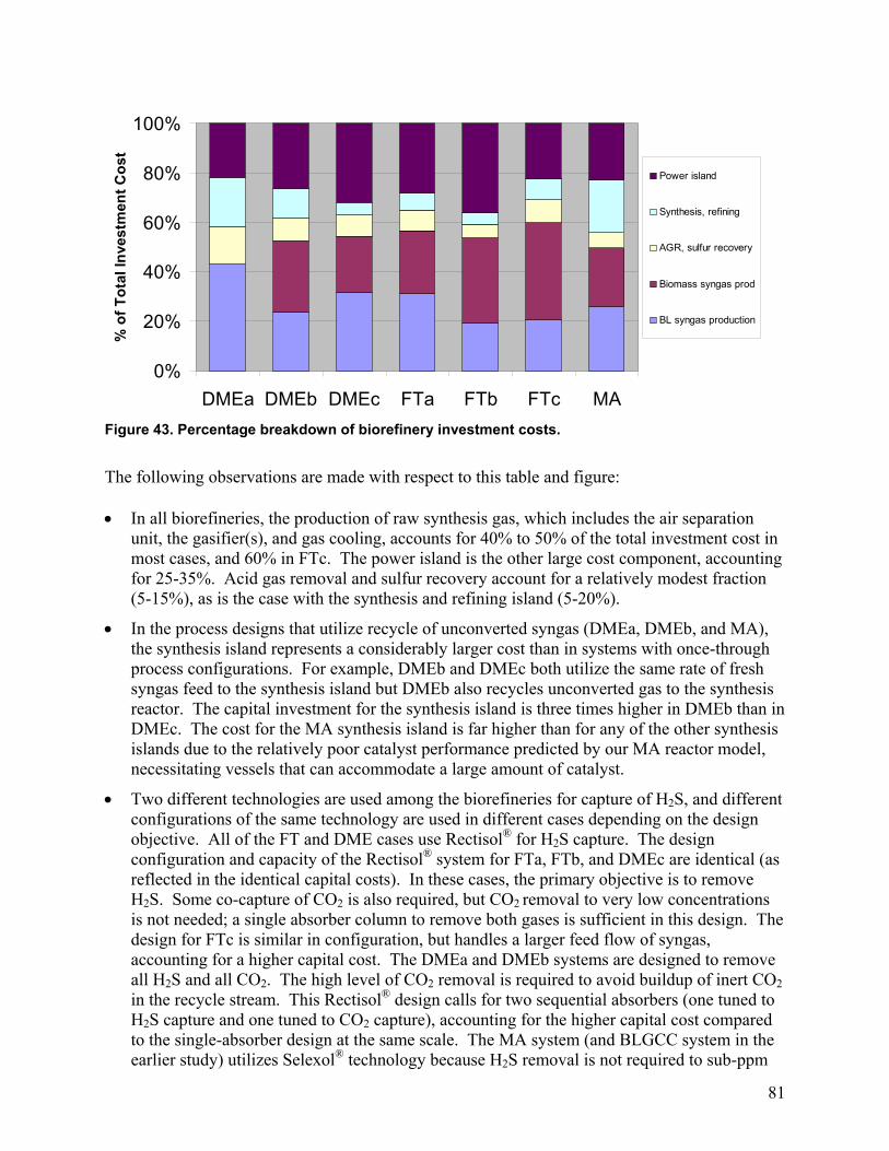
81

0%

20%

40%

60%

80%

100%

DMEa DMEb DMEc FTa FTb FTc MA

% o

f Tot

al In

vest

men

t Cos

t

Power island

Synthesis, refining

AGR, sulfur recovery

Biomass syngas prod

BL syngas production

Figure 43. Percentage breakdown of biorefinery investment costs.

The following observations are made with respect to this table and figure: • In all biorefineries, the production of raw synthesis gas, which includes the air separation

unit, the gasifier(s), and gas cooling, accounts for 40% to 50% of the total investment cost in most cases, and 60% in FTc. The power island is the other large cost component, accounting for 25-35%. Acid gas removal and sulfur recovery account for a relatively modest fraction (5-15%), as is the case with the synthesis and refining island (5-20%).

• In the process designs that utilize recycle of unconverted syngas (DMEa, DMEb, and MA), the synthesis island represents a considerably larger cost than in systems with once-through process configurations. For example, DMEb and DMEc both utilize the same rate of fresh syngas feed to the synthesis island but DMEb also recycles unconverted gas to the synthesis reactor. The capital investment for the synthesis island is three times higher in DMEb than in DMEc. The cost for the MA synthesis island is far higher than for any of the other synthesis islands due to the relatively poor catalyst performance predicted by our MA reactor model, necessitating vessels that can accommodate a large amount of catalyst.

• Two different technologies are used among the biorefineries for capture of H2S, and different configurations of the same technology are used in different cases depending on the design objective. All of the FT and DME cases use Rectisol® for H2S capture. The design configuration and capacity of the Rectisol® system for FTa, FTb, and DMEc are identical (as reflected in the identical capital costs). In these cases, the primary objective is to remove H2S. Some co-capture of CO2 is also required, but CO2 removal to very low concentrations is not needed; a single absorber column to remove both gases is sufficient in this design. The design for FTc is similar in configuration, but handles a larger feed flow of syngas, accounting for a higher capital cost. The DMEa and DMEb systems are designed to remove all H2S and all CO2. The high level of CO2 removal is required to avoid buildup of inert CO2 in the recycle stream. This Rectisol® design calls for two sequential absorbers (one tuned to H2S capture and one tuned to CO2 capture), accounting for the higher capital cost compared to the single-absorber design at the same scale. The MA system (and BLGCC system in the earlier study) utilizes Selexol® technology because H2S removal is not required to sub-ppm

82

levels (for which Rectisol® is better suited). For applications suitable for Selexol®, this system will generally have lower capital cost than a Rectisol® system designed for the same application.

7.2.1 Specific Capital Investments per Unit of Biofuel Production For comparison with other biofuel production systems, it is of interest to compare the capital investment required per unit of liquid fuels production capacity. Figure 44 shows the specific capital investment for the pulp mill biorefinery designs developed in this study, along with specific investment costs for biofuel production systems from other published studies. The other studies correspond to those described in Section 0 and Figure 32, except in Figure 44 we have chosen to show only systems that we judge are at comparable distances from commercial maturity, i.e., those that are near commercially-ready. Thus, we have included NREL’s estimate for corn-stover to ethanol by enzymatic hydrolysis, but we have excluded NREL’s projections for advanced lignocellulosic conversion to ethanol and we have excluded NREL’s and our own mixed-alcohols analyses, key components of which have not yet been demonstrated at pilot scale and which appear to require R&D breakthroughs to achieve cost/performance targets. Because biorefineries produce energy products (and/or chemical services) in addition to liquid fuels, it is appropriate for comparison purposes to charge some fraction of the capital investment to the other products and services in order to produce a fair comparison of liquid-fuel capital intensity. For the biorefineries not attached to pulp mills in Figure 44, we have charged a portion of the investment cost against the electricity co-product of these biorefineries. We have charged capital against electricity capacity at a rate of $968/kW, the estimated overnight investment cost for an advanced, large-scale stand-alone biomass-IGCC electricity generating facility, once the technology reaches commercial maturity [106]. This accounting is shown in Figure 45(a).

0

20000

40000

60000

80000

100000

120000

140000

160000

180000

200000

0 1000 2000 3000 4000 5000 6000 7000 8000

Liquids capacity, barrels per day diesel equivalent

Liqu

ids

Cap

ital i

nten

sity

($/b

bl p

er d

ay)

This study

NREL

RBAEF

EU studyDMEc

FTb

FTa DMEb

DMEa

FTc

FT

DMEMeOH

EtOH-2000

FT-OTDME-OT DME-RC

Coal to liquids

Gas to liquids

Petroleum refining

Liquids from fossil fuels @

100,000 - 150,000 barrels per day

0

20000

40000

60000

80000

100000

120000

140000

160000

180000

200000

0 1000 2000 3000 4000 5000 6000 7000 8000

Liquids capacity, barrels per day diesel equivalent

Liqu

ids

Cap

ital i

nten

sity

($/b

bl p

er d

ay)

This study

NREL

RBAEF

EU studyDMEc

FTb

FTa DMEb

DMEa

FTc

FT

DMEMeOH

EtOH-2000

FT-OTDME-OT DME-RC

Coal to liquids

Gas to liquids

Petroleum refining

Liquids from fossil fuels @

100,000 - 150,000 barrels per day

Figure 44. Effective capital investment intensity (2005$ per barrel diesel-equivalent per day) for liquid fuels production as a function of liquids production capacity. See text for assumptions.

83

In the case of the pulp mill biorefineries, considering that they provide all of the services of a Tomlinson system in addition to producing liquid fuels, the capital investment represented in Figure 44 is the difference between the total investment for the biorefinery and the investment for a Tomlinson power/recovery system (representing the non-liquid fuel services provided by the biorefinery), with a correction made if the biorefinery’s electricity generating capacity differs from the Tomlinson’s generating capacity – see Figure 45(b) and Figure 45(c).39

NREL and RBAEF SystemsDMEb, DMEc, FTa, FTb, FTc, MAPulp/Paper Mill Biorefineries

DMEa, EU-FTD, EU-DME, EU-MeOHPulp/Paper Mill Biorefineries

Additional capital charged to liquid fuels = kW electricpurchased by mill x $968/kW

X Barrels per day liquid

fuel

Current levelof Tomlinson

chem. recov. +process steam

+ someelectricity

Capital costcharged toequivalentTomlinsonservices

= cost of new Tomlinson

Capital Cost

Capital costcharged toX bbl/dayliquid fuels

ProductionCapacities

Additional capital charged to liquid fuels = kW electricpurchased by mill x $968/kW

X Barrels per day liquid

fuel

Current levelof Tomlinson

chem. recov. +process steam

+ someelectricity

Capital costcharged toequivalentTomlinsonservices

= cost of new Tomlinson

Capital Cost

Capital costcharged toX bbl/dayliquid fuels

ProductionCapacitiesCapital cost

charged toX bbl/dayliquid fuels

Capital Cost

ProductionCapacities

X Barrels perday liquid

fuel

Y KilowattsElectricity

Capital costcharged to

electricity @ Y x $968/kW

Capital costcharged toX bbl/dayliquid fuels

Capital Cost

ProductionCapacities

X Barrels perday liquid

fuel

Y KilowattsElectricity

Capital costcharged to

electricity @ Y x $968/kW

Capital costcharged toX bbl/dayliquid fuels

X Barrels perday liquid

fuel

Servicesequivalent to

currentTomlinson

(chem. recov.,process steamand electricity)

Capital costcharged toequivalentTomlinsonservices

= cost of new Tomlinson

Capital costcharged to

electricity @Y x $968/kW

Y kW electric> Tomlinson

Capital Cost

ProductionCapacities

Capital costcharged toX bbl/dayliquid fuels

X Barrels perday liquid

fuel

Servicesequivalent to

currentTomlinson

(chem. recov.,process steamand electricity)

Capital costcharged toequivalentTomlinsonservices

= cost of new Tomlinson

Capital costcharged to

electricity @Y x $968/kW

Y kW electric> Tomlinson

Capital Cost

ProductionCapacities

(a) (b) (c)

NREL and RBAEF SystemsDMEb, DMEc, FTa, FTb, FTc, MAPulp/Paper Mill Biorefineries

DMEa, EU-FTD, EU-DME, EU-MeOHPulp/Paper Mill Biorefineries

Additional capital charged to liquid fuels = kW electricpurchased by mill x $968/kW

X Barrels per day liquid

fuel

Current levelof Tomlinson

chem. recov. +process steam

+ someelectricity

Capital costcharged toequivalentTomlinsonservices

= cost of new Tomlinson

Capital Cost

Capital costcharged toX bbl/dayliquid fuels

ProductionCapacities

Additional capital charged to liquid fuels = kW electricpurchased by mill x $968/kW

X Barrels per day liquid

fuel

Current levelof Tomlinson

chem. recov. +process steam

+ someelectricity

Capital costcharged toequivalentTomlinsonservices

= cost of new Tomlinson

Capital Cost

Capital costcharged toX bbl/dayliquid fuels

ProductionCapacitiesCapital cost

charged toX bbl/dayliquid fuels

Capital Cost

ProductionCapacities

X Barrels perday liquid

fuel

Y KilowattsElectricity

Capital costcharged to

electricity @ Y x $968/kW

Capital costcharged toX bbl/dayliquid fuels

Capital Cost

ProductionCapacities

X Barrels perday liquid

fuel

Y KilowattsElectricity

Capital costcharged to

electricity @ Y x $968/kW

Capital costcharged toX bbl/dayliquid fuels

X Barrels perday liquid

fuel

Servicesequivalent to

currentTomlinson

(chem. recov.,process steamand electricity)

Capital costcharged toequivalentTomlinsonservices

= cost of new Tomlinson

Capital costcharged to

electricity @Y x $968/kW

Y kW electric> Tomlinson

Capital Cost

ProductionCapacities

Capital costcharged toX bbl/dayliquid fuels

X Barrels perday liquid

fuel

Servicesequivalent to

currentTomlinson

(chem. recov.,process steamand electricity)

Capital costcharged toequivalentTomlinsonservices

= cost of new Tomlinson

Capital costcharged to

electricity @Y x $968/kW

Y kW electric> Tomlinson

Capital Cost

ProductionCapacities

NREL and RBAEF SystemsDMEb, DMEc, FTa, FTb, FTc, MAPulp/Paper Mill Biorefineries

DMEa, EU-FTD, EU-DME, EU-MeOHPulp/Paper Mill Biorefineries

Additional capital charged to liquid fuels = kW electricpurchased by mill x $968/kW

X Barrels per day liquid

fuel

Current levelof Tomlinson

chem. recov. +process steam

+ someelectricity

Capital costcharged toequivalentTomlinsonservices

= cost of new Tomlinson

Capital Cost

Capital costcharged toX bbl/dayliquid fuels

ProductionCapacities

Additional capital charged to liquid fuels = kW electricpurchased by mill x $968/kW

X Barrels per day liquid

fuel

Current levelof Tomlinson

chem. recov. +process steam

+ someelectricity

Capital costcharged toequivalentTomlinsonservices

= cost of new Tomlinson

Capital Cost

Capital costcharged toX bbl/dayliquid fuels

ProductionCapacitiesCapital cost

charged toX bbl/dayliquid fuels

Capital Cost

ProductionCapacities

X Barrels perday liquid

fuel

Y KilowattsElectricity

Capital costcharged to

electricity @ Y x $968/kW

Capital costcharged toX bbl/dayliquid fuels

Capital Cost

ProductionCapacities

X Barrels perday liquid

fuel

Y KilowattsElectricity

Capital costcharged to

electricity @ Y x $968/kW

Capital costcharged toX bbl/dayliquid fuels

X Barrels perday liquid

fuel

Servicesequivalent to

currentTomlinson

(chem. recov.,process steamand electricity)

Capital costcharged toequivalentTomlinsonservices

= cost of new Tomlinson

Capital costcharged to

electricity @Y x $968/kW

Y kW electric> Tomlinson

Capital Cost

ProductionCapacities

Capital costcharged toX bbl/dayliquid fuels

X Barrels perday liquid

fuel

Servicesequivalent to

currentTomlinson

(chem. recov.,process steamand electricity)

Capital costcharged toequivalentTomlinsonservices

= cost of new Tomlinson

Capital costcharged to

electricity @Y x $968/kW

Y kW electric> Tomlinson

Capital Cost

ProductionCapacities

(a) (b) (c) Figure 45. Accounting used to calculate the capital intensity of liquid biofuel production.

Capital intensities for the biofuel systems vary significantly, depending on the specific plant design. Figure 44 shows some dependence of specific investment cost on scale of liquid production, but the full scale range shown on the graph is tiny compared to typical scales for fossil fuel conversion. Some reference points are shown on the right in Figure 44 to provide perspective: large-scale petroleum refining (~150,000 bpd) involves much lower specific investment costs – about $15,000 per bpd. Large gas-to-liquid plants have costs of $25,000 to $50,000 per bpd, and large coal-to-liquids plants have costs of $50,000 to $70,000 per bpd [134]. Thus, the investment costs we estimate here for relatively small biorefineries are in the same range as investment costs for coal-to-liquids facilities with installed capacities 20 to 50 times as large. That small biorefinery systems have capital intensities on a par with much larger coal-to-liquids facilities derives largely from the benefit provided by integrating the biorefinery with the pulp and paper mill. Another representation of capital costs commonly used in the fossil fuel industry is the “development” (capital) costs per annual barrel of liquid fuel capacity. In the oil and gas industry, this indicator is normally associated with exploration and extraction costs associated with developing an oil or gas field, but here we apply the figure to the conversion step in the 39 A charge of ($968/kW x DeltaCapacity, where DeltaCapacity = Tomlinson electric capacity – Biorefinery electric capacity) is added to the difference in total investment cost between the biorefinery and the Tomlinson.

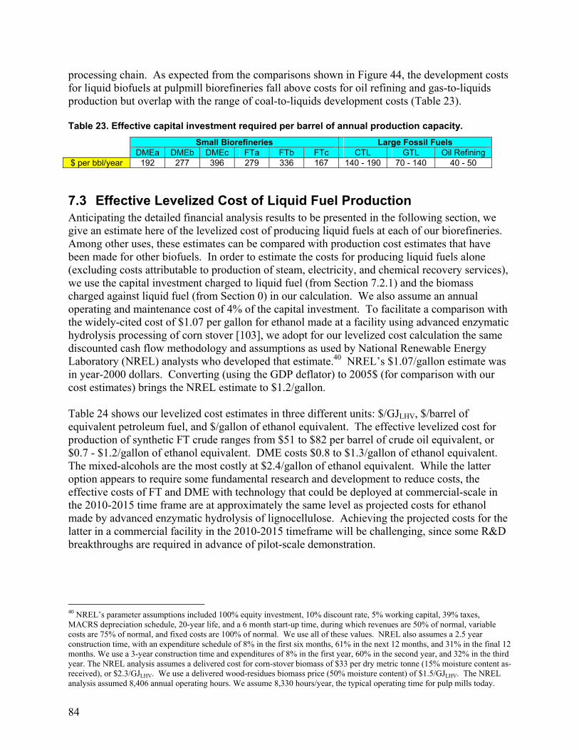
84

processing chain. As expected from the comparisons shown in Figure 44, the development costs for liquid biofuels at pulpmill biorefineries fall above costs for oil refining and gas-to-liquids production but overlap with the range of coal-to-liquids development costs (Table 23). Table 23. Effective capital investment required per barrel of annual production capacity. Small Biorefineries Large Fossil Fuels DMEa DMEb DMEc FTa FTb FTc CTL GTL Oil Refining $ per bbl/year 192 277 396 279 336 167 140 - 190 70 - 140 40 - 50

7.3 Effective Levelized Cost of Liquid Fuel Production Anticipating the detailed financial analysis results to be presented in the following section, we give an estimate here of the levelized cost of producing liquid fuels at each of our biorefineries. Among other uses, these estimates can be compared with production cost estimates that have been made for other biofuels. In order to estimate the costs for producing liquid fuels alone (excluding costs attributable to production of steam, electricity, and chemical recovery services), we use the capital investment charged to liquid fuel (from Section 7.2.1) and the biomass charged against liquid fuel (from Section 0) in our calculation. We also assume an annual operating and maintenance cost of 4% of the capital investment. To facilitate a comparison with the widely-cited cost of $1.07 per gallon for ethanol made at a facility using advanced enzymatic hydrolysis processing of corn stover [103], we adopt for our levelized cost calculation the same discounted cash flow methodology and assumptions as used by National Renewable Energy Laboratory (NREL) analysts who developed that estimate.40 NREL’s $1.07/gallon estimate was in year-2000 dollars. Converting (using the GDP deflator) to 2005$ (for comparison with our cost estimates) brings the NREL estimate to $1.2/gallon. Table 24 shows our levelized cost estimates in three different units: $/GJLHV, $/barrel of equivalent petroleum fuel, and $/gallon of ethanol equivalent. The effective levelized cost for production of synthetic FT crude ranges from $51 to $82 per barrel of crude oil equivalent, or $0.7 - $1.2/gallon of ethanol equivalent. DME costs $0.8 to $1.3/gallon of ethanol equivalent. The mixed-alcohols are the most costly at $2.4/gallon of ethanol equivalent. While the latter option appears to require some fundamental research and development to reduce costs, the effective costs of FT and DME with technology that could be deployed at commercial-scale in the 2010-2015 time frame are at approximately the same level as projected costs for ethanol made by advanced enzymatic hydrolysis of lignocellulose. Achieving the projected costs for the latter in a commercial facility in the 2010-2015 timeframe will be challenging, since some R&D breakthroughs are required in advance of pilot-scale demonstration.

40 NREL’s parameter assumptions included 100% equity investment, 10% discount rate, 5% working capital, 39% taxes, MACRS depreciation schedule, 20-year life, and a 6 month start-up time, during which revenues are 50% of normal, variable costs are 75% of normal, and fixed costs are 100% of normal. We use all of these values. NREL also assumes a 2.5 year construction time, with an expenditure schedule of 8% in the first six months, 61% in the next 12 months, and 31% in the final 12 months. We use a 3-year construction time and expenditures of 8% in the first year, 60% in the second year, and 32% in the third year. The NREL analysis assumes a delivered cost for corn-stover biomass of $33 per dry metric tonne (15% moisture content as-received), or $2.3/GJLHV. We use a delivered wood-residues biomass price (50% moisture content) of $1.5/GJLHV. The NREL analysis assumed 8,406 annual operating hours. We assume 8,330 hours/year, the typical operating time for pulp mills today.

85

Table 24. Effective levelized cost of liquid fuels production at pulp mill biorefineries. FTa FTb FTc DMEa DMEb DMEc MA $ per GJ (LHV)

Capital 7.38 8.87 4.55 5.18 7.40 10.46 18.76 Working capital 0.26 0.31 0.16 0.18 0.26 0.37 0.66

Taxes 0.72 0.47 1.87 1.85 1.32 0.39 0.82 O&M 2.06 2.49 1.24 1.42 2.05 2.94 5.26

Biomass 1.73 2.08 1.06 1.21 1.73 2.45 4.40 Total 12.16 14.23 8.88 9.83 12.76 16.60 29.90

$ per bbl equivalent petroleum fuela Capital 42.4 51.0 26.1 29.7 42.5 60.0 63.4

Working capital 1.5 1.8 0.9 1.0 1.5 2.1 2.2 Taxes 4.1 2.7 10.8 10.6 7.6 2.2 2.8 O&M 11.9 14.3 7.1 8.1 11.8 16.8 17.8

Biomass 9.9 12.0 6.1 6.9 9.9 14.1 14.9 Total 69.8 81.7 51.0 56.4 73.2 95.3 101.1

$ per gallon of ethanol equivalent Capital 0.59 0.71 0.37 0.42 0.60 0.84 1.51

Working capital 0.02 0.02 0.01 0.01 0.02 0.03 0.05 Taxes 0.06 0.04 0.15 0.15 0.11 0.03 0.07 O&M 0.17 0.20 0.10 0.11 0.17 0.24 0.42

Biomass 0.14 0.17 0.09 0.10 0.14 0.20 0.35 Total 0.98 1.15 0.71 0.79 1.03 1.34 2.41

(a) Equivalent petroleum fuel is crude oil for the FT product, motor diesel for DME, and motor gasoline for MA.

8 Mill-Level Financial Analysis To assess the prospective economics of integrated biorefineries at the mill level, comprehensive cash flow analyses are carried out assuming that an investment would be made to replace an existing Tomlinson system (with performance characterized by the Tomlinson described in Section 3.3.1 and summarized in Table 12) that had reached the end of its working life. Specifically, the internal rate of return (IRR) is calculated on the incremental capital investment required for a biorefinery over a new Tomlinson system. The net present value (NPV) is also calculated, assuming a specified return on equity (hurdle rate). The IRR and NPV are calculated both without and with consideration of the potential economic value of environmental benefits. In addition to a baseline set of results, sensitivity analyses are carried out around key input parameter values, namely capital costs and future energy prices. The baseline and sensitivity analyses are done initially without assigning any value to environmental benefits of biorefining, nor with any financial incentives included. Then, a separate set of financial results are generated with environmental credits and incentives included. In the latter analyses, it is assumed that 100% of the wood-derived fuels used at the mill are renewable and (considering their photosynthetic origin) result in no net CO2 emissions to the atmosphere.

86

8.1 Assumptions

8.1.1 General The financial analysis is intended to account for all major changes to mill operations that would result from the conversion from a Tomlinson-based system to an integrated biorefinery. The capital expenditures are almost entirely in the power/recovery area, but the analysis also considers the reduced wood costs due to higher digester yield with polysulfide pulping, the increased use of #6 fuel oil in the lime kiln, the purchase of natural gas (in BLGCC case only), the purchase of wood residues, the sale of electricity and biofuels, and other factors affecting incremental costs and potential savings. Avoided costs (e.g., avoided grid power purchases) are treated as revenues in the cash flow analysis. Key inputs to the financial analysis, which are consistent with those from our earlier BLGCC analysis [5], include:

• The detailed mass/energy balances and engineering cost estimates for each of the process configurations described in earlier sections of this report,

• Expected future prices for natural gas, fuel oil, purchased wood residuals, electricity purchased by the mill and electricity sold to the grid, as discussed in the next section, and

• Financial assumptions (e.g., construction period, debt/equity split, cost of debt and return on equity, inflation rate, project life, and income tax rate), as summarized in Table 25.41,42

Sensitivity analysis is undertaken to examine variations from a baseline set of assumptions regarding energy and feedstock prices, capital costs, monetization of renewable energy and environmental benefits and the application of renewable energy production tax credits and other incentives. One footnote regarding economic opportunities with pulp mill biorefining. There are a number of potential options for enhancing the integration of a biorefinery with existing mill operations that might generate additional revenues and/or cost savings. We have included one such option in our analysis – enlarging the air separation unit (beyond the size needed to supply O2 for gasification) to provide O2 for delignification, replacing previously purchased O2 (see footnote 38). Other integration options could include sale or internal use (for production of paper filler material) of CO2 captured at the acid gas removal island;43 sale of argon generated by the ASU; and other options. In the context of the present study, such measures would likely improve the calculated IRRs, but not substantially so we have not included any other than the ASU upsizing.

41 Since the power/recovery economics must ultimately be evaluated within the financial performance of the entire

company, any negative net cash flows in early years (e.g., during construction and startup) were assumed to generate tax savings that could be captured elsewhere by the mill owner in that year. These savings were therefore factored into the IRR results shown here.

42 The biorefinery ownership structure (e.g., 100% mill, 100% energy company, 100% third party, or some mix of these) will be critically important in actual implementation. However, different structures were not examined here, since this would complicate the analysis without fundamentally changing the relative costs/benefits of Tomlinson versus biorefinery technology – the comparison of interest in this study.

43 At some pulp and paper mills today, CO2 is stripped from lime kiln flue gases for this purpose.

87

Table 25: Summary of key input assumptions for the financial analysis.

Financial Parameters Inflation Rate 2.14% Debt Fraction 50% Equity Fraction 50% Interest Rate on Debt 8% Return on Equity (hurdle rate)a 15% Income Tax Rate (combined Federal & State) 40% Property Tax & Insurance 2% Economic Life (years) 25 Depreciation Method 20-year MACRS rate scheduleb

Construction time for Tomlinson systems 24 months Construction time for BLGCC & Biorefinery systems 30 months P&P Industry/Mill Assumptions O&M cost inflator (% per year, current $)c 2.67% Annual Operating Hours 8,330 Start-up Assumptions (% of full output)

Year 1 of Operation 80% Year 2 of Operation (and beyond) 100%

(a) This is the discount rate used for the NPV calculations (b) The Modified Accelerated Cost Recovery System (MACRS) is a property depreciation system defined by the Internal

Revenue Service that applies to assets placed in service after 1986. It results in more rapid depreciation than straight-line depreciation.

(c) Based on [135].

8.1.2 Energy Price Forecasts One of the most challenging aspects of the biorefinery economic analysis is deciding what future energy prices to use. While energy price forecasting is difficult under any circumstances, it is compounded by recent historically high prices and the high degree of uncertainty regarding the future. The U.S. DOE Annual Energy Outlook (AEO) [134] forms the basis of the price scenarios developed here and provides a bracket for future energy prices. Specifically, both the AEO’s Reference and High Price cases are used. The High Price case is representative of an extrapolation of mid-2006 prices, with crude oil climbing gradually to $90-95/barrel by 2030 (in constant $2004). In contrast, the Reference case has crude oil stabilizing in the $45-55/barrel range over the forecast period. The Low Price case, where oil returns to $28-35/barrel, and stays there, is not considered here, as it is deemed the least likely of the three possibilities. Thus, we use the AEO Reference and High Price cases to create two energy price scenarios for our analysis. We call these the Reference Energy Prices (REP) and Tight Supplies Energy Prices (TSEP) scenarios. As we describe in detail below, we utilize year-by-year values for oil and other energy prices over the 25 years spanned in each of these two scenarios. The scenarios can be characterized in short-hand by the levelized world crude oil price calculated from our year-by-year oil price assumptions. In the REP scenario, this levelized price is $50 per barrel. In the TSEP scenario, this levelized price is $78 per barrel. An additional challenge in developing price forecasts for DME, FT crude and mixed alcohols for use as fuels is that none exist in the literature. Therefore, prices for other fuels must be used to

88

estimate what the selling price might be for these alternatives. Moreover, the available forecasts are for wholesale prices, but it is necessary here to estimate plant gate prices, which would be lower, to account for transportation to the wholesale terminal. The AEO has a wholesale price forecast for ethanol, but not for any other alternative fuel. Also, the AEO includes the effects of current incentives for ethanol, but does not explicitly break them out. Thus, there is no forecast available for ethanol or any other alternative fuel that looks at what the price would be, at the plant gate, without incentives. Since the major incentive for ethanol is the excise tax credit, which is given to blenders and not producers, it is also not possible to know how much, if any, of the credit actually flows to the producer. Plus, this value would fluctuate from year to year depending on market conditions. Despite some limitations, since the only biofuel for which there is an actual forecast is ethanol, this forms the starting point for estimating prices for the biofuels being studied here. There are two main considerations in developing the plant gate price: • The need to subtract from the AEO wholesale ethanol price, an estimate of the cost of

transportation from the plant gate • The need to estimate the impact of the excise tax credit so as to estimate a price without

incentives (needed for our baseline economic analysis) Addressing the first issue is straight forward – we assume that the cost of transportation is 15 ¢/gallon in the near term, falling to 10 ¢/gallon by 2009 and 5 ¢/gallon by 2016. The gradual reduction reflects the expected economies of scale from increased biofuels production and the increasing sophistication of the biofuels supply chain. In comparison, transportation of petroleum products, which typically occurs via pipeline, is less than 5 ¢/gallon. The second issue is more complex. Figure 46 illustrates the approach used for ethanol and mixed alcohols. (For mixed alcohols – MA – we assume a pricing structure exactly like ethanol, corrected for the slightly higher energy content per gallon, i.e., MA has the same price in $/MMBtu as ethanol). Our estimate of the marginal production cost of ethanol today provides a floor price for these fuels, which is almost never reached with the approach outlined in Figure 46. One output of the approach is an estimate (albeit a crude one) of the amount of the excise tax credit that flows to the producer in any given year. We assume that all biofuels receive this same credit (corrected for energy content), and that the fraction of that credit that flows to producers is the same as for ethanol, corrected for energy content.44 In this way, the forecasts for all of the biofuels reflect the AEO’s estimate of the price premium (if any) that the market is willing to bear for biofuels relative to conventional fuels, both with and without the applicability of the excise tax credit. This is important because the AEO Reference Case price projections (used in our REP scenario) suggest that ethanol prices remain above what one would expect if it were valued only on energy content relative to gasoline. This implies that the market continues to be willing to pay a premium for ethanol over gasoline (perhaps reflecting a Federal RFS or the value of ethanol for emissions reductions and/or octane enhancement). For consistency, we reflect this premium in all the biofuels prices. In comparison, in our TSEP scenario, where fossil fuels are much more expensive, ethanol is priced much closer to gasoline, corrected for energy content, and therefore, almost none of the tax credit effectively flows to the producer.

44 There are currently different levels of the excise tax credit for different biofuels, but for ease of comparison, we have assumed that they are eventually harmonized – on an energy basis – as part of evolving energy policy.

89

Will the excise tax credit

stay in place?

Ethanol price is the greater of:

• EIA forecast corrected for relevant transportation costs

• Estimated marginal production cost (serves as a floor price)

Start

Yes

The difference between the two forecasts is the amount of the tax credit that effectively

flows to the producer.

No

Ethanol price is the greater of:

• Gasoline price forecast, corrected for energy content

• EIA ethanol forecast with tax credit, minus the tax credit

• Estimated marginal production cost (serves as a floor price)

• In all cases, correct for relevant transportation costs to convert from wholesale to plant gate

Correct for energy content to convert the ethanol price to a mixed alcohol price with and

without the tax credit

Figure 46: Basic logic for the ethanol/mixed alcohol price forecast

For biorefinery DME and FT crude products, Figure 47 illustrates our basic logic for estimating prices. It is similar to the approach for ethanol and MA, except that there is no direct forecast from the AEO, as there is with ethanol. As discussed above the impact of the excise tax on the producer is assumed to be the same as is calculated for ethanol, corrected for energy content.

Will the excise tax credit

stay in place?

Price is equal to:

• Price without the excise tax credit plus the estimated value of the ethanol excise tax credit in that year, corrected for energy content.

• Tax credit value is that portion estimated to flow to the producer, not the full amount.

Start

Yes

No

Price is the greater of:

• Diesel or LPG (for DME) or crude oil price (for FT crude), corrected for energy content

• Estimated marginal production cost (serves as a floor price)

• In all cases, correct for relevant transportation costs to convert from wholesale to plant gate

Figure 47: Basic logic for the DME and FT crude price forecasts

For the prices of electricity, natural gas and residual fuel oil (#6 oil), all of which are inputs to the biorefinery, the EIA national average forecasts for industrial customers are used, without making any adjustments. For electricity exported, the EIA estimate of the wholesale cost component of electricity generation is used. This value is slightly lower than the industrial retail

90

price. Table 26 summarizes all the energy commodity prices used, expressed as levelized prices (over the assumed 25-year, 2010-2034, analysis period). The actual year-by-year estimates are provided in Figure 48 through Figure 50. Based on the AEO forecasts for ethanol, gasoline, diesel and LPG, and the approach described above, mixed alcohols receives the highest price in the market, followed by DME and then FT crude.45 Table 26: Levelized costs (in constant 2005$) for energy commodities (plant gate, no incentives). Fuel prices are on a higher heating value basis.a

Energy Commodity Reference Energy Prices (REP) Scenario

Tight Supplies Energy Price (TSEP) Scenario

World crude oil price $50/bbl $78/bbl Electricity – avoided purchases $53.3/MWh $56.2/MWh Electricity – sales to grid $48.2/MWh $51.8/MWh Natural gas purchases $5.82/MCF $7.00/MCF Residual fuel oil purchases $1.00/gallon $1.62/gallon DME sales as motor diesel substitute $0.72/gallon $1.10/gallon DME sales as LPG substitute $0.66/gallon $0.99/gallon FT crude sales as petroleum crude substitute $0.96/gallon $1.54/gallon FT crude sales as petroleum crude substituteb $40.3/barrel $64.7/barrel Mixed alcohol sales $1.43/gallon $1.77/gallon Ethanol sales $1.09/gallon $1.35/gallon Methanol sales $0.54/gallon $0.67/gallon Propanol salesc $3.64/gallon $3.90/gallon Purchased wood $1.53/MMBtu $1.53/MMBtu (a) The prices for fuels, when reported on a per-unit energy basis (in this table and elsewhere in this report), are given on a

higher heating value basis, since this is conventionally how fuel prices are reported in the United States. (b) These plant gate values correspond to the refinery-gate world oil prices given in the first row of the table, since there would

be transportation costs added for the FT crude to reach a refinery. (c) Propanol is used to represent all higher alcohols in the kinetic model used to model mixed alcohol production.

It is also possible that blenders/wholesalers may apply either a discount or premium to the purchase of biofuels. For example, if handling the biofuel is more complex than the conventional fuel or entails special equipment, they may only be willing to buy it at a discount to the energy equivalent fossil fuel price. Conversely, if the biofuel has superior performance characteristics, it may command a performance premium over the conventional alternative.46 So as not to further complicate the analysis of fuel prices, no such discount/premium has been assumed in the baseline forecasts beyond what is implied by the AEO forecast for ethanol. However, for FT crude we do consider a performance premium of 10¢/gallon as a sensitivity. This would be driven by the refiner viewing the FT crude more favorably than crude petroleum because of its properties (especially zero sulfur and high cetane number). Although DME is an ultra-clean diesel alternative, it was assumed that any performance premium would be negated by the need to retrofit vehicles to use it. When compared to LPG, DME would not result in any material 45 We project the wholesale price for LPG as EIA’s industrial price projection minus 20%, since EIA does not project wholesale price. Historically, LPG prices track crude oil prices, but the EIA Reference Case forecast shows a gradual divergence, with LPG becoming more expensive in relative terms. The assumption behind this diversion in the EIA forecast is not known, but it may be that EIA expects a tightening in LPG supplies in the long term. 46 Separately from this, biofuels mandates could lead to higher prices, particularly if supply falls short of demand needed for compliance.

91

performance improvement. Similarly, it has been assumed that MA are viewed as identical to ethanol from a performance and handling perspective, and therefore do not command a premium or incur a discount relative to ethanol. Figure 48: Study assumptions for electricity prices.

$40

$45

$50

$55

$60

$65

2007

2008

2009

2010

2011

2012

2013

2014

2015

2016

2017

2018

2019

2020

2021

2022

2023

2024

2025

2026

2027

2028

2029

2030

2031

2032

2033

2034

$/MWh ($2005)

Industrial ‐ Tight Energy SuppliesIndustrial ‐ ReferenceWholesale ‐ Tight Energy SuppliesWholesale ‐ Reference

Source: DOE Energy Information Administration Annual Energy Outlook 2006 national average price forecasts. The Tight Energy Suppliesscenario is based on the “high price” case in the AEO and is consistent with an extrapolation of current prices. The Reference scenario is based on the “reference price” case in the AEO and is based on a moderation of energy prices consistent with petroleum in the $45‐55/barrel range.

The industrial price is used for avoided electricity purchases. The wholesale price is used for the sale of exported power.

$40

$45

$50

$55

$60

$65

2007

2008

2009

2010

2011

2012

2013

2014

2015

2016

2017

2018

2019

2020

2021

2022

2023

2024

2025

2026

2027

2028

2029

2030

2031

2032

2033

2034

$/MWh ($2005)

Industrial ‐ Tight Energy SuppliesIndustrial ‐ ReferenceWholesale ‐ Tight Energy SuppliesWholesale ‐ Reference

Source: DOE Energy Information Administration Annual Energy Outlook 2006 national average price forecasts. The Tight Energy Suppliesscenario is based on the “high price” case in the AEO and is consistent with an extrapolation of current prices. The Reference scenario is based on the “reference price” case in the AEO and is based on a moderation of energy prices consistent with petroleum in the $45‐55/barrel range.

The industrial price is used for avoided electricity purchases. The wholesale price is used for the sale of exported power.

Figure 49: Study assumptions for purchased wood, #6 oil and natural gas prices ($/MMBtu, HHV).

Source: DOE Energy Information Administration Annual Energy Outlook 2006 national average price forecasts. The Tight Energy Suppliesscenario is based on the “high price” case in the AEO and is consistent with an extrapolation of current prices. The Reference scenario is based on the “reference price” case in the AEO and is based on a moderation of energy prices consistent with petroleum in the $45‐55/barrel range.

$0

$2

$4

$6

$8

$10

$12

$14

$16

2007 2009 2011 2013 2015 2017 2019 2021 2023 2025 2027 2029 2031 2033

$/MMBtu ($2005) #6 Oil ‐ Industrial (tight supplies)

#6 Oil ‐ Industrial (reference)

Natural Gas ‐ Industrial (tight supplies)Natural Gas ‐ Industrial (reference)

Purchased Wood

Source: DOE Energy Information Administration Annual Energy Outlook 2006 national average price forecasts. The Tight Energy Suppliesscenario is based on the “high price” case in the AEO and is consistent with an extrapolation of current prices. The Reference scenario is based on the “reference price” case in the AEO and is based on a moderation of energy prices consistent with petroleum in the $45‐55/barrel range.

$0

$2

$4

$6

$8

$10

$12

$14

$16

2007 2009 2011 2013 2015 2017 2019 2021 2023 2025 2027 2029 2031 2033

$/MMBtu ($2005) #6 Oil ‐ Industrial (tight supplies)

#6 Oil ‐ Industrial (reference)

Natural Gas ‐ Industrial (tight supplies)Natural Gas ‐ Industrial (reference)

Purchased Wood

92

Figure 50: Biorefinery product prices forecasts – no incentives ($/MMBtu, HHV).

$6

$8

$10

$12

$14

$16

$18

$20

$22

2007 2009 2011 2013 2015 2017 2019 2021 2023 2025 2027 2029 2031 2033

$/MMBtu ($2005)

Mixed Alcohols ‐ Tight Supplies

Mixed Alcohols ‐ Reference

DME as Diesel ‐ Tight Supplies

DME as Diesel ‐ Reference

DME as LPG ‐ Tight Supplies

DME as LPG ‐ Reference

FT Crude ‐ Tight Supplies

FT Crude ‐ Reference

Source: Based on the DOE Energy Information Administration Annual Energy Outlook 2006 national average price forecasts. The Tight Energy Suppliesscenario is based on the “high price” case in the AEO and is consistent with an extrapolation of current prices. The Reference scenario is based on the “reference price” case in the AEO and is based on a moderation of energy prices consistent with petroleum in the $45‐55/barrel range. FT Crude is based on low sulfur crude oil on an energy basis. Mixed alcohols are the same as ethanol on an energy basis. Note that the AEO prices have been corrected for wholesale vs. plant gate and other factors. See main text for additional explanation of the approach to estimating product prices.

$6

$8

$10

$12

$14

$16

$18

$20

$22

2007 2009 2011 2013 2015 2017 2019 2021 2023 2025 2027 2029 2031 2033

$/MMBtu ($2005)

Mixed Alcohols ‐ Tight Supplies

Mixed Alcohols ‐ Reference

DME as Diesel ‐ Tight Supplies

DME as Diesel ‐ Reference

DME as LPG ‐ Tight Supplies

DME as LPG ‐ Reference

FT Crude ‐ Tight Supplies

FT Crude ‐ Reference

Source: Based on the DOE Energy Information Administration Annual Energy Outlook 2006 national average price forecasts. The Tight Energy Suppliesscenario is based on the “high price” case in the AEO and is consistent with an extrapolation of current prices. The Reference scenario is based on the “reference price” case in the AEO and is based on a moderation of energy prices consistent with petroleum in the $45‐55/barrel range. FT Crude is based on low sulfur crude oil on an energy basis. Mixed alcohols are the same as ethanol on an energy basis. Note that the AEO prices have been corrected for wholesale vs. plant gate and other factors. See main text for additional explanation of the approach to estimating product prices.

8.1.3 Incentives and the Monetary Value of Environmental Attributes An important aspect of biorefinery economics will be the ability to convert environmental and renewable energy benefits of the technology into monetary value, e.g., by selling excess NOx allowances or garnering a premium for renewable electricity sold to meet a renewable portfolio standard or voluntary green power program. In the longer term, carbon trading or some other scheme to reduce emissions of greenhouse gases may also come into play. Other factors affecting biorefinery economics include existing and potential federal and state incentives (biofuels excise tax credits, tax exemptions and production tax credits) designed to promote the development of renewable energy resources. The impact on IRR of environmental improvements arising from the application of biorefinery technology is examined here by applying a range of monetary values to a selected set of plausible incentives and environmental attributes (Table 27). These values are estimated in most cases based on existing types of incentives and programs, assuming similar incentives might apply, as detailed in the notes to Table 27. A number of other programs and incentives could provide additional value, but for various reasons, were not included at the present time (Table 28). Notably, this list includes the current Federal Renewable Fuel Standard (RFS). The RFS, a minimum biofuels content requirement for transportation fuels, is potentially very significant. However, in its current form, two factors led to the decision to exclude it from the current analysis, (i) the final rules, to be set by the EPA, are not yet in place, and (ii) the current RFS, calling for 7.5 billion gallons of renewable fuels production by 2012 and a percentage fixed at the 2012 level beyond 2012, appears likely to be reached well before 2012, in which case there will be relatively little RFS premium available for production in excess of that mandated by the RFS. Moreover, since the AEO seems to imply a premium for ethanol (based on energy content), adding an explicit premium for the RFS may be double counting.

93

Table 27. Values assumed for financial incentives and monetized environmental benefits.

Potential Credit Basis for Credit Approach to Analysis

Volumetric Excise Tax Credit

• Existing 51¢/gallon credit for ethanol • Based on discussion in the text, the value of the credit

as reflected in the plant gate price received for ethanol averages 46.4¢/gallon in our REP scenario and 42.7¢/gallon in the TSEP scenario.

• Although different credits exist for different biofuels today, not all biofuels currently qualify for a tax credit

• It was assumed that in the future the tax credit would be harmonized across all biofuels at the same level as the current ethanol credit, corrected for energy content.a

• Credit is assumed to run for the entire 25-year analysis period

Gasification Investment Tax Credit

• EPAct 2005, Sec. 1307 contains a gasification investment tax credit allowing 20% income tax credit against gasification-related investments

• From CAPEX estimates, estimate fraction that is “gasification related” and apply 20% credit to this amount in year 1.

Renewable Electricity Premiuma

• MWh sales into a voluntary “green power” program or to satisfy a mandated Renewable Portfolio Standard (RPS), e.g. through sale of renewable energy certificates (RECs) or “green tags”.

• Green power programs continue to grow in popularity and more than 20 U.S. states have implemented an RPS.

• RECs are emerging as the dominant accounting system for RPS and other attribute-based standards, such as labeling, emission performance standards, and substantiation of marketing claims.

• Value of $20/MWh, indexed to inflation, consistent with existing price for RPS compliance and voluntary green power.b

• Applies to all incremental electricity generation above Tomlinson level, consistent with existing definitions of “new renewable generation,” e.g., as in the current Massachusetts RPS.

• Premium is assumed to run for the entire 25-year analysis period, indexed to inflation

Renewable Energy Production Tax Credit (PTC)b

• Existing Federal renewable energy production tax credit for open loop biomass.

• $9/MWh for ten years from initial operation, indexed to inflation.c

• Applied to all incremental renewable generation over the Tomlinson level (but in theory, may apply to ALL renewable generation if the plant is considered a “new generator”).

Carbon Credit • Future “cap and trade” system similar to that for SO2 allowances

• $25 per metric t CO2, indexed to inflation (base year = 2010), for entire 25-yr analysis period.

• Applied to net reductions, including grid offsets and conventional fuel chain offsets.d

Biofuel Performance Premium

• Superior performance and/or properties of biofuels relative to conventional fuels

• 10 ¢/gallon for crude FT.e • Premium is assumed to run for the entire 25-year

analysis period, not indexed to inflation.

(a) Currently, non-ethanol alcohols receive a 60¢/gal tax credit, ethers derived from alcohols receive the alcohol gallon equivalent of the tax credit, and “renewable diesel” as defined in Section 1346 of the 2005 EPAct, receives a $1/gal credit. The computed values of the tax credits used here are: DME, 45.6¢/gal; mixed alcohols, 67.2¢/gal; crude FT, 72.4¢/gal.

(b) Currently, there exist active government-sanctioned markets for renewable energy certificates (RECs) in Texas (ERCOT), New England (NEPOOL), the mid-Atlantic states (PJM), the European Union, Australia and New Zealand, and elsewhere. In the United States, market prices for compliance RECs range from about $5-50/MWh depending on the region. In most cases, there is a ceiling price for RECs. In Massachusetts it is $50/MWh (with inflation adjustments). The cap is set by establishing a penalty for non-compliance with required REC purchases. Voluntary green power markets also place a premium on renewable electricity and may use RECs or may simply charge a premium for the power. The average premium for these programs is around $20/MWh.

(c) Under Section 45 of the Internal Revenue Code, qualifying renewable energy technologies receive a Renewable Energy Production Tax Credit (PTC), currently valued at 0.9¢/kWh (indexed to inflation) for the first ten years of operation for “open loop” biomass.

(d) Because significant environmental benefits of biorefineries occur as a result of displacing grid power and conventional fuels, the emissions analysis here includes these in the estimate of the total value of carbon credits. The rationale is that the biorefinery creates the benefit and therefore the monetary value associated with it. In practice, it may be difficult to monetize these indirect emissions benefits, but we have included them here to illustrate their potential value.

(e) This estimate is lower than an estimate made by UOP [136] of $312/ton total value (or equivalent to a premium of ~21 ¢/gal) to a refinery with petroleum prices at $40/bbl. It is higher than an estimate made by Texaco [137], and close to an estimate made by EIA [138] of the impact of the ultra low sulfur diesel requirements on retail diesel prices of 9 ¢/gallon. The authors note here that some members of the Steering Committee of this project (Figure 4) thought that a 10 ¢/gallon premium for the crude FT product might be optimistically high. Nevertheless, the analysis presented here shows that even at this level, this premium has only a minor impact on the economics.

94

Table 28. Renewable energy programs and incentives not included in the financial analysis.

Potentially Available Credit Rationale for not including in the current analysis

Volumetric income tax credits

• Cannot be taken in addition to the excise tax credit and the excise tax credit is more popular as it is easier to claim.

Small ethanol producer credit

• Currently for ethanol and biodiesel only • Limited to the first 15 million gallons of output for producers smaller than 60 million

gallons/year, so would not apply in all cases.

Federal Renewable Fuels Standard

• Final RFS rules not yet in place, so value is difficult to estimate • Current RFS targets are likely to be easily reached, suggesting minimal value for the

RFS premium • EIA AEO 2006 price forecast for ethanol already appears to build in some premium for

ethanol, which has been reflected in our price scenarios. Biomass Production Incentive • Currently tied to forest fire mitigation projects only and limited to $500,000 per grant.

Production incentive for cellulosic biofuels (from EPAct 2005)

• Difficult to predict value (program rules not yet determined) • Not clear if black liquor would qualify

Biorefinery demonstration program

• Not considered applicable to Nth plant

NOx Allowances

• Larson, et al. [5] showed these were not significant and impacts here would be less (NOx impact is partly at the tailpipe, not at the mill or power plant)

• Difficult to monetize if savings occur beyond mill boundary • Would apply only in “SIP call” states

NOx Emissions Reductions Credits (ERC)

• Applies today only in ozone non-attainment areas, which largely exclude areas with pulp and paper mills

• Prices vary considerably by state

8.2 Results of Financial Analysis Table 29 summarizes the annual material and energy flows used in our cash flow/IRR analyses, considering 8,330 annual hours of full-load operation (as assumed in [5]).

8.2.1 BLGCC Figure 51 shows for the BLGCC system the internal rate of return (IRR) relative to a new Tomlinson system for a range of incremental capital investment levels (including our baseline cost estimate from Table 22) and for our two energy price scenarios. For a desired IRR and assumed energy price scenario, this figure shows the acceptable incremental capital investment relative to the investment for a new Tomlinson system. Under the baseline set of assumptions (labeled “Our Capital Cost Estimate”) and our Reference Energy Price (REP) scenario, the incremental investment of $82 million gives an IRR of 21.7%. The calculated NPV is $24.7 million. The added capital investment needed for the BLGCC plus purchase of additional wood residuals, lime kiln fuel, and a small amount of natural gas are compensated by the benefits of electricity sales, reduced pulpwood requirements (Table 29), and avoided power purchases compared with the Tomlinson case, leading to respectable financial performance. Under our Tight Supplies Energy Price (TESP) scenario, the IRR and NPV are not significantly different from those in the REP scenario since electricity is the only export revenue, and electricity prices are not significantly different between the two scenarios.

95

Figure 52 shows the sensitivity of the BLGCC incremental IRR to the assumed price of biomass purchased for energy (not for paper production) and electricity price, assuming the invested capital corresponds to “Our Capital Cost Estimate” shown in Figure 51. The prices for these two commodities can vary independently of the broader energy markets, and should also show stronger regional variation than prices for petroleum-based fuels. This chart can therefore be used to estimate variations in IRR depending on where a plant may be located. Not surprisingly, for the BLGCC configuration, variations in electricity price have a much stronger effect than variations in purchased biomass price, since electricity is the sole energy product and there is relatively little biomass purchased. The above financial results were generated assuming no financial incentives or monetary values assigned to environmental or renewable energy attributes of biorefinery products. Figure 53 shows the IRRs for the BLGCC configuration (relative to an investment in a new Tomlinson system) when a range of different incentives or monetized environmental benefits are included under our REP scenario. Figure 51: Allowable incremental capital cost for BLGCC relative to new Tomlinson to achieve different target IRR values under the REP and TSEP scenarios.

0%

5%

10%

15%

20%

25%

30%

35%

40%

45%

$20 $40 $60 $80 $100 $120 $140Incremental Installed Cost for BLG Option over New Tomlinson ($ million)

IRR of Incremental Capital Investment 

Relative to New Tomlinson

Tight Supplies Energy Prices

Reference Energy Prices

Note:Our estimate of the capital cost for the BLGCC system is $218 million, and for the New Tomlinson is $136.2 million. This chart is meant to show the impact of different capital costs and product prices, all else equal.

Our Capital Cost Estimate

0%

5%

10%

15%

20%

25%

30%

35%

40%

45%

$20 $40 $60 $80 $100 $120 $140Incremental Installed Cost for BLG Option over New Tomlinson ($ million)

IRR of Incremental Capital Investment 

Relative to New Tomlinson

Tight Supplies Energy Prices

Reference Energy Prices

Note:Our estimate of the capital cost for the BLGCC system is $218 million, and for the New Tomlinson is $136.2 million. This chart is meant to show the impact of different capital costs and product prices, all else equal.

Our Capital Cost Estimate

96

Table 29. Annual material and energy flows for the alternative power/recovery/biorefinery systems.

Biorefinery Cases Parameter Units per year Tomlinson

BLGCC DMEa DMEb DMEc FTa FTb FTc MAd

Annual Material Flows Mill Operating Hours Hours 8,330 Total Pulp Production Bone dry short tons 548,277 Total Wood to Mill Bone dry short tons 1,309,943 1,223,482 Hog Fuel Production Bone dry short tons 117,895 110,113 Wood Purchases for Energy Bone dry short tons --- 55,155 157,746 398,483 149,697 207,161 751,009 919,753 181,893Avoided Pulpwood Purchases Bone dry short tons --- 86,461 Black Liquor Production Short tons BL solids 1,041,250 940,534 Biofuel Production Million Gallons --- --- 69.29 69.29 30.61 28.30 28.30 86.93 16.76

Annual Energy Flows (on higher heating value basis for fuels) Mill Electricity Usea MWh 833,800 Net Electricity Productionb

(without extra O2 Production) MWh 535,619 955,451 9,496 736,705 759,113 735,289 1,911,568 648,824 770,275

Net Electricity Productionb

(with extra O2 Production) MWh 535,619 950,610 4,667 731,859 754,259 730,443 1,906,714 643,979 765,416

Net Electricity Purchased MWh 298,181 --- 829,133 101,940 79,541 103,357 --- 189,821 68,383Net Electricity Exported MWh --- 116,811 --- --- --- --- 1,072,914 --- ---Incremental Electricityc MWh --- 414,991 (530,952) 196,240 218,640 194,824 1,371,095 108,360 229,797Natural Gas Purchased MMBtu --- 407,129 --- --- --- --- --- --- ---Total Lime Kiln Fuel MMBtu 940,806 1,085,764 Incremental Lime Kiln Fuel MMBtu --- 144,958 Hog Fuel + Wood Residues MMBtu 2,023,835 2,842,613 4,607,176 8,747,851 4,468,733 5,457,111 14,811,308 17,713,706 5,022,505Purchased Wood Residuals MMBtu --- 948,663 2,713,226 6,853,901 2,574,783 3,563,161 12,917,358 15,819,756 3,128,555Biofuel Production MMBtu --- --- 5,239,067 5,239,067 2,314,618 3,396,896 3,396,896 10,434,890 1,866,613

(a) Excludes power/fuels/recovery parasitic loads. (b) Net production is after subtracting power/fuels/recovery parasitic loads. The case labeled “without extra O2 production” corresponds to the mass-energy balances presented in

Figure 23 through Figure 29. The case labeled “with extra O2 production” includes the incremental power requirements to generate additional purified oxygen with the ASU to replace existing mill O2 requirements for oxygen delignification. The ASU at a biorefinery presents to opportunity to meet other O2 needs of the mill that may be currently being met with purchased O2. Because of the favorable economics of doing so (see footnote 38), all our financial results include O2 production for use in O2 delignification.

(c) This is the incremental electricity produced relative to the new Tomlinson case. All electricity is generated from biomass so is therefore considered 100% renewable (in the financial analysis). In the BLGCC case, some natural gas is used in the duct burner to enhance steam production, but since the electricity generated is nevertheless assumed to come from biomass.

(d) Values shown are for the case where the mixed-alcohols product is sold as a single commodity.

97

Figure 52: Allowable incremental capital cost for BLGCC relative to new Tomlinson to achieve different target IRR values with indicated biomass and power prices under our Reference Energy Price scenario and for baseline incremental capital cost estimate.

0%3%5%8%10%13%15%18%20%23%25%28%30%33%

$1.00 $1.20 $1.40 $1.60 $1.80 $2.00 $2.20 $2.40 $2.60 $2.80 $3.00

Purchased Biomass Price ($/MMBtu, 2005 dollars)

IRR of Incremental Capital Investment 

Relative to New Tomlinson

AEO + 50%

AEO +25%

AEO reference

AEO ‐ 25%

AEO ‐ 50%

Electricity Price

Baseline Assumptions

0%3%5%8%10%13%15%18%20%23%25%28%30%33%

$1.00 $1.20 $1.40 $1.60 $1.80 $2.00 $2.20 $2.40 $2.60 $2.80 $3.00

Purchased Biomass Price ($/MMBtu, 2005 dollars)

IRR of Incremental Capital Investment 

Relative to New Tomlinson

AEO + 50%

AEO +25%

AEO reference

AEO ‐ 25%

AEO ‐ 50%

Electricity Price

Baseline Assumptions

Some benefits, e.g., the sale of renewable energy certificates47 (RECs) and a production tax credit (PTC), would be additive,48 as would be the impact of fuel excise tax credits, so the impact of a plausible combination of benefits is also shown along with impacts of individual benefits. Credits for emissions reductions are not shown as additive to RECs or a PTC, although it is possible that different emissions reductions could be additive with each other as well as with RECs or PTCs. 49 Also, since the ability of a biorefinery to monetize carbon credits is not straight-forward, it is only shown separately to highlight its potential value. Still, even if the biorefinery could not directly monetize the benefit of its net CO2 reductions, different GHG reduction programs would still add value to a biorefinery by increasing the cost of conventional options. In that regard, the CO2 calculations here can be viewed as a measure of the potential impact of such programs. For the BLGCC case, four key incentives all provide similar impacts on IRR, with the highest incremental returns associated with environmental credits that are tied to incremental production of renewable electricity. This analysis assumed a $20/MWh premium for green power, but higher premiums in line with current values for RECs are possible. Still, coupled with renewable energy production tax credit and the gasification credit, IRRs in excess of 35% for BLGCC are

47 For eligible renewable resources, every MWh of generation also produces a renewable energy certificate (REC).

These RECs can then be sold to satisfy renewable portfolio standards or to meet voluntary green power programs. RECs are rapidly becoming the “currency” for the trading of renewable energy attributes.

48 For example, in Texas today, wind farms receive a Federal PTC at the same time they receive payments for the Renewable Energy Certificates they generate that are used to satisfy the Texas renewable portfolio standard.

49 Different emissions credits (e.g., NOx allowances and CO2 credits) could be additive to each other and to a PTC, and possibly to a REC, but some important certifying agencies (e.g., the Center for Resource Solutions, which provides “Green-e” certification) have taken the position that the attributes of “tradable renewable certificates” cannot be unbundled and must be sold together. This would effectively prevent someone from selling CO2 credits and then using the same electricity associated with the CO2 credit to sell a renewable energy certificate. These issues are not yet fully resolved.

98

estimated. Obviously, the biofuel excise tax credit has no impact on BLGCC. The results are almost identical under the TSEP scenario, and these results are not shown here. Figure 53: IRR of incremental capital invested for BLGCC relative to new Tomlinson, with different environmental benefits monetized and for our Reference Energy Price (REP) scenario.

0% 5% 10% 15% 20% 25% 30% 35% 40%

No incentives

Excise Tax Credit (ETC)

Investment Tax Credit (ITC)

Production Tax Credit (PTC) ($9/MWh)

Renewable Energy Credit (REC) ($20/MWh)

CO2 Credits ($25/ Metric Ton CO2)

ETC + ITC + PTC + REC

IRR of Incremental Capital Investment Relative to New Tomlinson (%)

Note: Investment tax credit = 20% gasification tax credit

0% 5% 10% 15% 20% 25% 30% 35% 40%

No incentives

Excise Tax Credit (ETC)

Investment Tax Credit (ITC)

Production Tax Credit (PTC) ($9/MWh)

Renewable Energy Credit (REC) ($20/MWh)

CO2 Credits ($25/ Metric Ton CO2)

ETC + ITC + PTC + REC

IRR of Incremental Capital Investment Relative to New Tomlinson (%)

Note: Investment tax credit = 20% gasification tax credit

0% 5% 10% 15% 20% 25% 30% 35% 40%

No incentives

Excise Tax Credit (ETC)

Investment Tax Credit (ITC)

Production Tax Credit (PTC) ($9/MWh)

Renewable Energy Credit (REC) ($20/MWh)

CO2 Credits ($25/ Metric Ton CO2)

ETC + ITC + PTC + REC

IRR of Incremental Capital Investment Relative to New Tomlinson (%)

Note: Investment tax credit = 20% gasification tax credit

0% 5% 10% 15% 20% 25% 30% 35% 40%

No incentives

Excise Tax Credit (ETC)

Investment Tax Credit (ITC)

Production Tax Credit (PTC) ($9/MWh)

Renewable Energy Credit (REC) ($20/MWh)

CO2 Credits ($25/ Metric Ton CO2)

ETC + ITC + PTC + REC

IRR of Incremental Capital Investment Relative to New Tomlinson (%)

Note: Investment tax credit = 20% gasification tax credit

8.2.2 DME Results We have carried out two sets of financial analysis for DME biorefineries. One set of analyses considers the DME product being sold as a motor fuel for compression ignition vehicles. The second set considers DME being blended with LPG for sale into the LPG market. Because the results of these two sets of analyses are quite similar for each of the three DME biorefinery configurations, we show details of both sets of analysis only for the DMEa configuration. For DMEb and DMEc, we show only the results for DME as a vehicle fuel.

8.2.2.1 DMEa Figure 54 shows, for the DMEa biorefinery configuration and with DME as a motor diesel fuel, the IRR on capital invested relative to a new Tomlinson investment. With “Our Capital Cost Estimate” and the REP scenario, the IRR is 16.4%, with a calculated negative NPV of $7.4 million. The DMEa biorefinery produces no electricity for sale, so the economics are very sensitive to the assumed energy price scenario. Under the TSEP scenario, the IRR and NPV are 29.2% and positive $98.2 million, respectively. The high cost of purchasing all of the mill’s electricity needs (100 MW) also negatively affects the overall incremental economics. Figure 55 shows the sensitivity of the IRR to the assumed biomass-energy and electricity prices. As just noted, the economics are very sensitive to electricity price. Moreover, the economics are less favorable at higher electricity prices. This is opposite of the situation for all other biorefinery configurations, which generate substantial amounts of electricity, and thus benefit from higher

99

electricity prices. So, even though the baseline assumptions produce reasonable returns, this configuration is particularly sensitive to electricity price variability.50 Figure 54: Allowable incremental capital cost for DMEa biorefinery (with DME sold as vehicle fuel) relative to new Tomlinson investment for different target IRR values under our two energy price scenarios.

0%

5%

10%

15%

20%

25%

30%

35%

40%

45%

50%

$40 $60 $80 $100 $120 $140 $160 $180 $200Incremental Installed Cost for BLG Option over New Tomlinson ($ million)

IRR of Incremental Capital Investment 

Relative to New Tomlinson

Tight Supplies Energy Prices

Reference Energy Prices

Note:Our estimate of the capital cost for the BLG system is $252 million, and for the New Tomlinson is $136.2 million. This chart is meant to show the impact of different capital costs and product prices, all else equal.

Our Capital Cost Estimate

DME = $1.10/gal = $14.59/MMBtu

DME = $0.72/gal = $9.48/MMBtu

Levelized Price ($2005)

0%

5%

10%

15%

20%

25%

30%

35%

40%

45%

50%

$40 $60 $80 $100 $120 $140 $160 $180 $200Incremental Installed Cost for BLG Option over New Tomlinson ($ million)

IRR of Incremental Capital Investment 

Relative to New Tomlinson

Tight Supplies Energy Prices

Reference Energy Prices

Note:Our estimate of the capital cost for the BLG system is $252 million, and for the New Tomlinson is $136.2 million. This chart is meant to show the impact of different capital costs and product prices, all else equal.

Our Capital Cost Estimate

DME = $1.10/gal = $14.59/MMBtu

DME = $0.72/gal = $9.48/MMBtu

Levelized Price ($2005)

Figure 55: IRR on incremental capital cost for DMEa biorefinery (with DME sold as vehicle fuel) relative to new Tomlinson system with indicated biomass and power prices and other energy prices as in the REP scenario.

‐3%

2%

7%

12%

17%

22%

27%

32%

$1.00 $1.20 $1.40 $1.60 $1.80 $2.00 $2.20 $2.40 $2.60 $2.80 $3.00

Purchased Biomass Price ($/MMBtu, 2005 dollars)

IRR of Incremental Capital Investment 

Relative to New Tomlinson

AEO ‐ 50%

AEO ‐ 25%

AEO reference

AEO +25%

AEO + 50%

Electricity Price

Baseline Assumptions

‐3%

2%

7%

12%

17%

22%

27%

32%

$1.00 $1.20 $1.40 $1.60 $1.80 $2.00 $2.20 $2.40 $2.60 $2.80 $3.00

Purchased Biomass Price ($/MMBtu, 2005 dollars)

IRR of Incremental Capital Investment 

Relative to New Tomlinson

AEO ‐ 50%

AEO ‐ 25%

AEO reference

AEO +25%

AEO + 50%

Electricity Price

Baseline Assumptions

50 It is interesting to note that this is somewhat analogous to the impact of higher natural gas prices on corn-ethanol production. In that case, conventional dry mill ethanol plants require significant inputs of natural gas, roughly 35,000-40,000 Btu for every gallon of ethanol. Thus, as natural gas prices have risen over the last 2-3 years, this has led to an increase in production costs of about 10-20 ¢/gallon, or about 10-20% of total production costs.

100

When incentives are considered (Figure 56 and Figure 57), the excise tax credit has by far the greatest impact as there is no impact for electricity-related incentives. The ETC nearly doubles the IRR under the REP scenario. Its relative impact under the TSEP scenario is smaller, but still significant, resulting in IRRs reaching over 40%. Also, since relatively little additional biomass is used in this configuration, the impact of carbon credits is minimal. Figure 56: IRR on incremental capital investment in DMEa biorefinery (with DME sold as vehicle fuel) relative to a new Tomlinson system with different environmental benefits monetized under REP scenario.

0% 5% 10% 15% 20% 25% 30% 35% 40%

No incentives

Excise Tax Credit (ETC)

Investment Tax Credit (ITC)

Production Tax Credit (PTC) ($9/MWh)

Renewable Energy Credit (REC) ($20/MWh)

CO2 Credits ($25/ Metric Ton CO2)

ETC + ITC + PTC + REC

IRR of Incremental Capital Investment Relative to New Tomlinson (%)

Note: Investment tax credit = 20% gasification tax credit

0% 5% 10% 15% 20% 25% 30% 35% 40%

No incentives

Excise Tax Credit (ETC)

Investment Tax Credit (ITC)

Production Tax Credit (PTC) ($9/MWh)

Renewable Energy Credit (REC) ($20/MWh)

CO2 Credits ($25/ Metric Ton CO2)

ETC + ITC + PTC + REC

IRR of Incremental Capital Investment Relative to New Tomlinson (%)

Note: Investment tax credit = 20% gasification tax credit Figure 57: IRR on incremental capital investment in DMEa biorefinery (with DME sold as vehicle fuel) relative to a new Tomlinson system with different environmental benefits monetized and for our TSEP scenario.

0% 5% 10% 15% 20% 25% 30% 35% 40% 45% 50%

No incentives

Excise Tax Credit (ETC)

Investment Tax Credit (ITC)

Production Tax Credit (PTC) ($9/MWh)

Renewable Energy Credit (REC) ($20/MWh)

CO2 Credits ($25/ Metric Ton CO2)

ETC + ITC + PTC + REC

IRR of Incremental Capital Investment Relative to New Tomlinson (%)

Note: Investment tax credit = 20% gasification tax credit

0% 5% 10% 15% 20% 25% 30% 35% 40% 45% 50%

No incentives

Excise Tax Credit (ETC)

Investment Tax Credit (ITC)

Production Tax Credit (PTC) ($9/MWh)

Renewable Energy Credit (REC) ($20/MWh)

CO2 Credits ($25/ Metric Ton CO2)

ETC + ITC + PTC + REC

IRR of Incremental Capital Investment Relative to New Tomlinson (%)

Note: Investment tax credit = 20% gasification tax credit

101

Figure 58 shows results for the DMEa biorefinery when DME is used as an LPG substitute. IRRs are a little lower than when DME is sold as a vehicle fuel because of the lower assumed selling price into the LPG market. In reality, if DME becomes an energy commodity, there would likely be a single DME price in the market, such that the results here for the LPG and vehicle cases might bracket potential returns. Figure 59 shows the sensitivity of the IRR to the assumed biomass-energy and electricity prices. Again, results are slightly lower than when DME is considered as a diesel substitute. Figure 58: Allowable incremental capital cost for DMEa biorefinery (with DME sold as LPG substitute) relative to new Tomlinson investment for different target IRR values under our two energy price scenarios.

0%

5%

10%

15%

20%

25%

30%

35%

40%

$40 $60 $80 $100 $120 $140 $160 $180 $200Incremental Installed Cost for BLG Option over New Tomlinson ($ million)

IRR of Incremental Capital Investment 

Relative to New Tomlinson

Tight Supplies Energy Prices

Reference Energy Prices

Note:Our estimate of the capital cost for the BLG system is $252 million, and for the New Tomlinson is $136.2 million. This chart is meant to show the impact of different capital costs and product prices, all else equal.

Our Capital Cost Estimate

DME = $0.99/gal = $13.11/MMBtu

DME = $0.66/gal = $8.67/MMBtu

Levelized Price ($2005)

0%

5%

10%

15%

20%

25%

30%

35%

40%

$40 $60 $80 $100 $120 $140 $160 $180 $200Incremental Installed Cost for BLG Option over New Tomlinson ($ million)

IRR of Incremental Capital Investment 

Relative to New Tomlinson

Tight Supplies Energy Prices

Reference Energy Prices

Note:Our estimate of the capital cost for the BLG system is $252 million, and for the New Tomlinson is $136.2 million. This chart is meant to show the impact of different capital costs and product prices, all else equal.

Our Capital Cost Estimate

DME = $0.99/gal = $13.11/MMBtu

DME = $0.66/gal = $8.67/MMBtu

Levelized Price ($2005)

Figure 59: IRR on incremental capital cost for DMEa biorefinery (with DME sold as LPG substitute) relative to new Tomlinson system with indicated biomass and power prices and other energy prices as in the REP scenario.

‐8%

‐3%

3%

8%

13%

18%

23%

28%

$1.00 $1.20 $1.40 $1.60 $1.80 $2.00 $2.20 $2.40 $2.60 $2.80 $3.00

Purchased Biomass Price ($/MMBtu, 2005 dollars)

IRR of Incremental Capital Investment 

Relative to New Tomlinson

AEO ‐ 50%

AEO ‐ 25%

AEO reference

AEO +25%

AEO + 50%

Electricity Price

Baseline Assumptions

‐8%

‐3%

3%

8%

13%

18%

23%

28%

$1.00 $1.20 $1.40 $1.60 $1.80 $2.00 $2.20 $2.40 $2.60 $2.80 $3.00

Purchased Biomass Price ($/MMBtu, 2005 dollars)

IRR of Incremental Capital Investment 

Relative to New Tomlinson

AEO ‐ 50%

AEO ‐ 25%

AEO reference

AEO +25%

AEO + 50%

Electricity Price

Baseline Assumptions

102

When incentives are considered (Figure 60 and Figure 61), the excise tax credit has by far the greatest impact. It more than doubles the IRR under the REP scenario. Its relative impact in the TSEP scenario is smaller, but still significant. It is important to note that the excise tax credit applies to motor fuels and so may not be applicable to DME used to substitute LPG. However, there is precedent for claiming the excise tax credit for biodiesel when it is used as a heating fuel, and we assume here that it is in general the spirit of the law to provide a credit for the use of a renewable fuel that displaces a fossil fuel. Thus, even for DME blended into LPG for non-transportation applications, we apply the tax credit. Figure 60: IRR on incremental capital invested in DMEa biorefinery (with DME sold as LPG substitute) relative to new Tomlinson with environmental benefits monetized under REP scenario.

0% 5% 10% 15% 20% 25% 30% 35%

No incentives

Excise Tax Credit (ETC)

Investment Tax Credit (ITC)

Production Tax Credit (PTC) ($9/MWh)

Renewable Energy Credit (REC) ($20/MWh)

CO2 Credits ($25/ Metric Ton CO2)

ETC + ITC + PTC + REC

IRR of Incremental Capital Investment Relative to New Tomlinson (%)

Note: Investment tax credit = 20% gasification tax credit

0% 5% 10% 15% 20% 25% 30% 35%

No incentives

Excise Tax Credit (ETC)

Investment Tax Credit (ITC)

Production Tax Credit (PTC) ($9/MWh)

Renewable Energy Credit (REC) ($20/MWh)

CO2 Credits ($25/ Metric Ton CO2)

ETC + ITC + PTC + REC

IRR of Incremental Capital Investment Relative to New Tomlinson (%)

Note: Investment tax credit = 20% gasification tax credit Figure 61: IRR on incremental capital invested in DMEa biorefinery (with DME sold as LPG substitute) relative to new Tomlinson, with environmental benefits monetized in TSEP scenario.

0% 5% 10% 15% 20% 25% 30% 35% 40% 45%

No incentives

Excise Tax Credit (ETC)

Investment Tax Credit (ITC)

Production Tax Credit (PTC) ($9/MWh)

Renewable Energy Credit (REC) ($20/MWh)

CO2 Credits ($25/ Metric Ton CO2)

ETC + ITC + PTC + REC

IRR of Incremental Capital Investment Relative to New Tomlinson (%)

Note: Investment tax credit = 20% gasification tax credit

0% 5% 10% 15% 20% 25% 30% 35% 40% 45%

No incentives

Excise Tax Credit (ETC)

Investment Tax Credit (ITC)

Production Tax Credit (PTC) ($9/MWh)

Renewable Energy Credit (REC) ($20/MWh)

CO2 Credits ($25/ Metric Ton CO2)

ETC + ITC + PTC + REC

IRR of Incremental Capital Investment Relative to New Tomlinson (%)

Note: Investment tax credit = 20% gasification tax credit

103

8.2.2.2 DMEb Figure 62 shows, for the DMEb biorefinery (with DME sold as a vehicle fuel) the IRR on investments relative to investment in a new Tomlinson system. With “Our Capital Cost Estimate” and the REP scenario, the incremental investment ($280 million) gives an IRR of 16.2%, with a calculated NPV of $13.5 million. Under the TSEP scenario, the IRR and NPV are 23.6% and $112 million, respectively. Figure 63 shows the sensitivity of the IRR to the assumed biomass-energy and electricity prices. When compared to DMEa, this configuration exhibits little sensitivity to electricity price and moderate sensitivity to biomass price. This is because in this configuration, the biorefinery produces most of the electricity requirements of the mill. Because more biomass is used than in DMEa, the overall economics are somewhat sensitive to the assumed price, but overall since biomass is relatively inexpensive compared to other commodities, this impact is not that significant. Figure 62: Allowable incremental capital cost for DMEb biorefinery (with DME sold as vehicle fuel) relative to new Tomlinson investment for different target IRR values under our two energy price scenarios.

0%

5%

10%

15%

20%

25%

30%

35%

40%

$150 $200 $250 $300 $350 $400Incremental Installed Cost for BLG Option over New Tomlinson ($ million)

IRR of Incremental Capital Investment 

Relative to New Tomlinson

Tight Supplies Energy Prices

Reference Energy Prices

Note:Our estimate of the capital cost for the BLG system is $416 million, and for the New Tomlinson is $136.2 million. This chart is meant to show the impact of different capital costs and product prices, all else equal.

Our Capital Cost Estimate

Levelized Price ($2005)

DME = $1.10/gal = $14.59/MMBtu

DME = $0.72/gal = $9.48/MMBtu

0%

5%

10%

15%

20%

25%

30%

35%

40%

$150 $200 $250 $300 $350 $400Incremental Installed Cost for BLG Option over New Tomlinson ($ million)

IRR of Incremental Capital Investment 

Relative to New Tomlinson

Tight Supplies Energy Prices

Reference Energy Prices

Note:Our estimate of the capital cost for the BLG system is $416 million, and for the New Tomlinson is $136.2 million. This chart is meant to show the impact of different capital costs and product prices, all else equal.

Our Capital Cost Estimate

Levelized Price ($2005)

DME = $1.10/gal = $14.59/MMBtu

DME = $0.72/gal = $9.48/MMBtu

When incentives are considered (Figure 64 and Figure 65), the excise tax credit again has by far the greatest impact, but there is now also a modest impact from electricity-related incentives. However, because the IRR with no incentives is greater than for the DMEa case, the relative impacts of added incentives on IRR are lower here than in DMEa. Also, because the DMEb case has a larger initial capital investment, the same incremental revenues from the excise tax credit have a smaller impact on IRR. Still, the combination of incentives brings the IRR to nearly 29% in the REP scenario and to more than 35% in the TSEP scenario.

104

Figure 63: IRR on incremental capital cost for DMEb biorefinery (with DME sold as vehicle fuel) relative to new Tomlinson system with indicated biomass and power prices and other energy prices as in the REP scenario.

0%

3%

5%

8%

10%

13%

15%

18%

20%

$1.00 $1.20 $1.40 $1.60 $1.80 $2.00 $2.20 $2.40 $2.60 $2.80 $3.00

Purchased Biomass Price ($/MMBtu, 2005 dollars)

IRR of Incremental Capital Investment 

Relative to New Tomlinson

AEO + 50%

AEO +25%

AEO reference

AEO ‐ 25%

AEO ‐ 50%

Electricity Price

Baseline Assumptions

0%

3%

5%

8%

10%

13%

15%

18%

20%

$1.00 $1.20 $1.40 $1.60 $1.80 $2.00 $2.20 $2.40 $2.60 $2.80 $3.00

Purchased Biomass Price ($/MMBtu, 2005 dollars)

IRR of Incremental Capital Investment 

Relative to New Tomlinson

AEO + 50%

AEO +25%

AEO reference

AEO ‐ 25%

AEO ‐ 50%

Electricity Price

Baseline Assumptions

Figure 64: IRR on incremental capital investment in DMEb biorefinery (with DME sold as vehicle fuel) relative to a new Tomlinson system with different environmental benefits monetized under REP scenario.

0% 5% 10% 15% 20% 25% 30% 35%

No incentives

Excise Tax Credit (ETC)

Investment Tax Credit (ITC)

Production Tax Credit (PTC) ($9/MWh)

Renewable Energy Credit (REC) ($20/MWh)

CO2 Credits ($25/ Metric Ton CO2)

ETC + ITC + PTC + REC

IRR of Incremental Capital Investment Relative to New Tomlinson (%)

Note: Investment tax credit = 20% gasification tax credit

0% 5% 10% 15% 20% 25% 30% 35%

No incentives

Excise Tax Credit (ETC)

Investment Tax Credit (ITC)

Production Tax Credit (PTC) ($9/MWh)

Renewable Energy Credit (REC) ($20/MWh)

CO2 Credits ($25/ Metric Ton CO2)

ETC + ITC + PTC + REC

IRR of Incremental Capital Investment Relative to New Tomlinson (%)

Note: Investment tax credit = 20% gasification tax credit

105

Figure 65: IRR on incremental capital investment in DMEb biorefinery (with DME sold as vehicle fuel) relative to a new Tomlinson system with different environmental benefits monetized and for our TSEP scenario.

0% 5% 10% 15% 20% 25% 30% 35% 40%

No incentives

Excise Tax Credit (ETC)

Investment Tax Credit (ITC)

Production Tax Credit (PTC) ($9/MWh)

Renewable Energy Credit (REC) ($20/MWh)

CO2 Credits ($25/ Metric Ton CO2)

ETC + ITC + PTC + REC

IRR of Incremental Capital Investment Relative to New Tomlinson (%)

Note: Investment tax credit = 20% gasification tax credit

0% 5% 10% 15% 20% 25% 30% 35% 40%

No incentives

Excise Tax Credit (ETC)

Investment Tax Credit (ITC)

Production Tax Credit (PTC) ($9/MWh)

Renewable Energy Credit (REC) ($20/MWh)

CO2 Credits ($25/ Metric Ton CO2)

ETC + ITC + PTC + REC

IRR of Incremental Capital Investment Relative to New Tomlinson (%)

Note: Investment tax credit = 20% gasification tax credit

8.2.2.3 DMEc Figure 66 shows, for the DMEc biorefinery (with DME sold as vehicle fuel) the IRR relative to a new Tomlinson investment. With “Our Capital Cost Estimate” and under the REP scenario, the incremental investment ($188 million) gives an IRR of 15.4%, with a calculated NPV of $3.2 million. Under the TSEP scenario, the IRR and NPV are 20.6% and $46.9 million, respectively. Figure 67 shows the sensitivity of the IRR to the assumed biomass-energy and electricity prices under the REP scenario. Figure 66: Allowable incremental capital cost for DMEc biorefinery (with DME sold as vehicle fuel) relative to new Tomlinson investment for different target IRR values under our two energy price scenarios.

0%

5%

10%

15%

20%

25%

30%

35%

$80 $100 $120 $140 $160 $180 $200 $220 $240 $260 $280Incremental Installed Cost for BLG Option over New Tomlinson ($ million)

IRR of Incremental Capital Investment 

Relative to New Tomlinson

Tight Supplies Energy Prices

Reference Energy Prices

Note:Our estimate of the capital cost for the BLG system is $324 million, and for the New Tomlinson is $136.2 million. This chart is meant to show the impact of different capital costs and product prices, all else equal.

Our Capital Cost Estimate

Levelized Price ($2005)

DME = $1.10/gal = $14.59/MMBtu

DME = $0.72/gal = $9.48/MMBtu

0%

5%

10%

15%

20%

25%

30%

35%

$80 $100 $120 $140 $160 $180 $200 $220 $240 $260 $280Incremental Installed Cost for BLG Option over New Tomlinson ($ million)

IRR of Incremental Capital Investment 

Relative to New Tomlinson

Tight Supplies Energy Prices

Reference Energy Prices

Note:Our estimate of the capital cost for the BLG system is $324 million, and for the New Tomlinson is $136.2 million. This chart is meant to show the impact of different capital costs and product prices, all else equal.

Our Capital Cost Estimate

Levelized Price ($2005)

DME = $1.10/gal = $14.59/MMBtu

DME = $0.72/gal = $9.48/MMBtu

106

Figure 67: IRR on incremental capital cost for DMEc biorefinery (with DME sold as vehicle fuel) relative to new Tomlinson system with indicated biomass and power prices and other energy prices as in the REP scenario.

0%

3%

5%

8%

10%

13%

15%

18%

20%

$1.00 $1.20 $1.40 $1.60 $1.80 $2.00 $2.20 $2.40 $2.60 $2.80 $3.00

Purchased Biomass Price ($/MMBtu, 2005 dollars)

IRR of Incremental Capital Investment 

Relative to New Tomlinson

AEO + 50%

AEO +25%

AEO reference

AEO ‐ 25%

AEO ‐ 50%

Electricity Price

Baseline Assumptions

0%

3%

5%

8%

10%

13%

15%

18%

20%

$1.00 $1.20 $1.40 $1.60 $1.80 $2.00 $2.20 $2.40 $2.60 $2.80 $3.00

Purchased Biomass Price ($/MMBtu, 2005 dollars)

IRR of Incremental Capital Investment 

Relative to New Tomlinson

AEO + 50%

AEO +25%

AEO reference

AEO ‐ 25%

AEO ‐ 50%

Electricity Price

Baseline Assumptions

When incentives are considered (Figure 68 and Figure 69), the excise tax credit has the greatest impact, but not to the same extent as for other DME configurations because less fuel and more power are produced than in the other cases. Nevertheless, the overall results when considering all the possible incentives, are similar to DMEb under the REP scenario. In the TSEP scenario, the DMEb case, which produces more fuel, fares better because there is a greater spread between transport fuel prices than between electricity prices in the two energy price scenarios. Figure 68: IRR on incremental capital in DMEc biorefinery (with DME sold as vehicle fuel) relative to a new Tomlinson with different environmental benefits monetized under REP scenario.

0% 5% 10% 15% 20% 25% 30%

No incentives

Excise Tax Credit (ETC)

Investment Tax Credit (ITC)

Production Tax Credit (PTC) ($9/MWh)

Renewable Energy Credit (REC) ($20/MWh)

CO2 Credits ($25/ Metric Ton CO2)

ETC + ITC + PTC + REC

IRR of Incremental Capital Investment Relative to New Tomlinson (%)

Note: Investment tax credit = 20% gasification tax credit

0% 5% 10% 15% 20% 25% 30%

No incentives

Excise Tax Credit (ETC)

Investment Tax Credit (ITC)

Production Tax Credit (PTC) ($9/MWh)

Renewable Energy Credit (REC) ($20/MWh)

CO2 Credits ($25/ Metric Ton CO2)

ETC + ITC + PTC + REC

IRR of Incremental Capital Investment Relative to New Tomlinson (%)

Note: Investment tax credit = 20% gasification tax credit

107

Figure 69: IRR on incremental capital investment in DMEc biorefinery (with DME sold as vehicle fuel) relative to a new Tomlinson system with different environmental benefits monetized and for our TSEP scenario.

0% 5% 10% 15% 20% 25% 30% 35%

No incentives

Excise Tax Credit (ETC)

Investment Tax Credit (ITC)

Production Tax Credit (PTC) ($9/MWh)

Renewable Energy Credit (REC) ($20/MWh)

CO2 Credits ($25/ Metric Ton CO2)

ETC + ITC + PTC + REC

IRR of Incremental Capital Investment Relative to New Tomlinson (%)

Note: Investment tax credit = 20% gasification tax credit

0% 5% 10% 15% 20% 25% 30% 35%

No incentives

Excise Tax Credit (ETC)

Investment Tax Credit (ITC)

Production Tax Credit (PTC) ($9/MWh)

Renewable Energy Credit (REC) ($20/MWh)

CO2 Credits ($25/ Metric Ton CO2)

ETC + ITC + PTC + REC

IRR of Incremental Capital Investment Relative to New Tomlinson (%)

Note: Investment tax credit = 20% gasification tax credit

8.2.3 FT Results The FT analysis considers that the raw liquid product at the biorefinery gate has the value of crude petroleum at a petroleum refinery gate less transportation costs to move the FT crude from the biorefinery to an existing petroleum refinery for upgrading to finished product. The attractive characteristics of the FT crude (e.g., zero sulfur content and high cetane number distillate fraction) are not assigned any enhanced value over crude oil under our baseline set of assumptions.

8.2.3.1 FTa Figure 70 shows, for the FTa configuration, the IRR relative to a new Tomlinson investment. With “Our Capital Cost Estimate” and under the REP scenario, the incremental investment ($194 million) gives an IRR of 14.2%, with a calculated NPV of negative $5.9 million. Under the TSEP scenario, the IRR and NPV are 20.9% and $53.6 million, respectively. Figure 71 shows the sensitivity of the IRR to the assumed biomass-energy and electricity prices. The FTa configuration is moderately sensitive to both electricity price and purchased biomass price. When incentives are considered (Figure 72 and Figure 73), the excise tax credit has the greatest impact, followed by the carbon credits. When the bundle of incentives is considered the IRR is nearly 28% under the REP scenario and exceeds 33% under the TSEP scenario. The impact of a 10¢/gallon performance premium, which may be a relatively high premium,51 is to increase the IRR by 1 to 1.5 percentage points. 51 The premium value of FT crude over petroleum crude is unknown, but the 10¢/gallon we assumed here may be on the upper end of what is realistic. Two members of the project steering committee suggested (at the final project review meeting, October 2006) that a value of 1.3 to 3.6¢/gallon ($1 to $1.5 per barrel) might be more realistic.

108

Figure 70: Allowable incremental capital cost for FTa biorefinery relative to new Tomlinson investment for different target IRR values under our two energy price scenarios.

0%

5%

10%

15%

20%

25%

30%

35%

$100 $120 $140 $160 $180 $200 $220 $240 $260 $280 $300Incremental Installed Cost for BLG Option over New Tomlinson ($ million)

IRR of Incremental Capital Investment 

Relative to New Tomlinson

Tight Supplies Energy Prices

Reference Energy Prices

Note:Our estimate of the capital cost for the BLG system is $330 million, and for the New Tomlinson is $136.2 million. This chart is meant to show the impact of different capital costs and product prices, all else equal.

Our Capital Cost Estimate

FT Crude = $1.54/gal = $12.79/MMBtu

FT Crude = $0.96/gal = $8.02/MMBtu

Levelized Price ($2005)

0%

5%

10%

15%

20%

25%

30%

35%

$100 $120 $140 $160 $180 $200 $220 $240 $260 $280 $300Incremental Installed Cost for BLG Option over New Tomlinson ($ million)

IRR of Incremental Capital Investment 

Relative to New Tomlinson

Tight Supplies Energy Prices

Reference Energy Prices

Note:Our estimate of the capital cost for the BLG system is $330 million, and for the New Tomlinson is $136.2 million. This chart is meant to show the impact of different capital costs and product prices, all else equal.

Our Capital Cost Estimate

FT Crude = $1.54/gal = $12.79/MMBtu

FT Crude = $0.96/gal = $8.02/MMBtu

Levelized Price ($2005)

Figure 71: IRR on incremental capital cost for FTa biorefinery relative to new Tomlinson system with indicated biomass and power prices and other energy prices as in the REP scenario.

0%

2%

4%

6%

8%

10%

12%

14%

16%

18%

20%

$1.00 $1.20 $1.40 $1.60 $1.80 $2.00 $2.20 $2.40 $2.60 $2.80 $3.00

Purchased Biomass Price ($/MMBtu, 2005 dollars)

IRR of Incremental Capital Investment 

Relative to New Tomlinson

AEO + 50%

AEO +25%

AEO reference

AEO ‐ 25%

AEO ‐ 50%

Electricity Price

Baseline Assumptions

0%

2%

4%

6%

8%

10%

12%

14%

16%

18%

20%

$1.00 $1.20 $1.40 $1.60 $1.80 $2.00 $2.20 $2.40 $2.60 $2.80 $3.00

Purchased Biomass Price ($/MMBtu, 2005 dollars)

IRR of Incremental Capital Investment 

Relative to New Tomlinson

AEO + 50%

AEO +25%

AEO reference

AEO ‐ 25%

AEO ‐ 50%

Electricity Price

Baseline Assumptions

109

Figure 72: IRR on incremental capital investment in FTa biorefinery relative to a new Tomlinson system with different environmental benefits monetized under our REP scenario.

0% 5% 10% 15% 20% 25% 30%

No incentives

Excise Tax Credit (ETC)

Investment Tax Credit (ITC)

Production Tax Credit (PTC) ($9/MWh)

Renewable Energy Credit (REC) ($20/MWh)

CO2 Credits ($25/ Metric Ton CO2)

FT Crude Premium (10¢/gal)

ETC + ITC + PTC + REC

IRR of Incremental Capital Investment Relative to New Tomlinson (%)

Note: Investment tax credit = 20% gasification tax credit

0% 5% 10% 15% 20% 25% 30%

No incentives

Excise Tax Credit (ETC)

Investment Tax Credit (ITC)

Production Tax Credit (PTC) ($9/MWh)

Renewable Energy Credit (REC) ($20/MWh)

CO2 Credits ($25/ Metric Ton CO2)

FT Crude Premium (10¢/gal)

ETC + ITC + PTC + REC

IRR of Incremental Capital Investment Relative to New Tomlinson (%)

Note: Investment tax credit = 20% gasification tax credit Figure 73: IRR on incremental capital investment in FTa biorefinery relative to a new Tomlinson system with different environmental benefits monetized under our TSEP scenario.

0% 5% 10% 15% 20% 25% 30% 35% 40%

No incentives

Excise Tax Credit (ETC)

Investment Tax Credit (ITC)

Production Tax Credit (PTC) ($9/MWh)

Renewable Energy Credit (REC) ($20/MWh)

CO2 Credits ($25/ Metric Ton CO2)

FT Crude Premium (10¢/gal)

ETC + ITC + PTC + REC

IRR of Incremental Capital Investment Relative to New Tomlinson (%)

Note: Investment tax credit = 20% gasification tax credit

0% 5% 10% 15% 20% 25% 30% 35% 40%

No incentives

Excise Tax Credit (ETC)

Investment Tax Credit (ITC)

Production Tax Credit (PTC) ($9/MWh)

Renewable Energy Credit (REC) ($20/MWh)

CO2 Credits ($25/ Metric Ton CO2)

FT Crude Premium (10¢/gal)

ETC + ITC + PTC + REC

IRR of Incremental Capital Investment Relative to New Tomlinson (%)

Note: Investment tax credit = 20% gasification tax credit

8.2.3.2 FTb Figure 74 shows, for the FTb configuration, the IRR relative to a new Tomlinson investment. With “Our Capital Cost Estimate” and under the REP scenario, the incremental investment ($366 million) gives an IRR of 18.2%. The calculated NPV is $46.8 million. Under the TSEP scenario, the IRR and NPV are 22.7% and $121 million, respectively. The results are better than the FTa

110

case, driven by the economies of scale of a larger power island and the relatively low cost of purchased biomass compared to other commodities. Figure 75 shows the sensitivity of the IRR to the assumed biomass-energy and electricity prices. The FTb configuration is relatively sensitive to both parameters, given the fact that electricity is a major co-product and biomass is a significant input – there is only one case (FTc) that uses more biomass than FTb. Figure 74: Allowable incremental capital cost for FTb biorefinery relative to new Tomlinson investment for different target IRR values under our two energy price scenarios.

0%

5%

10%

15%

20%

25%

30%

35%

$200 $250 $300 $350 $400 $450 $500 $550Incremental Installed Cost for BLG Option over New Tomlinson ($ million)

IRR of Incremental Capital Investment 

Relative to New Tomlinson

Tight Supplies Energy Prices

Reference Energy Prices

Note:Our estimate of the capital cost for the BLG system is $502 million, and for the New Tomlinson is $136.2 million. This chart is meant to show the impact of different capital costs and product prices, all else equal.

Our Capital Cost Estimate

Levelized Price ($2005)

FT Crude = $1.54/gal = $12.79/MMBtu

FT Crude = $0.96/gal = $8.02/MMBtu

0%

5%

10%

15%

20%

25%

30%

35%

$200 $250 $300 $350 $400 $450 $500 $550Incremental Installed Cost for BLG Option over New Tomlinson ($ million)

IRR of Incremental Capital Investment 

Relative to New Tomlinson

Tight Supplies Energy Prices

Reference Energy Prices

Note:Our estimate of the capital cost for the BLG system is $502 million, and for the New Tomlinson is $136.2 million. This chart is meant to show the impact of different capital costs and product prices, all else equal.

Our Capital Cost Estimate

Levelized Price ($2005)

FT Crude = $1.54/gal = $12.79/MMBtu

FT Crude = $0.96/gal = $8.02/MMBtu

Figure 75: IRR on incremental capital cost for FTb biorefinery relative to new Tomlinson system with indicated biomass and power prices and other energy prices as in the REP scenario.

‐5%

0%

5%

10%

15%

20%

25%

30%

$1.00 $1.20 $1.40 $1.60 $1.80 $2.00 $2.20 $2.40 $2.60 $2.80 $3.00

Purchased Biomass Price ($/MMBtu, 2005 dollars)

IRR of Incremental Capital Investment 

Relative to New Tomlinson

AEO + 50%

AEO +25%

AEO reference

AEO ‐ 25%

AEO ‐ 50%

Electricity Price

Baseline Assumptions

‐5%

0%

5%

10%

15%

20%

25%

30%

$1.00 $1.20 $1.40 $1.60 $1.80 $2.00 $2.20 $2.40 $2.60 $2.80 $3.00

Purchased Biomass Price ($/MMBtu, 2005 dollars)

IRR of Incremental Capital Investment 

Relative to New Tomlinson

AEO + 50%

AEO +25%

AEO reference

AEO ‐ 25%

AEO ‐ 50%

Electricity Price

Baseline Assumptions

111

When incentives are considered (Figure 76 and Figure 77), the renewable electricity credit is the most important, followed by the carbon credits. This is due to electricity being the major product and, based on this study’s assumptions, displacing grid power results in greater net carbon reductions per unit of biomass consumed than displacing transportation fuels. When the bundle of incentives is considered the IRR exceeds 34% under the REP scenario and exceeds 38% under the TSEP scenario, making this one of the most attractive options. Note that we have not included the FT performance premium in the bundle of incentives, which would increase the IRR slightly. Figure 76: IRR on incremental capital investment in FTb biorefinery relative to a new Tomlinson system with different environmental benefits monetized under our REP scenario.

0% 5% 10% 15% 20% 25% 30% 35% 40%

No incentives

Excise Tax Credit (ETC)

Investment Tax Credit (ITC)

Production Tax Credit (PTC) ($9/MWh)

Renewable Energy Credit (REC) ($20/MWh)

CO2 Credits ($25/ Metric Ton CO2)

FT Crude Premium (10¢/gal)

ETC + ITC + PTC + REC

IRR of Incremental Capital Investment Relative to New Tomlinson (%)

Note: Investment tax credit = 20% gasification tax credit

0% 5% 10% 15% 20% 25% 30% 35% 40%

No incentives

Excise Tax Credit (ETC)

Investment Tax Credit (ITC)

Production Tax Credit (PTC) ($9/MWh)

Renewable Energy Credit (REC) ($20/MWh)

CO2 Credits ($25/ Metric Ton CO2)

FT Crude Premium (10¢/gal)

ETC + ITC + PTC + REC

IRR of Incremental Capital Investment Relative to New Tomlinson (%)

Note: Investment tax credit = 20% gasification tax credit Figure 77: IRR on incremental capital investment in FTb biorefinery relative to a new Tomlinson system with different environmental benefits monetized under our TSEP scenario.

0% 5% 10% 15% 20% 25% 30% 35% 40%

No incentives

Excise Tax Credit (ETC)

Investment Tax Credit (ITC)

Production Tax Credit (PTC) ($9/MWh)

Renewable Energy Credit (REC) ($20/MWh)

CO2 Credits ($25/ Metric Ton CO2)

FT Crude Premium (10¢/gal)

ETC + ITC + PTC + REC

IRR of Incremental Capital Investment Relative to New Tomlinson (%)

Note: Investment tax credit = 20% gasification tax credit

0% 5% 10% 15% 20% 25% 30% 35% 40%

No incentives

Excise Tax Credit (ETC)

Investment Tax Credit (ITC)

Production Tax Credit (PTC) ($9/MWh)

Renewable Energy Credit (REC) ($20/MWh)

CO2 Credits ($25/ Metric Ton CO2)

FT Crude Premium (10¢/gal)

ETC + ITC + PTC + REC

IRR of Incremental Capital Investment Relative to New Tomlinson (%)

Note: Investment tax credit = 20% gasification tax credit

112

8.2.3.3 FTc Figure 78 shows, for the FTc configuration, the IRR relative to a new Tomlinson investment. With “Our Capital Cost Estimate” and under the REP scenario, the incremental investment of $329 million gives an IRR of 17.7%. The calculated NPV is $37 million. Under the TSEP scenario, the IRR and NPV are 28% and $219 million, respectively. FTc has very similar baseline financial performance to FTb, but shows greater improvement in the TSEP scenario because of the greater emphasis on fuel production versus electricity production. Figure 79 shows the sensitivity of the IRR to the assumed biomass-energy and electricity prices. Because fuel is the dominant product, FTc financial performance shows very little sensitivity to electricity price. There is a relatively strong correlation with biomass price, however, because this configuration uses more purchased biomass than any other option. Figure 78: Allowable incremental capital cost for FTc biorefinery relative to new Tomlinson investment for different target IRR values under our two energy price scenarios.

0%

5%

10%

15%

20%

25%

30%

35%

40%

$180 $230 $280 $330 $380 $430 $480Incremental Installed Cost for BLG Option over New Tomlinson ($ million)

IRR of Incremental Capital Investment 

Relative to New Tomlinson

Tight Supplies Energy Prices

Reference Energy Prices

Note:Our estimate of the capital cost for the BLG system is $465 million, and for the New Tomlinson is $136.2 million. This chart is meant to show the impact of different capital costs and product prices, all else equal.

Our Capital Cost Estimate

Levelized Price ($2005)

FT Crude = $1.54/gal = $12.79/MMBtu

FT Crude = $0.96/gal = $8.02/MMBtu

0%

5%

10%

15%

20%

25%

30%

35%

40%

$180 $230 $280 $330 $380 $430 $480Incremental Installed Cost for BLG Option over New Tomlinson ($ million)

IRR of Incremental Capital Investment 

Relative to New Tomlinson

Tight Supplies Energy Prices

Reference Energy Prices

Note:Our estimate of the capital cost for the BLG system is $465 million, and for the New Tomlinson is $136.2 million. This chart is meant to show the impact of different capital costs and product prices, all else equal.

Our Capital Cost Estimate

Levelized Price ($2005)

FT Crude = $1.54/gal = $12.79/MMBtu

FT Crude = $0.96/gal = $8.02/MMBtu

Figure 79: IRR on incremental capital cost for FTc biorefinery relative to new Tomlinson system with indicated biomass and power prices and other energy prices as in the REP scenario.

0%

5%

10%

15%

20%

25%

$1.00 $1.20 $1.40 $1.60 $1.80 $2.00 $2.20 $2.40 $2.60 $2.80 $3.00

Purchased Biomass Price ($/MMBtu, 2005 dollars)

IRR of Incremental Capital Investment 

Relative to New Tomlinson

AEO + 50%

AEO +25%

AEO reference

AEO ‐ 25%

AEO ‐ 50%

Electricity Price

Baseline Assumptions

0%

5%

10%

15%

20%

25%

$1.00 $1.20 $1.40 $1.60 $1.80 $2.00 $2.20 $2.40 $2.60 $2.80 $3.00

Purchased Biomass Price ($/MMBtu, 2005 dollars)

IRR of Incremental Capital Investment 

Relative to New Tomlinson

AEO + 50%

AEO +25%

AEO reference

AEO ‐ 25%

AEO ‐ 50%

Electricity Price

Baseline Assumptions

113

When incentives are considered (Figure 80 and Figure 81), the excise tax credit is the most important, followed by the carbon credits and investment tax credit. When the bundle of incentives is considered the IRR exceeds 33% under the REP scenario and approaches 43% under the TSEP scenario. The bundle of incentives does not include the FT performance premium, which would increase the IRR slightly. Figure 80: IRR on incremental capital investment in FTc biorefinery relative to a new Tomlinson system with different environmental benefits monetized under our REP scenario.

0% 5% 10% 15% 20% 25% 30% 35% 40%

No incentives

Excise Tax Credit (ETC)

Investment Tax Credit (ITC)

Production Tax Credit (PTC) ($9/MWh)

Renewable Energy Credit (REC) ($20/MWh)

CO2 Credits ($25/ Metric Ton CO2)

FT Crude Premium (10¢/gal)

ETC + ITC + PTC + REC

IRR of Incremental Capital Investment Relative to New Tomlinson (%)

Note: Investment tax credit = 20% gasification tax credit

0% 5% 10% 15% 20% 25% 30% 35% 40%

No incentives

Excise Tax Credit (ETC)

Investment Tax Credit (ITC)

Production Tax Credit (PTC) ($9/MWh)

Renewable Energy Credit (REC) ($20/MWh)

CO2 Credits ($25/ Metric Ton CO2)

FT Crude Premium (10¢/gal)

ETC + ITC + PTC + REC

IRR of Incremental Capital Investment Relative to New Tomlinson (%)

Note: Investment tax credit = 20% gasification tax credit Figure 81: IRR on incremental capital investment in FTc biorefinery relative to a new Tomlinson system with different environmental benefits monetized under our TSEP scenario.

0% 5% 10% 15% 20% 25% 30% 35% 40% 45%

No incentives

Excise Tax Credit (ETC)

Investment Tax Credit (ITC)

Production Tax Credit (PTC) ($9/MWh)

Renewable Energy Credit (REC) ($20/MWh)

CO2 Credits ($25/ Metric Ton CO2)

FT Crude Premium (10¢/gal)

ETC + ITC + PTC + REC

IRR of Incremental Capital Investment Relative to New Tomlinson (%)

Note: Investment tax credit = 20% gasification tax credit

0% 5% 10% 15% 20% 25% 30% 35% 40% 45%

No incentives

Excise Tax Credit (ETC)

Investment Tax Credit (ITC)

Production Tax Credit (PTC) ($9/MWh)

Renewable Energy Credit (REC) ($20/MWh)

CO2 Credits ($25/ Metric Ton CO2)

FT Crude Premium (10¢/gal)

ETC + ITC + PTC + REC

IRR of Incremental Capital Investment Relative to New Tomlinson (%)

Note: Investment tax credit = 20% gasification tax credit

114

An interesting comparison is between the FTa and FTc cases, which allows, at least at a high level, an examination of the scale economies gained by up-sizing the synthesis area of the plant. Since both cases use the same gas turbine, the main distinction between the two configurations is the scale of the synthesis island (and, connected to this, the scale of biomass gasification needed to supply the synthesis island). The FTc case has a little more than three times the synthesis island capacity of the FTa case, yet requires just 41% more capital investment in absolute terms ($465 million vs. $330 million). When considering the difference in the incremental capital investment over the new Tomlinson, the FTc case has a 71% increase in the investment required ($329 million vs. $194 million). The increase in liquids production scale from FTa to FTc, factoring in higher O&M costs for the larger system and other changes in annual operating costs (e.g., interest expenses), results in an increase in the net annual cash flow of approximately $20 million per year in the REP scenario and approximately $50 million per year in the TSEP scenario. The IRR on the incremental capital invested between the FTc and FTa cases is 22.5% in the REP scenario and 37.5% in the TSEP scenario. The corresponding NPVs are $43 million and $166 million. Thus, one may conclude from this analysis that there are strong economies of scale to be gained with synfuels production.

8.2.4 MA (Mixed Alcohol) Results We present two sets of results for the MA biorefinery economic analysis. In one case, we assume that the MA liquid fuel product is sold as a mixture for use in blending with gasoline (much as ethanol is sold today). In a second set of results, we assume some additional capital investments are made to enable the separation of the component alcohols in the mixture, with the resulting ethanol sold as fuel and higher alcohols sold into chemicals markets. Table 30 shows the composition of the alcohol mixture predicted in our mass/energy balance simulations. In our simulations, we use propanol as a surrogate for all other higher alcohols. Our simulation results give a much higher fraction of C3+ alcohols than other work that has been published (e.g., [46]), even as our total alcohols yield (as discussed earlier) is lower. While yield is the main factor affecting economics when the mixed alcohols are sold as a mixture, the relative yield of ethanol and C3+ alcohols has a major bearing on the economics when the achohols are separated for sale into individual markets. Table 30. Composition of mixed alcohol product.

Component Percent by Volumea Methanol 1% Ethanol 55%

Propanol 44% (a) the raw mixed alcohol product also includes some water.

8.2.4.1 MA sold as mixture Figure 82 shows, for the MA biorefinery, the IRR relative to investment in a new Tomlinson system. In this chart, the mixed alcohols are sold as a single commodity that is assumed to have the same price as ethanol, corrected for energy content. Under the baseline set of assumptions (“Our Capital Cost Estimate”) and the REP scenario, the incremental investment of $260 million gives an IRR of only 10.4% and a NPV of negative $40 million. Under the TSEP scenario, the IRR and NPV improve to 13.1% and negative $18.4 million, respectively. The financial performance for the MA biorefinery is weaker than any of the DME or FT options due to the low liquid yields and high capital costs, with the latter driven largely by the very large synthesis

115

reactor volume needed to support the large amount of catalyst. Even with significantly lower assumed capital costs (Figure 82), the MA configuration would not meet the hurdle rate. Figure 83 shows the sensitivity of the IRR to the assumed biomass-energy and electricity prices. There is no combination of biomass and electricity price within the range we have examined for which this configuration meets our hurdle rate. When incentives are considered (Figure 84 and Figure 85) and the MA product is still sold as a single commodity, the full bundle of incentives is needed to achieve an IRR that exceeds the 15% hurdle rate under the REP scenario. With the TSEP scenario the hurdle rate can be met if either the excise tax credit or the investment tax credit or the CO2 credit is available. With the bundle of incentives, the IRR reaches 22% in this scenario. Note that under the TSEP scenario, the impact of the excise tax credit, on an IRR basis, is lower than in the REP scenario because the baseline fuel prices are higher. Figure 82: Allowable incremental capital cost for MA biorefinery (with MA sold as a fuel) relative to new Tomlinson investment for different target IRR values under our two energy price scenarios.

0%

5%

10%

15%

20%

25%

$100 $150 $200 $250 $300 $350 $400Incremental Installed Cost for BLG Option over New Tomlinson ($ million)

IRR of Incremental Capital Investment 

Relative to New Tomlinson

Tight Supplies Energy Prices

Reference Energy Prices

Note:Our estimate of the capital cost for the BLG system is $396 million, and for the New Tomlinson is $136.2 million. This chart is meant to show the impact of different capital costs and product prices, all else equal.

Our Capital Cost Estimate

MA = $1.77/gal = $15.92/MMBtu

MA = $1.43/gal = $12.87/MMBtu

Levelized Price ($2005)

116

Figure 83: IRR on incremental capital cost for MA biorefinery (with MA sold as fuel) with indicated biomass and power prices and other energy prices as in the REP scenario.

‐8%

‐3%

2%

7%

12%

17%

$1.00 $1.20 $1.40 $1.60 $1.80 $2.00 $2.20 $2.40 $2.60 $2.80 $3.00

Purchased Biomass Price ($/MMBtu, 2005 dollars)

IRR of Incremental Capital Investment 

Relative to New Tomlinson

AEO + 50%

AEO +25%

AEO reference

AEO ‐ 25%

AEO ‐ 50%

Electricity Price

Baseline Assumptions

‐8%

‐3%

2%

7%

12%

17%

$1.00 $1.20 $1.40 $1.60 $1.80 $2.00 $2.20 $2.40 $2.60 $2.80 $3.00

Purchased Biomass Price ($/MMBtu, 2005 dollars)

IRR of Incremental Capital Investment 

Relative to New Tomlinson

AEO + 50%

AEO +25%

AEO reference

AEO ‐ 25%

AEO ‐ 50%

Electricity Price

Baseline Assumptions

Figure 84: IRR on incremental capital investment in MA biorefinery (with MA sold as a fuel mixture) relative to a new Tomlinson system with different environmental benefits monetized under our REP scenario.

0% 5% 10% 15% 20% 25%

No incentives

Excise Tax Credit (ETC)

Investment Tax Credit (ITC)

Production Tax Credit (PTC) ($9/MWh)

Renewable Energy Credit (REC) ($20/MWh)

CO2 Credits ($25/ Metric Ton CO2)

ETC + ITC + PTC + REC

IRR of Incremental Capital Investment Relative to New Tomlinson (%)

Note: Investment tax credit = 20% gasification tax credit

0% 5% 10% 15% 20% 25%

No incentives

Excise Tax Credit (ETC)

Investment Tax Credit (ITC)

Production Tax Credit (PTC) ($9/MWh)

Renewable Energy Credit (REC) ($20/MWh)

CO2 Credits ($25/ Metric Ton CO2)

ETC + ITC + PTC + REC

IRR of Incremental Capital Investment Relative to New Tomlinson (%)

Note: Investment tax credit = 20% gasification tax credit

117

Figure 85: IRR on incremental capital investment in MA biorefinery (with MA sold as a fuel mixture) relative to a new Tomlinson system with different environmental benefits monetized under our TSEP scenario.

0% 5% 10% 15% 20% 25%

No incentives

Excise Tax Credit (ETC)

Investment Tax Credit (ITC)

Production Tax Credit (PTC) ($9/MWh)

Renewable Energy Credit (REC) ($20/MWh)

CO2 Credits ($25/ Metric Ton CO2)

ETC + ITC + PTC + REC

IRR of Incremental Capital Investment Relative to New Tomlinson (%)

Note: Investment tax credit = 20% gasification tax credit

0% 5% 10% 15% 20% 25%

No incentives

Excise Tax Credit (ETC)

Investment Tax Credit (ITC)

Production Tax Credit (PTC) ($9/MWh)

Renewable Energy Credit (REC) ($20/MWh)

CO2 Credits ($25/ Metric Ton CO2)

ETC + ITC + PTC + REC

IRR of Incremental Capital Investment Relative to New Tomlinson (%)

Note: Investment tax credit = 20% gasification tax credit

8.2.4.2 MA sold as components By separating the MA product into component alcohols, it may be feasible to improve the economics over those described in the previous section because the additional capital investment needed to separate the alcohols is relatively modest, while the sale prices for higher alcohols as chemicals are much higher than fuel prices. For example, as of August 2006, Dow Chemical [139] was quoting a price for n-propanol of $1.04/lb, or about $6.90/gallon, more than double the spot price at the time for fuel ethanol of about $3/gallon. Isopropanol was listing for $0.84/lb, still well above the price of ethanol. In the past, these prices have been lower [140,141], with a spread between ethanol and propanol closer to $2.50/gallon. We have chosen to use a price differential of $2.50/gallon between ethanol and higher alcohols. We have further used an NREL estimate of $0.11/gallon as the incremental capital-plus-operating cost of separating the MA product into separate alcohols [142],the ethanol portion of which is sold as motor fuel and the other components of which are sold as chemical commodities.

Figure 86 shows, for the MA biorefinery with alcohols sold separately, the IRR relative to an investment in a new Tomlinson system. With “Our Capital Cost Estimate” and the REP scenario, the incremental investment of $260 million52 gives an IRR of 31%. The NPV is $203 million. Under the TSEP scenario, the IRR and NPV are 32.7% and $243 million, respectively. Figure 87 shows the sensitivity of the IRR to the assumed biomass-energy and electricity prices. Because C3+ alcohols are a major fraction of the product mix (Table 30) the modest costs for separating them from the ethanol are more than compensated by the much higher selling price. The markets for higher alcohols are much smaller than for ethanol, but they are large enough to support the output of several pulp mill biorefineries. 52 The incremental investment here is without the capital cost associated with separating component alcohols from each other. For ease of this calculation, we have included the $0.11/gallon separation cost (capital plus operating costs) as strictly an operating cost.

118

When incentives are considered (Figure 88 and Figure 89), the impacts are relatively minor when compared to the other configurations because the initial IRR is so high that the incremental value of the credits is smaller. When the bundle of incentives is considered, the IRR is 39.5% in the REP scenario. It is slightly better (41.3%) in the TSEP scenario. Figure 86: Allowable incremental capital cost for MA biorefinery (with MA sold as components) relative to new Tomlinson investment for different target IRR values under our two energy price scenarios.52

0%

5%

10%

15%

20%

25%

30%

35%

40%

45%

50%

$100 $150 $200 $250 $300 $350 $400Incremental Installed Cost for BLG Option over New Tomlinson ($ million)

IRR of Incremental Capital Investment 

Relative to New Tomlinson

Tight Supplies Energy Prices

Reference Energy Prices

Note:Our estimate of the capital cost for the BLG system is $396 million, and for the New Tomlinson is $136.2 million. This chart is meant to show the impact of different capital costs and product prices, all else equal.

Our Capital Cost Estimate

Ethanol = $1.35/gal = $15.92/MMBtu

Propanol = $3.90/gal = $40.21/MMBtu

Levelized Price ($2005)

Ethanol = $1.09/gal = $12.87/MMBtu

Propanol = $3.64/gal = $37.55/MMBtu

0%

5%

10%

15%

20%

25%

30%

35%

40%

45%

50%

$100 $150 $200 $250 $300 $350 $400Incremental Installed Cost for BLG Option over New Tomlinson ($ million)

IRR of Incremental Capital Investment 

Relative to New Tomlinson

Tight Supplies Energy Prices

Reference Energy Prices

Note:Our estimate of the capital cost for the BLG system is $396 million, and for the New Tomlinson is $136.2 million. This chart is meant to show the impact of different capital costs and product prices, all else equal.

Our Capital Cost Estimate

Ethanol = $1.35/gal = $15.92/MMBtu

Propanol = $3.90/gal = $40.21/MMBtu

Levelized Price ($2005)

Ethanol = $1.09/gal = $12.87/MMBtu

Propanol = $3.64/gal = $37.55/MMBtu

Figure 87: IRR on incremental capital cost for MA biorefinery (with MA sold as components) relative to new Tomlinson system with indicated biomass and power prices and other energy prices as in the REP scenario.

0%

5%

10%

15%

20%

25%

30%

35%

40%

$1.00 $1.20 $1.40 $1.60 $1.80 $2.00 $2.20 $2.40 $2.60 $2.80 $3.00

Purchased Biomass Price ($/MMBtu, 2005 dollars)

IRR of Incremental Capital Investment 

Relative to New Tomlinson

AEO + 50%

AEO +25%

AEO reference

AEO ‐ 25%

AEO ‐ 50%

Electricity Price

Baseline Assumptions

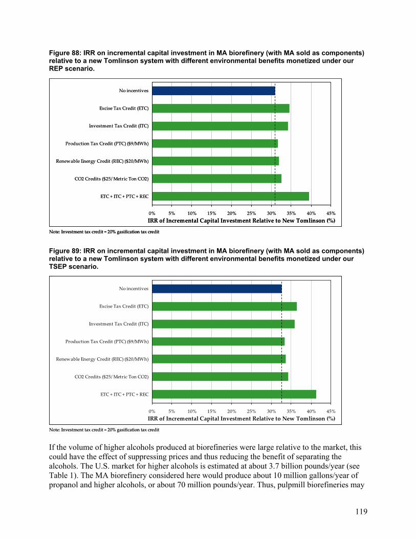
119

Figure 88: IRR on incremental capital investment in MA biorefinery (with MA sold as components) relative to a new Tomlinson system with different environmental benefits monetized under our REP scenario.

0% 5% 10% 15% 20% 25% 30% 35% 40% 45%

No incentives

Excise Tax Credit (ETC)

Investment Tax Credit (ITC)

Production Tax Credit (PTC) ($9/MWh)

Renewable Energy Credit (REC) ($20/MWh)

CO2 Credits ($25/ Metric Ton CO2)

ETC + ITC + PTC + REC

IRR of Incremental Capital Investment Relative to New Tomlinson (%)

Note: Investment tax credit = 20% gasification tax credit

0% 5% 10% 15% 20% 25% 30% 35% 40% 45%

No incentives

Excise Tax Credit (ETC)

Investment Tax Credit (ITC)

Production Tax Credit (PTC) ($9/MWh)

Renewable Energy Credit (REC) ($20/MWh)

CO2 Credits ($25/ Metric Ton CO2)

ETC + ITC + PTC + REC

IRR of Incremental Capital Investment Relative to New Tomlinson (%)

Note: Investment tax credit = 20% gasification tax credit

0% 5% 10% 15% 20% 25% 30% 35% 40% 45%

No incentives

Excise Tax Credit (ETC)

Investment Tax Credit (ITC)

Production Tax Credit (PTC) ($9/MWh)

Renewable Energy Credit (REC) ($20/MWh)

CO2 Credits ($25/ Metric Ton CO2)

ETC + ITC + PTC + REC

IRR of Incremental Capital Investment Relative to New Tomlinson (%)

Note: Investment tax credit = 20% gasification tax credit

Figure 89: IRR on incremental capital investment in MA biorefinery (with MA sold as components) relative to a new Tomlinson system with different environmental benefits monetized under our TSEP scenario.

0% 5% 10% 15% 20% 25% 30% 35% 40% 45%

No incentives

Excise Tax Credit (ETC)

Investment Tax Credit (ITC)

Production Tax Credit (PTC) ($9/MWh)

Renewable Energy Credit (REC) ($20/MWh)

CO2 Credits ($25/ Metric Ton CO2)

ETC + ITC + PTC + REC

IRR of Incremental Capital Investment Relative to New Tomlinson (%)

Note: Investment tax credit = 20% gasification tax credit

0% 5% 10% 15% 20% 25% 30% 35% 40% 45%

No incentives

Excise Tax Credit (ETC)

Investment Tax Credit (ITC)

Production Tax Credit (PTC) ($9/MWh)

Renewable Energy Credit (REC) ($20/MWh)

CO2 Credits ($25/ Metric Ton CO2)

ETC + ITC + PTC + REC

IRR of Incremental Capital Investment Relative to New Tomlinson (%)

Note: Investment tax credit = 20% gasification tax credit If the volume of higher alcohols produced at biorefineries were large relative to the market, this could have the effect of suppressing prices and thus reducing the benefit of separating the alcohols. The U.S. market for higher alcohols is estimated at about 3.7 billion pounds/year (see Table 1). The MA biorefinery considered here would produce about 10 million gallons/year of propanol and higher alcohols, or about 70 million pounds/year. Thus, pulpmill biorefineries may

120

not exert a material impact on pricing, even if several mills were to pursue mixed alcohol production for sale into the chemicals market.

8.3 Summary Discussion of Financial Results By way of summarizing the financial analyses, our baseline set of IRR and NPV results are presented for all cases in Table 31 (no incentives) and Table 32 (with bundled incentives). In the no-incentives cases, the incremental IRRs for most configurations under the Reference Energy Prices scenario meet the assumed hurdle rate of 15%. The large FT cases (FTb and FTc) demonstrate the most attractive economics, after the BLGCC case. In the Tight Supplies Energy Prices scenario, which represents an extrapolation of mid-2006 oil prices, with fuel prices increasing gradually in real terms through 2030, the incremental IRRs of all but the MA configuration exceed the hurdle rate by a comfortable margin, indicating that the economics are very favorable. FTb and FTc are very attractive, along with DMEa and DMEb, and all of these surpass the IRR of the BLGCC configuration by several percentage points, since the BLGCC configuration is largely unaffected by changes in petroleum prices. The weakest financial performance is displayed by the mixed-alcohol configuration when the liquid product is sold as a single fuel commodity, but separating the alcohols for sale as chemicals provides for very high returns, even without incentives. The lower financial performance of the MA configuration in the former case is due largely to the low yield of liquid product coupled with high capital costs. If the yields were more in line with DME or FT, then the economics of this configuration would be more in line as well. These results differ from the only prior published systems analysis of mixed alcohols synthesis from biomass of which we are aware [46]. This prior analysis showed somewhat more favorable results, but used a simplified approach to estimating synthesis reactor performance. Taken with such prior analyses, the results shown here suggest the need for more work to better understand the performance and costs that can be expected for production of mixed alcohols from syngas with “Nth plant” technology. This is unlike the situation for DME and FT synthesis, where the commercial potential is, by comparison, well understood.

Table 31: Summary of IRR and NPV results for all cases, assuming no incentives. Reference Energy Price Scenario Tight Supplies Energy Price Scenario IRR (%) NPV ($ million) IRR (%) NPV ($million) BLGCC 21.7% $24.7 22.0% $25.4 DMEa (diesel) 16.4% $7.4 29.2% $98.2 DMEb (diesel) 16.2% $13.5 23.6% $112 DMEc (diesel) 15.4% $3.2 20.6% $46.9 DMEa (LPG) 13.5% $(8.2) 25.3% $70 DMEb (LPG) 14.8% $(2) 21.5% $83.8 DMEc (LPG) 14.5% $(3.6) 19.2% $34.4 FTa 14.2% $(5.9) 20.9% $53.6 FTb 18.2% $46.8 22.7% $121 FTc 17.7% $37 28.0% $219 MA 10.4% $(40) 13.1% $(18.4) MA (sep.) 30.9% $203 32.7% $243

When multiple environmental values are explicitly included in the analysis in the form of incentives and price premiums (Table 32), the financial performance is overwhelmingly attractive for all but the mixed alcohols configuration (no product separation), with IRRs generally being in excess of 30% in the Reference Energy Prices scenario. The IRRs are even

121

better in the Tight Supplies Energy Prices scenario, but not as high as might be expected, in part because in that price scenario, the amount of the excise tax credit (which is in most cases the most important incentive) that is reflected in the plant gate price is lower than in the Reference Energy Prices scenario. This would be expected in a high-price environment, where the market is sufficient to provide producers with adequate margins.

Table 32: Summary of IRR and NPV results for all cases, assuming bundled incentives, including ETC, ITC, PTC, and RECs.b

Reference Energy Price Scenario Tight Supplies Energy Price Scenario IRR (%) NPV ($ million) IRR (%) NPV ($million) BLGCC 36.0% 77.1 36.3% 77.8 DMEa (diesel) 35.2% 120 46.0% 210 DMEb (diesel) 28.8% 159 35.4% 256 DMEc (diesel) 27.5% 91.1 32.1% 134 DMEa (LPG) 32.7% 104 42.4% 181 DMEb (LPG) 27.4% 143 33.4% 228 DMEc (LPG) 26.6% 84.3 30.7% 122 FTa 27.8% 101 33.6% 160 FTb 34.3% 284 38.1% 358 FTc 33.5% 275 42.8% 455 MA 19.7% 41.9 21.7% 63.1 MA (sep.) 39.5% 312 41.3% 351

(a) ETC = Excise Tax Credit, ITC = Gasification Investment Tax Credit, PTC = Production Tax Credit, REC = Renewable Energy Credit (electricity)

9 National Impacts of a Pulp Mill Biorefinery Industry Building on the mill-level analyses in prior sections of this report, we present here an analysis of potential energy and environmental impacts at the national level in the United States, assuming alternative rates of commercial deployment of biorefinery systems.

9.1 Market Penetration Scenarios Three technology market penetration scenarios were developed in our prior BLGCC analysis [5], and these form the basis for the scenarios used here. The biorefinery commercial deployment rates in these scenarios are based on the well-documented S-shaped trajectory for commercial market penetration of new industrial technologies [143]: when a new technology enters the market, the initial period is characterized by a low penetration rate by early adopters, while the bulk of the market waits for lower costs and/or more proven performance; rapid adoption by the broader market follows the slow initial phase; adoption then tails off as the technology approaches saturation of the technical market potential. The technical market potential (maximum physical limit) was estimated here based on a detailed industry database of existing recovery boilers.53 Given the uncertainty regarding the timing of introduction of biorefineries, some simplifying assumptions were made for the market penetration analysis: 53 The Black Liquor Recovery Boiler Committee (BLRBC) of the American Forest and Paper Association maintains

a database of individual recovery boilers with information on capacity, location, age, rebuild year (if any), and in some cases, the nature of the rebuild. This database can be used to calculate the average boiler size, average boiler age when a rebuild occurred (~20 years), and to identify which boilers will be ready for replacement in any given future year.

122

• The current industry capacity was taken as the starting point for the analysis. Given the recent contraction of the industry this was felt to be a reasonable starting assumption. Also, because further industry consolidation and mill closures are expected, and few if any new mills are likely to be built, the analysis is based on total capacity rather than the number of mills in operation.

• The analysis assumes 2010 as the first year a biorefinery will be commercially operating. Any boiler requiring rebuild or replacement prior to 2010 is assumed to be rebuilt using conventional technology and thereby not available for replacement until the next rebuild cycle for that boiler. Starting in 2010, boilers coming due for rebuild or replacement are assumed to be eligible for repowering with black liquor gasification in biorefinery configurations, but due to the nature of the market penetration curve, broader adoption does not occur before about 2015. Thus, the market penetration analysis effectively captures the time required for validation and refinement of the commercial design, which would then be followed by broader adoption of the “Nth” plant design by the industry in the post-2013 timeframe.

• Based on data and forecasts supplied by the American Forest and Paper Association [144], an annual growth rate of 1.27% for total pulp production is estimated.

The output of the technical market potential analysis is a year-by-year estimate of the annual and cumulative boiler capacity eligible for replacement with black liquor gasification. To quantify the market penetration, a Fisher-Pry model [145] was used to generate an S-curve trajectory calibrated based on knowledge of historical market adoption rates for new industrial technologies. New technologies that are capital intensive, have long equipment lives (>20 years), and entail major changes at the facility level (as opposed to changes to individual process steps), typically have market saturation times54 of 20-40 years. Other factors that influence market penetration include the growth rate of the industry, the industry’s risk tolerance, and whether or not government regulations are forcing changes. These factors and the significant technology change that biorefining would represent for the pulp and paper industry, suggest that saturation times greater than 20 years could be expected. However, the situation with Tomlinson recovery boilers presents unique conditions that also suggest that more rapid penetration could occur.55146 First, the Tomlinson boiler fleet is old and is facing the need for another major wave of rebuilds in the next 10-20 years. Second, competitive pressures from foreign producers may drive the U.S. pulp and paper industry to accelerate adoption of technologies like gasification and biorefining that can help maintain its competitive position in global markets. Third, increasing implementation of Renewable Portfolio Standards, Renewable Fuel Standards and other mechanisms to stimulate renewable energy markets in North America and Europe may create additional financial incentives to accelerate the deployment of biorefineries.56 To cover a range of possible market deployment scenarios, three market penetration scenarios were developed (Table 33). The “Base” market penetration scenario assumes a 20-year saturation time and relatively shorter replacement/rebuild cycles for Tomlinson boilers. The “Low” scenario assumes a 30-year saturation time and longer replacement/rebuild cycles. The 54 Defined as the time required to go from a market penetration of 10% to 90% of the technical potential. 55 The use of ClO2 took 55 years to fully penetrate into the US industry (from early ‘50s to today). Similarly, oxygen delignification started in the 1970s and now has penetrated about 40% of the US industry. By comparison, in Finland it only took about 5 years to reach 100% penetration [146]. 56 For example, the Energy Policy Act of 2005 contains significant gasification-related incentives.

123

“Aggressive” scenario assumes the same replacement/rebuild cycle as the Base scenario, but a 10-year saturation time. While this saturation time is more typical of rapid-payback, discretionary-spending investments, it is used here to illustrate what might be possible with the right set of circumstances. It can also be used to represent a situation in which peak oil has been reached or the United States’ government takes more proactive measures to reduce GHG emissions than has been the case to date. In all cases, the ultimate penetration of the technology is assumed to be 90% of the total industry capacity, to reflect the fact that some mills will never adopt biorefinery technology. The final element of the market penetration analysis is to apply a reasonable growth rate to the industry. Based on historical data and near-term forecasts provided by the AF&PA, a growth rate of 1.27% per year was assumed, as noted earlier. The assumptions in Table 33 give the market penetration estimates (in million lbs/day black liquor solids capacity) in Figure 90 used to assess the potential national impacts of biorefinery technologies in the United States. To avoid “graph-overload” in this volume of the report, only the results of selected impact calculations are shown in this volume. A complete set of impact analysis results is provided in Volume 3. Table 33: Summary of biorefinery market penetration scenarios developed in this study.

Low Scenario

Base Scenario Aggressive Scenario

Technical Market Potentiala

• 180 operable recovery boilers • Combined capacity of ~472 million lbs/day dry solids (~86 million t/yr)

Ultimate Adoption Rate • 90% of the technical market potential

Industry Growth • 1.27% per year, based on total black liquor capacity

Basis

• Traditional market penetration “S” curve for capital intensive, facility-level investments

• Aggressive penetration curve assuming that normal rules of market penetration may not apply due to the age of the Tomlinson boiler fleet and other market drivers (see main text for discussion)

Saturation Time (years)b 30 20 10

Age of “New” boilers when replacement with BLGCC is considered

35 30 30

Age of “Rebuilt” boilers when replacement with BLGCC is considered

15 10 10

(a) Because additional industry consolidation and mill closures are expected, and few if any new mills are likely to be built, the analysis is based on total capacity rather than number of mills.

(b) Defined as the time required to go from 10% penetration to 90% penetration.

An important consideration for the Aggressive market penetration scenario is whether or not this rate of deployment would be achievable in practice. At its peak rate of deployment (around the year 2018-2019 – see Figure 90), there would be capacity equivalent to 14 case study mills undergoing conversion to biorefineries, with a combined biofuels capacity of 190-970 million gallons/yr, depending on the configuration. The associated capital investment at that point of

124

peak deployment would be approximately $3.5-6.6 billion, or $1.6-4.7 billion more than building new Tomlinson systems instead. The total cumulative 25-year investment would be approximately $24-45 billion ($11-32 billion incremental to the cost of new Tomlinsons), or an average of about $1.0-1.8 billion per year ($0.4-1.3 billion incremental to new Tomlinsons). While these are large numbers, the current biofuels “boom” suggests that they are within the ability of the financial community57 to support. Consider the following recent statistics:58

• As of October 2006, there were 45 corn-ethanol plants under construction, plus 7 expansions, for a total of ~3.4 billion gallons of capacity under construction.

• As of September 2006, there were 65 biodiesel plants under construction, plus 13 expansions, for a total of ~1.4 billion gallons of capacity under construction.

Assuming typical investment requirements of $1-1.5 per gallon/year of ethanol capacity and $0.80-1.0 per gallon/year of biodiesel capacity, the current round of biofuels plant construction in the United States involves an investment of $4.5-6.5 billion. Thus, based on the number of facilities under construction, the combined capacity and the combined investment, even the Aggressive market penetration scenario appears feasible. There may be other factors that limit the rate of deployment, but for projects with attractive economics, access to capital does not appear to be a constraint, especially when one considers the current biofuels investments in the context of the much larger concurrent investments being made in renewable energy more broadly.

9.2 Energy and Environmental Impacts There are a variety of potential energy and environmental impacts that could result from commercial deployment of pulp mill biorefinery systems, including fossil fuel savings, emissions reductions, economic development, job retention, and improved industry competitiveness. Easily quantifiable national benefits include total fossil fuel energy savings and greenhouse gas reductions. A more difficult benefit to quantify is the value of spin-offs from the R&D that would be required to bring the pulp mill biorefinery technologies to market, but these developments could have far-reaching impacts on the bioenergy and biofuels industry more broadly, which, at the time of writing, is undergoing significant expansion and change. The following national impacts are discussed in detail below: • Fossil energy savings • Renewable energy markets • Emissions reductions • Energy security and fuel diversity • Economic development • Reaping the benefits of government RD&D

9.2.1 Fossil Fuel Energy Savings Fossil fuel displacement is a strategic, national-level benefit that is relatively straight-forward to estimate. The benefits of fossil fuel displacement include the associated emissions reductions, the conservation of finite resources, the positive effects on fossil fuel price volatility, and in the case

57 This includes traditional lenders, investment banks and private equity, all of whom have been investing in ethanol and biodiesel production capacity in the United States. 58 Renewable Fuels Association and National Biodiesel Board websites, accessed October 2006.

125

of petroleum, the reduction of imports, which enhances energy supply security. Generally, an economy that is less dependent on fossil fuels is less susceptible to the negative impacts of fuel price volatility, which has increased in recent years. National fossil energy savings are estimated relative to the continued use of Tomlinson technology with the same degree of industry growth and assuming displaced grid electricity generation results in savings based on the average utility fuel mix and heat rate (which change over time – see Table 18). No improvement in mill energy efficiency over time is considered, which is likely conservative. Figure 91 shows that pulp/paper mill biorefineries, relative to Tomlinson systems, have the potential to offset anywhere from about 200 to 1,200 trillion Btu/year (0.2 to 1.2 quads/yr) within 25 years of introduction (Aggressive market penetration scenario), depending on the biorefinery configuration being considered. These reductions are net reductions and consider all the fossil fuel use at the mill and the fossil fuel savings from displaced grid power and conventional transportation fuels. The BLGCC and DMEa cases provide the least fossil fuel savings because they involve the lowest level of purchased biomass use. FTb produces the largest impacts due to the large amount of biomass used and the quantity of grid power displaced, owing to the importance of coal in power generation. Figure 90: Market penetration estimates used to assess energy and environmental impacts of biorefinery implementation in the United States.

0

100

200

300

400

500

600

700

2010

2011

2012

2013

2014

2015

2016

2017

2018

2019

2020

2021

2022

2023

2024

2025

2026

2027

2028

2029

2030

2031

2032

2033

2034

Cumulative Capacity

(million pounds per day black liquor solids)

0

10

20

30

40

50

60

70

80

90

100

110

Number of Reference Case Mills

Total IndustryAggressive Scenario

Base ScenarioLow  Scenario

126

Figure 91: Net national fossil fuel savings relative to continued use of Tomlinson systems for the Aggressive biorefinery market penetration scenario.

0

200

400

600

800

1,000

1,200

1,40020

10

2011

2012

2013

2014

2015

2016

2017

2018

2019

2020

2021

2022

2023

2024

2025

2026

2027

2028

2029

2030

2031

2032

2033

2034

Annual Fossil Energy Savings Relative 

to New Tomlinson (trillion Btu/yr)

FTbFTcDMEbFTaDMEcMABLGCCDMEa

Note: Transportation of the crude FT product to the oil refinery included in FT cases.Note on vehicle end use: FT cases assume FT gasoline blend in gasoline engines and FT diesel blend in CIDI engines.  MA case assumes low‐level blend with gasoline.

0

200

400

600

800

1,000

1,200

1,40020

10

2011

2012

2013

2014

2015

2016

2017

2018

2019

2020

2021

2022

2023

2024

2025

2026

2027

2028

2029

2030

2031

2032

2033

2034

Annual Fossil Energy Savings Relative 

to New Tomlinson (trillion Btu/yr)

FTbFTcDMEbFTaDMEcMABLGCCDMEa

Note: Transportation of the crude FT product to the oil refinery included in FT cases.Note on vehicle end use: FT cases assume FT gasoline blend in gasoline engines and FT diesel blend in CIDI engines.  MA case assumes low‐level blend with gasoline.

Figure 92 shows the cumulative fossil fuel savings in the three market penetration scenarios over the first 25 years following introduction. Net fossil fuel savings relative to continued use of Tomlinson systems range from 1 to 5.5 quads (Low scenario) up to 3 to 17 quads (Aggressive scenario). As noted above, this analysis assumes constant energy efficiency in pulp and paper manufacturing. Reductions in manufacturing energy intensities would lead to higher net energy savings than estimated here.59 The difference between the Low and Aggressive market penetration scenarios can be thought of as a proxy for the “lost” fossil fuel savings if implementation of pulp mill biorefineries is delayed. Alternatively the difference between the two scenarios might be viewed as the payoff on government support for more aggressive commercialization of biorefinery technologies.

59 The case-study integrated pulp and paper mill in this analysis is relatively efficient (e.g., with process steam use

about 10% lower than typical “best practice” in the U.S. industry today), but no additional efficiency gains are assumed over the 25 year analysis period. Efficiency gains could: (i) reduce or eliminate the need for fossil fuel use in the mill, such as lime kiln fuel, or reduce the need for purchased wood wastes; (ii) enable greater electricity generation from the same amount of renewale energy inputs; (iii) reduce mill electricity demand, enabling greater power exports. All of these benefits would translate directly to increased energy and emissions benefits, in addition to cost savings to the mill.

127

Figure 92: Cumulative (25-year) national net fossil fuel savings relative to continued use of Tomlinson systems under different biorefinery market penetration scenarios.

0

2

4

6

8

10

12

14

16

18

BLGCC DMEa DMEb DMEc FTa FTb FTc MA

Cum

ulative Fossil Energy Savings

 2010‐2034 (quadrillion Btu)

ʺLowʺ ScenarioʺBaseʺ ScenarioʺAggressiveʺ Scenario

Cost of delaying implementation

Note: Assumes that DME substitutes for diesel and that FT gasoline, FT diesel and Mixed Alcohols are used in low‐level blends with conventional fuels.

0

2

4

6

8

10

12

14

16

18

BLGCC DMEa DMEb DMEc FTa FTb FTc MA

Cum

ulative Fossil Energy Savings

 2010‐2034 (quadrillion Btu)

ʺLowʺ ScenarioʺBaseʺ ScenarioʺAggressiveʺ Scenario

Cost of delaying implementation

Note: Assumes that DME substitutes for diesel and that FT gasoline, FT diesel and Mixed Alcohols are used in low‐level blends with conventional fuels.

Cost of delaying implementation

Note: Assumes that DME substitutes for diesel and that FT gasoline, FT diesel and Mixed Alcohols are used in low‐level blends with conventional fuels.

9.2.2 Renewable Energy Markets Distinct markets for renewable energy and its associated attributes are developing in the United States and elsewhere. In many cases the structure of the programs and markets effectively create markets for the attributes of renewable energy that are separate from energy markets, adding a second revenue stream for renewable energy producers. These markets may be regional, national or even international (e.g., with carbon trading). These markets are both voluntary and mandatory in nature. Voluntary markets are those in which renewables are cost competitive with conventional options (including the effects of financial incentives, if any), or consumers are willing to pay a premium for renewable energy, such as with green power. While these markets are growing in importance, the main driver that has emerged for renewable energy markets are various mandates: Renewable Portfolio Standards (RPS) for power generation and Renewable Fuel Standards (RFS) for transportation fuels. RPS mandates, currently in place in more than 20 states, if fully implemented will result in the addition of approximately 30,000 MW of new renewable generating capacity from 2003 to 2015. The Federal RFS, which basically replaces the Federal mandate for oxygenates in reformulated gasoline, targets a total consumption of 7.5 billion gallons of biofuels by 2012, almost double the 4 billion gallons produced in 2005. In addition, a growing number of states are setting their own biofuels targets. Emissions trading is another compliance-type market that is established in the United States for SO2 and NOx. Emerging trading regimes for CO2 and other mechanisms that bring renewable energy projects into existing trading schemes, such as “set-aside” programs, could create additional value for renewable power and fuels in the future.60 These cap-and-trade regimes also increase the cost of conventional energy, which benefits renewable energy indirectly.

60 Renewable “set-asides” are essentially free emissions allowances created by regulatory mechanisms and given to

renewable energy producers, who can sell them in the marketplace to those who need allowances to operate. Because biomass is not an emissions-free source of power, it does not always qualify for set-aside allowances.

128

Although compliance markets are very important, from a pulp/paper industry perspective it is important to note several issues: • Most of the US pulp mill capacity is located in the Southeast. Currently, no Southeast US

states have RPS, and several attempts to pass a Federal RPS have failed. • The Federal RFS targets are actually quite modest and are likely to be met well before 2012.

If that occurs, the economic value of the RFS is expected to be minimal, unless targets are increased, which is under consideration by Congress.

• Biomass is not always RPS eligible, and even if it is, the definitions of eligible biomass resources and technologies vary, with black liquor not always considered a qualifying fuel for RPS compliance. However, gasification generally meets criteria for “advanced technology” in states where such criteria exist.

Biomass is potentially the most significant renewable energy resource in certain parts of the country, including the Southeast and Northeast, and is also very important in the Northwest and potentially in the Midwest (with the Midwest being driven more by agriculture than forest products). Given that the pulp and paper industry is the largest single industrial user of biomass for energy, biorefineries could play an important role in meeting current and future RPS and RFS mandates. To illustrate the value of biorefineries in this context, Table 34 shows the technical potential of the pulp/paper industry to contribute to the current national RFS. The table does not factor in market penetration, but rather shows the maximum contribution possible. The contribution could vary considerably depending on the market penetration rate, but this analysis shows the contribution with the current size of the industry (2010 columns in the table) could be between 18% and 92% of the current RFS target for 2012. With a larger scale pulp mill biorefinery industry (2034 columns in the table), that figure could range from about 24% to 123%. Note that these are based on actual volumes, not corrected for energy content. Some additional points of comparison are worth noting:

• In 2005, U.S. ethanol and biodiesel production were approximately 4 billion and 75 million gallons, respectively

• Annual U.S. gasoline + diesel consumption is currently about 170 billion gallons • U.S. crude oil imports from OPEC countries in 2005 averaged approximately 5.6 million

barrels/day, or about 86 billion gallons per year. • Total U.S. crude oil imports from all countries in 2005 averaged approximately 13.7

million barrels/day, or about 210 billion gallons per year. • Total U.S. petroleum consumption in 2005 averaged approximately 21 million barrels per

day, or about 322 billion gallons per year. In this context, it is clear that pulpmill biorefineries have the potential to be major contributors to biofuels supply, but the magnitude of the current U.S. petroleum consumption suggests that pulpmill biorefineries are likely to be able to contribute less than 5% to overall petroleum usage.

129

Table 34. Biofuel production potential (billion gal/year) for different biorefinery configurations.a These are actual volumes, not corrected for energy content, and are for the total industry. The estimates are total technical potential and do not consider any market penetration scenario. The current RFS target is 7.5 billion gallons by 2012.

For forecast 2010 pulp/paper industry sizeb For forecast 2034 pulp/paper industry sizec

Billion galyr

% of Current

2012 RFS Target

Biomass Energy

Purchases (106 dry t/yr)

Net Biomass Required

(106dry t/yr)d

Billion gal/yr

% of Current

2012 RFS Target

Biomass Energy

Purchases (106dry t/yr)

Net Biomass Required

(106dry t/yr)d

Gallons of liquid fuel per net ton purchased biomasse

DMEa 5.5 74% 12.6 5.7 7.4 98% 16.8 7.6 ~ 440

DMEb 5.5 74% 31.7 24.8 7.4 98% 42.4 33.2 ~ 175

DMEc 2.4 33% 11.9 5.0 3.3 43% 15.9 6.7 ~ 210

FTa 2.3 30% 16.5 9.6 3.0 40% 22.1 12.9 ~ 140

FTb 2.3 30% 59.8 52.9 3.0 40% 80.0 70.8 ~ 40

FTc 6.9 92% 73.2 66.4 9.3 123% 97.9 88.7 ~ 95

MA 1.3 18% 14.5 7.6 1.8 24% 19.4 10.2 ~ 90

(a) These are actual volumes, not corrected for energy content, and are for the total industry, based on the assumed annual capacity factor of the biorefineries. The estimates are total technical potential and do not consider any market penetration scenario. The current RFS target is 7.5 billion gallons by 2012.

(b) The current size (2006) is slightly smaller. Figures here are based on the assumption of an annual growth rate of 1.27%. (c) Figures here are based on the assumption of an annual growth rate of 1.27%. (d) This is the total biomass (short tons) required after subtracting pulpwood savings from polysulfide pulping. These are for the

entire biorefinery, including for pulpwood and for energy. (e) This is the total annual liquid fuel production shown in this table divided by the total annual biomass purchases for energy

shown in this table.

Table 34 also shows the annual wood requirements to produce these volumes of biofuels. In the highest case (FTc), this approaches 100 million dry tons per year (though due to substantial savings in pulpwood that result from higher-yielding pulping enabled by the use of black liquor gasification, the net wood requirement is less than the total biomass energy purchases). As a result of integrating the biorefinery with the pulp mill, the liquid fuel produced per unit of purchased wood energy (right-hand column of Table 34) is high in most cases, indicating very efficient use of the biomass resource. To put in perspective the 100 million tons/year of biomass energy required, it is helpful to compare them to the amount of woody biomass available from existing forests as estimated in the “billion ton study” [1]. That study estimated that existing forests can sustainably provide 368 million dry tons per year of woody biomass. This includes approximately 142 million dry tons currently being used. Thus, there is an estimated 226 million dry tons of additional biomass available, more than twice the requirements of the most aggressive case we have examined. It is also worthwhile to note that the estimated U.S. forest standing inventory is in excess of 20 billion dry tons, such that 100 million dry tons/yr is less than 0.5% of the standing inventory, and a smaller figure than the expected net annual growth [1]. The figure of 100 million tons is also considerably lower than the estimate in [1] of the agricultural biomass available from perennial crops (as much as 377 million dry tons/yr) and crop residues (as much as 46 million dry tons/yr).

130

Thus, even aggressive deployment of pulpmill biorefineries appears feasible without placing undue pressure on forest land usage or current agricultural commodities. In addition, certain biorefinery configurations studied here produce significant amounts of power, in particular FTb, although other configurations could also be set up with a large power component through the use of additional biomass. If a national RPS were to be put in place or if Southeast states begin to adopt RPS or otherwise promote renewable energy development, biorefineries could also play a role in meeting the overall targets and would also ensure that many of the benefits of renewable energy (e.g., reduced emissions and local economic development) would be more evenly distributed around the country.61 Table 35 shows the potential contributions. Since power was not a major design criterion in most of our biorefinery configurations, the net increase in generation over continued use of Tomlinson systems is 1,000-2,000 MW, whereas the BLGCC case provides a net increase of 4,600-6,200 MW. But FTb, which does emphasize power generation, would result in an increase of 15,000-20,000 MW while still producing 2.6-3.5 billion gallons of fuel annually. The relative value of power versus fuels in the context of multiple, potentially competing, renewable energy mandates is likely to influence decisions relating to the biorefinery product slate and the desire to build some flexibility into that product slate, in order to take advantage of changes over time in markets for power versus fuels. There may also be regional differences driven by the existence and aggressiveness of state RPS mandates relative to regional transportation fuel requirements.

9.2.3 National Emissions Reductions Here the potential national emissions impacts are discussed and illustrated for the Aggressive market penetration scenario. The impacts are similar for the other two market penetration scenarios, but generally reduced in proportion to the rate of market penetration. (See Volume 3.) The key assumptions used to generate these results include: • Emissions savings estimates are made relative to continued use of Tomlinson systems for the

same degree of market penetration and industry growth, i.e., the estimates show the difference between Tomlinson and biorefinery systems.62

• Estimates include all mill-level emissions sources, net offsets from grid power and the net impacts from the rest of the biofuels and conventional fuel chains, as discussed earlier.

• Grid-power emissions change over time (see Table 18) in line with expected changes in fuel mix and emissions as forecast by the DOE [134].

• Vehicle emissions and related fuel chain emissions are those consistent with the 2010 timeframe.

• CO2 emissions shown here exclude the CO2 originating from biomass. Refer to Volume 3 for quantification of biomass-associated CO2 emissions.

61 Wind power is the leading source for new renewable energy today and would likely play a major role in meeting

any future Federal RPS. However, good wind power sites are distributed unevenly across the country, which could turn some regions into major exporters of RECs and others into importers. In contrast, biomass is more evenly distributed across the country, and in fact some regions that are richer in biomass (e.g., Northwest, Southeast, Northeast) are actually poorer in wind potential.

62 Even if the industry were to never deploy biorefinery technology, as the industry grows it will generate more power internally and therefore offset additional grid power. This “moving baseline” forms the basis for evaluating the incremental impacts of biorefineries.

131

• Estimates do not assume any improvements in mill efficiency over time, which may be a conservative assumption (i.e., as mill efficiency improves more energy is available for power and biofuels production).59

Table 35. Power production potential (MW) for different biorefinery configurations – incremental power production relative to continued use of Tomlinson technology.a

Net Incremental Generation per

mill (MW)b

Total Pulp/Paper Industry in 2010

(MW)c

Total Pulp/Paper Industry in 2034

(MW)d

BLGCC 50 4,618 6,176

DMEa (64) (5,909) (7,901)

DMEb 24 2,184 2,920

DMEc 26 2,433 3,254

FTa 23 2,168 2,899

FTb 165 15,258 20,404

FTc 13 1,206 1,613

MA 28 2,557 3,420

(a) These estimates are for the total industry and represent the technical potential without consideration of any market penetration scenario.

(b) From Table 12. (c) The current size (2006) is slightly smaller. Figures here are based on the assumption of an annual growth rate of 1.27%. (d) Figures here are based on the assumption of an annual growth rate of 1.27%.

Figure 93 illustrates the potential net national CO2 emissions benefits of biorefineries for the Aggressive market penetration scenario. Our pulp mill biorefinery designs, relative to continued use of Tomlinson technology, have the potential to offset as much as 110 million short tons of CO2 per year. This is equivalent to about 5% of the transportation sector CO2 emissions in the U.S. in 2004. The main driver affecting the amount of CO2 benefit is the amount of biomass used, but in comparing FTb to FTc, which use similar quantities of purchased biomass, electricity displacement results in greater CO2 reductions per unit of biomass consumed than petroleum fuel displacement.

132

Figure 93. Net annual national CO2 emissions reductions relative to continued use of Tomlinson systems under the Aggressive biorefinery market penetration scenario.

0

20,000,000

40,000,000

60,000,000

80,000,000

100,000,000

120,000,000

2010

2011

2012

2013

2014

2015

2016

2017

2018

2019

2020

2021

2022

2023

2024

2025

2026

2027

2028

2029

2030

2031

2032

2033

2034

Annual CO2 Em

issions Reductions (with credit for 

biomass CO2) Relative to New Tomlinson (tons/yr)

FTbFTcDMEbFTaDMEcMABLGCCDMEa

Transportation of the crude FT product to the oil refinery included in FT cases.Note: excludes any emissions from land use changes and biomass growth that are not related to harvesting and transportation.Note on vehicle end use: FT cases assume FT gasoline blend in gasoline engines and FT diesel blend in CIDI engines.  MA case assumes low‐level blend with gasoline.

0

20,000,000

40,000,000

60,000,000

80,000,000

100,000,000

120,000,000

2010

2011

2012

2013

2014

2015

2016

2017

2018

2019

2020

2021

2022

2023

2024

2025

2026

2027

2028

2029

2030

2031

2032

2033

2034

Annual CO2 Em

issions Reductions (with credit for 

biomass CO2) Relative to New Tomlinson (tons/yr)

FTbFTcDMEbFTaDMEcMABLGCCDMEa

Transportation of the crude FT product to the oil refinery included in FT cases.Note: excludes any emissions from land use changes and biomass growth that are not related to harvesting and transportation.Note on vehicle end use: FT cases assume FT gasoline blend in gasoline engines and FT diesel blend in CIDI engines.  MA case assumes low‐level blend with gasoline.

Figure 94 illustrates the potential net national SO2 emissions benefits of biorefineries for the Aggressive market penetration scenario. The picture is quite different than for CO2 for two reasons. First, conventional transportation fuel chains do not produce significant quantities of SO2. Second, as SO2 emissions from grid power decrease over time, so do the net annual reductions, particularly for configurations that generate a lot of power, like BLGCC and FTb. In fact, over time, if the grid achieves the levels of SO2 reductions projected in the DOE forecast, then for FTb, it could change from a net reduction of SO2 to net increase around the year 2030. Also, in cases where the additional biomass is used directly for power generation (all cases except FTc and MA), it is not subject to acid gas scrubbing. Therefore, all the sulfur in that biomass, although relatively low, is emitted as SO2. Nevertheless, pulp mill biorefineries, relative to Tomlinson systems, have the potential to offset more than 30,000 tons of SO2 per year, although this level of reduction may not be sustainable given the foregoing discussion of grid SO2 emissions.

133

Figure 94. Net annual national SO2 emissions reductions relative to continued use of Tomlinson systems under the Aggressive biorefinery market penetration scenario.

‐40,000

‐30,000

‐20,000

‐10,000

0

10,000

20,000

30,000

40,000

2010

2011

2012

2013

2014

2015

2016

2017

2018

2019

2020

2021

2022

2023

2024

2025

2026

2027

2028

2029

2030

2031

2032

2033

2034

Annual SO2 Em

issions Reductions 

Relative to New Tomlinson (tons/yr)

FTcBLGCCMADMEcFTaFTbDMEbDMEa

Transportation of the crude FT product to the oil refinery included in FT cases.Note on vehicle end use: FT cases assume FT gasoline blend in gasoline engines and FT diesel blend in CIDI engines.  MA case assumes low‐level blend with gasoline.

‐40,000

‐30,000

‐20,000

‐10,000

0

10,000

20,000

30,000

40,000

2010

2011

2012

2013

2014

2015

2016

2017

2018

2019

2020

2021

2022

2023

2024

2025

2026

2027

2028

2029

2030

2031

2032

2033

2034

Annual SO2 Em

issions Reductions 

Relative to New Tomlinson (tons/yr)

FTcBLGCCMADMEcFTaFTbDMEbDMEa

Transportation of the crude FT product to the oil refinery included in FT cases.Note on vehicle end use: FT cases assume FT gasoline blend in gasoline engines and FT diesel blend in CIDI engines.  MA case assumes low‐level blend with gasoline.

Figure 95 illustrates the potential net national NOx emissions benefits of biorefineries for the Aggressive market penetration scenario. Pulp mill biorefineries, relative to continued use of Tomlinson systems, have the potential to offset up to nearly 90,000 tons of NOx per year. Displacement of both grid power and conventional fuels result in NOx benefits, but generally speaking, for the biorefinery configurations studied here, grid power is a greater source of emissions reductions, since gas-turbine-based generation has much lower NOx emissions than the grid average. Still, as with SO2, grid-based NOx emissions are forecasted to fall significantly under the EPA CAIR program. For transportation fuels, DME results in lower tailpipe NOx emissions, whereas the use of mixed alcohols and FT fuels in low-level blends with gasoline or diesel are not expected to have significant NOx benefits. The impacts of using biofuels as neat fuels instead of in low-level blends is discussed later in this section and additional details are provided in Volume 3. Another consideration is that NOx emissions are higher for configurations that use large quantities of purchased biomass, because of the heavy duty vehicles used upstream to collect and deliver the biomass to the biorefinery. That is a key driver in the poorer net NOx results for FTb and FTc compared to FTa. Figure 96 illustrates the potential net national VOC emissions benefits of biorefineries for the Aggressive market penetration scenario. Pulp mill biorefineries, relative to continued use of Tomlinson technology, have the potential to offset as much as 18,000 tons of VOCs per year. DMEa and DMEb fare well because DME handling is similar to propane and is a closed system so there are fewer fugitive emissions. Tailpipe VOC emissions can also be controlled with an oxidation catalyst. VOC emissions reductions for DMEc are lower because less DME is produced. For FTc and the remaining configurations, the main source of VOC reductions are in the conventional fuel chain upstream of the vehicle. Thus, FTc, which displaces the greatest

134

amount of fuel results in the largest reductions. Estimates of VOC emissions from grid power and from the biorefinery fuel chains are small and so have less impact on the results. Figure 95. Net annual national NOx emissions reductions relative to continued use of Tomlinson technology under the Aggressive biorefinery market penetration scenario.

0

10,000

20,000

30,000

40,000

50,000

60,000

70,000

80,000

90,000

100,000

2010

2011

2012

2013

2014

2015

2016

2017

2018

2019

2020

2021

2022

2023

2024

2025

2026

2027

2028

2029

2030

2031

2032

2033

2034

Annual NOx Em

issions Reductions 

Relative to New Tomlinson (tons/yr)

DMEbDMEcFTaMAFTbFTcBLGCCDMEa

Transportation of the crude FT product to the oil refinery included in FT cases.Note on vehicle end use: FT cases assume FT gasoline blend in gasoline engines and FT diesel blend in CIDI engines.  MA case assumes low‐level blend with gasoline.

0

10,000

20,000

30,000

40,000

50,000

60,000

70,000

80,000

90,000

100,000

2010

2011

2012

2013

2014

2015

2016

2017

2018

2019

2020

2021

2022

2023

2024

2025

2026

2027

2028

2029

2030

2031

2032

2033

2034

Annual NOx Em

issions Reductions 

Relative to New Tomlinson (tons/yr)

DMEbDMEcFTaMAFTbFTcBLGCCDMEa

Transportation of the crude FT product to the oil refinery included in FT cases.Note on vehicle end use: FT cases assume FT gasoline blend in gasoline engines and FT diesel blend in CIDI engines.  MA case assumes low‐level blend with gasoline.

Figure 96. Net annual national VOC emissions reductions relative to continued use of Tomlinson technology under the Aggressive biorefinery market penetration scenario.

0

2,000

4,000

6,000

8,000

10,000

12,000

14,000

16,000

18,000

20,000

2010

2011

2012

2013

2014

2015

2016

2017

2018

2019

2020

2021

2022

2023

2024

2025

2026

2027

2028

2029

2030

2031

2032

2033

2034

Annual VOC Emissions Reductions 

Relative to New Tomlinson (tons/yr)

FTcDMEbDMEaMADMEcFTaFTbBLGCC

Transportation of the crude FT product to the oil refinery included in FT cases.Note on vehicle end use: FT cases assume FT gasoline blend in gasoline engines and FT diesel blend in CIDI engines.  MA case assumes low‐level blend with gasoline.

0

2,000

4,000

6,000

8,000

10,000

12,000

14,000

16,000

18,000

20,000

2010

2011

2012

2013

2014

2015

2016

2017

2018

2019

2020

2021

2022

2023

2024

2025

2026

2027

2028

2029

2030

2031

2032

2033

2034

Annual VOC Emissions Reductions 

Relative to New Tomlinson (tons/yr)

FTcDMEbDMEaMADMEcFTaFTbBLGCC

Transportation of the crude FT product to the oil refinery included in FT cases.Note on vehicle end use: FT cases assume FT gasoline blend in gasoline engines and FT diesel blend in CIDI engines.  MA case assumes low‐level blend with gasoline.

135

Figure 97 illustrates the potential net national CO emissions benefits of biorefineries for the Aggressive market penetration scenario. Pulp mill biorefineries, relative to continued use of Tomlinson systems, have the potential to offset as much as 140,000 tons of CO per year. With the exceptions of the BLGCC and DMEa configurations, the results are closely clustered regardless of the biofuels or relative mix of power and fuels. For BLGCC, grid power is already relatively low in CO emissions and for DMEa, the reductions from DME use are offset by the increased use of grid power. More importantly, for these two configurations, the use of hog fuel boilers for the additional biomass results in higher CO emissions than for those configurations that use biomass gasification. Figure 97. Net annual national CO emissions reductions relative to continued use of Tomlinson technology under the Aggressive biorefinery market penetration scenario.

‐20,000

0

20,000

40,000

60,000

80,000

100,000

120,000

140,000

160,000

2010

2011

2012

2013

2014

2015

2016

2017

2018

2019

2020

2021

2022

2023

2024

2025

2026

2027

2028

2029

2030

2031

2032

2033

2034

Annual CO Emissions Reductions 

Relative to New Tomlinson (tons/yr)

DMEbDMEcFTaMAFTcFTbBLGCCDMEa

Transportation of the crude FT product to the oil refinery included in FT cases.Note on vehicle end use: FT cases assume FT gasoline blend in gasoline engines and FT diesel blend in CIDI engines.  MA case assumes low‐level blend with gasoline.

‐20,000

0

20,000

40,000

60,000

80,000

100,000

120,000

140,000

160,000

2010

2011

2012

2013

2014

2015

2016

2017

2018

2019

2020

2021

2022

2023

2024

2025

2026

2027

2028

2029

2030

2031

2032

2033

2034

Annual CO Emissions Reductions 

Relative to New Tomlinson (tons/yr)

DMEbDMEcFTaMAFTcFTbBLGCCDMEa

Transportation of the crude FT product to the oil refinery included in FT cases.Note on vehicle end use: FT cases assume FT gasoline blend in gasoline engines and FT diesel blend in CIDI engines.  MA case assumes low‐level blend with gasoline.

Figure 98 illustrates the potential net national PM10 emissions benefits of biorefineries for the Aggressive market penetration scenario. Pulp mill biorefineries, relative to continued use of Tomlinson technology, have the potential to offset nearly 40,000 tons of PM10 emissions per year, depending on the configuration. Emissions reductions come from the displacement of both power and conventional transportation fuels, with the former generally being a more significant source of reductions. This is because the conventional vehicle PM10 emissions are assumed to be quite low. Also, PM10 emissions from vehicles include brake and tire wear, which are assumed to be the same in all cases.

136

Figure 98. Net annual national PM10 emissions reductions relative to continued use of Tomlinson technology under the Aggressive biorefinery market penetration scenario.

0

5,000

10,000

15,000

20,000

25,000

30,000

35,000

40,000

2010

2011

2012

2013

2014

2015

2016

2017

2018

2019

2020

2021

2022

2023

2024

2025

2026

2027

2028

2029

2030

2031

2032

2033

2034

Annual PM10 Emissions Reducitons

Relative to New Tomlinson (tons/yr)

FTbDMEbDMEcMAFTaFTcBLGCCDMEa

Transportation of the crude FT product to the oil refinery included in FT cases.Note on vehicle end use: FT cases assume FT gasoline blend in gasoline engines and FT diesel blend in CIDI engines.  MA case assumes low‐level blend with gasoline.

0

5,000

10,000

15,000

20,000

25,000

30,000

35,000

40,000

2010

2011

2012

2013

2014

2015

2016

2017

2018

2019

2020

2021

2022

2023

2024

2025

2026

2027

2028

2029

2030

2031

2032

2033

2034

Annual PM10 Emissions Reducitons

Relative to New Tomlinson (tons/yr)

FTbDMEbDMEcMAFTaFTcBLGCCDMEa

Transportation of the crude FT product to the oil refinery included in FT cases.Note on vehicle end use: FT cases assume FT gasoline blend in gasoline engines and FT diesel blend in CIDI engines.  MA case assumes low‐level blend with gasoline.

Conversion to biorefineries is also expected to reduce TRS emissions. In the analysis presented here, the only sources of TRS are assumed to be the Tomlinson recovery boiler and the lime kiln. TRS emissions increase somewhat from the lime kiln due to increased load with black liquor gasification, but this is more than offset by the elimination of the Tomlinson boiler. Mill-level estimates were presented earlier in Section 6.7.7.

9.2.3.1 Use of Neat Biofuels vs. Low-Level Blends All of the foregoing results assumed that mixed alcohols and FT biofuels were used in low-level blends with their conventional counterparts, for example a 10% blend of mixed alcohols with gasoline and a 10% blend of FT diesel with low-sulfur diesel. However, with some relatively minor engine modifications these fuels can also be used in either high-level blends or as neat (100%) biofuels. Data are either limited or non-existent regarding light-duty vehicle performance on neat biofuels. Nevertheless, based on a review of the literature, it is reasonable to expect reductions in certain tailpipe emissions when vehicles are optimized for biofuels usage. Based on [130,131], the key emissions changes that could be expected are:

• VOC emissions: tailpipe VOCs may be further reduced (relative to those assumed in preparing Figure 96) when neat FT diesel is used instead of low-sulfur diesel. Also, evaporative VOC emissions should be lower when mixed alcohols are used in a flex fuel vehicle compared to gasoline vehicles.

• CO emissions: CO may be reduced (from levels indicated in Figure 97) when neat FT diesel is used instead of low-sulfur diesel.

• There would be modest reductions in SO2 and possibly NOx, but these are expected to be minimal.

137

Volume 3 provides the specific tailpipe emissions factors assumed and contains figures that show these potential reductions at the national level.

9.2.4 Energy Security and Fuel Diversity The nation’s transportation sector remains more than 95% dependent of petroleum. No other sector of the economy is so dependent on a single energy source. Much has been written and said in recent months about the nation’s “addiction to oil” and the resulting consequences, including environmental degradation, negative balance of trade, energy insecurity, and its distorting effect on foreign policy. It is not the objective here to provide a detailed accounting of these issues, but rather to highlight the fact that biorefineries offer the potential to diversify the fuel mix in transportation away from oil and towards a domestic renewable resource. Figure 99 shows that petroleum displacement represents a significant portion of the total fossil fuel displacement potential with biorefineries. Cumulative petroleum displacement could exceed 2.2 billion barrels of oil over a 25-year period under the Aggressive market penetration scenario. By the end of the forecast period, the corresponding annual petroleum savings in the FTc configuration (the one with the largest oil savings) would be approximately 165 million barrels per year, or 0.45 million barrels per day. This is equivalent to nearly 10% of the 2005 level of imports to the United States of oil from OPEC countries. As with the rest of the analysis here, the values shown include the net effects along the entire fuel chain, including, for example, the need to use petroleum in the transportation and distribution of biofuels. Figure 99: Cumulative (25-year) national net fossil fuel and petroleum savings relative to continued use of Tomlinson systems under the Aggressive biorefinery market penetration scenario.

‐2

0

2

4

6

8

10

12

14

16

18

BLGCC DMEa DMEb DMEc FTa FTb FTc MA

CumulativeFossil Energy Savings Relative 

to New Tomlinson (quadrillion Btu)

‐345

155

655

1,155

1,655

2,155

2,655

Million barrels of oil

Petroleum

All Fossil fuels

Notes• Transportation of the crude FT product to the oil refinery included in FT cases.• Vehicle end use: FT cases assume FT gasoline blend in gasoline engines and FT diesel blend in CIDI engines.  MA case assumes low‐level blend with gasoline.

•250,000 bbl/day average•450,000 bbl/day in 2034•OPEC imports ~5,600,000 bbl/day in 2005

The nation’s power sector uses a much more diverse fuel mix than the transportation sector, but it too is heavily dependent on fossil fuels, and has become increasingly dependent on gas-fired combined cycle technology for new power generation capacity. The shift to gas-fired GTCC technology has been driven by several factors, including low capital and operating costs, high

138

efficiency, low emissions, rapid construction, and small footprint. These factors have made GTCC technology the lowest cost option for new power plants at the start of this century. They also greatly facilitate financing and siting relative to other central station generation options. However, the increasing reliance on natural gas has some important energy cost, fuel diversity and energy security implications: • Natural-gas fired power plants will increasingly set the marginal price for power. • Natural gas prices have risen significantly since the early 2000s and they have also been

volatile and are expected to remain so, driven in part by increasing summer demand for power generation.63 As of mid-2006, natural gas spot prices remained well above historical long-term averages, and may remain there as natural gas demand grows and domestic production matures. With limited ability to import gas into North America, the United States will continue to be susceptible to the gas price volatility it has experienced in the last 2-3 years.64

• In the post-9/11 world, natural gas supply infrastructure is seen as vulnerable to disruption by terrorist attack. Thus, the electric industry is vulnerable both directly (via attacks on electric infrastructure) and indirectly (via attacks on natural gas infrastructure)

With the rise in natural gas prices, GTCC technology has become less favored and many utilities are rethinking the role of coal and nuclear power in meeting future power needs. This too presents its own set of problems. Biorefineries that have a significant power component have the potential to help address all of these concerns. First, they provide a way to diversify the electric power fuel mix, thereby reducing dependence on fossil fuels. Not only does this conserve finite resources, but it has the potential, along with other renewable energy technologies, to ease natural gas price volatility by easing pressure on the supply-demand balance for natural gas. Second, biorefineries represent a form of distributed generation, and would be more numerous and dispersed than other central station power plants of equal total capacity. All else equal, this would make the overall electricity supply infrastructure less vulnerable to disruption, for example by terrorist attacks or other causes.

9.2.5 Economic Development Biorefineries could have important economic development benefits, stemming from the enhancement of the competitiveness of the pulp/paper industry. The financial analysis illustrated the potential for attractive financial returns and significantly increased cash flows relative to Tomlinson systems. The related economic development benefits include preserving and growing employment in the industry and potentially adding to rural and semi-rural employment by creating increased demand for raw materials for paper production and biomass supply and, in the longer term, energy and other products derived from biomass. On a national scale these impacts are likely to be modest, but in certain regions or states (especially the Southeast), the impacts 63 For example, the summer months are used to add natural gas to underground storage, for use during winter, but

with increasing amounts of natural gas being used in the summer for power generation, this creates the possibility of having too little gas in storage heading into the winter heating season. All else equal, this tends to increase price volatility, as occurred in the winter of 2000-2001.

64 Environmental considerations are also decreasing the ability of large gas users like electric utilities to fuel switch (e.g., to #2 oil). This is making demand for gas less elastic than in the past. Similarly, gas production can only respond so quickly to match demand. Thus, while overall supply and demand are in relative balance, short term drivers (e.g., a cold winter or hot summer) can lead to price volatility by temporarily upsetting the supply-demand balance.

139

could be very significant. However, if biorefineries help catalyze a new, larger, bio-energy industry, the economic impacts would be more substantial at the national level as well.

9.2.6 Reaping the Benefits of Government RD&D The U.S. Department of Energy has been supporting research, development, and demonstration (RD&D) of black liquor and biomass gasification technologies for over 20 years at varying levels [147]. It is clear that much has been learned as a result of this government investment, such that gasification technologies are now on the cusp of commercial viability. (There probably have also been unanticipated and un-quantifiable R&D spin-off values.) While a return on investment in RD&D is difficult to quantify, it is possible to estimate the cost of delaying the additional RD&D needed for gasification technology to reach commercial readiness. With delayed commercial deployment, some energy and emissions savings that would otherwise have occurred would be foregone. Such delay in market introduction might be represented by the difference between the Low and Aggressive market penetration scenarios described earlier. The difference in cumulative energy savings between the scenarios can be viewed as the cost of delaying implementation, or conversely, the benefits of more aggressive deployment and of “front loading” the market penetration curve. If biorefineries were to penetrate slowly rather than rapidly into the market, the cumulative (25-year) energy savings would be roughly 2-12 quads less (Figure 92). Assuming a rough average fossil fuel price range of $5-10/MMBtu (which corresponds to $29 to $58 per barrel of crude oil or 1.7 to 3.4 ¢/kWh of electricity), the corresponding added energy costs would be $10 to $120 billion over this period. For certain emissions it is also possible to estimate a market value since there are existing cap-and-trade markets. At $625/ton (the recent price for SO2 allowances65), and assuming prices remain at this level in real terms, SO2 reductions have a cumulative value of up to $301 million over the 25-year period following commercial introduction of biorefineries. (In some of the configurations, the net SO2 benefit is negative because of the large decreases expected in grid power SO2 emissions discussed earlier.) NOx, if valued at $2,100/ton over the same period, has a market value as high as of $1.5-2.6 billion in the Aggressive market penetration scenario. If a system for trading CO2 is put in place, the CO2 value could be as high as $37 billion in the Aggressive market penetration scenario at a price of $25/metric ton of CO2. While it will likely be difficult for biorefineries to capture all of these additional revenue streams, these estimates provide an indication of the value to the nation of emissions reductions that biorefineries could enable. Thus, in addition to energy costs savings, the value of lost SO2, NOx, and CO2 emissions reductions (Table 36) due to slower market penetration, could also be in the billions of dollars.

65 Evolution Markets, accessed 8/4/2006.

140

Table 36. Cumulative market value (25 year) of certain emissions reductions relative to Tomlinson systems under the three market penetration scenarios in this study

Aggressive Market Penetration Scenario (million 2005$) SO2 @ $625/MT NOx @ $2,100/MT CO2 @ $25/MT BLGCC $314 $1,757 $7,939 DMEa ---- $1,476 $4,386 DMEb ---- $2,617 $20,082 DMEc $69 $2,609 $11,529 FTa ---- $2,597 $13,014 FTb $86 $2,206 $37,405 FTc $301 $1,802 $29,017 MA $278 $2,441 $10,028 Base Market Penetration Scenario (million 2005$) BLGCC $196 $1,135 $5,182 DMEa ---- $975 $2,853 DMEb ---- $1,701 $13,096 DMEc $40 $1,696 $7,520 FTa ---- $1,689 $8,488 FTb $27 $1,404 $24,407 FTc $194 $1,172 $18,921 MA $177 $1,586 $6.542 Low Market Penetration Scenario (million 2005$) BLGCC $99 $589 $2,710 DMEa ---- $515 $1,488 DMEb ---- $887 $6,845 DMEc $19 $884 $3,931 FTa ---- $881 $4,437 FTb $4 $721 $12,761 FTc $100 $612 $9,889 MA $90 $827 $3,420

10 Conclusions and Next Steps One may consider a modern pulp and paper mill as a first-generation forest biorefinery, with steam, power and other products being produced alongside the wide range of paper products we normally associate with the industry. Black liquor and biomass gasification are key technology platforms for realizing the forest biorefinery of the future. Our analysis has shown that gasification-based pulp mill biorefinery technologies, once fully commercialized, offer the potential for attractive investment returns. They also offer the potential for important contributions toward national petroleum savings, emissions reductions, improved energy security, and rural economic development – contributions that could be two times or larger the size of contributions from the existing U.S. corn-ethanol industry. These potential private and public benefits arise, fundamentally, because of the integration of biorefining with pulp and paper production, such that the biorefinery is providing chemical recovery services, process steam, and process electricity in addition to exporting liquid fuel and perhaps some electricity. We have analyzed in detail a variety of integrated pulp/paper mill biorefinery designs encompassing a broad range of product slates. An overarching finding is that integration can effectively enable more efficient use of biomass resources for liquid biofuel production compared to non-integrated biofuel production (Figure 32). Integration also can effectively reduce the capital investment required per unit of biofuel production to levels comparable to investments needed for coal-to-liquids facilities that are an order of magnitude or more larger than prospective pulp mill biorefineries (Figure 44). Finally, integration can

141

effectively reduce the cost of producing gasification-based biofuels to ~$1 per gallon of ethanol equivalent (Table 24), which would make them competitive with the 2012 cost target developed by analysts at the National Renewable Energy Laboratory for ethanol made from lignocellulosic biomass by enzymatic hydrolysis/fermentation processes. The one caveat to this broad conclusion stems from our results for mixed alcohols production. Our analysis relied on the very limited data that have been published on the performance of mixed-alcohol synthesis catalysts. Catalysts that perform better than the one we modeled are needed for mixed-alcohol fuel to be as competitive as production of DME or Fischer-Tropsch liquids. On the other hand, even with the mixed-alcohol catalyst we used in our design, separating the component alcohols for sale into chemicals markets provides very attractive returns – in fact higher returns than any of the fuel options examined in our analysis. Our analysis highlighted the fact that all of the component technologies needed for gasification-based biofuels production at a pulp/paper mill biorefinery are either already commercially used (in non-biorefinery applications) or are undergoing pilot-scale demonstration (Table 11), such that with some modest additional targeted research and development work commercial-scale facilities could begin to be built in the 2010-2015 timeframe. Again, the one caveat to this conclusion is catalysts for synthesis of mixed-alcohols from syngas. Development and demonstration at significant scale of synthesis catalysts that perform better than the one we modeled are needed to gain confidence that mixed-alcohols could be produced competitively as a fuel. While the Nth plant financial performance levels for integrated biorefineries appear largely attractive (even with a modest – $50/bbl – oil price assumption and without considering incentives or monetization of environmental benefits), they may not be sufficiently attractive to motivate technology commercialization efforts by the private-sector alone, since the first few plants can be expected to give lower financial performance than Nth plants, and risks will be higher. Sustained higher oil prices would provide improved financial performance, but relying on such oil prices for financial returns would be considered risky by investors in the first few plants. Capturing incentives and monetizing environmental benefits would be another means by which financial performance would improve, but there are uncertainties associated with this route as well. For example, some environmental values that we included in our analysis will be difficult for private investors to capture, e.g., indirect benefits arising from grid emissions offsets.66 Moreover, black liquor (and biomass in general) does not currently benefit from the same level of tax credits or image as “green” electricity generated directly from the wind or the sun. This is an important consideration, since electricity is a significant co-product from most of the biorefinery configurations we have analyzed. Nevertheless, it is worth noting that in the last few years the policy environment for renewable energy has improved considerably at both the state and federal levels. For example, production tax credit (PTC) eligibility has continued to expand to additional resources, and the 2005 Energy Policy Act (EPAct) further expanded it to include spent pulping liquors. In 2004, the federal 66 On the other hand, there may be environmental benefits we have not included in our quantitative analysis, but which might be able to be captured by investors, e.g., HAPs, water pollution, the impacts of reduced pulpwood required due to polysulfide pulping, etc. Further analysis of these issues may be warranted.

142

excise tax credit was expanded to a range of biofuels and their derivatives and the EPAct extended its time horizon and the eligible biofuels. EPAct also created other biofuels incentives and programs, the impact of which are not yet fully known. In parallel, state governments have continued their leadership on renewable energy programs. The number of states with Renewable Portfolio Standards (RPS) has increased from 14 in 2003 to more than 20 in late 2006, and several states with existing RPS programs have increased their targets (e.g., California, Texas, Wisconsin). States have also begun to adopt their own renewable fuel mandates, and many provide a range of biofuel incentives. At the same time momentum continues to build for setting limits on greenhouse gas emissions, most notably in California and the Northeast states. Thus, while some of the key incentives will require legislative renewals to apply in the future, it seems reasonable to expect that they will be extended. If anything, the core drivers behind the policies – energy security, economic development and environmental protection, especially climate change – will only get stronger in the future. But, it is possible that as the biofuels industry matures, incentive structures could evolve differently than how we have modeled them. For example, it is possible that the excise tax credit could be modified from a fixed value to a variable value, with the value based on the market price for transportation fuels. In this case a scenario of high energy prices and large tax credits (one set of conditions included in our modeling) would not be sustainable. Similarly, market-based programs, like the Federal Renewable Fuels Standard, could partially replace tax subsidies as the means of monetizing energy and environmental benefits of biofuels. Thus, the impacts of incentives that we have shown here should be viewed as indicative, rather than definitive. Given the above discussion, a public-private partnership will likely be needed, and can be justified on the basis of the public and private benefits that will accrue, for building and operating the first few pulp/paper mill biorefineries. Moreover, given that production of fuels and chemicals is largely outside the experience of today’s forest products industry, strategic partnerships involving the forest products industry and other relevant industries (e.g., petroleum, electricity) would be beneficial. Assuming forest biorefinery technologies are successfully commercialized, the private sector capital needed for broader deployment is likely to become available. In recent years, private investors have shown that they are ready, willing and able to make significant capital available to the renewable energy industry. Today, global investment in wind power, solar power and first-generation biofuels (ethanol and biodiesel) exceeds $25 billion annually. There are several areas where further analytical efforts might be helpful in supporting commercialization efforts. Four of these are mentioned here. One area relates to the potential supply of biomass energy feedstocks to pulp/paper mill biorefineries. Our analysis in the present study indicates that, based on the “billion ton” study [1], there are plentiful forest biomass resources in the United States to support both growing pulp/paper production, as well as a vigorous gasification-based biorefinery industry over at least the next two to three decades. The billion ton study estimated that existing forests can sustainably provide some 226 million dry tons of biomass above and beyond currently used woody biomass, while our estimate is that a fully-implemented biorefinery industry might require of the order of 100 million dry tons per year of additional biomass. Furthermore, it was suggested by members of the Steering Committee of this project (Figure 4) that the amount of wood available on a sustainable basis from existing forests would be even higher than estimated

143

in the billion ton study if management of those forests shifted to practices geared towards energy, timber and fiber production and not just timber and fiber. Nevertheless, it is important to understand at regional and local levels, the potential availability and costs of woody biomass residue feedstocks for biorefining. Examining potential wood supply in the Southeasten United States, where most of the country’s pulp/paper capacity is located, would be especially important. A related analysis might examine how, over time, a gasification-based biorefinery industry might grow beyond the use of forest residues to the use of dedicated biomass energy crops or crop residues. The billion ton study has estimated that the agricultural biomass available from perennial crops could be as much as 377 million dry tons/yr and from crop residues could be as much as 46 million dry tons/yr. A second area for further analysis would be to understand at the same level of detail as in this current study the potential costs and benefits of biorefineries where energy is extracted from wood prior to pulping (e.g., conversion of hemicellulose into ethanol by enzynamic hydrolysis/fermentation processes) in combination with gasification-based downstream conversion of black liquor and biomass. Extracting energy prior to pulping will reduce the amount of black liquor available for downstream energy conversion, such that performance and economics are likely to be considerably different from those reported in the current study. Key issues to examine include understanding what biorefinery configurations provide for the most effective integration with the pulp/paper mill and what the implications are for overall economics. A third area where additional analysis may be fruitful stems from one of the conclusions of the current study, namely that gasification-based (gas turbine) electricity production for export from a pulp/paper mill will provide higher returns (though not necessarily higher NPV) than gasification-based liquid fuels production under our baseline assumptions ($50/bbl oil price scenario, no financial incentives). This result may be due to the fact that the scale of a pulp/paper mill’s biomass energy supply is closer to the “natural” scale for gas turbine power generation than for synfuels production. If gasification-based energy facilities could be scaled up, financial performance would likely improve more for synfuels production than for electricity production. In this context, it would be of interest to assess biorefinery strategies for co-utilizing biomass and fossil fuel feedstocks in order to be able to gain scale economies in the conversion process. Co-utilization of coal is of particular interest since it is domestically produced, is relatively inexpensive, and is already utilized to some degree as a supplemental boiler fuel at many pulp/paper mills. One final suggested area for additional analysis follows from the previous one. Larger-scale facilities would enable consideration to be given to capture and underground storage of CO2 as a means to further reduce net greenhouse gas emissions associated with biorefining.67 This is an especially important consideration with co-utilization of fossil fuels at a biorefinery, since net emissions of CO2 would otherwise increase. With carbon capture and storage, carbon of recent photosynthetic origin (i.e., carbon entering a biorefinery as biomass) that is captured at the biorefinery and sent for long-term underground storage, is effectively a negative carbon

67 In the biorefinery designs we developed in the present study, CO2 is removed from syngas as a requisite part of the process and then vented to the atmosphere. With relatively little additional capital investment, the CO2 could be compressed instead for pipeline delivery to a storage site. The strong scale economies associated with building a new pipeline infrastructure will argue for larger-scale synfuels production in order to supply larger quantities of CO2 to the pipeline.

144

emission. Biomass is the only renewable energy resource for which this is possible. The carbon emissions offset by using the biorefinery product in place of a fossil fuel are supplemented by a further reduction of carbon emissions due to storing away from the atmosphere some of the carbon originally contained in the biomass. If coal were to be co-utilized with biomass to make liquid fuels, the negative emission effect provided by the biomass could help reduce or offset completely the carbon emissions associated with the coal [148]. Carbon capture and storage (CCS) schemes are difficult to justify financially without a monetizable value for the carbon emissions they would avoid, but such a policy regime seems likely to be implemented in the United States within 5 to 10 years’ time, i.e., on the time scale within which a gasification-based forest biorefining industry may launch commercially. Thus, understanding the potential viability of CCS and its cost implications for biorefining may provide important input to strategic planning of biorefinery investments in the 2015-2020 time frame.

145

11 References 1. Perlack, R.D., Wright, L.L., Turhollow, A., Graham, R.L., Stokes, B., and Erback, D.C., Biomass as

Feedstocks for a Bioenergy and Bioproducts Industry: The Technical Feasibility of a Billion-Ton Annual Supply, ORNL/TM-2005/66 for USDA and USDOE, April 2005.

2. E.D. Larson, R.H. Williams, and H. Jin, “Electricity and Fuels from Biomass with Carbon Capture and Storage,” Proceedings of 8th International Conference on Greenhouse Gas Control Technologies, Trondheim, Norway, 19-22 June 2006.

3. See Proceedings of the 5th Annual Conference on Carbon Capture and Sequestration, US Dept. of Energy, Alexandria, VA, 8-11 May 2006, and Proceedings of 8th International Conference on Greenhouse Gas Control Technologies, Trondheim, Norway, 19-22 June 2006.

4. Ekbom, T., Berglin, N., and Logdberg, S., “Black Liquor Gasification with Motor Fuel Production – BLGMF-II: A techno-economic feasibility study on catalytic Fischer-Tropsch synthesis for synthetic diesel production in comparison with methanol and DME as transport fuels,” P21384-1, Nykomb Synergetics AB, Stockholm, December 2005.

5. Larson, E.D., Consonni, S., and Katofsky, R.E., “A Cost-Benefit Assessment of Biomass Gasification Power Generation in the Pulp and Paper Industry,” final report, Princeton Environmental Institute, Princeton, NJ, 8 October 2003. (Downloadable from www.princeton.edu/~energy)

6. Werpy, T. and Petersen, G. (editors), “Top Value Added Chemicals from Biomass: Vol. I: Results of Screening for Potential Candidates from Sugars and Synthesis Gas,” for Office of Biomass Program, EE/RE, US Dept. of Energy, August 2004.

7. Spath, P.L. and Dayton, D.C., “Preliminary Screening Technical and Economic Assessment of Synthesis Gas to Fuels and Chemicals with Emphasis on the Potential for Biomass-Derived Syngas,” NREL/TP-510-34929, National Renewable Energy Laboratory, December 2003.

8. Energy Information Administration, Monthly Energy Review, US Dept. of Energy, Washington, DC, March 2006.

9. Energy Information Administration, Annual Energy Outlook 2006, with Projections to 2030, DOE/EIA-0383(2006), U.S. Department of Energy, February 2006.

10. Dry, M.E. 2002. “The Fischer-Tropsch Process: 1950-2000,” Catalysis Today, 71: 227-241.

11. Oukaci, R. 2002. “Fischer-Tropsch Synthesis,” presented at the 2nd Annual Global GTL Summit, London, 28-30 May.

12. Rahmim, I.I. 2003. “Gas-to-Liquid Technologies: Recent Advances, Economics, Prospects,” presented at the 26th IAEE Annual International Conference, Prague, June.

13. Larson, E.D. and Jin, H., “Biomass Conversion to Fischer-Tropsch Liquids: Preliminary Energy Balances,” Proceedings of the 4th Biomass Conference of the Americas, Elsevier Science, Oxford, UK, pp. 843-853, 1999.

14. Larson, E.D. and Jin, H., “A Preliminary Assessment of Biomass Conversion to Fischer-Tropsch Cooking Fuels for Rural China,” Proceedings of the 4th Biomass Conference of the Americas, Elsevier Science, Oxford, UK, pp. 855-863, 1999.

15. Bechtel, 1998. “Aspen process flowsheet simulation model of a Battelle biomass-based gasification, Fischer-Tropsch liquefaction and combined-cycle power plant,” DE-AC22-93PC91029-16, May, US Dept. of Energy, Pittsburgh, Pennsylvania.

16. Tijmensen, M.J.A. 2000. “The Production of Fischer Tropsch Liquids and Power through Biomass Gasification,” Ph.D. thesis, Dept. of Science, Technology and Society, Utrecht University, Utrecht, The Netherlands, November, 66 pp.

146

17. Tijmensen, M.J.A., Faaij, A.P.C., Hamelinck, C.N. nad van Hardeveld, M.R.M. 2002. “Exploration of the

Possibilities for Production of Fischer Tropsch Liquids and Power via Biomass Gasification,” Biomass and Bioenergy, 23: 129-152.

18. Hamelinck, C.N., Faaij, A.P.C., den Uil, H., and Boerrigter, H. 2003. “Production of FT Transportation Fuels from Biomass; Technical Options, Process Analysis and Optimisation, and Development Potential,” report NWS-E-2003-08, Copernicus Inst., Dept. of Science, Technology and Society, Utrecht University, Utrecht, The Netherlands, March, 69 pp.

19. Hamelinck C.N., Faaij, A.P.C., den Uil, H., and Boerrigter, H. 2004, “Production of FT Transportation Fuels from Biomass; Technical Options, Process Analysis and Optimisation, and Development Potential,” Energy, 29:1743-1771.

20. Boerrigter, H. and van der Drift, A. 2003. “Liquid Fuels from Biomass: The ECN Concept(s) for Integrated FT-Diesel Production Systems,” presented at the Biomass Gasification Conference, Leipzig, Germany, 1-2 October.

21. Shell Deutschland Oil GmbH, 2005. “Shell Partners with CHOREN in the World’s First Commercial SunFuel Development,” press release, August 17.

22. M. Rudloff, “Operation Experiences of Carbo-V Process for FTD Production,” Synbios: Second Generation Automotive Biofuel Conference, Stockholm, 18-20 May 2005.

23. Schulze, O., “Advanced Gas Cleaning for Biomass Gasification,” presented at International Energy Agency Task 33 (Thermal Gasification of Biomass) Spring Technical Meeting, Dresden, Germany, 12-14 June 2006.

24. T.H. Fleisch, “Small is Beautiful,” World GTL Summit, London, 18-19 May 2005.

25. Hansen, J.B., Voss, B., Joensen, F., and Sigurdardottir, I.D., "Large-Scale Manufacture of Dimethyl Ether -- a New Alternative Diesel Fuel from Natural Gas" SAE Paper 950063, 1995.

26. International DME Association (www.aboutdme.org).

27. Naqvi, S., “Dimethyl Ether as Alternate Fuel,” Report 245, Process Economics Program, SRI Consulting, Menlo Park, California, June, 2002.

28. T.H. Fleisch, “DME and IDA: Progress, Opportunities, and Challenges,” Second International DME Conference, London, 15-17 May 2006.

29. Z. Huang, “An Overview of DME Activities in China,” Second International DME Conference, London, 15-17 May 2006.

30. Anonymous, “SEK 62 Million for Volvo for Continued Development of DME Technology,” press release, Swedish Energy Agency, Stockholm, 16 June 2006.

31. H. Landalv and H. Salsing, “DME at Volvo, and Recent Combustion Research,” Second International DME Conference, London, 15-17 May 2006.

32. Y. Ohno, “The Role of DME in the World: A Perspective,” Second International DME Conference, London, 15-17 May 2006.

33. Stahl, K., Waldheim, L., Morris, M., and Gardmark, L., “Liquid Fuel Activities at Vaxjo Varnamo Biomass Gasification Center, VVBGC,” First International DME Conference, Paris, 12-14 October 2004.

34. Marklund, M. Gebart, R., and Tegman, R., “Sclae-Up Method for High Temperature Black Liquor Gasification in Prssurized Entrained Flow Gasifiers,” presented at the 7th International Colloquium on Black Liquor Combustion and Gasification,” Jyvaskyla, Finland, 2 August 2006.

35. M. Marchiona, “LPG/DME Mixtures: Domestic and Automotive Uses,” 4th Meeting of the International DME Association, Lyngby, Denmark, 29-30 April 2002.

36. D. Griffith, “DME Interchangeability with LPG – A Theoretical Study,” 4th Meeting of the International DME Association, Lyngby, Denmark, 29-30 April 2002.

147

37. J. Rockall and B. de Calan, “DME Opportunities in LP Gas Markets,” Second International DME Conference,

London, 15-17 May 2006.

38. World LP Gas Association, Statistical Review of Global LP Gas 2005, Paris, 2005.

39. M. Oguma and S. Goto, “Evaluation of Medium Duty DME Truck Performances - field test results and trace level emissions measurement,” Second International DME Conference, London, 15-17 May 2006.

40. Renewable Fuels Association, “From Niche to Nation: Ethanol Industry Outlook 2006,” Washington DC, 2006. (Accessed June 19, 2006 at http://www.ethanolrfa.org/objects/pdf/outlook/outlook_2006.pdf)

41. “BP and Dupont Announce Partnership to Develop Advanced Biofuels,” press release, 20 June 2006, accessed at http://www.bp.com/genericarticle.do?categoryId=2012968&contentId=7018942, 27 June 2006.

42. Greene, N. (principal author), “Growing Energy: How Biofuels Can Help End America’s Dependence on Oil,” Natural Resources Defense Council, New York, December 2004.

43. W. Bruce (BRI Energy President) testimony in front of United States Senate Natural Resources Committee, Washington, DC, 1 May 2006.

44. Powelson, R., “Company plans big ethanol plant in Oak Ridge,” 1 May 2006 article accessed 14 June 2006 at http://www.knoxnews.com/kns/local_news/article/0,1406,KNS_347_4664543,00.html.

45. Nexant, “Equipment Design and Cost Estimation for Small Modular Biomass Systems, Synthesis Gas Cleanup, and Oxygen Separation Equipment, Task 9: Mixed Alcohols from Syngas State of Technology,” for National Renewable Energy Laboratory, Golden, CO, May 2005.

46. Aden, A., Spath, P., and Atherton, B., “The Potential of Thermochemical Ethanol via Mixed Alcohols Production,” Milestone Completion Report, National Renewable Energy Laboratory, Golden, CO, 31 October 2005.

47. BCT, Inc., http://www.bio-conversiontechnologies.com/Bio-Conversion%20Technologies/Home.html

48. Power Energy Fuels, Inc., http://www.powerenergy.com.

49. Nova Fuels, Inc., http://www.novafuels.com/index.cfm.

50. Syntec Biofuel, Inc. http://www.syntecbiofuel.com/index.html.

51. Jameel, H. and Renard, J., “Pulping Options with Black Liquor Gasification,” Proceedings of the Colloquium on Black Liquor Combustion and Gasification (L. Baxter and K. Whitty, chairmen), Park City, Utah, 13-16 May 2003.

52. Consonni, S., Larson, E.D., Kreutz, T.G. and Berglin, N., “Black Liquor Gasifier/Gas Turbine Cogeneration,” J. of Engineering for Gas Turbines and Power, 120: 442-449, 1998.

53. Whitty, K. and Nilsson, A., “Experience from a High Temperature, Pressurized Black Liquor Gasification Pilot Plant,” Proceedings of the Tappi Chemical International Recovery Conference, Tappi Press, Atlanta, pp. 655-662, 2001.

54. Chemrec, “Chemrec Pressurized BLG (Black Liquor Gasification) – Status and Future Plans,” presented at the 7th International Colloquium on Black Liquor Combustion and Gasification,” Jyvaskyla, Finland, 2 August 2006.

55. Mansour, M.N., Chandran, R.R. and Rockvam, L., “The Evolution of and Advances in Steam Reforming of Black Liquor,” Proceedings of the Tappi Chemical Recovery Conference, Tappi Press, Atlanta, 2001.

56. Whitty, K., “Conversion of Black Liquor in a Fluidized Bed Steam Reformer,” presented at the 7th International Colloquium on Black Liquor Combustion and Gasification,” Jyvaskyla, Finland, 2 August 2006.

57. Lindstrom, M., Kirkman, A., Jameel, H., Cheng, J., Huggins, C. and Bray, B., “Economics of Integrating Black Liquor Gasification with Pulping: Part I, Effect of Sulfur Profiling,” Proceedings of the Pulping and Engineering Conference, Tappi Press, Atlanta, 2002.

58. Larson, E.D. and Ren, T. 2003, “Synthetic fuels production by indirect coal liquefaction,” Energy for Sustainable Development, VII(4): 79-102.

148

59. S. Consonni and E.D. Larson, "Biomass-Gasifier/Aeroderivative Gas Turbine Combined Cycles, Part A:

Technologies and Performance Modeling, and Part B: Performance Calculations and Economic Assessment," ASME Journal of Engineering for Gas Turbines and Power, Vol. 118, July 1996, pp. 507-525.

60. The Rectisol® Process for Gas Purification, Lurgi Engineering Oel-Gas-Chemie, brochure available at http://www.lurgi.com.

61. Sharp, C.R., Kubek, D.J., Kuper, D.E., Clark, M.E., and DiDio, M., “Recent Selexol Operating Experience with Gasification, including CO2 Capture,” Fifth European Gasification Conference, 8 - 10 April 2002 Noordwijk, The Netherlands.

62. Babu, S.P., “Observations on the Current Status of Biomass Gasification,” 2 May 2005, published at http://www.gastechnology.org/webroot/downloads/en/IEA/58_BiomassGasification.pdf.

63. Knoef, H.A.M. (editor), Handbook Biomass Gasification, BTG Biomass Technology Group, Enschede, The Netherlands, September 2005.

64. Engstrom, S., Lindman, N., Rensfelt, E., and Waldheim, L. 1981. “A New Synthesis Gas Process for Biomass and Peat,” Energy from Biomass and Wastes V, Institute of Gas Technology, Chicago.

65. Strom, E., Liinanki, L., Sjostrom, K., Rensfelt, E., Waldheim, L., and Blackadder, W. 1984. “Gasification of Biomass in the MINO-Process,” Bioenergy 84, Vol. III (Biomass Conversion), H. Egneus and A. Ellegard (eds), Elsevier Applied Science Publishers, London, pp. 57-64.

66. Kosowski, G.M., Onischak, M., and Babu, S.P. 1984. “Development of Biomass Gasification to Produce Substitute Fuels,” Proceedings of the 16th Biomass Thermochemical Conversion Contractors’ Meeting, Pacific Northwest Laboratory, Richland, WA, pp. 39-59.

67. Evans, R.J., Knight, R.A., Onischak, M., and Babu, S.P. 1987. “Process Performance and Environmental Assessment of the Renugas Process,” Energy from Biomass and Wastes X, D.L. Klass (ed.), Elsevier Applied Science (London) and Institute of Gas Technology (Chicago), pp. 677-694.

68. Lau, F.S., Bowen, D.A., Dihu, R., Doong, S., Hughes, E.E., Remick, R., Slimane, R., Turn, S.Q., and Zabransky, R. 2003. “Techno-economic analysis of hydrogen production by gasification of biomass,” final technical report for the period 15 Sept 2001 – 14 Sept 2002, contract DE-FC36-01GO11089 for US Dept. of Energy, Gas Technology Inst., Des Plaines, IL, June (rev.), 145 pp.

69. McKeough, P. and Kurkela, E., “Production of Transportation Fuels from Biomass at Pulp and Paper Mills – the Finnish Approach,” presented at the 7th International Colloquium on Black Liquor Combustion and Gasification,” Jyvaskyla, Finland, 2 August 2006

70. Brammer J.G. and Bridgwater A.V., 1999. “Drying technologies for an integrated gasifcation bio-energy plant,” Renewable and Sustainable Energy Reviews, 3: 243-289.

71. Lau, F.S., Carty, R.H., Onischak, M., and Bain, R.L., “Development of the IGT Renugas Process,” Conference on Strategic Benefits of Biomass and Waste Fuels, Electric Power Research Institute, Washington, DC, 30 March – 1 April, 1993.

72. Blackadder, W.H., Lundberg, H., Rensfelt, E., and Waldheim, L., “Heat and Power Production via Gasification in the Range 5 50 MWe,” in Advances In Biomass Thermochemical Conversion, A.V. Bridgwater (ed.), Balckie Academic & Professional Press, London, 1994.

73. Larson, E.D., Jin, H., and Celik, F.E. 2005, “Gasification-Based Fuels and Electricity Production from Biomass, Without and With Carbon Capture and Storage,” Princeton Environmental Institute, Princeton University, Princeton, NJ, October.

74. Sydkraft, Elforsk, and Nutek, 2001. Varnamo Demonstration Plant: The Demonstration Program, 1996-2000, Berlings Skogs, Trelleborg, Sweden, 133 pp.

75. Simell P., Kurkela, E., Stahlberg P. and Hepola, J., “Catalytic hot gas cleaning of gasification gas.” Catalysis Today, 27(1-2): 55-62, 1996.

149

76. Wright, I.G., Leyens, C., and Pint, B.A., “An Analysis of the Potential for Deposition, Erosion, or Corrosion

in Gas Turbines Fueled by the Products of Biomass Gasification or Combustion,” Paper 2000-GT-19, American Society of Mechanical Engineers, New York, NY, 2000.

77. Lippert, T.E., Bruck, G.J., Sanjana, Z.N., Newby, R.A., and Bachovchin, D.M., “ Westinghouse Advanced Particle Filter System,” Proceedings of Advanced Coal Fired Power Systems Review Meeting, Federal Energy Technology Center, Pittsburgh, PA, 1996.

78. See General Electric web site: www.gepower.com.

79. Bechtel Group, Inc. 1990. Slurry Reactor Design Studies. Slurry vs. Fixed-Bed Reactors for Fischer-Tropsch and Methanol: Final Report, US Dept. of Energy Project No. DE-AC22-89PC89867, Pittsburgh Energy Technology Center, Pittsburgh.

80. Adachi, Y., Komoto, M., Watanabe, I., Ohno, Y. and Fujimoto, K. 2000. “Effective Utilization of Remote Coal Through Dimethyl Ether Synthesis,” Fuel, 79: 229-234.

81. Fujimoto, K., Shikada, T. and Yamaoka, Y. 1995. “Method of producing dimethyl ether,” US pat. 5466720, Nov. 14.

82. Brown, D.M., Bhatt, B.L., Hsiung, T.H., Lewnard, J.J. and Waller, F.J. 1991. “Novel Technology for the Synthesis of Dimethyl Ether from Syngas,” Catalysis Today, 8:279-304.

83. Lewnard, J.J., Hsiung, T.H., White, J.F. and Brown, D.M. 1990, “Single-Step Synthesis of Dimethyl Ether in a Slurry Reactor,” Chemical Engineering Science, 45(8): 2735-2741.

84. Lewnard, J.J., Hsiung, T.H., White, J.F. and Bhatt, B.L. 1993. "Liquid phase process for dimethyl ether synthesis," US pat. 5,218,003, June 8.

85. Air Products and Chemicals, Inc. 1993. “Synthesis of Dimethyl Ether and Alternative Fuels in the Liquid Phase from Coal-Derived Synthesis Gas,” report DOE/PC/89865-T8, U.S. Dept. of Energy, Pittsburgh Energy Tech. Center, Pittsburgh, PA, Feb.

86. Peng, X.D., Toseland, B.A. and Tijm, P.J.A. 1999. “Kinetic Understanding of the Chemical Synergy Under LPDME Conditions—Once-Through Applications,” Chemical Engineering Science, 54: 2787-2792.

87. Peng, X.D., Wang, A.W., Toseland, B.A. and Tijm, P.J.A. 1999. “Single-Step Syngas-to-Dimethyl Ether Processes for Optimal Productivity, Minimal Emissions, and Natural Gas-Derived Syngas,” IEC Research, Nov.

88. Niu, Y. 2000. “Dimethyl Ether – Clean Fuel in the 21st Century,” Inst. of Coal Chemistry, Chinese Academy of Sciences, presented at the Workshop on Polygeneration, Working Group on Energy Strategies and Technologies, China Council for International Cooperation on Environment and Development, Beijing, May.

89. NKK Corporation, 2003. (http://www.nkk.co.jp/nkknews/40-1/art02.html).

90. Eastman Chemical and Air Products and Chemicals, 2003. “Project Data on Eastman Chemical Company’s Chemicals-from-Coal Complex in Kingsport, TN,” prepared for US Department of Energy (under cooperative agreement DE-FC22-92PC90543).

91. Air Products and Chemicals, Inc. 2001. “Liquid Phase Dimethyl Ether Demonstration in the LaPorte Alternative Fuels Development Unit,” prepared for US Dept. of Energy by APCI, Allentown, Pennsylvania, January.

92. Air Products and Chemicals, Inc. 2002. “Market Outlook for Dimethyl Ether (DME),” prepared for US Dept. of Energy by APCI, Allentown, Pennsylvania, April.

93. Voss, B., Joensen, F. and Hansen, J.B., 1999. “Preparation of fuel grade dimethyl ether,” US pat. 5908963, June 1.

94. Zahner, J.C. 1977. “Conversion of modified synthesis gas to oxygenated organic chemicals,” US pat. 4011275, March 8.

95. Pagani, G. 1978. “Process for the production of dimethyl ether,” US pat. 4098809, July 4.

150

96. Xu H., Ge Q., Li W., Hou S., Yu C. and Jia M. 2001. “The synthesis of dimethyl ether from syngas obtained

by catalytic partial oxidation of methane and air,” presented at the 6th Natural Gas Conversion Conference, Girdwood, Alaska, 17-22 June.

97. Fleisch, T.H., “Status of GTL technology and business,” presented at the Princeton Biorefinery Project Steering Group Meeting, 30-31 January 2006.

98. Fox III, J. M. and Tam, S.S. 1995. “Correlations of Slurry Reaction Fischer-Tropsch Yield Data”, Topics in Catalysis, 2: 285-300.

99. Liu Z., Li X., Close M.R., Kugler E.L., Peterson J.L., and Dadyburjor D.B., “Screening of Alkali-Promoted Vapor-Phase-Synthesized Molybdenum Sulfide Catalysts for the Production of Alcohols from Synthesis Gas,” Ind. Eng. Chem. Res., 36, 3085-3093, 1997.

100. Gunturu A.K., Kugler E.L., Cropley J.B. and Dadyburjor D.B. “A Kinetic Model for the Synthesis of High-Molecular-Weight Alcohols over a Sulfided Co-K-Mo/C Catalyst”, Ind. Eng. Chem. Res. 37: 2107-2115, 1998.

101. R. Bain (personal communication), National Renewable Energy Laboratory, Golden, CO, 27 Nov. 2006.

102. McAloon A, Taylor F, Yee W (Agricultural Research Service, Eastern Regional Research Centre, US Dept Agriculture), Ibsen K, Wooley R (Biotechnology Center for Fuels and Chemicals, NREL), “Determining the cost of producing ethanol from corn starch and lignocellulosic feedstocks, “ NREL/TP-580-28893, National Renewable Energy Lab, October 2000.

103. Aden A, Ruth M, Ibsen K, Jechura J, Neeves K, Sheehan J, Wallace B (NREL), Montague L, Slayton A, Lukas J (Harris Group, Seattle, Washington), “Lignocellulosic biomass to ethanol process design and economics utilizing co-current dilute acid hydrolysis and enzymatic hydrolysis for corn stover,” NREL/TP-510-32438, National Renewable Energy Lab, June 2002.

104. TSS Consultants, “Gridley Ethanol Demonstration Project Utilizing Biomass Gasification Technology: Pilot Plant Gasifier and Syngas Conversion Testing, August 2002-June 2004,” NREL/SR-510-37581, National Renewable Energy Laboratory, Golden, CO, February 2005.

105. Larson, E.D., Jin, H., and Celik, F.E., “Large-Scale Gasification-Based Co-Production of Fuels and Electricity from Switchgrass,” draft submitted to Biomass and Bioenergy, October 2006.

106. Jin, H., Larson, E.D., and Celik, F.E., “Performance and Cost Analysis of Future, Commercially-Mature Gasification-Based Electric Power Generation from Switchgrass,” draft submitted to Biomass and Bioenergy, October 2006.

107. Argonne National Laboratory, “Greenhouse Gases, Regulated Emissions, and Energy Use in Transportation (GREET) Model, version 1.7 (beta), released January 18, 2006.

108. Environmental Protection Agency, AP-42, Compilation of Air Pollutant Emission Factors. Section 1.6:Wood Residue combustion in Boilers. Research Triangle Park, NC: U.S. Environmental Protection Agency, March 2002.

109. Environmental Protection Agency, AP-42, Compilation of Air Pollutant Emission Factors. Section 1.4: Natural Gas Combustion. Research Triangle Park, NC: U.S. Environmental Protection Agency, July 1998.

110. Miner, R., NCASI, Personal Communication, 21 August 2003.

111. National Council for Air and Stream Improvement, Inc., “An Analysis of Kraft Recovery Furnace NOx Emissions and Related Parameters.” Technical Bulletin No. 636. New York, NY: National Council of the Paper Industry for Air and Stream Improvement, Inc., July 1992.

112. National Council for Air and Stream Improvement, Inc., “Calculation Tools for Estimating Greenhouse Gas Emissions from Pulp and Paper Mills. Version 1.0,” Research Triangle Park, NC: National Council for Air and Stream Improvement, Inc., December, 2002.

113. National Council for Air and Stream Improvement, Inc., “Compilation of Speciated Reduced Sulfur Compound and Total Reduced Sulfur Emissions Data for Kraft Mill Sources,” Technical Bulletin No. 849. Research Triangle Park, NC: National Council for Air and Stream Improvement, Inc., August 2002.

151

114. National Council for Air and Stream Improvement, Inc., “Performance of EPA Stack Sampling Methods for

PM10, PM2.5 and Condensible Particulate Matter on Sources Equipped With Electrostatic Precipitators,” Technical Bulletin No. 852, Research Triangle Park, NC: National Council for Air and Stream Improvement, Inc., September, 2002.

115. National Council for Air and Stream Improvement, Inc., “Table: Summary of ‘Air Toxic’ Emissions from NDCE Kraft Recovery Furnaces,” Personal facsimile communication from John Pinkerton, December, 2002.

116. National Council for Air and Stream Improvement, Inc., “Sulfur Dioxide and Nitrogen Oxides Emissions from Pulp And Paper Mills In 2000,” NCASI Special Report No. 02-06, December 2002.

117. National Council for Air and Stream Improvement, Inc., “Factors Affecting NOx Emissions from Lime Kilns,” Technical Bulletin No. 855, Research Triangle Park, NC: National Council for Air and Stream Improvement, Inc., January 2003.

118. National Council for Air and Stream Improvement, “Calculation Tools for Estimating Greenhouse Gas Emissions from Pulp and Paper Mills, Version 1.0,” a project for ICFPA, available at www.ncasi.org, August 2006.

119. Gasification Technologies Council, “Gasification Offers Significant Environmental and Economic Benefits,” accessed at http://www.gasification.org, 16 June 2003.

120. Orr, D. and Maxwell, D., “A Comparison of Gasification and Incineration of Hazardous Wastes: Final Report,” DCN 99.803931.02. Austin, TX: Radian International, LLC, March 2000.

121. Ratafia-Brown, J.A., Manfredo, L.M., Hoffmann, J.W., and Massood, R. (Science Applications International Inc.) and Gary J. Stiegel (U.S. DOE/National Energy Technology Laboratory), “An Environmental Assessment of IGCC Power Systems,” presented at 19th Annual Pittsburgh Coal Conf., September 2002.

122. Simbeck, D, “Future of U.S. Coal-Fired Power Generation: Band-Aids or Corrective Surgery,” presented at the Gasification Technologies Conference, San Francisco, October 2002.

123. Simbeck, D., “Process Screening Analysis of Alternative Gas Treating and Sulfur Recovery for Gasification,” presented at the Nineteenth Annual Pittsburgh Coal Conf., September 2002.

124. Teco Energy, “Polk Power Station IGCC”, DOE/NARUC Clean Coal Technology Forum, 8 December 2002.

125. Ubis, T., Bressan, L. and O’Keefe, L., “The 800 MW PIEMSA IGCC Project,” presented at the Gasification Technologies Conference, San Francisco, October 2000.

126. Environmental Protection Agency, AP-42, Compilation of Air Pollutant Emission Factors. Section 3.1: Stationary Gas Turbines. Research Triangle Park, NC: U.S. Environmental Protection Agency, April 2000.

127. Energy Information Administration, Annual Energy Outlook 2005 with Projections to 2030. DOE/EIA-0383 (2005). Washington, DC: U.S. Dept. of Energy, January, 2005.

128. Environmental Protection Agency (EPA). Inventory of U.S. Greenhouse Gas Emissions and Sinks: 1990-2003. EPA 430-R-05-003. Washington, DC: U.S. Environmental Protection Agency, April, 2005.

129. Environmental Protection Agency (EPA), National Emissions Inventory Trends Report, updated July 18, 2005. See also the NEI Air Pollutant Emissions Trends Data at www.epa.gov/ttn/chief/trends.

130. Oguma, M. and Goto, S. "Evaluation of Medium Duty DME Truck Performances - Field Test Results and Trace Level Emissions Measurement.” Presented at the 2nd International DME Conference (DME2), London, UK, May 15-17, 2006.

131. Delucchi, Mark, Institute for Transportation Studies, UC Davis, “A Lifecycle Emissions Model (LEM): Lifecycle Emissions from Transportation Fuels, Motor Vehicle, Transportation Modes, Electricity Use, Heating and Cooking Fuels, and Materials, Documentation of methods and data,” UCD-ITS-RR-03-17, Main Report, December, 2003.

132. Weyerhaeuser Company, “Biomass Gasification Combined Cycle,” final report under contract DE-FC36-96GO10173 to U.S. Department of Energy, Federal Way, Washington, 2000, 160 pages.

133. M. Themens, Barr-Rosin Ltd., Boisbriand, Quebec, Canada, personal communication, 21 Nov. 2006.

152

134. Energy Information Administration, Annual Energy Outlook 2006, with Projections to 2030, DOE/EIA-

0383(2006), U.S. Department of Energy, February 2006.

135. Office of Compensation Levels and Trends. Employment Cost Index. Bureau of Labor Statistics, Washington, DC, October 2002.

136. Marker, T. (UOP), “Opportunities for Forest Biorenewables in Oil Refineries,” unpublished presentation at meeting of this project’s Steering Committee, 3 June 2005.

137. Texaco Energy Systems, “Early Entrance Coproduction Plant,” DOE cooperative agreement, No. DE-FC26-99FT40658, 2001.

138. Energy Information Administration, Annual Energy Outlook 2002 with Projections to 2020. DOE/EIA-0383 (2002). Washington, DC: U.S. Dept. of Energy, January 2002.

139. Dow Chemical, “Dow Announces June 1 Price Increases for Oxygenated Solvents,” press release, 2 May 2006.

140. National Renewable Energy Laboratory, “Production of Mixed Alcohols from Spent Pulping Liquors,” presented at DOE’s Syngas to Value-Added Fuel Products Meeting, Washington DC, 9 March, 2005.

141. Aulich, T., “Ethanol Market Opportunities Beyond Gasoline”, presented at Governors’ Ethanol Coalition Meeting, Sioux Falls, South Dakota, 1 August 2003.

142. A. Aden, National Renewable Energy Laboratory, personal communication 2006.

143. Gilshannon, S.T. and Brown, D.R., Review of Methods for Forecasting the Market Penetration of New Technologies, Pacific Northwest National Laboratory, December 1996.

144. American Forest & Paper Association, personal communication from Elizabeth Davies, 22 May 2006.

145. Fisher, J.C. and Pry, R.H., “A Simple Substitution Model of Technological Change,” Technological Forecasting and Social Change, 3:75-88, 1971.

146. Homer, G. Air Liquide, personal communication, 31 January 2006.

147. National Research Council, Division on Engineering & Physical Sciences, Board on Energy and Environmental Systems, Committee on Benefits of DOE R&D in Energy Efficiency and Fossil Energy, Energy Research at DOE, was it worth it? Energy Efficiency and Fossil Energy Research 1978-2000, Appendix E: Case Studies for the Energy Efficiency Program, National Academy Press, Wash. DC, 2001.

148. R.H. Williams, E.D. Larson, and H. Jin, “Comparing Climate-Change Mitigating Potentials of Alternative Synthetic Liquid Fuel Technologies Using Biomass and Coal,” Proceedings, Fifth Annual Conference on Carbon Capture and Sequestration, US Department of Energy, Washington DC, 8-11 May 2006.