Prepared for the U.S. Department of Energy under Contract DE-AC02-09CH11466.

Princeton Plasma Physics Laboratory

PPPL-

Princeton Plasma Physics Laboratory Report Disclaimers

   Full Legal Disclaimer

 

This report was prepared as an account of work sponsored by an agency of the United States Government. Neither the United States Government nor any agency thereof, nor any of their employees, nor any of their contractors, subcontractors or their employees, makes any warranty, express or implied, or assumes any legal liability or responsibility for the accuracy, completeness, or any third party’s use or the results of such use of any information, apparatus, product, or process disclosed, or represents that its use would not infringe privately owned rights. Reference herein to any specific commercial product, process, or service by trade name, trademark, manufacturer, or otherwise, does not necessarily constitute or imply its endorsement, recommendation, or favoring by the United States Government or any agency thereof or its contractors or subcontractors. The views and opinions of authors expressed herein do not necessarily state or reflect those of the United States Government or any agency thereof.  

Trademark Disclaimer  

Reference herein to any specific commercial product, process, or service by trade name, trademark, manufacturer, or otherwise, does not necessarily constitute or imply its endorsement, recommendation, or favoring by the United States Government or any agency thereof or its contractors or subcontractors.

     

PPPL Report Availability  

 

Princeton Plasma Physics Laboratory:  

http://www.pppl.gov/techreports.cfm  Office of Scientific and Technical Information (OSTI):

 

http://www.osti.gov/scitech/  

   

Related Links: U.S. Department of Energy Office of Scientific and Technical Information

Tomographic inversion techniques incorporating physical constraints for lineintegrated spectroscopy in stellarators and tokamaksa)

N.A. Pablant,1 R.E. Bell,1 M. Bitter,1 L. Delgado-Aparicio,1 K.W. Hill,1 S. Lazerson,1 and S. Morita21)Princeton Plasma Physics Laboratory, Princeton, New Jersey 08543, USA2)National Institute for Fusion Science, Toki 509-5292, Gifu, Japan

(Dated: 18 July 2014)

Accurate tomographic inversion is important for diagnostic systems on stellarators and tokamaks which relyon measurements of line integrated emission spectra. A tomographic inversion technique based on splineoptimization with enforcement of constraints is described that can produce unique and physically relevantinversions even in situations with noisy or incomplete input data. This inversion technique is routinely usedin the analysis of data from the x-ray imaging crystal spectrometer (XICS) installed at LHD. The XICSdiagnostic records a 1D image of line integrated emission spectra from impurities in the plasma. Throughthe use of Doppler spectroscopy and tomographic inversion, XICS can provide profile measurements of thelocal emissivity, temperature and plasma flow. Tomographic inversion requires the assumption that thesemeasured quantities are flux surface functions, and that a known plasma equilibrium reconstruction is available.In the case of low signal levels or partial spatial coverage of the plasma cross-section, standard inversiontechniques utilizing matrix inversion and linear-regularization often cannot produce unique and physicallyrelevant solutions. The addition of physical constraints, such as parameter ranges, derivative directions, andboundary conditions, allow for unique solutions to be reliably found. The constrained inversion techniquedescribed here utilizes a modified Levenberg-Marquardt optimization scheme, which introduces a conditionavoidance mechanism by selective reduction of search directions. The constrained inversion technique alsoallows for the addition of more complicated parameter dependencies, for example geometrical dependence ofthe emissivity due to asymmetries in the plasma density arising from fast rotation. The accuracy of thisconstrained inversion technique is discussed, with an emphasis on its applicability to systems with limitedplasma coverage.

I. INTRODUCTION

Many types of diagnostic systems in use on tokamaksand stellarators (as well as other systems) make use of 1Dimaging or arrays of line-integrated measurements. Forplasma properties that are expected to be constant on fluxsurfaces (or where the poloidal dependence on a flux sur-face is known) it is possible to determine the local profilesthrough a tomographic inversion1. This paper describesan general inversion process that is well suited for compli-cated flux surface geometry and which can be used evenwith poor signal levels or severely limited viewing geom-etry. It is applicable to a large class of diagnostics andgeometries.

This inversion process has been developed for the X-Ray Imaging Crystal Spectrometer (XICS) installed onThe Large Helical Device (LHD)2, and results from thisdiagnostic will be presented. The XICS diagnostic uti-lizes a spherically bent quartz crystal to provide a 1Dimage of line integrated spectra from highly charged im-purity species in the plasma. The diagnostic concept hasbeen explained in detail by Bitter et al.3 and a conceptuallayout can be found in Ref. 3, Fig. 2. The details of thediagnostic hardware design, configuration and calibrationon LHD have been reported previously in Ref. 2.

The XICS system on LHD has been designed to viewimpurity emission from helium-like Ar16+. A spectral fit-ting process is used to determine line-integrated plasmaparameters from the recorded spectra. Standard Doppler

a)Contributed paper published as part of the Proceedings of the20th Topical Conference on High-Temperature Plasma Diagnostics,Atlanta, Georgia, June, 2014.

1.0

1.0

0.8

0.8

0.6

0.6

0.4

0.4

0.20.2

2.5-0.6

-0.4

-0.2

-0.0

0.2

0.4

0.6

z (m

)

ρ contours shot: 107612 - 5.5s

3.0 3.5 4.0 4.5R (m)

FIG. 1. Flux surfaces corresponding to the LHD XICS sight-lines traced through a vmec equilibrium reconstructed usingthe stellopt4 software suite. The figure does not represent aplanar cut as the XICS sightlines fall on a cone and are notstrictly radial. The viewing volume corresponding to a singlepixel on the detector is shown in blue and defines the bestachievable spatial resolution of the system.

spectroscopy techniques are used to determine the ion-temperature (Ti), poloidal flow velocity (VP ) and theAr16+ density. The electron-temperature (Te) is foundfrom the relative intensities of n ≥ 3 dielectronic satellitelines to the resonant emission line.

II. INVERSION

Local profiles for the plasma emissivity, temperaturesand flow can be found from the line-integrated measure-ments given the following assumptions: these plasmaproperties are constant on flux surfaces (or have a knowndependence on poloidal angle), and the ion energy distri-bution is Maxwellian.

The basic process of inversion involves finding a solu-tion for the local profiles that when integrated along thesightlines, reproduce the line-integrated measurements.For Doppler spectroscopy this process can be framed asa matrix inversion problem involving moments of the lineintegrated spectral lines, as described in Ref. 5,6. For

2

the inversion procedure described in this paper, we re-tain the matrix formulation of the inversion problem andutilize the same set of equations described in the papersreferenced above. The present procedure however usesa spline representation for the plasma profiles, and em-ploys a least-squares minimization procedure rather thana matrix inversion approach.

The first step in the inversion process is to define a setof sightlines that correspond to each of the line-integratedmeasurements, and trace them through a three dimen-sional reconstruction of the plasma equilibrium4. Ratherthan do a full volume integral, each sightline is approx-imated as a central line. To obtain a better approxima-tion of the true volume integral that contributes to a givenXICS spectrum, multiple sightlines within the volume canbe traced and averaged.

To minimize computation time, a pathlength matrix isconstructed that can be subsequently used to quickly per-form integration in flux space along the sightline. Eachelement contains the pathlength, in flux space, of a par-ticular sightline through a particular flux zone. Equallyspaced flux surfaces, in normalized radius ρ =

√Ψ/Ψedge,

are used to define the boundaries of each flux zone.The tomographic inversion is then done in three steps.

First the brightness of the resonance and satellite linesare inverted to find the emissivities as a function of fluxsurface. From the ratio of these inverted emissivities theelectron temperature can be determined. Next an in-version of the flow velocity is completed, which requiresthe inverted emissivity of the resonance line. Finally theion-temperature can be inverted, which requires both theinverted emissivity and the inverted flow velocity.

For each inversion, the local profile is represented as aquadratic spline with zero derivative at ρ = 0. Quadraticsplines are chosen in order to simplify the construction ofconstraints based on the first and second derivatives. Asmall number of knots, typically between three and five, isused to provide a smooth solution. With sufficient signalquality, additional spline knots can be added to improvethe inversion resolution.

The locations of the knots are determined by using aleast-squares minimization technique. The residual usedfor minimization is determined by integrating the localprofile along each sightline and comparing against themeasured line-integrated profile.

During the minimization process, constraints are im-posed in order to ensure that the spline representing thelocal profile remains realistic and physically plausible.Constraints are imposed through the spline definition,limits on the knot locations and by the implementationof avoidance conditions in the minimization procedure.The implementation of avoidance conditions is describedin Section IV.

The resonance and satellite lines are inverted simulta-neously to allow for the following shared constraints: 1.The profiles must always be positive. 2. Only a singlepeak (not necessarily on axis) is allowed in the emissiv-ity profile. This is implemented through derivative con-straints. 3. The emissivity of the resonance and satellitelines goes to zero at the same flux surface. While it is pos-sible that the emissivity of the resonance line may go outfurther than the satellite lines due to recombination of

hydrogen-like argon, we expect that this constraint willbe a reasonable approximation in most cases. 4. Knotspacing is constrained towards equal spacing in ρ. Thisconstraint, along with the number of chosen knots, actsas a smoothing constraint on the emissivity profile. Thisis implemented as part of the residual, and a weightingfactor controls the amount of smoothing imposed on theprofile.

The XICS system on LHD provides a nearly radialview with is insensitive to toroidal flow. In addition thepoloidal flow velocity on LHD is significantly larger thanthe toroidal flow velocity. For these two reasons, we as-sume a purely poloidal flow in the current work. It ispossible however to separate the toroidal and poloidalrotation with an accurate wavelength calibration and aview of both the upper and lower half of the plasma. Theunique constraints used during the velocity inversion are:1. The poloidal flow velocity is zero at the magnetic axis(ρ = 0.0). 2. The spline knots are limited to stay withina range of 1/(Nk) of their original ρ location, where Nk

is the number of knots.Finally, the following unique constraints are used when

inverting the ion-temperature: 1. The profile must al-ways be positive. 2. The first and second derivatives arenegative at all values of ρ. 3. The spline knots are lim-ited to stay within a range of 1/(Nk) of their original ρlocation.

III. CONSISTENCY AND ERROR ANALYSIS

Consistency of the profile models with the measureddata can be immediately verified by looking at the finalresiduals. Any systematic mismatch, outside of the errorbars, indicates a problem with the profile models or theequilibrium being used.

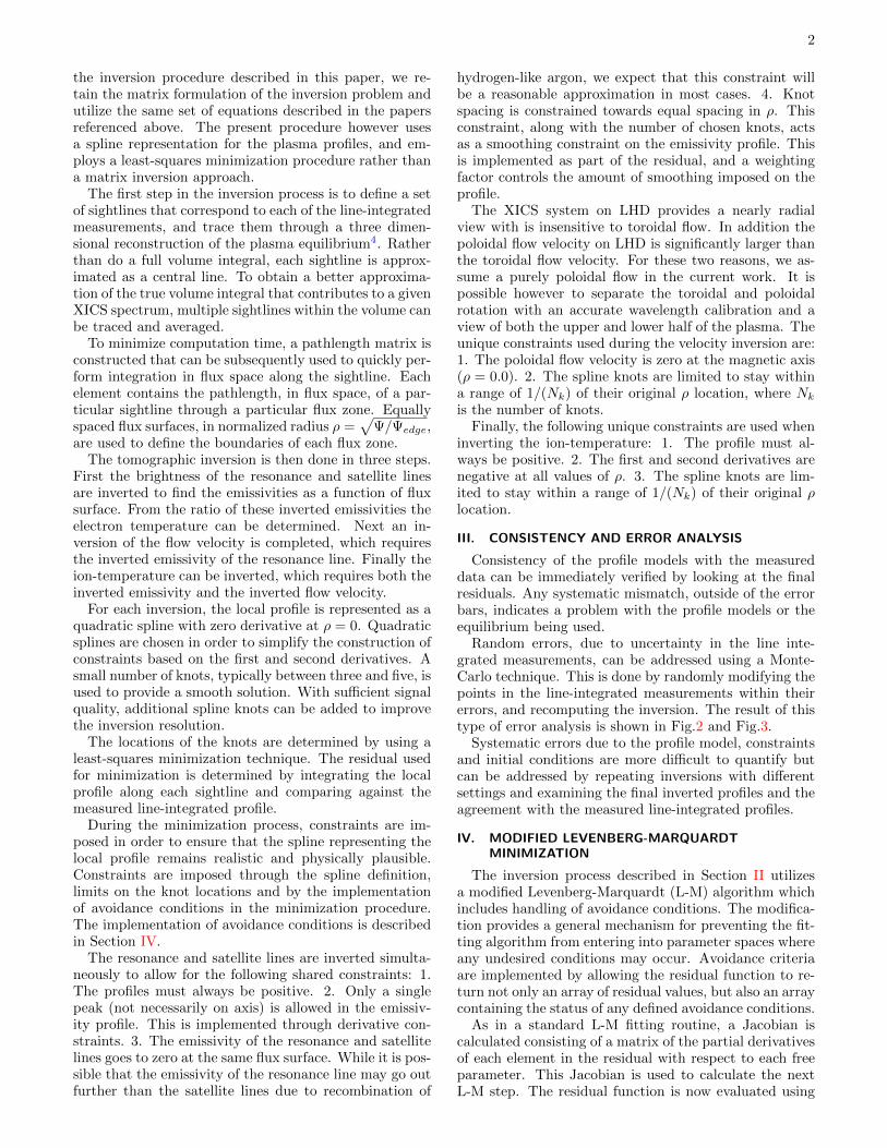
Random errors, due to uncertainty in the line inte-grated measurements, can be addressed using a Monte-Carlo technique. This is done by randomly modifying thepoints in the line-integrated measurements within theirerrors, and recomputing the inversion. The result of thistype of error analysis is shown in Fig.2 and Fig.3.

Systematic errors due to the profile model, constraintsand initial conditions are more difficult to quantify butcan be addressed by repeating inversions with differentsettings and examining the final inverted profiles and theagreement with the measured line-integrated profiles.

IV. MODIFIED LEVENBERG-MARQUARDTMINIMIZATION

The inversion process described in Section II utilizesa modified Levenberg-Marquardt (L-M) algorithm whichincludes handling of avoidance conditions. The modifica-tion provides a general mechanism for preventing the fit-ting algorithm from entering into parameter spaces whereany undesired conditions may occur. Avoidance criteriaare implemented by allowing the residual function to re-turn not only an array of residual values, but also an arraycontaining the status of any defined avoidance conditions.

As in a standard L-M fitting routine, a Jacobian iscalculated consisting of a matrix of the partial derivativesof each element in the residual with respect to each freeparameter. This Jacobian is used to calculate the nextL-M step. The residual function is now evaluated using

3

ρ

RESO

NA

NCE

EMIS

SIVI

TYSA

TELL

ITE

EMIS

SIVI

TYTi

(keV

)Te

(keV

)Vp

(km

/s)

RESO

NA

NCE

INTE

NSI

TYSA

TELL

ITE

INTE

NSI

TYTi

(keV

)Vp

(km

/s)

a

b

FIG. 2. LHD shot 114722 at 4000ms. Fig a. compares the fi-nal inverted plasma profiles (red lines) with the measured lineintegrated profiles (black lines). Error bars are derived froma Monte-Carlo error analysis. The red shaded region showsthe variance in the M-C solutions and is centered about themean. The yellow shaded region represents the extreme M-Csolutions. For the line integrated measurements, the ρ coordi-nate is taken from the minimum value of ρ that the sightlinepasses through. The large error bars on Te near the core aredue both to the large error in emissivity of the n=3 satellitelines and to the insensitivity of the Te calculation above 4keV.Fig. b. compares integrated profiles from the inverted solutionand the original measurements. The gray shaded area showsthe variance in the line-integrated measurements reported bythe spectral fitting algorithm.

RESO

NA

NCE

EMIS

SIVI

TYSA

TELL

ITE

EMIS

SIVI

TYTi

(keV

)Te

(keV

)Vp

(km

/s)

RESO

NA

NCE

INTE

NSI

TYSA

TELL

ITE

INTE

NSI

TYTi

(keV

)Vp

(km

/s)

ρ

a

b

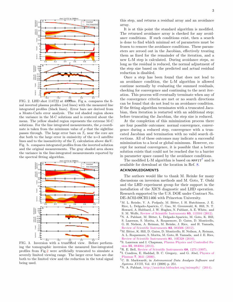
FIG. 3. Inversion with a truncated view. Before perform-ing the tomographic inversion the measured line-integratedprofiles from Fig.2 were artificially truncated to simulate aseverely limited viewing range. The larger error bars are dueboth to the limited view and the reduction in the total signalbeing used.

this step, and returns a residual array and an avoidancearray.

It is at this point the standard algorithm is modified.The returned avoidance array is checked for any avoid-ance conditions. If such conditions exist, then a searchis done to find which minimal set of parameters must befrozen to remove the avoidance conditions. These param-eters are zeroed out in the Jacobian, effectively treatingthem as fixed for the remainder of the iteration, and anew L-M step is calculated. During avoidance steps, solong as the residual is reduced, the normal adjustment ofthe step size based on the predicted and actual residualreduction is disabled.

Once a step has been found that does not lead toan avoidance condition, the L-M algorithm is allowedcontinue normally by evaluating the summed residuals,checking for convergence and continuing to the next iter-ation. This process will eventually terminate when any ofthe convergence criteria are met or no search directionscan be found that do not lead to an avoidance condition.If the fitting algorithm terminates with a truncated Jaco-bian, then iteration is restarted with an additional step:before truncating the Jacobian, the step size is reduced.

At the completion of this minimization process thereare four possible outcomes: normal convergence, conver-gence during a reduced step, convergence with a trun-cated Jacobian and termination with no valid search di-rections. All of these outcomes may indicate a successfulminimization to a local or global minimum. However, ex-cept for normal convergence, it is possible that a bettersolution exists that could not be reached due to a barrierin parameter space caused by the avoidance conditions.

The modified L-M algorithm is based on mpfit7 and isavailable for download at the location in Ref. 8.

ACKNOWLEDGMENTS

The authors would like to thank M. Reinke for manydiscussions on inversion methods and M. Goto, T. Oishiand the LHD experiment group for their support in theinstallation of the XICS diagnostic and LHD operation.Research supported by the U.S. DOE under Contract No.DE-AC02-09CH11466 with Princeton University.1M. L. Reinke, Y. A. Podpaly, M. Bitter, I. H. Hutchinson, J. E.Rice, L. Delgado-Aparicio, C. Gao, M. Greenwald, K. Hill, N. T.Howard, A. Hubbard, J. W. Hughes, N. Pablant, A. E. White, andS. M. Wolfe, Review of Scientific Instruments 83, 113504 (2012).

2N. A. Pablant, M. Bitter, L. Delgado-Aparicio, M. Goto, K. Hill,S. Lazerson, S. Morita, A. Roquemore, D. Gates, D. Monticello,G. H. Nielson, A. Reiman, M. Reinke, J. Rice, and H. Yamada,Review of Scientific Instruments 83, 083506 (2012).

3M. Bitter, K. Hill, D. Gates, D. Monticello, H. Neilson, A. Reiman,A. L. Roquemore, S. Morita, M. Goto, H. Yamada, and J. E. Rice,Review of Scientific Instruments 81, 10E328 (2010).

4S. Lazerson and I. Chapman, Plasma Physics and Controlled Fu-sion 55, 084004 (2013).

5R. E. Bell, Review of Scientific Instruments 68, 1273 (1997).6I. Condrea, E. Haddad, B. C. Gregory, and G. Abel, Physics ofPlasmas 7, 3641 (2000).

7C. B. Markwardt, in Astronomical Data Analysis Software andSystems XVIII, Vol. 411 (2009) p. 251.

8N. A. Pablant, http://amicitas.bitbucket.org/mirmpfit/ (2014).

 

 

Princeton Plasma Physics Laboratory Office of Reports and Publications

Managed by Princeton University

under contract with the

U.S. Department of Energy (DE-AC02-09CH11466)

P.O. Box 451, Princeton, NJ 08543 E-mail: publications@pppl.gov Phone: 609-243-2245 Fax: 609-243-2751 Website: http://www.pppl.gov