Principal-Agent Assignment: Implications for Incentivesand IncomeDistribution in Tenancy Relationships

Kanis.ka Dam

Centro de Investigación y Docencia EconómicasCarretera México-Toluca 3655, Colonia Lomas de Santa Fe

01210 Mexico, D. F., Mexico.

Abstract

I analyze a problem of assigning heterogeneous agents (tenants) to heterogeneous principals (landlords),where partnerships are subject to moral hazard in effort choice. The agents differ in wealth endowmentand the principals differ in land quality. When the liability of each agent is limited by his initial wealth, ashare contract is typically incentive compatible. A pure rent contract, on the other hand, is optimal in theabsence of incentive problems. In a Walrasian equilibrium of the economy, wealthier agents work in moreproductive lands following a positively assortative matching pattern since higher wealth has greater effectin high-productivity lands. Agent’s share of the match output is in general non-monotone with respect toinitial wealth. If wealth is more unequally distributed than land quality, then the equilibrium share (of theagents) is a monotonically increasing function of wealth. Under symmetric information, all agents earnthe same expected wage, and hence no income inequality is observed in equilibrium. When incentiveproblems are important, wealthier agents earn higher wages, and the income inequality decreases if theagents are more heterogeneous than the principals.

I owe thanks to Sonia Di Giannatale, Dilip Mookherjee, DavidPérez-Castrillo, Larry Samuelson and Javier Suárez forhelpful comments on an earlier and the current versions of the paper.

Email address:kaniska.dam@cide.edu (Kanis.ka Dam)

1. Introduction

While a plethora of writings on the theory of sharecropping have stressed the role of the agent’swealth endowment in determining his output share in a tenancy relationship, the roles of land qualityand outside option have been paid little attention. It has been argued that share tenancy emerges as anincentive device when the agent’s liability is limited by his initial wealth (e.g. Shetty, 1988; Laffont andMatoussi, 1995; Ray and Singh, 2001), and wealth has a positive effect on the agent’s output share be-cause higher wealth implies the possibility of greater rentextraction by the principal without weakeningincentives.1 Rao (1971) and Braido (2008), among few others, have emphasized the role of land qualityin share contracts.2 On the other hand, the role of agent’s outside option in determining his share isalso important. Banerjee, Gertler, and Ghatak (2002) argued that higher outside options following theintroduction ofOperation Barga, the land reform act of 1978 in the Indian state of West Bengal, hadsignificant favorable effects on the output share and productivity of the sharecroppers. In the presentpaper I propose a unified framework that analyzes the joint effects of land and wealth heterogeneities onthe tenancy contracts through endogenous outside option.

Most of the theoretical works on share tenancy employ variants of the partial equilibrium agencymodel (e.g. Grossman and Hart, 1983) where a principal (landlord) of given characteristics leases herland to an agent (tenant) of given characteristics, and offers a tenancy contract that consists of a fixedrent component and a given share of output. The optimal contract determines the incentive structure ofthe final payoff to the agent. In such models, the level of earning of the agent is determined entirelyby his exogenously given outside option. Endogenous determination of the agent’s outside option thuscalls for a general equilibrium framework. The present paper starts with this motivation. It extends Sat-tinger’s (1979) ‘differential rent’ model to a situation where agents are assigned to principals, and eachprincipal-agent relationship is subject to limited liability and moral hazard in effort choice. In particular,I consider a model where principals are heterogeneous with respect to the quality or productivity of thelands they own, and agents differ in wealth endowment. In an equilibrium, each principal of a given typechooses optimally an agent by maximizing her residual profits, taking the expected wages as given. AWalrasian equilibrium implies that each agent must receivean expected wage equal to his outside option,defined as the maximum of the payoffs that could be obtained byswitching to alternative partnerships.As wealthier agents and more productive principals have absolute advantages in any partnership, equilib-rium wage and profit are increasing respectively in wealth and land quality. Optimal choice of agents bythe principals also implies that wealthier agents work in high-productivity lands following a positively as-sortative matching pattern because higher wealth has greater (marginal) effect in more productive lands.The equilibrium relationship between the output shares andinitial wealths of the agents determines theequilibrium share function. The equilibrium output share of an agent depends on his initial wealth, onthe productivity of the land he cultivates through the equilibrium matching function, and on his outsideoption via the equilibrium wage function. A principal can extract more surplus from a wealthy agent inthe form of fixed rent without affecting incentives, and hence higher wealth implies greater output share.

1Basu (1992), Sengupta (1997), and Ghatak and Pandey (2000) have been important contributions to the literature whichargue that share tenancy emerges due to limited liability even if the agent may have zero wealth. There is also a large literaturewhich claims that sharecropping emerges because of pure risk-sharing motives (e.g. Stiglitz, 1974; Newbery, 1977), oras anincentive device under moral hazard (e.g. Eswaran and Kotwal, 1985).

2Rao (1971), using farm management data from India, shows that the quality of land has explained 90% variations incontracts offered to the share croppers. Braido (2008) argues that typically lower quality lands are leased out to the sharetenants.

2

In a more productive land, less incentive is required in order to induce a given effort level, and hencelower shares are associated with high-quality lands. Finally, higher outside option, which implies greaterincentives to shirk, implies higher output share. Because of these two opposing effects the output sharesof the agents are in general non-monotone with respect to initial wealth. It is shown that when wealth ismore heterogeneously distributed relative to land quality, the positive effects dampen the negative effectof land quality on the output shares of the agents, and the equilibrium share thus increases with wealths.

As the levels of earnings of the agents are endogenously determined, the equilibrium of the model hasinteresting implications for earnings inequality. First,a Walrasian equilibrium implies that the outsideoption of each agent is determined endogenously, which in turn implies the endogenous determination ofthe agents’ bargaining power. Second, I show that if the distribution of wealth is more disperse relativeto the distribution of land quality, then the equilibrium wage function is concave. A concave wagefunction implies a lower income inequality since the wage differential decreases as the wealth levelsof the agents go up. A convex wage function, on the other hand,increases wage inequality. Finally,similar to Sattinger’s (1979) assignment model, the present work also implies that the final distributionof equilibrium wages is skewed to the right relative to the distribution of wealths. With heterogeneouslands, agents with greater wealth are assigned to more productive lands which boosts their expectedincomes above what they would be earning if all lands were identical.

The present paper contributes to the recent literature on the problems of assigning agents to princi-pals in environments characterized by informational asymmetries. In particular, in the context of sharetenancy, this paper is related to Ghatak and Karaivanov (2010) who analyze a model of partnership basedon double-sided moral hazard, and show that partnerships may not emerge in equilibrium if the individ-uals differ in terms of degrees of absolute advantage in accomplishing specific tasks and the matching isendogenous. They also found conditions under which a matching may be assortative or non-monotone.One major contribution of their work is that sharecropping may emerge as a consequence of endogenousmatching between principals and agents. In an important contribution to this literature, Ackerberg andBotticini (2002) have analyzed the landlord-tenant contracts in renaissance Tuscany, and showed thatcontracts are influenced in a significant way by the endogenous nature matching between the landlordsand tenants. Chakraborty and Citanna (2005) show, in a modelof occupational choice, that less wealth-constrained individuals choose to take up projects in whichincentive problems are more important due toendogenous sorting effects. Unlike most of the recent contributions, e.g. the present model, Chakrabortyand Citanna’s (2005) paper is a model of one-sided matching.It is worth mentioning that, while thecurrent paper generalizes the popular assignment models (e.g. Sattinger, 1975, 1979) by considering sit-uations in which matches are subject to moral hazard in a Walrasian equilibrium framework, most ofthe aforementioned papers consider partnership formationas a cooperative matching game, and employstability as the solution concept. Serfes’s (2005) is an assignment model that analyzes the trade-off be-tween risk-sharing and incentives, and shows a non-monotone relationship between risk and incentive.Legros and Newman (2007) propose a sufficient condition, called thegeneralized difference condition,under which stable allocations exhibit assortative matching when the two-sided matching induces a non-transferable utility (a concave Pareto frontier) game. Similar conditions are obtained in Lemma 1(b).

3

2. A model of principal-agent assignment

2.1. Description

Consider an economy with a continuum[0, 1] of heterogeneous risk-neutral principals and a con-tinuum [0, 1] of heterogeneous risk-neutral agents. The positive real numbersλ ∈ Λ ≡ [λmin, λmax]andω ∈ Ω ≡ [ωmin, ωmax] denote the ‘qualities’ of the principals and the agents, respectively. Qualityor type of an individual may be interpreted as productivity,efficiency, wealth, etc. which would influ-ence final payoffs. For example, higher values ofλ could imply more productive (“better”) principals.The distributions of qualities are exogenous to the model. LetG(λ) be the cumulative distribution ofλ, which denotes the fraction of principals with qualities lower thanλ, andg(λ) be the correspondingdensity function. Similarly, letF (ω) be the cumulative distribution ofω with the corresponding densityf(ω). I denote byξ ≡ (F, G) the principal-agent economy.

Principals and agents are assigned to each other to form partnerships or matches. Each individ-ual in a given match has to take a set of actions which are inputs to the final match output. Some ofthese actions such as effort, investment decision may not bepublicly verifiable which induce incentiveproblems in each partnership. This section extends the ‘differential rents’ model of Sattinger (1979) tosituations where matches are subject to incentive problems.3 Individuals of identical quality will be per-fect substitutes, and hence only qualities and not the namesmatter. The principal-agent assignment canbe described by a one-to-one correspondencel : Ω −→ Λ or its inversew ≡ l−1. Therefore ifλ = l(ω),or equivalentlyω = w(λ), then(λ, ω) denotes a typical match or partnership.

In a match(λ, ω), the principal and agent write a binding contractc(λ, ω) which specifies the waythe total match-surplus is to be divided between them. Let the surplus be given byφ(λ, ω, u(ω)) whereu(ω) is the expected wage of the agent.4 The expected profit of the principal is thus given by:

v(λ) = φ(λ, ω, u(ω)) − u(ω). (1)

I make the following assumptions onφ(λ, ω, u(ω)):

1. φ(λ, ω, u(ω)) is twice differentiable, whereφi denotes the partial derivative ofφ with respect to thei-th argument, andφij denotes the cross partial derivative with respect to thei-th andj-th arguments;

2. φi > 0, for i = 1, 2, andφ3 ∈ [0, 1): the match-surplus is strictly increasing in the qualitiesof theprincipal and the agent, and increasing in the agent’s wage;

3. φ22 ≤ 0 andφ33 ≤ 0: concavity of the surplus function with respect to the quality and wage of theagent.

In a Walrasian equilibrium, each typeλ principal picks an agent with qualityω in order to maximize her

3Edmans, Gabaix, and Landier (2009), and Dam (2010) also build on the assignment model presented in Sattinger (1979)to incorporate incentive problems.

4The match-surplus depends on the qualities of the principaland the agent, and on the agent’s wage.Sattinger’s (1979)model is an assignment model with transferable utilities due to the absence of any incentive problems. It is well-known that,in the presence of incentive problems in a principal-agent relationship, optimality of contracts is not defined by totalsurplusmaximization since how much surplus would be produced depends on how it is distributed within the match. Consequently,incentive problems give rise to non-transferabilities which implies that the match-surplus also depends on the expected wage ofthe agent. In an assignment model similar to Sattinger (1979), the surplus function will be given byφ(λ, ω).

4

expected profit, i.e., each typeλ principal solves

v(λ) = maxω′

φ(λ, ω′, u(ω′)) − u(ω′), (P)

taking the wagesu(ω) as given. Therefore, an equilibrium consists of an assignment rule l orw, and thevectors of profits(v(λ))λ∈Λ and wages(u(ω))ω∈Ω such that

(a) w(λ) = argmaxωφ(λ, ω, u(ω)) − u(ω) for eachλ: each principal chooses her partner optimally;(b) If [λ1, λ2] = l([ω1, ω2]) for any subintervals[ω1, ω2] of Ω and [λ1, λ2] of Λ, then it must be the

case thatG(λ2) −G(λ1) = F (ω2) − F (ω1): market clearing.

The first condition implies that the principal-agent assignment is optimal. The second is a measureconsistency requirement which says that if an interval of agent-types[ω1, ω2] is mapped by the rulelinto an interval of principal-types[λ1,λ2], then these two sets cannot have different measures. This isthe standard market clearing condition for each type.

2.2. Equilibrium

The equilibrium wagesu(ω) and profitsv(λ) are determined by solving the maximization problem(P) of each typeλ principal. While solving (P), a principal must guarantee the agent his outside option.An agent’s outside option is the maximum payoff he can obtainby switching to other matches. In aWalrasian equilibrium, the expected wage of a typeω agent must be equal to his outside option. A wageoffer less than the outside option will not be accepted. On the other hand, if the wage of an agent isstrictly higher than his outside option, then the principalcan lower her offer a bit and still the offer willbe accepted by the agent, thereby contradicting the notion of equilibrium. The first-order condition ofthe maximization problem (P) is given by:

φ2(λ, ω, u(ω)) + [φ3(λ, ω, u(ω)) − 1]u′(ω) = 0,

i.e., u′(ω) =φ2(λ, ω, u(ω))

1 − φ3(λ, ω, u(ω))for λ = l(ω). (FOC)

It follows from the Envelope theorem that

v′(λ) = φ1(λ, ω, u(ω)) for λ = l(ω). (E)

Given the assumptions on the match-surplus function, the above two expressions are positive. In everymatch, an agent’s wage and a principal’s profit are paid according to their contributions to the match-surplus. For example, the marginal wage of a typeω agent is equal to his marginal contribution to thetotal surplusφ(λ, ω, u(ω)). The equilibrium wagesu(ω) and profitsv(λ) are found by solving thedifferential equations (FOC) and (E) for each match(λ, ω).

Suppose that the equilibrium assignment is given byλ = l(ω). The next step is to determine the signof l′(ω). The following definition introduces the notion of assortative or monotone matching.

Definition 1 If l′(ω) ≥ (≤) 0, then the assignment is said to be positively (negatively) assortative.

Whether the equilibrium matching is assortative is determined by the second-order conditions of themaximization problem (P). In Appendix A it is shown that thissecond-order condition is satisfied if and

5

only if[φ21(l(ω), ω, u(ω)) + φ31(l(ω), ω, u(ω))u′(ω)]l′(ω) ≥ 0. (SOC)

It follows from the above inequality that ifφ21(λ, ω, u(ω)) andφ31(λ, ω, u(ω)) are both positive (neg-ative), thenl′(ω) ≥ (≤) 0. The following lemma summarizes the above findings.

Lemma 1 Letλ = l(ω) be an equilibrium principal-agent assignment, andu(ω) andv(λ) be the asso-ciated equilibrium wages and profits, respectively.

(a) The equilibrium wages and profits are increasing functions of the qualities of the agents and theprincipals, respectively;

(b) If φ21(λ, ω, u(ω)) ≥ (≤) 0 andφ31(λ, ω, u(ω)) ≥ (≤) 0 for all (λ, ω, u(ω)), then the equilibriumassignment is positively (negatively) assortative.

The proofs of the above assertions and those of the subsequent ones are relegated to the Appendix.The above lemma extends the results of Sattinger (1979) to environments with non-transferable utility.Similar results have also been proved by Legros and Newman (2007). High-quality individuals haveabsolute advantages in any partnership becauseφ1 > 0 andφ2 > 0, i.e., the match surplus is increasingin λ andω. Therefore, “better” individuals consume higher expectedpayoffs in an equilibrium, which isthe assertion of Part (a) of the above lemma. Also, two individuals of the same quality must obtain sameexpected payoffs. Thus, the equilibrium satisfies ‘equal treatment of equals’ property. The equilibriumwage and profit functions are similar to the ‘hedonic prices’in Rosen (1974). An important differencebetween the aforementioned works and the present paper is that I introduce non-transferability in anassignment model.

An assortative matching is a consequence of complementarity or substitutability between the principal-and agent-qualities. Consider the case of a positively assortative assignment. Complementarity impliesthat high-quality agents have comparative advantages overthe low-quality ones in matches involvinghigh-quality principals. This sort of comparative advantage determines that a better agents must beassigned better principals. In the context of non-transferable utilities, the complementarity has two as-pects. First,φ21 ≥ 0 implies that a high-quality principal and a high-quality agent together producehigher aggregate surplus. This is the usual ‘type-type’ complementarity, which also determines positivesorting in the standard assignment models (e.g. Rosen, 1974; Sattinger, 1979). Second,φ31 ≥ 0 impliesthat it is (marginally) less costly for a high-type principal to transfer surplus to a high-type agent. This‘type-payoff’ complementarity reinforces the reasons under which an equilibrium induces a positivelyassortative matching.5

5Notice the difference between the above optimality conditions and those in an assignment model with transferable utilities.In Sattinger’s (1979) differential rents model, the first-order condition associated with the principal’s optimal choice is givenby:

u′(ω) =∂φ(λ, ω)

∂ω.

And the second-order condition is given by:∂2φ(λ, ω)

∂λ∂ωl′(ω) ≥ 0.

6

3. Application: tenancy contracts under limited liability

This section considers optimal share-tenancy contracts between risk-neutral principals (landlords)and risk-neutral agents (tenants) in an attempt to identifya situation to which the results of Lemma 1apply. Principals own a plot of land apiece which can be leased out to a sharecropper, the agent. Agentsare heterogeneous with respect to their initial wealthω ∈ Ω ⊂ R++, which is uniformly distributed.Here initial wealth represents the type or quality of an agent. On the other hand,λ ∈ Λ ⊂ (0, 1)represents the productivity of lands, which is also uniformly distributed. I assume thatλ2/8 ≤ ω forall (λ, ω). I further assume that there is no alternative markets for land and labor services. Hence, anunused plot of land generates zero profit to its owner, and an unemployed agent consumes his wealthendowment. A land with qualityλ produces a stochastic output which is given by:

y =

1 with probability λe,

0 with probability 1 − λe,

wheree ∈ [0, 1] is the non-verifiable effort exerted by an agent. The cost effort is an increasing andconvex functionψ(e). For simplicity, I assume thatψ(e) = e2/2.

A tenancy contract for an arbitrary match(λ, ω) is a vectorc(λ, ω) = (α(λ, ω), R(λ, ω)) whereαis the agent’s share of output, andR is the fixed rental payment made to the principal. I restrict attentionto the class of contracts for whichR ≥ 0 andα ∈ [0, 1]. If α = 1 andR > 0, then the contract is apurerent contract. A contract withα < 1 andR > 0, on the other hand, is referred to as ashare contract.6

Givenc(λ, ω), the expected payoffs of the principals and the agents are respectively given by:

V (c(λ, ω)) = λe(λ, ω)[1 − α(λ, ω)] +R(λ, ω), (2)

U(c(λ, ω)) = λe(λ, ω)α(λ, ω) −R(λ, ω) − [e(λ, ω)]2

2. (3)

Within a principal-agent relationship(λ, ω), the principal therefore solves the following maximizationproblem.

maxc(λ, ω)

λe(λ, ω)[1 − α(λ, ω)] +R(λ, ω) (M)

subject to λe(λ, ω)α(λ, ω) −R(λ, ω) − [e(λ, ω)]2

2= u(ω), (PC)

e(λ, ω) = argmaxe

λeα(λ, ω) −R(λ, ω) − e2

2

, (IC)

R(λ, ω) ≤ ω. (LL)

The first constraint is the participation constraint of the agent. In the context of a Walrasian equilibrium,this constraint requires a bit more attention. In a standardagency model (e.g. Ray and Singh, 2001), agiven principal-agent relationship is treated as an isolated entity, and the participation constraint of the

6I do not address the issue of existence of share contracts. See Sengupta (1997), and Ray and Singh (2001) for a discussionon its existence, and why one can restrict attention to the values ofα in the interval[0, 1].

7

agent is given by:

λe(λ, ω)α(λ, ω) −R(λ, ω) − [e(λ, ω)]2

2≥ u, (4)

whereu is the agent’soutside option, which is defined as the maximum of the expected wages that theagent may earn by switching to alternative matches. Therefore, a contractc(λ, ω) must guarantee theagent at least his outside option. Unlike the agency models that involve only one principal and oneagent, the outside option of an agent is no more exogenous since it depends on the contract offers bythe other principals. First notice that in a Walrasian equilibrium an agent’s expected wage must be equalto his outside option, otherwise another agent of the same type may bid his wage down tou. Second,the participation constraint of the typeω must be binding. If it is not the case, then the principal canlower the agent’s wage a bit, and the contract will still be accepted which contradicts the definition ofan equilibrium. Therefore, I replaceu by u(ω), and write the participation constraint with equality.The second constraint is the incentive compatibility constraint, which says that the agent will choosethe effort level that maximizes his expected wage. The last one is the limited liability constraint whichguarantees non-negative final income to the agent even when the match output is zero. In a principal-agent relationship, if the agent’s limited liability constraint does not bind at the optimum, provision ofincentives is not costly for the principal, and hence thefirst-besteffort level can be implemented. Thisis equivalent to the situation where the principal could enforce any level of effort she liked. When thelimited liability constraint is binding, it is typically costly for the principal to provide incentives, andonly thesecond-besteffort can be implemented. Define by:

Γ := (λ, ω) | λ2/8 ≤ ω + u(ω) ≤ λ2/2 ⊂ S = Λ × Ω.

It is easy to show that if(λ, ω) ∈ S \ Γ, then the limited liability constraint (LL) does not bind, and theoptimal contract and effort are at their first-best levels. On the other hand, if(λ, ω) ∈ Γ, then the limitedliability constraint binds, and only the second-best contract and effort are implemented. The optimaloutput shareα∗(λ, ω, u(ω)) of the agent, rental paymentR∗(λ, ω, u(ω)), and efforte∗(λ, ω, u(ω)) aredescribed in Table 1.

Table 1: Optimal contract, effort and surplus of an arbitrary match(λ, ω)

First-best Second-best

Agent’s output share 1 (1/λ)√

2(ω + u(ω))

Rental payment (λ2/2) − u(ω) ω

Effort λ√

2(ω + u(ω))

The optimal contract terms and effort, in general, depend onthe productivity of the land, the wealth of theagent and the agent’s wage. I omit the standard analysis of the optimal contract. Under the first-best, theagent gets the entire share of output, and pays a fixed rent in both states of the nature for leasing out theland. Therefore, the optimal tenancy contract is a pure rentcontract. The optimal effort is at its highestlevel, and does not depend on the agent’s wealth and his wage.When the limited liability constraint

8

binds, the second-best contracts are implemented, and the agent obtains an output share strictly lowerthan 1 but higher than 1/2. It is increasing inω andu(ω), but decreases withλ. The optimal effort islower than its first-best level, which is increasing inω andu(ω), but constant with respect toλ.

Given the optimal contracts and effort, it is now easy to compute the match surplus, which equals theexpected match outputλe(λ, ω) minus the effort costψ(e(λ, ω)).

Lemma 2 Consider an arbitrary match(λ, ω).

(a) When(λ, ω) ∈ S \Γ, i.e., when the first-best contract and effort are implemented, the match surplusis given by:

φ(λ, ω, u(ω)) =λ2

2,

with φ1(λ, ω, u(ω)) ∈ (0, 1) andφ2(λ, ω, u(ω)) = φ3(λ, ω, u(ω)) = 0;(b) When(λ, ω) ∈ Γ, i.e., when the second-best contract and effort are implemented, the match surplus

is given by:φ(λ, ω, u(ω)) = λ

√

2(ω + u(ω)) − ω − u(ω),

with φi(λ, ω, u(ω)) ∈ (0, 1) for i = 1, 2, 3.

In the first-best situation, when the agent gets the entire share of output, the match surplus takes itsmaximum value. Under a share contract (second-best), matchsurplus is lower because there is loss ofefficiency due to informational asymmety.7

3.1. The equilibrium wages, profits and assignment

As the value of the match surplusφ(λ, ω, u(ω)) is known for each arbitrary match, the next step isto determine the equilibrium wageu(ω) and profitv(λ) functions, which are the equilibrium relation-ships between the expected payoffs of the individuals and their types. First, the marginal functions aredetermined using equations (FOC) and (E). Hence one should check whether the conditions for Lemma1(a) are satisfied in this context.

v′(λ) = φ1(λ, ω, u(ω)) ∈ (0, 1), (5)

u′(ω) =φ2(λ, ω, u(ω))

1 − φ3(λ, ω, u(ω))≥ 0. (6)

The following proposition describes the marginal profit andwage functions.

Proposition 1 The equilibrium profitv(λ) is an increasing function of land-productivity, and the equi-librium wageu(ω) is an increasing function of the initial wealth.

When the first-best contracts are implemented in all matches, the match surplus is independent ofω asthe limited liability constraints do not bind, i.e., the initial wealth of each agent does not enter into thecontract offered to him. The fixed rental payment does not appear in the surplus because it is a transfer

7It can be shown that, forω + u(ω) < λ2/8, the agent’s limited liability constraint binds, but the participation constraintdoes not. I ignore this situation as the optimal contracts must be parts of a Walrasian equilibrium.

9

from the agent to the principal. Therefore, the surplus is also independent ofu(ω). As a consequence,one hasφ2 = φ3 = 0. Sinceφ for each match depends only on the productivity of land, the marginalsurplus is higher for better principals, and hence they receive higher equilibrium profits. As all agentsreceive the entire share of output and exert the first-best effort, their wages are the same irrespectiveof the wealth levels. When the second-best contracts are implemented in all matches, it is the casethat φ1 > 0 andφ2 > 0, i.e., owners of more productive lands and wealthier agentshave absoluteadvantages in producing surplus in any match. Hence, high-quality principals obtain greater equilibriumprofits, and wealthier agents consume higher wages in equilibrium. Therefore, the equilibrium wageis a constant function under the first-best, whereas in the second-best situation, the equilibrium wageis a stricly increasing function of wealth. Also notice thatunder second-best, for given wages and foreach typeλ principal, her expected profit,φ(λ, ω, u(ω)) − u(ω), is increasing in wealth. This is thewell-known tenancy ladderphenomenon, i.e., wealthier agents are always preferred tothe less wealthyones.

Prior to determining the equilibrium matching pattern, notice that an Walrasian equilibrium impliesfull employment, i.e., no agent is unemployed and no land is left idle. To see this, suppose in an equilib-rium there is one agent of a given typeω is unemployed. Then there must be one principal with her plotof land uncultivated. Suppose that the idle plot is of a givenproductivityλ. In this situation the unem-ployed agent consumesω and the principal consumes zero profit. Then the principal can offer a contractto the agent, which consists ofα = 1/2 andR = 0. This contract satisfies the limited liability constraintand generates a profit equal toλ2/4 > 0 to the principal, and a gross expected payoffλ2/8 + ω > ω tothe agent. This contradicts the definition of Walrasian equilibrium.

Lemma 1(b) provides sufficient conditions for assortative matching. In order to determine an equi-librium assignment, it is thus sufficient to check the signs of φ21 andφ31 in the present context. FromLemma 2(a), it is immediate to show thatφ21 = φ31 = 0 if the first-best contracts are implemented.Under the second-best, on the other hand,

φ21(λ, ω, u(ω)) = φ31(λ, ω, u(ω)) =1

√

2(ω + u(ω))> 0. (7)

Therefore the equilibrium matching pattern follows from Lemma 1(b), which is described in the follow-ing proposition.

Proposition 2 Letλ = l(ω) be an equilibrium assignment.

(a) If the first-best contracts are implemented in all matches, then any matching pattern is consistentwith an equilibrium;

(b) If the second-best contracts are implemented in every match, then the equilibrium assignment ispositively assortative, i.e., wealthier agents cultivatemore productive lands.

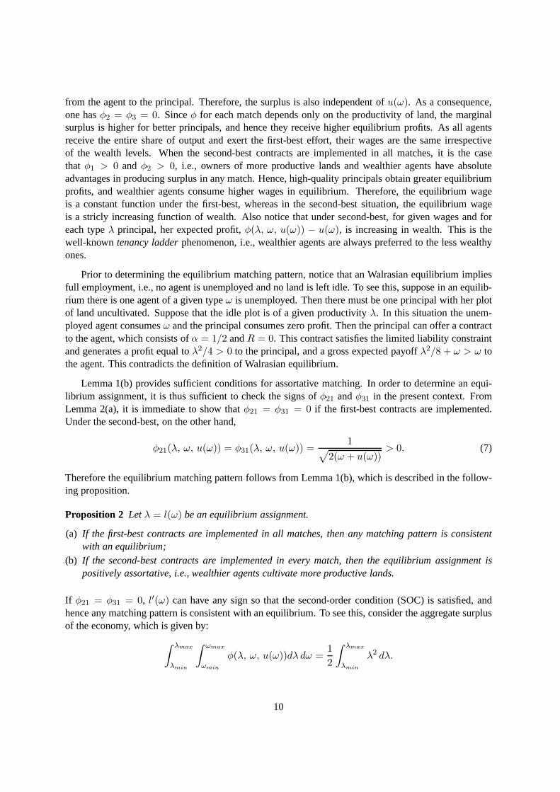
If φ21 = φ31 = 0, l′(ω) can have any sign so that the second-order condition (SOC) issatisfied, andhence any matching pattern is consistent with an equilibrium. To see this, consider the aggregate surplusof the economy, which is given by:

∫ λmax

λmin

∫ ωmax

ωmin

φ(λ, ω, u(ω))dλ dω =1

2

∫ λmax

λmin

λ2 dλ.

10

Since the above expression is independent ofω, the aggregate surplus is maximized for any matchingpattern. When the limited liability constraints bind in allmatches, the equilibrium contracts depend onthe wealth endowment. Asφ21 andφ31 are both strictly positive, higher wealth has greater impact on thematch-surplus when combined with more productive land. In other words, wealthier agents have compar-ative advantages in matches consisting of more productive principal, and hence the unique equilibriummatching is positively assortative.

If in a Walrasian equilibrium a given land-qualityλ is assigned to a given wealth levelω, then apositively assortative matching implies

F (ω) − F (ωmin) = G(λ) −G(λmin),

or, l(ω) = λmin + (∆λ/∆ω)(ω − ωmin),

where∆λ ≡ λmax−λmin and∆ω ≡ ωmax−ωmin. Notice that the slopel′(ω) is an increasing functionof the relative dispersion∆λ/∆ω. If the lands are homogeneous, i.e.,∆λ = 0, then the matchingfunction is horizontal. On the other hand, homogeneity of the agents implies a vertical matching function.

As the equilibrium matching function is known, it is now possible to write down the expression formarginal wageu′(ω). Using Lemma 2 in equation (6), it is easy to show that

u′(ω) =1 − α∗(λ, ω, u(ω))

2α∗(λ, ω, u(ω)) − 1(8)

In the first-best situationα∗ = 1, i.e., each tenant gets the entire share of the match-output, and henceu′(ω) = 0. When the second-best contracts are implemented, substituting forα∗ from 3 andλ = l(ω) =λmin + (∆λ/∆ω)(ω − ωmin) in the above expression, one gets the following marginal wage function.

u′(ω) =

0 if the first-best contracts are implemented,λmin+(∆ λ/∆ ω)(ω−ωmin)−

√2(ω+u(ω))

2√

2(ω+u(ω))−λmin−(∆ λ/∆ ω)(ω−ωmin)if the second-best contracts are implemented.

(9)

The levels of equilibrium wages are found by solving the differential equation (9). Notice that if thefirst-best contracts are implemented in all matches, thenu(ω) is a constant function. In order to solvethe second equation in (9), first one needs to determined the associated constant of integration. In anWalrasian equilibrium, the last agent employed must be an agent with the lowest wealthωmin, whichgives the boundary condition for solving (9). It is easy to check that the constant of integration mustbe equal tou(ωmin). Since no principals other than the ones of typeλmin would hire the least wealthyagents, they will be pushed to theirreservation wage, the minimum wage rate at which an agent is notwilling to work, which must be equal toωmin. Unfortunately, it is not possible to explicitly solve theequilibrium wage function when the second-best contracts are implemented. In Subsection 3.3, I willanalyze more properties of the wage function.

3.2. Equilibrium contracts

The principal objective of this subsection is to analyze behavior of the equilibrium contracts andeffort with respect to initial wealth. In a partial equilibrium setup where a principal-agent pair is treatedin isolation, the contract for the pair in general depends onthree parameters: the productivity of the land,the wealth of the agent and the outside option of the agent. For instance, the optimal output share of the

11

agent in an arbitrary pair is given byα∗(λ, ω, u(ω)). To analyze the behavior ofα in this context withrespect toω, one must determine the sign of∂α∗/∂ω. If (λ, ω) ∈ Γ, the optimal share (of the typeωagent)α is an increasing function of the agent’s wealth, i.e., the partial derivative ofα with respect toωis positive (e.g. Ray and Singh, 2001, Proposition 3). In this subsection I show that the monotonicity ofthe agents’ output share with respect to initial wealth may not hold in a principal-agent market with two-sided heterogeneity, and look for sufficient conditions under which the equilibrium share is increasing inwealth.

Notice that in an equilibrium with the first-best contracts neither the optimal output shareα northe efforte depends on the initial wealth. I therefore focus only on the equilibrium with second-bestcontracts. The initial wealthω, apart from directly influencing the incentive compatible contracts andeffort, affects the optimal values in two indirect ways: through the matching and the wage functions.Thus in equilibrium, the contracts and effort are solely functions ofω, which are given by:

α(ω) = α∗(l(ω), ω, u(ω)) =1

l(ω)

√

2(ω + u(ω)), (10)

R(ω) = R∗(l(ω), ω, u(ω)) = ω, (11)

e(ω) = e∗(l(ω), ω, u(ω)) =√

2(ω + u(ω)). (12)

First notice from equations (11) and (12) that the equilibrium rent and effort are strictly increasing func-tions ofω becauseR′(ω) = 1 and

e′(ω) =∂e∗

∂λl′(ω) +

∂e∗

∂ω+∂e∗

∂uu′(ω) =

1 + u′(ω)

e(ω)> 0.

Now consider the equilibrium share functionα(ω). Differentiation of (10) with respect toω gives

α′(ω) =∂α∗

∂λl′(ω) +

∂α∗

∂ω+∂α∗

∂uu′(ω) =

α(ω)

l(ω)

[

1 + u′(ω)

l(ω)α2(ω)− l′(ω)

]

. (13)

Therefore, the sign ofα′(ω) depends on that of(1 + u′(ω))/(l(ω)α2(ω)) − l′(ω), which is a conditionon the endogenous variables of the model. The equilibrium share functionα(ω) is, in general, non-monotone. Under the second-best contracts, it is easy to show that

1 + u′(ω)

l(ω)α2(ω)=

1

l(ω)α2(ω)

(

1 +1 − α(ω)

2α(ω) − 1

)

=1

l(ω)α(ω)[2α(ω) − 1]≥ 1

since each term of the denominator is less than 1. Therefore,a sufficient condition forα(ω) to beincreasing inω is that l′(ω) = ∆λ/∆ω < 1, i.e., the matching function is sufficiently flat. Now, asufficiently flat matching function results in when∆λ < ∆ω, i.e., wealth is more unequally distributedthan land-productivity. The following proposition summarizes the above findings.

Proposition 3 Lete(ω),R(ω) andα(ω) be the equilibrium effort, rent and share functions, respectively.Then in an Walrasian equilibrium,

(a) effort and rent are increasing functions ofω;(b) the share function is in general non-monotone. If wealth is more unequally distributed than land-

productivity, then output share is an increasing function of ω.

12

As I have mentioned earlier, there are three effects that determine the behavior of incentives with respectto wealth. The first one is thematching effect. In the current model, land-productivity works as asubstitute for incentive as the agent who cultivates a high-productivity land requires lower incentive.Therefore,α tends to be lower in a match involving the owner of a high-quality land. The second effectis thewealth effect. Since the fixed rent component is higher for higher wealth (becauseR(ω) = ω), awealthier agent is given a higher share of output in order to have the same level of incentive. Therefore,agent’s output share and effort increase with initial wealth. The aforementioned effects are also present ina partial equilibrium setup consisting of one principal andone agent. The third effect is theoutside optioneffect, which emerges because of wage is determined endogenously in a general equilibrium model. Ahigher outside option turn implies greater bargaining power for the agents. Since the agent has littleincentives to work hard, the principal has to offer higher share of the match output. Therefor higherexpected wage has favorable impact on effort and output share. As equilibrium effort and rent do notdepend on the land-productivity, they increase with wealth. Because of the aforementioned two opposingeffects, the share function may be non-monotone.8

The sufficient condition in Proposition 3(b) is not hard to understand. When the agents are moreheterogeneously distributed than the principals, the negative effect of land-quality on incentives is damp-ened by the positive wealth and outside option effects. Therefore, higher output share for the agent isassociated with higher initial wealth. It is also easy to seethat if the distribution of wealth is too “tight”relative to the distribution of quality of the land, then a less wealthy agent receives a greater output sharecompared to the wealthier agents.

3.3. Wage inequality

In Subsection 3.1 it has been mentioned that it was not possible to have an explicit analytical solutionto the second differential equation in (9), i.e., it was not possible to determine the level of equilibriumwage when the second-best contracts are implemented. Yet itis possible to analyze the shape of theequilibrium wage function. In this subsection I relate the shape of the wage function to the nature ofwage/income inequality in equilibrium. To this end, the first task is to determine under what conditionsthe equilibrium wage is either a concave or a convex functionof initial wealth. Therefore I will studythe sign ofu′′(ω), the second derivative of the wage function which is found bydifferentiating the wageequation (9). When the first-best contracts are implemented, the wage function is flat sinceu′(ω) = 0.From equation (8), it is easy to check that

sgn[u′′(ω)] = − sgn[α′(ω)]. (14)

Therefore following Proposition 3(b), it is possible to relate the shape of the wage function to the initialdistributions of types.

Proposition 4 Letu(ω) be the equilibrium wage function.

(a) If the first-best contracts are implemented in all matches, then the equilibrium wage is a constantfunction of the initial wealth;

8Serfes (2005) also establishes a non-monotone share function. The main difference of the current model with that of Serfes(2005) is that the latter assumes zero outside option for each agent, whereas outside option is endogenous in the presentpaper.Besley and Ghatak (2005) identify the matching and outside option effects that determine contracts between principalsandagents.

13

(b) Suppose that the second-best contracts are implemented in all matches. If wealth is more unequallydistributed than land-productivity, then the equilibriumwage function is concave. On the otherhand, if the distribution of wealth is too tight relative to that of productivity of the lands, then thewage function is convex.

A constant wage function implies that the wage differentialassociated with any two wealth levels iszero for all levels of wealth. In other words, when the first-best contracts are implemented, there is nowage inequality among the agents. The non-trivial case emerges when the second-best contracts areimplemented in all matches. In this case the wage function may be non-linear. The above propositionprovides sufficient conditions under which the equilibriumwage function is either concave or convex. Aconcave wage function reduces wage inequality since the wage differentialu′(ω) goes down as the wealthlevel increases. This situation occurs when the matching function is relatively flat, i.e., the principals arerelatively more homogeneous than the agents. A convex wage function, on the other hand, raises thewages of the wealthier agents relative to the less-wealthy ones, and hence increases the wage inequality.

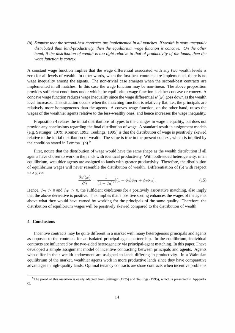
Proposition 4 relates the initial distributions of types tothe changes in wage inequality, but does notprovide any conclusions regarding the final distribution ofwage. A standard result in assignment models(e.g. Sattinger, 1979; Kremer, 1993; Teulings, 1995) is that the distribution of wage is positively skewedrelative to the initial distribution of wealth. The same is true in the present context, which is implied bythe condition stated in Lemma 1(b).9

First, notice that the distribution of wage would have the same shape as the wealth distribution if allagents have chosen to work in the lands with identical productivity. With both-sided heterogeneity, in anequilibrium, wealthier agents are assigned to lands with greater productivity. Therefore, the distributionof equilibrium wages will never resemble the distribution of wealth. Differentiation of (6) with respectto λ gives

∂u′(ω)

∂λ=

1

(1 − φ3)2[(1 − φ3)φ21 + φ2φ31]. (15)

Hence,φ21 > 0 andφ31 > 0, the sufficient conditions for a positively assortative matching, also implythat the above derivative is positive. This implies that a positive sorting enhances the wages of the agentsabove what they would have earned by working for the principals of the same quality. Therefore, thedistribution of equilibrium wages will be positively skewed compared to the distribution of wealth.

4. Conclusions

Incentive contracts may be quite different in a market with many heterogenous principals and agentsas opposed to the contracts for an isolated principal-agentpartnership. In the equilibrium, individualcontracts are influenced by the two-sided heterogeneity viaprincipal-agent matching. In this paper, I havedeveloped a simple assignment model of incentive contracting between principals and agents. Agentswho differ in their wealth endowment are assigned to lands differing in productivity. In a Walrasianequilibrium of the market, wealthier agents work in more productive lands since they have comparativeadvantages in high-quality lands. Optimal tenancy contracts are share contracts when incentive problems

9The proof of this assertion is easily adapted from Sattinger(1975) and Teulings (1995), which is presented in AppendixG.

14

are important in all matches. It is shown that when wealth is more heterogeneously distributed relative toland-productivity, higher output shares for the agents areassociated with higher initial wealths, althoughshare is in general non-monotone in wealth. It is also shown that if the distribution of wealth is relativelymore disperse than that of land-productivity, then the equilibrium wage function is concave in wealthimplying a reduction in income inequality. Moreover, because of positively assortative matching thedistribution of equilibrium wage is positively skewed relative to the distribution of initial wealth.

In the present model the first-best contracts may not be implemented due to informational asymme-tries. In particular, the market failure stems from the factthat, in the presence of limited liability, lesswealthy agents cannot be expected to exert high effort, as they cannot be forced to share losses with theprincipals in the event of failure. An important assumptionin the paper is the fact that the relationshipbetween a principal and an agent lasts only for one period. Possibly, such a relationship usually involvesdynamic considerations too, which in turn implies some degree of relaxation on the limited liabilityconstraint, and the conclusions of the current paper may alter. Aghion and Bolton (1997) consider amodel of income inequality and analyze the trickle down effects of wealth accumulation. They showthat high capital accumulation induces an invariant wealthdistribution, and redistribution of wealth fromrich to poor enhances the productive efficiency of the economy. Mookherjee and Ray (2002) analyze adynamic model of equilibrium short period credit contractsassuming that the bargaining power is ex-ogenously distributed between the lenders (principals) and the borrowers (agents). When lenders haveall the bargaining power, less wealthy borrowers have no incentive to save and poverty traps emerge. Onthe other hand, if the borrowers have all the bargaining power, income inequality reduces due to strongincentives for savings. An important difference between the model of Mookherjee and Ray (2002) andthat of mine is that in the present model the bargaining powerof each agent is endogenously determinedvia endogenous outside option. Land-quality, on the other hand, may also vary in a dynamic model dueto technological changes. Ray (2005) considers a dynamic landlord-tenant relationship where the tenanthas to make land-specific investments in order to maintain the land-quality, and shows that share tenancyarises because of this sort of multi-task. Extension of the present model to a dynamic model of principal-agent market, which incorporates the above-mentioned features, would be an interesting research agendafor the future.

Appendix A. Proof of Lemma 1

The first part of the lemma immediately follows from the assumptions onφ(λ, ω, u(ω)). Given thatφ is twice-continuously differentiable, one hasφij = φji. The second-order condition is given by:

∂2φ

∂ω2= [φ22 + φ32u

′(ω)] + [φ32 + φ33u′(ω)]u′(ω) + (1 − φ3)u

′′(ω) ≤ 0,

=⇒ [φ22 + φ32u′(ω)] + [φ32 + φ33u

′(ω)]u′(ω) ≤ (1 − φ3)u′′(ω). (A.1)

Differentiating (FOC) with respect toω, one gets

u′′(ω) =1

(1 − φ3)2

[

(1 − φ3)∂φ2

∂ω+ φ2

∂φ3

∂ω

]

=1

1 − φ3

[

∂φ2

∂ω+ u′(ω)

∂φ3

∂ω

]

.

15

Now,

∂φ2

∂ω

∣

∣

∣

∣

λ=l(ω)

= φ21l′(ω) + φ22 + φ32u

′(ω),

∂φ3

∂ω

∣

∣

∣

∣

λ=l(ω)

= φ31l′(ω) + φ32 + φ33u

′(ω).

Therefore,(1 − φ3)u′′(ω) evaluated atλ = l(ω) is given by:

(1 − φ3)u′′(ω) = [φ21 + φ31u

′(ω)] + [φ22 + φ32u′(ω)] + [φ32 + φ33u

′(ω)]u′(ω). (A.2)

Substituting for(1−φ3)u′′(ω) from the above expression into (A.1), the second-order condition reduces

to:[φ21 + φ31u

′(ω)]l′(ω) ≥ 0. (A.3)

From the above inequality, it follows thatl′(ω) ≥ (≤) 0 if and only ifφ21+φ31u′(ω) ≥ (≤) 0. Therefore,

(SOC) is a necessary and sufficient condition for monotone matching. Clearly,φ21 ≥ (≤) 0 andφ31 ≥(≤) 0 are sufficient conditions for monotone assignment.

Appendix B. Proof of Lemma 2

For an arbitrary match(λ, ω), the surplus is given by:

φ(λ, ω, u(ω)) = λe∗(λ, ω, u(ω)) − [e∗(λ, ω, u(ω))]2

2.

Substituting for the values ofe∗(λ, ω, u(ω)), both under the first- and second-best, from Table 1 onegets

φ(λ, ω, u(ω)) =

λ2

2 if the first-best contracts are implemented,

λ√

2(ω + u(ω)) − ω − u(ω) if the second-best contracts are implemented.

Differentiating the first equation with respect toλ, ω andu(ω), one gets

φ1(λ, ω, u(ω)) = λ ∈ (0, 1),

φ2(λ, ω, u(ω)) = 0,

φ3(λ, ω, u(ω)) = 0.

Differentiating the second equation with respect toλ, ω andu(ω), one gets

φ1(λ, ω, u(ω)) =√

2(ω + u(ω)) = e∗(λ, ω, u(ω)) ∈ (0, 1),

φ2(λ, ω, u(ω)) =λ

√

2(ω + u(ω))− 1 =

1

α∗(λ, ω, u(ω))− 1 ∈ (0, 1),

φ3(λ, ω, u(ω)) =λ

√

2(ω + u(ω))− 1 =

1

α∗(λ, ω, u(ω))− 1 ∈ (0, 1).

16

The last two expressions lie in(0, 1) becauseα∗(λ, ω, u(ω)) > 1/2.

Appendix C. Proof of Proposition 1

Lemma 2 describes the match-surplus functionφ(λ, ω, u(ω)) for an arbitrary match(λ, ω). Whenthe first-best contracts are implemented, one hasφ1(λ, ω, u(ω)) = λ ∈ (0, 1), φ2(λ, ω, u(ω)) = 0andφ3(λ, ω, u(ω)) = 0. Therefore,v′(λ) = λ ∈ (0, 1) andu′(ω) = 0. Now consider the second-bestcontracts. From Lemma 2, one gets

φ2(λ, ω, u(ω))

1 − φ3(λ, ω, u(ω))=

λ−√

2(ω + u(ω))

2√

2(ω + u(ω)) − λ=

1 − α∗

2α∗ − 1> 0

sinceα∗ ∈ (1/2, 1). Therefore,v′(λ) ∈ (0, 1) andu′(ω) > 0.

Appendix D. Proof of Proposition 2

To determine the equilibrium matching pattern one only needs to check the signs ofφ21 andφ31, andthen apply Lemma 1(b). When the first-best contracts are implemented, from the proof of the previouslemma, one hasφ2 = φ3 = 0. Therefore,φ21 = φ31 = 0. Hence,l′(ω) may have any sign in order tosatisfy the condition stated in Lemma 1(b). Now consider thesecond-best contracts. From the proof ofProposition 1 it follows that

φ21(λ, ω, u(ω)) = φ31(λ, ω, u(ω)) =1

√

2(ω + u(ω))> 0.

Therefore,l′(ω) must be positive in order that the second-order condition (SOC) is satisfied.

Appendix E. Proof of Proposition 3

Here I consider only the second-best contracts. From Table 1it follows that

∂e∗

∂λ= 0,

∂e∗

∂ω=

∂e∗

∂u(ω)=

1√

2(ω + u(ω))> 0.

Therefore,

e′(ω) =1 + u′(ω)

√

2(ω + u(ω))> 0.

Given thatR(ω) = ω,R′(ω) = 1 > 0. From the expression ofα∗ in Table 1, one has

∂α∗

∂λ= −

√

2(ω + u(ω))

l2(ω)< 0,

∂α∗

∂ω=

∂α∗

∂u(ω)=

1

l(ω)√

2(ω + u(ω))> 0.

Therefore,

α′(ω) =α(ω)

l(ω)

[

1 + u′(ω)

l(ω)α2(ω)− l′(ω)

]

.

17

Notice that equation (8) implies that

1 + u′(ω)

l(ω)α2(ω)=

1

l(ω)α(ω)[2α(ω) − 1]≥ 1.

Therefore,

sgn[α′(ω)] = sgn

[

1

l(ω)α(ω)[2α(ω) − 1]− ∆λ

∆ω

]

,

and the proof follows.

Appendix F. Proof of Proposition 4

When the first-best contracts are implemented, the differential equation for wage is given byu′(ω) =0 which implies thatu(ω) is a constant function. Under the second-best contracts,

u′(ω) =1 − α(ω)

2α(ω) − 1.

The above equation implies that

u′′(ω) = − α(ω)

[2α(ω) − 1]2⇐⇒ sgn[u′′(ω)] = − sgn[α′(ω)],

and hence the result follows.

Appendix G. Skewness of the income distribution

Consider two arbitrary levels of wealthω1 andω2 with ω2 > ω1, and suppose that, in a Walrasianequilibrium, both types choose to work in the same qualityλ of lands. Since these assignments areoptimal one must have

u(ω2) − u(ω1) = φ(λ, ω2, u(ω2)) − φ(λ, ω1, u(ω1)). (G.1)

Following Sattinger (1975), it is easy to show that ifφ21 = φ31 = 0, e.g. under first-best contracts, thenthe distribution of wage and wealth will have the same shape.10 Take an arbitrary wealth levelω and letλ = l(ω) be the corresponding land quality. Consider a distributionof wage defined byu∗(ω) = u(ω)and

u∗(ω) − u∗(ω) = φ(λ, ω, u∗(ω)) − φ(λ, ω, u∗(ω)).

10Notice thatφ21 = φ31 = 0 implies

∂u′(ω)

∂λ=

∂

∂λ

»

φ2(λ, ω, u(ω))

1 − φ3(λ, ω, u(ω))

–

= 0,

i.e.,u′(ω) is independent ofλ, which is the case under the first-best. Now notice that equation (FOC) implies

dφ(λ, ω, u(ω))

dω= φ2(λ, ω, u(ω)) + φ3(λ, ω, u(ω))u′(ω) =

φ2(λ, ω, u(ω))

1 − φ3(λ, ω, u(ω)).

18

So the distributions ofu∗(ω) andω have the same shape, and both the wage functionsu(ω) andu∗(ω)yield the same wage atω. Take an wealth levelω2 > ω. Positive assortment impliesλ(ω2) > λ. Then

u(ω2) − u(ω) =

∫ ω2

ω

φ2(λ, ω, u(ω))

1 − φ3(λ, ω, u(ω))

∣

∣

∣

∣

λ=l(ω)

dω

>

∫ ω2

ω

φ2(λ, ω, u(ω))

1 − φ3(λ, ω, u(ω))dω

= φ(λ, ω2, u(ω2)) − φ(λ, ω, u(ω))

The above together withu(ω) = u∗(ω) imply that

u(ω2) > u∗(ω2) + [φ(λ, ω2, u(ω2)) − φ(λ, ω2, u∗(ω2))]

= u∗(ω2) + φ3(λ, ω, u(ω))[u(ω2) − u∗(ω2)]

⇐⇒ [1 − φ3(λ, ω, u(ω))][u(ω2) − u∗(ω2)] > 0

⇐⇒ u(ω2) > u∗(ω2).

Similarly, for a wealth levelω1 < ω it is easy to show thatu(ω1) > u∗(ω1). In a Walrasian equilibrium,low-wealth and high-wealth agents choose to work in lands with low- and high-productivity, respectivelyinstead of lands of intermediate-quality (equal toλ) because their wages are higher with the principalsthey are matched with. This means that the density ofu(ω) can be obtained fromu∗(ω) by shifting apositive mass from the left tail to the right, i.e., the distribution of u(ω) is positively skewed relative tothe distribution ofu(ω).

References

Ackerberg, D. and M. Botticini (2002), “Endogenous Matching and the Empirical Determinants of Con-tract Form.”Journal of Political Economy, 110, 564–591.

Aghion, P. and P. Bolton (1997), “A Theory of Trickle-Down Growth and Development.”The Review ofEconomic Studies, 64, 151–172.

Banerjee, A. V., P. Gertler, and M. Ghatak (2002), “Empowerment and Efficiency: Tenancy Reform inWest Bengal.”Journal of Political Economy, 110, 239–280.

Basu, K. (1992), “Limited Liability and the Existence of Share Tenancy.”Journal of Development Eco-nomics, 38, 203–220.

Besley, T. and M. Ghatak (2005), “Competition and Incentives with Motivated Agents.”The AmericanEconomic Review, 95, 616–636.

Since the wealth levelsω1 andω2 are arbitrarily chosen, equation (G.1) is equivalent to

u′(ω) =φ2(λ, ω, u(ω))

1 − φ3(λ, ω, u(ω)),

i.e.,u′(ω) is independent ofλ, and hence the distributions of wage and initial wealth willhave the same shape.

19

Braido, L. (2008), “Evidence on the Incentive Properties ofShare Contracts.”Journal of Law and Eco-nomics, 51, 327–349.

Chakraborty, A. and A. Citanna (2005), “Occupational Choice, Incentives and Wealth Distribution.”Journal of Economic Theory, 122, 206–224.

Dam, K. (2010), “Optimal Assignment of CEOs to Firms: Implications for Market Power, ExecutiveCompensation and Managerial Incentive.” Mimeo, Centro de Investigación y Docencia Económicas.

Edmans, A., X. Gabaix, and A. Landier (2009), “A Multiplicative Model of Optimal CEO Incentives inMarket Equilibrium.”The Review of Financial Studies, 22, 4881–4917.

Eswaran, M. and A. Kotwal (1985), “A Theory of Contractual Structure in Agriculture.”The AmericanEconomic Review, 75, 352–367.

Ghatak, M. and A. Karaivanov (2010), “Contractual Structure in Agriculture with Endogenous Match-ing.” Mimeo, London School of Economics.

Ghatak, M. and P. Pandey (2000), “Contract Choice in Agriculture with Joint Moral Hazard in Effort andRisk.” Journal of Development Economics, 63, 303–326.

Grossman, S. and O. Hart (1983), “An Analysis of the Principal-Agent Problem.”Econometrica, 51,7–45.

Kremer, M. (1993), “The O-Ring Theory of Economic Development.” The Quarterly Journal of Eco-nomics, 108, 551–575.

Laffont, J.-J. and M. Matoussi (1995), “Moral Hazard, Financial Constraints and Sharecropping in ElOulja.” The Review of Economic Studies, 62, 381–399.

Legros, P. and A. Newman (2007), “Beauty is a Beast, Frog is a Prince: Assortative Matching in aNontransferable World.”Econometrica, 75, 1073–1102.

Mookherjee, D. and D. Ray (2002), “Contractual Structure and Wealth Accumulation.”The AmericanEconomic Review, 92, 818–849.

Newbery, D. (1977), “Risk Sharing, Sharecropping and Uncertain Labour Markets.”The Review of Eco-nomic Studies, 44, 585–594.

Rao, C. H. (1971), “Uncertainty, Entrepreneurship, and Sharecropping in India.”Journal of PoliticalEconomy, 79, 578–595.

Ray, T. (2005), “Sharecropping, Land Exploitation and LandImproving Investments.”Japanese Eco-nomic Review, 56, 127–143.

Ray, T. and N. Singh (2001), “Limited Liability, Contractual Choice, and the Tenancy Ladder.”Journalof Development Economics, 66, 289–303.

Rosen, S. (1974), “Hedonic Prices and Implicit Markets: Product Differentiation in Pure Competition.”Journal of Political Economy, 82, 34–55.

20

Sattinger, M. (1975), “Comparative Advantage and the Distributions of Earnings and Abilities.”Econo-metrica, 43, 455–468.

Sattinger, M. (1979), “Differential Rents and the Distribution of Earnings.”Oxford Economic Papers,31, 60–71.

Sengupta, K. (1997), “Limited Liability, Moral Hazard and Share Tenancy.”Journal of DevelopmentEconomics, 52, 393–407.

Serfes, K. (2005), “Risk Sharing vs. Incentives: Contract Design under Two-Sided Heterogeneity.”Eco-nomics Letters, 88, 343–349.

Shetty, S. (1988), “Limited Liability, Wealth Differences, and the Tenancy Ladder in Agrarian.”Journalof Development Economics, 29, 1–22.

Stiglitz, J. (1974), “Incentives and Risk Sharing in Sharecropping.”The Review of Economic Studies, 41,219–255.

Teulings, C. (1995), “The Wage Distribution in a Model of theAssignment of Skills to Jobs.”Journal ofPolitical Economy, 103, 280–315.

21