principal component analysis, second edition
TRANSCRIPT

Principal ComponentAnalysis,
Second Edition
I.T. Jolliffe
Springer


Preface to the Second Edition
Since the first edition of the book was published, a great deal of new ma-terial on principal component analysis (PCA) and related topics has beenpublished, and the time is now ripe for a new edition. Although the size ofthe book has nearly doubled, there are only two additional chapters. Allthe chapters in the first edition have been preserved, although two havebeen renumbered. All have been updated, some extensively. In this updat-ing process I have endeavoured to be as comprehensive as possible. Thisis reflected in the number of new references, which substantially exceedsthose in the first edition. Given the range of areas in which PCA is used,it is certain that I have missed some topics, and my coverage of others willbe too brief for the taste of some readers. The choice of which new topicsto emphasize is inevitably a personal one, reflecting my own interests andbiases. In particular, atmospheric science is a rich source of both applica-tions and methodological developments, but its large contribution to thenew material is partly due to my long-standing links with the area, and notbecause of a lack of interesting developments and examples in other fields.For example, there are large literatures in psychometrics, chemometricsand computer science that are only partially represented. Due to consid-erations of space, not everything could be included. The main changes arenow described.
Chapters 1 to 4 describing the basic theory and providing a set of exam-ples are the least changed. It would have been possible to substitute morerecent examples for those of Chapter 4, but as the present ones give niceillustrations of the various aspects of PCA, there was no good reason to doso. One of these examples has been moved to Chapter 1. One extra prop-
vi Preface to the Second Edition
erty (A6) has been added to Chapter 2, with Property A6 in Chapter 3becoming A7.
Chapter 5 has been extended by further discussion of a number of ordina-tion and scaling methods linked to PCA, in particular varieties of the biplot.Chapter 6 has seen a major expansion. There are two parts of Chapter 6concerned with deciding how many principal components (PCs) to retainand with using PCA to choose a subset of variables. Both of these topicshave been the subject of considerable research in recent years, although aregrettably high proportion of this research confuses PCA with factor anal-ysis, the subject of Chapter 7. Neither Chapter 7 nor 8 have been expandedas much as Chapter 6 or Chapters 9 and 10.
Chapter 9 in the first edition contained three sections describing theuse of PCA in conjunction with discriminant analysis, cluster analysis andcanonical correlation analysis (CCA). All three sections have been updated,but the greatest expansion is in the third section, where a number of othertechniques have been included, which, like CCA, deal with relationships be-tween two groups of variables. As elsewhere in the book, Chapter 9 includesyet other interesting related methods not discussed in detail. In general,the line is drawn between inclusion and exclusion once the link with PCAbecomes too tenuous.
Chapter 10 also included three sections in first edition on outlier de-tection, influence and robustness. All have been the subject of substantialresearch interest since the first edition; this is reflected in expanded cover-age. A fourth section, on other types of stability and sensitivity, has beenadded. Some of this material has been moved from Section 12.4 of the firstedition; other material is new.
The next two chapters are also new and reflect my own research interestsmore closely than other parts of the book. An important aspect of PCA isinterpretation of the components once they have been obtained. This maynot be easy, and a number of approaches have been suggested for simplifyingPCs to aid interpretation. Chapter 11 discusses these, covering the well-established idea of rotation as well recently developed techniques. Thesetechniques either replace PCA by alternative procedures that give simplerresults, or approximate the PCs once they have been obtained. A smallamount of this material comes from Section 12.4 of the first edition, butthe great majority is new. The chapter also includes a section on physicalinterpretation of components.
My involvement in the developments described in Chapter 12 is less directthan in Chapter 11, but a substantial part of the chapter describes method-ology and applications in atmospheric science and reflects my long-standinginterest in that field. In the first edition, Section 11.2 was concerned with‘non-independent and time series data.’ This section has been expandedto a full chapter (Chapter 12). There have been major developments inthis area, including functional PCA for time series, and various techniquesappropriate for data involving spatial and temporal variation, such as (mul-

Preface to the Second Edition vii
tichannel) singular spectrum analysis, complex PCA, principal oscillationpattern analysis, and extended empirical orthogonal functions (EOFs).Many of these techniques were developed by atmospheric scientists andare little known in many other disciplines.
The last two chapters of the first edition are greatly expanded and be-come Chapters 13 and 14 in the new edition. There is some transfer ofmaterial elsewhere, but also new sections. In Chapter 13 there are threenew sections, on size/shape data, on quality control and a final ‘odds-and-ends’ section, which includes vector, directional and complex data, intervaldata, species abundance data and large data sets. All other sections havebeen expanded, that on common principal component analysis and relatedtopics especially so.
The first section of Chapter 14 deals with varieties of non-linear PCA.This section has grown substantially compared to its counterpart (Sec-tion 12.2) in the first edition. It includes material on the Gifi system ofmultivariate analysis, principal curves, and neural networks. Section 14.2on weights, metrics and centerings combines, and considerably expands,the material of the first and third sections of the old Chapter 12. Thecontent of the old Section 12.4 has been transferred to an earlier part inthe book (Chapter 10), but the remaining old sections survive and areupdated. The section on non-normal data includes independent compo-nent analysis (ICA), and the section on three-mode analysis also discussestechniques for three or more groups of variables. The penultimate sectionis new and contains material on sweep-out components, extended com-ponents, subjective components, goodness-of-fit, and further discussion ofneural nets.
The appendix on numerical computation of PCs has been retainedand updated, but, the appendix on PCA in computer packages hasbeen dropped from this edition mainly because such material becomesout-of-date very rapidly.
The preface to the first edition noted three general texts on multivariateanalysis. Since 1986 a number of excellent multivariate texts have appeared,including Everitt and Dunn (2001), Krzanowski (2000), Krzanowski andMarriott (1994) and Rencher (1995, 1998), to name just a few. Two largespecialist texts on principal component analysis have also been published.Jackson (1991) gives a good, comprehensive, coverage of principal com-ponent analysis from a somewhat different perspective than the presentbook, although it, too, is aimed at a general audience of statisticians andusers of PCA. The other text, by Preisendorfer and Mobley (1988), con-centrates on meteorology and oceanography. Because of this, the notationin Preisendorfer and Mobley differs considerably from that used in main-stream statistical sources. Nevertheless, as we shall see in later chapters,especially Chapter 12, atmospheric science is a field where much devel-opment of PCA and related topics has occurred, and Preisendorfer andMobley’s book brings together a great deal of relevant material.
viii Preface to the Second Edition
A much shorter book on PCA (Dunteman, 1989), which is targeted atsocial scientists, has also appeared since 1986. Like the slim volume byDaultrey (1976), written mainly for geographers, it contains little technicalmaterial.
The preface to the first edition noted some variations in terminology.Likewise, the notation used in the literature on PCA varies quite widely.Appendix D of Jackson (1991) provides a useful table of notation for some ofthe main quantities in PCA collected from 34 references (mainly textbookson multivariate analysis). Where possible, the current book uses notationadopted by a majority of authors where a consensus exists.
To end this Preface, I include a slightly frivolous, but nevertheless in-teresting, aside on both the increasing popularity of PCA and on itsterminology. It was noted in the preface to the first edition that bothterms ‘principal component analysis’ and ‘principal components analysis’are widely used. I have always preferred the singular form as it is compati-ble with ‘factor analysis,’ ‘cluster analysis,’ ‘canonical correlation analysis’and so on, but had no clear idea whether the singular or plural form wasmore frequently used. A search for references to the two forms in key wordsor titles of articles using the Web of Science for the six years 1995–2000, re-vealed that the number of singular to plural occurrences were, respectively,1017 to 527 in 1995–1996; 1330 to 620 in 1997–1998; and 1634 to 635 in1999–2000. Thus, there has been nearly a 50 percent increase in citationsof PCA in one form or another in that period, but most of that increasehas been in the singular form, which now accounts for 72% of occurrences.Happily, it is not necessary to change the title of this book.
I. T. JolliffeApril, 2002
Aberdeen, U. K.
Preface to the First Edition
Principal component analysis is probably the oldest and best known ofthe techniques of multivariate analysis. It was first introduced by Pear-son (1901), and developed independently by Hotelling (1933). Like manymultivariate methods, it was not widely used until the advent of elec-tronic computers, but it is now well entrenched in virtually every statisticalcomputer package.
The central idea of principal component analysis is to reduce the dimen-sionality of a data set in which there are a large number of interrelatedvariables, while retaining as much as possible of the variation present inthe data set. This reduction is achieved by transforming to a new set ofvariables, the principal components, which are uncorrelated, and which areordered so that the first few retain most of the variation present in all ofthe original variables. Computation of the principal components reduces tothe solution of an eigenvalue-eigenvector problem for a positive-semidefinitesymmetric matrix. Thus, the definition and computation of principal com-ponents are straightforward but, as will be seen, this apparently simpletechnique has a wide variety of different applications, as well as a num-ber of different derivations. Any feelings that principal component analysisis a narrow subject should soon be dispelled by the present book; indeedsome quite broad topics which are related to principal component analysisreceive no more than a brief mention in the final two chapters.
Although the term ‘principal component analysis’ is in common usage,and is adopted in this book, other terminology may be encountered for thesame technique, particularly outside of the statistical literature. For exam-ple, the phrase ‘empirical orthogonal functions’ is common in meteorology,

x Preface to the First Edition
and in other fields the term ‘factor analysis’ may be used when ‘princi-pal component analysis’ is meant. References to ‘eigenvector analysis ’ or‘latent vector analysis’ may also camouflage principal component analysis.Finally, some authors refer to principal components analysis rather thanprincipal component analysis. To save space, the abbreviations PCA andPC will be used frequently in the present text.
The book should be useful to readers with a wide variety of backgrounds.Some knowledge of probability and statistics, and of matrix algebra, isnecessary, but this knowledge need not be extensive for much of the book.It is expected, however, that most readers will have had some exposure tomultivariate analysis in general before specializing to PCA. Many textbookson multivariate analysis have a chapter or appendix on matrix algebra, e.g.Mardia et al. (1979, Appendix A), Morrison (1976, Chapter 2), Press (1972,Chapter 2), and knowledge of a similar amount of matrix algebra will beuseful in the present book.
After an introductory chapter which gives a definition and derivation ofPCA, together with a brief historical review, there are three main parts tothe book. The first part, comprising Chapters 2 and 3, is mainly theoreticaland some small parts of it require rather more knowledge of matrix algebraand vector spaces than is typically given in standard texts on multivariateanalysis. However, it is not necessary to read all of these chapters in orderto understand the second, and largest, part of the book. Readers who aremainly interested in applications could omit the more theoretical sections,although Sections 2.3, 2.4, 3.3, 3.4 and 3.8 are likely to be valuable tomost readers; some knowledge of the singular value decomposition whichis discussed in Section 3.5 will also be useful in some of the subsequentchapters.
This second part of the book is concerned with the various applicationsof PCA, and consists of Chapters 4 to 10 inclusive. Several chapters in thispart refer to other statistical techniques, in particular from multivariateanalysis. Familiarity with at least the basic ideas of multivariate analysiswill therefore be useful, although each technique is explained briefly whenit is introduced.
The third part, comprising Chapters 11 and 12, is a mixture of theory andpotential applications. A number of extensions, generalizations and uses ofPCA in special circumstances are outlined. Many of the topics covered inthese chapters are relatively new, or outside the mainstream of statisticsand, for several, their practical usefulness has yet to be fully explored. Forthese reasons they are covered much more briefly than the topics in earlierchapters.
The book is completed by an Appendix which contains two sections.The first section describes some numerical algorithms for finding PCs,and the second section describes the current availability of routinesfor performing PCA and related analyses in five well-known computerpackages.

Preface to the First Edition xi
The coverage of individual chapters is now described in a little moredetail. A standard definition and derivation of PCs is given in Chapter 1,but there are a number of alternative definitions and derivations, both ge-ometric and algebraic, which also lead to PCs. In particular the PCs are‘optimal’ linear functions of x with respect to several different criteria, andthese various optimality criteria are described in Chapter 2. Also includedin Chapter 2 are some other mathematical properties of PCs and a discus-sion of the use of correlation matrices, as opposed to covariance matrices,to derive PCs.
The derivation in Chapter 1, and all of the material of Chapter 2, is interms of the population properties of a random vector x. In practice, a sam-ple of data is available, from which to estimate PCs, and Chapter 3 discussesthe properties of PCs derived from a sample. Many of these properties cor-respond to population properties but some, for example those based onthe singular value decomposition, are defined only for samples. A certainamount of distribution theory for sample PCs has been derived, almostexclusively asymptotic, and a summary of some of these results, togetherwith related inference procedures, is also included in Chapter 3. Most ofthe technical details are, however, omitted. In PCA, only the first few PCsare conventionally deemed to be useful. However, some of the properties inChapters 2 and 3, and an example in Chapter 3, show the potential useful-ness of the last few, as well as the first few, PCs. Further uses of the last fewPCs will be encountered in Chapters 6, 8 and 10. A final section of Chapter3 discusses how PCs can sometimes be (approximately) deduced, withoutcalculation, from the patterns of the covariance or correlation matrix.
Although the purpose of PCA, namely to reduce the number of variablesfrom p to m( p), is simple, the ways in which the PCs can actually beused are quite varied. At the simplest level, if a few uncorrelated variables(the first few PCs) reproduce most of the variation in all of the originalvariables, and if, further, these variables are interpretable, then the PCsgive an alternative, much simpler, description of the data than the originalvariables. Examples of this use are given in Chapter 4, while subsequentchapters took at more specialized uses of the PCs.
Chapter 5 describes how PCs may be used to look at data graphically,Other graphical representations based on principal coordinate analysis, bi-plots and correspondence analysis, each of which have connections withPCA, are also discussed.
A common question in PCA is how many PCs are needed to account for‘most’ of the variation in the original variables. A large number of ruleshas been proposed to answer this question, and Chapter 6 describes manyof them. When PCA replaces a large set of variables by a much smallerset, the smaller set are new variables (the PCs) rather than a subset of theoriginal variables. However, if a subset of the original variables is preferred,then the PCs can also be used to suggest suitable subsets. How this can bedone is also discussed in Chapter 6.

xii Preface to the First Edition
In many texts on multivariate analysis, especially those written by non-statisticians, PCA is treated as though it is part of the factor analysis.Similarly, many computer packages give PCA as one of the options in afactor analysis subroutine. Chapter 7 explains that, although factor analy-sis and PCA have similar aims, they are, in fact, quite different techniques.There are, however, some ways in which PCA can be used in factor analysisand these are briefly described.
The use of PCA to ‘orthogonalize’ a regression problem, by replacinga set of highly correlated regressor variables by their PCs, is fairly wellknown. This technique, and several other related ways of using PCs inregression are discussed in Chapter 8.
Principal component analysis is sometimes used as a preliminary to, orin conjunction with, other statistical techniques, the obvious example beingin regression, as described in Chapter 8. Chapter 9 discusses the possibleuses of PCA in conjunction with three well-known multivariate techniques,namely discriminant analysis, cluster analysis and canonical correlationanalysis.
It has been suggested that PCs, especially the last few, can be useful inthe detection of outliers in a data set. This idea is discussed in Chapter 10,together with two different, but related, topics. One of these topics is therobust estimation of PCs when it is suspected that outliers may be presentin the data, and the other is the evaluation, using influence functions, ofwhich individual observations have the greatest effect on the PCs.
The last two chapters, 11 and 12, are mostly concerned with modifica-tions or generalizations of PCA. The implications for PCA of special typesof data are discussed in Chapter 11, with sections on discrete data, non-independent and time series data, compositional data, data from designedexperiments, data with group structure, missing data and goodness-offitstatistics. Most of these topics are covered rather briefly, as are a numberof possible generalizations and adaptations of PCA which are described inChapter 12.
Throughout the monograph various other multivariate techniques are in-troduced. For example, principal coordinate analysis and correspondenceanalysis appear in Chapter 5, factor analysis in Chapter 7, cluster analy-sis, discriminant analysis and canonical correlation analysis in Chapter 9,and multivariate analysis of variance in Chapter 11. However, it has notbeen the intention to give full coverage of multivariate methods or even tocover all those methods which reduce to eigenvalue problems. The varioustechniques have been introduced only where they are relevant to PCA andits application, and the relatively large number of techniques which havebeen mentioned is a direct result of the widely varied ways in which PCAcan be used.
Throughout the book, a substantial number of examples are given, usingdata from a wide variety of areas of applications. However, no exercises havebeen included, since most potential exercises would fall into two narrow

Preface to the First Edition xiii
categories. One type would ask for proofs or extensions of the theory given,in particular, in Chapters 2, 3 and 12, and would be exercises mainly inalgebra rather than statistics. The second type would require PCAs to beperformed and interpreted for various data sets. This is certainly a usefultype of exercise, but many readers will find it most fruitful to analyse theirown data sets. Furthermore, although the numerous examples given in thebook should provide some guidance, there may not be a single ‘correct’interpretation of a PCA.
I. T. JolliffeJune, 1986
Kent, U. K.

This page intentionally left blank

Acknowledgments
My interest in principal component analysis was initiated, more than 30years ago, by John Scott, so he is, in one way, responsible for this bookbeing written.
A number of friends and colleagues have commented on earlier draftsof parts of the book, or helped in other ways. I am grateful to PatriciaCalder, Chris Folland, Nick Garnham, Tim Hopkins, Byron Jones, WojtekKrzanowski, Philip North and Barry Vowden for their assistance and en-couragement. Particular thanks are due to John Jeffers and Byron Morgan,who each read the entire text of an earlier version of the book, and mademany constructive comments which substantially improved the final prod-uct. Any remaining errors and omissions are, of course, my responsibility,and I shall be glad to have them brought to my attention.
I have never ceased to be amazed by the patience and efficiency of MavisSwain, who expertly typed virtually all of the first edition, in its variousdrafts. I am extremely grateful to her, and also to my wife, Jean, whotook over my role in the household during the last few hectic weeks ofpreparation of that edition. Finally, thanks to Anna, Jean and Nils for helpwith indexing and proof-reading.
Much of the second edition was written during a period of research leave.I am grateful to the University of Aberdeen for granting me this leave andto the host institutions where I spent time during my leave, namely theBureau of Meteorology Research Centre, Melbourne, the Laboratoire deStatistique et Probabilites, Universite Paul Sabatier, Toulouse, and theDepartamento de Matematica, Instituto Superior Agronomia, Lisbon, forthe use of their facilities. Special thanks are due to my principal hosts at

xvi Acknowledgments
these institutions, Neville Nicholls, Philippe Besse and Jorge Cadima. Dis-cussions with Wasyl Drosdowsky, Antoine de Falguerolles, Henri Caussinusand David Stephenson were helpful in clarifying some of my ideas. WasylDrosdowsky, Irene Oliveira and Peter Baines kindly supplied figures, andJohn Sheehan and John Pulham gave useful advice. Numerous authorssent me copies of their (sometimes unpublished) work, enabling the bookto have a broader perspective than it would otherwise have had.
I am grateful to John Kimmel of Springer for encouragement and to fouranonymous reviewers for helpful comments.
The last word must again go to my wife Jean, who, as well as demon-strating great patience as the project took unsociable amounts of time, hashelped with some the chores associated with indexing and proofreading.
I. T. JolliffeApril, 2002
Aberdeen, U. K.
Contents
Preface to the Second Edition v
Preface to the First Edition ix
Acknowledgments xv
List of Figures xxiii
List of Tables xxvii
1 Introduction 11.1 Definition and Derivation of Principal Components . . . 11.2 A Brief History of Principal Component Analysis . . . . 6
2 Properties of Population Principal Components 102.1 Optimal Algebraic Properties of Population
Principal Components . . . . . . . . . . . . . . . . . . . 112.2 Geometric Properties of Population Principal Components 182.3 Principal Components Using a Correlation Matrix . . . . 212.4 Principal Components with Equal and/or Zero Variances 27
3 Properties of Sample Principal Components 293.1 Optimal Algebraic Properties of Sample
Principal Components . . . . . . . . . . . . . . . . . . . 303.2 Geometric Properties of Sample Principal Components . 333.3 Covariance and Correlation Matrices: An Example . . . 393.4 Principal Components with Equal and/or Zero Variances 43
xviii Contents
3.4.1 Example . . . . . . . . . . . . . . . . . . . . . . . 433.5 The Singular Value Decomposition . . . . . . . . . . . . 443.6 Probability Distributions for Sample Principal Components 473.7 Inference Based on Sample Principal Components . . . . 49
3.7.1 Point Estimation . . . . . . . . . . . . . . . . . . 503.7.2 Interval Estimation . . . . . . . . . . . . . . . . . 513.7.3 Hypothesis Testing . . . . . . . . . . . . . . . . . 53
3.8 Patterned Covariance and Correlation Matrices . . . . . 563.8.1 Example . . . . . . . . . . . . . . . . . . . . . . . 57
3.9 Models for Principal Component Analysis . . . . . . . . 59
4 Interpreting Principal Components: Examples 634.1 Anatomical Measurements . . . . . . . . . . . . . . . . . 644.2 The Elderly at Home . . . . . . . . . . . . . . . . . . . . 684.3 Spatial and Temporal Variation in Atmospheric Science . 714.4 Properties of Chemical Compounds . . . . . . . . . . . . 744.5 Stock Market Prices . . . . . . . . . . . . . . . . . . . . . 76
5 Graphical Representation of Data UsingPrincipal Components 785.1 Plotting Two or Three Principal Components . . . . . . 80
5.1.1 Examples . . . . . . . . . . . . . . . . . . . . . . 805.2 Principal Coordinate Analysis . . . . . . . . . . . . . . . 855.3 Biplots . . . . . . . . . . . . . . . . . . . . . . . . . . . . 90
5.3.1 Examples . . . . . . . . . . . . . . . . . . . . . . 965.3.2 Variations on the Biplot . . . . . . . . . . . . . . 101
5.4 Correspondence Analysis . . . . . . . . . . . . . . . . . . 1035.4.1 Example . . . . . . . . . . . . . . . . . . . . . . . 105
5.5 Comparisons Between Principal Components andother Methods . . . . . . . . . . . . . . . . . . . . . . . . 106
5.6 Displaying Intrinsically High-Dimensional Data . . . . . 1075.6.1 Example . . . . . . . . . . . . . . . . . . . . . . . 108
6 Choosing a Subset of Principal Components or Variables 1116.1 How Many Principal Components? . . . . . . . . . . . . 112
6.1.1 Cumulative Percentage of Total Variation . . . . 1126.1.2 Size of Variances of Principal Components . . . . 1146.1.3 The Scree Graph and the Log-Eigenvalue Diagram 1156.1.4 The Number of Components with Unequal Eigen-
values and Other Hypothesis Testing Procedures 1186.1.5 Choice of m Using Cross-Validatory or Computa-
tionally Intensive Methods . . . . . . . . . . . . . 1206.1.6 Partial Correlation . . . . . . . . . . . . . . . . . 1276.1.7 Rules for an Atmospheric Science Context . . . . 1276.1.8 Discussion . . . . . . . . . . . . . . . . . . . . . . 130

Contents xix
6.2 Choosing m, the Number of Components: Examples . . . 1336.2.1 Clinical Trials Blood Chemistry . . . . . . . . . . 1336.2.2 Gas Chromatography Data . . . . . . . . . . . . . 134
6.3 Selecting a Subset of Variables . . . . . . . . . . . . . . . 1376.4 Examples Illustrating Variable Selection . . . . . . . . . 145
6.4.1 Alate adelges (Winged Aphids) . . . . . . . . . . 1456.4.2 Crime Rates . . . . . . . . . . . . . . . . . . . . . 147
7 Principal Component Analysis and Factor Analysis 1507.1 Models for Factor Analysis . . . . . . . . . . . . . . . . . 1517.2 Estimation of the Factor Model . . . . . . . . . . . . . . 1527.3 Comparisons Between Factor and Principal Component
Analysis . . . . . . . . . . . . . . . . . . . . . . . . . . . 1587.4 An Example of Factor Analysis . . . . . . . . . . . . . . 1617.5 Concluding Remarks . . . . . . . . . . . . . . . . . . . . 165
8 Principal Components in Regression Analysis 1678.1 Principal Component Regression . . . . . . . . . . . . . . 1688.2 Selecting Components in Principal Component Regression 1738.3 Connections Between PC Regression and Other Methods 1778.4 Variations on Principal Component Regression . . . . . . 1798.5 Variable Selection in Regression Using Principal Compo-
nents . . . . . . . . . . . . . . . . . . . . . . . . . . . . . 1858.6 Functional and Structural Relationships . . . . . . . . . 1888.7 Examples of Principal Components in Regression . . . . 190
8.7.1 Pitprop Data . . . . . . . . . . . . . . . . . . . . 1908.7.2 Household Formation Data . . . . . . . . . . . . . 195
9 Principal Components Used with Other MultivariateTechniques 1999.1 Discriminant Analysis . . . . . . . . . . . . . . . . . . . . 2009.2 Cluster Analysis . . . . . . . . . . . . . . . . . . . . . . . 210
9.2.1 Examples . . . . . . . . . . . . . . . . . . . . . . 2149.2.2 Projection Pursuit . . . . . . . . . . . . . . . . . 2199.2.3 Mixture Models . . . . . . . . . . . . . . . . . . . 221
9.3 Canonical Correlation Analysis and Related Techniques . 2229.3.1 Canonical Correlation Analysis . . . . . . . . . . 2229.3.2 Example of CCA . . . . . . . . . . . . . . . . . . 2249.3.3 Maximum Covariance Analysis (SVD Analysis),
Redundancy Analysis and Principal Predictors . . 2259.3.4 Other Techniques for Relating Two Sets of Variables 228
xx Contents
10 Outlier Detection, Influential Observations andRobust Estimation 23210.1 Detection of Outliers Using Principal Components . . . . 233
10.1.1 Examples . . . . . . . . . . . . . . . . . . . . . . 24210.2 Influential Observations in a Principal Component Analysis 248
10.2.1 Examples . . . . . . . . . . . . . . . . . . . . . . 25410.3 Sensitivity and Stability . . . . . . . . . . . . . . . . . . 25910.4 Robust Estimation of Principal Components . . . . . . . 26310.5 Concluding Remarks . . . . . . . . . . . . . . . . . . . . 268
11 Rotation and Interpretation of Principal Components 26911.1 Rotation of Principal Components . . . . . . . . . . . . . 270
11.1.1 Examples . . . . . . . . . . . . . . . . . . . . . . 27411.1.2 One-step Procedures Using Simplicity Criteria . . 277
11.2 Alternatives to Rotation . . . . . . . . . . . . . . . . . . 27911.2.1 Components with Discrete-Valued Coefficients . . 28411.2.2 Components Based on the LASSO . . . . . . . . 28611.2.3 Empirical Orthogonal Teleconnections . . . . . . 28911.2.4 Some Comparisons . . . . . . . . . . . . . . . . . 290
11.3 Simplified Approximations to Principal Components . . 29211.3.1 Principal Components with Homogeneous, Contrast
and Sparsity Constraints . . . . . . . . . . . . . . 29511.4 Physical Interpretation of Principal Components . . . . . 296
12 PCA for Time Series and Other Non-Independent Data 29912.1 Introduction . . . . . . . . . . . . . . . . . . . . . . . . . 29912.2 PCA and Atmospheric Time Series . . . . . . . . . . . . 302
12.2.1 Singular Spectrum Analysis (SSA) . . . . . . . . 30312.2.2 Principal Oscillation Pattern (POP) Analysis . . 30812.2.3 Hilbert (Complex) EOFs . . . . . . . . . . . . . . 30912.2.4 Multitaper Frequency Domain-Singular Value
Decomposition (MTM SVD) . . . . . . . . . . . . 31112.2.5 Cyclo-Stationary and Periodically Extended EOFs
(and POPs) . . . . . . . . . . . . . . . . . . . . . 31412.2.6 Examples and Comparisons . . . . . . . . . . . . 316
12.3 Functional PCA . . . . . . . . . . . . . . . . . . . . . . . 31612.3.1 The Basics of Functional PCA (FPCA) . . . . . . 31712.3.2 Calculating Functional PCs (FPCs) . . . . . . . . 31812.3.3 Example - 100 km Running Data . . . . . . . . . 32012.3.4 Further Topics in FPCA . . . . . . . . . . . . . . 323
12.4 PCA and Non-Independent Data—Some Additional Topics 32812.4.1 PCA in the Frequency Domain . . . . . . . . . . 32812.4.2 Growth Curves and Longitudinal Data . . . . . . 33012.4.3 Climate Change—Fingerprint Techniques . . . . . 33212.4.4 Spatial Data . . . . . . . . . . . . . . . . . . . . . 33312.4.5 Other Aspects of Non-Independent Data and PCA 335
Contents xxi
13 Principal Component Analysis for Special Types of Data 33813.1 Principal Component Analysis for Discrete Data . . . . . 33913.2 Analysis of Size and Shape . . . . . . . . . . . . . . . . . 34313.3 Principal Component Analysis for Compositional Data . 346
13.3.1 Example: 100 km Running Data . . . . . . . . . . 34913.4 Principal Component Analysis in Designed Experiments 35113.5 Common Principal Components . . . . . . . . . . . . . . 35413.6 Principal Component Analysis in the Presence of Missing
Data . . . . . . . . . . . . . . . . . . . . . . . . . . . . . 36313.7 PCA in Statistical Process Control . . . . . . . . . . . . 36613.8 Some Other Types of Data . . . . . . . . . . . . . . . . . 369
14 Generalizations and Adaptations of PrincipalComponent Analysis 37314.1 Non-Linear Extensions of Principal Component Analysis 374
14.1.1 Non-Linear Multivariate Data Analysis—Gifi andRelated Approaches . . . . . . . . . . . . . . . . . 374
14.1.2 Additive Principal Componentsand Principal Curves . . . . . . . . . . . . . . . . 377
14.1.3 Non-Linearity Using Neural Networks . . . . . . . 37914.1.4 Other Aspects of Non-Linearity . . . . . . . . . . 381
14.2 Weights, Metrics, Transformations and Centerings . . . . 38214.2.1 Weights . . . . . . . . . . . . . . . . . . . . . . . 38214.2.2 Metrics . . . . . . . . . . . . . . . . . . . . . . . . 38614.2.3 Transformations and Centering . . . . . . . . . . 388
14.3 PCs in the Presence of Secondary or Instrumental Variables 39214.4 PCA for Non-Normal Distributions . . . . . . . . . . . . 394
14.4.1 Independent Component Analysis . . . . . . . . . 39514.5 Three-Mode, Multiway and Multiple Group PCA . . . . 39714.6 Miscellanea . . . . . . . . . . . . . . . . . . . . . . . . . 400
14.6.1 Principal Components and Neural Networks . . . 40014.6.2 Principal Components for Goodness-of-Fit Statis-
tics . . . . . . . . . . . . . . . . . . . . . . . . . . 40114.6.3 Regression Components, Sweep-out Components
and Extended Components . . . . . . . . . . . . . 40314.6.4 Subjective Principal Components . . . . . . . . . 404
14.7 Concluding Remarks . . . . . . . . . . . . . . . . . . . . 405
A Computation of Principal Components 407A.1 Numerical Calculation of Principal Components . . . . . 408
Index 458
Author Index 478

This page intentionally left blank

List of Figures
1.1 Plot of 50 observations on two variables x1,x2. . . . . . . 2
1.2 Plot of the 50 observations from Figure 1.1 with respect totheir PCs z1, z2. . . . . . . . . . . . . . . . . . . . . . . . 3
1.3 Student anatomical measurements: plots of 28 students withrespect to their first two PCs. × denotes women; denotes men. . . . . . . . . . . . . . . . . . . . . . . . . 4
2.1 Contours of constant probability based on Σ1 =(
8044
4480
). 23
2.2 Contours of constant probability based on Σ2 =(
8000440
44080
). 23
3.1 Orthogonal projection of a two-dimensional vector onto aone-dimensional subspace. . . . . . . . . . . . . . . . . . 35
4.1 Graphical representation of the coefficients in the secondPC for sea level atmospheric pressure data. . . . . . . . . 73
5.1 (a). Student anatomical measurements: plot of the first twoPC for 28 students with convex hulls for men andwomen superimposed. . . . . . . . . . . . . . . . . . . . . 82
5.1 (b). Student anatomical measurements: plot of the first twoPCs for 28 students with minimum spanningtree superimposed. . . . . . . . . . . . . . . . . . . . . . . 83
xxiv List of Figures
5.2 Artistic qualities of painters: plot of 54 painters with respectto their first two PCs. The symbol × denotes member of the‘Venetian’ school. . . . . . . . . . . . . . . . . . . . . . . 85
5.3 Biplot using α = 0 for artistic qualities data. . . . . . . . 975.4 Biplot using α = 0 for 100 km running data (V1, V2, . . . ,
V10 indicate variables measuring times on first, second, . . . ,tenth sections of the race). . . . . . . . . . . . . . . . . . 100
5.5 Biplot using α = 12 for 100 km running data (numbers
indicate finishing position in race). . . . . . . . . . . . . . 1015.6 Correspondence analysis plot for summer species at Irish
wetland sites. The symbol × denotes site; denotes species. 1055.7 Local authorities demographic data: Andrews’ curves for
three clusters. . . . . . . . . . . . . . . . . . . . . . . . . 109
6.1 Scree graph for the correlation matrix: bloodchemistry data. . . . . . . . . . . . . . . . . . . . . . . . . 116
6.2 LEV diagram for the covariance matrix: gaschromatography data. . . . . . . . . . . . . . . . . . . . . 136
7.1 Factor loadings for two factors with respect to original andorthogonally rotated factors. . . . . . . . . . . . . . . . . 155
7.2 Factor loadings for two factors with respect to original andobliquely rotated factors. . . . . . . . . . . . . . . . . . . 156
9.1 Two data sets whose direction of separation is the same asthat of the first (within-group) PC. . . . . . . . . . . . . 202
9.2 Two data sets whose direction of separation is orthogonalto that of the first (within-group) PC. . . . . . . . . . . . 203
9.3 Aphids: plot with respect to the first two PCs showing fourgroups corresponding to species. . . . . . . . . . . . . . . 215
9.4 English counties: complete-linkage four-cluster solutionsuperimposed on a plot of the first two PCs. . . . . . . . 218
10.1 Example of an outlier that is not detectable by looking atone variable at a time. . . . . . . . . . . . . . . . . . . . . 234
10.2 The data set of Figure 10.1, plotted with respect to its PCs. 23610.3 Anatomical measurements: plot of observations with respect
to the last two PCs. . . . . . . . . . . . . . . . . . . . . . 24410.4 Household formation data: plot of the observations with
respect to the first two PCs. . . . . . . . . . . . . . . . . 24610.5 Household formation data: plot of the observations with
respect to the last two PCs. . . . . . . . . . . . . . . . . . 247
11.1 Loadings of first rotated autumn components for threenormalization constraints based on (a) Am; (b) Am; (c) ˜Am 275
List of Figures xxv
11.2 Loadings of first autumn components for PCA, RPCA,SCoT, SCoTLASS and simple component analysis. . . . . 280
11.3 Loadings of second autumn components for PCA, RPCA,SCoT, SCoTLASS and simple component analysis. . . . . 281
11.4 Loadings of first winter components for PCA, RPCA, SCoT,SCoTLASS and simple component analysis. . . . . . . . . 282
11.5 Loadings of second winter components for PCA, RPCA,SCoT, SCoTLASS and simple component analysis. . . . . 283
12.1 Plots of loadings for the first two components in an SSAwith p = 61 of the Southern Oscillation Index data. . . . 305
12.2 Plots of scores for the first two components in an SSA withp = 61 for Southern Oscillation Index data. . . . . . . . . 306
12.3 Southern Oscillation Index data together with a reconstruc-tion using the first two components from an SSA withp = 61. . . . . . . . . . . . . . . . . . . . . . . . . . . . . 306
12.4 The first four EOFs for Southern Hemisphere SST. . . . 31212.5 Real and imaginary parts of the first Hilbert EOF for
Southern Hemisphere SST. . . . . . . . . . . . . . . . . . 31212.6 Plots of temporal scores for EOF1 and EOF3 for Southern
Hemisphere SST. . . . . . . . . . . . . . . . . . . . . . . . 31312.7 Plots of temporal scores for real and imaginary parts of the
first Hilbert EOF for Southern Hemisphere SST. . . . . . 31312.8 Propagation of waves in space and time in Hilbert EOF1,
Hilbert EOF2, and the sum of these two Hilbert EOFs. . 31412.9 Plots of speed for 80 competitors in a 100 km race. . . . 32112.10 Coefficients for first three PCs from the 100 km speed data. 32112.11 Smoothed version of Figure 12.10 using a spline basis; dots
are coefficients from Figure 12.10. . . . . . . . . . . . . . 32212.12 Coefficients (eigenfunctions) for the first three components
in a functional PCA of the 100 km speed data using a splinebasis; dots are coefficients from Figure 12.10. . . . . . . . 322

This page intentionally left blank

List of Tables
3.1 Correlations and standard deviations for eight bloodchemistry variables. . . . . . . . . . . . . . . . . . . . . . 40
3.2 Principal components based on the correlation matrix foreight blood chemistry variables. . . . . . . . . . . . . . . 41
3.3 Principal components based on the covariance matrix foreight blood chemistry variables. . . . . . . . . . . . . . . 41
3.4 Correlation matrix for ten variables measuring reflexes. . 583.5 Principal components based on the correlation matrix of
Table 3.4 . . . . . . . . . . . . . . . . . . . . . . . . . . . 59
4.1 First three PCs: student anatomical measurements. . . . 654.2 Simplified version of the coefficients in Table 4.1. . . . . . 664.3 Variables used in the PCA for the elderly at home. . . . . 694.4 Interpretations for the first 11 PCs for the ‘elderly at home.’ 704.5 Variables and substituents considered by
Hansch et al. (1973). . . . . . . . . . . . . . . . . . . . . . 754.6 First four PCs of chemical data from Hansch et al. (1973). 754.7 Simplified coefficients for the first two PCs:
stock market prices. . . . . . . . . . . . . . . . . . . . . . 77
5.1 First two PCs: artistic qualities of painters. . . . . . . . . 845.2 First two PCs: 100 km running data. . . . . . . . . . . . 99
xxviii List of Tables
6.1 First six eigenvalues for the correlation matrix, bloodchemistry data. . . . . . . . . . . . . . . . . . . . . . . . . 133
6.2 First six eigenvalues for the covariance matrix, bloodchemistry data. . . . . . . . . . . . . . . . . . . . . . . . . 134
6.3 First six eigenvalues for the covariance matrix, gas chro-matography data. . . . . . . . . . . . . . . . . . . . . . . 135
6.4 Subsets of selected variables, Alate adelges. . . . . . . . . 1466.5 Subsets of selected variables, crime rates. . . . . . . . . . 148
7.1 Coefficients for the first four PCs: children’sintelligence tests. . . . . . . . . . . . . . . . . . . . . . . . 163
7.2 Rotated factor loadings–four factors: children’sintelligence tests. . . . . . . . . . . . . . . . . . . . . . . . 163
7.3 Correlations between four direct quartimin factors: chil-dren’s intelligence tests. . . . . . . . . . . . . . . . . . . . 164
7.4 Factor loadings—three factors, varimax rotation: children’sintelligence tests. . . . . . . . . . . . . . . . . . . . . . . . 164
8.1 Variation accounted for by PCs of predictor variables inmonsoon data for (a) predictor variables,(b) dependent variable. . . . . . . . . . . . . . . . . . . . 174
8.2 Correlation matrix for the pitprop data. . . . . . . . . . . 1928.3 Principal component regression for the pitprop data: coef-
ficients, variances, regression coefficients and t-statistics foreach component. . . . . . . . . . . . . . . . . . . . . . . . 193
8.4 Variable selection using various techniques on the pitpropdata. (Each row corresponds to a selected subset with ×denoting a selected variable.) . . . . . . . . . . . . . . . . 194
8.5 Variables used in the household formation example. . . . 1958.6 Eigenvalues of the correlation matrix and order of impor-
tance in predicting y for the householdformation data. . . . . . . . . . . . . . . . . . . . . . . . 196
9.1 Demographic variables used in the analysis of 46English counties. . . . . . . . . . . . . . . . . . . . . . . . 216
9.2 Coefficients and variances for the first four PCs: Englishcounties data. . . . . . . . . . . . . . . . . . . . . . . . . 216
9.3 Coefficients for the first two canonical variates in a canonicalcorrelation analysis of species and environmental variables. 225
10.1 Anatomical measurements: values of d21i, d2
2i, d4i for themost extreme observations. . . . . . . . . . . . . . . . . . 243

List of Tables xxix
10.2 Artistic qualities of painters: comparisons between esti-mated (empirical) and actual (sample) influence of indi-vidual observations for the first two PCs, based on thecovariance matrix. . . . . . . . . . . . . . . . . . . . . . . 255
10.3 Artistic qualities of painters: comparisons between esti-mated (empirical) and actual (sample) influence of indi-vidual observations for the first two PCs, based on thecorrelation matrix. . . . . . . . . . . . . . . . . . . . . . . 256
11.1 Unrotated and rotated loadings for components 3 and 4:artistic qualities data. . . . . . . . . . . . . . . . . . . . . 277
11.2 Hausmann’s 6-variable example: the first two PCs andconstrained components. . . . . . . . . . . . . . . . . . . 285
11.3 Jeffers’ pitprop data - coefficients and variance for thefirst component. . . . . . . . . . . . . . . . . . . . . . . . 287
11.4 Jeffers’ pitprop data - coefficients and cumulative variancefor the fourth component. . . . . . . . . . . . . . . . . . . 287
13.1 First two PCs: 100 km compositional data. . . . . . . . . 35013.2 First two PCs: Aitchison’s (1983) technique for 100 km
compositional data. . . . . . . . . . . . . . . . . . . . . . 350

This page intentionally left blank

1Introduction
The central idea of principal component analysis (PCA) is to reduce thedimensionality of a data set consisting of a large number of interrelatedvariables, while retaining as much as possible of the variation present inthe data set. This is achieved by transforming to a new set of variables,the principal components (PCs), which are uncorrelated, and which areordered so that the first few retain most of the variation present in all ofthe original variables.
The present introductory chapter is in two parts. In the first, PCA isdefined, and what has become the standard derivation of PCs, in terms ofeigenvectors of a covariance matrix, is presented. The second part gives abrief historical review of the development of PCA.
1.1 Definition and Derivation ofPrincipal Components
Suppose that x is a vector of p random variables, and that the variancesof the p random variables and the structure of the covariances or corre-lations between the p variables are of interest. Unless p is small, or thestructure is very simple, it will often not be very helpful to simply lookat the p variances and all of the 1
2p(p − 1) correlations or covariances. Analternative approach is to look for a few ( p) derived variables that pre-serve most of the information given by these variances and correlations orcovariances.
2 1. Introduction
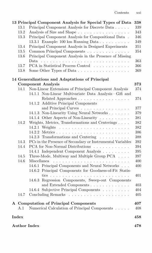
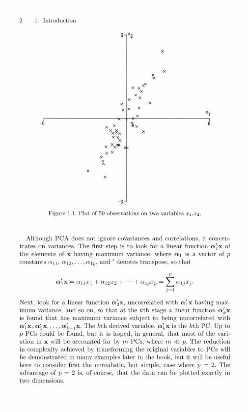
Figure 1.1. Plot of 50 observations on two variables x1,x2.
Although PCA does not ignore covariances and correlations, it concen-trates on variances. The first step is to look for a linear function α′
1x ofthe elements of x having maximum variance, where α1 is a vector of pconstants α11, α12, . . . , α1p, and ′ denotes transpose, so that
α′1x = α11x1 + α12x2 + · · · + α1pxp =
p∑
j=1
α1jxj .
Next, look for a linear function α′2x, uncorrelated with α′
1x having max-imum variance, and so on, so that at the kth stage a linear function α′
kxis found that has maximum variance subject to being uncorrelated withα′
1x, α′2x, . . . ,α′
k−1x. The kth derived variable, α′kx is the kth PC. Up to
p PCs could be found, but it is hoped, in general, that most of the vari-ation in x will be accounted for by m PCs, where m p. The reductionin complexity achieved by transforming the original variables to PCs willbe demonstrated in many examples later in the book, but it will be usefulhere to consider first the unrealistic, but simple, case where p = 2. Theadvantage of p = 2 is, of course, that the data can be plotted exactly intwo dimensions.

1.1. Definition and Derivation of Principal Components 3
Figure 1.2. Plot of the 50 observations from Figure 1.1 with respect to their PCsz1, z2.
Figure 1.1 gives a plot of 50 observations on two highly correlated vari-ables x1, x2 . There is considerable variation in both variables, thoughrather more in the direction of x2 than x1. If we transform to PCs z1, z2,we obtain the plot given in Figure 1.2.
It is clear that there is greater variation in the direction of z1 than ineither of the original variables, but very little variation in the direction ofz2. More generally, if a set of p (> 2) variables has substantial correlationsamong them, then the first few PCs will account for most of the variationin the original variables. Conversely, the last few PCs identify directionsin which there is very little variation; that is, they identify near-constantlinear relationships among the original variables.
As a taster of the many examples to come later in the book, Figure 1.3provides a plot of the values of the first two principal components in a7-variable example. The data presented here consist of seven anatomicalmeasurements on 28 students, 11 women and 17 men. This data set andsimilar ones for other groups of students are discussed in more detail inSections 4.1 and 5.1. The important thing to note here is that the first twoPCs account for 80 percent of the total variation in the data set, so that the

4 1. Introduction
Figure 1.3. Student anatomical measurements: plots of 28 students with respectto their first two PCs. × denotes women; denotes men.
2-dimensional picture of the data given in Figure 1.3 is a reasonably faith-ful representation of the positions of the 28 observations in 7-dimensionalspace. It is also clear from the figure that the first PC, which, as we shallsee later, can be interpreted as a measure of the overall size of each student,does a good job of separating the women and men in the sample.
Having defined PCs, we need to know how to find them. Consider, for themoment, the case where the vector of random variables x has a known co-variance matrix Σ. This is the matrix whose (i, j)th element is the (known)covariance between the ith and jth elements of x when i = j, and the vari-ance of the jth element of x when i = j. The more realistic case, where Σis unknown, follows by replacing Σ by a sample covariance matrix S (seeChapter 3). It turns out that for k = 1, 2, · · · , p, the kth PC is given byzk = α′
kx where αk is an eigenvector of Σ corresponding to its kth largesteigenvalue λk. Furthermore, if αk is chosen to have unit length (α′
kαk = 1),then var(zk) = λk, where var(zk) denotes the variance of zk.
The following derivation of these results is the standard one given inmany multivariate textbooks; it may be skipped by readers who mainlyare interested in the applications of PCA. Such readers could also skip
1.1. Definition and Derivation of Principal Components 5
much of Chapters 2 and 3 and concentrate their attention on later chapters,although Sections 2.3, 2.4, 3.3, 3.4, 3.8, and to a lesser extent 3.5, are likelyto be of interest to most readers.
To derive the form of the PCs, consider first α′1x; the vector α1 max-
imizes var[α′1x] = α′
1Σα1. It is clear that, as it stands, the maximumwill not be achieved for finite α1 so a normalization constraint must beimposed. The constraint used in the derivation is α′
1α1 = 1, that is, thesum of squares of elements of α1 equals 1. Other constraints, for exampleMaxj |α1j | = 1, may more useful in other circumstances, and can easily besubstituted later on. However, the use of constraints other than α′
1α1 =constant in the derivation leads to a more difficult optimization problem,and it will produce a set of derived variables different from the PCs.
To maximize α′1Σα1 subject to α′
1α1 = 1, the standard approach is touse the technique of Lagrange multipliers. Maximize
α′1Σα1 − λ(α′
1α1 − 1),
where λ is a Lagrange multiplier. Differentiation with respect to α1 gives
Σα1 − λα1 = 0,
or
(Σ − λIp)α1 = 0,
where Ip is the (p × p) identity matrix. Thus, λ is an eigenvalue of Σ andα1 is the corresponding eigenvector. To decide which of the p eigenvectorsgives α′
1x with maximum variance, note that the quantity to be maximizedis
α′1Σα1 = α′
1λα1 = λα′1α1 = λ,
so λ must be as large as possible. Thus, α1 is the eigenvector correspondingto the largest eigenvalue of Σ, and var(α′
1x) = α′1Σα1 = λ1, the largest
eigenvalue.In general, the kth PC of x is α′
kx and var(α′kx) = λk, where λk is
the kth largest eigenvalue of Σ, and αk is the corresponding eigenvector.This will now be proved for k = 2; the proof for k ≥ 3 is slightly morecomplicated, but very similar.
The second PC, α′2x, maximizes α′
2Σα2 subject to being uncorrelatedwith α′
1x, or equivalently subject to cov[α′1x,α′
2x] = 0, where cov(x, y)denotes the covariance between the random variables x and y . But
cov [α′1x,α′
2x] = α′1Σα2 = α′
2Σα1 = α′2λ1α
′1 = λ1α
′2α1 = λ1α
′1α2.
Thus, any of the equations
α′1Σα2 = 0, α′
2Σα1 = 0,α′
1α2 = 0, α′2α1 = 0
6 1. Introduction
could be used to specify zero correlation between α′1x and α′
2x. Choosingthe last of these (an arbitrary choice), and noting that a normalizationconstraint is again necessary, the quantity to be maximized is
α′2Σα2 − λ(α′
2α2 − 1) − φα′2α1,
where λ, φ are Lagrange multipliers. Differentiation with respect to α2
gives
Σα2 − λα2 − φα1 = 0
and multiplication of this equation on the left by α′1 gives
α′1Σα2 − λα′
1α2 − φα′1α1 = 0,
which, since the first two terms are zero and α′1α1 = 1, reduces to φ = 0.
Therefore, Σα2 − λα2 = 0, or equivalently (Σ − λIp)α2 = 0, so λ is oncemore an eigenvalue of Σ, and α2 the corresponding eigenvector.
Again, λ = α′2Σα2, so λ is to be as large as possible. Assuming that
Σ does not have repeated eigenvalues, a complication that is discussed inSection 2.4, λ cannot equal λ1. If it did, it follows that α2 = α1, violatingthe constraint α′
1α2 = 0. Hence λ is the second largest eigenvalue of Σ,and α2 is the corresponding eigenvector.
As stated above, it can be shown that for the third, fourth, . . . , pthPCs, the vectors of coefficients α3,α4, . . . ,αp are the eigenvectors of Σcorresponding to λ3, λ4, . . . , λp, the third and fourth largest, . . . , and thesmallest eigenvalue, respectively. Furthermore,
var[α′kx] = λk for k = 1, 2, . . . , p.
This derivation of the PC coefficients and variances as eigenvectors andeigenvalues of a covariance matrix is standard, but Flury (1988, Section 2.2)and Diamantaras and Kung (1996, Chapter 3) give alternative derivationsthat do not involve differentiation.
It should be noted that sometimes the vectors αk are referred toas ‘principal components.’ This usage, though sometimes defended (seeDawkins (1990), Kuhfeld (1990) for some discussion), is confusing. It ispreferable to reserve the term ‘principal components’ for the derived vari-ables α′
kx, and refer to αk as the vector of coefficients or loadings for thekth PC. Some authors distinguish between the terms ‘loadings’ and ‘coef-ficients,’ depending on the normalization constraint used, but they will beused interchangeably in this book.
1.2 A Brief History of Principal ComponentAnalysis
The origins of statistical techniques are often difficult to trace. Preisendor-fer and Mobley (1988) note that Beltrami (1873) and Jordan (1874)
1.2. A Brief History of Principal Component Analysis 7
independently derived the singular value decomposition (SVD) (see Sec-tion 3.5) in a form that underlies PCA. Fisher and Mackenzie (1923) usedthe SVD in the context of a two-way analysis of an agricultural trial. How-ever, it is generally accepted that the earliest descriptions of the techniquenow known as PCA were given by Pearson (1901) and Hotelling (1933).Hotelling’s paper is in two parts. The first, most important, part, togetherwith Pearson’s paper, is among the collection of papers edited by Bryantand Atchley (1975).
The two papers adopted different approaches, with the standard alge-braic derivation given above being close to that introduced by Hotelling(1933). Pearson (1901), on the other hand, was concerned with findinglines and planes that best fit a set of points in p-dimensional space, andthe geometric optimization problems he considered also lead to PCs, as willbe explained in Section 3.2
Pearson’s comments regarding computation, given over 50 years beforethe widespread availability of computers, are interesting. He states that hismethods ‘can be easily applied to numerical problems,’ and although hesays that the calculations become ‘cumbersome’ for four or more variables,he suggests that they are still quite feasible.
In the 32 years between Pearson’s and Hotelling’s papers, very littlerelevant material seems to have been published, although Rao (1964) in-dicates that Frisch (1929) adopted a similar approach to that of Pearson.Also, a footnote in Hotelling (1933) suggests that Thurstone (1931) wasworking along similar lines to Hotelling, but the cited paper, which isalso in Bryant and Atchley (1975), is concerned with factor analysis (seeChapter 7), rather than PCA.
Hotelling’s approach, too, starts from the ideas of factor analysis but, aswill be seen in Chapter 7, PCA, which Hotelling defines, is really ratherdifferent in character from factor analysis.
Hotelling’s motivation is that there may be a smaller ‘fundamental setof independent variables . . . which determine the values’ of the original pvariables. He notes that such variables have been called ‘factors’ in thepsychological literature, but introduces the alternative term ‘components’to avoid confusion with other uses of the word ‘factor’ in mathematics.Hotelling chooses his ‘components’ so as to maximize their successive con-tributions to the total of the variances of the original variables, and callsthe components that are derived in this way the ‘principal components.’The analysis that finds such components is then christened the ‘method ofprincipal components.’
Hotelling’s derivation of PCs is similar to that given above, using La-grange multipliers and ending up with an eigenvalue/eigenvector problem,but it differs in three respects. First, he works with a correlation, ratherthan covariance, matrix (see Section 2.3); second, he looks at the originalvariables expressed as linear functions of the components rather than com-ponents expressed in terms of the original variables; and third, he does notuse matrix notation.

8 1. Introduction
After giving the derivation, Hotelling goes on to show how to find thecomponents using the power method (see Appendix A1). He also discussesa different geometric interpretation from that given by Pearson, in terms ofellipsoids of constant probability for multivariate normal distributions (seeSection 2.2). A fairly large proportion of his paper, especially the secondpart, is, however, taken up with material that is not concerned with PCAin its usual form, but rather with factor analysis (see Chapter 7).
A further paper by Hotelling (1936) gave an accelerated version of thepower method for finding PCs; in the same year, Girshick (1936) providedsome alternative derivations of PCs, and introduced the idea that samplePCs were maximum likelihood estimates of underlying population PCs.
Girshick (1939) investigated the asymptotic sampling distributions of thecoefficients and variances of PCs, but there appears to have been only asmall amount of work on the development of different applications of PCAduring the 25 years immediately following publication of Hotelling’s paper.Since then, however, an explosion of new applications and further theoret-ical developments has occurred. This expansion reflects the general growthof the statistical literature, but as PCA requires considerable computingpower, the expansion of its use coincided with the widespread introductionof electronic computers. Despite Pearson’s optimistic comments, it is not re-ally feasible to do PCA by hand, unless p is about four or less. But it is pre-cisely for larger values of p that PCA is most useful, so that the full potentialof the technique could not be exploited until after the advent of computers.
Before ending this section, four papers will be mentioned; these appearedtowards the beginning of the expansion of interest in PCA and have becomeimportant references within the subject. The first of these, by Anderson(1963), is the most theoretical of the four. It discussed the asymptoticsampling distributions of the coefficients and variances of the sample PCs,building on the earlier work by Girshick (1939), and has been frequentlycited in subsequent theoretical developments.
Rao’s (1964) paper is remarkable for the large number of new ideas con-cerning uses, interpretations and extensions of PCA that it introduced, andwhich will be cited at numerous points in the book.
Gower (1966) discussed links between PCA and various other statisticaltechniques, and also provided a number of important geometric insights.
Finally, Jeffers (1967) gave an impetus to the really practical side of thesubject by discussing two case studies in which the uses of PCA go beyondthat of a simple dimension-reducing tool.
To this list of important papers the book by Preisendorfer and Mobley(1988) should be added. Although it is relatively unknown outside thedisciplines of meteorology and oceanography and is not an easy read, itrivals Rao (1964) in its range of novel ideas relating to PCA, some ofwhich have yet to be fully explored. The bulk of the book was written byPreisendorfer over a number of years, but following his untimely death themanuscript was edited and brought to publication by Mobley.

1.2. A Brief History of Principal Component Analysis 9
Despite the apparent simplicity of the technique, much research is stillbeing done in the general area of PCA, and it is very widely used. This isclearly illustrated by the fact that the Web of Science identifies over 2000articles published in the two years 1999–2000 that include the phrases ‘prin-cipal component analysis’ or ‘principal components analysis’ in their titles,abstracts or keywords. The references in this book also demonstrate thewide variety of areas in which PCA has been applied. Books or articlesare cited that include applications in agriculture, biology, chemistry, clima-tology, demography, ecology, economics, food research, genetics, geology,meteorology, oceanography, psychology and quality control, and it wouldbe easy to add further to this list.

2Mathematical and StatisticalProperties of Population PrincipalComponents
In this chapter many of the mathematical and statistical properties of PCsare discussed, based on a known population covariance (or correlation)matrix Σ. Further properties are included in Chapter 3 but in the contextof sample, rather than population, PCs. As well as being derived from astatistical viewpoint, PCs can be found using purely mathematical argu-ments; they are given by an orthogonal linear transformation of a set ofvariables optimizing a certain algebraic criterion. In fact, the PCs optimizeseveral different algebraic criteria and these optimization properties, to-gether with their statistical implications, are described in the first sectionof the chapter.
In addition to the algebraic derivation given in Chapter 1, PCs can also belooked at from a geometric viewpoint. The derivation given in the originalpaper on PCA by Pearson (1901) is geometric but it is relevant to samples,rather than populations, and will therefore be deferred until Section 3.2.However, a number of other properties of population PCs are also geometricin nature and these are discussed in the second section of this chapter.
The first two sections of the chapter concentrate on PCA based on acovariance matrix but the third section describes how a correlation, ratherthan a covariance, matrix may be used in the derivation of PCs. It alsodiscusses the problems associated with the choice between PCAs based oncovariance versus correlation matrices.
In most of this text it is assumed that none of the variances of the PCs areequal; nor are they equal to zero. The final section of this chapter explainsbriefly what happens in the case where there is equality between some ofthe variances, or when some of the variances are zero.

2.1. Optimal Algebraic Properties of Population Principal Components 11
Most of the properties described in this chapter have sample counter-parts. Some have greater relevance in the sample context, but it is moreconvenient to introduce them here, rather than in Chapter 3.
2.1 Optimal Algebraic Properties of PopulationPrincipal Components and Their StatisticalImplications
Consider again the derivation of PCs given in Chapter 1, and denote byz the vector whose kth element is zk, the kth PC, k = 1, 2, . . . , p. (Unlessstated otherwise, the kth PC will be taken to mean the PC with the kthlargest variance, with corresponding interpretations for the ‘kth eigenvalue’and ‘kth eigenvector.’) Then
z = A′x, (2.1.1)
where A is the orthogonal matrix whose kth column, αk, is the ktheigenvector of Σ. Thus, the PCs are defined by an orthonormal lineartransformation of x. Furthermore, we have directly from the derivationin Chapter 1 that
ΣA = AΛ, (2.1.2)
where Λ is the diagonal matrix whose kth diagonal element is λk, the ktheigenvalue of Σ, and λk = var(α′
kx) = var(zk). Two alternative ways ofexpressing (2.1.2) that follow because A is orthogonal will be useful later,namely
A′ΣA = Λ (2.1.3)
and
Σ = AΛA′. (2.1.4)
The orthonormal linear transformation of x, (2.1.1), which defines z, has anumber of optimal properties, which are now discussed in turn.
Property A1. For any integer q, 1 ≤ q ≤ p, consider the orthonormallinear transformation
y = B′x, (2.1.5)
where y is a q-element vector and B′ is a (q×p) matrix, and let Σy = B′ΣBbe the variance-covariance matrix for y. Then the trace of Σy, denotedtr (Σy), is maximized by taking B = Aq, where Aq consists of the first qcolumns of A.

12 2. Properties of Population Principal Components
Proof. Let βk be the kth column of B; as the columns of A form a basisfor p-dimensional space, we have
βk =p∑
j=1
cjkαj , k = 1, 2, . . . , q,
where cjk, j = 1, 2, . . . , p, k = 1, 2, . . . , q, are appropriately defined con-stants. Thus B = AC, where C is the (p× q) matrix with (j, k)th elementcjk, and
B′ΣB = C′A′ΣAC = C′ΛC, using (2.1.3)
=p∑
j=1
λjcjc′j
where c′j is the jth row of C. Therefore
tr(B′ΣB) =p∑
j=1
λj tr(cjc′j)
=p∑
j=1
λj tr(c′jcj)
=p∑
j=1
λjc′jcj
=p∑
j=1
q∑
k=1
λjc2jk. (2.1.6)
Now
C = A′B, soC′C = B′AA′B = B′B = Iq,
because A is orthogonal, and the columns of B are orthonormal. Hencep∑
j=1
q∑
k=1
c2jk = q, (2.1.7)
and the columns of C are also orthonormal. The matrix C can be thoughtof as the first q columns of a (p × p) orthogonal matrix, D, say. But therows of D are orthonormal and so satisfy d′
jdj = 1, j = 1, . . . , p. As therows of C consist of the first q elements of the rows of D, it follows thatc′jcj ≤ 1, j = 1, . . . , p, that is
q∑
k=1
c2jk ≤ 1. (2.1.8)

2.1. Optimal Algebraic Properties of Population Principal Components 13
Now∑q
k=1 c2jk is the coefficient of λj in (2.1.6), the sum of these coefficients
is q from (2.1.7), and none of the coefficients can exceed 1, from (2.1.8).Because λ1 > λ2 > · · · > λp, it is fairly clear that
∑pj=1(∑q
k=1 c2jk)λj will
be maximized if we can find a set of cjk for whichq∑
k=1
c2jk =
1, j = 1, . . . , q,0, j = q + 1, . . . , p.
(2.1.9)
But if B′ = A′q, then
cjk =
1, 1 ≤ j = k ≤ q,0, elsewhere,
which satisfies (2.1.9). Thus tr(Σy) achieves its maximum value when B′ =A′
q.
Property A2. Consider again the orthonormal transformation
y = B′x,
with x, B, A and Σy defined as before. Then tr(Σy) is minimized by takingB = A∗
q where A∗q consists of the last q columns of A.
Proof. The derivation of PCs given in Chapter 1 can easily be turnedaround for the purpose of looking for, successively, linear functions of xwhose variances are as small as possible, subject to being uncorrelatedwith previous linear functions. The solution is again obtained by findingeigenvectors of Σ, but this time in reverse order, starting with the smallest.The argument that proved Property A1 can be similarly adapted to proveProperty A2.
The statistical implication of Property A2 is that the last few PCs arenot simply unstructured left-overs after removing the important PCs. Be-cause these last PCs have variances as small as possible they are useful intheir own right. They can help to detect unsuspected near-constant linearrelationships between the elements of x (see Section 3.4), and they mayalso be useful in regression (Chapter 8), in selecting a subset of variablesfrom x (Section 6.3), and in outlier detection (Section 10.1).Property A3. (the Spectral Decomposition of Σ)
Σ = λ1α1α′1 + λ2α2α
′2 + · · · + λpαpα
′p. (2.1.10)
Proof.
Σ = AΛA′ from (2.1.4),
and expanding the right-hand side matrix product shows that Σ equalsp∑
k=1
λkαkα′k,
as required (see the derivation of (2.1.6)).

14 2. Properties of Population Principal Components
This result will prove to be useful later. Looking at diagonal elements,we see that
var(xj) =p∑
k=1
λkα2kj .
However, perhaps the main statistical implication of the result is that notonly can we decompose the combined variances of all the elements of xinto decreasing contributions due to each PC, but we can also decomposethe whole covariance matrix into contributions λkαkα′
k from each PC. Al-though not strictly decreasing, the elements of λkαkα′
k will tend to becomesmaller as k increases, as λk decreases for increasing k, whereas the ele-ments of αk tend to stay ‘about the same size’ because of the normalizationconstraints
α′kαk = 1, k = 1, 2, . . . , p.
Property Al emphasizes that the PCs explain, successively, as much aspossible of tr(Σ), but the current property shows, intuitively, that theyalso do a good job of explaining the off-diagonal elements of Σ. This isparticularly true when the PCs are derived from a correlation matrix, andis less valid when the covariance matrix is used and the variances of theelements of x are widely different (see Section 2.3).
It is clear from (2.1.10) that the covariance (or correlation) matrix canbe constructed exactly, given the coefficients and variances of the first rPCs, where r is the rank of the covariance matrix. Ten Berge and Kiers(1999) discuss conditions under which the correlation matrix can be exactlyreconstructed from the coefficients and variances of the first q (< r) PCs.
A corollary of the spectral decomposition of Σ concerns the conditionaldistribution of x, given the first q PCs, zq, q = 1, 2, . . . , (p − 1). It canbe shown that the linear combination of x that has maximum variance,conditional on zq, is precisely the (q + 1)th PC. To see this, we use theresult that the conditional covariance matrix of x, given zq, is
Σ − ΣxzΣ−1zz Σzx,
where Σzz is the covariance matrix for zq, Σxz is the (p × q) matrixwhose (j, k)th element is the covariance between xj and zk, and Σzx isthe transpose of Σxz (Mardia et al., 1979, Theorem 3.2.4).
It is seen in Section 2.3 that the kth column of Σxz is λkαk. The matrixΣ−1
zz is diagonal, with kth diagonal element λ−1k , so it follows that
ΣxzΣ−1zz Σzx =
q∑
k=1
λkαkλ−1k λkα′
k
=q∑
k=1
λkαkα′k,

2.1. Optimal Algebraic Properties of Population Principal Components 15
and, from (2.1.10),
Σ − ΣxzΣ−1zz Σzx =
p∑
k=(q+1)
λkαkα′k.
Finding a linear function of x having maximum conditional variancereduces to finding the eigenvalues and eigenvectors of the conditional co-variance matrix, and it easy to verify that these are simply (λ(q+1),α(q+1)),(λ(q+2),α(q+2)), . . . , (λp,αp). The eigenvector associated with the largestof these eigenvalues is α(q+1), so the required linear function is α′
(q+1)x,namely the (q + 1)th PC.
Property A4. As in Properties A1, A2, consider the transformationy = B′x. If det(Σy) denotes the determinant of the covariance matrix y,then det(Σy) is maximized when B = Aq.
Proof. Consider any integer, k, between 1 and q, and let Sk =the subspace of p-dimensional vectors orthogonal to α1, . . . ,αk−1. Thendim(Sk) = p− k + 1, where dim(Sk) denotes the dimension of Sk. The ktheigenvalue, λk, of Σ satisfies
λk = Supα∈Skα =0
α′Σα
α′α
.
Suppose that µ1 > µ2 > · · · > µq, are the eigenvalues of B′ΣB and thatγ1, γ2, · · · ,γq, are the corresponding eigenvectors. Let Tk = the subspaceof q-dimensional vectors orthogonal to γk+1, · · · ,γq, with dim(Tk) = k.Then, for any non-zero vector γ in Tk,
γ′B′ΣBγ
γ′γ≥ µk.
Consider the subspace Sk of p-dimensional vectors of the form Bγ for γ inTk.
dim(Sk) = dim(Tk) = k (because B is one-to-one; in fact,B preserves lengths of vectors).
From a general result concerning dimensions of two vector spaces, we have
dim(Sk ∩ Sk) + dim(Sk + Sk) = dim Sk + dim Sk.
But
dim(Sk + Sk) ≤ p, dim(Sk) = p − k + 1 and dim(Sk) = k,
so
dim(Sk ∩ Sk) ≥ 1.

16 2. Properties of Population Principal Components
There is therefore a non-zero vector α in Sk of the form α = Bγ for aγ in Tk, and it follows that
µk ≤ γ′B′ΣBγ
γ′γ=
γ′B′ΣBγ
γB′Bγ=
α′Σα
α′α≤ λk.
Thus the kth eigenvalue of B′ΣB ≤ kth eigenvalue of Σ for k = 1, · · · , q.This means that
det(Σy) =q∏
k=1
(kth eigenvalue of B′ΣB) ≤q∏
k=1
λk.
But if B = Aq, then the eigenvalues of B′ΣB are
λ1, λ2, · · · , λq, so that det(Σy) =q∏
k=1
λk
in this case, and therefore det(Σy) is maximized when B = Aq.
The result can be extended to the case where the columns of B are notnecessarily orthonormal, but the diagonal elements of B′B are unity (seeOkamoto (1969)). A stronger, stepwise version of Property A4 is discussedby O’Hagan (1984), who argues that it provides an alternative derivation ofPCs, and that this derivation can be helpful in motivating the use of PCA.O’Hagan’s derivation is, in fact, equivalent to (though a stepwise versionof) Property A5, which is discussed next.
Note that Property A1 could also have been proved using similar reason-ing to that just employed for Property A4, but some of the intermediateresults derived during the earlier proof of Al are useful elsewhere in thechapter.
The statistical importance of the present result follows because the de-terminant of a covariance matrix, which is called the generalized variance,can be used as a single measure of spread for a multivariate random vari-able (Press, 1972, p. 108). The square root of the generalized variance,for a multivariate normal distribution is proportional to the ‘volume’ inp-dimensional space that encloses a fixed proportion of the probability dis-tribution of x. For multivariate normal x, the first q PCs are, therefore, asa consequence of Property A4, q linear functions of x whose joint probabil-ity distribution has contours of fixed probability enclosing the maximumvolume.
Property A5. Suppose that we wish to predict each random variable, xj
in x by a linear function of y, where y = B′x, as before. If σ2j is the residual
variance in predicting xj from y, then Σpj=1σ
2j is minimized if B = Aq.
The statistical implication of this result is that if we wish to get the bestlinear predictor of x in a q-dimensional subspace, in the sense of minimizingthe sum over elements of x of the residual variances, then this optimalsubspace is defined by the first q PCs.
2.1. Optimal Algebraic Properties of Population Principal Components 17
It follows that although Property A5 is stated as an algebraic property,it can equally well be viewed geometrically. In fact, it is essentially thepopulation equivalent of sample Property G3, which is stated and provedin Section 3.2. No proof of the population result A5 will be given here; Rao(1973, p. 591) outlines a proof in which y is replaced by an equivalent setof uncorrelated linear functions of x, and it is interesting to note that thePCs are the only set of p linear functions of x that are uncorrelated andhave orthogonal vectors of coefficients. This last result is prominent in thediscussion of Chapter 11.
A special case of Property A5 was pointed out in Hotelling’s (1933)original paper. He notes that the first PC derived from a correlation matrixis the linear function of x that has greater mean square correlation withthe elements of x than does any other linear function. We return to thisinterpretation of the property, and extend it, in Section 2.3.
A modification of Property A5 can be introduced by noting that if x ispredicted by a linear function of y = B′x, then it follows from standardresults from multivariate regression (see, for example, Mardia et al., 1979,p. 160), that the residual covariance matrix for the best such predictor is
Σx − ΣxyΣ−1y Σyx, (2.1.11)
where Σx = Σ,Σy = B′ΣB, as defined before, Σxy is the matrix whose(j, k)th element is the covariance between the jth element of x and thekth element of y, and Σyx is the transpose of Σxy. Now Σyx = B′Σ, andΣxy = ΣB, so (2.1.11) becomes
Σ − ΣB(B′ΣB)−1B′Σ. (2.1.12)
The diagonal elements of (2.1.12) are σ2j , j = 1, 2, . . . , p, so, from Property
A5, B = Aq minimizes
p∑
j=1
σ2j = tr[Σ − ΣB(B′ΣB)−1B′Σ].
A derivation of this result in the sample case, and further discussion of it,is provided by Jong and Kotz (1999).
An alternative criterion is ‖Σ−ΣB(B′ΣB)−1B′Σ‖, where ‖ · ‖ denotesthe Euclidean norm of a matrix and equals the square root of the sum ofsquares of all the elements in the matrix. It can be shown (Rao, 1964) thatthis alternative criterion is also minimized when B = Aq.
This section has dealt with PCs derived from covariance matrices. Manyof their properties are also relevant, in modified form, for PCs based oncorrelation matrices, as discussed in Section 2.3. That section also containsa further algebraic property which is specific to correlation matrix-basedPCA.

18 2. Properties of Population Principal Components
2.2 Geometric Properties of Population PrincipalComponents
It was noted above that Property A5 can be interpreted geometrically, aswell as algebraically, and the discussion following Property A4 shows thatA4, too, has a geometric interpretation. We now look at two further, purelygeometric, properties.Property G1. Consider the family of p-dimensional ellipsoids
x′Σ−1x = const. (2.2.1)
The PCs define the principal axes of these ellipsoids.
Proof. The PCs are defined by the transformation (2.1.1) z = A′x, andsince A is orthogonal, the inverse transformation is x = Az. Substitutinginto (2.2.1) gives
(Az)′Σ−1(Az) = const = z′A′Σ−1Az.
It is well known that the eigenvectors of Σ−1 are the same as those of Σ,and that the eigenvalues of Σ−1 are the reciprocals of those of Σ, assumingthat they are all strictly positive. It therefore follows, from a correspondingresult to (2.1.3), that AΣ−1A = Λ−1 and hence
z′Λ−1z = const.
This last equation can be rewrittenp∑
k=1
z2k
λk= const (2.2.2)
and (2.2.2) is the equation for an ellipsoid referred to its principal axes.Equation (2.2.2) also implies that the half-lengths of the principal axes areproportional to λ
1/21 , λ
1/22 , . . . , λ
1/2p .
This result is statistically important if the random vector x has a mul-tivariate normal distribution. In this case, the ellipsoids given by (2.2.1)define contours of constant probability for the distribution of x. The first(largest) principal axis of such ellipsoids will then define the direction inwhich statistical variation is greatest, which is another way of expressingthe algebraic definition of the first PC given in Section 1.1. The directionof the first PC, defining the first principal axis of constant probability el-lipsoids, is illustrated in Figures 2.1 and 2.2 in Section 2.3. The secondprincipal axis maximizes statistical variation, subject to being orthogonalto the first, and so on, again corresponding to the algebraic definition. Thisinterpretation of PCs, as defining the principal axes of ellipsoids of constantdensity, was mentioned by Hotelling (1933) in his original paper.
It would appear that this particular geometric property is only of directstatistical relevance if the distribution of x is multivariate normal, whereas
2.2. Geometric Properties of Population Principal Components 19
for most other properties of PCs no distributional assumptions are required.However, the property will be discussed further in connection with PropertyG5 in Section 3.2, where we see that it has some relevance even withoutthe assumption of multivariate normality. Property G5 looks at the sampleversion of the ellipsoids x′Σx = const. Because Σ and Σ−1 share the sameeigenvectors, it follows that the principal axes of the ellipsoids x′Σx = constare the same as those of x′Σ−1x = const, except that that their order isreversed.
We digress slightly here to note that some authors imply, or even stateexplicitly, as do Qian et al. (1994), that PCA needs multivariate normal-ity. This text takes a very different view and considers PCA as a mainlydescriptive technique. It will become apparent that many of the propertiesand applications of PCA and related techniques described in later chap-ters, as well as the properties discussed in the present chapter, have noneed for explicit distributional assumptions. It cannot be disputed thatlinearity and covariances/correlations, both of which play a central role inPCA, have especial relevance when distributions are multivariate normal,but this does not detract from the usefulness of PCA when data have otherforms. Qian et al. (1994) describe what might be considered an additionalproperty of PCA, based on minimum description length or stochastic com-plexity (Rissanen and Yu, 2000), but as they use it to define a somewhatdifferent technique, we defer discussion to Section 14.4.
Property G2. Suppose that x1, x2 are independent random vectors, bothhaving the same probability distribution, and that x1, x2, are both subjectedto the same linear transformation
yi = B′xi, i = 1, 2.
If B is a (p × q) matrix with orthonormal columns chosen to maximizeE[(y1 − y2)′(y1 − y2)], then B = Aq, using the same notation as before.
Proof. This result could be viewed as a purely algebraic property, and,indeed, the proof below is algebraic. The property is, however, includedin the present section because it has a geometric interpretation. This isthat the expected squared Euclidean distance, in a q-dimensional subspace,between two vectors of p random variables with the same distribution, ismade as large as possible if the subspace is defined by the first q PCs.
To prove Property G2, first note that x1, x2 have the same mean µ andcovariance matrix Σ. Hence y1, y2 also have the same mean and covariancematrix, B′µ, B′ΣB respectively.
E[(y1 − y2)′(y1 − y2)] = E[(y1 − B′µ) − (y2 − (B′µ)]′[(y1 − B′µ)− (y2 − B′µ)]
= E[(y1 − B′µ)′(y1 − B′µ)]+ E[(y2 − B′µ)′(y2 − B′µ)].
20 2. Properties of Population Principal Components
The cross-product terms disappear because of the independence of x1, x2,and hence of y1, y2.
Now, for i = 1, 2, we have
E[(yi − B′µ)′(yi − B′µ)] = Etr[(yi − B′µ)′(yi − B′µ)]= Etr[(yi − B′µ)(yi − B′µ)′]= trE[(yi − B′µ)(yi − B′µ)′]= tr(B′ΣB).
But tr(B′ΣB) is maximized when B = Aq, from Property A1, and thepresent criterion has been shown above to be 2 tr(B′ΣB). Hence PropertyG2 is proved.
There is a closely related property whose geometric interpretation is moretenuous, namely that with the same definitions as in Property G2,
detE[(y1 − y2)(y1 − y2)′]
is maximized when B = Aq (see McCabe (1984)). This property says thatB = Aq makes the generalized variance of (y1 − y2) as large as possible.Generalized variance may be viewed as an alternative measure of distanceapart of y1 and y2 in q-dimensional space, though a less intuitively obviousmeasure than expected squared Euclidean distance.
Finally, Property G2 can be reversed in the sense that if E[(y1−y2)′(y1−y2)] or detE[(y1 − y2)(y1 − y2)′] is to be minimized, then this can beachieved by taking B = A∗
q .The properties given in this section and in the previous one show that
covariance matrix PCs satisfy several different optimality criteria, but thelist of criteria covered is by no means exhaustive; for example, Devijverand Kittler (1982, Chapter 9) show that the first few PCs minimize rep-resentation entropy and the last few PCs minimize population entropy.Diamantaras and Kung (1996, Section 3.4) discuss PCA in terms of max-imizing mutual information between x and y. Further optimality criteriaare given by Hudlet and Johnson (1982), McCabe (1984) and Okamoto(1969). The geometry of PCs is discussed at length by Treasure (1986).
The property of self-consistency is useful in a non-linear extension ofPCA (see Section 14.1.2). For two p-variate random vectors x, y, the vectory is self-consistent for x if E(x|y) = y. Flury (1997, Section 8.4) shows thatif x is a p-variate random vector with a multivariate normal or ellipticaldistribution, and y is the orthogonal projection of x onto the q-dimensionalsubspace spanned by the first q PCs for x, then y is self-consistent for x.Tarpey (1999) uses self-consistency of principal components after lineartransformation of the variables to characterize elliptical distributions.

2.3. Principal Components Using a Correlation Matrix 21
2.3 Principal Components Using a CorrelationMatrix
The derivation and properties of PCs considered above are based on theeigenvectors and eigenvalues of the covariance matrix. In practice, as willbe seen in much of the remainder of this text, it is more common to defineprincipal components as
z = A′x∗, (2.3.1)
where A now has columns consisting of the eigenvectors of the correlationmatrix, and x∗ consists of standardized variables. The goal in adoptingsuch an approach is to find the principal components of a standardizedversion x∗ of x, where x∗ has jth element xj/σ
1/2jj , j = 1, 2, . . . , p, xj is
the jth element of x, and σjj is the variance of xj . Then the covariancematrix for x∗ is the correlation matrix of x, and the PCs of x∗ are givenby (2.3.1).
A third possibility, instead of using covariance or correlation matrices,is to use covariances of xj/wj , where the weights wj are chosen to reflectsome a priori idea of the relative importance of the variables. The specialcase wj = σ
1/2jj leads to x∗, and to PCs based on the correlation matrix,
but various authors have argued that the choice of wj = σ1/2jj is somewhat
arbitrary, and that different values of wj might be better in some applica-tions (see Section 14.2.1). In practice, however, it is relatively unusual thata uniquely appropriate set of wj suggests itself.
All the properties of the previous two sections are still valid for corre-lation matrices, or indeed for covariances based on other sets of weights,except that we are now considering PCs of x∗ (or some other transformationof x), instead of x.
It might seem that the PCs for a correlation matrix could be obtainedfairly easily from those for the corresponding covariance matrix, since x∗
is related to x by a very simple transformation. However, this is not thecase; the eigenvalues and eigenvectors of the correlation matrix have nosimple relationship with those of the corresponding covariance matrix. Inparticular, if the PCs found from the correlation matrix are expressed interms of x by transforming back from x∗ to x, then these PCs are notthe same as the PCs found from Σ, except in very special circumstances(Chatfield and Collins, 1989, Section 4.4). One way of explaining this isthat PCs are invariant under orthogonal transformations of x but not, ingeneral, under other transformations (von Storch and Zwiers, 1999, Section13.1.10). The transformation from x to x∗ is not orthogonal. The PCsfor correlation and covariance matrices do not, therefore, give equivalentinformation, nor can they be derived directly from each other. We nowdiscuss the relative merits of the two types of PC.
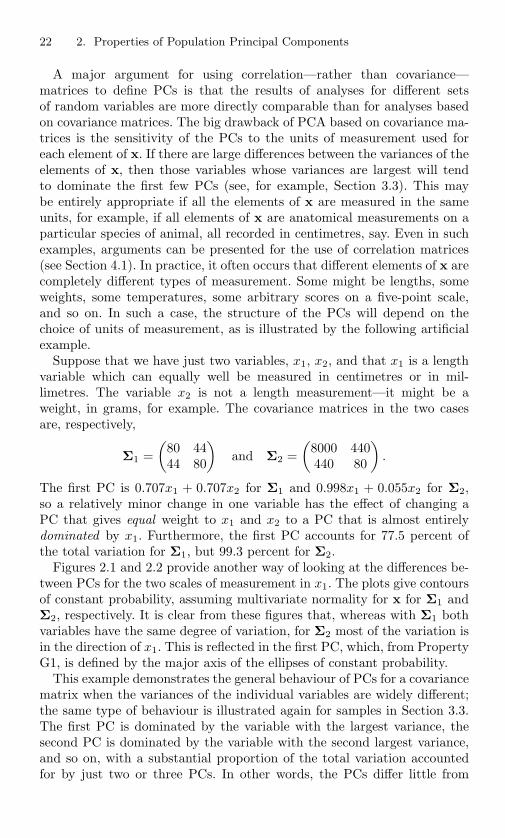
22 2. Properties of Population Principal Components
A major argument for using correlation—rather than covariance—matrices to define PCs is that the results of analyses for different setsof random variables are more directly comparable than for analyses basedon covariance matrices. The big drawback of PCA based on covariance ma-trices is the sensitivity of the PCs to the units of measurement used foreach element of x. If there are large differences between the variances of theelements of x, then those variables whose variances are largest will tendto dominate the first few PCs (see, for example, Section 3.3). This maybe entirely appropriate if all the elements of x are measured in the sameunits, for example, if all elements of x are anatomical measurements on aparticular species of animal, all recorded in centimetres, say. Even in suchexamples, arguments can be presented for the use of correlation matrices(see Section 4.1). In practice, it often occurs that different elements of x arecompletely different types of measurement. Some might be lengths, someweights, some temperatures, some arbitrary scores on a five-point scale,and so on. In such a case, the structure of the PCs will depend on thechoice of units of measurement, as is illustrated by the following artificialexample.
Suppose that we have just two variables, x1, x2, and that x1 is a lengthvariable which can equally well be measured in centimetres or in mil-limetres. The variable x2 is not a length measurement—it might be aweight, in grams, for example. The covariance matrices in the two casesare, respectively,
Σ1 =(
80 4444 80
)and Σ2 =
(8000 440440 80
).
The first PC is 0.707x1 + 0.707x2 for Σ1 and 0.998x1 + 0.055x2 for Σ2,so a relatively minor change in one variable has the effect of changing aPC that gives equal weight to x1 and x2 to a PC that is almost entirelydominated by x1. Furthermore, the first PC accounts for 77.5 percent ofthe total variation for Σ1, but 99.3 percent for Σ2.
Figures 2.1 and 2.2 provide another way of looking at the differences be-tween PCs for the two scales of measurement in x1. The plots give contoursof constant probability, assuming multivariate normality for x for Σ1 andΣ2, respectively. It is clear from these figures that, whereas with Σ1 bothvariables have the same degree of variation, for Σ2 most of the variation isin the direction of x1. This is reflected in the first PC, which, from PropertyG1, is defined by the major axis of the ellipses of constant probability.
This example demonstrates the general behaviour of PCs for a covariancematrix when the variances of the individual variables are widely different;the same type of behaviour is illustrated again for samples in Section 3.3.The first PC is dominated by the variable with the largest variance, thesecond PC is dominated by the variable with the second largest variance,and so on, with a substantial proportion of the total variation accountedfor by just two or three PCs. In other words, the PCs differ little from
2.3. Principal Components Using a Correlation Matrix 23
Figure 2.1. Contours of constant probability based on Σ1 =(
8044
4480
).
Figure 2.2. Contours of constant probability based on Σ2 =(
8000440
44080
).

24 2. Properties of Population Principal Components
the original variables rearranged in decreasing order of the size of theirvariances. Also, the first few PCs account for little of the off-diagonal ele-ments of Σ in this case (see Property A3) above. In most circumstances,such a transformation to PCs is of little value, and it will not occur if thecorrelation, rather than covariance, matrix is used.
The example has shown that it is unwise to use PCs on a covariancematrix when x consists of measurements of different types, unless there is astrong conviction that the units of measurements chosen for each element ofx are the only ones that make sense. Even when this condition holds, usingthe covariance matrix will not provide very informative PCs if the variableshave widely differing variances. Furthermore, with covariance matrices andnon-commensurable variables the PC scores are difficult to interpret—whatdoes it mean to add a temperature to a weight? For correlation matrices, thestandardized variates are all dimensionless and can be happily combinedto give PC scores (Legendre and Legendre, 1983, p. 129).
Another problem with the use of covariance matrices is that it is moredifficult than with correlation matrices to compare informally the resultsfrom different analyses. Sizes of variances of PCs have the same implicationsfor different correlation matrices of the same dimension, but not for differentcovariance matrices. Also, patterns of coefficients in PCs can be readilycompared for different correlation matrices to see if the two correlationmatrices are giving similar PCs, whereas informal comparisons are oftenmuch trickier for covariance matrices. Formal methods for comparing PCsfrom different covariance matrices are, however, available (see Section 13.5).
The use of covariance matrices does have one general advantage overcorrelation matrices, and a particular advantage seen in a special case. Thegeneral advantage is that statistical inference regarding population PCsbased on sample PCs is easier for covariance matrices than for correlationmatrices, as will be discussed in Section 3.7. This is relevant when PCAis used in a context where statistical inference is important. However, inpractice, it is more common to use PCA as a descriptive, rather than aninferential, tool, and then the potential advantage of covariance matrixPCA is irrelevant.
The second advantage of covariance matrices holds in the special casewhen all elements of x are measured in the same units. It can then beargued that standardizing the elements of x to give correlations is equiv-alent to making an arbitrary choice of measurement units. This argumentof arbitrariness can also be applied more generally to the use of correlationmatrices, but when the elements of x are measurements of different types,the choice of measurement units leading to a covariance matrix is evenmore arbitrary, so that the correlation matrix is again preferred.
Standardizing the variables may be thought of as an attempt to removethe problem of scale dependence from PCA. Another way of doing this isto compute PCs of the logarithms of the original data (Flury, 1997, Section8.4), though this is only feasible and sensible for restricted types of data,

2.3. Principal Components Using a Correlation Matrix 25
as in allometry (Section 13.2) and for compositional data (Section 13.3).We conclude this section by looking at three interesting properties which
hold for PCs derived from the correlation matrix. The first is that thePCs depend not on the absolute values of correlations, but only on theirratios. This follows because multiplication of all off-diagonal elements ofa correlation matrix by the same constant leaves the eigenvectors of thematrix unchanged (Chatfield and Collins, 1989, p. 67).
The second property, which was noted by Hotelling (1933) in his originalpaper, is that if, instead of the normalization α′
kαk = 1, we use
α′kαk = λk, k = 1, 2, . . . , p, (2.3.2)
then, αkj the jth element of αk, is the correlation between the jth stan-dardized variable x∗
j and the kth PC. To see this note that for k =1, 2, . . . , p,
αk = λ1/2k αk, var(zk) = λk,
and the p-element vector Σαk has as its jth element the covariance betweenx∗
j and zk. But Σαk = λkαk, so the covariance between x∗j and zk is λkαkj .
Also var(x∗j ) = 1, and the correlation between x∗
j and zk is therefore
λkαjk
[var(x∗j ) var(zk)]1/2
= λ1/2k αkj
= αkj ,
as required.Because of this property the normalization (2.3.2) is quite often used, in
particular in computer packages, but it has the disadvantage that it is lesseasy to informally interpret and compare a set of PCs when each PC has adifferent normalization on its coefficients. This remark is, of course, relevantto sample, rather than population, PCs, but, as with some other parts ofthe chapter, it is included here to avoid a possibly disjointed presentation.
Both of these properties that hold for correlation matrices can bemodified for covariance matrices, but the results are, in each case, lessstraightforward.
The third property is sufficiently substantial to deserve a label. It isincluded in this section because, at first sight, it is specific to correlationmatrix PCA although, as we will see, its implications are much wider.Proofs of the result are available in the references cited below and will notbe reproduced here.Property A6. For any integer q, 1 ≤ q ≤ p, consider the orthonormallinear transformation
y = B′x, (2.3.3)
as defined in Property A1. Let R2j:q be the squared multiple correlation be-
tween xj and the q variables y1, y2, . . . , yq, defined by the elements of y.
26 2. Properties of Population Principal Components
The criterion
p∑
j=1
R2j:q
is maximized when y1, y2, . . . , yq are the first q correlation matrix PCs.The maximized value of the criterion is equal to the sum of the q largesteigenvalues of the correlation matrix.
Because the principal components are uncorrelated, the criterion inProperty A6 reduces to
p∑
j=1
q∑
k=1
r2jk
where r2jk is the squared correlation between the jth variable and the
kth PC. The criterion will be maximized by any matrix B that givesy spanning the same q-dimensional space as the first q PCs. How-ever, the correlation matrix PCs are special, in that they successivelymaximize the criterion for q = 1, 2, . . . , p. As noted following Prop-erty A5, this result was given by Hotelling (1933) alongside his originalderivation of PCA, but it has subsequently been largely ignored. It isclosely related to Property A5. Meredith and Millsap (1985) derivedProperty A6 independently and noted that optimizing the multiple cor-relation criterion gives a scale invariant method (as does Property A5;Cadima, 2000). One implication of this scale invariance is that it givesadded importance to correlation matrix PCA. The latter is not simplya variance-maximizing technique for standardized variables; its derivedvariables are also the result of optimizing a criterion which is scaleinvariant, and hence is relevant whether or not the variables are stan-dardized. Cadima (2000) discusses Property A6 in greater detail andargues that optimization of its multiple correlation criterion is actuallya new technique, which happens to give the same results as correla-tion matrix PCA, but is broader in its scope. He suggests that thederived variables be called Most Correlated Components. Looked at fromanother viewpoint, this broader relevance of correlation matrix PCAgives another reason to prefer it over covariance matrix PCA in mostcircumstances.
To conclude this discussion, we note that Property A6 can be easilymodified to give a new property for covariance matrix PCA. The first qcovariance marix PCs maximize, amongst all orthonormal linear transfor-mations of x, the sum of squared covariances between x1, x2, . . . , xp andthe derived variables y1, y2, . . . , yq. Covariances, unlike correlations, are notscale invariant, and hence neither is covariance matrix PCA.

2.4. Principal Components with Equal and/or Zero Variances 27
2.4 Principal Components with Equal and/or ZeroVariances
The final, short, section of this chapter discusses two problems that mayarise in theory, but are relatively uncommon in practice. In most of thischapter it has been assumed, implicitly or explicitly, that the eigenvaluesof the covariance or correlation matrix are all different, and that none ofthem is zero.
Equality of eigenvalues, and hence equality of variances of PCs, will occurfor certain patterned matrices. The effect of this occurrence is that for agroup of q equal eigenvalues, the corresponding q eigenvectors span a certainunique q-dimensional space, but, within this space, they are, apart frombeing orthogonal to one another, arbitrary. Geometrically (see PropertyG1), what happens for q = 2 or 3 is that the principal axes of a circle orsphere cannot be uniquely defined; a similar problem arises for hypersphereswhen q > 3. Thus individual PCs corresponding to eigenvalues in a group ofequal eigenvalues are not uniquely defined. A further problem with equal-variance PCs is that statistical inference becomes more complicated (seeSection 3.7).
The other complication, variances equal to zero, occurs rather more fre-quently, but is still fairly unusual. If q eigenvalues are zero, then the rankof Σ is (p − q) rather than p, and this outcome necessitates modificationsto the proofs of some properties given in Section 2.1 above. Any PC withzero variance defines an exactly constant linear relationship between theelements of x. If such relationships exist, then they imply that one variableis redundant for each relationship, as its value can be determined exactlyfrom the values of the other variables appearing in the relationship. Wecould therefore reduce the number of variables from p to (p − q) withoutlosing any information. Ideally, exact linear relationships should be spottedbefore doing a PCA, and the number of variables reduced accordingly. Al-ternatively, any exact or near-exact linear relationships uncovered by thelast few PCs can be used to select a subset of variables that contain mostof the information available in all of the original variables. This and relatedideas are more relevant to samples than to populations and are discussedfurther in Sections 3.4 and 6.3.
There will always be the same number of zero eigenvalues for a cor-relation matrix as for the corresponding covariance matrix, since an exactlinear relationship between the elements of x clearly implies an exact linearrelationship between the standardized variables, and vice versa. There isnot the same equivalence, however, when it comes to considering equal vari-ance PCs. Equality of some of the eigenvalues in a covariance (correlation)matrix need not imply that any of the eigenvalues of the correspondingcorrelation (covariance) matrix are equal. A simple example is when the pvariables all have equal correlations but unequal variances. If p > 2, then

28 2. Properties of Population Principal Components
the last (p−1) eigenvalues of the correlation matrix are equal (see Morrison,1976, Section 8.6), but this relationship will not hold, in general, for thecovariance matrix. Further discussion of patterns in covariance or correla-tion matrices, and their implications for the structure of the correspondingPCs, is given in Section 3.8.

3Mathematical and StatisticalProperties of Sample PrincipalComponents
The first part of this chapter is similar in structure to Chapter 2, exceptthat it deals with properties of PCs obtained from a sample covariance(or correlation) matrix, rather than from a population covariance (or cor-relation) matrix. The first two sections of the chapter, as in Chapter 2,describe, respectively, many of the algebraic and geometric properties ofPCs. Most of the properties discussed in Chapter 2 are almost the same forsamples as for populations. They will be mentioned again, but only briefly.There are, in addition, some properties that are relevant only to samplePCs, and these will be discussed more fully.
The third and fourth sections of the chapter again mirror those of Chap-ter 2. The third section discusses, with an example, the choice betweencorrelation and covariance matrices, while the fourth section looks at theimplications of equal and/or zero variances among the PCs, and illustratesthe potential usefulness of the last few PCs in detecting near-constantrelationships between the variables.
The last five sections of the chapter cover material having no counterpartin Chapter 2. Section 3.5 discusses the singular value decomposition, whichcould have been included in Section 3.1 as an additional algebraic property.However, the topic is sufficiently important to warrant its own section, asit provides a useful alternative approach to some of the theory surroundingPCs, and also gives an efficient practical method for actually computingPCs.
The sixth section looks at the probability distributions of the coefficientsand variances of a set of sample PCs, in other words, the probability distri-butions of the eigenvectors and eigenvalues of a sample covariance matrix.
30 3. Properties of Sample Principal Components
The seventh section then goes on to show how these distributions may beused to make statistical inferences about the population PCs, based onsample PCs.
Section 3.8 demonstrates how the approximate structure and variancesof PCs can sometimes be deduced from patterns in the covariance or cor-relation matrix. Finally, in Section 3.9 we discuss models that have beenproposed for PCA. The material could equally well have been included inChapter 2, but because the idea of maximum likelihood estimation arisesin some of the models we include it in the present chapter.
3.1 Optimal Algebraic Properties of SamplePrincipal Components
Before looking at the properties themselves, we need to establish somenotation. Suppose that we have n independent observations on the p-element random vector x; denote these n observations by x1,x2, . . . ,xn.Let zi1 = a′
1xi, i = 1, 2, . . . , n, and choose the vector of coefficients a′1 to
maximize the sample variance
1n − 1
n∑
i=1
(zi1 − z1)2
subject to the normalization constraint a′1a1 = 1. Next let zi2 = a′
2xi, i =1, 2, . . . , n, and choose a′
2 to maximize the sample variance of the zi2 subjectto the normalization constraint a′
2a2 = 1, and subject also to the zi2 beinguncorrelated with the zi1 in the sample. Continuing this process in anobvious manner, we have a sample version of the definition of PCs given inSection 1.1. Thus a′
kx is defined as the kth sample PC, k = 1, 2, . . . , p, andzik is the score for the ith observation on the kth PC. If the derivation inSection 1.1 is followed through, but with sample variances and covariancesreplacing population quantities, then it turns out that the sample varianceof the PC scores for the kth sample PC is lk, the kth largest eigenvalue of thesample covariance matrix S for x1,x2, . . . ,xn, and ak is the correspondingeigenvector for k = 1, 2, . . . , p.
Define the (n × p) matrices X and Z to have (i, k)th elements equal tothe value of the kth element xik of xi, and to zik, respectively. Then Z andX are related by Z = XA, where A is the (p×p) orthogonal matrix whosekth column is ak.
If the mean of each element of x is known to be zero, then S = 1nX′X.
It is far more usual for the mean of x to be unknown, and in this case the(j, k)th element of S is
1n − 1
n∑
i=1
(xij − xj)(xik − xk),
3.1. Optimal Algebraic Properties of Sample Principal Components 31
where
xj =1n
n∑
i=1
xij , j = 1, 2, . . . , p.
The matrix S can therefore be written as
S =1
n − 1X′X, (3.1.1)
where X is an (n × p) matrix with (i, j)th element (xij − xj); the repre-sentation (3.1.1) will be very useful in this and subsequent chapters. Thenotation xij will be used to denote the (i, j)th element of X, so that xij isthe value of the jth variable measured about its mean xj for the ith obser-vation. A final notational point is that it will be convenient to define thematrix of PC scores as
Z = XA, (3.1.2)
rather than as it was in the earlier definition. These PC scores will haveexactly the same variances and covariances as those given by Z, but willhave zero means, rather than means zk, k = 1, 2, . . . , p.
Another point to note is that the eigenvectors of 1n−1X
′X and X′X areidentical, and the eigenvalues of 1
n−1X′X are simply 1
n−1 (the eigenvaluesof X′X). Because of these relationships it will be convenient in some placesbelow to work in terms of eigenvalues and eigenvectors of X′X, rather thandirectly with those of S.
Turning to the algebraic properties A1–A5 listed in Section 2.1, define
yi = B′xi for i = 1, 2, . . . , n, (3.1.3)
where B, as in Properties A1, A2, A4, A5, is a (p×q) matrix whose columnsare orthonormal. Then Properties A1, A2, A4, A5, still hold, but with thesample covariance matrix of the observations yi, i = 1, 2, . . . , n, replacingΣy, and with the matrix A now defined as having kth column ak, withAq, A∗
q , respectively, representing its first and last q columns. Proofs inall cases are similar to those for populations, after making appropriatesubstitutions of sample quantities in place of population quantities, andwill not be repeated. Property A5 reappears as Property G3 in the nextsection and a proof will be given there.
The spectral decomposition, Property A3, also holds for samples in theform
S = l1a1a′1 + l2a2a′
2 + · · · + lpapa′p. (3.1.4)
The statistical implications of this expression, and the other algebraic prop-erties, A1, A2, A4, A5, are virtually the same as for the correspondingpopulation properties in Section 2.1, except that they must now be viewedin a sample context.
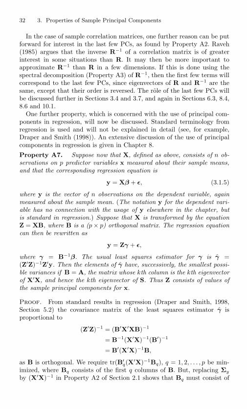
32 3. Properties of Sample Principal Components
In the case of sample correlation matrices, one further reason can be putforward for interest in the last few PCs, as found by Property A2. Raveh(1985) argues that the inverse R−1 of a correlation matrix is of greaterinterest in some situations than R. It may then be more important toapproximate R−1 than R in a few dimensions. If this is done using thespectral decomposition (Property A3) of R−1, then the first few terms willcorrespond to the last few PCs, since eigenvectors of R and R−1 are thesame, except that their order is reversed. The role of the last few PCs willbe discussed further in Sections 3.4 and 3.7, and again in Sections 6.3, 8.4,8.6 and 10.1.
One further property, which is concerned with the use of principal com-ponents in regression, will now be discussed. Standard terminology fromregression is used and will not be explained in detail (see, for example,Draper and Smith (1998)). An extensive discussion of the use of principalcomponents in regression is given in Chapter 8.
Property A7. Suppose now that X, defined as above, consists of n ob-servations on p predictor variables x measured about their sample means,and that the corresponding regression equation is
y = Xβ + ε, (3.1.5)
where y is the vector of n observations on the dependent variable, againmeasured about the sample mean. (The notation y for the dependent vari-able has no connection with the usage of y elsewhere in the chapter, butis standard in regression.) Suppose that X is transformed by the equationZ = XB, where B is a (p × p) orthogonal matrix. The regression equationcan then be rewritten as
y = Zγ + ε,
where γ = B−1β. The usual least squares estimator for γ is γ =(Z′Z)−1Z′y. Then the elements of γ have, successively, the smallest possi-ble variances if B = A, the matrix whose kth column is the kth eigenvectorof X′X, and hence the kth eigenvector of S. Thus Z consists of values ofthe sample principal components for x.
Proof. From standard results in regression (Draper and Smith, 1998,Section 5.2) the covariance matrix of the least squares estimator γ isproportional to
(Z′Z)−1 = (B′X′XB)−1
= B−1(X′X)−1(B′)−1
= B′(X′X)−1B,
as B is orthogonal. We require tr(B′q(X
′X)−1Bq), q = 1, 2, . . . , p be min-imized, where Bq consists of the first q columns of B. But, replacing Σy
by (X′X)−1 in Property A2 of Section 2.1 shows that Bq must consist of
3.2. Geometric Properties of Sample Principal Components 33
the last q columns of a matrix whose kth column is the kth eigenvectorof (X′X)−1. Furthermore, (X′X)−1 has the same eigenvectors as X′X, ex-cept that their order is reversed, so that Bq must have columns equal tothe first q eigenvectors of X′X. As this holds for q = 1, 2, . . . , p, PropertyA7 is proved.
This property seems to imply that replacing the predictor variables in aregression analysis by their first few PCs is an attractive idea, as those PCsomitted have coefficients that are estimated with little precision. The flaw inthis argument is that nothing in Property A7 takes account of the strengthof the relationship between the dependent variable y and the elements ofx, or between y and the PCs. A large variance for γk, the kth element ofγ, and hence an imprecise estimate of the degree of relationship between yand the kth PC, zk, does not preclude a strong relationship between y andzk (see Section 8.2). Further discussion of Property A7 is given by Fombyet al. (1978).
There are a number of other properties of PCs specific to the samplesituation; most have geometric interpretations and are therefore dealt within the next section.
3.2 Geometric Properties of Sample PrincipalComponents
As with the algebraic properties, the geometric properties of Chapter 2are also relevant for sample PCs, although with slight modifications to thestatistical implications. In addition to these properties, the present sectionincludes a proof of a sample version of Property A5, viewed geometrically,and introduces two extra properties which are relevant to sample, but notpopulation, PCs.
Property G1 is still valid for samples if Σ is replaced by S. The ellipsoidsx′S−1x = const no longer have the interpretation of being contours ofconstant probability, though they will provide estimates of such contoursif x1,x2, . . . ,xn are drawn from a multivariate normal distribution. Re-introducing a non-zero mean, the ellipsoids
(x − x)′S−1(x − x) = const
give contours of equal Mahalanobis distance from the sample mean x.Flury and Riedwyl (1988, Section 10.6) interpret PCA as successively find-ing orthogonal directions for which the Mahalanobis distance from thedata set to a hypersphere enclosing all the data is minimized (see Sec-tions 5.3, 9.1 and 10.1 for discussion of Mahalanobis distance in a varietyof forms).

34 3. Properties of Sample Principal Components
Property G2 may also be carried over from populations to samples asfollows. Suppose that the observations x1,x2, . . .xn are transformed by
yi = B′xi, i = 1, 2, . . . , n,
where B is a (p × q) matrix with orthonormal columns, so thaty1,y2, . . . ,yn, are projections of x1,x2, . . . ,xn onto a q-dimensionalsubspace. Then
n∑
h=1
n∑
i=1
(yh − yi)′(yh − yi)
is maximized when B = Aq. Conversely, the same criterion is minimizedwhen B = A∗
q .This property means that if the n observations are projected onto a
q-dimensional subspace, then the sum of squared Euclidean distances be-tween all pairs of observations in the subspace is maximized when thesubspace is defined by the first q PCs, and minimized when it is definedby the last q PCs. The proof that this property holds is again rather sim-ilar to that for the corresponding population property and will not berepeated.
The next property to be considered is equivalent to Property A5.Both are concerned, one algebraically and one geometrically, with leastsquares linear regression of each variable xj on the q variables containedin y.
Property G3. As before, suppose that the observations x1,x2, . . . ,xn
are transformed by yi = B′xi, i = 1, 2, . . . , n, where B is a (p × q) ma-trix with orthonormal columns, so that y1,y2, . . . ,yn are projections ofx1,x2, . . . ,xn onto a q-dimensional subspace. A measure of ‘goodness-of-fit’ of this q-dimensional subspace to x1,x2, . . . ,xn can be defined as thesum of squared perpendicular distances of x1,x2, . . . ,xn from the subspace.This measure is minimized when B = Aq.
Proof. The vector yi is an orthogonal projection of xi onto a q-dimensional subspace defined by the matrix B. Let mi denote the positionof yi in terms of the original coordinates, and ri = xi − mi. (See Fig-ure 3.1 for the special case where p = 2, q = 1; in this case yi is a scalar,whose value is the length of mi.) Because mi is an orthogonal projectionof xi onto a q-dimensional subspace, ri is orthogonal to the subspace, sor′imi = 0. Furthermore, r′iri is the squared perpendicular distance of xi
from the subspace so that the sum of squared perpendicular distances ofx1,x2, . . . ,xn from the subspace is
n∑
i=1
r′iri.
3.2. Geometric Properties of Sample Principal Components 35
Figure 3.1. Orthogonal projection of a two-dimensional vector onto a one-dimen-sional subspace.
Now
x′ixi = (mi + ri)′(mi + ri)
= m′imi + r′iri + 2r′imi
= m′imi + r′iri.
Thusn∑
i=1
r′iri =n∑
i=1
x′ixi −
n∑
i=1
m′imi,
so that, for a given set of observations, minimization of the sum of squaredperpendicular distances is equivalent to maximization of
∑ni=1 m′
imi. Dis-tances are preserved under orthogonal transformations, so the squareddistance m′
imi of yi from the origin is the same in y coordinates as inx coordinates. Therefore, the quantity to be maximized is
∑ni=1 y′
iyi. But
n∑
i=1
y′iyi =
n∑
i=1
x′iBB′xi
36 3. Properties of Sample Principal Components
= trn∑
i=1
(x′iBB′xi)
=n∑
i=1
tr(x′iBB′xi)
=n∑
i=1
tr(B′xix′iB)
= tr
[
B′(
n∑
i=1
xix′i
)
B
]
= tr[B′X′XB]= (n − 1) tr(B′SB).
Finally, from Property A1, tr(B′SB) is maximized when B = Aq.
Instead of treating this property (G3) as just another property of samplePCs, it can also be viewed as an alternative derivation of the PCs. Ratherthan adapting for samples the algebraic definition of population PCs givenin Chapter 1, there is an alternative geometric definition of sample PCs.They are defined as the linear functions (projections) of x1,x2, . . . ,xn thatsuccessively define subspaces of dimension 1, 2, . . . , q, . . . , (p− 1) for whichthe sum of squared perpendicular distances of x1,x2, . . . ,xn from the sub-space is minimized. This definition provides another way in which PCs canbe interpreted as accounting for as much as possible of the total variationin the data, within a lower-dimensional space. In fact, this is essentiallythe approach adopted by Pearson (1901), although he concentrated on thetwo special cases, where q = 1 and q = (p − 1). Given a set of points in p-dimensional space, Pearson found the ‘best-fitting line,’ and the ‘best-fittinghyperplane,’ in the sense of minimizing the sum of squared deviations ofthe points from the line or hyperplane. The best-fitting line determines thefirst principal component, although Pearson did not use this terminology,and the direction of the last PC is orthogonal to the best-fitting hyper-plane. The scores for the last PC are simply the perpendicular distances ofthe observations from this best-fitting hyperplane.
Property G4. Let X be the (n × p) matrix whose (i, j)th element isxij − xj, and consider the matrix XX′. The ith diagonal element of XX′
is∑p
j=1(xij − xj)2, which is the squared Euclidean distance of xi from thecentre of gravity x of the points x1,x2, . . . ,xn, where x = 1
n
∑ni=1 xi. Also,
the (h, i)th element of XX′ is∑p
j=1(xhj − xj)(xij − xj), which measuresthe cosine of the angle between the lines joining xh and xi to x, multipliedby the distances of xh and xi from x. Thus XX′ contains informationabout the configuration of x1,x2, . . . ,xn relative to x. Now suppose thatx1,x2, . . . ,xn are projected onto a q-dimensional subspace with the usualorthogonal transformation yi = B′xi, i = 1, 2, . . . , n. Then the transfor-

3.2. Geometric Properties of Sample Principal Components 37
mation for which B = Aq minimizes the distortion in the configuration asmeasured by ‖YY′ − XX′‖, where ‖ · ‖ denotes Euclidean norm and Y isa matrix with (i, j)th element yij − yj.
Proof. Y = XB, so
YY′ = XBB′X and ‖YY′ − XX′‖ = ‖XBB′X′ − XX′‖.A matrix result given by Rao (1973, p. 63) states that if F is a symmetricmatrix of rank p with spectral decomposition
F = f1φ1φ′1 + f2φ2φ
′2 + · · · + fpφpφ
′p,
and G is a matrix of rank q < p chosen to minimize ||F − G||, then
G = f1φ1φ′1 + f2φ2φ
′2 + · · · + fqφqφ
′q.
Assume that X has rank p, so that xi − x, i = 1, 2, . . . , n, span p-dimensional space, and are not contained in any proper subspace. ThenXX′ also has rank p, and Rao’s result can be used with F = XX′, andG = YY′.
Now, if lk, ak denote the kth eigenvalue and eigenvector, respectively, ofX′X, then the kth eigenvalue and eigenvector of XX′ are lk and l
−1/2k Xak,
respectively, k = 1, 2, . . . , p. The remaining (n − p) eigenvalues of XX′ arezero.
Using Rao’s result above, ‖YY′ − XX′‖ is minimized when
G = XBB′X′ = l−11 l1Xa1a′
1X′ + l−1
2 l2Xa2a′2X
′ + · · · + l−1q lqXaqa′
qX′,
or
XBB′X′ = Xa1a′1X
′ + Xa2a′2X
′ + · · · + Xaqa′qX
′.
Multiplying both sides of this equation on the left by (X′X)−1X′ and onthe right by X(X′X)−1, gives
BB′ = a1a′1 + a2a′
2 + · · · + aqa′q,
from which it follows that the columns of B and the first q eigenvectorsof X′X, or equivalently of S, span the same q-dimensional subspace. Inother words, the transformation B = Aq provides the required optimalsubspace.
Note that the result given by Rao (1973, p. 63) which was used inthe above proof implies that the sum of the first q terms in the spec-tral decomposition of the sample covariance (or correlation) matrix Sprovides the rank q matrix qS that minimizes ‖qS − S‖. Furthermore,‖qS − S‖ =
∑pk=q+1 lk, where lk now denotes the kth eigenvalue of S,
rather than that of X′X. The result follows because
‖qS − S‖ =
∥∥∥∥∥∥
p∑
k=q+1
lkaka′k
∥∥∥∥∥∥
38 3. Properties of Sample Principal Components
=p∑
k=q+1
lk ‖aka′k‖
=p∑
k=q+1
lk
p∑
i=1
p∑
j=1
(akiakj)2
1/2
=p∑
k=q+1
lk
p∑
i=1
a2ki
p∑
j=1
a2kj
1/2
=p∑
k=q+1
lk,
as a′kak = 1, k = 1, 2, . . . , p.
Property G4 is very similar to another optimality property of PCs, dis-cussed in terms of the so-called RV-coefficient by Robert and Escoufier(1976). The RV-coefficient was introduced as a measure of the similaritybetween two configurations of n data points, as described by XX′ andYY′. The distance between the two configurations is defined by Robertand Escoufier (1976) as
∥∥∥∥
XX′
tr(XX′)21/2− YY′
tr(YY′)21/2
∥∥∥∥ , (3.2.1)
where the divisors of XX′, YY′ are introduced simply to standardize therepresentation of each configuration in the sense that
∥∥∥∥
XX′
tr(XX′)21/2
∥∥∥∥ =
∥∥∥∥
YY′
tr(YY′)21/2
∥∥∥∥ = 1.
It can then be shown that (3.2.1) equals [2(1 − RV(X,Y))]1/2, where theRV-coefficient is defined as
RV(X,Y) =tr(XY′YX′)
tr(XX′)2 tr(YY′)21/2. (3.2.2)
Thus, minimizing the distance measure (3.2.1) which, apart from stan-dardizations, is the same as the criterion of Property G4, is equivalent tomaximization of RV(X,Y). Robert and Escoufier (1976) show that severalmultivariate techniques can be expressed in terms of maximizing RV(X,Y)for some definition of X and Y. In particular, if Y is restricted to be ofthe form Y = XB, where B is a (p × q) matrix such that the columns ofY are uncorrelated, then maximization of RV(X,Y) leads to B = Aq, thatis Y consists of scores on the first q PCs. We will meet the RV-coefficientagain in Chapter 6 in the context of variable selection.Property G5. The algebraic derivation of sample PCs reduces to find-ing, successively, vectors ak, k = 1, 2, . . . , p, that maximize a′
kSak subjectto a′
kak = 1, and subject to a′kal = 0 for l < k. This statement of the
problem can be viewed geometrically as follows (Stuart, 1982).

3.3. Covariance and Correlation Matrices: An Example 39
Consider the first PC; this maximizes a′Sa subject to a′a = 1. Buta′Sa = const defines a family of ellipsoids and a′a = 1 defines a hyper-sphere in p-dimensional space, both centred at the origin. The hyperspherea′a = 1 will intersect more than one of the ellipsoids in the family a′Sa(unless S is the identity matrix), and the points at which the hypersphereintersects the ‘biggest’ such ellipsoid (so that a′Sa is maximized) lie onthe shortest principal axis of the ellipsoid. A simple diagram, as given byStuart (1982), readily verifies this result when p = 2. The argument can beextended to show that the first q sample PCs are defined by the q shortestprincipal axes of the family of ellipsoids a′Sa = const. Although Stuart(1982) introduced this interpretation in terms of sample PCs, it is equallyvalid for population PCs.
The earlier geometric property G1 was also concerned with ellipsoids butin the context of multivariate normality, where the ellipsoids x′Σ−1x =const define contours of constant probability and where the first (longest)q principal axes of such ellipsoids define the first q population PCs. In lightof Property G5, it is clear that the validity of the Property G1 does notreally depend on the assumption of multivariate normality. Maximization ofa′Sa is equivalent to minimization of a′S−1a, and looking for the ‘smallest’ellipsoids in the family a′S−1a = const that intersect the hypersphere a′a =1 will lead to the largest principal axis of the family a′S−1a. Thus the PCsdefine, successively, the principal axes of the ellipsoids a′S−1a = const.Similar considerations hold for the population ellipsoids a′Σ−1a = const,regardless of any assumption of multivariate normality. However, withoutmultivariate normality the ellipsoids lose their interpretation as contoursof equal probability, or as estimates of such contours in the sample case.
Further discussion of the geometry of sample PCs, together with con-nections with other techniques such as principal coordinate analysis (seeSection 5.2) and special cases such as compositional data (Section 13.3), isgiven by Gower (1967).
As with population properties, our discussion of sample properties ofPCA is not exhaustive. For example, Qian et al. (1994) consider the con-cept of stochastic complexity or minimum description length, as describedby Rissanen and Yu (2000). They minimize the expected difference in com-plexity between a p-dimensional data set and the projection of the data ontoa q-dimensional subspace. Qian et al. show that, if multivariate normalityis assumed, the subset spanned by the first q PCs is obtained.
3.3 Covariance and Correlation Matrices: AnExample
The arguments for and against using sample correlation matrices as op-posed to covariance matrices are virtually identical to those given forpopulations in Section 2.3. Furthermore, it is still the case that there is no

40 3. Properties of Sample Principal Components
Table 3.1. Correlations and standard deviations for eight blood chemistryvariables.
Correlation matrix (n = 72)
rblood plate wblood neut lymph bilir sodium potass
rblood 1.000plate 0.290 1.000wblood 0.202 0.415 1.000neut −0.055 0.285 0.419 1.000lymph −0.105 −0.376 −0.521 −0.877 1.000bilir −0.252 −0.349 −0.441 −0.076 0.206 1.000sodium −0.229 −0.164 −0.145 0.023 0.034 0.192 1.000potass 0.058 −0.129 −0.076 −0.131 0.151 0.077 0.423 1.000
Standard 0.371 41.253 1.935 0.077 0.071 4.037 2.732 0.297deviations
straightforward relationship between the PCs obtained from a correlationmatrix and those based on the corresponding covariance matrix. The mainpurpose of the present section is to give an example illustrating some of theproperties of PCs based on sample covariance and correlation matrices.
The data for this example consist of measurements on 8 blood chemistryvariables for 72 patients in a clinical trial. The correlation matrix for thesedata, together with the standard deviations of each of the eight variables,is given in Table 3.1. Two main points emerge from Table 3.1. First, thereare considerable differences in the standard deviations, caused mainly bydifferences in scale for the eight variables, and, second, none of the correla-tions is particularly large in absolute value, apart from the value of −0.877for NEUT and LYMPH.
The large differences in standard deviations give a warning that theremay be considerable differences between the PCs for the correlation andcovariance matrices. That this is indeed true can be seen in Tables 3.2and 3.3, which give coefficients for the first four components, based on thecorrelation and covariance matrices respectively. For ease of comparison,the coefficients are rounded to the nearest 0.2. The effect of such severerounding is investigated for this example in Section 10.3.
Each of the first four PCs for the correlation matrix has moderate-sizedcoefficients for several of the variables, whereas the first four PCs for thecovariance matrix are each dominated by a single variable. The first com-ponent is a slight perturbation of the single variable PLATE, which has thelargest variance; the second component is almost the same as the variableBILIR with the second highest variance; and so on. In fact, this patterncontinues for the fifth and sixth components, which are not shown in Ta-ble 3.3. Also, the relative percentages of total variation accounted for byeach component closely mirror the variances of the corresponding variables.
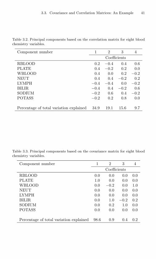
3.3. Covariance and Correlation Matrices: An Example 41
Table 3.2. Principal components based on the correlation matrix for eight bloodchemistry variables.
Component number 1 2 3 4Coefficients
RBLOOD 0.2 −0.4 0.4 0.6PLATE 0.4 −0.2 0.2 0.0WBLOOD 0.4 0.0 0.2 −0.2NEUT 0.4 0.4 −0.2 0.2LYMPH −0.4 −0.4 0.0 −0.2BILIR −0.4 0.4 −0.2 0.6SODIUM −0.2 0.6 0.4 −0.2POTASS −0.2 0.2 0.8 0.0
Percentage of total variation explained 34.9 19.1 15.6 9.7
Table 3.3. Principal components based on the covariance matrix for eight bloodchemistry variables.
Component number 1 2 3 4Coefficients
RBLOOD 0.0 0.0 0.0 0.0PLATE 1.0 0.0 0.0 0.0WBLOOD 0.0 −0.2 0.0 1.0NEUT 0.0 0.0 0.0 0.0LYMPH 0.0 0.0 0.0 0.0BILIR 0.0 1.0 −0.2 0.2SODIUM 0.0 0.2 1.0 0.0POTASS 0.0 0.0 0.0 0.0
Percentage of total variation explained 98.6 0.9 0.4 0.2

42 3. Properties of Sample Principal Components
Because variable PLATE has a variance 100 times larger than any othervariable, the first PC accounts for over 98 percent of the total variation.Thus the first six components for the covariance matrix tell us almost noth-ing apart from the order of sizes of variances of the original variables. Bycontrast, the first few PCs for the correlation matrix show that certainnon-trivial linear functions of the (standardized) original variables accountfor substantial, though not enormous, proportions of the total variation inthe standardized variables. In particular, a weighted contrast between thefirst four and the last four variables is the linear function with the largestvariance.
This example illustrates the dangers in using a covariance matrix to findPCs when the variables have widely differing variances; the first few PCswill usually contain little information apart from the relative sizes of vari-ances, information which is available without a PCA. There are, however,circumstances in which it has been argued that using the covariance matrixhas some advantages; see, for example, Naik and Khattree (1996), althoughthese authors transform their data (track record times for Olympic eventsare transformed to speeds) in order to avoid highly disparate variances.
Apart from the fact already mentioned in Section 2.3, namely, that itis more difficult to base statistical inference regarding PCs on correlationmatrices, one other disadvantage of correlation matrix PCs is that theygive coefficients for standardized variables and are therefore less easy to in-terpret directly. To interpret the PCs in terms of the original variables eachcoefficient must be divided by the standard deviation of the correspondingvariable. An example which illustrates this is given in the next section.It must not be forgotten, however, that correlation matrix PCs, when re-expressed in terms of the original variables, are still linear functions of xthat maximize variance with respect to the standardized variables and notwith respect to the original variables.
An alternative to finding PCs for either covariance or correlation matricesis to calculate the eigenvectors of X′X rather than X′X, that is, measurevariables about zero, rather than about their sample means, when comput-ing ‘covariances’ and ‘correlations.’ This idea was noted by Reyment andJoreskog (1993, Section 5.4) and will be discussed further in Section 14.2.3.‘Principal component analysis’ based on measures of association of thisform, but for observations rather than variables, has been found useful forcertain types of geological data (Reyment and Joreskog, 1993). Anothervariant, in a way the opposite of that just mentioned, has been used byBuckland and Anderson (1985), among others. Their idea, which is alsodiscussed further in Section 14.2.3, and which again is appropriate for aparticular type of data, is to ‘correct for the mean’ in both the rows andcolumns of X. Further possibilities, such as the use of weights or metrics,are described in Section 14.2.
3.4. Principal Components with Equal and/or Zero Variances 43
3.4 Principal Components with Equal and/or ZeroVariances
The problems that arise when some of the eigenvalues of a populationcovariance matrix are zero and/or equal were discussed in Section 2.4;similar considerations hold when dealing with a sample.
In practice, exactly equal non-zero eigenvalues are extremely rare. Evenif the underlying population covariance or correlation matrix has a patternthat gives equal eigenvalues, sampling variation will almost always ensurethat the sample eigenvalues are unequal. It should be noted, however, thatnearly equal eigenvalues need careful attention. The subspace spanned by aset of nearly equal eigenvalues that are well-separated from all other eigen-values is well-defined and stable, but individual PC directions within thatsubspace are unstable (see Section 10.3). This has implications for decidinghow many components to retain (Section 6.1), for assessing which observa-tions are influential (Section 10.2) and for deciding which components torotate (Section 11.1).
With carefully selected variables, PCs with zero variances are a relativelyrare occurrence. When q zero eigenvalues do occur for a sample covarianceor correlation matrix, the implication is that the points x1,x2, . . . ,xn liein a (p− q)-dimensional subspace of p-dimensional space. This means thatthere are q separate linear functions of the p original variables having con-stant values for each of the observations x1,x2, . . . ,xn. Ideally, constantrelationships between the variables should be detected before doing a PCA,and the number of variables reduced so as to avoid them. However, priordetection will not always be possible, and the zero-variance PCs will enableany unsuspected constant relationships to be detected. Similarly, PCs withvery small, but non-zero, variances will define near-constant linear rela-tionships. Finding such near-constant relationships may be of considerableinterest. In addition, low-variance PCs have a number of more specific po-tential uses, as will be discussed at the end of Section 3.7 and in Sections 6.3,8.4, 8.6 and 10.1.
3.4.1 Example
Here we consider a second set of blood chemistry data, this time consistingof 16 variables measured on 36 patients. In fact, these observations andthose discussed in the previous section are both subsets of the same largerdata set. In the present subset, four of the variables, x1, x2, x3, x4, sum to1.00 for 35 patients and to 0.99 for the remaining patient, so that x1 +x2 + x3 + x4 is nearly constant. The last (sixteenth) PC for the correlationmatrix has variance less than 0.001, much smaller than the fifteenth, andis (rounding coefficients to the nearest 0.1) 0.7x∗
1 + 0.3x∗2 + 0.7x∗
3 + 0.1x∗4,
with all of the other 12 variables having negligible coefficients. Thus, the

44 3. Properties of Sample Principal Components
near-constant relationship has certainly been identified by the last PC, butnot in an easily interpretable form. However, a simple interpretation can berestored if the standardized variables are replaced by the original variablesby setting x∗
j = xj/s1/2jj , where s
1/2jj is the sample standard deviation of xj .
When this is done, the last PC becomes (rounding coefficients to the nearestinteger) 11x1 + 11x2 + 11x3 + 11x4. The correct near-constant relationshiphas therefore been discovered exactly, to the degree of rounding used, bythe last PC.
3.5 The Singular Value Decomposition
This section describes a result from matrix theory, namely the singularvalue decomposition (SVD), which is relevant to PCA in several respects.Given an arbitrary matrix X of dimension (n× p), which for our purposeswill invariably be a matrix of n observations on p variables measured abouttheir means, X can be written
X = ULA′, (3.5.1)
where
(i) U, A are (n × r), (p × r) matrices, respectively, each of which hasorthonormal columns so that U′U = Ir,A′A = Ir;
(ii) L is an (r × r) diagonal matrix;
(iii) r is the rank of X.
To prove this result, consider the spectral decomposition of X′X. The last(p − r) terms in (3.1.4) and in the corresponding expression for X′X arezero, since the last (p − r) eigenvalues are zero if X, and hence X′X, hasrank r. Thus
(n − 1)S = X′X = l1a1a′1 + l2a2a′
2 + · · · + lrara′r.
[Note that in this section it is convenient to denote the eigenvalues of X′X,rather than those of S, as lk, k = 1, 2, . . . , p.] Define A to be the (p × r)matrix with kth column ak, define U as the (n × r) matrix whose kthcolumn is
uk = l−1/2k Xak, k = 1, 2, . . . , r,
and define L to be the (r × r) diagonal matrix with kth diagonal elementl1/2k . Then U, L, A satisfy conditions (i) and (ii) above, and we shall now
3.5. The Singular Value Decomposition 45
show that X = ULA′.
ULA′ = U
l1/21 a′
1
l1/22 a′
2...
l1/2r a′
r
=r∑
k=1
l−1/2k Xakl
1/2k a′
k =r∑
k=1
Xaka′k
=p∑
k=1
Xaka′k.
This last step follows because ak, k = (r+1), (r+2), . . . , p, are eigenvectorsof X′X corresponding to zero eigenvalues. The vector Xak is a vector ofscores on the kth PC; the column-centering of X and the zero variance ofthe last (p−r) PCs together imply that Xak = 0, k = (r+1), (r+2), . . . , p.Thus
ULA′ = Xp∑
k=1
aka′k = X,
as required, because the (p × p) matrix whose kth column is ak, isorthogonal, and so has orthonormal rows.
The importance of the SVD for PCA is twofold. First, it provides acomputationally efficient method of actually finding PCs (see AppendixA1). It is clear that if we can find U, L, A satisfying (3.5.1), then A andL will give us the eigenvectors and the square roots of the eigenvalues ofX′X, and hence the coefficients and standard deviations of the principalcomponents for the sample covariance matrix S. As a bonus we also get inU scaled versions of PC scores. To see this multiply (3.5.1) on the rightby A to give XA = ULA′A = UL, as A′A = Ir. But XA is an (n × r)matrix whose kth column consists of the PC scores for the kth PC (see(3.1.2) for the case where r = p). The PC scores zik are therefore given by
zik = uikl1/2k , i = 1, 2, . . . , n, k = 1, 2, . . . , r,
or, in matrix form, Z = UL, or U = ZL−1. The variance of the scoresfor the kth PC is lk
(n−1) , k = 1, 2, . . . , p. [Recall that lk here denotes thekth eigenvalue of X′X, so that the kth eigenvalue of S is lk
(n−1) .] Thereforethe scores given by U are simply those given by Z, but scaled to havevariance 1
(n−1) . Note also that the columns of U are the eigenvectors ofXX′ corresponding to non-zero eigenvalues, and these eigenvectors are ofpotential interest if the roles of ‘variables’ and ‘observations’ are reversed.
A second virtue of the SVD is that it provides additional insight intowhat a PCA actually does, and it gives useful means, both graphical and
46 3. Properties of Sample Principal Components
algebraic, of representing the results of a PCA. This has been recognizedin different contexts by Mandel (1972), Gabriel (1978), Rasmusson et al.(1981) and Eastment and Krzanowski (1982), and will be discussed fur-ther in connection with relevant applications in Sections 5.3, 6.1.5, 9.3,13.4, 13.5 and 13.6. Furthermore, the SVD is useful in terms of bothcomputation and interpretation in PC regression (see Section 8.1 and Man-del (1982)) and in examining the links between PCA and correspondenceanalysis (Sections 13.1 and 14.2).
In the meantime, note that (3.5.1) can be written element by element as
xij =r∑
k=1
uikl1/2k ajk, (3.5.2)
where uik, ajk are the (i, k)th, (j, k)th elements of U, A, respectively, andl1/2k is the kth diagonal element of L. Thus xij can be split into parts
uikl1/2k ajk, k = 1, 2, . . . , r,
corresponding to each of the first r PCs. If only the first m PCs are retained,then
mxij =m∑
k=1
uikl1/2k ajk (3.5.3)
provides an approximation to xij . In fact, it can be shown (Gabriel, 1978;Householder and Young, 1938) that mxij gives the best possible rank mapproximation to xij , in the sense of minimizing
n∑
i=1
p∑
j=1
(mxij − xij)2, (3.5.4)
where mxij is any rank m approximation to xij . Another way of express-ing this result is that the (n × p) matrix whose (i, j)th element is mxij
minimizes ‖mX−X‖ over all (n× p) matrices mX with rank m. Thus theSVD provides a sequence of approximations to X of rank 1, 2, . . . , r, whichminimize the Euclidean norm of the difference between X and the approx-imation mX. This result provides an interesting parallel to the result givenearlier (see the proof of Property G4 in Section 3.2): that the spectral de-composition of X′X provides a similar optimal sequence of approximationsof rank 1, 2, . . . , r to the matrix X′X. Good (1969), in a paper extolling thevirtues of the SVD, remarks that Whittle (1952) presented PCA in termsof minimizing (3.5.4).
Finally in this section we note that there is a useful generalization of theSVD, which will be discussed in Chapter 14.

3.6. Probability Distributions for Sample Principal Components 47
3.6 Probability Distributions for Sample PrincipalComponents
A considerable amount of mathematical effort has been expended on deriv-ing probability distributions, mostly asymptotic, for the coefficients in thesample PCs and for the variances of sample PCs or, equivalently, findingdistributions for the eigenvectors and eigenvalues of a sample covariancematrix. For example, the first issue of Journal of Multivariate Analysis in1982 contained three papers, totalling 83 pages, on the topic. In recentyears there has probably been less theoretical work on probability distri-butions directly connected to PCA; this may simply reflect the fact thatthere is little remaining still to do. The distributional results that havebeen derived suffer from three drawbacks:
(i) they usually involve complicated mathematics;
(ii) they are mostly asymptotic;
(iii) they are often based on the assumption that the original set of variableshas a multivariate normal distribution.
Despite these drawbacks, the distributional results are useful in some cir-cumstances, and a selection of the main circumstances is given in thissection. Their use in inference about the population PCs, given samplePCs, is discussed in the next section.
Assume that x ∼ N(µ,Σ), that is, x has a p-variate normal distributionwith mean µ and covariance matrix Σ. Although µ need not be given, Σis assumed known. Then
(n − 1)S ∼ Wp(Σ, n − 1),
that is (n − 1)S has the so-called Wishart distribution with parametersΣ, (n−1) (see, for example, Mardia et al. (1979, Section 3.4)). Therefore, in-vestigation of the sampling properties of the coefficients and variances of thesample PCs is equivalent to looking at sampling properties of eigenvectorsand eigenvalues of Wishart random variables.
The density function of a matrix V that has the Wp(Σ, n−1) distributionis
c|V|(n−p−2)/2 exp−1
2tr(Σ−1V)
,
where
c−1 = 2p(n−1)/2Πp(1−p)/4|Σ|(n−1)/2
p∏
j=1
Γ(
n − j
2
),
and various properties of Wishart random variables have been thoroughlyinvestigated (see, for example, Srivastava and Khatri, 1979, Chapter 3).

48 3. Properties of Sample Principal Components
Let lk, ak, for k = 1, 2, . . . , p be the eigenvalues and eigenvectors of S,respectively, and let λk, αk, for k = 1, 2, . . . , p, be the eigenvalues andeigenvectors of Σ, respectively. Also, let l, λ be the p-element vectors con-sisting of the lk and λk, respectively and let the jth elements of ak, αk beakj , αkj , respectively. [The notation ajk was used for the jth element of ak
in the previous section, but it seems more natural to use akj in this and thenext, section. We also revert to using lk to denote the kth eigenvalue of Srather than that of X′X.] The best known and simplest results concerningthe distribution of the lk and the ak assume, usually quite realistically, thatλ1 > λ2 > · · · > λp > 0; in other words all the population eigenvalues arepositive and distinct. Then the following results hold asymptotically:
(i) all of the lk are independent of all of the ak;
(ii) l and the ak are jointly normally distributed;
(iii)
E(l) = λ, E(ak) = αk, k = 1, 2, . . . , p; (3.6.1)
(iv)
cov(lk, lk′) =
2λ2k
n − 1k = k′,
0 k = k′,(3.6.2)
cov(akj , ak′j′) =
λk
(n − 1)
p∑
l=1l =k
λlαljαlj′
(λl − λk)2k = k′,
− λkλk′αkjαk′j′
(n − 1)(λk − λk′)2k = k′.
(3.6.3)
An extension of the above results to the case where some of the λk maybe equal to each other, though still positive, is given by Anderson (1963),and an alternative proof to that of Anderson can be found in Srivastavaand Khatri (1979, Section 9.4.1).
It should be stressed that the above results are asymptotic and there-fore only approximate for finite samples. Exact results are available, butonly for a few special cases, such as when Σ = I (Srivastava and Khatri,1979, p. 86) and more generally for l1, lp, the largest and smallest eigen-values (Srivastava and Khatri, 1979, p. 205). In addition, better but morecomplicated approximations can be found to the distributions of l and theak in the general case (see Srivastava and Khatri, 1979, Section 9.4; Jack-son, 1991, Sections 4.2, 4.5; and the references cited in these sources). Onespecific point regarding the better approximations is that E(l1) > λ1 andE(lp) < λp. In general the larger eigenvalues tend to be overestimated andthe smaller ones underestimated. By expanding the bias of l as an esti-mator of λ in terms of powers of n−1, ‘corrected’ estimates of λk can beconstructed (Jackson, 1991, Section 4.2.2).
3.7. Inference Based on Sample Principal Components 49
If a distribution other than the multivariate normal is assumed, distribu-tional results for PCs will typically become less tractable. Jackson (1991,Section 4.8) gives a number of references that examine the non-normal case.In addition, for non-normal distributions a number of alternatives to PCscan reasonably be suggested (see Sections 13.1, 13.3 and 14.4).
Another deviation from the assumptions underlying most of the distri-butional results arises when the n observations are not independent. Theclassic examples of this are when the observations correspond to adjacentpoints in time (a time series) or in space. Another situation where non-independence occurs is found in sample surveys, where survey designs areoften more complex than simple random sampling, and induce dependencebetween observations (see Skinner et al. (1986)). PCA for non-independentdata, especially time series, is discussed in detail in Chapter 12.
As a complete contrast to the strict assumptions made in most workon the distributions of PCs, Efron and Tibshirani (1993, Section 7.2) lookat the use of the ‘bootstrap’ in this context. The idea is, for a particularsample of n observations x1, x2,. . . , xn, to take repeated random samplesof size n from the distribution that has P [x = xi] = 1
n , i = 1, 2, . . . , n,calculate the PCs for each sample, and build up empirical distributions forPC coefficients and variances. These distributions rely only on the structureof the sample, and not on any predetermined assumptions. Care needs tobe taken in comparing PCs from different bootstrap samples because ofpossible reordering and/or sign switching in the PCs from different samples.Failure to account for these phenomena is likely to give misleadingly widedistributions for PC coefficients, and distributions for PC variances thatmay be too narrow.
3.7 Inference Based on Sample PrincipalComponents
The distributional results outlined in the previous section may be usedto make inferences about population PCs, given the sample PCs, providedthat the necessary assumptions are valid. The major assumption that x hasa multivariate normal distribution is often not satisfied and the practicalvalue of the results is therefore limited. It can be argued that PCA shouldonly ever be done for data that are, at least approximately, multivariatenormal, for it is only then that ‘proper’ inferences can be made regardingthe underlying population PCs. As already noted in Section 2.2, this isa rather narrow view of what PCA can do, as it is a much more widelyapplicable tool whose main use is descriptive rather than inferential. Itcan provide valuable descriptive information for a wide variety of data,whether the variables are continuous and normally distributed or not. Themajority of applications of PCA successfully treat the technique as a purely

50 3. Properties of Sample Principal Components
descriptive tool, although Mandel (1972) argued that retaining m PCs inan analysis implicitly assumes a model for the data, based on (3.5.3). Therehas recently been an upsurge of interest in models related to PCA; this isdiscussed further in Section 3.9.
Although the purely inferential side of PCA is a very small part of theoverall picture, the ideas of inference can sometimes be useful and arediscussed briefly in the next three subsections.
3.7.1 Point Estimation
The maximum likelihood estimator (MLE) for Σ, the covariance matrix ofa multivariate normal distribution, is not S, but (n−1)
n S (see, for example,Press (1972, Section 7.1) for a derivation). This result is hardly surprising,given the corresponding result for the univariate normal. If λ, l, αk, ak andrelated quantities are defined as in the previous section, then the MLEs ofλ and αk, k = 1, 2, . . . , p, can be derived from the MLE of Σ and are equalto λ = (n−1)
n l, and αk = ak, k = 1, 2, . . . , p, assuming that the elements ofλ are all positive and distinct. The MLEs are the same in this case as theestimators derived by the method of moments. The MLE for λk is biasedbut asymptotically unbiased, as is the MLE for Σ. As noted in the previoussection, l itself, as well as λ, is a biased estimator for λ, but ‘corrections’can be made to reduce the bias.
In the case where some of the λk are equal, the MLE for their commonvalue is simply the average of the corresponding lk, multiplied by (n−1)/n.The MLEs of the αk corresponding to equal λk are not unique; the (p× q)matrix whose columns are MLEs of αk corresponding to equal λk can bemultiplied by any (q × q) orthogonal matrix, where q is the multiplicity ofthe eigenvalues, to get another set of MLEs.
Most often, point estimates of λ, αk are simply given by l, ak, and theyare rarely accompanied by standard errors. An exception is Flury (1997,Section 8.6). Jackson (1991, Sections 5.3, 7.5) goes further and gives ex-amples that not only include estimated standard errors, but also estimatesof the correlations between elements of l and between elements of ak andak′ . The practical implications of these (sometimes large) correlations arediscussed in Jackson’s examples. Flury (1988, Sections 2.5, 2.6) gives athorough discussion of asymptotic inference for functions of the variancesand coefficients of covariance-based PCs.
If multivariate normality cannot be assumed, and if there is no obviousalternative distributional assumption, then it may be desirable to use a‘robust’ approach to the estimation of the PCs: this topic is discussed inSection 10.4.
3.7. Inference Based on Sample Principal Components 51
3.7.2 Interval Estimation
The asymptotic marginal distributions of lk and akj given in the previoussection can be used to construct approximate confidence intervals for λk
and αkj , respectively. For lk, the marginal distribution is, from (3.6.1) and(3.6.2), approximately
lk ∼ N(λk,2λ2
k
n − 1) (3.7.1)
solk − λk
λk[2/(n − 1)]1/2∼ N(0, 1),
which leads to a confidence interval, with confidence coefficient (1− α) forλk, of the form
lk[1 + τzα/2]1/2
< λk <lk
[1 − τzα/2]1/2, (3.7.2)
where τ2 = 2/(n − 1), and zα/2 is the upper (100)α/2 percentile of thestandard normal distribution N(0, 1). In deriving this confidence intervalit is assumed that n is large enough so that τzα/2 < 1. As the distribu-tional result is asymptotic, this is a realistic assumption. An alternativeapproximate confidence interval is obtained by looking at the distributionof ln(lk). Given (3.7.1) it follows that
ln(lk) ∼ N(ln(λk),2
n − 1) approximately,
thus removing the dependence of the variance on the unknown parameterλk. An approximate confidence interval for ln(λk), with confidence coeffi-cient (1 − α), is then ln(lk) ± τzα/2, and transforming back to λk gives anapproximate confidence interval of the form
lke−τzα/2 ≤ λk ≤ lkeτzα/2 . (3.7.3)
The lk are asymptotically independent, and joint confidence regions forseveral of the λk are therefore obtained by simply combining intervals of theform (3.7.2) or (3.7.3), choosing individual confidence coefficients so as toachieve an overall desired confidence level. Approximate confidence inter-vals for individual αkj can be obtained from the marginal distributions ofthe akj whose means and variances are given in (3.6.1) and (3.6.3). The in-tervals are constructed in a similar manner to those for the λk, although theexpressions involved are somewhat more complicated. Expressions becomestill more complicated when looking at joint confidence regions for severalαkj , partly because of the non-independence of separate akj . Consider ak:From (3.6.1), (3.6.3) it follows that, approximately,
ak ∼ N(αk,Tk),

52 3. Properties of Sample Principal Components
where
Tk =λk
(n − 1)
p∑
l=1l =k
λl
(λl − λk)2αlα
′l.
The matrix Tk has rank (p − 1) as it has a single zero eigenvalue corre-sponding to the eigenvector αk. This causes further complications, but itcan be shown (Mardia et al., 1979, p. 233) that, approximately,
(n − 1)(ak − αk)′(lkS−1 + l−1k S − 2Ip)(ak − αk) ∼ χ2
(p−1). (3.7.4)
Because ak is an eigenvector of S with eigenvalue lk, it follows thatl−1k Sak = l−1
k lkak = ak, lkS−1ak = lkl−1k ak = ak, and
(lkS−1 + l−1k S − 2Ip)ak = ak + ak − 2ak = 0,
so that the result (3.7.4) reduces to
(n − 1)α′k(lkS−1 + l−1
k S − 2Ip)αk ∼ χ2(p−1). (3.7.5)
From (3.7.5) an approximate confidence region for αk, with confidencecoefficient (1−α), has the form (n−1)α′
k(lkS−1+l−1k S−2Ip)αk ≤ χ2
(p−1);α
with fairly obvious notation.Moving away from assumptions of multivariate normality, the non-
parametric bootstrap of Efron and Tibshirani (1993), noted in Section 3.6,can be used to find confidence intervals for various parameters. In theirSection 7.2, Efron and Tibshirani (1993) use bootstrap samples to esti-mate standard errors of estimates for αkj , and for the proportion of totalvariance accounted for by an individual PC. Assuming approximate nor-mality and unbiasedness of the estimates, the standard errors can then beused to find confidence intervals for the parameters of interest. Alterna-tively, the ideas of Chapter 13 of Efron and Tibshirani (1993) can be usedto construct an interval for λk with confidence coefficient (1 − α), for ex-ample, consisting of a proportion (1−α) of the values of lk arising from thereplicated bootstrap samples. Intervals for elements of αk can be found ina similar manner. Milan and Whittaker (1995) describe a related but differ-ent idea, the parametric bootstrap. Here, residuals from a model based onthe SVD, rather than the observations themselves, are bootstrapped. Anexample of bivariate confidence intervals for (α1j , α2j) is given by Milanand Whittaker.
Some theory underlying non-parametric bootstrap confidence intervalsfor eigenvalues and eigenvectors of covariance matrices is given by Beranand Srivastava (1985), while Romanazzi (1993) discusses estimation andconfidence intervals for eigenvalues of both covariance and correlation ma-trices using another computationally intensive distribution-free procedure,the jackknife. Romanazzi (1993) shows that standard errors of eigenvalueestimators based on the jackknife can have substantial bias and are sen-sitive to outlying observations. Bootstrapping and the jackknife have also

3.7. Inference Based on Sample Principal Components 53
been used to assess the stability of subspaces defined by a subset of thePCs, and hence to choose how many PCs to retain. In these circumstancesthere is more than one plausible way in which to conduct the bootstrap(see Section 6.1.5).
3.7.3 Hypothesis Testing
The same results, obtained from (3.6.1)–(3.6.3), which were used aboveto derive confidence intervals for individual lk and akj , are also useful forconstructing tests of hypotheses. For example, if it is required to test H0 :λk = λk0 against H1 : λk = λk0, then a suitable test statistic is
lk − λk0
τλk0,
which has, approximately, an N(0, 1) distribution under H0, so that H0
would be rejected at significance level α if∣∣∣∣lk − λk0
τλk0
∣∣∣∣ ≥ zα/2.
Similarly, the result (3.7.5) can be used to test H0 : αk = αk0 vs. H1 :αk = αk0. A test of H0 against H1 will reject H0 at significance level α if
(n − 1)α′k0(lkS
−1 + l−1k S − 2Ip)αk0 ≥ χ2
(p−1);α.
This is, of course, an approximate test, although modifications can be madeto the test statistic to improve the χ2 approximation (Schott, 1987). Othertests, some exact, assuming multivariate normality of x, are also available(Srivastava and Khatri, 1979, Section 9.7; Jackson, 1991, Section 4.6). De-tails will not be given here, partly because it is relatively unusual that aparticular pattern can be postulated for the coefficients of an individualpopulation PC, so that such tests are of limited practical use. An excep-tion is the isometry hypothesis in the analysis of size and shape (Jolicoeur(1984)). Size and shape data are discussed briefly in Section 4.1, and inmore detail in Section 13.2.
There are a number of tests concerning other types of patterns in Σ andits eigenvalues and eigenvectors. The best known of these is the test ofH0q : λq+1 = λq+2 = · · · = λp, that is, the case where the last (p−q) eigen-values are equal, against the alternative H1q, the case where at least twoof the last (p− q) eigenvalues are different. In his original paper, Hotelling(1933) looked at the problem of testing the equality of two consecutiveeigenvalues, and tests of H0q have since been considered by a number ofauthors, including Bartlett (1950), whose name is sometimes given to suchtests. The justification for wishing to test H0q is that the first q PCs mayeach be measuring some substantial component of variation in x, but thelast (p− q) PCs are of equal variation and essentially just measure ‘noise.’Geometrically, this means that the distribution of the last (p− q) PCs has

54 3. Properties of Sample Principal Components
spherical contours of equal probability, assuming multivariate normality,and the last (p − q) PCs are therefore not individually uniquely defined.By testing H0q for various values of q it can be decided how many PCs aredistinguishable from ‘noise’ and are therefore worth retaining. This ideafor deciding how many components to retain will be discussed critically inSection 6.1.4. It is particularly relevant if a model similar to those describedin Section 3.9 is assumed for the data.
A test statistic for H0q against a general alternative H1q can be found byassuming multivariate normality and constructing a likelihood ratio (LR)test. The test statistic takes the form
Q =
p∏
k=q+1
lk
/
p∑
k=q+1
lk/(p − q)
p−q
n/2
.
The exact distribution of Q is complicated, but we can use the well-knowngeneral result from statistical inference concerning LR tests, namely that−2 ln(Q) has, approximately, a χ2 distribution with degrees of freedomequal to the difference between the number of independently varying pa-rameters under H0q∪H1q and under H0q. Calculating the number of degreesof freedom is non-trivial (Mardia et al., 1979, p. 235), but it turns out tobe ν = 1
2 (p − q + 2)(p − q − 1), so that approximately, under H0q,
n
(p − q) ln(l) −p∑
k=q+1
ln(lk)
∼ χ2ν , (3.7.6)
where
l =p∑
k=q+1
lkp − q
.
In fact, the approximation can be improved if n is replaced by n′ = n −(2p + 11)/6, so H0q is rejected at significance level α if
n′
(p − q) ln(l) −p∑
k=q+1
ln(lk)
≥ χ2ν;α.
Another, more complicated, improvement to the approximation is given bySrivastava and Khatri (1979, p. 294). The test is easily adapted so thatthe null hypothesis defines equality of any subset of (p − q) consecutiveeigenvalues, not necessarily the smallest (Flury, 1997, Section 8.6). Anothermodification is to test whether the last (p − q) eigenvalues follow a lineartrend (Bentler and Yuan, 1998). The relevance of this null hypothesis willbe discussed in Section 6.1.4.
A special case of the test of the null hypothesis H0q occurs when q = 0,in which case H0q is equivalent to all the variables being independent and
3.7. Inference Based on Sample Principal Components 55
having equal variances, a very restrictive assumption. The test with q = 0reduces to a test that all variables are independent, with no requirementof equal variances, if we are dealing with a correlation matrix. However, itshould be noted that all the results in this and the previous section are forcovariance, not correlation, matrices, which restricts their usefulness stillfurther.
In general, inference concerning PCs of correlation matrices is morecomplicated than for covariance matrices (Anderson, 1963; Jackson, 1991,Section 4.7), as the off-diagonal elements of a correlation matrix are non-trivial functions of the random variables which make up the elements ofa covariance matrix. For example, the asymptotic distribution of the teststatistic (3.7.6) is no longer χ2 for the correlation matrix, although Lawley(1963) provides an alternative statistic, for a special case, which does havea limiting χ2 distribution.
Another special case of the test based on (3.7.6) occurs when it isnecessary to test
H0 : Σ = σ2
1 ρ · · · ρρ 1 · · · ρ...
...ρ ρ · · · 1
against a general alternative. The null hypothesis H0 states that all vari-ables have the same variance σ2, and all pairs of variables have the samecorrelation ρ, in which case
σ2[1 + (p − 1)ρ] = λ1 > λ2 = λ3 = · · · = λp = σ2(1 − ρ)
(Morrison, 1976, Section 8.6), so that the last (p−1) eigenvalues are equal.If ρ, σ2 are unknown, then the earlier test is appropriate with q = 1, but ifρ, σ2 are specified then a different test can be constructed, again based onthe LR criterion.
Further tests regarding λ and the ak can be constructed, such as thetest discussed by Mardia et al. (1979, Section 8.4.2) that the first q PCsaccount for a given proportion of the total variation. However, as stated atthe beginning of this section, these tests are of relatively limited value inpractice. Not only are most of the tests asymptotic and/or approximate, butthey also rely on the assumption of multivariate normality. Furthermore, itis arguable whether it is often possible to formulate a particular hypothesiswhose test is of interest. More usually, PCA is used to explore the data,rather than to verify predetermined hypotheses.
To conclude this section on inference, we note that little has been donewith respect to PCA from a Bayesian viewpoint. Bishop (1999) is an ex-ception. He introduces prior distributions for the parameters of a modelfor PCA (see Section 3.9). His main motivation appears to be to providea means of deciding the dimensionality of the model (see Section 6.1.5).
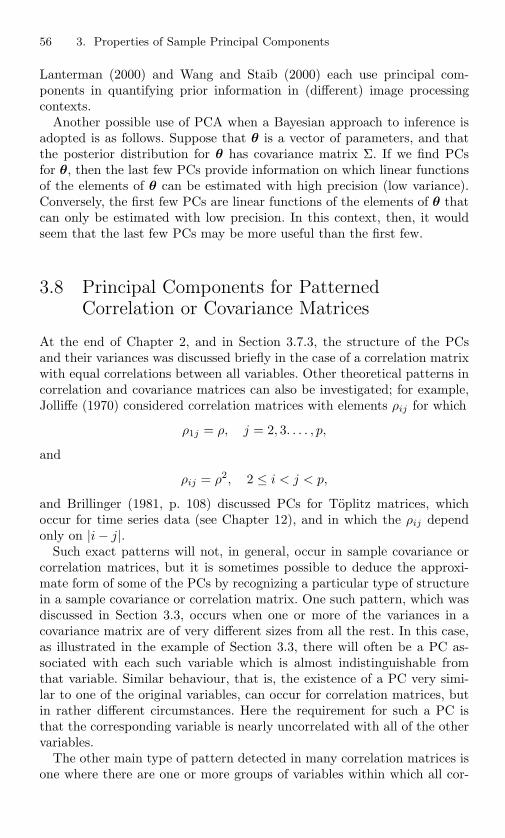
56 3. Properties of Sample Principal Components
Lanterman (2000) and Wang and Staib (2000) each use principal com-ponents in quantifying prior information in (different) image processingcontexts.
Another possible use of PCA when a Bayesian approach to inference isadopted is as follows. Suppose that θ is a vector of parameters, and thatthe posterior distribution for θ has covariance matrix Σ. If we find PCsfor θ, then the last few PCs provide information on which linear functionsof the elements of θ can be estimated with high precision (low variance).Conversely, the first few PCs are linear functions of the elements of θ thatcan only be estimated with low precision. In this context, then, it wouldseem that the last few PCs may be more useful than the first few.
3.8 Principal Components for PatternedCorrelation or Covariance Matrices
At the end of Chapter 2, and in Section 3.7.3, the structure of the PCsand their variances was discussed briefly in the case of a correlation matrixwith equal correlations between all variables. Other theoretical patterns incorrelation and covariance matrices can also be investigated; for example,Jolliffe (1970) considered correlation matrices with elements ρij for which
ρ1j = ρ, j = 2, 3. . . . , p,
and
ρij = ρ2, 2 ≤ i < j < p,
and Brillinger (1981, p. 108) discussed PCs for Toplitz matrices, whichoccur for time series data (see Chapter 12), and in which the ρij dependonly on |i − j|.
Such exact patterns will not, in general, occur in sample covariance orcorrelation matrices, but it is sometimes possible to deduce the approxi-mate form of some of the PCs by recognizing a particular type of structurein a sample covariance or correlation matrix. One such pattern, which wasdiscussed in Section 3.3, occurs when one or more of the variances in acovariance matrix are of very different sizes from all the rest. In this case,as illustrated in the example of Section 3.3, there will often be a PC as-sociated with each such variable which is almost indistinguishable fromthat variable. Similar behaviour, that is, the existence of a PC very simi-lar to one of the original variables, can occur for correlation matrices, butin rather different circumstances. Here the requirement for such a PC isthat the corresponding variable is nearly uncorrelated with all of the othervariables.
The other main type of pattern detected in many correlation matrices isone where there are one or more groups of variables within which all cor-

3.8. Patterned Covariance and Correlation Matrices 57
relations are positive and not close to zero. Sometimes a variable in such agroup will initially have entirely negative correlations with the other mem-bers of the group, but the sign of a variable is often arbitrary, and switchingthe sign will give a group of the required structure. If correlations betweenthe q members of the group and variables outside the group are close tozero, then there will be q PCs ‘associated with the group’ whose coeffi-cients for variables outside the group are small. One of these PCs will havea large variance, approximately 1 + (q − 1)r, where r is the average corre-lation within the group, and will have positive coefficients for all variablesin the group. The remaining (q − 1) PCs will have much smaller variances(of order 1− r), and will have some positive and some negative coefficients.Thus the ‘large variance PC’ for the group measures, roughly, the averagesize of variables in the group, whereas the ‘small variance PCs’ give ‘con-trasts’ between some or all of the variables in the group. There may beseveral such groups of variables in a data set, in which case each group willhave one ‘large variance PC’ and several ‘small variance PCs.’ Conversely,as happens not infrequently, especially in biological applications when allvariables are measurements on individuals of some species, we may findthat all p variables are positively correlated. In such cases, the first PCis often interpreted as a measure of size of the individuals, whereas sub-sequent PCs measure aspects of shape (see Sections 4.1, 13.2 for furtherdiscussion).
The discussion above implies that the approximate structure and vari-ances of the first few PCs can be deduced from a correlation matrix,provided that well-defined groups of variables are detected, including pos-sibly single-variable groups, whose within-group correlations are high, andwhose between-group correlations are low. The ideas can be taken further;upper and lower bounds on the variance of the first PC can be calculated,based on sums and averages of correlations (Friedman and Weisberg, 1981;Jackson, 1991, Section 4.2.3). However, it should be stressed that althoughdata sets for which there is some group structure among variables are notuncommon, there are many others for which no such pattern is apparent.In such cases the structure of the PCs cannot usually be found withoutactually performing the PCA.
3.8.1 Example
In many of the examples discussed in later chapters, it will be seen that thestructure of some of the PCs can be partially deduced from the correlationmatrix, using the ideas just discussed. Here we describe an example in whichall the PCs have a fairly clear pattern. The data consist of measurements ofreflexes at 10 sites of the body, measured for 143 individuals. As with theexamples discussed in Sections 3.3 and 3.4, the data were kindly suppliedby Richard Hews of Pfizer Central Research.
58 3. Properties of Sample Principal Components
Table 3.4. Correlation matrix for ten variables measuring reflexes.
V1 V2 V3 V4 V5 V6 V7 V8 V9 V10V1 1.00V2 0.98 1.00V3 0.60 0.62 1.00V4 0.71 0.73 0.88 1.00V5 0.55 0.57 0.61 0.68 1.00V6 0.55 0.57 0.56 0.68 0.97 1.00V7 0.38 0.40 0.48 0.53 0.33 0.33 1.00V8 0.25 0.28 0.42 0.47 0.27 0.27 0.90 1.00V9 0.22 0.21 0.19 0.23 0.16 0.19 0.40 0.41 1.00V10 0.20 0.19 0.18 0.21 0.13 0.16 0.39 0.40 0.94 1.00
The correlation matrix for these data is given in Table 3.4, and thecoefficients of, and the variation accounted for by, the corresponding PCsare presented in Table 3.5. It should first be noted that the ten variablesfall into five pairs. Thus, V1, V2, respectively, denote strength of reflexesfor right and left triceps, with V3, V4, V5, V6, V7, V8, V9, V10similarly defined for right and left biceps, right and left wrists, right and leftknees, and right and left ankles. The correlations between variables withineach pair are large, so that the differences between variables in each pairhave small variances. This is reflected in the last five PCs, which are mainlywithin-pair contrasts, with the more highly correlated pairs correspondingto the later components.
Turning to the first two PCs, there is a suggestion in the correlationmatrix that, although all correlations are positive, the variables can bedivided into two groups V1–V6, V7–V10. These correspond to sites inthe arms and legs, respectively. Reflecting this group structure, the first andsecond PCs have their largest coefficients on the first and second groups ofvariables, respectively. Because the group structure is not clear-cut, thesetwo PCs also have contributions from the less dominant group, and thefirst PC is a weighted average of variables from both groups, whereas thesecond PC is a weighted contrast between the groups.
The third, fourth and fifth PCs reinforce the idea of the two groups. Thethird PC is a contrast between the two pairs of variables in the second(smaller) group and the fourth and fifth PCs both give contrasts betweenthe three pairs of variables in the first group.
It is relatively rare for examples with as many as ten variables to havesuch a nicely defined structure as in the present case for all their PCs.However, as will be seen in the examples of subsequent chapters, it is notunusual to be able to deduce the structure of at least a few PCs in thismanner.

3.9. Models for Principal Component Analysis 59
Table 3.5. Principal components based on the correlation matrix of Table 3.4
Component 1 2 3 4 5 6 7 8 9 10number
Coefficients
V1 0.3 −0.2 0.2 −0.5 0.3 0.1 −0.1 −0.0 −0.6 0.2V2 0.4 −0.2 0.2 −0.5 0.3 0.0 −0.1 −0.0 0.7 −0.3V3 0.4 −0.1 −0.1 −0.0 −0.7 0.5 −0.2 0.0 0.1 0.1V4 0.4 −0.1 −0.1 −0.0 −0.4 −0.7 0.3 −0.0 −0.1 −0.1V5 0.3 −0.2 0.1 0.5 0.2 0.2 −0.0 −0.1 −0.2 −0.6V6 0.3 −0.2 0.2 0.5 0.2 −0.1 −0.0 0.1 0.2 0.6V7 0.3 0.3 −0.5 −0.0 0.2 0.3 0.7 0.0 −0.0 0.0V8 0.3 0.3 −0.5 0.1 0.2 −0.2 −0.7 −0.0 −0.0 −0.0V9 0.2 0.5 0.4 0.0 −0.1 0.0 −0.0 0.7 −0.0 −0.1
V10 0.2 0.5 0.4 0.0 −0.1 0.0 0.0 −0.7 0.0 0.0
Percentage of 52.3 20.4 11.0 8.5 5.0 1.0 0.9 0.6 0.2 0.2total variation explained
3.9 Models for Principal Component Analysis
There is a variety of interpretations of what is meant by a model in thecontext of PCA. Mandel (1972) considers the retention of m PCs, basedon the SVD (3.5.3), as implicitly using a model. Caussinus (1986) discussesthree types of ‘model.’ The first is a ‘descriptive algebraic model,’ which inits simplest form reduces to the SVD. It can also be generalized to includea choice of metric, rather than simply using a least squares approach. Suchgeneralizations are discussed further in Section 14.2.2. This model has norandom element, so there is no idea of expectation or variance. Hence itcorresponds to Pearson’s geometric view of PCA, rather than to Hotelling’svariance-based approach.
Caussinus’s (1986) second type of model introduces probability distri-butions and corresponds to Hotelling’s definition. Once again, the ‘model’can be generalized by allowing a choice of metric.
The third type of model described by Caussinus is the so-called fixedeffects model (see also Esposito (1998)). In this model we assume thatthe rows x1,x2, . . . ,xn of X are independent random variables, such thatE(xi) = zi, where zi lies in a q-dimensional subspace, Fq. Furthermore,if ei = xi − zi, then E(ei) = 0 and var(ei) = σ2
wiΓ, where Γ is a positive
definite symmetric matrix and the wi are positive scalars whose sum is 1.Both Γ and the wi are assumed to be known, but σ2, the zi and thesubspace Fq all need to be estimated. This is done by minimizing
n∑
i=1
wi ‖xi − zi‖2M , (3.9.1)
60 3. Properties of Sample Principal Components
where M denotes a metric (see Section 14.2.2) and may be related to Γ.This statement of the model generalizes the usual form of PCA, for whichwi = 1
n , i = 1, 2, . . . , n and M = Ip, to allow different weights on the ob-servations and a choice of metric. When M = Γ−1, and the distribution ofthe xi is multivariate normal, the estimates obtained by minimizing (3.9.1)are maximum likelihood estimates (Besse, 1994b). An interesting aspect ofthe fixed effects model is that it moves away from the idea of a sample ofidentically distributed observations whose covariance or correlation struc-ture is to be explored, to a formulation in which the variation among themeans of the observations is the feature of interest.
Tipping and Bishop (1999a) describe a model in which column-centredobservations xi are independent normally distributed random variableswith zero means and covariance matrix BB′ + σ2Ip, where B is a (p × q)matrix. We shall see in Chapter 7 that this is a special case of a factoranalysis model. The fixed effects model also has links to factor analysisand, indeed, de Leeuw (1986) suggests in discussion of Caussinus (1986)that the model is closer to factor analysis than to PCA. Similar modelsdate back to Young (1941).
Tipping and Bishop (1999a) show that, apart from a renormalization ofcolumns, and the possibility of rotation, the maximum likelihood estimateof B is the matrix Aq of PC coefficients defined earlier (see also de Leeuw(1986)). The MLE for σ2 is the average of the smallest (p − q) eigenval-ues of the sample covariance matrix S. Tipping and Bishop (1999a) fittheir model using the EM algorithm (Dempster et al. (1977)), treating theunknown underlying components as ‘missing values.’ Clearly, the compli-cation of the EM algorithm is not necessary once we realise that we aredealing with PCA, but it has advantages when the model is extended tocope with genuinely missing data or to mixtures of distributions (see Sec-tions 13.6, 9.2.3). Bishop (1999) describes a Bayesian treatment of Tippingand Bishop’s (1999a) model. The main objective in introducing a prior dis-tribution for B appears to be as a means of deciding on its dimension q(see Section 6.1.5).
Roweis (1997) also uses the EM algorithm to fit a model for PCA. Hismodel is more general than Tipping and Bishop’s, with the error covariancematrix allowed to take any form, rather than being restricted to σ2Ip. Inthis respect it is more similar to the fixed effects model with equal weights,but differs from it by not specifying different means for different observa-tions. Roweis (1997) notes that a full PCA, with all p PCs, is obtainedfrom his model in the special case where the covariance matrix is σ2Ip andσ2 → 0. He refers to the analysis based on Tipping and Bishop’s (1999a)model with σ2 > 0 as sensible principal component analysis.
Martin (1988) considers another type of probability-based PCA, in whicheach of the n observations has a probability distribution in p-dimensionalspace centred on it, rather than being represented by a single point. In

3.9. Models for Principal Component Analysis 61
the one non-trivial example considered by Martin (1988), the distributionsare identical for each observation and spherical, so that the underlyingcovariance matrix has the form Σ + σ2Ip. Lynn and McCulloch (2000) usePCA to estimate latent fixed effects in a generalized linear model, and deFalguerolles (2000) notes that PCA can be viewed as a special case of thelarge family of generalized bilinear models.
Although PCA is a largely descriptive tool, it can be argued that build-ing a model gives a better understanding of what the technique does, helpsto define circumstances in which it would be inadvisable to use it, andsuggests generalizations that explore the structure of a data set in a moresophisticated way. We will see how either the fixed effects model or Tip-ping and Bishop’s (1999a) model can be used in deciding how many PCsto retain (Section 6.1.5); in examining mixtures of probability distributions(Section 9.2.3); in a robust version of PCA (Section 10.4); in analysing func-tional data (Section 12.3.4); in handling missing data (Section 13.6); and ingeneralizations of PCA (Section 14.1, 14.2). One application that belongsin the present chapter is described by Ferre (1995a). Here µ1, µ2, . . . , µk
are estimates, derived from k samples of sizes n1, n2, . . . , nk of vectors of pparameters µ1,µ2, . . . ,µk. Ferre (1995a) proposes estimates that minimizean expression equivalent to (3.9.1) in which wi = ni
n where n =∑k
i=1 ni;xi, zi are replaced by µi, µi where µi is a projection onto an optimal q-dimensional space; and M is chosen to be S−1 where S is an estimate ofthe common covariance matrix for the data from which µ1,µ2, . . . ,µk areestimated. The properties of such estimators are investigated in detail byFerre (1995a)

This page intentionally left blank

4Principal Components as a SmallNumber of Interpretable Variables:Some Examples
The original purpose of PCA was to reduce a large number (p) of variablesto a much smaller number (m) of PCs whilst retaining as much as possibleof the variation in the p original variables. The technique is especially usefulif m p and if the m PCs can be readily interpreted.
Although we shall see in subsequent chapters that there are many otherways of applying PCA, the original usage as a descriptive, dimension-reducing technique is probably still the most prevalent single application.This chapter simply introduces a number of examples from several differentfields of application where PCA not only reduces the dimensionality of theproblem substantially, but has PCs which are easily interpreted. Graphicalrepresentations of a set of observations with respect to the m retained PCsand discussion of how to choose an appropriate value of m are deferreduntil Chapters 5 and 6, respectively.
Of course, if m is very much smaller than p, then the reduction of dimen-sionality alone may justify the use of PCA, even if the PCs have no clearmeaning, but the results of a PCA are much more satisfying if intuitivelyreasonable interpretations can be given to some or all of the m retainedPCs.
Each section of this chapter describes one example in detail, but otherexamples in related areas are also mentioned in most sections. Some of theexamples introduced in this chapter are discussed further in subsequentchapters; conversely, when new examples are introduced later in the book,an attempt will be made to interpret the first few PCs where appropriate.The examples are drawn from a variety of fields of application, demon-strating the fact that PCA has been found useful in a very large number

64 4. Interpreting Principal Components: Examples
of subject areas, of which those illustrated in this book form only a subset.It must be emphasized that although in many examples the PCs can be
readily interpreted, this is by no means universally true. There is no rea-son, a priori, why a mathematically derived linear function of the originalvariables (which is what the PCs are) should have a simple interpreta-tion. It is remarkable how often it seems to be possible to interpret thefirst few PCs, though it is probable that some interpretations owe a lotto the analyst’s ingenuity and imagination. Careful thought should go intoany interpretation and, at an earlier stage, into the choice of variables andwhether to transform them. In some circumstances, transformation of vari-ables before analysis may improve the chances of a simple interpretation(see Sections 13.2, 13.3, 14.1 and 14.2). Conversely, the arbitrary inclusionof logarithms, powers, ratios, etc., of the original variables can make it un-likely that any simple interpretation will be found. Further discussion ofthe difficulties of interpretation, and of some alternative approaches, willbe given in Chapter 11.
Many interesting applications have appeared since the first edition of thisbook, and some will be discussed in detail later in this edition. However,in the current chapter the original selection of examples, which illustratesa nice range of applications, has been kept. Extra references are given, butno new examples are discussed in detail. Texts such as Jackson (1991), Krz-anowski (1988), Krzanowski and Marriott (1994) and Rencher (1995) areuseful sources for additional examples. A non-exhaustive list of disciplinesin which PCA has been applied was given at the end of Chapter 1.
4.1 Anatomical Measurements
One type of application where PCA has been found useful is identificationof the most important sources of variation in anatomical measurements forvarious species. Typically, a large number of measurements are made onindividuals of a species, and a PCA is done. The first PC almost alwayshas positive coefficients for all variables and simply reflects overall ‘size’ ofthe individuals. Later PCs usually contrast some of the measurements withothers, and can often be interpreted as defining certain aspects of ‘shape’that are important for the species. Blackith and Reyment (1971, Chap-ter 12) mention applications to squirrels, turtles, ammonites, foraminifera(marine microorganisms) and various types of insects. The analysis of sizeand shape is a large topic in its own right, and will discussed in greaterdetail in Section 13.2. Here a small data set is examined in which sevenmeasurements were taken for a class of 28 students (15 women, 13 men).The seven measurements are circumferences of chest, waist, wrist and head,lengths of hand and forearm, and overall height. A similar data set for adifferent group of students was introduced in Chapter 1.

4.1. Anatomical Measurements 65
Table 4.1. First three PCs: student anatomical measurements.
Component number 1 2 3Women
Hand 0.33 0.56 0.03Wrist 0.26 0.62 0.11Height 0.40 −0.44 −0.00Forearm
Coefficients 0.41 −0.05 −0.55Head 0.27 −0.19 0.80Chest 0.45 −0.26 −0.12Waist 0.47 0.03 −0.03
Eigenvalue 3.72 1.37 0.97
Cumulative percentageof total variation 53.2 72.7 86.5
MenHand 0.23 0.62 0.64Wrist 0.29 0.53 −0.42Height 0.43 −0.20 0.04Forearm
Coefficients 0.33 −0.53 0.38Head 0.41 −0.09 −0.51Chest 0.44 0.08 −0.01Waist 0.46 −0.07 0.09
Eigenvalue 4.17 1.26 0.66
Cumulative percentageof total variation 59.6 77.6 87.0
The PCA was done on the correlation matrix, even though it could beargued that, since all measurements are made in the same units, the co-variance matrix might be more appropriate (see Sections 2.3 and 3.3). Thecorrelation matrix was preferred because it was desired to treat all variableson an equal footing: the covariance matrix gives greater weight to larger,and hence more variable, measurements, such as height and chest girth, andless weight to smaller measurements such as wrist girth and hand length.
Some of the results of the PC analyses, done separately for women andmen, are given in Tables 4.1 and 4.2.
It can be seen that the form of the first two PCs is similar for the twosexes, with some similarity, too, for the third PC. Bearing in mind the smallsample sizes, and the consequent large sampling variation in PC coefficients,it seems that the major sources of variation in the measurements, as givenby the first three PCs, are similar for each sex. A combined PCA using all 28

66 4. Interpreting Principal Components: Examples
Table 4.2. Simplified version of the coefficients in Table 4.1.
Component number 1 2 3Women
Hand + +Wrist + +Height + −Forearm + −Head + (−) +Chest + (−)Waist +
MenHand + + +Wrist + + −Height + (−)Forearm + − +Head + −Chest +Waist +
observations therefore seems appropriate, in order to get better estimatesof the first three PCs. It is, of course, possible that later PCs are differentfor the two sexes, and that combining all 28 observations will obscure suchdifferences. However, if we are interested solely in interpreting the first few,high variance, PCs, then this potential problem is likely to be relativelyunimportant.
Before we attempt to interpret the PCs, some explanation of Table 4.2is necessary. Typically, computer packages that produce PCs give the co-efficients to several decimal places. When we interpret PCs, as with othertypes of tabular data, it is usually only the general pattern of the coeffi-cients that is really of interest, not values to several decimal places, whichmay give a false impression of precision. Table 4.1 gives only two decimalplaces and Table 4.2 simplifies still further. A + or − in Table 4.2 indicatesa coefficient whose absolute value is greater than half the maximum coeffi-cient (again in absolute value) for the relevant PC; the sign of the coefficientis also indicated. Similarly, a (+) or (−) indicates a coefficient whose ab-solute value is between a quarter and a half of the largest absolute valuefor the PC of interest. There are, of course, many ways of constructing asimplified version of the PC coefficients in Table 4.1. For example, anotherpossibility is to rescale the coefficients in each PC so that the maximumvalue is ±1, and tabulate only the values of the coefficients, rounded toone decimal place whose absolute values are above a certain cut-off, say 0.5or 0.7. Values of coefficients below the cut-off are omitted, leaving blank
4.1. Anatomical Measurements 67
spaces, as in Table 4.2. Some such simple representation is often helpfulin interpreting PCs, particularly if a PCA is done on a large number ofvariables.
Sometimes a simplification such as that given in Table 4.2 may be rathertoo extreme, and it is therefore advisable to present the coefficients roundedto one or two decimal places as well. Principal components with roundedcoefficients will no longer be optimal, so that the variances of the first fewwill tend to be reduced, and exact orthogonality will be lost. However, ithas been shown (Bibby, 1980; Green, 1977) that fairly drastic roundingof coefficients makes little difference to the variances of the PCs (see Sec-tion 10.3). Thus, presentation of rounded coefficients will still give linearfunctions of x with variances very nearly as large as those of the PCs, whileat the same time easing interpretations.
It must be stressed that interpretation of PCs is often more subtle thanis generally realised. Simplistic interpretation can be misleading. As well astruncation or rounding of PC coefficients, a number of other ideas are avail-able to aid interpretation. Some of these involve manipulation of the PCcoefficients themselves, whilst others are based on alternative, but similar,techniques to PCA. In this chapter we concentrate on simple interpreta-tion. Its dangers, and various alternative ways of tackling interpretation,are discussed in Chapter 11.
Turning now to the interpretation of the PCs in the present example,the first PC clearly measures overall ‘size’ for both sexes, as would be ex-pected (see Section 3.8), as all the correlations between the seven variablesare positive. It accounts for 53% (women) or 60% (men) of the total varia-tion. The second PC for both sexes contrasts hand and wrist measurementswith height, implying that, after overall size has been accounted for, themain source of variation is between individuals with large hand and wristmeasurements relative to their heights, and individuals with the converserelationship. For women, head and chest measurements also have some con-tribution to this component, and for men the forearm measurement, whichis closely related to height, partially replaces height in the component.This second PC accounts for slightly less than 20% of the total variation,for both sexes.
It should be noted that the sign of any PC is completely arbitrary. Ifevery coefficient in a PC, zk = a′
kx, has its sign reversed, the variance of zk
is unchanged, and so is the orthogonality of ak with all other eigenvectors.For example, the second PC for men as recorded in Tables 4.1 and 4.2 haslarge positive values for students with large hand and wrist measurementsrelative to their height. If the sign of a2, and hence z2, is reversed, thelarge positive values now occur for students with small hand and wristmeasurements relative to height. The interpretation of the PC remains thesame, even though the roles of ‘large’ and ‘small’ are reversed.
The third PCs differ more between the sexes but nevertheless retainsome similarity. For women it is almost entirely a contrast between head

68 4. Interpreting Principal Components: Examples
and forearm measurements; for men these two measurements are also im-portant, but, in addition, hand and wrist measurements appear with thesame signs as forearm and head, respectively. This component contributes9%–14% of total variation.
Overall, the first three PCs account for a substantial proportion of to-tal variation, 86.5% and 87.0% for women and men respectively. Althoughdiscussion of rules for deciding how many PCs to retain is deferred un-til Chapter 6, intuition strongly suggests that these percentages are largeenough for three PCs to give an adequate representation of the data.
A similar but much larger study, using seven measurements on 3000 crim-inals, was reported by Macdonell (1902) and is quoted by Maxwell (1977).The first PC again measures overall size, the second contrasts head andlimb measurements, and the third can be readily interpreted as measuringthe shape (roundness versus thinness) of the head. The percentages of totalvariation accounted for by each of the first three PCs are 54.3%, 21.4% and9.3%, respectively, very similar to the proportions given in Table 4.1.
The sample size (28) is rather small in our example compared to that ofMacdonnell’s (1902), especially when the sexes are analysed separately, socaution is needed in making any inference about the PCs in the populationof students from which the sample is drawn. However, the same variableshave been measured for other classes of students, and similar PCs havebeen found (see Sections 5.1 and 13.5). In any case, a description of thesample, rather than inference about the underlying population, is oftenwhat is required, and the PCs describe the major directions of variationwithin a sample, regardless of the sample size.
4.2 The Elderly at Home
Hunt (1978) described a survey of the ‘Elderly at Home’ in which valuesof a large number of variables were collected for a sample of 2622 elderlyindividuals living in private households in the UK in 1976. The variablescollected included standard demographic information of the type found inthe decennial censuses, as well as information on dependency, social contact,mobility and income. As part of a project carried out for the Departmentsof the Environment and Health and Social Security, a PCA was done on asubset of 20 variables from Hunt’s (1978) data. These variables are listedbriefly in Table 4.3. Full details of the variables, and also of the project asa whole, are given by Jolliffe et al. (1982a), while shorter accounts of themain aspects of the project are available in Jolliffe et al. (1980, 1982b). Itshould be noted that many of the variables listed in Table 4.3 are discrete,or even dichotomous.
Some authors suggest that PCA should only be done on continuousvariables, preferably with normal distributions. However, provided that
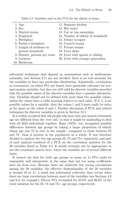
4.2. The Elderly at Home 69
Table 4.3. Variables used in the PCA for the elderly at home.
1. Age 11. Separate kitchen2. Sex 12. Hot water3. Marital status 13. Car or van ownership4. Employed 14. Number of elderly in household5. Birthplace 15. Owner occupier6. Father’s birthplace 16. Council tenant7. Length of residence in 17. Private tenant
present household 18. Lives alone8. Density: persons per room 19. Lives with spouse or sibling9. Lavatory 20. Lives with younger generation
10. Bathroom
inferential techniques that depend on assumptions such as multivariatenormality (see Section 3.7) are not invoked, there is no real necessity forthe variables to have any particular distribution. Admittedly, correlationsor covariances, on which PCs are based, have particular relevance for nor-mal random variables, but they are still valid for discrete variables providedthat the possible values of the discrete variables have a genuine interpreta-tion. Variables should not be defined with more than two possible values,unless the values have a valid meaning relative to each other. If 0, 1, 3 arepossible values for a variable, then the values 1 and 3 must really be twiceas far apart as the values 0 and 1. Further discussion of PCA and relatedtechniques for discrete variables is given in Section 13.1.
It is widely accepted that old people who have only just passed retirementage are different from the ‘very old,’ so that it might be misleading to dealwith all 2622 individuals together. Hunt (1978), too, recognized possibledifferences between age groups by taking a larger proportion of elderlywhose age was 75 or over in her sample—compared to those between 65and 74—than is present in the population as a whole. It was thereforedecided to analyse the two age groups 65–74 and 75+ separately, and partof each analysis consisted of a PCA on the correlation matrices for the20 variables listed in Table 4.3. It would certainly not be appropriate touse the covariance matrix here, where the variables are of several differenttypes.
It turned out that for both age groups as many as 11 PCs could bereasonably well interpreted, in the sense that not too many coefficientswere far from zero. Because there are relatively few strong correlationsamong the 20 variables, the effective dimensionality of the 20 variablesis around 10 or 11, a much less substantial reduction than occurs whenthere are large correlations between most of the variables (see Sections 4.3and 6.4, for example). Eleven PCs accounted for 85.0% and 86.6% of thetotal variation for the 65–74 and 75+ age groups, respectively.
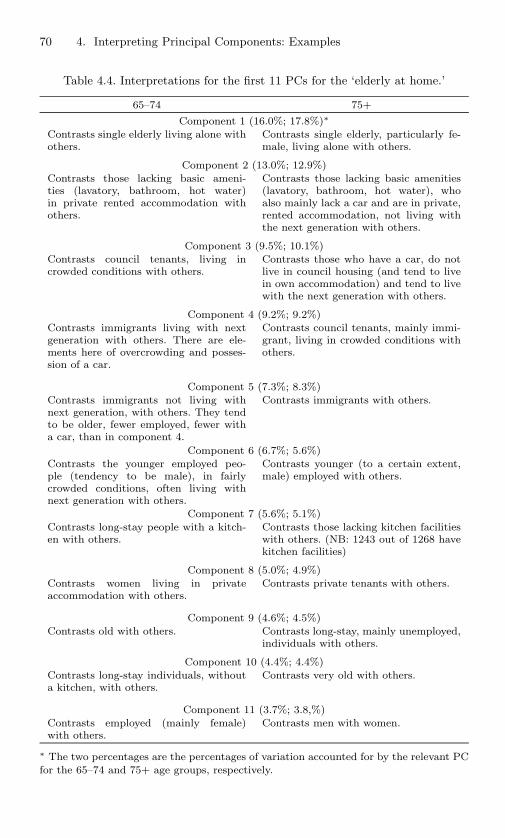
70 4. Interpreting Principal Components: Examples
Table 4.4. Interpretations for the first 11 PCs for the ‘elderly at home.’
65–74 75+
Component 1 (16.0%; 17.8%)∗Contrasts single elderly living alone withothers.
Contrasts single elderly, particularly fe-male, living alone with others.
Component 2 (13.0%; 12.9%)Contrasts those lacking basic ameni-ties (lavatory, bathroom, hot water)in private rented accommodation withothers.
Contrasts those lacking basic amenities(lavatory, bathroom, hot water), whoalso mainly lack a car and are in private,rented accommodation, not living withthe next generation with others.
Component 3 (9.5%; 10.1%)Contrasts council tenants, living incrowded conditions with others.
Contrasts those who have a car, do notlive in council housing (and tend to livein own accommodation) and tend to livewith the next generation with others.
Component 4 (9.2%; 9.2%)Contrasts immigrants living with nextgeneration with others. There are ele-ments here of overcrowding and posses-sion of a car.
Contrasts council tenants, mainly immi-grant, living in crowded conditions withothers.
Component 5 (7.3%; 8.3%)Contrasts immigrants not living withnext generation, with others. They tendto be older, fewer employed, fewer witha car, than in component 4.
Contrasts immigrants with others.
Component 6 (6.7%; 5.6%)Contrasts the younger employed peo-ple (tendency to be male), in fairlycrowded conditions, often living withnext generation with others.
Contrasts younger (to a certain extent,male) employed with others.
Component 7 (5.6%; 5.1%)Contrasts long-stay people with a kitch-en with others.
Contrasts those lacking kitchen facilitieswith others. (NB: 1243 out of 1268 havekitchen facilities)
Component 8 (5.0%; 4.9%)Contrasts women living in privateaccommodation with others.
Contrasts private tenants with others.
Component 9 (4.6%; 4.5%)Contrasts old with others. Contrasts long-stay, mainly unemployed,
individuals with others.
Component 10 (4.4%; 4.4%)Contrasts long-stay individuals, withouta kitchen, with others.
Contrasts very old with others.
Component 11 (3.7%; 3.8,%)Contrasts employed (mainly female)with others.
Contrasts men with women.
∗ The two percentages are the percentages of variation accounted for by the relevant PCfor the 65–74 and 75+ age groups, respectively.

4.3. Spatial and Temporal Variation in Atmospheric Science 71
Interpretations of the first 11 PCs for the two age groups are given inTable 4.4, together with the percentage of total variation accounted for byeach PC. The variances of corresponding PCs for the two age groups differvery little, and there are similar interpretations for several pairs of PCs, forexample the first, second, sixth and eighth. In other cases there are groupsof PCs involving the same variables, but in different combinations for thetwo age groups, for example the third, fourth and fifth PCs. Similarly, theninth and tenth PCs involve the same variables for the two age groups, butthe order of the PCs is reversed.
Principal component analysis has also been found useful in other de-mographic studies, one of the earliest being that described by Moser andScott (1961). In this study, there were 57 demographic variables measuredfor 157 British towns. A PCA of these data showed that, unlike the elderlydata, dimensionality could be vastly reduced; there are 57 variables, butas few as four PCs account for 63% of the total variation. These PCs alsohave ready interpretations as measures of social class, population growthfrom 1931 to 1951, population growth after 1951, and overcrowding.
Similar studies have been done on local authority areas in the UK byImber (1977) and Webber and Craig (1978) (see also Jolliffe et al. (1986)).In each of these studies, as well as Moser and Scott (1961) and the ‘elderly athome’ project, the main objective was to classify the local authorities, townsor elderly individuals, and the PCA was done as a prelude to, or as partof, cluster analysis. The use of PCA in cluster analysis is discussed furtherin Section 9.2, but the PCA in each study mentioned here provided usefulinformation, separate from the results of the cluster analysis, For example,Webber and Craig (1978) used 40 variables, and they were able to interpretthe first four PCs as measuring social dependence, family structure, agestructure and industrial employment opportunity. These four componentsaccounted for 29.5%, 22.7%, 12.0% and 7.4% of total variation, respectively,so that 71.6% of the total variation is accounted for in four interpretabledimensions.
4.3 Spatial and Temporal Variation inAtmospheric Science
Principal component analysis provides a widely used method of describingpatterns of pressure, temperature, or other meteorological variables over alarge spatial area. For example, Richman (1983) stated that, over the pre-vious 3 years, more than 60 applications of PCA, or similar techniques, hadappeared in meteorological/climatological journals. More recently, 53 outof 215 articles in the 1999 and 2000 volumes of the International Journal ofClimatology used PCA in some form. No other statistical technique cameclose to this 25% rate of usage. The example considered in detail in this
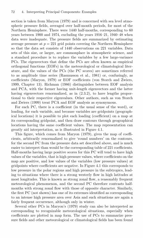
72 4. Interpreting Principal Components: Examples
section is taken from Maryon (1979) and is concerned with sea level atmo-spheric pressure fields, averaged over half-month periods, for most of theNorthern Hemisphere. There were 1440 half-months, corresponding to 60years between 1900 and 1974, excluding the years 1916–21, 1940–48 whendata were inadequate. The pressure fields are summarized by estimatingaverage pressure at p = 221 grid points covering the Northern Hemisphereso that the data set consists of 1440 observations on 221 variables. Datasets of this size, or larger, are commonplace in atmospheric science, anda standard procedure is to replace the variables by a few large-variancePCs. The eigenvectors that define the PCs are often known as empiricalorthogonal functions (EOFs) in the meteorological or climatological liter-ature, and the values of the PCs (the PC scores) are sometimes referredto as amplitude time series (Rasmusson et al., 1981) or, confusingly, ascoefficients (Maryon, 1979) or EOF coefficients (von Storch and Zwiers,1999, Chapter 13). Richman (1986) distinguishes between EOF analysisand PCA, with the former having unit-length eigenvectors and the latterhaving eigenvectors renormalized, as in (2.3.2), to have lengths propor-tional to their respective eigenvalues. Other authors, such as von Storchand Zwiers (1999) treat PCA and EOF analysis as synonymous.
For each PC, there is a coefficient (in the usual sense of the word), orloading, for each variable, and because variables are gridpoints (geograph-ical locations) it is possible to plot each loading (coefficient) on a map atits corresponding gridpoint, and then draw contours through geographicallocations having the same coefficient values. The map representation cangreatly aid interpretation, as is illustrated in Figure 4.1.
This figure, which comes from Maryon (1979), gives the map of coeffi-cients, arbitrarily renormalized to give ‘round numbers’ on the contours,for the second PC from the pressure data set described above, and is mucheasier to interpret than would be the corresponding table of 221 coefficients.Half-months having large positive scores for this PC will tend to have highvalues of the variables, that is high pressure values, where coefficients on themap are positive, and low values of the variables (low pressure values) atgridpoints where coefficients are negative. In Figure 4.1 this corresponds tolow pressure in the polar regions and high pressure in the subtropics, lead-ing to situations where there is a strong westerly flow in high latitudes atmost longitudes. This is known as strong zonal flow, a reasonably frequentmeteorological phenomenon, and the second PC therefore contrasts half-months with strong zonal flow with those of opposite character. Similarly,the first PC (not shown) has one of its extremes identified as correspondingto an intense high pressure area over Asia and such situations are again afairly frequent occurrence, although only in winter.
Several other PCs in Maryon’s (1979) study can also be interpreted ascorresponding to recognizable meteorological situations, especially whencoefficients are plotted in map form. The use of PCs to summarize pres-sure fields and other meteorological or climatological fields has been found

4.3. Spatial and Temporal Variation in Atmospheric Science 73
Figure 4.1. Graphical representation of the coefficients in the second PC for sealevel atmospheric pressure data.
to be so valuable that it is almost routine. For example, Craddock andFlood (1969) find PCs with ready interpretations for Northern Hemispheric500 mb geopotential surfaces, Craddock and Flintoff (1970) do the same for1000 mb surfaces and 1000–500 mb thickness, Overland and Preisendorfer(1982) interpret the first three PCs for data on spatial distributions of cy-clone frequencies in the Bering Sea, Wigley et al. (1984) discuss PCs forEuropean precipitation data, and Folland et al. (1985) find interpretablepatterns in PCs of worldwide sea surface temperature anomalies. Somepatterns recur in different data sets. For example, Figure 4.1 could beinterpreted as the North Atlantic Oscillation (NAO), which reflects thestrength of the zonal flow in the North Atlantic and neighbouring areas, asmeasured by the pressure difference between the Azores and Iceland. Thispattern, and a small number of others, notably ENSO (El Nino–SouthernOscillation), have been identified as major modes of climate variability indifferent parts of the world. They have been studied extensively (see, forexample, Ambaum et al. (2001) for a discussion of the NAO).

74 4. Interpreting Principal Components: Examples
It is not always the case that interpretation is straightforward. In atmo-spheric science the PCs or EOFS are often rotated in an attempt to findmore clearly interpretable patterns. We return to this topic in Chapter 11.
Not only are the first few PCs readily interpreted in many meteoro-logical and climatological examples, possibly after rotation, but they alsofrequently enable a considerable reduction to be made in the dimensions ofthe data set. In Maryon’s (1979) study, for example, there are initially 221variables, but 16 PCs account for over 90% of the total variation. Nor isthis due to any disparity between variances causing a few dominant PCs;size of variance is fairly similar for all 221 variables.
Maryon’s (1979) analysis was for a covariance matrix, which is reasonablesince all variables are measured in the same units (see Sections 2.3 and 3.3).However, some atmospheric scientists advocate using correlation, ratherthan covariance, matrices so that patterns of spatial correlation can bedetected without possible domination by the stations and gridpoints withthe largest variances (see Wigley et al. (1984)).
It should be clear from this section that meteorologists and climatolo-gists have played a leading role in applying PCA. In addition, they havedeveloped many related methods to deal with the peculiarities of theirdata, which often have correlation structure in both time and space. Asubstantial part of Chapter 12 is devoted to these developments.
4.4 Properties of Chemical Compounds
The main example given in this section is based on a subset of data givenby Hansch et al. (1973); the PCA was described by Morgan (1981). Sevenproperties (variables) were measured for each of 15 chemical substituents;the properties and substituents are listed in Table 4.5. Some of the results ofa PCA based on the correlation matrix for these data are given in Table 4.6.
The aim of the work of Hansch et al. (1973), and of much subsequent re-search in quantitative structure–activity relationships (QSAR), is to relateaspects of the structure of chemicals to their physical properties or activi-ties so that ‘new’ chemicals can be manufactured whose activities may bepredicted in advance. Although PCA is less evident recently in the exten-sive QSAR literature, it appeared in a number of early papers on QSAR.For example, it was used in conjunction with regression (see Chapter 8and Mager (1980a)), and as a discriminant technique (see Section 9.1 andMager (1980b)). Here we look only at the reduction of dimensionality andinterpretations obtained by Morgan (1981) in this analysis of Hansch etal.’s (1973) data. The first two PCs in Table 4.6 account for 79% of thetotal variation; the coefficients for each have a moderately simple structure.The first PC is essentially an average of all properties except π and MR,whereas the most important contribution to the second PC is an average of

4.4. Properties of Chemical Compounds 75
Table 4.5. Variables and substituents considered by Hansch et al. (1973).
(a) Variables
1. π Hansch’s measure of lipophylicity
2. F3. R
measures of electronic effect: F denotes ‘field’; R denotes resonance
4. MR molar refraction
5. σm
6. σp
further measures of electronic effect
7. MW molecular weight
(b) Substituents
1. Br 2. Cl 3. F 4. I 5. CF3
6. CH3 7. C2H5 8. C3H7 9. C4H2 10. OH11. NH2 12. CH2OH 13. SO2CH3 14. SOCH3 15. SO2(NH2)
Table 4.6. First four PCs of chemical data from Hansch et al. (1973).
Component number 1 2 3 4π 0.15 0.49 0.70 −0.45F −0.42 −0.36 0.34 0.13R −0.37 0.30 −0.44 −0.54MR
Coefficients −0.16 0.62 −0.23 0.49σm −0.48 −0.24 0.19 −0.03σp −0.50 0.01 −0.11 −0.30MW −0.40 0.30 0.31 0.40Eigenvalue 3.79 1.73 0.74 0.59Cumulative percentage
of total variation 54.1 78.8 89.4 97.8

76 4. Interpreting Principal Components: Examples
π and MR. Morgan (1981) also reports PCAs for a number of other similardata sets, in several of which the PCs provide useful interpretations.
4.5 Stock Market Prices
The data in this example are the only set in this chapter that previouslyappeared in a textbook (Press, 1972, Section 9.5.2). Both the data, andthe PCs have interesting structures. The data, which were originally anal-ysed by Feeney and Hester (1967), consist of 50 quarterly measurementsbetween 1951 and 1963 of US stock market prices for the 30 industrialstocks making up the Dow-Jones index at the end of 1961. Table 4.7 gives,in the simplified form described for Table 4.2, the coefficients of the firsttwo PCs, together with the percentage of variation accounted for by eachPC, for both covariance and correlation matrices.
Looking at the PCs for the correlation matrix, the first is a ‘size’ com-ponent, similar to those discussed in Section 4.1. It reflects the fact thatall stock prices rose fairly steadily during the period 1951–63, with the ex-ception of Chrysler. It accounts for roughly two-thirds of the variation inthe 30 variables. The second PC can be interpreted as a contrast between‘consumer’ and ‘producer’ stocks. ‘Consumer’ companies are those thatmainly supply goods or services directly to the consumer, such as AT&T,American Tobacco, General Foods, Proctor and Gamble, Sears, and Wool-worth, whereas ‘producer’ companies sell their goods or services mainly toother companies, and include Alcoa, American Can, Anaconda, Bethlehem,Union Carbide, and United Aircraft.
The PCs for the covariance matrix can be similarly interpreted, albeitwith a change of sign for the second component, but the interpretationis slightly confounded, especially for the first PC, by the different-sizedvariances for each variable.
Feeney and Hester (1967) also performed a number of other PCAs usingthese and related data. In one analysis, they removed a linear trend from thestock prices before calculating PCs, and found that they had eliminated thesize (trend) PC, and that the first PC was now very similar in form to thesecond PC in the original analyses. They also calculated PCs based on ‘rate-of-return’ rather than price, for each stock, and again found interpretablePCs. Finally, PCs were calculated for subperiods of 12 years of data inorder to investigate the stability of the PCs, a topic that is discussed moregenerally in Section 10.3.
To conclude this example, note that it is of a special type, as each variableis a time series, in which consecutive observations are not independent.Further discussion of PCA for time series data is given in Chapter 12. Apossible technique for finding PCs that are free of the trend in a vector oftime series, which is more general than the technique noted above for thepresent example, is described in Section 14.3.
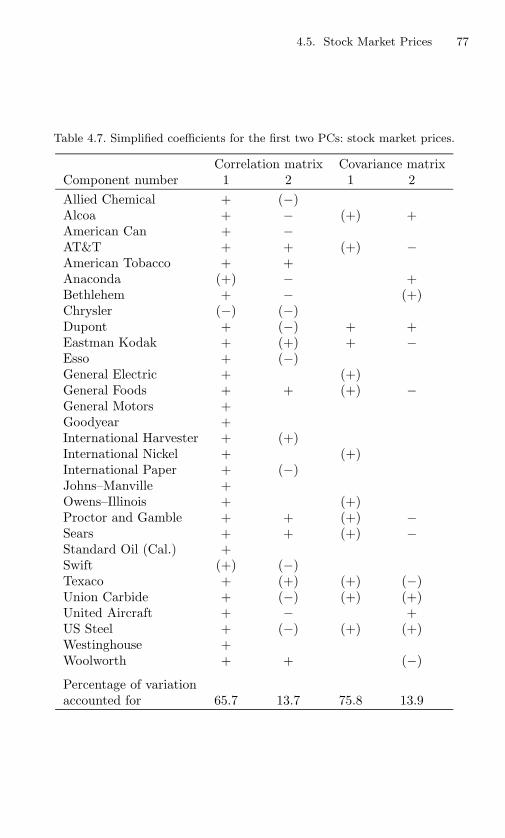
4.5. Stock Market Prices 77
Table 4.7. Simplified coefficients for the first two PCs: stock market prices.
Correlation matrix Covariance matrixComponent number 1 2 1 2Allied Chemical + (−)Alcoa + − (+) +American Can + −AT&T + + (+) −American Tobacco + +Anaconda (+) − +Bethlehem + − (+)Chrysler (−) (−)Dupont + (−) + +Eastman Kodak + (+) + −Esso + (−)General Electric + (+)General Foods + + (+) −General Motors +Goodyear +International Harvester + (+)International Nickel + (+)International Paper + (−)Johns–Manville +Owens–Illinois + (+)Proctor and Gamble + + (+) −Sears + + (+) −Standard Oil (Cal.) +Swift (+) (−)Texaco + (+) (+) (−)Union Carbide + (−) (+) (+)United Aircraft + − +US Steel + (−) (+) (+)Westinghouse +Woolworth + + (−)
Percentage of variationaccounted for 65.7 13.7 75.8 13.9
5Graphical Representation of DataUsing Principal Components
The main objective of a PCA is to reduce the dimensionality of a set ofdata. This is particularly advantageous if a set of data with many variableslies, in reality, close to a two-dimensional subspace (plane). In this case thedata can be plotted with respect to these two dimensions, thus giving astraightforward visual representation of what the data look like, instead ofappearing as a large mass of numbers to be digested. If the data fall closeto a three-dimensional subspace it is still possible to gain a good visualimpression of the data using interactive computer graphics. Even with afew more dimensions it is possible, with some degree of ingenuity, to geta ‘picture’ of the data (see, for example, Chapters 10–12 (by Tukey andTukey) in Barnett (1981)) although we shall concentrate almost entirelyon two-dimensional representations in the present chapter.
If a good representation of the data exists in a small number of dimen-sions then PCA will find it, since the first q PCs give the ‘best-fitting’q-dimensional subspace in the sense defined by Property G3 of Section 3.2.Thus, if we plot the values for each observation of the first two PCs, weget the best possible two-dimensional plot of the data (similarly for threeor more dimensions). The first section of this chapter simply gives exam-ples illustrating this procedure. We largely defer until the next chapter theproblem of whether or not two PCs are adequate to represent most of thevariation in the data, or whether we need more than two.
There are numerous other methods for representing high-dimensionaldata in two or three dimensions and, indeed, the book by Everitt (1978)is almost entirely on the subject, as are the conference proceedings editedby Wang (1978) and by Barnett (1981) (see also Chapter 5 of the book
5. Graphical Representation of Data Using Principal Components 79
by Chambers et al. (1983)). A more recent thorough review of graphicsfor multivariate data is given by Carr (1998). A major advance has beenthe development of dynamic multivariate graphics, which Carr (1998) de-scribes as part of ‘the visual revolution in computer science.’ The techniquesdiscussed in the present chapter are almost exclusively static, althoughsome could be adapted to be viewed dynamically. Only those graph-ics that have links with, or can be used in conjunction with, PCA areincluded.
Section 5.2 discusses principal coordinate analysis, which constructs low-dimensional plots of a set of data from information about similarities ordissimilarities between pairs of observations. It turns out that the plotsgiven by this analysis are equivalent to plots with respect to PCs in certainspecial cases.
The biplot, described in Section 5.3, is also closely related to PCA. Thereare a number of variants of the biplot idea, but all give a simultaneousdisplay of n observations and p variables on the same two-dimensionaldiagram. In one of the variants, the plot of observations is identical toa plot with respect to the first two PCs, but the biplot simultaneouslygives graphical information about the relationships between variables. Therelative positions of variables and observations, which are plotted on thesame diagram, can also be interpreted.
Correspondence analysis, which is discussed in Section 5.4, again givestwo-dimensional plots, but only for data of a special form. Whereas PCAand the biplot operate on a matrix of n observations on p variables,and principal coordinate analysis and other types of scaling or ordinationtechniques use data in the form of a similarity or dissimilarity matrix, cor-respondence analysis is used on contingency tables, that is, data classifiedaccording to two categorical variables. The link with PCA is less straight-forward than for principal coordinate analysis or the biplot, but the ideasof PCA and correspondence analysis have some definite connections. Thereare many other ordination and scaling methods that give graphical displaysof multivariate data, and which have increasingly tenuous links to PCA.Some of these techniques are noted in Sections 5.2 and 5.4, and in Sec-tion 5.5 some comparisons are made, briefly, between PCA and the othertechniques introduced in this chapter.
Another family of techniques, projection pursuit, is designed to find low-dimensional representations of a multivariate data set that best displaycertain types of structure such as clusters or outliers. Discussion of projec-tion pursuit will be deferred until Chapters 9 and 10, which include sectionson cluster analysis and outliers, respectively.
The final section of this chapter describes some methods which have beenused for representing multivariate data in two dimensions when more thantwo or three PCs are needed to give an adequate representation of the data.The first q PCs can still be helpful in reducing the dimensionality in suchcases, even when q is much larger than 2 or 3.

80 5. Graphical Representation of Data Using Principal Components
Finally, we note that as well as the graphical representations describedin the present chapter, we have already seen, in Section 4.3, one other typeof plot that uses PCs. This type of plot is rather specialized, but is usedextensively in atmospheric science. Related plots are discussed further inChapter 12.
5.1 Plotting Data with Respect to the First Two(or Three) Principal Components
The idea here is simple: if a data set x1,x2, . . . ,xn has p variables, thenthe observations can be plotted as points in p-dimensional space. If we wishto plot the data in a ‘best-fitting’ q-dimensional subspace (q < p), where‘best-fitting’ is defined, as in Property G3 of Section 3.2, as minimizing thesum of squared perpendicular distances of x1,x2, . . . ,xn from the subspace,then the appropriate subspace is defined by the first q PCs.
Two-dimensional plots are particularly useful for detecting patterns inthe data, and three-dimensional plots or models, though generally less easyto interpret quickly, can sometimes give additional insights. If the data donot lie close to a two- (or three-) dimensional subspace, then no two- (orthree-) dimensional plot of the data will provide an adequate represen-tation, although Section 5.6 discusses briefly the use of indirect ways forpresenting the data in two dimensions in such cases. Conversely, if the dataare close to a q-dimensional subspace, then most of the variation in thedata will be accounted for by the first q PCs and a plot of the observationswith respect to these PCs will give a realistic picture of what the datalook like, unless important aspects of the data structure are concentratedin the direction of low variance PCs. Plotting data sets with respect tothe first two PCs is now illustrated by two examples, with further illustra-tions given, in conjunction with other examples, later in this chapter andin subsequent chapters.
It should be noted that the range of structures that may be revealed byplotting PCs is limited by the fact that the PCs are uncorrelated. Hencesome types of group structure or outlier patterns or non-linear relationshipsbetween PCs, may be visible, but linear relationships between PCs areimpossible.
5.1.1 Examples
Two examples are given here that illustrate the sort of interpretation whichmay be given to plots of observations with respect to their first two PCs.These two examples do not reveal any strong, but previously unknown,structure such as clusters; examples illustrating clusters will be presentedin Section 9.2. Nevertheless, useful information can still be gleaned fromthe plots.
5.1. Plotting Two or Three Principal Components 81
Anatomical Measurements
The data presented here consist of the same seven anatomical measure-ments as in the data set of Section 4.1, but for a different set of students,this time comprising 11 women and 17 men. A PCA was done on the cor-relation matrix for all 28 observations and, as in the analyses of Section 4.1for each sex separately, the first PC is an overall measurement of size. Thesecond PC is a contrast between the head measurement and the other sixvariables, and is therefore not particularly similar to any of the first threePCs for the separate sexes found in Section 4.1, though it is closest to thethird component for the women. The difference between the second PC andthose from the earlier analyses may be partially due to the fact that thesexes have been combined, but it is also likely to reflect some instabilityin all but the first PC due to relatively small sample sizes. The first twoPCs for the present data account for 69% and 11% of the total variation,respectively, so that a two-dimensional plot with respect to these PCs, re-presenting 80% of the variation, gives a reasonably good approximation tothe relative positions of the observations in seven-dimensional space.
A plot of these data with respect to the first two PCs was given inFigure 1.3, and it was noted that the first PC is successful in separatingthe women from the men. It can also be seen in Figure 1.3 that there is oneclear outlier with respect to the second PC, seen at the bottom of the plot.A second observation, at the left of the plot, is rather extreme on the firstPC. These two observations and other potential outliers will be discussedfurther in Section 10.1. The observation at the bottom of the diagram hassuch an extreme value for the second PC, roughly twice as large in absoluteterms as any other observation, that it could be mainly responsible for thesecond PC taking the form that it does. This possibility will be discussedfurther in Section 10.2.
Figures 5.1(a) and (b) are the same as Figure 1.3 except that super-imposed on them are convex hulls for the two groups, men and women(Figure 5.1(a)), and the minimum spanning tree (Figure 5.1(b)). Convexhulls are useful in indicating the areas of a two-dimensional plot coveredby various subsets of observations. Here they confirm that, although theareas covered by men and women overlap slightly, the two sexes largelyoccupy different areas of the diagrams. The separation is mainly in termsof the first PC (overall size) with very little differentiation between sexeson the second PC. The plot therefore displays the unsurprising result thatthe two groups of observations corresponding to the two sexes differ mainlyin terms of overall size.
It was noted above that the two-dimensional plot represents 80% of thetotal variation of the 28 observations in seven-dimensional space. Percent-age of total variation is an obvious measure of how good two-dimensionalrepresentation is, but many of the other criteria that are discussed in Sec-tion 6.1 could be used instead. Alternatively, an informal way of judgingthe goodness-of-fit in two dimensions is to superimpose a minimum span-
82 5. Graphical Representation of Data Using Principal Components
Figure 5.1. (a). Student anatomical measurements: plot of the first two PC for28 students with convex hulls for men and women superimposed.
ning tree (MST) on the diagram, as in Figure 5.1(b). The MST is a set oflines drawn between pairs of points such that
(i) each point is connected to every other point by a sequence of lines;
(ii) there are no closed loops;
(iii) the sum of ‘lengths’ of lines is minimized.
If the ‘lengths’ of the lines are defined as distances in seven-dimensionalspace, then the corresponding MST will give an indication of the closeness-of-fit of the two-dimensional representation. For example, it is seen thatobservations 5 and 14, which are very close in two dimensions, are joinedvia observation 17, and so must both be closer to observation 17 in seven-dimensional space than to each other. There is therefore some distortionin the two-dimensional representation in the vicinity of observations 5 and14. Similar remarks apply to observations 12 and 23, and to the group ofobservations 19, 22, 25, 27, 28. However, there appears to be little distortionfor the better-separated observations.

5.1. Plotting Two or Three Principal Components 83
Figure 5.1. (b). Student anatomical measurements: plot of the first two PCs for28 students with minimum spanning tree superimposed.
Artistic Qualities of Painters
The second data set described in this section was analysed by Davenportand Studdert-Kennedy (1972). It consists of a set of subjective mea-surements of the artistic qualities ‘composition,’ ‘drawing,’ ‘colour’ and‘expression’ for 54 painters. The measurements, on a scale from 0 to 20,were compiled in France in 1708 by Roger de Piles for painters ‘of estab-lished reputation.’ Davenport and Studdert-Kennedy (1972) give data for56 painters, but for two painters one measurement is missing, so thesepainters are omitted from the analysis.
Table 5.1 gives the variances and coefficients for the first two PCs basedon the correlation matrix for the 54 painters with complete data. The com-ponents, and their contributions to the total variation, are very similar tothose found by Davenport and Studdert-Kennedy (1972) for the covari-ance matrix. This strong similarity between the PCs for correlation andcovariance matrices is relatively unusual (see Section 3.3) and is due to thenear-equality of the variances for the four variables. The first component
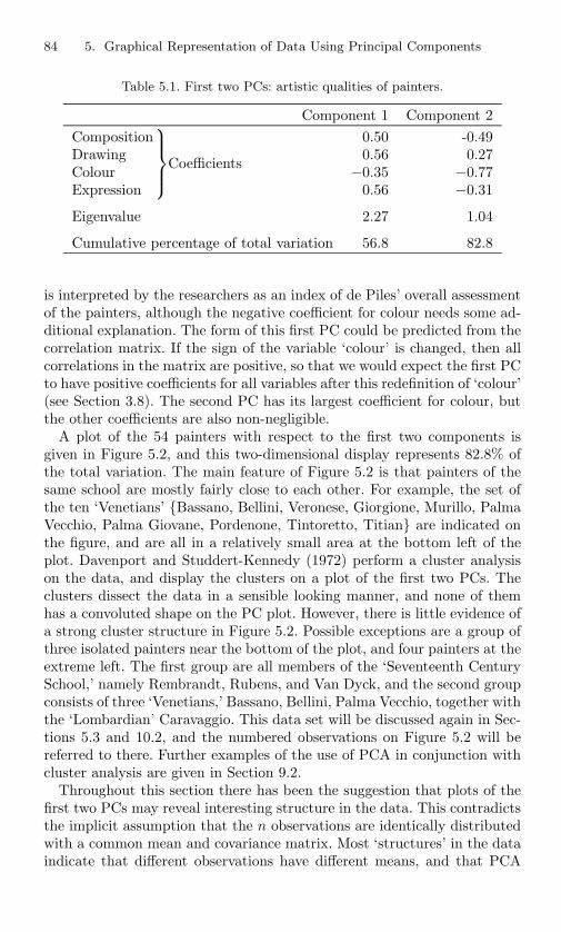
84 5. Graphical Representation of Data Using Principal Components
Table 5.1. First two PCs: artistic qualities of painters.
Component 1 Component 2Composition 0.50 -0.49Drawing 0.56 0.27
CoefficientsColour −0.35 −0.77
Expression 0.56 −0.31
Eigenvalue 2.27 1.04
Cumulative percentage of total variation 56.8 82.8
is interpreted by the researchers as an index of de Piles’ overall assessmentof the painters, although the negative coefficient for colour needs some ad-ditional explanation. The form of this first PC could be predicted from thecorrelation matrix. If the sign of the variable ‘colour’ is changed, then allcorrelations in the matrix are positive, so that we would expect the first PCto have positive coefficients for all variables after this redefinition of ‘colour’(see Section 3.8). The second PC has its largest coefficient for colour, butthe other coefficients are also non-negligible.
A plot of the 54 painters with respect to the first two components isgiven in Figure 5.2, and this two-dimensional display represents 82.8% ofthe total variation. The main feature of Figure 5.2 is that painters of thesame school are mostly fairly close to each other. For example, the set ofthe ten ‘Venetians’ Bassano, Bellini, Veronese, Giorgione, Murillo, PalmaVecchio, Palma Giovane, Pordenone, Tintoretto, Titian are indicated onthe figure, and are all in a relatively small area at the bottom left of theplot. Davenport and Studdert-Kennedy (1972) perform a cluster analysison the data, and display the clusters on a plot of the first two PCs. Theclusters dissect the data in a sensible looking manner, and none of themhas a convoluted shape on the PC plot. However, there is little evidence ofa strong cluster structure in Figure 5.2. Possible exceptions are a group ofthree isolated painters near the bottom of the plot, and four painters at theextreme left. The first group are all members of the ‘Seventeenth CenturySchool,’ namely Rembrandt, Rubens, and Van Dyck, and the second groupconsists of three ‘Venetians,’ Bassano, Bellini, Palma Vecchio, together withthe ‘Lombardian’ Caravaggio. This data set will be discussed again in Sec-tions 5.3 and 10.2, and the numbered observations on Figure 5.2 will bereferred to there. Further examples of the use of PCA in conjunction withcluster analysis are given in Section 9.2.
Throughout this section there has been the suggestion that plots of thefirst two PCs may reveal interesting structure in the data. This contradictsthe implicit assumption that the n observations are identically distributedwith a common mean and covariance matrix. Most ‘structures’ in the dataindicate that different observations have different means, and that PCA

5.2. Principal Coordinate Analysis 85
Figure 5.2. Artistic qualities of painters: plot of 54 painters with respect to theirfirst two PCs. The symbol × denotes member of the ‘Venetian’ school.
is looking for major directions of variation between means rather thanmajor directions of variation in a common distribution (de Falguerolles,personal communication). This view is in line with the fixed effect modelof Section 3.9, and is discussed further in Section 5.3.
A variation of the simple plot of PC scores for the first two PCs isproposed by Tarpey (2000). Lines are added to the plot, correspondingto the directions of the first PC for two subsets of the data, derived bydividing the full data set according to the sign of the first PC for the wholedata set. The idea is to indicate possible non-linearity in the data (seeSection 14.1.3).
5.2 Principal Coordinate Analysis
Principal coordinate analysis is a scaling or ordination method, sometimesknown as classical scaling. It was popularized by Gower (1966). Torgerson(1952, 1958) discussed similar ideas, but did not point out the links be-

86 5. Graphical Representation of Data Using Principal Components
tween principal coordinate analysis and PCA that were noted by Gower.Like the more widely known non-metric multidimensional scaling (Kruskal,1964a,b), the technique starts with a matrix of similarities or dissimilari-ties between a set of observations, and aims to produce a low-dimensionalgraphical plot of the data in such a way that distances between points inthe plot are close to the original dissimilarities. There are numerous scalingtechniques; Cox and Cox (2001) provide a good overview of many of them.
The starting point (an (n × n) matrix of (dis)similarities) of principalcoordinate analysis is different from that of PCA, which usually beginswith the (n×p) data matrix. However, in special cases discussed below thetwo techniques give precisely the same low-dimensional representation. Fur-thermore, PCA may be used to find starting configurations for the iterativealgorithms associated with non-metric multidimensional scaling (Davison,1983, Chapters 5, 6). Before showing the equivalences between PCA andprincipal coordinate analysis, we need first to describe principal coordinateanalysis in some detail.
Suppose that T is an (n × n) positive-semidefinite symmetric matrix ofsimilarities among a set of n observations. (Note that it is fairly standardnotation to use A, rather than T, here. However, we have avoided theuse of A in this context, as it is consistently taken to be the matrix ofPC coefficients in the current text.) From the spectral decomposition of T(Property A3 of Sections 2.1 and 3.1 gives the spectral decomposition ofa covariance matrix, but the same idea is valid for any symmetric matrix)we have
T = τ1b1b′1 + τ2b2b′
2 + · · · + τnbnb′n, (5.2.1)
where τ1 ≥ τ2 ≥ · · · ≥ τn are the eigenvalues of T and b1,b2, · · · ,bn arethe corresponding eigenvectors. Alternatively, this may be written
T = c1c′1 + c2c′2 + · · · + cnc′n, (5.2.2)
where
cj = τ1/2j bj , j = 1, 2, . . . , n.
Now consider the n observations as points in n-dimensional space withthe jth coordinate for the ith observation equal to cij , the ith element ofcj . With this geometric interpretation of the n observations, the Euclideandistance between the hth and ith observations is
∆2hi =
n∑
j=1
(chj − cij)2
=n∑
j=1
c2hj +
n∑
j=1
c2ij − 2
n∑
j=1
chjcij .
5.2. Principal Coordinate Analysis 87
But from (5.2.2), the (h, i)th element of T can be written
thi =n∑
j=1
chjcij , h, i = 1, 2, . . . , n,
so
∆2hi = thh + tii − 2thi.
Principal coordinate analysis then attempts to find the ‘best-fitting’ q-dimensional (q < n) approximation to the n-dimensional representationdefined above. ‘Best-fitting’ is defined here in the same way as in the ge-ometric definition of PCA (Property G3 of Section 3.2), so that ‘principalcomponents’ are now found for the n ‘observations’ defined in n dimensionsby the coordinates cij . A q-dimensional principal coordinate representationis then given by plotting the coordinates of the observations with respectto the first q ‘PCs’. Principal coordinate analysis therefore consists of twostages, both of which involve finding eigenvalues and eigenvectors of (n×n)matrices:
(i) Find the eigenvectors c1, c2, . . . , cn of T, normalized to have lengthsequal to their respective eigenvalues, and represent the n observa-tions as points in n-dimensional space with coordinate cij for the ithobservation in the jth dimension.
(ii) Find the PCs for the ‘data set’ in n dimensions defined in (i), andcalculate coordinates of the n observations with respect to the first qPCs.
If the vectors cj defined in the first stage have∑n
i=1 cij = 0 then thecovariance matrix that is calculated in stage (ii) will be proportional toC′C where C is the (n × n) matrix with jth column cj , j = 1, 2, . . . , n.But
c′jck =
τj j = k0 j = k
,
as the eigenvectors in the spectral decomposition (5.2.1) have the property
b′jbk =
1 j = k0 j = k
and
cj = τ1/2j bj , j = 1, 2, . . . , n.
The matrix C′C is therefore diagonal with diagonal elements τj , j =1, 2, . . . , n, so that the first q principal coordinates of the n observationsare simply the values of cij for i = 1, 2, . . . , n; j = 1, 2, . . . , q. Thus when∑n
i=1 cij = 0, stage (ii) is unnecessary.In general, although a similarity matrix T need not lead to
∑ni=1 cij =
0, this property can be readily achieved by replacing T by an adjusted

88 5. Graphical Representation of Data Using Principal Components
similarity matrix. In this adjustment, thi is replaced by thi − th − ti + twhere th denotes the mean of the elements in the hth row (or column,since T is symmetric) of T, and t is the mean of all elements in T. Thisadjusted similarity matrix has
∑ni=1 cij = 0, and gives the same value
of ∆2hi for each pair of observations as does T (Gower, 1966). Thus we
can replace the second stage of principal coordinate analysis by an initialadjustment of T, for any similarity matrix T.
Principal coordinate analysis is equivalent to a plot with respect to thefirst q PCs when the measure of similarity between two points is propor-tional to −d2
hi, where d2hi is the Euclidean squared distance between the
hth and ith observations, calculated from the usual (n × p) data matrix.Assume thi = −γd2
hi, where γ is a positive constant; then if stage (i) of aprincipal coordinate analysis is carried out, the ‘distance’ between a pairof points in the constructed n-dimensional space is
∆2hi = (thh + tii − 2thi)
= γ(−d2hh − d2
ii + 2d2hi)
= 2γd2hi,
as Euclidean distance from a point to itself is zero. Thus, apart from apossible rescaling if γ is taken to be a value other than 1
2 , the first stage ofprincipal coordinate analysis correctly reproduces the relative positions ofthe n observations, which lie in a p-dimensional subspace of n-dimensionalspace, so that the subsequent PCA in stage (ii) gives the same result as aPCA on the original data.
Two related special cases are of interest. First, consider the situationwhere all variables are binary. A commonly used measure of similarity be-tween individuals h and i is the proportion of the p variables for which hand i take the same value, and it can be easily demonstrated (Gower, 1966)that this measure is equivalent to Euclidean distance. Thus, although PCAof discrete—and in particular—binary data has its critics, it is equivalentto principal coordinate analysis with a very plausible measure of similar-ity. Principal component analysis for discrete data is discussed further inSection 13.1.
The second special case occurs when the elements of the similarity matrixT are defined as ‘covariances’ between observations, so that T is propor-tional to XX′, where X, as before, is the column-centred (n × p) matrixwhose (i, j)th element is the value of the jth variable, measured about itsmean xj , for the ith observation. In this case the (h, i)th similarity is, apartfrom a constant,
thi =p∑
j=1
xhjxij
and the distances between the points in the n-dimensional space con-

5.2. Principal Coordinate Analysis 89
structed in the first stage of the principal coordinate analysis are
∆2hi = thh + tii − 2thi
=p∑
j=1
x2hj +
p∑
j=1
x2ij − 2
p∑
j=1
xhjxij
=p∑
j=1
(xhj − xij)2
= d2hi,
the Euclidean distance between the observations using the original p vari-ables. As before, the PCA in the second stage of principal coordinateanalysis gives the same results as a PCA on the original data. Note, how-ever, that XX′ is not a very obvious similarity matrix. For a ‘covariancematrix’ between observations it is more natural to use a row-centred, ratherthan column-centred, version of X.
Even in cases where PCA and principal coordinate analysis give equiv-alent two-dimensional plots, there is a difference, namely that in principalcoordinate analysis there are no vectors of coefficients defining the axesin terms of the original variables. This means that, unlike PCA, theaxes in principal coordinate analysis cannot be interpreted, unless thecorresponding PCA is also done.
The equivalence between PCA and principal coordinate analysis in thecircumstances described above is termed a duality between the two tech-niques by Gower (1966). The techniques are dual in the sense that PCAoperates on a matrix of similarities between variables, whereas principal co-ordinate analysis operates on a matrix of similarities between observations(individuals), but both can lead to equivalent results.
To summarize, principal coordinate analysis gives a low-dimensional rep-resentation of data when the data are given in the form of a similarity ordissimilarity matrix. As it can be used with any form of similarity or dissim-ilarity matrix, it is, in one sense, ‘more powerful than,’ and ‘extends,’ PCA(Gower, 1967). However, as will be seen in subsequent chapters, PCA hasmany uses other than representing data graphically, which is the overridingpurpose of principal coordinate analysis.
Except in the special cases discussed above, principal coordinate analysishas no direct relationship with PCA, so no examples will be given of thegeneral application of the technique. In the case where principal coordinateanalysis gives an equivalent representation to that of PCA, nothing newwould be demonstrated by giving additional examples. The examples givenin Section 5.1 (and elsewhere) which are presented as plots with respectto the first two PCs are, in fact, equivalent to two-dimensional princi-pal coordinate plots if the ‘dissimilarity’ between observations h and i isproportional to the Euclidean squared distance between the hth and ithobservations in p dimensions.
90 5. Graphical Representation of Data Using Principal Components
In most cases, if the data are available in the form of an (n × p) matrixof p variables measured for each of n observations, there is no advantagein doing a principal coordinate analysis instead of a PCA, unless for somereason a dissimilarity measure other than Euclidean distance is deemedto be appropriate. However, an exception occurs when n < p, especially ifn p as happens for some types of chemical, meteorological and biologicaldata. As principal coordinate analysis and PCA find eigenvectors of an(n × n) matrix and a (p × p) matrix respectively, the dual analysis basedon principal coordinates will have computational advantages in such cases.
5.3 Biplots
The two previous sections describe plots of the n observations, usuallyin two dimensions. Biplots similarly provide plots of the n observations,but simultaneously they give plots of the relative positions of the p vari-ables in two dimensions. Furthermore, superimposing the two types of plotsprovides additional information about relationships between variables andobservations not available in either individual plot.
Since the publication of the first edition, there have been substantialdevelopments in biplots. In particular, the monograph by Gower and Hand(1996) considerably extends the definition of biplots. As these authors notethemselves, their approach to biplots is unconventional, but it is likelyto become increasingly influential. The material on biplots which follows ismostly concerned with what Gower and Hand (1996) call ‘classical biplots,’although correspondence analysis, which is discussed in Section 5.4, alsofalls under Gower and Hand’s (1996) biplot umbrella. A number of othervariations of biplots are discussed briefly at the end of the present sectionand in later chapters. As with other parts of this book, the choice of howfar to stray from PCA in following interesting diversions such as these isinevitably a personal one. Some readers may prefer to go further downthe biplot road; reference to Gower and Hand (1996) should satisfy theircuriosity.
Classical biplots, which might also be called ‘principal component bi-plots,’ were principally developed and popularized by Gabriel (1971, andseveral subsequent papers), although Jolicoeur and Mosimann (1960) hadearlier given an example of similar diagrams and they are periodically redis-coverd in other disciplines (see, for example, Berry et al. (1995), who referto the same idea as ‘latent semantic indexing’). The plots are based on thesingular value decomposition (SVD), which was described in Section 3.5.This states that the (n × p) matrix X of n observations on p variablesmeasured about their sample means can be written
X = ULA′, (5.3.1)
where U, A are (n×r), (p×r) matrices respectively, each with orthonormal

5.3. Biplots 91
columns, L is an (r × r) diagonal matrix with elements l1/21 ≥ l
1/22 ≥ · · · ≥
l1/2r , and r is the rank of X. Now define Lα, for 0 ≤ α ≤ 1, as the diagonalmatrix whose elements are l
α/21 , l
α/22 , · · · , l
α/2r with a similar definition for
L1−α, and let G = ULα,H′ = L1−αA′. Then
GH′ = ULαL1−αA′ = ULA′ = X,
and the (i, j)th element of X can be written
xij = g′ihj , (5.3.2)
where g′i, i = 1, 2, . . . , n and h′
j , j = 1, 2, . . . , p are the rows of G and H,respectively. Both the gi and hj have r elements, and if X has rank 2, allcould be plotted as points in two-dimensional space. In the more generalcase, where r > 2, it was noted in Section 3.5 that (5.3.1) can be written
xij =r∑
k=1
uikl1/2k ajk (5.3.3)
which is often well approximated by
mxij =m∑
k=1
uikl1/2k ajk, with m < r. (5.3.4)
But (5.3.4) can be written
mxij =m∑
k=1
gikhjk
= g∗′i h∗
j ,
where g∗i , h∗
j contain the first m elements of gi and hj , respectively. In thecase where (5.3.4) with m = 2 provides a good approximation to (5.3.3),g∗
i , i = 1, 2, . . . , n; h∗j , j = 1, 2, . . . , p together give a good two-dimensional
representation of both the n observations and the p variables. This typeof approximation can, of course, be used for values of m > 2, but thegraphical representation is then less clear. Gabriel (1981) referred to theextension to m ≥ 3 as a bimodel, reserving the term ‘biplot’ for the casewhere m = 2. However, nine years later Gabriel adopted the more commonusage of ‘biplot’ for any value of m (see Gabriel and Odoroff (1990), whichgives several examples of biplots including one with m = 3). Bartkowiakand Szustalewicz (1996) discuss how to display biplots in three dimensions.
In the description of biplots above there is an element of non-uniqueness,as the scalar α which occurs in the definition of G and H can take any valuebetween zero and one and still lead to a factorization of the form (5.3.2).Two particular values of α, namely α = 0 and α = 1, provide especiallyuseful interpretations for the biplot.

92 5. Graphical Representation of Data Using Principal Components
If α = 0, then G = U and H′ = LA′ or H = AL. This means that
X′X = (GH′)′(GH′)= HG′GH′
= HU′UH′
= HH′,
because the columns of U are orthonormal. The product h′jhk is there-
fore equal to (n − 1) multiplied by the covariance sjk between the jthand kth variables, and h∗′
j h∗k, where h∗
j , j = 1, 2, · · · , p are as definedabove, provides an approximation to (n − 1)sjk. The lengths h′
jhj of thevectors hj , i = 1, 2, · · · , p are proportional to the variances of the vari-ables x1, x2, · · · , xp, and the cosines of the angles between the hj representcorrelations between variables. Plots of the h∗
j therefore provide a two-dimensional picture (usually an approximation, but often a good one) ofthe elements of the covariance matrix S, and such plots are advocatedby Corsten and Gabriel (1976) as a means of comparing the variance-covariance structures of several different data sets. An earlier paper byGittins (1969), which is reproduced in Bryant and Atchley (1975), alsogives plots of the h∗
j , although it does not discuss their formal properties.Not only do the hj have a ready graphical interpretation when α = 0, but
the gi also have the satisfying property that the Euclidean distance betweengh and gi in the biplot is proportional to the Mahalanobis distance betweenthe hth and ith observations in the complete data set. The Mahalanobisdistance between two observations xh, xi, assuming that X has rank p sothat S−1 exists, is defined as
δ2hi = (xh − xi)′S−1(xh − xi), (5.3.5)
and is often used as an alternative to the Euclidean distance
d2hi = (xh − xi)′(xh − xi).
Whereas Euclidean distance treats all variables on an equal footing, whichessentially assumes that all variables have equal variances and are uncor-related, Mahalanobis distance gives relatively less weight to variables withlarge variances and to groups of highly correlated variables.
To prove this Mahalanobis distance interpretation, rewrite (5.3.2) as
x′i = g′
iH′, i = 1, 2, . . . , n,
and substitute in (5.3.5) to give
δ2hi = (gh − gi)′H′S−1H(gh − gi)
= (n − 1)(gh − gi)′LA′(X′X)−1AL(gh − gi), (5.3.6)
as H′ = LA′ and S−1 = (n − 1)(X′X)−1.

5.3. Biplots 93
But
X′X = (ULA′)′(ULA′)= AL(U′U)LA′
= AL2A′,
and
(X′X)−1 = AL−2A′.
Substituting in (5.3.6) gives
δ2hi = (n − 1)(gh − gi)′L(A′A)L−2(A′A)L(gh − gi)
= (n − 1)(gh − gi)′LL−2L(gh − gi)(as the columns of A are orthonormal),
= (n − 1)(gh − gi)′(gh − gi), as required.
An adaptation to the straightforward factorization given above for α = 0improves the interpretation of the plot still further. If we multiply the gi
by (n − 1)1/2 and correspondingly divide the hj by (n − 1)1/2, then thedistances between the modified gi are equal (not just proportional) to theMahalanobis distance and, if m = 2 < p, then the Euclidean distancebetween g∗
h and g∗i gives an easily visualized approximation to the Ma-
halanobis distance between xh and xi. Furthermore, the lengths h′jhj are
equal to variances of the variables. This adaptation was noted by Gabriel(1971), and is used in the examples below.
A further interesting property of the biplot when α = 0 is that measurescan be written down of how well the plot approximates
(a) the column-centred data matrix X;
(b) the covariance matrix S;
(c) the matrix of Mahalanobis distances between each pair of observations.
These measures are, respectively, (Gabriel 1971)
(a) (l1 + l2)/ r∑
k=1
lk;
(b) (l21 + l22)/ r∑
k=1
l2k;
(c) (l01 + l02)/ r∑
k=1
l0k = 2/r.
Because l1 ≥ l2 ≥ · · · ≥ lr, these measures imply that the biplot gives abetter approximation to the variances and covariances than to the (Ma-halanobis) distances between observations. This is in contrast to principalcoordinate plots, which concentrate on giving as good a fit as possible to
94 5. Graphical Representation of Data Using Principal Components
interobservation dissimilarities or distances, and do not consider directlythe elements of X or S.
We have now seen readily interpretable properties of both the g∗i and the
h∗j separately for the biplot when α = 0, but there is a further property,
valid for any value of α, which shows that the plots of the g∗i and h∗
j canbe usefully superimposed rather than simply considered separately.
From the relationship xij = g′ihj , it follows that xij is represented by
the projection of gi onto hj . Remembering that xij is the value for the ithobservation of the jth variable measured about its sample mean, values ofxij close to zero, which correspond to observations close to the sample meanof the jth variable, will only be achieved if gi and hj are nearly orthogonal.Conversely, observations for which xij is a long way from zero will have gi
lying in a similar direction to hj . The relative positions of the points definedby the gi and hj , or their approximations in two dimensions, the g∗
i andh∗
j , will therefore give information about which observations take large,average and small values on each variable.
Turning to the biplot with α = 1, the properties relating to gi and hj
separately are different from those for α = 0. With α = 1 we have
G = UL, H′ = A′,
and instead of (gh − gi)′(gh − gi) being proportional to the Mahalanobisdistance between xh and xi, it is now equal to the Euclidean distance. Thisfollows because
(xh − xi)′(xh − xi) = (gh − gi)′H′H(gh − gi)= (gh − gi)′A′A(gh − gi)= (gh − gi)′(gh − gi).
Therefore, if we prefer a plot on which the distance between g∗h and
g∗i is a good approximation to Euclidean, rather than Mahalanobis, dis-
tance between xh and xi then the biplot with α = 1 will be preferredto α = 0. Note that using Mahalanobis distance emphasizes the dis-tance between the observations in the direction of the low-variance PCsand downweights distances in the direction of high-variance PCs, whencompared with Euclidean distance (see Section 10.1).
Another interesting property of the biplot with α = 1 is that the positionsof the g∗
i are identical to those given by a straightforward plot with respectto the first two PCs, as described in Section 5.1. It follows from equation(5.3.3) and Section 3.5 that we can write
xij =r∑
k=1
zikajk,
where zik = uikl1/2k is the value of the kth PC for the ith observation. But
α = 1 implies that G = UL, so the kth element of gi is uikl1/2k = zik.

5.3. Biplots 95
The vector g∗i consists of the first two elements of gi, which are simply the
values of the first two PCs for the ith observation.The properties of the hj that were demonstrated above for α = 0 will
no longer be valid exactly for α = 1, although similar interpretations canstill be made, at least in qualitative terms. In fact, the coordinates of h∗
j
are simply the coefficients of the jth variable for the first two PCs. Theadvantage of superimposing the plots of the g∗
i and h∗j is preserved for
α = 1, as xij still represents the projection of gi onto hj . In many ways,the biplot with α = 1 is nothing new, since the g∗
i give PC scores andthe h∗
j give PC coefficients, both of which are widely used on their own.The biplot, however, superimposes both the g∗
i and h∗j to give additional
information.Other values of α could also be used; for example, Gabriel (1971) men-
tions α = 12 , in which the sum of squares of the projections of plotted points
onto either one of the axes is the same for observations as for variables (Os-mond, 1985), but most applications seem to have used α = 0, or sometimesα = 1. For other values of α the general qualitative interpretation of therelative positions of the gi and the hj remains the same, but the exactproperties that hold for α = 0 and α = 1 are no longer valid.
Another possibility is to superimpose the g∗i and the h∗
j correspondingto different values of α. Choosing a single standard value of α for boththe g∗
i and h∗j may mean that the scales of observations and variables are
so different that only one type of entity is visible on the plot. Digby andKempton (1987, Section 3.2) choose scales for observations and variablesso that both can easily be seen when plotted together. This is done ratherarbitrarily, but is equivalent to using different values of α for the two typesof entity. Mixing values of α in this way will, of course, lose the propertythat xij is the projection of gi onto hj , but the relative positions of theg∗
i and h∗j still give qualitative information about the size of each variable
for each observation. Another way of mixing values of α is to use g∗i cor-
responding to α = 1 and h∗j corresponding to α = 0, so that the g∗
i givea PC plot, and the h∗
j have a direct interpretation in terms of variancesand covariances. This is referred to by Gabriel (2001) as a ‘correspondenceanalysis’ (see Section 5.4) plot. Gower and Hand (1996) and Gabriel (2001),among others, have noted that different plotting positions can be chosento give optimal approximations to two, but not all three, of the following:
(a) the elements of X, as given by the scalar products g∗′i h∗
j ;
(b) Euclidean distances between the rows of X;
(c) the covariance structure in the columns of X.
We noted earlier that for α = 0, (b) is fitted less well than (c). For α = 1,(c) rather than (b) is sacrificed, while the correspondence analysis plot loses(a). Choosing α = 1
2 approximates (a) optimally, but is suboptimal for (b)and (c). For each of these four choices Gabriel (2001) investigates how
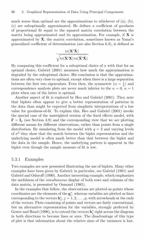
96 5. Graphical Representation of Data Using Principal Components
much worse than optimal are the approximations to whichever of (a), (b),(c) are suboptimally approximated. He defines a coefficient of goodnessof proportional fit equal to the squared matrix correlation between thematrix being approximated and its approximation. For example, if X isapproximated by X, the matrix correlation, sometimes known as Yanai’sgeneralized coefficient of determination (see also Section 6.3), is defined as
tr(X′X)√
tr(X′X) tr(X′X).
By comparing this coefficient for a suboptimal choice of α with that for anoptimal choice, Gabriel (2001) measures how much the approximation isdegraded by the suboptimal choice. His conclusion is that the approxima-tions are often very close to optimal, except when there is a large separationbetween the first two eigenvalues. Even then, the symmetric (α = 1
2 ) andcorrespondence analysis plots are never much inferior to the α = 0, α = 1plots when one of the latter is optimal.
Another aspect of fit is explored by Heo and Gabriel (2001). They notethat biplots often appear to give a better representation of patterns inthe data than might be expected from simplistic interpretations of a lowvalue for goodness-of-fit. To explain this, Heo and Gabriel (2001) invokethe special case of the unweighted version of the fixed effects model, withΓ = Ip (see Section 3.9) and the corresponding view that we are plottingdifferent means for different observations, rather than points from a singledistribution. By simulating from the model with q = 2 and varying levelsof σ2 they show that the match between the biplot representation and theunderlying model is often much better than that between the biplot andthe data in the sample. Hence, the underlying pattern is apparent in thebiplot even though the sample measure of fit is low.
5.3.1 Examples
Two examples are now presented illustrating the use of biplots. Many otherexamples have been given by Gabriel; in particular, see Gabriel (1981) andGabriel and Odoroff (1990). Another interesting example, which emphasizesthe usefulness of the simultaneous display of both rows and columns of thedata matrix, is presented by Osmond (1985).
In the examples that follow, the observations are plotted as points whosecoordinates are the elements of the g∗
i , whereas variables are plotted as linescorresponding to the vectors h∗
j , j = 1, 2, . . . , p, with arrowheads at the endsof the vectors. Plots consisting of points and vectors are fairly conventional,but an alternative representation for the variables, strongly preferred byGower and Hand (1996), is to extend the vectors h∗
j right across the diagramin both directions to become lines or axes. The disadvantage of this typeof plot is that information about the relative sizes of the variances is lost.
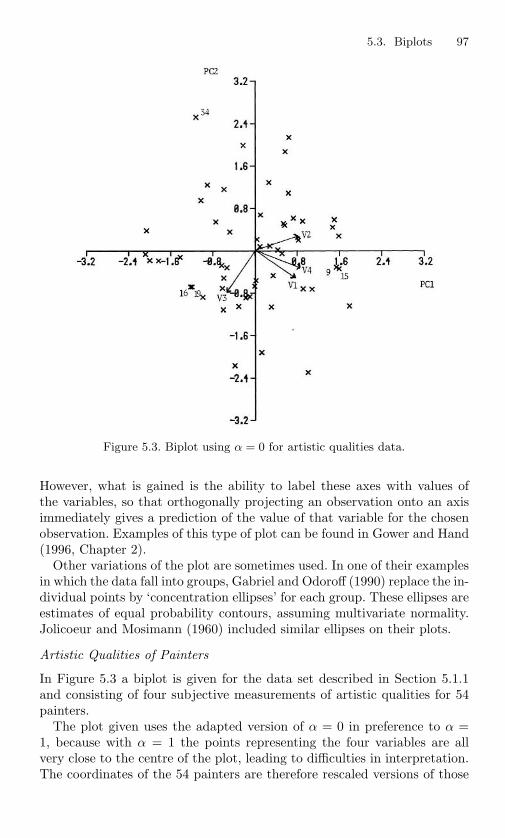
5.3. Biplots 97
Figure 5.3. Biplot using α = 0 for artistic qualities data.
However, what is gained is the ability to label these axes with values ofthe variables, so that orthogonally projecting an observation onto an axisimmediately gives a prediction of the value of that variable for the chosenobservation. Examples of this type of plot can be found in Gower and Hand(1996, Chapter 2).
Other variations of the plot are sometimes used. In one of their examplesin which the data fall into groups, Gabriel and Odoroff (1990) replace the in-dividual points by ‘concentration ellipses’ for each group. These ellipses areestimates of equal probability contours, assuming multivariate normality.Jolicoeur and Mosimann (1960) included similar ellipses on their plots.
Artistic Qualities of Painters
In Figure 5.3 a biplot is given for the data set described in Section 5.1.1and consisting of four subjective measurements of artistic qualities for 54painters.
The plot given uses the adapted version of α = 0 in preference to α =1, because with α = 1 the points representing the four variables are allvery close to the centre of the plot, leading to difficulties in interpretation.The coordinates of the 54 painters are therefore rescaled versions of those

98 5. Graphical Representation of Data Using Principal Components
displayed in Figure 5.2, but their relative positions are similar. For example,the group of three ‘Seventeenth Century’ painters at the bottom of the plotis still visible. Because of the compression of the horizontal relative to thevertical scale, the group of four painters at the left of the plot now seemsto have been joined by a fifth, Murillo, who is from the same school asthree of the others in this group. There is also an outlying painter, Fr.Penni, observation number 34, whose isolated position in the top left ofthe plot is perhaps more obvious on Figure 5.3 than Figure 5.2. The maindistinguishing feature of this painter is that de Piles gave him a 0 score forcomposition, compared to a minimum of 4 and a maximum of 18 for allother painters.
Now consider the positions on the biplot of the vectors corresponding tothe four variables. It is seen that composition and expression (V1 and V4)are close together, reflecting their relatively large positive correlation, andthat drawing and colour (V2 and V3) are in opposite quadrants, confirm-ing their fairly large negative correlation. Other correlations, and hencepositions of vectors, are intermediate.
Finally, consider the simultaneous positions of painters and variables.The two painters, numbered 9 and 15, that are slightly below the positivehorizontal axis are Le Brun and Domenichino. These are close to the direc-tion defined by V4, and not far from the directions of V1 and V2, whichimplies that they should have higher than average scores on these threevariables. This is indeed the case: Le Brun scores 16 on a scale from 0 to20 on all three variables, and Domenichino scores 17 on V2 and V4 and 15on V1. Their position relative to V3 suggests an average or lower score onthis variable; the actual scores are 8 and 9, which confirms this suggestion.As another example consider the two painters 16 and 19 (Giorgione andDa Udine), whose positions are virtually identical, in the bottom left-handquadrant of Figure 5.3. These two painters have high scores on V3 (18 and16) and below average scores on V1, V2 and V4. This behaviour, but withlower scores on V2 than on V1, V4, would be predicted from the points’positions on the biplot.
100 km Running Data
The second example consists of data on times taken for each of ten 10km sections by the 80 competitors who completed the Lincolnshire 100 kmrace in June 1984. There are thus 80 observations on ten variables. (I amgrateful to Ron Hindley, the race organizer, for distributing the results ofthe race in such a detailed form.)
The variances and coefficients for the first two PCs, based on the correla-tion matrix for these data, are given in Table 5.2. Results for the covariancematrix are similar, though with higher coefficients in the first PC for thelater sections of the race, as (means and) variances of the times takenfor each section tend to increase later in the race. The first component

5.3. Biplots 99
Table 5.2. First two PCs: 100 km running data.
Component 1 Component 2First 10 km −0.30 0.45Second 10 km −0.30 0.45Third 10 km −0.33 0.34Fourth 10 km −0.34 0.20Fifth 10 km −0.34 −0.06
CoefficientsSixth 10 km −0.35 −0.16Seventh 10 km −0.31 −0.27Eighth 10 km −0.31 −0.30Ninth 10 km −0.31 −0.29Tenth 10 km −0.27 −0.40
Eigenvalue 72.4 1.28
Cumulative percentage of total variation 7.24 85.3
measures the overall speed of the runners, and the second contrasts thoserunners who slow down substantially during the course of the race withthose runners who maintain a more even pace. Together, the first two PCsaccount for more than 85% of the total variation in the data.
The adapted α = 0 biplot for these data is shown in Figure 5.4.As with the previous example, the plot using α = 1 is not very sat-
isfactory because the vectors corresponding to the variables are all veryclose to the centre of the plot. Figure 5.4 shows that with α = 0 we havethe opposite extreme—the vectors corresponding to the variables and thepoints corresponding to the observations are completely separated. As acompromise, Figure 5.5 gives the biplot with α = 1
2 , which at least hasapproximately the same degree of spread for variables and observations.As with α = 0, the plot has been modified from the straightforward fac-torization corresponding to α = 1
2 . The gi have been multiplied, and thehj divided, by (n − 1)1/4, so that we have a compromise between α = 1and the adapted version of α = 0. The adapted plot with α = 1
2 is still notentirely satisfactory, but even an arbitrary rescaling of observations and/orvariables, as suggested by Digby and Kempton (1987, Section 3.2), wouldstill have all the vectors corresponding to variables within a very narrowsector of the plot. This is unavoidable for data that, as in the present case,have large correlations between all variables. The tight bunching of the vec-tors simply reflects large correlations, but it is interesting to note that theordering of the vectors around their sector corresponds almost exactly totheir position within the race. (The ordering is the same for both diagrams,but to avoid congestion, this fact has not been indicated on Figure 5.5.)With hindsight, this is not surprising as times in one part of the race are
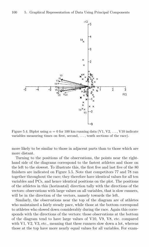
100 5. Graphical Representation of Data Using Principal Components
Figure 5.4. Biplot using α = 0 for 100 km running data (V1, V2, . . . , V10 indicatevariables measuring times on first, second, . . . , tenth sections of the race).
more likely to be similar to those in adjacent parts than to those which aremore distant.
Turning to the positions of the observations, the points near the right-hand side of the diagrams correspond to the fastest athletes and those onthe left to the slowest. To illustrate this, the first five and last five of the 80finishers are indicated on Figure 5.5. Note that competitors 77 and 78 rantogether throughout the race; they therefore have identical values for all tenvariables and PCs, and hence identical positions on the plot. The positionsof the athletes in this (horizontal) direction tally with the directions of thevectors: observations with large values on all variables, that is slow runners,will be in the direction of the vectors, namely towards the left.
Similarly, the observations near the top of the diagram are of athleteswho maintained a fairly steady pace, while those at the bottom correspondto athletes who slowed down considerably during the race. Again this corre-sponds with the directions of the vectors: those observations at the bottomof the diagram tend to have large values of V10, V9, V8, etc. comparedwith V1, V2, V3, etc., meaning that these runners slow down a lot, whereasthose at the top have more nearly equal values for all variables. For exam-
5.3. Biplots 101
Figure 5.5. Biplot using α = 12
for 100 km running data (numbers indicatefinishing position in race).
ple, consider the outlying observation at the top of Figures 5.4 and 5.5. Thispoint corresponds to the 54th finisher, who was the only competitor to runthe final 10 km faster than the first 10 km. To put this into perspective itshould be noted that the average times taken for the first and last 10 kmby the 80 finishers were 47.6 min, and 67.0 min respectively, showing thatmost competitors slowed down considerably during the race.
At the opposite extreme to the 54th finisher, consider the two athletescorresponding to the points at the bottom left of the plots. These are the65th and 73rd finishers, whose times for the first and last 10 km were 50.0min and 87.8 min for the 65th finisher and 48.2 min and 110.0 min for the73rd finisher. This latter athlete therefore ran at a nearly ‘average’ pacefor the first 10 km but was easily one of the slowest competitors over thelast 10 km.
5.3.2 Variations on the Biplot
The classical biplot described above is based on the SVD of X, the column-centred data matrix. This in turn is linked to the spectral decomposition

102 5. Graphical Representation of Data Using Principal Components
of X′X, and hence to PCA. The variations discussed so far relate only tochoices within this classical plot, for example the choice of α in defining gi
and hj (5.3.2), the possible rescaling by a factor (n − 1)1/2 and the formof display (axes or arrowheads, concentration ellipses).
Gower and Hand (1996) describe many other variations. In particular,they look at biplots related to multivariate techniques other than PCA,including multidimensional scaling, canonical variate analysis, correspon-dence analysis and multiple correspondence analysis. Gabriel (1995a,b) alsodiscusses biplots related to multivariate methods other than PCA, in partic-ular multiple correspondence analysis and MANOVA (multivariate analysisof variance).
A key distinction drawn by Gower and Hand (1996) is between interpo-lation and prediction in a biplot. The former is concerned with determiningwhere in the diagram to place an observation, given its values on the mea-sured variables. Prediction refers to estimating the values of these variables,given the position of an observation in the plot. Both are straightforwardfor classical biplots—g∗
i is used for interpolation and 2xij for prediction—but become more complicated for other varieties of biplot. Gower and Hand(1996, Chapter 7) describe a framework for generalized biplots that includesmost other versions as special cases. One important special case is that ofnon-linear biplots. These will be discussed further in Section 14.1, whichdescribes a number of non-linear modifications of PCA. Similarly, discus-sion of robust biplots, due to Daigle and Rivest (1992), will be deferreduntil Section 10.4, which covers robust versions of PCA.
The discussion and examples of the classical biplot given above use anunstandardized form of X and hence are related to covariance matrix PCA.As noted in Section 2.3 and elsewhere, it is more usual, and often moreappropriate, to base PCA on the correlation matrix as in the examplesof Section 5.3.1. Corresponding biplots can be derived from the SVD ofX, the column-centred data matrix whose jth column has been scaled bydividing by the standard deviation of xj , j = 1, 2, . . . , p. Many aspects ofthe biplot remain the same when the correlation, rather than covariance,matrix is used. The main difference is in the positions of the hj . Recall thatif α = 0 is chosen, together with the scaling factor (n−1)1/2, then the lengthh∗′
jh∗j approximates the variance of xj . In the case of a correlation-based
analysis, var(xj) = 1 and the quality of the biplot approximation to thejth variable by the point representing h∗
j can be judged by the closeness ofh∗
j to the unit circle centred at the origin. For this reason, the unit circle issometimes drawn on correlation biplots to assist in evaluating the quality ofthe approximation (Besse, 1994a). Another property of correlation biplotsis that the squared distance between hj and hk is 2(1 − rjk), where rjk isthe correlation between xj and xk. The squared distance between h∗
j andh∗
k approximates this quantity.An alternative to the covariance and correlation biplots is the coefficient
of variation biplot, due to Underhill (1990). As its name suggests, instead

5.4. Correspondence Analysis 103
of dividing the jth column of X by the standard deviation of xj to give acorrelation biplot, here the jth column is divided by the mean of xj . Ofcourse, this only makes sense for certain types of non-negative variables,but Underhill (1990) shows that for such variables the resulting biplot givesa useful view of the data and variables. The cosines of the angles betweenthe h∗
j still provide approximations to the correlations between variables,but the lengths of the vectors h∗
j now give information on the variabilityof the xj relative to their means.
Finally, the biplot can be adapted to cope with missing values by in-troducing weights wij for each observation xij when approximating xij byg∗′
i h∗j . A weight of zero is given to missing values and a unit weight to those
values which are present. The appropriate values for g∗i ,h∗
j can be calcu-lated using an algorithm which handles general weights, due to Gabriel andZamir (1979). For a more general discussion of missing data in PCA seeSection 13.6.
5.4 Correspondence Analysis
The technique commonly called correspondence analysis has been ‘redis-covered’ many times in several different guises with various names, suchas ‘reciprocal averaging’ or ‘dual scaling.’ Greenacre (1984) provides acomprehensive treatment of the subject; in particular his Section 1.3 andChapter 4 discuss, respectively, the history and the various different ap-proaches to the topic. Benzecri (1992) is also comprehensive, and morerecent, but its usefulness is limited by a complete lack of references toother sources. Two shorter texts, which concentrate on the more practi-cal aspects of correspondence analysis, are Clausen (1998) and Greenacre(1993).
The name ‘correspondence analysis’ is derived from the French ‘analysedes correspondances’ (Benzecri, 1980). Although, at first sight, correspon-dence analysis seems unrelated to PCA it can be shown that it is, in fact,equivalent to a form of PCA for discrete (generally nominal) variables (seeSection 13.1). The technique is often used to provide a graphical representa-tion of data in two dimensions. The data are normally presented in the formof a contingency table, but because of this graphical usage the technique isintroduced briefly in the present chapter. Further discussion of correspon-dence analysis and various generalizations of the technique, together withits connections to PCA, is given in Sections 13.1, 14.1 and 14.2.
Suppose that a set of data is presented in the form of a two-way contin-gency table, in which a set of n observations is classified according to itsvalues on two discrete random variables. Thus the information available isthe set of frequencies nij , i = 1, 2, . . . , r; j = 1, 2, . . . , c, where nij is thenumber of observations that take the ith value for the first (row) variable

104 5. Graphical Representation of Data Using Principal Components
and the jth value for the second (column) variable. Let N be the (r × c)matrix whose (i, j)th element is nij .
There are a number of seemingly different approaches, all of which leadto correspondence analysis; Greenacre (1984, Chapter 4) discusses thesevarious possibilities in some detail. Whichever approach is used, the finalproduct is a sequence of pairs of vectors (f1,g1), (f2,g2), . . . , (fq,gq) wherefk, k = 1, 2, . . ., are r-vectors of scores or coefficients for the rows of N,and gk, k = 1, 2, . . . are c-vectors of scores or coefficients for the columnsof N. These pairs of vectors are such that the first q such pairs give a ‘best-fitting’ representation in q dimensions, in a sense defined in Section 13.1,of the matrix N, and of its rows and columns. It is common to take q = 2.The rows and columns can then be plotted on a two-dimensional diagram;the coordinates of the ith row are the ith elements of f1, f2, i = 1, 2, . . . , r,and the coordinates of the jth column are the jth elements of g1,g2, j =1, 2, . . . , c.
Such two-dimensional plots cannot in general be compared in any directway with plots made with respect to PCs or classical biplots, as N isa different type of data matrix from that used for PCs or their biplots.However, Greenacre (1984, Sections 9.6 and 9.10) gives examples wherecorrespondence analysis is done with an ordinary (n × p) data matrix,X replacing N. This is only possible if all variables are measured in thesame units. In these circumstances, correspondence analysis produces asimultaneous two-dimensional plot of the rows and columns of X, which isprecisely what is done in a biplot, but the two analyses are not the same.
Both the classical biplot and correspondence analysis determine theplotting positions for rows and columns of X from the singular value de-composition (SVD) of a matrix (see Section 3.5). For the classical biplot,the SVD is calculated for the column-centred matrix X, but in correspon-dence analysis, the SVD is found for a matrix of residuals, after subtracting‘expected values assuming independence of rows and columns’ from X/n(see Section 13.1). The effect of looking at residual (or interaction) terms is(Greenacre, 1984, p. 288) that all the dimensions found by correspondenceanalysis represent aspects of the ‘shape’ of the data, whereas in PCA thefirst PC often simply represents ‘size’ (see Sections 4.1, 13.2). Correspon-dence analysis provides one way in which a data matrix may be adjustedin order to eliminate some uninteresting feature such as ‘size,’ before find-ing an SVD and hence ‘PCs.’ Other possible adjustments are discussed inSections 13.2 and 14.2.3.
As with the biplot and its choice of α, there are several different ways ofplotting the points corresponding to rows and columns in correspondenceanalysis. Greenacre and Hastie (1987) give a good description of the geom-etry associated with the most usual of these plots. Whereas the biplot mayapproximate Euclidean or Mahalanobis distances between rows, in corre-spondence analysis the points are often plotted to optimally approximateso-called χ2 distances (see Greenacre (1984), Benzecri (1992)).
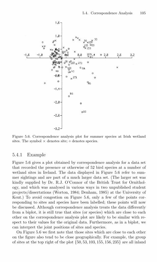
5.4. Correspondence Analysis 105
Figure 5.6. Correspondence analysis plot for summer species at Irish wetlandsites. The symbol × denotes site; denotes species.
5.4.1 Example
Figure 5.6 gives a plot obtained by correspondence analysis for a data setthat recorded the presence or otherwise of 52 bird species at a number ofwetland sites in Ireland. The data displayed in Figure 5.6 refer to sum-mer sightings and are part of a much larger data set. (The larger set waskindly supplied by Dr. R.J. O’Connor of the British Trust for Ornithol-ogy, and which was analysed in various ways in two unpublished studentprojects/dissertations (Worton, 1984; Denham, 1985) at the University ofKent.) To avoid congestion on Figure 5.6, only a few of the points cor-responding to sites and species have been labelled; these points will nowbe discussed. Although correspondence analysis treats the data differentlyfrom a biplot, it is still true that sites (or species) which are close to eachother on the correspondence analysis plot are likely to be similar with re-spect to their values for the original data. Furthermore, as in a biplot, wecan interpret the joint positions of sites and species.
On Figure 5.6 we first note that those sites which are close to each otheron the figure also tend to be close geographically. For example, the groupof sites at the top right of the plot 50, 53, 103, 155, 156, 235 are all inland

106 5. Graphical Representation of Data Using Principal Components
sites in the south west of Ireland, and the group 43, 168, 169, 171, 172 inthe bottom right of the diagram are all coastal sites in the south and east.
If we look at species, rather than sites, we find that similar species tendto be located in the same part of Figure 5.6. For example, three of thefour species of goose which were recorded are in the bottom-right of thediagram (BG, WG, GG).
Turning to the simultaneous positions of species and sites, the Grey-lag Goose (GG) and Barnacle Goose (BG) were only recorded at site171, among those sites which are numbered on Figure 5.6. On the plot,site 171 is closest in position of any site to the positions of these twospecies. The Whitefronted Goose (WG) is recorded at sites 171 and 172only, the Gadwall (GA) at sites 43, 103, 168, 169, 172 among those la-belled on the diagram, and the Common Sandpiper (CS) at all sites inthe coastal group 43, 168, 169, 171, 172, but at only one of the inlandgroup 50, 53, 103, 155, 156, 235. Again, these occurrences might be pre-dicted from the relative positions of the sites and species on the plot.However, simple predictions are not always valid, as the Coot (CO), whoseposition on the plot is in the middle of the inland sites, is recorded at all11 sites numbered on the figure.
5.5 Comparisons Between Principal Coordinates,Biplots, Correspondence Analysis and PlotsBased on Principal Components
For most purposes there is little point in asking which of the graphicaltechniques discussed so far in this chapter is ‘best.’ This is because they areeither equivalent, as is the case of PCs and principal coordinates for sometypes of similarity matrix, so any comparison is trivial, or the data set is ofa type such that one or more of the techniques are not really appropriate,and so should not be compared with the others. For example, if the dataare in the form of a contingency table, then correspondence analysis isclearly relevant, but the use of the other techniques is more questionable.As demonstrated by Gower and Hand (1996) and Gabriel (1995a,b), thebiplot is not restricted to ‘standard’ (n × p) data matrices, and could beused on any two-way array of data. The simultaneous positions of the g∗
i
and h∗j still have a similar interpretation to that discussed in Section 5.3,
even though some of the separate properties of the g∗i and h∗
j , for instance,those relating to variances and covariances, are clearly no longer valid. Acontingency table could also be analysed by PCA, but this is not reallyappropriate, as it is not at all clear what interpretation could be givento the results. Principal coordinate analysis needs a similarity or distancematrix, so it is hard to see how it could be used directly on a contingencytable.
5.6. Displaying Intrinsically High-Dimensional Data 107
There are a number of connections between PCA and the othertechniques–links with principal coordinate analysis and biplots have al-ready been discussed, while those with correspondence analysis are deferreduntil Section 13.1—but for most data sets one method is more appropriatethan the others. Contingency table data imply correspondence analysis,and similarity or dissimilarity matrices suggest principal coordinate analy-sis, whereas PCA is defined for ‘standard’ data matrices of n observationson p variables. Notwithstanding these distinctions, different techniqueshave been used on the same data sets and a number of empirical compar-isons have been reported in the ecological literature. Digby and Kempton(1987, Section 4.3) compare twelve ordination methods, including principalcoordinate analysis, with five different similarity measures and correspon-dence analysis, on both species abundances and presence/absence data.The comparison is by means of a second-level ordination based on simi-larities between the results of the twelve methods. Gauch (1982, Chapter4) discusses criteria for choosing an appropriate ordination technique forecological data, and in Gauch (1982, Chapter 3) a number of studies aredescribed which compare PCA with other techniques, including correspon-dence analysis, on simulated data. The data are generated to have a similarstructure to that expected in some types of ecological data, with addednoise, and investigations are conducted to see which techniques are ‘best’at recovering the structure. However, as with comparisons between PCAand correspondence analysis given by Greenacre (1994, Section 9.6), therelevance to the data analysed of all the techniques compared is open todebate. Different techniques implicitly assume that different types of struc-ture or model are of interest for the data (see Section 14.2.3 for some furtherpossibilities) and which technique is most appropriate will depend on whichtype of structure or model is relevant.
5.6 Methods for Graphical Display of IntrinsicallyHigh-Dimensional Data
Sometimes it will not be possible to reduce a data set’s dimensionalityto two or three without a substantial loss of information; in such cases,methods for displaying many variables simultaneously in two dimensionsmay be useful. Plots of trigonometric functions due to Andrews (1972),illustrated below, and the display in terms of faces suggested by Chernoff(1973), for which several examples are given in Wang (1978), became pop-ular in the 1970s and 1980s. There are many other possibilities (see, forexample, Tukey and Tukey (1981) and Carr(1998)) which will not be dis-cussed here. Recent developments in the visualization of high-dimensionaldata using the ever-increasing power of computers have created displayswhich are dynamic, colourful and potentially highly informative, but there

108 5. Graphical Representation of Data Using Principal Components
remain limitations on how many dimensions can be effectively shown si-multaneously. The less sophisticated ideas of Tukey and Tukey (1981) stillhave a role to play in this respect.
Even when dimensionality cannot be reduced to two or three, a reduc-tion to as few dimensions as possible, without throwing away too muchinformation, is still often worthwhile before attempting to graph the data.Some techniques, such as Chernoff’s faces, impose a limit on the numberof variables that can be handled, although a modification due to Flury andRiedwyl (1981) increases the limit, and for most other methods a reductionin the number of variables leads to simpler and more easily interpretablediagrams. An obvious way of reducing the dimensionality is to replace theoriginal variables by the first few PCs, and the use of PCs in this contextwill be particularly successful if each PC has an obvious interpretation (seeChapter 4). Andrews (1972) recommends transforming to PCs in any case,because the PCs are uncorrelated, which means that tests of significancefor the plots may be more easily performed with PCs than with the origi-nal variables. Jackson (1991, Section 18.6) suggests that Andrews’ curvesof the residuals after ‘removing’ the first q PCs, that is, the sum of the last(r − q) terms in the SVD of X, may provide useful information about thebehaviour of residual variability.
5.6.1 Example
In Jolliffe et al. (1986), 107 English local authorities are divided into groupsor clusters, using various methods of cluster analysis (see Section 9.2), onthe basis of measurements on 20 demographic variables.
The 20 variables can be reduced to seven PCs, which account for over90% of the total variation in the 20 variables, and for each local authorityan Andrews’ curve is defined on the range −π ≤ t ≤ π by the function
f(t) =z1√2
+ z2 sin t + z3 cos t + z4 sin 2t + z5 cos 2t + z6 sin 3t + z7 cos 3t,
where z1, z2, . . . , z7 are the values of the first seven PCs for the local au-thority. Andrews’ curves may be plotted separately for each cluster. Thesecurves are useful in assessing the homogeneity of the clusters. For example,Figure 5.7 gives the Andrews’ curves for three of the clusters (Clusters 2,11 and 12) in a 13-cluster solution, and it can be seen immediately thatthe shape of the curves is different for different clusters.
Compared to the variation between clusters, the curves fall into fairlynarrow bands, with a few exceptions, for each cluster. Narrower bands forthe curves imply greater homogeneity in the cluster.
In Cluster 12 there are two curves that are somewhat different fromthe remainder. These curves have three complete oscillations in the range(−π, π), with maxima at 0 and ±2π/3. This implies that they are domi-nated by cos 3t and hence z7. Examination of the seventh PC shows that

5.6. Displaying Intrinsically High-Dimensional Data 109
Figure 5.7. Local authorities demographic data: Andrews’ curves for threeclusters.

110 5. Graphical Representation of Data Using Principal Components
its largest coefficients are all positive and correspond to numbers of elderlypersons who have recently moved to the area, numbers in privately rentedaccommodation, and population sparsity (Area/Population). The implica-tion of the outlying curves for Cluster 12 is that the two local authoritiescorresponding to the curves (Cumbria, Northumberland) have substantiallylarger values for the seventh PC than do the other local authorities in thesame cluster (Cornwall, Gloucestershire, Kent, Lincolnshire, Norfolk, NorthYorkshire, Shropshire, Somerset and Suffolk). This is, indeed, the case andit further implies atypical values for Northumberland and Cumbria, com-pared to the remainder of the cluster, for the three variables having thelargest coefficients for the seventh PC.
Another example of using Andrews’ curves to examine the homogeneityof clusters in cluster analysis and to investigate potential outliers is givenby Jolliffe et al. (1980) for the data set discussed in Section 4.2.

6Choosing a Subset of PrincipalComponents or Variables
In this chapter two separate, but related, topics are considered, both ofwhich are concerned with choosing a subset of variables. In the first section,the choice to be examined is how many PCs adequately account for thetotal variation in x. The major objective in many applications of PCA isto replace the p elements of x by a much smaller number m of PCs, whichnevertheless discard very little information. It is crucial to know how smallm can be taken without serious information loss. Various rules, many adhoc, have been proposed for determining a suitable value of m, and theseare discussed in Section 6.1. Examples of their use are given in Section 6.2.
Using m PCs instead of p variables considerably reduces the dimension-ality of the problem when m p, but usually the values of all p variablesare still needed in order to calculate the PCs, as each PC is likely to bea function of all p variables. It might be preferable if, instead of using mPCs we could use m, or perhaps slightly more, of the original variables,to account for most of the variation in x. The question arises of how tocompare the information contained in a subset of variables with that inthe full data set. Different answers to this question lead to different criteriaand different algorithms for choosing the subset. In Section 6.3 we concen-trate on methods that either use PCA to choose the variables or aim toreproduce the PCs in the full data set with a subset of variables, thoughother variable selection techniques are also mentioned briefly. Section 6.4gives two examples of the use of variable selection methods.
All of the variable selection methods described in the present chapterare appropriate when the objective is to describe variation within x aswell as possible. Variable selection when x is a set of regressor variables

112 6. Choosing a Subset of Principal Components or Variables
in a regression analysis, or a set of predictor variables in a discriminantanalysis, is a different type of problem as criteria external to x must beconsidered. Variable selection in regression is the subject of Section 8.5. Therelated problem of choosing which PCs to include in a regression analysisor discriminant analysis is discussed in Sections 8.2, 9.1 respectively.
6.1 How Many Principal Components?
In this section we present a number of rules for deciding how many PCsshould be retained in order to account for most of the variation in x (orin the standardized variables x∗ in the case of a correlation matrix-basedPCA).
In some circumstances the last few, rather than the first few, PCs are ofinterest, as was discussed in Section 3.4 (see also Sections 3.7, 6.3, 8.4, 8.6and 10.1). In the present section, however, the traditional idea of tryingto reduce dimensionality by replacing the p variables by the first m PCs(m < p) is adopted, and the possible virtues of the last few PCs are ignored.
The first three types of rule for choosing m, described in Sections 6.1.1–6.1.3, are very much ad hoc rules-of-thumb, whose justification, despitesome attempts to put them on a more formal basis, is still mainly thatthey are intuitively plausible and that they work in practice. Section 6.1.4discusses rules based on formal tests of hypothesis. These make distribu-tional assumptions that are often unrealistic, and they frequently seem toretain more variables than are necessary in practice. In Sections 6.1.5, 6.1.6a number of statistically based rules, most of which do not require distri-butional assumptions, are described. Several use computationally intensivemethods such as cross-validation and bootstrapping. Some procedures thathave been suggested in the context of atmospheric science are presentedbriefly in Section 6.1.7, and Section 6.1.8 provides some discussion of anumber of comparative studies, and a few comments on the relative meritsof various rules.
6.1.1 Cumulative Percentage of Total Variation
Perhaps the most obvious criterion for choosing m, which has already beeninformally adopted in some of the examples of Chapters 4 and 5, is toselect a (cumulative) percentage of total variation which one desires thatthe selected PCs contribute, say 80% or 90%. The required number ofPCs is then the smallest value of m for which this chosen percentage isexceeded. It remains to define what is meant by ‘percentage of variationaccounted for by the first m PCs,’ but this poses no real problem. Principalcomponents are successively chosen to have the largest possible variance,and the variance of the kth PC is lk. Furthermore,
∑pk=1 lk =
∑pj=1 sjj ,

6.1. How Many Principal Components? 113
that is the sum of the variances of the PCs is equal to the sum of thevariances of the elements of x. The obvious definition of ‘percentage ofvariation accounted for by the first m PCs’ is therefore
tm = 100m∑
k=1
lk
/ p∑
j=1
sjj = 100m∑
k=1
lk
/ p∑
k=1
lk,
which reduces to
tm =100p
m∑
k=1
lk
in the case of a correlation matrix.Choosing a cut-off t∗ somewhere between 70% and 90% and retaining m
PCs, where m is the smallest integer for which tm > t∗, provides a rulewhich in practice preserves in the first m PCs most of the information inx. The best value for t∗ will generally become smaller as p increases, oras n, the number of observations, increases. Although a sensible cutoff isvery often in the range 70% to 90%, it can sometimes be higher or lowerdepending on the practical details of a particular data set. For example,a value greater than 90% will be appropriate when one or two PCs repre-sent very dominant and rather obvious sources of variation. Here the lessobvious structures beyond these could be of interest, and to find them acut-off higher than 90% may be necessary. Conversely, when p is very largechoosing m corresponding to 70% may give an impractically large value ofm for further analyses. In such cases the threshold should be set somewhatlower.
Using the rule is, in a sense, equivalent to looking at the spectral de-composition of the covariance (or correlation) matrix S (see Property A3of Sections 2.1, 3.1), or the SVD of the data matrix X (see Section 3.5). Ineither case, deciding how many terms to include in the decomposition inorder to get a good fit to S or X respectively is closely related to lookingat tm, because an appropriate measure of lack-of-fit of the first m terms ineither decomposition is
∑pk=m+1 lk. This follows because
n∑
i=1
p∑
j=1
(mxij − xij)2 = (n − 1)p∑
k=m+1
lk,
(Gabriel, 1978) and ‖mS−S‖ =∑p
k=m+1 lk (see the discussion of PropertyG4 in Section 3.2), where mxij is the rank m approximation to xij basedon the SVD as given in equation (3.5.3), and mS is the sum of the first mterms of the spectral decomposition of S.
A number of attempts have been made to find the distribution of tm,and hence to produce a formal procedure for choosing m, based on tm.Mandel (1972) presents some expected values for tm for the case where allvariables are independent, normally distributed, and have the same vari-

114 6. Choosing a Subset of Principal Components or Variables
ance. Mandel’s results are based on simulation studies, and although exactresults have been produced by some authors, they are only for limited spe-cial cases. For example, Krzanowski (1979a) gives exact results for m = 1and p = 3 or 4, again under the assumptions of normality, independenceand equal variances for all variables. These assumptions mean that theresults can be used to determine whether or not all variables are indepen-dent, but are of little general use in determining an ‘optimal’ cut-off fortm. Sugiyama and Tong (1976) describe an approximate distribution for tmwhich does not assume independence or equal variances, and which can beused to test whether l1, l2, . . . , lm are compatible with any given structurefor λ1, λ2, . . . , λm, the corresponding population variances. However, thetest still assumes normality and it is only approximate, so it is not clearhow useful it is in practice for choosing an appropriate value of m.
Huang and Tseng (1992) describe a ‘decision procedure for determiningthe number of components’ based on tm. Given a proportion of populationvariance τ , which one wishes to retain, and the true minimum number ofpopulation PCs mτ that achieves this, Huang and Tseng (1992) developa procedure for finding a sample size n and a threshold t∗ having a pre-scribed high probability of choosing m = mτ . It is difficult to envisagecircumstances where this would be of practical value.
A number of other criteria based on∑p
k=m+1 lk are discussed briefly byJackson (1991, Section 2.8.11). In situations where some desired residualvariation can be specified, as sometimes happens for example in qualitycontrol (see Section 13.7), Jackson (1991, Section 2.8.5) advocates choosingm such that the absolute, rather than percentage, value of
∑pk=m+1 lk first
falls below the chosen threshold.
6.1.2 Size of Variances of Principal Components
The previous rule is equally valid whether a covariance or a correlationmatrix is used to compute the PCs. The rule described in this section isconstructed specifically for use with correlation matrices, although it canbe adapted for some types of covariance matrices. The idea behind therule is that if all elements of x are independent, then the PCs are thesame as the original variables and all have unit variances in the case ofa correlation matrix. Thus any PC with variance less than 1 contains lessinformation than one of the original variables and so is not worth retaining.The rule, in its simplest form, is sometimes called Kaiser’s rule (Kaiser,1960) and retains only those PCs whose variances lk exceed 1. If the dataset contains groups of variables having large within-group correlations, butsmall between group correlations, then there is one PC associated with eachgroup whose variance is > 1, whereas any other PCs associated with thegroup have variances < 1 (see Section 3.8). Thus, the rule will generallyretain one, and only one, PC associated with each such group of variables,which seems to be a reasonable course of action for data of this type.
6.1. How Many Principal Components? 115
As well as these intuitive justifications, Kaiser (1960) put forward a num-ber of other reasons for a cut-off at lk = 1. It must be noted, however, thatmost of the reasons are pertinent to factor analysis (see Chapter 7), ratherthan PCA, although Kaiser refers to PCs in discussing one of them.
It can be argued that a cut-off at lk = 1 retains too few variables. Con-sider a variable which, in the population, is more-or-less independent ofall other variables. In a sample, such a variable will have small coefficientsin (p − 1) of the PCs but will dominate one of the PCs, whose variancelk will be close to 1 when using the correlation matrix. As the variableprovides independent information from the other variables it would be un-wise to delete it. However, deletion will occur if Kaiser’s rule is used, andif, due to sampling variation, lk < 1. It is therefore advisable to choosea cut-off l∗ lower than 1, to allow for sampling variation. Jolliffe (1972)suggested, based on simulation studies, that l∗ = 0.7 is roughly the correctlevel. Further discussion of this cut-off level will be given with respect toexamples in Sections 6.2 and 6.4.
The rule just described is specifically designed for correlation matrices,but it can be easily adapted for covariance matrices by taking as a cut-off l∗
the average value l of the eigenvalues or, better, a somewhat lower cut-offsuch as l∗ = 0.7l. For covariance matrices with widely differing variances,however, this rule and the one based on tk from Section 6.1.1 retain veryfew (arguably, too few) PCs, as will be seen in the examples of Section 6.2.
An alternative way of looking at the sizes of individual variances is to usethe so-called broken stick model. If we have a stick of unit length, brokenat random into p segments, then it can be shown that the expected lengthof the kth longest segment is
l∗k =1p
p∑
j=k
1j.
One way of deciding whether the proportion of variance accounted for bythe kth PC is large enough for that component to be retained is to comparethe proportion with l∗k. Principal components for which the proportionexceeds l∗k are then retained, and all other PCs deleted. Tables of l∗k areavailable for various values of p and k (see, for example, Legendre andLegendre (1983, p. 406)).
6.1.3 The Scree Graph and the Log-Eigenvalue Diagram
The first two rules described above usually involve a degree of subjectiv-ity in the choice of cut-off levels, t∗ and l∗ respectively. The scree graph,which was discussed and named by Cattell (1966) but which was alreadyin common use, is even more subjective in its usual form, as it involveslooking at a plot of lk against k (see Figure 6.1, which is discussed in detailin Section 6.2) and deciding at which value of k the slopes of lines joining

116 6. Choosing a Subset of Principal Components or Variables
Figure 6.1. Scree graph for the correlation matrix: blood chemistry data.
the plotted points are ‘steep’ to the left of k, and ‘not steep’ to the right.This value of k, defining an ‘elbow’ in the graph, is then taken to be thenumber of components m to be retained. Its name derives from the simi-larity of its typical shape to that of the accumulation of loose rubble, orscree, at the foot of a mountain slope. An alternative to the scree graph,which was developed in atmospheric science, is to plot log(lk), rather thanlk, against k; this is known as the log-eigenvalue (or LEV) diagram (seeFarmer (1971), Maryon (1979)).
In introducing the scree graph, Cattell (1966) gives a somewhat differentformulation from that above, and presents strong arguments that when itis used in factor analysis it is entirely objective and should produce the‘correct’ number of factors (see Cattell and Vogelmann (1977) for a largenumber of examples). In fact, Cattell (1966) views the rule as a means ofdeciding upon an upper bound to the true number of factors in a factoranalysis after rotation (see Chapter 7). He did not seem to envisage its usein PCA, although it has certainly been widely adopted for that purpose.
The way in which Cattell (1966) formulates the rule goes beyond a simplechange of slope from ‘steep’ to ‘shallow.’ He looks for the point beyond

6.1. How Many Principal Components? 117
which the scree graph defines a more-or-less straight line, not necessarilyhorizontal. The first point on the straight line is then taken to be the lastfactor/component to be retained. If there are two or more straight linesformed by the lower eigenvalues, then the cut-off is taken at the upper (left-hand) end of the left-most straight line. Cattell (1966) discusses at somelength whether the left-most point on the straight line should correspondto the first excluded factor or the last factor to be retained. He concludesthat it is preferable to include this factor, although both variants are usedin practice.
The rule in Section 6.1.1 is based on tm =∑m
k=1 lk, the rule in Sec-tion 6.1.2 looks at individual eigenvalues lk, and the current rule, as appliedto PCA, uses lk−1 − lk as its criterion. There is, however, no formal nu-merical cut-off based on lk−1 − lk and, in fact, judgments of when lk−1 − lkstops being large (steep) will depend on the relative values of lk−1 − lkand lk − lk+1, as well as the absolute value of lk−1 − lk. Thus the rule isbased subjectively on the second, as well as the first, differences amongthe lk. Because of this, it is difficult to write down a formal numerical ruleand the procedure has until recently remained purely graphical. Tests thatattempt to formalize the procedure, due to Bentler and Yuan (1996,1998),are discussed in Section 6.1.4.
Cattell’s formulation, where we look for the point at which lk−1 − lkbecomes fairly constant for several subsequent values, is perhaps less sub-jective, but still requires some degree of judgment. Both formulations ofthe rule seem to work well in practice, provided that there is a fairly sharp‘elbow,’ or change of slope, in the graph. However, if the slope graduallybecomes less steep, with no clear elbow, as in Figure 6.1, then it is clearlyless easy to use the procedure.
A number of methods have been suggested in which the scree plot iscompared with a corresponding plot representing given percentiles, often a95 percentile, of the distributions of each variance (eigenvalue) when PCAis done on a ‘random’ matrix. Here ‘random’ usually refers to a correlationmatrix obtained from a random sample of n observations on p uncorrelatednormal random variables, where n, p are chosen to be the same as for thedata set of interest. A number of varieties of this approach, which goesunder the general heading parallel analysis, have been proposed in thepsychological literature. Parallel analysis dates back to Horn (1965), whereit was described as determining the number of factors in factor analysis.Its ideas have since been applied, sometimes inappropriately, to PCA.
Most of its variants use simulation to construct the 95 percentiles em-pirically, and some examine ‘significance’ of loadings (eigenvectors), as wellas eigenvalues, using similar reasoning. Franklin et al. (1995) cite many ofthe most relevant references in attempting to popularize parallel analysisamongst ecologists. The idea in versions of parallel analysis that concen-trate on eigenvalues is to retain m PCs, where m is the largest integer forwhich the scree graph lies above the graph of upper 95 percentiles. Boot-
118 6. Choosing a Subset of Principal Components or Variables
strap versions of these rules are used by Jackson (1993) and are discussedfurther in Section 6.1.5. Stauffer et al. (1985) informally compare screeplots from a number of ecological data sets with corresponding plots fromrandom data sets of the same size. They incorporate bootstrap confidenceintervals (see Section 6.1.5) but their main interest is in the stability ofthe eigenvalues (see Section 10.3) rather than the choice of m. Preisendor-fer and Mobley’s (1988) Rule N, described in Section 6.1.7 also uses ideassimilar to parallel analysis.
Turning to the LEV diagram, an example of which is given in Sec-tion 6.2.2 below, one of the earliest published descriptions was in Craddockand Flood (1969), although, like the scree graph, it had been used routinelyfor some time before this. Craddock and Flood argue that, in meteorology,eigenvalues corresponding to ‘noise’ should decay in a geometric progres-sion, and such eigenvalues will therefore appear as a straight line on theLEV diagram. Thus, to decide on how many PCs to retain, we shouldlook for a point beyond which the LEV diagram becomes, approximately,a straight line. This is the same procedure as in Cattell’s interpretation ofthe scree graph, but the results are different, as we are now plotting log(lk)rather than lk. To justify Craddock and Flood’s procedure, Farmer (1971)generated simulated data with various known structures (or no structure).For purely random data, with all variables uncorrelated, Farmer found thatthe whole of the LEV diagram is approximately a straight line. Further-more, he showed that if structures of various dimensions are introduced,then the LEV diagram is useful in indicating the correct dimensionality, al-though real examples, of course, give much less clear-cut results than thoseof simulated data.
6.1.4 The Number of Components with Unequal Eigenvaluesand Other Hypothesis Testing Procedures
In Section 3.7.3 a test, sometimes known as Bartlett’s test, was describedfor the null hypothesis
H0,q : λq+1 = λq+2 = · · · = λp
against the general alternative that at least two of the last (p−q) eigenvaluesare unequal. It was argued that using this test for various values of q, itcan be discovered how many of the PCs contribute substantial amounts ofvariation, and how many are simply ‘noise.’ If m, the required number ofPCs to be retained, is defined as the number of PCs that are not noise,then the test is used sequentially to find m.
H0,p−2 is tested first, that is λp−1 = λp, and if H0,p−2 is not rejected thenH0,p−3 is tested. If H0,p−3 is not rejected, H0,p−4 is tested next, and thissequence continues until H0,q is first rejected at q = q∗, say. The value ofm is then taken to be q∗ +1 (or q∗ +2 if q∗ = p−2). There are a number ofdisadvantages to this procedure, the first of which is that equation (3.7.6)

6.1. How Many Principal Components? 119
is based on the assumption of multivariate normality for x, and is onlyapproximately true even then. The second problem is concerned with thefact that unless H0,p−2 is rejected, there are several tests to be done, sothat the overall significance level of the sequence of tests is not the sameas the individual significance levels of each test. Furthermore, it is difficultto get even an approximate idea of the overall significance level becausethe number of tests done is not fixed but random, and the tests are notindependent of each other. It follows that, although the testing sequencesuggested above can be used to estimate m, it is dangerous to treat theprocedure as a formal piece of statistical inference, as significance levels areusually unknown. The reverse sequence H00,H01, . . . can be used insteaduntil the first non-rejection occurs (Jackson, 1991, Section 2.6), but thissuffers from similar problems.
The procedure could be added to the list of ad hoc rules, but it hasone further, more practical, disadvantage, namely that in nearly all realexamples it tends to retain more PCs than are really necessary. Bartlett(1950), in introducing the procedure for correlation matrices, refers to itas testing how many of the PCs are statistically significant, but ‘statisticalsignificance’ in the context of these tests does not imply that a PC accountsfor a substantial proportion of the total variation. For correlation matrices,Jolliffe (1970) found that the rule often corresponds roughly to choosing acut-off l∗ of about 0.1 to 0.2 in the method of Section 6.1.2. This is muchsmaller than is recommended in that section, and occurs because definingunimportant PCs as those with variances equal to that of the last PC isnot necessarily a sensible way of finding m. If this definition is acceptable,as it may be if the model of Tipping and Bishop (1999a) (see Section 3.9) isassumed, for example, then the sequential testing procedure may producesatisfactory results, but it is easy to construct examples where the methodgives silly answers. For instance, if there is one near-constant relationshipamong the elements of x, with a much smaller variance than any otherPC, then the procedure rejects H0,p−2 and declares that all PCs need tobe retained, regardless of how nearly equal are the next few eigenvalues.
The method of this section is similar in spirit to, though more formal-ized than, one formulation of the scree graph. Looking for the first ‘shallow’slope in the graph corresponds to looking for the first of two consecutiveeigenvalues that are nearly equal. The scree graph differs from the formaltesting procedure in that it starts from the largest eigenvalue and com-pares consecutive eigenvalues two at a time, whereas the tests start withthe smallest eigenvalues and compare blocks of two, three, four and so on.Another difference is that the ‘elbow’ point is retained in Cattell’s formu-lation of the scree graph, but excluded in the testing procedure. The screegraph is also more subjective but, as has been stated above, the objectivityof the testing procedure is something of an illusion.
Cattell’s original formulation of the scree graph differs from the abovesince it is differences lk−1 − lk, rather than lk, which must be equal beyond
120 6. Choosing a Subset of Principal Components or Variables
the cut-off point. In other words, in order to retain q PCs the last (p −q) eigenvalues should have a linear trend. Bentler and Yuan (1996,1998)develop procedures for testing in the case of covariance and correlationmatrices, respectively, the null hypothesis
H∗q : λq+k = α + βxk, k = 1, 2, . . . , (p − q)
where α, β are non-negative constants and xk = (p − q) − k.For covariance matrices a maximum likelihood ratio test (MLRT) can
be used straightforwardly, with the null distribution of the test statisticapproximated by a χ2 distribution. In the correlation case Bentler andYuan (1998) use simulations to compare the MLRT, treating the correlationmatrix as a covariance matrix, with a minimum χ2 test. They show thatthe MLRT has a seriously inflated Type I error, even for very large samplesizes. The properties of the minimum χ2 test are not ideal, but the testgives plausible results in the examples examined by Bentler and Yuan.They conclude that it is reliable for sample sizes of 100 or larger. Thediscussion section of Bentler and Yuan (1998) speculates on improvementsfor smaller sample sizes, on potential problems caused by possible differentorderings of eigenvalues in populations and samples, and on the possibilityof testing hypotheses for specific non-linear relationships among the last(p − q) eigenvalues.
Ali et al. (1985) propose a method for choosing m based on testing hy-potheses for correlations between the variables and the components. Recallfrom Section 2.3 that for a correlation matrix PCA and the normalizationα′
kαk = λk, the coefficients αkj are precisely these correlations. Similarly,the sample coefficients akj are correlations between the kth PC and thejth variable in the sample. The normalization constraint means that thecoefficients will decrease on average as k increases. Ali et al. (1985) suggestdefining m as one fewer than the index of the first PC for which none ofthese correlation coefficients is significantly different from zero at the 5%significance level. However, there is one immediate difficulty with this sug-gestion. For a fixed level of significance, the critical values for correlationcoefficients decrease in absolute value as the sample size n increases. Hencefor a given sample correlation matrix, the number of PCs retained dependson n. More components will be kept as n increases.
6.1.5 Choice of m Using Cross-Validatory orComputationally Intensive Methods
The rule described in Section 6.1.1 is equivalent to looking at how well thedata matrix X is fitted by the rank m approximation based on the SVD.The idea behind the first two methods discussed in the present section issimilar, except that each element xij of X is now predicted from an equationlike the SVD, but based on a submatrix of X that does not include xij . Inboth methods, suggested by Wold (1978) and Eastment and Krzanowski

6.1. How Many Principal Components? 121
(1982), the number of terms in the estimate for X, corresponding to thenumber of PCs, is successively taken as 1, 2, . . . , and so on, until overallprediction of the xij is no longer significantly improved by the addition ofextra terms (PCs). The number of PCs to be retained, m, is then taken tobe the minimum number necessary for adequate prediction.
Using the SVD, xij can be written, as in equations (3.5.2),(5.3.3),
xij =r∑
k=1
uikl1/2k ajk,
where r is the rank of X. (Recall that, in this context, lk, k = 1, 2, . . . , pare eigenvalues of X′X, rather than of S.)
An estimate of xij , based on the first m PCs and using all the data, is
mxij =m∑
k=1
uikl1/2k ajk, (6.1.1)
but what is required is an estimate based on a subset of the data that doesnot include xij . This estimate is written
mxij =m∑
k=1
uik l1/2k ajk, (6.1.2)
where uik, lk, ajk are calculated from suitable subsets of the data. The sumof squared differences between predicted and observed xij is then
PRESS(m) =n∑
i=1
p∑
j=1
(mxij − xij)2. (6.1.3)
The notation PRESS stands for PREdiction Sum of Squares, and is takenfrom the similar concept in regression, due to Allen (1974). All of the aboveis essentially common to both Wold (1978) and Eastment and Krzanowski(1982); they differ in how a subset is chosen for predicting xij , and in how(6.1.3) is used for deciding on m.
Eastment and Krzanowski (1982) use an estimate ajk in (6.1.2) based onthe data set with just the ith observation xi deleted. uik is calculated withonly the jth variable deleted, and lk combines information from the twocases with the ith observation and the jth variable deleted, respectively.Wold (1978), on the other hand, divides the data into g blocks, where herecommends that g should be between four and seven and must not be adivisor of p, and that no block should contain the majority of the elementsin any row or column of X. Quantities equivalent to uik, lk and ajk arecalculated g times, once with each block of data deleted, and the estimatesformed with the hth block deleted are then used to predict the data in thehth block, h = 1, 2, . . . , g.
With respect to the choice of m, Wold (1978) and Eastment and Krza-nowski (1982) each use a (different) function of PRESS(m) as a criterion
122 6. Choosing a Subset of Principal Components or Variables
for choosing m. To decide on whether to include the mth PC, Wold (1978)examines the ratio
R =PRESS(m)
∑ni=l
∑pj=1((m−1)xij − xij)2
. (6.1.4)
This compares the prediction error sum of squares after fitting m compo-nents, with the sum of squared differences between observed and estimateddata points based on all the data, using (m − 1) components. If R < 1,then the implication is that a better prediction is achieved using m ratherthan (m − 1) PCs, so that the mth PC should be included.
The approach of Eastment and Krzanowski (1982) is similar to that in ananalysis of variance. The reduction in prediction (residual) sum of squaresin adding the mth PC to the model, divided by its degrees of freedom, iscompared to the prediction sum of squares after fitting m PCs, divided byits degrees of freedom. Their criterion is thus
W =[PRESS(m − 1) − PRESS(m)]/νm,1
PRESS(m)/νm,2, (6.1.5)
where νm,1, νm,2 are the degrees of freedom associated with the numeratorand denominator, respectively. It is suggested that if W > 1, then inclusionof the mth PC is worthwhile, although this cut-off at unity is to be inter-preted with some flexibility. It is certainly not appropriate to stop addingPCs as soon as (6.1.5) first falls below unity, because the criterion is notnecessarily a monotonic decreasing function of m. Because the orderingof the population eigenvalues may not be the same as that of the sam-ple eigenvalues, especially if consecutive eigenvalues are close, Krzanowski(1987a) considers orders of the components different from those implied bythe sample eigenvalues. For the well-known alate adelges data set (see Sec-tion 6.4), Krzanowski (1987a) retains components 1–4 in a straightforwardimplementation of W , but he keeps only components 1,2,4 when reorder-ings are allowed. In an example with a large number (100) of variables,Krzanowski and Kline (1995) use W in the context of factor analysis andsimply take the number of components with W greater than a threshold,regardless of their position in the ordering of eigenvalues, as an indicator ofthe number of factors to retain. For example, the result where W exceeds0.9 for components 1, 2, 4, 18 and no others is taken to indicate that a4-factor solution is appropriate.
It should be noted that although the criteria described in this sectionare somewhat less ad hoc than those of Sections 6.1.1–6.1.3, there is stillno real attempt to set up a formal significance test to decide on m. Someprogress has been made by Krzanowski (1983) in investigating the sam-pling distribution of W using simulated data. He points out that there aretwo sources of variability to be considered in constructing such a distri-bution; namely the variability due to different sample covariance matricesS for a fixed population covariance matrix Σ and the variability due to

6.1. How Many Principal Components? 123
the fact that a fixed sample covariance matrix S can result from differentdata matrices X. In addition to this two-tiered variability, there are manyparameters that can vary: n, p, and particularly the structure of Σ. Thismeans that simulation studies can only examine a fraction of the possibleparameter values, and are therefore of restricted applicability. Krzanowski(1983) looks at several different types of structure for Σ, and reaches theconclusion that W chooses about the right number of PCs in each case, al-though there is a tendency for m to be too small. Wold (1978) also found,in a small simulation study, that R retains too few PCs. This underestima-tion for m can clearly be overcome by moving the cut-offs for W and R,respectively, slightly below and slightly above unity. Although the cut-offsat R = 1 and W = 1 seem sensible, the reasoning behind them is not rigid,and they could be modified slightly to account for sampling variation in thesame way that Kaiser’s rule (Section 6.1.2) seems to work better when l∗
is changed to a value somewhat below unity. In later papers (Krzanowski,1987a; Krzanowski and Kline, 1995) a threshold for W of 0.9 is used.
Krzanowski and Kline (1995) investigate the use of W in the context offactor analysis, and compare the properties and behaviour of W with threeother criteria derived from PRESS(m). Criterion P is based on the ratio
(PRESS(1) − PRESS(m))PRESS(m)
,
P ∗ on
(PRESS(0) − PRESS(m))PRESS(m)
,
and R (different from Wold’s R) on
(PRESS(m − 1) − PRESS(m))(PRESS(m − 1) − PRESS(m + 1))
.
In each case the numerator and denominator of the ratio are divided byappropriate degrees of freedom, and in each case the value of m for whichthe criterion is largest gives the number of factors to be retained. On thebasis of two previously analysed psychological examples, Krzanowski andKline (1995) conclude that W and P ∗ select appropriate numbers of factors,whereas P and R are erratic and unreliable. As discussed later in thissection, selection in factor analysis needs rather different considerationsfrom PCA. Hence a method that chooses the ‘right number’ of factors mayselect too few PCs.
Cross-validation of PCs is computationally expensive for large data sets.Mertens et al. (1995) describe efficient algorithms for cross-validation, withapplications to principal component regression (see Chapter 8) and in theinvestigation of influential observations (Section 10.2). Besse and Ferre(1993) raise doubts about whether the computational costs of criteria basedon PRESS(m) are worthwhile. Using Taylor expansions, they show that

124 6. Choosing a Subset of Principal Components or Variables
for large n, PRESS(m) and W are almost equivalent to the much simplerquantities
∑pk=m+1 lk and
lm∑pk=m+1 lk
,
respectively. However, Gabriel (personal communication) notes that thisconclusion holds only for large sample sizes.
In Section 3.9 we introduced the fixed effects model. A number of authorshave used this model as a basis for constructing rules to determine m,with some of the rules relying on the resampling ideas associated with thebootstrap and jackknife. Recall that the model assumes that the rows xi ofthe data matrix are such that E(xi) = zi, where zi lies in a q-dimensionalspace Fq. If ei is defined as (xi − zi), then E(ei) = 0 and var(ei) = σ2
wiΓ,
where Γ is a positive definite symmetric matrix and the wi are positivescalars whose sum is unity. For fixed q, the quantity
n∑
i=1
wi ‖xi − zi‖2M , (6.1.6)
given in equation (3.9.1), is to be minimized in order to estimate σ2, the zi
and Fq (Γ and the wi are assumed known). The current selection problemis not only to estimate the unknown parameters, but also to find q. Wewish our choice of m, the number of components retained, to coincide withthe true value of q, assuming that such a value exists.
To choose m, Ferre (1990) attempts to find q so that it minimizes theloss function
fq = E[n∑
i=1
wi ‖zi − zi‖2Γ−1 ], (6.1.7)
where zi is the projection of xi onto Fq. The criterion fq cannot be calcu-lated, but must be estimated, and Ferre (1990) shows that a good estimateof fq is
fq =p∑
k=q+1
λk + σ2[2q(n + q − p) − np + 2(p − q) + 4q∑
l=1
p∑
k=q+1
λl
(λl − λk)],
(6.1.8)where λk is the kth largest eigenvalue of VΓ−1 and
V =p∑
i=1
wi(xi − x)(xi − x)′.
In the special case where Γ = Ip and wi = 1n , i = 1, . . . , n, we have
VΓ−1 = (n−1)n S, and λk = (n−1)
n lk, where lk is the kth largest eigenvalueof the sample covariance matrix S. In addition, zi is the projection of xi
onto the space spanned by the first q PCs. The residual variance σ2 still
6.1. How Many Principal Components? 125
needs to be estimated; an obvious estimate is the average of the (p − q)smallest eigenvalues of S.
Besse and de Falguerolles (1993) start from the same fixed effects modeland concentrate on the special case just noted. They modify the lossfunction to become
Lq =12
∥∥∥Pq − Pq
∥∥∥
2
, (6.1.9)
where Pq = AqA′q, Aq is the (p × q) matrix whose kth column is the
kth eigenvalue of S, Pq is the quantity corresponding to Pq for the trueq-dimensional subspace Fq, and ‖.‖ denotes Euclidean norm. The loss func-tion Lq measures the distance between the subspace Fq and its estimateFq spanned by the columns of Aq.
The risk function that Besse and de Falguerolles (1993) seek to mini-mize is Rq = E[Lq]. As with fq, Rq must be estimated, and Besse andde Falguerolles (1993) compare four computationally intensive ways of do-ing so, three of which were suggested by Besse (1992), building on ideasfrom Daudin et al. (1988, 1989). Two are bootstrap methods; one is basedon bootstrapping residuals from the q-dimensional model, while the otherbootstraps the data themselves. A third procedure uses a jackknife esti-mate and the fourth, which requires considerably less computational effort,constructs an approximation to the jackknife.
Besse and de Falguerolles (1993) simulate data sets according to the fixedeffects model, with p = 10, q = 4 and varying levels of the noise varianceσ2. Because q and σ2 are known, the true value of Rq can be calculated.The four procedures outlined above are compared with the traditional screegraph and Kaiser’s rule, together with boxplots of scores for each principalcomponent. In the latter case a value m is sought such that the boxplotsare much less wide for components (m + 1), (m + 2), . . . , p than they arefor components 1, 2, . . . ,m.
As the value of σ2 increases, all of the criteria, new or old, deteriorate intheir performance. Even the true value of Rq does not take its minimumvalue at q = 4, although q = 4 gives a local minimum in all the simulations.Bootstrapping of residuals is uninformative regarding the value of q, butthe other three new procedures each have strong local minima at q = 4. Allmethods have uninteresting minima at q = 1 and at q = p, but the jackknifetechniques also have minima at q = 6, 7 which become more pronouncedas σ2 increases. The traditional methods correctly choose q = 4 for smallσ2, but become less clear as σ2 increases.
The plots of the risk estimates are very irregular, and both Besse (1992)and Besse and de Falguerolles (1993) note that they reflect the importantfeature of stability of the subspaces retained. Many studies of stability (see,for example, Sections 10.2, 10.3, 11.1 and Besse, 1992) show that pairs ofconsecutive eigenvectors are unstable if their corresponding eigenvalues areof similar size. In a similar way, Besse and de Falguerolles’ (1993) risk

126 6. Choosing a Subset of Principal Components or Variables
estimates depend on the reciprocal of the difference between lm and lm+1
where, as before, m is the number of PCs retained. The usual implemen-tations of the rules of Sections 6.1.1, 6.1.2 ignore the size of gaps betweeneigenvalues and hence do not take stability into account. However, it is ad-visable when using Kaiser’s rule or one of its modifications, or a rule basedon cumulative variance, to treat the threshold with flexibility, and be pre-pared to move it, if it does not correspond to a good-sized gap betweeneigenvalues.
Besse and de Falguerolles (1993) also examine a real data set with p = 16and n = 60. Kaiser’s rule chooses m = 5, and the scree graph suggests eitherm = 3 or m = 5. The bootstrap and jackknife criteria behave similarly toeach other. Ignoring the uninteresting minimum at m = 1, all four methodschoose m = 3, although there are strong secondary minima at m = 8 andm = 5.
Another model-based rule is introduced by Bishop (1999) and, eventhough one of its merits is said to be that it avoids cross-validation, itseems appropriate to mention it here. Bishop (1999) proposes a Bayesianframework for Tipping and Bishop’s (1999a) model, which was described inSection 3.9. Recall that under this model the covariance matrix underlyingthe data can be written as BB′ + σ2Ip, where B is a (p × q) matrix. Theprior distribution of B in Bishop’s (1999) framework allows B to have itsmaximum possible value of q (= p − 1) under the model. However if theposterior distribution assigns small values for all elements of a column bk ofB, then that dimension is removed. The mode of the posterior distributioncan be found using the EM algorithm.
Jackson (1993) discusses two bootstrap versions of ‘parallel analysis,’which was described in general terms in Section 6.1.3. The first, whichis a modification of Kaiser’s rule defined in Section 6.1.2, uses bootstrapsamples from a data set to construct confidence limits for the popula-tion eigenvalues (see Section 3.7.2). Only those components for which thecorresponding 95% confidence interval lies entirely above 1 are retained.Unfortunately, although this criterion is reasonable as a means of decidingthe number of factors in a factor analysis (see Chapter 7), it is inappropri-ate in PCA. This is because it will not retain PCs dominated by a singlevariable whose correlations with all the other variables are close to zero.Such variables are generally omitted from a factor model, but they provideinformation not available from other variables and so should be retained ifmost of the information in X is to be kept. Jolliffe’s (1972) suggestion ofreducing Kaiser’s threshold from 1 to around 0.7 reflects the fact that weare dealing with PCA and not factor analysis. A bootstrap rule designedwith PCA in mind would retain all those components for which the 95%confidence interval for the corresponding eigenvalue does not lie entirelybelow 1.
A second bootstrap approach suggested by Jackson (1993) finds 95%confidence intervals for both eigenvalues and eigenvector coefficients. To
6.1. How Many Principal Components? 127
decide on m, two criteria need to be satisfied. First, the confidence inter-vals for λm and λm+1 should not overlap, and second no component shouldbe retained unless it has at least two coefficients whose confidence intervalsexclude zero. This second requirement is again relevant for factor analy-sis, but not PCA. With regard to the first criterion, it has already beennoted that avoiding small gaps between lm and lm+1 is desirable becauseit reduces the likelihood of instability in the retained components.
6.1.6 Partial Correlation
For PCA based on a correlation matrix, Velicer (1976) suggested that thepartial correlations between the p variables, given the values of the firstm PCs, may be used to determine how many PCs to retain. The criterionproposed is the average of the squared partial correlations
V =p∑
i=1i=j
p∑
j=1
(r∗ij)2
p(p − 1),
where r∗ij is the partial correlation between the ith and jth variables, giventhe first m PCs. The statistic r∗ij is defined as the correlation between theresiduals from the linear regression of the ith variable on the first m PCs,and the residuals from the corresponding regression of the jth variable onthese m PCs. It therefore measures the strength of the linear relationshipbetween the ith and jth variables after removing the common effect of thefirst m PCs.
The criterion V first decreases, and then increases, as m increases, andVelicer (1976) suggests that the optimal value of m corresponds to theminimum value of the criterion. As with Jackson’s (1993) bootstrap rulesof Section 6.1.5, and for the same reasons, this criterion is plausible asa means of deciding the number of factors in a factor analysis, but it isinappropriate in PCA. Numerous other rules have been suggested in thecontext of factor analysis (Reddon, 1984, Chapter 3). Many are subjective,although some, such as parallel analysis (see Sections 6.1.3, 6.1.5) attempta more objective approach. Few are relevant to, or useful for, PCA unlessthey are modified in some way.
Beltrando (1990) gives a sketchy description of what appears to be an-other selection rule based on partial correlations. Instead of choosing m sothat the average squared partial correlation is minimized, Beltrando (1990)selects m for which the number of statistically significant elements in thematrix of partial correlations is minimized.
6.1.7 Rules for an Atmospheric Science Context
As mentioned in Section 4.3, PCA has been widely used in meteorologyand climatology to summarize data that vary both spatially and tempo-

128 6. Choosing a Subset of Principal Components or Variables
rally, and a number of rules for selecting a subset of PCs have been putforward with this context very much in mind. The LEV diagram, discussedin Section 6.1.3, is one example, as is Beltrando’s (1990) method in Sec-tion 6.1.6, but there are many others. In the fairly common situation wheredifferent observations correspond to different time points, Preisendorfer andMobley (1988) suggest that important PCs will be those for which there isa clear pattern, rather than pure randomness, present in their behaviourthrough time. The important PCs can then be discovered by forming atime series of each PC, and testing which time series are distinguishablefrom white noise. Many tests are available for this purpose in the timeseries literature, and Preisendorfer and Mobley (1988, Sections 5g–5j) dis-cuss the use of a number of them. This type of test is perhaps relevantin cases where the set of multivariate observations form a time series (seeChapter 12), as in many atmospheric science applications, but in the moreusual (non-meteorological) situation where the observations are indepen-dent, such techniques are irrelevant, as the values of the PCs for differentobservations will also be independent. There is therefore no natural order-ing of the observations, and if they are placed in a sequence, they shouldnecessarily look like a white noise series.
Chapter 5 of Preisendorfer and Mobley (1988) gives a thorough review ofselection rules used in atmospheric science. In Sections 5c–5e they discussa number of rules similar in spirit to the rules of Sections 6.1.3 and 6.1.4above. They are, however, derived from consideration of a physical model,based on spring-coupled masses (Section 5b), where it is required to distin-guish signal (the important PCs) from noise (the unimportant PCs). Thedetails of the rules are, as a consequence, somewhat different from thoseof Sections 6.1.3 and 6.1.4. Two main ideas are described. The first, calledRule A4 by Preisendorfer and Mobley (1988), has a passing resemblance toBartlett’s test of equality of eigenvalues, which was defined and discussedin Sections 3.7.3 and 6.1.4. Rule A4 assumes that the last (p−q) populationeigenvalues are equal, and uses the asymptotic distribution of the averageof the last (p− q) sample eigenvalues to test whether the common popula-tion value is equal to λ0. Choosing an appropriate value for λ0 introducesa second step into the procedure and is a weakness of the rule.
Rule N , described in Section 5d of Preisendorfer and Mobley (1988) ispopular in atmospheric science. It is similar to the techniques of parallelanalysis, discussed in Sections 6.1.3 and 6.1.5, and involves simulating alarge number of uncorrelated sets of data of the same size as the real dataset which is to be analysed, and computing the eigenvalues of each sim-ulated data set. To assess the significance of the eigenvalues for the realdata set, the eigenvalues are compared to percentiles derived empiricallyfrom the simulated data. The suggested rule keeps any components whoseeigenvalues lie above the 95% level in the cumulative distribution of thesimulated data. A disadvantage is that if the first eigenvalue for the datais very large, it makes it difficult for later eigenvalues to exceed their own
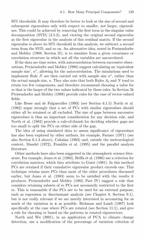
6.1. How Many Principal Components? 129
95% thresholds. It may therefore be better to look at the size of second andsubsequent eigenvalues only with respect to smaller, not larger, eigenval-ues. This could be achieved by removing the first term in the singular valuedecomposition (SVD) (3.5.2), and viewing the original second eigenvalueas the first eigenvalue in the analysis of this residual matrix. If the secondeigenvalue is above its 95% threshold in this analysis, we subtract a secondterm from the SVD, and so on. An alternative idea, noted in Preisendorferand Mobley (1988, Section 5f), is to simulate from a given covariance orcorrelation structure in which not all the variables are uncorrelated.
If the data are time series, with autocorrelation between successive obser-vations, Preisendorfer and Mobley (1988) suggest calculating an ‘equivalentsample size’, n∗, allowing for the autocorrelation. The simulations used toimplement Rule N are then carried out with sample size n∗, rather thanthe actual sample size, n. They also note that both Rules A4 and N tend toretain too few components, and therefore recommend choosing a value form that is the larger of the two values indicated by these rules. In Section 5kPreisendorfer and Mobley (1988) provide rules for the case of vector-valuedfields.
Like Besse and de Falguerolles (1993) (see Section 6.1.5) North et al.(1982) argue strongly that a set of PCs with similar eigenvalues shouldeither all be retained or all excluded. The size of gaps between successiveeigenvalues is thus an important consideration for any decision rule, andNorth et al. (1982) provide a rule-of-thumb for deciding whether gaps aretoo small to split the PCs on either side of the gap.
The idea of using simulated data to assess significance of eigenvalueshas also been explored by other authors, for example, Farmer (1971) (seealso Section 6.1.3 above), Cahalan (1983) and, outside the meteorologicalcontext, Mandel (1972), Franklin et al. (1995) and the parallel analysisliterature.
Other methods have also been suggested in the atmospheric science liter-ature. For example, Jones et al. (1983), Briffa et al. (1986) use a criterion forcorrelation matrices, which they attribute to Guiot (1981). In this methodPCs are retained if their cumulative eigenvalue product exceeds one. Thistechnique retains more PCs than most of the other procedures discussedearlier, but Jones et al. (1983) seem to be satisfied with the results itproduces. Preisendorfer and Mobley (1982, Part IV) suggest a rule thatconsiders retaining subsets of m PCs not necessarily restricted to the firstm. This is reasonable if the PCs are to be used for an external purpose,such as regression or discriminant analysis (see Chapter 8, Section 9.1),but is not really relevant if we are merely interested in accounting for asmuch of the variation in x as possible. Richman and Lamb (1987) lookspecifically at the case where PCs are rotated (see Section 11.1), and givea rule for choosing m based on the patterns in rotated eigenvectors.
North and Wu (2001), in an application of PCA to climate changedetection, use a modification of the percentage of variation criterion of
130 6. Choosing a Subset of Principal Components or Variables
Section 6.1.1. They use instead the percentage of ‘signal’ accounted for,although the PCA is done on a covariance matrix other than that associ-ated with the signal (see Section 12.4.3). Buell (1978) advocates stabilitywith respect to different degrees of approximation of a continuous spatialfield by discrete points as a criterion for choosing m. Section 13.3.4 of vonStorch and Zwiers (1999) is dismissive of selection rules.
6.1.8 Discussion
Although many rules have been examined in the last seven subsections,the list is by no means exhaustive. For example, in Section 5.1 we notedthat superimposing a minimum spanning tree on a plot of the observationswith respect to the first two PCs gives a subjective indication of whether ornot a two-dimensional representation is adequate. It is not possible to givedefinitive guidance on which rules are best, but we conclude this sectionwith a few comments on their relative merits. First, though, we discuss asmall selection of the many comparative studies that have been published.
Reddon (1984, Section 3.9) describes nine such studies, mostly from thepsychological literature, but all are concerned with factor analysis ratherthan PCA. A number of later studies in the ecological, psychological andmeteorological literatures have examined various rules on both real andsimulated data sets. Simulation of multivariate data sets can always becriticized as unrepresentative, because they can never explore more thana tiny fraction of the vast range of possible correlation and covariancestructures. Several of the published studies, for example Grossman et al.(1991), Richman (1988), are particularly weak in this respect, looking onlyat simulations where all p of the variables are uncorrelated, a situationwhich is extremely unlikely to be of much interest in practice. Anotherweakness of several psychology-based studies is their confusion betweenPCA and factor analysis. For example, Zwick and Velicer (1986) state that‘if PCA is used to summarize a data set each retained component mustcontain at least two substantial loadings.’ If the word ‘summarize’ impliesa descriptive purpose the statement is nonsense, but in the simulation studythat follows all their ‘components’ have three or more large loadings. Withthis structure, based on factor analysis, it is no surprise that Zwick andVelicer (1986) conclude that some of the rules they compare, which weredesigned with descriptive PCA in mind, retain ‘too many’ factors.
Jackson (1993) investigates a rather broader range of structures, includ-ing up to 12 variables in up to 3 correlated groups, as well as the completelyuncorrelated case. The range of stopping rules is also fairly wide, includ-ing: Kaiser’s rule; the scree graph; the broken stick rule; the proportion oftotal variance; tests of equality of eigenvalues; and Jackson’s two bootstrapprocedures described in Section 6.1.5. Jackson (1993) concludes that thebroken stick and bootstrapped eigenvalue-eigenvector rules give the bestresults in his study. However, as with the reasoning used to develop his

6.1. How Many Principal Components? 131
bootstrap rules, the results are viewed from a factor analysis rather than aPCA perspective.
Franklin et al. (1995) compare 39 published analyses from ecology. Theyseem to start from the unproven premise that ‘parallel analysis’ (see Sec-tion 6.1.3) selects the ‘correct’ number of components or factors to retain,and then investigate in how many of the 39 analyses ‘too many’ or ‘too few’dimensions are chosen. Franklin et al. (1995) claim that 2
3 of the 39 analysesretain too many dimensions. However, as with a number of other referencescited in this chapter, they fail to distinguish between what is needed forPCA and factor analysis. They also stipulate that PCAs require normallydistributed random variables, which is untrue for most purposes. It seemsdifficult to instil the message that PCA and factor analysis require differ-ent rules. Turner (1998) reports a large study of the properties of parallelanalysis, using simulation, and notes early on that ‘there are importantdifferences between principal component analysis and factor analysis.’ Hethen proceeds to ignore the differences, stating that the ‘term factors willbe used throughout [the] article [to refer] to either factors or components.’
Ferre (1995b) presents a comparative study which is extensive in itscoverage of selection rules, but very limited in the range of data for whichthe techniques are compared. A total of 18 rules are included in the study,as follows:
• From Section 6.1.1 the cumulative percentage of variance with fourcut-offs: 60%, 70%, 80%, 90%.
• From Section 6.1.2 Kaiser’s rule with cut-off 1, together withmodifications whose cut-offs are 0.7 and 2; the broken stick rule.
• From Section 6.1.3 the scree graph.
• From Section 6.1.4 Bartlett’s test and an approximation due toMardia.
• From Section 6.1.5 four versions of Eastment and Krzanowski’s cross-validation methods, where two cut-offs, 1 and 0.9, are used and, foreach threshold, the stopping rule can be based on either the first orlast occasion that the criterion dips below the threshold; Ferre’s fq;Besse and de Falguerolles’s approximate jackknife criterion.
• From Section 6.1.6 Velicer’s test.
The simulations are based on the fixed effects model described in Sec-tion 6.1.5. The sample size is 20, the number of variables is 10, and eachsimulated data matrix is the sum of a fixed (20 × 10) matrix Z of rank 8and a matrix of independent Gaussian noise with two levels of the noisevariance. This is a fixed effects model with q = 8, so that at first sight wemight aim to choose m = 8. For the smaller value of noise, Ferre (1995b)considers this to be appropriate, but the higher noise level lies between the
132 6. Choosing a Subset of Principal Components or Variables
second and third largest eigenvalues of the fixed matrix Z, so he arguesthat m = 2 should be chosen. This implies a movement away from theobjective ‘correct’ choice given by the model, back towards what seems tobe the inevitable subjectivity of the area.
The simulations are replicated 100 times for each of the two noise levels,and give results which are consistent with other studies. Kaiser’s modifiedrule with a threshold at 2, the broken stick rule, Velicer’s test, and cross-validation rules that stop after the first fall below the threshold—all retainrelatively few components. Conversely, Bartlett’s test, cumulative variancewith a cut-off of 90%, fq and the approximate jackknife retain greaternumbers of PCs. The approximate jackknife displays the strange behaviourof retaining more PCs for larger than for smaller noise levels. If we considerm = 8 to be ‘correct’ for both noise levels, all rules behave poorly for thehigh noise level. For the low noise level, fq and Bartlett’s tests do best.If m = 2 is deemed correct for the high noise level, the best proceduresare Kaiser’s modified rule with threshold 2, the scree graph, and all fourvarieties of cross-validation. Even within this restricted study no rule isconsistently good.
Bartkowiak (1991) gives an empirical comparison for some meteorologi-cal data of: subjective rules based on cumulative variance and on the screeand LEV diagrams; the rule based on eigenvalues greater than 1 or 0.7; thebroken stick rule; Velicer’s criterion. Most of the rules lead to similar deci-sions, except for the broken stick rule, which retains too few components,and the LEV diagram, which is impossible to interpret unambiguously.The conclusion for the broken stick rule is the opposite of that in Jackson’s(1993) study.
Throughout our discussion of rules for choosing m we have empha-sized the descriptive role of PCA and contrasted it with the model-basedapproach of factor analysis. It is usually the case that the number of compo-nents needed to achieve the objectives of PCA is greater than the numberof factors in a factor analysis of the same data. However, this need notbe the case when a model-based approach is adopted for PCA (see Sec-tions 3.9, 6.1.5). As Heo and Gabriel (2001) note in the context of biplots(see Section 5.3), the fit of the first few PCs to an underlying populationpattern (model) may be much better than their fit to a sample. This im-plies that a smaller value of m may be appropriate for model-based PCAthan for descriptive purposes. In other circumstances, too, fewer PCs maybe sufficient for the objectives of the analysis. For example, in atmosphericscience, where p can be very large, interest may be restricted only to thefirst few dominant and physically interpretable patterns of variation, eventhough their number is fewer than that associated with most PCA-basedrules. Conversely, sometimes very dominant PCs are predictable and henceof less interest than the next few. In such cases more PCs will be retainedthan indicated by most rules. The main message is that different objec-tives for a PCA lead to different requirements concerning how many PCs

6.2. Choosing m, the Number of Components: Examples 133
Table 6.1. First six eigenvalues for the correlation matrix, blood chemistry data.
Component number 1 2 3 4 5 6Eigenvalue, lk 2.79 1.53 1.25 0.78 0.62 0.49tm = 100
∑mk=1 lk/p 34.9 54.1 69.7 79.4 87.2 93.3
lk−1 − lk 1.26 0.28 0.47 0.16 0.13
to retain. In reading the concluding paragraph that follows, this messageshould be kept firmly in mind.
Some procedures, such as those introduced in Sections 6.1.4 and 6.1.6,are usually inappropriate because they retain, respectively, too many or toofew PCs in most circumstances. Some rules have been derived in particularfields of application, such as atmospheric science (Sections 6.1.3, 6.1.7) orpsychology (Sections 6.1.3, 6.1.6) and may be less relevant outside thesefields than within them. The simple rules of Sections 6.1.1 and 6.1.2 seemto work well in many examples, although the recommended cut-offs mustbe treated flexibly. Ideally the threshold should not fall between two PCswith very similar variances, and it may also change depending on the valueson the values of n and p, and on the presence of variables with dominantvariances (see the examples in the next section). A large amount of researchhas been done on rules for choosing m since the first edition of this bookappeared. However it still remains true that attempts to construct ruleshaving more sound statistical foundations seem, at present, to offer littleadvantage over the simpler rules in most circumstances.
6.2 Choosing m, the Number of Components:Examples
Two examples are given here to illustrate several of the techniques describedin Section 6.1; in addition, the examples of Section 6.4 include some relevantdiscussion, and Section 6.1.8 noted a number of comparative studies.
6.2.1 Clinical Trials Blood Chemistry
These data were introduced in Section 3.3 and consist of measurementsof eight blood chemistry variables on 72 patients. The eigenvalues for thecorrelation matrix are given in Table 6.1, together with the related infor-mation that is required to implement the ad hoc methods described inSections 6.1.1–6.1.3.
Looking at Table 6.1 and Figure 6.1, the three methods of Sections 6.1.1–6.1.3 suggest that between three and six PCs should be retained, but thedecision on a single best number is not clear-cut. Four PCs account for
134 6. Choosing a Subset of Principal Components or Variables
Table 6.2. First six eigenvalues for the covariance matrix, blood chemistry data.
Component number 1 2 3 4 5 6
Eigenvalue, lk 1704.68 15.07 6.98 2.64 0.13 0.07lk/l 7.88 0.07 0.03 0.01 0.0006 0.0003
tm = 100
∑m
k=1lk∑p
k=1lk
98.6 99.4 99.8 99.99 99.995 99.9994
lk−1 − lk 1689.61 8.09 4.34 2.51 0.06
nearly 80% of the total variation, but it takes six PCs to account for 90%.A cut-off at l∗ = 0.7 for the second criterion retains four PCs, but the nexteigenvalue is not very much smaller, so perhaps five should be retained. Inthe scree graph the slope actually increases between k = 3 and 4, but thenfalls sharply and levels off, suggesting that perhaps only four PCs shouldbe retained. The LEV diagram (not shown) is of little help here; it has noclear indication of constant slope after any value of k, and in fact has itssteepest slope between k = 7 and 8.
Using Cattell’s (1966) formulation, there is no strong straight-line be-haviour after any particular point, although perhaps a cut-off at k = 4 ismost appropriate. Cattell suggests that the first point on the straight line(that is, the ‘elbow’ point) should be retained. However, if we consider thescree graph in the same light as the test of Section 6.1.4, then all eigen-values after, and including, the elbow are deemed roughly equal and so allcorresponding PCs should be deleted. This would lead to the retention ofonly three PCs in the present case.
Turning to Table 6.2, which gives information for the covariance matrix,corresponding to that presented for the correlation matrix in Table 6.1, thethree ad hoc measures all conclusively suggest that one PC is sufficient. Itis undoubtedly true that choosing m = 1 accounts for the vast majorityof the variation in x, but this conclusion is not particularly informativeas it merely reflects that one of the original variables accounts for nearlyall the variation in x. The PCs for the covariance matrix in this examplewere discussed in Section 3.3, and it can be argued that it is the use ofthe covariance matrix, rather than the rules of Sections 6.1.1–6.1.3, that isinappropriate for these data.
6.2.2 Gas Chromatography Data
These data, which were originally presented by McReynolds (1970), andwhich have been analysed by Wold (1978) and by Eastment and Krzanow-ski (1982), are concerned with gas chromatography retention indices. Afterremoval of a number of apparent outliers and an observation with a missingvalue, there remain 212 (Eastment and Krzanowski) or 213 (Wold) mea-surements on ten variables. Wold (1978) claims that his method indicates

6.2. Choosing m, the Number of Components: Examples 135
Table 6.3. First six eigenvalues for the covariance matrix, gas chromatographydata.
Component number 1 2 3 4 5 6
Eigenvalue, lk 312187 2100 768 336 190 149lk/l 9.88 0.067 0.024 0.011 0.006 0.005
tm = 100
∑m
k=1lk∑p
k=1lk
98.8 99.5 99.7 99.8 99.9 99.94
lk−1 − lk 310087 1332 432 146 51R 0.02 0.43 0.60 0.70 0.83 0.99W 494.98 4.95 1.90 0.92 0.41 0.54
the inclusion of five PCs in this example but, in fact, he slightly modifieshis criterion for retaining PCs. His nominal cut-off for including the kthPC is R < 1; the sixth PC has R = 0.99 (see Table 6.3) but he neverthelesschooses to exclude it. Eastment and Krzanowski (1982) also modify theirnominal cut-off but in the opposite direction, so that an extra PC is in-cluded. The values of W for the third, fourth and fifth PCs are 1.90, 0.92,0.41 (see Table 6.3) so the formal rule, excluding PCs with W < 1, wouldretain three PCs. However, because the value of W is fairly close to unity,Eastment and Krzanowski (1982) suggest that it is reasonable to retain thefourth PC as well.
It is interesting to note that this example is based on a covariance ma-trix, and has a very similar structure to that of the previous example whenthe covariance matrix was used. Information for the present example, cor-responding to Table 6.2, is given in Table 6.3, for 212 observations. Alsogiven in Table 6.3 are Wold’s R (for 213 observations) and Eastment andKrzanowski’s W .
It can be seen from Table 6.3, as with Table 6.2, that the first two ofthe ad hoc methods retain only one PC. The scree graph, which cannot besensibly drawn because l1 l2, is more equivocal; it is clear from Table 6.3that the slope drops very sharply after k = 2, indicating m = 2 (or 1), buteach of the slopes for k = 3, 4, 5, 6 is substantially smaller than the previousslope, with no obvious levelling off. Nor is there any suggestion, for any cut-off, that the later eigenvalues lie on a straight line. There is, however, anindication of a straight line, starting at m = 4, in the LEV plot, which isgiven in Figure 6.2.
It would seem, therefore, that the cross-validatory criteria R and W dif-fer considerably from the ad hoc rules (except perhaps the LEV plot) in theway in which they deal with covariance matrices that include a very domi-nant PC. Whereas most of the ad hoc rules will invariably retain only onePC in such situations, the present example shows that the cross-validatorycriteria may retain several more. Krzanowski (1983) suggests that W looksfor large gaps among the ordered eigenvalues, which is a similar aim to thatof the scree graph, and that W can therefore be viewed as an objective ana-
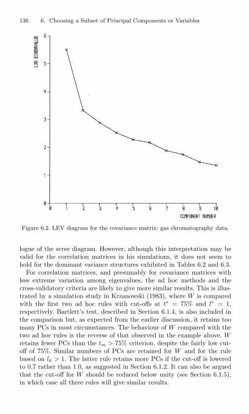
136 6. Choosing a Subset of Principal Components or Variables
Figure 6.2. LEV diagram for the covariance matrix: gas chromatography data.
logue of the scree diagram. However, although this interpretation may bevalid for the correlation matrices in his simulations, it does not seem tohold for the dominant variance structures exhibited in Tables 6.2 and 6.3.
For correlation matrices, and presumably for covariance matrices withless extreme variation among eigenvalues, the ad hoc methods and thecross-validatory criteria are likely to give more similar results. This is illus-trated by a simulation study in Krzanowski (1983), where W is comparedwith the first two ad hoc rules with cut-offs at t∗ = 75% and l∗ = 1,respectively. Bartlett’s test, described in Section 6.1.4, is also included inthe comparison but, as expected from the earlier discussion, it retains toomany PCs in most circumstances. The behaviour of W compared with thetwo ad hoc rules is the reverse of that observed in the example above. Wretains fewer PCs than the tm > 75% criterion, despite the fairly low cut-off of 75%. Similar numbers of PCs are retained for W and for the rulebased on lk > 1. The latter rule retains more PCs if the cut-off is loweredto 0.7 rather than 1.0, as suggested in Section 6.1.2. It can also be arguedthat the cut-off for W should be reduced below unity (see Section 6.1.5),in which case all three rules will give similar results.

6.3. Selecting a Subset of Variables 137
Krzanowski (1983) examines the gas chromatography example furtherby generating six different artificial data sets with the same sample covari-ance matrix as the real data. The values of W are fairly stable across thereplicates and confirm the choice of four PCs obtained above by slightly de-creasing the cut-off for W . For the full data set, with outliers not removed,the replicates give some different, and useful, information from that in theoriginal data.
6.3 Selecting a Subset of Variables
When p, the number of variables observed, is large it is often the case thata subset of m variables, with m p, contains virtually all the informationavailable in all p variables. It is then useful to determine an appropriatevalue of m, and to decide which subset or subsets of m variables are best.
Solution of these two problems, the choice of m and the selection of agood subset, depends on the purpose to which the subset of variables isto be put. If the purpose is simply to preserve most of the variation inx, then the PCs of x can be used fairly straightforwardly to solve bothproblems, as will be explained shortly. A more familiar variable selectionproblem is in multiple regression, and although PCA can contribute in thiscontext (see Section 8.5), it is used in a more complicated manner. This isbecause external considerations, namely the relationships of the predictor(regressor) variables with the dependent variable, as well as the internalrelationships between the regressor variables, must be considered. Externalconsiderations are also relevant in other variable selection situations, forexample in discriminant analysis (Section 9.1); these situations will not beconsidered in the present chapter. Furthermore, practical considerations,such as ease of measurement of the selected variables, may be important insome circumstances, and it must be stressed that such considerations, aswell as the purpose of the subsequent analysis, can play a prominent role invariable selection, Here, however, we concentrate on the problem of findinga subset of x in which the sole aim is to represent the internal variation ofx as well as possible.
Regarding the choice of m, the methods of Section 6.1 are all relevant.The techniques described there find the number of PCs that account formost of the variation in x, but they can also be interpreted as finding theeffective dimensionality of x. If x can be successfully described by only mPCs, then it will often be true that x can be replaced by a subset of m (orperhaps slightly more) variables, with a relatively small loss of information.
Moving on to the choice of m variables, Jolliffe (1970, 1972, 1973) dis-cussed a number of methods for selecting a subset of m variables thatpreserve most of the variation in x. Some of the methods compared, andindeed some of those which performed quite well, are based on PCs. Other
138 6. Choosing a Subset of Principal Components or Variables
methods, including some based on cluster analyses of variables (see Sec-tion 9.2) were also examined but, as these do not use the PCs to selectvariables, they are not described here. Three main types of method usingPCs were examined.
(i) Associate one variable with each of the last m∗1(= p − m1) PCs and
delete those m∗1 variables. This can either be done once only or iter-
atively. In the latter case a second PCA is performed on the m1
remaining variables, and a further set of m∗2 variables is deleted, if ap-
propriate. A third PCA can then be done on the p−m∗1−m∗
2 variables,and the procedure is repeated until no further deletions are considerednecessary. The choice of m∗
1,m∗2, . . . is based on a criterion determined
by the size of the eigenvalues lk.The reasoning behind this method is that small eigenvalues correspondto near-constant relationships among a subset of variables. If one ofthe variables involved in such a relationship is deleted (a fairly obviouschoice for deletion is the variable with the highest coefficient in abso-lute value in the relevant PC) little information is lost. To decide onhow many variables to delete, the criterion lk is used as described inSection 6.1.2. The criterion tm of Section 6.1.1 was also tried by Jolliffe(1972), but shown to be less useful.
(ii) Associate a set of m∗ variables en bloc with the last m∗ PCs, andthen delete these variables. Jolliffe (1970, 1972) investigated this typeof method, with the m∗ variables either chosen to maximize sums ofsquares of coefficients in the last m∗ PCs or to be those m∗ variablesthat are best predicted by regression on the first m = p − m∗ PCs.Choice of m∗ is again based on the sizes of the lk. Such methodswere found to be unsatisfactory, as they consistently failed to selectan appropriate subset for some simple correlation structures.
(iii) Associate one variable with each of the first m PCs, namely the variablenot already chosen with the highest coefficient in absolute value ineach successive PC. These m variables are retained, and the remainingm∗ = p − m are deleted. The arguments leading to this approach aretwofold. First, it is an obvious complementary approach to (i) and,second, in cases where there are groups of highly correlated variables itis designed to select just one variable from each group. This will happenbecause there will be exactly one high-variance PC associated with eachgroup (see Section 3.8). The approach is a plausible one, as a singlevariable from each group should preserve most of the information givenby that group when all variables in the group are highly correlated.
In Jolliffe (1972) comparisons were made, using simulated data, betweennon-iterative versions of method (i) and method (iii), called methods B2, B4respectively, and with several other subset selection methods that did notuse the PCs. The results showed that the PC methods B2, B4 retained the
6.3. Selecting a Subset of Variables 139
‘best’ subsets more often than the other methods considered, but they alsoselected ‘bad,’ as opposed to ‘good’ or ‘moderate’, subsets more frequentlythan the other methods. Method B4 was most extreme in this respect; itselected ‘best’ and ‘bad’ subsets more frequently than any other method,and ‘moderate’ or ‘good’ subsets less frequently.
Similarly, for various real data sets Jolliffe (1973) found that none ofthe variable selection methods was uniformly best, but several of them,including B2 and B4, found reasonable subsets in most cases.
McCabe (1984) adopted a somewhat different approach to the variableselection problem. He started from the fact that, as has been seen in Chap-ters 2 and 3, PCs satisfy a number of different optimality criteria. A subsetof the original variables that optimizes one of these criteria is termed a setof principal variables by McCabe (1984). Property A1 of Sections 2.1, 3.1,is uninteresting as it simply leads to a subset of variables whose variancesare largest, but other properties lead to one of these four criteria:
(a) Minimizem∗∏
j=1
θj
(b) Minimizem∗∑
j=1
θj
(c) Minimizem∗∑
j=1
θ2j
(d) Minimizem−∑
j=1
ρ2j
where θj , j = 1, 2, . . . ,m∗ are the eigenvalues of the conditional covariance(or correlation) matrix of the m∗ deleted variables, given the values ofthe m selected variables, and ρj , j = 1, 2, . . . ,m− = min(m,m∗) are thecanonical correlations between the set of m∗ deleted variables and the setof m selected variables.
Consider, for example, Property A4 of Sections 2.1 and 3.1, wheredet(Σy) (or det(Sy) for samples) is to be maximized. In PCA, y consistsof orthonormal linear functions of x; for principal variables y is a subset ofx.
From a well-known result concerning partitioned matrices, det(Σ) =det(Σy) det(Σy∗· y), where Σy∗· y is the matrix of conditional covariances forthose variables not in y, given the value of y. Because Σ, and hence det(Σ),is fixed for a given random vector x, maximizing det(Σy) is equivalent tominimizing det(Σy∗· y). Now det(Σy∗· y) =
∏m∗
j=1 θj , so that Property A4becomes McCabe’s criterion (a) when deriving principal variables. Otherproperties of Chapters 2 and 3 can similarly be shown to be equivalent to

140 6. Choosing a Subset of Principal Components or Variables
one of McCabe’s four criteria when dealing with principal variables.Of the four criteria, McCabe (1984) argues that only for the first is it
computationally feasible to explore all possible subsets, although the secondcan be used to define a stepwise variable-selection procedure; Bhargava andIshizuka (1991) describe such a procedure. The third and fourth criteria arenot explored further in McCabe’s paper.
Several of the methods for selecting subsets of variables that preservemost of the information in the data associate variables with individual PCs.Cadima and Jolliffe (2001) extend the ideas of Cadima and Jolliffe (1995)for individual PCs, and look for subsets of variables that best approximatethe subspace spanned by a subset of q PCs, in the the sense that thesubspace spanned by the chosen variables is close to that spanned by thePCs of interest. A similar comparison of subspaces is the starting pointfor Besse and de Falguerolles’s (1993) procedures for choosing the numberof components to retain (see Section 6.1.5). In what follows we restrictattention to the first q PCs, but the reasoning extends easily to any set ofq PCs.
Cadima and Jolliffe (2001) argue that there are two main ways of assess-ing the quality of the subspace spanned by a subset of m variables. Thefirst compares the subspace directly with that spanned by the first q PCs;the second compares the data with its configuration when projected ontothe m-variable subspaces.
Suppose that we wish to approximate the subspace spanned by the firstq PCs using a subset of m variables. The matrix of orthogonal projectionsonto that subspace is given by
Pq =1
(n − 1)XS−
q X′, (6.3.1)
where Sq =∑q
k=1 lkaka′k is the sum of the first q terms in the spectral
decomposition of S, and S−q =
∑qk=1 l−1
k aka′k is a generalized inverse of Sq.
The corresponding matrix of orthogonal projections onto the space spannedby a subset of m variables is
Pm =1
(n − 1)XImS−1
m I′mX′, (6.3.2)
where Im is the identity matrix of order m and S−1m is the inverse of the
(m × m) submatrix of S corresponding to the m selected variables.The first measure of closeness for the two subspaces considered by
Cadima and Jolliffe (2001) is the matrix correlation between Pq and Pm,defined by
corr(Pq,Pm) =tr(P′
qPm)√
tr(P′qPq) tr(P′
mPm). (6.3.3)
This measure is also known as Yanai’s generalized coefficient of determina-tion (Yanai, 1980). It was used by Tanaka (1983) as one of four criteria for

6.3. Selecting a Subset of Variables 141
variable selection in factor analysis. Cadima and Jolliffe (2001) show thatYanai’s coefficient can be written as
corr(Pq,Pm) =1√qm
q∑
k=1
r2km (6.3.4)
where rkm is the multiple correlation between the kth PC and the set ofm selected variables.
The second indicator examined by Cadima and Jolliffe (2001) is again amatrix correlation, this time between the data matrix X and the matrixformed by orthogonally projecting X onto the space spanned by the mselected variables. It can be written
corr(X,PmX) =
√∑pk=1 λkr2
km∑pk=1 λk
. (6.3.5)
It turns out that this measure is equivalent to the second of McCabe’s(1984) criteria defined above (see also McCabe (1986)). Cadima and Jol-liffe (2001) discuss a number of other interpretations, and relationshipsbetween their measures and previous suggestions in the literature. Bothindicators (6.3.4) and (6.3.5) are weighted averages of the squared multi-ple correlations between each PC and the set of selected variables. In thesecond measure, the weights are simply the eigenvalues of S, and hence thevariances of the PCs. For the first indicator the weights are positive andequal for the first q PCs, but zero otherwise. Thus the first indicator ignoresPCs outside the chosen q-dimensional subspace when assessing closeness,but it also gives less weight than the second indicator to the PCs with thevery largest variances relative to those with intermediate variances.
Cadima and Jolliffe (2001) discuss algorithms for finding good subsetsof variables and demonstrate the use of the two measures on three exam-ples, one of which is large (p = 62) compared to those typically used forillustration. The examples show that the two measures can lead to quitedifferent optimal subsets, implying that it is necessary to know what aspectof a subspace it is most desirable to preserve before choosing a subset ofvariables to achieve this. They also show that
• the algorithms usually work efficiently in cases where numbers ofvariables are small enough to allow comparisions with an exhaustivesearch;
• as discussed elsewhere (Section 11.3), choosing variables on the basisof the size of coefficients or loadings in the PCs’ eigenvectors can beinadvisable;
• to match the information provided by the first q PCs it is often onlynecessary to keep (q + 1) or (q + 2) variables.
For data sets in which p is too large to conduct an exhaustive searchfor the optimal subset, algorithms that can find a good subset are needed.

142 6. Choosing a Subset of Principal Components or Variables
Cadima et al. (2002) compare various algorithms for finding good subsetsaccording to the measures (6.3.4) and (6.3.5), and also with respect to theRV-coefficient, which is discussed briefly below (see also Section 3.2). Twoversions of simulated annealing, a genetic algorithm, and a restricted im-provement algorithm, are compared with a number of stepwise algorithms,on a total of fourteen data sets. The results show a general inferiority ofthe stepwise methods, but no single algorithm outperforms all the others.Cadima et al. (2002) recommend using simulated annealing or a genetic al-gorithm to provide a starting point for a restricted improvement algorithm,which then refines the solution. They make the interesting point that forlarge p the number of candidate subsets is so large that, for criteria whoserange of values is bounded, it is almost inevitable that there are many solu-tions that are very close to optimal. For instance, in one of their examples,with p = 62, they find 800 solutions corresponding to a population size of800 in their genetic algorithm. The best of these has a value 0.8079 for thecriterion (6.3.5), but the worst is 0.8060, less than 0.3% smaller. Of course,it is possible that the global optimum is much greater than the best ofthese 800, but it seems highly unlikely.
Al-Kandari (1998) provides an extensive study of a large number ofvariable selection methods. The ideas of Jolliffe (1972, 1973) and McCabe(1984) are compared with a variety of new methods, based on loadings inthe PCs, on correlations of the PCs with the variables, and on versions ofMcCabe’s (1984) principal variables that are constructed from correlation,rather than covariance, matrices. The methods are compared on simulateddata with a wide range of covariance or correlation structures, and on var-ious real data sets that are chosen to have similar covariance/correlationstructures to those of the simulated data. On the basis of the results ofthese analyses, it is concluded that few of the many techniques consideredare uniformly inferior to other methods, and none is uniformly superior.The ‘best’ method varies, depending on the covariance or correlation struc-ture of a data set. It also depends on the ‘measure of efficiency’ used todetermine how good is a subset of variables, as noted also by Cadima andJolliffe (2001). In assessing which subsets of variables are best, Al-Kandari(1998) additionally takes into account the interpretability of the PCs basedon the subset, relative to the PCs based on all p variables (see Section 11.3).
Al-Kandari (1998) also discusses the distinction between criteria used tochoose subsets of variables and criteria used to evaluate how good a chosensubset is. The latter are her ‘measures of efficiency’ and ideally these samecriteria should be used to choose subsets in the first place. However, thismay be computationally infeasible so that a suboptimal but computation-ally straightforward criterion is used to do the choosing instead. Some ofAl-Kandari’s (1998) results are reported in Al-Kandari and Jolliffe (2001)for covariance, but not correlation, matrices.
King and Jackson (1999) combine some of the ideas of the present Sectionwith some from Section 6.1. Their main objective is to select a subset

6.3. Selecting a Subset of Variables 143
of m variables, but rather than treating m as fixed they also considerhow to choose m. They use methods of variable selection due to Jolliffe(1972, 1973), adding a new variant that was computationally infeasible in1972. To choose m, King and Jackson (1999) consider the rules describedin Sections 6.1.1 and 6.1.2, including the broken stick method, togetherwith a rule that selects the largest value of m for which n/m > 3. Toassess the quality of a chosen subset of size m, King and Jackson (1999)compare plots of scores on the first two PCs for the full data set and forthe data set containing only the m selected variables. They also compute aProcrustes measure of fit (Krzanowski, 1987a) between the m-dimensionalconfigurations given by PC scores in the full and reduced data sets, and aweighted average of correlations between PCs in the full and reduced datasets.
The data set analyzed by King and Jackson (1999) has n = 37 andp = 36. The results of applying the various selection procedures to thesedata confirm, as Jolliffe (1972, 1973) found, that methods B2 and B4 doreasonably well. The results also confirm that the broken stick methodgenerally chooses smaller values of m than the other methods, though itssubsets do better with respect to the Procrustes measure of fit than somemuch larger subsets. The small number of variables retained by the brokenstick implies a corresponding small proportion of total variance accountedfor by the subsets it selects. King and Jackson’s (1999) recommendation ofmethod B4 with the broken stick could therefore be challenged.
We conclude this section by briefly describing a number of other possiblemethods for variable selection. None uses PCs directly to select variables,but all are related to topics discussed more fully in other sections or chap-ters. Bartkowiak (1991) uses a method described earlier in Bartkowiak(1982) to select a set of ‘representative’ variables in an example that alsoillustrates the choice of the number of PCs (see Section 6.1.8). Variablesare added sequentially to a ‘representative set’ by considering each vari-able currently outside the set as a candidate for inclusion. The maximumresidual sum of squares is calculated from multiple linear regressions ofeach of the other excluded variables on all the variables in the set plus thecandidate variable. The candidate for which this maximum sum of squaresis minimized is then added to the set. One of Jolliffe’s (1970, 1972, 1973)rules uses a similar idea, but in a non-sequential way. A set of m variablesis chosen if it maximizes the minimum multiple correlation between eachof the (p − m) non-selected variables and the set of m selected variables.
The RV-coefficient, due to Robert and Escoufier (1976), was defined inSection 3.2. To use the coefficient to select a subset of variables, Robertand Escoufier suggest finding X1 which maximizes RV(X,M′X1), whereRV(X,Y) is defined by equation (3.2.2) of Section 3.2. The matrix X1
is the (n × m) submatrix of X consisting of n observations on a subsetof m variables, and M is a specific (m × m) orthogonal matrix, whoseconstruction is described in Robert and Escoufier’s paper. It is interesting

144 6. Choosing a Subset of Principal Components or Variables
to compare what is being optimized here with the approaches describedearlier.
• The RV-coefficient compares linear combinations of subsets ofvariables with the full set of variables.
• Some methods, such as those of Jolliffe (1970, 1972, 1973), com-pare principal components of subsets of variables with principalcomponents from the full set.
• Some approaches, such as McCabe’s (1984) principal variables, simplycompare subsets of the variables with the full set of variables.
• Some criteria, such as Yanai’s generalized coefficient of determination,compare subspaces spanned by a subset of variables with subspacesspanned by a subset of PCs, as in Cadima and Jolliffe (2001).
No examples are presented by Robert and Escoufier (1976) of how theirmethod works in practice. However, Gonzalez et al. (1990) give a stepwisealgorithm for implementing the procedure and illustrate it with a smallexample (n = 49; p = 6). The example is small enough for all subsets ofeach size to be evaluated. Only for m = 1, 2, 3 does the stepwise algorithmgive the best subset with respect to RV, as identified by the full search.Escoufier (1986) provides further discussion of the properties of the RV-coefficient when used in this context.
Tanaka and Mori (1997) also use the RV-coefficient, as one of two criteriafor variable selection. They consider the same linear combinations M′X1 ofa given set of variables as Robert and Escoufier (1976), and call these lin-ear combinations modified principal components. Tanaka and Mori (1997)assess how well a subset reproduces the full set of variables by means ofthe RV-coefficient. They also have a second form of ‘modified’ principalcomponents, constructed by minimizing the trace of the residual covari-ance matrix obtained by regressing X on M′X1. This latter formulation issimilar to Rao’s (1964) PCA of instrumental variables (see Section 14.3).The difference between Tanaka and Mori’s (1997) instrumental variableapproach and that of Rao (1964) is that Rao attempts to predict X2, the(n × (p − m)) complementary matrix to X1 using linear functions of X1,whereas Tanaka and Mori try to predict the full matrix X.
Both of Tanaka and Mori’s modified PCAs solve the same eigenequation
(S211 + S12S21)a = lS11a, (6.3.6)
with obvious notation, but differ in the way that the quality of a sub-set is measured. For the instrumental variable approach, the criterionis proportional to
∑mk=1 lk, whereas for the components derived via the
RV-coefficient, quality is based on∑m
k=1 l2k, where lk is the kth largesteigenvalue in the solution of (6.3.6). A backward elimination method isused to delete variables until some threshold is reached, although in the
6.4. Examples Illustrating Variable Selection 145
examples given by Tanaka and Mori (1997) the decision on when to stopdeleting variables appears to be rather subjective.
Mori et al. (1999) propose that the subsets selected in modified PCAare also assessed by means of a PRESS criterion, similar to that defined inequation (6.1.3), except that mxij is replaced by the prediction of xij foundfrom modified PCA with the ith observation omitted. Mori et al. (2000)demonstrate a procedure in which the PRESS citerion is used directly toselect variables, rather than as a supplement to another criterion. Tanakaand Mori (1997) show how to evaluate the influence of variables on param-eters in a PCA (see Section 10.2 for more on influence), and Mori et al.(2000) implement and illustrate a backward-elimination variable selectionalgorithm in which variables with the smallest influence are successivelyremoved.
Hawkins and Eplett (1982) describe a method which can be used forselecting a subset of variables in regression; their technique and an ear-lier one introduced by Hawkins (1973) are discussed in Sections 8.4 and8.5. Hawkins and Eplett (1982) note that their method is also potentiallyuseful for selecting a subset of variables in situations other than multipleregression, but, as with the RV-coefficient, no numerical example is givenin the original paper. Krzanowski (1987a,b) describes a methodology, us-ing principal components together with Procrustes rotation for selectingsubsets of variables. As his main objective is preserving ‘structure’ such asgroups in the data, we postpone detailed discussion of his technique untilSection 9.2.2.
6.4 Examples Illustrating Variable Selection
Two examples are presented here; two other relevant examples are given inSection 8.7.
6.4.1 Alate adelges (Winged Aphids)
These data were first presented by Jeffers (1967) and comprise 19 differentvariables measured on 40 winged aphids. A description of the variables,together with the correlation matrix and the coefficients of the first fourPCs based on the correlation matrix, is given by Jeffers (1967) and willnot be reproduced here. For 17 of the 19 variables all of the correlationcoefficients are positive, reflecting the fact that 12 variables are lengthsor breadths of parts of each individual, and some of the other (discrete)variables also measure aspects of the size of each aphid. Not surprisingly,the first PC based on the correlation matrix accounts for a large proportion(73.0%) of the total variation, and this PC is a measure of overall size ofeach aphid. The second PC, accounting for 12.5% of total variation, has its

146 6. Choosing a Subset of Principal Components or Variables
Table 6.4. Subsets of selected variables, Alate adelges.
(Each row corresponds to a selected subset with × denoting a selected variable.)
Variables5 8 9 11 13 14 17 18 19
McCabe, using criterion (a)best × × ×
Three variables
second best × × ×best × × × ×
Four variables
second best × × × ×Jolliffe, using criteria B2, B4
B2 × × ×Three variables
B4 × × ×B2 × × × ×
Four variables
B4 × × × ×Criterion (6.3.4)Three variables × × ×Four variables × × × ×Criterion (6.3.5)Three variables × × ×Four variables × × × ×
largest coefficients on five of the seven discrete variables, and the third PC(3.9%) is almost completely dominated by one variable, number of antennalspines. This variable, which is one of the two variables negatively correlatedwith size, has a coefficient in the third PC that is five times as large as anyother variable.
Table 6.4 gives various subsets of variables selected by Jolliffe (1973)and by McCabe (1982) in an earlier version of his 1984 paper that includedadditional examples. The subsets given by McCabe (1982) are the best twoaccording to his criterion (a), whereas those from Jolliffe (1973) are selectedby the criteria B2 and B4 discussed above. Only the results for m = 3 aregiven in Jolliffe (1973), but Table 6.4 also gives results for m = 4 using hismethods. In addition, the table includes the ‘best’ 3- and 4-variable subsetsaccording to the criteria (6.3.4) and (6.3.5).
There is considerable overlap between the various subsets selected. Inparticular, variable 11 is an almost universal choice and variables 5, 13 and17 also appear in subsets selected by at least three of the four methods.Conversely, variables 1–4, 6, 7, 10, 12, 15, 16 appear in none of subsets ofTable 6.4. It should be noted the variable 11 is ‘number of antennal spines,’which, as discussed above, dominates the third PC. Variables 5 and 17, mea-suring number of spiracles and number of ovipositor spines, respectively, are
6.4. Examples Illustrating Variable Selection 147
both among the group of dominant variables for the second PC, and vari-able 13 (tibia length 3) has the largest coefficient of any variable for PC1.
Comparisons can be made regarding how well Jolliffe’s and McCabe’s se-lections perform with respect to the criteria (6.3.4) and (6.3.5). For (6.3.5),Jolliffe’s choices are closer to optimality than McCabe’s, achieving valuesof 0.933 and 0.945 for four variables, compared to 0.907 and 0.904 forMcCabe, whereas the optimal value is 0.948. Discrepancies are generallylarger but more variable for criterion (6.3.4). For example, the B2 selec-tion of three variables achieves a value of only 0.746 compared the optimalvalue of 0.942, which is attained by B4. Values for McCabe’s selections areintermediate (0.838, 0.880).
Regarding the choice of m, the lk criterion of Section 6.1.2 was foundby Jolliffe (1972), using simulation studies, to be appropriate for methodsB2 and B4, with a cut-off close to l∗ = 0.7. In the present example thecriterion suggests m = 3, as l3 = 0.75 and l4 = 0.50. Confirmation that mshould be this small is given by the criterion tm of Section 6.1.1. Two PCsaccount for 85.4% of the variation, three PCs give 89.4% and four PCscontribute 92.0%, from which Jeffers (1967) concludes that two PCs aresufficient to account for most of the variation. However, Jolliffe (1973) alsolooked at how well other aspects of the structure of data are reproduced forvarious values of m. For example, the form of the PCs and the division intofour distinct groups of aphids (see Section 9.2 for further discussion of thisaspect) were both examined and found to be noticeably better reproducedfor m = 4 than for m = 2 or 3, so it seems that the criteria of Sections 6.1.1and 6.1.2 might be relaxed somewhat when very small values of m areindicated, especially when coupled with small values of n, the sample size.McCabe (1982) notes that four or five of the original variables are necessaryin order to account for as much variation as the first two PCs, confirmingthat m = 4 or 5 is probably appropriate here.
Tanaka and Mori (1997) suggest, on the basis of their two criteria andusing a backward elimination algorithm, that seven or nine variables shouldbe kept, rather more than Jolliffe (1973) or McCabe (1982). If only fourvariables are retained, Tanaka and Mori’s (1997) analysis keeps variables5, 6, 14, 19 according to the RV-coefficient, and variables 5, 14, 17, 18 usingresiduals from regression. At least three of the four variables overlap withchoices made in Table 6.4. On the other hand, the selection rule basedon influential variables suggested by Mori et al. (2000) retains variables2, 4, 12, 13 in a 4-variable subset, a quite different selection from those ofthe other methods.
6.4.2 Crime Rates
These data were given by Ahamad (1967) and consist of measurements ofthe crime rate in England and Wales for 18 different categories of crime(the variables) for the 14 years, 1950–63. The sample size n = 14 is very
148 6. Choosing a Subset of Principal Components or Variables
Table 6.5. Subsets of selected variables, crime rates.
(Each row corresponds to a selected subset with × denoting a selected variable.)
Variables
1 3 4 5 7 8 10 13 14 16 17
McCabe, using criterion (a)best × × ×
Three variables
second best × × ×best × × × ×
Four variables
second best × × × ×Jolliffe, using criteria B2, B4
B2 × × ×Three variables
B4 × × ×B2 × × × ×
Four variables
B4 × × × ×Criterion (6.3.4)Three variables × × ×Four variables × × × ×Criterion (6.3.5)Three variables × × ×Four variables × × × ×
small, and is in fact smaller than the number of variables. Furthermore,the data are time series, and the 14 observations are not independent (seeChapter 12), so that the effective sample size is even smaller than 14. Leav-ing aside this potential problem and other criticisms of Ahamad’s analysis(Walker, 1967), subsets of variables that are selected using the correlationmatrix by the same methods as in Table 6.4 are shown in Table 6.5.
There is a strong similarity between the correlation structure of thepresent data set and that of the previous example. Most of the variablesconsidered increased during the time period considered, and the correla-tions between these variables are large and positive. (Some elements of thecorrelation matrix given by Ahamad (1967) are incorrect; Jolliffe (1970)gives the correct values.)
The first PC based on the correlation matrix therefore has large coeffi-cients on all these variables; it measures an ‘average crime rate’ calculatedlargely from 13 of the 18 variables, and accounts for 71.7% of the totalvariation. The second PC, accounting for 16.1% of the total variation, haslarge coefficients on the five variables whose behaviour over the 14 yearsis ‘atypical’ in one way or another. The third PC, accounting for 5.5% ofthe total variation, is dominated by the single variable ‘homicide,’ whichstayed almost constant compared with the trends in other variables overthe period of study. On the basis of tm only two or three PCs are necessary,
6.4. Examples Illustrating Variable Selection 149
as they account for 87.8%, 93.3%, respectively, of the total variation. Thethird and fourth eigenvalues are 0.96, 0.68 so that a cut-off of l∗ = 0.70gives m = 3, but l4 is so close to 0.70 that caution suggests m = 4. Suchconservatism is particularly appropriate for small sample sizes, where sam-pling variation may be substantial. As in the previous example, Jolliffe(1973) found that the inclusion of a fourth variable produced a markedimprovement in reproducing some of the results given by all 18 variables.McCabe (1982) also indicated that m = 3 or 4 is appropriate.
The subsets chosen in Table 6.5 overlap less than in the previous example,and McCabe’s subsets change noticeably in going from m = 3 to m = 4.However, there is still substantial agreement; for example, variable 1 isa member of all but one of the selected subsets and variable 13 is alsoselected by all four methods, whereas variables 2, 6, 9, 11, 12, 15, 18 arenot selected at all.
Of the variables that are chosen by all four methods, variable 1 is ‘homi-cide,’ which dominates the third PC and is the only crime whose occurrenceshows no evidence of serial correlation during the period 1950–63. Becauseits behaviour is different from that of all the other variables, it is impor-tant that it should be retained in any subset that seeks to account for mostof the variation in x. Variable 13 (assault) is also atypical of the generalupward trend—it actually decreased between 1950 and 1963.
The values of the criteria (6.3.4) and (6.3.5) for Jolliffe’s and McCabe’ssubsets are closer to optimality and less erratic than in the earlier exam-ple. No chosen subset does worse with respect to (6.3.5) than 0.925 for 3variables and 0.964 for 4 variables, compared to optimal values of 0.942,0.970 respectively. The behaviour with respect to (6.3.4) is less good, butfar less erratic than in the previous example.
In addition to the examples given here, Al-Kandari (1998), Cadima andJolliffe (2001), Gonzalez et al. (1990), Jolliffe (1973), King and Jackson(1999) and McCabe (1982, 1984) all give further illustrations of variableselection based on PCs. Krzanowski (1987b) looks at variable selection forthe alate adelges data set of Section 6.4.1, but in the context of preservinggroup structure. We discuss this further in Chapter 9.

7Principal Component Analysis andFactor Analysis
Principal component analysis has often been dealt with in textbooks as aspecial case of factor analysis, and this practice is continued by some widelyused computer packages, which treat PCA as one option in a program forfactor analysis. This view is misguided since PCA and factor analysis, asusually defined, are really quite distinct techniques. The confusion mayhave arisen, in part, because of Hotelling’s (1933) original paper, in whichprincipal components were introduced in the context of providing a smallnumber of ‘more fundamental’ variables that determine the values of thep original variables. This is very much in the spirit of the factor modelintroduced in Section 7.1, although Girschick (1936) indicates that therewere soon criticisms of Hotelling’s PCs as being inappropriate for factoranalysis. Further confusion results from the fact that practitioners of ‘fac-tor analysis’ do not always have the same definition of the technique (seeJackson, 1991, Section 17.1). In particular some authors, for example Rey-ment and Joreskog (1993), Benzecri (1992, Section 4.3) use the term toembrace a wide spectrum of multivariate methods. The definition adoptedin this chapter is, however, fairly standard.
Both PCA and factor analysis aim to reduce the dimensionality of aset of data, but the approaches taken to do so are different for the twotechniques. Principal component analysis has been extensively used as partof factor analysis, but this involves ‘bending the rules’ that govern factoranalysis and there is much confusion in the literature over the similaritiesand differences between the techniques. This chapter attempts to clarifythe issues involved, and starts in Section 7.1 with a definition of the basicmodel for factor analysis. Section 7.2 then discusses how a factor model

7.1. Models for Factor Analysis 151
may be estimated and how PCs are, but should perhaps not be, used inthis estimation process. Section 7.3 contains further discussion of differencesand similarities between PCA and factor analysis, and Section 7.4 gives anumerical example, which compares the results of PCA and factor analysis.Finally, in Section 7.5, a few concluding remarks are made regarding the‘relative merits’ of PCA and factor analysis, and the possible use of rotationwith PCA. The latter is discussed further in Chapter 11.
7.1 Models for Factor Analysis
The basic idea underlying factor analysis is that p observed random vari-ables, x, can be expressed, except for an error term, as linear functionsof m (< p) hypothetical (random) variables or common factors, thatis if x1, x2, . . . , xp are the variables and f1, f2, . . . , fm are the factors,then
x1 = λ11f1 + λ12f2 + . . . + λ1mfm + e1 (7.1.1)x2 = λ21f1 + λ22f2 + . . . + λ2mfm + e2
...xp = λp1f1 + λp2f2 + . . . + λpmfm + ep
where λjk, j = 1, 2, . . . , p; k = 1, 2, . . . ,m are constants called the factorloadings, and ej , j = 1, 2, . . . , p are error terms, sometimes called specificfactors (because ej is ‘specific’ to xj , whereas the fk are ‘common’ to sev-eral xj). Equation (7.1.1) can be rewritten in matrix form, with obviousnotation, as
x = Λf + e. (7.1.2)
One contrast between PCA and factor analysis is immediately ap-parent. Factor analysis attempts to achieve a reduction from p tom dimensions by invoking a model relating x1, x2, . . . , xp to m hy-pothetical or latent variables. We have seen in Sections 3.9, 5.3 and6.1.5 that models have been postulated for PCA, but for most prac-tical purposes PCA differs from factor analysis in having no explicitmodel .
The form of the basic model for factor analysis given in (7.1.2) is fairlystandard, although some authors give somewhat different versions. For ex-ample, there could be three terms on the right-hand side correspondingto contributions from common factors, specific factors and measurementerrors (Reyment and Joreskog, 1993, p. 36), or the model could be madenon-linear. There are a number of assumptions associated with the factormodel, as follows:
(i) E[e] = 0, E[f ] = 0, E[x] = 0.

152 7. Principal Component Analysis and Factor Analysis
Of these three assumptions, the first is a standard assumption for errorterms in most statistical models, and the second is convenient and loses nogenerality. The third may not be true, but if it is not, (7.1.2) can be simplyadapted to become x = µ + Λf + e, where E[x] = µ. This modificationintroduces only a slight amount of algebraic complication compared with(7.1.2), but (7.1.2) loses no real generality and is usually adopted.
(ii) E[ee′] = Ψ (diagonal)E[fe′] = 0 (a matrix of zeros)E[ff ′] = Im (an identity matrix)
The first of these three assumptions is merely stating that the error termsare uncorrelated which is a basic assumption of the factor model, namelythat all of x which is attributable to common influences is contained inΛf , and ej , ek, j = k are therefore uncorrelated. The second assumption,that the common factors are uncorrelated with the specific factors, is alsoa fundamental one. However, the third assumption can be relaxed so thatthe common factors may be correlated (oblique) rather than uncorrelated(orthogonal). Many techniques in factor analysis have been developed forfinding orthogonal factors, but some authors, such as Cattell (1978, p.128), argue that oblique factors are almost always necessary in order toget a correct factor structure. Such details will not be explored here asthe present objective is to compare factor analysis with PCA, rather thanto give a full description of factor analysis, and for convenience all threeassumptions will be made.
(iii) For some purposes, such as hypothesis tests to decide on an appropriatevalue of m, it is necessary to make distributional assumptions. Usuallythe assumption of multivariate normality is made in such cases but,as with PCA, many of the results of factor analysis do not depend onspecific distributional assumptions.
(iv) Some restrictions are generally necessary on Λ, because without anyrestrictions there will be a multiplicity of possible Λs that give equallygood solutions. This problem will be discussed further in the nextsection.
7.2 Estimation of the Factor Model
At first sight, the factor model (7.1.2) looks like a standard regression modelsuch as that given in Property A7 of Section 3.1 (see also Chapter 8). How-ever, closer inspection reveals a substantial difference from the standardregression framework, namely that neither Λ nor f in (7.1.2) is known,whereas in regression Λ would be known and f would contain the only un-known parameters. This means that different estimation techniques must

7.2. Estimation of the Factor Model 153
be used, and it also means that there is indeterminacy in the solutions—the‘best-fitting’ solution is not unique.
Estimation of the model is usually done initially in terms of the pa-rameters in Λ and Ψ, while estimates of f are found at a later stage.Given the assumptions of the previous section, the covariance matrix canbe calculated for both sides of (7.1.2) giving
Σ = ΛΛ′ + Ψ. (7.2.1)
In practice, we have the sample covariance (or correlation) matrix S, ratherthan Σ, and Λ and Ψ are found so as to satisfy
S = ΛΛ′ + Ψ,
(which does not involve the unknown vector of factor scores f) as closely aspossible. The indeterminacy of the solution now becomes obvious; if Λ, Ψis a solution of (7.2.1) and T is an orthogonal matrix, then Λ∗, Ψ is alsoa solution, where Λ∗ = ΛT. This follows since
Λ∗Λ∗′= (ΛT)(ΛT)′
= ΛTT′Λ′
= ΛΛ′,
as T is orthogonal.Because of the indeterminacy, estimation of Λ and Ψ typically proceeds
in two stages. In the first, some restrictions are placed on Λ in order to finda unique initial solution. Having found an initial solution, other solutionswhich can be found by rotation of Λ, that is, multiplication by an orthog-onal matrix T, are explored. The ‘best’ of these rotated solutions is chosenaccording to some particular criterion. There are several possible criteria,but all are designed to make the structure of Λ as simple as possible in somesense, with most elements of Λ either ‘close to zero’ or ‘far from zero,’ andwith as few as possible of the elements taking intermediate values. Moststatistical computer packages provide options for several different rotationcriteria, such as varimax, quartimax and promax. Cattell (1978, p. 136),Richman (1986) give non-exhaustive lists of eleven and nineteen automaticrotation methods, respectively, including some like oblimax that enable thefactors to become oblique by allowing T to be not necessarily orthogonal.For illustration, we give the formula for what is probably the most popularrotation criterion, varimax. It is the default in several of the best knownsoftware packages. For details of other rotation criteria see Cattell (1978,p. 136), Lawley and Maxwell (1971, Chapter 6), Lewis-Beck (1994, SectionII.3), Richman (1986) or Rummel (1970, Chapters 16 and 17) An exampleillustrating the results of using two rotation criteria is given in Section 7.4.
Suppose that B = ΛT and that B has elements bjk, j = 1, 2, . . . , p; k =1, 2, . . . ,m. Then for varimax rotation the orthogonal rotation matrix T is

154 7. Principal Component Analysis and Factor Analysis
chosen to maximize
Q =m∑
k=1
[p∑
j=1
b4jk − 1
p
( p∑
j=1
b2jk
)2]
. (7.2.2)
The terms in the square brackets are proportional to the variances ofsquared loadings for each rotated factor. In the usual implementations offactor analysis the loadings are necessarily between −1 and 1, so the cri-terion tends to drive squared loadings towards the end of the range 0 to 1,and hence loadings towards −1, 0 or 1 and away from intermediate values,as required. The quantity Q in equation (7.2.2) is the raw varimax criterion.A normalized version is also used in which bjk is replaced by
bjk√∑mk=1 b2
jk
in (7.2.2).As discussed in Section 11.1, rotation can be applied to principal compo-
nent coefficients in order to simplify them, as is done with factor loadings.The simplification achieved by rotation can help in interpreting the factorsor rotated PCs. This is illustrated nicely using diagrams (see Figures 7.1and 7.2) in the simple case where only m = 2 factors or PCs are retained.Figure 7.1 plots the loadings of ten variables on two factors. In fact, theseloadings are the coefficients a1, a2 for the first two PCs from the exam-ple presented in detail later in the chapter, normalized so that a′
kak = lk,where lk is the kth eigenvalue of S, rather than a′
kak = 1. When an orthog-onal rotation method (varimax) is performed, the loadings for the rotatedfactors (PCs) are given by the projections of each plotted point onto theaxes represented by dashed lines in Figure 7.1.
Similarly, rotation using an oblique rotation method (direct quartimin)gives loadings after rotation by projecting onto the new axes shown inFigure 7.2. It is seen that in Figure 7.2 all points lie close to one or otherof the axes, and so have near-zero loadings on the factor represented bythe other axis, giving a very simple structure for the loadings. The loadingsimplied for the rotated factors in Figure 7.1, whilst having simpler structurethan the original coefficients, are not as simple as those for Figure 7.2, thusillustrating the advantage of oblique, compared to orthogonal, rotation.
Returning to the first stage in the estimation of Λ and Ψ, there is some-times a problem with identifiability, meaning that the size of the data setis too small compared to the number of parameters to allow those param-eters to be estimated (Jackson, 1991, Section 17.2.6; Everitt and Dunn,2001, Section 12.3)). Assuming that identifiability is not a problem, thereare a number of ways of constructing initial estimates (see, for example,Lewis-Beck (1994, Section II.2); Rencher (1998, Section 10.3); Everitt andDunn (2001, Section 12.2)). Some, such as the centroid method (see Cat-tell, 1978, Section 2.3), were developed before the advent of computers and

7.2. Estimation of the Factor Model 155
Figure 7.1. Factor loadings for two factors with respect to original andorthogonally rotated factors.
were designed to give quick computationally feasible results. Such methodsdo a reasonable job of getting a crude factor model, but have little or nofirm mathematical basis for doing so. This, among other aspects of fac-tor analysis, gave it a ‘bad name’ among mathematicians and statisticians.Chatfield and Collins (1989, Chapter 5), for example, treat the topic ratherdismissively, ending with the recommendation that factor analysis ‘shouldnot be used in most practical situations.’
There are more ‘statistically respectable’ approaches, such as theBayesian approach outlined by Press (1972, Section 10.6.2) and the widelyimplemented idea of maximum likelihood estimation of Ψ and Λ, assumingmultivariate normality of f and e. Finding maximum likelihood estimatesof Ψ and Λ leads to an iterative procedure involving a moderate amountof algebra, which will not be repeated here (see, for example, Lawley andMaxwell (1971)).
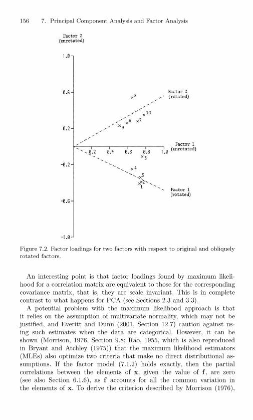
156 7. Principal Component Analysis and Factor Analysis
Figure 7.2. Factor loadings for two factors with respect to original and obliquelyrotated factors.
An interesting point is that factor loadings found by maximum likeli-hood for a correlation matrix are equivalent to those for the correspondingcovariance matrix, that is, they are scale invariant. This is in completecontrast to what happens for PCA (see Sections 2.3 and 3.3).
A potential problem with the maximum likelihood approach is thatit relies on the assumption of multivariate normality, which may not bejustified, and Everitt and Dunn (2001, Section 12.7) caution against us-ing such estimates when the data are categorical. However, it can beshown (Morrison, 1976, Section 9.8; Rao, 1955, which is also reproducedin Bryant and Atchley (1975)) that the maximum likelihood estimators(MLEs) also optimize two criteria that make no direct distributional as-sumptions. If the factor model (7.1.2) holds exactly, then the partialcorrelations between the elements of x, given the value of f , are zero(see also Section 6.1.6), as f accounts for all the common variation inthe elements of x. To derive the criterion described by Morrison (1976),

7.2. Estimation of the Factor Model 157
a sample estimate of the matrix of partial correlations is calculated. Thedeterminant of this matrix will attain its maximum value of unity whenall its off-diagonal elements are zero, so that maximizing this determi-nant is one way of attempting to minimize the absolute values of thepartial correlations. This maximization problem leads to the MLEs, buthere they appear regardless of whether or not multivariate normalityholds.
The procedure suggested by Rao (1955) is based on canonical correla-tion analysis (see Section 9.3) between x and f . He looks, successively,for pairs of linear functions a′
k1x,a′k2f that have maximum correlation
subject to being uncorrelated with previous pairs. The factor loadings arethen proportional to the elements of the ak2, k = 1, 2, . . . , m, which inturn leads to the same loadings as for the MLEs based on the assump-tion of multivariate normality (Rao, 1955). As with the criterion based onpartial correlations, no distributional assumptions are necessary for Rao’scanonical analysis.
In a way, the behaviour of the partial correlation and canonical cor-relation criteria parallels the phenomenon in regression where the leastsquares criterion is valid regardless of the distribution of error terms, butif errors are normally distributed then least squares estimators have theadded attraction of maximizing the likelihood function.
An alternative but popular way of getting initial estimates for Λ is touse the first m PCs. If z = A′x is the vector consisting of all p PCs, withA defined to have αk, the kth eigenvector of Σ, as its kth column as in(2.1.1), then x = Az because of the orthogonality of A. If A is partitionedinto its first m and last (p−m) columns, with a similar partitioning of therows of z, then
x = (Am | A∗p−m)
(zm
z∗p−m
)(7.2.3)
= Amzm + A∗p−mz∗p−m
= Λf + e,
where
Λ = Am, f = zm and e = A∗p−mz∗p−m.
Equation (7.2.3) looks very much like the factor model (7.1.2) but it violatesa basic assumption of the factor model, because the elements of e in (7.2.3)are not usually uncorrelated. Despite the apparently greater sophisticationof using the sample version of Am as an initial estimator, compared withcrude techniques such as centroid estimates, its theoretical justification isreally no stronger.
As well as the straightforward use of PCs to estimate Λ, many varietiesof factor analysis use modifications of this approach; this topic will bediscussed further in the next section.
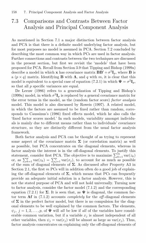
158 7. Principal Component Analysis and Factor Analysis
7.3 Comparisons and Contrasts Between FactorAnalysis and Principal Component Analysis
As mentioned in Section 7.1 a major distinction between factor analysisand PCA is that there is a definite model underlying factor analysis, butfor most purposes no model is assumed in PCA. Section 7.2 concluded bydescribing the most common way in which PCs are used in factor analysis.Further connections and contrasts between the two techniques are discussedin the present section, but first we revisit the ‘models’ that have beenproposed for PCA. Recall from Section 3.9 that Tipping and Bishop (1999a)describe a model in which x has covariance matrix BB′ +σ2Ip, where B isa (p × q) matrix. Identifying B with Λ, and q with m, it is clear that thismodel is equivalent to a special case of equation (7.2.1) in which Ψ = σ2Ip,so that all p specific variances are equal.
De Leeuw (1986) refers to a generalization of Tipping and Bishop’s(1999a) model, in which σ2Ip is replaced by a general covariance matrix forthe error terms in the model, as the (random factor score) factor analysismodel. This model is also discussed by Roweis (1997). A related model,in which the factors are assumed to be fixed rather than random, corre-sponds to Caussinus’s (1986) fixed effects model, which he also calls the‘fixed factor scores model.’ In such models, variability amongst individu-als is mainly due to different means rather than to individuals’ covariancestructure, so they are distinctly different from the usual factor analysisframework.
Both factor analysis and PCA can be thought of as trying to representsome aspect of the covariance matrix Σ (or correlation matrix) as wellas possible, but PCA concentrates on the diagonal elements, whereas infactor analysis the interest is in the off-diagonal elements. To justify thisstatement, consider first PCA. The objective is to maximize
∑mk=1 var(zk)
or, as∑p
k=1 var(zk) =∑p
j=1 var(xj), to account for as much as possibleof the sum of diagonal elements of Σ. As discussed after Property A3 inSection 2.1, the first m PCs will in addition often do a good job of explain-ing the off-diagonal elements of Σ, which means that PCs can frequentlyprovide an adequate initial solution in a factor analysis. However, this isnot the stated purpose of PCA and will not hold universally. Turning nowto factor analysis, consider the factor model (7.1.2) and the correspondingequation (7.2.1) for Σ. It is seen that, as Ψ is diagonal, the common fac-tor term Λf in (7.1.2) accounts completely for the off -diagonal elementsof Σ in the perfect factor model, but there is no compulsion for the diag-onal elements to be well explained by the common factors. The elements,ψj , j = 1, 2, . . . , p, of Ψ will all be low if all of the variables have consid-erable common variation, but if a variable xj is almost independent of allother variables, then ψj = var(ej) will be almost as large as var(xj). Thus,factor analysis concentrates on explaining only the off-diagonal elements of

7.3. Comparisons Between Factor and Principal Component Analysis 159
Σ by a small number of factors, whereas, conversely, PCA concentrates onthe diagonal elements of Σ.
This leads to another difference between the two techniques concerningthe number of dimensions m which give an adequate representation of thep dimensional variable x. In PCA, if any individual variables are almostindependent of all other variables, then there will be a PC correspondingto each such variable, and that PC will be almost equivalent to the corre-sponding variable. Such ‘single variable’ PCs are generally included if anadequate representation of x is required, as was discussed in Section 6.1.5.In contrast, a common factor in factor analysis must contribute to at leasttwo of the variables, so it is not possible to have a ‘single variable’ commonfactor. Instead, such factors appear as specific factors (error terms) and donot contribute to the dimensionality of the model. Thus, for a given setof data, the number of factors required for an adequate factor model is nolarger—and may be strictly smaller—than the number of PCs required toaccount for most of the variation in the data. If PCs are used as initialfactors, then the ideal choice of m is often less than that determined bythe rules of Section 6.1, which are designed for descriptive PCA. As notedseveral times in that Section, the different objectives underlying PCA andfactor analysis have led to confusing and inappropriate recommendationsin some studies with respect to the best choice of rules.
The fact that a factor model concentrates on accounting for the off-diagonal elements, but not the diagonal elements, of Σ leads to variousmodifications of the idea of using the first m PCs to obtain initial esti-mates of factor loadings. As the covariance matrix of the common factors’contribution to x is Σ−Ψ, it seems reasonable to use ‘PCs’ calculated forΣ − Ψ rather than Σ to construct initial estimates, leading to so-calledprincipal factor analysis. This will, of course, require estimates of Ψ, whichcan be found in various ways (see, for example, Rencher, 1998, Section 10.3;Rummel, 1970, Chapter 13), either once-and-for-all or iteratively, leadingto many different factor estimates. Many, though by no means all, of thedifferent varieties of factor analysis correspond to simply using differentestimates of Ψ in this type of ‘modified PC’ procedure. None of these esti-mates has a much stronger claim to absolute validity than does the use ofthe PCs of Σ, although arguments have been put forward to justify variousdifferent estimates of Ψ.
Another difference between PCA and (after rotation) factor analysis isthat changing m, the dimensionality of the model, can have much moredrastic effects on factor analysis than it does on PCA. In PCA, if m isincreased from m1 to m2, then an additional (m2 −m1) PCs are included,but the original m1 PCs are still present and unaffected. However, in factoranalysis an increase from m1 to m2 produces m2 factors, none of which needbear any resemblance to the original m1 factors.
A final difference between PCs and common factors is that the formercan be calculated exactly from x, whereas the latter typically cannot. The

160 7. Principal Component Analysis and Factor Analysis
PCs are exact linear functions of x and have the form
z = A′x.
The factors, however, are not exact linear functions of x; instead x is definedas a linear function of f apart from an error term, and when the relationshipis reversed, it certainly does not lead to an exact relationship between fand x. Indeed, the fact that the expected value of x is a linear functionof f need not imply that the expected value of f is a linear function ofx (unless multivariate normal assumptions are made). Thus, the use ofPCs as initial factors may force the factors into an unnecessarily restrictivelinear framework. Because of the non-exactness of the relationship betweenf and x, the values of f , the factor scores, must be estimated, and thereare several possible ways of doing this (see, for example, Bartholomew andKnott (1999, 3.23–3.25); Jackson (1991, Section 17.7); Lawley and Maxwell(1971, Chapter 8); Lewis-Beck (1994, Section II.6)).
To summarize, there are many ways in which PCA and factor analysisdiffer from one another. Despite these differences, they both have the aim ofreducing the dimensionality of a vector of random variables. The use of PCsto find initial factor loadings, though having no firm justification in theory(except when Ψ = σ2Ip as in Tipping and Bishop’s (1999a) model) willoften not be misleading in practice. In the special case where the elementsof Ψ are proportional to the diagonal elements of Σ, Gower (1966) showsthat the configuration of points produced by factor analysis will be similarto that found by PCA. In principal factor analysis, the results are equivalentto those of PCA if all (non-zero) elements of Ψ are identical (Rao, 1955).More generally, the coefficients found from PCA and the loadings foundfrom (orthogonal) factor analysis will often be very similar, although thiswill not hold unless all the elements of Ψ are of approximately the same size(Rao, 1955), which again relates to Tipping and Bishop’s (1999a) model.
Schneeweiss and Mathes (1995) provide detailed theoretical comparisonsbetween factor analysis and PCA. Assuming the factor model (7.2.1), theycompare Λ with estimates of Λ obtained from PCA and from factor anal-ysis. Comparisons are also made between f , the PC scores, and estimatesof f using factor analysis. General results are given, as well as comparisonsfor the special cases where m = 1 and where Σ = σ2I. The theorems, lem-mas and corollaries given by Schneeweiss and Mathes provide conditionsunder which PCs and their loadings can be used as adequate surrogatesfor the common factors and their loadings. One simple set of conditionsis that p is large and that the elements of Ψ are small, although, un-like the conventional factor model, Ψ need not be diagonal. Additionalconditions for closeness of factors and principal components are given bySchneeweiss (1997). Further, mainly theoretical, discussion of relationshipsbetween factor analysis and PCA appears in Ogasawara (2000).
The results derived by Schneeweiss and Mathes (1995) and Schneeweiss(1997) are ‘population’ results, so that the ‘estimates’ referred to above
7.4. An Example of Factor Analysis 161
are actually derived from correlation matrices corresponding exactly to theunderlying model. In practice, the model itself is unknown and must beestimated from a data set. This allows more scope for divergence betweenthe results from PCA and from factor analysis. There have been a numberof studies in which PCA and factor analysis are compared empirically ondata sets, with comparisons usually based on a subjective assessment ofhow well and simply the results can be interpreted. A typical study ofthis sort from atmospheric science is Barring (1987). There have also beena number of comparative simulation studies, such as Snook and Gorsuch(1989), in which, unsurprisingly, PCA is inferior to factor analysis in findingunderlying structure in data simulated from a factor model.
There has been much discussion in the behavioural science literature ofthe similarities and differences between PCA and factor analysis. For exam-ple, 114 pages of the first issue in 1990 of Multivariate Behavioral Researchwas devoted to a lead article by Velicer and Jackson (1990) on ‘Componentanalysis versus common factor analysis . . . ,’ together with 10 shorter dis-cussion papers by different authors and a rejoinder by Velicer and Jackson.Widaman (1993) continued this debate, and concluded that ‘. . . principalcomponent analysis should not be used if a researcher wishes to obtainparameters reflecting latent constructs or factors.’ This conclusion reflectsthe fact that underlying much of the 1990 discussion is the assumption thatunobservable factors are being sought from which the observed behaviouralvariables can be derived. Factor analysis is clearly designed with this ob-jective in mind, whereas PCA does not directly address it. Thus, at best,PCA provides an approximation to what is truly required.
PCA and factor analysis give similar numerical results for many exam-ples. However PCA should only be used as a surrogate for factor analysiswith full awareness of the differences between the two techniques, and eventhen caution is necessary. Sato (1990), who, like Schneeweiss and Mathes(1995) and Schneeweiss (1997), gives a number of theoretical comparisons,showed that for m = 1 and small p the loadings given by factor analysisand by PCA can sometimes be quite different.
7.4 An Example of Factor Analysis
The example that follows is fairly typical of the sort of data that are oftensubjected to a factor analysis. The data were originally discussed by Yuleet al. (1969) and consist of scores for 150 children on ten subtests of theWechsler Pre-School and Primary Scale of Intelligence (WPPSI); there arethus 150 observations on ten variables. The WPPSI tests were designedto measure ‘intelligence’ of children aged 41
2–6 years, and the 150 childrentested in the Yule et al. (1969) study were a sample of children who enteredschool in the Isle of Wight in the autumn of 1967, and who were tested
162 7. Principal Component Analysis and Factor Analysis
during their second term in school. Their average age at the time of testingwas 5 years, 5 months. Similar data sets are analysed in Lawley and Maxwell(1971).
Table 7.1 gives the variances and the coefficients of the first four PCs,when the analysis is done on the correlation matrix. It is seen that thefirst four components explain nearly 76% of the total variation, and thatthe variance of the fourth PC is 0.71. The fifth PC, with a variance of0.51, would be discarded by most of the rules described in Section 6.1and, indeed, in factor analysis it would be more usual to keep only two,or perhaps three, factors in the present example. Figures 7.1, 7.2 earlier inthe chapter showed the effect of rotation in this example when only twoPCs are considered; here, where four PCs are retained, it is not possible toeasily represent the effect of rotation in the same diagrammatic way.
All of the correlations between the ten variables are positive, so thefirst PC has the familiar pattern of being an almost equally weighted‘average’ of all ten variables. The second PC contrasts the first five vari-ables with the final five. This is not unexpected as these two sets ofvariables are of different types, namely ‘verbal’ tests and ‘performance’tests, respectively. The third PC is mainly a contrast between variables6 and 9, which interestingly were at the time the only two ‘new’ tests inthe WPSSI battery, and the fourth does not have a very straightforwardinterpretation.
Table 7.2 gives the factor loadings when the first four PCs are rotatedusing an orthogonal rotation method (varimax), and an oblique method(direct quartimin). It would be counterproductive to give more varietiesof factor analysis for this single example, as the differences in detail tendto obscure the general conclusions that are drawn below. Often, resultsare far less sensitive to the choice of rotation criterion than to the choiceof how many factors to rotate. Many further examples can be found intexts on factor analysis such as Cattell (1978), Lawley and Maxwell (1971),Lewis-Beck (1994) and Rummel (1970).
In order to make comparisons between Table 7.1 and Table 7.2 straight-forward, the sum of squares of the PC coefficients and factor loadings arenormalized to be equal to unity for each factor. Typically, the output fromcomputer packages that implement factor analysis uses the normalization inwhich the sum of squares of coefficients in each PC before rotation is equalto the variance (eigenvalue) associated with that PC (see Section 2.3). Thelatter normalization is used in Figures 7.1 and 7.2. The choice of normal-ization constraints is important in rotation as it determines the propertiesof the rotated factors. Detailed discussion of these properties in the contextof rotated PCs is given in Section 11.1.
The correlations between the oblique factors in Table 7.2 are given inTable 7.3 and it can be seen that there is a non-trivial degree of correlationbetween the factors given by the oblique method. Despite this, the structureof the factor loadings is very similar for the two factor rotation methods.

7.4. An Example of Factor Analysis 163
Table 7.1. Coefficients for the first four PCs: children’s intelligence tests.
Component number 1 2 3 41 0.34 −0.39 0.09 −0.082 0.34 −0.37 −0.08 −0.233 0.35 −0.10 0.05 0.034 0.30 −0.24 −0.20 0.63
Variable 5 0.34 −0.32 0.19 −0.28
number 6 0.27 0.24 −0.57 0.307 0.32 0.27 −0.27 −0.348 0.30 0.51 0.19 −0.279 0.23 0.22 0.69 0.43
10 0.36 0.33 −0.03 0.02
Eigenvalue 4.77 1.13 0.96 0.71
Cumulative percentageof total variation 47.7 59.1 68.6 75.7
Table 7.2. Rotated factor loadings–four factors: children’s intelligence tests.
Factor number 1 2 3 4Varimax
1 0.48 0.09 0.17 0.142 0.49 0.15 0.18 −0.033 0.35 0.22 0.24 0.224 0.26 −0.00 0.64 0.20
Variable 5 0.49 0.16 0.02 0.15
number 6 0.05 0.34 0.60 −0.097 0.20 0.51 0.18 −0.078 0.10 0.54 −0.02 0.329 0.10 0.13 0.07 0.83
10 0.17 0.46 0.28 0.26
Direct quartimin1 0.51 −0.05 0.05 0.052 0.53 0.04 0.05 −0.143 0.32 0.13 0.16 0.154 0.17 −0.19 0.65 0.20
Variable 5 0.54 0.06 −0.13 0.05
number 6 −0.07 0.28 0.67 −0.127 0.16 0.53 0.13 −0.178 0.03 0.62 −0.09 0.269 0.00 0.09 0.02 0.87
10 0.08 0.45 0.24 0.21

164 7. Principal Component Analysis and Factor Analysis
Table 7.3. Correlations between four direct quartimin factors: children’s intelli-gence tests.
Factor number1 2 3
Factor 2 0.349number 3 0.418 0.306
4 0.305 0.197 0.112
Table 7.4. Factor loadings—three factors, varimax rotation: children’s intelligencetests.
Factor number1 2 3
1 0.47 0.09 0.142 0.47 0.17 0.053 0.36 0.23 0.244 0.37 0.23 0.00
Variable 5 0.45 0.08 0.23
number 6 0.12 0.55 −0.057 0.17 0.48 0.178 0.05 0.36 0.529 0.13 −0.01 0.66
10 0.18 0.43 0.36
The first factor in both methods has its highest loadings in variables 1, 2,3 and 5, with the next highest loadings on variables 4 and 7. In factors2, 3, 4 there is the same degree of similarity in the position of the highestloadings: for factor 2, the loadings for variables 7, 8, 10 are highest, with anintermediate value on variable 6; factor 3 has large loadings on variables 4and 6 and an intermediate value on variable 10; and factor 4 is dominated byvariable 9 with intermediate values on variables 8 and 10. The only notabledifference between the results for the two methods is that obliqueness allowsthe second method to achieve slightly higher values on the highest loadingsand correspondingly lower values on the low loadings, as indeed it is meantto.
By contrast, the differences between the loadings before and after ro-tation are more substantial. After rotation, the ‘general factor’ withcoefficients of similar size on all variables disappears, as do most nega-tive coefficients, and the structure of the loadings is simplified. Again, thisis precisely what rotation is meant to achieve.

7.5. Concluding Remarks 165
To illustrate what happens when different numbers of factors are re-tained, Table 7.4 gives factor loadings for three factors using varimaxrotation. The loadings for direct quartimin (not shown) are again very sim-ilar. Before rotation, changing the number of PCs simply adds or deletesPCs, leaving the remaining PCs unchanged. After rotation, however, dele-tion or addition of factors will usually change all of the factor loadings.In the present example, deletion of the fourth unrotated factor leaves thefirst rotated factor almost unchanged, except for a modest increase in theloading for variable 4. Factor 2 here is also similar to factor 2 in the four-factor analysis, although the resemblance is somewhat less strong than forfactor 1. In particular, variable 6 now has the largest loading in factor 2,whereas previously it had only the fourth largest loading. The third factorin the three-factor solution is in no way similar to factor 3 in the four-factoranalysis. In fact, it is quite similar to the original factor 4, and the originalfactor 3 has disappeared, with its highest loadings on variables 4 and 6partially ‘transferred’ to factors 1 and 2, respectively.
The behaviour displayed in this example, when a factor is deleted, isnot untypical of what happens in factor analysis generally, although the‘mixing-up’ and ‘rearrangement’ of factors can be much more extreme thanin the present case.
7.5 Concluding Remarks
Factor analysis is a large subject, and this chapter has concentrated onaspects that are most relevant to PCA. The interested reader is referred toone of the many books on the subject such as Cattell (1978), Lawley andMaxwell (1971), Lewis-Beck (1994) or Rummell (1970) for further details.Factor analysis is one member of the class of latent variable models (seeBartholomew and Knott (1999)) which have been the subject of muchrecent research. Mixture modelling, discussed in Section 9.2.3, is anotherof the many varieties of latent variable models.
It should be clear from the discussion of this chapter that it does notreally make sense to ask whether PCA is ‘better than’ factor analysis orvice versa, because they are not direct competitors. If a model such as(7.1.2) seems a reasonable assumption for a data set, then factor analysis,rather than PCA, is appropriate. If no such model can be assumed, thenfactor analysis should not really be used.
Despite their different formulations and objectives, it can be informa-tive to look at the results of both techniques on the same data set. Eachtechnique gives different insights into the data structure, with PCA con-centrating on explaining the diagonal elements, and factor analysis theoff-diagonal elements, of the covariance matrix, and both may be useful.Furthermore, one of the main ideas of factor analysis, that of rotation, can

166 7. Principal Component Analysis and Factor Analysis
be ‘borrowed’ for PCA without any implication that a factor model is be-ing assumed. Once PCA has been used to find an m-dimensional subspacethat contains most of the variation in the original p variables, it is possibleto redefine, by rotation, the axes (or derived variables) that form a basisfor this subspace. The rotated variables will together account for the sameamount of variation as the first few PCs, but will no longer successivelyaccount for the maximum possible variation. This behaviour is illustratedby Tables 7.1 and 7.2; the four rotated PCs in Table 7.2 together accountfor 75.7% of the total variation, as did the unrotated PCs in Table 7.1.However, the percentages of total variation accounted for by individualfactors (rotated PCs) are 27.4, 21.9, 14.2 and 12.1, compared with 47.7,11.3, 9.6 and 7.1 for the unrotated PCs. The rotated PCs, when expressedin terms of the original variables, may be easier to interpret than the PCsthemselves because their coefficients will typically have a simpler structure.This is discussed in more detail in Chapter 11. In addition, rotated PCs of-fer advantages compared to unrotated PCs in some types of analysis basedon PCs (see Sections 8.5 and 10.1).

8Principal Components in RegressionAnalysis
As illustrated elsewhere in this book, principal components are used inconjunction with a variety of other statistical techniques. One area in whichthis activity has been extensive is regression analysis.
In multiple regression, one of the major difficulties with the usual leastsquares estimators is the problem of multicollinearity, which occurs whenthere are near-constant linear functions of two or more of the predictor,or regressor, variables. A readable review of the multicollinearity problemis given by Gunst (1983). Multicollinearities are often, but not always,indicated by large correlations between subsets of the variables and, if mul-ticollinearities exist, then the variances of some of the estimated regressioncoefficients can become very large, leading to unstable and potentially mis-leading estimates of the regression equation. To overcome this problem,various approaches have been proposed. One possibility is to use only a sub-set of the predictor variables, where the subset is chosen so that it does notcontain multicollinearities. Numerous subset selection methods are avail-able (see, for example, Draper and Smith, 1998, Chapter 15; Hocking, 1976;Miller, 1984, 1990), and among the methods are some based on PCs. Thesemethods will be dealt with later in the chapter (Section 8.5), but first somemore widely known uses of PCA in regression are described.
These uses of PCA follow from a second class of approaches to overcom-ing the problem of multicollinearity, namely the use of biased regressionestimators. This class includes ridge regression, shrinkage estimators, par-tial least squares, the so-called LASSO, and also approaches based on PCA.The best-known such approach, generally known as PC regression, simplystarts by using the PCs of the predictor variables in place of the predic-

168 8. Principal Components in Regression Analysis
tor variables. As the PCs are uncorrelated, there are no multicollinearitiesbetween them, and the regression calculations are also simplified. If all thePCs are included in the regression, then the resulting model is equivalentto that obtained by least squares, so the large variances caused by multi-collinearities have not gone away. However, calculation of the least squaresestimates via PC regression may be numerically more stable than directcalculation (Flury and Riedwyl, 1988, p. 212).
If some of the PCs are deleted from the regression equation, estima-tors are obtained for the coefficients in the original regression equation.These estimators are usually biased, but can simultaneously greatly reduceany large variances for regression coefficient estimators caused by multi-collinearities. Principal component regression is introduced in Section 8.1,and strategies for deciding which PCs to delete from the regression equa-tion are discussed in Section 8.2; some connections between PC regressionand other forms of biased regression are described in Section 8.3.
Variations on the basic idea of PC regression have also been proposed.One such variation, noted in Section 8.3, allows the possibility that a PCmay be only ‘partly deleted’ from the regression equation. A rather differentapproach, known as latent root regression, finds the PCs of the predictorvariables together with the dependent variable. These PCs can then beused to construct biased regression estimators, which differ from those de-rived from PC regression. Latent root regression in various forms, togetherwith its properties, is discussed in Section 8.4. A widely used alternativeto PC regression is partial least squares (PLS). This, too, is included inSection 8.4, as are a number of other regression-related techniques thathave connections with PCA. One omission is the use of PCA to detect out-liers. Because the detection of outliers is important in other areas as wellas regression, discussion of this topic is postponed until Section 10.1.
A topic which is related to, but different from, regression analysis isthat of functional and structural relationships. The idea is, like regressionanalysis, to explore relationships between variables but, unlike regression,the predictor variables as well as the dependent variable may be subjectto error. Principal component analysis can again be used in investigat-ing functional and structural relationships, and this topic is discussed inSection 8.6.
Finally in this chapter, in Section 8.7 two detailed examples are givenof the use of PCs in regression, illustrating many of the ideas discussed inearlier sections.
8.1 Principal Component Regression
Consider the standard regression model, as defined in equation (3.1.5), thatis,
y = Xβ + ε, (8.1.1)

8.1. Principal Component Regression 169
where y is a vector of n observations on the dependent variable, measuredabout their mean, X is an (n×p) matrix whose (i, j)th element is the valueof the jth predictor (or regressor) variable for the ith observation, againmeasured about its mean, β is a vector of p regression coefficients and ε isa vector of error terms; the elements of ε are independent, each with thesame variance σ2. It is convenient to present the model (8.1.1) in ‘centred’form, with all variables measured about their means. Furthermore, it isconventional in much of the literature on PC regression to assume that thepredictor variables have been standardized so that X′X is proportional tothe correlation matrix for the predictor variables, and this convention isfollowed in the present chapter. Similar derivations to those below are pos-sible if the predictor variables are in uncentred or non-standardized form,or if an alternative standardization has been used, but to save space andrepetition, these derivations are not given. Nor do we discuss the contro-versy that surrounds the choice of whether or not to centre the variablesin a regression analysis. The interested reader is referred to Belsley (1984)and the discussion which follows that paper.
The values of the PCs for each observation are given by
Z = XA, (8.1.2)
where the (i, k)th element of Z is the value (score) of the kth PC for theith observation, and A is a (p × p) matrix whose kth column is the ktheigenvector of X′X.
Because A is orthogonal, Xβ can be rewritten as XAA′β = Zγ, whereγ = A′β. Equation (8.1.1) can therefore be written as
y = Zγ + ε, (8.1.3)
which has simply replaced the predictor variables by their PCs in the re-gression model. Principal component regression can be defined as the useof the model (8.1.3) or of the reduced model
y = Zmγm + εm, (8.1.4)
where γm is a vector of m elements that are a subset of elements of γ,Zm is an (n × m) matrix whose columns are the corresponding subset ofcolumns of Z, and εm is the appropriate error term. Using least squares toestimate γ in (8.1.3) and then finding an estimate for β from the equation
β = Aγ (8.1.5)
is equivalent to finding β by applying least squares directly to (8.1.1).The idea of using PCs rather than the original predictor variables is not
new (Hotelling, 1957; Kendall, 1957), and it has a number of advantages.First, calculating γ from (8.1.3) is more straightforward than finding βfrom (8.1.1) as the columns of Z are orthogonal. The vector γ is
γ = (Z′Z)−1Z′y = L−2Z′y, (8.1.6)

170 8. Principal Components in Regression Analysis
where L is the diagonal matrix whose kth diagonal element is l1/2k , and
lk is defined here, as in Section 3.5, as the kth largest eigenvalue of X′X,rather than S. Furthermore, if the regression equation is calculated for PCsinstead of the predictor variables, then the contributions of each trans-formed variable (PC) to the equation can be more easily interpreted thanthe contributions of the original variables. Because of uncorrelatedness, thecontribution and estimated coefficient of a PC are unaffected by which otherPCs are also included in the regression, whereas for the original variablesboth contributions and coefficients can change dramatically when anothervariable is added to, or deleted from, the equation. This is especially truewhen multicollinearity is present, but even when multicollinearity is nota problem, regression on the PCs, rather than the original predictor vari-ables, may have advantages for computation and interpretation. However, itshould be noted that although interpretation of the separate contributionsof each transformed variable is improved by taking PCs, the interpretationof the regression equation itself may be hindered if the PCs have no clearmeaning.
The main advantage of PC regression occurs when multicollinearities arepresent. In this case, by deleting a subset of the PCs, especially those withsmall variances, much more stable estimates of β can be obtained. To seethis, substitute (8.1.6) into (8.1.5) to give
β = A(Z′Z)−1Z′y (8.1.7)
= AL−2Z′y
= AL−2A′X′y
=p∑
k=1
l−1k aka′
kX′y, (8.1.8)
where lk is the kth diagonal element of L2 and ak is the kth column of A.Equation (8.1.8) can also be derived more directly from β = (X′X)−1X′y,by using the spectral decomposition (see Property A3 of Sections 2.1 and3.1) of the matrix (X′X)−1, which has eigenvectors ak and eigenvaluesl−1k , k = 1, 2, . . . , p.
Making the usual assumption that the elements of y are uncorrelated,each with the same variance σ2 (that is the variance-covariance matrix ofy is σ2In), it is seen from (8.1.7) that the variance-covariance matrix of βis
σ2A(Z′Z)−1Z′Z(Z′Z)−1A′ = σ2A(Z′Z)−1A′
= σ2AL−2A′
= σ2
p∑
k=1
l−1k aka′
k. (8.1.9)

8.1. Principal Component Regression 171
This expression gives insight into how multicollinearities produce largevariances for the elements of β. If a multicollinearity exists, then it appearsas a PC with very small variance (see also Sections 3.4 and 10.1); in otherwords, the later PCs have very small values of lk (the variance of the kthPC is lk/(n−1) in the present notation), and hence very large values of l−1
k .Thus (8.1.9) shows that any predictor variable having moderate or largecoefficients in any of the PCs associated with very small eigenvalues willhave a very large variance.
One way of reducing this effect is to delete the terms from (8.1.8) thatcorrespond to very small lk, leading to an estimator
β =m∑
k=1
l−1k aka′
kX′y, (8.1.10)
where lm+1, lm+2, . . . , lp are the very small eigenvalues. This is equivalentto setting the last (p − m) elements of γ equal to zero.
Then the variance-covariance matrix V (β) for β is
σ2m∑
j=1
l−1j aja′
jX′X
m∑
k=1
l−1k aka′
k.
Substituting
X′X =p∑
h=1
lhaha′h
from the spectral decomposition of X′X, we have
V (β) = σ2
p∑
h=1
m∑
j=1
m∑
k=1
lhl−1j l−1
k aja′jaha′
haka′k.
Because the vectors ah, h = 1, 2, . . . , p are orthonormal, the only non-zeroterms in the triple summation occur when h = j = k, so that
V (β) = σ2m∑
k=1
l−1k aka′
k (8.1.11)
If none of the first m eigenvalues lk is very small, then none of the variancesgiven by the diagonal elements of (8.1.11) will be large.
The decrease in variance for the estimator β given by (8.1.10), comparedwith the variance of β, is achieved at the expense of introducing bias intothe estimator β. This follows because
β = β −p∑
k=m+1
l−1k aka′
kX′y, E(β) = β,

172 8. Principal Components in Regression Analysis
and
E
[p∑
k=m+1
l−1k aka′
kX′y
]
=p∑
k=m+1
l−1k aka′
kX′Xβ
=p∑
k=m+1
aka′kβ.
This last term is, in general, non-zero so that E(β) = β. However, ifmulticollinearity is a serious problem, the reduction in variance can besubstantial, whereas the bias introduced may be comparatively small. Infact, if the elements of γ corresponding to deleted components are actuallyzero, then no bias will be introduced.
As well as, or instead of, deleting terms from (8.1.8) corresponding tosmall eigenvalues, it is also possible to delete terms for which the cor-responding elements of γ are not significantly different from zero. Thequestion of which elements are significantly non-zero is essentially a variableselection problem, with PCs rather than the original predictor variables asvariables. Any of the well-known methods of variable selection for regres-sion (see, for example, Draper and Smith, 1998, Chapter 15) can be used.However, the problem is complicated by the desirability of also deletinghigh-variance terms from (8.1.8).
The definition of PC regression given above in terms of equations (8.1.3)and (8.1.4) is equivalent to using the linear model (8.1.1) and estimatingβ by
β =∑
M
l−1k aka′
kX′y, (8.1.12)
where M is some subset of the integers 1, 2, . . . , p. A number of authors con-sider only the special case (8.1.10) of (8.1.12), in which M = 1, 2, . . . ,m,but this is often too restrictive, as will be seen in Section 8.2. In the generaldefinition of PC regression, M can be any subset of the first p integers, sothat any subset of the coefficients of γ, corresponding to the complement ofM , can be set to zero. The next section will consider various strategies forchoosing M , but we first note that once again the singular value decompo-sition (SVD) of X defined in Section 3.5 can be a useful concept (see alsoSections 5.3, 6.1.5, 13.4, 13.5, 13.6, 14.2 and Appendix A1). In the presentcontext it can be used to provide an alternative formulation of equation(8.1.12) and to help in the interpretation of the results of a PC regression.Assuming that n ≥ p and that X has rank p, recall that the SVD writes Xin the form
X = ULA′,
where
(i) A and L are as defined earlier in this section;

8.2. Selecting Components in Principal Component Regression 173
(ii) the columns of U are those eigenvectors of XX′ that correspond tonon-zero eigenvalues, normalized so that U′U = Ip.
Then Xβ can be rewritten ULA′β = Uδ, where δ = LA′β, so thatβ = AL−1δ. The least squares estimator for δ is
δ = (U′U)−1U′y = U′y,
leading to β = AL−1δ.The relationship between γ, defined earlier, and δ is straightforward,
namely
γ = A′β = A′(AL−1δ) = (A′A)L−1δ = L−1δ,
so that setting a subset of elements of δ equal to zero is equivalent to settingthe same subset of elements of γ equal to zero. This result means that theSVD can provide an alternative computational approach for estimating PCregression equations, which is an advantage, as efficient algorithms exist forfinding the SVD of a matrix (see Appendix A1).
Interpretation of the results of a PC regression can also be aided by usingthe SVD, as illustrated by Mandel (1982) for artificial data (see also Nelder(1985)).
8.2 Strategies for Selecting Components inPrincipal Component Regression
When choosing the subset M in equation (8.1.12) there are two partiallyconflicting objectives. In order to eliminate large variances due to multi-collinearities it is essential to delete all those components whose variancesare very small but, at the same time, it is undesirable to delete componentsthat have large correlations with the dependent variable y. One strategyfor choosing M is simply to delete all those components whose variancesare less than l∗, where l∗ is some cut-off level. The choice of l∗ is ratherarbitrary, but when dealing with correlation matrices, where the averagevalue of the eigenvalues is 1, a value of l∗ somewhere in the range 0.01 to0.1 seems to be useful in practice.
An apparently more sophisticated way of choosing l∗ is to look at so-called variance inflation factors (VIFs) for the p predictor variables. TheVIF for the jth variable when using standardized variables is defined ascjj/σ2 (which equals the jth diagonal element of (X′X)−1—Marquardt,1970), where cjj is the variance of the jth element of the least squaresestimator for β. If all the variables are uncorrelated, then all the VIFsare equal to 1, but if severe multicollinearities exist then the VIFs for βwill be very large for those variables involved in the multicollinearities. Bysuccessively deleting the last few terms in (8.1.8), the VIFs for the resultingbiased estimators will be reduced; deletion continues until all VIFs are

174 8. Principal Components in Regression Analysis
Table 8.1. Variation accounted for by PCs of predictor variables in monsoon datafor (a) predictor variables, (b) dependent variable.
Componentnumber 1 2 3 4 5 6 7 8 9 10
Percentage (a) Predictorvariation variables 26 22 17 11 10 7 4 3 1 < 1
accounted (b) Dependentfor variable 3 22 < 1 1 3 3 6 24 5 20
below some desired level. The original VIF for a variable is related to thesquared multiple correlation R2 between that variable and the other (p−1)predictor variables by the formula VIF = (1−R2)−1. Values of VIF > 10correspond to R2 > 0.90, and VIF > 4 is equivalent to R2 > 0.75, so thatvalues of R2 can be considered when choosing how small a level of VIF isdesirable. However, the choice of this desirable level is almost as arbitraryas the choice of l∗ above.
Deletion based solely on variance is an attractive and simple strategy, andProperty A7 of Section 3.1 gives it, at first sight, an added respectability.However, low variance for a component does not necessarily imply thatthe corresponding component is unimportant in the regression model. Forexample, Kung and Sharif (1980) give an example from meteorology where,in a regression of monsoon onset dates on all of the (ten) PCs, the mostimportant PCs for prediction are, in decreasing order of importance, theeighth, second and tenth (see Table 8.1). The tenth component accountsfor less than 1% of the total variation in the predictor variables, but isan important predictor of the dependent variable, and the most importantPC in the regression accounts for 24% of the variation in y but only 3% ofthe variation in x. Further examples of this type are presented in Jolliffe(1982). Thus, the two objectives of deleting PCs with small variances andof retaining PCs that are good predictors of the dependent variable maynot be simultaneously achievable.
Some authors (for example, Hocking, 1976; Mosteller and Tukey, 1977,pp. 397–398; Gunst and Mason, 1980, pp. 327–328) argue that the choiceof PCs in the regression should be made entirely, or mainly, on the basis ofvariance reduction but, as can be seen from the examples cited by Jolliffe(1982), such a procedure can be dangerous if low-variance components havepredictive value. Jolliffe (1982) notes that examples where this occurs seemto be not uncommon in practice. Berk’s (1984) experience with six datasets indicates the opposite conclusion, but several of his data sets are ofa special type, in which strong positive correlations exist between all theregressor variables and between the dependent variable and the regressorvariables. In such cases the first PC is a (weighted) average of the regres-sor variables, with all weights positive (see Section 3.8), and as y is also

8.2. Selecting Components in Principal Component Regression 175
positively correlated with each regressor variable it is strongly correlatedwith the first PC. Hadi and Ling (1998) (see also Cuadras (1998)) definePC regression in terms of equation (8.1.10), and argue that the techniqueis flawed because predictive low-variance PCs may be excluded. With themore general definition of PC regression, based on (8.1.12), this criticismdisappears.
In contrast to selection based solely on size of variance, the oppositeextreme is to base selection only on values of t-statistics measuring the(independent) contribution of each PC to the regression equation. This, too,has its pitfalls. Mason and Gunst (1985) showed that t-tests for low-variancePCs have reduced power compared to those for high-variance components,and so are less likely to be selected. A compromise between selection on thebasis of variance and on the outcome of t-tests is to delete PCs sequentiallystarting with the smallest variance, then the next smallest variance andso on; deletion stops when the first significant t-value is reached. Such astrategy is likely to retain more PCs than are really necessary.
Hill et al. (1977) give a comprehensive discussion of various, more so-phisticated, strategies for deciding which PCs to delete from the regressionequation. Their criteria are of two main types, depending on whether theprimary objective is to get β close to β, or to get Xβ, the estimate of y,close to y or to E(y). In the first case, estimation of β is the main interest;in the second it is prediction of y which is the chief concern. Whether ornot β is an improvement on β is determined for several of the criteria bylooking at mean square error (MSE) so that variance and bias are bothtaken into account.
More specifically, two criteria are suggested of the first type, the ‘weak’and ‘strong’ criteria. The weak criterion, due to Wallace (1972), prefers β
to β if tr[MSE(β)] ≤ tr[MSE(β)], where MSE(β) is the matrix E[(β −β)(β − β)′], with a similar definition for the matrix MSE(β). This simplymeans that β is preferred when the expected Euclidean distance betweenβ and β is smaller than that between β and β.
The strong criterion insists that
MSE(c′β) ≤ MSE(c′β)
for every non-zero p-element vector c, where
MSE(c′β) = E[(c′β − c′β)2],
with, again, a similar definition for MSE(c′β).Among those criteria of the second type (where prediction of y rather
than estimation of β is the main concern) that are considered by Hill et al.(1977), there are again two which use MSE. The first is also due to Wallace(1972) and is again termed a ‘weak’ criterion. It prefers β to β if
E[(Xβ − Xβ)′(Xβ − Xβ)] ≤ E[(Xβ − Xβ)′(Xβ − Xβ)],
176 8. Principal Components in Regression Analysis
so that β is preferred to β if the expected Euclidean distance between Xβ(the estimate of y) and Xβ (the expected value of y) is smaller than thecorresponding distance between Xβ and Xβ. An alternative MSE criterionis to look at the distance between each estimate of y and the actual, ratherthan expected, value of y. Thus β is preferred to β if
E[(Xβ − y)′(Xβ − y)] ≤ E[(Xβ − y)′(Xβ − y)].
Substituting y = Xβ + ε it follows that
E[(Xβ − y)′(Xβ − y)] = E[(Xβ − Xβ)′(Xβ − Xβ)] + nσ2,
with a similar expression for β. At first sight, it seems that this secondcriterion is equivalent to the first. However σ2 is unknown and, althoughit can be estimated, we may get different estimates when the equation isfitted using β, β, respectively.
Hill et al. (1977) consider several other criteria; further details may befound in their paper, which also describes connections between the variousdecision rules for choosing M and gives illustrative examples. They arguethat the choice of PCs should not be based solely on the size of theirvariance, but little advice is offered on which of their criteria gives an overall‘best’ trade-off between variance and bias; rather, separate circumstancesare identified in which each may be the most appropriate.
Gunst and Mason (1979) also consider integrated MSE of predictionsas a criterion for comparing different regression estimators. Friedman andMontgomery (1985) prefer to use the predictive ability for individual obser-vations, rather than averaging this ability over a distribution of potentialobservations as is done by Gunst and Mason (1979).
Another way of comparing predicted and observed values of y is by meansof cross-validation. Mertens et al. (1995) use a version of PRESS, definedin equation (6.1.3), as a criterion for deciding how many PCs to retain inPC regression. Their criterion is
n∑
i=1
(yi − yM(i))2,
where yM(i) is the estimate of yi obtained from a PC regression based ona subset M and using the data matrix X(i), which is X with its ith rowdeleted. They have an efficient algorithm for computing all PCAs with eachobservation deleted in turn, though the algebra that it uses is applicableonly to covariance, not correlation, matrices. Mainly for reasons of conve-nience, they also restrict their procedure to implementing (8.1.10), ratherthan the more general (8.1.12).
Yet another approach to deletion of PCs that takes into account bothvariance and bias is given by Lott (1973). This approach simply calculates
8.3. Connections Between PC Regression and Other Methods 177
the adjusted multiple coefficient of determination,
R2 = 1 − (n − 1)(n − p − 1)
(1 − R2),
where R2 is the usual multiple coefficient of determination (squared multi-ple correlation) for the regression equation obtained from each subset M ofinterest. The ‘best’ subset is then the one that maximizes R2. Lott demon-strates that this very simple procedure works well in a limited simulationstudy. Soofi (1988) uses a Bayesian approach to define the gain of informa-tion from the data about the ith element γi of γ. The subset M is chosento consist of integers corresponding to components with the largest val-ues of this measure of information. Soofi shows that the measure combinesthe variance accounted for by a component with its correlation with thedependent variable.
It is difficult to give any general advice regarding the choice of a decisionrule for determining M . It is clearly inadvisable to base the decision en-tirely on the size of variance; conversely, inclusion of highly predictive PCscan also be dangerous if they also have very small variances, because ofthe resulting instability of the estimated regression equation. Use of MSEcriteria provides a number of compromise solutions, but they are essentiallyarbitrary.
What PC regression can do, which least squares cannot, is to indicateexplicitly whether a problem exists with respect to the removal of multi-collinearity, that is whether instability in the regression coefficients can onlybe removed by simultaneously losing a substantial proportion of the pre-dictability of y. An extension of the cross-validation procedure of Mertenset al. (1995) to general subsets M would provide a less arbitrary way thanmost of deciding which PCs to keep, but the choice of M for PC regressionremains an open question.
8.3 Some Connections Between PrincipalComponent Regression and Other BiasedRegression Methods
Using the expressions (8.1.8), (8.1.9) for β and its variance-covariance ma-trix, it was seen in the previous section that deletion of the last few termsfrom the summation for β can dramatically reduce the high variances of el-ements of β caused by multicollinearities. However, if any of the elements ofγ corresponding to deleted components are non-zero, then the PC estimatorβ for β is biased. Various other methods of biased estimation that aim toremove collinearity-induced high variances have also been proposed. A fulldescription of these methods will not be given here as several do not involve

178 8. Principal Components in Regression Analysis
PCs directly, but there are various relationships between PC regression andother biased regression methods which will be briefly discussed.
Consider first ridge regression, which was described by Hoerl and Ken-nard (1970a,b) and which has since been the subject of much debate inthe statistical literature. The estimator of β using the technique can bewritten, among other ways, as
βR =p∑
k=1
(lk + κ)−1aka′kX
′y,
where κ is some fixed positive constant and the other terms in the expres-sion have the same meaning as in (8.1.8). The variance-covariance matrixof βR, is equal to
σ2
p∑
k=1
lk(lk + κ)−2aka′k.
Thus, ridge regression estimators have rather similar expressions to thosefor least squares and PC estimators, but variance reduction is achievednot by deleting components, but by reducing the weight given to the latercomponents. A generalization of ridge regression has p constants κk, k =1, 2, . . . , p that must be chosen, rather than a single constant κ.
A modification of PC regression, due to Marquardt (1970) uses a simi-lar, but more restricted, idea. Here a PC regression estimator of the form(8.1.10) is adapted so that M includes the first m integers, excludes theintegers m + 2,m + 3, . . . , p, but includes the term corresponding to inte-ger (m + 1) with a weighting less than unity. Detailed discussion of suchestimators is given by Marquardt (1970).
Ridge regression estimators ‘shrink’ the least squares estimators towardsthe origin, and so are similar in effect to the shrinkage estimators pro-posed by Stein (1960) and Sclove (1968). These latter estimators start withthe idea of shrinking some or all of the elements of γ (or β) using argu-ments based on loss functions, admissibility and prior information; choiceof shrinkage constants is based on optimization of MSE criteria. Partialleast squares regression is sometimes viewed as another class of shrinkageestimators. However, Butler and Denham (2000) show that it has peculiarproperties, shrinking some of the elements of γ but inflating others.
All these various biased estimators have relationships between them. Inparticular, all the present estimators, as well as latent root regression,which is discussed in the next section along with partial least squares,can be viewed as optimizing (β − β)′X′X(β − β), subject to differentconstraints for different estimators (see Hocking (1976)). If the data setis augmented by a set of dummy observations, and least squares is usedto estimate β from the augmented data, Hocking (1976) demonstratesfurther that ridge, generalized ridge, PC regression, Marquardt’s modifi-cation and shrinkage estimators all appear as special cases for particular
8.4. Variations on Principal Component Regression 179
choices of the dummy observations and their variances. In a slightly differ-ent approach to the same topic, Hocking et al. (1976) give a broad classof biased estimators, which includes all the above estimators, includingthose derived from PC regression, as special cases. Oman (1978) showshow several biased regression methods, including PC regression, can befitted into a Bayesian framework by using different prior distributions forβ; Leamer and Chamberlain (1976) also look at a Bayesian approach toregression, and its connections with PC regression. Other biased estima-tors have been suggested and compared with PC regression by Iglarsh andCheng (1980) and Trenkler (1980), and relationships between ridge regres-sion and PC regression are explored further by Hsuan (1981). Trenkler andTrenkler (1984) extend Hsuan’s (1981) results, and examine circumstancesin which ridge and other biased estimators can be made close to PC re-gression estimators, where the latter are defined by the restrictive equation(8.1.10).
Hoerl et al. (1986) describe a simulation study in which PC regression iscompared with other biased estimators and variable selection methods, andfound to be inferior. However, the comparison is not entirely fair. Severalvarieties of ridge regression are included in the comparison, but only oneway of choosing M is considered for PC regression. This is the restrictivechoice of M consisting of 1, 2, . . . ,m, where m is the largest integer forwhich a t-test of the PC regression coefficient γm gives a significant result.Hoerl et al. (1986) refer to a number of other simulation studies comparingbiased regression methods, some of which include PC regression. Theoret-ical comparisons between PC regression, least squares and ridge regressionwith respect to the predictive ability of the resulting regression equationsare made by Gunst and Mason (1979) and Friedman and Montgomery(1985), but only for p = 2.
Essentially the same problem arises for all these biased methods as oc-curred in the choice of M for PC regression, namely, the question of whichcompromise should be chosen in the trade-off between bias and variance.In ridge regression, this compromise manifests itself in the choice of κ, andfor shrinkage estimators the amount of shrinkage must be determined. Sug-gestions have been made regarding rules for making these choices, but thedecision is usually still somewhat arbitrary.
8.4 Variations on Principal Component Regression
Marquardt’s (1970) fractional rank estimator, which was described in theprevious section, is one modification of PC regression as defined in Sec-tion 8.1, but it is a fairly minor modification. Another approach, suggestedby Oman (1991), is to use shrinkage estimators, but instead of shrink-ing the least squares estimators towards zero or some other constant, the

180 8. Principal Components in Regression Analysis
shrinkage is towards the first few PCs. This tends to downweight the con-tribution of the less stable low-variance PC but does not ignore them.Oman (1991) demonstrates considerable improvements over least squareswith these estimators.
A rather different type of approach, which, nevertheless, still uses PCs ina regression problem, is provided by latent root regression. The main dif-ference between this technique and straightforward PC regression is thatthe PCs are not calculated for the set of p predictor variables alone. In-stead, they are calculated for a set of (p + 1) variables consisting of thep predictor variables and the dependent variable. This idea was suggestedindependently by Hawkins (1973) and by Webster et al. (1974), and termed‘latent root regression’ by the latter authors. Subsequent papers (Gunst etal., 1976; Gunst and Mason, 1977a) investigated the properties of latentroot regression, and compared it with other biased regression estimators.As with the biased estimators discussed in the previous section, the latentroot regression estimator can be derived by optimizing a quadratic func-tion of β, subject to constraints (Hocking, 1976). Latent root regression,as defined in Gunst and Mason (1980, Section 10.2), will now be described;the technique introduced by Hawkins (1973) has slight differences and isdiscussed later in this section.
In latent root regression, a PCA is done on the set of (p + 1) variablesdescribed above, and the PCs corresponding to the smallest eigenvaluesare examined. Those for which the coefficient of the dependent vari-able y is also small are called non-predictive multicollinearities, and aredeemed to be of no use in predicting y. However, any PC with a smalleigenvalue will be of predictive value if its coefficient for y is large.Thus, latent root regression deletes those PCs which indicate multi-collinearities, but only if the multicollinearities appear to be useless forpredicting y.
Let δk be the vector of the p coefficients on the p predictor variablesin the kth PC for the enlarged set of (p + 1) variables; let δ0k be thecorresponding coefficient of y, and let lk be the corresponding eigenvalue.Then the latent root estimator for β is defined as
βLR =∑
MLR
fkδk, (8.4.1)
where MLR is the subset of the integers 1, 2, . . . , p + 1, in which integerscorresponding to the non-predictive multicollinearities defined above, andno others, are deleted; the fk are coefficients chosen to minimize residualsums of squares among estimators of the form (8.4.1).
The fk can be determined by first using the kth PC to express y as alinear function of X to provide an estimator yk. A weighted average, yLR,of the yk for k ∈ MLR is then constructed, where the weights are chosenso as to minimize the residual sum of squares (yLR − y)′(yLR − y). Thevector yLR is then the latent root regression predictor XβLR, and the fk

8.4. Variations on Principal Component Regression 181
are given by
fk = −δ0kηy l−1k
(∑
MLR
δ20k l−1
k
)−1
, (8.4.2)
where η2y =∑n
i=1(yi − y)2, and δ0k, lk are as defined above. Note that theleast squares estimator β can also be written in the form (8.4.1) if MLR in(8.4.1) and (8.4.2) is taken to be the full set of PCs.
The full derivation of this expression for fk is fairly lengthy, and canbe found in Webster et al. (1974). It is interesting to note that fk is pro-portional to the size of the coefficient of y in the kth PC, and inverselyproportional to the variance of the kth PC; both of these relationships areintuitively reasonable.
In order to choose the subset MLR it is necessary to decide not only howsmall the eigenvalues must be in order to indicate multicollinearities, butalso how large the coefficient of y must be in order to indicate a predictivemulticollinearity. Again, these are arbitrary choices, and ad hoc rules havebeen used, for example, by Gunst et al. (1976). A more formal procedurefor identifying non-predictive multicollinearities is described by White andGunst (1979), but its derivation is based on asymptotic properties of thestatistics used in latent root regression.
Gunst et al. (1976) compared βLR and β in terms of MSE, using asimulation study, for cases of only one multicollinearity, and found thatβLR showed substantial improvement over β when the multicollinearityis non-predictive. However, in cases where the single multicollinearity hadsome predictive value, the results were, unsurprisingly, less favourable toβLR. Gunst and Mason (1977a) reported a larger simulation study, whichcompared PC, latent root, ridge and shrinkage estimators, again on thebasis of MSE. Overall, latent root estimators did well in many, but not all,situations studied, as did PC estimators, but no simulation study can everbe exhaustive, and different conclusions might be drawn for other types ofsimulated data.
Hawkins (1973) also proposed finding PCs for the enlarged set of (p+1)variables, but he used the PCs in a rather different way from that of latentroot regression as defined above. The idea here is to use the PCs themselves,or rather a rotated version of them, to decide upon a suitable regressionequation. Any PC with a small variance gives a relationship between yand the predictor variables whose sum of squared residuals orthogonal tothe fitted plane is small. Of course, in regression it is squared residuals inthe y-direction, rather than orthogonal to the fitted plane, which are tobe minimized (see Section 8.6), but the low-variance PCs can neverthelessbe used to suggest low-variability relationships between y and the predic-tor variables. Hawkins (1973) goes further by suggesting that it may bemore fruitful to look at rotated versions of the PCs, instead of the PCsthemselves, in order to indicate low-variance relationships. This is done

182 8. Principal Components in Regression Analysis
by rescaling and then using varimax rotation (see Chapter 7), which hasthe effect of transforming the PCs to a different set of uncorrelated vari-ables. These variables are, like the PCs, linear functions of the original(p + 1) variables, but their coefficients are mostly close to zero or a longway from zero, with relatively few intermediate values. There is no guaran-tee, in general, that any of the new variables will have particularly large orparticularly small variances, as they are chosen by simplicity of structureof their coefficients, rather than for their variance properties. However, ifonly one or two of the coefficients for y are large, as should often happenwith varimax rotation, then Hawkins (1973) shows that the correspondingtransformed variables will have very small variances, and therefore suggestlow-variance relationships between y and the predictor variables. Otherpossible regression equations may be found by substitution of one subset ofpredictor variables in terms of another, using any low-variability relation-ships between predictor variables that are suggested by the other rotatedPCs.
The above technique is advocated by Hawkins (1973) and by Jeffers(1981) as a means of selecting which variables should appear in the regres-sion equation (see Section 8.5), rather than as a way of directly estimatingtheir coefficients in the regression equation, although the technique couldbe used for the latter purpose. Daling and Tamura (1970) also discussedrotation of PCs in the context of variable selection, but their PCs were forthe predictor variables only.
In a later paper, Hawkins and Eplett (1982) propose another variant of la-tent root regression one which can be used to efficiently find low-variabilityrelationships between y and the predictor variables, and which also can beused in variable selection. This method replaces the rescaling and varimaxrotation of Hawkins’ earlier method by a sequence of rotations leading toa set of relationships between y and the predictor variables that are sim-pler to interpret than in the previous method. This simplicity is achievedbecause the matrix of coefficients defining the relationships has non-zeroentries only in its lower-triangular region. Despite the apparent complexityof the new method, it is also computationally simple to implement. Thecovariance (or correlation) matrix Σ of y and all the predictor variables isfactorized using a Cholesky factorization
Σ = DD′,
where D is lower-triangular. Then the matrix of coefficients defining therelationships is proportional to D−1, which is also lower-triangular. To findD it is not necessary to calculate PCs based on Σ, which makes the linksbetween the method and PCA rather more tenuous than those betweenPCA and latent root regression. The next section discusses variable selec-tion in regression using PCs, and because all three variants of latent rootregression described above can be used in variable selection, they will allbe discussed further in that section.

8.4. Variations on Principal Component Regression 183
Another variation on the idea of PC regression has been used in severalmeteorological examples in which a multivariate (rather than multiple)regression analysis is appropriate, that is, where there are several dependentvariables as well as regressor variables. Here PCA is performed on thedependent variables and, separately, on the predictor variables. A numberof PC regressions are then carried out with, as usual, PCs of predictorvariables in place of the predictor variables but, in each regression, thedependent variable is now one of the high variance PCs of the original setof dependent variables. Preisendorfer and Mobley (1988, Chapter 9) discussthis set-up in some detail, and demonstrate links between the results andthose of canonical correlation analysis (see Section 9.3) on the two setsof variables. Briffa et al. (1986) give an example in which the dependentvariables are mean sea level pressures at 16 grid-points centred on theUK and France, and extending from 45–60N, and from 20W–10E. Thepredictors are tree ring widths for 14 oak ring width chronologies from theUK and Northern France. They transform the relationships found betweenthe two sets of PCs back into relationships between the original sets ofvariables and present the results in map form.
The method is appropriate if the prediction of high-variance PCs of thedependent variables is really of interest, in which case another possibil-ity is to regress PCs of the dependent variables on the original predictorvariables. However, if overall optimal prediction of linear functions of de-pendent variables from linear functions of predictor variables is required,then canonical correlation analysis (see Section 9.3; Mardia et al., 1979,Chapter 10; Rencher, 1995, Chapter 11) is more suitable. Alternatively,if interpretable relationships between the original sets of dependent andpredictor variables are wanted, then multivariate regression analysis or arelated technique (see Section 9.3; Mardia et al., 1979, Chapter 6; Rencher,1995, Chapter10) may be the most appropriate technique.
The so-called PLS (partial least squares) method provides yet anotherbiased regression approach with links to PC regression. The method hasa long and complex history and various formulations (Geladi, 1988; Wold,1984). It has often been expressed only in terms of algorithms for its im-plementation, which makes it difficult to understand exactly what it does.A number of authors, for example, Garthwaite (1994) and Helland (1988,1990), have given interpretations that move away from algorithms towardsa more model-based approach, but perhaps the most appealing interpre-tation from a statistical point of view is that given by Stone and Brooks(1990). They show that PLS is equivalent to successively finding linearfunctions of the predictor variables that have maximum covariance withthe dependent variable, subject to each linear function being uncorrelatedwith previous ones. Whereas PC regression in concerned with variances de-rived from X, and least squares regression maximizes correlations betweeny and X, PLS combines correlation and variance to consider covariance.Stone and Brooks (1990) introduce a general class of regression procedures,

184 8. Principal Components in Regression Analysis
called continuum regression, in which least squares and PC regression aretwo extremes of the class, and PLS lies halfway along the continuum inbetween them. As well as different algorithms and interpretations, PLS issometimes known by a quite different name, albeit with the same acronym,in the field of statistical process control (see Section 13.7). Martin et al.(1999), for example, refer to it as ‘projection to latent structure.’
Lang et al. (1998) define another general class of regression estimates,called cyclic subspace regression, which includes both PC regression andPLS as special cases. The nature of the special cases within this frameworkshows that PLS uses information from the directions of all the eigenvectorsof X′X, whereas PC regression, by definition, uses information from onlya chosen subset of these directions.
Naes and Helland (1993) propose a compromise between PC regres-sion and PLS, which they call restricted principal component regression(RPCR). The motivation behind the method lies in the idea of components(where ‘component’ means any linear function of the predictor variables x)or subspaces that are ‘relevant’ for predicting y. An m-dimensional sub-space M in the space of the predictor variables is strongly relevant if thelinear functions of x defining the (p − m)-dimensional subspace M, or-thogonal to M, are uncorrelated with y and with the linear functions ofx defining M. Using this definition, if an m-dimensional relevant subspaceexists it can be obtained by taking the first component found by PLS as thefirst component in this subspace, followed by (m − 1) components, whichcan be considered as PCs in the space orthogonal to the first PLS com-ponent. Naes and Helland (1993) show, in terms of predictive ability, thatwhen PC regression and PLS differ considerably in performance, RPCRtends to be close to the better of the two. Asymptotic comparisons be-tween PLS, RPCR and PC regression (with M restricted to contain thefirst m integers) are made by Helland and Almøy (1994). Their conclusionsare that PLS is preferred in many circumstances, although in some casesPC regression is a better choice.
A number of other comparisons have been made between least squares,PC regression, PLS and other biased regression techniques, and adapta-tions involving one or more of the biased methods have been suggested.A substantial proportion of this literature is in chemometrics, in particu-lar concentrating on the analysis of spectroscopic data. Naes et al. (1986)find that PLS tends to be superior to PC regression, although only therule based on (8.1.10) is considered for PC regression. For near infraredspectroscopy data, the researchers also find that results are improved bypre-processing the data using an alternative technique which they call mul-tiple scatter correction, rather than simple centering. Frank and Friedman(1993) give an extensive comparative discussion of PLS and PC regres-sion, together with other strategies for overcoming the problems caused bymulticollinearity. From simulations and other considerations they concludethat the two techniques are superior to variable selection but inferior to
8.5. Variable Selection in Regression Using Principal Components 185
ridge regression, although this latter conclusion is disputed by S. Wold inthe published discussion that follows the article.
Naes and Isaksson (1992) use a locally weighted version of PC regressionin the calibration of spectroscopic data. PCA is done on the predictorvariables, and to form a predictor for a particular observation only the kobservations closest to the chosen observation in the space of the first mPCs are used. These k observations are given weights in a regression of thedependent variable on the first m PCs whose values decrease as distancefrom the chosen observation increases. The values of m and k are chosenby cross-validation, and the technique is shown to outperform both PCregression and PLS.
Bertrand et al. (2001) revisit latent root regression, and replace the PCAof the matrix of (p + 1) variables formed by y together with X by theequivalent PCA of y together with the PC scores Z. This makes it easierto identify predictive and non-predictive multicollinearities, and gives asimple expression for the MSE of the latent root estimator. Bertrand et al.(2001) present their version of latent root regression as an alternative toPLS or PC regression for near infrared spectroscopic data.
Marx and Smith (1990) extend PC regression from linear models to gen-eralized linear models. Straying further from ordinary PCA, Li et al. (2000)discuss principal Hessian directions, which utilize a variety of generalizedPCA (see Section 14.2.2) in a regression context. These directions are usedto define splits in a regression tree, where the objective is to find directionsalong which the regression surface ‘bends’ as much as possible. A weightedcovariance matrix SW is calculated for the predictor variables, where theweights are residuals from a multiple regression of y on all the predictorvariables. Given the (unweighted) covariance matrix S, their derivation ofthe first principal Hessian direction is equivalent to finding the first eigen-vector in a generalized PCA of SW with metric Q = S−1 and D = 1
nIn, inthe notation of Section 14.2.2.
8.5 Variable Selection in Regression UsingPrincipal Components
Principal component regression, latent root regression, and other biased re-gression estimates keep all the predictor variables in the model, but changethe estimates from least squares estimates in a way that reduces the ef-fects of multicollinearity. As mentioned in the introductory section of thischapter, an alternative way of dealing with multicollinearity problems is touse only a subset of the predictor variables. Among the very many possiblemethods of selecting a subset of variables, a few use PCs.
As noted in the previous section, the procedures due to Hawkins (1973)and Hawkins and Eplett (1982) can be used in this way. Rotation of the PCs

186 8. Principal Components in Regression Analysis
produces a large number of near-zero coefficients for the rotated variables,so that in low-variance relationships involving y (if such low-variance rela-tionships exist) only a subset of the predictor variables will have coefficientssubstantially different from zero. This subset forms a plausible selection ofvariables to be included in a regression model. There may be other low-variance relationships between the predictor variables alone, again withrelatively few coefficients far from zero. If such relationships exist, and in-volve some of the same variables as are in the relationship involving y,then substitution will lead to alternative subsets of predictor variables.Jeffers (1981) argues that in this way it is possible to identify all good sub-regressions using Hawkins’ (1973) original procedure. Hawkins and Eplett(1982) demonstrate that their newer technique, incorporating Cholesky fac-torization, can do even better than the earlier method. In particular, for anexample that is analysed by both methods, two subsets of variables selectedby the first method are shown to be inappropriate by the second.
Principal component regression and latent root regression may also beused in an iterative manner to select variables. Consider, first, PC regressionand suppose that β given by (8.1.12) is the proposed estimator for β.Then it is possible to test whether or not subsets of the elements of β aresignificantly different from zero, and those variables whose coefficients arefound to be not significantly non-zero can then be deleted from the model.Mansfield et al. (1977), after a moderate amount of algebra, construct theappropriate tests for estimators of the form (8.1.10), that is, where thePCs deleted from the regression are restricted to be those with the smallestvariances. Provided that the true coefficients of the deleted PCs are zeroand that normality assumptions are valid, the appropriate test statisticsare F -statistics, reducing to t-statistics if only one variable is considered ata time. A corresponding result will also hold for the more general form ofestimator (8.1.12).
Although the variable selection procedure could stop at this stage, it maybe more fruitful to use an iterative procedure, similar to that suggested byJolliffe (1972) for variable selection in another (non-regression) context (seeSection 6.3, method (i)). The next step in such a procedure is to performa PC regression on the reduced set of variables, and then see if any furthervariables can be deleted from the reduced set, using the same reasoningas before. This process is repeated, until eventually no more variables aredeleted. Two variations on this iterative procedure are described by Mans-field et al. (1977). The first is a stepwise procedure that first looks for thebest single variable to delete, then the best pair of variables, one of which isthe best single variable, then the best triple of variables, which includes thebest pair, and so on. The procedure stops when the test for zero regressioncoefficients on the subset of excluded variables first gives a significant result.The second variation is to delete only one variable at each stage, and thenrecompute the PCs using the reduced set of variables, rather than allowingthe deletion of several variables before the PCs are recomputed. According
8.5. Variable Selection in Regression Using Principal Components 187
to Mansfield et al. (1977) this second variation gives, for several examples,an improved performance for the selected variables compared with subsetsselected by the other possibilities. Only one example is described in detailin their paper, and this will be discussed further in the final section ofthe present chapter. In this example, they adapt their method still furtherby discarding a few low variance PCs before attempting any selection ofvariables.
A different iterative procedure is described by Boneh and Mendieta(1994). The method works on standardized variables, and hence on thecorrelation matrix. The first step is to do a PC regression and choose Mto contain those PCs that contribute significantly to the regression. Signif-icance is judged mainly by the use of t-tests. However, a modification isused for the PCs with the smallest variance, as Mason and Gunst (1985)have shown that t-tests have reduced power for such PCs.
Each of the p predictor variables is then regressed on the PCs in M ,and the variable with the smallest residual sum of squares is selected. Atsubsequent stages in the iteration, suppose that a set Q of q variables hasbeen selected and that Q is the complement of Q, consisting of (p − q)variables. The variables in Q are individually regressed on all the variablesin Q, and a vector of residuals is found for each variable in Q. Principalcomponents are then found for the (p − q) residual variables and the de-pendent variable y is regressed on these (p − q) PCs, together with theq variables in Q. If none of the PCs contributes significantly to this re-gression, the procedure stops. Otherwise, each of the residual variables isregressed on the significant PCs, and the variable is selected for which theresidual sum of squares is smallest. As well as these forward selection steps,Boneh and Mendieta’s (1994) procedure includes backward looks, in whichpreviously selected variables can be deleted from (and never allowed to re-turn to) Q. Deletion of a variable occurs if its contribution is sufficientlydiminished by the later inclusion of other variables. Boneh and Mendieta(1994) claim that, using cross-validation, their method often does betterthan its competitors with respect to prediction error.
A similar procedure to that of Mansfield et al. (1977) for PC regressioncan be constructed for latent root regression, this time leading to approxi-mate F -statistics (see Gunst and Mason (1980, p. 339)). Such a procedureis described and illustrated by Webster et al. (1974) and Gunst et al. (1976).
Baskerville and Toogood (1982) also suggest that the PCs appearing inlatent root regression can be used to select subsets of the original predictorvariables. Their procedure divides the predictor variables into four groupson the basis of their coefficients in the PCs, where each of the groups hasa different degree of potential usefulness in the regression equation. Thefirst group of predictor variables they define consists of ‘isolated’ variables,which are virtually uncorrelated with y and with all other predictor vari-ables; such variables can clearly be deleted. The second and third groupscontain variables that are involved in nonpredictive and predictive multi-

188 8. Principal Components in Regression Analysis
collinearities, respectively; those variables in the second group can usuallybe excluded from the regression analysis, whereas those in the third groupcertainly cannot. The fourth group simply consists of variables that do notfall into any of the other three groups. These variables may or may notbe important in the regression, depending on the purpose of the analysis(for example, prediction or identification of structure) and each must beexamined individually (see Baskerville and Toogood (1982) for an example).
A further possibility for variable selection is based on the idea of associ-ating a variable with each of the first few (last few) components and thenretaining (deleting) those variables associated with the first few (last few)PCs. This procedure was described in a different context in Section 6.3,and it is clearly essential to modify it in some way for use in a regressioncontext. In particular, when there is not a single clear-cut choice of whichvariable to associate with a particular PC, the choice should be determinedby looking at the strength of the relationships between the candidate vari-ables and the dependent variable. Great care is also necessary to avoiddeletion of variables that occur in a predictive multicollinearity.
Daling and Tamura (1970) adopt a modified version of this type of ap-proach. They first delete the last few PCs, then rotate the remaining PCsusing varimax, and finally select one variable associated with each of thoserotated PCs which has a ‘significant’ correlation with the dependent vari-able. The method therefore takes into account the regression context of theproblem at the final stage, and the varimax rotation increases the chancesof an unambiguous choice of which variable to associate with each rotatedPC. The main drawback of the approach is in its first stage, where dele-tion of the low-variance PCs may discard substantial information regardingthe relationship between y and the predictor variables, as was discussed inSection 8.2.
8.6 Functional and Structural Relationships
In the standard regression framework, the predictor variables are implicitlyassumed to be measured without error, whereas any measurement error inthe dependent variable y can be included in the error term ε. If all thevariables are subject to measurement error the problem is more compli-cated, even when there is only one predictor variable, and much has beenwritten on how to estimate the so-called functional or structural relation-ships between the variables in such cases (see, for example, Kendall andStuart (1979, Chapter 29); Anderson (1984); Cheng and van Ness (1999)).The term ‘functional and structural relationships’ seems to have gone outof fashion, but there are close connections to the ‘errors-in-variables’ mod-els from econometrics (Darnell, 1994) and to some of the approaches ofSection 9.3.

8.6. Functional and Structural Relationships 189
Consider the case where there are (p+1) variables x0, x1, x2, . . . , xp thathave a linear functional relationship (Kendall and Stuart, 1979, p. 416)
p∑
j=0
βjxj = const (8.6.1)
between them, but which are all subject to measurement error, so that weactually have observations on ξ0, ξ1, ξ2, . . . , ξp, where
ξj = xj + ej , j = 0, 1, 2, . . . , p,
and ej is a measurement error term. The distinction between ‘functional’and ‘structural’ relationships is that x1, x2, . . . , xp are taken as fixed in theformer but are random variables in the latter. We have included (p + 1)variables in order to keep a parallel with the case of linear regression withdependent variable y and p predictor variables x1, x2, . . . , xp, but there is noreason here to treat any one variable differently from the remaining p. Onthe basis of n observations on ξj , j = 0, 1, 2, . . . , p, we wish to estimate thecoefficients β0, β1, . . . βp in the relationship (8.6.1). If the ej are assumed tobe normally distributed, and (the ratios of) their variances are known, thenmaximum likelihood estimation of β0, β1, . . . , βp leads to the coefficients ofthe last PC from the covariance matrix of ξ0/σ0, ξ1/σ1, . . . , ξp/σp, whereσ2
j = var(ej). This holds for both functional and structural relationships. Ifthere is no information about the variances of the ej , and the xj are distinct,then no formal estimation procedure is possible, but if it is expected thatthe measurement errors of all (p + 1) variables are of similar variability,then a reasonable procedure is to use the last PC of ξ0, ξ1, . . . , ξp.
If replicate observations are available for each xj , they can be used toestimate var(ej). In this case, Anderson (1984) shows that the maximumlikelihood estimates for functional, but not structural, relationships aregiven by solving an eigenequation, similar to a generalized PCA in whichthe PCs of between-xj variation are found with respect to a metric basedon within-xj variation (see Section 14.2.2). Even if there is no formal re-quirement to estimate a relationship such as (8.6.1), the last few PCs arestill of interest in finding near-constant linear relationships among a set ofvariables, as discussed in Section 3.4.
When the last PC is used to estimate a ‘best-fitting’ relationship betweena set of (p + 1) variables, we are finding the p-dimensional hyperplane forwhich the sum of squares of perpendicular distances of the observationsfrom the hyperplane is minimized. This was, in fact, one of the objectives ofPearson’s (1901) original derivation of PCs (see Property G3 in Section 3.2).By contrast, if one of the (p + 1) variables y is a dependent variable andthe remaining p are predictor variables, then the ‘best-fitting’ hyperplane,in the least squares sense, minimizes the sum of squares of the distancesin the y direction of the observations from the hyperplane and leads to adifferent relationship.
190 8. Principal Components in Regression Analysis
A different way of using PCs in investigating structural relationshipsis illustrated by Rao (1964). In his example there are 20 variables corre-sponding to measurements of ‘absorbance’ made by a spectrophotometerat 20 different wavelengths. There are 54 observations of the 20 variables,corresponding to nine different spectrophotometers, each used under threeconditions on two separate days. The aim is to relate the absorbance mea-surements to wavelengths; both are subject to measurement error, so thata structural relationship, rather than straightforward regression analysis, isof interest. In this example, the first PCs, rather than the last, proved to beuseful in investigating aspects of the structural relationship. Examinationof the values of the first two PCs for the 54 observations identified sys-tematic differences between spectrophotometers in the measurement errorsfor wavelength. Other authors have used similar, but rather more compli-cated, ideas based on PCs for the same type of data. Naes (1985) refers tothe problem as one of multivariate calibration (see also Martens and Naes(1989)) and investigates an estimate (which uses PCs) of some chemicalor physical quantity, given a number of spectrophotometer measurements.Sylvestre et al. (1974) take as their objective the identification and estima-tion of mixtures of two or more overlapping curves in spectrophotometry,and again use PCs in their procedure.
8.7 Examples of Principal Components inRegression
Early examples of PC regression include those given by Kendall (1957,p. 71), Spurrell (1963) and Massy (1965). Examples of latent root regres-sion in one form or another, and its use in variable selection, are given byGunst et al. (1976), Gunst and Mason (1977b), Hawkins (1973), Baskervilleand Toogood (1982) and Hawkins and Eplett (1982). In Gunst and Mason(1980, Chapter 10) PC regression, latent root regression and ridge regres-sion are all illustrated, and can therefore be compared, for the same dataset. In the present section we discuss two examples illustrating some of thetechniques described in this chapter.
8.7.1 Pitprop Data
No discussion of PC regression would be complete without the examplegiven originally by Jeffers (1967) concerning strengths of pitprops, whichhas since been analysed by several authors. The data consist of 14 vari-ables which were measured for each of 180 pitprops cut from Corsican pinetimber. The objective is to construct a prediction equation for one of thevariables (compressive strength y) using the values of the other 13 variables.These other 13 variables are physical measurements on the pitprops that

8.7. Examples of Principal Components in Regression 191
could be measured fairly straightforwardly without destroying the props.The variables are listed by Jeffers (1967, 1981) and the correlation matrixfor all 14 variables is reproduced in Table 8.2. In his original paper, Jeffers(1967) used PC regression to predict y from the 13 variables. The coef-ficients of the variables for each of the PCs are given in Table 8.3. Thepattern of correlations in Table 8.2 is not easy to interpret; nor is it sim-ple to deduce the form of the first few PCs from the correlation matrix.However, Jeffers (1967) was able to interpret the first six PCs.
Also given in Table 8.3 are variances of each component, the percentageof total variation accounted for by each component, the coefficients γk ina regression of y on the PCs, and the values of t-statistics measuring theimportance of each PC in the regression.
Judged solely on the basis of size of variance it appears that the lastthree, or possibly four, PCs should be deleted from the regression. However,looking at values of γk and the corresponding t-statistics, it can be seen thatthe twelfth component is relatively important as a predictor of y, despitethe fact that it accounts for only 0.3% of the total variation in the predictorvariables. Jeffers (1967) only retained the first, second, third, fifth and sixthPCs in his regression equation, whereas Mardia et al. (1979, p. 246) suggestthat the seventh, eighth and twelfth PCs should also be included.
This example has been used by various authors to illustrate techniquesof variable selection, and some of the results are given in Table 8.4. Jeffers(1981) used Hawkins’ (1973) variant of latent root regression to select sub-sets of five, six or seven regressor variables. After varimax rotation, onlyone of the rotated components has a substantial coefficient for compressivestrength, y. This rotated component has five other variables that have largecoefficients, and it is suggested that these should be included in the regres-sion equation for y; two further variables with moderate coefficients mightalso be included. One of the five variables definitely selected by this methodis quite difficult to measure, and one of the other rotated components sug-gests that it can be replaced by another, more readily measured, variable.However, this substitution causes a substantial drop in the squared multiplecorrelation for the five-variable regression equation, from 0.695 to 0.581.
Mansfield et al. (1977) used an iterative method based on PC regressionand described above in Section 8.5, to select a subset of variables for thesedata. The procedure is fairly lengthy as only one variable is deleted at eachiteration, but the F -criterion used to decide whether to delete an extravariable jumps from 1.1 to 7.4 between the fifth and sixth iterations, givinga clear-cut decision to delete five variables, that is to retain eight variables.The iterative procedure of Boneh and Mendieta (1994) also selects eightvariables. As can be seen from Table 8.4, these eight-variable subsets havea large degree of overlap with the subsets found by Jeffers (1981).
Jolliffe (1973) also found subsets of the 13 variables, using various meth-ods, but the variables in this case were chosen to reproduce the relationshipsbetween the regressor variables, rather than to predict y as well as possi-
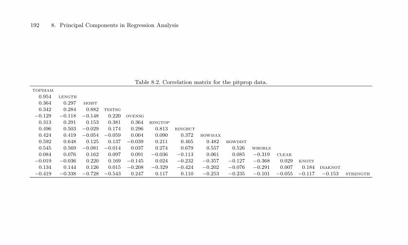
Table 8.2. Correlation matrix for the pitprop data.
topdiam0.954 length0.364 0.297 moist0.342 0.284 0.882 testsg
−0.129 −0.118 −0.148 0.220 ovensg0.313 0.291 0.153 0.381 0.364 ringtop0.496 0.503 −0.029 0.174 0.296 0.813 ringbut0.424 0.419 −0.054 −0.059 0.004 0.090 0.372 bowmax0.592 0.648 0.125 0.137 −0.039 0.211 0.465 0.482 bowdist0.545 0.569 −0.081 −0.014 0.037 0.274 0.679 0.557 0.526 whorls0.084 0.076 0.162 0.097 0.091 −0.036 −0.113 0.061 0.085 −0.319 clear
−0.019 −0.036 0.220 0.169 −0.145 0.024 −0.232 −0.357 −0.127 −0.368 0.029 knots0.134 0.144 0.126 0.015 −0.208 −0.329 −0.424 −0.202 −0.076 −0.291 0.007 0.184 diaknot
−0.419 −0.338 −0.728 −0.543 0.247 0.117 0.110 −0.253 −0.235 −0.101 −0.055 −0.117 −0.153 strength
192 8. Principal Components in Regression Analysis
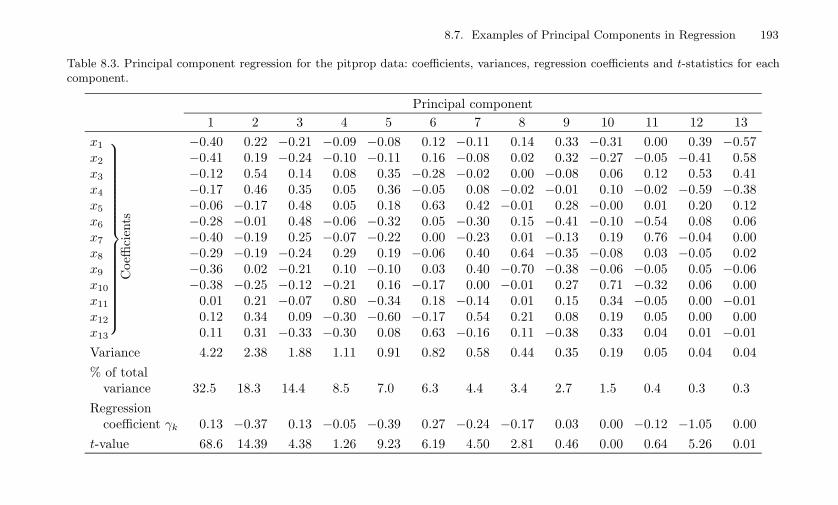
Table 8.3. Principal component regression for the pitprop data: coefficients, variances, regression coefficients and t-statistics for eachcomponent.
Principal component1 2 3 4 5 6 7 8 9 10 11 12 13
x1 −0.40 0.22 −0.21 −0.09 −0.08 0.12 −0.11 0.14 0.33 −0.31 0.00 0.39 −0.57x2 −0.41 0.19 −0.24 −0.10 −0.11 0.16 −0.08 0.02 0.32 −0.27 −0.05 −0.41 0.58x3 −0.12 0.54 0.14 0.08 0.35 −0.28 −0.02 0.00 −0.08 0.06 0.12 0.53 0.41x4 −0.17 0.46 0.35 0.05 0.36 −0.05 0.08 −0.02 −0.01 0.10 −0.02 −0.59 −0.38x5 −0.06 −0.17 0.48 0.05 0.18 0.63 0.42 −0.01 0.28 −0.00 0.01 0.20 0.12x6 −0.28 −0.01 0.48 −0.06 −0.32 0.05 −0.30 0.15 −0.41 −0.10 −0.54 0.08 0.06x7
Coe
ffici
ents
−0.40 −0.19 0.25 −0.07 −0.22 0.00 −0.23 0.01 −0.13 0.19 0.76 −0.04 0.00x8 −0.29 −0.19 −0.24 0.29 0.19 −0.06 0.40 0.64 −0.35 −0.08 0.03 −0.05 0.02x9 −0.36 0.02 −0.21 0.10 −0.10 0.03 0.40 −0.70 −0.38 −0.06 −0.05 0.05 −0.06x10 −0.38 −0.25 −0.12 −0.21 0.16 −0.17 0.00 −0.01 0.27 0.71 −0.32 0.06 0.00x11 0.01 0.21 −0.07 0.80 −0.34 0.18 −0.14 0.01 0.15 0.34 −0.05 0.00 −0.01x12 0.12 0.34 0.09 −0.30 −0.60 −0.17 0.54 0.21 0.08 0.19 0.05 0.00 0.00x13 0.11 0.31 −0.33 −0.30 0.08 0.63 −0.16 0.11 −0.38 0.33 0.04 0.01 −0.01Variance 4.22 2.38 1.88 1.11 0.91 0.82 0.58 0.44 0.35 0.19 0.05 0.04 0.04% of total
variance 32.5 18.3 14.4 8.5 7.0 6.3 4.4 3.4 2.7 1.5 0.4 0.3 0.3Regression
coefficient γk 0.13 −0.37 0.13 −0.05 −0.39 0.27 −0.24 −0.17 0.03 0.00 −0.12 −1.05 0.00t-value 68.6 14.39 4.38 1.26 9.23 6.19 4.50 2.81 0.46 0.00 0.64 5.26 0.01
8.7. Examples of Principal Components in Regression 193

194 8. Principal Components in Regression Analysis
Table 8.4. Variable selection using various techniques on the pitprop data. (Eachrow corresponds to a selected subset with × denoting a selected variable.)
Variables1 2 3 4 5 6 7 8 9 10 11 12 13
Five variablesJeffers (1981) × × × × ×
× × × × ×McCabe (1982) × × × × ×
× × × × ×× × × × ×
× × × × ×Six variablesJeffers (1981) × × × × × ×McCabe (1982) × × × × × ×Jolliffe (1973) × × × × × ×
× × × × × ×× × × × × ×
McCabe (1982)
× × × × × ×Jolliffe (1973) × × × × × ×
Eight variablesMansfield et al. × × × × × × × ×(1977)Boneh and × × × × × × × ×Mendieta (1994)
ble. McCabe (1982), using a technique related to PCA (see Section 6.3),and with a similar purpose to Jolliffe’s (1973) methods, chose subsets ofvarious sizes. McCabe’s subsets in Table 8.4 are the best few with re-spect to a single criterion, whereas Jolliffe gives the single best subset butfor several different methods. The best subsets due to Jolliffe (1973) andMcCabe (1982) have considerable overlap with each other, but there aresubstantial differences from the subsets of Jeffers (1981) and Mansfield etal. (1977). This reflects the different aims of the different selection methods.It shows again that substantial variation within the set of regressor vari-ables does not necessarily imply any relationship with y and, conversely,that variables having little correlation with the first few PCs can still beimportant in predicting y. Interestingly, the subset chosen by Boneh andMendieta (1994) overlaps less with Jeffers’ (1981) selection than that ofMansfield et al. (1977), but more than do those of Jolliffe (1973) or McCabe(1982).

8.7. Examples of Principal Components in Regression 195
Table 8.5. Variables used in the household formation example.
No. Description1. Population in non-private establishments2. Population age 0–143. Population age 15–444. Population age 60/65+5. Females currently married6. Married males 15–297. Persons born ex UK8. Average population increase per annum (not births and deaths)9. Persons moved in previous 12 months
10. Households in owner occupation11. Households renting from Local Authority12. Households renting private unfurnished13. Vacant dwellings14. Shared dwellings15. Households over one person per room16. Households with all exclusive amenities17. Ratio households to rateable units18. Domestic rateable value (£) per head19. Rateable units with rateable value < £10020. Students age 15+21. Economically active married females22. Unemployed males seeking work23. Persons employed in agriculture24. Persons employed in mining and manufacturing25. Males economically active or retired in socio-economic
group 1, 2, 3, 4, 1326. Males economically active or retired in socio-economic
group 5, 6, 8, 9, 12, 1427. With degrees (excluding students with degree)28. Economically active males socio-economic group 3, 429. Average annual total income (£) per adult
8.7.2 Household Formation Data
This example uses part of a data set that arose in a study of householdformation. The subset of data used here has 29 demographic variables mea-sured in 1971 for 168 local government areas in England and Wales. Thevariables are listed in Table 8.5. All variables, except numbers 17, 18 and29, are expressed as numbers per 1000 of population; precise definitions ofeach variable are given in Appendix B of Bassett et al. (1980).

196 8. Principal Components in Regression Analysis
Table 8.6. Eigenvalues of the correlation matrix and order of importance inpredicting y for the household formation data.
PC Eigenvalue Order of PC Eigenvalue Order ofnumber importance number importance
in predicting y in predicting y
1 8.62 1 15 0.24 172 6.09 4 16 0.21 253 3.40 2 17 0.18 164 2.30 8 18 0.14 105 1.19 9 19 0.14 76 1.06 3 20 0.10 217 0.78 13 21 0.10 288 0.69 22 22 0.07 69 0.58 20 23 0.07 1810 0.57 5 24 0.05 1211 0.46 11 25 0.04 1412 0.36 15 26 0.03 2713 0.27 24 27 0.02 1914 0.25 23 28 0.003 26
Although this was not the purpose of the original project, the objectiveconsidered here is to predict the final variable (average annual total incomeper adult) from the other 28. This objective is a useful one, as informationon income is often difficult to obtain accurately, and predictions from other,more readily available, variables would be valuable. The results presentedbelow were given by Garnham (1979) in an unpublished M.Sc. disserta-tion, and further details of the regression analysis can be found in thatsource. A full description of the project from which the data are taken isavailable in Bassett et al. (1980). Most regression problems with as manyas 28 regressor variables have multicollinearities, and the current exampleis no exception. Looking at the list of variables in Table 8.5 it is clear,even without detailed definitions, that there are groups of variables thatare likely to be highly correlated. For example, several variables relate totype of household, whereas another group of variables considers rates ofemployment in various types of job. Table 8.6, giving the eigenvalues of thecorrelation matrix, confirms that there are multicollinearities; some of theeigenvalues are very small.
Consider now PC regression and some of the strategies that can be usedto select a subset of PCs to be included in the regression. Deleting compo-nents with small variance, with a cut-off of about l∗ = 0.10, implies thatbetween seven and nine components can be left out. Sequential deletionof PCs with the smallest variances using t-statistics at each stage suggeststhat only six PCs can be deleted. However, from the point of view of R2,the squared multiple correlation coefficient, deletion of eight or more might

8.7. Examples of Principal Components in Regression 197
be acceptable; R2 is 0.874 for the full model including all 28 variables, andit is reduced to 0.865, 0.851, respectively, when five and eight componentsare deleted.
It is interesting to examine the ordering of size of correlations between yand the PCs, or equivalently the ordering of the individual t-values, whichis also given in Table 8.6. It is seen that those PCs with small variances donot necessarily have small correlations with y. The 18th, 19th and 22nd insize of variance are in the first ten in order of importance for predicting y; inparticular, the 22nd PC with variance 0.07, has a highly significant t-value,and should almost certainly be retained.
An approach using stepwise deletion based solely on the size of corre-lation between y and each PC produces, because of the zero correlationsbetween PCs, the subset whose value of R2 is maximized for any givensubset size. Far fewer PCs need to be retained using this approach thanthe 20 to 23 indicated when only small-variance components are rejected.In particular, if the 10 PCs are retained that best predict y, then R2 is0.848, compared with 0.874 for the full model and 0.851 using the first 20PCs. It would appear that a strategy based solely on size of variance isunsatisfactory.
The two ‘weak MSE’ criteria described in Section 8.2 were also tested, ina limited way, on these data. Because of computational constraints it wasnot possible to find the overall ‘best’ subset M , so a stepwise approach wasadopted, deleting PCs according to either size of variance, or correlationwith y. The first criterion selected 22 PCs when selection was based onsize of variance, but only 6 PCs when correlation with y was the basis forstepwise selection. The corresponding results for the second (predictive)criterion were 24 and 12 PCs, respectively. It is clear, once again, thatselection based solely on order of size of variance retains more componentsthan necessary but may still miss predictive components.
The alternative approach of Lott (1973) was also investigated for thesedata in a stepwise manner using correlation with y to determine order ofselection, with the result that R2 was maximized for 19 PCs. This is asubstantially larger number than indicated by those other methods thatuse correlation with y to define order of selection and, given the concensusfrom the other methods, suggests that Lott’s (1973) method is not ideal.
When PCs are found for the augmented set of variables, including y andall the regressor variables, as required for latent root regression, there isremarkably little change in the PCs, apart from the addition of an extra one.All of the coefficients on the regressor variables are virtually unchanged,and the PCs that have largest correlation with y are in very nearly thesame order as in the PC regression.
It may be of more interest to select a subset of variables, rather than asubset of PCs, to be included in the regression, and this was also attempted,using various methods, for the household formation data. Variable selec-tion based on PC regression, deleting just one variable at a time before

198 8. Principal Components in Regression Analysis
recomputing the PCs as suggested by Mansfield et al. (1977), indicatedthat only 12, and possibly fewer, variables need to be retained. R2 for the12-variable subset given by this method is 0.862, and it only drops to 0.847for the 8-variable subset, compared with 0.874 for the full model and 0.851using the first 20 PCs in the regression. Other variable selection methods,described by Jolliffe (1972) and in Section 6.3, were also tried, but these didnot produce quite such good results as the Mansfield et al. (1977) method.This is not surprising since, as noted in the previous example, they are notspecifically tailored for variable selection in the context of regression. How-ever, they did confirm that only eight to ten variables are really necessaryin order to provide an adequate prediction of ‘income’ for these data.

9Principal Components Used withOther Multivariate Techniques
Principal component analysis is often used as a dimension-reducing tech-nique within some other type of analysis. For example, Chapter 8 describedthe use of PCs as regressor variables in a multiple regression analysis. Thepresent chapter discusses three classes of multivariate techniques, namelydiscriminant analysis, cluster analysis and canonical correlation analysis;for each these three there are examples in the literature that use PCA asa dimension-reducing technique.
Discriminant analysis is concerned with data in which each observationcomes from one of several well-defined groups or populations. Assumptionsare made about the structure of the populations, and the main objectiveis to construct rules for assigning future observations to one of the popula-tions so as to minimize the probability of misclassification or some similarcriterion. As with regression, there can be advantages in replacing the vari-ables in a discriminant analysis by their principal components. The useof PCA in this way in linear discriminant analysis is discussed in Section9.1. In addition, the section includes brief descriptions of other discrimi-nant techniques that use PCs, and discussion of links between PCA andcanonical discriminant analysis.
Cluster analysis is one of the most frequent contexts in which PCs arederived in order to reduce dimensionality prior to the use of a differentmultivariate technique. Like discriminant analysis, cluster analysis dealswith data sets in which the observations are to be divided into groups.However, in cluster analysis little or nothing is known a priori about thegroups, and the objective is to divide the given observations into groups orclusters in a ‘sensible’ way. There are two main ways in which PCs are em-

200 9. Principal Components Used with Other Multivariate Techniques
ployed within cluster analysis: to construct distance measures or to providea graphical representation of the data; the latter is often called ordinationor scaling (see also Section 5.1) and is useful in detecting or verifying acluster structure. Both roles are described and illustrated with examplesin Section 9.2. The idea of clustering variables rather than observationsis sometimes useful, and a connection between PCA and this idea is de-scribed. Also discussed in Section 9.2 are projection pursuit, which searchesfor clusters using techniques bearing some resemblance to PCA, and theconstruction of models for clusters which are mixtures of the PC modelintroduced in Section 3.9.
‘Discriminant analysis’ and ‘cluster analysis’ are standard statisticalterms, but the techniques may be encountered under a variety of othernames. For example, the word ‘classification’ is sometimes used in a broadsense, including both discrimination and clustering, but it also has morethan one specialized meaning. Discriminant analysis and cluster analysisare prominent in both the pattern recognition and neural network liter-atures, where they fall within the areas of supervised and unsupervisedlearning, respectively (see, for example, Bishop (1995)). The relatively new,but large, field of data mining (Hand et al. 2001; Witten and Frank, 2000)also includes ‘clustering methods. . . [and] supervised classification methodsin general. . . ’ (Hand, 1998).
The third, and final, multivariate technique discussed in this chapter, inSection 9.3, is canonical correlation analysis. This technique is appropriatewhen the vector of random variables x is divided into two parts, xp1 ,xp2 ,and the objective is to find pairs of linear functions of xp1 and xp2 , respec-tively, such that the correlation between the linear functions within eachpair is maximized. In this case the replacement of xp1 , xp2 by some or allof the PCs of xp1 , xp2 , respectively, has been suggested in the literature. Anumber of other techniques linked to PCA that are used to investigate rela-tionships between two groups of variables are also discussed in Section 9.3.Situations where more than two groups of variables are to be analysed areleft to Section 14.5.
9.1 Discriminant Analysis
In discriminant analysis, observations may be taken from any of G ≥ 2 pop-ulations or groups. Assumptions are made regarding the structure of thesegroups, namely that the random vector x associated with each observa-tion is assumed to have a particular (partly or fully specified) distributiondepending on its group membership. Information may also be availableabout the overall relative frequencies of occurrence of each group. In ad-dition, there is usually available a set of data x1,x2, . . . ,xn (the trainingset) for which the group membership of each observation is known. Based

9.1. Discriminant Analysis 201
on the assumptions about group structure and on the training set if oneis available, rules are constructed for assigning future observations to oneof the G groups in some ‘optimal’ way, for example, so as to minimize theprobability or cost of misclassification.
The best-known form of discriminant analysis occurs when there are onlytwo populations, and x is assumed to have a multivariate normal distribu-tion that differs between the two populations with respect to its mean butnot its covariance matrix. If the means µ1, µ2 and the common covariancematrix Σ are known, then the optimal rule (according to several differentcriteria) is based on the linear discriminant function x′Σ−1(µ1−µ2). If µ1,µ2, Σ are estimated from a ‘training set’ by x1, x2, Sw, respectively, then arule based on the sample linear discriminant function x′S−1
w (x1−x2) is oftenused. There are many other varieties of discriminant analysis (McLach-lan, 1992), depending on the assumptions made regarding the populationstructure, and much research has been done, for example, on discriminantanalysis for discrete data and on non-parametric approaches (Goldsteinand Dillon, 1978; Hand, 1982).
The most obvious way of using PCA in a discriminant analysis is toreduce the dimensionality of the analysis by replacing x by the first m(high variance) PCs in the derivation of a discriminant rule. If the first twoPCs account for a high proportion of the variance, they can also be usedto provide a two-dimensional graphical representation of the data showinghow good, or otherwise, the separation is between the groups.
The first point to be clarified is exactly what is meant by the PCs ofx in the context of discriminant analysis. A common assumption in manyforms of discriminant analysis is that the covariance matrix is the samefor all groups, and the PCA may therefore be done on an estimate of thiscommon within-group covariance (or correlation) matrix. Unfortunately,this procedure may be unsatisfactory for two reasons. First, the within-group covariance matrix may be different for different groups. Methods forcomparing PCs from different groups are discussed in Section 13.5, and laterin the present section we describe techniques that use PCs to discriminatebetween populations when equal covariance matrices are not assumed. Forthe moment, however, we make the equal covariance assumption.
The second, more serious, problem encountered in using PCs based on acommon within-group covariance matrix to discriminate between groups isthat there is no guarantee that the separation between groups will be in thedirection of the high-variance PCs. This point is illustrated diagramaticallyin Figures 9.1 and 9.2 for two variables. In both figures the two groups arewell separated, but in the first the separation is in the direction of the firstPC (that is parallel to the major axis of within-group variation), whereas inthe second the separation is orthogonal to this direction. Thus, the first fewPCs will only be useful for discriminating between groups in the case wherewithin- and between-group variation have the same dominant directions. Ifthis does not occur (and in general there is no particular reason for it to
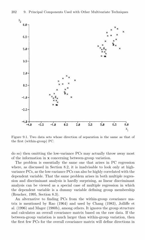
202 9. Principal Components Used with Other Multivariate Techniques
Figure 9.1. Two data sets whose direction of separation is the same as that ofthe first (within-group) PC.
do so) then omitting the low-variance PCs may actually throw away mostof the information in x concerning between-group variation.
The problem is essentially the same one that arises in PC regressionwhere, as discussed in Section 8.2, it is inadvisable to look only at high-variance PCs, as the low-variance PCs can also be highly correlated with thedependent variable. That the same problem arises in both multiple regres-sion and discriminant analysis is hardly surprising, as linear discriminantanalysis can be viewed as a special case of multiple regression in whichthe dependent variable is a dummy variable defining group membership(Rencher, 1995, Section 8.3).
An alternative to finding PCs from the within-group covariance ma-trix is mentioned by Rao (1964) and used by Chang (1983), Jolliffe etal. (1996) and Mager (1980b), among others. It ignores the group structureand calculates an overall covariance matrix based on the raw data. If thebetween-group variation is much larger than within-group variation, thenthe first few PCs for the overall covariance matrix will define directions in

9.1. Discriminant Analysis 203
Figure 9.2. Two data sets whose direction of separation is orthogonal to that ofthe first (within-group) PC.
which there are large between-group differences. Such PCs therefore seemmore useful than those based on within-group covariance matrices, but thetechnique should be used with some caution, as it will work well only ifbetween-group variation dominates within-group variation.
It is well known that, for two completely specified normal populations,differing only in mean, the probability of misclassification using the lineardiscriminant function is a monotonically decreasing function of the squaredMahalanobis distance ∆2 between the two populations (Rencher, 1998,Section 6.4). Here ∆2 is defined as
∆2 = (µ1 − µ2)′Σ−1(µ − µ2). (9.1.1)
Note that we meet a number of other varieties of Mahalanobis distance else-where in the book. In equation (5.3.5) of Section 5.3, Mahalanobis distancebetween two observations in a sample is defined, and there is an obvious sim-ilarity between (5.3.5) and the definition given in (9.1.1) for Mahalanobisdistance between two populations. Further modifications define Mahalanobis
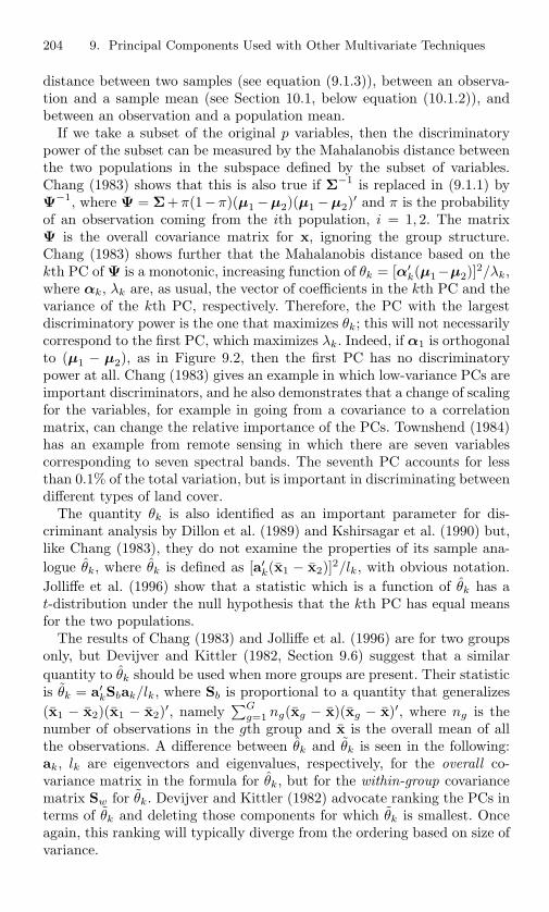
204 9. Principal Components Used with Other Multivariate Techniques
distance between two samples (see equation (9.1.3)), between an observa-tion and a sample mean (see Section 10.1, below equation (10.1.2)), andbetween an observation and a population mean.
If we take a subset of the original p variables, then the discriminatorypower of the subset can be measured by the Mahalanobis distance betweenthe two populations in the subspace defined by the subset of variables.Chang (1983) shows that this is also true if Σ−1 is replaced in (9.1.1) byΨ−1, where Ψ = Σ+π(1−π)(µ1 −µ2)(µ1 −µ2)′ and π is the probabilityof an observation coming from the ith population, i = 1, 2. The matrixΨ is the overall covariance matrix for x, ignoring the group structure.Chang (1983) shows further that the Mahalanobis distance based on thekth PC of Ψ is a monotonic, increasing function of θk = [α′
k(µ1−µ2)]2/λk,where αk, λk are, as usual, the vector of coefficients in the kth PC and thevariance of the kth PC, respectively. Therefore, the PC with the largestdiscriminatory power is the one that maximizes θk; this will not necessarilycorrespond to the first PC, which maximizes λk. Indeed, if α1 is orthogonalto (µ1 − µ2), as in Figure 9.2, then the first PC has no discriminatorypower at all. Chang (1983) gives an example in which low-variance PCs areimportant discriminators, and he also demonstrates that a change of scalingfor the variables, for example in going from a covariance to a correlationmatrix, can change the relative importance of the PCs. Townshend (1984)has an example from remote sensing in which there are seven variablescorresponding to seven spectral bands. The seventh PC accounts for lessthan 0.1% of the total variation, but is important in discriminating betweendifferent types of land cover.
The quantity θk is also identified as an important parameter for dis-criminant analysis by Dillon et al. (1989) and Kshirsagar et al. (1990) but,like Chang (1983), they do not examine the properties of its sample ana-logue θk, where θk is defined as [a′
k(x1 − x2)]2/lk, with obvious notation.Jolliffe et al. (1996) show that a statistic which is a function of θk has at-distribution under the null hypothesis that the kth PC has equal meansfor the two populations.
The results of Chang (1983) and Jolliffe et al. (1996) are for two groupsonly, but Devijver and Kittler (1982, Section 9.6) suggest that a similarquantity to θk should be used when more groups are present. Their statisticis θk = a′
kSbak/lk, where Sb is proportional to a quantity that generalizes(x1 − x2)(x1 − x2)′, namely
∑Gg=1 ng(xg − x)(xg − x)′, where ng is the
number of observations in the gth group and x is the overall mean of allthe observations. A difference between θk and θk is seen in the following:ak, lk are eigenvectors and eigenvalues, respectively, for the overall co-variance matrix in the formula for θk, but for the within-group covariancematrix Sw for θk. Devijver and Kittler (1982) advocate ranking the PCs interms of θk and deleting those components for which θk is smallest. Onceagain, this ranking will typically diverge from the ordering based on size ofvariance.

9.1. Discriminant Analysis 205
Corbitt and Ganesalingam (2001) also examine an extension to morethan two groups based on the ideas of Dillon et al. (1989), but most of theirpaper consists of case studies in which only two groups are present. Corbittand Ganesalingam (2001) show that a two-group version of their interpreta-tion of Dillon et al.’s methodology is inferior to Jolliffe et al.’s (1996) t-testswith respect to correct classification. However, both are beaten in severalof the examples studied by selecting a subset of the original variables.
Friedman (1989) demonstrates that a quantity similar to θk is also rel-evant in the case where the within-group covariance matrices are notnecessarily equal. In these circumstances a discriminant score is formedfor each group, and an important part of that score is a term correspond-ing to θk, with lk, ak replaced by the eigenvalues and eigenvectors of thecovariance matrix for that group. Friedman (1989) notes that sample esti-mates of large eigenvalues are biased upwards, whereas estimates of smalleigenvalues are biased downwards and, because the reciprocals of the eigen-values appear in the discriminant scores, this can lead to an exaggeratedinfluence of the low-variance PCs in the discrimination. To overcome this,he proposes a form of ‘regularized’ discriminant analysis in which samplecovariance matrices for each group are shrunk towards the pooled estimateSw. This has the effect of decreasing large eigenvalues and increasing smallones.
We return to regularized discriminant analysis later in this section, butwe first note that Takemura (1985) also describes a bias in estimating eigen-values in the context of one- and two-sample tests for multivariate normalmeans, based on Hotelling T 2. For two groups, the question of whether ornot it is worth calculating a discriminant function reduces to testing thenull hypothesis H0 : µ1 = µ2. This is often done using Hotelling’s T 2.Lauter (1996) suggests a statistic based on a subset of the PCs of the over-all covariance matrix. He concentrates on the case where only the first PCis used, for which one-sided, as well as global, alternatives to H0 may beconsidered.
Takemura (1985) proposes a decomposition of T 2 into contributionsdue to individual PCs. In the two-sample case this is equivalent to cal-culating t-statistics to decide which PCs discriminate between the groupscorresponding to the samples, although in Takemura’s case the PCs arecalculated from the within-group, rather than overall, covariance matrix.Takemura (1985) suggests that later PCs might be deemed significant,and hence selected, too often. However, Jolliffe et al. (1996) dispel theseworries for their tests by conducting a simulation study which shows notendency for over-selection of the low-variance PCs in the null case, andwhich also gives indications of the power of the t-test when the null hypoth-esis of equal means in the two populations is false. Interestingly, Mason andGunst (1985) noted bias in the opposite direction in PC regression, namelythat low-variance PCs are selected less, rather than more, often than thehigh-variance components. Given the links between regression and discrim-
206 9. Principal Components Used with Other Multivariate Techniques
ination, it may be that the opposite effects described by Mason and Gunst(1985) and by Takemura (1985) roughly balance in the case of using PCsin discriminant analysis.
The fact that separation between populations may be in the directionsof the last few PCs does not mean that PCs should not be used at all indiscriminant analysis. They can still provide a reduction of dimensionalityand, as in regression, their uncorrelatedness implies that in linear discrim-inant analysis each PC’s contribution can be assessed independently. Thisis an advantage compared to using the original variables x, where the con-tribution of one of the variables depends on which other variables are alsoincluded in the analysis, unless all elements of x are uncorrelated. The mainpoint to bear in mind when using PCs in discriminant analysis is that thebest subset of PCs does not necessarily simply consist of those with thelargest variances. It is easy to see, because of their uncorrelatedness, whichof the PCs are best at discriminating between the populations. However,as in regression, some caution is advisable in using PCs with very low vari-ances, because at least some of the estimated coefficients in the discriminantfunction will have large variances if low variance PCs are included. Manyof the comments made in Section 8.2 regarding strategies for selecting PCsin regression are also relevant in linear discriminant analysis.
Some of the approaches discussed so far have used PCs from the over-all covariance matrix, whilst others are based on the pooled within-groupcovariance matrix. This latter approach is valid for types of discriminantanalysis in which the covariance structure is assumed to be the same forall populations. However, it is not always realistic to make this assump-tion, in which case some form of non-linear discriminant analysis may benecessary. If the multivariate normality assumption is kept, the most usualapproach is quadratic discrimination (Rencher, 1998, Section 6.2.2). Withan assumption of multivariate normality and G groups with sample meansand covariance matrices xg,Sg, g = 1, 2, . . . , G, the usual discriminant ruleassigns a new vector of observations x to the group for which
(x − xg)′S−1g (x − xg) + ln(|Sg|) (9.1.2)
is minimized. When the equal covariance assumption is made, Sg is replacedby the pooled covariance matrix Sw in (9.1.2), and only the linear part ofthe expression is different for different groups. In the general case, (9.1.2) isa genuine quadratic function of x, leading to quadratic discriminant anal-ysis. Flury (1995) suggests two other procedures based on his commonprincipal component (CPC) framework, whose assumptions are interme-diate compared to those of linear and quadratic discrimination. Furtherdetails will be given when the CPC framework is discussed in Section 13.5.
Alternatively, the convenience of looking only at linear functions of xcan be kept by computing PCs separately for each population. In a num-ber of papers (see, for example, Wold, 1976; Wold et al., 1983), Wold andothers have described a method for discriminating between populations
9.1. Discriminant Analysis 207
that adopts this approach. The method, called SIMCA (Soft IndependentModelling of Class Analogy), does a separate PCA for each group, andretains sufficient PCs in each to account for most of the variation withinthat group. The number of PCs retained will typically be different for dif-ferent populations. The square of this distance for a particular populationis simply the sum of squares of the values of the omitted PCs for that pop-ulation, evaluated for the observation in question (Mertens, et al., 1994).The same type of quantity is also used for detecting outliers (see Section10.1, equation (10.1.1)).
To classify a new observation, a ‘distance’ of the observation from thehyperplane defined by the retained PCs is calculated for each population.If future observations are to be assigned to one and only one population,then assignment is to the population from which the distance is minimized.Alternatively, a firm decision may not be required and, if all the distancesare large enough, the observation can be left unassigned. As it is not closeto any of the existing groups, it may be an outlier or come from a newgroup about which there is currently no information. Conversely, if thegroups are not all well separated, some future observations may have smalldistances from more than one population. In such cases, it may again beundesirable to decide on a single possible class; instead two or more groupsmay be listed as possible ‘homes’ for the observation.
According to Wold et al. (1983), SIMCA works with as few as five ob-jects from each population, although ten or more is preferable, and thereis no restriction on the number of variables. This is important in manychemical problems where the number of variables can greatly exceed thenumber of observations. SIMCA can also cope with situations where oneclass is very diffuse, simply consisting of all observations that do not be-long in one of a number of well-defined classes. Frank and Freidman (1989)paint a less favourable picture of SIMCA. They use a number of datasets and a simulation study to compare its performance with that of linearand quadratic discriminant analyses, with regularized discriminant analysisand with a technique called DASCO (discriminant analysis with shrunkencovariances).
As already explained, Friedman’s (1989) regularized discriminant analy-sis shrinks the individual within-group covariance matrices Sg towards thepooled estimate Sw in an attempt to reduce the bias in estimating eigen-values. DASCO has a similar objective, and Frank and Freidman (1989)show that SIMCA also has a similar effect. They note that in terms ofexpression (9.1.2), SIMCA ignores the log-determinant term and replacesS−1
g by a weighted and truncated version of its spectral decomposition,which in its full form is S−1
g =∑p
k=1 l−1gk agka′
gk, with fairly obvious nota-tion. If qg PCs are retained in the gth group, then SIMCA’s replacement
for S−1g is
∑pk=qg+1 l−1
g agka′gk, where lg =
∑p
k=qg+1lgk
(p−qg) . DASCO treats thelast (p− qg) PCs in the same way as SIMCA, but adds the terms from the

208 9. Principal Components Used with Other Multivariate Techniques
spectral decomposition corresponding to the first qg PCs. Thus it replacesS−1
g in (9.1.2) by
qg∑
k=1
l−1gk agka′
gk +p∑
k=qg+1
l−1g agka′
gk.
Another difference between DASCO and SIMCA is that DASCO retainsthe log-determinant term in (9.1.2).
In Frank and Freidman’s (1989) simulation studies and data analyses,SIMCA is outperformed by both DASCO and regularized discriminantanalysis in many circumstances, especially when the covariance structuresare different in different groups. This is perhaps not surprising, given itsomission of the log-determinant term from (9.1.2). The absence of the firstqg PCs from SIMCA’s measure of discrepancy of an observation from agroup also means that it is unlikely to do well when the groups differin the directions of these PCs (Mertens et al., 1994). These latter authorstreat SIMCA’s measure of discrepancy between an observation and a groupas an indication of the outlyingness of the observation with respect to thegroup, and suggest modifications of SIMCA in which other outlier detectionmeasures are used (see Section 10.1).
A similar idea to SIMCA is suggested by Asselin de Beauville (1995).As with SIMCA, separate PCAs are done for each group, but here anobservation is assigned on the basis of a measure that combines the smallestdistance of the observation from an axis defining a PC for a group and itsscore on that PC.
It has been noted above that discriminant analysis can be treated as amultiple regression problem, with dummy variables, corresponding to thegroup membership, as dependent variables. Other regression techniques,as well as PC regression, can therefore be adapted for the discriminantproblem. In particular, partial least squares (PLS — see Section 8.4), whichis, in a sense, a compromise between least squares and PC regression, canbe used in the discriminant context (Vong et al. (1990)).
SIMCA calculates PCs separately within each group, compared with themore usual practice of finding PCs from the overall covariance matrix, orfrom a pooled within-group covariance matrix. Yet another type of PCcan be derived from the between-group covariance matrix Sb. However,if the dominant direction of Sb coincides with that of the within-groupcovariance matrix Sw, there may be better discriminatory power in a dif-ferent direction, corresponding to a low-variance direction for Sw. Thisleads Devijver and Kittler (1982, Section 9.7) to ‘prewhiten’ the data,using Sw, before finding PCs with respect to Sb. This is equivalent tothe well-known procedure of canonical variate analysis or canonical dis-criminant analysis, in which uncorrelated linear functions are found thatdiscriminate as well as possible between the groups. Canonical variates aredefined as γ′
1x, γ′2x, . . . ,γ′
g−1x where γ′kx maximizes the ratio γ′Sbγ
γ′Swγ , of

9.1. Discriminant Analysis 209
between- to within-group variance of γ′x, subject to being uncorrelatedwith γ′
1x, γ′2x, . . . ,γ′
k−1x. For more details see, for example, McLachlan(1992, Section 9.2) or Mardia et al. (1979, Section 12.5).
A variation on prewhitening using Sw is to ‘standardize’ Sb by dividingeach variable by its within-group standard deviation and then calculate abetween-group covariance matrix S∗
b from these rescaled variables. FindingPCs based on S∗
b is called discriminant principal components analysis byYendle and MacFie (1989). They compare the results of this analysis withthose from a PCA based on Sb and also with canonical discriminant analysisin which the variables x are replaced by their PCs. In two examples, Yendleand MacFie (1989) find, with respect to misclassification probabilities, theperformance of PCA based on S∗
b to be superior to that based on Sb, andcomparable to that of canonical discriminant analysis using PCs. However,in the latter analysis only the restrictive special case is examined, in whichthe first q PCs are retained. It is also not made explicit whether the PCsused are obtained from the overall covariance matrix S or from Sw, thoughit seems likely that S is used.
To conclude this section, we note some relationships between PCA andcanonical discriminant analysis, via principal coordinate analysis (see Sec-tion 5.2), which are described by Gower (1966). Suppose that a principalcoordinate analysis is done on a distance matrix whose elements are Ma-halanobis distances between the samples from the G populations. Thesedistances are defined as the square roots of
δ2hi = (xh − xi)′S−1
w (xh − xi); h, i = 1, 2, . . . , G. (9.1.3)
Gower (1966) then shows that the configuration found in m(< G) di-mensions is the same as that provided by the first m canonical variatesfrom canonical discriminant analysis. Furthermore, the same results maybe found from a PCA with X′X replaced by (XW)′(XW), where WW′ =S−1
w and X is the (G × p) matrix whose hth row gives the sample meansof the p variables for the hth population, h = 1, 2, . . . , G. Yet another, re-lated, way of finding canonical variates is via a two-stage PCA, as describedby Campbell and Atchley (1981). At the first stage PCs are found, basedon the within-group covariance matrix Sw, and standardized to have unitvariance. The values of the means of these standardised PCs for each of theG groups are then subjected to a weighted PCA (see Section 14.2.1), withweights proportional to the sample sizes ni in each group. The PC scoresat this second stage are the values of the group means with respect to thecanonical variates. Krzanowski (1990) generalizes canonical discriminantanalysis, based on the common PCA model due to Flury (1988), using thistwo-stage derivation. Bensmail and Celeux (1996) also describe an approachto discriminant analysis based on the common PCA framework; this willbe discussed further in Section 13.5. Campbell and Atchley (1981) note thepossibility of an alternative analysis, different from canonical discriminantanalysis, in which the PCA at the second of their two stages is unweighted.

210 9. Principal Components Used with Other Multivariate Techniques
Because of the connections between PCs and canonical variates, Mardia etal. (1979, p. 344) refer to canonical discriminant analysis as the analoguefor grouped data of PCA for ungrouped data. Note also that with an ap-propriate choice of metric, generalized PCA as defined in Section 14.2.2 isequivalent to a form of discriminant analysis.
No examples have been given in detail in this section, although some havebeen mentioned briefly. An interesting example, in which the objective isto discriminate between different carrot cultivars, is presented by Horganet al. (2001). Two types of data are available, namely the positions of‘landmarks’ on the outlines of the carrots and the brightness of each pixelin a cross-section of each carrot. The two data sets are subjected to separatePCAs, and a subset of PCs taken from both analyses is used to constructa discriminant function.
9.2 Cluster Analysis
In cluster analysis, it is required to divide a set of observations into groupsor clusters in such a way that most pairs of observations that are placed inthe same group are more similar to each other than are pairs of observationsthat are placed into two different clusters. In some circumstances, it maybe expected or hoped that there is a clear-cut group structure underlyingthe data, so that each observation comes from one of several distinct popu-lations, as in discriminant analysis. The objective then is to determine thisgroup structure where, in contrast to discriminant analysis, there is little orno prior information about the form that the structure takes. Cluster anal-ysis can also be useful when there is no clear group structure in the data.In this case, it may still be desirable to segment or dissect (using the ter-minology of Kendall (1966)) the observations into relatively homogeneousgroups, as observations within the same group may be sufficiently similarto be treated identically for the purpose of some further analysis, whereasthis would be impossible for the whole heterogeneous data set. There arevery many possible methods of cluster analysis, and several books haveappeared on the subject, for example Aldenderfer and Blashfield (1984),Everitt et al. (2001), Gordon (1999). Most methods can be used eitherfor detection of clear-cut groups or for dissection/segmentation, althoughthere is increasing interest in mixture models, which explicitly assume theexistence of clusters (see Section 9.2.3).
The majority of cluster analysis techniques require a measure of sim-ilarity or dissimilarity between each pair of observations, and PCs havebeen used quite extensively in the computation of one type of dissimilarity.If the p variables that are measured for each observation are quantitativeand in similar units, then an obvious measure of dissimilarity between twoobservations is the Euclidean distance between the observations in the p-

9.2. Cluster Analysis 211
dimensional space defined by the variables. If the variables are measuredin non-compatible units, then each variable can be standardized by divid-ing by its standard deviation, and an arbitrary, but obvious, measure ofdissimilarity is then the Euclidean distance between a pair of observationsin the p-dimensional space defined by the standardized variables.
Suppose that a PCA is done based on the covariance or correlation ma-trix, and that m (< p) PCs account for most of the variation in x. A possiblealternative dissimilarity measure is the Euclidean distance between a pairof observations in the m-dimensional subspace defined by the first m PCs;such dissimilarity measures have been used in several published studies, forexample Jolliffe et al. (1980). There is often no real advantage in using thismeasure, rather than the Euclidean distance in the original p-dimensionalspace, as the Euclidean distance calculated using all p PCs from the co-variance matrix is identical to that calculated from the original variables.Similarly, the distance calculated from all p PCs for the correlation matrixis the same as that calculated from the p standardized variables. Using minstead of p PCs simply provides an approximation to the original Euclideandistance, and the extra calculation involved in finding the PCs far outweighsany saving which results from using m instead of p variables in computingthe distance. However, if, as in Jolliffe et al. (1980), the PCs are being cal-culated in any case, the reduction from p to m variables may be worthwhile.
In calculating Euclidean distances, the PCs have the usual normalization,so that the sample variance of a′
kx is lk, k = 1, 2, . . . , p and l1 ≥ l2 ≥ · · · ≥lp, using the notation of Section 3.1. As an alternative, a distance can becalculated based on PCs that have been renormalized so that each PChas the same variance. This renormalization is discussed further in thecontext of outlier detection in Section 10.1. In the present setting, wherethe objective is the calculation of a dissimilarity measure, its use is basedon the following idea. Suppose that one of the original variables is almostindependent of all the others, but that several of the remaining variables aremeasuring essentially the same property as each other. Euclidean distancewill then give more weight to this property than to the property describedby the ‘independent’ variable. If it is thought desirable to give equal weightto each property then this can be achieved by finding the PCs and thengiving equal weight to each of the first m PCs.
To see that this works, consider a simple example in which four meteo-rological variables are measured. Three of the variables are temperatures,namely air temperature, sea surface temperature and dewpoint, and thefourth is the height of the cloudbase. The first three variables are highlycorrelated with each other, but nearly independent of the fourth. For asample of 30 measurements on these variables, a PCA based on the corre-lation matrix gave a first PC with variance 2.95, which is a nearly equallyweighted average of the three temperature variables. The second PC, withvariance 0.99 is dominated by cloudbase height, and together the first twoPCs account for 98.5% of the total variation in the four variables.

212 9. Principal Components Used with Other Multivariate Techniques
Euclidean distance based on the first two PCs gives a very close ap-proximation to Euclidean distance based on all four variables, but it givesroughly three times as much weight to the first PC as to the second. Al-ternatively, if the first two PCs are renormalized to have equal weight, thisimplies that we are treating the one measurement of cloudbase height asbeing equal in importance to the three measurements of temperature.
In general, if Euclidean distance is calculated using all p renormalizedPCs, then this is equivalent to calculating the Mahalanobis distance for theoriginal variables (see Section 10.1, below equation (10.1.2), for a proof ofthe corresponding property for Mahalanobis distances of observations fromsample means, rather than between pairs of observations). Mahalanobisdistance is yet another plausible dissimilarity measure, which takes intoaccount the variances and covariances between the elements of x. Naes andIsaksson (1991) give an example of (fuzzy) clustering in which the distancemeasure is based on Mahalanobis distance, but is truncated to exclude thelast few PCs when the variances of these are small and unstable.
Regardless of the similarity or dissimilarity measure adopted, PCA hasa further use in cluster analysis, namely to give a two-dimensional repre-sentation of the observations (see also Section 5.1). Such a two-dimensionalrepresentation can give a simple visual means of either detecting or verify-ing the existence of clusters, as noted by Rao (1964), provided that most ofthe variation, and in particular the between-cluster variation, falls in thetwo-dimensional subspace defined by the first two PCs.
Of course, the same problem can arise as in discriminant analysis, namelythat the between-cluster variation may be in directions other than those ofthe first two PCs, even if these two PCs account for nearly all of the totalvariation. However, this behaviour is generally less likely in cluster analysis,as the PCs are calculated for the whole data set, not within-groups. Aspointed out in Section 9.1, if between-cluster variation is much greater thanwithin-cluster variation, such PCs will often successfully reflect the clusterstructure. It is, in any case, frequently impossible to calculate within-groupPCs in cluster analysis as the group structure is usually unknown a priori.
It can be argued that there are often better directions than PCs inwhich to view the data in order to ‘see’ structure such as clusters. Pro-jection pursuit includes a number of ideas for finding such directions, andwill be discussed in Section 9.2.2. However, the examples discussed belowillustrate that plots with respect to the first two PCs can give suitabletwo-dimensional representations on which to view the cluster structure ifa clear structure exists. Furthermore, in the case where there is no clearstructure, but it is required to dissect the data using cluster analysis, therecan be no real objection to the use of a plot with respect to the first twoPCs. If we wish to view the data in two dimensions in order to see whethera set of clusters given by some procedure ‘looks sensible,’ then the first twoPCs give the best possible representation in two dimensions in the sensedefined by Property G3 of Section 3.2.

9.2. Cluster Analysis 213
Before looking at examples of the uses just described of PCA in clusteranalysis, we discuss a rather different way in which cluster analysis canbe used and its connections with PCA. So far we have discussed clusteranalysis on observations or individuals, but in some circumstances it isdesirable to divide variables, rather than observations, into groups. In fact,by far the earliest book on cluster analysis (Tryon, 1939) was concernedwith this type of application. Provided that a suitable measure of similaritybetween variables can be defined—the correlation coefficient is an obviouscandidate—methods of cluster analysis used for observations can be readilyadapted for variables.
One connection with PCA is that when the variables fall into well-definedclusters, then, as discussed in Section 3.8, there will be one high-variancePC and, except in the case of ‘single-variable’ clusters, one or more low-variance PCs associated with each cluster of variables. Thus, PCA willidentify the presence of clusters among the variables, and can be thoughtof as a competitor to standard cluster analysis of variables. The use ofPCA in this way in fairly common in climatology (see, for example, Cohen(1983), White et al. (1991), Romero et al. (1999)). In an analysis of aclimate variable recorded at stations over a large geographical area, theloadings of the PCs at the various stations can be used to divide the areainto regions with high loadings on each PC. In fact, this regionalizationprocedure is usually more effective if the PCs are rotated (see Section 11.1)so that most analyses are done using rotated loadings.
Identifying clusters of variables may be of general interest in investigatingthe structure of a data set but, more specifically, if we wish to reducethe number of variables without sacrificing too much information, then wecould retain one variable from each cluster. This is essentially the ideabehind some of the variable selection techniques based on PCA that weredescribed in Section 6.3.
Hastie et al. (2000) describe a novel clustering procedure for ‘variables’which uses PCA applied in a genetic context. They call their method ‘geneshaving.’ Their data consist of p = 4673 gene expression measurementsfor n = 48 patients, and the objective is to classify the 4673 genes intogroups that have coherent expressions. The first PC is found for these dataand a proportion of the genes (typically 10%) having the smallest absoluteinner products with this PC are deleted (shaved). PCA followed by shavingis repeated for the reduced data set, and this procedure continues untilultimately only one gene remains. A nested sequence of subsets of genesresults from this algorithm and an optimality criterion is used to decidewhich set in the sequence is best. This gives the first cluster of genes. Thewhole procedure is then repeated after centering the data with respect tothe ‘average gene expression’ in the first cluster, to give a second clusterand so on.
Another way of constructing clusters of variables, which simultaneouslyfinds the first PC within each cluster, is proposed by Vigneau and Qannari
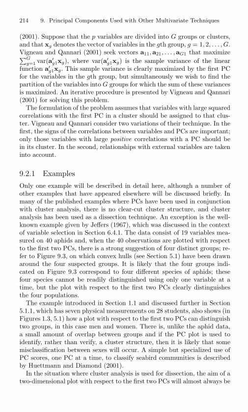
214 9. Principal Components Used with Other Multivariate Techniques
(2001). Suppose that the p variables are divided into G groups or clusters,and that xg denotes the vector of variables in the gth group, g = 1, 2, . . . , G.Vigneau and Qannari (2001) seek vectors a11,a21, . . . ,aG1 that maximize∑G
g=1 var(a′g1xg), where var(a′
g1xg) is the sample variance of the linearfunction a′
g1xg. This sample variance is clearly maximized by the first PCfor the variables in the gth group, but simultaneously we wish to find thepartition of the variables into G groups for which the sum of these variancesis maximized. An iterative procedure is presented by Vigneau and Qannari(2001) for solving this problem.
The formulation of the problem assumes that variables with large squaredcorrelations with the first PC in a cluster should be assigned to that clus-ter. Vigneau and Qannari consider two variations of their technique. In thefirst, the signs of the correlations between variables and PCs are important;only those variables with large positive correlations with a PC should bein its cluster. In the second, relationships with external variables are takeninto account.
9.2.1 Examples
Only one example will be described in detail here, although a number ofother examples that have appeared elsewhere will be discussed briefly. Inmany of the published examples where PCs have been used in conjunctionwith cluster analysis, there is no clear-cut cluster structure, and clusteranalysis has been used as a dissection technique. An exception is the well-known example given by Jeffers (1967), which was discussed in the contextof variable selection in Section 6.4.1. The data consist of 19 variables mea-sured on 40 aphids and, when the 40 observations are plotted with respectto the first two PCs, there is a strong suggestion of four distinct groups; re-fer to Figure 9.3, on which convex hulls (see Section 5.1) have been drawnaround the four suspected groups. It is likely that the four groups indi-cated on Figure 9.3 correspond to four different species of aphids; thesefour species cannot be readily distinguished using only one variable at atime, but the plot with respect to the first two PCs clearly distinguishesthe four populations.
The example introduced in Section 1.1 and discussed further in Section5.1.1, which has seven physical measurements on 28 students, also shows (inFigures 1.3, 5.1) how a plot with respect to the first two PCs can distinguishtwo groups, in this case men and women. There is, unlike the aphid data,a small amount of overlap between groups and if the PC plot is used toidentify, rather than verify, a cluster structure, then it is likely that somemisclassification between sexes will occur. A simple but specialized use ofPC scores, one PC at a time, to classify seabird communities is describedby Huettmann and Diamond (2001).
In the situation where cluster analysis is used for dissection, the aim of atwo-dimensional plot with respect to the first two PCs will almost always be
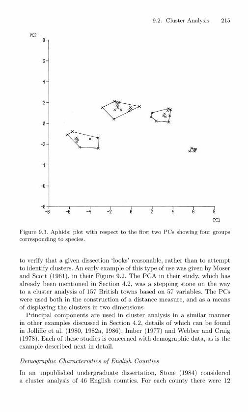
9.2. Cluster Analysis 215
Figure 9.3. Aphids: plot with respect to the first two PCs showing four groupscorresponding to species.
to verify that a given dissection ‘looks’ reasonable, rather than to attemptto identify clusters. An early example of this type of use was given by Moserand Scott (1961), in their Figure 9.2. The PCA in their study, which hasalready been mentioned in Section 4.2, was a stepping stone on the wayto a cluster analysis of 157 British towns based on 57 variables. The PCswere used both in the construction of a distance measure, and as a meansof displaying the clusters in two dimensions.
Principal components are used in cluster analysis in a similar mannerin other examples discussed in Section 4.2, details of which can be foundin Jolliffe et al. (1980, 1982a, 1986), Imber (1977) and Webber and Craig(1978). Each of these studies is concerned with demographic data, as is theexample described next in detail.
Demographic Characteristics of English Counties
In an unpublished undergraduate dissertation, Stone (1984) considereda cluster analysis of 46 English counties. For each county there were 12
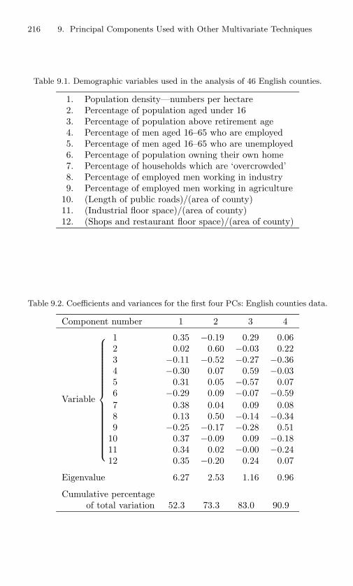
216 9. Principal Components Used with Other Multivariate Techniques
Table 9.1. Demographic variables used in the analysis of 46 English counties.
1. Population density—numbers per hectare2. Percentage of population aged under 163. Percentage of population above retirement age4. Percentage of men aged 16–65 who are employed5. Percentage of men aged 16–65 who are unemployed6. Percentage of population owning their own home7. Percentage of households which are ‘overcrowded’8. Percentage of employed men working in industry9. Percentage of employed men working in agriculture
10. (Length of public roads)/(area of county)11. (Industrial floor space)/(area of county)12. (Shops and restaurant floor space)/(area of county)
Table 9.2. Coefficients and variances for the first four PCs: English counties data.
Component number 1 2 3 4
1 0.35 −0.19 0.29 0.062 0.02 0.60 −0.03 0.223 −0.11 −0.52 −0.27 −0.364 −0.30 0.07 0.59 −0.035 0.31 0.05 −0.57 0.076 −0.29 0.09 −0.07 −0.59
Variable
7 0.38 0.04 0.09 0.088 0.13 0.50 −0.14 −0.349 −0.25 −0.17 −0.28 0.51
10 0.37 −0.09 0.09 −0.1811 0.34 0.02 −0.00 −0.2412 0.35 −0.20 0.24 0.07
Eigenvalue 6.27 2.53 1.16 0.96
Cumulative percentageof total variation 52.3 73.3 83.0 90.9

9.2. Cluster Analysis 217
demographic variables, which are listed in Table 9.1.The objective of Stone’s analysis, namely dissection of local authority
areas into clusters, was basically the same as that in other analyses byImber (1977), Webber and Craig (1978) and Jolliffe et al. (1986), but thesevarious analyses differ in the variables used and in the local authoritiesconsidered. For example, Stone’s list of variables is shorter than those of theother analyses, although it includes some variables not considered by any ofthe others. Also, Stone’s list of local authorities includes large metropolitancounties such as Greater London, Greater Manchester and Merseyside assingle entities, whereas these large authorities are subdivided into smallerareas in the other analyses. A comparison of the clusters obtained fromseveral different analyses is given by Jolliffe et al. (1986).
As in other analyses of local authorities, PCA is used in Stone’s analysisin two ways: first, to summarize and explain the major sources of variationin the data, and second, to provide a visual display on which to judge theadequacy of the clustering.
Table 9.2 gives the coefficients and variances for the first four PCs usingthe correlation matrix for Stone’s data. It is seen that the first two compo-nents account for 73% of the total variation, but that most of the relevantrules of Section 6.1 would retain four components (the fifth eigenvalueis 0.41).
There are fairly clear interpretations for each of the first three PCs. Thefirst PC provides a contrast between urban and rural areas, with positivecoefficients for variables that are high in urban areas, such as densities ofpopulation, roads, and industrial and retail floor space; negative coefficientsoccur for owner occupation, percentage of employed men in agriculture, andoverall employment level, which at the time of the study tended to be higherin rural areas. The main contrast for component 2 is between the percent-ages of the population below school-leaving age and above retirement age.This component is therefore a measure of the age of the population in eachcounty, and it identifies, at one extreme, the south coast retirement areas.
The third PC contrasts employment and unemployment rates. This con-trast is also present in the first urban versus rural PC, so that the thirdPC is measuring variation in employment/unemployment rates within ru-ral areas and within urban areas, rather than between the two types ofarea.
Turning now to the cluster analysis of the data, Stone (1984) examinesseveral different clustering methods, and also considers the analysis withand without Greater London, which is very different from any other area,but whose omission produces surprisingly little change. Figure 9.4 showsthe position of the 46 counties with respect to the first two PCs, with thefour-cluster solution obtained using complete-linkage cluster analysis (seeGordon, 1999, p. 85) indicated by different symbols for different clusters.The results for complete-linkage are fairly similar to those found by severalof the other clustering methods investigated.
In the four-cluster solution, the single observation at the bottom left of

218 9. Principal Components Used with Other Multivariate Techniques
Figure 9.4. English counties: complete-linkage four-cluster solution superimposedon a plot of the first two PCs.
the diagram is Greater London and the four-county cluster at the top leftconsists of other metropolitan counties. The counties at the right of thediagram are more rural, confirming the interpretation of the first PC givenearlier. The split between the larger groups at the right of the plot is rathermore arbitrary but, as might be expected from the interpretation of thesecond PC, most of the retirement areas have similar values in the verticaldirection; they are all in the bottom part of the diagram. Conversely, manyof the counties towards the top have substantial urban areas within them,and so have somewhat lower values on the first PC as well.
The clusters are rather nicely located in different areas of the figure,although the separation between them is not particularly clear-cut, exceptfor Greater London. This behaviour is fairly similar to what occurs for otherclustering methods in this example, and for different numbers of clusters.For example, in the eight-cluster solution for complete-linkage clustering,one observation splits off from each of the clusters in the top left and bottomright parts of the diagram to form single-county clusters. The large 27-
9.2. Cluster Analysis 219
county cluster in the top right of the plot splits into three groups containing13, 10 and 4 counties, with some overlap between them.
This example is typical of many in which cluster analysis is used fordissection. Examples like that of Jeffers’ (1967) aphids, where a very clear-cut and previously unknown cluster structure is uncovered, are relativelyunusual, although another illustration is given by Blackith and Reyment(1971, p. 155). In their example, a plot of the observations with respect tothe second and third (out of seven) PCs shows a very clear separation intotwo groups. It is probable that in many circumstances ‘projection-pursuit’methods, which are discussed next, will provide a better two-dimensionalspace in which to view the results of a cluster analysis than that defined bythe first two PCs. However, if dissection rather than discovery of a clear-cutcluster structure is the objective of a cluster analysis, then there is likelyto be little improvement over a plot with respect to the first two PCs.
9.2.2 Projection Pursuit
As mentioned earlier in this chapter, it may be possible to find low-dimensional representations of a data set that are better than the first fewPCs at displaying ‘structure’ in the data. One approach to doing this is todefine structure as ‘interesting’ and then construct an index of ‘interesting-ness,’ which is successively maximized. This is the idea behind projectionpursuit, with different indices leading to different displays. If ‘interesting’is defined as ‘large variance,’ it is seen that PCA is a special case of projec-tion pursuit. However, the types of structure of interest are often clustersor outliers, and there is no guarantee that the high-variance PCs will findsuch features. The term ‘projection pursuit’ dates back to Friedman andTukey (1974), and a great deal of work was done in the early 1980s. Thisis described at length in three key papers: Friedman (1987), Huber (1985),and Jones and Sibson (1987). The last two both include extensive discus-sion, in addition to the paper itself. Some techniques are good at findingclusters, whereas others are better at detecting outliers.
Most projection pursuit techniques start from the premise that the leastinteresting structure is multivariate normality, so that deviations fromnormality form the basis of many indices. There are measures based onskewness and kurtosis, on entropy, on looking for deviations from unifor-mity in transformed data, and on finding ‘holes’ in the data. More recently,Foster (1998) suggested looking for directions of high density, after ‘spher-ing’ the data to remove linear structure. Sphering operates by transformingthe variables x to z = S− 1
2 (x−x), which is equivalent to converting to PCs,which are then standardized to have zero mean and unit variance. Friedman(1987) also advocates sphering as a first step in his version of projectionpursuit. After identifying the high-density directions for the sphered data,Foster (1998) uses the inverse transformation to discover the nature of theinteresting structures in terms of the original variables.
220 9. Principal Components Used with Other Multivariate Techniques
Projection pursuit indices usually seek out deviations from multivariatenormality. Bolton and Krzanowski (1999) show that if normality holds thenPCA finds directions for which the maximized likelihood is minimized. Theyinterpret this result as PCA choosing interesting directions to be those forwhich normality is least likely, thus providing a link with the ideas of pro-jection pursuit. A different projection pursuit technique with an implicitassumption of normality is based on the fixed effects model of Section 3.9.Recall that the model postulates that, apart from an error term ei withvar(ei) = σ2
wiΓ, the variables x lie in a q-dimensional subspace. To find
the best-fitting subspace,∑n
i=1 wi ‖xi − zi‖2M is minimized for an appro-
priately chosen metric M. For multivariate normal ei the optimal choicefor M is Γ−1. Given a structure of clusters in the data, all wi equal, andei describing variation within clusters, Caussinus and Ruiz (1990) suggesta robust estimate of Γ, defined by
Γ =
∑n−1i=1
∑nj=i+1 K[‖xi − xj‖2
S−1 ](xi − xj)(xi − xj)′∑n−1
i=1
∑nj=i+1 K[‖xi − xj‖2
S−1 ], (9.2.1)
where K[.] is a decreasing positive real function (Caussinus and Ruiz, 1990,use K[d] = e−
β2 t for β > 0) and S is the sample covariance matrix. The best
fit is then given by finding eigenvalues and eigenvectors of SΓ−1
, which isa type of generalized PCA (see Section 14.2.2). There is a similarity herewith canonical discriminant analysis (Section 9.1), which finds eigenvaluesand eigenvectors of SbS−1
w , where Sb, Sw are between and within-groupcovariance matrices. In Caussinus and Ruiz’s (1990) form of projectionpursuit, S is the overall covariance matrix, and Γ is an estimate of thewithin-group covariance matrix. Equivalent results would be obtained if Swere replaced by an estimate of between-group covariance, so that the onlyreal difference from canonical discriminant analysis is that the groups areknown in the latter case but are unknown in projection pursuit. Furthertheoretical details and examples of Caussinus and Ruiz’s technique canbe found in Caussinus and Ruiz-Gazen (1993, 1995). The choice of valuesfor β is discussed, and values in the range 0.5 to 3.0 are recommended.There is a link between Caussinus and Ruiz-Gazen’s technique and themixture models of Section 9.2.3. In discussing theoretical properties of theirtechnique, they consider a framework in which clusters arise from a mixtureof multivariate normal distributions. The q dimensions of the underlyingmodel correspond to q clusters and Γ represents ‘residual’ or within-groupcovariance.
Although not projection pursuit as such, Krzanowski (1987b) also looksfor low-dimensional representations of the data that preserve structure, butin the context of variable selection. Plots are made with respect to the firsttwo PCs calculated from only a subset of the variables. A criterion for
9.2. Cluster Analysis 221
choosing a subset of k variables is based on how closely a Procrustes rota-tion of the configuration of scores on the first q PCs for a selected subset ofvariables matches the corresponding configuration based on the first q PCsfor the full set of variables. It is shown that the visibility of group structuremay be enhanced by plotting with respect to PCs that are calculated fromonly a subset of variables. The selected variables differ from those chosenby the methods of Section 6.3 (Krzanowski, 1987b; Jmel, 1992), which il-lustrates again that different selection rules are needed, depending on thepurpose for which the variables are chosen (Jolliffe, 1987a).
Some types of projection pursuit are far more computationally demand-ing than PCA, and for large data sets an initial reduction of dimensionmay be necessary before they can be implemented. In such cases, Friedman(1987) suggests reducing dimensionality by retaining only the high-variancePCs from a data set and conducting the projection pursuit on those. Causs-inus (1987) argues that an initial reduction of dimensionality using PCAmay be useful even when there are no computational problems.
9.2.3 Mixture Models
Cluster analysis traditionally consisted of a wide variety of rather ad hocdescriptive techniques, with little in the way of statistical underpinning.The consequence was that it was fine for dissection, but less satisfactoryfor deciding whether clusters actually existed and, if so, how many therewere. An attractive alternative approach is to model the cluster structureby a mixture model, in which the probability density function (p.d.f.) forthe vector of variables x is expressed as
f(x;θ) =G∑
g=1
πgfg(x;θg), (9.2.2)
where G is the number of clusters, πg is the probability of an observationcoming from the gth cluster, fg(x;θg) is the p.d.f. in the gth cluster, andθ′ = (θ′
1,θ′2, . . . ,θ
′G) is a vector of parameters that must be estimated.
A particular form needs to be assumed for each p.d.f. fg(x;θg), the mostusual choice being multivariate normality in which θg consists of the meanvector µg, and the covariance matrix Σg, for the gth cluster.
The problem of fitting a model such as (9.2.2) is difficult, even for smallvalues of p and G, so the approach was largely ignored at the time whenmany clustering algorithms were developed. Later advances in theory, incomputational sophistication, and in computing speed made it possible forversions of (9.2.2) to be developed and fitted, especially in the univariatecase (see, for example, Titterington et al. (1985); McLachlan and Bashford(1988); Bohning (1999)). However, many multivariate problems are stillintractable because of the large number of parameters that need to be esti-mated. For example, in a multivariate normal mixture the total number of

222 9. Principal Components Used with Other Multivariate Techniques
parameters in the πg, µg and Σg is 12G[p2 + 3p + 2] − 1. To overcome this
intractability, the elements of the Σg can be constrained in some way, anda promising approach was suggested by Tipping and Bishop (1999b), basedon their probabilistic model for PCA which is described in Section 3.9. Inthis approach, the p.d.f.s in (9.2.2) are replaced by p.d.f.s derived from Tip-ping and Bishop’s (1999a,b) model. These p.d.f.s are multivariate normal,but instead of having general covariance matrices, the matrices take theform BgB′
g + σ2gIp, where Bg is a (p × q) matrix, and q (< p) is the same
for all groups. This places constraints on the covariance matrices, but theconstraints are not as restrictive as the more usual ones, such as equality ordiagonality of matrices. Tipping and Bishop (1999b) describe a two-stageEM algorithm for finding maximum likelihood estimates of all the parame-ters in the model. As with Tipping and Bishop’s (1999a) single populationmodel, it turns out the columns of Bg define the space spanned by the firstq PCs, this time within each cluster. There remains the question of thechoice of q, and there is still a restriction to multivariate normal distribu-tions for each cluster, but Tipping and Bishop (1999b) provide exampleswhere the procedure gives clear improvements compared to the imposi-tion of more standard constraints on the Σg. Bishop (1999) outlines how aBayesian version of Tipping and Bishop’s (1999a) model can be extendedto mixtures of distributions.
9.3 Canonical Correlation Analysis and RelatedTechniques
Canonical correlation analysis (CCA) is the central topic in this section.Here the variables are in two groups, and relationships are sought betweenthese groups of variables. CCA is probably the most commonly used tech-nique for tackling this objective. The emphasis in this section, as elsewherein the book, is on how PCA can be used with, or related to, the tech-nique. A number of other methods have been suggested for investigatingrelationships between groups of variables. After describing CCA, and illus-trating it with an example, some of these alternative approaches are brieflydescribed, with their connections to PCA again highlighted. Discussion oftechniques which analyse more than two sets of variables simultaneously islargely deferred to Section 14.5.
9.3.1 Canonical Correlation Analysis
Suppose that xp1 , xp2 are vectors of random variables with p1, p2 elements,respectively. The objective of canonical correlation analysis (CCA) is to findsuccessively for k = 1, 2, . . . , min[p1, p2], pairs a′
k1xp1 ,a′k2xp2 of linear
functions of xp1 , xp2 , respectively, called canonical variates, such that the

9.3. Canonical Correlation Analysis and Related Techniques 223
correlation between a′k1xp1 and a′
k2xp2 is maximized, subject to a′k1xp1 ,
a′k2xp2 both being uncorrelated with a′
jhxph, j = 1, 2, . . . , (k − 1); h =
1, 2. The name of the technique is confusingly similar to ‘canonical variateanalysis,’ which is used in discrimination (see Section 9.1). In fact, there is alink between the two techniques (see, for example, Gittins, 1985, Chapter 4;Mardia et al. 1979, Exercise 11.5.4), but this will not be discussed in detailhere. Because of this link, the view of canonical discriminant analysis as atwo-stage PCA, noted by Campbell and Atchley (1981) and discussed inSection 9.1, is also a valid perspective for CCA. Although CCA treats thetwo sets of variables xp1 , xp2 on an equal footing, it can still be used, asin the example of Section 9.3.2, if one set is clearly a set of responses whilethe other is a set of predictors. However, alternatives such as multivariateregression and other techniques discussed in Sections 8.4, 9.3.3 and 9.3.4may be more appropriate in this case.
A number of authors have suggested that there are advantages in calcu-lating PCs zp1 , zp2 separately for xp1 ,xp2 and then performing the CCA onzp1 , zp2 rather than xp1 ,xp2 . Indeed, the main derivation of CCA given byPreisendorfer and Mobley (1988, Chapter 8) is in terms of the PCs for thetwo groups of variables. If zp1 , zp2 consist of all p1, p2 PCs, respectively,then the results using zp1 , zp2 are equivalent to those for xp1 ,xp2 . Thisfollows as zp1 , zp2 are exact linear functions of xp1 ,xp2 , respectively, and,conversely, xp1 ,xp2 are exact linear functions of zp1 , zp2 , respectively. Weare looking for ‘optimal’ linear functions of zp1 , zp2 , but this is equivalentto searching for ‘optimal’ linear functions of xp1 ,xp2 so we have the sameanalysis as that based on xp1 ,xp2 .
Muller (1982) argues that using zp1 , zp2 instead of xp1 ,xp2 can makesome of the theory behind CCA easier to understand, and that it canhelp in interpreting the results of such an analysis. He also illustrates theuse of PCA as a preliminary dimension-reducing technique by performingCCA based on just the first few elements of zp1 and zp2 . Von Storch andZwiers (1999, Section 14.1.6) note computational advantages in workingwith the PCs and also suggest using only the first few PCs to constructthe canonical variates. This works well in the example given by Muller(1982), but cannot be expected to do so in general, for reasons similarto those already discussed in the contexts of regression (Chapter 8) anddiscriminant analysis (Section 9.1). There is simply no reason why thoselinear functions of xp1 that are highly correlated with linear functions ofxp2 should necessarily be in the subspace spanned by the first few PCsof xp1 ; they could equally well be related to the last few PCs of xp1 .The fact that a linear function of xp1 has a small variance, as do thelast few PCs, in no way prevents it from having a high correlation withsome linear function of xp2 . As well as suggesting the use of PCs in CCA,Muller (1982) describes the closely related topic of using canonical corre-lation analysis to compare sets of PCs. This will be discussed further inSection 13.5.

224 9. Principal Components Used with Other Multivariate Techniques
An interesting connection between PCA and CCA is given by consider-ing the problem of minimizing var[a′
1xp1 −a′2xp2 ]. If constraints a′
1Σ11a1 =a′
2Σ22a2 = 1 are added to this problem, where Σ11, Σ22 are the covariancematrices for xp1 , xp2 , respectively, we obtain the first pair of canonicalvariates. If, instead, the constraint a′
1a1 + a′2a2 = 1 is added, the co-
efficients (a′1,a
′2)
′ define the last PC for the vector of random variablesx = (x′
p1,x′
p2)′. There has been much discussion in the literature of a va-
riety of connections between multivariate techniques, including PCA andCCA. Gittins (1985, Sections 4.8, 5.6, 5.7) gives numerous references. Inthe special case where p1 = p2 and the same variables are measured inboth xp1 and xp2 , perhaps at different time periods or for matched pairsof individuals, Flury and Neuenschwander (1995) demonstrate a theoret-ical equivalence between the canonical variates and a common principalcomponent model (see Section 13.5) when the latter model holds.
9.3.2 Example of CCA
Jeffers (1978, p. 136) considers an example with 15 variables measured on272 sand and mud samples taken from various locations in Morecambe Bay,on the north west coast of England. The variables are of two types: eightvariables are chemical or physical properties of the sand or mud samples,and seven variables measure the abundance of seven groups of invertebratespecies in the samples. The relationships between the two groups of vari-ables, describing environment and species, are of interest, so that canonicalcorrelation analysis is an obvious technique to use.
Table 9.3 gives the coefficients for the first two pairs of canonical variates,together with the correlations between each pair—the canonical corre-lations. The definitions of each variable are not given here (see Jeffers(1978, pp. 103, 107)). The first canonical variate for species is dominatedby a single species. The corresponding canonical variate for the environ-mental variables involves non-trivial coefficients for four of the variables,but is not difficult to interpret (Jeffers, 1978, p. 138). The second pair ofcanonical variates has fairly large coefficients for three species and threeenvironmental variables.
Jeffers (1978, pp. 105–109) also looks at PCs for the environmental andspecies variables separately, and concludes that four and five PCs, respec-tively, are necessary to account for most of the variation in each group. Hegoes on to look, informally, at the between-group correlations for each setof retained PCs.
Instead of simply looking at the individual correlations between PCs fordifferent groups, an alternative is to do a canonical correlation analysisbased only on the retained PCs, as suggested by Muller (1982). In thepresent example this analysis gives values of 0.420 and 0.258 for the firsttwo canonical correlations, compared with 0.559 and 0.334 when all thevariables are used. The first two canonical variates for the environmental

9.3. Canonical Correlation Analysis and Related Techniques 225
Table 9.3. Coefficients for the first two canonical variates in a canonical correlationanalysis of species and environmental variables.
First canonical variates Second canonical variatesx1 0.03 0.17x2 0.51 0.52x3 0.56 0.49
Environment x4 0.37 0.67
variables x5 0.01 −0.08x6 0.03 0.07x7 −0.00 0.04x8 0.53 −0.02
x9 0.97 −0.19x10 −0.06 −0.25x11 0.01 −0.28
Species
x12 0.14 0.58variables
x13 0.19 0.00x14 0.06 0.46x15 0.01 0.53
Canonicalcorrelation 0.559 0.334
variables and the first canonical variate for the species variables are eachdominated by a single PC, and the second canonical variate for the speciesvariables has two non-trivial coefficients. Thus, the canonical variates forPCs look, at first sight, easier to interpret than those based on the origi-nal variables. However, it must be remembered that, even if only one PCoccurs in a canonical variate, the PC itself is not necessarily an easily in-terpreted entity. For example, the environmental PC that dominates thefirst canonical variate for the environmental variables has six large coeffi-cients. Furthermore, the between-group relationships found by CCA of theretained PCs are different in this example from those found from CCA onthe original variables.
9.3.3 Maximum Covariance Analysis (SVD Analysis),Redundancy Analysis and Principal Predictors
The first technique described in this section has been used in psychology formany years, dating back to Tucker (1958), where it is known as inter-batteryfactor analysis. This method postulates a model in which
xp1 = µ1 + Λ1z + Γ1y1 + e1 (9.3.1)xp2 = µ2 + Λ2z + Γ2y2 + e2,

226 9. Principal Components Used with Other Multivariate Techniques
where µ1,µ2 are vectors of means, Λ1,Λ2,Γ1,Γ2 are matrices of coeffi-cients, z is a vector of latent variables common to both xp1 and xp2 , y1,y2
are vectors of latent variables specific to xp1 ,xp2 , and e1, e2 are vectorsof errors. Tucker (1958) fits the model using the singular value decom-position of the (p1 × p2) matrix of correlations between two batteries oftests xp1 ,xp2 , and notes that his procedure is equivalent to finding linearcombinations of the two batteries that have maximum covariance. Browne(1979) demonstrates some algebraic connections between the results of thistechnique and those of CCA.
The method was popularised in atmospheric science by Bretherton etal. (1992) and Wallace et al. (1992) under the name singular value de-composition (SVD) analysis. This name arose because, as Tucker (1958)showed, the analysis can be conducted via an SVD of the (p1 × p2) matrixof covariances between xp1 and xp2 , but the use of this general term for aspecific technique is potentially very confusing. The alternative canonicalcovariance analysis, which Cherry (1997) notes was suggested in unpub-lished work by Muller, is a better descriptor of what the technique does,namely that it successively finds pairs of linear functions of xp1 and xp2
that have maximum covariance and whose vectors of loadings are orthog-onal. Even better is maximum covariance analysis, which is used by vonStorch and Zwiers (1999, Section 14.1.7) and others (Frankignoul, personalcommunication), and we will adopt this terminology. Maximum covarianceanalysis differs from CCA in two ways: covariance rather than correlationis maximized, and vectors of loadings are orthogonal instead of derivedvariates being uncorrelated. The rationale behind maximum covarianceanalysis is that it may be important to explain a large proportion ofthe variance in one set of variables using the other set, and a pair ofvariates from CCA with large correlation need not necessarily have largevariance.
Bretherton et al. (1992) and Wallace et al. (1992) discuss maximumcovariance analysis (SVD analysis) in some detail, make comparisons withcompeting techniques and give examples. Cherry (1997) and Hu (1997)point out some disadvantages of the technique, and Cherry (1997) alsodemonstrates a relationship with PCA. Suppose that separate PCAs aredone on the two sets of variables and that the values (scores) of the nobservations on the first q PCs are given by the (n × q) matrices Z1, Z2
for the two sets of variables. If B1, B2 are orthogonal matrices chosen tominimize ‖Z1B1 −Z2B2‖, the resulting matrices Z1B1, Z2B2 contain thevalues for the n observations of the first q pairs of variates from a maximumcovariance analysis. Thus, maximum covariance analysis can be viewed astwo PCAs, followed by rotation to match up the results of the two analysesas closely as possible.
Like maximum covariance analysis, redundancy analysis attempts to in-corporate variance as well as correlation in its search for relationshipsbetween two sets of variables. The redundancy coefficient was introduced

9.3. Canonical Correlation Analysis and Related Techniques 227
by Stewart and Love (1968), and is an index of the average proportionof the variance of the variables in one set that is reproducible from thevariables in the other set. One immediate difference from both CCA andmaximum covariance analysis is that it does not view the two sets of vari-ables symmetrically. One set is treated as response variables and the otheras predictor variables, and the results of the analysis are different depend-ing on the choice of which set contains responses. For convenience, in whatfollows xp1 and xp2 consist of responses and predictors, respectively.
Stewart and Love’s (1968) redundancy index, given a pair of canonicalvariates, can be expressed as the product of two terms. These terms arethe squared canonical correlation and the variance of the canonical variatefor the response set. It is clear that a different value results if the roles ofpredictor and response variables are reversed. The redundancy coefficientcan be obtained by regressing each response variable on all the predictorvariables and then averaging the p1 squared multiple correlations fromthese regressions. This has a link to the interpretation of PCA given inthe discussion of Property A6 in Chapter 2, and was used by van denWollenberg (1977) and Thacker (1999) to introduce two slightly differenttechniques.
In van den Wollenberg’s (1977) redundancy analysis, linear functionsa′
k2xp2 of xp2 are found that successively maximize their average squaredcorrelation with the elements of the response set xp1 , subject to the vectorsof loadings a12, a22, . . . being orthogonal. It turns out (van den Wollenberg,1977) that finding the required linear functions is achieved by solving theequation
RxyRyxak2 = lkRxxak2, (9.3.2)
where Rxx is the correlation matrix for the predictor variables, Rxy is thematrix of correlations between the predictor and response variables, andRyx is the transpose of Rxy. A linear function of xp1 can be found byreversing the roles of predictor and response variables, and hence replacingx by y and vice versa, in equation (9.3.2).
Thacker (1999) also considers a linear function z1 = a′12xp2 of the pre-
dictors xp2 . Again a12 is chosen to maximize∑p1
j=1 r21j , where r1j is the
correlation between z1 and the jth response variable. The variable z1 iscalled the first principal predictor by Thacker (1999). Second, third, . . .principal predictors are defined by maximizing the same quantity, subjectto the constraint that each principal predictor must be uncorrelated withall previous principal predictors. Thacker (1999) shows that the vectors ofloadings a12, a22, . . . are solutions of the equation
Sxy[diag(Syy)]−1Syxak2 = lkSxxak2, (9.3.3)
where Sxx, Syy, Sxy and Syx are covariance matrices defined analogously tothe correlation matrices Rxx, Ryy, Rxy and Ryx above. The eigenvalue lkcorresponding to ak2 is equal to the sum of squared correlations
∑p1j=1 r2
kj

228 9. Principal Components Used with Other Multivariate Techniques
between a′k2xp2 and each of the variables xj . The difference between prin-
cipal predictors and redundancy analysis is that the principal predictorsare uncorrelated, whereas the derived variables in redundancy analysis arecorrelated but have vectors of loadings that are orthogonal. The presenceof correlation in redundancy analysis may be regarded as a drawback, andvan den Wollenberg (1977) suggests using the first few derived variablesfrom redundancy analysis as input to CCA. This will then produce uncor-related canonical variates whose variances are unlikely to be small. Thepossibility of using the first few PCs from each set as input to CCA wasmentioned above, as was the disadvantage that excluded low-variance PCsmight contain strong inter-set correlations. As low-variance directions areunlikely to be of interest in redundancy analysis, using the first few PCsas input seems to be far safer in this case and is another option.
It is of interest to note the similarity between equations (9.3.2), (9.3.3)and the eigenequation whose solution gives the loadings ak2 on xp2 forcanonical correlation analysis, namely
SxyS−1yy Syxak2 = lkSxxak2, (9.3.4)
using the present notation. Wang and Zwiers (2001) solve a version of(9.3.2) with covariance matrices replacing correlation matrices, by firstsolving the eigenequation
SyxS−1xx Sxybk2 = lkbk2, (9.3.5)
and then setting ak2 = l− 1
2k S−1
xx Sxybk2. This is equivalent to a PCA ofthe covariance matrix SyxS−1
xx Sxy of the predicted values of the responsevariables obtained from a multivariate regression on the predictor variables.Multivariate regression is discussed further in Section 9.3.4.
Van den Wollenberg (1977) notes that PCA is a special case of redun-dancy analysis (and principal predictors, but not CCA) when xp1 and xp2
are the same (see also Property A6 in Chapter 2). Muller (1981) showsthat redundancy analysis is equivalent to orthogonally rotating the resultsof a multivariate regression analysis. DeSarbo and Jedidi (1986) give anumber of other properties, together with modifications and extensions, ofredundancy analysis.
9.3.4 Other Techniques for Relating Two Sets of Variables
A number of other techniques for relating two sets of variables were notedin Section 8.4. They include separate PCAs on the two groups of variables,followed by the calculation of a regression equation to predict, again sepa-rately, each PC from one set from the PCs in the other set. Another way ofusing PCA is to concatenate the two sets of variables and find PCs for thecombined set of (p1 + p2) variables. This is sometimes known as combinedPCA, and is one of the methods that Bretherton et al. (1992) compare with

9.3. Canonical Correlation Analysis and Related Techniques 229
maximum covariance analysis. The reasoning behind the analysis, apartfrom being very easy to implement, is that two variables are more likelyto simultaneously have large loadings in the same high-variance combinedPC if they are strongly correlated. Thus, by looking at which variablesfrom different groups appear together in the same high-variance compo-nents, some ideas can be gained about the relationships between the twogroups. This is true to some extent, but the combined components do notdirectly quantify the precise form of the relationships, nor their strength,in the way that CCA or maximum covariance analysis does. One otherPCA-based technique considered by Bretherton et al. (1992) is to look atcorrelations between PCs of one set of variables and the variables them-selves from the other set. This takes us back to a collection of simple PCregressions.
Another technique from Section 8.4, partial least squares (PLS), can begeneralized to the case of more than one response variable (Wold, 1984).Like single-response PLS, multiresponse PLS is often defined in terms of analgorithm, but Frank and Friedman (1993) give an interpretation showingthat multiresponse PLS successively maximizes the covariance between lin-ear functions of the two sets of variables. It is therefore similar to maximumcovariance analysis, which was discussed in Section 9.3.3, but differs fromit in not treating response and predictor variables symmetrically. Whereasin maximum covariance analysis the vectors of coefficients of the linearfunctions are orthogonal within each set of variables, no such restrictionis placed on the response variables in multiresponse PLS. For the predic-tor variables there is a restriction, but it is that the linear functions areuncorrelated, rather than having orthogonal vectors of coefficients.
The standard technique when one set of variables consists of responsesand the other is made up of predictors is multivariate linear regression.Equation (8.1.1) generalizes to
Y = XB + E, (9.3.6)
where Y, X are (n×p1), (n×p2) matrices of n observations on p1 responsevariables and p2 predictor variables, respectively, B is a (p2×p1) matrix ofunknown parameters, and E is an (n × p1) matrix of errors. The numberof parameters to be estimated is at least p1p2 (as well as those in B, thereare usually some associated with the covariance matrix of the error term).Various attempts have been made to reduce this number by simplifying themodel. The reduced rank models of Davies and Tso (1982) form a generalclass of this type. In these models B is assumed to be of rank m < p2. Thereis more than one way to estimate the unknown parameters in a reducedrank regression model. That recommended by Davies and Tso (1982) firstfinds the least squares estimate B of B in (9.3.6) and uses this to obtainpredicted values Y = XB for Y. Next a singular value decomposition (withits usual meaning) is done on Y and B is then projected onto the subspace

230 9. Principal Components Used with Other Multivariate Techniques
spanned by the first m terms in the SVD. This is equivalent to projectingthe rows of Y onto the subspace spanned by the first m PCs of Y.
Two further equivalences are noted by ter Braak and Looman (1994),namely that the reduced rank regression model estimated in this way isequivalent to redundancy analysis, and also to PCA of instrumental vari-ables, as introduced by Rao (1964) (see Section 14.3). Van den Brink andter Braak (1999) also refer to redundancy analysis as ‘PCA in which samplescores are constrained to be linear combinations of the explanatory [pre-dictor] variables.’ They extend redundancy analysis to the case where thevariables in X and Y are observed over several time periods and the modelchanges with time. This extension is discussed further in Section 12.4.2.Because of the link with PCA, it is possible to construct biplots (see Sec-tion 5.3) of the regression coefficients in the reduced rank regression model(ter Braak and Looman, 1994).
Aldrin (2000) proposes a modification of reduced rank regression, calledsoftly shrunk reduced-rank regression (SSRRR), in which the terms in theSVD of Y are given varying non-zero weights, rather than the all-or-nothinginclusion/exclusion of terms in reduced rank regression. Aldrin (2000) alsosuggests that a subset of PCs of the predictor variables may be used asinput for a reduced rank regression or SSRRR instead of the predictorvariables themselves. In a simulation study comparing least squares with anumber of biased multivariate regression procedures, SSRRR with PCs asinput seems to be the best method overall.
Reduced rank regression models essentially assume a latent structureunderlying the predictor variables, so that their dimensionality can be re-duced below p2. Burnham et al. (1999) describe so-called latent variablemultivariate regression models, which take the idea of reduced rank regres-sion further by postulating overlapping latent structures underlying boththe response and predictor variables. The model can be written
X = ZXΓX + EX
Y = ZY ΓY + EY ,
where ZX , ZY are of dimension (n × m) and contain values of m latentvariables for the n observations; ΓX , ΓY are (m × p1), (m × p2) matricesof unknown parameters, and EX , EY are matrices of errors.
To fit this model, Burnham et al. (1999) suggest carrying out PCAson the data in X, on that in Y, and on the combined (n × (p1 + p2))matrix containing both response and predictor variables. In each PCA, ajudgment is made of how many PCs seem to represent common underlyingstructure and how many represent error or noise. Suppose that the numbersof non-noisy PCs in the three analyses are mX , mY and mC , with obviousnotation. The implication is then that the overlapping part of the latentstructures has dimension mX + mY − mC . If mX = mY = mC there iscomplete overlap, whereas if mC = mX + mY there is none. This model

9.3. Canonical Correlation Analysis and Related Techniques 231
is very similar to that of (9.3.1). The difference is that the separationinto latent variables common to both sets of measured variables and thosespecific to one set of measured variables is explicit in (9.3.1). Burnhamet al. (1999) successfully fit their model to a number of examples fromchemometrics.

10Outlier Detection, InfluentialObservations, Stability, Sensitivity,and Robust Estimation of PrincipalComponents
This chapter deals with four related topics, which are all concerned withsituations where some of the observations may, in some way, be atypical ofthe bulk of the data.
First, we discuss the problem of detecting outliers in a set of data. Out-liers are generally viewed as observations that are a long way from, orinconsistent with, the remainder of the data. Such observations can, butneed not, have a drastic and disproportionate effect on the results of var-ious analyses of a data set. Numerous methods have been suggested fordetecting outliers (see, for example, Barnett and Lewis, 1994; Hawkins,1980); some of the methods use PCs, and these methods are described inSection 10.1.
The techniques described in Section 10.1 are useful regardless of the typeof statistical analysis to be performed, but in Sections 10.2–10.4 we lookspecifically at the case where a PCA is being done. Depending on theirposition, outlying observations may or may not have a large effect on theresults of the analysis. It is of interest to determine which observations doindeed have a large effect. Such observations are called influential observa-tions and are discussed in Section 10.2. Leaving out an observation is onetype of perturbation to a data set. Sensitivity and stability of PCA withrespect to other types of perturbation is the subject of Section 10.3.
Given that certain observations are outliers or influential, it may bedesirable to adapt the analysis to remove or diminish the effects of suchobservations; that is, the analysis is made robust. Robust analyses havebeen developed in many branches of statistics (see, for example, Huber(1981); Hampel et al. (1986) for some of the theoretical background, and
10.1. Detection of Outliers Using Principal Components 233
Hoaglin et al. (1983) for a more readable approach), and robustness withrespect to distributional assumptions, as well as with respect to outlying orinfluential observations, may be of interest. A number of techniques havebeen suggested for robustly estimating PCs, and these are discussed in thefourth section of this chapter; the final section presents a few concludingremarks.
10.1 Detection of Outliers Using PrincipalComponents
There is no formal, widely accepted, definition of what is meant by an ‘out-lier.’ The books on the subject by Barnett and Lewis (1994) and Hawkins(1980) both rely on informal, intuitive definitions, namely that outliers areobservations that are in some way different from, or inconsistent with, theremainder of a data set. For p-variate data, this definition implies that out-liers are a long way from the rest of the observations in the p-dimensionalspace defined by the variables. Numerous procedures have been suggestedfor detecting outliers with respect to a single variable, and many of theseare reviewed by Barnett and Lewis (1994) and Hawkins (1980). The lit-erature on multivariate outliers is less extensive, with each of these twobooks containing only one chapter (comprising less than 15% of their totalcontent) on the subject. Several approaches to the detection of multivariateoutliers use PCs, and these will now be discussed in some detail. As well asthe methods described in this section, which use PCs in fairly direct waysto identify potential outliers, techniques for robustly estimating PCs (seeSection 10.4) may also be used to detect outlying observations.
A major problem in detecting multivariate outliers is that an observationthat is not extreme on any of the original variables can still be an outlier,because it does not conform with the correlation structure of the remainderof the data. It is impossible to detect such outliers by looking solely at theoriginal variables one at a time. As a simple example, suppose that heightsand weights are measured for a sample of healthy children of various agesbetween 5 and 15 years old. Then an ‘observation’ with height and weightof 175 cm (70 in) and 25 kg (55 lb), respectively, is not particularly extremeon either the height or weight variables individually, as 175 cm is a plausibleheight for the older children and 25 kg is a plausible weight for the youngestchildren. However, the combination (175 cm, 25 kg) is virtually impossible,and will be a clear outlier because it combines a large height with a smallweight, thus violating the general pattern of a positive correlation betweenthe two variables. Such an outlier is apparent on a plot of the two variables(see Figure 10.1) but, if the number of variables p is large, it is quite possiblethat some outliers will not be apparent on any of the 1
2p(p−1) plots of twovariables at a time. Thus, for large p we need to consider the possibility

234 10. Outlier Detection, Influential Observations and Robust Estimation
Figure 10.1. Example of an outlier that is not detectable by looking at one variableat a time.
that outliers will manifest themselves in directions other than those whichare detectable from simple plots of pairs of the original variables.
Outliers can be of many types, which complicates any search for direc-tions in which outliers occur. However, there are good reasons for lookingat the directions defined by either the first few or the last few PCs in orderto detect outliers. The first few and last few PCs will detect different typesof outlier, and in general the last few are more likely to provide additionalinformation that is not available in plots of the original variables.
As discussed in Gnanadesikan and Kettenring (1972), the outliers thatare detectable from a plot of the first few PCs are those which inflatevariances and covariances. If an outlier is the cause of a large increasein one or more of the variances of the original variables, then it must beextreme on those variables and thus detectable by looking at plots of singlevariables. Similarly, an observation that inflates a covariance or correlationbetween two variables will usually be clearly visible on a plot of these two
10.1. Detection of Outliers Using Principal Components 235
variables, and will often be extreme with respect to one or both of thesevariables looked at individually.
By contrast, the last few PCs may detect outliers that are not apparentwith respect to the original variables. A strong correlation structure be-tween variables implies that there are linear functions of the variables withsmall variances compared to the variances of the original variables. In thesimple height-and-weight example described above, height and weight havea strong positive correlation, so it is possible to write
x2 = βx1 + ε,
where x1, x2 are height and weight measured about their sample means,β is a positive constant, and ε is a random variable with a much smallervariance than x1 or x2. Therefore the linear function
x2 − βx1
has a small variance, and the last (in this case the second) PC in an analysisof x1, x2 has a similar form, namely a22x2 − a12x1, where a12, a22 > 0.Calculation of the value of this second PC for each observation will detectobservations such as (175 cm, 25 kg) that are outliers with respect to thecorrelation structure of the data, though not necessarily with respect toindividual variables. Figure 10.2 shows a plot of the data from Figure 10.1,with respect to the PCs derived from the correlation matrix. The outlyingobservation is ‘average’ for the first PC, but very extreme for the second.
This argument generalizes readily when the number of variables p isgreater than two; by examining the values of the last few PCs, we may beable to detect observations that violate the correlation structure imposedby the bulk of the data, but that are not necessarily aberrant with respectto individual variables. Of course, it is possible that, if the sample size isrelatively small or if a few observations are sufficiently different from therest, then the outlier(s) may so strongly influence the last few PCs thatthese PCs now reflect mainly the position of the outlier(s) rather than thestructure of the majority of the data. One way of avoiding this maskingor camouflage of outliers is to compute PCs leaving out one (or more)observations and then calculate for the deleted observations the values ofthe last PCs based on the reduced data set. To do this for each observationis a heavy computational burden, but it might be worthwhile in smallsamples where such camouflaging is, in any case, more likely to occur.Alternatively, if PCs are estimated robustly (see Section 10.4), then theinfluence of outliers on the last few PCs should be reduced and it may beunnecessary to repeat the analysis with each observation deleted.
A series of scatterplots of pairs of the first few and last few PCs maybe useful in identifying possible outliers. One way of presentating each PCseparately is as a set of parallel boxplots. These have been suggested as ameans of deciding how many PCs to retain (see Section 6.1.5), but theymay also be useful for flagging potential outliers (Besse, 1994).

236 10. Outlier Detection, Influential Observations and Robust Estimation
Figure 10.2. The data set of Figure 10.1, plotted with respect to its PCs.
As well as simple plots of observations with respect to PCs, it is possibleto set up more formal tests for outliers based on PCs, assuming that the PCsare normally distributed. Strictly, this assumes that x has a multivariatenormal distribution but, because the PCs are linear functions of p randomvariables, an appeal to the Central Limit Theorem may justify approximatenormality for the PCs even when the original variables are not normal. Abattery of tests is then available for each individual PC, namely those fortesting for the presence of outliers in a sample of univariate normal data(see Hawkins (1980, Chapter 3) and Barnett and Lewis (1994, Chapter 6)).The latter reference describes 47 tests for univariate normal data, plus 23for univariate gamma distributions and 17 for other distributions. Othertests, which combine information from several PCs rather than examiningone at a time, are described by Gnanadesikan and Kettenring (1972) andHawkins (1974), and some of these will now be discussed. In particular, wedefine four statistics, which are denoted d2
1i, d22i, d2
3i and d4i.The last few PCs are likely to be more useful than the first few in de-
tecting outliers that are not apparent from the original variables, so one

10.1. Detection of Outliers Using Principal Components 237
possible test statistic, d21i, suggested by Rao (1964) and discussed further
by Gnanadesikan and Kettenring (1972), is the sum of squares of the valuesof the last q (< p) PCs, that is
d21i =
p∑
k=p−q+1
z2ik, (10.1.1)
where zik is the value of the kth PC for the ith observation. The statis-tics d2
1i, i = 1, 2, . . . , n should, approximately, be independent observationsfrom a gamma distribution if there are no outliers, so that a gamma prob-ability plot with suitably estimated shape parameter may expose outliers(Gnanadesikan and Kettenring, 1972).
A possible criticism of the statistic d21i is that it still gives insufficient
weight to the last few PCs, especially if q, the number of PCs contributing tod21i, is close to p. Because the PCs have decreasing variance with increasing
index, the values of z2ik will typically become smaller as k increases, and
d21i therefore implicitly gives the PCs decreasing weight as k increases. This
effect can be severe if some of the PCs have very small variances, and thisis unsatisfactory as it is precisely the low-variance PCs which may be mosteffective in determining the presence of certain types of outlier.
An alternative is to give the components equal weight, and this can beachieved by replacing zik by z∗ik = zik/l
1/2k , where lk is the variance of the
kth sample PC. In this case the sample variances of the z∗ik will all be equalto unity. Hawkins (1980, Section 8.2) justifies this particular renormaliza-tion of the PCs by noting that the renormalized PCs, in reverse order,are the uncorrelated linear functions ˜a′
px, ˜a′p−1x, . . . ,
˜a′1x of x which, when
constrained to have unit variances, have coefficients ˜ajk that successivelymaximize the criterion
∑pj=1
˜a2jk, for k = p, (p− 1), . . . , 1. Maximization of
this criterion is desirable because, given the fixed-variance property, linearfunctions that have large absolute values for their coefficients are likely to bemore sensitive to outliers than those with small coefficients (Hawkins,1980,Section 8.2). It should be noted that when q = p, the statistic
d22i =
p∑
k=p−q+1
z2ik
lk(10.1.2)
becomes∑p
k=1 z2ik/lk, which is simply the (squared) Mahalanobis distance
D2i between the ith observation and the sample mean, defined as D2
i =(xi − x)′S−1(xi − x). This follows because S = AL2A′ where, as usual,L2 is the diagonal matrix whose kth diagonal element is lk, and A is thematrix whose (j, k)th element is ajk. Furthermore,
S−1 = AL−2A′
x′i = z′iA
′
x′ = z′A′,
238 10. Outlier Detection, Influential Observations and Robust Estimation
so D2i is
(xi − x)′S−1(xi − x) = (zi − z)′A′AL−2A′A(zi − z)
= (zi − z)′L−2(zi − z)
=p∑
k=1
z2ik
lk,
where zik is the kth PC score for the ith observation, measured about themean of the scores for all observations. Flury (1997, p. 609-610) suggeststhat a plot of (D2
i − d22i) versus d2
2i will reveal observations that are notwell represented by the first (p − q) PCs. Such observations are potentialoutliers.
Gnanadesikan and Kettenring (1972) consider also the statistic
d23i =
p∑
k=1
lkz2ik, (10.1.3)
which emphasizes observations that have a large effect on the first fewPCs, and is equivalent to (xi − x)′S(xi − x). As stated earlier, the firstfew PCs are useful in detecting some types of outlier, and d2
3i emphasizessuch outliers. However, we repeat that such outliers are often detectablefrom plots of the original variables, unlike the outliers exposed by the lastfew PCs. Various types of outlier, including some that are extreme withrespect to both the first few and and the last few PCs, are illustrated inthe examples given later in this section.
Hawkins (1974) prefers to use d22i with q < p rather than q = p (again, in
order to emphasize the low-variance PCs), and he considers how to choosean appropriate value for q. This is a rather different problem from thatconsidered in Section 6.1, as we now wish to decide how many of the PCs,starting with the last rather than starting with the first, need to be retained.Hawkins (1974) suggests three possibilities for choosing q, including the‘opposite’ of Kaiser’s rule (Section 6.1.2)—that is, the retention of PCs witheigenvalues less than unity. In an example, he selects q as a compromisebetween values suggested by his three rules.
Hawkins (1974) also shows that outliers can be successfully detectedusing the statistic
d4i = maxp−q+1≤k≤p
|z∗ik|, (10.1.4)
and similar methods for choosing q are again suggested. Fellegi (1975),too, is enthusiastic about the performance of the statistic d4i. Hawkinsand Fatti (1984) claim that outlier detection is improved still further bya series of transformations, including varimax rotation (see Sections 7.2and 11.1), before computing d4i. The test statistic for the ith observationthen becomes the maximum absolute value of the last q renormalized androtated PCs evaluated for that observation.
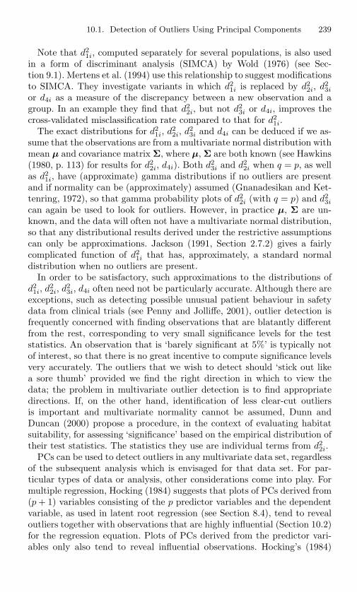
10.1. Detection of Outliers Using Principal Components 239
Note that d21i, computed separately for several populations, is also used
in a form of discriminant analysis (SIMCA) by Wold (1976) (see Sec-tion 9.1). Mertens et al. (1994) use this relationship to suggest modificationsto SIMCA. They investigate variants in which d2
1i is replaced by d22i, d2
3i
or d4i as a measure of the discrepancy between a new observation and agroup. In an example they find that d2
2i, but not d23i or d4i, improves the
cross-validated misclassification rate compared to that for d21i.
The exact distributions for d21i, d2
2i, d23i and d4i can be deduced if we as-
sume that the observations are from a multivariate normal distribution withmean µ and covariance matrix Σ, where µ, Σ are both known (see Hawkins(1980, p. 113) for results for d2
2i, d4i). Both d23i and d2
2i when q = p, as wellas d2
1i, have (approximate) gamma distributions if no outliers are presentand if normality can be (approximately) assumed (Gnanadesikan and Ket-tenring, 1972), so that gamma probability plots of d2
2i (with q = p) and d23i
can again be used to look for outliers. However, in practice µ, Σ are un-known, and the data will often not have a multivariate normal distribution,so that any distributional results derived under the restrictive assumptionscan only be approximations. Jackson (1991, Section 2.7.2) gives a fairlycomplicated function of d2
1i that has, approximately, a standard normaldistribution when no outliers are present.
In order to be satisfactory, such approximations to the distributions ofd21i, d2
2i, d23i, d4i often need not be particularly accurate. Although there are
exceptions, such as detecting possible unusual patient behaviour in safetydata from clinical trials (see Penny and Jolliffe, 2001), outlier detection isfrequently concerned with finding observations that are blatantly differentfrom the rest, corresponding to very small significance levels for the teststatistics. An observation that is ‘barely significant at 5%’ is typically notof interest, so that there is no great incentive to compute significance levelsvery accurately. The outliers that we wish to detect should ‘stick out likea sore thumb’ provided we find the right direction in which to view thedata; the problem in multivariate outlier detection is to find appropriatedirections. If, on the other hand, identification of less clear-cut outliersis important and multivariate normality cannot be assumed, Dunn andDuncan (2000) propose a procedure, in the context of evaluating habitatsuitability, for assessing ‘significance’ based on the empirical distribution oftheir test statistics. The statistics they use are individual terms from d2
2i.PCs can be used to detect outliers in any multivariate data set, regardless
of the subsequent analysis which is envisaged for that data set. For par-ticular types of data or analysis, other considerations come into play. Formultiple regression, Hocking (1984) suggests that plots of PCs derived from(p + 1) variables consisting of the p predictor variables and the dependentvariable, as used in latent root regression (see Section 8.4), tend to revealoutliers together with observations that are highly influential (Section 10.2)for the regression equation. Plots of PCs derived from the predictor vari-ables only also tend to reveal influential observations. Hocking’s (1984)
240 10. Outlier Detection, Influential Observations and Robust Estimation
suggestions are illustrated with an example, but no indication is given ofwhether the first few or last few PCs are more likely to be useful—his ex-ample has only three predictor variables, so it is easy to look at all possibleplots. Mason and Gunst (1985) refer to outliers among the predictor vari-ables as leverage points. They recommend constructing scatter plots of thefirst few PCs normalized to have unit variance, and claim that such plotsare often effective in detecting leverage points that cluster and leveragepoints that are extreme in two or more dimensions. In the case of multi-variate regression, another possibility for detecting outliers (Gnanadesikanand Kettenring, 1972) is to look at the PCs of the (multivariate) residualsfrom the regression analysis.
Pena and Yohai (1999) propose a PCA on a matrix of regression diagnos-tics that is also useful in detecting outliers in multiple regression. Supposethat a sample of n observations is available for the analysis. Then an (n×n)matrix can be calculated whose (h, i)th element is the difference yh − yh(i)
between the predicted value of the dependent variable y for the hth obser-vation when all n observations are used in the regression, and when (n−1)observations are used with the ith observation omitted. Pena and Yohai(1999) refer to this as a sensitivity matrix and seek a unit-length vectorsuch that the sum of squared lengths of the projections of the rows of thematrix onto that vector is maximized. This leads to the first principal com-ponent of the sensitivity matrix, and subsequent components can be foundin the usual way. Pena and Yohai (1999) call these components principalsensitivity components and show that they also represent directions thatmaximize standardized changes to the vector of the regression coefficient.The definition and properties of principal sensitivity components mean thathigh-leverage outliers are likely to appear as extremes on at least one ofthe first few components.
Lu et al. (1997) also advocate the use of the PCs of a matrix of regres-sion diagnostics. In their case the matrix is what they call the standardizedinfluence matrix (SIM). If a regression equation has p unknown parame-ters and n observations with which to estimate them, a (p × n) influencematrix can be formed whose (j, i)th element is a standardized version ofthe theoretical influence function (see Section 10.2) for the jth parame-ter evaluated for the ith observation. Leaving aside the technical details,the so-called complement of the standardized influence matrix (SIMc) canbe viewed as a covariance matrix for the ‘data’ in the influence matrix.Lu et al. (1997) show that finding the PCs of these standardized data,and hence the eigenvalues and eigenvectors of SIMc, can identify outliersand influential points and give insights into the structure of that influence.Sample versions of SIM and SIMc are given, as are illustrations of theiruse.
Another specialized field in which the use of PCs has been proposed inorder to detect outlying observations is that of statistical process control,which is the subject of Section 13.7. A different way of using PCs to detect

10.1. Detection of Outliers Using Principal Components 241
outliers is proposed by Gabriel and Zamir (1979). This proposal uses theidea of weighted PCs, and will be discussed further in Section 14.2.1.
Projection pursuit was introduced in Section 9.2.2 as a family of tech-niques for finding clusters, but it can equally well be used to look foroutliers. PCA is not specifically designed to find dimensions which bestdisplay either clusters or outliers. As with clusters, optimizing a criterionother than variance can give better low-dimensional displays in which toidentify outliers. As noted in Section 9.2.2, projection pursuit techniquesfind directions in p-dimensional space that optimize some index of ‘interest-ingness,’ where ‘uninteresting’ corresponds to multivariate normality and‘interesting’ implies some sort of ‘structure,’ such as clusters or outliers.
Some indices are good at finding clusters, whereas others are better atdetecting outliers (see Friedman (1987); Huber (1985); Jones and Sibson(1987)). Sometimes the superiority in finding outliers has been observedempirically; in other cases the criterion to be optimized has been chosenwith outlier detection specifically in mind. For example, if outliers ratherthan clusters are of interest, Caussinus and Ruiz (1990) suggest replacingthe quantity in equation (9.2.1) by
Γ =∑n
i=1 K[‖xi − x∗‖2S−1 ](xi − x∗)(xi − x∗)′
∑ni=1 K[‖xi − x∗‖2
S−1 ], (10.1.5)
where x∗ is a robust estimate of the centre of the xi such as a multivariatemedian, and K[.], S are defined as in (9.2.1). Directions given by the firstfew eigenvectors of SΓ
−1are used to identify outliers. Further theoretical
details and examples of the technique are given by Caussinus and Ruiz-Gazen (1993, 1995). A mixture model is assumed (see Section 9.2.3) inwhich one element in the mixture corresponds to the bulk of the data, andthe other elements have small probabilities of occurrence and correspondto different types of outliers. In Caussinus et al. (2001) it is assumed thatif there are q types of outlier, then q directions are likely needed to detectthem. The bulk of the data is assumed to have a spherical distribution, sothere is no single (q+1)th direction corresponding to these data. The ques-tion of an appropriate choice for q needs to be considered. Using asymptoticresults for the null (one-component mixture) distribution of a matrix whichis closely related to SΓ
−1, Caussinus et al. (2001) use simulation to derive
tables of critical values for its eigenvalues. These tables can then be usedto assess how many eigenvalues are ‘significant,’ and hence decide on anappropriate value for q. The use of the tables is illustrated by examples.
The choice of the value of β is discussed by Caussinus and Ruiz-Gazen(1995) and values in the range 0.1 to 0.5 are recommended. Caussinuset al. (2001) use somewhat smaller values in constructing their tables,which are valid for values of β in the range 0.01 to 0.1. Penny and Jol-liffe (2001) include Caussinus and Ruiz-Gazen’s technique in a comparative
242 10. Outlier Detection, Influential Observations and Robust Estimation
study of methods for detecting multivariate outliers. It did well compared toother methods in some circumstances, particularly when there are multipleoutliers and p is not too large.
Before turning to examples, recall that an example in which outliersare detected using PCs in a rather different way was given in Section 5.6.In that example, Andrews’ curves (Andrews, 1972) were computed usingPCs and some of the observations stood out as different from the otherswhen plotted as curves. Further examination of these different observationsshowed that they were indeed ‘outlying’ in some respects, compared to theremaining observations.
10.1.1 Examples
In this section one example will be discussed in some detail, while threeothers will be described more briefly.
Anatomical Measurements
A set of seven anatomical measurements on 28 students was discussed inSection 5.1.1 and it was found that on a plot of the first two PCs (Fig-ures 1.3, 5.1) there was an extreme observation on the second PC. Whenthe measurements of this individual were examined in detail, it was foundthat he had an anomalously small head circumference. Whereas the other27 students all had head girths in the narrow range 21–24 cm, this student(no. 16) had a measurement of 19 cm. It is impossible to check whetherthis was an incorrect measurement or whether student 16 indeed had anunusually small head (his other measurements were close to average), butit is clear that this observation would be regarded as an ‘outlier’ accordingto most definitions of the term.
This particular outlier is detected on the second PC, and it was sug-gested above that any outliers detected by high-variance PCs are usuallydetectable on examination of individual variables; this is indeed the casehere. Another point concerning this observation is that it is so extreme onthe second PC that it may be suspected that it alone is largely responsiblefor the direction of this PC. This question will be investigated at the endof Section 10.2, which deals with influential observations.
Figure 1.3 indicates one other possible outlier at the extreme left ofthe diagram. This turns out to be the largest student in the class—190cm (6 ft 3 in) tall, with all measurements except head girth at least aslarge as all other 27 students. There is no suspicion here of any incorrectmeasurements.
Turning now to the last few PCs, we hope to detect any observationswhich are ‘outliers’ with respect to the correlation structure of the data.Figure 10.3 gives a plot of the scores of the observations for the last twoPCs, and Table 10.1 gives the values of d2
1i, d22i and d4i, defined in equa-
tions (10.1.1), (10.1.2) and (10.1.4), respectively, for the six ‘most extreme’
10.1. Detection of Outliers Using Principal Components 243
Table 10.1. Anatomical measurements: values of d21i, d2
2i, d4i for the most extremeobservations.
Number of PCs used, qq = 1 q = 2
d21i Obs. No. d2
1i Obs. No. d22i Obs. No. d4i Obs. No.
0.81 15 1.00 7 7.71 15 2.64 150.47 1 0.96 11 7.69 7 2.59 110.44 7 0.91 15 6.70 11 2.01 10.16 16 0.48 1 4.11 1 1.97 70.15 4 0.48 23 3.52 23 1.58 230.14 2 0.36 12 2.62 12 1.49 27
q = 3d21i Obs. No. d2
2i Obs. No. d4i Obs. No.1.55 20 9.03 20 2.64 151.37 5 7.82 15 2.59 51.06 11 7.70 5 2.59 111.00 7 7.69 7 2.53 200.96 1 7.23 11 2.01 10.93 15 6.71 1 1.97 7
observations on each statistic, where the number of PCs included, q, is 1, 2or 3. The observations that correspond to the most extreme values of d2
1i,d22i and d4i are identified in Table 10.1, and also on Figure 10.3.Note that when q = 1 the observations have the same ordering for all
three statistics, so only the values of d21i are given in Table 10.1. When q
is increased to 2 or 3, the six most extreme observations are the same (ina slightly different order) for both d2
1i and d22i. With the exception of the
sixth most extreme observation for q = 2, the same observations are alsoidentified by d4i. Although the sets of the six most extreme observationsare virtually the same for d2
1i, d22i and d4i, there are some differences in
ordering. The most notable example is observation 15 which, for q = 3, ismost extreme for d4i but only sixth most extreme for d2
1i.Observations 1, 7 and 15 are extreme on all seven statistics given in Ta-
ble 10.1, due to large contributions from the final PC alone for observation15, the last two PCs for observation 7, and the fifth and seventh PCs forobservation 1. Observations 11 and 20, which are not extreme for the finalPC, appear in the columns for q = 2 and 3 because of extreme behaviouron the sixth PC for observation 11, and on both the fifth and sixth PCsfor observation 20. Observation 16, which was discussed earlier as a clearoutlier on the second PC, appears in the list for q = 1, but is not notablyextreme for any of the last three PCs.

244 10. Outlier Detection, Influential Observations and Robust Estimation
Figure 10.3. Anatomical measurements: plot of observations with respect to thelast two PCs.
Most of the observations identified in Table 10.1 are near the edge of theplot given in Figure 10.3. Observations 2, 4, 5, 12, 16, 20, 23 and 27 areclose to the main body of the data, but observations 7, 11, 15, and to alesser extent 1, are sufficiently far from the remaining data to be worthy offurther consideration. To roughly judge their ‘significance,’ recall that, if nooutliers are present and the data are approximately multivariate normal,then the values of d4i, are (approximately) absolute values of a normalrandom variable with zero mean and unit variance. The quantities given inthe relevant columns of Table 10.1 are therefore the six largest among 28qsuch variables, and none of them look particularly extreme. Nevertheless,it is of interest to investigate the reasons for the outlying positions of someof the observations, and to do so it is necessary to examine the coefficientsof the last few PCs. The final PC, accounting for only 1.7% of the totalvariation, is largely a contrast between chest and hand measurements withpositive coefficients 0.55, 0.51, and waist and height measurements, whichhave negative coefficients −0.55, −0.32. Looking at observation 15, we find

10.1. Detection of Outliers Using Principal Components 245
that this (male) student has the equal largest chest measurement, but thatonly 3 of the other 16 male students are shorter than him, and only twohave a smaller waist measurement—perhaps he was a body builder? Similaranalyses can be done for other observations in Table 10.1. For example,observation 20 is extreme on the fifth PC. This PC, which accounts for2.7% of the total variation, is mainly a contrast between height and forearmlength with coefficients 0.67, −0.52, respectively. Observation 20 is (jointlywith one other) the shortest student of the 28, but only one of the otherten women has a larger forearm measurement. Thus, observations 15 and20, and other observations indicated as extreme by the last few PCs, arestudents for whom some aspects of their physical measurements contradictthe general positive correlation among all seven measurements.
Household Formation Data
These data were described in Section 8.7.2 and are discussed in detail byGarnham (1979) and Bassett et al. (1980). Section 8.7.2 gives the results ofa PC regression of average annual total income per adult on 28 other de-mographic variables for 168 local government areas in England and Wales.Garnham (1979) also examined plots of the last few and first few PCs ofthe 28 predictor variables in an attempt to detect outliers. Two such plots,for the first two and last two PCs, are reproduced in Figures 10.4 and 10.5.An interesting aspect of these figures is that the most extreme observationswith respect to the last two PCs, namely observations 54, 67, 41 (and 47,53) are also among the most extreme with respect to the first two PCs.Some of these observations are, in addition, in outlying positions on plotsof other low-variance PCs. The most blatant case is observation 54, whichis among the few most extreme observations on PCs 24 to 28 inclusive, andalso on PC1. This observation is ‘Kensington and Chelsea,’ which must bean outlier with respect to several variables individually, as well as beingdifferent in correlation structure from most of the remaining observations.
In addition to plotting the data with respect to the last few and first fewPCs, Garnham (1979) examined the statistics d2
1i for q = 1, 2, . . . , 8 usinggamma plots, and also looked at normal probability plots of the values ofvarious PCs. As a combined result of these analyses, he identified six likelyoutliers, the five mentioned above together with observation 126, which ismoderately extreme according to several analyses.
The PC regression was then repeated without these six observations. Theresults of the regression were noticeably changed, and were better in tworespects than those derived from all the observations. The number of PCswhich it was necessary to retain in the regression was decreased, and theprediction accuracy was improved, with the standard error of predictionreduced to 77.3% of that for the full data set.

246 10. Outlier Detection, Influential Observations and Robust Estimation
Figure 10.4. Household formation data: plot of the observations with respect tothe first two PCs.

10.1. Detection of Outliers Using Principal Components 247
Figure 10.5. Household formation data: plot of the observations with respect tothe last two PCs.

248 10. Outlier Detection, Influential Observations and Robust Estimation
Trace Element Concentrations
These data, which are discussed by Hawkins and Fatti (1984), consist ofmeasurements of the log concentrations of 12 trace elements in 75 rock-chipsamples. In order to detect outliers, Hawkins and Fatti simply look at thevalues for each observation on each variable, on each PC, and on trans-formed and rotated PCs. To decide whether an observation is an outlier, acut-off is defined assuming normality and using a Bonferroni bound withsignificance level 0.01. On the original variables, only two observations sat-isfy this criterion for outliers, but the number of outliers increases to sevenif (unrotated) PCs are used. Six of these seven outlying observations areextreme on one of the last four PCs, and each of these low-variance PCsaccounts for less than 1% of the total variation. The PCs are thus againdetecting observations whose correlation structure differs from the bulk ofthe data, rather than those that are extreme on individual variables. In-deed, one of the ‘outliers’ on the original variables is not detected by thePCs.
When transformed and rotated PCs are considered, nine observations aredeclared to be outliers, including all those detected by the original variablesand by the unrotated PCs. There is a suggestion, then, that transfomationand rotation of the PCs as advocated by Hawkins and Fatti (1984) providesan even more powerful tool for detecting outliers.
Epidemiological Data
Bartkowiak et al. (1988) use PCs in a number of ways to search for potentialoutliers in a large epidemiological data set consisting of 2433 observationson 7 variables. They examine the first two and last two PCs from bothcorrelation and covariance matrices. In addition, some of the variables aretransformed to have distributions closer to normality, and the PCAs are re-peated after transformation. The researchers report that (unlike Garnham’s(1979) analysis of the household formation data) the potential outliersfound by the various analyses overlap only slightly. Different analyses arecapable of identifying different potential outliers.
10.2 Influential Observations in a PrincipalComponent Analysis
Outliers are generally thought of as observations that in some way are atyp-ical of a data set but, depending on the analysis done, removal of an outliermay or may not have a substantial effect on the results of that analysis.Observations whose removal does have a large effect are called ‘influential,’and, whereas most influential observations are outliers in some respect, out-liers need not be at all influential. Also, whether or not an observation is

10.2. Influential Observations in a Principal Component Analysis 249
influential depends on the analysis being done on the data set; observationsthat are influential for one type of analysis or parameter of interest maynot be so for a different analysis or parameter. This behaviour is evident inPCA where observations that are influential for the coefficients of a PC arenot necessarily influential for the variance of that PC, and vice versa. Wehave seen in the Section 10.1 that PCA can be used to search for influen-tial observations in a regression analysis. The present section concentrateson looking for observations that are influential for some aspect of a PCA,either the variances, the coefficients (loadings) or the PCs themselves (thePC scores).
The intuitive definition of the influence of an observation on a statistic,such as the kth eigenvalue lk or eigenvector ak of a sample covariance ma-trix, is simply the change in lk or ak, perhaps renormalized in some way,when the observation is deleted from the sample. For example, the sampleinfluence function for the ith observation on a quantity θ, which might belk or ak, is defined by Critchley (1985) as (n − 1)(θ − θ(i)), where n is thesample size and θ(i) is the quantity corresponding to θ when the ith obser-vation is omitted from the sample. Gnanadesikan and Kettenring (1972)suggested similar leave-one-out statistics for the correlation coefficient andfor∑p
k=1 lk. The problems with influence defined in this manner are: theremay be no closed form for the influence function; the influence needs tobe computed afresh for each different sample. Various other definitions ofsample influence have been proposed (see, for example, Cook and Weisberg,1982, Section 3.4; Critchley, 1985); some of these have closed-form expres-sions for regression coefficients (Cook and Weisberg, 1982, Section 3.4), butnot for the statistics of interest in PCA. Alternatively, a theoretical influ-ence function may be defined that can be expressed as a once-and-for-allformula and, provided that sample sizes are not too small, can be used toestimate the influence of actual and potential observations within a sample.
To define the theoretical influence function, suppose that y is a p-variaterandom vector, and let y have cumulative distribution function (c.d.f.)F (y). If θ is a vector of parameters of the distribution of y (such as λk, αk,respectively, the kth eigenvalue and eigenvector of the covariance matrix ofy) then θ can be written as a functional of F . Now let F (y) be perturbedto become
F (y) = (1 − ε)F (y) + εδx,
where 0 < ε < 1 and δx is the c.d.f. of the random variable that takes thevalue x with certainty; let θ be the value of θ when F becomes F . Thenthe influence function I(x;θ) for θ evaluated at a value x of the randomvariable is defined to be (Hampel, 1974)
I(x;θ) = limε→0
θ − θ
ε.

250 10. Outlier Detection, Influential Observations and Robust Estimation
Alternatively, if θ is expanded about θ as a power series in ε, that is
θ = θ + c1ε + c2ε2 + · · · , (10.2.1)
then the influence function is the coefficient c1 of ε in this expansion.Some of the above may appear somewhat abstract, but in many situa-
tions an expression can be derived for I(x;θ) without too much difficultyand, as we shall see in examples below, I(x;θ) can provide valuableguidance about the influence of individual observations in samples.
The influence functions for λk and αk are given by Radhakrishnan andKshirsagar (1981) and by Critchley (1985) for the case of covariance matri-ces. Critchley (1985) also discusses various sample versions of the influencefunction and considers the coefficients of ε2, as well as ε, in the expansion(10.2.1). Pack et al. (1988) give the main results for correlation matri-ces, which are somewhat different in character from those for covariancematrices. Calder (1986) can be consulted for further details.
For covariance matrices, the theoretical influence function for λk can bewritten very simply as
I(x;λk) = z2k − λk, (10.2.2)
where zk is the value of the kth PC for the given value of x, that is, zk isthe kth element of z, where z = A′x, using the same notation as in earlierchapters. Thus, the influence of an observation on λk depends only on itsscore on the kth component; an observation can be extreme on any or allof the other components without affecting λk. This illustrates the pointmade earlier that outlying observations need not necessarily be influentialfor every part of an analysis.
For correlation matrices, I(x;λk) takes a different form, which can bewritten most conveniently as
I(x;λk) =p∑
i=1
p∑
j=1
i=j
αkiαkjI(x; ρij), (10.2.3)
where αkj is the jth element of αk, I(x; ρij) = − 12ρij(x2
i +x2j )+xixj , and xi,
xj are elements of x standardized to zero mean and unit variance. I(x; ρij)is the influence function for the correlation coefficient ρij , which is givenby Devlin et al. (1975). The expression (10.2.3) is relatively simple, and itshows that investigation of the influence of an observation on the correlationcoefficients is useful in determining the influence of the observation on λk.
There is a corresponding expression to (10.2.3) for covariance matricesthat expresses I(x;λk) in terms of influence functions for the elements ofthe covariance matrix. However, when I(x;λk) in (10.2.3) is written interms of x, or the PCs, by substituting for I(x; ρij), it cannot be expressedin as simple a form as in (10.2.2). In particular, I(x;λk) now depends onzj , j = 1, 2, . . . , p, and not just on zk. This result reflects the fact that a
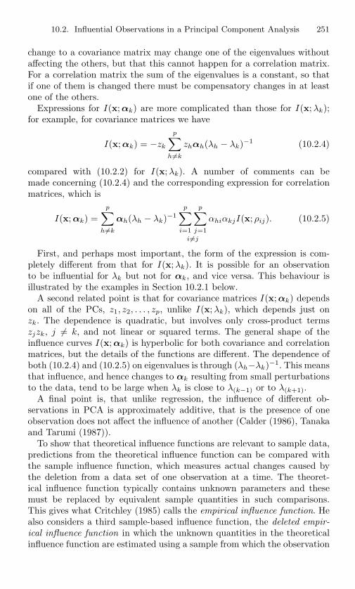
10.2. Influential Observations in a Principal Component Analysis 251
change to a covariance matrix may change one of the eigenvalues withoutaffecting the others, but that this cannot happen for a correlation matrix.For a correlation matrix the sum of the eigenvalues is a constant, so thatif one of them is changed there must be compensatory changes in at leastone of the others.
Expressions for I(x;αk) are more complicated than those for I(x;λk);for example, for covariance matrices we have
I(x;αk) = −zk
p∑
h=k
zhαh(λh − λk)−1 (10.2.4)
compared with (10.2.2) for I(x;λk). A number of comments can bemade concerning (10.2.4) and the corresponding expression for correlationmatrices, which is
I(x;αk) =p∑
h=k
αh(λh − λk)−1
p∑
i=1
p∑
j=1
i=j
αhiαkjI(x; ρij). (10.2.5)
First, and perhaps most important, the form of the expression is com-pletely different from that for I(x;λk). It is possible for an observationto be influential for λk but not for αk, and vice versa. This behaviour isillustrated by the examples in Section 10.2.1 below.
A second related point is that for covariance matrices I(x;αk) dependson all of the PCs, z1, z2, . . . , zp, unlike I(x;λk), which depends just onzk. The dependence is quadratic, but involves only cross-product termszjzk, j = k, and not linear or squared terms. The general shape of theinfluence curves I(x;αk) is hyperbolic for both covariance and correlationmatrices, but the details of the functions are different. The dependence ofboth (10.2.4) and (10.2.5) on eigenvalues is through (λh−λk)−1. This meansthat influence, and hence changes to αk resulting from small perturbationsto the data, tend to be large when λk is close to λ(k−1) or to λ(k+1).
A final point is, that unlike regression, the influence of different ob-servations in PCA is approximately additive, that is the presence of oneobservation does not affect the influence of another (Calder (1986), Tanakaand Tarumi (1987)).
To show that theoretical influence functions are relevant to sample data,predictions from the theoretical influence function can be compared withthe sample influence function, which measures actual changes caused bythe deletion from a data set of one observation at a time. The theoret-ical influence function typically contains unknown parameters and thesemust be replaced by equivalent sample quantities in such comparisons.This gives what Critchley (1985) calls the empirical influence function. Healso considers a third sample-based influence function, the deleted empir-ical influence function in which the unknown quantities in the theoreticalinfluence function are estimated using a sample from which the observation

252 10. Outlier Detection, Influential Observations and Robust Estimation
whose influence is to be assessed is omitted. The first example given in Sec-tion 10.2.1 below illustrates that the empirical influence function can givea good approximation to the sample influence function for moderate sam-ple sizes. Critchley (1985) compares the various influence functions from amore theoretical viewpoint.
A considerable amount of work was done in the late 1980s and early 1990son influence functions in multivariate analysis, some of which extends thebasic results for PCA given earlier in this section. Benasseni in France andTanaka and co-workers in Japan were particularly active in various aspectsof influence and sensitivity for a wide range of multivariate techniques.Some of their work on sensitivity will be discussed further in Section 10.3.
Tanaka (1988) extends earlier work on influence in PCA in two relatedways. The first is to explicitly consider the situation where there are equaleigenvalues—equations (10.2.4) and (10.2.5) break down in this case. Sec-ondly he considers influence functions for subspaces spanned by subsetsof PCs, not simply individual PCs. Specifically, if Aq is a matrix whosecolumns are a subset of q eigenvectors, and Λq is the diagonal matrix of cor-responding eigenvalues, Tanaka (1988) finds expressions for I(x;AqΛqA′
q)and I(x;AqA′
q). In discussing a general strategy for analysing influencein multivariate methods, Tanaka (1995) suggests that groups of observa-tions with similar patterns of influence across a set of parameters may bedetected by means of a PCA of the empirical influence functions for eachparameter.
Benasseni (1990) examines a number of measures for comparing principalcomponent subspaces computed with and without one of the observa-tions. After eliminating some possible measures such as the RV-coefficient(Robert and Escoufier, 1976) and Yanai’s generalized coefficient of deter-mination (Yanai, 1980) for being too insensitive to perturbations, he settleson
ρ1(i) = 1 −q∑
k=1
‖ak − P(i)ak‖q
and
ρ2(i) = 1 −q∑
k=1
‖ak(i) − Pak(i)‖q
where ak,ak(i) are eigenvectors with and without the ith observation,P,P(i) are projection matrices onto the subspaces derived with and withoutthe ith observation, and the summation is over the q eigenvectors withinthe subspace of interest. Benasseni (1990) goes on to find expressions forthe theoretical influence functions for these two quantities, which can thenbe used to compute empirical influences.
Reducing the comparison of two subspaces to a single measure inevitablyleads to a loss of information about the structure of the differences be-
10.2. Influential Observations in a Principal Component Analysis 253
tween the two. Ramsier (1991) introduces a graphical method, using ideassimilar to those of Andrews’ curves (see Section 5.6), in which curves re-presenting subspaces with and without individual observations omitted aredisplayed. It is not easy to deduce exactly how a particular change in sub-space structure is reflected in differences between curves. However, curvesplotted with an observation missing that are close to the curve for the fulldata set imply negligible influence on the subspace for that observation,and similarly shaped curves for different omitted observations suggest thatthese observations have similar detailed effects on the subspace’s structure.
Krzanowski (1987a) notes that the algorithm used by Eastment and Krz-anowski (1982) to decide how many components to retain (see Section 6.1.5)calculates elements of the singular value decomposition of the data matrixX with individual observations or variables omitted. It can therefore beused to evaluate the influence of each observation on the subspace spannedby however many components it has been decided to keep. Mertens et al.(1995) similarly use a cross-validation algorithm to give easily computedexpressions for the sample influence of observations on the eigenvalues ofa covariance matrix. They also provide a closed form expression for theangle between an eigenvector of that matrix using all the data and thecorresponding eigenvector when an observation is omitted. An example il-lustrating the use of these expressions for spectroscopic data is given byMertens (1998), together with some discussion of the relationships betweenmeasures of influence and outlyingness.
Wang and Nyquist (1991) provide a number of algebraic results, proofsand approximations relating eigenvalues and eigenvectors of covariance ma-trices with and without the removal of one of the n observations. Hadi andNyquist (1993) give improved approximations for eigenvalues, and Wangand Liski (1993) extend the results for both eigenvalues and eigenvectorsto the situation where more than one observation is removed. Comparisonsare made with Critchley’s (1985) results for the special case of a singledeleted observation.
Brooks (1994) uses simulation to address the question of when an ap-parently influential observation can be declared ‘significant.’ He points outthat the sample influence function (which he confusingly refers to as the‘empirical influence function’) for an observation xi depends on all theother observations in the sample, so that simulation of repeated values ofthis function under some null hypothesis needs whole samples to be gen-erated. The theoretical influence function can be evaluated more easilybecause equations (10.2.2)—(10.2.5) depend only on the eigenvalues andeigenvectors of the correlation or covariance matrix together with the singleobservation whose influence is to be assessed. Thus, if the sample correlationor covariance matrix is used as a surrogate for the corresponding populationmatrix, it is only necessary to simulate individual observations, rather thana whole new sample, in order to generate a value for this influence func-tion. Of course, any simulation study requires some assumption about the
254 10. Outlier Detection, Influential Observations and Robust Estimation
distribution from which the simulated data are generated. Brooks (1994)gives an example in which 1000 simulated observations are generated froma 7-variable multivariate normal distribution whose parameters are thoseestimated from the available sample of data. Empirical distributions of theestimated theoretical influence functions for eigenvalues and eigenvectors ofthe correlation matrix are constructed from the simulated observations bycomputing the values of these functions for each of the 1000 observations.The actual values of the functions for the same 7 anatomical variables aswere discussed in Sections 5.1.1 and 10.1, but for a different sample of 44students, are then compared to these distributions. Observations whose val-ues are in the upper 5% (1%) tails of the distributions can be considered tobe ‘significantly influential’ at the 5% (1%) level. Brooks (1994) finds that,on this basis, 10 of the 44 observations are significant at the 5% level formore than one of the 7 eigenvalues and/or eigenvectors. Brooks (1994) usesthe same reasoning to investigate ‘significantly influential’ observations ina two-dimensional principal component subspace based on Tanaka’s (1988)influence functions I(x;AqΛqA′
q) and I(x;AqA′q).
10.2.1 Examples
Two examples are now given, both using data sets that have been discussedearlier. In the first example we examine the usefulness of expressions fortheoretical influence in predicting the actual effect of omitting observationsfor the data on artistic qualities of painters described in Section 5.1.1. Asa second illustration, we follow up the suggestion, made in Section 10.1,that an outlier is largely responsible for the form of the second PC in thestudent anatomical data.
Artistic Qualities of Painters
We consider again the set of four subjectively assessed variables for 54painters, which was described by Davenport and Studdert-Kennedy (1972)and discussed in Section 5.1.1. Tables 10.2 and 10.3 give some comparisonsbetween the values of the influence functions obtained from expressionssuch as (10.2.2), (10.2.3), (10.2.4) and (10.2.5) by substituting sample quan-tities lk, akj , rij in place of the unknown λk, αkj , ρij , and the actual changesobserved in eigenvalues and eigenvectors when individual observations areomitted. The information given in Table 10.2 relates to PCs derived fromthe covariance matrix; Table 10.3 gives corresponding results for the cor-relation matrix. Some further explanation is necessary of exactly how thenumbers in these two tables are derived.
First, the ‘actual’ changes in eigenvalues are precisely that—the dif-ferences between eigenvalues with and without a particular observationincluded in the analysis. The tables give the four largest and four small-est such changes for each PC, and identify those observations for which
Table 10.2. Artistic qualities of painters: comparisons between estimated (empirical) and actual (sample) influence of individualobservations for the first two PCs, based on the covariance matrix.
Component number 1 2
Influence Influence
Eigenvalue Eigenvector Eigenvalue Eigenvector
Estimated Actual Obs. no. Estimated Actual Obs. no. Estimated Actual Obs. no. Estimated Actual Obs. no.
2.490 2.486 31 6.791 6.558 34 1.759 1.854 44 11.877 13.767 342.353 2.336 7 5.025 4.785 44 1.757 1.770 48 5.406 5.402 442.249 2.244 28 3.483 4.469 42 1.478 1.491 34 3.559 4.626 422.028 2.021 5 1.405 1.260 48 1.199 1.144 43 2.993 3.650 43...
......
......
......
......
......
...0.248 0.143 44 0.001 0.001 53 −0.073 −0.085 49 0.016 0.017 24
−0.108 −0.117 52 0.000 0.000 17 −0.090 −0.082 20 0.009 0.009 1−0.092 −0.113 37 0.000 0.000 24 0.039 0.045 37 0.000 0.001 30
0.002 −0.014 11 0.000 0.000 21 −0.003 −0.010 10 0.000 0.000 53
10.2. Influential Observations in a Principal Component Analysis 255

Table 10.3. Artistic qualities of painters: comparisons between estimated (empirical) and actual (sample) influence of individualobservations for the first two PCs, based on the correlation matrix.
Component number 1 2
Influence Influence
Eigenvalue Eigenvector Eigenvalue Eigenvector
Estimated Actual Obs. no. Estimated Actual Obs. no. Estimated Actual Obs. no. Estimated Actual Obs. no.
−0.075 −0.084 34 1.406 1.539 26 0.075 0.080 34 5.037 7.546 340.068 0.074 31 1.255 1.268 44 0.064 0.070 44 4.742 6.477 43
−0.067 −0.073 43 0.589 0.698 42 0.061 0.062 43 4.026 4.333 260.062 0.067 28 0.404 0.427 22 0.047 0.049 39 1.975 2.395 42...
......
......
......
......
......
...−0.003 −0.003 6 0.001 0.001 33 −0.001 −0.002 45 0.011 0.012 21−0.001 −0.001 32 0.000 0.000 53 −0.001 −0.001 14 0.010 0.012 38
0.001 0.001 11 0.000 0.000 30 −0.000 −0.001 42 0.001 0.001 300.001 0.001 13 0.000 0.000 21 −0.000 −0.000 11 0.001 0.001 53
256 10. Outlier Detection, Influential Observations and Robust Estimation
10.2. Influential Observations in a Principal Component Analysis 257
changes occur. The ‘estimated’ changes in eigenvalues given in Tables 10.2and 10.3 are derived from multiples of I(·) in (10.2.2), (10.2.3), respectively,with the value of the kth PC for each individual observation substituted forzk, and with lk, akj , rij replacing λk, αkj , ρij . The multiples are requiredbecause Change = Influence× ε, and we need a replacement for ε; here wehave used 1/(n − 1), where n = 54 is the sample size. Thus, apart from amultiplying factor (n − 1)−1, ‘actual’ and ‘estimated’ changes are sampleand empirical influence functions, respectively.
In considering changes to an eigenvector, there are changes to each ofthe p (= 4) coefficients in the vector. Comparing vectors is more difficultthan comparing scalars, but Tables 10.2 and 10.3 give the sum of squaresof changes in the individual coefficients of each vector, which is a plausiblemeasure of the difference between two vectors. This quantity is a mono-tonically increasing function of the angle in p-dimensional space betweenthe original and perturbed versions of ak, which further increases its plau-sibility. The idea of using angles between eigenvectors to compare PCs isdiscussed in a different context in Section 13.5.
The ‘actual’ changes for eigenvectors again come from leaving out oneobservation at a time, recomputing and then comparing the eigenvectors,while the estimated changes are computed from multiples of sample ver-sions of the expressions (10.2.4) and (10.2.5) for I(x;αk). The changes ineigenvectors derived in this way are much smaller in absolute terms thanthe changes in eigenvalues, so the eigenvector changes have been multipliedby 103 in Tables 10.2 and 10.3 in order that all the numbers are of com-parable size. As with eigenvalues, apart from a common multiplier we arecomparing empirical and sample influences.
The first comment to make regarding the results given in Tables 10.2 and10.3 is that the estimated values are extremely good in terms of obtain-ing the correct ordering of the observations with respect to their influence.There are some moderately large discrepancies in absolute terms for the ob-servations with the largest influences, but experience with this and severalother data sets suggests that the most influential observations are correctlyidentified unless sample sizes become very small. The discrepancies in ab-solute values can also be reduced by taking multiples other than (n− 1)−1
and by including second order (ε2) terms.A second point is that the observations which are most influential for
a particular eigenvalue need not be so for the corresponding eigenvector,and vice versa. For example, there is no overlap between the four mostinfluential observations for the first eigenvalue and its eigenvector in eitherthe correlation or covariance matrix. Conversely, observations can some-times have a large influence on both an eigenvalue and its eigenvector (seeTable 10.3, component 2, observation 34).
Next, note that observations may be influential for one PC only, or affecttwo or more. An observation is least likely to affect more than one PC inthe case of eigenvalues for a covariance matrix—indeed there is no over-
258 10. Outlier Detection, Influential Observations and Robust Estimation
lap between the four most influential observations for the first and secondeigenvalues in Table 10.2. However, for eigenvalues in a correlation matrix,more than one value is likely to be affected by a very influential observa-tion, because the sum of eigenvalues remains fixed. Also, large changes inan eigenvector for either correlation or covariance matrices result in at leastone other eigenvector being similarly changed, because of the orthogonalityconstraints. These results are again reflected in Tables 10.2 and 10.3, withobservations appearing as influential for both of the first two eigenvectors,and for both eigenvalues in the case of the correlation matrix.
Comparing the results for covariance and correlation matrices in Ta-bles 10.2 and 10.3, we see that several observations are influential for bothmatrices. This agreement occurs because, in the present example, the orig-inal variables all have similar variances, so that the PCs for correlationand covariance matrices are similar. In examples where the PCs based oncorrelation and covariance matrices are very different, the sets of influentialobservations for the two analyses often show little overlap.
Turning now to the observations that have been identified as influentialin Table 10.3, we can examine their positions with respect to the first twoPCs on Figures 5.2 and 5.3. Observation 34, which is the most influentialobservation on eigenvalues 1 and 2 and on eigenvector 2, is the painter indi-cated in the top left of Figure 5.2, Fr. Penni. His position is not particularlyextreme with respect to the first PC, and he does not have an unduly largeinfluence on its direction. However, he does have a strong influence on boththe direction and variance (eigenvalue) of the second PC, and to balance theincrease which he causes in the second eigenvalue there is a compensatorydecrease in the first eigenvalue. Hence, he is influential on that eigenvaluetoo. Observation 43, Rembrandt, is at the bottom of Figure 5.2 and, likeFr. Penni, has a direct influence on PC2 with an indirect but substantialinfluence on the first eigenvalue. The other two observations, 28 and 31,Caravaggio and Palma Vecchio, which are listed in Table 10.3 as being in-fluential for the first eigenvalue, have a more direct effect. They are the twoobservations with the most extreme values on the first PC and appear atthe extreme left of Figure 5.2.
Finally, the observations in Table 10.3 that are most influential on thefirst eigenvector, two of which also have large values of influence for thesecond eigenvector, appear on Figure 5.2 in the second and fourth quadrantsin moderately extreme positions.
Student Anatomical Measurements
In the discussion of the data on student anatomical measurements in Sec-tion 10.1 it was suggested that observation 16 is so extreme on the secondPC that it could be largely responsible for the direction of that component.Looking at influence functions for these data enables us to investigate thisconjecture. Not surprisingly, observation 16 is the most influential observa-

10.3. Sensitivity and Stability 259
tion for the second eigenvector and, in fact, has an influence nearly six timesas large as that of the second most influential observation. It is also themost influential on the first, third and fourth eigenvectors, showing that theperturbation caused by observation 16 to the second PC has a ‘knock-on’effect to other PCs in order to preserve orthogonality. Although observation16 is very influential on the eigenvectors, its effect is less marked on theeigenvalues. It has only the fifth highest influence on the second eigenvalue,though it is highest for the fourth eigenvalue, second highest for the first,and fourth highest for the third. It is clear that values of influence on eigen-values need not mirror major changes in the structure of the eigenvectors,at least when dealing with correlation matrices.
Having said that observation 16 is clearly the most influential, for eigen-vectors, of the 28 observations in the data set, it should be noted that itsinfluence in absolute terms is not outstandingly large. In particular, the co-efficients rounded to one decimal place for the second PC when observation16 is omitted are
0.2 0.1 − 0.4 0.8 − 0.1 − 0.3 − 0.2.
The corresponding coefficients when all 28 observations are included are
−0.0 − 0.2 − 0.2 0.9 − 0.1 − 0.0 − 0.0.
Thus, when observation 16 is removed, the basic character of PC2 as mainlya measure of head size is unchanged, although the dominance of head sizein this component is reduced. The angle between the two vectors definingthe second PCs, with and without observation 16, is about 24, which isperhaps larger than would be deduced from a quick inspection of the sim-plified coefficients above. Pack et al. (1988) give a more thorough discussionof influence in the context of this data set, together with similar data setsmeasured on different groups of students (see also Brooks (1994)). A prob-lem that does not arise in the examples discussed here, but which does inPack et al.’s (1988) larger example, is the possibility that omission of anobservation causes switching or rotation of eigenvectors when consecutiveeigenvalues have similar magnitudes. What appear to be large changes ineigenvectors may be much smaller when a possible reordering of PCs inthe modified PCA is taken into account. Alternatively, a subspace of twoor more PCs may be virtually unchanged when an observation is deleted,but individual eigenvectors spanning that subspace can look quite different.Further discussion of these subtleties in the context of an example is givenby Pack et al. (1988).
10.3 Sensitivity and Stability
Removing a single observation and estimating its influence explores onetype of perturbation to a data set, but other perturbations are possible. In

260 10. Outlier Detection, Influential Observations and Robust Estimation
one the weights of one or more observations are reduced, without removingthem entirely. This type of ‘sensitivity’ is discussed in general for multivari-ate techniques involving eigenanalyses by Tanaka and Tarumi (1985, 1987),with PCA as a special case. Benasseni (1986a) also examines the effect ofdiffering weights for observations on the eigenvalues in a PCA. He givesbounds on the perturbed eigenvalues for any pattern of perturbations ofthe weights for both covariance and correlation-based analyses. The workis extended in Benasseni (1987a) to include bounds for eigenvectors as wellas eigenvalues. A less structured perturbation is investigated empiricallyby Tanaka and Tarumi (1986). Here each element of a (4×4) ‘data’ matrixhas an independent random perturbation added to it.
In Tanaka and Mori (1997), where the objective is to select a subsetof variables reproducing all the p variables as well as possible and hencehas connections with Section 6.3, the influence of variables is discussed.Fujikoshi et al. (1985) examine changes in the eigenvalues of a covariancematrix when additional variables are introduced. Krzanowski (1987a) in-dicates how to compare data configurations given by sets of retained PCs,including all the variables and with each variable omitted in turn. Thecalculations are done using an algorithm for computing the singular valuedecomposition (SVD) with a variable missing, due to Eastment and Krza-nowski (1982), and the configurations are compared by means of Procrustesrotation (see Krzanowski and Marriott 1994, Chapter 5). Holmes-Junca(1985) gives an extensive discussion of the effect of omitting observationsor variables from a PCA. As in Krzanowski (1987a), the SVD plays a promi-nent role, but the framework in Holmes-Junca (1985) is a more general onein which unequal weights may be associated with the observations, and ageneral metric may be associated with the variables (see Section 14.2.2).
A different type of stability is investigated by Benasseni (1986b). He con-siders replacing each of the n p-dimensional observations in a data set bya p-dimensional random variable whose probability distribution is centredon the observed value. He relates the covariance matrix in the perturbedcase to the original covariance matrix and to the covariance matrices ofthe n random variables. From this relationship, he deduces bounds on theeigenvalues of the perturbed matrix. In a later paper, Benasseni (1987b)looks at fixed, rather than random, perturbations to one or more of theobservations. Expressions are given for consequent changes to eigenvaluesand eigenvectors of the covariance matrix, together with approximationsto those changes. A number of special forms for the perturbation, for ex-ample where it affects only one of the p variables, are examined in detail.Corresponding results for the correlation matrix are discussed briefly.
Dudzinski et al. (1975) discuss what they call ‘repeatability’ of principalcomponents in samples, which is another way of looking at the stabilityof the components’ coefficients. For each component of interest the angleis calculated between the vector of coefficients in the population and thecorresponding vector in a sample. Dudzinski et al. (1975) define a repeata-
10.3. Sensitivity and Stability 261
bility index as the proportion of times in repeated samples that this anglehas a cosine whose value is greater than 0.95. They conduct a simulationstudy to examine the dependence of this index on sample size, on the ratioof consecutive population eigenvalues, and on whether or not the data arenormally distributed. To generate non-normal samples, Dudzinski and re-searchers use the bootstrap idea of sampling with replacement from a dataset that is clearly non-normal. This usage predates the first appearanceof the term ‘bootstrap.’ Their simulation study is relatively small, but itdemonstrates that repeatability is often greater for normal than for non-normal data with the same covariance structure, although the differencesare usually small for the cases studied and become very small as the re-peatability increases with sample size. Repeatability, as with other formsof stability, decreases as consecutive eigenvalues become closer.
Dudzinski et al. (1975) implemented a bootstrap-like method for assess-ing stability. Daudin et al. (1988) use a fully-fledged bootstrap and, in fact,note that more than one bootstrapping procedure may be relevant in re-sampling to examine the properties of PCA, depending in part on whethera correlation-based or covariance- based analysis is done. They consider anumber of measures of stability for both eigenvalues and eigenvectors, butthe stability of subspaces spanned by subsets of PCs is deemed to be ofparticular importance. This idea is used by Besse (1992) and Besse and deFalguerolles (1993) to choose how many PCs to retain (see Section 6.1.5).Stability indices based on the jackknife are also used by the latter au-thors, and Daudin et al. (1989) discuss one such index in detail for bothcorrelation- and covariance-based PCA. Besse and de Falguerolles (1993)describe the equally weighted version of the criterion (6.1.6) as a naturalcriterion for stability, but prefer
Lq =12‖Pq − Pq‖2
in equation (6.1.9). Either (6.1.6) or the expectation of Lq can be used as ameasure of the stability of the first q PCs or the subspace spanned by them,and q is then chosen to optimize stability. Besse and de Falguerolles (1993)discuss a variety of ways of estimating their stability criterion, includingsome based on the bootstrap and jackknife. The bootstrap has also beenused to estimate standard errors of elements of the eigenvectors ak (seeSection 3.7.2), and these standard errors can be viewed as further measuresof stability of PCs, specifically the stability of their coefficients.
Stauffer et al. (1985) conduct a study that has some similarities to that ofDudzinski et al. (1975). They take bootstrap samples from three ecologicaldata sets and use them to construct standard errors for the eigenvalues ofthe correlation matrix. The stability of the eigenvalues for each data setis investigated when the full data set is replaced by subsets of variablesor subsets of observations. Each eigenvalue is examined as a percentage ofvariation remaining after removing earlier PCs, as well as in absolute terms.
262 10. Outlier Detection, Influential Observations and Robust Estimation
Comparisons are made with corresponding results derived from ‘random,’that is uncorrelated, data sets of the same size as the real data sets. This isdone with an objective similar to that of parallel analysis (see Section 6.1.3)in mind.
A different approach to influence from that described in Section 10.2 wasproposed by Cook (1986) and called local influence. Shi (1997) developsthese ideas in the context of PCA. It is included in this section rather thanin 10.2 because, as with Tanaka and Tarumi (1985, 1987) and Benasseni(1986a, 1987a) weights are attached to each observation, and the weightsare varied. In Shi’s (1997) formulation the ith observation is expressed as
xi(w) = wi(xi − x),
and w = (w1, w2, . . . , wn)′ is a vector of weights. The vector w0 =(1, 1, . . . , 1)′ gives the unperturbed data, and Shi considers perturbations ofthe form w = w0+εh, where h is a fixed unit-length vector. The generalizedinfluence function for a functional θ is defined as
GIF(θ,h) = limε→0
θ(w0 + εh) − θ(w0)ε
.
For a scalar θ, such as an eigenvalue, local influence investigates the di-rection h in which GIF(θ,h) is maximized. For a vector θ, such as aneigenvector, GIF(.) is converted into a scalar (a norm) via a quadraticform, and then h is found for which this norm is maximized.
Yet another type of stability is the effect of changes in the PC coefficientsak on their variances lk and vice versa. Bibby (1980) and Green (1977)both consider changes in variances, and other aspects such as the non-orthogonality of the changed ak when the elements of ak are rounded. Thisis discussed further in Section 11.3.
Krzanowski (1984b) considers what could be thought of as the oppositeproblem to that discussed by Bibby (1980). Instead of looking at the effectof small changes in ak on the value of lk, Krzanowski (1984b) examinesthe effect of small changes in the value of lk on ak, although he addressesthe problem in the population context and hence works with αk and λk.He argues that this is an important problem because it gives informationon another aspect of the stability of PCs: the PCs can only be confidentlyinterpreted if their coefficients are stable with respect to small changes inthe values of the λk.
If λk is decreased by an amount ε, then Krzanowski (1984b) looks fora vector αε
k that is maximally different from αk, subject to var(α′εk x) =
λk − ε. He finds that the angle θ between αk and αεk is given by
cos θ = [1 +ε
(λk − λk+1)]−1/2, (10.3.1)
and so depends mainly on the difference between λk and λk+1. If λk, λk+1
are close, then the kth PC, α′kx = zk, is more unstable than if λk, λk+1 are
10.4. Robust Estimation of Principal Components 263
well separated. A similar analysis can be carried out if λk is increased byan amount ε, in which case the stability of zk depends on the separationbetween λk and λk−1. Thus, the stability of a PC depends on the sepa-ration of its variance from the variances of adjacent PCs, an unsurprisingresult, especially considering the discussion of ‘influence’ in Section 10.2.The ideas in Section 10.2 are, as here, concerned with how perturbationsaffect αk, but they differ in that the perturbations are deletions of individ-ual observations, rather than hypothetical changes in λk. Nevertheless, wefind in both cases that the changes in αk are largest if λk is close to λk+1
or λk−1 (see equations (10.2.4) and (10.2.5)).As an example of the use of the sample analogue of the expression
(10.3.1), consider the PCs presented in Table 3.2. Rounding the coeffi-cients in the PCs to the nearest 0.2 gives a change of 9% in l1 and changesthe direction of a1 through an angle of about 8 (see Section 11.3). We canuse (10.3.1) to find the maximum angular change in a1 that can occur ifl1 is decreased by 9%. The maximum angle is nearly 25, so that roundingthe coefficients has certainly not moved a1 in the direction of maximumsensitivity.
The eigenvalues l1, l2 and l3 in this example are 2.792, 1.532 and 1.250,respectively, so that the separation between l1 and l2 is much greater thanthat between l2 and l3. The potential change in a2 for a given decrease inl2 is therefore larger than that for a1, given a corresponding decrease in l1.In fact, the same percentage decrease in l2 as that investigated above forl1 leads to a maximum angular change of 35; if the change is made thesame in absolute (rather than percentage) terms, then the maximum anglebecomes 44.
10.4 Robust Estimation of Principal Components
It has been noted several times in this book that for PCA’s main (descrip-tive) role, the form of the distribution of x is usually not very important.The main exception to this statement is seen in the case where outliersmay occur. If the outliers are, in fact, influential observations, they willhave a disproportionate effect on the PCs, and if PCA is used blindly inthis case, without considering whether any observations are influential, thenthe results may be largely determined by such observations. For example,suppose that all but one of the n observations lie very close to a planewithin p-dimensional space, so that there are two dominant PCs for these(n− 1) observations. If the distance of the remaining observation from theplane is greater than the variation of the (n − 1) observations within theplane, then the first component for the n observations will be determinedsolely by the direction of the single outlying observation from the plane.This, incidentally, is a case where the first PC, rather than last few, will

264 10. Outlier Detection, Influential Observations and Robust Estimation
detect the outlier (see Section 10.1), but if the distance from the plane islarger than distances within the plane, then the observation is likely to‘stick out’ on at least one of the original variables as well.
To avoid such problems, it is possible to use robust estimation of thecovariance or correlation matrix, and hence of the PCs. Such estimationdownweights or discards the effect of any outlying observations. Five ro-bust estimators using three different approaches are investigated by Devlinet al. (1981). The first approach robustly estimates each element of thecovariance or correlation matrix separately and then ‘shrinks’ the elementsto achieve positive-definiteness if this is not achieved with the initial esti-mates. The second type of approach involves robust regression of xj on(x1, x2, . . . , xj−1) for j = 2, 3, . . . , p. An illustration of the robust regressionapproach is presented for a two-variable example by Cleveland and Guarino(1976). Finally, the third approach has three variants; in one (multivariatetrimming) the observations with the largest Mahalanobis distances Di froma robust estimate of the mean of x are discarded, and in the other two theyare downweighted. One of these variants is used by Coleman (1985) in thecontext of quality control. Both of the downweighting schemes are examplesof so-called M-estimators proposed by Maronna (1976). One is the max-imum likelihood estimator for a p-variate elliptical t distribution, whichhas longer tails than the multivariate normal distribution for which theusual non-robust estimate is optimal. The second downweighting schemeuses Huber weights (1964, 1981) which are constant for values of Di up toa threshold D∗
i , and equal to D∗i /Di thereafter.
All but the first of these five estimates involve iteration; full details aregiven by Devlin et al. (1981), who also show that the usual estimator ofthe covariance or correlation matrix can lead to misleading PCs if outlyingobservations are included in the analysis. Of the five possible robust alter-natives which they investigate, only one, that based on robust regression,is clearly dominated by other methods, and each of the remaining four maybe chosen in some circumstances.
Robust estimation of covariance matrices, using an iterative procedurebased on downweighting observations with large Mahalanobis distance fromthe mean, also based on M -estimation, was independently described byCampbell (1980). He uses Huber weights and, as an alternative, a so-calledredescending estimate in which the weights decrease more rapidly than Hu-ber weights for values of Di larger than the threshold D∗
i . Campbell (1980)notes that, as a by-product of robust estimation, the weights given to eachdata point give an indication of potential outliers. As the weights are non-increasing functions of Mahalanobis distance, this procedure is essentiallyusing the statistic d2
2i, defined in Section 10.1, to identify outliers, exceptthat the mean and covariance matrix of x are estimated robustly in thepresent case.
Other methods for robustly estimating covariance or correlation matriceshave been suggested since Devlin et al.’s (1981) work. For example, Mehro-
10.4. Robust Estimation of Principal Components 265
tra (1995) proposes a new elementwise estimate, and compares it to Devlinet al.’s (1981) estimates via a simulation study whose structure is the sameas that of Devlin and co-workers. Maronna and Yohai (1998) review manyof the robust covariance estimators. As Croux and Haesbroek (2000) pointout, every new robust covariance matrix estimator has a new robust PCAmethod associated with it.
Campbell (1980) also proposed a modification of his robust estimationtechnique in which the weights assigned to an observation, in estimatingthe covariance matrix, are no longer functions of the overall Mahalanobisdistance of each observation from the mean. Instead, when estimating thekth PC, the weights are a decreasing function of the absolute value ofthe score of each observation for the kth PC. As with most of the tech-niques tested by Devlin et al. (1981), the procedure is iterative and thealgorithm to implement it is quite complicated, with nine separate steps.However, Campbell (1980) and Matthews (1984) each give an example forwhich the technique works well, and as well as estimating the PCs robustly,both authors use the weights found by the technique to identify potentialoutliers.
The discussion in Section 10.2 noted that observations need not be partic-ularly ‘outlying’ in order to be influential. Thus, robust estimation methodsthat give weights to each observation based on Mahalanobis distance will‘miss’ any influential observations that are not extreme with respect to Ma-halanobis distance. It would seem preferable to downweight observationsaccording to their influence, rather than their Mahalanobis distance. As yet,no systematic work seems to have been done on this idea, but it should benoted that the influence function for the kth eigenvalue of a covariancematrix is an increasing function of the absolute score on the kth PC (seeequation (10.2.2)). The weights used in Campbell’s (1980) procedure there-fore downweight observations according to their influence on eigenvalues(though not eigenvectors) of the covariance (but not correlation) matrix.
It was noted above that Devlin et al. (1981) and Campbell (1980) useM -estimators in some of their robust PCA estimates. A number of otherauthors have also considered M -estimation in the context of PCA. For ex-ample, Daigle and Rivest (1992) use it to construct a robust version of thebiplot (see Section 5.3). Ibazizen (1986) gives a thorough discussion of anM -estimation approach to robust PCA in which the definition of the firstrobust PC is based on a robust version of Property A5 in Section 2.1. Thisproperty implies that the first PC minimizes the sum of residual variancesarising from predicting each variable from the same single linear function ofthe variables. Each variance is an expected squared difference between thevariable and its mean. To robustify this quantity the mean is replaced bya robust estimator of location, and the square of the difference is replacedby another function, namely one of those typically chosen in M -estimation.Ibazizen (1986) includes a substantial amount of underlying theory for thisrobust PC, together with details of an algorithm to implement the proce-
266 10. Outlier Detection, Influential Observations and Robust Estimation
dure for both the first and suitably defined second, third, . . . robust PCs.Xu and Yuille (1995) present a robust PCA using a ‘statistical physics’ ap-proach within a neural network framework (see Sections 14.1.3, 14.6.1). Thefunction optimized in their algorithm can be regarded as a generalizationof a robust redescending M -estimator.
Locantore et al. (1999) discuss robust PCA for functional data (see Sec-tion 12.3). In fact, their data are images rather than functions, but apre-processing step turns them into functions. Both means and covariancematrices are robustly estimated, the latter by shrinking extreme observa-tions to the nearest point on the surface of a hypersphere or hyperellipsoidcentred at the robustly estimated mean, a sort of multivariate Winsoriza-tion. Locantore et al.’s (1999) paper is mainly a description of an interestingcase study in opthalmology, but it is followed by contributions from 9 setsof discussants, and a rejoinder, ranging over many aspects of robust PCAin a functional context and more generally.
A different type of approach to the robust estimation of PCs is discussedby Gabriel and Odoroff (1983). The approach relies on the fact that PCsmay be computed from the singular value decomposition (SVD) of the(n × p) data matrix X (see Section 3.5 and Appendix Al). To find theSVD, and hence the PCs, a set of equations involving weighted meansof functions of the elements of X must be solved iteratively. Replacingthe weighted means by medians, weighted trimmed means, or some othermeasure of location which is more robust than the mean leads to estimatesof PCs that are less sensitive than the usual estimates to the presence of‘extreme’ observations.
Yet another approach, based on ‘projection pursuit,’ is proposed by Liand Chen (1985). As with Gabriel and Odoroff (1983), and unlike Camp-bell (1980) and Devlin et al. (1981), the PCs are estimated directly withoutfirst finding a robustly estimated covariance matrix. Indeed, Li and Chensuggest that it may be better to estimate the covariance matrix Σ fromthe robust PCs via the spectral decomposition (see Property A3 of Sec-tions 2.1 and 3.1), rather than estimating Σ directly. Their idea is to findlinear functions of x that maximize a robust estimate of scale, rather thanfunctions that maximize variance. Properties of their estimates are inves-tigated, and the estimates’ empirical behaviour is compared with that ofDevlin et al. (1981)’s estimates using simulation studies. Similar levels ofperformance are found for both types of estimate, although, as noted byCroux and Haesbroeck (2000), methods based on robust estimation of co-variance matrices have poor properties for large values of p and projectionpursuit-based techniques may be preferred in such cases. One disadvantageof Li and Chen’s (1985) approach is that it is complicated to implement.Both Xie et al. (1993) and Croux and Ruiz-Gazen (1995) give improvedalgorithms for doing so.
Another way of ‘robustifying’ PCA directly, rather than doing so viaa robust covariance or correlation matrix, is described by Baccini et al.

10.4. Robust Estimation of Principal Components 267
(1996). When the unweighted version of the fixed effects model of Sec-tion 3.9 assumes a multivariate normal distribution for its error termei, maximum likelihood estimation of the model leads to the usual PCs.However, if the elements of ei are instead assumed to be independentLaplace random variables with probability density functions f(eij) =12σ exp(− 1
σ |eij |), maximum likelihood estimation requires the minimizationof∑n
i=1
∑pj=1 |xij −zij |, leading to an L1-norm variant of PCA. Baccini et
al. (1996) show that the L1-norm PCs can be estimated using a canonicalcorrelation analysis (see Section 9.3) of the original variables and rankedversion of the variables. Although by no means a robust method, it seemsnatural to note here the minimax approach to component analysis pro-posed by Bargmann and Baker (1977). Whereas PCA minimizes the sum ofsquared discrepancies between xij and a rank-m approximation, and Bac-cini et al. (1996) minimize the sum of absolute discrepencies, Bargmann andBaker (1977) suggest minimizing the maximum discrepancy. They providearguments to justify the procedure, but it is clearly sensitive to extremeobservations and could even be thought of as ’anti-robust.’
A different, but related, topic is robust estimation of the distribution ofthe PCs, their coefficients and their variances, rather than robust estima-tion of the PCs themselves. It was noted in Section 3.6 that this can bedone using bootstrap estimation (Diaconis and Efron, 1983). The ‘shape’of the estimated distributions should also give some indication of whetherany highly influential observations are present in a data set (the distribu-tions may be multimodal, corresponding to the presence or absence of theinfluential observations in each sample from the data set), although themethod will not directly identify such observations.
The ideas of robust estimation and influence are brought together inJaupi and Saporta (1993), Croux and Haesbroeck (2000) and Croux andRuiz-Gazen (2001). Given a robust PCA, it is of interest to examine in-fluence functions for the results of such an analysis. Jaupi and Saporta(1993) investigate influence for M-estimators, and Croux and Haesbroek(2000) extend these results to a much wider range of robust PCAs for bothcovariance and correlation matrices. Croux and Ruiz-Gazen (2001) deriveinfluence functions for Li and Chen’s (1985) projection pursuit-based ro-bust PCA. Croux and Haesbroeck (2000) also conduct a simulation studyusing the same structure as Devlin et al. (1981), but with a greater range ofrobust procedures included. They recommend the S-estimator, describedin Rousseeuw and Leroy (1987, p. 263) for practical use.
Naga and Antille (1990) explore the stability of PCs derived from robustestimators of covariance matrices, using the measure of stability definedby Daudin et al. (1988) (see Section 10.3). PCs derived from covarianceestimators based on minimum variance ellipsoids perform poorly with re-spect to this type of stability on the data sets considered by Naga andAntille (1990), but those associated with M -estimated covariance matricesare much better.
268 10. Outlier Detection, Influential Observations and Robust Estimation
Finally, we mention that Ruymgaart (1981) discusses a class of robust PCestimators. However, his discussion is restricted to bivariate distributions(that is p = 2) and is entirely theoretical in nature. Ibazizen (1986) suggeststhat it would be difficult to generalize Ruymgaart’s (1981) ideas to morethan two dimensions.
10.5 Concluding Remarks
The topics discussed in this chapter pose difficult problems in data analysis.Much research has been done and is continuing on all of them. It is usefulto identify potentially outlying observations, and PCA provides a numberof ways of doing so. Similarly, it is important to know which observationshave the greatest influence on the results of a PCA.
Identifying potential outliers and influential observations is, however,only part of the problem; the next, perhaps more difficult, task is to de-cide whether the most extreme or influential observations are sufficientlyextreme or influential to warrant further action and, if so, what that actionshould be. Tests of significance for outliers were discussed only briefly inSection 10.1 because they are usually only approximate, and tests of signif-icance for influential observations in PCA have not yet been widely used.Perhaps the best advice is that observations that are much more extreme orinfluential than most of the remaining observations in a data set should bethoroughly investigated, and explanations sought for their behaviour. Theanalysis could also be repeated with such observations omitted, althoughit may be dangerous to act as if the deleted observations never existed.Robust estimation provides an automatic way of dealing with extreme (orinfluential) observations but, if at all possible, it should be accompaniedby a careful examination of any observations that have been omitted orsubstantially downweighted by the analysis.

11Rotation and Interpretation ofPrincipal Components
It was noted earlier, especially in Chapter 4, that PCs are particularlyuseful if they can be simply interpreted. The word reification is sometimesused for this process of interpretation, and a number of examples have beenseen in previous chapters for which this has been successful. However, theconstruction of PCs as linear combinations of all the measured variablesmeans that interpretation is not always easy. Various suggestions have beenmade to simplify the process of interpretation. These are the subject of thischapter.
One way to aid interpretation is to rotate the components, as is donewith the factor loadings in factor analysis (see Chapter 7). Rotation of PCsis discussed in Section 11.1. The approach can provide useful simplificationin some cases, but it has a number of drawbacks, and some alternativeapproaches are described. In one the two steps of PCA followed by rotationare replaced by a single optimization problem which takes into account bothvariance maximization and simplicity. In others simplification criteria areemphasized at the expense of variance maximization.
Section 11.2 describes some alternatives to PCA which aim to providesimpler ‘components.’ Some techniques restrict the coefficients of the vari-ables in each component to integer values, whilst another drives some of thecoefficients to zero. The purpose of these techniques is to provide replace-ments for PCs that are simpler to interpret, but which do not sacrificemuch variance. In other circumstances, the objective may be to approx-imate the PCs in a way which makes them simpler to interpret, againwithout much loss of variance. The most common way of doing this is toignore (effectively set to zero) coefficients whose absolute values fall below
270 11. Rotation and Interpretation of Principal Components
some threshold. There are links here to variable selection (see Section 6.3).This strategy and some of the problems associated with it are discussedin Section 11.3, and the chapter concludes with a short section on the de-sire in some disciplines to attach physical interpretations to the principalcomponents.
11.1 Rotation of Principal Components
In Chapter 7 it was seen that rotation is an integral part of factor analysis,with the objective of making the rotated factors as simple as possible tointerpret. The same ideas can be used to simplify principal components.A principal component is a linear function of all the p original variables.If the coefficients or loadings for a PC are all of a similar size, or if a feware large and the remainder small, the component looks easy to interpret,although, as will be seen in Section 11.3, looks can sometimes be deceiving.Several examples in Chapter 4 are like this, for instance, components 1 and2 in Section 4.1. If there are intermediate loadings, as well as large andsmall ones, the component can be more difficult to interpret, for example,component 4 in Table 7.1.
Suppose that it has been decided that the first m components accountfor most of the variation in a p-dimensional data set. It can then be ar-gued that it is more important to interpret simply the m-dimensional spacedefined by these m components than it is to interpret each individual com-ponent. One way to tackle this objective is to rotate the axes within thism-dimensional space in a way that simplifies the interpretation of the axesas much as possible. More formally, suppose that Am is the (p×m) matrixwhose kth column is the vector of loadings for the kth PC. Following simi-lar steps to those in factor analysis (see Section 7.2), orthogonally rotatedPCs have loadings given by the columns of Bm, where Bm = AmT, andT is a (m × m) orthogonal matrix. The matrix T is chosen so as to opti-mize one of many simplicity criteria available for factor analysis. Rotationof PCs is commonplace in some disciplines, such as atmospheric science,where there has been extensive discussion of its advantages and disadvan-tages (see, for example Richman (1986, 1987); Jolliffe (1987b); Rencher(1995, Section 12.8.2)). Oblique, instead of orthogonal, rotation is possible,and this gives extra flexibility (Cohen, 1983; Richman, 1986). As noted inChapter 7, the choice of simplicity criterion is usually less important thanthe choice of m, and in the examples of the present chapter only the well-known varimax criterion is used (see equation (7.2.2)). Note, however, thatJackson (1991, Section 8.5.1) gives an example in which the results fromtwo orthogonal rotation criteria (varimax and quartimax) have non-trivialdifferences. He states that neither is helpful in solving the problem that hewishes to address for his example.
11.1. Rotation of Principal Components 271
It is certainly possible to simplify interpretion of PCs by using rotation.For example, Table 7.2 gives two versions of rotated loadings for the firstfour PCs in a study of scores on 10 intelligence tests for 150 children fromthe Isle of Wight. The two versions correspond to varimax rotation andto an oblique rotation criterion, direct quartimin. The unrotated loadingsare given in Table 7.1. The type of simplicity favoured by almost all ro-tation criteria attempts to drive loadings towards zero or towards theirmaximum possible absolute value, which with most scalings of the loadingsis 1. The idea is that it should then be clear which variables are ‘impor-tant’ in a (rotated) component, namely, those with large absolute valuesfor their loadings, and those which are not important (loadings near zero).Intermediate-value loadings, which are difficult to interpret, are avoidedas much as possible by the criteria. Comparing Tables 7.1 and 7.2, it isapparent that this type of simplicity has been achieved by rotation.
There are other types of simplicity. For example, the first unrotatedcomponent in Table 7.1 has all its loadings of similar magnitude and thesame sign. The component is thus simple to interpret, as an average ofscores on all ten tests. This type of simplicity is shunned by most rotationcriteria, and it is difficult to devise a criterion which takes into account morethan one type of simplicity, though Richman (1986) attempts to broadenthe definition of simple structure by graphical means.
In the context of PCA, rotation has a number of drawbacks:
• A choice has to made from a large number of possible rotation criteria.Cattell (1978) and Richman (1986), respectively, give non-exhaustivelists of 11 and 19 such criteria. Frequently, the choice is made arbitrar-ily, for example by using the default criterion in a computer package(often varimax). Fortunately, as noted already, different choices of cri-teria, at least within orthogonal rotation, often make little differenceto the results.
• PCA successively maximizes variance accounted for. When rotationis done, the total variance within the rotated m-dimensional subspaceremains unchanged; it is still the maximum that can be achieved, butit is redistributed amongst the rotated components more evenly thanbefore rotation. This means that information about the nature ofany really dominant components may be lost, unless they are already‘simple’ in the sense defined by the chosen rotation criterion.
• The choice of m can have a large effect on the results after rotation.This is illustrated in Tables 7.4 and 7.2 when moving from m = 3to m = 4 for the children’s intelligence example. Interpreting the‘most important dimensions’ for a data set is clearly harder if those‘dimensions’ appear, disappear, and possibly reappear, as m changes.
• The choice of normalization constraint used for the columns in thematrix Am changes the properties of the rotated loadings. From the
272 11. Rotation and Interpretation of Principal Components
theory of PCA, it is natural to expect the columns of Am to benormalized so as to have unit length, but it is far more commonin computer packages to rotate a matrix Am whose columns havelengths equal to their corresponding eigenvalues, as in the sampleversion of equation (2.3.2). The main reason for this convention isalmost certainly due to the fact that it has been borrowed from factoranalysis. This is discussed further later in this section, but first theproperties associated with the rotated components under these twonormalizations are explored.
In PCA the components possess two ‘orthogonality’ properties. First
A′mAm = Im, (11.1.1)
where Im is the identity matrix of order m. Hence, the vectors of loadings fordifferent components are orthogonal. Second, if A and Z are, as in previouschapters, the (p×p) matrix of loadings or coefficients and the (n×p) matrixof scores, respectively, for all p PCs, and L2, as in Chapter 5, is the diagonalmatrix whose elements are eigenvalues of X′X, then
Z′Z = A′X′XA = A′AL2A′A = L2. (11.1.2)
The second equality in (11.1.2) follows from the algebra below equation(5.3.6), and the last equality is a result of the orthogonality of A. Theimplication of this result is that all the p unrotated components, includingthe first m, are uncorrelated with other.
The fact that orthogonality of vectors of loadings and uncorrelatednessof component scores both hold for PCs is because the loadings are given byeigenvectors of the covariance matrix S corresponding to the result for Σin Section 1.1. After rotation, one or both of these properties disappears.Let Zm = XAm be the (n×m) matrix of PC scores for n observations onthe first m PCs, so that
ZRm = XBm = XAmT = ZmT (11.1.3)
is the corresponding matrix of rotated PC scores. Consider
B′mBm = T′A′
mAmT, (11.1.4)
and
Z′Rm ZR
m = T′Z′mZmT. (11.1.5)
With the usual PCA normalization a′kak = 1, or A′
mAm = Im, equation(11.1.4) becomes T′T, which equals Im for orthogonal rotation. However,if L2
m is the (m × m) submatrix of L2 consisting of its first m rows andcolumns then, from (11.1.2), equation (11.1.5) becomes T′L2
mT, which isnot diagonal. Hence the rotated components using this normalization haveorthogonal loadings, but are not uncorrelated.
Next consider the common alternative normalization, corresponding toequation (2.3.2), in which each column ak of Am is multiplied by the square
11.1. Rotation of Principal Components 273
root of the corresponding eigenvalue of S, giving
ak =(
lkn − 1
) 12
ak
or
Am = (n − 1)−12 AmLm
[Note that in this section we are using the notation of Section 5.3. Hencethe matrix L has elements l
1/2k that are square roots of the eigenvalues of
X′X. As S = X′X/(n−1), the square roots of its eigenvalues are(
lkn−1
)1/2].For this normalization, equation (11.1.4) becomes T′L2
mT/(n − 1) and(11.1.5) is T′L4
mT/(n − 1). Neither of these matrices is diagonal, so therotated PCs are correlated and have loadings that are not orthogonal.To obtain uncorrelated components a different normalization is needed inwhich each column ak of Am is divided by the square root of the corre-sponding eigenvalue of S. This normalization is used in the discussion ofoutlier detection in Section 10.1. Here it gives
˜Am = (n − 1)12 AmL−1
m
and equation (11.1.5) becomes (n− 1)T′T = (n− 1)Im, which is diagonal.Hence, the components are uncorrelated when this normalization is used.However, equation (11.1.4) is now (n − 1)T′L−2
m T, which is not diagonal,so the loadings of the rotated components are not orthogonal.
It would seem that the common normalization Am = (n − 1)−12 AmLm
should be avoided, as it has neither orthogonal loadings nor uncorrelatedcomponents once rotation is done. However, it is often apparently usedin atmospheric science with a claim that the components are uncorrelated.The reason for this is that rotation is interpreted in a factor analysis frame-work rather than in terms of rotating PCA loadings. If the loadings Bm areused to calculate rotated PC scores, then the properties derived above hold.However, in a factor analysis context an attempt is made to reconstruct Xfrom the underlying factors. With notation based on that of Chapter 7, wehave X ≈ FΛ′, and if PCs are used as factors this becomes X ≈ ZR
mA′m.
If a column of Am is multiplied by(
lkn−1
)1/2, then a corresponding columnof ZR
m must be divided by the same quantity to preserve the approxima-tion to X. This is similar to what happens when using the singular valuedecomposition (SVD) of X to construct different varieties of biplot (Sec-tion 5.3). By contrast, in the PCA approach to rotation multiplicationof a column of Am by a constant implies that the corresponding columnof ZR
m is multiplied by the same constant. The consequence is that whenthe factor analysis (or SVD) framework is used, the scores are found us-ing the normalization ˜Am = (n − 1)1/2AmL−1
m when the normalizationAm = (n− 1)−
12 AmLm is adopted for the loadings, and vice versa. Jolliffe

274 11. Rotation and Interpretation of Principal Components
(1995) and Mestas-Nunez (2000) discuss the effects of different normaliza-tions. Mestas-Nunez distinguishes between the PCA and factor analysisapproaches as corresponding to the ‘analysis’ and ‘synthesis’ formulae, re-spectively. This terminology comes from Preisendorfer and Mobley (1988,Section 2b). Other terminology used by Mestas-Nunez is less helpful. Herefers to unit-length eigenvectors as defining the ‘EOF model,’ and eigen-vectors with squared lengths equal to their eigenvalues as the ‘PCA model.’This distinction, which was used by Richman (1986), is confusing—it ismore usual to refer to the eigenvectors as EOFs, and the derived variablesas PCs, whatever their normalization.
Von Storch and Zwiers (1999, Section 13.1.11) note a further implicationof the two approaches. In PCA using a covariance matrix with all variablesmeasured in the same units, it is clear that that the loadings in the PCs aredimensionless, and the PCs themselves have the same units as the originalvariables. For example, if each of the measured variables is a temperature,so are the PCs. In the factor analysis approach, dividing each PC by itsstandard deviation makes the resulting components dimensionless, and theloadings are now measured in the same units as the original variables.Things are different when PCA is done on a correlation matrix, as thestandardized variables forming the input to the analysis are themselvesdimensionless.
Arbuckle and Friendly (1977) describe a different way of rotating PCs.Their data consist of p measurements over time of the same quantity, forn individuals. There is an assumption that the measurements representdiscrete points on an underlying smooth curve, so that the coefficients inany PC should also vary smoothly over time. Such data can be analysedusing functional PCA (see Section 12.3), but Arbuckle and Friendly (1997)treat smoothness as a form of simplicity and attempt to rotate a chosensubset of PCs towards smoothness rather than towards the more usualform of simple structure. The criterion which they minimize over possiblerotations is the sum of squared first differences of the coefficients when theyare arranged in time order.
11.1.1 Examples
Mediterranean Sea Surface Temperatures
The data presented here were originally analysed by Bartzokas et al. (1994).They consist of values of sea surface temperatures (SST) for sixteen 5×5
grid boxes covering most of the Mediterranean, averaged over 3-month sea-sons, for each of the 43 years 1946–1988. Here we consider data for autumn.Figure 11.1 shows the varimax rotated loadings of the ‘first’ rotated PCwhen three PCs are rotated. The three plots within Figure 11.1 provideresults from analyses in which three different normalization constraints areused, corresponding to Am, Am and ˜Am. Of course, the term ‘first’ ro-
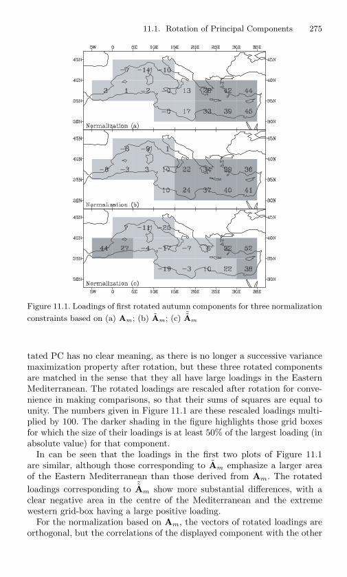
11.1. Rotation of Principal Components 275
Figure 11.1. Loadings of first rotated autumn components for three normalization
constraints based on (a) Am; (b) Am; (c) ˜Am
tated PC has no clear meaning, as there is no longer a successive variancemaximization property after rotation, but these three rotated componentsare matched in the sense that they all have large loadings in the EasternMediterranean. The rotated loadings are rescaled after rotation for conve-nience in making comparisons, so that their sums of squares are equal tounity. The numbers given in Figure 11.1 are these rescaled loadings multi-plied by 100. The darker shading in the figure highlights those grid boxesfor which the size of their loadings is at least 50% of the largest loading (inabsolute value) for that component.
In can be seen that the loadings in the first two plots of Figure 11.1are similar, although those corresponding to Am emphasize a larger areaof the Eastern Mediterranean than those derived from Am. The rotatedloadings corresponding to ˜Am show more substantial differences, with aclear negative area in the centre of the Mediterranean and the extremewestern grid-box having a large positive loading.
For the normalization based on Am, the vectors of rotated loadings areorthogonal, but the correlations of the displayed component with the other

276 11. Rotation and Interpretation of Principal Components
two rotated components are 0.21 and 0.35. The rotated components cor-responding to ˜Am are uncorrelated, but the angles between the vector ofloadings for the displayed component and those of the other two rotatedcomponents are 61 and 48, respectively, rather than 90 as required fororthogonality. For the normalization based on Am the respective correla-tions between the plotted component and the other rotated componentsare 0.30 and 0.25, with respective corresponding angles between vectors ofloadings equal to 61 and 76.
Artistic Qualities of Painters
In the SST example, there are quite substantial differences in the rotatedloadings, depending on which normalization constraint is used. Jolliffe(1989) suggests a strategy for rotation that avoids this problem, and alsoalleviates two of the other three drawbacks of rotation noted above. Thisstrategy is to move away from necessarily rotating the first few PCs, butinstead to rotate subsets of components with similar eigenvalues. The ef-fect of different normalizations on rotated loadings depends on the relativelengths of the vectors of loadings within the set of loadings that are rotated.If the eigenvalues are similar for all PCs to be rotated, any normalizationin which lengths of loading vectors are functions of eigenvalues is similar toa normalization in which lengths are constant. The three constraints abovespecify lengths of 1, lk
n−1 , and n−1lk
, and it therefore matters little which isused when eigenvalues in the rotated set are similar.
With similar eigenvalues, there is also no dominant PC or PCs withinthe set being rotated, so the second drawback of rotation is removed. Thearbitary choice of m also disappears, although it is replaced by another ar-bitrary choice of which sets of eigenvalues are sufficiently similar to justifyrotation. However, there is a clearer view here of what is required (closeeigenvalues) than in choosing m. The latter is multifaceted, depending onwhat the m retained components are meant to achieve, as evidenced bythe variety of possible rules described in Section 6.1. If approximate mul-tivariate normality can be assumed, the choice of which subsets to rotatebecomes less arbitrary, as tests are available for hypotheses averring thatblocks of consecutive population eigenvalues are equal (Flury and Riedwyl,1988, Section 10.7). These authors argue that when such hypotheses cannotbe rejected, it is dangerous to interpret individual eigenvectors—only thesubspace defined by the block of eigenvectors is well-defined, not individualeigenvectors. A possible corollary of this argument is that PCs correspond-ing to such subspaces should always be rotated in order to interpret thesubspace as simply as possible.
Jolliffe (1989) gives three examples of rotation for PCs with similar eigen-values. One, which we summarize here, is the four-variable artistic qualitiesdata set described in Section 5.1. In this example the four eigenvalues are2.27, 1.04, 0.40 and 0.29. The first two of these are well-separated, and
11.1. Rotation of Principal Components 277
Table 11.1. Unrotated and rotated loadings for components 3 and 4: artisticqualities data.
PC3 PC4 RPC3 RPC4Composition −0.59 −0.41 −0.27 0.66Drawing 0.60 −0.50 0.78 −0.09Colour 0.49 −0.22 0.53 0.09Expression 0.23 0.73 −0.21 0.74
Percentage of 10.0 7.3 9.3 8.0total variation
together they account for 83% of the total variation. Rotating them maylose information on individual dominant sources of variation. On the otherhand, the last two PCs have similar eigenvalues and are candidates for ro-tation. Table 11.1 gives unrotated (PC3, PC4) and rotated (RPC3, RPC4)loadings for these two components, using varimax rotation and the normal-ization constraints a′
kak = 1. Jolliffe (1989) shows that using alternativerotation criteria to varimax makes almost no difference to the rotated load-ings. Different normalization constraints also affect the results very little.Using a′
kak = lk gives vectors of rotated loadings whose angles with thevectors for the constraint a′
kak = 1 are only 6 and 2.It can be seen from Table 11.1 that rotation of components 3 and 4 con-
siderably simplifies their structure. The rotated version of component 4 isalmost a pure contrast between expression and composition, and compo-nent 3 is also simpler than either of the unrotated components. As well asillustrating rotation of components with similar eigenvalues, this examplealso serves as a reminder that the last few, as well as the first few, compo-nents are sometimes of interest (see Sections 3.1, 3.7, 6.3, 8.4–8.6, 9.1 and10.1).
In such cases, interpretation of the last few components may have asmuch relevance as interpretation of the first few, and for the last fewcomponents close eigenvalues are more likely.
11.1.2 One-step Procedures Using Simplicity Criteria
Kiers (1993) notes that even when a PCA solution is rotated to simplestructure, the result may still not be as simple as required. It may there-fore be desirable to put more emphasis on simplicity than on variancemaximization, and Kiers (1993) discusses and compares four techniquesthat do this. Two of these explicitly attempt to maximize one of the stan-dard simplicity criteria, namely varimax and quartimax respectively, overall possible sets of orthogonal components, for a chosen number of compo-nents m. A third method divides the variables into non-overlapping clusters
278 11. Rotation and Interpretation of Principal Components
and associates exactly one component with each cluster. The criterion tobe optimized is the sum over variables of squared loadings for each variablefor the single component associated with that variable’s cluster. The finalmethod is similar to the one that maximizes the quartimax criterion, butit relaxes the requirement of orthogonality of components.
Gains in simplicity achieved by any of the methods are paid for by aloss of variance explained compared to rotated PCA, but none of the fourmethods explicitly takes into account the desirability of minimizing thevariance lost. Kiers (1993) investigates the trade-off between simplicity gainand variance loss for the four methods in a simulation study. He finds thatneither of the first two methods offers any advantage over rotated PCA.The third and fourth methods show some improvement over rotated PCAin recovering the simple structures that are built into the simulated data,and the fourth is better than the third in terms of retaining variance.
Two of the disadvantages of standard rotation noted earlier are the loss ofthe successive optimization property and the possible sensitivity of the re-sults to the choice of m. All four techniques compared by Kiers (1993) sharethese disadvantages. We now describe a method that avoids these draw-backs and explicitly takes into account both variance and simplicity. LikeKiers’ (1993) methods it replaces the two stages of rotated PCA by a sin-gle step. Linear combinations of the p variables are successively found thatmaximize a criterion in which variance is combined with a penalty func-tion that pushes the linear combination towards simplicity. The method isknown as the Simplified Component Technique (SCoT) (Jolliffe and Uddin,2000).
Let c′kxi be the value of the kth simplified component (SC) for the ithobservation. Suppose that Sim(ck) is a measure of simplicity for the vectorck, for example the varimax criterion, and V ar(c′kx) denotes the samplevariance c′kSck of c′kx. Then SCoT successively maximizes
(1 − ψ)V ar(c′kx) + ψSim(ck) (11.1.6)
subject to c′kck = 1 and (for k ≥ 2, h < k) c′hck = 0. Here ψ is a sim-plicity/complexity parameter, which needs to be chosen. The value ψ = 0corresponds to PCA, and as ψ increases the SCs move away from the PCstowards greater simplicity. When ψ = 1, each SC is identical to one of theoriginal variables, with zero loadings for all other variables.
Mediterranean SST
We return to the Mediterranean SST data, which were introduced earlier inthis section, but here we describe results for both autumn and winter. Fig-ures 11.2–11.5, reproduced with permission from Jolliffe et al. (2002b), showthe loadings for the first two PCs, and the first two simplified components,for each of the two seasons. Also included in the figures are two varimaxrotated PCs, using the normalization corresponding to Am, and the firsttwo components from the SCoTLASS and simple component techniques

11.2. Alternatives to Rotation 279
which are described in Section 11.2. The normalization of loadings and theshading in Figures 11.2–11.5 follow the same conventions as in Figure 11.1,except that any loadings which are exactly zero are unshaded in the figures.
For the autumn data, the first two SCoT components may be viewedas slightly simpler versions of PC1 and PC2. The largest loadings becomelarger and the smallest become smaller, as is often observed during rotation.The strong similarity between SCoT and PCA components is reflected bythe fact that the first two SCoT components account for 78.0% of thetotal variation compared to 78.2% for the first two PCs. Turning to thewinter data, the first two PCs and RPCs in Figures 11.4, 11.5 are not toodifferent from those in autumn (Figures 11.2, 11.3), but there are biggerdifferences for SCoT. In particular, the second SCoT component is verymuch dominated by a single grid box in the Eastern Mediterranean. Thisextreme simplicity leads to a reduction in the total variation accounted forby the first two SCoT components to 55.8%, compared to 71.0% for thefirst two PCs.
Results are presented for only one value of the tuning parameter ψ, andthe choice of this value is not an easy one. As ψ increases, there is oftena rapid jump from components that are very close to the correspondingPC, like those in autumn, to components that are dominated by a singlevariable, as for SC2 in winter. This jump is usually accompanied by a largedrop in the proportion of variation accounted for, compared to PCA. Thisbehaviour as ψ varies can also be seen in a later example (Tables 11.3,11.4), and is an unsatisfactory feature of SCoT. Choosing different valuesψ1, ψ2, . . . of ψ for SC1, SC2, . . . , only partially alleviates this problem.The cause seems to be the presence of a number of local maxima for thecriterion defined by (11.1.6). As ψ changes, a different local maximum maytake over as the global maximum, leading to a sudden switch betweentwo quite different solutions. Further discussion of the properties of SCoT,together with additional examples, is given by Jolliffe and Uddin (2000)and Uddin (1999).
Filzmoser (2000) argues that sometimes there is simple structure in aplane but not in any single direction within that plane. He derives a wayof finding such simply structured planes—which he calls principal planes.Clearly, if a data set has such structure, the methods discussed in thissection and the next are unlikely to find simple single components withouta large sacrifice in variance.
11.2 Alternatives to Rotation
This section describes two ideas for constructing linear functions of the poriginal variables having large variances; these techniques differ from PCAin imposing additional constraints on the loadings or coefficients of the

280 11. Rotation and Interpretation of Principal Components
Figure 11.2. Loadings of first autumn components for PCA, RPCA, SCoT,SCoTLASS and simple component analysis.

11.2. Alternatives to Rotation 281
Figure 11.3. Loadings of second autumn components for PCA, RPCA, SCoT,SCoTLASS and simple component analysis.
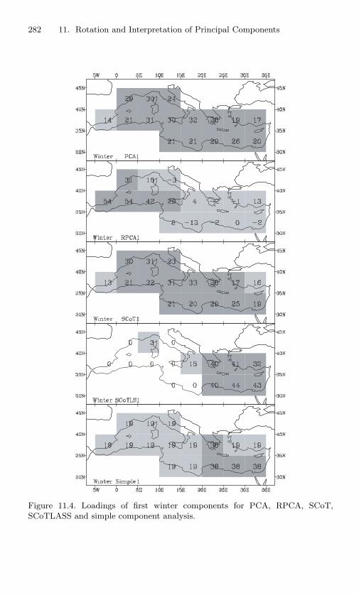
282 11. Rotation and Interpretation of Principal Components
Figure 11.4. Loadings of first winter components for PCA, RPCA, SCoT,SCoTLASS and simple component analysis.

11.2. Alternatives to Rotation 283
Figure 11.5. Loadings of second winter components for PCA, RPCA, SCoT,SCoTLASS and simple component analysis.

284 11. Rotation and Interpretation of Principal Components
variables in the functions. The constraints are designed to make the result-ing components simpler to interpret than PCs, but without sacrificing toomuch of the variance accounted for by the PCs. The first idea, discussedin Section 11.2.1, is a simple one, namely, restricting coefficients to a set ofintegers, though it is less simple to put into practice. The second type oftechnique, described in Section 11.2.2, borrows an idea from regression, thatof the LASSO (Least Absolute Shrinkage and Selection Operator). By im-posing an additional constraint in the PCA optimization problem, namely,that the sum of the absolute values of the coefficients in a component isbounded, some of the coefficients can be forced to zero. A technique fromatmospheric science, empirical orthogonal teleconnections, is described inSection 11.2.3, and Section 11.2.4 makes comparisons between some of thetechniques introduced so far in the chapter.
11.2.1 Components with Discrete-Valued Coefficients
A fairly obvious way of constructing simpler versions of PCs is to succes-sively find linear functions of the p variables that maximize variance, as inPCA, but with a restriction on the values of coefficients in those functionsto a small number of values. An extreme version of this was suggested byHausmann (1982), in which the loadings are restricted to the values +1,−1 and 0. To implement the technique, Hausman (1982) suggests the useof a branch-and-bound algorithm. The basic algorithm does not includean orthogonality constraint on the vectors of loadings of successive ‘com-ponents,’ but Hausmann (1982) adapts it to impose this constraint. Thisimproves interpretability and speeds up the algorithm, but has the impli-cation that it may not be possible to find as many as p components. In the6-variable example given by Hausmann (1982), after 4 orthogonal compo-nents have been found with coefficients restricted to −1, 0,+1 the nullvector is the only vector with the same restriction that is orthogonal to allfour already found. In a unpublished M.Sc. project report, Brooks (1992)discusses some other problems associated with Hausmann’s algorithm.
Further information is given on Hausmann’s example in Table 11.2. Herethe following can be seen:
• The first component is a straightforward average or ‘size’ componentin both analyses.
• Despite a considerable simplication, and a moderately different inter-pretation, for the second constrained component, there is very littleloss in variance accounted by the first two constrained componentscompared to first two PCs.
A less restrictive method is proposed by Vines (2000), in which the co-efficients are also restricted to integers. The algorithm for finding so-calledsimple components starts with a set of p particularly simple vectors of

11.2. Alternatives to Rotation 285
Table 11.2. Hausmann’s 6-variable example: the first two PCs and constrainedcomponents.
First component Second component
Variable PC Constrained PC Constrained
Sentence structure 0.43 1 −0.28 0Logical relationships 0.44 1 0.12 0Essay 0.32 1 −0.66 1Composition 0.46 1 −0.18 1Computation 0.39 1 0.53 −1Algebra 0.40 1 0.40 −1
Percentage of total 74.16 74.11 16.87 16.66variation
loadings chosen without worrying about the variances of the correspond-ing components. Typically this is the set of vectors ak where akk = 1 andakj = 0 (k = 1, 2, . . . , p; j = 1, 2, . . . , p; j = k), akj being the jth elementof ak. A sequence of ‘simplicity-preserving’ transformations is then appliedto these vectors. Each transformation chooses a pair of the vectors and ro-tates them orthogonally in such a way that the variance associated with thecurrently higher variance component of the pair is increased at the expenseof the lower variance component. The algorithm stops when no non-trivialsimplicity-preserving transformation leads to an improvement in variance.
Simplicity is achieved by considering a restricted set of angles for eachrotation. Only angles that result in the elements of the transformed vec-tors being proportional to integers are allowed. Thus, ‘simple’ vectors aredefined in this technique as those whose elements are proportional to in-tegers. It is usually the case that the transformed vector associated withthe higher variance tends to be simpler (proportional to smaller magnitudeintegers) than the other transformed vector. Cumulatively, this means thatwhen the algorithm terminates, all the vectors of loadings are simple, withthose for the first few components tending to be simpler than those forlater components. The choice of which pair of vectors to rotate at eachstage of the algorithm is that pair for which the increase in variance ofthe higher-variance component resulting from a simplicity-preserving rota-tion is maximized, although this strict requirement is relaxed to enablemore than one rotation of mutually exclusive pairs to be implementedsimultaneously.
The algorithm for simple components includes a tuning parameter c,which determines the number of angles considered for each simplicity-preserving transformation. This number is 2c+2 for c = 0, 1, 2, . . . . As cincreases, the simple components tend to become closer to the principalcomponents, but simplicity is sacrificed as the elements of the vectors ofloadings progressively become proportional to larger magnitude integers.
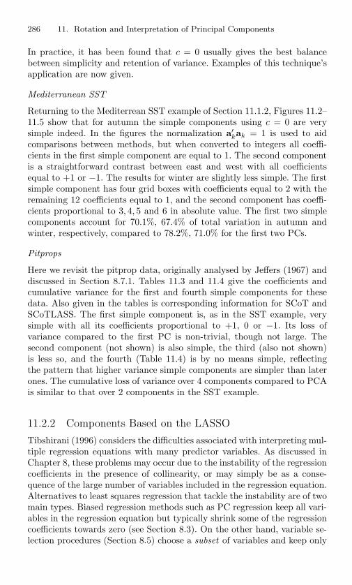
286 11. Rotation and Interpretation of Principal Components
In practice, it has been found that c = 0 usually gives the best balancebetween simplicity and retention of variance. Examples of this technique’sapplication are now given.
Mediterranean SST
Returning to the Mediterrean SST example of Section 11.1.2, Figures 11.2–11.5 show that for autumn the simple components using c = 0 are verysimple indeed. In the figures the normalization a′
kak = 1 is used to aidcomparisons between methods, but when converted to integers all coeffi-cients in the first simple component are equal to 1. The second componentis a straightforward contrast between east and west with all coefficientsequal to +1 or −1. The results for winter are slightly less simple. The firstsimple component has four grid boxes with coefficients equal to 2 with theremaining 12 coefficients equal to 1, and the second component has coeffi-cients proportional to 3, 4, 5 and 6 in absolute value. The first two simplecomponents account for 70.1%, 67.4% of total variation in autumn andwinter, respectively, compared to 78.2%, 71.0% for the first two PCs.
Pitprops
Here we revisit the pitprop data, originally analysed by Jeffers (1967) anddiscussed in Section 8.7.1. Tables 11.3 and 11.4 give the coefficients andcumulative variance for the first and fourth simple components for thesedata. Also given in the tables is corresponding information for SCoT andSCoTLASS. The first simple component is, as in the SST example, verysimple with all its coefficients proportional to +1, 0 or −1. Its loss ofvariance compared to the first PC is non-trivial, though not large. Thesecond component (not shown) is also simple, the third (also not shown)is less so, and the fourth (Table 11.4) is by no means simple, reflectingthe pattern that higher variance simple components are simpler than laterones. The cumulative loss of variance over 4 components compared to PCAis similar to that over 2 components in the SST example.
11.2.2 Components Based on the LASSO
Tibshirani (1996) considers the difficulties associated with interpreting mul-tiple regression equations with many predictor variables. As discussed inChapter 8, these problems may occur due to the instability of the regressioncoefficients in the presence of collinearity, or may simply be as a conse-quence of the large number of variables included in the regression equation.Alternatives to least squares regression that tackle the instability are of twomain types. Biased regression methods such as PC regression keep all vari-ables in the regression equation but typically shrink some of the regressioncoefficients towards zero (see Section 8.3). On the other hand, variable se-lection procedures (Section 8.5) choose a subset of variables and keep only
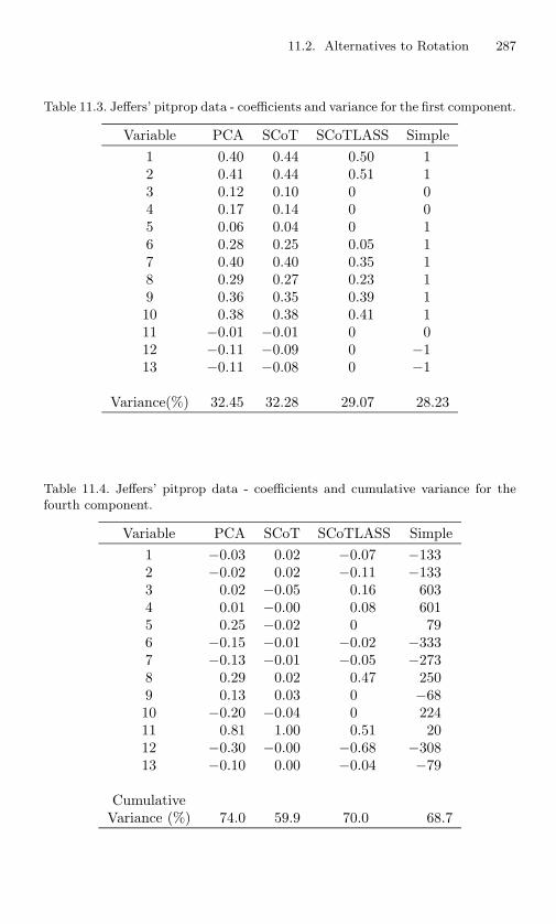
11.2. Alternatives to Rotation 287
Table 11.3. Jeffers’ pitprop data - coefficients and variance for the first component.
Variable PCA SCoT SCoTLASS Simple1 0.40 0.44 0.50 12 0.41 0.44 0.51 13 0.12 0.10 0 04 0.17 0.14 0 05 0.06 0.04 0 16 0.28 0.25 0.05 17 0.40 0.40 0.35 18 0.29 0.27 0.23 19 0.36 0.35 0.39 110 0.38 0.38 0.41 111 −0.01 −0.01 0 012 −0.11 −0.09 0 −113 −0.11 −0.08 0 −1
Variance(%) 32.45 32.28 29.07 28.23
Table 11.4. Jeffers’ pitprop data - coefficients and cumulative variance for thefourth component.
Variable PCA SCoT SCoTLASS Simple1 −0.03 0.02 −0.07 −1332 −0.02 0.02 −0.11 −1333 0.02 −0.05 0.16 6034 0.01 −0.00 0.08 6015 0.25 −0.02 0 796 −0.15 −0.01 −0.02 −3337 −0.13 −0.01 −0.05 −2738 0.29 0.02 0.47 2509 0.13 0.03 0 −6810 −0.20 −0.04 0 22411 0.81 1.00 0.51 2012 −0.30 −0.00 −0.68 −30813 −0.10 0.00 −0.04 −79
CumulativeVariance (%) 74.0 59.9 70.0 68.7

288 11. Rotation and Interpretation of Principal Components
the selected variables in the equation. Tibshirani (1996) proposes a newmethod, the ‘least absolute shrinkage and selection operator’ or LASSO,which is a hybrid of variable selection and shrinkage estimators. The pro-cedure shrinks the coefficients of some of the variables not simply towardszero, but exactly to zero, giving an implicit form of variable selection. TheLASSO idea can be transferred to PCA, as will now be shown.
In standard multiple regression we have the equation
yi = β0 +p∑
j=1
βjxij + εi, i = 1, 2, . . . , n,
where y1, y2, . . . , yn are measurements on a response variable y; xij , i =1, 2, . . . , n, j = 1, 2, . . . , p, are corresponding values of p predictor variables;β0, β1, β2, . . . , βp are parameters in the regression equation; and εi is anerror term. In least squares regression, the parameters are estimated byminimizing the residual sum of squares,
n∑
i=1
(yi − β0 −
p∑
j=1
βjxij
)2
.
The LASSO imposes an additional restriction on the coefficients, namelyp∑
j=1
|βj | ≤ t
for some ‘tuning parameter’ t. For suitable choices of t this constrainthas the interesting property that it forces some of the coefficients in theregression equation to zero.
Now consider PCA, in which linear combinations a′kx, k = 1, 2, . . . , p,
of the p measured variables x are found that successively have maximumvariance a′
kSak, subject to a′kak = 1 (and, for k ≥ 2, a′
hak = 0, h < k).Jolliffe et al. (2002a) suggest an adaptation of PCA, which they call
the Simplified Component Technique—LASSO (SCoTLASS), in which theadditional constraint
p∑
j=1
|akj | ≤ t (11.2.1)
is added to the PCA optimization problem, where akj is the jth elementof the kth vector ak, k = 1, 2, . . . , p, and t is a ‘tuning’ parameter.
SCoTLASS differs from PCA in the inclusion of the constraints defined in(11.2.1), and a decision must be made on the value of the tuning parameter,t. It is easy to see that
• for t ≥ √p, we get PCA;
• for t < 1, there is no solution;
• for t = 1, we must have exactly one non-zero akj for each k.

11.2. Alternatives to Rotation 289
As t decreases from√
p, the SCoTLASS components move progressivelyaway from PCA and some of the loadings become zero. Eventually, for t =1, a solution is reached in which only one variable has a non-zero loading oneach component, as with ψ = 1 in SCoT (Section 11.1.2). Examples follow.
Mediterranean SST
We return to the Mediterranean SST example and Figures 11.2–11.5 oncemore. As with SCoT in Section 11.1.2, results are given for one value of thetuning parameter, in this case t, chosen to give a compromise between vari-ance retention and simplicity. In the autumn, SCoTLASS behaves ratherlike rotated PCA, except that its patterns are more clearcut, with sev-eral grid boxes having zero rather than small loadings. Its first componentconcentrates on the Eastern Mediterranean, as does rotated PCA, but itssecond component is centred a little further west than the second rotatedPC. The patterns found in winter are fairly similar to those in autumn,and again similar to those of rotated PCA except for a reversal in order.In autumn and winter, respectively, the first two SCoTLASS componentsaccount for 70.5%, 65.9% of the total variation. This compares with 78.2%,71.0% for PCA and 65.8%, 57.9% for rotated PCA. The comparison withrotated PCA is somewhat unfair to the latter as we have chosen to dis-play only two out of three rotated PCs. If just two PCs had been rotated,the rotated PCs would account for the same total variation as the first twoPCs. However, the fact that the first two SCoTLASS components are muchsimplified versions of the two displayed rotated PCs, and at the same timehave substantially larger variances, suggests that SCoTLASS is superior torotated PCA in this example.
Pitprops
Tables 11.3 and 11.4 give coefficients and cumulative variances for the firstand fourth SCoTLASS components for Jeffers’ (1967) pitprop data. Thefirst component sacrifices about the same amount of variance comparedto PCA as the first simple component. Both achieve a greatly simplifiedpattern of coefficients compared to PCA, but, as in the SST example, ofquite different types. For the fourth component, the cumulative varianceis again similar to that of the simple components, but the SCoTLASScomponent is clearly simpler in this case. Further examples and discussionof the properties of SCoTLASS can be found in Jolliffe et al. (2002a) andUddin (1999).
11.2.3 Empirical Orthogonal Teleconnections
Van den Dool et al. (2000) propose a technique, the results of which theyrefer to as empirical orthogonal teleconnections (EOTs). The data they con-sider have the standard atmospheric science form in which the p variables
290 11. Rotation and Interpretation of Principal Components
correspond to measurements of the same quantity at p different spatial lo-cations and the n observations are taken at n different points in time (seeSection 12.2). Suppose that rjk is the correlation between the jth and kthvariables (spatial locations), and s2
k is the sample variance at location k.Then the location j∗ is found for which the criterion
∑pk=1 r2
jks2k is maxi-
mized. The first EOT is then the vector whose elements are the coefficientsin separate regressions of each variable on the chosen variable j∗. The firstderived variable is not the linear combination of variables defined by thisEOT, but simply the time series at the chosen location j∗. To find a secondEOT, the residuals are calculated from the separate regressions that definethe first EOT, and the original analysis is repeated on the resulting matrixof residuals. Third, fourth, . . . EOTs can be found in a similar way. At thisstage it should be noted that ‘correlation’ appears to be defined by van denDool et al. (2000) in a non-standard way. Both ‘variances’ and ‘covariances’are obtained from uncentred products, as in the uncentred version of PCA(see Section 14.2.3). This terminology is reasonable if means can be as-sumed to be zero. However, it does not appear that this assumption can bemade in van den Dool and co-workers’ examples, so that the ‘correlations’and ‘regressions’ employed in the EOT technique cannot be interpreted inthe usual way.
Leaving aside for the moment the non-standard definition of correlations,it is of interest to investigate whether there are links between the procedurefor finding the optimal variable j∗ that determines the first EOT and ‘prin-cipal variables’ as defined by McCabe (1984) (see Section 6.3). Recall thatMcCabe’s (1984) idea is to find subsets of variables that optimize the samecriteria as are optimized by the linear combinations of variables that arethe PCs. Now from the discussion following Property A6 in Section 2.3 thefirst correlation matrix PC is the linear combination of variables that max-imizes the sum of squared correlations between the linear combination andeach of the variables, while the first covariance matrix PC similarly maxi-mizes the corresponding sum of squared covariances. If ‘linear combinationof variables’ is replaced by ‘variable,’ these criteria become
∑pk=1 r2
jk and∑pk=1 r2
jks2ks2
j , respectively, compared to∑p
k=1 r2jks2
k for the first EOT. In asense, then, the first EOT is a compromise between the first principal vari-ables for covariance and correlation matrices. However, the non-standarddefinitions of variances and correlations make it difficult to understandexactly what the results of the analysis represent.
11.2.4 Some Comparisons
In this subsection some comparisons are made between the two main tech-niques described in the section, and to other methods discussed earlierin the chapter. Further discussion of the properties of SCoT and SCoT-LASS can be found in Uddin (1999). Another approach to simplification isdescribed in Section 14.6.3.

11.2. Alternatives to Rotation 291
• SCoT, SCoTLASS and Vines’ (2000) simple components all havetuning parameters which must be chosen. At present there is no pro-cedure for choosing the tuning parameters automatically, and it isadvisable to try more than one value and judge subjectively when asuitable compromise between simplicity and variance retention hasbeen achieved. For simple components c = 0 is often a good choice.The sudden switching between solutions as ψ varies, noted for SCoT,seems not to be a problem with respect to t or c for SCoTLASS orsimple components.
• Principal components have the special property that the vectorsof loadings are orthogonal and the component scores are uncor-related. It was noted in Section 11.1 that rotated PCs lose atleast one of these properties, depending on which normalizationconstraint is used. None of the new techniques is able to retainboth properties either. SCoT and SCoTLASS, as defined aboveand implemented in the examples, retain orthogonality of the vec-tors of loadings but sacrifice uncorrelatedness of the components.It is straightforward, though a little more complicated computa-tionally, to implement versions of SCoT and SCoTLASS that keepuncorrelatedness rather than orthogonality. All that is required is tosubstitute the conditions c′hSck = 0, h < k (or a′
hSak = 0, h < k)for c′hck = 0, h < k (or a′
hak = 0, h < k) in the definitionsof the techniques in Sections 11.1.2 and 11.2.2. Because of thepresence of orthogonal rotations at the heart of the algorithm forsimple components, it is not obvious how a modification replac-ing orthogonality by uncorrelatedness could be constructed for thistechnique.
• As noted in Section 11.1, ordinary two-stage rotation of PCshas a number of drawbacks. The nature of the new techniquesmeans that all four of the listed difficulties can be avoided, butthe fourth is replaced by a choice between orthogonal vectors ofloadings or uncorrelated components. The removal of the draw-backs is paid for by a loss in variation accounted for, althoughthe reduction can be small for solutions that provide consider-able simplification, as demonstrated in the examples above. Oneway to quantify simplicity is to calculate the value of the vari-max criterion, or whatever other criterion is used in rotated PCA,for individual components derived from any of the methods. Thenew techniques often do better than two-stage rotation with re-spect to the latter’s own simplicity criterion, with only a smallreduction in variance, giving another reason to prefer the newtechniques.

292 11. Rotation and Interpretation of Principal Components
11.3 Simplified Approximations to PrincipalComponents
The techniques of the previous section are alternatives to PCA that sacri-fice some variance in order to enhance simplicity. A different approach toimproving interpretability is to find the PCs, as usual, but then to approx-imate them. In Chapter 4, especially its first section, it was mentioned thatthere is usually no need to express the coefficients of a set of PCs to morethan one or two decimal places. Rounding the coefficients in this manner isone way of approximating the PCs. The vectors of rounded coefficients willno longer be exactly orthogonal, the rounded PCs will not be uncorrelatedand their variances will be changed, but typically these effects will not bevery great, as demonstrated by Green (1977) and Bibby (1980). The latterpaper presents bounds on the changes in the variances of the PCs (both inabsolute and relative terms) that are induced by rounding coefficients, andshows that in practice the changes are quite small, even with fairly severerounding.
To illustrate the effect of severe rounding, consider again Table 3.2,in which PCs for eight blood chemistry variables have their coefficientsrounded to the nearest 0.2. Thus, the coefficients for the first PC, forexample, are given as
0.2 0.4 0.4 0.4 − 0.4 − 0.4 − 0.2 − 0.2.
Their values to three decimal place are, by comparison,
0.195 0.400 0.459 0.430 − 0.494 − 0.320 − 0.177 − 0.171.
The variance of the rounded PC is 2.536, compared to an exact varianceof 2.792, a change of 9%. The angle between the vectors of coefficientsdefining the exact and rounded PCs is about 8. For the second, third andfourth PCs given in Table 3.2, the changes in variances are 7%, 11% and11%, respectively, and the angles between vectors of coefficients for exactand rounded PCs are 8 in each case. The angle between the vectors ofcoefficients for the first two rounded PCs is 99 and their correlation is−0.15. None of these changes or angles is unduly extreme considering theseverity of the rounding that is employed. However, in an example fromquality control given by Jackson (1991, Section 7.3) some of correlationsbetween PCs whose coefficients are approximated by integers are worringlylarge.
Bibby (1980) and Jackson (1991, Section 7.3) also mention the pos-sibility of using conveniently chosen integer values for the coefficients.For example, the simplified first PC from Table 3.2 is proportional to2(x2 +x3 +x4)+x1− (x7 +x8)−2(x5 +x6), which should be much simplerto interpret than the exact form of the PC. This is in the same spirit as thetechniques of Section 11.2.1, which restrict coefficients to be proportional
11.3. Simplified Approximations to Principal Components 293
to integer values. The difference is that the latter methods provide simpleralternatives to PCA, whereas Bibby’s (1980) suggestion approximates thePCs. Both types of simplification increase the interpretability of individ-ual components, but comparisons between components are more difficultwhen integers are used, because different components have different valuesof a′
kak.It is possible to test whether a single simplified (rounded or otherwise)
PC is a plausible ‘population’ PC using the result in equation (3.7.5) (seeJackson (1991, Section 7.4)) but the lack of orthogonality between a setof simplified PCs means that it is not possible for them to simultaneouslyrepresent population PCs.
Green (1977) investigates a different effect of rounding in PCA. Insteadof looking at the direct impact on the PCs, he looks at the proportionsof variance accounted for in each individual variable by the first m PCs,and examines by how much these proportions are reduced by rounding. Heconcludes that changes due to rounding are small, even for quite severerounding, and recommends rounding to the nearest 0.1 or even 0.2, asthis will increase interpretability with little effect on other aspects of theanalysis.
It is fairly common practice in interpreting a PC to ignore (set to zero),either consciously or subconsciously, the variables whose coefficients havethe smallest absolute values for that principal component. A second stagethen focuses on these ‘truncated’ components to see whether the pattern ofnon-truncated coefficients can be interpreted as a simple weighted averageor contrast for the non-ignored variables. Cadima and Jolliffe (1995) showthat the first ‘truncation’ step does not always do what might be expectedand should be undertaken with caution. In particular, this step can beconsidered as choosing a subset of variables (those not truncated) withwhich to approximate a PC. Cadima and Jolliffe (1995) show that
• for the chosen subset of variables, the linear combination given bythe coefficients in the untruncated PC may be far from the optimallinear approximation to that PC using those variables;
• a different subset of the same size may provide a better approxima-tion.
As an illustration of the first point, consider an example given by Cadimaand Jolliffe (1995) using data presented by Lebart et al. (1982). In thisexample there are seven variables measuring yearly expenditure of groups ofFrench families on 7 types of foodstuff. The loadings on the variables in thesecond PC to two decimal places are 0.58, 0.41,−0.10,−0.11,−0.24, 0.63and 0.14, so a truncated version of this component is
z2 = 0.58x1 + 0.41x2 + 0.63x6.
Thus, PC2 can be interpreted as a weighted average of expenditure on
294 11. Rotation and Interpretation of Principal Components
bread (x1), vegetables (x2) and milk (x6). However, a question that arisesis whether this truncated version of PC2 is the best linear approximation toPC2 using only these three variables. The answer is an emphatic ‘No.’ Thebest linear approximation in a least squares sense is obtained by regressingPC2 on x1, x2 and x6. This gives ˆz2 = 0.55x1 − 0.27x2 + 0.73x7, whichdiffers notably in interpretation from z2, as the expenditure on vegetablesis now contrasted, rather than averaged, with expenditure on bread andmilk. Furthermore ˆz2 has a correlation of 0.964 with PC2, whereas thecorrelation between PC2 and z2 is 0.766. Hence the truncated componentz2 not only gives a misleading interpretation of PC2 in terms of x1, x2 andx6, but also gives an inferior approximation compared to ˆz2.
To illustrate Cadima and Jolliffe’s (1995) second point, the third PC inthe same example has coefficients 0.40,−0.29,−0.34, 0.07, 0.38,−0.23 and0.66 on the 7 variables. If the 4 variables x1, x3, x5, x7 are kept, the bestlinear approximation to PC3 has coefficients −0.06,−0.48, 0.41, 0.68, re-spectively, so that x1 looks much less important. The correlation of theapproximation with PC3 is increased to 0.979, compared to 0.773 for thetruncated component. Furthermore, although x1 has the second highestcoefficient in PC3, it is not a member of the 3-variable subset x3, x5, x7that best approximates PC3. This subset does almost as well as the best4-variable subset, achieving a correlation of 0.975 with PC3.
Ali et al. (1985) also note that using loadings to interpret PCs can bemisleading, and suggest examining correlations between variables and PCsinstead. In a correlation matrix-based PCA, these PC-variable correlationsare equal to the loadings when the normalization ak is used (see Section 2.3for the population version of this result). The use of PCA in regionalizationstudies in climatology, as discussed in Section 9.2, often uses these correla-tions to define and interpret clusters. However, Cadima and Jolliffe (1995)show that neither the absolute size of loadings in a PC nor the absolute sizeof correlations between variables and components gives reliable guidanceon which subset of variables best approximates a PC (see also Rencher(1995, Section 12.8.3)). Cadima and Jolliffe (2001) give further examplesof this phenomenon in the context of variable selection (see Section 6.3).
Richman and Gong (1999) present an extensive study, which starts fromthe explicit premise that loadings greater than some threshold are retained,while those below the threshold are set to zero. Their objective is to findan optimal value for this threshold in a spatial atmospheric science con-text. The loadings they consider are, in fact, based on the normalizationak, so for correlation matrix PCA they are correlations between PCs andvariables. Rotated PCs and covariance matrix PCs are also included in thestudy. Richman and Gong (1999) use biserial correlation to measure howwell the loadings in a truncated PC (or truncated rotated PC) match thepattern of correlations between the spatial location whose loading on thePC (rotated PC) is largest, and all other spatial locations in a data set.The optimum threshold is the one for which this match is best. Results

11.3. Simplified Approximations to Principal Components 295
are given that show how the optimum threshold changes as sample sizeincreases (it decreases) for unrotated, orthogonally rotated and obliquelyrotated PCs. The precision of the results is indicated by boxplots. Thepaper provides useful guidance on choosing a threshold in the spatial at-mospheric science setting if truncation is to be done. However, it largelyignores the fact stressed above that neither the size of loadings nor thatof correlations are necessarily reliable indicators of how to interpret a PC,and hence that truncation according to a fixed threshold should be usedwith extreme caution.
Interpretation can play a role in variable selection. Section 6.3 defines anumber of criteria for choosing a subset of variables; these criteria are basedon how well the subset represents the full data set in one sense or another.Often there will be several, perhaps many for large p, subsets that do almostas well as the best in terms of the chosen criterion. To decide between themit may be desirable to select those variables that are most easily measuredor, alternatively, those that can be most easily interpreted. Taking this trainof thought a little further, if PCs are calculated from a subset of variables,it is preferable that the chosen subset gives PCs that are easy to interpret.Al-Kandari and Jolliffe (2001) take this consideration into account in astudy that compares the merits of a number of variable selection methodsand also compares criteria for assessing the value of subsets. A much fullerdiscussion is given by Al-Kandari (1998).
11.3.1 Principal Components with Homogeneous, Contrastand Sparsity Constraints
Chipman and Gu (2001) present a number of related ideas that lead toresults which appear similar in form to those produced by the techniquesin Section 11.2. However, their reasoning is closely related to truncationso they are included here. Components with homogeneous constraints havetheir coefficients restricted to −1, 0 and +1 as with Hausmann (1982), butinstead of solving a different optimization problem we start with the PCsand approximate them. For a threshold τH a vector of PC coefficients ak
is replaced by a vector aHk with coefficients
aHkj =
sign(akj) if akj ≥ τH
0 if akj < τH .
The threshold τH is chosen to minimize the angle between the vectorsaH
k and ak.Contrast constraints allow coefficients aC
kj to take the values −c1, 0 andc2, where c1, c2 > 0 and
∑pj=1 aC
kj = 0. Again a threshold τC determines
296 11. Rotation and Interpretation of Principal Components
the coefficients. We have
aCkj =
−c1 if akj ≤ −τC
0 if |akj | < τC
c2 if akj ≥ τC ,
and τC is chosen to minimize the angle between aCk and ak.
The idea behind sparsity constraints as defined by Chipman and Gu(2001) is different. An approximating vector aS
k is simply the vector ak
with all except its q largest coefficients in absolute value truncated to zero.The value of q is chosen by minimizing the quantity (2θ
π + ηqp ) with respect
to q, where θ is the angle between aSk and ak and η is a tuning parameter.
As η increases, so the optimal value of q decreases and the componentbecomes more ‘sparse.’
The three ideas of homogeneous, contrast and sparsity constraints for-malize and extend the informal procedure of truncation, and Chipman andGu (2001) give interesting examples of their use. It must, however, beremembered that these techniques implicitly assume that the sizes of coef-ficients or loadings for a PC are a reliable guide to interpreting that PC.As we have seen, this is not necessarily true.
11.4 Physical Interpretation of PrincipalComponents
There is often a desire to physically interpret principal components. Inpsychology, for example, it is frequently assumed that there are certainunderlying factors that cannot be measured directly, but which can bededuced from responses to questions or scores on tests of a sample of in-dividuals. PCA can be used to look for such factors. In psychology, factoranalysis, which builds a model that includes the factors, is usually rightlypreferred to PCA, although the software used may be such that PCA isactually done.
Atmospheric science is another area where it is believed that there arefundamental modes of variation underlying a data set, and PCA or somemodification of it is often used to look for them. Preisendorfer and Mobley(1988, Chapters 3 and 10) discuss at length the interplay between PCA andthe dominant modes of variation in physical systems, and use a versionof PCA for continuous variables (functional PCA—see Section 12.3) toexplore the relationships between EOFs (the vectors of coefficients) andthe physical modes of the atmosphere. Recent discussions of the NorthAtlantic Oscillation and Arctic Oscillation (Ambaum et al., 2001) and theIndian Ocean dipole (Allan et al., 2001) illustrate the controversy thatsometimes surrounds the physical interpretation of PCs.
11.4. Physical Interpretation of Principal Components 297
In practice, there may be a circularity of argument when PCA is usedto search for physically meaningful modes in atmospheric data. The formof these modes is often assumed known and PCA is used in an attempt toconfirm them. When it fails to do so, it is ‘accused’ of being inadequate.However, it has very clear objectives, namely finding uncorrelated derivedvariables that in succession maximize variance. If the physical modes arenot expected to maximize variance and/or to be uncorrelated, PCA shouldnot be used to look for them in the first place.
One of the reasons why PCA ‘fails’ to find the expected physical modesin some cases in atmospheric science is because of its dependence on thesize and shape of the spatial domain over which observations are taken.Buell (1975) considers various spatial correlation functions, both circular(isotropic) and directional (anisotropic), together with square, triangularand rectangular spatial domains. The resulting EOFs depend on the size ofthe domain in the sense that in a small domain with positive correlationsbetween all points within it, the first EOF is certain to have all its elementsof the same sign, with the largest absolute values near the centre of thedomain, a sort of ‘overall size’ component (see Section 13.2). For largerdomains, there may be negative as well as positive correlations, so that thefirst EOF represents a more complex pattern. This gives the impressionof instability, because patterns that are present in the analysis of a largedomain are not necessarily reproduced when the PCA is restricted to asubregion of this domain.
The shape of the domain also influences the form of the PCs. For ex-ample, if the first EOF has all its elements of the same sign, subsequentones must represent ‘contrasts,’ with a mixture of positive and negative val-ues, in order to satisfy orthogonality constraints. If the spatial correlationis isotropic, the contrast represented by the second PC will be betweenregions with the greatest geographical separation, and hence will be de-termined by the shape of the domain. Third and subsequent EOFs canalso be predicted for isotropic correlations, given the shape of the domain(see Buell (1975) for diagrams illustrating this). However, if the correlationis anisotropic and/or non-stationary within the domain, things are lesssimple. In any case, the form of the correlation function is important indetermining the PCs, and it is only when it takes particularly simple formsthat the nature of the PCs can be easily predicted from the size and shapeof the domain. PCA will often give useful information about the sourcesof maximum variance in a spatial data set, over and above that availablefrom knowledge of the size and shape of the spatial domain of the data.However, in interpreting PCs derived from spatial data, it should not beforgotten that the size and shape of the domain can have a strong influenceon the results. The degree of dependence of EOFs on domain shape hasbeen, like the use of rotation and the possibility of physical interpretation,a source of controversy in atmospheric science. For an entertaining andenlightening exchange of strong views on the importance of domain shape,

298 11. Rotation and Interpretation of Principal Components
which also brings in rotation and interpretation, see Legates (1991, 1993)and Richman (1993).
Similar behaviour occurs for PCA of time series when the autocorrelationfunction (see Section 12.1) takes a simple form. Buell (1979) discusses thiscase, and it is well-illustrated by the road-running data which are analysedin Sections 5.3 and 12.3. The first PC has all its loadings of the samesign, with the greatest values in the middle of the race, while the secondPC is a contrast between the race segments with the greatest separationin time. If there are predictable patterns in time or in spatial data, itmay be of interest to examine the major sources of variation orthogonalto these predictable directions. This is related to what is done in lookingfor ‘shape’ components orthogonal to the isometric size vector for size andshape data (see Section 13.2). Rao’s ‘principal components uncorrelatedwith instrumental variables’ (Section 14.3) also have similar objectives.
A final comment is that even when there is no underlying structure ina data set, sampling variation ensures that some linear combinations ofthe variables have larger variances than others. Any ‘first PC’ which hasactually arisen by chance can, with some ingenuity, be ‘interpreted.’ Ofcourse, completely unstructured data is a rarity but we should always tryto avoid ‘overinterpreting’ PCs, in the same way that in other branches ofstatistics we should be wary of spurious regression relationships or clusters,for example.

12Principal Component Analysis forTime Series and OtherNon-Independent Data
12.1 Introduction
In much of statistics it is assumed that the n observations x1,x2, . . . ,xn
are independent. This chapter discusses the implications for PCA of non-independence among x1,x2, . . . ,xn. Much of the chapter is concerned withPCA for time series data, the most common type of non-independent data,although data where x1,x2, . . . ,xn are measured at n points in space arealso discussed. Such data often have dependence which is more complicatedthan for time series. Time series data are sufficiently different from ordinaryindependent data for there to be aspects of PCA that arise only for suchdata, for example, PCs in the frequency domain.
The results of Section 3.7, which allow formal inference procedures tobe performed for PCs, rely on independence of x1, x2, . . . ,xn, as well as(usually) on multivariate normality. They cannot therefore be used if morethan very weak dependence is present between x1,x2, . . . ,xn. However,when the main objective of PCA is descriptive, not inferential, complica-tions such as non-independence do not seriously affect this objective. Theeffective sample size is reduced below n, but this reduction need not betoo important. In fact, in some circumstances we are actively looking fordependence among x1,x2, . . . ,xn. For example, grouping of observations ina few small areas of the two-dimensional space defined by the first two PCsimplies dependence between those observations that are grouped together.Such behaviour is actively sought in cluster analysis (see Section 9.2) andis often welcomed as a useful insight into the structure of the data, ratherthan decried as an undesirable feature.
300 12. PCA for Time Series and Other Non-Independent Data
We have already seen a number of examples where the data are timeseries, but where no special account is taken of the dependence betweenobservations. Section 4.3 gave an example of a type that is common inatmospheric science, where the variables are measurements of the samemeteorological variable made at p different geographical locations, and then observations on each variable correspond to different times. Section 12.2largely deals with techniques that have been developed for data of this type.The examples given in Section 4.5 and Section 6.4.2 are also illustrations ofPCA applied to data for which the variables (stock prices and crime rates,respectively) are measured at various points of time. Furthermore, one ofthe earliest published applications of PCA (Stone, 1947) was on (economic)time series data.
In time series data, dependence between the x vectors is induced bytheir relative closeness in time, so that xh and xi will often be highlydependent if |h−i| is small, with decreasing dependence as |h−i| increases.This basic pattern may in addition be perturbed by, for example, seasonaldependence in monthly data, where decreasing dependence for increasing|h − i| is interrupted by a higher degree of association for observationsseparated by exactly one year, two years, and so on.
Because of the emphasis on time series in this chapter, we need to intro-duce some of its basic ideas and definitions, although limited space permitsonly a rudimentary introduction to this vast subject (for more informationsee, for example, Brillinger (1981); Brockwell and Davis (1996); or Hamilton(1994)). Suppose, for the moment, that only a single variable is measured atequally spaced points in time. Our time series is then . . . x−1, x0, x1, x2, . . . .Much of time series analysis is concerned with series that are stationary, andwhich can be described entirely by their first- and second-order moments;these moments are
µ = E(xi), i = . . . ,−1, 0, 1, 2, . . .
γk = E[(xi − µ)(xi+k − µ)], i = . . . ,−1, 0, 1, 2, . . . (12.1.1)k = . . . ,−1, 0, 1, 2, . . . ,
where µ is the mean of the series and is the same for all xi in stationaryseries, and γk, the kth autocovariance, is the covariance between xi andxi+k, which depends on k but not i for stationary series. The informationcontained in the autocovariances can be expressed equivalently in terms ofthe power spectrum of the series
f(λ) =12π
∞∑
k=−∞γke−ikλ, (12.1.2)
where i =√−1 and λ denotes angular frequency. Roughly speaking, the
function f(λ) decomposes the series into oscillatory portions with differentfrequencies of oscillation, and f(λ) measures the relative importance ofthese portions as a function of their angular frequency λ. For example, if a
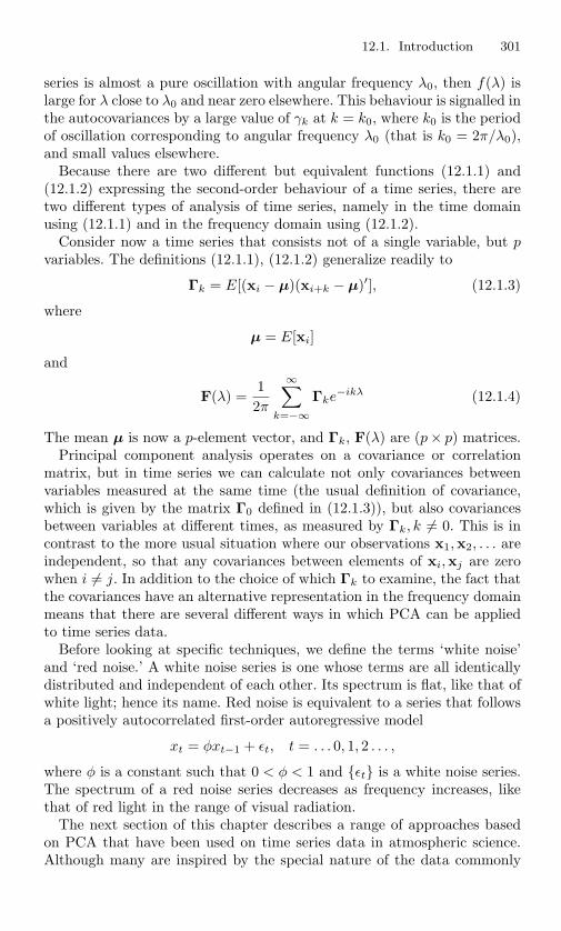
12.1. Introduction 301
series is almost a pure oscillation with angular frequency λ0, then f(λ) islarge for λ close to λ0 and near zero elsewhere. This behaviour is signalled inthe autocovariances by a large value of γk at k = k0, where k0 is the periodof oscillation corresponding to angular frequency λ0 (that is k0 = 2π/λ0),and small values elsewhere.
Because there are two different but equivalent functions (12.1.1) and(12.1.2) expressing the second-order behaviour of a time series, there aretwo different types of analysis of time series, namely in the time domainusing (12.1.1) and in the frequency domain using (12.1.2).
Consider now a time series that consists not of a single variable, but pvariables. The definitions (12.1.1), (12.1.2) generalize readily to
Γk = E[(xi − µ)(xi+k − µ)′], (12.1.3)
where
µ = E[xi]
and
F(λ) =12π
∞∑
k=−∞Γke−ikλ (12.1.4)
The mean µ is now a p-element vector, and Γk, F(λ) are (p× p) matrices.Principal component analysis operates on a covariance or correlation
matrix, but in time series we can calculate not only covariances betweenvariables measured at the same time (the usual definition of covariance,which is given by the matrix Γ0 defined in (12.1.3)), but also covariancesbetween variables at different times, as measured by Γk, k = 0. This is incontrast to the more usual situation where our observations x1,x2, . . . areindependent, so that any covariances between elements of xi,xj are zerowhen i = j. In addition to the choice of which Γk to examine, the fact thatthe covariances have an alternative representation in the frequency domainmeans that there are several different ways in which PCA can be appliedto time series data.
Before looking at specific techniques, we define the terms ‘white noise’and ‘red noise.’ A white noise series is one whose terms are all identicallydistributed and independent of each other. Its spectrum is flat, like that ofwhite light; hence its name. Red noise is equivalent to a series that followsa positively autocorrelated first-order autoregressive model
xt = φxt−1 + εt, t = . . . 0, 1, 2 . . . ,
where φ is a constant such that 0 < φ < 1 and εt is a white noise series.The spectrum of a red noise series decreases as frequency increases, likethat of red light in the range of visual radiation.
The next section of this chapter describes a range of approaches basedon PCA that have been used on time series data in atmospheric science.Although many are inspired by the special nature of the data commonly

302 12. PCA for Time Series and Other Non-Independent Data
encountered in this area, with observations corresponding to times andvariables to spatial position, they are not necessarily restricted to suchdata.
Time series are usually measured at discrete points in time, but some-times the series are curves. The analysis of such data is known as functionaldata analysis (functional PCA is the subject of Section 12.3). The final sec-tion of the chapter collects together a number of largely unconnected ideasand references concerning PCA in the context of time series and othernon-independent data.
12.2 PCA-Related Techniques for (Spatio-)Temporal Atmospheric Science Data
It was noted in Section 4.3 that, for a common type of data in atmosphericscience, the use of PCA, more often referred to as empirical orthogonalfunction (EOF) analysis, is widespread. The data concerned consist of mea-surements of some variable, for example, sea level pressure, temperature,. . . , at p spatial locations (usually points on a grid) at n different times. Themeasurements at different spatial locations are treated as variables and thetime points play the role of observations. An example of this type was givenin Section 4.3. It is clear that, unless the observations are well-separatedin time, there is likely to be correlation between measurements at adjacenttime points, so that we have non-independence between observations. Sev-eral techniques have been developed for use in atmospheric science that takeaccount of correlation in both time and space, and these will be describedin this section. First, however, we start with the simpler situation wherethere is a single time series. Here we can use a principal component-liketechnique, called singular spectrum analysis (SSA), to analyse the autocor-relation in the series. SSA is described in Section 12.2.1, as is its extensionto several time series, multichannel singular spectrum analysis (MSSA).
Suppose that a set of p series follows a multivariate first-order autore-gressive model in which the values of the series at time t are linearly relatedto the values at time (t − 1), except for a multivariate white noise term.An estimate of the matrix defining the linear relationship can be subjectedto an eigenanalysis, giving insight into the structure of the series. Such ananalysis is known as principal oscillation pattern (POP) analysis, and isdiscussed in Section 12.2.2.
One idea underlying POP analysis is that there may be patterns in themaps comprising our data set, which travel in space as time progresses, andthat POP analysis can help to find such patterns. Complex (Hilbert) em-pirical orthogonal functions (EOFs), which are described in Section 12.2.3,are designed to achieve the same objective. Detection of detailed oscilla-tory behaviour is also the aim of multitaper frequency-domain singularvalue decomposition, which is the subject of Section 12.2.4.

12.2. PCA and Atmospheric Time Series 303
Some time series have cyclic behaviour with fixed periods, such as anannual or diurnal cycle. Modifications of POP analysis and PCA that takesuch cycles into account are discussed in Section 12.2.5. A brief discussionof examples and comparative studies is given in Section 12.2.6.
12.2.1 Singular Spectrum Analysis (SSA)
Like a number of other statistical techniques, SSA appears to have been‘invented’ independently in a number of different fields. Elsner and Tsonis(1996) give references from the 1970s and 1980s from chaos theory, biolog-ical oceanography and signal processing, and the same idea is described inthe statistical literature by Basilevsky and Hum (1979), where it is referredto as the ‘Karhunen-Loeve method,’ a term more often reserved for con-tinuous time series (see Section 12.3). Other names for the technique are‘Pisarenko’s method’ (Smyth, 2000) and ‘singular systems analysis’ (vonStorch and Zwiers, 1999, Section 13.6); fortunately the latter has the sameacronym as the most popular name. A comprehensive coverage of SSA isgiven by Golyandina et al. (2001).
The basic idea in SSA is simple: a principal component analysis is donewith the variables analysed being lagged versions of a single time seriesvariable. More specifically, our p variables are xt, x(t+1), . . . , x(t+p−1) and,assuming the time series is stationary, their covariance matrix is such thatthe (i, j)th element depends only on |i − j|. Such matrices are knownas Toplitz matrices. In the present case the (i, j)th element is the au-tocovariance γ|i−j|. Because of the simple structure of Toplitz matrices,the behaviour of the first few PCs, and their corresponding eigenvaluesand eigenvectors (the EOFs) which are trigonometric functions (Brillinger,1981, Section 3.7), can be deduced for various types of time series structure.The PCs are moving averages of the time series, with the EOFs providingthe weights in the moving averages.
Toplitz matrices also occur when the p-element random vector x consistsof non-overlapping blocks of p consecutive values of a single time series. Ifthe time series is stationary, the covariance matrix Σ for x has Toplitzstructure, with the well-known pattern of trigonometric functions for itseigenvalues and eigenvectors. Craddock (1965) performed an analysis ofthis type on monthly mean temperatures for central England for the periodNovember 1680 to October 1963. The p (= 12) elements of x are meantemperatures for the 12 months of a particular year, where a ‘year’ startsin November. There is some dependence between different values of x, butit is weaker than that between elements within a particular x; between-yearcorrelation was minimized by starting each year at November, when therewas apparently evidence of very little continuity in atmospheric behaviourfor these data. The sample covariance matrix does not, of course, haveexact Toplitz structure, but several of the eigenvectors have approximatelythe form expected for such matrices.
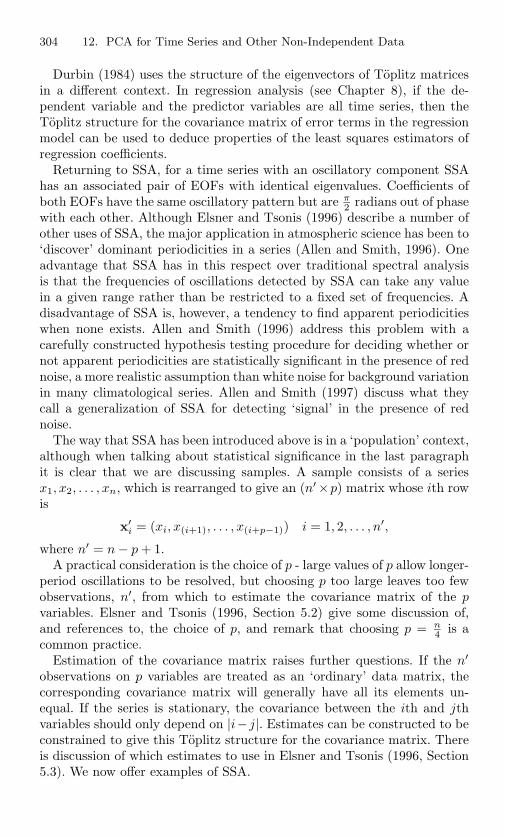
304 12. PCA for Time Series and Other Non-Independent Data
Durbin (1984) uses the structure of the eigenvectors of Toplitz matricesin a different context. In regression analysis (see Chapter 8), if the de-pendent variable and the predictor variables are all time series, then theToplitz structure for the covariance matrix of error terms in the regressionmodel can be used to deduce properties of the least squares estimators ofregression coefficients.
Returning to SSA, for a time series with an oscillatory component SSAhas an associated pair of EOFs with identical eigenvalues. Coefficients ofboth EOFs have the same oscillatory pattern but are π
2 radians out of phasewith each other. Although Elsner and Tsonis (1996) describe a number ofother uses of SSA, the major application in atmospheric science has been to‘discover’ dominant periodicities in a series (Allen and Smith, 1996). Oneadvantage that SSA has in this respect over traditional spectral analysisis that the frequencies of oscillations detected by SSA can take any valuein a given range rather than be restricted to a fixed set of frequencies. Adisadvantage of SSA is, however, a tendency to find apparent periodicitieswhen none exists. Allen and Smith (1996) address this problem with acarefully constructed hypothesis testing procedure for deciding whether ornot apparent periodicities are statistically significant in the presence of rednoise, a more realistic assumption than white noise for background variationin many climatological series. Allen and Smith (1997) discuss what theycall a generalization of SSA for detecting ‘signal’ in the presence of rednoise.
The way that SSA has been introduced above is in a ‘population’ context,although when talking about statistical significance in the last paragraphit is clear that we are discussing samples. A sample consists of a seriesx1, x2, . . . , xn, which is rearranged to give an (n′×p) matrix whose ith rowis
x′i = (xi, x(i+1), . . . , x(i+p−1)) i = 1, 2, . . . , n′,
where n′ = n − p + 1.A practical consideration is the choice of p - large values of p allow longer-
period oscillations to be resolved, but choosing p too large leaves too fewobservations, n′, from which to estimate the covariance matrix of the pvariables. Elsner and Tsonis (1996, Section 5.2) give some discussion of,and references to, the choice of p, and remark that choosing p = n
4 is acommon practice.
Estimation of the covariance matrix raises further questions. If the n′
observations on p variables are treated as an ‘ordinary’ data matrix, thecorresponding covariance matrix will generally have all its elements un-equal. If the series is stationary, the covariance between the ith and jthvariables should only depend on |i− j|. Estimates can be constructed to beconstrained to give this Toplitz structure for the covariance matrix. Thereis discussion of which estimates to use in Elsner and Tsonis (1996, Section5.3). We now offer examples of SSA.

12.2. PCA and Atmospheric Time Series 305
Figure 12.1. Plots of loadings for the first two components in an SSA with p = 61of the Southern Oscillation Index data.
Southern Oscillation Index
The data considered here are monthly values of the Southern OscillationIndex (SOI) for the years 1876–2000, produced by the Australian Bureauof Meteorology’s National Climate Centre. The number of observations inthe series is therefore n = 12 × 125 = 1500. The index is a measure ofthe East-West pressure gradient between Tahiti in the mid-Pacific Oceanand Darwin, Australia. It is a major source of climate variation. SSA wascarried on the data with p = 61, and Figure 12.1 gives a plot of the loadingsfor the first two EOFs. Their eigenvalues correspond to 13.7% and 13.4%of the total variation. The closeness of the eigenvalues suggests a quasi-oscillatory pattern, and this is clearly present in the loadings of Figure 12.1.Note, however, that the relationship between the two EOFs is not a simpledisplacement by π
2 . Figure 12.2 shows time series plots of the scores for thefirst two components (PCs) in the SSA. These again reflect the oscillatorynature of the components. A reconstruction of the series using only the firsttwo PCs shown in Figure 12.3 captures some of the major features of theoriginal series, but a large amount of other variability remains, reflecting thefact that the two components only account for 27.1% of the total variation.
Multichannel SSA
In multichannel SSA (MSSA) we have the more usual atmospheric scienceset-up of p spatial locations and n time points, but rather than findinga covariance matrix directly from the (n × p) data matrix, the data arerearranged into a larger (n′ × p′) matrix, where n′ = n − m + 1, p′ = mp
306 12. PCA for Time Series and Other Non-Independent Data
Figure 12.2. Plots of scores for the first two components in an SSA with p = 61for Southern Oscillation Index data.
Figure 12.3. Southern Oscillation Index data together with a reconstruction usingthe first two components from an SSA with p = 61.

12.2. PCA and Atmospheric Time Series 307
and a typical row of the matrix is
x′i = (xi1, x(i+1)1, . . . , x(i+m−1)1, xi2, . . . , x(i+m−1)2, . . . , x(i+m−1)p),
i = 1, 2, . . . , n′, where xij is the value of the measured variable at the ithtime point and the jth spatial location, and m plays the same role in MSSAas p does in SSA. The covariance matrix for this data matrix has the form
S11 S12 · · · S1p
S21 S22 · · · S2p
......
Sp1 Sp2 · · · Spp
,
where Skk is an (m × m) covariance matrix at various lags for the kthvariable (location), with the same structure as the covariance matrix inan SSA of that variable. The off-diagonal matrices Skl, k = l, have (i, j)thelement equal to the covariance between locations k and l at time lag |i−j|.Plaut and Vautard (1994) claim that the ‘fundamental property’ of MSSAis its ability to detect oscillatory behaviour in the same manner as SSA, butrather than an oscillation of a single series the technique finds oscillatoryspatial patterns. Furthermore, it is capable of finding oscillations with thesame period but different spatially orthogonal patterns, and oscillationswith the same spatial pattern but different periods.
The same problem of ascertaining ‘significance’ arises for MSSA as inSSA. Allen and Robertson (1996) tackle this problem in a similar mannerto that adopted by Allen and Smith (1996) for SSA. The null hypoth-esis here extends one-dimensional ‘red noise’ to a set of p independentAR(1) processes. A general multivariate AR(1) process is not appropriateas it can itself exhibit oscillatory behaviour, as exemplified in POP analysis(Section 12.2.2).
MSSA extends SSA from one time series to several, but if the number oftime series p is large, it can become unmanageable. A solution, which is usedby Benzi et al. (1997), is to carry out PCA on the (n×p) data matrix, andthen implement SSA separately on the first few PCs. Alternatively for largep, MSSA is often performed on the first few PCs instead of the variablesthemselves, as in Plaut and Vautard (1994).
Although MSSA is a natural extension of SSA, it is also equivalent toextended empirical orthogonal function (EEOF) analysis which was intro-duced independently of SSA by Weare and Nasstrom (1982). Barnett andHasselmann (1979) give an even more general analysis, in which differentmeteorological variables, as well as or instead of different time lags, may beincluded at the various locations. When different variables replace differ-ent time lags, the temporal correlation in the data is no longer taken intoaccount, so further discussion is deferred to Section 14.5.
The general technique, including both time lags and several variables,is referred to as multivariate EEOF (MEEOF) analysis by Mote et al.
308 12. PCA for Time Series and Other Non-Independent Data
(2000), who give an example of the technique for five variables, and comparethe results to those of separate EEOFs (MSSAs) for each variable. Moteand coworkers note that it is possible that some of the dominant MEEOFpatterns may not be dominant in any of the individual EEOF analyses,and this may viewed as a disadvantage of the method. On the other hand,MEEOF analysis has the advantage of showing directly the connectionsbetween patterns for the different variables. Discussion of the properties ofMSSA and MEEOF analysis is ongoing (in addition to Mote et al. (2000),see Monahan et al. (1999), for example). Compagnucci et al. (2001) proposeyet another variation on the same theme. In their analysis, the PCA is doneon the transpose of the matrix used in MSSA, a so-called T-mode instead ofS-mode analysis (see Section 14.5). Compagnucci et al. call their techniqueprincipal sequence pattern analysis.
12.2.2 Principal Oscillation Pattern (POP) Analysis
SSA, MSSA, and other techniques described in this chapter can be viewedas special cases of PCA, once the variables have been defined in a suitableway. With the chosen definition of the variables, the procedures performan eigenanalysis of a covariance matrix. POP analysis is different, but itis described briefly here because its results are used for similar purposesto those of some of the PCA-based techniques for time series includedelsewhere in the chapter. Furthermore its core is an eigenanalysis, albeitnot on a covariance matrix.
POP analysis was introduced by Hasselman (1988). Suppose that we havethe usual (n×p) matrix of measurements on a meteorological variable, takenat n time points and p spatial locations. POP analysis has an underlyingassumption that the p time series can be modelled as a multivariate first-order autoregressive process. If x′
t is the tth row of the data matrix, wehave
(x(t+1) − µ) = Υ(xt − µ) + εt, t = 1, 2, . . . , (n − 1), (12.2.1)
where Υ is a (p × p) matrix of constants, µ is a vector of means for the pvariables and εt is a multivariate white noise term. Standard results frommultivariate regression analysis (Mardia et al., 1979, Chapter 6) lead to esti-mation of Υ by Υ = S1S−1
0 , where S0 is the usual sample covariance matrixfor the p variables, and S1 has (i, j)th element equal to the sample covari-ance between the ith and jth variables at lag 1. POP analysis then finds theeigenvalues and eigenvectors of Υ. The eigenvectors are known as princi-pal oscillation patterns (POPs) and denoted p1,p2, . . . ,pp. The quantitieszt1, zt2, . . . , ztp which can be used to reconstitute xt as
∑pk=1 ztkpk are
called the POP coefficients. They play a similar role in POP analysis tothat of PC scores in PCA.
One obvious question is why this technique is called principal oscil-lation pattern analysis. Because Υ is not symmetric it typically has a

12.2. PCA and Atmospheric Time Series 309
mixture of real and complex eigenvectors. The latter occur in pairs, witheach pair sharing the same eigenvalue and having eigenvectors that arecomplex conjugate pairs. The real eigenvectors describe non-oscillatory,non-propagating damped patterns, but the complex eigenvectors repre-sent damped oscillations and can include standing waves and/or spatiallypropagating waves, depending on the relative magnitudes of the real andimaginary parts of each complex POP (von Storch et al., 1988).
As with many other techniques, the data may be pre-processed usingPCA, with x in equation (12.2.1) replaced by its PCs. The description ofPOP analysis in Wu et al. (1994) includes this initial step, which providesadditional insights.
Kooperberg and O’Sullivan (1996) introduce and illustrate a techniquewhich they describe as a hybrid of PCA and POP analysis. The analo-gous quantities to POPs resulting from the technique are called PredictiveOscillation Patterns (PROPs). In their model, xt is written as a lineartransformation of a set of underlying ‘forcing functions,’ which in turn arelinear functions of xt. Kooperberg and O’Sullivan (1996) find an expressionfor an upper bound for forecast errors in their model, and PROP analy-sis minimizes this quantity. The criterion is such that it simultaneouslyattempts to account for as much as possible of xt, as with PCA, and toreproduce as well as possible the temporal dependence in xt, as in POPanalysis.
In an earlier technical report, Kooperberg and O’Sullivan (1994) mentionthe possible use of canonical correlation analysis (CCA; see Section 9.3) ina time series context. Their suggestion is that a second group of variablesis created by shifting the usual measurements at p locations by one timeperiod. CCA is then used to find relationships between the original andtime-lagged sets of variables.
12.2.3 Hilbert (Complex) EOFs
There is some confusion in the literature over the terminology ‘complexEOFs,’ or ‘complex PCA.’ It is perfectly possible to perform PCA on com-plex numbers, as well as real numbers, whether or not the measurements aremade over time. We return to this general version of complex PCA in Sec-tion 13.8. Within the time series context, and especially for meteorologicaltime series, the term ‘complex EOFs’ has come to refer to a special type ofcomplex series. To reduce confusion, von Storch and Zwiers (1999) suggest(for reasons that will soon become apparent) referring to this procedureas Hilbert EOF analysis. We will follow this recommendation. Baines hassuggested removing ambiguity entirely by denoting the analysis as ‘com-plex Hilbert EOF analysis.’ The technique seems to have originated withRasmusson et al. (1981), by whom it was referred to as Hilbert singulardecomposition.
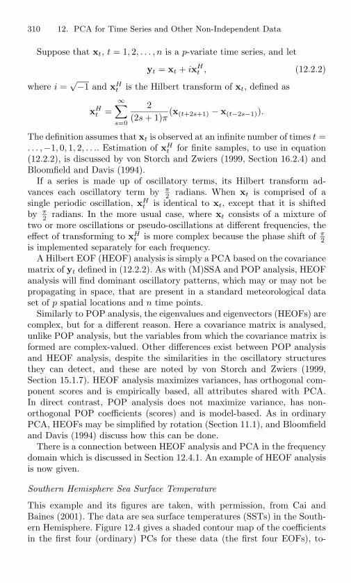
310 12. PCA for Time Series and Other Non-Independent Data
Suppose that xt, t = 1, 2, . . . , n is a p-variate time series, and let
yt = xt + ixHt , (12.2.2)
where i =√−1 and xH
t is the Hilbert transform of xt, defined as
xHt =
∞∑
s=0
2(2s + 1)π
(x(t+2s+1) − x(t−2s−1)).
The definition assumes that xt is observed at an infinite number of times t =. . . ,−1, 0, 1, 2, . . .. Estimation of xH
t for finite samples, to use in equation(12.2.2), is discussed by von Storch and Zwiers (1999, Section 16.2.4) andBloomfield and Davis (1994).
If a series is made up of oscillatory terms, its Hilbert transform ad-vances each oscillatory term by π
2 radians. When xt is comprised of asingle periodic oscillation, xH
t is identical to xt, except that it is shiftedby π
2 radians. In the more usual case, where xt consists of a mixture oftwo or more oscillations or pseudo-oscillations at different frequencies, theeffect of transforming to xH
t is more complex because the phase shift of π2
is implemented separately for each frequency.A Hilbert EOF (HEOF) analysis is simply a PCA based on the covariance
matrix of yt defined in (12.2.2). As with (M)SSA and POP analysis, HEOFanalysis will find dominant oscillatory patterns, which may or may not bepropagating in space, that are present in a standard meteorological dataset of p spatial locations and n time points.
Similarly to POP analysis, the eigenvalues and eigenvectors (HEOFs) arecomplex, but for a different reason. Here a covariance matrix is analysed,unlike POP analysis, but the variables from which the covariance matrix isformed are complex-valued. Other differences exist between POP analysisand HEOF analysis, despite the similarities in the oscillatory structuresthey can detect, and these are noted by von Storch and Zwiers (1999,Section 15.1.7). HEOF analysis maximizes variances, has orthogonal com-ponent scores and is empirically based, all attributes shared with PCA.In direct contrast, POP analysis does not maximize variance, has non-orthogonal POP coefficients (scores) and is model-based. As in ordinaryPCA, HEOFs may be simplified by rotation (Section 11.1), and Bloomfieldand Davis (1994) discuss how this can be done.
There is a connection between HEOF analysis and PCA in the frequencydomain which is discussed in Section 12.4.1. An example of HEOF analysisis now given.
Southern Hemisphere Sea Surface Temperature
This example and its figures are taken, with permission, from Cai andBaines (2001). The data are sea surface temperatures (SSTs) in the South-ern Hemisphere. Figure 12.4 gives a shaded contour map of the coefficientsin the first four (ordinary) PCs for these data (the first four EOFs), to-
12.2. PCA and Atmospheric Time Series 311
gether with the variance accounted for by each PC. Figure 12.5 displayssimilar plots for the real and imaginary parts of the first Hilbert EOF (la-belled CEOFs on the plots). It can be seen that the real part of the firstHilbert EOF in Figure 12.5 looks similar to EOF1 in Figure 12.4. There arealso similarities between EOF3 and the imaginary part of the first HilbertEOF.
Figures 12.6, 12.7 show plots of time series (scores), labelled temporalcoefficients in 12.7, for the first and third ordinary PCs, and the real andimaginary parts of the first HEOF, respectively. The similarity betweenthe first PC and the real part of the first HEOF is obvious. Both representthe same oscillatory behaviour in the series. The imaginary part of thefirst HEOF is also very similar, but lagged by π
2 , whereas the scores on thethird EOF show a somewhat smoother and more regular oscillation. Cai andBaines (2001) note that the main oscillations visible in Figures 12.6, 12.7can be identified with well-known El Nino-Southern Oscillation (ENSO)events. They also discuss other physical interpretations of the results ofthe HEOF analysis relating them to other meteorological variables, andthey provide tests for statistical significance of HEOFs.
The main advantage of HEOF analysis over ordinary PCA is its abilityto identify and reconstruct propagating waves, whereas PCA only findsstanding oscillations. For the first and second Hilbert EOFs, and for theirsum, this propagating behaviour is illustrated in Figure 12.8 by the move-ment of similar-valued coefficients from west to east as time progresses inthe vertical direction.
12.2.4 Multitaper Frequency Domain-Singular ValueDecomposition (MTM SVD)
In a lengthy paper, Mann and Park (1999) describe MTM-SVD, developedearlier by the same authors. It combines multitaper spectrum estimationmethods (MTM) with PCA using the singular value decomposition (SVD).The paper also gives a critique of several of the other techniques discussed inthe present section, together with frequency domain PCA which is coveredin Section 12.4.1. Mann and Park (1999) provide detailed examples, bothreal and artificial, in which MTM-SVD is implemented.
Like MSSA, POP analysis, HEOF analysis and frequency domain PCA,MTM-SVD looks for oscillatory behaviour in space and time. It is closestin form to PCA of the spectral matrix F(λ) (Section 12.4.1), as it operatesin the frequency domain. However, in transferring from the time domainto the frequency domain MTM-SVD constructs a set of different taperedFourier transforms (hence the ‘multitaper’ in its name). The frequency do-main matrix is then subjected to a singular value decomposition, giving‘spatial’ or ‘spectral’ EOFs, and ‘principal modulations’ which are analo-gous to principal component scores. Mann and Park (1999) state that the

312 12. PCA for Time Series and Other Non-Independent Data
Figure 12.4. The first four EOFs for Southern Hemisphere SST.
Figure 12.5. Real and imaginary parts of the first Hilbert EOF for SouthernHemisphere SST.

12.2. PCA and Atmospheric Time Series 313
1980 1985 1990 1995 2000Time (years)
15.0
10.0
5.0
0.0
5.0
10.0
15.0
EOF1EOF3
Figure 12.6. Plots of temporal scores for EOF1 and EOF3 for SouthernHemisphere SST.
1980 1985 1990 1995 2000Time (years)
15.0
10.0
5.0
0.0
5.0
10.0
15.0
CEOFSST1.rCEOFSST1.i
Figure 12.7. Plots of temporal scores for real and imaginary parts of the firstHilbert EOF for Southern Hemisphere SST.
314 12. PCA for Time Series and Other Non-Independent Data
Figure 12.8. Propagation of waves in space and time in Hilbert EOF1, HilbertEOF2, and the sum of these two Hilbert EOFs.
distinction between MTM-SVD and standard frequency domain PCA isthat the former provides a local frequency domain decomposition of thedifferent spectral estimates given by the multitapers, whereas the latterproduces a global frequency domain decomposition over the spectral esti-mates. Mann and Park (1999) describe tests for the statistical significanceof the oscillations found by MTM-SVD using a bootstrap approach, which,it is claimed, is effective for a general, smoothly varying, coloured noisebackground, and is not restricted to red noise as in Allen and Smith (1996)and Allen and Robertson (1996).
12.2.5 Cyclo-Stationary and Periodically Extended EOFs(and POPs)
The assumption of temporal stationarity is implicit for most of the methodsdescribed in this chapter. In meteorological data there is often a cycle witha fixed period, most commonly the annual cycle but sometimes a diurnalcycle. There may then be stationarity for times at the same point in thecycle but not across different points in the cycle. For example, for monthlydata the probability distribution may be same every April but different in
12.2. PCA and Atmospheric Time Series 315
April than in June. Similarly, the joint distribution for April and August,which have a four-month separation, may be the same in different years,but different from the joint distribution for June and October, even thoughthe latter are also separated by four months. Such behaviour is known ascyclo-stationarity, and both PCA and POP analysis have been modifiedfor such data.
The modification is easier to explain for POP analysis than for PCA.Suppose that τ is the length of the cycle; for example τ = 12 for monthlydata and an annual cycle. Then for a time series of length n = n′τ equation(12.2.1) is replaced by
(x(sτ+t+1) − µ(t+1)) = Υt(x(sτ+t) − µt) + ε(sτ+t), (12.2.3)
t = 0, 1, . . . , (τ − 2); s = 0, 1, 2, . . . , (n′ − 1),
with (t + 1) replaced by 0, and s replaced by (s + 1) on the left-hand sideof (12.2.3) when t = (τ − 1) and s = 0, 1, 2, . . . , (n′ − 2). Here the mean µt
and the matrix Υt can vary within cycles, but not between cycles. Cyclo-stationary POP analysis estimates Υ0,Υ1, . . . ,Υ(τ−1) and is based on aneigenanalysis of the product of those estimates Υ0Υ1 . . . Υ(τ−1).
The cyclo-stationary variety of PCA is summarized by Kim and Wu(1999) but is less transparent in its justification than cyclo-stationaryPOP analysis. First, vectors a0t,a1t, . . . ,a(τ−1)t are found such that xt =∑τ−1
j=0 ajte2πijt
τ , and a new vector of variables is then constructed byconcatenating a0t,a1t, . . . ,a(τ−1)t. Cyclo-stationary EOFs (CSEOFs) areobtained as eigenvectors of the covariance matrix formed from this vectorof variables. Kim and Wu (1999) give examples of the technique, and alsogive references explaining how to calculate CSEOFs.
Kim and Wu (1999) describe an additional modification of PCA thatdeals with periodicity in a time series, and which they call a periodicallyextended EOF technique. It works by dividing a series of length n = n′τinto n′ blocks of length τ . A covariance matrix, SEX , is then computed as
SEX11 SEX
12 · · · SEX1n′
SEX21 SEX
22 · · · SEX2n′
......
SEXn′1 SEX
n′2 · · · SEXn′n′
,
in which the (i, j)th element of SEXkl is the sample covariance between
the measurements at the ith location at time k in each block and at thejth location at time l in the same block. The description of the techniquein Kim and Wu (1999) is sketchy, but it appears that whereas in ordinaryPCA, covariances are calculated by averaging over all time points, here theaveraging is done over times at the same point within each block acrossblocks. A similar averaging is implicit in cyclo-stationary POP analysis.Examples of periodically extended EOFs are given by Kim and Wu (1999).

316 12. PCA for Time Series and Other Non-Independent Data
12.2.6 Examples and Comparisons
Relatively few examples have been given in this section, due in part to theircomplexity and their rather specialized nature. Several of the techniquesdescribed claim to be able to detect stationary and propagating wavesin the standard type of spatio-temporal meteorological data. Each of themethods has proponents who give nice examples, both real and artificial, inwhich their techniques appear to work well. However, as with many otheraspects of PCA and related procedures, caution is needed, lest enthusiasmleads to ‘over-interpretation.’ With this caveat firmly in mind, examples ofSSA can be found in Elsner and Tsonis (1996), Vautard (1995); MSSA inPlaut and Vautard (1994), Mote et al. (2000); POPs in Kooperberg andO’Sullivan (1996) with cyclo-stationary POPs in addition in von Storchand Zwiers (1999, Chapter 15); Hilbert EOFs in Horel (1984), Cai andBaines (2001); MTM-SVD in Mann and Park (1999); cyclo-stationary andperiodically extended EOFs in Kim and Wu (1999). This last paper com-pares eight techniques (PCA, PCA plus rotation, extended EOFs (MSSA),Hilbert EOFs, cyclo-stationary EOFs, periodically extended EOFs, POPsand cyclo-stationary POPs) on artificial data sets with stationary pat-terns, with patterns that are stationary in space but which have amplitudeschanging in time, and with patterns that have periodic oscillations in space.The results largely confirm what might be expected. The procedures de-signed to find oscillatory patterns do not perform well for stationary data,the converse holds when oscillations are present, and those techniquesdevised for cyclo-stationary data do best on such data.
12.3 Functional PCA
There are many circumstances when the data are curves. A field in whichsuch data are common is that of chemical spectroscopy (see, for exam-ple, Krzanowski et al. (1995), Mertens (1998)). Other examples includethe trace on a continuously recording meteorological instrument such as abarograph, or the trajectory of a diving seal. Other data, although mea-sured at discrete intervals, have an underlying continuous functional form.Examples include the height of a child at various ages, the annual cycle oftemperature recorded as monthly means, or the speed of an athlete duringa race.
The basic ideas of PCA carry over to this continuous (functional) case,but the details are different. In Section 12.3.1 we describe the generalset-up in functional PCA (FPCA), and discuss methods for estimating func-tional PCs in Section 12.3.2. Section 12.3.3 presents an example. Finally,Section 12.3.4 briefly covers some additional topics including curve registra-tion, bivariate FPCA, smoothing, principal differential analysis, prediction,discrimination, rotation, density estimation and robust FPCA.
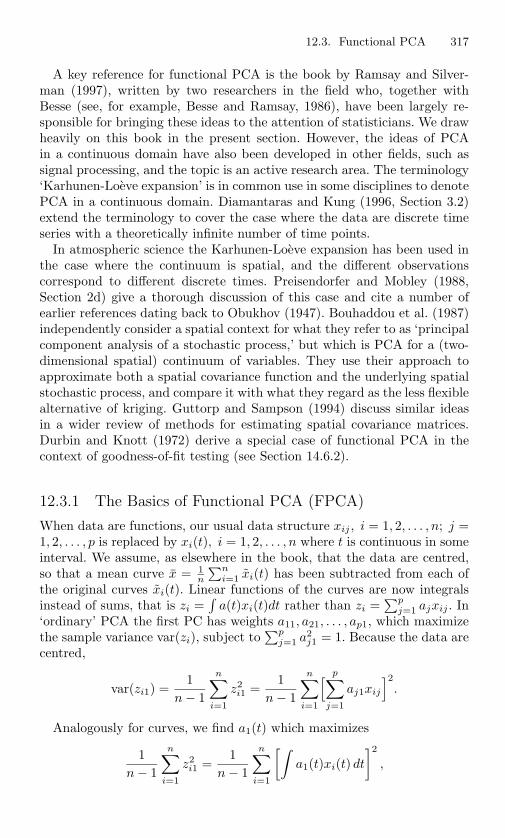
12.3. Functional PCA 317
A key reference for functional PCA is the book by Ramsay and Silver-man (1997), written by two researchers in the field who, together withBesse (see, for example, Besse and Ramsay, 1986), have been largely re-sponsible for bringing these ideas to the attention of statisticians. We drawheavily on this book in the present section. However, the ideas of PCAin a continuous domain have also been developed in other fields, such assignal processing, and the topic is an active research area. The terminology‘Karhunen-Loeve expansion’ is in common use in some disciplines to denotePCA in a continuous domain. Diamantaras and Kung (1996, Section 3.2)extend the terminology to cover the case where the data are discrete timeseries with a theoretically infinite number of time points.
In atmospheric science the Karhunen-Loeve expansion has been used inthe case where the continuum is spatial, and the different observationscorrespond to different discrete times. Preisendorfer and Mobley (1988,Section 2d) give a thorough discussion of this case and cite a number ofearlier references dating back to Obukhov (1947). Bouhaddou et al. (1987)independently consider a spatial context for what they refer to as ‘principalcomponent analysis of a stochastic process,’ but which is PCA for a (two-dimensional spatial) continuum of variables. They use their approach toapproximate both a spatial covariance function and the underlying spatialstochastic process, and compare it with what they regard as the less flexiblealternative of kriging. Guttorp and Sampson (1994) discuss similar ideasin a wider review of methods for estimating spatial covariance matrices.Durbin and Knott (1972) derive a special case of functional PCA in thecontext of goodness-of-fit testing (see Section 14.6.2).
12.3.1 The Basics of Functional PCA (FPCA)
When data are functions, our usual data structure xij , i = 1, 2, . . . , n; j =1, 2, . . . , p is replaced by xi(t), i = 1, 2, . . . , n where t is continuous in someinterval. We assume, as elsewhere in the book, that the data are centred,so that a mean curve x = 1
n
∑ni=1 xi(t) has been subtracted from each of
the original curves xi(t). Linear functions of the curves are now integralsinstead of sums, that is zi =
∫a(t)xi(t)dt rather than zi =
∑pj=1 ajxij . In
‘ordinary’ PCA the first PC has weights a11, a21, . . . , ap1, which maximizethe sample variance var(zi), subject to
∑pj=1 a2
j1 = 1. Because the data arecentred,
var(zi1) =1
n − 1
n∑
i=1
z2i1 =
1n − 1
n∑
i=1
[ p∑
j=1
aj1xij
]2.
Analogously for curves, we find a1(t) which maximizes
1n − 1
n∑
i=1
z2i1 =
1n − 1
n∑
i=1
[∫a1(t)xi(t) dt
]2,

318 12. PCA for Time Series and Other Non-Independent Data
subject to∫
a21(t)dt = 1. Here, and elsewhere, the integral is over the range
of values of t for which the data are observed. Subsequent FPCs are definedsuccessively, as with ordinary PCA, to maximise
var(zik) =1
n − 1
n∑
i=1
[∫ak(t)xi(t) dt
]2,
subject to∫
a2k(t)dt = 1;
∫ak(t)ah(t)dt = 0, k = 2, 3, . . . ; h = 1, 2, . . .;
h < k.The sample covariance between x(s) and x(t) can be defined as S(s, t) =1
(n−1)
∑ni=1 xi(s)xi(t), with a corresponding definition for correlation, and
to find the functional PCs an eigenequation is solved involving thiscovariance function. Specifically, we solve
∫S(s, t)a(t)dt = la(s). (12.3.1)
Comparing (12.3.1) to the eigenequation Sa = la for ordinary PCA, thepre-multiplication of a vector of weights by a matrix of covariances on theleft-hand side is replaced by an integral operator in which the covariancefunction is multiplied by a weight function a(t) and then integrated. Inordinary PCA the number of solutions to the eigenequation is usually p,the number of variables. Here the p variables are replaced by a infinitenumber of values for t but the number of solutions is still finite, because thenumber of curves n is finite. The number of non-zero eigenvalues l1, l2, . . .,and corresponding functions a1(t), a2(t), . . . cannot exceed (n − 1).
12.3.2 Calculating Functional PCs (FPCs)
Unless the curves are all fairly simple functional forms, it is not possibleto solve (12.3.1) exactly. Ramsay and Silverman (1997, Section 6.4) givethree computational methods for FPCA, but in most circumstances theyrepresent approximate solutions to (12.3.1). In the first of the three, thedata are discretized. The values xi(t1), xi(t2), . . . , xi(tp) form the ith rowof an (n×p) data matrix which is then analysed using standard PCA. Thetimes t1, t2, . . . , tp are usually chosen to be equally spaced in the range ofcontinuous values for t. To convert the eigenvectors found from this PCAinto functional form, it is necessary to renormalize the eigenvectors andthen interpolate them with a suitable smoother (Ramsay and Silverman,1997, Section 6.4.1).
A second approach assumes that the curves xi(t) can be expressed lin-early in terms of a set of G basis functions, where G is typically lessthan n. If φ1(t), φ2(t), . . . , φG(t) are the basis functions, then xi(t) =∑G
g=1 cigφg(t), i = 1, 2, . . . , n or, in matrix form, x(t) = Cφ(t), wherex′(t) = (x1(t), x2(t), . . . , xn(t)), φ′(t) = (φ1(t), φ2(t), . . . , φG(t)) and C isan (n × G) matrix with (i, g)th element cig.

12.3. Functional PCA 319
The sample covariance between x(s) and x(t) can be written
1n − 1
x′(s)x(t) =1
n − 1φ′(s)C′Cφ(t).
Any eigenfunction a(t) can be expressed in terms of the basis func-tions as a(t) =
∑Gg=1 bgφg(t) = φ′(t)b for some vector of coefficients
b′ = (b1, b2, . . . , bG). The left-hand-side of equation (12.3.1) is then∫
S(s, t)a(t) dt =∫
1n − 1
φ′(s)C′Cφ(t)φ′(t)b dt
=1
n − 1φ′(s)C′C
[∫φ(t)φ′(t) dt
]b.
The integral is a (G×G) matrix W whose (g, h)th element is∫
φg(t)φh(t)dt.If the basis is orthogonal, W is simply the identity matrix IG. Hence choos-ing an orthogonal basis in circumstances where such a choice makes sense,as with a Fourier basis for periodic data, gives simplified calculations. Ingeneral (12.3.1) becomes
1n − 1
φ′(s)C′CWb = lφ′(s)b
but, because this equation must hold for all available values of s, it reducesto
1n − 1
C′CWb = lb. (12.3.2)
When∫
a2(t)dt = 1 it follows that
1 =∫
a2(t) dt =∫
b′φ(t)φ′(t)b dt = b′Wb.
If ak(t) is written in terms of the basis functions as ak(t) =∑G
g=1 bkgφg(t),with a similar expression for al(t), then ak(t) is orthogonal to al(t) ifb′
kWbl = 0, where b′k = (bk1, bk2, . . . , bkG), and b′
l is defined similarly.In an eigenequation, the eigenvector is usually normalized to have unit
length (norm). To convert (12.3.2) into this form, define u = W12 b. Then
u′u = 1 and (12.3.2) can be written
1n − 1
W12 C′CW
12 u = lu. (12.3.3)
Equation (12.3.3) is solved for l and u, b is obtained as W− 12 u, and finally
a(t) = φ′(t)b = φ′(t)W− 12 u.
The special case where the basis is orthogonal has already been men-tioned. Here W = IG, so b = u is an eigenvector of 1
n−1C′C. Another
special case, noted by Ramsay and Silverman (1997), occurs when thedata curves themselves are taken as the basis. Then C = In and u isan eigenvector of 1
n−1W.
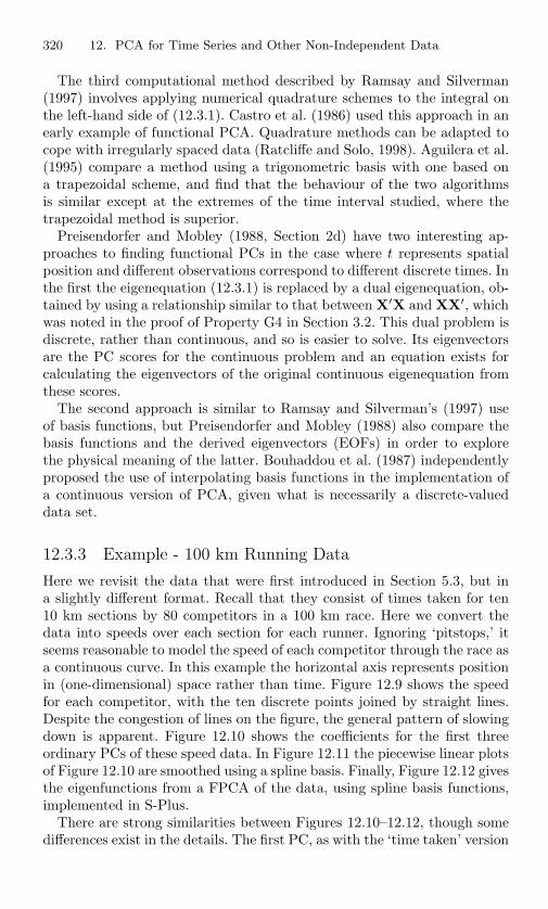
320 12. PCA for Time Series and Other Non-Independent Data
The third computational method described by Ramsay and Silverman(1997) involves applying numerical quadrature schemes to the integral onthe left-hand side of (12.3.1). Castro et al. (1986) used this approach in anearly example of functional PCA. Quadrature methods can be adapted tocope with irregularly spaced data (Ratcliffe and Solo, 1998). Aguilera et al.(1995) compare a method using a trigonometric basis with one based ona trapezoidal scheme, and find that the behaviour of the two algorithmsis similar except at the extremes of the time interval studied, where thetrapezoidal method is superior.
Preisendorfer and Mobley (1988, Section 2d) have two interesting ap-proaches to finding functional PCs in the case where t represents spatialposition and different observations correspond to different discrete times. Inthe first the eigenequation (12.3.1) is replaced by a dual eigenequation, ob-tained by using a relationship similar to that between X′X and XX′, whichwas noted in the proof of Property G4 in Section 3.2. This dual problem isdiscrete, rather than continuous, and so is easier to solve. Its eigenvectorsare the PC scores for the continuous problem and an equation exists forcalculating the eigenvectors of the original continuous eigenequation fromthese scores.
The second approach is similar to Ramsay and Silverman’s (1997) useof basis functions, but Preisendorfer and Mobley (1988) also compare thebasis functions and the derived eigenvectors (EOFs) in order to explorethe physical meaning of the latter. Bouhaddou et al. (1987) independentlyproposed the use of interpolating basis functions in the implementation ofa continuous version of PCA, given what is necessarily a discrete-valueddata set.
12.3.3 Example - 100 km Running Data
Here we revisit the data that were first introduced in Section 5.3, but ina slightly different format. Recall that they consist of times taken for ten10 km sections by 80 competitors in a 100 km race. Here we convert thedata into speeds over each section for each runner. Ignoring ‘pitstops,’ itseems reasonable to model the speed of each competitor through the race asa continuous curve. In this example the horizontal axis represents positionin (one-dimensional) space rather than time. Figure 12.9 shows the speedfor each competitor, with the ten discrete points joined by straight lines.Despite the congestion of lines on the figure, the general pattern of slowingdown is apparent. Figure 12.10 shows the coefficients for the first threeordinary PCs of these speed data. In Figure 12.11 the piecewise linear plotsof Figure 12.10 are smoothed using a spline basis. Finally, Figure 12.12 givesthe eigenfunctions from a FPCA of the data, using spline basis functions,implemented in S-Plus.
There are strong similarities between Figures 12.10–12.12, though somedifferences exist in the details. The first PC, as with the ‘time taken’ version
12.3. Functional PCA 321
distance (km)
spee
d (m
eter
s pe
r se
cond
)
0.5 1.5 2.5 3.5 4.5 5.5 6.5 7.5 8.5 9.5
1.5
22.
53
3.5
44.
5
Figure 12.9. Plots of speed for 80 competitors in a 100 km race.
distance (km)
coef
ficie
nt
0.5 1.5 2.5 3.5 4.5 5.5 6.5 7.5 8.5 9.5
-0.4
-0.2
0
0.2
0.4
PC1PC2PC3
Figure 12.10. Coefficients for first three PCs from the 100 km speed data.

322 12. PCA for Time Series and Other Non-Independent Data
distance (km)
Sm
ooth
ed c
oeffi
cien
t
0.5 1.5 2.5 3.5 4.5 5.5 6.5 7.5 8.5 9.5
-0.4
-0.2
0
0.2
0.4
0.6
Smoothed PC1Smoothed PC2Smoothed PC3
Figure 12.11. Smoothed version of Figure 12.10 using a spline basis; dots arecoefficients from Figure 12.10.
distance (km)
eige
nfun
ctio
n va
lue
0.5 1.5 2.5 3.5 4.5 5.5 6.5 7.5 8.5 9.5
-0.4
-0.2
0
0.2
0.4
0.6
0.8
FPC1FPC2FPC3
Figure 12.12. Coefficients (eigenfunctions) for the first three components in afunctional PCA of the 100 km speed data using a spline basis; dots are coefficientsfrom Figure 12.10.

12.3. Functional PCA 323
of the data in Section 5.3, is a measure of overall speed throughout therace. The second component in all cases represents the degree to whichrunners slow down during the race. The pattern in Figure 12.10 is verymuch like that in Table 5.2. Figures 12.11 and 12.12 have a similar shapefor this component, although the absolute values of the eigenfunction inFigure 12.12 are slightly larger than the coefficients in Figure 12.11. Thereason for this is that the speed for the first 10 km section is plotted atdistance equal to 0.5 km, the speed for the second section at 1.5 km and soon. The eigenfunctions for the FPCs are then calculated over the interval0.5 to 9.5, a range of 9, whereas there are 10 elements in the ordinaryPC eigenvectors, leading to different normalizations. Calculating the FPCsover the range 0 to 10 leads to erratic behaviour at the ends of the interval.The pattern for the third PC is again similar in all three figures, except atthe extreme right-hand end.
12.3.4 Further Topics in FPCA
This subsection collects together briefly a number of topics that are relevantto FPCA. As in the rest of this section, the main reference is Ramsay andSilverman (1997).
Curve Registration
In some examples where the data are functions, the individual curves xi(t)may be observed over different ranges for t. Most procedures for analysingfunctional data assume the same range of t for all curves. Furthermore, it isoften the case that the horizontal extent of the curve is of less importancethan its shape. For example, suppose that the trajectory of underwaterdives made by seals is of interest (see Schreer et al. (1998)). Although thelengths of the dives may be informative, so are their shapes, and to comparethese the curves should be aligned to start and finish at the same respectivetimes. This process is known as curve registration. Another example ariseswhen outlines of sliced carrots are examined in order to determine to whichvariety of carrot an individual specimen belongs (Horgan et al., 2001).More complicated situations are discussed by Ramsay and Silverman (1997,Chapter 5), in which several landmarks along the curves must be aligned,leading to differential stretching and expansion of ‘time’ for different partsof the curves. Capra and Muller (1997) use an accelerated time model toalign mortality curves for medflies. They refer to their accelerated time as‘eigenzeit.’
Sometimes alignment is desirable in the vertical, as well the horizontal,direction. Consider again the dive trajectories of seals. If the shapes of thedives are more important than their depths, then the dives can be alignedvertically at their deepest points.
To analyse only the registered curves, without taking into account ofwhat was done in the registration process, is to throw away information.

324 12. PCA for Time Series and Other Non-Independent Data
Keeping one or more parameters for each curve, defining how registrationwas done, leads to what Ramsay and Silverman (1997) called ‘mixed data.’Each observation for such data consists of a curve, together with p other‘ordinary’ variables. Ramsay and Silverman (1997, Chapter 8) discuss theanalysis of such data.
Bivariate FPCA
In other cases, the data are not ‘mixed’ but there is more than one curveassociated with each individual. An example involving changes of angles inboth hip and knee during a gait cycle is described by Ramsay and Silverman(1997, Section 6.5). They discuss the analysis of bivariate curves from thisexample using bivariate FPCA. Suppose that the two sets of curves arex1(t), x2(t), . . . , xn(t); y1(t), y2(t), . . . , yn(t). Define a bivariate covariancefunction S(s, t) as
[SXX(s, t) SXY (s, t)SY X(s, t) SY Y (s, t)
],
where SXX(s, t), SY Y (s, t) are covariance functions defined, as earlier, for(x(s), x(t)) and (y(s), y(t)), respectively, and SXY (s, t) has elements thatare covariances between x(s) and y(t). Suppose that
zXi =∫
aX(t)xi(t) dt, zY i =∫
aY (t)yi(t)dt.
Finding aX(t), aY (t) to maximize 1n−1
∑ni=1(z
2Xi + z2
Y i) leads to theeigenequations
∫SXX(s, t)aX(t) dt +
∫SXY (s, t)aY (t) dt = laX(t)
∫SY X(s, t)aX(t) dt +
∫SY Y (s, t)aY (t) dt = laY (t).
This analysis can be extended to the case of more than two curves perindividual.
Smoothing
If the data are not smooth, the weighting functions a(t) in FPCA may notbe smooth either. With most curves, an underlying smoothness is expected,with the superimposed roughness being due to noise that should ideallybe removed. Ramsay and Silverman (1997, Chapter 7) tackle this prob-lem. Their main approach incorporates a roughness penalty into FPCA’svariance-maximizing problem. The second derivative of a curve is oftentaken as a measure of its roughness and, if D2a(t) represents the secondderivative of a(t), a smooth curve requires a small value of D2a(t). Ramsayand Silverman’s approach is to maximize
1n−1
∑ni=1[∫
a(t)xi(t)dt]2∫
a2(t)dt + λ∫
(D2a(t))2dt(12.3.4)

12.3. Functional PCA 325
subject to∫
a2(t)dt = 1, where λ is a tuning parameter. Taking λ = 0simply gives unsmoothed FPCA; as λ increases, so does the smoothnessof the optimal a(t). Ramsay and Silverman (1997, Section 7.3) show thatsolving the optimization problem reduces to solving the eigenequation
∫S(s, t)a(t)dt = l(1 + λD4)a(s), (12.3.5)
where D4a(s) is the fourth derivative of a(s). In their Section 7.4 they givesome computational methods for (approximately) solving equation (12.3.5),with the choice of λ discussed in Section 7.5. Minimizing (12.3.4) by solving(12.3.5) implies a form of orthogonality between successive ak(t) that isdifferent from the usual one. Ocana et al. (1999) interpret this as a differentchoice of norm and inner product, and discuss the choice of norm in FPCAfrom a theoretical point of view. If (12.3.5) is solved by using basis functionsfor the data, the number of basis functions and the smoothing parameterλ both need to be chosen. Ratcliffe and Solo (1998) address the problemof choosing both simultaneously and propose an improved cross-validationprocedure for doing so.
An alternative to incorporating smoothing directly into FPCA is tosmooth the data first and then conduct unsmoothed FPCA on thesmoothed curves. The smoothing step uses the well-known idea of minimi-zing the sum of squares between fitted and observed curves, supplementedby a penalty function based on lack of smoothness (a roughness penalty).The quantity we wish to minimize can be written succicntly as
‖x(t) − x(t)‖2 + λ‖x(t)‖2, (12.3.6)
where x(t), x(t) denote observed and fitted curves, respectively, ‖ . ‖ de-notes an appropriately chosen norm, not necessarily the same in the twoparts of the expression, and λ is a tuning parameter. The second norm isoften related to the second derivative, D2[x(t)], which is a commonly usedmeasure of roughness.
Besse et al. (1997) use a similar approach in which they optimize a crite-rion which, like (12.3.6), is a sum of two terms, one a measure of fit and theother a roughness penalty with a tuning parameter λ. Besse et al.’s modelassumes that, apart from noise, the curves lie in a q-dimensional space.A version Rq of the criterion Rq, suggested by Besse and de Falguerolles(1993) and discussed in Section 6.1.5, is minimized with respect to q andλ simultaneously. If smoothing of the data is done using splines, then thePCA on the resulting interpolated data is equivalent to a PCA on the orig-inal data, but with a different metric (Besse, 1988). We return to this topicin Section 14.2.2.
A more complicated approach to smoothing followed by PCA, involvingdifferent smoothing parameters for different FPCs, is discussed by Ram-say and Silverman (1997, Section 7.8). Grambsch et al. (1995) also use asmoothing process—though a different one—for the data, followed by PCA

326 12. PCA for Time Series and Other Non-Independent Data
on the smoothed data. Kneip (1994) independently suggested smoothingthe data, followed by PCA on the smoothed data, in the context of fittinga model in which a small number of functions is assumed to underlie aset of regression curves. Theoretical properties of Kneip’s (1994) procedureare examined in detail in his paper. Champely and Doledec (1997) uselo(w)ess (locally weighted scatterplot smoothing—Cleveland, 1979, 1981)to fit smooth trend and periodic curves to water quality data, and thenapply FPCA separately to the trend and periodic curves.
Principal Differential Analysis
Principal differential analysis (PDA), a term coined by Ramsay (1996) anddiscussed in Ramsay and Silverman (1997, Chapter 14) is another methodof approximating a set of curves by a smaller number of functions. AlthoughPDA has some similarities to FPCA, which we note below, it concentrateson finding functions that have a certain type of smoothness, rather thanmaximizing variance. Define a linear differential operator
L = w0I + w1D + . . . + wm−1Dm−1 + Dm,
where Di, as before, denotes the ith derivative operator and I is the identityoperator. PDA finds weights w0, w1, . . . , wm−1 for which [Lxi(t)]2 is smallfor each observed curve xi(t). Formally, we minimize
∑ni=1
∫[Lxi(t)]2 dt
with respect to w0, w1, . . . , wm−1.Once w0, w1, . . . , wm−1 and hence L are found, any curve satisfying
Lx(t) = 0 can be expressed as a linear combination of m linearly inde-pendent functions spanning the null space of the operator L. Any observedcurve xi(t) can be approximated by expanding it in terms of these m func-tions. This is similar to PCA, where the original data can be approximatedby expanding them in terms of the first few (say m) PCs. The difference isthat PCA finds an m-dimensional space with a least squares fit to the orig-inal data, whereas PDA finds a space which penalizes roughness. This lastinterpretation follows because Lxi(t) is typically rougher than xi(t), andPDA aims to make Lxi(t), or rather [Lxi(t)]2, as small as possible whenaveraged over i and t. An application of PDA to the study of variations inhandwriting is presented by Ramsay (2000).
Prediction and Discrimination
Aguilera et al. (1997, 1999a) discuss the idea of predicting a continuoustime series by regressing functional PCs for the future on functional PCsfrom the past. To implement this methodology, Aguilera et al. (1999b)propose cutting the series into a number of segments n of equal length,which are then treated as n realizations of the same underlying process.Each segment is in turn divided into two parts, with the second, shorter,part to be predicted from the first. In calculating means and covariancefunctions, less weight is given to the segments from the early part of the

12.3. Functional PCA 327
series than to those closer to the present time from where the future is tobe predicted. Besse et al. (2000) also use functional PCA to predict timeseries, but in the context of a smoothed first order autoregessive model.The different replications of the function correspond to different years,while the function ranges over the months within years. A ‘local’ versionof the technique is developed in which the assumption of stationarity isrelaxed.
Hall et al. (2001) advocate the use of functional PCA as a dimension-reducing step in the context of discriminating between different types ofradar signal. Although this differs from the usual set-up for PCA in dis-criminant analysis (see Section 9.1) because it notionally has an infinitenumber of variables in a continuum, there is still the possibility that someof the later discarded components may contain non-trivial discriminatorypower.
Rotation
As with ordinary PCA, the interpretation of FPCA may be improved byrotation. In addition to the conventional rotation of coefficients in a sub-set of PCs (see Section 11.1), Ramsay and Silverman (1997, Section 6.3.3)suggest that the coefficients b1,b2, . . . ,bm of the first m eigenfunctionswith respect to a chosen set of basis functions, as defined in Section 12.3.2,could also be rotated to help interpretation. Arbuckle and Friendly (1977)propose a variation on the usual rotation criteria of Section 11.1 for vari-ables that are measurements at discrete points on a continuous curve. Theysuggest rotating the results of an ordinary PCA towards smoothness ratherthan towards simplicity as usually defined (see Section 11.1).
Density Estimation
Kneip and Utikal (2001) discuss functional PCA as a means of examiningcommon structure and differences in a set of probability density functions.The densities are first estimated from a number of data sets using kerneldensity estimators, and these estimates are then subjected to functionalPCA. As well as a specific application, which examines how densities evolvein data sets collected over a number of years, Kneip and Utikal (2001)introduce some new methodology for estimating functional PCs and fordeciding how many components should be retained to represent the densityestimates adequately. Their paper is followed by published discussion fromfour sets of discussants.
Robustness
Locantore et al. (1999) consider robust estimation of PCs for functionaldata (see Section 10.4).

328 12. PCA for Time Series and Other Non-Independent Data
12.4 PCA and Non-Independent Data—SomeAdditional Topics
In this section we collect together a number of topics from time series,and other contexts in which non-independent data arise, where PCA orrelated techniques are used. Section 12.4.1 describes PCA in the frequencydomain, and Section 12.4.2 covers growth curves and longitudinal data. InSection 12.4.3 a summary is given of another idea (optimal fingerprints)from climatology, though one that is rather different in character fromthose presented in Section 12.2. Section 12.4.4 discusses spatial data, andthe final subsection provides brief coverage of a few other topics, includingnon-independence induced by survey designs.
12.4.1 PCA in the Frequency Domain
The idea of PCA in the frequency domain clearly has no counterpart fordata sets consisting of independent observations. Brillinger (1981, Chap-ter 9) devotes a whole chapter to the subject (see also Priestley et al.(1974)). To see how frequency domain PCs are derived, note that PCs fora p-variate random vector x, with zero mean, can be obtained by finding(p × q) matrices B, C such that
E[(x − Cz)′(x − Cz)]
is minimized, where z = B′x. This is equivalent to the criterion that definesProperty A5 in Section 2.1 It turns out that B = C and that the columnsof B are the first q eigenvectors of Σ, the covariance matrix of x, so thatthe elements of z are the first q PCs for x. This argument can be extendedto a time series of p variables as follows. Suppose that our series is . . .x−1,x0, x1, x2, . . . and that E[xt] = 0 for all t. Define
zt =∞∑
u=−∞B′
t−uxu,
and estimate xt by∑∞
u=−∞ Ct−uzu, where
. . .Bt−1,Bt,Bt+1,Bt+2, . . . ,Ct−1,Ct,Ct+1,Ct+2, . . .
are (p × q) matrices that minimize
E[(
xt −∞∑
u=−∞Ct−uzu
)∗(xt −
∞∑
u=−∞Ct−uzu
)],
where * denotes conjugate transpose. The difference between this formula-tion and that for ordinary PCs above is that the relationships between zand x are in terms of all values of xt and zt, at different times, rather thanbetween a single x and z. Also, the derivation is in terms of general complex
12.4. PCA and Non-Independent Data—Some Additional Topics 329
series, rather than being restricted to real series. It turns out (Brillinger,1981, p. 344) that
B′u =
12π
∫ 2π
0
B(λ)eiuλdλ
Cu =12π
∫ 2π
0
C(λ)eiuλdλ,
where C(λ) is a (p × q) matrix whose columns are the first q eigenvectorsof the matrix F(λ) given in (12.1.4), and B(λ) is the conjugate transposeof C(λ).
The q series that form the elements of zt are called the first q PC series ofxt. Brillinger (1981, Sections 9.3, 9.4) discusses various properties and esti-mates of these PC series, and gives an example in Section 9.6 on monthlytemperature measurements at 14 meteorological stations. Principal com-ponent analysis in the frequency domain has also been used on economictime series, for example on Dutch provincial unemployment data (Bartels,1977, Section 7.7).
There is a connection between frequency domain PCs and PCs definedin the time domain (Brillinger, 1981, Section 9.5). The connection involvesHilbert transforms and hence, as noted in Section 12.2.3, frequency do-main PCA has links to HEOF analysis. Define the vector of variablesyH
t (λ) = (x′t(λ),x′H
t (λ))′, where xt(λ) is the contribution to xt at fre-quency λ (Brillinger, 1981, Section 4.6), and xH
t (λ) is its Hilbert transform.Then the covariance matrix of yH
t (λ) is proportional to[
Re(F(λ)) Im(F(λ))− Im(F(λ)) Re(F(λ))
],
where the functions Re(.), Im(.) denote the real and imaginary parts, re-spectively, of their argument. A PCA of yH
t gives eigenvalues that are theeigenvalues of F(λ) with a corresponding pair of eigenvectors
[Re(Cj(λ))Im(Cj(λ))
],
[ − Im(Cj(λ))Re(Cj(λ))
],
where Cj(λ) is the jth column of C(λ).Horel (1984) interprets HEOF analysis as frequency domain PCA av-
eraged over all frequency bands. When a single frequency of oscillationdominates the variation in a time series, the two techniques become thesame. The averaging over frequencies of HEOF analysis is presumably thereason behind Plaut and Vautard’s (1994) claim that it is less good thanMSSA at distinguishing propagating patterns with different frequencies.
Preisendorfer and Mobley (1988) describe a number of ways in whichPCA is combined with a frequency domain approach. Their Section 4ediscusses the use of PCA after a vector field has been transformed intothe frequency domain using Fourier analysis, and for scalar-valued fields

330 12. PCA for Time Series and Other Non-Independent Data
their Chapter 12 examines various combinations of real and complex-valuedharmonic analysis with PCA.
Stoffer (1999) describes a different type of frequency domain PCA, whichhe calls the spectral envelope. Here a PCA is done on the spectral matrixF(λ) relative to the time domain covariance matrix Γ0. This is a form ofgeneralized PCA for F(λ) with Γ0 as a metric (see Section 14.2.2), andleads to solving the eigenequation [F(λ) − l(λ)Γ0]a(λ) = 0 for varyingangular frequency λ. Stoffer (1999) advocates the method as a way of dis-covering whether the p series x1(t), x2(t), . . . xp(t) share common signalsand illustrates its use on two data sets involving pain perception and bloodpressure.
The idea of cointegration is important in econometrics. It has a technicaldefinition, but can essentially be described as follows. Suppose that theelements of the p-variate time series xt are stationary after, but not before,differencing. If there are one or more vectors α such that α′xt is stationarywithout differencing, the p series are cointegrated. Tests for cointegrationbased on the variances of frequency domain PCs have been put forward bya number of authors. For example, Cubadda (1995) points out problemswith previously defined tests and suggests a new one.
12.4.2 Growth Curves and Longitudinal Data
A common type of data that take the form of curves, even if they are notnecessarily recorded as such, consists of measurements of growth for animalsor children. Some curves such as heights are monotonically increasing, butothers such as weights need not be. The idea of using principal componentsto summarize the major sources of variation in a set of growth curves datesback to Rao (1958), and several of the examples in Ramsay and Silverman(1997) are of this type. Analyses of growth curves are often concerned withpredicting future growth, and one way of doing this is to use principalcomponents as predictors. A form of generalized PC regression developedfor this purpose is described by Rao (1987).
Caussinus and Ferre (1992) use PCA in a different type of analysis ofgrowth curves. They consider a 7-parameter model for a set of curves, andestimate the parameters of the model separately for each curve. These 7-parameter estimates are then taken as values of 7 variables to be analyzedby PCA. A two-dimensional plot in the space of the first two PCs givesa representation of the relative similarities between members of the set ofcurves. Because the parameters are not estimated with equal precision, aweighted version of PCA is used, based on the fixed effects model describedin Section 3.9.
Growth curves constitute a special case of longitudinal data, also knownas ‘repeated measures,’ where measurements are taken on a number of in-dividuals at several different points of time. Berkey et al. (1991) use PCAto model such data, calling their model a ‘longitudinal principal compo-

12.4. PCA and Non-Independent Data—Some Additional Topics 331
nent model.’ As they are in Rao’s (1987) generalized principal componentregression, the PCs are used for prediction.
Growth curves are also the subject of James et al. (2000). Their objec-tive is to model growth curves when the points at which the curves aremeasured are possibly irregular, different for different individuals (obser-vations), and sparse. Various models are proposed for such data and thedifferences and connections between models are discussed. One of theirmodels is the reduced rank model
xi(t) = µ(t) +q∑
k=1
ak(t)zik + εi(t), i = 1, 2, . . . , n, (12.4.1)
where xi(t) represents the growth curve for the ith individual, µ(t) is amean curve, εi(t) is an error term for the ith individual and ak(t), zik arecurves defining the principal components and PC scores, respectively, as inSection 12.3.1. James et al. (2000) consider a restricted form of this modelin which µ(t) and ak(t) are expressed in terms of a spline basis, leading toa model
xi = Φib0 + ΦiBz + εi, i = 1, 2, . . . , n. (12.4.2)
Here xi, εi are vectors of values xi(t), εi(t) at the times for which mea-surements are made on the ith individual; b0,B contain coefficients in theexpansions of µ(t), ak(t), respectively in terms of the spline basis; and Φi
consists of values of that spline basis at the times measured for the ith indi-vidual. When all individuals are measured at the same time, the subscripti disappears from Φi in (12.4.2) and the error term has covariance matrixσ2Ip, where p is the (common) number of times that measurements aremade. James et al. (2000) note that the approach is then equivalent to aPCA of the spline coefficients in B. More generally, when the times of mea-surement are different for different individuals, the analysis is equivalent toa PCA with respect to the metric Φ′
iΦi. This extends the idea of metric-based PCA described in Section 14.2.2 in allowing different (non-diagonal)metrics for different observations. James et al. (2000) discuss how to choosethe number of knots in the spline basis, the choice of q in equation (12.4.1),and how to construct bootstrap-based confidence intervals for the meanfunction, the curves defining the principal components, and the individualcurves.
As noted in Section 9.3.4, redundancy analysis can be formulated as PCAon the predicted responses in a multivariate regression. Van den Brink andter Braak (1999) extend this idea so that some of the predictor variablesin the regression are not included among the predictors on which the PCAis done. The context in which they implement their technique is wherespecies abundances depend on time and on which ‘treatment’ is applied.The results of this analysis are called principal response curves.

332 12. PCA for Time Series and Other Non-Independent Data
12.4.3 Climate Change—Fingerprint Techniques
In climate change detection, the objective is not only to discover whetherchange is taking place, but also to explain any changes found. If certaincauses are suspected, for example increases in greenhouse gases, variationsin solar output, or volcanic activity, then changes in these quantities can bebuilt into complex atmospheric models, and the models are run to discoverwhat happens to parameters of interest such as the global pattern of tem-perature. Usually changes in one (or more) of the potential causal variableswill manifest themselves, according to the model, in different ways in differ-ent geographical regions and for different climatic variables. The predictedpatterns of change are sometimes known as ‘fingerprints’ associated withchanges in the causal variable(s). In the detection of climate change it isusually more productive to attempt to detect changes that resemble suchfingerprints than to search broadly over a wide range of possible changes.The paper by Hasselmann (1979) is usually cited as the start of interestin this type of climate change detection, and much research has been donesubsequently. Very similar techniques have been derived via a number ofdifferent approaches. Zwiers (1999) gives a good, though not exhaustive,summary of several of these techniques, together with a number of appli-cations. North and Wu (2001) describe a number of recent developments,again with applications.
The basic idea is that the observed data, which are often values of someclimatic variable xtj , where t indexes time and j indexes spatial position,can be written
xtj = stj + etj .
Here stj is the deterministic response to changes in the potential causalvariables (the signal), and etj represents the stochastic noise associatedwith ‘normal’ climate variation.
Suppose that an optimal detection variable At at time t is constructed asa linear combination of the observed data xsj for s = t, (t−1), . . . , (t−l+1)and j = 1, 2, . . . , m, where m is the number of spatial locations for whichdata are available. The variable At can be written as At = w′x, where x isan ml-vector of observed measurements at times t, (t − 1), . . . , (t − l + 1),and all m spatial locations, and w is a vector of weights. Then w is chosento maximize the signal to noise ratio
[E(At)]2
var(At)=
[w′st]2
w′Σew,
where st is an ml-vector of known signal at time t and Σe is the spatio-temporal covariance matrix of the noise term. It is straightforward to showthat the optimal detector, sometimes known as the optimal fingerprint, hasthe form w = Σ−1
e st. The question then arises: Where does PCA fit intothis methodology?
12.4. PCA and Non-Independent Data—Some Additional Topics 333
Underlying the answer to this question is the fact that Σe needs tobe estimated, usually from a ‘control run’ of the atmospheric model inwhich no changes are made to the potential causal variables. Because thedimension ml of Σe is large, it may be nearly singular, and estimation ofΣ−1
e , which is required in calculating w, will be unstable. To avoid thisinstability, the estimate of Σe is replaced by the first few terms in itsspectral decomposition (Property A3 of Section 2.1), that is by using itsfirst few PCs. Allen and Tett (1999) discuss the choice of how many PCsto retain in this context. ‘First few’ is perhaps not quite the right phrase insome of these very large problems; North and Wu (2001) suggest keepingup to 500 out of 3600 in one of their studies.
Expressing the optimal fingerprint in terms of the PCs of the estimateof Σe also has advantages in interpretation, as in principal componentregression (Chapter 8), because of the uncorrelatedness of the PCs (Zwiers,1999, equations (13), (14)).
12.4.4 Spatial Data
Many of the techniques discussed earlier in the chapter have a spatial di-mension. In Section 12.2, different points in space mostly correspond todifferent ‘variables.’ For MSSA, variables correspond to combinations oftime lag and spatial position, and Plaut and Vautard (1994) refer to theoutput of MSSA as ‘space-time EOFs.’ North and Wu (2001) use the sameterm in a different situation where variables also correspond to space-timecombinations, but with time in separated rather than overlapping blocks.
The possibility was also raised in Section 12.3 that the continuum of vari-ables underlying the curves could be in space rather than time. The exampleof Section 12.3.3 is a special case of this in which space is one-dimensional,while Bouhaddou et al. (1987) and Guttorp and Sampson (1994) discussestimation of continuous (two-dimensional) spatial covariances. ExtendedEOF analysis (see Sections 12.2.1, 14.5) has several variables measuredat each spatial location, but each space × variable combination is treatedas a separate ‘variable’ in this type of analysis. Another example in whichvariables correspond to location is described by Boyles (1996). Here a qual-ity control regime includes measurements taken on a sample of n partsfrom a production line. The measurements are made at p locations form-ing a lattice on each manufactured part. We return to this example inSection 13.7.
In some situations where several variables are measured at each of nspatial locations, the different spatial locations correspond to different ob-servations rather than variables, but the observations are typically notindependent. Suppose that a vector x of p variables is measured at each ofn spatial locations. Let the covariance between the elements xj and xk ofx for two observations which are separated in space by a vector h be the(j, k)th element of a matrix Σh. This expression assumes second order sta-

334 12. PCA for Time Series and Other Non-Independent Data
tionarity in the sense that the covariances do not depend on the location ofthe two observations, only on the vector joining them. On the other hand,it does not require isotropy—the covariance may depend on the directionof h as well as its length. The intrinsic correlation model (Wackernagel,1995, Chapter 22) assumes that Σh = ρhΣ. Because all terms in Σ aremultiplied by the same spatial factor, this factor cancels when correlationsare calculated from the covariances and the correlation between xj and xk
does not depend on h. Wackernagel (1995, Chapter 22) suggests testingwhether or not this model holds by finding principal components based onsample covariance matrices for the p variables. Cross-covariances betweenthe resulting PCs are then found at different separations h. For k = l, thekth and lth PCs should be uncorrelated for different values of h under theintrinsic correlation model, because Σh has the same eigenvectors for all h.
An extension of the intrinsic correlation model to a ‘linear model of core-gionalization’ is noted by Wackernagel (1995, Chapter 24). In this modelthe variables are expressed as a sum of (S + 1) spatially uncorrelatedcomponents, and the covariance matrix now takes the form
Σh =S∑
u=0
ρuhΣu.
Wackernagel (1995, Chapter 25) suggests that separate PCAs of the esti-mates of the matrices Σ0,Σ1, . . . ,ΣS may be informative, but it is notclear how these matrices are estimated, except that they each representdifferent spatial scales.
As well as dependence on h, the covariance or correlation between xj andxk may depend on the nature of the measurements made (point measure-ments, averages over an area where the area might be varied) and on the sizeof the domain. Vargas-Guzman et al. (1999) discuss each of these aspects,but concentrate on the last. They describe a procedure they name growingscale PCA, in which the nature of the measurements is fixed and averaging(integration) takes place with respect to h, but the size of the domain isallowed to vary continuously. As it does, the PCs and their variances alsoevolve continuously. Vargas-Guzman et al. illustrate this technique and alsothe linear model of coregionalization with a three-variable example. The ba-sic form of the PCs is similar at all domain sizes and stabilizes as the sizeincreases, but there are visible changes for small domain sizes. The examplealso shows the changes that occur in the PCs for four different areal extentsof the individual measurements. Buell (1975) also discussed the dependenceof PCA on size and shape of spatial domains (see Section 11.4), but hisemphasis was on the shape of the domain and, unlike Vargas-Guzman etal. (1999), he made no attempt to produce a continuum of PCs dependenton size.
Kaplan et al. (2001) consider optimal interpolation and smoothing ofspatial field data that evolve in time. There is a basic first-order autore-
12.4. PCA and Non-Independent Data—Some Additional Topics 335
gressive structure relating the vector of true values of the field at time(t + 1) to that at time t, as in equation (12.2.1), but in addition the valuesare measured with error, so that there is a second equation, relating theobserved field yt to the true field xt, which is
yt = Ξxt + ξt, (12.4.3)
where Ξ is a (p × p) matrix and ξt is a vector of observational errors. Inthe most general case the matrices Υ and Ξ in equations (12.2.1), (12.4.1)may depend on t, and the covariance matrices of the error terms εt and ξt
need not be proportional to the identity matrix, or even diagonal. Thereare standard procedures for optimal interpolation and smoothing, but thesebecome computationally prohibitive for the large data sets considered byKaplan and researchers. They therefore suggest projecting the data ontothe first few principal components of the covariance matrix of the anomalyfield, that is, the field constructed by subtracting the long-term climaticmean from the measurements at each spatial location in the field. Kaplan etal. (2001) describe a number of subtleties associated with the approach. Themain problem is the need to estimate the covariance matrices associatedwith εt and ξt. Difficulties arise because of possible non-stationarity inboth means and covariance, and because of changing spatial coverage overtime, among other things, but Kaplan and his coworkers propose solutionsto overcome the difficulties.
Among the procedures considered computationally ‘extremely expensive’by Kaplan et al. (2001) is the Kalman filter. Wikle and Cressie (1999)propose a form of the Kalman filter in which there is an additional non-dynamic term that captures small-scale spatial variability. Apart from thisterm, their model is similar to that of Kaplan et al. and they, too, sug-gest dimension reduction using principal components. Wikle and Cressie’smodel has space defined continuously but the principal components thatgive their dimension reduction are derived from predicted values of thespatial process on a regular grid.
In a spatial discriminant analysis example, Storvik (1993) suggests lin-early transforming the data, but not to PCs. Instead, he finds linearfunctions a′
kx of x that successively minimize autocorrelation betweena′
kx(s) and a′kx(s + ∆), where the argument for x denotes spatial position
and ∆ is a fixed distance apart in space. It turns out that the functions arederived via an eigenanalysis of S−1S∆, where S is the usual sample covari-ance matrix for x and S∆ is the sample covariance matrix for x(s)−x(s+∆).This analysis has some resemblance to the procedure for POP analysis(Section 12.2.2), but in a spatial rather than time series context.
12.4.5 Other Aspects of Non-Independent Data and PCA
A different type of non-independence between observations is induced insample surveys for which the survey design is more complex than simple
336 12. PCA for Time Series and Other Non-Independent Data
random sampling. Skinner et al. (1986) consider what happens to PCAwhen the selection of a sample of observations on p variables x dependson a vector of covariates z. They use Taylor expansions to approximatethe changes (compared to simple random sampling) in the eigenvalues andeigenvectors of the sample covariance matrix when samples are chosen inthis way. Skinner et al. present a simulation study in which stratified sam-ples are taken, based on the value of a single covariate z, whose correlationswith 6 measured variables range from 0.48 to 0.60. Substantial biases arisein the estimates of the eigenvalues and eigenvectors for some of the strat-ification schemes examined, and these biases are well-approximated usingthe Taylor expansions. By assuming multivariate normality, Skinner andcoworkers show that a maximum likelihood estimate of the covariance ma-trix can be obtained, given knowledge of the survey design, and they showthat using the eigenvalues and eigenvectors of this estimate corrects for thebiases found for the usual covariance matrix. Tortora (1980) presents anexample illustrating the effect of a disproportionate stratified survey designon some of the rules for variable selection using PCA that are described inSection 6.3.
Similar structure to that found in sample surveys can arise in observa-tional as well as design-based data sets. For example, Konishi and Rao(1992) consider multivariate data, which could be genetic or epidemiologi-cal, for samples of families. There are correlations between members of thesame family, and families may be of unequal sizes. Konishi and Rao (1992)propose a model for the correlation structure in such familial data, whichthey use to suggest estimates of the principal components underlying thedata.
Solow (1994) notes that when a trend is present in a set of time series, it isoften a major source of variation and will be found by an early PC. However,he argues that to identify trends it is better to look for a linear combinationof the p series that has maximum autocorrelation, rather than maximumvariance. Solow (1994) solves this maximization problem by finding thesmallest eigenvalues and corresponding eigenvectors of S−1SD, where SD
is the covariance matrix of first differences of the series. This is the sameeigenproblem noted in the Section 12.4.4, which Storvik (1993) solved in aspatial setting, but its objectives are different here so that autocorrelationis maximized rather than minimized. Solow (1994) also modifies his proce-dure to deal with compositional data, based on the approach suggested byAitchison (1983) for PCA (see Section 13.3).
Pena and Box (1987) consider a factor analysis model for time seriesin which p time series are assumed to be derived linearly from a smallernumber m of underlying factors. Each factor follows an autoregressivemoving-average (ARMA) model. Pena and Box (1987) use the eigenvaluesand eigenvectors of covariance matrices between the series measured simul-taneously (essentially a PCA) and at various lags to deduce the structure oftheir factor model. They claim that considerable simplification is possible
12.4. PCA and Non-Independent Data—Some Additional Topics 337
compared to a multivariate ARMA model involving all p of the originalseries.
Wold (1994) suggests exponentially weighted moving principal compo-nents in the context of process control (see Section 13.7), and Diamantarasand Kung (1996, Section 3.5) advocate PCs based on weighted covariancematrices for multivariate time series, with weights decreasing exponentiallyfor less recent observations.
Yet another role for PCs in the analysis of time series data is presentedby Doran (1976). In his paper, PCs are used to estimate the coefficients in aregression analysis of one time series variable on several others. The idea issimilar to that of PC regression (see Section 8.1), but is more complicatedas it involves the frequency domain. Consider the distributed lag model,which is a time series version of the standard regression model y = Xβ + εof equation (8.1.1), with the time series structure leading to correlationbetween elements of ε. There is a decomposition of the least squares es-timator of the regression coefficients β rather like equation (8.1.8) fromPC regression, except that the eigenvalues are replaced by ratios of spec-tral density estimates for the predictors (signal) and error (noise). Doran(1976) suggests using an estimate in which the terms corresponding tothe smallest values of this signal to noise ratio are omitted from the leastsquares decomposition.
13Principal Component Analysis forSpecial Types of Data
The viewpoint taken in much of this text is that PCA is mainly a descrip-tive tool with no need for rigorous distributional or model assumptions.This implies that it can be used on a wide range of data, which can di-verge considerably from the ‘ideal’ of multivariate normality. There are,however, certain types of data where some modification or special care isdesirable when performing PCA. Some instances of this have been encoun-tered already, for example in Chapter 9 where the data are grouped eitherby observations or by variables, and in Chapter 12 where observations arenon-independent. The present chapter describes a number of other specialtypes of data for which standard PCA should be modified in some way, orwhere related techniques may be relevant.
Section 13.1 looks at a number of ideas involving PCA for discrete data.In particular, correspondence analysis, which was introduced as a graphicaltechnique in Section 5.4, is discussed further, and procedures for dealingwith data given as ranks are also described.
When data consist of measurements on animals or plants it is sometimesof interest to identify ‘components’ of variation that quantify size and var-ious aspects of shape. Section 13.2 examines modifications of PCA thatattempt to find such components.
In Section 13.3, compositional data in which the p elements of x are con-strained to sum to the same constant (usually 1 or 100) for all observationsare discussed, and in Section 13.4 the role of PCA in analysing data fromdesigned experiments is described.
Section 13.5 looks at a number of ways of defining ‘common’ PCs, orcommon subspaces, when the observations come from several distinct pop-

13.1. Principal Component Analysis for Discrete Data 339
ulations, and also examines how PCs from the different populations can becompared.
Section 13.6 discusses possible ways of dealing with missing data in aPCA, and Section 13.7 describes the use of PCs in statistical process con-trol. Finally, Section 13.8 covers a number of other types of data ratherbriefly. These include vector or directional data, data presented as intervals,species abundance data and large data sets.
13.1 Principal Component Analysis forDiscrete Data
When PCA is used as a descriptive technique, there is no reason for thevariables in the analysis to be of any particular type. At one extreme, xmay have a multivariate normal distribution, in which case all the relevantinferential results mentioned in Section 3.7 can be used. At the oppositeextreme, the variables could be a mixture of continuous, ordinal or evenbinary (0/1) variables. It is true that variances, covariances and correlationshave especial relevance for multivariate normal x, and that linear functionsof binary variables are less readily interpretable than linear functions ofcontinuous variables. However, the basic objective of PCA—to summarizemost of the ‘variation’ that is present in the original set of p variables usinga smaller number of derived variables—can be achieved regardless of thenature of the original variables.
For data in which all variables are binary, Gower (1966) points out thatusing PCA does provide a plausible low-dimensional representation. Thisfollows because PCA is equivalent to a principal coordinate analysis basedon the commonly used definition of similarity between two individuals (ob-servations) as the proportion of the p variables for which the two individualstake the same value (see Section 5.2). Cox (1972), however, suggests an al-ternative to PCA for binary data. His idea, which he calls ‘permutationalprincipal components,’ is based on the fact that a set of data consistingof p binary variables can be expressed in a number of different but equiv-alent ways. As an example, consider the following two variables from acloud-seeding experiment:
x1 =
1 if rain falls in seeded area,0 if no rain falls in seeded area
x2 =
1 if rain falls in control area,0 if no rain falls in control area.
Instead of x1, x2 we could define
x′1 =
0 if both areas have rain or both areas dry1 if one area has rain, the other is dry
340 13. Principal Component Analysis for Special Types of Data
and x′2 = x1. There is also a third possibility namely x′′
1 = x′1, x′′
2 = x2. Forp > 2 variables there are many more possible permutations of this type,and Cox (1972) suggests that an alternative to PCA might be to trans-form to independent binary variables using such permutations. Bloomfield(1974) investigates Cox’s suggestion in more detail, and presents an ex-ample having four variables. In examples involving two variables we canwrite
x′1 = x1 + x2 (modulo 2), using the notation above.
For more than two variables, not all permutations can be written inthis way, but Bloomfield restricts his attention to those permutationswhich can. Thus, for a set of p binary variables x1, x2, . . . , xp, he consid-ers transformations to z1, z2, . . . , zp such that, for k = 1, 2, . . . , p, we haveeither
zk = xj for some j,
or
zk = xi + xj (modulo 2) for some i, j, i = j.
He is thus restricting attention to linear transformations of the variables(as in PCA) and the objective in this case is to choose a transformationthat simplifies the structure between variables. The data can be viewed asa contingency table, and Bloomfield (1974) interprets a simpler structureas one that reduces high order interaction terms between variables. Thisidea is illustrated on a 4-variable example, and several transformations areexamined, but (unlike PCA) there is no algorithm for finding a unique‘best’ transformation.
A second special type of discrete data occurs when, for each observation,only ranks and not actual values are given for each variable. For such data,all the columns of the data matrix X have the same sum, so that thedata are constrained in a way similar to that which holds for compositionaldata (see Section 13.3). Gower (1967) discusses some geometric implicationsthat follow from the constraints imposed by this type of ranked data andby compositional data.
Another possible adaptation of PCA to discrete data is to replace vari-ances and covariances by measures of dispersion and association that aremore relevant to discrete variables. For the particular case of contingencytable data, many different measures of association have been suggested(Bishop et al., 1975, Chapter 11). It is also possible to define measures ofvariation other than variance for such data, for example Gini’s measure(see Bishop et al., 1975, Section 11.3.4). An approach of this sort is pro-posed by Korhonen and Siljamaki (1998) for ordinal data. The objectivethey tackle is to find an ‘optimal’ ordering or ranking of the multivariatedata so that, instead of assigning a score on a continuum to each of n ob-servations, what is required is a rank between 1 and n. They note that the

13.1. Principal Component Analysis for Discrete Data 341
first PC maximizes the (weighted) sum of squared correlations between thePC and each of the p variables. The weights are unity for correlation-basedPCA and equal to the sample variances for covariance-based PCA. Theseresults follow from the sample version of Property A6 in Section 2.3 andthe discussion that follows the property.
Korhonen and Siljamaki (1998) define the first ordinal principal compo-nent as the ranking of the n observations for which the sum of squaredrank correlation coefficients between the ordinal PC and each of the p vari-ables is maximized. They suggest that either Spearman’s rank correlationor Kendall’s τ could be used as the ‘rank correlation’ in this definition. Thefirst ordinal PC can be computed when the data themselves are ordinal,but it can also be obtained for continuous data, and may be useful if anoptimal ordering of the data, rather than a continuous derived variable thatmaximizes variance, is of primary interest. Computationally the first ordi-nal principal component may be found by an exhaustive search for smallexamples, but the optimization problem is non-trivial for moderate or largedata sets. Korhonen and Siljamaki (1998) note that the development of afast algorithm for the procedure is a topic for further research, as is thequestion of whether it is useful and feasible to look for 2nd, 3rd, . . . ordinalPCs.
Baba (1995) uses the simpler procedure for ranked data of calculatingrank correlations and conducting an ordinary PCA on the resulting (rank)correlation matrix. It is shown that useful results may be obtained for sometypes of data.
Returning to contingency tables, the usual ‘adaptation’ of PCA to suchdata is correspondence analysis. This technique is the subject of the remain-der of this section. Correspondence analysis was introduced in Section 5.4as a graphical technique, but is appropriate to discuss it in a little moredetail here because, as well as being used as a graphical means of displayingcontingency table data (see Section 5.4), the technique has been describedby some authors (for example, De Leeuw and van Rijckevorsel, 1980) as aform of PCA for nominal data. To see how this description is valid, con-sider, as in Section 5.4, a data set of n observations arranged in a two-waycontingency table, with nij denoting the number of observations that takethe ith value for the first (row) variable and the jth value for the second(column) variable, i = 1, 2, . . . , r; j = 1, 2, . . . , c. Let N be the (r × c) ma-trix with (i, j)th element nij , and define P = 1
nN, r = Plc, c = P′lr, andX = P − rc′, where lc, lr, are vectors of c and r elements, respectively,with all elements unity. If the variable defining the rows of the contingencytable is independent of the variable defining the columns, then the matrixof ‘expected counts’ is given by nrc′. Thus, X is a matrix of the residualsthat remain when the ‘independence’ model is fitted to P.
The generalized singular value decomposition (SVD) of X, is defined by
X = VMB′, (13.1.1)

342 13. Principal Component Analysis for Special Types of Data
where V′ΩV = I, B′ΦB = I, Ω and Φ are (r × r) and (c × c) matrices,respectively, and M, I are diagonal and identity matrices whose dimensionsequal the rank of X (see Section 14.2.1). If Ω = D−1
r ,Φ = D−1c , where Dr,
Dc are diagonal matrices whose diagonal entries are the elements of r, c,respectively, then the columns of B define principal axes for the set of r ‘ob-servations’ given by the rows of X. Similarly, the columns of V define prin-cipal axes for the set of c ‘observations’ given by the columns of X, and fromthe first q columns of B and V, respectively, we can derive the ‘coordinates’of the row and column profiles of N in q-dimensional space (see Greenacre,1984, p. 87) which are the end products of a correspondence analysis.
A correspondence analysis is therefore based on a generalized SVD of X,and, as will be shown in Section 14.2.1, this is equivalent to an ‘ordinary’SVD of
X = Ω1/2XΦ1/2
= D−1/2r XD−1/2
c
= D−1/2r
(1nN − rc′
)D−1/2
c .
The SVD of X can be written
X = WKC′ (13.1.2)
with V, M, B of (13.1.1) defined in terms of W, K, C of (13.1.2) as
V = Ω−1/2W, M = K, B = Φ−1/2C.
If we consider X as a matrix of r observations on c variables, then the coef-ficients of the PCs for X are given in the columns of C, and the coordinates(scores) of the observations with respect to the PCs are given by the ele-ments of WK (see the discussion of the biplot with α = 1 in Section 5.3).Thus, the positions of the row points given by correspondence analysis arerescaled versions of the values of the PCs for the matrix X. Similarly, thecolumn positions given by correspondence analysis are rescaled versions ofvalues of PCs for the matrix X′, a matrix of c observations on r variables.In this sense, correspondence analysis can be thought of as a form of PCAfor a transformation X of the original contingency table N (or a generalizedPCA for X; see Section 14.2.1).
Because of the various optimality properties of PCs discussed in Chap-ters 2 and 3, and also the fact that the SVD provides a sequence of‘best-fitting’ approximations to X of rank 1, 2, . . . as defined by equa-tion (3.5.4), it follows that correspondence analysis provides coordinatesfor rows and columns of N that give the best fit in a small number ofdimensions (usually two) to a transformed version X of N. This ratherconvoluted definition of correspondence analysis demonstrates its connec-tion with PCA, but there are a number of other definitions that turn outto be equivalent, as shown in Greenacre (1984, Chapter 4). In particular,
13.2. Analysis of Size and Shape 343
the techniques of reciprocal averaging and dual (or optimal) scaling arewidely used in ecology and psychology, respectively. The rationale behindeach technique is different, and differs in turn from that given above forcorrespondence analysis, but numerically all three techniques provide thesame results for a given table of data.
The ideas of correspondence analysis can be extended to contingencytables involving more than two variables (Greenacre, 1984, Chapter 5), andlinks with PCA remain in this case, as will now be discussed very briefly.Instead of doing a correspondence analysis using the (r× c) matrix N, it ispossible to carry out the same type of analysis on the [n··×(r+c)] indicatormatrix Z = (Z1 Z2). Here Z1 is (n·· × r) and has (i, j)th element equalto 1 if the ith observation takes the jth value for the first (row) variable,and zero otherwise. Similarly, Z2 is (n·· × c), with (i, j)th element equalto 1 if the ith observation takes the jth value for the second (column)variable and zero otherwise. If we have a contingency table with morethan two variables, we can extend the correspondence analysis based onZ by adding further indicator matrices Z3,Z4, . . . , to Z, one matrix foreach additional variable, leading to ‘multiple correspondence analysis’ (seealso Section 14.1.1). Another alternative to carrying out the analysis onZ = (Z1 Z2 Z3 . . .) is to base the correspondence analysis on the so-calledBurt matrix Z′Z (Greenacre, 1984, p. 140).
In the case where each variable can take only two values, Greenacre(1984, p. 145) notes two relationships between (multiple) correspondenceanalysis and PCA. He states that correspondence analysis of Z is closelyrelated to PCA of a matrix Y whose ith column is one of the two columnsof Zi, standardized to have unit variance. Furthermore, the correspondenceanalysis of the Burt matrix Z′Z is equivalent to a PCA of the correlationmatrix 1
n··Y′Y. Thus, the idea of correspondence analysis as a form of
PCA for nominal data is valid for any number of binary variables. A finalrelationship between correspondence analysis and PCA (Greenacre, 1984,p. 183) occurs when correspondence analysis is done for a special type of‘doubled’ data matrix, in which each variable is repeated twice, once in itsoriginal form, and the second time in a complementary form (for details,see Greenacre (1984, Chapter 6)).
We conclude this section by noting one major omission, namely the non-linear principal component analyses of Gifi (1990, Chapter 4). These aremost relevant to discrete data, but we defer detailed discussion of them toSection 14.1.1.
13.2 Analysis of Size and Shape
In a number of examples throughout the book the first PC has all its co-efficients of the same sign and is a measure of ‘size.’ The orthogonalityconstraint in PCA then demands that subsequent PCs are contrasts be-
344 13. Principal Component Analysis for Special Types of Data
tween variables or measures of ‘shape.’ When the variables are physicalmeasurements on animals or plants the terms ‘size’ and ‘shape’ take onreal meaning. The student anatomical measurements that were analysed inSections 1.1, 4.1, 5.1 and 10.1 are of this type, and there is a large literatureon the study of size and shape for non-human animals. Various approacheshave been adopted for quantifying size and shape, only some of which in-volve PCA. We shall concentrate on the latter, though other ideas will benoted briefly.
The study of relationships between size and shape during the growth oforganisms is sometimes known as allometry (Hills, 1982). The idea of usingthe first PC as a measure of size, with subsequent PCs defining various as-pects of shape, dates back at least to Jolicoeur (1963). Sprent (1972) givesa good review of early work in the area from a mathematical/statisticalpoint of view, and Blackith and Reyment (1971, Chapter 12) provide ref-erences to a range of early examples. It is fairly conventional, for reasonsexplained in Jolicoeur (1963), to take logarithms of the data, with PCAthen conducted on the covariance matrix of the log-transformed data.
In circumstances where all the measured variables are thought to beof equal importance, it seems plausible that size should be an weightedaverage of the (log-transformed) variables with all weights equal. This isknown as isometric size. While the first PC may have roughly equal weights(coefficients), sampling variability ensures that they are never exactly equal.Somers (1989) argues that the first PC contains a mixture of size and shapeinformation, and that in order to examine ‘shape,’ an isometric componentrather than the first PC should be removed. A number of ways of ‘removing’isometric size and then quantifying different aspects of shape have beensuggested and are now discussed.
Recall that the covariance matrix (of the log-transformed data) can bewritten using the spectral decomposition in equation (3.1.4) as
S = l1a1a′1 + l2a2a′
2 + . . . + lpapa′p.
Removal of the first PC is achieved by removing the first term in this de-composition. The first, second, . . . , PCs of the reduced matrix are then thesecond, third, . . . PCs of S. Somers (1986) suggests removing l0a0a′
0 fromS, where a0 = 1√
p (1, 1, . . . , 1) is the isometric vector and l0 is the samplevariance of a′
0x, and then carrying out a ‘PCA’ on the reduced matrix. Thisprocedure has a number of drawbacks (Somers, 1989; Sundberg, 1989), in-cluding the fact that, unlike PCs, the shape components found in this wayare correlated and have vectors of coefficients that are not orthogonal.
One alternative suggested by Somers (1989) is to find ‘shape’ componentsby doing a ‘PCA’ on a doubly-centred version of the log-transformed data.The double-centering is considered to remove size (see also Section 14.2.3)because the isometric vector is one of the eigenvectors of its ‘covariance’matrix, with zero eigenvalue. Hence the vectors of coefficients of the shape

13.2. Analysis of Size and Shape 345
components are orthogonal to the isometric vector, but the shape compo-nents themselves are correlated with the isometric component. Cadima andJolliffe (1996) quote an example in which these correlations are as large as0.92.
Ranatunga (1989) introduced a method for which the shape componentsare uncorrelated with the isometric component, but her technique sacri-fices orthogonality of the vectors of coefficients. A similar problem, namelylosing either uncorrelatedness or orthogonality when searching for simplealternatives to PCA, was observed in Chapter 11. In the present context,however, Cadima and Jolliffe (1996) derived a procedure combining aspectsof double-centering and Ranatunga’s approach and gives shape componentsthat are both uncorrelated with the isometric component and have vectorsof coefficients orthogonal to a0. Unfortunately, introducing one desirableproperty leads to the loss of another. As pointed out by Mardia et al.(1996), if xh = cxi where xh, xi are two observations and c is a constant,then in Cadima and Jolliffe’s (1996) method the scores of the two obser-vations are different on the shape components. Most definitions of shapeconsider two observations related in this manner to have the same shape.
Decomposition into size and shape of the variation in measurementsmade on organisms is a complex problem. None of the terms ‘size,’ ‘shape,’‘isometric’ or ‘allometry’ is uniquely defined, which leaves plenty of scopefor vigorous debate on the merits or otherwise of various procedures (see,for example, Bookstein (1989); Jungers et al. (1995)).
One of the other approaches to the analysis of size and shape is to definea scalar measure of size, and then calculate a shape vector as the orig-inal vector x of p measurements divided by the size. This is intuitivelyreasonable, but needs a definition of size. Darroch and Mosimann (1985)list a number of possibilities, but home in on ga(x) =
∏pk=1 xak
k , wherea′ = (a1, a2, . . . , ap) and
∑pk=1 ak = 1. The size is thus a generalization
of the geometric mean. Darroch and Mosimann (1985) discuss a numberof properties of the shape vector x/ga(x) and its logarithm, and advo-cate the use of PCA on the log-transformed shape vector, leading to shapecomponents. The log shape vector generalizes the vector v used by Aitchi-son (1983) in the analysis of compositional data (see Section 13.3), butthe PCs are invariant with respect to the choice of a. As with Aitchison’s(1983) analysis, the covariance matrix of the log shape data has the isomet-ric vector a0 as an eigenvector, with zero eigenvalue. Hence all the shapecomponents are contrasts between log-transformed variables. Darroch andMosimann (1985) give an example in which both the first and last shapecomponents are of interest.
The analysis of shapes goes well beyond the size and shape of organisms(see, for example, Dryden and Mardia (1998) and Bookstein (1991)). Acompletely different approach to the analysis of shape is based on ‘land-marks.’ These are well-defined points on an object whose coordinates definethe shape of the object, after the effects of location, scale and rotation have

346 13. Principal Component Analysis for Special Types of Data
been removed. Landmarks can be used to examine the shapes of animalsand plants, but they are also relevant to the analysis of shapes of manyother types of object. Here, too, PCA can be useful and it may be im-plemented in a variety of forms. Kent (1994) distinguishes four versionsdepending on the choice of coordinates and on the choice of whether to usereal or complex PCA (see also Section 13.8).
Kent (1994) describes two coordinate systems due to Kendall (1984)and to Bookstein (1991). The two systems arise because of the differentpossible ways of removing location and scale. If there are p landmarks,then the end result in either system of coordinates is that each object isrepresented by a set of (p−1) two-dimensional vectors. There is now a choiceof whether to treat the data as measurements on 2(p− 1) real variables, oras measurements on (p − 1) complex variables where the two coordinatesat each landmark point give the real and imaginary parts. Kent (1994)discusses the properties of the four varieties of PCA thus produced, andcomments that complex PCA is rather uninformative. He gives an exampleof real PCA for both coordinate systems.
Horgan (2000) describes an application of PCA to the comparison ofshapes of carrots. After bringing the carrots into the closest possible align-ment, distances are calculated between each pair of carrots based on theamount of non-overlap of their shapes. A principal coordinate analysis(Section 5.2) is done on these distances, and Horgan (2000) notes thatthis is equivalent to a principal component analysis on binary variablesrepresenting the presence or absence of each carrot at a grid of points in two-dimensional space. Horgan (2000) also notes the similarity between his tech-nique and a PCA on the grey scale levels of aligned images, giving so-calledeigenimages. This latter procedure has been used to analyse faces (see, forexample Craw and Cameron, 1992) as well as carrots (Horgan, 2001).
13.3 Principal Component Analysis forCompositional Data
Compositional data consist of observations x1,x2, . . . ,xn for which eachelement of xi is a proportion, and the elements of xi are constrained tosum to unity. Such data occur, for example, when a number of chemicalcompounds or geological specimens or blood samples are analysed, and theproportion in each of a number of chemical elements is recorded. As notedin Section 13.1, Gower (1967) discusses some geometric implications thatfollow from the constraints on the elements of x, but the major reference forPCA on compositional data is Aitchison (1983). Because of the constraintson the elements of x, and also because compositional data apparently of-ten exhibit non-linear rather than linear structure among their variables,Aitchison (1983) proposes that PCA be modified for such data.

13.3. Principal Component Analysis for Compositional Data 347
At first sight, it might seem that no real difficulty is implied by thecondition
xi1 + xi2 + · · · + xip = 1, (13.3.1)
which holds for each observation. If a PCA is done on x, there will be a PCwith zero eigenvalue identifying the constraint. This PC can be ignored be-cause it is entirely predictable from the form of the data, and the remainingPCs can be interpreted as usual. A counter to this argument is that corre-lations and covariances, and hence PCs, cannot be interpreted in the usualway when the constraint is present. In particular, the constraint (13.3.1)introduces a bias towards negative values among the correlations, so thata set of compositional variables that are ‘as independent as possible’ willnot all have zero correlations between them.
One way of overcoming this problem is to do the PCA on a subset of(p−1) of the p compositional variables, but this idea has the unsatisfactoryfeature that the choice of which variable to leave out is arbitrary, anddifferent choices will lead to different PCs. For example, suppose that twovariables have much larger variances than the other (p − 2) variables. If aPCA is based on the covariance matrix for (p−1) of the variables, then theresult will vary considerably, depending on whether the omitted variablehas a large or small variance. Furthermore, there remains the restrictionthat the (p−1) chosen variables must sum to no more than unity, so that theinterpretation of correlations and covariances is still not straightforward.
The alternative that is suggested by Aitchison (1983) is to replace x byv = log[x/g(x)], where g(x) = (
∏pi=1 xi)
1p is the geometric mean of the
elements of x. Thus, the jth element of v is
vj = log xj − 1p
p∑
i=1
log xi, j = 1, 2, . . . , p. (13.3.2)
A PCA is then done for v rather than x. There is one zero eigen-value whose eigenvector is the isometric vector with all elements equal; theremaining eigenvalues are positive and, because the corresponding eigen-vectors are orthogonal to the final eigenvector, they define contrasts (thatis, linear functions whose coefficients sum to zero) for the log xj .
Aitchison (1983) also shows that these same functions can equivalentlybe found by basing a PCA on the non-symmetric set of variables v(j), where
v(j) = log[x(j)/xj ] (13.3.3)
and x(j) is the (p−1)-vector obtained by deleting the jth element xj from x.The idea of transforming to logarithms before doing the PCA can, of course,be used for data other than compositional data (see also Section 13.2).However, there are a number of particular advantages of the log-ratio trans-formation (13.3.2), or equivalently (13.3.3), for compositional data. Theseinclude the following, which are discussed further by Aitchison (1983)

348 13. Principal Component Analysis for Special Types of Data
(i) It was noted above that the constraint (13.3.1) introduces a negativebias to the correlations between the elements of x, so that any notionof ‘independence’ between variables will not imply zero correlations. Anumber of ideas have been put forward concerning what should con-stitute ‘independence,’ and what ‘null correlations’ are implied, forcompositional data. Aitchison (1982) presents arguments in favour ofa definition of independence in terms of the structure of the covariancematrix of v(j) (see his equations (4.1) and (5.1)). With this definition,the PCs based on v (or v(j)) for a set of ‘independent’ variables aresimply the elements of v (or v(j)) arranged in descending size of theirvariances. This is equivalent to what happens in PCA for ‘ordinary’data with independent variables.
(ii) There is a tractable class of probability distributions for v(j) and forlinear contrasts of the elements of v(j), but there is no such tractableclass for linear contrasts of the elements of x when x is restricted bythe constraint (13.3.1).
(iii) Because the log-ratio transformation removes the effect of the con-straint on the interpretation of covariance, it is possible to definedistances between separate observations of v in a way that is notpossible with x.
(iv) It is easier to examine the variability of subcompositions (sub-sets of x renormalized to sum to unity) compared to that of thewhole composition, if the comparison is done in terms of v ratherthan x.
Aitchison (1983) provides examples in which the proposed PCA of vis considerably superior to a PCA of x. This seems to be chiefly becausethere is curvature inherent in many compositional data sets; the proposedanalysis is very successful in uncovering correct curved axes of maximumvariation, whereas the usual PCA, which is restricted to linear functions ofx, is not. However, Aitchison’s (1983) proposal does not necessarily makemuch difference to the results of a PCA, as is illustrated in the examplegiven below in Section 13.3.1. Aitchison (1986, Chapter 8) covers simi-lar material to Aitchison (1983), although more detail is given, includingexamples, of the analysis of subdecompositions.
A disadvantage of Aitchison’s (1983) approach is that it cannot handlezeros for any of the xj (see equation (13.3.2)). One possibility is to omitfrom the analysis any variables which have zeros, though discarding infor-mation in this way is undesirable. Alternatively, any zeros can be replacedby a small positive number, but the results are sensitive to the choiceof that number. Bacon-Shone (1992) proposes an approach to composi-tional data based on ranks, which allows zeros to be present. The values ofxij , i = 1, 2, . . . , n; j = 1, 2, . . . , p are ranked either within rows or withincolumns or across the whole data matrix, and the data values are then
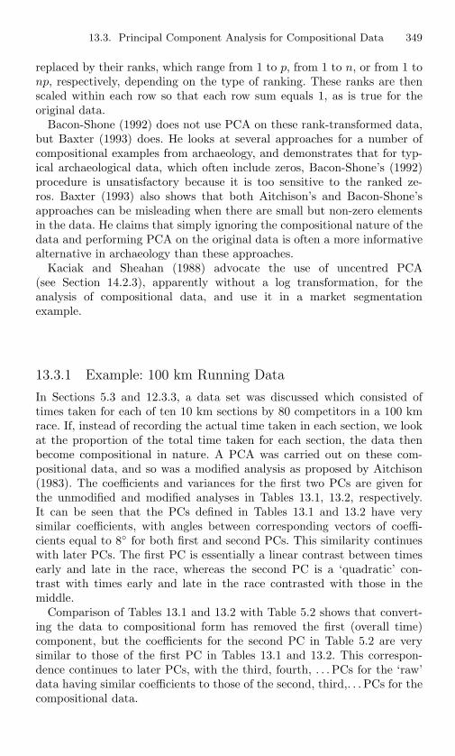
13.3. Principal Component Analysis for Compositional Data 349
replaced by their ranks, which range from 1 to p, from 1 to n, or from 1 tonp, respectively, depending on the type of ranking. These ranks are thenscaled within each row so that each row sum equals 1, as is true for theoriginal data.
Bacon-Shone (1992) does not use PCA on these rank-transformed data,but Baxter (1993) does. He looks at several approaches for a number ofcompositional examples from archaeology, and demonstrates that for typ-ical archaeological data, which often include zeros, Bacon-Shone’s (1992)procedure is unsatisfactory because it is too sensitive to the ranked ze-ros. Baxter (1993) also shows that both Aitchison’s and Bacon-Shone’sapproaches can be misleading when there are small but non-zero elementsin the data. He claims that simply ignoring the compositional nature of thedata and performing PCA on the original data is often a more informativealternative in archaeology than these approaches.
Kaciak and Sheahan (1988) advocate the use of uncentred PCA(see Section 14.2.3), apparently without a log transformation, for theanalysis of compositional data, and use it in a market segmentationexample.
13.3.1 Example: 100 km Running Data
In Sections 5.3 and 12.3.3, a data set was discussed which consisted oftimes taken for each of ten 10 km sections by 80 competitors in a 100 kmrace. If, instead of recording the actual time taken in each section, we lookat the proportion of the total time taken for each section, the data thenbecome compositional in nature. A PCA was carried out on these com-positional data, and so was a modified analysis as proposed by Aitchison(1983). The coefficients and variances for the first two PCs are given forthe unmodified and modified analyses in Tables 13.1, 13.2, respectively.It can be seen that the PCs defined in Tables 13.1 and 13.2 have verysimilar coefficients, with angles between corresponding vectors of coeffi-cients equal to 8 for both first and second PCs. This similarity continueswith later PCs. The first PC is essentially a linear contrast between timesearly and late in the race, whereas the second PC is a ‘quadratic’ con-trast with times early and late in the race contrasted with those in themiddle.
Comparison of Tables 13.1 and 13.2 with Table 5.2 shows that convert-ing the data to compositional form has removed the first (overall time)component, but the coefficients for the second PC in Table 5.2 are verysimilar to those of the first PC in Tables 13.1 and 13.2. This correspon-dence continues to later PCs, with the third, fourth, . . . PCs for the ‘raw’data having similar coefficients to those of the second, third,. . . PCs for thecompositional data.
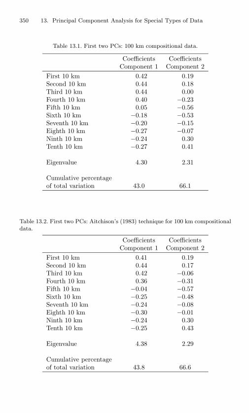
350 13. Principal Component Analysis for Special Types of Data
Table 13.1. First two PCs: 100 km compositional data.
Coefficients CoefficientsComponent 1 Component 2
First 10 km 0.42 0.19Second 10 km 0.44 0.18Third 10 km 0.44 0.00Fourth 10 km 0.40 −0.23Fifth 10 km 0.05 −0.56Sixth 10 km −0.18 −0.53Seventh 10 km −0.20 −0.15Eighth 10 km −0.27 −0.07Ninth 10 km −0.24 0.30Tenth 10 km −0.27 0.41
Eigenvalue 4.30 2.31
Cumulative percentageof total variation 43.0 66.1
Table 13.2. First two PCs: Aitchison’s (1983) technique for 100 km compositionaldata.
Coefficients CoefficientsComponent 1 Component 2
First 10 km 0.41 0.19Second 10 km 0.44 0.17Third 10 km 0.42 −0.06Fourth 10 km 0.36 −0.31Fifth 10 km −0.04 −0.57Sixth 10 km −0.25 −0.48Seventh 10 km −0.24 −0.08Eighth 10 km −0.30 −0.01Ninth 10 km −0.24 0.30Tenth 10 km −0.25 0.43
Eigenvalue 4.38 2.29
Cumulative percentageof total variation 43.8 66.6

13.4. Principal Component Analysis in Designed Experiments 351
13.4 Principal Component Analysis in DesignedExperiments
In Chapters 8 and 9 we discussed ways in which PCA could be used as a pre-liminary to, or in conjunction with, other standard statistical techniques.The present section gives another example of the same type of application;here we consider the situation where p variables are measured in the courseof a designed experiment. The standard analysis would be either a set ofseparate analyses of variance (ANOVAs) for each variable or, if the variablesare correlated, a multivariate analysis of variance (MANOVA—Rencher,1995, Chapter 6) could be done.
As an illustration, consider a two-way model of the form
xijk = µ + τ j + βk + εijk, i = 1, 2, . . . , njk; j = 1, 2, . . . , t; k = 1, 2, . . . , b,
where xijk is the ith observation for treatment j in block k of a p-variatevector x. The vector xijk is therefore the sum of an overall mean µ, atreatment effect τ j , a block effect βk and an error term εijk.
The most obvious way in which PCA can be used in such analyses issimply to replace the original p variables by their PCs. Then either sepa-rate ANOVAs can be done on each PC, or the PCs can be analysed usingMANOVA. Jackson (1991, Sections 13.5–13.7) discusses the use of sep-arate ANOVAs for each PC in some detail. In the context of analysinggrowth curves (see Section 12.4.2) Rao (1958) suggests that ‘methods ofmultivariate analysis for testing the differences between treatments’ can beimplemented on the first few PCs, and Rencher (1995, Section 12.2) advo-cates PCA as a first step in MANOVA when p is large. However, as notedby Rao (1964), for most types of designed experiment this simple analy-sis is often not particularly useful. This is because the overall covariancematrix represents a mixture of contributions from within treatments andblocks, between treatments, between blocks, and so on, whereas we usuallywish to separate these various types of covariance. Although the PCs areuncorrelated overall, they are not necessarily so, even approximately, withrespect to between-group or within-group variation. This is a more compli-cated manifestation of what occurs in discriminant analysis (Section 9.1),where a PCA based on the covariance matrix of the raw data may proveconfusing, as it inextricably mixes up variation between and within pop-ulations. Instead of a PCA of all the xijk, a number of other PCAs havebeen suggested and found to be useful in some circumstances.
Jeffers (1962) looks at a PCA of the (treatment×block) means xjk, j =1, 2, . . . , t; k = 1, 2, . . . , b, where
xjk =1
njk
njk∑
i=1
xijk,
that is, a PCA of a data set with tb observations on a p-variate random vec-

352 13. Principal Component Analysis for Special Types of Data
tor. In an example on tree seedlings, he finds that ANOVAs carried out onthe first five PCs, which account for over 97% of the variation in the orig-inal eight variables, give significant differences between treatment means(averaged over blocks) for the first and fifth PCs. This result contrastswith ANOVAs for the original variables, where there were no significantdifferences. The first and fifth PCs can be readily interpreted in Jeffers’(1962) example, so that transforming to PCs produces a clear advantage interms of detecting interpretable treatment differences. However, PCs willnot always be interpretable and, as in regression (Section 8.2), there is noreason to expect that treatment differences will necessarily manifest them-selves in high variance, rather than low variance, PCs. For example, whileJeffer’s first component accounts for over 50% of total variation, his fifthcomponent accounts for less than 5%.
Jeffers (1962) looked at ‘between’ treatments and blocks PCs, but thePCs of the ‘within’ treatments or blocks covariance matrices can also pro-vide useful information. Pearce and Holland (1960) give an example havingfour variables, in which different treatments correspond to different root-stocks, but which has no block structure. They carry out separate PCAsfor within- and between-rootstock variation. The first PC is similar in thetwo cases, measuring general size. Later PCs are, however, different for thetwo analyses, but they are readily interpretable in both cases so that thetwo analyses each provide useful but separate information.
Another use of ‘within-treatments’ PCs occurs in the case where there areseveral populations, as in discriminant analysis (see Section 9.1), and ‘treat-ments’ are defined to correspond to different populations. If each populationhas the same covariance matrix Σ, and within-population PCs based onΣ are of interest, then the ‘within-treatments’ covariance matrix providesan estimate of Σ. Yet another way in which ‘error covariance matrix PCs’can contribute is if the analysis looks for potential outliers as suggested formultivariate regression in Section 10.1.
A different way of using PCA in a designed experiment is describedby Mandel (1971, 1972). He considers a situation where there is only onevariable, which follows the two-way model
xjk = µ + τj + βk + εjk, j = 1, 2, . . . , t; k = 1, 2, . . . , b, (13.4.1)
that is, there is only a single observation on the variable x at each com-bination of treatments and blocks. In Mandel’s analysis, estimates µ, τj ,βk are found for µ, τj , βk, respectively, and residuals are calculated asejk = xjk − µ− τj − βk. The main interest is then in using ejk to estimatethe non-additive part εjk of the model (13.4.1). This non-additive part isassumed to take the form
εjk =m∑
h=1
ujhlhakh, (13.4.2)
13.4. Principal Component Analysis in Designed Experiments 353
where m, lh, ujh, akh, are suitably chosen constants. Apart from slightchanges in notation, the right-hand side of (13.4.2) is the same as that ofthe singular value decomposition (SVD) in (3.5.3). Thus, the model (13.4.2)is fitted by finding the SVD of the matrix E whose (j, k)th element isejk, or equivalently finding the PCs of the covariance matrix based on thedata matrix E. This analysis also has links with correspondence analysis(see Section 13.1). In both cases we find an SVD of a two-way table ofresiduals, the difference being that in the present case the elements of thetable are residuals from an additive model for a quantitative variable, ratherthan residuals from an independence (multiplicative) model for counts. Asnoted in Section 1.2, R.A. Fisher used the SVD in a two-way analysis of anagricultural trial, leading to an eigenanalysis of a multiple of a covariancematrix as long ago as 1925.
A substantial amount of work has been done on the model defined by(13.4.1) and (13.4.2). Freeman (1975) showed that Mandel’s approach canbe used for incomplete as well as complete two-way tables, and a numberof authors have constructed tests for the rank m of the interaction term.For example, Boik (1986) develops likelihood ratio and union-intersectiontests, and Milliken and Johnson (1989) provide tables of critical points forlikelihood ratio statistics. Boik (1986) also points out that the model is areduced-rank regression model (see Section 9.3.4).
Shafii and Price (1998) give an example of a more complex design inwhich seed yields of 6 rapeseed cultivars are measured in 27 environ-ments spread over three separate years, with 4 replicates at each of the(6 × 27) combinations. There are additional terms in the model comparedto (13.4.1), but the non-additive part is still represented as in (13.4.2).The first two terms in (13.4.2) are deemed significant using Milliken andJohnson’s (1989) tables; they account for 80% of the variability that wouldbe explained by taking m of full rank 5. The results of the analysis of thenon-additive term are interpreted using biplots (see Section 5.3).
Gower and Krzanowski (1999) consider the situation in which the datahave a MANOVA structure but where the assumptions that underlie formalMANOVA procedures are clearly invalid. They suggest a number of graph-ical displays to represent and interpret such data; one is based on weightedPCA. Goldstein (1995, Section 4.5) notes the possibility of using PCA toexplore the structure of various residual matrices in a multilevel model.
Planned surveys are another type of designed experiment, and one par-ticular type of survey design is based on stratified sampling. Pla (1991)suggests that when the data from a survey are multivariate, the first PCcan be used to define the strata for a stratified sampling scheme. She showsthat stratification in this manner leads to reduced sampling variability com-pared to stratification based on only one or two variables. Skinner et al.(1986) and Tortora (1980) demonstrate the effect of the non-independenceinduced by other methods of stratification on subsequently calculated PCs(see Section 12.4.5).

354 13. Principal Component Analysis for Special Types of Data
Observations of the atmosphere certainly do not constitute a designedexperiment, but a technique proposed by Zheng et al. (2001) is includedhere because of its connections to analysis of variance. Measurements ofmeteorological fields can be thought of as the sum of long-term variabilitycaused by external forcing and the slowly varying internal dynamics of theatmosphere, and short-term day-to-day weather variability. The first termis potentially predictable over seasonal or longer time scales, whereas thesecond term is not. It is therefore of interest to separate out the potentiallypredictable component and examine its major sources of variation. Zhenget al. (2001) do this by estimating the covariance matrix of the day-to-dayvariation and subtracting it from the ‘overall’ covariance matrix, whichassumes independence of short- and long-term variation. A PCA is thendone on the resulting estimate of the covariance matrix for the potentiallypredictable variation, in order to find potentially predictable patterns.
Returning to designed experiments, in optimal design it is desirable toknow the effect of changing a design by deleting design points or augment-ing it with additional design points. Jensen (1998) advocates the use ofprincipal components of the covariance matrix of predicted values at a cho-sen set of design points to investigate the effects of such augmentation ordeletion. He calls these components principal predictors, though they arequite different from the entities with the same name defined by Thacker(1999) and discussed in Section 9.3.3. Jensen (1998) illustrates the use ofhis principal predictors for a variety of designs.
13.5 Common Principal Components andComparisons of Principal Components
Suppose that observations on a p-variate random vector x may have comefrom any one of G distinct populations, and that the mean and covariancematrix for the gth population are, respectively, µg, Σg, g = 1, 2, . . . , G. Thisis the situation found in discriminant analysis (see Section 9.1) althoughin discriminant analysis it is often assumed that all the Σg are the same,so that the populations differ only in their means. If the Σg are all thesame, then the ‘within-population PCs’ are the same for all G populations,though, as pointed out in Section 9.1, within-population PCs are oftendifferent from PCs found by pooling data from all populations together.
If the Σg are different, then there is no uniquely defined set of within-population PCs that is common to all populations. However, a number ofauthors have examined ‘common principal components,’ which can usefullybe defined in some circumstances where the Σg are not all equal. The ideaof ‘common’ PCs arises if we suspect that the same components underliethe covariance matrices of each group, but that they have different weightsin different groups. For example, if anatomical measurements are made on

13.5. Common Principal Components 355
different but closely related species of animals, then the same general ‘size’and ‘shape’ components (see Section 13.2) may be present for each species,but with varying importance. Similarly, if the same variables are measuredon the same individuals but at different times, so that ‘groups’ correspondto different times as in longitudinal studies (see Section 12.4.2), then thecomponents may remain the same but their relative importance may varywith time.
One way of formally expressing the presence of ‘common PCs’ as justdefined is by the hypothesis that there is an orthogonal matrix A thatsimultaneously diagonalizes all the Σg so that
A′ΣgA = Λg, (13.5.1)
where Λg, g = 1, 2, . . . , G are all diagonal. The kth column of A gives thecoefficients of the kth common PC, and the (diagonal) elements of Λg givethe variances of these PCs for the gth population. Note that the order ofthese variances need not be the same for all g, so that different PCs mayhave the largest variance in different populations.
In a series of papers in the 1980s Flury developed ways of estimating andtesting the model implied by (13.5.1). Much of this work later appearedin a book (Flury, 1988), in which (13.5.1) is the middle level of a 5-levelhierarchy of models for a set of G covariance matrices. The levels are these:
• Σ1 = Σ2 = . . . = ΣG (equality).
• Σg = ρgΣ1 for some positive constants ρ2, ρ3, . . . , ρg (proportional-ity).
• A′ΣgA = Λg (the common PC model).
• Equation (13.5.1) can also be written, using spectral decompositions(2.1.10) of each covariance matrix, as
Σg = λg1α1α′1 + λg2α2α
′2 + . . . + λgpαpα
′p.
Level 4 (the partial common PC model) replaces this by
Σg = λg1α1α′1+. . .+λgqαqα
′q+λg(q+1)α
(g)q+1α
′(g)q+1+. . .+λgpα
(g)p α
′(g)p
(13.5.2)Thus, q of the p PCs have common eigenvectors in the G groups,whereas the other (p− q) do not. The ordering of the components in(13.5.2) need not in general reflect the size of the eigenvalues. Anysubset of q components can be ‘common.’
• No restriction on Σ1,Σ2, . . . ,Σg.
The first and last levels of the hierarchy are trivial, but Flury (1988)devotes a chapter to each of the three intermediate ones, covering maximumlikelihood estimation, asymptotic inference and applications. The partialcommon PC model is modified to give an additional level of the hierarchy

356 13. Principal Component Analysis for Special Types of Data
in which q of the components span a common subspace, but there is norequirement that the individual components should be the same. Likelihoodratio tests are described by Flury (1988) for comparing the fit of models atdifferent levels of the hierarchy. Model selection can also be made on thebasis of Akaike’s information criterion (AIC) (Akaike, 1974).
One weakness of the theory described in Flury (1988) is that it is onlyreally applicable to covariance-based PCA and not to the more frequentlyencountered correlation-based analysis.
Lefkovitch (1993) notes that Flury’s (1988) procedure for fitting a com-mon PC model can be time-consuming for moderate or large data sets. Heproposes a technique that produces what he calls consensus components,which are much quicker to find. They are based on the so-called polar de-composition of a data matrix, and approximately diagonalize two or morecovariance matrices simultaneously. In the examples that Lefkovitch (1993)presents the consensus and common PCs are similar and, if the commonPCs are what is really wanted, the consensus components provide a goodstarting point for the iterative process that leads to common PCs.
A number of topics that were described briefly by Flury (1988) in achapter on miscellanea were subsequently developed further. Schott (1988)derives an approximate test of the partial common PC model for G = 2when the common subspace is restricted to be that spanned by the first qPCs. He argues that in dimension-reducing problems this, rather than anyq-dimensional subspace, is the subspace of interest. His test is extended toG > 2 groups in Schott (1991), where further extensions to correlation-based analyses and to robust PCA are also considered. Yuan and Bentler(1994) provide a test for linear trend in the last few eigenvalues under thecommon PC model.
Flury (1988, Section 8.5) notes the possibility of using models within hishierarchy in the multivariate Behrens-Fisher problem of testing equalitybetween the means of two p-variate groups when their covariance matricescannot be assumed equal. Nel and Pienaar (1998) develop this idea, whichalso extends Takemura’s (1985) decomposition of Hotelling’s T 2 statis-tic with respect to principal components when equality of covariances isassumed (see also Section 9.1). Flury et al. (1995) consider the same two-group set-up, but test the hypothesis that a subset of the p means is thesame in the two groups, while simultaneously estimating the covariancematrices under the common PC model. Bartoletti et al. (1999) considertests for the so-called allometric extension model defined by Hills (1982).In this model, the size and shape of organisms (see Section 13.2) are suchthat for two groups of organisms not only is the first PC common to bothgroups, but the difference in means between the two groups also lies in thesame direction as this common PC.
In the context of discriminant analysis, Bensmail and Celeux (1996) usea similar hierarchy of models for the covariance matrices of G groups tothat of Flury (1988), though the hierarchy is augmented to include special
13.5. Common Principal Components 357
cases of interest such as identity or diagonal covariance matrices. Krzanow-ski (1990) and Flury (1995) also discuss the use of the common principalcomponent model in discriminant analysis (see Section 9.1).
Flury and Neuenschwander (1995) look at the situation in which the as-sumption that the G groups of variables are independent is violated. Thiscan occur, for example, if the same variables are measured for the sameindividuals at G different times. They argue that, in such circumstances,when G = 2 the common PC model can provide a useful alternative tocanonical correlation analysis (CCA) ( see Section 9.3) for examining rela-tionships between two groups and, unlike CCA, it is easily extended to thecase of G > 2 groups. Neuenschwander and Flury (2000) discuss in detailthe theory underlying the common PC model for dependent groups.
Krzanowski (1984a) describes a simpler method of obtaining estimatesof A and Λg based on the fact that if (13.5.1) is true then the columns of Acontain the eigenvectors not only of Σ1,Σ2, . . . ,ΣG individually but of anylinear combination of Σ1,Σ2, . . . ,ΣG. He therefore uses the eigenvectorsof S1 +S2 + . . .+SG, where Sg is the sample covariance matrix for the gthpopulation, to estimate A, and then substitutes this estimate and Sg for Aand Σg, respectively, in (13.5.1) to obtain estimates of Λg, g = 1, 2, . . . , G.
To assess whether or not (13.5.1) is true, the estimated eigenvectorsof S1 + S2 + . . . + SG can be compared with those estimated for someother weighted sum of S1,S2, . . . ,SG chosen to have different eigenvectorsfrom S1 +S2 + . . .+SG if (13.5.1) does not hold. The comparison betweeneigenvectors can be made either informally or using methodology developedby Krzanowski (1979b), which is now described.
Suppose that sample covariance matrices S1, S2 are available for twogroups of individuals, and that we wish to compare the two sets of PCsfound from S1 and S2. Let A1q,A2q be (p × q) matrices whose columnscontain the coefficients of the first q PCs based on S1,S2, respectively.Krzanowski’s (1979b) idea is to find the minimum angle δ between thesubspaces defined by the q columns of A1q and A2q, together with asso-ciated vectors in these two subspaces that subtend this minimum angle.This suggestion is based on an analogy with the congruence coefficient,which has been widely used in factor analysis to compare two sets of factorloadings (Korth and Tucker, 1975) and which, for two vectors, can be in-terpreted as the cosine of the angle between those vectors. In Krzanowski’s(1979b) set-up, it turns out that δ is given by
δ = cos−1(ν
1/21
),
where ν1 is the first (largest) eigenvalue of A′1qA2qA′
2qA1q, and the vec-tors that subtend the minimum angle are related, in a simple way, to thecorresponding eigenvector.
The analysis can be extended by looking at the second, third,. . . , eigen-values and corresponding eigenvectors of A′
1qA2qA′2qA1q; from these can be
358 13. Principal Component Analysis for Special Types of Data
found pairs of vectors, one each in the two subspaces spanned by A1q,A2q,that have minimum angles between them, subject to being orthogonalto previous pairs of vectors. Krzanowski (1979b) notes that the sum ofeigenvalues tr(A′
1qA2qA′2qA1q) can be used as an overall measure of the
similarity between the two subspaces. Crone and Crosby (1995) define atransformed version of this trace as an appropriate measure of subspacesimilarity, examine some of its properties, and apply it to an example fromsatellite meteorology.
Another extension is to G > 2 groups of individuals with covariancematrices S1,S2, . . . ,SG and matrices A1q,A2q, . . . ,AGq containing the firstq eigenvectors (PC coefficients) for each group. We can then look for avector that minimizes
∆ =G∑
g=1
cos2 δg,
where δg is the angle that the vector makes with the subspace defined bythe columns of Agq. This objective is achieved by finding eigenvalues andeigenvectors of
G∑
g=1
AgqA′gq,
and Krzanowski (1979b) shows that for g = 2 the analysis reduces to thatgiven above.
In Krzanowski (1979b) the technique is suggested as a descriptive tool—if δ (for G = 2) or ∆ (for G > 2) is ‘small enough’ then the subsets of qPCs for the G groups are similar, but there is no formal definition of ‘smallenough.’ In a later paper, Krzanowski (1982) investigates the behaviour ofδ using simulation, both when all the individuals come from populationswith the same covariance matrix, and when the covariance matrices aredifferent for the two groups of individuals. The simulation encompassesseveral different values for p, q and for the sample sizes, and it also includesseveral different structures for the covariance matrices. Krzanowski (1982)is therefore able to offer some limited guidance on what constitutes a ‘smallenough’ value of δ, based on the results from his simulations.
As an example, consider anatomical data similar to those discussed inSections 1.1, 4.1, 5.1, 10.1 and 10.2 that were collected for different groups ofstudents in different years. Comparing the first three PCs found for the 1982and 1983 groups of students gives a value of 2.02 for δ; the correspondingvalue for 1982 and 1984 is 1.25, and that for 1983 and 1984 is 0.52.Krzanowski (1982) does not have a table of simulated critical angles for thesample sizes and number of variables relevant to this example. In addition,his tables are for covariance matrices whereas the student data PCAs arefor correlation matrices. However, for illustration we note that the threevalues quoted above are well below the critical angles corresponding to the

13.5. Common Principal Components 359
values of p, q and sample size in his tables closest to those of the presentexample. Hence, if Krzanowski’s tables are at all relevant for correlationmatrices, the sets of the first three PCs are not significantly different forthe three years 1982, 1983, 1984 as might be expected from such smallangles.
If all three years are compared simultaneously, then the angles betweenthe subspaces formed by the first three PCs and the nearest vector to allthree subspaces are
1982 1983 19841.17 1.25 0.67
Again, the angles are very small; although no tables are available for as-sessing the significance of these angles, they seem to confirm the impressiongiven by looking at the years two at a time that the sets of the first threePCs are not significantly different for the three years.
Two points should be noted with respect to Krzanowski’s technique.First, it can only be used to compare subsets of PCs—if q = p, thenA1p,A2p will usually span p-dimensional space (unless either S1 or S2
has zero eigenvalues), so that δ is necessarily zero. It seems likely that thetechnique will be most valuable for values of q that are small compared to p.The second point is that while δ is clearly a useful measure of the closenessof two subsets of PCs, the vectors and angles found from the second, third,. . . , eigenvalues and eigenvectors of A′
1qA2qA′2qA1q are successively less
valuable. The first two or three angles give an idea of the overall differencebetween the two subspaces, provided that q is not too small. However, if wereverse the analysis and look at the smallest eigenvalue and correspondingeigenvector of A′
1qA2qA′2qA1q, then we find the maximum angle between
vectors in the two subspaces (which will often be 90, unless q is small).Thus, the last few angles and corresponding vectors need to be interpretedin a rather different way from that of the first few. The general problemof interpreting angles other than the first can be illustrated by again con-sidering the first three PCs for the student anatomical data from 1982 and1983. We saw above that δ = 2.02, which is clearly very small; the secondand third angles for these data are 25.2 and 83.0, respectively. Theseangles are fairly close to the 5% critical values given in Krzanowski (1982)for the second and third angles when p = 8, q = 3 and the sample sizes areeach 50 (our data have p = 7, q = 3 and sample sizes around 30), but it isdifficult to see what this result implies. In particular, the fact that the thirdangle is close to 90 might intuitively suggest that the first three PCs aresignificantly different for 1982 and 1983. Intuition is, however, contradictedby Krzanowski’s Table I, which shows that for sample sizes as small as 50(and, hence, certainly for samples of size 30), the 5% critical value for thethird angle is nearly 90. For q = 3 this is not particularly surprising—thedimension of A′
1qA2qA′2qA1q is (3 × 3) so the third angle is the maximum
angle between subspaces.
360 13. Principal Component Analysis for Special Types of Data
Cohn (1999) considers four test statistics for deciding the equivalenceor otherwise of subspaces defined by sets of q PCs derived from each oftwo covariance matrices corresponding to two groups of observations. Oneof the statistics is the likelihood ratio test used by Flury (1988) and twoothers are functions of the eigenvalues, or corresponding cosines, derivedby Krzanowski (1979b). The fourth statistic is based on a sequence of two-dimensional rotations from one subspace towards the other, but simulationsshow it to be less reliable than the other three. There are a number ofnovel aspects to Cohn’s (1999) study. The first is that the observationswithin the two groups are not independent; in his motivating example thedata are serially correlated time series. To derive critical values for the teststatistics, a bootstrap procedure is used, with resampling in blocks becauseof the serial correlation. The test statistics are compared in a simulationstudy and on the motivating example.
Keramidas et al. (1987) suggest a graphical procedure for comparingeigenvectors of several covariance matrices S1,S2, . . . ,SG. Much of the pa-per is concerned with the comparison of a single eigenvector from eachmatrix, either with a common predetermined vector or with a ‘typical’vector that maximizes the sum of squared cosines between itself and theG eigenvectors to be compared. If agk is the kth eigenvector for the gthsample covariance matrix, g = 1, 2, . . . , G, and a0k is the predetermined ortypical vector, then distances
kδ2g = min[(agk − a0k)′(agk − a0k), (agk + a0k)′(agk + a0k)]
are calculated. If the sample covariance matrices are drawn from the samepopulation, then kδ2
g has an approximate gamma distribution, so Kerami-das et al. (1987) suggest constructing gamma Q-Q plots to detect differencesfrom this null situation. Simulations are given for both the null and non-null cases. Such plots are likely to be more useful when G is large thanwhen there is only a handful of covariance matrices to be compared.
Keramidas et al. (1987) extend their idea to compare subspaces spannedby two or more eigenvectors. For two subspaces, their overall measure ofsimilarity, which reduces to kδ2
g when single eigenvectors are compared, is
the sum of the square roots ν1/2k of eigenvalues of A′
1qA2qA′2qA1q. Recall
that Krzanowski (1979b) uses the sum of these eigenvalues, not their squareroots as his measure of overall similarity. Keramidas et al. (1987) stressthat individual eigenvectors or subspaces should only be compared whentheir eigenvalues are well-separated from adjacent eigenvalues so that theeigenvectors or subspaces are well-defined.
Ten Berge and Kiers (1996) take a different and more complex view ofcommon principal components than Flury (1988) or Krzanowski (1979b).They refer to generalizations of PCA to G (≥ 2) groups of individuals, withdifferent generalizations being appropriate depending on what is taken asthe defining property of PCA. They give three different defining criteria and

13.5. Common Principal Components 361
draw distinctions between the properties of principal components found byeach. Although the different criteria lead to a number of different general-izations, it is arguable just how great a distinction should be drawn betweenthe three ungeneralized analyses (see Cadima and Jolliffe (1997); ten Bergeand Kiers (1997)).
The first property considered by ten Berge and Kiers (1996) corre-sponds to Property A1 of Section 2.1, in which tr(B′ΣB) is minimized.For G groups of individuals treated separately this leads to minimiza-tion of
∑Gg=1 tr(B′
gΣgBg), but taking Bg the same for each group givessimultaneous components that minimize
G∑
g=1
tr(B′ΣgB) = tr[B′(G∑
g=1
Σg)B]
= G tr(B′ΣB),
where Σ is the average of Σ1,Σ2, . . . ,ΣG.Ten Berge and Kiers’ (1996) second property is a sample version of
Property A5 in Section 2.1. They express this property as minimizing‖X − XBC′‖2. For G groups treated separately, the quantity
G∑
g=1
‖Xg − XgBgC′g‖2 (13.5.3)
is minimized. Ten Berge and Kiers (1996) distinguish three different waysof adapting this formulation to find simultaneous components.
• Minimize∑G
g=1 ‖Xg − XgBC′g‖2.
• Minimize∑G
g=1 ‖Xg − XgBgC′‖2.
• Minimize (13.5.3) subject to ΣgBg = SDg, where Dg is diagonal andS is a ‘common component structure.’
The third optimality criterion considered by Ten Berge and Kiers (1996)is that noted at the end of Section 2.1, and expressed by Rao (1964) asminimizing ‖Σ − ΣB(B′ΣB)−1B′Σ‖. Ten Berge and Kiers (1996) writethis as minimizing ‖Σ−FF′‖2, which extends to G groups by minimizing∑G
g=1 ‖Σg −FgF′g‖2. This can then be modified to give simultaneous com-
ponents by minimizing∑G
g=1 ‖Σg − FF′‖2. They show that this criterionand the criterion based on Property A1 are both equivalent to the secondof their generalizations derived from Property A5.
Ten Berge and Kiers (1996) compare properties of the three generaliza-tions of Property A5, but do not reach any firm conclusions as to whichis preferred. They are, however, somewhat dismissive of Flury’s (1988)approach on the grounds that it has at its heart the simultaneous diag-onalization of G covariance matrices and ‘it is by no means granted that

362 13. Principal Component Analysis for Special Types of Data
components which diagonalize the covariance or correlation matrices reflectthe most important sources of variation in the data.’
Muller (1982) suggests that canonical correlation analysis of PCs (seeSection 9.3) provides a way of comparing the PCs based on two sets ofvariables, and cites some earlier references. When the two sets of variablesare, in fact, the same variables measured for two groups of observations,Muller’s analysis is equivalent to that of Krzanowski (1979b); the latterpaper notes the links between canonical correlation analysis and its owntechnique.
In a series of five technical reports, Preisendorfer and Mobley (1982) ex-amine various ways of comparing data sets measured on the same variablesat different times, and part of their work involves comparison of PCs fromdifferent sets (see, in particular, their third report, which concentrates oncomparing the singular value decompositions (SVDs, Section 3.5) of twodata matrices X1,X2). Suppose that the SVDs are written
X1 = U1L1A′1
X2 = U2L2A′2.
Then Preisendorfer and Mobley (1982) define a number of statistics thatcompare U1 with U2,A1 with A2,L1 with L2 or compare any two of thethree factors in the SVD for X1 with the corresponding factors in the SVDfor X2. All of these comparisons are relevant to comparing PCs, since Acontains the coefficients of the PCs, L provides the standard deviations ofthe PCs, and the elements of U are proportional to the PC scores (see Sec-tion 3.5). The ‘significance’ of an observed value of any one of Preisendorferand Mobley’s statistics is assessed by comparing the value to a ‘referencedistribution’, which is obtained by simulation. Preisendorfer and Mobley’s(1982) research is in the context of atmospheric science. A more recent ap-plication in this area is that of Sengupta and Boyle (1998), who illustratethe use of Flury’s (1988) common principal component model to comparedifferent members of an ensemble of forecasts from a general circulationmodel (GCM) and to compare outputs from different GCMs. Applicationsin other fields of the common PC model and its variants can be found inFlury (1988, 1997).
When the same variables are measured on the same n individuals in thedifferent data sets, it may be of interest to compare the configurations ofthe points defined by the n individuals in the subspaces of the first few PCsin each data set. In this case, Procrustes analysis (or generalized Procrustesanalysis) provides one possible way of doing this for two (more than two)data sets (see Krzanowski and Marriott (1994, Chapter 5)). The techniquein general involves the SVD of the product of one data matrix and thetranspose of the other, and because of this Davison (1983, Chapter 8) linksit to PCA.
13.6. Principal Component Analysis in the Presence of Missing Data 363
13.6 Principal Component Analysis in thePresence of Missing Data
In all the examples given in this text, the data sets are complete. However,it is not uncommon, especially for large data sets, for some of the valuesof some of the variables to be missing. The most usual way of dealing withsuch a situation is to delete, entirely, any observation for which at least oneof the variables has a missing value. This is satisfactory if missing values arefew, but clearly wasteful of information if a high proportion of observationshave missing values for just one or two variables. To meet this problem, anumber of alternatives have been suggested.
The first step in a PCA is usually to compute the covariance or cor-relation matrix, so interest often centres on estimating these matrices inthe presence of missing data. There are a number of what Little and Ru-bin (1987, Chapter 3) call ‘quick’ methods. One option is to compute the(j, k)th correlation or covariance element-wise, using all observations forwhich the values of both xj and xk are available. Unfortunately, this leads tocovariance or correlation matrices that are not necessarily positive semidef-inite. Beale and Little (1975) note a modification of this option. Whencomputing the summation
∑i(xij − xj)(xik − xk) in the covariance or cor-
relation matrix, xj , xk are calculated from all available values of xj , xk,respectively, instead of only for observations for which both xj and xk havevalues present, They state that, at least in the regression context, the re-sults can be unsatisfactory. However, Mehrota (1995), in discussing robustestimation of covariance matrices (see Section 10.4), argues that the prob-lem of a possible lack of positive semi-definiteness is less important thanmaking efficient use of as many data as possible. He therefore advocateselement-wise estimation of the variances and covariances in a covariancematrix, with possible adjustment if positive semi-definiteness is lost.
Another quick method is to replace missing values for variable xj by themean value xj , calculated from the observations for which the value of xj
is available. This is a simple way of ‘imputing’ rather than ignoring missingvalues. A more sophisticated method of imputation is to use regression ofthe missing variables on the available variables case-by-case. An extensionto the idea of imputing missing values is multiple imputation. Each missingvalue is replaced by a value drawn from a probability distribution, andthis procedure is repeated M times (Little and Rubin, 1987, Section 12.4;Schafer, 1997, Section 4.3). The analysis, in our case PCA, is then doneM times, corresponding to each of the M different sets of imputed values.The variability in the results of the analyses gives an indication of theuncertainty associated with the presence of missing values.
A different class of procedures is based on maximum likelihood estima-tion (Little and Rubin, 1987, Section 8.2). The well-known EM algorithm(Dempster et al., 1977) can easily cope with maximum likelihood estimation

364 13. Principal Component Analysis for Special Types of Data
of the mean and covariance matrix in the presence of missing values, underthe assumption of multivariate normality. Little and Rubin (1987, Section8.2) describe three versions of the EM algorithm for solving this problem;a number of other authors, for example, Anderson (1957), De Ligny et al.(1981), tackled the same problem earlier by less efficient means.
The multivariate normal assumption is a restrictive one, and Little (1988)relaxes it by adapting the EM algorithm to find MLEs when the data arefrom a multivariate t-distribution or from a mixture of two multivariate nor-mals with different covariance matrices. He calls these ‘robust’ methods fordealing with missing data because they assume longer-tailed distributionsthan multivariate normal. Little (1988) conducts a simulation study, theresults of which demonstrate that his robust MLEs cope well with missingdata, compared to other methods discussed earlier in this section. However,the simulation study is limited to multivariate normal data, and to datafrom distributions that are similar to those assumed by the robust MLEs.It is not clear that the good performance of the robust MLEs would berepeated for other distributions. Little and Rubin (1987, Section 8.3) alsoextend their multivariate normal procedures to deal with covariance ma-trices on which some structure is imposed. Whilst this may be appropriatefor factor analysis it is less relevant for PCA.
Another adaptation of the EM algorithm for estimation of covariancematrices, the regularized EM algorithm, is given by Schneider (2001). Itis particularly useful when the number of variables exceeds the numberof observations. Schneider (2001) adds a diagonal matrix to the currentestimate of the covariance matrix before inverting the matrix, a similaridea to that used in ridge regression.
Tipping and Bishop (1999a) take the idea of maximum likelihood estima-tion using the EM algorithm further. They suggest an iterative algorithmin which their EM procedure for estimating the probabilistic PCA model(Section 3.9) is combined with Little and Rubin’s (1987) methodology forestimating the parameters of a multivariate normal distribution in the pres-ence of missing data. The PCs are estimated directly, rather than by goingthrough the intermediate step of estimating the covariance or correlationmatrix. An example in which data are randomly deleted from a data set isused by Tipping and Bishop (1999a) to illustrate their procedure.
In the context of satellite-derived sea surface temperature measurementswith missing data caused by cloud cover, Houseago-Stokes and Challenor(2001) compare Tipping and Bishop’s procedure with a standard inter-polation technique followed by PCA on the interpolated data. The twoprocedures give similar results but the new method is computationallymuch more efficent. This is partly due to the fact that only the first fewPCs are found and that they are calculated directly, without the inter-mediate step of estimating the covariance matrix. Houseago-Stokes andChallenor note that the quality of interpolated data using probabilisticPCA depends on the number of components q in the model. In the absence

13.6. Principal Component Analysis in the Presence of Missing Data 365
of prior knowledge about q, there is, at present, no procedure for choosingits value without repeating the analysis for a range of values.
Most published work, including Little and Rubin (1987), does not ex-plicitly deal with PCA, but with the estimation of covariance matrices ingeneral. Tipping and Bishop (1999a) is one of relatively few papers thatfocus specifically on PCA when discussing missing data. Another is Wiberg(1976). His approach is via the singular value decomposition (SVD), whichgives a least squares approximation of rank m to the data matrix X. Inother words, the approximation mxij minimizes
n∑
i=1
p∑
j=1
(mxij − xij)2,
where mxij is any rank m approximation to xij (see Section 3.5). Principalcomponents can be computed from the SVD (see Section 3.5 and AppendixAl). With missing data, Wiberg (1976) suggests minimizing the same quan-tity, but with the summation only over values of (i, j) for which xij is notmissing; PCs can then be estimated from the modified SVD. The same ideais implicitly suggested by Gabriel and Zamir (1979). Wiberg (1976) reportsthat for simulated multivariate normal data his method is slightly worsethan the method based on maximum likelihood estimation. However, hismethod has the virtue that it can be used regardless of whether or not thedata come from a multivariate normal distribution.
For the specialized use of PCA in analysing residuals from an addi-tive model for data from designed experiments (see Section 13.4), Freeman(1975) shows that incomplete data can be easily handled, although mod-ifications to procedures for deciding the rank of the model are needed.Michailidis and de Leeuw (1998) note three ways of dealing with miss-ing data in non-linear multivariate analysis, including non-linear PCA(Section 14.1).
A special type of ‘missing’ data occurs when observations or variablescorrespond to different times or different spatial locations, but with irreg-ular spacing between them. In the common atmospheric science set-up,where variables correspond to spatial locations, Karl et al. (1982) examinedifferences between PCAs when locations are on a regularly spaced grid,and when they are irregularly spaced. Unsurprisingly, for the irregular datathe locations in areas with the highest density of measurements tend to in-crease their loadings on the leading PCs, compared to the regularly spaceddata. This is because of the larger correlations observed in the high-densityregions. Kaplan et al. (2001) discuss methodology based on PCA for inter-polating spatial fields (see Section 12.4.4). Such interpolation is, in effect,imputing missing data.
Another special type of data in which some values are missing occurswhen candidates choose to take a subset of p′ out of p examinations, withdifferent candidates choosing different subsets. Scores on examinations not
366 13. Principal Component Analysis for Special Types of Data
taken by a candidate are therefore ‘missing.’ Shibayama (1990) devises amethod for producing a linear combination of the examination scores thatrepresents the overall performance of each candidate. When p′ = p themethod is equivalent to PCA.
Anderson et al. (1983) report a method that they attribute to Dear(1959), which is not for dealing with missing values in a PCA, but whichuses PCA to impute missing data in a more general context. The idea seemsto be to first substitute zeros for any missing cells in the data matrix, andthen find the SVD of this matrix. Finally, the leading term in the SVD,corresponding to the first PC, is used to approximate the missing values.If the data matrix is column-centred, this is a variation on using means ofvariables in place of missing values. Here there is the extra SVD step thatadjusts the mean values using information from other entries in the datamatrix.
Finally, note that there is a similarity of purpose in robust estimation ofPCs (see Section 10.4) to that present in handling missing data. In bothcases we identify particular observations which we cannot use in unadjustedform, either because they are suspiciously extreme (in robust estimation),or because they are not given at all (missing values). To completely ignoresuch observations may throw away valuable information, so we attemptto estimate ‘correct’ values for the observations in question. Similar tech-niques may be relevant in each case. For example, we noted above thepossibility of imputing missing values for a particular observation by re-gressing the missing variables on the variables present for that observation,an idea that dates back at least to Beale and Little (1975), Frane (1976)and Gleason and Staelin (1975) (see Jackson (1991, Section 14.1.5)). Asimilar idea, namely robust regression of the variables on each other, isincluded in Devlin et al.’s (1981) study of robust estimation of PCs (seeSection 10.4).
13.7 PCA in Statistical Process Control
The topic of this section, finding outliers, is closely linked to that of Sec-tion 10.1, and many of the techniques used are based on those describedin that section. However, the literature on using PCA in multivariate sta-tistical process control (SPC) is sufficiently extensive to warrant its ownsection. In various manufacturing processes improved technology meansthat greater numbers of variables are now measured in order to monitorwhether or not a process is ‘in control.’ It has therefore become increas-ingly relevant to use multivariate techniques for control purposes, ratherthan simply to monitor each variable separately.
The main ways in which PCA is used in this context are (Martin et al.,1999):

13.7. PCA in Statistical Process Control 367
• One- or two-dimensional plots of PC scores. It was noted in Sec-tion 10.1 that both the first few and the last few PCs may be usefulfor detecting (different types of) outliers, and plots of both are usedin process control. In the published discussion of Roes and Does(1995), Sullivan et al. (1995) argue that the last few PCs are per-haps more useful in SPC than the first few, but in their reply tothe discussion Roes and Does disagree. If p is not too large, sucharguments can be overcome by using a scatterplot matrix to displayall two-dimensional plots of PC scores simultaneously. Plots can beenhanced by including equal-probability contours, assuming approx-imate multivariate normality, corresponding to warning and actionlimits for those points that fall outside them (Jackson, 1991, Section1.7; Martin et al., 1999).
• Hotelling’s T 2. It was seen in Section 10.1 that this is a special casefor q = p of the statistic d2
2i in equation (10.1.2). If multivariate nor-mality is assumed, the distribution of T 2 is known, and control limitscan be set based on that distribution (Jackson, 1991, Section 1.7).
• The squared prediction error (SPE). This is none other than thestatistic d2
1i in equation (10.1.1). It was proposed by Jackson andMudholkar (1979), who constructed control limits based on anapproximation to its distribution. They prefer d2
1i to d22i for com-
putational reasons and because of its intuitive appeal as a sum ofsquared residuals from the (p − q)-dimensional space defined by thefirst (p − q) PCs. However, Jackson and Hearne (1979) indicate thatthe complement of d2
2i, in which the sum of squares of the first fewrather than the last few renormalized PCs is calculated, may be use-ful in process control when the objective is to look for groups of‘out-of-control’ or outlying observations, rather than single outliers.Their basic statistic is decomposed to give separate information aboutvariation within the sample (group) of potentially outlying observa-tions, and about the difference between the sample mean and someknown standard value. In addition, they propose an alternative statis-tic based on absolute, rather than squared, values of PCs. Jacksonand Mudholkar (1979) also extend their proposed control procedure,based on d2
1i, to the multiple-outlier case, and Jackson (1991, Figure6.2) gives a sequence of significance tests for examining subgroups ofobservations in which each test is based on PCs in some way.
Eggett and Pulsipher (1989) compare T 2, SPE, and the complement ofd22i suggested by Jackson and Hearne (1979), in a simulation study and find
the third of these statistics to be inferior to the other two. On the basis oftheir simulations, they recommend Hotelling’s T 2 for large samples, withSPE or univariate control charts preferred for small samples. They alsodiscussed the possibility of constructing CUSUM charts based on the threestatistics.

368 13. Principal Component Analysis for Special Types of Data
The control limits described so far are all based on the assumption ofapproximate multivariate normality. Martin and Morris (1996) introducea non-parametric procedure that provides warning and action contourson plots of PCs. These contours can be very different from the normal-based ellipses. The idea of the procedure is to generate bootstrap samplesfrom the data set and from each of these calculate the value of a (pos-sibly vector-valued) statistic of interest. A smooth approximation to theprobability density of this statistic is then constructed using kernel densityestimation, and the required contours are derived from this distribution.Coleman (1985) suggests that when using PCs in quality control, the PCsshould be estimated robustly (see Section 10.4). Sullivan et al. (1995) dothis by omitting some probable outliers, identified from an initial scan ofthe data, before carrying out a PCA.
When a variable is used to monitor a process over time, its successivevalues are likely to be correlated unless the spacing between observations islarge. One possibility for taking into account this autocorrelation is to plotan exponentially weighted moving average of the observed values. Wold(1994) suggests that similar ideas should be used when the monitoringvariables are PC scores, and he describes an algorithm for implementing‘exponentially weighted moving principal components analysis.’
Data often arise in SPC for which, as well as different variables and differ-ent times of measurement, there is a third ‘mode,’ namely different batches.So-called multiway, or three-mode, PCA can then be used (see Section 14.5and Nomikos and MacGregor (1995)). Grimshaw et al. (1998) note thepossible use of multiway PCA simultaneously on both the variables moni-toring the process and the variables measuring inputs or initial conditions,though they prefer a regression-based approach involving modifications ofHotelling’s T 2 and the SPE statistic.
Boyles (1996) addresses the situation in which the number of variablesexceeds the number of observations. The sample covariance matrix S isthen singular and Hotelling’s T 2 cannot be calculated. One possibility isto replace S−1 by
∑rk=1 l−1
k aka′k for r < n, based on the first r terms
in the spectral decomposition of S (the sample version of Property A3 inSection 2.1). However, the data of interest to Boyles (1996) have variablesmeasured at points of a regular lattice on the manufactured product. Thisstructure implies that a simple pattern exists in the population covariancematrix Σ. Using knowledge of this pattern, a positive definite estimate ofΣ can be calculated and used in T 2 in place of S. Boyles finds appropriateestimates for three different regular lattices.
Lane et al. (2001) consider the case where a several products or processesare monitored simultaneously. They apply Flury’s common PC subspacemodel (Section 13.5) to this situation. McCabe (1986) suggests the useof principal variables (see Section 6.3) to replace principal components inquality control.

13.8. Some Other Types of Data 369
Apley and Shi (2001) assume that a vector of p measured features froma process or product can be modelled as in the probabilistic PCA model ofTipping and Bishop (1999a), described in Section 3.9. The vector thereforehas covariance matrix BB′ + σ2Ip, where in the present context the qcolumns of B are taken to represent the effects of q uncorrelated faultson the p measurements. The vectors of principal component coefficients(loadings) that constitute the columns of B thus provide information aboutthe nature of the faults. To allow for the fact that the faults may notbe uncorrelated, Apley and Shi suggest that interpreting the faults maybe easier if the principal component loadings are rotated towards simplestructure (see Section 11.1).
13.8 Some Other Types of Data
In this section we discuss briefly some additional types of data with specialfeatures.
Vector-valued or Directional Data—Complex PCA
Section 12.2.3 discussed a special type of complex PCA in which the seriesxt + ixH
t is analysed, where xt is a p-variate time series, xHt is its Hilbert
transform and i =√−1. More generally, if xt, yt are two real-valued p-
variate series, PCA can be done on the complex series xt + iyt, and thisgeneral form of complex PCA is relevant not just in a time series context,but whenever two variables are recorded in each cell of the (n × p) datamatrix. This is then a special case of three-mode data (Section 14.5) forwhich the index for the third mode takes only two values.
One situation in which such data arise is for landmark data (see Sec-tion 13.2). Another is when the data consist of vectors in two dimensions,as with directional data. A specific example is the measurement of wind,which involves both strength and direction, and can be expressed as avector whose elements are the zonal (x or easterly) and meridional (y ornortherly) components.
Suppose that X is an (n × p) data matrix whose (h, j)th element isxhj + iyhj . A complex covariance matrix is defined as
S =1
n − 1X†X,
where X† is the conjugate transpose of X. Complex PCA is then doneby finding the eigenvalues and eigenvectors of S. Because S is Hermitianthe eigenvalues are real and can still be interpreted as proportions of totalvariance accounted for by each complex PC. However, the eigenvectors arecomplex, and the PC scores, which are obtained as in the real case by mul-tiplying the data matrix by the matrix of eigenvectors, are also complex.
370 13. Principal Component Analysis for Special Types of Data
Hence both the PC scores and their vectors of loadings have real and imag-inary parts that can be examined separately. Alternatively, they can beexpressed in polar coordinates, and displayed as arrows whose lengths anddirections are defined by the polar coordinates. Such displays for loadingsare particularly useful when the variables correspond to spatial locations,as in the example of wind measurements noted above, so that a map of thearrows can be constructed for the eigenvectors. For such data, the ‘obser-vations’ usually correspond to different times, and a different kind of plotis needed for the PC scores. For example, Klink and Willmott (1989) usetwo-dimensional contour plots in which the horizontal axis corresponds totime (different observations), the vertical axis gives the angular coordinateof the complex score, and contours represent the amplitudes of the scores.
The use of complex PCA for wind data dates back to at least Waltonand Hardy (1978). An example is given by Klink and Willmott (1989) inwhich two versions of complex PCA are compared. In one, the real andimaginary parts of the complex data are zonal (west-east) and meridional(south-north) wind velocity components, while wind speed is ignored in theother with real and imaginary parts corresponding to sines and cosines ofthe wind direction. A third analysis performs separate PCAs on the zonaland meridional wind components, and then recombines the results of thesescalar analyses into vector form. Some similarities are found between theresults of the three analyses, but there are non-trivial differences. Klink andWillmott (1989) suggest that the velocity-based complex PCA is most ap-propriate for their data. Von Storch and Zwiers (1999, Section 16.3.3) havean example in which ocean currents, as well as wind stresses, are considered.
One complication in complex PCA is that the resulting complex eigenvec-tors can each be arbitrarily rotated in the complex plane. This is differentin nature from rotation of (real) PCs, as described in Section 11.1, be-cause the variance explained by each component is unchanged by rotation.Klink and Willmott (1989) discuss how to produce solutions whose meandirection is not arbitrary, so as to aid interpretation.
Preisendorfer and Mobley (1988, Section 2c) discuss the theory ofcomplex-valued PCA in some detail, and extend the ideas to quaternion-valued and matrix-valued data sets. In their Section 4e they suggest thatit may sometimes be appropriate with vector-valued data to take Fouriertransforms of each element in the vector, and conduct PCA in the fre-quency domain. There are, in any case, connections between complex PCAand PCA in the frequency domain (see Section 12.4.1 and Brillinger (1981,Chapter 9)).
PCA for Data Given as Intervals
Sometimes, because the values of the measured variables are imprecise orbecause of other reasons, an interval of values is given for a variable ratherthan a single number. An element of the (n × p) data matrix is then aninterval (xij , xij) instead of the single value xij . Chouakria et al. (2000)
13.8. Some Other Types of Data 371
discuss two adaptations of PCA for such data. In the first, called the VER-TICES method, the ith row of the (n × p) data matrix is replaced by the2p distinct rows whose elements have either xij or xij in their jth column.A PCA is then done on the resulting (n2p × p) matrix. The value or scoreof a PC from this analysis can be calculated for each of the n2p rows of thenew data matrix. For the ith observation there are 2p such scores and aninterval can be constructed for the observation, bounded by the smallestand largest of these scores. In plotting the observations, either with respectto the original variables or with respect to PCs, each observation is repre-sented by a rectangle or hyperrectangle in two or higher-dimensional space.The boundaries of the (hyper)rectangle are determined by the intervals forthe variables or PC scores. Chouakria et al. (2000) examine a number ofindices measuring the quality of representation of an interval data set bya small number of ‘interval PCs’ and the contributions of each observationto individual PCs.
For large values of p, the VERTICES method produces very large matri-ces. As an alternative, Chouakria et al. suggest the CENTERS procedure,in which a PCA is done on the (n × p) matrix whose (i, j)th element is(xij +xij)/2. The immediate results give a single score for each observationon each PC, but Chouakria and coworkers use the intervals of possible val-ues for the variables to construct intervals for the PC scores. This is doneby finding the combinations of allowable values for the variables, which,when inserted in the expression for a PC in terms of the variables, give themaximum and minimum scores for the PC. An example is given to comparethe VERTICES and CENTERS approaches.
Ichino and Yaguchi (1994) describe a generalization of PCA that can beused on a wide variety of data types, including discrete variables in which ameasurement is a subset of more than one of the possible values for a vari-able; continuous variables recorded as intervals are also included. To carryout PCA, the measurement on each variable is converted to a single value.This is done by first calculating a ‘distance’ between any two observationson each variable, constructed from a formula that involves the union andintersection of the values of the variable taken by the two observations.From these distances a ‘reference event’ is found, defined as the observa-tion whose sum of distances from all other observations is minimized, wheredistance here refers to the sum of ‘distances’ for each of the p variables.The coordinate of each observation for a particular variable is then takenas the distance on that variable from the reference event, with a suitablyassigned sign. The coordinates of the n observations on the p variables thusdefined form a data set, which is then subjected to PCA.
Species Abundance Data
These data are common in ecology—an example was given in Section 5.4.1.When the study area has diverse habitats and many species are included,

372 13. Principal Component Analysis for Special Types of Data
there may be a large number of zeros in the data. If two variables xj
and xk simultaneously record zero for a non-trivial number of sites, thecalculation of covariance or correlation between this pair of variables islikely to be distorted. Legendre and Legendre (1983, p. 285) argue that dataare better analysed by nonmetric multidimensional scaling (Cox and Cox,2001) or with correspondence analysis (as in Section 5.4.1), rather than byPCA, when there are many such ‘double zeros’ present. Even when suchzeros are not a problem, species abundance data often have highly skeweddistributions and a transformation; for example, taking logarithms, may beadvisable before PCA is contemplated.
Another unique aspect of species abundance data is an interest in thediversity of species at the various sites. It has been argued that to exam-ine diversity, it is more appropriate to use uncentred than column-centredPCA. This is discussed further in Section 14.2.3, together with doublycentred PCA which has also found applications to species abundance data.
Large Data Sets
The problems of large data sets are different depending on whether thenumber of observations n or the number of variables p is large, with thelatter typically causing greater difficulties than the former. With large nthere may be problems in viewing graphs because of superimposed observa-tions, but it is the size of the covariance or correlation matrix that usuallydetermines computational limitations. However, if p > n it should beremembered (Property G4 of Section 3.2) that the eigenvectors of X′X cor-responding to non-zero eigenvalues can be found from those of the smallermatrix XX′.
For very large values of p, Preisendorfer and Mobley (1988, Chapter 11)suggest splitting the variables into subsets of manageable size, performingPCA on each subset, and then using the separate eigenanalyses to approx-imate the eigenstructure of the original large data matrix. Developmentsin computer architecture may soon allow very large problems to be tackledmuch faster using neural network algorithms for PCA (see Appendix A1and Diamantaras and Kung (1996, Chapter 8)).
14Generalizations and Adaptations ofPrincipal Component Analysis
The basic technique of PCA has been generalized or adapted in many ways,and some have already been discussed, in particular in Chapter 13 whereadaptations for special types of data were described. This final chapter dis-cusses a number of additional generalizations and modifications; for severalof them the discussion is very brief in comparison to the large amount ofmaterial that has appeared in the literature.
Sections 14.1 and 14.2 present some definitions of ‘non-linear PCA’ and‘generalized PCA,’ respectively. In both cases there are connections withcorrespondence analysis, which was discussed at somewhat greater lengthin Section 13.1. Non-linear extensions of PCA (Section 14.1) include theGifi approach, principal curves, and some types of neural network, whilethe generalizations of Section 14.2 cover many varieties of weights, metrics,transformations and centerings.
Section 14.3 describes modifications of PCA that may be useful whensecondary or ‘instrumental’ variables are present, and in Section 14.4 somepossible alternatives to PCA for data that are are non-normal are discussed.These include independent component analysis (ICA).
Section 14.5 introduces the ideas of three-mode and multiway PCA.These analyses are appropriate when the data matrix, as well as havingtwo dimensions corresponding to individuals and variables, respectively,has one or more extra dimensions corresponding, for example, to time.
The penultimate miscellaneous section (14.6) collects together someideas from neural networks and goodness-of-fit, and presents some othermodifications of PCA. The chapter ends with a few concluding remarks.

374 14. Generalizations and Adaptations of Principal Component Analysis
14.1 Non-Linear Extensions of PrincipalComponent Analysis
One way of introducing non-linearity into PCA is what Gnanade-sikan (1977) calls ‘generalized PCA.’ This extends the vector of pvariables x to include functions of the elements of x. For example,if p = 2, so x′ = (x1, x2), we could consider linear functions ofx′
+ = (x1, x2, x21, x
22, x1x2) that have maximum variance, rather than
restricting attention to linear functions of x′. In theory, any functionsg1(x1, x2, . . . , xp), g2(x1, x2, . . . , xp), . . . , gh(x1, x2, . . . , xp) of x1, x2, . . . , xp
could be added to the original vector x, in order to construct an extendedvector x+ whose PCs are then found. In practice, however, Gnanadesikan(1977) concentrates on quadratic functions, so that the analysis is a proce-dure for finding quadratic rather than linear functions of x that maximizevariance.
An obvious alternative to Gnanadesikan’s (1977) proposal is to replacex by a function of x, rather than add to x as in Gnanadesikan’s analysis.Transforming x in this way might be appropriate, for example, if we areinterested in products of powers of the elements of x. In this case, taking log-arithms of the elements and doing a PCA on the transformed data providesa suitable analysis. Another possible use of transforming to non-linear PCsis to detect near-constant, non-linear relationships between the variables. Ifan appropriate transformation is made, such relationships will be detectedby the last few PCs of the transformed data. Transforming the data is sug-gested before doing a PCA for allometric data (see Section 13.2) and forcompositional data (Section 13.3). Kazmierczak (1985) also advocates log-arithmic transformation followed by double-centering (see Section 14.2.3)for data in which it is important for a PCA to be invariant to changes inthe units of measurement and to the choice of which measurement is usedas a ‘reference.’ However, as noted in the introduction to Chapter 4, trans-formation of variables should only be undertaken, in general, after carefulthought about whether it is appropriate for the data set at hand.
14.1.1 Non-Linear Multivariate Data Analysis—Gifi andRelated Approaches
The most extensively developed form of non-linear multivariate data anal-ysis in general, and non-linear PCA in particular, is probably the Gifi(1990) approach. ‘Albert Gifi’ is the nom de plume of the members of theDepartment of Data Theory at the University of Leiden. As well as the1990 book, the Gifi contributors have published widely on their systemof multivariate analysis since the 1970s, mostly under their own names.Much of it is not easy reading. Here we attempt only to outline the ap-proach. A rather longer, accessible, description is provided by Krzanowski

14.1. Non-Linear Extensions of Principal Component Analysis 375
and Marriott (1994, Chapter 8), and Michailidis and de Leeuw (1998) givea review.
Gifi’s (1990) form of non-linear PCA is based on a generalization of theresult that if, for an (n × p) data matrix X, we minimize
tr(X − YB′)′(X − YB′), (14.1.1)
with respect to the (n× q) matrix Y whose columns are linear functions ofcolumns of X, and with respect to the (q×p) matrix B′ where the columnsof B are orthogonal, then the optimal Y consists of the values (scores) ofthe first q PCs for the n observations, and the optimal matrix B consistsof the coefficients of the first q PCs. The criterion (14.1.1) corresponds tothat used in the sample version of Property A5 (see Section 2.1), and canbe rewritten as
tr
p∑
j=1
(xj − Ybj)′(xj − Ybj)
, (14.1.2)
where xj , bj are the jth columns of X, B′, respectively.Gifi’s (1990) version of non-linear PCA is designed for categorical vari-
ables so that there are no immediate values of xj to insert in (14.1.2). Anyvariables that are continuous are first converted to categories; then valuesneed to be derived for each category of every variable. We can express thisalgebraically as the process minimizing
tr
p∑
j=1
(Gjcj − Ybj)′(Gjcj − Ybj)
, (14.1.3)
where Gj is an (n × gj) indicator matrix whose (h, i)th value is unity ifthe hth observation is in the ith category of the jth variable and is zerootherwise, and cj is a vector of length gj containing the values assignedto the gj categories of the jth variable. The minimization takes place withrespect to both cj and Ybj , so that the difference from (linear) PCA isthat there is optimization over the values of the variables in addition tooptimization of the scores on the q components. The solution is found byan alternating least squares (ALS) algorithm which alternately fixes thecj and minimizes with respect to the Ybj , then fixes the Ybj at the newvalues and minimizes with respect to the cj , fixes the cj at the new valuesand minimizes over Ybj , and so on until convergence. This is implementedby the Gifi-written PRINCALS computer program (Gifi, 1990, Section 4.6)which is incorporated in the SPSS software.
A version of non-linear PCA also appears in another guise within theGifi system. For two categorical variables we have a contingency table thatcan be analysed by correspondence analysis (Section 13.1). For more thantwo categorical variables there is an extension of correspondence analysis,called multiple correspondence analysis (see Section 13.1 and Greenacre,

376 14. Generalizations and Adaptations of Principal Component Analysis
1984, Chapter 5). This technique has at its core the idea of assigning scoresto each category of each variable. It can be shown that if a PCA is doneon the correlation matrix of these scores, the first PC is equivalent to thefirst non-trivial multiple correspondence analysis dimension (Bekker andde Leeuw, 1988). These authors give further discussion of the relationshipsbetween the different varieties of non-linear PCA.
Mori et al. (1998) combine the Gifi approach with the procedure de-scribed by Tanaka and Mori (1997) for selecting a subset of variables (seeSection 6.3). Using the optimal values of the variables cj found by minimi-zing (14.1.3), variables are selected in the same way as in Tanaka and Mori(1997). The results can be thought of as either an extension of Tanaka andMori’s method to qualitative data, or as a simplication of Gifi’s non-linearPCA by using only a subset of variables.
An approach that overlaps with—but differs from—the main Gifi ideasunderlying non-linear PCA is described by Meulman (1986). Categori-cal data are again transformed to give optimal scores or values for eachcategory of each variable, and simultaneously a small number of opti-mal dimensions is found within which to represent these scores. The‘non-linearity’ of the technique becomes more obvious when a continuousvariable is fitted into this framework by first dividing its range of valuesinto a finite number of categories and then assigning a value to each cat-egory. The non-linear transformation is thus a step function. Meulman’s(1986) proposal, which is known as the distance approach to nonlinearmultivariate data analysis, differs from the main Gifi (1990) frameworkby using different optimality criteria (loss functions) instead of (14.1.3).Gifi’s (1990) algorithms concentrate on the representation of the variablesin the analysis, so that representation of the objects (observations) canbe suboptimal. The distance approach directly approximates distances be-tween objects. Krzanowski and Marriott (1994, Chapter 8) give a readableintroduction to, and an example of, the distance approach.
An example of Gifi non-linear PCA applied in an agricultural contextand involving a mixture of categorical and numerical variables is given byKroonenberg et al. (1997). Michailidis and de Leeuw (1998) discuss variousaspects of stability for Gifi-based methods, and Verboon (1993) describesa robust version of a Gifi-like procedure.
A sophisticated way of replacing the variables by functions of the vari-ables, and hence incorporating non-linearity, is described by Besse andFerraty (1995). It is based on an adaptation of the fixed effects modelwhich was introduced in Section 3.9. The adaptation is that, whereas be-fore we had E(xi) = zi, now E[f(xi)] = zi, where f(xi) is a p-dimensionalvector of functions of xi. As before, zi lies in a q-dimensional subspace Fq,but var(ei) is restricted to be σ2Ip. The quantity to be minimized is similarto (3.9.1) with xi replaced by f(xi). In the current problem it is necessaryto choose q and then optimize with respect to the q-dimensional subspaceFq and with respect to the functions f(.). The functions must be restricted
14.1. Additive Principal Components and Principal Curves 377
in some way to make the optimization problem tractable. One choice is touse step functions, which leads back towards Gifi’s (1990) system of non-linear PCA. Besse and Ferraty (1995) favour an approach based on splines.They contrast their proposal, in which flexibility of the functional trans-formation is controlled by the choice of smoothing parameters, with earlierspline-based procedures controlled by the number and positioning of knots(see, for example, van Rijckevorsel (1988) and Winsberg (1988)). Usingsplines as Besse and Ferraty do is equivalent to adding a roughness penaltyfunction to the quantity to be minimized. This is similar to Besse et al.’s(1997) approach to analysing functional data described in Section 12.3.4using equation (12.3.6).
As with Gifi’s (1990) non-linear PCA, Besse and Ferraty’s (1995) pro-posal is implemented by means of an alternating least squares algorithmand, as in Besse and de Falgerolles (1993) for the linear case (see Sec-tion 6.1.5), bootstrapping of residuals from a q-dimensional model is usedto decide on the best fit. Here, instead of simply using the bootstrap tochoose q, simultaneous optimization with respect q and with respect to thesmoothing parameters which determine the function f(x) is needed. At thisstage it might be asked ‘where is the PCA in all this?’ The name ‘PCA’is still appropriate because the q-dimensional subspace is determined byan optimal set of q linear functions of the vector of transformed randomvariables f(x), and it is these linear functions that are the non-linear PCs.
14.1.2 Additive Principal Components and Principal Curves
Fowlkes and Kettenring (1985) note that one possible objective for trans-forming data before performing a PCA is to find near-singularities in thetransformed data. In other words, x′ = (x1, x2, . . . , xp) is transformed tof ′(x) = (f1(x1), f2(x2), . . . , fp(xp)), and we are interested in finding linearfunctions a′f(x) of f(x) for which var[a′f(x)] ≈ 0. Fowlkes and Kettenring(1985) suggest looking for a transformation that minimizes the determi-nant of the correlation matrix of the transformed variables. The last fewPCs derived from this correlation matrix should then identify the requirednear-constant relationships, if any exist.
A similar idea underlies additive principal components, which are dis-cussed in detail by Donnell et al. (1994). The additive principal componentstake the form
∑pj=1 φj(xj) instead of
∑pj=1 ajxj in standard PCA, and, as
with Fowlkes and Kettenring (1985), interest centres on components forwhich var[
∑pj=1 φj(xj)] is small. To define a non-linear analogue of PCA
there is a choice of either an algebraic definition that minimizes variance,or a geometric definition that optimizes expected squared distance fromthe additive manifold
∑pj=1 φj(xj) = const. Once we move away from lin-
ear PCA, the two definitions lead to different solutions, and Donnell etal. (1994) choose to minimize variance. The optimization problem to be

378 14. Generalizations and Adaptations of Principal Component Analysis
solved is then to successively find p-variate vectors φ(k), k = 1, 2, . . . , whoseelements are φ
(k)j (xj), which minimize
var[ p∑
j=1
φ(k)j (xj)
]
subject to∑p
j=1 var[φ(k)j (xj)] = 1, and for k > 1, k > l,
p∑
j=1
cov[φ(k)j (xj)φ
(l)j (xj)] = 0.
As with linear PCA, this reduces to an eigenvalue problem. The mainchoice to be made is the set of functions φ(.) over which optimization is totake place. In an example Donnell et al. (1994) use splines, but their theo-retical results are quite general and they discuss other, more sophisticated,smoothers. They identify two main uses for low-variance additive principalcomponents, namely to fit additive implicit equations to data and to iden-tify the presence of ‘concurvities,’ which play the same role and cause thesame problems in additive regression as do collinearities in linear regression.
Principal curves are included in the same section as additive principalcomponents despite the insistence by Donnell and coworkers in a responseto discussion of their paper by Flury that they are very different. One dif-ference is that although the range of functions allowed in additive principalcomponents is wide, an equation is found relating the variables via thefunctions φj(xj), whereas a principal curve is just that, a smooth curvewith no necessity for a parametric equation. A second difference is thatadditive principal components concentrate on low-variance relationships,while principal curves minimize variation orthogonal to the curve.
There is nevertheless a similarity between the two techniques, in thatboth replace an optimum line or plane produced by linear PCA by anoptimal non-linear curve or surface. In the case of principal curves, a smoothone-dimensional curve is sought that passes through the ‘middle’ of the dataset. With an appropriate definition of ‘middle,’ the first PC gives the beststraight line through the middle of the data, and principal curves generalizethis using the idea of self-consistency, which was introduced at the end ofSection 2.2. We saw there that, for p-variate random vectors x, y, thevector of random variables y is self-consistent for x if E[x|y] = y. Considera smooth curve in the p-dimensional space defined by x. The curve can bewritten f(λ), where λ defines the position along the curve, and the vectorf(λ) contains the values of the elements of x for a given value of λ. A curvef(λ) is self-consistent, that is, a principal curve, if E[x | f−1(x) = λ] = f(λ),where f−1(x) is the value of λ for which ‖x−f(λ)‖ is minimized. What thismeans intuitively is that, for any given value of λ, say λ0, the average of allvalues of x that have f(λ0) as their closest point on the curve is preciselyf(λ0).

14.1. Additive Principal Components and Principal Curves 379
It follows from the discussion in Section 2.2 that for multivariate normaland elliptical distributions the first principal component defines a principalcurve, though there may also be other principal curves which are differ-ent from the first PC. Hence, non-linear principal curves may be thoughtof as a generalization of the first PC for other probability distributions.The discussion so far has been in terms of probability distributions, but asimilar idea can be defined for samples. In this case a curve is fitted itera-tively, alternating between ‘projection’ and ‘conditional-expectation’ steps.In a projection step, the closest point on the current curve is found for eachobservation in the sample, and the conditional-expectation step then calcu-lates the average of observations closest to each point on the curve. Theseaverages form a new curve to be used in the next projection step. In afinite data set there will usually be at most one observation correspond-ing to a given point on the curve, so some sort of smoothing is requiredto form the averages. Hastie and Stuetzle (1989) provide details of somepossible smoothing schemes, together with examples. They also discuss thepossibility of extension from curves to higher-dimensional surfaces.
Tarpey (1999) describes a ‘lack-of-fit’ test that can be used to decidewhether or not a principal curve is simply the first PC. The test involvesthe idea of principal points which, for populations, are defined as follows.Suppose that x is a p-variate random vector and y is a discrete p-variaterandom vector, taking only the k values y1,y2, . . . ,yk. If y is such thatE[ ‖x − y‖2] is minimized over all possible choices of the k values fory, then y1,y2, . . . ,yk are the k principal points for the distribution of x.There is a connection with self-consistency, as y is self-consistent for xin this case. Flury (1993) discusses several methods for finding principalpoints in a sample.
There is another link between principal points and principal components,namely that if x has a multivariate normal or elliptical distribution, and theprincipal points y1,y2, . . . ,yk for the distribution lie in a q (< p) subspace,then the subspace is identical to that spanned by the vectors of coefficientsdefining the first q PCs of x (Flury, 1995, Theorem 2.3). Tarpey (2000)introduces the idea of parallel principal axes, which are parallel hyperplanesorthogonal to the axis defined by the first PC that intersect that axis at theprincipal points of the marginal distribution of x along the axis. He showsthat self-consistency of parallel principal axes characterizes multivariatenormal distributions.
14.1.3 Non-Linearity Using Neural Networks
A considerable amount of work has been done on PCA in the context ofneural networks. Indeed, there is a book on the subject (Diamantaras andKung, 1996) which gives a good overview. Here we describe only thosedevelopments that provide non-linear extensions of PCA. Computationalmatters are discussed in Appendix A1, and other aspects of the PCA/neural

380 14. Generalizations and Adaptations of Principal Component Analysis
networks interface are covered briefly in Section 14.6.1.Diamantaras and Kung (1996, Section 6.6) give a general definition of
non-linear PCA as minimizing
E[‖x − g(h(x))‖2], (14.1.4)
where y = h(x) is a q(< p)-dimensional function of x and g(y) is a p-dimensional function of y. The functions g(.), h(.) are chosen from somegiven sets of non-linear functions so as to minimize (14.1.4). When g(.)and h(.) are restricted to be linear functions, it follows from Property A5of Section 2.1 that minimizing (14.1.4) gives the usual (linear) PCs.
Diamantaras and Kung (1996, Section 6.6.1) note that for some typesof network allowing non-linear functions leads to no improvement in mi-nimizing (14.1.4) compared to the linear case. Kramer (1991) describes anetwork for which improvement does occur. There are two parts to thenetwork, one that creates the components zk from the p variables xj , anda second that approximates the p variables given a reduced set of m (< p)components. The components are constructed from the variables by meansof the formula
zk =N∑
l=1
wlk2σ[ p∑
j=1
wjl1xj + θl
],
where
σ[ p∑
j=1
wjl1xj + θl
]=[1 + exp
(−
p∑
j=1
wjl1xj − θl
)]−1
, (14.1.5)
in which wlk2, wjl1, θl, j = 1, 2, . . . , p; k = 1, 2, . . . ,m; l = 1, 2, . . . , N areconstants to be chosen, and N is the number of nodes in the hidden layer.A similar equation relates the estimated variables xj to the components zk,and Kramer (1991) combines both relationships into a single network. Theobjective is find the values of all the unknown constants so as to minimizethe Euclidean norm of the matrix of residuals formed by estimating nvalues of each xj by the corresponding values of xj . This is therefore aspecial case of Diamantaras and Kung’s general formulation with g(.),h(.)both restricted to the class of non-linear functions defined by (14.1.5).
For Kramer’s network, m and N need to chosen, and he discusses variousstrategies for doing this, including the use of information criteria such asAIC (Akaike, 1974) and the comparison of errors in training and test setsto avoid overfitting. In the approach just described, m components arecalculated simultaneously, but Kramer (1991) also discusses a sequentialversion in which one component at a time is extracted. Two examples aregiven of very different sizes. One is a two-variable artificial example in whichnon-linear PCA finds a built-in non-linearity. The second is from chemicalengineering with 100 variables, and again non-linear PCA appears to besuperior to its linear counterpart.

14.1. Additive Principal Components and Principal Curves 381
Since Kramer’s paper appeared, a number of authors in the neural net-work literature have noted limitations to his procedure and have suggestedalternatives or modifications (see, for example, Jia et al., 2000), althoughit is now used in a range of disciplines including climatology (Monahan,2001). Dong and McAvoy (1996) propose an algorithm that combines theprincipal curves of Section 14.1.2 (Hastie and Stuetzle, 1989) with the auto-associative neural network set-up of Kramer (1991). Principal curves alonedo not allow the calculation of ‘scores’ with respect to the curves for newobservations, but their combination with a neural network enables suchquantities to be computed.
An alternative approach, based on a so-called input-training net, is sug-gested by Tan and Mavrovouniotis (1995). In such networks, the inputs arenot fixed, but are trained along with the other parameters of the network.With a single input the results of the algorithm are equivalent to principalcurves, but with a larger number of inputs there is increased flexibility togo beyond the additive model underlying principal curves.
Jia et al. (2000) use Tan and Mavrovouniotis’s (1995) input-trainingnet, but have an ordinary linear PCA as a preliminary step. The non-linear algorithm is then conducted on the first m linear PCs, where mis chosen to be sufficiently large, ensuring that only PCs with very smallvariances are excluded. Jia and coworkers suggest that around 97% of thetotal variance should be retained to avoid discarding dimensions that mightinclude important non-linear variation. The non-linear components are usedin process control (see Section 13.7), and in an example they give improvedfault detection compared to linear PCs (Jia et al., 2000). The preliminarystep reduces the dimensionality of the data from 37 variables to 12 linearPCs, whilst retaining 98% of the variation.
Kambhatla and Leen (1997) introduce non-linearity in a different way, us-ing a piecewise-linear or ‘local’ approach. The p-dimensional space definedby the possible values of x is partitioned into Q regions, and linear PCsare then found separately for each region. Kambhatla and Leen (1997) notethat this local PCA provides a faster algorithm than a global non-linearneural network. A clustering algorithm is used to define the Q regions.Roweis and Saul (2000) describe a locally linear embedding algorithm thatalso generates local linear reconstructions of observations, this time basedon a set of ‘neighbours’ of each observation. Tarpey (2000) implements asimilar but more restricted idea. He looks separately at the first PCs withintwo regions defined by the sign of the first PC for the whole data set, as ameans of determining the presence of non-linear structure in the data.
14.1.4 Other Aspects of Non-Linearity
We saw in Section 5.3 that biplots can provide an informative way of dis-playing the results of a PCA. Modifications of these ‘classical’ biplots tobecome non-linear are discussed in detail by Gower and Hand (1996, Chap-

382 14. Generalizations and Adaptations of Principal Component Analysis
ter 6), and a shorter description is given by Krzanowski and Marriott (1994,Chapter 8). The link between non-linear biplots and PCA is somewhattenuous, so we introduce them only briefly. Classical biplots are basedon the singular value decomposition of the data matrix X, and providea best possible rank 2 approximation to X in a least squares sense (Sec-tion 3.5). The distances between observations in the 2-dimensional spaceof the biplot with α = 1 (see Section 5.3) give optimal approximations tothe corresponding Euclidean distances in p-dimensional space (Krzanow-ski and Marriott, 1994). Non-linear biplots replace Euclidean distance byother distance functions. In plots thus produced the straight lines or ar-rows representing variables in the classical biplot are replaced by curvedtrajectories. Different trajectories are used to interpolate positions of ob-servations on the plots and to predict values of the variables given theplotting position of an observation. Gower and Hand (1996) give examplesof interpolation biplot trajectories but state that they ‘do not yet have anexample of prediction nonlinear biplots.’
Tenenbaum et al. (2000) describe an algorithm in which, as withnon-linear biplots, distances between observations other than Euclideandistance are used in a PCA-related procedure. Here so-called geodesic dis-tances are approximated by finding the shortest paths in a graph connectingthe observations to be analysed. These distances are then used as input towhat seems to be principal coordinate analysis, a technique which is relatedto PCA (see Section 5.2).
14.2 Weights, Metrics, Transformations andCenterings
Various authors have suggested ‘generalizations’ of PCA. We have met ex-amples of this in the direction of non-linearity in the previous section. Anumber of generalizations introduce weights or metrics on either observa-tions or variables or both. The related topics of weights and metrics makeup two of the three parts of the present section; the third is concerned withdifferent ways of transforming or centering the data.
14.2.1 Weights
We start with a definition of generalized PCA which was given by Greenacre(1984, Appendix A). It can viewed as introducing either weights or metricsinto the definition of PCA. Recall the singular value decomposition (SVD)of the (n × p) data matrix X defined in equation (3.5.1), namely
X = ULA′. (14.2.1)
14.2. Weights, Metrics, Transformations and Centerings 383
The matrices A, L give, respectively, the eigenvectors and the square rootsof the eigenvalues of X′X, from which the coefficients and variances of thePCs for the sample covariance matrix S are easily found.
In equation (14.2.1) we have U′U = Ir,A′A = Ir, where r is the rank ofX, and Ir is the identity matrix of order r. Suppose now that Ω and Φ arespecified positive-definite symmetric matrices and that we replace (14.2.1)by a generalized SVD
X = VMB′, (14.2.2)
where V, B are (n×r), (p×r) matrices, respectively satisfying V′ΩV = Ir,B′ΦB = Ir, and M is a (r × r) diagonal matrix.
This representation follows by finding the ordinary SVD of X =Ω1/2XΦ1/2. If we write the usual SVD of X as
X = WKC′, (14.2.3)
where K is diagonal, W′W = Ir,C′C = Ir, then
X = Ω−1/2XΦ−1/2
= Ω−1/2WKC′Φ−1/2.
Putting V = Ω−1/2W,M = K,B = Φ−1/2C gives (14.2.2), where M isdiagonal, V′ΩV = Ir, and B′ΦB = Ir, as required. With this representa-tion, Greenacre (1984) defines generalized PCs as having coefficients givenby the columns of B, in the case where Ω is diagonal. Rao (1964) sug-gested a similar modification of PCA, to be used when oblique rather thanorthogonal axes are desired. His idea is to use the transformation Z = XB,where B′ΦB = I, for some specified positive-definite matrix, Φ; this ideaclearly has links with generalized PCA, as just defined.
It was noted in Section 3.5 that, if we take the usual SVD and retainonly the first m PCs so that xij is approximated by
mxij =m∑
k=1
uikl1/2k ajk (with notation as in Section 3.5),
then mxij provides a best possible rank m approximation to xij in thesense of minimizing
∑ni=1
∑pj=1(mxij − xij)2 among all possible rank m
approximations mxij . It can also be shown (Greenacre, 1984, p. 39) that ifΩ, Φ are both diagonal matrices, with elements ωi, i = 1, 2, . . . , n; φj , j =1, 2, . . . , p, respectively, and if m
˜xij =∑m
k=1 vikmkbjk, where vik, mk, bjk
are elements of V, M, B defined in (14.2.2), then m˜xij minimizes
n∑
i=1
p∑
j=1
ωiφj(mxij − xij)2 (14.2.4)
among all possible rank m approximations mxij to xij . Thus, the spe-cial case of generalized PCA, in which Φ as well as Ω is diagonal, is
384 14. Generalizations and Adaptations of Principal Component Analysis
a form of ‘weighted PCA,’ where different variables can have differentweights, φ1, φ2, . . . , φp, and different observations can have different weightsω1, ω2, . . . , ωn. Cochran and Horne (1977) discuss the use of this type ofweighted PCA in a chemistry context.
It is possible that one set of weights, but not the other, is present. Forexample, if ω1 = ω2 = · · · = ωn but the φj are different, then only thevariables have different weights and the observations are treated identi-cally. Using the correlation matrix rather than the covariance matrix isa special case in which φj = 1/sjj where sjj is the sample variance ofthe jth variable. Deville and Malinvaud (1983) argue that the choice ofφj = 1/sjj is somewhat arbitrary and that other weights may be appropri-ate in some circumstances, and Rao (1964) also suggested the possibility ofusing weights for variables. Gower (1966) notes the possibility of dividingthe variables by their ranges rather than standard deviations, or by theirmeans (for positive random variables, leading to an analysis of coefficientsof variation), or ‘even [by] the cube root of the sample third moment.’ Inother circumstances, there may be reasons to allow different observationsto have different weights, although the variables remain equally weighted.
In practice, it must be rare that an obvious uniquely appropriate set ofthe ωi or φj is available, though a general pattern may suggest itself. Forexample, when data are time series Diamantaras and Kung (1996, Section3.5) suggest basing PCA on a weighted estimate of the covariance matrix,where weights of observations decrease geometrically as the distance in timefrom the end of the series increases. In forecasting functional data, Aguil-era et al. (1999b) cut a time series into segments, which are then treatedas different realizations of a single series (see Section 12.3.4). Those seg-ments corresponding to more recent parts of the original series are givengreater weight in forming functional PCs for forecasting than are segmentsfurther in the past. Both linearly decreasing and exponentially decreasingweights are tried. These are examples of weighted observations. An exampleof weighted variables, also from functional PCA, is presented by Ramsayand Abrahamowicz (1989). Here the functions are varying binomial param-eters, so that at different parts of the curves, weights are assigned that areinversely proportional to the binomial standard deviation for that part ofthe curve.
An even more general set of weights than that given in (14.2.4) isproposed by Gabriel and Zamir (1979). Here X is approximated byminimizing
n∑
i=1
p∑
j=1
wij(mxij − xij)2, (14.2.5)
where the rank m approximation to X has elements mxij of the form mxij =∑mk=1 gikhjk for suitably chosen constants gik, hjk, i = 1, 2, . . . , n, j =
1, 2, . . . , p, k = 1, 2, . . . ,m. This does not readily fit into the generalized
14.2. Weights, Metrics, Transformations and Centerings 385
PC framework above unless the wij can be written as products wij =ωiφj , i = 1, 2, . . . , n; j = 1, 2, . . . , p, although this method involves similarideas. The examples given by Gabriel and Zamir (1979) can be expressed ascontingency tables, so that correspondence analysis rather than PCA maybe more appropriate, and Greenacre (1984), too, develops generalized PCAas an offshoot of correspondence analysis (he shows that another specialcase of the generalized SVD (14.2.2) produces correspondence analysis, aresult which was discussed further in Section 13.1). The idea of weightingcould, however, be used in PCA for any type of data, provided that suitableweights can be defined.
Gabriel and Zamir (1979) suggest a number of ways in which special casesof their weighted analysis may be used. As noted in Section 13.6, it canaccommodate missing data by giving zero weight to missing elements of X.Alternatively, the analysis can be used to look for ‘outlying cells’ in a datamatrix. This can be achieved by using similar ideas to those introducedin Section 6.1.5 in the context of choosing how many PCs to retain. Anyparticular element xij of X is estimated by least squares based on a subsetof the data that does not include xij . This (rank m) estimate mxij isreadily found by equating to zero a subset of weights in (14.2.5), includingwij , The difference between xij and mxij provides a better measure of the‘outlyingness’ of xij compared to the remaining elements of X, than doesthe difference between xij and a rank m estimate, mxij , based on the SVDfor the entire matrix X. This result follows because mxij is not affected byxij , whereas xij contributes to the estimate mxij .
Commandeur et al. (1999) describe how to introduce weights for bothvariables and observations into Meulman’s (1986) distance approach tononlinear multivariate data analysis (see Section 14.1.1).
In the standard atmospheric science set-up, in which variables correspondto spatial locations, weights may be introduced to take account of unevenspacing between the locations where measurements are taken. The weightsreflect the size of the area for which a particular location (variable) isthe closest point. This type of weighting may also be necessary when thelocations are regularly spaced on a latitude/longitude grid. The areas of thecorresponding grid cells decrease towards the poles, and allowance shouldbe made for this if the latitudinal spread of the data is moderate or large. Anobvious strategy is to assign to the grid cells weights that are proportionalto their areas. However, if there is a strong positive correlation within cells,it can be argued that doubling the area, for example, does not double theamount of independent information and that weights should reflect this.Folland (1988) implies that weights should be proportional to (Area)c,where c is between 1
2 and 1. Hannachi and O’Neill (2001) weight their databy the cosine of latitude.
Buell (1978) and North et al. (1982) derive weights for irregularly spacedatmospheric data by approximating a continuous version of PCA, based onan equation similar to (12.3.1).
386 14. Generalizations and Adaptations of Principal Component Analysis
14.2.2 Metrics
The idea of defining PCA with respect to a metric or an inner-product datesback at least to Dempster (1969, Section 7.6). Following the publication ofCailliez and Pages (1976) it became, together with an associated ‘dualitydiagram,’ a popular view of PCA in France in the 1980s (see, for example,Caussinus, 1986; Escoufier, 1987). In this framework, PCA is defined interms of a triple (X,Q,D), the three elements of which are:
• the matrix X is the (n × p) data matrix, which is usually but notnecessarily column-centred;
• the (p × p) matrix Q defines a metric on the p variables, so that thedistance between two observations xj and xk is (xj −xk)′Q(xj −xk);
• the (n × n) matrix D is usually diagonal, and its diagonal elementsconsist of a set of weights for the n observations. It can, however, bemore general, for example when the observations are not independent,as in time series (Caussinus, 1986; Escoufier, 1987).
The usual definition of covariance-based PCA has Q = Ip the identitymatrix, and D = 1
nIn, though to get the sample covariance matrix withdivisor (n − 1) it is necessary to replace n by (n − 1) in the definition ofD, leading to a set of ‘weights’ which do not sum to unity. Correlation-based PCA is achieved either by standardizing X, or by taking Q to bethe diagonal matrix whose jth diagonal element is the reciprocal of thestandard deviation of the jth variable, j = 1, 2, . . . , p.
Implementation of PCA with a general triple (X,Q,D) is readilyachieved by means of the generalized SVD, described in Section 14.2.1,with Φ and Ω from that section equal to Q and D from this section. Thecoefficients of the generalized PCs are given in the columns of the matrixB defined by equation (14.2.2). Alternatively, they can be found from aneigenanalysis of X′DXQ or XQX′D (Escoufier, 1987).
A number of particular generalizations of the standard form of PCA fitwithin this framework. For example, Escoufier (1987) shows that, in addi-tion to the cases already noted, it can be used to: transform variables; toremove the effect of an observation by putting it at the origin; to look atsubspaces orthogonal to a subset of variables; to compare sample and theo-retical covariance matrices; and to derive correspondence and discriminantanalyses. Maurin (1987) examines how the eigenvalues and eigenvectors ofa generalized PCA change when the matrix Q in the triple is changed.
The framework also has connections with the fixed effects model of Sec-tion 3.9. In that model, the observations xi are such that xi = zi + ei,where zi lies in a q-dimensional subspace and ei is an error term with zeromean and covariance matrix σ2
wiΓ. Maximum likelihood estimation of the
model, assuming a multivariate normal distribution for e, leads to a gener-alized PCA, where D is diagonal with elements wi and Q (which is denoted

14.2. Weights, Metrics, Transformations and Centerings 387
M in (3.9.1)) is equal to Γ−1 (see Besse (1994b)). Futhermore, it can beshown (Besse, 1994b) that Γ−1 is approximately optimal even without theassumption of multivariate normality. Optimality is defined here as find-ing Q for which E[ 1
n
∑ni=1 ‖zi − zi‖2
A] is minimized, where A is any givenEuclidean metric. The matrix Q enters this expression because zi is theQ-orthogonal projection of xi onto the optimal q-dimensional subspace.
Of course, the model is often a fiction, and even when it might be be-lieved, Γ will typically not be known. There are, however, certain types ofdata where plausible estimators exist for Γ. One is the case where the datafall into groups or clusters. If the groups are known, then within-groupvariation can be used to estimate Γ, and generalized PCA is equivalentto a form of discriminant analysis (Besse, 1994b). In the case of unknownclusters, Caussinus and Ruiz (1990) use a form of generalized PCA as aprojection pursuit technique to find such clusters (see Section 9.2.2). An-other form of generalized PCA is used by the same authors to look foroutliers in a data set (Section 10.1).
Besse (1988) searches for an ‘optimal’ metric in a less formal manner. Inthe context of fitting splines to functional data, he suggests several familiesof metric that combine elements of closeness between vectors with closenessbetween their smoothness. A family is indexed by a parameter playinga similar role to λ in equation (12.3.6), which governs smoothness. Theoptimal value of λ, and hence the optimal metric, is chosen to give themost clear-cut decision on how many PCs to retain.
Thacker (1996) independently came up with a similar approach, whichhe refers to as metric-based PCA. He assumes that associated with a setof p variables x is a covariance matrix E for errors or uncertainties. If Sis the covariance matrix of x, then rather than finding a′x that maximizesa′Sa, it may be more relevant to maximize a′Sa
a′Ea . This reduces to solvingthe eigenproblem
Sak = lkEak (14.2.6)
for k = 1, 2, . . . , p.Second, third, and subsequent ak are subject to the constraints a′
hEak =0 for h < k. In other words, a′
1x,a′2x, . . . are uncorrelated with respect
to the error covariance matrix. The eigenvalue lk corresponding to theeigenvector ak is equal to the ratio of the variances a′
kSak, a′kEak of a′
kxcalculated using the overall covariance matrix S and the error covariancematrix E, respectively. To implement the technique it is necessary to knowE, a similar difficulty to requiring knowledge of Γ to choose an optimalmetric for the fixed effects model. Another way of viewing the optimizationproblem is seeing that we maximize the variance a′
kSak of a′kx subject to
the normalization constraint a′kEak = 1, so that the normalization is in
terms of the error variance of a′kx rather than in terms of the length of a,
as in ordinary PCA.
388 14. Generalizations and Adaptations of Principal Component Analysis
Metric-based PCA, as defined by Thacker (1996), corresponds to thetriple (X,E−1, 1
nIn), and E plays the same role as does Γ in the fixedeffects model. Tipping and Bishop’s (1999a) model (Section 3.9) can befitted as a special case with E = σ2Ip. In this case the ak are simplyeigenvectors of S.
Consider a model for x in which x is the sum of a signal and an indepen-dent noise term, so that the overall covariance matrix can be decomposedas S = SS + SN , where SS , SN are constructed from signal and noise,respectively. If SN = E, then SS = S − E and
SSak = Sak − Eak = lkEak − Eak = (lk − 1)Eak,
so the ak are also eigenvectors of the signal covariance matrix, using themetric defined by E−1. Hannachi (2000) demonstrates equivalences between
• Thacker’s technique;
• a method that finds a linear function of x that minimizes the prob-ability density of noise for a fixed value of the probability density ofthe data, assuming both densities are multivariate normal;
• maximization of signal to noise ratio as defined by Allen and Smith(1997).
Diamantaras and Kung (1996, Section 7.2) discuss maximization of signalto noise ratio in a neural network context using what they call ‘orientedPCA.’ Their optimization problem is again equivalent to that of Thacker(1996). The fingerprint techniques in Section 12.4.3 also analyse signal tonoise ratios, but in that case the signal is defined as a squared expectation,rather than in terms of a signal covariance matrix.
Because any linear transformation of x affects both the numerator anddenominator of the ratio in the same way, Thacker’s (1996) technique shareswith canonical variate analysis and CCA an invariance to the units ofmeasurement. In particular, unlike PCA, the results from covariance andcorrelation matrices are equivalent.
14.2.3 Transformations and Centering
Data may be transformed in a variety of ways before PCA is carried out,and we have seen a number of instances of this elsewhere in the book.Transformations are often used as a way of producing non-linearity (Sec-tion 14.1) and are a frequent preprocessing step in the analysis of specialtypes of data. For example, discrete data may be ranked (Section 13.1)and size/shape data, compositional data and species abundance data (Sec-tions 13.2, 13.3, 13.8) may each be log-transformed before a PCA is done.The log transformation is particularly common and its properties, with andwithout standardization, are illustrated by Baxter (1995) using a numberof examples from archaeology.
14.2. Weights, Metrics, Transformations and Centerings 389
Standardization, in the sense of dividing each column of the data matrixby its standard deviation, leads to PCA based on the correlation matrix,and its pros and cons are discussed in Sections 2.3 and 3.3. This can bethought of a version of weighted PCA (Section 14.2.1). So, also, can dividingeach column by its range or its mean (Gower, 1966), in the latter casegiving a matrix of coefficients of variation. Underhill (1990) suggests abiplot based on this matrix (see Section 5.3.2). Such plots are only relevantwhen variables are non-negative, as with species abundance data.
Principal components are linear functions of x whose coefficients aregiven by the eigenvectors of a covariance or correlation matrix or, equiva-lently, the eigenvectors of a matrix X′X. Here X is a (n× p) matrix whose(i, j)th element is the value for the ith observation of the jth variable,measured about the mean for that variable. Thus, the columns of X havebeen centred, so that the sum of each column is zero, though Holmes-Junca(1985) notes that centering by either medians or modes has been suggestedas an alternative to centering by means.
Two alternatives to ‘column-centering’ are:
(i) the columns of X are left uncentred, that is xij is now the value forthe ith observation of the jth variable, as originally measured;
(ii) both rows and columns of X are centred, so that sums of rows, as wellas sums of columns, are zero.
In either (i) or (ii) the analysis now proceeds by looking at linear func-tions of x whose coefficients are the eigenvectors of X′X, with X nownon-centred or doubly centred. Of course, these linear functions no longermaximize variance, and so are not PCs according to the usual definition,but it is convenient to refer to them as non-centred and doubly centredPCs, respectively.
Non-centred PCA is a fairly well-established technique in ecology (TerBraak,1983). It has also been used in chemistry (Jackson, 1991, Section3.4; Cochran and Horne, 1977) and geology (Reyment and Joreskog, 1993).As noted by Ter Braak (1983), the technique projects observations ontothe best fitting plane (or flat) through the origin, rather than through thecentroid of the data set. If the data are such that the origin is an importantpoint of reference, then this type of analysis can be relevant. However, if thecentre of the observations is a long way from the origin, then the first ‘PC’will dominate the analysis, and will simply reflect the position of the cen-troid. For data that consist of counts of a number of biological species (thevariables) at various sites (the observations), Ter Braak (1983) claims thatnon-centred PCA is better than standard (centred) PCA at simultaneouslyrepresenting within-site diversity and between-site diversity of species (seealso Digby and Kempton (1987, Section 3.5.5)). Centred PCA is better atrepresenting between-site species diversity than non-centred PCA, but it ismore difficult to deduce within-site diversity from a centred PCA.
390 14. Generalizations and Adaptations of Principal Component Analysis
Reyment and Joreskog (1993, Section 8.7) discuss an application of themethod (which they refer to as Imbrie’s Q-mode method) in a similar con-text concerning the abundance of various marine micro-organisms in corestaken at a number of sites on the seabed. The same authors also suggestthat this type of analysis is relevant for data where the p variables areamounts of p chemical constituents in n soil or rock samples. If the degreeto which two samples have the same proportions of each constituent is con-sidered to be an important index of similarity between samples, then thesimilarity measure implied by non-centred PCA is appropriate (Reymentand Joreskog, 1993, Section 5.4). An alternative approach if proportions areof interest is to reduce the data to compositional form (see Section 13.3).
The technique of empirical orthogonal teleconnections (van den Doolet al., 2000), described in Section 11.2.3, operates on uncentred data.Here matters are confused by referring to uncentred sums of squares andcross-products as ‘variances’ and ‘correlations.’ Devijver and Kittler (1982,Section 9.3) use similar misleading terminology in a population derivationand discussion of uncentred PCA.
Doubly centred PCA was proposed by Buckland and Anderson (1985) asanother method of analysis for data that consist of species counts at varioussites. They argue that centred PCA of such data may be dominated bya ‘size’ component, which measures the relative abundance of the variousspecies. It is possible to simply ignore the first PC, and concentrate on laterPCs, but an alternative is provided by double centering, which ‘removes’ the‘size’ PC. The same idea has been suggested in the analysis of size/shapedata (see Section 13.2). Double centering introduces a component with zeroeigenvalue, because the constraint xi1+xi2+. . .+xip = 0 now holds for all i.A further alternative for removing the ‘size’ effect of different abundancesof different species is, for some such data sets, to record only whether aspecies is present or absent at each site, rather than the actual counts foreach species.
In fact, what is being done in double centering is the same as Mandel’s(1971, 1972) approach to data in a two-way analysis of variance (see Sec-tion 13.4). It removes main effects due to rows/observations/sites, and dueto columns/variables/species, and concentrates on the interaction betweenspecies and sites. In the regression context, Hoerl et al. (1985) suggestthat double centering can remove ‘non-essential ill-conditioning,’ which iscaused by the presence of a row (observation) effect in the original data.Kazmierczak (1985) advocates a logarithmic transformation of data, fol-lowed by double centering. This gives a procedure that is invariant to pre-and post-multiplication of the data matrix by diagonal matrices. Hence itis invariant to different weightings of observations and to different scalingsof the variables.
One reason for the suggestion of both non-centred and doubly-centredPCA for counts of species at various sites is perhaps that it is not entirely

14.2. Weights, Metrics, Transformations and Centerings 391
clear which of ‘sites’ and ‘species’ should be treated as ‘variables’ and whichas ‘observations.’ Another possibility is to centre with respect to sites, butnot species, in other words, carrying out an analysis with sites rather thanspecies as the variables. Buckland and Anderson (1985) analyse their datain this way.
Yet another technique which has been suggested for analysing sometypes of site-species data is correspondence analysis (see, for example, Sec-tion 5.4.1 and Gauch, 1982). As pointed out in Section 13.4, correspondenceanalysis has some similarity to Mandel’s approach, and hence to doublycentred PCA. In doubly centred PCA we analyse the residuals from anadditive model for row and column (site and species) effects, whereas incorrespondence analysis the residuals from a multiplicative (independence)model are considered.
Both uncentred and doubly centred PCA perform eigenanalyses on ma-trices whose elements are not covariances or correlations, but which canstill be viewed as measures of similarity or association between pairs ofvariables. Another technique in the same vein is proposed by Elmore andRichman (2001). Their idea is to find ‘distances’ between variables whichcan then be converted into similarities and an eigenanalysis done on theresulting similarity matrix. Although Elmore and Richman (2001) notea number of possible distance measures, they concentrate on Euclideandistance, so that the distance djk between variables j and k is
[ n∑
i=1
(xij − xik)2] 1
2.
If D is largest of the p2 djk, the corresponding similarity matrix is definedto have elements
sjk = 1 − djk
D.
The procedure is referred to as PCA based on ES (Euclidean similarity).There is an apparent connection with principal coordinate analysis (Sec-tion 5.2) but for ES-based PCA it is distances between variables, ratherthan between observations, that are analysed.
The technique is only appropriate if the variables are all measured in thesame units—it makes no sense to compute a distance between a vector oftemperatures and a vector of heights, for example. Elmore and Richman(2001) report that the method does better at finding known ‘modes’ in adata set than PCA based on either a covariance or a correlation matrix.However, as with uncentred and doubly centred PCA, it is much less clearthan it is for PCA what is optimized by the technique, and hence it is moredifficult to know how to interpret its results.
392 14. Generalizations and Adaptations of Principal Component Analysis
14.3 Principal Components in the Presence ofSecondary or Instrumental Variables
Rao (1964) describes two modifications of PCA that involve what he calls‘instrumental variables.’ These are variables which are of secondary im-portance, but which may be useful in various ways in examining thevariables that are of primary concern. The term ‘instrumental variable’ isin widespread use in econometrics, but in a rather more restricted context(see, for example, Darnell (1994, pp. 197–200)).
Suppose that x is, as usual, a p-element vector of primary variables,and that w is a vector of s secondary, or instrumental, variables. Rao(1964) considers the following two problems, described respectively as ‘prin-cipal components of instrumental variables’ and ‘principal components. . . uncorrelated with instrumental variables’:
(i) Find linear functions γ′1w,γ′
2w, . . . , of w that best predict x.
(ii) Find linear functions α′1x,α′
2x, . . . with maximum variances that,as well as being uncorrelated with each other, are also uncorrelatedwith w.
For (i), Rao (1964) notes that w may contain some or all of the elementsof x, and gives two possible measures of predictive ability, corresponding tothe trace and Euclidean norm criteria discussed with respect to PropertyA5 in Section 2.1. He also mentions the possibility of introducing weightsinto the analysis. The two criteria lead to different solutions to (i), oneof which is more straightforward to derive than the other. There is a su-perficial resemblance between the current problem and that of canonicalcorrelation analysis, where relationships between two sets of variables arealso investigated (see Section 9.3), but the two situations are easily seen tobe different. However, as noted in Sections 6.3 and 9.3.4, the methodologyof Rao’s (1964) PCA of instrumental variables has reappeared under othernames. In particular, it is equivalent to redundancy analysis (van den Wol-lenberg, 1977) and to one way of fitting a reduced rank regression model(Davies and Tso, 1982).
The same technique is derived by Esposito (1998). He projects the matrixX onto the space spanned by W, where X,W are data matrices associatedwith x,w, and then finds principal components of the projected data. Thisleads to an eigenequation
SXW S−1WW SWXak = lkak,
which is the same as equation (9.3.5). Solving that equation leads to re-dundancy analysis. Kazi-Aoual et al. (1995) provide a permutation test,using the test statistic tr(SWXS−1
XXSXW ) to decide whether there is anyrelationship between the x and w variables.
14.3. PCs in the Presence of Secondary or Instrumental Variables 393
Inevitably, the technique has been generalized. For example, Sabatieret al. (1989) do so using the generalization of PCA described in Sec-tion 14.2.2, with triples (X,Q1,D), (W,Q2,D). They note that Rao’s(1964) unweighted version of PCA of instrumental variables results fromdoing a generalized PCA on W, with D = 1
nIn, and Q2 chosen to mini-mize ‖XX′−WQ2W′‖, where ‖.‖ denotes Euclidean norm. Sabatier et al.(1989) extend this to minimize ‖XQ1X′D − WQ2W′D‖ with respect toQ2. They show that for various choices of Q1 and D, a number of otherstatistical techniques arise as special cases. Another generalization is givenby Takane and Shibayama (1991). For an (n1×p1) data matrix X, considerthe prediction of X not only from an (n1 × p2) matrix of additional vari-ables measured on the same individuals, but also from an (n2 × p1) matrixof observations on a different set of n2 individuals for the same variables asin X. PCA of instrumental variables occurs as a special case when only thefirst predictor matrix is present. Takane et al. (1995) note that redundancyanalysis, and Takane and Shibayama’s (1991) extension of it, amount toprojecting the data matrix X onto a subspace that depends on the externalinformation W and then conducting a PCA on the projected data. Thisprojection is equivalent to putting constraints on the PCA, with the sameconstraints imposed in all dimensions. Takane et al. (1995) propose a fur-ther generalization in which different constraints are possible in differentdimensions. The principal response curves of van den Brink and ter Braak(1999) (see Section 12.4.2) represent another extension.
One situation mentioned by Rao (1964) in which problem type (ii)(principal components uncorrelated with instrumental variables) might berelevant is when the data x1,x2, . . . ,xn form a multiple time series with pvariables and n time points, and it is required to identify linear functionsof x that have large variances, but which are uncorrelated with ‘trend’in the time series (see Section 4.5 for an example where the first PC isdominated by trend). Rao (1964) argues that such functions can be foundby defining instrumental variables which represent trend, and then solv-ing the problem posed in (ii), but he gives no example to illustrate thisidea. A similar idea is employed in some of the techniques discussed in Sec-tion 13.2 that attempt to find components that are uncorrelated with anisometric component in the analysis of size and shape data. In the contextof neural networks, Diamantaras and Kung (1996, Section 7.1) describe aform of ‘constrained PCA’ in which the requirement of uncorrelatedness inRao’s method is replaced by orthogonality of the vectors of coefficients inthe constrained PCs to the subspace spanned by a set of constraints (seeSection 14.6.1).
Kloek and Mennes (1960) also discussed the use of PCs as ‘instrumentalvariables,’ but in an econometric context. In their analysis, a number ofdependent variables y are to be predicted from a set of predictor variablesx. Information is also available concerning another set of variables w (theinstrumental variables) not used directly in predicting y, but which can

394 14. Generalizations and Adaptations of Principal Component Analysis
be used to obtain improved estimates of the coefficients B in the equationpredicting y from x. Kloek and Mennes (1960) examine a number of waysin which PCs of w or PCs of the residuals obtained from regressing w onx or PCs of the combined vector containing all elements of w and x, canbe used as ‘instrumental variables’ in order to obtain improved estimatesof the coefficients B.
14.4 Alternatives to Principal Component Analysisfor Non-Normal Distributions
We have noted several times that for many purposes it is not necessary toassume any particular distribution for the variables x in a PCA, althoughsome of the properties of Chapters 2 and 3 rely on the assumption ofmultivariate normality.
One way of handling possible non-normality, especially if the distributionhas heavy tails, is to use robust estimation of the covariance or correla-tion matrix, or of the PCs themselves. The estimates may be designedto allow for the presence of aberrant observations in general, or may bebased on a specific non-normal distribution with heavier tails, as in Bac-cini et al. (1996) (see Section 10.4). In inference, confidence intervals ortests of hypothesis may be constructed without any need for distributionalassumptions using the bootstrap or jackknife (Section 3.7.2). The paperby Dudzinski et al. (1995), which was discussed in Section 10.3, investi-gates the effect of non-normality on repeatability of PCA, albeit in a smallsimulation study.
Another possibility is to assume that the vector x of random variableshas a known distribution other than the multivariate normal. A numberof authors have investigated the case of elliptical distributions, of whichthe multivariate normal is a special case. For example, Waternaux (1984)considers the usual test statistic for the null hypothesis H0q, as defined inSection 6.1.4, of equality of the last (p−q) eigenvalues of the covariance ma-trix. She shows that, with an adjustment for kurtosis, the same asymptoticdistribution for the test statistic is valid for all elliptical distributions withfinite fourth moments. Jensen (1986) takes this further by demonstratingthat for a range of hypotheses relevant to PCA, tests based on a multivari-ate normal assumption have identical level and power for all distributionswith ellipsoidal contours, even those without second moments. Things getmore complicated outside the class of elliptical distributions, as shown byWaternaux (1984) for H0q.
Jensen (1987) calls the linear functions of x that successively maximize‘scatter’ of a conditional distribution, where conditioning is on previouslyderived linear functions, principal variables. Unlike McCabe’s (1984) usageof the same phrase, these ‘principal variables’ are not a subset of the original

14.4. PCA for Non-Normal Distributions 395
variables, but linear functions of them. Jensen (1997) shows that when‘scatter’ is defined as variance and x has a multivariate normal distribution,then his principal variables turn out to be the principal components. Thisresult is discussed following the spectral decomposition of the covariancematrix (Property A3) in Section 2.1. Jensen (1997) greatly extends theresult by showing that for a family of elliptical distributions and for awide class of definitions of scatter, his principal variables are the same asprincipal components.
An idea which may be considered an extension of PCA to non-normaldata is described by Qian et al. (1994). They investigate linear transfor-mations of the p-variable vector x to q (< p) derived variables y thatminimize what they call an index of predictive power. This index is basedon minimum description length or stochastic complexity (see, for example,Rissanen and Yu (2000)) and measures the difference in stochastic com-plexity between x and y. The criterion is such that the optimal choice ofy depends on the probability distribution of x, and Qian and coworkers(1994) show that for multivariate normal x, the derived variables y arethe first q PCs. This can be viewed as an additional property of PCA, butconfusingly they take it as a definition of principal components. This leadsto their ‘principal components’ being different from the usual principalcomponents when the distribution of x is nonnormal. They discuss variousproperties of their components and include a series of tests of hypothesesfor deciding how many components are needed to adequately represent allthe original variables.
Another possible extension of PCA to non-normal data is hinted at byO’Hagan (1994, Section 2.15). For a multivariate normal distribution, thecovariance matrix is given by the negative of the inverse ‘curvature’ of thelog-probability density function, where ‘curvature’ is defined as the matrixof second derivatives with respect to the elements of x. In the Bayesian set-up where x is replaced by a vector of parameters θ, O’Hagan (1994) refersto the curvature evaluated at the modal value of θ as the modal dispersionmatrix. He suggests finding eigenvectors, and hence principal axes, basedon this matrix, which is typically not the covariance matrix for non-normaldistributions.
14.4.1 Independent Component Analysis
The technique, or family of techniques, known as independent componentanalysis (ICA) has been the subject of a large amount of research, startingin the late 1980s, especially in signal processing. It has been applied tovarious biomedical and imaging problems, and is beginning to be used inother fields such as atmospheric science. By the end of the 1990s it hadits own annual workshops and at least one book (Lee, 1998). Althoughit is sometimes presented as a competitor to PCA, the links are not par-ticularly strong-as we see below it seems closer to factor analysis—so the
396 14. Generalizations and Adaptations of Principal Component Analysis
description here is brief. Stone and Porrill (2001) provide a more detailedintroduction.
PCA has as its main objective the successive maximization of variance,and the orthogonality and uncorrelatedness constraints are extras, whichare included to ensure that the different components are measuring sep-arate things. By contrast, independent component analysis (ICA) takesthe ‘separation’ of components as its main aim. ICA starts from the viewthat uncorrelatedness is rather limited as it only considers a lack of linearrelationship, and that ideally components should be statistically indepen-dent. This is a stronger requirement than uncorrelatedness, with the twoonly equivalent for normal (Gaussian) random variables. ICA can thus beviewed as a generalization of PCA to non-normal data, which is the reasonfor including it in the present section. However this may lead to the mis-taken belief, as implied by Aires et al. (2000), that PCA assumes normality,which it does not. Aires and coworkers also describe PCA as assuming amodel in which the variables are linearly related to a set of underlyingcomponents, apart from an error term. This is much closer to the set-upfor factor analysis, and it is this ‘model’ that ICA generalizes.
ICA assumes, instead of the factor analysis model x = Λf + e given inequation (7.1.1), that x = Λ(f), where Λ is some, not necessarily linear,function and the elements of f are independent. The components (factors)f are estimated by f , which is a function of x. The family of functions fromwhich Λ can be chosen must be defined. As in much of the ICA litera-ture so far, Aires et al. (2000) and Stone and Porrill (2001) concentrateon the special case where Λ is restricted to linear functions. Within thechosen family, functions are found that minimize an ‘objective cost func-tion,’ based on information or entropy, which measures how far are theelements of f from independence. This differs from factor analysis in thatthe latter has the objective of explaining correlations. Some details of a‘standard’ ICA method, including its entropy criterion and an algorithmfor implementation, are given by Stone and Porrill (2001).
Typically, an iterative method is used to find the optimal f , and likeprojection pursuit (see Section 9.2.2), a technique with which Stone andPorrill (2001) draw parallels, it is computationally expensive. As with pro-jection pursuit, PCA can be used to reduce dimensionality (use the first m,rather than all p) before starting the ICA algorithm, in order to reduce thecomputational burden (Aires et al., 2000; Stone and Porrill, 2001). It is alsosuggested by Aires and coworkers that the PCs form a good starting pointfor the iterative algorithm, as they are uncorrelated. These authors givean example involving sea surface temperature, in which they claim thatthe ICs are physically more meaningful than PCs. The idea that physicallymeaningful signals underlying a data set should be independent is a ma-jor motivation for ICA. This is very different from the view taken in someapplications of factor analysis or rotated PCA, where it is believed that un-
14.5. Three-Mode, Multiway and Multiple Group PCA 397
derlying factors will very often be correlated, and that it is too restrictiveto force them to be uncorrelated, let alone independent (see, for exampleCattell (1978, p. 128); Richman (1986)).
14.5 Three-Mode, Multiway and Multiple GroupPrincipal Component Analysis
Principal component analysis is usually done on a single (n×p) data matrixX, but there are extensions to many other data types. In this section wediscuss briefly the case where there are additional ‘modes’ in the data. Aswell as rows (individuals) and columns (variables) there are other layers,such as different time periods.
The ideas for three-mode methods were first published by Tucker in themid-1960s (see, for example, Tucker, 1966) and by the early 1980s the topicof three-mode principal component analysis was, on its own, the subject ofa 398-page book (Kroonenberg, 1983a). A 33-page annotated bibliogra-phy (Kroonenberg, 1983b) gave a comprehensive list of references for theslightly wider topic of three-mode factor analysis. The term ‘three-mode’refers to data sets that have three modes by which the data may be classi-fied. For example, when PCs are obtained for several groups of individualsas in Section 13.5, there are three modes corresponding to variables, groupsand individuals. Alternatively, we might have n individuals, p variables andt time points, so that ‘individuals,’ ‘variables’ and ‘time points’ define thethree modes. In this particular case we have effectively n time series of pvariables, or a single time series of np variables. However, the time pointsneed not be equally spaced, nor is the time-order of the t repetitions neces-sarily relevant in the sort of data for which three-mode PCA is used, in thesame way that neither individuals nor variables usually have any particulara priori ordering.
Let xijk be the observed value of the jth variable for the ith individualmeasured on the kth occasion. The basic idea in three-mode analysis is toapproximate xijk by the model
xijk =m∑
h=1
q∑
l=1
s∑
r=1
aihbjlckrghlr.
The values m, q, s are less, and if possible very much less, than n, p,t, respectively, and the parameters aih, bjl,ckr, ghlr, i = 1, 2, . . . , n, h =1, 2, . . . ,m, j = 1, 2, . . . , p, l = 1, 2, . . . , q, k = 1, 2, . . . , t, r = 1, 2, . . . , sare chosen to give a good fit of xijk to xijk for all i, j, k. There are anumber of methods for solving this problem and, like ordinary PCA, theyinvolve finding eigenvalues and eigenvectors of cross-product or covariancematrices, in this case by combining two of the modes (for example, combine
398 14. Generalizations and Adaptations of Principal Component Analysis
individuals and observations to give a mode with np categories) beforefinding cross-products. Details will not be given here (see Tucker (1966) orKroonenberg (1983a), where examples may also be found).
The substantial literature on the subject that existed at the time ofKroonenberg’s (1983a) book has continued to grow. A key reference, col-lecting together material from many of those working in the area in the late1980s, is Coppi and Bolasco (1989). Research is still being done on variousextensions, special cases and properties of the three-mode model (see, forexample, Timmerman and Kiers (2000)). One particular extension is to thecase where more than three modes are present. Such data are usually called‘multiway’ rather than ‘multimode’ data.
Although multiway analysis has its roots in the psychometric literature,it has more recently been adopted enthusiastically by the chemometricscommunity. Volume 14, Issue 3 of the Journal of Chemometrics, publishedin 2000, is a special issue on multiway analysis. The issue contains relativelylittle on multiway PCA itself, but there is no shortage of articles on it inthe chemometrics literature and in the overlapping field of process control(see, for example, Dahl et al. (1999)). In process control the three mostcommonly encountered modes are different control variables, different timeintervals and different batch runs (Nomikos and MacGregor, 1995).
Another context in which three-mode data arise is in atmospheric science,where one mode is spatial location, a second is time and a third is a set ofdifferent meteorological variables. It was noted in Section 12.2.1 that theanalysis of such data, which amalgamates the p locations and n differentmeteorological variables into a combined set of np variables, is sometimesknown as extended EOF analysis.
An alternative strategy for analysing data of this type is to consider pairsof two modes, fixing the third, and then perform some form of PCA on eachchosen pair of modes. There are six possible pairs, leading to six possibleanalyses. These are known as O-, P-, Q-, R-, S- and T-mode analyses (Rich-man, 1986), a terminology that has its roots in psychology (Cattell, 1978,Chapter 12). In atmospheric science the most frequently used mode is S-mode (locations = variables; times = observations; meteorological variablefixed), but T-mode (times = variables; locations = observations; mete-orological variable fixed) is not uncommon (see, for example, Salles et al.(2001)). Richman (1986) discusses the other four possibilities. Weare (1990)describes a tensor-based variation of PCA for data having four ‘dimen-sions,’ three in space together with time. He notes a similarity between histechnique and three-mode factor analysis.
Some types of multiway data convert naturally into other forms. In somecases one of the modes corresponds to different groups of individuals mea-sured on the same variables, so that the analyses of Section 13.5 may berelevant. In other circumstances, different modes may correspond to dif-ferent groups of variables. For two such groups, Section 9.3 describes anumber of techniques with some connection to PCA, and many of these

14.5. Three-Mode, Multiway and Multiple Group PCA 399
procedures can be extended to more than two groups. For example, Casin(2001) reviews a number of techniques for dealing with K sets of variables,most of which involve a PCA of the data arranged in one way or another.He briefly compares these various methods with his own ‘generalization’ ofPCA, which is now described.
Suppose that Xk is an (n× pk) data matrix consisting of measurementsof pk variables on n individuals, k = 1, 2, . . . ,K. The same individuals areobserved for each k. The first step in Casin’s (2001) procedure is a PCAbased on the correlation matrix obtained from the (n × p) supermatrix
X = (X1 X2 . . . XK),
where p =∑K
k=1 pk. The first PC, z(1), thus derived is then projected ontothe subspaces spanned by the columns of Xk, k = 1, 2, . . . ,K, to give a‘first component’ z
(1)k for each Xk. To obtain a second component, residual
matrices X(2)k are calculated. The jth column of X(2)
k consists of residualsfrom a regression of the jth column of Xk on z
(1)k . A covariance matrix
PCA is then performed for the supermatrix
X(2) = (X(2)1 X(2)
2 . . . X(2)K ).
The first PC from this analysis is next projected onto the subspaces spannedby the columns of X(2)
k , k = 1, 2, . . . ,K to give a second component z(2)k for
Xk. This is called a ‘second auxiliary’ by Casin (2001). Residuals from re-gressions of the columns of X(2)
k on z(2)k give matrices X(3)
k , and a covariancematrix PCA is carried out on the supermatrix formed from these matrices.From this, third auxiliaries z
(3)k are calculated, and so on. Unlike an ordi-
nary PCA of X, which produces p PCs, the number of auxiliaries for thekth group of variables is only pk. Casin (2001) claims that this procedure isa sensible compromise between separate PCAs for each Xk, which concen-trate on within-group relationships, and extensions of canonical correlationanalysis, which emphasize relationships between groups.
Van de Geer (1984) reviews the possible ways in which linear relation-ships between two groups of variables can be quantified, and then discusseshow each might be generalized to more than two groups (see also van deGeer (1986)). One of the properties considered by van de Geer (1984) inhis review is the extent to which within-group, as well as between-group,structure is considered. When within-group variability is taken into accountthere are links to PCA, and one of van de Geer’s (1984) generalizations isequivalent to a PCA of all the variables in the K groups, as in extendedEOF analysis. Lafosse and Hanafi (1987) extend Tucker’s inter-batterymodel, which was discussed in Section 9.3.3, to more than two groups.

400 14. Generalizations and Adaptations of Principal Component Analysis
14.6 Miscellanea
This penultimate section discusses briefly some topics involving PCA thatdo not fit very naturally into any of the other sections of the book.
14.6.1 Principal Components and Neural Networks
This subject is sufficiently large to have a book devoted to it (Diaman-taras and Kung, 1996). The use of neural networks to provide non-linearextensions of PCA is discussed in Section 14.1.3 and computational as-pects are revisited in Appendix A1. A few other related topics are notedhere, drawing mainly on Diamantaras and Kung (1996), to which the in-terested reader is referred for further details. Much of the work in thisarea is concerned with constructing efficient algorithms, based on neuralnetworks, for deriving PCs. There are variations depending on whether asingle PC or several PCs are required, whether the first or last PCs areof interest, and whether the chosen PCs are found simultaneously or se-quentially. The advantage of neural network algorithms is greatest whendata arrive sequentially, so that the PCs need to be continually updated.In some algorithms the transformation to PCs is treated as deterministic;in others noise is introduced (Diamantaras and Kung, 1996, Chapter 5). Inthis latter case, the components are written as
y = B′x + e,
and the original variables are approximated by
x = Cy = CB′x + Ce,
where B,C are (p × q) matrices and e is a noise term. When e = 0, mi-nimizing E[(x − x)′(x − x)] with respect to B and C leads to PCA (thisfollows from Property A5 of Section 2.1), but the problem is complicatedby the presence of the term Ce in the expression for x. Diamantaras andKung (1996, Chapter 5) describe solutions to a number of formulations ofthe problem of finding optimal B and C. Some constraints on B and/or Care necessary to make the problem well-defined, and the different formu-lations correspond to different constraints. All solutions have the commonfeature that they involve combinations of the eigenvectors of the covariancematrix of x with the eigenvectors of the covariance matrix of e. As withother signal/noise problems noted in Sections 12.4.3 and 14.2.2, there isthe necessity either to know the covariance matrix of e or to be able toestimate it separately from that of x.
Networks that implement extensions of PCA are described in Diamanta-ras and Kung (1996, Chapters 6 and 7). Most have links to techniquesdeveloped independently in other disciplines. As well as non-linearextensions, the following analysis methods are discussed:
14.6. Miscellanea 401
• Linear Approximation Asymmetric PCA. This leads to an equationthat is equivalent to (9.3.2). Hence the technique is the same as re-dundancy analysis, one form of reduced rank regression and PCA ofinstrumental variables (Sections 9.3.3, 9.3.4, 14.3).
• Cross-correlation Asymmetric PCA. This reduces to finding the SVDof the matrix of covariances between two sets of variables, and so isequivalent to maximum covariance analysis (Section 9.3.3).
• Constrained PCA. This technique finds ‘principal components’ thatare constrained to be orthogonal to a space defined by a set of con-straint vectors. It is therefore closely related to the idea of projectingorthogonally to the isometric vector for size and shape data (Sec-tion 13.2) and is similar to Rao’s (1964) PCA uncorrelated withinstrumental variables (Section 14.3). A soft-constraint version of thistechnique, giving a compromise between constrained PCA and or-dinary PCA, is discussed in Diamantaras and Kung (1996, Section7.3).
• Oriented PCA. In general terms, the objective is to find a1,a2, . . . ,
ak, . . . that successively maximize a′kS1ak
a′kS2ak
, where S1,S2 are two covari-ance matrices. Diamantaras and Kung (1996, Section 7.2) note thatspecial cases include canonical discriminant analysis (Section 9.1) andmaximization of a signal to noise ratio (Sections 12.4.3, 14.2.2).
Xu and Yuille (1992) describe a neural network approach based on statis-tical physics that gives a robust version of PCA (see Section 10.4). Fancourtand Principe (1998) propose a network that is tailored to find PCs forlocally stationary time series.
As well as using neural networks to find PCs, the PCs can also beused as inputs to networks designed for other purposes. Diamantaras andKung (1996, Section 4.6) give examples in which PCs are used as inputsto discriminant analysis (Section 9.1) and image processing. McGinnis(2000) uses them in a neural network approach to predicting snowpackaccumulation from 700 mb geopotential heights.
14.6.2 Principal Components for Goodness-of-Fit Statistics
The context of this application of PCA is testing whether or not a (uni-variate) set of data y1, y2, . . . , yn could have arisen from a given probabilitydistribution with cumulative distribution function G(y); that is, we want agoodness-of-fit test. If the transformation
xi = G(yi), i = 1, 2, . . . , n
is made, then we can equivalently test whether or not x1, x2, . . . , xn arefrom a uniform distribution on the range (0, 1). Assume, without loss of
402 14. Generalizations and Adaptations of Principal Component Analysis
generality, that x1 ≤ x2 ≤ . . . ≤ xn, and define the sample distributionfunction as Fn(x) = i/n for xi ≤ x < xi+1, i = 0, 1, . . . , n, where x0,xn+1 are defined as 0, 1 respectively. Then a well-known test statistic is theCramer-von Mises statistic:
W 2n = n
∫ 1
0
(Fn(x) − x)2 dx.
Like most all-purpose goodness-of-fit statistics, W 2n can detect many differ-
ent types of discrepancy between the observations and G(y); a large valueof W 2
n on its own gives no information about what type has occurred. Forthis reason a number of authors, for example Durbin and Knott (1972),Durbin et al. (1975), have looked at decompositions of W 2
n into a numberof separate ‘components,’ each of which measures the degree to which adifferent type of discrepancy is present.
It turns out that a ‘natural’ way of partitioning W 2n is (Durbin and Knott,
1972)
W 2n =
∞∑
k=1
z2nk,
where
znk = (2n)1/2
∫ 1
0
(Fn(x) − x) sin (kπx) dx, k = 1, 2, . . . ,
are the PCs of√
n(Fn(x) − x). The phrase ‘PCs of√
n(Fn(x) − x)’ needsfurther explanation, since
√n(Fn(x) − x) is not, as is usual when defining
PCs, a p-variable vector. Instead, it is an infinite-dimensional random vari-able corresponding to the continuum of values for x between zero and one.Durbin and Knott (1972) solve an equation of the form (12.3.1) to obtaineigenfunctions ak(x), and hence corresponding PCs
znk =√
n
∫ 1
0
ak(x)(Fn(x) − x) dx,
where ak(x) =√
2 sin(kπx).The components znk, k = 1, 2, ... are discussed in considerable detail,
from both theoretical and practical viewpoints, by Durbin and Knott(1972), and Durbin et al. (1975), who also give several additional referencesfor the topic.
Another use of PCA in goodness-of-fit testing is noted by Jackson (1991,Section 14.3), namely using an extension to the multivariate case of theShapiro-Wilk test for normality, based on PCs rather than on the origi-nal variables. Kaigh (1999) also discusses something described as ‘principalcomponents’ in the context of goodness-of-fit, but these appear to be relatedto Legendre polynomials, rather than being the usual variance-maximizingPCs.

14.6. Miscellanea 403
14.6.3 Regression Components, Sweep-out Components andExtended Components
Ottestad (1975) proposed an alternative to PCA that he called regressioncomponents. He developed this for standardized variables, and hence it isa correlation-based analysis. The new variables, or regression components,y1, y2, . . . , yp are defined in terms of the original (standardized) variablesx1, x2, . . . , xp as y1 = x1, y2 = x2 − b21x1, y3 = x3 − b31x1 − b32x2, . . . ,
yp = xp − bp1x1 − bp2x2 − . . . bp(p−1)x(p−1),
where bjk is the regression coefficient of xk in a regression of xj on all othervariables on the right hand-side of the equation defining yj . It should bestressed that the labelling in these defining equations has been chosen forsimplicity to correspond to the order in which the y variables are defined. Itwill usually be different from the labelling of the data as originally recorded.The x variables can be selected in any order to define the y variables andthe objective of the technique is to choose a best order from the p! pos-sibilities. This is done by starting with yp, for which xp is chosen to bethe original variable that has maximum multiple correlation with the other(p − 1) variables. The next variable x(p−1), from which y(p−1) is defined,minimizes (1 + bp(p−1))2(1 − R2), where R2 denotes the multiple correla-tion of x(p−1) with x(p−2), x(p−3), . . . , x1, and so on until only x1 is left.The reasoning behind the method, which gives uncorrelated components,is that it provides results that are simpler to interpret than PCA in theexamples that Ottestad (1975) studies. However, orthogonality of vectorsof coefficients and successive variance maximization are both lost. Unlikethe techniques described in Chapter 11, no explicit form of simplicity istargeted and neither is there any overt attempt to limit variance loss, sothe method is quite different from PCA.
A variation on the same theme is proposed by Atiqullah and Uddin(1993). They also produce new variables y1, y2, . . . , yp from a set of mea-sured variables x1, x2, . . . , xp in a sequence y1 = x1, y2 = x2 − b21x1,y3 = x3 − b31x1 − b32x2, . . . ,
yp = xp − bp1x1 − bp2x2 − . . . bp(p−1)x(p−1),
but for a different set of bkj . Although the details are not entirely clear itappears that, unlike Ottestad’s (1975) method, the ordering in the sequenceis not determined by statistical criteria, but simply corresponds to thelabels on the original x variables. Atiqullah and Uddin (1993) transformthe covariance matrix for the x variables into upper triangular form, withdiagonal elements equal to unity. The elements of this matrix above thediagonal are then the bkj . As with Ottestad’s method, the new variables,called sweep-out components, are uncorrelated.
Rather than compare variances of y1, y2, . . . , yp, which do not sum to∑pj=1 var(xi), both Ottestad (1975) and Atiqullah and Uddin (1993) de-

404 14. Generalizations and Adaptations of Principal Component Analysis
compose var(∑p
j=1 xj) into parts due to each component. In this respectthere are similarities with a method proposed by Vermeiren et al. (2001),which they call extended principal component analysis. This also decom-poses var(
∑pj=1 xj), but does so with rescaled PCs. Denote the kth such
component by zEk = aE′
k x, where aEk = ckak, ak is the usual vector of
coefficients for the kth PC with a′kak = 1, and ck is a rescaling constant.
Vermeiren et al. (2001) stipulate that∑p
k=1 zEk =
∑pj=1 xj and then show
that this condition is satisfied by c = A′1p, where the kth column of Ais ak and the kth element of c is ck. Thus ck is the sum of the coefficientsin ak and will be large when all coefficients in ak are of the same sign,or when a PC is dominated by a single variable. The importance of suchPCs is enhanced by the rescaling. Conversely, ck is small for PCs that arecontrasts between groups of variables, and rescaling makes these compo-nents less important. The rescaled or ‘extended’ components are, like theunscaled PCs zk, uncorrelated, so that
var[ p∑
j=1
xj
]= var
[ p∑
k=1
zEk
]=
p∑
k=1
var(zEk ) =
p∑
k=1
c2k var(zk) =
p∑
k=1
c2klk.
Hence var[∑p
j=1 xj ] may be decomposed into contributions c2klk, k =
1, 2, . . . , p from each rescaled component. Vermeiren et al. (2001) suggestthat such a decomposition is relevant when the variables are constituentsof a financial portfolio.
14.6.4 Subjective Principal Components
Korhonen (1984) proposes a technique in which a user has input into theform of the ‘components.’ The slightly tenuous link with PCA is that it isassumed that the user wishes to maximize correlation between the chosencomponent and one or more of the original variables. The remarks followingthe spectral decomposition (Property A3) in Section 2.1, Property A6 inSection 2.3, and the discussion of different normalization constraints at theend of that section, together imply that the first few PCs tend to havelarge correlations with the variables, especially in a correlation matrix-based PCA. Korhonen’s (1984) procedure starts by presenting the userwith the correlations between the elements of x and the ‘component’ a′
0x,where a0 is the isometric vector 1√
p (1, 1, . . . , 1) (see Section 13.2). The useris then invited to choose a variable for which the correlation is desiredto be larger. The implications for other correlations of modifying a0 soas to increase the selected correlation are displayed graphically. On thebasis of this information, the user then chooses by how much to increasethe correlation and hence change a0, giving the first subjective principalcomponent.
If second, third, . . . , subjective components are desired, emphasizingcorrelations with different variables, a similar procedure is repeated in the

14.7. Concluding Remarks 405
space orthogonal to the components found so far. Clearly, this techniqueloses the variance maximization property of PCA but, like the techniquesof Section 11.2, it can be thought of as an alternative that simplifies inter-pretation. In the present case simplification is in the direction of the user’sexpectations.
14.7 Concluding Remarks
It has been seen in this book that PCA can be used in a wide variety of dif-ferent ways. Many of the topics covered, especially in the last four chapters,are of recent origin and it is likely that there will be further advances inthe near future that will help to clarify the usefulness, in practice, of someof the newer techniques. Developments range from an increasing interest inmodel-based approaches on the one hand to the mainly algorithmic ideas ofneural networks on the other. Additional uses and adaptations of PCA arecertain to be proposed and, given the large number of fields of applicationin which PCA is employed, it is inevitable that there are already some usesand modifications of which the present author is unaware.
In conclusion, it should be emphasized again that, far from being an oldand narrow technique, PCA is the subject of much recent research and hasgreat versatility, both in the ways in which it can be applied, and in thefields of application for which it is useful.

This page intentionally left blank
Appendix AComputation of Principal Components
This Appendix is the only part of the book that has shrunk compared to thefirst edition, where it consisted of two sections. The first described efficientmethods for deriving PCs, that is efficient techniques from numerical anal-ysis for calculating eigenvectors and eigenvalues of positive semi-definitematrices; the second section discussed the facilities for computing PCs,and performing related analyses, which were then available in five of thebest known statistical computer packages.
The first topic has been updated in this edition and some general com-ments on the second topic are included. However much of the detail onthe latter topic has been removed from this edition, mainly because suchmaterial rapidly becomes out of date. This is readily illustrated by twoquotations from the first edition.
Despite the likelihood that personal computers will become themain tool for . . . users of PCA . . . [it] is still usually carried outon mainframe computers . . . [T]he author has no experience yetof PCA on personal computers.
MINITAB does not have any direct instructions for finding PCs.
Five packages were described in the first edition—BMDP, GENSTAT,MINITAB, SAS and SPSSX . Since then a number a new packages or lan-guages have appeared. Perhaps the biggest change is the greatly expandeduse by statisticians of S-PLUS and its ‘open source’ relative R. The MAT-LAB software should also be mentioned. Although it is not primarily astatistical package, it has found increasing favour among statisticians as a

408 Appendix A. Computation of Principal Components
programming environment within which new statistical techniques can beimplemented. PCA is also included in some neural network software.
All the main statistical software packages incorporate procedures for find-ing the basic results of a PCA. There are some variations in output, such asthe choice of normalization constraints used for the vectors of loadings orcoefficients. This can cause confusion for the unwary user (see Section 11.1),who may also be confused by the way in which some software erroneouslytreats PCA as a special case of factor analysis (see Chapter 7). However,even with this misleading approach, numerically correct answers are pro-duced by all the major statistical software packages, and provided that theuser is careful to ensure that he or she understands the details of how theoutput is presented, it is usually adequate to use whichever software is mostreadily available.
Most statistical packages produce the basic results of a PCA satisfacto-rily, but few provide much in the way of extensions or add-ons as standardfeatures. Some allow (or even encourage) rotation, though not necessarilyin a sufficiently flexible manner to be useful, and some will display biplots.With most it is fairly straightforward to use the output from PCA in an-other part of the package so that PC regression, or discriminant or clusteranalysis using PCs instead of the measured variables (see Chapters 8 and9) are easily done. Beyond that, there are two possibilities for many of theextensions to PCA. Either software is available from the originator of thetechnique, or extra functions or code can be added to the more flexiblesoftware, such as S-PLUS or R.
A.1 Numerical Calculation of PrincipalComponents
Most users of PCA, whether statisticians or non-statisticians, have littledesire to know about efficient algorithms for computing PCs. Typically, astatistical program or package can be accessed that performs the analysisautomatically. Thus, the user does not need to write his or her own pro-grams; often the user has little or no interest in whether or not the softwareavailable performs its analyses efficiently. As long as the results emerge, theuser is satisfied.
However, the type of algorithm used can be important, in particular ifsome of the last few PCs are of interest or if the data set is very large.Many programs for PCA are geared to looking mainly at the first few PCs,especially if PCA is included only as part of a factor analysis routine. Inthis case, several algorithms can be used successfully, although some willencounter problems if any pairs of the eigenvalues are very close together.When the last few or all of the PCs are to be calculated, difficulties are morelikely to arise for some algorithms, particularly if some of the eigenvaluesare very small.
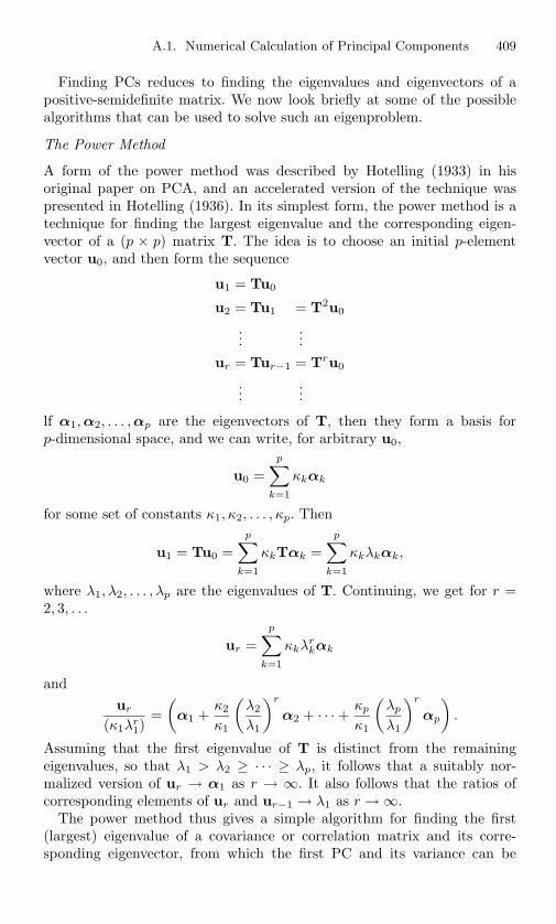
A.1. Numerical Calculation of Principal Components 409
Finding PCs reduces to finding the eigenvalues and eigenvectors of apositive-semidefinite matrix. We now look briefly at some of the possiblealgorithms that can be used to solve such an eigenproblem.
The Power Method
A form of the power method was described by Hotelling (1933) in hisoriginal paper on PCA, and an accelerated version of the technique waspresented in Hotelling (1936). In its simplest form, the power method is atechnique for finding the largest eigenvalue and the corresponding eigen-vector of a (p × p) matrix T. The idea is to choose an initial p-elementvector u0, and then form the sequence
u1 = Tu0
u2 = Tu1 = T2u0
......
ur = Tur−1 = Tru0
......
lf α1,α2, . . . ,αp are the eigenvectors of T, then they form a basis forp-dimensional space, and we can write, for arbitrary u0,
u0 =p∑
k=1
κkαk
for some set of constants κ1, κ2, . . . , κp. Then
u1 = Tu0 =p∑
k=1
κkTαk =p∑
k=1
κkλkαk,
where λ1, λ2, . . . , λp are the eigenvalues of T. Continuing, we get for r =2, 3, . . .
ur =p∑
k=1
κkλrkαk
andur
(κ1λr1)
=(
α1 +κ2
κ1
(λ2
λ1
)r
α2 + · · · + κp
κ1
(λp
λ1
)r
αp
).
Assuming that the first eigenvalue of T is distinct from the remainingeigenvalues, so that λ1 > λ2 ≥ · · · ≥ λp, it follows that a suitably nor-malized version of ur → α1 as r → ∞. It also follows that the ratios ofcorresponding elements of ur and ur−1 → λ1 as r → ∞.
The power method thus gives a simple algorithm for finding the first(largest) eigenvalue of a covariance or correlation matrix and its corre-sponding eigenvector, from which the first PC and its variance can be
410 Appendix A. Computation of Principal Components
derived. It works well if λ1 λ2, but converges only slowly if λ1 is not wellseparated from λ2. Speed of convergence also depends on the choice of theinitial vector u0; convergence is most rapid if u0 is close to α1,
If λ1 = λ2 > λ3, a similar argument to that given above shows that asuitably normalized version of ur → α1 + (κ2/κ1)α2 as r → ∞. Thus,the method does not lead to α1, but it still provides information aboutthe space spanned by α1, α2. Exact equality of eigenvalues is extremelyunlikely for sample covariance or correlation matrices, so we need not worrytoo much about this case.
Rather than looking at all ur, r = 1, 2, 3, . . . , attention can be restrictedto u1,u2,u4,u8, . . . (that is Tu0,T2u0,T4u0,T8u0, . . .) by simply squaringeach successive power of T. This accelerated version of the power methodwas suggested by Hotelling (1936). The power method can be adapted tofind the second, third, . . . PCs, or the last few PCs (see Morrison, 1976,p. 281), but it is likely to encounter convergence problems if eigenvaluesare close together, and accuracy diminishes if several PCs are found by themethod. Simple worked examples for the first and later components can befound in Hotelling (1936) and Morrison (1976, Section 8.4) .
There are various adaptations to the power method that partially over-come some of the problems just mentioned. A large number of suchadaptations are discussed by Wilkinson (1965, Chapter 9), although someare not directly relevant to positive-semidefinite matrices such as covari-ance or correlation matrices. Two ideas that are of use for such matriceswill be mentioned here. First, the origin can be shifted, that is the matrixT is replaced by T − ρIp, where Ip is the identity matrix, and ρ is chosento make the ratio of the first two eigenvalues of T − ρIp much larger thanthe corresponding ratio for T, hence speeding up convergence.
A second modification is to use inverse iteration (with shifts), in whichcase the iterations of the power method are used but with (T − ρIp)−1
replacing T. This modification has the advantage over the basic powermethod with shifts that, by using appropriate choices of ρ (different fordifferent eigenvectors), convergence to any of the eigenvectors of T canbe achieved. (For the basic method it is only possible to converge in thefirst instance to α1 or to αp.) Furthermore, it is not necessary to explicitlycalculate the inverse of T−ρIp, because the equation ur = (T−ρIp)−1ur−1
can be replaced by (T − ρIp)ur = ur−1. The latter equation can thenbe solved using an efficient method for the solution of systems of linearequations (see Wilkinson, 1965, Chapter 4). Overall, computational savingswith inverse iteration can be large compared to the basic power method(with or without shifts), especially for matrices with special structure, suchas tridiagonal matrices. It turns out that an efficient way of computingPCs is to first transform the covariance or correlation matrix to tridiagonalform using, for example, either the Givens or Householder transformations(Wilkinson, 1965, pp. 282, 290), and then to implement inverse iterationwith shifts on this tridiagonal form.
A.1. Numerical Calculation of Principal Components 411
There is one problem with shifting the origin that has not yet beenmentioned. This is the fact that to choose efficiently the values of ρ thatdetermine the shifts, we need some preliminary idea of the eigenvaluesof T. This preliminary estimation can be achieved by using the methodof bisection, which in turn is based on the Sturm sequence property oftridiagonal matrices. Details will not be given here (see Wilkinson, 1965,pp. 300–302), but the method provides a quick way of finding approximatevalues of the eigenvalues of a tridiagonal matrix. In fact, bisection could beused to find the eigenvalues to any required degree of accuracy, and inverseiteration implemented solely to find the eigenvectors.
Two major collections of subroutines for finding eigenvalues and eigen-vectors for a wide variety of classes of matrix are the EISPACK package(Smith et al., 1976), which is distributed by IMSL, and parts of the NAGlibrary of subroutines. In both of these collections, there are recommen-dations as to which subroutines are most appropriate for various types ofeigenproblem. In the case where only a few of the eigenvalues and eigenvec-tors of a real symmetric matrix are required (corresponding to finding justa few of the PCs for a covariance or correlation matrix) both EISPACKand NAG recommend transforming to tridiagonal form using Householdertransformations, and then finding eigenvalues and eigenvectors using bisec-tion and inverse iteration respectively. NAG and EISPACK both base theirsubroutines on algorithms published in Wilkinson and Reinsch (1971), asdo the ‘Numerical Recipes’ for eigensystems given by Press et al. (1992,Chapter 11).
The QL Algorithm
If all of the PCs are required, then methods other than those just describedmay be more efficient. For example, both EISPACK and NAG recommendthat we should still transform the covariance or correlation matrix to tridi-agonal form, but at the second stage the so-called QL algorithm should nowbe used, instead of bisection and inverse iteration. Chapter 8 of Wilkinson(1965) spends over 80 pages describing the QR and LR algorithms (whichare closely related to the QL algorithm), but only a very brief outline willbe given here.
The basic idea behind the QL algorithm is that any non-singular matrixT can be written as T = QL, where Q is orthogonal and L is lowertriangular. (The QR algorithm is similar, except that T is written insteadas T = QR, where R is upper triangular, rather than lower triangular.) IfT1 = T and we write T1 = Q1L1, then T2 is defined as T2 = L1Q1. Thisis the first step in an iterative procedure. At the next step, T2 is writtenas T2 = Q2L2 and T3 is defined as T3 = L2Q2. In general, Tr is writtenas QrLr and Tr+1 is then defined as LrQr, r = 1, 2, 3, . . . , where Q1, Q2,Q3, . . . are orthogonal matrices, and L1, L2, L3, . . . are lower triangular. Itcan be shown that Tr converges to a diagonal matrix, with the eigenvalues

412 Appendix A. Computation of Principal Components
of T in decreasing absolute size down the diagonal. Eigenvectors can befound by accumulating the transformations in the QL algorithm (Smith etal., 1976, p. 468).
As with the power method, the speed of convergence of the QL algorithmdepends on the ratios of consecutive eigenvalues. The idea of incorporatingshifts can again be implemented to improve the algorithm and, unlike thepower method, efficient strategies exist for finding appropriate shifts thatdo not rely on prior information about the eigenvalues (see, for example,Lawson and Hanson (1974, p. 109)). The QL algorithm can also cope withequality between eigenvalues.
It is probably fair to say that the algorithms described in detail byWilkinson (1965) and Wilkinson and Reinsch (1971), and implemented invarious IMSL and NAG routines, have stood the test of time. They stillprovide efficient ways of computing PCs in many circumstances. However,we conclude the Appendix by discussing two alternatives. The first is imple-mentation via the singular value decomposition (SVD) of the data matrix,and the second consists of the various algorithms for PCA that have beensuggested in the neural networks literature. The latter is a large topic andwill be summarized only briefly.
One other type of algorithm that has been used recently to find PCs isthe EM algorithm (Dempster et al., 1977). This is advocated by Tippingand Bishop (1999a,b) and Roweis (1997), and has its greatest value in caseswhere some of the data are missing (see Section 13.6).
Singular Value Decomposition
The suggestion that PCs may best be computed using the SVD of thedata matrix (see Section 3.5) is not new. For example, Chambers (1977, p.111) talks about the SVD providing the best approach to computation ofprincipal components and Gnanadesikan (1977, p. 10) states that ‘. . . therecommended algorithm for . . . obtaining the principal components is eitherthe . . . QR method . . . or the singular value decomposition.’ In constructingthe SVD, it turns out that similar algorithms to those given above canbe used. Lawson and Hanson (1974, p. 110) describe an algorithm (seealso Wilkinson and Reinsch (1971)) for finding the SVD, which has twostages; the first uses Householder transformations to transform to an upperbidiagonal matrix, and the second applies an adapted QR algorithm. Themethod is therefore not radically different from that described earlier.
As noted at the end of Section 8.1, the SVD can also be useful in com-putations for regression (Mandel, 1982; Nelder, 1985), so the SVD hasfurther advantages if PCA is used in conjunction with regression. Nashand Lefkovitch (1976) describe an algorithm that uses the SVD to providea variety of results for regression, as well as PCs.
Another point concerning the SVD is that it provides simultaneously notonly the coefficients and variances for the PCs, but also the scores of each
A.1. Numerical Calculation of Principal Components 413
observation on each PC, and hence all the information that is requiredto construct a biplot (see Section 5.3). The PC scores would otherwiseneed to be derived as an extra step after calculating the eigenvalues andeigenvectors of the covariance or correlation matrix S = 1
n−1X′X.
The values of the PC scores are related to the eigenvectors of XX′, whichcan be derived from the eigenvectors of X′X (see the proof of Property G4in Section 3.2); conversely, the eigenvectors of X′X can be found fromthose of XX′. In circumstances where the sample size n is smaller than thenumber of variables p, XX′ has smaller dimensions than X′X, so that itcan be advantageous to use the algorithms described above, based on thepower method or QL method, on a multiple of XX′ rather than X′X in suchcases. Large computational savings are possible when n p, as in chemicalspectroscopy or in the genetic example of Hastie et al. (2000), which isdescribed in Section 9.2 and which has n = 48, p = 4673. Algorithms alsoexist for updating the SVD if data arrive sequentially (see for exampleBerry et al. (1995)).
Neural Network Algorithms
Neural networks provide ways of extending PCA, including some non-lineargeneralizations (see Sections 14.1.3, 14.6.1). They also give alternative al-gorithms for estimating ‘ordinary’ PCs. The main difference between thesealgorithms and the techniques described earlier in the Appendix is thatmost are ‘adaptive’ rather than ‘batch’ methods. If the whole of a dataset is collected before PCA is done and parallel processing is not possible,then batch methods such as the QR algorithm are hard to beat (see Dia-mantaras and Kung, 1996 (hereafter DK96), Sections 3.5.3, 4.4.1). On theother hand, if data arrive sequentially and PCs are re-estimated when newdata become available, then adaptive neural network algorithms come intotheir own. DK96, Section 4.2.7 note that ‘there is a plethora of alternative[neural network] techniques that perform PCA.’ They describe a selectionof single-layer techniques in their Section 4.2, with an overview of these intheir Table 4.1. Different algorithms arise depending on
• whether the first or last few PCs are of interest;
• whether one or more than one PC is required;
• whether individual PCs are wanted or whether subspaces spanned byseveral PCs will suffice;
• whether the network is required to be biologically plausible.
DK96, Section 4.2.7 treat finding the last few PCs as a different technique,calling it minor component analysis.
In their Section 4.4, DK96 compare the properties, including speed, ofseven algorithms using simulated data. In Section 4.5 they discuss multi-layer networks.

414 Appendix A. Computation of Principal Components
Neural network algorithms are feasible for larger data sets than batchmethods because they are better able to take advantage of developmentsin computer architecture. DK96, Chapter 8, discuss the potential for ex-ploiting parallel VSLI (very large scale integration) systems, where themost appropriate algorithms may be different from those for non-parallelsystems (DK96, Section 3.5.5). They discuss both digital and analogueimplementations and their pros and cons (DK96, Section 8.3). Classicaleigenvector-based algorithms are not easily parallelizable, whereas neuralnetwork algorithms are (DK96 pp. 205–207).
References
Aguilera, A.M., Gutierrez, R., Ocana, F.A. and Valderrama, M.J. (1995).Computational approaches to estimation in the principal componentanalysis of a stochastic process. Appl. Stoch. Models Data Anal., 11,279–299.
Aguilera, A.M., Ocana, F.A. and Valderrama, M.J. (1997). An ap-proximated principal component prediction model for continuous timestochastic processes. Appl. Stoch. Models Data Anal., 13, 61–72.
Aguilera, A.M., Ocana, F.A. and Valderrama, M.J. (1999a). Forecastingwith unequally spaced data by a functional principal component analysis.Test, 8, 233–253.
Aguilera, A.M., Ocana, F.A. and Valderrama, M.J. (1999b). Forecastingtime series by functional PCA. Discussion of several weighted approaches.Computat. Statist., 14, 443–467.
Ahamad, B. (1967). An analysis of crimes by the method of principalcomponents. Appl. Statist., 16, 17–35.
Aires, F., Chedin, A. and Nadal, J.P. (2000). Independent component anal-ysis of multivariate time series: Application to tropical SST variability.J. Geophys. Res.—Atmos., 105 (D13), 17,437–17,455.
Aitchison, J. (1982). The statistical analysis of compositional data (withdiscussion). J. R. Statist. Soc. B, 44, 139–177.
Aitchison, J. (1983). Principal component analysis of compositional data.Biometrika, 70, 57–65.
Aitchison, J. (1986). The Statistical Analysis of Compositional Data.London: Chapman and Hall.

416 References
Akaike, H. (1974). A new look at the statistical model identification. IEEETrans. Autom. Cont., 19, 716–723.
Aldenderfer, M.S. and Blashfield, R.K. (1984). Cluster Analysis. BeverlyHills: Sage.
Aldrin, M. (2000). Multivariate prediction using softly shrunk reduced-rankregression. Amer. Statistician, 54, 29–34.
Ali, A., Clarke, G.M. and Trustrum, K. (1985). Principal component anal-ysis applied to some data from fruit nutrition experiments. Statistician,34, 365–369.
Al-Kandari, N. (1998). Variable Selection and Interpretation in PrincipalComponent Analysis. Unpublished Ph.D. thesis, University of Aberdeen.
Al-Kandari, N.M. and Jolliffe, I.T. (2001). Variable selection and inter-pretation of covariance principal components. Commun. Statist.—Simul.Computat., 30, 339-354.
Allan, R., Chambers, D., Drosdowsky, W., Hendon, H., Latif, M., Nicholls,N., Smith, I., Stone, R. and Tourre, Y. (2001). Is there an Indian Oceandipole, and is it independent of the El Nino—Southern Oscillation?CLIVAR Exchanges, 6, 18–22.
Allen, D.M. (1974). The relationship between variable selection and dataaugmentation and a method for prediction. Technometrics, 16, 125–127.
Allen M.R. and Robertson, A.W. (1996). Distinguishing modulated oscilla-tions from coloured noise in multivariate datasets. Climate Dynam., 12,775–784.
Allen M.R. and Smith, L.A. (1996). Monte Carlo SSA: Detecting irregularoscillations in the presence of colored noise. J. Climate, 9, 3373–3404.
Allen M.R. and Smith, L.A. (1997). Optimal filtering in singular spectrumanalysis. Phys. Lett. A, 234, 419–428.
Allen, M.R. and Tett, S.F.B. (1999). Checking for model consistency inoptimal fingerprinting. Climate Dynam., 15, 419–434.
Ambaum, M.H.P., Hoskins, B.J. and Stephenson, D.B. (2001). Arcticoscillation or North Atlantic Oscillation. J. Climate, 14, 3495–3507.
Anderson, A.B., Basilevsky, A. and Hum, D.P.J. (1983). Missing data: Areview of the literature. In Handbook of Survey Research, eds. P.H. Rossi,J.D. Wright and A.B. Anderson, 415–494.
Anderson, T.W. (1957). Maximum likelihood estimates for a multivari-ate normal distribution when some observations are missing. J. Amer.Statist. Assoc., 52, 200–203.
Anderson, T.W. (1963). Asymptotic theory for principal componentanalysis. Ann. Math. Statist., 34, 122–148.
Anderson, T.W. (1984). Estimating linear statistical relationships. Ann.Statist., 12, 1–45.
Andrews, D.F. (1972). Plots of high-dimensional data. Biometrics, 28, 125–136.

References 417
Apley, D.W. and Shi, J. (2001). A factor-analysis method for diagnosingvariability in multivariate manufacturing processes. Technometrics, 43,84–95.
Arbuckle, J. and Friendly, M.L. (1977). On rotating to smooth functions.Psychometrika, 42, 127–140.
Asselin de Beauville, J.-P. (1995). Non parametric discrimination by thenearest principal axis method (NPA)—preliminary study. In Data Sci-ence and Its Application, eds. Y. Escoufier, B. Fichet, E. Diday, L. Lebart,C. Hayashi, N. Ohsumi and Y. Baba, 145–154. Tokyo: Academic Press.
Atiqullah, M. and Uddin, M. (1993). Sweep-out components analysis. J.Appl. Statist. Sci., 1, 67–79.
Baba, Y. (1995). Scaling methods for ranked data. In Data Science and ItsApplication, eds. Y. Escoufier, B. Fichet, E. Diday, L. Lebart, C. Hayashi,N. Ohsumi and Y. Baba, 133–144. Tokyo: Academic Press.
Baccini, A., Besse, P. and de Falguerolles, A. (1996). A L1-norm PCA anda heuristic approach. In Ordinal and Symbolic Data Analysis, eds. E.Diday, Y. Lechevalier and O. Opitz, 359–368. Berlin: Springer-Verlag.
Bacon-Shone, J. (1992). Ranking methods for compositional data. Appl.Statist., 41, 533–537.
Bargmann, R.E. and Baker, F.D. (1977). A minimax approach to compo-nent analysis. In Applications of Statistics, ed. P.R. Krishnaiah, 55–69.Amsterdam: North-Holland.
Barnett, T.P. and Hasselmann, K. (1979). Techniques of linear prediction,with application to oceanic and atmospheric fields in the tropical Pacific.Rev. Geophys. Space Phys., 17, 949–968.
Barnett, V. (1981). Interpreting Multivariate Data. Chichester: Wiley.Barnett, V. and Lewis, T. (1994). Outliers in Statistical Data, 3rd edition.
Chichester: Wiley.Barring, L. (1987). Spatial patterns of daily rainfall in central Kenya: Ap-
plication of principal component analysis, common factor analysis andspatial correlation. J. Climatol., 7, 267–289.
Bartels, C.P.A. (1977). Economic Aspects of Regional Welfare, IncomeDistribution and Unemployment. Leiden: Martinus Nijhoff.
Bartholomew, D.J. and Knott, M. (1999). Latent Variable Models andFactor Analysis, 2nd edition. London: Arnold.
Bartkowiak, A. (1982). The choice of representative variables by stepwiseregression. Zastosowania Matematyki, 17, 527–538.
Bartkowiak, A. (1991). How to reveal dimensionality of the data? In Ap-plied Stochastic Models and Data Analysis, eds. R. Gutierrez and M.J.Valderrama, 55–64. Singapore: World Scientific.
Bartkowiak, A., Lukasik, S., Chwistecki, K., Mrukowicz, M. and Mor-genstern, W. (1988). Transformation of data and identification ofoutliers—as experienced in an epidemiological study. EDV in Medizinund Biologie, 19, 64–69.
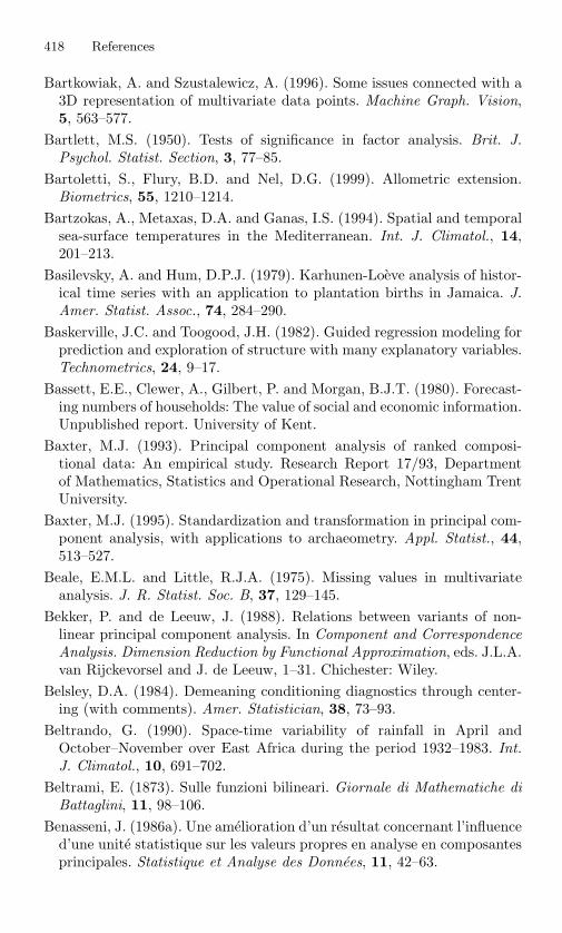
418 References
Bartkowiak, A. and Szustalewicz, A. (1996). Some issues connected with a3D representation of multivariate data points. Machine Graph. Vision,5, 563–577.
Bartlett, M.S. (1950). Tests of significance in factor analysis. Brit. J.Psychol. Statist. Section, 3, 77–85.
Bartoletti, S., Flury, B.D. and Nel, D.G. (1999). Allometric extension.Biometrics, 55, 1210–1214.
Bartzokas, A., Metaxas, D.A. and Ganas, I.S. (1994). Spatial and temporalsea-surface temperatures in the Mediterranean. Int. J. Climatol., 14,201–213.
Basilevsky, A. and Hum, D.P.J. (1979). Karhunen-Loeve analysis of histor-ical time series with an application to plantation births in Jamaica. J.Amer. Statist. Assoc., 74, 284–290.
Baskerville, J.C. and Toogood, J.H. (1982). Guided regression modeling forprediction and exploration of structure with many explanatory variables.Technometrics, 24, 9–17.
Bassett, E.E., Clewer, A., Gilbert, P. and Morgan, B.J.T. (1980). Forecast-ing numbers of households: The value of social and economic information.Unpublished report. University of Kent.
Baxter, M.J. (1993). Principal component analysis of ranked composi-tional data: An empirical study. Research Report 17/93, Departmentof Mathematics, Statistics and Operational Research, Nottingham TrentUniversity.
Baxter, M.J. (1995). Standardization and transformation in principal com-ponent analysis, with applications to archaeometry. Appl. Statist., 44,513–527.
Beale, E.M.L. and Little, R.J.A. (1975). Missing values in multivariateanalysis. J. R. Statist. Soc. B, 37, 129–145.
Bekker, P. and de Leeuw, J. (1988). Relations between variants of non-linear principal component analysis. In Component and CorrespondenceAnalysis. Dimension Reduction by Functional Approximation, eds. J.L.A.van Rijckevorsel and J. de Leeuw, 1–31. Chichester: Wiley.
Belsley, D.A. (1984). Demeaning conditioning diagnostics through center-ing (with comments). Amer. Statistician, 38, 73–93.
Beltrando, G. (1990). Space-time variability of rainfall in April andOctober–November over East Africa during the period 1932–1983. Int.J. Climatol., 10, 691–702.
Beltrami, E. (1873). Sulle funzioni bilineari. Giornale di Mathematiche diBattaglini, 11, 98–106.
Benasseni, J. (1986a). Une amelioration d’un resultat concernant l’influenced’une unite statistique sur les valeurs propres en analyse en composantesprincipales. Statistique et Analyse des Donnees, 11, 42–63.
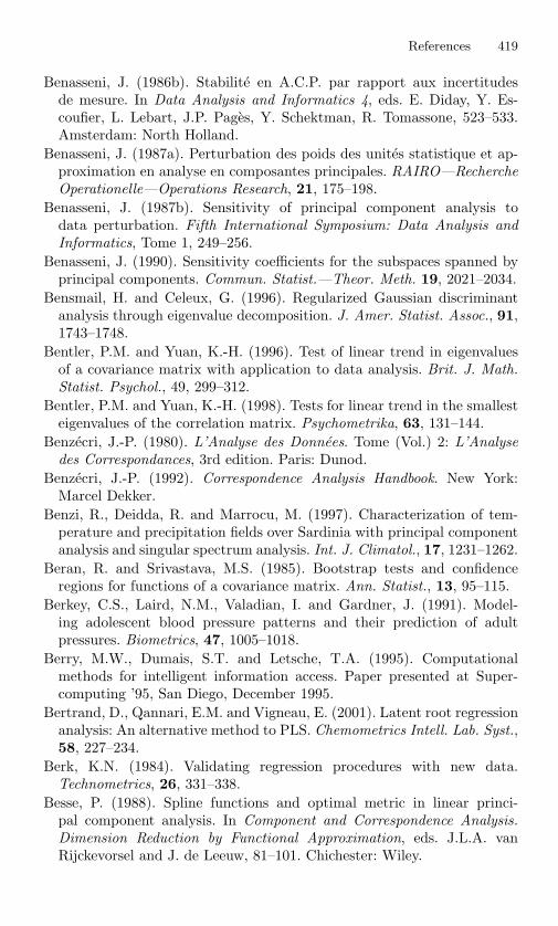
References 419
Benasseni, J. (1986b). Stabilite en A.C.P. par rapport aux incertitudesde mesure. In Data Analysis and Informatics 4, eds. E. Diday, Y. Es-coufier, L. Lebart, J.P. Pages, Y. Schektman, R. Tomassone, 523–533.Amsterdam: North Holland.
Benasseni, J. (1987a). Perturbation des poids des unites statistique et ap-proximation en analyse en composantes principales. RAIRO—RechercheOperationelle—Operations Research, 21, 175–198.
Benasseni, J. (1987b). Sensitivity of principal component analysis todata perturbation. Fifth International Symposium: Data Analysis andInformatics, Tome 1, 249–256.
Benasseni, J. (1990). Sensitivity coefficients for the subspaces spanned byprincipal components. Commun. Statist.—Theor. Meth. 19, 2021–2034.
Bensmail, H. and Celeux, G. (1996). Regularized Gaussian discriminantanalysis through eigenvalue decomposition. J. Amer. Statist. Assoc., 91,1743–1748.
Bentler, P.M. and Yuan, K.-H. (1996). Test of linear trend in eigenvaluesof a covariance matrix with application to data analysis. Brit. J. Math.Statist. Psychol., 49, 299–312.
Bentler, P.M. and Yuan, K.-H. (1998). Tests for linear trend in the smallesteigenvalues of the correlation matrix. Psychometrika, 63, 131–144.
Benzecri, J.-P. (1980). L’Analyse des Donnees. Tome (Vol.) 2: L’Analysedes Correspondances, 3rd edition. Paris: Dunod.
Benzecri, J.-P. (1992). Correspondence Analysis Handbook. New York:Marcel Dekker.
Benzi, R., Deidda, R. and Marrocu, M. (1997). Characterization of tem-perature and precipitation fields over Sardinia with principal componentanalysis and singular spectrum analysis. Int. J. Climatol., 17, 1231–1262.
Beran, R. and Srivastava, M.S. (1985). Bootstrap tests and confidenceregions for functions of a covariance matrix. Ann. Statist., 13, 95–115.
Berkey, C.S., Laird, N.M., Valadian, I. and Gardner, J. (1991). Model-ing adolescent blood pressure patterns and their prediction of adultpressures. Biometrics, 47, 1005–1018.
Berry, M.W., Dumais, S.T. and Letsche, T.A. (1995). Computationalmethods for intelligent information access. Paper presented at Super-computing ’95, San Diego, December 1995.
Bertrand, D., Qannari, E.M. and Vigneau, E. (2001). Latent root regressionanalysis: An alternative method to PLS. Chemometrics Intell. Lab. Syst.,58, 227–234.
Berk, K.N. (1984). Validating regression procedures with new data.Technometrics, 26, 331–338.
Besse, P. (1988). Spline functions and optimal metric in linear princi-pal component analysis. In Component and Correspondence Analysis.Dimension Reduction by Functional Approximation, eds. J.L.A. vanRijckevorsel and J. de Leeuw, 81–101. Chichester: Wiley.

420 References
Besse, P. (1992). PCA stability and choice of dimensionality. Stat. Prob.Lett., 13, 405–410.
Besse, P.C. (1994a). Insight of a dreamed PCA. In SEUGI/CLUB SASProceedings, 744–759.
Besse, P.C. (1994b). Models for multivariate data analysis. In COMPSTAT94, eds. R. Dutter and W. Grossmann, 271–285. Heidelberg: Physica-Verlag.
Besse, P.C., Cardot, H. and Ferraty, F. (1997). Simultaneous non-parametric regressions of unbalanced longitudinal data. Computat.Statist. Data Anal., 24, 255–270.
Besse, P.C., Cardot, H. and Stephenson, D.B. (2000). Autoregressive fore-casting of some functional climatic variations. Scand. J. Statist., 27,673–687.
Besse, P. and de Falguerolles, A. (1993). Application of resampling methodsto the choice of dimension in principal component analysis. In ComputerIntensive Methods in Statistics, eds. W. Hardle and L. Simar, 167–176.Heidelberg: Physica-Verlag.
Besse, P.C. and Ferraty, F. (1995). A fixed effect curvilinear model.Computat. Statist., 10, 339–351.
Besse, P. and Ferre, L. (1993). Sur l’usage de la validation croisee en analyseen composantes principales. Rev. Statistique Appliquee, 41, 71–76.
Besse, P. and Ramsay, J.O. (1986). Principal components analysis ofsampled functions. Psychometrika, 51, 285–311.
Bhargava, R.P. and Ishizuka, T. (1981). Selection of a subset of variablesfrom the viewpoint of variation—an alternative to principal componentanalysis. In Proc. Indian Statist. Inst. Golden Jubilee Int. Conf. onStatistics: Applications and New Directions, 33–44.
Bibby, J. (1980). Some effects of rounding optimal estimates. Sankhya B,42, 165–178.
Bishop, C.M. (1995) Neural Networks for Pattern Recognition. Oxford:Clarendon Press.
Bishop, C.M. (1999). Bayesian PCA. In Advances in Neural InformationProcessing Systems, 11, eds. S.A. Solla, M.S. Kearns and D.A. Cohn,382–388. Cambridge: MIT Press.
Bishop, Y.M.M., Fienberg, S.E. and Holland, P.W. (1975). DiscreteMultivariate Analysis: Theory and Practice. Cambridge: MIT Press.
Blackith, R.E. and Reyment, R.A. (1971). Multivariate Morphometrics.London: Academic Press.
Bloomfield, P. (1974). Linear transformations for multivariate binary data.Biometrics, 30, 609–617.
Bloomfield, P. and Davis, J.M. (1994). Orthogonal rotation of complexprincipal components. Int. J. Climatol., 14, 759–775.
Bohning, D. (1999). Computer-Assisted Analysis of Mixtures and Ap-plications Meta-analysis, Disease Mapping and Others. Boca Raton:Chapman and Hall/CRC.
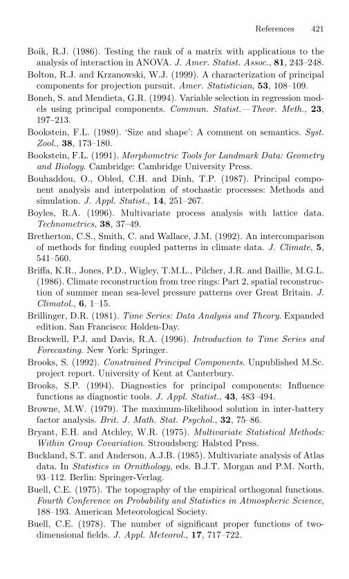
References 421
Boik, R.J. (1986). Testing the rank of a matrix with applications to theanalysis of interaction in ANOVA. J. Amer. Statist. Assoc., 81, 243–248.
Bolton, R.J. and Krzanowski, W.J. (1999). A characterization of principalcomponents for projection pursuit. Amer. Statistician, 53, 108–109.
Boneh, S. and Mendieta, G.R. (1994). Variable selection in regression mod-els using principal components. Commun. Statist.—Theor. Meth., 23,197–213.
Bookstein, F.L. (1989). ‘Size and shape’: A comment on semantics. Syst.Zool., 38, 173–180.
Bookstein, F.L. (1991). Morphometric Tools for Landmark Data: Geometryand Biology. Cambridge: Cambridge University Press.
Bouhaddou, O., Obled, C.H. and Dinh, T.P. (1987). Principal compo-nent analysis and interpolation of stochastic processes: Methods andsimulation. J. Appl. Statist., 14, 251–267.
Boyles, R.A. (1996). Multivariate process analysis with lattice data.Technometrics, 38, 37–49.
Bretherton, C.S., Smith, C. and Wallace, J.M. (1992). An intercomparisonof methods for finding coupled patterns in climate data. J. Climate, 5,541–560.
Briffa, K.R., Jones, P.D., Wigley, T.M.L., Pilcher, J.R. and Baillie, M.G.L.(1986). Climate reconstruction from tree rings: Part 2, spatial reconstruc-tion of summer mean sea-level pressure patterns over Great Britain. J.Climatol., 6, 1–15.
Brillinger, D.R. (1981). Time Series: Data Analysis and Theory. Expandededition. San Francisco: Holden-Day.
Brockwell, P.J. and Davis, R.A. (1996). Introduction to Time Series andForecasting. New York: Springer.
Brooks, S. (1992). Constrained Principal Components. Unpublished M.Sc.project report. University of Kent at Canterbury.
Brooks, S.P. (1994). Diagnostics for principal components: Influencefunctions as diagnostic tools. J. Appl. Statist., 43, 483–494.
Browne, M.W. (1979). The maximum-likelihood solution in inter-batteryfactor analysis. Brit. J. Math. Stat. Psychol., 32, 75–86.
Bryant, E.H. and Atchley, W.R. (1975). Multivariate Statistical Methods:Within Group Covariation. Stroudsberg: Halsted Press.
Buckland, S.T. and Anderson, A.J.B. (1985). Multivariate analysis of Atlasdata. In Statistics in Ornithology, eds. B.J.T. Morgan and P.M. North,93–112. Berlin: Springer-Verlag.
Buell, C.E. (1975). The topography of the empirical orthogonal functions.Fourth Conference on Probability and Statistics in Atmospheric Science,188–193. American Meteorological Society.
Buell, C.E. (1978). The number of significant proper functions of two-dimensional fields. J. Appl. Meteorol., 17, 717–722.

422 References
Buell, C.E. (1979). On the physical interpretation of empirical orthogonalfunctions. Sixth Conference on Probability and Statistics in AtmosphericScience, 112–117. American Meteorological Society.
Burnham, A.J., MacGregor, J.F. and Viveros, R. (1999). Latent variablemultivariate regression modelling. Chemometrics Intell. Lab. Syst., 48,167–180.
Butler, N.A. and Denham, M.C. (2000). The peculiar shrinkage propertiesof partial least squares regression. J. R. Statist. Soc. B, 62, 585–593.
Cadima, J. (2000). A scale-invariant component analysis: MCCA. Tech-nical report 4, Departamento de Matematica, Instituto Superior deAgronomia, Universidade Tecnica de Lisboa.
Cadima, J., Cerdeira, J.O. and Minhoto, M. (2002). A computational studyof algorithms for variable selection in multivariate statistics. Submittedfor publication.
Cadima, J. and Jolliffe, I.T. (1995). Loadings and correlations in theinterpretation of principal components. J. Appl. Statist., 22, 203–214.
Cadima, J.F.C.L. and Jolliffe, I.T. (1996). Size- and shape-related principalcomponent analysis. Biometrics, 52, 710–716.
Cadima, J. and Jolliffe, I. (1997). Some comments on ten Berge, J.M.F.and Kiers, H.A.L. (1996). Optimality criteria for principal componentanalysis and generalizations. Brit. J. Math. Stat. Psychol., 50, 365–366.
Cadima, J.F.C.L. and Jolliffe, I.T. (2001). Variable selection and the in-terpretation of principal subspaces. J. Agri. Biol. Environ. Statist., 6,62–79.
Cahalan, R.F. (1983). EOF spectral estimation in climate analysis. Sec-ond International Meeting on Statistical Climatology, Preprints volume,4.5.1–4.5.7.
Cai, W. and Baines, P. (2001). Forcing of the Antarctic Circumpolar Waveby ENSO teleconnections. J. Geophys. Res.—Oceans, 106, 9019–9038.
Cailliez, F. and Pages, J.-P. (1976). Introduction a l’Analyse des Donnees.Paris: SMASH.
Calder, P. (1986). Influence Functions in Multivariate Analysis. Unpub-lished Ph.D. thesis, University of Kent at Canterbury.
Campbell, N.A. (1980). Robust procedures in multivariate analysis 1:Robust covariance estimation. Appl. Statist., 29, 231–237.
Campbell, N.A. and Atchley, W.R. (1981). The geometry of canonicalvariate analysis. Syst. Zool., 30, 268–280.
Capra, W.B. and Muller, H.-G. (1997). An accelerated-time model forresponse curves. J. Amer. Statist. Assoc., 92, 72–83.
Carr, D.B. (1998). Multivariate graphics. In Encyclopedia of Biostatistics,eds. P. Armitage and T. Colton, 2864–2886. Chichester: Wiley.
Casin, Ph. (2001). A generalization of principal component analysis to Ksets of variables. Computat. Statist. Data Anal., 35, 417–428.
References 423
Castro, P.E., Lawton, W.H., and Sylvestre, E.A. (1986). Principal modesof variation for processes with continuous sample curves. Technometrics,28, 329–337.
Cattell, R.B. (1966). The scree test for the number of factors. Multiv.Behav. Res., 1, 245–276.
Cattell, R.B. (1978). The Scientific Use of Factor Analysis in Behavioraland Life Sciences. New York: Plenum Press.
Cattell, R.B. and Vogelmann, S. (1977). A comprehensive trial of the screeand KG criteria for determining the number of factors. Mult. Behav.Res., 12, 289–325.
Caussinus, H. (1986). Models and uses of principal component analysis: Acomparison emphasizing graphical displays and metric choices. In Mul-tidimensional Data Analysis, eds. J. de Leeuw, W. Heiser, J. Meulmanand F. Critchley, 149–178. Leiden: DSWO Press.
Caussinus, H. (1987). Discussion of ‘What is projection pursuit?’ by Jonesand Sibson. J. R. Statist. Soc. A, 150, 26.
Caussinus, H. and Ferre, L. (1992). Comparing the parameters of a modelfor several units by means of principal component analysis. Computat.Statist. Data Anal., 13, 269–280.
Caussinus, H., Hakam, S. and Ruiz-Gazen, A. (2001). Projections reve-latrices controlees. Recherche d’individus atypiques. To appear in Rev.Statistique Appliquee.
Caussinus, H. and Ruiz, A. (1990) Interesting projections of multidi-mensional data by means of generalized principal component analysis.In COMPSTAT 90, eds. K. Momirovic and V. Mildner, 121–126.Heidelberg: Physica-Verlag.
Caussinus, H. and Ruiz-Gazen, A. (1993). Projection pursuit and general-ized principal component analysis. In New Directions in Statistical DataAnalysis and Robustness, eds. S. Morgenthaler, E. Ronchetti and W.A.Stahel, 35–46. Basel: Birkhauser Verlag.
Caussinus, H. and Ruiz-Gazen, A. (1995). Metrics for finding typical struc-tures by means of principal component analysis. In Data Science and ItsApplication, eds. Y. Escoufier, B. Fichet, E. Diday, L. Lebart, C. Hayashi,N. Ohsumi and Y. Baba, 177–192. Tokyo: Academic Press.
Chambers, J.M. (1977). Computational Methods for Data Analysis. NewYork: Wiley.
Chambers, J.M., Cleveland, W.S., Kleiner, B. and Tukey, P.A. (1983).Graphical Methods for Data Analysis. Belmont: Wadsworth.
Champely, S. and Doledec, S. (1997). How to separate long-term trendsfrom periodic variation in water quality monitoring. Water Res., 11,2849–2857.
Chang, W.-C. (1983). On using principal components before separatinga mixture of two multivariate normal distributions. Appl. Statist., 32,267–275.
424 References
Chatfield, C. and Collins, A.J. (1989). Introduction to MultivariateAnalysis. London: Chapman and Hall.
Cheng, C.-L. and van Ness, J.W. (1999). Statistical Regression withMeasurement Error. London: Arnold.
Chernoff, H. (1973). The use of faces to represent points in k-dimensionalspace graphically. J. Amer. Statist. Assoc., 68, 361–368.
Cherry, S. (1997). Some comments on singular value decompositionanalysis. J. Climate, 10, 1759–1761.
Chipman, H.A. and Gu, H. (2002). Interpretable dimension reduction. Toappear in J. Appl. Statist.
Chouakria, A., Cazes, P. and Diday, E. (2000). Symbolic principal com-ponent analysis. In Analysis of Symbolic Data. Exploratory Methods forExtracting Statistical Information from Complex Data, eds. H.-H. Bockand E. Diday, 200–212. Berlin: Springer-Verlag.
Clausen, S.-E. (1998). Applied Correspondence Analysis: An Introduction.Thousand Oaks: Sage.
Cleveland, W.S. (1979). Robust locally weighted regression and smoothingscatterplots. J. Amer. Statist. Assoc., 74, 829–836.
Cleveland, W.S. (1981). LOWESS: A program for smoothing scatterplotsby robust locally weighted regression. Amer. Statistician, 35, 54.
Cleveland, W.S. and Guarino, R. (1976). Some robust statistical proceduresand their application to air pollution data. Technometrics, 18, 401–409.
Cochran, R.N. and Horne, F.H., (1977). Statistically weighted principalcomponent analysis of rapid scanning wavelength kinetics experiments.Anal. Chem., 49, 846–853.
Cohen, S.J. (1983). Classification of 500 mb height anomalies usingobliquely rotated principal components. J. Climate Appl. Meteorol., 22,1975–1988.
Cohn, R.D. (1999). Comparisons of multivariate relational structures inserially correlated data. J. Agri. Biol. Environ. Statist., 4, 238–257.
Coleman, D. (1985). Hotelling’s T 2, robust principal components, andgraphics for SPC. Paper presented at the 1985 Annual Meeting of theAmerican Statistical Association.
Commandeur, J.J.F, Groenen, P.J.F and Meulman, J.J. (1999). A distance-based variety of nonlinear multivariate data analysis, including weightsfor objects and variables. Psychometrika, 64, 169–186.
Compagnucci, R.H., Araneo, D. and Canziani, P.O. (2001). Principal se-quence pattern analysis: A new approach to classifying the evolution ofatmospheric systems. Int. J. Climatol., 21, 197–217.
Compagnucci, R.H. and Salles, M.A. (1997). Surface pressure patternsduring the year over Southern South America. Int. J. Climatol., 17,635–653.
Cook, R.D. and Weisberg, S. (1982). Residuals and Influence in Regression.New York: Chapman and Hall.
References 425
Cook, R.D. (1986). Assessment of local influence. J. R. Statist. Soc. B, 48,133–169 (including discussion).
Coppi, R. and Bolasco, S. (eds.) (1989). Multiway Data Analysis. Amster-dam: North-Holland.
Corbitt, B. and Ganesalingam, S. (2001). Comparison of two leading mul-tivariate techniques in terms of variable selection for linear discriminantanalysis. J. Statist. Manag. Syst., 4, 93–108.
Corsten, L.C.A. and Gabriel, K.R. (1976). Graphical exploration incomparing variance matrices. Biometrics, 32, 851–863.
Cox, D.R. (1972). The analysis of multivariate binary data. Appl. Statist.,21, 113–120.
Cox, T.F. and Cox, M.A.A. (2001). Multidimensional Scaling, 2nd edition.Boca Raton: Chapman and Hall.
Craddock, J.M. (1965). A meteorological application of principal compo-nent analysis. Statistician, 15, 143–156.
Craddock, J.M. and Flintoff, S. (1970). Eigenvector representations ofNorthern Hemispheric fields. Q.J.R. Met. Soc., 96, 124–129.
Craddock, J.M. and Flood, C.R. (1969). Eigenvectors for representing the500 mb. geopotential surface over the Northern Hemisphere. Q.J.R. Met.Soc., 95, 576–593.
Craw, I. and Cameron, P. (1992). Face recognition by computer. Proc. Br.Machine Vision Conf., 489–507. Berlin: Springer-Verlag.
Critchley, F. (1985). Influence in principal components analysis. Biome-trika, 72, 627–636.
Crone, L.J. and Crosby, D.S. (1995). Statistical applications of a metric onsubspaces to satellite meteorology. Technometrics, 37, 324–328.
Croux, C. and Haesbroeck, G. (2000). Principal component analysis basedon robust estimators of the covariance or correlation matrix: Influencefunctions and efficiencies. Biometrika, 87, 603–618.
Croux, C. and Ruiz-Gazen, A. (1995). A fast algorithm for robust principalcomponents based on projection pursuit. In COMPSTAT 96, ed. A. Prat,211–216.
Croux, C. and Ruiz-Gazen, A. (2000). High breakdown estimatorsfor principal components: the projection-pursuit approach revisited.Preprint 2000/149. Institut de Statistique et de Recherche Operationelle,Universite Libre de Bruxelles.
Cuadras, C.M. (1998). Comment on ‘Some cautionary notes on the use ofprincipal components regression’. Amer. Statistician, 52, 371.
Cubadda, G. (1995). A note on testing for seasonal co-integration usingprincipal components in the frequency domain. J. Time Series Anal.,16, 499–508.
Dahl, K.S., Piovoso, M.J. and Kosanovich, K.A. (1999). Translating third-order data analysis methods to chemical batch processes. ChemometricsIntell. Lab. Syst., 46, 161–180.

426 References
Daigle, G. and Rivest, L.-P. (1992). A robust biplot. Canad. J. Statist., 20,241–255.
Daling, J.R. and Tamura, H. (1970). Use of orthogonal factors for selectionof variables in a regression equation—an illustration. Appl. Statist., 19,260–268.
Darnell, A.C. (1994). A Dictionary of Econometrics. Aldershot: EdwardElgar.
Darroch, J.N. and Mosimann, J.E. (1985). Canonical and principalcomponents of shape. Biometrika, 72, 241–252.
Daudin, J.J., Duby, C. and Trecourt, P. (1988). Stability of principalcomponent analysis studied by the bootstrap method. Statistics, 19,241–258.
Daudin, J.J., Duby, C. and Trecourt, P. (1988). PCA stability studied bythe bootstrap and the infinitesimal jackknife method. Statistics, 20, 255–270.
Daultrey, S. (1976). Principal Components Analysis. Norwich: Geo Ab-stracts.
Davenport, M. and Studdert-Kennedy, G. (1972). The statistical analysisof aesthetic judgment: An exploration. Appl. Statist., 21, 324–333.
Davies, P.T. and Tso, M.K.-S. (1982). Procedures for reduced-rankregression. Appl. Statist., 31, 244–255.
Davison, M.L. (1983). Multidimensional Scaling. New York: Wiley.Dawkins, B. (1990). Reply to Comment on Dawkins (1989) by W.F.
Kuhfeld. Amer. Statistician, 44, 58–60.Dear, R.E. (1959). A Principal Components Missing Data Method for Mul-
tiple Regression Models. SP-86. Santa Monica: Systems DevelopmentCorporation.
de Falguerolles, A. (2000). GBMs: GLMs with bilinear terms. In COMP-STAT 2000, eds. J.G. Bethlehem and P.G.M. van der Heijden, 53–64.Heidelberg: Physica-Verlag.
de Falguerolles, A. and Jmel, S. (1993). Un critere de choix de variables enanalyses en composantes principales fonde sur des modeles graphiquesgaussiens particuliers. Canad. J. Statist., 21, 239–256.
de Leeuw, J. (1986). Comment on Caussinus. In Multidimensional DataAnalysis, eds. J. de Leeuw, W. Heiser, J. Meulman and F. Critchley,171–176. Leiden: DSWO Press.
de Leeuw, J. and van Rijckevorsel, J. (1980). Homals and Princals. Somegeneralizations of principal components analysis. In Data Analysis andInformatics, eds. E. Diday, L. Lebart, J.P. Pages and R. Tomassone,231–242. Amsterdam: North-Holland.
de Ligny, C.L., Nieuwdorp, G.H.E., Brederode, W.K., Hammers, W.E. andvan Houwelingen, J.C. (1981). An application of factor analysis withmissing data. Technometrics, 23, 91–95.
Dempster, A.P. (1969). Elements of Continuous Multivariate Analysis.Reading, Massachusetts: Addison-Wesley.

References 427
Dempster, A.P., Laird, N.M. and Rubin, D.B. (1977). Maximum likelihoodfrom incomplete data via the EM algorithm. J. R. Statist. Soc. B, 39,1–38 (including discussion).
Denham, M.C. (1985). Unpublished postgraduate diploma project report.University of Kent at Canterbury.
DeSarbo, W. and Jedidi, K. (1987). Redundancy analysis. In Encyclopediaof Statistical Science, Vol 7, eds. S. Kotz and N.L. Johnson, 662–666.New York: Wiley.
Devijver, P.A. and Kittler, J. (1982). Pattern Recognition: A StatisticalApproach. Englewood Cliffs: Prentice Hall.
Deville, J.C. and Malinvaud, E. (1983). Data analysis in official socio-economic statistics (with discussion). J. R. Statist. Soc. A, 146,335–361.
Devlin, S.J., Gnanadesikan, R. and Kettenring, J.R. (1975). Robust esti-mation and outlier detection with correlation coefficients. Biometrika,62, 531–545.
Devlin, S.J., Gnanadesikan, R. and Kettenring, J.R. (1981). Robust estima-tion of dispersion matrices and principal components. J. Amer. Statist.Assoc., 76, 354–362.
Diaconis, P. and Efron, B. (1983). Computer-intensive methods instatistics. Scientific Amer., 248, 96–108.
Diamantaras, K.I. and Kung, S.Y. (1996). Principal Component NeuralNetworks Theory and Applications. New York: Wiley.
Digby, P.G.N. and Kempton, R.A. (1987). Multivariate Analysis ofEcological Communities. London: Chapman and Hall.
Dillon, W.R., Mulani, N. and Frederick, D.G. (1989). On the use of com-ponent scores in the presence of group structures. J. Consum. Res., 16,106–112.
Dong, D. and McAvoy, T.J. (1996). Non-linear principal component anal-ysis based on principal curve and neural networks. Computers Chem.Engng., 20, 65–78.
Donnell, D.J., Buja, A. and Stuetzle, W. (1994). Analysis of additive depen-dencies and concurvities using smallest additive principal components.Ann. Statist., 22, 1635–1673.
Doran, H.E. (1976). A spectral principal components estimator of thedistributed lag model. Int. Econ. Rev., 17, 8–25.
Draper, N.R. and Smith, H. (1998). Applied Regression Analysis, 3rdedition. New York: Wiley.
Dryden, I.L. and Mardia, K.V. (1998). Statistical Shape Analysis. Chich-ester: Wiley.
Dudzinski, M.L., Norris, J.M., Chmura, J.T. and Edwards, C.B.H.(1975). Repeatability of principal components in samples: Normaland non-normal data sets compared. Multiv. Behav. Res., 10, 109–117.
428 References
Dunn, J.E. and Duncan, L. (2000). Partitioning Mahalanobis D2 tosharpen GIS classification. University of Arkansas Statistical LaboratoryTechnical Report No. 29.
Dunteman, G.H. (1989). Principal Components Analysis. Beverly Hills:Sage.
Durbin, J. (1984). Time series analysis. Present position and potentialdevelopments: Some personal views. J. R. Statist. Soc. A, 147, 161–173.
Durbin, J. and Knott, M. (1972). Components of Cramer–von Misesstatistics I. J. R. Statist. Soc. B, 34, 290–307 (correction, 37, 237).
Durbin, J., Knott, M. and Taylor, C.C. (1975). Components of Cramer–vonMises statistics II. J. R. Statist. Soc. B, 37, 216–237.
Eastment, H.T. and Krzanowski, W.J. (1982). Cross-validatory choiceof the number of components from a principal component analysis.Technometrics, 24, 73–77.
Efron, B. and Tibshirani, R.J. (1993). An Introduction to the Bootstrap.New York: Chapman and Hall.
Eggett, D.L. and Pulsipher, B.A. (1989). Principal components in mul-tivariate control charts. Paper presented at the American StatisticalAssociation Annual Meeeting, August 1989, Washington, D.C.
Elmore, K.L. and Richman, M.B. (2001). Euclidean distance as a similaritymetric for principal component analysis. Mon. Weather Rev., 129, 540–549.
Elsner, J.B. and Tsonis, A.A. (1996). Singular Spectrum Analysis: A NewTool in Time Series Analyis. New York: Plenum Press.
Escoufier, Y. (1986). A propos du choix des variables en analyse desdonnees. Metron, 44, 31–47.
Escoufier, Y. (1987). The duality diagram: a means for better practicalapplication. In Developments in Numerical Ecology, eds. P. Legendreand L. Legendre, 139-156. Berlin: Springer-Verlag.
Esposito, V. (1998). Deterministic and probabilistic models for symmetricaland non symmetrical principal component analysis. Metron, 56, 139–154.
Everitt, B.S. (1978). Graphical Techniques for Multivariate Data. London:Heinemann Educational Books.
Everitt, B.S. and Dunn, G. (2001). Applied Multivariate Data Analysis,2nd edition. London: Arnold.
Everitt, B.S., Landau, S. and Leese, M. (2001). Cluster Analysis, 4thedition. London: Arnold.
Fancourt, C.L. and Principe, J.C. (1998). Competitive principal componentanalysis for locally stationary time series. IEEE Trans. Signal Proc., 11,3068–3081.
Farmer, S.A. (1971). An investigation into the results of principal com-ponent analysis of data derived from random numbers. Statistician, 20,63–72.

References 429
Feeney, G.J. and Hester, D.D. (1967). Stock market indices: A principalcomponents analysis. In Risk Aversion and Portfolio Choice, eds. D.D.Hester and J. Tobin, 110–138. New York: Wiley.
Fellegi, I.P. (1975). Automatic editing and imputation of quantitative data.Bull. Int. Statist. Inst., 46, (3), 249–253.
Ferre, L. (1990). A mean square error criterion to determine the number ofcomponents in a principal component analysis with known error struc-ture. Preprint. Laboratoire de Statistique et Probabilites, University PaulSabatier, Toulouse.
Ferre, L. (1995a). Improvement of some multidimensional estimates byreduction of dimensionality. J. Mult. Anal., 54, 147–162.
Ferre, L. (1995b). Selection of components in principal component anal-ysis: A comparison of methods. Computat. Statist. Data Anal., 19,669–682.
Filzmoser, P. (2000). Orthogonal principal planes. Psychometrika, 65, 363–376.
Fisher, R.A. and Mackenzie, W.A. (1923). Studies in crop variation II. Themanurial response of different potato varieties. J. Agri. Sci., 13, 311–320.
Flury, B. (1988). Common Principal Components and Related Models. NewYork: Wiley.
Flury, B.D. (1993). Estimation of principal points. Appl. Statist., 42, 139–151.
Flury B.D. (1995). Developments in principal component analysis. InRecent Advances in Descriptive Multivariate Analysis, ed. W.J. Krza-nowski, 14–33. Oxford: Clarendon Press.
Flury, B.D. (1997). A First Course in Multivariate Statistics. New York:Springer.
Flury, B.D., Nel, D.G. and Pienaar, I. (1995). Simultaneous detection ofshift in means and variances. J. Amer. Statist. Assoc., 90, 1474–1481.
Flury, B.D. and Neuenschwander, B.E. (1995). Principal component mod-els for patterned covariance matrices with applications to canonicalcorrelation analysis of several sets of variables. In Recent Advances inDescriptive Multivariate Analysis, ed. W.J. Krzanowski, 90–112. Oxford:Clarendon Press.
Flury, B. and Riedwyl, H. (1981). Graphical representation of multivariatedata by means of asymmetrical faces. J. Amer. Statist. Assoc., 76, 757–765.
Flury, B. and Riedwyl, H. (1988). Multivariate Statistics. A PracticalApproach. London: Chapman and Hall.
Folland, C. (1988). The weighting of data in an EOF analysis. Met 0 13Discussion Note 113. UK Meteorological Office.
Folland, C.K., Parker, D.E. and Newman, M. (1985). Worldwide marinetemperature variations on the season to century time scale. Proceedingsof the Ninth Annual Climate Diagnostics Workshop, 70–85.

430 References
Fomby, T.B., Hill, R.C. and Johnson, S.R. (1978). An optimal property ofprincipal components in the context of restricted least squares. J. Amer.Statist. Assoc., 73, 191–193.
Foster, P. (1998). Exploring multivariate data using directions of highdensity. Statist. Computing, 8, 347–355.
Fowlkes, E.B. and Kettenring, J.R. (1985). Comment on ‘Estimating op-timal transformations for multiple regression and correlation’ by L.Breiman and J.H. Friedman. J. Amer. Statist. Assoc., 80, 607–613.
Frane, J.W. (1976). Some simple procedures for handling missing data inmultivariate analysis. Psychometrika, 41, 409–415.
Frank, I.E. and Friedman, J.H. (1989). Classification: Oldtimers andnewcomers. J. Chemometrics, 3, 463–475.
Frank, I.E. and Friedman, J.H. (1993). A statistical view of somechemometrics tools. Technometrics, 35, 109–148 (including discussion).
Franklin, S.B., Gibson, D.J., Robertson, P.A., Pohlmann, J.T. and Fral-ish, J.S. (1995). Parallel analysis: A method for determining significantprincipal components. J. Vegetat. Sci., 6, 99–106.
Freeman, G.H. (1975). Analysis of interactions in incomplete two-waytables. Appl. Statist., 24, 46–55.
Friedman, D.J. and Montgomery, D.C. (1985). Evaluation of the predictiveperformance of biased regression estimators. J. Forecasting, 4, 153-163.
Friedman, J.H. (1987). Exploratory projection pursuit. J. Amer. Statist.Assoc., 82, 249–266.
Friedman, J.H. (1989). Regularized discriminant analysis. J. Amer. Statist.Assoc., 84, 165–175.
Friedman, J.H. and Tukey, J.W. (1974). A projection pursuit algorithm forexploratory data analysis. IEEE Trans. Computers C, 23, 881–889.
Friedman, S. and Weisberg, H.F. (1981). Interpreting the first eigenvalueof a correlation matrix. Educ. Psychol. Meas., 41, 11–21.
Frisch, R. (1929). Correlation and scatter in statistical variables. NordicStatist. J., 8, 36–102.
Fujikoshi, Y., Krishnaiah, P.R. and Schmidhammer, J. (1985). Effect ofadditional variables in principal component analysis, discriminant anal-ysis and canonical correlation analysis. Tech. Report 85-31, Center forMultivariate Analysis, University of Pittsburgh.
Gabriel, K.R. (1971). The biplot graphic display of matrices withapplication to principal component analysis. Biometrika, 58, 453–467.
Gabriel, K.R. (1978). Least squares approximation of matrices by additiveand multiplicative models. J. R. Statist. Soc. B, 40, 186–196.
Gabriel, K.R. (1981). Biplot display of multivariate matrices for inspectionof data and diagnosis. In Interpreting Multivariate Data, ed. V. Barnett,147–173. Chichester: Wiley.
Gabriel K.R. (1995a). Biplot display of multivariate categorical data,with comments on multiple correspondence analysis. In Recent Advances
References 431
in Descriptive Multivariate Analysis, ed. W.J. Krzanowski, 190–226.Oxford: Clarendon Press.
Gabriel K.R. (1995b). MANOVA biplots for two-way contingency ta-bles. In Recent Advances in Descriptive Multivariate Analysis, ed. W.J.Krzanowski, 227–268. Oxford: Clarendon Press.
Gabriel, K.R. (2002). Goodness of fit of biplots and correspondenceanalysis. To appear in Biometrika.
Gabriel, K.R. and Odoroff C.L. (1983). Resistant lower rank approximationof matrices. Technical report 83/02, Department of Statistics, Universityof Rochester, New York.
Gabriel, K.R. and Odoroff, C.L. (1990). Biplots in biomedical research.Statist. Med., 9, 469–485.
Gabriel, K.R. and Zamir, S. (1979). Lower rank approximation of matricesby least squares with any choice of weights. Technometrics, 21, 489–498.
Garnham, N. (1979). Some aspects of the use of principal components inmultiple regression. Unpublished M.Sc. dissertation. University of Kentat Canterbury.
Garthwaite, P.H. (1994). An interpretation of partial least squares. J.Amer. Statist. Assoc., 89, 122–127.
Gauch, H.G. (1982). Multivariate Analysis in Community Ecology. Cam-bridge: Cambridge University Press.
Geladi, P. (1988). Notes on the history and nature of partial least squares(PLS) modelling. J. Chemometrics, 2, 231–246.
Gifi, A. (1990). Nonlinear Multivariate Analysis. Chichester: Wiley.Girshick, M.A. (1936). Principal components. J. Amer. Statist. Assoc., 31,
519–528.Girshick, M.A. (1939). On the sampling theory of roots of determinantal
equations. Ann. Math. Statist., 10, 203–224.Gittins, R. (1969). The application of ordination techniques. In Ecological
Aspects of the Mineral Nutrition of Plants, ed. I. H. Rorison, 37–66.Oxford: Blackwell Scientific Publications.
Gittins, R. (1985). Canonical Analysis. A Review with Applications inEcology. Berlin: Springer.
Gleason, T.C. and Staelin, R. (1975). A proposal for handling missing data.Psychometrika, 40, 229–252.
Gnanadesikan, R. (1977). Methods for Statistical Data Analysis of Multi-variate Observations. New York: Wiley.
Gnanadesikan, R. and Kettenring, J.R. (1972). Robust estimates, residuals,and outlier detection with multiresponse data. Biometrics, 28, 81–124.
Goldstein, H. (1995). Multilevel Statistical Models, 2nd edition. London:Arnold.
Goldstein, M. and Dillon, W.R. (1978). Discrete Discriminant Analysis.New York: Wiley.
432 References
Golyandina, N.E., Nekrutin, V.V. and Zhigljavsky, A.A. (2001). Analysisof Time Series Structure. SSA and Related Techniques. Boca Raton:Chapman and Hall.
Gonzalez, P.L., Evry, R., Cleroux, R. and Rioux, B. (1990). Selecting thebest subset of variables in principal component analysis. In COMP-STAT 90, eds. K. Momirovic and V. Mildner, 115–120. Heidelberg:Physica-Verlag.
Good, I.J. (1969). Some applications of the singular value decompositionof a matrix. Technometrics, 11, 823–831.
Gordon, A.D. (1999). Classification, 2nd edition. Boca Raton: Chapmanand Hall/CRC.
Gower, J.C. (1966). Some distance properties of latent root and vectormethods used in multivariate analysis. Biometrika, 53, 325–338.
Gower, J.C. (1967). Multivariate analysis and multidimensional geometry.Statistician, 17, 13–28.
Gower, J.C. and Hand, D.J. (1996). Biplots. London: Chapman and Hall.Gower, J.C. and Krzanowski, W.J. (1999). Analysis of distance for struc-
tured multivariate data and extensions to multivariate analysis ofvariance. Appl. Statist., 48, 505–519.
Grambsch, P.M., Randall, B.L., Bostick, R.M., Potter, J.D. and Louis,T.A. (1995). Modeling the labeling index distribution: An application offunctional data analysis. J. Amer. Statist. Assoc., 90, 813–821.
Green, B.F. (1977). Parameter sensitivity in multivariate methods. J.Multiv. Behav. Res., 12, 263–287.
Greenacre, M.J. (1984). Theory and Applications of CorrespondenceAnalysis. London: Academic Press.
Greenacre, M.J. (1993). Correspondence Analysis in Practice. London:Academic Press.
Greenacre, M. and Hastie, T. (1987). The geometric interpretation ofcorrespondence analysis. J. Amer. Statist. Assoc., 82, 437–447.
Grimshaw, S.D., Shellman, S.D. and Hurwitz, A.M. (1998). Real-timeprocess monitoring for changing inputs. Technometrics, 40, 283–296.
Grossman, G.D., Nickerson, D.M. and Freeman, M.C. (1991). Principalcomponent analyses of assemblage structure data: Utility of tests basedon eigenvalues. Ecology, 72, 341–347.
Guiot, J. (1981). Analyse Mathematique de Donnees Geophysique. Applica-tions a la Dendroclimatologie. Unpublished Ph.D. dissertation, UniversiteCatholique de Louvain.
Gunst, R.F. (1983). Regression analysis with multicollinear predictor vari-ables: Definition, detection and effects. Commun. Statist.—Theor. Meth.,12, 2217–2260.
Gunst, R.F. and Mason, R.L. (1977a). Biased estimation in regression:An evaluation using mean squared error. J. Amer. Statist. Assoc., 72,616–628.

References 433
Gunst, R.F. and Mason, R.L. (1977b). Advantages of examining multi-collinearities in regression analysis. Biometrics, 33, 249–260.
Gunst, R.F. and Mason, R.L. (1979). Some considerations in the evaluationof alternative prediction equations. Technometrics, 21, 55–63.
Gunst, R.F. and Mason, R.L. (1980). Regression Analysis and ItsApplications: A Data-Oriented Approach. New York: Dekker.
Gunst, R.F., Webster, J.T. and Mason, R.L. (1976). A comparison of leastsquares and latent root regression estimators. Technometrics, 18, 75–83.
Guttorp, P. and Sampson, P.D. (1994). Methods for estimating heteroge-neous spatial covariance functions with environmental applications. InHandbook of Statistics, Vol. 12, eds. G.P. Patil and C.R. Rao, 661–689.Amsterdam: Elsevier.
Hadi, A.S. and Nyquist, H. (1993). Further theoretical results and a com-parison between two methods for approximating eigenvalues of perturbedcovariance matrices. Statist. Computing, 3, 113–123.
Hadi, A.S. and Ling, R.F. (1998). Some cautionary notes on the use ofprincipal components regression. Amer. Statistician, 52, 15–19.
Hall, P., Poskitt, D.S., and Presnell, B. (2001). A functional data-analyticapproach to signal discrimination. Technometrics, 43, 1–9.
Hamilton, J.D. (1994). Time Series Analysis. Princeton: Princeton Univer-sity Press.
Hampel, F.R. (1974). The influence curve and its role in robust estimation.J. Amer. Statist. Assoc., 69, 383–393.
Hampel, F.R., Ronchetti, E.M., Rousseeuw, P.J. and Stahel, W.A. (1986).Robust Statistics: The Approach Based on Influence Functions. NewYork: Wiley.
Hand, D.J. (1982). Kernel Discriminant Analysis. Chichester: ResearchStudies Press.
Hand, D.J. (1998). Data mining: Statistics and more? Amer. Statistician,52, 112–118.
Hand, D, Mannila, H. and Smyth, P. (2001). Principles of Data Mining.Cambridge: MIT Press.
Hannachi, A. (2000). Probabilistic-based approach to optimal filtering.Phys. Rev. E, 61, 3610–3619.
Hannachi, A. and O’Neill, A. (2001). Atmospheric multiple equilibria andnon-Gaussian behaviour in model simulations. Q.J.R. Meteorol. Soc. 127,939-958.
Hansch, C., Leo, A., Unger, S.H., Kim, K.H., Nikaitani, D. and Lien,E.J. (1973). ‘Aromatic’ substituent constants for structure–activitycorrelations. J. Medicinal Chem., 16, 1207–1216.
Hasselmann, K. (1979). On the signal-to-noise problem in atmospheric re-sponse studies. In Meteorology Over the Tropical Oceans, ed. B. D. Shaw,251–259. Bracknell: Royal Meteorological Society.
434 References
Hasselmann, K. (1988). PIPs and POPs: The reduction of complex dy-namical systems using principal interaction and oscillation patterns. J.Geophys. Res., 93, 11,015–11,021.
Hastie, T. and Stuetzle, W. (1989). Principal curves. J. Amer. Statist.Assoc., 84, 502–516.
Hastie, T., Tibshirani, R., Eisen, M.B., Alizadeh, A., Levy, R., Staudt,L., Chan, W.C., Botstein, D. and Brown, P. (2000). ‘Gene shaving’ asa method for identifying distinct sets of genes with similar expressionpatterns. Genome Biol., 1, research 0003.1–003.21.
Hausmann, R. (1982). Constrained multivariate analysis. In Optimisationin Statistics, eds. S.H. Zanckis and J.S. Rustagi, 137–151. Amsterdam:North-Holland.
Hawkins, D.M. (1973). On the investigation of alternative regressions byprincipal component analysis. Appl. Statist., 22, 275–286.
Hawkins, D.M. (1974). The detection of errors in multivariate data usingprincipal components. J. Amer. Statist. Assoc., 69, 340–344.
Hawkins, D.M. (1980). Identification of Outliers. London: Chapman andHall.
Hawkins, D.M. and Eplett, W.J.R. (1982). The Cholesky factorizationof the inverse correlation or covariance matrix in multiple regression.Technometrics, 24, 191–198.
Hawkins, D.M. and Fatti, L.P. (1984). Exploring multivariate data usingthe minor principal components. Statistician, 33, 325–338.
Helland, I.S. (1988). On the structure of partial least squares regression.Commun. Statist.—Simul., 17, 581–607.
Helland, I.S. (1990). Partial least squares regression and statistical models.Scand. J. Statist., 17, 97–114.
Helland, I.S. and Almøy, T. (1994). Comparison of prediction methodswhen only a few components are relevant. J. Amer. Statist. Assoc., 89,583–591 (correction 90, 399).
Heo, M. and Gabriel, K.R. (2001). The fit of graphical displays to patternsof expectations. Computat. Statist. Data Anal., 36, 47-67.
Hill, R.C., Fomby, T.B. and Johnson, S.R. (1977). Component selectionnorms for principal components regression. Commun. Statist., A6, 309–334.
Hills, M. (1982). Allometry. In Encyclopedia of Statistical Sciences Vol 1,eds. S. Kotz and N.L. Johnson, 48–54. New York: Wiley.
Hoaglin, D.C., Mosteller, F. and Tukey, J.W. (1983). Understanding Robustand Exploratory Data Analysis. New York: Wiley.
Hocking, R.R. (1976). The analysis and selection of variables in linearregression. Biometrics, 32, 1–49.
Hocking, R.R. (1984). Discussion of ‘K-clustering as a detection toolfor influential subsets in regression’ by J.B. Gray and R.F. Ling.Technometrics, 26, 321–323.
References 435
Hocking, R.R., Speed, F.M. and Lynn, M.J. (1976). A class of biasedestimators in linear regression. Technometrics, 18, 425–437.
Hoerl, A.E. and Kennard, R.W. (1970a). Ridge regression: Biased estima-tion for nonorthogonal problems. Technometrics, 12, 55–67.
Hoerl, A.E. and Kennard, R.W. (1970b). Ridge regression: Applications tononorthogonal problems. Technometrics, 12, 69–82.
Hoerl, A.E., Kennard, R.W. and Hoerl, R.W. (1985). Practical use of ridgeregression: A challenge met. Appl. Statist., 34, 114–120.
Hoerl, R.W., Schuenemeyer, J.H. and Hoerl, A.E. (1986). A simula-tion of biased estimation and subset selection regression techniques.Technometrics, 28, 369–380.
Holmes-Junca, S. (1985). Outils Informatiques pour l’evaluation de la Per-tinence d’un Resultat en Analyse des Donnees. Unpublished Ph.D. thesis,Universite des Sciences et Techniques du Languedoc.
Horel, J.D. (1984). Complex principal component analysis: Theory andexamples. J. Climate Appl. Meteorol., 23, 1660–1673.
Horgan, G.W. (2000). Principal component analysis of random particles.J. Math. Imaging Vision, 12, 169–175.
Horgan, G.W. (2001). The statistical analysis of plant part appearance—Areview. Computers Electronics Agri., 31, 169–190.
Horgan, G.W., Talbot, M. and Davey, J.C. (2001). Use of statistical imageanalysis to discriminate carrot cultivars. Computers Electronics Agri.,31, 191–199.
Horn, J.L. (1965). A rationale and test for the number of factors in a factoranalysis. Psychometrika, 30, 179–185.
Hotelling, H. (1933). Analysis of a complex of statistical variables intoprincipal components. J. Educ. Psychol., 24, 417–441, 498–520.
Hotelling, H. (1936). Simplified calculation of principal components.Psychometrika, 1, 27–35.
Hotelling, H. (1957). The relations of the newer multivariate statisticalmethods to factor analysis. Brit. J. Statist. Psychol., 10, 69–79.
Houseago-Stokes, R. and Challenor, P. (2001). Using PPCA to estimateEOFs in the presence of missing data. Submitted for publication.
Householder, A.S. and Young, G. (1938). Matrix approximation and latentroots. Amer. Math. Mon., 45, 165–171.
Hsuan, F.C. (1981). Ridge regression from principal component point ofview. Commun. Statist., A10, 1981–1995.
Hu, Q. (1997). On the uniqueness of the singular value decomposition inmeteorological applications. J. Climate, 10, 1762–1766.
Huang, D-Y. and Tseng, S-T. (1992). A decision procedure for determiningthe number of components in principal component analysis. J. Statist.Plan. Inf., 30, 63–71.
Huber, P.J. (1964). Robust estimation for a location parameter. Ann. Math.Stat., 35, 73–101.
Huber, P.J. (1981). Robust Statistics. New York: Wiley.

436 References
Huber, P.J. (1985). Projection pursuit. Ann. Statist., 13, 435–475 (includ-ing discussion).
Hudlet, R. and Johnson, R.A. (1982). An extension of some optimalproperties of principal components. Ann. Inst. Statist. Math., 34,105–110.
Huettmann, F. and Diamond, A.W. (2001). Using PCA scores to clas-sify species communities: An example for pelagic seabird distribution. J.Appl. Statist., 28, 843–853.
Hunt, A. (1978). The elderly at home. OPCS Social Survey Division,Publication SS 1078. London: HMSO.
Ibazizen, M. (1986). Contribution de l’etude d’une Analyse en ComposantesPrincipales Robuste. Unpublished Ph.D. thesis. Universite Paul Sabatierde Toulouse.
Ichino, M. and Yaguchi, H. (1994). Generalized Minkowski matrices formixed feature-type data analysis. IEEE Trans. Syst. Man Cybernet., 24,698–708.
Iglarsh, H.J. and Cheng, D.C. (1980). Weighted estimators in regressionwith multicollinearity. J. Statist. Computat. Simul., 10, 103–112.
Imber, V. (1977). A classification of the English personal social services au-thorities. DHSS Statistical and Research Report Series. No. 16. London:HMSO.
Jackson, D.A. (1993). Stopping rules in principal components analysis: Acomparison of heuristical and statistical approaches. Ecology, 74, 2204–2214.
Jackson, J.E. (1981). Principal components and factor analysis: Part III—What is factor analysis? J. Qual. Tech., 13, 125–130.
Jackson, J.E. (1991). A User’s Guide to Principal Components. New York:Wiley.
Jackson, J.E. and Hearne, F.T. (1973). Relationships among coefficients ofvectors used in principal components. Technometrics, 15, 601–610.
Jackson, J.E. and Hearne, F.T. (1979). Hotelling’s T 2M for principal
components—What about absolute values? Technometrics, 21, 253–255.Jackson, J.E. and Mudholkar, G.S. (1979). Control procedures for residuals
associated with principal component analysis. Technometrics, 21, 341–349.
James, G.M., Hastie, T.J. and Sugar, C.A. (2000). Principal componentmodels for sparse functional data. Biometrika, 87, 587–602.
Jaupi, L. and Saporta, G. (1993). Using the influence function in robustprincipal components analysis. In New Directions in Statistical DataAnalysis and Robustness, eds. S. Morgenthaler, E. Ronchetti and W.A.Stahel, 147–156. Basel: Birkhauser.
Jeffers, J.N.R. (1962). Principal component analysis of designed experi-ment. Statistician, 12, 230–242.
Jeffers, J.N.R. (1967). Two case studies in the application of principalcomponent analysis. Appl. Statist., 16, 225–236.
References 437
Jeffers, J.N.R. (1978). An Introduction to Systems Analysis: With Ecolog-ical Applications. London: Edward Arnold.
Jeffers, J.N.R. (1981). Investigation of alternative regressions: Somepractical examples. Statistician, 30, 79–88.
Jensen, D.R. (1986). The structure of ellipsoidal distributions II. Principalcomponents. Biom. J., 28, 363–369.
Jensen, D.R. (1997). Conditioning and concentration of principal compo-nents. Austral. J. Statist., 39, 93–104.
Jensen, D.R. (1998). Principal predictors and efficiency in small second-order designs. Biom. J., 40, 183–203.
Jia, F., Martin, E.B. and Morris, A.J. (2000). Non-linear principal compo-nents analysis with application to process fault detection. Int. J. Syst.Sci., 31, 1473–1487.
Jmel, S. (1992). Application des Modeles Graphiques au Choix de Variableset a l’analyse des Interactions dans une Table de Contingence Multiple.Unpublished doctoral dissertation. Universite Paul Sabatier, Toulouse.
Jolicoeur, P. (1963). The multivariate generalization of the allometryequation. Biometrics, 19, 497–499.
Jolicoeur, P. (1984). Principal components, factor analysis, and mul-tivariate allometry: A small-sample directional test. Biometrics, 40,685–690.
Jolicoeur, P. and Mosimann, J.E. (1960). Size and shape variation in thepainted turtle. A principal component analysis. Growth, 24, 339–354.
Jolliffe, I.T. (1970). Redundant Variables in Multivariate Analysis. Unpub-lished D. Phil. thesis. University of Sussex.
Jolliffe, I.T. (1972). Discarding variables in a principal component analysis1: Artificial data. Appl. Statist., 21, 160–173.
Jolliffe, I.T. (1973). Discarding variables in a principal component analysisII: Real data. Appl. Statist., 22, 21–31.
Jolliffe, I.T. (1982). A note on the use of principal components in regression.Appl. Statist., 31, 300–303.
Jolliffe, I.T. (1987a). Selection of variables. Appl. Statist., 36, 373–374.Jolliffe, I.T. (1987b). Rotation of principal components: Some comments.
J. Climatol., 7, 507–510.Jolliffe, I.T. (1989). Rotation of ill-defined principal components. Appl.
Statist., 38, 139–147.Jolliffe, I.T. (1995). Rotation of principal components: Choice of normal-
ization constraints. J. Appl. Statist., 22, 29–35.Jolliffe, I.T., Jones, B. and Morgan, B.J.T. (1980). Cluster analysis of the
elderly at home: A case study. In Data Analysis and Informatics , eds. E.Diday, L. Lebart, J.P. Pages and R. Tomassone, 745–757. Amsterdam:North-Holland.
Jolliffe, I.T., Jones, B. and Morgan, B.J.T. (1982a). An approach to assess-ing the needs of the elderly. Clearing House for Local Authority, SocialServices Research, 2, 1–102.
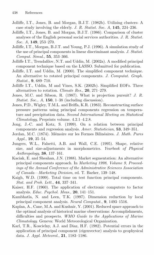
438 References
Jolliffe, I.T., Jones, B. and Morgan, B.J.T. (1982b). Utilising clusters: Acase study involving the elderly. J. R. Statist. Soc. A, 145, 224–236.
Jolliffe, I.T., Jones, B. and Morgan, B.J.T. (1986). Comparison of clusteranalyses of the English personal social services authorities. J. R. Statist.Soc. A, 149, 253–270.
Jolliffe, I.T., Morgan, B.J.T. and Young, P.J. (1996). A simulation study ofthe use of principal components in linear discriminant analysis. J. Statist.Comput. Simul., 55, 353–366.
Jolliffe I.T., Trendafilov, N.T. and Uddin, M. (2002a). A modified principalcomponent technique based on the LASSO. Submitted for publication.
Jolliffe, I.T. and Uddin, M. (2000). The simplified component technique.An alternative to rotated principal components. J. Computat. Graph.Statist., 9, 689–710.
Jolliffe I.T., Uddin, M and Vines, S.K. (2002b). Simplified EOFs. Threealternatives to rotation. Climate Res., 20, 271–279.
Jones, M.C. and Sibson, R. (1987). What is projection pursuit? J. R.Statist. Soc., A, 150, 1–38 (including discussion).
Jones, P.D., Wigley, T.M.L. and Briffa, K.R. (1983). Reconstructing surfacepressure patterns using principal components regression on tempera-ture and precipitation data. Second International Meeting on StatisticalClimatology, Preprints volume. 4.2.1–4.2.8.
Jong, J.-C. and Kotz, S. (1999). On a relation between principalcomponents and regression analysis. Amer. Statistician, 53, 349–351.
Jordan, M.C. (1874). Memoire sur les Formes Bilineaires. J. Math. PuresAppl., 19, 35–54.
Jungers, W.L., Falsetti, A.B. and Wall, C.E. (1995). Shape, relativesize, and size-adjustments in morphometrics. Yearbook of PhysicalAnthropology, 38, 137–161.
Kaciak, E. and Sheahan, J.N. (1988). Market segmentation: An alternativeprincipal components approach. In Marketing 1998, Volume 9, Proceed-ings of the Annual Conference of the Administrative Sciences Associationof Canada—Marketing Division, ed. T. Barker, 139–148.
Kaigh, W.D. (1999). Total time on test function principal components.Stat. and Prob. Lett., 44, 337–341.
Kaiser, H.F. (1960). The application of electronic computers to factoranalysis. Educ. Psychol. Meas., 20, 141–151.
Kambhatla, N. and Leen, T.K. (1997). Dimension reduction by localprincipal component analysis. Neural Computat., 9, 1493–1516.
Kaplan, A., Cane, M.A. and Kushnir, Y. (2001). Reduced space approach tothe optimal analysis of historical marine observations: Accomplishments,difficulties and prospects. WMO Guide to the Applications of MarineClimatology. Geneva: World Meteorological Organization.
Karl, T.R., Koscielny, A.J. and Diaz, H.F. (1982). Potential errors in theapplication of principal component (eigenvector) analysis to geophysicaldata. J. Appl. Meteorol., 21, 1183–1186.
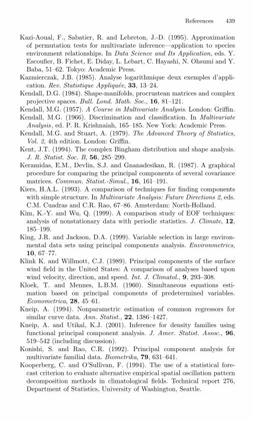
References 439
Kazi-Aoual, F., Sabatier, R. and Lebreton, J.-D. (1995). Approximationof permutation tests for multivariate inference—application to speciesenvironment relationships. In Data Science and Its Application, eds. Y.Escoufier, B. Fichet, E. Diday, L. Lebart, C. Hayashi, N. Ohsumi and Y.Baba, 51–62. Tokyo: Academic Press.
Kazmierczak, J.B. (1985). Analyse logarithmique deux exemples d’appli-cation. Rev. Statistique Appliquee, 33, 13–24.
Kendall, D.G. (1984). Shape-manifolds, procrustean matrices and complexprojective spaces. Bull. Lond. Math. Soc., 16, 81–121.
Kendall, M.G. (1957). A Course in Multivariate Analysis. London: Griffin.Kendall, M.G. (1966). Discrimination and classification. In Multivariate
Analysis, ed. P. R. Krishnaiah, 165–185. New York: Academic Press.Kendall, M.G. and Stuart, A. (1979). The Advanced Theory of Statistics,
Vol. 2, 4th edition. London: Griffin.Kent, J.T. (1994). The complex Bingham distribution and shape analysis.
J. R. Statist. Soc. B, 56, 285–299.Keramidas, E.M., Devlin, S.J. and Gnanadesikan, R. (1987). A graphical
procedure for comparing the principal components of several covariancematrices. Commun. Statist.-Simul., 16, 161–191.
Kiers, H.A.L. (1993). A comparison of techniques for finding componentswith simple structure. In Multivariate Analysis: Future Directions 2, eds.C.M. Cuadras and C.R. Rao, 67–86. Amsterdam: North-Holland.
Kim, K.-Y. and Wu, Q. (1999). A comparison study of EOF techniques:analysis of nonstationary data with periodic statistics. J. Climate, 12,185–199.
King, J.R. and Jackson, D.A. (1999). Variable selection in large environ-mental data sets using principal components analysis. Environmetrics,10, 67–77.
Klink K. and Willmott, C.J. (1989). Principal components of the surfacewind field in the United States: A comparison of analyses based uponwind velocity, direction, and speed. Int. J. Climatol., 9, 293–308.
Kloek, T. and Mennes, L.B.M. (1960). Simultaneous equations esti-mation based on principal components of predetermined variables.Econometrica, 28, 45–61.
Kneip, A. (1994). Nonparametric estimation of common regressors forsimilar curve data. Ann. Statist., 22, 1386–1427.
Kneip, A. and Utikal, K.J. (2001). Inference for density families usingfunctional principal component analysis. J. Amer. Statist. Assoc., 96,519–542 (including discussion).
Konishi, S. and Rao, C.R. (1992). Principal component analysis formultivariate familial data. Biometrika, 79, 631–641.
Kooperberg, C. and O’Sullivan, F. (1994). The use of a statistical fore-cast criterion to evaluate alternative empirical spatial oscillation patterndecomposition methods in climatological fields. Technical report 276,Department of Statistics, University of Washington, Seattle.

440 References
Kooperberg, C. and O’Sullivan, F. (1996). Predictive oscillation patterns:A synthesis of methods for spatial-temporal decomposition of randomfields. J. Amer. Statist. Assoc., 91, 1485–1496.
Korhonen, P.J. (1984). Subjective principal component analysis. Computat.Statist. Data Anal., 2, 243–255.
Korhonen, P. and Siljamaki, A. (1998). Ordinal principal component anal-ysis: Theory and an application. Computat. Statist. Data Anal., 26,411–424.
Korth, B. and Tucker, L.R. (1975). The distribution of chance congruencecoefficients from simulated data. Psychometrika, 40, 361–372.
Kramer, M.A. (1991). Nonlinear principal component analysis usingautoassociative neural networks. AIChE J., 37, 233–243.
Kroonenberg, P.M. (1983a). Three-Mode Principal Component Analysis.Leiden: DSWO Press.
Kroonenberg, P.M. (1983b). Annotated bibliography of three-mode factoranalysis. Brit. J. Math. Statist. Psychol., 36, 81–113.
Kroonenberg, P.M., Harch, B.D., Basford, K.E. and Cruickshank, A.(1997). Combined analysis of categorical and numerical descriptors ofAustralian groundnut accessions using nonlinear principal componentanalysis. J. Agri. Biol. Environ. Statist., 2, 294–312.
Kruskal, J.B. (1964a). Multidimensional scaling by optimizing goodness offit to a nonmetric hypothesis. Psychometrika, 29, 1–27.
Kruskal, J.B. (1964b). Nonmetric multidimensional scaling: A numericalmethod. Psychometrika, 29, 115–129.
Krzanowski, W.J. (1979a). Some exact percentage points of a statis-tic useful in analysis of variance and principal component analysis.Technometrics, 21, 261–263.
Krzanowski, W.J. (1979b). Between-groups comparison of principal com-ponents. J. Amer. Statist. Assoc., 74, 703–707 (correction 76, 1022).
Krzanowski, W.J. (1982). Between-group comparison of principal compo-nents—some sampling results. J. Statist. Computat. Simul., 15, 141–154.
Krzanowski, W.J. (1983). Cross-validatory choice in principal componentanalysis: Some sampling results. J. Statist. Computat. Simul., 18, 299–314.
Krzanowski, W.J. (1984a). Principal component analysis in the presence ofgroup structure. Appl. Statist., 33, 164–168.
Krzanowski, W.J. (1984b). Sensitivity of principal components. J. R.Statist. Soc. B, 46, 558–563.
Krzanowski, W.J. (1987a). Cross-validation in principal component analy-sis. Biometrics, 43, 575–584.
Krzanowski, W.J. (1987b). Selection of variables to preserve multivariatedata structure, using principal components. Appl. Statist., 36, 22–33.
Krzanowski, W.J. (1990). Between-group analysis with heterogeneous co-variance matrices: The common principal component model. J. Classific.,7, 81–98.

References 441
Krzanowski, W.J. (2000). Principles of Multivariate Analysis: A User’sPerspective, 2nd edition. Oxford: Oxford University Press.
Krzanowski, W.J., Jonathan, P., McCarthy, W.V. and Thomas, M.R.(1995). Discriminant analysis with singular covariance matrices: Methodsand applications to spectroscopic data. Appl. Statist., 44, 101–115.
Krzanowski, W.J. and Kline, P. (1995). Cross-validation for choosing thenumber of important components in principal component analysis. Mult.Behav. Res., 30, 149–166.
Krzanowski, W.J. and Marriott, F.H.C. (1994). Multivariate Analysis, Part1. Distributions, Ordination and Inference. London: Arnold.
Kshirsagar, A.M., Kocherlakota, S. and Kocherlakota, K. (1990). Clas-sification procedures using principal component analysis and stepwisediscriminant function. Commun. Statist.—Theor. Meth., 19, 92–109.
Kuhfeld, W.F. (1990). Comment on Dawkins (1989). Amer. Statistician,44, 58–59.
Kung, E.C. and Sharif, T.A. (1980). Multi-regression forecasting of theIndian summer monsoon with antecedent patterns of the large-scale cir-culation. WMO Symposium on Probabilistic and Statistical Methods inWeather Forecasting, 295–302.
Lafosse, R. and Hanafi, M. (1997). Concordance d’un tableau aveck tableaux: Definition de k + 1 uples synthetiques. Rev. StatistiqueAppliquee, 45, 111-136.
Lane, S., Martin, E.B., Kooijmans, R. and Morris, A.J. (2001). Performancemonitoring of a multi-product semi-batch process. J. Proc. Cont., 11,1–11.
Lang, P.M., Brenchley, J.M., Nieves, R.G. and Halivas, J.H. (1998). Cyclicsubspace regression. J. Mult. Anal., 65, 58–70.
Lanterman, A.D. (2000). Bayesian inference of thermodynamic state incor-porating Schwarz-Rissanen complexity for infrared target recognition.Optical Engng., 39, 1282–1292.
Lauter, J. (1996). Exact t and F tests for analyzing studies with multipleendpoints. Biometrics, 52, 964–970.
Lawley, D.N. (1963). On testing a set of correlation coefficients for equality.Ann. Math. Statist., 34, 149–151.
Lawley, D.N. and Maxwell, A.E. (1971). Factor Analysis as a StatisticalMethod, 2nd edition. London: Butterworth.
Lawson, C.L. and Hanson, R.J. (1974). Solving Least Squares Problems.Englewood Cliffs, NJ: Prentice-Hall.
Leamer, E.E. and Chamberlain, G. (1976). A Bayesian interpretation ofpretesting. J. R. Statist. Soc. B, 38, 85–94.
Lebart, L., Morineau, A. and Fenelon, J.-P. (1982). Traitement des DonneesStatistique. Paris: Dunod.
Lee, T.-W. (1998). Independent Component Analysis. Theory and Applica-tions. Boston: Kluwer.
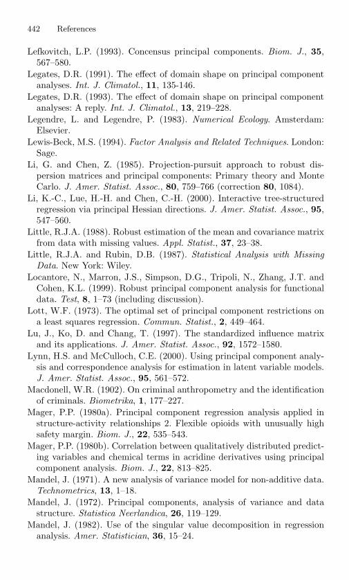
442 References
Lefkovitch, L.P. (1993). Concensus principal components. Biom. J., 35,567–580.
Legates, D.R. (1991). The effect of domain shape on principal componentanalyses. Int. J. Climatol., 11, 135-146.
Legates, D.R. (1993). The effect of domain shape on principal componentanalyses: A reply. Int. J. Climatol., 13, 219–228.
Legendre, L. and Legendre, P. (1983). Numerical Ecology. Amsterdam:Elsevier.
Lewis-Beck, M.S. (1994). Factor Analysis and Related Techniques. London:Sage.
Li, G. and Chen, Z. (1985). Projection-pursuit approach to robust dis-persion matrices and principal components: Primary theory and MonteCarlo. J. Amer. Statist. Assoc., 80, 759–766 (correction 80, 1084).
Li, K.-C., Lue, H.-H. and Chen, C.-H. (2000). Interactive tree-structuredregression via principal Hessian directions. J. Amer. Statist. Assoc., 95,547–560.
Little, R.J.A. (1988). Robust estimation of the mean and covariance matrixfrom data with missing values. Appl. Statist., 37, 23–38.
Little, R.J.A. and Rubin, D.B. (1987). Statistical Analysis with MissingData. New York: Wiley.
Locantore, N., Marron, J.S., Simpson, D.G., Tripoli, N., Zhang, J.T. andCohen, K.L. (1999). Robust principal component analysis for functionaldata. Test, 8, 1–73 (including discussion).
Lott, W.F. (1973). The optimal set of principal component restrictions ona least squares regression. Commun. Statist., 2, 449–464.
Lu, J., Ko, D. and Chang, T. (1997). The standardized influence matrixand its applications. J. Amer. Statist. Assoc., 92, 1572–1580.
Lynn, H.S. and McCulloch, C.E. (2000). Using principal component analy-sis and correspondence analysis for estimation in latent variable models.J. Amer. Statist. Assoc., 95, 561–572.
Macdonell, W.R. (1902). On criminal anthropometry and the identificationof criminals. Biometrika, 1, 177–227.
Mager, P.P. (1980a). Principal component regression analysis applied instructure-activity relationships 2. Flexible opioids with unusually highsafety margin. Biom. J., 22, 535–543.
Mager, P.P. (1980b). Correlation between qualitatively distributed predict-ing variables and chemical terms in acridine derivatives using principalcomponent analysis. Biom. J., 22, 813–825.
Mandel, J. (1971). A new analysis of variance model for non-additive data.Technometrics, 13, 1–18.
Mandel, J. (1972). Principal components, analysis of variance and datastructure. Statistica Neerlandica, 26, 119–129.
Mandel, J. (1982). Use of the singular value decomposition in regressionanalysis. Amer. Statistician, 36, 15–24.
References 443
Mann, M.E. and Park, J. (1999). Oscillatory spatiotemporal signal detec-tion in climate studies: A multi-taper spectral domain approach. Adv.Geophys., 41, 1–131.
Mansfield, E.R., Webster, J.T. and Gunst, R.F. (1977). An analytic variableselection technique for principal component regression. Appl. Statist., 26,34–40.
Mardia, K.V., Coombes, A., Kirkbride, J., Linney, A. and Bowie, J.L.(1996). On statistical problems with face identification from photographs.J. Appl. Statist., 23, 655–675.
Mardia, K.V., Kent, J.T. and Bibby, J.M. (1979). Multivariate Analysis.London: Academic Press.
Maronna, R.A. (1976). Robust M-estimators of multivariate location andscatter. Ann. Statist., 4, 51–67.
Maronna, R.A. and Yohai, V.J. (1998). Robust estimation of multivariatelocation and scatter. In Encyclopedia of Statistical Sciences, Update 2,eds. S. Kotz, C.B. Read and D.L. Banks, 589–596. New York: Wiley.
Marquardt, D.W. (1970). Generalized inverses, ridge regression, biasedlinear estimation, and nonlinear estimation. Technometrics, 12, 591–612.
Martens, H. and Naes, T. (1989). Multivariate Calibration. New York:Wiley.
Martin, E.B. and Morris, A.J. (1996). Non-parametric confidence boundsfor process performance monitoring charts. J. Proc. Cont., 6, 349–358.
Martin, E.B., Morris, A.J. and Kiparissides, C. (1999). Manufacturing per-formance enhancement through multivariate statistical process control.Ann. Rev. Cont., 23, 35-44.
Martin, J.-F. (1988). On probability coding. In Component and Correspon-dence Analysis. Dimension Reduction by Functional Approximation, eds.J.L.A. van Rijckevorsel and J. de Leeuw, 103–114. Chichester: Wiley.
Marx, B.D. and Smith, E.P. (1990). Principal component estimation forgeneralized linear regression. Biometrika, 77, 23–31.
Maryon, R.H. (1979). Eigenanalysis of the Northern Hemispherical 15-daymean surface pressure field and its application to long-range fore-casting. Met O 13 Branch Memorandum No. 82 (unpublished). UKMeteorological Office, Bracknell.
Mason, R.L. and Gunst, R.F. (1985). Selecting principal components inregression. Stat. Prob. Lett., 3, 299–301.
Massy, W.F. (1965). Principal components regression in exploratorystatistical research. J. Amer. Statist. Assoc., 60, 234–256.
Matthews, J.N.S. (1984). Robust methods in the assessment of multivariatenormality. Appl. Statist., 33, 272–277.
Maurin, M. (1987). A propos des changements de metriques en ACP. FifthInternational Symposium: Data Analysis and Informatics, Posters, 15–18.
Maxwell, A.E. (1977). Multivariate Analysis in Behavioural Research.London: Chapman and Hall.

444 References
McCabe, G.P. (1982). Principal variables. Technical Report No. 82–3,Department of Statistics, Purdue University.
McCabe, G.P. (1984). Principal variables. Technometrics, 26, 137–144.McCabe, G.P. (1986). Prediction of principal components by variable sub-
sets. Unpublished Technical Report, 86-19, Department of Statistics,Purdue University.
McGinnis, D.L. (2000). Synoptic controls on upper Colorado River Basinsnowfall. Int. J. Climatol., 20, 131–149.
McLachlan, G.J. (1992). Discriminant Analysis and Statistical PatternRecognition. New York: Wiley.
McLachlan, G.J. and Bashford, K.E. (1988) Mixture Models. Inference andApplications to Clustering. New York: Marcel Dekker.
McReynolds, W.O. (1970). Characterization of some liquid phases. J.Chromatogr. Sci., 8, 685–691.
Mehrotra, D.V. (1995). Robust elementwise estimation of a dispersionmatrix. Biometrics, 51, 1344–1351.
Meredith, W. and Millsap, R.E. (1985). On component analysis. Psychome-trika, 50, 495–507.
Mertens, B.J.A. (1998). Exact principal component influence measures ap-plied to the analysis of spectroscopic data on rice. Appl. Statist., 47,527–542.
Mertens, B., Fearn, T. and Thompson, M. (1995). The efficient cross-validation of principal components applied to principal componentregression. Statist. Comput., 5, 227–235.
Mertens, B., Thompson, M. and Fearn, T. (1994). Principal componentoutlier detection and SIMCA: A synthesis. Analyst, 119, 2777–2784.
Mestas-Nunez, A.M. (2000). Orthogonality properties of rotated empiricalmodes. Int. J. Climatol., 20, 1509–1516.
Meulman, J. (1986). A Distance Approach to Nonlinear MultivariateAnalysis. Leiden: DSWO Press.
Michailidis, G. and de Leeuw, J. (1998). The Gifi system of descriptivemultivariate analysis. Statist. Sci., 13, 307–336.
Milan, L. and Whittaker, J. (1995). Application of the parametric bootstrapto models that incorporate a singular value decomposition. Appl. Statist.,44, 31–49.
Miller, A.J. (1984). Selection of subsets of regression variables (withdiscussion). J. R. Statist. Soc. A, 147, 389–425.
Miller, A.J. (1990). Subset Selection in Regression. London: Chapman andHall.
Milliken, G.A. and Johnson, D.E. (1989). Analysis of Messy Data Vol. 2:Nonreplicated Experiments. New York: Van Nostrand-Reinhold.
Monahan, A.H. (2001). Nonlinear principal component analysis: TropicalIndo-Pacific sea surface temperature and sea level pressure. J. Climate,14, 219–233.

References 445
Monahan, A.H., Tangang, F.T. and Hsieh, W.W. (1999). A potential prob-lem with extended EOF analysis of standing wave fields. Atmos.–Ocean,37, 241–254.
Mori, Y., Iizuka, M., Tarumi, T. and Tanaka, Y. (1999). Variable selectionin “principal component analysis based on a subset of variables”. Bul-letin of the International Statistical Institute 52nd Session ContributedPapers, Tome LVIII, Book 2, 333–334.
Mori, Y., Iizuka, M., Tarumi, T. and Tanaka, Y. (2000). Study of variableselection criteria in data analysis. Proc. 10th Japan and Korea JointConference of Statistics, 547–554.
Mori, Y., Tanaka, Y. and Tarumi, T. (1998). Principal component analysisbased on a subset of variables for qualitative data. In Data Science,Classification, and Related Methods, eds. C. Hayashi, N. Ohsumi, K.Yajima, Y. Tanaka, H.H. Bock and Y. Baba, 547–554. Tokyo: Springer-Verlag.
Morgan, B.J.T. (1981). Aspects of QSAR: 1. Unpublished report, CSIRODivision of Mathematics and Statistics, Melbourne.
Morrison, D.F. (1976). Multivariate Statistical Methods, 2nd edition. Tokyo:McGraw-Hill Kogakusha.
Moser, C.A. and Scott, W. (1961). British Towns. Edinburgh: Oliver andBoyd.
Mosteller, F. and Tukey, J.W. (1977). Data Analysis and Regression: ASecond Course in Statistics. Reading, MA: Addison-Wesley.
Mote, P.W., Clark, H.L., Dunkerton, T.J., Harwood, R.S., and Pumphrey,H.C. (2000). Intraseasonal variations of water vapor in the tropical uppertroposphere and tropopause region. J. Geophys. Res., 105, 17457–17470.
Muller, K.E. (1981). Relationships between redundancy analysis, canonicalcorrelation and multivariate regression. Psychometrika, 46, 139–142.
Muller, K.E. (1982). Understanding canonical correlation through the gen-eral linear model and principal components. Amer. Statistician, 36,342–354.
Naes, T. (1985). Multivariate calibration when the error covariance matrixis structured. Technometrics, 27, 301–311.
Naes, T. and Helland, I.S. (1993). Relevant components in regression.Scand. J. Statist., 20, 239–250.
Naes, T., Irgens, C. and Martens, H. (1986). Comparison of linear statisticalmethods for calibration of NIR instruments. Appl. Statist., 35, 195–206.
Naes, T. and Isaksson, T. (1991). Splitting of calibration data by clusteranalysis. J. Chemometrics, 5, 49–65.
Naes, T. and Isaksson, T. (1992). Locally weighted regression in diffusenear-infrared transmittance spectroscopy. Appl. Spectroscopy, 46, 34–43.
Naga, R.A. and Antille, G. (1990). Stability of robust and non-robustprincipal components analysis. Computat. Statist. Data Anal., 10,169–174.

446 References
Naik, D.N. and Khattree, R. (1996). Revisiting Olympic track records:Some practical considerations in the principal component analysis. Amer.Statistician, 50, 140–144.
Nash, J.C. and Lefkovitch, L.P. (1976). Principal components and regres-sion by singular value decomposition on a small computer. Appl. Statist.,25, 210–216.
Nel, D.G. and Pienaar, I. (1998). The decomposition of the Behrens-Fisherstatistic in q-dimensional common principal common submodels. Ann.Inst. Stat. Math., 50, 241–252.
Nelder, J.A. (1985). An alternative interpretation of the singular-valuedecomposition in regression. Amer. Statistician, 39, 63–64.
Neuenschwander, B.E. and Flury, B.D. (2000). Common principal compo-nents for dependent random vectors. J. Mult. Anal., 75, 163–183.
Nomikos, P. and MacGregor, J.F. (1995). Multivariate SPC charts formonitoring batch processes. Technometrics, 37, 41–59.
North, G.R., Bell, T.L., Cahalan, R.F. and Moeng, F.J. (1982). Samplingerrors in the estimation of empirical orthogonal functions. Mon. WeatherRev., 110, 699–706.
North, G.R. and Wu, Q. (2001). Detecting climate signals using space-timeEOFs. J. Climate, 14, 1839–1863.
Obukhov, A.M. (1947). Statistically homogeneous fields on a sphere. Usp.Mat. Nauk., 2, 196–198.
Ocana, F.A., Aguilera, A.M. and Valderrama, M.J. (1999). Functionalprincipal components analysis by choice of norms. J. Mult. Anal., 71,262–276.
Ogasawara, H. (2000). Some relationships between factors and components.Psychometrika, 65, 167–185.
O’Hagan, A. (1984). Motivating principal components, and a strongeroptimality result. Statistician, 33, 313–315.
O’Hagan, A. (1994). Kendall’s Advanced Theory of Statistics. Volume 2BBayesian Inference. London: Arnold.
Okamoto, M. (1969). Optimality of principal components. In MultivariateAnalysis II , ed. P. R. Krishnaiah, 673–685. New York: Academic Press.
Oman, S.D. (1978). A Bayesian comparison of some estimators used inlinear regression with multicollinear data. Commun. Statist., A7, 517–534.
Oman, S.D. (1991). Random calibration with many measurements: Anapplication of Stein estimation. Technometrics, 33, 187–195.
Osmond, C. (1985). Biplot models applied to cancer mortality rates. Appl.Statist., 34, 63–70.
Ottestad, P. (1975). Component analysis: An alternative system. Int. Stat.Rev., 43, 83–107.
Overland, J.E. and Preisendorfer, R.W. (1982). A significance test for prin-cipal components applied to a cyclone climatology. Mon. Weather Rev.,110, 1–4.

References 447
Pack, P., Jolliffe, I.T. and Morgan, B.J.T. (1988). Influential observations inprincipal component analysis: A case study. J. Appl. Statist., 15, 39–52.
Pearce, S.C. and Holland, D.A. (1960). Some applications of multivariatemethods in botany. Appl. Statist., 9, 1–7.
Pearson, K. (1901). On lines and planes of closest fit to systems of pointsin space. Phil. Mag. (6), 2, 559–572.
Pena, D. and Box, G.E.P. (1987). Identifying a simplifying structure intime series. J. Amer. Statist. Assoc., 82, 836–843.
Pena, D. and Yohai, V. (1999). A fast procedure for outlier diagnostics inlarge regression problems. J. Amer. Statist. Assoc., 94, 434–445.
Penny, K.I. and Jolliffe, I.T (2001). A comparison of multivariate outlierdetection methods for clinical laboratory safety data. Statistician, 50,295-308.
Pla, L. (1991). Determining stratum boundaries with multivariate realdata. Biometrics, 47, 1409–1422.
Plaut, G. and Vautard, R. (1994). Spells of low-frequency oscillations andweather regimes in the Northern Hemisphere. J. Atmos. Sci., 51, 210–236.
Preisendorfer, R.W. (1981). Principal component analysis and applica-tions. Unpublished lecture notes.Amer. Met. Soc. Workshop on PrincipalComponent Analysis, Monterey.
Preisendorfer, R.W. and Mobley, C.D. (1982). Data intercomparisontheory, I-V. NOAA Tech. Memoranda ERL PMEL Nos. 38–42.
Preisendorfer, R.W. and Mobley, C.D. (1988). Principal ComponentAnalysis in Meteorology and Oceanography. Amsterdam: Elsevier.
Press, S.J. (1972). Applied Multivariate Analysis. New York: Holt, Rinehartand Winston.
Press, W.H., Teukolsky, S.A., Vetterling, W.T. and Flannery, B.P. (1992)Numerical Recipes in C, 2nd edition. Cambridge: Cambridge UniversityPress.
Priestley, M.B., Subba Rao, T. and Tong, H. (1974). Applications ofprincipal component analysis and factor analysis in the identifica-tion of multivariable systems. IEEE Trans. Autom. Cont., AC-19,730–734.
Qian, G., Gabor, G. and Gupta, R.P. (1994). Principal components selec-tion by the criterion of the minimum mean difference of complexity. J.Multiv. Anal., 49, 55–75.
Radhakrishnan, R. and Kshirsagar, A.M. (1981). Influence functions forcertain parameters in multivariate analysis. Commun. Statist., A10,515–529.
Ramsay, J.O. (1996). Principal differential analysis: Data reduction bydifferential operators. J. R. Statist. Soc. B, 58, 495–508.
Ramsay, J.O. (2000). Functional components of variation in handwriting.J. Amer. Statist. Assoc., 95, 9–15.
448 References
Ramsay, J.O. and Abrahamowicz, M. (1989). Binomial regression withmonotone splines: A psychometric application. J. Amer. Statist. Assoc.,84, 906–915.
Ramsay, J.O. and Silverman, B.W. (1997). Functional Data Analyis. NewYork: Springer.
Ramsier, S.W. (1991). A graphical method for detection of influential ob-servations in principal component analysis. In Proc. Section on StatisticalGraphics, Joint Statistical Meetings, American Statistical Association.
Ranatunga, C. (1989). Methods of Removing ‘Size’ from a Data Set.Unpublished M.Sc. dissertation. University of Kent at Canterbury.
Rao, C.R. (1955). Estimation and tests of significance in factor analysis.Psychometrika, 20, 93–111.
Rao, C.R. (1958). Some statistical methods for comparison of growthcurves. Biometrics, 14, 1–17.
Rao, C.R. (1964). The use and interpretation of principal componentanalysis in applied research. Sankhya A, 26, 329–358.
Rao, C.R. (1973). Linear Statistical Inference and Its Applications, 2ndedition. New York: Wiley.
Rao, C.R. (1987). Prediction of future observations in growth curve models.Statist. Sci., 2, 434–471 (including discussion).
Rasmusson, E.M., Arkin, P.A., Chen, W.Y. and Jalickee, J.B. (1981). Bien-nial variations in surface temperature over the United States as revealedby singular decomposition. Mon. Weather Rev., 109, 587–598.
Ratcliffe, S.J. and Solo, V. (1998). Some issues in functional principal com-ponent analysis. In Section on Statistical Computing, Joint StatisticalMeetings, American Statistical Association, 206–209.
Raveh, A. (1985). On the use of the inverse of the correlation matrix inmultivariate data analysis. Amer. Statistician, 39, 39–42.
Reddon, J.R. (1984). The Number of Principal Components Problem: AMonte Carlo Study. Unpublished Ph.D. thesis. University of WesternOntario.
Rencher, A.C. (1995). Methods of Multivariate Analysis. New York: Wiley.Rencher, A.C. (1998). Multivariate Statistical Inference and Applications.
New York: Wiley.Reyment, R.A. and Joreskog, K.G. (1993). Applied Factor Analysis in the
Natural Sciences. Cambridge: Cambridge University Press.Richman, M.B. (1983). Specification of complex modes of circulation with
T -mode factor analysis. Second International Meeting on StatisticalClimatology, Preprints volume, 5.1.1–5.1.8.
Richman, M.B. (1986). Rotation of principal components. J. Climatol., 6,293–335.
Richman, M.B. (1987). Rotation of principal components: A reply. J.Climatol., 7, 511–520.
Richman, M.B. (1988). A cautionary note concerning a commonly appliedeigenanalysis procedure. Tellus, 40B, 50–58.
References 449
Richman M.B. (1993). Comments on ‘The effect of domain shape onprincipal component analyses.’ Int. J. Climatol., 13, 203–218.
Richman, M.B. and Gong, X. (1999). Relationships between the definitionof the hyperplane width to the fidelity of principal component loadingpatterns. J. Climate, 12, 1557–1576.
Richman, M.B. and Lamb, P.J. (1987). Pattern analysis of growing seasonprecipitation in Southern Canada. Atmos.—Ocean, 25, 137–158.
Rissanen, J. and Yu, B. (2000). Coding and compression: A happy unionof theory and practice. J. Amer. Statist. Assoc., 95, 986–989.
Robert, P. and Escoufier, Y. (1976). A unifying tool for linear multivariatestatistical methods: The RV coefficient. Appl. Statist., 25, 257–265.
Roes, K.C.B. and Does, R.J.M.M. (1995). Shewhart-type charts innonstandard situations. Technometrics, 37, 15–24.
Romanazzi, M. (1993). Jackknife estimation of the eigenvalues of thecovariance matrix. Comput. Statist. Data Anal., 15, 179–198.
Romero, R., Ramis, C., Guijarro, J.A. and Sumner, G. (1999). Daily rainfallaffinity areas in Mediterranean Spain. Int. J. Climatol., 19, 557–578.
Rousseeuw, P.J. and Leroy, A.M. Robust Regression and Outlier Detection.New York: Wiley.
Roweis, S. (1997). EM algorithms for PCA and SPCA. Neural Inf. Proc.Syst., 10, 626–632.
Roweis, S.T. and Saul, L.K. (2000). Nonlinear dimensionality reduction bylocally linear embedding. Science, 290, 2323–2326.
Rummel, R.J. (1970). Applied Factor Analysis. Evanston: NorthwesternUniversity Press.
Ruymgaart, F.H. (1981). A robust principal component analysis. J. Multiv.Anal., 11, 485–497.
Sabatier, R., Lebreton, J.-D. and Chessel, D. (1989). Principal componentanalysis with instrumental variables as a tool for modelling compositiondata. In Multiway Data Analysis, eds R. Coppi and S. Bolasco, 341–352.Amsterdam: North-Holland.
Salles, M.A., Canziani, P.O. and Compagnucci, R.H. (2001). The spatialand temporal behaviour of the lower stratospheric temperature over theSouthern Hemisphere: The MSU view. Part II: Spatial behaviour. Int. J.Climatol., 21, 439–454.
Sato, M. (1990). Some remarks on principal component analysis as a sub-stitute for factor analysis in monofactor cases. J. Jap. Statist. Soc., 20,23–31.
Schafer, J.L. (1997). Analysis of Incomplete Multivariate Data. London:Chapman and Hall.
Schneeweiss, H. (1997). Factors and principal components in the nearspherical case. Mult. Behav. Res., 32, 375–401.
Schneeweiss, H. and Mathes, H. (1995). Factor analysis and principalcomponents. J. Mult. Anal., 55, 105–124.
450 References
Schneider, T. (2001). Analysis of incomplete climate data: Estimation ofmean values and covariance matrices and imputation of missing values.J. Climate, 14, 853–871.
Schott, J.R. (1987). An improved chi-squared test for a principal compo-nent. Stat. Prob. Lett., 5, 361–365.
Schott, J.R. (1988). Common principal component subspaces in two groups.Biometrika, 75, 229–236.
Schott, J.R. (1991). Some tests for common principal component subspacesin several groups. Biometrika, 78, 771–777.
Schreer, J.F., O’Hara Hines, R.J. and Kovacs, K.M. (1998). Classificationof dive profiles: A comparison of statistical clustering techniques andunsupervised artificial neural networks. J. Agri. Biol. Environ. Statist.,3, 383–404.
Sclove, S.L. (1968). Improved estimators for coefficients in linear regression.J. Amer. Statist. Assoc., 63, 596–606.
Sengupta, S. and Boyle, J.S. (1998). Using common principal componentsfor comparing GCM simulations. J. Climate, 11, 816–830.
Shafii, B. and Price, W.J. (1998). Analysis of genotype-by-environmentinteraction using the additive main effects and multiplicative interactionmodel and stability estimates. J. Agri. Biol. Environ. Statist., 3, 335–345.
Shi, L. (1997). Local influence in principal components analysis. Biome-trika, 84, 175–186.
Shibayama, T. (1990). A linear composite method for test scores withmissing values. Unpublished technical report. Department of Psychology,McGill University.
Sibson, R. (1984). Multivariate analysis. Present position and potentialdevelopments: Some personal views. J. R. Statist. Soc. A, 147, 198–207.
Skinner, C.J., Holmes, D.J. and Smith, T.M.F. (1986). The effect of sampledesign on principal component analysis. J. Amer. Statist. Assoc., 81,789–798.
Smith, B.T., Boyle, J.M., Dongarra, J.J., Garbow, B.S., Ikebe, Y., Klema,V.C., and Moler, C.B. (1976). Matrix Eigensystem Routines—EISPACKguide, 2nd edition. Berlin: Springer-Verlag.
Smyth, G.K. (2000). Employing symmetry constraints for improvedfrequency estimation by eigenanalysis methods. Technometrics, 42,277–289.
Snook, S.C. and Gorsuch, R.L. (1989). Component analysis versus commonfactor analysis: A Monte Carlo study. Psychol. Bull., 106, 148–154.
Solow, A.R. (1994). Detecting change in the composition of a multispeciescommunity. Biometrics, 50, 556–565.
Somers, K.M. (1986). Multivariate allometry and removal of size withprincipal components analysis. Syst. Zool., 35, 359–368.
Somers, K.M. (1989). Allometry, isometry and shape in principal compo-nent analysis. Syst. Zool., 38, 169–173.

References 451
Soofi, E.S. (1988). Principal component regression under exchangeability.Commun. Statist.—Theor. Meth., 17, 1717–1733.
Sprent, P. (1972). The mathematics of size and shape. Biometrics, 28,23–37.
Spurrell, D.J. (1963). Some metallurgical applications of principal compo-nents. Appl. Statist., 12, 180–188.
Srivastava, M.S. and Khatri, C.G. (1979). An Introduction to MultivariateStatistics. New York: North-Holland.
Stauffer, D.F., Garton, E.O. and Steinhorst, R.K. (1985). A comparisonof principal components from real and random data. Ecology, 66, 1693–1698.
Stein, C.M. (1960). Multiple regression. In Contributions to Probability andStatistics. Essays in Honour of Harold Hotelling, ed. I. Olkin, 424–443.Stanford: Stanford University Press.
Stewart, D. and Love, W. (1968). A general canonical correlation index.Psychol. Bull., 70, 160–163.
Stoffer, D.S. (1999). Detecting common signals in multiple time series usingthe spectral envelope. J. Amer. Statist. Assoc., 94, 1341–1356.
Stone, E.A. (1984). Cluster Analysis of English Counties Accordingto Socio-economic Factors. Unpublished undergraduate dissertation.University of Kent at Canterbury.
Stone, J.V. and Porrill, J. (2001). Independent component analysis andprojection pursuit: A tutorial introduction. Unpublished technical report.Psychology Department, University of Sheffield.
Stone, M. and Brooks, R.J. (1990). Continuum regression: Cross-validatedsequentially constructed prediction embracing ordinary least squares,partial least squares and principal components regression (with discus-sion). J. R. Statist. Soc. B, 52, 237–269.
Stone, R. (1947). On the interdependence of blocks of transactions (withdiscussion). J. R. Statist. Soc. B, 9, 1–45.
Storvik, G. (1993). Data reduction by separation of signal and noisecomponents for multivariate spatial images. J. Appl. Statist., 20,127–136.
Stuart, M. (1982). A geometric approach to principal components analysis.Amer. Statistician, 36, 365–367.
Sugiyama, T. and Tong, H. (1976). On a statistic useful in dimensionalityreduction in multivariable linear stochastic system. Commun. Statist.,A5, 711–721.
Sullivan, J.H., Woodall, W.H. and Gardner, M.M. (1995) Discussion of‘Shewhart-type charts in nonstandard situations,’ by K.C.B. Roes andR.J.M.M. Does. Technometrics, 37, 31–35.
Sundberg, P. (1989). Shape and size-constrained principal componentsanalysis. Syst. Zool., 38, 166–168.
Sylvestre, E.A., Lawton, W.H. and Maggio, M.S. (1974). Curve resolutionusing a postulated chemical reaction. Technometrics, 16, 353–368.

452 References
Takane, Y., Kiers, H.A.L. and de Leeuw, J. (1995). Component analysiswith different sets of constraints on different dimensions. Psychometrika,60, 259–280.
Takane, Y. and Shibayama, T. (1991). Principal component analysis withexternal information on both subjects and variables. Psychometrika, 56,97–120.
Takemura, A. (1985). A principal decomposition of Hotelling’s T 2 statistic.In Multivariate Analysis VI, ed. P.R. Krishnaiah, 583–597. Amsterdam:Elsevier.
Tan, S. and Mavrovouniotis, M.L. (1995). Reducing data dimensionalitythrough optimizing neural network inputs. AIChE J., 41, 1471–1480.
Tanaka, Y. (1983). Some criteria for variable selection in factor analysis.Behaviormetrika, 13, 31–45.
Tanaka, Y. (1988). Sensitivity analysis in principal component analysis:Influence on the subspace spanned by principal components. Commun.Statist.—Theor. Meth., 17, 3157–3175.
Tanaka, Y. (1995). A general strategy of sensitivity analysis in multivari-ate methods. In Data Science and Its Application, eds. Y. Escoufier,B. Fichet, E. Diday, L. Lebart, C. Hayashi, N. Ohsumi and Y. Baba,117–131. Tokyo: Academic Press.
Tanaka, Y. and Mori, Y. (1997). Principal component analysis based on asubset of variables: Variable selection and sensitivity analysis. Amer. J.Math. Manag. Sci., 17, 61–89.
Tanaka, Y. and Tarumi, T. (1985). Computational aspect of sensitivityanalysis in multivariate methods. Technical report No. 12. OkayamaStatisticians Group. Okayama, Japan.
Tanaka, Y. and Tarumi, T. (1986). Sensitivity analysis in multivariatemethods and its application. Proc. Second Catalan Int. Symposium onStatistics, 335–338.
Tanaka, Y. and Tarumi, T. (1987). A numerical investigation of sensitivityanalysis in multivariate methods. Fifth International Symposium: DataAnalysis and Informatics, Tome 1, 237–247.
Tarpey, T. (1999). Self-consistency and principal component analysis. J.Amer. Statist. Assoc., 94, 456–467.
Tarpey, T. (2000). Parallel principal axes. J. Mult. Anal., 75, 295–313.ten Berge, J.M.F. and Kiers, H.A.L. (1996). Optimality criteria for prin-
cipal component analysis and generalizations. Brit. J. Math. Statist.Psychol., 49, 335–345.
ten Berge, J.M.F. and Kiers, H.A.L. (1997). Are all varieties of PCA thesame? A reply to Cadima and Jolliffe. Brit. J. Math. Statist. Psychol.,50, 367–368.
ten Berge, J.M.F. and Kiers, H.A.L. (1999). Retrieving the correlation ma-trix from a truncated PCA solution: The inverse principal componentproblem. Psychometrika, 64, 317–324.

References 453
Tenenbaum, J.B., de Silva, V. and Langford, J.C. (2000). A global geo-metric framework for nonlinear dimensionality reduction. Science, 290,2319–2323.
ter Braak, C.J.F. (1983). Principal components biplots and alpha and betadiversity. Ecology, 64, 454–462.
ter Braak, C.J.F. and Looman, C.W.N. (1994). Biplots in reduced rankregression. Biom. J., 36, 983–1003.
Timmerman, M.E. and Kiers, H.A.L. (2000). Three-mode principal com-ponents analysis: Choosing the numbers of components and sensitivityto local optima. Brit. J. Math. Stat. Psychol., 53, 1–16.
Thacker, W.C. (1996). Metric-based principal components: Data uncertain-ties. Tellus, 48A, 584–592.
Thacker, W.C. (1999). Principal predictors. Int. J. Climatol., 19, 821–834.Thurstone, L.L. (1931). Multiple factor analysis. Psychol. Rev., 38, 406–
427.Tibshirani, R. (1996). Regression shrinkage and selection via the lasso. J.
R. Statist. Soc. B, 58, 267–288.Tipping, M.E. and Bishop, C.M. (1999a). Probabilistic principal compo-
nent analysis. J. R. Statist. Soc. B, 61, 611–622.Tipping, M.E. and Bishop, C.M. (1999b). Mixtures of probabilistic
principal component analyzers. Neural Computat., 11, 443–482.Titterington, D.M., Smith, A.F.M. and Makov, U.E. (1985). Statistical
Analysis of Finite Mixture Distributions. New York: Wiley.Townshend, J.R.G. (1984). Agricultural land-cover discrimination using
thematic mapper spectral bands. Int. J. Remote Sensing, 5, 681–698.Torgerson, W.S. (1958). Theory and Methods of Scaling. New York: Wiley.Tortora, R.D. (1980). The effect of a disproportionate stratified design on
principal component analysis used for variable elimination. Proceedingsof the Amer. Statist. Assoc. Section on Survey Research Methods, 746–750.
Treasure, F.P. (1986). The geometry of principal components. Unpublishedessay. University of Cambridge.
Trenkler, D. and Trenkler, G. (1984). On the Euclidean distance betweenbiased estimators. Commun. Statist.—Theor. Meth., 13, 273–284.
Trenkler, G. (1980). Generalized mean squared error comparisons of biasedregression estimators. Commun. Statist., A9, 1247–1259.
Tryon, R.C. (1939). Cluster Analysis. Ann Arbor: Edwards Brothers.Tucker, L.R. (1958). An inter-battery method of factor analysis. Psychome-
trika, 23, 111–136.Tucker, L.R. (1966). Some mathematical notes on three-mode factor
analysis. Psychometrika, 31, 279–311.Tukey, P.A. and Tukey, J.W. (1981). Graphical display of data sets in three
or more dimensions. Three papers in Interpreting Multivariate Data (ed.V. Barnett), 189–275. Chichester: Wiley.

454 References
Turner, N.E. (1998). The effect of common variance and structure patternon random data eigenvalues: implications for the accuracy of parallelanalysis. Educ. Psychol. Meas., 58, 541–568.
Uddin, M. (1999). Interpretation of Results from Simplified PrincipalComponents. Unpublished Ph.D. thesis. University of Aberdeen.
Underhill, L.G. (1990). The coefficient of variation biplot. J. Classific., 7,241–256.
van de Geer, J.P. (1984). Linear relations among k sets of variables.Psychometrika, 49, 79–94.
van de Geer, J.P. (1986). Introduction to Linear Multivariate DataAnalysis—Volume 2. Leiden: DSWO Press.
van den Brink, P.J. and ter Braak, C.J.F. (1999). Principal responsecurves: Analysis of time-dependent multivariate responses of biologicalcommunity to stress. Environ. Toxicol. Chem., 18, 138–148.
van den Dool, H.M., Saha, S. and Johansson, A. (2000) Empiricalorthogonal teleconnections. J. Climate 13, 1421-1435.
van den Wollenberg, A.L. (1977). Redundancy analysis. An alternative forcanonical correlation analysis. Psychometrika, 42, 207–219.
van Rijckevorsel, J.L.A. (1988). Fuzzy coding and B-splines. In Compo-nent and Correspondence Analysis. Dimension Reduction by FunctionalApproximation, eds. J.L.A. van Rijckevorsel and J. de Leeuw, 33–54.Chichester: Wiley.
Vargas-Guzman, J.A., Warrick, A.W. and Myers, D.E. (1999). Scale ef-fect on principal component analysis for vector random functions. Math.Geol., 31, 701–722.
Vautard, R. (1995). Patterns in time: SSA and MSSA. In Analysis ofClimate Variability: Applications of Statistical Techniques, eds. H. vonStorch and A. Navarra, 259–279. Berlin: Springer.
Velicer, W.F. (1976). Determining the number of components from thematrix of partial correlations. Psychometrika, 41, 321–327.
Velicer, W.F. and Jackson, D.N. (1990). Component analysis versus com-mon factor analysis—some issues in selecting an appropriate procedure.Mult. Behav. Res., 25, 1–28.
Verboon, P. (1993). Stability of resistant principal component analysis forqualitative data. In New Directions in Statistical Data Analysis and Ro-bustness, eds. S. Morgenthaler, E. Ronchetti and W. A. Stahel, 265–273.Basel: Birkhauser.
Vermeiren, D., Tavella, D. and Horovitz, A. (2001). Extending principalcomponent analysis to identify portfolio risk contributors. Submitted forpublication.
Vigneau, E. and Qannari, E.M. (2001). Clustering of variables aroundlatent components. Submitted for publication.
Vines, S.K. (2000). Simple principal components. Appl. Statist., 49, 441–451.
References 455
Vong, R., Geladi, P., Wold, S. and Esbensen, K. (1988). Some contributionsto ambient aerosol calculated by discriminant partial least squares (PLS).J. Chemometrics, 2, 281–296.
von Storch, H., Bruns, T., Fischer-Bruns, I. and Hasselmann, K. (1988).Principal oscillation pattern analysis of the 30- to 60-day oscillation ingeneral circulation model equatorial troposphere. J. Geophys. Res., 93,11,022–11,036.
von Storch, H. and Zweirs, F.W. (1999). Statistical Analysis in ClimateResearch. Cambridge: Cambridge University Press.
Wackernagel, H. (1995). Multivariate Geostatistics. An Introduction withApplications. Berlin: Springer.
Walker, M.A, (1967). Some critical comments on ‘An analysis of crimes bythe method of principal components,’ by B. Ahamad. Appl. Statist., 16,36–38.
Wallace, J.M., Smith, C. and Bretherton, C.S. (1992). Singular value de-composition of wintertime sea surface temperature and 500-mb heightanomalies. J. Climate, 5, 561–576.
Wallace, T.D. (1972). Weaker criteria and tests for linear restrictions inregression. Econometrica, 40, 689–698.
Walton, J.J. and Hardy, D.M. (1978). Principal components analysis andits application to wind field pattern recognition. Lawrence LivermoreLaboratory Technical Report UCRL-52488.
Wang, P.C.C. (1978). Graphical Representation of Multivariate Data. NewYork: Academic Press.
Wang, S.-G. and Liski, E.P. (1993). Effects of observations on the eigen-system of a sample covariance structure. J. Stat. Plan. Inf., 36,215–226.
Wang, S.-G. and Nyquist, H. (1991). Effects on the eigenstructure of a datamatrix when deleting an observation. Computat. Statist. Data Anal., 11,179–188.
Wang, X.L. and Zwiers, F.W. (2001). Using redundancy analysis to im-prove dynamical seasonal mean 500 hPa geopotential forecasts. Int. J.Climatol., 21, 637–654.
Wang, Y.M. and Staib, L.H. (2000). Boundary finding with prior shapeand smoothness models. IEEE Trans. Patt. Recog. Machine Intell., 22,738–743.
Waternaux, C.M. (1984). Principal components in the nonnormal case: Thetest of equality of Q roots. J. Multiv. Anal., 14, 323–335.
Weare, B.C. (1990). Four-dimensional empirical orthogonal analysis ofclimate variables. Int. J. Climatol., 10, 313–319.
Weare, B.C. and Nasstrom, J.S. (1982). Examples of extended empiricalorthogonal function analyses. Mon. Weather Rev., 110, 481–485.
Webber, R. and Craig, J. (1978). Socio-economic classification of local au-thority areas. OPCS Studies on Medical and Population Subjects, No. 35.London: HMSO.
456 References
Webster, J.T., Gunst, R.F. and Mason, R.L. (1974). Latent root regressionanalysis. Technometrics, 16, 513–522.
White, D., Richman, M. and Yarnal, B. (1991). Climate regionalizationand rotation of principal components. Int. J. Climatol., 11, 1–25.
White, J.W. and Gunst, R.F. (1979). Latent root regression: Large sampleanalysis. Technometrics, 21, 481–488.
Whittaker, J. (1990). Graphical Models in Applied Multivariate Analysis.Chichester: Wiley.
Whittle, P. (1952). On principal components and least squares methods offactor analysis. Skand. Actuar., 35, 223–239.
Wiberg, T. (1976). Computation of principal components when data aremissing. In Compstat 1976 , eds. J. Gordesch and P. Naeve, 229–236.Wien: Physica-Verlag.
Widaman, K.F. (1993). Common factor analysis versus principal compo-nent analysis: Differential bias in representing model parameters. Mult.Behav. Res., 28, 263–311.
Wigley, T.M.L., Lough, J.M. and Jones, P.D. (1984). Spatial patterns ofprecipitation in England and Wales and a revised, homogeneous Englandand Wales precipitation series. J. Climatol., 4, 1–25.
Wikle, C.K. and Cressie, N. (1999). A dimension-reduced approach tospace-time Kalman filtering. Biometrika, 86, 815–829.
Wilkinson, J.H. (1965). The Algebraic Eigenvalue Problem. Oxford: OxfordUniversity Press.
Wilkinson, J.H. and Reinsch, C. (1971). Handbook for Automatic Compu-tation, Vol. 11, Linear Algebra. Berlin: Springer-Verlag.
Winsberg, S. (1988). Two techniques: Monotone spline transformationsfor dimension reduction in PCA and easy-to generate metrics forPCA of sampled functions. In Component and Correspondence Analy-sis. Dimension Reduction by Functional Approximation, eds. J.L.A. vanRijckevorsel and J. de Leeuw, 115–135. Chichester: Wiley.
Witten, I.H. and Frank, E. (2000). Data Mining. Practical Machine Learn-ing Tools and Techniques with Java Implementations. San Francisco:Morgan Kaufmann.
Wold, H. (1984). Partial least squares. In Encyclopedia of Statistical Sci-ence, Vol 6, eds. N. L. Johnson and S. Kotz, 581–591. New York:Wiley.
Wold, S. (1976). Pattern recognition by means of disjoint principalcomponents models. Patt. Recog., 8, 127–139.
Wold, S. (1978). Cross-validatory estimation of the number of componentsin factor and principal components models. Technometrics, 20, 397–405.
Wold, S. (1994). Exponentially weighted moving principal componentsanalysis and projections to latent structures. Chemometrics Intell. Lab.Syst., 23, 149–161.
Wold, S., Albano, C., Dunn, W.J., Esbensen, K., Hellberg, S., Johans-son, E. and Sjostrom, M. (1983). Pattern recognition: Finding and using

References 457
regularities in multivariate data. In Food Research and Data Analysis,eds. H. Martens and H. Russwurm, 147–188. London: Applied SciencePublishers.
Worton, B.J. (1984). Statistical Aspects of Data Collected in Year 1974–1975 of the Irish Wetlands Enquiry. Unpublished M.Sc. dissertation.University of Kent at Canterbury.
Wu, D.-H., Anderson, D.L.T. and Davey, M.K. (1994). ENSO predictionexperiments using a simple ocean-atmosphere model. Tellus, A. Dynam.Meteorol. Oceanog., 46, 465–480.
Xie, Y.-L., Wang, J.-H., Liang, Y.-Z., Sun, L.-X., Song, X-H. and Yu, R-Q.(1993). Robust principal component analysis by projection pursuit. J.Chemometrics, 7, 527–541.
Xu, L. and Yuille, A. (1995). Robust principal component analysis byself-organizing rules based on statistical physics approach. IEEE Trans.Neural Networks, 6, 131–143.
Yanai, H. (1980). A proposition of generalized method for forward selectionof variables. Behaviormetrika, 7, 95–107.
Yendle, P.W. and MacFie, H.J.H. (1989). Discriminant principal compo-nents analysis. J. Chemometrics, 3, 589–600.
Young, G. (1941). Maximum likelihood estimation and factor analysis.Psychometrika, 6, 49–53.
Yuan, K.-H. and Bentler, P.M. (1994). Test of linear trend in eigenval-ues of K covariance matrices with applications in common principalcomponents analysis. Commun. Stat.—Theor. Meth., 23, 3141–3156.
Yule, W., Berger, M., Butler, S., Newham, V. and Tizard, J. (1969). TheWPPSL. An empirical evaluation with a British sample. Brit. J. Educ.Psychol., 39, 1–13.
Zheng, X., Frederiksen, C.S. and Basher, R.E. (2002). EOFs of the poten-tially predictable and weather noise components of seasonal mean fields.Part 1 Methodology. Submitted for publication.
Zwick, W.R. and Velicer, W.F. (1986). Comparison of five rules for de-termining the number of components to retain. Psychol. Bull., 99,432–446.
Zwiers, F.W. (1999). The detection of climate change. In AnthropogenicClimate Change, eds. H. von Storch and G. Floser, 161–206. Berlin:Springer.

Index
additive principal components 377,378
agriculture 9, 353, 376carrots 210, 323, 346see also designed experiments
algebraic derivations of PCs 4–6,10, 11, 13, 21, 30, 39
algebraic properties of PCs 10–21,25, 26, 29–34, 86, 139, 158,170, 174, 266, 328, 342, 361,362, 375, 392, 394, 400, 404
statistical implications 10, 11,13, 25, 26, 31
allometry 344, 345, 374allometric extension 356
alternating least squares (ALS)375, 377
analysis of variance (ANOVA) 122,351–354, 390
blocks and treatments 351, 352two-way models 351, 352, 390see also multivariate analysis of
varianceanatomical measurements 22, 57,
58, 64–68, 81–83, 145–147,
214, 219, 233–236, 242–245,254, 258, 259, 354, 358-359
children 233–236criminals 68reflexes 57-58students 64–68, 81–83, 214,
242–245, 254, 258, 259,358-359
Andrews’ curves 107–110, 242, 253approximations to PCs 269,
292–296see also discrete PC coefficients,
rounded PC coefficients,truncation of PC coefficients
archaeology 349, 388artistic qualities 83–85, 97, 98,
254-258, 276, 277asymptotic probability
distributions, seeprobability distributions
athleticsOlympic track records 42road running 98-101, 298, 316,
320–323, 349, 350atmospheric science 70–74, 80, 112,
458

Index 459
116, 127-130, 133, 270, 274,284, 289, 294–297, 302–317,332, 354, 362, 364, 385
see also meteorology andclimatology
autocorrelation/autocovariance129, 149, 298, 335, 336
autoregressive processesARMA models 336, 337first order 301, 327, 334, 335multivariate first order 302, 308
auxiliaries 399
Bartlett’s test see hypothesistesting for equality of PCvariances
basis functions 318–320, 325, 327Fourier basis 319spline basis 320, 322, 325, 331
Bayesian inference 222, 395in factor analysis 155in regression 177, 179posterior distribution 56, 126prior distribution 60, 126, 179using PCs 56, 60
Behrens-Fisher problem,multivariate 356
best-fittinglines, planes and hyperplanes 7,
36, 189, 389subspaces 34–36, 78, 80, 87, 342
best linear approximation to PCsusing subset of variables294
best linear predictors 16, 17, 392between–group variation 202, 203,
209, 220, 399between–treatment (and –block)
PCs 352biased regression methods 167,
168, 171, 172, 177–179,183–185, 230, 286
see also PC regression, ridgeregression, shrinkagemethods
binary variables 68, 88, 339, 340,343, 346
presence/absence data 105, 107,390
biological applications 9, 57, 64,90, 390
aphids 122, 145-147, 214, 219birds
Irish wetland birds 105–106seabird communities 214
diving seals 316, 323see also ecology, size and shape
PCsbiplots 79, 90–103, 132, 230, 342,
353, 408bimodel 91classical 90, 101coefficient of variation 102, 389computation 413correspondence analysis 95, 96generalized 102interpolation and prediction 102,
382non-linear 102, 381, 382robust 102, 265symmetric 96
bisection method 411Bonferroni bound 248bootstrap estimation 49, 112, 117,
125, 126, 261, 267, 314, 394confidence intervals 52, 118, 126,
331in quality control 368non-parametric 52of residuals 125, 377parametric 52resampling in blocks 360
boxplots 295of PC scores 125, 235
branch-and-bound algorithm 284broken stick model 115, 130, 132,
143Burt matrix 343
calibration 190
460 Index
canonical correlation analysis 157,183, 199, 200, 222–229, 267,309, 362, 392, 399
canonical correlations 139, 157,224–225
canonical covariance analysissee maximum covarianceanalysis
canonical (factor) analysis 157canonical variate (discriminant)
analysis 102, 199, 209, 210,220, 223, 401
centering by medians or modes 389Central Limit Theorem 236centroid method 154, 157
see also point estimation forfactor loadings
chaos theory 303chemistry 9, 90, 384, 389
blood chemistry 40, 41, 116,133–134, 292, 346
chemical engineering 380chemometrics 184, 231, 398gas chromatography 134–137properties of chemical
compounds 74–76, 346properties of sand/mud/rock
samples 224, 248, 390quantitative structure–activity
relationships (QSAR) 74spectrophotometry 190spectroscopy 184, 185, 253, 316,
413Chernoff’s faces 107children
heights and weights 233–236,316, 330
intelligence tests 161–165, 271chi-squared distance 105Cholesky factorization 182, 186classification, see cluster analysisclimate change/variation 73, 129,
183, 305fingerprint techniques 328, 332,
333, 388
potentially predictable variation354
climatology, see atmosphericscience, meteorology andclimatology
cluster analysiscomplete linkage 217, 218for observations 71, 84, 108–110,
199, 200, 210–222, 299, 381,387, 408
for variables 138, 200, 213, 214fuzzy clustering 212see also dissection, minimum
spanning treeclusters 80, 147, 241, 294, 298coefficient of determination,
see multiple correlationcoefficient
coefficient of variation 102, 384,389
combined PCA 228common PCs 206, 209, 224, 338,
354–362, 368estimation and hypothesis
testing 355, 357, 360for dependent groups 357partial common PC models 355
comparisonsbetween clusters 217between covariance structures 92between data configurations 125,
140, 141, 261between PCs 22, 24, 201, 257,
259–263, 339, 349, 354–362between subspaces 140, 141, 252
complex PCA 302, 309–314, 328,329, 346, 369, 370
complex eigenval-ues/eigenvectors309, 310, 369, 370
compositional data 25, 39, 338,340, 346–350, 374, 388
independence 347, 348non-linear structure 346, 348
Index 461
computationin (PC) regression 46, 168, 170,
173, 182, 412, 413of factors 154, 364of PCs 7, 8, 29, 46, 90, 364
efficient calculation 407–414in computer packages 407, 408
parallel processing 413, 414using neural networks 400, 413,
414see also biplots, correspondence
analysis, principal co-ordinate analysis, singularvalue decomposition
computationally intensive methods112, 120-127
see also bootstrap,cross-validation, jackknife
computer languages 407-412computer pack-
ages/libraries/software 25,66, 150, 153, 162, 271, 407,408
BMDP 407EISPACK 411IMSL 411MATLAB 407NAG 411PRINCALS 375R/S-PLUS 407-412SAS 407SPSS 375, 407
computer science 79concentration ellipses 97, 102concurvities 378conditional covariance or
correlation matrix 15, 139confidence intervals, see interval
estimationcongruence coefficient 357consensus components 356constraints on PCs 393, 401
constrained PCA 401contrast, homogeneous and
sparsity constraints 295,
296soft constraints 401
contingency tables 79, 103, 106,107, 340–343, 375, 385
see also interactions, principalaxes
continuum regression 184contours of constant probability
16, 18, 23, 33, 39, 54, 367,368
enclosing maximum volume 16contrasts between variables 42, 57,
58, 67, 76, 81, 99, 162, 217,244, 245, 294, 297, 344, 347,349
convex hulls 81, 82, 214correlation between PCs and
variables 25, 141, 214, 404correlation vs. covariance
for influence functions 250–251in discriminant analysis 204in factor analysis 156in PCA 7, 10, 14, 21–26, 40, 42,
65, 74, 76, 83, 98, 134see also conditional
covariance/correlationmatrices, influencefunctions, maximumlikelihood estimation,partial correlation, robustestimation
correspondence analysis 46, 79,102, 104–107, 338, 341–343,353, 372, 373, 375, 385, 386,391
multiple correspondence analysis102, 343, 375, 376
Cramer–von Mises statistic 402decomposition into ‘PCs’ 402
crime rates 147–149, 300cross-correlation asymmetric PCA
401cross-validation 112, 120–127, 131,
132, 175, 177, 185, 187, 239,253

462 Index
cumulative percentage of totalvariation 55, 112–114, 126,130–137, 147, 166, 201, 211,249
see also rules for selecting PCscurve alignment/registration 316,
323, 324cyclic subspace regression 184cyclo-stationary EOFs and POPs
314-316
DASCO (discriminant analysiswith shrunken covariances)207, 208
data given as intervals 339, 370,371
data mining 200definitions of PCs 1–6, 18, 30, 36,
377, 394demography 9, 68–71, 108–110,
195–198, 215–219, 245–247density estimation 316, 327, 368derivation of PCs, see algebraic
derivations, geometricderivations
descriptive use of PCs 19, 24, 49,55, 59, 63–77, 130, 132, 159,263, 299, 338, 339
see also first few PCsdesigned experiments 336, 338,
351–354, 365optimal design 354see also analysis of variance,
between-treatment PCs,multivariate analysis ofvariance, optimal design,PCs of residuals
detection of outliers 13, 168, 207,211, 233–248, 263, 268, 352
masking or camouflage 235tests and test statistics 236–241,
245, 251, 268see also influential observations,
outliers
dimensionality reduction 1–4, 46,74, 78, 107, 108, 111–150,160
preprocessing using PCA 167,199, 200, 211, 221, 223, 396,401
redundant variables 27dimensionless quantity 24directional data 339, 369, 370discrete PC coefficients 269,
284-286see also rounded PC coefficients,
simplified PC coefficientsdiscrete variables 69, 88, 103, 145,
201, 339–343, 371, 388categorical variables 79, 156,
375, 376measures of association and
dispersion 340see also binary variables,
contingency tables,discriminant analysis, Gini’smeasure of dispersion,ranked data
discriminant analysis 73, 111, 129,137, 199–210, 212, 223, 335,351, 354, 357, 386, 408
assumptions 200, 201, 206for discrete data 201for functional data 327linear discriminant function 201,
203non-linear 206non-parametric 201probability/cost of
misclassification 199, 201,203, 209
quadratic discrimination 206training set 200, 201see also between-group
variation, canonicalvariate (discriminant)analysis, regularizeddiscriminant analysis,SIMCA, within–groups PCs
Index 463
discriminant principal componentanalysis 209
dissection 84, 210, 212, 214, 215,217, 219
distance/dissimilarity measuresbetween observations 79, 86,
89, 90, 92, 93, 106, 200,210-212, 215, 348
between variables 391geodesic distance 382see also Euclidean distance,
Mahalanobis distance,similarity measures
dominant PCs 22, 40, 42, 113, 131,134, 135, 263, 271, 276, 389
doubly-centred PCA 42, 344, 372,374, 389-391
duality between PCA and principalcoordinate analysis 86-90
duality diagram 386
ecology 9, 117, 118, 130, 131, 224,261, 343, 371, 389
habitat suitability 239see also biological applications
economics and finance 9, 300, 329econometrics 188, 330, 393financial portfolio 404stock market 76, 77, 300
eigenzeit 323elderly at home 68–71, 110ellipsoids, see concentration
ellipses, contours ofconstant probability,interval estimation,principal axes of ellipsoids
elliptical distributions 20, 264, 379,394
El Nino-Southern Oscillation(ENSO) 73, 305, 306, 311
EM algorithm 60, 222, 363, 364,412
regularized EM algorithm 364empirical orthogonal functions
(EOFs) 72, 74, 274, 296,
297, 303, 320space-time EOFs 333see also cyclostationary EOFs,
extended EOFs, HilbertEOFs
empirical orthogonal telecon-nections 284, 289, 290,390
entropy 20, 219, 396equal-variance PCs 10, 27, 28, 43,
44, 252, 410, 412nearly equal variances, see
nearly equal eigenvaluessee also hypothesis testing for
equality of PC varianceserror covariance matrix 59, 387,
400errors-in-variables models 188estimation, see bootstrap
estimation, intervalestimation, leastsquares (LS) estimation,maximum likelihoodestimation, method ofmoments estimation,point estimation, robustestimation
Euclidean norm 17, 37, 46, 113,380, 387, 392
exact linear relationships betweenvariables, see zero-variancePCs
extended components 404extended EOF analysis (EEOF
analysis) 307, 308, 333, 398,399
multivariate EEOF analysis 307,308
factor analysis 7, 8, 60, 115, 116,122, 123, 126, 127, 130–132,150–166, 269, 270, 272–274,296, 336, 357, 364, 396, 408
comparisons with PCA 158–161factor rotation, see rotation
464 Index
first few (high variance) PCscomputation 408–411, 413dominated by single variables
22, 24, 41, 56in canonical correlation analysis
223, 224, 362in climate change detection 332,
333in cluster analysis 211–219in discriminant analysis 200–202,
207, 208in factor analysis 157–162in independent component
analysis 396in outlier detection 234–236,
238, 239, 263, 367in projection pursuit 221in regression 171–174, 186–188,
191in variable selection 138,
186-188, 191, 197see also cumulative percentage of
total variation, descriptiveuse of PCs, dimensionalityreduction, dominant PCs,interpretation of PCs,residuals after fitting firstfew PCs, rotation, rulesfor selecting PCs, size andshape PCs, two-dimensionalPC plots
fixed effects model for PCA 59–61,86, 96, 124, 125, 131, 158,220, 267, 330, 376, 386
Fourier analysis/transforms 311,329, 370
frequency domain PCs 299, 310,328-330, 370
multitaper frequencydomain singular valuedecomposition (MTM-SVD)303, 311, 314
functional and structuralrelationships 168, 188–190
functional data 61, 266, 302,
320–323, 331, 384, 387functional PCA (FPCA) 274,
316-327, 384, 402bivariate FPCA 324estimating functional PCs 316,
318–320, 327prediction of time series 316,
326, 327robust FPCA 266, 316, 327see also rotation
gamma distributionprobability plots 237, 239, 245
gas chromatography, see chemistryGaussian distribution, see normal
distributiongeneralizations of PCA 60, 189,
210, 220, 342, 360, 361,373–401
generalized linear models 61, 185bilinear models 61
generalized SVD, see singularvalue decomposition
generalized variance 16, 20genetics 9, 336, 413
gene shaving 213geology 9, 42, 346, 389, 390
trace element concentrations 248geometric derivation of PCs 7, 8,
10, 36, 59, 87, 189geometric properties of PCs 7, 8,
10, 18–21, 27, 29, 33–40, 46,53, 78, 80, 87, 113, 189, 212,320, 340, 347, 372
statistical implications 18, 33Gini’s measure of dispersion 340Givens transformation 410goodness-of-fit tests 317, 373, 401,
402lack-of-fit test 379
graphical representationcomparing covariance matrices
360dynamic graphics 79

Index 465
of correlations between variablesand components 404
of data 63, 78–110, 130, 200,201, 212, 214, 215, 217–219,235–236, 242, 244–247, 338,341, 353, 367
of intrinsically high-dimensionaldata 107–110
group structure 80, 145, 299, 387,398
see also cluster analysis,discriminant analysis
growing scale PCA 334growth curves 328, 330, 331
Hilbert EOF analysis see complexPCA
Hilbert transforms 310, 329, 369history of PCs 6–9Hotelling’s T 2 205, 356, 367, 368household formation 195–198,
245–247Householder transformation 410,
412how many factors? 116, 126, 130,
131, 159, 162how many PCs? 43, 53, 54, 63, 78,
111–137, 159, 222, 230, 238,253, 261, 271, 327, 332, 333,338, 385, 387, 395
see also parallel analysis, rulesfor selecting PCs
hypothesis testingfor common PCs 356–360for cumulative proportion of
total variance 55for equality of multivariate
means 205for equality of PC variances
53–55, 118, 119, 128, 131,132, 136, 276, 394
for equivalence of subspaces 360for Hilbert EOFs 311for linear trend in PC variances
120, 356
for normality 402for outliers 236, 238, 239, 241,
367, 368for periodicities 304, 314for specified PC coefficients 53,
293, 394for specified PC variances 53,
114, 394see also likelihood ratio test,
minimum χ2 test
ill-conditioning 390see also multicollinearity
image processing 56, 346, 395, 401eigenimages 346
Imbrie’s Q-mode method 390imputation of missing values 363,
366independent component analysis
(ICA) 373, 395, 396indicator matrices 343inference for PCs see estimation,
hypothesis testing, intervalestimation
influence functionadditivity 251deleted empirical influence
function 251empirical influence function 251
for PC coefficients andvariances 253–259
local 262sample influence function 249,
250, 252for PC coefficients and
variances 253–259for regression coefficients 249
standardized influence matrix240
theoretical influence functionfor correlation coefficients 250for PC coefficients and
variances 249–251, 253, 263for robust PCA 267for subspaces 252–254

466 Index
influential observations 43, 81, 123,232, 235, 239, 242, 248–259,265, 268
tests of significance 253, 254, 268influential variables 145, 147, 260information see entropyinstability see stabilityinstrumental variables 144, 230,
298, 373, 392–394, 401integer-valued PC coefficients, see
discrete PC coefficientsintelligence tests, see childreninteractions 104, 353, 390
see also PCs of residualsinter-battery factor analysis 225,
399interpolation see smoothing and
interpolationinterpretation of PCs and related
techniques 22, 25, 40, 43,44, 56–58, 63–77, 84, 99,142, 166, 191, 217–218, 225,244, 245, 269–298, 333, 339,347, 352, 370, 391, 403, 404
over-interpretation 298interpretation of two-dimensional
plotsbiplots 91–103, 106, 107correspondence analysis 103–107PC plots 80–85, 89, 106, 107principal co-ordinate plots 89,
106, 107interval data see data given as
intervalsinterval estimation
for PC coefficients and variances51–53, 394
invariancescale invariance 26under orthogonal
transformations21
inverse of correlation matrix 32irregularly-spaced data 320, 331,
365, 385
isometric vector 53, 344, 345, 347,393, 401, 404
Isle of Wight 161, 271
jackknife 52, 125, 126, 131, 132,261, 394
Kaiser’s rule 114, 115, 123, 126,130–132, 238
Kalman filter 335Karhunen-Loeve expansion 303,
317kriging 317kurtosis 219
L1-norm PCA 267Lagrange multipliers 5, 6l’analyse des correspondances, see
correspondence analysislandmark data 210, 323, 345, 346,
369Laplace distribution 267large data sets 72, 123, 221, 333,
339, 372, 408, 414LASSO (Least Absolute Shrinkage
and Selection Operator)167, 284, 286–291
last few (low variance) PCs 3, 27,32, 34, 36, 56, 94, 112, 277,347, 352, 374, 377, 378
computation 409, 410examples 43, 44, 58, 242–248in canonical correlation analysis
223in discriminant analysis 202,
204, 205, 207, 208in outlier detection 234, 235,
237–239, 242–248, 263, 367in regression 171, 174, 180–182,
186–188, 191, 197in variable selection 138,
186–188, 191, 197minor component analysis 413treated as noise 53, 118, 128

Index 467
see also hypothesis testing forequality of PC variances,near-constant relationships,residuals after fitting firstfew PCs, zero variance PCs
latent root regression 168, 178,180–182, 185–187, 190, 191,197, 239
latent semantic indexing 90latent variables 151, 165, 226, 230,
231latent variable multivariate
regression 230, 231least squares estimation/estimators
32, 34, 59, 157, 167–173,175–179, 181, 184, 185, 189,208, 229, 286, 288, 294, 304,326, 382, 385
see also partial least squaresleverage points 240
see also influential observationslikelihood ratio test 54, 55, 120,
353, 356, 360linear approximation asymmetric
PCA 401loadings see factor loadings, PC
coefficientslocal authorities
British towns 71, 215England and Wales 195–198,
245–247English counties 108–110,
215–219local PCA 381log-eigenvalue (LEV) diagram
115–118, 128, 134-136log transform see transformed
variableslongitudinal data 328, 330, 331,
355lower (or upper) triangular
matrices 182, 411, 412lower rank approximations to
matrices 38, 46, 113, 120,342, 365, 383, 385
LR algorithm 411
M -estimators 264, 265, 267Mahalanobis distances 33, 93, 94,
104, 203, 204, 209, 212, 237,264, 265
manufacturing processes 366–368matrix correlation 96, 140, 141matrix-valued data 370maximum covariance analysis 225,
226, 229, 401maximum likelihood estimation
220, 264for common PCs 355for covariance matrices 50, 336,
363, 364for factor loadings 155–157for functional and structural
relationships 189for PC coefficients and variances
8, 50, 365in PC models 60, 222, 267, 364,
386measurement errors 151, 188, 189medical applications
biomedical problems 395clinical trials 40, 239epidemiology 248, 336opthalmology 266see also chemistry (blood
chemistry)meteorology and climatology 8, 9,
90, 183, 213, 381atmospheric pressure 71–73, 401cloudbase heights 211cloud-seeding 339monsoon onset date 174satellite meteorology 358wind data 369, 370see also atmospheric science,
climate change/variation,ENSO, NAO, temperatures
method of moments estimationfor PC coefficients andvariances 50
468 Index
metrics 42, 59, 60, 185, 189, 210,220, 260, 325, 331, 373, 382,386–388
optimal metric 387minimax components 267minimum χ2 test 120minimum description length 19,
39, 395minimum spanning tree (MST)
81–83, 130minimum variance ellipsoids 267misclassification probabilities, see
discriminant analysismissing data 60, 61, 83, 134, 339,
363–366, 412estimating covari-
ance/correlationmatrices 363–365
estimating PCs 365, 385in biplots 103, 104in designed experiments 353, 365in regression 363
mixtures of distributions 61, 165,200, 221, 222, 241, 364
modal dispersion matrix 395models for PCA 50, 54, 59–61, 119,
124–126, 132, 151, 158–160,220, 364, 369, 405
see also fixed effects model forPCA
modified principal components 144most correlated components 26multichannel singular spectrum
analysis (MSSA) 302, 305,307, 308, 310, 311, 316, 329
multicollinearities 167, 168,170–173, 177, 180, 181, 185,188, 196, 286, 378
predictive and non-predictivemulticollinearities 180, 181,185, 188
variance inflation factors (VIFs)173, 174
see also ill-conditioning
multidimensional scaling seescaling or ordinationtechniques
multilevel models 353multiple correlation coefficient 25,
141, 143, 174, 177, 191, 197,198, 403
multiple correspondence analysis,see correspondence analysis
multiple regression, see regressionanalysis
multivariate analysis of variance(MANOVA) 102, 351, 353
multivariate normal distribution 8,16, 18, 20, 22, 33, 39, 47–55,60, 69, 119, 152, 155–157,160, 201, 207, 220–222, 236,239, 244, 254, 264, 267, 276,299, 338, 339, 365, 367, 368,379, 386, 388
curvature 395see also contours of constant
probability, inference forPCs
multivariate regression 17, 183,223, 228–230, 331, 352
multiway PCA, see three-modePCA
near-constant relationshipsbetween variables 3, 13, 27,28, 42–44, 119, 138, 167,181, 182, 189, 235, 374, 377,378
nearly equal eigenvalues 43, 262,263, 276, 277, 360, 408, 410
see also stabilityneural networks 200, 266, 373,
379–381, 388, 400, 401, 405,408, 412–414
analogue/digital 414autoassociative 381biological plausibility 413first or last PCs 400, 413input training net 381
Index 469
PC algorithms with noise 400sequential or simultaneous 380single layer/multi-layer 413, 414see also computation, cross-
correlation asymmetricPCA, linear approximationasymmetric PCA, orientedPCA
nominal data, see binary variables,contingency tables, discretevariables
non-additive part of a two-waymodel, see interactions in atwo-way model
non-centred PCA, see uncentredPCA
non-independent data, see samplesurveys, spatial data, timeseries
non-linear PCA 20, 102, 343, 365,373–382, 388, 400, 413
distance approach 376, 385Gifi approach 343, 374–377
non-linear relationships 80, 85non-metric multidimensional
scaling, see scaling orordination techniques
non-normal data/distributions 49,261, 373, 394–396
normal (Gaussian) distribution 68,114, 131, 186, 189, 261
probability plots 245see also multivariate normal
distributionnormalization constraints on PC
coefficients 6, 14, 25, 30, 72,154, 162, 211, 237, 271, 277,278, 286, 291, 297, 323, 387,404, 408, 410
North Atlantic Oscillation (NAO)73, 296
oblique factors/rotation 152–154,156, 162–165, 270, 271, 295,383
see also rotationoceanography 8, 9, 303, 370O-mode to T-mode analyses 398optimal algebraic properties, see
algebraic propertiesordinal principal components 341ordination or scaling techniques,
see scaling or ordinationtechniques
oriented PCA 401orthogonal factors/rotation
153–155, 161–165, 166,270-274, 291
see also rotationorthogonal projections, see
projections onto a subspaceorthonormal linear transformations
10, 11, 31, 37oscillatory behaviour in time series
302-316, 329propagating waves 309, 311, 314,
316, 329standing waves 309, 311, 316
outliers 81, 98, 101, 134, 137, 219,232–248, 262–265, 268, 387,394
Andrews’ curves 110, 242cells in a data matrix 385in quality control 240, 366–368with respect to correlation
structure 233–239, 242, 244,245, 248
with respect to individualvariables 233–239, 242, 245,248
see also detection of outliers,influential observations
painters, see artistic qualitiesparallel analysis 117, 127–129, 131,
262parallel principal axes 379partial correlations 127, 157partial least squares (PLS) 167,
168, 178, 183–185, 208, 229

470 Index
pattern recognition 200patterned correlation/covariance
matrices 27, 30, 56–58all correlations equal 27, 55, 56all correlations positive 57, 58,
67, 84, 99, 145, 148, 162,174, 245
all correlations (near) zero 54,55, 206, 348
groups of correlated variables56–58, 114, 138, 167, 196,213
widely differing variances 22, 40,56, 115, 134, 135
see also structure of PCs,Toplitz matrices
PC coefficientsalternative terminology 6, 72arbitrariness of sign 67hypothesis testing 53interval estimation 52maps of coefficients 72, 73, 80,
275, 284–283point estimation 50, 66use in variable selection 138,
138, 141see also comparisons between
PCs, computation of PCs,discrete PC coefficients, firstfew PCs, influence functionsfor PC coefficients, lastfew PCs, normalizationconstraints, probabilitydistributions, roundedPC coefficients, samplingvariation, simplified PCcoefficients, stability ofPCs, structure of PCs
PC loadings see PC coefficientsPC regression 32, 123, 167–199,
202, 245, 337, 352computation 46, 173, 408, 412interpretation 170, 173locally weighted 185
PC scores 30, 31, 36, 39, 45, 72,169, 238, 265, 342, 362, 413
PC series, see point estimationPC variances
hypothesis testing 53–55, 114,117–120, 128, 129, 136
interval estimation 51, 52lower bounds 57point estimation 50tests for equality 53–55, 118,
119, 128, 134see also Bartlett’s test,
computation of PCs,first few PCs, influencefunctions for PC variances,last few PCs, probabilitydistributions, rules forselecting PCs, samplingvariation
PCA based on Euclidean similarity391
PCA of residuals/errors 240, 304,352, 353, 365, 391, 394
see also interactionspenalty function 278
roughness penalty 325, 326, 377periodically extended EOFs
314-316permutational PCs 339, 340perturbed data 259–262physical interpretion
in ICA 396of PCs 132, 270, 296–298, 320modes of the atmosphere 132,
296, 297, 391Pisarenko’s method 303pitprops 190–194, 286, 287, 289point estimation
for factor loadings 151–157for factor scores 153, 160for PC coefficients 50, 66for PC series 329for PC variances 50in econometrics 393, 394

Index 471
in functional and structuralrelationships 189
in functional PCA 318–320in regression 167–173, 175–186,
304, 337see also bootstrap estimation,
least squares estimation,maximum likelihoodestimation, method ofmoments estimation, robustestimation
power method 8, 409–411accelerated version 8, 410convergence 410with inverse iteration 410with shifts 410, 411
prediction sum of squares (PRESS)121–124, 145, 175
predictive oscillation patterns(PROPs) 309
predictor variables 227–230see also regression analysis
pre-processing data using PCA seedimensionality reduction
principal axesfor contingency table data 342of ellipsoids 18, 22, 27, 39
principal co-ordinate analysis 39,79, 85–90, 93, 106, 107, 209,339, 346, 382
principal curves 373, 377–379, 381principal differential analysis 316,
326principal factor analysis 159, 160
see also point estimation forfactor loadings
principal Hessian directions 185principal oscillation pattern (POP)
analysis 302, 303, 307–311,314-316, 335
principal planes 279principal points 379principal predictors 227, 228, 354principal response curves 331, 393
principal sensitivity components240
principal sequence pattern analysis308
principal variables 139–141, 144,146–149, 368, 394, 395
see also selection of variablesprobabilistic PCA, see models for
PCAprobability distributions 59
asymptotic distributions 9,47–49, 51, 53
empirical distributions 49, 128,129
exact distributions 48for noise 388for PC coefficients and variances
8, 9, 29, 47–49, 51, 53, 128,129
see also models for PCAprocess control, see statistical
process controlProcrustes rotation 143, 145, 221,
260, 362projection pursuit 79, 200, 219-221,
241, 266, 387, 396projections
in a biplot 94, 95onto a subspace 20, 21, 34–37,
61, 140–141, 393, 399onto rotated axes 154
properties of PCs, see algebraicproperties, geometricproperties
psychology/psychometrics 7, 9,117, 130, 133, 225, 296, 343,398
QL algorithm 411–413convergence 412incorporating shifts 412
QR algorithm 411–413quality control, see statistical
process controlquantitative structure-activity

472 Index
relationships (QSAR), seechemistry
quartimin/quartimax rotation 153,154, 162–165, 270, 271, 277,278
quaternion valued data 370
ranked data 267, 338, 340, 341,348, 349, 388
rank correlation 341reciprocal averaging, see scaling or
ordinationred noise 301, 304, 307, 314reduced rank regression 229, 230,
331, 353, 392, 401softly shrunk reduced rank
regression 230reduction of dimensionality, see
dimensionality reductionredundancy analysis 225–230, 331,
393, 401redundancy coefficient/index 226,
227redundant variables, see
dimensionality reductionregionalization studies 213, 294regression analysis 13, 32, 33, 74,
111, 112, 121, 127, 129, 137,144, 145, 157, 167–199, 202,205, 223, 227, 239, 240, 284,286, 288, 290, 294, 304, 326,337, 352, 363, 366, 368, 378,390, 399, 412
computation 46, 168, 170, 173,182, 412
influence function 249, 250interpretation 46, 168, 170, 173,
182, 412residuals 127, 399variable selection 111, 112, 137,
145, 167, 172, 182, 185–188,190, 191, 194, 197, 198, 286
see also biased regressionmethods, econometrics,influence functions,
latent root regression,least squares estimation,multivariate regression, PCregression, point estimation,reduced rank regression,ridge regression, robustregression, selection ofvariables
regression components 403regression tree 185regularized discriminant analysis
205, 207, 208reification 269repeatability of PCA 261, 394repeated measures, see longitudinal
datarescaled PCs 403, 404residual variation 16, 17, 108, 114,
129, 220, 240, 290, 399see also error covariance matrix,
PCA of residualsresiduals in a contingency table,
see interactionsresponse variables 227–230
PCs of predicted responses 228,230
see also regression analysisrestricted PC regression 184ridge regression 167, 178, 179, 181,
185, 190, 364road running, see athleticsrobust estimation 232, 262–268
in functional PCA 266, 316, 327in non-linear PCA 376in regression 264, 366of biplots 102, 265of covariance/correlation
matrices 264, 265–267, 363,364, 394
of distributions of PCs 267of means 241, 264, 265of PCs 50, 61, 233, 235, 263–268,
356, 366, 368, 394, 401of scale 266see also M-estimators, minimum
Index 473
variance ellipsoids,S-estimators
rotationof factors 116, 153–156, 159,
162–165of functional PCs 316, 327of PCs 43, 74, 151, 154, 162,
163, 165, 166, 182, 185, 188,191, 213, 238, 248, 269–279,291, 295, 297, 298, 370, 396,407
of subsets of PCs with similarvariances 276, 277
rotation/switching of PCs 259to simple components 285, 291to simple structure 153, 154,
182, 185, 270, 271, 276, 277,369
see also oblique factors,orthogonal factors,quartimin rotation, varimaxrotation
rounded PC coefficients 40, 42–44,67, 259, 263, 292, 293
see also discrete PC coefficients,simplified PC coefficients
row-centered data 89rules for selecting PCs 54, 111–137,
159, 162, 217ad hoc rules 112–118, 130–135,
136, 138, 147, 149, 238based on cross-validation 112,
120–127, 130–132, 135–137based on cumulative variances of
PCs 112–114, 117, 130–136,138, 147, 147
based on gaps betweeneigenvalues 126, 127, 129,133
based on individual variances ofPCs 114–118, 123, 130–136,138, 147, 149, 238
based on partial correlation 127from atmospheric science 112,
116, 118, 127–130, 132–136
statistically based rules 112,118–137
see also broken stick model,equal variance PCs, howmany PCs, Kaiser’s rule,log eigenvalue diagram,parallel analysis, screegraph, selection of a subsetof PCs
RV-coefficient 38, 143–145, 147,252
S-estimators 267S-mode analysis 308, 398sample sizes
effective/equivalent 129, 148,299
large see large data setsmoderate 249, 252small 65, 68, 148, 235, 257smaller than number of variables
90, 148, 207, 413sample surveys 49, 328, 335, 336,
353, 353stratified survey design 336, 353
sampling variationPC coefficients 65PC variances 115, 123
scale dependence of covariancematrices 24, 26
see also invariance (scaleinvariance)
scaling or ordination techniques85–90, 102, 106, 107, 200
classical scaling 85dual scaling 103, 343non-metric multidimensional
scaling 86, 372reciprocal averaging 103, 343see also principal co-ordinate
analysisscatter, definitions of 395scores for PCs, see PC scoresSCoT (simplified component
technique) 278–279, 287,

474 Index
289, 290, 291SCoTLASS (simplified component
technique - LASSO)280–283, 287–291
scree graph 115–118, 125, 126,130–132, 134, 135
selection of subsets of PCsin discriminant analysis 201,
202, 204–206in latent root regression 180, 181in PC regression 168, 170–177,
196–198, 202, 205, 245see also how many PCs, rules
for selecting PCsselection of variables
in non-regression contexts 13,27, 38, 111, 137–149, 186,188, 191, 198, 220, 221, 260,270, 286, 288, 290, 293–295,376
stepwise selection/backwardelimination algorithms 142,144, 145, 147
see also principal variables,regression analysis (variableselection)
self-consistency 20, 378, 379sensible PCA 60sensitivity matrix 240sensitivity of PCs 232, 252,
259–263, 278shape and size PCs, see size and
shape PCsShapiro-Wilk test 402shrinkage methods 167, 178–181,
264, 288signal detection 130, 304, 332signal processing 303, 317, 395signal to noise ratio 337, 388, 401SIMCA 207–208, 239similarity measures
between configurations 38between observations 79, 89,
106, 210-212, 339, 390between variables 89, 213, 391
see also distance/dissimilaritymeasures
simple components 280–287, 291simplicity/simplification 269–271,
274, 277–286, 403, 405simplified PC coefficients 66, 67,
76, 77see also approximations to PCs,
discrete PC coefficients,rounded PC coefficients
simultaneous components 361singular spectrum analysis (SSA)
302–308, 310, 316singular value decomposition
(SVD) 7, 29, 44–46, 52, 59,101, 104, 108, 113, 120, 121,129, 172, 173, 226, 229, 230,253, 260, 266, 273, 353, 365,366, 382, 383
comparison of SVDs 362computation based on SVD 46,
173, 412, 413generalized SVD 46, 342, 383,
385, 386multitaper frequency domain
SVD (MTM-SVD) 302, 311,314, 316
size and shape PCs 53, 57, 64, 67,68, 81, 104, 297, 298, 338,343–346, 355, 356, 388, 393,401
see also contrasts betweenvariables, interpretationof PCs, patternedcorrelation/covariancematrices
skewness 219, 372smoothing and interpolation 274,
316, 318, 320, 322, 324–326,334, 335, 377–379
of spatial data 334, 335, 364, 365lo(w)ess 326splines 320, 322, 331, 377, 378,
387sparse data 331

Index 475
spatial correlation/covariance 297,302, 317, 333–335
intrinsic correlation model 334isotropy and anisotropy 297, 334linear model of co-regionalization
334non-stationarity 297
spatial data 71–74, 130, 274, 275,278–283, 289, 294, 295, 300,302, 307–317, 320, 328, 329,332–339, 364, 365, 370, 385,398
spatial lattice 368spatial domain, size and shape
297, 334species abundance data 105–107,
224–225, 339, 371, 372,389–391
between- and within-site speciesdiversity 372, 389
spectral decomposition of a matrix13, 14, 31, 37, 44, 46, 86,87, 101, 113, 170, 171, 266,333, 344, 355, 368, 395, 404
weighted 207spectral/spectrum analysis of a
time series 300, 301, 311,337
spectrophotometry, see chemistrysphering data 219splines see smoothing and
interpolationstability/instability
of PC subspaces 42, 53, 259, 261of PCs and their variances 76,
81, 118, 126, 127, 232,259–263, 267, 297
of spatial fields 130see also influence function,
influential variablesstandard errors for PC coefficients
and variances 50, 52standardized variables 21, 24–27,
42, 112, 169, 211, 250, 274,388, 389
statistical physics 266, 401statistical process control 114, 184,
240, 333, 337, 339, 366–369,381, 398
CUSUM charts 367exponentially-weighted moving
principal components 337,368
squared prediction error (SPE)367, 368
stochastic complexity 19, 39, 395strategies for selecting PCs in
regressionsee selection of subsets of PCs
structural relationships, seefunctional and structuralrelationships
structure of PCs 24, 27, 28, 30,56–59
PCs similar to original variables22, 24, 40, 41, 43, 56, 115,127, 134, 135, 146, 149, 159,211, 259
see also contrasts betweenvariables, interpretationof PCs, patternedcorrelation/covariancematrices, PC coefficients,size and shape PCs
student anatomical measurements,see anatomicalmeasurements
Sturm sequences 411subjective PCs 404subset selection, see selection of
subsets of PCs, selection ofvariables
subspacesspanned by subsets of PCs 43,
53, 140, 141, 144, 229, 230,259, 261, 276, 357–361
spanned by subsets of variables140, 141, 144
see also comparisons betweensubspaces
476 Index
supervised/unsupervised learning200
SVD analysis, see maximumcovariance analysis
SVD see singular valuedecomposition
sweep-out components 403switching of components 259
t-distribution/t-tests 186, 187, 191,193, 196, 197, 204, 205
multivariate t-distribution 264,364
T -mode analysis 308, 398temperatures 22, 274, 316, 332
air temperatures 71, 211, 302,303, 329
sea-surface temperatures 73,211, 274, 275, 278–283, 286,289, 310–314, 364, 396
tensor-based PCA 398three-mode factor analysis 397three-mode PCA 368, 397, 398time series 49, 56, 72, 74, 76, 128,
129, 148, 274, 290, 298–337,360, 365, 369, 370, 384, 393,397, 398, 401
co-integration 330distributed lag model 337moving averages 303, 368seasonal dependence 300, 303,
314, 315stationarity 300, 303, 304, 314,
316, 327, 330tests for randomness (white
noise) 128see also autocorrelation,
autoregressive processes,frequency domain PCs, rednoise, spectral analysis,trend, white noise
Toplitz matrices 56, 303, 304transformed variables 64, 248, 374,
376, 377, 382, 386logarithmic transformation 24,
248, 344, 345, 347–349, 372,388, 390
trend 148, 326, 336removal of trend 76, 393
tri-diagonal matrices 410truncation of PC coefficients 67,
293–296two-dimensional PC plots 2–4,
78–85, 130, 201–203, 212,214–219, 234–236, 242–247,258, 299
see also biplots, correspondenceanalysis, interpretationof two-dimensional plots,principal co-ordinateanalysis, projection pursuit
two-stage PCA 209, 223
uncentred ‘covariances’ 290, 390uncentred PCA 41, 42, 349, 372,
389, 391units of measurement 22, 24, 65,
74, 211, 274, 374, 388, 391upper triangular matrices, see
lower triangular matrices
variable selection, see selection ofvariables
variance inflation factors (VIFs),see multicollinearities
variances for PCs, see PCvariances
variation between means 60, 85,96, 158
varimax rotation 153, 154,162–165, 182, 188, 191, 238,270, 271, 274, 277–278
vector-valued data 129, 369, 370
weighted PCA 21, 209, 241, 330,353, 382–385
weightsexponentially decreasing 337,
368, 384

Index 477
for covariance matrices 264, 265,337, 384
for observations 103, 260–262,264–266, 268, 373, 383-386,390
for PCs 354for variables 21, 383–385in fixed effects model 60, 96,
124, 220, 267, 330, 386in singular value decomposition
230, 266, 383, 384well separated eigenvalues, see
nearly equal eigenvalueswhite noise 128, 301, 304
multivariate white noise 302
Winsorization 266Wishart distribution 47within-group PCs 201–209,
212–214, 352within-group variation 201–209,
212, 220, 351, 399within-treatment (or block) PCs,
see PCs of residuals
Yanai’s generalized coefficient ofdetermination (GCD) 96,140, 141, 144, 252
zeros in data 348, 349, 372zero-variance PCs 10, 27, 42, 43,
345, 347, 359, 390

Author Index
Abrahamowicz, M. 384Aguilera, A.M. 320, 326, 384Ahamad, B. 147, 148Aires, F. 396Aitchison, J. 336, 346–350Akaike, H. 356, 380Aldenderfer, M.S. 210Aldrin, M. 230Ali, A. 120, 294Al-Kandari, N. 142, 149, 295Allan, R. 296Allen, D.M. 121Allen, M.R. 304, 307, 314, 333, 388Almøy, T. 184Ambaum, M.H.P. 73, 296Anderson, A.B. 366Anderson, A.J.B. 42, 390Anderson, T.W. 8, 48, 55, 188,
189, 364Andrews, D.F. 107, 108, 242Antille, G. 267Apley, D.W. 369Arbuckle, J. 274, 327Asselin de Beauville, J.-P. 208Atchley, W.R. 7, 92, 156, 209, 223
Atiqullah, M. 403
Baba, Y. 341Baccini, A. 266, 267, 394Bacon-Shone, J. 348, 349Baines, P. 309–311, 316Baker, F.D. 267Bargmann, R.E. 267Barnett, T.P. 307Barnett, V. 78, 232, 233, 236Barring, L. 161Bartels, C.P.A. 329Bartholomew, D.J. 160, 165Bartkowiak, A. 91, 132, 143, 248Bartlett, M. S. 53, 118, 119, 131,
132, 136Bartoletti, S. 356Bartzokas, A. 274Bashford, K.E. 221Basilevsky, A. 303Baskerville, J.C. 187, 188, 190Bassett, E.E. 195, 196, 245Baxter, M.J. 349, 388Beale, E.M.L. 363Bekker, P. 376
478

Author Index 479
Belsley, D.A. 169Beltrami, E. 6Beltrando, G. 127Benasseni, J. 252, 260, 262Bensmail, H. 209, 356Bentler, P.M. 54, 117, 120, 356Benzecri, J.-P. 103, 104, 150Benzi, R. 307Beran, R. 52Berk, K.N. 174Berkey, C.S. 330Berry, M.W. 90, 413Bertrand, D. 185Besse, P. 60, 102, 123, 125, 126,
129, 131, 140, 235, 261, 317,325, 327, 376, 377, 387
Bhargava R.P. 140Bibby, J.M. 67, 262, 292, 293Bishop, C.M. 55, 60, 61, 126, 158,
160, 200, 222, 364, 365, 369,388, 412
Bishop, Y.M.M. 340Blackith, R.E. 64, 219, 344Blashfield, R.K. 210Bloomfield, P. 310, 340Bohning, D. 221Boik, R.J. 353Bolasco, S. 398Bolton, R.J. 220Boneh, S. 187, 191, 194Bookstein, F.L. 345, 346Bouhaddou, O. 317, 320, 333Box, G.E.P. 336Boyle, J.S. 362Boyles, R.A. 333, 368Bretherton, C.S. 226, 228Briffa, K.R. 129, 183Brillinger, D.R. 56, 300, 303, 328,
329, 370Brockwell, P.J. 300Brooks, R.J. 183Brooks, S.P. 253, 254, 259, 284Browne, M.W. 226Bryant, E.H. 7, 92, 156Buckland, S.T. 42, 390
Buell, C.E. 130, 297, 298, 334, 385Burnham, A.J. 230, 231Butler, N.A. 178
Cadima, J.F.C.L. 26, 140-142, 144,149, 293, 294, 345, 361
Cahalan, R.F. 129Cai, W. 310, 311, 316Cailliez, F. 386Calder, P. 250, 251Cameron, P. 346Campbell, N.A. 209, 223, 264, 265Capra, W.B. 323Carr, D.B. 79, 107Casin, Ph. 399Castro, P.E. 320Cattell, R.B. 115-117, 119, 134,
152-154, 162, 271, 397, 398Caussinus, H. 59, 158, 220, 241,
241, 330, 386, 387Celeux, G. 209, 356Challenor, P. 364Chamberlain, G. 179Chambers, J.M. 79, 412Champeley, S. 326Chang, W.-C. 202, 204Chatfield, C. 21, 25, 155Chen, Z. 266, 267Cheng, C.-L. 188Cheng, D.C. 179Chernoff, H. 107Cherry, S. 226Chipman, H.A. 295, 296Choukria, A. 370, 371Clausen, S.-E. 103Cleveland, W.S. 264Cochran, R.N. 384, 389Cohen, S.J. 213, 270Cohn, R.D. 360Coleman, D. 182, 368Collins, A.J. 21, 25, 155Commandeur, J.J.F. 385Compagnucci, R.H. 308Cook, R.D. 249Coppi, R. 398

480 Author Index
Corbitt, B. 205Corsten, L.C.A. 92Cox, D.R. 339, 340Cox, M.A.A. 86, 372Cox, T.F. 86, 372Craddock, J.M. 73, 118, 303Craig, J. 71, 215, 217Craw, I. 346Cressie, N. 335Critchley, F. 249–253Crone, L.J. 358Crosby, D.S. 358Croux, C. 265–267Cuadras, C.M. 178Cubadda, G. 330
Dahl, K.S. 398Daigle, G. 265Daling, J.R. 182, 188Darnell, A.C. 188, 392Darroch, J.N. 345Daudin, J.J. 125, 261, 267Davenport, M. 83, 84, 254Davies, P.T. 229, 392Davis, J.M. 310Davis, R.A. 300Davison, M.L. 86, 362Dawkins, B. 6de Falguerolles, A. 61, 85, 125,
126, 129, 131, 140, 261, 377de Leeuw, J. 60, 158, 341, 365,
375, 376de Ligny, C.L. 364de Piles, R. 83, 84, 98Dear, R.E. 366Dempster, A.P. 60, 363, 386, 412Denham, M.C. 105, 178DeSarbo, W. 228Devijver, P.A. 20, 204, 208, 390Deville, J.-C. 384Devlin, S.J. 250, 263–267Diaconis, P. 267Diamantaras, K.I. 6, 20, 317, 337,
379, 380, 384, 388, 393, 400,401, 413, 414
Diamond, A.W. 214Digby, P.G.N. 95, 99, 107, 389Dillon, W.R. 201, 204Does, R.J.M.M. 367Doledec, S. 326Dong, D. 381Donnell, D.J. 377, 378Doran, H.E. 337Draper, N.R. 32, 167, 172Dryden, I.L. 345Dudzinski, M.L. 260, 261, 394Duncan, L. 239Dunn, G. 154, 156Dunn, J.E. 239Durbin, J. 304, 317, 402
Eastment, H.T. 46, 120-122, 134,135, 253, 260
Efron, B. 49, 52, 267Eggett, D.L. 367Elmore, K.L. 391Elsner, J.B. 303, 304, 316Eplett, W.J.R. 145, 182, 186, 190Escoufier, Y. 38, 143, 144, 386Esposito, V. 59, 392Everitt, B.S. 78, 154, 156, 210
Fancourt, C.L. 401Farmer, S.A. 116, 118, 129Fatti, L.P. 238, 248Feeney, G.J. 76Fellegi, I.P. 238Ferraty, F. 376, 377Ferre, L. 61, 123, 124, 131, 330Filzmoser, P. 279Fisher, R.A. 7, 353Flintoff, S. 73Flood C.R. 73, 118Flury, B.N. 6, 20, 24, 33, 50, 54,
108, 168, 206, 209, 224, 238,276, 355–357, 360–362, 368,378, 379
Folland, C.K. 73, 385Fomby, T.B. 33Foster, P. 219

Author Index 481
Fowlkes, E.B. 377Frane, J.W. 366Frank, E. 200Frank, I.E. 184, 207, 208, 229Frankignoul, C. 226Franklin, S.B. 117, 129, 131Freeman, G.H. 353, 365Friedman, D.J. 176, 179Friedman, J.H. 184, 205, 207, 208,
219, 229Friedman, S. 57Friendly, M.L. 274, 327Frisch, R. 7Fujikoshi, Y. 260
Gabriel, K.R. 46, 90–93, 95–97,102, 103, 106, 113, 124, 132,241, 266, 365, 384, 385
Ganesalingam, S. 205Garnham, N. 195, 196, 245, 248Garthwaite, P.H. 183Gauch, H.G. 107, 391Geladi, P. 183Gifi, A. 343, 374–377Girshick, M.A. 8, 150Gittins, R. 92, 223, 224Gleason, T.C. 366Gnanadesikan, R. 234, 237–240,
249, 374, 412Goldstein, H. 353Goldstein, M. 201Golyandina, N.E. 303Gong, X. 294Gonzalez, P.L. 144, 149Good, I.J. 46Gordon, A.D. 210, 217Gorsuch, R.L. 161Gower, J.C. 8, 39, 85, 86, 88–90,
95, 102, 106, 160, 209, 339,340, 346, 353, 381, 382, 384,389
Grambsch, P.M. 325Green, B.F. 67, 262, 292, 293Greenacre, M.J. 103, 104, 107, 342,
343, 375
Grimshaw, S.D. 368Grossman, G.D. 130Gu, H. 295, 296Guarino, R. 264Guiot, J. 129Gunst, R.F. 167, 174–176,
179–181, 187, 190, 205, 206,240
Guttorp, P. 317, 333
Hadi, A.S. 175, 253Haesbroeck, G. 265–267Hall, P. 327Hamilton, J.D. 300Hampel, F.R. 232, 249Hanafi, M. 399Hand, D.J. 90, 95, 102, 106, 200,
201, 381, 382Hannachi, A. 385, 388Hansch, C. 74, 75Hanson, R.J. 412Hardy, D.M. 370Hasselmann, K. 307, 308, 332Hastie, T. 104, 213, 379, 381, 413Hausmann, R. 284, 285, 295Hawkins, D.M. 145, 180–182, 186,
190, 232, 233, 236–238, 248Hearne, F.T. 367Helland, I.S. 183, 184Heo, M. 96, 132Hester, D.D. 76Hews, R. 57Hill, R.C. 175, 176Hills, M. 344, 356Hindley, R. 98Hoaglin, D.C. 233Hocking, R.R. 167, 174, 178, 179,
239Hoerl, A.E. 178, 390Hoerl, R.W. 179Holland, D.A. 352Holmes-Junca, S. 260, 389Horel, J.D. 316, 329Horgan, G.W. 210, 323, 346Horn, J.L. 117
482 Author Index
Horne, F.H. 384, 389Hotelling, H. 7, 8, 17, 18, 25, 26,
53, 59, 150, 169, 409, 410Houseago-Stokes, R. 364Householder, A.S. 46, 411, 412Hsuan, F.C. 179Hu, Q. 226Huang, D.-Y. 114Huber, P.J. 219, 232, 241, 264Hudlet, R. 20Huettmann, F. 214Hum, D.P.J. 303Hunt, A. 68, 69
Ibazizen, M. 265, 267Ichino, M. 371Iglarsh, H.J. 179Imber, V. 71, 215, 217Isaksson, T. 185, 212Ishizuka, T. 140
Jackson, D.A. 118, 126, 130, 132,142, 143, 149
Jackson, D.N. 161Jackson, J.E. 48, 50, 53, 55, 57, 64,
108, 114, 119, 150, 154, 160,239, 270, 292, 366, 367, 389,402
James, G.M. 331Jaupi, L. 267Jedidi, K. 228Jeffers, J.N.R. 8, 145, 147, 182,
186, 190, 191, 194, 214, 219,224, 286, 287, 289, 352
Jensen, D.R. 354, 394, 395Jia, F. 381Jmel, S. 221Johnson, D.E. 353Johnson, R.A. 20Jolicoeur, P. 53, 90, 97, 344Jolliffe, I.T. 56, 68, 71, 108, 110,
115, 119, 126, 137–144,146–149, 174, 186, 194, 198,202, 205, 211, 215, 217, 221,
239, 241, 270, 273, 276-279,288, 289, 293–295, 345, 361
Jones, M.C. 219, 241Jones, P.D. 129Jong, J.-C. 17Jordan, M.C. 6Joreskog, K.G. 42, 151, 389, 390Jungers, W.L. 345
Kaciak, E. 349Kaigh, W.D. 402Kaiser, H.F. 114Kambhatla, N. 381Kaplan, A. 334, 335, 365Karl, T.R. 365Kazi-Aoual, F. 392Kazmierczak, J.B. 374, 390Kempton, R.A. 95, 99, 107, 389Kendall, D.G. 346Kendall, M.G. 169, 188, 189, 210Kennard, R.W. 178Kent, J.T. 346Keramidas, E.M. 360Kettenring, J.R. 234, 237–240,
249, 377Khatri, C.G. 48, 53, 54Khattree, R. 42Kiers, H.A.L. 14, 277, 278, 360,
361, 398Kim, K.-Y. 315, 316King, J.R. 142, 143, 149Kittler, J. 20, 204, 208, 390Kline, P. 122, 123Klink, K. 370Kloek, T. 393, 394Kneip, A. 326, 327Knott, M. 160, 165, 317, 402Konishi, S. 336Kooperberg, C. 309, 316Korhonen, P.J. 340, 341, 404Korth, B. 357Kotz, S. 17Kramer, M.A. 380, 381Kroonenberg, P.M. 397, 398Kruskal, J.B. 86

Author Index 483
Krzanowski, W.J. 46, 64, 114,120–122, 131, 134–137, 143,145, 209, 220, 221, 253, 260,262, 316, 353, 357–362, 374,376, 382
Kshirsagar, A.M. 204, 250Kuhfeld, W.F. 6Kung, E.C. 174Kung, S.Y. 6, 20, 317, 337, 379,
380, 384, 388, 393, 400, 401,413, 414
Lafosse, R. 399Lamb, P.J. 129Lane, S. 368Lang, P.M. 184Lanterman, A.D. 56Lauter, J. 205Lawley, D.N. 55, 153, 155, 160,
162, 165Lawson, C.L. 412Leamer, E.E. 179Lebart, L. 293Lee, T.-W. 395Leen, T.K. 381Lefkovitch, L.P. 356, 412Legates, D.R. 298Legendre, L. 24, 115, 372Legendre, P. 24, 115, 372Leroy, A.M. 267Lewis, T. 232, 233, 236Lewis-Beck, M.S. 153, 154, 160,
162, 165Li, G. 266, 267Li, K.-C. 185Ling, R.F. 175Liski, E.P. 253Little, R.J.A. 363–366Locantore, N. 266, 327Looman, C.W.N. 230Lott, W.F. 176, 197Love, W. 227Lu, J. 240Lynn, H.S. 61
Macdonell, W.R. 68MacFie, H.J.H. 209MacGregor, J.F. 368, 398MacKenzie, W.A. 7Mager, P.P. 74, 202Malinvaud, E. 384Mandel, J. 46, 50, 59, 113, 129,
173, 352, 390, 391, 412Mann, M.E. 311, 314, 316Mansfield, E.R. 186, 187, 191, 194,
198Mardia, K.V. 17, 47, 52, 54, 55,
131, 183, 191, 210, 223, 308,345
Maronna, R.A. 265Marquardt, D.W. 173, 178, 179Marriott, F.H.C. 64, 260, 362, 375,
376, 382Martens, H. 190Martin, E.B. 366, 368Martin, J.-F. 60, 61Marx, B.D. 185Maryon, R.H. 72, 74, 116Mason, R.L. 174–176, 179–181,
187, 190, 205, 206, 240Massy, W.F. 190Mathes, H. 160Matthews, J.N.S. 265Maurin, M. 386Mavrovouniotis, M.L. 381Maxwell, A.E. 68, 153, 155, 160,
162, 165McAvoy, T.J. 381McCabe, G.P. 20, 139–141, 144,
146–149, 194, 290, 368, 394McCulloch, C.E. 61McGinnis, D.L. 401McLachlan, G.J. 201, 209, 221McReynolds, W.O. 134Mehrota, D.V. 264, 265, 363Mendieta, G.R. 187, 191, 194Mennes, L.B.M. 393, 394Meredith, W. 26Mertens, B. 123, 176, 177, 207,
208, 239, 253, 316

484 Author Index
Mestas-Nunez, A.M. 273Meulman, J. 376, 385Michailidis, G. 365, 375, 376Milan, L. 52Miller, A.J. 167Milliken, G.A. 353Millsap, R.E. 26Mobley, C.D. 6, 8, 118, 128, 129,
183, 223, 274, 296, 317, 320,329, 362, 370, 372
Monahan, A.H. 308, 381Montgomery, D.C. 176, 179Morgan, B.J.T. 74, 76Mori, Y. 144, 145, 147, 260, 376Morris, A.J. 368Morrison, D.F. 28, 55, 153, 156,
410Moser, C.A. 71, 215Mosimann, J.E. 90, 97, 345Mosteller, F. 174Mote, P.W. 308, 316Mudholkar, G.S. 367Muller, H.-G. 323Muller, K.E. 223, 224, 226, 362
Naes, T. 184, 185, 190, 212Naga, R.A. 267Naik, D.N. 42Nash, J.C. 412Nasstrom, J.S. 307Nel, D.G. 356Nelder, J.A. 173, 412Neuenschwander, B.E. 224, 357Nomikos, P. 368, 398North, G.R. 129, 332, 333, 385Nyquist, H. 253
Obukhov, A.M. 317Ocana, F.A. 325O’Connor, R.J. 105Odoroff, C.L. 91, 96, 97, 266Ogawasara, H. 160O’Hagan, A. 16, 395Okamoto, M. 16, 20Oman, S.D. 179
O’Neill, A. 385Osmond, C. 95O’Sullivan, F. 309, 316Ottestad, P. 403Overland, J.E. 73
Pack, P. 250, 259Pages, J.-P. 386Park, J. 311, 314, 316Pearce, S.C. 352Pearson, K. 7, 8, 10, 36, 189Pena, D. 240, 336Penny, K.I. 239, 241Pienaar, I. 356Pla, L. 353Plaut, G. 307, 316, 329, 333Porrill, J. 396Preisendorfer, R.W. 6, 8, 73, 118,
128, 129, 183, 223, 274, 296,317, 320, 329, 362, 370, 372
Press, S.J. 16, 50, 76, 155Press, W.H. 411Price, W.J. 353Priestley, M.B. 328Principe, J.C. 401Pulsipher, B.A. 367
Qannari, E.M. 214Qian, G. 19, 39, 395
Radhakrishnan, R. 250Ramsay, J.O. 317–320, 323–327,
330, 384Ramsier, S.W. 253Ranatunga, C. 345Rao, C.R. 7, 8, 17, 37, 144, 156,
157, 160, 190, 202, 212, 230,237, 298, 330, 336, 351, 361,383, 384, 392, 393, 401
Rasmusson, E.M. 46, 72, 309Ratcliffe, S.J. 320, 325Raveh, A. 32Reddon, J.R. 127, 130Reinsch, C. 411, 412

Author Index 485
Rencher, A.C. 64, 154, 159, 183,202, 203, 206, 270, 294, 351
Reyment, R.A. 42, 64, 151, 219,344, 389, 390
Richman, M.B. 71, 72, 129, 130,153, 270, 271, 274, 294, 298,391, 397, 398
Riedwyl, H. 33, 108, 168, 276Rissanen, J. 19, 39, 395Rivest, L.-P. 265Robert, P. 38, 143, 144Robertson, A.W. 307, 314Roes, K.C.B. 367Romanazzi, M. 52Romero, R. 213Rousseeuw, P.J. 267Roweis, S.T. 60, 158, 381, 412Rubin, D.B. 363–365Ruiz-Gazen, A. 220, 241, 266, 267,
387Rummel, R.J. 153, 159, 162, 165Ruymgaart, F.H. 267
Sabatier, R. 393Salles, M.A. 398Sampson, P.D. 317, 333Saporta, G. 267Sato, M. 161Saul, L.K. 381Schafer, J.L. 363Schneeweiss, H. 160, 161Schneider, T. 364Schott, J.R. 53, 356Schreer, J.F. 323Sclove, S.L. 178Scott, W. 71, 215Sengupta, S. 362Shafii, B. 353Sharif, T.A. 174Sheahan, J. 349Shi, J. 369Shi, L. 262Shibayama, T. 366, 393Sibson, R. 219, 241Siljamaki A. 340, 391
Silverman, B.W. 317–320, 323–327,330
Skinner, C.J. 49, 336, 353Smith, B.T. 411Smith, E.P. 185Smith, H. 32, 167, 172Smith, L.A. 304, 307, 314, 388Smyth, G.K. 303Snook, S.C. 161Solo, V. 320, 325Solow, A.R. 336Somers, K.M. 344Soofi, E.S. 177Sprent, P. 344Spurrell, D.J. 190Srivastava, M.S. 48, 52–54Staelin, R. 366Staib, L.H. 56Stauffer, D.F. 118, 261Stein, C.M. 178Stewart, D. 227Stoffer, D.S. 330Stone, E.A. 215, 217Stone, J.V. 396Stone, M. 183Stone, R. 300Storvik, G. 335, 336Stuart, A. 188, 189Stuart, M. 38, 39Studdert-Kennedy, G. 83, 84, 254Stuetzle, W. 379, 381Sugiyama, T. 114Sullivan, J.H. 367, 368Sundberg, P. 344Sylvestre, E.A. 190Szustalewicz, A. 91
Takane, Y. 393Takemura, A. 205, 206, 356Tamura, H. 182, 188Tan, S. 381Tanaka, Y. 144, 145, 147, 251, 252,
260, 261, 376Tarpey, T. 20, 85, 379, 381Tarumi T. 251, 260, 262

486 Author Index
ten Berge, J.M.F. 14, 360, 361Tenenbaum, J.B. 382ter Braak, C.J.F. 230, 331, 389,
393Tett, S.F.B. 333Thacker, W.C. 227, 354, 387, 388Thurstone, L.L. 7Tibshirani, R. 49, 52, 286, 288Timmerman, M.E. 398Tipping, M.E. 60, 61, 126, 158,
160, 222, 364, 365, 369, 388,412
Titterington, D.M. 221Tong, H. 114Toogood, J.H. 187, 188, 190Torgerson, W.S. 85Tortora, R.D. 336, 353Townshend, J.R.G. 204Treasure, F.P. 20Trenkler, D. 179Trenkler, G. 179Tryon, R.C. 213Tseng, S.-T. 114Tso M.K.-S. 229, 392Tsonis, A.A. 303, 304, 316Tucker, L.R. 225, 226, 357, 397,
398Tukey, J.W. 78, 107, 108, 174, 219Tukey, P.A. 78, 107, 108Turner, N.E. 131
Uddin, M. 278, 279, 289, 290, 403Underhill, L.G. 102, 103, 389Utikal, K.J. 327
van de Geer, J.P. 399van den Brink, P.J. 230, 331, 393van den Dool, H.M. 289, 290, 390van den Wollenberg, A.L. 227, 228,
392van Ness, J.W. 188van Rijckevorsel, J. 341, 377Vargas-Guzman, J.A. 334Vautard, R. 307, 316, 329, 333Velicer, W.F. 127, 130–132, 161
Verboon, P. 376Vermeiren, D. 404Vigneau, E. 214Vines, S.K. 284, 291Vogelmann, S. 116Vong, R. 208von Storch, H. 21, 72, 130, 223,
274, 303, 309, 310, 316, 370
Wackernagel, H. 334Walker, M.A. 148Wallace, J.M. 226Wallace, T.D. 175Walton, J.J. 370Wang, P.C.C. 78, 107Wang, S.-G. 253Wang, X.L. 228Wang, Y.M. 56Waternaux, C.M. 394Weare, B.C. 307, 398Webber, R. 71, 215, 217Webster, J.T. 180, 181, 187Weisberg, H.F. 57Weisberg, S. 249White, D. 213White, J.W. 181Whittaker, J. 52Whittle, P. 46Wiberg, T. 365Widaman, K.F. 161Wigley, T.M.L. 73Wikle, C.K. 335Wilkinson, J.H. 410–412Willmott, C.J. 370Winsberg, S. 377Witten, I.H. 200Wold, H. 183, 229Wold, S. 120–123, 134, 135, 185,
206, 207, 239, 337, 368Worton, B.J. 105Wu, D.-H. 309Wu, Q. 129, 315, 316, 332, 333
Xie, Y.-L. 266Xu, L. 266, 401

Author Index 487
Yaguchi, H. 371Yanai, H. 96, 140, 141, 144, 252Yendle, P.W. 209Yohai, V. 240, 265Young, G. 46, 60Yu, B. 19, 39, 395Yuan, K.-H. 54, 117, 120, 356
Yuille, A. 266, 401Yule, W. 161
Zamir, S. 103, 241, 365, 384, 385Zheng, X. 354Zwick, W.R. 130Zwiers, F.W. 21, 72, 130, 223, 228,
274, 303, 309, 316, 332, 333,370